أنماط تغير ترسيب النيتروجين العالمي المدفوعة بالتنمية الاجتماعية والاقتصادية Changing patterns of global nitrogen deposition driven by socio-economic development
لقد أعادت التقدمات في التصنيع والتجارة تشكيل أنماط ترسيب النيتروجين العالمية، إلا أن ديناميكياتها ومحركاتها لا تزال غير واضحة. هنا، نقوم بتجميع قاعدة بيانات شاملة لترسيب النيتروجين العالمي تمتد من 1977 إلى 2021، تجمع 52,671 سنة موقع من بيانات شبكات المراقبة والمقالات المنشورة. تُظهر هذه القاعدة أن ترسيب النيتروجين العالمي على اليابسة بلغ 92.7 TgN في عام 2020. يزيد إجمالي ترسيب النيتروجين في البداية، ثم يستقر بعد أن بلغ ذروته في عام 2015. تظهر الدول النامية في خطوط العرض المنخفضة والمتوسطة كمراكز جديدة. وُجد أن الناتج المحلي الإجمالي للفرد مرتبط بشكل كبير وغير خطي بتطور ديناميات ترسيب النيتروجين العالمي، وأن ترسيب النيتروجين المخفض يصل إلى ذروته أعلى وأسرع من ترسيب النيتروجين المؤكسد. تؤكد نتائجنا على الحاجة إلى سياسات تتماشى مع التقدم الزراعي والصناعي لتسهيل تحول الذروة أو تقليل ترسيب النيتروجين في الدول النامية وتعزيز التدابير لمعالجةنقاط انبعاث في الدول المتقدمة.
لقد غيرت الأنشطة البشرية المكثفة دورة النيتروجين (N) على الأرض بشكل كبير. وقد تم تقدير الانبعاثات العالمية من النيتروجين التفاعلي (Nr) بحوالي 164 طنًا في عام 1997 و 210 طنًا فيتهيمن الأمونيا على مصادر النيتروجين الجوي.بشكل رئيسي من الإنتاج الزراعي، وأكاسيد النيتروجين من احتراق الوقود الأحفوريبعد التحول الكيميائي والنقل الفيزيائي في الغلاف الجوي، و تتم إزالتها عن طريق الترسيب الرطب والجاف ) يمكن أن يعزز ترسيب النيتروجين نمو النباتات، وإنتاج المحاصيل، واحتجاز الكربون في النظم البيئية.ومع ذلك، فإن إدخال النيتروجين المفرط يسبب حموضة التربة والمياه.، يقلل من قدرة التربة على التخفيفيقلل من تنوع النباتاتويهدد صحة الإنسان.
مع التطور السريع للصناعة والزراعة والتحضر، أصبحت أمريكا الشمالية وأوروبا وشرق آسيا نقاط ساخنة لإيداع النيتروجين العالمي.. ومع ذلك، فإن تدفق ترسيب النيتروجين ( ) في الدول المتقدمة [التي تعرفها البنك الدولي بأنها تلك التي لديها دخل قومي إجمالي للفرد يزيد عن 14,005 دولار أمريكي ($)] أو المناطق المتقدمة (التي تشمل مجموعات من الدول المتقدمة)، بما في ذلك الولايات المتحدة وأوروبا، قد انخفضت بشكل كبير، و في
لقد استقرت الصين أو انخفضت مؤخرًا بسبب تحسين الحوكمة البيئية وتحول الهيكل الاقتصادي.الزيادة المتوقعة في عدد السكان العالمي، الطلب العالي على الغذاء والطاقة، نقل الصناعات وتطور التجارة السريعمن المحتمل أن تغير أنماطومع ذلك، فإن شبكات مراقبة الترسيب تقع بشكل أساسي في الولايات المتحدة وأوروبا وشرق آسيا.توجد عدد قليل من مواقع المراقبة في البلدان النامية (تلك التي لديها دخل قومي إجمالي للفرد أقل من ) والمناطق النامية (مجموعات من الدول النامية)، وتوجد فجوات كبيرة في السجلات في أمريكا اللاتينية وأفريقيا تقتصر المراجعات المنهجية لبيانات مراقبة ترسيب النيتروجين العالمية على القليل، وتتمتع نماذج ترسيب النيتروجين العالمية بدقة مكانية متواضعة وتعتمد بشكل أساسي على سجلات انبعاثات غير مؤكدة إلى حد كبير..
رقم الانبعاثات (توزيع، وشدة النشاط الزراعي والصناعي والمناخ هي عوامل رئيسية تؤثر على الأنماط الزمانية والمكانية لـوتلوث النيتروجين الزراعي مرتبط ارتباطًا وثيقًا بالتنمية الاجتماعية والاقتصادية، مثل الناتج المحلي الإجمالي للفرد (GDPpc)أدت المحاولات للتوفيق بين التنمية الاقتصادية وحوكمة البيئة إلى إدخال إدارة أفضل للنيتروجين والتقنيات، وإعادة توطين الصناعات.. ومع ذلك، مقارنةً بالدول المتقدمة، تتخلف الدول النامية في كفاءة استخدام النيتروجين، وإدارة النيتروجين، والاستخدام الواسع لتقنيات تقليل الانبعاثاتمن المهم توضيح كيف يقود التطور الاجتماعي والاقتصادي التطور الديناميكي وتغير الأنماط العالمية.في البلدان النامية، مما له آثار كبيرة على تحقيق هدف تقليص نفايات النيتروجين إلى النصف، كما هو موضح في إعلان كولومبو.
في هذا العمل، نقوم بتجميع البيانات من شبكات ترسيب النيتروجين الدولية و1390 ورقة منشورة وننشئ قاعدة بيانات ترسيب النيتروجين العالمية المعتمدة على المراقبة (MGND) للفترة من 1977 إلى 2021، والتي تشمل أكثر من 50,000 سنة موقع من البيانات (الجدول التكميلي 1 والشكل التكميلي 1). استنادًا إلى الشبكة المتسلسلة للناتج المحلي الإجمالي للفرد.تركيز عمود الأقمار الصناعية، على سبيل المثال، أو العوامل الجوية (مثل، متوسط هطول الأمطار السنوي، MAP)الذي يمثل آلية القيادة والعلاقة النوعية لإيداع النيتروجين العالمي، نقوم بتطوير إطار عمل لإنشاء مجموعة بيانات شبكة إيداع النيتروجين العالمية. بدقةللفترة من 2008 إلى 2020. نكشف عن النمط والتطور الديناميكي لإيداع النيتروجين العالمي، نستكشف الآليات التي تدفع إيداع النيتروجين، بما في ذلك التنمية الاجتماعية والاقتصادية، ونقترح تدابير لتحسين إدارة النيتروجين في البلدان النامية.
النتائج والمناقشة
حالة ترسيب النيتروجين العالمي في عام 2020
معدل تدفق ترسيب النيتروجين الكلي العالمي المتوسط ) إلى المناطق الأرضية في عام 2020 كان الذي يحتوي على الأمونيوم ( ) ونيترات ( ساهمت بـ 4.3 و“، على التوالي (الجدول 1). كانت المدخلات العالمية السنوية من النيتروجين من خلال الترسيب على اليابسة في عام 2020 حوالي 92.7 طن نيتروجين، وهو ما يعادل 84% من استخدام الأسمدة النيتروجينية الزراعية العالمية في ذلك العام (110.5 طن نيتروجين”.وأقل من التقدير العالمي لـ، الجدول التكميلي 2). تقديرنا قابل للمقارنة مع نتائج المحاكاة لعدة نماذج نقل المواد الكيميائية الجوية.إلى الأراضي العالمية في ) وعمل دمج نموذج القياس ( إلى الأراضي العالمية في )، وأعلى من ذلك من النتائج التي تم تقييمها من تاريخ المدخلات النيتروجينية الناتجة عن الأنشطة البشرية إلى الأراضي العالمية في العقد 2010 ).
النمط المكاني الحالي لإيداع النيتروجين العالمي مرتفع في خطوط العرض المتوسطة والمنخفضة ) ومنخفض في خطوط العرض العالية ( و ) (الشكل 1أ). في جنوب آسيا وشرق آسيا وجنوب شرق آسيا وأمريكا الجنوبية أعلى من تلك الموجودة في غرب أوروبا وأمريكا الشمالية (الجدول 1). مستويات مرتفعة بشكل خاص منمركزة في شمال الهند، شمال الصين، وشرق الصين، مع قيم منأنماط التوزيع المكاني لـ و هي نفسها مثل تلك لـ (الشكل التوضيحي 2). مستوى مرتفع بشكل مدهش من بقيمةيتم العثور عليه أيضًا في إفريقيا، وهو أعلى بكثير من النتائج السابقةتحليل إضافي يظهر أنفي أفريقيا يكاد يكون قابلاً للمقارنة مع ذلك في أمريكا الشمالية وشرق آسيا وأوروبا الغربية في السنوات الأخيرة (الشكل التكميلي 3)، وهو ما يتماشى مع الأبحاث السابقة.المبلغ الإجماليانبعاثات ( ) من سجل انبعاثات نظام بيانات الانبعاثات المجتمعية (CEDS) في أفريقيا أعلى أيضًا من ذلك في أمريكا الشمالية وأوروبا الغربية. وهذا يشير إلى أن الدراسات السابقة قد تكون قد قللت بشكل كبير من تقدير ترسيب النيتروجين في أفريقيا.
الجدول 1 | الغلاف الجوي الإقليميتدفق الترسيب والإدخال الكلي في عام 2020
المناطق
N مدخلات (Tg )
NHx
لا
NHx+NOy
NHx
لا
NHx+NOy
NHx
لا
NHx+NOy
NHx+NOy
أفريقيا
أمريكا الوسطى
آسيا الوسطى
شرق آسيا
شرق أوروبا
غرينلاند
أمريكا الشمالية
أوقيانوسيا
أمريكا الجنوبية
جنوب آسيا
جنوب شرق آسيا
غرب آسيا
أوروبا الغربية
عالمي
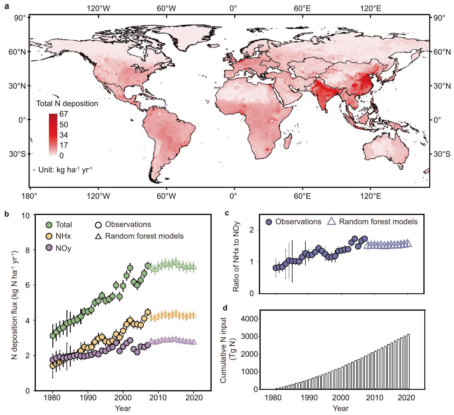
الشكل 1 | الأنماط الزمانية والمكانية للأرض العالميةالإيداع. أ توزيع مكاني للإيداع الكلي للنيتروجين في عام 2020. ب الديناميات الزمنية للإيداع الكلي، NHx، و NOy من 1980 إلى 2020؛ الدوائر تمثل الملاحظات المباشرة وأشرطة الخطأ تشير إلى SE (التباين بين مواقع المراقبة)؛ المثلثات مقدرة من نماذج الغابة العشوائية وأشرطة الخطأ تشير إلى SE (التباينات). عبر ثلاثة نماذج غابة عشوائية مختلفة). تمثل الألوان المختلفة مكونات مختلفة من ترسيب النيتروجين. ج الديناميات الزمنية لنسبة ترسيب NHx إلى NOy من 1980 إلى 2020. د المدخل التراكمي لترسيب النيتروجين من 1980 إلى 2020. ملاحظة: القارة القطبية الجنوبية غير مدرجة. تم توفير بيانات المصدر كملف بيانات مصدر.
التغيرات في ترسيب النيتروجين العالمي من 1980 إلى 2020
الأرضية العالميةازداد ثم استقر وانخفض قليلاً خلال الفترة من 1980 إلى 2020، ليصل إلى ذروته في عام 2015 عند (الشكل 1ب). من 1980 إلى 1982، كان أقل قليلاً من، ولكن الزيادة اللاحقة فيكان أسرع بكثير من و انخفضت قليلاً بعد عام 2015 (الشكل 1ب). على مدى الأربعين عامًا الماضية، كانت نسبةإلىقد زاد تدريجياً من 0.81 في عام 1980 إلى أقصى حد بلغ 1.73 في عام 2007. ثم بدأ في الانخفاض واستقر عند 1.5 بعد عام 2010 (الشكل 1c). المدخل التراكمي لـإلى الأراضي العالمية من 1980 إلى 2020 كان حوالي 3117 طن نيتروجين (الشكل 1d) في حين كان استخدام الأسمدة النيتروجينية العالمية حوالي. وبالتالي، كانت مدخلات النيتروجين إلى النظم البيئية الأرضية من خلال الترسيب الجوي تقريبًا تعادل مدخلات النيتروجين من الأسمدة خلال تلك الفترة.
ديناميات ترسيب النيتروجين الإقليمي من 1980 إلى 2020
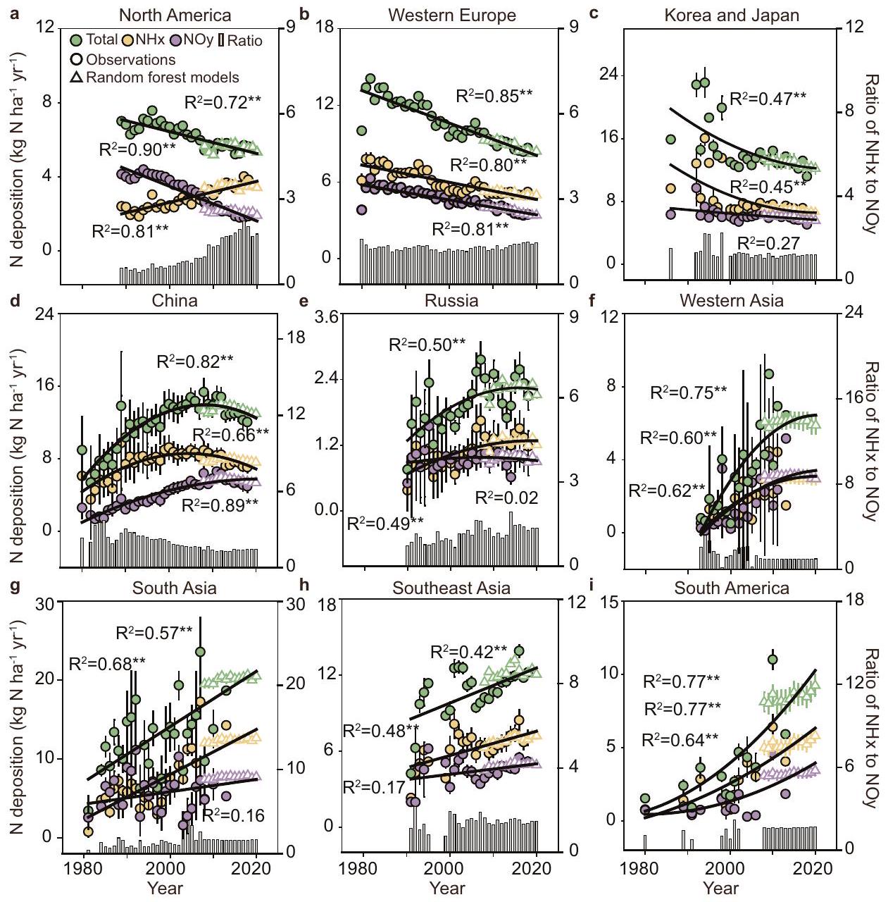
يمكن تقسيم الديناميات الإقليمية لإيداع النيتروجين من 1980 إلى 2020 إلى ثلاثة أنواع (الشكل 2). النوع 1 يظهر تراجعًا، والذي يحدث بشكل رئيسي في الدول المتقدمة مثل أمريكا الشمالية، وأوروبا الغربية، واليابان، وكوريا الجنوبية (الشكل 2أ-ج). باستثناء أمريكا الشمالية، و كلها انخفضت؛ في أمريكا الشماليةزاد أو كان تقريبًا ثابتًا. النوع 2 يظهر انتقالًا ويحدث بشكل رئيسي في الصين وروسيا وغرب آسيا ودول أخرى ذات دخل متوسط (مجمعة حسب الدخل) فئة وفقًا لتصنيف البنك الدولي، الدخل القومي الإجمالي للفرد بين و ) (الشكل 2د-و). هنا و زاد الجميع أولاً ثم استقر أو انخفض.وصل إلى الحد الأقصى وانخفض، كما هو الحال في الصين، أو كان تقريبًا ثابتًا. يجب أن نلاحظ أنه، على عكس توقعاتنا، وجدنا أن ترسيب النيتروجين في أفريقيا أظهر أيضًا زيادة ثم استقر (الشكل التكميلي 4). كشفت التحليلات الإضافية أن و في أفريقيا قد انخفض كلاهما (الشكل التوضيحي 4)، وقد شهد الناتج المحلي الإجمالي للفرد نمواً راكداً في العقد الماضي (الشكل التوضيحي 5). على الرغم منقد زاد قليلاً، لكنه لم يغير الانخفاض العام فيفي أفريقيا. النوع 3 يظهر زيادة ويحدث بشكل رئيسي في البلدان ذات الدخل المنخفض (الدخل القومي الإجمالي للفرد أقل منمثل جنوب آسيا وجنوب شرق آسيا وأمريكا الجنوبية. هنا، و أظهرت زيادات ملحوظة، وكما زادت أيضًا (الشكل 2g-i).
نقل بؤر ترسيب النيتروجين العالمية من 2008 إلى 2020
الأرضية العالميةكان مستقرًا نسبيًا على مدار العقد الماضي (الشكل 1ب) ولكن، كما ذُكر أعلاه،في الدول المتقدمة انخفض، بينما زاد في الدول النامية في جنوب آسيا وجنوب شرق آسيا وأمريكا الجنوبية (الشكل 2). تشير حساباتنا إلى أن النقاط الساخنة العالمية لـتتحرك من المناطق المتقدمة إلى المناطق النامية. إلى
الشكل 2 | الديناميات الإقليمية لتساقط النيتروجين الجوي من 1980 إلى 2020. أ الديناميات في أمريكا الشمالية. ب الديناميات في غرب أوروبا. ج الديناميات في كوريا واليابان. د الديناميات في الصين. هـ الديناميات في روسيا. و الديناميات في غرب آسيا. الديناميات في جنوب آسيا. الديناميات في جنوب شرق آسيا. الديناميات في أمريكا الجنوبية. الدوائر تمثل الملاحظات المباشرة وأشرطة الخطأ تشير إلى الانحراف المعياري (التباين بين مواقع المراقبة). المثلثات تمثل النتائج من نماذج الغابة العشوائية وأشرطة الخطأ تشير إلى الانحراف المعياري (التباينات عبر ثلاثة نماذج عشوائية). نماذج الغابات). تمثل الألوان المختلفة مكونات مختلفة لإيداع النيتروجين. يتم ملاءمة اتجاه إيداع النيتروجين باستخدام دوال خطية أو ثنائية. هو معامل التحديد، ** يمثل مستوى الدلالة عند ، و * تمثل مستوى الدلالة عند يوضح الرسم البياني الشريطي في أسفل كل مخطط ديناميات نسبة ترسيب NHx إلى NOy في المنطقة. يتم توفير بيانات المصدر كملف بيانات مصدر. للتحقق من قوة هذا الاستنتاج، قمنا بتحليل الاتجاهات فيمن 2008 إلىزاد بشكل ملحوظ في البلدان النامية عند خطوط العرض المتوسطة والمنخفضة في جنوب آسيا وجنوب شرق آسيا والبرازيل. ومع ذلك، انخفض بشكل ملحوظ في البلدان أو المناطق المتقدمة مثل أوروبا والولايات المتحدة الشرقية واليابان. في الوقت نفسه، انخفض ترسيب النيتروجين في بعض مناطق أفريقيا وغرب آسيا والأرجنتين أيضًا (الشكل 3أ). انخفاضات و في تلك المناطق من إفريقيا وغرب آسيا والأرجنتين يمكن أن تساهم بشكل مباشر في الانخفاض فيفي هذه المناطق (الشكل التوضيحي 6).
قمنا أيضًا بتحليل الاتجاهات بشكل منفصل فيفي الدول المتقدمة والنامية من 2008 إلى 2020. ديناميات التغيرات فيفي البلدان النامية والمتقدمة كانت مختلفة، مع نسبةبين الدول النامية والدول المتقدمة يظهر زيادة خطية ملحوظةالشكل 3ب). في الدول المتقدمة، الاتجاه العام الطفيف نحو الانخفاض فيكان ذلك بشكل أساسي بسبب انخفاض كبير في، بينما أظهر فقط انخفاضًا طفيفًا وغير ذي دلالة إحصائية (الشكل 3ج). وهذا يبرز الحاجة إلى أن تعزز الدول المتقدمة التدابير للحد مننقاط انبعاث ساخنة. على النقيض من ذلك، فإن الزيادة الكبيرة في الدول النامية تعود إلى الزيادة الكبيرة في، الشكل 3ج).
قمنا بتحليل الاتجاهات في المواقع التي تحتوي على ملاحظات مستمرة لبيانات الترسيب الرطب منذ عام 2000 (الشكل التوضيحي 7). هذا يؤكد أن نقاط ساخنة عالمية منانتقلت من الدول المتقدمة إلى الدول النامية. يجب أن نلاحظ أن هذه المناطق التي تفتقر إلى المراقبة الجيدة (أي، أفريقيا، آسيا الوسطى، أمريكا اللاتينية، وأستراليا) لا تزال تعاني من أكبر قدر من عدم اليقين في، وتشمل هذه المناطق غير المؤكدة بشكل كبير العديد من المناطق التي تظهر اتجاهات متزايدة، مما يتطلب مزيدًا من المراقبة. في الوقت نفسه، انخفضت بعض الاتجاهات طويلة الأجل للمؤشرات، مثل محتوى النيتروجين في الأوراق وتركيز النترات في المياه السطحية، في الولايات المتحدة.وأوروباوزادت في الغابات الاستوائية والهند ، والتي تعكس بشكل محتمل النقاط الساخنة المتغيرة لـ.
محركات العالميةإيداع
هو آلية مهمة تدفع التغيرات الديناميكية فيقمنا بتحليل العلاقات بين ونصيب الفرد من الناتج المحلي الإجمالي، وخرائط في خمس مناطق عالمية رئيسية على المستويات الوطنية والإقليمية.انبعاثات أكاسيد النيتروجين (NOx) ) ، و وكانت MAP مرتبطة بـ، و كانت قوة الإيجابية أو السلبية للارتباطات تختلف حسب المنطقة (الشكل التوضيحي 8) مما يظهر أنيتأثر بشدة بالنشاط البشري والعوامل الجوية، وهو ما يتماشى مع الأبحاث السابقة .
لقد طورت الأبحاث السابقة إطارًا للعوامل النشطةالعوامل الجويةلتحليل العوامل والآليات المؤثرة. ومع ذلك، فإن هذا لا يظهر بوضوح دور الاجتماعي
الشكل 3 | الاتجاهات فيترسيب النيتروجين في الدول المتقدمة والنامية من 2008 إلى 2020. أ تحليل الاتجاه لإجمالي ترسيب النيتروجين من 2008 إلى 2020. ب الديناميات الزمنية ونسب إجمالي ترسيب النيتروجين في الدول المتقدمة والنامية (المتوسط ± الخطأ المعياري). ج الديناميات الزمنية لترسيب NHx و NOy في الدول المتقدمة والنامية (المتوسط ± الخطأ المعياري). اتجاه ترسيب النيتروجين هو تم تركيبها باستخدام دوال خطية أو ثنائية. هو معامل التحديد، ** و * يمثلان مستوى الدلالة عند و على التوالي، وأشار SE (شريط الخطأ في الشكل) إلى التباين عبر نماذج الغابة العشوائية الثلاثة. تم توفير بيانات المصدر كملف بيانات مصدر. وتطور الاقتصاد في التغيرات فيوجدنا أن الناتج المحلي الإجمالي للفرد كان له ارتباط سلبي كبير معفي أمريكا الشمالية، وأوروبا الغربية، وشرق آسيا. كما لاحظنا ارتباطًا إيجابيًا أقل وضوحًا وأقل أهمية معفي جنوب شرق آسيا وأفريقيا (الشكل التوضيحي التكميلي 8). لذلك قمنا ببناء شبكة متسلسلة من الناتج المحلي الإجمالي للفردخريطةاستخدام نماذج المعادلات الهيكلية. يمكن أن تفسر العوامل في هذه النماذج والعمليات التي تؤثر عليهاالتغير الزماني المكاني (الأشكال التكميلية 9 و 10)، مما يؤكد أهمية التنمية الاجتماعية والاقتصادية في تحديد التغيرات فيومكوناته.
ثم قمنا بتحليل العلاقات بين الناتج المحلي الإجمالي للفرد وعلى المستوى العالمي باستخدام بيانات من عدة دول أو مناطق. العلاقات بينوأن الناتج المحلي الإجمالي للفرد في البلدان أو المناطق في مراحل مختلفة من تطورها الاقتصادي يتناسب تمامًا مع منحنى التوزيع الطبيعي (الشكل 4 أ-ج؛ الشكل التكميلي 11 أ، ب). وهذا يتماشى مع نموذج منحنى كوزنتس البيئي الكلاسيكي.عندما اختبرنا نموذج المعادلة التكعيبية اللوغاريتمية لـ EKC، كانت جميع منحنيات التوزيع الطبيعي ذات دلالة إحصائية. ) (الشكل 4د-و؛ الشكل التوضيحي 11ج، د؛ الجدول التوضيحي 3). ذروة كان في حواليوقمم و كانوا في و (الجدول التكميلي 3)، على التوالي. الذروة لـ كان في حواليوذلك منحوالي. كان مستمدًا بشكل أساسي من الأنشطة الزراعية وبلغ ذروته قبل (من حيث الوقت و/أو التنمية الاقتصادية)، الذي كان مدفوعًا في الغالب بالأنشطة الصناعية. وهذا يشير إلى أن التنمية الاجتماعية والاقتصادية، كما يعبر عنها بالناتج المحلي الإجمالي للفرد، هي عامل مهم في تحديد النمط المكاني الزمني لـ، وأن التطور الديناميكي للمساهمات النسبية للأنشطة الزراعية والصناعية يحدد العلاقة بين ذروات و .
التداعيات على المستوى العالميإدارة
الإدخال التراكمي لـكان إجمالي النيتروجين المودع في النظم البيئية الأرضية من 1980 إلى 2020 (3117 Tg N) يعادل تقريبًا تطبيق الأسمدة النيتروجينية العالمية (3549 Tg N) خلال نفس الفترة. يمكن أن يزيد ترسيب النيتروجين بشكل كبير من إنتاجية النظام البيئي للغابات والمراعي والمسطحات المائية.لذا فإن تأثير مثل هذه الكمية الكبيرة من التسميد الطبيعي بالنيتروجين على دورة الكربون وامتصاص الكربون في النظم البيئية يتطلب البحث.، ويجب إعادة تقييم تأثيرات ترسيب النيتروجين على تنوع الأنواع، وانبعاثات غازات الدفيئة، وتحمض التربة، وما إلى ذلك. لقد انتقلت النقاط الساخنة، وهي مناطق الترسيب المكثف للنيتروجين، من الدول المتقدمة إلى الدول النامية في خطوط العرض المتوسطة والمنخفضة. غالبًا ما يكون نمو النباتات في النظم البيئية الاستوائية في خطوط العرض المنخفضة محدودًا بالفوسفور.، وزيادة مدخلات النيتروجين تميل إلى تفاقم هذا القيد وتقليل إنتاجية الأشجار، مما يهدد بشكل أكبر الهيكل والوظيفة للأنظمة البيئية الاستوائية. علاوة على ذلك، فإن الدول المتقدمة والنامية لديها اتجاهات ديناميكية مختلفة من
الشكل 4 | العلاقات بينالإيداع والناتج المحلي الإجمالي للفرد على مستوى عالمي. العلاقات بين الإجماليوإيداع NOy (c، f) والناتج المحلي الإجمالي للفرد (GDPpc). البيانات المستخدمة فيهي ملاحظات لإيداع النيتروجين والناتج المحلي الإجمالي للفرد؛ تلك فيهي القيم اللوغاريتمية لإيداع النيتروجين والناتج المحلي الإجمالي للفرد. الدول الأفريقية هي النيجر ومالي والكاميرون. وساحل العاج. دول جنوب شرق آسيا هي فيتنام وماليزيا وإندونيسيا وتايلاند. دول شرق آسيا هي الصين وكوريا الجنوبية واليابان. دول غرب أوروبا هي دول الاتحاد الأوروبي (EU27). دول أمريكا الشمالية هي الولايات المتحدة وكندا. هو معامل التحديد، ** يمثل مستوى الدلالة عند تُقدم بيانات المصدر كملف بيانات مصدر. (الشكل 2)، التي تؤثر على النظم البيئية بشكل مختلف: يمكن أن تظهر النباتات تفضيلًا قويًا لـأو وتأثيرات وتختلف الترسيبات على تحمض التربة وانبعاثات غازات الدفيئة أيضًا. تغييرات في قد تؤدي لذلك إلى تغييرات في تركيب الأنواع في النظم البيئية الطبيعية وشبه الطبيعية.
يتطلب تقليل انبعاثات النيتروجين وترسيبها في الدول النامية تعاونًا عالميًا وفهمًا أفضل لمساهمات الصناعة والزراعة.ظل الدور السائد في ترسيب النيتروجين العالمي في عام 2020، لكن المساهمة النسبية للتغيرإلى التغييرات فيكان يتناقص (الشكل التوضيحي 12). في الوقت نفسه، وجدنا أنمن ذروة الزراعة قبلبشكل رئيسي من الأنشطة الصناعية، مع قيمة ذروة أعلى لـ (الشكل 4). التكلفة الحدية للزراعة الخفض أقل بكثير من الصناعيتقليلجعل إدارة النيتروجين بشكل أفضل في الزراعة مسارًا اقتصاديًا فعالًا لتقليل انبعاثات النيتروجين مع زيادة إنتاج المحاصيل وكفاءة استخدام النيتروجينلذا، يجب على الدول النامية أن تعطي الأولوية لتقنيات تقليل انبعاثات الزراعة لتحقيق الذروةقبل. ومع ذلك، تفتقر معظم الدول إلى وضوحسياسات وتقنيات خفض الانبعاثاتلذلك، يجب على الدول النامية تمويل الزراعة لدعم تطبيقات تكنولوجيا تقليل الانبعاثات السريعة جنبًا إلى جنب مع التنمية الصناعية. من خلال إنشاء زراعة أكثر كفاءة، ستتجنب الدول النامية والدول الانتقالية اتباع نفس مسار تلوث النيتروجين كما فعلت الدول المتقدمة. وتجنب أحداث التلوث مثل الضباب الكيميائي الضوئي، والأمطار الحمضية، والضباب، وتحمض التربة التي شهدتها أوروبا وأمريكا الشمالية والصين.
تحليل عدم اليقين على المستوى العالميتقييم الإيداع
استنادًا إلى قاعدة بيانات MGND، طورت هذه الدراسة إطارًا لإجراء مجموعة بيانات شبكية عالمية وتقييم منهجي للحالة الحالية، والتغير الديناميكي، والأنماط الإقليمية، وانتقالات النقاط الساخنة لإيداع النيتروجين العالمي. هذا تقييم عالمي مستقل عن محاكاة نماذج النقل الكيميائي الجوي ويعتمد على بيانات المراقبة الواسعة. على الرغم من أن التقدير الإجمالي لإيداع النيتروجين العالمي المدخل إلى اليابسة ) أعلى من النتائج الناتجة عن محاكاة نماذج النقل الكيميائي الجوي من خلال تلخيص العوامل الطبيعية والأنثروبوجينية العالميةوجدنا أن الإجمالي العالمييمكن أن تصل (الجدول التكميلي 2)، مما يشير إلى أن تقديرنا لإيداع النيتروجين يقع ضمن نطاق معقول.
جرد انبعاثات الأنشطة البشرية (أي، و NOx ) هي بيانات مهمة لنماذج النقل الكيميائي في الغلاف الجوي التي تحاكي ترسيب النيتروجين في الغلاف الجوي. حاليًا، يتم استخدام سجلات من CEDS قاعدة بيانات الانبعاثات للبحث العالمي في الغلاف الجوي (EDGAR)تستخدم على نطاق واسع في هذه النماذج. يتم تقدير هذين المجموعتين من البيانات باستخدام نهج من الأسفل إلى الأعلى استنادًا إلى معلومات نشاط الانبعاثات وعوامل الانبعاث. ومع ذلك، فإن هذا النهج شديد غير مؤكد، خاصة في المناطق التي تفتقر إلى الإحصاءات الاجتماعية والاقتصادية (مثل أفريقيا) والمكونات التي تكون عوامل انبعاثها متغيرة بشكل كبير وأكثر تعقيدًا. دراسات حديثة تستخدم لتصحيح سجلات الانبعاثات أظهرت أن التقديرات من الأسفل إلى الأعلى لـيتم التقليل من قيمتها بشكل كبير، مع و مُقَدَّر بأقل منو38%، على التوالي (الجدول التكميلي 2)، مما قد يسهم في الانخفاضتقديرات من النماذج مقارنة بتقديراتنا.
قمنا بمقارنة منهجية لـالتقديرات في أمريكا الشمالية وأوروبا والصين من دراسات أخرى مع دراستنا، بالإضافة إلى ما يتوافق مع ذلك، ووجدت نتائج متسقة عبر جميع الدراسات (الجدول التكميلي 4). عدم اليقين النسبي لـكان أقل منفي معظم المناطق (الشكل التوضيحي 13). قد يؤدي التوزيع غير المتساوي لمواقع المراقبة في شبكة ترسيب النيتروجين الجوي العالمية إلى إدخال تحيز في نماذج التعلم الآلي، خاصة في أفريقيا وآسيا الوسطى وأمريكا اللاتينية وأستراليا، حيث تكون المواقع نادرة. على الرغم من الشبكة المتسلسلة للناتج المحلي الإجمالي للفردعوامل الأرصاد الجويةيتم تطبيقه على مستوى العالم، من الضروري تعزيز ملاحظات ترسيب النيتروجين في المناطق التي تفتقر إلى البيانات لتقليل عدم اليقين في التقييم.
طرق
مجموعة من الأجواءبيانات ملاحظة موقع الإيداع
استخدمنا ثلاثة مصادر لبيانات ترسيب النيتروجين: (1) بيانات من 43 موقعًا تراقب الغابات، والمراعي، والأراضي الزراعية، والأراضي الرطبة، والصحاري، والمدن من عام 2013 إلى 2020 في شبكة المراقبة الصينية لترسيب المياه (ChinaWD).“; (2) بيانات مشتركة من شبكات مراقبة ترسيب النيتروجين العالمية: برنامج المراقبة والتقييم الأوروبي (EMEP) في أوروبا، شبكة حالة وجودة الهواء والاتجاهات (CASTNET)، نظام جودة الهواء (AQS)، وشبكة مراقبة الأمونيا (AMoN) في الولايات المتحدة، شبكة مراقبة الهواء والهطول الكندية (CAPMoN) وبرنامج المراقبة الوطنية لتلوث الهواء (NAPS) في كندا، شبكة مراقبة ترسيب الأحماض (EANET) في شرق آسيا، الشبكة الدولية لدراسة الترسيب وتركيب الغلاف الجوي في أفريقيا (INDAAF)، وشبكة المراقبة الوطنية لترسيب النيتروجين (NNDMN) من جامعة الزراعة الصينية.; (3) 1390 ورقة منشورة تتعلق ببيانات ترسيب النيتروجين من مواقع مختلفة (البيانات التكميلية 1). كانت المعايير لاختيار مجموعات البيانات من الأدبيات هي أن مؤشر المراقبة يجب أن يتضمن (i) الأمونيوم، النترات، الترسيب الكلي الرطب (مجموع الأمونيوم والنترات) أو تركيزاتها في الهطول؛ (ii) التركيز أو الترسيب الجاف لـ و ; (iii) تكرارات الملاحظة اليومية أو الأسبوعية أو الشهرية؛ (iv) فترة ملاحظة أطول من سنة واحدة.
تتضمن قاعدة بيانات MGND الناتجة اسم الموقع، الموقع، وقت المراقبة، طريقة المراقبة، نوع النظام البيئي، هطول الأمطار السنوي، تركيز النيتروجين وتدفق كل مكون، ومصدر البيانات. تمتد من 1977 إلى 2021 وتشتمل على 25,808 سنة موقع من الترسيب الرطب و26,863 سنة موقع من الترسيب الجاف (الشكل التوضيحي التكميلي 1 والجدول التكميلي 1). كان الترسيب الرطب يتكون من الأمونيوم ( ) ونيترات ( ؛ يتكون الترسيب الجاف من غازاتجزئيغازيغازي ( ) وجزيئي (الجدول التكميلي 1).
مصادر بيانات التحليل المساعدة
مصادر بيانات التحليل المساعدة والمعلومات التفصيلية المستخدمة في هذه الدراسة موضحة في الجدول التكميلي 5. تأتي البيانات المناخية بشكل رئيسي من وحدة الأبحاث المناخية (CRU، النسخة cru_ts4.05)ومن منتج إعادة التحليل لـ NECP-NCAR (إعادة تحليل NECEP-NCAR 1)بما في ذلك خريطة، ومتوسط درجة الحرارة السنوية (MAT)، وأيام الرطوبة (WET)، وضغط البخار (VAP)، وتدفق الإشعاع القصير الصافي (Nswrs)، والضغط السطحي (Pres)، والرطوبة النسبية (Shum) وسرعة الرياح (Wspd).
تم الحصول على سجلات انبعاث الملوثات الناتجة عن الأنشطة البشرية من CEDS (الإصدار CEDS v_2021_04_21). لقد استخدمنا أيضًا من EDGARولو وآخرون. تم الحصول على البيانات من جهاز قياس التداخل للأشعة تحت الحمراء في الغلاف الجوي (IASI)استخدمنا إعادة تحليل البيانات الثانوية على المقياس الشهري القياسي للفترة من 2008 إلى 2020.تم الحصول على البيانات من أداة مراقبة الأوزون (OMI) وتجربة مراقبة الأوزون العالمية (GOME) ومطياف الامتصاص التصويري المسحي لخرائط الغلاف الجوي (SCIAMACHY)تم دمج مجموعات البيانات الثلاثة من الأقمار الصناعية في مجموعة بيانات واحدة وشملت الفترة من 1996 إلى 2020.. تركيز العمود ( ) تم الحصول عليها من OMI/Aura SO بيانات L3 اليومية لإجمالي العمود.
تم الحصول على بيانات الناتج المحلي الإجمالي للفرد وسكان كل دولة من قاعدة بيانات مشروع ماديسون.كان الناتج المحلي الإجمالي للفرد يعتمد على الأسعار في عام 2011، مما أزال تأثير تغييرات الأسعار وعكس القيم الحقيقية لإنتاج المنتجات على مدى فترات مختلفة. بالإضافة إلى ذلك، استخدمنا أيضًاضوء الليلالناتج المحلي الإجمالي للشبكةالسكانمؤشر الفرق النباتي الطبيعي (NDVI)بيانات الإنتاج العالمي – مساحة المعيشة – الفضاء البيئيمجموعة بيانات بصمة الإنسان الأرضيةمجموعة بيانات تخص تخصيب النيتروجين حسب المحاصيلوبيانات إحصائية عن تطبيق الأسمدة النيتروجينية لكل وحدة مساحة (الجدول التكميلي 5).
تحليل الديناميكية الزمنية من ملاحظة الموقع
قمنا بتحليل التباين فيفي عشر دول أو مناطق رئيسية: أوروبا الغربية، أمريكا الشمالية، أمريكا الجنوبية، روسيا، أفريقيا، جنوب شرق آسيا، جنوب آسيا، غرب آسيا، الصين، اليابان وكوريا الجنوبية. السنويفي كل منطقة تم حسابه كمتوسط حسابي سنوي وخطأ معياري لجميع البيانات الملاحظة لتلك المنطقة، بما في ذلك، و .
استخدمنا معادلات خطية أو غير خطية لتحليل الاتجاهات في الترسيب من 1980 إلى 2020 في كل منطقة. قمنا بتقدير البيانات المفقودة بناءً على النموذج المثالي الملائم لـمع الوقت لمنطقة أو فترة معينة. القيم المتوسطة والاتجاهات في العالميةتم حسابها باستخدام طريقة المتوسط المرجح. اخترنا 352 موقعًا للرصد مع خمس سنوات من المراقبة المستمرة منذ عام 2000 واستخدمنا طريقة مان-كيندال للتحليل.الاتجاهات على مستوى الموقع.
تم تحليل جميع البيانات باستخدام برنامج SPSS الإصدار 13.0. كانت العلاقات بين ونصيب الفرد من الناتج المحلي الإجمالي، وتم تحليل MAP في خمس مناطق عالمية رئيسية على المستويات الوطنية والإقليمية. تم استخدام نموذج المعادلات الهيكلية لاستكشاف المؤشرات والمسارات المؤثرة لـ. تم رسم جميع الأشكال باستخدام برنامج SigmaPlot الإصدار 12.0. أشكال النمط المكاني لـتم رسمها باستخدام برنامج ArcGIS 10.0.
بناء عالميمجموعة بيانات شبكة الإيداع
قمنا بتطوير إطار عمل لإنشاء شبكة عالميةمن بيانات ملاحظات الموقع بين عامي 2008 و2020 (الشكل التوضيحي 14). لم نقم بتمديد البيانات إلى ما قبل عام 2008 بسبب عدم توفر بيانات كافية لبعض المتغيرات المهمة (أي،لتقليل تأثير توزيع مواقع المراقبة غير المتساوي على توقع ترسيب النيتروجين العالمي، قمنا بتصنيف اليابسة العالمية إلى فئتين: البرية والمناطق المعدلة بواسطة الإنسان، استنادًا إلى بيانات البصمة البشرية العالمية، و تعكس البصمة البشرية العالمية جوانب مختلفة من الضغوط البشرية باستخدام ثمانية متغيرات، بما في ذلك البيئات المبنية، وكثافة السكان، والضوء الليلي، والأراضي الزراعية، والأراضي الرعوية، والطرق، والسكك الحديدية، والممرات المائية القابلة للملاحة.لقد عرفنا مناطق البرية على أنها تقاطع المناطق حيث تكون بيانات البصمة البشرية العالميةفي الأدنى، و في أدنى 2.5% لكل عام.
بشكل عام، تقع المناطق البرية بشكل أساسي في المناطق الشمالية ذات العرض الجغرافي العالي مثل ألاسكا، غرينلاند، وسيبيريا، بالإضافة إلى صحراء السهارا في أفريقيا، وهضبة التبت في الصين، والمناطق الصحراوية في أستراليا. فرضيتنا هي أن هذه المناطق البرية أقل تأثراً بالأنشطة البشرية، مما يؤدي إلى مستويات منخفضة من. مناطق ذات مستوى أعلىلديهم أعلى. لذلك، في هذه المناطق هو مُقدَّر كما في المعادلة (1):
أينيمثل تدفق ترسيب النيتروجين ( ); يمثل تطبيع; يمثل تطبيع; i تمثل مكونات N؛ j تمثل السنوات من 2008 إلى 2020؛ 0.01 هو عامل تحويل الوحدة الذي يأخذ في الاعتبار مستويات ترسيب N قبل الصناعة ( ).
بالنسبة للمناطق المعدلة من قبل الإنسان، استخدمنا طرق التعلم الآلي لزيادة الدقة.من مقياس الموقع إلى مقياس الشبكة العالمية. تم اختيار البيانات فقط من الشبكات الرئيسية لمراقبة الترسيب العالمية كمتغير مستقل لتحقيق الاتساق والاستمرارية في الملاحظات والأساليب. ومن الجدير بالذكر أن نماذج الغابة العشوائية أظهرت دقة تنبؤية متفوقة، كما يتضح من ارتفاعالقيم في كل من مجموعات التدريب والاختبار، مقارنةً بآلة الدعم الناقل وشبكة الأعصاب BP (الجدول التكميلي 6). استخدمنا حصريًا نماذج الغابة العشوائية للتنبؤ بإيداع النيتروجين العالمي في المناطق المعدلة بشريًا، معتمدين على ثلاثة مسارات رئيسية: نموذج n6، أفضل نموذج n 22، ونموذج الشلال (الجدول التكميلي 7).
حزمة randomForestتم استخدام برنامج R لبناء جميع نماذج التنبؤ المذكورة أعلاه. خلال بناء النموذج،تم اختيار البيانات بشكل عشوائي كمجموعة تدريب لتقييم دقة نموذج التنبؤ وتم اختيارها كمجموعة اختبار لتقييم أداء التنبؤ للنموذج. نماذج الغابة العشوائية لـتم بناء الترسيب باستخدام تركيزات المراقبة الأرضية للمكونات المختلفة. تم تقدير الترسيب من خلال ضرب تركيزات المراقبة الأرضية بسرعة الترسيب المقابلة. استخدمنا طريقة الإزالة التكرارية للميزات (RFE) للحصول على أفضل مجموعة متغيرة في النموذج الأفضل n 22 ونموذج الشلال. بالإضافة إلى ذلك، لجميع النماذج، استخدمنا طريقة البحث الشبكي لاختيار أفضل المعلمات الفائقة، مثل عدد الأشجار (بين 100 و 1000)، mtry (بين 1 وعدد المتغيرات التنبؤية أومن المتغيرات التنبؤية لأفضل 22 نموذجًا)، وحجم العقدة (عدد المتغيرات المستخدمة في كل انقسام عقدة، بين 1 وعدد المتغيرات التنبؤية)، لتعظيم الأداء خارج العينةتم حساب قيم شابلي (SHAP) لتحديد أهمية الميزات وتحليل حساسية الناتج تجاه المتغيرات المدخلة.
تم بناء نموذج n6 بأقل مجموعة متغيرة استنادًا إلى شبكة التدفق الناتج المحلي الإجمالي للفرد.خريطةلقد تم إثبات ذلك للصين في أبحاثنا السابقة. تراوحت التباينات التي تفسرها النماذج الستة من إلى (الجدول التكميلي 7). كان هو المؤشر الأكثر أهمية لمعظم مكونات ترسيب النيتروجين بينماكان من أهم المؤشرات للأرض و تركيز (الشكل التوضيحي الإضافي 15).
النموذج 22 الأفضل يبني على النموذج 6، مما يعزز قدراته التفسيرية والتنبؤية. باستخدام طريقة RFE، قمنا بتحسين أفضل مجموعة من المتغيرات من 22 متغيرًا. كما هو متوقع، فإن معدلات التفسير للنموذج 22 الأفضل أعلى من تلك الخاصة بالنموذج 6، باستثناء الأرض. و التركيز (الجدول التكميلي 7). كان أهم متنبئ في النموذج الأفضل n 22 مشابهًا تقريبًا لما كان عليه في النماذج n 6 (الشكل التكميلي 16).
نظرًا للاختلافات الكبيرة في بيانات جرد الانبعاثات، خاصةً لـ، افترضنا أن هذه البيانات ستؤثر بشكل كبير على نتائج التنبؤ. لذلك، صممنا نموذج السلسلة لاستخدامه أولاًالنشاط الاقتصادي، واستخدام الأراضي للتنبؤ. ثم، استخدمنا التنبؤ بـمهمة، مقترن بـالعوامل الجوية، وبيانات انبعاث الملوثات الجوية، للتنبؤ (الجدول التكميلي 7). قمنا باستخراج أربع مجموعات من بيانات الراستر (من CEDS وEDGAR ومن منتجين في لو وآخرون.بأقل من 10% تباين في، تم تحديده على أنه البيانات النقطية الأكثر دقة لـالتقييم، واستخدمتها كمتغير تابع عند التنبؤفي نموذج الشلال.كان من أهم المؤشرات للتنبؤ، والمتغير كان من أهم المؤشرات لـ (الشكل التوضيحي 17).
أخيرًا، قمنا بدمج مجموعة بيانات ترسيب النيتروجين للمناطق البرية والمناطق المعدلة بشريًا لإنشاء مجموعة بيانات مكانية عالمية.من 2008 إلى 2020 بدقة مكانية قدرها. كانت المدخلات العالمية السنوية من النيتروجين من خلال الترسيب على اليابسة في عام 2020 هي الأعلى وفقًا لنموذج الشلال ( )، تليها أفضل 22 نموذج ( )، ثم نموذج n 6 ( 85.6 Tg N ) (الجدول التكميلي 8). تم حساب عدم اليقين النسبي عند كل بكسل عبر ثلاثة نماذج. تم تعريف عدم اليقين النسبي على أنه نسبة الخطأ المعياري إلى القيمة المتوسطة للنماذج الثلاثة. كما استخدمنا الوسيط ثيل-سين (تقدير ميل سين) لتحليل اتجاه ترسيب النيتروجين العالمي خلال الفترة من 2008 إلى 2020. تم استخدام اختبار مان-كيندال غير المعلمي لتحديد دلالة الاتجاهات.
ربط الإيداع بالنمو الاقتصادي
قمنا بدمج البيانات العالمية لخمس مناطق – شرق آسيا، جنوب شرق آسيا، أفريقيا، غرب أوروبا وأمريكا الشمالية – التي كانت لديها ملاحظات عن ترسيب النيتروجين على مدى فترة طويلة نسبياً في مراحل مختلفة من التنمية الاجتماعية في مجموعة بيانات إقليمية واحدة. تم استخدام طريقتين لتحليل العلاقة بين والناتج المحلي الإجمالي للفرد، ولتحديد ما إذا كان يتوافق مع منحنى كوزنتس البيئي. أولاً، استنادًا إلى الرسوم البيانية المبعثرة، تم استخدام معادلة من رتبة عالية لاستكشاف العلاقة بين الناتج المحلي الإجمالي للفرد وفي كل منطقة. ثانياً، معادلة مكعبة لوغاريتمية (المعادلة (2))تم استخدامه لتحليل العلاقة بين ومعلمات ملاءمة المعادلة التكعيبية اللوغاريتمية مدرجة في الجدول التكميلي 5.
أين هو الناتج المحلي الإجمالي الحقيقي للفرد في كل منطقة في سنة معينة، هو تدفق متوسط ترسيب النيتروجين المقابل، و يمثل الأمونيوم، النترات، الترسيب الرطب، الجاف أو الكلي. هو ثابت و ، و هي المعاملات المقدرة.
ملخص التقرير
معلومات إضافية حول تصميم البحث متاحة في ملخص تقارير مجموعة نيتشر المرتبط بهذه المقالة.
الشفرة الأساسية المستخدمة في هذه الدراسة متاحة علىhttps://doi.org/10. 6084/m9.figshare.26778574.
References
Malik, A. et al. Drivers of global nitrogen emissions. Environ. Res. Lett. 17, 015006 (2022).
Fowler, D. et al. The global nitrogen cycle in the twenty-first century. Philos. Trans. R. Soc. B 368, 20130164 (2013).
Dentener, F. et al. Nitrogen and sulfur deposition on regional and global scales: A multimodel evaluation. Global Biogeochem. Cycles 20, GB4003 (2006).
Reay, D. S., Dentener, F., Smith, P., Grace, J. & Feely, R. A. Global nitrogen deposition and carbon sinks. Nat. Geosci. 1, 430-437(2008).
Thomas, R. Q., Canham, C. D., Weathers, K. C. & Goodale, C. L. Increased tree carbon storage in response to nitrogen deposition in the US. Nat. Geosci. 3, 13-17 (2010).
Guo, J. H. et al. Significant acidification in major Chinese croplands. Science 327, 1008-1010 (2010).
Bowman, W. D., Cleveland, C. C., Halada, L., Hresko, J. & Baron, J. S. Negative impact of nitrogen deposition on soil buffering capacity. Nat. Geosci. 1, 767-770 (2008).
Bobbink, R. et al. Global assessment of nitrogen deposition effects on terrestrial plant diversity: a synthesis. Ecol. Appl. 20, 30-59 (2010).
Richter, A., Burrows, J. P., Nuss, H., Granier, C. & Niemeier, U. Increase in tropospheric nitrogen dioxide over China observed from space. Nature 437, 129-132 (2005).
Ge, Y., Vieno, M., Stevenson, D. S., Wind, P. & Heal, M. R. A new assessment of global and regional budgets, fluxes, and lifetimes of atmospheric reactive N and S gases and aerosols. Atmos. Chem. Phys. 22, 8343-8368 (2022).
Liu, X. J. et al. Enhanced nitrogen deposition over China. Nature 494, 459-462 (2013).
Engardt, M., Simpson, D., Schwikowski, M. & Granat, L. Deposition of sulphur and nitrogen in Europe 1900-2050. Model calculations and comparison to historical observations. Tellus B: Chem. Phys. Meteorol. 69, 1328945 (2017).
Li, Y. et al. Increasing importance of deposition of reduced nitrogen in the United States. Proc. Natl. Acad. Sci. USA. 113, 5874-5879 (2016).
Wen, Z. et al. Changes of nitrogen deposition in China from 1980 to 2018. Environ. Int. 144, 106022 (2020).
Yu, G. et al. Stabilization of atmospheric nitrogen deposition in China over the past decade. Nat. Geosci. 12, 424-429 (2019).
Uwizeye, A. et al. Nitrogen emissions along global livestock supply chains. Nat. Food 1, 437-446 (2020).
Vet, R. et al. A global assessment of precipitation chemistry and deposition of sulfur, nitrogen, sea salt, base cations, organic acids, acidity and pH, and phosphorus. Atmos. Environ. 93, 3-100 (2014).
Vishwakarma, S., Zhang, X., Dobermann, A., Heffer, P. & Zhou, F. Global nitrogen deposition inputs to cropland at national scale from 1961 to 2020. Sci. Data 10, 488 (2023).
Gu, B. et al. Cleaning up nitrogen pollution may reduce future carbon sinks. Global Environ. Change 48, 56-66 (2018).
Zhang, X. et al. Managing nitrogen for sustainable development. Nature 528, 51-59 (2015).
Tan, J. et al. Multi-model study of HTAP II on sulfur and nitrogen deposition. Atmos. Chem. Phys. 18, 6847-6866 (2018).
Rubin, H. J. et al. Global nitrogen and sulfur deposition mapping using a measurement-model fusion approach. Atmos. Chem. Phys. 23, 7091-7102 (2023).
Tian, H. et al. History of anthropogenic Nitrogen inputs ( HaNi ) to the terrestrial biosphere: a 5 arcmin resolution annual dataset from 1860 to 2019. Earth Syst. Sci. Data 14, 4551-4568 (2022).
Ackerman, D., Millet, D. B. & Chen, X. Global estimates of inorganic nitrogen deposition across four decades. Global Biogeochem. Cycles 33, 100-107 (2019).
Van Damme, M. et al. Global, regional and national trends of atmospheric ammonia derived from a decadal (2008-2018) satellite record. Environ. Res. Lett. 16, 055017 (2021).
O’Rourke P. R. et al. CEDS v-2021_04_21 Gridded Emissions Data (accessed on 1 Dec 2021, available at https://data.pnnl.gov/ dataset/CEDS-4-21-21). (2021).
Mason, R. E. et al. Evidence, causes, and consequences of declining nitrogen availability in terrestrial ecosystems. Science 376, eabh3767 (2022).
McLauchlan, K. K., Ferguson, C. J., Wilson, I. E., Ocheltree, T. W. & Craine, J. M. Thirteen decades of foliar isotopes indicate declining nitrogen availability in central North American grasslands. New Phytol. 187, 1135-1145 (2010).
Eshleman, K. N., Sabo, R. D. & Kline, K. M. Surface water quality is improving due to declining atmospheric N deposition. Environ. Sci. Technol. 47, 12193-12200 (2013).
Penuelas, J. et al. Increasing atmospheric concentrations correlate with declining nutritional status of European forests. Commun. Biol. 3, 125 (2020).
Vuorenmaa, J. et al. Long-term changes (1990-2015) in the atmospheric deposition and runoff water chemistry of sulphate, inorganic nitrogen and acidity for forested catchments in Europe in relation to changes in emissions and hydrometeorological conditions. Sci. Total Environ. 625, 1129-1145 (2018).
Hietz, P. et al. Long-term change in the nitrogen cycle of tropical forests. Science 334, 664-666 (2011).
Pandey, J., Singh, A. V., Singh, A. & Singh, R. Impacts of changing atmospheric deposition chemistry on nitrogen and phosphorus loading to Ganga River (India). Bull. Environ. Contamination Toxicol. 91, 184-190 (2013).
Dinda, S. Environmental Kuznets Curve hypothesis: A survey. Ecol. Econ. 49, 431-455 (2004).
Eastman, B. A. et al. Altered plant carbon partitioning enhanced forest ecosystem carbon storage after 25 years of nitrogen additions. New Phytol. 230, 1435-1448 (2021).
Stevens, C. J. et al. Anthropogenic nitrogen deposition predicts local grassland primary production worldwide. Ecology 96, 1459-1465 (2015).
Zaehle, S. Terrestrial nitrogen – carbon cycle interactions at the global scale. Philos. Trans. R. Soc. B 368, 20130125 (2013).
Du, E. Z. et al. Global patterns of terrestrial nitrogen and phosphorus limitation. Nat. Geosci. 13, 221-226 (2020).
Li, Y., Niu, S. & Yu, G. Aggravated phosphorus limitation on biomass production under increasing nitrogen loading: a meta-analysis. Global Change Biol. 22, 934-943 (2016).
Ashton, I. W., Miller, A. E., Bowman, W. D. & Suding, K. N. Niche complementarity due to plasticity in resource use: plant partitioning of chemical N forms. Ecology 91, 3252-3260 (2010).
Song, M. H., Zheng, L. L., Suding, K. N., Yin, T. F. & Yu, F. H. Plasticity in nitrogen form uptake and preference in response to long-term nitrogen fertilization. Plant Soil 394, 215-224 (2015).
Galloway, J. N. Acid deposition: Perspectives in time and space. Water Air Soil Pollut. 85, 15-24 (1995).
Li, X. et al. The contrasting effects of deposited and on soil and fluxes in a subtropical plantation, southern China. Ecol. Eng. 85, 317-327 (2015).
Gu, B. J. et al. Abating ammonia is more cost-effective than nitrogen oxides for mitigating air pollution. Science 374, 758-762 (2021).
Gu, B. et al. Cost-effective mitigation of nitrogen pollution from global croplands. Nature 613, 77-84 (2023).
Guo, Y. X. et al. Air quality, nitrogen use efficiency and food security in China are improved by cost-effective agricultural nitrogen management. Nat. Food 1, 648-658 (2020).
Liu, L. et al. Exploring global changes in agricultural ammonia emissions and their contribution to nitrogen deposition since 1980. Proc. Natl. Acad. Sci. USA. 119, e2121998119 (2022).
Fowler, D. et al. A chronology of global air quality. Philos. Trans. R. Soc. A 378, 20190314 (2020).
Menz, F. C. & Seip, H. M. Acid rain in Europe and the United States: an update. Environ. Sci. Policy 7, 253-265 (2004).
Johansson, L., Jalkanen, J.-P. & Kukkonen, J. Global assessment of shipping emissions in 2015 on a high spatial and temporal resolution. Atmos. Environ. 167, 403-415 (2017).
Luo, Z. et al. Estimating global ammonia emissions based on IASI observations from 2008 to 2018. Atmos. Chem. Phys. 22, 10375-10388 (2022).
Miyazaki, K. et al. Decadal changes in global surface NOx emissions from multi-constituent satellite data assimilation. Atmos. Chem. Phys. 17, 807-837 (2017).
Zhu, J. et al. The composition, spatial patterns, and influencing factors of atmospheric wet nitrogen deposition in Chinese terrestrial ecosystems. Sci. Total Environ. 511, 777-785 (2015).
Harris, I., Osborn, T. J., Jones, P. & Lister, D. Version 4 of the CRU TS monthly high-resolution gridded multivariate climate dataset. Sci. Data 7, 109 (2020).
Kalnay, E. et al. The NCEP/NCAR 40-Year reanalysis project. J. Bullet. Am. Meteorol. Soc. 77, 437-472 (1996).
Van Damme, M. et al. Version 2 of the IASI neural network retrieval algorithm: near-real-time and reanalysed datasets. Atmos. Meas. Tech. 10, 4905-4914 (2017).
Boersma, K. F. et al. An improved tropospheric column retrieval algorithm for the Ozone Monitoring Instrument. Atmos. Meas. Tech. 4, 1905-1928 (2011).
Li, C. et al. Version 2 Ozone Monitoring Instrument product ( ): new anthropogenic vertical column density dataset. Atmos. Meas. Tech. 13, 6175-6191 (2020).
Bolt J., Jan LvZ. Maddison Project Database (accessed on 1 Feb 2022, available at https://www.rug.nl/ggdc/historicaldevelopment/ maddison/releases/maddison-project-database-2020). (2020).
van Donkelaar, A. et al. Monthly global estimates of fine particulate matter and their uncertainty. Environ. Sci. Technol. 55, 15287-15300 (2021).
Chen, Z. et al. An extended time series (2000-2018) of global NPP-VIIRS-like nighttime light data from a cross-sensor calibration. Earth Syst. Sci. Data 13, 889-906 (2021).
Chen, J. et al. Global gridded revised real gross domestic product and electricity consumption during 1992-2019 based on calibrated nighttime light data. Sci. Data 9, 202 (2022).
K. Didan, A. Huete, DAAC NL. MOD13C2 MODIS/Terra Vegetation Indices Monthly L3 Global 0.05Deg CMG (access on 5 Jun 2022, available at https://doi.org/10.5067/MODIS/MOD13C2.006). (2015).
Fu, J., Gao, Q., Jiang, D., Li, X. & Lin, G. Spatial-temporal distribution of global production-living-ecological space during the period 2000-2020. Sci. Data 10, 589 (2023).
Mu, H. et al. A global record of annual terrestrial Human Footprint dataset from 2000 to 2018. Sci. Data 9, 176 (2022).
Adalibieke, W., Cui, X., Cai, H., You, L. & Zhou, F. Global crop-specific nitrogen fertilization dataset in 1961-2020. Sci. Data 10, 617 (2023).
Breiman, L. Random forests. Mach. Learn. 45, 5-32 (2001).
شكر وتقدير
تم دعم هذا العمل من قبل المؤسسة الوطنية للعلوم الطبيعية في الصين (31988102، ج.ي.، 32201364، ج.ز.، و31872690، ق.و.)، ومشروع الأكاديمية الصينية للعلوم للعلماء الشباب في البحث الأساسي (YSBR-037، ج.ز.). نحن نقر بالاستخدام المجاني للغلاف الجوي.بيانات العمود من أجهزة استشعار OMI و GOME و SCIAMACHY من www.temis.nl و بيانات العمود من IASI. نشكر جميع رعاة الشبكات التسع للمراقبة المستخدمة في هذه الدراسة، بما في ذلك البرنامج التعاوني لمراقبة وتقييم النقل بعيد المدى للملوثات الجوية في أوروبا (برنامج المراقبة والتقييم الأوروبي، EMEP)، شبكة حالة وجودة الهواء والاتجاهات (CASTNET) في الولايات المتحدة، نظام جودة الهواء (AQS) في الولايات المتحدة، شبكة مراقبة الأمونيا (AMoN) في الولايات المتحدة، شبكة مراقبة الهواء والهطول الكندية (CAPMoN)، برنامج المراقبة الوطنية لتلوث الهواء (NAPS) في كندا، شبكة مراقبة الترسيب الحمضي في شرق آسيا (EANET)، والشبكة الدولية لدراسة الترسيب وتركيب الغلاف الجوي في أفريقيا (INDAAF). نحن ممتنون للمحطات البيئية وجميع المراقبين من شبكة البحث البيئي الصينية (CERN)، ChinaFLUX، وChinaWD لجمع العينات. نشكر الدكتور U.C. Kulshrestha من المعهد الهندي للتكنولوجيا الكيميائية على توفير بيانات مراقبة ترسيب النيتروجين في الهند. كما نشكر جميع العلماء الذين تم استخدام بياناتهم في تحليلنا.
مساهمات المؤلفين
قام ج.ي. بتصميم البحث. قام ج.ز.، ي.ج.، ن.هـ.، ق.و.، ز.ج.، هـ.هـ.، ش.ز.، و ب.ل. بإجراء البحث (جمع البيانات وتحليلها). كتب ج.ز.، ي.ج.، و ج.ي. المخطوطة. علق ك.ل.، ك.ج.، د.ف.، ب.ف. و ف.ز. على المخطوطة وقاموا بتنقيحها.
يجب توجيه المراسلات والطلبات للحصول على المواد إلى غويروي يو.
معلومات مراجعة الأقران تشكر مجلة Nature Communications هانكين تيان والمراجعين الآخرين المجهولين على مساهمتهم في مراجعة هذا العمل. يتوفر ملف مراجعة الأقران.
ملاحظة الناشر: تظل شركة سبرينجر ناتشر محايدة فيما يتعلق بالمطالبات القضائية في الخرائط المنشورة والانتماءات المؤسسية.
الوصول المفتوح هذه المقالة مرخصة بموجب رخصة المشاع الإبداعي النسب-غير التجارية-عدم الاشتقاق 4.0 الدولية، التي تسمح بأي استخدام غير تجاري، ومشاركة، وتوزيع، وإعادة إنتاج في أي وسيلة أو صيغة، طالما أنك تعطي الائتمان المناسب للمؤلفين الأصليين والمصدر، وتوفر رابطًا لرخصة المشاع الإبداعي، وتوضح إذا قمت بتعديل المادة المرخصة. ليس لديك إذن بموجب هذه الرخصة لمشاركة المواد المعدلة المشتقة من هذه المقالة أو أجزاء منها. الصور أو المواد الأخرى من طرف ثالث في هذه المقالة مشمولة في رخصة المشاع الإبداعي الخاصة بالمقالة، ما لم يُشار إلى خلاف ذلك في سطر الائتمان للمادة. إذا لم تكن المادة مشمولة في رخصة المشاع الإبداعي الخاصة بالمقالة وكان استخدامك المقصود غير مسموح به بموجب اللوائح القانونية أو يتجاوز الاستخدام المسموح به، فستحتاج إلى الحصول على إذن مباشرة من صاحب حقوق الطبع والنشر. لعرض نسخة من هذه الرخصة، قم بزيارة http:// creativecommons.org/licenses/by-nc-nd/4.0/.
المختبر الرئيسي لمراقبة النظم البيئية ونمذجتها، معهد علوم الجغرافيا والبحوث الطبيعية، الأكاديمية الصينية للعلوم، بكين، الصين.كلية الغابات، جامعة خبي الزراعية، باودينغ، الصين.كلية الموارد والبيئة، جامعة الأكاديمية الصينية للعلوم، بكين، الصين.معهد الحياد الكربوني، جامعة الغابات الشمالية، هاربين، الصين.كلية الزراعة، جامعة شنيانغ الزراعية، شنيانغ، الصين.معهد علوم نظام سطح الأرض، كلية علوم نظام الأرض، جامعة تيانجين، تيانجين، الصين.المختبر الوطني الرئيسي لاستخدام وإدارة المغذيات، كلية الموارد والعلوم البيئية، الأكاديمية الوطنية للتنمية الخضراء الزراعية، جامعة الزراعة الصينية، بكين، الصين.قسم العلوم الزراعية المستدامة، أبحاث روثامستيد، هاربدن، المملكة المتحدة.مركز علم البيئة والهيدرولوجيا، بينيكويك، المملكة المتحدة.قسم البيولوجيا، جامعة ستانفورد، ستانفورد، الولايات المتحدة الأمريكية.ساهم هؤلاء المؤلفون بالتساوي: جيانشينغ زو، يانلونغ جيا. ⟶ البريد الإلكتروني: yugr@igsnrr.ac.cn
القيم هي المتوسط ± الانحراف المعياري بين نتائج النماذج الثلاثة للغابات العشوائية. ، و هي ترسيب النيتروجين الرطب، الجاف، والإجمالي، على التوالي.
Changing patterns of global nitrogen deposition driven by socio-economic development
Received: 29 March 2024
Accepted: 5 December 2024
Published online: 02 January 2025
Check for updates
Jianxing Zhu , Yanlong Jia , Guirui Yu® , Qiufeng Wang , Nianpeng He , Zhi Chen , Honglin He , Xianjin Zhu , Pan Li , Fusuo Zhang , Xuejun Liu , Keith Goulding , David Fowler & Peter Vitousek
Advances in manufacturing and trade have reshaped global nitrogen deposition patterns, yet their dynamics and drivers remain unclear. Here, we compile a comprehensive global nitrogen deposition database spanning 1977-2021, aggregating 52,671 site-years of data from observation networks and published articles. This database show that global nitrogen deposition to land is 92.7 TgN in 2020. Total nitrogen deposition increases initially, stabilizing after peaking in 2015. Developing countries at low and middle latitudes emerge as new hotspots. The gross domestic product per capita is found to be highly and nonlinearly correlated with global nitrogen deposition dynamic evolution, and reduced nitrogen deposition peaks higher and earlier than oxidized nitrogen deposition. Our findings underscore the need for policies that align agricultural and industrial progress to facilitate the peak shift or reduction of nitrogen deposition in developing countries and to strengthen measures to address emission hotspots in developed countries.
Intense human activity has significantly altered Earth’s nitrogen (N) cycle. Global emissions of reactive nitrogen ( Nr ) were estimated to be approximately 164 Tg in 1997 and 210 Tg in . Sources of atmospheric Nr are dominated by ammonia mainly from agricultural production, and N oxides from fossil fuel combustion . After chemical transformation and physical transport in the atmosphere, and are removed by wet and dry deposition ( ) . N deposition can promote plant growth, crop yields and ecosystem carbon sinks . However, excessive N input causes soil and water acidification ,
reduces soil buffering capacity , decreases plant diversity and threatens human health .
With the rapid development of industry, agriculture and urbanization, North America, Europe and East Asia became hotspots of global N deposition . However, N deposition flux ( ) in developed countries [defined by the World Bank as those with a gross national income per capita above 14,005 United States Dollar ($)] or developed regions (which include groups of developed countries), including the United States and Europe, has decreased substantially , and in
China has stabilized or declined recently because of better environmental governance and economic structural transformation . The predicted global population increase, high demand for food and energy, industrial relocation and rapid trade development are likely to change patterns of . However, deposition observation networks are predominantly located in the United States, Europe and East Asia . Few observation sites exist in developing countries (those with a gross national income per capita below ) and developing regions (groups of developing countries), and substantial gaps in records exist in Latin America and Africa . Systematic reviews of global N deposition monitoring data are limited, and models of global N deposition have modest spatial resolution and are based primarily on highly uncertain emission inventories .
Nr emission ( ) distribution, the intensity of agricultural and industrial activity and climate are key factors affecting the spatiotemporal patterns of and agricultural N pollution are closely related to socioeconomic development, such as gross domestic product per capita (GDPpc) . Attempts to reconcile economic development and environmental governance have led to the introduction of better N management and technologies, and the relocation of industries . However, compared with developed countries, developing countries lag behind in terms of N use efficiency, N management and the widespread use of emission reduction technologies . It is important to clarify how socioeconomic development drives the dynamic evolution and changing global patterns of in developing countries, which has significant implications for realizing the goal of halve nitrogen waste, as outlined in the Colombo Declaration .
In this work, we compile data from international N deposition networks and 1390 published papers and construct a Monitoring-based Global Nitrogen Deposition (MGND) database for 1977-2021, encompassing more than 50,000 site-years of data (Supplementary Table 1 and Supplementary fig. 1). Based on the cascading network of GDPpc satellite N column concentration , e.g., or meteorological factors (e.g., mean annual precipitation, MAP) , which represents the driving mechanism and qualitative relationship of global N deposition, we develop a framework to generate a global N deposition grid dataset
with a resolution of for 2008-2020. We reveal the pattern and dynamic evolution of global N deposition, explore the mechanisms driving N deposition, including socioeconomic development, and propose measures for better N management in developing countries.
Results and discussion
Status of global N deposition in 2020
The global average total N deposition flux ( ) to land areas in 2020 was , of which ammonium ( ) and nitrate ( ) contributed 4.3 and , respectively (Table 1). The global annual input of N through deposition to land in 2020 was approximately 92.7 Tg N , equivalent to 84% of the global agricultural N fertilizer use in that year ( 110.5 Tg N, and lower than global estimate of , Supplementary Table 2). Our estimate is comparable to the simulation results of multiple atmospheric chemical transport models ( to global land in ) and measurement-model fusion work ( to global land in ), and higher than that from results evaluated from the history of anthropogenic N inputs to global land in 2010s ).
The current spatial pattern of global N deposition is high in middle and low latitudes ( ) and low in high latitudes ( and ) (Fig. 1a). in South Asia, East Asia, Southeast Asia, and South America is higher than that in Western Europe and North America (Table 1). Especially high levels of are concentrated in northern India, north China, and eastern China, with values of . The spatial distribution patterns of and are the same as those of (Supplementary Fig. 2). A surprisingly high level of with value of is also found in Africa, which is far higher than previous results . Further analysis shows that in Africa is almost comparable with that in North America, East Asia, and Western Europe in recent years (Supplementary Fig. 3), consistent with previous research . The total amount of emissions ( ) from the emission inventory of Community Emission Data System (CEDS) in Africa is also higher than that in North America and Western Europe. This suggests that previous studies may have greatly underestimated N deposition in Africa.
Table 1 | Regional atmospheric deposition flux and total input in 2020
Regions
N inputs (Tg )
NHx
NOy
NHx+NOy
NHx
NOy
NHx+NOy
NHx
NOy
NHx+NOy
NHx+NOy
Africa
Central America
Central Asia
East Asia
East Europe
Greenland
North America
Oceania
South America
South Asia
Southeast Asia
West Asia
West Europe
Global
Fig. 1 | Spatio-temporal patterns of global terrestrial deposition. a Spatial distribution of total N deposition in 2020. b Temporal dynamics of total, NHx, and NOy deposition from 1980 to 2020; the circles are direct observations and their error bars indicate SE (the variation among the monitoring sites); the triangles are estimated from random forest models and their error bars indicate SE (variations
across three random forest models). Different colors represent different N deposition components. c Temporal dynamics of ratio of NHx to NOy deposition from 1980 to 2020. d Cumulative N deposition input from 1980 to 2020. Note: The Antarctic is not included. Source data are provided as a Source Data file.
Changes in global N deposition from 1980 to 2020
Global terrestrial increased and then stabilized and slightly decreased during 1980-2020, reaching a peak in 2015 at (Fig. 1b). From 1980 to 1982, was slightly lower than , but the subsequent increase in was much faster than that of and decreased slightly after 2015 (Fig. 1b). Over the last 40 years the ratio of to has gradually increased from 0.81 in 1980 to a maximum of 1.73 in 2007. It then began to decline and stabilized at 1.5 after 2010 (Fig. 1c). The cumulative input of to global land from 1980 to 2020 was approximately 3117 Tg N (Fig. 1d) whereas global N fertilizer use was approximately . Thus, N inputs to terrestrial ecosystems through atmospheric deposition were almost equivalent to those of fertilizer N over that period.
Regional N deposition dynamics from 1980 to 2020
The regional dynamics of N deposition from 1980 to 2020 can be divided into three types (Fig. 2). Type 1 shows a decline, which predominantly occurs in developed countries such as North America, Western Europe, Japan and South Korea (Fig. 2a-c). Except in North America, and all decreased; in North America increased or was approximately constant. Type 2 shows transition and mainly occurs in China, Russia, West Asia and other middle-income countries (grouped by income
class according to the World Bank classification, gross national income per capita between and ) (Fig. 2d-f). Here and all first increased and then stabilized or decreased. reached a maximum and decreased, as in China, or was approximately constant. It should be noted that, in contrast to our expectations, we found that N deposition in Africa also showed an increase and then stabilized (Supplementary Fig. 4). Further analysis revealed that the and in Africa have both been decreasing (Supplementary Fig. 4), and GDPpc has experienced stagnant growth in the past decade (Supplementary Fig. 5). Although has slightly increased, it has not changed the overall decline of in Africa. Type 3 shows an increase and predominantly occurs in low-income countries (gross national income per capita less than ) such as South Asia, Southeast Asia and South America. Here , and showed significant increases, and noy also increased (Fig. 2g-i).
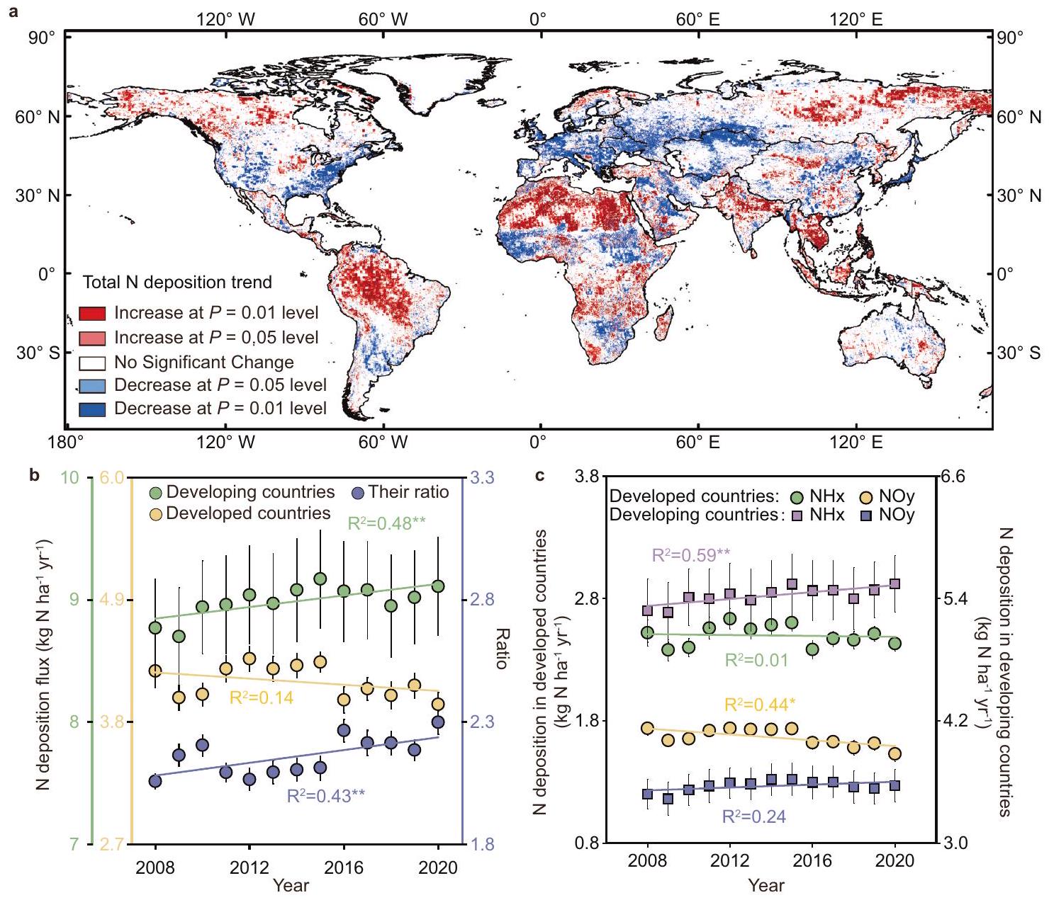
Transfer of global N deposition hotspots from 2008 to 2020
The global terrestrial has been relatively stable over the last decade (Fig. 1b) but, as noted above, in developed countries decreased, whereas it increased in developing countries in South Asia, Southeast Asia and South America (Fig. 2). Our calculations suggest that global hotspots of are moving from developed to developing regions. To
Fig. 2 | Regional dynamics of atmospheric N deposition from 1980 to 2020. a Dynamics in North America. b Dynamics in Western Europe. c Dynamics in Korea and Japan. d Dynamics in China. e Dynamics in Russia. f Dynamics in Western Asia. Dynamics in South Asia. Dynamics in Southeast Asia. i Dynamics in South America. The circles are direct observations and their error bars indicate SE (the variation among the monitoring sites). The triangles are results from the random forest models and their error bars indicate SE (variations across three random
forest models). Different colors represent different N deposition components. The trend of N deposition is fitted using linear or binomial functions. is the coefficient of determination,** represents the significance level at , and * represents the significance level at . The bar chart at the bottom of each plot shows the dynamics of the ratio of NHx to NOy deposition in the region. Source data are provided as a Source Data file.
verify the robustness of this conclusion, we analyzed trends in from 2008 to significantly increased in developing countries at middle and low latitudes in South Asia, Southeast Asia, and Brazil. However, it significantly decreased in developed countries or regions such as Europe, the eastern United States, and Japan. Meanwhile, N deposition in some regions of Africa, West Asia, and Argentina has also decreased (Fig. 3a). Decreases of and in those regions of Africa, West Asia and Argentina could directly contribute to the decline of in these areas (Supplementary fig. 6).
We also separately analyzed trends in in developed and developing countries from 2008 to 2020. The dynamics of changes in in developing and developed countries were different, with the ratio of between developing and developed countries showing a significant linear increase , Fig. 3b). In developed countries, the slight overall downtrend in was primarily due to a significant decrease in , while showed only a slight and nonsignificant decrease (Fig. 3c). This emphasizes the need for developed countries to strengthen measures to reduce emission hotspots. In contrast, the significant increase in developing countries is due to the significant increase of , Fig. 3c).
We analyzed trends at sites with continuous observations of wet deposition data from 2000 (Supplementary Fig. 7). This confirms that
global hotspots of have moved from developed to developing countries. It should be noted that these poorly monitored regions (i.e., Africa, Central Asia, Latin America, and Australia) still have the greatest uncertainty in , and these highly uncertain regions include many of those with increasing trends, which requires further observation. Meanwhile, some long-term trends of indicators, such as foliar N content and surface water nitrate concentration, declined in United States and Europe and increased in tropical forest and India , which potentially reflect the changing hotspots of .
Drivers of global deposition
is an important mechanism driving the dynamic changes in . We analyzed the correlations between and GDPpc, and MAP in five major global regions at national and regional scales. , NOx emissions ( ), and , and MAP were correlated with , and . The strength and positivity or negativity of the correlations varied according to region (Supplementary Fig. 8) showing that is strongly influenced by anthropogenic and meteorological factors, which is consistent with previous research .
Past research has developed a framework of active factors meteorological factors to analyze the factors and mechanisms influencing . However, this does not clearly show the role of social
Fig. 3 | Trends in deposition in developed and developing countries from 2008 to 2020. a Trend analysis of total N deposition from 2008 to 2020. b Temporal dynamics and ratios of total N deposition in developed and developing countries (Mean ± SE). c Temporal dynamics of NHx and NOy deposition in developed and developing countries (Mean ± SE). The trend of N deposition is
fitted using linear or binomial functions. is the coefficient of determination, ** and * represents the significance level at and , respectively, and SE (error bar in figure) indicated the variation across the three random forest models. Source data are provided as a Source Data file.
and economic development in changes in . We found that GDPpc had a significant negative correlation with in North America, Western Europe and East Asia. We also observed a less pronounced, less significant positive correlation with in Southeast Asia and Africa (Supplementary Fig. 8). We therefore built a cascade network of GDPpc MAP using structural equation models. The factors in these models and the processes that influence them can explain of the spatiotemporal variation (Supplementary Figs. 9 and 10), confirming the importance of socioeconomic development in determining changes in and its components.
We then analyzed the relationships between GDPpc and at the global scale using data from several countries or regions. The relationships between and GDPpc of countries or regions at different stages in their economic development fitted perfectly on a normal distribution curve (Fig. 4a-c; Supplementary Fig. 11a, b). This is consistent with the classical environmental Kuznets curve (EKC) model . When we tested the logarithmic cubic equation model of EKC, the normal distribution curves were all significant ( ) (Fig. 4d-f; Supplementary Fig. 11c, d; Supplementary Table 3). The peak of was at approximately , and the peaks of and were at and (Supplementary Table 3), respectively. The peak for was at approximately and that of at approximately . was predominantly derived from agricultural activities and reached its peak
before (in terms of time and/or economic development) , which was mostly driven by industrial activities. This indicates that socioeconomic development, as expressed by GDPpc, is an important factor in determining the spatiotemporal pattern of , and that the dynamic evolution of the relative contributions of agricultural and industrial activities determines the relationship between the peaks of and .
Implications for global management
The cumulative input of to terrestrial ecosystems from 1980 to 2020 ( 3117 Tg N ) was almost equivalent to the global N fertilizer application ( 3549 Tg N ) over the same period. N deposition can significantly increase the ecosystem productivity for forests, grasslands and water bodies , so the impact of such a substantial amount of natural N fertilization on the carbon cycle and carbon sink in ecosystems requires research , and the impacts of N deposition on species diversity, greenhouse gas emissions, soil acidification, etc., need to be re-assessed. Hotspots, areas of intensive N deposition, have moved from developed to developing countries at middle and low latitudes. Plant growth in tropical ecosystems in low latitudes is often limited by phosphorus , and an increase in N input tends to aggravate this limitation and reduce tree productivity , further threatening the structure and function of tropical ecosystems. Moreover, developed and developing countries have different dynamic trends of
Fig. 4 | Relationships between deposition and gross domestic product per capita on a global scale. Relationships between total and NOy (c, f) deposition and gross domestic product per capita (GDPpc). The data used in are observations of N deposition and GDPpc; those in are the logarithmic values of N deposition and of GDPpc. African countries are Niger, Mali, Cameroon
and Cote d’Ivoire. Southeast Asian countries are Vietnam, Malaysia, Indonesia and Thailand. East Asian countries are China, South Korea and Japan. Western European countries are EU countries (EU27). North American countries are the United States and Canada. is the coefficient of determination, ** represents the significance level at . Source data are provided as a Source Data file.
(Fig. 2), which affect ecosystems differently: plants can show a strong preference for or and the impacts of and deposition on soil acidification and greenhouse gas emissions also differ . Changes in may therefore lead to changes in the species composition of natural and semi-natural ecosystems.
Reducing N emissions and deposition in developing countries requires global cooperation and a better understanding of industry and agriculture contributions. remained the dominant role in global N deposition in 2020, but the relative contribution of changing to changes in was decreasing (Supplementary Fig. 12). Meanwhile, we found that from agriculture peaks before mainly from industrial activities, with higher peak value for (Fig. 4). The marginal cost of agricultural reduction is substantially lower than industrial reduction , making better N management in agriculture an economically efficient path for reducing N emissions while increasing crop yield and N use efficiency . Thus, developing countries should prioritize agricultural emission reduction technologies to peak before . However, most countries lack clear emission reduction policies and technologies . Therefore, developing countries should fund agriculture to support rapid emission reduction technology applications alongside industrial development. By creating more efficient agriculture, developing and transitioning countries will avoid following the same path of N pollution as developed countries,
and avoid the pollution events such as photochemical smog, acid rain, haze and soil acidification that Europe, North America and China have experienced .
Uncertainty analysis of global deposition evaluation
Based on the MGND database, this study developed a framework to conduct a global grid dataset and systematically evaluate the current status, dynamic change, regional patterns, and hotspots transfers of global N deposition. This is a global evaluation independent of atmospheric chemical transport model simulations and based on extensive observation data. Although the estimated global total N deposition input to land ( ) is higher than the results from atmospheric chemical transport model simulations , by summarizing global natural and anthropogenic , we found that total global can reach (Supplementary Table 2), indicating that our N deposition estimate is within a reasonable range.
Anthropogenic emission inventories (i.e., and NOx ) are important driving data for atmospheric chemical transport models that simulate atmospheric N deposition. Currently, inventories from the CEDS and Emissions Database for Global Atmospheric Research (EDGAR) are widely used in these models. These two datasets are estimated using a bottom-up approach based on emission activity information and emission factors. However, this approach is highly
uncertain, especially in regions lacking socio-economic statistics (such as Africa) and for components whose emission factors are highly variable and more complex . Recent studies using to correct emission inventories have shown that bottom-up estimates of are significantly underestimated, with and underestimated by about and 38%, respectively (Supplementary Table 2) , which may contribute to the lower estimates from models compared to our estimates.
We systematically compared the estimates in North America, Europe and China from other studies with our study, as well as the corresponding , and found consistent results across all studies (Supplementary Table 4). The relative uncertainty of was less than over most of areas (Supplementary Fig. 13). The uneven distribution of observation sites in the global atmospheric N deposition network may introduce bias in the machine learning models, especially in Africa, Central Asia, Latin America, and Australia, where sites are sparse. Although the cascading network of GDPpc meteorological factors → is globally applicable, it is crucial to strengthen N deposition observations in regions with limited data to reduce evaluation uncertainty.
Methods
Collection of atmospheric deposition site observation data
We used three sources of N deposition data: (1) data from 43 sites monitoring forests, grasslands, croplands, wetlands, deserts and cities from 2013 to 2020 in the Chinese Wet Deposition observation network (ChinaWD) ; (2) shared data from worldwide N deposition monitoring networks: European Monitoring and Evaluation Programme (EMEP) in Europe, the Clean Air Status and Trends Network (CASTNET), the Air Quality System (AQS), and the Ammonia Monitoring Network (AMoN) in the United States, the Canadian Air and Precipitation Monitoring Network (CAPMoN) and the National Air Pollution Surveillance Program (NAPS) in Canada, the Acid Deposition Monitoring Network (EANET) in East Asia, the International Network to Study Deposition and Atmospheric Composition in Africa (INDAAF), and the Nationwide Nitrogen Deposition Monitoring Network (NNDMN) from China Agricultural University ; (3) 1390 published papers reporting N deposition-related data from various locations (Supplementary Data 1). The criteria for selecting datasets from the literature were that the monitoring index had to include (i) ammonium, nitrate, total wet deposition (sum of ammonium and nitrate) or their concentrations in precipitation; (ii) the concentration or dry deposition of and ; (iii) daily, weekly or monthly observation frequencies; (iv) an observation period longer than one year.
The resultant MGND database includes site name, location, monitoring time, monitoring method, ecosystem type, annual rainfall, N concentration and flux of each component, and the data source. It spans 1977-2021 and includes 25,808 site years of wet deposition and 26,863 site years of dry deposition (Supplementary fig. 1 and Supplementary Table 1). Wet deposition comprised ammonium ( ) and nitrate ( ); dry deposition comprised gaseous , particulate , gaseous , gaseous ( ) and particulate (Supplementary Table 1).
Sources of auxiliary analysis data
The sources of auxiliary analysis data and detailed information used in this study are shown in Supplementary Table 5. Meteorological data mainly come from Climatic Research Unit (CRU, version cru_ts4.05) and the reanalysis product of NECP-NCAR (NECEP-NCAR Reanalysis 1) , including MAP, mean annual temperature (MAT), Wet days (WET), Vapor pressure (VAP), net shortwave radiation flux (Nswrs), surface pressure (Pres), specific humidity (Shum) and wind speed (Wspd).
Anthropogenic pollutants emission inventories were obtained from CEDS (version CEDS v_2021_04_21) . We also used from EDGAR and Luo et al. . data were obtained from the Infrared Atmospheric Sounding Interferometer (IASI) . We used the standard monthly scale reanalysis of tertiary data products for 2008-2020. data were obtained from the Ozone Monitoring Instrument (OMI), Global Ozone Monitoring Experiment (GOME) and Scanning Imaging Absorption Spectrometer for Atmospheric Chartography (SCIAMACHY) . The three satellite datasets were integrated into one dataset and covered 1996-2020 . column concentration ( ) were obtained from OMI/Aura SO total column daily L3 data .
Data on the GDPpc and the population of each country were derived from the Maddison Project Database . The GDPpc were based on prices in 2011, which eliminated the impact of price changes and reflected the real values of product output over different periods. In addition, we also used , night light , grid GDP , population , Normalized Difference Vegetation Index (NDVI) , global production-living-ecological space data , terrestrial human footprint dataset , crop-specific N fertilization dataset , and statistics data on N fertilizer application per unit area (Supplementary Table 5).
Analysis of temporal dynamic from site observation
We analyzed the variation of in ten major countries or regions: Western Europe, North America, South America, Russia, Africa, Southeast Asia, South Asia, Western Asia, China, Japan and South Korea. The annual in each area was calculated as the annual arithmetic mean and standard error of all the observed data for that area, including , and .
We used linear or nonlinear equations to analyze the trends in deposition from 1980 to 2020 in each area. We interpolated missing data based on the optimal fitted model for with time for a specific area or period. Mean values and trends in global were calculated using the weighted average method. We selected 352 observation sites with five years of continuous monitoring since 2000 and used the Mann-Kendall method to analyze trends at the site scale.
All data were analyzed with SPSS version 13.0 statistical software. The correlations between and GDPpc, and MAP in five major global regions at national and regional scales were analyzed. The structural equation model was used to explore the predicators and influencing paths of . All figures were drawn using SigmaPlot version 12.0 software. The spatial pattern figures for were plotted with ArcGIS 10.0 software.
Construction of global deposition grid dataset
We developed a framework to generate global grid from site observation data between 2008 and 2020 (Supplementary Fig. 14). We did not extend the data to before 2008 due to insufficient data availability of some important variable (i.e., ). To minimize the influence of unevenly distribution observation sites on predicting global N deposition, we classified the global land into two categories: wilderness and human-modified area, based on global human footprint data, and . The global human footprint reflects various aspects of human pressures using eight variables, including built environments, population density, nighttime light, croplands, pasture lands, roadways, railways, and navigable waterways . We defined wilderness areas as the intersection of regions where the global human footprint data is is in the lowest , and is in the lowest 2.5% for each year.
In general, wilderness areas are primarily located in high-latitude northern regions such as Alaska, Greenland, and Siberia, as well as the Sahara Desert in Africa, the Tibetan Plateau in China, and the desert regions of Australia. Our hypothesis is that these wilderness areas are less disturbed by anthropogenic activities, resulting in low levels of . Areas with higher have higher . Therefore, in these areas is
estimated as Eq. (1):
where represents the N deposition flux ( ); represents normalization of ; represents normalization of ; i represents N components; j represents years from 2008 to 2020; 0.01 is a unit conversion factor that considers pre-industrial N deposition levels ( ).
For human modified area, we used machine learning methods to upscale from the site scale to the global grid scale. Only data from the main worldwide deposition observation networks was selected as the independent variable to achieve consistency and continuity of observations and methods. Notably, the random forest models demonstrated superior predictive accuracy, indicated by higher values both in the training and test sets, compared to support vector machine and BP neural network (Supplementary Table 6). We exclusively used random forest models to predict global N deposition in human-modified areas, employing three key pathways: the n6 model, the n 22 best model, and the cascade model (Supplementary Table 7).
The randomForest package in R software was used to build all the prediction model mentioned above. During model building, of the data were randomly selected as the training set to evaluate the accuracy of the prediction model and selected as the test set to evaluate the prediction performance of the model. The random forest models for deposition were constructed using the ground monitoring concentrations of the different components. Deposition was estimated by multiplying the ground monitoring concentrations by the corresponding deposition velocity. We used recursive feature elimination (RFE) method to obtain the optimal variable combination in the n 22 best model and the cascade model. Additionally, for all models, we used grid search method to select the best hyperparameters, such as the number of trees (between 100 and 1000), mtry (between 1 and the number of predictor variables or of predictor variables for the n 22 best models), and nodesize (the number of variables used at each node split, between 1 and the number of predictor variables), to maximize out-of-bag value. Shapley values (SHAP) were calculated to determine feature importance and analyze the sensitivity of the output to the input variable.
The n6 model was built with least variable combination based on the cascade network of GDPpc MAP that was proven for China in our previous research . The variation explained by the n 6 models ranged from to (Supplementary Table 7). was the most important predictor for most N deposition components while was the most important predictors for ground and concentration (Supplementary Fig. 15).
The n 22 best model builds on the n 6 model, further enhancing its explanatory and predictive abilities. Using the RFE method, we optimized the best variable combination from 22 variables. As expected, the n 22 best models’ explanation rates are higher than those of the n 6 models, except for ground and concentration (Supplementary Table 7). The most important predictor in the n 22 best model was nearly the same as in the n 6 models (Supplementary Fig. 16).
Given the large uncertainties in the emission inventory data, especially for , we assumed this data would significantly impact the prediction results. Therefore, we designed the cascade model to first use , economic activity, and land use to predict . Then, we used the predicted mission , combined with , meteorological factors, and atmospheric pollutant emission data, to predict (Supplementary Table 7). We extracted four sets of raster data ( from CEDS, EDGAR, and two products in Luo et al. ) with less than 10 % variation in , identified as the more accurate raster data for assessment, and used them as the dependent variable when predicting in cascade model. was the most important predictors for predicting , and the variable was the most important predictors for (Supplementary Fig. 17).
Finally, we combined the N deposition dataset for wilderness and human-modified area to generate a spatial dataset for global from 2008-2020 with a spatial resolution of . The global annual input of N through deposition to land in 2020 was highest according to the cascade model ( ), followed by the n 22 best model ( ), and then the n 6 model ( 85.6 Tg N ) (Supplementary Table 8). The relative uncertainty at each pixel were calculated across three models. The relative uncertainty was defined as the ratio of standard error to the mean value of three models. We also used the Theil-Sen Median (Sen slope estimate) to analyze the trend of global N deposition during 2008-2020. The Mann-Kendall nonparametric test was used to determine the significance of the trends.
Relating deposition to economic growth
We integrated the global data of five regions – East Asia, Southeast Asia, Africa, Western Europe and North America – that had relatively longterm N deposition observations at different stages of social development into one reginal dataset. Two methods were used to analyze the relationship between and GDPpc, and to determine whether it conforms to the EKC. Firstly, based on scatter plots, a high-order equation was used to explore the relationship between GDPpc and in each area. Secondly, a logarithmic cubic equation (Eq. (2)) was used to analyze the relationship between and GDPpc. The logarithmic cubic equation fitting parameters are listed in Supplementary Table 5.
where is the real per capita GDP of each area in certain year, is the corresponding average N deposition flux, and represents ammonium, nitrate, wet, dry or total deposition. is a constant and , and are the estimated coefficients.
Reporting summary
Further information on research design is available in the Nature Portfolio Reporting Summary linked to this article.
The primary code used in this study is available at https://doi.org/10. 6084/m9.figshare.26778574.
References
Malik, A. et al. Drivers of global nitrogen emissions. Environ. Res. Lett. 17, 015006 (2022).
Fowler, D. et al. The global nitrogen cycle in the twenty-first century. Philos. Trans. R. Soc. B 368, 20130164 (2013).
Dentener, F. et al. Nitrogen and sulfur deposition on regional and global scales: A multimodel evaluation. Global Biogeochem. Cycles 20, GB4003 (2006).
Reay, D. S., Dentener, F., Smith, P., Grace, J. & Feely, R. A. Global nitrogen deposition and carbon sinks. Nat. Geosci. 1, 430-437(2008).
Thomas, R. Q., Canham, C. D., Weathers, K. C. & Goodale, C. L. Increased tree carbon storage in response to nitrogen deposition in the US. Nat. Geosci. 3, 13-17 (2010).
Guo, J. H. et al. Significant acidification in major Chinese croplands. Science 327, 1008-1010 (2010).
Bowman, W. D., Cleveland, C. C., Halada, L., Hresko, J. & Baron, J. S. Negative impact of nitrogen deposition on soil buffering capacity. Nat. Geosci. 1, 767-770 (2008).
Bobbink, R. et al. Global assessment of nitrogen deposition effects on terrestrial plant diversity: a synthesis. Ecol. Appl. 20, 30-59 (2010).
Richter, A., Burrows, J. P., Nuss, H., Granier, C. & Niemeier, U. Increase in tropospheric nitrogen dioxide over China observed from space. Nature 437, 129-132 (2005).
Ge, Y., Vieno, M., Stevenson, D. S., Wind, P. & Heal, M. R. A new assessment of global and regional budgets, fluxes, and lifetimes of atmospheric reactive N and S gases and aerosols. Atmos. Chem. Phys. 22, 8343-8368 (2022).
Liu, X. J. et al. Enhanced nitrogen deposition over China. Nature 494, 459-462 (2013).
Engardt, M., Simpson, D., Schwikowski, M. & Granat, L. Deposition of sulphur and nitrogen in Europe 1900-2050. Model calculations and comparison to historical observations. Tellus B: Chem. Phys. Meteorol. 69, 1328945 (2017).
Li, Y. et al. Increasing importance of deposition of reduced nitrogen in the United States. Proc. Natl. Acad. Sci. USA. 113, 5874-5879 (2016).
Wen, Z. et al. Changes of nitrogen deposition in China from 1980 to 2018. Environ. Int. 144, 106022 (2020).
Yu, G. et al. Stabilization of atmospheric nitrogen deposition in China over the past decade. Nat. Geosci. 12, 424-429 (2019).
Uwizeye, A. et al. Nitrogen emissions along global livestock supply chains. Nat. Food 1, 437-446 (2020).
Vet, R. et al. A global assessment of precipitation chemistry and deposition of sulfur, nitrogen, sea salt, base cations, organic acids, acidity and pH, and phosphorus. Atmos. Environ. 93, 3-100 (2014).
Vishwakarma, S., Zhang, X., Dobermann, A., Heffer, P. & Zhou, F. Global nitrogen deposition inputs to cropland at national scale from 1961 to 2020. Sci. Data 10, 488 (2023).
Gu, B. et al. Cleaning up nitrogen pollution may reduce future carbon sinks. Global Environ. Change 48, 56-66 (2018).
Zhang, X. et al. Managing nitrogen for sustainable development. Nature 528, 51-59 (2015).
Tan, J. et al. Multi-model study of HTAP II on sulfur and nitrogen deposition. Atmos. Chem. Phys. 18, 6847-6866 (2018).
Rubin, H. J. et al. Global nitrogen and sulfur deposition mapping using a measurement-model fusion approach. Atmos. Chem. Phys. 23, 7091-7102 (2023).
Tian, H. et al. History of anthropogenic Nitrogen inputs ( HaNi ) to the terrestrial biosphere: a 5 arcmin resolution annual dataset from 1860 to 2019. Earth Syst. Sci. Data 14, 4551-4568 (2022).
Ackerman, D., Millet, D. B. & Chen, X. Global estimates of inorganic nitrogen deposition across four decades. Global Biogeochem. Cycles 33, 100-107 (2019).
Van Damme, M. et al. Global, regional and national trends of atmospheric ammonia derived from a decadal (2008-2018) satellite record. Environ. Res. Lett. 16, 055017 (2021).
O’Rourke P. R. et al. CEDS v-2021_04_21 Gridded Emissions Data (accessed on 1 Dec 2021, available at https://data.pnnl.gov/ dataset/CEDS-4-21-21). (2021).
Mason, R. E. et al. Evidence, causes, and consequences of declining nitrogen availability in terrestrial ecosystems. Science 376, eabh3767 (2022).
McLauchlan, K. K., Ferguson, C. J., Wilson, I. E., Ocheltree, T. W. & Craine, J. M. Thirteen decades of foliar isotopes indicate declining nitrogen availability in central North American grasslands. New Phytol. 187, 1135-1145 (2010).
Eshleman, K. N., Sabo, R. D. & Kline, K. M. Surface water quality is improving due to declining atmospheric N deposition. Environ. Sci. Technol. 47, 12193-12200 (2013).
Penuelas, J. et al. Increasing atmospheric concentrations correlate with declining nutritional status of European forests. Commun. Biol. 3, 125 (2020).
Vuorenmaa, J. et al. Long-term changes (1990-2015) in the atmospheric deposition and runoff water chemistry of sulphate, inorganic nitrogen and acidity for forested catchments in Europe in relation to changes in emissions and hydrometeorological conditions. Sci. Total Environ. 625, 1129-1145 (2018).
Hietz, P. et al. Long-term change in the nitrogen cycle of tropical forests. Science 334, 664-666 (2011).
Pandey, J., Singh, A. V., Singh, A. & Singh, R. Impacts of changing atmospheric deposition chemistry on nitrogen and phosphorus loading to Ganga River (India). Bull. Environ. Contamination Toxicol. 91, 184-190 (2013).
Dinda, S. Environmental Kuznets Curve hypothesis: A survey. Ecol. Econ. 49, 431-455 (2004).
Eastman, B. A. et al. Altered plant carbon partitioning enhanced forest ecosystem carbon storage after 25 years of nitrogen additions. New Phytol. 230, 1435-1448 (2021).
Stevens, C. J. et al. Anthropogenic nitrogen deposition predicts local grassland primary production worldwide. Ecology 96, 1459-1465 (2015).
Zaehle, S. Terrestrial nitrogen – carbon cycle interactions at the global scale. Philos. Trans. R. Soc. B 368, 20130125 (2013).
Du, E. Z. et al. Global patterns of terrestrial nitrogen and phosphorus limitation. Nat. Geosci. 13, 221-226 (2020).
Li, Y., Niu, S. & Yu, G. Aggravated phosphorus limitation on biomass production under increasing nitrogen loading: a meta-analysis. Global Change Biol. 22, 934-943 (2016).
Ashton, I. W., Miller, A. E., Bowman, W. D. & Suding, K. N. Niche complementarity due to plasticity in resource use: plant partitioning of chemical N forms. Ecology 91, 3252-3260 (2010).
Song, M. H., Zheng, L. L., Suding, K. N., Yin, T. F. & Yu, F. H. Plasticity in nitrogen form uptake and preference in response to long-term nitrogen fertilization. Plant Soil 394, 215-224 (2015).
Galloway, J. N. Acid deposition: Perspectives in time and space. Water Air Soil Pollut. 85, 15-24 (1995).
Li, X. et al. The contrasting effects of deposited and on soil and fluxes in a subtropical plantation, southern China. Ecol. Eng. 85, 317-327 (2015).
Gu, B. J. et al. Abating ammonia is more cost-effective than nitrogen oxides for mitigating air pollution. Science 374, 758-762 (2021).
Gu, B. et al. Cost-effective mitigation of nitrogen pollution from global croplands. Nature 613, 77-84 (2023).
Guo, Y. X. et al. Air quality, nitrogen use efficiency and food security in China are improved by cost-effective agricultural nitrogen management. Nat. Food 1, 648-658 (2020).
Liu, L. et al. Exploring global changes in agricultural ammonia emissions and their contribution to nitrogen deposition since 1980. Proc. Natl. Acad. Sci. USA. 119, e2121998119 (2022).
Fowler, D. et al. A chronology of global air quality. Philos. Trans. R. Soc. A 378, 20190314 (2020).
Menz, F. C. & Seip, H. M. Acid rain in Europe and the United States: an update. Environ. Sci. Policy 7, 253-265 (2004).
Johansson, L., Jalkanen, J.-P. & Kukkonen, J. Global assessment of shipping emissions in 2015 on a high spatial and temporal resolution. Atmos. Environ. 167, 403-415 (2017).
Luo, Z. et al. Estimating global ammonia emissions based on IASI observations from 2008 to 2018. Atmos. Chem. Phys. 22, 10375-10388 (2022).
Miyazaki, K. et al. Decadal changes in global surface NOx emissions from multi-constituent satellite data assimilation. Atmos. Chem. Phys. 17, 807-837 (2017).
Zhu, J. et al. The composition, spatial patterns, and influencing factors of atmospheric wet nitrogen deposition in Chinese terrestrial ecosystems. Sci. Total Environ. 511, 777-785 (2015).
Harris, I., Osborn, T. J., Jones, P. & Lister, D. Version 4 of the CRU TS monthly high-resolution gridded multivariate climate dataset. Sci. Data 7, 109 (2020).
Kalnay, E. et al. The NCEP/NCAR 40-Year reanalysis project. J. Bullet. Am. Meteorol. Soc. 77, 437-472 (1996).
Van Damme, M. et al. Version 2 of the IASI neural network retrieval algorithm: near-real-time and reanalysed datasets. Atmos. Meas. Tech. 10, 4905-4914 (2017).
Boersma, K. F. et al. An improved tropospheric column retrieval algorithm for the Ozone Monitoring Instrument. Atmos. Meas. Tech. 4, 1905-1928 (2011).
Li, C. et al. Version 2 Ozone Monitoring Instrument product ( ): new anthropogenic vertical column density dataset. Atmos. Meas. Tech. 13, 6175-6191 (2020).
Bolt J., Jan LvZ. Maddison Project Database (accessed on 1 Feb 2022, available at https://www.rug.nl/ggdc/historicaldevelopment/ maddison/releases/maddison-project-database-2020). (2020).
van Donkelaar, A. et al. Monthly global estimates of fine particulate matter and their uncertainty. Environ. Sci. Technol. 55, 15287-15300 (2021).
Chen, Z. et al. An extended time series (2000-2018) of global NPP-VIIRS-like nighttime light data from a cross-sensor calibration. Earth Syst. Sci. Data 13, 889-906 (2021).
Chen, J. et al. Global gridded revised real gross domestic product and electricity consumption during 1992-2019 based on calibrated nighttime light data. Sci. Data 9, 202 (2022).
K. Didan, A. Huete, DAAC NL. MOD13C2 MODIS/Terra Vegetation Indices Monthly L3 Global 0.05Deg CMG (access on 5 Jun 2022, available at https://doi.org/10.5067/MODIS/MOD13C2.006). (2015).
Fu, J., Gao, Q., Jiang, D., Li, X. & Lin, G. Spatial-temporal distribution of global production-living-ecological space during the period 2000-2020. Sci. Data 10, 589 (2023).
Mu, H. et al. A global record of annual terrestrial Human Footprint dataset from 2000 to 2018. Sci. Data 9, 176 (2022).
Adalibieke, W., Cui, X., Cai, H., You, L. & Zhou, F. Global crop-specific nitrogen fertilization dataset in 1961-2020. Sci. Data 10, 617 (2023).
Breiman, L. Random forests. Mach. Learn. 45, 5-32 (2001).
Acknowledgements
This work was supported by the National Natural Science Foundation of China (31988102, G.Y., 32201364, J.Z., and 31872690, Q.W.), and the CAS (Chinese Academy of Sciences) Project for Young Scientists in Basic Research (YSBR-037, J.Z.). We acknowledge the free use of tropospheric column data from the OMI, GOME, and SCIAMACHY sensors from www.temis.nl and column data from the IASI. We thank all the sponsors of the nine monitoring networks used in this study, including the Co-operative Programme for Monitoring and Evaluation of the LongRange Transmission of Air Pollutants in Europe (European Monitoring and Evaluation Programme, EMEP), the Clean Air Status and Trends Network (CASTNET) in the United States, the Air Quality System (AQS) in the United States, the Ammonia Monitoring Network (AMoN) in the United States, the Canadian Air and Precipitation Monitoring Network (CAPMoN), the National Air Pollution Surveillance Program (NAPS) in Canada, the Acid Deposition Monitoring Network in East Asia (EANET), and International Network to study Deposition and Atmospheric composition in Africa (INDAAF). We are grateful to the ecological stations and all monitors from the Chinese Ecosystem Research Network (CERN), ChinaFLUX, and ChinaWD for sample collecting. We thank Dr. U.C. Kulshrestha from Indian Institute of Chemical Technology for providing monitoring N deposition data of India. We also thank all the scientists whose data were used in our synthesis.
Author contributions
G.Y. designed the research. J.Z., Y.J., N.H., Q.W., Z.C., H.H., X.Z., and P. L. conducted the research (collected the datasets and analyzed the data). J.Z., Y.J., and G.Y. wrote the manuscript. X.L., K.G., D.F., P.V. and F.Z. commented and revised on the manuscript.
Correspondence and requests for materials should be addressed to Guirui Yu.
Peer review information Nature Communications thanks Hanqin Tian, and the other, anonymous, reviewer(s) for their contribution to the peer review of this work. A peer review file is available.
Publisher’s note Springer Nature remains neutral with regard to jurisdictional claims in published maps and institutional affiliations.
Open Access This article is licensed under a Creative Commons Attribution-NonCommercial-NoDerivatives 4.0 International License, which permits any non-commercial use, sharing, distribution and reproduction in any medium or format, as long as you give appropriate credit to the original author(s) and the source, provide a link to the Creative Commons licence, and indicate if you modified the licensed material. You do not have permission under this licence to share adapted material derived from this article or parts of it. The images or other third party material in this article are included in the article’s Creative Commons licence, unless indicated otherwise in a credit line to the material. If material is not included in the article’s Creative Commons licence and your intended use is not permitted by statutory regulation or exceeds the permitted use, you will need to obtain permission directly from the copyright holder. To view a copy of this licence, visit http:// creativecommons.org/licenses/by-nc-nd/4.0/.
Key Laboratory of Ecosystem Network Observation and Modeling, Institute of Geographic Sciences and Natural Resources Research, Chinese Academy of Sciences, Beijing, China. College of Forestry, Hebei Agricultural University, Baoding, China. College of Resources and Environment, University of Chinese Academy of Sciences, Beijing, China. Institute of Carbon Neutrality, Northeast Forestry University, Harbin, China. College of Agronomy, Shenyang Agricultural University, Shenyang, China. Institute of Surface-Earth System Science, School of Earth System Science, Tianjin University, Tianjin, China. State Key Laboratory of Nutrient Use and Management, College of Resources and Environmental Sciences, National Academy of Agriculture Green Development, China Agricultural University, Beijing, China. Sustainable Agricultural Sciences Department, Rothamsted Research, Harpenden, UK. Centre for Ecology and Hydrology, Penicuik, UK. Department of Biology, Stanford University, Stanford, USA. These authors contributed equally: Jianxing Zhu, Yanlong Jia. ⟶ e-mail: yugr@igsnrr.ac.cn
The values are Mean ± SD among the three random forest models’ results. , and are wet, dry, and total N deposition, respectively.