تعتبر ملاءمة واستقرار مناخ الأرض أمراً حاسماً لبقاء الإنسان (كارلسون وآخرون، 2022؛ كافيتشولي وآخرون، 2019) والتنمية (براون وآخرون، 2023؛ راي وآخرون، 2015؛ دياز ومور، 2017). ومع ذلك، اعتباراً من يناير 2024، تسارعت درجات حرارة السطح العالمية بمقدار منذ الفترة ما قبل الصناعية (بيركلي، 2024). وفقاً لتقرير تقييم المناخ السابع للهيئة الحكومية الدولية المعنية بتغير المناخ (AR 7)، فإن الاحترار العالمي ناتج “بلا لبس” أساساً عن الأنشطة البشرية وانبعاثات غازات الدفيئة الناتجة عن الإنسان (IPCC، 2023). عند الاعتراف المجتمعي بالسببية، تبرز مسألة كيفية تحويل نموذج التنمية الحالي ليتماشى مع مبادئ التخفيف من تغير المناخ كتركيز مركزي للاهتمام الحكومي (دوان وآخرون، 2021؛ داي وآخرون، 2023) والأكاديمي (فوزي وآخرون، 2020؛ هوغ-غولدبرغ وآخرون، 2019؛ فانكهاوزر وآخرون، 2022).

يعتبر منحنى كوزنتس البيئي (EKC) من بين أكثر نماذج المحاكاة الاقتصادية-البيئية انتشاراً المستخدمة في تحليل السياسات (زو وآخرون، 2022؛ كوندهار وآخرون، 2021؛ ماو وآخرون، 2022). ربطت فرضية EKC التنمية الاقتصادية بجودة البيئة في مثل هذا النموذج: يرتفع دخل الفرد وانبعاثات ثاني أكسيد الكربون للفرد معاً حتى يتم الوصول إلى نقطة انعطاف معينة في الدخل، وبعد ذلك يتوقف نمو الملوثات ثم ينقلب (غروس مان وكروجر، 1995). تم تأكيد مثل هذه الأنماط غير الخطية على شكل حرف U المعكوس تجريبياً في عدد لا يحصى من الدراسات المبكرة، وتُعطى التفسيرات بشكل رئيسي من خلال تقنيات الإنتاج غير الفعالة والملوثة في المراحل ما قبل الصناعية وتعزيز اللوائح البيئية والتقنيات النظيفة المتقدمة في المراحل المتقدمة (بالسالوبري-لورينتي وآخرون، 2018). على مدى العقود الثلاثة الماضية، غالباً ما كانت مثل هذه النماذج من “النمو أولاً والتنظيف لاحقاً” بمثابة معيار لنماذج المناخ الأخرى وحتى كمرجع للخطط الوطنية (كوندهار وآخرون، 2021؛ كايكا وزيرفاس، 2013a).

ومع ذلك، تشير العديد من الأخبار والأحداث التي نسمعها ونلاحظها مؤخراً إلى ضعف العلاقة بين الاقتصادات المتقدمة والبيئة المحسنة، مما يبدو أنه يتعارض مع التفسير الحالي. أولاً، من المعروف أن بعض الدول المتقدمة بما في ذلك الولايات المتحدة تعاني من عجز بيئي (أوسمان وآخرون، 2020؛ لارك وآخرون، 2020). علاوة على ذلك، في نوفمبر 2020، كأكبر اقتصاد في العالم وثاني أكبر مصدر للكربون، تعهدت الولايات المتحدة بالانسحاب من اتفاقية باريس لإعادة تشغيل قطاعاتها التقليدية والملوثة بشدة (شيريماير، 2020؛ رولفسيما وآخرون، 2020). أخيراً، تعود العديد من الدول المتقدمة، بما في ذلك ألمانيا وهولندا والنمسا، مرة أخرى إلى الفحم لتوليد الكهرباء والتدفئة بينما تكافح مع أزمة الطاقة الأوروبية التي triggered by the Russia-Ukraine conflict beginning in 2022 (Tollefson, 2022; Guan et al., 2023).

تسلط هذه الأحداث الضوء على الحاجة إلى إعادة النظر في منحنى كوزنتس البيئي العالمي، مع مناقشة منحنى الشكل N بشكل خاص. من ناحية، فإن النموذج الجديد لمنحنى الشكل N أكثر ملاءمة للوضع الفعلي الحالي من منحنى كوزنتس البيئي المعكوس على شكل حرف U. وذلك لأن مسار انبعاثات الكربون قد لا يزال ينحني لأعلى عند مستوى عالٍ من التنمية الاقتصادية إذا لم تتمكن التأثيرات التكنولوجية الناتجة عن الابتكار الأخضر من مواكبة تأثيرات الحجم المتزايدة (لورينتي وآلڤاريز-هيررانز، 2016). من ناحية أخرى، بمجرد أن يتم خيبة أمل الالتزام بـ “التنمية أولاً، والتنظيف لاحقاً” من نظرية منحنى كوزنتس البيئي المعكوس السابقة، لا يمكن للدول النامية أن تجلس وتستبعد من جدول أعمال المناخ وخطط تخفيض الانبعاثات (كوندهار وآخرون، 2021؛ كايكا وزيرفاس، 2013a). ومن ثم، فإن الفهم الدقيق للشكل الحالي لمنحنى كوزنتس البيئي العالمي أمر حاسم لفئات الدول المختلفة لتحديد محركات انبعاثات الكربون الفريدة الخاصة بها واتخاذ إجراءات سريعة.

تظهر الحالة الحالية، من الجانب الآخر، أيضاً تعقيد القواعد المحددة لانبعاثات الكربون.

على الرغم من أن بعض المتغيرات الإضافية بما في ذلك الانفتاح التجاري، وجودة المؤسسات، واستهلاك الطاقة قد تم دمجها على نطاق واسع في إطار منحنى كوزنتس البيئي (ليال وماركيز، 2022)، فقد أثبتت الأبحاث الحديثة وجود بعض الروابط الجديدة بين العوامل الخارجية وانبعاثات الكربون. على سبيل المثال، تم إثبات أن المخاطر الجيوسياسية والمخاطر السياسية والاقتصادية والمالية الوطنية لديها القدرة على تغيير أنماط التنمية الاقتصادية واستخدام الطاقة في الدول (أنسر وآخرون، 2021؛ حسن وآخرون، 2022؛ كيانغ وانغ وآخرون، 2023a). تم العثور على أن التكنولوجيا الرقمية والذكاء الاصطناعي، كعوامل رئيسية في الثورتين الصناعيتين الثالثة والرابعة، لها تأثيرات مخفضة للكربون في بعض الدراسات (جينينغ زانغ وآخرون، 2022a؛ دينغ وآخرون، 2023). تم تأكيد الانتقال من الوقود الأحفوري التقليدي إلى مصادر الطاقة الجديدة بشكل تجريبي كوسيلة فعالة للتخفيف من تلوث الهواء وتسريع الحياد الكربوني (فينغ دونغ وآخرون، 2022b؛ نعيم وآخرون، 2023). أخيراً، تم تضمين بعض القضايا الاجتماعية، بما في ذلك شيخوخة السكان (فان وآخرون، 2021) والأمن الغذائي (نسيم وآخرون، 2020)، أيضاً في التحليل البيئي. كما أشار (ستيرن، 2017) إلى أنه من الضروري الكشف عن تأثيرات المتغيرات الأخرى بخلاف النمو الاقتصادي ضمن إطار منحنى كوزنتس البيئي. بالاعتماد على هذه القضايا الحالية المتعلقة بالبيئة العالمية وانبعاثات الكربون، نطرح الأسئلة التالية: ما هو الشكل الحالي لمنحنى كوزنتس البيئي العالمي عند أخذ عوامل إضافية جديدة في الاعتبار؟ هل هناك عدم تجانس في تأثير العوامل المختلفة على انبعاثات الكربون في أنواع مختلفة من الدول؟

تهدف هذه المقالة إلى الإجابة على الأسئلة المذكورة أعلاه من خلال دراسة شكل منحنى كوزنتس البيئي العالمي الحالي بشكل تجريبي وأخذ تأثير عوامل انبعاث الكربون المتعددة والتباين في العينة بعين الاعتبار. على وجه التحديد، تسهم هذه الورقة في الأدبيات في الجوانب الثلاثة التالية. أولاً، تدرس هذه الورقة منحنى كوزنتس البيئي على شكل N في 214 دولة وتدمج 12 عاملاً مؤسسياً أو تكنولوجياً أو مواردياً أو اجتماعياً تقليدياً أو جديداً كمتغيرات إضافية في معادلة منحنى كوزنتس البيئي. توفر هذه الدراسة معلومات أولية ولكنها حاسمة لإجراءات التخفيف من خلال توضيح العلاقة بين التنمية الاقتصادية العالمية وانبعاثات الكربون وتحديد العوامل المحتملة لانبعاثات الكربون. ثانياً، للتعامل مع تباين الدول، نطور نموذج فك الارتباط ثنائي الأبعاد بناءً على منحنى كوزنتس البيئي من النوع N لتقييم مرحلة التنمية الاقتصادية ووضع فك الارتباط لكل دولة. نعتقد أن بدء مناقشة مصنفة ومفصلة يمكن أن يساعد في الكشف بشكل أكثر منهجية عن الأوضاع أو المشكلات المختلفة في التنمية الاقتصادية وتقليل انبعاثات الكربون في الدول حول العالم. أخيراً، استناداً إلى نتائج التجميع، نقوم بتحليل التباين بين المجموعات في تأثيرات انبعاثات الكربون للمتغيرات الاقتصادية والإضافية، مما يوفر مرجعاً أساسياً للدول في مراحل مختلفة لوضع سياسات فعالة وموجهة لتقليل انبعاثات الكربون.

تم ترتيب بقية هذه المقالة على النحو التالي. تستعرض قسم “مراجعة الأدبيات والخلفية النظرية” الدراسات المتعلقة بمنحنى كوزنتس البيئي والمتغيرات الإضافية وتطور الفرضيات الرئيسية. يقدم قسم “الطريقة والبيانات” مقدمة موجزة عن المنهجية والنموذج والبيانات. في قسم “النتائج التجريبية”، نناقش النتائج البحثية العالمية والمجموعة. يُترك قسم “الملاحظات الختامية” للاختتام.

الأصل والتطور والنقد ذي الصلة لمنحنى كوزنتس البيئي. تم إعادة تفسير العلاقة غير الخطية بين دخل الفرد وعدم المساواة في الدخل التي اقترحها (كوزنتس، 1955) على أنها منحنى كوزنتس البيئي في مجال الاقتصاد البيئي في التسعينيات. تم اقتراح مفهوم منحنى كوزنتس البيئي، الذي استخدم في الأصل لوصف العلاقة على شكل U مقلوب بين النمو الاقتصادي
وتدهور البيئة، من قبل (غروس مان وكروجر، 1991) في دراستهم الرائدة حول الآثار البيئية لاتفاقية التجارة الحرة لأمريكا الشمالية. قام الباحثون الأوائل في منحنى كوزنتس البيئي بتحليل العلاقة بين النمو الاقتصادي ومؤشرات تدهور البيئة المختلفة دون أي متغيرات تفسيرية أخرى وحصلوا على الكثير من الأدلة على وجود علاقة على شكل U مقلوب من الارتباطات الإيجابية ثم السلبية بين الاثنين (غروس مان وكروجر، 1991؛ بيكرمان، 1992؛ غروس مان وكروجر، 1995؛ هيرينك وآخرون، 2001).

أجرت الأبحاث اللاحقة تحسينين رئيسيين على إطار البحث التجريبي الكلاسيكي لمنحنى كوزنتس البيئي. من ناحية، تم اقتراح منحنيات كوزنتس البيئي على شكل N نظرياً وتم تأكيدها تجريبياً في الدراسات العالمية والدراسات عبر الدول والدراسات الفردية في أحدث الدراسات التجريبية. على سبيل المثال، اختبر ألارد وآخرون (2018) العلاقة بين انبعاثات CO2 والناتج المحلي الإجمالي للفرد في أربع مجموعات دخل (منخفضة، ومتوسطة عليا، ومتوسطة دنيا، وعالية الدخل) تحتوي على إجمالي 74 دولة ووجدوا منحنى كوزنتس البيئي على شكل N لجميع مجموعات الدخل باستثناء دول الدخل المتوسط العليا. باستخدام البصمة البيئية كمتغير بديل لتلوث البيئة، حصل نعمان وآخرون (2022) على استنتاجات مشابهة جداً بين مجموعات الدول من أربعة مستويات دخل تشمل 85 دولة. بالإضافة إلى ذلك، تم العثور على منحنيات على شكل N أيضاً في حالة تسع دول رائدة في إنتاج الطاقة النووية (جاهانجر وآخرون، 2023)، ودول أوبك (أولاه وآخرون، 2023)، ودول E-10 (فاخر وآخرون، 2023)، و14 دولة ناشئة (رشدان وآخرون، 2021). تم أيضاً اكتشاف ارتباطات على شكل N بين النمو والتلوث بشكل فردي في الهند (حسين وآخرون، 2023)، والصين (تشنغشيا وآخرون، 2023)، والجزائر (شهزاد وآخرون، 2022)، ودول أخرى.

تحسين رئيسي آخر هو إضافة متغيرات إضافية إلى الجانب الأيمن من معادلات منحنى كوزنتس البيئي التجريبية. من خلال إزالة العوامل السياسية أو الاجتماعية أو التكنولوجية ومناقشة تأثيرها على انبعاثات الكربون بشكل منفصل، قام العلماء بتضييق وتوضيح مفهوم التنمية الاقتصادية في معادلة منحنى كوزنتس البيئي التقليدية (ليال وماركيس، 2022). توفر هذه الدراسات رؤى أكثر دقة وغنى مما سيكون ممكناً بدون تضمين المتغيرات الضابطة. في هذا الصدد، تم تأسيسه لأول مرة من قبل (كول، 2004)، أصبحت انفتاح التجارة حتى الآن متغيراً إضافياً رئيسياً في إطار منحنى كوزنتس البيئي. غالباً ما يكون تضمين هذا المتغير ذا صلة باختبار فرضية ملاذ التلوث (PHH). لأنه في ظل نموذج انفتاح التجارة، ستؤثر الصناعات الملوثة التي تنتقل من الدول المتقدمة إلى الدول النامية بشكل مباشر على مستوى التنمية الاقتصادية ومستويات انبعاث الكربون وكذلك العلاقة بين الاثنين (كيانغ وانغ وآخرون، 2023ب). استهلاك الطاقة هو متغير إضافي آخر مثبت جيداً (كيانغ وانغ وآخرون، 2024أ). في الأدبيات الرائدة (أنغ، 2008)، تم تضمين استهلاك الطاقة في إطار منحنى كوزنتس البيئي وأكدت النتائج وجود علاقة سببية طويلة الأمد وإيجابية بين النمو الاقتصادي واستخدام الطاقة والتلوث في ماليزيا. من حيث المؤسسات الوطنية، دمج أبيرغيس وأوزتورك (2015) أربعة متغيرات لجودة المؤسسات وهي الاستقرار السياسي وكفاءة الحكومة وجودة التنظيم ومكافحة الفساد في معادلة البحث وأكدوا فرضية منحنى كوزنتس البيئي في عينة من 14 دولة آسيوية. وأكدوا أن المؤسسات الوطنية توفر آلية ضمنها لمشاركة المعرفة ونشر التقنيات حول كفاءة الطاقة ومراقبة الانبعاثات. ناقش لانتز وفينغ (2006) وهيغون وآخرون (2017) دور التقدم التكنولوجي وتكنولوجيا المعلومات والاتصالات في إطار منحنى كوزنتس البيئي. تشير كلا النتيجتين إلى أن منحنى كوزنتس البيئي التقليدي لا يوجد وأنه تم استبداله بعلاقة على شكل U مقلوب بين التكنولوجيا وانبعاثات الكربون.

أخيراً، تستعرض هذه المقالة بعض الانتقادات النظرية والتجريبية لمنحنى كوزنتس البيئي. تتعلق هذه الانتقادات بأفكار البحث في هذه المقالة والاتجاهات التطويرية للبحوث المستقبلية.
تتعلق القضية الأولى التي تم انتقادها على نطاق واسع بالتباين المزعوم الموجود في دراسة عينة منحنى كوزنتس البيئي. لتوفير تقييم ومرجع أوسع، تختار عدد كبير من دراسات منحنى كوزنتس البيئي استخدام بيانات مقطعية أو بيانات عينة تشمل مجموعة من الدول (كاكا وزيرفاس، 2013ب). على الرغم من أن هذه الدراسات غالباً ما تجادل بأن اختيار مجموعات الدول يعتمد على الروابط الوثيقة بينها (مثل الروابط الإقليمية، وروابط التجارة، والاتفاقيات الدولية، إلخ)، إلا أن منحنيات منحنى كوزنتس البيئي التي تم الحصول عليها من مجموعات الدول غالباً ما تثبت أنها غير مناسبة لكل منها (ليال وماركيس، 2022). انتقاد ثانٍ معقد يتساءل عن الصلة العملية لإطار مفهوم منحنى كوزنتس البيئي ونموذج التنمية (غيل وآخرون، 2018). حتى إذا تم تقييم منحنى كوزنتس البيئي لكل دولة بدقة، فإنه سيصور فقط مسار تطوير أساسي للمستقبل. ومع ذلك، فإن القضية الأكثر أهمية في الوقت الحاضر هي كيفية تقليل التلوث البيئي وإصلاح الأضرار البيئية وفقاً لرؤية منحنى كوزنتس البيئي بدلاً من مجرد “النمو الآن والتنظيف لاحقاً” (غيل وآخرون، 2018). القضية الثالثة مقترحة في (ستيرن، 2017). بعد مراجعة 25 عاماً من تطور أبحاث منحنى كوزنتس البيئي، أعرب عن قلقه من أن نموذج منحنى كوزنتس البيئي يتجاهل تأثيرات أخرى باستثناء النمو وأكد أن “هم القوة المعاكسة لتأثير الحجم.” بالإضافة إلى ذلك، تم الإشارة أيضاً إلى قضايا اقتصادية قياسية أخرى، بما في ذلك اختيار متغيرات التلوث، وحساسية النتائج لطرق القياس، وعقلانية نقاط الانعطاف (ليال وماركيس، 2022).

فجوات البحث وتصميم البحث. من خلال مناقشة متعمقة للأدبيات حول EKC، نحن مقتنعون بأن بحثنا يعتمد على أسس قوية. ومع ذلك، من الضروري الإشارة إلى فجوة البحث لتحقيق مساهمة هذه المقالة وتعزيز تطوير الأدبيات ذات الصلة. أولاً، حسب أفضل ما يعرفه المؤلفون، لا يزال هناك نقص في اختبار اللوحات العالمية لوجود EKC على شكل N، خاصةً لعدد إجمالي من 214 دولة. ثانياً، غالبًا ما تختار الدراسات الحالية بشكل ذاتي منظورًا واحدًا أو عددًا قليلاً من المتغيرات لتضمينها في معادلة EKC، بدلاً من استخدام مجموعة متغيرات شاملة تغطي جوانب مختلفة قد تؤثر على انبعاثات الكربون. ثالثًا، استنادًا إلى النقد الموجه لعدم تجانس EKC، غالبًا ما يدرس العلماء شكل EKC في مجموعات الدخل المختلفة التي تحددها البنك الدولي للتعامل مع عدم التجانس. ومع ذلك، لا تزال هذه الحلول تعاني من قيود رئيسية. من ناحية، ليست فعالة بما يكفي للتعامل مع عدم التجانس من خلال تجميع الدول فقط من المنظور الاقتصادي، متجاهلةً الأوضاع البيئية المختلفة التي تواجهها الدول في نفس مرحلة التنمية. من ناحية أخرى، مع النقد الثاني لـ EKC، لا تزال الدراسات السابقة تركز على تحديد شكل EKC بعد التجميع، بينما تتجاهل السؤال حول كيفية تقليل كل مجموعة من الدول لانبعاثات الكربون أو إصلاح المشكلات البيئية، مما قد يؤدي إلى نقص في الآثار السياسية القابلة للتطبيق ومرجع العمل.

لمعالجة القضية الأولى، بدأنا فحصًا تجريبيًا لوجود EKCs على شكل N في لوحة عالمية كاملة من 214 دولة. بالنسبة للمشكلة الثانية، اخترنا 12 متغيرًا إضافيًا ليتم تضمينها في معادلة EKC. تغطي هذه المتغيرات أربعة جوانب: المؤسسات والمخاطر، التكنولوجيا الرقمية، استخدام الموارد والطاقة، وعوامل اجتماعية أخرى، وتغطي بعض المتغيرات الجديدة التي نادرًا ما تم تضمينها في EKC في الماضي. فيما يتعلق بالأخيرة، نطور نموذج فك ارتباط ثنائي الأبعاد يمكنه أن يأخذ في الاعتبار تمامًا عدم تجانس الدول من حيث التنمية الاقتصادية وحالة فك ارتباط انبعاثات الكربون لتحقيق تجميع الدول. في دراسة المجموعة، ركزنا على التأثير غير المتجانس لعوامل مختلفة بدلاً من شكل EKC، لاقتراح حلول أكثر استهدافًا وقابلية للتطبيق لكل مجموعة من الدول لتقليل انبعاثات الكربون.

الخلفية النظرية والفرضية. استنادًا إلى تصميم البحث، نستعرض في هذا القسم الخلفية النظرية المتعلقة بشكل EKC والمتغيرات الإضافية التي سيتم تضمينها في الدراسة. وفقًا لذلك، سنقترح فرضيات بحثية محددة لمزيد من البحث التجريبي.

نظرية حول شكل EKC. تعتقد نظرية EKC التقليدية أن هناك شكلًا مقلوبًا على شكل U بين النمو الاقتصادي والتلوث البيئي (غروس مان وكروجر، 1995؛ 1991) وتفترض ضمنيًا تغييرات هيكلية في عملية النمو الاقتصادي (ديندا، 2004). بعبارة أخرى، مع انتقال التنمية الاقتصادية من مرحلة أدنى إلى مرحلة أعلى، يتغير أيضًا قطاع الإنتاج من الإنتاج الزراعي إلى الإنتاج الصناعي، وأخيرًا إلى القطاع الثالث. بالإضافة إلى ذلك، بموجب مخطط EKC، في كل من العمليات المذكورة أعلاه، ستسيطر تأثيرات الحجم، وتأثيرات التركيب، والتأثيرات التقنية بالتتابع. ضمن هذا الإطار، يستخدم العلماء الأحجام النسبية للتأثيرات التقنية وتأثيرات الحجم لشرح التغيرات في العلاقة بين التنمية الاقتصادية والتلوث البيئي (ديندا، 2004؛ كوندهار وآخرون، 2021؛ أندريوني وليفينسون، 2001): في المرحلة الأولى من EKC على شكل U، أي المرحلة ما قبل الصناعية، سيؤدي تطوير الصناعات الأولية ذات الكفاءة المنخفضة إلى إنتاج تأثيرات الحجم والتلوث. يتم تفسير سبب ظهور المرحلة الثانية من EKC على أنه استبدال تقنيات أكثر تلوثًا بتقنيات أنظف في عملية الإنتاج. لذلك، تتجاوز التأثيرات التكنولوجية الناتجة عن الابتكار تأثيرات الحجم وتحقق تحسينات بيئية كما في المرحلة المتقدمة (أندريوني وليفينسون، 2001).

ومع ذلك، اقترح العلماء الذين يدعمون EKC على شكل N نظرية مختلفة. اعتقدوا أنه حتى في مرحلة أعلى من التنمية الاقتصادية، إذا لم يكن الابتكار قادرًا على مواكبة سرعة النمو الاقتصادي وزيادة التأثيرات التكنولوجية أبطأ من تأثير الحجم، قد يظهر التلوث البيئي مرة أخرى (لورينتي وألفاريز-هيررانز، 2016). بعبارة أخرى، قد يمتد شكل EKC من شكل U المقلوب إلى شكل N. يفترض هذا النموذج على شكل N أن النمو الاقتصادي يؤدي إلى تدهور بيئي يتراجع مع التقدم الاقتصادي بعد الوصول إلى ذروة إيجابية وأن مستويات التلوث تقترب من ذروة سلبية قبل أن تبدأ في الارتفاع مرة أخرى مع مزيد من التقدم الاقتصادي. مقارنةً بـ EKC على شكل U المقلوب، يكمن الفجوة الأكثر أهمية في انتعاش التلوث البيئي في المرحلة الثالثة. يشير العلماء إلى هذا النمط باسم تأثير التقادم التكنولوجي، الذي يمثل إعادة ظهور تأثيرات الحجم والتغلب على تأثيرات التركيب والتأثيرات التكنولوجية التي سبقت النقطة الثانية (لورينتي وألفاريز-هيررانز، 2016؛ بالسالوبري-لورينتي وآخرون، 2018). يُعتقد أن ظهور هذه الظاهرة مرتبط باللوائح البيئية المهملة وبطء الابتكار التكنولوجي. أظهرت العديد من الدراسات كيف يمكن أن يضعف الابتكار التكنولوجي المدمج مع اللوائح البيئية التقادم التكنولوجي ويؤخر الاتجاهات الجديدة المتزايدة في التلوث (ألفاريز-هيررانز وآخرون، 2017؛ لورينتي وألفاريز-هيررانز، 2016). تشير هذه التحليلات النظرية إلى أن EKC على شكل N قد تظهر عندما يكون تطوير الوعي بحماية البيئة، واستخدام الطاقة منخفضة الكربون، وتقنية الإنتاج النظيف بطيئًا. بالاقتران مع العدد الكبير من الحالات الواقعية من الدول المتقدمة التي تم مناقشتها في المقدمة، فإن هذه الظاهرة موجودة بالفعل واقترحنا الفرضية أدناه:

H1: الشكل الحالي لـ EKC العالمي هو على شكل N.
H2: يبقى EKC على شكل N قويًا مع المتغيرات الإضافية.

العلاقة بين المتغيرات الإضافية وانبعاثات الكربون. الغرض من هذا القسم هو إقامة العلاقة
بين المتغيرات الإضافية الـ 12 المعنية وانبعاثات الكربون استنادًا إلى الأدبيات السابقة. تغطي هذه العوامل أربعة جوانب: المؤسسات والمخاطر، التكنولوجيا الرقمية، استخدام الموارد والطاقة، وعوامل اجتماعية أخرى.

تعتبر المؤسسات السليمة والبيئة الوطنية المستقرة أساسية لتطوير الدولة (أسييدو، 2006). تعتبر مرتبطة ارتباطًا وثيقًا بانبعاثات الكربون من خلال السياسات والاقتصاد والمسارات التقنية (كريم وآخرون، 2022). جودة المؤسسات هي متغير بحث تقليدي نسبيًا، يمثل فعالية واستقرار صياغة السياسات في الدولة، والقوانين، واللوائح، وهياكل الحكم. في دراسة تهدف إلى التحقق من EKC في 47 سوقًا ناشئة واقتصادات نامية (لي وأوزتورك، 2020)، وُجد أن جودة المؤسسات تعزز انبعاثات الكربون. ومع ذلك، أكدت البيانات السنوية من 30 دولة في أفريقيا جنوب الصحراء (كريم وآخرون، 2022) أن مكافحة الفساد، وجودة التنظيم، وسيادة القانون في ستة مؤشرات WGI يمكن أن تقلل بشكل كبير من انبعاثات ثاني أكسيد الكربون. أدت الأوبئة والصراعات مؤخرًا إلى تراكم المخاطر العالمية والمحلية. جذبت المخاطر الوطنية والمخاطر الجيوسياسية انتباه بعض العلماء. ومع ذلك، لا يوجد توافق في الآراء حول تأثير المخاطر المختلفة على انبعاثات الكربون. وجد أنسر وآخرون (2021) وحسن وآخرون (2022) على التوالي أن المخاطر الجيوسياسية والمخاطر السياسية تعزز انبعاثات الكربون، بينما وجد جون زهاو وآخرون (2021أ) أن المخاطر المالية تقلل من انبعاثات الكربون.

تعتبر التأثيرات التقنية القوة الرئيسية في تقليل التلوث في نظرية منحنى البيئة كمنحنى (EKC). ومن بين هذه التأثيرات، تعتبر التقنيات الرقمية وتقنيات الاتصال هي التي أثارت الثورة الصناعية الثالثة. لذلك، حظيت العلاقة بين التكنولوجيا الرقمية وانبعاثات الكربون باهتمام بحثي كبير. تُعتبر تكنولوجيا المعلومات والاتصالات (ICT) متغيرًا تمثيليًا للتكنولوجيا الرقمية، وعادة ما يتم تمثيلها من خلال توفر معدات الاتصال أو الوظائف الرقمية (شارف الدين وأوملاي، 2023). قام الباحثون بإجراء العديد من الدراسات حول العلاقة بين تكنولوجيا المعلومات والاتصالات وانبعاثات الكربون (كيانغ وانغ وآخرون، 2024ب). كما تم تلخيص النتائج البحثية بشكل جيد من قبل شارف الدين وأوملاي (2023)، حيث تغطي النتائج البحثية علاقات غير ذات صلة، وعلاقات إيجابية، وعلاقات سلبية، وعلاقات على شكل حرف U، وعلاقات على شكل حرف U مقلوب، وذلك بسبب الاختلافات في النطاق والأساليب والبدائل في البحث. تأتي مقاربة جديدة نسبيًا لقياس التكنولوجيا الرقمية من منظور ما يُسمى بالاقتصاد الرقمي، الذي يولي اهتمامًا أكبر للتكامل بين التكنولوجيا الذكية والصناعات مقارنة بتكنولوجيا المعلومات والاتصالات. بشكل عام، يقوم هذا الاتجاه البحثي ببناء مؤشرات متعددة لقياس الاقتصاد الرقمي من أبعاد مثل بنية تكنولوجيا المعلومات والاتصالات، والتأثيرات الاقتصادية، والفوائد الاجتماعية. على عكس الجدل الشديد في أبحاث تكنولوجيا المعلومات والاتصالات، تدعم معظم نتائج الأبحاث تأثير تقليل التكنولوجيا الرقمية على انبعاثات الكربون (فينغ دونغ وآخرون، 2022أ؛ يي وآخرون، 2022)، على الرغم من وجود آراء معارضة (لو زانغ وآخرون، 2022ب). المتغير الأحدث في التكنولوجيا الرقمية يتعلق بالذكاء الاصطناعي. حيث أن استهلاك الطاقة لتدريب نماذج اللغة الكبيرة مثل ChatGPT قد جذب مؤخرًا انتباه الجمهور والباحثين، فقد تم دراسة تأثير الطاقة والبيئة للذكاء الاصطناعي بشكل متزايد. في الدراسات التجريبية الأخيرة، استخدم معظم الباحثين مخزون الروبوتات الصناعية كبديل للذكاء الاصطناعي (تشونغ وآخرون، 2023)، وقام عدد قليل من الباحثين ببناء مؤشر مركب لتطوير الذكاء الاصطناعي في دول محددة مثل الصين (دينغ وآخرون، 2023). تدعم معظم نتائج الأبحاث تأثير تقليل الذكاء الاصطناعي أو الروبوتات الصناعية على انبعاثات الكربون (تشونغ وآخرون، 2023؛ يايا لي وآخرون، 2022؛ مينغفانغ دونغ وآخرون، 2023)، على الرغم من أن (لوآن وآخرون، 2022) حصلوا على نتيجة معاكسة و(ليو وآخرون، 2024) يحملون وجهة نظر غير خطية.

استخدام المجتمع البشري للموارد الطبيعية والطاقة مرتبط مباشرة بانبعاثات الكربون الناتجة عن الأنشطة البشرية. تمثل إيرادات الموارد الطبيعية درجة استخدام الإنسان للموارد التقليدية. ومع ذلك، فإن تأثير إيرادات الموارد الطبيعية على الكربون
تخضع الانبعاثات لنقاش مكثف. وجدت الدراسات التجريبية التي أجراها رونغ رونغ لي وآخرون (2023) أن استكشاف الموارد الطبيعية يحفز مباشرة النمو الاقتصادي ومن ثم يزيد من البصمة البيئية. بالمقابل، يعتقد بعض العلماء (شيومين وآخرون، 2021؛ رونغ رونغ لي وآخرون، 2024) أنه مع دمج الطاقة النظيفة وتقنيات حماية البيئة، يمكن أن يؤدي استخراج الموارد الطبيعية أيضًا إلى تحسين البيئة المحلية. من ناحية أخرى، تمثل انتقال الطاقة نتيجة مبادرة البشر للتخلص من الوقود الأحفوري التقليدي والتحول إلى الطاقة النظيفة. تدعم النتائج التجريبية أن هذا التحول النظامي في نظام الطاقة يمكن أن يقلل بشكل فعال من انبعاثات الكربون في معظم البلدان (دوغان وسكير، 2016؛ إنغليسي-لوتز ودوغان، 2018) على الرغم من أن التباين بين البلدان في مجموعات الدخل المختلفة غالبًا ما يكون كبيرًا (نجوين وكاكيناكا، 2019).

لقد تم ربط القضايا الاجتماعية مؤخرًا بشكل متزايد بتغير المناخ. المتغير الأول الذي سيتم تضمينه في الدراسة هو انفتاح التجارة، والذي يُستخدم لاختبار وجود فرضية جنة التلوث في الأدبيات (Qiang Wang et al., 2023b). الرأي المعاكس لفرضية جنة التلوث يُسمى فرضية هالة التلوث، التي تفترض أن الدول المتقدمة تنشر تقنيات نظيفة متقدمة للدول المضيفة في عملية الاستثمار الأجنبي (Bashir, 2022; Qiang Wang et al., 2023b). ومع ذلك، فقد لخص (Bashir, 2022) أنه لا يوجد رأي واحد يهيمن حاليًا، وأن الدراسات التي تدعم العلاقات الإيجابية والسلبية بين انفتاح التجارة وانبعاثات الكربون تتزايد. عدم المساواة في الدخل مرتبط في البداية بنظرية منحنى كوزنتس البيئي كمتغير رئيسي. ومع ذلك، فإن تأثير عدم المساواة في الدخل على انبعاثات الكربون غير واضح. يفسر العلماء ذلك على أنه التأثير المزدوج لعدم المساواة في الدخل: حيث أن عدم المساواة الشديدة في الدخل تضعف القدرة على استهلاك الكربون العالي لدى عدد كبير من الفئات المتوسطة والمنخفضة الدخل، بينما تحفز الأثرياء على اعتماد نمط حياة عالي التلوث (Rojas-Vallejos وLastuka، 2020). كما يُعتبر تأثير الكربون الناتج عن شيخوخة السكان مزدوجًا. على الرغم من أن المجتمع المتقدم في السن يقلل من القدرة الإنتاجية والطلب على المنتجات الصناعية عالية الكربون، إلا أنه يزيد أيضًا من الطلب على الخدمات الطبية وغيرها (Zhou et al., 2023). بعد الجائحة، أصبحت سلامة الغذاء أولوية قصوى للعديد من الدول النامية. ومع ذلك، من خلال الحكم على مراجعة حديثة (Cheng et al., 2023)، فإن الدراسات التجريبية التي تربط بين الأمن الغذائي وانبعاثات الكربون تفتقر إلى الوجود. يبدو أن الأدبيات الوحيدة تركز على باكستان، حيث وجد (Akbar et al., 2019) علاقة سببية سلبية بين غلات الحبوب وانبعاثات الكربون، بينما كشف (Naseem et al., 2020) أن زيادة في مؤشر الأمن الغذائي قد تؤدي إلى انبعاثات كربونية إضافية. بناءً على المناقشة أعلاه، وجدنا أن المتغيرات المذكورة قد تؤثر كل منها على انبعاثات الكربون من خلال قنوات مختلفة. علاوة على ذلك، هناك جدل في النتائج في الأدبيات لمواضيع بحث مختلفة، مما يشير إلى أنه قد يكون هناك تباين بين الدول في العلاقة بين هذه المتغيرات وانبعاثات الكربون. لذلك نقترح الفرضية التالية:

H3: عند تضمينها في نموذج EKC، فإن جميع المتغيرات الإضافية الاثني عشر لها تأثيرات كبيرة على انبعاثات الكربون.

H4: العلاقة بين المتغيرات الإضافية الاثني عشر وانبعاثات الكربون غير متجانسة بين مجموعات مختلفة من الدول.

طرق الاختبار الأولية
طريقة اختبار التعدد الخطي: عامل تضخم التباين (VIF): يحدث التعدد الخطي عندما يمكن التنبؤ بدقة بخطية من متغير مستقل واحد بواسطة متغيرات مستقلة أخرى.
الذي يقلل من استقرار تقدير المعلمات للمتغيرات المتأثرة. يهدف هذا المقال إلى تحليل شكل منحنى EKC العالمي تحت تأثير 12 متغيرًا إضافيًا. على الرغم من أننا بذلنا قصارى جهدنا لاختيار المحددات من زوايا مختلفة للاقتراب من منحنى انبعاث الكربون، قد تتداخل البيانات الأصلية المستخدمة في حساب المتغيرات البديلة جزئيًا. لذلك، نقوم بفحص درجة التعدد الخطي في النموذج لضمان التوازن بين الشمولية وعدم تكرار تركيبات المتغيرات.

يختبر عامل تضخم التباين (VIF) شدة مشكلة التعدد الخطي من خلال قياس مدى زيادة التعدد الخطي في تباين المعاملات المقدرة. على سبيل المثال، في الانحدار المتعدد التالي:

تباين القيمة المقدرة لـ هو:

أين هو معامل التحديد للانحدار لـ على معامل التضخم المتغير (VIF) لـ يتم تعريفه على أنه:

لذلك، VIF هو مضاعف لتباين يعني VIF أكبر قيمة أكبر وانخفاض دقة التقدير لـ وفقًا لقاعدة عامة، إذا كانت مجموعة المتغيرات التفسيرية لديها VIF أكبر من 10، فهذا يعني أن هناك مشاكل خطيرة في التعدد الخطي يجب حلها.

طرق اختبار الجذر الأحادي للوحدات: الفكرة الأساسية لاختبار الجذر الأحادي (URT) هي اختبار ما إذا كان هناك اتجاه واضح صعودي أو هبوطي في المتغيرات من خلال اقتراح فرضية العدم التي تفترض وجود جذر أحادي في تسلسل العينة. إذا تم رفض فرضية العدم، فهذا يعني أنه لا يوجد اتجاه واضح في التسلسل ويعتبر المتغير مستقراً. تشمل أكثر طرق اختبار الجذر الأحادي للوحدات استخداماً في اللوحات IPS و LLC واختبارات فيشر (بما في ذلك اختبار فيشر-ADF واختبار فيشر-PP) وغيرها (Im et al.، 2023). نظرًا لأن هذه الورقة تستخدم بيانات غير متوازنة، فإننا نختار اختبار فيشر الذي ينطبق على حالتنا. مع أخذ اختبار فيشر-ADF كمثال، في العملية الذاتية التكرارية البسيطة للمتغير :

أين هو معامل الارتباط الذاتي، وإحصائية فيشر-ADF هي:

أين يمثل -قيمة اختبار ADF للمجموعة i من المقطع العرضي. يمثل إحصاء فيشر-ADF المهم رفض الفرضية الصفرية التي تقول في المعادلة (4)، مما يعني أن سلسلة المتغير لا يحتوي على جذر وحدة وهو ثابت.

طرق اختبار التكامل المشترك: تفترض معظم نماذج الانحدار أن مصطلح الاضطراب هو متغير عشوائي طبيعي بمتوسط صفر وتباين ثابت. عندما لا يكون مصطلح الاضطراب ثابتًا، ستصبح نتائج التقدير متحيزة وغير موثوقة، وهو ما يُعرف بالانحدار الزائف. لمنع مشاكل الانحدار الزائف، يتم غالبًا تطبيق اختبار التكامل المشترك لاختبار ما إذا كانت سلسلة المتبقيات ثابتة. تركز هذه الورقة على اختبار كاو (كاو، 1999)، الذي ينطبق على اللوحات غير المتوازنة في حالتنا. تستند هذه الطريقة إلى فرضية أن كل من المتغيرات التفسيرية والتابعة ثابتة من الدرجة الأولى. مع أخذ شكل الانحدار البسيط دون مصطلح الاتجاه.
كمثال، في معادلة الانحدار التالية:

و يجب أولاً أن يحقق شرط الاستقرار من الدرجة الأولى:

أين يمثل الفرد و يمثل الوقت. و هي مصطلحات اضطراب عشوائية بمتوسط صفر وتباين ثابت. اقترح كاو (1999) استخدام إحصائيات DF أو ADF لاختبار استقرارية على وجه التحديد، فإن معادلة الانحدار الذاتي المتبقية القابلة للاستخدام في اختبار DF هي:

معادلة الانحدار الذاتي المتبقي القابلة للاستخدام في اختبار ADF هي:

أين يمثل طول التأخير الأمثل المحدد. و هي مصطلحات الاضطراب العشوائي. العلاقة بين التكامل المشترك و يتم اختباره بواسطة الفرضية الصفرية والفرضية البديلة .

الإطار التجريبي المعكوس -شكل و -شكل EKC. في الأدبيات الرائدة (غروس مان وكروجر، 1991؛ 1995)، تم اقتراح فرضية EKC التقليدية لأول مرة. تفترض هذه الفرضية أن هناك علاقة على شكل U مقلوب بين مستويات تلوث البيئة والناتج المحلي الإجمالي للفرد. تجريبيًا، يستخدم العلماء النماذج الاقتصادية التالية لوصف واختبار شكل EKC (ديندا، 2004):

أين يمثل مستوى تلوث البيئة في البلد في السنة ، و يمثل مستوى الدخل الفردي. يمثل نظريًا عوامل أخرى تؤثر على مستويات تلوث البيئة، بينما غالبًا ما يتم التعامل معها ببساطة كثوابت لراحة التحليل. هو مصطلح الاضطراب العشوائي. يقيم الباحثون شكل منحنى البيئة الاقتصادية (EKC) من خلال علامة و : إيجابي وسلبي تمثل منحنى كوزنتس البيئي على شكل حرف U، وسلبي وإيجابي سوف ينتج شكل U مقلوب. إذا كانت غير مهمة أو تساوي 0، فهذا يعني أن هناك علاقة خطية بين الناتج المحلي الإجمالي للفرد والتلوث البيئي.

في الأدبيات اللاحقة، اعتبر العلماء أيضًا منحنى كوزنتس البيئي المعقد على شكل حرف N، والذي يمكن التعبير عنه بالمعادلة التالية (لورينتي وآلvarez-هيررانز، 2016):

يمكن ملاحظة أن الحد التكعيبي من pgdp مدرج في هذه المعادلة. المعادلات الجديدة توسع الأشكال الممكنة لمنحنى كوزنيك. إذا كانت غير صفرية، فإن المنحنى يكون تكعيبيًا؛ وإلا، فسوف يتم تقليصه إلى منحنى تربيعي. على وجه التحديد، يمكن للباحثين اتباع الجدول 1 لتحديد شكل EKC.

استنادًا إلى الشكل المحدد، يمكن حساب نقاط الانعطاف في المنحنى. عندما يمر الناتج المحلي الإجمالي للفرد من خلال هذه النقاط، سيتغير اتجاه التغير في تلوث البيئة، مثل الانتقال من السالب إلى الموجب أو من الموجب إلى السالب. من بينها، تنتمي أشكال N وN المقلوبة إلى المنحنيات التكعبية، مما ينتج عنه نقطتا انعطاف، على التوالي.

وعكس الأشكال هي منحنيات تربيعية تحتوي على نقطة انحناء واحدة فقط تُعطى بواسطة:

نموذج فك الارتباط ثنائي الأبعاد تابيو المعتمد على شكل EKC. تفترض فرضية EKC، سواء كانت على شكل U مقلوب أو شكل N، وجود علاقة واحد إلى واحد بين التنمية الاقتصادية والتلوث البيئي. ومع ذلك، لا يستطيع الباحثون حاليًا العثور على EKC مثالي لجميع البلدان (كاكا وزيرفاس، 2013ب). لذلك، بالإضافة إلى EKC، هناك حاجة أيضًا إلى طرق أخرى لتحديد العلاقة بين التنمية الاقتصادية والتلوث البيئي للتحقق من EKC وتكملته.

فهم منحنى كوزنتس البيئي من منظور معامل تفكيك تابيو: يستغل معامل تفكيك تابيو المرونة النسبية بين التنمية الاقتصادية والتلوث البيئي لتوضيح مدى تغيرهما في الوقت نفسه (تابيو، 2005؛ كايفينغ وانغ وآخرون، 2021). يتم حساب المعامل بواسطة:

أين وتمثل Y معامل مرونة فك الارتباط تابيو، ومستوى التلوث البيئي، ومستوى التنمية الاقتصادية في البلد في الفترة على التوالي. تشير إلى التغيير بين الفترتين t و .

تتوافق مرونات فك الارتباط المختلفة مع علاقات مختلفة بين التنمية الاقتصادية والتلوث البيئي. كلما كان معامل المرونة أكبر، كانت العلاقة بين التنمية الاقتصادية والتلوث البيئي أقرب. يقسم تابيو (2005) مستوى فك الارتباط إلى ثماني حالات وفقًا لاتجاه التغير في وحجم مرونة الفصل (كما هو موضح في الجدول 2). النمو الاقتصادي ( ) والركود الاقتصادي ( ) كل منها يتوافق مع أربع حالات، مع مرونات فك الارتباط لـ 1.2 كقيم حرجة.

تصف EKC العلاقة غير الخطية بين التلوث البيئي (EP) والتنمية الاقتصادية (Y) المقاسة بالناتج المحلي الإجمالي للفرد. يمكن أيضًا تفسير EKC من منظور حالات فك الارتباط لتابيو (Kaifeng Wang et al.، 2021). بشكل محدد، قبل نقطة الانعطاف في EKC المقلوب على شكل حرف U الموضحة في الشكل 1، مع زيادة Y، تتناقص المرونة تدريجياً من أكثر من 1.2 إلى أقل من 0.8. تمر المراحل بتسلسل فك الارتباط السلبي التوسعي، والاتصال التوسعي، وفك الارتباط النسبي. ومع ذلك، عندما يتجاوز Y نقطة الانعطاف yl، ستظل المرونة سلبية وتحافظ على فك الارتباط المطلق. هناك نقطة انعطاف إضافية y2 في EKC على شكل حرف N كما هو موضح في الرسم البياني الأيمن من الشكل 1. الوضع قبل يتماشى ذلك مع منحنى كيرك المعكوس على شكل حرف U؛ ومع ذلك، بعد y2، يعيد النمو الاقتصادي “الاتصال” بالتلوث بعد الانفصال المطلق. يمكن ملاحظة أن معامل الانفصال يتغير ليصبح إيجابيًا مرة أخرى ويزداد تدريجيًا وأخيرًا يتجاوز 1.2. لذلك، يتضمن منحنى كيرك على شكل حرف N في النهاية سبع مراحل من الانفصال، وتظهر هذه المراحل نمط تغيير متناظر. بالتأكيد، مع تراجع الاقتصاد على طول منحنى كيرك، قد يمر بأربع مراحل أخرى.

الشكل 1 حالات فك الارتباط لتابيو المرتبطة بمؤشرات الكفاءة البيئية.
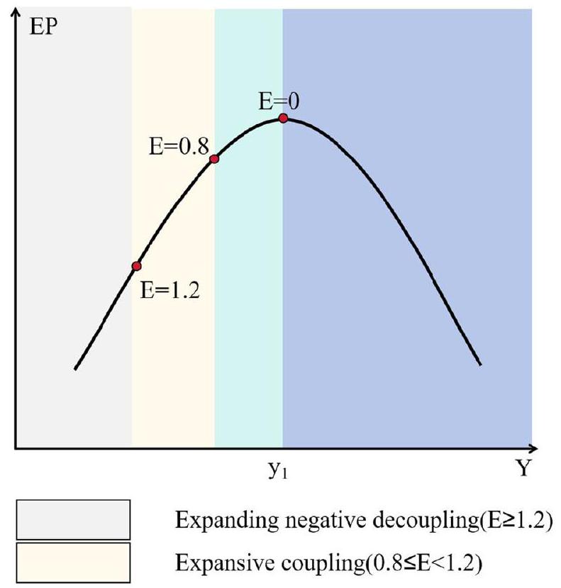
فصل الانفصال (الحالات 5-8)، والتي، مع ذلك، تتجاوز نطاق نظرية EKC.

نموذج فك الارتباط ثنائي الأبعاد: تعتمد فعالية أنماط التغيير الموصوفة في حالات فك الارتباط التي تم مناقشتها أعلاه على فعالية EKC. ومع ذلك، فإن EKC يفشل أحيانًا في العمل، خاصة عند النظر في إمكانية أن تكون بعض الدول متقدمة أو متأخرة في عملية تطويرها (كايفنغ وانغ وآخرون، 2021). على سبيل المثال، على الرغم من أن بعض الدول لديها ناتج محلي إجمالي للفرد أقل، إلا أن التنمية الاقتصادية والتلوث البيئي يمكن أن تحافظ على فك ارتباط مطلق لفترة طويلة. من ناحية أخرى، فإن الدول التي تنتمي إلى مراحل تطوير مختلفة قد يكون لديها أيضًا نفس مرونة فك الارتباط Tapio، انظر EKC على شكل N. لذلك، لا يمكن الحكم بدقة على العلاقة بين التنمية الاقتصادية والتلوث البيئي لدولة ما فقط من خلال المستوى المطلق للتنمية الاقتصادية أو حالة فك الارتباط.

يتم استخدام نموذج فك الارتباط ثنائي الأبعاد (2D) لمعالجة القضايا المذكورة أعلاه (كايفنغ وانغ وآخرون، 2021). بناءً على نقطة الانعطاف لـ EKC ومعامل مرونة فك الارتباط Tapio، يقوم النموذج بإنشاء عدة أرباع في نظام الإحداثيات ثنائي الأبعاد Y-E (التنمية الاقتصادية – مرونة فك الارتباط) لاستيعاب علاقات مختلفة بين التنمية الاقتصادية والتلوث البيئي. بناءً على شكل EKC، يمكن أن يحتوي نموذج فك الارتباط ثنائي الأبعاد على نقطة انعطاف واحدة (شكل U، شكل U المقلوب) أو نقطتين انعطاف (شكل N، شكل N المقلوب).
تقوم خطان عموديان و بتقسيم المحور الأفقي إلى ثلاث مناطق. تمثل المناطق المختلفة مراحل مختلفة من EKC على شكل N. في كل منطقة، وفقًا لـ و ، يتم تقسيم المحور العمودي إلى ثلاث مناطق، تتوافق مع فك الارتباط المطلق، وفك الارتباط النسبي، وعدم فك الارتباط (بما في ذلك الارتباط التوسعي وفك الارتباط السلبي المتزايد). لذلك، يتم تقسيم الطائرة بالكامل إلى تسع مناطق، تتوافق مع تسع حالات فك ارتباط ثنائية الأبعاد (انظر الشكل 2).

هذا النموذج يخفف من الافتراض الصارم في نموذج EKC بأن Y و EP يت correspondان مباشرة، ويتغلب أيضًا على مشكلة فك الارتباط Tapio التي تأخذ في الاعتبار فقط العلاقة التغير النسبية بين الاثنين. من خلال هذا التقسيم، يمكننا تصنيف الدول ذات الظروف الاقتصادية والبيئية المماثلة بوضوح ودقة في نفس الفئة لإجراء أبحاث منهجية وموجهة. نظرًا لأن العديد من الدول تفتقر إلى بيانات لسنوات فردية، لتقليل الأخطاء الإحصائية والأخطاء العشوائية، نستخدم المتوسط لعشر سنوات كفترة واحدة لتصنيف مستويات التنمية الاقتصادية وانبعاثات الكربون لكل دولة. على وجه التحديد، نقسم الدول إلى مراحل مختلفة من EKC وفقًا لمتوسط الناتج المحلي الإجمالي للفرد من 2010 إلى 2020. كما نحسب حالة فك الارتباط باستخدام متوسط الناتج المحلي الإجمالي للفرد وانبعاثات الكربون لكل فرد من 2000 إلى 2010 ومن 2010 إلى 2020 كبيانات في الفترة t-1 والفترة t، على التوالي.

إعدادات النموذج التجريبي. لاختبار H1 والتحقيق في شكل منحنى EKC العالمي، نقوم أولاً بإنشاء نموذج الانحدار التالي بناءً على نموذج EKC التجريبي الكلاسيكي المتوافق مع المعادلة 10:

من بينها، PCE و PGDP هما المتغيران التابعان والمتغيران المستقلان، على التوالي، يمثلان انبعاثات الكربون لكل فرد والناتج المحلي الإجمالي لكل فرد.

نضيف مزيدًا من المتغيرات الضابطة إلى النموذج أعلاه لاختبار H2 و H3:

حيث يمثل متجه المتغيرات الضابطة، بما في ذلك المخاطر الجيوسياسية، والمخاطر المركبة، وجودة المؤسسات، وتكنولوجيا المعلومات والاتصالات، والاقتصاد الرقمي، وتطوير الذكاء الاصطناعي، وإيجارات الموارد الطبيعية، وانتقال الطاقة، والانفتاح التجاري، وشيخوخة السكان، وعدم المساواة في الدخل، وأمن الغذاء. بناءً على نتائج تقدير هذه المعادلة، يمكننا تحديد شكل EKC بناءً على نتائج و ومناقشة تأثير المتغيرات الإضافية بناءً على نتائج .

أخيرًا، لفحص H4 واستكشاف محددات انبعاثات الكربون في مجموعات الدول في مراحل فك الارتباط ثنائية الأبعاد المختلفة، قمنا أولاً بتقسيم العينة الكاملة المكونة من 214 دولة إلى عدة مجموعات وفقًا لنموذج فك الارتباط ثنائي الأبعاد، وأجرينا الانحدارات التالية في كل مجموعة:

مع متسقة مع المعادلة.
تعريف المتغيرات ووصف البيانات. وفقًا لمتطلبات الطرق والنماذج التي تم مناقشتها سابقًا، يستخدم هذا المقال انبعاثات الكربون لكل فرد كمتغير مفسر، والناتج المحلي الإجمالي لكل فرد كمتغير مفسر، و12 متغيرًا تغطي المخاطر المؤسسية، والتكنولوجيا الرقمية، واستخدام الموارد، والقضايا الاجتماعية كمتغيرات ضابطة. بناءً على توفر البيانات، يتم تحديد نطاق البحث في هذا المقال ليكون 214 دولة من 1960 إلى 2020. يتم تلخيص التعريفات، ووحدات القياس، ومصادر البيانات لجميع المتغيرات في الجدول S1. يمكن ملاحظة أن المتغيرات المفسرة والمتغيرات المفسرة كلها مستمدة من قاعدة بيانات WDI التي طورتها البنك الدولي (Worldbank، 2023a).

تشمل المتغيرات الضابطة 12 متغيرًا. تشمل المخاطر المؤسسية ثلاثة متغيرات، من بينها تأتي المخاطر الجيوسياسية من العمل الحسابي لـ (كالدرا وإياكوفييلو، 2022). يتم تحديث هذه القاعدة البيانات يوميًا ويمكن أن تعكس بشكل شامل وفعال مستوى خطر التهديدات الجيوسياسية وأفعال الدول المختلفة. تأتي المخاطر المركبة من ICGR التي نشرتها مجموعة PRS منذ عام 1980 (PRS، 2023)، والتي تأخذ في الاعتبار المخاطر السياسية والاقتصادية والمالية المحلية. يتم حساب جودة المؤسسات من خلال متوسط ستة مؤشرات من مؤشر الحوكمة العالمية (WGI) الذي أصدره البنك الدولي (Worldbank، 2023b)، والذي يعكس نزاهة وفعالية مؤسسات كل دولة.

تشمل المتغيرات التكنولوجية تكنولوجيا المعلومات والاتصالات، والاقتصاد الرقمي، والذكاء الاصطناعي (AI). وفقًا لـ (شوفانغ تشاو وآخرون، 2022)، يتم تمثيل تكنولوجيا المعلومات والاتصالات من خلال اشتراكات الهواتف المحمولة. يتم حساب الاقتصاد الرقمي بواسطة طريقة وزن الانتروبيا ويمثل مستوى تطوير تكنولوجيا المعلومات الرقمية والصناعة الرقمية في دولة ما. تستخدم عملية الحساب 12 مؤشرًا ثانويًا من الاتحاد الدولي للاتصالات (ITU، 2023) وWDI، تغطي أربعة جوانب: البنية التحتية، والدعم الاجتماعي، والتأثيرات الاجتماعية، والتأثيرات الاقتصادية، كما هو موضح في الجدول S2. يتم تمثيل الذكاء الاصطناعي بعدد الروبوتات الصناعية العاملة التي تأتي من تقرير الروبوتات العالمي الذي أصدره الاتحاد الدولي للروبوتات (IFR، 2023).

تشمل المتغيرات المتعلقة باستخدام الموارد إجمالي إيجارات الموارد الطبيعية ومستوى انتقال الطاقة الممثل بحصة استهلاك الطاقة المتجددة. أخيرًا، من بين المتغيرات الاجتماعية، يتم التعبير عن شيخوخة السكان كنسبة السكان الذين تزيد أعمارهم عن 65 عامًا. يتم اشتقاق سلامة الغذاء من مؤشر إنتاج الغذاء من قاعدة بيانات WDI. يتم قياس الانفتاح التجاري بحجم تجارة الدولة كنسبة من ناتجها المحلي الإجمالي. يمثل معامل جيني مستوى عدم المساواة في الدخل. جميع هذه المتغيرات من WDI. يتم عرض الإحصائيات الوصفية للمتغيرات في الجدول S3.

التعامل مع مشكلة التعدد الخطي. أولاً، نعرض مصفوفة معامل الارتباط وVIF (انظر الشكل S1). وصل أعلى معامل ارتباط إلى 0.87، متجاوزًا الخط الآمن البالغ 0.85، مما يمثل الحاجة إلى تحليل VIF لاستبعاد مشكلة التعدد الخطي. تظهر النتائج أن VIF لجميع المتغيرات أقل من 10، مما يعني أن مشكلة التعدد الخطي بين المتغيرات ليست خطيرة. نظرًا لأن

الأخطاء المعيارية بين قوسين. y1 و y2 تمثل نقاط الانعطاف للمنحنى التكعيبي المحسوب بناءً على نتائج التقدير.

قيمة VIF لجودة المؤسسات أقرب إلى 10 مقارنة بالمتغيرات الأخرى، نختار إضافتها في الخطوة الأخيرة من الانحدار التدريجي لتجنب التداخل المحتمل.

التعامل مع مشكلة الانحدار الزائف. لتجنب الانحدار الزائف، نحتاج إلى اختبار استقرارية مصطلح الاضطراب، أي اختبار علاقة التكامل المشترك بين المتغيرات. يتطلب اختبار التكامل المشترك أن تكون كل سلسلة متغيرة متكاملة من الدرجة الأولى، ويجب إجراء اختبار الجذر الأحادي على كل متغير أولاً. لذلك، يتم استخدام اختبارات فيشر-ADF وفيشر-PP لاختبار استقرارية البيانات. كلا النتيجتين لجميع المتغيرات في طريقتي الاختبار ثابتة من الدرجة الأولى (انظر الجدول S4). أخيرًا، يتم استخدام اختبار كاو لاختبار التكامل المشترك (انظر الجدول S4). نتائج إحصائيات كاو ADF ترفض الفرضية الصفرية التي تفيد بعدم وجود علاقة تكامل مشترك بين متغيرات اللوحة عند الـ هذا يشير إلى أن العلاقة المستقرة على المدى الطويل بين المتغيرات موجودة وأن مشكلة الانحدار الزائف لا تنطبق.

اختيار نموذج التقدير. تعتبر نماذج التأثيرات الثابتة (FE) ونماذج التأثيرات الثابتة ذات الاتجاهين ونماذج GMM الديناميكية (نظام-/فرق-) من بين النماذج الأكثر شيوعًا في الدراسات السابقة. نموذج التأثيرات الثابتة هو واحد من أكثر النماذج استخدامًا في البحث. إنه يقضي على مشاكل الاندماج الناتجة عن عوامل غير قابلة للملاحظة تتعلق بالأفراد من خلال مقدرات داخل المجموعة. كل من التأثيرات الثابتة ذات الاتجاهين وGMM الديناميكي يحسنان FE من خلال إضافة متغيرات تفسيرية إلى النموذج: الأول يضيف متجهًا من متغيرات وهمية زمنية، بينما يتضمن الأخير مصطلح التأخير للمتغير المفسر. ومع ذلك، اختارت هذه الدراسة متغيرات إضافية من زوايا مختلفة لتتبع التغيرات في منحنى انبعاثات الكربون بدقة وفتح الصندوق الأسود لعوامل انبعاثات الكربون، مما يجعل إضافة المزيد من المتغيرات إلى النموذج زائدة عن الحاجة وقد تكون ضارة (مثل تفاقم مشاكل التعدد الخطي). لذلك، نختار في النهاية اعتماد نماذج FE الأساسية في عمليتنا التجريبية. تُستخدم نماذج أخرى كطرق للتحقق من القوة.

تأكيد شكل EKC بدون متغيرات إضافية. لاختبار H1، نقوم بإجراء التقدير واختبار القوة على معادلة الانحدار بدون متغيرات إضافية المعادلة (16). النتائج هي
موضح في الجدول 3. أولاً، معامل الحد التكعيبي للناتج المحلي الإجمالي للفرد (PGDP3) في النموذج 1 أكبر بكثير من 0 عند المستوى، مما يشير إلى وجود منحنى بيئي كينزي مكعب. بالإضافة إلى ذلك، فإن معامل الحد التربيعي سالب بشكل كبير ومعامل الحد الخطي موجب بشكل كبير. يظهر أنه مع زيادة الناتج المحلي الإجمالي للفرد تدريجياً، تتوافق انبعاثات الكربون للفرد مع الاتجاه على شكل حرف N. من خلال تضمين معاملات الانحدار المذكورة أعلاه في المعادلة (13)، يمكن حساب نقاط الانعطاف لمنحنى EKC دون النظر في المتغيرات التحكمية وهي 34.44 و 77.54 (ألف دولار أمريكي/شخص) على التوالي. يمكننا اعتبار هذه كعتبتين. في البداية، يؤدي زيادة الناتج المحلي الإجمالي للفرد إلى زيادة انبعاثات الكربون للفرد وتصل إلى ذروتها عندما يصل الناتج المحلي الإجمالي للفرد إلى 34.44. ومع ذلك، عندما تزداد PGDP تدريجياً وتتجاوز هذه القيمة، ستنعكس انبعاثات الكربون للفرد وتتغير من الارتفاع إلى الانخفاض. أخيراً، عندما زاد الناتج المحلي الإجمالي للفرد أكثر وبلغ 77.54، تغير اتجاه انبعاثات الكربون للفرد مرة أخرى نحو الارتفاع.

نستخدم أيضًا أربع طرق للتحقق من قوة منحنى كوزنيك N، كما هو موضح في النموذج R1-R4 في الجدول 3. أولاً، تغيير مؤشر تلوث البيئة من انبعاثات الكربون للفرد إلى إجمالي انبعاثات الكربون. ثانيًا، يتم استبدال نموذج تقدير التأثيرات الثابتة بنموذج التأثيرات الثابتة الفردية-الزمان-ثنائية الاتجاه. ثالثًا، سيتم استخدام نموذج التأثيرات العشوائية. رابعًا، استخدام نظام GMM. أولاً، اختبار سارجان. -القيمة و AR(2) في النموذج R4 أكبر من 0.1، مما يشير إلى أن نتائج تقدير النموذج الديناميكي صالحة. جميع النماذج الأربعة تظهر أن معاملات PGDP و الحد التكعيبي له أكبر بكثير من 0، بينما معاملات الحد التربيعي أقل بكثير من 0. بالإضافة إلى ذلك، نتائج و يظهر أن هناك نقطتين انحناء في منحنى البيئة الاقتصادية (EKC) تتوافقان مع النماذج الأربعة، وجميعها تقع ضمن فترة العينة. في الختام، يوجد منحنى EKC العالمي على شكل حرف N عندما لا تؤخذ المتغيرات الضابطة في الاعتبار ويتم تأكيد الفرضية H1. أخذ فاروق وآخرون (2022) 185 دولة حول العالم كعينة، وأكدوا وجود الحد الإيجابي الخطي والحد التربيعي السلبي للناتج المحلي الإجمالي للفرد (PGDP)، وحصلوا على نتيجة منحنى EKC على شكل حرف U مقلوب. ومع ذلك، تظهر نتائجنا أن الحد التكعيبي الإيجابي موجود أيضًا بشكل قوي، لذا تعيد هذه الورقة ضبط شكل منحنى EKC العالمي ليكون على شكل حرف N. من منظور آخر، تعمم هذه النتيجة منحنى EKC على شكل حرف N الذي تم تأكيده في دراسة نومان وآخرون (2022) في 85 دولة إلى 191 دولة.

ملاحظة: لأغراض التحليل، لم يتم الإبلاغ عن الأخطاء المعيارية. انظر الجدول S5 للحصول على النتائج الكاملة. .

حدد شكل منحنى كوزنتس البيئي ونقاط الانعطاف تحت متغيرات إضافية. توضح الجدول 4 نتائج إضافة متغيرات التحكم لاختبار H2 و H3. لتقليل تأثير اختلافات أحجام العينات للمتغيرات المختلفة وتخفيف مشكلة التعدد الخطي، نعتمد على الانحدارات التدريجية. لعرض نتائج إضافة المتغيرات المشتركة. من بينها، يستخدم النموذج 1 فقط PGDP وعباراته التربيعية والتكعيبية كمتغيرات تفسيرية، وبلغت قيمة R المربعة 0.122. النموذج 2 – النموذج 6 أضاف تدريجياً 12 متغير تحكم، وزادت قيمة R المربعة تبعاً لذلك إلى 0.718 في النموذج 6. وهذا يظهر أن إضافة المتغيرات التفسيرية يمكن أن تفسر بدقة التغيرات في انبعاثات الكربون. مع إضافة متغيرات التحكم باستمرار إلى النماذج 2-6، كانت العبارة التكعيبية لـ PGDP دائماً إيجابية بشكل كبير عند المستوى الإحصائي. بالإضافة إلى ذلك، فإن الإشارة والمستوى الإحصائي لـ PGDP وعبارته التربيعية متسقة تمامًا مع النموذج 1. وهذا يعني أنه بعد إضافة المتغيرات الضابطة، لا يزال شكل منحنى كوزنتس البيئي (EKC) على شكل N قياسي وتم تأكيد H2.

بعد الحساب، فإن نقطتي الانعطاف لنموذج EKC على شكل N في النموذج 6 هما 45.08 و 73.44 (ألف دولار لكل)
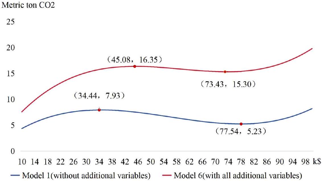
الشخص)، على التوالي. هذه النتيجة تختلف عن نقطة الانعطاف في EKC في النموذج 1. نحن نقارن بين منحنيات المعادلة التكعيبية التي تتوافق مع المعاملات المقدرة في الشكل 3 لمناقشة تأثير المتغيرات الضابطة على شكل EKC. يظهر الشكل 3 أنه بعد أخذ المتغيرات الضابطة في الاعتبار، لم يتقلص فقط الفضاء الاقتصادي بين نقطتي الانعطاف من 43.10 ألف دولار أمريكي إلى 28.35 ألف دولار أمريكي، ولكن أيضًا انخفضت انبعاثات الكربون للفرد بين نقطتي الانعطاف من حوالي 2.70 طن متري إلى حوالي 1.05 طن متري. وهذا يشير إلى أن EKC يبدو أنه ينحني لأعلى عند محاولة حساب متغيرات تفسيرية أخرى. ونتيجة لذلك، فإن الجزء الوحيد المتناقص من منحنى انبعاثات الكربون على شكل N قد تقلص في كل من “المدة” و”الفضاء المتناقص”، مما يكشف عن وضع أكثر حدة في التخفيف من تغير المناخ العالمي.

ناقش دور المتغيرات الإضافية على انبعاثات الكربون. العوامل المؤسسية والتكنولوجية والموارد والاجتماعية لا تؤثر فقط على شكل EKC ولكن لها أيضًا تأثير مهم على
انبعاثات الكربون. وهذا يؤدي إلى مناقشة H3. يضيف النموذج 2 أربعة متغيرات ضابطة بناءً على النموذج 1. مع اعتبار مستوى الدلالة 5% كمعيار، فإن معاملات تأثير تكنولوجيا المعلومات والاتصالات والأمن الغذائي إيجابية، بينما معاملات تأثير الاقتصاد الرقمي وشيخوخة السكان سلبية. نحن نفحص قوة تأثير هذه المتغيرات بالتزامن مع نتائج أخرى من الانحدارات التدريجية. مقارنة نتائج تقدير النموذج 2 مع النماذج الأربعة اللاحقة (النموذج )، يظهر أن النتائج المذكورة أعلاه يمكن تأكيدها من قبل نموذجين على الأقل. على وجه التحديد، كانت نتائج تكنولوجيا المعلومات والاتصالات إيجابية بشكل ملحوظ في كل من النموذج 3 والنموذج 4؛ يوجد معامل إيجابي للأمن الغذائي في النماذج 3-5؛ وتظل المعاملات السلبية للاقتصاد الرقمي وشيخوخة السكان قائمة في جميع النماذج. وهذا يظهر أن نتائج تقدير تكنولوجيا المعلومات والاتصالات والأمن الغذائي والاقتصاد الرقمي وشيخوخة السكان في النموذج 2 موثوقة كقرارات.

تعتبر مقدرات العوامل الثلاثة المضافة في النموذج 3 جميعها ذات دلالة. من بينها، فإن معامل تأثير إيجار الموارد الطبيعية إيجابي، بينما تأثير انفتاح التجارة وانتقال الطاقة سلبي. ومع ذلك، تدعم النتائج من النماذج اللاحقة تأثيرات انتقال الطاقة بدلاً من تأثيرات إيجارات الموارد الطبيعية وانفتاح التجارة. تظهر جميع النماذج أن معامل تأثير انتقال الطاقة سالب بشكل ملحوظ، بينما تأثيرات إيجارات الموارد الطبيعية وانفتاح التجارة غير دالة في اثنين من النماذج الثلاثة اللاحقة. يضيف النموذج 4 المخاطر الشاملة. بالاقتران مع نتائج تقدير النموذج 4-6، يتم تحديد تأثير المخاطر الشاملة على انبعاثات الكربون بأنه سلبي، مما يشير إلى أنه كلما زاد مستوى المخاطر العامة في البلاد، زادت انبعاثات الكربون المقابلة. من خلال مقارنة نتائج النموذج 5 والنموذج 6، حددنا أن تأثيرات الذكاء الاصطناعي وعدم المساواة في الدخل ليست ذات دلالة. أخيرًا، تظهر نتائج النموذج 6 أن المخاطر الجيوسياسية تعزز انبعاثات الكربون، بينما يمكن أن تؤدي تحسينات جودة المؤسسات إلى تقليل انبعاثات الكربون. تظهر هذه النتائج أن H3 تم تأكيده جزئيًا.

نلخص تأثير كل متغير على انبعاثات الكربون في الجدول 5 لإجراء مناقشة إضافية. من منظور عوامل المخاطر المؤسسية، فإن ارتفاع المخاطر الجيوسياسية والمخاطر الشاملة الوطنية قد عزز بشكل كبير انبعاثات الكربون. وهذا يتماشى مع بعض نتائج الأبحاث الحديثة حول المخاطر الجيوسياسية (أنسر وآخرون، 2021) والمخاطر السياسية (حسن وآخرون، 2022)، ولكنه يتعارض مع نتائج الأبحاث حول المخاطر المالية (جون تشاو وآخرون، 2021أ). قد تسبب المخاطر الذعر وقصر النظر بين

ملاحظة: تمثل التأثير الإيجابي (السلبي) على انبعاثات الكربون للفرد على الأقل عند مستوى الدلالة. الفراغ يمثل تأثيرًا غير دال.
تسبب الحكومات والمستثمرون، والتي غالبًا ما ترتبط بنماذج الإنتاج غير المسؤولة وسوء استخدام الوقود الأحفوري (فاكولتشوك وآخرون، 2020؛ زوكسينغ تشاو وآخرون، 2023). التأثير المخفض لجودة المؤسسات على انبعاثات الكربون العالمية يتماشى مع فرضية التأثير التنظيمي ويتماشى مع الأبحاث السابقة لـ 3 دول آسيوية (سلمان وآخرون، 2019) و30 دولة في أفريقيا جنوب الصحراء (كريم وآخرون، 2022). لذلك، يلعب بيئة التنمية الدولية والمحلية المستقرة والأنظمة الفعالة دورًا لا يمكن تعويضه في تقليل انبعاثات الكربون وتحقيق التخفيف من تغير المناخ العالمي.

تعتبر نتائج العوامل التكنولوجية مثيرة للقلق. يمكن أن يقلل الاقتصاد الرقمي من انبعاثات الكربون، بينما تعزز صناعة تكنولوجيا المعلومات والاتصالات انبعاثات الكربون. المتغيران متشابهان من الناحية المفاهيمية، ولكن لماذا يمكن أن يكون لهما تأثيرات متعارضة تمامًا على انبعاثات الكربون العالمية؟ على الرغم من نقص المناقشة والتفسير لهذه الظاهرة في الأدبيات، تقدم دراسة حديثة (جينينغ زانغ وآخرون، 2022أ) منظورًا جيدًا. ناقشوا تأثير أبعاد مختلفة من الاقتصاد الرقمي على التنمية منخفضة الكربون ووجدوا أن الرقمنة الصناعية لها التأثير الأكثر أهمية على التنمية منخفضة الكربون، تليها الرقمنة الصناعية، مع كون الحامل له الدور الأصغر. بعبارة أخرى، إن دمج التكنولوجيا الرقمية والاقتصاد هو الذي يعزز تقليل الانبعاثات، وليس مجرد تطوير تكنولوجيا ومعدات تكنولوجيا المعلومات والاتصالات (جينينغ زانغ وآخرون، 2022أ). تأثير الذكاء الاصطناعي ليس ذا دلالة، ربما لأن تأثيرات الذكاء الاصطناعي في دول مختلفة تلغي بعضها البعض. وجد لوان وآخرون (2022) أن الروبوتات الصناعية عززت تلوث الهواء في 74 دولة بينما ادعى (تشونغ وآخرون، 2023) أن الذكاء الاصطناعي قلل من انبعاثات الكربون في 66 دولة. باختصار، على عكس آراء العقلانيين التكنولوجيين، تشير نتائجنا إلى أن التطورات التكنولوجية الذكية وحدها قد لا تحسن البيئة بالضرورة. بدلاً من ذلك، قد يكون الاستخدام العقلاني للتكنولوجيا لصالح الاقتصاد والمجتمع نهجًا فعالًا لتحقيق تقليل انبعاثات الكربون.

تؤكد النتائج المتعلقة باستخدام الموارد على ضرورة تطوير ونشر الطاقة النظيفة. من ناحية، تؤكد النتائج التأثير الكبير لتغيير الطاقة على تقليل انبعاثات الكربون. وهذا يظهر أن استبدال البنية التحتية للطاقة الحالية بأخرى تعتمد على الطاقة المتجددة يمكن أن يقلل بشكل كبير من انبعاثات الكربون للفرد، وهو ما لا يتجاوز استنتاجات الأبحاث الأخرى (دوغان وسكر، 2016؛ إنغليسي-لوتز ودوغان، 2018). من ناحية أخرى، فإن تأثير إيجارات الموارد الطبيعية غير مؤكد، وهو ما يتماشى مع الجدل في الأدبيات. كما تسلط النتائج الضوء على التأثير المحتمل للعوامل الاجتماعية على انبعاثات الكربون. تعتبر شيخوخة السكان مساهمًا سلبيًا في انبعاثات الكربون. وهذا يتوافق مع (تشو وآخرون، 2023) بينما يتعارض مع نتائج (بالسالوبري-لورينتي وآخرون، 2021) و(فان وآخرون، 2021). يعتبر الأمن الغذائي مساهمًا إيجابيًا في انبعاثات الكربون، مدعومًا بـ (نسيم وآخرون، 2020). يظهر أنه يجب إيلاء المزيد من الاهتمام لقضايا إزالة الغابات واستخدام الأراضي واستهلاك الأغذية عالية الكربون مع ضمان سلامة الغذاء في التنمية الزراعية العالمية. تأثيرات انفتاح التجارة وعدم المساواة في الدخل ليست ذات دلالة.

قبل اختبار H4، نقوم أولاً بتصنيف الدول وفقًا لمرحلة التنمية وحالة خفض الانبعاثات لحل مشكلة التباين التي توجد عند اختبار فرضية EKC باستخدام الطريقة التقليدية للبانل. لذلك، تستخدم هذه الورقة أولاً نموذج فك الارتباط ثنائي الأبعاد لتحقيق تصنيف دقيق للدول بناءً على مستويات التنمية الاقتصادية وحالات فك الارتباط لانبعاثات الكربون. يمكن تقسيم عملية الحساب والتجميع إلى ثلاث خطوات: (1) المجموعة

الدول وفقًا لمتوسط الناتج المحلي الإجمالي للفرد في العقد الماضي ونقطة الانعطاف في منحنى كوزنتس البيئي. (2) تصنيف الدول وفقًا لمرونة فك الارتباط لتابيو بين العقدين الماضيين والقيم الحرجة (0 و 0.8). (3) مطابقة نتائج الخطوتين السابقتين مع المراحل التسع لفك الارتباط ثنائي الأبعاد الموضحة في

الشكل 2، والحصول على التجميع النهائي بناءً على نموذج الفصل ثنائي الأبعاد. النتائج موضحة في الشكل 4.

وفقًا للشكل 4أ، تم تقسيم 214 دولة عينة إلى ثلاث مجموعات بناءً على نقاط الانعطاف على شكل N المقدرة في نتائج الانحدار الأساسية. المرحلة الأولى من

ملاحظة: من أجل وضوح تحليلي، الأخطاء المعيارية والمعاملات غير المهمة عند الـ لم يتم الإبلاغ عن المستوى. انظر الجدول S7 للحصول على النتائج الكاملة. .

لا تزال EKC هي الموضوع الرئيسي للتنمية العالمية. أكثر من توجد دول في هذه المرحلة، حيث يبلغ متوسط نصيب الفرد من الناتج المحلي الإجمالي بين عامي 2010 و2020 أقل من 45,080 دولار أمريكي. هناك 11 دولة في المرحلة الثانية. يتجاوز متوسط نصيب الفرد من الناتج المحلي الإجمالي على مدى عشر سنوات 45,080 ولكنه أقل من 73,438. تتمتع هذه الدول بمستويات عالية نسبيًا من التنمية الاقتصادية، وتشمل بشكل رئيسي الولايات المتحدة، وأستراليا، وبعض الدول الأوروبية. وفقًا لفرضية منحنى كوزنتس البيئي، لديهم أفضل أمل في تحقيق النمو الاقتصادي مع تقليل انبعاثات الكربون. فقط 9 دول لديها متوسط نصيب الفرد من الناتج المحلي الإجمالي على مدى عشر سنوات أعلى من 73,439 وهي في المرحلة الثالثة، وتقع جميعها تقريبًا في أوروبا. لقد وصلت هذه الدول إلى مستويات عالية جدًا من التنمية الاقتصادية، لكنها قد تكون مسؤولة بشكل مباشر عن الزيادة الثانية في منحنى كوزنتس البيئي من النوع N والانتعاش في مستويات التلوث.

تظهر الشكل 4 ب أن عدد الدول في حالات فك الارتباط المختلفة متساوي نسبيًا وأن هناك خصائص تجميع إقليمية. عدد الدول التي لا تفك الارتباط، وفك الارتباط الضعيف، وفك الارتباط القوي هو 57 و47 و55 على التوالي، و34 دولة تعاني من ركود اقتصادي. نتائج الدول غير المفككة تثير القلق. تظهر النتائج أن هذه الدول التي لا تزال تتمتع بمرونة فك ارتباط أعلى من 0.8 في السنوات العشرين الماضية تقع بشكل رئيسي في أفريقيا جنوب الصحراء الكبرى، وأمريكا اللاتينية، والشرق الأوسط. تتميز هذه الدول بتطور اقتصادي يعتمد بشكل كبير على استخراج أو استخدام الموارد الطبيعية (دو، 2021). كيف يمكن مساعدتها في تقليل انبعاثات الكربون هو تحدٍ مهم للتخفيف من آثار تغير المناخ العالمي. يمكن ملاحظة أن معظم دول فك الارتباط الضعيف تقع في آسيا غير الشرق الأوسط. العديد من هذه الدول، مثل الهند والصين، حققت درجة من التصنيع والتحضر، مما أدى إلى فك ارتباط اقتصاداتها تدريجيًا عن انبعاثات الكربون. دول فك الارتباط القوي موزعة بشكل رئيسي في أمريكا الشمالية، وأوروبا، وأوقيانوسيا، ولها درجة عالية من التداخل مع الدول في المرحلتين الثانية والثالثة من منحنى كوزنتس البيئي. أخيرًا، تواجه بعض الدول الأفريقية، بما في ذلك ليبيا وجمهورية إفريقيا الوسطى، ركودًا اقتصاديًا. إن استقرار الاقتصاد هو الأولوية القصوى لهذه الدول.

أخيرًا، نصنف الدول بناءً على نموذج فك الارتباط ثنائي الأبعاد. عدد الدول في كل مرحلة موضح في الشكل 4c. أولاً، تظهر النتائج أن جميع الدول في
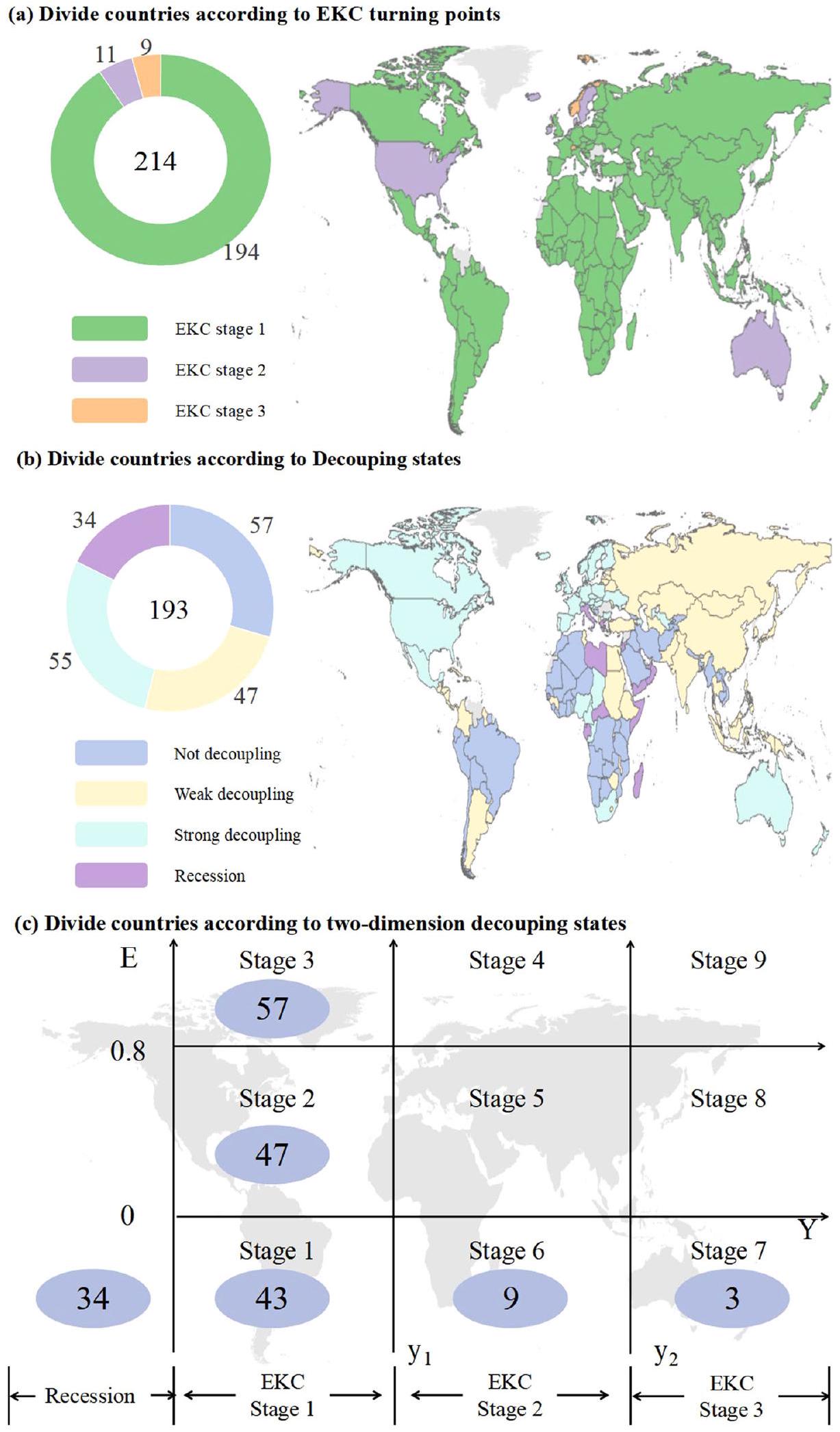
العينة التي يكون فيها الناتج المحلي الإجمالي للفرد أعلى من نقطة الانعطاف الأولى في منحنى كوزنتس البيئي قد حققت انفصالاً قوياً. بعبارة أخرى، من بين المراحل الستة ثنائية الأبعاد للانفصال التي تتوافق مع المرحلتين الثانية والثالثة من منحنى كوزنتس البيئي (المرحلة 4-9)، يوجد 9 دول في المرحلة 6، و3 دول في المرحلة. بدون وجود دول في مراحل أخرى. وهذا يعني أنه من منظور العشرين عامًا الماضية، حققت تلك الدول التي تتمتع بتطور اقتصادي متقدم نسبيًا انفصالًا مثاليًا نسبيًا بين التنمية الاقتصادية وانبعاثات الكربون. من بين ثلاث حالات انفصال ثنائي الأبعاد (المرحلة 1-3) التي تنتمي إلى المرحلة الأولى من منحنى كوزنتس البيئي، هناك 43 و47 و57 دولة في حالات انفصال قوي، انفصال ضعيف، وعدم انفصال على التوالي، وهو ما لا يتماشى تمامًا مع نظرية منحنى كوزنتس البيئي. في نظرية منحنى كوزنتس البيئي، سيكون تطور الاقتصاد في الدول التي يقل نصيب الفرد من الناتج المحلي الإجمالي فيها عن نقطة التحول الأولى مصحوبًا بتدهور بيئي، لكن تحليل الانفصال الثنائي الأبعاد يظهر أن العلاقة بين التنمية الاقتصادية والتلوث البيئي في الدول في هذه المرحلة لها أيضًا ظروف مختلفة. باختصار، نجحنا في تصنيف الدول من نفس النوع من خلال نموذج الانفصال الثنائي الأبعاد، مما يتيح لنا إجراء بحث محدد حول محددات انبعاثات الكربون في كل مجموعة من الدول.

آثار غير متجانسة لجميع المتغيرات على انبعاثات الكربون. استنادًا إلى المجموعات الستة المقسمة من الدول، نقوم بإجراء اختبارات الجذر الأحادي في اللوحة واختبارات التكامل المشترك لكل عينة. تظهر النتائج أنه في مستوى الدلالة، في كل عينة، المتغيرات ثابتة من الدرجة الأولى ومتزامنة (انظر الجدول S6). لمناقشة التأثير غير المتجانس للعوامل الاقتصادية والمؤسسية والتكنولوجية والموارد والاجتماعية على انبعاثات الكربون وفحص H4، تظهر نتائج الانحدار لست مجموعات من الدول في الجدول 6.

أولاً، هناك تباين واضح في تأثير الناتج المحلي الإجمالي للفرد على انبعاثات الكربون. في المرحلة الأولى من منحنى كوزنتس البيئي، وفقًا لنتائج تقدير النموذج 7 والنموذج 9، يرتبط التطور الاقتصادي في كل من الدول غير المفككة والدول ذات التفكك الضعيف بزيادة كبيرة في انبعاثات الكربون. في الدول غير المفككة والدول ذات التفكك الضعيف، مقابل كل زيادة قدرها 1 دولار أمريكي في الناتج المحلي الإجمالي للفرد، تزداد انبعاثات الكربون للفرد بمعدل 0.2658 طن متري و0.3806 طن متري.
على التوالي. قد يكون من المحير في البداية أن معامل تأثير التنمية الاقتصادية على انبعاثات الكربون أكثر وضوحًا في الدول ذات الفصل الضعيف مقارنة بالدول غير المفصولة. يمكن أن يكون السبب في ذلك أن نماذج التنمية الاقتصادية لهذه الدول، بما في ذلك معظم الدول النامية في آسيا، قد تم تحسينها إلى حد ما في العقدين الماضيين، لكن تكاليفها البيئية المتوسطة طوال عملية التنمية لا تزال مرتفعة (رونغ رونغ لي وآخرون، 2021). تحتاج هذه الدول إلى الاستفادة الكاملة من نتائج التنمية الاقتصادية السابقة والسعي للتحول من الفصل الضعيف إلى الفصل القوي (هانيف وآخرون، 2019). يظهر النموذج 9 أنه في عينة الفصل القوي في المرحلة الأولى من منحنى كوزنتس البيئي، فإن تأثير الناتج المحلي الإجمالي للفرد على انبعاثات الكربون للفرد ليس له دلالة إحصائية. وهذا يتماشى مع نظرية الفصل، مما يشير إلى أنهم لا يتطورون مباشرة بتكلفة بيئية عالية. يظهر النموذج 10 أنه في الدول التي دخلت فيها التنمية الاقتصادية المرحلة الثانية من منحنى كوزنتس البيئي، فإن كل زيادة بمقدار 1 دولار أمريكي في الناتج المحلي الإجمالي للفرد تؤدي إلى زيادة انبعاثات الكربون للفرد بمقدار 0.0855 طن متري. بالنظر إلى الحجم النسبي الصغير للمعامل، يمكن اعتبار أن منحنى كوزنتس البيئي على شكل N مدعوم، أي أن التنمية الاقتصادية مصحوبة بتلوث بيئي أقل في المرحلة الثانية من منحنى كوزنتس البيئي. ومع ذلك، يظهر النموذج 11 أنه عندما تدخل التنمية الاقتصادية المرحلة الثالثة من منحنى كوزنتس البيئي، يتم إعادة الاتصال بين النمو الاقتصادي وانبعاثات الكربون. مقارنة بالمرحلة الثانية من منحنى كوزنتس البيئي، فإن انبعاثات الكربون للفرد لكل سيزداد الناتج المحلي الإجمالي للفرد من 0.0855 طن متري إلى 0.1721 طن متري. وقد أكدت هذه النتيجة تأثير التقادم الفني (جاهانجر وآخرون، 2023). أخيرًا، فإن تكاليف انبعاثات الكربون الناتجة عن التنمية الاقتصادية في الدول التي واجهت ركودًا اقتصاديًا في السنوات العشرين الماضية مرتفعة للغاية أيضًا. تحتاج هذه الدول بشكل عاجل إلى استقرار اقتصاداتها بتكاليف بيئية قابلة للتحكم.

من منظور المخاطر المؤسسية، فإن تأثير المخاطر الجيوسياسية ليس كبيرًا في معظم العينات، مما يشير إلى أن المخاطر الجيوسياسية لم تؤثر بعد بشكل كبير على انبعاثات الكربون في معظم دول العالم. ومع ذلك، في العينة غير المفككة في المرحلة الأولى من منحنى كوزنتس البيئي، فإن المخاطر الجيوسياسية تقلل بشكل كبير من انبعاثات الكربون. قد يكون هذا مرتبطًا بالصراعات والأزمات الناتجة عن الثروات الطبيعية الغنية لهذه الدول (دو، 2021). العلاقة السلبية مدعومة من قبل (ويجون تشاو وآخرون، 2021ب) الذين أكدوا أن المخاطر الجيوسياسية قد تعيق الاستثمار والتجارة واستهلاك الطاقة لتقليل انبعاثات الكربون. يمكن أن يؤدي كل زيادة وحدة في مؤشر المخاطر المركب إلى تقليل انبعاثات الكربون للفرد بمقدار 0.0123 طن متري و0.0067 طن متري، على التوالي، في الدول في المرحلة 2 والمرحلة 1 من فك الارتباط ثنائي الأبعاد، وهو ما يتماشى مع نتيجة البحث في العينة الكاملة. نتائج جودة المؤسسات غنية بالتنوع. تأثيرها في تقليل انبعاثات الكربون يظهر فقط في الدول في المرحلة 3، وتحتاج هذه الدول غير المفككة إلى تعزيز بناء المؤسسة الوطنية. ومع ذلك، في المرحلة 1 والمرحلة 6 والمرحلة 10، تزيد جودة المؤسسات من انبعاثات الكربون. كما أشار (لي وأوزتورك، 2020) إلى أن اللوائح المعقدة والبيروقراطية قد تؤخر بدورها تنفيذ إجراءات حماية البيئة.

من المثير تحليل تأثير متغيرات التكنولوجيا الرقمية. الاستنتاج بأن التحول الرقمي، بدلاً من تكنولوجيا المعلومات والاتصالات، يمكن أن يقلل بشكل كبير من انبعاثات الكربون ويحقق تنمية منخفضة الكربون هو صحيح في المرحلة 1، المرحلة 6، والمرحلة 10، مما يشير إلى أن معظم الدول يجب أن تركز على رقمنة الصناعة والاقتصاد. ومع ذلك، فإن هذا لا ينطبق دائمًا، لأنه في المرحلة 3 يكون العكس تمامًا: تكنولوجيا المعلومات والاتصالات تقلل من انبعاثات الكربون، بينما الاقتصاد الرقمي يعزز انبعاثات الكربون. على الرغم من أن هذه الدول في حالة فصل ضعيف، فإن معامل تأثير الناتج المحلي الإجمالي للفرد على انبعاثات الكربون هو الأعلى بين جميع العينات. إن الجمع بين التنمية الاقتصادية الخشنة
قد تؤدي النماذج والتكنولوجيا الرقمية إلى انبعاثات كربونية مفرطة (Feng Dong et al., 2022a). لذلك، تحتاج هذه الدول إلى التركيز على بصمة الكربون لنموذج التنمية الاقتصادية الرقمية أثناء تطوير تكنولوجيا المعلومات والاتصالات. تقلل الذكاء الاصطناعي من الانبعاثات في الدول من المرحلة الثالثة بينما تزيد من الانبعاثات في الدول من المرحلة الثانية، وهو ما ليس له دلالة كبيرة في المجموعات الأخرى، مما يشير إلى أن الذكاء الاصطناعي يحتاج إلى استخدامه في الاقتصاد والمجتمع بحذر أكبر.

من حيث استخدام الموارد، أدى الانتقال إلى الطاقة إلى تقليل انبعاثات الكربون بشكل كبير في جميع العينات الست وفقًا للجدول 6. ومع ذلك، كان هذا التأثير أكثر وضوحًا في البلدان في المرحلة 3 من منحنى كوزنتس البيئي، تليها المرحلة 2 من منحنى كوزنتس البيئي. كل زيادة نسبة الطاقة المتجددة ستؤدي إلى انخفاض في انبعاثات الكربون للفرد بمقدار 0.4661 طن متري في المجموعة الأولى و0.1096 طن متري في المجموعة الثانية. تأثيرات تقليل الانبعاثات في الدول في المرحلة الأولى من منحنى كوزنتس البيئي (EKC) ضعيفة نسبيًا، وتتناقص في الدول ذات الفصل القوي، الفصل الضعيف، وعدم الفصل. نمط توزيع معامل التأثير يظهر أن زيادة مستويات التنمية الاقتصادية والفصل تؤدي إلى نتائج أفضل في انتقال الطاقة. هذه النتيجة مدعومة من قبل (نجوين وكاكنيكا، 2019)، الذين استنتجوا أنه في مجموعة الدخل المنخفض، يعيق تطوير الطاقة المتجددة التنمية الاقتصادية ويعزز انبعاثات الكربون؛ بينما في مجموعة الدخل المرتفع، يحدث العكس. على العكس من ذلك، فإن ريع الموارد الطبيعية يعزز انبعاثات الكربون في الدول في المرحلة الثانية والسادسة وليس له تأثير كبير على الدول الأخرى.

أخيرًا، بين العوامل الاجتماعية الأربعة، فإن تأثير شيخوخة السكان متسق نسبيًا. يؤثر بشكل رئيسي على الدول في المرحلة 2 والمرحلة 1 ويؤدي إلى تقليل انبعاثات الكربون. نتيجة OPEN لا تدعم وجود فرضية PHH لأنه لا يوجد دليل واضح على أن الدول التي لديها تنظيمات بيئية أفضل قد خفضت انبعاثات الكربون من خلال الانفتاح. بصراحة، الانفتاح التجاري يجلب المزيد من انبعاثات الكربون في معظم العينات (المرحلة 1، 7، 10)، ويقلل من انبعاثات الكربون فقط في عينات المرحلة 2. وهذا يعني أن التبادلات المتكررة للسلع والخدمات قد تزيد من أعباء اللوجستيات والنقل في العديد من الدول (رونغ رونغ لي وآخرون، 2021). تأثيرات الأمن الغذائي وعدم المساواة في الدخل أيضًا غير متجانسة وقد يكون لها تأثيرات متعارضة في دول مختلفة. على وجه التحديد، يقلل الأمن الغذائي من انبعاثات الكربون في الدول في المرحلة 1 ولكنه يزيد من انبعاثات الكربون في الدول في المرحلة 2 والمرحلة 10. عدم المساواة في الدخل يساهم في انبعاثات الكربون في الدول في المرحلة 1 والمرحلة 6، ولكن العكس هو الصحيح بالنسبة لدول المرحلة 2. النتائج المذكورة أعلاه تسلط الضوء على التباين بين المجموعات في اتجاه وحجم تأثيرات انبعاثات الكربون لجميع المتغيرات، مما يؤسس H4.

استراتيجيات تقليل الكربون التفاضلية للدول في مراحل فك الارتباط ثنائية الأبعاد المختلفة. تُظهر المناقشة الأولية لنتائج الجدول 6 أن العلاقة بين الناتج المحلي الإجمالي للفرد وانبعاثات الكربون لا تظهر فقط قواعد غير خطية وغير متجانسة، ولكن تأثير المتغيرات الإضافية على انبعاثات الكربون يختلف أيضًا بشكل كبير في أنواع الدول المختلفة. لذلك، يمكن للدول في حالات فك الارتباط ثنائية الأبعاد المختلفة اعتماد استراتيجيات مؤسسية وتكنولوجية ومواردية واجتماعية متمايزة لتحقيق تقليل انبعاثات الكربون. نحن نلخص المحركات الإيجابية والسلبية لانبعاثات الكربون في الشكل 5 وفقًا لمرحلة فك الارتباط ثنائية الأبعاد.

تنتمي دول المرحلة الأولى إلى حالة الانفصال القوي في المرحلة الأولى من منحنى كوزنتس البيئي. هذه هي المجموعة الوحيدة من الدول التي لا يكون فيها تأثير النمو الاقتصادي على انبعاثات الكربون كبيرًا، مما يعني أن نماذج التنمية السابقة لهذه الدول لم تأتِ على حساب جودة البيئة.

ومع ذلك، تشير النتائج في الشكل 5 إلى أنه بالإضافة إلى التنمية الاقتصادية، تؤثر العديد من العوامل الأخرى بشكل كبير على جودة البيئة وبالتالي تتطلب اهتمامًا خاصًا. أولاً، من حيث المؤسسات، تعزز جودة المؤسسات انبعاثات الكربون، بينما يشير مؤشر المخاطر الشامل للدولة
يقلل من انبعاثات الكربون. الدلالة السياسية هي أن هذه الدول يجب أن تحسن من بناء وتنفيذ اللوائح البيئية بينما تسعى إلى استقرار البيئة الاقتصادية والسياسية والمالية المحلية (كريم وآخرون، 2022). من حيث التكنولوجيا الرقمية، تعزز تكنولوجيا المعلومات والاتصالات الكربون
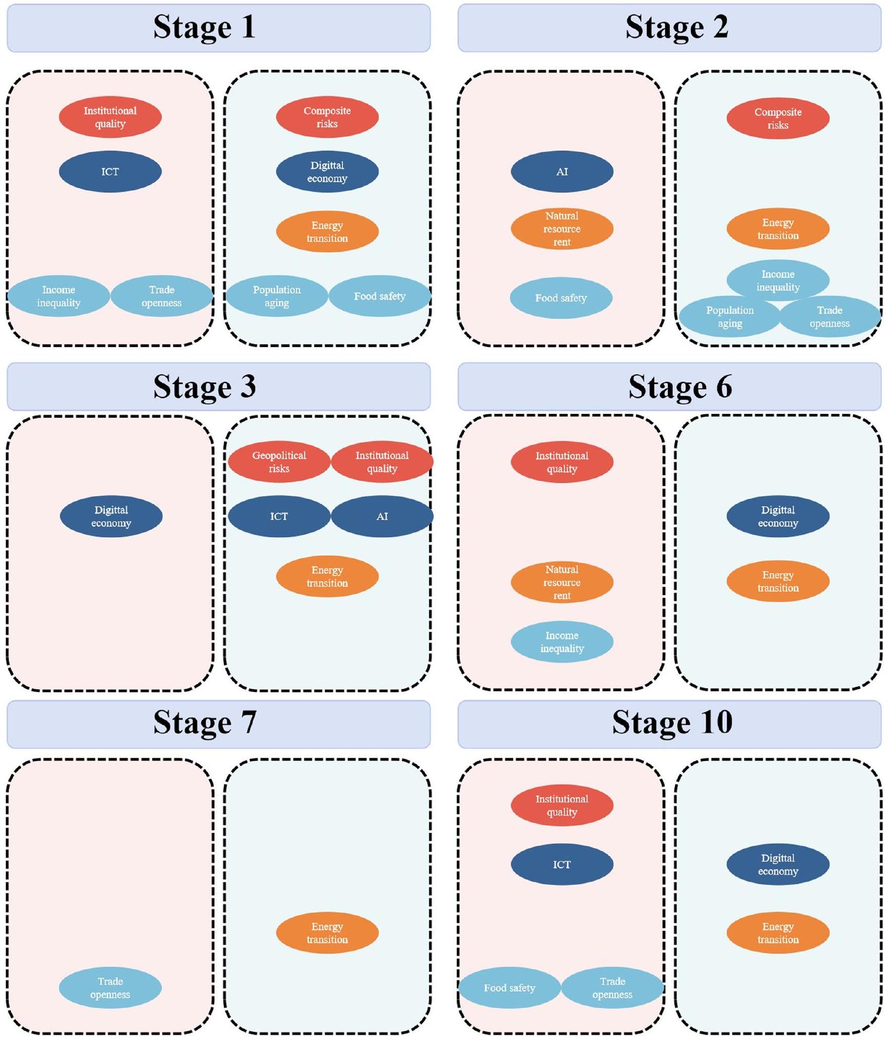
تقلل التكنولوجيا الرقمية من انبعاثات الكربون. يُظهر ذلك أن هذه الدول يجب أن تولي اهتمامًا لقضية بصمة الكربون في صناعة تكنولوجيا المعلومات والاتصالات وتشجع على اختراق تكنولوجيا المعلومات والاتصالات في القطاعات الاقتصادية الأخرى لتشكيل صناعة اقتصادية رقمية أوسع وأعمق. من حيث استخدام الموارد، فإن تأثير تقليل الانبعاثات الناتج عن انتقال الطاقة كبير. بالنظر إلى أن حجم التأثير ليس مثاليًا، يجب على الدول التي لا تزال في المرحلة الأولى أن تعطي الأولوية للتنمية الاقتصادية وتقوم تدريجيًا بنشر إنتاج واستخدام الطاقة النظيفة بالتزامن مع التنمية الاقتصادية. من حيث الإدارة الاجتماعية، فإن عدم المساواة في الدخل والانفتاح التجاري يجلبان المزيد من انبعاثات الكربون، بينما يقلل شيخوخة السكان والأمن الغذائي من انبعاثات الكربون. يبدو أنه من ناحية، يجب على هذه الدول أن تقدم سياسات مالية وزراعية لتعزيز التوزيع العادل للثروة وتحسين أمن إنتاج الغذاء (أكبر وآخرون، 2019). من ناحية أخرى، تحتاج إلى تقديم المزيد من المنتجات والتقنيات الخضراء في عملية التجارة الدولية أو تعزيز الاستثمار (كيانغ وانغ وآخرون، 2023ب).

بالنسبة للدول في المرحلة الثانية، فهي في حالة من الانفصال النسبي، بين عدم الانفصال والانفصال الكامل. وهذا يدل على أن هذه الدول لديها طرق معينة لتقليل التلوث في التنمية، ولكن لا يزال هناك مجال كبير لتقليل الانبعاثات. تحتاج هذه الدول إلى فهم شامل للعوامل الإيجابية والسلبية التي تؤثر على انبعاثات الكربون لتحقيق تحول من الانفصال النسبي إلى الانفصال المطلق. على وجه الخصوص، تشير نتائج هذه الدراسة إلى أن الذكاء الاصطناعي، وإيجارات الموارد الطبيعية، والأمن الغذائي تساهم في انبعاثات الكربون للفرد. لذلك، قد يكون تعزيز اللوائح البيئية وإدخال تقنيات معيارية وصديقة للبيئة في تكنولوجيا الذكاء الاصطناعي، واستخراج الموارد الطبيعية، وعمليات إنتاج الغذاء هو المفتاح لتحقيق انفصال قوي. تشير الحوافز السلبية لانبعاثات الكربون إلى أن الحفاظ على الاستقرار الوطني، وانتقال الطاقة، والانفتاح التجاري هي أيضًا أمور مهمة. الدول في المرحلة الثالثة هي دول غير منفصلة. إن تنميتها الاقتصادية مصحوبة بانبعاثات كربونية عالية، لذا فإن الأمر الأكثر أهمية هو حل مشكلة التنمية الخشنة. بالإضافة إلى ذلك، لا تزال المتغيرات الضابطة تقدم خيارات لتقليل الانبعاثات من وجهات نظر مؤسسية وتقنية وطبيعية. بالنسبة لهم، فإن المحرك الإيجابي لانبعاثات الكربون هو في المقام الأول الاقتصاد الرقمي. بالمقارنة، فإن تطوير تكنولوجيا المعلومات والاتصالات والذكاء الاصطناعي لا يمكن أن يحد من انبعاثات الكربون. وهذا يبرز الحاجة إلى فصل التنمية الاقتصادية عن انبعاثات الكربون. بالإضافة إلى ذلك، يمكن أن تؤدي زيادة مستويات المخاطر الجيوسياسية، وجودة المؤسسات، وانتقال الطاقة أيضًا إلى تقليل انبعاثات الكربون.

تتمتع دول المرحلة السادسة بمستوى عالٍ نسبيًا من التنمية وقد دخلت المرحلة الثانية من منحنى كوزنتس البيئي وحققت انفصالًا قويًا. ولكن يمكنها أيضًا السعي لتحقيق نتائج بيئية أفضل. استنادًا إلى المحركات السلبية لانبعاثات الكربون، يجب على هذه الدول التركيز على بناء المؤسسات البيئية، وتقييد استخدام الموارد الطبيعية التقليدية، وتحسين هياكل الدخل. بما يتماشى مع المحركات الإيجابية لانبعاثات الكربون، يلعب المزيد من تطوير الاقتصاد الرقمي وانتقال الطاقة دورًا مهمًا في تحسين جودة البيئة.

بالنسبة لدول المرحلة 7، فإن مستوى تطورها الاقتصادي أعلى من مستوى المرحلة 6، لكن تطورها الاقتصادي وانبعاثات الكربون قد أعيد ربطهما. بسبب العينة المحدودة، فإن نتائج معظم العوامل ليست ذات دلالة إحصائية. ومع ذلك، تشير نتائجنا إلى فكرتين لتقليل الانبعاثات. من ناحية، فإن آثار تحول الطاقة في هذه الدول أفضل بكثير من الدول الأخرى، ويجب تطوير ونشر الطاقة النظيفة بشكل أكبر في هذه الدول؛ من ناحية أخرى، فإن الانفتاح التجاري مرتبط إيجابياً بانبعاثات الكربون، ويجب عليهم فحص السلع المستوردة أو الاستثمارات الأجنبية بشكل أكثر صرامة. بينما تواجه دول المرحلة 10 تحديات اقتصادية.
الركود، التنمية الاقتصادية لها معامل تأثير عالٍ على انبعاثات الكربون. هذه الدول تحتاج ليس فقط إلى استقرار اقتصادها ولكن من المفترض أيضًا أن تجد طرقًا لتقليل التكاليف البيئية. تشير النتائج إلى أنها بحاجة إلى وضع لوائح بيئية أكثر صرامة ومعالجة قضايا انبعاثات الكربون في تكنولوجيا المعلومات والاتصالات، وإنتاج الغذاء، والانفتاح التجاري. بالإضافة إلى ذلك، يمكن اعتبار الاقتصاد الرقمي وانتقال الطاقة كخطوات إضافية في تطوير الصناعات الخضراء.

قدمت الأبحاث المبكرة أساسًا نظريًا قويًا وأدلة تجريبية لنموذج منحنى كوزنتس البيئي على شكل حرف U مقلوب. ومع ذلك، مع تزايد الحاجة الملحة للتخفيف من تغير المناخ، لاحظنا أن العديد من الدول المتقدمة تعاني من تدهور بيئي، واستهلاك مرتفع للطاقة، وانبعاثات كربونية. وهذا يجبرنا على البدء في التفكير في نموذج منحنى كوزنتس البيئي العالمي على شكل حرف N. بالإضافة إلى ذلك، فإن تأثير المخاطر، والتكنولوجيا الرقمية، وانتقال الطاقة، وعوامل اجتماعية متنوعة على الأنشطة الاجتماعية، والتنمية الاقتصادية، واستخدام الطاقة ثبت أيضًا أنه مساهمات كبيرة في انبعاثات الكربون. في هذا السياق، قمنا بتضمين أكبر عدد ممكن من الدول في الدراسة، وأعدنا فحص شكل منحنى كوزنتس البيئي في اللوحة العالمية، وأدرجنا 12 عاملًا مؤسسيًا وتقنيًا وموارد اجتماعية تقليدية وجديدة كمتغيرات إضافية في معادلة منحنى كوزنتس البيئي. بالإضافة إلى ذلك، طورنا نموذج فك الارتباط ثنائي الأبعاد بناءً على نقطة الانعطاف في منحنى كوزنتس البيئي على شكل N لتحقيق مناقشة جماعية للدول العينة. أخيرًا، استنادًا إلى التجميع، ناقشنا التأثير غير المتجانس لجميع المتغيرات وحلول تقليل الانبعاثات المختلفة لكل مجموعة بين المجموعات وحققنا سلسلة من الاستنتاجات.

أولاً، في اللوحة العالمية، يوجد شكل N من منحنى كيركوس البيئي بشكل قوي بغض النظر عما إذا كانت المتغيرات الإضافية تؤخذ في الاعتبار أم لا. بعبارة أخرى، فإن الحدود التكعيبية والخطية للناتج المحلي الإجمالي للفرد إيجابية بشكل كبير، بينما الحد التربيعي سالب بشكل كبير. من بينها، عندما لا تؤخذ المتغيرات الإضافية في الاعتبار، فإن الشكل N قد اجتاز أربع اختبارات للمتانة. عند النظر في المتغيرات الإضافية، فإن هذا الشكل N من منحنى كيركوس البيئي يبقى صحيحًا في كل خطوة من خطوات الانحدار التدريجي. وبالتالي، تم تأكيد H1 و H2 بشكل كامل. بعد تحديد وجود الشكل N، قمنا أخيرًا بحساب نقاط الانعطاف لمنحنى كيركوس البيئي بما في ذلك جميع المتغيرات الضابطة، والتي كانت 45.08 و 73.44 (ألف دولار/شخص) على التوالي. من خلال مقارنة منحنى كيركوس البيئي النهائي بشكل N مع المنحنى N بدون إضافة المتغيرات الضابطة، وجدنا أن كل من “المدة” و “مساحة الانخفاض” في الجزء المتناقص الوحيد من المنحنى قد تقلصت، مما يجعل التخفيف من تغير المناخ العالمي أكثر حدة. من خلال التحقق المتبادل لكل خطوة من خطوات الانحدار التدريجي، حددنا أخيرًا اتجاه تأثير جميع المتغيرات الإضافية. من بينها، تم تأكيد أن المخاطر الجيوسياسية، وتكنولوجيا المعلومات والاتصالات، والأمن الغذائي لها تأثير إيجابي على انبعاثات الكربون للفرد. ومع ذلك، وُجد أن المخاطر الشاملة، وجودة المؤسسات، والاقتصاد الرقمي، وانتقال الطاقة، وشيخوخة السكان لها تأثير سلبي قوي. كما أن الذكاء الاصطناعي، وإيجارات الموارد الطبيعية، والانفتاح التجاري، وعدم المساواة في الدخل لها تأثيرات غير ملحوظة على انبعاثات الكربون. هذه النتائج أكدت جزئيًا H3.

في دراسة المجموعة، استخدمنا أولاً الناتج المحلي الإجمالي للفرد البالغ 45.08 و73.44 (ألف دولار أمريكي لكل شخص) الذي تم الحصول عليه في منحنى كوزنتس البيئي كأساس للتصنيف، وقمنا في البداية بتقسيم جميع الدول إلى ثلاث مراحل من منحنى كوزنتس البيئي. ونتيجة لذلك، تنتمي 194 دولة إلى المرحلة الأولى، و11 دولة إلى المرحلة الثانية، و9 دول إلى المرحلة الثالثة. ثانياً، قمنا بحساب معامل مرونة فك الارتباط لطابيو بين العقدين الماضيين لجميع الدول وقمنا بتقسيم الدول إلى ثلاث حالات باستخدام 0 و0.8 كعتبات. تظهر النتائج أن هناك 57 و47 و55 و34 دولة في حالة عدم فك الارتباط، وفك الارتباط الضعيف،
فصل قوي، وركود، على التوالي. بناءً على ذلك، قمنا بإنشاء إحداثيات فصل ثنائية الأبعاد ودمجنا الحالات الثلاث لكل من البعدين المذكورين مع بعضها للحصول على تسع حالات فصل ثنائية الأبعاد. نقسم العينة إلى خمس مجموعات من خلال مطابقة نتائج العينة غير الركودية مع تسع حالات الفصل. من بينها، هناك 43 و47 و57 و9 و3 دول في المراحل 1 و2 و3 و6 و7، على التوالي. بإضافة الدول المتراجعة (المرحلة 10) نحصل على 6 لوحات. نقوم أيضًا بإجراء انحدارات خطية متعددة في هذه اللوحات ونناقش التأثيرات المتباينة للتنمية الاقتصادية و12 متغيرًا إضافيًا على انبعاثات الكربون. النتائج تؤكد تمامًا الفرضية H4 وتظهر أن تأثيرات معظم المتغيرات تختلف وفقًا لظروف الدول. المتغير الأكثر قوة هو انتقال الطاقة، الذي يظهر تأثيرًا كبيرًا في تقليل الكربون في جميع المجموعات. ومع ذلك، فإن حجم تأثير انتقال الطاقة أيضًا متباين. في الدول ذات مستويات التنمية الاقتصادية الأعلى والفصل، تكون تأثيرات انتقال الطاقة أقوى. أخيرًا، نناقش خطط تقليل الانبعاثات المختلفة للدول في مراحل الفصل الثنائية الأبعاد المختلفة بناءً على اتجاه تأثير المتغيرات.

تتمتع النتائج المذكورة أعلاه بتداعيات سياسية قيمة. أولاً وقبل كل شيء، تظهر النتائج العالمية أن منحنى كوزنيك N أكثر حدة من منحنى U المقلوب. تؤكد التحقق التجريبي من التقادم التكنولوجي على ضرورة أن تعزز الدول المتقدمة في جميع أنحاء العالم تركيزها على اللوائح البيئية الداخلية ورفع مستويات الابتكار في التقنيات النظيفة. علاوة على ذلك، فإن تضمين متغيرات إضافية في تحليلنا يبرز الدور المحوري الذي تلعبه بيئة التنمية الدولية والمحلية المستقرة جنبًا إلى جنب مع الأطر المؤسسية الفعالة في الحد من انبعاثات الكربون وتعزيز جهود التخفيف من آثار تغير المناخ العالمية. إن السعي غير النقدي وراء التقدم التكنولوجي الرقمي أو الذكي لا يترجم بالضرورة إلى تحسين بيئي. على العكس من ذلك، فإن الاستخدام الحكيم للتكنولوجيا من أجل تحسين كل من الاقتصاد والمجتمع يمثل طريقًا واعدًا لتحقيق تخفيضات في انبعاثات الكربون. علاوة على ذلك، تؤكد نتائجنا حول استخدام الموارد على الحاجة الملحة لتسريع تطوير واعتماد مصادر الطاقة النظيفة. في معالجة المحددات الاجتماعية، يجب إيلاء اهتمام خاص لتحسين استخدام الأراضي وتقليل انتشار الأطعمة ذات البصمة الكربونية العالية في الإنتاج الزراعي. أخيرًا، تم مناقشة أفكار محددة لتقليل الانبعاثات لكل دولة بعمق في القسم “استراتيجيات تقليل الكربون المختلفة للدول في مراحل فك الارتباط ثنائية الأبعاد المختلفة”.

نحتاج إلى الإشارة إلى قيود هذه المقالة لتقديم أفكار للتحسين. أولاً، بسبب عدم تجانس مصادر البيانات، يستخدم عمليتنا التجريبية لوحة غير متوازنة. في بعض الخطوات، لا تغطي العينة الفعالة جميع الدول الـ 214. قد يتسبب ذلك في تجاهل المعلومات من بعض الدول. ثانياً، ندرج بعض المتغيرات الإضافية المهمة أو الجديدة لمناقشة شاملة لعوامل انبعاثات الكربون بخلاف النمو. ومع ذلك، لا يمكننا اعتبار جميع العوامل. ثالثاً، طورنا فكرتين لفصل الدول إلى 9 مراحل بناءً على شكل N لأخذ التباين بين الدول في الاعتبار بشكل كامل. ومع ذلك، فإن هذا التصنيف أيضًا لا يتعامل بشكل كامل مع التباين. دراستنا العامة ليست بديلاً عن دراسات الحالة في دولة واحدة أو الدراسات دون الوطنية. لذلك، قام الباحثون اللاحقون بإجراء أبحاث أكثر عمقًا من منظور تحسين وحدة مصادر البيانات، وتقديم متغيرات إضافية أكثر حداثة ونقدية، وإجراء دراسات حالة أكثر دقة.

يجب أن تكون مجموعات البيانات المتاحة للجمهور من خلالhttps://doi.org/10.7910/DVN/0I1EYG.

تاريخ الاستلام: 16 نوفمبر 2023؛ تاريخ القبول: 23 يناير 2024؛
نُشر على الإنترنت: 21 فبراير 2024

1 عند تحديد ترتيب إضافة المتغيرات، نأخذ في الاعتبار خصائص البيانات للمتغيرات، وخاصة حجم البيانات، بحيث يتم تضمين أكبر عدد ممكن من الدول في كل خطوة.
2 عدد الدول التي تنتمي إلى المرحلتين الثانية والثالثة من EKC في فك الارتباط ثنائي الأبعاد في الشكل 4c أقل من تلك الموجودة في الشكل 4a. وذلك لأن بعض الدول لديها فقط بيانات الناتج المحلي الإجمالي للفرد ولكن لا تملك بيانات كافية عن انبعاثات الكربون في العقدين الماضيين.

Akbar A, Ali I, Samiullah NU, Khan SA, Rehman Z, Rehman S (2019) Functional, antioxidant, antimicrobial potential and food safety applications of Curcuma longa and Cuminum cyminum. Pak J Bot 51(3):1129-1135
Allard A, Takman J, Uddin GS, Ahmed A (2018) The N-shaped environmental Kuznets curve: an empirical evaluation using a panel quantile regression approach. Environ Sci Pollut Res 25:5848-5861
Álvarez-Herránz A, Balsalobre D, Cantos JM, Shahbaz M (2017) Energy innovations-GHG emissions nexus: fresh empirical evidence from OECD countries. Energy Policy 101:90-100
Andreoni J, Levinson A (2001) The simple analytics of the environmental Kuznets curve. J Public Econ 80(2):269-286
Ang JB (2008) Economic development, pollutant emissions and energy consumption in Malaysia. J Policy Model 30(2):271-278
Anser MK, Syed QR, Apergis N (2021) Does geopolitical risk escalate emissions? Evidence from the BRICS countries. Environ Sci Pollut Res 28(35):48011-48021
Apergis N, Ozturk I (2015) Testing environmental Kuznets curve hypothesis in Asian countries. Ecol Indic 52:16-22
Asiedu E (2006) Foreign direct investment in Africa: The role of natural resources, market size, government policy, institutions and political instability. World Econ 29(1):63-77
Balsalobre-Lorente D, Shahbaz M, Roubaud D, Farhani S (2018) How economic growth, renewable electricity and natural resources contribute to emissions? Energy policy 113:356-367
Balsalobre-Lorente D, Sinha A, Driha OM, Mubarik MS (2021) Assessing the impacts of ageing and natural resource extraction on carbon emissions: a proposed policy framework for European economies. J Clean Prod 296:126470
Bashir MF (2022) Discovering the evolution of Pollution Haven Hypothesis: a literature review and future research agenda. Environ Sci Pollut Res 29(32):48210-48232
Beckerman W (1992) Economic growth and the environment: Whose growth? Whose environment? World Dev 20(4):481-496
Berkeley (2024) Press Release: 2023 was warmest year since 1850. Berkeley Earth. https://berkeleyearth.org/press-release-2023-was-the-warmest-year-on-recordpress-release/
Brown PT, Hanley H, Mahesh A, Reed C, Strenfel SJ, Davis SJ et al. (2023) Climate warming increases extreme daily wildfire growth risk in California. Nature 621(7980):760-766. https://doi.org/10.1038/s41586-023-06444-3
Caldara D, Iacoviello M (2022) Measuring geopolitical risk. Am Econ Rev 112(4):1194-1225
Carlson CJ, Albery GF, Merow C, Trisos CH, Zipfel CM, Eskew EA et al. (2022) Climate change increases cross-species viral transmission risk. Nature 607(7919):555-562. https://doi.org/10.1038/s41586-022-04788-w
Cavicchioli R, Ripple WJ, Timmis KN, Azam F, Bakken LR, Baylis M et al. (2019) Scientists’ warning to humanity: microorganisms and climate change. Nat Rev Microbiol 17(9):569-586
Charfeddine L, Umlai M (2023) ICT sector, digitization and environmental sustainability: a systematic review of the literature from 2000 to 2022. Renew Sustain Energy Rev 184:113482
Cheng P, Tang H, Lin F, Kong X (2023) Bibliometrics of the nexus between food security and carbon emissions: hotspots and trends. Environ Sci Pollut Res 30(10):25981-25998
Cole MA (2004) Trade, the pollution haven hypothesis and the environmental Kuznets curve: examining the linkages. Ecol Econ 48(1):71-81
Dai M, Sun M, Chen B, Shi L, Jin M, Man Y et al. (2023) Country-specific net-zero strategies of the pulp and paper industry. Nature 626:327-334. https://doi. org/10.1038/s41586-023-06962-0
Diaz D, Moore F (2017) Quantifying the economic risks of climate change. Nat Clim Change 7(11):774-782
Dinda S (2004) Environmental Kuznets curve hypothesis: a survey. Ecol Econ 49(4):431-455

Ding T, Li J, Shi X, Li X, Chen Y (2023) Is artificial intelligence associated with carbon emissions reduction? Case of China. Resour Policy 85:103892
Do TK (2021) Resource curse or rentier peace? The impact of natural resource rents on military expenditure. Resour Policy 71:101989
Dogan E, Seker F (2016) Determinants of emissions in the European Union: the role of renewable and non-renewable energy. Renew Energy 94:429-439
Dong F, Hu M, Gao Y, Liu Y, Zhu J, Pan Y (2022a) How does digital economy affect carbon emissions? Evidence from global 60 countries. Sci Total Environ 852:158401
Dong F, Li Y, Gao Y, Zhu J, Qin C, Zhang X (2022b) Energy transition and carbon neutrality: exploring the non-linear impact of renewable energy development on carbon emission efficiency in developed countries. Resour Conserv Recycl 177:106002
Dong M, Wang G, Han X (2023) Artificial intelligence, industrial structure optimization, and emissions. Environ Sci Pollut Res 30(50):108757-108773
Duan H, Zhou S, Jiang K, Bertram C, Harmsen M, Kriegler E et al. (2021) Assessing China’s efforts to pursue the 1.5 C warming limit. Science 372(6540):378-385
Fakher HA, Ahmed Z, Acheampong AO, Nathaniel SP (2023) Renewable energy, nonrenewable energy, and environmental quality nexus: an investigation of the N-shaped Environmental Kuznets Curve based on six environmental indicators. Energy 263:125660
Fan J, Zhou L, Zhang Y, Shao S, Ma M (2021) How does population aging affect household carbon emissions? Evidence from Chinese urban and rural areas. Energy Econ 100:105356
Fankhauser S, Smith SM, Allen M, Axelsson K, Hale T, Hepburn C et al. (2022) The meaning of net zero and how to get it right. Nat Clim Change 12(1):15-21
Farooq S, Ozturk I, Majeed MT, Akram R (2022) Globalization and emissions in the presence of EKC: a global panel data analysis. Gondwana Res 106:367-378
Fawzy S, Osman AI, Doran J, Rooney DW (2020) Strategies for mitigation of climate change: a review. Environ Chem Lett 18:2069-2094
Gill AR, Viswanathan KK, Hassan S (2018) The Environmental Kuznets Curve (EKC) and the environmental problem of the day. Renew Sustain Energy Rev 81:1636-1642
Grossman GM, Krueger AB (1991) Environmental impacts of a North American free trade agreement. National Bureau of Economic Research Cambridge, MA, USA
Grossman GM, Krueger AB (1995) Economic growth and the environment. Q J Econ 110(2):353-377
Guan Y, Yan J, Shan Y, Zhou Y, Hang Y, Li R et al. (2023) Burden of the global energy price crisis on households. Nat Energy 8(3):304-316
Hanif I, Raza SMF, Gago-de-Santos P, Abbas Q (2019) Fossil fuels, foreign direct investment, and economic growth have triggered emissions in emerging Asian economies: some empirical evidence. Energy 171:493-501
Hassan T, Khan Y, He C, Chen J, Alsagr N, Song H (2022) Environmental regulations, political risk and consumption-based carbon emissions: evidence from OECD economies. J Environ Manag 320:115893
Heerink N, Mulatu A, Bulte E (2001) Income inequality and the environment: aggregation bias in environmental Kuznets curves. Ecol Econ 38(3):359-367
Higón DA, Gholami R, Shirazi F (2017) ICT and environmental sustainability: a global perspective. Telemat Inform 34(4):85-95
Hoegh-Guldberg O, Jacob D, Taylor M, Guillén Bolaños T, Bindi M, Brown S et al. (2019) The human imperative of stabilizing global climate change at 1.5 C . Science 365(6459):eaaw6974
Hossain MR, Rej S, Awan A, Bandyopadhyay A, Islam MS, Das N et al. (2023) Natural resource dependency and environmental sustainability under N-shaped EKC: the curious case of India. Resour Policy 80:103150
IFR (2023) World Robotics 2023 Report. International Federation of Robotics. https://ifr.org/ifr-press-releases/news/world-robotics-2023-report-asia-ahead-of-europe-and-the-americas
Im KS, Pesaran MH, Shin Y (2023) Reflections on “Testing for unit roots in heterogeneous panels”. J Econ 234:111-114
Inglesi-Lotz R, Dogan E (2018) The role of renewable versus non-renewable energy to the level of emissions a panel analysis of sub-Saharan Africa’s Big 10 electricity generators. Renew Energy 123:36-43
IPCC (2023) AR 6. intergovernmental panel on climate change. https://www.ipcc. ch/report/ar6/syr/downloads/report/IPCC_AR6_SYR_SPM.pdf
ITU (2023) ICT statistics. International Telecommunication Union. https://www. itu.int/en/ITU-D/Statistics/Pages/stat/default.aspx
Jahanger A, Hossain MR, Onwe JC, Ogwu SO, Awan A, Balsalobre-Lorente D (2023) Analyzing the N-shaped EKC among top nuclear energy generating nations: a novel dynamic common correlated effects approach. Gondwana Res 116:73-88
Kaika D, Zervas E (2013a) The environmental Kuznets curve (EKC) theory-Part A: concept, causes and the emissions case. Energy Policy 62:1392-1402
Kaika D, Zervas E (2013b) The environmental Kuznets curve (EKC) theory. Part B: critical issues. Energy Policy 62:1403-1411

Kao C (1999) Spurious regression and residual-based tests for cointegration in panel data. J Econ 90(1):1-44
Karim S, Appiah M, Naeem MA, Lucey BM, Li M (2022) Modelling the role of institutional quality on carbon emissions in Sub-Saharan African countries. Renew Energy 198:213-221
Koondhar MA, Shahbaz M, Memon KA, Ozturk I, Kong R (2021) A visualization review analysis of the last two decades for environmental Kuznets curve “EKC” based on co-citation analysis theory and pathfinder network scaling algorithms. Environ Sci Pollut Res 28:16690-16706
Kuznets (1955) Economic growth and income inequality. Am Econ Rev 45(1):1-28
Lantz V, Feng Q (2006) Assessing income, population, and technology impacts on emissions in Canada: where’s the EKC? Ecol Econ 57(2):229-238
Lark TJ, Spawn SA, Bougie M, Gibbs HK (2020) Cropland expansion in the United States produces marginal yields at high costs to wildlife. Nat Commun 11(1):4295
Le HP, Ozturk I (2020) The impacts of globalization, financial development, government expenditures, and institutional quality on emissions in the presence of environmental Kuznets curve. Environ Sci Pollut Res 27:22680-22697
Leal PH, Marques AC (2022) The evolution of the environmental Kuznets curve hypothesis assessment: a literature review under a critical analysis perspective. Heliyon
Li R, Wang Q, Guo J (2024) Revisiting the environmental Kuznets curve (EKC) hypothesis of carbon emissions: exploring the impact of geopolitical risks, natural resource rents, corrupt governance, and energy intensity. J Environ Manag 351:119663. https://doi.org/10.1016/j.jenvman.2023.119663
Li R, Wang Q, Li L, Hu S (2023) Do natural resource rent and corruption governance reshape the environmental Kuznets curve for ecological footprint? Evidence from 158 countries. Resour Policy 85:103890
Li R, Wang Q, Liu Y, Jiang R (2021) Per-capita carbon emissions in 147 countries: the effect of economic, energy, social, and trade structural changes. Sustain Prod Consum 27:1149-1164
Li Y, Zhang Y, Pan A, Han M, Veglianti E (2022) Carbon emission reduction effects of industrial robot applications: Heterogeneity characteristics and influencing mechanisms. Technol Soc 70:102034
Liu B, Yang X, Zhang J (2024) Nonlinear effect of industrial robot applications on carbon emissions: evidence from China. Environ Impact Assess Rev 104:107297
Lorente DB, Álvarez-Herranz A (2016) Economic growth and energy regulation in the environmental Kuznets curve. Environ Sci Pollut Res 23:16478-16494
Luan F, Yang X, Chen Y, Regis PJ (2022) Industrial robots and air environment: a moderated mediation model of population density and energy consumption. Sustain Prod Consum 30:870-888
Mao F, Miller JD, Young SL, Krause S, Hannah DM (2022) Inequality of household water security follows a Development Kuznets Curve. Nat Commun 13(1):4525
Naeem MA, Appiah M, Taden J, Amoasi R, Gyamfi BA (2023) Transitioning to clean energy: assessing the impact of renewable energy, bio-capacity and access to clean fuel on carbon emissions in OECD economies. Energy Econ 127:107091. https://doi.org/10.1016/j.eneco.2023.107091
Naseem S, Guang Ji T, Kashif U (2020) Asymmetrical ARDL correlation between fossil fuel energy, food security, and carbon emission: providing fresh information from Pakistan. Environ Sci Pollut Res 27:31369-31382
Nguyen KH, Kakinaka M (2019) Renewable energy consumption, carbon emissions, and development stages: some evidence from panel cointegration analysis. Renew Energy 132:1049-1057
Numan U, Ma B, Meo MS, Bedru HD (2022) Revisiting the N-shaped environmental Kuznets curve for economic complexity and ecological footprint. J Clean Prod 365:132642
PRS (2023) ICRG. The International Country Risk Guide. https://www.prsgroup. com/explore-our-products/icrg/
Rashdan MOJ, Faisal F, Tursoy T, Pervaiz R (2021) Investigating the N-shape EKC using capture fisheries as a biodiversity indicator: empirical evidence from selected 14 emerging countries. Environ Sci Pollut Res 28:36344-36353
Ray DK, Gerber JS, MacDonald GK, West PC (2015) Climate variation explains a third of global crop yield variability. Nat Commun 6(1):5989
Roelfsema M, van Soest HL, Harmsen M, van Vuuren DP, Bertram C, den Elzen M et al. (2020) Taking stock of national climate policies to evaluate implementation of the Paris Agreement. Nat Commun 11(1):2096
Rojas-Vallejos J, Lastuka A (2020) The income inequality and carbon emissions trade-off revisited. Energy Policy 139:111302
Salman M, Long X, Dauda L, Mensah CN (2019) The impact of institutional quality on economic growth and carbon emissions: Evidence from Indonesia, South Korea and Thailand. J Clean Prod 241:118331
Schiermeier Q (2020) The US has left the Paris climate deal-what’s next? Nature 2022. https://doi.org/10.1038/d41586-020-03066-x

Shehzad K, Zeraibi A, Zaman U (2022) Testing the N-shaped environmental Kuznets Curve in Algeria: an imperious role of natural resources and economic globalization. Resour Policy 77:102700

Stern DI (2017) The environmental Kuznets curve after 25 years. J Bioeconomics 19:7-28
Tapio P (2005) Towards a theory of decoupling: degrees of decoupling in the EU and the case of road traffic in Finland between 1970 and 2001. Transp Policy 12(2):137-151
Tollefson J (2022) What the war in Ukraine means for energy, climate and food. Nature 604(7905):232-233
Ullah A, Khan S, Khamjalas K, Ahmad M, Hassan A, Uddin I (2023) Environmental regulation, renewable electricity, industrialization, economic complexity, technological innovation, and sustainable environment: testing the N-shaped EKC hypothesis for the G-10 economies. Environ Sci Pollut Res 30(44):99713-99734
Usman O, Alola AA, Sarkodie SA (2020) Assessment of the role of renewable energy consumption and trade policy on environmental degradation using innovation accounting: evidence from the US. Renew Energy 150:266-277
Vakulchuk R, Overland I, Scholten D (2020) Renewable energy and geopolitics: a review. Renew Sustain Energy Rev 122:109547
Wang K, Zhu Y, Zhang J (2021) Decoupling economic development from municipal solid waste generation in China’s cities: Assessment and prediction based on Tapio method and EKC models. Waste Manag 133:37-48
Wang Q, Ge Y, Li R (2024a) Does improving economic efficiency reduce ecological footprint? The role of financial development, renewable energy, and industrialization. Energy Environ 0958305X231183914. https://doi.org/10.1177/ 0958305X231183914
Wang Q, Hu S, Li R (2024b) Could information and communication technology (ICT) reduce carbon emissions? The role of trade openness and financial development. Telecommunications Policy, 102699. https://doi.org/10.1016/j. telpol.2023.102699
Wang Q, Ren F, Li R (2023a) Exploring the impact of geopolitics on the environmental Kuznets curve research. Sustain Dev 2023. https://doi.org/10.1002/sd. 2743
Wang Q, Wang L, Li R (2023b) Trade openness helps move towards carbon neutrality-insight from 114 countries. Sustain Dev 2023. https://doi.org/10. 1002/sd. 2720
Worldbank (2023a) WDI. World Development Index. https://datatopics. worldbank.org/world-development-indicators/
Worldbank (2023b) WGI. World Governance Index. https://www.govindicators.org/
Xiaoman W, Majeed A, Vasbieva DG, Yameogo CEW, Hussain N (2021) Natural resources abundance, economic globalization, and carbon emissions: advancing sustainable development agenda. Sustain Dev 29(5):1037-1048
Yi M, Liu Y, Sheng MS, Wen L (2022) Effects of digital economy on carbon emission reduction: new evidence from China. Energy Policy 171:113271
Zhang J, Lyu Y, Li Y, Geng Y (2022a) Digital economy: an innovation driving factor for low-carbon development. Environ Impact Assess Rev 96:106821
Zhang L, Mu R, Zhan Y, Yu J, Liu L, Yu Y et al. (2022b) Digital economy, energy efficiency, and carbon emissions: evidence from provincial panel data in China. Sci Total Environ 852:158403
Zhao J, Shahbaz M, Dong X, Dong K (2021a) How does financial risk affect global emissions? The role of technological innovation. Technol Forecast Soc Change 168:120751
Zhao S, Hafeez M, Faisal CMN (2022) Does ICT diffusion lead to energy efficiency and environmental sustainability in emerging Asian economies? Environ Sci Pollut Res 29:12198-12207
Zhao W, Zhong R, Sohail S, Majeed MT, Ullah S (2021b) Geopolitical risks, energy consumption, and emissions in BRICS: an asymmetric analysis. Environ Sci Pollut Res 28:39668-39679
Zhao Z, Gozgor G, Lau MCK, Mahalik MK, Patel G, Khalfaoui R (2023) The impact of geopolitical risks on renewable energy demand in OECD countries. Energy Econ 122:106700
Zhengxia T, Haseeb M, Usman M, Shuaib M, Kamal M, Khan MF (2023) The role of monetary and fiscal policies in determining environmental pollution: revisiting the N-shaped EKC hypothesis for China. Environ Sci Pollut Res 30(38):89756-89769

Zhong J, Zhong Y, Han M, Yang T, Zhang Q (2023) The impact of AI on carbon emissions: evidence from 66 countries. Appl Econ 2023:1-15. https://doi.org/ 10.1080/00036846.2023.2203461

Zhou Y, Wang H, Qiu H (2023) Population aging reduces carbon emissions: evidence from China’s latest three censuses. Appl Energy 351:121799
Zou T, Zhang X, Davidson E (2022) Global trends of cropland phosphorus use and sustainability challenges. Nature 611(7934):81-87

هذا العمل مدعوم من قبل المؤسسة الوطنية للعلوم الطبيعية في الصين (أرقام المنح: 72104246، 71874203).

QW: التصور، المنهجية، البرمجيات، تنظيم البيانات، إعداد المسودة الأصلية، الإشراف، مراجعة الكتابة وتحريرها. YL: المنهجية، البرمجيات، تنظيم البيانات، التحقيق في كتابة المسودة الأصلية، مراجعة الكتابة وتحريرها. RL: التصور، المنهجية، تنظيم البيانات، التحقيق في كتابة المسودة الأصلية، مراجعة الكتابة.

يعلن المؤلفون عدم وجود مصالح متنافسة.

لا يحتوي هذا المقال على أي دراسات مع مشاركين بشريين أجراها أي من المؤلفين.

لا يحتوي هذا المقال على أي دراسات مع مشاركين بشريين أجراها أي من المؤلفين.

معلومات إضافية النسخة الإلكترونية تحتوي على مواد إضافية متاحة فيhttps://doi.org/10.1057/s41599-024-02736-9.

يجب توجيه المراسلات والطلبات للحصول على المواد إلى تشيانغ وانغ أو رونغ رونغ لي.

معلومات إعادة الطباعة والإذن متاحة علىhttp://www.nature.com/reprints
ملاحظة الناشر: تظل شركة سبرينغر ناتشر محايدة فيما يتعلق بالمطالبات القضائية في الخرائط المنشورة والانتماءات المؤسسية.

الوصول المفتوح. هذه المقالة مرخصة بموجب رخصة المشاع الإبداعي النسب 4.0 الدولية، التي تسمح بالاستخدام والمشاركة والتكيف والتوزيع وإعادة الإنتاج بأي وسيلة أو صيغة، طالما أنك تعطي الائتمان المناسب للمؤلفين الأصليين والمصدر، وتوفر رابطًا لرخصة المشاع الإبداعي، وتوضح ما إذا تم إجراء تغييرات. الصور أو المواد الأخرى من طرف ثالث في هذه المقالة مشمولة في رخصة المشاع الإبداعي الخاصة بالمقالة، ما لم يُشار إلى خلاف ذلك في سطر الائتمان للمواد. إذا لم تكن المادة مشمولة في رخصة المشاع الإبداعي الخاصة بالمقالة وكان استخدامك المقصود غير مسموح به بموجب اللوائح القانونية أو يتجاوز الاستخدام المسموح به، ستحتاج إلى الحصول على إذن مباشرة من صاحب حقوق الطبع والنشر. لعرض نسخة من هذه الرخصة، قم بزيارة http://creativecommons.org/licenses/by/4.0/.
© المؤلفون 2024

The suitability and stability of the Earth’s climate are crucial for human survival (Carlson et al., 2022; Cavicchioli et al., 2019) and development (Brown et al., 2023; Ray et al., 2015; Diaz and Moore, 2017). However, as of January 2024, global surface temperatures have accelerated by since the preindustrial period (Berkeley, 2024). According to the IPCC’s 7th climate assessment report (AR 7), the global warming is “unequivocally” caused primarily by human activities and anthropogenic greenhouse gas emissions (IPCC, 2023). Upon the societal acknowledgment of the causality, the question of how to transform the existing development paradigm to conform with climate mitigation principles emerges as a central focus for the governmental (Duan et al., 2021; Dai et al., 2023) and scholarly attention (Fawzy et al., 2020; Hoegh-Guldberg et al., 2019; Fankhauser et al., 2022).

The environmental Kuznets curve (EKC) is among the most prevalent economic-environmental simulation models utilized for policy analysis (Zou et al., 2022; Koondhar et al., 2021; Mao et al., 2022). The EKC hypothesis linked economic development to environmental quality in such a paradigm: per capita income and per capita carbon dioxide emissions increase together until a certain inflection point in income is reached, after which the growth of pollutants levels off and then overturns (Grossman and Krueger, 1995). Such inverted U-shaped nonlinear patterns have been empirically confirmed in countless number of early studies and explanations are mainly given by inefficient and dirty production techniques in the pre-industrial stages and the strengthened environmental regulations and advanced clean technologies in the developed stages (Balsalobre-Lorente et al., 2018). Over the past three decades, such paradigms of “grow first and clean later” have often served as a benchmark for other climate models and even as references for national plans (Koondhar et al., 2021; Kaika and Zervas, 2013a).

However, many of the news and events we hear and observe recently suggest a weakening relationship between advanced economies and improved environment, which seems to contradict the existing explanation. First, some developed countries including the United States are known to be ecologically deficit (Usman et al., 2020; Lark et al., 2020). Moreover, in November 2020, as the world’s largest economy and second-largest carbon emitter, the U.S. vowed to withdraw from the Paris Agreement to restart its traditional and highly polluting sectors (Schiermeier, 2020; Roelfsema et al., 2020). Finally, many developed countries, including Germany, the Netherlands, and Austria, are once again turning to coal for electricity and heating as they struggle with a European energy crisis triggered by the Russia-Ukraine conflict beginning in 2022 (Tollefson, 2022; Guan et al., 2023).

These events highlight the need to revisit the global EKC, specifically discussing the N -shaped curve. On the one hand, the new paradigm of the N -shaped curve is more suitable for the current actual situation than the inverted U-shaped EKC. This is because the carbon emission trajectory may still be bent upward at a high level of economic development if the technological effects brought about by green innovation cannot keep up with the growing scale effects (Lorente and Álvarez-Herranz, 2016). On the other hand, once the “development first, clean later” commitment of the previous inverted U-shaped EKC theory is disillusioned, then developing countries can no longer sit back and be excluded from the climate agenda and emission reduction plans (Koondhar et al., 2021; Kaika and Zervas, 2013a). Hence, an accurate understanding of the current shape of global EKC is critical for different categories of countries to identify their unique drivers of carbon emissions and adopt prompt action.

The current situation, on the other side, also demonstrates the complexity of the determining rules of carbon emissions.

Although some additional variables including trade openness, institutional quality, and energy consumption have been widely incorporated into the EKC framework (Leal and Marques, 2022), recent research has established some new links between external factors and carbon emissions. For example, geopolitical risks and national political, economic, and financial risks are proven to have the potential to change countries’ economic development and energy use patterns (Anser et al., 2021; Hassan et al., 2022; Qiang Wang et al., 2023a). Digital technology and artificial intelligence, as key to the third and fourth industrial revolutions, have been found to have carbon-reducing effects in some studies (Jinning Zhang et al., 2022a; Ding et al., 2023). The transition from traditional fossil fuels to new energy sources has been empirically confirmed to effectively mitigate air pollution and accelerate carbon neutrality (Feng Dong et al., 2022b; Naeem et al., 2023). Finally, some social issues, including population aging (Fan et al., 2021) and food security (Naseem et al., 2020), are also included in the environmental analysis. As (Stern, 2017) note, it is necessary to reveal the effects of other variables other than economic growth within the EKC framework. Banking on these current issues of global environment and carbon emissions, we ask the following questions: What is the current shape of global EKC when new additional factors are taken into account? Is there heterogeneity in the impact of various factors on carbon emissions in different types of countries?

This article aims to answer the above questions by empirically examining the current shape of the global EKC and fully considering the impact of multiple carbon emission drivers and the heterogeneity in the panel. Specifically, this paper contributes to the literature in the following three aspects. First, this paper studies N -shaped EKC in 214 countries and incorporates 12 traditional or novel institutional, technological, resource, and social factors as additional variables in the EKC equation. This work provides preliminary but crucial information for mitigation actions by elucidating the relationship between global economic development and carbon emissions and identifying potential drivers of carbon emissions. Second, to handle the heterogeneity of countries, we develop a two-dimensional Tapio decoupling model based on N-type EKC to evaluate the economic development stage and decoupling situation of each country. We believe that starting a classified and detailed discussion can help to more systematically reveal the different situations or problems in economic development and carbon emission reduction in countries around the world. Finally, based on the grouping results, we analyze the inter-group heterogeneity of the carbon emission effects of economic and additional variables, providing a baseline reference for countries at different stages to formulate targeted and effective carbon emission reduction policies.

The remainder of this article is arranged as follows. The section “Literature review and theoretical background” reviews studies related to EKC and additional variables and develops key hypotheses. The section “Method and data” briefly introduces the methodology, model and data. In the section “Empirical results”, we discuss the global and group research results. The section “Concluding remarks” is left for conclusion.

The origin, evolution, and relevant criticism of EKC. The nonlinear relationship between per capita income and income inequality proposed by (Kuznets, 1955) was re-interpreted as the environmental Kuznets curve (EKC) in the environmental economics field in the 1990s. The EKC concept, originally used to describe the inverted U-shaped relationship between economic
growth and environmental degradation, was proposed by (Grossman and Krueger, 1991) in their landmark study of the environmental impacts of the North American Free Trade Agreement. Early EKC researchers analyzed the relationship between economic growth and various environmental degradation indicators without any other explanatory variables and obtained much evidence for an inverted U-shaped of first positive and then negative linkages between the two (Grossman and Krueger, 1991; Beckerman, 1992; Grossman and Krueger, 1995; Heerink et al., 2001).

Subsequent research mainly made two key improvements to the classic EKC empirical research framework. On the one hand, N -shaped EKCs have been theoretically proposed and they were empirically confirmed in global, cross-country, and singlecountry studies in the latest empirical studies. For example, Allard et al. (2018) tested the relationship between CO2 emissions and GDP per capita in four income groups (low, upper-middle, lower-middle, and high-income groups) containing a total of 74 countries and found N-shaped EKC for all income groups except upper-middle-income countries. Using ecological footprint as a proxy variable for environmental pollution, Numan et al. (2022) obtained very similar conclusions among the country groups of four income levels including 85 countries. In addition, N-shaped curves were also found in the case of nine top nuclear-producing countries (Jahanger et al., 2023), OPEC countries (Ullah et al., 2023), E-10 countries (Fakher et al., 2023), and 14 emerging countries (Rashdan et al., 2021). N-shaped linkages between growth and pollution were also individually detected in India (Hossain et al., 2023), China (Zhengxia et al., 2023), Algeria (Shehzad et al., 2022), and other countries.

Another major improvement is to add additional variables to the right-hand side of the empirical EKC equations. By stripping out political, social, or technological factors and discussing their impact on carbon emissions separately, scholars have narrowed and clarified the concept of economic development in the traditional EKC equation (Leal and Marques, 2022). These studies provide more accurate and richer insights than would be possible without the inclusion of control variables. In this regard, first established by (Cole, 2004), trade openness has so far become a key additional variable in the EKC framework. The inclusion of this variable is often relevant for testing the Pollution Haven Hypothesis (PHH). Because under the trade-opening paradigm, polluting industries shifting from developed countries to developing countries will directly affect the level of economic development and carbon emission levels as well as the relationship between the two (Qiang Wang et al., 2023b). Energy consumption is another well-established additional variable (Qiang Wang et al., 2024a). In the pioneering literature (Ang, 2008), energy consumption was included in the EKC framework and the results confirmed the long-term and positive Granger causality between economic growth, energy use, and pollution in Malaysia. In terms of national institutions, Apergis and Ozturk (2015) incorporated the four institutional quality variables of political stability, government efficiency, regulatory quality, and corruption control into the research equation and confirmed the EKC hypothesis in a panel of 14 Asian countries. They emphasized that national institutions provide a mechanism within which to share knowledge and diffuse technologies on energy efficiency and emissions control. Lantz and Feng (2006) and Higón et al. (2017) discuss the role of technological progress and ICT in the EKC framework. Both results indicate that traditional EKC does not exist and is replaced by an inverted U-shaped techonology-carbon emissions nexus.

Finally, this article reviews some theoretical and empirical criticisms of EKC. They are related to the research ideas of this article and the development directions of future research. The
first issue that has been widely criticized relates to the alleged heterogeneity present in the EKC panel study. To provide a broader assessment and reference, a considerable number of EKC studies choose to use cross-sectional or panel data including a group of countries (Kaika and Zervas, 2013b). Although these studies often argue that the selection of country groups is based on the close links between them (such as regional links, trade links, international agreements, etc.), however, the EKC curves obtained from country groups often prove to be unsuitable for each of them (Leal and Marques, 2022). A second thorny criticism questions the practical relevance of the EKC conceptual framework and development model (Gill et al., 2018). Even if each country’s EKC curve were accurately assessed, it would only depict a baseline development trajectory for the future. However, the more important issue at present is how to reduce environmental pollution and repair environmental damage according to the EKC insight rather than just “grow now and clean later”(Gill et al., 2018). The third issue is proposed in (Stern, 2017). After reviewing the 25 years of evolution of EKC research, he worried that the EKC model ignores the impact of other effects except growth and underscored that “they are the opposite force of the scale effect.” In addition, other econometrics issues, including the selection of pollution variables, the sensitivity of results to measurement methods, and the rationality of inflection points, were also pointed out (Leal and Marques, 2022).

Research gaps and research design. Through an in-depth discussion of the literature on EKC, we are convinced that our research is based on solid foundations. However, it is necessary to point out the research gap to realize the contribution of this article and promote the development of related literature. First, to the best of the authors’ knowledge, there is still a lack of global panel testing of the existence of N-shaped EKC, especially for a total of 214 countries. Second, existing studies often subjectively select one perspective or a few variables to incorporate into the EKC equation, rather than using a comprehensive variable set to cover various aspects that potentially affect carbon emissions. Third, based on the criticism of the heterogeneity of EKC, scholars often study the shape of EKC in different income groups defined by the World Bank to handle heterogeneity. However, this solution still suffered from two main limitations. On the one hand, it is not effective enough to handle heterogeneity by grouping countries only from the economic perspective, ignoring the different environmental situations faced by countries at the same stage of development. On the other hand, with the second criticism of EKC, previous studies still focus on determining the shape of EKC after grouping, while neglecting the question of how each group of countries can reduce carbon emissions or repair environmental problems, which may lead to a lack of feasible policy implications and action reference.

To address the first issue, we initiated an empirical examination of the existence of N -shaped EKCs in a complete global panel of 214 countries. For the second problem, we selected 12 additional variables to be included in the EKC equation. These variables cover four perspectives: institutions and risks, digital technology, resource and energy utilization, and other social factors, and cover some new variables that have rarely been included in EKC in the past. Regarding the last one, we develop a two-dimensional decoupling model that can fully consider the heterogeneity of countries in terms of economic development and carbon emission decoupling status to achieve country grouping. In the group study, we focused on the heterogeneous impact of various factors rather than the shape of EKC, to propose more targeted and feasible solutions for each group of countries to reduce carbon emissions.

Theoretical background and hypothesis. Based on the research design, we review in this section the theoretical background regarding EKC shape and additional variables to be included in the study. Accordingly, we will propose specific research hypotheses for further empirical research.

Theory about the shape of EKC. The traditional EKC theory believes that there is an inverted-U shape between economic growth and environmental pollution (Grossman and Krueger, 1995; 1991) and implicitly assumes structural changes in the process of economic growth (Dinda, 2004). In other words, as economic development moves from a lower stage to a higher stage, the production sector also changes from agricultural production to industrial production, and finally to the third sector. In addition, under the scheme of EKC, in each of the above processes, scale effects, composition effects, and technical effects will successively dominate. Within this framework, scholars use the relative sizes of technical effects and scale effects to explain changes in the relationship between economic development and environmental pollution (Dinda, 2004; Koondhar et al., 2021; Andreoni and Levinson, 2001): In the first stage of U-shaped EKC, that is, the pre-industrial stage, the development of primary, low-efficiency industries will produce scale effects and pollution. The reason for the emergence of the second stage of EKC is explained as the replacement of dirtier technologies with cleaner technologies in the production process. Therefore technological effects brought about by innovation exceed the scale effects and achieve environmental improvements as in the developed stage (Andreoni and Levinson, 2001).

However, scholars supporting N -shaped EKC have proposed a different theory. They believed that even at a higher stage of economic development if innovation cannot keep up with the speed of economic growth and the increase in technological effects is slower than the scale effect, environmental pollution may reappear (Lorente and Álvarez-Herranz, 2016). In other words, the shape of the EKC may extend from an inverted U -shape to an N -shape. This N -shaped model assumes that economic growth leads to environmental degradation that reverses with economic progress after reaching a positive peak and that pollution levels approach a negative peak before starting to rise again with further economic progress. Compared with the inverted U-shaped EKC, the most critical gap lies in the rebound of environmental pollution in the third stage. Scholars refer to this pattern as the technological obsolescence effect, representing the re-emergence of scale effects and overcoming the compositional and technological effects that preceded the second turning point (Lorente and Álvarez-Herranz, 2016; Balsalobre-Lorente et al., 2018). The emergence of this phenomenon is believed to be related to neglected environmental regulations and slow technological innovation. Many studies have shown how technological innovation combined with environmental regulation can weaken technological obsolescence and delay new rising trends in pollution (Álvarez-Herránz et al., 2017; Lorente and ÁlvarezHerranz, 2016). These theoretical analyses indicate that N-shaped EKC may appear when the development of environmental protection awareness, low-carbon energy utilization, and clean production technology is slow. Combined with the large number of real-life cases from developed countries discussed in the introduction, this phenomenon does exist and we proposed the hypothesis below:

H1: The current shape of the global EKC is N-shaped.
H2: The N-shaped EKC remains robust with additional variables.

The relationship between additional variables and carbon emissions. The purpose of this section is to establish the relationship
between the involved 12 additional variables and carbon emissions based on previous literature. These factors cover four perspectives: institutions and risks, digital technology, resource and energy utilization, and other social factors.

Sound institutions and a stable national environment are fundamental to a country’s development (Asiedu, 2006). They are considered closely linked to carbon emissions through policy, economic, and technical pathways (Karim et al., 2022). Institutional quality is a relatively traditional research variable, which represents the effectiveness and stability of a country’s policy formulation, laws, regulations, and governance structures. In a study aimed at validating the EKC in 47 emerging markets and developing economies (Le and Ozturk, 2020), institutional quality was found to boost carbon emissions. However, using annual data from 30 sub-Saharan African countries (Karim et al., 2022) confirmed that corruption control, regulatory quality, and rule of law in six WGI indices can significantly reduce carbon dioxide emissions. Epidemics and conflicts have recently led to the accumulation of global and domestic risks. National risks and geopolitical risks have attracted the attention of some scholars. However, there is no consensus on the impact of various risks on carbon emissions. Anser et al. (2021) and Hassan et al. (2022), respectively, found that geopolitical risk and political risk promoted carbon emissions, while Jun Zhao et al. (2021a) found that financial risks reduce carbon emissions.

Technical effects are the key force in pollution reduction in EKC theory. Among them, digital and communication technologies are considered to have triggered the third industrial revolution. Therefore, the relationship between digital technology and carbon emissions has received much research attention. ICT is a representative digital technology variable, generally represented by the availability of communication equipment or digital functions (Charfeddine and Umlai, 2023). Scholars have conducted numerous studies on the ICT-carbon emissions nexus (Qiang Wang et al., 2024b). As is well summarized by Charfeddine and Umlai (2023), the research findings cover irrelevant, positive relationships, negative relationships, U-shaped relationships, and inverted U-shaped relationships due to the differences in scope, methods, and proxies in the research. A relatively novel approach to measuring digital technology comes from a so-called digital economy perspective, which pays more attention to the integration among smart technology and the industries than ICT. This stream of research generally constructs multi-index indices to measure the digital economy from dimensions such as ICT infrastructure, economic effects and social benefits. Unlike the fierce controversy in ICT research, most research results support the reduction effect of digital technology on carbon emissions (Feng Dong et al., 2022a; Yi et al., 2022), though opposing views exist (Lu Zhang et al., 2022b). The latest digital technology variable is related to AI. As the energy consumption of training large language models such as Chatgpt has recently attracted the attention of the public and scholars, the energy and environmental impact of AI has been increasingly studied. In recent empirical studies, most scholars used the industrial robot stock to proxy AI (Zhong et al., 2023), and a few scholars constructed a composite index for AI development in specific countries like China (Ding et al., 2023). Most research results support the reduction effect of AI or industrial robots on carbon emissions (Zhong et al., 2023; Yaya Li et al., 2022; Mingfang Dong et al., 2023), although (Luan et al., 2022) got the opposite result and (Liu et al., 2024) hold a nonlinear view.

Human society’s use of natural resources and energy is directly related to anthropogenic carbon emissions. Natural resource rents represent the degree of human utilization of traditional resources. However, the impact of natural resource rents on carbon
emissions is subject to intense debate. Empirically Rongrong Li et al. (2023) found that the exploration of natural resources directly triggers economic growth and subsequently stimulates an increase in ecological footprint. In contrast, combined with clean energy and environmental protection technology, some scholars (Xiaoman et al., 2021; Rongrong Li et al., 2024) believe that natural resource extraction can also improve the local environment. On the other hand, energy transition represents the result of human beings taking the initiative to eliminate traditional fossil fuels and shift to clean energy. Empirical results support that this systemic transformation of the energy system can effectively reduce carbon emissions in most countries (Dogan and Seker, 2016; Inglesi-Lotz and Dogan, 2018) though the heterogeneity among country in different income groups is often significant (Nguyen and Kakinaka, 2019).

Social issues have recently been increasingly linked to climate change. The first variable to be included in the study is trade openness, which is used to test the existence of the pollution paradise hypothesis in the literature (Qiang Wang et al., 2023b). The opposite view to PHH is called the pollution halo hypothesis, which holds that developed countries spread advanced clean technologies to host countries in the process of foreign investment (Bashir, 2022; Qiang Wang et al., 2023b). However (Bashir, 2022) summarized that no single view currently dominates, and that studies supporting positive and negative correlations between trade openness and carbon emissions are both growing. Income inequality is initially closely related to EKC theory as a key variable. However, the impact of income inequality on carbon emissions is not clear. Scholars explain this as the dual impact of income inequality: severe income inequality weakens the high-carbon consumption capacity of the large number of middle- and low-income groups, while triggering rich people to adopt a high-pollution lifestyle (Rojas-Vallejos and Lastuka, 2020). The carbon impact of an aging population is also considered twofold. Although an aging society reduces the production capacity and demand for high-carbon industrial products, it also increases the demand for medical and other services (Zhou et al., 2023). The latter is an energy- and pollutionintensive industry. After the pandemic, food safety has become a top priority for many underdeveloped countries. However, judging from a recent review (Cheng et al., 2023), empirical studies linking food security and carbon emissions are lacking. The only literature seems to focus on Pakistan, where (Akbar et al., 2019) found a negative causal relationship between cereal yields and carbon emissions, while (Naseem et al., 2020) revealed that an increase in the food security index may bring additional carbon emissions. Based on the above discussion, we found that the above variables may each have an impact on carbon emissions through various channels. Furthermore, there are controversies in findings in the literature for different research subjects, suggesting that there may be country heterogeneity in the relationship between these variables and carbon emissions. Therefore we propose the following hypothesis:

H3: When included in the EKC model, all of the 12 additional variables have significant impacts on carbon emissions.

H4: The relationship between the 12 additional variables and carbon emissions is heterogeneous among different groups of countries.

Preliminary test methods
Multicollinearity test method: variance inflation factor (VIF): Multicollinearity results from one independent variable being accurately linearly predicted by other independent variables,
which reduces the stability of parameter estimation for the affected variables. This article aims to analyze the shape of the global EKC curve under the influence of 12 additional variables. Even though we have made the best efforts to select determinants from different lenses to approach the carbon emission curve, the original data used in the calculation of different proxy variables may partially overlap. Therefore, we examine the degree of multicollinearity in the model to ensure balance between comprehensiveness and non-replication of variable combinations.

The variance inflation factor (VIF) tests the severity of the multicollinearity problem by measuring how much multicollinearity increases the variance of the estimated coefficients. For example, in the following multiple regression:

the variance of the estimated value of is:

where is the determining coefficient of the regression of on . The VIF of is defined as:

Therefore, VIF is a multiplier of the variance of . A larger VIF means a larger , and lower accuracy of the estimation of . According to a rule of thumb, if the combination of explanatory variables has a VIF greater than 10 , it means that serious multicollinearity problems exist and must be solved.

Panel unit root test methods: The basic idea of the unit root test (URT) is to test whether there is an obvious upward or downward trend in variables by proposing the null hypothesis that a unit root exists in the sample sequence. If the null hypothesis is rejected, it means that there is no obvious trend in the sequence and the variable is considered stable. The most commonly used panel URT methods include IPS, LLC, Fisher tests (including Fisher-ADF test and Fisher-PP test), etc (Im et al., 2023). Because this paper uses unbalanced data, we choose the Fisher test which applies to our case. Taking fisher-ADF as an example, in the simple autoregressive process of variable :

where is the auto-correlation coefficient, and the Fisher-ADF statistic is:

where represents the -value of the ADF test for the i-th group of the cross-section. The significant Fisher-ADF statistic represents the rejection of the null hypothesis that in Eq. (4), which means that the series of variable does not have a unit root and is stationary.

Cointegration test methods: Most regression models assume that the disturbance term is a normal random variable with zero mean and constant variance. Once the disturbance term is not stationary, the estimation results will become biased and incredible, which is so-called pseudo-regression. To prevent pseudoregression problems, the cointegration test is often applied to test whether the station of residual sequence. This paper focuses on the Kao test (Kao, 1999), which applies to the unbalanced panels in our case. This method is based on the premise that both the explanatory and dependent variables are first-order stationary. Taking the simple regression form without a trend term
as an example, in the following regression equation:

and should first satisfy the first-order stationary condition:

where represents the individual and represents time. and are random disturbance terms with zero mean and constant variance. Kao (1999) proposed to use DF or ADF statistics to test the stationarity of . Specifically, the residual autoregressive equation applicable to the DF test is:

The residual autoregressive equation applicable to the ADF test is:

where represents the selected optimal lag length. and are random disturbance terms. The cointegration relationship between and is tested by the null hypothesis and the alternative hypothesis .

Empirical framework of inverted -shaped and -shaped EKC. In the pioneer literature (Grossman and Krueger, 1991; 1995), the traditional EKC hypothesis was first proposed. This hypothesis holds that there is an inverted U-shaped relationship between environmental pollution levels and per capita GDP. Empirically, scholars use the following econometric models to describe and test the shape of EKC (Dinda, 2004):

where represents the environmental pollution level of country in year , and represents the per capita income level. theoretically represents other factors influencing environmental pollution levels, while are often simply treated as constants for the convenience of analysis. is the random disturbance term. Researchers judge the shape of the EKC by the sign of and : a positive and a negative represent a U-shaped EKC, and a negative and a positive will yield an inverted U-shape one. If it is not significant or is 0 , it means there is a linear relationship between per capita GDP and environmental pollution.

In the subsequent literature, scholars also considered a more complex N-shaped EKC, which can be expressed by the following equation (Lorente and Álvarez-Herranz, 2016):

It can be seen that the cubic term of pgdp is included in this equation. The new equations expand the possible shapes of the EKC. When is nonzero, the curve is cubic; otherwise, it will be reduced to a quadratic curve. Specifically, researchers can follow Table 1 to determine the EKC shape.

Based on the determined shape, the inflection points of the curve can be computed. When GDP per capita passes through these points, the direction of change in environmental pollution will overturn, such as from negative to positive or from positive to negative. Among them, N and inverted N shapes belong to cubic curves, yielding two inflection points, respectively

and inverted shapes are quadratic curves with an only inflection point given by:

Two-dimensional Tapio decoupling model based on -shaped EKC. The EKC hypothesis, whether it is an inverted U -shape or an N -shape, describes a one-to-one relationship between economic development and environmental pollution. However, researchers currently cannot find an EKC that is optimal for all countries (Kaika and Zervas, 2013b). Therefore, in addition to EKC, other methods are also needed to determine the relationship between economic development and environmental pollution to verify and supplement EKC.

Understanding EKC from the perspective of Tapio decoupling coefficient: The Tapio decoupling coefficient exploits the relative elasticity between economic development and environmental pollution to illustrate the extent to which they change simultaneously (Tapio, 2005; Kaifeng Wang et al., 2021). The coefficient is computed by:

where , and Y represent the Tapio decoupling elasticity coefficient, environmental pollution level, and economic development level of country in period , respectively. indicates the change between periods t and .

Different decoupling elasticities correspond to different relationships between economic development and environmental pollution. The larger the elasticity coefficient, the closer the connection between economic development and environmental pollution. Tapio (2005) divides the decoupling level into eight states according to the direction of change of and the size of the decoupling elasticity (as shown in Table 2). Economic growth ( ) and economic recession ( ) each correspond to four states, with decoupling elasticities of , and 1.2 as the critical values.

EKC describes the nonlinear relationship between environmental pollution (EP) and economic development (Y) measured by GDP per capita. EKC can also be explained from the perspective of Tapio decoupling states (Kaifeng Wang et al., 2021). Specifically, before the inflection point in the inverted U-shaped EKC shown in Fig. 1, as Y increases, the elasticity gradually diminishes from more than 1.2 to less than 0.8 . It goes through the stages of expansion negative decoupling, expansion connection, and relative decoupling in sequence. However, when Y exceeds the inflection point yl, the elasticity will remain negative and maintain absolute decoupling. There is an additional inflection point y 2 in N -shaped EKC as shown in the right graph of Fig. 1. The situation before is consistent with the inverted U-shaped EKC; however, after y2, economic growth “reconnects” with pollution after absolute decoupling. It can be seen that the decoupling coefficient changes to positive again and gradually increases and finally surpasses 1.2. Therefore, the N-shaped EKC ultimately includes seven decoupling stages, and these stages show a symmetrical change pattern. Certainly, as the economy recesses along the EKC curve, it may go through four other stages

Fig. 1 Tapio decoupling states corresponding to EKCs.
of decoupling (States 5-8), which, however, are beyond the scope of the EKC theory.

Two-dimensional decoupling model: The effectiveness of the change patterns described in the decoupling states discussed above depends on the effectiveness of EKC. However, EKC fails to function sometimes, especially when considering the possibility that some countries may be ahead or lagging in their development process (Kaifeng Wang et al., 2021). For example, although some countries have lower per capita GDP, economic development and environmental pollution can maintain an absolute decoupling for a long time. On the other hand, countries belonging to different development stages also probably have the same Tapio decoupling elasticity, see N-shaped EKC. Therefore, the relationship between economic development and environmental pollution of a country cannot be accurately judged solely by the absolute level of economic development or the state of decoupling.

A two-dimensional (2D) decoupling model is used to address the above issues (Kaifeng Wang et al., 2021). Based on the inflection point of EKC and the Tapio decoupling elasticity coefficient, the model constructs multiple quadrants in the twodimensional plane coordinate system of Y-E (economic development-decoupling elasticity) to accommodate different economic development-environmental pollution relationships. Based on the shape of the EKC, the two-dimensional decoupling model can contain one inflection point (U-shape, inverted U-
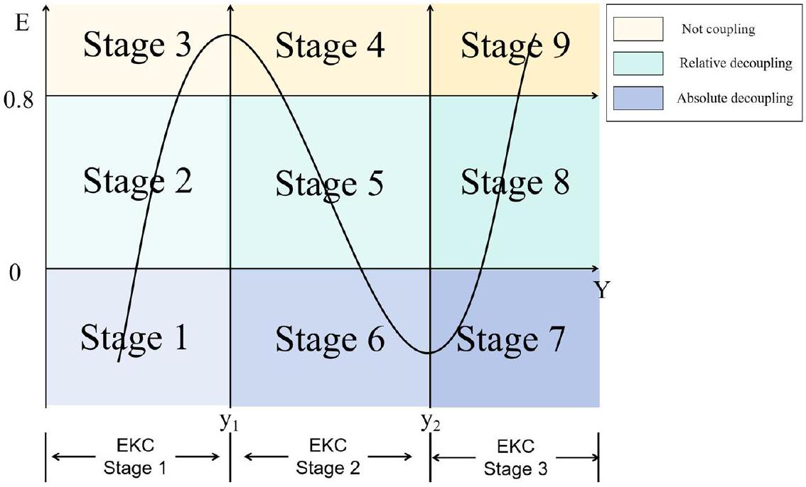
shape) or two inflection points ( N -shape, inverted N -shape). Taking the 2D decoupling model based on N-shaped EKC as an example, two vertical lines and divide the horizontal axis into three areas. Different regions represent different stages of N -shaped EKC . In each area, according to and , the vertical axis is further divided into three areas, corresponding to absolute decoupling, relative decoupling, and non-decoupling (including Expansive coupling and Expanding negative decoupling). Therefore, the entire plane is divided into nine areas, corresponding to nine 2D decoupling states (see Fig. 2).

This model relaxes the strict assumption in the EKC model that Y and EP are directly corresponding, and also overcomes the problem of Tapio decoupling that only considers the relative change relationship between the two. Through this division, we can clearly and accurately classify countries with similar economic and environmental development conditions into the same category to conduct systematic and targeted research. Considering that many countries lack data for individual years, to reduce statistical errors and random errors, we use the ten-year average as one period to classify the economic development and carbon emission levels of each country. Specifically, we divide countries into different EKC stages according to the average GDP per capita from 2010 to 2020 . We also calculate the decoupling status using the average GDP per capita and carbon emissions per capita from 2000 to 2010 and 2010 to 2020 as data in period t-1 and period t , respectively.

Empirical model settings. To test H1 and investigate the shape of the global EKC curve, we first establish the following regression model based on the classic EKC empirical model corresponding to Eq. 10:

Among them, PCE and PGDP are dependent variables and independent variables, respectively, representing per capita carbon emissions and per capita GDP.

We further add control variables to the above model to test H2 and H 3 :

where represents the vector of control variables, including geopolitical risk, composite risk, institutional quality, ICT, digital economy, AI development, natural resource rents, energy transition, trade openness, population aging, income inequality, and food security. Based on the estimation results of this equation, we can determine the shape of the EKC based on the results of , and and discuss the influence of additional variables based on the results of .

Finally, to examine H4 and explore the determinants of carbon emissions in country groups at different two-dimensional decoupling stages, we first divided the full sample of 214 countries into several groups according to the two-dfimensional decoupling model, and carried out the following regressions in each group:

with consistent with the equation.
Variable definition and data description. According to the requirements of the methods and models discussed previously, this article uses per capita carbon emissions as the explained variable, per capita GDP as the explanatory variable, and 12 variables covering institutional risks, digital technology, resource utilization, and social issues as control variables. Based on data availability, the research scope of this article is determined to be 214 countries from 1960 to 2020 . The definitions, measurement units, and data sources of all variables are summarized in Table S 1 . It can be seen that the explanatory variables and the explained variables are all derived from the WDI database developed by the World Bank (Worldbank, 2023a).

Control variables include 12 variables. Institutional risk includes three variables, among which geopolitical risk comes from the calculation work of (Caldara and Iacoviello, 2022). This database is updated every day and can comprehensively and effectively reflect the risk level of geopolitical threats and actions of various countries. Composite risk is derived from the ICGR published by PRS Group since 1980 (PRS, 2023), which takes into account domestic political, economic, and financial risks. Institutional quality is calculated by the average of six indices of the World Governance Index(WGI) released by the World Bank (Worldbank, 2023b), which reflects the integrity and effectiveness of each country’s institutions.

Technology variables include ICT, digital economy, and artificial intelligence (AI). Following (Shufang Zhao et al., 2022), ICT is represented by mobile cellular subscriptions. The digital economy is calculated by the entropy weight method and represents the development level of a country’s digital technology and digital industry. The calculation process uses 12 secondary indicators from the International Telecommunication Union (ITU, 2023) and WDI, covering four aspects: infrastructure, social support, social effects, and economic effects, as shown in Table S2. AI is represented by the number of industrial robots operational stocks which comes from the World Robotics Report released by the International Federation of Robotics (IFR, 2023).

Variables related to resource use include total natural resource rents and the level of energy transition represented by the share of renewable energy consumption. Finally, among the social variables, population aging is expressed as the proportion of the population over 65 years old. Food safety is derived from the food production index from WDI database. Trade openness is measured by a country’s trade volume as a share of its GDP. The GINI coefficient represents the level of income inequality. These variables are all from WDI. The descriptive statistics of the variables are shown in Table S3.

Handling the multicollinearity problem. First, we show the correlation coefficient matrix and VIF (see Fig. S1). The highest correlation coefficient reached 0.87, exceeding the safety line of 0.85 , representing the need to analyze VIF to rule out the multicollinearity problem. The results show that the VIF of all variables is less than 10 , which means that the multicollinearity problem between variables is not serious. Considering that the

Standard errors in parentheses. . y 1 and y 2 represent the inflection points of the cubic curve calculated based on the estimation results.

VIF of institutional quality is closer to 10 compared to other variables, we choose to add it in the last step of the stepwise regression to avoid potential interference.

Handling the pseudo-regression problem. To avoid pseudoregression, we need to test the stationarity of the disturbance term, that is, test the cointegration relationship between variables. The cointegration test requires that each variable sequence is firstorder integrated, and a unit root test needs to be performed on each variable first. Therefore, fisher-adf and fisher-pp tests are used to test the data stationarity. Both results of all variables in the two test methods are stationary in first order (see Table S4). Finally, the Kao test is used to test the cointegration (see Table S4). The results of Kao ADF statistics reject the null hypothesis that there is no cointegration relationship between panel variables at the level. This indicates that the long-term stable relationship between variables exists and the pseudo-regression problem does not hold.

Selecting the estimation model. Fixed effects models (FE), two-way fixed effects models, and dynamic (system-/difference-) GMM models are among the most popular models in previous panel studies. The fixed effects model is one of the most commonly used models in research. It eliminates endogeneity problems caused by unobservable factors related to individuals through within-group estimators. Both two-way fixed effects and dynamic GMM improve FE by adding explanatory variables to the model: the former adds a vector of time dummy variables, while the latter includes the lagged term of the explained variable. However, this study has selected additional variables from various perspectives to accurately track the changes in the carbon emissions curve and open the black box of the determinants of carbon emissions, making the addition of more variables to the model redundant and potentially harmful (such as exacerbating multicollinearity problems). Therefore, we finally choose to adopt the basic FE models in our empirical process. Other models are used as robustness check methods.

Confirm -shaped EKC without additional variables. To test H1, we perform estimation and robustness testing on the regression equation without additional variables Eq. (16). The results are
shown in Table 3. First, the coefficient of the cubic term of per capita GDP (PGDP3) in Model 1 is significantly greater than 0 at the level, indicating a cubic EKC. In addition, the coefficient of the quadratic term is significantly negative and the coefficient of the linear term is significantly positive. It shows that as PGDP gradually increases, per capita carbon emissions conform to the N -shaped trend. Including the above regression coefficients into Eq. (13), it can be calculated that the EKC inflection points without considering control variables are 34.44 and 77.54 (thousand US dollars/person), respectively. We can think of these as two thresholds. Initially, the increase in per capita GDP leads to an increase in per capita carbon emissions and reaches a peak when per capita GDP reaches 34.44. However, when PGDP gradually increases and exceeds this value, per capita carbon emissions will reverse and change from rising to falling. Finally, when per capita GDP further increased and reached 77.54, the trend of per capita carbon emissions changed upward again.

We also utilize four methods to check the robustness of N-shaped EKC, as shown in Model R1-R4 of Table 3. First, change the environmental pollution indicator from per capita carbon emissions to total carbon emissions. Second, the fixed effects estimation model is replaced by an individual-time-twoway fixed effects model. Third, a random effects model will be used. Fourth, use the system GMM. First, the Sargan test -value and AR(2) in Model R4 are greater than 0.1, indicating that the dynamic model estimation results are valid. All four models show that the coefficients of PGDP and its cubic term are significantly greater than 0 , while the coeffecients of the quadratic term is significantly less than 0 . In addition, the results of and show that there are two inflection points in the EKC corresponding to the four models, and they all fall within the sample interval. In conclusion, the global N -shaped EKC exists when control variables are not considered and H 1 is confirmed. Farooq et al. (2022) took 185 countries around the world as a sample, confirmed the positive linear term and negative quadratic term of PGDP, and obtained the result of the inverted U-shaped EKC. However, our results show that the positive cubic term also exists robustly, so this paper resets the shape of the global EKC to an N -shape. From another perspective, this result generalizes the N -shaped EKC confirmed in Numan et al. (2022) in 85 countries to 191 countries.

Note: For analytical clarity, standard errors are not reported. See Table S5 for complete results. .

Determine the EKC shape and inflection points under additional variables. Table 4 shows the results of adding control variables for testing H2 and H3. To reduce the impact of differences in sample sizes of different variables and alleviate the problem of multicollinearity, we adopt stepwise regressions to display the results of adding covariates. Among them, Model 1 only uses PGDP and its quadratic and cubic terms as explanatory variables, and the R square is 0.122 . Model 2 -Model 6 gradually added 12 control variables, and the R square increased accordingly to 0.718 in Model 6. This shows that the addition of explanatory variables can accurately explain changes in carbon emissions. As control variables are continuously added to Models 2-6, the cubic term of PGDP is always significantly positive at the statistical level. In addition, the sign and statistical level of PGDP and its quadratic term are also completely consistent with Model 1. This means that after adding control variables, the shape of the EKC is still a standard N -shape and H 2 is confirmed.

After calculation, the two inflection points of the N -shaped EKC in Model 6 are 45.08 and 73.44 (thousand dollars per
person), respectively. This result is different from the EKC inflection point in Model 1. We juxtapose the cubic equation curves corresponding to the estimated coefficients in Fig. 3 to discuss the influence of the control variables on the shape of the EKC. Figure 3 shows that after taking control variables into account, not only did the economic growth space between the two inflection points shrink from 43.10 thousand US dollars to 28.35 thousand US dollars, but also the reduction of per capita carbon emissions between the inflection points is compressed from about 2.70 metric tons to about 1.05 metric tons. This suggests that the EKC appears to be bent upwards when trying to account for other explanatory variables. As a result, the only declining part of the N -shaped carbon emissions curve has shrunk in both “duration” and “descending space,” revealing a more severe global climate mitigation situation.

Discuss the role of additional variables on carbon emissions. Institutional, technology, resources, and social factors not only affect the shape of EKC but also have an important impact on
carbon emissions. This leads to the discussion of H3. Model 2 adds four control variables based on Model 1. Taking the 5% significance level as the standard, the impact coefficients of ICT and food security are positive, and the impact coefficients of digital economy and population aging are negative. We examine the robustness of the effects of these variables in conjunction with other results of the stepwise regressions. Comparing the estimation results of Model 2 with the subsequent four models (Model ), it shows that the above results can be confirmed by at least two models. Specifically, the results of ICT are significantly positive in both Model 3 and Model 4; the positive coefficient of food security exists in Models 3-5; the negative coefficients of digital economy and population aging hold in all models. This shows that the estimation results of ICT, food security, digital economy, and population aging in Model 2 are reliable as decisions.

The estimators of the three factors added in Model 3 are all significant. Among them, the impact coefficient of natural resource rent is positive, and the impact of trade openness and energy transition is negative. However, results from subsequent models support the effects of energy transition rather than that of natural resource rents and trade openness. All models show that the impact coefficient of energy transition is significantly negative, while the effects of natural resource rents and trade openness are insignificant in two of the three subsequent models. Model 4 adds comprehensive risk. Combined with the estimation results of Model 4-6, the impact of comprehensive risk on carbon emissions is determined to be negative, which indicates that the higher the overall country risk level, the higher the corresponding carbon emissions. By comparing the results of Model 5 and Model 6, we determined that the effects of artificial intelligence and income inequality are not significant. Finally, the results of Model 6 show that geopolitical risks intensify carbon emissions, while improvements in institutional quality can reduce carbon emissions. These results show that H3 is partially confirmed.

We summarize the impact of each variable on carbon emissions in Table 5 to make further discussion. From the perspective of institutional risk factors, the rise in geopolitical risks and national comprehensive risks has significantly promoted carbon emissions. This is consistent with some recent research results on geopolitical risks (Anser et al., 2021) and political risks (Hassan et al., 2022), but is inconsistent with the research results on financial risks (Jun Zhao et al., 2021a). Risks may cause panic and short-sightedness among

Note: representing positively(negatively) affecting per capita carbon emissions at least at significance level. Blank represents an insignificant effect.
governments and investors, which are often linked to irresponsible production models and misuse of fossil fuels (Vakulchuk et al., 2020; Zuoxiang Zhao et al., 2023). The reducing effect of institutional quality on global carbon emissions is consistent with the regulatory effect hypothesis and consistent with previous research for 3 Asian countries (Salman et al., 2019) and 30 Sub-Saharan African countries (Karim et al., 2022). Therefore, a stable international and domestic development environment and effective systems play an irreplaceable role in reducing carbon emissions and achieving global climate mitigation.

The results of technological factors are sobering. The digital economy can reduce carbon emissions, while the single ICT industry promotes carbon emissions. The two variables are conceptually similar, but why could they have completely opposite impacts on global carbon emissions? Despite a lack of discussion and explanation of this phenomenon in the literature, a recent study (Jinning Zhang et al., 2022a) offers a good perspective. They discussed the impact of different dimensions of the digital economy on low-carbon development and found that industrial digitalization has the most significant impact on lowcarbon development, followed by digital industrialization, with the carrier playing the smallest role. In other words, it is the integration of digital technology and the economy, that promotes emission reduction, not just the development of ICT technology and equipment (Jinning Zhang et al., 2022a). The impact of AI is not significant, possibly because the effects of AI in different countries cancel each other out. Luan et al. (2022) found that industrial robots promoted air pollution in 74 countries while (Zhong et al., 2023) claimed that AI reduced carbon emissions in 66 countries. In summary, inconsistent with the views of technological rationalists, our results suggest that smart technological developments alone may not necessarily improve the environment. Alternatively, the rational use of technology to benefit the economy and society may be an efficient approach to achieving carbon emission reductions.

The results on resource utilization emphasize the urgency of clean energy development and deployment. On the one hand, the results confirm the significant reduction effect of the energy transition on carbon emissions. This shows that replacing existing energy infrastructure with one that relies on renewable energy can indeed significantly reduce carbon emissions per capita, which does not exceed the research conclusions of other scholars (Dogan and Seker, 2016; Inglesi-Lotz and Dogan, 2018). On the other hand, the impact of natural resource rents is uncertain, consistent with the controversy in the literature. The results also highlight the potential impact of social factors on carbon emissions. Population aging is a negative contributor to carbon emissions. This corresponds with (Zhou et al., 2023) while contradicting the findings of (Balsalobre-Lorente et al., 2021) and (Fan et al., 2021). Food security is a positive contributor to carbon emissions, supported by (Naseem et al., 2020). It shows that more attention needs to be paid to deforestation, land use, and highcarbon food consumption issues while ensuring food safety in global agricultural development. The effects of trade openness and income inequality are not significant.

Before testing H4, we first classify countries according to the development stage and emission reduction status to solve the heterogeneity problem that exists when testing the EKC hypothesis using the traditional panel method. Therefore, this paper first uses a two-dimensional decoupling model to achieve an accurate classification of countries based on their economic development levels and the carbon emissions decoupling states. The calculation and grouping process can be broken down into three steps: (1) Group

countries according to the average per capita GDP in the past decade and the EKC inflection point. (2) Group countries according to Tapio decoupling elasticity between the past two decades and the critical values ( 0 and 0.8 ). (3) Match the results of the above two steps with the nine two-dimensional decoupling stages shown in

Fig. 2, and obtain the final grouping based on the two-dimensional decoupling model. The results are shown in Fig. 4.

According to Fig. 4a, the 214 sample countries are divided into three groups based on the N-shaped EKC inflection points estimated in the baseline regression results. The first phase of

Note: For analytical clarity, standard errors and coefficients not significant at the level are not reported. See Table S7 for complete results. .

EKC is still the main theme of global development. More than of countries are in this stage, with their average per capita GDP between 2010 and 2020 being less than US$45,080. There are 11 countries in the second stage. Their ten-year average per capita GDP exceeds 45,080 but is less than 73,438 . These countries have relatively high levels of economic development, mainly including the United States, Australia, and some European countries. According to the EKC hypothesis, they have the best hope of achieving economic growth while reducing carbon emissions. Only 9 countries have a ten-year average per capita GDP higher than 73,439 and are in the third stage, almost all of which are located in Europe. These countries have reached extremely high levels of economic development, but they may be directly responsible for the second upslope of N-type EKC and the rebound in pollution levels.

Figure 4 b shows that the number of countries in different decoupling states is relatively even and that there are regional aggregation characteristics. The number of countries with nondecoupling, weak decoupling, and strong decoupling is 57,47 , and 55, respectively, and 34 countries are suffering an economic recession. The results of non-decoupling countries are concerning. The results show that these countries with decoupling elasticity still higher than 0.8 in the past 20 years are mainly located in sub-Saharan Africa, Latin America, and the Middle East. These countries are characterized by economic development that relies heavily on the extraction or utilization of natural resources (Do, 2021). How to help them reduce carbon emissions is an important challenge for global climate mitigation. It can be seen that most of the weak decoupling countries are located in non-Middle East Asia. Many of these countries, such as India and China, have achieved a degree of industrialization and urbanization, thereby gradually decoupling their economies from carbon emissions. Strong decoupling countries are mainly distributed in North America, Europe, and Oceania, and have a high degree of overlap with the countries in the second and third stages of the EKC. Finally, some African countries, including Libya and the Central African Republic, are facing economic recession. Stabilizing the economy is the top priority for these countries.

Finally, we classify countries based on the two-dimensional decoupling model. The number of countries in each stage is shown in Fig. 4c. First, the results show that all countries in the
sample whose GDP per capita is higher than the first inflection point of the EKC have achieved strong decoupling. In other words, among the six two-dimensional decoupling stages corresponding to the second and third stages of EKC (Stage 4-9), 9 countries are in Stage 6, and 3 countries are in Stage with no country in other stages. This means that from the perspective of the past 20 years, those countries with relatively advanced economic development have achieved a relatively ideal decoupling of economic development and carbon emissions. Among the three two-dimensional decoupling states (Stage 1-3) belonging to the first stage of EKC, there are 43,47 , and 57 countries in strong decoupling, weak decoupling, and nondecoupling, respectively, which is also not entirely consistent with the EKC theory. In the EKC theory, the economic development of countries whose per capita GDP is lower than the first turning point will be accompanied by environmental deterioration, but two-dimensional decoupling analysis shows that the relationship between economic development and environmental pollution in countries at this stage also has different conditions. In summary, we successfully classified countries of the same type through the two-dimensional decoupling model, so that we can conduct specific research on the determinants of carbon emissions in each country group.

Heterogeneous effects of all variables on carbon emissions. Based on the six divided country groups, we perform panel unit root tests and cointegration tests for each sample. The results show that at the significance level, in each sample, the variables are first-order stationary and cointegrated (see Table S6). To discuss the heterogeneous impact of economic, institutional, technological, resource, and social factors on carbon emissions and examine H4, the regression results of six country groups are shown in Table 6.

First, there is obvious heterogeneity in the impact of per capita GDP on carbon emissions. In the first stage of the EKC, according to the estimation results of Model 7 and Model 9, economic development in both non-decoupling and weak-decoupling countries is accompanied by much carbon emissions. In nondecoupling and weakly decoupling countries, for every US$1 increase in per capita GDP, per capita carbon emissions increase by an average of 0.2658 metric tons and 0.3806 metric tons,
respectively. It may be puzzling at first that the impact coefficient of economic development on carbon emissions is more pronounced in weak decoupling countries than in nondecoupling countries. The reason can be that the economic development models of these countries, including most Asian developing countries, have been optimized to a certain extent in the past two decades, but their average environmental costs throughout the development process are still high (Rongrong Li et al., 2021). These countries need to make full use of the results of past economic development and strive to transform from weak decoupling to strong decoupling (Hanif et al., 2019). Model 9 shows that in the sample of strong decoupling in the first stage of EKC, the impact of per capita GDP on per capita carbon emissions is not significant. This is consistent with the decoupling theory, suggesting that they are not developing directly at a high ecological cost. Model 10 shows that in countries whose economic development has entered the second stage of EKC, for every US$1 increase in GDP per capita, carbon emissions per capita increase by 0.0855 metric tons. Considering the relatively small size of the coefficient, it can be considered that N-shaped EKC is supported, that is, economic development accompanied by less environmental pollution in the second phase of EKC. However, Model 11 shows that when economic development enters the third stage of EKC, economic growth and carbon emissions are reconnected. Compared to the second phase of EKC, carbon emissions per capita for every increase in GDP per capita will double from 0.0855 metric tons to 0.1721 metric tons. This result confirmed the technical obsolescence effect (Jahanger et al., 2023). Finally, the carbon emission costs of economic development in countries that have faced economic recession in the past 20 years are also extremely high. These countries urgently need to stabilize their economies at controllable environmental costs.

From the perspective of institutional risk, the impact of geopolitical risk is not significant in most samples, indicating that geopolitical risk has not yet significantly affected carbon emissions in most countries around the world. However, in the non-decoupling sample in the first phase of the EKC, geopolitical risk significantly reduces carbon emissions. This may be related to conflicts and crises caused by the rich natural resources of these countries (Do, 2021). The negative relationship is supported by (Weijun Zhao et al., 2021b) who asserted that geopolitical risks may inhibit investment, trade, and energy consumption to reduce carbon emissions. Each unit increase in the composite risk index can reduce per capita carbon emissions by 0.0123 metric tons and 0.0067 metric tons, respectively, in countries in Stage 2 and Stage 1 of two-dimensional decoupling, which is consistent with the full sample research result. The results for institutional quality are rich in heterogeneity. Its effect of reducing carbon emissions is only reflected in Stage 3 countries, and these non-decoupling countries need to strengthen the construction of the national institution. However, in Stage 1, Stage 6, and Stage 10, institutional quality increases carbon emissions. As (Le and Ozturk, 2020) pointed out, cumbersome regulations and bureaucracy may in turn delay the implementation of environmental protection actions.

It is interesting to analyze the impact of digital technology variables. The conclusion that DE, rather than ICT, can significantly reduce carbon emissions and achieve low-carbon development is true in Stage 1, Stage 6, and Stage 10, indicating that most countries should focus on the digitalization of industry and economy. However, this does not always hold, because in Stage 3 it is exactly the opposite: ICT reduces carbon emissions, while the digital economy promotes carbon emissions. Although these countries are in a weak decoupling state, the impact coefficient of PGDP on carbon emissions is the highest among all samples. The combination of a rough economic development
model and digital technology may lead to excessive carbon emissions (Feng Dong et al., 2022a). Therefore, these countries need to focus on the carbon footprint of the digital economic development model in the process of developing ICT. AI reduces emissions in Stage 3 countries while increasing emissions in Stage 2 countries, which is not significant in other groups, indicating that AI needs to be used in the economy and society with more caution.

In terms of resource use, the energy transition significantly reduced carbon emissions in all six samples according to Table 6. However, this effect was most pronounced in countries in EKC stage 3, followed by EKC stage 2. Every increase in the proportion of renewable energy will lead to a decrease in per capita carbon emissions of 0.4661 metric tons in the former and 0.1096 metric tons in the latter. The emission reduction effects of countries in the first stage of EKC are relatively weak, diminishing in countries with strong decoupling, weak decoupling, and nondecoupling. The distribution pattern of the influence coefficient shows that increased levels of economic development and decoupling lead to better energy transition outcomes. This result is supported by (Nguyen and Kakinaka, 2019), who conclude that in the low-income group, renewable energy development inhibits economic development and promotes carbon emissions; while in the high-income group, the opposite holds. On the contrary, natural resource rent promotes carbon emissions in Stage 2 and Stage 6 countries and has no significant impact on other countries.

Finally, among the four social factors, the impact of population aging is relatively consistent. It mainly affects Stage 2 and Stage 1 countries and brings about reductions in carbon emissions. The result of OPEN does not support the existence of the PHH because there is no obvious evidence that countries with better environmental regulations have reduced carbon emissions through openness. Honestly, trade openness brings more carbon emissions in most samples (Stage 1, 7, 10), and reduces carbon emissions only in Stage 2 samples. This means that frequent exchanges of goods and services may increase the logistics and transportation burdens of many countries (Rongrong Li et al., 2021). The effects of food security and income inequality are also heterogeneous and may have opposite effects in different countries. Specifically, food security reduces carbon emissions in Stage 1 countries but increases carbon emissions in Stage 2 and Stage 10 countries. Income inequality is a contributor to carbon emissions for Stage 1 and Stage 6 countries, but the opposite is true for Stage 2 countries. The above results highlight betweengroup heterogeneity in the direction and magnitude of carbon emissions effects for all variables, which establishes H4.

Differential carbon reduction strategies of countries in different two-dimensional decoupling stages. A preliminary discussion of the results of Table 6 shows that not only does the relationship between per capita GDP and carbon emissions exhibit nonlinear and heterogeneous rules, but the impact of the additional variables on carbon emissions also significantly varies in different types of countries. Therefore, countries in different two-dimensional decoupling states can adopt differentiated institutional, technological, resource, and social development strategies to achieve carbon emission reductions. We summarize the positive and negative drivers of carbon emissions in Fig. 5 according to the two-dimensional decoupling stage.

Stage 1 countries belong to the strong decoupling state of the first stage of the EKC. This is the only group of countries where the impact of economic growth on carbon emissions is not significant, meaning that the past development models of these countries did not come at the expense of environmental quality.

However, the results in Fig. 5 indicate that in addition to economic development, many other factors significantly affect environmental quality and therefore require special attention. First, in terms of institutions, institutional quality promotes carbon emissions, while the comprehensive country risk index
reduces carbon emissions. The policy implication is that these countries should improve the construction and implementation of environmental regulations while striving to stabilize the domestic economic, political, and financial environment (Karim et al., 2022). In terms of digital technology, ICT promotes carbon
emissions, while digital technology reduces carbon emissions. It shows that these countries should pay attention to the carbon footprint issue of the ICT industry and encourage the penetration of ICT into other economic sectors to form a broader and deeper digital economic industry. In terms of resource utilization, the emission reduction effect of the energy transition is significant. Considering that the magnitude of the effect is not ideal, countries currently in Stage 1 should prioritize economic development and gradually deploy the production and utilization of clean energy in conjunction with economic development. In terms of social management, income inequality, and trade openness bring more carbon emissions, while population aging and food security reduce carbon emissions. It seems that, on the one hand, these countries should introduce fiscal and agricultural production policies to promote fair distribution of wealth and improve food production security (Akbar et al., 2019). On the other hand, they need to introduce more green products and technologies in the process of international trade or investment promotion (Qiang Wang et al., 2023b).

For Stage 2 countries, they are in a state of relative decoupling, between non-decoupling and complete decoupling. It shows that these countries have certain methods to reduce pollution in development, but there is still a lot of room for emission reduction. These countries need to comprehensively understand the positive and negative factors affecting carbon emissions to achieve a transformation from relative decoupling to absolute decoupling. In particular, the results of this study indicate that AI, natural resource rents, and food security are contributing to per capita carbon emissions. Therefore, strengthening environmental regulations and introducing normative and environmentally friendly technologies in artificial intelligence technology, natural resource extraction, and food production processes may be the key to achieving strong decoupling. Disincentives to carbon emissions suggest that maintaining national stability, energy transition and trade openness are also important. Countries in Stage 3 are nondecoupling. Their economic development is accompanied by high carbon emissions, so the most important thing is to solve the problem of rough development. In addition, the control variables still provide emission reduction options from institutional, technical, and natural resource perspectives. For them, the positive driver of carbon emissions is primarily the digital economy. In comparison, the development of ICT and AI technologies cannot curb carbon emissions. This further emphasizes the need to decouple economic development and carbon emissions. In addition, rising levels of geopolitical risks, institutional quality, and energy transition can also reduce carbon emissions.

Stage 6 countries have a relatively high level of development and have entered the second stage of EKC and achieved strong decoupling. But they can also pursue better environmental outcomes. Based on the negative drivers of carbon emissions, these countries should focus on building environmental institutions, limiting the use of traditional natural resources, and optimizing income structures. In line with the positive drivers of carbon emissions, further development of the digital economy and energy transition has an important role in improving environmental quality.

For Stage 7 countries, their economic development level is higher than that of Stage 6, but their economic development and carbon emissions have been reconnected. Due to the limited sample, the results of most factors are not significant. However, our results still point to two emission reduction ideas. On the one hand, the effects of energy transformation in these countries are far better than in other countries, and clean energy should be further developed and deployed in these countries; on the other hand, trade openness is positively related to carbon emissions, and they should more strictly scrutinize imported goods or foreign investment. While Stage 10 countries are facing economic
recession, economic development has a high coefficient of impact on carbon emissions. These countries not only need to stabilize their economy but are also supposed to find ways to reduce environmental costs. The results indicate that they need to establish more robust environmental regulations and address carbon emissions issues in ICT, food production, and trade openness. In addition, the digital economy and energy transition can be seen as further developments in green industries.

Early research provided a solid theoretical foundation and empirical evidence for the inverted U-shaped EKC. However, with the increasing urgency of mitigating climate change, we have observed that many developed countries are struggling with environmental degradation, high energy consumption, and carbon emissions. This forces us to start considering N -shaped global EKC. In addition, the impact of risks, digital technology, energy transition, and various social factors on social activities, economic development, and energy use are also proven to be significant contributors to carbon emissions. Against this background, we included as many countries as possible in the study, re-examined the shape of the EKC in the global panel, and incorporated 12 traditional and novel institutional, technological, resource, and social factors as additional variables into the EKC equation. In addition, we developed a two-dimensional Tapio decoupling model based on the inflection point in N-shaped EKC to achieve group discussion of sample countries. Finally, based on grouping, we discussed the heterogeneous impact of all variables and the differential emission reduction solutions of each group between groups and obtained a series of conclusions.

First, in the global panel, N-shaped EKC exists robustly regardless of whether additional variables are taken into account. In other words, the cubic and linear terms of GDP per capita are significantly positive, while the quadratic term is significantly negative. Among them, when additional variables are not considered, the N-shape has passed four robustness tests. When considering additional variables, this N-shaped EKC also holds at each step of the stepwise regression. Thus H1 and H2 are completely confirmed. After determining the existence of the N-shape, we finally calculated the inflection points of EKC including all control variables, which were 45.08 and 73.44 (thousand dollars/ person), respectively. By comparing the final N-shaped EKC curve with the N-shaped curve without adding control variables, we found that both the “duration” and “dropping space” of the only declining part in the curve have shrunk, which makes global climate mitigation even more severe. Through mutual verification of each step of the stepwise regression, we finally determined the direction of influence of all additional variables. Among them, geopolitical risks, ICT, and food security were confirmed to have a positive impact on per capita carbon emissions. However, comprehensive risks, institutional quality, digital economy, energy transition, and population aging were found to have a robust negative impact. Artificial intelligence, natural resource rents, trade openness, and income inequality have insignificant effects on carbon emissions. These results partially confirmed H3.

In the group study, we first used the per capita GDP of 45.08 and 73.44 (thousand US dollars per person) obtained in the EKC as the basis for classification, and initially divided all countries into three EKC stages. As a result, 194 countries belong to the first stage, 11 countries belong to the second stage, and 9 countries belong to the third stage. Secondly, we calculated the Tapio decoupling elasticity coefficient between the past two decades for all countries and further divided the countries into three states using 0 and 0.8 as thresholds. The results show that there are 57, 47,55 , and 34 countries in non-decoupling, weak decoupling,
strong decoupling, and recession, respectively. Based on this, we established two-dimensional decoupling coordinates and combined the three states of each of the above two dimensions with each other to obtain nine two-dimensional decoupling states. We divide the sample into five groups by matching the non-recession sample results to the nine decoupling conditions. Among them, there are 43, 47, 57, 9, and 3 countries in Stages 1, 2, 3, 6, and 7, respectively. Adding the declining countries (Stage 10) we get 6 panels. We also conduct multiple linear regressions in these panels and discuss the heterogeneous effects of economic development and 12 additional variables on carbon emissions. The results completely validate H4 and show that the effects of most variables vary according to country conditions. The most robust variable is the energy transition, which shows a significant carbon reduction effect in all groupings. However, the magnitude of the impact of energy transition is also heterogeneous. In countries with higher levels of economic development and decoupling, the effects of energy transition are stronger. Finally, we discuss the differential emission reduction plans of countries in different two-dimensional decoupling stages based on the direction of influence of variables.

The above findings have valuable policy implications. First of all, global results show that the N -shaped EKC is more severe than the inverted U-shaped EKC. The empirical validation of technological obsolescence underscores the imperative for developed nations worldwide to bolster their focus on internal environmental regulations and elevate levels of innovation in clean technologies. Furthermore, the inclusion of additional variables in our analysis underscores the pivotal role played by a stable international and domestic developmental milieu alongside effective institutional frameworks in curbing carbon emissions and advancing global climate mitigation efforts. The uncritical pursuit of purely digital or smart technological advancements does not inherently translate into environmental amelioration. Conversely, a judicious harnessing of technology for the betterment of both the economy and society presents a promising avenue for achieving reductions in carbon emissions. Moreover, our findings on resource utilization underscore the pressing need for accelerated development and adoption of clean energy sources. Addressing social determinants, particular attention is warranted towards optimizing land usage and curtailing the prevalence of high-carbon footprint foods within agricultural production. Finally, specific emission reduction ideas for each country have also been discussed in depth in the section “Differential carbon reduction strategies of countries in different two-dimensional decoupling stages”.

We need to point out the limitations of this article to provide ideas for improvement. First, due to non-uniform data sources, our empirical process uses an unbalanced panel. In some steps, the effective sample does not cover all 214 countries. This may ignore information from certain countries. Second, we include some important or novel additional variables to comprehensively discuss the determinants of carbon emissions other than growth. However, we cannot consider all factors. Second, we developed Tapio twodimensional decoupling based on N-shape to divide countries into 9 stages to fully consider the heterogeneity between countries. However, this classification also fails to fully handle heterogeneity. Our overall study is not a substitute for single-country and subnational case studies. Therefore, subsequent scholars have conducted more in-depth research from the perspective of improving the unity of data sources, providing more novel and critical additional variables, and conducting more refined case studies.

The datasets publicly available should be through https://doi.org/ 10.7910/DVN/0I1EYG.

Received: 16 November 2023; Accepted: 23 January 2024;
Published online: 21 February 2024

1 When determining the order in which variables are added, we consider the data characteristics of the variables, particularly the data volume, so that as many countries as possible are included in each step.
2 The number of countries belonging to the second and third stages of EKC in twodimensional decoupling in Fig. 4c is smaller than that in Fig. 4a. This is because some countries only have per capita GDP data but do not have enough carbon emission data in the past two decades.

Akbar A, Ali I, Samiullah NU, Khan SA, Rehman Z, Rehman S (2019) Functional, antioxidant, antimicrobial potential and food safety applications of Curcuma longa and Cuminum cyminum. Pak J Bot 51(3):1129-1135
Allard A, Takman J, Uddin GS, Ahmed A (2018) The N-shaped environmental Kuznets curve: an empirical evaluation using a panel quantile regression approach. Environ Sci Pollut Res 25:5848-5861
Álvarez-Herránz A, Balsalobre D, Cantos JM, Shahbaz M (2017) Energy innovations-GHG emissions nexus: fresh empirical evidence from OECD countries. Energy Policy 101:90-100
Andreoni J, Levinson A (2001) The simple analytics of the environmental Kuznets curve. J Public Econ 80(2):269-286
Ang JB (2008) Economic development, pollutant emissions and energy consumption in Malaysia. J Policy Model 30(2):271-278
Anser MK, Syed QR, Apergis N (2021) Does geopolitical risk escalate emissions? Evidence from the BRICS countries. Environ Sci Pollut Res 28(35):48011-48021
Apergis N, Ozturk I (2015) Testing environmental Kuznets curve hypothesis in Asian countries. Ecol Indic 52:16-22
Asiedu E (2006) Foreign direct investment in Africa: The role of natural resources, market size, government policy, institutions and political instability. World Econ 29(1):63-77
Balsalobre-Lorente D, Shahbaz M, Roubaud D, Farhani S (2018) How economic growth, renewable electricity and natural resources contribute to emissions? Energy policy 113:356-367
Balsalobre-Lorente D, Sinha A, Driha OM, Mubarik MS (2021) Assessing the impacts of ageing and natural resource extraction on carbon emissions: a proposed policy framework for European economies. J Clean Prod 296:126470
Bashir MF (2022) Discovering the evolution of Pollution Haven Hypothesis: a literature review and future research agenda. Environ Sci Pollut Res 29(32):48210-48232
Beckerman W (1992) Economic growth and the environment: Whose growth? Whose environment? World Dev 20(4):481-496
Berkeley (2024) Press Release: 2023 was warmest year since 1850. Berkeley Earth. https://berkeleyearth.org/press-release-2023-was-the-warmest-year-on-recordpress-release/
Brown PT, Hanley H, Mahesh A, Reed C, Strenfel SJ, Davis SJ et al. (2023) Climate warming increases extreme daily wildfire growth risk in California. Nature 621(7980):760-766. https://doi.org/10.1038/s41586-023-06444-3
Caldara D, Iacoviello M (2022) Measuring geopolitical risk. Am Econ Rev 112(4):1194-1225
Carlson CJ, Albery GF, Merow C, Trisos CH, Zipfel CM, Eskew EA et al. (2022) Climate change increases cross-species viral transmission risk. Nature 607(7919):555-562. https://doi.org/10.1038/s41586-022-04788-w
Cavicchioli R, Ripple WJ, Timmis KN, Azam F, Bakken LR, Baylis M et al. (2019) Scientists’ warning to humanity: microorganisms and climate change. Nat Rev Microbiol 17(9):569-586
Charfeddine L, Umlai M (2023) ICT sector, digitization and environmental sustainability: a systematic review of the literature from 2000 to 2022. Renew Sustain Energy Rev 184:113482
Cheng P, Tang H, Lin F, Kong X (2023) Bibliometrics of the nexus between food security and carbon emissions: hotspots and trends. Environ Sci Pollut Res 30(10):25981-25998
Cole MA (2004) Trade, the pollution haven hypothesis and the environmental Kuznets curve: examining the linkages. Ecol Econ 48(1):71-81
Dai M, Sun M, Chen B, Shi L, Jin M, Man Y et al. (2023) Country-specific net-zero strategies of the pulp and paper industry. Nature 626:327-334. https://doi. org/10.1038/s41586-023-06962-0
Diaz D, Moore F (2017) Quantifying the economic risks of climate change. Nat Clim Change 7(11):774-782
Dinda S (2004) Environmental Kuznets curve hypothesis: a survey. Ecol Econ 49(4):431-455

Ding T, Li J, Shi X, Li X, Chen Y (2023) Is artificial intelligence associated with carbon emissions reduction? Case of China. Resour Policy 85:103892
Do TK (2021) Resource curse or rentier peace? The impact of natural resource rents on military expenditure. Resour Policy 71:101989
Dogan E, Seker F (2016) Determinants of emissions in the European Union: the role of renewable and non-renewable energy. Renew Energy 94:429-439
Dong F, Hu M, Gao Y, Liu Y, Zhu J, Pan Y (2022a) How does digital economy affect carbon emissions? Evidence from global 60 countries. Sci Total Environ 852:158401
Dong F, Li Y, Gao Y, Zhu J, Qin C, Zhang X (2022b) Energy transition and carbon neutrality: exploring the non-linear impact of renewable energy development on carbon emission efficiency in developed countries. Resour Conserv Recycl 177:106002
Dong M, Wang G, Han X (2023) Artificial intelligence, industrial structure optimization, and emissions. Environ Sci Pollut Res 30(50):108757-108773
Duan H, Zhou S, Jiang K, Bertram C, Harmsen M, Kriegler E et al. (2021) Assessing China’s efforts to pursue the 1.5 C warming limit. Science 372(6540):378-385
Fakher HA, Ahmed Z, Acheampong AO, Nathaniel SP (2023) Renewable energy, nonrenewable energy, and environmental quality nexus: an investigation of the N-shaped Environmental Kuznets Curve based on six environmental indicators. Energy 263:125660
Fan J, Zhou L, Zhang Y, Shao S, Ma M (2021) How does population aging affect household carbon emissions? Evidence from Chinese urban and rural areas. Energy Econ 100:105356
Fankhauser S, Smith SM, Allen M, Axelsson K, Hale T, Hepburn C et al. (2022) The meaning of net zero and how to get it right. Nat Clim Change 12(1):15-21
Farooq S, Ozturk I, Majeed MT, Akram R (2022) Globalization and emissions in the presence of EKC: a global panel data analysis. Gondwana Res 106:367-378
Fawzy S, Osman AI, Doran J, Rooney DW (2020) Strategies for mitigation of climate change: a review. Environ Chem Lett 18:2069-2094
Gill AR, Viswanathan KK, Hassan S (2018) The Environmental Kuznets Curve (EKC) and the environmental problem of the day. Renew Sustain Energy Rev 81:1636-1642
Grossman GM, Krueger AB (1991) Environmental impacts of a North American free trade agreement. National Bureau of Economic Research Cambridge, MA, USA
Grossman GM, Krueger AB (1995) Economic growth and the environment. Q J Econ 110(2):353-377
Guan Y, Yan J, Shan Y, Zhou Y, Hang Y, Li R et al. (2023) Burden of the global energy price crisis on households. Nat Energy 8(3):304-316
Hanif I, Raza SMF, Gago-de-Santos P, Abbas Q (2019) Fossil fuels, foreign direct investment, and economic growth have triggered emissions in emerging Asian economies: some empirical evidence. Energy 171:493-501
Hassan T, Khan Y, He C, Chen J, Alsagr N, Song H (2022) Environmental regulations, political risk and consumption-based carbon emissions: evidence from OECD economies. J Environ Manag 320:115893
Heerink N, Mulatu A, Bulte E (2001) Income inequality and the environment: aggregation bias in environmental Kuznets curves. Ecol Econ 38(3):359-367
Higón DA, Gholami R, Shirazi F (2017) ICT and environmental sustainability: a global perspective. Telemat Inform 34(4):85-95
Hoegh-Guldberg O, Jacob D, Taylor M, Guillén Bolaños T, Bindi M, Brown S et al. (2019) The human imperative of stabilizing global climate change at 1.5 C . Science 365(6459):eaaw6974
Hossain MR, Rej S, Awan A, Bandyopadhyay A, Islam MS, Das N et al. (2023) Natural resource dependency and environmental sustainability under N-shaped EKC: the curious case of India. Resour Policy 80:103150
IFR (2023) World Robotics 2023 Report. International Federation of Robotics. https://ifr.org/ifr-press-releases/news/world-robotics-2023-report-asia-ahead-of-europe-and-the-americas
Im KS, Pesaran MH, Shin Y (2023) Reflections on “Testing for unit roots in heterogeneous panels”. J Econ 234:111-114
Inglesi-Lotz R, Dogan E (2018) The role of renewable versus non-renewable energy to the level of emissions a panel analysis of sub-Saharan Africa’s Big 10 electricity generators. Renew Energy 123:36-43
IPCC (2023) AR 6. intergovernmental panel on climate change. https://www.ipcc. ch/report/ar6/syr/downloads/report/IPCC_AR6_SYR_SPM.pdf
ITU (2023) ICT statistics. International Telecommunication Union. https://www. itu.int/en/ITU-D/Statistics/Pages/stat/default.aspx
Jahanger A, Hossain MR, Onwe JC, Ogwu SO, Awan A, Balsalobre-Lorente D (2023) Analyzing the N-shaped EKC among top nuclear energy generating nations: a novel dynamic common correlated effects approach. Gondwana Res 116:73-88
Kaika D, Zervas E (2013a) The environmental Kuznets curve (EKC) theory-Part A: concept, causes and the emissions case. Energy Policy 62:1392-1402
Kaika D, Zervas E (2013b) The environmental Kuznets curve (EKC) theory. Part B: critical issues. Energy Policy 62:1403-1411

Kao C (1999) Spurious regression and residual-based tests for cointegration in panel data. J Econ 90(1):1-44
Karim S, Appiah M, Naeem MA, Lucey BM, Li M (2022) Modelling the role of institutional quality on carbon emissions in Sub-Saharan African countries. Renew Energy 198:213-221
Koondhar MA, Shahbaz M, Memon KA, Ozturk I, Kong R (2021) A visualization review analysis of the last two decades for environmental Kuznets curve “EKC” based on co-citation analysis theory and pathfinder network scaling algorithms. Environ Sci Pollut Res 28:16690-16706
Kuznets (1955) Economic growth and income inequality. Am Econ Rev 45(1):1-28
Lantz V, Feng Q (2006) Assessing income, population, and technology impacts on emissions in Canada: where’s the EKC? Ecol Econ 57(2):229-238
Lark TJ, Spawn SA, Bougie M, Gibbs HK (2020) Cropland expansion in the United States produces marginal yields at high costs to wildlife. Nat Commun 11(1):4295
Le HP, Ozturk I (2020) The impacts of globalization, financial development, government expenditures, and institutional quality on emissions in the presence of environmental Kuznets curve. Environ Sci Pollut Res 27:22680-22697
Leal PH, Marques AC (2022) The evolution of the environmental Kuznets curve hypothesis assessment: a literature review under a critical analysis perspective. Heliyon
Li R, Wang Q, Guo J (2024) Revisiting the environmental Kuznets curve (EKC) hypothesis of carbon emissions: exploring the impact of geopolitical risks, natural resource rents, corrupt governance, and energy intensity. J Environ Manag 351:119663. https://doi.org/10.1016/j.jenvman.2023.119663
Li R, Wang Q, Li L, Hu S (2023) Do natural resource rent and corruption governance reshape the environmental Kuznets curve for ecological footprint? Evidence from 158 countries. Resour Policy 85:103890
Li R, Wang Q, Liu Y, Jiang R (2021) Per-capita carbon emissions in 147 countries: the effect of economic, energy, social, and trade structural changes. Sustain Prod Consum 27:1149-1164
Li Y, Zhang Y, Pan A, Han M, Veglianti E (2022) Carbon emission reduction effects of industrial robot applications: Heterogeneity characteristics and influencing mechanisms. Technol Soc 70:102034
Liu B, Yang X, Zhang J (2024) Nonlinear effect of industrial robot applications on carbon emissions: evidence from China. Environ Impact Assess Rev 104:107297
Lorente DB, Álvarez-Herranz A (2016) Economic growth and energy regulation in the environmental Kuznets curve. Environ Sci Pollut Res 23:16478-16494
Luan F, Yang X, Chen Y, Regis PJ (2022) Industrial robots and air environment: a moderated mediation model of population density and energy consumption. Sustain Prod Consum 30:870-888
Mao F, Miller JD, Young SL, Krause S, Hannah DM (2022) Inequality of household water security follows a Development Kuznets Curve. Nat Commun 13(1):4525
Naeem MA, Appiah M, Taden J, Amoasi R, Gyamfi BA (2023) Transitioning to clean energy: assessing the impact of renewable energy, bio-capacity and access to clean fuel on carbon emissions in OECD economies. Energy Econ 127:107091. https://doi.org/10.1016/j.eneco.2023.107091
Naseem S, Guang Ji T, Kashif U (2020) Asymmetrical ARDL correlation between fossil fuel energy, food security, and carbon emission: providing fresh information from Pakistan. Environ Sci Pollut Res 27:31369-31382
Nguyen KH, Kakinaka M (2019) Renewable energy consumption, carbon emissions, and development stages: some evidence from panel cointegration analysis. Renew Energy 132:1049-1057
Numan U, Ma B, Meo MS, Bedru HD (2022) Revisiting the N-shaped environmental Kuznets curve for economic complexity and ecological footprint. J Clean Prod 365:132642
PRS (2023) ICRG. The International Country Risk Guide. https://www.prsgroup. com/explore-our-products/icrg/
Rashdan MOJ, Faisal F, Tursoy T, Pervaiz R (2021) Investigating the N-shape EKC using capture fisheries as a biodiversity indicator: empirical evidence from selected 14 emerging countries. Environ Sci Pollut Res 28:36344-36353
Ray DK, Gerber JS, MacDonald GK, West PC (2015) Climate variation explains a third of global crop yield variability. Nat Commun 6(1):5989
Roelfsema M, van Soest HL, Harmsen M, van Vuuren DP, Bertram C, den Elzen M et al. (2020) Taking stock of national climate policies to evaluate implementation of the Paris Agreement. Nat Commun 11(1):2096
Rojas-Vallejos J, Lastuka A (2020) The income inequality and carbon emissions trade-off revisited. Energy Policy 139:111302
Salman M, Long X, Dauda L, Mensah CN (2019) The impact of institutional quality on economic growth and carbon emissions: Evidence from Indonesia, South Korea and Thailand. J Clean Prod 241:118331
Schiermeier Q (2020) The US has left the Paris climate deal-what’s next? Nature 2022. https://doi.org/10.1038/d41586-020-03066-x

Shehzad K, Zeraibi A, Zaman U (2022) Testing the N-shaped environmental Kuznets Curve in Algeria: an imperious role of natural resources and economic globalization. Resour Policy 77:102700

Stern DI (2017) The environmental Kuznets curve after 25 years. J Bioeconomics 19:7-28
Tapio P (2005) Towards a theory of decoupling: degrees of decoupling in the EU and the case of road traffic in Finland between 1970 and 2001. Transp Policy 12(2):137-151
Tollefson J (2022) What the war in Ukraine means for energy, climate and food. Nature 604(7905):232-233
Ullah A, Khan S, Khamjalas K, Ahmad M, Hassan A, Uddin I (2023) Environmental regulation, renewable electricity, industrialization, economic complexity, technological innovation, and sustainable environment: testing the N-shaped EKC hypothesis for the G-10 economies. Environ Sci Pollut Res 30(44):99713-99734
Usman O, Alola AA, Sarkodie SA (2020) Assessment of the role of renewable energy consumption and trade policy on environmental degradation using innovation accounting: evidence from the US. Renew Energy 150:266-277
Vakulchuk R, Overland I, Scholten D (2020) Renewable energy and geopolitics: a review. Renew Sustain Energy Rev 122:109547
Wang K, Zhu Y, Zhang J (2021) Decoupling economic development from municipal solid waste generation in China’s cities: Assessment and prediction based on Tapio method and EKC models. Waste Manag 133:37-48
Wang Q, Ge Y, Li R (2024a) Does improving economic efficiency reduce ecological footprint? The role of financial development, renewable energy, and industrialization. Energy Environ 0958305X231183914. https://doi.org/10.1177/ 0958305X231183914
Wang Q, Hu S, Li R (2024b) Could information and communication technology (ICT) reduce carbon emissions? The role of trade openness and financial development. Telecommunications Policy, 102699. https://doi.org/10.1016/j. telpol.2023.102699
Wang Q, Ren F, Li R (2023a) Exploring the impact of geopolitics on the environmental Kuznets curve research. Sustain Dev 2023. https://doi.org/10.1002/sd. 2743
Wang Q, Wang L, Li R (2023b) Trade openness helps move towards carbon neutrality-insight from 114 countries. Sustain Dev 2023. https://doi.org/10. 1002/sd. 2720
Worldbank (2023a) WDI. World Development Index. https://datatopics. worldbank.org/world-development-indicators/
Worldbank (2023b) WGI. World Governance Index. https://www.govindicators.org/
Xiaoman W, Majeed A, Vasbieva DG, Yameogo CEW, Hussain N (2021) Natural resources abundance, economic globalization, and carbon emissions: advancing sustainable development agenda. Sustain Dev 29(5):1037-1048
Yi M, Liu Y, Sheng MS, Wen L (2022) Effects of digital economy on carbon emission reduction: new evidence from China. Energy Policy 171:113271
Zhang J, Lyu Y, Li Y, Geng Y (2022a) Digital economy: an innovation driving factor for low-carbon development. Environ Impact Assess Rev 96:106821
Zhang L, Mu R, Zhan Y, Yu J, Liu L, Yu Y et al. (2022b) Digital economy, energy efficiency, and carbon emissions: evidence from provincial panel data in China. Sci Total Environ 852:158403
Zhao J, Shahbaz M, Dong X, Dong K (2021a) How does financial risk affect global emissions? The role of technological innovation. Technol Forecast Soc Change 168:120751
Zhao S, Hafeez M, Faisal CMN (2022) Does ICT diffusion lead to energy efficiency and environmental sustainability in emerging Asian economies? Environ Sci Pollut Res 29:12198-12207
Zhao W, Zhong R, Sohail S, Majeed MT, Ullah S (2021b) Geopolitical risks, energy consumption, and emissions in BRICS: an asymmetric analysis. Environ Sci Pollut Res 28:39668-39679
Zhao Z, Gozgor G, Lau MCK, Mahalik MK, Patel G, Khalfaoui R (2023) The impact of geopolitical risks on renewable energy demand in OECD countries. Energy Econ 122:106700
Zhengxia T, Haseeb M, Usman M, Shuaib M, Kamal M, Khan MF (2023) The role of monetary and fiscal policies in determining environmental pollution: revisiting the N-shaped EKC hypothesis for China. Environ Sci Pollut Res 30(38):89756-89769