DOI: https://doi.org/10.1038/s42256-023-00788-1
تاريخ النشر: 2024-02-06
استغلال نماذج اللغة الكبيرة في الكيمياء التنبؤية
تم القبول: 22 ديسمبر 2023
نُشر على الإنترنت: 6 فبراير 2024
(د) التحقق من التحديثات
الملخص
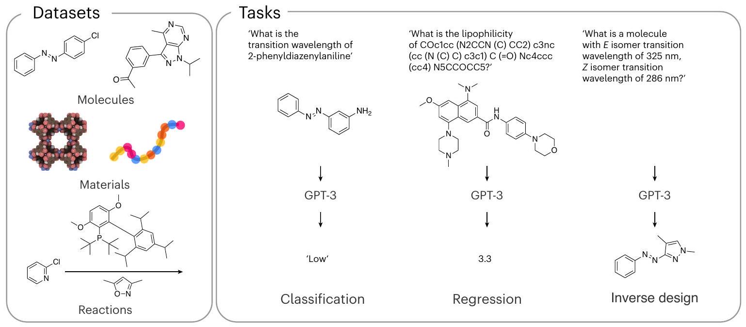
لقد حولت التعلم الآلي العديد من المجالات ووجدت مؤخرًا تطبيقات في الكيمياء وعلوم المواد. أدت مجموعات البيانات الصغيرة التي توجد عادة في الكيمياء إلى تطوير أساليب متقدمة في التعلم الآلي تتضمن المعرفة الكيميائية لكل تطبيق، وبالتالي تتطلب خبرة متخصصة للتطوير. هنا نوضح أن GPT-3، وهو نموذج لغوي كبير تم تدريبه على كميات هائلة من النصوص المستخرجة من الإنترنت، يمكن تكييفه بسهولة لحل مهام متنوعة في الكيمياء وعلوم المواد من خلال ضبطه للإجابة على الأسئلة الكيميائية باللغة الطبيعية مع الإجابة الصحيحة. قمنا بمقارنة هذا النهج مع نماذج التعلم الآلي المخصصة للعديد من التطبيقات التي تشمل خصائص الجزيئات والمواد إلى عائد التفاعلات الكيميائية. من المدهش أن النسخة المعدلة من GPT-3 يمكن أن تؤدي بشكل مشابه أو حتى تتفوق على تقنيات التعلم الآلي التقليدية، خاصة في حدود البيانات القليلة. بالإضافة إلى ذلك، يمكننا إجراء تصميم عكسي ببساطة عن طريق عكس الأسئلة. يمكن أن يؤثر سهولة الاستخدام والأداء العالي، خاصة لمجموعات البيانات الصغيرة، على النهج الأساسي لاستخدام التعلم الآلي في العلوم الكيميائية وعلوم المواد. بالإضافة إلى البحث في الأدبيات، قد يصبح استعلام نموذج لغوي كبير مدرب مسبقًا طريقة روتينية لبدء مشروع من خلال الاستفادة من المعرفة الجماعية المشفرة في هذه النماذج الأساسية، أو لتوفير خط أساس للمهام التنبؤية.
حل مهام الانحدار والتصنيف الجدولية البسيطة نسبيًا
التعديل الدقيق المتصل باللغة للتصنيف والانحدار
نهج
ستشكل المعادن محلولًا صلبًا أو مراحل متعددة. لذا، السؤال الذي نود طرحه هو: ‘ما هي مرحلة <تركيب السبيكة عالية الانتروبيا>؟’ ويجب أن يقدم نموذجنا إكمال نصي من مجموعة الإجابات الممكنة {مرحلة واحدة، مراحل متعددة}.
تصنيف
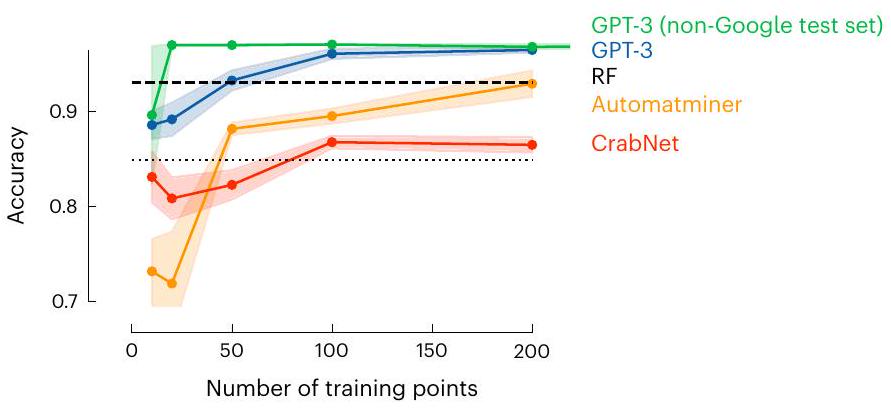
معلومات في سبائك عالية الانتروبيا. الشكل يقارن دقة النموذج كدالة لعدد نقاط التدريب. الخط الأفقي المتقطع يشير إلى الأداء المبلغ عنه في المرجع 24 باستخدام الغابة العشوائية (RF) مع مجموعة بيانات تتكون من 1,252 نقطة و10-fold cross-validation، أي ما يعادل حجم مجموعة تدريب حوالي 1,126 نقطة. الخط المنقط يظهر أداء قاعدة بسيطة تعتمد على القواعد ‘إذا كانت موجودة في التركيبة، صنفها كمرحلة واحدة، وإلا كمرحلة متعددة’. الخط الأصفر الذي حصلنا عليه باستخدام Automatminer.
ما وراء ضبط نماذج OpenAI
حساسية التمثيل
أو سلاسل مدمجة ذاتية الإشارة (SELFIES)
الانحدار
التصميم العكسي
تمديد الحدود
ملاحظات ختامية
جميع التجارب الفاشلة أو الناجحة جزئيًا
طرق
مقارنة كفاءة البيانات
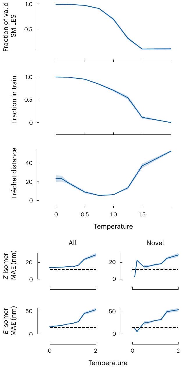
فحوصات الصلاحية
نموذج GPT-J
توفر البيانات
توفر الشيفرة
References
- Bommasani, R. et al. On the opportunities and risks of foundation models. Preprint at https://arxiv.org/abs/2108.07258 (2021).
- Vaswani, A. et al. Attention is all you need. Adv. Neural Inf. Process. Syst. https://proceedings.neurips.cc/paper/2017/file/ 3f5ee243547dee91fbd053c1c4a845aa-Paper.pdf (2017).
- Chowdhery, A. et al. PaLM: scaling language modeling with pathways. J. Mach. Learn. Res. 24, 1-113 (2023).
- Hoffmann, J. et al. An empirical analysis of compute-optimal large language model training. Adv. Neural Inf. Process. Syst. 35, 30016-30030 (2022).
- Brown, T. et al. Language models are few-shot learners. Adv. Neural Inf. Process. Syst. 33, 1877-1901 (2020).
- Edwards, C. N., Lai, T., Ros, K., Honke, G. & Ji, H. Translation between molecules and natural language. in Conference On Empirical Methods In Natural Language Processing (eds Goldberg, Y. et al.) 375-413 (Association for Computational Linguistics, 2022).
- Hocky, G. M. & White, A. D. Natural language processing models that automate programming will transform chemistry research and teaching. Digit. Discov. 1, 79-83 (2022).
- White, A. D. et al. Assessment of chemistry knowledge in large language models that generate. Digit. Discov. 2, 368-376 (2023).
- Taylor, R. et al. Galactica: a large language model for science. Preprint at https://arxiv.org/abs/2211.09085 (2022).
- Dunn, A. et al. Structured information extraction from complex scientific text with fine-tuned large language models. Adv. Neural Inf. Process. Syst. 35, 11763-11784 (2022).
- Choudhary, K. & Kelley, M. L. ChemNLP: a natural language-processing-based library for materials chemistry text data. J. Phys. Chem. C 127, 17545-17555 (2023).
- Jablonka, K. M. et al. 14 examples of how LLMs can transform materials science and chemistry: a reflection on a large language model hackathon. Digit. Discov. 2, 1233-1250 (2023).
- Dinh, T. et al. LIFT: language-interfaced fine-tuning for non-language machine learning tasks. Adv. Neural Inf. Process. Syst. 35, 11763-11784 (2022).
- Karpov, P., Godin, G. & Tetko, I. V. Transformer-CNN: Swiss knife for QSAR modeling and interpretation. J. Cheminform. 12, 17 (2020).
- Tshitoyan, V. et al. Unsupervised word embeddings capture latent knowledge from materials science literature. Nature 571, 95-98 (2019).
- Born, J. & Manica, M. Regression transformer enables concurrent sequence regression and generation for molecular language modelling. Nat. Mach. Intell. 5, 432-444 (2023).
- Yüksel, A., Ulusoy, E., Ünlü, A. & Doğan, T. SELFormer: molecular representation learning via SELFIES language models. Mach. Learn. Sci. Technol. 4, 025035 (2023).
- van Deursen, R., Ertl, P., Tetko, I. V. & Godin, G. GEN: highly efficient SMILES explorer using autodidactic generative examination networks. J. Cheminform.12, 22 (2020).
- Flam-Shepherd, D., Zhu, K. & Aspuru-Guzik, A. Language models can learn complex molecular distributions. Nat. Commun. 13, 3293 (2022).
- Grisoni, F. Chemical language models for de novo drug design: challenges and opportunities. Curr. Opin. Struct. Biol. 79, 102527 (2023).
- Ramos, M. C., Michtavy, S. S., Porosoff, M. D. & White, A. D. Bayesian optimization of catalysts with in-context learning. Preprint at https://arxiv.org/abs/2304.05341 (2023).
- Guo, T. et al. What indeed can GPT models do in chemistry? A comprehensive benchmark on eight tasks. Preprint at https://arxiv.org/abs/2305.18365 (2023).
- Howard, J. & Ruder, S. Universal language model fine-tuning for text classification. In Proc. 56th Annual Meeting of the Association for Computational Linguistics (Volume 1: Long Papers) 328-339 (Association for Computational Linguistics, 2018); https:// aclanthology.org/P18-1031
- Pei, Z., Yin, J., Hawk, J. A., Alman, D. E. & Gao, M. C. Machine-learning informed prediction of high-entropy solid solution formation: beyond the Hume-Rothery rules. npj Comput. Mater. https://doi.org/10.1038/s41524-020-0308-7 (2020).
- Dunn, A., Wang, Q., Ganose, A., Dopp, D. & Jain, A. Benchmarking materials property prediction methods: the Matbench test set and Automatminer reference algorithm. npj Comput. Mater. https://doi.org/10.1038/s41524-020-00406-3 (2020).
- Goldblum, M., Finzi, M., Rowan, K. & Wilson, A. The no free lunch theorem, Kolmogorov complexity, and the role of inductive biases in machine learning. ICLR 2024 Conference, OpenReview https://openreview.net/forum?id=X7nz6ljg9Y (2023).
- Schwaller, P. et al. Molecular transformer: a model for uncertainty-calibrated chemical reaction prediction. ACS Cent. Sci. 5, 1572-1583 (2019).
- Winter, B., Winter, C., Schilling, J. & Bardow, A. A smile is all you need: predicting limiting activity coefficients from SMILES with natural language processing. Digit. Discov. 1, 859-869 (2022).
- Dai, D. et al. Why can GPT learn in-context? Language models secretly perform gradient descent as meta-optimizers. Preprint at https://arxiv.org/abs/2212.10559 (2022).
- Weininger, D. SMILES, a chemical language and information system. 1. Introduction to methodology and encoding rules. J. Chem. Inf. Comput. Sci. 28, 31-36 (1988).
- Krenn, M., Häse, F., Nigam, A., Friederich, P. & Aspuru-Guzik, A. Self-referencing embedded strings (SELFIES): a 100% robust molecular string representation. Mach. Learn. Sci. Technol. 1, 045024 (2020).
- Krenn, M. et al. SELFIES and the future of molecular string representations. Patterns 3, 100588 (2022).
- Sanchez-Lengeling, B. & Aspuru-Guzik, A. Inverse molecular design using machine learning: generative models for matter engineering. Science 361, 360-365 (2018).
- Yao, Z. et al. Inverse design of nanoporous crystalline reticular materials with deep generative models. Nat. Mach. Intell. 3, 76-86 (2021).
- Gómez-Bombarelli, R. et al. Automatic chemical design using a data-driven continuous representation of molecules. ACS Cent. Sci. 4, 268-276 (2018).
- Kim, B., Lee, S. & Kim, J. Inverse design of porous materials using artificial neural networks. Sci. Adv. 6, eaax9324 (2020).
- Lee, S., Kim, B. & Kim, J. Predicting performance limits of methane gas storage in zeolites with an artificial neural network. J. Mater. Chem. A 7, 2709-2716 (2019).
- Nigam, A., Friederich, P., Krenn, M. & Aspuru-Guzik, A. Augmenting genetic algorithms with deep neural networks for exploring the chemical space. In ICLR (2019).
- Jablonka, K. M., Mcilwaine, F., Garcia, S., Smit, B. & Yoo, B. A reproducibility study of ‘augmenting genetic algorithms with deep neural networks for exploring the chemical space’. Preprint at https://arxiv.org/abs/2102.00700 (2021).
- Chung, Y. G. et al. In silico discovery of metal-organic frameworks for precombustion
capture using a genetic algorithm. Sci. Adv. 2, e1600909 (2016). - Lee, S. et al. Computational screening of trillions of metalorganic frameworks for high-performance methane storage. ACS Appl. Mater. Interfaces 13, 23647-23654 (2021).
- Collins, S. P., Daff, T. D., Piotrkowski, S. S. & Woo, T. K. Materials design by evolutionary optimization of functional groups in metal-organic frameworks. Sci. Adv. https://doi.org/10.1126/ sciadv. 1600954 (2016).
- Griffiths, R.-R. et al. Data-driven discovery of molecular photoswitches with multioutput Gaussian processes. Chem. Sci. 13, 13541-13551 (2022).
- Ertl, P. & Schuffenhauer, A. Estimation of synthetic accessibility score of drug-like molecules based on molecular complexity and fragment contributions. J. Cheminform. 1, 8 (2009).
- Jablonka, K. M., Jothiappan, G. M., Wang, S., Smit, B. & Yoo, B. Bias free multiobjective active learning for materials design and discovery. Nat. Commun. https://doi.org/10.1038/s41467-021-22437-0 (2021).
- Bannwarth, C., Ehlert, S. & Grimme, S. GFN2-xTB-an accurate and broadly parametrized self-consistent tight-binding quantum chemical method with multipole electrostatics and density-dependent dispersion contributions. J. Chem. Theory Comput. 15, 1652-1671 (2019).
- Isert, C., Atz, K., Jiménez-Luna, J. & Schneider, G. QMugs: quantum mechanical properties of drug-like molecules https://doi.org/10.3929/ethz-b-000482129 (2021).
- Isert, C., Atz, K., Jiménez-Luna, J. & Schneider, G. QMugs, quantum mechanical properties of drug-like molecules. Sci. Data 9, 273 (2022).
- Westermayr, J., Gilkes, J., Barrett, R. & Maurer, R. J. High-throughput property-driven generative design of functional organic molecules. Nat. Comput. Sci. 3, 139-148 (2023).
- Jablonka, K. M., Patiny, L. & Smit, B. Making the collective knowledge of chemistry open and machine actionable. Nat. Chem. 14, 365-376 (2022).
- Brown, N., Fiscato, M., Segler, M. H. & Vaucher, A. C. GuacaMol: benchmarking models for de novo molecular design. J. Chem. Inf. Model. 59, 1096-1108 (2019).
- Wang, B. Mesh-Transformer-JAX: model-parallel implementation of transformer language model with JAX. GitHub https://github. com/kingoflolz/mesh-transformer-jax (2021).
- Wang, B. & Komatsuzaki, A. GPT-J-6B: a 6 billion parameter autoregressive language model. GitHub https://github.com/ kingoflolz/mesh-transformer-jax (2021).
- Gao, L. et al. The Pile: an 800 BG dataset of diverse text for language modeling. Preprint at https://arxiv.org/abs/2101.00027 (2020).
- Dettmers, T., Lewis, M., Belkada, Y. & Zettlemoyer, L. GPT3.int8(): 8-bit matrix multiplication for transformers at scale. Adv. Neural Inf. Process. Syst. 35, 30318-30332 (2022).
- Dettmers, T., Lewis, M., Shleifer, S. & Zettlemoyer, L. 8-bit optimizers via block-wise quantization. in The Tenth International Conference on Learning Representations (2022).
- Hu, E. J. et al. LoRA: low-rank adaptation of large language models. in International Conference On Learning Representations (2021).
- Jablonka, K. M. kjappelbaum/gptchem: initial release. Zenodo https://doi.org/10.5281/zenodo. 7806672 (2023).
- Jablonka, K. M. chemlift. Zenodo https://doi.org/10.5281/ zenodo. 10233422 (2023).
- Dubbeldam, D., Calero, S. & Vlugt, T. J. iRASPA: GPU-accelerated visualization software for materials scientists. Mol. Simul. 44, 653-676 (2018).
- Le, T. T., Fu, W. & Moore, J. H. Scaling tree-based automated machine learning to biomedical big data with a feature set selector. Bioinformatics 36, 250-256 (2020).
- Wang, A. Y.-T., Kauwe, S. K., Murdock, R. J. & Sparks, T. D. Compositionally restricted attention-based network for materials property predictions. npj Comput. Mater. 7, 77 (2021).
- RDKit contributors. RDKit: Open-source Cheminformatics; (2023) http://www.rdkit.org
- Preuer, K., Renz, P., Unterthiner, T., Hochreiter, S. & Klambauer, G. Fréchet ChemNet distance: a metric for generative models for molecules in drug discovery. J. Chem. Inf. Model. 58, 1736-1741 (2018).
- Probst, D. & Reymond, J.-L. Visualization of very large high-dimensional data sets as minimum spanning trees. J. Cheminform. 12, 12 (2020).
- Probst, D. & Reymond, J.-L. A probabilistic molecular fingerprint for big data settings. J. Cheminform. 10, 66 (2018).
- Ertl, P. & Rohde, B. The Molecule Cloud-compact visualization of large collections of molecules. J. Cheminform. 4, 12 (2012).
- Wang, Y., Wang, J., Cao, Z. & Farimani, A. B. Molecular contrastive learning of representations via graph neural networks. Nat. Mach. Intell. 4, 279-287 (2022).
- Breuck, P.-P. D., Evans, M. L. & Rignanese, G.-M. Robust model benchmarking and bias-imbalance in data-driven materials science: a case study on MODNet. J. Phys. Condens. Matter 33, 404002 (2021).
- Hollmann, N., Müller, S., Eggensperger, K. & Hutter, F. TabPFN: a transformer that solves small tabular classification problems in a second. Preprint at https://arxiv.org/abs/2207.01848 (2022).
- Griffiths, R.-R. et al. Gauche: a library for Gaussian processes in chemistry. in ICML 2022 2nd AI for Science Workshop https:// openreview.net/forum?id=i9MKI7zrWal (2022)
- Chen, T. & Guestrin, C. XGBoost: a scalable tree boosting system. in Proc. 22nd ACM SIGKDD International Conference on Knowledge Discovery and Data Mining 785-794 (ACM, 2016).
- Moosavi, S. M. et al. Understanding the diversity of the metalorganic framework ecosystem. Nat. Commun. 11, 4068 (2020).
- Moosavi, S. M. et al. A data-science approach to predict the heat capacity of nanoporous materials. Nat. Mater. 21, 1419-1425 (2022).
- Probst, D., Schwaller, P. & Reymond, J.-L. Reaction classification and yield prediction using the differential reaction fingerprint DRFP. Digit. Discov. 1, 91-97 (2022).
- Raffel, C. et al. Exploring the limits of transfer learning with a unified text-to-text transformer. J. Mach. Learn. Res. 21, 5485-5551 (2020).
- Radford, A. et al. Language models are unsupervised multitask learners. OpenAl blog 1, 9 (2019).
- Mobley, D. L. & Guthrie, J. P. FreeSolv: a database of experimental and calculated hydration free energies, with input files. J. Comput. Aided Mol. Des. 28, 711-720 (2014).
- Delaney, J. S. ESOL: estimating aqueous solubility directly from molecular structure. J. Chem. Inf. Comput. Sci. 44, 1000-1005 (2004).
- Mitchell, J. B. O. DLS-100 solubility dataset. University of St Andrews https://risweb.st-andrews.ac.uk:443/portal/en/ datasets/dls100-solubility-dataset(3a3a5abc-8458-4924-8e6c-b804347605e8).html (2017).
- Walters, P. Predicting aqueous solubility-it’s harder than it looks. Practical Cheminformatics https://practicalcheminformatics. blogspot.com/2018/09/predicting-aqueous-solubility-its.html (2018).
- Bento, A. P. et al. The ChEMBL bioactivity database: an update. Nucleic Acids Res. 42, D1083-D1090 (2014).
- Gaulton, A. et al. ChEMBL: a large-scale bioactivity database for drug discovery. Nucleic Acids Res. 40, D1100-D1107 (2012).
- Nagasawa, S., Al-Naamani, E. & Saeki, A. Computer-aided screening of conjugated polymers for organic solar cell: classification by random forest. J. Phys. Chem. Lett. 9, 2639-2646 (2018).
- Kawazoe, Y., Yu, J.-Z., Tsai, A.-P. & Masumoto, T. (eds) Nonequilibrium Phase Diagrams of Ternary Amorphous Alloys Landolt-Börnstein: Numerical Data and Functional Relationships in Science and Technology-New Series (Springer, 2006).
- Zhuo, Y., Tehrani, A. M. & Brgoch, J. Predicting the band gaps of inorganic solids by machine learning. J. Phys. Chem. Lett. 9, 1668-1673 (2018).
- Ahneman, D. T., Estrada, J. G., Lin, S., Dreher, S. D. & Doyle, A. G. Predicting reaction performance in C-N cross-coupling using machine learning. Science 360, 186-190 (2018).
- Perera, D. et al. A platform for automated nanomole-scale reaction screening and micromole-scale synthesis in flow. Science 359, 429-434 (2018).
الشكر والتقدير
مساهمات المؤلفين
التمويل
المصالح المتنافسة
معلومات إضافية
© المؤلفون 2024
البيانات الموسعة الجدول 1 | أمثلة على المطالبات والاكتمالات لتوقع مرحلة سبائك عالية الانتروبيا
| مطالبة | اكتمال | تجريبي |
| ما هي مرحلة Co1Cu1Fe1Ni1V1؟### | 0@@@ | متعددة المراحل |
| ما هي مرحلة Pu0.75Zr0.25؟### | 1@@@ | مرحلة واحدة |
| ما هي مرحلة BeFe؟### | 0@@@ | متعددة المراحل |
| ما هي مرحلة LiTa؟### | 0@@@ | متعددة المراحل |
| ما هي مرحلة Nb0.5Ta0.5؟### | 1@@@ | مرحلة واحدة |
| ما هي مرحلة Al0.1W0.9؟### | 1@@@ | مرحلة واحدة |
| ما هي مرحلة Cr0.5Fe0.5؟### | 1@@@ | مرحلة واحدة |
| ما هي مرحلة Al1Co1Cr1Cu1Fe1Ni1Ti1؟### | 0@@@ | متعددة المراحل |
| ما هي مرحلة Cu0.5Mn0.5؟### | 1@@@ | مرحلة واحدة |
| ما هي مرحلة OsU؟### | 0@@@ | متعددة المراحل |
| مجموعة | معيار | سنة النشر | أفضل غير DL | أفضل خط أساس للتعلم العميق |
| جزيئات | طول موج انتقال المفتاح الضوئي | ٢٠٢٢ | 1.1 (ن) | 1.2 (ت) |
| الطاقة الحرة للذوبان | 2014 | 3.1 (ز) | 1.3 (ت) | |
| الذوبانية | ٢٠٠٤ | 1.0 (س) | 0.002 (م) | |
| محبة الدهون | 2012 | 3.43 (غ) | 0.97 (ت) | |
| فجوة HOMO-LUMO | ٢٠٢٢ | 4.3 (س) | 0.62 (طن) | |
| OPV PCE | 2018 | 0.95 (ن) | 0.76 (ط) | |
| المواد | طاقة الامتزاز الخالية من السطحي | ٢٠٢١ | 1.4 (سج) | 0.37 (ت) |
|
|
٢٠٢٠ | 0.40 (س) | 12 (ت) | |
|
|
٢٠٢٠ | 0.52 (إكس إم أو) | 0.60 (ت) | |
| السعة الحرارية | ٢٠٢٢ | 0.24 (شهر) | 0.76 (ج) | |
| مرحلة HEA | ٢٠٢٠ | 24 (بروف) | 9.0 (ج) | |
| قدرة تشكيل الزجاج المعدني الكتلي | 2006 | 0.98 (أ) | 0.62 (وحدة) | |
| سلوك معدني | 2018 | 0.52 (أ) | 0.46 (وحدة) | |
| ردود الفعل | التقاطع بين C-N | 2018 | 2.9 (در ف ب) | |
| التقاطع بين C-C | 2022 | 0.98 (ن) |
مختبر المحاكاة الجزيئية (LSMO)، معهد العلوم والهندسة الكيميائية، المدرسة الفيدرالية Polytechnic في لوزان (EPFL)، سيون، سويسرا. مركز الكيمياء البيئية والطاقة في يينا (CEEC Jena)، جامعة فريدريش شيلر في يينا، يينا، ألمانيا. مختبر الكيمياء العضوية والبوليمرية (IOMC)، جامعة فريدريش شيلر يينا، يينا، ألمانيا. معهد هلمهولتز للبوليمرات في تطبيقات الطاقة، يينا، ألمانيا. مختبر الذكاء الكيميائي الاصطناعي (LIAC)، المدرسة الفيدرالية Polytechnic في لوزان (EPFL)، لوزان، سويسرا. – البريد الإلكتروني: berend.smit@epfl.ch
DOI: https://doi.org/10.1038/s42256-023-00788-1
Publication Date: 2024-02-06
Leveraging large language models for predictive chemistry
Accepted: 22 December 2023
Published online: 6 February 2024
(D) Check for updates
Abstract
Machine learning has transformed many fields and has recently found applications in chemistry and materials science. The small datasets commonly found in chemistry sparked the development of sophisticated machine learning approaches that incorporate chemical knowledge for each application and, therefore, require specialized expertise to develop. Here we show that GPT-3, a large language model trained on vast amounts of text extracted from the Internet, can easily be adapted to solve various tasks in chemistry and materials science by fine-tuning it to answer chemical questions in natural language with the correct answer. We compared this approach with dedicated machine learning models for many applications spanning the properties of molecules and materials to the yield of chemical reactions. Surprisingly, our fine-tuned version of GPT-3 can perform comparably to or even outperform conventional machine learning techniques, in particular in the low-data limit. In addition, we can perform inverse design by simply inverting the questions. The ease of use and high performance, especially for small datasets, can impact the fundamental approach to using machine learning in the chemical and material sciences. In addition to a literature search, querying a pre-trained large language model might become a routine way to bootstrap a project by leveraging the collective knowledge encoded in these foundation models, or to provide a baseline for predictive tasks.
solve relatively simple tabular regression and classification tasks
Language-interfaced fine-tuning for classification and regression
Approach
metals will form a solid solution or multiple phases. Hence, the question we would like to ask is: ‘What is the phase of <composition of the high-entropy alloy>?’ and our model should give a text completion from the set of possible answers {single phase, multi-phase}.
Classification
formation in high-entropy alloys. The figure compares the model’s accuracy as a function of the number of training points. The dashed horizontal line indicates the performance reported in ref. 24 using random forest (RF) with a dataset of 1,252 points and 10 -fold cross-validation, that is, corresponding to a training set size of around 1,126 points. The dotted line shows the performance of a simple rule-based baseline ‘if present in the composition, classify as single phase, else multi-phase’. The yellow line we obtained using the Automatminer
Beyond fine-tuning of OpenAI models
Representation sensitivity
or self-referencing embedded strings (SELFIES)
Regression
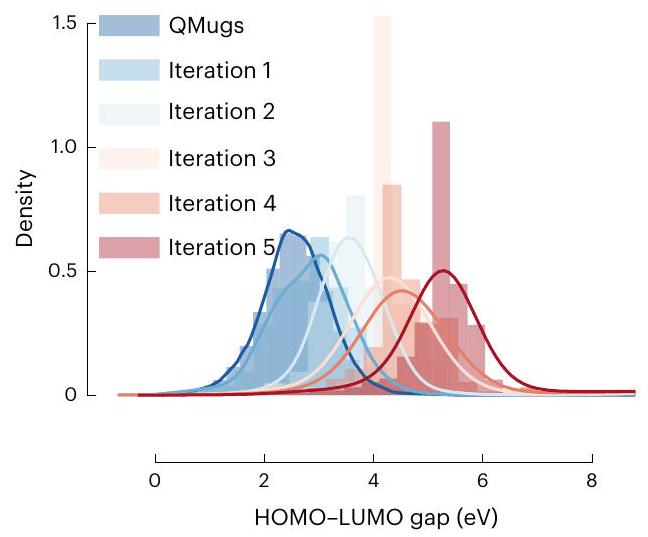
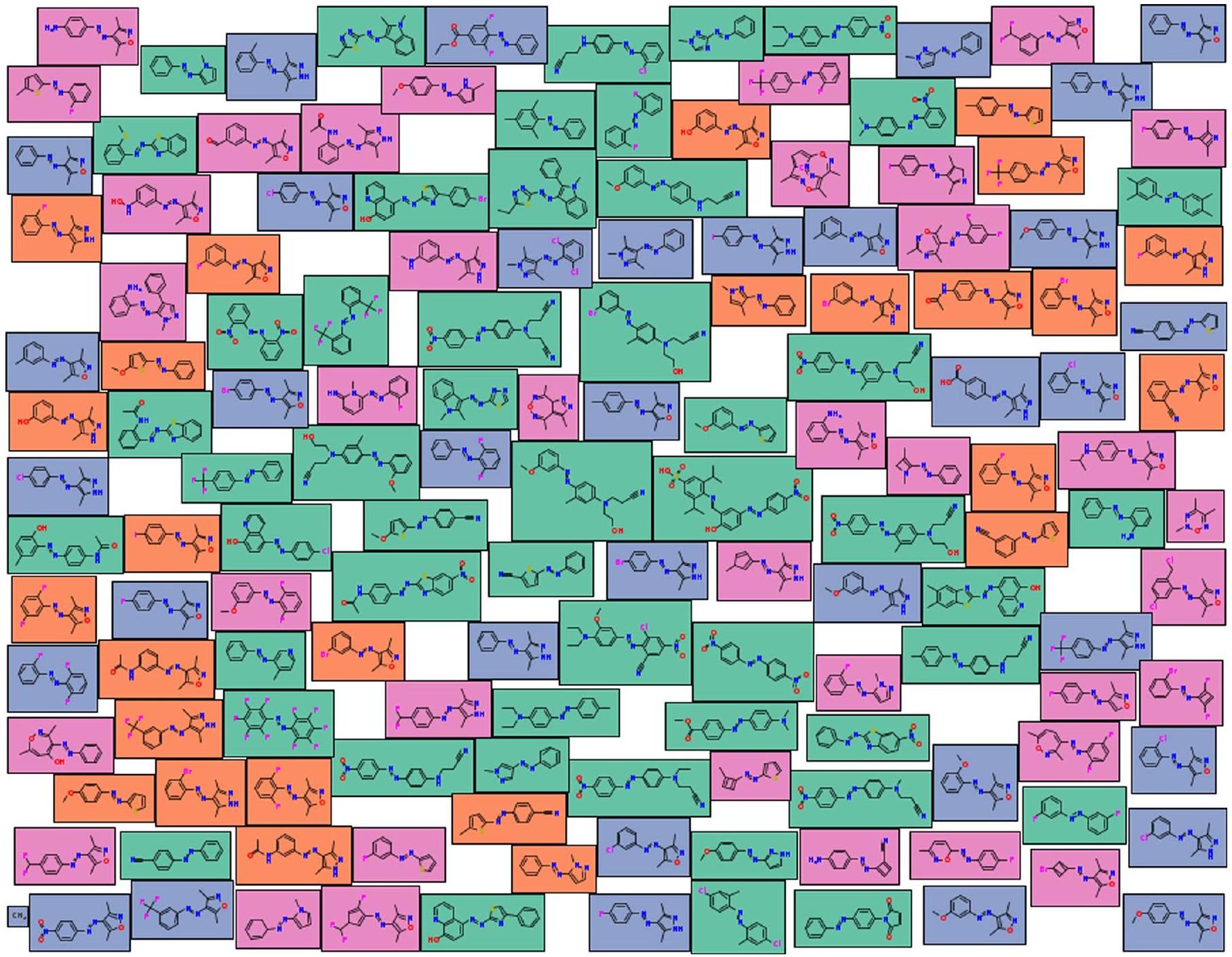
Inverse design
Stretching the limits
Concluding remarks
all failed or partially successful experiments
Methods
Data efficiency comparison
Validity checks
GPT-J model
Data availability
Code availability
References
- Bommasani, R. et al. On the opportunities and risks of foundation models. Preprint at https://arxiv.org/abs/2108.07258 (2021).
- Vaswani, A. et al. Attention is all you need. Adv. Neural Inf. Process. Syst. https://proceedings.neurips.cc/paper/2017/file/ 3f5ee243547dee91fbd053c1c4a845aa-Paper.pdf (2017).
- Chowdhery, A. et al. PaLM: scaling language modeling with pathways. J. Mach. Learn. Res. 24, 1-113 (2023).
- Hoffmann, J. et al. An empirical analysis of compute-optimal large language model training. Adv. Neural Inf. Process. Syst. 35, 30016-30030 (2022).
- Brown, T. et al. Language models are few-shot learners. Adv. Neural Inf. Process. Syst. 33, 1877-1901 (2020).
- Edwards, C. N., Lai, T., Ros, K., Honke, G. & Ji, H. Translation between molecules and natural language. in Conference On Empirical Methods In Natural Language Processing (eds Goldberg, Y. et al.) 375-413 (Association for Computational Linguistics, 2022).
- Hocky, G. M. & White, A. D. Natural language processing models that automate programming will transform chemistry research and teaching. Digit. Discov. 1, 79-83 (2022).
- White, A. D. et al. Assessment of chemistry knowledge in large language models that generate. Digit. Discov. 2, 368-376 (2023).
- Taylor, R. et al. Galactica: a large language model for science. Preprint at https://arxiv.org/abs/2211.09085 (2022).
- Dunn, A. et al. Structured information extraction from complex scientific text with fine-tuned large language models. Adv. Neural Inf. Process. Syst. 35, 11763-11784 (2022).
- Choudhary, K. & Kelley, M. L. ChemNLP: a natural language-processing-based library for materials chemistry text data. J. Phys. Chem. C 127, 17545-17555 (2023).
- Jablonka, K. M. et al. 14 examples of how LLMs can transform materials science and chemistry: a reflection on a large language model hackathon. Digit. Discov. 2, 1233-1250 (2023).
- Dinh, T. et al. LIFT: language-interfaced fine-tuning for non-language machine learning tasks. Adv. Neural Inf. Process. Syst. 35, 11763-11784 (2022).
- Karpov, P., Godin, G. & Tetko, I. V. Transformer-CNN: Swiss knife for QSAR modeling and interpretation. J. Cheminform. 12, 17 (2020).
- Tshitoyan, V. et al. Unsupervised word embeddings capture latent knowledge from materials science literature. Nature 571, 95-98 (2019).
- Born, J. & Manica, M. Regression transformer enables concurrent sequence regression and generation for molecular language modelling. Nat. Mach. Intell. 5, 432-444 (2023).
- Yüksel, A., Ulusoy, E., Ünlü, A. & Doğan, T. SELFormer: molecular representation learning via SELFIES language models. Mach. Learn. Sci. Technol. 4, 025035 (2023).
- van Deursen, R., Ertl, P., Tetko, I. V. & Godin, G. GEN: highly efficient SMILES explorer using autodidactic generative examination networks. J. Cheminform.12, 22 (2020).
- Flam-Shepherd, D., Zhu, K. & Aspuru-Guzik, A. Language models can learn complex molecular distributions. Nat. Commun. 13, 3293 (2022).
- Grisoni, F. Chemical language models for de novo drug design: challenges and opportunities. Curr. Opin. Struct. Biol. 79, 102527 (2023).
- Ramos, M. C., Michtavy, S. S., Porosoff, M. D. & White, A. D. Bayesian optimization of catalysts with in-context learning. Preprint at https://arxiv.org/abs/2304.05341 (2023).
- Guo, T. et al. What indeed can GPT models do in chemistry? A comprehensive benchmark on eight tasks. Preprint at https://arxiv.org/abs/2305.18365 (2023).
- Howard, J. & Ruder, S. Universal language model fine-tuning for text classification. In Proc. 56th Annual Meeting of the Association for Computational Linguistics (Volume 1: Long Papers) 328-339 (Association for Computational Linguistics, 2018); https:// aclanthology.org/P18-1031
- Pei, Z., Yin, J., Hawk, J. A., Alman, D. E. & Gao, M. C. Machine-learning informed prediction of high-entropy solid solution formation: beyond the Hume-Rothery rules. npj Comput. Mater. https://doi.org/10.1038/s41524-020-0308-7 (2020).
- Dunn, A., Wang, Q., Ganose, A., Dopp, D. & Jain, A. Benchmarking materials property prediction methods: the Matbench test set and Automatminer reference algorithm. npj Comput. Mater. https://doi.org/10.1038/s41524-020-00406-3 (2020).
- Goldblum, M., Finzi, M., Rowan, K. & Wilson, A. The no free lunch theorem, Kolmogorov complexity, and the role of inductive biases in machine learning. ICLR 2024 Conference, OpenReview https://openreview.net/forum?id=X7nz6ljg9Y (2023).
- Schwaller, P. et al. Molecular transformer: a model for uncertainty-calibrated chemical reaction prediction. ACS Cent. Sci. 5, 1572-1583 (2019).
- Winter, B., Winter, C., Schilling, J. & Bardow, A. A smile is all you need: predicting limiting activity coefficients from SMILES with natural language processing. Digit. Discov. 1, 859-869 (2022).
- Dai, D. et al. Why can GPT learn in-context? Language models secretly perform gradient descent as meta-optimizers. Preprint at https://arxiv.org/abs/2212.10559 (2022).
- Weininger, D. SMILES, a chemical language and information system. 1. Introduction to methodology and encoding rules. J. Chem. Inf. Comput. Sci. 28, 31-36 (1988).
- Krenn, M., Häse, F., Nigam, A., Friederich, P. & Aspuru-Guzik, A. Self-referencing embedded strings (SELFIES): a 100% robust molecular string representation. Mach. Learn. Sci. Technol. 1, 045024 (2020).
- Krenn, M. et al. SELFIES and the future of molecular string representations. Patterns 3, 100588 (2022).
- Sanchez-Lengeling, B. & Aspuru-Guzik, A. Inverse molecular design using machine learning: generative models for matter engineering. Science 361, 360-365 (2018).
- Yao, Z. et al. Inverse design of nanoporous crystalline reticular materials with deep generative models. Nat. Mach. Intell. 3, 76-86 (2021).
- Gómez-Bombarelli, R. et al. Automatic chemical design using a data-driven continuous representation of molecules. ACS Cent. Sci. 4, 268-276 (2018).
- Kim, B., Lee, S. & Kim, J. Inverse design of porous materials using artificial neural networks. Sci. Adv. 6, eaax9324 (2020).
- Lee, S., Kim, B. & Kim, J. Predicting performance limits of methane gas storage in zeolites with an artificial neural network. J. Mater. Chem. A 7, 2709-2716 (2019).
- Nigam, A., Friederich, P., Krenn, M. & Aspuru-Guzik, A. Augmenting genetic algorithms with deep neural networks for exploring the chemical space. In ICLR (2019).
- Jablonka, K. M., Mcilwaine, F., Garcia, S., Smit, B. & Yoo, B. A reproducibility study of ‘augmenting genetic algorithms with deep neural networks for exploring the chemical space’. Preprint at https://arxiv.org/abs/2102.00700 (2021).
- Chung, Y. G. et al. In silico discovery of metal-organic frameworks for precombustion
capture using a genetic algorithm. Sci. Adv. 2, e1600909 (2016). - Lee, S. et al. Computational screening of trillions of metalorganic frameworks for high-performance methane storage. ACS Appl. Mater. Interfaces 13, 23647-23654 (2021).
- Collins, S. P., Daff, T. D., Piotrkowski, S. S. & Woo, T. K. Materials design by evolutionary optimization of functional groups in metal-organic frameworks. Sci. Adv. https://doi.org/10.1126/ sciadv. 1600954 (2016).
- Griffiths, R.-R. et al. Data-driven discovery of molecular photoswitches with multioutput Gaussian processes. Chem. Sci. 13, 13541-13551 (2022).
- Ertl, P. & Schuffenhauer, A. Estimation of synthetic accessibility score of drug-like molecules based on molecular complexity and fragment contributions. J. Cheminform. 1, 8 (2009).
- Jablonka, K. M., Jothiappan, G. M., Wang, S., Smit, B. & Yoo, B. Bias free multiobjective active learning for materials design and discovery. Nat. Commun. https://doi.org/10.1038/s41467-021-22437-0 (2021).
- Bannwarth, C., Ehlert, S. & Grimme, S. GFN2-xTB-an accurate and broadly parametrized self-consistent tight-binding quantum chemical method with multipole electrostatics and density-dependent dispersion contributions. J. Chem. Theory Comput. 15, 1652-1671 (2019).
- Isert, C., Atz, K., Jiménez-Luna, J. & Schneider, G. QMugs: quantum mechanical properties of drug-like molecules https://doi.org/10.3929/ethz-b-000482129 (2021).
- Isert, C., Atz, K., Jiménez-Luna, J. & Schneider, G. QMugs, quantum mechanical properties of drug-like molecules. Sci. Data 9, 273 (2022).
- Westermayr, J., Gilkes, J., Barrett, R. & Maurer, R. J. High-throughput property-driven generative design of functional organic molecules. Nat. Comput. Sci. 3, 139-148 (2023).
- Jablonka, K. M., Patiny, L. & Smit, B. Making the collective knowledge of chemistry open and machine actionable. Nat. Chem. 14, 365-376 (2022).
- Brown, N., Fiscato, M., Segler, M. H. & Vaucher, A. C. GuacaMol: benchmarking models for de novo molecular design. J. Chem. Inf. Model. 59, 1096-1108 (2019).
- Wang, B. Mesh-Transformer-JAX: model-parallel implementation of transformer language model with JAX. GitHub https://github. com/kingoflolz/mesh-transformer-jax (2021).
- Wang, B. & Komatsuzaki, A. GPT-J-6B: a 6 billion parameter autoregressive language model. GitHub https://github.com/ kingoflolz/mesh-transformer-jax (2021).
- Gao, L. et al. The Pile: an 800 BG dataset of diverse text for language modeling. Preprint at https://arxiv.org/abs/2101.00027 (2020).
- Dettmers, T., Lewis, M., Belkada, Y. & Zettlemoyer, L. GPT3.int8(): 8-bit matrix multiplication for transformers at scale. Adv. Neural Inf. Process. Syst. 35, 30318-30332 (2022).
- Dettmers, T., Lewis, M., Shleifer, S. & Zettlemoyer, L. 8-bit optimizers via block-wise quantization. in The Tenth International Conference on Learning Representations (2022).
- Hu, E. J. et al. LoRA: low-rank adaptation of large language models. in International Conference On Learning Representations (2021).
- Jablonka, K. M. kjappelbaum/gptchem: initial release. Zenodo https://doi.org/10.5281/zenodo. 7806672 (2023).
- Jablonka, K. M. chemlift. Zenodo https://doi.org/10.5281/ zenodo. 10233422 (2023).
- Dubbeldam, D., Calero, S. & Vlugt, T. J. iRASPA: GPU-accelerated visualization software for materials scientists. Mol. Simul. 44, 653-676 (2018).
- Le, T. T., Fu, W. & Moore, J. H. Scaling tree-based automated machine learning to biomedical big data with a feature set selector. Bioinformatics 36, 250-256 (2020).
- Wang, A. Y.-T., Kauwe, S. K., Murdock, R. J. & Sparks, T. D. Compositionally restricted attention-based network for materials property predictions. npj Comput. Mater. 7, 77 (2021).
- RDKit contributors. RDKit: Open-source Cheminformatics; (2023) http://www.rdkit.org
- Preuer, K., Renz, P., Unterthiner, T., Hochreiter, S. & Klambauer, G. Fréchet ChemNet distance: a metric for generative models for molecules in drug discovery. J. Chem. Inf. Model. 58, 1736-1741 (2018).
- Probst, D. & Reymond, J.-L. Visualization of very large high-dimensional data sets as minimum spanning trees. J. Cheminform. 12, 12 (2020).
- Probst, D. & Reymond, J.-L. A probabilistic molecular fingerprint for big data settings. J. Cheminform. 10, 66 (2018).
- Ertl, P. & Rohde, B. The Molecule Cloud-compact visualization of large collections of molecules. J. Cheminform. 4, 12 (2012).
- Wang, Y., Wang, J., Cao, Z. & Farimani, A. B. Molecular contrastive learning of representations via graph neural networks. Nat. Mach. Intell. 4, 279-287 (2022).
- Breuck, P.-P. D., Evans, M. L. & Rignanese, G.-M. Robust model benchmarking and bias-imbalance in data-driven materials science: a case study on MODNet. J. Phys. Condens. Matter 33, 404002 (2021).
- Hollmann, N., Müller, S., Eggensperger, K. & Hutter, F. TabPFN: a transformer that solves small tabular classification problems in a second. Preprint at https://arxiv.org/abs/2207.01848 (2022).
- Griffiths, R.-R. et al. Gauche: a library for Gaussian processes in chemistry. in ICML 2022 2nd AI for Science Workshop https:// openreview.net/forum?id=i9MKI7zrWal (2022)
- Chen, T. & Guestrin, C. XGBoost: a scalable tree boosting system. in Proc. 22nd ACM SIGKDD International Conference on Knowledge Discovery and Data Mining 785-794 (ACM, 2016).
- Moosavi, S. M. et al. Understanding the diversity of the metalorganic framework ecosystem. Nat. Commun. 11, 4068 (2020).
- Moosavi, S. M. et al. A data-science approach to predict the heat capacity of nanoporous materials. Nat. Mater. 21, 1419-1425 (2022).
- Probst, D., Schwaller, P. & Reymond, J.-L. Reaction classification and yield prediction using the differential reaction fingerprint DRFP. Digit. Discov. 1, 91-97 (2022).
- Raffel, C. et al. Exploring the limits of transfer learning with a unified text-to-text transformer. J. Mach. Learn. Res. 21, 5485-5551 (2020).
- Radford, A. et al. Language models are unsupervised multitask learners. OpenAl blog 1, 9 (2019).
- Mobley, D. L. & Guthrie, J. P. FreeSolv: a database of experimental and calculated hydration free energies, with input files. J. Comput. Aided Mol. Des. 28, 711-720 (2014).
- Delaney, J. S. ESOL: estimating aqueous solubility directly from molecular structure. J. Chem. Inf. Comput. Sci. 44, 1000-1005 (2004).
- Mitchell, J. B. O. DLS-100 solubility dataset. University of St Andrews https://risweb.st-andrews.ac.uk:443/portal/en/ datasets/dls100-solubility-dataset(3a3a5abc-8458-4924-8e6c-b804347605e8).html (2017).
- Walters, P. Predicting aqueous solubility-it’s harder than it looks. Practical Cheminformatics https://practicalcheminformatics. blogspot.com/2018/09/predicting-aqueous-solubility-its.html (2018).
- Bento, A. P. et al. The ChEMBL bioactivity database: an update. Nucleic Acids Res. 42, D1083-D1090 (2014).
- Gaulton, A. et al. ChEMBL: a large-scale bioactivity database for drug discovery. Nucleic Acids Res. 40, D1100-D1107 (2012).
- Nagasawa, S., Al-Naamani, E. & Saeki, A. Computer-aided screening of conjugated polymers for organic solar cell: classification by random forest. J. Phys. Chem. Lett. 9, 2639-2646 (2018).
- Kawazoe, Y., Yu, J.-Z., Tsai, A.-P. & Masumoto, T. (eds) Nonequilibrium Phase Diagrams of Ternary Amorphous Alloys Landolt-Börnstein: Numerical Data and Functional Relationships in Science and Technology-New Series (Springer, 2006).
- Zhuo, Y., Tehrani, A. M. & Brgoch, J. Predicting the band gaps of inorganic solids by machine learning. J. Phys. Chem. Lett. 9, 1668-1673 (2018).
- Ahneman, D. T., Estrada, J. G., Lin, S., Dreher, S. D. & Doyle, A. G. Predicting reaction performance in C-N cross-coupling using machine learning. Science 360, 186-190 (2018).
- Perera, D. et al. A platform for automated nanomole-scale reaction screening and micromole-scale synthesis in flow. Science 359, 429-434 (2018).
Acknowledgements
Author contributions
Funding
Competing interests
Additional information
© The Author(s) 2024
Extended Data Table 1 | Example prompts and completions for predicting the phase of high-entropy alloys
| prompt | completion | experimental |
| What is the phase of Co1Cu1Fe1Ni1V1?### | 0@@@ | multi-phase |
| What is the phase of Pu0.75Zr0.25?### | 1@@@ | single-phase |
| What is the phase of BeFe?### | 0@@@ | multi-phase |
| What is the phase of LiTa?### | 0@@@ | multi-phase |
| What is the phase of Nb0.5Ta0.5?### | 1@@@ | single-phase |
| What is the phase of Al0.1W0.9?### | 1@@@ | single-phase |
| What is the phase of Cr0.5Fe0.5?### | 1@@@ | single-phase |
| What is the phase of Al1Co1Cr1Cu1Fe1Ni1Ti1?### | 0@@@ | multi-phase |
| What is the phase of Cu0.5Mn0.5?### | 1@@@ | single-phase |
| What is the phase of OsU?### | 0@@@ | multi-phase |
| group | benchmark | publication year | best nonDL | best DL baseline |
| molecules | photoswitch transition wavelength | 2022 | 1.1 (n) | 1.2 (t) |
| free energy of solvation | 2014 | 3.1 (g) | 1.3 (t) | |
| solubility | 2004 | 1.0 (x) | 0.002 (m) | |
| lipophilicity | 2012 | 3.43 (g) | 0.97 (t) | |
| HOMO-LUMO gap | 2022 | 4.3 (x) | 0.62 (t) | |
| OPV PCE | 2018 | 0.95 (n) | 0.76 (t) | |
| materials | surfactant free energy of adsorption | 2021 | 1.4 (xj) | 0.37 (t) |
|
|
2020 | 0.40 (x) | 12 (t) | |
|
|
2020 | 0.52 (xmo) | 0.60 (t) | |
| heat capacity | 2022 | 0.24 (mo) | 0.76 (c) | |
| HEA phase | 2020 | 24 (prf) | 9.0 (c) | |
| bulk metallic glass formation ability | 2006 | 0.98 (a) | 0.62 (mod) | |
| metallic behavior | 2018 | 0.52 (a) | 0.46 (mod) | |
| reactions | C-N cross-coupling | 2018 | 2.9 (drfp) | |
| C-C cross-coupling | 2022 | 0.98 (n) |
Laboratory of Molecular Simulation (LSMO), Institut des Sciences et Ingénierie Chimiques, École Polytechnique Fédérale de Lausanne (EPFL), Sion, Switzerland. Center for Energy and Environmental Chemistry Jena (CEEC Jena), Friedrich Schiller University Jena, Jena, Germany. Laboratory of Organic and Macromolecular Chemistry (IOMC), Friedrich Schiller University Jena, Jena, Germany. Helmholtz Institute for Polymers in Energy Applications, Jena, Germany. Laboratory of Artificial Chemical Intelligence (LIAC), École Polytechnique Fédérale de Lausanne (EPFL), Lausanne, Switzerland. – e-mail: berend.smit@epfl.ch