الالتزام الاقتصادي بتغير المناخ The economic commitment of climate change

المجلة: Nature، المجلد: 628، العدد: 8008
DOI: https://doi.org/10.1038/s41586-024-07219-0
PMID: https://pubmed.ncbi.nlm.nih.gov/38632481
تاريخ النشر: 2024-04-17

الالتزام الاقتصادي بتغير المناخ

https://doi.org/10.1038/s41586-024-07219-0
تاريخ الاستلام: 25 يناير 2023
تم القبول: 21 فبراير 2024
نُشر على الإنترنت: 17 أبريل 2024
الوصول المفتوح
تحقق من التحديثات

الملخص

ماكسيميليان كوتز أندرس ليفرمان وليوني وينز

تأخذ التوقعات العالمية للأضرار الاقتصادية الكلية الناتجة عن تغير المناخ عادةً في الاعتبار التأثيرات الناتجة عن متوسط درجات الحرارة السنوية والوطنية على مدى فترات زمنية طويلة. هنا نستخدم نتائج تجريبية حديثة من أكثر من 1600 منطقة حول العالم على مدى الأربعين عامًا الماضية لتقدير الأضرار على المستوى دون الوطني الناتجة عن درجات الحرارة وهطول الأمطار، بما في ذلك التغير اليومي والتقلبات الشديدة. باستخدام نهج تجريبي يوفر حدًا أدنى قويًا لاستمرارية التأثيرات على النمو الاقتصادي، نجد أن الاقتصاد العالمي ملتزم بتقليص الدخل بمقدار خلال السنوات الست والعشرين القادمة بغض النظر عن خيارات الانبعاثات المستقبلية (بالنسبة لخط أساس بدون تأثيرات مناخية، النطاق المحتمل لـ محاسبة المناخ الفيزيائي وعدم اليقين التجريبي). هذه الأضرار تتجاوز بالفعل تكاليف التخفيف المطلوبة للحد من ارتفاع درجة حرارة الأرض إلى بمعدل ستة أضعاف خلال هذه الفترة الزمنية القريبة، ومن ثم تتباين بشكل قوي اعتمادًا على خيارات الانبعاثات. تنشأ الأضرار الملتزمة بشكل أساسي من التغيرات في متوسط درجة الحرارة، ولكن أخذ المزيد من المكونات المناخية في الاعتبار يزيد التقديرات بحوالي ويؤدي ذلك إلى زيادة التباين الإقليمي. من المتوقع حدوث خسائر مؤكدة في جميع المناطق باستثناء تلك التي تقع عند خطوط العرض العالية جداً، حيث تؤدي الانخفاضات في تقلبات درجات الحرارة إلى فوائد. أكبر الخسائر تحدث في خطوط العرض المنخفضة في المناطق ذات الانبعاثات التاريخية التراكمية المنخفضة والدخل الحالي المنخفض.

تعد توقعات الأضرار الاقتصادية الكلية الناجمة عن تغير المناخ المستقبلي ضرورية لإبلاغ النقاشات العامة والسياسية حول التكيف والتخفيف والعدالة المناخية. من ناحية، يجب تبرير التكيف ضد آثار المناخ والتخطيط له بناءً على فهم حجمها المستقبلي وتوزيعها المكاني. . هذا أيضًا مهم في سياق العدالة المناخية بالإضافة إلى الفاعلين الرئيسيين في المجتمع، بما في ذلك الحكومات والبنوك المركزية والشركات الخاصة، التي تتطلب بشكل متزايد تضمين مخاطر المناخ في توقعاتها الاقتصادية الكلية لمساعدة اتخاذ القرارات التكيفية. من ناحية أخرى، يتم تقييم سياسة التخفيف من آثار المناخ مثل اتفاقية باريس للمناخ غالبًا من خلال موازنة تكاليف تنفيذها مقابل فوائد تجنب الأضرار المادية المتوقعة. يحدث هذا التقييم بشكل رسمي من خلال تحليلات التكلفة والفائدة. بالإضافة إلى ذلك، بشكل غير رسمي من خلال التصور العام لتكاليف التخفيف والأضرار .
تواجه توقعات الأضرار المستقبلية تحديات عند إبلاغ هذه النقاشات، لا سيما التحيزات البشرية المتعلقة بعدم اليقين والبعد التي تثيرها وجهات النظر طويلة الأجل. . هنا نهدف إلى التغلب على مثل هذه التحديات من خلال تقييم مدى الأضرار الاقتصادية الناتجة عن تغير المناخ التي التزم بها العالم بالفعل بسبب الانبعاثات التاريخية والركود الاجتماعي والاقتصادي (مجموعة سيناريوهات الانبعاثات المستقبلية التي تعتبر قابلة للتطبيق من الناحية الاجتماعية والاقتصادية). ). مثل هذا التركيز على المدى القريب يحد من الشكوك الكبيرة حول مسارات الانبعاثات المستقبلية المتباينة، والاستجابة المناخية طويلة الأجل الناتجة، وصلاحية تطبيق العلاقات المناخية-الاقتصادية التي تم ملاحظتها تاريخياً على مدى فترات زمنية طويلة قد تتغير فيها الظروف الاجتماعية والتقنية بشكل كبير. وبالتالي، يهدف هذا التركيز إلى تبسيط التواصل وزيادة مصداقية الأضرار الاقتصادية المتوقعة من تغير المناخ في المستقبل.
في توقع الأضرار الاقتصادية المستقبلية الناتجة عن تغير المناخ، نستخدم التقدمات الحديثة في اقتصاديات المناخ التي تقدم أدلة على التأثيرات على النمو الاقتصادي على المستوى الفرعي من العديد من مكونات توزيع درجات الحرارة اليومية وهطول الأمطار. باستخدام نماذج الانحدار الثابتة لتأثيرات اللوحات للتحكم في العوامل المربكة المحتملة، تستغل هذه الدراسات التباين داخل المنطقة في درجات الحرارة المحلية وهطول الأمطار في مجموعة تضم أكثر من 1600 منطقة حول العالم، والتي تشمل بيانات المناخ والدخل على مدى الأربعين عامًا الماضية، لتحديد الآثار المحتملة المسببة للتغيرات في عدة متغيرات مناخية على الإنتاجية الاقتصادية. على وجه التحديد، تم تحديد التأثيرات الاقتصادية الكلية الناتجة عن تغير تقلبات درجات الحرارة اليومية، وإجمالي هطول الأمطار السنوي، وعدد الأيام الممطرة سنويًا، والأمطار اليومية الشديدة التي تحدث بالإضافة إلى تلك التي تم تحديدها بالفعل نتيجة لتغير متوسط درجة الحرارة. علاوة على ذلك، تم العثور على تباين إقليمي في هذه التأثيرات بناءً على الظروف المناخية المحلية السائدة باستخدام مصطلحات التفاعل. يتبع اختيار هذه المتغيرات المناخية أدلة على المستوى الدقيق تتعلق بالآليات المرتبطة بتأثيرات متوسط درجات الحرارة على الإنتاجية في العمل والزراعة. ، لتقلبات درجات الحرارة على الإنتاجية الزراعية والصحة بالإضافة إلى تأثير هطول الأمطار على الإنتاجية الزراعية، ونتائج العمل، وأضرار الفيضانات (انظر الجدول الإضافي 1 للحصول على نظرة عامة، بما في ذلك مراجع أكثر تفصيلاً). تحتوي المراجع 7 و8 على دافع أكثر تفصيلاً لاستخدام هذه المتغيرات المناخية المحددة وتقدم اختبارات تجريبية واسعة حول قوة وطبيعة تأثيراتها على الناتج الاقتصادي، والتي تم تلخيصها في الأساليب. من خلال أخذ هذه المتغيرات المناخية الإضافية في الاعتبار على المستوى دون الوطني، نهدف إلى تقديم وصف أكثر شمولاً لتأثيرات المناخ مع مزيد من التفاصيل عبر الزمن والمكان.

تقييد استمرارية التأثيرات

عامل رئيسي ومصدر للاختلاف في تقديرات حجم الأضرار المناخية المستقبلية هو مدى استمرار تأثير متغير المناخ على معدلات النمو الاقتصادي. الحالتان المتطرفتان اللتان يستمر فيهما هذه التأثيرات إلى ما لا نهاية أو فقط بشكل فوري تُعرفان عادةً بتأثيرات النمو أو تأثيرات المستوى. (انظر قسم الطرق ‘تحديد النموذج التجريبي: نماذج التأخير الموزع ذات التأثيرات الثابتة’ للتعريفات الرياضية). تظهر الأعمال الحديثة أن الأضرار المستقبلية الناتجة عن تغير المناخ تعتمد بشكل كبير على ما إذا كانت آثار النمو أو المستوى مفترضة. بالاستناد إلى المراجع 2 و18، نقدم قيودًا على هذه الاستمرارية من خلال استخدام نماذج التأخير الموزع لاختبار دلالة التأثيرات المتأخرة بشكل منفصل لكل متغير مناخي. ومن الجدير بالذكر، وعلى عكس المراجع 2 و18، أننا نستخدم المتغيرات المناخية في شكلها الأولي المعدل وفقًا للمراجع 3، مما يعني اعتماد معدل النمو على تغيير في المتغيرات المناخية. تعني هذه الاختيار أن المواصفة الأساسية بدون أي تأخيرات تشكل نموذجًا سابقًا لتأثيرات المستوى البحتة، حيث أن التغيير الدائم في المناخ له تأثير فوري فقط على معدل النمو. من خلال تضمين التأخيرات، يمكن بعد ذلك اختبار ما إذا كانت هناك أي آثار قد تستمر لفترة أطول. وهذا يتعارض مع المواصفة المستخدمة من قبل المراجع 2، 18، حيث يتم استخدام متغيرات المناخ دون أخذ الفرق الأول، مما يعني اعتماد معدل النمو على مستوى متغيرات المناخ. في هذه الحالة البديلة، تشكل المواصفة الأساسية بدون أي تأخيرات نموذجًا سابقًا لآثار النمو الخالصة، حيث يكون للتغيير في المناخ تأثير دائم غير محدود على معدل النمو. وبالتالي، فإن تضمين مزيد من التأخيرات في هذه الحالة البديلة يختبر ما إذا كان التأثير الأولي للنمو قد تم استعادته. . تعاني كل من هذه المواصفات من إمكانية محدودة، حيث إذا تم تضمين عدد قليل جداً من التأخيرات، قد يتم قبول النموذج بشكل خاطئ. تعني القيود المترتبة على تضمين عدد كبير جداً من التأخيرات، بما في ذلك فقدان البيانات وزيادة عدم اليقين الإحصائي مع زيادة عدد المعلمات، أن مثل هذه الإمكانية محتملة. من خلال اختيار مواصفة يكون فيها النموذج السابق أحد تأثيرات المستوى، فإن نهجنا محافظ من حيث التصميم، متجنباً الافتراضات حول الاستمرارية اللانهائية لتأثيرات المناخ على النمو، وبدلاً من ذلك يوفر حداً أدنى على هذه الاستمرارية بناءً على ما هو قابل للرصد تجريبياً (انظر قسم الطرق ‘تحديد النموذج التجريبي: نماذج التأخير الموزعة ذات التأثيرات الثابتة’ لمزيد من الشرح حول هذا الإطار). من المحتمل أن يكون الطابع المحافظ لمثل هذا الاختيار هو السبب في أن المرجع 19 يجد توافقاً أكبر بكثير بين التأثيرات المتوقعة من النماذج التي تستخدم الفرق الأول من المتغيرات المناخية، بدلاً من مستوياتها.
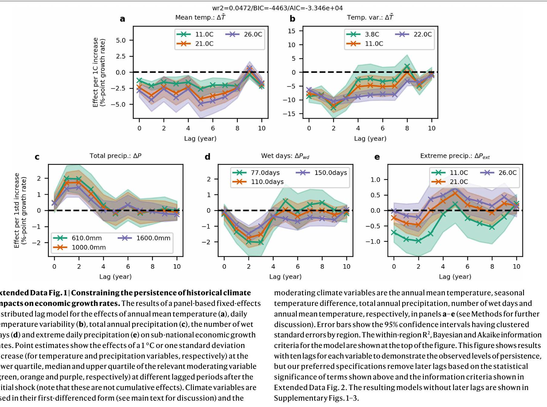
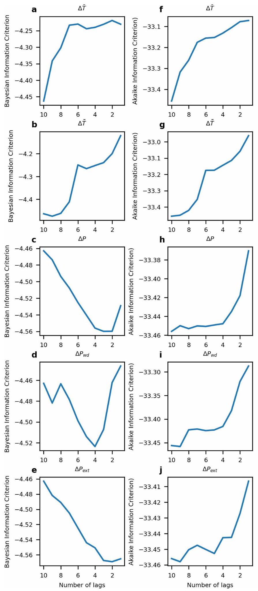
نبدأ تحليلنا التجريبي لاستمرارية تأثيرات المناخ على النمو باستخدام عشرة تأخيرات من المتغيرات المناخية ذات الفرق الأول في نماذج التأخير الموزعة ذات التأثيرات الثابتة. نكتشف تأثيرات كبيرة على النمو الاقتصادي في تأخيرات زمنية تصل إلى حوالي 8-10 سنوات بالنسبة لمصطلحات درجة الحرارة وحوالي 4 سنوات لمصطلحات الهطول (الشكل 1 من البيانات الموسعة والجدول 2 من البيانات الموسعة). علاوة على ذلك، تشير التقييمات من خلال معايير المعلومات إلى أن تضمين جميع المتغيرات المناخية الخمسة واستخدام هذه الأعداد من التأخيرات يوفر توازناً مفضلاً بين أفضل ملاءمة للبيانات وتضمين مصطلحات إضافية قد تسبب الإفراط في التخصيص، مقارنة بمواصفات النماذج التي تستبعد المتغيرات المناخية أو تتضمن المزيد أو القليل من التأخيرات (الشكل 3 من البيانات الموسعة، قسم الطرق التكميلية 1 والجدول 1 من البيانات التكميلية). لذلك، نقوم بإزالة المصطلحات غير المهمة إحصائياً في التأخيرات اللاحقة (الأشكال التكميلية 1-3 والجدول 2-4 من البيانات التكميلية). تظهر اختبارات إضافية باستخدام محاكاة مونت كارلو أن النماذج التجريبية قوية أمام الارتباط الذاتي في المتغيرات المناخية المتأخرة (قسم الطرق التكميلية 2 والأشكال التكميلية 4 و5)، وأن معايير المعلومات توفر مؤشراً فعالاً لاختيار التأخير (قسم الطرق التكميلية 2 والشكل التكميلية 6)، وأن النتائج قوية أمام مخاوف التعدد الخطي غير المثالي بين المتغيرات المناخية وأن تضمين عدة متغيرات مناخية ضروري فعلاً لعزل تأثيراتها المنفصلة (قسم الطرق التكميلية 3 والشكل التكميلية 7).
نقدم فحصاً إضافياً للمتانة باستخدام نموذج تأخير موزع مقيد للحد من التذبذبات في تقديرات المعلمات المتأخرة التي قد تنتج عن الارتباط الذاتي، حيث نجد أنه يوفر تقديرات مشابهة للتأثيرات الهامشية التراكمية للنموذج غير المقيد (قسم الطرق التكميلية 4 والأشكال التكميلية 8 و9). أخيراً، لأخذ أي عدم يقين متبقي ناشئ عن الاختيار الدقيق لعدد التأخيرات في الاعتبار، نقوم بتضمين نماذج تجريبية بأعداد مختلفة قليلاً من التأخيرات في إجراء أخذ العينات من الأخطاء في توقعاتنا للأضرار المستقبلية. بناءً على إجراء اختيار التأخير (أهمية المصطلحات المتأخرة في الشكل 1 من البيانات الموسعة والجدول 2 من البيانات الموسعة، بالإضافة إلى معايير المعلومات في الشكل 3 من البيانات الموسعة)، نقوم بأخذ عينات من نماذج تحتوي على ثمانية إلى عشرة تأخيرات لدرجة الحرارة وأربعة للهطول (النماذج المعروضة في الأشكال التكميلية 1-3 والجدول 2-4 من البيانات التكميلية). باختصار، هذا النهج التجريبي لتقييد استمرارية تأثيرات المناخ على معدلات النمو الاقتصادي هو محافظ من حيث التصميم في تجنب الافتراضات حول الاستمرارية اللانهائية، ولكنه مع ذلك يوفر حداً أدنى على مدى استمرارية التأثير الذي هو قوي أمام الاختبارات العديدة الموضحة أعلاه.

الأضرار الملتزمة حتى منتصف القرن

نجمع بين هذه الوظائف الاقتصادية التجريبية (الأشكال التكميلية 1-3 والجدول 2-4 من البيانات التكميلية) مع مجموعة من 21 نموذج مناخي (انظر الجدول 5 من البيانات التكميلية) من مشروع مقارنة النماذج المتصلة المرحلة 6 (CMIP-6) لتوقع الأضرار الاقتصادية الكلية الناتجة عن هذه المكونات من التغير المناخي الفيزيائي (انظر الطرق لمزيد من التفاصيل). يتم استخدام نماذج مناخية مصححة للانحياز توفر إعادة إنتاج دقيقة للغاية للأنماط المناخية المرصودة مع عدم يقين محدود (الجدول 6 من البيانات التكميلية) لتجنب إدخال انحيازات في التوقعات. بناءً على أدبيات مطورة جيداً ، لا تهدف هذه التوقعات إلى تقديم توقع لنمو اقتصادي مستقبلي. بدلاً من ذلك، هي توقع للأثر الخارجي للظروف المناخية المستقبلية على الاقتصاد بالنسبة للأسس المحددة من قبل التوقعات الاجتماعية والاقتصادية، بناءً على العلاقات السببية المحتملة المستنتجة من النماذج التجريبية ويفترض أن تظل العوامل الأخرى ثابتة. يتم افتراض أن العوامل الخارجية الأخرى ذات الصلة بتوقع الناتج الاقتصادي ثابتة عمداً.
تستخدم إجراء مونت كارلو الذي يأخذ عينات من توقعات نماذج المناخ، والنماذج التجريبية بأعداد مختلفة من التأخيرات وتقديرات معلمات النموذج (المستمدة من 1,000 إعادة أخذ عينات بالكتل لكل من الانحدارات في الأشكال التكميلية 1-3 والجدول 2-4 من البيانات التكميلية) لتقدير عدم اليقين المدمج من هذه المصادر. بالنظر إلى هذه التوزيعات من عدم اليقين، نجد أن الأضرار العالمية المتوقعة لا يمكن تمييزها إحصائياً عبر السيناريوهين الأكثر تطرفاً من حيث الانبعاثات حتى عام 2049 (عند مستوى ؛ الشكل 1). وبالتالي، فإن الأضرار المناخية التي تحدث قبل هذا الوقت تشكل تلك التي التزم بها العالم بالفعل بسبب مزيج من الانبعاثات السابقة ونطاق السيناريوهات المستقبلية من الانبعاثات التي تعتبر اجتماعيًا واقتصاديًا معقولة . تتكون هذه الأضرار الملتزمة من انخفاض دائم في الدخل بنسبة 19% في المتوسط عالمياً (متوسط مرجح حسب عدد السكان) مقارنة بأساس بدون تأثيرات تغير المناخ (مع نطاق محتمل من ، وفقاً لتصنيف الاحتمالية المعتمد من قبل الهيئة الحكومية الدولية المعنية بتغير المناخ (IPCC)؛ انظر تعليق الشكل 1). على الرغم من أن مستويات الدخل للفرد بشكل عام لا تزال تزيد مقارنة بتلك الموجودة اليوم، إلا أن هذا يشكل انخفاضاً دائماً في الدخل لمعظم المناطق، بما في ذلك أمريكا الشمالية وأوروبا (كل منهما مع انخفاضات متوسطة في الدخل تبلغ حوالي ) ومع جنوب آسيا وأفريقيا الأكثر تأثراً (كل منهما مع انخفاضات متوسطة في الدخل تبلغ حوالي ؛ الشكل 1). في ظل سيناريو متوسط لتطور الدخل المستقبلي (SSP2، حيث SSP تعني المسار الاجتماعي والاقتصادي المشترك)، يتوافق هذا مع أضرار سنوية عالمية في عام 2049 تبلغ 38 تريليون دولار أمريكي دولي لعام 2005 (نطاق محتمل من 19-59 تريليون دولار أمريكي دولي لعام 2005). مقارنة بالمواصفات التجريبية التي تفترض نموًا خالصًا أو تأثيرات مستوى خالصة،
الشكل 1| الالتزام والانحراف لأضرار المناخ الاقتصادية مقابل تكاليف التخفيف. تقديرات الانخفاض المتوقع في الدخل للفرد الناتج عن التغيرات في جميع المتغيرات المناخية بناءً على نماذج تجريبية لتأثيرات المناخ على الناتج الاقتصادي مع حد أدنى قوي على استمراريتها (الشكل 1 من البيانات الموسعة) تحت سيناريو انبعاثات منخفضة متوافقة مع هدف للاحترار وسيناريو انبعاثات عالية (SSP2-RCP2.6 وSSP5-RCP8.5، على التوالي) موضحة باللون الأرجواني والبرتقالي، على التوالي. يمثل التظليل و فترات الثقة التي تعكس النطاقات المحتملة والمرجحة جداً، على التوالي (وفقاً لتصنيف الاحتمالية المعتمد من قبل الهيئة الحكومية الدولية المعنية بتغير المناخ)، بعد تقدير عدم اليقين من إجراء مونت كارلو، الذي يأخذ عينات من عدم اليقين الناتج عن اختيار نماذج المناخ الفيزيائية، والنماذج التجريبية بأعداد مختلفة من التأخيرات وتقديرات المعلمات الانحدارية الموضحة في الأشكال التكميلية 1-3. تظهر الخطوط العمودية المتقطعة الوقت الذي تتباعد فيه الأضرار المناخية للسيناريوهين من الانبعاثات عند و مستويات الأهمية بناءً على توزيع الفروق بين سيناريوهات الانبعاثات الناشئة عن أخذ عينات عدم اليقين التي تم مناقشتها أعلاه. لاحظ أن عدم اليقين في الفرق بين السيناريوهين أقل من عدم اليقين المدمج للسيناريوهين المعنيين لأن عينات عدم اليقين (اختيار نموذج المناخ والنموذج التجريبي، بالإضافة إلى إعادة تعيين معلمات النموذج) متسقة عبر سيناريوهين الانبعاثات، وبالتالي يحدث تباين الأضرار بينما لا تزال حدود عدم اليقين للسيناريوهين المنفصلين تتداخل. تُظهر تقديرات تكاليف التخفيف العالمية من النماذج الثلاثة التي تقدم نتائج لسيناريو الأساس SSP2 و SSP2-RCP2.6 باللون الأخضر الفاتح في اللوحة العلوية، مع عرض الوسيط لهذه التقديرات بخط عريض.
تحديدنا المفضل الذي يوفر حدًا أدنى قويًا على مدى استمرارية تأثير المناخ ينتج أضرارًا بين هذين الافتراضين المتطرفين (الشكل 3 من البيانات الموسعة).

الأضرار تفوق بالفعل تكاليف التخفيف

نقارن الأضرار التي التزم بها العالم على مدى السنوات الـ 25 القادمة مع تقديرات تكاليف التخفيف المطلوبة لتحقيق اتفاقية باريس للمناخ. من خلال أخذ تقديرات تكاليف التخفيف من النماذج الثلاثة للتقييم المتكامل (IAMs) في قاعدة بيانات IPCC AR6 التي تقدم نتائج تحت سيناريوهات قابلة للمقارنة (أساس SSP2 و SSP2-RCP2.6، حيث تشير RCP إلى مسار التركيز التمثيلي)، نجد أن الأضرار المناخية المتوسطة الملتزمة أكبر من تكاليف التخفيف المتوسطة في عام 2050 (ستة تريليونات دولار أمريكي في دولارات 2005 الدولية) بحوالي ستة أضعاف (لاحظ أن تقديرات تكاليف التخفيف تُقدم فقط كل 10 سنوات من قبل IAMs وبالتالي لا يمكن إجراء مقارنة في عام 2049). تهدف هذه المقارنة ببساطة إلى مقارنة حجم الأضرار المستقبلية مقابل تكاليف التخفيف، بدلاً من إجراء تحليل رسمي للتكلفة والفائدة للانتقال من مسار انبعاث إلى آخر. التحليلات الرسمية
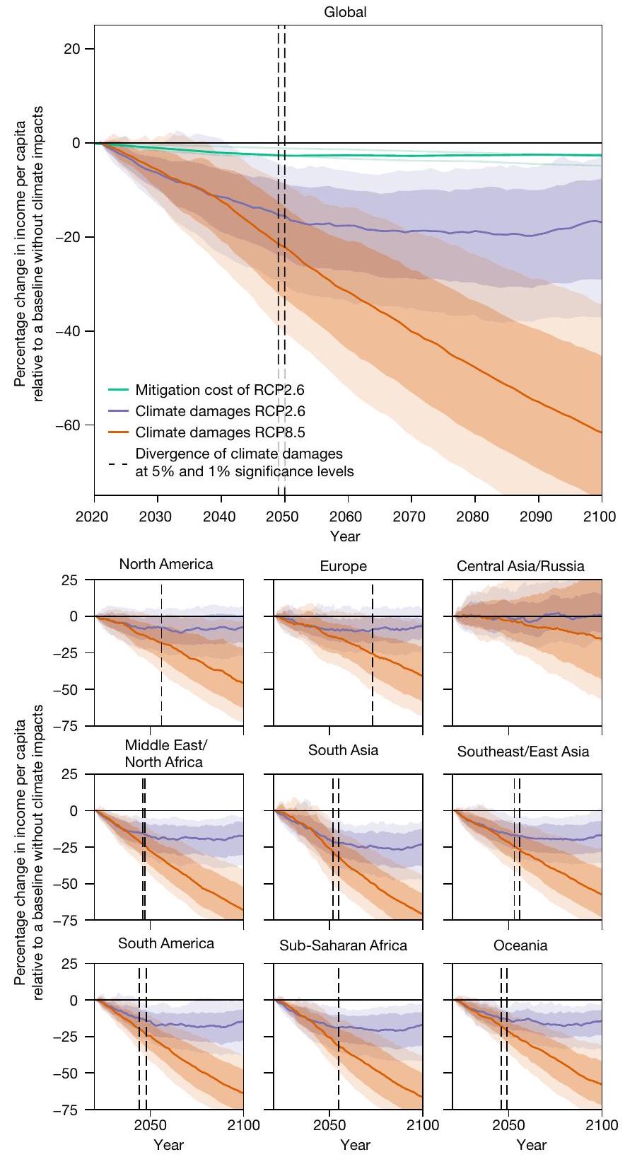
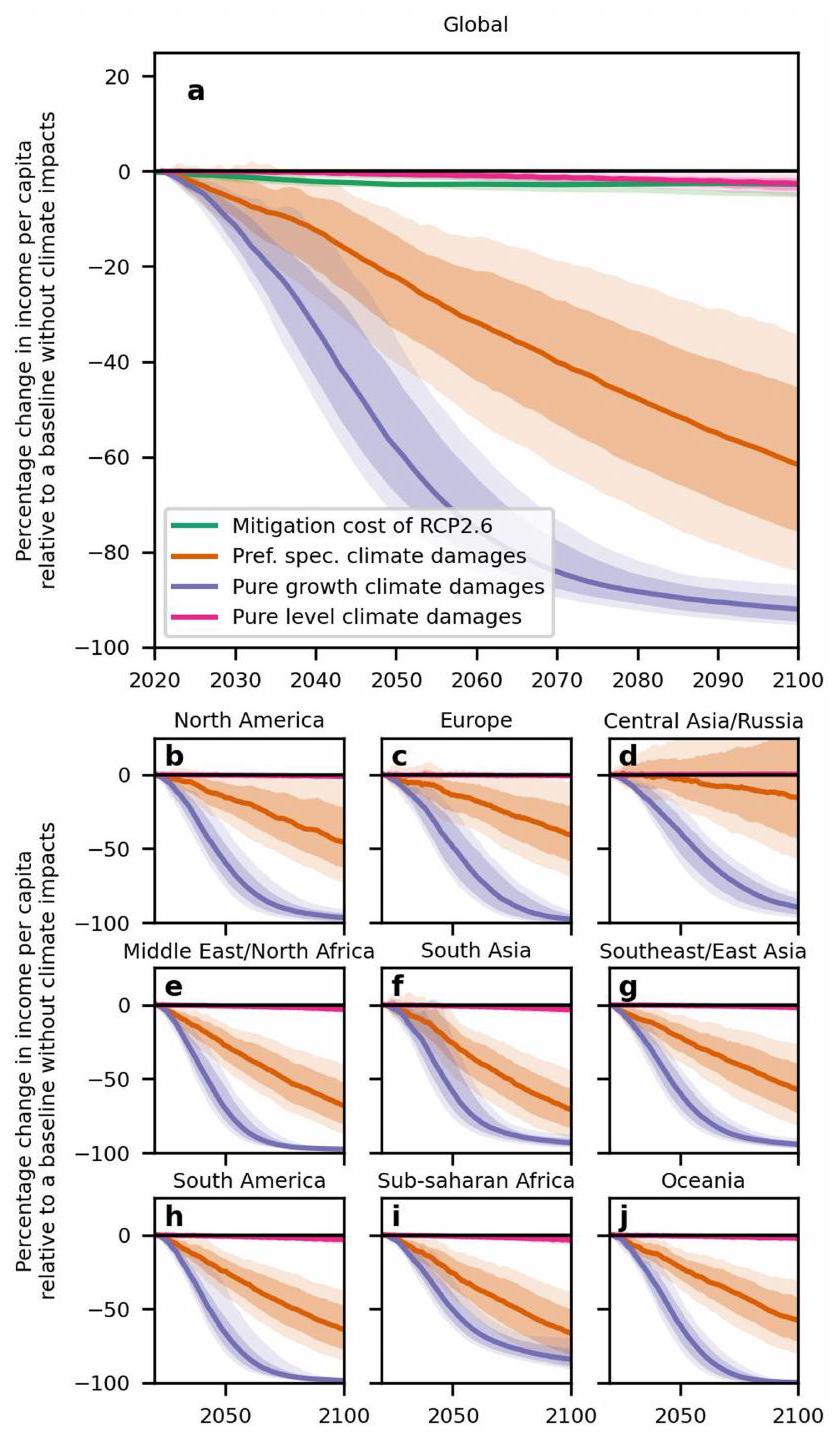
عادةً ما تجد تحليلات التكلفة والفائدة أن الفوائد الصافية للتخفيف تظهر فقط بعد عام 2050 (المرجع 5)، مما قد يقود البعض إلى الاستنتاج بأن الأضرار المادية الناتجة عن تغير المناخ ليست كبيرة بما يكفي لتفوق تكاليف التخفيف حتى النصف الثاني من القرن. توضح مقارنتنا البسيطة لحجمها أن الأضرار أكبر بالفعل بكثير من تكاليف التخفيف وأن ظهور الفوائد الصافية للتخفيف المتأخرة ناتج بشكل أساسي عن حقيقة أن الأضرار عبر مسارات الانبعاثات المختلفة لا يمكن تمييزها حتى منتصف القرن (الشكل 1).
على الرغم من أن هذه الأضرار القريبة المدى تشكل تلك التي التزم بها العالم بالفعل، نلاحظ أن تقديرات الأضرار تتباين بشدة عبر سيناريوهات الانبعاثات بعد عام 2049، مما ينقل الفوائد الواضحة للتخفيف من وجهة نظر اقتصادية بحتة التي تم التأكيد عليها في الدراسات السابقة . بالإضافة إلى عدم اليقين الذي تم تقييمه في الشكل 1، فإن هذه الاستنتاجات قوية تجاه الخيارات الهيكلية، مثل الإطار الزمني الذي يتم من خلاله تقدير التغيرات في المتغيرات المعدلة للنماذج التجريبية (الأشكال التكميلية 10 و 11)، بالإضافة إلى الترتيب الذي يتم من خلاله حساب المكونات الزمنية والدولية لمقارنة العملات (الشكل التكميلية 12؛ انظر الأساليب لمزيد من التفاصيل).

الأضرار الناتجة عن التباين والظواهر المتطرفة

تنشأ الأضرار الملتزمة بشكل أساسي من خلال التغيرات في متوسط درجة الحرارة (الشكل 2). وهذا يعكس حقيقة أن التغيرات المتوقعة في متوسط درجة الحرارة أكبر من تلك في المتغيرات المناخية الأخرى عند التعبير عنها كدالة لتباينها التاريخي بين السنوات (الشكل 4 من البيانات الموسعة). نظرًا لأن التباين التاريخي هو الذي يتم تقدير النماذج التجريبية بناءً عليه، فإن التغيرات المتوقعة الأكبر مقارنةً بهذا التباين تؤدي على الأرجح إلى تأثيرات مستقبلية أكبر من الناحية الإحصائية البحتة. من منظور آلي، يمكن للمرء أن يفسر هذه النتيجة بشكل معقول على أنها تعني أن التغيرات المستقبلية في متوسط درجة الحرارة هي الأكثر غير مسبوقة من منظور التقلبات التاريخية التي اعتادت عليها الاقتصاد وبالتالي ستسبب أكبر الأضرار. قد تكون هذه الرؤية مفيدة من حيث توجيه تدابير التكيف نحو مصادر الأضرار الأكبر.
ومع ذلك، فإن الأضرار المستقبلية المستندة إلى النماذج التجريبية التي تأخذ في الاعتبار التغيرات في متوسط درجة الحرارة السنوي فقط وتستبعد المتغيرات المناخية الأخرى تشكل تخفيضات في الدخل بنسبة 13% فقط في عام 2049
الشكل 2 | الأضرار الاقتصادية الملتزمة الناتجة عن تغير المناخ حسب المنطقة الفرعية والمكون المناخي. تقديرات الانخفاض المتوسط المتوقع في الدخل الفرعي للفرد عبر سيناريوهات الانبعاثات (SSP2-RCP2.6 و SSP2-RCP8.5) بالإضافة إلى عدم اليقين في نموذج المناخ، النموذج التجريبي وعدم اليقين في معلمات النموذج في السنة التي تتباين فيها الأضرار المناخية عند مستوى 5% (2049، كما هو محدد في الشكل 1). أ، التأثيرات الناشئة من جميع المتغيرات المناخية. ب-ف، التأثيرات
الناشئة بشكل منفصل من التغيرات في متوسط درجة الحرارة السنوي (ب)، تباين درجة الحرارة اليومية (ج)، إجمالي هطول الأمطار السنوي (د)، عدد الأيام الممطرة سنويًا ( )(هـ) وهطول الأمطار اليومية المتطرفة (و) (انظر الأساليب لمزيد من التعريفات). تم الحصول على بيانات الحدود الإدارية الوطنية من قاعدة بيانات GADM الإصدار 3.6 وهي متاحة مجانًا للاستخدام الأكاديمي (https://gadm.org/).
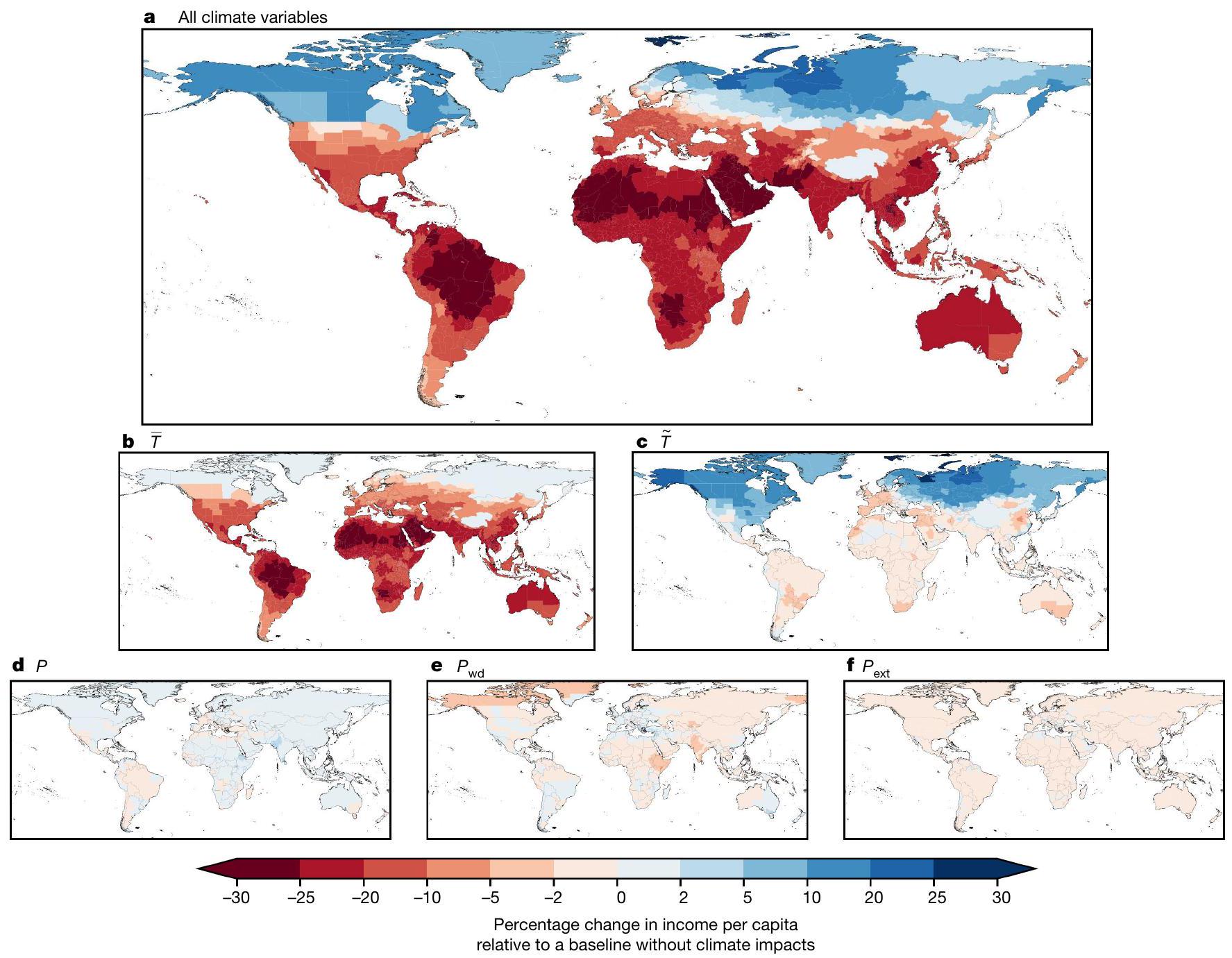
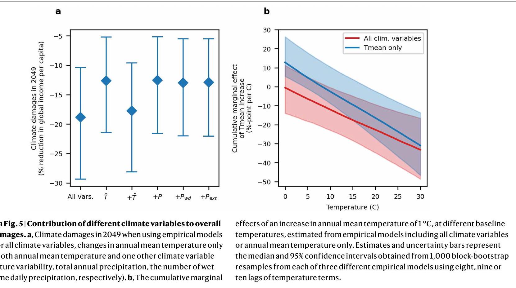
(الشكل 5 من البيانات الموسعة أ، النطاق المحتمل 5-21%). وهذا يشير إلى أن الأخذ في الاعتبار المكونات الأخرى لتوزيع درجة الحرارة وهطول الأمطار يزيد الأضرار الصافية بنحو 50%. ينشأ هذا الارتفاع من الأضرار الإضافية التي تسببها هذه المكونات المناخية، ولكن أيضًا لأن إدراجها يكشف عن استجابة اقتصادية سلبية أقوى لدرجات الحرارة المتوسطة (الشكل 5 من البيانات الموسعة ب). يتماشى هذا الاكتشاف مع محاكاة مونت كارلو لدينا، التي تشير إلى أن حجم تأثير درجة الحرارة المتوسطة على النمو الاقتصادي يتم التقليل من قيمته ما لم يتم الأخذ في الاعتبار تأثيرات المتغيرات المناخية الأخرى المرتبطة (الشكل التكميلية 7).
من حيث المساهمات النسبية للمكونات المناخية المختلفة في الأضرار الإجمالية، نجد أن الأخذ في الاعتبار تباين درجة الحرارة اليومية يسبب أكبر زيادة في الأضرار الإجمالية مقارنةً بالأطر التجريبية التي تأخذ في الاعتبار فقط التغيرات في متوسط درجة الحرارة السنوي (4.9 نقطة مئوية، النطاق المحتمل نقاط مئوية، ما يعادل حوالي 10 تريليونات دولار دولي). يؤدي الأخذ في الاعتبار هطول الأمطار إلى زيادات أصغر في الأضرار الإجمالية، والتي تظل مع ذلك تعادل حوالي 1.2 تريليون دولار دولي: 0.01 نقطة مئوية ( نقاط مئوية)، 0.34 نقطة مئوية ( نقاط مئوية) و
0.36 نقطة مئوية ( نقاط مئوية) من إجمالي هطول الأمطار السنوي، وعدد الأيام الممطرة وهطول الأمطار اليومية المتطرفة، على التوالي. علاوة على ذلك، يبدو أن نماذج المناخ تقلل من تقديرات التغيرات المستقبلية في تباين درجة الحرارة وهطول الأمطار المتطرفة استجابةً للقوى البشرية مقارنةً بما لوحظ تاريخيًا، مما يشير إلى أن التأثيرات الحقيقية من هذه المتغيرات قد تكون أكبر.

توزيع الأضرار الملتزمة

يعكس التوزيع المكاني للأضرار الملتزمة (الشكل 2أ) تفاعلًا معقدًا بين أنماط التغير المستقبلي في عدة مكونات مناخية وتلك المتعلقة بالضعف الاقتصادي التاريخي تجاه التغيرات في تلك المتغيرات. الأضرار الناتجة عن زيادة متوسط درجة الحرارة السنوي (الشكل 2ب) سلبية تقريبًا في كل مكان على مستوى العالم، وأكبر في خطوط العرض المنخفضة في المناطق التي تكون فيها درجات الحرارة أعلى بالفعل ويكون الضعف الاقتصادي تجاه زيادة درجات الحرارة أكبر (انظر تباين الاستجابة لدرجة الحرارة المتوسطة المتجسد في الشكل 1أ من البيانات الموسعة). يحدث هذا على الرغم من الاحترار المعزز المتوقع في خطوط العرض العليا ، مما يشير إلى تباين إقليمي
الشكل 3 | الظلم الناتج عن الأضرار المناخية الناجمة عن الانبعاثات التاريخية التراكمية والدخل. تقديرات التغير الوسيط المتوقع في الدخل القومي للفرد عبر سيناريوهات الانبعاثات (RCP2.6 و RCP8.5) بالإضافة إلى عدم اليقين في نموذج المناخ، النموذج التجريبي وعدم اليقين في معلمات النموذج في السنة التي تتباين فيها الأضرار المناخية عند مستوى 5% (2049، كما هو محدد في الشكل 1) تم رسمها مقابل الانبعاثات الوطنية التراكمية للفرد في عام 2020 (من الـ
مشروع الكربون العالمي) وملون حسب الدخل القومي للفرد في عام 2020 (من البنك الدولي) في وعكس ذلك في . في كل لوحة، يتم وزن حجم كل نقطة تشتت بناءً على عدد السكان الوطني في عام 2020 (من البنك الدولي). تشير الأرقام في الزاوية إلى معامل ارتباط سبيرمان. و -قيم لاختبار الفرضية التي تفترض عدم وجود ارتباط، بالإضافة إلى معامل ارتباط سبيرمان مرجح بعدد السكان الوطني.
تتجاوز الضعف الاقتصادي تجاه تغيرات درجات الحرارة التباين في حجم الاحترار المستقبلي (الشكل التكميلي 13a). تظهر الأضرار الاقتصادية الناتجة عن تقلبات درجات الحرارة اليومية (الشكل 2c) استقطابًا قويًا حسب خطوط العرض، مما يعكس بشكل أساسي الاستجابة الفيزيائية لتقلبات درجات الحرارة اليومية تجاه تأثيرات الاحتباس الحراري، حيث تتناقض الزيادات في التقلبات عبر خطوط العرض المنخفضة (وأوروبا) مع الانخفاضات في خطوط العرض العالية. (الشكل التكميلي 13ب). هذان المصطلحان المتعلقان بدرجات الحرارة هما المحددان الرئيسيان لنمط الأضرار العامة (الشكل 2أ)، الذي يظهر قطبية قوية مع أضرار عبر معظم أنحاء العالم باستثناء أعلى خطوط العرض الشمالية. التغيرات المستقبلية في إجمالي هطول الأمطار السنوي تجلب فوائد اقتصادية بشكل رئيسي باستثناء المناطق التي تعاني من الجفاف، مثل منطقة البحر الأبيض المتوسط وأمريكا الجنوبية الوسطى (الشكل 2د والشكل التكميلي 13ج)، ولكن هذه الفوائد تتعارض مع التغيرات في عدد الأيام الممطرة، التي تنتج أضرارًا بنمط مشابه ولكن بعكس الإشارة (الشكل 2هـ والشكل التكميلي 13د). بالمقابل، فإن التغيرات في هطول الأمطار اليومية الشديدة تنتج أضرارًا في جميع المناطق، مما يعكس تفاقم شدة هطول الأمطار اليومية في المناطق الأرضية العالمية. (الشكل 2f والشكل التكميلي 13e).
تشير التوزيعات المكانية للأضرار الملتزمة إلى ظلم كبير على بعدين: المسؤولية عن الانبعاثات التاريخية التي تسببت في تغير المناخ ومستويات الرفاهية الاجتماعية والاقتصادية الموجودة مسبقًا. تشير ارتباطات ترتيب سبيرمان إلى أن الأضرار الملتزمة أكبر بكثير في البلدان التي لديها انبعاثات تاريخية تراكمية أقل، وكذلك في المناطق التي لديها دخل أقل حاليًا للفرد (الشكل 3). وهذا يعني أن تلك البلدان التي ستعاني أكثر من الأضرار التي تم الالتزام بها هي تلك التي تتحمل أقل مسؤولية عن تغير المناخ والتي لديها أيضًا أقل الموارد للتكيف معه.
لتحديد هذه التباينات بشكل أكبر، نقوم بتقييم الفرق في الأضرار الملتزمة بين الربعين العلوي والسفلي من المناطق عند تصنيفها حسب مستويات الدخل الحالية والانبعاثات التراكمية التاريخية (باستخدام وزن سكاني لتعريف الأرباع وتقدير متوسطات المجموعات). في المتوسط، فإن ربع الدول ذات الدخل المنخفض ملتزم بفقدان دخل يزيد بمقدار 8.9 نقطة مئوية (أو 61%) عن الربع العلوي (الشكل 6 من البيانات الموسعة)، مع نطاق محتمل من نقاط النسبة عبر عينة عدم اليقين من توقعات الأضرار لدينا (بعد
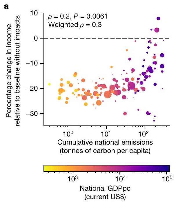
تصنيف الاحتمالية المعتمد من قبل الهيئة الحكومية الدولية المعنية بتغير المناخ). وبالمثل، فإن الربع من الدول التي لديها انبعاثات تراكمية تاريخية أقل ملتزم بخسارة في الدخل تبلغ 6.9 نقطة مئوية (أو أكبر من الربع العلوي، مع نطاق محتمل من نقاط مئوية. تعيد هذه الأنماط التأكيد على انتشار الظلم في آثار المناخ في سياق الأضرار التي التزم بها العالم بالفعل نتيجة الانبعاثات التاريخية والركود الاجتماعي والاقتصادي.

تحديد حجم الأضرار

حجم الأضرار الاقتصادية المتوقعة يتجاوز تقديرات الأدبيات السابقة ، الناشئة عن عدة تطورات تم إجراؤها على الأساليب السابقة. تقديراتنا أكبر من تلك الواردة في المرجع 2 (انظر الصف الأول من جدول البيانات الموسع 3)، ويرجع ذلك أساسًا إلى أن التقديرات دون الوطنية تظهر عادة استجابة أكثر حدة لدرجات الحرارة (انظر أيضًا المراجع 3، 34) وأن أخذ المكونات المناخية الأخرى في الاعتبار يزيد من تقديرات الأضرار (الشكل 5 من البيانات الموسعة). ومع ذلك، نلاحظ أن نهجنا التجريبي باستخدام متغيرات المناخ ذات الفروق الأولى هو نهج محافظ مقارنةً بتلك الواردة في المرجع 2 فيما يتعلق باستمرارية تأثيرات المناخ على النمو (انظر المقدمة وقسم الطرق “تحديد النموذج التجريبي: نماذج التأثيرات الثابتة ذات التأخير الموزع”)، وهو عامل مهم في تحديد حجم الأضرار على المدى الطويل. استخدام مواصفة تجريبية مشابهة للمرجع 2، التي تفترض استمرارية غير محدودة مع الحفاظ على بقية نهجنا (البيانات دون الوطنية ومتغيرات المناخ الأخرى)، ينتج أضرارًا أكبر بكثير (المنحنى الأرجواني في الشكل 3 من البيانات الموسعة). بالمقارنة مع الدراسات التي تأخذ الفرق الأول لمتغيرات المناخ تقديراتنا أيضًا أكبر (انظر الصفين الثاني والثالث من الجدول الإضافي 3). إن تضمين مزيد من المتغيرات المناخية (الشكل الإضافي 5) وعدد كافٍ من التأخيرات لالتقاط مدى استمرارية التأثير بشكل أكثر ملاءمة (الأشكال الإضافية 1 و2) هي المصادر الرئيسية لهذا الاختلاف، كما أن استخدام المواصفات التي تلتقط عدم الخطية في استجابة درجة الحرارة عند مقارنتها بالمرجع 35. باختصار، تطور تقديراتنا على الدراسات السابقة من خلال دمج أحدث البيانات والرؤى التجريبية. بالإضافة إلى ذلك، في تقديم حد أدنى تجريبي قوي على استمرارية التأثيرات على النمو الاقتصادي، والذي يشكل أرضية وسطى بين تطرفي نقاش النمو مقابل المستويات. (الشكل 3 من البيانات الموسعة).
مقارنةً بالجزء من التباين الذي تفسره النماذج التجريبية تاريخياً (<5%)، قد يبدو أن التوقعات بتقليص الدخل بنسبة 19% كبيرة. وهذا ينشأ بسبب أن التغيرات المتوقعة في الظروف المناخية أكبر بكثير من تلك التي تم تجربتها تاريخياً، لا سيما بالنسبة للتغيرات في متوسط درجة الحرارة (الشكل 4 من البيانات الموسعة). وبالتالي، فإن أي تقييم لتأثيرات تغير المناخ في المستقبل يتطلب بالضرورة استقراءً خارج نطاق البيانات التاريخية التي تم تقييم النماذج التجريبية بناءً عليها. ومع ذلك، تشكل هذه النماذج أحدث الأساليب لاستنتاج التأثيرات المناخية المحتملة بناءً على البيانات الملاحظة. علاوة على ذلك، نتخذ خطوات صريحة للحد من الاستقراء خارج العينة من خلال تحديد متغيرات التعديل في مصطلحات التفاعل عند النسبة المئوية 95 من التوزيع التاريخي (انظر الطرق). هذا يتجنب استقراء التأثيرات الهامشية خارج ما تم ملاحظته تاريخياً. نظراً للاستجابة غير الخطية للإنتاج الاقتصادي لدرجة الحرارة المتوسطة السنوية (الشكل 1 من البيانات الموسعة والجدول 2 من البيانات الموسعة)، فإن هذا خيار محافظ يحد من حجم الأضرار التي نتوقعها. علاوة على ذلك، تشير الحسابات الأولية إلى أن الأضرار المتوقعة تتماشى مع حجم وأنماط التنمية الاقتصادية التاريخية (انظر قسم المناقشة التكميلية 5).

آثار مفقودة وتداعيات مكانية

على الرغم من تقييم عدة مكونات مناخية تم تحديد الآثار الاقتصادية الناتجة عنها مؤخرًا يجب ألا يُعتبر هذا التقييم للأضرار المناخية الإجمالية شاملاً. هناك قنوات مهمة مثل التأثيرات الناتجة عن موجات الحر ارتفاع مستوى سطح البحر العواصف الاستوائية ونقاط التحول بالإضافة إلى الأضرار غير السوقية مثل تلك التي تلحق بالنظم البيئية وصحة الإنسان , لا تؤخذ في الاعتبار في هذه التقديرات. من غير المحتمل أن يتم دمج ارتفاع مستوى سطح البحر بشكل قابل للتطبيق في التقييمات التجريبية مثل هذه لأن تقلب مستوى سطح البحر التاريخي غالبًا ما يكون صغيرًا. الأضرار غير السوقية بطبيعتها غير قابلة للحل ضمن تقديراتنا للتأثيرات على الناتج النقدي الإجمالي ويمكن اعتبار تقديرات هذه التأثيرات بشكل من الأشكال كإضافات لتلك المحددة هنا. تشير الأعمال التجريبية الحديثة إلى أن الأخذ في الاعتبار هذه القنوات من المحتمل أن يزيد تقديرات هذه الأضرار الملتزمة، مع استمرار ظهور أضرار أكبر في الجنوب العالمي .
علاوة على ذلك، لا تقيم تحليلاتنا التجريبية الرئيسية بشكل صريح إمكانية تأثيرات المناطق المحلية في إنتاج آثار ‘تتسرب’ إلى مناطق أخرى. قد تخفف هذه التأثيرات أو تضخم التأثيرات التي نقيمها، على سبيل المثال، إذا قامت الشركات بنقل الإنتاج من منطقة متأثرة إلى أخرى أو إذا انتشرت التأثيرات على طول سلاسل الإمداد. تشير الأدبيات الحالية إلى أن التجارة تلعب دورًا كبيرًا في نشر تأثيرات التسرب , مما يجعل تقييمها على المستوى دون الوطني تحديًا دون توفر بيانات عن الاعتماد التجاري دون الوطني. تشير الدراسات التي تأخذ في الاعتبار فقط الجيران المجاورين مكانيًا إلى أن التأثيرات السلبية في منطقة واحدة تحفز مزيدًا من التأثيرات السلبية في المناطق المجاورة , مما يشير إلى أن الأضرار المتوقعة لدينا ربما تكون محافظة من خلال استبعاد هذه التأثيرات. في الشكل التكميلي 14، نقيم التسربات من المناطق المجاورة باستخدام نموذج التأخير المكاني. من أجل البساطة، يستبعد هذا التحليل التأخيرات الزمنية، مع التركيز فقط على التأثيرات المعاصرة. تظهر النتائج أن الأخذ في الاعتبار التسربات المكانية يمكن أن يضخم الحجم العام، وكذلك التباين، للتأثيرات. يتماشى ذلك مع الأدبيات السابقة، مما يشير إلى أن الحجم العام (الشكل 1) والتباين (الشكل 3) للأضرار التي نتوقعها في مواصفاتنا الرئيسية قد تكون محافظة دون الأخذ في الاعتبار التسربات بشكل صريح. نلاحظ أن مزيدًا من التحليل الذي يتناول كل من التسربات المكانية والمتصلة بالتجارة، مع الأخذ في الاعتبار التأثيرات المتأخرة باستخدام التأخيرات الزمنية، سيكون ضروريًا لمعالجة هذا السؤال بشكل كامل. تقدم هذه الأساليب طرقًا مثمرة لمزيد من البحث ولكنها تتجاوز نطاق هذه المخطوطة، التي تهدف بشكل أساسي إلى استكشاف تأثيرات ظروف المناخ المختلفة واستمراريتها.

الآثار السياسية

نجد أن الأضرار الاقتصادية الناتجة عن تغير المناخ حتى عام 2049 هي تلك التي التزمت بها الاقتصاد العالمي بالفعل وأن هذه تفوق بكثير التكاليف المطلوبة للتخفيف من الانبعاثات بما يتماشى مع هدف اتفاق باريس للمناخ (الشكل 1). هذا التقييم مكمل للتحليلات الرسمية للتكاليف والفوائد الصافية المرتبطة بالانتقال من مسار انبعاثات إلى آخر، والتي تجد عادةً أن الفوائد الصافية للتخفيف تظهر فقط في النصف الثاني من القرن . توضح مقارنتنا البسيطة لحجم الأضرار وتكاليف التخفيف أن هذا يرجع أساسًا إلى أن الأضرار لا يمكن تمييزها عبر سيناريوهات الانبعاثات – أي أنها ملتزمة – حتى منتصف القرن (الشكل 1) وأنها في الواقع أكبر بكثير من تكاليف التخفيف. من أجل البساطة، وبسبب توفر البيانات، نقارن الأضرار بتكاليف التخفيف على المستوى العالمي. قد تسلط التقديرات الإقليمية لتكاليف التخفيف مزيدًا من الضوء على الحوافز الوطنية للتخفيف التي تشير إليها نتائجنا بالفعل، والتي لها صلة بسياسة المناخ الدولية. على الرغم من أن هذه الأضرار ملتزمة من منظور التخفيف، قد توفر التكيف فرصة لتقليلها. علاوة على ذلك، فإن الانحراف القوي للأضرار بعد منتصف القرن يعيد التأكيد على الفوائد الواضحة للتخفيف من منظور اقتصادي بحت، كما تم تسليط الضوء عليه في الدراسات السابقة .

المحتوى عبر الإنترنت

أي طرق، مراجع إضافية، ملخصات تقارير Nature Portfolio، بيانات المصدر، بيانات موسعة، معلومات تكملية، شكر وتقدير، معلومات مراجعة الأقران؛ تفاصيل مساهمات المؤلفين والمصالح المتنافسة؛ وبيانات توفر البيانات والرموز متاحة على https://doi.org/10.1038/s41586-024-07219-0.
  1. Glanemann, N., Willner, S. N. & Levermann, A. اتفاق باريس للمناخ يجتاز اختبار التكلفة والفائدة. Nat. Commun. 11, 110 (2020).
  2. Burke, M., Hsiang, S. M. & Miguel, E. التأثير غير الخطي العالمي لدرجة الحرارة على الإنتاج الاقتصادي. Nature 527, 235-239 (2015).
  3. Kalkuhl, M. & Wenz, L. تأثير ظروف المناخ على الإنتاج الاقتصادي. أدلة من لوحة عالمية من المناطق. J. Environ. Econ. Manag. 103, 102360 (2020).
  4. Moore, F. C. & Diaz, D. B. تأثيرات درجة الحرارة على النمو الاقتصادي تتطلب سياسة تخفيف صارمة. Nat. Clim. Change 5, 127-131 (2015).
  5. Drouet, L., Bosetti, V. & Tavoni, M. الفوائد الاقتصادية الصافية للسيناريوهات التي تقل عن والشكوك المرتبطة بها. Oxf. Open Clim. Change 2, kgac003 (2022).
  6. Ueckerdt, F. et al. الحد الأمثل للاحتباس الحراري من الناحية الاقتصادية للكوكب. Earth Syst. Dyn. 10, 741-763 (2019).
  7. Kotz, M., Wenz, L., Stechemesser, A., Kalkuhl, M. & Levermann, A. تقلب درجة الحرارة من يوم لآخر يقلل من النمو الاقتصادي. Nat. Clim. Change 11, 319-325 (2021).
  8. Kotz, M., Levermann, A. & Wenz, L. تأثير تغييرات الأمطار على الإنتاج الاقتصادي. Nature 601, 223-227 (2022).
  9. Kousky, C. إبلاغ التكيف المناخي: مراجعة للتكاليف الاقتصادية للكوارث الطبيعية. Energy Econ. 46, 576-592 (2014).
  10. Harlan, S. L. et al. في تغير المناخ والمجتمع: وجهات نظر سوسيولوجية (محرران Dunlap, R. E. & Brulle, R. J.) 127-163 (Oxford Univ. Press, 2015).
  11. Bolton, P. et al. البجعة الخضراء (كتب BIS، 2020).
  12. Alogoskoufis, S. et al. اختبار الإجهاد المناخي على مستوى الاقتصاد: المنهجية والنتائج البنك المركزي الأوروبي، 2021).
  13. Weber, E. U. ما الذي يشكل تصورات تغير المناخ؟ Wiley Interdiscip. Rev. Clim. Change 1, 332-342 (2010).
  14. Markowitz, E. M. & Shariff, A. F. تغير المناخ والحكم الأخلاقي. Nat. Clim. Change 2, 243-247 (2012).
  15. Riahi, K. et al. المسارات الاجتماعية والاقتصادية المشتركة وآثارها على الطاقة، واستخدام الأراضي، وانبعاثات غازات الدفيئة: نظرة عامة. Glob. Environ. Change 42, 153-168 (2017).
  16. Auffhammer, M., Hsiang, S. M., Schlenker, W. & Sobel, A. استخدام بيانات الطقس ومخرجات نماذج المناخ في التحليلات الاقتصادية لتغير المناخ. Rev. Environ. Econ. Policy 7, 181-198 (2013).
  17. Kolstad, C. D. & Moore, F. C. تقدير التأثيرات الاقتصادية لتغير المناخ باستخدام ملاحظات الطقس. Rev. Environ. Econ. Policy 14, 1-24 (2020).
  18. Dell, M., Jones, B. F. & Olken, B. A. صدمات درجة الحرارة والنمو الاقتصادي: أدلة من النصف الأخير من القرن. Am. Econ. J. Macroecon. 4, 66-95 (2012).
  19. Newell, R. G., Prest, B. C. & Sexton, S. E. العلاقة بين الناتج المحلي الإجمالي ودرجة الحرارة: الآثار المترتبة على أضرار تغير المناخ. J. Environ. Econ. Manag. 108, 102445 (2021).
  20. Kikstra, J. S. et al. التكلفة الاجتماعية لثاني أكسيد الكربون تحت تأثيرات المناخ والاقتصاد وتقلبات درجة الحرارة. Environ. Res. Lett. 16, 094037 (2021).
  21. Bastien-Olvera, B. & Moore, F. التأثير المستمر لدرجة الحرارة على الناتج المحلي الإجمالي المحدد من تقلبات درجة الحرارة ذات التردد المنخفض. Environ. Res. Lett. 17, 084038 (2022).
  22. Eyring, V. et al. نظرة عامة على تصميم وتنظيم مشروع المقارنة بين النماذج المتصلة المرحلة 6 (CMIP6). Geosci. Model Dev. 9, 1937-1958 (2016).
  23. Byers, E. et al. قاعدة بيانات سيناريوهات AR6. Zenodo https://zenodo.org/records/7197970 (2022).
  24. Burke, M., Davis, W. M. & Diffenbaugh, N. S. تقليل كبير محتمل في الأضرار الاقتصادية بموجب أهداف التخفيف التابعة للأمم المتحدة. Nature 557, 549-553 (2018).
  25. Kotz, M., Wenz, L. & Levermann, A. بصمة التأثيرات الناتجة عن الاحتباس الحراري في تقلبات درجة الحرارة اليومية. Proc. Natl Acad. Sci. 118, e2103294118 (2021).
  26. Myhre, G. et al. تزداد وتيرة الأمطار الغزيرة بشكل كبير مع ندرة الأحداث تحت الاحتباس الحراري العالمي. Sci. Rep. 9, 16063 (2019).
  27. Min, S.-K., Zhang, X., Zwiers, F. W. & Hegerl, G. C. المساهمة البشرية في زيادة شدة الأمطار الغزيرة. Nature 470, 378-381 (2011).
  28. إنجلترا، م. ر.، آيزنمان، إ.، لوتسكو، ن. ج. وواجنر، ت. ج. الظهور الحديث لتضخيم القطب الشمالي. رسائل أبحاث الجيوفيزياء 48، e2021GL094086 (2021).
  29. فيشر، إ. م. وكنوتي، ر. المساهمة البشرية في حدوث الأمطار الغزيرة وارتفاع درجات الحرارة على مستوى العالم. نات. مناخ. تغيير 5، 560-564 (2015).
  30. Pfahl، س.، O’Gorman، ب. أ. و Fischer، إ. م. فهم النمط الإقليمي للتغيرات المستقبلية المتوقعة في الأمطار الغزيرة. Nat. Clim. Change 7، 423-427 (2017).
  31. كالاهان، سي. دبليو. ومانكين، جي. إس. التأثير غير المتساوي عالميًا للحرارة الشديدة على النمو الاقتصادي. ساينس أدفانس. 8، eadd3726 (2022).
  32. ديفنباخ، ن. س. وبورك، م. الاحتباس الحراري قد زاد من عدم المساواة الاقتصادية العالمية. وقائع الأكاديمية الوطنية للعلوم 116، 9808-9813 (2019).
  33. كالاهان، سي. دبليو. ومانكين، جي. إس. النسبة الوطنية للأضرار المناخية التاريخية. تغير المناخ 172، 40 (2022).
  34. بورك، م. وتاناتاما، ف. القيود المناخية على الناتج الاقتصادي الإجمالي. المكتب الوطني للبحوث الاقتصادية، ورقة عمل 25779.https://doi.org/10.3386/w25779 (2019).
  35. خان، م. إ. وآخرون. الآثار الاقتصادية الكلية طويلة الأجل لتغير المناخ: تحليل عبر البلدان. اقتصاد الطاقة. 104، 105624 (2021).
  36. ديسميت، ك. وآخرون. تقييم التكلفة الاقتصادية للفيضانات الساحلية. المكتب الوطني للبحوث الاقتصادية، ورقة عمل 24918.https://doi.org/10.3386/w24918 (2018).
  37. شيانغ، س. م. وجينا، أ. س. التأثير السببي لكارثة بيئية على النمو الاقتصادي على المدى الطويل: أدلة من 6700 إعصار. المكتب الوطني للبحوث الاقتصادية، ورقة عمل 20352.https://doi.org/10.3386/w2035 (2014).
  38. ريتش، ب. د. وآخرون. التحولات في استخدام الأراضي الوطنية وإنتاج الغذاء في بريطانيا العظمى بعد نقطة تحول مناخية. نات. فود 1، 76-83 (2020).
  39. ديتس، س.، رايزينغ، ج.، ستورك، ت. وواجنر، ج. التأثيرات الاقتصادية لنقاط التحول في نظام المناخ. وقائع الأكاديمية الوطنية للعلوم 118، e2103081118 (2021).
  40. باستيان-أولفيرا، ب. أ. ومور، ف. س. قيمة الاستخدام وعدم الاستخدام للطبيعة والتكلفة الاجتماعية للكربون. الطبيعة. الاستدامة. 4، 101-108 (2021).
  41. كارلتون، ت. وآخرون. تقييم العواقب العالمية للوفيات الناتجة عن تغير المناخ مع الأخذ في الاعتبار تكاليف وفوائد التكيف. ربع سنوي. ج. اقتصاد. 137، 2037-2105 (2022).
  42. باستيان-أولفيرا، ب. أ. وآخرون. تأثيرات المناخ غير المتكافئة على القيم العالمية لرأس المال الطبيعي. ناتشر 625، 722-727 (2024).
  43. مالك، أ. وآخرون. تأثيرات تغير المناخ والطقس القاسي على سلاسل إمداد الغذاء تتساقط عبر القطاعات والمناطق في أستراليا. نات. فود 3، 631-643 (2022).
  44. كوهلا، ك.، ويلنر، س. ن.، أوتو، ج.، جيجر، ت. ولفرمان، أ. تأثير رنين التموج يعزز فقدان الرفاهية الاقتصادية الناتج عن الظروف الجوية المتطرفة. رسائل البحث البيئي 16، 114010 (2021).
  45. شلايبن، ج. ر.، ميستري، م. ن.، سعيد، ف. وداسغوبتا، س. مشاركة العبء: قياس تأثيرات تغير المناخ في الاتحاد الأوروبي بموجب اتفاق باريس. تحليل الاقتصاد المكاني 17، 67-82 (2022).
  46. داسغوبتا، س.، بوسيلو، ف.، دي سيان، إ. ومستري، م. تأثيرات درجة الحرارة العالمية على النشاط الاقتصادي والعدالة: تحليل مكاني. المعهد الأوروبي للاقتصاد والبيئة، ورقة عمل 22-1 (2022).
  47. نيل، ت. أهمية تأثيرات الطقس الخارجي في توقع الآثار الاقتصادية الكلية لتغير المناخ. ورقة عمل اقتصادية من جامعة UNSW 2023-09 (2023).
  48. ديريوغينا، ت. وشيانغ، س. م. هل لا يزال للبيئة أهمية؟ درجة الحرارة اليومية والدخل في الولايات المتحدة. المكتب الوطني للبحوث الاقتصادية، ورقة عمل 20750.https://doi.org/10.3386/w20750 (2014).
ملاحظة الناشر: تظل شركة سبرينجر ناتشر محايدة فيما يتعلق بالمطالبات القضائية في الخرائط المنشورة والانتماءات المؤسسية.
الوصول المفتوح هذه المقالة مرخصة بموجب رخصة المشاع الإبداعي النسب 4.0 الدولية، التي تسمح بالاستخدام والمشاركة والتكيف والتوزيع وإعادة الإنتاج بأي وسيلة أو صيغة، طالما أنك تعطي الائتمان المناسب للمؤلفين الأصليين والمصدر، وتوفر رابطًا لرخصة المشاع الإبداعي، وتوضح إذا ما تم إجراء تغييرات. الصور أو المواد الأخرى من طرف ثالث في هذه المقالة مشمولة في رخصة المشاع الإبداعي الخاصة بالمقالة، ما لم يُشار إلى خلاف ذلك في سطر الائتمان للمواد. إذا لم تكن المادة مشمولة في رخصة المشاع الإبداعي الخاصة بالمقالة وكان استخدامك المقصود غير مسموح به بموجب اللوائح القانونية أو يتجاوز الاستخدام المسموح به، فسيتعين عليك الحصول على إذن مباشرة من صاحب حقوق الطبع والنشر. لعرض نسخة من هذه الرخصة، قم بزيارةhttp://creativecommons.org/licenses/by/4.0/.
(ج) المؤلف(ون) 2024

طرق

بيانات المناخ التاريخية

يومي تاريخي تم الحصول على درجات الحرارة وإجمالي هطول الأمطار (بالملم) للفترة من 1979 إلى 2019 من قاعدة بيانات W5E5. تأتي مجموعة بيانات W5E5 من ERA-5، وهي إعادة تحليل متطورة للملاحظات التاريخية، ولكن تم تعديلها لتصحيح الانحياز من خلال تطبيق النسخة 2.0 من بيانات WATCH Forcing على بيانات إعادة تحليل ERA-5 وبيانات هطول الأمطار من النسخة 2.3 من مشروع المناخ العالمي لهطول الأمطار لتعكس بشكل أفضل القياسات المستندة إلى الأرض. . نحن نحصل على هذه البيانات على شبكة من قاعدة بيانات مشروع المقارنة بين نماذج التأثيرات بين القطاعات (ISIMIP). من الجدير بالذكر أن هذه البيانات التاريخية قد تم استخدامها لضبط التحيز في توقعات المناخ المستقبلية من CMIP-6 (انظر القسم التالي)، مما يضمن التناسق بين توزيع الطقس اليومي التاريخي الذي تم تقدير نماذجنا التجريبية بناءً عليه وتوقعات المناخ المستخدمة لتقدير الأضرار المستقبلية. هذه البيانات متاحة للجمهور من قاعدة بيانات ISIMIP. انظر المراجع 7 و8 لاختبارات القوة لنماذج التجريبية بناءً على اختيار منتجات إعادة تحليل بيانات المناخ.

بيانات المناخ المستقبلية

تم أخذ درجات الحرارة اليومية وكمية الأمطار (بالمليمتر) من 21 نموذجًا مناخيًا تشارك في CMIP-6 تحت سيناريو انبعاثات غازات الدفيئة العالية (RCP8.5) والمنخفضة (RCP2.6) من عام 2015 إلى عام 2100. تم تعديل البيانات لتصحيح الانحياز وتم تقليلها إحصائيًا إلى شبكة مشتركة نصف درجة لتعكس التوزيع التاريخي لدرجات الحرارة اليومية وكمية الأمطار من مجموعة بيانات W5E5 باستخدام الطريقة التي تحافظ على الاتجاه والتي تم تطويرها بواسطة ISIMIP. وبالتالي، فإن بيانات نموذج المناخ تعيد إنتاج الأنماط المناخية الملاحظة بشكل استثنائي جيد (الجدول التكميلي 5). البيانات الموزعة متاحة للجمهور من قاعدة بيانات ISIMIP.

البيانات الاقتصادية التاريخية

تأتي البيانات الاقتصادية التاريخية من قاعدة بيانات DOSE للإنتاج الاقتصادي دون الوطني . نستخدم مراجعة حديثة لمجموعة بيانات DOSE التي توفر بيانات عبر 83 دولة و1,660 منطقة فرعية وطنية بتغطية زمنية متفاوتة من 1960 إلى 2019. تشكل الوحدات الفرعية الوطنية أول تقسيم إداري تحت الوطني، على سبيل المثال، الولايات في الولايات المتحدة الأمريكية والمقاطعات في الصين. تأتي البيانات من مقاييس الناتج الإقليمي الإجمالي للفرد (GRPpc) أو الدخل للفرد بالعملات المحلية، مما يعكس القيم المبلغ عنها في الوكالات الإحصائية الوطنية، وسجلات السنوات، وفي بعض الحالات، الأدبيات الأكاديمية. نتبع الأدبيات السابقة. وتقييم الناتج المحلي الإجمالي الحقيقي للفرد على المستوى دون الوطني من خلال تحويل القيم من العملات المحلية إلى الدولارات الأمريكية أولاً، وذلك لأخذ الاختلافات في الاتجاهات التضخمية الوطنية في الاعتبار، ثم أخذ التضخم الأمريكي في الاعتبار باستخدام مُخفض أمريكي. بدلاً من ذلك، يمكن للمرء أن يأخذ التضخم الوطني في الاعتبار أولاً ثم يقوم بالتحويل بين العملات. توضح الشكل التوضيحي 12 أن استنتاجاتنا متسقة عند أخذ تغييرات الأسعار في الترتيب المعكوس، على الرغم من أن حجم الأضرار المقدرة يختلف. انظر توثيق مجموعة بيانات DOSE لمزيد من المناقشة حول هذه الخيارات. يتم إجراء التحويلات بين العملات باستخدام أسعار الصرف من قاعدة بيانات FRED التابعة لبنك الاحتياطي الفيدرالي في سانت لويس. ومؤشرات الانكماش الوطنية من البنك الدولي .

البيانات الاجتماعية والاقتصادية المستقبلية

تم أخذ بيانات الناتج المحلي الإجمالي (GDP) والبيانات السكانية الموزعة على الشبكة الأساسية للفترة من 2015 إلى 2100 من سيناريو الطريق الأوسط SSP2 (المرجع 15). تم تقليل بيانات السكان إلى شبكة نصف درجة بواسطة ISIMIP وفقًا للمنهجيات الواردة في المراجع 57 و58، والتي نقوم بعد ذلك بتجميعها إلى المستوى دون الوطني لبياناتنا الاقتصادية باستخدام إجراء التجميع المكاني الموضح أدناه. نظرًا لأن المنهجيات الحالية لتقليل الناتج المحلي الإجمالي لسيناريوهات SSP تستخدم السكان المخفضين للقيام بذلك، فإن تقديرات الناتج المحلي الإجمالي للفرد مع
التوزيع الواقعي على المستوى دون الوطني غير متوفر بسهولة لسيناريوهات التنمية المشتركة (SSPs). لذلك، نستخدم توقعات الناتج المحلي الإجمالي للفرد (GDPpc) على المستوى الوطني لجميع المناطق دون الوطنية في بلد معين، مع افتراض التجانس داخل البلدان من حيث الناتج المحلي الإجمالي للفرد الأساسي. هنا نستخدم التوقعات التي تم تحديثها لأخذ تأثير جائحة COVID-19 في الاعتبار على مسار الدخل المستقبلي، مع الحفاظ على التوافق مع التنمية طويلة الأجل لسيناريوهات التنمية المشتركة. اختيار خط الأساس SSP يؤثر على حجم الأضرار المناخية المتوقعة من حيث القيمة النقدية، ولكن عند تقييمها من حيث النسبة المئوية للتغيير من الخط الأساسي، فإن اختيار السيناريو الاجتماعي والاقتصادي يكون غير ذي أهمية. تتوفر بيانات السكان الموزعة جغرافياً وبيانات الناتج المحلي الإجمالي للفرد على المستوى الوطني بشكل علني من قاعدة بيانات ISIMIP. التقديرات دون الوطنية كما تم استخدامها في هذه الدراسة متاحة في ملفات تكرار الشيفرة والبيانات.

متغيرات المناخ

استنادًا إلى الأدبيات الحديثة نحن نحسب مجموعة من المتغيرات المناخية التي تم تحديد تأثيرات كبيرة لها على الناتج الاقتصادي الكلي بشكل تجريبي، مدعومة بمزيد من الأدلة على المستوى الجزئي لآليات أساسية محتملة. انظر المراجع 7 و8 للحصول على دافع شامل لاستخدام هذه المتغيرات المناخية المحددة ولإجراء اختبارات تجريبية مفصلة حول طبيعة وموثوقية تأثيراتها على الناتج الاقتصادي. لتلخيص ذلك، وجدت هذه الدراسات أدلة على تأثيرات مستقلة على معدلات النمو الاقتصادي من متوسط درجة الحرارة السنوي، وتقلب درجة الحرارة اليومية، وإجمالي هطول الأمطار السنوي، وعدد الأيام الممطرة سنويًا، وهطول الأمطار اليومية الشديدة. تم تحفيز تقييمات تقلب درجة الحرارة اليومية من خلال أدلة على تأثيرات على الإنتاج الزراعي وصحة الإنسان، بالإضافة إلى الأدبيات الاقتصادية الكلية حول تأثيرات التقلبات على النمو عندما تظهر في أبعاد مختلفة، مثل الإنفاق الحكومي، وأسعار الصرف، وحتى الناتج نفسه. كانت التقييمات لتأثيرات هطول الأمطار مدفوعة بأدلة على تأثيراتها على إنتاجية الزراعة، ونتائج العمل في المناطق الحضرية، والنزاعات، بالإضافة إلى الأضرار التي تسببها الفيضانات المفاجئة. . انظر الجدول البياني الموسع 1 للحصول على مراجع مفصلة للدراسات التجريبية حول هذه الآليات الفيزيائية. تم تحديد تأثيرات ملحوظة لتقلبات درجة الحرارة اليومية، وإجمالي هطول الأمطار السنوي، وعدد الأيام الممطرة، وهطول الأمطار اليومية الشديدة على الناتج الاقتصادي الكلي بشكل قوي عبر مجموعات بيانات مناخية مختلفة، وأنظمة تجميع مكاني، ومواصفات الاتجاهات الزمنية الإقليمية، ونهج تجميع الأخطاء. كما وُجد أنها قوية عند النظر في درجات الحرارة القصوى. . علاوة على ذلك، تم تحديد هذه المتغيرات المناخية على أنها تؤثر بشكل مستقل على الناتج الاقتصادي والتي نشرحها بشكل أكبر هنا باستخدام محاكاة مونت كارلو لإظهار قوة النتائج تجاه القلق من التعدد الخطي غير المثالي بين المتغيرات المناخية (قسم الطرق التكميلية 2)، بالإضافة إلى استخدام معايير المعلومات (الجدول التكميلية 1) لإظهار أن تضمين عدة متغيرات مناخية متأخرة يوفر توازنًا مفضلًا بين وصف البيانات بشكل مثالي والحد من إمكانية الإفراط في التكيف.
نحسب هذه المتغيرات من توزيع البيانات اليومية، درجة الحرارة وهطول الأمطار، ، في خلية الشبكة، ، المستوى لكل من البيانات المناخية التاريخية والمستقبلية. بالإضافة إلى متوسط درجة الحرارة السنوي، ، وإجمالي هطول الأمطار السنوي، نحسب سنويًا، مقاييس تقلب درجات الحرارة اليومية، :
عدد الأيام الممطرة :
وأمطار يومية شديدة:
في أي هي درجة الحرارة اليومية المحددة لكل خلية شبكة في الشهر وسنة هو العام والشهر المحدد لكل خلية شبكية، متوسط درجة الحرارة، و عدد الأيام في شهر معين أو سنة على التوالي، دالة هيفيسايد، 1 مم العتبة المستخدمة لتعريف الأيام الممطرة و هو النسبة المئوية 99.9 من الهطول اليومي التاريخي (1979-2019) على مستوى خلية الشبكة. وحدات قياسات المناخ هي درجات مئوية لدرجة الحرارة السنوية المتوسطة وتقلب درجة الحرارة اليومية، والمليمترات للهطول السنوي الكلي والهطول اليومي الشديد، وعدد الأيام ببساطة لعدد الأيام الممطرة السنوية.
قمنا أيضًا بحساب الانحرافات المعيارية الموزونة لمجموع الأمطار الشهرية كما تم استخدامه في المرجع 8، لكننا لا ندرجها في توقعاتنا لأننا نجد أنه عند أخذ التأثيرات المتأخرة في الاعتبار، يصبح تأثيرها غير واضح إحصائيًا ومن الأفضل التقاطه من خلال التغيرات في مجموع الأمطار السنوية.

التجميع المكاني

نقوم بتجميع مقاييس المناخ التاريخية والمستقبلية على مستوى خلايا الشبكة، بالإضافة إلى الناتج المحلي الإجمالي للفرد المستقبلي والسكان على مستوى خلايا الشبكة، إلى مستوى الوحدة الإدارية الأولى تحت المستوى الوطني من قاعدة بيانات GADM، باستخدام خوارزمية وزن المساحة التي تقدر الجزء من كل خلية شبكة يقع ضمن حدود إدارية. نستخدم هذا كمعيار أساسي لدينا بناءً على النتائج السابقة التي تشير إلى أن تأثير وزن المساحة أو السكان على المستوى دون الوطني ضئيل. .

تحديد النموذج التجريبي: نماذج التأخير الموزع ذات التأثيرات الثابتة

في أعقاب مجموعة واسعة من الأدبيات الاقتصادية المناخية نستخدم نماذج الانحدار اللوحي مع اختيار من التأثيرات الثابتة والاتجاهات الزمنية لعزل التباين المحتمل الخارجي الذي يمكننا من زيادة الثقة في التفسير السببي لتأثيرات المناخ على معدلات النمو الاقتصادي. استخدام تأثيرات ثابتة على المستوى الإقليمي، يأخذ في الاعتبار الفروق غير الملحوظة الثابتة عبر الزمن بين المناطق، مثل المعايير المناخية السائدة ومعدلات النمو بسبب العوامل التاريخية والجيوسياسية. استخدام التأثيرات الثابتة السنوية، ، تأخذ في الاعتبار الصدمات السنوية غير المتغيرة إقليمياً على المناخ أو الاقتصاد العالمي مثل ظاهرة النينيو- oscillation الجنوبية أو الركود العالمي. في مواصفاتنا الأساسية، ندرج أيضاً اتجاهات زمنية خطية محددة إقليمياً، لاستبعاد احتمال وجود ارتباطات زائفة ناتجة عن الاتجاهات البطيئة المشتركة في المناخ والنمو.
استمرار تأثيرات المناخ على معدلات النمو الاقتصادي هو عامل رئيسي يحدد حجم الأضرار على المدى الطويل. وقد استخدمت الطرق لاستنتاج مدى الاستمرارية في التأثيرات على معدلات النمو عادةً متغيرات المناخ المتأخرة لتقييم وجود تأثيرات متأخرة أو ديناميات تعويض. . على سبيل المثال، اعتبر البدء من نموذج حيث تكون حالة المناخ، ، (على سبيل المثال، متوسط درجة الحرارة السنوي) يؤثر على معدل النمو، (الفرق الأول لوغاريتم الناتج الإقليمي الإجمالي) للمنطقة في السنة :
الذي نشير إليه كنموذج ‘تأثيرات النمو الخالص’ في النص الرئيسي. عادةً ما يتم تضمين تأخيرات إضافية،
ويتم تقييم الأثر التراكمي لجميع المصطلحات المتأخرة لتقدير مدى استمرار تأثير المناخ على معدلات النمو. وفقًا للمرجع 18، في حالة أن،
النتيجة هي أن التأثيرات على معدل النمو تستمر حتى NL سنة بعد الصدمة الأولية (ربما بشكل أضعف أو أقوى)، بينما إذا
ثم يتم استعادة التأثير الأولي على معدل النمو بعد NL سنوات، ويكون التأثير فقط على مستوى الإنتاج. ومع ذلك، نلاحظ أن مثل هذه الأساليب محدودة بحقيقة أنه عند تضمين عدد غير كافٍ من التأخيرات لاكتشاف تعافي معدلات النمو، قد نجد أن المعادلة (6) مُرضية ونفترض بشكل غير صحيح أن تغيير الظروف المناخية يؤثر على معدل النمو إلى ما لا نهاية. في الممارسة العملية، وبالنظر إلى سجل محدود من البيانات التاريخية، فإن تضمين عدد قليل جداً من التأخيرات لاستنتاج موثوق بتأثير دائم إلى ما لا نهاية على معدل النمو هو أمر محتمل، خاصة على المدى الطويل الذي غالباً ما يتم فيه توقع الأضرار المناخية المستقبلية. لتجنب هذه المشكلة، نبدأ بدلاً من ذلك تحليلنا بنموذج يكون فيه مستوى الإنتاج، يعتمد على مستوى متغير المناخ، :
نظرًا لعدم استقرار مستوى الإنتاج، نتبع الأدبيات وتقدير مثل هذه المعادلة في شكل الفرق الأول كما هو:
الذي نشير إليه كنموذج لـ ‘آثار المستوى النقي’ في النص الرئيسي. يشكل هذا النموذج مواصفة أساسية حيث ينتج عن تغيير دائم في المتغير المناخي تأثير فوري على معدل النمو وتأثير دائم فقط على مستوى الإنتاج. من خلال تضمين المتغيرات المتأخرة في هذه المواصفة،
نحن قادرون على اختبار ما إذا كانت التأثيرات على معدل النمو تستمر لفترة أطول من اللحظة الحالية من خلال تقييم ما إذا كان تختلف إحصائيًا بشكل كبير عن الصفر. على الرغم من أن هذا الإطار محدود أيضًا بإمكانية تضمين عدد قليل جدًا من التأخيرات، فإن اختيار نموذج أساسي يتم فيه عدم استمرار التأثيرات على معدل النمو يعني أنه في حالة تضمين عدد قليل جدًا من التأخيرات، يعود الإطار إلى المواصفة الأساسية لتأثيرات المستوى. وبالتالي، فإن هذا الإطار محافظ فيما يتعلق باستمرار التأثيرات وحجم الأضرار المستقبلية. إنه يتجنب بشكل طبيعي الافتراضات المتعلقة بالاستمرارية اللانهائية، ونحن قادرون على تفسير أي استمرارية نحددها مع المعادلة (9) كحد أدنى على مدى استمرارية تأثير المناخ على معدلات النمو. انظر النص الرئيسي لمزيد من المناقشة حول اختيار هذه المواصفة، وخاصة فيما يتعلق بطبيعتها المحافظة مقارنة بتقديرات الأدبيات السابقة، مثل المراجع 2، 18.
نسمح لاستجابة التغيرات المناخية أن تختلف عبر المناطق، باستخدام تفاعلات المتغيرات المناخية مع الظروف المناخية المتوسطة التاريخية (1979-2019) التي تعكس التأثيرات المتنوعة التي تم تحديدها في الأعمال السابقة. . بناءً على هذا العمل السابق، تشكل المتغيرات المعدلة لهذه المصطلحات التفاعلية المتوسط التاريخي إما للمتغير نفسه أو لفارق درجة الحرارة الموسمي، أو متوسط درجة الحرارة السنوي، في حالة تقلبات درجة الحرارة اليومية وأمطار يومية شديدة، على التوالي .
معادلة الانحدار الناتجة مع و المتغيرات المتأخرة، على التوالي، تقرأ:
في أي هو معدل النمو السنوي الإقليمي للناتج المحلي الإجمالي للفرد، يقاس كأول فرق لوغاريتمي للناتج المحلي الإجمالي الحقيقي للفرد، وفقًا للأعمال السابقة. تم إجراء انحدارات التأثيرات الثابتة باستخدام حزمة fixest في R (المرجع 61).
تقديرات معاملات الاهتمام مُعروضة في الشكل 1 من البيانات الموسعة لـ تأخيرات ولخيارنا المفضل لعدد التأخيرات في الأشكال التكميلية 1-3. في الشكل التمديدي 1، تُظهر الأخطاء متجمعة على المستوى الإقليمي، ولكن من أجل بناء توقعات الأضرار، نقوم بإعادة تجميع الانحدارات بطريقة البلوك بوتستراب حسب المنطقة 1,000 مرة لتوفير مجموعة من تقديرات المعلمات التي يمكن استخدامها لعينات عدم اليقين في التوقعات (اتباع المراجع 2، 31).

نموذج التأخير المكاني

في الشكل التكميلية 14، نقدم النتائج من نموذج التأخير المكاني الذي يستكشف الإمكانية لتأثيرات المناخ أن ‘تتسرب’ إلى المناطق المجاورة مكانيًا. نقيس المسافة بين مراكز كل زوج من المناطق الفرعية الوطنية ونبني تأخيرات مكانية تأخذ متوسط المتغيرات المناخية ذات الفرق الأول وشروط تفاعلها عبر المناطق المجاورة التي تكون على مسافات من و (التأخيرات المكانية، ‘SL’، من 1 إلى 4). من أجل البساطة، نقوم بعد ذلك بتقييم نموذج التأخير المكاني بدون التأخيرات الزمنية لتقييم التأثيرات المكانية للتأثيرات المناخية المعاصرة. يأخذ هذا النموذج الشكل:
حيث تشير SL إلى التأخير المكاني لكل متغير مناخي وعبارة التفاعل. في الشكل التوضيحي 14، نرسم التأثير الهامشي التراكمي لكل متغير مناخي في ظروف المناخ الأساسية المختلفة من خلال جمع المعاملات لكل متغير مناخي وعبارة التفاعل، على سبيل المثال، لتأثيرات متوسط درجة الحرارة كما يلي:
يمكن اعتبار هذه التأثيرات الهامشية التراكمية كالأثر العام المعتمد على الموقع لمنطقة فردية عند حدوث صدمة واحدة لوحدة متغيرة مناخية في تلك المنطقة وجميع المناطق المجاورة عند قيمة معينة للمتغير المعدل في مصطلح التفاعل.

بناء توقعات الأضرار الاقتصادية الناتجة عن تغير المناخ في المستقبل

نقوم بإنشاء توقعات للأضرار المناخية المستقبلية من خلال تطبيق المعاملات المقدرة في المعادلة (10) والمبينة في الجداول التكميلية 2-4 (عند تضمين التأخيرات ذات التأثيرات الإحصائية المهمة فقط في المواصفات التي تحد من الإفراط في التخصيص؛ انظر قسم الطرق التكميلية 1) على توقعات تغير المناخ المستقبلية من نماذج CMIP-6. يتم حساب التغيرات السنوية في كل متغير مناخي رئيسي ذي اهتمام لتعكس التغيرات السنوية المستخدمة في النماذج التجريبية. يتم حساب المتوسطات المتحركة على مدى 30 عامًا للمتغيرات المعدلة لمصطلحات التفاعل لتعكس المتوسط الطويل الأجل للظروف المناخية التي تم استخدامها للمتغيرات المعدلة في النماذج التجريبية. من خلال استخدام المتوسطات المتحركة في التوقعات، نأخذ في الاعتبار تغير القابلية للصدمات المناخية بناءً على الظروف الطويلة الأجل المتطورة (تظهر الأشكال التكميلية 10 و11 أن النتائج قوية بالنسبة للاختيار الدقيق لفترة هذا المتوسط المتحرك). على الرغم من أن هذه المتغيرات المناخية لم يتم تفريقها، فإن حقيقة أن نماذج المناخ المعدلة وفقًا للتحيز تعيد إنتاج الأنماط المناخية المرصودة عبر المناطق بدقة كبيرة لهذه المتغيرات المعدلة (الجدول التكميلية 6) مع انتشار محدود عبر النماذج (<3%) تمنع إمكانية إدخال أي تحيز أو عدم يقين كبير من خلال هذا الاختيار المنهجي. ومع ذلك، نفرض حدودًا على هذه المتغيرات المعدلة عند النسبة المئوية 95 التي تم ملاحظتها في البيانات التاريخية لمنع استقراء التأثيرات الهامشية خارج النطاق الذي تم تقدير الانحدارات فيه. هذا اختيار محافظ يحد من حجم توقعات الأضرار لدينا.
تُجمع السلاسل الزمنية للمتغيرات المناخية الأساسية والمتغيرات المناخية المعدلة مع تقديرات معلمات النموذج التجريبي لتقييم معاملات الانحدار في المعادلة (10)، مما ينتج عنه سلسلة زمنية من تخفيضات معدل نمو الناتج المحلي الإجمالي للفرد السنوي لسيناريو انبعاثات معين، ونموذج مناخي ومجموعة من معلمات النموذج التجريبي. تعكس سلسلة الزمن الناتجة عن تأثيرات معدل النمو تلك التي تحدث بسبب تغير المناخ المستقبلي. بالمقابل، سيكون السيناريو المستقبلي الذي لا يشهد تغيرًا مناخيًا هو السيناريو الذي لا تتغير فيه المتغيرات المناخية (بخلاف التقلبات العشوائية من سنة إلى أخرى) وبالتالي سيكون التقييم المتوسط الزمني للمعادلة (10) صفرًا. لذلك، تقارن طريقتنا ضمنيًا سيناريو تغير المناخ المستقبلي بهذا السيناريو الأساسي الذي لا يشهد تغيرًا مناخيًا.
سلسلة الزمن لتأثيرات معدل النمو الناتجة عن تغير المناخ المستقبلي في المنطقة وسنة ثم تُضاف إلى معدلات النمو الأساسية المستقبلية، (بصيغة الفرق اللوغاريتمي)، تم الحصول عليها من سيناريو SSP2 لإنتاج مسارات معدلات نمو الناتج المحلي الإجمالي التالف، تُجمع هذه المسارات على مدى الزمن لتقدير المسار المستقبلي لـ GRPpc مع تأثيرات المناخ المستقبلية:
في أي هو مستوى السجل الأولي لـ GRPpc. نبدأ تقديرات الأضرار في عام 2020 لتعكس الأضرار التي حدثت منذ نهاية الفترة التي نقدر فيها النماذج التجريبية (1979-2019) ولتتناسب مع توقيت تقديرات تكاليف التخفيف من معظم نماذج التقييم المتكامل (انظر أدناه).
لكل سيناريو انبعاث، يتم تكرار هذه العملية 1,000 مرة مع أخذ عينات عشوائية من اختيار نماذج المناخ، واختيار النماذج التجريبية مع أعداد مختلفة من التأخيرات (الموضحة في الأشكال التكميلية 1-3 والجداول التكميلية 2-4) وتقديرات معادلات الانحدار المعاد تشكيلها. والنتيجة هي مجموعة من مسارات GRPpc المستقبلية التي تعكس عدم اليقين من
كلا من التغير المناخي الفيزيائي وعدم اليقين الهيكلي والعيني للنماذج التجريبية.

تقديرات تكاليف التخفيف

نحصل على تقديرات الهيئة الحكومية الدولية المعنية بتغير المناخ (IPCC) للتكاليف الإجمالية لتخفيف الانبعاثات من مستكشف السيناريوهات وقاعدة البيانات AR6 التي تستضيفها IIASA. . على وجه التحديد، نبحث في قاعدة بيانات سيناريوهات AR6 العالمية v1.1 عن نماذج التقييم المتكاملة (IAMs) التي قدمت تقديرات للناتج المحلي الإجمالي العالمي والسكان تحت كل من سيناريو الأساس SSP2 وسيناريو SSP2-RCP2.6 للحفاظ على التناسق مع السيناريوهات الاجتماعية والاقتصادية والانبعاثات لتوقعات أضرار المناخ. نجد خمسة نماذج IAM تقدم بيانات لهذه السيناريوهات، وهي: MESSAGE-GLOBIOM 1.0، REMIND-MAgPIE 1.5، AIM/GCE 2.0، GCAM 4.2 وWITCH-GLOBIOM 3.1. من بين هذه النماذج الخمسة، نستخدم النتائج فقط من الثلاثة الأولى التي اجتازت إجراءات التحقق من قبل الهيئة الحكومية الدولية المعنية بتغير المناخ (IPCC) لإعادة إنتاج انبعاثات المناخ والمسارات التاريخية. ثم نقوم بتقدير تكاليف التخفيف العالمية كنسبة مئوية من الفرق في الناتج المحلي الإجمالي العالمي للفرد بين سيناريو الأساس SSP2 وسيناريو انبعاثات SSP2-RCP2.6. في حالة أحد هذه النماذج، تبدأ تقديرات تكاليف التخفيف في عام 2020، بينما في حالة نموذجين آخرين، تبدأ تكاليف التخفيف في عام 2010. تقديرات تكاليف التخفيف قبل عام 2020 في هذين النموذجين تكون في الغالب غير ملحوظة، واختيارنا لبدء المقارنة مع تقديرات الأضرار في عام 2020 هو خيار محافظ بالنسبة للوزن النسبي لأضرار المناخ مقارنة بتكاليف التخفيف لهذين النموذجين.

توفر البيانات

البيانات المتعلقة بالإنتاج الاقتصادي وبيانات المناخ ERA-5 متاحة للجمهور علىhttps://doi.org/10.5281/zenodo. 4681306 (مرجع 62) وhttps://www.ecmwf.int/ar/forecasts/datasets/reanalysis-datasets/era5، على التوالي. تتوفر بيانات تكاليف التخفيف للجمهور على https:// data.ene.iiasa.ac.at/ar6/#/downloadsتمت معالجة بيانات المناخ والاقتصاد، بالإضافة إلى جميع البيانات الأخرى اللازمة لإعادة إنتاج النتائج، وهي متاحة في المستودع العامhttps://doi.org/10.5281/زينودو. 10562951 (مرجع 63).

توفر الشيفرة

جميع الشيفرات اللازمة لإعادة إنتاج النتائج متاحة في المستودع العامhttps://doi.org/10.5281/zenodo. 10562951 (مرجع 63).
49. هيرسباخ، هـ. وآخرون. إعادة التحليل العالمية ERA5. مجلة الجمعية الملكية للأرصاد الجوية 146، 1999-2049 (2020).
50. كوتشي، م. وآخرون. WFDE5: بيانات إعادة تحليل ERA5 المعدلة لتناسب التحيز لدراسات التأثير. بيانات علوم الأرض 12، 2097-2120 (2020).
51. أدلر، ر. وآخرون. النسخة الجديدة 2.3 من مشروع المناخ العالمي لهطول الأمطار (GPCP) منتج التحليل الشهري 1072-1084 (جامعة ماريلاند، 2016).
52. لانج، س. تعديل الانحياز الذي يحافظ على الاتجاه والتقليل الإحصائي باستخدام ISIMIP3BASD (الإصدار 1.0). تطوير نماذج علوم الأرض 12، 3055-3070 (2019).
53. وينز، ل.، كار، ر. د.، كوجل، ن.، كوتز، م. وكالكول، م. DOSE – مجموعة بيانات عالمية للإنتاج الاقتصادي المبلغ عنه على المستوى دون الوطني. بيانات علمية 10، 425 (2023).
54. جينايولي، ن.، لا بورتا، ر.، لوبيز دي سيلانيس، ف. وشلايفر، أ. النمو في المناطق. مجلة نمو الاقتصاد 19، 259-309 (2014).
55. مجلس محافظي النظام الاحتياطي الفيدرالي (الولايات المتحدة). سعر صرف الدولار الأمريكي مقابل اليورو.https://fred.stlouisfed.org/series/AEXUSEU (2022).
56. البنك الدولي. مُعَدِّل الناتج المحلي الإجمالي.https://data.worldbank.org/indicator/NY.GDP.DEFL.ZS (2022).
57. جونز، ب. وأونيل، ب. سي. سيناريوهات سكانية عالمية محددة مكانيًا تتماشى مع المسارات الاجتماعية والاقتصادية المشتركة. رسائل البحث البيئي 11، 084003 (2016).
58. موراكامي، د. وياماغاتا، ي. تقدير سيناريوهات السكان والناتج المحلي الإجمالي الموزعة على الشبكة باستخدام تقنيات التحجيم الإحصائي المكاني. الاستدامة 11، 2106 (2019).
59. كوتش، ج. وليمباخ، م. تحديث توقعات الناتج المحلي الإجمالي لبرنامج SSP: التقاط التغيرات الأخيرة في المحاسبة الوطنية، تحويل القوة الشرائية وتأثيرات كوفيد 19. الاقتصاد البيئي 206 (2023).
60. كارلتون، ت. أ. و هسيانغ، س. م. الآثار الاجتماعية والاقتصادية للمناخ. العلوم 353، aad9837 (2016).
61. بيرجي، ل. تقدير فعال لنماذج الاحتمالية القصوى مع تأثيرات ثابتة متعددة: حزمة R FENmlm. سلسلة أوراق مناقشة DEM 18-13 (2018).
62. كالكوهل، م.، كوتز، م. و وينز، ل. DOSE – قاعدة بيانات الناتج الاقتصادي دون الوطني من MCC-PIK. زينودوhttps://zenodo.org/doi/10.5281/zenodo. 4681305 (2021).
63. كوتز، م.، وينز، ل. وليفرمان، أ. البيانات والرمز لـ “الالتزام الاقتصادي لتغير المناخ”. زينودوhttps://zenodo.org/doi/10.5281/zenodo. 10562951 (2024).
64. داسغوبتا، س. وآخرون. آثار تغير المناخ على إنتاجية العمل المجمعة والإمداد: دراسة تجريبية متعددة النماذج. لانسيت كوكب. الصحة 5، e455-e465 (2021).
65. لوبيلي، د. ب. وآخرون. الدور الحاسم للحرارة الشديدة في إنتاج الذرة في الولايات المتحدة. نات. مناخ. تغيير 3، 497-501 (2013).
66. زهاو، سي. وآخرون. زيادة درجة الحرارة تقلل من الغلات العالمية للمحاصيل الرئيسية في أربع تقديرات مستقلة. وقائع الأكاديمية الوطنية للعلوم 114، 9326-9331 (2017).
67. ويلر، ت. ر.، كراوفورد، ب. كيو.، إليس، ر. هـ.، بورتير، ج. ر. & براساد، ب. ف. تقلب درجة الحرارة وعائد المحاصيل السنوية. البيئة الزراعية والنظم البيئية 82، 159-167 (2000).
68. روحاني، ب.، لوبي، د. ب.، ليندرمان، م. ورامانكوتي، ن. تقلب المناخ وإنتاج المحاصيل في تنزانيا. الزراعة والغابات والأرصاد الجوية 151، 449-460 (2011).
69. سيجلار، أ.، توتي، أ.، ليسيرف، ر.، فان دير فيلدي، م. ودينتينر، ف. تأثير العوامل الجوية على تباين محصول المحاصيل الإقليمي بين السنوات في فرنسا. الأرصاد الجوية الزراعية والغابات 216، 58-67 (2016).
70. شي، ل.، كلوج، إ.، زانوبتي، أ.، ليو، ب. وشوارتز، ج. د. تأثيرات درجة الحرارة وتقلبها على الوفيات في نيو إنجلاند. نات. مناخ. تغيير 5، 988-991 (2015).
71. شيو، تي، زو، تي، تشنغ، واي وزانغ، كيو. تراجع في الصحة النفسية مرتبط بتلوث الهواء وتقلبات درجة الحرارة في الصين. نات. كوميونيك. 10، 2165 (2019).
72. ليانغ، إكس.-زد. وآخرون. تحديد تأثيرات المناخ على إجمالي الإنتاجية الزراعية في الولايات المتحدة. وقائع الأكاديمية الوطنية للعلوم 114، E2285-E2292 (2017).
73. ديسبورو، س. وروديلا، أ.-س. الجفاف في المدينة: الأثر الاقتصادي لنقص المياه في المناطق الحضرية في أمريكا اللاتينية. التنمية العالمية. 114، 13-27 (2019).
74. دامانيا، ر. اقتصاد ندرة المياه وتغيرها. مراجعة أكسفورد للسياسة الاقتصادية 36، 24-44 (2020).
75. دافنبورت، ف. ف.، بيرك، م. وديفنباخ، ن. س. مساهمة تغير هطول الأمطار التاريخي في أضرار الفيضانات في الولايات المتحدة. وقائع الأكاديمية الوطنية للعلوم 118، e2017524118 (2021).
76. ديف، ر.، سوبرا مانيان، س. س. وبهاتيا، أ. الأحداث المتزامنة الناتجة عن هطول الأمطار الشديدة تؤدي إلى اضطرابات طويلة الأمد في شبكات الطرق الإقليمية. رسائل البحث البيئي 16، 104050 (2021).
الشكر والتقدير نعبّر عن امتناننا للتمويل المقدم من مؤسسة فولكس فاجن والجمعية الألمانية للتعاون الدولي (GIZ) نيابة عن حكومة جمهورية ألمانيا الاتحادية ووزارة التعاون الاقتصادي والتنمية (BMZ).
مساهمات المؤلفين ساهم جميع المؤلفين في تصميم التحليل. قام م.ك. بإجراء التحليل وإنتاج الأشكال. ساهم جميع المؤلفين في تفسير وعرض النتائج. كتب م.ك. و ل.و. المخطوطة.
تمويل تمويل الوصول المفتوح المقدم من معهد بوتسدام لأبحاث تأثير المناخ (PIK) e.V.
المصالح المتنافسة يعلن المؤلفون عدم وجود مصالح متنافسة.

معلومات إضافية

معلومات إضافية النسخة الإلكترونية تحتوي على مواد إضافية متاحة فيhttps://doi.org/10.1038/s41586-024-07219-0.
يجب توجيه المراسلات والطلبات للحصول على المواد إلى ليوني وينز.
تُعرب مجلة Nature عن شكرها لـ Xin-Zhong Liang و Chad Thackeray والمراجعين الآخرين المجهولين على مساهمتهم في مراجعة هذا العمل. تقارير مراجعي الأقران متاحة.
معلومات إعادة الطبع والتصاريح متاحة علىhttp://www.nature.com/reprints.

مقالة

الشكل 2 من البيانات الموسعة | إجراء اختيار التأخير التزايدي باستخدام معايير المعلومات وداخل المنطقة . بدءًا من نموذج التأثيرات الثابتة الموزعة القائم على اللوحات الذي يقدر تأثيرات المناخ على النمو الاقتصادي باستخدام البيانات التاريخية الحقيقية (كما في المعادلة (4)) مع عشرة تأخيرات لجميع متغيرات المناخ (كما هو موضح في الشكل 1 من البيانات الموسعة)، يتم إزالة التأخيرات بشكل تدريجي لمتغير مناخي واحد في كل مرة. يتم عرض معايير بايزيان ومعايير أكايك في و على التوالي، وداخل المنطقة وعدد الملاحظات في و ، على التوالي. صفوف مختلفة
عرض النتائج عند إزالة التأخيرات من متغيرات المناخ المختلفة، مرتبة من الأعلى إلى الأسفل كما يلي: متوسط درجة الحرارة السنوي، تقلب درجة الحرارة اليومية، إجمالي هطول الأمطار السنوي، عدد الأيام الممطرة وهطول الأمطار السنوي الشديد. تظهر معايير المعلومات الحد الأدنى عند حوالي أربعة تأخيرات لمتغيرات الهطول وعشرة إلى ثمانية لمتغيرات درجة الحرارة، مما يشير إلى أن تضمين هذه الأعداد من التأخيرات لا يؤدي إلى الإفراط في التكيف. انظر الجدول التكميلي 1 لتقييم استخدام معايير المعلومات لتحديد ما إذا كان تضمين متغيرات مناخية إضافية يسبب الإفراط في التكيف.

مقالة

الشكل 3 من البيانات الموسعة | الأضرار في مواصفاتنا المفضلة التي توفر حدًا أدنى قويًا لاستمرارية تأثيرات المناخ على النمو الاقتصادي مقابل الأضرار في مواصفات النمو الخالص أو المستوى الخالص
تقديرات الأضرار المستقبلية كما هو موضح في الشكل 1 ولكن تحت سيناريو الانبعاثات RCP8.5 لثلاثة مواصفات تجريبية منفصلة: باللون البرتقالي، مواصفتنا المفضلة، التي توفر حدًا أدنى تجريبيًا لاستمرارية تأثيرات المناخ على معدلات النمو الاقتصادي مع تجنب افتراضات الاستمرارية اللانهائية (انظر النص الرئيسي لمزيد من المناقشة)؛ باللون الأرجواني، مواصفة ‘تأثيرات النمو الخالص’ التي لا يتم فيها أخذ الفرق الأول من متغيرات المناخ ولا يتم تضمين متغيرات مناخية متأخرة (المواصفة الأساسية في المرجع 2)؛ وباللون الوردي، مواصفة ‘تأثيرات المستوى الخالص’ التي يتم فيها أخذ الفرق الأول من متغيرات المناخ ولكن لا يتم تضمين أي مصطلحات متأخرة.
الشكل البياني الممتد 4 | التغيرات المناخية في متغيرات مختلفة كدالة للتغيرات السنوية التاريخية. التغيرات في كل متغير مناخي ذي أهمية من 1979-2019 إلى 2035-2065 تحت سيناريو الانبعاثات العالية SSP5-RCP8.5، معبرًا عنها كنسبة مئوية من التغير التاريخي لكل مقياس. يتم تقدير التغير التاريخي كمعيار الانحراف لكل متغير مناخي غير متجه على مدى الفترة من 1979-2019 التي تم خلالها استخدام النماذج التجريبية.
تم تحديد (إن إزالة الاتجاهات مناسبة بسبب تضمين الاتجاهات الزمنية الخطية الخاصة بالمنطقة في النماذج التجريبية). انظر الشكل التكميلي 13 للتغييرات المعبر عنها بوحدات قياسية. تم الحصول على بيانات الحدود الإدارية الوطنية من قاعدة بيانات GADM الإصدار 3.6 وهي متاحة مجانًا للاستخدام الأكاديمي.https://gadm.org/).

مقالة


الشكل التوضيحي الممتد 6 | الفرق في الأضرار الملتزمة بين الربعين العلوي والسفلي من الدول عند ترتيبها حسب الناتج المحلي الإجمالي والانبعاثات التاريخية التراكمية. يتم تعريف الأرباع باستخدام وزن السكان، كما هو الحال مع متوسط الأضرار الملتزمة عبر كل مجموعة ربع. تشير الرسوم البيانية على شكل كمان إلى توزيع الفروق بين الأرباع عبر سيناريوهين متطرفين من الانبعاثات (RCP2.6 و RCP8.5) وإجراء أخذ عينات عدم اليقين الموضح في الطرق، والذي يأخذ في الاعتبار عدم اليقين الناجم عن اختيار التأخيرات في النماذج التجريبية، وعدم اليقين في تقديرات معلمات النموذج التجريبي، فضلاً عن توقعات نموذج المناخ. تشير الأعمدة إلى الوسيط، بالإضافة إلى النسب المئوية العاشرة والتسعين والسدس العلوي والسفلي من التوزيع الذي يعكس النطاقات المحتملة جداً والمحتملة وفقاً لتصنيف الاحتمالية المعتمد من قبل الهيئة الحكومية الدولية المعنية بتغير المناخ (IPCC).

مقالة

البيانات الموسعة الجدول 1 | ملخص لعدة آليات فيزيائية قد تفسر تأثير المتغيرات المناخية المختلفة على النمو الاقتصادي الكلي، مع الإشارة إلى الأدلة التجريبية
متغير المناخ آليات فيزيائية المراجع
متوسط درجة الحرارة السنوية إنتاجية العمل والإمداد؛ إنتاجية الزراعة داسغوبتا وآخرون (2021) ; لوبيلي وآخرون (2013) تشاو وآخرون (2017)
تغير درجة الحرارة اليومية الإنتاجية الزراعية؛ الصحة البدنية؛ الصحة النفسية ويلر وآخرون روهاني وآخرون سيجلار وآخرون ; شي وآخرون (2015) ; شيو وآخرون (2019)
إجمالي هطول الأمطار السنوي إنتاجية الزراعة؛ نتائج العمل في المناطق الحضرية؛ الصراع ليانغ وآخرون (2017) ; ديسبرو ورفاقه (2019) ; دامانيا وآخرون (2020)
عدد الأيام الممطرة اضطراب في السفر يفتقر
هطول الأمطار الشديد اليومي أضرار الفيضانات؛ اضطراب دافنبورت وآخرون (2021) ديف وآخرون (2021)
لا يُقصد من هذه الملخص أن يكون قائمة شاملة لجميع الآليات أو المراجع. في حالة معظم متغيرات المناخ، توجد عدة آليات فيزيائية معقولة مدعومة بأدلة تجريبية. الاستثناء الوحيد هنا هو عدد الأيام الممطرة، حيث يتم سرد آليات معقولة ولكن لا توجد أدلة تجريبية حتى الآن (حسب علم المؤلفين). لذلك، فإن استخدام عدد الأيام الممطرة في النماذج التجريبية الرئيسية يستند بشكل أساسي إلى الأدلة التجريبية التي تشير إلى تأثيرات قوية على النمو الاقتصادي. . المراجع في الجدول.
البيانات الموسعة الجدول 2 | نتائج الانحدار لتأثيرات المناخ المختلفة على معدلات النمو الاقتصادي دون الوطني في الفترة من 1979 إلى 2019
متغير صيغة تأخير 0 تأخير 1 لاج 2 لاج 3 لاج 4 تأخر 5 تأخر 6 لاج 7 لاج 8 لاج 9 تأخر 10
متوسط درجة الحرارة السنوي -0.17 -0.57 -0.78 -0.23 -0.79 -0.96 -0.23 -0.71 -1.8** -1.1* -2.5***
(0.32) (0.5) (0.54) (0.57) (0.57) (0.65) (0.67) (0.73) (0.63) (0.48) (0.35)
-0.0011*** (0.00029) -0.0014** (0.00049) -0.00072 (0.00051) -0.0015** (0.00055) -0.00072 (0.00047) -0.0015** (0.0005) -0.0017*** (0.00046) -0.0012** (0.00047) -0.00029 (0.0004) 0.00065* (0.00032) 0.00029 (0.00023)
تغير درجة الحرارة اليومية -9.3*** -8.1*** -13*** -9.3*** -1.5 -1.2 -2.4 -1.8 3.3 -5.3** -0.34
(1.3) (2) (2.3) (2.7) (3.1) (3.2) (3) (2.9) (2.5) (1.9) (1.3)
0.0013* (0.00054) -0.0003 (0.00083) 0.0013 (0.00087) -0.00011 (0.0011) -0.0034** (0.0012) -0.0032* (0.0013) -0.0025* (0.0012) -0.0029* (0.0012) -0.003** (0.0011) 0.00079 (0.00078) -0.00037 (0.00057)
إجمالي هطول الأمطار السنوي 0.002 (0.0016) 0.0094*** (0.002) 0.009*** (0.0023) 0.0068** (0.0024) 0.0021 (0.0024) -0.0012 (0.0025) 0.0013 (0.0025) -0.001 (0.0023) -0.0001 (0.0021) 0.0012 (0.0019) 0.0005 (0.0015)
(٦.٩e-٠٩) -2.6e-08** (8.5e-09) (9.7e-09) -2.6e-08** (9.8e-09) (1e-08) (1e-08) (1e-08) (9.3e-09) -1.2e-09 (8.6e-09) -1.3e-08 (7.8e-09) -9.4e-09 (6.1e-09)
عدد الأيام الممطرة السنوي -0.028 (0.038) -0.12** (0.043) -0.17** (0.055) -0.2*** (0.055) -0.038 (0.052) 0.12 (0.065) 0.037 (0.068) 0.079 (0.058) 0.1 * (0.048) 0.045 (0.04) -0.03 (0.032)
(2.3e-06) (2.7e-06) (3.6e-06) 9.2e-06* (3.6e-06) ( ) -1e-05* (4.1e-06) -5.5e-06 (4.1e-06) -7.1e-06 (3.6e-06) -9e-06** (3e-06) -5.6e-06 * (2.5e-06) 2.2e-06 (1.9e-06)
أقصى هطول للأمطار بيكست -0.023*** (0.0053) -0.028*** (0.0073) -0.029*** (0.0084) -0.029** (0.0094) -0.01 (0.0098) -0.0032 (0.01) -0.013 (0.011) -0.017 (0.01) -0.019* (0.0093) -0.013 (0.0079) 0.0054 (0.0052)
بيكست 8.8e-06*** (2.5e-06) 9.6e-06** (3.4e-06) 9.6e-06* ( ) 1.4e-05** (4.6e-06) (4.7e-06) (4.9e-06) 8e-06 (4.9e-06) 8.8e-06 (4.8e-06) (٤.٥ × ١٠^-٦) 8.1e-06* ( ) -1.2e-06 (2.7e-06)
0.291
0.0472
بيك -٤.٤٦e+٠٣
إيه آي سي
34855
مع عشرة تأخيرات لكل متغير مناخي (أي أن كل إدخال في الجدول يدل على معامل انحدار محدد) من نفس النموذج كما هو موضح في المعادلة (4)). يتم عرض الأخطاء المعيارية بين قوسين و * و ** و *** تشير إلى الدلالة عند و المستويات، على التوالي، مع الأخذ في الاعتبار الأخطاء المعيارية المجمعة حسب المنطقة. يتم الإشارة إلى صيغ متغيرات المناخ وعبارات التفاعل الخاصة بها كما هو موضح في المعادلة (4). لاحظ أن تفسير دلالة تأثيرات متغير المناخ المعين يتطلب تقييم كل من معامل المناخ
داخل المنطقة (الـ على طول البعد الزمني)، يتم أيضًا عرض معيار معلومات أكايكي (AIC) ومعيار معلومات بايزي (BIC) وعدد الملاحظات.

مقالة

البيانات الموسعة الجدول 3 | مقارنة لحجم الأضرار الاقتصادية المقدرة الناتجة عن تغير المناخ المستقبلي عبر دراسات تجريبية قائمة على اللوحات الحديثة
دراسة قرار عدد المتغيرات المناخية المواصفات الأساسية لتأثيرات النمو أو المستوى عدد التأخيرات الأضرار بحلول عام 2100 تحت سيناريو RCP8.5
بورك وآخرون (2015) وطني واحد النمو لا شيء 25%
خان وآخرون (2019) وطني واحد مستوى أربعة 7.2%
كالكول و وينز (2020) دون الوطني واحد مستوى واحد 14.2%
هذه الدراسة دون الوطني خمسة مستوى ثمانية-عشرة/أربعة 61.6%

  1. تستخدم جميع الدراسات انحدارات بانل ذات تأثيرات ثابتة. تصف الأعمدة الأربعة الأولى الفروقات في البيانات الأساسية والمواصفات التجريبية. يوضح العمود الثالث طبيعة المواصفة الأساسية بدون تأخيرات فيما يتعلق بتأثيرات النمو أو المستوى (انظر النص الرئيسي لمزيد من المناقشة). يقارن العمود الأخير توقعات الأضرار الاقتصادية المستقبلية تحت RCP8.5 بحلول عام 2100 كما ورد في الدراسة المعنية.

Journal: Nature, Volume: 628, Issue: 8008
DOI: https://doi.org/10.1038/s41586-024-07219-0
PMID: https://pubmed.ncbi.nlm.nih.gov/38632481
Publication Date: 2024-04-17

The economic commitment of climate change

https://doi.org/10.1038/s41586-024-07219-0
Received: 25 January 2023
Accepted: 21 February 2024
Published online: 17 April 2024
Open access
Check for updates

Abstract

Maximilian Kotz , Anders Levermann & Leonie Wenz

Global projections of macroeconomic climate-change damages typically consider impacts from average annual and national temperatures over long time horizons . Here we use recent empirical findings from more than 1,600 regions worldwide over the past 40 years to project sub-national damages from temperature and precipitation, including daily variability and extremes . Using an empirical approach that provides a robust lower bound on the persistence of impacts on economic growth, we find that the world economy is committed to an income reduction of within the next 26 years independent of future emission choices (relative to a baseline without climate impacts, likely range of accounting for physical climate and empirical uncertainty). These damages already outweigh the mitigation costs required to limit global warming to by sixfold over this near-term time frame and thereafter diverge strongly dependent on emission choices. Committed damages arise predominantly through changes in average temperature, but accounting for further climatic components raises estimates by approximately and leads to stronger regional heterogeneity. Committed losses are projected for all regions except those at very high latitudes, at which reductions in temperature variability bring benefits. The largest losses are committed at lower latitudes in regions with lower cumulative historical emissions and lower present-day income.

Projections of the macroeconomic damage caused by future climate change are crucial to informing public and policy debates about adaptation, mitigation and climate justice. On the one hand, adaptation against climate impacts must be justified and planned on the basis of an understanding of their future magnitude and spatial distribution . This is also of importance in the context of climate justice , as well as to key societal actors, including governments, central banks and private businesses, which increasingly require the inclusion of climate risks in their macroeconomic forecasts to aid adaptive decision-making . On the other hand, climate mitigation policy such as the Paris Climate Agreement is often evaluated by balancing the costs of its implementation against the benefits of avoiding projected physical damages. This evaluation occurs both formally through cost-benefit analyses , as well as informally through public perception of mitigation and damage costs .
Projections of future damages meet challenges when informing these debates, in particular the human biases relating to uncertainty and remoteness that are raised by long-term perspectives . Here we aim to overcome such challenges by assessing the extent of economic damages from climate change to which the world is already committed by historical emissions and socio-economic inertia (the range of future emission scenarios that are considered socio-economically plausible ). Such a focus on the near term limits the large uncertainties about diverging future emission trajectories, the resulting long-term climate response and the validity of applying historically observed climate-economic relations over long timescales during which socio-technical conditions may change considerably. As such, this focus aims to simplify the communication and maximize the credibility of projected economic damages from future climate change.
In projecting the future economic damages from climate change, we make use of recent advances in climate econometrics that provide evidence for impacts on sub-national economic growth from numerous components of the distribution of daily temperature and precipitation . Using fixed-effects panel regression models to control for potential confounders, these studies exploit within-region variation in local temperature and precipitation in a panel of more than 1,600 regions worldwide, comprising climate and income data over the past 40 years, to identify the plausibly causal effects of changes in several climate variables on economic productivity . Specifically, macroeconomic impacts have been identified from changing daily temperature variability, total annual precipitation, the annual number of wet days and extreme daily rainfall that occur in addition to those already identified from changing average temperature . Moreover, regional heterogeneity in these effects based on the prevailing local climatic conditions has been found using interactions terms. The selection of these climate variables follows micro-level evidence for mechanisms related to the impacts of average temperatures on labour and agricultural productivity , of temperature variability on agricultural productivity and health , as well as of precipitation on agricultural productivity, labour outcomes and flood damages (see Extended Data Table 1 for an overview, including more detailed references). References 7,8 contain a more detailed motivation for the use of these particular climate variables and provide extensive empirical tests about the robustness and nature of their effects on economic output, which are summarized in Methods. By accounting for these extra climatic variables at the sub-national level, we aim for a more comprehensive description of climate impacts with greater detail across both time and space.

Constraining the persistence of impacts

A key determinant and source of discrepancy in estimates of the magnitude of future climate damages is the extent to which the impact of a climate variable on economic growth rates persists. The two extreme cases in which these impacts persist indefinitely or only instantaneously are commonly referred to as growth or level effects (see Methods section ‘Empirical model specification: fixed-effects distributed lag models’ for mathematical definitions). Recent work shows that future damages from climate change depend strongly on whether growth or level effects are assumed . Following refs. 2,18, we provide constraints on this persistence by using distributed lag models to test the significance of delayed effects separately for each climate variable. Notably, and in contrast to refs. 2,18, we use climate variables in their first-differenced form following ref. 3, implying a dependence of the growth rate on a change in climate variables. This choice means that a baseline specification without any lags constitutes a model prior of purely level effects, in which a permanent change in the climate has only an instantaneous effect on the growth rate . By including lags, one can then test whether any effects may persist further. This is in contrast to the specification used by refs. 2,18 , in which climate variables are used without taking the first difference, implying a dependence of the growth rate on the level of climate variables. In this alternative case, the baseline specification without any lags constitutes a model prior of pure growth effects, in which a change in climate has an infinitely persistent effect on the growth rate. Consequently, including further lags in this alternative case tests whether the initial growth impact is recovered . Both of these specifications suffer from the limiting possibility that, if too few lags are included, one might falsely accept the model prior. The limitations of including a very large number of lags, including loss of data and increasing statistical uncertainty with an increasing number of parameters, mean that such a possibility is likely. By choosing a specification in which the model prior is one of level effects, our approach is therefore conservative by design, avoiding assumptions of infinite persistence of climate impacts on growth and instead providing a lower bound on this persistence based on what is observable empirically (see Methods section ‘Empirical model specification: fixed-effects distributed lag models’ for further exposition of this framework). The conservative nature of such a choice is probably the reason that ref. 19 finds much greater consistency between the impacts projected by models that use the first difference of climate variables, as opposed to their levels.
We begin our empirical analysis of the persistence of climate impacts on growth using ten lags of the first-differenced climate variables in fixed-effects distributed lag models. We detect substantial effects on economic growth at time lags of up to approximately 8-10 years for the temperature terms and up to approximately 4 years for the precipitation terms (Extended Data Fig. 1 and Extended Data Table 2). Furthermore, evaluation by means of information criteria indicates that the inclusion of all five climate variables and the use of these numbers of lags provide a preferable trade-off between best-fitting the data and including further terms that could cause overfitting, in comparison with model specifications excluding climate variables or including more or fewer lags (Extended Data Fig. 3, Supplementary Methods Section 1 and Supplementary Table 1). We therefore remove statistically insignificant terms at later lags (Supplementary Figs. 1-3 and Supplementary Tables 2-4). Further tests using Monte Carlo simulations demonstrate that the empirical models are robust to autocorrelation in the lagged climate variables (Supplementary Methods Section 2 and Supplementary Figs. 4 and 5), that information criteria provide an effective indicator for lag selection (Supplementary Methods Section 2 and Supplementary Fig. 6), that the results are robust to concerns of imperfect multicollinearity between climate variables and that including several climate variables is actually necessary to isolate their separate effects (Supplementary Methods Section 3 and Supplementary Fig. 7).
We provide a further robustness check using a restricted distributed lag model to limit oscillations in the lagged parameter estimates that may result from autocorrelation, finding that it provides similar estimates of cumulative marginal effects to the unrestricted model (Supplementary Methods Section 4 and Supplementary Figs. 8 and 9). Finally, to explicitly account for any outstanding uncertainty arising from the precise choice of the number of lags, we include empirical models with marginally different numbers of lags in the error-sampling procedure of our projection of future damages. On the basis of the lag-selection procedure (the significance of lagged terms in Extended Data Fig. 1 and Extended Data Table 2, as well as information criteria in Extended Data Fig. 3), we sample from models with eight to ten lags for temperature and four for precipitation (models shown in Supplementary Figs. 1-3 and Supplementary Tables 2-4). In summary, this empirical approach to constrain the persistence of climate impacts on economic growth rates is conservative by design in avoiding assumptions of infinite persistence, but nevertheless provides a lower bound on the extent of impact persistence that is robust to the numerous tests outlined above.

Committed damages until mid-century

We combine these empirical economic response functions (Supplementary Figs. 1-3 and Supplementary Tables 2-4) with an ensemble of 21 climate models (see Supplementary Table 5) from the Coupled Model Intercomparison Project Phase 6 (CMIP-6) to project the macroeconomic damages from these components of physical climate change (see Methods for further details). Bias-adjusted climate models that provide a highly accurate reproduction of observed climatological patterns with limited uncertainty (Supplementary Table 6) are used to avoid introducing biases in the projections. Following a well-developed literature , these projections do not aim to provide a prediction of future economic growth. Instead, they are a projection of the exogenous impact of future climate conditions on the economy relative to the baselines specified by socio-economic projections, based on the plausibly causal relationships inferred by the empirical models and assuming ceteris paribus. Other exogenous factors relevant for the prediction of economic output are purposefully assumed constant.
A Monte Carlo procedure that samples from climate model projections, empirical models with different numbers of lags and model parameter estimates (obtained by 1,000 block-bootstrap resamples of each of the regressions in Supplementary Figs.1-3 and Supplementary Tables 2-4) is used to estimate the combined uncertainty from these sources. Given these uncertainty distributions, we find that projected global damages are statistically indistinguishable across the two most extreme emission scenarios until 2049 (at the significance level; Fig. 1). As such, the climate damages occurring before this time constitute those to which the world is already committed owing to the combination of past emissions and the range of future emission scenarios that are considered socio-economically plausible . These committed damages comprise a permanent income reduction of 19% on average globally (population-weighted average) in comparison with a baseline without climate-change impacts (with a likely range of , following the likelihood classification adopted by the Intergovernmental Panel on Climate Change (IPCC); see caption of Fig. 1). Even though levels of income per capita generally still increase relative to those of today, this constitutes a permanent income reduction for most regions, including North America and Europe (each with median income reductions of approximately ) and with South Asia and Africa being the most strongly affected (each with median income reductions of approximately ; Fig. 1). Under a middle-of-the road scenario of future income development (SSP2, in which SSP stands for Shared Socio-economic Pathway), this corresponds to global annual damages in 2049 of 38 trillion in 2005 international dollars (likely range of 19-59 trillion 2005 international dollars). Compared with empirical specifications that assume pure growth or pure level effects,
Fig. 1| The commitment and divergence of economic climate damages versus mitigation costs. Estimates of the projected reduction in income per capita from changes in all climate variables based on empirical models of climate impacts on economic output with a robust lower bound on their persistence (Extended Data Fig. 1) under a low-emission scenario compatible with the warming target and a high-emission scenario (SSP2-RCP2.6 and SSP5-RCP8.5, respectively) are shown in purple and orange, respectively. Shading represents the and confidence intervals reflecting the likely and very likely ranges, respectively (following the likelihood classification adopted by the IPCC), having estimated uncertainty from a Monte Carlo procedure, which samples the uncertainty from the choice of physical climate models, empirical models with different numbers of lags and bootstrapped estimates of the regression parameters shown in Supplementary Figs.1-3. Vertical dashed lines show the time at which the climate damages of the two emission scenarios diverge at the and significance levels based on the distribution of differences between emission scenarios arising from the uncertainty sampling discussed above. Note that uncertainty in the difference of the two scenarios is smaller than the combined uncertainty of the two respective scenarios because samples of the uncertainty (climate model and empirical model choice, as well as model parameter bootstrap) are consistent across the two emission scenarios, hence the divergence of damages occurs while the uncertainty bounds of the two separate damage scenarios still overlap. Estimates of global mitigation costs from the three IAMs that provide results for the SSP2 baseline and SSP2-RCP2.6 scenario are shown in light green in the top panel, with the median of these estimates shown in bold.
our preferred specification that provides a robust lower bound on the extent of climate impact persistence produces damages between these two extreme assumptions (Extended Data Fig.3).

Damages already outweigh mitigation costs

We compare the damages to which the world is committed over the next 25 years to estimates of the mitigation costs required to achieve the Paris Climate Agreement. Taking estimates of mitigation costs from the three integrated assessment models (IAMs) in the IPCC AR6 database that provide results under comparable scenarios (SSP2 baseline and SSP2-RCP2.6, in which RCP stands for Representative Concentration Pathway), we find that the median committed climate damages are larger than the median mitigation costs in 2050 (six trillion in 2005 international dollars) by a factor of approximately six (note that estimates of mitigation costs are only provided every 10 years by the IAMs and so a comparison in 2049 is not possible). This comparison simply aims to compare the magnitude of future damages against mitigation costs, rather than to conduct a formal cost-benefit analysis of transitioning from one emission path to another. Formal
cost-benefit analyses typically find that the net benefits of mitigation only emerge after 2050 (ref. 5), which may lead some to conclude that physical damages from climate change are simply not large enough to outweigh mitigation costs until the second half of the century. Our simple comparison of their magnitudes makes clear that damages are actually already considerably larger than mitigation costs and the delayed emergence of net mitigation benefits results primarily from the fact that damages across different emission paths are indistinguishable until mid-century (Fig. 1).
Although these near-term damages constitute those to which the world is already committed, we note that damage estimates diverge strongly across emission scenarios after 2049, conveying the clear benefits of mitigation from a purely economic point of view that have been emphasized in previous studies . As well as the uncertainties assessed in Fig. 1, these conclusions are robust to structural choices, such as the timescale with which changes in the moderating variables of the empirical models are estimated (Supplementary Figs. 10 and 11), as well as the order in which one accounts for the intertemporal and international components of currency comparison (Supplementary Fig. 12; see Methods for further details).

Damages from variability and extremes

Committed damages primarily arise through changes in average temperature (Fig. 2). This reflects the fact that projected changes in average temperature are larger than those in other climate variables when expressed as a function of their historical interannual variability (Extended Data Fig. 4). Because the historical variability is that on which the empirical models are estimated, larger projected changes in comparison with this variability probably lead to larger future impacts in a purely statistical sense. From a mechanistic perspective, one may plausibly interpret this result as implying that future changes in average temperature are the most unprecedented from the perspective of the historical fluctuations to which the economy is accustomed and therefore will cause the most damage. This insight may prove useful in terms of guiding adaptation measures to the sources of greatest damage.
Nevertheless, future damages based on empirical models that consider changes in annual average temperature only and exclude the other climate variables constitute income reductions of only 13% in 2049
Fig. 2 | The committed economic damages of climate change by sub-national region and climatic component. Estimates of the median projected reduction in sub-national income per capita across emission scenarios (SSP2-RCP2.6 and SSP2-RCP8.5) as well as climate model, empirical model and model parameter uncertainty in the year in which climate damages diverge at the 5% level (2049, as identified in Fig.1). a, Impacts arising from all climate variables.b-f, Impacts
arising separately from changes in annual mean temperature (b), daily temperature variability (c), total annual precipitation (d), the annual number of wet days ( ) (e) and extreme daily rainfall (f) (see Methods for further definitions). Data on national administrative boundaries are obtained from the GADM database version 3.6 and are freely available for academic use (https://gadm.org/).
(Extended Data Fig. 5a, likely range 5-21%). This suggests that accounting for the other components of the distribution of temperature and precipitation raises net damages by nearly 50%. This increase arises through the further damages that these climatic components cause, but also because their inclusion reveals a stronger negative economic response to average temperatures (Extended Data Fig. 5b). The latter finding is consistent with our Monte Carlo simulations, which suggest that the magnitude of the effect of average temperature on economic growth is underestimated unless accounting for the impacts of other correlated climate variables (Supplementary Fig. 7).
In terms of the relative contributions of the different climatic components to overall damages, we find that accounting for daily temperature variability causes the largest increase in overall damages relative to empirical frameworks that only consider changes in annual average temperature ( 4.9 percentage points, likely range percentage points, equivalent to approximately 10 trillion international dollars). Accounting for precipitation causes smaller increases in overall damages, which are-nevertheless-equivalent to approximately 1.2 trillion international dollars: 0.01 percentage points ( percentage points), 0.34 percentage points ( percentage points) and
0.36 percentage points ( percentage points) from total annual precipitation, the number of wet days and extreme daily precipitation, respectively. Moreover, climate models seem to underestimate future changes in temperature variability and extreme precipitation in response to anthropogenic forcing as compared with that observed historically, suggesting that the true impacts from these variables may be larger.

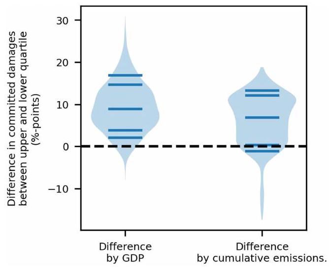
The distribution of committed damages

The spatial distribution of committed damages (Fig. 2a) reflects a complex interplay between the patterns of future change in several climatic components and those of historical economic vulnerability to changes in those variables. Damages resulting from increasing annual mean temperature (Fig. 2b) are negative almost everywhere globally, and larger at lower latitudes in regions in which temperatures are already higher and economic vulnerability to temperature increases is greatest (see the response heterogeneity to mean temperature embodied in Extended Data Fig. 1a). This occurs despite the amplified warming projected at higher latitudes , suggesting that regional heterogeneity
Fig. 3 | The injustice of committed climate damages by cumulative historical emissions and income. Estimates of the median projected change in national income per capita across emission scenarios (RCP2.6 and RCP8.5) as well as climate model, empirical model and model parameter uncertainty in the year in which climate damages diverge at the 5% level (2049, as identified in Fig.1) are plotted against cumulative national emissions per capita in 2020 (from the
Global Carbon Project) and coloured by national income per capita in 2020 (from the World Bank) in and vice versa in . In each panel, the size of each scatter point is weighted by the national population in 2020 (from the World Bank). Inset numbers indicate the Spearman’s rank correlation and -values for a hypothesis test whose null hypothesis is of no correlation, as well as the Spearman’s rank correlation weighted by national population.
in economic vulnerability to temperature changes outweighs heterogeneity in the magnitude of future warming (Supplementary Fig. 13a). Economic damages owing to daily temperature variability (Fig. 2c) exhibit a strong latitudinal polarisation, primarily reflecting the physical response of daily variability to greenhouse forcing in which increases in variability across lower latitudes (and Europe) contrast decreases at high latitudes (Supplementary Fig. 13b). These two temperature terms are the dominant determinants of the pattern of overall damages (Fig. 2a), which exhibits a strong polarity with damages across most of the globe except at the highest northern latitudes. Future changes in total annual precipitation mainly bring economic benefits except in regions of drying, such as the Mediterranean and central South America (Fig. 2d and Supplementary Fig. 13c), but these benefits are opposed by changes in the number of wet days, which produce damages with a similar pattern of opposite sign (Fig. 2e and Supplementary Fig. 13d). By contrast, changes in extreme daily rainfall produce damages in all regions, reflecting the intensification of daily rainfall extremes over global land areas (Fig. 2f and Supplementary Fig. 13e).
The spatial distribution of committed damages implies considerable injustice along two dimensions: culpability for the historical emissions that have caused climate change and pre-existing levels of socio-economic welfare. Spearman’s rank correlations indicate that committed damages are significantly larger in countries with smaller historical cumulative emissions, as well as in regions with lower current income per capita (Fig. 3). This implies that those countries that will suffer the most from the damages already committed are those that are least responsible for climate change and which also have the least resources to adapt to it.
To further quantify this heterogeneity, we assess the difference in committed damages between the upper and lower quartiles of regions when ranked by present income levels and historical cumulative emissions (using a population weighting to both define the quartiles and estimate the group averages). On average, the quartile of countries with lower income are committed to an income loss that is 8.9 percentage points (or 61%) greater than the upper quartile (Extended Data Fig. 6), with a likely range of percentage points across the uncertainty sampling of our damage projections (following the
likelihood classification adopted by the IPCC). Similarly, the quartile of countries with lower historical cumulative emissions are committed to an income loss that is 6.9 percentage points (or ) greater than the upper quartile, with a likely range of percentage points. These patterns reemphasize the prevalence of injustice in climate impacts in the context of the damages to which the world is already committed by historical emissions and socio-economic inertia.

Contextualizing the magnitude of damages

The magnitude of projected economic damages exceeds previous literature estimates , arising from several developments made on previous approaches. Our estimates are larger than those of ref. 2 (see first row of Extended Data Table3), primarily because of the facts that sub-national estimates typically show a steeper temperature response (see also refs. 3,34) and that accounting for other climatic components raises damage estimates (Extended Data Fig. 5). However, we note that our empirical approach using first-differenced climate variables is conservative compared with that of ref. 2 in regard to the persistence of climate impacts on growth (see introduction and Methods section ‘Empirical model specification: fixed-effects distributed lag models’), an important determinant of the magnitude of long-term damages . Using a similar empirical specification to ref. 2, which assumes infinite persistence while maintaining the rest of our approach (sub-national data and further climate variables), produces considerably larger damages (purple curve of Extended Data Fig. 3). Compared with studies that do take the first difference of climate variables , our estimates are also larger (see second and third rows of Extended Data Table 3). The inclusion of further climate variables (Extended Data Fig. 5) and a sufficient number of lags to more adequately capture the extent of impact persistence (Extended Data Figs. 1 and 2) are the main sources of this difference, as is the use of specifications that capture nonlinearities in the temperature response when compared with ref. 35. In summary, our estimates develop on previous studies by incorporating the latest data and empirical insights , as well as in providing a robust empirical lower bound on the persistence of impacts on economic growth, which constitutes a middle ground between the extremes of the growth-versus-levels debate (Extended Data Fig. 3).
Compared with the fraction of variance explained by the empirical models historically (<5%), the projection of reductions in income of 19% may seem large. This arises owing to the fact that projected changes in climatic conditions are much larger than those that were experienced historically, particularly for changes in average temperature (Extended Data Fig. 4). As such, any assessment of future climate-change impacts necessarily requires an extrapolation outside the range of the historical data on which the empirical impact models were evaluated. Nevertheless, these models constitute the most state-of-the-art methods for inference of plausibly causal climate impacts based on observed data. Moreover, we take explicit steps to limit out-of-sample extrapolation by capping the moderating variables of the interaction terms at the 95th percentile of the historical distribution (see Methods). This avoids extrapolating the marginal effects outside what was observed historically. Given the nonlinear response of economic output to annual mean temperature (Extended Data Fig. 1 and Extended Data Table 2), this is a conservative choice that limits the magnitude of damages that we project. Furthermore, back-of-the-envelope calculations indicate that the projected damages are consistent with the magnitude and patterns of historical economic development (see Supplementary Discussion Section 5).

Missing impacts and spatial spillovers

Despite assessing several climatic components from which economic impacts have recently been identified , this assessment of aggregate climate damages should not be considered comprehensive. Important channels such as impacts from heatwaves , sea-level rise , tropical cyclones and tipping points , as well as non-market damages such as those to ecosystems and human health , are not considered in these estimates. Sea-level rise is unlikely to be feasibly incorporated into empirical assessments such as this because historical sea-level variability is mostly small. Non-market damages are inherently intractable within our estimates of impacts on aggregate monetary output and estimates of these impacts could arguably be considered as extra to those identified here. Recent empirical work suggests that accounting for these channels would probably raise estimates of these committed damages, with larger damages continuing to arise in the global south .
Moreover, our main empirical analysis does not explicitly evaluate the potential for impacts in local regions to produce effects that ‘spill over’ into other regions. Such effects may further mitigate or amplify the impacts we estimate, for example, if companies relocate production from one affected region to another or if impacts propagate along supply chains. The current literature indicates that trade plays a substantial role in propagating spillover effects , making their assessment at the sub-national level challenging without available data on sub-national trade dependencies. Studies accounting for only spatially adjacent neighbours indicate that negative impacts in one region induce further negative impacts in neighbouring regions , suggesting that our projected damages are probably conservative by excluding these effects. In Supplementary Fig. 14, we assess spillovers from neighbouring regions using a spatial-lag model. For simplicity, this analysis excludes temporal lags, focusing only on contemporaneous effects. The results show that accounting for spatial spillovers can amplify the overall magnitude, and also the heterogeneity, of impacts. Consistent with previous literature, this indicates that the overall magnitude (Fig. 1) and heterogeneity (Fig. 3) of damages that we project in our main specification may be conservative without explicitly accounting for spillovers. We note that further analysis that addresses both spatially and trade-connected spillovers, while also accounting for delayed impacts using temporal lags, would be necessary to adequately address this question fully. These approaches offer fruitful avenues for further research but are beyond the scope of this manuscript, which primarily aims to explore the impacts of different climate conditions and their persistence.

Policy implications

We find that the economic damages resulting from climate change until 2049 are those to which the world economy is already committed and that these greatly outweigh the costs required to mitigate emissions in line with the target of the Paris Climate Agreement (Fig. 1). This assessment is complementary to formal analyses of the net costs and benefits associated with moving from one emission path to another, which typically find that net benefits of mitigation only emerge in the second half of the century . Our simple comparison of the magnitude of damages and mitigation costs makes clear that this is primarily because damages are indistinguishable across emissions scenarios-that is, committed-until mid-century (Fig. 1) and that they are actually already much larger than mitigation costs. For simplicity, and owing to the availability of data, we compare damages to mitigation costs at the global level. Regional estimates of mitigation costs may shed further light on the national incentives for mitigation to which our results already hint, of relevance for international climate policy. Although these damages are committed from a mitigation perspective, adaptation may provide an opportunity to reduce them. Moreover, the strong divergence of damages after mid-century reemphasizes the clear benefits of mitigation from a purely economic perspective, as highlighted in previous studies .

Online content

Any methods, additional references, Nature Portfolio reporting summaries, source data, extended data, supplementary information, acknowledgements, peer review information; details of author contributions and competing interests; and statements of data and code availability are available at https://doi.org/10.1038/s41586-024-07219-0.
  1. Glanemann, N., Willner, S. N. & Levermann, A. Paris Climate Agreement passes the cost-benefit test. Nat. Commun. 11, 110 (2020).
  2. Burke, M., Hsiang, S. M. & Miguel, E. Global non-linear effect of temperature on economic production. Nature 527, 235-239 (2015).
  3. Kalkuhl, M. & Wenz, L. The impact of climate conditions on economic production. Evidence from a global panel of regions. J. Environ. Econ. Manag. 103, 102360 (2020).
  4. Moore, F. C. & Diaz, D. B. Temperature impacts on economic growth warrant stringent mitigation policy. Nat. Clim. Change 5, 127-131 (2015).
  5. Drouet, L., Bosetti, V. & Tavoni, M. Net economic benefits of well-below scenarios and associated uncertainties. Oxf. Open Clim. Change 2, kgac003 (2022).
  6. Ueckerdt, F. et al. The economically optimal warming limit of the planet. Earth Syst. Dyn. 10, 741-763 (2019).
  7. Kotz, M., Wenz, L., Stechemesser, A., Kalkuhl, M. & Levermann, A. Day-to-day temperature variability reduces economic growth. Nat. Clim. Change 11, 319-325 (2021).
  8. Kotz, M., Levermann, A. & Wenz, L. The effect of rainfall changes on economic production. Nature 601, 223-227 (2022).
  9. Kousky, C. Informing climate adaptation: a review of the economic costs of natural disasters. Energy Econ. 46, 576-592 (2014).
  10. Harlan, S. L. et al. in Climate Change and Society: Sociological Perspectives (eds Dunlap, R. E. & Brulle, R. J.) 127-163 (Oxford Univ. Press, 2015).
  11. Bolton, P. et al. The Green Swan (BIS Books, 2020).
  12. Alogoskoufis, S. et al. ECB Economy-wide Climate Stress Test: Methodology and Results European Central Bank, 2021).
  13. Weber, E. U. What shapes perceptions of climate change? Wiley Interdiscip. Rev. Clim. Change 1, 332-342 (2010).
  14. Markowitz, E. M. & Shariff, A. F. Climate change and moral judgement. Nat. Clim. Change 2, 243-247 (2012).
  15. Riahi, K. et al. The shared socioeconomic pathways and their energy, land use, and greenhouse gas emissions implications: an overview. Glob. Environ. Change 42, 153-168 (2017).
  16. Auffhammer, M., Hsiang, S. M., Schlenker, W. & Sobel, A. Using weather data and climate model output in economic analyses of climate change. Rev. Environ. Econ. Policy 7, 181-198 (2013).
  17. Kolstad, C. D. & Moore, F. C. Estimating the economic impacts of climate change using weather observations. Rev. Environ. Econ. Policy 14, 1-24 (2020).
  18. Dell, M., Jones, B. F. & Olken, B. A. Temperature shocks and economic growth: evidence from the last half century. Am. Econ. J. Macroecon. 4, 66-95 (2012).
  19. Newell, R. G., Prest, B. C. & Sexton, S. E. The GDP-temperature relationship: implications for climate change damages. J. Environ. Econ. Manag. 108, 102445 (2021).
  20. Kikstra, J. S. et al. The social cost of carbon dioxide under climate-economy feedbacks and temperature variability. Environ. Res. Lett. 16, 094037 (2021).
  21. Bastien-Olvera, B. & Moore, F. Persistent effect of temperature on GDP identified from lower frequency temperature variability. Environ. Res. Lett. 17, 084038 (2022).
  22. Eyring, V. et al. Overview of the Coupled Model Intercomparison Project Phase 6 (CMIP6) experimental design and organization. Geosci. Model Dev. 9, 1937-1958 (2016).
  23. Byers, E. et al. AR6 scenarios database. Zenodo https://zenodo.org/records/7197970 (2022).
  24. Burke, M., Davis, W. M. & Diffenbaugh, N. S. Large potential reduction in economic damages under UN mitigation targets. Nature 557, 549-553 (2018).
  25. Kotz, M., Wenz, L. & Levermann, A. Footprint of greenhouse forcing in daily temperature variability. Proc. Natl Acad. Sci. 118, e2103294118 (2021).
  26. Myhre, G. et al. Frequency of extreme precipitation increases extensively with event rareness under global warming. Sci. Rep. 9, 16063 (2019).
  27. Min, S.-K., Zhang, X., Zwiers, F. W. & Hegerl, G. C. Human contribution to more-intense precipitation extremes. Nature 470, 378-381 (2011).
  28. England, M. R., Eisenman, I., Lutsko, N. J. & Wagner, T. J. The recent emergence of Arctic Amplification. Geophys. Res. Lett. 48, e2021GL094086 (2021).
  29. Fischer, E. M. & Knutti, R. Anthropogenic contribution to global occurrence of heavyprecipitation and high-temperature extremes. Nat. Clim. Change 5, 560-564 (2015).
  30. Pfahl, S., O’Gorman, P. A. & Fischer, E. M. Understanding the regional pattern of projected future changes in extreme precipitation. Nat. Clim. Change 7, 423-427 (2017).
  31. Callahan, C. W. & Mankin, J. S. Globally unequal effect of extreme heat on economic growth. Sci. Adv. 8, eadd3726 (2022).
  32. Diffenbaugh, N. S. & Burke, M. Global warming has increased global economic inequality. Proc. Natl Acad. Sci. 116, 9808-9813 (2019).
  33. Callahan, C. W. & Mankin, J. S. National attribution of historical climate damages. Clim. Change 172, 40 (2022).
  34. Burke, M. & Tanutama, V. Climatic constraints on aggregate economic output. National Bureau of Economic Research, Working Paper 25779. https://doi.org/10.3386/w25779 (2019).
  35. Kahn, M. E. et al. Long-term macroeconomic effects of climate change: a cross-country analysis. Energy Econ. 104, 105624 (2021).
  36. Desmet, K. et al. Evaluating the economic cost of coastal flooding. National Bureau of Economic Research, Working Paper 24918. https://doi.org/10.3386/w24918 (2018).
  37. Hsiang, S. M. & Jina, A. S. The causal effect of environmental catastrophe on long-run economic growth: evidence from 6,700 cyclones. National Bureau of Economic Research, Working Paper 20352. https://doi.org/10.3386/w2035 (2014).
  38. Ritchie, P. D. et al. Shifts in national land use and food production in Great Britain after a climate tipping point. Nat. Food 1, 76-83 (2020).
  39. Dietz, S., Rising, J., Stoerk, T. & Wagner, G. Economic impacts of tipping points in the climate system. Proc. Natl Acad. Sci. 118, e2103081118 (2021).
  40. Bastien-Olvera, B. A. & Moore, F. C. Use and non-use value of nature and the social cost of carbon. Nat. Sustain. 4, 101-108 (2021).
  41. Carleton, T. et al. Valuing the global mortality consequences of climate change accounting for adaptation costs and benefits. Q. J. Econ. 137, 2037-2105 (2022).
  42. Bastien-Olvera, B. A. et al. Unequal climate impacts on global values of natural capital. Nature 625, 722-727 (2024).
  43. Malik, A. et al. Impacts of climate change and extreme weather on food supply chains cascade across sectors and regions in Australia. Nat. Food 3, 631-643 (2022).
  44. Kuhla, K., Willner, S. N., Otto, C., Geiger, T. & Levermann, A. Ripple resonance amplifies economic welfare loss from weather extremes. Environ. Res. Lett. 16, 114010 (2021).
  45. Schleypen, J. R., Mistry, M. N., Saeed, F. & Dasgupta, S. Sharing the burden: quantifying climate change spillovers in the European Union under the Paris Agreement. Spat. Econ. Anal. 17, 67-82 (2022).
  46. Dasgupta, S., Bosello, F., De Cian, E. & Mistry, M. Global temperature effects on economic activity and equity: a spatial analysis. European Institute on Economics and the Environment, Working Paper 22-1 (2022).
  47. Neal, T. The importance of external weather effects in projecting the macroeconomic impacts of climate change. UNSW Economics Working Paper 2023-09 (2023).
  48. Deryugina, T. & Hsiang, S. M. Does the environment still matter? Daily temperature and income in the United States. National Bureau of Economic Research, Working Paper 20750. https://doi.org/10.3386/w20750 (2014).
Publisher’s note Springer Nature remains neutral with regard to jurisdictional claims in published maps and institutional affiliations.
Open Access This article is licensed under a Creative Commons Attribution 4.0 International License, which permits use, sharing, adaptation, distribution and reproduction in any medium or format, as long as you give appropriate credit to the original author(s) and the source, provide a link to the Creative Commons licence, and indicate if changes were made. The images or other third party material in this article are included in the article’s Creative Commons licence, unless indicated otherwise in a credit line to the material. If material is not included in the article’s Creative Commons licence and your intended use is not permitted by statutory regulation or exceeds the permitted use, you will need to obtain permission directly from the copyright holder. To view a copy of this licence, visit http://creativecommons.org/licenses/by/4.0/.
(c) The Author(s) 2024

Methods

Historical climate data

Historical daily temperature and precipitation totals (in mm ) are obtained for the period 1979-2019 from the W5E5 database. The W5E5 dataset comes from ERA-5, a state-of-the-art reanalysis of historical observations, but has been bias-adjusted by applying version 2.0 of the WATCH Forcing Data to ERA-5 reanalysis data and precipitation data from version 2.3 of the Global Precipitation Climatology Project to better reflect ground-based measurements . We obtain these data on a grid from the Inter-Sectoral Impact Model Intercomparison Project (ISIMIP) database. Notably, these historical data have been used to bias-adjust future climate projections from CMIP-6 (see the following section), ensuring consistency between the distribution of historical daily weather on which our empirical models were estimated and the climate projections used to estimate future damages. These data are publicly available from the ISIMIP database. See refs. 7,8 for robustness tests of the empirical models to the choice of climate data reanalysis products.

Future climate data

Daily 2 -m temperature and precipitation totals (in mm) are taken from 21 climate models participating in CMIP-6 under a high (RCP8.5) and a low (RCP2.6) greenhouse gas emission scenario from 2015 to 2100. The data have been bias-adjusted and statistically downscaled to a common half-degree grid to reflect the historical distribution of daily temperature and precipitation of the W5E5 dataset using the trend-preserving method developed by the ISIMIP . As such, the climate model data reproduce observed climatological patterns exceptionally well (Supplementary Table 5). Gridded data are publicly available from the ISIMIP database.

Historical economic data

Historical economic data come from the DOSE database of subnational economic output . We use a recent revision to the DOSE dataset that provides data across 83 countries, 1,660 sub-national regions with varying temporal coverage from 1960 to 2019. Sub-national units constitute the first administrative division below national, for example, states for the USA and provinces for China. Data come from measures of gross regional product per capita (GRPpc) or income per capita in local currencies, reflecting the values reported in national statistical agencies, yearbooks and, in some cases, academic literature. We follow previous literature and assess real subnational output per capita by first converting values from local currencies to US dollars to account for diverging national inflationary tendencies and then account for US inflation using a US deflator. Alternatively, one might first account for national inflation and then convert between currencies. Supplementary Fig. 12 demonstrates that our conclusions are consistent when accounting for price changes in the reversed order, although the magnitude of estimated damages varies. See the documentation of the DOSE dataset for further discussion of these choices. Conversions between currencies are conducted using exchange rates from the FRED database of the Federal Reserve Bank of St. Louis and the national deflators from the World Bank .

Future socio-economic data

Baseline gridded gross domestic product (GDP) and population data for the period 2015-2100 are taken from the middle-of-the-road scenario SSP2 (ref. 15). Population data have been downscaled to a halfdegree grid by the ISIMIP following the methodologies of refs. 57,58, which we then aggregate to the sub-national level of our economic data using the spatial aggregation procedure described below. Because current methodologies for downscaling the GDP of the SSPs use downscaled population to do so, per-capita estimates of GDP with a
realistic distribution at the sub-national level are not readily available for the SSPs. We therefore use national-level GDP per capita (GDPpc) projections for all sub-national regions of a given country, assuming homogeneity within countries in terms of baseline GDPpc. Here we use projections that have been updated to account for the impact of the COVID-19 pandemic on the trajectory of future income, while remaining consistent with the long-term development of the SSPs . The choice of baseline SSP alters the magnitude of projected climate damages in monetary terms, but when assessed in terms of percentage change from the baseline, the choice of socio-economic scenario is inconsequential. Gridded SSP population data and national-level GDPpc data are publicly available from the ISIMIP database. Sub-national estimates as used in this study are available in the code and data replication files.

Climate variables

Following recent literature , we calculate an array of climate variables for which substantial impacts on macroeconomic output have been identified empirically, supported by further evidence at the micro level for plausible underlying mechanisms. See refs. 7,8 for an extensive motivation for the use of these particular climate variables and for detailed empirical tests on the nature and robustness of their effects on economic output. To summarize, these studies have found evidence for independent impacts on economic growth rates from annual average temperature, daily temperature variability, total annual precipitation, the annual number of wet days and extreme daily rainfall. Assessments of daily temperature variability were motivated by evidence of impacts on agricultural output and human health, as well as macroeconomic literature on the impacts of volatility on growth when manifest in different dimensions, such as government spending, exchange rates and even output itself . Assessments of precipitation impacts were motivated by evidence of impacts on agricultural productivity, metropolitan labour outcomes and conflict, as well as damages caused by flash flooding . See Extended Data Table 1 for detailed references to empirical studies of these physical mechanisms. Marked impacts of daily temperature variability, total annual precipitation, the number of wet days and extreme daily rainfall on macroeconomic output were identified robustly across different climate datasets, spatial aggregation schemes, specifications of regional time trends and error-clustering approaches. They were also found to be robust to the consideration of temperature extremes . Furthermore, these climate variables were identified as having independent effects on economic output , which we further explain here using Monte Carlo simulations to demonstrate the robustness of the results to concerns of imperfect multicollinearity between climate variables (Supplementary Methods Section 2), as well as by using information criteria (Supplementary Table 1) to demonstrate that including several lagged climate variables provides a preferable trade-off between optimally describing the data and limiting the possibility of overfitting.
We calculate these variables from the distribution of daily, , temperature, and precipitation, , at the grid-cell, , level for both the historical and future climate data. As well as annual mean temperature, , and annual total precipitation, , we calculate annual, , measures of daily temperature variability, :
the number of wet days, :
and extreme daily rainfall:
in which is the grid-cell-specific daily temperature in month and year is the year and grid-cell-specific monthly, , mean temperature, and the number of days in a given month or year , respectively, the Heaviside step function, 1 mm the threshold used to define wet days and is the 99.9 th percentile of historical (1979-2019) daily precipitation at the grid-cell level. Units of the climate measures are degrees Celsius for annual mean temperature and daily temperature variability, millimetres for total annual precipitation and extreme daily precipitation, and simply the number of days for the annual number of wet days.
We also calculated weighted standard deviations of monthly rainfall totals as also used in ref. 8 but do not include them in our projections as we find that, when accounting for delayed effects, their effect becomes statistically indistinct and is better captured by changes in total annual rainfall.

Spatial aggregation

We aggregate grid-cell-level historical and future climate measures, as well as grid-cell-level future GDPpc and population, to the level of the first administrative unit below national level of the GADM database, using an area-weighting algorithm that estimates the portion of each grid cell falling within an administrative boundary. We use this as our baseline specification following previous findings that the effect of area or population weighting at the sub-national level is negligible .

Empirical model specification: fixed-effects distributed lag models

Following a wide range of climate econometric literature , we use panel regression models with a selection of fixed effects and time trends to isolate plausibly exogenous variation with which to maximize confidence in a causal interpretation of the effects of climate on economic growth rates. The use of region fixed effects, , accounts for unobserved time-invariant differences between regions, such as prevailing climatic norms and growth rates owing to historical and geopolitical factors. The use of yearly fixed effects, , accounts for regionally invariant annual shocks to the global climate or economy such as the El Niño-Southern Oscillation or global recessions. In our baseline specification, we also include region-specific linear time trends, , to exclude the possibility of spurious correlations resulting from common slow-moving trends in climate and growth.
The persistence of climate impacts on economic growth rates is a key determinant of the long-term magnitude of damages. Methods for inferring the extent of persistence in impacts on growth rates have typically used lagged climate variables to evaluate the presence of delayed effects or catch-up dynamics . For example, consider starting from a model in which a climate condition, , (for example, annual mean temperature) affects the growth rate, (the first difference of the logarithm of gross regional product) of region in year :
which we refer to as a ‘pure growth effects’ model in the main text. Typically, further lags are included,
and the cumulative effect of all lagged terms is evaluated to assess the extent to which climate impacts on growth rates persist. Following ref. 18, in the case that,
the implication is that impacts on the growth rate persist up to NL years after the initial shock (possibly to a weaker or a stronger extent), whereas if
then the initial impact on the growth rate is recovered after NL years and the effect is only one on the level of output. However, we note that such approaches are limited by the fact that, when including an insufficient number of lags to detect a recovery of the growth rates, one may find equation (6) to be satisfied and incorrectly assume that a change in climatic conditions affects the growth rate indefinitely. In practice, given a limited record of historical data, including too few lags to confidently conclude in an infinitely persistent impact on the growth rate is likely, particularly over the long timescales over which future climate damages are often projected . To avoid this issue, we instead begin our analysis with a model for which the level of output, , depends on the level of a climate variable, :
Given the non-stationarity of the level of output, we follow the literature and estimate such an equation in first-differenced form as,
which we refer to as a model of ‘pure level effects’ in the main text. This model constitutes a baseline specification in which a permanent change in the climate variable produces an instantaneous impact on the growth rate and a permanent effect only on the level of output. By including lagged variables in this specification,
we are able to test whether the impacts on the growth rate persist any further than instantaneously by evaluating whether are statistically significantly different from zero. Even though this framework is also limited by the possibility of including too few lags, the choice of a baseline model specification in which impacts on the growth rate do not persist means that, in the case of including too few lags, the framework reverts to the baseline specification of level effects. As such, this framework is conservative with respect to the persistence of impacts and the magnitude of future damages. It naturally avoids assumptions of infinite persistence and we are able to interpret any persistence that we identify with equation (9) as a lower bound on the extent of climate impact persistence on growth rates. See the main text for further discussion of this specification choice, in particular about its conservative nature compared with previous literature estimates, such as refs. 2,18.
We allow the response to climatic changes to vary across regions, using interactions of the climate variables with historical average (1979-2019) climatic conditions reflecting heterogenous effects identified in previous work . Following this previous work, the moderating variables of these interaction terms constitute the historical average of either the variable itself or of the seasonal temperature difference, , or annual mean temperature, , in the case of daily temperature variability and extreme daily rainfall, respectively .
The resulting regression equation with and lagged variables, respectively, reads:
in which is the annual, regional GRPpc growth rate, measured as the first difference of the logarithm of real GRPpc, following previous work . Fixed-effects regressions were run using the fixest package in R (ref. 61).
Estimates of the coefficients of interest are shown in Extended Data Fig. 1 for lags and for our preferred choice of the number of lags in Supplementary Figs. 1-3. In Extended Data Fig. 1, errors are shown clustered at the regional level, but for the construction of damage projections, we block-bootstrap the regressions by region 1,000 times to provide a range of parameter estimates with which to sample the projection uncertainty (following refs. 2,31).

Spatial-lag model

In Supplementary Fig. 14, we present the results from a spatial-lag model that explores the potential for climate impacts to ‘spill over’ into spatially neighbouring regions. We measure the distance between centroids of each pair of sub-national regions and construct spatial lags that take the average of the first-differenced climate variables and their interaction terms over neighbouring regions that are at distances of and (spatial lags, ‘SL’, 1 to 4). For simplicity, we then assess a spatial-lag model without temporal lags to assess spatial spillovers of contemporaneous climate impacts. This model takes the form:
in which SL indicates the spatial lag of each climate variable and interaction term. In Supplementary Fig. 14, we plot the cumulative marginal effect of each climate variable at different baseline climate conditions by summing the coefficients for each climate variable and interaction term, for example, for average temperature impacts as:
These cumulative marginal effects can be regarded as the overall spatially dependent impact to an individual region given a oneunit shock to a climate variable in that region and all neighbouring regions at a given value of the moderating variable of the interaction term.

Constructing projections of economic damage from future climate change

We construct projections of future climate damages by applying the coefficients estimated in equation (10) and shown in Supplementary Tables 2-4 (when including only lags with statistically significant effects in specifications that limit overfitting; see Supplementary Methods Section1) to projections of future climate change from the CMIP-6 models. Year-on-year changes in each primary climate variable of interest are calculated to reflect the year-to-year variations used in the empirical models. 30-year moving averages of the moderating variables of the interaction terms are calculated to reflect the long-term average of climatic conditions that were used for the moderating variables in the empirical models. By using moving averages in the projections, we account for the changing vulnerability to climate shocks based on the evolving long-term conditions (Supplementary Figs. 10 and 11 show that the results are robust to the precise choice of the window of this moving average). Although these climate variables are not differenced, the fact that the bias-adjusted climate models reproduce observed climatological patterns across regions for these moderating variables very accurately (Supplementary Table 6) with limited spread across models (<3%) precludes the possibility that any considerable bias or uncertainty is introduced by this methodological choice. However, we impose caps on these moderating variables at the 95th percentile at which they were observed in the historical data to prevent extrapolation of the marginal effects outside the range in which the regressions were estimated. This is a conservative choice that limits the magnitude of our damage projections.
Time series of primary climate variables and moderating climate variables are then combined with estimates of the empirical model parameters to evaluate the regression coefficients in equation (10), producing a time series of annual GRPpc growth-rate reductions for a given emission scenario, climate model and set of empirical model parameters. The resulting time series of growth-rate impacts reflects those occurring owing to future climate change. By contrast, a future scenario with no climate change would be one in which climate variables do not change (other than with random year-to-year fluctuations) and hence the time-averaged evaluation of equation (10) would be zero. Our approach therefore implicitly compares the future climate-change scenario to this no-climate-change baseline scenario.
The time series of growth-rate impacts owing to future climate change in region and year , are then added to the future baseline growth rates, (in log-diff form), obtained from the SSP2 scenario to yield trajectories of damaged GRPpc growth rates, . These trajectories are aggregated over time to estimate the future trajectory of GRPpc with future climate impacts:
in which is the initial log level of GRPpc. We begin damage estimates in 2020 to reflect the damages occurring since the end of the period for which we estimate the empirical models (1979-2019) and to match the timing of mitigation-cost estimates from most IAMs (see below).
For each emission scenario, this procedure is repeated 1,000 times while randomly sampling from the selection of climate models, the selection of empirical models with different numbers of lags (shown in Supplementary Figs. 1-3 and Supplementary Tables 2-4) and bootstrapped estimates of the regression parameters. The result is an ensemble of future GRPpc trajectories that reflect uncertainty from
both physical climate change and the structural and sampling uncertainty of the empirical models.

Estimates of mitigation costs

We obtain IPCC estimates of the aggregate costs of emission mitigation from the AR6 Scenario Explorer and Database hosted by IIASA . Specifically, we search the AR6 Scenarios Database World v1.1 for IAMs that provided estimates of global GDP and population under both a SSP2 baseline and a SSP2-RCP2.6 scenario to maintain consistency with the socio-economic and emission scenarios of the climate damage projections. We find five IAMs that provide data for these scenarios, namely, MESSAGE-GLOBIOM 1.0, REMIND-MAgPIE 1.5, AIM/GCE 2.0, GCAM 4.2 and WITCH-GLOBIOM 3.1. Of these five IAMs, we use the results only from the first three that passed the IPCC vetting procedure for reproducing historical emission and climate trajectories. We then estimate global mitigation costs as the percentage difference in global per capita GDP between the SSP2 baseline and the SSP2-RCP2.6 emission scenario. In the case of one of these IAMs, estimates of mitigation costs begin in 2020, whereas in the case of two others, mitigation costs begin in 2010. The mitigation cost estimates before 2020 in these two IAMs are mostly negligible, and our choice to begin comparison with damage estimates in 2020 is conservative with respect to the relative weight of climate damages compared with mitigation costs for these two IAMs.

Data availability

Data on economic production and ERA-5 climate data are publicly available at https://doi.org/10.5281/zenodo. 4681306 (ref. 62) and https://www.ecmwf.int/en/forecasts/datasets/reanalysis-datasets/era5, respectively. Data on mitigation costs are publicly available at https:// data.ene.iiasa.ac.at/ar6/#/downloads. Processed climate and economic data, as well as all other necessary data for reproduction of the results, are available at the public repository https://doi.org/10.5281/ zenodo. 10562951 (ref. 63).

Code availability

All code necessary for reproduction of the results is available at the public repository https://doi.org/10.5281/zenodo. 10562951 (ref. 63).
49. Hersbach, H. et al. The ERA5 global reanalysis. Q. J. R. Meteorol. Soc. 146, 1999-2049 (2020).
50. Cucchi, M. et al. WFDE5: bias-adjusted ERA5 reanalysis data for impact studies. Earth Syst. Sci. Data 12, 2097-2120 (2020).
51. Adler, R. et al. The New Version 2.3 of the Global Precipitation Climatology Project (GPCP) Monthly Analysis Product 1072-1084 (University of Maryland, 2016).
52. Lange, S. Trend-preserving bias adjustment and statistical downscaling with ISIMIP3BASD (v1.0). Geosci. Model Dev. 12, 3055-3070 (2019).
53. Wenz, L., Carr, R. D., Kögel, N., Kotz, M. & Kalkuhl, M. DOSE – global data set of reported sub-national economic output. Sci. Data 10, 425 (2023).
54. Gennaioli, N., La Porta, R., Lopez De Silanes, F. & Shleifer, A. Growth in regions. J. Econ. Growth 19, 259-309 (2014).
55. Board of Governors of the Federal Reserve System (US). U.S. dollars to euro spot exchange rate. https://fred.stlouisfed.org/series/AEXUSEU (2022).
56. World Bank. GDP deflator. https://data.worldbank.org/indicator/NY.GDP.DEFL.ZS (2022).
57. Jones, B. & O’Neill, B. C. Spatially explicit global population scenarios consistent with the Shared Socioeconomic Pathways. Environ. Res. Lett. 11, 084003 (2016).
58. Murakami, D. & Yamagata, Y. Estimation of gridded population and GDP scenarios with spatially explicit statistical downscaling. Sustainability 11, 2106 (2019).
59. Koch, J. & Leimbach, M. Update of SSP GDP projections: capturing recent changes in national accounting, PPP conversion and Covid 19 impacts. Ecol. Econ. 206 (2023).
60. Carleton, T. A. & Hsiang, S. M. Social and economic impacts of climate. Science 353, aad9837 (2016).
61. Bergé, L. Efficient estimation of maximum likelihood models with multiple fixed-effects: the R package FENmlm. DEM Discussion Paper Series 18-13 (2018).
62. Kalkuhl, M., Kotz, M. & Wenz, L. DOSE – The MCC-PIK Database Of Subnational Economic output. Zenodo https://zenodo.org/doi/10.5281/zenodo. 4681305 (2021).
63. Kotz, M., Wenz, L. & Levermann, A. Data and code for “The economic commitment of climate change”. Zenodo https://zenodo.org/doi/10.5281/zenodo. 10562951 (2024).
64. Dasgupta, S. et al. Effects of climate change on combined labour productivity and supply: an empirical, multi-model study. Lancet Planet. Health 5, e455-e465 (2021).
65. Lobell, D. B. et al. The critical role of extreme heat for maize production in the United States. Nat. Clim. Change 3, 497-501 (2013).
66. Zhao, C. et al. Temperature increase reduces global yields of major crops in four independent estimates. Proc. Natl Acad. Sci. 114, 9326-9331 (2017).
67. Wheeler, T. R., Craufurd, P. Q., Ellis, R. H., Porter, J. R. & Prasad, P. V. Temperature variability and the yield of annual crops. Agric. Ecosyst. Environ. 82, 159-167 (2000).
68. Rowhani, P., Lobell, D. B., Linderman, M. & Ramankutty, N. Climate variability and crop production in Tanzania. Agric. For. Meteorol. 151, 449-460 (2011).
69. Ceglar, A., Toreti, A., Lecerf, R., Van der Velde, M. & Dentener, F. Impact of meteorological drivers on regional inter-annual crop yield variability in France. Agric. For. Meteorol. 216, 58-67 (2016).
70. Shi, L., Kloog, I., Zanobetti, A., Liu, P. & Schwartz, J. D. Impacts of temperature and its variability on mortality in New England. Nat. Clim. Change 5, 988-991 (2015).
71. Xue, T., Zhu, T., Zheng, Y. & Zhang, Q. Declines in mental health associated with air pollution and temperature variability in China. Nat. Commun. 10, 2165 (2019).
72. Liang, X.-Z. et al. Determining climate effects on US total agricultural productivity. Proc. Natl Acad. Sci. 114, E2285-E2292 (2017).
73. Desbureaux, S. & Rodella, A.-S. Drought in the city: the economic impact of water scarcity in Latin American metropolitan areas. World Dev. 114, 13-27 (2019).
74. Damania, R. The economics of water scarcity and variability. Oxf. Rev. Econ. Policy 36, 24-44 (2020).
75. Davenport, F. V., Burke, M. & Diffenbaugh, N. S. Contribution of historical precipitation change to US flood damages. Proc. Natl Acad. Sci. 118, e2017524118 (2021).
76. Dave, R., Subramanian, S. S. & Bhatia, U. Extreme precipitation induced concurrent events trigger prolonged disruptions in regional road networks. Environ. Res. Lett. 16, 104050 (2021).
Acknowledgements We gratefully acknowledge financing from the Volkswagen Foundation and the Deutsche Gesellschaft für Internationale Zusammenarbeit (GIZ) GmbH on behalf of the Government of the Federal Republic of Germany and Federal Ministry for Economic Cooperation and Development (BMZ).
Author contributions All authors contributed to the design of the analysis. M.K. conducted the analysis and produced the figures. All authors contributed to the interpretation and presentation of the results. M.K. and L.W. wrote the manuscript.
Funding Open access funding provided by Potsdam-Institut für Klimafolgenforschung (PIK) e.V.
Competing interests The authors declare no competing interests.

Additional information

Supplementary information The online version contains supplementary material available at https://doi.org/10.1038/s41586-024-07219-0.
Correspondence and requests for materials should be addressed to Leonie Wenz.
Peer review information Nature thanks Xin-Zhong Liang, Chad Thackeray and the other, anonymous, reviewer(s) for their contribution to the peer review of this work. Peer reviewer reports are available.
Reprints and permissions information is available at http://www.nature.com/reprints.

Article

Extended Data Fig. 2 | Incremental lag-selection procedure using information criteria and within-region . Starting from a panel-based fixedeffects distributed lag model estimating the effects of climate on economic growth using the real historical data (as in equation (4)) with ten lags for all climate variables (as shown in Extended Data Fig. 1), lags are incrementally removed for one climate variable at a time. The resulting Bayesian and Akaike information criteria are shown in and , respectively, and the within-region and number of observations in and , respectively. Different rows
show the results when removing lags from different climate variables, ordered from top to bottom as annual mean temperature, daily temperature variability, total annual precipitation, the number of wet days and extreme annual precipitation. Information criteria show minima at approximately four lags for precipitation variables and ten to eight for temperature variables, indicating that including these numbers of lags does not lead to overfitting. See Supplementary Table 1 for an assessment using information criteria to determine whether including further climate variables causes overfitting.

Article

Extended Data Fig. 3|Damages in our preferred specification that provides a robust lower bound on the persistence of climate impacts on economic growth versus damages in specifications of pure growth or pure level
effects. Estimates of future damages as shown in Fig. 1 but under the emission scenario RCP8.5 for three separate empirical specifications: in orange our preferred specification, which provides an empirical lower bound on the persistence of climate impacts on economic growth rates while avoiding assumptions of infinite persistence (see main text for further discussion); in purple a specification of ‘pure growth effects’ in which the first difference of climate variables is not taken and no lagged climate variables are included (the baseline specification of ref. 2); and in pink a specification of ‘pure level effects’ in which the first difference of climate variables is taken but no lagged terms are included.
Extended Data Fig. 4 | Climate changes in different variables as a function of historical interannual variability. Changes in each climate variable of interest from 1979-2019 to 2035-2065 under the high-emission scenario SSP5-RCP8.5, expressed as a percentage of the historical variability of each measure. Historical variability is estimated as the standard deviation of each detrended climate variable over the period 1979-2019 during which the empirical models were
identified (detrending is appropriate because of the inclusion of region-specific linear time trends in the empirical models). See Supplementary Fig. 13 for changes expressed in standard units. Data on national administrative boundaries are obtained from the GADM database version 3.6 and are freely available for academic use (https://gadm.org/).

Article


Extended Data Fig. 6 | The difference in committed damages between the upper and lower quartiles of countries when ranked by GDP and cumulative historical emissions. Quartiles are defined using a population weighting, as are the average committed damages across each quartile group. The violin plots indicate the distribution of differences between quartiles across the two extreme emission scenarios (RCP2.6 and RCP8.5) and the uncertainty sampling procedure outlined in Methods, which accounts for uncertainty arising from the choice of lags in the empirical models, uncertainty in the empirical model parameter estimates, as well as the climate model projections. Bars indicate the median, as well as the 10th and 90th percentiles and upper and lower sixths of the distribution reflecting the very likely and likely ranges following the likelihood classification adopted by the IPCC.

Article

Extended Data Table 1 | A summary of several physical mechanisms that plausibly underlie the impact of the different climate variables on macroeconomic growth, with references to empirical evidence
Climate variable Physical mechanisms References
Average annual temperature Labour productivity and supply; agricultural productivity Dasgupta et al. (2021) ; Lobell et al. (2013) , Zhao et al. (2017)
Daily temperature variability Agricultural productivity; physical health; mental health Wheeler et al. , Rowhani et al. , Ceglar et al. ; Shi et al. (2015) ; Xue et al. (2019)
Total annual precipitation Agricultural productivity; metropolitan labour outcomes; conflict Liang et al. (2017) ; Desbreaux et al. (2019) ; Damania et al. (2020)
Number of wet days Travel disruption Lacking
Extreme daily precipitation Flood damages; disruption Davenport et al. (2021) , Dave et al. (2021)
This summary is not intended to be an exhaustive list of all mechanisms or references. In the case of most climate variables, several plausible physical mechanisms supported by empirical evidence exist. The only exception here is the number of wet days, for which plausible mechanisms are listed but empirical evidence does not yet exist (as far as the authors are aware). The use of the number of wet days in the main empirical models is therefore guided primarily by the empirical evidence indicating robust impacts on economic growth . References in the table.
Extended Data Table 2 | Regression results for the historical effects of different climate variables on sub-national economic growth rates in the period 1979-2019
Variable Formula Lag 0 Lag 1 Lag 2 Lag 3 Lag 4 Lag 5 Lag 6 Lag 7 Lag 8 Lag 9 Lag 10
Annual mean temperature -0.17 -0.57 -0.78 -0.23 -0.79 -0.96 -0.23 -0.71 -1.8** -1.1* -2.5***
(0.32) (0.5) (0.54) (0.57) (0.57) (0.65) (0.67) (0.73) (0.63) (0.48) (0.35)
-0.0011*** (0.00029) -0.0014** (0.00049) -0.00072 (0.00051) -0.0015** (0.00055) -0.00072 (0.00047) -0.0015** (0.0005) -0.0017*** (0.00046) -0.0012** (0.00047) -0.00029 (0.0004) 0.00065* (0.00032) 0.00029 (0.00023)
Daily temp. variability -9.3*** -8.1*** -13*** -9.3*** -1.5 -1.2 -2.4 -1.8 3.3 -5.3** -0.34
(1.3) (2) (2.3) (2.7) (3.1) (3.2) (3) (2.9) (2.5) (1.9) (1.3)
0.0013* (0.00054) -0.0003 (0.00083) 0.0013 (0.00087) -0.00011 (0.0011) -0.0034** (0.0012) -0.0032* (0.0013) -0.0025* (0.0012) -0.0029* (0.0012) -0.003** (0.0011) 0.00079 (0.00078) -0.00037 (0.00057)
Total annual precipitation 0.002 (0.0016) 0.0094*** (0.002) 0.009*** (0.0023) 0.0068** (0.0024) 0.0021 (0.0024) -0.0012 (0.0025) 0.0013 (0.0025) -0.001 (0.0023) -0.0001 (0.0021) 0.0012 (0.0019) 0.0005 (0.0015)
(6.9e-09) -2.6e-08** (8.5e-09) (9.7e-09) -2.6e-08** (9.8e-09) (1e-08) (1e-08) (1e-08) (9.3e-09) -1.2e-09 (8.6e-09) -1.3e-08 (7.8e-09) -9.4e-09 (6.1e-09)
Annual no. wet days -0.028 (0.038) -0.12** (0.043) -0.17** (0.055) -0.2*** (0.055) -0.038 (0.052) 0.12 (0.065) 0.037 (0.068) 0.079 (0.058) 0.1* (0.048) 0.045 (0.04) -0.03 (0.032)
(2.3e-06) (2.7e-06) (3.6e-06) 9.2e-06* (3.6e-06) ( ) -1e-05* (4.1e-06) -5.5e-06 (4.1e-06) -7.1e-06 (3.6e-06) -9e-06** (3e-06) -5.6e-06* (2.5e-06) 2.2e-06 (1.9e-06)
Precipitation extremes Pext -0.023*** (0.0053) -0.028*** (0.0073) -0.029*** (0.0084) -0.029** (0.0094) -0.01 (0.0098) -0.0032 (0.01) -0.013 (0.011) -0.017 (0.01) -0.019* (0.0093) -0.013 (0.0079) 0.0054 (0.0052)
Pext 8.8e-06*** (2.5e-06) 9.6e-06** (3.4e-06) 9.6e-06* ( ) 1.4e-05** (4.6e-06) (4.7e-06) (4.9e-06) 8e-06 (4.9e-06) 8.8e-06 (4.8e-06) (4.5e-06) 8.1e-06* ( ) -1.2e-06 (2.7e-06)
0.291
0.0472
BIC -4.46e+03
AIC
34855
with ten lags for each climate variable (that is, each table entry denotes a specific regression coefficient of the same model as indicated in equation (4)). Standard errors are shown in parentheses and *, ** and *** denote significance at the and levels, respectively, having clustered standard errors by region. Formulas for climate variables and their interaction terms are denoted as in equation (4). Note that an interpretation of the significance of the effects of a given climate variable requires an assessment of both the coefficient of the climate
within-region (the along the temporal dimension), Akaike information criterion (AIC), Bayesian information criterion (BIC) and number of observations are also shown.

Article

Extended Data Table 3 | A comparison of the magnitude of estimated economic damage from future climate change across recent panel-based empirical studies
Study Resolution Number of climate variables Baseline specification of growth- or level-effects Number of lags Damages by 2100 under RCP8.5
Burke et al. (2015) National One Growth None 25%
Kahn et al. (2019) National One Level Four 7.2%
Kalkuhl & Wenz (2020) Sub-national One Level One 14.2%
This study Sub-national Five Level Eight-ten/four 61.6%

  1. All studies use fixed-effects panel regressions. The first four columns describe differences in the underlying data and empirical specification. The third column shows the nature of the baseline specification without lags with regards to growth or level effects (see main text for further discussion). The last column compares projections of future economic damage under RCP8.5 by 2100 as reported by the respective study.