المجلة: Scientific Reports، المجلد: 15، العدد: 1
DOI: https://doi.org/10.1038/s41598-025-97547-6
PMID: https://pubmed.ncbi.nlm.nih.gov/40263348
تاريخ النشر: 2025-04-22
DOI: https://doi.org/10.1038/s41598-025-97547-6
PMID: https://pubmed.ncbi.nlm.nih.gov/40263348
تاريخ النشر: 2025-04-22
افتح
التعلم الجماعي مع الذكاء الاصطناعي القابل للتفسير لتحسين توقعات أمراض القلب استنادًا إلى مجموعات بيانات متعددة
أمراض القلب هي واحدة من الأسباب الرئيسية للوفاة في جميع أنحاء العالم. إن التنبؤ بأمراض القلب واكتشافها مبكرًا أمر بالغ الأهمية، حيث يسمح للمهنيين الطبيين باتخاذ الإجراءات المناسبة والضرورية في مراحل مبكرة. يمكن لمتخصصي الرعاية الصحية تشخيص الحالات القلبية بدقة أكبر من خلال تطبيق تكنولوجيا التعلم الآلي. كانت هذه الدراسة تهدف إلى تعزيز التنبؤ بأمراض القلب باستخدام طرق التجميع والتصويت. تم تدريب خمسة عشر نموذجًا أساسيًا على مجموعتين مختلفتين من بيانات أمراض القلب. بعد تقييم تركيبات مختلفة، تم توصيل ستة نماذج أساسية لتطوير نماذج تجميعية باستخدام نموذج ميتا (التجميع) وتصويت الأغلبية (التصويت). تم مقارنة أداء نماذج التجميع والتصويت مع أداء النماذج الأساسية الفردية. لضمان قوة تقييم الأداء، قمنا بإجراء تحليل إحصائي باستخدام اختبار فريدمان للرتب المتوافقة ومقارنات زوجية بعد هولم. أشارت النتائج إلى أن النماذج التجميعية المطورة، وخاصة التجميع، تفوقت باستمرار على النماذج الأخرى، محققة دقة أعلى ونتائج تنبؤية محسنة. أكدت هذه التحقق الإحصائي الصارم موثوقية الطرق المقترحة. علاوة على ذلك، قمنا بإدماج الذكاء الاصطناعي القابل للتفسير (XAI) من خلال تحليل SHAP لتفسير تنبؤات النموذج، مما يوفر الشفافية والرؤية حول كيفية تأثير الميزات الفردية على التنبؤ بأمراض القلب. تشير هذه النتائج إلى أن دمج تنبؤات نماذج متعددة من خلال التجميع أو التصويت قد يعزز أداء التنبؤ بأمراض القلب ويكون أداة قيمة في اتخاذ القرارات السريرية.
الكلمات الرئيسية: توقع أمراض القلب، التعلم الجماعي، التكديس، التصويت، الذكاء الاصطناعي القابل للتفسير، SHAP
تظل الأمراض القلبية الوعائية، وخاصة أمراض القلب، السبب الرئيسي للوفاة على مستوى العالم. وفقًا لبيانات من منظمات الرعاية الصحية الدولية، فإن 17.9 مليون شخص (
تظل الأمراض القلبية الوعائية، وخاصة أمراض القلب، السبب الرئيسي للوفاة على مستوى العالم. وفقًا لبيانات من منظمات الرعاية الصحية الدولية، فإن 17.9 مليون شخص (
أفضل طريقة لتقليل هذه الوفيات هي التنبؤ باحتمالية الإصابة بأمراض القلب أو اكتشافها في أقرب وقت ممكن، مما يسمح باتخاذ تدابير احترازية مسبقًا. تؤثر عدة عوامل، بما في ذلك العمر، والعادات الغذائية، ونمط الحياة الخامل، على الاضطرابات المتعلقة بالقلب.
التشخيص المبكر والدقيق أمر حاسم لتقليل معدلات المرض والوفيات. لقد ظهرت تقنيات التعلم الآلي كأداة واعدة للتنبؤ واكتشاف مختلف الأمراض في مراحلها المبكرة. وقد استكشفت العديد من الدراسات تطبيق التعلم الآلي في التنبؤ وتشخيص أمراض القلب، مستفيدة من مصادر بيانات متنوعة مثل السجلات الطبية وتخطيط القلب الكهربائي (ECGs).
على الرغم من أن نماذج التعلم الآلي الفردية قد أظهرت وعدًا في التنبؤ بأمراض القلب، إلا أن قيودها غالبًا ما تؤدي إلى أداء دون المستوى الأمثل.
تقنيات التعلم الآلي التقليدية، مما يؤدي إلى الإفراط في التكيف والحساسية لضوضاء البيانات. يمكن أن تؤثر عوامل مثل جودة البيانات، واختيار الميزات، ومعلمات النموذج بشكل كبير على أداء هذه الخوارزميات.
في التشخيص الطبي، يُعتبر التعلم الجماعي على نطاق واسع واحدًا من أكثر خوارزميات التعلم الآلي فعالية. تجمع طرق التجميع العديد من المتعلمين الأساسيين لإنشاء نموذج واحد أكثر قوة.
تهدف هذه الدراسة إلى إظهار فعالية التعلم الجماعي، وخاصة تجميع النماذج والتصويت، في تحسين توقعات أمراض القلب. نظرًا للطبيعة الحرجة لهذا التطبيق، فإن هدفنا هو تطوير نموذج يعرض دقة محسّنة، ومقاييس أداء إضافية، وموثوقية في توقع أمراض القلب. نعتقد أن هذا النهج يمكن أن يحسن من دقة وموثوقية وقابلية تفسير نماذج توقع أمراض القلب، مما يؤدي في النهاية إلى تحسين نتائج الرعاية الصحية للمرضى في جميع أنحاء العالم.
المساهمات الرئيسية لهذا البحث هي كما يلي:
- تصميم نماذج التكديس والتصويت لتوقع أمراض القلب: نقدم إطار عمل شاملاً يجمع بين خوارزميات تعلم الآلة المتنوعة لتعزيز الأداء التنبؤي.
- معالجة اختيار نماذج أساسية متنوعة: نحن نعتبر مجموعة من خوارزميات التعلم الآلي التي تتيح لنماذجنا التقاط نقاط القوة في أساليب مختلفة والتخفيف من نقاط ضعفها.
- إجراء تجارب على مجموعات بيانات متعددة: تم إجراء تجاربنا الدقيقة على مجموعتين متميزتين من بيانات أمراض القلب.
- تقييم شامل للنماذج: يتم تقييم النماذج المجمعة المقترحة بدقة باستخدام مقاييس متنوعة، مما يظهر تفوقها على النماذج الأساسية الفردية والنماذج المتطورة.
- تطبيق تحليل إحصائي صارم: لضمان الأهمية الإحصائية لتحسينات الأداء، يتم تنفيذ إطار إحصائي قوي – بما في ذلك اختبار رتب فريدمان المتوافقة وتحليل هولم بعد الاختبار.
- دمج الذكاء الاصطناعي القابل للتفسير (XAI) من خلال SHAP: تدمج دراستنا تقنيات XAI، وبشكل خاص SHAP (تفسيرات شابلي الإضافية)، لتفسير التنبؤات التي تقوم بها نماذج التجميع والتصويت. وهذا يمكننا من توفير الشفافية في تنبؤات النموذج وفهم أفضل لكيفية تأثير الميزات المختلفة على القرار النهائي، مما يعالج التحديات المتعلقة بالتفسير التي غالبًا ما ترتبط بالنماذج المركبة المعقدة.
يتكون باقي الورقة على النحو التالي: القسم 2 يستعرض الأعمال ذات الصلة، مقدماً لمحة عامة عن الدراسات الموجودة في توقع أمراض القلب ويبرز ضرورة استخدام طرق التجميع. القسم 3 يحدد منهجية البحث المعتمدة في هذه الدراسة، موضحاً الإطار والعمليات الرئيسية المعنية. القسم 4 يقدم معلومات شاملة عن مجموعات البيانات المستخدمة، بما في ذلك مصادرها وخصائصها وخطوات المعالجة المسبقة. القسم 5 يشرح إعداد التجارب ويعرض نتائج تقييم النماذج. القسم 6 يوفر تحليلاً شاملاً للنتائج التجريبية، متضمناً مناقشة نقدية للنتائج ومقارنة بين نماذج التجميع والتصويت مع أعمال أخرى قابلة للمقارنة. القسم 7 يختتم الدراسة، ملخصاً المساهمات الرئيسية ومشيراً إلى المجالات المحتملة للبحث المستقبلي.
الأعمال ذات الصلة
أدى انتشار التعلم الآلي إلى تطبيقه في العديد من المجالات، مثل تشخيص الأمراض والتنبؤ بها.
تشاندراسيخار وبيداكرشنا
تحليل فعالية التعلم الجماعي في تعزيز دقة التنبؤ بتشخيص أمراض القلب. من بين جميع المصنفات، أظهر التصويت نتائج ملحوظة على مجموعة بيانات أمراض القلب من UCI (UHDD)، محققًا دقة، ودرجة F1، واسترجاع، ودقة، ونوعية قدرها
تحليل فعالية التعلم الجماعي في تعزيز دقة التنبؤ بتشخيص أمراض القلب. من بين جميع المصنفات، أظهر التصويت نتائج ملحوظة على مجموعة بيانات أمراض القلب من UCI (UHDD)، محققًا دقة، ودرجة F1، واسترجاع، ودقة، ونوعية قدرها
تستند هذه الدراسة إلى الأبحاث السابقة التي استخدمت التجميع والتصويت للتنبؤ بأمراض القلب. ومع ذلك، تميزت من خلال الجوانب التالية:
- قمنا باستكشاف شامل لمجموعة متنوعة من النماذج الأساسية ذات الخصائص المختلفة لتطوير أطر العمل الخاصة بالتكديس والتصويت.
- قمنا بتصميم خطوط أنابيب فريدة لتعزيز الفعالية والعمومية والصلابة لهذه الأطر الخاصة بالتكديس والتصويت.
- قمنا بدراسة دور التكديس والتصويت في تقديم رؤى قيمة حول الميزات والنماذج الأساسية التي تؤثر على التنبؤ النهائي، مما يعزز فهمًا أفضل للمرض.
- استخدمنا اختبار رتب فريدمان المتوافقة مع تحليل هولم اللاحق لتأكيد الدلالة الإحصائية لأداء النموذج المصمم.
- على عكس العديد من الدراسات السابقة التي تعتبر نماذج التجميع كـ “صناديق سوداء”، يدمج عملنا الذكاء الاصطناعي القابل للتفسير لتوفير الشفافية في توقعات النموذج. وهذا يميز دراستنا من خلال تقديم رؤى قابلة للتفسير حول كيفية تأثير الميزات الفردية على التوقع النهائي، مما يعالج القضية التي غالبًا ما يتم تجاهلها وهي قابلية تفسير النموذج في توقع أمراض القلب.
منهجية البحث
يوفر هذا القسم نظرة شاملة على إجراءات البحث التي تم اتخاذها وطرق التعلم الجماعي المستخدمة خلال التجربة.
سير عمل البحث
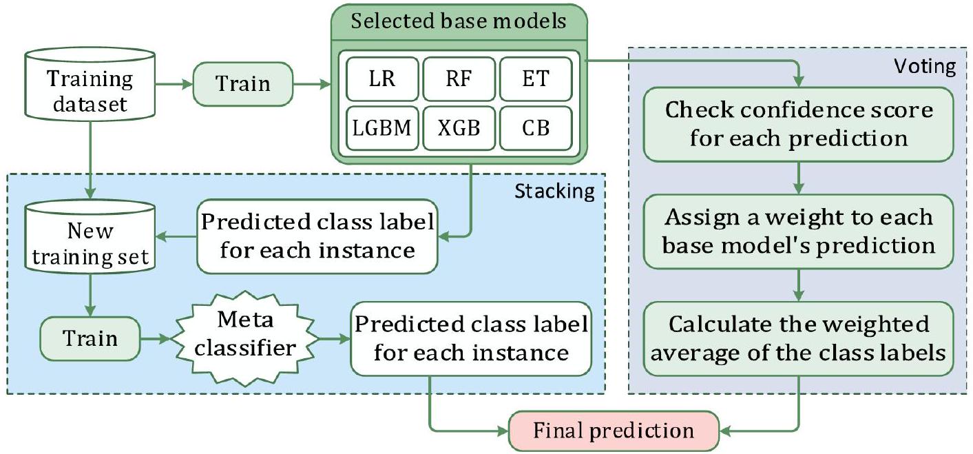
توضح الشكل 1 تدفق العمل المقترح. لقد اعتبرنا مجموعتين مختلفتين من بيانات أمراض القلب لهذه الدراسة. في البداية، قمنا بإجراء تحليل استكشافي للبيانات لتقييم وتعزيز جودة مجموعات البيانات. بحثنا عن القيم المفقودة والقيم الشاذة، لكن لم نجد أي حالات من هذا القبيل. بعد ذلك، تم تطبيع البيانات وتوحيدها وفقًا للإجراءات المعتمدة. ثم تم استخدام بيانات التدريب لبناء النموذج. قمنا أولاً بتقييم خمسة عشر نموذجًا أساسيًا. بعد التجريب مع تركيبات مختلفة من هذه النماذج الأساسية، اخترنا ستة لإنشاء نماذج التجميع والتصويت. تم تدريب النماذج المقترحة على
التكديس والتصويت
المفهوم الأساسي وراء التعلم الجماعي هو أن عدة نماذج تقليدية من التعلم الآلي يتم دمجها للتخفيف من عيوب أي نموذج واحد. النموذج المدمج الجديد يدمج نقاط القوة لمختلف النماذج، مما يؤدي إلى تحسين الأداء. تصف الأدبيات عدة طرق للتعلم الجماعي، مثل التكديس، والتصويت، والتعزيز، والتجميع.
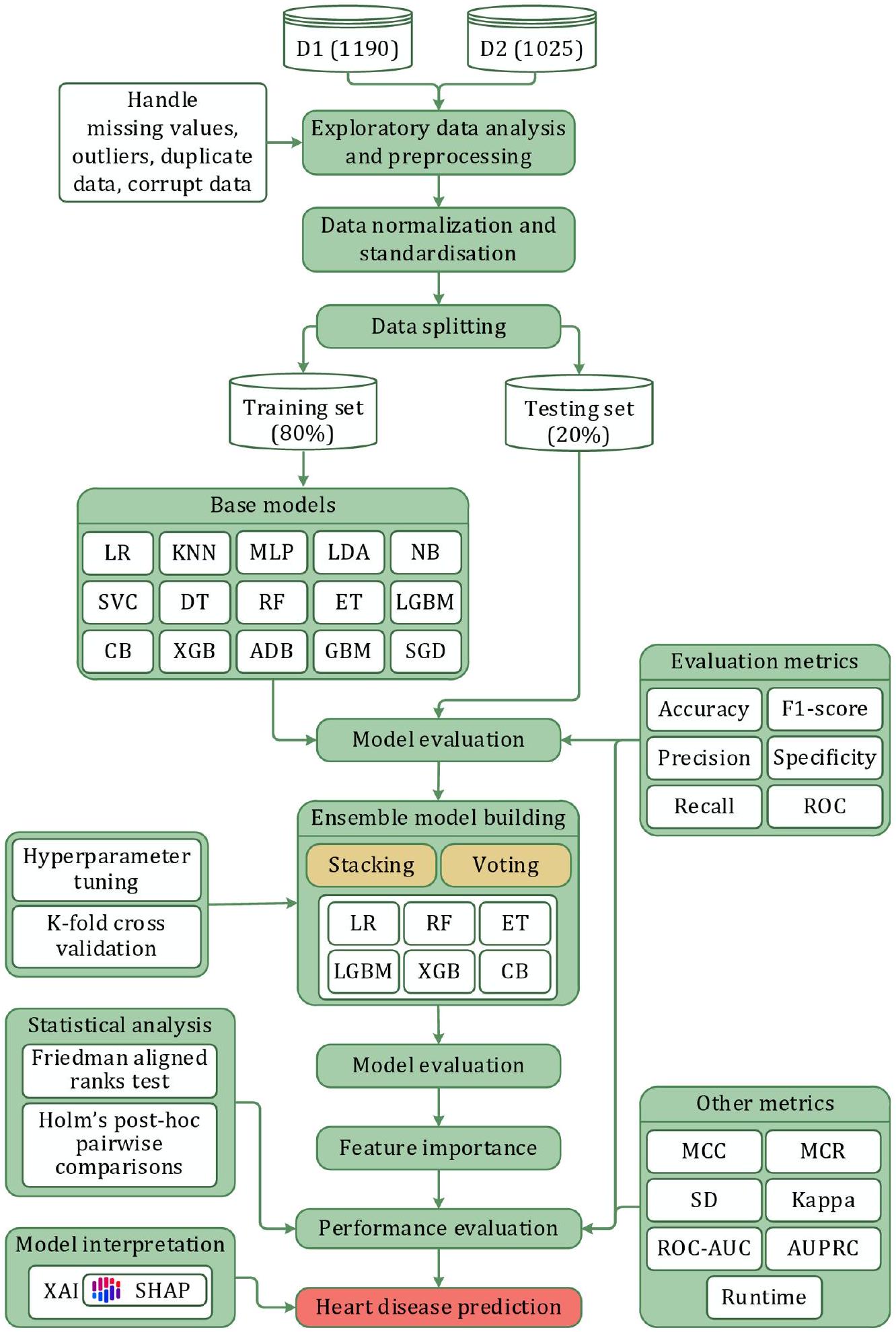
الشكل 1. المنهجية المقترحة للبحث.
ومشكلة التنبؤ المطروحة. بشكل عام، توفر تقنيات التجميع والتصويت مرونة وموثوقية من خلال الاستفادة من خصائص النماذج المختلفة، بينما تركز تقنيات التعزيز والتجميع على تقليل التباين وتصحيح الأخطاء بشكل متسلسل. في هذه الدراسة، اخترنا طرق التجميع والتصويت نظرًا لمزاياها (كما هو موضح في الشكلين 2 و 3، على التوالي) مقارنةً بالتعزيز والتجميع. تعتبر كل من تقنيات التجميع والتصويت فعالة في استغلال تنوع النماذج المتعددة لتعزيز دقة التنبؤ وموثوقيتها في مهام التعلم الآلي. فيما يلي نظرة عامة موجزة عن طرق التجميع والتصويت.

الشكل 2. مزايا التكديس.
الشكل 3. مزايا التصويت.
تكديس
تكديس (التعميم المكدس) يتضمن تدريب نماذج فردية متعددة ثم دمج توقعاتها باستخدام نموذج آخر، غالبًا ما يُشار إليه باسم النموذج الفوقي. خلال مرحلة تدريب التكديس، تتضمن الخطوة الأولى تدريب مجموعة من النماذج الأساسية المتنوعة باستخدام بيانات التدريب المتاحة. يمكن اختيار هذه النماذج الأساسية بناءً على خوارزميات أو معلمات مختلفة، مما يسمح بتوقعات مختلفة. بمجرد تدريب هذه النماذج الأساسية، يتم استخدامها لتوليد توقعات لنفس بيانات التدريب التي تم تدريبها عليها. تؤدي هذه الخطوة إلى مجموعة جديدة من التوقعات، والتي يتم دمجها بعد ذلك مع الميزات الأصلية لإنشاء مجموعة بيانات جديدة. تتكون هذه المجموعة الجديدة من البيانات من الميزات الأصلية والتوقعات التي قدمتها النماذج الأساسية. في الخطوة النهائية من مرحلة التدريب، يتم تدريب نموذج فوقي باستخدام هذه المجموعة الجديدة من البيانات، مع كون المتغير المستهدف هو النتيجة الحقيقية أو التسمية. يتعلم هذا النموذج الفوقي كيفية تقديم توقعات بناءً على المعلومات المجمعة من النماذج الأساسية والميزات الأصلية، مما يحسن الأداء العام للنموذج. خلال مرحلة توقع التكديس، تكون الخطوة الأولى هي توليد توقعات لبيانات الاختبار من خلال استخدام النماذج الأساسية المدربة. يتم تحقيق ذلك من خلال تطبيق كل من النماذج الأساسية المدربة على بيانات الاختبار، مما يؤدي إلى مجموعة من التوقعات من كل نموذج. الخطوة التالية هي دمج هذه التوقعات لإنشاء مجموعة بيانات جديدة. تتكون هذه المجموعة الجديدة من البيانات فقط من التوقعات التي قدمتها النماذج الأساسية على بيانات الاختبار. في الخطوة النهائية من مرحلة التوقع، يتم استخدام النموذج الفوقي المدرب للوصول إلى التوقع النهائي بناءً على هذه المجموعة الجديدة من البيانات. يستخدم النموذج الفوقي المعلومات من توقعات النماذج الأساسية لتقديم توقع نهائي أكثر دقة لبيانات الاختبار. إن استخدام نموذج فوقي مدرب لاستنتاج توقع نهائي بناءً على توقعات نماذج أساسية متعددة يجعل التكديس تقنية قوية لتعزيز أداء نماذج التعلم الآلي.
التصويت
يتضمن التصويت دمج توقعات نماذج متعددة من خلال أخذ تصويت الأغلبية أو متوسط مخرجاتها. يمكن أن يتم ذلك بطريقتين رئيسيتين: التصويت الصارم والتصويت الناعم. في التصويت الصارم، ينتج كل نموذج في المجموعة توقعًا، ويتم تحديد التوقع النهائي من خلال اختيار الفئة التي تتلقى أغلبية الأصوات من النماذج. في حالة الانحدار، يمكن أن يكون التوقع النهائي هو متوسط التوقعات التي قدمتها النماذج. هذه الطريقة بسيطة وفعالة، حيث تسمح بالاستفادة من نقاط القوة لكل نموذج.
مما يؤدي إلى توقع أكثر دقة. على العكس من ذلك، يتضمن التصويت الناعم أن ينتج كل نموذج في المجموعة توزيع احتمالات على الفئات. ثم يتم حساب متوسط أو دمج الاحتمالات المتوقعة من كل نموذج بطريقة ما، ويتم اتخاذ التوقع النهائي من خلال اختيار الفئة ذات أعلى احتمال مجمع. يمكن إجراء التصويت بأوزان متساوية لكل نموذج، أو يمكن تعيين أوزان بناءً على أداء أو ثقة النماذج.
مما يؤدي إلى توقع أكثر دقة. على العكس من ذلك، يتضمن التصويت الناعم أن ينتج كل نموذج في المجموعة توزيع احتمالات على الفئات. ثم يتم حساب متوسط أو دمج الاحتمالات المتوقعة من كل نموذج بطريقة ما، ويتم اتخاذ التوقع النهائي من خلال اختيار الفئة ذات أعلى احتمال مجمع. يمكن إجراء التصويت بأوزان متساوية لكل نموذج، أو يمكن تعيين أوزان بناءً على أداء أو ثقة النماذج.
نماذج المكونات
تُعزز هذه الطريقة في التعلم الجماعي نتائج التنبؤ من خلال إنشاء ميزات جديدة لمجموعات التدريب من خلال دمج التنبؤات من المتعلمين الأساسيين. تُولد هذه الطريقة الميزات الميتا اللازمة للتنبؤ النهائي من خلال دمج كل من المصنفات التقليدية والمتقدمة. تقدم هذه القسم مناقشة موجزة حول المتعلمين الأساسيين المكونين المستخدمين لبناء نماذج التكديس والتصويت. يتم اختيار المتعلمين الأساسيين لضمان التنوع داخل الدراسة. تمتلك النماذج خصائص وآليات تعلم مختلفة.
نماذج ضعيفة
المتعلمون الضعفاء هم عمومًا نماذج بسيطة تؤدي بشكل أفضل قليلاً من الصدفة العشوائية في مهمة معينة. على الرغم من أنهم قد لا يكونون دقيقين بشكل خاص بمفردهم، إلا أنهم يعملون كأساس لنماذج أكثر تعقيدًا. تُعتبر الخوارزميات التقليدية التالية في تعلم الآلة نماذج ضعيفة.
الشبكة العصبية متعددة الطبقات (MLP) هي شبكة عصبية تغذية أمامية تتكون من عدة طبقات من العقد المترابطة (الخلايا العصبية). تستخدم دوال التنشيط والأوزان لتمثيل العلاقات غير الخطية المعقدة بين ميزات الإدخال والمتغيرات المستهدفة. إنها نموذج قوي وقابل للتكيف قادر على تقريب مجموعة واسعة من الدوال. تعمل بشكل جيد لمشاكل الانحدار والتصنيف ويمكنها التعامل مع الأنماط المعقدة.
تحليل التمييز الخطي (LDA) هو خوارزمية تصنيف خطي تحدد تركيبة خطية من الميزات لتعظيم فصل الفئات. يقوم بتحويل بيانات الإدخال إلى فضاء ذي أبعاد أقل مع الحفاظ على تمييز الفئات. إنها تقنية لتقليل الأبعاد تقلل من عدد ميزات الإدخال مع الاحتفاظ بمعلومات تمييز الفئات. تعمل بشكل أفضل مع الفئات المفصولة جيدًا وتوزيعات الميزات الغاوسية.
مصنف الدعم المتجه (SVC) هو خوارزمية تعلم تحت الإشراف تحدد أفضل مستوى فائق لتقسيم الفئات بأكبر هامش.
شجرة القرار (DT) هي هيكل هرمي يقسم بيانات الإدخال وفقًا لقيم الميزات بطريقة تكرارية.
نماذج التجميع
لجعل عملية التكديس والتصويت أكثر كفاءة وموثوقية، قمنا أيضًا بدراسة عدة نماذج تجميعية لبناء الأنابيب. تستخدم هذه الدراسة الخوارزميات التجميعية التالية بناءً على شعبيتها وقدرتها.
الأشجار الإضافية (ET) هي طريقة تعلم جماعي مشابهة للأشجار العشوائية (RF). تقوم ببناء عدة أشجار قرار باستخدام مجموعات فرعية عشوائية من البيانات ثم تقوم بمتوسط النتائج لتوليد التنبؤات. على عكس الأشجار العشوائية، تستخدم الأشجار الإضافية خوارزمية عشوائية أكثر عدوانية لاختيار الميزات. تقلل الأشجار الإضافية من تكاليف الحوسبة والتكيف الزائد من خلال استخدام المزيد من العشوائية في طريقة اختيار الميزات. يمكنها التعامل مع البيانات المزعجة والمفقودة وتؤدي بشكل جيد مع البيانات عالية الأبعاد.
LGBM هو إطار عمل يعتمد على طرق التعلم المعتمدة على الأشجار. يقوم ببناء نموذج قوي من خلال تدريب العديد من النماذج الضعيفة بشكل متتابع، حيث يقوم كل نموذج لاحق بتصحيح الأخطاء التي ارتكبتها النماذج السابقة. يوفر LGBM تدريبًا وتنبؤًا سريعًا وفعالًا، مما يجعله مثاليًا لمجموعات البيانات الكبيرة ووقت-
التطبيقات المقيدة. إنه يولد نماذج دقيقة وقوية، ويتعامل بكفاءة مع الميزات الفئوية، ويدعم تحليل أهمية الميزات وتخصيص المعلمات الفائقة.
التطبيقات المقيدة. إنه يولد نماذج دقيقة وقوية، ويتعامل بكفاءة مع الميزات الفئوية، ويدعم تحليل أهمية الميزات وتخصيص المعلمات الفائقة.
تعزيز الفئات (CB) هو طريقة تعزيز تدرج تعمل بشكل جيد مع الميزات الفئوية. تستخدم نوعًا من تعزيز التدرج المعروف باسم “تعزيز مرتب” وتقنيات فريدة للتعامل مع البيانات الفئوية دون الحاجة إلى معالجة بشرية مسبقة. لا يتطلب CatBoost ترميز واحد-ساخن أو ترميز تسميات لأنه يمكنه التعامل مع ميزات الفئات مباشرة. يعمل بشكل جيد مع المعلمات الفائقة الافتراضية ويتضمن دعمًا مدمجًا للقيم المفقودة. كما يدعم CatBoost تسريع GPU لتسريع التدريب والاستدلال.
XGB، تقنية أخرى من تقنيات GB، معروفة جيدًا بقابليتها للتوسع وكفاءتها. إنها تبني نموذج تجميعي قوي من خلال دمج طرق GB مع النماذج المعتمدة على الأشجار. يتعامل XGB بكفاءة مع مجموعات البيانات الكبيرة ذات الميزات عالية الأبعاد. يدعم مجموعة متنوعة من دوال الخسارة وقياسات التقييم ويقدم تقنيات تنظيمية لمنع الإفراط في التكيف. بالإضافة إلى ذلك، يوفر XGBoost مرونة من حيث المعالجة المتوازية وخيارات التخصيص.
تعزيز التكيف (ADB) يستخدم التعلم الجماعي لإنتاج مصنف قوي من مصنفات أضعف. يمنح أوزانًا أكبر للحالات التي تم تصنيفها بشكل خاطئ في كل تكرار للتعامل مع العينات الصعبة ويعدل أوزان المصنفات الضعيفة بناءً على أدائها. ADB فعال في التعامل مع مشاكل التصنيف المعقدة ويحقق دقة عالية. حتى مع المصنفات الأساسية الضعيفة، فإنه يؤدي بشكل جيد وأقل عرضة للتكيف الزائد. ADB قادر على تصنيف كل من الحالات الثنائية والمتعددة الفئات.
الانحدار العشوائي التدرجي (SGD) هو تقنية تحسين شائعة لنماذج التعلم الآلي. في كل تكرار، يتم تغيير معلمات النموذج باستخدام مجموعة صغيرة عشوائية من بيانات التدريب، مما يجعله فعالاً من حيث الحوسبة. يعتبر SGD مثالياً لمجموعات البيانات الكبيرة وسيناريوهات التعلم عبر الإنترنت حيث تصل البيانات بشكل مستمر. يتعامل بشكل فعال مع البيانات عالية الأبعاد ويدعم مجموعة متنوعة من دوال الخسارة. بالإضافة إلى ذلك، يمكن تنفيذ SGD بشكل متوازي ويكون موفرًا للذاكرة.
مجموعة البيانات للتجربة
استخدمنا مجموعتين من البيانات تتضمن معلومات عن مرضى القلب. مجموعة البيانات الأولى (D1)، HDDC، ومجموعة البيانات الثانية (D2)، UHDD، تم جمعها من كاجل. توزيع المتغيرات المستهدفة في كلا مجموعتي البيانات موضح في الشكل 4. تحتوي D1 على سجلات لعدد إجمالي من 1,190 فردًا، حيث يعاني 629 منهم من مرض القلب، بينما لم يكن 561 منهم يعانون من ذلك. بالمقابل، كان 526 من أصل 1,025 فردًا في D2 يعانون من مرض القلب، مما يترك 499 خاليين من أمراض القلب. تتكون D1 من اثني عشر سمة لكل سجل، حيث السمة الحادية عشرة هي مستقلة (أو فرضية)، والسمة الأخيرة تعتمد (أو مستهدفة). بالإضافة إلى الاثني عشر سمة في D1، تتضمن D2 سمتين إضافيتين. تفاصيل جميع السمات في كلا مجموعتي البيانات موضحة في الجدول 1.
تم استخدام طرق IQRs والتعويض لتحديد أي قيم شاذة وقيم مفقودة في مجموعات البيانات. ومع ذلك، لم يتم العثور على مثل هذه الحالات في كل من D1 و D2. لتحديد وإدارة التعدد الخطي، استخدمنا عامل تضخم التباين (VIF)، وهو مقياس إحصائي يساعد في تحديد ومعالجة القضايا المحتملة للتعدد الخطي، مما يعزز من قابلية تفسير وموثوقية النموذج. يمكن أن يؤدي التعدد الخطي بين الميزات إلى تشويه معاملات النموذج التنبؤي، مما يؤدي إلى توقعات غير مستقرة. تشير الميزات ذات قيم VIF العالية إلى وجود تعدد خطي كبير، وفي مثل هذه الحالات، قد تحتاج إلى الاستبعاد أو التحويل.
في تحليلنا، أظهرت عدة ميزات قيم VIF مرتفعة (على سبيل المثال، AG: 34.318 في D1؛ RBP: 57.953 في D2)، كما هو موضح في الجدول 2. بينما يُعتبر VIF أكبر من 10 غالبًا مؤشرًا على وجود تعدد خطي كبير.
علاوة على ذلك، استخدمنا طريقة تحليل معامل الارتباط (CCA) لتحديد وتصوير العلاقات بين ميزات مجموعة البيانات. إنها تكشف عن قوة واتجاه العلاقة الخطية بين متغيرين وتستخدم لاختيار الميزات، وتحديد الميزات الزائدة، أو تقييم مدى صلة الميزات بالمتغير المستهدف. تساعد CCA في تحديد المتغيرات المرتبطة بقوة بنتيجة المرض وتلغي الميزات الزائدة التي ترتبط ارتباطًا وثيقًا ببعضها البعض، مما قد يعقد النموذج دون إضافة قيمة. تؤثر بشكل مباشر على عملية بناء النموذج من خلال تحسين جودة البيانات المقدمة للنماذج، مما يضمن أن يتم تدريب طرق التجميع على مجموعة أكثر فعالية من الميزات. من خلال تقليل تكرار الميزات والتعدد الخطي، تقلل CCA بشكل أساسي من خطر الإفراط في التكيف، والذي في
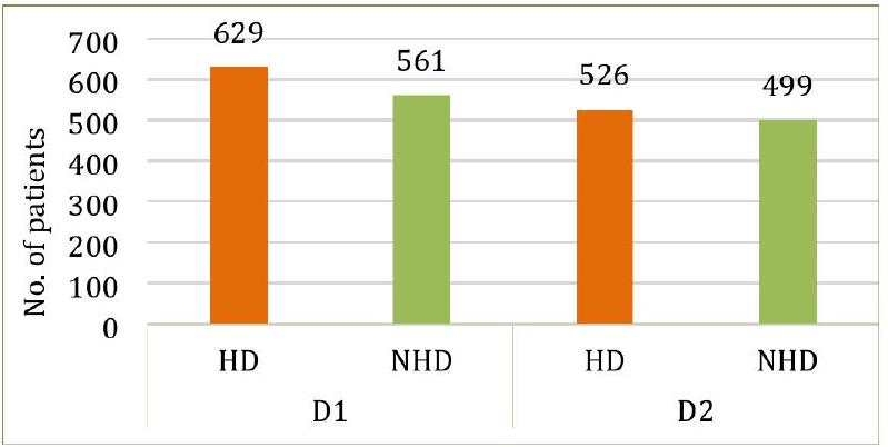
الشكل 4. توزيع المتغيرات المستهدفة في كلا المجموعتين البيانيّتين.
| صفة | اختصار | وحدة | من | ماكس | معنى | SD | 25% | 50٪ | 75% | |||||||
| D1 | D2 | D1 | D2 | D1 | D2 | D1 | D2 | D1 | D2 | D1 | D2 | D1 | D2 | |||
| عمر | AG | رقمي | ٢٨ | ٢٩ | 77 | 77 | 53.72 | 54.43 | 9.35 | 9.07 | ٤٧ | ٤٨ | ٥٤ | ٥٦ | 60 | 61 |
| جنس | جي دي | فئوي (0: أنثى، 1: ذكر) | 0 | 0 | 1 | 1 | 0.76 | 0.69 | 0.42 | 0.46 | 1 | 0 | 1 | 1 | 1 | 1 |
| نوع ألم الصدر | سي بي | رقمي | 1 | 0 | ٤ | ٣ | ٣.٢٣ | 0.94 | 0.93 | 1.02 | ٣ | 0 | ٤ | 1 | ٤ | 2 |
| ضغط الدم أثناء الراحة | RBP | مم زئبق | 0 | 94 | ٢٠٠ | ٢٠٠ | ١٣٢.١٥ | 131.61 | 18.36 | 17.51 | ١٢٠ | ١٢٠ | ١٣٠ | 130 | ١٤٠ | ١٤٠ |
| الكوليسترول في المصل | سي إل | ملغم/دل | 0 | ١٢٦ | ٦٠٣ | 564 | 210.36 | 246 | ١٠١.٤٢ | ٥١.٥٩ | 188 | 211 | 229 | ٢٤٠ | ٢٦٩.٧٥ | 275 |
| سكر الدم الصائم | FBS | ملغم/دل | 0 | 0 | 1 | 1 | 0.21 | 0.14 | 0.40 | 0.35 | 0 | 0 | 0 | 0 | 0 | 0 |
| نتائج تخطيط القلب أثناء الراحة | تسجيل | رقمي | 0 | 0 | 2 | 2 | 0.69 | 0.52 | 0.87 | 0.52 | 0 | 0 | 0 | 1 | ٢ | 1 |
| أقصى معدل ضربات قلب تم تحقيقه | MHR | رقمي | 60 | 71 | ٢٠٢ | ٢٠٢ | ١٣٩.٧٣ | 149.11 | 25.51 | 23 | 121 | 132 | ١٤٠.٥٠ | ١٥٢ | ١٦٠ | 166 |
| الذبحة الصدرية الناتجة عن التمارين | EA | فئوي (0: لا، 1: نعم) | 0 | 0 | 1 | 1 | 0.38 | 0.33 | 0.48 | 0.47 | 0 | 0 | 0 | 0 | 1 | 1 |
| الانخفاض القديم (انخفاض ST الناتج عن التمرين مقارنة بالراحة) | OP | رقمي | 2.6 | 0 | ٦ | 6.2 | 0.92 | 1.07 | 1.08 | 1.17 | 0 | 0 | 0.6 | 0.8 | 1.6 | 1.8 |
| ميل جزء ST في قمة التمرين | STS | رقمي | 0 | 0 | ٣ | 2 | 1.62 | 1.38 | 0.61 | 0.61 | 1 | 1 | 2 | 1 | ٢ | 2 |
| عدد الأوعية الرئيسية الملونة بواسطة الفلورسكوبي | CF | رقمي | – | 0 | – | ٤ | – | 0.75 | – | 1.03 | – | 0 | – | 0 | – | 1 |
| ثال (معدل ضربات قلب الثاليوم) | ث | فئوي (0: طبيعي، 1: عيب ثابت، 2: عيب قابل للعكس) | – | 0 | – | ٣ | – | 2.32 | – | 0.62 | – | 2 | – | 2 | – | ٣ |
| أمراض القلب | إتش دي | فئوي (0: لا، 1: نعم) | 0 | 0 | 1 | 1 | 0.52 | 0.51 | 0.49 | 0.50 | 0 | 0 | 1 | 1 | 1 | 1 |
الجدول 1. معلومات السمات لكلا المجموعتين البيانيّتين.
| مجموعة بيانات | AG | جي دي | سي بي | RBP | سي إل | FBS | تسجيل | MHR | EA | OP | STS | CF | ث |
| D1 | ٣٤.٣١٨ | ٤.٤٥٠ | ١٤.٤٢٠ | ٤٦.٨١٤ | 6.387 | 1.413 | 1.757 | ٢٣.٢٨٧ | ٢.٤٢٤ | ٢.٤٩٩ | 11.932 | إكس | إكس |
| D2 | ٣٨.٦٩٩ | ٣.٦١٣ | ٢.٣٧٦ | ٥٧.٩٥٣ | ٢٦.١٨٥ | 1.272 | 2.052 | 42.598 | 2.073 | 3.117 | 9.854 | 1.830 | ١٦٫٧٢٤ |
الجدول 2. قيم VIF لكلا مجموعتي البيانات.
| AG | جي دي | سي بي | RBP | سي إل | FBS | تسجيل | MHR | EA | OP | STS | إتش دي | |
| AG | 1.000 | 0.015 | 0.150 | 0.260 | -0.046 | 0.180 | 0.190 | -0.370 | 0.190 | 0.250 | 0.240 | 0.260 |
| جي دي | 0.015 | 1.000 | 0.140 | -0.006 | -0.210 | 0.110 | -0.022 | -0.180 | 0.190 | 0.096 | 0.130 | 0.310 |
| سي بي | 0.150 | 0.140 | 1.000 | 0.010 | -0.110 | 0.076 | 0.036 | -0.340 | 0.400 | 0.220 | 0.280 | 0.460 |
| RBP | 0.260 | -0.006 | 0.010 | 1.000 | 0.099 | 0.088 | 0.096 | -0.100 | 0.140 | 0.180 | 0.089 | 0.120 |
| سي إل | -0.046 | -0.210 | -0.110 | 0.099 | 1.000 | -0.240 | 0.150 | 0.240 | -0.033 | 0.057 | -0.100 | -0.200 |
| FBS | 0.180 | 0.110 | 0.076 | 0.088 | -0.240 | 1.000 | 0.032 | -0.120 | 0.053 | 0.031 | 0.150 | 0.220 |
| تسجيل | 0.190 | -0.022 | 0.036 | 0.096 | 0.150 | 0.032 | 1.000 | 0.059 | 0.038 | 0.130 | 0.094 | 0.073 |
| MHR | -0.370 | -0.180 | -0.340 | -0.100 | 0.240 | -0.120 | 0.059 | 1.000 | -0.380 | -0.180 | -0.350 | -0.410 |
| EA | 0.190 | 0.190 | 0.400 | 0.140 | -0.033 | 0.053 | 0.038 | -0.380 | 1.000 | 0.370 | 0.390 | 0.480 |
| OP | 0.250 | 0.096 | 0.220 | 0.180 | 0.057 | 0.031 | 0.130 | -0.180 | 0.370 | 1.000 | 0.520 | 0.400 |
| STS | 0.240 | 0.130 | 0.280 | 0.089 | -0.100 | 0.150 | 0.094 | -0.350 | 0.390 | 0.520 | 1.000 | 0.510 |
| إتش دي | 0.260 | 0.310 | 0.460 | 0.120 | -0.200 | 0.220 | 0.073 | -0.410 | 0.480 | 0.400 | 0.510 | 1.000 |
الشكل 5. تحليل معامل الارتباط لـ D1.
| AG | جي دي | سي بي | RBP | سي إل | FBS | تسجيل | MHR | EA | OP | STS | CF | ث | إتش دي | |
| AG | 1.000 | -0.100 | -0.072 | 0.270 | 0.220 | 0.120 | -0.130 | -0.390 | 0.088 | 0.210 | -0.170 | 0.270 | 0.072 | -0.230 |
| جي دي | -0.100 | 1.000 | -0.041 | -0.079 | -0.200 | 0.027 | -0.055 | -0.049 | 0.140 | 0.085 | -0.027 | 0.110 | 0.200 | -0.280 |
| سي بي | -0.072 | -0.041 | 1.000 | 0.038 | -0.082 | 0.079 | 0.044 | 0.310 | -0.400 | -0.170 | 0.130 | -0.180 | -0.160 | 0.430 |
| RBP | 0.270 | -0.079 | 0.038 | 1.000 | 0.130 | 0.180 | -0.120 | -0.039 | 0.061 | 0.190 | -0.120 | 0.100 | 0.059 | -0.140 |
| سي إل | 0.220 | -0.200 | -0.082 | 0.130 | 1.000 | 0.027 | -0.150 | -0.022 | 0.067 | 0.065 | -0.014 | 0.074 | 0.100 | -0.100 |
| FBS | 0.120 | 0.027 | 0.079 | 0.180 | 0.027 | 1.000 | -0.100 | -0.009 | 0.049 | 0.011 | -0.062 | 0.140 | -0.042 | -0.041 |
| تسجيل | -0.130 | -0.055 | 0.٠٤٤ | -0.120 | -0.150 | -0.100 | 1.000 | 0.048 | -0.066 | -0.050 | 0.086 | -0.078 | -0.021 | 0.130 |
| MHR | -0.390 | -0.049 | 0.310 | -0.039 | -0.022 | -0.009 | 0.048 | 1.000 | -0.380 | -0.350 | 0.400 | -0.210 | -0.098 | 0.420 |
| EA | 0.088 | 0.140 | -0.400 | 0.061 | 0.067 | 0.049 | -0.066 | -0.380 | 1.000 | 0.310 | -0.270 | 0.110 | 0.200 | -0.440 |
| OP | 0.210 | 0.085 | -0.170 | 0.190 | 0.065 | 0.011 | -0.050 | -0.350 | 0.310 | 1.000 | -0.580 | 0.220 | 0.200 | -0.440 |
| STS | -0.170 | -0.027 | 0.130 | -0.120 | -0.014 | -0.062 | 0.068 | 0.400 | -0.270 | -0.580 | 1.000 | -0.073 | -0.094 | 0.350 |
| CF | 0.270 | 0.110 | -0.180 | 0.100 | 0.074 | 0.140 | -0.078 | -0.210 | 0.110 | 0.220 | -0.073 | 1.000 | 0.150 | -0.380 |
| ث | 0.072 | 0.200 | -0.160 | 0.059 | 0.100 | -0.042 | -0.021 | -0.098 | 0.200 | 0.200 | -0.094 | 0.150 | 1.000 | -0.340 |
| إتش دي | -0.230 | -0.280 | 0.430 | -0.140 | -0.100 | -0.041 | 0.130 | 0.240 | -0.440 | -0.440 | 0.350 | -0.380 | -0.340 | 1.000 |
الشكل 6. تحليل معامل الارتباط لـ D2.
تحسن التدوير قدرة النموذج على التعميم
تتكون كلا المجموعتين من بيانات من مزيج من المتغيرات غير المتجانسة، بما في ذلك الميزات الفئوية والعشرية والعددية. كان من الضروري تطبيع البيانات لضمان أن تسهم جميع الميزات بشكل متساوٍ في أداء النموذج، حيث يمكن أن تهيمن بعض الميزات ذات النطاقات العددية الأكبر على عملية التعلم. لتطبيع قيم الميزات في كلا المجموعتين، استخدمنا المعادلة 1 التي تقوم بتعديل قيم الميزات من 0 إلى 1. تم اختيار مقياس الحد الأدنى والحد الأقصى بشكل خاص لأنه تقنية تطبيع مستخدمة على نطاق واسع تحول جميع الميزات إلى مقياس مشترك (عادةً بين 0 و 1)، وهو فعال بشكل خاص للمجموعات التي تحتوي على أنواع وقياسات ميزات متنوعة، كما هو الحال هنا. لاحظنا أن تطبيق مقياس الحد الأدنى والحد الأقصى حسّن من استقرار النماذج وتقاربها، حيث منع بعض الميزات من التأثير بشكل غير متناسب على المتعلمين الأساسيين.
أين
التجربة والنتائج
يقدم القسم التالي التفاصيل التجريبية لتوقع أمراض القلب باستخدام خوارزميات التعلم الجماعي. تحتوي الجدول 3 على تفاصيل إعداد التجربة وتكوين الكمبيوتر الذي تم إجراء التجربة عليه.
مقاييس التقييم
تقيم مقاييس التقييم مدى فعالية أداء النموذج بالنسبة لبيان المشكلة. يتم تطبيق مقاييس تقييم مختلفة اعتمادًا على طبيعة البيانات ونوع المشكلة التي يتم تحليلها. تلخص الجدول 4 مقاييس الأداء المستخدمة لتقييم النتائج التجريبية للنماذج المقدمة في هذه الدراسة. تستخدم هذه المقاييس التدابير الأساسية التالية:
- الإيجابي الحقيقي (TP) يعني أن المريض يعاني من مرض القلب، وأن النموذج يتنبأ بذلك بشكل صحيح.
- السلبية الحقيقية (TN) تعني أن المريض لا يعاني من مرض القلب، وأن النموذج يتنبأ بذلك بدقة.
- تشير الإيجابيات الكاذبة (FPs) إلى أن المريض لا يعاني من مرض القلب، ومع ذلك يتنبأ النموذج بشكل غير صحيح بنتيجة إيجابية لمرض القلب.
- يمثل السلبية الكاذبة (FN) حالة يكون فيها المريض مصابًا بأمراض القلب، لكن النموذج يتنبأ بشكل غير صحيح بنتيجة سلبية.
نتائج التنبؤ للنماذج الأساسية
يقدم هذا القسم نتائج التنبؤ للمتعلمين الأساسيين، كما تم مناقشته في القسم 3.3. يتم تقييم النماذج بناءً على ستة مقاييس: الدقة، الدقة الإيجابية، الاسترجاع، الخصوصية، درجة F1، وROC. توضح الأشكال 7 و8 نتائج التنبؤ لـ D1 وD2، على التوالي. حقق ET أعلى دقة في كلا الحالتين، بينما كان لدى KNN أدنى دقة في D1، وكان لدى MLP أدنى دقة في D2. في المتوسط، أظهرت RF وET وLGBM وCB وXGB نتائج أفضل على كلا مجموعتي البيانات.
تصميم خط الأنابيب للتكديس والتصويت
لبناء نموذج تجميعي فعال، هدفنا إلى تحديد التركيبة المثلى من النماذج الأساسية. في البداية، جربنا خمسة عشر نموذجًا أساسيًا، كما تم مناقشته في القسم السابق. قمنا بتجربة مختلف التباديل والتركيبات، كما هو موضح في الشكل 9. في التركيبة الأولى، استخدمنا أفضل عشرة نماذج، بناءً بشكل أساسي على دقتها. في التركيبة الثانية، تم استخدام عشرة نماذج تم اختيارها عشوائيًا بواسطة البرنامج. تم اعتبار ستة نماذج مشتركة بين التركبتين للمجموعة النهائية. كانت هذه النماذج الستة هي الأفضل أداءً في كلا التركبتين.
باستخدام النماذج الستة المختارة (LR، ET، RF، CB، XGB، وLGBM)، قمنا ببناء خط أنابيب لكل من التكديس والتصويت، كما هو موضح في الشكل 10. يتم تقديم عمليات بناء خط الأنابيب للتكديس والتصويت في الخوارزمية 1 والخوارزمية 2، على التوالي.
كما هو موضح في الخوارزمية 1، تم استخدام الانحدار اللوجستي كنموذج ميتا في دراستنا للتكديس. كان اختيار الانحدار اللوجستي كالمصنف الميتا مستندًا إلى الأدبيات الأساسية والتحقق التجريبي. وولبرت
في هذه الدراسة، جربنا أيضًا مصنفات ميتا بديلة مثل KNN و LDA. ومع ذلك، كما هو متوقع، لم تحقق هذه النماذج أداءً تنافسيًا مقارنة بـ LR، سواء من حيث الدقة أو الاستقرار. يتم عرض الأداء المقارن لـ LR و KNN و LDA كمتعلمين ميتا في الشكل 11. أظهر LR قدرة تفوق في التعميم عند تجميع التنبؤات من متعلمين أساسيين متنوعين، ولهذا السبب تم الاحتفاظ به كنموذج ميتا في نموذج التكديس لدينا.
| الأجهزة/البرامج | المواصفات |
| المعالج | الجيل الحادي عشر من إنتل
|
| الذاكرة العشوائية | 8.00 جيجابايت (7.80 جيجابايت قابلة للاستخدام) (DDR4) |
| وحدة التخزين SSD | 256 جيجابايت (NVMe) |
| القرص الصلب | 2 تيرابايت (HDD) |
| نظام التشغيل | ويندوز 11 هوم بلغة واحدة 64 بت (10.0) |
| لغة البرمجة | بايثون |
| المنصة | دفتر جوبتر |
الجدول 3. الأجهزة والبرامج المستخدمة لإجراء التجربة.
| المقاييس | الحساب | الوصف |
| الدقة |
|
تقيس الدقة صحة التنبؤات العامة للنموذج، بما في ذلك كل من TPs و TNs. |
| الدقة |
|
تقيس الدقة نسبة التنبؤات الإيجابية الصحيحة من إجمالي التنبؤات الإيجابية التي قام بها النموذج، أي أنها تشير إلى قدرة النموذج على تحديد المرضى الذين يعانون من أمراض القلب بشكل صحيح. إنها مفيدة عندما يكون تقليل FPs أمرًا حاسمًا. |
| الاسترجاع |
|
يقيس الاسترجاع نسبة التنبؤات الإيجابية الصحيحة من الحالات الإيجابية الفعلية، أي أنه يعكس قدرة النموذج على اكتشاف المرضى الذين يعانون من أمراض القلب بشكل صحيح. إنه مهم في الحالات التي تكون فيها FNs حاسمة. |
| درجة F1 |
|
تعطي درجة F1 مقياسًا واحدًا يوازن بين الاسترجاع والدقة من خلال أخذ المتوسط التوافقي بين الاثنين. إنها مفيدة بشكل خاص عندما تكون مجموعة البيانات غير متوازنة أو عندما تكون الدقة والاسترجاع متساويين في الأهمية. تشير درجة F1 العالية إلى توازن جيد بين الدقة والاسترجاع. |
| الخصوصية |
|
تقيس الخصوصية عدد حالات أمراض القلب التي تم التنبؤ بها سلبًا والتي تبين أنها TN. تشير إلى قدرة النموذج على تحديد الأفراد الذين لا يعانون من أمراض القلب بشكل صحيح. الخصوصية مهمة عندما يكون تقليل FPs أمرًا حاسمًا، لأن FPs قد تؤدي إلى إجراءات طبية غير ضرورية. |
| المتوسط الكلي (MA) |
|
يحدد MA متوسط الأداء عبر جميع الفئات أو الفئات. هنا،
|
| المتوسط المرجح (WA) |
|
يوفر WA ملخصًا للأداء يأخذ في الاعتبار توزيع الفئات. إنه مفيد في مجموعات البيانات غير المتوازنة عندما تحتوي بعض الفئات على عدد أكبر بكثير من الحالات مقارنةً بأخرى. |
| الانحراف المعياري (SD) |
|
يقيم SD تباين مقاييس الأداء عبر عدة طيات، مما يوفر رؤى حول اتساق النموذج أو استقراره. يشير SD الأقل إلى نتائج أكثر اتساقًا. (
|
| كاررا |
|
كابا كوهين هو مقياس لقياس درجة الاتفاق بين التسميات الفعلية والمتوقعة للفئات التي تأخذ في الاعتبار الاتفاق المحتمل بالصدفة. عندما يكون توزيع الفئات منحرفًا، أو كانت الفئة الغالبة شائعة جدًا، فإنه يساعد في تقييم مدى جودة أداء النموذج. |
| معامل ارتباط ماثيو (MCC) |
|
يقيس MCC جودة التصنيفات الثنائية. يتراوح بين -1 و +1، حيث تشير +1 إلى تصنيف صحيح، و 0 تشير إلى تصنيف عشوائي، و -1 تشير إلى تصنيف خاطئ تمامًا. يشير MCC الأكبر إلى تحسين أداء النموذج. |
| منحنى خصائص التشغيل المستقبلية (ROC) | TPR (محور Y) مقابل FPR (محور X) | يوضح منحنى ROC التوازن بين الاسترجاع والخصوصية. يظهر مدى جودة أداء النموذج عند إعدادات عتبة مختلفة لتنبؤ أمراض القلب. يشير ROC الأعلى إلى أداء أفضل للنموذج. |
| المساحة تحت المنحنى (AUC) |
|
تمثل AUC المساحة تحت منحنى ROC وتوفر قيمة عددية واحدة تلخص الأداء العام لنموذج التنبؤ. تشير AUC الأعلى إلى تمييز أكثر دقة بين الحالات الإيجابية والسلبية لأمراض القلب بين المرضى. |
| المساحة تحت منحنى الدقة والاسترجاع (AUPRC) |
|
مؤشر على مدى جودة أداء النموذج على مجموعات البيانات غير المتوازنة، AUPRC هي المساحة تحت منحنى الدقة والاسترجاع. تأخذ في الاعتبار التوازن بين الدقة والاسترجاع. تشير AUPRC الأعلى إلى أداء أفضل، خاصة عند تحديد الحالات الإيجابية بشكل صحيح. |
| معدل التصنيف الخاطئ (MCR) |
|
نسبة الحالات التي تم تصنيفها بشكل خاطئ بالنسبة لإجمالي الحالات تُسمى MCR، وتُعرف أيضًا بمعدل الخطأ. تكمل الدقة من خلال إعطاء نسبة الأحداث المصنفة بشكل خاطئ. يشير انخفاض معدل التصنيف الخاطئ إلى تحسين أداء النموذج. |
| وقت التنفيذ | – | وقت تنفيذ الخوارزمية بالثواني. |
الجدول 4. مقاييس تقييم الأداء.
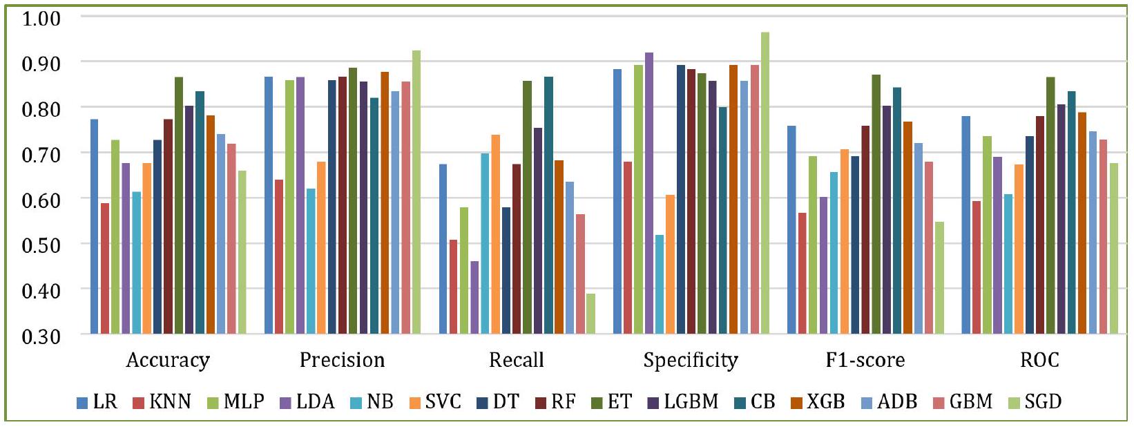
الشكل 7. أداء النماذج الأساسية مع D1.
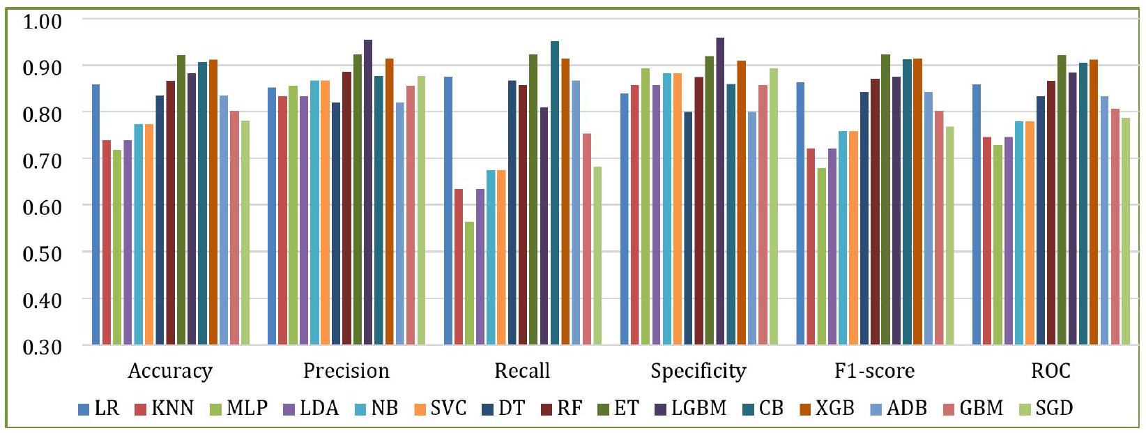
الشكل 8. أداء النماذج الأساسية مع D2.
الشكل 9. اختيار النموذج.
الشكل 10. بناء خط الأنابيب للتكديس والتصويت.
الشكل 11. الأداء المقارن لـ LR و KNN و LDA كمتعلمين ميتا.
Input: a) Training/validation dataset $boldsymbol{T}_{boldsymbol{R}}=left{boldsymbol{x}_{boldsymbol{i}}, boldsymbol{y}_{boldsymbol{i}}right}_{boldsymbol{i}=mathbf{1}}^{boldsymbol{n}}, boldsymbol{n}$ is no. of instances
    b) Base models: $boldsymbol{B}_{boldsymbol{L}}=left{boldsymbol{b}_{boldsymbol{1}}+boldsymbol{b}_{boldsymbol{2}}+ldots+boldsymbol{b}_{boldsymbol{k}}right}$
    c) A meta-classifier (LR)
Output: Ensemble stacking classifier S
    Initialize an empty 2D array $boldsymbol{S}$ of size $n times k$ to store base learner predictions
    For each base learner $boldsymbol{b}_{boldsymbol{j}}$ in $boldsymbol{B}_{boldsymbol{L}}$ do
        Initialize hyperparameters for $boldsymbol{b}_{boldsymbol{j}}$
        Initialize an empty 1D array $boldsymbol{P}$ to store validation metrics $boldsymbol{P}_{i}$
        For each instance $boldsymbol{i} in{1,2,3, ldots, n}$
            Train $boldsymbol{b}_{boldsymbol{j}}$ on $boldsymbol{T}_{boldsymbol{R}}^{(-boldsymbol{i})}$ // Train all instances except $i^{text {th }}$; keep one for cross-validation
            Predict $boldsymbol{x}_{boldsymbol{i}}$ and compute performance metric $boldsymbol{P}_{boldsymbol{i}}$
            Append $boldsymbol{P}_{boldsymbol{i}}$ to $boldsymbol{P}$
        End
        Compute average validation score $boldsymbol{P}=frac{mathbf{1}}{boldsymbol{n}} sum_{boldsymbol{i}=mathbf{1}}^{boldsymbol{n}} boldsymbol{P}_{boldsymbol{i}} / /$ Aggregate performance
        Adjust hyperparameters to maximize $boldsymbol{P}$ // Optimize hyperparameters
        Go to Step 4 until $boldsymbol{P}$ improvement $<1 %$ || Saturation
        Store the best hyperparameters for $boldsymbol{b}_{boldsymbol{j}}$
        Train $boldsymbol{b}_{boldsymbol{j}}$ on full $boldsymbol{T}_{boldsymbol{R}} / /$ Final training
        Perform cross-validation using the remaining instance
        Store the predicted class labels for $boldsymbol{T}_{boldsymbol{R}}$ in column $boldsymbol{j}$ of $boldsymbol{S}$
    End
    Initialize another $2 D$ array $boldsymbol{T}_{boldsymbol{N}}$ of size $n times(k+1) / /$ Prepare meta-dataset
    Concatenate $boldsymbol{S}$ with original labels $boldsymbol{y}: boldsymbol{T}_{boldsymbol{N}}=[boldsymbol{S} boldsymbol{y}]$
    For each instance $boldsymbol{i} in{1,2,3, ldots, n} / /$ Train meta-learner (LR)
        Train $boldsymbol{L} boldsymbol{R}$ on $boldsymbol{T}_{boldsymbol{N}}^{(-boldsymbol{i})}$ // Train all instances except $i^{text {th }}$; keep one for cross-validation
        Predict $boldsymbol{x}_{boldsymbol{i}}$ and store the result in $boldsymbol{S}$
    End
    Return the predicted class labels in $boldsymbol{S}$
الخوارزمية 1. إجراء التكديس.
Input: a) Training/validation dataset $boldsymbol{T}_{boldsymbol{R}}=left{boldsymbol{x}_{boldsymbol{i}}, boldsymbol{y}_{boldsymbol{i}}right}_{boldsymbol{i}=mathbf{1}}^{boldsymbol{n}}, boldsymbol{n}$ is no. of instances
        b) Base models: $boldsymbol{B}_{L}=left{boldsymbol{b}_{1}+boldsymbol{b}_{2}+ldots+boldsymbol{b}_{k}right}$
Output: Ensemble voting classifier $boldsymbol{V}$
    Initialize an empty 2D array $boldsymbol{V}$ of size $n times k$ to store base learner predictions
    Initialize an empty 2D array $boldsymbol{C}$ to store confidence scores for each prediction
    For each base learner $boldsymbol{b}_{boldsymbol{j}}$ in $boldsymbol{B}_{boldsymbol{L}}$ do
        Initialize hyperparameters for $boldsymbol{b}_{boldsymbol{j}}$
        Initialize an empty 1D array $boldsymbol{P}$ to store validation metrics $boldsymbol{P}_{boldsymbol{i}}$
        For each instance $boldsymbol{i} in{1,2,3, ldots, n}$
            Train $boldsymbol{b}_{boldsymbol{j}}$ on $boldsymbol{T}_{boldsymbol{R}}^{(-boldsymbol{i})}$ // Train all instances except $i^{text {th }}$; keep one for cross-validation
            Predict $boldsymbol{x}_{boldsymbol{i}}$ and compute performance metric $boldsymbol{P}_{boldsymbol{i}}$
            Append $boldsymbol{P}_{boldsymbol{i}}$ to $boldsymbol{P}$
        End
        Compute the average validation score $boldsymbol{P}=frac{mathbf{1}}{boldsymbol{n}} sum_{boldsymbol{i}=mathbf{1}}^{boldsymbol{n}} boldsymbol{P}_{boldsymbol{i}} / /$ Aggregate performance
        Adjust hyperparameters to maximize $boldsymbol{P}$ // Optimize hyperparameters
        Go to Step 4 until $boldsymbol{P}$ improvement < $1 %$ // Saturation
        Store the best hyperparameters for $boldsymbol{b}_{boldsymbol{j}}$
        Train $boldsymbol{b}_{boldsymbol{j}}$ on full $boldsymbol{T}_{boldsymbol{R}} / /$ Final training
        Perform cross-validation using the remaining instance
    Store the predicted class labels for $boldsymbol{T}_{R}$ in column $boldsymbol{j}$ of $boldsymbol{V}$ and confidence scores in $boldsymbol{C}$
    End
    Calculate the weighted vote for each class label based on the confidence scores in $boldsymbol{C}$
    Assign the class label with the highest weighted vote to $V$ for this instance
    Return the predicted class labels in $V$
الخوارزمية 2. إجراء التصويت.
التحقق المتقاطع
يتم استخدام التحقق المتقاطع K -fold عادةً لتقليل التحيز الموجود في مجموعة البيانات. في هذه التقنية، يتم تقسيم مجموعة البيانات إلى
تقييم أهمية الميزات
يتم تصنيف المتغيرات المتنبئة (السمات المدخلة) في إجراء أهمية الميزات وفقًا للمدى الذي تساهم به في التنبؤ بالمتغير المستهدف (الميزة الناتجة). هذه المرحلة ضرورية لنماذج التعلم الآلي والتعلم الجماعي لتحقيق تنبؤات أكثر دقة. استخدمنا درجة أهمية الميزات (درجة F)، وهي مقياس يشير إلى مدى تكرار استخدام سمة ما للتقسيم أثناء عملية التدريب والتي يتم تعريفها بواسطة المعادلة
حيث،
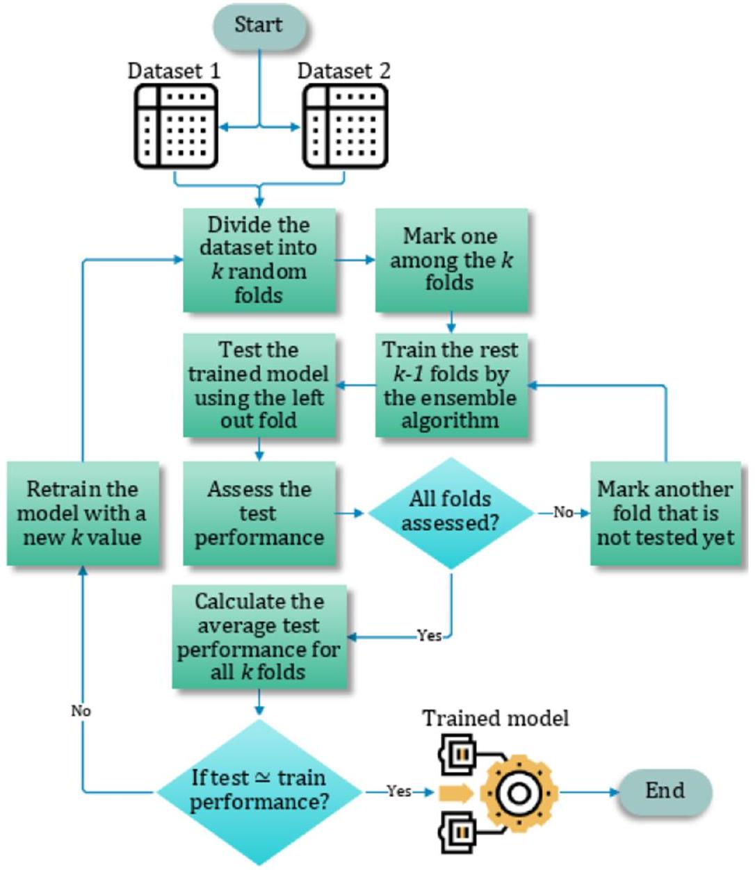
الشكل 12. عملية التحقق المتقاطع
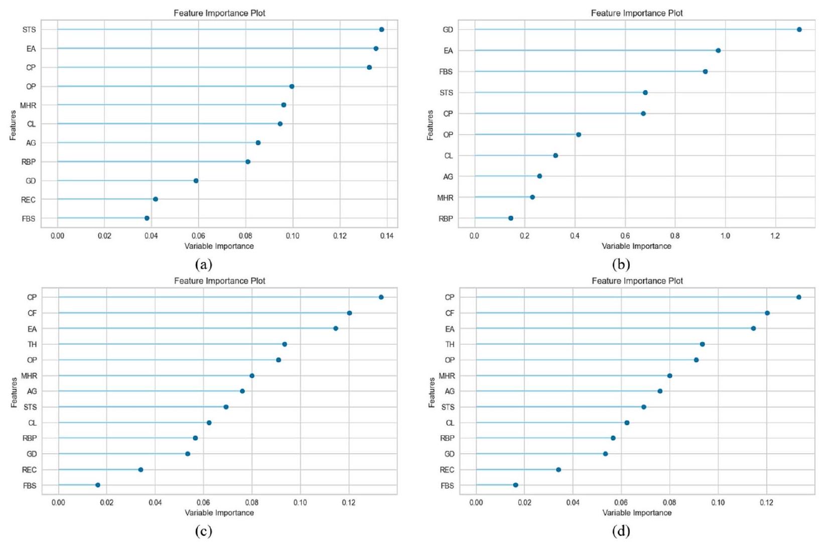
الشكل 13. أهمية الميزات لـ (أ) التكديس مع D1، (ب) التصويت مع D1، (ج) التكديس مع D2 و (د) التصويت مع D2.
الميزة i من الحالة السلبية k. يشير البسط إلى التمييز بين العينات الإيجابية والسلبية، بينما يحدد المقام التمييز داخل كل من العينتين. تشير درجة F الأكبر إلى أن هذه الميزة أكثر تمييزًا
تظهر المساهمات لكل معلمة تنبؤية تم استخدامها في هذه الدراسة في حدوث أمراض القلب في الشكل 13. عندما تم تطبيق التكديس على D1، ساهمت STS و FBS بأكبر وأقل مساهمة على التوالي. في سياق التصويت مع D1، ساهمت GD و RBP بأكبر وأقل مساهمة على التوالي. وبالمثل، أظهرت CP و FBS أكبر وأقل مساهمات على التوالي، مع D2 باستخدام كل من التكديس والتصويت.
تعديل المعلمات الفائقة
يعد تعديل المعلمات الفائقة عملية مهمة للغاية، حيث تتحكم في سلوك خوارزمية التدريب وتؤثر بشكل كبير على تقييم أداء النموذج. استخدمنا PyCaret (https://pycare t.org/)، أداة شائعة لأتمتة سير عمل تعلم الآلة، لضبط المعلمات الفائقة وتحقيق الأداء الأمثل في النموذج المقترح. تم تقديم تفاصيل المعلمات الفائقة لكل نموذج في الجدول 5. وقد حدد تجربتنا أن القيم المحددة لكل معلمة في النموذج المعني هي القيم المثلى.
نتائج التنبؤ لنماذج التجميع والتصويت
تم تقييم أداء التصنيف للخوارزميات باستخدام مصفوفة الالتباس. يتم عرض مصفوفات الالتباس من تجارب التكديس والتصويت على كلا المجموعتين في الشكل 14. يشير الشكل 14c إلى أن نموذج التكديس المصمم حقق أفضل أداء مع D2. من بين 308 حالات في D2، تم تصنيف جميع الحالات بشكل صحيح، بينما تم تصنيف حالتين بشكل خاطئ. بالمقابل، من بين 357 حالة في D1، كما هو موضح في الشكل 14b، قام نموذج التصويت المصمم بتصنيف 330 حالة بشكل صحيح بينما تم تصنيف 27 حالة بشكل خاطئ.
توضح دقة نماذج التجميع والتصويت لـ D1 و D2 في الشكل 15. يقدم الشكل دقة كل طية من كلا النموذجين المصممين بالإضافة إلى متوسط الـ 10 طيات. أظهر كل من التجميع والتصويت دقة متوسطة قدرها
تم تقديم انحرافات الأداء لنماذج التجميع والتصويت مع كلا المجموعتين عبر عشرة طيات لكل مقياس في الشكل 17. أظهر التجميع مع D1 أكبر قدر من الاتساق لكل مقياس باستثناء الاسترجاع. كان التصويت مع D1 الأكثر عدم اتساق عبر جميع المقاييس باستثناء الاسترجاع، حيث أظهر التجميع مع D1 انحرافًا أكبر.
| الهايبر بارامترز | LR | إي تي | RF | إكس جي بي | سي بي | LGBM |
| نسبة التعبئة | – | – | – | – | – | 0.7 |
| تكرار التعبئة | – | – | – | – | – | 2 |
| مصفوفة بايزيان للتسجيل | – | – | – | – | 0.1 | – |
| أفضل_نموذج_أدنى_عدد_من_الأشجار | – | – | – | – | 1 | – |
| تعزيز من المتوسط | – | – | – | – | زائف | – |
| معزز | – | – | – | شجرة جي بي | – | – |
| نوع التعزيز | – | – | – | – | سهل | gbdt |
| بوتستراب | – | خاطئ | صحيح | – | – | – |
| نوع الإقلاع | – | – | – | – | MVS | – |
| عدد الحدود | – | – | – | – | 254 | – |
| ج | 0.431 | – | – | – | – | – |
| ccp_alpha | – | 0 | 0 | – | – | – |
| أسماء الفئات | – | – | – | – | [0, 1] | – |
| وزن_الفئة | متوازن | – | – | – | – | – |
| عدد الفصول | – | – | – | – | 0 | – |
| نسبة العينة من الشجرة | – | – | – | 0.7 | – | 1 |
| معيار | – | جيني | جيني | – | – | – |
| عمق | – | – | – | – | ٦ | – |
| جهاز | – | – | – | وحدة المعالجة المركزية | – | – |
| ثنائي | زائف | – | – | – | – | – |
| تمكين الفئات | – | – | – | زائف | – | – |
| تقييم الكسر | – | – | – | – | 0 | – |
| مقياس التقييم | – | – | – | – | خسارة اللوغاريتم | – |
| نوع حدود الميزة | – | – | – | – | جمع السجل الجشع | – |
| نسبة الميزة | – | – | – | – | – | 0.5 |
| توافق التقاطع | صحيح | – | – | – | – | – |
| وزن_زوج_الوحدة_القوة_التلقائي | – | – | – | – | زائف | – |
| سياسة النمو | – | – | – | – | شجرة متناظرة | – |
| نوع الأهمية | – | – | – | – | – | انقسام |
| تعديل الاعتراض | 1 | – | – | – | – | – |
| تكرارات | – | – | – | – | 1000 | – |
| 12_ورقة_تنظيم | – | – | – | – | ٣ | – |
| تقدير_ورقة_التراجع | – | – | – | – | أي تحسين | – |
| عدد_iterations_تقدير_الورقة | – | – | – | – | 10 | – |
| طريقة تقدير الورقة | – | – | – | – | نيوتن | – |
| معدل التعلم | – | – | – | 0.0001 | 0.008938 | 0.0000001 |
| دالة الخسارة | – | – | – | – | خسارة اللوغاريتم | – |
| العمق الأقصى | – | – | – | ٨ | – | -1 |
| عدد الميزات القصوى | – | جذر | جذر | – | – | – |
| max_iter | 1000 | – | – | – | – | – |
| max_leaves | – | – | – | – | 64 | – |
| عدد العينات في الطفل الأدنى | – | – | – | – | – | 91 |
| وزن_الطفل_الأدنى | – | – | – | ٣ | – | 0.001 |
| min_data_in_leaf | – | – | – | – | 1 | – |
| انخفاض الشوائب الدنيا | – | 0 | 0 | – | – | – |
| عدد العينات في الورقة | – | 1 | 1 | – | – | – |
| عدد العينات المطلوبة للتقسيم | – | 2 | 2 | – | – | – |
| حد الكسب الأدنى | – | – | – | – | – | 0.1 |
| نسبة الوزن الأدنى للورقة | – | 0 | 0 | – | – | – |
| وضع تقليص النموذج | – | – | – | – | ثابت | – |
| معدل انكماش النموذج | – | – | – | – | 0 | – |
| حجم_النموذج_تنظيم | – | – | – | – | 0.5 | – |
| متعدد الفئات | سيارة | – | – | – | – | – |
| عدد النماذج | – | 100 | 100 | 10 | – | ٢٠٠ |
| عدد الوظائف | – | -1 | -1 | -1 | – | -1 |
| وضع نان | – | – | – | – | من | – |
| مستمر | ||||||
| الهايبر بارامترز | LR | إي تي | RF | إكس جي بي | СВ | LGBM |
| عدد الأوراق | – | – | – | – | – | ٨ |
| درجة خارجية | – | زائف | زائف | – | – | – |
| معامل العقوبات | – | – | – | – | 1 | – |
| عقوبة | ل2 | – | – | – | – | – |
| خيارات_معلومات_المسبح | – | – | – | – | {‘tags’: {}} | – |
| العينة اللاحقة | – | – | – | – | زائف | – |
| نوع_score_عشوائي | – | – | – | – | عادي مع تقليل حجم النموذج | – |
| حالة عشوائية | 42 | 42 | 42 | 42 | 42 | 42 |
| قوة عشوائية | – | – | – | – | 1 | – |
| الرجوع_ألفا | – | – | – | 0.001 | – | 0.000001 |
| اللامدا التنظيمية | – | – | – | 0.0005 | – | 0.0005 |
| رسم | – | – | – | – | 1 | – |
| تردد العينة | – | – | – | – | بير تري | – |
| وزن_مقياس_الإيجابية | – | – | – | 8.5 | – | – |
| دالة النتيجة | – | – | – | – | جيب التمام | – |
| حل | لبفغس | – | – | – | – | – |
| نسبة صراع الميزات النادرة | – | – | – | – | 0 | – |
| عينة فرعية | – | – | – | 1 | 0.8 | 1 |
| تحت عينة من أجل الصندوق | – | – | – | – | – | ٢٠٠,٠٠٠ |
| تردد العينة الفرعية | – | – | – | – | – | 0 |
| نوع المهمة | – | – | – | – | وحدة المعالجة المركزية | – |
| تول | 0.0001 | – | – | – | – | – |
| طريقة الشجرة | – | – | – | سيارة | – | – |
| استخدام أفضل نموذج | – | – | – | – | خاطئ | – |
| مُطوَّل | 0 | 0 | 0 | 0 | – | – |
| بدء دافئ | زائف | زائف | زائف | – | – | – |
الجدول 5. المعلمات الفائقة للنماذج المتسلسلة المستخدمة في التكديس والتصويت.
وفقًا لدرجات ROC-AUC، كما هو موضح في الشكل 18، كانت أداء التكديس والتصويت متشابهًا (0.97 لكلا الفئتين) بالنسبة لـ D2، بينما بالنسبة لـ D1، كان التكديس (0.92 لكلا الفئتين) متقدمًا قليلاً على التصويت (0.91 لكلا الفئتين). على العكس من ذلك، هناك تباين كبير في أداء التكديس والتصويت فيما يتعلق بـ AUPRC. كما هو موضح في الشكل 19، تم تحقيق أفضل AUPRC بواسطة التكديس مع D2 (0.98)، بينما أدى التصويت مع D2 إلى أدنى AUPRC (0.91). الشكل 20 أشار إلى أن MCR للتكديس مع D2 كان الأدنى عند 1.67، بينما كان التصويت مع D1 لديه أعلى MCR وهو 9.12.
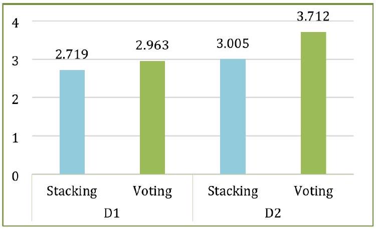
قمنا أيضًا بتسجيل وقت التشغيل لأربعة تركيبات من النماذج ومجموعات البيانات. كما هو موضح في الشكل 21، كانت عملية التجميع أسرع قليلاً من التصويت، وكما هو متوقع، كانت النماذج تحتاج إلى وقت أقل مع D1 مقارنة بـ D2 بسبب أن D1 أصغر حجمًا من D2.
التحليل والمناقشة
تحلل هذه القسم بدقة وتناقش الأداء التنبؤي لنماذج التجميع والتصويت المقترحة من زوايا مختلفة، مقارنتها بالنماذج الأساسية الفردية والأبحاث التجريبية التي استخدمت التجميع أو التصويت في التنبؤ بأمراض القلب.
نماذج التجميع والتصويت مقارنة بالنماذج الأساسية
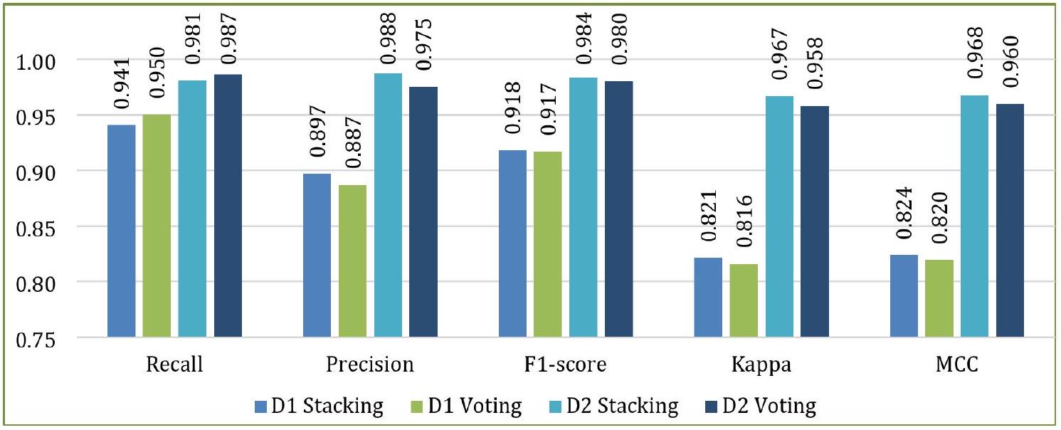
تمت مقارنة أداء نماذج التجميع والتصويت المصممة مع أداء النماذج المكونة التي تم النظر فيها. كانت المقارنة مبنية على الدقة، والدقة الإيجابية، والاسترجاع، ودرجة F1، ومقاييس ROC لكلا مجموعتي البيانات. تم مقارنة أفضل الأداءات بين 15 نموذجًا لكل مقياس مع تلك الخاصة بنماذج التجميع والتصويت، كما هو موضح في الشكل 22. على سبيل المثال، كما تم مناقشته في القسم 5.2، أظهر نموذج ET أفضل دقة عبر كلا مجموعتي البيانات. يوضح الشكل 22a أن كلا من نماذج التجميع والتصويت تحقق دقة أعلى من ET. وبالمثل، أظهر نموذج CB أفضل استرجاع بين النماذج الـ 15. كما هو موضح في الشكل 22c، حققت نماذج التجميع والتصويت استرجاعًا أعلى من CB. لذلك، تتفوق نماذج التجميع والتصويت المقترحة على جميع النماذج المكونة ذات الأداء الأفضل عبر كلا مجموعتي البيانات، باستثناء الدقة على D1، حيث يتفوق نموذج SGD على نماذج التجميع والتصويت.
التحليل الإحصائي لنماذج التجميع والتصويت
لتقييم الأهمية الإحصائية للاختلافات في الأداء بين النماذج، قمنا بإجراء اختبار فريدمان المرتب غير المعلمي.
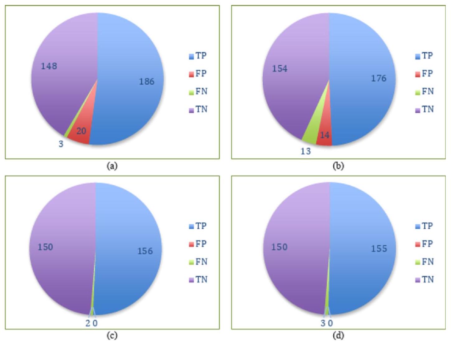
الشكل 14. مصفوفات الالتباس لـ (أ) التكديس مع D1، (ب) التصويت مع D1، (ج) التكديس مع D2 و (د) التصويت مع D2.
الشكل 15. دقة التجميع والتصويت بعشرة أضعاف على كلا المجموعتين البيانيّتين.
تم استخدام اختبار الرتب المتوافقة مع فريدمان لمقارنة النماذج بشكل شامل عبر مجموعات البيانات والمعايير مع الأخذ في الاعتبار تباين مجموعة البيانات.
الشكل 16. مقاييس أداء أخرى للتكديس والتصويت على كلا المجموعتين البيانيّتين.
الشكل 17. الانحراف المعياري للطيّات لمقاييس مختلفة للتكديس والتصويت مع كلا المجموعتين البيانيّتين.
0.2059 ، وهو فوق عتبة الدلالة (
تحليل ما بعد الحدث. المقارنات بعد الحدث باستخدام طريقة هولم.
تفسير نماذج التكديس والتصويت باستخدام SHAP
تهدف XAI إلى تعزيز الشفافية وقابلية التفسير لنماذج التعلم الآلي، مما يسمح للمستخدمين بفهم الأسباب وراء التنبؤات. هذا أمر بالغ الأهمية بشكل خاص في المجالات الحساسة مثل الرعاية الصحية، حيث الثقة والمساءلة أمران أساسيان.
في سياق توقع أمراض القلب، يثبت SHAP أنه لا يقدر بثمن. إنه يساعد الأطباء والباحثين في تحديد السمات التي تلعب الأدوار الأكثر أهمية في تشخيص أمراض القلب. من خلال توضيح الأهمية النسبية لهذه الميزات، لا يعزز SHAP فقط قابلية تفسير النماذج، بل يعزز أيضًا الثقة في تطبيقها السريري، مما يضمن أن التوقعات دقيقة وقابلة للتنفيذ.
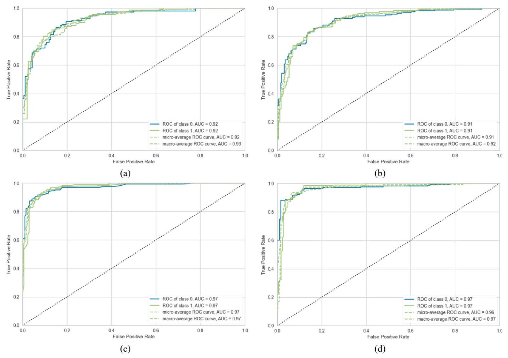
الشكل 18. ROC-AUC لـ (أ) التكديس مع D1، (ب) التصويت مع D1، (ج) التكديس مع D2 و (د) التصويت مع D2.
تفسير عالمي
تساعد التفسيرات العالمية في فهم كيفية أداء نموذج الذكاء الاصطناعي عبر مجموعة بيانات كاملة من خلال الكشف عن الاتجاهات العامة والعلاقات بين المتغيرات (مثل العمر، العلامات الجينية، نتائج المختبر) ونتائج النموذج. تحدد هذه التفسيرات الخصائص الأكثر تأثيرًا على التنبؤات، مما يمكّن من التحقق من صحة هذه التنبؤات مقابل المعرفة المتخصصة في المجال، مثل الإرشادات الطبية. يساعد ذلك في التحقق من أداء النموذج وتحديد المجالات التي تتطلب تحسينًا.
علاوة على ذلك، فإن التفسيرات العالمية ضرورية في اكتشاف التحيزات، وتعزيز العدالة عبر مجموعات سكانية متنوعة، وضمان الامتثال للمعايير الأخلاقية والتنظيمية مثل اللائحة العامة لحماية البيانات (GDPR) ومتطلبات قانون نقل التأمين الصحي والمساءلة (HIPAA) وإدارة الغذاء والدواء (FDA). مثل هذه الشفافية تبني الثقة في أنظمة الرعاية الصحية.
في تحليلنا، استخدمنا قيم أهمية ميزات SHAP المطلقة المتوسطة لترتيب الميزات وفقًا لتأثيرها العام على التنبؤات، بغض النظر عما إذا كان تأثيرها إيجابيًا أو سلبيًا. يتم توضيح التحليلات العالمية لنماذج التجميع والتصويت عبر D1 و D2 في الأشكال 23 و 24، على التوالي. يتم تنظيم الميزات حسب الأهمية على المحور الرأسي، مع عرض قيم SHAP المتوسطة على المحور الأفقي لرؤية غير متحيزة لأهميتها النسبية.
في نموذج التكديس المطبق على D1، يظهر ميل ذروة شريحة ST أثناء التمرين (STS) كأهم ميزة، مما يعكس ارتباطه القوي بأمراض القلب. وبالمثل، يعد نوع ألم الصدر (CP) عاملاً حاسماً، متماشياً مع أهميته التشخيصية المعروفة. تشمل الميزات المؤثرة الأخرى الكوليسترول في الدم (CL) والجنس (GD)، اللذان يساهمان بشكل معتدل في قوة النموذج التنبؤية. بالمقابل، تظهر ميزات مثل سكر الدم الصائم (FBS) ونتائج تخطيط القلب الكهربائي أثناء الراحة (REC) وأقصى معدل ضربات قلب تم تحقيقه (MHR) تأثيراً محدوداً، ربما بسبب الروابط الأضعف مع أمراض القلب في هذه المجموعة من البيانات.
بالنسبة لـ D2، يبرز نموذج التكديس عدد الأوعية الرئيسية الملونة بواسطة الفلوروسكوبي (CF) كمتنبئ رئيسي، مما يشير إلى أهميته في تمييز أمراض القلب ضمن هذه الفئة السكانية. ومن المثير للاهتمام أن CP يحتفظ بقيمة SHAP عالية، مما يبرز أهميته الشائعة عبر مجموعات البيانات. كما تكتسب ميزات مثل معدل ضربات القلب بالثاليوم (TH) وoldpeak (OP) أهمية في D2، مما يعكس زيادة أهميتها في التركيبة السكانية للمرضى في هذه المجموعة. تشير هذه الاختلافات إلى تأثير الخصائص المحددة لمجموعة البيانات على سلوك النموذج.
يقدم نموذج التصويت تأثيرًا أكثر توزيعًا للميزات، مع تباينات أكثر سلاسة في قيم SHAP. في D1، تظل STS و CP من أهم المتنبئين، لكن هيمنتهما تتقلص قليلاً مقارنةً بنموذج التكديس. تحافظ ميزات مثل CL والجنس على أهمية معتدلة، مما يعكس اتجاهًا ثابتًا. في الوقت نفسه، تظهر الخصائص ذات التأثير المنخفض مثل ضغط الدم أثناء الراحة (RBP) والذبحة الصدرية الناتجة عن التمارين (EA) مساهمة ضئيلة.
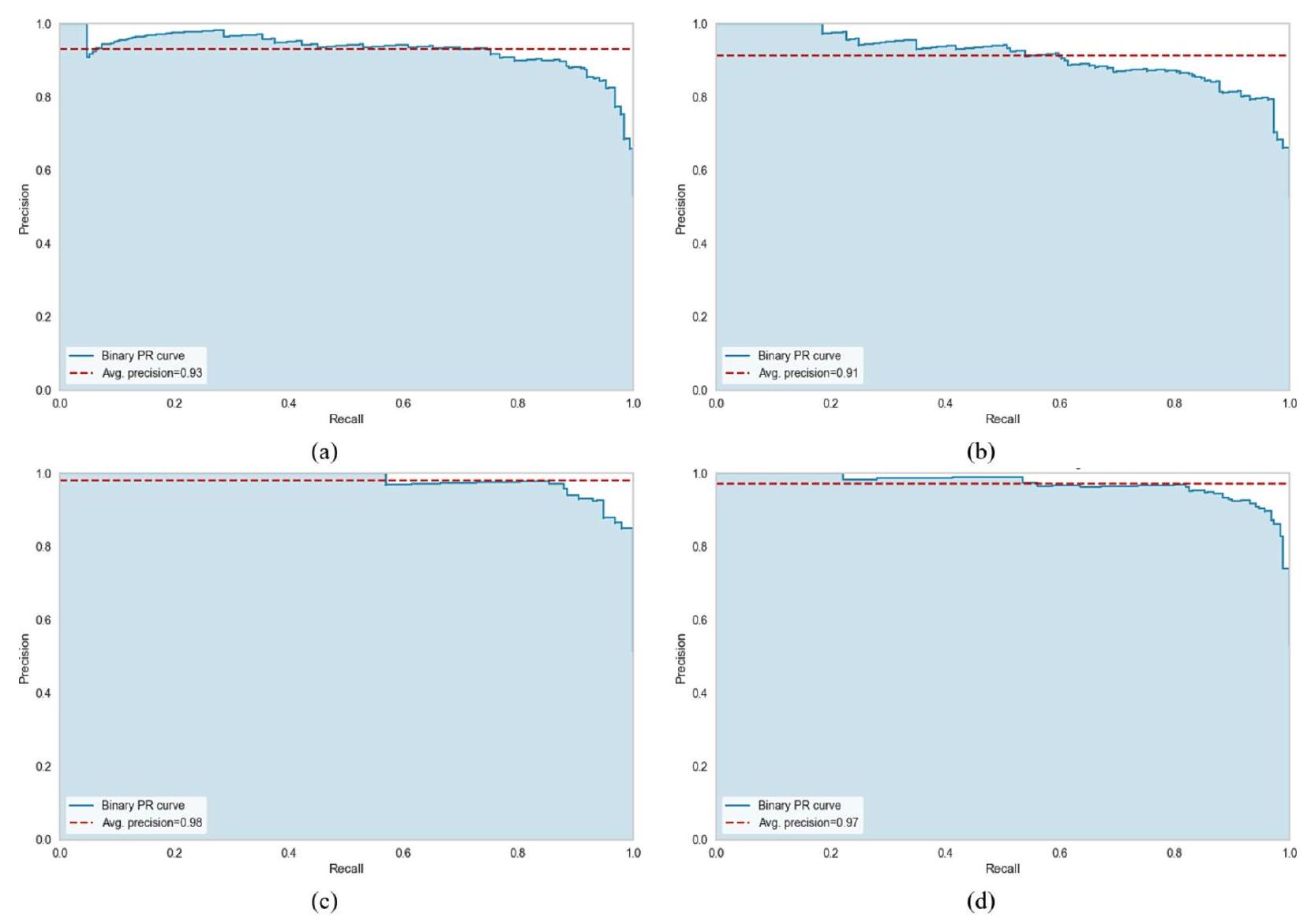
الشكل 19. AUPRC لـ (أ) التكديس مع D1، (ب) التصويت مع D1، (ج) التكديس مع D2 و (د) التصويت مع D2.
الشكل 20. MCR للتكديس والتصويت مع كلا المجموعتين البيانيّتين.
في D2، يبرز نموذج التصويت مرة أخرى CP و CF كمتنبئين رئيسيين. ومع ذلك، فإن تأثير TH و GD أقل وضوحًا قليلاً مقارنةً بنموذج التكديس، مما يشير إلى اعتماد أكثر توازنًا على الميزات. قد تجعل التوزيع المتساوي لأهمية الميزات في نموذج التصويت أكثر قوة في مجموعات البيانات المتنوعة.
بشكل عام، يظهر CP باستمرار كأحد أفضل المؤشرات عبر جميع النماذج ومجموعات البيانات، مما يبرز قيمته التشخيصية العالمية. يؤكد D2 على أهمية CF وTH، اللذان يكونان أقل بروزًا في D1. يبدو أن نموذج التكديس أكثر ملاءمة لمجموعات البيانات ذات الميزات المميزة والواضحة، بينما يعد نموذج التصويت مفيدًا لمجموعات البيانات التي تتطلب تمثيلًا أوسع للميزات. تسلط هذه النتائج الضوء على الحاجة إلى تخصيص اختيار النموذج وتركيز الميزات وفقًا لخصائص مجموعة البيانات لتحقيق دقة تنبؤ مثلى.
تفسير محلي
تفسير محلي يركز على فهم الأسباب وراء توقع محدد قدمه نموذج الذكاء الاصطناعي لحالة فردية، مثل تشخيص مريض معين. هذه الطريقة ذات قيمة خاصة في الرعاية الصحية، حيث أن العلاج المخصص أمر حاسم. تفسيرات محلية تسلط الضوء على العوامل الفريدة، مثل
الشكل 21. وقت التنفيذ (بالثواني) للتكديس والتصويت على كلا المجموعتين البيانيّتين.
الشكل 22. مقارنة نماذج التكديس والتصويت مع نماذج الأداء الأعلى من حيث (أ) الدقة، (ب) الدقة الإيجابية، (ج) الاسترجاع، (د) درجة F1، و(هـ) ROC مع كلا المجموعتين البيانيات.
| مقياس | مجموعة بيانات | نموذج | إحصائية |
|
رتبة | تم قبول H0 |
| دقة | D1 | تكديس | 1.6 | 0.2059 | ٣.٥ | نعم |
| التصويت | 1.5 | نعم | ||||
| D2 | تكديس | ٣.٥ | نعم | |||
| التصويت | 1.5 | نعم | ||||
| دقة | D1 | تكديس | 1.6 | 0.2059 | ٣.٥ | نعم |
| التصويت | 1.5 | نعم | ||||
| D2 | تكديس | ٣.٥ | نعم | |||
| التصويت | 1.5 | نعم | ||||
| استدعاء | D1 | تكديس | 1.6 | 0.2059 | ٣.٥ | نعم |
| التصويت | 1.5 | نعم | ||||
| D2 | تكديس | 3.5 | نعم | |||
| التصويت | 1.5 | نعم | ||||
| درجة F1 | D1 | تكديس | 1.6 | 0.2059 | ٣.٥ | نعم |
| التصويت | 1.5 | نعم | ||||
| D2 | تكديس | 3.5 | نعم | |||
| التصويت | 1.5 | نعم | ||||
| كابا | D1 | تكديس | 1.6 | 0.2059 | ٣.٥ | نعم |
| التصويت | 1.5 | نعم | ||||
| D2 | تكديس | ٣.٥ | نعم | |||
| التصويت | 1.5 | نعم | ||||
| MCC | D1 | تكديس | 1.6 | 0.2059 | 3.5 | نعم |
| التصويت | 1.5 | نعم | ||||
| D2 | تكديس | ٣.٥ | نعم | |||
| التصويت | 1.5 | نعم |
الجدول 6. اختبار رينك المتراصة فريدمان لنماذج التجميع والتصويت.
| المقياس | نتائج الاختبار | D1 | D2 |
| الدقة | الإحصائية | 1.5492 | 1.5492 |
| قيمة p المعدلة | 0.1213 | 0.1213 | |
| تم قبول H0 | نعم | نعم | |
| الدقة | الإحصائية | 1.5492 | 1.5492 |
| قيمة p المعدلة | 0.1213 | 0.1213 | |
| تم قبول H0 | نعم | نعم | |
| الاسترجاع | الإحصائية | 1.5492 | 1.5492 |
| قيمة p المعدلة | 0.1213 | 0.1213 | |
| تم قبول H0 | نعم | نعم | |
| درجة F1 | الإحصائية | 1.5492 | 1.5492 |
| قيمة p المعدلة | 0.1213 | 0.1213 | |
| تم قبول H0 | نعم | نعم | |
| كابا | الإحصائية | 1.5492 | 1.5492 |
| قيمة p المعدلة | 0.1213 | 0.1213 | |
| تم قبول H0 | نعم | نعم | |
| MCC | الإحصائية | 1.5492 | 1.5492 |
| قيمة p المعدلة | 0.1213 | 0.1213 | |
| تم قبول H0 | نعم | نعم |
الجدول 7. اختبار ما بعد hoc للتجميع مقابل التصويت لكلا مجموعتي البيانات.
المؤشرات الحيوية أو التاريخ الطبي، التي أثرت على قرار النموذج لمريض معين، مما يساعد في إنشاء استراتيجيات علاج مخصصة. من خلال تقديم هذه الرؤية الخاصة بالحالة، تعزز هذه التفسيرات أيضًا الثقة في القرارات المدعومة بالذكاء الاصطناعي، خاصة في السيناريوهات الطبية الحرجة.
تساعد التفسيرات المحلية أيضًا في تحديد الأخطاء من خلال الكشف عن الميزات التي ساهمت في النتائج غير الصحيحة، مما يمكّن من تحسين النموذج وزيادة موثوقيته. كما أنها تسمح للمهنيين الطبيين بتقييم ما إذا كانت توقعات النموذج تتماشى مع الأبحاث الطبية المعتمدة، مما يعزز الشفافية في تشخيصات الذكاء الاصطناعي.
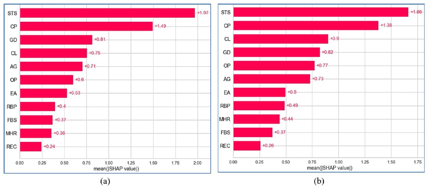
الشكل 23. متوسط SHAP المطلق لـ (أ) التجميع و (ب) التصويت على D1.
الشكل 24. متوسط SHAP المطلق لـ (أ) التجميع و (ب) التصويت على D2.
في هذا البحث، تم استخدام مخططات الشلال والقوة لـ SHAP لتقديم تفسيرات محلية للتوقعات التي قدمها نموذج التجميع في اكتشاف أمراض القلب. يكسر مخطط الشلال كيف تؤثر الميزات الفردية على التوقع خطوة بخطوة، بدءًا من الناتج الأساسي للنموذج. من ناحية أخرى، يمثل مخطط القوة بصريًا كيف تزيد أو تقلل ميزات معينة من التوقع، موضحًا بوضوح العوامل التي تؤثر على النتيجة.
مخطط الشلال يعد مخطط الشلال لـ SHAP أداة تصور فعالة لفهم كيف تساهم الميزات الفردية في توقع النموذج بطريقة منهجية، خطوة بخطوة. يكسر هذا المخطط التوقع إلى مساهمات من ميزات محددة، مميزًا بوضوح بين التأثيرات الإيجابية والسلبية على المتغير المستهدف. يمثل المحور السيني القيمة المتوقعة، بينما يسرد المحور الصادي الميزات التي تؤثر على النتيجة. تُظهر الميزات التي تساهم إيجابيًا في التوقع باللون الأحمر. تُظهر الميزات التي تساهم سلبًا في التوقع باللون الأزرق. يمثل حجم كل شريط حجم التأثير على ناتج النموذج.
تعتبر هذه التصور ذات قيمة خاصة في توقع أمراض القلب. يبرز كيف أن عوامل مثل الحالات الصحية أو الخصائص الديموغرافية تشكل بشكل كبير التوقع لكل فرد، مما يعزز قابلية تفسير النموذج من خلال تحديد الميزات الأكثر أهمية في سياق محدد للمريض. تعرض الأشكال 25 و 26 مخططات الشلال لـ SHAP لـ D1 باستخدام التجميع والتصويت، على التوالي. مخططات الشلال لـ SHAP
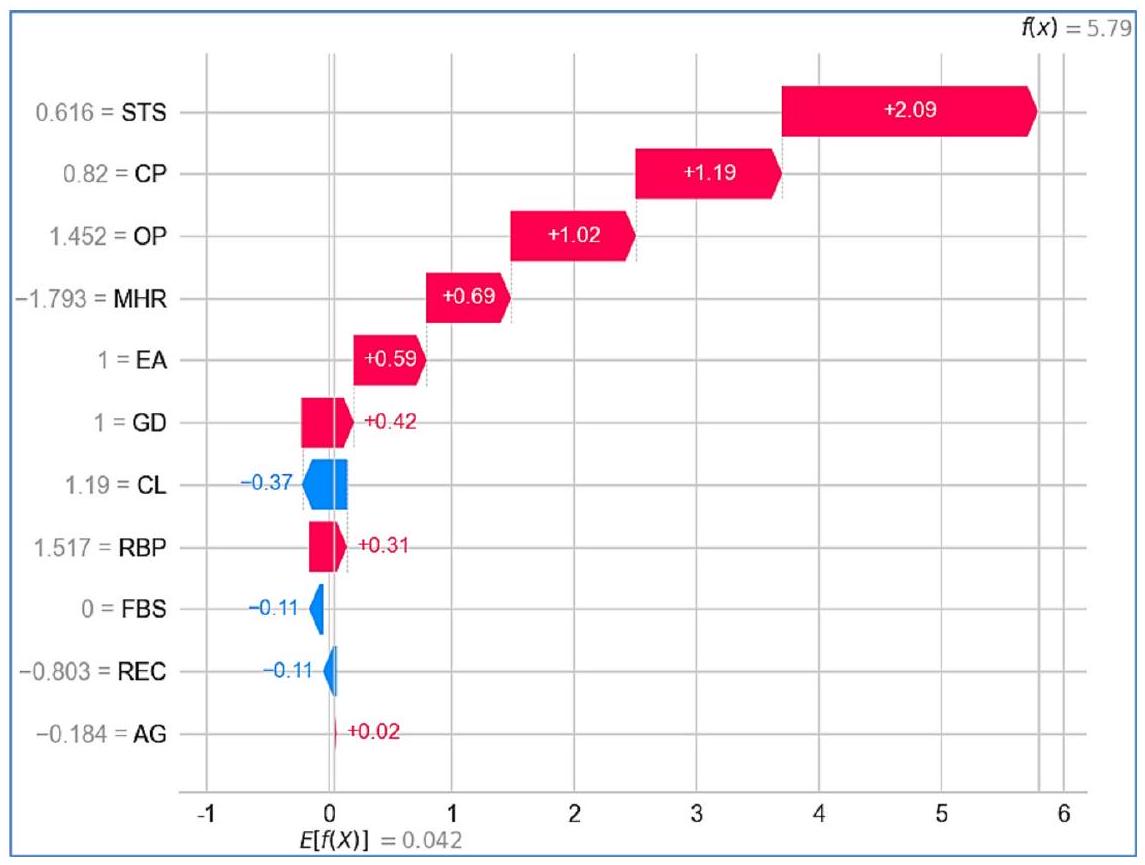
الشكل 25. مخطط الشلال للتجميع على D1.
الشكل 26. مخطط الشلال للتصويت على D1.
لـ D2، باستخدام التجميع والتصويت، موضحة في الأشكال 27 و 28، على التوالي. في كل حالة، تم استخدام بيانات المريض رقم 5 لتحليل مخطط الشلال لـ SHAP.
في نموذج التجميع، على D1 (الشكل 25)، القيمة المتوقعة الإجمالية (
الشكل 27. مخطط الشلال للتجميع على D2.
الشكل 28. مخطط الشلال للتصويت على D2.
يمكن أن تقلل من خطر الإصابة بأمراض القلب. تساهم CL (-0.37) أيضًا بشكل سلبي، مما يشير إلى أن ارتفاع الكوليسترول في هذا السياق يقلل قليلاً من الخطر، ربما بسبب تفاعلات البيانات أو أنماط معينة تعلمها النموذج. أخيرًا، تلعب AG عند +0.02 دورًا ثانويًا، مع مساهمة إيجابية صغيرة، مما يشير إلى أنه على الرغم من أن العمر عامل، إلا أنه أقل تأثيرًا في هذه الحالة المحددة. تؤدي المساهمات المجمعة إلى توقع نهائي معدل قدره +5.79، مما يشير إلى أن المريض معرض لخطر الإصابة بأمراض القلب.
الشكل 29. مخطط القوة لـ (أ) التجميع و (ب) التصويت على D1.
الشكل 30. مخطط القوة لـ (أ) التجميع و (ب) التصويت على D2.
بالنسبة لنفس المريض، ينتج نموذج التصويت قيمة متوقعة قدرها 3.686 لخطر الإصابة بأمراض القلب على D1 (الشكل 26). هنا، تظل STS (+1.74) أقوى مساهم إيجابي، بينما تظهر AG (1.18)، OP (+0.98)، و GD (+0.73) تأثيرات إيجابية حاسمة، مما يشير إلى أهميتها المتزايدة في هذا السياق. من المثير للاهتمام أن CP (-0.249) تقدم أعلى مساهمة سلبية، مما يختلف عن دورها في نموذج التجميع. كما تم تغيير مساهمة MHR (-0.29) من نموذج التجميع.
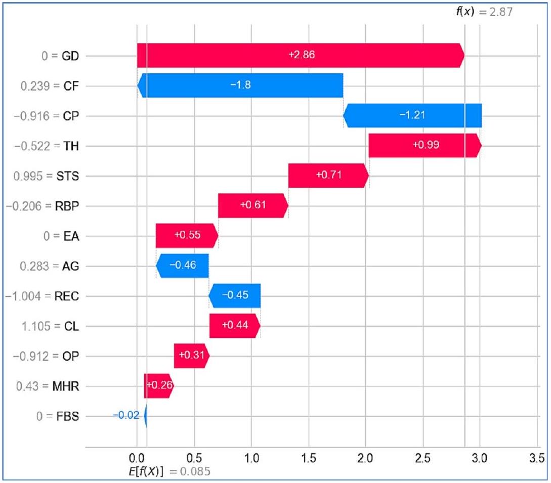
على العكس من ذلك، على D2، في نموذج التجميع، تظهر ميزة GD كأهم مساهم إيجابي بقيمة +2.86 (الشكل 27)، مما يشير إلى أن المريضة مرتبطة بقوة بزيادة خطر الإصابة بأمراض القلب. بعد GD، تتمتع CF (-1.8) و CP (-1.21) بمساهمات سلبية ملحوظة، مما يشير إلى أن القيم الأعلى لهذه الميزات قد ترتبط بانخفاض خطر الإصابة بأمراض القلب. تشمل الميزات الأخرى التي تساهم إيجابيًا TH (+0.99)، STS (+0.71)، EA (+0.55) و RBP (+0.61) مما يشير إلى أن هذه العوامل تزيد أيضًا من الخطر. على العكس من ذلك، فإن الميزات مثل
ينتج نموذج التصويت قيمة متوقعة أعلى قدرها 5.455 لخطر الإصابة بأمراض القلب على D2 (الشكل 28). هنا، تظل GD مساهمًا إيجابيًا حاسمًا، بقيمة +2.6، مما يعزز أهميتها في توقع أمراض القلب. تساهم الميزة
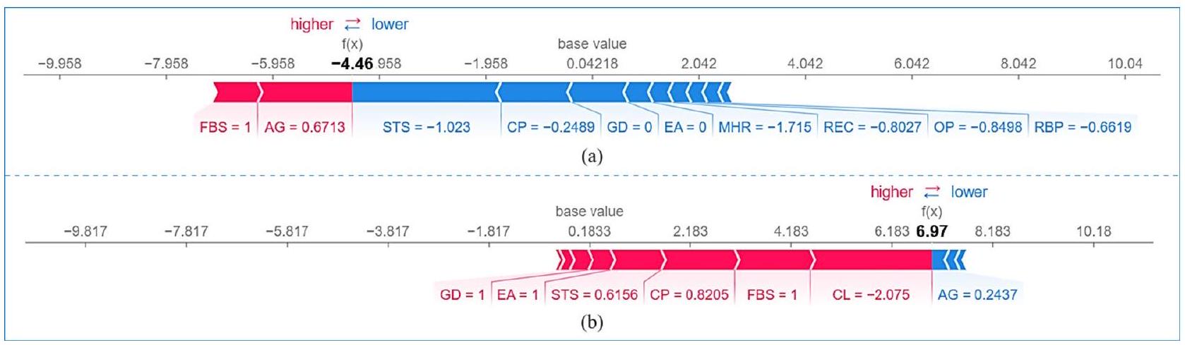
مخطط القوة بينما يقدم مخطط الشلال تحليلًا تسلسليًا لمساهمات الميزات، يبرز مخطط القوة لـ SHAP التأثير العام للميزات بالنسبة لقيمة أساسية. تنقل هذه المخططات بصريًا العوامل التي تؤثر على توقعات نموذج التجميع من خلال توضيح كيف تدعم ميزات معينة أو تعارض تصنيفًا معينًا. يتم تمثيل تأثير كل ميزة بأسهم تشير إلى اتجاهها (إيجابي أو سلبي) وحجمها، مما يوفر رؤية واضحة وقابلة للتفسير لقرارات النموذج. من خلال تقديم طريقة تفاعلية وسهلة الاستخدام لتحليل التوقعات، يسهل مخطط القوة فهمًا شاملاً لكيفية مساهمة الميزات الفردية في النتائج النهائية. تعرض الأشكال 29 و 30 مخططات القوة لـ SHAP لنماذج التجميع والتصويت على D1 و D2، على التوالي، لحالة معينة.
يظهر مخطط القوة لـ SHAP لنموذج التجميع على D1 (الشكل 29a) مساهمة سلبية بشكل أساسي من الميزات، مما يؤدي إلى درجة توقع منخفضة
بالنسبة لنموذج التصويت (الشكل 29ب) على نفس مجموعة البيانات (D1)، فإن التنبؤ مختلف بشكل ملحوظ، مع درجة تنبؤ إيجابية عالية (
تقدم نماذج التكديس والتصويت على D2 (الشكل 30) درجات تنبؤ إيجابية معتدلة (
التحليل النقدي تكشف مخططات SHAP المائية والقوة عن اختلافات كبيرة بين نماذج التكديس والتصويت في التنبؤ بأمراض القلب عبر مجموعتين من البيانات. يبرز مخطط الشلال تقييمات المخاطر المختلفة: على D1، يمنح نموذج التكديس درجة مخاطر أعلى (5.79) (الشكل 25) مقارنةً بنموذج التصويت (3.686) (الشكل 26)، بينما على D2، ينتج نموذج التصويت درجة أعلى (5.455) (الشكل 27) مقارنةً بالتكديس (2.87) (الشكل 28). تشير هذه الاختلافات إلى أن نموذج التكديس أكثر حساسية لتفاعلات الميزات الدقيقة، بينما يتفاعل نموذج التصويت بشكل أقوى مع مؤشرات المخاطر السائدة. تظهر الميزات الرئيسية مثل CP و MHR و REC على D1، و OP و CP و MHR على D2 اختلافات كبيرة في التفسير، مما يبرز كيف تؤثر استراتيجيات التعلم الجماعي المختلفة على أهمية الميزات. ومع ذلك، تبرز STS و GD باستمرار كعوامل مساهمة إيجابية سائدة، بينما يبقى FBS مساهمًا سلبيًا ضعيفًا باستمرار، مما يعزز دوره النسبي الضئيل في اتخاذ القرار للنموذج. تؤكد هذه الاختلافات على ضرورة مراعاة خصائص مجموعة البيانات واختيار النموذج عند إجراء التنبؤات السريرية.
يؤكد تحليل مخطط القوة هذه التمييزات. على D1، يتنبأ نموذج التكديس باحتمالية منخفضة للإصابة بأمراض القلب، مع اعتبار STS و CP و GD كعوامل وقائية، بينما تساهم العمر و FBS بشكل إيجابي في المخاطر (الشكل 29(أ)). في المقابل، يتنبأ نموذج التصويت باحتمالية عالية للإصابة بأمراض القلب، مدفوعًا بشكل أساسي بـ CL و FBS و CP و STS، مع لعب العمر دورًا سلبيًا طفيفًا فقط (الشكل 29(ب)). على D2، يتنبأ كلا النموذجين بمخاطر معتدلة، مع ظهور GD و OP و STS و CP و TH و RBP كعوامل خطر متسقة (الشكل 30). ومع ذلك، يختلف تفسير AG بشكل كبير – حيث يساهم بشكل إيجابي في نموذج التكديس (الشكل 30(أ)) ولكنه هو أقوى مساهم سلبي في التصويت (الشكل 30(ب))، مما يشير إلى أن النموذجين يقيمان العمر بشكل مختلف في تنبؤاتهما.
التمييز الرئيسي بين نماذج التكديس والتصويت ينشأ من استراتيجيات التعلم الجماعي المختلفة. يستخدم التكديس نماذج أساسية متعددة بطريقة هرمية، مما يلتقط تفاعلات الميزات المعقدة والاعتمادات، بينما يجمع التصويت التنبؤات بطريقة متوازية، مما يبرز المتنبئين الفرديين الأقوياء على التفاعلات الدقيقة.
أحد الأسباب الرئيسية لاختلاف تنبؤاتهما هو أن التكديس يصقل قراره النهائي من خلال نموذج ميتا، مما يجعله أكثر تكيفًا مع تأثيرات الميزات المتغيرة. يفسر هذا لماذا، على D1، يمنح التكديس أدوارًا تعزز المخاطر وأدوارًا وقائية لمميزات مختلفة، مما يؤدي إلى درجة تنبؤ أقل (الشكل 29(أ)). في المقابل، يميل التصويت، الذي يعتمد على قرار الأغلبية البسيطة، إلى المبالغة في التأكيد على عوامل الخطر السائدة، مثل الكوليسترول، مما يؤدي إلى درجة تنبؤ أعلى (الشكل 29(ب)).
تمييز آخر حاسم هو كيفية إدارة النماذج لارتباطات الميزات. يحدد التكديس التأثيرات التعويضية، مثل التأثير الوقائي لـ STS و CP في بعض الحالات (الشكل 29(أ))، مما يمنع المبالغة في تقدير مخاطر الإصابة بأمراض القلب. ومع ذلك، يعامل التصويت كل ميزة بشكل مستقل، مما يجعله أكثر عرضة للمبالغة في التأكيد على مؤشرات المخاطر العالية مثل CL و FBS (الشكل 29(ب)).
توضح معالجة العمر هذا الاختلاف بشكل أكبر. على D2، يعترف التكديس بالعمر كعامل خطر (الشكل 30(أ))، من المحتمل بالتزامن مع متغيرات طبية أخرى، بينما يمنح التصويت مساهمة سلبية كبيرة (الشكل 30(ب))، ربما بسبب تأثير العتبة حيث تقلل عوامل الخطر الأخرى من أهميته. يشير هذا إلى أن التصويت يعتمد أكثر على قوة الميزات المطلقة، بينما يقوم التكديس بتعديل التنبؤات بناءً على العلاقات المتداخلة بين الميزات.
في النهاية، يقدم التكديس تقييمًا أكثر وعيًا بالسياق ومتوازنًا من خلال دمج تفاعلات الميزات المتعددة، بينما يوفر التصويت نهجًا أكثر مباشرة وحساسية عالية من خلال إعطاء الأولوية للمتنبئين السائدين. يعد التكديس مفيدًا في الحالات المعقدة حيث تكون التفاعلات الدقيقة مهمة، بينما قد يُفضل التصويت عندما تتطلب عوامل الخطر الفردية القوية التأكيد.
على الرغم من التنبؤات المتوقعة عمومًا، تظهر بعض الملاحظات غير المتوقعة في كلا النموذجين. على سبيل المثال، في مخطط الشلال، تعمل CP (في التصويت على D1 (الشكل 26) والتكديس على D2 (الشكل 27)) و CL (في التكديس على D1 (الشكل 28)) كعوامل مساهمة سلبية، مما يتعارض مع المعرفة الطبية الراسخة. وبالمثل، في مخطط القوة للتصويت على D1 (الشكل 29(ب))، يكون الكوليسترول هو أقوى مساهم إيجابي، على الرغم من أن المريض لديه قيمة كوليسترول سلبية.
يمكن أن تُعزى هذه الشذوذات إلى عوامل مختلفة. أحد التفسيرات المحتملة هو الطبيعة غير الخطية للنموذج، حيث لا تزيد العلاقة بين الكوليسترول وأمراض القلب أو تنقص بشكل صارم. قد يكون النموذج قد حدد أن مستويات الكوليسترول المعتدلة تمثل خطرًا أقل من المستويات المنخفضة جدًا أو العالية جدًا، حيث يمكن أن تشير مستويات الكوليسترول المنخفضة جدًا أحيانًا إلى مشاكل صحية أساسية، مثل أمراض الكبد أو سوء التغذية.
عامل آخر هو التفاعلات بين الميزات في النموذج. تمثل قيم SHAP التأثير المشترك لعدة ميزات، مما يشير إلى أن تأثير الكوليسترول قد يعتمد على متغيرات أخرى مثل RBP و REC أو FBS. على سبيل المثال، إذا كان لدى المريض كوليسترول مرتفع معتدل ولكن علامات حيوية طبيعية بخلاف ذلك، قد يستنتج النموذج أن الكوليسترول لا يزيد من المخاطر بشكل كبير. علاوة على ذلك، قد تكون تقنيات المعالجة المسبقة مثل قياس الميزات والتحولات قد أثرت على هذه التفسيرات.
أخيرًا، قد تكون تحيزات مجموعة البيانات والارتباطات غير المتوقعة قد أثرت على هذه النتائج. إذا كانت مجموعة بيانات التدريب تتكون من عدد كبير من المرضى الذين لديهم كوليسترول منخفض والذين كانوا بالفعل يعانون من حالات قلبية وعائية (ربما بسبب علاجات خافضة للكوليسترول)، فقد يكون النموذج قد تعلم عن غير قصد رابطًا بين انخفاض الكوليسترول وزيادة خطر الإصابة بأمراض القلب. وهذا يبرز ضرورة تحليل توزيعات البيانات وارتباطات الميزات بدقة عند تفسير قيم SHAP.
مقارنة نماذج التكديس والتصويت مع أحدث التقنيات
تم تحديد أداء نموذجنا من خلال مقارنته بعدة أوراق بحثية مشابهة باستخدام مقاييس متنوعة، كما هو موضح في الجدول 8. في تجربتنا، أظهرت منهجية التكديس أفضل أداء بشكل عام في التنبؤ بأمراض القلب؛ وبالتالي، ركزنا فقط على النتائج التي تم الحصول عليها باستخدام التكديس. يمكن أن يُعزى التحسن في أداء نموذجنا مع التكديس إلى المنهجيات المطبقة، والتي تشمل اختيار النماذج الأساسية، واختيار المتعلم الميتا، والتحقق المتقاطع الفعال، وضبط المعلمات الفائقة بشكل صحيح.
الاستنتاجات، القيود، والاتجاهات المستقبلية
تستكشف هذه الورقة تطبيق تقنيات التعلم الجماعي، وبشكل خاص التجميع والتصويت، لتعزيز دقة التنبؤ بأمراض القلب. قام الباحثون بإجراء تجارب باستخدام مجموعات بيانات متعددة تتعلق بتنبؤ أمراض القلب وقارنوا أداء نماذج التجميع والتصويت مع نماذج فردية. أظهرت النتائج أن كلا من نماذج التجميع والتصويت تفوقت على النماذج الأساسية الفردية، بالإضافة إلى النماذج الموجودة، في التنبؤ بأمراض القلب، حيث أظهر نموذج التجميع دقة أعلى من نموذج التصويت. تؤكد التحليلات الإحصائية أيضًا تفوق نموذج التجميع. يمكن أن يُعزى التحسن في أداء نماذج التجميع والتصويت إلى المنهجيات المستخدمة، بما في ذلك اختيار النماذج الأساسية، واختيار المتعلم الميتا، والتقاطع الفعال، وضبط المعلمات الفائقة بشكل صحيح. بشكل خاص، سمح الجمع بين التنبؤات من نماذج متعددة بالاستفادة من نقاط القوة لكل نموذج فردي. تشير هذه النتائج إلى أن التجميع والتصويت يمكن أن يكونا قيمين في اتخاذ القرارات السريرية لتنبؤ بأمراض القلب.
ومع ذلك، فإن مقارنة نماذج التكديس والتصويت في تحليل SHAP توضح أساليبها المميزة في توقع المخاطر. يأخذ التكديس في الاعتبار الاعتمادات المتبادلة بين الميزات وتأثيرات التعويض، مما يؤدي إلى توقعات أكثر حساسية للسياق، بينما يركز التصويت على المتنبئين الفرديين الأقوياء، مما يؤدي غالبًا إلى تقييمات مخاطر أعلى. تبرز هذه الاختلافات أهمية اختيار تقنية تجميع مناسبة بناءً على المتطلبات السريرية أو التنبؤية المحددة. علاوة على ذلك، فإن التأثيرات غير المتوقعة للميزات تؤكد على الحاجة إلى تحليل بيانات دقيق، وهندسة ميزات، والتحقق، لضمان توافق العلاقات التي تعلمها النموذج مع المعرفة الطبية والأنماط الواقعية.
تتمتع هذه البحث بإمكانات كبيرة. يمكن أن تؤدي الدقة المحسّنة في التنبؤ بأمراض القلب إلى تشخيص مبكر، وأنظمة علاج مخصصة، وفي النهاية تحسين نتائج المرضى. علاوة على ذلك، فإن تحسين قابلية تفسير النموذج يساعد الأطباء في اتخاذ قرارات مستنيرة ووضع علاجات مخصصة. لتوسيع نطاق تطبيق هذه الدراسة، يمكن توسيع الطريقة المقترحة لتشمل مجموعات بيانات صحية إضافية ذات خصائص مشابهة.
بينما تُظهر هذه الدراسة فعالية تجميع النماذج والتصويت في التنبؤ بأمراض القلب، يجب الاعتراف بعدة قيود. أولاً، تقيّد قابلية تعميم النتائج استخدام مجموعات بيانات متاحة للجمهور، والتي قد لا تعكس تمامًا تنوع المرضى في العالم الحقيقي. من الضروري التحقق من هذه النتائج على مجموعات بيانات أكبر وأكثر تنوعًا لضمان قابليتها للتطبيق بشكل أوسع. ثانيًا، على الرغم من أن تحليل SHAP يعزز من قابلية التفسير، فإن بعض المساهمات غير المتوقعة للميزات تشير إلى وجود تحيزات أو شذوذات في البيانات تتطلب مزيدًا من التحقيق. يجب أن تستكشف الأبحاث المستقبلية سبل تحسين اختيار الميزات ومعالجة التحيزات المحتملة. ثالثًا، قد تشكل التعقيدات الحسابية لتجميع النماذج – خاصة فيما يتعلق بضبط المعلمات الفائقة والتحقق المتقاطع – تحديات للتنفيذ في بيئات الرعاية الصحية ذات الموارد المحدودة. يجب التحقيق في تقنيات تحسين فعالة وهياكل تجميع خفيفة الوزن للتخفيف من هذه المشكلة. أخيرًا، لم تفحص هذه الدراسة تحديات النشر في الوقت الحقيقي، مثل انحراف النموذج أو التكامل مع السجلات الصحية الإلكترونية (EHRs)، والتي تعتبر حاسمة للتبني العملي في البيئات السريرية. يجب أن تركز الأعمال المستقبلية على مواجهة هذه التحديات لتعزيز قابلية استخدام التعلم التجميعي في تطبيقات الرعاية الصحية في العالم الحقيقي.
لمعالجة قيود هذه الدراسة وتوسيع نطاق تطبيقها، يجب على الأبحاث المستقبلية استكشاف عدة اتجاهات رئيسية. أحد المسارات الواعدة هو تطوير التجميعات المتعددة الطبقات (MTSE)، حيث يمكن للهياكل الهرمية للتجميع مع طبقات متعددة من التعلم الميتا أن نمذج تفاعلات الميزات الأعمق. من خلال دمج مصادر بيانات متنوعة، يعزز MTSE القدرة على التكيف عبر السكان ويحسن من قابلية التفسير من خلال تحليل SHAP الهرمي، مما يجعل الرؤى المدفوعة بالذكاء الاصطناعي أكثر موثوقية للاستخدام السريري. قد تزيد تقنيات مثل وزن النموذج الديناميكي واختيار التجميع التكيفي من قدرة النماذج على التكيف عبر مجموعات المرضى المتنوعة. بالإضافة إلى ذلك، فإن دمج نماذج التجميع في سير العمل السريري المباشر جنبًا إلى جنب مع لوحات المعلومات التفاعلية للتفسير سيمكن الأطباء من التحقق من التنبؤات المدفوعة بالذكاء الاصطناعي وتنقيح خطط العلاج بشكل ديناميكي. منطقة أخرى مهمة هي مقارنة التجميعات المعتمدة على التكديس مع تقنيات الذكاء الاصطناعي المتقدمة، بما في ذلك هياكل التعلم العميق مثل المحولات والتجميعات الاحتمالية البايزية، لاكتشاف استراتيجيات لتعزيز كل من دقة التنبؤ وقياس عدم اليقين. علاوة على ذلك، يمكن أن يساعد دمج بيانات المرضى الطولية وطرق الاستدلال السببي نماذج التجميع في التمييز بين الارتباط والسببية، مما يؤدي إلى تنبؤات ذات مغزى سريري أكبر. ستؤدي هذه التطورات إلى
| عمل بحثي | الخوارزميات المدروسة | مجموعة البيانات المستخدمة | أعلى دقة (%) | الدقة (%) | استرجاع (%) | درجة F1 (%) | الخصوصية (%) | منطقة تحت منحنى التشغيل/الاستقبال (%) | القيم المتوقعة السلبية (%) | نسبة MCC (%) | معدل الإيجابيات الكاذبة | معدل النتائج السلبية الخاطئة | معدل الاكتشافات الكاذبة | معدل التصنيف الخاطئ | التحليل الإحصائي | XAI |
| تشاندراسيخار وبيداكرشنا [31] | التصويت | HDDC و IDD | 95 مع IEEE Dataport | ٩٦.٠٤ | 93.27 | 94.63 | 95 | – | 91.57 | ٨٧.٩٤ | 0.0500 | 0.0673 | 0.0396 | 0.0500 | × | × |
| تيwari وآخرون [32] | تكديس | IDD | 92.34 | 92 | 93.49 | 92.74 | 91.07 | 92.28 | 93.49 | 84.64 | 0.0893 | 0.0651 | 0.0800 | 0.0766 | × | × |
| رازا [33] | التصويت | مجموعة بيانات أمراض القلب StatLog | ٨٨.٨٨ | 89 | 85 | 87 | 87 | ٨٨ | ٨٨ | – | 0.1300 | 0.1500 | 0.1000 | 0.1100 | × | × |
| مينيي وآخرون [34] | تكديس | HDDC و FHSD | 93 مع FHSD | 96 | 91 | 93 | – | 93.30 | 91 | 91 | – | 0.0900 | 0.0400 | 0.0700 | × | × |
| أمبروز وآخرون [35] | التصويت | FHSD و UHDD | 91.96 مع UHDD | 92.40 | 91.72 | 91.69 | 90.77 | – | 91.72 | – | 0.0923 | 0.0828 | 0.0760 | 0.0804 | × | × |
| أشفاق [36] | تكديس | HDDC | 87 | 83 | 83 | 83 | – | 83 | 83 | 83 | – | 0.0170 | 0.0170 | 0.0130 | × | × |
| حبيب وتسنيم [37] | التصويت | FHSD | ٨٨.٤٢ | 100 | 43 | 82 | – | 73 | 43 | 43 | – | 0.5700 | 0 | 0.1158 | × | × |
| موهباترا وآخرون [38] | تكديس | UHDD | 91.8 | 92.6 | 92.6 | 92.6 | 90.9 | 91.7 | 92.6 | ٨٣.٥ | 0.0910 | 0.0740 | 0.0740 | 0.0820 | × | × |
| ورقتنا | تكديس | HDDC | 91 | 89.7 | 98.1 | 91.8 | – | 92 | 98.1 | 82.4 | – | 0.0190 | 0.0130 | 0.0888 |
|
|
| UHDD | 98 | 98.8 | 98.7 | 98.4 | – | 98 | 98.7 | 96.8 | – | 0.0130 | 0.0120 | 0.0167 |
الجدول 8. مقارنة العمل المقترح مع الأدبيات الحديثة.
دفع المرحلة التالية من توقع أمراض القلب المدفوعة بالذكاء الاصطناعي، مما يجعل النماذج أكثر قوة وقابلية للتفسير وملائمة عمليًا للنشر في بيئات الرعاية الصحية الواقعية.
دفع المرحلة التالية من توقع أمراض القلب المدفوعة بالذكاء الاصطناعي، مما يجعل النماذج أكثر قوة وقابلية للتفسير وملائمة عمليًا للنشر في بيئات الرعاية الصحية الواقعية.
توفر البيانات
تتوفر مجموعات البيانات المستخدمة في الدراسة الحالية في مستودع كاجل، [HDDC: https://www.kaggle. com/datasets/sid321axn/heart-statlog-cleveland-hungary-final، UHDD: https://www.kaggle.com/datasets/johnsmith88/مجموعة بيانات أمراض القلب
تاريخ الاستلام: 1 فبراير 2025؛ تاريخ القبول: 4 أبريل 2025
نُشر على الإنترنت: 22 أبريل 2025
نُشر على الإنترنت: 22 أبريل 2025
References
- WHO. Cardiovascular diseases (CVDs), 11 June 2021. [Online]. Available: https://www.who.int/news-room/fact-sheets/detail/car diovascular-diseases-(cvds). [Accessed 17 December 2023].
- Ahmad, G. N., Ullah, S., Algethami, A., Fatima, H. & Akhter, S. M. H. Comparative study of optimum medical diagnosis of human heart disease using machine learning technique with and without sequential feature selection. IEEE Access. 10, 23808-23828 (2022).
- Gheorghe, A. et al. The economic burden of cardiovascular disease and hypertension in low- and middle-income countries: a systematic review. BMC Public. Health. 18, 975 (2018). (Article number.
- Ruan, Y. et al. Cardiovascular disease (CVD) and associated risk factors among older adults in six low-and middle-income countries: results from SAGE wave 1. BMC Public. Health. 18(1), 1-13 (2018).
- Biglu, M. H., Ghavami, M. & Biglu, S. Cardiovascular diseases in the mirror of science. J. Cardiovasc. Thorac. Res. 8(4), 158-163 (2016).
- Ayano, Y. M., Schwenker, F., Dufera, B. D. & Debelee, T. G. Interpretable Machine Learning Techniques in ECG-Based Heart Disease Classification: A Systematic Review, Diagnostics, vol. 13, no. 1, p. 111, (2023).
- Rath, A., Mishra, D., Panda, G. & Satapathy, S. C. An exhaustive review of machine and deep learning based diagnosis of heart diseases. Multimedia Tools Appl. 81, 36069-36127 (2022).
- Ganie, S. M., Pramanik, P. K. D., Malik, M. B., Nayyar, A. & Kwak, K. S. An improved ensemble learning approach for heart disease prediction using boosting algorithms. Comput. Syst. Sci. Eng. 46(3), 3993-4006 (2023).
- Brown, G. Ensemble learning, in Encyclopedia of Machine Learning, (eds Sammut, C. & Webb, G. I.) Boston, MA, Springer, 312-320. (2011).
- Ganie, S. M. & Malik, M. B. An ensemble machine learning approach for predicting type-II diabetes mellitus based on lifestyle indicators. Healthc. Analytics. 22, 100092 (2022). (Article number.
- Naveen, R. K., Sharma & Nair, A. R. Efficient breast cancer prediction using ensemble machine learning models, in 4 th International Conference on Recent Trends on Electronics, Information, Communication & Technology (RTEICT), Bangalore, India, (2019).
- Oswald, G. J., Sathwika & Bhattacharya, A. Prediction of cardiovascular disease (CVD) using ensemble learning algorithms, in 5th Joint International Conference on Data Science & Management of Data (9th ACM IKDD CODS and 27th COMAD), Bangalore, India, (2022).
- Shanbhag, G. A., Prabhu, K. A., Subba Reddy, N. V. & Rao, B. A. Prediction of lung cancer using ensemble classifiers, Journal of Physics: Conference Series, vol. 2161 (012007), (2022).
- Verma, A. K., Pal, S. & Tiwari, B. B. Skin disease prediction using ensemble methods and a new hybrid feature selection technique. Iran. J. Comput. Sci. 3, 207-216(2020).
- Ganie, S. M. & Malik, M. B. Comparative analysis of various supervised machine learning algorithms for the early prediction of type-II diabetes mellitus. Int. J. Med. Eng. Inf. 14(6), 473-483 (2022).
- Shaikh, F. J. & Rao, D. S. Prediction of cancer disease using machine learning approach, Materialstoday: Proceedings, vol. 50 (Part 1), pp. 40-47, (2022).
- Senthilkumar, B. et al. Ensemble modelling for early breast cancer prediction from diet and lifestyle, IFAC-PapersOnLine, vol. 55, no. 1, pp. 429-435, (2022).
- Ganie, S. M. & Pramanik, P. K. D. Predicting chronic liver disease using boosting, in 1st International Conference on Artificial Intelligence for Innovations in Healthcare Industries (ICAIIHI-2023), Raipur, India, (2024).
- Ganie, S. M., Pramanik, P. K. D., Mallik, S. & Zhao, Z. Chronic kidney disease prediction using boosting techniques based on clinical parameters. PLoS ONE. 18(12), e0295234 (2023).
- Ganie, S. M., Pramanik, P. K. D., Malik, M. B., Mallik, S. & Qin, H. An ensemble learning approach for diabetes prediction using boosting techniques. Front. Genet. 14 (2023).
- Ganie, S. M. & Pramanik, P. K. D. A comparative analysis of boosting algorithms for chronic liver disease prediction. Healthc. Analytics 5, 100313 (2024).
- Shaik, H. S., RajyaLakshmi, G. V., Alane, V. & Kandimalla, N. D. Enhancing prediction of cardiovascular disease using bagging technique. in International Conference on Intelligent Data Communication Technologies and Internet of Things (IDCIoT).
- Yuan, X. et al. A High accuracy integrated bagging-fuzzy-GBDT prediction algorithm for heart disease diagnosis. in IEEE/CIC International Conference on Communications in China (ICCC)(2019).
- Deshmukh, V. M. Heart disease prediction using ensemble methods. Int. J. Recent. Technol. Eng. 8(3), 8521-8526 (2019).
- Mary, N. et al. Investigating of classification algorithms for heart disease risk prediction. J. Intell. Med. Healthc. 1(1), 11-31 (2022).
- Budholiya, K., Shrivastava, S. K. & Sharma, V. An optimized XGBoost based diagnostic system for effective prediction of heart disease. J. King Saud Univ. – Comput. Inform. Sci. 34(7), 4514-4523 (2022).
- Pan, C., Poddar, A., Mukherjee, R. & Ray, A. K. Impact of categorical and numerical features in ensemble machine learning frameworks for heart disease prediction. Biomed. Signal Process. Control. 76, 103666 (2022).
- Pouriyeh, S. et al. A comprehensive investigation and comparison of machine learning techniques in the domain of heart disease. in IEEE Symposium on Computers and Communications (ISCC) (2017).
- Shorewala, V. Early detection of coronary heart disease using ensemble techniques. Inf. Med. Unlocked, 26, 100655 (2021).
- Latha, C. B. C. & Jeeva, S. C. Improving the accuracy of prediction of heart disease risk based on ensemble classification techniques. Inf. Med. Unlocked 16, 100203 (2019).
- Chandrasekhar, N. & Peddakrishna, S. Enhancing heart disease prediction accuracy through machine learning techniques and optimization. Processes 11, (4), 1210 (2023).
- Tiwari, A., Chugh, A. & Sharma, A. Ensemble framework for cardiovascular disease prediction. Comput. Biol. Med. 146, 105624 (2022).
- Raza, K. Improving the prediction accuracy of heart disease with ensemble learning and majority voting rule. in U-Healthcare Monitoring Systems, Design and Applications (eds Dey, N. et al.) (Academic, 2019).
- Mienye, I. D., Sun, Y. & Wang, Z. An improved ensemble learning approach for the prediction of heart disease risk. Inf. Med. Unlocked. 20, 100402 (2020).
- Ambrews, A. B. et al. Ensemble based machine learning model for heart disease prediction. in International Conference on Communications, Information, Electronic and Energy Systems (CIEES) (2022).
- Ashfaq, A. et al. Multi-model ensemble based approach for heart disease diagnosis. in International Conference on Recent Advances in Electrical Engineering & Computer Sciences (RAEE & CS) (2022).
- Habib, A. Z. S. B. & Tasnim, T. An Ensemble hard voting model for cardiovascular disease prediction. in 2nd International Conference on Sustainable Technologies for Industry 4.0 (STI) (2020).
- Mohapatra, S. et al. A stacking classifiers model for detecting heart irregularities and predicting cardiovascular disease. Healthc. Analytics. 3, 100133 (2023).
- Saboor, A. et al. A method for improving prediction of human heart disease using machine learning algorithms, Mobile Inf. Syst. 2022, 1410169 (2022).
- Aldossary, Y., Ebrahim, M. & Hewahi, N. A comparative study of heart disease prediction using tree-based ensemble classification techniques. in International Conference on Data Analytics for Business and Industry (ICDABI) (2022).
- Duraisamy, P., Natarajan, Y., Ebin, N. L. & Jawahar Raja, P. Efficient way of heart disease prediction and analysis using different ensemble algorithm: A comparative study. in 6th International Conference on Electronics, Communication and Aerospace Technology (2023).
- Sagi, O. & Rokach, L. Ensemble learning: a survey. WIREs Data Min. Knowl. Discov. 8(4), e1249 (2018).
- Zhang, C. & Ma, Y. (eds) Ensemble Machine Learning: Methods and Applications (Springer, 2012).
- Hastie, T., Tibshirani, R. & Friedman, J. The Elements of Statistical Learning: Data Mining, Inference, and Prediction (Springer, 2009).
- Schapire, R. E. & Singer, Y. Improved boosting algorithms using Confidence-rated predictions. Mach. Learn. 37, 297-336 (1999).
- Freund, Y. & Schapire, R. E. A Decision-Theoretic generalization of On-Line learning and an application to boosting. J. Comput. Syst. Sci. 55(1), 119-139 (1997).
- Weisberg, S. Applied Linear Regression (Wiley, 2005).
- Kutner, M. H., Nachtsheim, C. J., Neter, J. & Li, W. Applied Linear Regression Models 5th edn (McGraw-Hill Irwin, 2005).
- Chan, J. Y. L. et al. Mitigating the multicollinearity problem and its machine learning approach: A review. Mathematics
(8), 1283 (2022). - Hotelling, H. Relations between two sets of variates. Biometrika 28(3/4), 321-377 (1936).
- Hardoon, D. R., Szedmak, S. & Shawe-Taylor, J. Canonical correlation analysis: an overview with application to learning methods. Neural Comput. 16(12), 2639-2664 (2004).
- James, G., Witten, D., Hastie, T. & Tibshirani, R. An Introduction To Statistical Learning with Applications in R (Springer, 2021).
- Lundberg, S. M. & Lee, S. I. A unified approach to interpreting model predictions. in 31st International Conference on Neural Information Processing Systems (NIPS’17) (2017).
- Mane, D. et al. Unlocking machine learning model decisions: A comparative analysis of LIME and SHAP for enhanced interpretability. J. Electr. Syst. 20(2) (2024).
- Wolpert, D. H. Stacked generalization. Neural Netw. 5(2), 241-259 (1992).
- Subramani, S. et al. Cardiovascular diseases prediction by machine learning incorporation with deep learning. Front. Med. 10 (2023).
- Ting, K. M. & Witten, I. H. Issues in stacked generalization. J. Artif. Intell. Res. 10, 271-289 (1999).
- Abbas, M. A. et al. A novel meta learning based stacked approach for diagnosis of thyroid syndrome. PLOS One (2024).
- Zhou, Z. H. Ensemble Methods – Foundations and Algorithms (Chapman & Hall/CRC, 2012).
- Ganie, S. M., Pramanik, P. K. D. & Zhao, Z. Improved liver disease prediction from clinical data through an evaluation of ensemble learning approaches. BMC Med. Inf. Decis. Mak., 24, 160 (2024).
- Liu, P., Li, L., Li, Y. & Stacking-Based, A. Heart disease classification prediction model. in 10th International Conference on Dependable Systems and Their Applications (DSA) (2023).
- Zaini, N. A. M. & Awang, M. K. Performance comparison between Meta-classifier algorithms for heart disease classification. Int. J. Adv. Comput. Sci. Appl. 13(10), 323-328 (2022).
- Chen, Y. W. & Lin, C. J. Combining SVMs with various feature selection strategies, in Feature Extraction. Studies in Fuzziness and Soft Computing, vol. 207, (eds Guyon, I., Nikravesh, M., Gunn, S. & Zadeh, L. A.) Berlin, Heidelberg, Springer, 315-324. (2006).
- Polat, K. & Güneş, S. A new feature selection method on classification of medical datasets: kernel F-score feature selection. Expert Syst. Appl. 36(7), 10367-10373 (2009).
- Hodges, J. L. Jr. & Lehmann, E. L. Rank methods for combination of independent experiments in analysis of variance, in Selected Works of E. L. Lehmann. Selected Works in Probability and Statistics, (ed Rojo, J.) Boston, MA, Springer, 403-418. (2012).
- Holm, S. A simple sequentially rejective multiple test procedure. Scand. J. Stat. 6(2), 65-70 (1979).
- García, S. & Herrera, F. AnExtension on statistical comparisons of classifiers over multiple data sets for all pairwise comparisons. J. Mach. Learn. Res. 9, 2677-2694 (2008).
- Demšar, J. Statistical comparisons of classifiers over multiple datasets. J. Mach. Learn. Res. 7, 1-30 (2006).
- Band, S. S. et al. Application of explainable artificial intelligence in medical health: A systematic review of interpretability methods. Inf. Med. Unlocked. 40, 101286 (2023).
- Ponce-Bobadilla, A. V., Schmitt, V., Maier, C. S., Mensing, S. & Stodtmann, S. Practical guide to SHAP analysis: explaining supervised machine learning model predictions in drug development. Clin. Transl. Sci. 17(11), e70056 (2024).
مساهمات المؤلفين
SMG: التصور، تنظيم البيانات، المنهجية، التجربة، التحليل الرسمي، التحقق، التصوير، الكتابة – المراجعة والتحرير؛ PKDP: التصور، المنهجية، التحقيق، التحليل الرسمي، التحقق، التصوير، الكتابة – المسودة الأصلية، الكتابة – المراجعة والتحرير؛ ZZ: الإشراف، التمويل، الكتابة – المراجعة والتحرير.
تمويل
ZZ يتم تمويله جزئيًا من صندوقه الاستثماري في مركز جامعة تكساس للعلوم الصحية في هيوستن، هيوستن، تكساس، الولايات المتحدة الأمريكية.
الإعلانات
المصالح المتنافسة
يعلن المؤلفون عدم وجود مصالح متنافسة.
معلومات إضافية
يجب توجيه المراسلات وطلبات المواد إلى P.K.D.P. أو Z.Z.
معلومات إعادة الطبع والتصاريح متاحة على www.nature.com/reprints.
ملاحظة الناشر: تظل Springer Nature محايدة فيما يتعلق بالمطالبات القضائية في الخرائط المنشورة والانتماءات المؤسسية.
معلومات إعادة الطبع والتصاريح متاحة على www.nature.com/reprints.
ملاحظة الناشر: تظل Springer Nature محايدة فيما يتعلق بالمطالبات القضائية في الخرائط المنشورة والانتماءات المؤسسية.
الوصول المفتوح: هذه المقالة مرخصة بموجب رخصة المشاع الإبداعي للاستخدام غير التجاري، والتي تسمح بأي استخدام غير تجاري، ومشاركة، وتوزيع، وإعادة إنتاج في أي وسيلة أو صيغة، طالما أنك تعطي الائتمان المناسب للمؤلفين الأصليين والمصدر، وتوفر رابطًا لرخصة المشاع الإبداعي، وتوضح إذا قمت بتعديل المادة المرخصة. ليس لديك إذن بموجب هذه الرخصة لمشاركة المواد المعدلة المشتقة من هذه المقالة أو أجزاء منها. الصور أو المواد الأخرى من طرف ثالث في هذه المقالة مشمولة في رخصة المشاع الإبداعي للمقالة، ما لم يُشار إلى خلاف ذلك في سطر الائتمان للمادة. إذا لم تكن المادة مشمولة في رخصة المشاع الإبداعي للمقالة واستخدامك المقصود غير مسموح به بموجب اللوائح القانونية أو يتجاوز الاستخدام المسموح به، ستحتاج إلى الحصول على إذن مباشرة من صاحب حقوق الطبع والنشر. لعرض نسخة من هذه الرخصة، قم بزيارة http://creativecommo ns.org/licenses/by-nc-nd/4.0/.
© المؤلفون 2025
© المؤلفون 2025
مركز أبحاث الذكاء الاصطناعي، قسم التحليلات، جامعة ووكسن، حيدر أباد، تيلانجانا 502345، الهند. كلية علوم الحاسوب والهندسة، جامعة جالغوتيا، غريتر نويدا، أوتار براديش 203201، الهند. مركز الصحة الدقيقة، كلية المعلوماتية الطبية الحيوية، مركز جامعة تكساس للعلوم الصحية في هيوستن، هيوستن، TX 77030، الولايات المتحدة الأمريكية. شارك شهيد محمد غاني وبيجوش كانتي دوتا برامانيك بالتساوي في هذا العمل. البريد الإلكتروني: pijushjld@yahoo.co.in; zhongming.zhao@uth.tmc.edu
Journal: Scientific Reports, Volume: 15, Issue: 1
DOI: https://doi.org/10.1038/s41598-025-97547-6
PMID: https://pubmed.ncbi.nlm.nih.gov/40263348
Publication Date: 2025-04-22
DOI: https://doi.org/10.1038/s41598-025-97547-6
PMID: https://pubmed.ncbi.nlm.nih.gov/40263348
Publication Date: 2025-04-22
OPEN
Ensemble learning with explainable AI for improved heart disease prediction based on multiple datasets
Heart disease is one of the leading causes of death worldwide. Predicting and detecting heart disease early is crucial, as it allows medical professionals to take appropriate and necessary actions at earlier stages. Healthcare professionals can diagnose cardiac conditions more accurately by applying machine learning technology. This study aimed to enhance heart disease prediction using stacking and voting ensemble methods. Fifteen base models were trained on two different heart disease datasets. After evaluating various combinations, six base models were pipelined to develop ensemble models employing a meta-model (stacking) and a majority vote (voting). The performance of the stacking and voting models was compared to that of the individual base models. To ensure the robustness of the performance evaluation, we conducted a statistical analysis using the Friedman aligned ranks test and Holm post-hoc pairwise comparisons. The results indicated that the developed ensemble models, particularly stacking, consistently outperformed the other models, achieving higher accuracy and improved predictive outcomes. This rigorous statistical validation emphasised the reliability of the proposed methods. Furthermore, we incorporated explainable AI (XAI) through SHAP analysis to interpret the model predictions, providing transparency and insight into how individual features influence heart disease prediction. These findings suggest that combining the predictions of multiple models through stacking or voting may enhance the performance of heart disease prediction and serve as a valuable tool in clinical decision-making.
Keywords Heart disease prediction, Ensemble learning, Stacking, Voting, Explainable AI, SHAP
Cardiovascular diseases, particularly heart disease, remain the leading cause of death globally. According to data from international healthcare organisations, 17.9 million people (
Cardiovascular diseases, particularly heart disease, remain the leading cause of death globally. According to data from international healthcare organisations, 17.9 million people (
The best way to reduce these deaths is to predict the likelihood of heart disease or detect it as early as possible, allowing for precautionary measures to be taken in advance. Several factors, including age, dietary habits, and a sedentary lifestyle, influence heart-related disorders
Early and accurate diagnosis is crucial for reducing morbidity and mortality rates. Machine learning has emerged as a promising tool for predicting and detecting various diseases in their early stages. Several studies have explored the application of machine learning in predicting and diagnosing heart disease, utilising diverse data sources such as medical records and electrocardiograms (ECGs)
Although individual machine learning models have shown promise in predicting heart disease, their limitations often result in suboptimal performance
conventional machine learning techniques, leading to overfitting and sensitivity to data noise. Factors such as data quality, feature selection, and model parameters can significantly influence the performance of these algorithms.
In medical diagnosis, ensemble learning is widely regarded as one of the most effective machine learning algorithms. Ensemble methods aggregate numerous base learners to create a single, more robust model
This study aims to demonstrate the efficacy of ensemble learning, particularly stacking and voting ensembles, in advancing heart disease prediction. Given the critical nature of this application, our objective is to develop a model that showcases enhanced accuracy, additional performance metrics, and robustness in heart disease prediction. We believe that this approach can improve the accuracy, robustness, and interpretability of heart disease prediction models, ultimately leading to better healthcare outcomes for patients worldwide.
The main contributions of this research are as follows:
- Designing stacking and voting models for heart disease prediction: We present a comprehensive framework that combines diverse machine learning algorithms to enhance predictive performance.
- Addressing the selection of diverse base models: We consider a range of machine learning algorithms that allow our models to capture the strengths of different approaches and mitigate their weaknesses.
- Conducting experiments on multiple datasets: Our rigorous experimentation was conducted on two distinct heart disease datasets.
- Comprehensive assessment of the models: The proposed ensemble models are rigorously evaluated using various metrics, showcasing their superiority over individual base models and state-of-the-art models.
- Application of rigorous statistical analysis: To ensure the statistical significance of performance improvements, a robust statistical framework-including the Friedman Aligned Ranks test and Holm post-hoc anal-ysis-is implemented.
- Incorporation of Explainable AI (XAI) through SHAP: Our study integrates XAI techniques, specifically SHAP (Shapley Additive Explanations), to interpret the predictions made by the stacking and voting models. This enables us to provide transparency in model predictions and better understand how various features influence the final decision, thereby addressing the interpretability challenges often associated with complex ensemble models.
The remainder of the paper is organised as follows: Section 2 reviews related work, providing an overview of existing studies in heart disease prediction and highlighting the necessity for ensemble methods. Section 3 outlines the research methodology adopted in this study, detailing the framework and key processes involved. Section 4 offers extensive information about the datasets used, including their sources, features, and preprocessing steps. Section 5 explains the experimental setup and presents the results of the model evaluations. Section 6 provides a thorough analysis of the experimental outcomes, featuring a critical discussion of the findings and a comparison of the stacking and voting models with other comparable works. Section 7 concludes the study, summarising the key contributions and indicating potential areas for future research.
Related work
The proliferation of machine learning has resulted in its implementation in numerous domains, such as disease diagnosis and prediction
Chandrasekhar and Peddakrishna
analysis of the effectiveness of ensemble learning in enhancing the prediction accuracy for heart disease diagnosis. Among all classifiers, voting showed notable results on the UCI heart disease dataset (UHDD), achieving an accuracy, F 1 -score, recall, precision, and specificity of
analysis of the effectiveness of ensemble learning in enhancing the prediction accuracy for heart disease diagnosis. Among all classifiers, voting showed notable results on the UCI heart disease dataset (UHDD), achieving an accuracy, F 1 -score, recall, precision, and specificity of
This study builds on prior research that employed stacking and voting to predict heart disease. However, it sets itself apart through the following aspects:
- We extensively explored various base models with differing characteristics for developing stacking and voting frameworks.
- We designed unique pipelines to enhance the efficacy, generalisability, and robustness of these stacking and voting frameworks.
- We examined the role of stacking and voting in providing valuable insights into the underlying features and models that influence the final prediction, thereby fostering a better understanding of the disease.
- We employed the Friedman Aligned Ranks test along with Holm’s post-hoc analysis to confirm the statistical significance of the designed model’s performance.
- Unlike many previous studies that regard ensemble models as “black boxes,” our work integrates XAI to provide transparency in model predictions. This sets our study apart by offering interpretable insights into how individual features impact the final prediction, addressing the frequently overlooked issue of model explainability in heart disease prediction.
Research methodology
This section provides a comprehensive overview of the research procedures undertaken and the ensemble learning methods utilised during the experiment.
Research workflow
The flow of the proposed work is illustrated in Fig. 1. We considered two different heart disease datasets for this study. Initially, we conducted exploratory data analysis to assess and enhance the quality of the datasets. We searched for missing values and outliers, but found no such instances. Following this, the data were normalised and standardised according to established procedures. The training data were then used for model building. We first evaluated fifteen base models. After experimenting with various combinations of these base models, we selected six to create the stacking and voting models. The proposed models were trained on
Stacking and voting
The fundamental concept behind ensemble learning is that several traditional machine learning models are combined to mitigate the shortcomings of any single model. The newly ensembled model integrates the strengths of various models, resulting in enhanced performance. The literature describes several ensemble learning approaches, such as stacking, voting, boosting, and bagging
Fig. 1. Proposed methodology for the research.
and the prediction problem at hand. Generally, stacking and voting offer versatility and resilience by leveraging the attributes of different models, whereas boosting and bagging focus on reducing variation and sequentially correcting errors. In this study, we opted for stacking and voting methods due to their merits (as illustrated in Figs. 2 and 3, respectively) in comparison to boosting and bagging. Both stacking and voting are effective techniques for harnessing the diversity of multiple models to enhance prediction accuracy and robustness in machine learning tasks. The following is a brief overview of the stacking and voting methods.
Fig. 2. Advantages of stacking.
Fig. 3. Advantages of voting.
Stacking
Stacking (stacked generalisation) involves training multiple individual models and then combining their predictions using another model, often referred to as a meta-model. During the training phase of stacking, the first step involves training a set of diverse base models with the available training data. These base models can be selected based on various algorithms or parameters, allowing for different predictions. Once these base models have been trained, they are used to generate predictions for the same training data on which they were trained. This step results in a new set of predictions, which are then combined with the original features to create a new dataset. This new dataset comprises the original features and the predictions made by the base models. In the final step of the training phase, a meta-model is trained using this new dataset, with the target variable being the true outcome or label. This meta-model learns to make predictions based on the combined information from the base models and original features, thus improving the model’s overall performance. During the stacking prediction phase, the first step is to generate predictions for the test data by employing the trained base models. This is achieved by applying each of the trained base models to the test data, leading to a set of predictions from each model. The next step is to combine these predictions to create a new dataset. This new dataset consists solely of the predictions made by the base models on the test data. In the final step of the prediction phase, the trained meta-model is used to arrive at the final prediction based on this new dataset. The meta-model utilises the information from the base model predictions to make a final, more accurate prediction for the test data. Using a trained meta-model to derive a final prediction based on the predictions of multiple base models makes stacking a powerful technique for enhancing the performance of machine learning models.
Voting
Voting involves combining the predictions of multiple models by taking a majority vote or averaging their outputs. It can be conducted in two main ways: hard and soft voting. In hard voting, each model in the ensemble produces a prediction, and the final prediction is determined by selecting the class that receives the majority of votes from the models. In the case of regression, the final prediction can be the average of the predictions made by the models. This approach is simple and effective, as it allows for the strengths of each model to be leveraged,
resulting in a more accurate prediction. Conversely, soft voting involves each model in the ensemble producing a probability distribution over the classes. The predicted probabilities from each model are then averaged or combined in some manner, and the final prediction is made by selecting the class with the highest combined probability. Voting can be performed with equal voting weights for each model, or weights can be assigned based on the performance or confidence of the models.
resulting in a more accurate prediction. Conversely, soft voting involves each model in the ensemble producing a probability distribution over the classes. The predicted probabilities from each model are then averaged or combined in some manner, and the final prediction is made by selecting the class with the highest combined probability. Voting can be performed with equal voting weights for each model, or weights can be assigned based on the performance or confidence of the models.
Constituent models
This ensemble learning method enhances prediction results by creating new features for training sets through the combination of predictions from the base learners. This approach generates the meta-features necessary for the final prediction by integrating both traditional and advanced classifiers. This section offers a brief discussion of the constituent base learners utilised to construct the stacking and voting models. The base learners are selected to ensure diversity within the study. The models possess different characteristics and learning mechanisms.
Weak models
Weak learners are generally simple models that perform just slightly better than random chance on a particular task. While they may not be especially accurate on their own, they act as a basis for more complex models. The following traditional machine learning algorithms are regarded as weak models.
A multilayer perceptron (MLP) is a feedforward neural network comprising several layers of interconnected nodes (neurons). It employs activation functions and weights to represent complex nonlinear relationships between input features and target variables. It is a robust and adaptable model capable of approximating a wide range of functions. It works well for regression and classification problems and can handle complicated patterns.
Linear discriminant analysis (LDA) is a linear classification algorithm that identifies a linear combination of features to maximize class separation. It maps the input data to a lower-dimensional space while maintaining class discrimination. It is a dimensionality reduction technique that reduces the number of input features while retaining class-discriminatory information. It works best with well-separated classes and Gaussian feature distributions.
The support vector classifier (SVC) is a supervised learning algorithm that determines the best hyperplane to divide the classes with the greatest margin
A decision tree (DT) is a hierarchical structure that divides the input data according to feature values in a recursive manner
Ensemble models
To make stacking and voting more efficient and robust, we also considered several ensemble models to build the pipelines. This study uses the following ensemble algorithms based on their popularity and capability.
Extra trees (ET) is another RF-like ensemble learning method. It builds several decision trees using arbitrary subsets of the data and then averages the outcomes to generate predictions. In contrast to RF, ET uses a more aggressive randomization algorithm to choose features. ET lowers computing costs and overfitting by employing more randomness in the feature selection method. It can manage noisy and missing data and performs well with high-dimensional data.
LGBM is a GB framework that relies on tree-based learning methods. It constructs a strong model by training numerous weak models successively, with each succeeding model correcting the errors committed by the prior models. LGBM provides rapid and efficient training and prediction, making it ideal for large datasets and time-
constrained applications. It generates accurate and powerful models, efficiently handles categorical features, and supports feature importance analysis and hyperparameter customization.
constrained applications. It generates accurate and powerful models, efficiently handles categorical features, and supports feature importance analysis and hyperparameter customization.
Categorical boosting (CB) is a GB method that works well with categorical features. It employs a variation of gradient boosting known as “ordered boosting” and unique techniques to cope with categorical data without requiring human preprocessing. CatBoost does not require one-hot or label encoding because it can handle category features directly. It performs well with the default hyperparameters and includes built-in support for missing values. CatBoost also supports GPU acceleration to expedite training and inference.
XGB, another GB technique, is well known for its scalability and efficiency. It builds a potent ensemble model by combining GB methods with tree-based models. XGB efficiently handles large datasets with highdimensional features. It supports various loss functions and evaluation measures and offers regularization techniques to prevent overfitting. Additionally, XGBoost provides versatility in terms of parallel processing and customization options.
Adaptive boosting (ADB) uses ensemble learning to produce a strong classifier from weaker classifiers. It gives greater weights to misclassified instances in each iteration to handle challenging samples and modifies the weights of weak classifiers based on their performance. ADB is effective in handling complex classification problems and achieves high accuracy. Even with weak base classifiers, it performs well and is less prone to overfitting. ADB is capable of classifying both binary and multiclass instances.
Stochastic gradient descent (SGD) is a popular optimization technique for machine learning models. Each iteration changes the model’s parameters using a random mini-batch of training data, making it computationally efficient. SGD is ideal for large-scale datasets and online learning scenarios in which data arrives in a steady stream. It handles high-dimensional data effectively and supports a variety of loss functions. Additionally, SGD is also parallelizable and memory-efficient.
Dataset for experiment
We used two datasets comprising information about heart disease patients. The first dataset (D1), HDDC, and the second dataset (D2), UHDD, were collected from Kaggle. The distribution of target variables in both datasets is shown in Fig. 4. D1 contains records for a total of 1,190 individuals, with 629 having heart disease, while the remaining 561 did not. In contrast, 526 out of 1,025 individuals in D2 had heart disease, leaving 499 free of heart ailments. D1 consists of twelve attributes for each record, where the first eleven attributes are independent (or predicate), and the final attribute is dependent (or target). In addition to the twelve attributes of D1, D2 includes two extra attributes. The specifics of all the attributes in both datasets are detailed in Table 1.
IQRs and imputation methods were used to identify any outliers and missing values in the datasets. However, no such occurrences were found in either D1 or D2. To quantify and manage multicollinearity, we employed the variance inflation factor (VIF), a statistical measure that helps in identifying and addressing potential multicollinearity issues, thus enhancing the interpretability and reliability of the model. Multicollinearity among features can distort the coefficients of the predictive model, leading to unstable predictions. Features with high VIF values indicate significant multicollinearity, and in such cases, they may need to be excluded or transformed.
In our analysis, several features exhibited elevated VIF values (e.g., AG: 34.318 in D1; RBP: 57.953 in D2), as shown in Table 2. While a VIF greater than 10 is often deemed indicative of significant multicollinearity
Furthermore, we employed the CCA (correlation coefficient analysis) method to ascertain and visualise the associations among the dataset’s features. It detects the strength and direction of the linear relationship between two variables and is used for feature selection, identifying redundant features, or assessing the relevance of features to the target variable. CCA helps identify variables that are strongly correlated with the disease outcome and eliminates redundant features that are highly correlated with each other, which could complicate the model without adding value. It directly influences the model-building process by enhancing the quality of the data supplied to the models, ensuring that the ensemble methods are trained on a more effective set of features. By mitigating feature redundancy and multicollinearity, CCA primarily reduces the risk of overfitting, which in
Fig. 4. Distribution of target variables in both datasets.
| Attribute | Abbre-viation | Unit | Min | Max | Mean | SD | 25% | 50% | 75% | |||||||
| D1 | D2 | D1 | D2 | D1 | D2 | D1 | D2 | D1 | D2 | D1 | D2 | D1 | D2 | |||
| Age | AG | Numeric | 28 | 29 | 77 | 77 | 53.72 | 54.43 | 9.35 | 9.07 | 47 | 48 | 54 | 56 | 60 | 61 |
| Gender | GD | Categorical (0: F, 1: M) | 0 | 0 | 1 | 1 | 0.76 | 0.69 | 0.42 | 0.46 | 1 | 0 | 1 | 1 | 1 | 1 |
| Chest pain type | CP | Numeric | 1 | 0 | 4 | 3 | 3.23 | 0.94 | 0.93 | 1.02 | 3 | 0 | 4 | 1 | 4 | 2 |
| Resting blood pressure | RBP | mm/Hg | 0 | 94 | 200 | 200 | 132.15 | 131.61 | 18.36 | 17.51 | 120 | 120 | 130 | 130 | 140 | 140 |
| Serum cholesterol | CL | mg/dl | 0 | 126 | 603 | 564 | 210.36 | 246 | 101.42 | 51.59 | 188 | 211 | 229 | 240 | 269.75 | 275 |
| Fasting blood sugar | FBS | mg/dl | 0 | 0 | 1 | 1 | 0.21 | 0.14 | 0.40 | 0.35 | 0 | 0 | 0 | 0 | 0 | 0 |
| Resting electrocardiographic results | REC | Numeric | 0 | 0 | 2 | 2 | 0.69 | 0.52 | 0.87 | 0.52 | 0 | 0 | 0 | 1 | 2 | 1 |
| Maximum heart rate achieved | MHR | Numeric | 60 | 71 | 202 | 202 | 139.73 | 149.11 | 25.51 | 23 | 121 | 132 | 140.50 | 152 | 160 | 166 |
| Exercise induced angina | EA | Categorical (0: no, 1: yes) | 0 | 0 | 1 | 1 | 0.38 | 0.33 | 0.48 | 0.47 | 0 | 0 | 0 | 0 | 1 | 1 |
| Oldpeak (ST depression induced by exercise relative to rest) | OP | Numeric | 2.6 | 0 | 6 | 6.2 | 0.92 | 1.07 | 1.08 | 1.17 | 0 | 0 | 0.6 | 0.8 | 1.6 | 1.8 |
| Slope of the peak exercise ST segment | STS | Numeric | 0 | 0 | 3 | 2 | 1.62 | 1.38 | 0.61 | 0.61 | 1 | 1 | 2 | 1 | 2 | 2 |
| Number of major vessels colored by flourosopy | CF | Numeric | – | 0 | – | 4 | – | 0.75 | – | 1.03 | – | 0 | – | 0 | – | 1 |
| Thal (thallium heart rate) | TH | Categorical (0: normal, 1: fixed defect, 2: reversible defect) | – | 0 | – | 3 | – | 2.32 | – | 0.62 | – | 2 | – | 2 | – | 3 |
| Heart disease | HD | Categorical (0: no, 1: yes) | 0 | 0 | 1 | 1 | 0.52 | 0.51 | 0.49 | 0.50 | 0 | 0 | 1 | 1 | 1 | 1 |
Table 1. Attribute information of both datasets.
| Dataset | AG | GD | CP | RBP | CL | FBS | REC | MHR | EA | OP | STS | CF | TH |
| D1 | 34.318 | 4.450 | 14.420 | 46.814 | 6.387 | 1.413 | 1.757 | 23.287 | 2.424 | 2.499 | 11.932 | X | X |
| D2 | 38.699 | 3.613 | 2.376 | 57.953 | 26.185 | 1.272 | 2.052 | 42.598 | 2.073 | 3.117 | 9.854 | 1.830 | 16.724 |
Table 2. VIF values for both datasets.
| AG | GD | CP | RBP | CL | FBS | REC | MHR | EA | OP | STS | HD | |
| AG | 1.000 | 0.015 | 0.150 | 0.260 | -0.046 | 0.180 | 0.190 | -0.370 | 0.190 | 0.250 | 0.240 | 0.260 |
| GD | 0.015 | 1.000 | 0.140 | -0.006 | -0.210 | 0.110 | -0.022 | -0.180 | 0.190 | 0.096 | 0.130 | 0.310 |
| CP | 0.150 | 0.140 | 1.000 | 0.010 | -0.110 | 0.076 | 0.036 | -0.340 | 0.400 | 0.220 | 0.280 | 0.460 |
| RBP | 0.260 | -0.006 | 0.010 | 1.000 | 0.099 | 0.088 | 0.096 | -0.100 | 0.140 | 0.180 | 0.089 | 0.120 |
| CL | -0.046 | -0.210 | -0.110 | 0.099 | 1.000 | -0.240 | 0.150 | 0.240 | -0.033 | 0.057 | -0.100 | -0.200 |
| FBS | 0.180 | 0.110 | 0.076 | 0.088 | -0.240 | 1.000 | 0.032 | -0.120 | 0.053 | 0.031 | 0.150 | 0.220 |
| REC | 0.190 | -0.022 | 0.036 | 0.096 | 0.150 | 0.032 | 1.000 | 0.059 | 0.038 | 0.130 | 0.094 | 0.073 |
| MHR | -0.370 | -0.180 | -0.340 | -0.100 | 0.240 | -0.120 | 0.059 | 1.000 | -0.380 | -0.180 | -0.350 | -0.410 |
| EA | 0.190 | 0.190 | 0.400 | 0.140 | -0.033 | 0.053 | 0.038 | -0.380 | 1.000 | 0.370 | 0.390 | 0.480 |
| OP | 0.250 | 0.096 | 0.220 | 0.180 | 0.057 | 0.031 | 0.130 | -0.180 | 0.370 | 1.000 | 0.520 | 0.400 |
| STS | 0.240 | 0.130 | 0.280 | 0.089 | -0.100 | 0.150 | 0.094 | -0.350 | 0.390 | 0.520 | 1.000 | 0.510 |
| HD | 0.260 | 0.310 | 0.460 | 0.120 | -0.200 | 0.220 | 0.073 | -0.410 | 0.480 | 0.400 | 0.510 | 1.000 |
Fig. 5. Correlation coefficient analysis for D1.
| AG | GD | CP | RBP | CL | FBS | REC | MHR | EA | OP | STS | CF | TH | HD | |
| AG | 1.000 | -0.100 | -0.072 | 0.270 | 0.220 | 0.120 | -0.130 | -0.390 | 0.088 | 0.210 | -0.170 | 0.270 | 0.072 | -0.230 |
| GD | -0.100 | 1.000 | -0.041 | -0.079 | -0.200 | 0.027 | -0.055 | -0.049 | 0.140 | 0.085 | -0.027 | 0.110 | 0.200 | -0.280 |
| CP | -0.072 | -0.041 | 1.000 | 0.038 | -0.082 | 0.079 | 0.044 | 0.310 | -0.400 | -0.170 | 0.130 | -0.180 | -0.160 | 0.430 |
| RBP | 0.270 | -0.079 | 0.038 | 1.000 | 0.130 | 0.180 | -0.120 | -0.039 | 0.061 | 0.190 | -0.120 | 0.100 | 0.059 | -0.140 |
| CL | 0.220 | -0.200 | -0.082 | 0.130 | 1.000 | 0.027 | -0.150 | -0.022 | 0.067 | 0.065 | -0.014 | 0.074 | 0.100 | -0.100 |
| FBS | 0.120 | 0.027 | 0.079 | 0.180 | 0.027 | 1.000 | -0.100 | -0.009 | 0.049 | 0.011 | -0.062 | 0.140 | -0.042 | -0.041 |
| REC | -0.130 | -0.055 | 0.044 | -0.120 | -0.150 | -0.100 | 1.000 | 0.048 | -0.066 | -0.050 | 0.086 | -0.078 | -0.021 | 0.130 |
| MHR | -0.390 | -0.049 | 0.310 | -0.039 | -0.022 | -0.009 | 0.048 | 1.000 | -0.380 | -0.350 | 0.400 | -0.210 | -0.098 | 0.420 |
| EA | 0.088 | 0.140 | -0.400 | 0.061 | 0.067 | 0.049 | -0.066 | -0.380 | 1.000 | 0.310 | -0.270 | 0.110 | 0.200 | -0.440 |
| OP | 0.210 | 0.085 | -0.170 | 0.190 | 0.065 | 0.011 | -0.050 | -0.350 | 0.310 | 1.000 | -0.580 | 0.220 | 0.200 | -0.440 |
| STS | -0.170 | -0.027 | 0.130 | -0.120 | -0.014 | -0.062 | 0.068 | 0.400 | -0.270 | -0.580 | 1.000 | -0.073 | -0.094 | 0.350 |
| CF | 0.270 | 0.110 | -0.180 | 0.100 | 0.074 | 0.140 | -0.078 | -0.210 | 0.110 | 0.220 | -0.073 | 1.000 | 0.150 | -0.380 |
| TH | 0.072 | 0.200 | -0.160 | 0.059 | 0.100 | -0.042 | -0.021 | -0.098 | 0.200 | 0.200 | -0.094 | 0.150 | 1.000 | -0.340 |
| HD | -0.230 | -0.280 | 0.430 | -0.140 | -0.100 | -0.041 | 0.130 | 0.240 | -0.440 | -0.440 | 0.350 | -0.380 | -0.340 | 1.000 |
Fig. 6. Correlation coefficient analysis for D2.
turn improves the model’s generalisation capability
Both datasets comprise a mix of heterogeneous variables, including categorical, decimal, and numeric features. Normalising the data was essential to ensure that all features contributed equally to the model’s performance, as some features with larger numeric ranges could dominate the learning process. To normalise the feature values in both datasets, we employed Eq. 1 which scales the feature values from 0 to 1 . Min-max scaling was specifically chosen because it is a widely used normalisation technique that transforms all features to a common scale (typically between 0 and 1 ), which is particularly effective for datasets with varied feature types and scales, as is the case here. We observed that applying min-max scaling improved the stability and convergence of the models, as it prevented certain features from disproportionately influencing the base learners.
where
Experiment and results
The following section presents the experimental details of predicting heart disease using ensemble learning algorithms. Table 3 contains the specifics of the experimental setup and the configuration of the computer on which the experiment was conducted.
Evaluation metrics
Evaluation metrics assess how effectively a model performs in relation to a problem statement. Various evaluation metrics are applied depending on the nature of the data and the type of problem being analysed. Table 4 summarises the performance metrics used to evaluate the experimental findings of the models presented in this study. These metrics utilise the following base measures:
- A true positive (TP) signifies that the patient has heart disease, and the model correctly predicts this.
- A true negative (TN) means that the patient does not have heart disease, and the model accurately predicts it.
- False positives (FPs) indicate that the patient does not have heart disease, yet the model incorrectly predicts a positive result for heart disease.
- A false negative (FN) represents a situation where the patient has heart disease, but the model incorrectly predicts a negative result.
Prediction results of the base models
This section presents the prediction results of the base learners, as discussed in Sect. 3.3. The models are assessed based on six metrics: accuracy, precision, recall, specificity, F1-score, and ROC. Figures 7 and 8 show the prediction results for D1 and D2, respectively. ET attained the highest accuracy in both cases, while KNN had the lowest accuracy in D1, and MLP had the lowest accuracy in D2. On average, RF, ET, LGBM, CB, and XGB exhibited better results on both datasets.
Pipeline design for stacking and voting
To construct an efficient ensemble model, we aimed to identify the optimal combination of base models. Initially, we experimented with fifteen base models, as discussed in the previous section. We tried various permutations and combinations, as shown in Fig. 9. In the first combination, we utilised the top ten models, primarily based on their accuracy. In the second combination, ten models randomly selected by the program were employed. Six models common to both combinations were considered for the final set. These six models performed best in both combinations.
Using the six selected models (LR, ET, RF, CB, XGB, and LGBM), we built a pipeline for both stacking and voting, as depicted in Fig. 10. The pipeline-building processes for stacking and voting are presented in Algorithm 1 and Algorithm 2, respectively.
As detailed in Algorithm 1, LR was utilised as the meta-model in our study for stacking. The choice of LR as the meta-classifier was grounded in both foundational literature and empirical validation. Wolpert
In this study, we also experimented with alternative meta-classifiers such as KNN and LDA. However, as anticipated, these models did not yield competitive performance in comparison to LR, both in terms of accuracy and stability. The comparative performance of LR, KNN, and LDA as meta-learners is shown in Fig. 11. LR exhibited superior generalisation ability when aggregating the predictions from diverse base learners, which is why it was retained as the meta-classifier in our stacking model.
| Hardware/software | Specification |
| Processor | 11th Gen Intel
|
| RAM | 8.00 GB (7.80 GB usable) (DDR4) |
| SSD | 256 GB (NVMe) |
| Hard disk | 2 TB (HDD) |
| Operating system | Windows 11 Home Single Language 64-bit (10.0) |
| Programming language | Python |
| Platform | Jupyter Notebook |
Table 3. Hardware and software used to conduct the experiment.
| Metrics | Calculation | Description |
| Accuracy |
|
Accuracy measures the overall correctness of the model’s predictions, including both TPs and TNs. |
| Precision |
|
Precision measures the proportion of TP predictions out of the total positive predictions made by the model, i.e., it indicates the model’s ability to identify patients with heart disease correctly. It is useful when minimizing FPs is crucial. |
| Recall |
|
Recall measures the proportion of TP predictions out of the actual positive instances, i.e., reflects the model’s ability to detect patients with heart disease correctly. It is important in situations where FN are critical. |
| F1-score |
|
The F1-score gives a single metric that balances both recall and precision by taking the harmonic mean of the two. It is particularly useful when the dataset is imbalanced or when precision and recall are equally important. A high F1-score indicates good precision-recall balance. |
| Specificity |
|
Specificity measures how many negatively predicted heart disease cases turned out to be TN. It indicates the model’s ability to identify individuals without heart disease correctly. Specificity is important when minimizing FPs are crucial, because FPs may lead to unnecessary medical procedures. |
| Macro average (MA) |
|
The MA determines the average performance across all classes or categories. Here,
|
| Weighted average (WA) |
|
WA provides a summary of performance that takes into consideration the distribution of classes. It is beneficial in unbalanced datasets when some classes have far more instances than others. |
| Standard deviation (SD) |
|
SD evaluates performance metrics’ variability across multiple folds, providing insights into model consistency or stability. A lower SD indicates more consistent outcomes. (
|
| Карра |
|
Cohen’s Kappa is a metric for measuring the degree of agreement between actual and predicted class labels that accounts for potential chance agreement. When the distribution of classes is skewed, or the majority class is very prevalent, it helps to evaluate how well the model performs. |
| Matthews correlation coefficient (MCC) |
|
The MCC measures the quality of binary classifications. It varies between -1 and +1 , with +1 signifying correct classification, 0 signifying random classification, and -1 signifying complete misclassification. A greater MCC suggests improved model performance. |
| Receiver operating characteristic (ROC) curve | TPR (y-axis) vs. FPR (x-axis) | The ROC curve illustrates the tradeoff between recall and specificity. It shows how well the model performs at various threshold settings for heart disease prediction. A higher ROC suggests better model performance. |
| Area under the curve (AUC) |
|
The AUC represents the area under the ROC curve and provides a single scalar value that summarizes the overall performance of the prediction model. A higher AUC indicates more accurate discrimination between positive and negative instances of heart disease among the patients. |
| Area under the precision-recall curve (AUPRC) |
|
An indicator of how well a model does on unbalanced datasets, the AUPRC is the area under the precision-recall curve. It considers the tradeoff between precision and recall. A higher AUPRC indicates better performance, particularly when correctly identifying positive instances is crucial. |
| Misclassification rate (MCR) |
|
The percentage of instances that are wrongly classified relative to the total instances is called the MCR, also called the error rate. It complements accuracy by giving the proportion of misclassified events. A decreased misclassification rate suggests improved model performance. |
| Execution time | – | Algorithm execution time in seconds. |
Table 4. Performance evaluation metrics.
Fig. 7. Performance of the base models with D1.
Fig. 8. Performance of the base models with D2.
Fig. 9. Model selection.
Fig. 10. Pipeline building for stacking and voting.
Fig. 11. Comparative performance of LR, KNN, and LDA as meta-learners.
Input: a) Training/validation dataset $boldsymbol{T}_{boldsymbol{R}}=left{boldsymbol{x}_{boldsymbol{i}}, boldsymbol{y}_{boldsymbol{i}}right}_{boldsymbol{i}=mathbf{1}}^{boldsymbol{n}}, boldsymbol{n}$ is no. of instances
    b) Base models: $boldsymbol{B}_{boldsymbol{L}}=left{boldsymbol{b}_{boldsymbol{1}}+boldsymbol{b}_{boldsymbol{2}}+ldots+boldsymbol{b}_{boldsymbol{k}}right}$
    c) A meta-classifier (LR)
Output: Ensemble stacking classifier S
    Initialize an empty 2D array $boldsymbol{S}$ of size $n times k$ to store base learner predictions
    For each base learner $boldsymbol{b}_{boldsymbol{j}}$ in $boldsymbol{B}_{boldsymbol{L}}$ do
        Initialize hyperparameters for $boldsymbol{b}_{boldsymbol{j}}$
        Initialize an empty 1D array $boldsymbol{P}$ to store validation metrics $boldsymbol{P}_{i}$
        For each instance $boldsymbol{i} in{1,2,3, ldots, n}$
            Train $boldsymbol{b}_{boldsymbol{j}}$ on $boldsymbol{T}_{boldsymbol{R}}^{(-boldsymbol{i})}$ // Train all instances except $i^{text {th }}$; keep one for cross-validation
            Predict $boldsymbol{x}_{boldsymbol{i}}$ and compute performance metric $boldsymbol{P}_{boldsymbol{i}}$
            Append $boldsymbol{P}_{boldsymbol{i}}$ to $boldsymbol{P}$
        End
        Compute average validation score $boldsymbol{P}=frac{mathbf{1}}{boldsymbol{n}} sum_{boldsymbol{i}=mathbf{1}}^{boldsymbol{n}} boldsymbol{P}_{boldsymbol{i}} / /$ Aggregate performance
        Adjust hyperparameters to maximize $boldsymbol{P}$ // Optimize hyperparameters
        Go to Step 4 until $boldsymbol{P}$ improvement $<1 %$ || Saturation
        Store the best hyperparameters for $boldsymbol{b}_{boldsymbol{j}}$
        Train $boldsymbol{b}_{boldsymbol{j}}$ on full $boldsymbol{T}_{boldsymbol{R}} / /$ Final training
        Perform cross-validation using the remaining instance
        Store the predicted class labels for $boldsymbol{T}_{boldsymbol{R}}$ in column $boldsymbol{j}$ of $boldsymbol{S}$
    End
    Initialize another $2 D$ array $boldsymbol{T}_{boldsymbol{N}}$ of size $n times(k+1) / /$ Prepare meta-dataset
    Concatenate $boldsymbol{S}$ with original labels $boldsymbol{y}: boldsymbol{T}_{boldsymbol{N}}=[boldsymbol{S} boldsymbol{y}]$
    For each instance $boldsymbol{i} in{1,2,3, ldots, n} / /$ Train meta-learner (LR)
        Train $boldsymbol{L} boldsymbol{R}$ on $boldsymbol{T}_{boldsymbol{N}}^{(-boldsymbol{i})}$ // Train all instances except $i^{text {th }}$; keep one for cross-validation
        Predict $boldsymbol{x}_{boldsymbol{i}}$ and store the result in $boldsymbol{S}$
    End
    Return the predicted class labels in $boldsymbol{S}$
Algorithm 1. Stacking procedure.
Input: a) Training/validation dataset $boldsymbol{T}_{boldsymbol{R}}=left{boldsymbol{x}_{boldsymbol{i}}, boldsymbol{y}_{boldsymbol{i}}right}_{boldsymbol{i}=mathbf{1}}^{boldsymbol{n}}, boldsymbol{n}$ is no. of instances
        b) Base models: $boldsymbol{B}_{L}=left{boldsymbol{b}_{1}+boldsymbol{b}_{2}+ldots+boldsymbol{b}_{k}right}$
Output: Ensemble voting classifier $boldsymbol{V}$
    Initialize an empty 2D array $boldsymbol{V}$ of size $n times k$ to store base learner predictions
    Initialize an empty 2D array $boldsymbol{C}$ to store confidence scores for each prediction
    For each base learner $boldsymbol{b}_{boldsymbol{j}}$ in $boldsymbol{B}_{boldsymbol{L}}$ do
        Initialize hyperparameters for $boldsymbol{b}_{boldsymbol{j}}$
        Initialize an empty 1D array $boldsymbol{P}$ to store validation metrics $boldsymbol{P}_{boldsymbol{i}}$
        For each instance $boldsymbol{i} in{1,2,3, ldots, n}$
            Train $boldsymbol{b}_{boldsymbol{j}}$ on $boldsymbol{T}_{boldsymbol{R}}^{(-boldsymbol{i})}$ // Train all instances except $i^{text {th }}$; keep one for cross-validation
            Predict $boldsymbol{x}_{boldsymbol{i}}$ and compute performance metric $boldsymbol{P}_{boldsymbol{i}}$
            Append $boldsymbol{P}_{boldsymbol{i}}$ to $boldsymbol{P}$
        End
        Compute the average validation score $boldsymbol{P}=frac{mathbf{1}}{boldsymbol{n}} sum_{boldsymbol{i}=mathbf{1}}^{boldsymbol{n}} boldsymbol{P}_{boldsymbol{i}} / /$ Aggregate performance
        Adjust hyperparameters to maximize $boldsymbol{P}$ // Optimize hyperparameters
        Go to Step 4 until $boldsymbol{P}$ improvement < $1 %$ // Saturation
        Store the best hyperparameters for $boldsymbol{b}_{boldsymbol{j}}$
        Train $boldsymbol{b}_{boldsymbol{j}}$ on full $boldsymbol{T}_{boldsymbol{R}} / /$ Final training
        Perform cross-validation using the remaining instance
    Store the predicted class labels for $boldsymbol{T}_{R}$ in column $boldsymbol{j}$ of $boldsymbol{V}$ and confidence scores in $boldsymbol{C}$
    End
    Calculate the weighted vote for each class label based on the confidence scores in $boldsymbol{C}$
    Assign the class label with the highest weighted vote to $V$ for this instance
    Return the predicted class labels in $V$
Algorithm 2. Voting procedure.
Cross-validation
K -fold cross-validation is commonly employed to minimise the bias present in the dataset. In this technique, the dataset is divided into
Assessing feature importance
The predictor variables (input attributes) are ranked in the feature significance procedure according to the extent to which they contribute to predicting the target variable (output feature). This stage is essential for machine learning and ensemble learning models to yield more accurate predictions. We utilised the feature significance score (F score), a metric that indicates how often an attribute is employed for splitting during the training process which is defined by Eq.
Where
Fig. 12. The
Fig. 13. Feature importance of (a) stacking with D1, (b) voting with D1, (c) stacking with D2 and (d) voting with D2.
the ith feature of the kth negative instance. The numerator indicates the discrimination between positive and negative samples, whereas the denominator defines the discrimination within each of the two samples. A larger F-score suggests that this feature is more discriminative
The contributions of each predicate parameter employed in this study to heart disease incidence are illustrated in Fig. 13. When stacking was applied to D1, STS and FBS contributed the most and least, respectively. In the context of voting with D1, GD and RBP contributed the most and least, respectively. Likewise, CP and FBS showed the greatest and least contributions, respectively, with D2 using both stacking and voting.
Hyperparameter tuning
Hyperparameter tuning is an extremely important process, as it controls the behaviour of the training algorithm and significantly influences the evaluation of the model’s performance. We employed PyCaret (https://pycare t.org/), a popular tool for automating machine learning workflows, to tune the hyperparameters and achieve optimal performance in the proposed model. The details of the hyperparameters for each model are presented in Table 5. Our experiment determined that the specified values for each parameter in the relevant model are the optimal values.
Prediction results of the stacking and voting models
The classification performances of the algorithms are evaluated using a confusion matrix. The confusion matrices from the stacking and voting experiments on both datasets are displayed in Fig. 14. Figure 14c indicates that the designed stacking model performed best with D2. Among the 308 instances in D2, all instances were classified correctly, while two instances were misclassified. In contrast, from the 357 instances in D1, as depicted in Fig. 14b, the designed voting model correctly classified 330 instances while misclassifying 27 instances.
The accuracies of the stacking and voting models for D1 and D2 are illustrated in Fig. 15. The figure presents the accuracies for each fold of both designed models as well as the mean of the 10 folds. Both stacking and voting exhibited a mean accuracy of
The performance deviations of the stacking and voting models with both datasets across ten folds for each metric are presented in Fig. 17. Stacking with D1 demonstrated the most consistency for each metric except for recall. Voting with D1 was the most inconsistent across all metrics except for recall, where stacking with D1 exhibited greater deviation.
| Hyperparameters | LR | ET | RF | XGB | CB | LGBM |
| bagging_fraction | – | – | – | – | – | 0.7 |
| bagging_freq | – | – | – | – | – | 2 |
| bayesian_matrix_reg | – | – | – | – | 0.1 | – |
| best_model_min_trees | – | – | – | – | 1 | – |
| boost_from_average | – | – | – | – | FALSE | – |
| booster | – | – | – | gbtree | – | – |
| boosting_type | – | – | – | – | Plain | gbdt |
| bootstrap | – | FALSE | TRUE | – | – | – |
| bootstrap_type | – | – | – | – | MVS | – |
| border_count | – | – | – | – | 254 | – |
| C | 0.431 | – | – | – | – | – |
| ccp_alpha | – | 0 | 0 | – | – | – |
| class_names | – | – | – | – | [0, 1] | – |
| class_weight | balanced | – | – | – | – | – |
| classes_count | – | – | – | – | 0 | – |
| colsample_bytree | – | – | – | 0.7 | – | 1 |
| criterion | – | gini | gini | – | – | – |
| depth | – | – | – | – | 6 | – |
| device | – | – | – | cpu | – | – |
| dual | FALSE | – | – | – | – | – |
| enable_categorical | – | – | – | FALSE | – | – |
| eval_fraction | – | – | – | – | 0 | – |
| eval_metric | – | – | – | – | Logloss | – |
| feature_border_type | – | – | – | – | GreedyLogSum | – |
| feature_fraction | – | – | – | – | – | 0.5 |
| fit_intercept | TRUE | – | – | – | – | – |
| force_unit_auto_pair_weights | – | – | – | – | FALSE | – |
| grow_policy | – | – | – | – | SymmetricTree | – |
| importance_type | – | – | – | – | – | Split |
| intercept_scaling | 1 | – | – | – | – | – |
| iterations | – | – | – | – | 1000 | – |
| 12_leaf_reg | – | – | – | – | 3 | – |
| leaf_estimation_backtracking | – | – | – | – | AnyImprovement | – |
| leaf_estimation_iterations | – | – | – | – | 10 | – |
| leaf_estimation_method | – | – | – | – | Newton | – |
| learning_rate | – | – | – | 0.0001 | 0.008938 | 0.0000001 |
| loss_function | – | – | – | – | Logloss | – |
| max_depth | – | – | – | 8 | – | -1 |
| max_features | – | sqrt | sqrt | – | – | – |
| max_iter | 1000 | – | – | – | – | – |
| max_leaves | – | – | – | – | 64 | – |
| min_child_samples | – | – | – | – | – | 91 |
| min_child_weight | – | – | – | 3 | – | 0.001 |
| min_data_in_leaf | – | – | – | – | 1 | – |
| min_impurity_decrease | – | 0 | 0 | – | – | – |
| min_samples_leaf | – | 1 | 1 | – | – | – |
| min_samples_split | – | 2 | 2 | – | – | – |
| min_split_gain | – | – | – | – | – | 0.1 |
| min_weight_fraction_leaf | – | 0 | 0 | – | – | – |
| model_shrink_mode | – | – | – | – | Constant | – |
| model_shrink_rate | – | – | – | – | 0 | – |
| model_size_reg | – | – | – | – | 0.5 | – |
| multi_class | auto | – | – | – | – | – |
| n_estimators | – | 100 | 100 | 10 | – | 200 |
| n_jobs | – | -1 | -1 | -1 | – | -1 |
| nan_mode | – | – | – | – | Min | – |
| Continued | ||||||
| Hyperparameters | LR | ET | RF | XGB | СВ | LGBM |
| num_leaves | – | – | – | – | – | 8 |
| oob_score | – | FALSE | FALSE | – | – | – |
| penalties_coefficient | – | – | – | – | 1 | – |
| penalty | l2 | – | – | – | – | – |
| pool_metainfo_options | – | – | – | – | {‘tags’: {}} | – |
| posterior_sampling | – | – | – | – | FALSE | – |
| random_score_type | – | – | – | – | NormalWithModelSizeDecrease | – |
| random_state | 42 | 42 | 42 | 42 | 42 | 42 |
| random_strength | – | – | – | – | 1 | – |
| reg_alpha | – | – | – | 0.001 | – | 0.000001 |
| reg_lambda | – | – | – | 0.0005 | – | 0.0005 |
| rsm | – | – | – | – | 1 | – |
| sampling_frequency | – | – | – | – | PerTree | – |
| scale_pos_weight | – | – | – | 8.5 | – | – |
| score_function | – | – | – | – | Cosine | – |
| solver | lbfgs | – | – | – | – | – |
| sparse_features_conflict_fraction | – | – | – | – | 0 | – |
| subsample | – | – | – | 1 | 0.8 | 1 |
| subsample_for_bin | – | – | – | – | – | 200,000 |
| subsample_freq | – | – | – | – | – | 0 |
| task_type | – | – | – | – | CPU | – |
| tol | 0.0001 | – | – | – | – | – |
| tree_method | – | – | – | auto | – | – |
| use_best_model | – | – | – | – | FALSE | – |
| verbose | 0 | 0 | 0 | 0 | – | – |
| warm_start | FALSE | FALSE | FALSE | – | – | – |
Table 5. Hyperparameters for the pipelined models used in stacking and voting.
According to the ROC-AUC scores, as displayed in Fig. 18, stacking and voting performed similarly ( 0.97 for both classes) for D2, while for D1, stacking ( 0.92 for both classes) was marginally ahead of voting ( 0.91 for both classes). Conversely, there is significant variation in the performance of stacking and voting regarding AUPRC. As illustrated in Fig. 19, the best AUPRC was achieved by stacking with D2 (0.98), whereas voting with D2 produced the lowest AUPRC ( 0.91 ). Figure 20 suggested that the MCR of stacking with D2 was the lowest at 1.67, while voting with D1 had the highest MCR of 9.12.
We also recorded the running time for the four combinations of the models and datasets. As shown in Fig. 21, stacking was slightly quicker than voting, and as anticipated, the models required less time with D1 compared to D2 due to D1 being smaller in size than D2.
Analysis and discussion
This section thoroughly analyses and discusses the predictive performance of the proposed stacking and voting models from various angles, comparing them with the individual base models and the empirical research that has utilised stacking or voting for heart disease prediction.
Stacking and voting models in comparison with the base models
The performances of the designed stacking and voting models were compared with those of the constituent models considered. The comparison was based on accuracy, precision, recall, F1-score, and ROC metrics for both datasets. The top performances among the 15 models for each metric were contrasted with those of the stacking and voting models, as shown in Fig. 22. For example, as discussed in Sect. 5.2, ET demonstrated the best accuracy across both datasets. Figure 22a illustrates that both the stacking and voting models achieve higher accuracy than ET. Similarly, CB exhibited the best recall among the 15 models. As depicted in Fig. 22c, the stacking and voting models attained higher recall than CB . Therefore, the proposed stacking and voting models outperform all the best-performing constituent models across both datasets, with the exception of precision on D1, where SGD surpasses the stacking and voting models.
Statistical analysis of the stacking and voting models
To assess the statistical significance of the performance differences among the models, we conducted a nonparametric Friedman-aligned ranks test
Fig. 14. Confusion matrices of (a) stacking with D1, (b) voting with D1, (c) stacking with D2 and (d) voting with D2.
Fig. 15. Accuracy of 10 -fold stacking and voting on both datasets.
Friedman-aligned ranks test To holistically compare models across datasets and metrics while accounting for dataset variability, the Friedman-aligned ranks test was employed
Fig. 16. Other performance metrics for stacking and voting on both datasets.
Fig. 17. Standard deviation of folds for different metrics for stacking and voting with both datasets.
0.2059 , which is above the significance threshold (
Post-hoc analysis The post-hoc comparisons employing the Holm method
Explainability of the stacking and voting models using SHAP
XAI aims to enhance the transparency and interpretability of machine learning models, allowing users to comprehend the reasoning behind predictions. This is particularly crucial in high-stakes domains like healthcare, where trust and accountability are essential
In the context of heart disease prediction, SHAP proves invaluable. It assists clinicians and researchers in identifying which attributes play the most significant roles in diagnosing heart disease. By illuminating the relative importance of these features, SHAP not only enhances the interpretability of models but also bolsters confidence in their clinical application, ensuring that predictions are both accurate and actionable.
Fig. 18. ROC-AUC of (a) stacking with D1, (b) voting with D1, (c) stacking with D2 and (d) voting with D2.
Global explanation
A global explanation aids in interpreting how an AI model performs across an entire dataset by revealing general trends and relationships between variables (e.g., age, genetic markers, lab results) and the model’s outcomes. It identifies the most influential features affecting predictions, enabling verification against domain-specific knowledge, such as medical guidelines. This assists in validating model performance and identifying areas that require optimisation.
Furthermore, global explanations are crucial in detecting biases, promoting fairness across diverse demographic groups, and ensuring compliance with ethical and regulatory standards like GDPR, HIPAA, and FDA requirements. Such transparency builds trustworthiness in healthcare systems.
In our analysis, we employed the mean absolute SHAP feature importance values to rank features according to their overall influence on predictions, irrespective of whether their impact was positive or negative. The global analyses of stacking and voting models across D1 and D2 are illustrated in Figs. 23 and 24, respectively. Features are organised by significance on the y -axis, with their mean SHAP values displayed on the x -axis for an unbiased view of their relative importance.
In the stacking model applied to D1, the slope of the peak exercise ST segment (STS) emerges as the most significant feature, reflecting its strong correlation with heart disease. Similarly, chest pain type (CP) is a critical factor, consistent with its established diagnostic relevance. Other influential features include serum cholesterol (CL) and gender (GD), which contribute moderately to the model’s predictive power. By contrast, features like fasting blood sugar (FBS), resting electrocardiographic results (REC), and maximum heart rate achieved (MHR) show limited impact, possibly due to weaker associations with heart disease in this dataset.
For D2, the stacking model highlights number of major vessels colored by fluoroscopy (CF) as a dominant predictor, suggesting its importance in distinguishing heart disease within this population. Interestingly, CP retains a high SHAP value, emphasizing its common relevance across datasets. Features such as thallium heart rate (TH) and oldpeak (OP) also gain prominence in D2, reflecting their increased significance in this dataset’s patient demographics. These differences suggest the influence of dataset-specific attributes on model behavior.
The voting model presents a more distributed influence of features, with smoother variations in SHAP values. In D1, STS and CP remain the top predictors, but their dominance is slightly reduced compared to the stacking model. Features like CL and gender maintain moderate importance, reflecting a consistent trend. Meanwhile, lower-impact attributes such as resting blood pressure (RBP) and exercise-induced angina (EA) show minimal contribution.
Fig. 19. The AUPRC of (a) stacking with D1, (b) voting with D1, (c) stacking with D2 and (d) voting with D2.
Fig. 20. MCR and for stacking and voting with both datasets.
In D2, the voting model again highlights CP and CF as key predictors. However, the impact of TH and GD is slightly less pronounced than in the stacking model, suggesting a more balanced reliance on features. The voting model’s even distribution of feature importance might make it more robust in diverse datasets.
Overall, CP consistently emerges as a top predictor across all models and datasets, underscoring its universal diagnostic value. D2 emphasizes the significance of CF and TH, which are less prominent in D1. The stacking model appears better suited for datasets with distinct, dominant features, while the voting model is advantageous for datasets requiring a broader feature representation. These findings highlight the need to tailor model selection and feature emphasis to the characteristics of the dataset for optimal prediction accuracy.
Local explanation
A local explanation focuses on understanding the reasons behind a specific prediction made by an AI model for an individual instance, such as diagnosing a particular patient. This approach is particularly valuable in healthcare, where personalized treatment is crucial. Local explanations shed light on the unique factors, such as
Fig. 21. Execution time (seconds) for stacking and voting on both datasets.
Fig. 22. Comparing stacking and voting models with the top performer base models in terms of (a) accuracy, (b) precision, (c) recall, (d) F1-score, and (e) ROC with both datasets.
| Metric | Dataset | Model | Statistic |
|
Rank | H0 accepted |
| Accuracy | D1 | Stacking | 1.6 | 0.2059 | 3.5 | Yes |
| Voting | 1.5 | Yes | ||||
| D2 | Stacking | 3.5 | Yes | |||
| Voting | 1.5 | Yes | ||||
| Precision | D1 | Stacking | 1.6 | 0.2059 | 3.5 | Yes |
| Voting | 1.5 | Yes | ||||
| D2 | Stacking | 3.5 | Yes | |||
| Voting | 1.5 | Yes | ||||
| Recall | D1 | Stacking | 1.6 | 0.2059 | 3.5 | Yes |
| Voting | 1.5 | Yes | ||||
| D2 | Stacking | 3.5 | Yes | |||
| Voting | 1.5 | Yes | ||||
| F1-score | D1 | Stacking | 1.6 | 0.2059 | 3.5 | Yes |
| Voting | 1.5 | Yes | ||||
| D2 | Stacking | 3.5 | Yes | |||
| Voting | 1.5 | Yes | ||||
| Kappa | D1 | Stacking | 1.6 | 0.2059 | 3.5 | Yes |
| Voting | 1.5 | Yes | ||||
| D2 | Stacking | 3.5 | Yes | |||
| Voting | 1.5 | Yes | ||||
| MCC | D1 | Stacking | 1.6 | 0.2059 | 3.5 | Yes |
| Voting | 1.5 | Yes | ||||
| D2 | Stacking | 3.5 | Yes | |||
| Voting | 1.5 | Yes |
Table 6. Friedman aligned ranks test of the stacking and voting models.
| Metric | Test results | D1 | D2 |
| Accuracy | Statistic | 1.5492 | 1.5492 |
| Adjusted p-value | 0.1213 | 0.1213 | |
| H0 accepted | Yes | Yes | |
| Precision | Statistic | 1.5492 | 1.5492 |
| Adjusted p-value | 0.1213 | 0.1213 | |
| H0 accepted | Yes | Yes | |
| Recall | Statistic | 1.5492 | 1.5492 |
| Adjusted p-value | 0.1213 | 0.1213 | |
| H0 accepted | Yes | Yes | |
| F1-score | Statistic | 1.5492 | 1.5492 |
| Adjusted p-value | 0.1213 | 0.1213 | |
| H0 accepted | Yes | Yes | |
| Kappa | Statistic | 1.5492 | 1.5492 |
| Adjusted p-value | 0.1213 | 0.1213 | |
| H0 accepted | Yes | Yes | |
| MCC | Statistic | 1.5492 | 1.5492 |
| Adjusted p-value | 0.1213 | 0.1213 | |
| H0 accepted | Yes | Yes |
Table 7. Post-hoc test of stacking vs. voting for both datasets.
biomarkers or medical history, that influenced the model’s decision for a specific patient, aiding in the creation of tailored treatment strategies. By providing this case-specific insight, these explanations also foster trust in AIassisted decisions, especially in critical medical scenarios.
Local explanations further assist in identifying errors by revealing features that contributed to incorrect outcomes, enabling model refinement and improved reliability. They also allow medical professionals to evaluate whether the model’s predictions align with established medical research, thus enhancing transparency in AI diagnostics.
Fig. 23. Absolute mean SHAP for (a) stacking and (b) voting on D1.
Fig. 24. Absolute mean SHAP for (a) stacking and (b) voting on D2.
In this research, SHAP’s waterfall and force plots were utilized to deliver localized explanations for predictions made by the stacking model in detecting heart disease. The waterfall plot breaks down how individual features influence the prediction step-by-step, starting from the model’s baseline output. On the other hand, the force plot visually represents how specific features increase or decrease the prediction, clearly illustrating the factors that impact the result.
Waterfall plot The SHAP waterfall plot is an effective visualization tool for understanding how individual features contribute to a model’s prediction in a systematic, step-by-step manner. This plot breaks down the prediction into contributions from specific features, clearly distinguishing between positive and negative impacts on the target variable. The x -axis represents the predicted value, while the y -axis lists the features influencing the outcome. Features contributing positively to the prediction are shown in red. Features contributing negatively to the prediction are shown in blue. The size of each bar represents the magnitude of impact on the model’s output.
This visualization is particularly valuable in predicting heart disease. It highlights how factors such as health conditions or demographic attributes significantly shape the prediction for each individual, enhancing the interpretability of the model by identifying the most critical features in a patient-specific context. Figures 25 and 26 showcase the SHAP waterfall plots for D1 using stacking and voting, respectively. The SHAP waterfall plots
Fig. 25. Waterfall plot for stacking on D1.
Fig. 26. Waterfall plot for voting on D1.
for D2, using stacking and voting are shown in Figs. 27 and 28, respectively. For each case, the data of patient no. 5 have been used for the SHAP waterfall plot analysis.
In the stacking model, on D1 (Fig. 25), the overall predicted value (
Fig. 27. Waterfall plot for stacking on D2.
Fig. 28. Waterfall plot for voting on D2.
can reduce the risk of heart disease. CL ( -0.37 ) also contributes negatively, indicating that higher cholesterol in this context slightly reduces the risk, potentially due to data interactions or specific patterns learned by the model. Finally, AG at +0.02 plays a minor role, with a small positive contribution, suggesting that while age is a factor, it is less impactful in this specific case. The combined contributions result in a final adjusted prediction of +5.79 , suggesting the patient is at risk of heart disease.
Fig. 29. Force plot for (a) stacking and (b) voting on D1.
Fig. 30. Force plot for (a) stacking and (b) voting on D2.
For the same patient, the voting model yields a predicted value of 3.686 for heart disease risk on D1 (Fig. 26). Here, STS ( +1.74 ) remains the strongest positive contributor, while AG (1.18), OP ( +0.98 ), and GD ( +0.73 ) exhibit crucial positive impacts, suggesting their heightened relevance in this context. Interestingly, CP ( -0.249 ) presents the highest negative contribution, differing from its role in the stacking model. The contribution of MHR (-0.29) has also been changed from the stacking model.
In contrast, on D2, in the stacking model, the feature GD emerges as the most significant positive contributor with a value of +2.86 (Fig. 27), indicating that the female patient is strongly associated with an increased risk of heart disease. Following GD, CF ( -1.8 ) and CP ( -1.21 ) have notable negative contributions, suggesting that higher values of these features might correlate with a reduced risk of heart disease. Other features contributing positively include TH ( +0.99 ), STS ( +0.71 ), EA ( +0.55 ) and RBP ( +0.61 ) indicating that these factors also increase the risk. Conversely, features like
The voting model yields a higher predicted value of 5.455 for heart disease risk on D2 (Fig. 28). Here, GD remains a critical positive contributor, with a value of +2.6 , reinforcing its importance in heart disease prediction. The feature
Force plot While the waterfall plot offers a sequential breakdown of feature contributions, the SHAP force plot highlights the overall impact of features in relation to a baseline value. These plots visually convey the factors influencing the stacking model’s predictions by demonstrating how specific features either support or oppose a given classification. The effect of each feature is represented with arrows indicating its direction (positive or negative) and magnitude, providing a clear and interpretable view of the model’s decisions. By offering an interactive and user-friendly method to analyse predictions, the force plot facilitates a comprehensive understanding of how individual features contribute to the final outcomes. Figures 29 and 30 present the SHAP force plots for the stacking and voting models on D1 and D2, respectively, for a specific instance.
The SHAP force plot for the stacking model on D1 (Fig. 29a) demonstrates a predominantly negative contribution from the features, resulting in a low prediction score
For the voting model (Fig. 29b) on the same dataset (D1), the prediction is markedly different, with a high positive prediction score (
The stacking and voting models on D2 (Fig. 30) present moderately positive prediction scores (
Critical analysis The SHAP waterfall and force plots reveal significant variations between the stacking and voting models in predicting heart disease across two datasets. The waterfall plot highlights differing risk assessments: on D1, the stacking model assigns a higher risk score (5.79) (Fig. 25) than the voting model (3.686) (Fig. 26), whereas on D2, the voting model produces a higher score (5.455) (Fig. 27) than stacking (2.87) (Fig. 28). These differences suggest that the stacking model is more sensitive to nuanced feature interactions, while the voting model reacts more strongly to dominant risk indicators. Key features such as CP, MHR, and REC on D1, and OP, CP, and MHR on D2 exhibit substantial variations in interpretation, emphasising how different ensemble learning strategies influence feature importance. However, STS and GD consistently emerge as dominant positive contributors, while FBS remains a consistently weak negative contributor, reinforcing its relatively minor role in the model’s decision-making. These variations underscore the necessity of considering both dataset characteristics and model selection when making clinical predictions.
The force plot analysis further emphasises these distinctions. On D1, the stacking model predicts a low likelihood of heart disease, considering STS, CP, and GD as protective factors, while age and FBS contribute positively to the risk (Fig. 29(a)). In contrast, the voting model predicts a high likelihood of heart disease, primarily driven by CL, FBS, CP, and STS, with age playing only a minor negative role (Fig. 29(b)). On D2, both models predict a moderate risk, with GD, OP, STS, CP, TH, and RBP emerging as consistent risk factors (Fig. 30). However, the interpretation of AG differs significantly-it contributes positively in the stacking model (Fig. 30(a)) but is the strongest negative contributor in voting (Fig. 30(b)), suggesting that the two models assess age differently in their predictions.
The key distinction between the stacking and voting models arises from their differing ensemble learning strategies. Stacking employs multiple base models in a hierarchical manner, capturing complex feature interactions and dependencies, whereas voting combines predictions in a parallel way, emphasising strong individual predictors over subtle interactions.
One major reason for their differing predictions is that stacking refines its final decision through a metamodel, making it more adaptable to varying feature influences. This explains why, on D1, stacking assigns both risk-enhancing and protective roles to different features, resulting in a lower prediction score (Fig. 29(a)). In contrast, voting, which relies on a simple majority decision, tends to overemphasise dominant risk factors, such as cholesterol, leading to a higher prediction score (Fig. 29(b)).
Another crucial distinction is how the models manage feature correlations. Stacking identifies compensatory effects, such as the protective influence of STS and CP in certain cases (Fig. 29(a)), which prevents an overestimation of heart disease risk. Voting, however, treats each feature independently, rendering it more susceptible to overemphasising high-risk indicators like CL and FBS (Fig. 29(b)).
The treatment of age further illustrates this difference. On D2, stacking acknowledges age as a risk factor (Fig. 30(a)), likely in conjunction with other medical variables, while voting assigns it a significant negative contribution (Fig. 30(b)), possibly due to a threshold effect where other risk factors diminish its importance. This indicates that voting relies more on absolute feature strength, whereas stacking adjusts predictions based on interdependent relationships between features.
Ultimately, stacking delivers a more context-aware and balanced assessment by integrating multiple feature interactions, whereas voting provides a more direct and high-sensitivity approach by prioritising dominant predictors. Stacking is beneficial in complex cases where nuanced interactions are important, while voting may be preferred when strong individual risk factors require emphasis.
Despite the generally expected predictions, certain unexpected observations arise in both models. For instance, in the waterfall plot, CP (in voting on D1 (Fig. 26) and stacking on D2 (Fig. 27)) and CL (in stacking on D1 (Fig. 28)) act as negative contributors, contradicting established medical knowledge. Similarly, in the force plot for voting on D1 (Fig. 29(b)), cholesterol is the strongest positive contributor, despite the patient having a negative cholesterol value.
These anomalies may be attributed to various factors. One possible explanation is the non-linear nature of the model, where the relationship between cholesterol and heart disease does not strictly increase or decrease. The model may have determined that moderate cholesterol levels present a lower risk than extremely low or very high levels, as very low cholesterol can sometimes indicate underlying health issues, such as liver disease or malnutrition.
Another factor is the interactions between features in the model. SHAP values represent the combined effect of multiple features, indicating that the influence of cholesterol may depend on other variables such as RBP, REC, or FBS. For instance, if a patient has moderately high cholesterol but otherwise normal vital signs, the model might conclude that cholesterol does not significantly increase risk. Furthermore, preprocessing techniques like feature scaling and transformations may have affected these interpretations.
Lastly, dataset biases and unforeseen correlations may have influenced these findings. If the training dataset consisted of a significant number of patients with low cholesterol who already had cardiovascular conditions (potentially due to cholesterol-lowering treatments), the model could have unintentionally learned a link between lower cholesterol and heightened heart disease risk. This underscores the necessity of thoroughly analysing data distributions and feature dependencies when interpreting SHAP values.
Comparing the stacking and voting models with state-of-the-art
The performance of our model was established by comparing it to several similar research papers using various metrics, as demonstrated in Table 8. In our experiment, the stacking methodology exhibited the best overall performance in predicting heart disease; thus, we focused solely on the results obtained with stacking. The improved performance of our model with stacking can be ascribed to the implemented methodologies, which include the selection of base models, the choice of the meta-learner, efficient cross-validation, and proper tuning of the hyperparameters.
Conclusions, limitations, and future directions
This paper explores the application of ensemble learning techniques, specifically stacking and voting, to enhance the accuracy of heart disease prediction. Researchers have conducted experiments using multiple datasets related to heart disease prediction and compared the performances of stacking and voting models against those of individual models. The results demonstrated that both the stacking and voting models outperformed the individual base models, as well as existing models, in predicting heart disease, with the stacking model exhibiting higher accuracy than the voting model. The statistical analysis further confirms the superiority of the stacking model. The improved performance of the stacking and voting models can be attributed to the employed methodologies, including the selection of base models, the choice of the meta-learner, efficient crossvalidation, and proper tuning of hyperparameters. Specifically, the combination of predictions from multiple models allowed for the strengths of each individual model to be harnessed. These findings suggest that stacking and voting can be valuable in clinical decision-making for heart disease prediction.
However, the comparison of stacking and voting models in SHAP analysis demonstrates their distinct approaches to risk prediction. Stacking accounts for feature interdependencies and compensatory effects, leading to more context-sensitive predictions, while voting emphasizes strong individual predictors, often resulting in higher risk assessments. These differences highlight the importance of selecting an appropriate ensemble technique based on the specific clinical or predictive requirements. Furthermore, unexpected feature impacts underline the need for careful data analysis, feature engineering, and validation, ensuring that the model’s learned relationships align with medical knowledge and real-world patterns.
This research holds significant potential. Enhanced accuracy and precision in heart disease prediction can lead to early diagnosis, customised treatment regimens, and ultimately improved patient outcomes. Furthermore, better model interpretability assists doctors in making informed decisions and devising tailored therapies. To broaden the applicability of this study, the proposed method may be extended to include additional healthcare datasets with similar characteristics.
While this study demonstrates the effectiveness of stacking and voting ensembles in heart disease prediction, several limitations must be acknowledged. Firstly, the generalisability of the findings is constrained by the use of publicly available datasets, which may not fully reflect the diversity of real-world patients. Validating these results on larger and more diverse datasets is crucial to ensuring their broader applicability. Secondly, although SHAP analysis enhances interpretability, certain unexpected feature contributions suggest the presence of biases or data anomalies that require further investigation. Future research should explore avenues to refine feature selection and address potential biases. Thirdly, the computational complexity of stacking-particularly regarding hyperparameter tuning and cross-validation-may pose challenges for implementation in resource-constrained healthcare environments. Efficient optimisation techniques and lightweight ensemble architectures should be investigated to alleviate this issue. Finally, this study did not examine the challenges of real-time deployment, such as model drift or integration with electronic health records (EHRs), which are critical for practical adoption in clinical settings. Future work should focus on confronting these challenges to enhance the real-world usability of ensemble learning in healthcare applications.
To address the limitations of this study and extend its applicability, future research should explore several key directions. One promising avenue is the development of multi-tier stacked ensembles (MTSE), where hierarchical stacking architectures with multiple meta-learning layers can model deeper feature interactions. By integrating diverse data sources, MTSE enhances adaptability across populations and improves explainability through hierarchical SHAP analysis, thereby making AI-driven insights more reliable for clinical use. Techniques such as dynamic model weighting and adaptive ensemble selection may further increase the models’ adaptability across varied patient populations. Additionally, incorporating ensemble models into live clinical workflows alongside interactive explainability dashboards would enable clinicians to validate AI-driven predictions and dynamically refine treatment plans. Another significant area is the comparison of stacking-based ensembles with advanced AI techniques, including deep learning architectures like transformers and Bayesian probabilistic ensembles, to uncover strategies for enhancing both predictive accuracy and uncertainty quantification. Furthermore, integrating longitudinal patient data and causal inference methods can assist ensemble models in distinguishing between correlation and causation, leading to more clinically meaningful predictions. These advancements will
| Research work | Algorithms considered | Dataset used | Highest accuracy (%) | Precision (%) | Recall (%) | F1score (%) | Specificity (%) | AUC/ROC (%) | Negative predicted values (%) | MCC (%) | Falsepositive rate | Falsenegative rate | False discovery rate | Misclassification rate | Statistical analysis | XAI |
| Chandrasekhar and Peddakrishna [31] | Voting | HDDC and IDD | 95 with IEEE Dataport | 96.04 | 93.27 | 94.63 | 95 | – | 91.57 | 87.94 | 0.0500 | 0.0673 | 0.0396 | 0.0500 | × | × |
| Tiwari et al. [32] | Stacking | IDD | 92.34 | 92 | 93.49 | 92.74 | 91.07 | 92.28 | 93.49 | 84.64 | 0.0893 | 0.0651 | 0.0800 | 0.0766 | × | × |
| Raza [33] | Voting | StatLog heart disease dataset | 88.88 | 89 | 85 | 87 | 87 | 88 | 88 | – | 0.1300 | 0.1500 | 0.1000 | 0.1100 | × | × |
| Mienye et al. [34] | Stacking | HDDC and FHSD | 93 with FHSD | 96 | 91 | 93 | – | 93.30 | 91 | 91 | – | 0.0900 | 0.0400 | 0.0700 | × | × |
| Ambrews et al. [35] | Voting | FHSD and UHDD | 91.96 with UHDD | 92.40 | 91.72 | 91.69 | 90.77 | – | 91.72 | – | 0.0923 | 0.0828 | 0.0760 | 0.0804 | × | × |
| Ashfaq [36] | Stacking | HDDC | 87 | 83 | 83 | 83 | – | 83 | 83 | 83 | – | 0.0170 | 0.0170 | 0.0130 | × | × |
| Habib and Tasnim [37] | Voting | FHSD | 88.42 | 100 | 43 | 82 | – | 73 | 43 | 43 | – | 0.5700 | 0 | 0.1158 | × | × |
| Mohapatra et al. [38] | Stacking | UHDD | 91.8 | 92.6 | 92.6 | 92.6 | 90.9 | 91.7 | 92.6 | 83.5 | 0.0910 | 0.0740 | 0.0740 | 0.0820 | × | × |
| Our paper | Stacking | HDDC | 91 | 89.7 | 98.1 | 91.8 | – | 92 | 98.1 | 82.4 | – | 0.0190 | 0.0130 | 0.0888 |
|
|
| UHDD | 98 | 98.8 | 98.7 | 98.4 | – | 98 | 98.7 | 96.8 | – | 0.0130 | 0.0120 | 0.0167 |
Table 8. Comparison of the proposed work with recent literature.
propel the next phase of AI-driven heart disease prediction, rendering models more robust, interpretable, and practically viable for deployment within real-world healthcare environments.
propel the next phase of AI-driven heart disease prediction, rendering models more robust, interpretable, and practically viable for deployment within real-world healthcare environments.
Data availability
The datasets used during the current study are available in the Kaggle repository, [HDDC: https://www.kaggle. com/datasets/sid321axn/heart-statlog-cleveland-hungary-final, UHDD: https://www.kaggle.com/datasets/john smith88/heart-disease-dataset]
Received: 1 February 2025; Accepted: 4 April 2025
Published online: 22 April 2025
Published online: 22 April 2025
References
- WHO. Cardiovascular diseases (CVDs), 11 June 2021. [Online]. Available: https://www.who.int/news-room/fact-sheets/detail/car diovascular-diseases-(cvds). [Accessed 17 December 2023].
- Ahmad, G. N., Ullah, S., Algethami, A., Fatima, H. & Akhter, S. M. H. Comparative study of optimum medical diagnosis of human heart disease using machine learning technique with and without sequential feature selection. IEEE Access. 10, 23808-23828 (2022).
- Gheorghe, A. et al. The economic burden of cardiovascular disease and hypertension in low- and middle-income countries: a systematic review. BMC Public. Health. 18, 975 (2018). (Article number.
- Ruan, Y. et al. Cardiovascular disease (CVD) and associated risk factors among older adults in six low-and middle-income countries: results from SAGE wave 1. BMC Public. Health. 18(1), 1-13 (2018).
- Biglu, M. H., Ghavami, M. & Biglu, S. Cardiovascular diseases in the mirror of science. J. Cardiovasc. Thorac. Res. 8(4), 158-163 (2016).
- Ayano, Y. M., Schwenker, F., Dufera, B. D. & Debelee, T. G. Interpretable Machine Learning Techniques in ECG-Based Heart Disease Classification: A Systematic Review, Diagnostics, vol. 13, no. 1, p. 111, (2023).
- Rath, A., Mishra, D., Panda, G. & Satapathy, S. C. An exhaustive review of machine and deep learning based diagnosis of heart diseases. Multimedia Tools Appl. 81, 36069-36127 (2022).
- Ganie, S. M., Pramanik, P. K. D., Malik, M. B., Nayyar, A. & Kwak, K. S. An improved ensemble learning approach for heart disease prediction using boosting algorithms. Comput. Syst. Sci. Eng. 46(3), 3993-4006 (2023).
- Brown, G. Ensemble learning, in Encyclopedia of Machine Learning, (eds Sammut, C. & Webb, G. I.) Boston, MA, Springer, 312-320. (2011).
- Ganie, S. M. & Malik, M. B. An ensemble machine learning approach for predicting type-II diabetes mellitus based on lifestyle indicators. Healthc. Analytics. 22, 100092 (2022). (Article number.
- Naveen, R. K., Sharma & Nair, A. R. Efficient breast cancer prediction using ensemble machine learning models, in 4 th International Conference on Recent Trends on Electronics, Information, Communication & Technology (RTEICT), Bangalore, India, (2019).
- Oswald, G. J., Sathwika & Bhattacharya, A. Prediction of cardiovascular disease (CVD) using ensemble learning algorithms, in 5th Joint International Conference on Data Science & Management of Data (9th ACM IKDD CODS and 27th COMAD), Bangalore, India, (2022).
- Shanbhag, G. A., Prabhu, K. A., Subba Reddy, N. V. & Rao, B. A. Prediction of lung cancer using ensemble classifiers, Journal of Physics: Conference Series, vol. 2161 (012007), (2022).
- Verma, A. K., Pal, S. & Tiwari, B. B. Skin disease prediction using ensemble methods and a new hybrid feature selection technique. Iran. J. Comput. Sci. 3, 207-216(2020).
- Ganie, S. M. & Malik, M. B. Comparative analysis of various supervised machine learning algorithms for the early prediction of type-II diabetes mellitus. Int. J. Med. Eng. Inf. 14(6), 473-483 (2022).
- Shaikh, F. J. & Rao, D. S. Prediction of cancer disease using machine learning approach, Materialstoday: Proceedings, vol. 50 (Part 1), pp. 40-47, (2022).
- Senthilkumar, B. et al. Ensemble modelling for early breast cancer prediction from diet and lifestyle, IFAC-PapersOnLine, vol. 55, no. 1, pp. 429-435, (2022).
- Ganie, S. M. & Pramanik, P. K. D. Predicting chronic liver disease using boosting, in 1st International Conference on Artificial Intelligence for Innovations in Healthcare Industries (ICAIIHI-2023), Raipur, India, (2024).
- Ganie, S. M., Pramanik, P. K. D., Mallik, S. & Zhao, Z. Chronic kidney disease prediction using boosting techniques based on clinical parameters. PLoS ONE. 18(12), e0295234 (2023).
- Ganie, S. M., Pramanik, P. K. D., Malik, M. B., Mallik, S. & Qin, H. An ensemble learning approach for diabetes prediction using boosting techniques. Front. Genet. 14 (2023).
- Ganie, S. M. & Pramanik, P. K. D. A comparative analysis of boosting algorithms for chronic liver disease prediction. Healthc. Analytics 5, 100313 (2024).
- Shaik, H. S., RajyaLakshmi, G. V., Alane, V. & Kandimalla, N. D. Enhancing prediction of cardiovascular disease using bagging technique. in International Conference on Intelligent Data Communication Technologies and Internet of Things (IDCIoT).
- Yuan, X. et al. A High accuracy integrated bagging-fuzzy-GBDT prediction algorithm for heart disease diagnosis. in IEEE/CIC International Conference on Communications in China (ICCC)(2019).
- Deshmukh, V. M. Heart disease prediction using ensemble methods. Int. J. Recent. Technol. Eng. 8(3), 8521-8526 (2019).
- Mary, N. et al. Investigating of classification algorithms for heart disease risk prediction. J. Intell. Med. Healthc. 1(1), 11-31 (2022).
- Budholiya, K., Shrivastava, S. K. & Sharma, V. An optimized XGBoost based diagnostic system for effective prediction of heart disease. J. King Saud Univ. – Comput. Inform. Sci. 34(7), 4514-4523 (2022).
- Pan, C., Poddar, A., Mukherjee, R. & Ray, A. K. Impact of categorical and numerical features in ensemble machine learning frameworks for heart disease prediction. Biomed. Signal Process. Control. 76, 103666 (2022).
- Pouriyeh, S. et al. A comprehensive investigation and comparison of machine learning techniques in the domain of heart disease. in IEEE Symposium on Computers and Communications (ISCC) (2017).
- Shorewala, V. Early detection of coronary heart disease using ensemble techniques. Inf. Med. Unlocked, 26, 100655 (2021).
- Latha, C. B. C. & Jeeva, S. C. Improving the accuracy of prediction of heart disease risk based on ensemble classification techniques. Inf. Med. Unlocked 16, 100203 (2019).
- Chandrasekhar, N. & Peddakrishna, S. Enhancing heart disease prediction accuracy through machine learning techniques and optimization. Processes 11, (4), 1210 (2023).
- Tiwari, A., Chugh, A. & Sharma, A. Ensemble framework for cardiovascular disease prediction. Comput. Biol. Med. 146, 105624 (2022).
- Raza, K. Improving the prediction accuracy of heart disease with ensemble learning and majority voting rule. in U-Healthcare Monitoring Systems, Design and Applications (eds Dey, N. et al.) (Academic, 2019).
- Mienye, I. D., Sun, Y. & Wang, Z. An improved ensemble learning approach for the prediction of heart disease risk. Inf. Med. Unlocked. 20, 100402 (2020).
- Ambrews, A. B. et al. Ensemble based machine learning model for heart disease prediction. in International Conference on Communications, Information, Electronic and Energy Systems (CIEES) (2022).
- Ashfaq, A. et al. Multi-model ensemble based approach for heart disease diagnosis. in International Conference on Recent Advances in Electrical Engineering & Computer Sciences (RAEE & CS) (2022).
- Habib, A. Z. S. B. & Tasnim, T. An Ensemble hard voting model for cardiovascular disease prediction. in 2nd International Conference on Sustainable Technologies for Industry 4.0 (STI) (2020).
- Mohapatra, S. et al. A stacking classifiers model for detecting heart irregularities and predicting cardiovascular disease. Healthc. Analytics. 3, 100133 (2023).
- Saboor, A. et al. A method for improving prediction of human heart disease using machine learning algorithms, Mobile Inf. Syst. 2022, 1410169 (2022).
- Aldossary, Y., Ebrahim, M. & Hewahi, N. A comparative study of heart disease prediction using tree-based ensemble classification techniques. in International Conference on Data Analytics for Business and Industry (ICDABI) (2022).
- Duraisamy, P., Natarajan, Y., Ebin, N. L. & Jawahar Raja, P. Efficient way of heart disease prediction and analysis using different ensemble algorithm: A comparative study. in 6th International Conference on Electronics, Communication and Aerospace Technology (2023).
- Sagi, O. & Rokach, L. Ensemble learning: a survey. WIREs Data Min. Knowl. Discov. 8(4), e1249 (2018).
- Zhang, C. & Ma, Y. (eds) Ensemble Machine Learning: Methods and Applications (Springer, 2012).
- Hastie, T., Tibshirani, R. & Friedman, J. The Elements of Statistical Learning: Data Mining, Inference, and Prediction (Springer, 2009).
- Schapire, R. E. & Singer, Y. Improved boosting algorithms using Confidence-rated predictions. Mach. Learn. 37, 297-336 (1999).
- Freund, Y. & Schapire, R. E. A Decision-Theoretic generalization of On-Line learning and an application to boosting. J. Comput. Syst. Sci. 55(1), 119-139 (1997).
- Weisberg, S. Applied Linear Regression (Wiley, 2005).
- Kutner, M. H., Nachtsheim, C. J., Neter, J. & Li, W. Applied Linear Regression Models 5th edn (McGraw-Hill Irwin, 2005).
- Chan, J. Y. L. et al. Mitigating the multicollinearity problem and its machine learning approach: A review. Mathematics
(8), 1283 (2022). - Hotelling, H. Relations between two sets of variates. Biometrika 28(3/4), 321-377 (1936).
- Hardoon, D. R., Szedmak, S. & Shawe-Taylor, J. Canonical correlation analysis: an overview with application to learning methods. Neural Comput. 16(12), 2639-2664 (2004).
- James, G., Witten, D., Hastie, T. & Tibshirani, R. An Introduction To Statistical Learning with Applications in R (Springer, 2021).
- Lundberg, S. M. & Lee, S. I. A unified approach to interpreting model predictions. in 31st International Conference on Neural Information Processing Systems (NIPS’17) (2017).
- Mane, D. et al. Unlocking machine learning model decisions: A comparative analysis of LIME and SHAP for enhanced interpretability. J. Electr. Syst. 20(2) (2024).
- Wolpert, D. H. Stacked generalization. Neural Netw. 5(2), 241-259 (1992).
- Subramani, S. et al. Cardiovascular diseases prediction by machine learning incorporation with deep learning. Front. Med. 10 (2023).
- Ting, K. M. & Witten, I. H. Issues in stacked generalization. J. Artif. Intell. Res. 10, 271-289 (1999).
- Abbas, M. A. et al. A novel meta learning based stacked approach for diagnosis of thyroid syndrome. PLOS One (2024).
- Zhou, Z. H. Ensemble Methods – Foundations and Algorithms (Chapman & Hall/CRC, 2012).
- Ganie, S. M., Pramanik, P. K. D. & Zhao, Z. Improved liver disease prediction from clinical data through an evaluation of ensemble learning approaches. BMC Med. Inf. Decis. Mak., 24, 160 (2024).
- Liu, P., Li, L., Li, Y. & Stacking-Based, A. Heart disease classification prediction model. in 10th International Conference on Dependable Systems and Their Applications (DSA) (2023).
- Zaini, N. A. M. & Awang, M. K. Performance comparison between Meta-classifier algorithms for heart disease classification. Int. J. Adv. Comput. Sci. Appl. 13(10), 323-328 (2022).
- Chen, Y. W. & Lin, C. J. Combining SVMs with various feature selection strategies, in Feature Extraction. Studies in Fuzziness and Soft Computing, vol. 207, (eds Guyon, I., Nikravesh, M., Gunn, S. & Zadeh, L. A.) Berlin, Heidelberg, Springer, 315-324. (2006).
- Polat, K. & Güneş, S. A new feature selection method on classification of medical datasets: kernel F-score feature selection. Expert Syst. Appl. 36(7), 10367-10373 (2009).
- Hodges, J. L. Jr. & Lehmann, E. L. Rank methods for combination of independent experiments in analysis of variance, in Selected Works of E. L. Lehmann. Selected Works in Probability and Statistics, (ed Rojo, J.) Boston, MA, Springer, 403-418. (2012).
- Holm, S. A simple sequentially rejective multiple test procedure. Scand. J. Stat. 6(2), 65-70 (1979).
- García, S. & Herrera, F. AnExtension on statistical comparisons of classifiers over multiple data sets for all pairwise comparisons. J. Mach. Learn. Res. 9, 2677-2694 (2008).
- Demšar, J. Statistical comparisons of classifiers over multiple datasets. J. Mach. Learn. Res. 7, 1-30 (2006).
- Band, S. S. et al. Application of explainable artificial intelligence in medical health: A systematic review of interpretability methods. Inf. Med. Unlocked. 40, 101286 (2023).
- Ponce-Bobadilla, A. V., Schmitt, V., Maier, C. S., Mensing, S. & Stodtmann, S. Practical guide to SHAP analysis: explaining supervised machine learning model predictions in drug development. Clin. Transl. Sci. 17(11), e70056 (2024).
Author contributions
SMG: Conceptualization, Data curation, Methodology, Experiment, Formal analysis, Validation, Visualization, Writing – review & editing; PKDP: Conceptualization, Methodology, Investigation, Formal analysis, Validation, Visualization, Writing – original draft, Writing – review & editing; ZZ: Supervision, Funding, Writing – review & editing.
Funding
ZZ is partially funded by his startup fund at The University of Texas Health Science Center at Houston, Houston, Texas, USA.
Declarations
Competing interests
The authors declare no competing interests.
Additional information
Correspondence and requests for materials should be addressed to P.K.D.P. or Z.Z.
Reprints and permissions information is available at www.nature.com/reprints.
Publisher’s note Springer Nature remains neutral with regard to jurisdictional claims in published maps and institutional affiliations.
Reprints and permissions information is available at www.nature.com/reprints.
Publisher’s note Springer Nature remains neutral with regard to jurisdictional claims in published maps and institutional affiliations.
Open Access This article is licensed under a Creative Commons Attribution-NonCommercial-NoDerivatives 4.0 International License, which permits any non-commercial use, sharing, distribution and reproduction in any medium or format, as long as you give appropriate credit to the original author(s) and the source, provide a link to the Creative Commons licence, and indicate if you modified the licensed material. You do not have permission under this licence to share adapted material derived from this article or parts of it. The images or other third party material in this article are included in the article’s Creative Commons licence, unless indicated otherwise in a credit line to the material. If material is not included in the article’s Creative Commons licence and your intended use is not permitted by statutory regulation or exceeds the permitted use, you will need to obtain permission directly from the copyright holder. To view a copy of this licence, visit http://creativecommo ns.org/licenses/by-nc-nd/4.0/.
© The Author(s) 2025
© The Author(s) 2025
AI Research Centre, Department of Analytics, Woxsen University, Hyderabad, Telangana 502345, India. School of Computer Science and Engineering, Galgotias University, Greater Noida, Uttar Pradesh 203201, India. Center for Precision Health, School of Biomedical Informatics, The University of Texas Health Science Center at Houston, Houston, TX 77030, USA. Shahid Mohammad Ganie and Pijush Kanti Dutta Pramanik contributed equally to this work. email: pijushjld@yahoo.co.in; zhongming.zhao@uth.tmc.edu