DOI: https://doi.org/10.1038/s41586-024-07145-1
PMID: https://pubmed.ncbi.nlm.nih.gov/38509278
تاريخ النشر: 2024-03-20
التنبؤ العالمي بالفيضانات الشديدة في الأحواض المائية غير المقاسة
تاريخ الاستلام: 29 يوليو 2023
تم القبول: 31 يناير 2024
نُشر على الإنترنت: 20 مارس 2024
الوصول المفتوح
(أ) التحقق من التحديثات
الملخص
تعتبر الفيضانات واحدة من أكثر الكوارث الطبيعية شيوعًا، ولها تأثير غير متناسب في البلدان النامية التي غالبًا ما تفتقر إلى شبكات قياس تدفق الأنهار الكثيفة.
في نهاية عقد النشر، أفادت IAHS بأنه لم يتم إحراز تقدم كبير في مواجهة المشكلة، مشيرة إلى أن “الكثير من النجاح حتى الآن كان في الأحواض المقاسة بدلاً من الأحواض غير المقاسة، مما له آثار سلبية بشكل خاص على الدول النامية”.
الذكاء الاصطناعي يحسن موثوقية التنبؤ
فترات العودة
فترة التنبؤ
القارات
قابلية التنبؤ بموثوقية التنبؤ
المبلغ عنه في النص الرئيسي. تُظهر الصناديق ربعيات التوزيع وتظهر الشعيرات النطاق الكامل باستثناء القيم الشاذة. الخط الأزرق المتقطع هو الدرجة الوسيطة لتنبؤات GloFAS ويتم رسمه كمرجع. بيانات محاكاة GloFAS من متجر بيانات المناخ
أفضل (أو مشابه) في كل حوض فردي. تم تدريب المصنف باستخدام
الخاتمة والمناقشة
المحتوى عبر الإنترنت
- رينتشلر، ج.، سلهب، م. وجافينو، ب. تعرض الفيضانات والفقر في 188 دولة. نات. كوميون. 13، 3527 (2022).
- هاليغاتي، س. حل فعال من حيث التكلفة لتقليل خسائر الكوارث في البلدان النامية: خدمات الهيدرولوجيا الجوية، التحذير المبكر، وسياسة الإخلاء ورقة عمل بحثية 6058 (البنك الدولي، 2012).
- التكلفة البشرية للكوارث الطبيعية: منظور عالمي (استراتيجية الأمم المتحدة الدولية للحد من الكوارث، 2015).
- 2021 حالة خدمات المناخ WMO-No. 1278 (المنظمة العالمية للأرصاد الجوية، 2021).
- ميلي، ب.، كريستوفر، د.، ويذيرالد، ر. ت.، داني، ك. أ. وديلورث، ت. ل. زيادة خطر الفيضانات الكبرى في مناخ متغير. ناتشر 415، 514-517 (2002).
- طبري، ح. تأثير تغير المناخ على الفيضانات وزيادة الأمطار الغزيرة مع توفر المياه. تقارير علمية 10، 13768 (2020).
- التقرير العالمي عن الغرق: الوقاية من قاتل رئيسي (منظمة الصحة العالمية، 2014).
- التقرير الفني حول المناخ العالمي 2001-2010: عقد من التطرف المناخي (منظمة الصحة العالمية، 2013).
- بيلون، ب. ج. إرشادات لتقليل خسائر الفيضانات تقرير فني (استراتيجية الأمم المتحدة الدولية للحد من الكوارث، 2002).
- روجرز، د. وتسيركونوف، ف. تكاليف وفوائد أنظمة الإنذار المبكر: تقرير التقييم العالمي حول تقليل مخاطر الكوارث (البنك الدولي، 2010).
- رازافي، س. وتولسون، ب. أ. إطار عمل فعال لمعايرة نموذج الهيدرولوجيا على فترات بيانات طويلة. موارد المياه. بحث. 49، 8418-8431 (2013).
- لي، تشوان-زه وآخرون. تأثير طول سلسلة بيانات المعايرة على الأداء والمعلمات المثلى لنموذج الهيدرولوجيا. علوم المياه والهندسة 3، 378-393 (2010).
- سيفابالان، م. وآخرون. عقد IAHS حول التنبؤات في الأحواض غير المقاسة (PUB)، 2003-2012: تشكيل مستقبل مثير لعلوم الهيدرولوجيا. مجلة علوم الهيدرولوجيا 48، 857-880 (2003).
- هراشوفيتس، م. وآخرون. عقد من التنبؤات في الأحواض غير المقاسة (PUB) – مراجعة. مجلة علوم المياه. 58، 1198-1255 (2013).
- كراتزرت، ف. وآخرون. نحو تحسين التنبؤات في الأحواض غير المقاسة: استغلال قوة التعلم الآلي. موارد المياه. أبحاث. 55، 11344-11354 (2019).
- ألفييري، ل. وآخرون. GloFAS – التنبؤ بتدفق الأنهار العالمي والتحذير المبكر من الفيضانات. علوم الأرض والهيدرولوجيا 17، 1161-1175 (2013).
- هاريغان، س.، زسوتر، إ.، كلوك، هـ.، سلامون، ب. & برودهوم، ج. إعادة توقعات تصريف الأنهار اليومية من مجموعة البيانات وتوقعات الوقت الحقيقي من نظام الوعي بالفيضانات العالمي التشغيلي. علوم الأرض والهيدرولوجيا 27، 1-19 (2023).
- أرهايمر، ب. وآخرون. نمذجة حوض المياه العالمية باستخدام HYPE العالمية (WWH)، البيانات المفتوحة، وتقدير المعلمات خطوة بخطوة. علوم الأرض والهيدرولوجيا 24، 535-559 (2020).
- سوفرونت ألكانتارا، م. أ. وآخرون. نمذجة الهيدرولوجيا كخدمة (HMaaS): نهج جديد لمعالجة تحديات المعلومات الهيدرولوجية في البلدان النامية. Front. Environ. Sci. 7، 158 (2019).
- شيفيلد، ج. وآخرون. نظام لمراقبة الجفاف وتوقعه لموارد المياه والأمن الغذائي في أفريقيا جنوب الصحراء. نشرة الجمعية الأمريكية للأرصاد الجوية 95، 861-882 (2014).
- هوخرتر، س. وشميدهوبر، ي. ذاكرة طويلة وقصيرة الأمد. الحوسبة العصبية. 9، 1735-1780 (1997).
- كراتزر، ف.، غوش، م.، نيرينغ، ج. س. وكلاوتز، د. NeuralHydrology – مكتبة بايثون لأبحاث التعلم العميق في علم الهيدرولوجيا. ج. البرمجيات مفتوحة المصدر 7، 4050 (2022).
- سيلارز، س. ل. ‘التحديات الكبرى’ في البيانات الضخمة وعلوم الأرض. نشرة الجمعية الأمريكية للأرصاد الجوية 99، ES95-ES98 (2018).
- توديني، إ. نمذجة حوض المياه: الماضي، الحاضر والمستقبل. علوم الأرض والهيدرولوجيا 11، 468-482 (2007).
- هيراث، هـ. م. ف. ف.، تشادالاوادا، ج. وبابوفيتش، ف. التعلم الآلي المستند إلى الهيدرولوجيا لنمذجة هطول الأمطار وتصريف المياه: نحو النمذجة الموزعة. علوم الأرض والهيدرولوجيا 25، 4373-4401 (2021).
- رايشتاين، م. وآخرون. التعلم العميق وفهم العمليات لعلوم نظام الأرض المعتمدة على البيانات. ناتشر 566، 195-204 (2019).
- فريم، ج. م. وآخرون. توقعات هطول الأمطار والتدفق الناتج عن التعلم العميق للأحداث المتطرفة. علوم الأرض والهيدرولوجيا 26، 3377-3392 (2022).
- لينك، س. وآخرون. الخصائص العالمية للفرع الهيدرولوجي والأنهار عند دقة مكانية عالية. بيانات علمية 6، 283 (2019).
- كراتزر، ف. وآخرون. نمذجة شبكة الأنهار على نطاق واسع باستخدام الشبكات العصبية البيانية. في ملخصات مؤتمر الجمعية الجيولوجية الأوروبية EGU21-13375 (الجمعية الجيولوجية الأوروبية، 2021).
- لينر، ب. وغريل، ج. غونتر. الهيدروغرافيا العالمية للأنهار وتوجيه الشبكات: بيانات أساسية وطرق جديدة لدراسة أنظمة الأنهار الكبيرة في العالم. عمليات الهيدرولوجيا. 27، 2171-2186 (2013).
- نيرينغ، ج. س. وآخرون. دمج البيانات والانحدار الذاتي لاستخدام ملاحظات تدفق المياه في الوقت القريب في شبكات الذاكرة القصيرة والطويلة. علوم الأرض الهيدرولوجية 26، 5493-5513 (2022).
- كراتزرت، ف. وآخرون. كارافان – مجموعة بيانات مجتمعية عالمية للهيدرولوجيا ذات العينة الكبيرة. بيانات العلوم 10، 61 (2023).
- غريمالدي، س. وآخرون. تدفق الأنهار والبيانات التاريخية ذات الصلة من نظام الوعي بالفيضانات العالمي. متجر بيانات المناخ https://doi.org/10.24381/cds.a4fdd6b9 (2023).
- جورداهل، ك. وآخرون. geopandas/geopandas: v0.8.1 https://zenodo.org/records/3946761 (2020).
(ج) المؤلفون 2024
نموذج الذكاء الاصطناعي
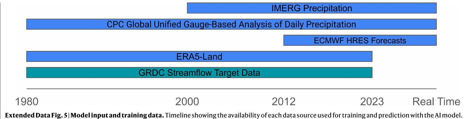
بيانات المدخلات
- توقعات يومية مجمعة من نموذج ECMWF المتكامل للتوقعات (IFS) عالي الدقة (HRES). تشمل المتغيرات: إجمالي هطول الأمطار (TP)، درجة الحرارة على ارتفاع 2 متر (T2M)، الإشعاع الشمسي الصافي السطحي (SSR)، الإشعاع الحراري الصافي السطحي (STR)، تساقط الثلوج (SF) والضغط السطحي (SP).
- نفس المتغيرات الستة من إعادة تحليل ECMWF ERA5-Land.
- تقديرات هطول الأمطار من مركز التنبؤ بالمناخ التابع للإدارة الوطنية للمحيطات والغلاف الجوي (NOAA) التحليل العالمي الموحد القائم على القياس اليومي لهطول الأمطار.
- تقديرات هطول الأمطار من عمليات استرجاع متعددة الأقمار الصناعية المتكاملة التابعة لناسا (IMERG) في التشغيل المبكر.
- سمات الحوض الجيولوجية والجيولوجية والبشرية من قاعدة بيانات HydroATLAS
.
بيانات الهدف والتقييم
التجارب
- تقسيمات التحقق المتقاطع عبر القارات (
). - تقسيمات التحقق المتقاطع عبر مناطق المناخ (
). - تقسيمات التحقق المتقاطع عبر مجموعات من الأحواض المائية المنفصلة هيدرولوجيًا (
)، مما يعني أنه لم يساهم أي حوض نهائي في أي نقاط قياس في نفس الوقت لكل من التدريب والاختبار في أي تقسيم تحقق متقاطع.
جلوفاس
- تستخدم جلوفاس ERA5 كبيانات قسرية، وليس ERA5-Land.
- جلوفاس (في مجموعة البيانات المستخدمة هنا) لا تستخدم ECMWF IFS كمدخلات للنموذج. (تستخدم بيانات IFS من قبل نموذج الذكاء الاصطناعي للتنبؤ فقط، ونحن نقارن دائمًا مع التنبؤات الفورية لجلوفاس.)
- لا تستخدم جلوفاس بيانات NOAA CPC أو بيانات NASA IMERG كمدخلات مباشرة للنموذج.
منطقة الصرف المقدمة من GRDC وشبكة صرف جلوفاس، تم استبعاد جميع محطات GRDC التي كانت منطقة صرفها أصغر من
على الرغم من أن CEMS تصدر إعادة تحليل تاريخية كاملة (بدون أوقات مسبقة) لإصدار جلوفاس 4، إلا أن الأرشيف طويل الأجل للتنبؤات السابقة (تنبؤات الماضي) لإصدار جلوفاس 4 لا يغطي السنة الكاملة في وقت التحليل. نظرًا لأن مقاييس الموثوقية يجب أن تأخذ في الاعتبار توقيت ذروات الأحداث، فهذا يعني أنه من الممكن فقط تقييم جلوفاس في وقت مسبق قدره 0 يوم.
المقاييس
تم الإبلاغ عنها للنماذج الموصوفة في هذه الورقة في الشكل 8 من البيانات الموسعة، بما في ذلك الانحياز، وكفاءة ناش-سوتكليف (NSE)
توفر البيانات
توفر الكود
35. كراتزرت، ف. وآخرون. نحو تعلم سلوكيات هيدرولوجية عالمية وإقليمية ومحلية عبر التعلم الآلي المطبق على مجموعات بيانات كبيرة. هيدرول. علوم نظم الأرض 23، 5089-5110 (2019).
36. كلوتز، د. وآخرون. تقدير عدم اليقين باستخدام التعلم العميق لنمذجة هطول الأمطار والجريان. هيدرول. علوم نظم الأرض 26، 1673-1693 (2022).
37. حقول الجريان المركب العالمية (CSRC-UNH و GRDC، 2002).
38. غريمالدي، س. منهجية ومعايير معايرة GloFAS v4. ECMWF https://confluence.ecmwf.int/display/CEMS/GloFAS+v4+calibration+methodology+and+parameters (2023).
39. اللجنة الاستشارية بين الوكالات لبيانات المياه. إرشادات لتحديد تكرار تدفق الفيضانات النشرة رقم 17B من اللجنة الفرعية للهيدرولوجيا (وزارة الداخلية الأمريكية، المسح الجيولوجي، 1982).
40. سوليفان، ج. م. وفاين، ر. استخدام حجم التأثير – أو لماذا
41. غوش، م. وآخرون. في الدفاع عن المقاييس: المقاييس تشفر بشكل كافٍ التفضيلات البشرية النموذجية فيما يتعلق بأداء النماذج الهيدرولوجية. موارد المياه. بحث. 59، e2022WRO33918 (2023).
42. طرق التحقق من التوقعات عبر مقاييس الزمن والمكان (برنامج أبحاث الطقس العالمي، 2016).
43. ناش، ج. إ. وسوتكليف، ج. ف. التنبؤ بتدفق الأنهار من خلال نماذج مفاهيمية الجزء الأول – مناقشة المبادئ. مجلة الهيدرولوجيا 10، 282-290 (1970).
مقالة
- غوبتا، هـ. ف.، كلينغ، هـ.، يلماظ، ك. ك. ومارتينيز، ج. ف. تحليل متوسط مربع الخطأ ومعايير أداء NSE: الآثار المترتبة على تحسين النمذجة الهيدرولوجية. مجلة الهيدرولوجيا 377، 80-91 (2009).
- نيرينغ، جي. الذكاء الاصطناعي يزيد من الوصول العالمي إلى توقعات الفيضانات الموثوقة. زينودوhttps://doi.org/10.5281/zenodo. 10397664 (2023).
- الناتج المحلي الإجمالي بالدولار الأمريكي الحالي. البنك الدوليhttps://data.worldbank.org/indicator/NY.GDP.MKTP.CD (2023).
من نموذج الذكاء الاصطناعي. ساعد المؤلفون الذين لديهم انتماء إلى ECMWF (S.H. و F.P. و C.P.) أيضًا في ضمان المعالجة الصحيحة لبيانات GloFAS. أكمل S.N. العمل أثناء وجوده في Google. أشرف Y.M. على البحث.
معلومات إضافية
يجب توجيه المراسلات والطلبات للحصول على المواد إلى جراي نيرينغ.
تُعرب مجلة Nature عن شكرها لـ Caihong Hu و Zhongrun Xiang والمراجعين الآخرين المجهولين على مساهمتهم في مراجعة هذا العمل. تقارير مراجعي الأقران متاحة.
معلومات إعادة الطبع والتصاريح متاحة علىhttp://www.nature.com/reprints.
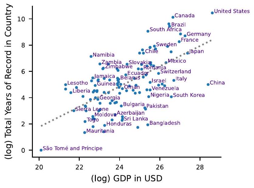
الشكل 1 من البيانات الموسعة | تتوافق توافر بيانات تدفق المياه مع الوطنية
الناتج المحلي الإجمالي (GDP) وإجمالي عدد سنوات بيانات تدفق المياه اليومية المتاحة في بلد ما من مركز بيانات الجريان العالمي. بيانات الناتج المحلي الإجمالي مستمدة من البنك الدولي.
مقالة
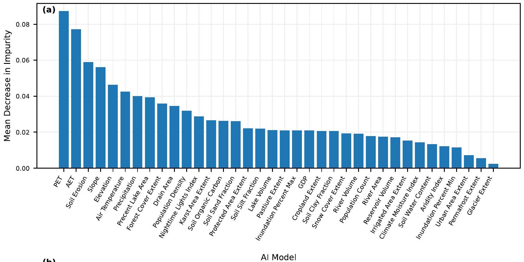
أكثر من المتوسط في أي موقع قياس معين. تُظهر تصنيفات أهمية الميزات هنا الصفات التي يستخدمها المصنف لإجراء تلك التنبؤات. بيانات محاكاة GloFAS من متجر بيانات المناخ
مقالة
مقالة
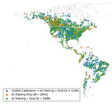
مناطق التجميع العليا إلى مناطق التجميع السفلية. تم إجراء جميع تقييمات نموذج الذكاء الاصطناعي خارج العينة من حيث الموقع والزمان. تم استبعاد بعض من 5,860 جهاز قياس تدريب من التقييم لأنه لم يكن من الممكن مطابقة تلك الأجهزة مع بكسل GloFAS. خريطة أساسية من GeoPandas
انقسامات المناخ
(ب)
(د)
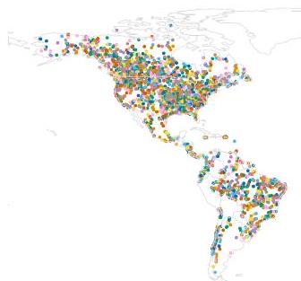
توجد القارات في مجموعة واحدة من التحقق المتقاطع. توضح اللوحة (ج) تقسيمات مناطق المناخ، بحيث تكون جميع الأحواض في كل من 13 منطقة مناخية في مجموعة واحدة من التحقق المتقاطع. توضح اللوحة (د) تقسيمات تجمع القياسات في الأحواض النهائية المنفصلة هيدرولوجيًا. خرائط الأساس من GeoPandas
مقالة
| – النموذج |
| – انقسام القارات |
| – انقسامات المناخ |
| – هيدرولوجيًا |
| – مفصول |
| – تشغيل الأحواض المقاسة |
| – جلوباس |
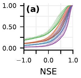
مع زيادة فترة الانتظار). يتم حساب المقاييس على الفترة الزمنية من 2014 إلى 2021. المقاييس في الألواح (أ-ز) مدرجة في الجدول الإضافي 1. بيانات محاكاة GloFAS من متجر بيانات المناخ
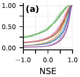
| – النموذج |
| – انقسام القارات |
| – انقسامات المناخ |
| – هيدرولوجيًا |
| – مفصول |
| – تشغيل الأحواض المقاسة |
| – جلوباس |
مقالة
| مقياس | وصف | مرجع |
| NSE | كفاءة ناش-سوتكليف | المعادلة 3 في
|
| لوغ-نسبة التغير | كفاءة ناش-سوتكليف في الفضاء اللوغاريتمي |
|
| ألفا-إن إس إي | نسبة الانحرافات المعيارية للتدفق المرصود والمحاكى | معادلة
|
| بيتا-إن إس إي | التحيز مقاسًا بانحراف المعيار للملاحظات | معادلة
|
| KGE | كفاءة كلينغ-غوبتا | معادلة
|
| لوغ-كيجي | كفاءة كلينغ-غوبتا في الفضاء اللوغاريتمي |
|
| بيتا-KGE | نسبة التدفق المحاكى المتوسط والتدفق المرصود المتوسط | معادلة
|
جوجلhttps://research.google/. المركز الأوروبي للتنبؤات الجوية متوسطة المدى، ريدينغ، المملكة المتحدة. مركز هلمهولتز للبحوث البيئية – UFZ، لايبزيغ، ألمانيا.
مؤسسة راند، لوس أنجلوس، كاليفورنيا، الولايات المتحدة الأمريكية. البريد الإلكتروني: nearing@google.com
DOI: https://doi.org/10.1038/s41586-024-07145-1
PMID: https://pubmed.ncbi.nlm.nih.gov/38509278
Publication Date: 2024-03-20
Global prediction of extreme floods in ungauged watersheds
Received: 29 July 2023
Accepted: 31 January 2024
Published online: 20 March 2024
Open access
(A) Check for updates
Abstract
Floods are one of the most common natural disasters, with a disproportionate impact in developing countries that often lack dense streamflow gauge networks
end of the PUB decade, the IAHS reported that little progress had been made against the problem, stating that “much of the success so far has been in gauged rather than in ungauged basins, which has negative effects in particular for developing countries”
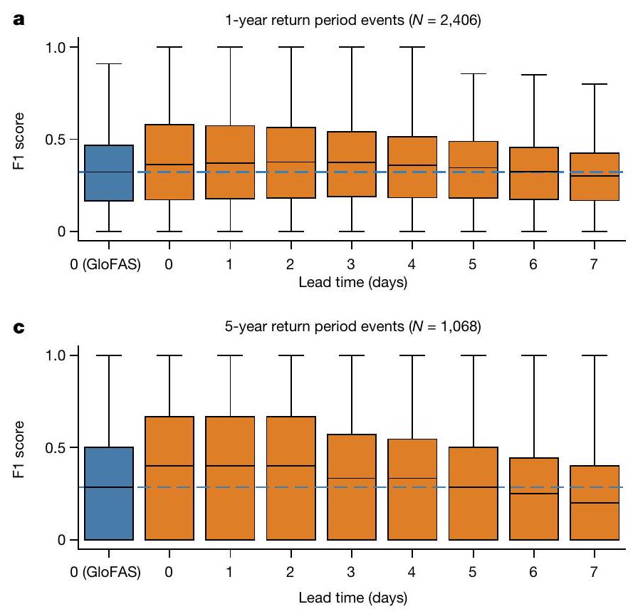
AI improves forecast reliability
Return periods
Forecast lead time
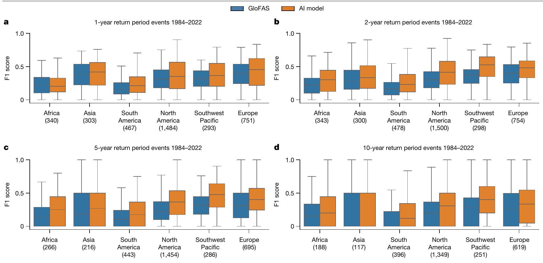
Continents
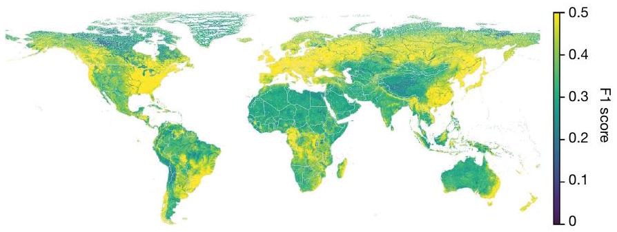
Predictability of forecast reliability
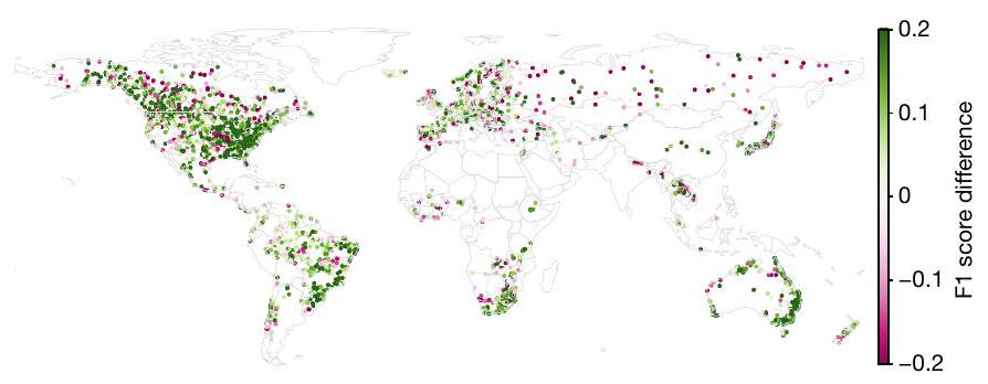
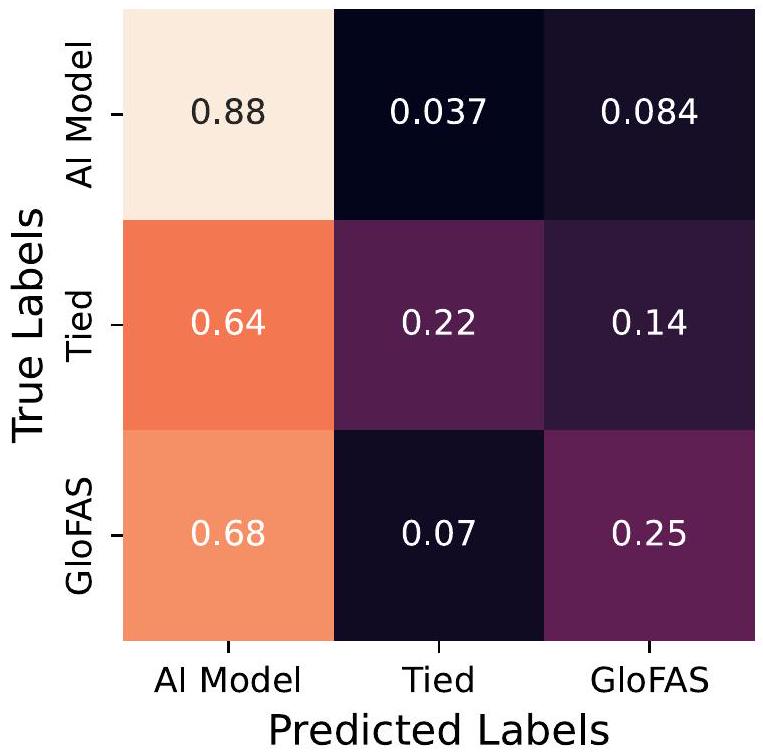
reported in the main text. The boxes show distribution quartiles and whiskers show the full range excluding outliers. The blue dashed line is the median score for GloFAS nowcasts and is plotted as a reference. GloFAS simulation data from the Climate Data Store
better (or similar) in each individual watershed. The classifier was trained with stratified
Conclusion and discussion
Online content
- Rentschler, J., Salhab, M. & Jafino, B. A. Flood exposure and poverty in 188 countries. Nat. Commun. 13, 3527 (2022).
- Hallegatte, S. A Cost Effective Solution to Reduce Disaster Losses in Developing Countries: Hydro-meteorological Services, Early Warning, and Evacuation Policy Research Working Paper 6058 (World Bank, 2012).
- The Human Cost of Natural Disasters: A Global Perspective (United Nations International Strategy for Disaster Reduction, 2015).
- 2021 State of Climate Services WMO-No. 1278 (World Meteorological Organization, 2021).
- Milly, P., Christopher, D., Wetherald, R. T., Dunne, K. A. & Delworth, T. L. Increasing risk of great floods in a changing climate. Nature 415, 514-517 (2002).
- Tabari, H. Climate change impact on flood and extreme precipitation increases with water availability. Sci. Rep. 10, 13768 (2020).
- Global Report on Drowning: Preventing A Leading Killer (World Health Organization, 2014).
- The Global Climate 2001-2010: A Decade of Climate Extremes Technical Report (World Health Organization, 2013).
- Pilon, P. J. Guidelines for Reducing Flood Losses Technical Report (United Nations International Strategy for Disaster Reduction, 2002).
- Rogers, D. & Tsirkunov, V. Costs and Benefits of Early Warning Systems: Global Assessment Report on Disaster Risk Reduction (The World Bank, 2010).
- Razavi, S. & Tolson, B. A. An efficient framework for hydrologic model calibration on long data periods. Water Resour. Res. 49, 8418-8431 (2013).
- Li, Chuan-zhe et al. Effect of calibration data series length on performance and optimal parameters of hydrological model. Water Sci. Eng. 3, 378-393 (2010).
- Sivapalan, M. et al. IAHS decade on predictions in ungauged basins (PUB), 2003-2012: shaping an exciting future for the hydrological sciences. Hydrol. Sci. J. 48, 857-880 (2003).
- Hrachowitz, M. et al. A decade of predictions in ungauged basins (PUB)-a review. Hydrol. Sci. J. 58, 1198-1255 (2013).
- Kratzert, F. et al. Toward improved predictions in ungauged basins: exploiting the power of machine learning. Water Resour. Res. 55, 11344-11354 (2019).
- Alfieri, L. et al. GloFAS—global ensemble streamflow forecasting and flood early warning. Hydrol. Earth Syst. Sci. 17, 1161-1175 (2013).
- Harrigan, S., Zsoter, E., Cloke, H., Salamon, P. & Prudhomme, C. Daily ensemble river discharge reforecasts and real-time forecasts from the operational global flood awareness system. Hydrol. Earth Syst. Sci. 27, 1-19 (2023).
- Arheimer, B. et al. Global catchment modelling using world-wide HYPE (WWH), open data, and stepwise parameter estimation. Hydrol. Earth Syst. Sci. 24, 535-559 (2020).
- Souffront Alcantara, M. A. et al. Hydrologic modeling as a service (HMaaS): a new approach to address hydroinformatic challenges in developing countries. Front. Environ. Sci. 7, 158 (2019).
- Sheffield, J. et al. A drought monitoring and forecasting system for sub-sahara African water resources and food security. Bull. Am. Meteorol. Soc. 95, 861-882 (2014).
- Hochreiter, S. & Schmidhuber, J. ürgen. Long short-term memory. Neural Comput. 9, 1735-1780 (1997).
- Kratzert, F., Gauch, M., Nearing, G. S. & Klotz, D. NeuralHydrology-a Python library for deep learning research in hydrology. J. Open Source Softw. 7, 4050 (2022).
- Sellars, S. L. ‘Grand challenges’ in big data and the Earth sciences. Bull. Am. Meteorol. Soc. 99, ES95-ES98 (2018).
- Todini, E. Hydrological catchment modelling: past, present and future. Hydrol. Earth Syst. Sci. 11, 468-482 (2007).
- Herath, H. M. V. V., Chadalawada, J. & Babovic, V. Hydrologically informed machine learning for rainfall-runoff modelling: towards distributed modelling. Hydrol. Earth Syst. Sci. 25, 4373-4401 (2021).
- Reichstein, M. et al. Deep learning and process understanding for data-driven Earth system science. Nature 566, 195-204 (2019).
- Frame, J. M. et al. Deep learning rainfall-runoff predictions of extreme events. Hydrol. Earth Syst. Sci. 26, 3377-3392 (2022).
- Linke, S. et al. Global hydro-environmental sub-basin and river reach characteristics at high spatial resolution. Sci. Data 6, 283 (2019).
- Kratzert, F. et al. Large-scale river network modeling using graph neural networks. In European Geosciences Union General Assembly Conference Abstracts EGU21-13375 (EGU General Assembly, 2021).
- Lehner, B. & Grill, G. ünther. Global river hydrography and network routing: baseline data and new approaches to study the world’s large river systems. Hydrol. Proces. 27, 2171-2186 (2013).
- Nearing, G. S. et al. Data assimilation and autoregression for using near-real-time streamflow observations in long short-term memory networks. Hydrol. Earth Syst. Sci. 26, 5493-5513 (2022).
- Kratzert, F. et al. Caravan-a global community dataset for large-sample hydrology. Sci. Data 10, 61 (2023).
- Grimaldi, S. et al. River discharge and related historical data from the Global Flood Awareness System. Climate Data Store https://doi.org/10.24381/cds.a4fdd6b9 (2023).
- Jordahl, K. et al. geopandas/geopandas: v0.8.1 https://zenodo.org/records/3946761 (2020).
(c) The Author(s) 2024
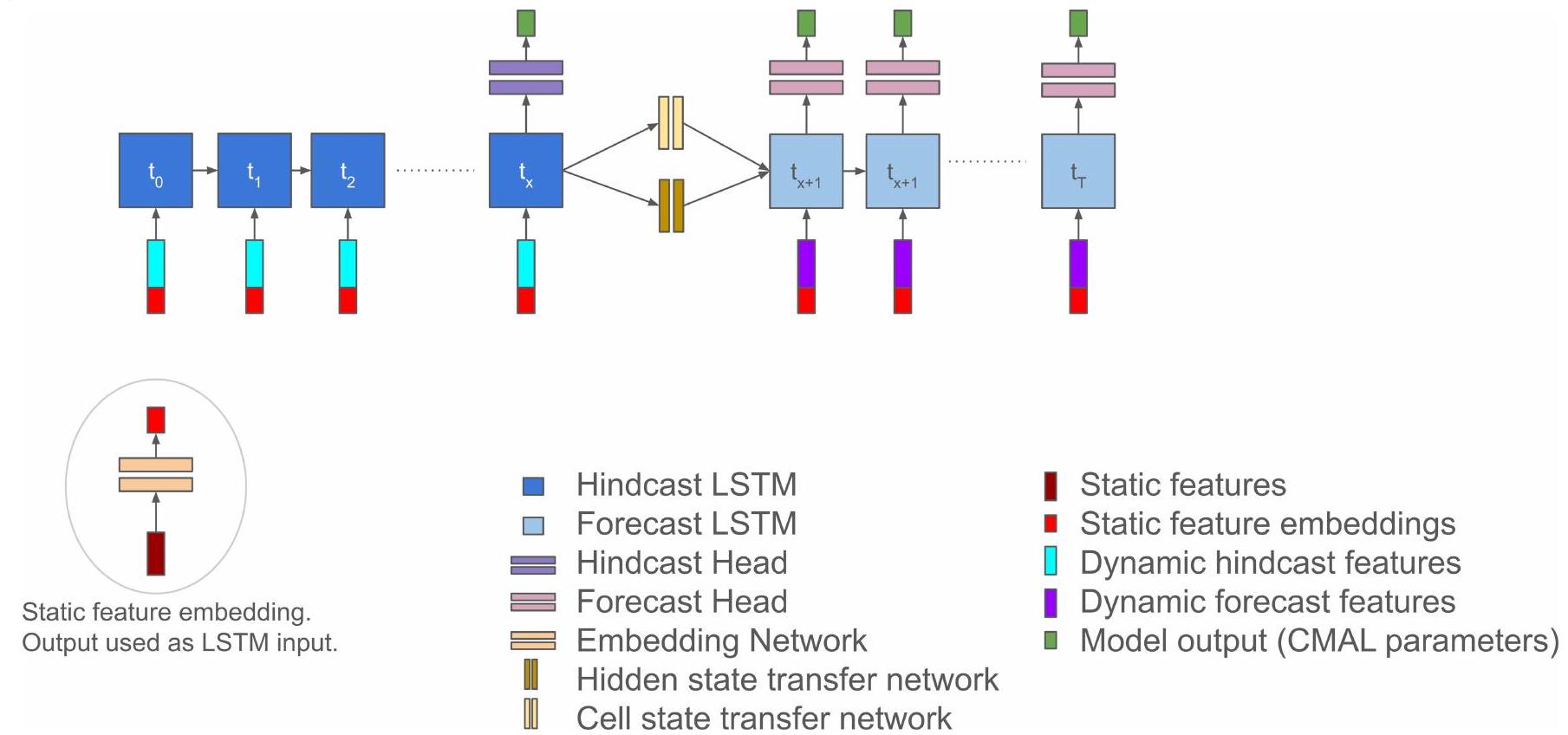
Al model
Input data
- Daily-aggregated single-level forecasts from the ECMWF Integrated Forecast System (IFS) High Resolution (HRES) atmospheric model. Variables include: total precipitation (TP), 2-m temperature (T2M), surface net solar radiation (SSR), surface net thermal radiation (STR), snowfall (SF) and surface pressure (SP).
- The same six variables from the ECMWF ERA5-Land reanalysis.
- Precipitation estimates from the National Oceanic and Atmospheric Administration (NOAA) Climate Prediction Center (CPC) Global Unified Gauge-Based Analysis of Daily Precipitation.
- Precipitation estimates from the NASA Integrated Multi-satellite Retrievals for GPM (IMERG) early run.
- Geological, geophysical and anthropogenic basin attributes from the HydroATLAS database
.
Target and evaluation data
Experiments
- Cross-validation splits across continents (
). - Cross-validation splits across climate zones (
). - Cross-validation splits across groups of hydrologically separated watersheds (
), meaning that no terminal watershed contributed any gauges simultaneously to both training and testing in any cross-validation split.
GloFAS
- GloFAS uses ERA5 as forcing data, and not ERA5-Land.
- GloFAS (in the dataset used here) does not use ECMWF IFS as input to the model. (IFS data are used by the AI model for forecasting only, and we always compare with GloFAS nowcasts.)
- GloFAS does not use NOAA CPC or NASA IMERG data as direct inputs to the model.
drainage area provided by the GRDC and the GloFAS drainage network, all GRDC stations with a drainage area smaller than
Although CEMS releases a full historical reanalysis (without lead times) for GloFAS version 4, long-term archive of reforecasts (forecasts of the past) of GloFAS version 4 do not span the full year at the time of the analysis. Given that reliability metrics must consider the timing of event peaks, this means that it is only possible to benchmark GloFAS at a 0-day lead time.
Metrics
are reported for the models described in this paper in Extended Data Fig. 8, including bias, Nash-Sutcliffe efficiency (NSE)
Data availability
Code availability
35. Kratzert, F. et al. Towards learning universal, regional, and local hydrological behaviors via machine learning applied to large-sample datasets. Hydrol. Earth Syst. Sci. 23, 5089-5110 (2019).
36. Klotz, D. et al. Uncertainty estimation with deep learning for rainfall-runoff modeling. Hydrol. Earth Syst. Sci. 26, 1673-1693 (2022).
37. Global Composite Runoff Fields (CSRC-UNH and GRDC, 2002).
38. Grimaldi, S. GloFAS v4 calibration methodology and parameters. ECMWF https:// confluence.ecmwf.int/display/CEMS/GloFAS+v4+calibration+methodology+and+ parameters (2023).
39. Interagency Advisory Committee on Water Data. Guidelines for Determining Flood Flow Frequency Bulletin #17B of the Hydrology Subcommittee (US Department of the Interior Geological Survey, 1982).
40. Sullivan, G. M. & Feinn, R. Using effect size-or why the
41. Gauch, M. et al. In defense of metrics: metrics sufficiently encode typical human preferences regarding hydrological model performance. Water Resour. Res. 59, e2022WRO33918 (2023).
42. Forecast Verification Methods Across Time and Space Scales (World Weather Research Programme, 2016).
43. Nash, J. E. & Sutcliffe, J. V. River flow forecasting through conceptual models part I-a discussion of principles. J. Hydrol. 10, 282-290 (1970).
Article
- Gupta, H. V., Kling, H., Yilmaz, K. K. & Martinez, G. F. Decomposition of the mean squared error and NSE performance criteria: implications for improving hydrological modelling. J. Hydrol. 377, 80-91 (2009).
- Nearing, G. AI increases global access to reliable flood forecasts. Zenodo https://doi.org/ 10.5281/zenodo. 10397664 (2023).
- GDP Current US$. World Bank https://data.worldbank.org/indicator/NY.GDP.MKTP.CD (2023).
of the AI model. Authors with ECMWF affiliation (S.H., F.P. and C.P.) additionally helped to ensure proper processing of GloFAS data. S.N. completed the work while at Google. Y.M. supervised the research.
Additional information
Correspondence and requests for materials should be addressed to Grey Nearing.
Peer review information Nature thanks Caihong Hu, Zhongrun Xiang and the other, anonymous, reviewer(s) for their contribution to the peer review of this work. Peer reviewer reports are available.
Reprints and permissions information is available at http://www.nature.com/reprints.
Extended Data Fig. 1 | Streamflow data availability correlates with national
Domestic Product (GDP) and the total number of years worth of daily streamflow data available in a country from the Global Runoff Data Center. GDP data are sourced from The World Bank
Article
than average in any given gauge location. The feature importance rankings shown here illustrate which catchment attributes the classifier uses to make those predictions. GloFAS simulation data from the Climate Data Store
Article
Article
head-catchments to downstream catchments. All AI model evaluation was done out-of-sample in both location and time. Some of the 5,860 training gauges were excluded from evaluation because it was not possible to match those gauges to a GloFAS pixel. Basemap from GeoPandas
Climate Splits
(b)
(d)
continent are in one cross validation group. Panel (c) shows climate zone splits, so that all basins in each of 13 climate zones are in one cross validation group. Panel (d) shows splits that group gauges in hydrologically-separated terminal basins. Basemaps from GeoPandas
Article
| – Al Model |
| – Continent Splits |
| – Climate Splits |
| – Hydrologically |
| – Separated |
| – Gauged Basins Run |
| – GloFAS |
with increasing lead time). Metrics are calculated on the time period 2014-2021. Metrics in panels (a-g) are listed in Extended Data Table 1. GloFAS simulation data from the Climate Data Store
| – Al Model |
| – Continent Splits |
| – Climate Splits |
| – Hydrologically |
| – Separated |
| – Gauged Basins Run |
| – GloFAS |
Article
| Metric | Description | Reference |
| NSE | Nash-Sutcliffe efflciency | Eq. 3 in
|
| log-NSE | Nash-Sutcliffe effliciency in logarithmic space |
|
| Alpha-NSE | Ratio of standard deviations of observed and simulated flow | Eq.
|
| Beta-NSE | Bias scaled by standard deviation of observations | Eq.
|
| KGE | Kling-Gupta efficiency | Eq.
|
| log-KGE | Kling-Gupta efficiency in logarithmic space |
|
| Beta-KGE | Ratio of mean simulated and mean observed flow | Eq.
|
Google, https://research.google/. European Centre for Medium-Range Weather Forecasts, Reading, UK. Helmholtz Centre for Environmental Research – UFZ, Leipzig, Germany.
RAND Corporation, Los Angeles, CA, USA. e-mail: nearing@google.com