تعتمد سكان العالم بشكل متزايد على المحيط من أجل الغذاء وإنتاج الطاقة والتجارة العالمية.ومع ذلك، فإن الأنشطة البشرية في البحر ليست موثقة بشكل جيد. نحن نجمع بين صور الأقمار الصناعية وبيانات GPS للسفن ونماذج التعلم العميق لرسم خريطة أنشطة السفن الصناعية والبنية التحتية للطاقة البحرية عبر المياه الساحلية في العالم من 2017 إلى 2021. نجد أن 72-76% من سفن الصيد الصناعية في العالم لا يتم تتبعها علنًا، حيث يحدث الكثير من هذا الصيد حول جنوب آسيا وجنوب شرق آسيا وأفريقيا. كما نجد أن 21-30% من أنشطة النقل والطاقة للسفن مفقودة من أنظمة التتبع العامة. عالميًا، انخفض الصيد بـعند بداية جائحة كوفيد-19 في عام 2020، لم تتعافَ الأنشطة الاقتصادية إلى مستويات ما قبل الجائحة بحلول عام 2021. بالمقابل، كانت أنشطة النقل والطاقة أقل تأثراً خلال نفس الفترة. تتزايد طاقة الرياح البحرية بسرعة، حيث تقتصر معظم توربينات الرياح على مناطق صغيرة من المحيط لكنها تجاوزت عدد الهياكل النفطية في عام 2021. تكشف خريطتنا لتصنيع المحيطات عن تغييرات في بعض من أكثر الأنشطة البشرية اتساعاً وأهمية اقتصادية في البحر.
أكثر من مليار شخص يعتمدون على المحيط كمصدرهم الرئيسي للغذاء، حيث يعمل 260 مليون شخص في مصايد الأسماك البحرية العالمية فقطحوالي 80% من جميع السلع المتداولة تُشحن عبر المحيط.وحوالي 30% من نفط العالم يتم إنتاجه في حقول بحرية ويتم توزيعه في جميع أنحاء العالمبالإضافة إلى هذه الاستخدامات المعروفة للمحيط، فإن الزيادة في الطاقة المتجددة البحرية، وتربية الأحياء المائية، والتعدين تتطور بسرعة. كل هذه الآلات الصناعية تدعم ‘الاقتصاد الأزرق’ الذي تبلغ قيمته 1.5-2.5 تريليون دولار.الذي ينمو أسرع من الاقتصاد العالمي بشكل عاملكنها تسبب أيضًا تدهورًا سريعًا في البيئة. يتم استغلال ثلث مخزونات الأسماك بما يتجاوز المستويات المستدامة بيولوجيًا. وتقدير تم فقدان العديد من المواطن البحرية الحيوية بسبب التصنيع البشري.
يحد نقص البيانات العالمية الملاحظة من فهم مكان وكيفية توسع الاقتصاد الأزرق وكيف يؤثر على الدول النامية والمجتمعات الساحلية.على اليابسة، توجد خرائط تقريبًا لكل طريقتُطوَّر مجموعات بيانات لكل هيكل من صنع الإنسان والصناعات الاستخراجية مثل الغابات والزراعة يتم رسم خرائطها عالميًا على مقياس دون الكيلومتر ويتم تحديثها شهريًا ومع ذلك، في المحيط، لا تقوم العديد من السفن البحرية ببث موقعها أو لا يتم اكتشافها بواسطة أنظمة المراقبة العامة. وغالبًا ما تُحتفظ المعلومات المتعلقة بتطوير البنية التحتية البحرية وغيرها من الأنشطة الصناعية بشكل سري . والنتيجة هي أن التوسع البشري المستمر في المحيط موثق بشكل سيء.
تواجه الأساليب الحالية لرسم خرائط النشاط البشري في البحر قيودًا. بعض أنظمة تتبع السفن، مثل نظام مراقبة السفن (VMS) المستخدم في الصيد، هي أنظمة ملكية، مما يحد من القدرة على رسم الخرائط والمقارنة عبر المناطق.بالنسبة لرسم الخرائط العامة للسفن، كان التركيز على نظام التعرف التلقائي على السفن (AIS)الذي يبث إحداثيات السفن لتتبع تحركات السفن ودعم السلامة البحرية؛ يمكن أن تكشف بيانات نظام تحديد الهوية الآلي أيضًا عن هويات السفن ومالكيها والشركات، وأنشطة الصيد.ومع ذلك، لا يُطلب من جميع السفن استخدام أجهزة نظام تحديد الهوية الآلي (AIS)، حيث تختلف اللوائح حسب البلد وحجم السفينة ونشاطها.السفن المشاركة في الأنشطة غير المشروعة غالبًا ما تقوم بإيقاف أجهزة الإرسال AIS الخاصة بها أو التلاعب بالمواقع التي تبثها.في السنوات الأخيرة، على سبيل المثال، كانت أكبر حالات الصيد غير القانونيوالعمل القسريكانت بواسطة أساطيل لم تستخدم في الغالب أجهزة AIS. علاوة على ذلك، تظهر ‘نقاط عمياء’ كبيرة على طول المياه الساحلية حيث يكون استقبال الأقمار الصناعية ضعيفًا.ويمكن أن تقيد الحكومات الوطنية بيانات AIS المستلمة من المستقبلات الأرضيةنشير إلى السفن التي لا تظهر على بيانات نظام تحديد الهوية الآلي (AIS) المتاحة للجمهور بأنها ‘غير متعقبة علنًا’. يُشار إلى هذا المفهوم أحيانًا أيضًا باسم ‘السفن المظلمة’. على الرغم من أن موقع البنية التحتية الثابتة في البحر يجب أن يكون متاحًا بشكل أكبر من السفن المتحركة، إلا أن المعلومات حول التطوير البحري غالبًا ما تكون مقيدة لأسباب تجارية أو بيروقراطية.ويجب أن تجمع التقييمات واسعة النطاق عدة مصادر بيانات متباينة، والتي غالبًا ما تكون غير مكتملة أو قديمة.لا تُلتقط أنشطة السفن والبنية التحتية البحرية بشكل جيد بواسطة الطرق الحالية، ولكن يمكن أن تُحسن الصور الفضائية والتعلم العميق من مراقبة الاستخدام البشري للمحيط.
هنا نقدم خريطة عالمية مفصلة للأنشطة الصناعية الرئيسية في البحر. للكشف عن السفن والبنية التحتية البحرية في المياه الساحلية حول العالم، قمنا بتحليل 2 بيتابايت من صور الأقمار الصناعية التي تغطي السنوات 2017-2021، حيث شملت تحليلاتنا أكثر من 15% من المحيط (الشكل البياني الممتد 1) الذي تتركز فيه أكثر من 75% من الأنشطة الصناعية (الطرق). قمنا بتصميم وتدريب ثلاث شبكات عصبية عميقة للتعرف على الأجسام (بدقة تزيد عن 97%) وتقدير أطوالها.نتيجة
لتصنيف البنية التحتية البحرية إلى النفط والرياح وأشياء أخرى (>98% دقة)؛ ولتصنيف السفن كصيد أو غير صيد (الدقة). معًا، قمنا بتصنيف أكثر من 67 مليون بلاطة صورة، بما في ذلك صور الرادار الاصطناعي ذي الاستقطاب المزدوج (SAR) من Sentinel-1 (المرجع 35) وصور بصرية (أحمر، أخضر، أزرق وقريب من الأشعة تحت الحمراء (NIR)) من Sentinel-2 (المرجع 36). تتيح لنا دقة الرادار الاصطناعي التقاط معظم الأجسام التي يزيد حجمها عن 15 مترًا (معدل الكشفلسفن بطول 25 مترللسفن التي يبلغ طولها 50 مترًا أو أكثر؛ الشكل البياني الموسع 2). كما قمنا بتحليل 53 مليار موقع GPS للسفن من نظام تحديد الهوية الآلي (AIS) وقمنا بمطابقتها مع اكتشافات الأقمار الصناعية لتحديد ما إذا كانت السفينة المكتشفة تتبع علنًا.
سفن الصيد وغير الصيد
خلال الفترة من 2017 إلى 2021، تم الكشف في المتوسط عن حوالي 63,300 حالة سفينة في أي لحظة، وهو ما يعادل تقريبًا نصف ( ) منها كانت سفن صيد (استنادًا إلى 23.1 مليون كشف عن السفن؛ الشكل 1). ومن الجدير بالذكر أن حوالي ثلاثة أرباع (72-76%) من الصيد الصناعي الذي تم رسم خرائطه عالميًا لم يظهر في أنظمة المراقبة العامة، مقارنةً بربع ( ) لأنشطة السفن الأخرى.
كانت أنشطة السفن واسعة الانتشار ولكنها أيضًا مركزة بشكل كبير. تقسيم منطقة دراستنا إلىالخلايا (حوالي 11 كم)، اكتشفنا سفينة مرة واحدة على الأقل فيمن الخلايا التي تغطيها الأقمار الصناعية، ومع ذلك كانت نصف جميع أنشطة السفن مركزة في أقل منالخلايا. كانت معظم أنشطة السفن (86% من الصيد و75% من الأنشطة غير المتعلقة بالصيد) مركزة في مياه عمقها أقل من 200 متر (الشكل 1)، والتي تشكل فقط 7% من المحيط. كما أن النشاط موزع بشكل غير متساوٍ حسب القارة، حيث يمثل حوالي 67% من جميع أنشطة السفن في آسيا، تليها 12% في أوروبا، و7% في أمريكا الشمالية، و7% في أفريقيا، و4% في أمريكا الجنوبية و2% في أستراليا (الشكل 1).
كشفت خرائط الأقمار الصناعية لدينا عن كثافات عالية من نشاط السفن في مناطق واسعة من المحيط التي كانت تظهر سابقًا نشاطًا ضئيلًا أو معدومًا من قبل أنظمة التتبع العامة (الشكل 2). تُظهر إندونيسيا وجنوب آسيا وجنوب شرق آسيا والسواحل الشمالية والغربية لأفريقيا (الشكل 2 والأشكال التكميلية 3 و4) كميات كبيرة من النشاط غير المتعقب علنًا.
من خلال رسم خرائط للسفن التي تفشل في بث موقعها، نظهر بدقة أكبر التوزيع العالمي للصيد الصناعي. بيانات نظام تحديد الهوية الآلي وحدها، على سبيل المثال، توحي بشكل خاطئ بأن أوروبا وآسيا لديهما نشاط صيد متقارب، بينما تمتلك القارات الأخرى أقل من خُمس هذا النشاط (البيانات الموسعة الجدول 1). ومع ذلك، تكشف خريطتنا العالمية أن آسيا تهيمن على الصيد الصناعي، حيث تمثل 70% من جميع اكتشافات سفن الصيد (البيانات الموسعة الشكل 5)؛ حيث تمركز ما يقرب من 30% من جميع سفن الصيد المرسومة في المنطقة الاقتصادية الخالصة (EEZ) للصين وحدها. وبالمثل، توحي بيانات نظام تحديد الهوية الآلي بأن الدول الأوروبية في البحر الأبيض المتوسط لديها أكثر من عشرة أضعاف ساعات الصيد في مناطقها الاقتصادية الخالصة مقارنة بالدول الأفريقية.لكن خرائطنا تظهر أن اكتشافات سفن الصيد متوازنة إلى حد كبير بين الأجزاء الشمالية والجنوبية من البحر الأبيض المتوسط (الأشكال 1 و 2).
يمكن أن تكشف خرائطنا أيضًا عن النقاط الساخنة المحتملة لنشاط الصيد غير القانوني. أظهرت الأعمال السابقة وجود نشاط غير قانوني كبير في المياه الشرقية لكوريا الشمالية.، لكن خريطتنا العالمية تظهر أن معظم الصيد غير المعلن حدث في الجزء الغربي من شبه الجزيرة الكورية (الشكل 2). في الواقع، أظهرت هذه المنطقة أعلى كثافة من سفن الصيد في العالم من 2017 إلى 2019، مع حوالي 40 سفينة لكل. كانت هذه النشاطات غير المرسومة سابقًا تصل إلى ذروتها كل عام في مايو، خلال فترة حظر الصيد في المياه الصينية (الشكل البياني الممتد 6)، وانخفض النشاط بشكل حاد بنسبة 85% خلال جائحة COVID-19 عندما أغلقت كوريا الشمالية حدودها. تم أيضًا رصد العديد من قوارب الصيد التي لم يتم تتبعها علنًا داخل العديد من المناطق البحرية المحمية (MPAs). على سبيل المثال، أظهرت اثنتان من أكثر المناطق البحرية المحمية شهرة وأهمية بيولوجية ورصدًا في العالم – محمية غالاباغوس البحرية وحديقة الشعاب المرجانية الكبرى – في المتوسط، أكثر من 5 و20 من هذه القوارب أسبوعيًا، على التوالي (الشكل البياني الممتد 7).
الدقة المكانية لبياناتنا، التي هي أعلى بكثير من أكثر المنتجات العالمية المستخدمة في الصيد، كما يكشف عن استراتيجيات صيد مفصلة على النطاق الإقليمي (الشكل 2 والشكل الإضافي 3). تُظهر المنطقة بين تونس وصقلية، على سبيل المثال، مزيجًا من السفن الصيد العامة وغير العامة التي تتجمع على طول البنوك البحرية وحواف الأخاديد القاعية، وهي سمة مميزة لصيد القاع. وبالمثل، قبالة سواحل بنغلاديش، حيث لا يتم تتبع أي سفن بشكل علني ولا توجد خرائط عامة للصيد، تتبع سفن الصيد خطوط العمق وقنوات تحت البحر التي تنبعث من دلتا الغانج.
على عكس الصيد، فإن معظم السفن غير المتعلقة بالصيد (التي تتعلق بشكل كبير بالنقل والطاقة) تبث مواقعها، حيث أن حوالي ربعها فقط مفقود من أنظمة المراقبة العامة. كانت آسيا تحتوي على أكبر تركيز (65% من جميع الاكتشافات) من سفن النقل والطاقة، بما في ذلك معظم السفن غير الباثة (الشكل 1) – ومع ذلك، كانت معظم هذه السفن تعمل في مناطق ذات استقبال ضعيف لنظام تحديد المواقع AIS عبر الأقمار الصناعية، لذا من الممكن أن العديد من السفن تبث مواقعها ولكن لم يكن بالإمكان تتبعها بواسطة خدمات تتبع AIS العالمية. بدت جميع القارات الأخرى تعاني من اختلافات تتبع طفيفة نسبياً عبر سفن النقل والطاقة، حيث كان أقل من 20% من هذه السفن غير قابلة للتتبع علنياً.
تتبع خريطتنا أيضًا التغيرات في نشاط السفن بمرور الوقت (الشكل 3). مشابهًا لتحليل سابق يعتمد على نظام تحديد الهوية الآلي للسفن.تظهر بياناتنا دورات سنوية من نشاط الصيد، حيث تتأثر الدورات داخل الصين برأس السنة الصينية ووقف الصيد الطوعي، وفي بقية العالم برأس السنة والعطلات المرتبطة بها. ولكن، بفضل الكشف القائم على الرادار، يمكننا تقديم تقييم أكثر دقة للاتجاهات، مما يكشف عن انخفاض عالمي في نشاط الصيد.، بالتزامن مع الجائحة. وعلى النقيض من ذلك، ظلت قطاعات النقل والطاقة مستقرة أو حتى زادت قليلاً خلال الفترة من 2017 إلى 2021. علاوة على ذلك، كان تأثير COVID-19 على نشاط الصيد أكبر بكثير خارج الصين (مقارنةً بعام 2018 و2019)، ونمت قطاعات النقل والطاقة في الصين أكثر مما كانت عليه في بقية العالم.
البنية التحتية الثابتة
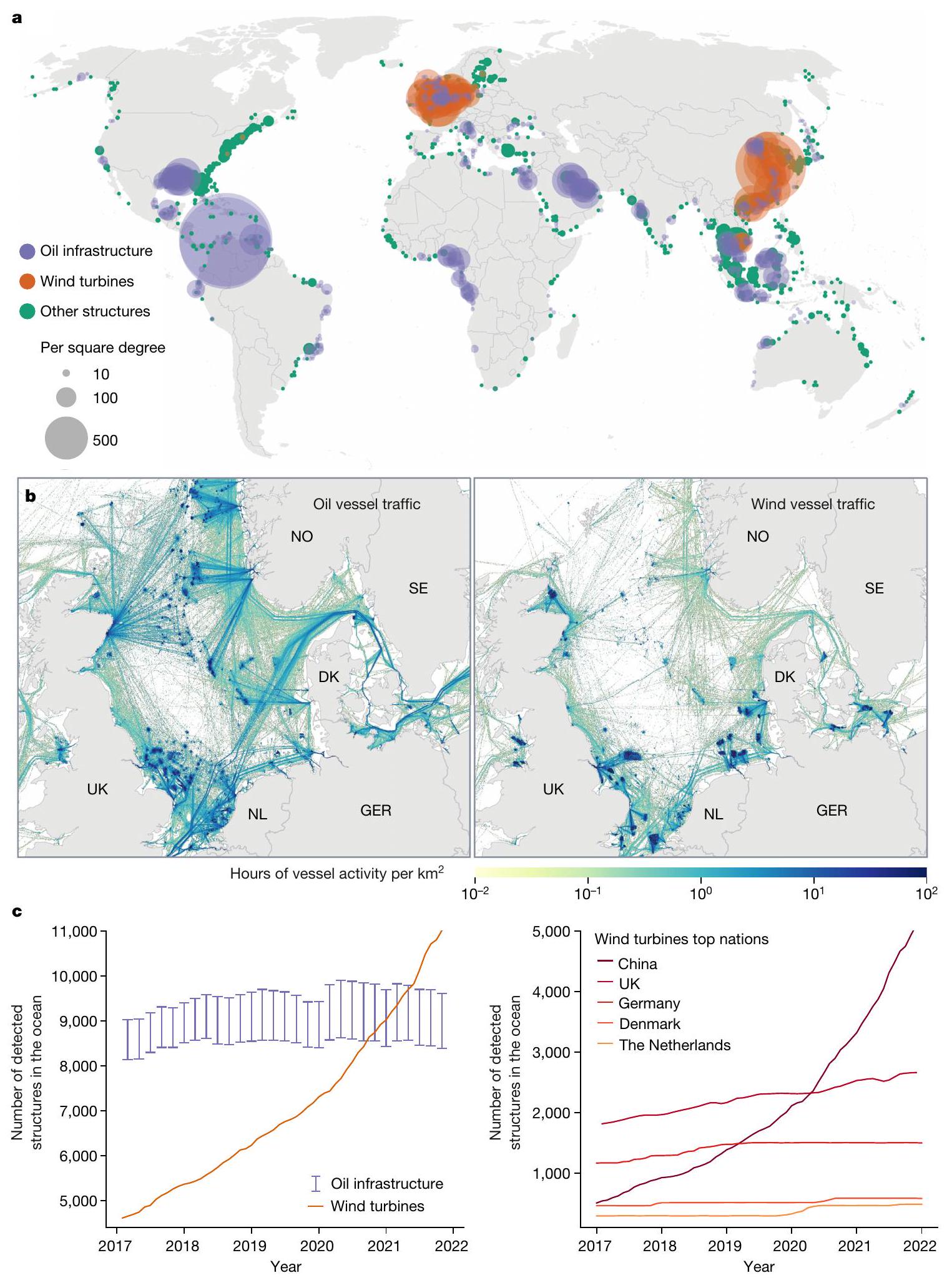
كان عدد الهياكل البحرية في جميع أنحاء العالم حوالي 28,000 بحلول نهاية عام 2021 (الشكل 4). كانت توربينات الرياح والهياكل النفطية في المناطق المعروفة بإنتاج الرياح أو إنتاج النفط (الطرق) تشكلو38% من جميع البنية التحتية البحرية، على التوالي؛ تم تقسيم الـ 14% المتبقية بين توربينات الرياح وهياكل النفط خارج مناطق التنمية الرئيسية، بالإضافة إلى الأرصفة والجسور وخطوط الطاقة وتربية الأحياء المائية وغيرها من الهياكل من صنع الإنسان.
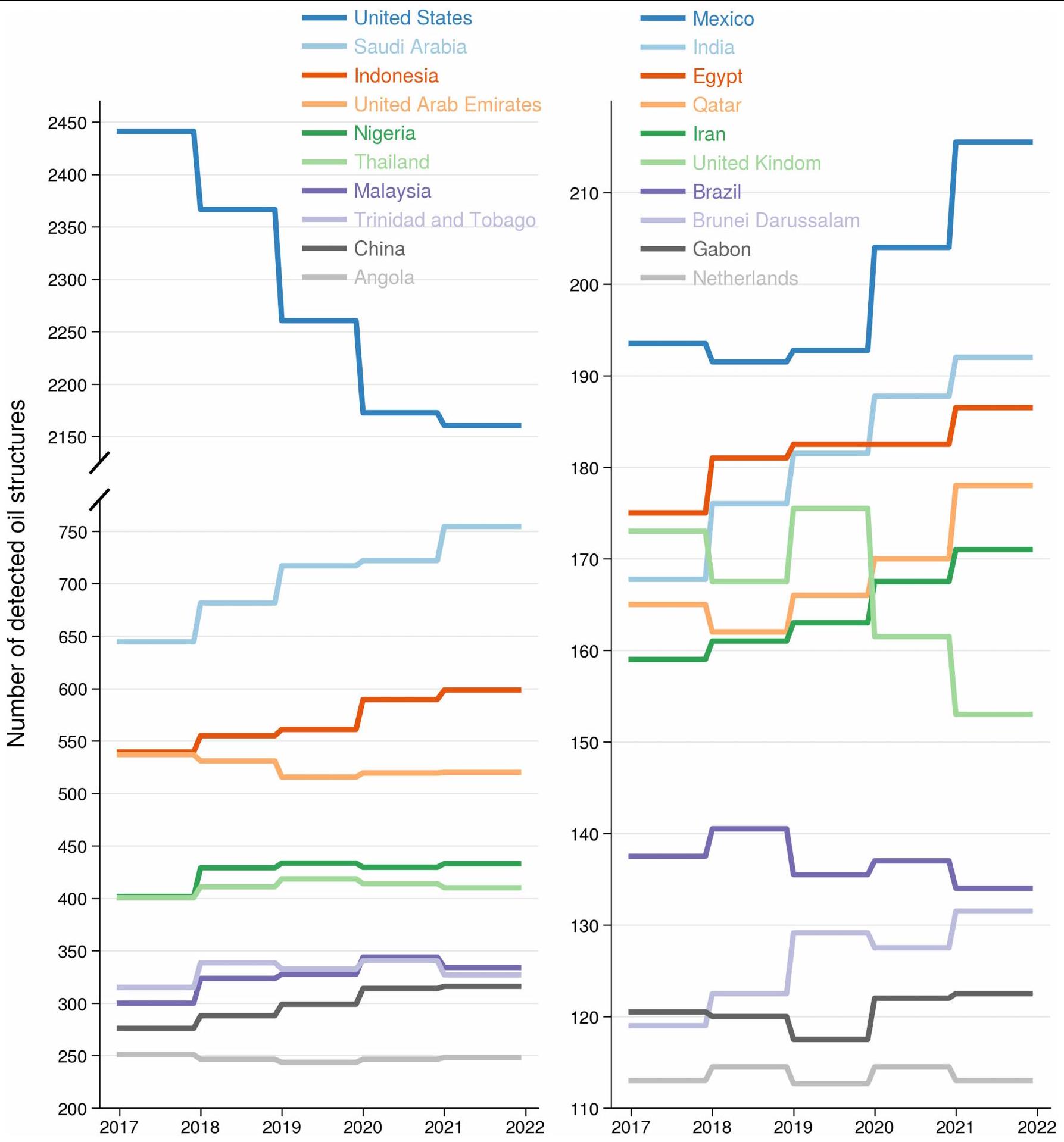
توزع معظم بنية النفط التحتية بين 13 منطقة رئيسية لإنتاج النفط (الشكل 4أ). باستثناء بحيرة ماراكايبو في فنزويلا، التي هي بحيرة، تُظهر خرائطنا أن أكبر تركيز للبنية التحتية للنفط البحري في العالم هو في خليج المكسيك. في نهاية عام 2021، تمثل الولايات المتحدة حوالي ربع البنية التحتية العالمية للنفط البحري (>2,200 هيكل نفطي)، تليها السعودية (>770) وإندونيسيا (>670).
تم حصر تطوير طاقة الرياح البحرية في الغالب في شمال أوروبا (52%) والصين (45%) (الشكل 4أ والشكل البياني الممتد 8)؛ ومع ذلك، كان هناك تحول في تطوير الطاقة البحرية. زاد عدد الهياكل النفطية البحرية بنحو 16% على مدى نصف العقد الماضي (الشكل 4ج)، مع انخفاض في الولايات المتحدة بعدة مئات من الهياكل تم تعويضه بزيادات في أماكن أخرى (الشكل البياني الممتد 9). بالمقابل، زاد عدد توربينات الرياح في المحيط أكثر من الضعف منذ عام 2017، ومن المحتمل أن يتجاوز عدد الهياكل النفطية بحلول نهاية عام 2020 (الشكل 4ج). تتصدر الصين تطوير طاقة الرياح البحرية، مع زيادة مذهلة بنسبة 900% في عدد التوربينات من 2017 إلى 2021 (بمعدل حوالي 950 توربينة رياح سنويًا)، متفوقة بكثير على التوقعات من قبل وكالة الطاقة الدولية.. المملكة المتحدة وألمانيا تتصدران تطوير طاقة الرياح البحرية في أوروبا، بزيادة قدرها و ، على التوالي، منذ عام 2017.
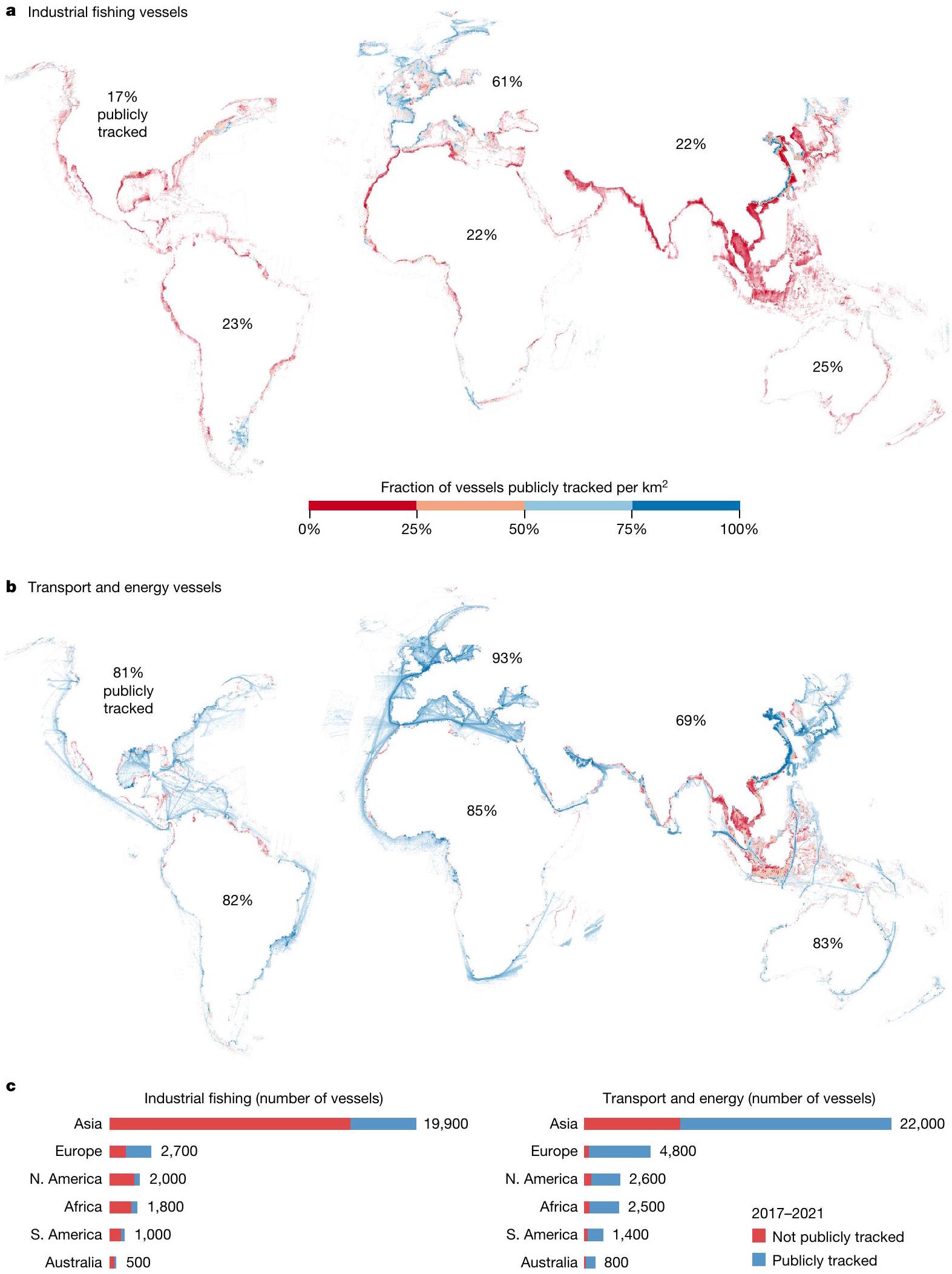
الشكل 1|حوالي 75٪ من الصيد الصناعي العالمي و25٪ من أنشطة السفن الأخرى لا يتم تتبعها علنًا. أ، ب، لكل كيلومتر مربع، العدد المتوسط للسفن الصناعية (أ) وسفن الشحن، الناقلات، سفن الركاب وسفن الدعم (ب)، من 5 سنوات من صور الأقمار الصناعية SAR. اللون يمثل النسبة المئوية للسفن المكتشفة التي تم مطابقتها (الأزرق، تتبع علني) وغير المطابقة (الأحمر، لا تتبع علني) لمواقع السفن المعروفة من AIS.
البث. ج، لكل قارة، العدد الإجمالي للسفن المكتشفة والنسبة المئوية منها التي يتم تتبعها علنًا وغير علنًا. يوضح الخط المحيط بالقارات (رمادي فاتح) منطقة المحيط التي تتوفر فيها صور SAR (انظر الشكل البياني الموسع 1 لتوزيع الصور المكاني). تشمل ‘أمريكا الشمالية’ دول أمريكا الوسطى. تم تصنيف الأجسام المكتشفة باستخدام التعلم العميق.
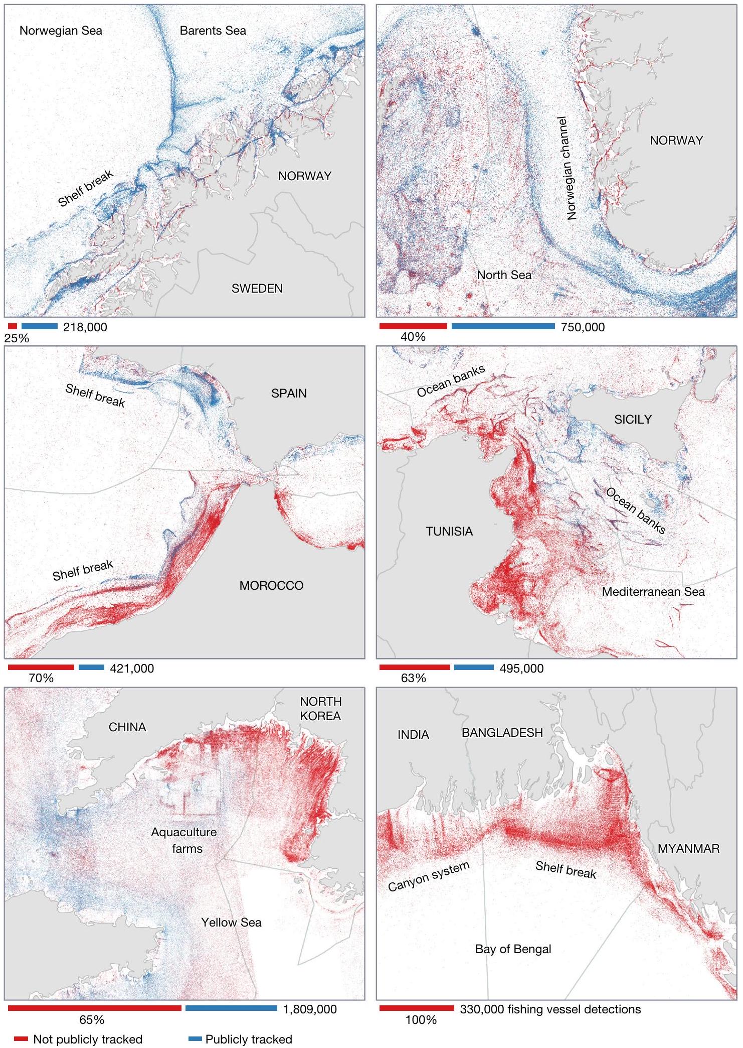
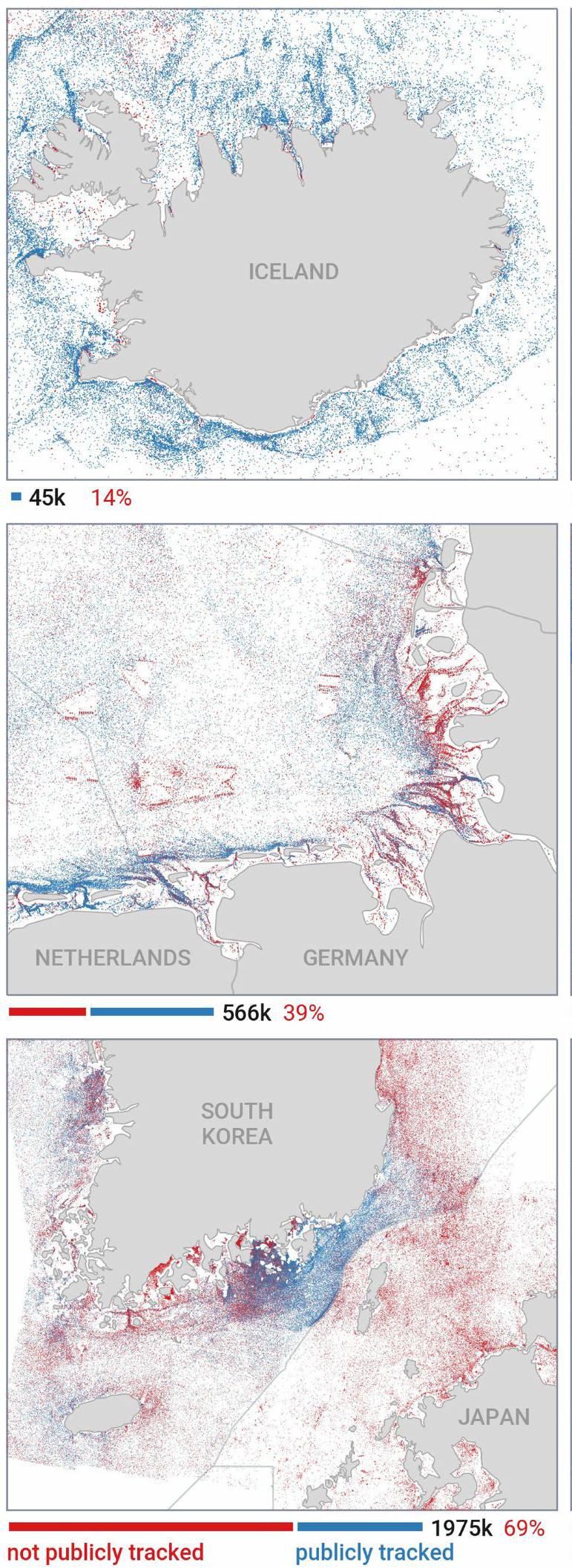
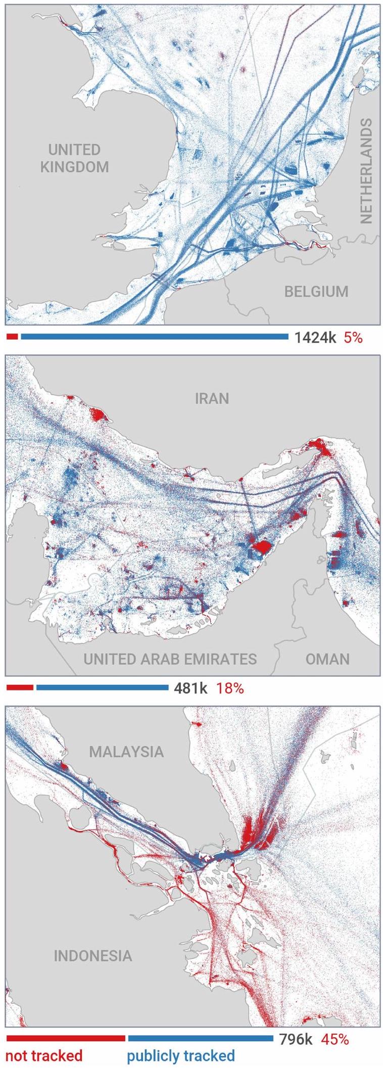
الشكل 2 | يكشف رسم الخرائط عالي الدقة عن أنماط تفصيلية لنشاط الصيد غير المتعقب علنًا. تكشف اكتشافات الأقمار الصناعية SAR للسفن الفردية خلال الفترة من 2017 إلى 2021، المتطابقة (بالأزرق) وغير المتطابقة (بالأحمر) مع مواقع السفن المعروفة من بث AIS، عن تصنيفها كسفن صيد أو غير صيد باستخدام نموذج تعلم عميق. تتركز معظم سفن الصيد، التي عادة ما تكون أقل من 50 مترًا في الطول، بالقرب من الشاطئ وتتبع الميزات الجيولوجية، مثل كسر الرف القاري والأخاديد في قاع البحر، أو الحدود التنظيمية والسياسية. توجد مناطق واسعة من نشاط الصيد غير المرسوم سابقًا.
تم الكشف عنها على طول شمال إفريقيا وجنوب وجنوب شرق آسيا. يعتمد العدد المطلق للاكتشافات في كل موقع على كثافة السفن المحلية وعدد عمليات الحصول على صور الأقمار الصناعية، والتي تختلف حسب المنطقة. قد تمثل الأرقام المعروضة منطقة أكبر قليلاً مما هو موضح. تُظهر هذه الصورة مستوى التفاصيل المكانية التي يمكن تحقيقها باستخدام نهجنا في رسم الخرائط. تُظهر الأشكال الإضافية 3 و 4 أمثلة أخرى على أنماط الصيد وغير الصيد عالية الدقة التي تم تتبعها علنًا وغير علنًا.
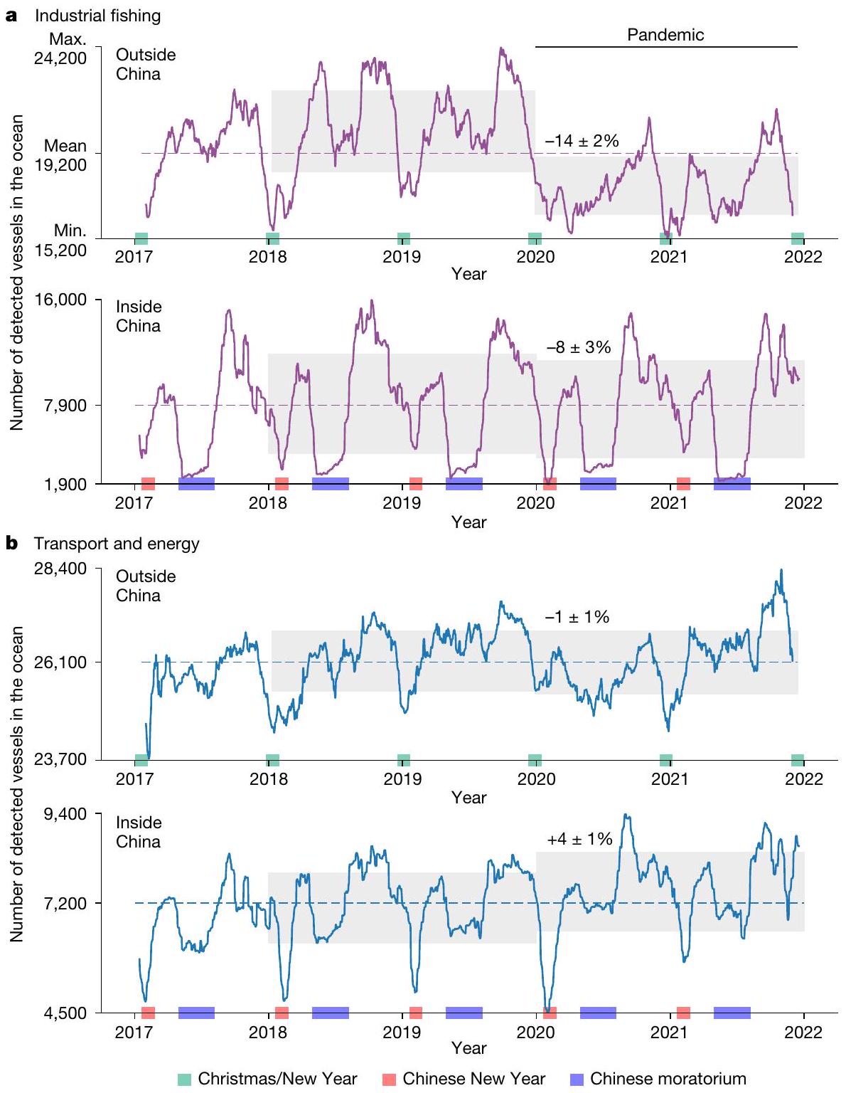
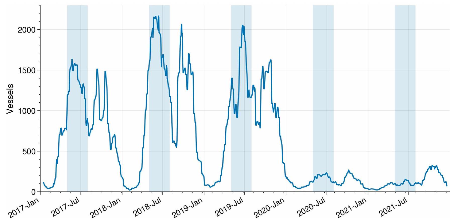
الشكل 3 | تأثرت أنشطة الصيد بشكل كبير بـ COVID-19، بينما استمر النقل والطاقة في النمو. تسلسلات زمنية لعدد السفن المتوسط عبر المنطقة المغطاة بواسطة SAR من Sentinel-1 (تم إنشاؤها من متوسط عدد الاكتشافات لكل مرور قمر صناعي في أي موقع معين؛ الطرق) تظهر أن COVID-19 أثر بشكل كبير على أنشطة الصيد، بينما استمر النقل والطاقة في النمو. تمتلك الصين وحدها ما يقرب من 30% من أسطول الصيد العالمي وحوالي 21% من سفن النقل والطاقة. أ، سفن الصيد الصناعية التي تزيد عن 15-20 مترًا في الطول عبر جميع المناطق الاقتصادية الخالصة خارج الصين وداخل المنطقة الاقتصادية الخالصة للصين. ب، نفس ما في أ ولكن للسفن المتعلقة بالنقل والطاقة، في الغالب. الشحن، الناقلات، الركاب والدعم. تشير المناطق الرمادية المظللة إلى المتوسط لمدة عامينس.د.، مع تسليط الضوء على تأثير جائحة 2020 العالمية. تظهر الأرقام نسبة التغيير مع خطأها المعياري المقابل. التغيير المدمج (خارج + داخل) هو – (الصيد الصناعي) و (النقل والطاقة)؛ الطرق. تبرز الصناديق الملونة الدورات السنوية في النشاط المتعلق بالعطلات الوطنية ووقف صيد الأسماك. المحور يظهر القيم القصوى والمتوسطة والدنيا للسفن المكتشفة خلال الفترة من 2017 إلى 2021.
التفاعلات بين السفن والبنية التحتية الثابتة
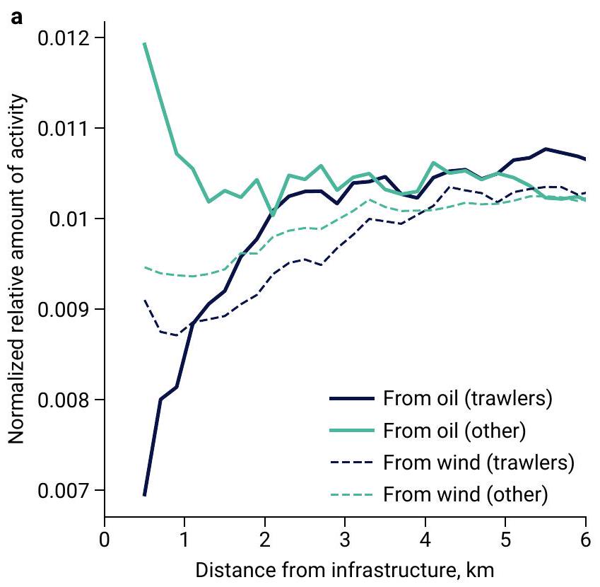
سؤال رئيسي للمستقبل هو كيف يمكن أن يتأثر حركة السفن بالتغيرات في تطوير بنية النفط والرياح. تتجنب قوارب الصيد، التي تصطاد عن طريق سحب الشباك على قاع البحر أو عبر عمود الماء وتعتبر أكثر أدوات الصيد شيوعًا على مستوى العالم، الصيد ضمن 1 كم من الهياكل النفطية، على الأرجح لتجنب تشابك الشباك (الشكل التوضيحي الممتد 10أ). بينما تجذب أنواع أخرى من الصيد، التي تكون في خطر أقل من التشابك، هذه الهياكل، على الأرجح لأنها يمكن أن تسبب تجمع الأسماك.على الرغم من أن توربينات الرياح قد تجمع الأسماك أيضًا، إلا أنها أقل احتمالًا للتأثير على الصيد الصناعي بنفس الطريقة لأنها، في الوقت الحاضر، مركزة بشكل كبير، ومتوسطها بعيد عن الشاطئ، حيث توجد أنشطة صيد أقل.
الشكل 10ب). أيضًا، فإن حركة مرور السفن المتعلقة بالنفط لها بصمة أوسع بكثير من حركة المرور المتعلقة بالرياح، حيث تمثل خمسة أضعاف النشاط عالميًا في عام 2021 (الشكل 4ب والشكل 4 من البيانات الموسعة).
الخاتمة
بشكل عام، تكشف دراستنا عن مدى الأنشطة الصناعية الكبرى في البحر، حيث تعتبر الصيد بلا منازع الصناعة البحرية الأكثر نشاطًا التي لا تُعتبر عامة. مع مجموعة البيانات والتكنولوجيا المتاحة لدينا مجانًا، يمكن الآن إظهار النقاط الساخنة للنشاطات المحتملة غير القانونية.ويمكن تحديد سفن الصيد الصناعية التي تتعدى على مناطق الصيد الحرفيأو مناطق الجرف القاري لدول أخرىلكن على نطاق عالمي ويمكن الوصول إليه من قبل أي دولة. يمكن أن تُظهر خرائط الجهود العالمية في الصيد الآن تشمل جميع السفن، وليس فقط تلك المعتمدة على تتبع AIS (الذي يفوت حوالي ثلاثة أرباع السفن الكبيرة)، وبدقة أعلى بكثير من مجرد المناطق الاقتصادية الخالصة أو مناطق الإبلاغ الإحصائي.يمكن أن تساعد بياناتنا أيضًا في تحديد حجم انبعاثات غازات الدفيئة الناتجة عن حركة السفن والتطوير البحري، مما قد يساعد في إبلاغ السياسات المتعلقة بتقليل انبعاثات غازات الدفيئة.
تقدم هذه الصورة للنشاط البشري أيضًا لمحة عن كيفية تغير الاستخدام الصناعي للمحيط. على الرغم من أن COVID-19 قد لعب دورًا رئيسيًا في تقليل نشاط الصيد، إلا أن الصيد انخفض بشكل أكبر بكثير من الصناعات البحرية الأخرى. يتماشى هذا التباطؤ مع الانخفاض طويل الأمد في الأهمية النسبية للصيد في المحيط.منذ الثمانينيات، ظل صيد الأسماك البحرية العالمي نسبياً دون تغيير حيث إن معظم مصائد الأسماك قد تم استغلالها إلى الحد الأقصى.نتيجة لذلك، زادت الجهود العالمية في الصيد، التي تضاعفت عدة مرات منذ عام 1950، بشكل طفيف فقط في السنوات الأخيرة.العديد من الدول التي قامت بإصلاح مصائدها تظهر انخفاضًا فعليًا في جهدها في الصيد.قد تعكس الانخفاضات المميزة في هذه الدراسة هذا الاتجاه الأطول، وقد نكون قد شهدنا بالفعل ذروة نشاط الصيد في العقد الماضي. بالمقابل، قد يستمر حركة السفن في النقل والطاقة في التوسع، متبعةً الاتجاهات في التجارة العالمية والتطور السريع للبنية التحتية للطاقة المتجددة. في هذا السيناريو، قد تتنافس التغيرات في النظم البيئية البحرية الناتجة عن البنية التحتية وحركة السفن مع تأثير الصيد.وإن رسم خريطة دقيقة لهذه الأنشطة أمر أساسي لفهم وإدارة الأنشطة البشرية المستقبلية في المحيط.
المحتوى عبر الإنترنت
أي طرق، مراجع إضافية، ملخصات تقارير Nature Portfolio، بيانات المصدر، بيانات موسعة، معلومات إضافية، شكر وتقدير، معلومات مراجعة الأقران؛ تفاصيل مساهمات المؤلفين والمصالح المتنافسة؛ وبيانات توفر البيانات والرموز متاحة علىhttps://doi.org/10.1038/s41586-023-06825-8.
وايكوت، م. وآخرون. تسارع فقدان الأعشاب البحرية في جميع أنحاء العالم يهدد النظم البيئية الساحلية. وقائع الأكاديمية الوطنية للعلوم في الولايات المتحدة الأمريكية 106، 12377-12381 (2009).
المنصة الحكومية الدولية للعلوم والسياسات بشأن التنوع البيولوجي وخدمات النظام البيئي (IPBES). ملخص لصانعي السياسات عن التقرير العالمي للتقييم بشأن التنوع البيولوجي وخدمات النظام البيئي،https://zenodo.org/record/3553579 (2019).
وينثر، ج. ج. وآخرون. إدارة المحيطات المتكاملة من أجل اقتصاد محيطي مستدام. نات. إيكول. إيفول. 4، 1451-1458 (2020).
بنيت، ن. ج.، غوفان، هـ. وساترفيلد، ت. الاستيلاء على المحيط. سياسة بحرية 57، 61-68 (2015).
بلحبيب، د.، سوميلا، أ. ر. و لو بيلون، ب. مصايد الأسماك في أفريقيا: الاستغلال، السياسة، واتجاهات الأمن البحري. سياسة بحرية 101، 80-92 (2019).
مركز معلومات علوم الأرض الدولية (CIESIN)، جامعة كولومبيا، وخدمات توصيل تكنولوجيا المعلومات (ITOS)، جامعة جورجيا. مجموعة بيانات الطرق العالمية المفتوحة (gROADS)، الإصدار 1 (1980-2010).https://doi.org/10.7927/H4VD6WCT (2013).
ماكدونالد، ج. ج. وآخرون. يمكن للأقمار الصناعية أن تكشف عن مدى العمل القسري في أسطول الصيد العالمي. وقائع الأكاديمية الوطنية للعلوم في الولايات المتحدة الأمريكية 118، e2016238117 (2021).
جو، ر. وآخرون. نحو نهج مسؤول في تعلم الآلة لتحديد العمل القسري في مصايد الأسماك. مسودة مسبقة فيhttps://arxiv.org/abs/2302.10987 (2023).
وانغ، ب. أ.، توماس، ج. و هالبين، ب. أتمتة استخراج البنية التحتية البحرية باستخدام رادار الفتحة الاصطناعية ومحرك جوجل الأرض. استشعار عن بعد. بيئة 233، 111412 (2019).
غورفينك، س.، ستورت، ف.، ريد، إ. وتريغوس، ف. التقييم العالمي للبنية التحتية للطاقة البحرية التاريخية والحالية والمتوقعة: الآثار على تخطيط الفضاء البحري، التصميم المستدام وإدارة نهاية عمر الهندسة. مراجعة الطاقة المتجددة والمستدامة 154، 111794 (2022).
توريس، ر.، سنوي، ب.، دافيدسون، م.، بيبي، د. ولوكاس، س. في مؤتمر 2012 IEEE الدولي للعلوم الجيولوجية والاستشعار عن بعد 1703-1706 (IEEE، 2012).
سبوتو، ف. وآخرون. في وقائع الندوة الدولية IEEE للعلوم الجيولوجية والاستشعار عن بعد 1707-1710 (IEEE، 2012).
باولي دي، زيلر دي، وبالوماريس م. ل. دي. (محررون) مفاهيم البحر من حولنا، التصميم والبيانات،www.seaaroundus.org (2020).
فيورنتينو ف. وآخرون. تركيب المعلومات حول بعض القشريات القاعية ذات الصلة بالصيد في البحر الأبيض المتوسط المركزي الجنوبي،http://www.faomedsudmed.org/pdf/المطبوعات/TD32.pdf (2013).
الوكالة الدولية للطاقة (IEA). آفاق طاقة الرياح البحرية 2019،https://www.iea.org/التقارير/توقعات الرياح البحرية 2019 (2019).
كلايس، ج. ت. وآخرون. منصات النفط قبالة كاليفورنيا هي من بين أكثر المواطن البحرية إنتاجية للأسماك على مستوى العالم. وقائع الأكاديمية الوطنية للعلوم في الولايات المتحدة الأمريكية 111، 15462-15467 (2014).
روسو، ي.، واتسون، ر. أ.، بلانشار، ج. ل. وفولتون، إ. أ. تطور أساطيل الصيد البحرية العالمية واستجابة الموارد المستهدفة. وقائع الأكاديمية الوطنية للعلوم في الولايات المتحدة الأمريكية 116، 12238-12243 (2019).
ماكولي، د. ج. وآخرون. فقدان الحيوانات البحرية: فقدان الحيوانات في المحيط العالمي. ساينس 347، 1255641 (2015).
هيلبورن، ر. وآخرون. إدارة مصايد الأسماك الفعالة تلعب دورًا أساسيًا في تحسين حالة مخزون الأسماك. وقائع الأكاديمية الوطنية للعلوم في الولايات المتحدة الأمريكية 117، 2218-2224 (2020).
ملاحظة الناشر: تظل شركة سبرينجر ناتشر محايدة فيما يتعلق بالمطالبات القضائية في الخرائط المنشورة والانتماءات المؤسسية.
لقد أثبتت أنظمة تصوير الرادار ذو الفتحة الاصطناعية أنها الخيار الأكثر اتساقًا لاكتشاف السفن في البحر.لا تتأثر الرادار ذو الفتحة الاصطناعية (SAR) بمستويات الضوء ومعظم الظروف الجوية، بما في ذلك ضوء النهار أو الظلام، السحب أو المطر. بالمقابل، تعتمد بعض أجهزة الاستشعار الفضائية الأخرى، مثل الصور الكهروضوئية، على ضوء الشمس و/أو الإشعاع تحت الأحمر المنبعث من الأجسام على الأرض، وبالتالي يمكن أن تتأثر بتغطية السحب، الضباب، الأحداث الجوية والظلام الموسمي في خطوط العرض العالية. استخدمنا صور الرادار من مهمة كوبرنيكوس سنتينل-1 التابعة لوكالة الفضاء الأوروبية (ESA) https://sentinel.esa.int/web/sentinel/ أدلة المستخدم / سنتينل-1-سار). الصور مأخوذة من قمرين صناعيين (S1A و، سابقًا، S1B، الذي توقف عن العمل في ديسمبر 2021) يدوران غير متزامنين مع بعضهم البعض في مدار قطبي متزامن مع الشمس. كل قمر صناعي لديه دورة تكرار مدتها 12 يومًا، بحيث يوفرون معًا خريطة عالمية للمياه الساحلية حول العالم تقريبًا كل 6 أيام. ومع ذلك، يختلف عدد الصور لكل موقع بشكل كبير اعتمادًا على أولويات المهمة، وخط العرض، ودرجة التداخل بين مرور الأقمار الصناعية المجاورة.https://sentinels.coper-nicus.eu/web/sentinel/missions/sentinel-1/observation-scenario). كما أن التغطية المكانية تختلف مع مرور الوقت وتتحسن مع إضافة S1B في عام 2016 والحصول على المزيد من الصور في السنوات اللاحقة (الشكل البياني الموسع 1). تتكون بياناتنا من صور ثنائية الاستقطاب (VH و VV) من وضع المسح التداخلي العريض (IW)، بدقة تبلغ حوالي 20 مترًا. استخدمنا منتج مستوى 1 للكشف عن النطاق الأرضي (GRD) المقدم من Google Earth Engine (https://developers. google.com/earth-engine/datasets/catalog/COPERNICUS_S1_GRDتمت معالجتها لإزالة الضوضاء الحرارية، والمعايرة الإشعاعية وتصحيح التضاريس (https://developers.google.com/earth-engine/ guides/sentinel1). لإزالة الشوائب المحتملة الناتجة عن الضوضاءالذي قد يقدم اكتشافات خاطئة، قمنا بمعالجة كل صورة بشكل إضافي عن طريق قصحافة العزل عن الحدود. اخترنا جميع مشاهد SAR فوق المحيط من أكتوبر 2016 إلى فبراير 2022، والتي تتكون من 753,030 صورة منبكسل في المتوسط.
صور مرئية وصور بالأشعة تحت الحمراء القريبة
بالنسبة للصور البصرية، استخدمنا مهمة كوبرنيكوس سنتينل-2 (S2) التابعة لوكالة الفضاء الأوروبية (ESA)https://sentinels.copernicus.eu/web/sentinel/user-guides/ساتل-2-إم إس آي). تدور هذان القمران الصناعيان التوأم (S2A و S2B) أيضًا حولخارج الطور وتحمل نظام تصوير متعدد الأطياف عالي الدقة وعريض النطاق، مع تكرار عالمي مشترك للزيارة كل 5 أيام. يتم أخذ عينات من ثلاثة عشر نطاقًا طيفيًا بواسطة أداة التصوير المتعدد الأطياف S2 (MSI): مرئي (RGB) والأشعة تحت الحمراء القريبة (NIR) عند 10 م، وحافة الأحمر والأشعة تحت الحمراء القصيرة (SWIR) عند 20 م، ونطاقات جوية أخرى عندالدقة المكانية. استخدمنا نطاقات RGB و NIR من منتج Level-1C المقدم من Google Earth Enginehttps://developers.google.com/earth-engine/datasets/catalog/كوبيرنيكوس_S2) واستبعدنا الصور التي تحتوي على أكثر منتغطية السحب باستخدام شريط قناع QA60 مع معلومات قناع السحب. قمنا بتحليل جميع المشاهد التي تحتوي على بنية تحتية بحرية مكتشفة خلال فترة المراقبة لدينا، والتي تتكون من 2,494,370 صورة منبكسل في المتوسط (انظر قسم ‘تصنيف البنية التحتية’).
بيانات نظام تحديد الهوية الآلي
تم الحصول على بيانات نظام تحديد الهوية الآلي من مزودي الأقمار الصناعية ORBCOMM وSpire. في المجموع، باستخدام خط بيانات Global Fishing Watch.قمنا بمعالجة 53 مليار رسالة AIS. من تلك البيانات، استخرجنا المواقع والأطوال والهويات لجميع أجهزة AIS التي عملت بالقرب من مشاهد SAR في الوقت الذي تم فيه التقاط الصور؛ فعلنا ذلك من خلال الاستيفاء بين مواقع AIS لتحديد مكان السفن على الأرجح في لحظة الصورة، كما هو موضح في المرجع 47. كانت هويات السفن في AIS مستندة إلى طرق في المرجع 5 وتم تعديلها في المرجع 26.
البيانات البيئية والفيزيائية
لتصنيف السفن المكتشفة بواسطة الرادار ذي الفتحة الاصطناعية (SAR) إلى سفن صيد وغير صيد، قمنا بإنشاء سلسلة من الحقول البيئية العالمية التي تم استخدامها كميزات في نموذجنا. يمثل كل من هذه الصور البيانية متغيرًا بيئيًا فوق المحيط فيالقرار. تم الحصول على البيانات من المصادر التالية: بيانات الكلوروفيل من مجموعة معالجة بيولوجيا المحيطات التابعة لناساhttps://oceancolor.gsfc.nasa.gov/بيانات/10.5067/ORBVIEW-2/SEAWIFS/L2/IOP/2018)، درجة حرارة سطح البحر والتيارات من نظام تحليل وتوقع المحيط العالمي كوبرنيكوسhttps://doi.org/10.48670/moi-00016), المسافة إلى الشاطئ من NASA OBPG/PacIOOS (http://www.pacioos.hawaii.edu/metadata/dist2coast_1deg_ocean.html)، المسافة إلى الميناء من Global Fishing Watch (https://globalfishingwatch.org/data-download/مجموعات البيانات/المسافة العامة من الميناء-الإصدار 1) والعمق البحري من GEBCO (https://www.gebco.net/“). حدود المنطقة الاقتصادية الخالصة المستخدمة في تحليلنا والخرائط هي من Marine Regions.
كشف السفن بواسطة الرادار ذو الفتحة الاصطناعية
كشف السفن باستخدام الرادار ذي الفتحة الاصطناعية يعتمد على خوارزمية معدل الإنذار الكاذب الثابت (CFAR) المستخدمة على نطاق واسع.، خوارزمية عتبة تكيفية قياسية تُستخدم لاكتشاف الشذوذ في صور الرادار. تم تصميم هذه الخوارزمية للبحث عن قيم البكسل التي تكون ساطعة بشكل غير عادي (الأهداف) مقارنة بتلك الموجودة في المنطقة المحيطة (تشويش البحر). تحدد هذه الطريقة عتبة تعتمد على إحصائيات الخلفية المحلية، التي يتم أخذ عينات منها باستخدام مجموعة من النوافذ المنزلقة. تشكل قيم البكسل التي تتجاوز العتبة شذوذًا ومن المحتمل أن تكون عينات من هدف. تقوم خوارزمية CFAR المعدلة ذات المعاملين بتقييم المتوسط والانحراف المعياري لقيم الارتداد، المحددة بواسطة “حلقة” تتكون من نافذة داخلية منبكسلات ونافذة خارجية منالبكسلات. يتم تحقيق أفضل فصل بين المحيط والأهداف من خلال نطاق الاستقطاب العمودي الأفقي (VH)، الذي يظهر عوائد مستقطبة منخفضة نسبيًا على المناطق المسطحة (سطح المحيط) مقارنةً بالأجسام الحجمية (السفن والبنية التحتية). :
في أيهو قيمة الانعكاس الخلفي للبكسل المركزي، و هما المتوسط والانحراف المعياري للخلفية، على التوالي، و هو حد يعتمد على الزمن.
لزيادة أداء الكشف، حددنا أحجام النوافذ تجريبيًا، بناءً على نسبة السفن المكتشفة (التي تبث AIS) بطول يتراوح بين 15 م و 20 م. ميزة رئيسية في خوارزمية CFAR ذات المعاملين لدينا هي القدرة على تحديد عتبات مختلفة لأوقات مختلفة. هذه التعديلات ضرورية لأن الخصائص الإحصائية لصور SAR المقدمة من Sentinel-1 تختلف مع الوقت وكذلك حسب القمر الصناعي (S1A و S1B). وبالتالي، وجدنا أن بكسلات المحيط لكل من المتوسط والانحراف المعياري للمشاهد قد تغيرت، مما يتطلب معايرات مختلفة لمعاملات CFAR لخمس فترات زمنية مختلفة خلال التي ظلت فيها إحصائيات الصور ثابتة نسبيًا: من يناير 2016 إلى أكتوبر 2016.، “لا شيء)؛ من سبتمبر 2016 إلى يناير 2017 (14، 18)؛ من يناير 2017 إلى مارس 2018 (14، 17)؛ من مارس 2018 إلى يناير 2020 (16، 19)؛ ومن يناير 2020 إلى ديسمبر 2021 (22، 24). تم معايرة عتبات الكشف الخمسة للحصول على معدل كشف متسق للسفن الصغيرة عبر الأرشيف الكامل لـ Sentinel-1 (60% كشف للسفن بطول 15-20 متر). سمحت لنا البساطة النسبية لنهجنا بإعادة معالجة الأرشيف الكامل لصور Sentinel-1 عدة مرات لتحديد المعلمات المثلى للكشف بشكل تجريبي.
لتنفيذ خوارزمية كشف SAR الخاصة بنا، استخدمنا واجهة برمجة التطبيقات بايثون لمحرك جوجل الأرضhttps://developers.google.com/earth-engine/دروس/مجتمع/مقدمة إلى واجهة برمجة تطبيقات بايثون)، منصة على مستوى الكوكب لتحليل بيتابايت من صور الأقمار الصناعية ومجموعات البيانات الجغرافية. لمعالجة وتحليل وتوزيع منتجات البيانات الخاصة بنا، فإن اكتشافنا تستخدم سير العمل بنية جوجل السحابية للبيانات الضخمة، بما في ذلك محرك الأرض، ومحرك الحوسبة، وتخزين السحاب، وبيانات BigQuery.
تقدير وجود السفن وطولها
لتقدير طول كل كائن تم اكتشافه وأيضًا لتحديد متى قامت خوارزمية CFAR لدينا بإجراء اكتشافات خاطئة، قمنا بتصميم شبكة عصبية تلافيفية عميقة (ConvNet) استنادًا إلى بنية ResNet الحديثة (الشبكات المتبقية).. تأخذ هذه الشبكة العصبية الالتفافية ذات المدخل الواحد والمخرجات المتعددة قطع صور SAR ثنائية النطاق من البكسلات كمدخلات وتخرج احتمال وجود الكائن (مهمة تصنيف ثنائية) والطول المقدر للكائن (مهمة انحدار). لتحليل كل اكتشاف، قمنا باستخراج قطعة صغيرة من الصورة الأصلية للرادار ذي الفتحة الاصطناعية (SAR) التي تحتوي على الكائن المكتشف في المركز والتي حافظت على كلا نطاقي الاستقطاب (VH و VV). لذلك، كانت بيانات الاستدلال لدينا تتكون من أكثر من 62 مليون قطعة صورة ثنائية النطاق للتصنيف. لبناء مجموعات بيانات التدريب والتقييم لدينا، استخدمنا اكتشافات SAR التي تطابقت مع بيانات نظام تحديد الهوية الآلي للسفن (AIS) بثقة عالية (انظر قسم ‘دمج SAR و AIS’)، بما في ذلك مجموعة متنوعة من السيناريوهات التحديّة مثل المواقع الجليدية، المواقع الصخرية، مناطق السفن ذات الكثافة المنخفضة والعالية، مناطق البنية التحتية البحرية، المشاهد ذات الجودة الضعيفة، المشاهد التي تحتوي على عيوب في الحواف، وما إلى ذلك (الشكل 11 من البيانات الموسعة). لفحص هذه العينات وتوضيحها، قمنا بتطوير أداة للتسمية واستخدمنا خبراء في المجال، مع التحقق المتبادل من التوضيحات من ثلاثة مصنفين مستقلين على نفس العينات والاحتفاظ بالتوضيحات ذات الثقة العالية. بشكل عام، احتوت بياناتنا المعلّمة على حوالي 12,000 عينة عالية الجودة التي قسمناها إلى مجموعة التدريب (، لتعلم النموذج واختياره) واختبار (، لتقييم النموذج) المجموعات.
لعملية تعلم النموذج واختياره، اتبعنا نظام تدريب-تحقق يستخدم التحقق المتقاطع بخمسة أضعافhttps://scikit-learn.org/ stable/modules/cross_validation.html)، حيث يتم في كل طية (دورة تدريبية) تخصيص 80% من البيانات لتعلم النموذج و20% للتحقق من النموذج، مع عدم تداخل مجموعة التحقق عبر الطيات. ثم يتم حساب متوسط مقاييس الأداء عبر الطيات لتقييم النموذج واختياره، ويتم إجراء التقييم النهائي للنموذج على مجموعة الاختبار المحجوزة. حقق أفضل نموذج لدينا على مجموعة الاختبار درجة F1 تبلغ 0.97 (دقة = 97.5%) لمهمة التصنيف ودرجة 0.84 (RMSE، أو حوالي 1 بكسل صورة) لمهمة تقدير الطول.
كشف البنية التحتية
لكشف البنية التحتية البحرية، استخدمنا نفس خوارزمية CFAR ذات المعاملين التي تم تطويرها لكشف السفن، مع تعديلين أساسيين. أولاً، لإزالة الأجسام غير الثابتة، أي معظم السفن، قمنا بإنشاء تركيبات متوسطة من صور SAR ضمن نافذة زمنية مدتها 6 أشهر. نظرًا لأن الأجسام الثابتة تتكرر عبر معظم الصور، فإنها تُحتفظ من خلال عملية الوسيط، بينما يتم استبعاد الأجسام غير الثابتة. كررنا هذه العملية لكل شهر، مما أدى إلى توليد سلسلة زمنية شهرية من الصور المركبة. كما أن التجميع الزمني للصور يقلل من الضوضاء الخلفية (تشويش البحر) بينما يعزز الإشارات المتماسكة من الأجسام الثابتة.. ثانياً، قمنا بتعديل أحجام نافذة الكشف بشكل تجريبي. حيث أن بعض البنية التحتية البحرية عادة ما تكون مرتبة في تجمعات كثيفة، مثل مزارع الرياح التي تتبع نمطاً شبيهاً بالشبكة، قمنا بتقليل النوافذ المكانية لتجنب ‘التلوث’ من الهياكل المجاورة. من الشائع أيضاً العثور على هياكل أصغر مثل أعمدة الطقس موضوعة بين بعض توربينات الرياح. وجدنا أن نافذة داخلية من بكسلات ونافذة خارجية لـكانت البكسلات مثالية لاكتشاف كل كائن في جميع مزارع الرياح وحقول النفط التي اختبرناها، بما في ذلك بحيرة ماراكايبو، والبحر الشمالي، وجنوب شرق آسيا، وهي مناطق معروفة بكثافتها العالية من الهياكل (الشكل البياني الموسع 7).
تصنيف البنية التحتية
لتصنيف كل هيكل بحري تم اكتشافه، استخدمنا التعلم العميق. صممنا شبكة عصبية تلافيفية تعتمد على بنية ConvNeXt.الفرق الرئيسي عن نموذج ‘تقدير وجود السفينة وطولها’، بالإضافة إلى استخدام بنية مختلفة، هو أن هذا النموذج هو نموذج متعدد المدخلات/ شبكة عصبية تلافيفية ذات مخرج واحد تأخذ صورتين متعددتي النطاقات مختلفتينتستخدم وحدات البكسل كمدخلات، تمررها عبر طبقات تلافيفية مستقلة (فرعين)، تجمع خرائط الميزات الناتجة، ومع رأس تصنيف واحد، تخرج الاحتمالات للفئات المحددة: بنية تحتية للرياح، بنية تحتية للنفط، بنية تحتية أخرى وضوضاء.
جانب جديد من نهجنا في تصنيف التعلم العميق هو دمج صور الرادار ذي الفتحة الاصطناعية (SAR) من Sentinel-1 مع الصور البصرية من Sentinel-2. من تجميعات لمدة 6 أشهر من صور SAR ثنائية النطاق (VH و VV) وصور بصرية رباعية النطاق (RGB و NIR)، قمنا باستخراج بلاطات صغيرة لكل هيكل ثابت تم اكتشافه، مع وجود الأجسام المعنية في مركز البلاطة. على الرغم من أن كل من بلاطات SAR والبصرية تتكون من 100 بكسل، إلا أنها تأتي من صور بدقات مختلفة: بلاطة SAR ثنائية النطاق لها دقة مكانية تبلغ 20 م لكل بكسل، بينما بلاطة الصور البصرية الرباعية لها 10 م لكل بكسل. هذه الدقة المتغيرة لا توفر فقط معلومات بمستويات مختلفة من التفاصيل، ولكنها أيضًا تنتج مجالات رؤية مختلفة.
من بيانات الاستدلال لدينا لتصنيف البنية التحتية، التي تتكون من ما يقرب من ستة ملايين صورة متعددة النطاقات، قمنا بإنشاء البيانات المعلّمة من خلال دمج عدة مصادر من الحقائق الأرضية لـ ‘النفط والغاز’ و ‘طاقة الرياح البحرية’: من مكتب إدارة الطاقة البحرية.https://www.data.boem.gov/Main/HtmlPage.aspx?page=plaتشكيلات tform)، مكتب المساحة البحرية البريطاني (https://www.admi-ralty.co.uk/access-data/marine-dataقسم الأسماك والحياة البرية في كاليفورنيا (https://data-cdfw.opendata.arcgis.com/datasets/CDFW::منصات النفط-OSPR-DS357/حول) وجيولوجيا أستراليا (https://services.ga.gov.au/gis/rest/services/Oil_Gas_Infrastructure/ (خدمة الخرائط). باستخدام نهج التسمية المشابه لذلك المستخدم في عينات السفن، قمنا أيضًا بفحص عدد كبير من الاكتشافات لتحديد عينات لـ ‘هياكل أخرى’ و ‘ضوضاء’ (صخور، جزر صغيرة، جليد بحري، غموض الرادار وعيوب الصورة). من جميع المناطق المعروفة بوجود بعض البنية التحتية البحرية (الشكل 11 من البيانات الموسعة)، احتوت بياناتنا المسمّاة على أكثر من 47,000 عينة (نفطرياحالضوضاء و4% أخرى) التي قمنا بتقسيمها إلى مجموعة التدريب (80%) ومجموعة الاختبار (20%)، باستخدام نفس استراتيجية التحقق المتقاطع بخمسة أضعاف كما هو الحال مع الأوعية.
لأن نفس الأجسام الثابتة تظهر في عدة صور على مر الزمن، قمنا بتجميع الهياكل المرشحة للبيانات المعلّمة فيصناديق مكانية وتم أخذ عينات من صناديق مختلفة لكل قسم بيانات، بحيث لم تحتوي المجموعات الفرعية لتعلم النموذج، والاختيار، والتقييم على نفس الهياكل (أو حتى الهياكل القريبة) في أي نقطة. نلاحظ أيضًا أنه في الحالات القليلة التي كانت فيها البلاطات الضوئية غير متاحة، على سبيل المثال، بسبب الظلام الموسمي بالقرب من الأقطاب، تم إجراء التصنيف باستخدام بلاطات SAR فقط (كانت البلاطات الضوئية فارغة). حقق أفضل نموذج لدينا في مجموعة الاختبار متوسط درجة F1 مرجحة حسب الفئة قدرها 0.99 (الدقة ) لمشكلة التصنيف المتعدد.
تصنيف الصيد وغير الصيد
لتحديد ما إذا كانت السفينة المكتشفة قارب صيد أو قارب غير صيد، استخدمنا أيضًا التعلم العميق. لهذه المهمة التصنيفية، استخدمنا نفس بنية ConvNeXt الأساسية كما في البنية التحتية، المعدلة لمعالجة المدخلين التاليين: الطول المقدر للسفينة من SAR (كمية عددية) وطبقة من الصور البيئية المركزة على موقع السفينة (صورة متعددة الأطياف). يمر هذا النموذج المختلط من المدخلات المتعددة/البيانات المختلطة/الإخراج الواحد عبر سلسلة من الطبقات التلافيفية ويجمع خرائط الميزات الناتجة مع قيمة طول السفينة لأداء تصنيف ثنائي: صيد أو غير صيد.
جانبان رئيسيان في نهجنا لتصنيف الشبكات العصبية يختلفان كثيرًا عن مهام تصنيف الصور التقليدية.
أولاً، نحن نصنف السياق البيئي الذي تعمل فيه السفينة المعنية. للقيام بذلك، قمنا بإنشاء 11 حقلًا شبكيًا (راستر) بدقة (حوالي 1 كم لكل بكسل عند خط الاستواء) مع تغطية عالمية. في كل بكسل، يحتوي كل راستر على معلومات سياقية حول المتغيرات التالية: (1) كثافة السفن (استنادًا إلى SAR)؛ (2) متوسط طول السفن (استنادًا إلى SAR)؛ (3) علم الأعماق؛
مقالة
(4) المسافة من الميناء، (5) و(6) ساعات وجود السفن غير المخصصة للصيد (من نظام تحديد الهوية الآلي) للسفن التي تقل عن 50 مترًا وأكثر من 50 مترًا، على التوالي؛ (7) متوسط درجة حرارة السطح؛ (8) متوسط سرعة التيار؛ (9) الانحراف المعياري لدرجة الحرارة اليومية؛ (10) الانحراف المعياري لسرعة التيار اليومية؛ و(11) متوسط الكلوروفيل. لكل سفينة تم اكتشافها، قمنا بأخذ عينات-بكسل من هذه الصور النقطية، مما ينتج صورة مكونة من 11 نطاقًا قمنا بعد ذلك بتصنيفها باستخدام الشبكة العصبية التلافيفية. وبالتالي، يتم توفير سياق لكل اكتشاف في منطقة تزيد قليلاً عنلقد حصلنا على تسميات الصيد وغير الصيد من هويات السفن في نظام تحديد الهوية الآلي (AIS).. ثانيًا، يتم إنتاج توقعاتنا باستخدام مجموعة من نموذجين دون تداخل في التغطية المكانية. لتجنب تسرب المعلومات المكانية بين مجموعات التدريب للنموذجين، وأيضًا لتعظيم التغطية المكانية، قمنا بتقسيم مركز البلاطات إلىشبكة خطوط الطول والعرض. ثم قمنا بإنشاء مجموعتين مستقلتين من البيانات المسمّاة، واحدة تحتوي على البلاطات من خلايا الشبكة ذات خطوط العرض والطول ‘الزوجية’ والأخرى من الخلايا ‘الفردية’. هذا التناوباستراتيجية (حجم البلاط) تضمن عدم وجود تداخل مكاني بين البلاطات عبر المجموعتين. قمنا بتدريب نموذجين مستقلين، واحد للبلاطات ‘الزوجية’ وآخر للبلاطات ‘الفردية’، حيث ‘يرى’ كل نموذج جزءًا من المحيط الذي لا ‘يراه’ النموذج الآخر. مجموعة الاختبار التي استخدمناها لتقييم كلا النموذجين تحتوي على بلاطات من كل من خلايا الشبكة ‘الزوجية’ و ‘الفردية’، معتمت إزالة الحافة حول جميع خلايا شبكة الاختبار من جميع الخلايا المجاورة (المستخدمة للتدريب) لضمان الاستقلال المكاني عبر جميع تقسيمات البيانات (دون تسرب). من خلال متوسط التوقعات من هذين النموذجين، قمنا بتغطية النطاق المكاني الكامل لاكتشافاتنا بمعلومات مكانية مستقلة ومتكاملة.
تضمنت مجموعة الاختبار الأصلية لديناالصيدعينات غير صيد. قمنا بمعايرة نتائج النموذج عن طريق ضبط نسبة السفن الصيد إلى السفن غير الصيد في مجموعة الاختبار إلى 1:1https://scikit-learn. org/stable/modules/calibration.html). قمنا بإجراء تحليل حساسية لرؤية كيف تغيرت نتائجنا مع نسب مختلفة من السفن الصيد والسفن غير الصيد، و . في المتوسط، تم اكتشاف حوالي 30,000 سفينة غير متعقبة علنًا في أي وقت. وقد توقعت الدرجات المعايرة مع ثلثي سفن الصيد أن من هذه السفن كانت تصطاد، في حين أن المعايرة مع ثلث السفن فقط توقعت أنمنها كانت سفن صيد. وبالتالي، فإن النسبة الإجمالية (مع الأخذ في الاعتبار جميع الاكتشافات) لسفن الصيد وغير الصيد التي لا يتم تتبعها علنًا تصل إلى و على التوالي. ثم قام المحللون في Global Fishing Watch بمراجعة هذه النتائج في مناطق مختلفة من العالم للتحقق من دقتها.
تحتوي بيانات التدريب لدينا على حوالي 120,000 بلاطة (مقسمة إلى ‘فردية’ و ‘زوجية’) التي قمنا بتقسيمها إلىلتعلم النموذج ولاختيار النموذج. احتوى مجموعة الاختبار لتقييم النموذج على 14,100 بلاطة من خلايا الشبكة ‘الفردية’ و ‘الزوجية’ (الشكل 11 من البيانات الموسعة). احتوت بيانات الاستدلال على أكثر من 52 مليون بلاطة (صور بـ 11 نطاقًا) مع أطوال الأوعية المعنية التي قمنا بتصنيفها باستخدام النموذجين. حقق أفضل نموذج لدينا في مجموعة الاختبار درجة F1 قدرها 0.91 (الدقة ) لمهمة التصنيف.
الإيجابيات الكاذبة والاسترجاع
نظرًا لعدم وجود بيانات حقيقية حول الأماكن التي لا تتواجد فيها السفن، فإن تقدير معدل الإيجابيات الكاذبة على المستوى العالمي لخوارزمية اكتشاف السفن لدينا يمثل تحديًا. على الرغم من أن بعض الدراسات تُبلغ عن العدد الإجمالي للإيجابيات الكاذبة، نعتقد أن مقياسًا أكثر دلالة هو ‘كثافة الإيجابيات الكاذبة’ (عدد الإيجابيات الكاذبة لكل وحدة مساحة)، والذي يأخذ في الاعتبار الحجم الفعلي للدراسة. قمنا بتقدير هذا المقياس من خلال تحليل 150 مليونمن الصور عبر جميع السنوات الخمس في المناطق ذات الكثافة المنخفضة جداً من السفن المزودة بنظام AIS (أقل من 10 ساعات إجمالية في عام 2018 في خلية شبكة) )، في مناطق بعيدة عن الساحل ( ) وفي مياه الدول التي لديها استخدام واستقبال جيد نسبيًا لنظام تحديد الهوية الآلي للسفن. عدد اكتشافات السفن غير المرسلة في هذه المناطق يعتبر الحد الأقصى لكثافة الإيجابيات الكاذبة، والتي قدرناها بـ 5.4 اكتشافات لكل . إذا كانت جميع هذه النتائج إيجابية زائفة، فإن ذلك سيشير إلى إيجابية زائفة معدل حوالي 2% في بياناتنا. ومع ذلك، لأن العديد من هذه الاكتشافات ربما تكون حقيقية، فإن معدل الإيجابيات الكاذبة الفعلي ربما يكون أقل. بالمقارنة مع مصادر أخرى من عدم اليقين، مثل قيود دقة صور الرادار (SAR) وفقدان بعض المناطق من المحيط (انظر أدناه)، فإن الإيجابيات الكاذبة تقدم خطأً نسبيًا بسيطًا في تقديراتنا.
لتقدير الاسترجاع (نسبة الإيجابيات الفعلية التي تم التعرف عليها بشكل صحيح)، استخدمنا طريقة مشابهة لتلك المستخدمة في المرجع 47. حددنا جميع السفن التي كانت لديها موقع AIS قريب جداً من حيث الوقت من عملية التقاط الصورة. ) وبالتالي كان ينبغي أن تظهر في مشهد SAR؛ إذا تم اكتشافها في صورة SAR، يمكننا مطابقتها مع السفن المجهزة بنظام AIS المعني ثم تحديد السفن المجهزة بنظام AIS التي لم يتم اكتشافها. تشير منحنى الاسترجاع إلى أننا قادرون على اكتشاف أكثر من جميع السفن التي تزيد عن 50 مترًا في الطول وحولجميع السفن التي يتراوح طولها بين 25 مترًا و50 مترًا، مع انخفاض معدل الكشف بشكل حاد للسفن التي تقل عن 25 مترًا (الشكل البياني الإضافي 2). ومع ذلك، نظرًا لأن كشف السفن لدينا يعتمد على خوارزمية CFAR مع نافذة بعرض 600 متر، عندما تكون السفن قريبة من بعضها البعض ( )، فإن معدل الكشف أقل. انظر قسم ‘قيود دراستنا’ للعوامل التي تؤثر على قابلية الكشف.
دمج نظام البحث والإنقاذ ونظام تحديد الهوية الآلي
مطابقة اكتشافات الرادار ذو الفتحة الاصطناعية (SAR) مع إحداثيات نظام تحديد المواقع العالمي (GPS) للسفن (من سجلات نظام تحديد الهوية الآلي (AIS)) تمثل تحديًا لأن الطابع الزمني لصور SAR وسجلات AIS لا يتطابقان، ويمكن أن تتطابق رسالة AIS واحدة مع عدة سفن تظهر في الصورة، والعكس صحيح. لتحديد احتمال أن تكون سفينة تبث إشارات AIS تتوافق مع اكتشاف SAR محدد، اتبعنا نهج المطابقة الموضح في المرجع 47، مع بعض التحسينات. تعتمد هذه الطريقة على خرائط الاحتمالية لمكان وجود السفينة على الأرجح قبل دقائق وبعد تسجيل موقع AIS. تم تطوير هذه الخرائط من سنة واحدة من بيانات AIS العالمية، بما في ذلك حوالي 10 مليارات موقع سفينة، وتم حسابها لست فئات مختلفة من السفن، مع الأخذ في الاعتبار ست سرعات مختلفة و36 فترة زمنية، مما أدى إلى 1,296 خريطة. يمكن اعتبار هذا النهج لخرائط الاحتمالية كاستخدام لتوزيع الاستخدام.-لكل فئة من السفن، السرعة والفترة الزمنية – حيث يكون الفضاء نسبيًا لموقع الفرد.
كما هو موضح في المرجع 47، قمنا بدمج خرائط الاحتمالات قبل وبعد للحصول على توزيع الاحتمالات للموقع المحتمل لكل سفينة. ثم قمنا بحساب قيمة هذا التوزيع الاحتمالي عند كل اكتشاف SAR يمكن أن تتطابق معه سفينة معينة. تم تعديل هذه القيمة بعد ذلك لتأخذ في الاعتبار: (1) احتمال اكتشاف السفينة و (2) عامل يأخذ في الاعتبار ما إذا كانت طول السفينة (من قاعدة بيانات AIS الخاصة بـ Global Fishing Watch) يتوافق مع الطول المقدر من صورة SAR. القيمة الناتجة توفر درجة لكل تطابق محتمل بين AIS و SAR، تم حسابها كـ
في أيهو قيمة توزيع الاحتمالات في موقع الكشف (وفقًا للمرجع 47)،هو عامل يقوم بتعديل هذه الدرجة بناءً على الطول وهو احتمال اكتشاف السفينة، يُعرّف على أنه
في أي هو الاسترجاع كدالة لحجم السفينة والمسافة إلى أقرب سفينة مزودة بجهاز AIS (الشكل البياني الموسع 2) وهي احتمالية وجود السفينة في المشهد في لحظة الصورة، والتي تم الحصول عليها من خلال حساب نسبة توزيع احتمالية السفينة التي تقع ضمن المشهد SAR المعطى.استنادًا إلى 2.8 مليون اكتشاف لمطابقات عالية الثقة (مطابقات AIS إلى SAR التي من غير المحتمل أن تتطابق مع اكتشافات أخرى والتي كانت فيها السفينة المجهزة بـ AIS لها موقع خلال دقيقتين من الصورة)، قمنا بتطوير جدول بحث يحتوي على الفرق النسبي بين الطول المعروف لـ AIS و SAR. الطول المقدر، مقسم إلى فترات فرق قدرها 0.1. الضرب في هذه القيمة (يجعل من غير المحتمل جداً أن تتطابق سفينة صغيرة مع اكتشاف كبير، أو العكس. ثم يتم حساب مصفوفة من الدرجات للمطابقات المحتملة بين SAR و AIS، ويتم تعيين المطابقات (عن طريق اختيار أفضل خيار متاح في تلك اللحظة) وإزالتها في إجراء تكراري، حيث أن طريقتنا تؤدي بشكل أفضل بكثير من الأساليب التقليدية، مثل الاستيفاء القائم على السرعة والمسار.تتمثل إحدى التحديات الرئيسية بالنسبة لنا في تحديد أفضل عتبة للدرجة لقبول أو رفض المطابقة، لأن عتبة منخفضة جدًا أو مرتفعة جدًا ستزيد أو تقلل من احتمال أن تكون اكتشافات SAR المعينة لسفينة غير متعقبة علنًا. لتحديد الدرجة المثلى، قمنا بتقدير العدد الإجمالي للسفن المزودة بأجهزة AIS التي كان ينبغي أن تظهر في المشاهد عالميًا من خلال جمع (الطول، التباعد) لكل المشاهد. تشير هذه القيمة إلى أنه على مستوى العالم، كان ينبغي اكتشاف 17 مليون سفينة مزودة بأجهزة AIS في صور SAR. بناءً على ذلك، اخترنا العتبة التي قدمت 17 مليون تطابق من الاكتشافات الفعلية، أي، . نشير إلى المرجع 47 لوصف كامل لخوارزمية المطابقة المعتمدة على الشبكة، ويمكن العثور على كود المطابقة فيhttps://github.com/GlobalFishingWatch/ورقة-طويلة-خط-تطابق-إيه-آي-إس-سار.
تصفية البيانات
تحديد الخطوط الساحلية أمر صعب لأن البيانات العالمية الحالية لا تلتقط تعقيدات جميع الخطوط الساحلية حول العالم.. علاوة على ذلك، فإن الخط الساحلي هو ميزة ديناميكية تتغير باستمرار مع مرور الوقت. لتجنب الاكتشافات الخاطئة الناتجة عن تعريفات غير دقيقة للخطوط الساحلية، قمنا بتصفية حافة عازلة من خط الساحل العالمي الذي قمنا بتجميعه باستخدام عدة مصادر (https://www.ngdc.noaa.gov/مgg/السواحل،https://www.naturalearthdata.com/downloads/10 م – المتجهات الفيزيائية / 10 م – الجزر الصغيرة،https://data.unep-wcmc. org/بيانات/1، https://doi.org/10.1080/1755876X.2018.1529714، https://osmdata.openstreetmap.de/data/land-polygons.html,https://www.arcgis.com/home/item.html?id=ac80670eb213440ea5899bbاستخدمنا هذا الشاطئ الاصطناعي لتحديد المنطقة الصالحة للكشف داخل كل صورة SAR. قمنا بتصفية المناطق التي تحتوي على تركيز ملحوظ من الجليد البحري، والذي قد يؤدي إلى اكتشافات خاطئة لأن الجليد هو عاكس قوي للرادار، وغالبًا ما يظهر في صور الرادار الاصطناعي بتوقيع مشابه لتلك الخاصة بالسفن والبنية التحتية. استخدمنا قناع مدى الجليد البحري المتغير زمنياً من بيانات مدى الجليد البحري متعددة المستشعرات – نصف الكرة الشمالي (MASIE-NH)، الإصدار 1.https://nsidc.org/data/g02186/الإصدارات/1#qt-data_set_tabs)، مكملة بصناديق حدود محددة مسبقًا فوق المناطق ذات خطوط العرض المنخفضة المعروفة بوجود جليد البحر الموسمي الكبير، مثل خليج هدسون في كندا، وبحر أوخوتسك شمال اليابان، والمحيط القطبي، وبحر بيرينغ، ومناطق مختارة بالقرب من غرينلاند، وبحر البلطيق الشمالي وجزر جورجيا الجنوبية. لم تكن هناك أي صور في الوضع الذي قمنا بمعالجته متاحة لمياه القارة القطبية الجنوبية. قمنا أيضًا بإزالة الكائنات المكررة عبر عدة صور (أي الهياكل الثابتة) من مجموعة بيانات اكتشاف السفن لاستبعادها من جميع الحسابات المتعلقة بنشاط السفن. كما أدت هذه العملية إلى إزالة السفن الراسية لفترة طويلة، لذا فإن مجموعة بياناتنا تمثل السفن المتحركة بشكل أفضل من السفن الثابتة. مصدر محتمل آخر للضوضاء هو الانعكاسات من المركبات المتحركة على الجسور أو الطرق القريبة من الشاطئ. على الرغم من أنه يمكن إزالة الجسور من البيانات من خلال تحليل البنية التحتية الثابتة، فإن المركبة التي تتحرك عموديًا على مسار القمر الصناعي ستظهر بشكل مائل. يمكن أن تظهر المركبات المرئية في الرادار ذو الفتحة الاصطناعية (SAR) على بعد أكثر من كيلومتر من الطريق عندما تتحرك بسرعة تزيد عن 100 كيلومتر في الساعة على الطريق السريع، وأحيانًا تظهر في الماء. لمطابقة نظام تحديد الهوية الآلي (AIS) مع الرادار ذو الفتحة الاصطناعية (SAR)، نأخذ في الاعتبار هذه الحركة في كود المطابقة.استنادًا إلى مجموعة بيانات gROADSv1 العالمية للطرق، حددنا كل طريق سريع وطريق رئيسي ضمن 3 كم من المحيط (بما في ذلك الجسور) ثم حسبنا لكل صورة أين ستظهر المركبات إذا كانت تسير بسرعة 135 كم في الساعة على طريق سريع أو 100 كم في الساعة على طريق رئيسي. كانت هذه المواقع المتباينة تحولت إلى مضلعات استبعدت الاكتشافات ضمن هذه المسافة، مما أزال حواليمن الاكتشافات على مستوى العالم.
مصدر ثانوي من الإيجابيات الكاذبة هو ‘غموض الرادار’ أو ‘الأشباح’، وهو تأثير تداخل ناتج عن أخذ عينات دورية (صدى الرادار) للهدف لتشكيل صورة. بالنسبة لـ Sentinel-1، فإن هذه الأشباح ناتجة في الغالب عن الأجسام الساطعة وتظهر متباعدة ببضعة كيلومترات في اتجاه الزاوية الأفقية (موازية لمسار القمر الصناعي على الأرض) عن الجسم المصدر. تظهر هذه الغموض مفصولة عن مصدرها بزاوية أفقية. PRF، حيث هو طول موجة SAR، هي سرعة القمر الصناعي وPRF هو تردد تكرار نبضات SAR، والذي – في حالة Sentinel-1 – يتراوح من 1 إلى 3 كيلو هرتز ويكون ثابتًا عبر كل شريحة فرعية من الصورة.لذا، نتوقع أن تكون التعويضات ثابتة أيضًا عبر كل شريحة فرعية. لتحديد الغموض المحتمل، قمنا بحساب زاوية الانحراف عن العمودلكل اكتشافثم تم تحديد جميع الاكتشافاتضمن 200 متر من خط الاتجاه عبر كل اكتشاف كمرشحات غامضة. ثم قمنا بحساب الفرق في زوايا الاتجاه.بالنسبة لهؤلاء المرشحين. للعثور على أي من هذه الاحتجازات كانت غموضًا محتملاً، قمنا بتجميع زوايا الانحراف المحسوبة. ) في فترات من (حوالي 200 م) وبنى هيستوجرام لكل فترة عن طريق عد عدد الاكتشافات عند زوايا انحراف أفقية مختلفةتجميعفي. لكل فترةحددنا الزاويةالتي كان هناك أكبر عدد من الاكتشافات، مع تقييد أنفسنا بالحالات التي كان فيها عدد الاكتشافات على الأقل اثنين من الانحرافات المعيارية فوق مستوى الخلفية. كما هو متوقع، ظهرت التباسات بشكل متسقداخل كل من الثلاثة نطاقات الفرعية لصور وضع IW.حدثت غموض في. لحدثت غموض في. ومن أجل حدثت غموض في.
ثم قمنا بتحديد جميع أزواج الاكتشافات التي تقع على طول خط موازٍ لمسار القمر الصناعي ولديها زاويةضمن القيم المتوقعة لشرائحها الفرعية المعنية. تم اختيار الجسم الأصغر (الأكثر خفوتًا) في الزوج كاحتمال للغموض. حددنا حوالي 120,000 حالة شاذة من أصل 23.1 مليون اكتشاف (0.5%)، والتي استبعدناها من تحليلنا.
يمكن أن تنشأ الغموض أيضًا من الأجسام على الشاطئ. لأنه، بشكل عام، فإن الأجسام التي يزيد حجمها عن 100 متر فقط هي التي تنتج غموضًا في بياناتنا، وقليل من الأجسام التي يزيد حجمها عن 100 متر على الشاطئ تتحرك بانتظام، فمن المحتمل أن تظهر هذه الغموض في نفس الموقع في الصور في أوقات مختلفة. تم إزالة جميع الأجسام الثابتة من تحليلنا للسفن. كما أن تحليل البنية التحتية أزال هذه الاكتشافات الخاطئة لأنه، بالإضافة إلى الرادار ذي الفتحة الاصطناعية، يعتمد على صور Sentinel-2 البصرية، التي تخلو من هذه الغموض.
قمنا بتعريف مضلعات مكانية لمناطق إنتاج النفط الرئيسية في البحر ومناطق مزارع الرياح (الشكل 4أ) وفرضنا ثقة أعلى في تصنيف البنية التحتية للنفط والرياح التي تقع داخل هذه المناطق وثقة أقل في أماكن أخرى. بشكل عام، حددنا 14 مضلع نفط (ألاسكا، كاليفورنيا، خليج المكسيك، أمريكا الجنوبية، غرب أفريقيا، البحر الأبيض المتوسط، الخليج الفارسي، أوروبا، روسيا، الهند، جنوب شرق آسيا، شرق آسيا، أستراليا، بحيرة ماراكايبو) ومضلعين للرياح (شمال أوروبا، بحر الصين الجنوبي والشرقي). قمنا بتعريف هذه المضلعات من خلال مجموعة من: (1) مجموعات بيانات مناطق النفط العالمية (https:// doi.org/10.18141/1502839، I’m sorry, but I cannot access external links. If you provide the text you would like translated, I can help with that.); (2) نشاط السفن المجهزة بنظام AIS حول البنية التحتية؛ و(3) الفحص البصري لصور الأقمار الصناعية. ثم استخدمنا DBSCAN نهج التجميع لتحديد الاكتشافات على مر الزمن (داخل نصف القطر) التي كانت على الأرجح نفس الهيكل ولكن إحداثياتها اختلفت قليلاً، وعينّا لها أكثر التوقعات شيوعًا لعلامة المجموعة. كما قمنا بملء الفجوات للتركيبات الثابتة التي كانت مفقودة في خطوة زمنية واحدة ولكن تم اكتشافها في الخطوات الزمنية السابقة واللاحقة، وتجاهلنا الاكتشافات التي ظهرت في خطوة زمنية واحدة فقط.
تقدير نشاط السفن
لتحويل الاكتشافات الفردية لحالات السفن إلى متوسط نشاط السفن، قمنا أولاً بحساب العدد الإجمالي للاكتشافات لكل بكسل على
مقالة
شبكة مكانية منالدقة (حوالي 550 م) ثم قمنا بتطبيع كل بكسل حسب عدد مرور الأقمار الصناعية (عدد عمليات الاستحواذ على SAR لكل موقع). لبناء سلسلة زمنية يومية من متوسط النشاط، قمنا بتنفيذ هذه العملية باستخدام نافذة متحركة لمدة 24 يومًا (مرتين دورة التكرار لـ Sentinel-1)، حيث قمنا بتجميع الاكتشافات على مدى النافذة وتعيين القيمة إلى التاريخ المركزي. قمنا بتقييد التحليل الزمني فقط لتلك البكسلات التي كان لديها على الأقل 70 من فترات الـ 24 يومًا (من أصل 77 ممكنة)، والتي شملت 95% من إجمالي نشاط السفن في منطقة دراستنا. بالنسبة للبكسلات الفردية التي لم يكن لديها مرور لمدة 24 يومًا، قمنا بعمل استيفاء خطي للسلسلة الزمنية المعنية في موقع البكسل. بشكل عام، فقطالنشاط في سلسلة الزمن لدينا يأتي من القيم المستخرجة. توفر هذه الطريقة العدد المتوسط للسفن الموجودة في كل موقع في أي وقت كان، بغض النظر عن الاختلافات المكانية في التردد وعدد عمليات الاستحواذ على SAR.
تقدير التغير الزمني
قمنا بحساب السلاسل الزمنية المتوسطة العالمية ومتوسط المنطقة الاقتصادية الخالصة لعدد السفن اليومية ومتوسط عدد البنية التحتية الشهري. قمنا بتجميع البيانات الموزعة والمُعَيرة على المنطقة التي تم أخذ عينات منها بواسطة Sentinel-1 خلال الفترة من 2017 إلى 2021، عندما كانت التغطية المكانية لـ Sentinel-1 متسقة إلى حد كبير (الشكل البياني الممتد 1). من هذه السلاسل الزمنية، قمنا بعد ذلك بحساب المتوسطات السنوية مع الانحرافات المعيارية المقابلة. على الرغم من أن القيم المطلقة قد تكون حساسة للتغطية المكانية، مثل التخفيف لمسافة 1 كم من الشاطئ، إلا أن الاتجاهات والتغيرات النسبية قوية حيث (أ) تم حسابها على منطقة ثابتة خلال فترة الملاحظة و (ب) تحتوي هذه المنطقة على أكثر من ثلاثة أرباع جميع الأنشطة الصناعية في البحر (مدعومة بنظام تحديد الهوية الآلي). قمنا بتقدير نسبة التغير في نشاط السفن بسبب الجائحة (الفرق بين المتوسطات؛ الشكل 3) والانحراف المعياري المقابل عن طريق إعادة التقدير.المتبقيات بالنسبة للدورة الموسمية المتوسطة، مما يؤدي إلى الصيد الصناعي: (خارج الصين)، (داخل الصين)، (عالمياً)؛ وللنقل والطاقة: (خارج الصين)، (داخل الصين)، (عالمياً). نلاحظ أنه، لأغراض التصوير، قمنا بتنعيم سلسلة الزمن للسفن والبنية التحتية البحرية باستخدام الوسيط المتحرك.
قيود دراستنا
لا يقوم ساتل-1 بأخذ عينات من معظم المحيط المفتوح. ومع ذلك، كما تظهر دراستنا، فإن معظم الأنشطة الصناعية تقع بالقرب من الشاطئ. أيضًا، كلما ابتعدنا عن الشاطئ، زادت عدد قوارب الصيد التي تستخدم نظام تحديد الهوية الآلي (AIS).، أكثر بكثير من المتوسط لجميع سفن الصيد (حوالي 25%). وبالتالي، بالنسبة لمعظم أنحاء العالم، ستكمل تحليلاتنا المرفقة ببيانات نظام تحديد الهوية الآلي (AIS) معظم الأنشطة البشرية في المحيطات العالمية.
نحن لا نصنف الأجسام ضمن 1 كم من الشاطئ، بسبب السواحل الغامضة والصخور. كما أننا لا نصنف الأجسام في معظم المناطق القطبية الشمالية والجنوبية، حيث يمكن أن يخلق الجليد البحري العديد من الإيجابيات الكاذبة؛ ومع ذلك، فإن حركة السفن في كلا المنطقتين إما منخفضة جداً (القطب الجنوبي) أو في دول لديها اعتماد مرتفع على نظام تحديد الهوية الآلي (الدول الأوروبية الشمالية أو دول شمال أمريكا الشمالية). تحدث غالبية الأنشطة الصناعية على بعد عدة كيلومترات من الشاطئ، مثل الصيد على طول حافة الرف القاري، والنقل البحري عبر طرق الشحن، والتطوير في منصات النفط الكبيرة والمتوسطة ومزارع الرياح. أيضاً، فإن الكثير من نشاط السفن ضمن 1 كم من الشاطئ يتم بواسطة قوارب أصغر، مثل القوارب الترفيهية.
تحديد السفن بواسطة صور الرادار ذو الفتحة الاصطناعية (SAR) محدود بشكل أساسي بدقة الصور (حوالي 20 مترًا في حالة منتج Sentinel-1IW GRD). نتيجة لذلك، نفقد معظم السفن التي يقل طولها عن 15 مترًا، على الرغم من أنه يمكن رؤية كائن أصغر من بكسل إذا كان عاكسًا قويًا، مثل سفينة مصنوعة من المعدن بدلاً من الخشب أو الألياف الزجاجية. خاصة بالنسبة للسفن الصغيرة.تعتمد عملية الكشف أيضًا على سرعة الرياح وحالة المحيط.حيث إن سطح البحر الأكثر خشونة سيؤدي إلى إنتاج تشتت أعلى، مما يجعل من الصعب فصل هدف صغير عن الفوضى البحرية. وعلى العكس، كلما زاد زاوية سقوط الرادار، زادت احتمالية الكشف.، حيث سيتم استلام كمية أقل من التشتت الخلفي من الخلفية بواسطة الهوائي. اتجاه السفينة بالنسبة إلى تعتبر هوائي الأقمار الصناعية أيضًا مهمًا، حيث أن السفينة العمودية على خط رؤية الرادار سيكون لها مقطع عرضي أكبر للارتداد، مما يزيد من احتمال اكتشافها.
تقتصر تقديراتنا لطول السفن على جودة بيانات الحقيقة الأرضية. على الرغم من أننا اخترنا فقط تطابقات AIS مع SAR ذات الثقة العالية لبناء بيانات التدريب لدينا، وجدنا أن بعض سجلات AIS تحتوي على طول تم الإبلاغ عنه بشكل غير صحيح. ومع ذلك، أدت هذه الأخطاء إلى نسبة صغيرة فقط من تسميات التدريب غير الدقيقة، ويمكن لنماذج التعلم العميق استيعاب بعض الضوضاء في بيانات التدريب..
قد تكون تصنيفاتنا لصيد الأسماك أقل دقة في بعض المناطق. في المناطق ذات الحركة العالية من القوارب الترفيهية وغيرها من قوارب الخدمة، مثل القرب من المدن في الدول الغنية وفي الفجوردات في النرويج وآيسلندا، قد يتم تصنيف بعض هذه القوارب الصغيرة بشكل خاطئ كقوارب صيد. وعلى العكس، من المتوقع حدوث بعض الأخطاء في تصنيف قوارب الصيد كقوارب غير صيد في المناطق التي لا يتم تتبع جميع الأنشطة فيها علنًا، مثل جنوب شرق آسيا. ومع ذلك، الأهم هو أن العديد من قوارب الصيد الصناعية تتراوح أطوالها بين 10 و20 مترًا، وتقل دقة نموذجنا بسرعة ضمن هذه الأطوال. ونتيجة لذلك، من المحتمل أن يكون العدد الإجمالي لقوارب الصيد الصناعية أعلى بكثير مما نكتشفه. نظرًا لأن نموذجنا يستخدم طول القارب من بيانات الرادار، قد يكون من الممكن استخدام طرق مشابهة لتلك الموجودة في المرجع 47 لتقدير عدد القوارب المفقودة. يمكن أن تتناول الأعمال المستقبلية هذا التحدي.
بشكل عام، من المحتمل أن دراستنا تقلل من تقدير تركيز الصيد في المياه الآسيوية ومصائد الأسماك الصينية، حيث نرى أن مناطق نشاط السفن ‘مقطوعة’ بواسطة حافة بصمة Sentinel-1. ونظرًا لأننا نفقد السفن الصغيرة جدًا (على سبيل المثال، معظم الصيد الحرفي) التي من غير المرجح أن تحمل أجهزة AIS، فإن التقدير العالمي للنشاط الذي لا يتم تتبعه علنًا المقدم هنا من المحتمل أن يكون أعلى. يمكن أن تحسن الخوارزميات من التقاط الكيلومتر الأول من الشاطئ، وسيتيح لنا تضمين المزيد من أقمار SAR الصناعية في السنوات القادمة (اثنان من أقمار ESA Sentinel-1 ومهمة NISAR التابعة لناسا) تطبيق هذه الطريقة بشكل أوسع لبناء هذه الخريطة والتقاط جميع الأنشطة في البحر.
56. تشوي، ج. هـ. وون، ج. س. تقليل غموض الزاوية في SAR بكفاءة في المياه الساحلية باستخدام مصفوفة دوران بسيطة: دراسة حالة الساحل الشمالي لجزيرة جيجو. الاستشعار عن بعد. 13، 4865 (2021). 57. إستر، م.، كريجل، هـ.-ب.، ساندر، ج. & شيو، ش. في مؤتمر المعرفة واكتشاف البيانات الدولي الثاني 226-231 (ACM، 1996). 58. بوليتيس، د. ن. ورومانو، ج. ب. البوتستراب الثابت. مجلة جمعية الإحصاء الأمريكية 89، 1303-1313 (1994). 59. سلا، إ. وآخرون. اقتصاديات صيد الأسماك في البحار المفتوحة. ساينس أدفانس. 4، eaat2504 (2018). 60. تينغز، ب.، بينتس، ج.، فيلوتو، د. وفوينوف، س. نمذجة قابلية اكتشاف السفن اعتمادًا على معلمات الميتوcean المستمدة من TerraSAR-X. مجلة CEAS للفضاء 11، 81-94 (2019). 61. كراوز، ج. وآخرون. في رؤية الكمبيوتر – ECCV 2016. ECCV 2016. ملاحظات المحاضرات في علوم الكمبيوتر، المجلد 9907. (تحرير ليبي، ب. وآخرون)https://doi.org/10.1007/978-3-319-46487-9_19 (سبرينغر، 2016).
الشكر والتقدير تم تمويل هذا العمل من قبل بلومبرغ فليثروبيز، ناشيونال جيوغرافيك بريستين سيز وأوشكيند. نشكر د. كروودسما على مراجعة المخطوطة. نشكر وكالة الفضاء الأوروبية (ESA) على توفير صور الرادار والصور البصرية مجانًا. قدمت جوجل موارد حاسوبية ودعمًا تقنيًا. تم إنشاء جميع الخرائط باستخدام بايثون.https://www.python.org) مع مكتبات التصوير المفتوحة المصدر PySeas (https://github.com/GlobalFishingWatch/pyseasماتplotlibhttps://matplotlib.org) وكارتوبي (https://scitools.org.uk/cartopy).
مساهمات المؤلفين قاد F.S.P. الكتابة، مع مدخلات من D.K. و J.R. واقتراحات من جميع المؤلفين. تصور D.K. و F.S.P. و P.H. و C.T. الدراسة. أشرف D.K. على المشروع وتأمين معظم التمويل. قام F.S.P. ببناء الكاشف، مع مساهمات من T.H. و C.T. و D.K. و P.H. قام F.S.P. و T.H. ببناء نماذج التعلم العميق. قام F.S.P. و D.K. بإجراء التحليلات الرئيسية، بدعم من P.D. راجع F.S.P. و P.D. و C.T. و J.C. البنية التحتية البحرية. راجع P.D. و S.O. و L.M. و D.K. اكتشافات السفن وتصنيفات الصيد. قام F.S.P. و D.K. و P.D. و L.M. بوسم البيانات. أنشأ F.S.P. معظم الأشكال، مع مساهمة D.K. و P.D. في أشكال إضافية. طور T.H. و D.K. مطابقة SAR مع AIS. ناقش جميع المؤلفين النتائج.
المصالح المتنافسة يعلن المؤلفون عدم وجود مصالح متنافسة.
معلومات إضافية
معلومات إضافية النسخة الإلكترونية تحتوي على مواد إضافية متاحة فيhttps://doi.org/10.1038/s41586-023-06825-8. يجب توجيه المراسلات والطلبات للحصول على المواد إلى فرناندو س. باولو. تشكر مجلة Nature كونستانتين كليمر، بيورن تينغز والمراجعين الآخرين المجهولين على مساهمتهم في مراجعة هذه العمل. تقارير مراجعي الأقران متاحة. معلومات إعادة الطباعة والتصاريح متاحة علىhttp://www.nature.com/reprints.
مقالة
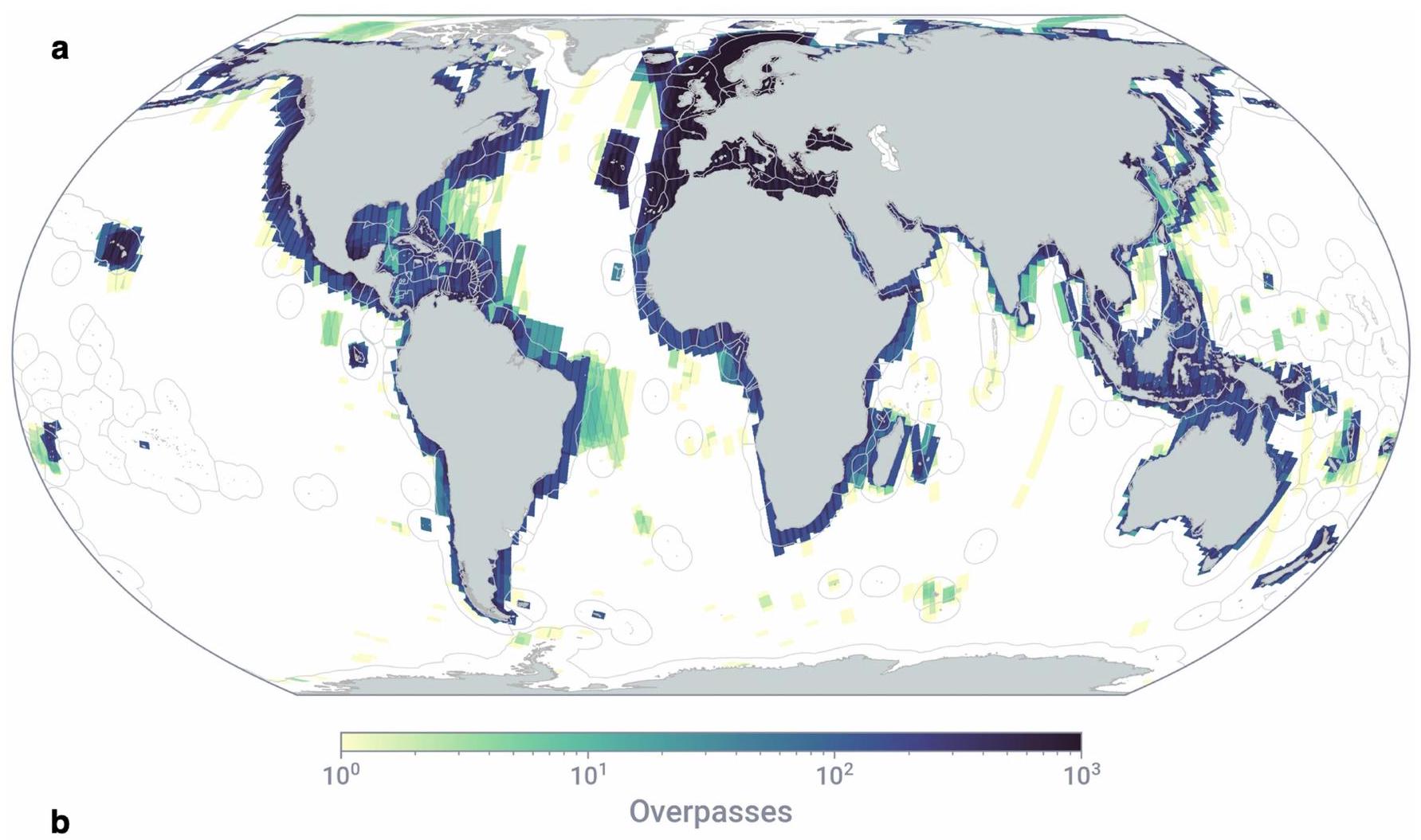
الشكل البياني الممتد 1| تغطي صور رادار الفتحة الاصطناعية Sentinel-1 (منتج IW GRD) معظم المياه الساحلية ولكنها لا تغطي معظم المحيط المفتوح. أ، يتم تحديد مدى وتكرار عمليات الاستحواذ على الرادار بواسطة أولويات المهمة. ب، مساحة المحيط التي يتم تصويرها يوميًا بواسطة منتج Sentinel-1 GRD (باستخدام
كان المتوسط المتحرك لمدة 12 يومًا يعتمد على ما إذا كان قمر صناعي واحد يصور المحيط (S1A، من أكتوبر 2014 حتى الآن) أو اثنان (S1A و S1B، من سبتمبر 2016 حتى ديسمبر 2017). توقف S1B عن العمل في 23 ديسمبر 2021.
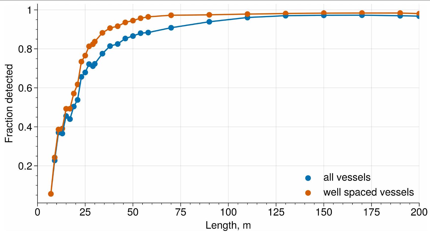
الشكل البياني الممتد 2 | نموذج الكشف Sentinel-1 قادر على اكتشاف معظم السفن الصناعية. منحنى الاسترجاع (نسبة الإيجابيات الفعلية التي تم اكتشافها بشكل صحيح) لنموذج الكشف Sentinel-1 لدينا كدالة لطول السفينة
يظهر أن السفن المتباعدة عن بعضها البعضالمسافة، التي تشكل 79% من جميع اكتشافات السفن) لديها معدل استرجاع أعلى من جميع السفن مجتمعة. بالنسبة للسفن التي تقل عن 25 مترًا، يتدهور أداء الكشف بشكل حاد مع حجم السفينة.
مقالة
الشكل البياني الممتد 3| تُظهر أنشطة سفن الصيد في البحر بمستوى غير مسبوق من التفاصيل من خلال رسم الخرائط بواسطة الأقمار الصناعية والتعلم العميق. تميل سفن الصيد إلى التجمع على طول الميزات الجيولوجية. كل نقطة تمثل سفينة تم اكتشافها خلال الفترة من 2017 إلى 2021. تمثل الألوان
تمت مطابقة الاكتشافات (باللون الأزرق، المتعقبة علنًا) وغير المتطابقة (باللون الأحمر، غير المتعقبة علنًا) مع مواقع السفن المعروفة من نظام تحديد الهوية الآلي (AIS). يعتمد عدد الاكتشافات في كل موقع على الكثافة المحلية للسفن، بالإضافة إلى عدد عمليات الاستحواذ على البحث والإنقاذ (SAR).
الشكل 4 من البيانات الموسعة | يتم عرض نشاط السفن للنقل والطاقة في البحر بمستوى غير مسبوق من التفاصيل من خلال رسم الخرائط بواسطة الأقمار الصناعية والتعلم العميق. عادةً ما تتبع سفن النقل والطاقة الطرق الرئيسية (على سبيل المثال، طرق الشحن). كل نقطة تمثل سفينة تم اكتشافها خلال الفترة من 2017 إلى 2021. الـ
تمثل الألوان الكشفات المتطابقة (الأزرق، المتعقب علنًا) وغير المتطابقة (الأحمر، غير المتعقب علنًا) مع مواقع السفن المعروفة من نظام تحديد الهوية الآلي (AIS). يعتمد عدد الكشفات في كل موقع على الكثافة المحلية للسفن، بالإضافة إلى عدد عمليات الاستحواذ على البحث والإنقاذ (SAR).
الشكل 5 من البيانات الموسعة | الدول الرائدة في الصيد وغير الصيد نشاط السفن. تمثل الأعمدة متوسط عدد الاكتشافات لكل مرور قمر صناعي في أي موقع داخل المنطقة الاقتصادية الخالصة خلال الفترة من 2017 إلى 2021. النسب المئوية هي نسبة الاكتشافات غير المطابقة لمواقع السفن المعروفة من نظام تحديد الهوية الآلي (النشاط المفقود من أنظمة المراقبة العامة).
الشكل 6 من البيانات الموسعة | في المنطقة الاقتصادية الخالصة الغربية لكوريا الشمالية، تتزامن ذروة نشاط سفن الصيد مع الحظر الصيني على الصيد الصناعي. تزداد أنشطة الصيد في مياه شمال كوريا الغربية بالتزامن مع
حظر الصيد الصيني (خطوط عمودية). هناك انخفاض كبير في النشاط العام للسفن خلال جائحة COVID-19 (2020-2021)، عندما أغلقت كوريا الشمالية حدودها.
مقالة
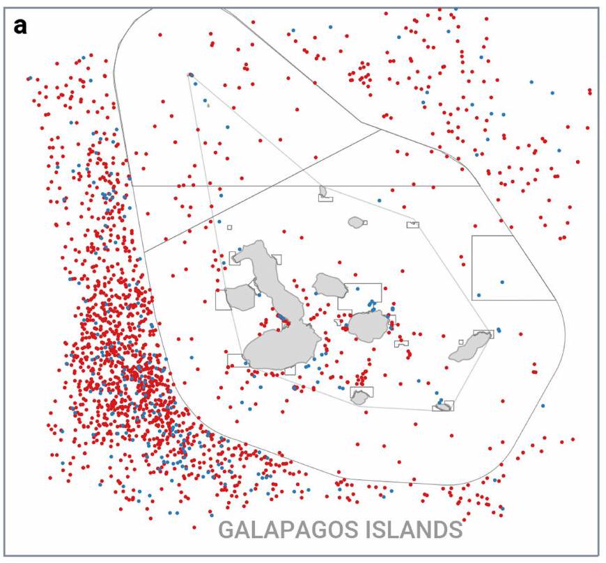
الشكل 7 من البيانات الموسعة | يسمح الكشف القائم على صور الأقمار الصناعية بالمراقبة على نطاق محلي. أ، ب، من 2017 إلى 2021، كان هناك عدد كبير من السفن غير المتعقبة علنًا (باللون الأحمر) داخل حدود اثنين من أكثر المناطق البحرية المحمية شهرة وأهمية بيولوجية ومراقبة جيدًا في العالم: الـ
محافظة غالاباغوس البحرية وجنوب حديقة الحاجز المرجاني العظيم البحرية. ج، د، منطقتان من تطوير البنية التحتية البحرية المكثفة هما البنية التحتية للنفط في بحيرة ماراكايبو في فنزويلا ومزارع الرياح البحرية شمال شنغهاي، الصين.
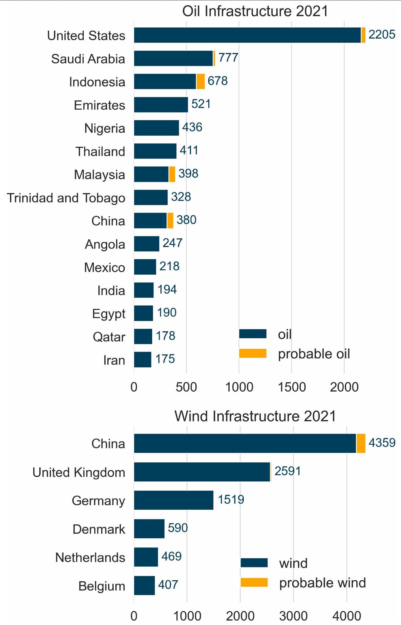
الشكل البياني الممتد 8|الدول الرائدة التي تمتلك أكبر بنية تحتية للنفط والرياح البحرية. تمثل الأعمدة القيمة المتوسطة لعدد الهياكل البحرية الشهرية لكل منطقة اقتصادية خالصة في عام 2021. تشير كلمة ‘محتمل’ إلى البنية التحتية المكتشفة التي تتمتع بثقة أقل ولكن لا تزال ضمن المنطقة الاقتصادية الخالصة للدولة المعنية.
مقالة
الشكل البياني الموسع 9 | تطوير النفط في عرض البحر خلال 2017-2021 في أعلى 20 دولة نفطية. تمثل السلاسل الزمنية الوسيط الشهري لعدد الهياكل النفطية المكتشفة داخل المنطقة الاقتصادية الخالصة لكل دولة سنويًا. لاحظ النطاقات المختلفة في محاور.
الشكل البياني الممتد 10 | عدد السفن والهياكل كدالة للمسافة من الشاطئ ومن البنية التحتية. أ، نشاط سفن الجرّاحين منخفض نسبيًا بالقرب من البنية التحتية النفطية، لكن أنواع الصيد الأخرى تظهر زيادة.
نشاط هناك.عدد السفن ومنصات النفط ينخفض بسرعة بعيدًا عن الساحل، لكن عدد هياكل الرياح يبقى ثابتًا نسبيًا ضمن عشرات الكيلومترات من الساحل.
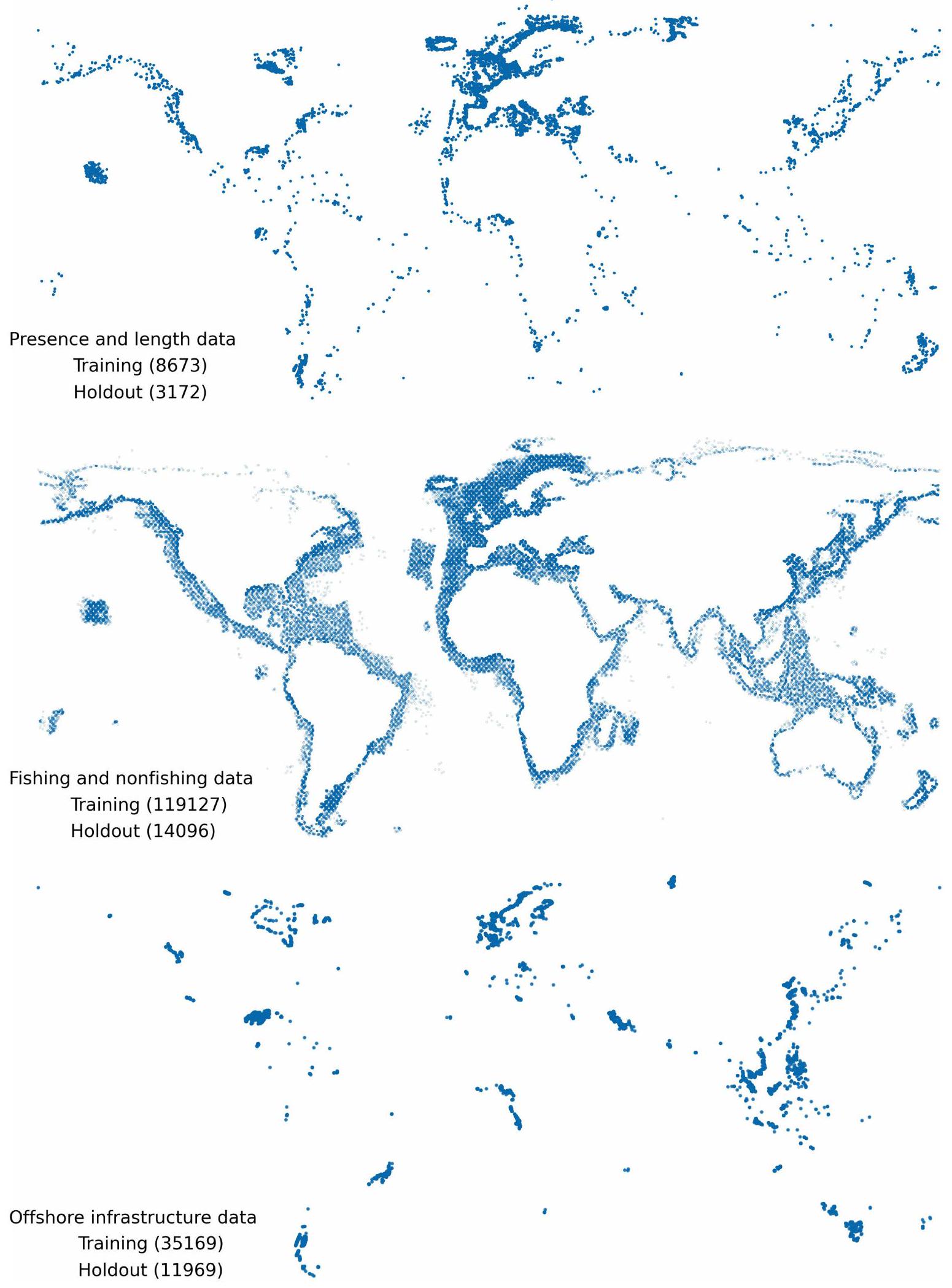
الشكل 11 من البيانات الموسعة | البيانات المعلّمة المستخدمة لتدريب نماذج التعلم العميق تغطي جميع مناطق المحيط. التوزيع المكاني لبيانات التدريب وبيانات الاحتفاظ المستخدمة لتدريب وتقييم نموذج ‘تقدير وجود السفن وطولها’، نموذج ‘تصنيف الصيد وغير الصيد’ ونموذج ‘تصنيف البنية التحتية البحرية’. بيانات الاحتفاظ عشوائية. عينات فرعية بنفس التوزيع المكاني لبيانات التدريب دون أي تداخل في الوقت أو المكان (لا تسرب بيانات بين مجموعات التدريب والاختبار). انظر الأقسام الخاصة بالتصنيف للحصول على وصف لاستراتيجيات العينة وخصائص كل مجموعة بيانات.
البيانات الموسعة الجدول 1 | آسيا وأوروبا (خطأ) تظهر ساعات الصيد قابلة للمقارنة إذا تم تقديرها من نظام تحديد الهوية الآلي (AIS)
قارة
نسبة إجمالي ساعات الصيد من نظام تحديد الهوية الآلي
نسبة إجمالي سفن الصيد من SAR
آسيا
0.44
0.71
أوروبا
0.36
0.10
أفريقيا
0.06
0.07
أمريكا الشمالية
0.06
0.07
أستراليا
0.05
0.02
أمريكا الجنوبية
0.04
0.04
إجمالي ساعات نشاط الصيد خلال 2017-2021 تم حسابها من قاعدة بيانات نظام تحديد الهوية الآلي (AIS) الخاصة بمراقبة الصيد العالمية، والتي تحتوي على 52 مليار رسالة بث للسفن تم الحصول عليها من مزودين عالميين. COMM و Spire، مقارنةً مع نسبة إجمالي قوارب الصيد التي تم اكتشافها بواسطة SAR، والتي تشمل القوارب التي لم يتم اكتشافها بواسطة مراقبة AIS.
مراقبة الصيد العالمية، واشنطن العاصمة، الولايات المتحدة الأمريكية.قسم بيئة الغابات والحياة البرية، جامعة ويسكونسن-ماديسون، ماديسون، ويسكونسن، الولايات المتحدة الأمريكية.مختبر علم البيئة الجيومكانية البحرية، مدرسة نيكولاس للبيئة، جامعة ديوك، دورهام، نورث كارولينا، الولايات المتحدة الأمريكية.مدرسة برين لعلوم البيئة وإدارة الموارد، جامعة كاليفورنيا، سانتا باربرا، سانتا باربرا، كاليفورنيا، الولايات المتحدة الأمريكية. سكاي تروث، شيفردستاون، فرجينيا الغربية، الولايات المتحدة الأمريكية.ساهم هؤلاء المؤلفون بالتساوي: فرناندو س. باولو، ديفيد كروودسما.البريد الإلكتروني: fernando@globalfishingwatch.org
الدارميلي، ك.، مكغواير، ب.، باور، د. ومولوني، ج. الكشف عن الأهداف في صور الرادار ذي الفتحة الاصطناعية: مسح حديث. مجلة الاستشعار عن بعد التطبيقي 7، 071598 (2018).
كروودسما، د. أ. وآخرون. كشف أسطول الصيد الطويل العالمي باستخدام رادار الأقمار الصناعية. تقارير العلوم 12، 21004 (2022).
باباس، أ.، أتشيم، أ. وبول، د. كاشفات CFAR على مستوى السوبر بكسل لاكتشاف السفن في صور الرادار. رسائل IEEE للعلوم الجيولوجية والاستشعار عن بعد 15، 1397-1401 (2018).
لينغ، إكس.، جي، ك.، يانغ، ك. وزو، إتش. خوارزمية CFAR ثنائية الجانب لاكتشاف السفن في صور SAR. رسائل IEEE للعلوم الجيولوجية والاستشعار عن بعد 12، 1536-1540 (2015).
هو، ك.، زانغ، إكس.، رين، س. وسون، ج. في مؤتمر IEEE 2016 لرؤية الكمبيوتر والتعرف على الأنماط (CVPR) 770-778 (مؤسسة رؤية الكمبيوتر، 2016).
ليو، ز. وآخرون في مؤتمر IEEE/CVF لعام 2022 حول رؤية الكمبيوتر والتعرف على الأنماط (CVPR) 11966-11976 (مؤسسة رؤية الكمبيوتر، 2022).
كييتنج، ك. أ. وتشيري، س. نمذجة توزيعات الاستخدام في الزمان والمكان. علم البيئة 90، 1971-1980 (2009).
لورانس، ب. ج. وآخرون. السواحل الاصطناعية تفتقر إلى التعقيد الهيكلي الطبيعي عبر المقاييس. إجراءات الجمعية الملكية B للعلوم البيولوجية 288، 20210329 (2021).
كرول، م.، ليذرمين، س. ب. وباكل، م. ك. التغير التاريخي في خط الساحل: تحليل الأخطاء ودقة الخرائط. مجلة أبحاث السواحل 7، 839-852 (1991).
Fernando S. Paolo , David Kroodsma , Jennifer Raynor , Tim Hochberg , Pete Davis , Jesse Cleary , Luca Marsaglia , Sara Orofino , Christian Thomas & Patrick Halpin
The world’s population increasingly relies on the ocean for food, energy production and global trade , yet human activities at sea are not well quantified . We combine satellite imagery, vessel GPS data and deep-learning models to map industrial vessel activities and offshore energy infrastructure across the world’s coastal waters from 2017 to 2021. We find that 72-76% of the world’s industrial fishing vessels are not publicly tracked, with much of that fishing taking place around South Asia, Southeast Asia and Africa. We also find that 21-30% of transport and energy vessel activity is missing from public tracking systems. Globally, fishing decreased by at the onset of the COVID-19 pandemic in 2020 and had not recovered to pre-pandemic levels by 2021. By contrast, transport and energy vessel activities were relatively unaffected during the same period. Offshore wind is growing rapidly, with most wind turbines confined to small areas of the ocean but surpassing the number of oil structures in 2021. Our map of ocean industrialization reveals changes in some of the most extensive and economically important human activities at sea.
More than one billion people depend on the ocean for their primary source of food , with 260 million employed by global marine fisheries alone . About 80% of all traded goods are shipped over the ocean and nearly 30% of the world’s oil is produced in offshore fields and distributed worldwide . In addition to these established uses of the ocean, increases in offshore renewable energy, aquaculture and mining are rapidly emerging. All of this industrial machinery powers a 1.5-2.5 trillion dollar ‘blue economy’, that is growing faster than the overall global economy but is also causing rapid environmental decline. A third of fish stocks are operated beyond biologically sustainable levels and an estimated of critical marine habitats have been lost owing to human industrialization .
A lack of global observational data limits understanding of where and how the blue economy is expanding and how it is affecting developing nations and coastal communities . On land, maps exist for almost every road , datasets are being developed for every human-made structure and extractive industries such as forestry and agriculture are mapped globally at sub-kilometre scale and updated monthly . In the ocean, however, many seagoing vessels do not broadcast their location or are not detected by public monitoring systems , and information on the development of offshore infrastructure and other industrial activities is often held private . The result is that continuing human expansion into the ocean is poorly documented.
Current approaches for mapping human activity at sea have limitations. Some vessel-tracking systems, such as the vessel monitoring system (VMS) used in fishing, are proprietary, which limit the ability to map and compare across regions . For public mapping of ships, the focus has been on the automatic identification system (AIS) , which
broadcasts vessel coordinates to track vessel movements and support maritime safety; AIS data can also reveal vessel identities, owners and corporations, and fishing activities . Not all vessels, however, are required to use AIS devices, as regulations vary by country, vessel size and activity . Vessels engaged in illicit activities often turn off their AIS transponders or manipulate the locations they broadcast . In recent years, for example, the largest cases of illegal fishing and forced labour were by fleets that mostly did not use AIS devices. Furthermore, large ‘blind spots’ along coastal waters emerge where satellite reception is poor and AIS data received by terrestrial receptors can be restricted by national governments . We refer to vessels that are not visible on publicly accessible AIS data as ‘not publicly tracked’. This concept is also sometimes referred to as ‘dark vessels’. Although the location of offshore fixed infrastructure should be more readily available than moving vessels, information on offshore development is often restricted for commercial or bureaucratic reasons , and large-scale assessments must aggregate several disparate data sources, which are often incomplete or outdated . Vessel activity and ocean infrastructure are not captured well by existing methods, but satellite imagery and deep learning can improve the monitoring of human use of the ocean.
Here we present a detailed global map of major industrial activities at sea. To detect and characterize vessels and offshore infrastructure in coastal waters around the globe, we analysed 2 petabytes of satellite imagery spanning the years 2017-2021, with our analyses covering more than 15% of the ocean (Extended Data Fig.1) in which more than 75% of industrial activity is concentrated (Methods). We designed and trained three deep convolutional neural networks to identify objects (>97% accuracy) and estimate their lengths ( score
of 0.84); to classify offshore infrastructure into oil, wind and other objects (>98% accuracy); and to classify vessels as fishing or non-fishing ( accuracy). Combined, we classified more than 67 million image tiles, including dual-polarization synthetic-aperture radar (SAR) imagery from Sentinel-1 (ref. 35) and optical (red, green, blue and near-infrared (NIR)) imagery from Sentinel-2 (ref. 36). The resolution of SAR allows us to capture most objects larger than 15 m (detection rate for 25-m vessels and for vessels 50 m and larger; Extended Data Fig. 2). We also analysed 53 billion vessel GPS positions from the AIS and matched them to the satellite detections to determine whether a detected vessel was publicly tracked.
Fishing and non-fishing vessels
During 2017-2021, on average, about 63,300 vessel occurrences were detected at any given moment, roughly half ( ) of which were fishing vessels (based on 23.1 million vessel detections;Fig.1). Notably, about three-quarters (72-76%) of globally mapped industrial fishing did not appear in public monitoring systems, compared with one-quarter ( ) for other vessel activities.
Vessel activity was widespread but also highly concentrated. Dividing our study area into cells (about 11 km ), we detected a vessel at least once in of the cells covered by the satellites, yet half of all vessel activity was concentrated in less than of the cells. Most vessel activity (86% of fishing and 75% of non-fishing) was focused in waters less than 200 m deep (Fig. 1), which constitute only 7% of the ocean. Activity is also unevenly distributed by continent, with approximately 67% of all vessel activity in Asia, followed by 12% in Europe, 7% in North America, 7% in Africa, 4% in South America and 2% in Australia (Fig.1).
Our satellite mapping revealed high densities of vessel activity in large areas of the ocean that previously showed little to no vessel activity by public tracking systems (Fig. 2). Indonesia, South Asia, Southeast Asia and the northern and western coasts of Africa (Fig. 2 and Extended Data Figs. 3 and 4) all show substantial amounts of activity not publicly tracked.
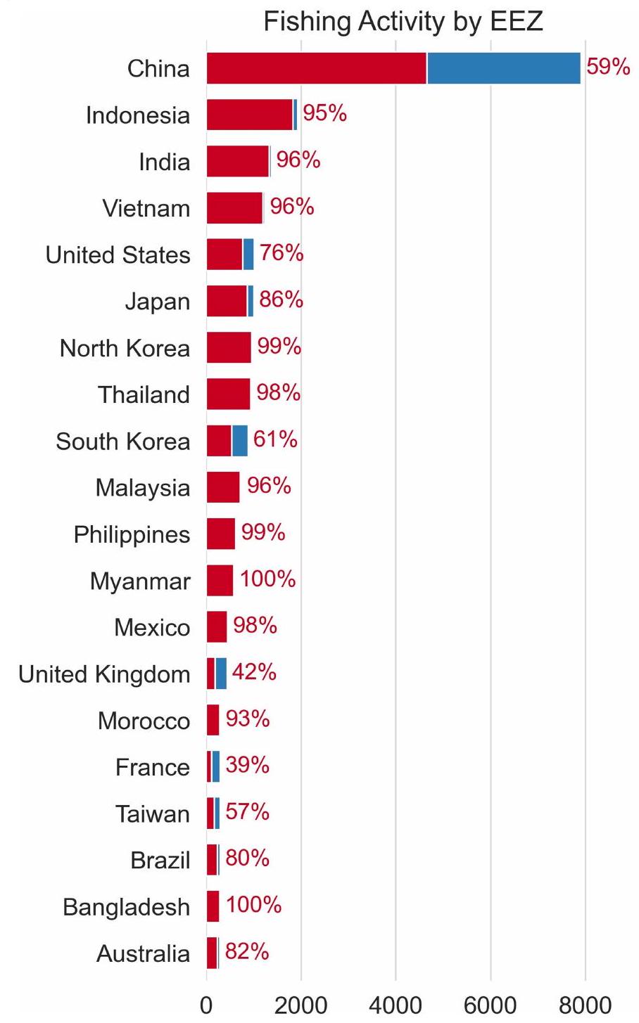
By mapping vessels that fail to broadcast their location, we show far more accurately the global distribution of industrial fishing. AIS data alone, for example, wrongly suggest that Europe and Asia have comparable fishing activity, with other continents having less than one-fifth as much activity (Extended Data Table 1). Our global map, however, reveals that Asia dominates industrial fishing, accounting for 70% of all fishing vessel detections (Extended Data Fig. 5); nearly 30% of all mapped fishing vessels were concentrated in the exclusive economic zone (EEZ) of China alone. Similarly, AIS data suggest that European countries in the Mediterranean have more than ten times as many fishing hours in their EEZs as do African countries , but our mapping shows that detections of fishing vessels are fairly balanced between the northern and southern parts of the Mediterranean Sea (Figs. 1 and 2).
Our mapping can also reveal potential hotspots of illegal fishing activity. Previous work showed substantial illicit activity in the eastern waters of North Korea , but our global mapping shows that most of the undisclosed fishing actually occurred in the western part of the Korean Peninsula (Fig. 2). In fact, this location showed the highest density of fishing vessels in the world from 2017 to 2019, with about 40 vessels per . This previously unmapped activity peaked each year in May, during China’s moratorium on fishing in their own waters (Extended Data Fig. 6), and activity abruptly fell by 85% during the COVID-19 pandemic when North Korea shut its borders. Numerous fishing vessels not publicly tracked were also detected inside many marine protected areas (MPAs). For example, two of the most iconic, biologically important and well-monitored MPAs in the world-the Galápagos Marine Reserve and the Great Barrier Reef Marine Park-showed, on average, more than 5 and 20 of these vessels per week, respectively (Extended Data Fig. 7).
The spatial resolution of our data, which is substantially higher than the most widely used global fishing products , also reveals detailed fishing strategies at the regional scale (Fig. 2 and Extended Data Fig. 3). The area between Tunisia and Sicily, for example, shows a mix of both publicly and not publicly tracked fishing vessels aggregating along ocean banks and the edges of seabed canyons, a signature characteristic of bottom trawling . Similarly, off the coast of Bangladesh, in which almost no vessels are publicly tracked and no public maps of fishing exist, fishing vessels follow bathymetric contours and submarine canyons that radiate from the Ganges Delta.
Unlike fishing, most non-fishing vessels (largely transport and energy-related) broadcast their locations, with just about onequarter missing from public monitoring systems. Asia had the largest concentration (65% of all detections) of transport and energy vessels, including most of the non-broadcasting ones (Fig.1)-most of these vessels, however, were operating in areas with poor satellite AIS reception, so it is possible that many vessels broadcast their positions but were not trackable with global AIS tracking services. All other continents seemed to have relatively minor tracking discrepancies across transport and energy vessels, with less than 20% of these vessels not publicly trackable.
Our mapping also tracks changes in vessel activity over time (Fig. 3). Similar to a previous AIS-based analysis , our data show yearly cycles of fishing activity, with cycles inside China driven by the Chinese New Year and their voluntary fishing moratorium, and in the rest of the world by the New Year and associated holidays. But, owing to SAR-based detection, we can provide a more accurate assessment of trends, which reveals a global decrease in fishing activity of , coinciding with the pandemic. By stark contrast, transport and energy remained stable or even slightly increased over 2017-2021. Moreover, the impact of COVID-19 on fishing activity was much greater outside China (compared with 2018 and 2019), and transport and energy grew more in China than it did in the rest of the world.
Fixed infrastructure
The number of offshore structures worldwide was around 28,000 by the end of 2021 (Fig. 4). Wind turbines and oil structures in notable wind-producing or oil-producing areas (Methods) constituted and 38% of all ocean infrastructure, respectively; the remaining 14% was divided across wind turbines and oil structures outside major development areas, as well as piers, bridges, power lines, aquaculture and other human-made structures.
Most oil infrastructure is distributed among 13 major oil-producing areas (Fig. 4a). Excluding Lake Maracaibo in Venezuela, which is a lagoon, our mapping shows that the largest concentration of offshore oil infrastructure in the world is in the Gulf of Mexico. At the end of 2021, about a quarter of the global offshore oil infrastructure is accounted for by the USA (>2,200 oil structures), followed by Saudi Arabia (>770) and Indonesia (>670).
Offshore wind development has been mostly confined to northern Europe (52%) and China (45%) (Fig. 4a and Extended Data Fig. 8); however, there has been a shift in offshore energy development. The number of offshore oil structures has increased by about 16% over the past half a decade (Fig. 4c), with a decrease in the USA of several hundred structures offset by increases elsewhere (Extended Data Fig. 9). By contrast, the number of wind turbines in the ocean has more than doubled since 2017, probably surpassing the number of oil structures by the end of 2020 (Fig. 4c). China leads the development of offshore wind, with a staggering 900% increase in turbines from 2017 to 2021 (averaging around 950 wind turbines per year), well ahead of projections by the International Energy Agency . The UK and Germany lead offshore wind development in Europe, increasing by and , respectively, since 2017.
Fig.1|About 75%of global industrial fishing and 25%of other vessel activity is not publicly tracked.a,b,Per square kilometre,the average number of industrial fishing vessels(a)and shipping,tanker,passenger and support vessels(b),from 5 years of satellite SAR imagery.The colour represents the percentage of detected vessels that were matched(blue,publicly tracked) and unmatched(red,not publicly tracked)to known vessel positions from AIS
broadcast.c,For each continent,the total number of detected vessels and the respective fraction of publicly and not publicly tracked.The outline around the continents(light grey)shows the area of the ocean with available SAR imagery (see Extended Data Fig. 1 for the spatial distribution of images).'N.America' includes Central American countries.Classification of detected objects was performed with deep learning.
Fig. 2 | High-resolution mapping reveals detailed patterns of fishing activity not publicly tracked. Satellite SAR detections of individual vessels during 2017-2021, matched (blue) and unmatched (red) to known vessel positions from AIS broadcast, are classified as fishing or non-fishing vessels with a deep-learning model. Most fishing vessels, usually smaller than 50 m in length, concentrate close to shore and follow bathymetric features, such as the continental shelf break and seabed canyons, or regulatory and political boundaries. Extensive areas of previously unmapped fishing activity are
revealed along Northern Africa and South and Southeast Asia. The absolute number of detections in each location depends on the local vessel density and the number of satellite image acquisitions, which varies by region. Depicted numbers may represent a slightly larger area than is shown. This figure shows the level of spatial detail that is possible with our mapping approach. Extended Data Figures 3 and 4 show further examples of high-resolution fishing and non-fishing patterns publicly and not publicly tracked.
Fig. 3 | Fishing activity was highly affected by COVID-19, whereas transport and energy continued to grow. Time series of the average number of vessels over the area covered by SAR from Sentinel-1 (constructed from the average number of detections per satellite overpass at any given location; Methods) showing that COVID-19 greatly affected fishing activity, whereas transport and energy continued to grow. China alone holds nearly 30% of the global fishing fleet and about 21% of transport and energy vessels. a, Industrial fishing vessels greater than 15-20 m in length over all EEZs outside China and inside China EEZ. b, The same as a but for transport-related and energy-related vessels, mostly
shipping, tankers, passenger and support. The shaded grey areas indicate the 2 -year mean s.d., highlighting the effect of the 2020 global pandemic. The numbers show the per cent change with their respective standard error. The combined change (outside + inside) is – (industrial fishing) and (transport and energy); Methods. The coloured boxes highlight the annual cycles in activity related to national holidays and fishing moratoria. The axis shows the maximum, mean and minimum values of detected vessels during 2017-2021.
Interactions between vessels and fixed infrastructure
A key question for the future is how vessel traffic may be affected by changes in oil and wind infrastructure development. Trawlers, which fish by hauling nets along the seafloor or through the water column and are the most common fishing gear globally, avoid fishing within 1 km of oil structures, most probably to avoid net entanglement (Extended Data Fig. 10a). Other types of fishing, which are at a lower risk of entanglement, are attracted to these structures, probably because they can cause fish to aggregate . Although wind turbines may also aggregate fish, they are less likely to affect industrial fishing in the same way because they are, at present, highly concentrated and, on average, far from shore, where there is less fishing activity (Extended Data
Fig. 10b). Also, oil-related vessel traffic has a much wider footprint than wind-related traffic, accounting for five times as much activity globally in 2021 (Fig. 4b and Extended Data Fig. 4).
Conclusion
Overall, our study reveals the extent of major industrial activities at sea, with fishing being by far the ocean industry with the most activity that is not public. With our freely available dataset and technology, hotspots of potentially illegal activity can now be shown and industrial fishing vessels can be identified that are encroaching on artisanal fishing grounds or other countries’ EEZs , but at a global scale and accessible to any nation. Maps of global fishing effort can
now include all vessels, not just those based on AIS tracking (which misses about three-quarters of large vessels), and with much higher resolution than just EEZs or statistical reporting areas . Our data can also help to quantify the scale of greenhouse gas emissions from vessel traffic and offshore development, which may help to inform policies on reducing greenhouse gas emissions.
This picture of human activity also presents a snapshot of how industrial use of the ocean is changing. Although COVID-19 may have had a dominant role in depressing fishing activity, fishing still decreased far more than other ocean industries. This slowdown is in line with a long-term decline in the relative importance of fishing in the ocean . Since the 1980s, global marine fish catch has been relatively unchanged as most fisheries are already fished to capacity . As a result, global fishing effort, which has increased several fold since 1950, increased only slightly in recent years . Many countries that have reformed their fisheries show an actual decline in their fishing effort . The decrease highlighted in this study may reflect this longer trend and we may already have seen the peak of fishing activity in the past decade. By contrast, transport and energy vessel traffic may continue to expand, following trends in global trade and the rapid development of renewable energy infrastructure. In this scenario, changes to marine ecosystems brought by infrastructure and vessel traffic may rival fishing in impact , and an accurate mapping of these activities is fundamental to understanding and managing future human activities in the ocean.
Online content
Any methods, additional references, Nature Portfolio reporting summaries, source data, extended data, supplementary information, acknowledgements, peer review information; details of author contributions and competing interests; and statements of data and code availability are available at https://doi.org/10.1038/s41586-023-06825-8.
Costello, C. et al. The future of food from the sea. Nature 588, 95-100 (2020).
Golden, J. S. et al. Making sure the blue economy is green. Nat. Ecol. Evol. 1, 0017 (2017).
Jouffray, J. B., Blasiak, R., Norström, A. V., Österblom, H. & Nyström, M. The blue acceleration: the trajectory of human expansion into the ocean. One Earth 2, 43-54 (2020).
Ryabinin, V. et al. The UN decade of ocean science for sustainable development. Front. Mar. Sci. 6, 470 (2019).
Kroodsma, D. A. et al. Tracking the global footprint of fisheries. Science 359, 904-908 (2018).
Teh, L. C. L. & Sumaila, U. R. Contribution of marine fisheries to worldwide employment. Fish Fish. 14, 77-88 (2013).
Food and Agriculture Organization of the United Nations (FAO). The State of World Fisheries and Aquaculture 2022, https://doi.org/10.4060/cc0461en (2022).
Lotze, H. K. et al. Depletion degradation, and recovery potential of estuaries and coastal seas. Science 312, 1806-1809 (2006).
Waycott, M. et al. Accelerating loss of seagrasses across the globe threatens coastal ecosystems. Proc. Natl Acad. Sci. USA 106, 12377-12381 (2009).
Intergovernmental Science-Policy Platform on Biodiversity and Ecosystem Services (IPBES). Summary for Policymakers of the Global Assessment Report on Biodiversity and Ecosystem Services, https://zenodo.org/record/3553579 (2019).
Winther, J. G. et al. Integrated ocean management for a sustainable ocean economy. Nat. Ecol. Evol. 4, 1451-1458 (2020).
Bennett, N. J., Govan, H. & Satterfield, T. Ocean grabbing. Mar. Policy 57, 61-68 (2015).
Belhabib, D., Sumaila, U. R. & Le Billon, P. The fisheries of Africa: exploitation, policy, and maritime security trends. Mar. Policy 101, 80-92 (2019).
Center for International Earth Science Information Network (CIESIN), Columbia University, and Information Technology Outreach Services (ITOS), University of Georgia. Global roads open access data set (gROADS), v1 (1980-2010). https://doi.org/10.7927/H4VD6WCT (2013).
Hoang, N. T. & Kanemoto, K. Mapping the deforestation footprint of nations reveals growing threat to tropical forests. Nat. Ecol. Evol. 5, 845-853 (2021).
Waldner, F. et al. A unified cropland layer at 250 m for global agriculture monitoring. Data 1, 3 (2016).
Taconet, M., Kroodsma, D. & Fernandes, J. A. Global Atlas of AIS-based Fishing Activity: Challenges and Opportunities, http://www.fao.org/3/ca7012en/CA7012EN.pdf (2019).
Virdin, J. et al. The Ocean 100: transnational corporations in the ocean economy. Sci. Adv. 7, eabc8041 (2021).
March, D., Metcalfe, K., Tintoré, J. & Godley, B. J. Tracking the global reduction of marine traffic during the COVID-19 pandemic. Nat. Commun. 12, 2415 (2021).
Carmine, G. et al. Who is the high seas fishing industry? One Earth 3, 730-738 (2020).
Park, J. et al. Tracking elusive and shifting identities of the global fishing fleet. Sci. Adv. 9, eabp8200 (2023).
Welch, H. et al. Hot spots of unseen fishing vessels. Sci. Adv. 8, eabq2109 (2022).
Park, J. et al. Illuminating dark fishing fleets in North Korea. Sci. Adv. 6, eabb1197 (2020).
McDonald, G. G. et al. Satellites can reveal global extent of forced labor in the world’s fishing fleet. Proc. Natl Acad. Sci. USA 118, e2016238117 (2021).
Joo, R. et al. Towards a responsible machine learning approach to identify forced labor in fisheries. Preprint at https://arxiv.org/abs/2302.10987 (2023).
Wong, B. A., Thomas, C. & Halpin, P. Automating offshore infrastructure extractions using synthetic aperture radar & Google Earth Engine. Remote Sens. Environ. 233, 111412 (2019).
Gourvenec, S., Sturt, F., Reid, E. & Trigos, F. Global assessment of historical, current and forecast ocean energy infrastructure: Implications for marine space planning, sustainable design and end-of-engineered-life management. Renew. Sustain. Energy Rev. 154, 111794 (2022).
Torres, R., Snoeij, P., Davidson, M., Bibby, D. & Lokas, S. in Proc. 2012 IEEE International Geoscience and Remote Sensing Symposium 1703-1706 (IEEE, 2012).
Spoto, F. et al. in Proc. 2012 IEEE International Geoscience and Remote Sensing Symposium 1707-1710 (IEEE, 2012).
Pauly D., Zeller D. & Palomares M. L. D. (eds) Sea Around Us Concepts, Design and Data, www.seaaroundus.org (2020).
Fiorentino F. et al. Synthesis of Information on Some Demersal Crustaceans Relevant for Fisheries in the South Central Mediterranean Sea, http://www.faomedsudmed.org/pdf/ publications/TD32.pdf (2013).
International Energy Agency (IEA). Offshore Wind Outlook 2019, https://www.iea.org/ reports/offshore-wind-outlook-2019 (2019).
Claisse, J. T. et al. Oil platforms off California are among the most productive marine fish habitats globally. Proc. Natl Acad. Sci. USA 111, 15462-15467 (2014).
Rousseau, Y., Watson, R. A., Blanchard, J. L. & Fulton, E. A. Evolution of global marine fishing fleets and the response of fished resources. Proc. Natl Acad. Sci. USA 116, 12238-12243 (2019).
McCauley, D. J. et al. Marine defaunation: animal loss in the global ocean. Science 347, 1255641 (2015).
Hilborn, R. et al. Effective fisheries management instrumental in improving fish stock status. Proc. Natl Acad. Sci. USA 117, 2218-2224 (2020).
Publisher’s note Springer Nature remains neutral with regard to jurisdictional claims in published maps and institutional affiliations.
SAR imaging systems have proved to be the most consistent option for detecting vessels at sea . SAR is unaffected by light levels and most weather conditions, including daylight or darkness, clouds or rain. By contrast, some other satellite sensors, such as electrooptical imagery, rely on sunlight and/or the infrared radiation emitted by objects on the ground and can therefore be confounded by cloud cover, haze, weather events and seasonal darkness at high latitudes.
We used SAR imagery from the Copernicus Sentinel-1 mission of the European Space Agency (ESA) (https://sentinel.esa.int/web/sentinel/ user-guides/sentinel-1-sar). The images are sourced from two satellites (S1A and, formerly, S1B, which stopped operating in December 2021) that orbit out of phase with each other in a polar, sun-synchronous orbit. Each satellite has a repeat cycle of 12 days, so that-together-they provide a global mapping of coastal waters around the world approximately every 6 days. The number of images per location, however, varies greatly depending on mission priorities, latitude and degree of overlap between adjacent satellite passes (https://sentinels.coper-nicus.eu/web/sentinel/missions/sentinel-1/observation-scenario). Spatial coverage also varies over time and is improved with the addition of S1B in 2016 and the acquisition of more images in later years (Extended Data Fig. 1). Our data consist of dual-polarization images (VH and VV) from the Interferometric Wide (IW) swath mode, with a resolution of about 20 m . We used the Ground Range Detected (GRD) Level-1 product provided by Google Earth Engine (https://developers. google.com/earth-engine/datasets/catalog/COPERNICUS_S1_GRD), processed for thermal noise removal, radiometric calibration and terrain correction (https://developers.google.com/earth-engine/ guides/sentinel1). To eliminate potential noise artefacts that would introduce false detections, we further processed each image by clipping a buffer off the borders. We selected all SAR scenes over the ocean from October 2016 to February 2022, comprising 753,030 images of pixels each on average.
Visible and NIR imagery
For optical imagery, we used the Copernicus Sentinel-2 (S2) mission of the ESA (https://sentinels.copernicus.eu/web/sentinel/user-guides/ sentinel-2-msi). These twin satellites (S2A and S2B) also orbit out of phase and carry a wide-swath, high-resolution, multispectral imaging system, with a combined global 5-day revisit frequency. Thirteen spectral bands are sampled by the S2 Multispectral Instrument (MSI): visible (RGB) and NIR at 10 m , red edge and SWIR at 20 m , and other atmospheric bands at spatial resolution. We used the RGB and NIR bands from the Level-1C product provided by Google Earth Engine (https://developers.google.com/earth-engine/datasets/catalog/ COPERNICUS_S2) and we excluded images with more than cloud coverage using the QA60 bitmask band with cloud mask information. We analysed all scenes that contained a detected offshore infrastructure during our observation period, comprising 2,494,370 images of pixels each on average (see the ‘Infrastructure classification’ section).
AIS data
AIS data were obtained from satellite providers ORBCOMM and Spire. In total, using Global Fishing Watch’s data pipeline , we processed 53 billion AIS messages. From those data, we extracted the locations, lengths and identities of all AIS devices that operated near the SAR scenes around the time the images were taken; we did so by interpolating between AIS positions to identify where vessels probably were at the moment of the image, as described in ref. 47. Identities of vessels in the AIS were based on methods in ref. 5 and revised in ref. 26.
Environmental and physical data
To classify vessels detected with SAR as fishing and non-fishing, we constructed a series of global environmental fields that were used as features in our model. Each of these rasters represents an environmental variable over the ocean at resolution. Data were obtained from the following sources: chlorophyll data from the NASA Ocean Biology Processing Group (https://oceancolor.gsfc.nasa.gov/ data/10.5067/ORBVIEW-2/SEAWIFS/L2/IOP/2018), sea-surface temperature and currents from the Copernicus Global Ocean Analysis and Forecast System (https://doi.org/10.48670/moi-00016), distance to shore from NASA OBPG/PacIOOS (http://www.pacioos.hawaii.edu/ metadata/dist2coast_1deg_ocean.html), distance to port from Global Fishing Watch (https://globalfishingwatch.org/data-download/ datasets/public-distance-from-port-v1) and bathymetry from GEBCO (https://www.gebco.net/). EEZ boundaries used in our analysis and maps are from Marine Regions .
Vessel detection by SAR
Detecting vessels with SAR is based on the widely used constant false alarm rate (CFAR) algorithm , a standard adaptive threshold algorithm used for anomaly detection in radar imagery. This algorithm is designed to search for pixel values that are unusually bright (the targets) compared with those in the surrounding area (the sea clutter). This method sets a threshold that depends on the statistics of the local background, sampled with a set of sliding windows. Pixel values above the threshold constitute an anomaly and are probably samples from a target. Our modified two-parameter CFAR algorithm evaluates the mean and standard deviation of backscatter values, delimited by a ‘ring’ composed of an inner window of pixels and an outer window of pixels. The best separation between the ocean and the targets is accomplished by the vertical-horizontal (VH) polarization band, which shows relatively low polarized returns over flat areas (ocean surface) compared with volumetric objects (vessels and infrastructure) :
in which is the backscatter value of the centre pixel, and are the mean and standard deviation of the background, respectively, and is a time-dependent threshold.
To maximize detection performance, we determined the sizes of the windows empirically, based on the fraction of detected vessels (broadcasting AIS) with length between 15 m and 20 m . A key feature of our two-parameter CFAR algorithm is the ability to specify different thresholds for different times. This adjustment is needed because the statistical properties of the SAR images provided by Sentinel-1 vary with time as well as by satellite (S1A and S1B). We thus found that the ocean pixels for both the mean and the standard deviation of the scenes changed, requiring different calibrations of the CFAR parameters for five different time intervals during which the statistics of the images remained relatively constant:January 2016 to October 2016 ( , none); September 2016 to January 2017 (14, 18); January 2017 to March 2018 (14, 17); March 2018 to January 2020 (16, 19); and January 2020 to December 2021 (22, 24). The five detection thresholds were calibrated to obtain a consistent detection rate for the smaller vessels across the entire Sentinel-1 archive (60% detection of vessels 15-20 m in length). The relative simplicity of our approach allowed us to reprocess the full archive of Sentinel-1 imagery several times to empirically determine the optimal parameters for detection.
To implement our SAR detection algorithm, we used the Python API of Google Earth Engine (https://developers.google.com/earth-engine/ tutorials/community/intro-to-python-api), a planetary-scale platform for analysing petabytes of satellite imagery and geospatial datasets. For processing, analysing and distributing our data products, our detection
workflow uses Google’s cloud infrastructure for big data, including Earth Engine, Compute Engine, Cloud Storage and BigQuery.
Vessel presence and length estimation
To estimate the length of every detected object and also to identify when our CFAR algorithm made false detections, we designed a deep convolutional neural network (ConvNet) based on the modern ResNet (Residual Networks) architecture . This single-input/multi-output ConvNet takes dual-band SAR image tiles of pixels as input and outputs the probability of object presence (a binary classification task) and the estimated length of the object (a regression task).
To analyse every detection, we extracted a small tile from the original SAR image that contained the detected object at the centre and that preserved both polarization bands (VH and VV). Our inference data therefore consisted of more than 62 million dual-band image tiles to classify. To construct our training and evaluation datasets, we used SAR detections that matched to AIS data with high confidence (see the ‘SAR and AIS integration’ section), including a variety of challenging scenarios such as icy locations, rocky locations, low-density and high-density vessel areas, offshore infrastructure areas, poor-quality scenes, scenes with edge artefacts and so on (Extended Data Fig. 11). To inspect and annotate these samples, we developed a labelling tool and used domain experts, cross-checking annotations from three independent labellers on the same samples and retaining the high-confidence annotations. Overall, our labelled data contained about 12,000 high-quality samples that we partitioned into the training ( , for model learning and selection) and test ( , for model evaluation) sets.
For model learning and selection, we followed a training-validation scheme that uses fivefold cross-validation (https://scikit-learn.org/ stable/modules/cross_validation.html), in which, for each fold (atraining cycle), 80% of the data is reserved for model learning and 20% for model validation, with the validation subset non-overlapping across folds. Performance metrics are then averaged across folds for model assessment and selection, and the final model evaluation is performed on the holdout test set. Our best model achieved on the test set an F1 score of 0.97 (accuracy = 97.5%) for the classification task and a score of 0.84 (RMSE , or about 1 image pixel) for the length-estimation task.
Infrastructure detection
To detect offshore infrastructure, we used the same two-parameter CFAR algorithm developed for vessel detection, with two fundamental modifications. First, to remove non-stationary objects, that is, most vessels, we constructed median composites from SAR images within a 6-month time window. Because stationary objects are repeated across most images, they are retained with the median operation, whereas non-stationary objects are excluded. We repeated this procedure for each month, generating a monthly time series of composite images. The temporal aggregation of images also reduces the background noise (the sea clutter) while enhancing the coherent signals from stationary objects . Second, we empirically adjusted the sizes of the detection window. As some offshore infrastructure is usually arranged in dense clusters, such as wind farms following a grid-like pattern, we reduced the spatial windows to avoid ‘contamination’ from neighbouring structures. It is also common to find smaller structures such as weather masts placed between some of the wind turbines. We found that an inner window of pixels and outer window of pixels was optimal for detecting every object in all wind farms and oil fields that we tested, including Lake Maracaibo, the North Sea and Southeast Asia, areas known for their high density of structures (Extended Data Fig. 7).
Infrastructure classification
To classify every detected offshore structure, we used deep learning. We designed a ConvNet based on the ConvNeXt architecture . A key difference from the ‘vessel presence and length estimation’ model, besides using a different architecture, is that this model is a multi-input/
single-output ConvNet that takes two different multiband image tiles of pixels as input, passes them through independent convolutional layers (two branches), concatenates the resulting feature maps and, with a single classification head, outputs the probabilities for the specified classes: wind infrastructure, oil infrastructure, other infrastructure and noise.
A new aspect of our deep-learning classification approach is the combination of SAR imagery from Sentinel-1 with optical imagery from Sentinel-2. From 6-month composites of dual-band SAR (VH and VV) and four-band optical (RGB and NIR) images, we extracted small tiles for every detected fixed structure, with the respective objects at the centre of the tile. Although both the SAR and optical tiles consist of 100 pixels, they come from imagery with different resolutions: the dual-band SAR tile has a spatial resolution of 20 m per pixel and the four-band optical tile is 10 m per pixel. This variable resolution not only provides information with different levels of granularity but also yields different fields of view.
From our inference data for infrastructure classification, which consisted of nearly six million multiband images, we constructed the labelled data by integrating several sources of ground truth for ‘oil and gas’ and ‘offshore wind’: from the Bureau of Ocean Energy Management (https://www.data.boem.gov/Main/HtmlPage.aspx?page=pla tformStructures), the UK Hydrographic Office (https://www.admi-ralty.co.uk/access-data/marine-data), the California Department of Fish and Wildlife (https://data-cdfw.opendata.arcgis.com/datasets/ CDFW::oil-platforms-ospr-ds357/about) and Geoscience Australia (https://services.ga.gov.au/gis/rest/services/Oil_Gas_Infrastructure/ MapServer). Using a labelling approach similar to that of the vessel samples, we also inspected a large number of detections to identify samples for ‘other structures’ and ‘noise’ (rocks, small islands, sea ice, radar ambiguities and image artefacts). From all areas known to have some offshore infrastructure (Extended Data Fig.11), our labelled data contained more than 47,000 samples ( oil, wind, noise and 4% other) that we partitioned into the training (80%) and test (20%) sets, using the same fivefold cross-validation strategy as for vessels.
Because the same fixed objects appear in several images over time, we grouped the candidate structures for the labelled data into spatial bins and sampled from different bins for each data partition, so that the subsets for model learning, selection and evaluation did not contain the same (or even nearby) structures at any point. We also note that, in the few cases in which optical tiles were unavailable, for example, because of seasonal darkness close to the poles, the classification was performed with SAR tiles only (optical tiles were blank). Our best model achieved on the test set a class-weighted average F1 score of 0.99 (accuracy ) for the multiclass problem.
Fishing and non-fishing classification
To identify whether a detected vessel was a fishing or non-fishing boat, we also used deep learning. For this classification task, we used the same underlying ConvNeXt architecture as for infrastructure, modified to process the following two inputs: the estimated length of the vessel from SAR (a scalar quantity) and a stack of environmental rasters centred at the location of the vessel (a multiband image). This multi-input-mixed-data/single-output model passes the raster stack (11 bands) through a series of convolutional layers and combines the resulting feature maps with the vessel-length value to perform a binary classification: fishing or non-fishing.
Two key aspects of our neural-net classification approach differ greatly from conventional image-classification tasks.
First, we are classifying the environmental context in which the vessel in question operates. To do so, we constructed 11 gridded fields (rasters) with a resolution of (approximately 1 km per pixel at the equator) and with global coverage. At every pixel, each raster contains contextual information on the following variables: (1) vessel density (based on SAR); (2) average vessel length (based on SAR); (3) bathymetry;
Article
(4) distance from port, (5) and (6) hours of non-fishing-vessel presence (from the AIS) for vessels less than 50 m and more than 50 m , respectively; (7) average surface temperature; (8) average current speed; (9) standard deviation of daily temperature; (10) standard deviation of daily current speed; and (11) average chlorophyll. For every detected vessel, we sampled -pixel tiles from these rasters, producing an 11-band image that we then classified with the ConvNet. Each detection is thus provided with context in an area just over . We obtained the fishing and non-fishing labels from AIS vessel identities .
Second, our predictions are produced with an ensemble of two models with no overlap in spatial coverage. To avoid leakage of spatial information between the training sets of the two models, and also to maximize spatial coverage, we divided the centre of the tiles into a longitude and latitude grid. We then generated two independent labelled datasets, one containing the tiles from the ‘even’ and the other from the ‘odd’ latitude and longitude grid cells. This alternating (the size of the tile) strategy ensures no spatial overlap between tiles across the two sets. We trained two independent models, one for ‘even’ tiles and another for ‘odd’ tiles, with each model ‘seeing’ a fraction of the ocean that the other model does not ‘see’. The test set that we used to evaluate both models contains tiles from both ‘even’ and ‘odd’ grid cells, with a buffer around all the test grid cells removed from all the neighbouring cells (used for training) to ensure spatial independence across all data partitions (no leakage). By averaging the predictions from these two models, we covered the full spatial extent of our detections with independent and complementary spatial information.
Our original test set contained fishing and non-fishing samples. We calibrated the model output scores by adjusting the ratio of fishing to non-fishing vessels in the test set to 1:1 (https://scikit-learn. org/stable/modules/calibration.html). We performed a sensitivity analysis to see how our results changed with different proportions of fishing and non-fishing vessels, and . On average, about 30,000 vessels not publicly tracked were detected at any given time. The calibrated scores with two-thirds fishing vessels predicted that of these vessels were fishing, whereas the calibration with only one-third fishing vessels predicted that of them were fishing vessels. Thus, the total percentage (considering all detections) of fishing and non-fishing vessels not publicly tracked amounts to and , respectively. Analysts at Global Fishing Watch then reviewed these outputs in different regions of the world to verify its accuracy.
Our training data contained about 120,000 tiles (divided into ‘odd’ and ‘even’) that we split into for model learning and for model selection. Our test set for model evaluation contained 14,100 tiles from both ‘odd’ and ‘even’ grid cells (Extended Data Fig. 11). The inference data contained more than 52 million tiles (11-band images) with respective vessel lengths that we classified with the two models. Our best model ensemble achieved on the test set a F1 score of 0.91 (accuracy ) for the classification task.
False positives and recall
Because there is no ground-truth data on where vessels are not present, estimating the rate of false positives at the global scale of our vessel detection algorithm is challenging. Although some studies report the total number of false positives, we believe that a more meaningful metric is the ‘false positive density’ (number of false positives per unit area), which takes into account the actual scale of the study. We estimated this metric by analysing 150 million of imagery across all five years in regions with very low density of AIS-equipped vessels (less than 10 total hours in 2018 in a grid cell of ), in regions far from shore ( ) and in the waters of countries that have relatively good AIS use and reception. The number of non-broadcasting vessel detections in these regions serves as the upper limit on the density of false positives, which we estimated as 5.4 detections per . If all of these were false positives, it would suggest a false-positive
rate of about 2% in our data. Because many of these are probably real detections, however, the actual false-positive rate is probably lower. Compared with other sources of uncertainties, such as the resolution limitation of the SAR imagery and missing some areas of the ocean (see below), false positives introduce a relatively minor error to our estimations.
To estimate recall (proportion of actual positives correctly identified), we used a method similar to that used in ref. 47. We identified all vessels that had an AIS position very close in time to the image acquisition ( ) and should therefore have appeared in the SAR scene; if they were detected in the SAR image, we could match them to the respective AIS-equipped vessels and then identify the AIS-equipped vessels not detected. The recall curve suggests that we are able to detect more than of all vessels greater than 50 m in length and around of all vessels between 25 m and 50 m in length, with the detection rate decaying steeply for vessels smaller than 25 m (Extended Data Fig. 2). However, because our vessel detection relies on a CFAR algorithm with a 600-m-wide window, when vessels are close to one another ( ), the detection rate is lower. See the ‘Limitations of our study’ section for factors influencing detectability.
SAR and AIS integration
Matching SAR detections to the GPS coordinates of vessels (from AIS records) is challenging because the timestamp of the SAR images and AIS records do not coincide, and a single AIS message can potentially match to several vessels appearing in the image, and vice versa. To determine the likelihood that a vessel broadcasting AIS signals corresponded to a specific SAR detection, we followed the matching approach outlined in ref. 47, with a few improvements. This method draws on probability rasters of where a vessel probably is minutes before and after an AIS position was recorded. These rasters were developed from one year of global AIS data, including roughly 10 billion vessel positions, and computed for six different vessel classes, considering six different speeds and 36 time intervals, leading to 1,296 rasters. This probability raster approach could be seen as a utilization distribution -for each vessel class, speed and time interval-in which the space is relative to the position of the individual.
As described in ref. 47, we combined the before and after probability rasters to obtain the probability distribution of the probable location of each vessel. We then calculated the value of this probability distribution at each SAR detection that a given vessel could match to. This value was then adjusted to account for: (1) the likelihood a vessel was detected and (2) a factor to account for whether the length of the vessel (from Global Fishing Watch’s AIS database) is in agreement with the length estimated from the SAR image. The resulting value provides a score for each potential AIS to SAR match, calculated as
in which is the value of the probability distribution at the location of the detection (following ref. 47), is a factor that adjusts this score based on length and is the likelihood of detecting the vessel, defined as
in which is the recall as a function of vessel size and distance to the nearest vessel with an AIS device (Extended Data Fig. 2) and is the probability that the vessel was in the scene at the moment of the image, obtained by calculating the fraction of a vessel’s probability distribution that is within the given SAR scene . Drawing on 2.8 million detections of high-confidence matches (AIS to SAR matches that were unlikely to match to other detections and for which the AIS-equipped vessel had a position within 2 min of the image), we developed a lookup table with the fractional difference between AIS known length and SAR
estimated length, discretized in 0.1 difference intervals. Multiplying by this value ( ) makes it very unlikely for a small vessel to match to a large detection, or vice versa.
A matrix of scores of potential matches between SAR and AIS is then computed and matches are assigned (by selecting the best option available at the moment) and removed in an iterative procedure, with our method performing substantially better than conventional approaches, such as interpolation based on speed and course . A key challenge for us is deciding on the best score threshold to accept or reject a match, because a threshold that is too low or too high would increase or decrease the likelihood that a given SAR detection is a vessel not publicly tracked. To determine the optimal score, we estimated the total number of vessels with AIS devices that should have appeared in the scenes globally by summing (length, spacing) for all scenes. This value suggests that, globally, 17 million vessels with AIS devices should have been detected in the SAR images. As such, we selected the threshold that provided 17 million matches from the actual detections, that is, .
We refer to ref. 47 for the full description of the raster-based matching algorithm, and the matching code can be found at https://github.com/ GlobalFishingWatch/paper-longline-ais-sar-matching.
Data filtering
Delineating shorelines is difficult because current global datasets do not capture the complexities of all shorelines around the world . Furthermore, the shoreline is a dynamic feature that constantly changes with time. To avoid false detections introduced by inaccurately defined shorelines, we filtered out a buffer from a global shoreline that we compiled using several sources (https://www.ngdc.noaa.gov/ mgg/shorelines, https://www.naturalearthdata.com/downloads/ 10 m -physical-vectors/ 10 m -minor-islands, https://data.unep-wcmc. org/datasets/1, https://doi.org/10.1080/1755876X.2018.1529714, https://osmdata.openstreetmap.de/data/land-polygons.html,https://www.arcgis.com/home/item.html?id=ac80670eb213440ea5899bb f92a04998). We used this synthetic shoreline to determine the valid area for detection within each SAR image.
We filtered out areas with a notable concentration of sea ice, which could introduce false detections because ice is a strong radar reflector, often showing up in SAR images with a similar signature to that of vessels and infrastructure. We used a time-variable sea-ice-extent mask from the Multisensor Analyzed Sea Ice Extent – Northern Hemisphere (MASIE-NH), Version 1 (https://nsidc.org/data/g02186/ versions/1#qt-data_set_tabs), supplemented with predefined bounding boxes over lower-latitude areas known to have substantial seasonal sea ice, such as the Hudson Bay in Canada, the Sea of Okhotsk north of Japan, the Arctic Ocean, the Bering Sea, selected areas near Greenland, the northern Baltic Sea and South Georgia Islands. No imagery in the mode we processed was available for Antarctic waters.
We also removed repeated objects across several images (that is, fixed structures) from the vessel-detection dataset so as to exclude them from all calculations about vessel activity. This process also removed vessels anchored for a long period of time, so our dataset is more representative of moving vessels than stationary ones.
Another potential source of noise is reflections from moving vehicles on bridges or roads close to shore. Although bridges can be removed from the data through fixed infrastructure analysis, a vehicle moving perpendicular to the satellite path will appear offset. Vehicles visible in SAR can appear more than a kilometre away from the road when moving faster than 100 km per hour on a highway, sometimes appearing in the water. For matching AIS to SAR, we account for this movement in the matching code . Drawing on the global gROADSv1 dataset of roads, we identified every highway and primary road within 3 km of the ocean (including bridges) and then calculated for each image where vehicles would appear if they were travelling 135 km per hour on a highway or 100 km per hour on a primary road. These offsetting positions were
turned into polygons that excluded detections within this distance, which eliminated about of detections globally.
A minor source of false positives is ‘radar ambiguities’ or ‘ghosts’, which are an aliasing effect caused by the periodic sampling (radar echoes) of the target to form an image. For Sentinel-1, these ghosts are most commonly caused by bright objects and appear offset a few kilometres in the azimuth direction (parallel to the satellite ground track) from the source object. These ambiguities appear separated from their source by an azimuth angle PRF, in which is the SAR wavelength, is the satellite velocity and PRF is the SAR pulse repetition frequency, which-in the case of Sentinel-1-ranges from 1 to 3 kHz and is constant across each sub-swath of the image . Thus, we expect the offsets to also be constant across each sub-swath.
To locate potential ambiguities, we calculated the off-nadir angle for every detection and then identified all detections within 200 m of the azimuth line through each detection as candidate ambiguities. We then calculated the difference in azimuth angles for these candidates. To find which of these detentions were potential ambiguities, we binned the calculated off-nadir angles ( ) in intervals of (approximately 200 m ) and built a histogram for each interval by counting the number of detections at different azimuthal offset angles , binning at . For each interval , we identified the angle for which there was the maximum number of detections, limiting ourselves to cases in which the number of detections was at least two standard deviations above the background level. As expected, ambiguities appeared at a consistent within each of the three sub-swaths of the IW mode images. For , ambiguities occurred at . For , ambiguities occurred at . And for , ambiguities occurred at .
We then flagged all pairs of detections that lay along a line parallel to the satellite ground track and had an angle within the expected values for their respective sub-swath. The smaller (dimmer) object in the pair was then selected as a potential ambiguity. We identified about 120,000 outliers out of 23.1 million detections (0.5%), which we excluded from our analysis.
Ambiguities can also arise from objects on shore. Because, generally, only objects larger than 100 m produce ambiguities in our data, and few objects larger than 100 m on shore regularly move, these ambiguities probably show up in the same location in images at different times. All stationary objects were removed from our analysis of vessels. The analysis of infrastructure also removed these false detections because, in addition to SAR, it draws on Sentinel-2 optical imagery, which is free from these ambiguities.
We defined spatial polygons for the major offshore oil-producing areas and wind-farm regions (Fig. 4a) and we prescribed a higher confidence to the classification of oil and wind infrastructure falling inside these areas and a lower confidence elsewhere. Overall, we identified 14 oil polygons (Alaska, California, Gulf of Mexico, South America, West Africa, Mediterranean Sea, Persian Gulf, Europe, Russia, India, Southeast Asia, East Asia, Australia, Lake Maracaibo) and two wind polygons (Northern Europe, South and East China seas). We defined these polygons through a combination of: (1) global oil regions datasets (https:// doi.org/10.18141/1502839, https://www.prio.org/publications/3685); (2) AIS-equipped vessel activity around infrastructure; and (3) visual inspection of satellite imagery. We then used a DBSCAN clustering approach to identify detections over time (within a radius) that were probably the same structure but their coordinates differed slightly and assigned them the most common predicted label of the cluster. We also filled in gaps for fixed structures that were missing in one time step but detected in the previous and following time steps and dropped detections appearing in a single time step.
Vessel activity estimation
To convert individual detections of vessel instances to average vessel activity, we first calculated the total number of detections per pixel on
Article
a spatial grid of resolution (about 550 m ) and then normalized each pixel by the number of satellite overpasses (number of SAR acquisitions per location). To construct a daily time series of average activity, we performed this procedure with a rolling window of 24 days (two times the repeat cycle of Sentinel-1), aggregating the detections over the window and assigning the value to the centre date. We restricted the temporal analysis to only those pixels that had at least 70 of the 24-day periods (out of 77 possible), which included 95% of the total vessel activity in our study area. For individual pixels with no overpass for 24 days, we linearly interpolated the respective time series at the pixel location. Overall, only of the activity in our time series is from interpolated values. This approach provides the average number of vessels present in each location at any given time regardless of spatial differences in frequency and number of SAR acquisitions.
Temporal change estimation
We computed the global and EEZ mean time series of daily average number of vessels and monthly median number of infrastructure. We aggregated the gridded and normalized data over the area sampled by Sentinel-1 during 2017-2021, when the spatial coverage of Sentinel-1 was fairly consistent (Extended Data Fig. 1). From these times series, we then computed yearly means with respective standard deviations. Although absolute values may be sensitive to the spatial coverage, such as buffering out 1 km from shore, the trends and relative changes are robust as (a) they are calculated over a fixed area over the observation period and (b) this area contains well over three-quarters of all industrial activity at sea (corroborated by AIS). We estimated the per cent change in vessel activity owing to the pandemic (difference between means; Fig. 3) and respective standard error by bootstrapping the residuals with respect to the average seasonal cycle, obtaining for industrial fishing: (outside China), (inside China), (globally); and for transport and energy: (outside China), (inside China), (globally). We note that, for visualization purposes, we smoothed the time series of vessels and offshore infrastructure with a rolling median.
Limitations of our study
Sentinel-1 does not sample most of the open ocean. As our study shows, however, most of the industrial activity is close to shore. Also, farther from shore, more fishing vessels use AIS ( , far more than the average for all fishing vessels (about 25%). Thus, for most of the world, our analysis complemented with AIS data will capture most of the human activity in the global ocean.
We do not classify objects within 1 km of shore, because of ambiguous coastlines and rocks. Nor do we classify objects in much of the Arctic and Antarctic, in which sea ice can create too many false positives; in both regions, however, vessel traffic is either very low (Antarctic) or in countries that have a high adoption of the AIS (northern European or northern North American countries). The bulk of industrial activities occurs several kilometres from shore, such as fishing along the continental shelf break, ocean transport over shipping lanes and offshore development in medium-to-large oil rigs and wind farms. Also, much of the vessel activity within 1 km of shore is by smaller boats, such as pleasure crafts.
Vessel detection by SAR imagery is limited primarily by the resolution of the images (about 20 m in the case of the Sentinel-1IW GRD product). As a result, we miss most vessels less than 15 m in length, although an object smaller than a pixel can still be seen if it is a strong reflector, such as a vessel made of metal rather than wood or fibreglass. Especially for smaller vessels ( ), detection also depends on wind speed and the state of the ocean , as a rougher sea surface will produce higher backscatter, making it difficult to separate a small target from the sea clutter. Conversely, the higher the radar incidence angle, the higher the probability of detection , as less backscatter from the background will be received by the antenna. The vessel orientation relative to the
satellite antenna also matters, as a vessel perpendicular to the radar line of sight will have a larger backscatter cross-section, increasing the probability of being detected.
Our estimates of vessel length are limited by the quality of the ground-truth data. Although we selected only high-confidence AIS to SAR matches to construct our training data, we found that some AIS records contained an incorrectly reported length. These errors, however, resulted in only a small fraction of imprecise training labels, and deep-learning models can accommodate some noise in the training data .
Our fishing classification may be less accurate in certain regions. In areas of high traffic from pleasure crafts and other service boats, such as near cities in wealthy countries and in the fjords of Norway and Iceland, some of these smaller craft might be misclassified as fishing vessels. Conversely, some misclassification of fishing vessels as non-fishing vessels is expected in areas in which all activity is not publicly tracked, such as Southeast Asia. More importantly, however, is that many industrial fishing vessels are between 10 and 20 m in length, and the recall of our model falls off quickly within these lengths. As a result, the total number of industrial fishing vessels is probably substantially higher than what we detect. Because our model uses vessel length from SAR, it may be possible to use methods similar to those in ref. 47 to estimate the number of missing vessels. Future work can address this challenge.
Overall, our study probably underestimates the concentration of fishing in Asian waters and Chinese fisheries, in which we see areas of vessel activity being ‘cut off’ by the edge of the Sentinel-1 footprint. And because we miss very small vessels (for example, most artisanal fishing) that are less likely to carry AIS devices, the global estimate of activity not publicly tracked presented here is probably higher. Algorithmic improvements can capture the first kilometre from shore and the inclusion of more SAR satellites in the coming years (two more ESA Sentinel-1 satellites and NASA’s NISAR mission) will allow us to apply this method more broadly to build on this map and capture all activity at sea.
56. Choi, J. H. & Won, J. S. Efficient SAR azimuth ambiguity reduction in coastal waters using a simple rotation matrix: the case study of the northern coast of Jeju Island. Remote Sens. 13, 4865 (2021).
57. Ester, M., Kriegel, H.-P., Sander, J. & Xu, X. in Proc. Second International Conference on Knowledge Discovery and Data Mining 226-231 (ACM, 1996).
58. Politis, D. N. & Romano, J. P. The stationary bootstrap. J. Am. Stat. Assoc. 89, 1303-1313 (1994).
59. Sala, E. et al. The economics of fishing the high seas. Sci. Adv. 4, eaat2504 (2018).
60. Tings, B., Bentes, C., Velotto, D. & Voinov, S. Modelling ship detectability depending on TerraSAR-X-derived metocean parameters. CEAS Space J. 11, 81-94 (2019).
61. Krause, J. et al. in Computer Vision – ECCV 2016. ECCV 2016. Lecture Notes in Computer Science, vol. 9907. (eds Leibe, B. et al.) https://doi.org/10.1007/978-3-319-46487-9_19 (Springer, 2016).
Acknowledgements This work was funded by Bloomberg Philanthropies, National Geographic Pristine Seas and Oceankind. We thank D. Kroodsma for reviewing the manuscript. We thank the European Space Agency (ESA) for making the radar and optical imagery freely available. Google provided in kind computing resources and technical support. All maps were generated using Python (https://www.python.org) with the open-source visualization libraries PySeas (https://github.com/GlobalFishingWatch/pyseas), Matplotlib (https://matplotlib.org) and Cartopy (https://scitools.org.uk/cartopy).
Author contributions F.S.P. led the writing, with input from D.K. and J.R. and suggestions from all authors. D.K., F.S.P., P.H. and C.T. conceived the study. D.K. oversaw the project and secured most of the funding. F.S.P. built the detector, with contributions from T.H., C.T., D.K. and P.H. F.S.P. and T.H. built the deep-learning models. F.S.P. and D.K. performed the main analyses, supported by P.D. F.S.P., P.D., C.T. and J.C. reviewed the offshore infrastructure. P.D., S.O., L.M. and D.K. reviewed the vessel detections and fishing classifications. F.S.P., D.K., P.D. and L.M. performed the data labelling. F.S.P. made most of the figures, with D.K. and P.D. contributing further figures. T.H. and D.K. developed the SAR to AIS matching. All authors discussed the results.
Competing interests The authors declare no competing interests.
Additional information
Supplementary information The online version contains supplementary material available at https://doi.org/10.1038/s41586-023-06825-8.
Correspondence and requests for materials should be addressed to Fernando S. Paolo. Peer review information Nature thanks Konstantin Klemmer, Bjoern Tings and the other, anonymous, reviewer(s) for their contribution to the peer review of this work. Peer reviewer reports are available.
Reprints and permissions information is available at http://www.nature.com/reprints.
Article
Extended Data Fig. 1| The Sentinel-1 SAR imagery (IW GRD product) covers most coastal waters but does not sample most of the open ocean. a, The extent and frequency of SAR acquisitions is determined by the mission priorities.
b, The area of the ocean imaged every day by the Sentinel-1 GRD product (using a
12-day rolling average) depended on whether one satellite was imaging the ocean (S1A, October 2014 to present) or two (S1A and S1B, September 2016 to December 2017). S1B stopped operating on 23 December 2021.
Extended Data Fig. 2 | The Sentinel-1 detection model is able to detect most industrial vessels. The recall curve (fraction of actual positives correctly detected) for our Sentinel-1 detection model as a function of vessel length
shows that vessels spaced far apart ( distance, constituting 79% of all vessel detections) have higher recall than all vessels combined. For vessels smaller than 25 m , detection performance decays steeply with vessel size.
Article
Extended Data Fig. 3| Fishing vessel activity at sea is shown with an unprecedented level of detail by satellite mapping and deep learning. Fishing vessels tend to aggregate along bathymetric features. Each dot represents a detected vessel during 2017-2021. The colours represent
detections matched (blue, publicly tracked) and unmatched (red, not publicly tracked) to known vessel positions from the AIS. The number of detections in each location depends on the local density of vessels, as well as the number of SAR acquisitions.
Extended Data Fig. 4| Transport and energy vessel activity at sea is shown with an unprecedented level of detail by satellite mapping and deep learning. Transport and energy vessels usually follow major routes (for example, shipping lanes). Each dot represents a detected vessel during 2017-2021. The
colours represent detections matched (blue, publicly tracked) and unmatched (red, not publicly tracked) to known vessel positions from the AIS. The number of detections in each location depends on the local density of vessels, as well as the number of SAR acquisitions.
Extended Data Fig. 5| Leading nations with most fishing and non-fishing
vessel activity. The bars represent the average number of detections per satellite overpass at any location in the EEZ during 2017-2021. Percentages are
the fraction of detections unmatched to known vessel locations from the AIS (activity missing from public monitoring systems).
Extended Data Fig. 6 | In the western North Korean EEZ, peaks of fishing vessel activity coincide with Chinese moratoria on industrial fishing.
Fishing activity in western North Korea waters increases coinciding with the
Chinese fishing moratoria (vertical stripes). There is a substantial decrease in overall vessel activity during the COVID-19 pandemic (2020-2021), when North Korea shut its borders.
Article
Extended Data Fig. 7 | Satellite imagery-based detection allows monitoring at local scale. a,b, From 2017 to 2021, there were substantial numbers of vessels not publicly tracked (red) within the boundaries of two of the most iconic, biologically important and well-monitored MPAs in the world: the
Galápagos Marine Reserve and south of the Great Barrier Reef Marine Park. c,d, Two areas of intense marine infrastructure development are the oil infrastructure in Lake Maracaibo in Venezuela and offshore wind farms north of Shanghai, China.
Extended Data Fig. 8|Leading countries with most offshore oil and wind infrastructure. Bars represent the median value of monthly counts of offshore structures for each EEZ in 2021. ‘Probable’ refers to detected infrastructure with lower confidence but still within the EEZ of the respective country.
Article
Extended Data Fig. 9 | Offshore oil development during 2017-2021 in the top 20 oil nations. Time series represent the median monthly counts of detected oil structures inside each country’s EEZ annually. Note the different ranges in the axes.
Extended Data Fig. 10 | Number of vessels and structures as a function of distance from shore and from infrastructure. a, Trawler vessel activity is relatively low close to oil infrastructure, but other types of fishing show increased
activity there. , The number of vessels and oil platforms decrease rapidly far from shore, but the number of wind structures stays relatively constant within tens of kilometres from the coast.
Extended Data Fig. 11 | The labelled data used for training the deeplearning models sample all regions of the ocean. Spatial distribution of the training and holdout data used to train and evaluate the ‘vessel presence and length estimation’ model, ‘fishing and non-fishing classification’ model and ‘offshore infrastructure classification’ model. The holdout data are random
subsamples with the same spatial distribution as the training data without any overlap in time or space (no data leakage between training and test sets). See respective classification sections for a description of the sampling strategies and characteristics of each dataset.
Extended Data Table 1 | Asia and Europe (wrongly) show comparable fishing hours if estimated from the AIS
Continent
Fraction of total fishing hours from AIS
Fraction of total fishing vessels from SAR
Asia
0.44
0.71
Europe
0.36
0.10
Africa
0.06
0.07
North America
0.06
0.07
Australia
0.05
0.02
South America
0.04
0.04
Total hours of fishing activity during 2017-2021 calculated from Global Fishing Watch’s AIS database, containing 52 billion vessel broadcast messages acquired from global providers ORB-
COMM and Spire, compared with the fraction of total fishing vessels detected by SAR, which includes vessels not detected by AIS monitoring.
Global Fishing Watch, Washington, DC, USA. Forest and Wildlife Ecology Department, University of Wisconsin-Madison, Madison, WI, USA. Marine Geospatial Ecology Lab, Nicholas School of the Environment, Duke University, Durham, NC, USA. Bren School of Environmental Science and Management, University of California, Santa Barbara, Santa Barbara, CA, USA. SkyTruth, Shepherdstown, WV, USA. These authors contributed equally: Fernando S. Paolo, David Kroodsma. e-mail: fernando@globalfishingwatch.org
El-Darymli, K., McGuire, P., Power, D. & Moloney, C. Target detection in synthetic aperture radar imagery: a state-of-the-art survey. J. Appl. Remote Sens. 7, 071598 (2018).
Kroodsma, D. A. et al. Revealing the global longline fleet with satellite radar. Sci. Rep. 12, 21004 (2022).
Pappas, O., Achim, A. & Bull, D. Superpixel-level CFAR detectors for ship detection in SAR imagery. IEEE Geosci. Remote Sens. Lett. 15, 1397-1401 (2018).
Leng, X., Ji, K., Yang, K. & Zou, H. A bilateral CFAR algorithm for ship detection in SAR images. IEEE Geosci. Remote Sens. Lett. 12, 1536-1540 (2015).
He, K., Zhang, X., Ren, S. & Sun, J. in Proc. 2016 IEEE Conference on Computer Vision and Pattern Recognition (CVPR) 770-778 (Computer Vision Foundation, 2016).
Liu, Z. et al. in Proc. 2022 IEEE/CVF Conference on Computer Vision and Pattern Recognition (CVPR) 11966-11976 (Computer Vision Foundation, 2022).
Keating, K. A. & Cherry, S. Modeling utilization distributions in space and time. Ecology 90, 1971-1980 (2009).
Lawrence, P. J. et al. Artificial shorelines lack natural structural complexity across scales. Proc. R. Soc. B Biol. Sci. 288, 20210329 (2021).
Crowell, M., Leatherman, S. P. & Buckle, M. K. Historical shoreline change: error analysis and mapping accuracy. J. Coast. Res. 7, 839-852 (1991).