https://doi.org/10.1038/s41586-025-08907-1
تم الاستلام: 26 أكتوبر 2023
تم القبول: 17 مارس 2025
تم النشر عبر الإنترنت: 7 مايو 2025
الوصول المفتوح

تؤثر الظروف المناخية المتطرفة سلبًا على المجتمع وتعتبر مصدر قلق رئيسي حول تغير المناخ . تم تحديد التأثيرات البشرية في موجات الحرارة، وفيضانات الأنهار، والجفاف، وفشل المحاصيل وبعض جوانب الحرائق البرية والأعاصير الاستوائية . مع استمرار الاحترار الجوي، من المتوقع أن تزداد شدة وتكرار ومدة بعض هذه الأحداث بشكل أكبر ، مع مستويات وانتشار متفاوتة اعتمادًا على الحدث المعني . يمكن أن تؤدي السياسات الحالية إلى ارتفاع متوسط درجة الحرارة العالمية (GMT) إلى فوق مستويات ما قبل الصناعة بحلول نهاية القرن . حيث من المتوقع أن يؤدي هذا الاحترار إلى زيادة تعرض البشر لظروف المناخ المتطرفة ، ستجني الأجيال الشابة عواقب التخفيف الحالي لانبعاثات غازات الدفيئة.

من المتوقع أن تحدث الظروف المناخية المتطرفة المذكورة أعلاه بشكل متكرر عبر حياة الأجيال الشابة الحالية . وبالتالي، يمكن أن يتجاوز عدد الظروف المناخية المتطرفة التي يتم تجربتها عبر حياة الشخص التعرض المتوقع في مناخ ما قبل الصناعة. ومع ذلك، لا يزال عدد الأشخاص الذين سيواجهون هذا التعرض غير المسبوق مدى الحياة (ULE) لظروف المناخ المتطرفة غير واضح. هنا نقوم بدمج مجموعة واسعة من توقعات النماذج المتعددة لظروف المناخ المتطرفة مع البيانات السكانية، ومسارات GMT، وقياسين للضعف. نقيم ظهور ULE للأحداث المتطرفة على مستوى الشبكة لتقدير العضوية العالمية لفئات المواليد التي ستواجه ULE (الطرق). ثم نوضح كيف يتم تصنيف هذه الفئة الفرعية من حيث الضعف. هذه واحدة من أولى التقديرات لعدد الأشخاص المتوقع أن يواجهوا ULE عبر إطار متعدد الأبعاد، بما في ذلك سنة الميلاد، وسيناريو الاحترار، والضعف.

نوضح ما يعنيه ULE لموجات الحرارة المتطرفة في خلية شبكة واحدة ( ) تقع فوق بروكسل، بلجيكا، لثلاثة مسارات GMT حيث يصل الاحترار فوق درجات حرارة ما قبل الصناعة إلى ، و بحلول عام 2100. من المتوقع أن يواجه الأشخاص المولودون في 1960 والذين يقضون حياتهم في بروكسل ثلاث موجات حرارة في حياتهم، مع إظهار حساسية قليلة لمسار GMT (الشكل 1a). في هذا الموقع، لا تتجاوز فئة المواليد لعام 1960 عتبة ULE، التي نعرفها على أنها النسبة المئوية 99.99 من عينة كبيرة من التعرضات مدى الحياة في مناخ تحكم ما قبل الصناعة، والتي هي ست موجات حرارة هنا (الشكل 1b، الرسم البياني الرمادي والخط المنقط). بالمقابل، تظهر فئة المواليد لعام 1990 في ULE للمسارين الأكثر دفئًا من GMT المعروضة (الشكل 1c،d). وهذا يعني أنه، تحت مسارات درجات الحرارة التي تصل إلى أو أعلى من الاحترار بحلول عام 2100، ستواجه هذه الفئة المزيد من موجات الحرارة مما كان من المتوقع أن تواجهه بفرصة واحدة من عشرة آلاف في غياب تغير المناخ. تسبب مسارات GMT المختلفة في مزيد من التباين في التعرض مدى الحياة لأولئك المولودين في 2020 في هذا الموقع (الشكل 1e،f). في المسار، من المتوقع أن تواجه فئة المواليد لعام 2020 ما يقرب من 11 موجة حرارة، ومع ذلك، فإن هذا يزيد إلى 18 و26 موجة حرارة في المسارات التي تصل إلى و ، على التوالي، بحلول نهاية القرن. هذا يتجاوز بكثير عتبة ULE تحت كل مسار GMT، مع عمر ظهور يبلغ حوالي 40 عامًا بالفعل للمسارين و (الشكل 1e). ثم نحسب عدد الأشخاص لكل فئة مواليد تصل في النهاية إلى ULE، باستخدام تقديرات السكان المطلقة على مستوى الشبكة و

الشكل 1| التعرض التراكمي لموجات الحرارة منذ الولادة لبروكسل، بلجيكا. أ،ج،هـ، متوسط سلسلة زمنية متعددة النماذج للتعرض التراكمي لموجات الحرارة للأشخاص المولودين في 1960 (أ)، 1990 (ج) و2020 (هـ) في (الخط الأزرق)، (الخط الذهبي) و (الخط الأحمر) المسارات. ب،د،ف، تظهر الرسوم البيانية لفئات المواليد لعام 1960 (ب)، 1990 (د) و2020 (ف) كثافة عينة ما قبل الصناعة من 40,000 تعرض مدى الحياة مدمجة مع التعرضات النهائية مدى الحياة من سلسلة الزمن
فئة المواليد. تظهر الخطوط المنقطة النسبة المئوية 99.99 من توزيع عينة ما قبل الصناعة، أي عتبة التعرض غير المسبوق مدى الحياة (ULE) لهذا الموقع، والفئة والمناخ المتطرف. تظهر أعداد الأشخاص (يمين د،ف) سكان فئة المواليد الذين تجاوزوا النسبة المئوية 99.99 من توزيع عينة ما قبل الصناعة.
أحجام الفئات النسبية على مستوى الدولة. في هذا الموقع، يُتوقع أن يواجه أفضل تقدير لـ 21,000 شخص من فئة المواليد لعام 1990 و24,000 شخص من فئة المواليد لعام 2020 ULE (باستثناء فئة المواليد لعام 1990 تحت المسار). تحت مسار ، تصل جميع الفئات المولودة في بروكسل بعد عام 1990 إلى ULE، بإجمالي 665,000 شخص. بالنسبة لمسار ، يبدأ ULE للأشخاص المولودين في 1978، مما يزيد هذا الإجمالي إلى 941,000 شخص. بالنسبة للفئات التي تظهر، من المؤكد تقريبًا (بفرصة لا تقل عن ) أن تعرضهم لموجات الحرارة مدى الحياة لا يمكن تفسيره بتغير المناخ الداخلي.

نكرر الآن هذا التحليل لكل خلية شبكة أرضية ونتوقع نسبة السكان من كل فئة مواليد تواجه ULE لموجات الحرارة عبر العالم ( لنسبة الفئة التي تصل إلى ULE لموجات الحرارة). من بين 81 مليون شخص مولود في 1960، في المتوسط، حوالي 16% (13 مليون شخص) يواجهون ULE لموجات الحرارة بغض النظر عن السيناريو. ترتفع هذه النسبة نحو الأجيال الشابة، ومن فئة المواليد لعام 1980 فصاعدًا، تبدأ في الاعتماد على مسارات GMT (الشكل 2a). في مسار ، تستقر للفئات المولودة الحديثة، لتصل إلى متوسط لفئة المواليد لعام 2020 (62 مليون شخص). بالمقارنة، من فئة المواليد لعام 2020 يتضاعف تقريبًا في مسار ، ليصل إلى 92%. وهذا يعني أن 111 مليون طفل مولود في 2020 سيعيشون حياة غير مسبوقة من حيث التعرض لموجات الحرارة
في عالم يسخن إلى مقارنة بـ 62 مليون في مسار .

على مستوى الدولة، لفئة المواليد لعام 2020 هو الأعلى في المناطق الاستوائية تحت مسارات GMT المنخفضة، ومع ذلك، تختفي هذه النمطية مع انتشار موجات الحرارة تحت مسارات GMT العالية (الشكل 2c-e والجدول التكميلي 1-3). تحت مسار ، تتمتع المناطق الاستوائية بارتفاع نسبي في ; من بين 177 دولة في هذا التحليل، تعيش 104 منها معظم سكان فئة المواليد لعام 2020 مع تعرض غير مسبوق لموجات الحرارة ( ; الشكل 2c). هذه النمطية العرضية أقل وضوحًا في مسار (الشكل 2d). هنا، 157 دولة لديها . في مسار ، 167 دولة لديها ، ودول لديها وفي 113 دولة تواجه الفئة المولودة بأكملها تعرضًا غير مسبوق لموجات الحرارة ; الشكل 2e .

ثم نقوم بتوسيع التحليل ليشمل إجمالي ستة ظروف مناخية متطرفة و 21 مسارًا للاحتباس الحراري (الشكل 3 والطرق). لكل مجموعة من مجموعة الولادة، والظروف المناخية المتطرفة، ومسار الاحتباس الحراري، نقوم بتحديد عدد الأشخاص الذين يعانون من ULE على مستوى الشبكة ومن ثم

نموذج التجميع). ب، تُظهر الأعمدة أحجام المجموعات العالمية بالملايين، مع المجموعات باللون الرمادي والأعداد الوسيطة للأشخاص الذين يصلون إلى ULE بسبب موجات الحرارة لـ (أزرق)، (ذهب) و مسارات (حمراء). ج-هـ، تعرض الخرائط مستوى الدولة من مجموعة المواليد لعام 2020 لـ و مسارات.
تتجمع على مستوى الدولة أو المستوى العالمي. نسبة الفئة (CF) للظواهر المناخية المتطرفة بخلاف موجات الحر أقل عبر جميع سنوات الميلاد ومسارات GMT لأنها عمومًا أقل انتشارًا من موجات الحر؛ ومع ذلك، لا تزال تؤثر على نسبة كبيرة من السكان (الشكل 3 والجداول التكميلية 4-18). في مسار، 29% من المولودين في عام 2020 سيعيشون تجربة تعرض غير مسبوق لفشل المحاصيل (الشكل 3ب). يلي ذلك الفيضانات النهرية، حيث ستواجه تعرضًا غير مسبوق لهذا الحدث المتطرف (الشكل 3e). نظرًا لأن ليس جميع توقعات المناخ تصل إلى مستويات ارتفاع حرارة عالية، فإن حجم المجموعة يتقلص نحو مستويات ارتفاع الحرارة الأعلى. ونتيجة لذلك، فإن فشل المحاصيل، والجفاف، والفيضانات النهرية، والأعاصير الاستوائية، التي تعتمد أكثر على التغيرات في دورة المياه مقارنة بموجات الحرارة، تظهر انقطاعات في CF عند بعض فترات GMT (الشكل 3b، d-f). تختفي هذه العيوب في العينة عند تصور CFs لمجموعة أصغر من المحاكاة المتاحة لجميع مسارات GMT (الملاحظة التكميلية 1 والشكل التكميلية 1). على الرغم من أن عدم اليقين في النماذج أكبر بالنسبة للظواهر المتطرفة بخلاف موجات الحرارة، فإن الفروق في CF عبر cohorts الولادة ذات دلالة إحصائية لجميع الظواهر المناخية الستة (الملاحظة التكميلية 2 والأشكال التكميلية 2 و3).

عبر جميع التوقعات المتاحة لـ مسار متماشي مع السياسات الحالية يحدث الانتقال من ULE إلى موجات الحرارة في الأمريكتين وأفريقيا والشرق الأوسط وأستراليا بالفعل بالنسبة لمجموعة المواليد لعام 1960 وعلى مستوى العالم لمجموعة المواليد لعام 2020 (الأشكال التكميلية 4 م -o و 5e,k). يتوسع الانتقال من ULE إلى فشل المحاصيل حول الولايات المتحدة وأمريكا الجنوبية وأفريقيا جنوب الصحراء الكبرى وشرق آسيا بين مجموعات المواليد لعامي 1960 و2020 (الأشكال التكميلية 4 و 5b,h). يحدث الانتقال من ULE إلى الفيضانات النهرية في خطوط العرض الشمالية لمجموعة المواليد لعام 1960، بما يتماشى مع الملاحظات ونماذج التوقعات لتغيرات هطول الأمطار. ويتوسع نحو الجنوب ليشمل جزءًا كبيرًا من العالم لفئة 2020 (الشكل التوضيحي التكميلي 5d,j).

من المتوقع أن يكون انخفاض عامل التكرار لبعض الظواهر المتطرفة، مثل الأعاصير الاستوائية، نتيجة للقيود الجغرافية لهذه الأحداث ومحركاتها الجوية المميزة. لذلك، يمكن إعادة تقييم الأعاصير الاستوائية من خلال تقييد التحليل بالمناطق التي يمكن أن تشهدها. نحن نعتبر هذه المناطق أي خلايا شبكية تعرضت على الأقل مرة واحدة للحدث عبر مجموعة توقعات التعرض لدينا (الشكل التوضيحي التكميلي 6). تقريبًا يتضاعف عند تقييد حجم مجموعة المواليد الإجمالية بالمناطق المعرضة. بالنسبة لمجموعة مواليد عام 2020، يتغير هذا التقدير من 6% إلى 11% في مسار ومن 10% إلى في مسار.

أخيرًا، نقوم بمقارنة توقعاتنا على نطاق الشبكة لظاهرة ارتفاع درجات الحرارة مع مؤشرين على نطاق الشبكة للضعف الاجتماعي والاقتصادي (الطرق): (1) مؤشر الحرمان النسبي العالمي الموزع على الشبكة الإصدار 1 (GRDI؛ المرجع 16)، الذي يعبر عن الحرمان النسبي وفقًا لستة مؤشرات اجتماعية واقتصادية؛ و(2) متوسط الناتج المحلي الإجمالي للفرد مدى الحياة (المشار إليه بـ GDP؛ المرجع 17). تقسيم أعضاء مجموعة المواليد لدينا إلى أعلى وأدنى 20% من GRDI (الشكل 4أ) وGDP (الشكل التكميلية 7أ) يمكّن من إجراء مقارنة على نطاق الشبكة لظاهرة ارتفاع درجات الحرارة لمجموعات سكانية ذات ضعف اجتماعي واقتصادي مرتفع ومنخفض. باستخدام GRDI، نجد أن أكثر الفئات ضعفًا من كل مجموعة مواليد متوقعة أن تواجه ظاهرة ارتفاع درجات الحرارة تحت السياسات الحالية أكبر بكثير من أقل الفئات ضعفًا. وهذا يعني أن الأشخاص المعرضين للضعف الاجتماعي والاقتصادي لديهم فرصة أعلى باستمرار لمواجهة تعرض غير مسبوق لظاهرة ارتفاع درجات الحرارة مدى الحياة مقارنة بأقل الأعضاء ضعفًا في جيلهم (الشكل 4ب). على سبيل المثال، من مجموعة مواليد عام 2020، أو 23 مليون عضو من الفئات ذات الحرمان العالي (الضعف الاجتماعي والاقتصادي العالي)

الشكل 3 | تعرض غير مسبوق أكبر لظروف المناخ المتطرفة للأجيال الشابة ومسارات الاحترار الأعلى. أ-د، نسبة الفئة (CF) عبر جميع سنوات الميلاد (1960-2020) ومسارات GMT (1.5-3.5 ) لموجات الحر
( فشل المحاصيل الحرائق البرية ) ، الجفاف ( فيضانات الأنهار ) والأعاصير الاستوائية ( كل لوحة حدث متطرف لها نطاق شريط الألوان الخاص بها.
تواجه مجموعة ULE موجات حر، بينما تبلغ هذه النسبة 78% (19 مليون) لمجموعة الفقر المنخفض. هذه الفجوة مشابهة عند استخدام الناتج المحلي الإجمالي، ولكن مع وجود اختلافات كبيرة فقط بين سنوات الميلاد 1974 وما بعدها عبر طبقات الضعف (الشكل التوضيحي 7). هنا، بالنسبة لسنة الميلاد 2020، يواجه 22 مليون من ذوي الدخل المنخفض ULE بموجب السياسات الحالية، في حين أن هذا هو (19 مليون) لفئة الدخل المرتفع. بموجب مسارات الاحترار البديلة لـ و على الرغم من أن نفس اتجاه الفجوات يبقى عبر طبقات الضعف، فإن المجموعات ذات الضعف الأدنى (انخفاض الحرمان وارتفاع الناتج المحلي الإجمالي) تستفيد أكثر من مسار الاحترار المنخفض (الشكل 4c، d والشكل التوضيحي 7c، d). تواجه المجموعات الضعيفة اجتماعيًا واقتصاديًا قدرة تكيفية أقل وتواجه المزيد من القيود عندما يتعلق الأمر بتنفيذ تدابير التكيف الفعالة. تُبرز نتائجنا أن هذه المجموعات التي تعاني من أعلى مستويات الضعف الاجتماعي والاقتصادي وأدنى إمكانيات التكيف تواجه أعلى فرصة للتعرض لموجات حر غير مسبوقة (الشكل 4). وهذا يسلط الضوء على المخاطر غير المتناسبة التي تواجه المجتمعات المحرومة في ضوء الظروف المناخية القاسية الماضية والمستقبلية.

تحليلنا يقيس فقط التعرض المحلي عن قصد؛ ومع ذلك، في الواقع، فإن آثار الظروف المناخية المتطرفة تتسلسل بشكل غير محلي. على سبيل المثال، في عام 2023، تم نقل الدخان من موسم حرائق الغابات النشط في كندا إلى الجنوب على طول الساحل الشرقي للولايات المتحدة، مما عرض ملايين الأشخاص لجودة هواء خطرة. مسببًا زيادة في عبء الأمراض القلبية الرئوية تؤثر التقلبات المناخية أيضًا على المجتمع من خلال التأثيرات الاقتصادية، بما في ذلك ارتفاع تكلفة المعيشة بسبب اضطرابات سلسلة التوريد. والضرائب لاستعادة البنية التحتية العامة على سبيل المثال، يهدد تغير المناخ إنتاج المحاصيل الأساسية في
الدول الرئيسية المنتجة للقمح التي تزود معظم احتياجاتنا من السعرات الحرارية على مستوى العالم ، مما يفرض عدم استقرار في السوق لا يمكن التعامل معه إلا من قبل الأغنياء تجعل هذه التأثيرات غير المحلية المفقودة تقديراتنا محافظة.

على النقيض من ذلك، نحن لا نلتقط كيف يتكيف الناس مع الظروف القصوى وبالتالي قد يقللون من تعرضهم أو ضعفهم. على سبيل المثال، يمكن تقليل التعرض لموجات الحرارة بالنسبة لمجموعات سكانية يمكنها تحمل تكاليف الوصول إلى تكييف الهواء. . ومع ذلك، يمكن أن تؤدي الاستجابات غير التكيفية لظروف المناخ المتطرفة إلى خلق حالات من الضعف والتعرض. . لذلك، فإن تقديرات تعرضنا مدى الحياة تستبعد نتائج التكيف المفيدة بالإضافة إلى الآثار الضارة غير المحلية وآثار سوء التكيف. أخيرًا، اختيار عتبة أقل من سوف يخفض العتبة ويزيد من تقديرات ULE، والعكس صحيح. ومع ذلك، فإن هذا التأثير محدود لأن توزيع المرجع يتكون عادة من أعداد صحيحة صغيرة. بالمقابل، فإن استخدام العتبات فوق يخاطر بالتكرار في عينة البيانات التي قمنا بتجميعها ذاتيًا (الطرق).

بعض الحقائق الديموغرافية لم تؤخذ في الاعتبار هنا. عوامل مثل الهجرة داخل البلاد، والخصوبة، والوفيات تستجيب في الواقع لظروف المناخ المتطرفة التي تم النظر فيها هنا. في الولايات المتحدة، حيث يواجه السكان التعرض لجميع التطرفات التي تم تحليلها في هذه الدراسة، تجذب مراكز المدن الشباب. وقد وُجدت تفاوتات في متوسط العمر المتوقع عبر تركيبات العرق والمقاطعة والإقامة الريفية الحضرية على سبيل المثال، متوسط العمر المتوقع أطول بالنسبة لأولئك الذين يعيشون في المدن، ومع ذلك، هنا نطبق متوسط العمر المتوقع على مستوى الدولة وتوزيع حجم الفئات بشكل موحد داخل كل دولة. علاوة على ذلك، نحن لا نأخذ في الاعتبار التباين داخل خلايا الشبكة، أي أننا نفوت بعض التغيرات الدقيقة في الضعف الاجتماعي الاقتصادي والتعرض في المناطق المتنوعة اجتماعيًا واقتصاديًا مثل المدن. أخيرًا، نركز على البعد الاجتماعي الاقتصادي للضعف.

ومجموعة الضعف، في حين تشير الألوان الداكنة إلى النسبة المتأثرة. تظهر أشرطة الخطأ الانحراف المعياري عبر التوقعات. تشير النجوم إلى أن مجموعة الضعف المنخفضة أو العالية من مجموعة الولادة المعينة تحتوي على عدد أكبر بشكل ملحوظ من الأعضاء الذين لديهم ULE لموجات الحرارة مقارنة بمجموعة الضعف البديلة من نفس مجموعة الولادة (عند الـ المستوى). ج، د، النسبة العالية من الحرمان (ج) والنسبة المنخفضة من الحرمان (د) من مجموعة المواليد التي من المتوقع أن تواجه ULE تحت (أزرق) و المسارات (الحمراء).
وبذلك يتم تجاهل أن الضعف أمام الظروف المناخية المتطرفة قد يختلف أيضًا حسب، على سبيل المثال، العمر أو الجنس أو حالة الإعاقة. مع توفر معلومات عن الضعف الديموغرافي ومتعدد الأبعاد بدقة مكانية أعلى وبشكل صريح تأخذ في الاعتبار توقعات تأثير المناخ، سيصبح من الممكن تعميق تحليل التفاعل بين تغير المناخ وديناميات السكان.

إن عدم اليقين في الظروف المتطرفة بخلاف موجات الحر لا يمكن تجاهله. المتغيرات الهيدرولوجية تتمتع بتقلبات مناخية داخلية عالية. وتتطلب توقع هذه الأحداث خطوة إضافية لنمذجة التأثير مقارنة بموجات الحرارة، التي يتم حسابها مباشرة من مخرجات نماذج المناخ العالمية (الطرق). علاوة على ذلك، فإن هذه الأحداث لها حساسية لجودة بيانات المدخلات وتمثيل العمليات عبر سلسلة النمذجة (الملاحظة التكميلية 2). كما أن عدم اليقين الآخر، مثل التمثيل الديموغرافي، غير مشمول في هذا التحليل. أخيرًا، نختار تقييم ULE على مستوى الشبكة بدلاً من المستوى الوطني. من خلال القيام بذلك، نقوم بتقليص بيانات الديموغرافيا بدلاً من توسيع بيانات المناخ، وبالتالي نتوقع التعرض مدى الحياة بناءً على المناخ المحلي لأعضاء مجموعة الولادة الفردية. وهذا يتطلب قبول التباين الطبيعي في المواقع عند
الذي يحدث فيه ULE، مع تقليل التباين من سنة إلى أخرى في تقديرات CF على مستوى الدول والعالم (الملاحظة التكميلية 3 والشكل التكميلية 8).

باختصار، نجد أن نسبًا كبيرة من الفئات العمرية العالمية المتوقعة ستتعرض لظروف غير مسبوقة من موجات الحر، والفيضانات النهرية، والجفاف، وفشل المحاصيل، والحرائق البرية، والأعاصير الاستوائية. مع زيادة تكرار هذه الستة من الظروف المناخية المتطرفة مع ارتفاع درجات الحرارة، تزداد أيضًا نسبة الأشخاص الذين سيواجهون تأثيرات غير مواتية لهذه الأحداث. هناك حاجة إلى سياسات أكثر طموحًا لتحقيق هدف اتفاق باريس في الحد من ارتفاع درجة الحرارة العالمية إلى بحلول عام 2100 بالنسبة لـ من المتوقع أن يحدث الاحترار تحت السياسات الحالية، خاصةً مع وجود المزيد من الأعضاء في الفئات الأكثر ضعفًا الذين من المتوقع أن يواجهوا تعرضًا غير مسبوق لموجات الحر. سيستفيد الأطفال بشكل مباشر من هذه الطموحات المتزايدة: سيتجنب ما مجموعه 613 مليون طفل وُلِدوا بين عامي 2003 و2020 التعرض لموجات الحر. بالنسبة لفشل المحاصيل، فإن العدد هو 98 مليون، وللفيضانات النهرية 64 مليون، وللأعاصير الاستوائية 76 مليون، وللجفاف 26 مليون، ولحرائق الغابات 17 مليون. وهذا يبرز الحاجة الملحة.
لتحقيق تخفيضات عميقة ومستدامة في انبعاثات غازات الدفيئة لحماية مستقبل الأجيال الشابة الحالية.

أي طرق، مراجع إضافية، ملخصات تقارير Nature Portfolio، بيانات المصدر، بيانات موسعة، معلومات تكميلية، شكر وتقدير، معلومات مراجعة الأقران؛ تفاصيل مساهمات المؤلفين والمصالح المتنافسة؛ وبيانات توفر البيانات والرموز متاحة علىhttps://doi.org/10.1038/s41586-025-08907-1.

ملاحظة الناشر: تظل شركة سبرينغر ناتشر محايدة فيما يتعلق بالمطالبات القضائية في الخرائط المنشورة والانتماءات المؤسسية.

الوصول المفتوح هذه المقالة مرخصة بموجب رخصة المشاع الإبداعي النسب 4.0 الدولية، التي تسمح بالاستخدام والمشاركة والتكيف والتوزيع وإعادة الإنتاج بأي وسيلة أو صيغة، طالما أنك تعطي الائتمان المناسب للمؤلفين الأصليين والمصدر، وتوفر رابطًا لرخصة المشاع الإبداعي، وتوضح ما إذا كانت هناك تغييرات قد أُجريت. الصور أو المواد الأخرى من طرف ثالث في هذه المقالة مشمولة في رخصة المشاع الإبداعي الخاصة بالمقالة، ما لم يُشار إلى خلاف ذلك في سطر الائتمان للمواد. إذا لم تكن المادة مشمولة في رخصة المشاع الإبداعي الخاصة بالمقالة وكان استخدامك المقصود غير مسموح به بموجب اللوائح القانونية أو يتجاوز الاستخدام المسموح به، فسيتعين عليك الحصول على إذن مباشرة من صاحب حقوق الطبع والنشر. لعرض نسخة من هذه الرخصة، قم بزيارةhttp://creativecommons.org/licenses/by/4.0/.
(ج) التاج 2025

مشروع المقارنة بين نماذج التأثيرات بين القطاعات (ISIMIP) يوفر بروتوكول محاكاة لتوقع تأثيرات تغير المناخ عبر قطاعات مثل البيئات الحيوية، الزراعة، البحيرات، المياه، مصايد الأسماك، النظم البيئية البحرية والتربة المتجمدة.www.isimip.org). في ISIMIP2b، يتم تشغيل نماذج التأثير التي تمثل هذه القطاعات باستخدام ظروف الحدود الجوية من مجموعة متسقة من نماذج المناخ العالمية المعدلة (GCMs) من المرحلة الخامسة من مشروع المقارنة بين النماذج المتصلة (CMIP5) التي تم اختيارها بناءً على توفر بيانات يومية وقدرتها على تمثيل مجموعة من حساسية المناخ. ; نموذج نظام الأرض من مختبر ديناميات السوائل الجيوفيزيائية (GFDL-ESM2M؛ المرجع 30)، التكوين البيئي لنموذج هادلي العالمي (HadGEM2-ES؛ المرجع 31)، نموذج الدورة العامة من نموذج المعهد بيير-سيمون لابلاس المتصل (IPSL-CM5A-LR؛ المرجع 32) ونموذج البحث بين التخصصات حول المناخ (MIROC5؛ المرجع 33). يتم تشغيل محاكاة التأثيرات لفترات السيطرة ما قبل الصناعية (286 جزء في المليون من ثاني أكسيد الكربون؛ 1666-2099)، التاريخية (1861-2005) والمستقبلية (2006-2099). تستند المحاكاة المستقبلية إلى مسارات التركيز التمثيلية (RCPs) 2.6 و6.0 و8.5 من مجموعات بيانات إدخال نموذج الدورة العامة. يتم حساب التوقعات العالمية لنسب التعرض السنوية على مستوى الشبكة لكل فئة من فئات الأحداث المتطرفة من محاكاة تأثير ISIMIP2b وبيانات إدخال نموذج الدورة العامة. للحصول على التفاصيل الكاملة لهذه الحسابات، نشير إلى المرجع 12، ولكننا نلخص تعريفات الأحداث المتطرفة أدناه.

بالنسبة لموجات الحر، والجفاف، وفشل المحاصيل، وفيضانات الأنهار، نستخدم عتبات محلية قبل الصناعة لتحديد حدوث الأحداث، بينما بالنسبة للأعاصير الاستوائية، نستخدم عتبة مطلقة واحدة، وتتم نمذجة حرائق الغابات بشكل صريح (الجدول التكميلي 20). تؤثر موجات الحر على خلية الشبكة بأكملها إذا تجاوز مؤشر شدة موجة الحر اليومي (HWMId؛ المراجع 34، 35) في ذلك العام عتبة في توزيع HWMId في السيطرة قبل الصناعة في تلك الخلية. على الرغم من أننا نشير إلى موجات الحر في جميع أنحاء الورقة، إلا أن تعريفنا يشير تقنيًا إلى حدث حرارة شديدة يستمر لمدة 3 أيام ومن المتوقع أن يحدث في المتوسط مرة واحدة كل قرن في ظل ظروف المناخ ما قبل الصناعة. تحدث هذه الأحداث الحرارية الشديدة، حسب التعريف، في كل مكان حول العالم، ولكن مع قيم درجات حرارة مطلقة مختلفة مرتبطة بها. وقد أظهرت التحليلات السابقة أن الفجوات بين الأجيال في التعرض لموجات الحر على مدى الحياة قوية عبر مجموعة من تعريفات موجات الحر. تستند فشل المحاصيل إلى مجموع المساحة التي تشغلها الذرة أو القمح أو فول الصويا أو الأرز داخل خلية الشبكة عندما ينخفض ​​محصولها المحاكى عن عتبة محصولها المرجعي قبل الصناعة. تؤثر الجفاف، مثل موجات الحر، على خلية الشبكة بأكملها إذا ظلت رطوبة التربة الشهرية لمدة 7 أشهر تحت عتبة مستويات رطوبة التربة قبل الصناعة. الفيضانات تتعلق فقط بفيضانات الأنهار، وتستمد المنطقة المغمورة من مقارنة محاكاة التدفق اليومي من نماذج قطاع المياه العالمي بتدفق ما قبل الصناعة. CaMa-Flood، نموذج توجيه الأنهار العالمي. يتم استخدامه لتحويل هذه القيم الخاصة بتصريف المياه إلى مناطق مغمورة. تحدث الأعاصير الاستوائية إذا تعرضت خلية الشبكة لرياح بقوة إعصار. عقدة) مرة واحدة على الأقل في السنة لا تشمل التعرض للأعاصير الاستوائية مخاطر الفيضانات المرتبطة عادةً بالأعاصير الاستوائية. تحدث حرائق الغابات عندما يتم محاكاة المنطقة المحترقة في خلية شبكية. يتم أخذ المنطقة المحترقة إما مباشرة من حسابات المنطقة المحترقة السنوية أو كمجموع سنوي للمنطقة المحترقة الشهرية في الحالات التي تحاكي فيها نماذج التأثير المنطقة المحترقة بشكل نصف سنوي، مع تحديدها عند لخلية الشبكة. نكرر أن جميع تعريفات التعرض هنا تتجاهل تدابير تقليل التعرض المحتملة والآثار غير المحلية.

نقوم بعد ذلك بتحديد تعرض البشر لظروف المناخ المتطرفة بطريقة تسهل المقارنة والتجميع عبر فئات الأحداث المتطرفة. نعتبر أن جميع الأشخاص في خلية شبكية معرضون لظرف مناخي متطرف في سنة معينة إذا حدث هذا الظرف المناخي في تلك السنة. وبالتالي نفترض أنه إذا حدثت مثل هذه الفيضانات النهرية أو حرائق الغابات في مكان ما في خلية الشبكة، هذا قريب بما فيه الكفاية من أي شخص موجود في تلك الخلية ليعتبر متأثراً بهذا الحدث المتطرف
باستخدام البيانات السكانية (انظر أدناه)، نقوم بعد ذلك بتحويل هذا التعرض البشري السنوي إلى تعرض مدى الحياة لفئات المواليد من خلال جمع النسب السنوية لفئات الأحداث الفردية عبر حياتهم.

تمكننا البيانات السكانية الخاصة بإجمالي السكان، وأحجام الفئات العمرية، ومتوسط العمر المتوقع من توقع تجربة CF للـ ULE في هذه الستة extremes. تأتي إجماليات السكان على مستوى الشبكة من قاعدة بيانات ISIMIP (الشكل 2b؛ المرجع 17) وتستند إلى تقديرات السكان من الإصدار 3.2 من قاعدة بيانات تاريخ البيئة العالمية (HYDE3.2؛ المراجع 39، 40) للفترة التاريخية (1860-2000) وتوقعات السكان من مسار التنمية الاجتماعية والاقتصادية المتوسطة (SSP2؛ المراجع 41، 42) للفترة المستقبلية (2010-2100). نلاحظ أن هذه المجموعات البيانية في الوقت الحالي لا تأخذ في الاعتبار تأثير المناخ على الديناميات السكانية، على سبيل المثال، من خلال التغيرات في الهجرة، والخصوبة، والوفيات، على الرغم من أن هذه التغذيات الراجعة قد تغير البيانات السكانية بشكل كبير. تأتي أحجام الفئات العمرية من مركز فيتجنشتاين للديموغرافيا ورأس المال البشري العالمي. تقدم تقديرات لإجمالي السكان على مستوى الدول كل 5 سنوات (بين 1950 و2100) لكل مجموعة عمرية مدتها 5 سنوات (من 0 إلى 4 سنوات، من 5 إلى 9 سنوات، وهكذا، حتى من 95 إلى 99 سنة ومجموعة عمرية أخيرة لمن هم 100 سنة أو أكثر). تأتي بيانات متوسط العمر المتوقع من توقعات الأمم المتحدة السكانية العالمية (UNWPP؛ المرجع 44) وتصف متوسط العمر المتوقع للأطفال الذين تبلغ أعمارهم 5 سنوات على مستوى الدول لفترات مدتها 5 سنوات (من 1950-1955 إلى 2015-2020). في هذه المجموعة من البيانات، يتم الإبلاغ عن متوسط العمر المتوقع للأطفال الذين تبلغ أعمارهم 5 سنوات لاستبعاد التحيزات الناتجة عن وفيات الرضع. الدول التي يمكن تحديدها مكانيًا على نطاق شبكة ISIMIP ولديها تقديرات للكوهرات ومتوسط العمر المتوقع في هذه المجموعات من البيانات تلبي متطلبات هذه الدراسة وتبلغ 177. نشير إلى المواد التكميلية للمرجع 11 لمناقشة أوسع حول هذه المجموعات من البيانات ولكن نشرح تطبيقنا لها في هذا التحليل أدناه.

تم تعديل جميع مجموعات البيانات السكانية لتمثيل الأعمار سنويًا، بدءًا من عام 1960 حتى عام 2020. يتم أولاً استيفاء متوسط العمر المتوقع لكل دولة إلى قيم سنوية من خلال افتراض أن قيم مجموعات الخمس سنوات الأصلية تمثل منتصف تلك المجموعة. علاوة على ذلك، نضيف 5 سنوات إلى متوسط الأعمار السنوية لالتقاط متوسط العمر المتوقع لكل مجموعة منذ الولادة، حيث تبدأ البيانات الأصلية من سن 5 سنوات. نظرًا لأن الحد الأقصى لمتوسط العمر المتوقع للأمم المتحدة للأشخاص المولودين في عام 2020 يحدد السنة النهائية في هذا التحليل (2113)، يجب استقراء إجمالي السكان السنوي للوصول إلى هذه السنة. بالنسبة لإجمالي السكان، نأخذ كل سنة بعد عام 2100 كمتوسط السنوات العشر السابقة من مجموعة البيانات، بحيث تكون أعداد السكان لعام 2101 هي متوسط السنوات من 2091 إلى 2100. بالنسبة لأحجام المجموعات في كل دولة، نقوم باستيفاء أحجام المجموعات السنوية والفئات العمرية من مجموعات الأعمار الأصلية ذات الخمس سنوات ونقسم إجمالي الأعمار على 5 للحفاظ على أحجام السكان الأصلية في مجموعة البيانات هذه ونستخرج هذه التقديرات خطيًا إلى عام 2113. وهذا يوفر الأعداد المطلقة للأشخاص الذين تتراوح أعمارهم بين 0 إلى 100 عام لكل سنة عبر الفترة من 1960 إلى 2113.

لتقليص هذه المعلومات الديموغرافية إلى مقياس الشبكة، نفترض تمثيلًا متجانسًا مكانيًا للفئة العمرية ومتوسط العمر المتوقع. يتم تمثيل حجم فئة المواليد كعدد الأشخاص الذين تبلغ أعمارهم 0 من سنة ميلاد معينة في خلية شبكة معينة. يتم تقدير ذلك من خلال ضرب العدد المطلق لسكان سنة الميلاد (باستخدام إجمالي السكان السنوي على مقياس الشبكة من ISIMIP) في الحجم النسبي لفئة العمر 0 (باستخدام إجمالي السكان من 0 إلى 100 سنة من بيانات فئة مركز فيتجنشتاين). وبالتالي، يتم تجاهل التباين المكاني في هيكل العمر ومتوسط العمر المتوقع داخل البلد في هذه الدراسة.

لإسقاط CF عبر مسارات الاحترار المختلفة بحلول عام 2100، نقوم بإنشاء سلسلة من مسارات GMT المتزايدة الاحترار بين عامي 1960 و2113 استنادًا إلى مسارات GMT المأخوذة من مستكشف السيناريو AR6. تم اختيار السلاسل الزمنية من مستكشف سيناريو AR6 كنقاط مرجعية للتداخل لإنتاج مجموعة من سلاسل الزمن GMT المحتملة. علاوة على ذلك، تم اختيارها لتقليل التجاوز في المراحل المبكرة.
سنوات من مسارات GMT المنخفضة على مسارات GMT الأعلى، والتي يمكن أن تشوه تقديرات التعرض مدى الحياة لولادات المجموعات المبكرة (الشكل التوضيحي التكميلي 9). كان الحد الأعلى من هذه المجموعة محدودًا إلى لصالح أخذ عينات من المزيد من المحاكاة للحصول على توقعات GMT أعلى، والتي نناقشها بمزيد من التفصيل أدناه. بالنسبة للحد الأدنى، تم اختياره لأنه سيناريو تسخين أدنى أكثر واقعية من . لاحظ أن سيناريو الربط يصل إلى الحد الأقصى قبل التخفيض إلى بحلول عام 2100. لذلك، يُشار إليه بـ خلال هذا التحليل. يتم الإبلاغ عن هذه المستويات من الاحترار بالنسبة لدرجات الحرارة ما قبل الصناعية من 1850 إلى 1900. وهذا ينتج عنه إجمالي 21 مسارًا لدرجة حرارة الأرض العالمية التي نتوقعها.

تمثل مجموعة بياناتنا عن تعرض الأحداث المتطرفة حدوث هذه الأحداث التي تتسبب بها المناخات التي تم نمذجتها بواسطة نماذج GCM. تتمتع هذه المناخات بمسارات تسخين GMT فريدة تعتمد على سيناريو الإشعاع القسري الخاص بها (تاريخي أو RCP)، كما هو موضح في بروتوكول نمذجة ISIMIP2b. لتوقع خرائط التعرض هذه على فترات متساوية من سيناريوهات التسخين، والتي لا توفرها المحاكاة الأصلية، نستخدم 21 مسار GMT الموضحة أعلاه. لكل زوج من 21 مسار GMT المستهدف والتوقعات التاريخية والمستقبلية المجمعة، نقوم بأخذ عينات من التعرضات من خلال مطابقة مستويات تسخين GMT لسلاسل التعرض مع سنوات مسارات GMT المستهدفة (الأشكال التكميلية 9 و10). يتم أولاً تنعيم مستويات تسخين GMT وراء توقعات التعرض بمتوسط متحرك لمدة 21 عامًا قبل أن يتم إجراء رسم خرائط GMT. في الحالات التي تتجاوز فيها مسارات GMT التي أنشأناها مستويات تسخين GMT لمحاكاة GCM بشكل كبير، فإن هذا الرسم يعيّن بشكل خاطئ سنة التعرضات التي تتوافق مع أقصى مستوى تسخين من نموذج GCM الخاص بها. لهذا الغرض، نقوم بتنفيذ قيد في إجراء أخذ العينات هذا بحيث يتم استخدام سلاسل رسم الخرائط GMT فقط إذا كانت أقصى اختلافات عبر جميع أزواج GMT لا تزيد عن . هذه القيود تقلل تدريجياً من أحجام مجموعة توقعات التعرض لمسارات GMT الأعلى (الجدول التكميلي 19).

تقدير التعرض مدى الحياة للأحداث المتطرفة يتطلب دمج بيانات متوسط العمر المتوقع على مستوى الدولة مع توقعات التعرض على نطاق الشبكة. لكل مسار من مسارات درجة حرارة الأرض (1.5-3.5 الفترات الزمنية)، سنة الميلاد (1960-2020) والدولة (177)، يتم جمع التعرضات عبر الحياة على مستوى الشبكة. هذا يفترض أن متوسط العمر المتوقع متجانس مكانيًا عبر كل دولة. يتم أيضًا تضمين التعرض خلال سنوات الوفاة في هذا المجموع من خلال ضرب هذه التوقعات بالتعرض في كسور السنة الأخيرة التي تم العيش فيها. ينتج عن ذلك خرائط على مستوى الدولة للتعرض مدى الحياة على مستوى الشبكة لكل مسار GMT وسنة ميلاد في هذا التحليل.

لتوليد توزيع أساسي للتعرض مدى الحياة في عالم بدون تغير مناخي، يتم استخدام عينات كبيرة من التعرضات مدى الحياة قبل الصناعة مع افتراض متوسط العمر المتوقع في كل بلد في عام 1960. هنا، لكل توقع تعرض ينشأ من محاكاة تحت مناخ ما قبل الصناعة، يتم تقدير 10,000 تعرض مدى الحياة من خلال إعادة أخذ عينات من سنوات التعرض مع الاستبدال. اعتمادًا على توفر بيانات ISIMIP2b، تتراوح مدة توقعات التعرض قبل الصناعة من 239 إلى 639 عامًا لكل محاكاة يتم أخذ العينات منها. . هذه العملية تولد خرائط على مستوى البلاد للتعرض مدى الحياة، اعتمادًا على الحدث المتطرف المعني وتوافر البيانات الأساسية، مما يمكّن من توقعات التعرض في مناخ ما قبل الصناعة. استخدام فترة ما قبل الصناعة كخط أساس يمكّن (1) إجراء خريطة GMT لدينا؛ (2) إنشاء سلسلة زمنية ثابتة لتحقيق مجموعة بيانات مرجعية كبيرة؛ و(3) إنتاج مجموعة بيانات مرجعية تحتوي على معلومات مستقلة عن التوقعات التي تشكل تقديرات ULE لدينا.

نحدد عتبة الظهور للـ ULE للأحداث المتطرفة على أنها النسبة المئوية 99.99 من عيناتنا على نطاق الشبكة للتعرض مدى الحياة قبل الصناعة. عندما يتعلق الأمر باختيار هذه النسبة المئوية، ذهبنا
بأقصى حد ممكن نظرًا لعملية التمهيد لتشغيل التحكم ما قبل الصناعية. تم اتخاذ هذا القرار بناءً على تحليل حساسية لقيم النسب المئوية المختلفة التي أظهرت استقرار التعرض مدى الحياة للنسب المئوية الأكثر تطرفًا من . وهذا يشير إلى أن النسبة المئوية 99.99 تحقق حد المعلومات الموثوقة التي يمكن استخراجها من التوزيع التجريبي. بالنسبة لكل حدث متطرف، سنة الميلاد، مسار GMT وخلايا الشبكة، نقيم ما إذا كانت التعرضات مدى الحياة تظهر أو تتجاوز هذا العتبة من التعرضات المتطرفة في مناخ ما قبل الصناعة. إذا تم تجاوز هذه العتبة، نعتبر أن جميع أفراد مجموعة الميلاد في هذه الخلية قد ظهرت، مع حساب حجمها بين مجموعة عالمية من نفس مجموعة الميلاد ومسار GMT للأشخاص المتوقع أن يعيشوا ULE. وهذا يعني أنه، في بعض المواقع، حتى لو لم تغطي مجموع كسور خلايا الشبكة المعرضة عبر مدى الحياة ما قبل الصناعة الخلية بأكملها، لا يزال بإمكاننا استخراج الحجم الكامل لمجموعة الميلاد المرتبطة بتلك الخلية. نجمع عدد الأشخاص الذين ظهروا في كل مجموعة ميلاد على مستوى العالم، على الرغم من أن هذه المجموعة لديها متوسط عمر مختلف في كل بلد. بمجرد حساب عدد الأشخاص الذين ظهروا على مستوى العالم، نقسم هذا على الأحجام الإجمالية المقابلة لتقدير CF لكل مجموعة ميلاد. لاحظ أن ULE، لذلك، لا تشير إلى غير المسبوق من حيث حجم الأصول أو الأشخاص المعرضين، ولكن بدلاً من ذلك من حيث عدد الأحداث المتراكمة عبر متوسط عمر الشخص مقارنة بما سيواجهونه في مناخ ما قبل الصناعة.

نستخدم مؤشرين على مستوى الشبكة للضعف للمقارنة مع تقديراتنا لـ ULE لموجات الحرارة. الأول هو مجموعة بيانات مدخلات الناتج المحلي الإجمالي ISIMIP2b باستخدام سلسلة زمنية تاريخية و SSP2 متصلة تغطي من 1860 إلى 2099 سنويًا . تم تفكيك هذه المجموعة من البيانات من مستوى الدولة إلى مستوى الشبكة باستخدام التفاعلات المكانية والاجتماعية والاقتصادية بين المدن، ومعلومات تغطية الأرض وشبكة الطرق وتقديرات SSP المقررة للتوسع الريفي والحضري . المؤشر الثاني هو مؤشر الحرمان النسبي العالمي الموزع v.1 (GRDI؛ المرجع 16)، الذي ينقل مستويات نسبية من الحرمان متعدد الأبعاد والفقر ( , الأقل إلى الأكثر حرمانًا). تستخدم هذه الدرجة من الحرمان ستة مكونات مدخلة. الأول هو نسبة اعتماد الأطفال، وهي النسبة بين عدد الأطفال وعدد السكان في سن العمل (15-64 عامًا). يمكن أن تشير هذه إلى الضعف، حيث تشير النسب العالية إلى اعتماد المفترضين من المستهلكين وغير المنتجين على السكان في سن العمل (المنتجين) . الثاني، معدلات وفيات الرضع (IMR)، تؤخذ كعدد الوفيات في الأطفال الذين تقل أعمارهم عن سنة واحدة لكل 1,000 ولادة حية سنويًا، وهي إشارة إلى صحة السكان وتشكل هدف التنمية المستدامة طويل الأجل للأمم المتحدة . الثالث، مؤشر التنمية البشرية دون الوطنية (SHDI)، وهو تقييم للرفاهية البشرية عبر التعليم والصحة ومستوى المعيشة، ينشأ من مؤشر التنمية البشرية، والذي يعتبر أحد أكثر المؤشرات شعبية لتقييم رفاهية الدول. يحسن SHDI على HDI من حيث المقياس المكاني وتمثيل 161 دولة عبر جميع مناطق العالم ومستويات التنمية . الرابع، حيث أن السكان الريفيين معرضون عمومًا للفقر متعدد الأبعاد , تشير القيم المنخفضة في نسبة المناطق المبنية إلى المناطق غير المبنية (BUILT) إلى حرمان عالٍ. تستخدم المكونان الخامس والسادس المتوسط (من 2020؛ VNL 2020) والانحدار (2012-2020؛ VNL Slope) لشدة الضوء الليلي، وهو مؤشر على النشاط البشري، والإنتاج الاقتصادي وتطوير البنية التحتية , للإشارة إلى الحرمان في المناطق ذات شدة الضوء الليلي المنخفضة. تتراوح هذه المكونات المدخلة من 30 ثانية قوسية (حوالي 1 كم) دقة إلى مناطق دون وطنية وتم تنسيقها في فئة ميزات ArcGIS Fishnet للتجميع على نطاق يمثل الحرمان من المنخفض إلى العالي. بالنسبة للتجميع النهائي، يتم إعطاء مكونات IMR و SHDI نصف وزن بقية المدخلات، نظرًا لدقتها الخشنة. وبالتالي، يجسد GRDI أبعادًا متعددة تواجه من خلالها الأجيال الحرمان وبالتالي الضعف الاجتماعي والاقتصادي تجاه الظروف المناخية المتطرفة. على الرغم من أن نهجنا لا يأخذ في الاعتبار بشكل صريح التكيف الفعلي أو المحتمل مع تغير المناخ، فإن هذا النهج متعدد الأبعاد لل
الضعف يوفر معلومات ذات صلة حول الإمكانات الحالية للتكيف لدى السكان المحليين.

نقوم بمعالجة منتجات الناتج المحلي الإجمالي و GRDI لتمكين مقارنتها مع تقديراتنا لـ ULE عبر سنوات الميلاد. بالنسبة للناتج المحلي الإجمالي، مشابهًا لمجموعات البيانات الأخرى في تحليلنا، نمد السلسلة إلى 2113 لاستيعاب أطول متوسط عمر لمجموعة الميلاد لعام 2020 عن طريق نسخ السنة الأخيرة من مجموعة البيانات الأصلية. ثم نستخدم إجماليات السكان ISIMIP لدينا لحساب الناتج المحلي الإجمالي للفرد على مستوى الشبكة. باستخدام مقياس الناتج المحلي الإجمالي للفرد، نحسب متوسط الناتج المحلي الإجمالي مدى الحياة للفرد باستخدام معلومات متوسط العمر لدينا لمجموعات الميلاد من 1960 إلى 2020. نشير إلى متوسط الناتج المحلي الإجمالي مدى الحياة للفرد ببساطة على أنه الناتج المحلي الإجمالي. بالنسبة لـ GRDI، نقوم بإعادة تجميع خلايا الشبكة الأصلية التي تبلغ حوالي 1 كم إلى شبكة ISIMIP. على الرغم من أن GRDI هو خريطة تتكون من بيانات تمتد من 2010 إلى 2020، نفترض أن هذا يمثل عام 2020، ولكن مع ذلك نقارنه مع نطاق مجموعة الميلاد من 1960 إلى 2020، مشابهًا لبقية التحليل.

ثم نحدد نطاقات الكمية (أي، (80-100]) للناتج المحلي الإجمالي مدى الحياة لكل سنة ميلاد ولخريطة GRDI الفردية (المفترض أنها تتماشى مع إجماليات السكان لعام 2020). لهذا الغرض، نقوم بترتيب مؤشرات الضعف ونطبق هذه الترتيبات على إجماليات مجموعات الميلاد لدينا على نفس الشبكة وللسنة المطابقة. على سبيل المثال، يتم محاذاة الترتيبات المأخوذة من متوسط الناتج المحلي الإجمالي مدى الحياة لمجموعة الميلاد لعام 2020 مع إجماليات سكان المواليد الجدد في عام 2020. أخيرًا، نقوم بتجميع مؤشرات الضعف المرتبة حسب إجماليات السكان المرتبطة بها في خمس مجموعات من السكان المتساوي تقريبًا (حيث أنه من غير الممكن تحقيق أحجام مثالية نظرًا لمجموعات إجماليات السكان على مستوى الشبكة). هذا يجمع الأغنياء والفقراء والأقل والأكثر حرمانًا في نطاقات الكمية المذكورة. ثم يكون نطاق الكمية لكل مؤشر ضعف خريطة يمكن استخدامها لتغطية المواقع الحالية لـ ULE، مثل سنوات الميلاد وجميع مسارات GMT. مع GRDI (الشكل التكميلي 11) و GDP (الشكل التكميلي 12)، نقارن الأدنى والأعلى لكل مؤشر حسب السكان.

تأتي البيانات لهذا التحليل من مصادر متعددة ويتم سردها هنا. مدخلات النموذج، محاكاة نموذج التأثير الخام والظروف المتطرفة المعالجة بعد (الأخيرة كبيانات مخرجات مشتقة) من ISIMIP2b، بالإضافة إلى بيانات الناتج المحلي الإجمالي، متاحة في مستودع ISIMIP هنا (https://data. isimip.org). يتم أخذ أحجام المجموعات من مركز فيتجنشتاين للديموغرافيا ورأس المال البشري العالمي (https://dataexplorer.witt-gensteincentre.org/wcde-v2). تأتي بيانات متوسط العمر من بوابة بيانات الديموغرافيا التابعة للأمم المتحدة (https://population.un.org/dataportal/ home?df=10750103-f8fa-4a7e-bb6a-b0f151970005). يتم استخراج متوسط درجات الحرارة العالمية من مستكشف سيناريو AR6 (https://doi. org/10.5281/zenodo.7197970). يتم استضافة GRDI على منصة NASA EARTHDATA (https://doi.org/10.7927/3xxe-ap97). تحتوي الخرائط في هذا التحليل على معلومات خريطة أساسية تم إنشاؤها باستخدام Natural Earth (naturalearthdata.com).

يمكن العثور على الكود لهذا التحليل في GitHub (https://github.com/ VUB-HYDR/2025_Grant_etal_Nature/tree/main).

31. جونز، C. D. وآخرون. تنفيذ HadGEM2-ES لمحاكاة CMIP5 المئوية. Geosci. Model Dev. 4، 543-570 (2011).
32. دوفريسن، J.-L. وآخرون. توقعات تغير المناخ باستخدام نموذج نظام الأرض IPSL-CM5: من CMIP3 إلى CMIP5. Clim. Dyn. 40، 2123-2165 (2013).
33. واتانابي، M. وآخرون. تحسين محاكاة المناخ بواسطة MIROC5: الحالات المتوسطة، والتقلبات، وحساسية المناخ. J. Clim. 23، 6312-6335 (2010).
34. روسو، S.، سيلمان، J. & فيشر، E. M. أفضل عشرة موجات حرارة أوروبية منذ عام 1950 وظهورها في العقود القادمة. Environ. Res. Lett. 10، 124003 (2015).
35. روسو، S.، سيلمان، J. & ستيرل، A. موجات الحرارة الرطبة عند مستويات الاحترار المختلفة. Sci. Rep. 7، 7477 (2017).
36. يامازاكي، د.، كاناي، س.، كيم، هـ. وأوكي، ت. وصف قائم على الفيزياء لديناميات غمر السهول الفيضية في نموذج توجيه الأنهار العالمي. موارد المياه. بحث. 47، W04501 (2011).
37. إيمانويل، ك. تقليص نماذج المناخ CMIP5 يظهر زيادة في نشاط الأعاصير الاستوائية خلال القرن الحادي والعشرين. وقائع الأكاديمية الوطنية للعلوم في الولايات المتحدة الأمريكية 110، 12219-12224 (2013).
38. هولندا، ج. نموذج معدل لضغط الرياح في الأعاصير. مراجعة الطقس الشهرية 136، 3432-3445 (2008).
39. كلاين غولدوويك، ك.، بيوسن، أ. وجانسون، ب. النمذجة الديناميكية طويلة الأجل للسكان العالميين والمساحات المبنية بطريقة محددة مكانيًا: HYDE 3.1. هولوسين 20، 565-573 (2010).
40. كلاين غولديك، ك.، بيوسن، أ. ودرخت، ج. ف. قاعدة البيانات المكانية الصريحة HYDE 3.1 للتغيرات في استخدام الأراضي العالمية الناتجة عن الإنسان على مدى الـ 12,000 سنة الماضية. البيئة العالمية. البيوجغرافيا 20، 73-86 (2011).
41. فريكو، أ. وآخرون. قياس المؤشرات لمسار التنمية الاجتماعية والاقتصادية المشترك 2: سيناريو وسط الطريق للقرن الحادي والعشرين. التغيير البيئي العالمي 42، 251-267 (2017).
42. سمير، ك. س. ولوتز، و. الجوهر البشري للمسارات الاجتماعية والاقتصادية المشتركة: سيناريوهات السكان حسب العمر والجنس ومستوى التعليم لجميع البلدان حتى عام 2100. التغير البيئي العالمي 42، 181-192 (2017).
43. لوتز، و.، غوجون، أ.، سمير، ك. س.، ستوناوسكي، م. وستيلياناكيس، ن. (محررون) سيناريوهات ديموغرافية ورأس المال البشري للقرن الحادي والعشرين: تقييم 2018 لـ 201 دولة (مكتب نشر الاتحاد الأوروبي، 2018).
44. إدارة الشؤون الاقتصادية والاجتماعية بالأمم المتحدة. آفاق السكان في العالم 2019 (الأمم المتحدة، 2019).
45. بايرز، إ. وآخرون. قاعدة بيانات سيناريوهات AR6 الإصدار 1.1. زينودوhttps://doi.org/10.5281/zenodo. 7197970 (2022).
46. موراكامي، د. وياماغاتا، ي. تقدير سيناريوهات السكان والناتج المحلي الإجمالي الموزعة على الشبكة باستخدام تقنيات التحجيم الإحصائي المكاني. الاستدامة 11، 2106 (2019).
47. بارترام، ل. وروا، ب. نسب الاعتماد: أدوات مفيدة لصنع السياسات؟ جيريات. جيرونتول. إنترناشونال. 5، 224-228 (2005).
48. شارو، د. وآخرون. الاتجاهات العالمية والإقليمية والوطنية في وفيات الأطفال دون سن الخامسة بين عامي 1990 و2019 مع توقعات قائمة على السيناريو حتى عام 2030: تحليل منهجي من قبل مجموعة الأمم المتحدة المشتركة لتقدير وفيات الأطفال. لانسيت الصحة العالمية 10، 195-206 (2022).
49. سميتس، ج. و بيرمانير، إ. قاعدة بيانات التنمية البشرية دون الوطنية. بيانات علمية 6، 190038 (2019).
50. لابورد ديبوقيه، د. ومارتن، و. تداعيات تباطؤ النمو العالمي على الفقر الريفي. الاقتصاد الزراعي 49، 325-338 (2018).
51. برويدرلي، أ. وهودلر، ر. الأضواء الليلية كبديل لتطور الإنسان على المستوى المحلي. PLoS One 13، O2O2231 (2018).

الشكر والتقدير نشكر معهد بوتسدام لأبحاث تأثير المناخ (PIK) على تنسيق ISIMIP والموديلين الذين ساهموا في تنفيذ ISIMIP2b. نشكر M. Andrijevic وC.-F. Schleussner وE. Byers على مناقشاتهم المتعلقة بهذه الورقة. W.T. يشكر على التمويل من المجلس الأوروبي للبحث (ERC) بموجب برنامج أفق البحث والابتكار التابع للاتحاد الأوروبي (اتفاقية منحة رقم 101076909؛ منحة ERC Consolidator LACRIMA). نشكر أيضًا على تمويل إضافي من الاتحاد الأوروبي بموجب اتفاقية المنحة رقم 101081369 (SPARCCLE). تم توفير الموارد والخدمات الحاسوبية المستخدمة في هذا العمل من قبل VSC (مركز الحواسيب الفائقة الفلمنكية)، الممول من مؤسسة البحث – فلاندرز (FWO) وحكومة فلاندرز، قسم EWI. تم دعم هذا العمل من قبل مؤسسة ويلكوم 309498/Z/24/Z.

مساهمات المؤلفين ساعدت L. Grant في تصور هذه الدراسة، وأجرت التحليل وكتبت الورقة. ساعد W.T. في تصور الدراسة وكتابة الورقة. ساعد I.V. في ترميز أجزاء من هذا التحليل وكتابة الورقة. ساعد L. Gudmundsson وE.F. وS.I.S. في توليد الأفكار للتحليل وتنظيم الورقة.

المصالح المتنافسة يعلن المؤلفون عدم وجود مصالح متنافسة.

معلومات إضافية النسخة الإلكترونية تحتوي على مواد إضافية متاحة فيhttps://doi.org/10.1038/s41586-025-08907-1.
يجب توجيه المراسلات والطلبات للحصول على المواد إلى لوك غرانت.
تُعرب مجلة Nature عن شكرها لستيفان هاليغاتي، دامون ماثيوز، رايا موتاراك، داهيتي ستون والمراجعين الآخرين المجهولين على مساهمتهم في مراجعة هذا العمل.
معلومات إعادة الطباعة والتصاريح متاحة علىhttp://www.nature.com/reprints.

https://doi.org/10.1038/s41586-025-08907-1
Received: 26 October 2023
Accepted: 17 March 2025
Published online: 7 May 2025
Open access

Climate extremes have detrimental effects on society and are a foremost concern around climate change . Anthropogenic influences have been identified in heatwaves, river floods, droughts, crop failures and certain aspects of wildfires and tropical cyclones . With continued atmospheric warming, the intensity, frequency and duration of some of these events are projected to increase further , with varying levels and spread depending on the event considered . Current policies could warm global mean temperature (GMT) to above pre-industrial levels by the end of the century . As this warming is expected to increase human exposure to climate extremes , young generations will reap the consequences of the present-day mitigation of greenhouse gas emissions.

The above climate extremes are projected to occur most frequently across the lifetimes of current young generations . As such, the number of climate extremes experienced across a person’s lifetime can far exceed the expected exposure under a pre-industrial climate. Yet, the number of people who will experience this unprecedented lifetime exposure (ULE) to climate extremes remains unclear. Here we cross an extensive portfolio of multi-model projections of climate extremes with demographic data, GMT trajectories and two measures of vulnerability. We evaluate the emergence of ULE to extreme events at the grid scale to estimate the global membership of birth cohorts that will face ULE (Methods). Then, we show how this sub-population is stratified in terms of vulnerability. This is one of the first estimates of the number of people projected to experience ULE across a multidimensional framework, including birth year, warming scenario and vulnerability.

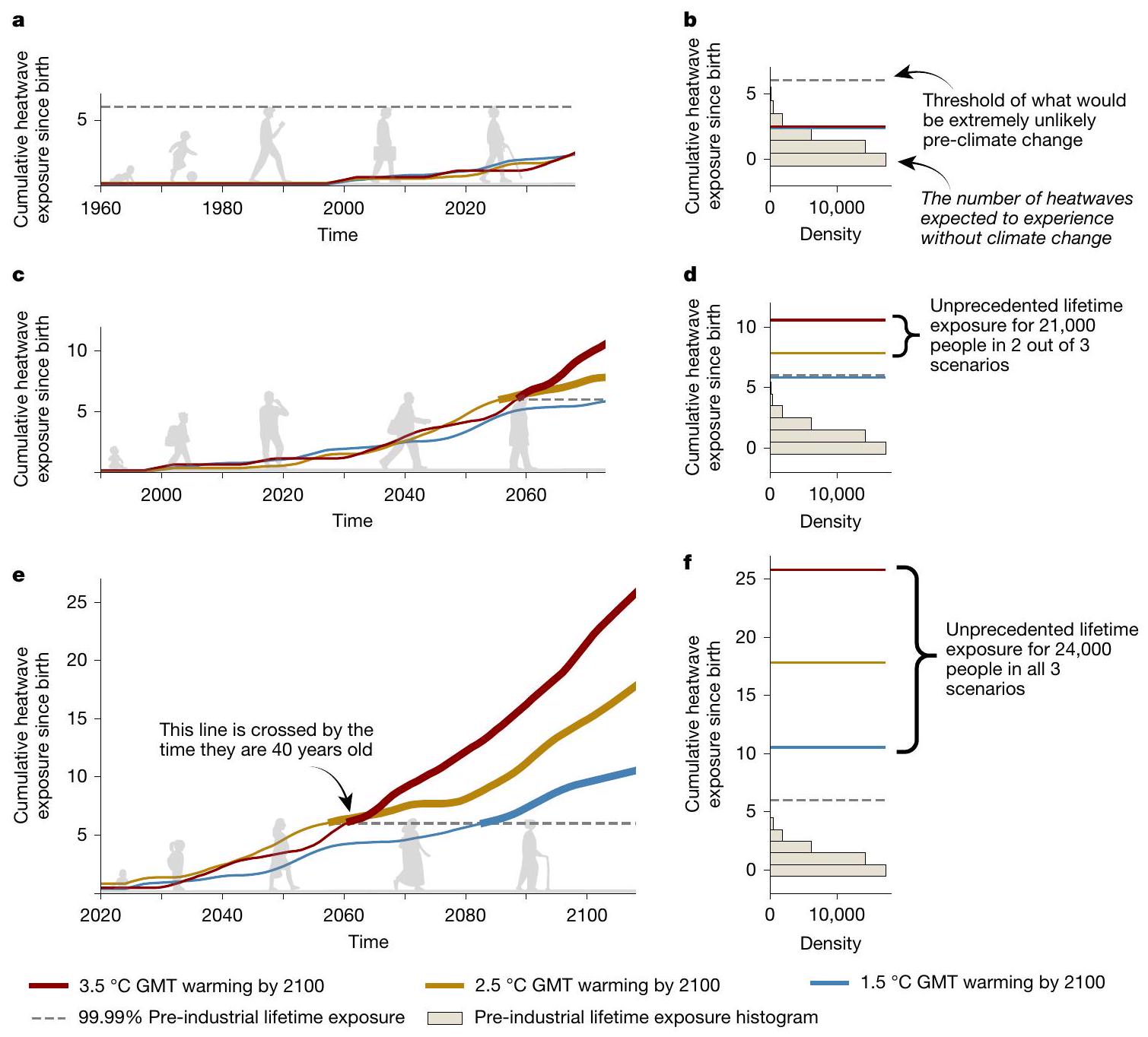
We illustrate what ULE means for extreme heatwaves in one grid cell ( ) located over Brussels, Belgium, for three GMT pathways in which warming above pre-industrial temperatures reaches , and by the year 2100. People born in 1960 and spending their life in Brussels are projected to experience three heatwaves in their lifetime, showing little sensitivity to the GMT pathway (Fig. 1a). In this location, the 1960 birth cohort does not exceed the threshold of ULE, which we define as the 99.99th percentile of a large sample of lifetime exposures in a pre-industrial control climate and which is six heatwaves here (Fig. 1b, grey histogram and dashed line). By contrast, the 1990 birth cohort emerges into ULE for the two warmest GMT pathways shown (Fig. 1c,d). This implies that, under temperature pathways reaching or higher warming by 2100 , this cohort will face more heatwaves than they would have been expected to experience with a one in ten thousand chance in the absence of climate change. Different GMT pathways cause a further divergence in the lifetime exposure of those born in 2020 in this location (Fig. 1e,f). In the pathway, the 2020 birth cohort is projected to experience nearly 11 heatwaves, yet this increases to 18 and 26 heatwaves in pathways reaching and , respectively, by the end of the century. This by far exceeds the ULE threshold under each GMT pathway, with an age of emergence already around 40 years old for the and pathways (Fig.1e). We then count the number of people per birth cohort that eventually reach ULE, using absolute population estimates at the grid scale and

Fig. 1| Cumulative heatwave exposure since birth for Brussels, Belgium. a,c,e, Multi-model mean time series of cumulative heatwave exposure for people born in 1960 (a), 1990 (c) and 2020 (e) in (blue line), (gold line) and (red line) pathways. b,d,f, Histograms for 1960 (b), 1990 (d) and 2020 (f) birth cohorts show the pre-industrial sample density of 40,000 bootstrapped lifetime exposures overlaid with final lifetime exposures from the time series of
the birth cohort. Dashed lines show the 99.99th percentile of the pre-industrial sample distribution, that is, the threshold of unprecedented lifetime exposure (ULE) for this location, cohort and climate extreme. Counts of people (right of d,f) show the population of the birth cohort that has emerged beyond the 99.99th percentile of the pre-industrial sample distribution.
relative cohort sizes at the country level. In this location, a best estimate of 21,000 people from the 1990 birth cohort and 24,000 people from the 2020 birth cohort are projected to experience ULE (except for the 1990 birth cohort under the pathway). Under a pathway, all cohorts born in Brussels after 1990 reach ULE, totalling 665,000 people. For a pathway, ULE begins for people born in 1978, increasing this total to 941,000 people. For cohorts that emerge, it is virtually certain (at least chance) that their lifetime heatwave exposure cannot be explained by internal climate variability.

We now repeat this analysis for every land grid cell and project the population fraction of each birth cohort experiencing ULE to heatwaves across the globe ( for cohort fraction reaching ULE to heatwaves). Of the 81 million people born in 1960, on average, around 16% (13 million people) face ULE to heatwaves regardless of the scenario. This fraction rises towards younger generations, and from the 1980 birth cohort onwards, begins to depend on GMT pathways (Fig. 2a). In a pathway, stabilizes for recent birth cohorts, reaching an average of for the 2020 birth cohort ( 62 million people). Comparatively, of the 2020 birth cohort is almost doubled in a pathway, reaching 92%. This implies that 111 million children born in 2020 will live an unprecedented life in terms of heatwave
exposure in a world that warms to compared with 62 million in a pathway.

At the country level, for the 2020 birth cohort is the highest in the tropics under low GMT pathways, yet this pattern disappears as heatwaves become widespread under high GMT pathways (Fig. 2c-e and Supplementary Tables 1-3). Under a pathway, equatorial regions have relatively high ; of the 177 countries in this analysis, 104 have most of the population of 2020 birth cohort living with unprecedented exposure to heatwaves ( ;Fig. 2c). This latitudinal pattern is less apparent in a pathway (Fig. 2d). Here, 157 countries have . In a pathway, 167 countries have countries have and in 113 countries the entire birth cohort faces unprecedented heatwave exposure ; Fig. 2e .

We then expand the analysis to a total of six climate extremes and 21 warming pathways (Fig. 3 and Methods). For every combination of birth cohort, climate extreme and warming pathway, we quantify the number of people experiencing ULE at the grid scale and subsequently

model ensemble). b, Bars show global cohort sizes in millions, with totals in grey and median numbers of people reaching ULE to heatwaves for (blue), (gold) and (red) pathways. c-e, Maps display country-level of the 2020 birth cohort for and pathways.
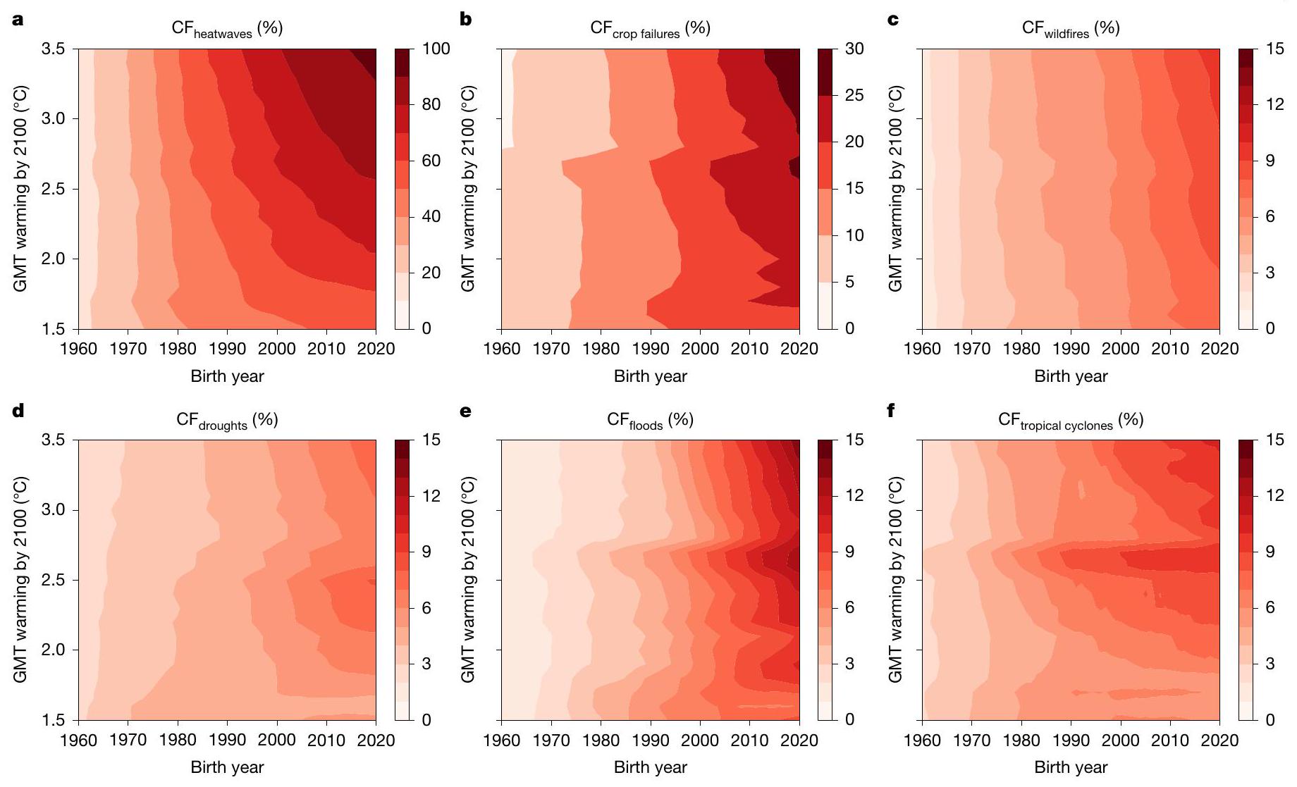
aggregate to the country or global level. Cohort fraction (CF) for climate extremes other than heatwaves is lower across all birth years and GMT pathways because they are generally less widespread than heatwaves; however, they still affect a large population fraction (Fig. 3 and Supplementary Tables 4-18). In a pathway, 29% of those born in 2020 will live through unprecedented exposure to crop failures (Fig. 3b). This is followed by river floods, in which will face unprecedented exposure to this extreme (Fig. 3e). As not all climate projections reach high warming levels, the ensemble size shrinks towards higher warming levels. Consequently, crop failures, droughts, river floods and tropical cyclones, which are more dependent on changes in the water cycle than heatwaves, exhibit discontinuities in CF at some GMT intervals (Fig. 3b,d-f). These sampling artefacts disappear when visualizing CFs for a smaller subset of simulations that are available for all GMT trajectories (Supplementary Note 1 and Supplementary Fig. 1). Although model uncertainties are larger for extremes other than heatwaves, differences in CF across birth cohorts are statistically significant for all six climate extremes (Supplementary Note 2 and Supplementary Figs. 2 and 3).

Across all projections available for the pathway aligned with current policies , ULE to heatwaves occurs in the Americas, Africa, the Middle East and Australia already for the 1960 birth cohort and globally for the 2020 birth cohort (Supplementary Figs. 4 m -o and 5e,k). The ULE to crop failures expands around the United States, South America, Sub-Saharan Africa and East Asia between 1960 and 2020 cohorts (Supplementary Figs. 4 and 5b,h). The ULE to river floods occurs in northern latitudes for the 1960 cohort, in line with the observations and model projections for precipitation changes and expands southwards into much of the world for the 2020 cohort (Supplementary Fig. 5d,j).

The lower CF of some extremes, such as tropical cyclones, is expected given the geographical constraints of these events and their distinct meteorological drivers. Tropical cyclones can, therefore, be re-evaluated by limiting the analysis to regions that can experience them. We consider these regions to be any grid cells exposed at least once to the event across our whole ensemble of exposure projections (Supplementary Fig. 6). nearly doubles when constraining total birth cohort size to exposed regions. For the 2020 birth cohort, this estimate changes from 6% to 11% in a pathway and from 10% to in a pathway.

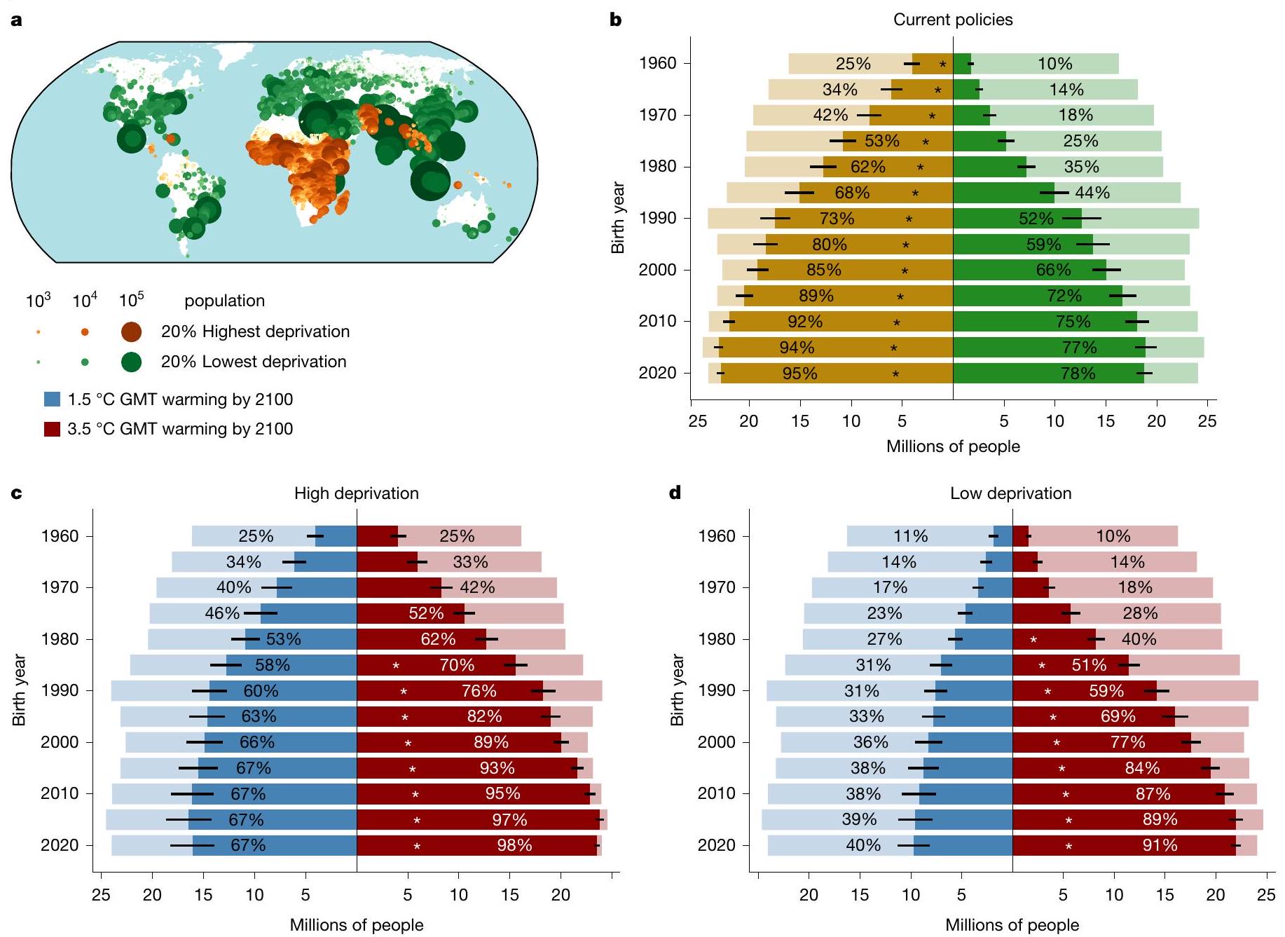
Finally, we cross our grid-scale projections for ULE to heatwaves against two grid-scale indicators of socioeconomic vulnerability (Methods): (1) the Global Gridded Relative Deprivation Index v. 1 (GRDI; ref. 16), which expresses relative deprivation according to six socioeconomic indicators; and (2) lifetime mean GDP per capita (denoted as GDP; ref. 17). Binning our birth cohort members into the top and bottom 20% of GRDI (Fig. 4a) and GDP (Supplementary Fig. 7a) enables a grid-scale comparison of ULE for population groups with high and low socioeconomic vulnerability. Using GRDI, we find that the most vulnerable subset of each birth cohort projected to experience ULE to heatwaves under current policies is substantially larger than the least vulnerable subset. This implies that socioeconomically vulnerable people have a consistently higher chance of facing unprecedented lifetime heatwave exposure compared with the least vulnerable members of their generation (Fig. 4b). For example, of the 2020 birth cohort, or 23 million members of the high deprivation (high socioeconomic vulnerability)

Fig. 3 | Greater unprecedented exposure to climate extremes for younger generations and higher warming pathways. a-d, Cohort fraction (CF) across all birth years (1960-2020) and GMT pathways (1.5-3.5 ) for heatwaves
( ), crop failures ( ), wildfires ( ), droughts ( ), river floods ( ) and tropical cyclones ( ). Each extreme event panel has its colour bar range.
group face ULE to heatwaves, whereas this is 78% (19 million) for the low deprivation group. This disparity is similar when using GDP, but with only 1974 and later birth years having significant differences across vulnerability strata (Supplementary Fig. 7). Here, for the 2020 birth year, ( 22 million) of the low-income group face ULE under current policies, whereas this is (19 million) for the high-income group. Under alternative warming pathways of and , although the same direction of disparities remains across vulnerability strata, the lowest vulnerability groups (low deprivation and high GDP) benefit the most from a low warming pathway (Fig. 4c,d and Supplementary Fig. 7c,d). Socioeconomically vulnerable groups have lower adaptive capacity and face more constraints when it comes to implementing effective adaptation measures . Our results highlight that precisely these groups with the highest socioeconomic vulnerability and lowest adaptation potential face the highest chance for unprecedented heatwave exposure (Fig. 4). This underlines the disproportionate risk for deprived communities in light of past and future climate extremes.

Our analysis only quantifies local exposure by design; yet in reality, the effects of climate extremes cascade non-locally. For example, in 2023, smoke from an active wildfire season in Canada was transported south along the east coast of the United States, exposing millions of people to hazardous air quality and causing an increased cardiopulmonary disease burden . Climate extremes also affect society through economic impacts, including the rising cost of living due to supply chain disruptions and taxation to recover public infrastructure . For instance, climate change endangers staple crop production in
the main breadbasket countries that supply most of our caloric intake globally , forcing market instabilities that only the wealthiest can cope with . These missing non-local impacts make our estimates conservative.

By contrast, we do not capture how people adapt to extremes and thereby potentially reduce their exposure or vulnerability. For example, exposure to heatwaves can be reduced for population groups that can afford access to air conditioning . However, maladaptive responses to climate extremes can instead create lock-ins of vulnerability and exposure . Therefore, our lifetime exposure estimates omit beneficial adaptation outcomes as well as detrimental non-local and maladaptation effects. Finally, opting for a threshold below would lower the bar and increase ULE estimates, and vice versa. Yet this effect is limited because the reference distribution is typically composed of small integers. By contrast, using thresholds above risks redundancy in our bootstrapped data sample (Methods).

Some demographic realities are not accounted for here. Factors such as within-country migration, fertility and mortality respond in reality to the climate extremes considered here . In the United States, where the population faces exposure to all extremes analysed in this study, city centres attract young people and disparities in life expectancy have been found across race-county combinations and rural-urban residency . For instance, life expectancy is longer for those living in cities, yet here we apply country-average life expectancy and cohort size distribution uniformly within each country. Furthermore, we do not account for within-grid-cell heterogeneity, that is, we miss some fine-scale variations in socioeconomic vulnerability and exposure in socioeconomically diverse regions such as cities. Finally, we focus on the socioeconomic dimension of vulnerability,

and vulnerability group, whereas dark colours indicate the affected fraction. Error bars show the standard deviation across projections. Asterisks indicate that a low- or high-vulnerability group from a given birth cohort has significantly more members with ULE to heatwaves than the alternative vulnerability group of the same birth cohort (at the level). c,d, The high deprivation (c) and low deprivation (d) share of the birth cohort that is projected to experience ULE under the (blue) and (red) pathways.
thereby neglecting that vulnerability to climate extremes may also vary with, for instance, age, gender or disability status. As demographic and multidimensional vulnerability information becomes available at ever higher spatial resolution and explicitly accounts for climate impact projections, it will become possible to deepen the analysis of the interaction between climate change and population dynamics.

The uncertainties of the extremes other than heatwaves are non-negligible. Hydrological variables have high internal climate variability and projecting these events requires an additional impact-modelling step relative to heatwaves, which are computed directly from global climate model output (Methods). Furthermore, these events have sensitivities to input data quality and process representation across the modelling chain (Supplementary Note 2). Other uncertainties, such as demographic representation, are not captured in this analysis. Finally, we opt for assessing ULE at the grid scale instead of at the country level. In doing so, we downscale demographic data instead of upscaling climate data, thereby projecting lifetime exposure based on the local climate of individual birth cohort members. This incurs a trade-off for accepting natural variability in locations at
which ULE occurs, yet minimizing year-to-year variability in country-and global-scale CF estimates (Supplementary Note 3 and Supplementary Fig. 8).

In summary, we find that large fractions of global birth cohorts are projected to live unprecedented exposure to heatwaves, river floods, droughts, crop failures, wildfires and tropical cyclones. As the frequency of these six climate extremes increases with warming, so does the fraction of people who will face ULE to these events. More ambitious policies are needed to achieve the goal of the Paris Agreement of limiting global warming to by 2100 relative to the warming expected under current policies, especially as the most vulnerable groups have more members projected to face unprecedented exposure to heatwaves. Children would reap the direct benefits of this increased ambition: a total of 613 million children born between 2003 and 2020 would then avoid ULE to heatwaves. For crop failures, this is 98 million, for river floods 64 million, for tropical cyclones 76 million, for droughts 26 million and for wildfires 17 million. This underlines the urgent need
for deep and sustained greenhouse gas emission reductions to safeguard the future of current young generations.

Any methods, additional references, Nature Portfolio reporting summaries, source data, extended data, supplementary information, acknowledgements, peer review information; details of author contributions and competing interests; and statements of data and code availability are available at https://doi.org/10.1038/s41586-025-08907-1.

Publisher’s note Springer Nature remains neutral with regard to jurisdictional claims in published maps and institutional affiliations.

Open Access This article is licensed under a Creative Commons Attribution 4.0 International License, which permits use, sharing, adaptation, distribution and reproduction in any medium or format, as long as you give appropriate credit to the original author(s) and the source, provide a link to the Creative Commons licence, and indicate if changes were made. The images or other third party material in this article are included in the article’s Creative Commons licence, unless indicated otherwise in a credit line to the material. If material is not included in the article’s Creative Commons licence and your intended use is not permitted by statutory regulation or exceeds the permitted use, you will need to obtain permission directly from the copyright holder. To view a copy of this licence, visit http://creativecommons.org/licenses/by/4.0/.
(c) Crown 2025

The Inter-Sectoral Impact Model Intercomparison Project (ISIMIP) provides a simulation protocol for projecting the impacts of climate change across sectors such as biomes, agriculture, lakes, water, fisheries, marine ecosystems and permafrost (www.isimip.org). In ISIMIP2b, impact models representing these sectors are run using atmospheric boundary conditions from a consistent set of bias-adjusted global climate models (GCMs) from phase 5 of the Coupled Model Intercomparison Project (CMIP5) that were selected based on their availability of daily data and ability to represent a range of climate sensitivities ; the Geophysical Fluid Dynamics Laboratory Earth System Model (GFDL-ESM2M; ref. 30), the earth system configuration of the Hadley Centre Global Environmental Model (HadGEM2-ES; ref. 31), the general circulation model from the Institut Pierre-Simon Laplace Coupled Model (IPSL-CM5A-LR;ref.32) and the Model for Interdisciplinary Research on Climate (MIROC5;ref.33). Impact simulations are run for pre-industrial control ( 286 ppm CO 2 ; 1666-2099), historical (1861-2005) and future (2006-2099) periods. Future simulations are based on Representative Concentration Pathways (RCPs) 2.6, 6.0 and 8.5 of GCM input datasets. Global projections of annual, grid-scale fractions of exposure to each extreme event category are calculated from ISIMIP2b impact simulations and GCM input data. For the full details of these computations, we refer to ref.12, but we summarize extreme event definitions below.

For heatwaves, droughts, crop failures and river floods, we use localized pre-industrial thresholds to determine event occurrences, whereas for tropical cyclones, we use a single absolute threshold, and wildfires are modelled explicitly (Supplementary Table 20). Heatwaves affect an entire grid cell if the Heat Wave Magnitude Index daily (HWMId; refs. 34,35) of that year exceeds a threshold in the pre-industrial control HWMId distribution in that grid cell . Although we refer to heatwaves throughout the paper, our definition technically refers to a 3-day extreme heat event that is expected on average once per century under pre-industrial climate conditions. These extreme heat events occur, by definition, everywhere across the world, but with different associated absolute temperature values. Previous analysis highlighted that intergenerational inequalities in lifetime heatwave exposure are robust across a range of heatwave definitions . Crop failures are based on the sum of the area occupied by maize, wheat, soy or rice within a grid cell when their simulated yield falls below a threshold of their pre-industrial reference yield. Droughts, such as heatwaves, affect an entire grid cell if, for 7 months, monthly soil moisture remains below a threshold of pre-industrial soil moisture levels. Floods only correspond to river flooding, and the flooded area is derived from comparing daily discharge simulations from models of the global water sector to pre-industrial discharge.CaMa-Flood, a global river-routing model , is used to convert these discharge values to flooded areas. Tropical cyclones occur if a grid cell sustains hurricane-force winds ( knots) at least once a year . Exposure to tropical cyclones does not encompass the flood hazards typically associated with tropical cyclones. Wildfires occur when the burnt area is simulated in a grid cell. Burnt area is either taken directly from annual burnt area calculations or as the annual sum of monthly burnt area in cases in which impact models simulate burnt area sub-annually, capped at of a grid cell. We reiterate that all exposure definitions here neglect potential exposure reduction measures and non-local effects.

We subsequently quantify human exposure to climate extremes in a way that facilitates comparison and aggregation across extreme event categories. We consider all people in a grid cell exposed to a climate extreme in a particular year if the climate extreme occurs in that year. We thereby assume that if such a river flood or wildfire occurs somewhere in a grid cell, this is sufficiently close to any person located in that grid cell to be considered affected by this extreme
event. Using demographic data (see below), we subsequently convert this annual human exposure to lifetime exposure of birth cohorts by summing annual grid fractions of individual event categories across their lifetimes.

Demographic data for population totals, cohort sizes and life expectancy enable our projection of the CF experiencing ULE to these six extremes. Population totals at the grid scale come from the ISIMIP database (Fig. 2b; ref. 17) and originate from population estimates from v.3.2 of the History Database of the Global Environment (HYDE3.2; refs. 39,40) for the historical period (1860-2000) and population projections from middle-of-the-road Shared Socioeconomic Pathway (SSP2; refs. 41,42) for the future period (2010-2100). We note that these datasets at present do not account for the impact of climate on population dynamics, for example, through changes in migration, fertility and mortality, although these feedbacks may substantially alter the demographic data. Cohort sizes from the Wittgenstein Centre for Demography and Global Human Capital provide estimates of country-level population totals every 5 years (between 1950 and 2100) for each 5-year age group (0- to 4-year-olds, 5- to 9-year-olds, and so on, until 95- to 99-year-olds and a final age group for those 100 years and older). Life expectancy data come from the United Nations World Population Prospects (UNWPP;ref. 44) and describe the life expectancy of 5-year-olds at the country level for 5-year blocks (1950-1955 to 2015-2020). In this dataset, life expectancy is reported for 5-year-olds to exclude biases from infant mortality. Countries that can be spatially resolved at the ISIMIP grid scale and have cohort and life expectancy estimates in these datasets meet the requirements of this study and total 177 . We refer to the supplementary material of ref. 11 for a broader discussion of these datasets but explain our application of them in this analysis below.

All demographic datasets are modified to represent lifetimes annually, beginning from 1960 to 2020. Life expectancies for each country are first linearly interpolated to annual values by assuming that the values of the original 5-year groups are representative of the middle of that group. Furthermore, we add 5 years to annual life expectancies to capture the life expectancy of each cohort since birth, as the original data begin at age 5 . As the maximum UNWPP life expectancy for people born in 2020 prescribes the final year in this analysis (2113), annual population totals must be extrapolated to reach this year. For population totals, we take each year beyond 2100 as the mean of the preceding 10 years of the dataset, such that population numbers for 2101 are the mean of 2091-2100. For cohort sizes in each country, we interpolate annual cohort sizes and age groups from the original 5-year age groups and divide age totals by 5 to maintain original population sizes in this dataset and linearly extrapolate these estimates to 2113. This provides the absolute numbers of 0- to 100-year-olds for each year across 1960-2113.

To downscale this demographic information to the grid scale, we assume spatially homogeneous cohort representation and life expectancy. Birth cohort size is represented as the number of people of age 0 of a given birth year in a given grid cell. This is estimated by multiplying the absolute population of the birth year (using the annual grid-scale population totals from ISIMIP) by the relative size of the age 0 cohort (using the interpolated 0 – to 100 -year-old population totals from the Wittgenstein Centre cohort data). Spatial variability in age structure and life expectancy within a country is therefore ignored in this study.

To project CF across different warming pathways by 2100 , we construct a series of incrementally warming GMT pathways between 1960 and 2113 based on GMT trajectories taken from the AR6 Scenario Explorer . The time series from the AR6 scenario explorer were chosen as anchor points for interpolation to produce a range of plausible GMT time series. Furthermore, they were selected to minimize overshooting in the early
years of low GMT pathways over higher GMT pathways, which can skew lifetime exposure estimates for early birth cohorts (Supplementary Fig. 9). The upper bound of this subset was limited to in favour of sampling more simulations for higher GMT projections, which we discuss further below. For the lower bound, was chosen because it is a more realistic minimal warming scenario than . Note that the anchor scenario maximally reaches before reducing to by 2100 . It is, therefore, referred to as throughout this analysis. These warming levels are reported relative to pre-industrial temperatures from 1850 to 1900 . This yields a total of 21 GMT pathways for which we project CF.

Our dataset of extreme event exposures represents occurrences of these extremes forced by GCM-modelled climates. These climates have unique GMT warming pathways that depend on their radiative forcing scenario (historical or RCP), as prescribed by the ISIMIP2b modelling protocol. To project these exposure maps along even intervals of warming scenarios, which the original simulations do not provide, we use the 21 GMT pathways described above. For each pairing of the 21 target GMT pathways and the concatenated historical and future exposure projections, we sample exposures by matching the GMT warming levels of the exposure series to the years of the target GMT pathways (Supplementary Figs. 9 and 10). The GMT warming levels behind the exposure projections are first smoothed with a 21-year rolling mean before GMT mapping is undertaken. In cases in which our constructed GMT pathways exceed the GMT warming levels of GCM simulations by too much, this mapping erroneously resamples the year of exposures corresponding to the maximum warming level of their forcing GCM. To this end, we implement a constraint in this sampling procedure such that GMT-mapped series are only used if the maximum difference across all GMT pairs is no larger than . This constraint incrementally reduces ensemble sizes of exposure projections for higher GMT pathways (Supplementary Table 19).

Estimating lifetime exposure to extreme events requires crossing life expectancy data at the country level with grid-scale exposure projections. For each GMT trajectory (1.5-3.5 intervals), birth year (1960-2020) and country (177), exposures are summed across lifetimes at the grid scale. This assumes life expectancy to be spatially homogeneous across each country. Exposure during the death years is also included in this sum by multiplying these exposure projections by the fraction of the final year lived. This produces country-wide maps of lifetime exposure at the grid scale for each GMT trajectory and birth year in this analysis.

To generate a baseline distribution of lifetime exposure in a world without climate change, large samples of pre-industrial lifetime exposures are bootstrapped assuming 1960 life expectancy in each country. Here, for each exposure projection originating from a simulation under a pre-industrial climate, 10,000 lifetime exposures are estimated by resampling exposure years with replacement. Depending on ISIMIP2b data availability, pre-industrial exposure projections have a length of 239-639 years per simulation from which to resample from . This process generates country-wide maps of lifetime exposure, depending on the extreme event considered and its underlying data availability, enabling exposure projections in a pre-industrial climate. Using the pre-industrial period as a baseline enables (1) our GMT mapping procedure; (2) bootstrapping a stationary time series to achieve a large reference dataset; and (3) the production of a reference dataset with information that is independent of the projections forming our ULE estimates.

We define an emergence threshold for ULE to extreme events as the 99.99th percentile of our grid-scale samples of pre-industrial lifetime exposure. When it comes to the selection of this percentile, we went
as extreme as possible given the bootstrapping of the pre-industrial control runs. This choice was based on a sensitivity analysis for different percentile values that showed a levelling off of lifetime exposure for percentiles more extreme than . This indicated that the 99.99th percentile achieves the limit of reliable information that can be extracted from the empirical distribution. For each extreme event, birth year, GMT pathway and grid cell, we assess if lifetime exposure emerges or passes this threshold of extreme exposure in a pre-industrial climate. If this threshold is passed, we consider the whole birth cohort in this grid cell to have emerged, tallying its size among a global pool of the same birth cohort and GMT trajectory of people projected to live ULE. This means that, in some locations, even if the sum of exposed grid cell fractions across a pre-industrial lifetime does not cover the entire grid cell, we still extract the entire birth cohort size associated with that grid cell. We sum the number of emerged people in each birth cohort globally, although this birth cohort has a different life expectancy in each country. Once the number of people who have emerged globally is tallied, we divide this by the respective total cohort sizes to estimate CF per birth cohort. Note that ULE, therefore, does not refer to unprecedented in terms of the magnitude of assets or people exposed, but rather in terms of the number of events accumulated across an average person’s lifespan in comparison with what they would face in a pre-industrial climate.

We use two grid-scale indicators of vulnerability to compare with our estimates of ULE to heat waves. The first is an ISIMIP2b GDP input dataset using concatenated historical and SSP2 time series covering 1860-2099 annually . This dataset was disaggregated from the country to grid level using spatial and socioeconomic interactions among cities, land cover and road network information and SSP-prescribed estimates of rural and urban expansion . The second indicator is the Global Gridded Relative Deprivation Index v.1 (GRDI; ref. 16), which communicates relative levels of multidimensional deprivation and poverty ( , least to most deprived). This deprivation score uses six input components. First is the child dependency ratio, which is the ratio between the population of children and the working-age population (15-64 years). This can indicate vulnerability, for which high ratios indicate a dependency of supposed consumers and non-producers on the working-age (producing) population . Second, infant mortality rates (IMR), taken as the deaths in children younger than 1 year of age per 1,000 live births annually, are a signal of population health and form a long-term Sustainable Development Goal of the United Nations . Third, the Subnational Human Development Index (SHDI), an assessment of human well-being across education, health and standard of living, originates from the Human Development Index, the latter of which is considered one of the most popular indices to assess country-level well-being. The SHDI improves on the HDI in terms of spatial scale and in representing 161 countries across all world regions and development levels . Fourth, as rural populations are generally prone to multidimensional poverty , low values in the ratio of built-up to non-built-up area (BUILT) signal high deprivation. The fifth and sixth components use the mean (of 2020; VNL 2020) and slope (2012-2020; VNL Slope) of nighttime light intensity, a proxy for human activity, economic output and infrastructure development , to indicate deprivation for areas of low nighttime light intensity. These input components range from 30 arc seconds (roughly 1 km ) resolution to subnational regions and are harmonized in an ArcGIS Fishnet feature class for aggregation onto a range representing low to high deprivation. For the final aggregation, the IMR and SHDI components are given half the weight of the rest of the inputs, given their coarser resolution. The GRDI, therefore, encapsulates multiple dimensions through which generations face deprivation and therewith socioeconomic vulnerability to climate extremes. Although our approach does not explicitly account for actual or potential adaptation to climate change, this multidimensional approach to
vulnerability provides relevant information on the current adaptation potential of local populations.

We preprocess GDP and GRDI products to enable their comparison with our ULE estimates across birth years. For GDP, similar to other datasets in our analysis, we extend the series to 2113 to accommodate the longest life expectancy of the 2020 birth cohort by copying the final year of the original dataset. We then use our ISIMIP population totals to compute GDP per capita at the grid scale. Using the GDP per capita metric, we calculate lifetime mean GDP per capita using our life expectancy information for the 1960-2020 birth cohorts. We refer to lifetime mean GDP per capita as simply GDP. For GRDI, we conservatively regrid the original grid cells of about 1 km to the ISIMIP grid. Although GRDI is a map composed of data spanning 2010-2020, we assume this to be representative of 2020, but nonetheless compare it with the 1960-2020 birth cohort range, similar to the rest of the analysis.

We then identify quantile ranges (that is, (80-100]) for the lifetime GDP of each birth year and for the singular GRDI map (assumed to align with 2020 population totals). To this end, we rank the vulnerability indicators and apply these ranks to our birth cohort totals on the same grid and for the matching year. For example, the ranks taken from the lifetime mean GDP of the 2020 birth cohort are aligned with the population totals of newborns in 2020. Finally, we bin the ranked vulnerability indicators by their associated population totals into five groups of nearly equal population (as it is not possible to achieve perfect bin sizes given the sums of grid-scale population totals). This groups the richest and poorest and least and most deprived into the aforementioned quantile ranges. The quantile range of each vulnerability indicator is then a map that can be used to mask the existing locations of ULE, such as birth years and all GMT pathways. With GRDI (Supplementary Fig. 11) and GDP (Supplementary Fig. 12), we compare the lowest and the highest of each indicator by population.

The data for this analysis originate from multiple sources and are hereby listed. Model inputs, raw impact model simulations and post-processed extremes (the latter as Derived Output Data) from ISIMIP2b, as well as GDP data, are accessible at the ISIMIP repository here (https://data. isimip.org). Cohort sizes are taken from the Wittgenstein Centre for Demography and Global Human Capital (https://dataexplorer.witt-gensteincentre.org/wcde-v2). Life expectancy data come from the UN demographics data portal (https://population.un.org/dataportal/ home?df=10750103-f8fa-4a7e-bb6a-b0f151970005). Global mean temperatures are extracted from the AR6 scenario explorer (https://doi. org/10.5281/zenodo.7197970). GRDI is hosted on the NASA EARTHDATA platform (https://doi.org/10.7927/3xxe-ap97). Maps in this analysis contain base map information made with Natural Earth (naturalearthdata.com).

The code for this analysis can be found at GitHub (https://github.com/ VUB-HYDR/2025_Grant_etal_Nature/tree/main).

31. Jones, C. D. et al. The HadGEM2-ES implementation of CMIP5 centennial simulations. Geosci. Model Dev. 4, 543-570 (2011).
32. Dufresne, J.-L. et al. Climate change projections using the IPSL-CM5 Earth System Model: from CMIP3 to CMIP5. Clim. Dyn. 40, 2123-2165 (2013).
33. Watanabe, M. et al. Improved climate simulation by MIROC5: mean states, variability, and climate sensitivity. J. Clim. 23, 6312-6335 (2010).
34. Russo, S., Sillmann, J. & Fischer, E. M. Top ten European heatwaves since 1950 and their occurrence in the coming decades. Environ. Res. Lett. 10, 124003 (2015).
35. Russo, S., Sillmann, J. & Sterl, A. Humid heat waves at different warming levels. Sci. Rep. 7, 7477 (2017).
36. Yamazaki, D., Kanae, S., Kim, H. & Oki, T. A physically based description of floodplain inundation dynamics in a global river routing model. Water Resour. Res. 47, W04501 (2011).
37. Emanuel, K. Downscaling CMIP5 climate models shows increased tropical cyclone activity over the 21st century. Proc. Natl Acad. Sci. USA 110, 12219-12224 (2013).
38. Holland, G. A revised hurricane pressure-wind model. Mon. Weather Rev. 136, 3432-3445 (2008).
39. Klein Goldewijk, K., Beusen, A. & Janssen, P. Long-term dynamic modeling of global population and built-up area in a spatially explicit way: HYDE 3.1. Holocene 20, 565-573 (2010).
40. Klein Goldewijk, K., Beusen, A. & Drecht, G. V. The HYDE 3.1 spatially explicit database of human-induced global land-use change over the past 12,000 years. Global Ecol. Biogeogr. 20, 73-86 (2011).
41. Fricko, O. et al. The marker quantification of the Shared Socioeconomic Pathway 2: a middle-of-the-road scenario for the 21st century. Global Environ. Change 42, 251-267 (2017).
42. Samir, K. C. & Lutz, W. The human core of the shared socioeconomic pathways: population scenarios by age, sex and level of education for all countries to 2100. Global Environ. Change 42, 181-192 (2017).
43. Lutz, W., Goujon, A., Samir, K. C., Stonawski, M. & Stilianakis, N. (eds) Demographic and Human Capital Scenarios for the 21st Century: 2018 Assessment for 201 Countries (Publications Office of the European Union, 2018).
44. United Nations Department of Economic and Social Affairs. World Population Prospects 2019 (United Nations, 2019).
45. Byers, E. et al. AR6 Scenarios Database v.1.1. Zenodo https://doi.org/10.5281/zenodo. 7197970 (2022).
46. Murakami, D. & Yamagata, Y. Estimation of gridded population and GDP scenarios with spatially explicit statistical downscaling. Sustainability 11, 2106 (2019).
47. Bartram, L. & Roe, B. Dependency ratios: useful policy-making tools? Geriatr. Gerontol. Int. 5, 224-228 (2005).
48. Sharrow, D. et al. Global, regional, and national trends in under- 5 mortality between 1990 and 2019 with scenario-based projections until 2030: a systematic analysis by the UN Inter-agency Group for Child Mortality Estimation. Lancet Glob. Health 10, 195-206 (2022).
49. Smits, J. & Permanyer, I. The Subnational Human Development Database. Sci. Data 6, 190038 (2019).
50. Laborde Debucquet, D. & Martin, W. Implications of the global growth slowdown for rural poverty. Agric. Econ. 49, 325-338 (2018).
51. Bruederle, A. & Hodler, R. Nighttime lights as a proxy for human development at the local level. PLoS One 13, O2O2231 (2018).

Acknowledgements We acknowledge the Potsdam Institute for Climate Impact Research (PIK) for their coordination of ISIMIP and the modellers contributing runs to ISIMIP2b. We thank M. Andrijevic, C.-F. Schleussner and E. Byers for their discussions regarding this paper. W.T. acknowledges funding from the European Research Council (ERC) under the Horizon Framework research and innovation programme of the European Union (grant agreement no. 101076909; ERC Consolidator Grant LACRIMA). We acknowledge further funding from the European Union under the grant agreement no. 101081369 (SPARCCLE). The computational resources and services used in this work were provided by the VSC (Flemish Supercomputer Center), funded by the Research Foundation – Flanders (FWO) and the Flemish Government, department EWI. This work was supported by the Wellcome Trust 309498/Z/24/Z.

Author contributions L. Grant helped to conceive this study, performed the analysis and wrote the paper. W.T. helped to conceive the study and write the paper. I.V. helped with coding parts of this analysis and writing the paper. L. Gudmundsson, E.F. and S.I.S. helped generate ideas for the analysis and curate the paper.

Competing interests The authors declare no competing interests.

Supplementary information The online version contains supplementary material available at https://doi.org/10.1038/s41586-025-08907-1.
Correspondence and requests for materials should be addressed to Luke Grant.
Peer review information Nature thanks Stephane Hallegatte, Damon Matthews, Raya Muttarak, Dáithí Stone and the other, anonymous, reviewer(s) for their contribution to the peer review of this work.
Reprints and permissions information is available at http://www.nature.com/reprints.