تاريخ الاستلام: 10 مايو 2023
تم القبول: 5 يناير 2024
نُشر على الإنترنت: 6 مارس 2024
الوصول المفتوح
تحقق من التحديثات

تؤكد العواقب الواسعة النطاق لتغير المناخ العالمي على المجتمعات البشرية والأنظمة البيئية في جميع أنحاء العالم. لقد بدأ تغير المناخ بالفعل في زيادة تكرار وشدة موجات الحر والأعاصير والحرائق البرية، ويؤثر بشكل كبير على موارد المياه العذبة في العالم من خلال ارتفاع مستوى سطح البحر، وزيادة تكرار الجفاف، والتغيرات في هطول الأمطار والتبخر. ، ومن المؤكد تقريبًا أن هذه التأثيرات ستزداد في المستقبل على الصعيد العالمي، ستشكل ارتفاع مستويات البحار تحديًا اقتصاديًا واجتماعيًا كبيرًا في القرن الحادي والعشرين، مما يؤثر بشكل أساسي على السكان البشريين والبنية التحتية والأنظمة البيئية على طول السواحل الرئيسية. لقد ارتفع متوسط مستوى سطح البحر العالمي بحوالي 0.17 متر على مدى المئة عام الماضية، مع تسارع معدلات ارتفاع مستوى البحر العالمية من حوالي 1.7 ملم سنويًا في أواخر القرن العشرين إلى حوالي 3.1 ملم سنويًا في أوائل القرن الحادي والعشرين استجابةً لارتفاع درجات الحرارة. وهي 3.7 مم سنويًا في الوقت الحاضر (مرجع 17). حتى إذا نجحت جهود التخفيف من تغير المناخ في استقرار درجات الحرارة في العقود القادمة، ستستمر مستويات البحر في الارتفاع نتيجة الاستجابة المستمرة للمحيطات للاحتباس الحراري السابق. . علاوة على ذلك، غالبًا ما تعاني المدن الساحلية من هبوط الأرض (ما يُعرف بانخفاض الأرض)، الذي يساهم تأثيره المتزايد في ارتفاع مستوى سطح البحر النسبي، مما يزيد من المخاطر والتهديدات الساحلية. في هذه الدراسة، نشير إلى ارتفاع مستوى البحر الذي يأخذ في الاعتبار تأثيرات حركة الأرض الرأسية (VLM) على أنه ‘ارتفاع مستوى البحر النسبي’، بينما يشير ‘ارتفاع مستوى البحر الجيومركزي’ إلى ارتفاع مستوى البحر بدون VLM. مع ارتفاع مستوى البحر وغمر الأرض، تزداد المخاطر المرتبطة بالظواهر المناخية المتطرفة (مثل الأعاصير والفيضانات الناتجة عن العواصف)، وتآكل الشواطئ وغمر المناطق الساحلية المنخفضة. .
على سواحل الولايات المتحدة المتجاورة، ترتفع مستويات البحر الناتجة عن المناخ بشكل أسرع من المتوسط العالمي. ، مع زيادة متوقعة على مدى العقود القليلة القادمة (الشكل 1 والشكل الإضافي 1). نظرًا لجغرافيتها وتوزيع سكانها، فإن الولايات المتحدة هي دولة ساحلية، حيث يوجد أكثر من من سكانها الذين يقيمون في المدن الساحلية، مما يولد إيرادات سنوية تقدر بحوالي 3.8 تريليون دولار أمريكي (المرجع 23).

وبالتالي، ستشكل الخسائر الاجتماعية والاقتصادية الناتجة عن ارتفاع مستوى سطح البحر الناجم عن المناخ جانبًا ملحوظًا من عواقب تغير المناخ في الولايات المتحدة الأمريكية. على المدى القصير (من عقد إلى ثلاثة عقود)، فإن الارتفاعات المستمرة الملحوظة في مستوى سطح البحر كافية فقط لتحفيز المخاطر المتتالية عبر المناطق الساحلية في الولايات المتحدة، مع زيادة متوقعة في تكرار وشدة العواصف، وتسلل المياه المالحة، والفيضانات الناتجة عن المد العالي، وتآكل السواحل. .
من المتوقع أن تتفاوت مستويات البحر بشكل طفيف في العقود القليلة المقبلة عبر سيناريوهات انبعاثات غازات الدفيئة المختلفة، في حين تشير التوقعات بنهاية القرن إلى تباين أكبر في الزيادة الناتجة عن الانبعاثات (الشكل البياني الممتد 1b-g). وبالتالي، فإن تقييمات الضعف على المدى القصير التي تأخذ في الاعتبار العوامل المحلية ذات صلة بصانعي السياسات لتطوير استراتيجيات تكيف شاملة تتجاوز تقليل الانبعاثات، حيث توفر رؤى حول المخاطر والتحديات الفورية للمجتمعات الساحلية. ومع ذلك، فإن التنبؤ بدقة بضعف السواحل يتطلب قياسات شاملة وعالية الدقة لتغير مستوى الأرض، وهو ما يفتقر إليه الوضع الحالي في الولايات المتحدة. تجعل هذه الفجوة في البيانات تقدير المخاطر الفعلية لارتفاع مستوى سطح البحر النسبي على المجتمعات الساحلية المختلفة تحديًا، وتساهم في ارتفاع مستوى عدم اليقين والأخطاء النظامية المحتملة في تقييم المخاطر الساحلية الحالي.

هنا نقدم نماذج مخاطر الفيضانات المستندة إلى سيناريوهات ساحلية للمدن الساحلية في الولايات المتحدة الأمريكية، مع التركيز على التوقعات القصيرة الأجل (2050) لارتفاع مستوى سطح البحر النسبي. تدمج نماذج الفيضانات لدينا بيانات تغير مستوى الأرض عالية الدقة على طول الساحل الأمريكي. (الشكل 1 والأشكال البيانية الموسعة 2-4) بدقة على مستوى المليمتر باستخدام رادار الفتحة الاصطناعية التداخلي (InSAR) (انظر الطرق)، إسقاطات قياسات الارتفاع الجيومركزي باستخدام تقنية قياس بعد الضوء (LiDAR) لنماذج الارتفاع الرقمية (DEMs) للتنبؤ بمعدلات ارتفاع مستوى سطح البحر النسبي وإنشاء خرائط غمر مفصلة لمجموعة من المدن الكبرى على طول الساحل الأمريكي. باستخدام بيانات التعداد السكاني الأمريكي لعام 2010 كتقديرات أساسية، نقيم تأثير ارتفاع مستوى سطح البحر النسبي على

الشكل 1 | المخاطر الساحلية عبر الولايات المتحدة الأمريكية. أ، التوزيع المكاني لمعدل تغير مستوى البحر عبر الساحل الأمريكي (صورة الخلفية: جوجل، إيرثستار). تشير معدلات تغير مستوى البحر الإيجابية إلى الارتفاع، بينما تشير المعدلات السلبية إلى الهبوط. تُظهر الخرائط الفردية لمعدل تغير مستوى البحر للسواحل الأطلسية والخليجية والهادئة في الولايات المتحدة في البيانات الموسعة الأشكال 2-4. الحدود الوطنية والولائية في الشكل أ تستند إلى بيانات متجهة من الملكية العامة من بنك البيانات العالمي.https://data.worldbank.org/) تم إنشاؤه في MATLAB. توقعات ارتفاع مستوى سطح البحر الجيومركزي مع خط أساسي لعام 2020 استنادًا إلى SSP2-4.5 (المراجع 17، 34) على الساحل الهادئ (North Spit، خليج هومبولت، كاليفورنيا) (ب)، الساحل الأطلسي (نقطة سيويل، فرجينيا) (ج) وساحل الخليج (غالفيستون II، تكساس) (د). تمثل الخطوط العريضة الوسيط (النسبة المئوية 50) لارتفاع مستوى سطح البحر الجيومركزي المتوقع والمناطق المظللة تمثل النسب المئوية 17 و 83. هـ، مخطط الصندوق
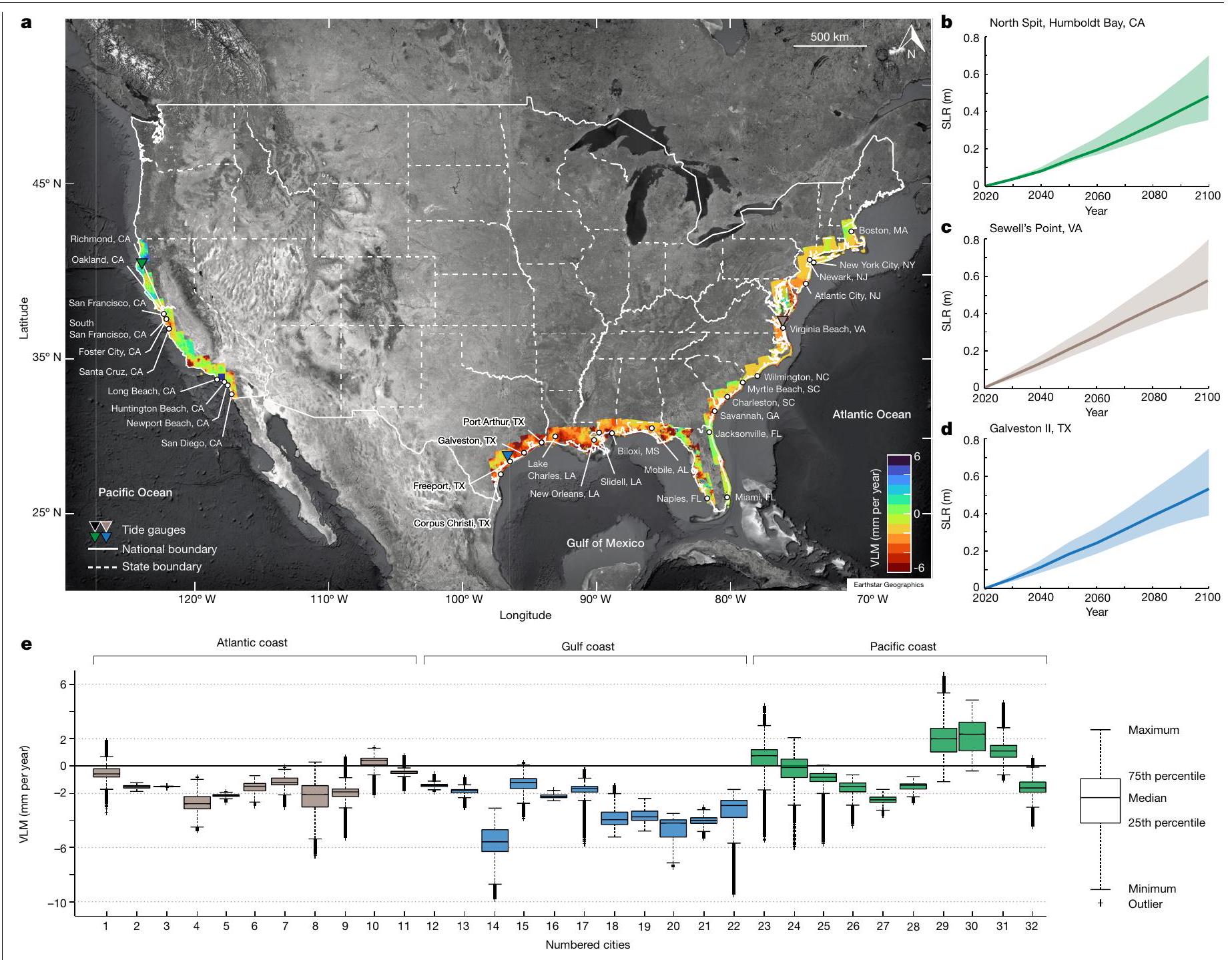
يمثل توزيع VLM لـ 32 مدينة ساحلية أمريكية تم تقييمها في هذه الدراسة. المدن الساحلية الـ 32 التي تم تقييمها في هذه الدراسة مميزة في الشكل (أ). تشمل المدن: الساحل الأطلسي الأمريكي: 1. بوسطن، ماساتشوستس؛ 2. مدينة نيويورك، نيويورك؛ 3. مدينة جيرسي، نيوجيرسي؛ 4. مدينة أتلانتيك، نيوجيرسي؛ 5. شاطئ فيرجينيا، فيرجينيا؛ 6. ويلمنغتون، كارولينا الشمالية؛ 7. شاطئ ميرتل، كارولينا الجنوبية؛ 8. تشارلستون، كارولينا الجنوبية؛ 9. سافانا، جورجيا؛ 10. جاكسونفيل، فلوريدا؛ 11. ميامي، فلوريدا؛ الساحل الخليجي الأمريكي: 12. نابولي، فلوريدا؛ 13. موبايل، ألاباما؛ 14. بيليوكسي، ميسيسيبي؛ 15. نيو أورلينز، لويزيانا؛ 16. سليديل، لويزيانا؛ 17. بحيرة تشارلز، لويزيانا؛ 18. بورت آرثر، تكساس؛ 19. مدينة تكساس، تكساس؛ 20. غالفستون، تكساس؛ 21. فريبورت، تكساس؛ 22. كوربوس كريستي، تكساس؛ الساحل الهادئ الأمريكي: 23. ريتشموند، كاليفورنيا؛ 24. أوكلاند، كاليفورنيا؛ 25. سان فرانسيسكو، كاليفورنيا؛ 26. سان فرانسيسكو الجنوبية، كاليفورنيا؛ 27. مدينة فوستر، كاليفورنيا؛ 28. سانتا كروز، كاليفورنيا؛ 29. لونغ بيتش، كاليفورنيا؛ 30. شاطئ هنتنغتون، كاليفورنيا؛ 31. شاطئ نيوبورت، كاليفورنيا؛ 32. سان دييغو، كاليفورنيا.
السكان وخصائص المجتمعات الساحلية في الولايات المتحدة واستكشاف عدة أنظمة تكيف لتقليل التأثيرات المحتملة في المستقبل.

تم نمذجة الفيضانات المستقبلية للمناطق الساحلية في 32 مدينة ساحلية (انظر الشكل 1) على طول السواحل الأمريكية باستخدام توقعات معدلات ارتفاع مستوى البحر الحالية على بيانات ارتفاع الساحل، وسيناريوهات توقعات مستوى سطح البحر الجيومركزي، وتقديرات المد العالي. يُقدّر إجمالي عدد سكان هذه المدن بحوالي 25 مليون شخص. من سكان السواحل الأمريكية الحاليين)، مع 10 ملايين عقار تقدر قيمتها بـ تريليون (الجدول التكميلية 1). تحللنا يقيس كيف أن مستوى سطح البحر النسبي
التغيرات، المنسوبة إلى ارتفاع مستوى البحر الجغرافي (VLM) وارتفاع مستوى البحر الجغرافي (SLR)، ستزيد من منطقة التعرض والسكان والممتلكات المعرضة للفيضانات الناتجة عن المد العالي بحلول عام 2050، باستخدام عام 2020 كخط أساس (انظر الطرق). بالنسبة للتحليل، نعتبر سيناريو ارتفاع مستوى البحر المستمد من سيناريو المسار الاجتماعي والاقتصادي المشترك (SSP) 2-4.5 (SSP2-4.5)، الذي يمثل مسار الانبعاثات الحالي. ، تعرض السكان والممتلكات باستخدام بيانات التعداد السكاني الأمريكي لعام 2010 وقيمة الممتلكات/المنازل باستخدام مؤشر قيمة المنزل من زيلو (ZHVI) (انظر الطرق). يقترح نموذجنا أنه بحلول عام 2050، قد يتسبب ارتفاع مستوى سطح البحر النسبي في زيادة مساحة الأراضي المعرضة بين 1,334 و في 32 مدينة ساحلية أمريكية إذا لم يتم تنفيذ هياكل الدفاع ضد الفيضانات (الأشكال 2-4، الجدول 1 والجدول التكميلي 2-4). نحن نقدر تعرض السكان بين 176,000 و518,000 نسمة من 94,000 إلى 288,000 عقار.

الشكل 2 | خرائط الفيضانات للمدن على الساحل الأطلسي للولايات المتحدة. المناطق المعرضة للمد والجزر العالي الحالي (2020) والمناطق المعرضة بشكل أكبر بحلول عام 2050 مع الأخذ في الاعتبار تغير مستوى سطح البحر الجيولوجي، وتوقع مستوى سطح البحر الجيولوجي تحت سيناريو SSP2-4.5 لـ: بوسطن، ماساتشوستس (أ)؛ مدينة نيويورك، نيويورك ومدينة جيرسي، نيوجيرسي (ب)؛ مدينة أتلانتيك، نيوجيرسي (ج)؛ شاطئ فيرجينيا، فيرجينيا (د)؛ ويلمنجتون، كارولينا الشمالية (هـ)؛ شاطئ ميرتل، كارولينا الجنوبية (و)؛ تشارلستون، كارولينا الجنوبية (ز)؛ سافانا، جورجيا (ح)؛ جاكسونفيل، فلوريدا (ط)؛ وميامي، فلوريدا (ي). ). صور الخلفية في هم من جوجل، إيرثستار.

يرجى ملاحظة أنه بالنسبة للتعرض الحالي، فإن قياس المسافة باستخدام نظام تحديد المواقع الجغرافي . الألوان الزرقاء والحمراء تمثل المناطق المعرضة حاليًا والمناطق المعرضة المتوقعة، على التوالي. BOS، مطار بوسطن لوجان الدولي، ماساتشوستس؛ JFK، مطار جون ف. كينيدي الدولي، نيويورك. ك، توزيع المزيد من المناطق المعرضة، والسكان، والممتلكات بحلول عام 2050. القيمة المركزية تمثل القيمة الوسيطة المقدرة من المعادلة (3)، بينما تمثل أشرطة الخطأ الحدود الدنيا والعليا من المعادلة (3).
مع قيمة إجمالية مقدرة للمنازل تتراوح بين 32-109 مليار دولار أمريكي بحلول عام 2050. يمثل الحد الأقصى من السكان والتعرض للممتلكات بحلول عام 2050 حوالي 1 من كل 50 شخصًا و1 من كل 35 ممتلكًا من 32 مدينة ساحلية.

من 11 مدينة على الساحل الأطلسي للولايات المتحدة، من المتوقع أن تكون المساحة الإضافية المعرضة للفيضانات بسبب المد العالي بحلول عام 2050 بين 773 و (الشكل 2). سيؤثر هذا على عدد يتراوح بين 59,000 و263,000 شخص و32,000 و163,000 عقار على الساحل الأطلسي للولايات المتحدة (الشكل 2 والجدول 1). إن تعرض الممتلكات والسكان على الساحل الأطلسي ليس متجانسًا عبر جميع المدن. على سبيل المثال، تمتلك ميامي (بمتوسط ارتفاع أقل من 2 متر فوق مستوى سطح البحر) أكبر حصة من التعرض، حيث تمثل من المنطقة المعرضة السكان المعرضين و (13,000-81,000) من الممتلكات المعرضة على طول الساحل الأطلسي (الجدول التكميلي 2). يُقدّر التعرض لقيمة المنازل بحلول عام 2050 في 11 مدينة ساحلية على الأطلسي بمبلغ يتراوح بين 14-64 مليار دولار أمريكي (الجدول 1). لا تأخذ القيمة المحسوبة في الاعتبار قيمة البنية التحتية الحيوية (مثل المطارات والمدارس والمستشفيات ومحطات الطاقة والطرق والسكك الحديدية)، فضلاً عن المراكز الاقتصادية والمعالم، وبالتالي تمثل قيمة محافظة.

بالنسبة لـ 11 مدينة على طول ساحل الخليج الأمريكي، يظهر توقعنا لعام 2050 لخطر الفيضانات منطقة مكشوفة تراوح بين 528 و (الشكل 3، الجدول 1 والجدول التكميلي 3). ستعرض هذه المناطق المتأثرة 110,000-225,000 شخص إضافي و58,000-109,000 ممتلكات بقيمة تتراوح بين 14-21 مليار دولار أمريكي (الجدول 1). يجب ملاحظة أن هناك مناطق كبيرة ( )، السكان ( ) وخصائص (176,000-209,000) في نيو أورلينز معرضة بالفعل لأحداث المد العالي في الوقت الحاضر، بسبب وجود مناطق تقع تحت مستوى سطح البحر (الجدول التكميلي 3). نؤكد أن تحليلنا يعتمد على نهج غير محمي، لا يأخذ في الاعتبار وجود هياكل التحكم في الفيضانات والتكيف المستقبلي. ومع ذلك، فإن نيو أورلينز محاطة بجدران فيضانات وأنظمة سدود واسعة النطاق وتتم تصريفها بشكل كبير. على الرغم من أن هياكل التحكم في الفيضانات تقدم حماية كبيرة للمناطق الساحلية، إلا أن فعاليتها ليست مضمونة. الأحداث التي تلت هبوط إعصار كاترينا في أغسطس 2005، والذي أودى بحياة أكثر من 1,500 شخص، هي تذكيرات مأساوية بالدمار المتزايد لنظام السدود الفاشل. لذا، قد تمثل اعتبارات أنظمة التحكم في الفيضانات وحدها حلاً مؤقتًا، كما سيتم مناقشته لاحقًا. من المتوقع أن تكون المطارات والطرق ومصافي النفط، المنتشرة في المدن، من بين البنية التحتية المعرضة للخطر على ساحل الخليج (الشكل 3).

الشكل 3 | خرائط الفيضانات للمدن على ساحل الخليج الأمريكي. المناطق المعرضة للمد والجزر العالي الحالي (2020) والمناطق المعرضة بشكل أكبر بحلول عام 2050 مع الأخذ في الاعتبار حركة الأرض العمودية، وتوقع ارتفاع مستوى سطح البحر الجغرافي تحت سيناريو SSP2-4.5 لـ: نابولي، فلوريدا (أ)؛ موبايل، ألاباما (ب)؛ بيلوكسي، ميسيسيبي (ج)؛ نيو أورلينز، لويزيانا (د)؛ سليديل، لويزيانا (هـ)؛ بحيرة تشارلز، لويزيانا (و)؛ بورت آرثر، تكساس (ز)؛ غالفستون ومدينة تكساس، تكساس (ح)؛ فريبورت، تكساس (ط)؛ وكوربوس كريستي، تكساس (ي). ). صور الخلفية في هم من جوجل، إيرثستار. لاحظ أن،
للتعرض الحالي، قياس المسافة بالليزر الجغرافي . الألوان الزرقاء والحمراء تمثل المناطق المعرضة حاليًا والمناطق المعرضة المتوقعة، على التوالي. APF، مطار نابولي، فلوريدا؛ MSY، مطار لويس أرمسترونغ الدولي في نيو أورلينز، لويزيانا. ك، توزيع المزيد من المناطق المعرضة والسكان والممتلكات بحلول عام 2050. القيمة المركزية تمثل القيمة الوسيطة المقدرة من المعادلة (3)، بينما تمثل أشرطة الخطأ الحدود الدنيا والعليا من المعادلة (3).

على الساحل الهادئ، نجد تباينًا كبيرًا في تأثيرات ارتفاع مستوى سطح البحر النسبي مقارنة بسواحل المحيط الأطلسي والخليج الأمريكي. بحلول عام 2050، ستكون المساحة المكشوفة التراكمية من عشر مدن على الساحل الهادئ الأمريكي هي مع تعرض السكان لـ الأشخاص و3,000-15,000 عقار بقيمة 4.5-22 مليار دولار أمريكي (الشكل 4، الجدول 1 والجدول التكميلي 4). قد يُعزى خطر الفيضانات المنخفض نسبيًا إلى الارتفاعات الطبوغرافية الأعلى، ومعدلات هبوط الأرض المنخفضة، ومعدلات ارتفاع مستوى سطح البحر الجيومركزي المنخفضة نسبيًا على الساحل الهادئ مقارنة بالسواحل الأطلسية والخليجية. على الرغم من أن خطر الفيضانات لمجتمعات الساحل الهادئ (ساحل كاليفورنيا) بحلول عام 2050 يعتبر معتدلاً نسبياً، فإن تآكل المنحدرات الصخرية والزيادة المتوقعة في الفيضانات الناتجة عن المد العالي هناك عوامل إضافية ستؤثر على بعض السكان والممتلكات الساحلية.

هبوط الأرض، وهو غرق أو استقرار سطح الأرض، هو قضية عالمية لها عواقب اقتصادية واجتماعية مكلفة. لتحديد مساهمة الهبوط الأرضي في مخاطر الفيضانات المستقبلية في 32 مدينة ساحلية أمريكية، نعتبر سيناريوهين: (1) المناطق المحتملة التي تقع تحت مستوى سطح البحر نتيجة الهبوط الأرضي فقط و(2) الأراضي المحتملة
المناطق التي تقع تحت مستوى سطح البحر نتيجة لمزيج من هبوط الأرض وتغير مستوى سطح البحر. باستخدام التوقعات الخطية لمعدل VLM الحالي وبيانات ارتفاع الساحل، نحدد المناطق الأرضية التي، على الرغم من كونها فوق مستوى سطح البحر في الوقت الحاضر، ستغمر بحلول عام 2050 تحت كلا السيناريوهين. تشير تحليلاتنا إلى أن المناطق الأرضية التي ستقع تحت مستويات البحر بحلول عام 2050 نتيجة لهبوط الأرض فقط تمثل (الساحل الأطلسي)، 22.9-35.4% (الساحل الخليجي) و4.8-8.1% (الساحل الهادئ) من إجمالي المناطق المغمورة عند أخذ هبوط الأرض وارتفاع مستوى سطح البحر الجيومركزي في الاعتبار (الشكل البياني الموسع 5a-c والجداول التكميلية 5-7).

علاوة على ذلك، مقارنة تغير مستوى الأرض الناتج عن تقنية InSAR مع تغير مستوى سطح البحر الجيومركزي في محطات قياس المد والجزر التابعة للخدمة الدائمة لمتوسط مستوى سطح البحر (PSMSL) المدرجة في توقعات الهيئة الحكومية الدولية المعنية بتغير المناخ (IPCC) عبر الولايات المتحدة الأمريكية (الشكل التوضيحي التكميلي 1) يكشف أن، في ثلاث محطات على ساحل الخليج، يتجاوز هبوط الأرض المحلي حاليًا ارتفاع مستوى سطح البحر الجغرافي (مع الأخذ في الاعتبار سيناريو انبعاثات منخفضة: SSP1-1.9) ويشكل مصدر قلق أكبر للمنطقة من تغير مستوى سطح البحر الجغرافي (مع الأخذ في الاعتبار سيناريو انبعاثات مرتفعة: SSP5-8.5) حتى عام 2045 (الشكل التوضيحي الإضافي 5d) و2070 (الشكل التوضيحي الإضافي 5e، 5f)، بافتراض هبوط مستمر خطيًا. هذه الملاحظة ملحوظة لأنها تبرز هبوط الأرض في مقدمة مناقشات المخاطر الساحلية وتسلط الضوء عليه كمؤشر حاسم في تصميم مرونة الكوارث الساحلية. .

الشكل 4 | خرائط الفيضانات للمدن على الساحل الهادئ الأمريكي. المناطق المعرضة للمد والجزر العالي الحالي (2020) والمناطق المعرضة بشكل أكبر بحلول عام 2050 مع الأخذ في الاعتبار تغير مستوى سطح البحر الجيومركزي تحت سيناريو SSP2-4.5 لـ: ريتشموند، كاليفورنيا (أ)؛ أوكلاند، كاليفورنيا (ب)؛ سان فرانسيسكو، كاليفورنيا (ج)؛ جنوب سان فرانسيسكو، كاليفورنيا (د)؛ فوستر سيتي، كاليفورنيا (هـ)؛ سانتا كروز، كاليفورنيا (و)؛ لونغ بيتش، كاليفورنيا (ز)؛ هنتنغتون بيتش، كاليفورنيا (ح)؛ نيو بورت بيتش، كاليفورنيا (ط)؛ وسان دييغو، صور الخلفية في هم من جوجل، إيرثستار.

يرجى ملاحظة أنه بالنسبة للتعرض الحالي، فإن قياس المسافة باستخدام نظام تحديد المواقع الجغرافي . الألوان الزرقاء والحمراء تمثل المناطق المعرضة حاليًا والمناطق المعرضة المتوقعة، على التوالي. SFO، مطار سان فرانسيسكو الدولي، كاليفورنيا. ك، توزيع المزيد من المناطق المعرضة، والسكان، والممتلكات بحلول عام 2050. القيمة المركزية تمثل القيمة المتوسطة المقدرة من المعادلة (3)، بينما تمثل أشرطة الخطأ الحدود الدنيا والعليا من المعادلة (3).

ومع ذلك، فإن بعض توقعات الفيضانات لا تأخذ في الاعتبار تأثيرات التغيرات في ارتفاعات الأراضي المتغيرة مكانيًا، مما يؤدي إلى توقعات غير دقيقة للتعرض المتوقع، مما قد يؤثر على استعداد المجتمعات الساحلية. على سبيل المثال، مقارنة التعرض المقدر بحلول عام 2050 لـ 32 مدينة تم الحصول عليها من هذه الدراسة مع التعرض المستمد باستخدام توقعات مستوى سطح البحر النسبية من الهيئة الحكومية الدولية المعنية بتغير المناخ. يظهر أن التعرض – من حيث المساحة والسكان والممتلكات – لا يمكن تمييزه ضمن عدم اليقين في معظم المدن وعلى نطاق واسع على طول الساحل الأمريكي (الجدول 1). ومع ذلك، نجد أن هناك تباينًا ملحوظًا في التعرض يحدث في بعض المدن، لا سيما على الساحل الأمريكي للخليج (الشكل 5 أ-ج والجدول التكميلي 8-10). من خلال مقارنة معدلات VLM باستخدام تقنية InSAR داخل المدن مع معدلات VLM المستمدة من IPCC من سجلات قياس المد والجزر، نحصل على رؤى حول الاختلافات الأساسية (الشكل 5 د والجدول التكميلي 11). في مدن مثل بوسطن، مدينة نيويورك، نابولي، بورت آرثر، كوربوس كريستي، ريتشموند، أوكلاند وسان فرانسيسكو، حيث تكون معدلات VLM من IPCC مشابهة لمعدلات VLM باستخدام InSAR داخل المدينة أو حيث تكون مساهمة VLM ضئيلة، فإن الفجوات بين التعرض المقدر متواضعة. ومع ذلك، يتم التقليل من تقدير التعرض في المدن التي يقلل فيها IPCC من مساهمة VLM (على سبيل المثال، مدينة أتلانتيك، تشارلستون، سافانا، موبايل وبيلوكسي). وبالمثل، في المدن التي يبالغ فيها IPCC في تقدير مساهمة VLM، يتم أيضًا المبالغة في تقدير التعرض (على سبيل المثال، فيرجينيا بيتش،

جاكسونفيل، ميامي، نيو أورلينز، سليديل، بحيرة تشارلز، بورت آرثر وهنتنغتون بيتش).

لتوفير فهم أكثر شمولاً لهذه الاختلافات الأساسية، قمنا بإجراء تحليل مقارن لمعدلات الهبوط الأرضي المستمدة من InSAR مع معدلات الهبوط الأرضي المستخدمة في تقرير التقييم السادس للهيئة الحكومية الدولية المعنية بتغير المناخ. لـ 74 محطة على طول الساحل الأمريكي (الجدول التكميلي 12 والشكل البياني الممتد 6). على الرغم من وجود 59% من التوافق في قياسات VLM في محطات قياس المد والجزر عبر الولايات المتحدة، قد لا تتمكن هذه المحطات – التي غالبًا ما تقع في أطراف المناطق الحضرية – من التقاط الديناميات المعاصرة لـ VLM المتغيرة مكانيًا داخل المدن نفسها (على سبيل المثال، بيلوكسي، نيو أورلينز وسان دييغو) (قارن المحطات في الشكل البياني الممتد 6 مع الشكل 5d). هذه القيود ذات صلة خاصة في المراكز الحضرية التي تؤثر فيها العوامل البشرية بشكل قوي على VLM، مما يساهم في الفجوات في تقديرات التعرض. تعتبر ملاحظات InSAR المعيار الذهبي لقياسات VLM بدقة مكانية غير مسبوقة وهي مفيدة لتعزيز دقة نماذج توقع الفيضانات.

يساهم تغير المناخ في تفاقم هشاشة المجتمعات الأكثر ضعفًا. عمومًا، تُجبر الفئات المحرومة على العيش في المناطق الأكثر عرضة للخطر لأن المناطق الأكثر أمانًا

و تمثل الحدود الدنيا والقيم الوسيطة والحدود العليا التي تم تقييمها باستخدام المعادلة (3). يتم تقدير التعرض المستمد من InSAR باستخدام VLM من InSAR وSLR الجيومركزي من IPCC.
التعرض لكل مدينة.
خارج نطاق الوصول تتزايد الأدبيات العلمية التي تركز على تأثيرات تغير المناخ على الفئات الضعيفة في مختلف البلدان. . ومع ذلك، تم وضع تركيز أقل على المناقشات حول عدم المساواة في تغير المناخ داخل البلدان تقرير حديث صادر عن وكالة حماية البيئة الأمريكية (EPA) ، جنبًا إلى جنب مع عمل شيانغ وآخرون. يساهم في زيادة الأدبيات التي تقيس المخاطر غير المتناسبة لتغير المناخ على المجتمعات الضعيفة في الولايات المتحدة الأمريكية.

هنا نفحص التأثيرات المتباينة للارتفاع النسبي لمستوى سطح البحر على المجتمعات الضعيفة عبر 32 مدينة في الولايات المتحدة الأمريكية، مما يقدم فهماً دقيقاً لعدم المساواة المناخية في الولايات المتحدة. لفحص الفوارق العرقية في المجتمعات المعرضة، ركزنا على ثمانية أعراق محددة من قبل بيانات التعداد السكاني الأمريكي كل عشر سنوات (انظر الطرق). يكشف تحليل نموذج الفيضانات للسكان المتأثرين بحلول عام 2050 عن تعرض متفاوت للارتفاع النسبي لمستوى سطح البحر على أسس عرقية (الشكل البياني الممتد 7 والجداول التكميلية 13-15). على طول السواحل الأطلسية والهادئة، يتم تمثيل السكان البيض بشكل زائد بين أولئك المعرضين للارتفاع النسبي لمستوى سطح البحر (الشكل البياني الممتد 7أ، ج). ومع ذلك، فإن توزيع السكان البيض المعرضين على هذه السواحل يعكس تقريباً التركيبة السكانية السائدة في هذه المناطق (الشكل البياني الممتد 7أ، ج والجداول التكميلية 13 و15).

على النقيض من ذلك، على ساحل الخليج، المجموعات المهمشة – الأفراد الذين يعرفون أنفسهم كأفارقة أمريكيين أو أمريكيين من أصل أفريقي؛ أمريكيين هنود أو من سكان ألاسكا الأصليين؛ آسيويين؛ هاوايين أصليين أو من جزر المحيط الهادئ الأخرى؛ من أصل إسباني أو لاتيني؛ وذوي مجموعتين أو أكثر. -تشكل جزءًا ملحوظًا من السكان المعرضين، على الرغم من عدم كونها المجموعة السائدة. على الرغم من أن المجموعات المهمشة تشكل من إجمالي السكان في 11 مدينة على ساحل الخليج، فإنهم ممثلون بشكل زائد في السكان المعرضين، حيث يشكلون أكثر من نصف (50.0-57.7%) من السكان المعرضين في حالة السكان السود أو الأمريكيين من أصل أفريقي فقط و عند النظر في جميع الأقليات (الشكل البياني الإضافي 7ب والجدول التكميلي 14). الآسيويون ممثلون بشكل زائد بين السكان المعرضين على سواحل الخليج والمحيط الهادئ، حيث يشكلون 2.6 و (الوسيط والحدود العليا فقط) من السكان المعرضين على سواحل الخليج والمحيط الهادئ، على التوالي، على الرغم من أنهم يمثلون 2.6% (ساحل الخليج) و17.8% (ساحل المحيط الهادئ) من إجمالي السكان. كما أن تحليل تأثيرات ارتفاع مستوى سطح البحر النسبي على عدم المساواة الاقتصادية (انظر الطرق) يظهر تعرضًا اقتصاديًا غير متناسب في نيو

أورليانز وبورت آرثر (الشكل 8 من البيانات الموسعة والجداول التكميلية 16-18)، اللذان يسيران بالتوازي مع زيادة تعرض مجتمعاتهم التي تتكون في الغالب من أقليات. يبرز تقاطع الفوارق العرقية والاقتصادية الضعف متعدد الأبعاد الذي تواجهه مجموعات معينة في هذه المدن في سياق ارتفاع مستوى سطح البحر النسبي.

أحد العوامل المساهمة في عدم المساواة الناتجة عن تغير المناخ هو القدرة المنقوصة للمجموعات المهمشة/ذات الدخل المنخفض على التكيف مع الآثار الحالية للأخطار والتعافي منها. لتأكيد هذه النقطة، اعتبر تأثير إعصار كاترينا على سكان بيلوكسي، ميسيسيبي. على الرغم من أن معظم الانتباه يتركز على الدمار الذي لحق بنيو أورلينز بسبب فشل السدود، فإن ولاية ميسيسيبي تكبدت الولايات المتحدة مليار في الأضرار المباشرة الناتجة عن العاصفة و100,000 شخص تم تهجيرهم نتيجة إعصار كاترينا كانت شرق بيلوكسي، حيث تعيش المجتمعات ذات الدخل المنخفض والمهمشة، لا تزال تعاني من آثار إعصار كاترينا بعد 10 سنوات من العاصفة، مع بنية تحتية مكسورة وغير مُعالجة، ومعدلات بطالة مرتفعة، وتشرد. على النقيض من ذلك، تلقت المجتمعات ذات الدخل المرتفع مساعدات فدرالية كبيرة لإعادة بناء البنية التحتية وهي ‘أفضل حالاً بعد العاصفة’ إن هذا الاستبعاد من مساعدات التعافي سيفرض بلا شك قيودًا على قدرة المجتمعات ذات الدخل المنخفض والمهمشة على التكيف مع تغير المناخ في المستقبل. وبالتالي، قد تمثل المجموعات المهمشة حصة غير متناسبة من الأضرار الجانبية الناتجة عن تغير المناخ، حتى لو كانت تشكل نسبة صغيرة نسبيًا من السكان المتأثرين. ببساطة، تجعل الفجوات القائمة الأشخاص المعرضين بالفعل للخطر أكثر عرضة للتأثيرات السلبية لتغير المناخ، مما يؤدي إلى زيادة التفاوت المتوقع. .

تتزايد التفاعلات البشرية مع الساحل في جميع أنحاء الولايات المتحدة الأمريكية ، وعلى الرغم من الخطر الواضح والحاضر الذي تشكله الزيادة النسبية في مستوى سطح البحر، غالبًا ما يتم تجاهل الحاجة إلى التخطيط للتكيف والمرونة أو يتم إعطاؤها أولوية غير كافية. التحديات المتزايدة التي تم تحديدها في هذه الورقة تمثل تحديًا كبيرًا، ومن المتوقع أن يتم التكيف في جميع المدن المعنية. هل ستتخذ المدن إجراءات استباقية وتكون مستعدة من خلال التقييم المفصل والتخطيط وتنفيذ تدابير التكيف، أم ستتفاعل مع الأحداث، في انتظار هذه التأثيرات والمخاطر؟

الشكل 5| مقارنة بين VLM المستمد من InSAR و VLM المستمد من IPCC والتعرض المقدر. الفروقات بين التعرض المقدر باستخدام VLM المستمد من InSAR و VLM المستمد من IPCC لمنطقة التعرض لعام 2050 (أ)، والسكان المعرضين (ب) والممتلكات المعرضة (ج). يتم تقدير التعرض المستمد من InSAR باستخدام VLM من InSAR و SLR الجيومركزي من IPCC كما هو موضح في الطرق، بينما يتم تقدير التعرض المستمد من IPCC باستخدام مجموعة بيانات SLR النسبية من IPCC. . القيمة المركزية تمثل القيمة الوسيطة المقدرة من المعادلة (3)، بينما تمثل أشرطة الخطأ الحدود السفلية والعلوية من المعادلة (3). سلبية
تشير القيم السلبية إلى المدن التي يتم فيها تقدير التعرض لمعدل ارتفاع مستوى البحر المستمد من IPCC بشكل مبالغ فيه، بينما تشير القيم الإيجابية إلى المناطق التي يتم فيها تقدير التعرض بشكل ناقص. د، مقارنة بين معدلات VLM باستخدام InSAR ومعدلات VLM المستمدة من IPCC لـ 32 مدينة. يتم الحصول على معدلات VLM باستخدام InSAR من خلال متوسط VLM لكل مدينة تم استخدامها في تحليل التعرض، بينما يتم اشتقاق معدلات VLM من IPCC من محطات قياس المد. تظهر نطاقات الخطأ لمعدلات VLM باستخدام InSAR وIPCC الانحراف المعياري. ملخص لمقارنة معدلات التعرض وVLM مفصل في الجداول التكميلية 8-11.
هل هناك بيان؟ هنا سننظر في الخيار الاستباقي. التكيف هو عملية طويلة الأمد ومن المحتمل أن يكون الجمع بين بعض الاستراتيجيات هو الأنسب، مرتبة وفق نهج المسارات التكيفية. ستختلف التفاصيل الدقيقة من مكان لآخر اعتمادًا على الوضع الفردي. يبدو أن الحالة المثالية هي مزيج من الاحتمالات التالية للمدن الساحلية: الحفاظ على الحماية المستندة إلى الطبيعة من المستنقعات والأشجار المانغروف؛ الحماية الهيكلية الجديدة والمطورة ورفع الأراضي؛ السيطرة على الهبوط؛ وتخطيط استخدام الأراضي لتقليل الضعف. .
تحمي الهياكل الاصطناعية للدفاع الساحلي، مثل السدود، والأرصفة، والسدود الترابية، وجدران الفيضانات، المجتمعات الساحلية من خلال تقليل عواقب الفيضانات والغمر في المناطق المعرضة. . ضمن 32 مدينة ساحلية تم النظر فيها في هذه الدراسة، هناك 131 هيكلًا للتحكم في الفيضانات، حيث تحمي أكثر من 50% من المدن على الساحل الهادئ (الجدول التكميلي 19). لإظهار القدرة الوقائية لهياكل التحكم في الفيضانات على الساحل الأمريكي حتى عام 2050، قمنا بنمذجة المناطق المعرضة للخطر في جميع المدن التي تحتوي على هيكل واحد على الأقل للتحكم في الفيضانات، مع الأخذ في الاعتبار سيناريو الدفاع (انظر الطرق). توضح البيانات الموسعة الشكل 9a-e الانخفاض المكاني في المناطق المعرضة للخطر والممتلكات في بعض المدن التي تحتوي على سدود وجدران فيضانات. يشير سيناريو الدفاع إلى أنه بحلول عام 2050، سيؤثر ارتفاع مستوى سطح البحر النسبي على مساحة من الأرض 273,000 شخص و31,000-171,000 عقار على السواحل الأمريكية، مع من المنطقة المعرضة من السكان المعرضين و80-89% من الممتلكات المعرضة تقع على الساحل الأطلسي (الشكل البياني الممتد 10 والجداول التكميلية 20-22). تعكس هذه الفعالية المحدودة في التخفيف من المخاطر على الساحل الأطلسي الأمريكي نقص نظام كافٍ لحماية الفيضانات في معظم المدن. عشر مدن على الساحل الأطلسي الأمريكي تم تقييمها في هذه الدراسة (باستثناء ميامي) لديها فقط ثلاثة أنظمة سدود (الشكل البياني الممتد 10d)، مختارةً طرق حماية أخرى، مثل تغذية الشاطئ، وتعزيز جمالية الشاطئ والممتلكات المطلة على الشاطئ، ولكن توفر المزيد من
حماية محدودة من الفيضانات. ومع ذلك، فإن معظم أنظمة الدفاع الساحلي المعتمدة على الهياكل الموجودة لم تُصمم مع مراعاة تغير المناخ، وقد تكون هناك حاجة إلى ترقيات كبيرة لتظل فعالة حتى عام 2050 (المرجع 45). وهذا ينطبق بشكل خاص حيث تؤثر الهبوط والهبوط غير المتساوي على استخدام هياكل التحكم في الفيضانات من خلال خفض ارتفاعها الفعال تحت أعماق الغمر وتعزيز الفشل الهيكلي. (الشكل 9f-j من البيانات الموسعة).

على الرغم من أنه ليس عالميًا، يجب أيضًا التخفيف من هبوط الأرض الناتج عن الأنشطة البشرية حيثما كان ذلك عمليًا. تاريخيًا، كان هبوط الأرض مشكلة صامتة مع القليل من المشاركة العامة أو الدراسات التي تركز على السياسات، وتجعل تطوره المعقد ومحركاته منه مشكلة سياسية ‘شريرة’. على الرغم من أن العمليات الطبيعية (على سبيل المثال، التكيف الجليدي الإيزوستاتيكي (GIA)) تؤثر على هبوط الأراضي الساحلية على سواحل الولايات المتحدة، فإن العمليات غير المتعلقة بـ GIA، بما في ذلك الهبوط الناتج عن الأنشطة السطحية والعميقة المتعددة، مثل الصرف، وسحب المياه الجوفية، واستخراج الهيدروكربونات، تساهم حالياً في ارتفاع مستوى سطح البحر النسبي حول الولايات المتحدة، لا سيما على سواحل المحيط الأطلسي والخليج. (الأشكال التكميلية 2 و 3). السياسات التي تهدف إلى تقليل الهبوط (على سبيل المثال، من خلال إعادة شحن المياه الجوفية المدارة) ضرورية في المدن المعنية. .

على الرغم من أن الفروق بين سيناريوهات الانبعاثات المنخفضة والعالية من حيث التعرض تعتبر متواضعة نسبيًا على المدى القصير، إلا أن هذه الاختلافات ليست بلا أهمية، نظرًا للارتفاع المستمر الحتمي في مستوى سطح البحر بعد عام 2050 وتسارعه المحتمل مع مزيد من الاحترار. لذلك، سيكون من الضروري وجود تكيف استباقي وطويل الأمد ومستمر يتجاوز الحماية الساحلية البسيطة. من أجل استدامة ومرونة المدن الساحلية الأمريكية، من الضروري اعتماد استراتيجية متعددة الأبعاد تتضمن تنفيذ تدابير تكيفية، وتنظيم الهبوط، وتنفيذ سياسات صارمة لمواجهة تغير المناخ تحافظ على انبعاثات الكربون منخفضة. والأهم من ذلك، أن هذه الاستراتيجيات للتخفيف والتكيف هي
مدفوعًا بالتأثيرات البشرية وقابل للتحقيق من خلال جهود مجتمعية منسقة على جميع المستويات (من صانعي السياسات إلى المواطنين).

أي طرق، مراجع إضافية، ملخصات تقارير Nature Portfolio، بيانات المصدر، بيانات موسعة، معلومات إضافية، شكر وتقدير، معلومات مراجعة الأقران؛ تفاصيل مساهمات المؤلفين والمصالح المت competing؛ وبيانات توفر البيانات والرموز متاحة علىhttps://doi.org/10.1038/s41586-024-07038-3.

ملاحظة الناشر: تظل شركة سبرينجر ناتشر محايدة فيما يتعلق بالمطالبات القضائية في الخرائط المنشورة والانتماءات المؤسسية.

الوصول المفتوح. هذه المقالة مرخصة بموجب رخصة المشاع الإبداعي للاستخدام والتوزيع والتكيف وإعادة الإنتاج في أي وسيلة أو صيغة، طالما أنك تعطي الائتمان المناسب للمؤلفين الأصليين والمصدر، وتوفر رابطًا لرخصة المشاع الإبداعي، وتوضح ما إذا تم إجراء تغييرات. الصور أو المواد الأخرى من طرف ثالث في هذه المقالة مشمولة في رخصة المشاع الإبداعي للمقالة، ما لم يُشار إلى خلاف ذلك في سطر الائتمان للمادة. إذا لم تكن المادة مشمولة في رخصة المشاع الإبداعي للمقالة وكان استخدامك المقصود غير مسموح به بموجب اللوائح القانونية أو يتجاوز الاستخدام المسموح به، فستحتاج إلى الحصول على إذن مباشرة من صاحب حقوق الطبع والنشر. لعرض نسخة من هذه الرخصة، قم بزيارة http://creativecommons.org/licenses/by/4.0/.
© المؤلفون 2024، نشر مصحح 2024

تستند بيانات VLM عالية الدقة إلى منتج VLM من مختبر مراقبة الأرض والابتكار (EOI) في جامعة فرجينيا تك، مع تغطية مستمرة مكانيًا لسواحل المحيط الهادئ والأطلسي والخليج في الولايات المتحدة . توفر مجموعة البيانات قياسات VLM بدقة مستوى المليمتر ودقة تبلغ حوالي 50 مترًا ضمن شريط على طول سواحل الولايات المتحدة. تم تحديد معدلات VLM لكل ساحل من خلال دمج صور SAR من الأقمار الصناعية Sentinel-1 A/B و ALOS-1 بين عامي 2007 و 2020 (انظر الجدول التكميلي 23 لإطارات الأقمار الصناعية المستخدمة لكل ساحل) مع ملاحظات للسرعات الأفقية والرأسية في محطات نظام الملاحة عبر الأقمار الصناعية (GNSS). لإنتاج خريطة تشوه السطح المستمرة مكانيًا، تم توليد إزاحات خط الرؤية (LOS) باستخدام InSAR للعديد من إطارات SAR على طول السواحل.

نستخدم برنامج GAMMA لمعالجة مجموعات بيانات SAR وخوارزمية InSAR المعتمدة على الموجات (WabInSAR) لأداء المعالجة اللاحقة والتحليل متعدد الأوقات (الشكل التكميلي 4a). لهذا الغرض، تم توليد آلاف من التداخلات عالية الجودة وتم تطبيق عدة تحليلات معتمدة على الموجات على التداخلات لإزالة الضوضاء من البكسلات وتقليل تأثيرات خطأ DEM غير المرتبط مكانيًا وتأخير الطور الجوي المرتبط طوبوغرافيًا . بعد ذلك، يتم حساب السرعة على طول اتجاه LOS لكل بكسل كميلان لأفضل خط ملائم للسلسلة الزمنية المرتبطة باستخدام تقدير المربعات الصغرى المعاد وزنه. أخيرًا، يتم تجميع العديد من إطارات SAR وفقًا لـ Ojha وآخرون. وتم اعتماد نموذج عشوائي، يجمع بين سرعات LOS مع مجموعات بيانات GNSS، لتوليد خريطة عالية الدقة لمعدل VLM (الشكل التكميلي 4b).

لتنفيذ النموذج العشوائي، قمنا بإعادة أخذ عينات من سرعات LOS لمسارات Sentinel-1 على مسار ALOS وقمنا بتداخل سرعات GNSS على البكسلات داخل مسار ALOS باستخدام تقنية تداخل كريغينغ مع وزن المسافة العكسية. وبالتالي، نحصل على عدة (5) ملاحظات لكل بكسل لكل ساحل، بما في ذلك ملاحظات LOS وسرعات GNSS. دع و تكون سرعات LOS المدمجة والتباينات، على التوالي، لبكسل معين، حيث تشير الأرقام الفرعية إلى الملاحظات المتاحة من الأقمار الصناعية (Sentinel-1/ALOS-1) والمدارات (صاعدة/هابطة) لساحل أمريكي معين (أطلسي/خليج/هادئ)، كما هو محدد في الجدول التكميلي 23. النموذج العشوائي لدمج سرعات LOS مع سرعات مجموعات بيانات GNSS لتوليد خريطة سلسة وعالية الدقة ودقيقة للحركات الشرقية (E) والشمالية (N) والرأسية (U) معطاة بالمعادلة (1):

حيث تمثل المتجهات الوحدوية التي تسقط الإزاحات ثلاثية الأبعاد على LOS، والتي هي دالة لزاويتي اتجاه القمر الصناعي وزاوية السقوط، هي أخطاء الملاحظة تساوي الانحرافات المعيارية ( )، و هي المجهولات و و هي سرعات GNSS الملاحظة المدمجة الشرقية والشمالية والرأسية، على التوالي. الحل للمعادلة (1) معطى بالمعادلة (2):

حيث تمثل المجهولات، هي دالة غرين المعطاة بالمتجهات الوحدوية، هي الملاحظة و هي مصفوفة الوزن، التي تتناسب عكسيًا مع تباين الملاحظات ( ). مصفوفة تباين-تغاير المعلمات هي ، حيث و df هي درجات الحرية. تظهر الانحرافات المعيارية (دقة النتائج) لكل بكسل على السواحل الأطلسية/الخليجية/الهادئة
في الشكل التكميلي 5a. توضح التوزيع المكاني للانحراف المعياري أن معظم القيم أقل من 3 مم سنويًا لسواحل الولايات المتحدة الأطلسية والخليجية. ومع ذلك، هناك بعض النقاط الساخنة ذات الانحراف المعياري العالي حول منطقة خليج تشيسابيك (ساحل الولايات المتحدة الأطلسي) وحول ساحل فلوريدا (ساحل الولايات المتحدة الخليجي). نلاحظ قيم انحراف معياري مقدرة أعلى في ساحل الولايات المتحدة الهادئ، وتحديدًا في شمال كاليفورنيا وحوض مقاطعة أورانج (الشكل التكميلي 5a). بشكل عام، تمثل قيم الانحراف المعياري الأعلى مناطق ذات دقة أقل. قد يُعزى الانخفاض الملحوظ في الدقة في بعض البكسلات إلى انخفاض نسبة إشارة الطور التداخلية إلى الضوضاء الناتجة عن الغطاء النباتي السطحي، وعدم الخطية في المعدلات بين فترات ملاحظات ALOS و Sentinel-1 بسبب إعادة شحن المياه الجوفية واستنزافها، وعدد محدود من محطات GNSS المستخدمة للتعديل وانحراف معياري أعلى نسبيًا لمحطة GNSS في المناطق المحددة . علاوة على ذلك، نتحقق من معدلات VLM باستخدام 756 محطة GNSS (ساحل الولايات المتحدة الأطلسي: 218؛ ساحل الولايات المتحدة الخليجي: 157؛ ساحل الولايات المتحدة الهادئ: 381) من مختبر الجيوديسيا في نيفادا و Shirzaei وآخرون. لأداء التحقق، قمنا بحساب متوسط معدلات VLM باستخدام InSAR ضمن دائرة نصف قطرها حول كل محطة GNSS للمقارنة مع معدلات GNSS الرأسية المقابلة (البيانات الموسعة الأشكال 2-4). حصلنا على انحراف معياري قدره 1.5 مم سنويًا ومتوسط فرق أقل من 0.3 مم سنويًا لسواحل الولايات المتحدة الأطلسية والخليجية والهادئة (الشكل التكميلي 5b-d).

يكشف التحليل المكاني لخريطة VLM المجمعة (الشكل 1 والبيانات الموسعة الأشكال 2-4) عن مناطق ساحلية واسعة بمعدلات هبوط تزيد عن 3 مم سنويًا. يبرز الشكل 1e VLM المتغير مكانيًا لـ 32 مدينة ساحلية رئيسية تم اختيارها لهذه الدراسة: ساحل الولايات المتحدة الأطلسي: بوسطن، ماساتشوستس؛ مدينة نيويورك، نيويورك؛ مدينة جيرسي، نيوجيرسي؛ مدينة الأطلسي، نيوجيرسي؛ شاطئ فيرجينيا، فيرجينيا؛ ويلمنجتون، كارولينا الشمالية؛ شاطئ ميرتل، كارولينا الجنوبية؛ تشارلستون، كارولينا الجنوبية؛ سافانا، جورجيا؛ جاكسونفيل، فلوريدا؛ ميامي، فلوريدا؛ ساحل الولايات المتحدة الخليجي: نابولي، فلوريدا؛ موبايل، ألاباما؛ بيلوكسي، ميسيسيبي؛ نيو أورلينز، لويزيانا؛ سليديل، لويزيانا؛ بحيرة تشارلز، لويزيانا؛ بورت آرثر، تكساس؛ غالفستون، تكساس؛ مدينة تكساس، تكساس؛ فريبورت، تكساس؛ كوربوس كريستي، تكساس؛ ساحل الولايات المتحدة الهادئ: ريتشموند، كاليفورنيا؛ أوكلاند، كاليفورنيا؛ سان فرانسيسكو، كاليفورنيا؛ سان فرانسيسكو الجنوبية، كاليفورنيا؛ مدينة فوستر، كاليفورنيا؛ سانتا كروز، كاليفورنيا؛ لونغ بيتش، كاليفورنيا؛ شاطئ هنتنغتون، كاليفورنيا؛ شاطئ نيو بورت، كاليفورنيا؛ سان دييغو، كاليفورنيا.

نجد معدلات هبوط تزيد عن 2 مم سنويًا في 24 من أصل 32 مدينة رئيسية على طول سواحل الولايات المتحدة الأطلسية والخليجية والهادئة، مع معدلات هبوط ملحوظة ( سنويًا) في مدن مثل تشارلستون (رقم المدينة 8)، بيلوكسي (رقم المدينة 14)، غالفستون (رقم المدينة 20) وكوربوس كريستي (رقم المدينة 22) (الشكل 1e). على ساحل الولايات المتحدة الهادئ، نلاحظ معدلات هبوط أقل مقارنة بالسواحل الأطلسية والخليجية، مع بعض المدن التي تتميز بارتفاع ملحوظ (مثل ريتشموند: رقم المدينة 23؛ لونغ بيتش: رقم المدينة 29؛ شاطئ هنتنغتون: رقم المدينة 30؛ وشاطئ نيو بورت: رقم المدينة 31).

يتم دفع الهبوط على طول الساحل بواسطة عمليات طبيعية وبشرية ويعتبر مساهمًا ملحوظًا في تغير مستوى سطح البحر النسبي . اقترحت الدراسات السابقة أن العمليات المعقدة تدفع الهبوط الملحوظ على طول سواحل الولايات المتحدة . تشمل هذه العوامل مجموعة من العمليات الطبيعية والبشرية، مثل GIA، وضغط الرواسب، وسحب المياه الجوفية، واستخراج الهيدروكربونات، وأنشطة تصريف المياه السطحية/تجفيفها، والأنشطة التكتونية الإقليمية. على نطاق واسع، فإن فك ارتباط مساهمة العمليات المدفوعة بالطبيعة والعمليات المدفوعة بالبشر أمر مهم لتطوير استراتيجيات فعالة للتخفيف أو التكيف مع آثار الهبوط في المدن الساحلية المنخفضة. من ناحية، في المدن التي يكون فيها الهبوط نتيجة لـ GIA وغيرها من العمليات الطبيعية، فإن التخفيف الفعال من الهبوط سيتطلب على الأرجح استجابة تكيفية، مثل الهياكل والبنية التحتية المرتفعة وتدابير حماية الفيضانات. من ناحية أخرى، بالنسبة للعمليات البشرية، قد تكون التدخلات السياسية الاستباقية وتدابير التخفيف للحد من الهبوط الناتج والسيطرة عليه، مثل تقليل سحب المياه الجوفية واستخراج النفط والغاز أو تغييرات في استخدام الأراضي، مفيدة في المدن الغارقة. حيث أن GIA هو المحرك الطبيعي الرئيسي، استخدمنا نموذج GIA ICE-6G-D لتقدير مساهمات GIA عند بكسلات SAR وطرح تأثيره من VLM المرصود لت
تقييم المساهمات غير GIA في VLM المقدرة على طول السواحل الأمريكية (الشكل التكميلي 2). تشير النسبة النسبية لتقليل الهبوط بواسطة , و للسواحل الأطلسية والخليجية والهادئة، على التوالي، إلى أن تأثير GIA على الهبوط هو السائد بشكل أساسي على طول الساحل الأطلسي الأمريكي وأدنى للسواحل الخليجية والهادئة (الشكل التكميلي 2c-e). على الرغم من أن معدلات الهبوط الوسيطة قد انخفضت لجميع المدن الساحلية الكبرى الـ 32، إلا أن عدة مناطق بمعدلات هبوط تزيد عن 2 مم سنويًا لا تزال واضحة في أكثر من نصف المدن المختارة، مثل بوسطن، مدينة الأطلسي، تشارلستون، بيلوكسي، نيو أورلينز، مدينة تكساس، سان فرانسيسكو، مدينة فوستر وسان دييغو (الشكل التكميلي 3).

لاختيار 32 مدينة للتحليل، اعتبرنا 41 مدينة ساحلية أمريكية كبرى مع بيانات VLM و LiDAR DEMs. أجرينا تحليلًا أوليًا لتحديد المنطقة المعرضة لكل مدينة، مع الأخذ في الاعتبار توقعات ارتفاع مستوى البحر المحلية (النسبية) من IPCC ومتوسط ارتفاع المياه (MHW) لأقرب مقياس للمد والجزر. بعد ذلك، قمنا بفرز المدن بناءً على أكبر منطقة معرضة واخترنا عشر مدن من كل منطقة ساحلية أمريكية على النحو التالي: الساحل الأطلسي الأمريكي: بوسطن، ماساتشوستس؛ مدينة نيويورك، نيويورك؛ مدينة الأطلسي، نيو جيرسي؛ شاطئ فيرجينيا، فيرجينيا؛ ويلمنجتون، كارولينا الشمالية؛ شاطئ ميرتل، كارولينا الجنوبية؛ تشارلستون، كارولينا الجنوبية؛ سافانا، جورجيا؛ جاكسونفيل، فلوريدا؛ ميامي، فلوريدا؛ الساحل الخليجي الأمريكي: نابولي، فلوريدا؛ موبايل، ألاباما؛ بيلوكسي، ميسيسيبي؛ نيو أورلينز، لويزيانا؛ سليديل، لويزيانا؛ بحيرة تشارلز، لويزيانا؛ بورت آرثر، تكساس؛ مدينة تكساس، تكساس؛ فريبورت، تكساس؛ كوربوس كريستي، تكساس؛ الساحل الهادئ الأمريكي: ريتشموند، كاليفورنيا؛ أوكلاند، كاليفورنيا؛ سان فرانسيسكو، كاليفورنيا؛ سان فرانسيسكو الجنوبية، كاليفورنيا؛ مدينة فوستر، كاليفورنيا؛ سانتا كروز، كاليفورنيا؛ لونغ بيتش، كاليفورنيا؛ هنتنغتون بيتش، كاليفورنيا؛ نيو بورت بيتش، كاليفورنيا؛ سان دييغو، كاليفورنيا.

على الساحل الهادئ، ركزنا فقط على مخاطر الفيضانات المستقبلية للمدن في كاليفورنيا. إن غياب المدن الساحلية من أوريغون وواشنطن هو نتيجة لعدم توفر بيانات VLM عالية الدقة للساحل الشمالي الغربي الأمريكي (الشكل 1) وتعقيدات مخاطر الفيضانات المستقبلية في المنطقة المدفوعة بمخاطر الزلازل والتسونامي. يمكن أن تتسبب آثار الزلازل ومخاطر التسونامي في هبوط كبير يتبعه غمر من أمواج التسونامي. يتطلب تقييم مثل هذه المخاطر تحليلًا احتماليًا لمخاطر الزلازل والتسونامي المستقبلية يتجاوز هذه الدراسة.

كما أضفنا مدينتين، مدينة جيرسي، نيو جيرسي ومدينة تكساس، تكساس، اللتين تقعان بالقرب من مدن مختارة أخرى (مدينة نيويورك، نيويورك وغيلفستون، تكساس، على التوالي) وهما أيضًا مراكز حضرية مهمة في مناطقهما.

نستخدم LiDAR DEM لبيانات الارتفاع الساحلي. تتوفر بيانات LiDAR DEM عالية الدقة التي تستضيفها إدارة المحيطات والغلاف الجوي الوطنية (NOAA) لمكتب إدارة السواحل للساحل الأمريكي . في هذه الدراسة، استخدمنا دقة الشبكة للمدن الـ 32، باستثناء سافانا (GA)، جاكسونفيل (FL)، ميامي (FL) وجميع المدن على الساحل الهادئ، والتي تم الحصول عليها بدقة (الجدول التكميلي 23). جميع DEMs لكل مدينة تستخدم مرجع الارتفاع العمودي الأمريكي الشمالي لعام 1988 (NAVD 88). تتوفر تفاصيل حول التنفيذ والدقة الرأسية والأفقية والأخطاء والنطاق الزمني مع تحميل البيانات .

نقدر بيانات السكان والخصائص لكل مدينة باستخدام نظام الترميز الجغرافي المتكامل طوبولوجيًا (TIGER) وسجلات البيانات الديموغرافية والاقتصادية المتاحة من مكتب الإحصاء الأمريكي (https://www.census.gov/geographies/ mapping-files/time-series/geo/tiger-data.2010.html). توفر مجموعة البيانات تقديرات السكان والخصائص لكل مدينة في الولايات المتحدة، مقسمة إلى كتل إحصائية بناءً على بيانات التعداد لعام 2010. استخدمنا مجموعة بيانات 2010 لأنها أحدث بيانات تعداد متاحة من مكتب الإحصاء الأمريكي. مجموعة البيانات السكانية العرقية تستند إلى بيانات التعداد العشرية (https://data.census.gov/cedsci/advanced) التي تتوافق مع تعداد 2010. لهذه الدراسة، اخترنا ثمانية أعراق: ‘الأبيض’، ‘الأسود أو الأمريكي الأفريقي’، ‘الأمريكيون الأصليون وألاسكا

السكان الأصليين’، ‘الآسيويون’، ‘هاواي الأصليون وغيرهم من سكان جزر المحيط الهادئ’، ‘الهسبانيون أو اللاتينيون’ وآخرون (‘بعض الأعراق الأخرى’ بمفردها و’اثنان أو أكثر من الأعراق’)، كما هو محدد من قبل البيانات العشرية.

نستخدم توقعات مستوى البحر المحلية من تقرير التقييم السادس للـ IPCC . تأخذ التوقعات في الاعتبار المساهمات في مستويات البحر المستقبلية من التأثيرات الديناميكية (التأثيرات الديناميكية للمحيط والتأثيرات الاستوائية)، والصفائح الجليدية (صفائح الجليد في القارة القطبية الجنوبية وغرينلاند)، وتخزين المياه الأرضية، وتوازن الكتلة السطحية للأنهار الجليدية والقبعات الجليدية، والتوسع الحراري وتقديرات IPCC لإجمالي VLM بناءً على ملاحظات مقياس المد والجزر – مما يعكس مجموع GIA وغيرها من عمليات VLM. لمنع العد المزدوج لـ VLM، حصلنا على توقعات SLR بدون تأثير VLM لتحليلنا (SLR الجيومركزي). توفر قاعدة البيانات توقعات مستوى البحر في محطات قياس المد والجزر في جميع أنحاء العالم تحت خمسة سيناريوهات SSP (SSP1-1.9، SSP1-2.6، SSP2-4.5، SSP3-7.0 وSSP5-8.5). يحدد SSP1-1.9 الاحترار إلى فوق مستويات 1850-1900 بحلول عام 2100، مما يعني صافي صفر الانبعاثات حول منتصف القرن. يحافظ SSP1-2.6 على الاحترار دون بالنسبة لـ ، مع توقعات صافي صفر من الانبعاثات في النصف الثاني من القرن. يتوقع سيناريو SSP2-4.5 أفضل تقدير للاحتباس الحراري بحوالي بنهاية القرن الحادي والعشرين مقارنةً بـ 1850-1900. يعد سيناريو SSP3-7.0 سيناريو مرجعي متوسط إلى مرتفع نتيجة لعدم وجود سياسة مناخية إضافية مع انبعاثات غير وذرات عالية بشكل خاص وارتفاع بمقدار . يعد سيناريو SSP5-8.5 سيناريو مرجعي مرتفع مع أعلى مستويات الانبعاثات (فوق مسار الانبعاثات الحالي) وارتفاع بمقدار . في هذه الدراسة، نطبق توقعات النسبة المئوية 17 (الحد الأدنى)، 50 (الوسيط) و83 (الحد الأعلى) تحت سيناريو SSP2-4.5، والذي يمثل مسار الانبعاثات الحالي. يلخص الجدول التكميلي 24 محطات قياس المد والجزر المستخدمة لتوقعات SLR في كل مدينة.

استخدمنا MHW في مقاييس المد والجزر لتقدير أحداث المد العالي لكل مدينة ساحلية. تم الحصول على قياسات مقياس المد والجزر من بيانات NOAA للمد والجزر والتي ، باستخدام مرجع NAVD 88، بما يتماشى مع مرجع الارتفاع وقياس المتوسط للعصر الحالي. تم اختيار محطات قياس المد والجزر المستخدمة لكل مدينة بناءً على قربها من المدينة، مما يوفر بيانات محلية حاسمة لتقييم دقيق للتعرض الحالي للمد العالي في المناطق الحضرية (الجدول التكميلي 24).

باستخدام نموذج حوض الاستحمام (انظر الشكل التكميلي 4c)، توقعنا مخاطر الغمر لـ 32 مدينة على السواحل الأمريكية. بيانات الإدخال لنموذج الغمر هي كما يلي:

لتوفير تقييم شامل للتعرض، ندمج مقياسين زمنيّين – الحالي (2020) والتعرض المتوقع (2050). أولاً، يتم تقييم التعرض الحالي للمد العالي باستخدام مستويات MHW. بعد ذلك، يتم تقييم التعرض المتوقع من خلال النظر في كل من VLM وSLR الجيومركزي. وبالتالي، يمثل التعرض المتوقع تعرضًا إضافيًا، مما يوفر خط أساس للتعرض الحالي يمكن من خلاله مقارنة السيناريوهات المستقبلية. لتنفيذ نموذج الفيضانات، أولاً، نقوم بإعادة أخذ عينات من معدلات VLM على نموذج الارتفاع LiDAR. بعد ذلك، نقوم بتعديل نموذج الارتفاع لأخذ توقعات VLM في الاعتبار، مع افتراض معدل VLM خطي من السنة الأساسية لنموذج الارتفاع إلى السنوات المستهدفة 2020 و2050 (المراجع 34، 48، 51). أخيرًا، قمنا بتقييم السيناريو الحالي (2020) من خلال طرح ارتفاع نموذج الارتفاع المعدل، الذي يأخذ في الاعتبار

توقعات VLM حتى عام 2020، من مستويات MHW (المعادلة (3)). بعد ذلك، بالنسبة لسيناريو 2050، نطبق توقعات SLR من خلال طرح ارتفاع نموذج الارتفاع المعدل، المحدث لتوقعات VLM حتى عام 2050، من كل من ارتفاع توقع SLR الجيومركزي ومستويات MHW (المعادلة (3)). المناطق التي يكون ارتفاعها المتوقع أقل من الصفر تتعرض للفيضانات. هذا النموذج الثابت المبسط مفيد لمحاكاة المواقع المغمورة على نطاق محلي متصل هيدرولوجيًا بالساحل. ومع ذلك، قد يبالغ أو يقلل من تقدير المناطق المغمورة على الساحل بسبب تقليل تعقيد النموذج. لتقليل الأخطاء المرتبطة بهذا النهج، قمنا بتنفيذ تحليل المكونات المتصلة لإزالة خلايا الشبكة المنفردة من نموذج الفيضانات، والتي تمثل المناطق المنخفضة المعزولة طوبوغرافيًا. علاوة على ذلك، نقدم أولاً نموذج الفيضانات لدينا كخريطة فيضانات غير محمية لا تأخذ في الاعتبار وجود السدود أو الجدران البحرية ونعرض ونناقش الآثار المحتملة للهياكل الخاصة بالتحكم في الفيضانات على تأثيرات SLR النسبي. بالنسبة للسيناريو المحمي، نأخذ في الاعتبار السدود والجدران البحرية الموجودة من خلال تعديل ارتفاع نموذج الارتفاع في موقع هياكل التحكم في الفيضانات فوق العتبة المحتملة للفيضانات.

لأخذ جميع مصادر الخطأ في بيانات الإدخال في الاعتبار، نعتبر عدم اليقين في نموذج الارتفاع وبيانات VLM وSLR. على وجه التحديد، نقوم بنشر النسب المئوية 17 و83 لتوقعات SLR الجيومركزي، والانحراف المعياري لـ VLM والأخطاء المتأصلة في نموذج الارتفاع (المعادلة (3)). توفر هذه التدابير حدًا للخطأ لتحليل الفيضانات، مما يضمن تقديرًا قويًا لعدم اليقين المرتبط بالتوقعات.

حيث تمثل Inun Inun وInun الحدود الوسطى والسفلى والعليا، على التوالي، لنماذج الفيضانات. نموذج الارتفاع هو ارتفاع نموذج الارتفاع المعدل، المحدث باستخدام توقعات VLM. نموذج الارتفاع هو الدقة الرأسية لنموذج الارتفاع. يمثل سنوات الهدف للتوقعات 2020 أو 2050. يمثل السنة الأساسية لنموذج الارتفاع. VLM هو انحراف معياري واحد من بيانات VLM. MHW يمثل متوسط المد العالي. و تمثل النسب المئوية 17 و50 و83، على التوالي، من توقعات SLR الجيومركزي. لاحظ أنه، لتقييم السيناريو الحالي/الأساسي (2020)، و هما صفر.

استخدمنا بيانات TIGER السكانية والاقتصادية لتقييم تعرض السكان والممتلكات، والتي تقدر إجمالي السكان والممتلكات مقسمة إلى كتل التعداد. نعتبر كتلة التعداد مغمورة إذا كانت أكثر من 20% من مساحتها مغمورة ونعين السكان والممتلكات لتلك الكتلة كسكان أو ممتلكات معرضة. لاختيار عتبة 20% لتعرض كل كتلة تعداد، أجرينا تحليلًا تجريبيًا عبر ست مدن تمثيلية. تبعت توزيع المناطق المعرضة ضمن هذه الكتل التعداد توزيع القيمة القصوى. كشفت المقاييس الإحصائية عن قيمة متوسطة للمساحة المعرضة تتراوح من 18% إلى 23% للمدن الست (الشكل التكميلي 6). علاوة على ذلك، أظهر التوزيع انخفاضًا حادًا بعد 10% (الشكل التكميلي 6). لذلك، تم وضع معيار كعتبة مناسبة لتحديد عدد السكان والممتلكات المعرضة. لتحديد تعرض قيمة المنزل، استخدمنا رمز ZIP ZHVI كمقياس لتكلفة الإسكان. تم حساب تقدير تعرض قيمة المنزل من خلال ضرب عدد الممتلكات المعرضة داخل كل مدينة في ZHVI المقابل (https://www.zillow.com/research/data/). قمنا بتعديل ZHVI للتضخم الاقتصادي الأخير باستخدام سعر الإسكان في منتصف عام 2021. تم الإبلاغ عن بيانات قيمة المنزل من Zillow لكل رمز ZIP مستخدم في هذه الدراسة في الجدول التكميلي 25.

لتحقيق في التأثيرات المختلفة الاجتماعية والديموغرافية والاقتصادية لـ SLR النسبي على المجموعات الضعيفة، ركزنا على تحليل الفوارق العرقية والاقتصادية في المجتمعات المعرضة. لفحص الفوارق العرقية في المجتمعات المعرضة، اعتبرنا ثمانية أعراق كما هو محدد في بيانات التعداد العشرية الأمريكية: ‘الأبيض’، ‘الأسود أو الأمريكي الأفريقي’، ‘الأمريكي الهندي وسكان ألاسكا الأصليين’، ‘الآسيوي’، ‘هاواي الأصلي وآخرون من جزر المحيط الهادئ’، ‘الهسباني أو اللاتيني’، ‘بعض الأعراق الأخرى’ بمفردها و’اثنان أو أكثر من الأعراق’. تُعرف المجموعات العرقية المهمشة بأنها الأفراد الذين يعرفون أنفسهم كأشخاص سود أو أمريكيين أفارقة؛ أمريكيين هنود أو سكان ألاسكا الأصليين؛ آسيويين؛ هاوايين أصليين أو آخرين من جزر المحيط الهادئ؛ هسبانيين أو لاتينيين؛ ومجموعتين أو أكثر. يُظهر التحليل تمثيلًا مفرطًا للسكان البيض على السواحل الأطلسية والهادئة، بينما يتم تمثيل السكان المهمشين بشكل مفرط على ساحل الخليج. على الساحل الأطلسي، يشكل السكان البيض 55.1-71.4% من السكان المعرضين بحلول عام 2050، وهو أعلى من حصتهم في إجمالي السكان (الشكل البياني الموسع 7 والجدول التكميلي 13). تشكل المجموعات المهمشة من إجمالي السكان على ساحل الخليج بينما تمثل من السكان المعرضين بحلول عام 2050 (الشكل البياني الموسع 7 والجدول التكميلي 14). على الساحل الهادئ، يشكل السكان البيض 57.6-70.9% من السكان المعرضين بحلول عام 2050، على الرغم من أنهم يشكلون فقط 41.8% من إجمالي السكان (الشكل البياني الموسع 7 والجدول التكميلي 15). في مدن مثل مدينة جيرسي، نيو أورلينز، بورت آرثر وأوكلاند، يتم تمثيل المجموعات الأقلية بشكل غير متناسب بين السكان المعرضين (الجداول التكملية 13-15).

لتقييم تأثيرات SLR النسبي على عدم المساواة الاقتصادية، استخدمنا قيمة الممتلكات كبديل للحالة الاقتصادية. باستخدام طريقة إحصائية Kolmogorov-Smirnov، نقارن القيم المتوسطة للمنازل في المناطق المعرضة لـ SLR النسبي بحلول عام 2050 بتلك الموجودة في كل مدينة، باستخدام قيمة ألفا 0.05 للدلالة الإحصائية. تلخص الجداول التكملية 16-18 الاختبار الإحصائي لـ 32 مدينة. لاحظ أن 9-22 مدينة (مع الأخذ في الاعتبار توقعات SLR النسبي من الحد الأدنى إلى الحد الأقصى) تم استبعادها من التحليل بسبب القيود المفروضة من نظرية الحد المركزي. عبر 14 مدينة تم فحصها (مع الأخذ في الاعتبار توقع SLR النسبي المتوسط)، نجد فوارق اقتصادية ذات دلالة إحصائية في 12 مدينة (الشكل البياني الموسع 8). في ثماني من هذه المدن، نجد أن القيمة المتوسطة للمنزل للسكان المعرضين أعلى من إجمالي قيمة المنزل في المدن (أي أن الممتلكات المعرضة مبالغ فيها). ومع ذلك، في مدينة أتلانتيك، نيو أورلينز، بورت آرثر ومدينة فوستر، نجد أن القيم المتوسطة للمنازل المعرضة أقل من القيمة المتوسطة العامة للمنزل داخل المدن، مما يبرز تعرضهم الاقتصادي غير المتناسب.

تم الحصول على ميزات المضلع للسدود عبر سواحل الولايات المتحدة من هيئة المهندسين بالجيش الأمريكي (USACE) . لتحديد التعرض للهبوط للسدود، قمنا باستخراج معدل VLM لكل نقطة على طول ميزة المضلع. يتم عرض تعرض الهبوط للسدود في خمس مدن (ميامي، فلوريدا؛ نيو أورلينز، لويزيانا؛ بورت آرثر، تكساس؛ فريبورت، تكساس؛ ومدينة فوستر، كاليفورنيا) في الشكل البياني الموسع 9.

تتوفر بيانات VLM للساحل الهادئ من خلال مستودع بيانات جامعة فرجينيا تك علىhttps://doi.org/10.7294/17711000تتوفر بيانات VLM لساحل المحيط الأطلسي من خلال مستودع بيانات جامعة فيرجينيا تك علىhttps://doi.org/10.7294/19350959تتوفر بيانات VLM لساحل الخليج من خلال مستودع جامعة فيرجينيا تك على https:// doi.org/10.7294/22731326الجداول التكميلية لهذه المخطوطة متاحة من خلال مستودع بيانات جامعة فيرجينيا تك علىhttps://doi.org/10.7294/24782199تتوفر مجموعة بيانات السدود من هيئة المهندسين بالجيش الأمريكي (USACE) في قاعدة بيانات السدود الوطنية.https://levees.sec.usace.army.mil). تتوفر مجموعات بيانات السكان والخصائص من مكتب التعداد الأمريكي (https://www. census.gov/). مجموعة بيانات التركيبة السكانية العرقية تستند إلى التعداد السكاني العشري

بيانات التعداد (https://data.census.gov/cedsci/advanced). يتم الحصول على قيمة الإسكان من مؤشر قيمة المنزل من زيلو (ZHVI) (https:// www.zillow.com/research/data/). بيانات الارتفاع الساحلي هي بيانات ارتفاع رقمية من LiDAR تستضيفها الإدارة الوطنية للمحيطات والغلاف الجوي (NOAA) (الساحل الرقمي: عارض الوصول إلى البيانات: https:// coast.noaa.gov/dataviewer/#/lidar/search/). تم الحصول على بيانات المد العالي من المد والجزر والتيارات: البيانات من NOAA (https://tidesandcurrents.noaa.gov/stations.html?type=Datums). جميع البيانات الأخرى اللازمة لتقييم الاستنتاجات مقدمة في الورقة والمواد التكميلية.

كود WabInSAR المستخدم لأداء تحليل رادار الفتحة الاصطناعية (SAR) متاح علىhttps://sites.google.com/vt.edu/eadar-lab/البرمجيات؟authuser=0.
51. ميلر، م. م. وشيرزائي، م. تقييم مخاطر الفيضانات المستقبلية لجنوب شرق تكساس: دمج هبوط الأرض، وارتفاع مستوى البحر، وسيناريوهات العواصف. رسائل أبحاث الجيوفيزياء 48، e2021GL092544 (2021).
52. بارنارد، ب. ل. وآخرون. المخاطر الساحلية المستقبلية على سواحل الولايات المتحدة في كارولينا الشمالية والجنوبية. إصدار بيانات المسح الجيولوجي الأمريكي.https://doi.org/10.5066/P9W91314 (2023).
53. بارنارد، ب. ل. وآخرون. المخاطر الساحلية المستقبلية على الساحل الأطلسي للولايات المتحدة. إصدار بيانات المسح الجيولوجي الأمريكي.https://doi.org/10.5066/P9BQQTCI (2023).
54. ويغنولر، U. وآخرون. دعم Sentinel-1 في برنامج GAMMA. إجراءات. علوم الحاسوب. 100، 1305-1312 (2016).
55. ويرنر، سي.، ويغمولر، يو.، ستروززي، تي.، وويزمان، أ. برنامج معالجة غاما SAR والتداخل. ندوة ERS – إنفيسات (2000).
56. شيرزائي، م. وبورغمان، ر. تصحيح تأخير الغلاف الجوي المرتبط بالتضاريس في التداخل الراداري باستخدام تحويلات الموجات. رسائل أبحاث الجيوفيزياء 39، L01305 (2012).
57. شيرزائي، م. خوارزمية DInSAR متعددة الزمن تعتمد على الموجات لمراقبة حركة سطح الأرض. رسائل IEEE للعلوم الجيولوجية والاستشعار عن بعد 10، 456-460 (2013).
58. شيرزائي، م.، بورغمان، ر. وفيلدينغ، إ. ج. قابلية تطبيق مراقبة التضاريس بواسطة ساتل-1 من خلال مسح متعدد الزمن باستخدام التداخل المتعدد لمراقبة الحركات الأرضية البطيئة في منطقة خليج سان فرانسيسكو. رسائل أبحاث الجيوفيزياء 44، 2733-2742 (2017).
59. شيرزائي، م.، مانغا، م. وزهاي، ج. الخصائص الهيدروليكية لتشكيلات الحقن المقيدة بتشوه السطح. رسائل علوم الأرض والكواكب 515، 125-134 (2019).
60. لي، ج.-س. وشيرزائي، م. خوارزميات جديدة لاختيار الأزواج والبكسلات وتصحيح الأخطاء الجوية في InSAR متعدد الأزمان. استشعار عن بعد. بيئة 286، 113447 (2023).
61. أوجا، سي.، شيرزائي، م.، ويرث، س.، أرجوس، د. ف. وفار، ت. ج. فقدان مستدام للمياه الجوفية في وادي كاليفورنيا المركزي تفاقم بفعل فترات الجفاف الشديدة. موارد المياه. بحث. 54، 4449-4460 (2018).
62. بليويت، ج.، هاموند، و. س. وكريمر، ج. استغلال انفجار بيانات نظام تحديد المواقع العالمي للعلوم متعددة التخصصات. إيوس 99، EO104623 (2018).
63. أليسون، م. وآخرون. المخاطر العالمية وأولويات البحث لانخفاض الساحل. إيوس 97، 1-14 (2016).
64. كاريجار، م. أ.، ديكسون، ت. هـ.، مالسيرفيسي، ر.، كوش، ج. وإنغلهارت، س. إ. الفيضانات المزعجة وارتفاع مستوى سطح البحر النسبي: أهمية حركة الأرض الحالية. تقارير العلوم 7، 11197 (2017).
65. كوندولف، ج. م. وآخرون. أنقذوا دلتا الميكونغ من الغرق. ساينس 376، 583-585 (2022).
66. كاريجار، م. أ.، ديكسون، ت. هـ. وإنغلهارت، س. إ. الهبوط على طول الساحل الأطلسي لأمريكا الشمالية: رؤى من بيانات GPS وبيانات مستوى سطح البحر النسبي في الهولوسين المتأخر. رسائل أبحاث الجيوفيزياء 43، 3126-3133 (2016).
67. مورتون، ر.، باستر، ن. أ. وكروهن، م. الضوابط تحت السطحية على معدلات الهبوط التاريخية وفقدان الأراضي الرطبة المرتبطة بها في جنوب وسط لويزيانا. معاملات جمعية جيولوجيي ساحل الخليج 52، 767-778 (2002).
68. كولكر، أ. س.، أليسون، م. أ. & حميد، س. تقييم لمعدلات الغوص وتغير مستوى سطح البحر في شمال خليج المكسيك. رسائل أبحاث الجيوفيزياء 38، L21404 (2011).
69. جونز، سي. إي. وآخرون. التأثيرات البشرية والجيولوجية على الهبوط في منطقة نيو أورلينز، لويزيانا. مجلة أبحاث الجيوفيزياء. الأرض الصلبة 121، 3867-3887 (2016).
70. بيلتييه، و. ر.، أرجوس، د. ف. ودريموند، ر. تعليق على “تقييم نموذج تعديل الجليد الإيزوستاتيكي ICE-6G_C (VM5a)” بواسطة بورسيل وآخرون. مجلة أبحاث الجيوفيزياء. الأرض الصلبة 123، 2019-2028 (2018).
71. الساحل الرقمي: عارض بيانات الوصول. NOAA.https://coast.noaa.gov/dataviewer/#/lidar/بحث/ (2022).
72. مجموعات بيانات المد والجزر. NOAA.https://tidesandcurrents.noaa.gov/stations. html?type=Datums (2022). تم الوصول إليه [2022-08-04].
73. هينكل، ج.، نيكولز، ر. ج.، فافيديس، أ. ت.، تول، ر. س. ج. وأفاجيانou، ت. تقييم مخاطر ووسائل التكيف مع ارتفاع مستوى سطح البحر في الاتحاد الأوروبي: تطبيق DIVA. استراتيجيات التخفيف والتكيف مع تغير المناخ العالمي 15، 703-719 (2010).
74. راميريز، ج. أ.، ليختير، م.، كولثارد، ت. ج. وسكينر، س. رسم خرائط عالي الدقة للفيضانات الناتجة عن العواصف المدارية والمد: مقارنة بين النماذج الثابتة والديناميكية. المخاطر الطبيعية 82، 571-590 (2016).
75. فيرنيمن، ر. & هوير، أ. نموذج الارتفاع الجديد القائم على الليدار يظهر أكبر زيادة في التعرض العالمي للفيضانات الناتجة عن ارتفاع مستوى سطح البحر في مراحله المبكرة. مستقبل الأرض 11، e2022EF002880 (2023).
76. هيئة المهندسين بالجيش الأمريكي. قاعدة بيانات السدود الوطنية.https://levees.sec. usace.army.mil/#/ (2022).

الشكر والتقدير نشكر S. A. Talke على مناقشة بيانات المد العالي. L.O.O. مدعوم من منحة من المسح الجيولوجي الأمريكي. M.S. مدعوم من منح المسح الجيولوجي الأمريكي ومؤسسة العلوم الوطنية.

مساهمات المؤلفين: صمم L.O.O. وM.S. البحث وأنشأوا الأشكال. قام L.O.O. وM.S. وC.O. بإجراء التحليل. كتب L.O.O. وM.S. وR.J.N. المسودة الأولى من الورقة. قام L.O.O. وM.S. وC.O. وS.F.S. وR.J.N. بتحليل النتائج وتحرير الورقة.

المصالح المتنافسة يعلن المؤلفون عدم وجود مصالح متنافسة.

معلومات إضافية النسخة الإلكترونية تحتوي على مواد إضافية متاحة فيhttps://doi.org/10.1038/s41586-024-07038-3.
يجب توجيه المراسلات والطلبات للحصول على المواد إلى ليونارد أو. أوهينهن. تشكر مجلة Nature روبرت كوب والمراجعين الآخرين المجهولين على مساهمتهم في مراجعة الأقران لهذا العمل. تقارير مراجعي الأقران متاحة.
معلومات إعادة الطبع والتصاريح متاحة علىhttp://www.nature.com/reprints.

الشكل البياني الموسع 1| مستوى البحر الحالي والمProjected SLR في محطات قياس المد والجزر المختارة على سواحل الولايات المتحدة. أ، متوسط مستوى البحر المحلي المقاس عند محطات قياس المد والجزر لسلاسل زمنية شهرية (خط منقط) وسنوية (خط مستمر). للتوضيح، تم إزاحة السلاسل الزمنية للسواحل الهادئة والأطلسية بعوامل +0.2 و +0.1 على التوالي. المواقع المقابلة لمحطات قياس المد والجزر لتغير مستوى البحر المتوقع وبيانات السلاسل الزمنية هي الأخضر والبني والأزرق المقلوب.
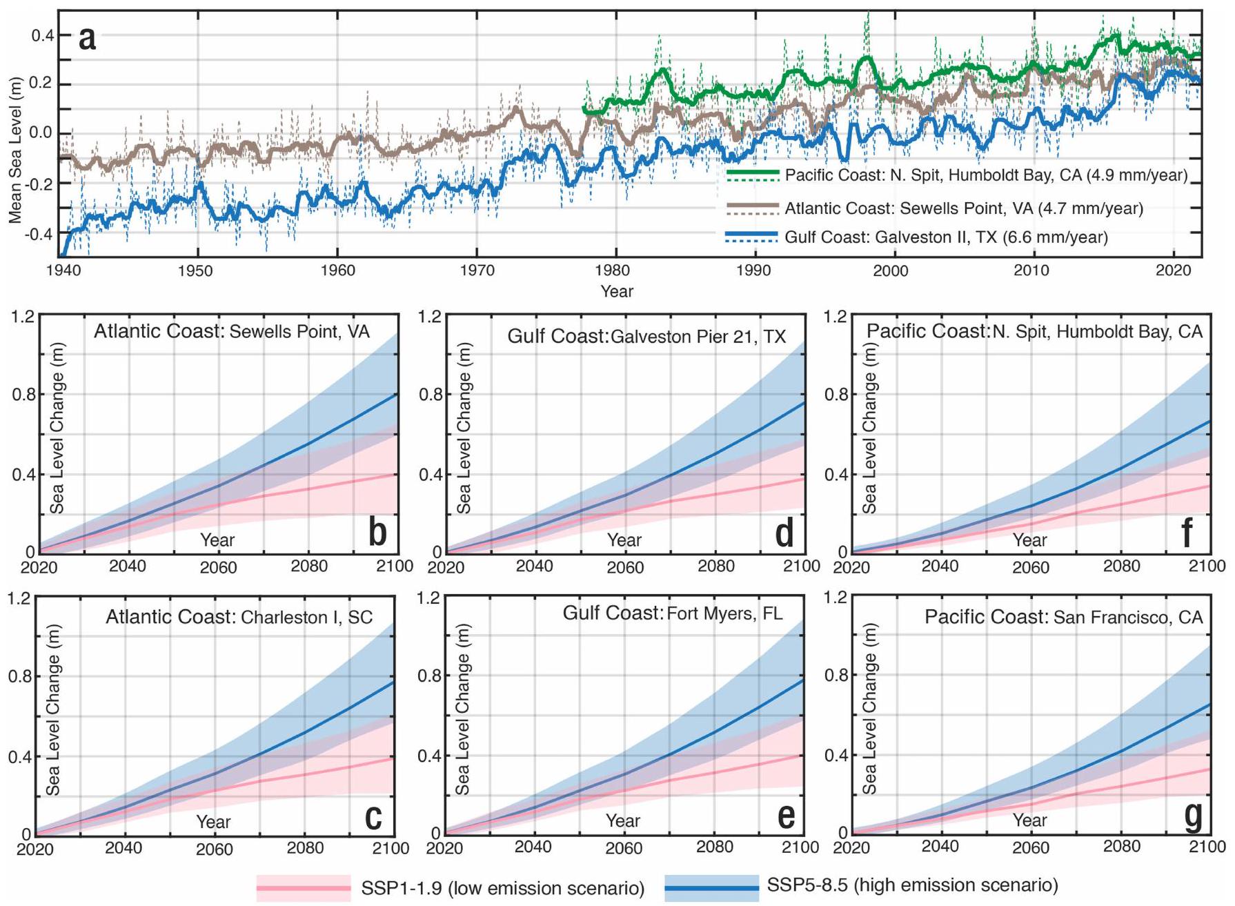
المثلثات الموضحة في الشكل 1أ. مقارنة بين سيناريوهات الانبعاثات المنخفضة (SSP1-1.9) وسيناريوهات الانبعاثات العالية (SSP5-8.5) (ثقة متوسطة) لساحل المحيط الأطلسي في نقطة سيويل، فيرجينيا (ب) وشارلستون I، ساوث كارولينا (ج)؛ ساحل الخليج في جالفستون رصيف 21، تكساس (د) وفورت مايرز، فلوريدا (هـ)؛ وساحل المحيط الهادئ في نورث سبايت، خليج هومبولت، كاليفورنيا (و) وسان فرانسيسكو، .

الشكل البياني الموسع 2 | التوزيع المكاني لمعدل مستوى سطح البحر عبر الساحل الأطلسي للولايات المتحدة. تشير معدلات مستوى سطح البحر الإيجابية إلى ارتفاع، بينما تشير المعدلات السلبية إلى هبوط. المدن الساحلية الأطلسية الـ 11 التي تم تقييمها في هذه الدراسة مميزة في الشكل. الصورة الخلفية من جوجل، إيرثستار. تُظهر السرعات الرأسية لمحطات التحقق من GNSS باستخدام دوائر ملونة على الخريطة. لاحظ أنه تم رسم مجموعة فرعية فقط من بيانات GNSS لتجنب الفوضى. يتم عرض مقارنة المعدلات الرأسية من 218 محطة GNSS
مع معدلات InSAR في الشكل التكميلي 11c. رموز الولايات: NH، نيوهامبشير؛ MA، ماساتشوستس؛ NY، نيويورك؛ PA، بنسلفانيا؛ NJ، نيوجيرسي؛ MD، ماريلاند؛ WV، فرجينيا الغربية؛ OH، أوهايو؛ VA، فرجينيا؛ NC، كارولينا الشمالية؛ SC، كارولينا الجنوبية؛ GA، جورجيا؛ FL، فلوريدا. حدود الولايات تعتمد على بيانات المتجهات العامة من بنك البيانات التابع للبنك الدولي (https://data. worldbank.org/) التي تم إنشاؤها في MATLAB.

الشكل البياني الموسع 3 | التوزيع المكاني لمعدل مستوى سطح البحر عبر الساحل الخليجي للولايات المتحدة. تشير معدلات مستوى سطح البحر الإيجابية إلى ارتفاع، بينما تشير المعدلات السلبية إلى هبوط. المدن الساحلية الخليجية الـ 11 التي تم تقييمها في هذه الدراسة مميزة في الشكل. الصورة الخلفية من جوجل، إيرثستار. تُظهر السرعات الرأسية لمحطات التحقق من GNSS باستخدام دوائر ملونة على الخريطة. لاحظ أنه تم رسم مجموعة فرعية فقط من بيانات GNSS لتجنب الفوضى. المقارنة
لمعدلات الرأسية من 157 محطة GNSS مع معدلات InSAR تظهر في الشكل التكميلي 11d. رموز الولايات: TX، تكساس؛ LA، لويزيانا؛ MS، ميسيسيبي؛ AL، ألاباما؛ GA، جورجيا؛ FL، فلوريدا. تعتمد الحدود الوطنية والولائية على بيانات المتجهات العامة من بنك البيانات التابع للبنك الدولي (https://data. worldbank.org/) التي تم إنشاؤها في MATLAB.

الشكل البياني الموسع 4 | التوزيع المكاني لمعدل مستوى سطح البحر عبر الساحل الهادئ للولايات المتحدة.
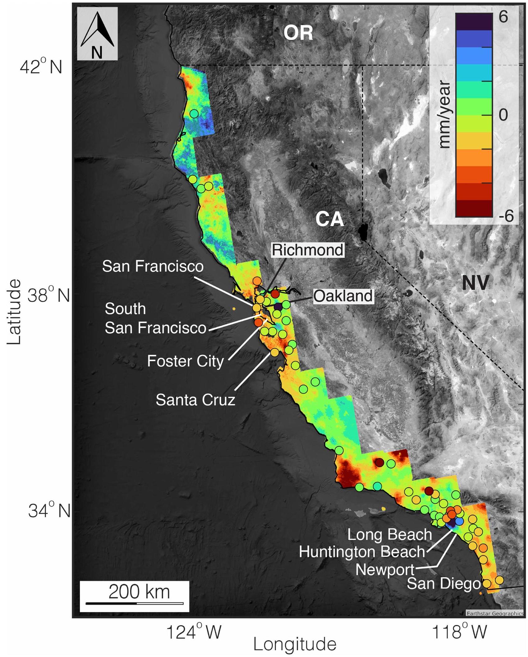
تشير معدلات مستوى سطح البحر الإيجابية إلى ارتفاع، بينما تشير المعدلات السلبية إلى هبوط. المدن الساحلية الهادئة العشر التي تم تقييمها في هذه الدراسة مميزة في الشكل. الصورة الخلفية من جوجل، إيرثستار. تُظهر السرعات الرأسية لمحطات التحقق من GNSS باستخدام دوائر ملونة على الخريطة. لاحظ أنه تم رسم مجموعة فرعية فقط من بيانات GNSS لتجنب الفوضى. تظهر المقارنة لمعدلات الرأسية من 381 محطة GNSS مع معدلات InSAR في الشكل التكميلي 11b. رموز الولايات: OR، أوريغون؛ CA، كاليفورنيا؛ NV، نيفادا. تعتمد الحدود الوطنية والولائية على بيانات المتجهات العامة من بنك البيانات التابع للبنك الدولي (https://data.worldbank.org/

المقال الشكل البياني الموسع 5 | مساهمة هبوط الأرض. دالة التوزيع التراكمي التجريبية للمنطقة المعرضة الكلية بحلول عام 2050 للساحل الأطلسي للولايات المتحدة (أ)، الساحل الخليجي (ب) والساحل الهادئ (ج). تُظهر الخطوط الزرقاء والمنطقة المظللة المساهمة من هبوط الأرض (LS) فقط، مع الأخذ في الاعتبار الإسقاط الخطي لمعدل مستوى سطح البحر من 2020 إلى 2050. تُظهر الخطوط الحمراء والمنطقة المظللة المساهمة من هبوط الأرض وارتفاع مستوى سطح البحر بحلول 2050 تحت سيناريو SSP2-4.5. تمثل الخطوط الحمراء في القيمة المتوسطة مع الأخذ في الاعتبار المعادلة (3)، بينما المنطقة المظللة هي الحدود الدنيا والعليا من المعادلة (3). المنطقة المعرضة الكلية لكل ساحل هي القيم في أ-ج. مقارنة التغير في مستوى سطح البحر الجغرافي من تقرير التقييم السادس للهيئة الحكومية الدولية المعنية بتغير المناخ
, مع التغير في مستوى البحر الناتج عن هبوط الأرض من قياسات InSAR في هذه الدراسة

في ثلاث محطات قياس المد على الساحل الخليجي: غالفستون رصيف 21، TX (د)؛ جزيرة يوجين، LA (هـ)؛ وجزيرة غراند، LA (و). تُظهر الخط الأحمر الصلب القيمة المتوسطة (النسبة المئوية 50) لتغير مستوى البحر IPCC تحت سيناريو SSP1-1.9 (سيناريو انبعاثات منخفضة)، بينما تُظهر النطاق المظلل الأحمر النسبة المئوية 17-83. تُظهر الخط البني الصلب القيمة المتوسطة (النسبة المئوية 50) لتغير مستوى البحر IPCC تحت سيناريو SSP5-8.5 (سيناريو انبعاثات عالية)، بينما تُظهر النطاق المظلل البني النسبة المئوية 17-83. تُظهر الخط الأزرق الصلب معدل مستوى البحر من InSAR من هذه الدراسة والنطاقات المظللة الزرقاء هي انحراف معياري واحد. تشير النقطة السوداء والخط المنقط إلى متى تتجاوز العمليات الأخرى التغير في مستوى البحر الناتج عن هبوط الأرض. يتم عرض مقارنة نموذجية لـ 20 محطة قياس المد عبر هبوط الأرض في الشكل التكميلي 1. الشكل البياني الموسع 6 | تغير مستوى البحر بسبب معدل مستوى البحر. أ، الفرق بين معدلات مستوى البحر من تقرير التقييم السادس للهيئة الحكومية الدولية المعنية بتغير المناخ مع تقدير مستوى البحر من قياسات InSAR في محطات قياس المد عبر الولايات المتحدة (الصورة الخلفية: جوجل، إيرثستار). تعتمد الحدود الوطنية والولائية في أ على بيانات المتجهات العامة من بنك البيانات التابع للبنك الدولي (https://data.worldbank.org/ ) التي تم إنشاؤها في MATLAB. للحصول على هذه المعدلات، قمنا بمتوسط معدلات مستوى البحر من وحدات InSAR ضمن دائرة نصف قطرها 200 متر من محطات قياس المد والانحراف المعياري المرتبط بكل وحدة InSAR لتقدير نطاقات الخطأ. تم إجراء اختبار
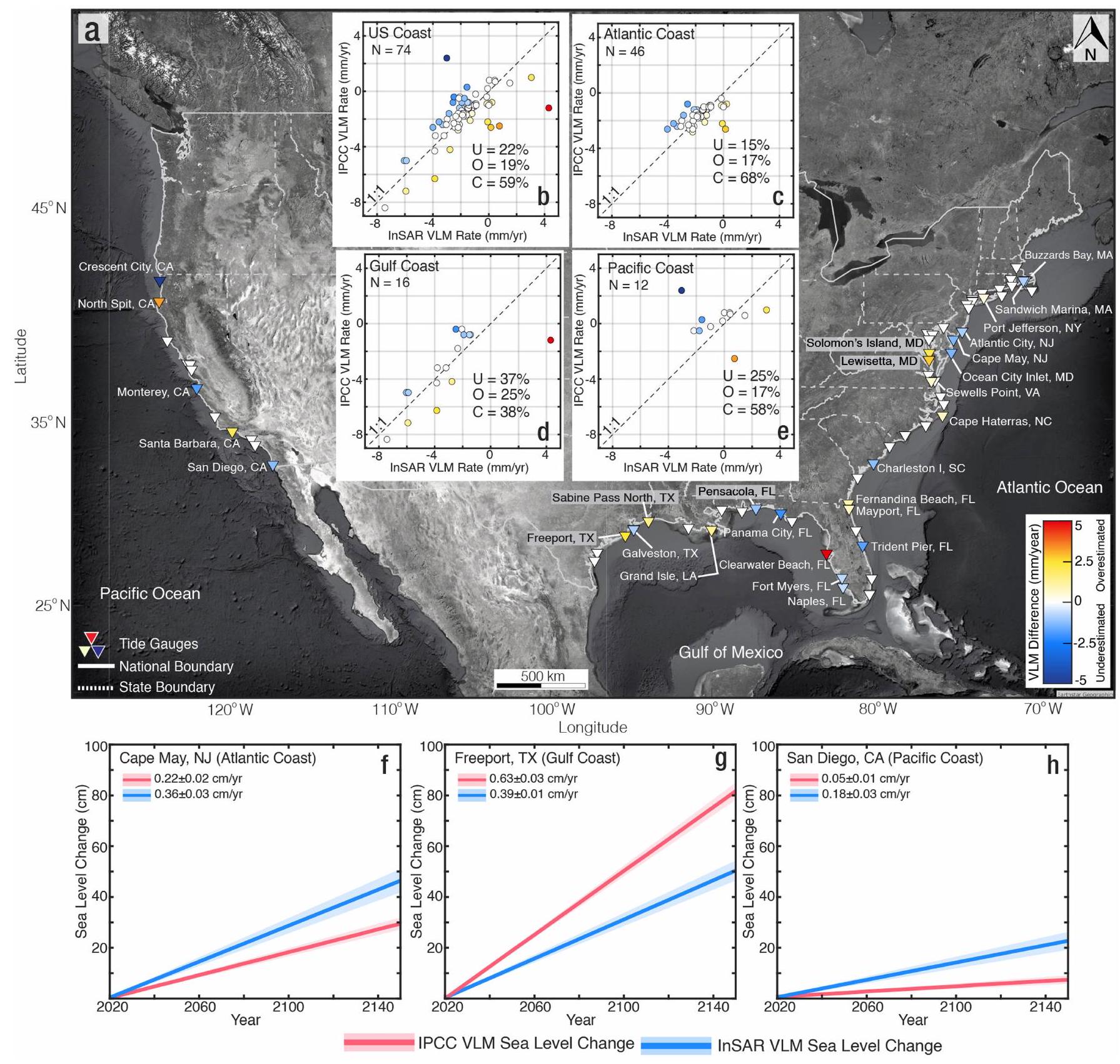
– في البداية لمقارنة معدلات مستوى البحر من كلا المصدرين. المحطات التي لم يُلاحظ فيها فرق إحصائي تم تمييزها باللون الأبيض، مما يدل على قيم مستوى البحر المتسقة (C). المحطات التي تكون فيها معدلات هبوط الأرض IPCC (معدل مستوى البحر السلبي) أعلى من تقديرات InSAR تم تمييزها باللون الأصفر أو الأحمر، مما يدل على المبالغة في التقدير (O)، بينما المحطات التي تكون فيها معدلات هبوط الأرض IPCC أقل تم تمييزها باللون الأزرق، مما يدل على التقليل من التقدير (U). لاحظ أنه تم تمييز المحطات التي تحمل U أو O فقط في أ. ملخص لمعدلات مستوى البحر من قياسات IPCC وInSAR و

المقال
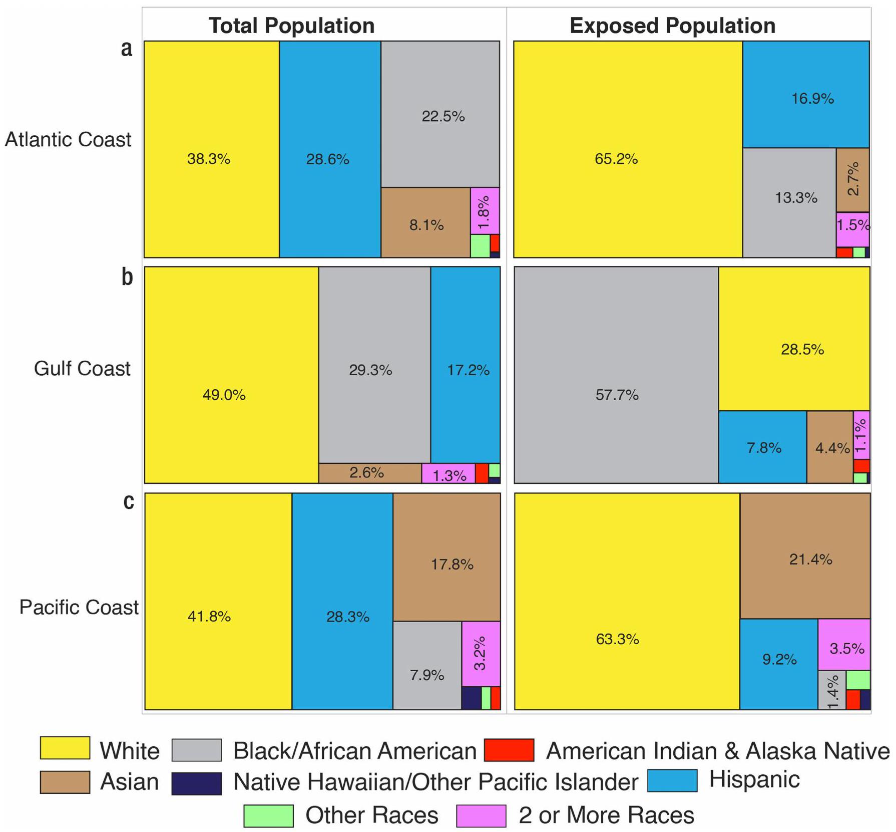
الشكل البياني الموسع 7 | إجمالي السكان مقابل السكان المعرضين بحلول عام 2050 لمختلف الفئات العرقية على الساحل الأمريكي. خريطة شجرية للسكان الإجماليين والمعرضين للساحل الأطلسي (أ)، الساحل الخليجي (ب) والساحل الهادئ (ج). يتم التعبير عن السكان الإجماليين والمعرضين كنسبة مئوية من إجمالي السكان للساحل. تمثل النسب المئوية للسكان المعرضين فقط القيم المتوسطة للتعرض التي تم تقييمها باستخدام

المعادلة (3). انظر الجداول التكملية 13-15 لسكان كل مدينة، بما في ذلك الحدود الدنيا والعليا. تشمل المجموعات المهمشة الأفراد الذين يعرفون أنفسهم كأفارقة أمريكيين، أمريكيين أصليين أو من ألاسكا، آسيويين، هاوايين أصليين أو من جزر المحيط الهادئ الأخرى، هسبانيين أو لاتينيين، أعراق أخرى ومجموعتين أو أكثر. الشكل البياني الموسع 8 | قيمة الممتلكات المعرضة المودلة بحلول عام 2050 مقابل القيمة الإجمالية للممتلكات للمدن على الساحل الأمريكي. مخططات الصندوق التي تُظهر توزيع الممتلكات الإجمالية (TP) وممتلكات التعرض (EP) لمدينة نيويورك (أ)، مدينة الأطلسي (ب)، شاطئ فرجينيا (ج)، تشارلستون (د)، سافانا (هـ)، جاكسونفيل (و)، ميامي (ز)، موبايل (ح)، بيلوكسي (ط)، نيو أورليانز (ي)، بورت آرثر (ك)، غالفستون (ل)، مدينة فوستر (م) وشاطئ نيوبورت (ن). المحور
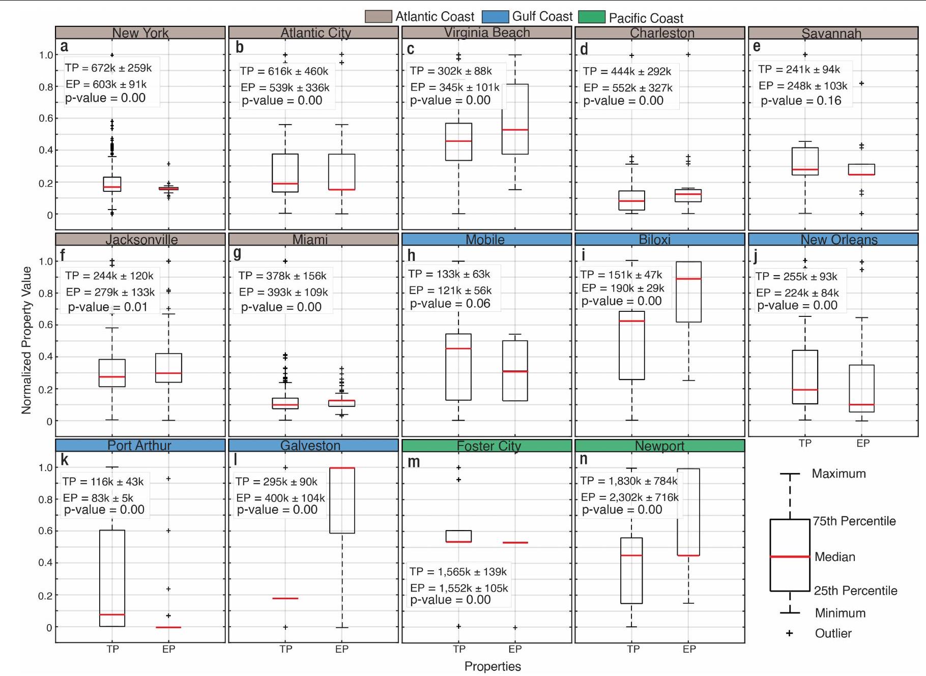
لـ TP و EP يُظهر القيم المعيارية. القيم لكل رسم تُظهر القيمة المتوسطة، الانحراف المعياري و – القيمة لـ TP و EP. يتم التعبير عن القيم المتوسطة والانحراف المعياري بالآلاف (ك). بالنسبة للاختبار، الفرضية الصفرية هي أنه لا يوجد فرق إحصائي بين قيمة TP في المدينة وقيمة EP. تُظهر مخططات الصندوق فقط القيم المتوسطة للتعرض التي تم تقييمها باستخدام المعادلة (3). انظر الجداول التكملية للحدود الدنيا والعليا لكل مدينة.

الشكل البياني الموسع 9 | تأثير هياكل التحكم في الفيضانات على التعرض المودل. المناطق المعرضة الحالية (2020) والمخططة (2050) مع الأخذ في الاعتبار هياكل الدفاع لـ: ميامي، FL (أ)؛ نيو أورليانز، LA (ب)؛ بورت آرثر، TX (ج)؛ فريبورت، TX (د)؛ مدينة فوستر، CA (هـ). تأخذ المناطق المعرضة في الاعتبار معدل مستوى البحر وارتفاع مستوى البحر تحت سيناريو SSP2-4.5. التعرض للهبوط بسبب التحكم في الفيضانات
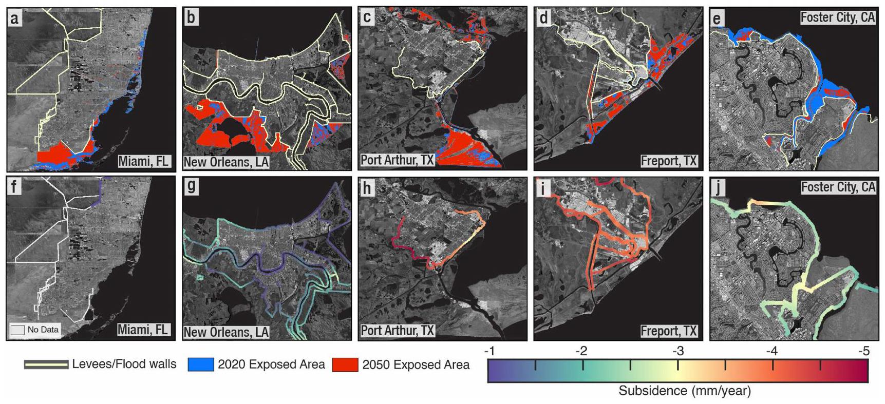
الهياكل في: ميامي، فلوريدا (ف); نيو أورلينز، لويزيانا (ج); بورت آرثر، تكساس (ح); فريبورت، تكساس (ي); فوستر سيتي، . الخطوط الصفراء في هي السدود/جدران الفيضانات. الصور الخلفية في أ-ي مأخوذة من جوجل، إيرثستار. رموز الولايات: فل، فلوريدا؛ لا، لويزيانا؛ تكس، تكساس؛ كال، كاليفورنيا.

تفاصيل حول السيناريوهات المدافعة لكل مدينة والتغير النسبي موضحة في الجداول التكميلية 20-22. القيمة المركزية في أ-ج تمثل القيمة الوسيطة المقدرة من المعادلة (3)، بينما تمثل أشرطة الخطأ الحدود الدنيا والعليا من المعادلة (3).

Received: 10 May 2023
Accepted: 5 January 2024
Published online: 6 March 2024
Open access
Check for updates

The widespread consequences of global climate change stress human communities and ecosystems worldwide. Climate change is already causing an increase in the frequency and intensity of heatwaves, hurricanes and wildfires and severely affecting the world’s freshwater resources through sea-level rise (SLR), more frequent droughts and changes in precipitation and evapotranspiration , and these effects will almost certainly grow in the future . Globally, SLR will pose a substantial socioeconomic challenge in the twenty-first century, primarily affecting human populations, infrastructure and ecosystems along major coastlines . Global mean sea level has risen by about 0.17 m over the past 100 years, with global rates of SLR accelerating from about 1.7 mm per year in the late twentieth century to about 3.1 mm per year in the early twenty-first century in response to warming temperatures and is 3.7 mm per year at present (ref. 17). Even if climate change mitigation efforts succeed in stabilizing temperature in the future decades, sea levels will continue to rise as a result of the continuing response of oceans to past warming . Furthermore, coastal cities often experience sinking land (so-called land subsidence), whose compounding effect contributes to relative SLR, exacerbating coastal hazards and risks . In this study, we refer to SLR that incorporates the effects of vertical land motion (VLM) as ‘relative SLR’, whereas ‘geocentric SLR’ refers to SLR without VLM. As sea level rises and land subsides, the hazards associated with climate extremes (for example, hurricanes and storm surges), shoreline erosion and inundation of low-lying coastal areas grow .
On the coasts of the conterminous USA, climate-induced sea levels are rising faster than the global average , with an expected increase over the next few decades (Fig. 1 and Extended Data Fig. 1). Owing to its geography and population distribution, the USA is a coastal nation, with more than of its population residing in coastal cities, generating an estimated annual revenue of US$3.8 trillion (ref. 23).

Consequently, socioeconomic losses from climate-induced SLR will represent a notable facet of climate-change consequences in the USA . In the short term (one to three decades), only continued observed rises in sea level are sufficient to trigger cascading hazards across US coastal regions, with a projected increase in the frequency and intensity of storm surges, saltwater intrusion, high-tide flooding and coastal erosion .
Sea levels are projected to vary minimally in the next few decades across the different greenhouse gas emission scenarios, whereas end-of-century projections indicate a more substantial divergence in increase by emissions (Extended Data Fig. 1b-g). Thus, short-term vulnerability assessments incorporating local drivers are relevant to policymakers for developing comprehensive adaptation strategies that extend beyond emission reduction, as they provide insights into the immediate risks and challenges of coastal communities. However, accurately projecting coastal vulnerability requires comprehensive and high-resolution measurements of VLM, which is lacking across the USA at present . This lack of data makes estimating the actual risks of relative SLR on different coastal communities challenging and contributes to high uncertainty and potentially systematic errors in existing coastal-hazard assessment.

Here we present coastal-scenario-based inundation hazard models for coastal cities in the USA, focusing on the short-term (2050) projection of relative SLR. Our inundation models integrate high-resolution VLM data across the US coast (Fig. 1 and Extended Data Figs. 2-4) at millimetre-level accuracy using interferometric synthetic aperture radar (InSAR) (see Methods), the projections of geocentric SLR and light detection and ranging (LiDAR) digital elevation models (DEMs) to forecast relative SLR rates and create granular inundation maps for a set of major cities along the US coastline. Using the 2010 US census data as baseline estimates, we assess the impact of relative SLR on the

Fig. 1 | Coastal hazards across the USA. a, Spatial distribution of VLM across the US coast (background image: Google, Earthstar). Positive VLM rates indicate uplift and negative VLM rates indicate subsidence. Individual VLM maps for the US Atlantic, Gulf and Pacific coasts are shown in Extended Data Figs. 2-4. National and state boundaries in a are based on public-domain vector data by the World Bank DataBank (https://data.worldbank.org/) generated in MATLAB. Projections of geocentric SLR with a baseline for the year 2020 based on SSP2-4.5 (refs. 17,34) on the Pacific coast (North Spit, Humboldt Bay, CA) (b), Atlantic coast (Sewell’s Point, VA) (c) and Gulf coast (Galveston II, TX) (d). The bold lines represent the median (50th percentile) projected geocentric SLR and the shaded regions represent the 17th and 83rd percentiles.e, Box plot
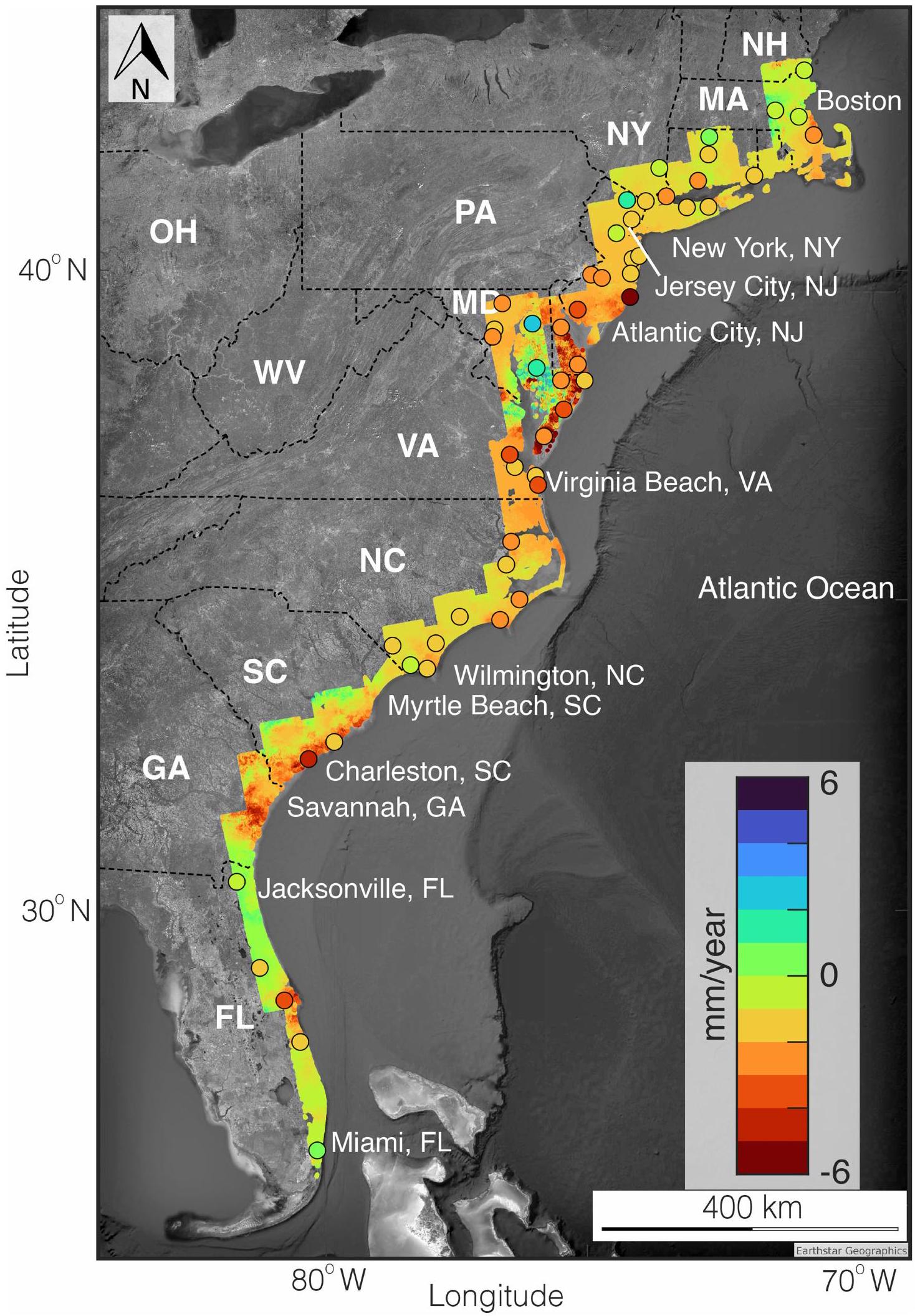
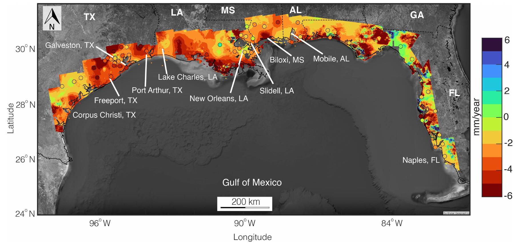
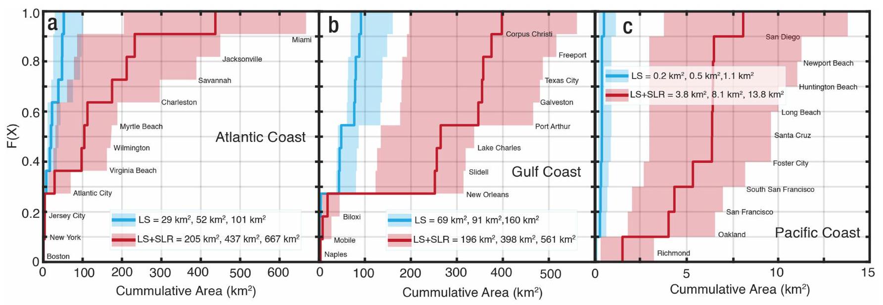
representing the distribution of VLM for 32 US coastal cities evaluated in this study. The 32 coastal cities evaluated in this study are highlighted in a. The cities include: US Atlantic coast:1. Boston, MA; 2. New York City, NY; 3.Jersey City, NJ; 4. Atlantic City, NJ; 5. Virginia Beach, VA; 6. Wilmington, NC; 7. Myrtle Beach, SC; 8. Charleston, SC; 9. Savannah, GA; 10. Jacksonville, FL; 11. Miami, FL; US Gulf coast: 12. Naples, FL; 13. Mobile, AL; 14. Biloxi, MS; 15. New Orleans, LA; 16. Slidell, LA;17. Lake Charles, LA;18. Port Arthur, TX;19. Texas City, TX;20. Galveston, TX; 21. Freeport, TX; 22. Corpus Christi, TX; US Pacific coast: 23. Richmond, CA;24. Oakland, CA;25. San Francisco, CA;26. South San Francisco, CA;27. Foster City, CA;28. Santa Cruz, CA;29. Long Beach, CA;30. Huntington Beach, CA; 31. Newport Beach, CA; 32. San Diego, CA.
population and properties of US coastal communities and explore several adaptation regimes to minimize potential future impacts.

Future inundation of coastal areas in 32 coastal cities (see Fig. 1) along the US coasts is modelled using projections of current VLM rates on coastal-elevation data, geocentric SLR projection scenarios and high-tide estimates. The aggregate population of these cities is estimated to be 25 million people (roughly of current US coastal inhabitants), with 10 million properties valued at US trillion (Supplementary Table 1). Our analysis quantifies how relative sea-level
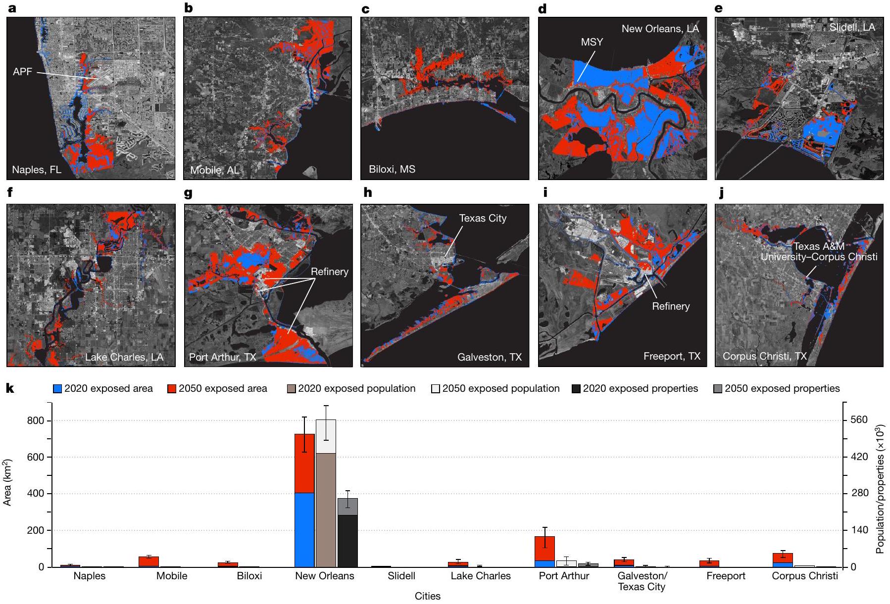
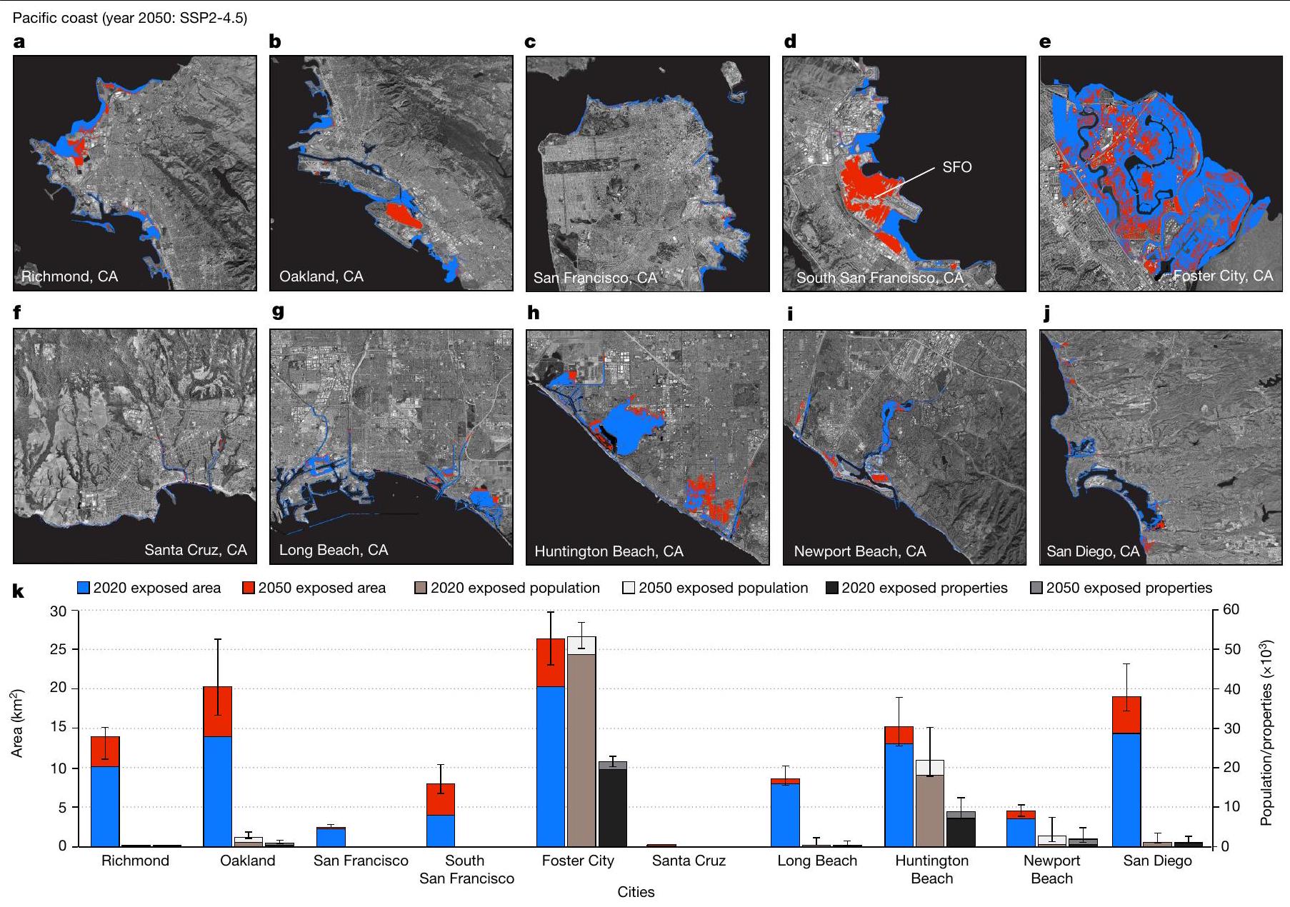
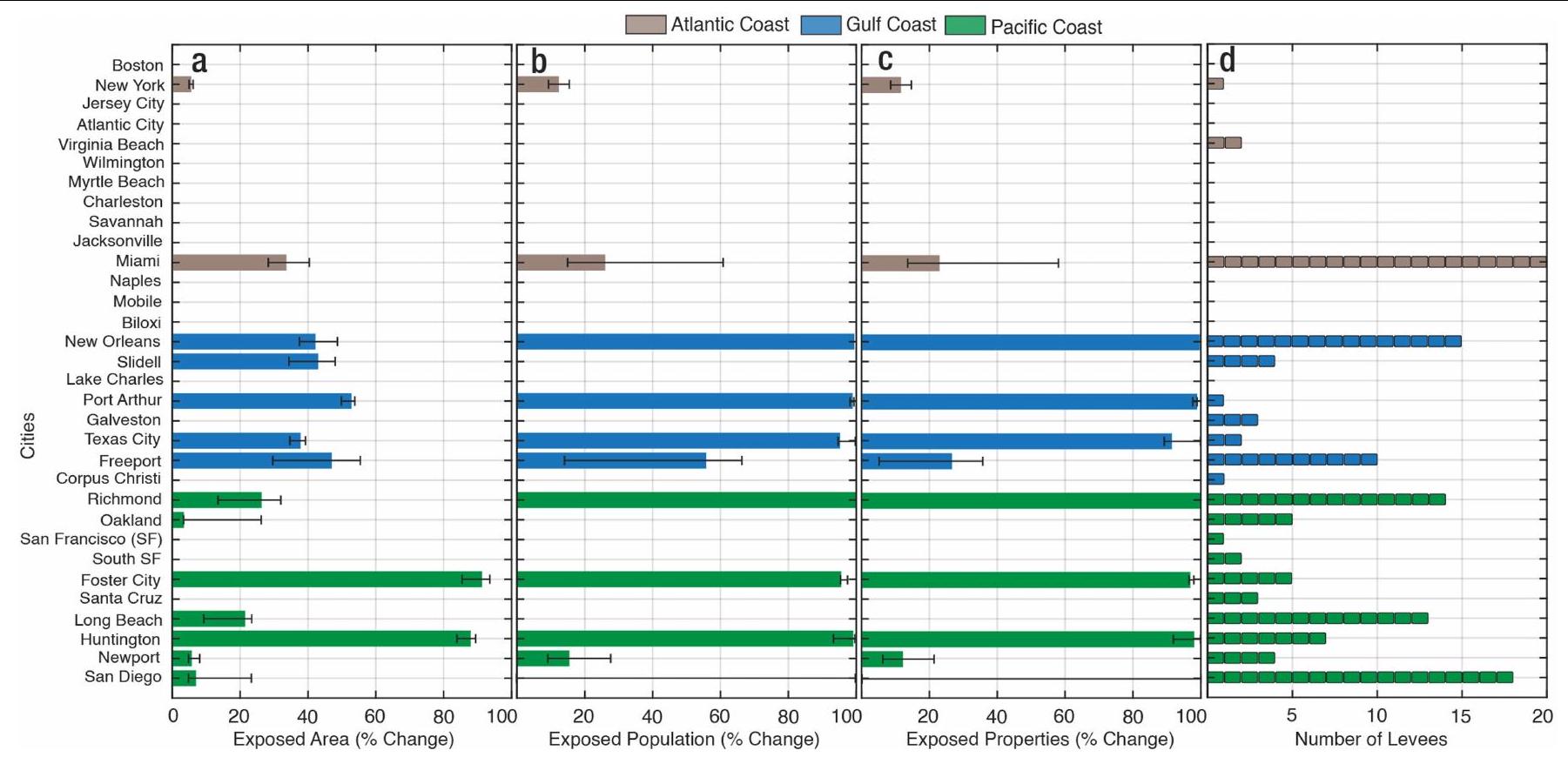
changes, attributable to VLM and geocentric SLR, will increase the exposure-area, population and properties-to high-tide flooding by 2050 , using 2020 as the baseline (see Methods). For the analysis, we consider the SLR scenario derived from Shared Socioeconomic Pathway (SSP) scenario 2-4.5 (SSP2-4.5), representing the current emissions trajectory , population and property exposure using the 2010 US census data and property/home value using the ZIP Code Zillow Home Value Index (ZHVI) (see Methods). Our model suggests that, by 2050, relative SLR could cause further exposed land area of between 1,334 and in 32 US coastal cities if no flood-defence structures are implemented (Figs. 2-4, Table 1 and Supplementary Tables 2-4). We estimate a population exposure of 176,000-518,000 inhabitants from 94,000-288,000 properties,

Fig. 2 | Inundation maps for cities on the US Atlantic coast. Areas exposed to current (2020) high tide and further exposed areas by 2050 considering VLM, geocentric SLR projection under SSP2-4.5 for: Boston, MA (a); New York City, NY and Jersey City, NJ (b); Atlantic City, NJ (c); Virginia Beach, VA (d); Wilmington, NC (e); Myrtle Beach, SC (f); Charleston, SC (g); Savannah, GA (h); Jacksonville, FL(i); and Miami, FL( ). Background images in are from Google, Earthstar.

Note that, for current exposure, geocentric SLR . The blue and red colours are the current and projected exposed areas, respectively. BOS, Boston Logan International Airport, MA;JFK, John F. Kennedy International Airport, NY. k, Distribution of further exposed areas, population and properties by 2050. The central value represents the estimated median value from equation (3), whereas the error bars represent the lower and upper bounds from equation (3).
with a total estimated home value of US$32-109 billion by 2050. The maximum population and property exposure by 2050 represents approximately 1 in 50 people and 1 in 35 properties from the 32 coastal cities.

From 11 cities on the US Atlantic coast, the projected extra area exposed to high-tide flooding by 2050 is between 773 and (Fig. 2). This would affect a population of 59,000-263,000 people and 32,000-163,000 properties on the US Atlantic coast (Fig. 2 and Table1). The property and population exposure on the Atlantic coast are not homogeneous across all cities. For example, Miami (average elevation of less than 2 m above sea level) has the greatest share of exposure, accounting for of the exposed area, of the exposed population and (13,000-81,000) of the exposed properties along the Atlantic coast (Supplementary Table 2). The home-value exposure by 2050 for the 11 Atlantic coastal cities is estimated at US$14-64 billion (Table 1). The calculated exposure does not account for the value of critical infrastructure (such as airports, schools, hospitals, power plants, roads and railways), as well as economic hubs and landmarks, and hence represents a conservative value.

For 11 cities along the US Gulf coast, our 2050 projection of inundation hazard shows a cumulative exposed area of between 528 and (Fig. 3, Table 1 and Supplementary Table 3). These affected areas will expose an extra 110,000-225,000 people and 58,000-109,000 properties worth US$14-21 billion (Table 1). It should be noted that substantial areas ( ), population ( ) and properties (176,000-209,000) in New Orleans are already exposed to high-tide events at present, owing to the existence of areas lying below sea level (Supplementary Table 3). We emphasize that our analysis applies an undefended approach, which does not consider the presence of flood-control structures and future adaptation. New Orleans, however, is surrounded by extensive floodwalls and levee systems and is heavily drained. Although flood-control structures offer substantial protection to coastal areas, their effectiveness is not guaranteed. The events following the landfall of Hurricane Katrina in August 2005, which claimed more than 1,500 lives, are tragic reminders of the heightened devastation of a failed levee system . Thus, considerations of flood-control systems alone may only represent a temporary solution, as discussed later. Airports, roadways and refineries, ubiquitous in cities, are projected to be among the Gulf coast’s exposed infrastructure (Fig. 3).

Fig. 3 | Inundation maps for cities on the US Gulf coast. Areas exposed to current (2020) high tide and further exposed areas by 2050 considering VLM, geocentric SLR projection under SSP2-4.5 for: Naples, FL (a); Mobile, AL (b); Biloxi, MS (c); New Orleans, LA (d); Slidell, LA (e); Lake Charles, LA (f); Port Arthur, TX (g); Galveston and Texas City, TX (h); Freeport, TX (i); and Corpus Christi, TX( ). Background images in are from Google, Earthstar. Note that,
for current exposure, geocentric SLR . The blue and red colours are the current and projected exposed areas, respectively. APF, Naples Airport, FL; MSY, Louis Armstrong New Orleans International Airport, LA. k, Distribution of further exposed areas, population and properties by 2050. The central value represents the estimated median value from equation (3), whereas the error bars represent the lower and upper bounds from equation (3).

On the Pacific coast, we find a considerable divergence in the impacts of relative SLR compared with the US Atlantic and Gulf coasts. By 2050, the cumulative exposed area from ten cities on the US Pacific coast is , with a population exposure of people and 3,000-15,000 properties worth US$4.5-22 billion (Fig. 4, Table 1 and Supplementary Table 4). The comparatively low inundation hazard may be attributable to the higher topographic elevations, lower rates of land subsidence and relatively low rates of geocentric SLR on the Pacific coast relative to the Atlantic and Gulf coasts . Although the inundation hazard for Pacific coast communities (California’s coast) by 2050 is relatively modest, rock coast cliff retreat and the projected increase in the high-tide flooding are further factors that would affect some coastal residents and properties.

Land subsidence, the sinking or settling of the land surface, is a global issue with costly socioeconomic consequences . To quantify the contribution of subsidence to future flooding hazards in the 32 US coastal cities, we consider two scenarios: (1) potential land areas below sea level resulting from land subsidence alone and (2) potential land
areas below sea level resulting from a combination of land subsidence and sea-level change. Using linear projections of the current VLM rate and coastal-elevation data, we determine the land areas that, despite being above sea level at present, will be inundated by 2050 under both scenarios. Our analysis indicates that land areas below sea levels by 2050 resulting from only land subsidence account for (Atlantic coast), 22.9-35.4% (Gulf coast) and 4.8-8.1% (Pacific coast) of total inundated areas when land subsidence and geocentric SLR are taken into consideration (Extended Data Fig. 5a-c and Supplementary Tables 5-7).

Furthermore, comparing our InSAR-derived VLM to geocentric sea-level change at Permanent Service for Mean Sea Level (PSMSL) tide-gauge stations included in the Intergovernmental Panel on Climate Change (IPCC) projections across the USA (Supplementary Fig. 1) reveals that, at three stations on the Gulf coast, local land subsidence currently outpaces geocentric SLR (considering a low-emission scenario: SSP1-1.9) and presents a greater concern for the region than geocentric sea-level change (considering a high-emission scenario: SSP5-8.5) to 2045 (Extended Data Fig. 5d) and 2070 (Extended Data Fig. 5e,f), assuming linearly continuous subsidence. This observation is notable because it brings land subsidence to the fore of coastal-hazard discussions and highlights it as a crucial index in coastal disaster resilience design .

Fig. 4 | Inundation maps for cities on the US Pacific coast. Areas exposed to current (2020) high tide and further exposed areas by 2050 considering VLM, geocentric SLR projection under SSP2-4.5 for:Richmond, CA(a); Oakland, CA(b); San Francisco, CA (c); South San Francisco, CA (d); Foster City, CA (e); Santa Cruz, CA (f); Long Beach, CA (g); Huntington Beach, CA (h); Newport Beach, CA (i); and San Diego, . Background images in are from Google, Earthstar.

Note that, for current exposure, geocentric SLR . The blue and red colours are the current and projected exposed areas, respectively. SFO, San Francisco International Airport, CA. k, Distribution of further exposed areas, population and properties by 2050 . The central value represents the estimated median value from equation (3), whereas the error bars represent the lower and upper bounds from equation (3).

Some flooding projections, however, do not consider the impacts of spatially variable land-elevation changes, resulting in inaccurate projections of expected exposure, which may affect the preparedness of coastal communities. For instance, a comparison of the estimated exposure by 2050 for the 32 cities derived for this study with exposure derived using the IPCC relative sea-level projections shows that the exposure-in terms of area, population and properties-is not distinguishable within uncertainty in most of the cities and broadly for the entire US coast (Table 1). However, we find that notable divergence in the exposure occurs in some cities, particularly on the US Gulf coast (Fig. 5a-c and Supplementary Tables 8-10). By comparing the InSAR VLM rates within the cities with the IPCC-derived VLM rates from tide-gauge records, we gain insight into the underlying differences (Fig. 5d and Supplementary Table 11). In cities such as Boston, New York City, Naples, Port Arthur, Corpus Christi, Richmond, Oakland and San Francisco, in which IPCC VLM rates are similar to the InSAR VLM rates within the city or where the contribution of VLM is minimal, the disparities between the estimated exposure is modest. However, the estimated exposure is underestimated in cities in which the IPCC VLM underestimates the contribution of VLM (for example, Atlantic City, Charleston, Savannah, Mobile and Biloxi). Similarly, in cities in which the IPCC VLM overestimates the contribution of VLM, the estimated exposure is also overestimated (for example, Virginia Beach,

Jacksonville, Miami, New Orleans, Slidell, Lake Charles, Port Arthur and Huntington Beach).

To provide a more comprehensive understanding of these underlying differences, we performed a comparative analysis of InSAR-derived VLM rates with the VLM rates used in the IPCC Sixth Assessment Report for 74 stations along the US coast (Supplementary Table 12 and Extended Data Fig. 6). Despite a 59% consistency in VLM measurements at the tide-gauge stations across the USA, these stations-often situated at the peripheries of urban areas-may not accurately capture the contemporary dynamics of spatially variable VLM within the cities themselves (for example, Biloxi, New Orleans and San Diego) (compare stations in Extended Data Fig. 6 with Fig. 5d). This limitation is particularly pertinent in urban centres in which anthropogenic drivers strongly influence VLM, thereby contributing to discrepancies in estimated exposure. InSAR observations are the gold standard of VLM measurements with unprecedented spatial resolution and are useful to enhance the accuracy of flood-prediction models.

Climate change contributes to and exacerbates the fragility of the most vulnerable communities. Generally, disadvantaged populations are compelled to live in the most susceptible regions because safer areas

and represent the lower bounds, median values and upper bounds evaluated using equation (3). The InSAR-derived exposure is estimated using InSAR VLM and IPCC geocentric SLR,
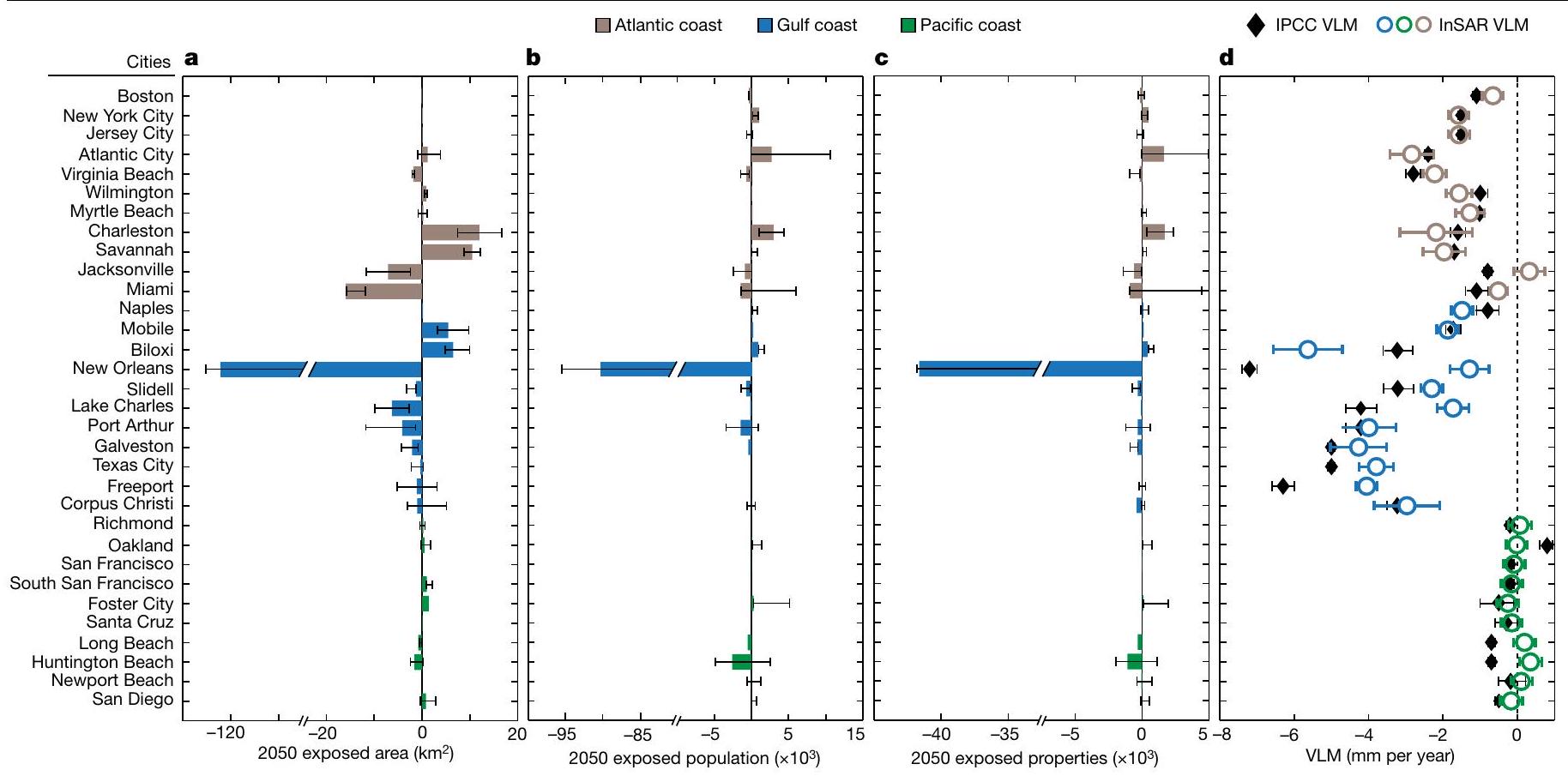
exposure for each city.
are out of reach . A growing body of scientific literature focuses on the impacts of climate change on vulnerable populations across countries . However, less emphasis has been placed on discussions on within-country climate-change inequality . A recent report by the United States Environmental Protection Agency (EPA) , along with the work of Hsiang et al. , contributes to the growing body of literature quantifying disproportionate climate-change risks to vulnerable communities in the USA.

Here we examine the disparate impacts of relative SLR on vulnerable communities across the 32 cities in the USA, offering a nuanced understanding of climate inequality in the USA. To examine the racial disparities in the exposed communities, we focused on eight races defined by the US census decennial data (see Methods). Our inundation model’s analysis of the affected population by 2050 reveals differential exposure to relative SLR along racial lines (Extended Data Fig. 7 and Supplementary Tables 13-15). Along the Atlantic and Pacific coasts, white residents are overrepresented among those exposed to relative SLR (Extended Data Fig. 7a,c). However, the distribution of white exposed population on these coasts approximately reflects the dominant demographic of these regions (Extended Data Fig. 7a,c and Supplementary Tables 13 and 15).

By contrast, on the Gulf coast, minoritized groups-individuals identifying as Black or African American; American Indian or Alaska Native; Asian; Native Hawaiian or Other Pacific Islander; Hispanic or Latino; and two or moregroups -constitute a noteworthy portion of the exposed population, despite not being the dominant population. Although minoritized groups make up of the total population across 11 cities in the Gulf coast, they are overrepresented in the exposed population, accounting for more than half (50.0-57.7%) of the exposed population in the case of Black or African American residents alone and when considering all minorities (Extended Data Fig. 7b and Supplementary Table 14). Asians are overrepresented among the exposed population on the Gulf and Pacific coasts, accounting for 2.6 and (median and upper bounds only) of the exposed population on the Gulf and Pacific coasts, respectively, despite making up 2.6% (Gulf coast) and 17.8% (Pacific coast) of the total population. Also, analysis of the impacts of relative SLR on economic inequality (see Methods) shows disproportionate economic exposure in New

Orleans and Port Arthur (Extended Data Fig. 8 and Supplementary Tables 16-18), which runs in parallel to the increased exposure of their predominantly minoritized communities. The intersection of racial and economic inequalities highlights the multidimensional vulnerability that specific populations in these cities face in the context of relative SLR.

One contributing factor to climate-change inequity is the diminished capacity of minoritized/low-income groups to adapt to and recover from the effects of existing hazards. To accentuate this point, consider the post-Hurricane Katrina impact on the population of Biloxi, MS. Although most attention is focused on the destruction to New Orleans caused by levee failures, Mississippi state incurred US billion in direct storm damage and 100,000 people were displaced as a result of Hurricane Katrina . East Biloxi, in which the low-income and marginalized community resides, was still suffering the impact of Hurricane Katrina 10 years after the storm, with broken, untended infrastructure, high unemployment rates and homelessness . By contrast, the high-income communities received substantial federal aid for infrastructure rebuilding and are ‘better off after the storm’ . This exclusion from recovery aid will undoubtedly impose constraints on the ability of low-income and minoritized communities to adapt to future climate change. Consequently, marginalized groups may account for a disproportionate share of climate-change collateral damage, even if they comprise a relatively small share of the affected population. In simple terms, existing inequalities make already vulnerable people more vulnerable to the adverse impacts of climate change, resulting in greater projected inequality .

Human interaction with the coast is increasing across the USA , and despite the clear and present danger posed by relative SLR, the need for adaptation and resilience planning is often overlooked or given insufficient priority. The growing risks identified in this paper pose a substantial challenge, and adaptation is to be expected in all the cities considered. Will cities be proactive and prepared through detailed assessment, planning and implementation of adaptive measures or will they be reactive to events, waiting for these impacts and risks to

Fig. 5|Comparing InSAR-derived and IPCC-derived VLM and estimated exposure. Differences between estimated exposure using InSAR-derived VLM and IPCC-derived VLM for 2050 exposed area (a), exposed population (b) and exposed properties (c). InSAR-derived exposure is estimated using InSAR VLM and IPCC geocentric SLR as detailed in Methods, whereas the IPCC-derived exposure is estimated using the IPCC relative SLR dataset . The central value represents the estimated median value from equation (3), whereas the error bars represent the lower and upper bounds from equation (3). Negative
values indicate cities in which IPCC-derived VLM exposure is overestimated, whereas positive values indicate areas in which exposure is underestimated. d, Comparison of InSAR versus IPCC VLM rates for the 32 cities. The InSAR VLM rates are obtained by averaging the VLM for each city used in the exposure analysis, whereas the IPCC VLM rates are derived from tide-gauge stations. The error ranges for the InSAR and IPCC VLM show standard deviation. A summary of the comparison of exposure and VLM rates is detailed in Supplementary Tables 8-11.
manifest? Here we will consider the proactive option. Adaptation is a long-term process and some combination of strategies is probably most appropriate sequenced following an adaptive-pathways approach . The precise details will vary from place to place depending on the individual situation. An ideal case seems to be a combination of the following possibilities for coastal cities: maintenance of nature-based protection from marshes and mangroves; new and upgraded structural protection and land raising; subsidence control; and land-use planning to reduce vulnerability .
Artificial coastal-defence structures, such as levees, berms, dykes and floodwalls, protect coastal communities by decreasing the consequences of flooding and inundation in exposed areas . Within the 32 coastal cities considered in this study, there are 131 flood-control structures, with more than 50% protecting the cities on the Pacific coast (Supplementary Table 19). To demonstrate the protective capacity of flood-control structures on the US coast to 2050, we modelled the exposed areas in all cities with at least one flood-control structure, considering a defended scenario (see Methods). Extended Data Fig. 9a-e depicts the spatial reduction in exposed areas and properties in some cities with levees and floodwalls. The defended scenario suggests that, by 2050 , relative SLR will affect a land area of 273,000 people and 31,000-171,000 properties on the US coasts, with of the exposed area, of the exposed population and 80-89% of the exposed properties being situated on the Atlantic coast (Extended Data Fig. 10 and Supplementary Tables 20-22). This ineffectiveness in hazard mitigation on the US Atlantic coast reflects the lack of an adequate flood-protection system in most cities. Ten cities on the US Atlantic coast evaluated in this study (excluding Miami) have only three levee systems (Extended Data Fig. 10d), opting for other protective approaches, such as beach nourishment, enhancing the beach and beachfront-property aesthetics, but providing more
limited flood protection. Nevertheless, most existing structure-based coastal-defence systems were not designed with climate change in mind, and large upgrades may be required to remain effective even to 2050 (ref. 45). This is most relevant where subsidence and differential subsidence affect the use of flood-control structures by lowering their effective height below inundation depths and promoting structural failure (Extended Data Fig. 9f-j).

Although not universal, human-induced land subsidence must also be mitigated where practical. Historically, land subsidence has been a silent problem with little public engagement or policy-focused studies, and its complex evolution and drivers make it a ‘wicked’ policy problem . Although natural processes (for example, glacial isostatic adjustment (GIA)) influence coastal land subsidence on the US coasts, non-GIA processes, including anthropogenic subsidence caused by the accumulation of several shallow and deep subsurface activities, such as drainage, groundwater withdrawal and hydrocarbon extraction, at present contribute to relative SLR around the USA, particularly on the Atlantic and Gulf coasts (Supplementary Figs. 2 and 3). Policies that aim to minimize subsidence (for example, through managed aquifer recharge) are crucial in the relevant cities .

Although the differences between low-emission and high-emission scenarios in terms of exposure are relatively modest in the short term, these variations are not inconsequential, given the inevitable continued rise in sea level beyond 2050 and its likely acceleration with further warming . Therefore, a long-term proactive and continuous adaptation beyond simple coastal protection would be needed . For the sustainability and resilience of US coastal cities, it is critical to adopt a built-upon multifaceted strategy involving the implementation of adaptive measures, the regulation of subsidence and the implementation of stringent climate-change policies that keep carbon emissions low. More importantly, these mitigation and adaptation strategies are
driven by anthropogenic influences and within reach with concerted societal efforts at all levels (policymakers to citizens).

Any methods, additional references, Nature Portfolio reporting summaries, source data, extended data, supplementary information, acknowledgements, peer review information; details of author contributions and competing interests; and statements of data and code availability are available at https://doi.org/10.1038/s41586-024-07038-3.

Publisher’s note Springer Nature remains neutral with regard to jurisdictional claims in published maps and institutional affiliations.

Open Access This article is licensed under a Creative Commons Attribution 4.0 International License, which permits use, sharing, adaptation, distribution and reproduction in any medium or format, as long as you give appropriate credit to the original author(s) and the source, provide a link to the Creative Commons licence, and indicate if changes were made. The images or other third party material in this article are included in the article’s Creative Commons licence, unless indicated otherwise in a credit line to the material. If material is not included in the article’s Creative Commons licence and your intended use is not permitted by statutory regulation or exceeds the permitted use, you will need to obtain permission directly from the copyright holder. To view a copy of this licence, visit http://creativecommons.org/licenses/by/4.0/.
© The Author(s) 2024, corrected publication 2024

High-resolution VLM data are based on the Virginia Tech Earth Observation and Innovation (EOI) Lab VLM product, with spatially continuous coverage for the Pacific, Atlantic and Gulf coasts of the USA . The dataset provides VLM measurements at millimetre-level accuracy and a resolution of about 50 m within a strip along the coasts of the USA. For each coast, the VLM rates were determined by integrating SAR images from Sentinel-1 A/B and ALOS-1 satellites between 2007 and 2020 (see Supplementary Table 23 for satellite frames used for each coast) with observations of horizontal and vertical velocities at global navigation satellite system (GNSS) stations. To produce the spatially continuous surface-deformation map, InSAR line-of-sight (LOS) displacements were generated for the numerous SAR frames along the coasts.

We use GAMMA software to process SAR datasets and the wavelet-based InSAR (WabInSAR) algorithm to perform post-processing and multitemporal analysis (Supplementary Fig. 4a). To this end, thousands of high-quality interferograms were generated and several wavelet-based analyses were applied to the interferograms to denoise the pixels and reduce the effects of spatially uncorrelated DEM error and topographically correlated atmospheric phase delay . Next, the velocity along the LOS direction for each pixel is calculated as the slope of the best-fitting line to the associated time series using a reweighted least-squares estimation. Last, the numerous SAR frames are mosaiced following Ojha et al. and a stochastic model, which combines the LOS velocities with the GNSS datasets, was adopted to generate a high-resolution map of the VLM rate (Supplementary Fig. 4b).

To implement the stochastic model, we resampled the LOS velocities of Sentinel-1 tracks onto the ALOS track and interpolated the GNSS velocities on the pixels within the ALOS track using a Kriging interpolation technique with inverse distance weighting. Thus, we obtain several (5) observations per pixel for each coast, including LOS observations and GNSS velocities. Let and be the interpolated LOS velocities and variances, respectively, for a given pixel, in which subscripts indicate the available satellite observations (Sentinel-1/ALOS-1) and orbits (ascending/descending) for a given US coast (Atlantic/Gulf/Pacific), as defined in Supplementary Table 23. The stochastic model to combine the LOS velocities with the velocities of GNSS datasets to generate a seamless, high-resolution and accurate map of east (E), north (N) and vertical (U) motions is given by equation (1):

in which represents the unit vectors projecting 3D displacements onto the LOS, which is a function of the satellite heading and incidence angles, is the observation errors equal to the standard deviations ( ), and are the unknowns and and are the observed interpolated east, north and up GNSS velocities, respectively. The solution to equation (1) is given by equation (2):

in which represents the unknowns, is the Green’s function given by the unit vectors is the observation and is the weight matrix, which is inversely proportional to the observant variance ( ). The parameters variance-covariance matrix is , in which and df is the degrees of freedom. The standard deviations (precision of the results) for each pixel on the Atlantic/Gulf/Pacific
coasts are shown in Supplementary Fig. 5a. The spatial distribution of the standard deviation shows that most values are below 3 mm per year for the US Atlantic and Gulf coasts. However, there are a few hotspots of high standard deviation around the Chesapeake Bay area (US Atlantic coast) and around the coast of Florida (US Gulf coast). We note higher estimated standard deviation values in the US Pacific coast, specifically in Northern California and the Orange County basin (Supplementary Fig. 5a). Generally, higher standard deviation values represent areas of lower precision. The observed lower precision in some pixels may be attributed to lower interferometric phase signal-to-noise ratio caused by surface vegetation, nonlinearity in the rates between the ALOS and Sentinel-1 observation periods owing to aquifer recharge and depletion, a limited number of GNSS stations used for the adjustment and a comparatively higher standard deviation of the GNSS station in the particular regions . Furthermore, we validate the VLM rates using 756 GNSS stations (US Atlantic coast: 218; US Gulf coast: 157; US Pacific coast: 381) from the Nevada Geodetic Laboratory and Shirzaei et al. . To perform the validation, we computed the average InSAR VLM rates within a radius around each GNSS station for comparison with the corresponding GNSS vertical rates (Extended Data Figs. 2-4). We obtained a standard deviation of 1.5 mm per year and a mean difference of less than 0.3 mm per year for the US Atlantic, Gulf and Pacific coasts (Supplementary Fig. 5b-d).

Spatial analysis of the complied VLM map (Fig. 1 and Extended Data Figs. 2-4) reveals extensive coastal areas with subsidence rates of more than 3 mm per year. Figure 1e highlights the spatially variable VLM for the 32 major coastal cities selected for this study: US Atlantic coast: Boston, MA; New York City, NY; Jersey City, NJ; Atlantic City, NJ; Virginia Beach, VA; Wilmington, NC; Myrtle Beach, SC; Charleston, SC; Savannah, GA; Jacksonville, FL; Miami, FL; US Gulf coast: Naples, FL; Mobile, AL; Biloxi, MS; New Orleans, LA; Slidell, LA; Lake Charles, LA; Port Arthur, TX; Galveston, TX; Texas City, TX; Freeport, TX; Corpus Christi, TX; US Pacific coast: Richmond, CA; Oakland, CA; San Francisco, CA; South San Francisco, CA; Foster City, CA; Santa Cruz, CA; Long Beach, CA; Huntington Beach, CA; Newport Beach, CA; San Diego, CA.

We find subsidence rates greater than 2 mm per year in 24 out of 32 major cities along the US Atlantic, Gulf and Pacific coasts, with notable subsidence rates ( per year) in cities such as Charleston (city number 8), Biloxi (city number 14), Galveston (city number 20) and Corpus Christi (city number 22) (Fig. 1e). On the US Pacific coast, we observe lower rates of land subsidence compared with the Atlantic and Gulf coasts, with some cities characterized by marked uplift (such as Richmond: city number 23; Long Beach: city number 29; Huntington Beach: city number 30; and Newport Beach: city number 31).

Subsidence along the coast is driven by natural and human processes and is a notable contributor to relative sea-level change . Earlier studies suggested that complex processes drive observed subsidence along the US coasts . These drivers include a combination of natural and anthropogenic processes, such as GIA, compaction of sediments, groundwater withdrawal, hydrocarbon extraction, surficial drainage/dewatering activities and regional tectonic activities. On a broad scale, disentangling the contribution of natural-driven and anthropogenic-driven processes is important for developing effective strategies to mitigate or adapt to the impacts of subsidence in low-lying coastal cities. On the one hand, in cities in which subsidence is a result of GIA and other natural processes, effective subsidence mitigation will probably involve an adaptive response, such as raised structures and infrastructure and flood-protection measures. On the other hand, for anthropogenic processes, proactive policy interventions and mitigation measures to reduce and control resulting subsidence, such as reducing groundwater and oil and gas extraction or changes in land use, may be helpful in sinking cities. As GIA is the main natural driver, we used the GIA ICE-6G-D model to estimate the GIA contributions at the SAR pixels and subtracted its effect from the observed VLM to
assess the non-GIA contributions to the estimated VLM along US coasts (Supplementary Fig. 2). The relative reduction of subsidence by , and for the Atlantic, Gulf and Pacific coasts, respectively, suggests that the effect of GIA on subsidence is dominant primarily along the US Atlantic coast and minimal for the Gulf and Pacific coasts (Supplementary Fig. 2c-e). Although the median rates of subsidence are reduced for all 32 major coastal cities, several areas with subsidence rates greater than 2 mm per year remain apparent in more than half of the selected cities, such as Boston, Atlantic City, Charleston, Biloxi, New Orleans, Texas City, San Francisco, Foster City and San Diego (Supplementary Fig. 3).

To select the 32 cities for analysis, we considered 41 major US coastal cities with VLM and LiDAR DEMs data. We conducted a preliminary analysis to determine the exposed area of each city, considering the IPCC localized (relative) SLR projections and mean high water (MHW) of the nearest tide gauge. Next, we screened the cities on the basis of the largest exposed area and selected ten cities from each US coastal region as follows: US Atlantic coast: Boston, MA; New York City, NY; Atlantic City, NJ; Virginia Beach, VA; Wilmington, NC; Myrtle Beach, SC; Charleston, SC; Savannah, GA; Jacksonville, FL; Miami, FL; US Gulf coast: Naples, FL; Mobile, AL; Biloxi, MS; New Orleans, LA; Slidell, LA; Lake Charles, LA; Port Arthur, TX; Texas City, TX; Freeport, TX; Corpus Christi, TX; US Pacific coast: Richmond, CA; Oakland, CA; San Francisco, CA; South San Francisco, CA; Foster City, CA; Santa Cruz, CA; Long Beach, CA; Huntington Beach, CA; Newport Beach, CA; San Diego, CA.

On the Pacific coast, we focused only on future inundation hazards for cities in California. The absence of coastal cities from Oregon and Washington is a result of the lack of high-resolution VLM data for the US northwest coast (Fig. 1) and the complexities of future inundation hazards in the region driven by earthquake and tsunami hazards. The aftermath of earthquake and tsunami hazards can cause substantial subsidence followed by inundation from tsunami waves. Evaluating such hazards requires a probabilistic analysis of future earthquake and tsunami hazards beyond this study.

Also, we added two cities, Jersey City, NJ and Texas City, TX that were located near other selected cities (New York City, NY and Galveston, TX, respectively) and are also important urban centres in their respective regions.

We use LiDAR DEM for the coastal-elevation data. The high-resolution LiDAR DEMs hosted by the National Oceanic and Atmospheric Administration (NOAA) Office for Coastal Management are available for the coastal USA . In this study, we used a grid resolution for the 32 cities, except Savannah (GA), Jacksonville (FL), Miami (FL) and all cities on the Pacific coast, which were obtained at a grid resolution (Supplementary Table 23). All DEMs for each city use the North American Vertical Datum of 1988 (NAVD 88) vertical datum. Details on the implementation, vertical and horizontal accuracy, errors and temporal range are available with the data download .

We estimate the population and property datasets for each city using the Topologically Integrated Geographic Encoding and Referencing (TIGER) system demographic and economic data records available from the US Census Bureau (https://www.census.gov/geographies/ mapping-files/time-series/geo/tiger-data.2010.html). The dataset provides population and property estimates for each city in the USA, subdivided into census blocks based on the 2010 census data. We used the 2010 dataset because it is the most recent census data available from the US Census Bureau. The racial demographic dataset is based on the decennial Census data (https://data.census.gov/cedsci/advanced) corresponding to the 2010 census. For this study, we selected eight races: ‘White’, ‘Black or African American’, ‘American Indian and Alaska

Native’, ‘Asian’, ‘Native Hawaiian and Other Pacific Islander’, ‘Hispanic or Latino’ and others (‘Some Other Race’ alone and ‘Two or More Races’), as defined by the decennial data.

We use the localized sea-level projections from the IPCC Sixth Assessment Report . The projections consider the contributions to future sea levels from sterodynamic effects (ocean steric and ocean dynamic effects), ice sheets (Antarctic and Greenland ice sheets), land water storage, glacier and ice cap surface mass balance, thermal expansion and the IPCC estimates of total VLM based on tide-gauge observa-tions-reflecting the sum of GIA and other VLM processes. To prevent double counting of VLM, we acquired the SLR projections without the effect of VLM for our analysis (geocentric SLR). The database provides projections of sea level at tide-gauge stations worldwide under five SSP scenarios (SSP1-1.9, SSP1-2.6, SSP2-4.5, SSP3-7.0 and SSP5-8.5). SSP1-1.9 limits warming to above 1850-1900 levels by 2100, implying net-zero emissions around the middle of the century. SSP1-2.6 keeps warming below relative to , with projected net-zero emissions in the second half of the century. The SSP2-4.5 scenario projects best-estimate warming of approximately by the end of the twenty-first century relative to 1850-1900. SSP3-7.0 is a medium to high reference scenario resulting from no further climate policy with particularly high non- and aerosol emissions and a warming of .SSP5-8.5 is a high reference scenario with the highest emission levels (above the current emissions trajectory) and warming of . In this study, we apply the 17 th (lower bound), 50th (median) and 83rd (upper bound) percentile projections under SSP2-4.5, which represents the current emissions trajectory. Supplementary Table 24 summarizes the tide-gauge stations used for the SLR projections in each city.

We used MHW at tide gauges to estimate the high-tide events for each coastal city. The tide-gauge measurements were obtained from NOAA tide and currents data , using the NAVD 88 datum, consistent with the elevation datum and mean measurement for the present epoch. Tide-gauge stations used for each city were selected on the basis of the proximity to the city, which provides localized data crucial for accurate evaluation of the current exposure to high tide in the urban areas (Supplementary Table 24).

Using a bathtub model (see Supplementary Fig. 4c), we projected the inundation hazards for 32 cities on the US coasts. The input data for the inundation model are as follows:

To provide a comprehensive exposure assessment, we incorporate two temporal scales-the current (2020) and projected exposure (2050). First, the current exposure to high tide is assessed using MHW levels. Subsequently, projected exposure is evaluated by considering both VLM and geocentric SLR. Thus, the projected exposure represents further exposure, providing a baseline of current exposure against which future scenarios can be compared. To implement the inundation model, first, we resample the VLM rates on the LiDAR DEM. Next, we modify the elevation model to account for VLM projections, assuming a linear VLM rate from the base year of the DEM to the target years of 2020 and 2050 (refs. 34,48,51). Last, we evaluated the current (2020) scenario by subtracting the modified DEM height, which accounts for

VLM projections up to the year 2020, from MHW levels (equation (3)). Subsequently, for the 2050 scenario, we apply SLR projections by subtracting the modified DEM height, updated for VLM projections to the year 2050, from both the geocentric SLR projection height and the MHW levels (equation (3)). Areas with a projected height below zero are inundated. This simplified static model is useful for local-scale simulations of inundated locations hydrologically connected to the coast . However, it may overestimate or underestimate inundated areas on the coast owing to the reduced complexity of the model . To reduce the errors associated with this approach, we implemented connected-component analysis to remove solitary grid cells from the inundation model, which represents topographically isolated low regions. Furthermore, we first present our inundation model as an undefended inundation map that does not account for the presence of levees or sea walls and we introduce and discuss the possible implications of flood-control structures on the impacts of relative SLR. For the defended scenario, we account for existing levees and sea walls by modifying the DEM height at the location of flood-control structures above the threshold for potential flooding.

To account for all error sources in the input data, we consider the uncertainties in the DEM, VLM and SLR datasets. Specifically, we propagate the 17th and 83rd percentiles for geocentric SLR projections, standard deviation for VLM and errors inherent in the DEM (equation (3)). These measures provide an error bound for the inundation analysis, ensuring robust estimation of the uncertainties associated with the projections.

in which Inun , Inun and Inun represent the median, lower and upper bounds, respectively, for the inundation models. DEM is the modified DEM height, updated using the VLM projections. DEM is the vertical accuracy of the DEM. represents the projection target years of 2020 or 2050. represents the base year of the DEM. VLM is one standard deviation from the VLM data. MHW represents mean high water. and represent the 17th, 50th and 83rd percentiles, respectively, from the geocentric SLR projections. Note that, for evaluating the current/baseline scenario (2020), and are zero.

We used the TIGER demographic and economic data to assess the population and property exposure, which estimates the total population and properties subdivided into census blocks. We consider a census block inundated if greater than 20% of its area is inundated and assign the population and property for that block as exposed population or properties. To select the 20% threshold for the exposure of each census block, we conducted an empirical analysis across six representative cities. The distribution of exposed areas within these census blocks followed an extreme-value distribution. Statistical metrics revealed a median value of exposed area ranging from 18% to 23% for the six cities (Supplementary Fig. 6). Furthermore, the distribution exhibited a sharp decline beyond 10% (Supplementary Fig. 6). Therefore, a criterion was established as a suitable threshold for quantifying the exposed population and properties. To quantify the home-value exposure, we used the ZIP Code ZHVI as a metric for housing cost. The estimated home-value exposure was calculated by multiplying the number of exposed properties within each city by the corresponding ZHVI (https://www.zillow.com/research/data/). We adjusted the ZHVI for the recent economic inflation using the mid-2021 housing price. The Zillow home-value data for each ZIP code used in this study is reported in Supplementary Table 25.

To investigate the disparate sociodemographic and socioeconomic impacts of relative SLR on vulnerable groups, we focused on analysing both racial and economic disparities in the exposed communities. To examine the racial disparities in the exposed communities, we considered eight races as defined by the US census decennial data: ‘White’, ‘Black or African American’, ‘American Indian and Alaska Native’, ‘Asian’, ‘Native Hawaiian and Other Pacific Islander’, ‘Hispanic or Latino’, ‘Some Other Race’ alone and ‘Two or More Races’. Racial minoritized groups are defined as individuals identifying as Black or African American; American Indian or Alaska Native; Asian; Native Hawaiian or Other Pacific Islander; Hispanic or Latino; and two or more groups . The analysis shows an overrepresentation of the white population on the Atlantic and Pacific coasts, whereas minoritized populations are overrepresented on the Gulf coast. On the Atlantic coast, the white population makes up 55.1-71.4% of the exposed population by 2050, which is higher than their share in the total population (Extended Data Fig. 7 and Supplementary Table 13). Minoritized groups make up of the total population on the Gulf coast while accounting for of the exposed population by 2050 (Extended Data Fig. 7 and Supplementary Table 14). On the Pacific coast, white residents comprise 57.6-70.9% of the exposed population by 2050, despite making up only 41.8% of the total population (Extended Data Fig. 7 and Supplementary Table 15). In cities such as Jersey City, New Orleans, Port Arthur and Oakland, minority groups are disproportionately represented among the exposed population (Supplementary Tables 13-15).

To assess the impacts of relative SLR on economic inequality, we used the property value as a proxy for economic status. Using a Kolmogo-rov-Smirnov statistical method, we compare the median home values in regions exposed to relative SLR by 2050 against those in each city, using an alpha value of 0.05 for statistical significance. Supplementary Tables 16-18 summarize the statistical test for the 32 cities. Note that 9-22 cities (considering lower to upper bound relative SLR projections) were excluded from the analysis because of limitations imposed by the central limit theorem. Across the 14 cities examined (considering median relative SLR projection), we find statistically significant economic disparities in 12 cities (Extended Data Fig. 8). In eight of these cities, we find that the median home value for the exposed population is higher than the total home value in the cities (that is, exposed properties are overvalued). However, in Atlantic City, New Orleans, Port Arthur and Foster City, we find that the median exposed-home values are lower than the overall median home value within the cities, highlighting their disproportionate economic exposure.

The polygon features for the levees across the US coasts were obtained from the United States Army Corps of Engineers (USACE) . To determine the exposure to subsidence for the levees, we extracted the VLM rate for each point along the polygon feature. The subsidence exposure for levees in five cities (Miami, FL; New Orleans, LA; Port Arthur, TX; Freeport, TX; and Foster City, CA) are shown in Extended Data Fig. 9.

The VLM data for the Pacific coast are available through the Virginia Tech Data Repository at https://doi.org/10.7294/17711000. The VLM data for the Atlantic coast are available through the Virginia Tech Data Repository at https://doi.org/10.7294/19350959. The VLM data for the Gulf coast are available through the Virginia Tech Repository at https:// doi.org/10.7294/22731326. The supplementary tables for this manuscript are made accessible through the Virginia Tech Data Repository at https://doi.org/10.7294/24782199. The levee dataset is available from the United States Army Corps of Engineers (USACE) National Levee Database (https://levees.sec.usace.army.mil). The population and properties datasets are available from the US Census Bureau (https://www. census.gov/). The racial demographic dataset is based on the Decennial

Census data (https://data.census.gov/cedsci/advanced). The housing value is obtained from the Zillow Home Value Index (ZHVI) (https:// www.zillow.com/research/data/). The coastal elevation data are LiDAR digital elevation data hosted by the National Oceanic and Atmospheric Administration (NOAA) (Digital Coast: Data Access Viewer: https:// coast.noaa.gov/dataviewer/#/lidar/search/). The high-tide data are obtained from Tides and Currents: Datums from NOAA (https://tidesandcurrents.noaa.gov/stations.html?type=Datums). All other data needed to evaluate the conclusions are presented in the paper and the supplementary materials.

The WabInSAR code used to perform the synthetic aperture radar (SAR) analysis is available at https://sites.google.com/vt.edu/eadar-lab/ software?authuser=0.
51. Miller, M. M. & Shirzaei, M. Assessment of future flood hazards for southeastern Texas: synthesizing subsidence, sea-level rise, and storm surge scenarios. Geophys. Res. Lett. 48, e2021GL092544 (2021).
52. Barnard, P. L. et al. Future Coastal Hazards Along the U.S. North and South Carolina Coasts. US Geological Survey data release. https://doi.org/10.5066/P9W91314 (2023).
53. Barnard, P. L. et al. Future Coastal Hazards Along the U.S. Atlantic Coast. US Geological Survey data release. https://doi.org/10.5066/P9BQQTCI (2023).
54. Wegnüller, U. et al. Sentinel-1 support in the GAMMA software. Proc. Comput. Sci. 100, 1305-1312 (2016).
55. Werner, C., Wegmüller, U., Strozzi, T., & Wiesmann, A. Gamma SAR and interferometric processing software. ERS – Envisat Symposium (2000).
56. Shirzaei, M. & Bürgmann, R. Topography correlated atmospheric delay correction in radar interferometry using wavelet transforms. Geophys. Res. Lett. 39, L01305 (2012).
57. Shirzaei, M. A wavelet-based multitemporal DInSAR algorithm for monitoring ground surface motion. IEEE Geosci. Remote Sens. Lett. 10, 456-460 (2013).
58. Shirzaei, M., Bürgmann, R. & Fielding, E. J. Applicability of Sentinel-1 terrain observation by progressive scans multitemporal interferometry for monitoring slow ground motions in the San Francisco Bay Area. Geophys. Res. Lett. 44, 2733-2742 (2017).
59. Shirzaei, M., Manga, M. & Zhai, G. Hydraulic properties of injection formations constrained by surface deformation. Earth Planet. Sci. Lett. 515, 125-134 (2019).
60. Lee, J.-C. & Shirzaei, M. Novel algorithms for pair and pixel selection and atmospheric error correction in multitemporal InSAR. Remote Sens. Environ. 286, 113447 (2023).
61. Ojha, C., Shirzaei, M., Werth, S., Argus, D. F. & Farr, T. G. Sustained groundwater loss in California’s Central Valley exacerbated by intense drought periods. Water Resour. Res. 54, 4449-4460 (2018).
62. Blewitt, G., Hammond, W. C. & Kreemer, C. Harnessing the GPS data explosion for interdisciplinary science. Eos 99, EO104623 (2018).
63. Allison, M. et al. Global risks and research priorities for coastal subsidence. Eos 97, 1-14 (2016).
64. Karegar, M. A., Dixon, T. H., Malservisi, R., Kusche, J. & Engelhart, S. E. Nuisance flooding and relative sea-level rise: the importance of present-day land motion. Sci. Rep. 7, 11197 (2017).
65. Kondolf, G. M. et al. Save the Mekong Delta from drowning. Science 376, 583-585 (2022).
66. Karegar, M. A., Dixon, T. H. & Engelhart, S. E. Subsidence along the Atlantic Coast of North America: insights from GPS and late Holocene relative sea level data. Geophys. Res. Lett. 43, 3126-3133 (2016).
67. Morton, R., Buster, N. A. & Krohn, M. Subsurface controls on historical subsidence rates and associated wetland loss in southcentral Louisiana. Gulf Coast Assoc. Geol. Soc. Trans. 52, 767-778 (2002).
68. Kolker, A. S., Allison, M. A. & Hameed, S. An evaluation of subsidence rates and sea-level variability in the northern Gulf of Mexico. Geophys. Res. Lett. 38, L21404 (2011).
69. Jones, C. E. et al. Anthropogenic and geologic influences on subsidence in the vicinity of New Orleans, Louisiana. J. Geophys. Res. Solid Earth 121, 3867-3887 (2016).
70. Peltier, W. R., Argus, D. F. & Drummond, R. Comment on “An Assessment of the ICE-6G_C (VM5a) Glacial Isostatic Adjustment Model” by Purcell et al. J. Geophys. Res. Solid Earth 123, 2019-2028 (2018).
71. Digital Coast: Data Access Viewer. NOAA. https://coast.noaa.gov/dataviewer/#/lidar/ search/ (2022).
72. Tide and Current Datums data sets. NOAA. https://tidesandcurrents.noaa.gov/stations. html?type=Datums (2022). Accessed [2022-08-04].
73. Hinkel, J., Nicholls, R. J., Vafeidis, A. T., Tol, R. S. J. & Avagianou, T. Assessing risk of and adaptation to sea-level rise in the European Union: an application of DIVA. Mitig. Adapt. Strateg. Glob. Chang. 15, 703-719 (2010).
74. Ramirez, J. A., Lichter, M., Coulthard, T. J. & Skinner, C. Hyper-resolution mapping of regional storm surge and tide flooding: comparison of static and dynamic models. Nat. Hazards 82, 571-590 (2016).
75. Vernimmen, R. & Hooijer, A. New lidar-based elevation model shows greatest increase in global coastal exposure to flooding to be caused by early-stage sea-level rise. Earths Future 11, e2022EF002880 (2023).
76. United States Army Corps of Engineers. National Levee Database. https://levees.sec. usace.army.mil/#/ (2022).

Acknowledgements We thank S. A. Talke for discussing the high-tide data. L.O.O. is supported by a U.S. Geological Survey grant. M.S. is supported by U.S. Geological Survey and National Science Foundation grants.

Author contributions L.O.O. and M.S. designed the research and created the figures. L.O.O., M.S. and C.O. performed the analysis. L.O.O., M.S. and R.J.N. wrote the first draft of the paper. L.O.O., M.S., C.O., S.F.S. and R.J.N. analysed the results and edited the paper.

Competing interests The authors declare no competing interests.

Supplementary information The online version contains supplementary material available at https://doi.org/10.1038/s41586-024-07038-3.
Correspondence and requests for materials should be addressed to Leonard O. Ohenhen. Peer review information Nature thanks Robert Kopp and the other, anonymous, reviewer(s) for their contribution to the peer review of this work. Peer reviewer reports are available.
Reprints and permissions information is available at http://www.nature.com/reprints.

Extended Data Fig. 1| Current and projected SLR at selected tide-gauge stations across the US coasts. a, Local mean sea level measured at tide gauges for monthly (dashed line) and annual (solid line) time series. For clarity, the time series for the Pacific and Atlantic coasts have been offset by factors of +0.2 and +0.1 , respectively. The corresponding tide-gauge locations for the projected sea-level change and time-series data are the green, brown and blue inverted
triangles shown in Fig. 1a. Comparison of low-emission scenarios (SSP1-1.9) with high-emission scenarios (SSP5-8.5) (medium confidence) for the Atlantic coast Sewell’s Point, VA (b) and Charleston I, SC (c); Gulf coast Galveston Pier 21, TX (d) and Fort Myers, FL (e); and Pacific coast North Spit, Humboldt Bay, CA (f) and San Francisco, .

Extended Data Fig. 2 | Spatial distribution of VLM across the US Atlantic coast. Positive VLM rates indicate an uplift and negative VLM rates indicate subsidence. The 11 US Atlantic coastal cities evaluated in this study are highlighted in the figure. Background image is from Google, Earthstar. The vertical velocities of GNSS validation stations are shown using colourcoded circles on the map. Note that only a subset of the GNSS data is plotted to prevent cluttering. The comparison of vertical rates from 218 GNSS stations
with InSAR rates is shown in Supplementary Fig. 11c. State codes: NH, New Hampshire; MA, Massachusetts; NY, New York; PA, Pennsylvania; NJ, New Jersey; MD, Maryland; WV, West Virginia; OH, Ohio; VA, Virginia; NC, North Carolina; SC, South Carolina; GA, Georgia; FL, Florida. State boundaries are based on public-domain vector data by the World Bank DataBank (https://data. worldbank.org/) generated in MATLAB.

Extended Data Fig. 3 | Spatial distribution of VLM across the US Gulf coast. Positive VLM rates indicate an uplift and negative VLM rates indicate subsidence. The 11 US Gulf coastal cities evaluated in this study are highlighted in the figure. Background image is from Google, Earthstar. The vertical velocities of GNSS validation stations are shown using colour-coded circles on the map. Note that only a subset of the GNSS data is plotted to prevent cluttering. The comparison
of vertical rates from 157 GNSS stations with InSAR rates is shown in Supplementary Fig. 11d. State codes: TX, Texas; LA, Louisiana; MS, Mississippi; AL, Alabama; GA, Georgia; FL, Florida. National and state boundaries are based on public-domain vector data by the World Bank DataBank (https://data. worldbank.org/) generated in MATLAB.

coast. Positive VLM rates indicate an uplift and negative VLM rates indicate subsidence. The ten US Pacific coastal cities evaluated in this study are highlighted in the figure. Background image is from Google, Earthstar. The vertical velocities of GNSS validation stations are shown using colour-coded circles on the map. Note that only a subset of the GNSS data is plotted to
prevent cluttering. The comparison of vertical rates from 381 GNSS stations with InSAR rates is shown in Supplementary Fig. 11b. State codes: OR, Oregon; CA, California; NV, Nevada. National and state boundaries are based on publicdomain vector data by the World Bank DataBank (https://data.worldbank.org/) generated in MATLAB.

Extended Data Fig. 5|Contribution of land subsidence. Empirical cumulative distribution function of the total exposed area by 2050 for the US Atlantic coast (a), Gulf coast (b) and Pacific coast (c). The blue lines and shaded area show the contribution from land subsidence (LS) alone, considering linear projection of VLM from 2020 to 2050. The red lines and shaded area show the contribution from land subsidence and 2050 SLR under SSP2-4.5. The red lines in represent the median value considering equation (3), whereas the shaded region is the lower and upper bounds from equation (3). The total exposed area for each coast are the values in a-c. Comparison of geocentric sea-level change from the IPCC Sixth Assessment Report , with sea-level change resulting from land subsidence from InSAR measurements in this study
at three tide-gauge stations on the Gulf coast: Galveston Pier 21, TX (d); Eugene Island, LA (e); and Grand Isle, LA (f). The solid red line shows the median (50th percentile) IPCC sea-level change under SSP1-1.9 (low-emission scenario), whereas the red shaded range shows the 17th-83rd percentile. The solid brown line shows the median (50th percentile) IPCC sea-level change under SSP5-8.5 (high-emission scenario), whereas the brown shaded range shows the 17th-83rd percentile. The solid blue line shows the InSAR VLM from this study and the blue shaded ranges are one standard deviation. The black point and dashed line indicate when other processes exceed sea-level change from land subsidence. An example comparison for 20 tide-gauge stations across the US subsidence is shown in Supplementary Fig.1.

Extended Data Fig. 6 | Sea-level change owing to VLM. a, Difference between VLM rates from the IPCC Sixth Assessment Report with VLM estimate from InSAR measurement at tide-gauge stations across the USA (background image: Google, Earthstar). National and state boundaries in a are based on publicdomain vector data by the World Bank DataBank (https://data.worldbank.org/) generated in MATLAB. To obtain these rates, we averaged the VLM rates of InSAR pixels within a 200 -m radius of the tide gauges and the standard deviation associated with each InSAR pixel to estimate the error ranges. A -test was initially conducted to compare the VLM rates from both sources. Stations for which no statistical difference was observed are marked in white, denoting consistent (C) VLM values. Stations for which the IPCC subsidence rates
(negative VLM) are higher than the InSAR estimates are marked in yellow or red, indicating overestimation (O), whereas stations in which the IPCC subsidence rates are lower are marked in blue, indicating underestimation(U). Note that only stations with U or O are labelled in a. Summary of the VLM rates from IPCC and InSAR measurements and the -test are detailed in Supplementary Table 12. Statistical comparison of IPCC VLM rate versus InSAR VLM rate for the US coast (b), Atlantic coast (c), Gulf coast (d) and Pacific coast (e). Examples of VLM comparison for the Atlantic coast (Cape May, NJ) (f), Gulf coast (Freeport, TX) (g) and Pacific coast (San Diego, CA) (h). State codes: MA, Massachusetts; NY, New York; NJ, New Jersey; MD, Maryland; VA, Virginia; NC, North Carolina; SC, South Carolina; GA, Georgia; FL, Florida; TX, Texas; LA, Louisiana; CA, California.

Extended Data Fig. 7| Total population versus exposed population by 2050 for different racial demographics on the US coast. Tree map of total and exposed populations for the Atlantic coast (a), Gulf coast (b) and Pacific coast (c). The total and exposed populations are expressed as a percentage of the cumulative population for the coast. The percentages for the exposed population represent only the median exposure values evaluated using
equation (3). See Supplementary Tables 13-15 for the population of each city, including the lower and upper bounds. Minoritized groups include individuals identifying as Black or African American, American Indian or Alaska Native, Asian, Native Hawaiian or Other Pacific Islander, Hispanic or Latino, other races and two or more groups.

Extended Data Fig. 8 | Modelled exposed properties value by 2050 versus the total properties value for cities on the US coast. Box plots showing the distribution of total properties (TP) and exposure properties (EP) for New York City (a), Atlantic City (b), Virginia Beach (c), Charleston (d), Savannah (e), Jacksonville (f), Miami (g), Mobile (h), Biloxi (i), New Orleans (j), Port Arthur (k), Galveston (l),Foster City (m) and Newport Beach (n). The axis for TP and EP shows the normalized values. The values for each graph show the median,
standard deviation and -value for the TP and EP. The median and standard deviation values are expressed in thousands ( k ). For the -test, the null hypothesis is that there is no statistical difference between the value of TP in the city and the value of EP. The box plots only show the median exposure values evaluated using equation (3). See Supplementary Tables for the lower and upper bounds for each city.

Extended Data Fig. 9 | Influence of flood-control structures on modelled exposure. Current (2020) and projected (2050) exposed areas considering defence structures for: Miami, FL (a); New Orleans, LA (b); Port Arthur, TX (c); Freeport, TX (d); Foster City, CA (e). The exposed areas consider VLM and SLR projection under SSP2-4.5. Exposure to subsidence for flood-control
structures in: Miami, FL (f); New Orleans, LA (g); Port Arthur, TX (h); Freeport, TX(i);Foster City, . The yellow lines in are the levees/floodwalls. Background images in a-j are from Google, Earthstar. State codes: FL, Florida; LA, Louisiana; TX, Texas; CA, California.

Details about the defended scenarios for each city and the percent change are shown in Supplementary Tables 20-22. The central value in a-c represents the estimated median value from equation (3), whereas the error bars represent the lower and upper bounds from equation (3).