انبعاثات ثاني أكسيد الكربون في الغلاف الجوي وتحمض المحيطات الناتجة عن الصيد بالشباك القاعية Atmospheric CO2 emissions and ocean acidification from bottom-trawling
انبعاثات ثاني أكسيد الكربون في الغلاف الجوي وتحمض المحيطات الناتجة عن الصيد بالشباك القاعية
تريشا ب. أتوودأنيستاسيا رومانوفتيم ديفريزبول إي. ليرنرخوان س. مايورغادارسي برادليرينييل ب. كابرالغافن أ. شميت وإنريك سالا قسم علوم أحواض المياه ومركز البيئة، جامعة ولاية يوتا، لوغان، يوتا، الولايات المتحدة،معهد غودارد لدراسات الفضاء التابع لناسا، نيويورك، نيويورك، الولايات المتحدة الأمريكيةقسم الفيزياء التطبيقية والرياضيات التطبيقية، جامعة كولومبيا، نيويورك، نيويورك، الولايات المتحدة،قسم الجغرافيا ومعهد أبحاث الأرض، جامعة كاليفورنيا، سانتا باربرا، سانتا باربرا، كاليفورنيا، الولايات المتحدة الأمريكية،جمعية ناشيونال جيوغرافيك، واشنطن العاصمة، الولايات المتحدة،مختبر الأسواق البيئية، جامعة كاليفورنيا، سانتا باربرا، سانتا باربرا، كاليفورنيا، الولايات المتحدة،معهد علوم البحار، جامعة كاليفورنيا، سانتا باربرا، كاليفورنيا، الولايات المتحدة الأمريكية،كلية العلوم والهندسة، جامعة جيمس كوك، تاونسفيل، كوينزلاند، أستراليا
الملخص
يمكن أن يؤدي جر قاع البحر إلى إزعاج الكربون الذي استغرق آلاف السنين لتراكمه، لكن مصير هذا الكربون وتأثيره على المناخ والأنظمة البيئية لا يزال غير معروف. باستخدام أحداث الصيد المستنتجة من الأقمار الصناعية ونماذج دورة الكربون، نجد أنالمائي الناتج عن الصيد بالشباكيتم إطلاقه إلى الغلاف الجوي على مدى 7-9 سنوات. باستخدام التقديرات الحديثة لتأثير الصيد القاعي على الكربون الرسوبي، وجدنا أنه بين عامي 1996-2020، كان من الممكن أن يطلق الصيد، على المستوى العالمي، ما يصل إلىإلى الغلاف الجوي، وتغيير درجة حموضة المياه محليًا في بعض البحار شبه المغلقة والتي تتعرض لصيد القاع بكثافة. تشير نتائجنا إلى أن إدارة جهود صيد القاع قد تكون حلاً مهماً لمشكلة المناخ.
الكلمات الرئيسية
تخفيف المناخ، الحلول المناخية الطبيعية، إدارة مصايد الأسماك، حماية المحيطات، الكربون الأزرق
1 المقدمة
يُعتقد أن الرواسب البحرية هي المخزن النهائي للكربون على المدى الطويل؛ فعندما تُدفن تحت الطبقة النشطة، يمكن أن يبقى الكربون العضوي غير معدني لآلاف السنين إلى عصور (بوردج، 2007؛ لاروي وآخرون، 2020). ومع ذلك، فإن الاضطرابات التي تحدث في قاع البحر بسبب الأنشطة البشرية تهدد ديمومة هذا الكربون البحري (ليفين وآخرون، 2020؛ باراديس وآخرون، 2021). في حالة الصيد بالشباك القاعية، فإن المعدات الثقيلة التي تُجر عبر قاع البحر تقوم بخلط وإعادة تعليق الرواسب، مما يكشف عنللكربون العضوي المدفون سابقًا إلى التحلل الميكروبي المحتمل (سالا وآخرون، 2021). ومع ذلك، فإن المصير النهائي لهذه الكمية من الكربون العضوي المضطرب لم يتم قياسه بعد، يعيق فهمنا لتأثيرات صيد القاع على دورة الكربون العالمية والآثار المحتملة على سياسات المناخ.
تم تحديد حماية الكربون العضوي المخزن في الرواسب البحرية والنباتات والحيوانات كأداة قوية لمواجهة تغير المناخ (هوغ-غولدبرغ وآخرون، 2019). ومع ذلك، فإن تبني الحلول المناخية المستندة إلى المحيطات كان بطيئًا بسبب السياسات المناخية السائدة وأسواق الكربون التي تعترف فقط بالأنشطة التخفيفية التي لها تأثيرات قابلة للقياس على الانبعاثات الجوية. تكمن التحديات في تحديد الحلول المستندة إلى المحيطات ضمن هذه الأنماط الحالية في تعقيد قياس الانبعاثات الجوية الناتجة عن الأنشطة البشرية التي تحدث تحت سطح المحيط (لويزتي وآخرون، 2020). لذلك، فإن البحث الذي يتناول هذا التحدي أمر حاسم لاكتشاف فرص جديدة يمكن أن تستفيد من الإمكانات الكاملة للمحيط في المساهمة في التخفيف من تغير المناخ.
هنا، قمنا بدراسة مصير الكربون الناتج عن الصيد بالشباك الذي تم إطلاقه في المحيط العالمي بين عامي 1996-2020 وتحت سيناريوهات مستقبلية، بالإضافة إلى تقدير نسبة المنبعثة إلى الغلاف الجوي. لتقدير التأثيرات الناتجة عن الصيد بالشباك الانبعاثات، استخدمنا الافتراضات والبيانات من Sala et al. (2021)، الدراسة الوحيدة حتى الآن التي تقدر التأثير العالمي للصيد بالشباك على التدفقات من الرواسب البحرية، واثنان من فئات نماذج دوران المحيط: (I) نموذج عكس دوران المحيط (OCIM؛القرار؛ هولزر وآخرون، 2021) و (II) نموذج E2.1 لمعهد غودارد لدراسات الفضاء التابع لناسا (دقة نموذج المحيط؛ ليرنر وآخرون، 2021). تم استخدام الأخير في محاكاة المناخ المترابطة تحت تحقيقين: الغلاف الجوي المفروضتركيزات (GISScon) والتنبؤات الجويةاستنادًا إلى الانبعاثات البشرية، وامتصاص اليابسة والمحيط، وصيد القاع (GISSemis؛ إيتو وآخرون، 2020). تُستخدم نماذج GISS وOCIM لتقدير تدفقات الهواء-المحيط والنقل الداخلي في المحيط.مع مرور الوقت من خلال محاكاة التفاعل المعقد بين العمليات الجوية والمحيطية. تقدم هذه النماذج تقديرات مكانية وزمنية مفصلة لـالتبادل بين المحيط والغلاف الجوي من خلال نمذجة حركةمن خلال التيارات، النقل، الخلط العمودي، العمليات البيولوجية (GISS فقط)، وتبادل الغازات السطحية. اعتمادًا على الموقع الجغرافي وعمق المياه لصيد القاع،يتعرض لسطح البحر خلال أشهر إلى قرون (سيجل وآخرون، 2021). يتم تقييم نماذج GISS و OCIM بشكل منهجي مقابل أحدث الملاحظات، وهي مقبولة دوليًا، وتستخدم في CMIP6 لتمثيل العمليات المحيطية (مثل تدفقات الهواء والبحر) لتقرير التقييم السادس (IPCC، 2022) وفي الميزانية العالمية للكربون لتقدير السطح (فرايدلينغشتاين وآخرون، 2020أ).
2 المواد والأساليب
2.1 كثافة الصيد بالشباكإعادة التمعدن
نحن نقدر المحلول المائيالتدفق الناتج عن الصيد القاعي باستخدام نفس النهج كما في Sala et al. (2021). تم الحصول على بيانات نشاط الصيد القاعي من Global Fishing Watch.https://globalfishingwatch.org/) عبر سلا وآخرون (2021). الكسر من إجمالي الكربون العضوي في المتر الأول من الرواسب البحرية الذي يتم إعادة معدنة إلى الحالة المائيةفي حالة معينةبكسليُقدّر بـ:
أينهو نسبة حجم السحب ويمثل جزء الكربون في البكسلالذي يتأثر بالصيد القاعي,هو نسبة الكربون العضوي الذي يعيد الاستقرار في البكسلبعد الصيد بالشباكهو جزء الكربون العضوي الذي يكون قابلًا للتغير، هو ثابت معدل التحلل من الدرجة الأولى، و يمثل الوقت، الذي تم تحديده بسنة واحدة. من أجل حساب التأثيرات الكربونية بدقة الناتجة عن معدات الصيد بالشباك ذات أعماق الاختراق المختلفة والتعرض الناتج لطبقات الرواسب السفلية بسبب الخسارة السنوية الصافية في الرواسب الناتجة عن أنشطة الصيد بالشباك، كان من الضروري تضمين مخزونات الكربون العضوي حتى عمق متر واحد. ومع ذلك، فإنالحد في نموذجنا يقيد تأثير حدث الصيد بالشباك إلى نسبة الكربون المخزنة فقط حتى عمق الاختراق للأداة المستخدمة في ذلك البكسل.
نسبة حجم السحبيُقدّر بـ:
أينهو نسبة مساحة المسح بالبكسلعن طريق السفن التي تستخدم المعدات، و هو عمق الاختراق المتوسط لنوع التروس.
يتم تقدير نسبة المساحة الممسوحة (SAR) كالتالي:
أينهو المسافة التي تم سحبها بواسطة السفينةبالبكسلهو عرض العتاد الذي تم سحبه بواسطة السفينة و هو المساحة الإجمالية للبكسل. تم تقدير المسافة المقطوعة باستخدام نشاط الصيد الذي تم الكشف عنه بواسطة بيانات أنظمة التعرف التلقائي على الهوية (AIS) من Global Fishing Watch.globalfishingwatch.org“) بين عامي 2016 و 2020. استخدمنا علاقات حجم السفن المبلغ عنها من قبل إيغارد وآخرون (2016) لحساب عرض معدات الصيد لكل سفينة. كانت أعماق الاختراق المتوسطة كما يلي: شباك الجر: 2.44 سم، شباك الشعاع: 2.72 سم، المجارف المجرورة: 5.47 سم، والمجارف الهيدروليكية: 16.11 سم (هيدينك وآخرون، 2017). كانت نسبة الكربون العضوي في كل خلية التي تعيد الاستقرار في نفس الخلية بعد الصيد ( ) تم افتراضه ثابتًا عند 0.87 (Sala et al.، 2021). كانت نسبة الكربون العضوي القابل للتغير ( تم تعيينها باستخدام نوع الرواسب مع القيم من سلا وآخرون (2021)؛ الرواسب الدقيقة: 0.7، الرواسب الخشنة: 0.286، والرواسب الرملية: 0.04 (الشكل S1). ثوابت معدل التحلل من الدرجة الأولىتم الحصول عليها أيضًا من سلا وآخرون (2021) وتم تخصيصها على النحو التالي للمناطق المحيطية المختلفة: شمال المحيط الهادئجنوب المحيط الهادئالأطلسيهندي4.76، البحر الأبيض المتوسط = 12.3، القطب الشمالي = 0.275، خليج المكسيك ومنطقة الكاريبي (سالا وآخرون، 2021).
أخيرًا، كمية الكربون العضوي المعاد معدنتها في البكسل، يُقدّر بـ:
أينهو مقدار الكربون العضوي المخزن في المتر الأول من الرواسب البحرية في البكسل (أتوود وآخرون، 2020)، هو الجزء من الكربون العضوي الذي يتم إعادة معدنته، و يتوافق مع عامل نقص الكربون العضوي الذي يأخذ في الاعتبار تاريخ الصيد بالشباك في بكسل معينباستخدام نفس النهج كما في دراسة سلا وآخرون (2021) ولكن بمعدل تراكم الكربون العضوي السنوي الأكثر تحفظًا الذي يفترض أن من التدفق السنوي للكربون يتم إعادة التمعدن بشكل طبيعي بغض النظر عن الصيد بالشباك (ويلكينسون وآخرون، 2018)، نحن نقدر أنتدفق في بكسل تم استكشافه لأكثر من عقد يستقر عندمن تدفق السنة الأولى (أي، السنة الأولى من الصيد بالشباك). وبالتالي، يتم تعيين عامل استنفاد الكربون العضوي للبكسلات التي تم صيدها بالشباك لأكثر من 10 سنوات.0.272. بالنسبة للبكسلات التي تم صيدها لأقل من 10 سنوات، افترضنا عامل استنزاف قدره 1. لتقدير عدد السنوات التي تم فيها الصيد في كل بكسل، استخدمنا إحصائيات الصيد المكانية من واتسون (2017). بشكل عام، تم صيد 94% من البكسلات التي تم صيدها بين 1996-2000 لأكثر من 10 سنوات.
بالنسبة لتقدير صيد القاع قبل عام 2016، نفترض أن متوسط كثافة ومدى صيد القاع بين عامي 2018 و2020 يمثل ما كان عليه منذ عام 1996 (واتسون، 2017؛ أموروسو وآخرون، 2018). يبدو أن مواقع صيد القاع متسقة من عام إلى عام كما يتضح من بيانات واتسون (2017) وأموروسو وآخرون (2018). من المحتمل أن يكون افتراضنا لكثافة صيد القاع محافظًا نظرًا لأن صيد القاع بلغ ذروته في عدة مناطق، بما في ذلك أوروبا وأمريكا الشمالية، في الثمانينيات والتسعينيات، وقد ظل عدد السفن وسعتها المثبتة (كيلووات) مستقراً منذ أوائل العقد الأول من القرن الحادي والعشرين (واتسون وآخرون، 2006؛ روسو وآخرون، 2019؛ باولي وآخرون، 2020).
2.2 محاكاة نموذج OCIM
OCIM هو نموذج مدمج للبيانات مع دوران محيطي في حالة مستقرة (Devries، 2014). النسخة المستخدمة هنا هي OCIM248 L المستخدمة في دراسة حديثة عن تهوية المحيط الهادئ العميق (Holzer et al.، 2021). يتم تنفيذ دورة كربونية غير حيوية في هذا النموذج باستخدام الصيغة في DeVries (2014). يتم تشغيل النموذج حتى يصل إلى التوازن باستخدام غلاف جوي ما قبل الصناعة.تركيز 280 جزء في المليون. ثم يتم تشغيل محاكاة عابرة باستخدام جو تفاعلي (يمثله صندوق مختلط جيدًا) وانبعاثات الكربون في الغلاف الجوي من ميزانية الكربون العالمية 2020 (فرايدلينغستين وآخرون، 2020أ). انبعاثات الكربون هي مجموع انبعاثات الكربون الناتجة عن حرق الوقود الأحفوري، وتصنيع الأسمنت، وتغير استخدام الأراضي، ناقص الكربون الممتص بواسطة مصيدة الكربون الأرضية (التي لا يتم تمثيلها في النموذج). يتم استخدام بيانات الانبعاثات التاريخية من 1780-2019، وبعد عام 2019 يتم تثبيت الانبعاثات عند مستويات عام 2019.
تم إجراء أربع محاكيات مختلفة لتقييم تأثيرات الصيد بالشباك على الهواء والبحرالتدفق. في محاكاة التحكم (A)، لا يوجد انبعاث للكربون غير العضوي المذاب (DIC) من نشاط الصيد بالشباك. في المحاكاة B، يتم تطبيق انبعاثات DIC من الصيد بالشباك للسنوات 1996-2020. في المحاكاة C، تحدث انبعاثات الصيد بالشباك من 1996-2030، وفي المحاكاة D، تحدث انبعاثات الصيد بالشباك من 1996-2070. جميع محاكاة النموذج تعمل حتى عام 2100.
الهواء والبحرتُقيَّم التدفقات، وتغيرات الكربون غير العضوي المذاب في المحيط، وتغيرات الرقم الهيدروجيني (انظر الطرق أدناه) الناتجة عن الصيد بالشباك عن طريق طرح هذه الكميات في كل محاكاة من تلك في المحاكاة A (بدون التجريف). حسابويتطلب نموذج pH أيضًا بيانات عن درجة الحرارة والملوحة والقلوية والمغذيات. هذه البيانات غير متعقبة في النموذج، بل يتم تثبيتها عند قيمها المعاصرة من أطلس المحيطات العالمي لدرجة الحرارة (Locarnini et al., 2019) والملوحة (Zweng et al., 2018) والمغذيات (Garcia et al., 2019)، ومشروع تحليل بيانات المحيطات العالمي المرحلة 2 (GLODAPv2) للقلوية (Olsen et al., 2016).وتم حساب pH باستخدام حاسبة CO2SYS (فان هيفن وآخرون، 2011). يمكن العثور على معلومات إضافية حول تطوير النموذج والمعلمات لنموذج OCIM في هولزر وآخرون (2021).
2.3 محاكاة نموذج GISS المترابطة
تمت أيضًا إجراء محاكاة باستخدام نموذج المناخ المتكامل E2.1-G من معهد غودارد لدراسات الفضاء التابع لناسا والذي يحتوي على و الدقة في الغلاف الجوي والمحيط على التوالي وترتبط بوحدة الكيمياء الحيوية للمحيط التابعة لناسا (NOBM) (غريغ وكيسي، 2007؛ رومانوا وآخرون، 2013).الضغط للفترة من 1996 إلى 2014 يأتي من الانبعاثات الملاحظة لـبينما يتبع التأثير المؤقت للفترة من 2015 إلى 2100 سيناريو SSP2-4.5، وهو سيناريو متوسط النطاق للمسار الاجتماعي والاقتصادي المشترك، من مشروع المقارنة بين النماذج المتصلة المرحلة 6 (CMIP6) (O’Neill et al.، 2016؛ Meinshausen et al.، 2020). يمكن العثور على معلومات إضافية حول تطوير نماذج GISS ومعلماتها في Ito et al. (2020) وLerner et al. (2021). تم فرع جميع التجارب لهذه الدراسة من محاكاة طويلة قبل الصناعة التي ضمنت أن تدفق الكربون في المحيط عند واجهة الهواء والبحر كان في حالة توازن، تلتها محاكاة تاريخية مع تأثيرات ملحوظة للفترة من 1850 إلى 1995 (Miller et al.، 2021). تم استخدام realizations متميزة من هذا النموذج لأغراض هذه الدراسة: أ) تشغيل واحد (GISScon) من نموذج GISS-E2.1-G (كما في Lerner et al.، 2021) حيث ترى الأرض والإشعاع فقط الغلاف الجوي الملاحظ المحدد.تركيزات. ب) مجموعة من 15 تجربة باستخدام نموذج نظام الأرض GISS-E2.1-GCC (GISSemis) الذي يختلف عن GISS-E2.1-G فقط في أن الإشعاع يستجيب للغلاف الجوي التنبؤي.استنادًا إلى الانبعاثات البشرية، فإن اليابسة والمحيط يمتصان (كما في إيتو وآخرون، 2020) بالإضافة إلى انبعاثات الصيد بالشباك. تأثيرات الصيد بالشباك على الهواء والبحرتم تقييم التدفق في GISScon و GISSemis باستخدام المحاكاة A-D كما هو موضح في القسم السابق. الغرض من مجموعة محاكاة GISSemis هو توفير حدود عدم اليقين للاستجابة لانبعاثات الصيد التي تتعلق بتنوع النظام الأرضي الداخلي (مثل الدورات الطبيعية للتنوع الاستوائي). مزيد من المعلومات متاحة في القسم التالي.
يتم حساب الرقم الهيدروجيني وحالة تشبع الأراجونيت وفقًا لروتينات كيمياء الكربونات الموصوفة في Orr et al. (2017). تأخذ هذه الروتينات كمدخلات DIC، والقلوية، والفوسفات، والسيليكات، ودرجة الحرارة، والملوحة، وكل منها يتم حسابه بشكل تنبؤي بواسطة النموذج. نظرًا لأن النموذج يحاكي النترات بدلاً من الفوسفات، يتم تقريب الفوسفات المذاب من خلال افتراض نسبة ثابتة من (نسبة ريدفيلد) إلى النترات. كالنسب السطحية يمكن أن تكون متغيرة للغاية، قمنا بدراسة تأثيرنسب دلتا pH ووجدت تأثيرًا ضئيلًا على مخرجات النموذج (الشكل S2 في المواد التكميلية). بالإضافة إلى ذلك، يُفترض أن مصادر ومصارف القلوية من خلال إنتاج الكربونات وحلها تتناسب مع الإنتاجية الأولية الصافية محليًا، وفقًا لبروتوكولات OCMIP2 (نجار وأور، 1999).
2.4 نسبة الصيد بالشباكانبعثت إلى الغلاف الجوي
كسر الـيتم حساب الانبعاثات الناتجة عن أنشطة الصيد بالشباك إلى الغلاف الجوي (الشكل 1) كالتالي:
أينهو الغلاف الجوي المتكامل عالميًا إلى المحيطتدفق في محاكاة مع الصيد بالشباك (إيجابي إلى المحيط)،هو الغلاف الجوي المتكامل عالميًا إلى المحيطتدفق في المحاكاة دون الصيد بالشباك، وهي الانبعاثات القاعية المتكاملة عالميًا لـبسبب الصيد بالشباك. لاحظ أنيعتمد فقط على النموذج المستخدم (GISSemis أو GISScon أو OCIM)، بينما و يعتمد أيضًا على سيناريو الصيد بالشباك الذي يتم اعتباره (تاريخي، يتوقف الصيد بالشباك في 2030، أو يتوقف الصيد بالشباك في 2070).
2.5 التغيرات التاريخية والمستقبلية في الرقم الهيدروجيني
لتحديد التغيرات التاريخية في الرقم الهيدروجيني، قمنا بحساب متوسط مرجح للرقم الهيدروجيني في الألف متر العليا من منطقة ما. يتم حساب المتوسط المرجح كالتالي:
أينهو مؤشر لموقع خلية شبكة أفقية للنموذج (خط العرض/خط الطول)، oarea هو مساحة المحيط في تلك الخلية الشبكية، و هو المتوسط العمودي لدرجة الحموضة في الألف متر العليا من تلك الخلية الشبكية. النتائج الخاصة ببحر الصين الشرقي/بحر الصين الجنوبي المبلغ عنها في المخطوطة هي للتغير المتوسط في درجة الحموضة بسبب الصيد بالشباك بين عامي 2000-2020. نحن نعتبر هذه الفترة كفترة متوسط لتجنب الانخفاض الحاد الأولي في درجة الحموضة في بداية المحاكاة، وهو ما من المحتمل أن يكون غير واقعي نظرًا لوجود أنشطة الصيد بالشباك قبل عام 1996.
من المهم أن نلاحظ أنه بينما تتفق GISS و OCIM على المناطق التي تكون فيها تغييرات pH أكبر، إلا أنهما تختلفان في حجم هذه التغييرات في بعض المواقع. خاصة بالنسبة لبحر شرق الصين/ بحر جنوب الصين، فإن تغييرات pH في OCIM أكبر من تغييرات GISS. من المحتمل أن تعكس هذه الاختلافات كيفية رسم بيانات الكربون المأخوذة من الصيد على شبكات النماذج ذات الأعماق المختلفة، خاصةً مع تضخيم هذه الاختلافات بالقرب من السواحل حيث يحدث معظم الصيد. وبالتالي، فإن هذه الاختلافات تعكس عدم اليقين الحقيقي في تغيير pH في كل منطقة، حيث أن النماذج تمثل واقعًا غير كامل. هناك أيضًا اختلافات في pH. بين GISS و OCIM بسبب الاختلافات في كيمياء الحالة الأساسية الخاصة بهم.
2.6 عدم اليقين
2.6.1 شدة الصيد بالشباك
تقديرنا لشدة الصيد بالشباك يعتمد على بصمة ثلاثية الأبعاد تستند إلى تقدير كل من المساحة الإجمالية التي تم صيدها وعمق اختراق معدات الصيد القاعية. نحن نناقش مصادر عدم اليقين ذات الصلة بكل منها.
أولاً، تقديرنا للمنطقة المتأثرة بالصيد القاعي يحتوي على ثلاثة مصادر محتملة للشك: (1) عدم اليقين في توقع النموذج لنشاط الصيد النشط من معلومات الموقع المستمدة من نظام تحديد الهوية الآلي (AIS)، (2) عدم اليقين في التغطية (أي، ما هي النسبة المئوية من الصيد العالمي التي يمكن ملاحظتها من خلال بيانات AIS)، و(3) عدم اليقين في تقدير عرض الشباك لكل سفينة. لدينا ثقة عالية في أن نشاط الصيد القاعي قد تم تقديره بدقة للسفن التي تحمل نظام AIS لأن الشبكة العصبية لـ Global Fishing Watch جيدة بشكل ملحوظ في اكتشاف الصيد النشط من قبل السفن الجرّارة (الدقةتذكر0.89 ، ودرجة F1 ) (تاكونيت وآخرون، 2019). ومع ذلك، فإن تغطية نظام تحديد الهوية الآلي على قوارب الجرّإجمالي الطول منخفض (Taconet et al.، 2019)؛ وبالتالي، نحن نبالغ في تقدير البصمة الإجمالية لصيد القاع على مستوى العالم لأن تقديرنا يغفل نشاط الصيد من الأساطيل الأصغر التي لا تمتلك نظام تحديد المواقع AIS. علاوة على ذلك، فإن التوزيع المكاني للفجوات المعروفة في التغطية ليس موحدًا. بينما يوفر نظام AIS أنماطًا مكانية دقيقة لنشاط الصيد وكثافته لبعض المناطق (مثل منطقة FAO 21، شمال غرب المحيط الأطلسي ومنطقة FAO 27، شمال شرق المحيط الأطلسي)، تم تحديد فجوات مهمة في التغطية في البحر القطبي (منطقة FAO 18)، والمحيط الهادئ الغربي المركزي (منطقة FAO 71)، والمحيط الهندي الشرقي (منطقة FAO 57) (Taconet et al.، 2019). على سبيل المثال، بيانات AIS غائبة تقريبًا عن المناطق التي يتم صيدها بشكل مكثف في جنوب شرق آسيا وإندونيسيا. يتم إدخال عدم اليقين الإضافي حول المنطقة التي تم صيدها بواسطة تقديرنا لعرض المعدات المستخدمة في الصيد، والتي نستخدم فيها علاقات حجم السفن والبصمة المبلغ عنها في دراسة حول صيد القاع على الرف القاري الأوروبي (Eigaard et al.، 2016). من الممكن أن تختلف علاقة حجم السفن والبصمة للأسطول الأوروبي عن الأساطيل العالمية الأخرى، لكن هذه البيانات لم يتم الإبلاغ عنها في مكان آخر.
ثانيًا، تم أخذ تقديرات عمق الاختراق الخاصة بكل نوع من المعدات من هيدينك وآخرون (2017)، الذين استخدموا مراجعة منهجية للأدبيات مقترنة بنموذج خطي متداخل للتنبؤ بعمق الاختراق لكل مكون من مكونات المعدات في كل نوع من الرواسب. للأسف، لم يتطرق هيدينك وآخرون (2017) إلى الأخطاء وعدم اليقين في نموذجهم لعمق اختراق الشباك.
2.6.2إعادة التمعدن
تم الحصول على تقديرات مخزون الكربون العضوي في الرواسب في الأفق العلوي بعمق 1 متر من Atwood et al. (2020)، والتي تمثل الدراسة الوحيدة حتى الآن التي quantifies المخزونات بشكل مكاني دقيق على نطاق عالمي حتى عمق 1 متر في الرواسب؛ حيث أن هذا العمق مطلوب لتقدير التأثيرات متعددة السنوات للصيد بالشباك بسبب العجز السنوي في الترسيب الذي يتطلب في النهاية تقديرات لمخزونات الكربون العضوي المدفونة في
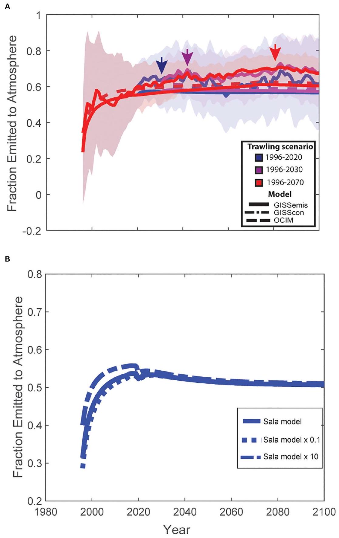
الشكل 1 نسبة الصيد بالشباك المنبعثة إلى الغلاف الجوي. (أ) نسبة الصيد بالشباك تم إصدارها إلى الغلاف الجوي من الصيد التاريخي (1996-2020) والتوقعات المستقبلية. تمثل الألوان سيناريوهات صيد مختلفة، حيث يشير اللون الأزرق إلى الصيد التاريخي من 1996-2020 وعدم وجود صيد بعد ذلك، ويشير اللون الأرجواني إلى سيناريو مستقبلي حيث يتوقف الصيد في عام 2030، ويشير اللون الأحمر إلى سيناريو مستقبلي حيث يتوقف الصيد العالمي في عام 2070. الخطوط المستمرة هي حلول متوسطة جماعية من تشغيلات GISSemis، والخطوط المنقطة المتقطعة هي من تشغيلات GISScon (غالبًا ما تكون غير مرئية في الرسم البياني بسبب تداخلها مع نقاط بيانات أخرى)، والخطوط المنقطة هي من محاكاة OCIM. يمثل التظليل التباين الداخلي في المحاكاة الجماعية باستخدام نموذج GISSemis. تشير الأسهم إلى متىمن إجمالي الانبعاثات التي يتم إطلاقها في الغلاف الجوي بعد الصيد بالشباك لكل من سيناريوهات الصيد الثلاثة. (ب) تأثير حجمتدفق على الكسر من المنبعثة إلى الغلاف الجوي. تمثل الخطوط البيانية الصلبة تدفق الصيد التاريخي (1996-2020) المقدر باستخدام نموذج الكربون لسالا وآخرون (2021)، بينما تمثل الخطوط المنقطة زيادة تعسفية (نموذج سالا) ) وانخفاض (نموذج سلاتقدير تدفق Sala وآخرون (2021) بزيادة مرتبة واحدة من الحجم. تمثل النماذج محاكاة OCIM.
طبقات الرواسب التي تكون أعمق من تلك التي تأثرت مباشرة بأدوات الصيد بالشباك. نموذج أتوود وآخرون (2020) شرحلتغير مخزونات الكربون العضوي وكان لديه خطأ جذر متوسط مربع قدرهعدم اليقين الإضافي في مخزونات الكربون الذي تم الاعتراف به، ولكن لم يتم تحديده من قبل أتوود وآخرون (2020) هو التباين في مخزونات الكربون مع عمق الرواسب. في العديد من الحالات، كان على أتوود وآخرون (2020) استقراء مخزونات الكربون إلى 1 متر باستخدام بيانات من عينات أقل عمقًا.
أكبر عدم يقين فينموذج إعادة التمعدن هو تقديرات ثوابت معدل التحلل من الدرجة الأولى-القيم). أظهرت الدراسات الميدانية أن-يمكن أن تتفاوت القيم بشكل كبير سواء من حيث الموقع أو العمق في الرواسب، وللأسف، فإن الدراسات التي تفحص تأثيرات الصيد بالشباك على نشاط الكربون العضوي والقيم محدودة للغاية. استخدمنا الـ-القيم المنشورة في سلا وآخرون (2021)، التي استخدمت مراجعة أدبية ومواقع تحقق مستقلة لتوصيف وتعميم الخصائص الإقليمية المحددةالقيم. عبر مواقع التحقق الخاصة بهم، كان متوسط نسبة خطأ النموذج لديهم في توقع الرواسب-الماءتراوحت التدفقات منإلىعند احتساب تدفق الكربون العضوي السنوي، مع متوسط خطأ مطلق قدره (أتوود وآخرون، 2023).
لقد اقترحت الدراسات أن تفاعل الكربون العضوي في الرواسب تحت السطحية قد يكون أقل بمقدار من مرتبتين إلى ثلاث مراتب من تلك المستخدمة في دراسة سلا وآخرون (2021) (إبستين وآخرون، 2022؛ هيدينك وآخرون، 2023). نتيجة لذلك، قمنا بالتحقيق في كيفية تأثير تخفيضات مرتبة واحدة ومرتبتين في معدلات التحلل من الدرجة الأولى في دراسة سلا وآخرون (2021) على تقديرات الانبعاثات الجوية. وجدنا أن تقديرات الانبعاثات في دراسة سلا وآخرون (2021) كانت قوية نسبيًا تجاه التغيرات في معدلات التحلل من الدرجة الأولى، لأن في نموذج الصيد متعدد السنوات، أدت التخفيضات في هذه المعلمة إلى تقليل كبير في استنفاد الكربون مع مرور الوقت. وفقًا لنموذج الكربون الأصلي في دراسة سلا وآخرون (2021) (العالمي )، قدرت نماذج GISS و OCIM أن الصيد بالشباك أطلق ما يصل إلى إلى الغلاف الجوي. عندما تم تقليل معدلات التحلل من الدرجة الأولى بمقدار مرتبة واحدة (المتوسط العالمي )، مما يؤدي إلى فقط كفاءة إعادة التمعدن للكربون العضوي المضطرب، ظلت كمية الانبعاثات الجوية مشابهة لنموذج سلا وآخرون (2021) الأصلي (0.19-0.21 بيغاطن من ثاني أكسيد الكربون سنويًا، أتوود وآخرون، 2023). الكميات قابلة للمقارنة لأن في نموذج سلا وآخرون (2021) الأصلي، يؤدي استنفاد الكربون العضوي بعد عقد من الصيد بالشباك إلى انبعاثات تكون من تدفق السنة الأولى. وعلى العكس، عندما تنخفض معدلات التحلل، يبقى المزيد من الكربون العضوي في النظام لفترة أطول، وتستقر التغيرات في التدفقات الناتجة عن الصيد بسرعة. ومع ذلك، فإن تقليل معدلات التحلل من الدرجة الأولى بمقدار مرتين (المتوسط العالمي; كفاءة إعادة التمعدن) تؤدي إلى انخفاض أكبر بكثير في الانبعاثات الجوية، والتي يتم تقليلها إلى (أتوود وآخرون، 2023)، أو من الانبعاثات العالمية الناتجة عن تغيير استخدام الأراضي (Friedlingstein et al., 2020a).
نماذجنا لا تأخذ في الاعتبار التأثيرات الناتجة عن الصيد بالشباك على إعادة معدنة الكربون العضوي بسبب التغيرات في الكائنات الحية في الرواسب (إبستين وآخرون، 2022). على الرغم من أن النموذج الحالي في علم التربة هو أن المجتمعات الميكروبية تهيمن على الأيض القاعى في الرواسب البحرية، وهي عملية تم أخذها في الاعتبار في نماذجنا، إلا أن الحيوانات تلعب بلا شك دورًا رئيسيًا في دورة الكربون في الرواسب البحرية (سنيلغروف وآخرون، 2018؛ لارو وآخرون، 2020؛ بيانكي وآخرون، 2021)؛ ومع ذلك، يتم تجاهل الحيوانات المائية والبرية بشكل عام في نماذج أنظمة الأرض (شميتز وآخرون، 2018؛ سنيلغروف وآخرون، 2018؛ بيانكي وآخرون، 2021). إن غياب الحيوانات عن نماذج أنظمة الأرض ينجم عن نقص التنبؤات القابلة للتعميم حول كيفية تأثير التغيرات في مجتمع الحيوانات على دورة الكربون (شميتز وآخرون، 2018؛ شميتز وآخرون، 2023). يمكن القول إن الصيد بالشباك يمكن أن يحفز أو يعيق إعادة معدنة الكربون العضوي من خلال تأثيراته المختلفة وغالبًا ما تكون معتمدة على السياق على مجتمعات الكائنات الحية في الرواسب (إبستين وآخرون، 2022). ومع ذلك، فإن الجسيمات الكبيرة يمكن أن تعوض عملية الخلط وغسل الرواسب الناتجة عن حركة معدات الصيد عبر قاع البحر بعض الخسائر المحتملة في عمليات مثل التربة الحيوية والري الحيوي. ومع ذلك، هناك حاجة إلى نماذج شاملة تشمل التأثيرات غير المباشرة للصيد بالشباك على إعادة تمعدن الكربون العضوي من خلال التغيرات في المجتمعات الحيوانية من أجل إجراء توقعات أكثر دقة، خاصة على مقاييس مكانية أصغر. ومع ذلك، من أجل تحسين توصيف التباين وعدم اليقين في معلمات النموذج، فإن الدراسات التجريبية واسعة النطاق حول العمليات البيولوجية والفيزيائية التي تتحكم في احتباس الكربون وإعادة تمعدنه في الرواسب البحرية، بالإضافة إلى كيفية تأثر هذه العمليات بالصيد بالشباك، تعتبر ضرورية.
2.6.3 الانبعاثات الجوية
من حيث استجابة النظام العالمي للهواء والبحرتدفق إلى نمط انبعاثات الصيد المحدد، تشير توافق النماذج إلى أن تقديرات الانبعاثات الجوية قوية إلى حد ما وأن التباين بين النماذج منخفض. بسبب دقة النماذج الخشنة (OCIM: القرار؛ GISS:القرار)، ومع ذلك، ستحتوي التقديرات الإقليمية على مزيد من عدم اليقين. وبالتالي، فإن أكبر قدر من عدم اليقين في تقديرات انبعاثات الغلاف الجوي يأتي من تحديدإعادة التمعدن الناتجة عن تأثيرات الصيد بالشباك على الكربون الرسوبي (انظر الشكوك أعلاه). الانبعاثات الجوية وكمية الصيد الناتج عن الشباكتم إعادة معدنة المقياس بشكل خطي لأن تقسيم الهواء والبحر يعتمد على زمن دوران المحيط وزمن تبادل الغاز، وكلاهما غير متأثر بالكمية الصغيرة نسبيًا من المنبعثة من الصيد بالشباك مقارنة بانبعاثات الوقود الأحفوري. لذلك، فإن أي تغييرات في كمية سيؤدي الناتج إلى تغيير متناسب مماثل في الغلاف الجويانبعاثات.
نماذجنا أيضًا لا تأخذ في الاعتبار إطلاق النيتروجين أو الفوسفور من الرواسب التي تم صيدها وإمكانية أن تحفز هذه العناصر الغذائية الإنتاجية الأولية في المياه المفتوحة. للأسف، لا توجد خرائط عالمية لمخزونات النيتروجين والفوسفور في الرواسب البحرية، وإلى علمنا، لا توجد دراسات تجريبية اختبرت هذه الفرضية بشكل صريح. ومع ذلك، اقترحت الدراسات والنظريات النمذجة أنه إذا كانت التأثيرات على تشتت الضوء الناتج عن الرواسب المعلقة قصيرة الأمد، فقد يؤدي الصيد إلى تحفيز الإنتاجية الأولية، وبالتالي امتصاص (دوناس وآخرون، 2007؛ إبستين وآخرون، 2022).
2.6.4 التغير المناخي الداخلي
تهدف مجموعة محاكاة GISSemis إلى تقييم الأهمية النسبية للاستجابة لانبعاثات الصيد بالمصائد مقارنة بتقلبات النظام الداخلية. متوسط المجموعة قريب جدًا من استجابات GISScon و OCIM بينما يمكن أن تنتج التقلبات الداخلية مجموعة واسعة من استجابات الأعضاء الفرديين في المجموعة التي يمكن أن تكونمتوسط المجموعة للغلاف الجويتغيير ومن متوسط المجموعة لتغير خزان الكربون في المحيط (انظر الجدول S1). ومع ذلك، فإن هذه الشكوك تعتمد على النموذج وقد تكون مختلفة بالنسبة لنماذج المناخ الأخرى.
3 النتائج والمناقشة
أظهرت تحليلاتنا الاستعادية والمستقبلية أنمنأُطلق في عمود الماء بواسطة الصيد بالشباك القاعية تأثيرات على مخزونات الكربون في الرواسب تُ emitted إلى الغلاف الجوي ضمنسنوات حدث الجر (الشكل 1). علاوة على ذلك، وجدنا أن نسبةتتراكم في الغلاف الجوي ظلت عندحتى نهاية محاكياتنا في عام 2100، بغض النظر عن حجممن المتوقع أن يتم إطلاقها في عمود الماء عن طريق الصيد بالشباك (الشكل 1). هذه النتائج مهمة لأنها تشير إلى أنيمكن تطبيق الكسر بسهولة لتقدير تأثير الصيد بالشباك.الانبعاثات إلى الغلاف الجوي تحت مجموعة متنوعة من سيناريوهات الصيد التاريخية والمستقبلية.
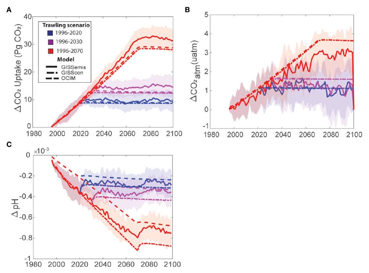
باستخدام تقديرات سلا وآخرون (2021) لتدفق الرواسب، تقترح نماذجنا أن الصيد بالشباك قد يكون قد أطلق كمية تراكمية منإلى الغلاف الجوي بين عامي 1996 و2020 (الجدول S1؛ الشكل 2)، مما يساهمإلى جويتركيزات (الشكل 2). ستعادل هذه الانبعاثات، وهو ما يعادل من الانبعاثات العالمية الناتجة عن تغيير استخدام الأراضي في عام 2020 (فريدلينغستين وآخرون، 2020ب)، أو ما يقرب من ضعف الانبعاثات السنوية المقدرة الناتجة عن احتراق الوقود لأسطول الصيد العالمي بأكمله (باركر وآخرون، 2018). تشير انبعاثات الصيد بالشباك إلى هذا الحجم إلى أن حماية الكربون العضوي في قاع البحر من معدات الصيد القاعية قد تثبت أنها حل مناخي مؤثر. على سبيل المثال، إذا استمرينا في الصيد بالشباك بنفس الكثافات والتوزيعات المكانية الحالية، فإننا نقدر أن الصيد القاعي قد يساهم بمزيد منفي الغلاف الجويتركيزات بحلول عام 2030 و1.03-1.36 جزء في المليون بحلول عام 2070 (الشكل 2).
سواء كانت التخفيضات في الصيد بالشباك يمكن تكييفها كحل مناخي أم لا، لا يعتمد فقط على حجم تخفيضات الانبعاثات، ولكن أيضًا على الإطار الزمني الذي يمكن تحقيق تلك التخفيضات فيه. وجدنا أن إطلاق الانبعاثات الناتجة عن الصيد بالشباكمن المحيط إلى الغلاف الجوي حدث بسرعة، معمن إجمالي الانبعاثات التي تحدث خلال 7-9 سنوات بعد الصيد القاعي (OCIM: 7 سنوات؛ GISScon: 9 سنوات؛ GISSemis: (الانحراف المعياري لأعضاء المجموعة). عندما تم زيادة الانبعاثات بشكل عشوائي بمقدار مرتبة واحدة، استغرق الأمر وقتًا أقل قليلاً (OCIM: ~5 سنوات) لإطلاق إجمالي الانبعاثات في الغلاف الجوي. الإطلاق السريع لـمن المحيط إلى الغلاف الجوي يشير إلى أن الصيد بالشباك له تأثيرات إرثية قصيرة الأجل فقط على انبعاثات الغلاف الجوي. وبالتالي، فإن السياسات التي تقضي على أو تحد بشكل كبير من تأثيرات الصيد بالشباك على مخزونات الكربون الرسوبية ستقلل بسرعة من مساهمة هذه الصناعة في ارتفاع مستويات الغلاف الجوي.تركيزات مع أقصى الفوائد التي تحدث بعد 7-9 سنوات من التنفيذ.
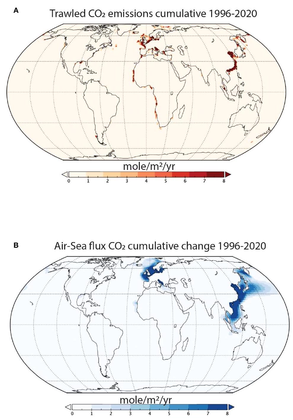
بشكل عام، الغلاف الجويتزامنت نقاط انبعاث الغازات مع المناطق التي كان لصيد القاع فيها أكبر تأثير على الكربون القاعي، وخاصة بحر الصين الشرقي، وبحر البلطيق، وبحر الشمال، وبحر غرينلاند (الشكل 3). ومع ذلك، يمكن أن تنقل الحركة الأفقية التأثيرات الناتجة عن صيد القاع.وإعادة تعليق الكربون العضوي إلى مواقع أخرى، مما يؤدي إلى تأثيرات عبر الحدود لصيد القاع على الدورات الكربونية المحلية. من المحتمل أن يفسر هذا الظاهرة سبب وجود بعض المناطق مثل بحر الصين الجنوبي، وبحر النرويج، قبالة الساحل الشرقي
الشكل 2 آثار الصيد القاعي علىانبعاثات ودرجة حموضة المياه القاعية. سلسلة زمنية لـتغيير في الامتصاص التراكمي للكربون بواسطة المحيط بسبب الصيد بالشباك، أو ما يعادل ذلك تدفقإلى الغلاف الجوي، (ب) تغيير في الغلاف الجويتركيزات بسبب الصيد بالشباك في محاكاة النماذج المختلفة (OCIM، GISScon، GISSemis)، و (C) تغيير pH في المحيط العالمي بسبب الصيد بالشباك. تمثل الألوان سيناريوهات صيد مختلفة، حيث يشير اللون الأزرق إلى الصيد التاريخي من 1996-2020 وعدم وجود صيد بعد ذلك، ويشير اللون الأرجواني إلى سيناريو مستقبلي حيث يتوقف الصيد في 2030، ويشير اللون الأحمر إلى سيناريو مستقبلي حيث يتوقف الصيد العالمي في 2070. الخطوط المستمرة هي حلول متوسط المجموعة من تشغيلات GISSemis، والخطوط المنقطة المتقطعة هي من تشغيلات GISScon، والخطوط المتقطعة هي من محاكاة OCIM. التظليل يمثل التباين الداخلي في محاكاة المجموعة باستخدام نموذج GISSemis.
الشكل 3 الاختلافات المكانية في التأثيرات التاريخية لصيد القاع بالشباك الانبعاثات. (أ) الانبعاثات التراكمية للصيد بالشباك بين 1996-2020. (ب) التغيرات التراكمية في الهواء والبحرالتدفق الناتج عن الصيد بالشباك بين عامي 1996-2020. من المهم ملاحظة أن هناك فجوات معرفية كبيرة بشأن نشاط الصيد بالشباك في بحر القطب الشمالي (منطقة الفاو 18) والمحيط الهادئ الغربي المركزي (منطقة الفاو 71) والمحيط الهندي الشرقي (منطقة الفاو 57) (تاكونيت وآخرون، 2019). وبالتالي، من المحتمل أن تكون الانبعاثات المنسوبة إلى الصيد بالشباك في هذه المناطق مقدرة بأقل من قيمتها الحقيقية.
ساحل اليابان في المحيط الهادئ كان لديه انبعاثات جوية أعلى من المتوقع بناءً على معدل انبعاثات الصيد بالشباك المحلي (الشكل 3). نتيجة لهذه التأثيرات العابرة للحدود، لا يمكننا افتراض أن جميع الانبعاثات الجوية داخل المياه القضائية لدولة ما تأتي من أنشطة الصيد بالشباك داخل تلك المنطقة.
كانت قدرتنا على قياس مدى أسطول الصيد القاعي العالمي عبر الزمن والمكان في هذه الدراسة محدودة بعض الشيء. تقديراتنا لا تشمل أنشطة الصيد القاعي قبل عام 1996، لأن كثافة وتوزيع الصيد القاعي قبل ذلك الوقت غير معروفة. ومع ذلك، بدأ الصيد القاعي على نطاق واسع في وقت مبكر من عام 1950 وبلغ ذروته في الثمانينيات والتسعينيات (واتسون وآخرون، 2006؛ واتسون وتيد، 2018). علاوة على ذلك، يعتمد نموذجنا على قاعدة بيانات تتبع السفن AIS المعالجة بواسطة Global Fishing Watch (https://globalfishingwatch.org/) لاشتقاق أحداث الجر على المستوى العالمي. للأسف، فإن تغطية نظام تحديد الهوية الآلي ضعيفة في بعض المناطق التي تتركز فيها أنشطة الصيد. وبالتالي، نحن بلا شك ن underestimate نشاط الجر في المناطق جنوب شرق آسيا، خليج البنغال، البحر العربي، أجزاء من أوروبا، وخليج المكسيك (تاكونيه وآخرون، 2019).
هناك عدم يقين إضافي في المعلمات المستخدمة لتقدير كمية الكربون العضوي المعاد التمعدن بعد الصيد بالشباك بسبب نقص الدراسات الميدانية الدقيقة. على الرغم من أن نموذجنا مُعَد باستخدام أفضل البيانات التجريبية المتاحة (سالا وآخرون، 2021؛ أتوود وآخرون، 2023)، إلا أن هناك خطًا بديلًا من التفكير يجادل بأن معدلات التحلل من الدرجة الأولى قد تكون أقل بمقدار من مرتبتين إلى ثلاث مراتب (هيدينك وآخرون، 2023). لأننا نجد أن انبعاثات الغلاف الجوي تتناسب خطيًا مع كمية الكربون العضوي المعاد التمعدن إلى الماء.من خلال الصيد بالشباك، يمكننا بشكل مباشر فحص حساسية نتائجنا تجاه هذا الافتراض البديل. بالاستفادة من اكتشاف أتود وآخرون (2023) بأن تقليل معدلات التحلل من الدرجة الأولى بمقدار مرتبة واحدة له تأثير ضئيل على المقدار المقدر للكربون العضوي المعاد التمعدن بعد 10 سنوات متتالية من الصيد بالشباك، نجد أن الاحتفاظ بهذا التخفيض لمعدلات التدهور من الدرجة الأولى يؤدي إلى تقديرتم انبعاثه إلى الغلاف الجوي بسبب الصيد القاعي بين عامي 1996-2020. ستؤدي تقليص بمقدار مرتبتين من حيث الحجم إلى تدهور من الدرجة الأولى إلىالمنبعثة خلال نفس الفترة الزمنية – مقارنة بإمكانات التخفيف لإدارة الحرائق في الغابات المعتدلة (غريسكم وآخرون، 2017).
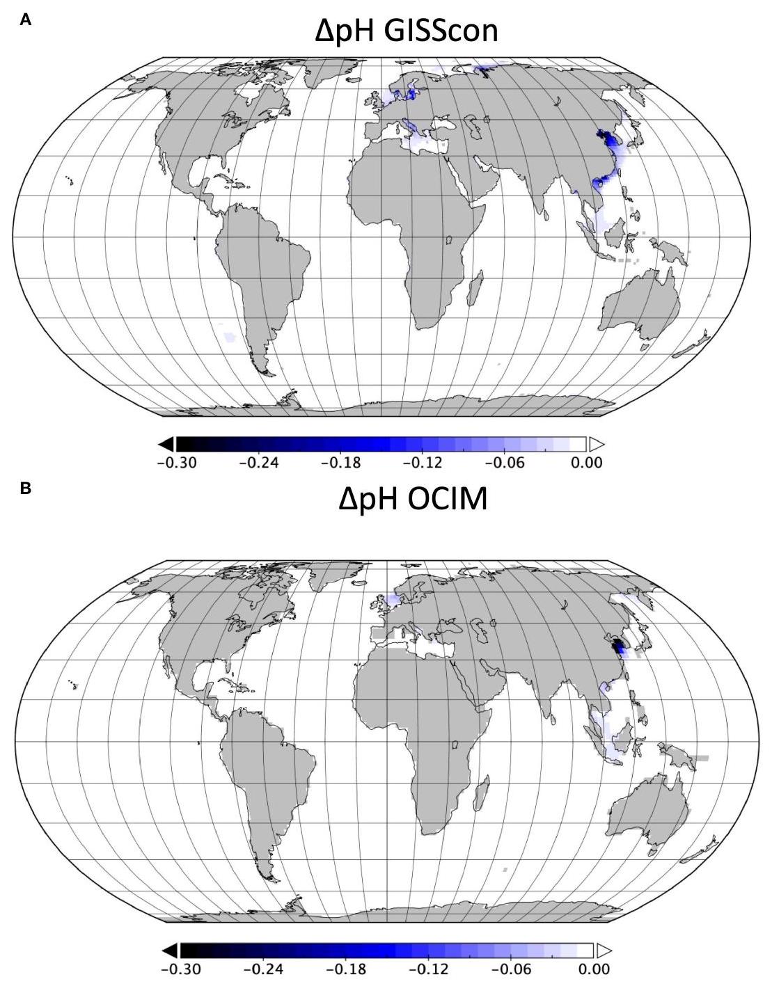
حالياً، الإجراءات المناخية التي تهدف إلى تقليلالانبعاثات الناتجة عن الممارسات البشرية (مثل أسواق الكربون، معايير الطاقة المتجددة، جهود إعادة التشجير، إلخ) تركز بشكل حصري على الانبعاثات الجوية. ومع ذلك، تتجاهل هذه الأطر التأثير الكلي لأنشطة تغيير استخدام المحيطات على دورة الكربون، لأنها تتجاهل كمية الكربون غير العضوي المذاب التي تبقى محجوزة في المحيط. في حالة الصيد بالشباك، وجدنا أنمن الصيد الجائر التراكمي الناتج عنظلّت الانبعاثات مذابة في مياه البحر، مما زاد من الحموضة التي تحدث بالفعل نتيجة احتراق الوقود الأحفوري. باستخدام نموذج الكربون لسالا وآخرون (2021)، وجدنا أن الصيد بالشباك زاد من المخزون العالمي من الكربون غير العضوي المذاب بحوالي 1.82-1.90 بيغاغرام من الكربون من 1996 إلى 2020 (الجدول S1). هذا الكربون غير العضوي المذاب الإضافي الناتج عن الصيد بالشباك يؤدي إلى زيادة حموضة المحيطات مع انخفاض عالمي في الرقم الهيدروجيني لـبحلول عام 2020 (الشكل 2). على المستوى العالمي، فإن انخفاض درجة الحموضة بهذا القدر بحلول عام 2020 ليس له دلالة كبيرة مقارنة بتأثير الانبعاثات البشرية الناتجة عن الوقود الأحفوري. ومع ذلك، تشير نماذجنا إلى أن بعض البحار شبه المغلقة قد تكون حساسة للغاية لحقنمن الأنشطة البشرية. على وجه الخصوص، أظهرت نماذجنا أن الصيد بالشباك الواسعة يمكن أن يؤدي إلى زيادة حموضة موضعية في بحر الصين الشرقي والجنوبي (الشكل 4). إن الانخفاض في درجة الحموضة في هذه المنطقة بسبب الصيد بالشباك بين عامي 2000 و2020 (GISSemis: -0.034+/-0.001؛ OCIM: -0.050) قابل للمقارنة مع ذلك الناتج عن ارتفاع الغازات في الغلاف الجوي.بسبب احتراق الوقود الأحفوري خلال نفس الفترة الزمنية (GISSemis: -0.034+/-0.004؛ OCIM: -0.020). تحذير مهم لنتائجنا المتعلقة بالرقم الهيدروجيني هو أن نماذجنا محدودة في حل العمليات الساحلية بسبب دقتها المنخفضة ونقص التعقيد البيوجيوكيميائي. ومع ذلك، بالنظر إلى أن
الشكل 4 الفروق المكانية في التأثيرات التاريخية للصيد القاعي على الرقم الهيدروجيني. التغير في متوسط الرقم الهيدروجيني في الألف متر العلوية بسبب الصيد في عام 2020 لـ (A) نتائج نموذج GISScon و (B) نتائج نموذج OCIM.
يمكن أن تؤثر كيمياء المحيطات على تطور الكائنات الحية، وعلم وظائف الأعضاء، والسلوك (باك ومندال، 2022)، وفي النهاية يمكن أن تؤثر على إنتاجية species وبقائها. يجب أن تأخذ الدراسات والسياسات المستقبلية في الاعتبار التأثيرات المحتملة التي يمكن أن يحدثها الصيد بالشباك على حموضة المحيطات المحلية.
4 الخاتمة
تقدم الحلول المستندة إلى المحيطات وعدًا في سد الفجوة في الانبعاثات للحد من زيادة درجات الحرارة العالمية إلى، بينما تدعم أيضًا الفوائد المشتركة مثل الحفاظ على التنوع البيولوجي والأمن الغذائي (هوغ غولدبرغ وآخرون، 2019؛ سلا وآخرون، 2021). ومع ذلك، تتطلب السياسات والأسواق المناخية الحالية تقديرات لانبعاثات الغازات المسببة للاحتباس الحراري التي تم تجنبها، مما يطرح تحديات لتحديد وتنفيذ هذه الحلول. دراستنا، التي تبرز أن منالذي يتم إنتاجه من الصيد القاعي يتم إطلاقه في الغلاف الجوي خلال تسع سنوات، ويصبح أداة حاسمة لتقييم تقليل جهد الصيد القاعي كحل فعال قائم على المحيطات لمشكلة المناخ. لتحسين تقديرات الانبعاثات الجوية، من الضروري أن تتناول الدراسات الميدانية الشكوك في فهمنا لكيفية تأثير الصيد القاعي على العمليات البيولوجية والفيزيائية التي تحكم إعادة معدنة الكربون والحفاظ عليه. علاوة على ذلك، سيكون دمج النماذج الإقليمية عالية الدقة التي تحل العمليات الصغيرة النطاق، مثل التيارات المحلية، محورياً في تقديم تقديرات انبعاثات أكثر دقة على مقاييس ذات صلة بالاعتبارات السياسية المحلية. أخيراً، تؤكد نتائجنا على الحاجة إلى سياسة تتجنب التركيز الحصري على الانبعاثات الجوية المتجنبة، حيث تظهر نتائجنا أن الزيادات الناتجة عن الصيد في DIC في مياه البحر قد يكون لها تداعيات خطيرة على حموضة المحيطات المحلية أو الإقليمية.
ساهم جميع المؤلفين في تصور وتصميم الدراسة. قام AR وPL وTD وJM بإجراء تحليلات البيانات. كتب TA الـ المسودة الأصلية للمخطوطة وشارك جميع المؤلفين في مراجعتها وتحريرها. ساهم جميع المؤلفين في المقالة ووافقوا على النسخة المقدمة.
تمويل
يعلن المؤلفون أن الدعم المالي قد تم تلقيه للبحث، والتأليف، و/أو نشر هذه المقالة. يقر TA و JM و DB و RC و ES بالحصول على تمويل من National Geographic Pristine Seas. تم تمويل TA من خلال زمالة بحثية مبكرة من برنامج أبحاث الخليج التابع للأكاديميات الوطنية للعلوم والهندسة والطب (المحتوى هو مسؤولية المؤلفين فقط ولا يمثل بالضرورة الآراء الرسمية لبرنامج أبحاث الخليج التابع للأكاديميات الوطنية للعلوم والهندسة والطب). تم تمويل TD من قبل المؤسسة الوطنية للعلوم بموجب منحة OCE1948955. تم دعم AR و PL و GS من قبل برنامج النمذجة والتحليل والتنبؤ من ناسا ومن قبل برنامج الحوسبة عالية الأداء من خلال مركز ناسا لمحاكاة المناخ في مركز غودارد لرحلات الفضاء.
الشكر والتقدير
نشكر Y. روسو على الأفكار حول الأنماط الزمنية في الصيد بالشباك.
تضارب المصالح
يعلن المؤلفون أن البحث تم إجراؤه في غياب أي علاقات تجارية أو مالية يمكن أن تُفسر على أنها تعارض محتمل للمصالح.
ملاحظة الناشر
جميع المطالبات المعبر عنها في هذه المقالة هي فقط تلك الخاصة بالمؤلفين ولا تمثل بالضرورة تلك الخاصة بالمنظمات التابعة لهم، أو الناشر، أو المحررين والمراجعين. أي منتج قد يتم تقييمه في هذه المقالة، أو أي ادعاء قد يتم تقديمه من قبل الشركة المصنعة له، غير مضمون أو مدعوم من قبل الناشر.
Amoroso, R. O., Pitcher, C. R., Rijnsdorp, A. D., McConnaughey, R. A., Parma, A. M., Suuronen, P., et al. (2018). ). Bottom trawl fishing footprints on the world’s continental shelves. Proc. Natl. Acad. Sci. 115, E10275-E10282. doi: 10.1073/pnas. 1802379115
Atwood, T., Sala, E., Mayorga, J., Bradley, D., Cabral, R. B., Auber, A., et al. (2023). Response to comment on “Quantifying the carbon benefits of ending bottom trawling. Nature 617, E3-E5. doi: 10.1038/s41586-023-06015-6
Atwood, T. B., Witt, A., Mayorga, J., Hammill, E., and Sala, E. (2020). Global patterns in marine sediment carbon stocks. Front. Mar. Sci. 7. doi: 10.3389/fmars.2020.00165
Baag, S., and Mandal, S. (2022). Combined effects of ocean warming and acidification on marine fish and shellfish: A molecule to ecosystem perspective. Sci. Total Environ. 802. doi: 10.1016/j.scitotenv.2021.149807
Bianchi, T. S., Aller, R. C., Atwood, T. B., Brown, C. J., Buatois, L. A., Levin, L. A., et al. (2021). What global biogeochemical consequences will marine animal-sediment interactions have during climate change. Elem. Sci. Anth. 9, 1-25. doi: 10.1525/elementa.2020.00180
Burdige, D. J. (2007). Preservation of organic matter in marine sediments: Controls, mechanisms, and an imbalance in sediment organic carbon budgets? Chem. Rev. 107, 467-485. doi: cr050347q
DeVries, T. (2014). The oceanic anthropogenic CO2 sink: Storage, air-sea fluxes, and transports over the industrial era. Global Biogeochem. Cycles 28, 631-647. doi: 10.1002/2013GB004739
Dounas, C., Davies, I., Triantafyllou, G., Koulouri, P., Petihakis, G., Arvanitidis, C., et al. (2007). Large-scale impacts of bottom trawling on shelf primary productivity. Cont. Shelf Res. 27, 2198-2210. doi: 10.1016/j.csr.2007.05.006
Eigaard, O. R., Bastardie, F., Breen, M., Dinesen, G. E., Hintzen, N. T., Laffargue, P., et al. (2016). Estimating seabed pressure from demersal trawls, seines, and dredges based on gear design and dimensions. ICES J. Mar. Sci. 73, i27-i43. doi: 10.1093/icesjms/fsv099
Epstein, G., Middelburg, J. J., Hawkins, J. P., Norris, C. R., and Roberts, C. M. (2022). The impact of mobile demersal fishing on carbon storage in seabed sediments. Glob. Change Biol. 28, 2875-2894. doi: 10.1111/gcb. 16105
Friedlingstein, P., O’Sullivan, M., Jones, M., Andrew, R., Hauck, J., Olsen, A., et al. (2020a). Global carbon budget 2021. Preprint 10.5194/es, 1-3. doi: 10.5194/essd-2020-286
Friedlingstein, P., O’Sullivan, M., Jones, M. W., Andrew, R. M., Hauck, J., Olsen, A., et al. (2020b). Global carbon budget 2020. Earth Syst. Sci. Data 12, 3269-3340. doi: 10.5194/essd-12-3269-2020
Garcia, H. E., Weathers, K. W., Paver, C. R., Smolyar, I. V., Boyer, T. P., Locarnini, R. A., et al. (2019). “Dissolved inorganic nutrients (phosphate, nitrate and nitrate + nitrite, silicate,” in World atlas 2018. Ed. A. V. Mishonov (Silver Springs, MD: USA Department of Commerce), 35. NOAA Atlas NESDIS 84.
Gregg, W. W., and Casey, N. W. (2007). Modeling coccolithophores in the global oceans. Deep. Res. Part II Top. Stud. Oceanogr. 54, 447-477. doi: 10.1016/j.dsr2.2006.12.007
Griscom, B. W., Adams, J., Ellis, P. W., Houghton, R. A., Lomax, G., Miteva, D. A., et al. (2017). Natural climate solutions. Proc. Natl. Acad. Sci. 114, 11645-11650. doi: 10.1073/pnas. 1710465114
Hiddink, J. G., Jennings, S., Sciberras, M., Szostek, C. L., Hughes, K. M., Ellis, N., et al. (2017). Global analysis of depletion and recovery of seabed biota after bottom trawling disturbance. Proc. Natl. Acad. Sci. U.S.A. 114, 8301-8306. doi: 10.1073/pnas. 1618858114
Hiddink, J. G., van de Velde, S., McConnaughey, R. A., De Borger, E., O’Neill, F. G., Tiano, J., et al. (2023). Quantifying the carbon benefits of ending bottom trawling. Nature 617, E1-E2. doi: 10.1038/s41586-023-06014-7
Hoegh-Guldberg, O., Northrop, E., and Lubchenco, J. (2019). The ocean is key to achieving climate and societal goal. Science 365, 1372-1374. doi: 10.1126/science.aaz4390
Holzer, M., DeVries, T., and de Lavergne, C. (2021). Diffusion controls the ventilation of a Pacific Shadow Zone above abyssal overturning. Nat. Commun. 12, 1-13. doi: 10.1038/s41467-021-24648-x
IPCC (2022). Climate change 2022: impacts, adaptation, and vulnerability. contribution of working group ii to the sixth assessment report of the intergovernmental panel on climate change. H.-O. Pörtner, D. C. Roberts, M. Tignor, E. S. Poloczanska, K. Mintenbeck, A. Alegría, M. Craig, S. Langsdorf, S. Löschke, V. Möller, A. Okem and B. Rama (eds.). (Cambridge, UK and New York, NY, USA: Cambridge University Press), 3056 pp. doi: 10.1017/9781009325844
Ito, G., Romanou, A., Kiang, N. Y., Faluvegi, G., Aleinov, I., Ruedy, R., et al. (2020). Global carbon cycle and climate feedbacks in the NASA GISS ModelE2.1. J. Adv. Model. Earth Syst. 12, 1-44. doi: 10.1029/2019MS002030
LaRowe, D. E., Arndt, S., Bradley, J. A., Estes, E. R., Hoarfrost, A., Lang, S. Q., et al. (2020). The fate of organic carbon in marine sediments – New insights from recent data and analysis. Earth-Science Rev. 204, 103146. doi: 10.1016/j.earscirev.2020.103146
Lerner, P., Romanou, A., Kelley, M., Romanski, J., Ruedy, R., and Russell, G. (2021). Drivers of air-sea CO2 flux seasonality and its long-term changes in the NASA-GISS model CMIP6 submission. J. Adv. Model. Earth Syst. 13, 1-33. doi: 10.1029/2019MS002028
Levin, L. A., Wei, C. L., Dunn, D. C., Amon, D. J., Ashford, O. S., Cheung, W. W. L., et al. (2020). Climate change considerations are fundamental to management of deepsea resource extraction. Glob. Change Biol. 26, 4664-4678. doi: 10.1111/gcb. 15223
Locarnini, R. A., Mishonov, A. V., Baranova, O. K., Boyer, T. P., Zweng, M. M., Garcia, H. E., et al. (2019). World ocean atlas 2018 , volume 1: temperatureEd.A. Mishonov (Silver Springs, MD: USA Department of Commerce).
Luisetti, T., Ferrini, S., Grilli, G., Jickells, T. D., Kennedy, H., Kröger, S., et al. (2020). Climate action requires new accounting guidance and governance frameworks to manage carbon in shelf seas. Nat. Commun. 11, 1-10. doi: 10.1038/ s41467-020-18242-w
Meinshausen, M., Nicholls, Z., Lewis, J., Gidden, M., Vogel, E., Freund, M., et al. (2020). The SSP greenhouse gas concentrations and their extensions to 2500. Geosci. Model. Dev. Discuss. 13, 3571-3605. doi: 10.5194/gmd-13-3571-2020
Miller, R. L., Schmidt, G. A., Nazarenko, L. S., Bauer, S. E., Kelley, M., Ruedy, R., et al. (2021). CMIP6 historical simulations, (1850-2014) with GISS-E2.1. J. Adv. Model. Earth Syst. 13, 1-35. doi: 10.1029/2019MS002034
Najjar, R., and Orr, J. (1999). “Design of ocmip-2 simulations of chlorofluorocarbons, the solubility pump and common biogeochemistry [OCMIP-2 Protocols],” in OCMIP web applications. (Silver Springs, MD: USA Department of Commerce). Available at: http:// ocmip5.ipsl.fr/documentation/OCMIP/phase2/.
Olsen, A., Key, R. M., Van Heuven, S., Lauvset, S. K., Velo, A., Lin, X., et al. (2016). The global ocean data analysis project version 2 (GLODAPv2) – An internally consistent data product for the world ocean. Earth Syst. Sci. Data 8, 297-323. doi: 10.5194/essd-8-297-2016
O’Neill, B. C., Tebaldi, C., Van Vuuren, D. P., Eyring, V., Friedlingstein, P., Hurtt, G., et al. (2016). The scenario model intercomparison project (ScenarioMIP) for CMIP6. Geosci. Model. Dev. 9, 3461-3482. doi: 10.5194/gmd-9-3461-2016
Orr, J. C., Najjar, R. G., Aumont, O., Bopp, L., Bullister, J. L., Danabasoglu, G., et al. (2017). Biogeochemical protocols and diagnostics for the CMIP6 ocean model intercomparison project (OMIP). J. Geophys. Res. Atmos. 112, 2169-2199. doi: 10.1029/2007JD008643
Paradis, S., Goñi, M., Masqué, P., Durán, R., Arjona-Camas, M., Palanques, A., et al. (2021). Persistence of biogeochemical alterations of deep-sea sediments by bottom trawling. Geophys. Res. Lett. 48, 1-12. doi: 10.1029/2020gl091279
Parker, R. W. R., Blanchard, J. L., Gardner, C., Green, B. S., Hartmann, K., Tyedmers, P. H., et al. (2018). Fuel use and greenhouse gas emissions of world fisheries. Nat. Clim. Change 8, 333-337. doi: 10.1038/s41558-018-0117-x
Pauly, D., Zeller, D., and Palomares, M. L. D. (2020). Sea around us concepts, design and data. (Silver Springs, MD: USA Department of Commerce).
Romanou, A., Gregg, W. W., Romanski, J., Kelley, M., Bleck, R., Healy, R., et al. (2013). Natural air-sea flux of CO2 in simulations of the NASA-GISS climate model: Sensitivity to the physical ocean model formulation. Ocean Model. 66, 26-44. doi: 10.1016/j.ocemod.2013.01.008
Rousseau, Y., Watson, R. A., Blanchard, J. L., and Fulton, E. A. (2019). Evolution of global marine fishing fleets and the response of fished resources. Proc. Natl. Acad. Sci. U.S.A. 116, 12238-12243. doi: 10.1073/pnas. 1820344116
Sala, E., Mayorga, J., Bradley, D., Cabral, R. B., Atwood, T. B., Auber, A., et al. (2021). Protecting the global ocean for biodiversity, food and climate. Nature 592, E25. doi: 10.1038/s41586-021-03496-1
Schmitz, O. J., Sylvén, M., Atwood, T. B., Bakker, E. S., Berzaghi, F., Brodie, J. F., et al. (2023). Trophic rewilding can expand natural climate solutions. Nat. Clim. Chang. 13, 324-333. doi: 10.1038/s41558-023-01631-6
Schmitz, O. J., Wilmers, C. C., Leroux, S. J., Doughty, C. E., Atwood, T. B., Galetti, M., et al. (2018). Animals and the zoogeochemistry of the carbon cycle. Sci. (80-. ). 362, eaar3213. doi: 10.1126/science.aar3213
Siegel, D. A., Devries, T., Doney, S. C., and Bell, T. (2021). Assessing the sequestration time scales of some ocean-based carbon dioxide reduction strategies. Environ. Res. Lett. 16, 104003. doi: 10.1088/1748-9326/ac0be0
Snelgrove, P. V. R., Soetaert, K., Solan, M., Thrush, S., Wei, C. L., Danovaro, R., et al. (2018). Global carbon cycling on a heterogeneous seafloor. Trends Ecol. Evol. 33, 96105. doi: 10.1016/j.tree.2017.11.004
Taconet, M., Kroodsma, D., and Fernandes, J. A. (2019). Global atlas of AIS-based fishing activity-Challenges and opportunities (FAO: Rome).
van Heuven, S., Pierrot, D., Rae, J. W. B., Lewis, E., and Walace, D. W. R. (2011). CO2SYS v 1.1 : MATLAB program developed for CO2 system calculations. ORNL/ CDIAC-105b. (Silver Springs, MD: USA Department of Commerce). doi: 10.3334/ CDIAC/otg.CO2SYS_MATLAB_v1.1
Watson, R. A. (2017). A database of global marine commercial, small-scale, illegal and unreported fisheries catch 1950-2014. Sci. Data 4, 1-9. doi: 10.1038/sdata.2017.39
Watson, R., Revenga, C., and Kura, Y. (2006). Fishing gear associated with global marine catches. II. Trends in trawling and dredging. Fish. Res. 79, 103-111. doi: 10.1016/j.fishres.2006.01.013
Watson, R. A., and Tidd, A. (2018). Mapping nearly a century and a half of global marine fishing: 1869-2015. Mar. Policy 93, 171-177. doi: 10.1016/ j.marpol.2018.04.023
Wilkinson, G. M., Besterman, A., Buelo, C., Gephart, J., and Pace, M. L. (2018). A synthesis of modern organic carbon accumulation rates in coastal and aquatic inland ecosystems. Sci. Rep. 8, 1-9. doi: 10.1038/s41598-018-34126-y
Zweng, M. M., Reagan, J. R., Seidov, D., Boyer, T. P., Locarnini, R. A., Garcia, A. V., et al. (2018). World ocean atlas 2018 volume 2 : salinityEd. A. Mishonov (Silver Springs, MD: USA Department of Commerce).
Maria Muñoz Muñoz,
University of Malaga, Spain
Simon Thrush,
The University of Auckland, New Zealand
*CORRESPONDENCE
Trisha B. Atwood Trisha.atwood@usu.edu
received 15 December 2022
ACCEPTED 01 December 2023
published 18 January 2024
CITATION
Atwood TB, Romanou A, DeVries T, Lerner PE, Mayorga JS, Bradley D, Cabral RB, Schmidt GA and Sala E (2024) Atmospheric emissions and ocean acidification from bottom-trawling.
Front. Mar. Sci. 10:1125137.
doi: 10.3389/fmars.2023.1125137
Atmospheric emissions and ocean acidification from bottom-trawling
Trisha B. Atwood , Anastasia Romanou , Tim DeVries , Paul E. Lerner , Juan S. Mayorga , Darcy Bradley , Reniel B. Cabral , Gavin A. Schmidt and Enric Sala Department of Watershed Sciences and the Ecology Center, Utah State University, Logan, UT, United States, NASA Goddard Institute for Space Studies, New York, NY, United States, Department of Applied Physics and Applied Mathematics, Columbia University, New York, NY, United States, Department of Geography and Earth Research Institute, University of California, Santa Barbara, Santa Barbara, CA, United States, National Geographic Society, Washington, DC, United States, Environmental Markets Lab, University of California, Santa Barbara, Santa Barbara, CA, United States, Marine Science Institute, University of California, Santa Barbara, CA, United States, College of Science and Engineering, James Cook University, Townsville, QLD, Australia
Abstract
Trawling the seafloor can disturb carbon that took millennia to accumulate, but the fate of that carbon and its impact on climate and ecosystems remains unknown. Using satellite-inferred fishing events and carbon cycle models, we find that of trawling-induced aqueous is released to the atmosphere over 7-9 years. Using recent estimates of bottom trawling’s impact on sedimentary carbon, we found that between 1996-2020 trawling could have released, at the global scale, up to to the atmosphere, and locally altered water pH in some semi-enclosed and heavy trawled seas. Our results suggest that the management of bottom-trawling efforts could be an important climate solution.
Marine sediments are thought to be the ultimate long-term carbon store; once buried below the active layer, organic carbon can remain unmineralized for millennia to eons (Burdige, 2007; LaRowe et al., 2020). However, disturbances to the seabed by human activities threaten the permanency of this marine carbon (Levin et al., 2020; Paradis et al., 2021). In the case of bottom trawling, heavy fishing gear that is dragged across the seafloor mixes and resuspends sediments, exposing of previously buried organic carbon to potential microbial degradation (Sala et al., 2021). However, the ultimate fate of this disturbed organic carbon stock is as yet unquantified,
hampering our understanding of the effects that bottom trawling has on the global carbon cycle and the potential implications for climate policies.
The protection of organic carbon stored in marine sediments, plants, and animals has been identified as a powerful tool for tackling climate change (Hoegh-Guldberg et al., 2019). However, the uptake of ocean-based climate solutions has been slow due to prevailing climate policies and carbon markets that only recognize mitigation activities with measurable impacts on atmospheric emissions. The challenge with identifying ocean-based solutions under those current paradigms lies in the complexity of quantifying atmospheric emissions generated by anthropogenic activities that occur below the ocean’s surface (Luisetti et al., 2020). Therefore, research addressing this challenge is crucial for discovering new opportunities that can harness the full potential of the ocean in contributing to mitigating climate change.
Here, we examined the fate of trawling-induced carbon released into the global ocean between 1996-2020 and under future scenarios, as well as estimated the fraction of emitted to the atmosphere. To estimate trawling-induced emissions, we used assumptions and data from Sala et al. (2021), the only study to date to estimate the global impact of trawling on fluxes from marine sediments, and two classes of ocean circulation models: (I) the Ocean Circulation Inverse Model (OCIM; resolution; Holzer et al., 2021) and (II) the NASA Goddard Institute for Space Studies (GISS) ModelE2.1 ( ocean model resolution; Lerner et al., 2021). The latter was used in coupled climate simulations under two realizations: prescribed atmospheric concentrations (GISScon) and prognostic atmospheric based on anthropogenic emissions, the land and ocean sink, and benthic trawling (GISSemis; Ito et al., 2020). GISS and OCIM models are used to estimate air-sea fluxes and internal oceanic transport of over time by simulating the complex interplay of atmospheric and oceanic processes. These models offer detailed spatial-temporal estimates of exchange between the ocean and atmosphere by modeling the movement of through currents, advection, vertical mixing, biological processes (GISS only), and surface gas exchange. Depending on the geographic location and water depth of bottom trawling, is exposed to the sea surface within months to centuries (Siegel et al., 2021). GISS and OCIM models are systematically appraised against the latest observations, are internationally accepted, and are being used in the CMIP6 to represent ocean processes (e.g., air-sea fluxes) for the 6th Assessment report (IPCC, 2022) and in the Global Carbon Budget to estimate surface (Friedlingstein et al, 2020a).
2 Materials and methods
2.1 Trawling intensity and remineralization
We estimate the aqueous efflux that results from bottom trawling using the same approach as Sala et al. (2021). Data on bottom trawling activity was obtained from Global Fishing Watch (https://globalfishingwatch.org/) via Sala et al. (2021). The fraction
of the total organic carbon in the first meter of marine sediments that is remineralized to aqueous in a given pixel is estimated as:
Where is the swept volume ratio and represents the fraction of the carbon in pixel that is disturbed by bottom trawling, is the proportion of organic carbon that resettles in pixel after trawling, is the fraction of organic carbon that is labile, is the first-order degradation rate constant, and represents time, which is set to one year. To accurately account for carbon impacts from trawling gear with various penetration depths and the resulting exposure of lower sediment layers due to a net annual loss in sediment from trawling activities, it was necessary to include organic carbon stocks down to one meter. However, the term in our model constrains the impact of a trawling event to the proportion of carbon stored only up to the penetration depth of the specific trawling gear utilized in that pixel.
The swept volume ratio is estimated as:
where is the swept area ratio in pixel by vessels using gear , and is the average penetration depth of gear type .
The swept area ratio (SAR) is estimated as:
where is the distance trawled by vessel in pixel is the width of the gear trawled by vessel and is the total area of pixel . The distance trawled was estimated using fishing activity detected by automatic identification systems (AIS) data from Global Fishing Watch (globalfishingwatch.org) between 2016 and 2020. We used the vessel-size-footprint relationships reported by Eigaard et al. (2016) to calculate the width of the trawl gear for each vessel. Average penetration depths were as follows; otter trawls: 2.44 cm , beam trawls: 2.72 cm , towed dredges 5.47 cm , and hydraulic dredges: 16.11 cm (Hiddink et al., 2017). The fraction of organic carbon in each cell that resettles in that same cell after trawling ( ) was assumed constant at 0.87 (Sala et al., 2021). The proportion of labile organic carbon ( ) was assigned using sediment type with values from Sala et al. (2021); fine sediments: 0.7, coarse sediments: 0.286 , and sandy sediments: 0.04 (Figure S1). First-order degradation rate constants were also obtained from Sala et al. (2021) and assigned as follows for the different oceanic region: North Pacific , South Pacific , Atlantic , Indian 4.76, Mediterranean = 12.3, Arctic = 0.275, Gulf of Mexico and Caribbean (Sala et al., 2021).
Finally, the amount of organic carbon remineralized in pixel , , is estimated as:
where is the amount of organic carbon stored in the first meter of marine sediments in pixel (Atwood et al., 2020), is the fraction of that organic carbon that is remineralized, and corresponds to
an organic carbon depletion factor that accounts for the history of trawling in a given pixel . Using the same approach as Sala et al. (2021) but with a more conservative annual organic carbon accumulation rate of that assumes that of the annual carbon flux is naturally remineralizing regardless of trawling (Wilkinson et al., 2018), we estimate that the efflux in a pixel that has been trawled for over a decade stabilizes at of the year one flux (i.e., first year of trawling). As such, pixels that have been trawled for more than 10 years are assigned an organic carbon depletion factor of 0.272 . For pixels trawled less than 10 years, we assumed a depletion factor of 1 . To estimate the number of years that trawling has taken place in each pixel we used spatial catch statistics from Watson (2017). Overall, 94% of trawled pixels between 1996-2000 have been trawled for > 10 years.
For hindcasting bottom trawling prior to 2016, we assume that the average intensity and extent of bottom trawling between 20182020 is representative of what it has been since 1996 (Watson, 2017; Amoroso et al., 2018). Bottom trawling locations appear to be consistent from year to year as illustrated by data from Watson (2017) and Amoroso et al. (2018). Our assumption of bottom trawling intensity is likely conservative given that bottom trawling catches peaked in several regions, including Europe and North America, in the 1980s and 1990s, and both the number of vessels and their installed capacity ( kW ) has been stable since the early 2000s (Watson et al., 2006; Rousseau et al., 2019; Pauly et al., 2020).
2.2 OCIM model simulations
OCIM is a data-assimilated model with a steady-state ocean circulation (Devries, 2014). The version used here is the OCIM248 L used in a recent study of the ventilation of the deep Pacific Ocean (Holzer et al., 2021). An abiotic carbon cycle is implemented in this model using the formulation in DeVries (2014). The model is spun up to equilibrium using a pre-industrial atmospheric concentration of 280 ppm . Then, a transient simulation is run using an interactive atmosphere (represented by a single well-mixed box) and carbon emissions into the atmosphere from the Global Carbon Budget 2020 (Friedlingstein et al., 2020a). Carbon emissions are the sum of carbon emissions from fossil fuel burning, cement manufacture, and land use change, minus the carbon absorbed by the terrestrial carbon sink (which is not represented in the model). The historical emissions data are used from 1780-2019, and after 2019 the emissions are held constant at 2019 levels.
Four different simulations are run to assess the impacts of trawling on the air-sea flux. For the control simulation (A), there is no emission of dissolved inorganic carbon (DIC) from trawling activity. In simulation B, DIC emissions from trawling are applied for the years 1996-2020. In simulation C, trawling emissions occur from 1996-2030, and in simulation D, trawling emissions occur from 1996-2070. All model simulations are run to 2100.
Air-sea fluxes, ocean DIC change, and pH changes (see methods below) due to trawling are assessed by subtracting these quantities in each simulation to that from simulation A (no
trawling). Calculating and pH in the model also requires temperature, salinity, alkalinity, and nutrient data. These are not tracked in the model, but are instead held fixed at their contemporary values from the World Ocean Atlas for temperature (Locarnini et al., 2019), salinity (Zweng et al., 2018), and nutrients (Garcia et al., 2019), and the Global Ocean Data Analysis Project phase 2 (GLODAPv2) for alkalinity (Olsen et al., 2016). and pH are calculated using the CO2SYS calculator (van Heuven et al., 2011). Additional information about model development and parameters for the OCIM model can be found in Holzer et al. (2021).
2.3 GISS coupled model simulations
Simulations were also performed with the NASA Goddard Institute for Space Studies (GISS) E2.1-G coupled climate model that has and resolution in the atmosphere and the ocean respectively and is coupled to the NASA Ocean Biogeochemistry Module (NOBM) (Gregg and Casey, 2007; Romanou et al., 2013). forcing for the period 1996-2014 comes from observed emissions of while transient forcing for the period 2015-2100 follows SSP2-4.5, a mid-range shared socioeconomic pathway scenario, of the Coupled Model Intercomparison Project Phase 6 (CMIP6) (O’Neill et al., 2016; Meinshausen et al., 2020). Additional information about the development of the GISS models and their parameters can be found in Ito et al. (2020) and Lerner et al. (2021). All experiments for this study were branched off a long preindustrial simulation that ensured the ocean carbon flux at the air-sea interface was at equilibrium followed by a historical simulation with observed forcings for the period 1850-1995 (Miller et al., 2021). Two distinct realizations of this model were employed for the purposes of this study: a) a single run (GISScon) of the GISS-E2.1-G model (as in Lerner et al., 2021) where land and radiation only see prescribed observed atmospheric concentrations. b) an ensemble of 15 runs with the Earth System Model GISS-E2.1-GCC (GISSemis) that differs from GISS-E2.1-G only in that radiation responds to prognostic atmospheric based on anthropogenic emissions, the land and the ocean sink (as in Ito et al., 2020) as well as trawling emissions. The impacts of trawling on the air-sea flux in GISScon and GISSemis are assessed using simulations A-D as described in the previous section. The purpose of the GISSemis suite of simulations is to provide uncertainty envelopes of the response to trawling emissions which are related to the Earth system’s intrinsic variability (e.g., natural cycles of tropical variability). More information is provided in the next section.
The pH and aragonite saturation state are computed following the carbonate chemistry routines described in Orr et al. (2017). These routines take as inputs DIC, alkalinity, phosphate, silicate, temperature, and salinity each of which is computed prognostically by the model. Since the model simulates nitrate instead of phosphate, dissolved phosphate is approximated by assuming a constant ratio of (Redfield ratio) to nitrate. As surface ratios
can be highly variable, we examined the effect of ratios on delta pH and found little effect on model output (Supplementary Material Figure S2). Additionally, sources and sinks of alkalinity through carbonate production and dissolution are assumed to be proportional to net primary productivity locally, following OCMIP2 protocols (Najjar and Orr, 1999).
2.4 Fraction of trawled emitted to the atmosphere
The fraction of from trawling activities emitted to the atmosphere (Figure 1) is calculated as:
where is the globally-integrated atmosphere to ocean flux in a simulation with trawling (positive into the ocean), is the globally-integrated atmosphere to ocean flux in the simulation without trawling, and is the globally-integrated benthic emissions of due to trawling. Note that only depends on the model used (GISSemis, GISScon, or OCIM), while and also depends on the trawling scenario considered (historical, trawling ceases in 2030, or trawling ceases in 2070).
2.5 Historical and future changes in pH
To quantify historical changes in pH , we calculated a weighted average of pH in the upper 1000 m of a region. The weighted average is calculated as:
where is an index for location of a model horizontal (lat/lon) grid cell, oarea is the ocean area of that grid cell, and is the vertical average of pH in the upper 1000 m of that grid cell. Results for the East China/South China Sea reported in the manuscript are for the average change in pH due to trawling between 2000-2020. We take this as the averaging period to avoid the initial steep decline in pH at the beginning of the simulations, which is likely unrealistic given that trawling activities did exist prior to 1996.
It is important to note that while GISS and OCIM agree on the regions where pH changes are largest, they differ in the magnitude of these changes in some locations. Particularly for the East China/ South China Sea, OCIM pH changes are larger than GISSemis changes. These differences likely reflect differences in how trawled carbon data is mapped onto model grids with different bathymetries, particularly as those differences become exaggerated near the coastlines where the majority of trawling is taking place. These differences therefore capture real uncertainty in the pH change in each region, as the models are an imperfect representation of reality. There are also differences in the pH
between GISS and OCIM due to differences in their base state chemistry.
2.6 Uncertainty
2.6.1 Trawling intensity
Our estimate of trawling intensity uses a three-dimensional footprint that relies on estimation of both the total area trawled and the penetration depth of bottom trawling gear. We discuss sources of uncertainty relevant to each.
First, our estimate of the area impacted by bottom trawling has three potential sources of uncertainty: (1) uncertainty in the model prediction of active fishing from AIS derived location information, (2) uncertainty in coverage (i.e., what fraction of global trawling is observable via AIS data), and (3) uncertainty in estimated trawl width for each vessel. We have high confidence that bottom trawling fishing activity has been accurately estimated for vessels carrying AIS because Global Fishing Watch’s neural net is notably good at detecting active fishing by trawlers (precision , recall 0.89 , and f 1 -score ) (Taconet et al., 2019). However, AIS coverage on trawlers in total length is low (Taconet et al., 2019); consequently, we underestimate the total footprint of bottom trawling globally because our estimate misses fishing activity from smaller fleets that are not equipped with AIS. Furthermore, the spatial distribution of known gaps in coverage is not uniform. While AIS provides accurate spatial patterns of fishing activity and intensity for some regions (e.g., FAO Area 21, Northwest Atlantic and FAO Area 27, Northeast Atlantic), important gaps in coverage have been identified in the Arctic Sea (FAO Area 18), Western Central Pacific (FAO Area 71), and the Eastern Indian Ocean (FAO Area 57) (Taconet et al., 2019). For example, AIS data are nearly absent from intensely fished regions in Southeast Asia and Indonesia. Additional uncertainty about the area trawled is introduced by our estimate of the width of the trawled gear, for which we use the vessel-size-footprint relationships reported by a study on bottom trawling on the European continental shelf (Eigaard et al., 2016). It is possible that the vessel-size-footprint relationship of the European fleet differs from other global fleets, but these data are not reported elsewhere.
Second, our gear-specific estimates of penetration depth are taken from Hiddink et al. (2017), who use a systematic literature review coupled with a nested linear model to predict the penetration depth for each gear component in each sediment type. Unfortunately, Hiddink et al. (2017) do not elaborate on error and uncertainty in their model for trawl penetration depth.
2.6.2 remineralization
Sediment organic carbon stock estimates in the top 1 m horizon were obtained from Atwood et al. (2020), which represents the only study to date to quantify spatially-explicit stocks at a global scale down to 1 m in the sediment; such a depth is required for estimating multiyear impacts of trawling due to annual sedimentation deficits that ultimately require estimates of organic carbon stocks buried in
FIGURE 1
Fraction of trawled emitted to the atmosphere. (A) The fraction of trawled emitted to the atmosphere from historical trawling (1996-2020) and future projections. Colors represent different trawling scenarios, with blue denoting historical trawling from 1996-2020 and zero trawling thereafter, magenta denoting a future scenario where trawling stops in 2030, and red denoting a future scenario where global trawling ceases in 2070. Continuous lines are ensemble mean solutions from the GISSemis runs, dashed-dotted lines are from the GISScon runs (often not visible in the graph due to overlap with other data points), and dashed lines are from the OCIM simulations. Shading represents the internal variability in the ensemble simulations with the GISSemis model. Arrows indicate when of the total emissions are released to the atmosphere post-trawling for each of the three trawling scenarios. (B) Effect of the magnitude of flux on the fraction of emitted to the atmosphere. The solid data line represents the historical (1996-2020) trawling flux estimated using the Sala et al. (2021) carbon model, the dotted lines represent an arbitrarily increase (Sala model ) and decrease (Sala model ) of Sala et al. (2021) flux estimate by one-order of magnitude. Models represent OCIM simulations.
sediment layers that are deeper than the ones immediately impacted by the trawling gear. Atwood et al. (2020) model explained of the variation in organic carbon stocks and had a root-mean-square error of . An additional uncertainty in carbon stocks
that is acknowledge, but not quantified by Atwood et al. (2020) is variation in carbon stocks with sediment depth. In many cases Atwood et al. (2020) had to extrapolate carbon stocks to 1 m using data from shallower samples.
The largest uncertainty in the remineralization model is the estimates of first-order degradation rate constants ( -values). Field studies have shown that -values can vary substantially both spatially and with depth in the sediment, and unfortunately, studies examining the effects of trawling on organic carbon activity and values are extremely limited. We used the -values published in Sala et al. (2021), which used a literature review and independent validation sites to characterize and generalize region-specific values. Across their validation sites, their average model percent error for predicting sediment-water fluxes ranged from to when accounting for annual organic carbon flux, with an average absolute error of (Atwood et al., 2023).
It has been suggested by studies that organic carbon reactivity in subsurface sediments could be one to two-orders of magnitude lower than those used in Sala et al. (2021) (Epstein et al., 2022; Hiddink et al., 2023). As a result, we investigated how reductions of one- and two-orders of magnitude in Sala et al. (2021) first-order degradation rates would impact estimated atmospheric emissions. We found that Sala et al. (2021) emission estimates were relatively robust to changes in first-order degradation rates because in the multiyear trawling model, reductions in this parameter substantially reduced carbon depletion through time. Under Sala et al. (2021) original carbon model (global ), GISS and OCIM models estimated that trawling emitted as much as to the atmosphere. When first-order degradation rates were reduced by 1 order of magnitude (global average ), resulting in only a remineralization efficiency of disturbed organic carbon, the magnitude of atmospheric emissions remained similar to Sala et al (2021) original model (0.19-0.21 Pg CO2 yr-1, Atwood et al., 2023). The magnitudes are comparable because in Sala et al, (2021) original model, organic carbon depletion after a decade of trawling results in emissions that are of the year one flux. Conversely, when degradation rates are reduced, more organic carbon stays in the system longer, and changes in trawling-induced fluxes across time stabilize quickly. However, a reduction of the first-order degradation rates by two orders of magnitude (global average ; remineralization efficiency) does result in a much larger decrease in atmospheric emissions, which are reduced to (Atwood et al., 2023), or of the global emissions from land-use change (Friedlingstein et al., 2020a).
Our models do not account for trawling-induced impacts on organic carbon remineralization due to changes in sediment biota (Epstein et al., 2022). Although the current paradigm in soil science is that microbial communities dominate benthic metabolism in marine sediments, a process that is accounted for in our models, animals undoubtedly play a key role in marine sediment carbon cycling (Snelgrove et al., 2018; LaRowe et al., 2020; Bianchi et al., 2021); yet aquatic and terrestrial animals are universally ignored in Earth Systems Models (Schmitz et al., 2018; Snelgrove et al., 2018; Bianchi et al., 2021). The absence of animals from Earth System Models stems from the lack of generalizable predictions about how animal community changes will likely affect carbon cycling (Schmitz et al., 2018; Schmitz et al., 2023). It can be argued that trawling can stimulate or retard organic carbon remineralization through its differing and often context-dependent effects on infauna communities (Epstein et al., 2022). Yet, the considerable particle
mixing and sediment flushing that results from the movement of fishing gear across the seabed could offset some of the potential loss of processes like bioturbation and bioirrigation. Nevertheless, holistic models that include the indirect effects of trawling on organic carbon remineralization through changes in animal communities are needed to make more accurate predictions, especially at smaller spatial scales. However, to better characterize variability and uncertainty in model parameters, further large-scale empirical studies on the biotic and physical processes controlling carbon retention and remineralization in marine sediments, as well as how these processes are affected by trawling, are critical.
2.6.3 Atmospheric emissions
In terms of the response of the global air-sea flux to a given trawling emissions pattern, the agreement of the two models suggests that atmospheric emission estimates are fairly robust and inter-model variation is low. Because of the coarse resolution of the models (OCIM: resolution; GISS: resolution), however, regional estimates will have more uncertainty. Thus, the greatest uncertainty in atmospheric emissions estimates comes from the quantification of remineralization from trawling impacts on sedimentary carbon (see uncertainties above). Atmospheric emissions and the amount of trawling-induced remineralized scale linearly because the air-sea partitioning depends on the circulation timescale and the gas exchange timescale, both of which are unaffected by the relatively small amount of emitted by trawling compared to fossil fuel emissions. Therefore, any changes to the amount of trawling-induced generated would result in a proportionally similar change in atmospheric emissions.
Our models also do not account for the release of N or P from trawled sediments and the potential for those nutrients to stimulate pelagic primary productivity. Unfortunately, there are no global maps of N and P stocks in marine sediments and to our knowledge no empirical studies have explicitly tested this hypothesis. However, modeling studies and theory suggested that if impacts to light attenuation from suspended sediments is short-term, trawling could potentially stimulate primary productivity, and thus uptake of (Dounas et al., 2007; Epstein et al., 2022).
2.6.4 Internal climate variability
The GISSemis suite of simulations aims to assess the relative importance of the response to the trawling emissions compared to the system’s internal variability. The ensemble mean is very close to the GISScon and OCIM responses while the internal variability can produce a wide range of individual ensemble member responses that can be of the ensemble average for the atmospheric change and of the ensemble average for the ocean carbon sink change (see Table S1). However, this uncertainty is model dependent and might be different for other climate models.
3 Results and discussion
Our retrospective and prospective analyses showed that of the released into the water column by bottom trawling
impacts on sediment carbon stocks is emitted to the atmosphere within years of the trawling event (Figure 1). Furthermore, we found that the fraction of accumulating in the atmosphere remained at until the end of our simulations at 2100 , regardless of the magnitude of predicted to be released into the water column by trawling (Figure 1). These results are significant in that they imply that the fraction can be easily applied to estimate trawling-induced emissions to the atmosphere under a variety of historical and future trawling scenarios.
Using Sala et al. (2021) estimates of sediment efflux, our models suggest that trawling could have emitted a cumulative into the atmosphere between 1996 and 2020 (Table S1; Figure 2), contributing to atmospheric concentrations (Figure 2). These emissions would equate to , which is equivalent to of the global emissions from land-use change in 2020 (Friedlingstein et al., 2020b), or nearly double the estimated annual emissions from fuel combustion for the entire global fishing fleet (Parker et al., 2018). Trawling emissions of this magnitude suggest that the protection of seabed organic carbon from benthic trawling gear could prove to be an impactful climate solution. For example, if we continue to trawl at current intensities and spatial distributions, we estimate that bottom trawling could contribute an additional in atmospheric concentrations by 2030 and 1.03-1.36 ppm by 2070 (Figure 2).
Whether or not reductions in trawling could be adapted as a climate solution not only depends on the magnitude of the emission reductions, but also the time frame over which those reductions can be achieved. We found that the release of trawling-induced from the ocean to the atmosphere occurred rapidly, with of the total emissions occurring within 7-9 years post-bottom trawling (OCIM: 7 yrs ; GISScon: 9 yrs ; GISSemis: (standard deviation of ensemble members). When emissions were arbitrarily increased by one order of magnitude, it took slightly less time (OCIM:~5 yrs) for total emissions to be released into the atmosphere. The rapid release of from the ocean to the atmosphere suggests that historical trawling has only short-term legacy effects on atmospheric emissions. Thus, policies that eliminate or significantly limit trawling impacts on sedimentary carbon stocks would quickly reduce this industry’s contribution to rising atmospheric concentrations with maximum benefits occurring 7-9 years after implementation.
In general, atmospheric emission hotspots coincided with areas where trawling had the most significant impact on benthic carbon, mainly the East China Sea, the Baltic and the North Sea, and the Greenland Sea (Figure 3). However, horizontal advection can transport trawling-induced and resuspended organic carbon to other locations, leading to cross-boundary effects of bottom trawling on local carbon cycles. This phenomenon likely explains why some areas such as the South China Sea, Norwegian Sea, and off the east
FIGURE 2
Effects of benthic trawling on emissions and bottom water pH . Time series of the change in cumulative carbon uptake by the ocean due to trawling, or equivalently a flux of to the atmosphere, (B) change in atmospheric concentrations due to trawling in the different model simulations (OCIM, GISScon, GISSemis), and (C) global ocean pH change due to trawling. Colors represent different trawling scenarios, with blue denoting historical trawling from 1996-2020 and zero trawling thereafter, magenta denoting a future scenario where trawling stops in 2030, and red denoting a future scenario where global trawling ceases in 2070. Continuous lines are ensemble mean solutions from the GISSemis runs, dasheddotted lines are from the GISScon runs, and dashed lines are from the OCIM simulations. Shading represents the internal variability in the ensemble simulations with the GISSemis model.
FIGURE 3
Spatial differences in the historical effects of benthic trawling on emissions. (A) Cumulative emissions of trawled between 1996-2020. (B) Cumulative changes in the air-sea flux due to trawling between 1996-2020. It is important to note that significant knowledge gaps exist regarding trawling activity in the Arctic Sea (FAO Area 18), Western Central Pacific (FAO Area 71), and the Eastern Indian Ocean (FAO Area 57) (Taconet et al., 2019). Consequently, emissions attributed to trawling in these regions are likely underestimated.
coast of Japan in the Pacific Ocean had higher atmospheric emissions than expected based on the local rate of trawling emissions (Figure 3). As a result of these cross-boundary effects, we cannot assume that all the atmospheric emissions within a country’s jurisdictional waters come from trawling activities within that zone.
Our ability to quantify the extent of the global bottom trawling fleet through time and space in this study was somewhat limited. Our estimates do not capture trawling activities before 1996, because the intensity and spatial distribution of bottom trawling before that time are unknown. Yet, large-scale bottom trawling began as early as 1950 and peaked in the 1980s and 1990s (Watson et al., 2006; Watson and Tidd, 2018). Furthermore, our model relies on the AIS vessel tracking database processed by Global Fishing Watch (https:// globalfishingwatch.org/) to derive trawling events at the global level. Unfortunately, AIS coverage is poor in some fishing-intensive areas. Thus, we undoubtedly underestimate trawling activity in areas
of Southeast Asia, the Bay of Bengal, the Arabian Sea, parts of Europe, and the Gulf of Mexico (Taconet et al., 2019).
There are additional uncertainties in the parameters used to estimate the amount of organic carbon remineralized after trawling due to a lack of rigorous field studies. Though our model is parameterized using the best available empirical data (Sala et al., 2021; Atwood et al., 2023), an alternative line of reasoning argues that first-order degradation rates could be one- to two orders of magnitude lower (Hiddink et al., 2023). Because we find that atmospheric emissions scale linearly with the amount of organic carbon remineralized to aqueous by trawling, we can straightforwardly examine the sensitivity of our results to this alternative assumption. Leveraging Atwood et al. (2023) finding that reducing first-order degradation rates by one order of magnitude has a negligible effect on the estimated magnitude of organic carbon remineralized after 10 consecutive years of trawling,
we find that retaining this reduction to first-order degradation rates results in an estimated emitted to the atmosphere due to bottom trawling between 1996-2020. A twoorders of magnitude reduction to first-order degradation would result in emitted over the same time period – comparable to the mitigation potential for managing fires in temperate forests (Griscom et al., 2017).
Currently, climate actions aimed at reducing emissions from anthropogenic practices (e.g., carbon markets, renewable energy standards, reforestation efforts, etc.) focus exclusively on atmospheric emissions. However, these frameworks overlook the total impact of ocean-use change activities on the carbon cycle, because they ignore the pool of DIC that remains sequestered by the ocean. In the case of trawling, we found that of the cumulative trawling-induced emissions remained dissolved in seawater, augmenting the acidification already occurring from the burning of fossil fuels. Using Sala et al. (2021) carbon model, we found that trawling increased the
global DIC inventory by ~1.82-1.90 Pg C from 1996-2020 (Table S1). This additional dissolved inorganic carbon from trawling results in increased ocean acidification with a global reduction in pH of by 2020 (Figure 2). At the global scale, a pH reduction of that magnitude by 2020 is not significant compared to the effect of anthropogenic emissions due to fossil fuels. However, our models suggest that some semi-enclosed seas could be highly sensitive to an injection of from anthropogenic activities. In particular, our models showed that extensive trawling could lead to increased localized acidification in the East and South China Sea (Figure 4). The decrease in pH in this region due to trawling between 2000 and 2020 (GISSemis: -0.034+/-0.001; OCIM: -0.050) is comparable to that from rising atmospheric due to the burning of fossil fuels over the same time period (GISSemis: -0.034+/-0.004; OCIM: -0.020). An important caveat to our pH findings is that our models are limited in resolving coastal processes both due to their coarse resolution and lack of biogeochemical complexity. Nevertheless, considering that
FIGURE 4
Spatial differences in the historical effects of benthic trawling on pH. Change in upper 1000-m average pH due to trawling in 2020 for (A) GISScon Model results and (B) OCIM Model results.
ocean chemistry can influence organismal development, physiology, and behavior (Baag and Mandal, 2022), and ultimately can affect a species’ productivity and survival, future studies and policy should consider the potential impacts trawling can have on localized ocean acidification.
4 Conclusion
Ocean-based solutions offer promise in closing the emissions gap to limit global temperature increases to , while also supporting cobenefits like biodiversity preservation and food security (HoeghGuldberg et al., 2019; Sala et al., 2021). However, current climate policies and markets require estimates of avoided atmospheric emissions, posing challenges for identifying and implementing these solutions. Our study, which highlights that of produced from bottom trawling is released into the atmosphere within nine years, becomes a crucial tool for evaluating the reduction of bottom trawling effort as an effective ocean-based climate solution. To refine atmospheric emission estimates, it is essential for field studies to tackle uncertainties in our understanding of how bottom trawling influences the biological and physical processes that govern carbon remineralization and preservation. Furthermore, the incorporation of high-resolution regional models that resolve small-scale processes, such as local currents, will be pivotal in delivering more precise emission estimates at scales pertinent to local policy considerations. Lastly, our findings emphasize the need for policy to avoid exclusive focus on avoided atmospheric emissions, as our results show that trawlinginduced increases in DIC in seawater could have severe implications for local or regional ocean acidification.
All authors contributed to the conceptualization and design of the study. AR, PL, TD, and JM ran data analyses. TA wrote the
original draft of the manuscript and all authors contributed to reviewing and editing. All authors contributed to the article and approved the submitted version.
Funding
The author(s) declare financial support was received for the research, authorship, and/or publication of this article. TA, JM, DB, RC, and ES acknowledge funding from National Geographic Pristine Seas. TA was funded by an Early Career Research Fellowship from the Gulf Research Program of the National Academies of Sciences, Engineering, and Medicine (The content is solely the responsibility of the authors and does not necessarily represent the official views of the Gulf Research Program of the National Academies of Sciences, Engineering, and Medicine). TD was funded by the National Science Foundation under grant OCE1948955. AR, PL, and GS were supported by the Modeling, Analysis and Prediction Program from NASA and by the High-End Computing Program through the NASA Center for Climate Simulation at Goddard Space Flight Center.
Acknowledgments
We thank Y. Rousseau for insights on temporal patterns in trawling.
Conflict of interest
The authors declare that the research was conducted in the absence of any commercial or financial relationships that could be construed as a potential conflict of interest.
Publisher’s note
All claims expressed in this article are solely those of the authors and do not necessarily represent those of their affiliated organizations, or those of the publisher, the editors and the reviewers. Any product that may be evaluated in this article, or claim that may be made by its manufacturer, is not guaranteed or endorsed by the publisher.
Amoroso, R. O., Pitcher, C. R., Rijnsdorp, A. D., McConnaughey, R. A., Parma, A. M., Suuronen, P., et al. (2018). ). Bottom trawl fishing footprints on the world’s continental shelves. Proc. Natl. Acad. Sci. 115, E10275-E10282. doi: 10.1073/pnas. 1802379115
Atwood, T., Sala, E., Mayorga, J., Bradley, D., Cabral, R. B., Auber, A., et al. (2023). Response to comment on “Quantifying the carbon benefits of ending bottom trawling. Nature 617, E3-E5. doi: 10.1038/s41586-023-06015-6
Atwood, T. B., Witt, A., Mayorga, J., Hammill, E., and Sala, E. (2020). Global patterns in marine sediment carbon stocks. Front. Mar. Sci. 7. doi: 10.3389/fmars.2020.00165
Baag, S., and Mandal, S. (2022). Combined effects of ocean warming and acidification on marine fish and shellfish: A molecule to ecosystem perspective. Sci. Total Environ. 802. doi: 10.1016/j.scitotenv.2021.149807
Bianchi, T. S., Aller, R. C., Atwood, T. B., Brown, C. J., Buatois, L. A., Levin, L. A., et al. (2021). What global biogeochemical consequences will marine animal-sediment interactions have during climate change. Elem. Sci. Anth. 9, 1-25. doi: 10.1525/elementa.2020.00180
Burdige, D. J. (2007). Preservation of organic matter in marine sediments: Controls, mechanisms, and an imbalance in sediment organic carbon budgets? Chem. Rev. 107, 467-485. doi: cr050347q
DeVries, T. (2014). The oceanic anthropogenic CO2 sink: Storage, air-sea fluxes, and transports over the industrial era. Global Biogeochem. Cycles 28, 631-647. doi: 10.1002/2013GB004739
Dounas, C., Davies, I., Triantafyllou, G., Koulouri, P., Petihakis, G., Arvanitidis, C., et al. (2007). Large-scale impacts of bottom trawling on shelf primary productivity. Cont. Shelf Res. 27, 2198-2210. doi: 10.1016/j.csr.2007.05.006
Eigaard, O. R., Bastardie, F., Breen, M., Dinesen, G. E., Hintzen, N. T., Laffargue, P., et al. (2016). Estimating seabed pressure from demersal trawls, seines, and dredges based on gear design and dimensions. ICES J. Mar. Sci. 73, i27-i43. doi: 10.1093/icesjms/fsv099
Epstein, G., Middelburg, J. J., Hawkins, J. P., Norris, C. R., and Roberts, C. M. (2022). The impact of mobile demersal fishing on carbon storage in seabed sediments. Glob. Change Biol. 28, 2875-2894. doi: 10.1111/gcb. 16105
Friedlingstein, P., O’Sullivan, M., Jones, M., Andrew, R., Hauck, J., Olsen, A., et al. (2020a). Global carbon budget 2021. Preprint 10.5194/es, 1-3. doi: 10.5194/essd-2020-286
Friedlingstein, P., O’Sullivan, M., Jones, M. W., Andrew, R. M., Hauck, J., Olsen, A., et al. (2020b). Global carbon budget 2020. Earth Syst. Sci. Data 12, 3269-3340. doi: 10.5194/essd-12-3269-2020
Garcia, H. E., Weathers, K. W., Paver, C. R., Smolyar, I. V., Boyer, T. P., Locarnini, R. A., et al. (2019). “Dissolved inorganic nutrients (phosphate, nitrate and nitrate + nitrite, silicate,” in World atlas 2018. Ed. A. V. Mishonov (Silver Springs, MD: USA Department of Commerce), 35. NOAA Atlas NESDIS 84.
Gregg, W. W., and Casey, N. W. (2007). Modeling coccolithophores in the global oceans. Deep. Res. Part II Top. Stud. Oceanogr. 54, 447-477. doi: 10.1016/j.dsr2.2006.12.007
Griscom, B. W., Adams, J., Ellis, P. W., Houghton, R. A., Lomax, G., Miteva, D. A., et al. (2017). Natural climate solutions. Proc. Natl. Acad. Sci. 114, 11645-11650. doi: 10.1073/pnas. 1710465114
Hiddink, J. G., Jennings, S., Sciberras, M., Szostek, C. L., Hughes, K. M., Ellis, N., et al. (2017). Global analysis of depletion and recovery of seabed biota after bottom trawling disturbance. Proc. Natl. Acad. Sci. U.S.A. 114, 8301-8306. doi: 10.1073/pnas. 1618858114
Hiddink, J. G., van de Velde, S., McConnaughey, R. A., De Borger, E., O’Neill, F. G., Tiano, J., et al. (2023). Quantifying the carbon benefits of ending bottom trawling. Nature 617, E1-E2. doi: 10.1038/s41586-023-06014-7
Hoegh-Guldberg, O., Northrop, E., and Lubchenco, J. (2019). The ocean is key to achieving climate and societal goal. Science 365, 1372-1374. doi: 10.1126/science.aaz4390
Holzer, M., DeVries, T., and de Lavergne, C. (2021). Diffusion controls the ventilation of a Pacific Shadow Zone above abyssal overturning. Nat. Commun. 12, 1-13. doi: 10.1038/s41467-021-24648-x
IPCC (2022). Climate change 2022: impacts, adaptation, and vulnerability. contribution of working group ii to the sixth assessment report of the intergovernmental panel on climate change. H.-O. Pörtner, D. C. Roberts, M. Tignor, E. S. Poloczanska, K. Mintenbeck, A. Alegría, M. Craig, S. Langsdorf, S. Löschke, V. Möller, A. Okem and B. Rama (eds.). (Cambridge, UK and New York, NY, USA: Cambridge University Press), 3056 pp. doi: 10.1017/9781009325844
Ito, G., Romanou, A., Kiang, N. Y., Faluvegi, G., Aleinov, I., Ruedy, R., et al. (2020). Global carbon cycle and climate feedbacks in the NASA GISS ModelE2.1. J. Adv. Model. Earth Syst. 12, 1-44. doi: 10.1029/2019MS002030
LaRowe, D. E., Arndt, S., Bradley, J. A., Estes, E. R., Hoarfrost, A., Lang, S. Q., et al. (2020). The fate of organic carbon in marine sediments – New insights from recent data and analysis. Earth-Science Rev. 204, 103146. doi: 10.1016/j.earscirev.2020.103146
Lerner, P., Romanou, A., Kelley, M., Romanski, J., Ruedy, R., and Russell, G. (2021). Drivers of air-sea CO2 flux seasonality and its long-term changes in the NASA-GISS model CMIP6 submission. J. Adv. Model. Earth Syst. 13, 1-33. doi: 10.1029/2019MS002028
Levin, L. A., Wei, C. L., Dunn, D. C., Amon, D. J., Ashford, O. S., Cheung, W. W. L., et al. (2020). Climate change considerations are fundamental to management of deepsea resource extraction. Glob. Change Biol. 26, 4664-4678. doi: 10.1111/gcb. 15223
Locarnini, R. A., Mishonov, A. V., Baranova, O. K., Boyer, T. P., Zweng, M. M., Garcia, H. E., et al. (2019). World ocean atlas 2018 , volume 1: temperatureEd.A. Mishonov (Silver Springs, MD: USA Department of Commerce).
Luisetti, T., Ferrini, S., Grilli, G., Jickells, T. D., Kennedy, H., Kröger, S., et al. (2020). Climate action requires new accounting guidance and governance frameworks to manage carbon in shelf seas. Nat. Commun. 11, 1-10. doi: 10.1038/ s41467-020-18242-w
Meinshausen, M., Nicholls, Z., Lewis, J., Gidden, M., Vogel, E., Freund, M., et al. (2020). The SSP greenhouse gas concentrations and their extensions to 2500. Geosci. Model. Dev. Discuss. 13, 3571-3605. doi: 10.5194/gmd-13-3571-2020
Miller, R. L., Schmidt, G. A., Nazarenko, L. S., Bauer, S. E., Kelley, M., Ruedy, R., et al. (2021). CMIP6 historical simulations, (1850-2014) with GISS-E2.1. J. Adv. Model. Earth Syst. 13, 1-35. doi: 10.1029/2019MS002034
Najjar, R., and Orr, J. (1999). “Design of ocmip-2 simulations of chlorofluorocarbons, the solubility pump and common biogeochemistry [OCMIP-2 Protocols],” in OCMIP web applications. (Silver Springs, MD: USA Department of Commerce). Available at: http:// ocmip5.ipsl.fr/documentation/OCMIP/phase2/.
Olsen, A., Key, R. M., Van Heuven, S., Lauvset, S. K., Velo, A., Lin, X., et al. (2016). The global ocean data analysis project version 2 (GLODAPv2) – An internally consistent data product for the world ocean. Earth Syst. Sci. Data 8, 297-323. doi: 10.5194/essd-8-297-2016
O’Neill, B. C., Tebaldi, C., Van Vuuren, D. P., Eyring, V., Friedlingstein, P., Hurtt, G., et al. (2016). The scenario model intercomparison project (ScenarioMIP) for CMIP6. Geosci. Model. Dev. 9, 3461-3482. doi: 10.5194/gmd-9-3461-2016
Orr, J. C., Najjar, R. G., Aumont, O., Bopp, L., Bullister, J. L., Danabasoglu, G., et al. (2017). Biogeochemical protocols and diagnostics for the CMIP6 ocean model intercomparison project (OMIP). J. Geophys. Res. Atmos. 112, 2169-2199. doi: 10.1029/2007JD008643
Paradis, S., Goñi, M., Masqué, P., Durán, R., Arjona-Camas, M., Palanques, A., et al. (2021). Persistence of biogeochemical alterations of deep-sea sediments by bottom trawling. Geophys. Res. Lett. 48, 1-12. doi: 10.1029/2020gl091279
Parker, R. W. R., Blanchard, J. L., Gardner, C., Green, B. S., Hartmann, K., Tyedmers, P. H., et al. (2018). Fuel use and greenhouse gas emissions of world fisheries. Nat. Clim. Change 8, 333-337. doi: 10.1038/s41558-018-0117-x
Pauly, D., Zeller, D., and Palomares, M. L. D. (2020). Sea around us concepts, design and data. (Silver Springs, MD: USA Department of Commerce).
Romanou, A., Gregg, W. W., Romanski, J., Kelley, M., Bleck, R., Healy, R., et al. (2013). Natural air-sea flux of CO2 in simulations of the NASA-GISS climate model: Sensitivity to the physical ocean model formulation. Ocean Model. 66, 26-44. doi: 10.1016/j.ocemod.2013.01.008
Rousseau, Y., Watson, R. A., Blanchard, J. L., and Fulton, E. A. (2019). Evolution of global marine fishing fleets and the response of fished resources. Proc. Natl. Acad. Sci. U.S.A. 116, 12238-12243. doi: 10.1073/pnas. 1820344116
Sala, E., Mayorga, J., Bradley, D., Cabral, R. B., Atwood, T. B., Auber, A., et al. (2021). Protecting the global ocean for biodiversity, food and climate. Nature 592, E25. doi: 10.1038/s41586-021-03496-1
Schmitz, O. J., Sylvén, M., Atwood, T. B., Bakker, E. S., Berzaghi, F., Brodie, J. F., et al. (2023). Trophic rewilding can expand natural climate solutions. Nat. Clim. Chang. 13, 324-333. doi: 10.1038/s41558-023-01631-6
Schmitz, O. J., Wilmers, C. C., Leroux, S. J., Doughty, C. E., Atwood, T. B., Galetti, M., et al. (2018). Animals and the zoogeochemistry of the carbon cycle. Sci. (80-. ). 362, eaar3213. doi: 10.1126/science.aar3213
Siegel, D. A., Devries, T., Doney, S. C., and Bell, T. (2021). Assessing the sequestration time scales of some ocean-based carbon dioxide reduction strategies. Environ. Res. Lett. 16, 104003. doi: 10.1088/1748-9326/ac0be0
Snelgrove, P. V. R., Soetaert, K., Solan, M., Thrush, S., Wei, C. L., Danovaro, R., et al. (2018). Global carbon cycling on a heterogeneous seafloor. Trends Ecol. Evol. 33, 96105. doi: 10.1016/j.tree.2017.11.004
Taconet, M., Kroodsma, D., and Fernandes, J. A. (2019). Global atlas of AIS-based fishing activity-Challenges and opportunities (FAO: Rome).
van Heuven, S., Pierrot, D., Rae, J. W. B., Lewis, E., and Walace, D. W. R. (2011). CO2SYS v 1.1 : MATLAB program developed for CO2 system calculations. ORNL/ CDIAC-105b. (Silver Springs, MD: USA Department of Commerce). doi: 10.3334/ CDIAC/otg.CO2SYS_MATLAB_v1.1
Watson, R. A. (2017). A database of global marine commercial, small-scale, illegal and unreported fisheries catch 1950-2014. Sci. Data 4, 1-9. doi: 10.1038/sdata.2017.39
Watson, R., Revenga, C., and Kura, Y. (2006). Fishing gear associated with global marine catches. II. Trends in trawling and dredging. Fish. Res. 79, 103-111. doi: 10.1016/j.fishres.2006.01.013
Watson, R. A., and Tidd, A. (2018). Mapping nearly a century and a half of global marine fishing: 1869-2015. Mar. Policy 93, 171-177. doi: 10.1016/ j.marpol.2018.04.023
Wilkinson, G. M., Besterman, A., Buelo, C., Gephart, J., and Pace, M. L. (2018). A synthesis of modern organic carbon accumulation rates in coastal and aquatic inland ecosystems. Sci. Rep. 8, 1-9. doi: 10.1038/s41598-018-34126-y
Zweng, M. M., Reagan, J. R., Seidov, D., Boyer, T. P., Locarnini, R. A., Garcia, A. V., et al. (2018). World ocean atlas 2018 volume 2 : salinityEd. A. Mishonov (Silver Springs, MD: USA Department of Commerce).