DOI: https://doi.org/10.1038/s41598-025-93675-1
PMID: https://pubmed.ncbi.nlm.nih.gov/40251253
تاريخ النشر: 2025-04-18
تقارير علمية
افتح
تحليل مقارن لتنبؤ أمراض القلب باستخدام الانحدار اللوجستي، وآلة الدعم الناقل، وجيران الأقرب، وغابة عشوائية مع التحقق المتقاطع لتحسين الدقة
الملخص
تؤكد هذه الورقة البحثية الأساسية على التحقق المتبادل، حيث يتم إعادة ترتيب عينات البيانات في كل تكرار لتشكيل مجموعات فرعية عشوائية مقسمة إلى n طيات. هذه الطريقة تحسن من أداء النموذج وتحقق دقة أعلى من نموذج الأساس. تكمن الجدة في عملية إعداد البيانات، حيث تم استيفاء الميزات العددية باستخدام المتوسط، وتم استيفاء الميزات الفئوية باستخدام طرق كاي-تربيع، وتم تطبيق التطبيع. تتضمن هذه الدراسة البحثية تحويل مجموعات البيانات الأصلية وتحليل النماذج المقارنة لأربعة طرق تحقق متبادل تشمل الانحدار اللوجستي (LR)، آلة الدعم الناقل (SVM)، الجار الأقرب (KNN)، وغابة عشوائية (RF) على مجموعات بيانات مفتوحة لأمراض القلب. الهدف هو تحديد متوسط دقة توقعات النموذج بسهولة ومن ثم تقديم توصيات لاختيار النموذج بناءً على زيادة نموذج التحقق المتبادل لإعداد البيانات (5 إلى
لقد تم تحويل الرعاية الصحية بواسطة التعلم الآلي، الذي يحمل وعدًا بتحسين دقة التشخيص في الأمراض المعقدة مثل أمراض القلب. ومع ذلك، لا تزال تقنيات التحقق المثلى لنماذج التنبؤ القوية بأمراض القلب غير مستكشفة بشكل كافٍ، مما يبرز الفجوة المعرفية من خلال تعزيز دقة التشخيص، لا سيما في الحالات المعقدة مثل أسباب أمراض القلب. مع استمرار كون أمراض القلب سببًا رئيسيًا للوفاة على مستوى العالم، لم تكن الحاجة إلى أدوات تشخيص دقيقة أكبر من أي وقت مضى. ومع ذلك، لا تزال تقنيات التحقق المثلى لنماذج التنبؤ القوية بأمراض القلب غير مستكشفة. التعلم الآلي هو عملية تصميم نموذج استنادًا إلى مجموعات بيانات التدريب والاختبار، والتي يتم تقييم قيمتها لاحقًا من مجموعات التحقق من العينة. تقسيم التدريب والاختبار هو طريقة مستخدمة على نطاق واسع لتقسيم مجموعات بيانات البحث إلى مجموعات فرعية للتدريب والاختبار. تعتمد دقة النموذج بشكل أساسي على مجموعات الإدخال والتحقق. يساعد التحقق المتقاطع، مع تكرارات متعددة، في تحسين النموذج لتحقيق درجات أداء مثلى. عادةً ما تبدأ نماذج التعلم الآلي بتقسيم مجموعة البيانات المتاحة إلى مجموعات تدريب والتحقق والاختبار، غالبًا باستخدام نسبة 70:15:15. يتم بناء النموذج وتدريبه باستخدام بيانات التدريب، ويتم تقييمه على مجموعة التحقق لتحسين أدائه، وأخيرًا يتم اختباره على مجموعة الاختبار غير المرئية لتقييم قدرته على التعميم.
نموذج الانحدار القائم على الخوارزمية لتوقع مستويات التضخم. يتم تدريب النموذج وتقييمه باستخدام البيانات. وبالمثل، المؤلفون
المنهجية
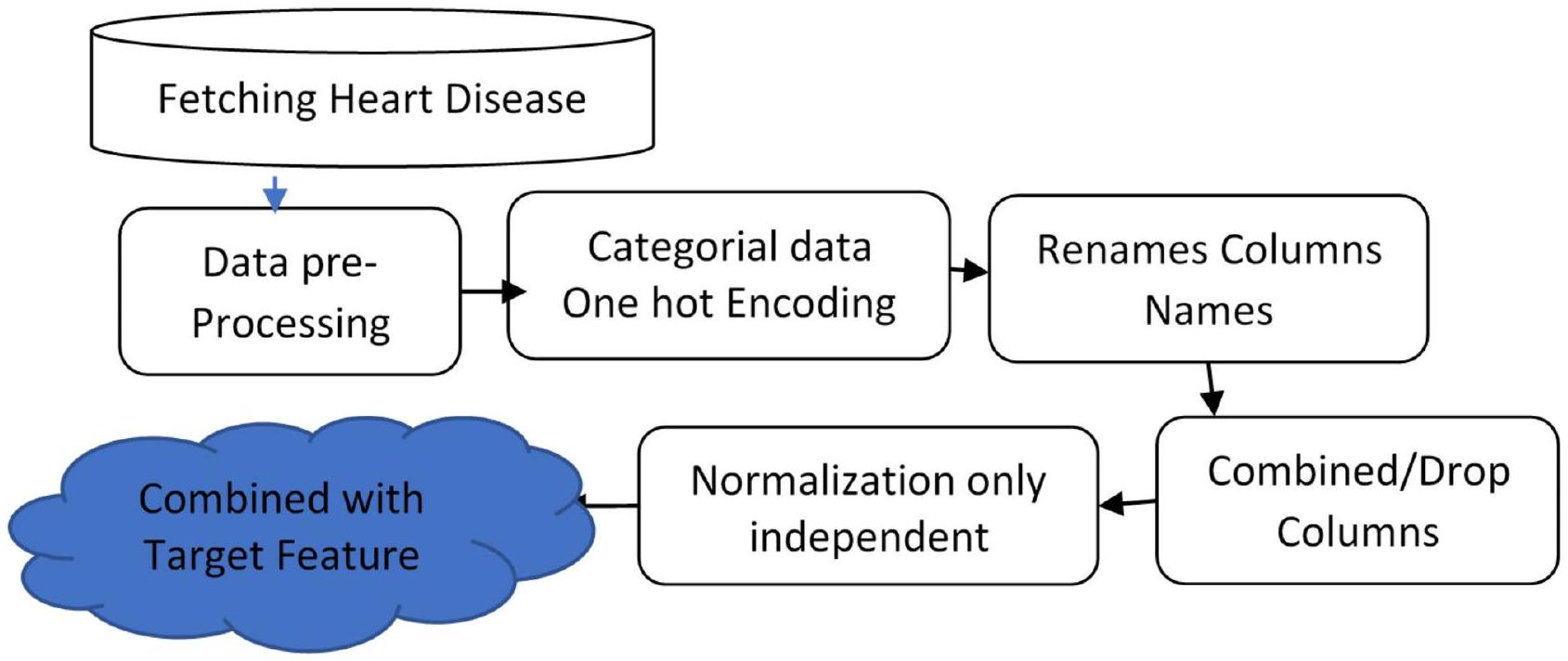
مخطط تدفق إعداد البيانات
| عمر | ضغط الدم الانقباضي | كول | ثلاث | الذروة القديمة | عمر | ضغط الدم الانقباضي | كول | ثلاث | أولدبيك | |
| 63 | 145 | 233 | 150 | 2.3 | قبل بعد | 0.952 | 0.763 | -0.256 | 0.0154 | 1.08 |
| 37 | ١٣٠ | ٢٥٠ | 187 | ٣.٥ | -1.91 | -0.092 | 0.0721 | 1.633 | 2.122 | |
| 41 | ١٣٠ | 204 | 172 | 1.4 | -1.47 | -0.092 | -0.816 | 0.977 | 0.3109 | |
| ٥٦ | ١٢٠ | 236 | 178 | 0.8 | 0.18 | -0.663 | -0.198 | 1.239 | -0.206 |
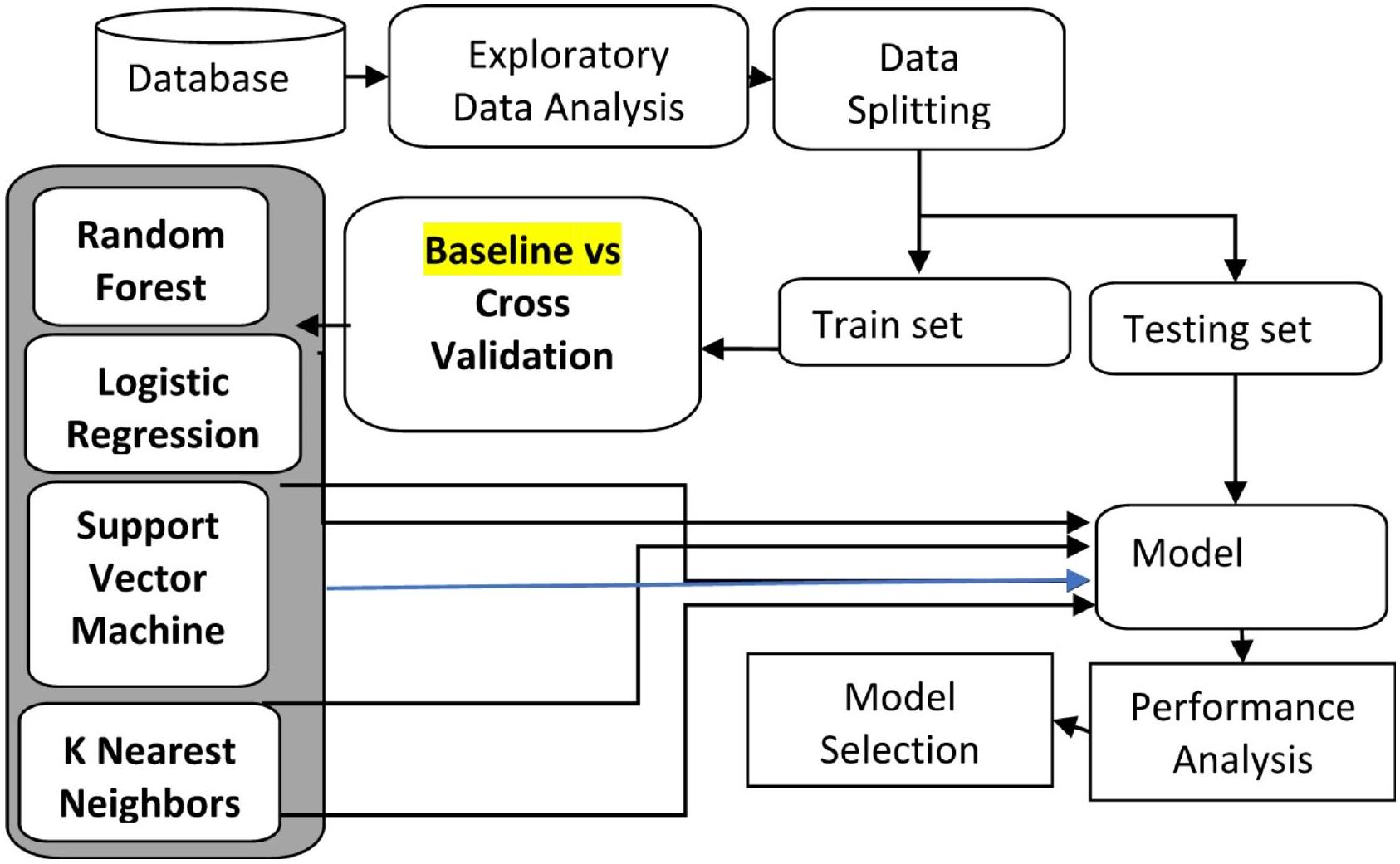
مخطط تصميم التحقق
خاصية فئوية، من معالجة مسبقة وهندسة ميزات، حيث يقوم ترميز one-hot بتوسيع البيانات إلى 76 عمودًا. يتم استخدام تقسيم 80:20 بين التدريب والاختبار مع تصنيف للحفاظ على نسب الفئات، يتبعه إجراء تحقق متقاطع من 5 طيات لتقييم قوي. بالإضافة إلى ذلك، يتم استخدام تحقق متقاطع من 5 طيات لرسم منحنيات التعلم، مما يضمن تقييمًا شاملاً لأداء النموذج. باستخدام مكتبة Seaborn في بايثون لرسم الخرائط الحرارية. لذا، حصل علماء البيانات على أفضل اختيار للنموذج من عينات البيانات المماثلة.
النتائج والمناقشة
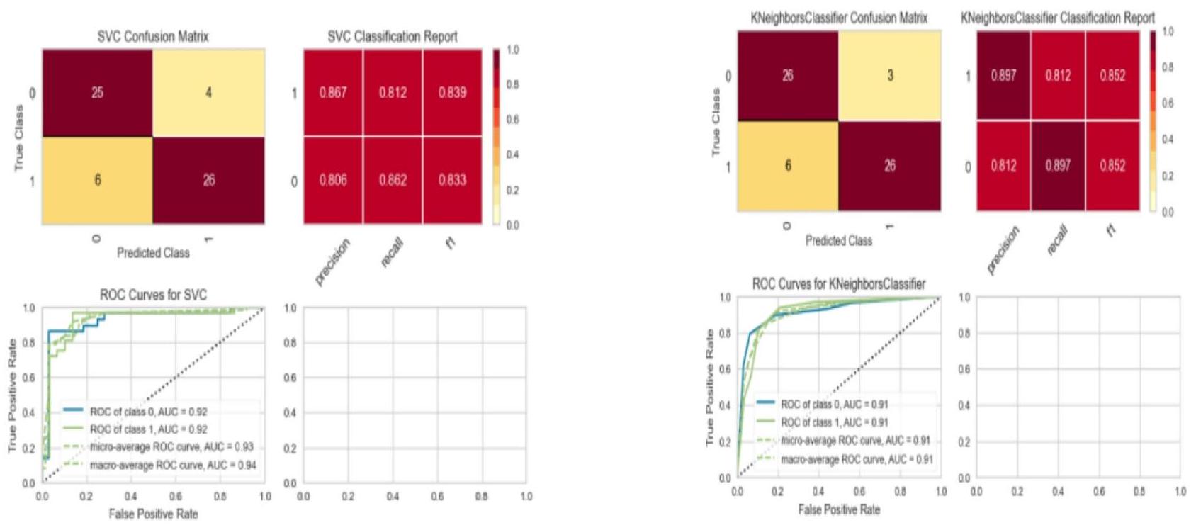
نموذج التعلم الآلي الأساسي بدون تحقق متقاطع
نموذج التعلم الآلي باستخدام التحقق المتقاطع
|
|
معدل
|
|
إحصائيات F: 17.71 | |
| معامل | معيار | ت | P | |
| ثابت | 0.54 | 0.019 | ٢٨.٢٩ | 0.00 |
| عمر | 0.20 | 0.024 | 1.023 | 0.30 |
| تريستبس | -0.41 | 0.021 | -0.92 | 0.56 |
| تشول | -0.016 | 0.026 | 1.67 | 0.42 |
| ثلاث | 0.042 | 0.027 | -1.80 | 0.9 |
| أولدبيك | -0.041 | 0.022 | -3.40 | 0.07 |
| الجنس_1 | -0.07 | 0.020 | ٢.٦٤ | 0.001 |
| فبس_1 | 0.011 | 0.043 | 0.58 | 0.00 |
| حد أدنى | الحد الأقصى | ||||||
| نسبة الدقة % | دقة | استدعاء | فورمولا 1 | دقة | استدعاء | فورمولا 1 | |
| الانحدار اللوجستي | 81.9 | 86 | ٨٨ | 87 | 86 | 83 | 84 |
| مصنف SVC | 78.6 | ٨٨ | 91 | ٨٨ | 85 | 81 | 85 |
| مصنف K NN | 81.9 | 89 | 92 | 89 | 86 | 83 | 86 |
| مصنف RF | 78.6 | 96 | 97 | 96 | 95 | 93 | 95 |
| نموذج/تكرار |
|
|
|
|
|
متوسط |
| الانحدار اللوجستي | ٨٨ | ٨٨ | ٨٠ | 83 | 78 | ٨٣.٨١ |
| دعم المتجه | ٨٨ | ٨٨ | 75 | 81 | 78 | 82.49 |
| الجوار الأقرب K | 85 | 86 | 81 | 85 | 81 | 84.15 |
| الغابة العشوائية | 83 | 90 | ٨٠ | 85 | 81 | 84.15 |
| نموذج/تكرار |
|
|
|
|
|
متوسط% |
| الانحدار اللوجستي | ٨٨.٥ | ٨٨ | ٨٠ | 83 | 78 | ٨٣.٨١ |
| دعم المتجه | ٨٨.٥ | ٨٨ | 75 | 81 | 78 | 82.49 |
| الجوار الأقرب K | 85.2 | 86 | 81 | 85 | 81 | 84.15 |
| الغابة العشوائية | 86.8 | 86 | 78 | 86 | 87 | 84.73 |
منحنى التعلم لجميع النماذج
الخاتمة
توفر البيانات
نُشر على الإنترنت: 18 أبريل 2025
References
- Stone, M. Cross-validatory choice and assessment of statistical predictions. J. R Stat. Soc. Ser. B Methodol. 36(2), 111-133. https:// doi.org/10.1111/j.2517-6161.1974.tb00994.x (1974).
- Chin, C. & Osborne, J. Students’ questions: a potential resource for teaching and learning science. Stud. Sci. Educ. 44(1), 1-39. https://doi.org/10.1080/03057260701828101 (2008).
- Maldonado, S., López, J. & Iturriaga, A. Out-of-time cross-validation strategies for classification in the presence of dataset shift. Appl. Intell. 52(5), 5770-5783. https://doi.org/10.1007/s10489-021-02735-2 (2022).
- Mahesh, T. R., Geman, O., Margala, M. & Guduri, M. The stratified K-folds cross-validation and class-balancing methods with high-performance ensemble classifiers for breast cancer classification. Healthc. Anal. 4, 100247. https://doi.org/10.1016/j.health. 2 023.100247 (2023).
- Barrow, D. K. & Crone, S. F. Cross-validation aggregation for combining autoregressive neural network forecasts, vol. 32, no. 4. 1120-1137 (Accessed 14 Jan 2025). https://www.sciencedirect.com/science/article/pii/S0169207016300188 https://doi.org/10.101 6/j.ijforecast.2015.12.011 (Elsevier, 2016).
- Schmidt, J., Marques, M. R., Botti, S. & Marques, M. A. Recent advances and applications of machine learning in solid-state materials science. Npj Comput. Mater. 5(1), 1-36. https://doi.org/10.1038/s41524-019-0221-0 (2019).
- Ye, Z. et al. Predicting beneficial effects of Atomoxetine and Citalopram on response Inhibition in P Arkinson’s disease with clinical and neuroimaging measures. Hum. Brain Mapp. 37(3), 1026-1037. https://doi.org/10.1002/hbm.23087 (2016).
- Gimenez-Nadal, J. I., Lafuente, M., Molina, J. A. & Velilla, J. Resampling and bootstrap algorithms to assess the relevance of variables: applications to cross section entrepreneurship data. Empir. Econ. 56(1), 233-267. https://doi.org/10.1007/s00181-017-1 355-x (2019).
- Dodge, J., Gururangan, S., Card, D., Schwartz, R. & Smith, N. A. Expected validation performance and estimation of a random variable’s maximum. (Accessed 04 Feb 2024) http://arxiv.org/abs/2110.00613 (2021).
- Belkin, M., Hsu, D., Ma, S. & Mandal, S. Reconciling modern machine-learning practice and the classical bias-variance trade-off. Proc. Natl. Acad. Sci. 116(32), 15849-15854,019. https://doi.org/10.1073/pnas. 1903070116
- Kernbach, J. M. & Staartjes, V. E. Foundations of machine learning-based clinical prediction modeling: Part II-generalization and overfitting. In Machine Learning in Clinical Neuroscience Acta Neurochirurgica Supplement, vol. 134, (eds Staartjes, V. E. et al.) 15-21. https://doi.org/10.1007/978-3-030-85292-4_3 (Springer International Publishing, 2022).
- Olaniyi, E. O., Oyedotun, O. K., Ogunlade, C. A. & Khashman, A. In-line grading system for Mango fruits using GLCM feature extraction and soft-computing techniques. Int. J. Appl. Pattern Recognit. 6(1), 58-75. https://doi.org/10.1504/IJAPR.2019.104294 (2019).
- Benjamin, E. J. et al. Heart disease and stroke statistics-2019 update: a report from the American Heart Association. Circulation. 139(10), e56-e528 (2019).
- Arora, S., Santiago, J. A., Bernstein, M. & Potashkin, J. A. Diet and lifestyle impact the development and progression of Alzheimer’s dementia. Front. Nutr. 10, https://doi.org/10.3389/fnut.2023.1213223 (2023).
- Zuhair, M. et al. Estimation of the worldwide seroprevalence of cytomegalovirus: A systematic review and meta-analysis. Rev. Med. Virol. 29(3), e2034. https://doi.org/10.1002/rmv. 2034 (2019).
- Xiong, B., Jiang, W. & Zhang, F. Semi-supervised classification considering space and spectrum constraint for remote sensing imagery. In 2010 18th International Conference on Geoinformatics, 1-6. https://doi.org/10.1109/GEOINFORMATICS.2010.55679 81 (IEEE, 2010).
- Nadar, N. & Kamatchi, R. A novel student risk identification model using machine learning approach. Int. J. Adv. Comput. Sci. Appl. 9, 305-309. https://doi.org/10.14569/IJACSA.2018.091142 (2018).
- Khan, A. & Ghosh, S. K. Student performance analysis and prediction in classroom learning: A review of educational data mining studies. Educ. Inf. Technol. 26(1), 205-240. https://doi.org/10.1007/s10639-020-10230-3 (2021).
- Yousafzai, B. K., Hayat, M. & Afzal, S. Application of machine learning and data mining in predicting the performance of intermediate and secondary education level student, Educ. Inf. Technol., 25(6), 4677-4697. https://doi.org/10.1007/s10639-020-10 189-1 (2020).
- Smirani, L. K., Yamani, H. A., Menzli, L. J. & Boulahia, J. A. Using ensemble learning algorithms to predict student failure and enabling customized educational paths, Sci. Program. 2022, 1-15. https://doi.org/10.1155/2022/3805235 (2022).
- Usama, M., Ahmad, B., Xiao, W., Hossain, M. S. & Muhammad, G. Self-attention based recurrent convolutional neural network for disease prediction using healthcare data, comput. Methods Programs Biomed. 190, 105191 (2020).
- Shukla, N., Hagenbuchner, M., Win, K. T. & Yang, J. Breast cancer data analysis for survivability studies and prediction, Comput. Methods Programs Biomed., 155, 199-208, https://doi.org/10.1016/j.cmpb.2017.12.011 (2018).
- Kaur, G. & Chhabra, A. Improved J48 classification algorithm for the prediction of diabetes. Int. J. Comput. Appl. 98(22), 13-17. https://doi.org/10.5120/17314-7433 (2014).
- Naz, H. et al. Deep learning approach for diabetes prediction using PIMA Indian dataset. J. Diabetes Metab. Disord. 19(1), 391-403 https://doi.org/10.1007/s40200-020-00520-5.
- Dharma, F. et al. Prediction of Indonesian inflation rate using regression model based on genetic algorithms. J. Online Inform. 5(1), 45-52 https://doi.org/10.15575/join.v5i1.532 (2020).
- Touzani, S., Granderson, J. & Fernandes, S. Gradient boosting machine for modeling the energy consumption of commercial buildings. Energy Build. 158, 1533-1543 https://doi.org/10.1016/j.enbuild.2017.11.039 (2018).
- Mohan, S., Thirumalai, C. & Srivastava, G. Effective heart disease prediction using hybrid machine learning techniques. IEEE Access. 7, 81542-81554. https://doi.org/10.1109/ACCESS.2019.2923707 (2019).
- Anuradha, C. & Velmurugan, T. A comparative analysis on the evaluation of classification algorithms in the prediction of students performance. Indian J. Sci. Technol. 8(15). https://doi.org/10.17485/ijst/2015/v8i15/74555 (2015).
- Hussain, A. A. & Dimililer, K. Student grade prediction using machine learning in iot era. In International Conference on Forthcoming Networks and Sustainability in the IoT Era, 65-81. https://doi.org/10.1007/978-3-030-69431-9_6 (Springer, 2021).
- Mathers, C. D., Boerma, T. & Ma Fat, D. Global and regional causes of death. vol. 92, no. 1, 7-32 (Accessed 14 Jan 2025). https://a cademic.oup.com/bmb/article-abstract/92/1/7/332071 https://doi.org/10.1093/bmb/ldp028 (Oxford University Press, 2009).
- Chowdhury, R. et al. Dynamic interventions to control COVID-19 pandemic: a multivariate prediction modelling study comparing 16 worldwide countries. Eur. J. Epidemiol. 35(5), 389-399. https://doi.org/10.1007/s10654-020-00649-w (2020).
- Townsend, N. et al. Epidemiology of cardiovascular disease in Europe. Nat. Rev. Cardiol. 19(2), 2 https://doi.org/10.1038/s41569-0 21-00607-3 (2022).
- Ansari, M. F., Alankar, B. & Kaur, H. A prediction of heart disease using machine learning algorithms. In Image Processing and Capsule Networks, vol. 1200, (eds Chen, J. I. Z. et al.) in Advances in Intelligent Systems and Computing, vol. 1200, 497-504. https://doi.org/10.1007/978-3-030-51859-2_45 (Springer International Publishing, 2021).
- Amarbayasgalan, T., Pham, V. H., Theera-Umpon, N., Piao, Y. & Ryu, K. H. An efficient prediction method for coronary heart disease risk based on two deep neural networks trained on well-ordered training datasets. IEEE Access. 9, 135210-135223. https:/ /doi.org/10.1109/ACCESS.2021.3116974 (2021).
- Barhoom, A. M., Almasri, A., Abu-Nasser, B. S. & Abu-Naser, S. S. Prediction of Heart Disease Using a Collection of Machine and Deep Learning Algorithms (Accessed 04 Feb 2024) https://philpapers.org/rec/BARPOH-4 (2022).
شكر وتقدير
مساهمات المؤلفين
الإعلانات
المصالح المتنافسة
معلومات إضافية
معلومات إعادة الطبع والتصاريح متاحة علىwww.nature.com/reprints.
ملاحظة الناشر: تظل شركة سبرينغر ناتشر محايدة فيما يتعلق بالمطالبات القضائية في الخرائط المنشورة والانتماءات المؤسسية.
© المؤلفون 2025
جامعة IIS (تعتبر جامعة)، جايبور، الهند. جامعة بوكهارا، بوكهارا، نيبال. IOE، حرم بولتشوك، باتان، نيبال. جامعة سيدني الغربية (WSU)، سيدني، أستراليا. كلية آسيا والمحيط الهادئ الدولية (APIC)، سيدني، أستراليا. جامعة مهارشي داياناند، روهتاك، الهند. البريد الإلكتروني: rimal.yagya@gmail.com
DOI: https://doi.org/10.1038/s41598-025-93675-1
PMID: https://pubmed.ncbi.nlm.nih.gov/40251253
Publication Date: 2025-04-18
scientific reports
OPEN
Comparative analysis of heart disease prediction using logistic regression, SVM, KNN, and random forest with cross-validation for improved accuracy
Abstract
This primary research paper emphasizes cross-validation, where data samples are reshuffled in each iteration to form randomized subsets divided into n folds. This method improves model performance and achieves higher accuracy than the baseline model. The novelty lies in the data preparation process, where numerical features were imputed using the mean, categorical features were imputed using chi-square methods, and normalization was applied. This research study involves transforming the original datasets and comparative model analysis of four Logistic Regression (LR), Support Vector Machine (SVM), K-Nearest Neighbor (KNN), and Random Forest (RF) cross-validation methodologies to heart disease open datasets. The objective is to easily identify the average accuracy of model predictions and subsequently make recommendations for model selection based on data preprocessing cross-validation model increased ( 5 to
Healthcare has been transformed by machine learning, which holds promise for better diagnostic precision in complicated illnesses like heart disease. However, optimal validation techniques for robust heart disease prediction models remain underexplored, highlighting the knowledge gap by enhancing diagnostic accuracy, particularly in complex conditions like heart disease causes. As heart disease continues to be a leading cause of death globally, the need for precise diagnostic tools has never been greater. However, optimal validation techniques for robust heart disease prediction models remain underexplored. Machine learning is the process of designing a model based on training and testing data sets whose value is further evaluated from validation sets of the sample. The train-test split is a widely used method for dividing research datasets into training and testing subsets. Model accuracy primarily depends on the input and validation sets. Cross-validation, with multiple-fold iterations, helps fine-tune the model to achieve optimal performance scores. Machine learning models typically begin by splitting the available dataset into training, validation, and testing sets, often using a ratio of 70:15:15. The model is built and trained using the training data, evaluated on the validation set to fine-tune its performance, and finally tested on the unseen testing set to assess its generalization capability
algorithm-primarily based regression model for predicting inflation levels. The version becomes educated and evaluates the usage of facts. Similarly, the authors
Methodology
Data preparation flow chart
| Age | trestbps | chol | thalach | oldpeak | Age | trestbps | chol | thalach | Oldpeak | |
| 63 | 145 | 233 | 150 | 2.3 | Before After | 0.952 | 0.763 | -0.256 | 0.0154 | 1.08 |
| 37 | 130 | 250 | 187 | 3.5 | -1.91 | -0.092 | 0.0721 | 1.633 | 2.122 | |
| 41 | 130 | 204 | 172 | 1.4 | -1.47 | -0.092 | -0.816 | 0.977 | 0.3109 | |
| 56 | 120 | 236 | 178 | 0.8 | 0.18 | -0.663 | -0.198 | 1.239 | -0.206 |
Validation design diagram
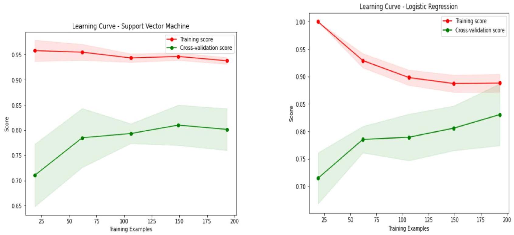
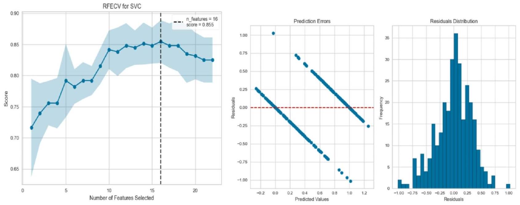
categorical attributes, undergoes preprocessing and feature engineering, where one-hot encoding expands the data to 76 columns. An 80:20 train-test split with stratification is used to maintain class proportions, followed by a 5 -fold cross-validation procedure for robust evaluation. Additionally, a 5 -fold cross-validation is employed to plot learning curves, ensuring a comprehensive assessment of model performance. Using Python’s Seaborn for heatmaps. So, data scientists received the best model selection of similar data samples.
Results and discussion
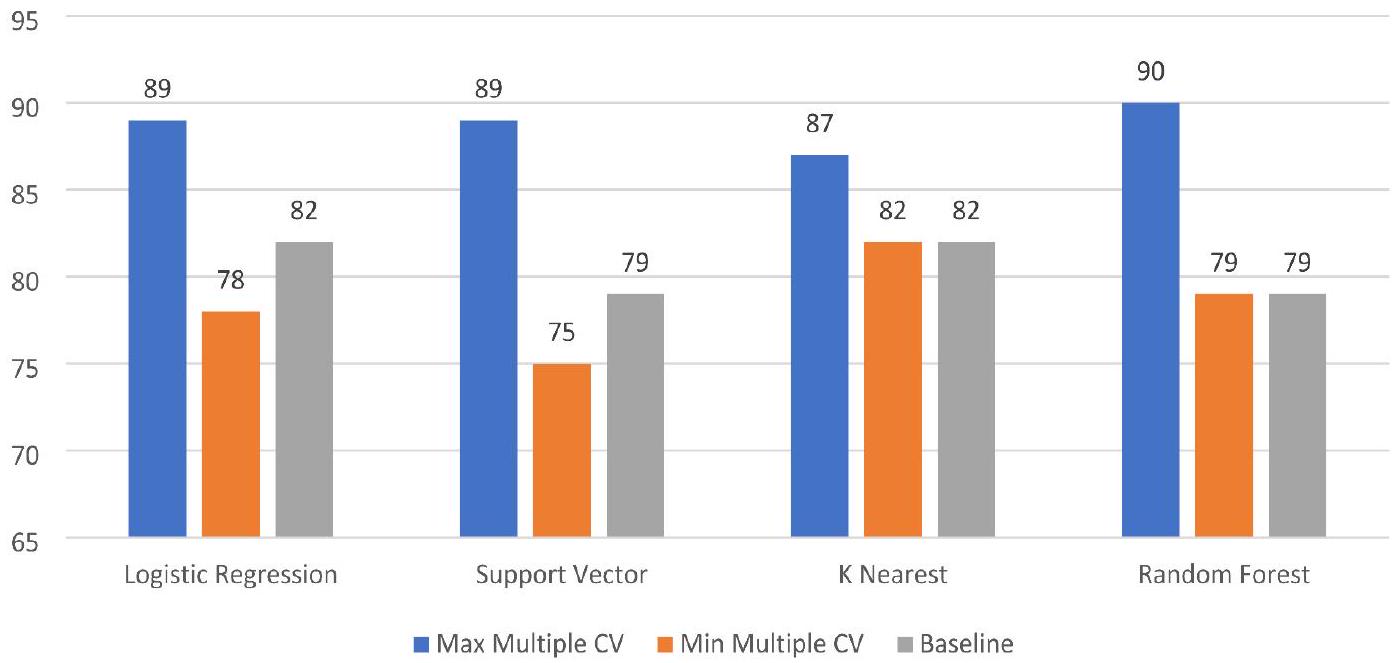
Baseline machine learning model without cross validation
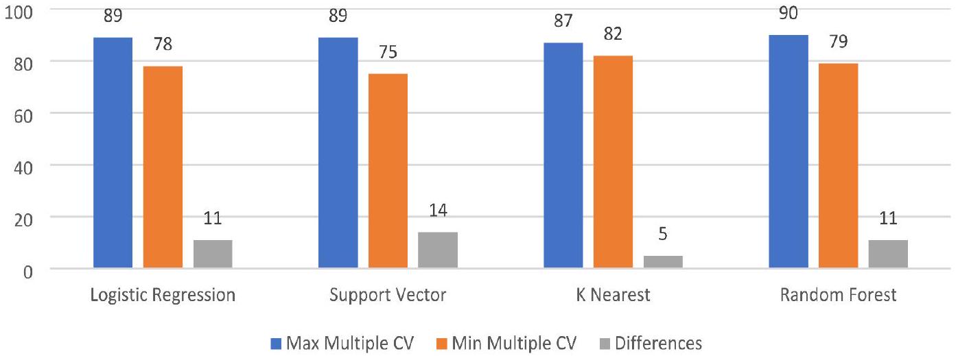
Machine learning model using cross-validation
|
|
Adjusted
|
|
F-stasticts:17.71 | |
| coef | Std | t | P | |
| Const | 0.54 | 0.019 | 28.29 | 0.00 |
| Age | 0.20 | 0.024 | 1.023 | 0.30 |
| Trestbps | -0.41 | 0.021 | -0.92 | 0.56 |
| Chol | -0.016 | 0.026 | 1.67 | 0.42 |
| Thalach | 0.042 | 0.027 | -1.80 | 0.9 |
| Oldpeak | -0.041 | 0.022 | -3.40 | 0.07 |
| Sex_1 | -0.07 | 0.020 | 2.64 | 0.001 |
| Fbs_1 | 0.011 | 0.043 | 0.58 | 0.00 |
| Minimum | Maximum | ||||||
| Accuracy % | Precision | Recall | F1 | Precision | Recall | F1 | |
| Logistic regression | 81.9 | 86 | 88 | 87 | 86 | 83 | 84 |
| SVC classifier | 78.6 | 88 | 91 | 88 | 85 | 81 | 85 |
| K NN classifier | 81.9 | 89 | 92 | 89 | 86 | 83 | 86 |
| RF classifier | 78.6 | 96 | 97 | 96 | 95 | 93 | 95 |
| Model/iteration |
|
|
|
|
|
Average |
| Logistic regression | 88 | 88 | 80 | 83 | 78 | 83.81 |
| Support vector | 88 | 88 | 75 | 81 | 78 | 82.49 |
| K-nearest neighbor | 85 | 86 | 81 | 85 | 81 | 84.15 |
| Random forest | 83 | 90 | 80 | 85 | 81 | 84.15 |
| Model/iteration |
|
|
|
|
|
Average% |
| Logistic regression | 88.5 | 88 | 80 | 83 | 78 | 83.81 |
| Support vector | 88.5 | 88 | 75 | 81 | 78 | 82.49 |
| K-nearest neighbor | 85.2 | 86 | 81 | 85 | 81 | 84.15 |
| Random forest | 86.8 | 86 | 78 | 86 | 87 | 84.73 |
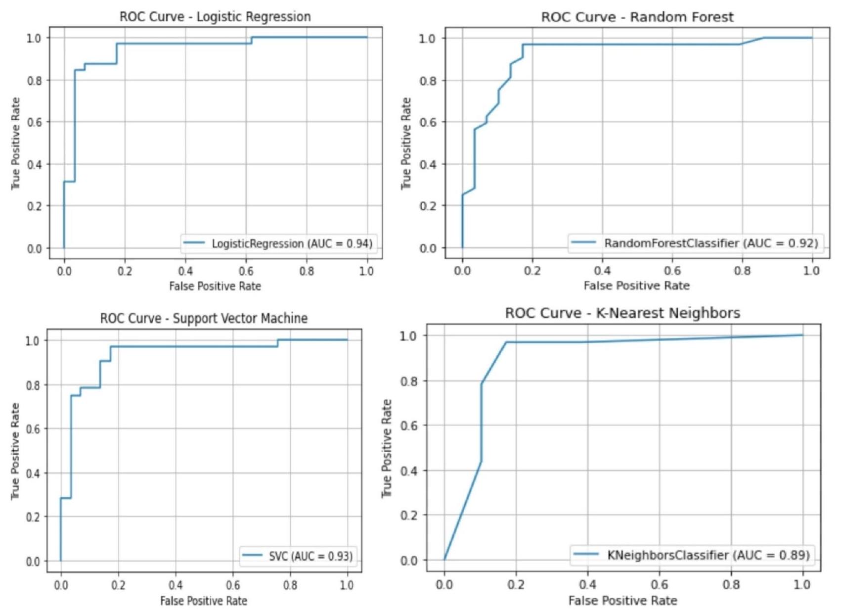
Learning curve of all models
Conclusion
Data availability
Published online: 18 April 2025
References
- Stone, M. Cross-validatory choice and assessment of statistical predictions. J. R Stat. Soc. Ser. B Methodol. 36(2), 111-133. https:// doi.org/10.1111/j.2517-6161.1974.tb00994.x (1974).
- Chin, C. & Osborne, J. Students’ questions: a potential resource for teaching and learning science. Stud. Sci. Educ. 44(1), 1-39. https://doi.org/10.1080/03057260701828101 (2008).
- Maldonado, S., López, J. & Iturriaga, A. Out-of-time cross-validation strategies for classification in the presence of dataset shift. Appl. Intell. 52(5), 5770-5783. https://doi.org/10.1007/s10489-021-02735-2 (2022).
- Mahesh, T. R., Geman, O., Margala, M. & Guduri, M. The stratified K-folds cross-validation and class-balancing methods with high-performance ensemble classifiers for breast cancer classification. Healthc. Anal. 4, 100247. https://doi.org/10.1016/j.health. 2 023.100247 (2023).
- Barrow, D. K. & Crone, S. F. Cross-validation aggregation for combining autoregressive neural network forecasts, vol. 32, no. 4. 1120-1137 (Accessed 14 Jan 2025). https://www.sciencedirect.com/science/article/pii/S0169207016300188 https://doi.org/10.101 6/j.ijforecast.2015.12.011 (Elsevier, 2016).
- Schmidt, J., Marques, M. R., Botti, S. & Marques, M. A. Recent advances and applications of machine learning in solid-state materials science. Npj Comput. Mater. 5(1), 1-36. https://doi.org/10.1038/s41524-019-0221-0 (2019).
- Ye, Z. et al. Predicting beneficial effects of Atomoxetine and Citalopram on response Inhibition in P Arkinson’s disease with clinical and neuroimaging measures. Hum. Brain Mapp. 37(3), 1026-1037. https://doi.org/10.1002/hbm.23087 (2016).
- Gimenez-Nadal, J. I., Lafuente, M., Molina, J. A. & Velilla, J. Resampling and bootstrap algorithms to assess the relevance of variables: applications to cross section entrepreneurship data. Empir. Econ. 56(1), 233-267. https://doi.org/10.1007/s00181-017-1 355-x (2019).
- Dodge, J., Gururangan, S., Card, D., Schwartz, R. & Smith, N. A. Expected validation performance and estimation of a random variable’s maximum. (Accessed 04 Feb 2024) http://arxiv.org/abs/2110.00613 (2021).
- Belkin, M., Hsu, D., Ma, S. & Mandal, S. Reconciling modern machine-learning practice and the classical bias-variance trade-off. Proc. Natl. Acad. Sci. 116(32), 15849-15854,019. https://doi.org/10.1073/pnas. 1903070116
- Kernbach, J. M. & Staartjes, V. E. Foundations of machine learning-based clinical prediction modeling: Part II-generalization and overfitting. In Machine Learning in Clinical Neuroscience Acta Neurochirurgica Supplement, vol. 134, (eds Staartjes, V. E. et al.) 15-21. https://doi.org/10.1007/978-3-030-85292-4_3 (Springer International Publishing, 2022).
- Olaniyi, E. O., Oyedotun, O. K., Ogunlade, C. A. & Khashman, A. In-line grading system for Mango fruits using GLCM feature extraction and soft-computing techniques. Int. J. Appl. Pattern Recognit. 6(1), 58-75. https://doi.org/10.1504/IJAPR.2019.104294 (2019).
- Benjamin, E. J. et al. Heart disease and stroke statistics-2019 update: a report from the American Heart Association. Circulation. 139(10), e56-e528 (2019).
- Arora, S., Santiago, J. A., Bernstein, M. & Potashkin, J. A. Diet and lifestyle impact the development and progression of Alzheimer’s dementia. Front. Nutr. 10, https://doi.org/10.3389/fnut.2023.1213223 (2023).
- Zuhair, M. et al. Estimation of the worldwide seroprevalence of cytomegalovirus: A systematic review and meta-analysis. Rev. Med. Virol. 29(3), e2034. https://doi.org/10.1002/rmv. 2034 (2019).
- Xiong, B., Jiang, W. & Zhang, F. Semi-supervised classification considering space and spectrum constraint for remote sensing imagery. In 2010 18th International Conference on Geoinformatics, 1-6. https://doi.org/10.1109/GEOINFORMATICS.2010.55679 81 (IEEE, 2010).
- Nadar, N. & Kamatchi, R. A novel student risk identification model using machine learning approach. Int. J. Adv. Comput. Sci. Appl. 9, 305-309. https://doi.org/10.14569/IJACSA.2018.091142 (2018).
- Khan, A. & Ghosh, S. K. Student performance analysis and prediction in classroom learning: A review of educational data mining studies. Educ. Inf. Technol. 26(1), 205-240. https://doi.org/10.1007/s10639-020-10230-3 (2021).
- Yousafzai, B. K., Hayat, M. & Afzal, S. Application of machine learning and data mining in predicting the performance of intermediate and secondary education level student, Educ. Inf. Technol., 25(6), 4677-4697. https://doi.org/10.1007/s10639-020-10 189-1 (2020).
- Smirani, L. K., Yamani, H. A., Menzli, L. J. & Boulahia, J. A. Using ensemble learning algorithms to predict student failure and enabling customized educational paths, Sci. Program. 2022, 1-15. https://doi.org/10.1155/2022/3805235 (2022).
- Usama, M., Ahmad, B., Xiao, W., Hossain, M. S. & Muhammad, G. Self-attention based recurrent convolutional neural network for disease prediction using healthcare data, comput. Methods Programs Biomed. 190, 105191 (2020).
- Shukla, N., Hagenbuchner, M., Win, K. T. & Yang, J. Breast cancer data analysis for survivability studies and prediction, Comput. Methods Programs Biomed., 155, 199-208, https://doi.org/10.1016/j.cmpb.2017.12.011 (2018).
- Kaur, G. & Chhabra, A. Improved J48 classification algorithm for the prediction of diabetes. Int. J. Comput. Appl. 98(22), 13-17. https://doi.org/10.5120/17314-7433 (2014).
- Naz, H. et al. Deep learning approach for diabetes prediction using PIMA Indian dataset. J. Diabetes Metab. Disord. 19(1), 391-403 https://doi.org/10.1007/s40200-020-00520-5.
- Dharma, F. et al. Prediction of Indonesian inflation rate using regression model based on genetic algorithms. J. Online Inform. 5(1), 45-52 https://doi.org/10.15575/join.v5i1.532 (2020).
- Touzani, S., Granderson, J. & Fernandes, S. Gradient boosting machine for modeling the energy consumption of commercial buildings. Energy Build. 158, 1533-1543 https://doi.org/10.1016/j.enbuild.2017.11.039 (2018).
- Mohan, S., Thirumalai, C. & Srivastava, G. Effective heart disease prediction using hybrid machine learning techniques. IEEE Access. 7, 81542-81554. https://doi.org/10.1109/ACCESS.2019.2923707 (2019).
- Anuradha, C. & Velmurugan, T. A comparative analysis on the evaluation of classification algorithms in the prediction of students performance. Indian J. Sci. Technol. 8(15). https://doi.org/10.17485/ijst/2015/v8i15/74555 (2015).
- Hussain, A. A. & Dimililer, K. Student grade prediction using machine learning in iot era. In International Conference on Forthcoming Networks and Sustainability in the IoT Era, 65-81. https://doi.org/10.1007/978-3-030-69431-9_6 (Springer, 2021).
- Mathers, C. D., Boerma, T. & Ma Fat, D. Global and regional causes of death. vol. 92, no. 1, 7-32 (Accessed 14 Jan 2025). https://a cademic.oup.com/bmb/article-abstract/92/1/7/332071 https://doi.org/10.1093/bmb/ldp028 (Oxford University Press, 2009).
- Chowdhury, R. et al. Dynamic interventions to control COVID-19 pandemic: a multivariate prediction modelling study comparing 16 worldwide countries. Eur. J. Epidemiol. 35(5), 389-399. https://doi.org/10.1007/s10654-020-00649-w (2020).
- Townsend, N. et al. Epidemiology of cardiovascular disease in Europe. Nat. Rev. Cardiol. 19(2), 2 https://doi.org/10.1038/s41569-0 21-00607-3 (2022).
- Ansari, M. F., Alankar, B. & Kaur, H. A prediction of heart disease using machine learning algorithms. In Image Processing and Capsule Networks, vol. 1200, (eds Chen, J. I. Z. et al.) in Advances in Intelligent Systems and Computing, vol. 1200, 497-504. https://doi.org/10.1007/978-3-030-51859-2_45 (Springer International Publishing, 2021).
- Amarbayasgalan, T., Pham, V. H., Theera-Umpon, N., Piao, Y. & Ryu, K. H. An efficient prediction method for coronary heart disease risk based on two deep neural networks trained on well-ordered training datasets. IEEE Access. 9, 135210-135223. https:/ /doi.org/10.1109/ACCESS.2021.3116974 (2021).
- Barhoom, A. M., Almasri, A., Abu-Nasser, B. S. & Abu-Naser, S. S. Prediction of Heart Disease Using a Collection of Machine and Deep Learning Algorithms (Accessed 04 Feb 2024) https://philpapers.org/rec/BARPOH-4 (2022).
Acknowledgements
Author contributions
Declarations
Competing interests
Additional information
Reprints and permissions information is available at www.nature.com/reprints.
Publisher’s note Springer Nature remains neutral with regard to jurisdictional claims in published maps and institutional affiliations.
© The Author(s) 2025
IIS (Deemed to be University), Jaipur, India. Pokhara University, Pokhara, Nepal. IOE, Pulchowk Campus, Patan, Nepal. Western Sydney University (WSU), Sydney, Australia. Asia Pacific International College (APIC), Sydney, Australia. Maharshi Dayanand University, Rohtak, India. email: rimal.yagya@gmail.com