تاريخ الاستلام: 6 ديسمبر 2023
تاريخ القبول: 25 نوفمبر 2024
تاريخ النشر على الإنترنت: 02 يناير 2025
تحقق من التحديثات

كونستانتين أ. ماسلوف ®، كلاوديو بيرسيلو ، توماس شيلينبرغر (D²) ألفريد شتاين (D)

يعد التخطيط الدقيق للأنهار الجليدية عالميًا أمرًا حيويًا لفهم تأثيرات تغير المناخ. على الرغم من أهميته، لا يزال التخطيط الآلي للأنهار الجليدية على نطاق عالمي غير مستكشف إلى حد كبير. هنا نتناول هذه الفجوة ونقترح Glacier-VisionTransformer-U-Net (GlaViTU)، وهو نموذج تعلم عميق يعتمد على التحويلات التلافيفية، وخمس استراتيجيات لتخطيط الأنهار الجليدية على نطاق عالمي متعدد الأوقات باستخدام صور الأقمار الصناعية المفتوحة. يُظهر تقييم التعميم المكاني والزماني وعبر المستشعرات أن أفضل استراتيجياتنا تحقق تقاطعًا على الاتحاد >0.85 على الصور التي لم تُلاحظ سابقًا في معظم الحالات، والتي تنخفض إلى >0.75 في المناطق الغنية بالحطام مثل آسيا الجبلية العالية وتزداد إلى للمناطق التي تهيمن عليها الجليد النظيف. تؤكد التحقق المقارن ضد عدم اليقين لدى الخبراء البشريين من حيث انحرافات المساحة والمسافة أداء GlaViTU، حيث يقترب أو يتطابق مع تحديد مستوى الخبراء. إن إضافة بيانات رادار الفتحة الاصطناعية، وهي، الارتداد والتماسك التداخلي، يزيد من الدقة في جميع المناطق المتاحة. يتم الإبلاغ عن الثقة المعايرة لامتدادات الأنهار الجليدية مما يجعل التنبؤات أكثر موثوقية وقابلية للتفسير. نحن أيضًا نطلق مجموعة بيانات مرجعية تغطي من الأنهار الجليدية في جميع أنحاء العالم. تدعم نتائجنا الجهود نحو التخطيط الآلي متعدد الأوقات والعالمي للأنهار الجليدية.

تكون الأنهار الجليدية حساسة للغاية للتغيرات في درجة الحرارة والهطول، مما يجعلها مؤشرات مهمة لتغير المناخ، ومعترف بها كمتغير مناخي أساسي ضمن برنامج نظام مراقبة المناخ العالمي (GCOS) . في العقود الأخيرة، انخفضت الغالبية العظمى من الأنهار الجليدية في جميع أنحاء العالم في الحجم ومن المتوقع أن تستمر في التراجع، و من الأنهار الجليدية من المحتمل أن تختفي بحلول عام 2100 بغض النظر عن سيناريو انبعاثات غازات الدفيئة . يساهم هذا الفقد في كتلة الأنهار الجليدية بشكل كبير في ارتفاع مستويات البحار، حيث يمثل حوالي من الزيادة الملحوظة منذ عام 1961، مع مناطق مثل ألاسكا، القطب الشمالي الكندي، محيط غرينلاند، جبال الأنديز الجنوبية، القطب الشمالي الروسي وسفالبارد التي تمتلك أكبر الحصص . يشكل الارتفاع المتوقع في مستوى البحر من الأنهار الجليدية ( إلى ملم مكافئ لمستوى البحر) تهديدًا خطيرًا لملايين الأسر المتوقعة أن تكون تحت
خطوط المد العالي بحلول نهاية القرن . بالإضافة إلى ذلك، يمكن أن تعوض جريان الأنهار الجليدية عن مواسم تدفق منخفض وتخفف من نقص المياه خلال فترات الجفاف . يؤثر تراجع الأنهار الجليدية على توليد الطاقة الكهرومائية ، جودة مياه الشرب، إنتاجية الزراعة ، النظم البيئية والتنوع البيولوجي وهو مرتبط بفيضانات بحيرات الأنهار الجليدية مع عواقب مدمرة محتملة ، على الرغم من أن شدتها تميل إلى التناقص مع مرور الوقت .

توفر سجلات الأنهار الجليدية المحدثة بانتظام، التي تتعقب مساحة الأنهار الجليدية كواحدة من منتجات المتغيرات المناخية الأساسية لـ GCOS ، معلومات قيمة لقياس، التنبؤ، التخفيف أو التكيف مع هذه التحديات. ومع ذلك، فإن معايير GSOC الحالية لتقدير تغير مساحة الأنهار الجليدية الإقليمية في معظم المناطق الجليدية على مدى عقد من الزمن لم يتم الوفاء بها . علاوة على ذلك، تحتوي سجلات الأنهار الجليدية الحالية على عدة قيود. تحتوي السجلات الإقليمية ودون الإقليمية على تغطية مكانية محدودة

وتفتقر إلى الاتساق في الأساليب والمبادئ المستخدمة لاشتقاق خطوط الأنهار الجليدية. تحتوي قاعدة بيانات Randolph Glacier Inventory (RGI) العالمية على تغطية زمنية محدودة حيث تم رسم معظم خطوط الأنهار الجليدية حول عام 2000. إنها تعمل كبيانات أساسية في العديد من الدراسات الجليدية ، لكن استخدامها محدود عند محاولة فهم التطور الزمني والتغيرات الأكثر حداثة . على غرار السجلات الإقليمية، تعاني قاعدة بيانات قياسات الجليد الأرضي العالمية من الفضاء (GLIMS)، وهي أكبر قاعدة بيانات سجلات وتعتبر مجموعة من RGI، على الرغم من كونها عالمية ومتعددة الأوقات، من مشكلات جودة البيانات حيث تتكون من تجميع سجلات إقليمية بمستويات متفاوتة من الدقة والاتساق. وهذا يجعل من الصعب الحصول على رؤية شاملة وموثوقة للأنهار الجليدية في جميع أنحاء العالم على مستوى متعدد الأوقات . لهذه القيود آثار علمية كبيرة. يعتمد علماء الجليد الذين يستخرجون منتجات الأنهار الجليدية الحيوية، مثل سرعات سطح الجليد، سمك الجليد والتوازن الكتلي الجيوديسي، على خطوط الأنهار الجليدية الدقيقة . أي أخطاء في هذه الخطوط قد تؤدي إلى أخطاء في المهام اللاحقة مما يؤثر على التحليلات والتطبيقات اللاحقة، مثل دراسات نمذجة التوازن الكتلي العالمي . علاوة على ذلك، تعتبر خطوط الأنهار الجليدية مدخلات أساسية لجهود النمذجة، مما يسمح للعلماء بعمل افتراضات مستنيرة حول العمليات الفيزيائية والتنبؤ بتطور الأنهار الجليدية. إن توفر خطوط الأنهار الجليدية المتسقة والمتعددة الأوقات، شريطة أن تتطابق أو تتجاوز جودة السجلات الحالية، لن يحسن فقط دقة مجموعات بيانات الأنهار الجليدية والدراسات المستقبلية ولكن أيضًا سيقدم أساسًا أكثر موثوقية لمعايرة نماذج الأنهار الجليدية لفترات سابقة. كما ستؤدي إلى تحسينات في تطوير نماذج تطور الأنهار الجليدية، على سبيل المثال، مما يسمح بإدماج هندسات الأنهار الجليدية المحدثة بانتظام في نماذج ديناميات الأنهار الجليدية وكذلك إدماج ديناميات الانفصال للأنهار الجليدية التي تنتهي في البحر وتمثيل أفضل للتغيرات الشديدة في المناطق، على سبيل المثال، من خلال التقدم عبر اندفاعات الأنهار الجليدية. بشكل عام، نتوقع العديد من الابتكارات المنهجية التي ستعزز قدرتنا على تقييد الماضي وتوقع تطور الأنهار الجليدية في المستقبل. ومع ذلك، فإن إنتاج سجلات متسقة هو مهمة صعبة وتستغرق وقتًا طويلاً وغالبًا ما تتطلب تفسيرًا بصريًا مكثفًا ورقمنة يدوية لصور الأقمار الصناعية بواسطة خبراء. وبالتالي، فإن هدفًا طويل الأمد حاسم هو أتمتة تخطيط الأنهار الجليدية عالميًا وعبر فترات زمنية متعددة بطريقة متسقة.

تعتبر عتبات بسيطة من نسب نطاقات الضوء طرقًا فعالة لتخطيط الأنهار الجليدية ذات الجليد النظيف على مقاييس مختلفة . ومع ذلك، يمكن أن تختلف قيم العتبة لظروف التصوير المختلفة وداخل مشهد . علاوة على ذلك، تتجاهل الطرق المعتمدة على العتبات الأنماط المكانية والمعلومات النسيجية، وبالتالي تفشل في تصنيف أجزاء الأنهار الجليدية المعقدة مثل الجليد المغطى بالحطام أو النباتات مما يتطلب تصحيحات يدوية تستغرق وقتًا طويلاً أو تطبيق طرق أكثر تعقيدًا . للتغلب على بعض هذه القيود، ركز الباحثون على دمج بيانات إضافية مع الصور الضوئية مثل نطاقات الأشعة تحت الحمراء الحرارية ، وبيانات رادار الفتحة الاصطناعية التداخلية (SAR) بالإضافة إلى سلسلة زمنية من سعة SAR . قام أليفو وآخرون بتطبيق التعلم الآلي على بيانات متعددة المصادر تجمع بين البيانات الضوئية وSAR والبيانات الحرارية ونموذج الارتفاع الرقمي (DEM) ووجدوا أن الغابات العشوائية تتوافق جيدًا مع الخطوط المستخرجة يدويًا.

في السنوات الأخيرة، تم تطبيق التعلم العميق على تخطيط الأنهار الجليدية. تم استخدام GlacierNet، وهو تعديل لـ SegNet ، في كاراكورام وهيمالايا نيبال مستفيدًا من كل من الميزات الضوئية والتضاريسية . بعد ذلك، قارن شيا وآخرون GlacierNet مع نماذج تلافيفية أخرى، حيث أظهر DeepLabv3+30 أداءً متفوقًا. اقترح يان وآخرون وحدة انتباه مكاني طيفي ودمجها مع U-Net لتخطيط الأنهار الجليدية على نطاق دون إقليمي في سلسلة نيانقنتانغلا، الصين. مؤخرًا، بعد تقديم المحولات البصرية (ViTs) ، القادرة على استخراج الاعتماديات بعيدة المدى في الصور بسبب آلية الانتباه العالمية، تم تكييف المحولات لمهام رؤية الكمبيوتر المختلفة بما في ذلك تقسيم الصور الدلالي . تم تطبيقها أيضًا في الاستشعار عن بعد غالبًا ما تقدم نماذج هجينة تلافيفية-تحويلية تهدف إلى
استغلال مزايا كلا النوعين من المعمارية . تم اختبار نموذج هجين واحد لتخطيط الجليد في جبال تشيليان، الصين . على الرغم من تنوع الأساليب، لم يتم تطبيق أي منها والتحقق من صحتها في رسم الخرائط الجليدية على نطاق واسع أو عالمي، مما يحد من قابليتها للنقل عبر الزمن والمكان.

يقدم رسم الخرائط الجليدية على نطاق عالمي تحديات فريدة، خاصة في تحقيق تعميم النموذج عبر ظروف بيئية متنوعة، ونطاقات زمنية، وأجهزة استشعار فضائية. بينما قد يكون من السهل نسبيًا رسم الخرائط الجليدية في منطقة واحدة وسنة واحدة، فإن توسيع ذلك إلى نطاق عالمي يضيف أبعادًا متعددة من التعقيد. أولاً، يتطلب الحجم الهائل من البيانات هندسة وإدارة بيانات فعالة. ثانيًا، يبرز الوصول إلى التعميم العالمي جوانب حاسمة من إعداد البيانات وجودتها بالإضافة إلى تمثيلها. علاوة على ذلك، لم يتم القيام بأي محاولة لت quantifying عدم اليقين في رسم الخرائط الآلي لحدود الأنهار الجليدية على الرغم من دوره الحاسم في تعزيز موثوقية الخرائط، وتسهيل تحليل السلاسل الزمنية، وتمكين التواصل الشفاف للنتائج التي تم إنتاجها باستخدام الذكاء الاصطناعي (AI) مع أصحاب المصلحة وصانعي القرار. بالإضافة إلى ذلك، كما سنظهر، يمكن استخدام quantifying عدم اليقين لتقدير جودة الرسم في غياب بيانات مرجعية. نحن نتناول هذه الفجوات في هذه الورقة.

تقدم هذه الدراسة عدة مساهمات في مجال رسم الخرائط الجليدية العالمية. نقدم نموذج تعلم عميق يعتمد على تحويل الالتفاف ونطلق مجموعة بيانات متعددة الوسائط شاملة (حوالي 400 جيجابايت) تستفيد من إمكانية استخدام بيانات الأقمار الصناعية البصرية وSAR في إطار عمل واحد للتقسيم الدلالي. تمتد مجموعة البيانات عبر بيئات جليدية متنوعة مع من جميع الأنهار الجليدية في جميع أنحاء العالم مشمولة. نستكشف خمس استراتيجيات تعتمد على التعلم العميق تهدف إلى تحقيق تعميم عالٍ عبر المناطق وأجهزة استشعار الأقمار الصناعية وعبر الزمن. تشير نتائجنا إلى أنه يمكن توقع درجة تقاطع على الاتحاد (IoU , حيث و هما المناطق المرجعية والمتوقعة، على التوالي) بمعدل 0.85 أو أعلى على صور الأقمار الصناعية غير الملاحظة سابقًا في المتوسط. ومع ذلك، قد تنخفض هذه النسبة إلى للمناطق الغنية بالحطام وتزداد إلى للمناطق التي تهيمن عليها الجليد النظيف. مقارنة النهج المقترح للتعلم العميق بعدم اليقين لدى الخبراء البشريين من حيث المساحة والمسافة تظهر أنه يقترب أو يتطابق مع تحديد الخبراء في معظم الحالات مع ضمان نتائج موضوعية وقابلة للتوسع وإعادة الإنتاج، وهو أمر ضروري لت quantifying تغييرات مساحة الأنهار الجليدية على مدى عقود. بالإضافة إلى ذلك، تكشف تحليل الثقة المتوقعة لدينا عن رؤى قيمة حول سلوك النموذج وقيوده، مما يعزز موثوقية التوقعات بالإضافة إلى توفير وسيلة لتصحيح الحدود للأنهار الجليدية ذات الاهتمام الخاص. بينما لا تزال التحديات قائمة، مثل تحديد الألسنة المغطاة بالحطام، وخلط الجليد، وبقع الثلج، والأنهار الجليدية في ظلال الجبال، تمثل نتائجنا خطوة كبيرة إلى الأمام نحو رسم الخرائط الجليدية العالمية الآلي، مما يوفر دقة محسنة وتوليد جرد جليدي أكثر كفاءة.

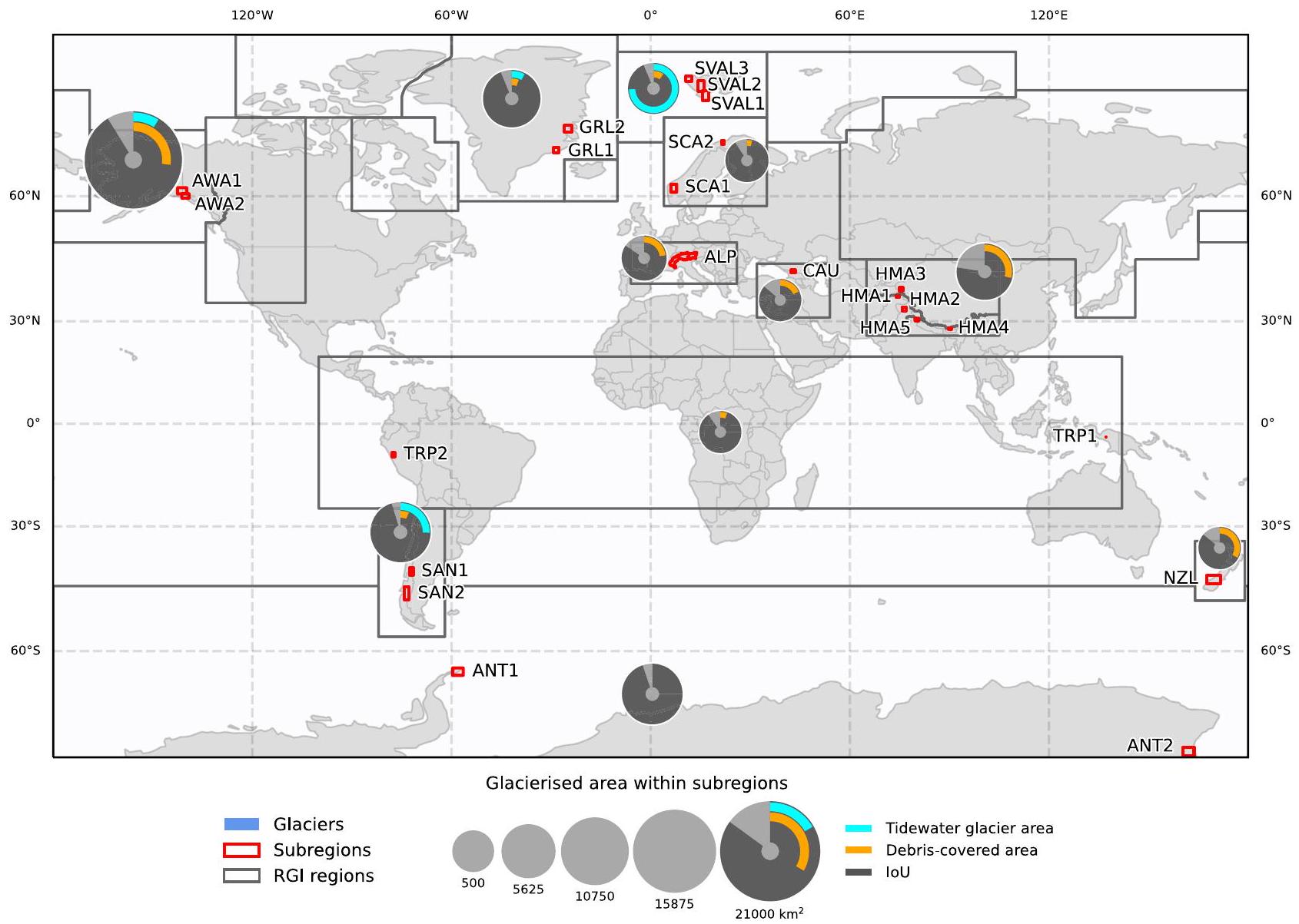
قمنا بتجميع مجموعتين شاملة من البيانات من صور الأقمار الصناعية المتاحة للجمهور وجرد الأنهار الجليدية – مجموعة بيانات قائمة على البلاط ومجموعة بيانات اختبار الاستحواذ المستقلة. تغطي مجموعة البيانات القائمة على البلاط (الشكل 1)، المستخدمة بشكل أساسي لتطوير واختبار النموذج الأولي، 11 منطقة متنوعة عالميًا وتمتد من 1988 إلى 2020. وهي منظمة في بلاطات قريبة من المربعات غير المتداخلة . تم تقسيم البلاطات عشوائيًا إلى مجموعات تدريب وتحقق واختبار. تحتوي هذه المجموعة على طيف واسع من أنواع الأنهار الجليدية عبر إعدادات بيئية مختلفة وتشمل ميزات بصرية وSAR وDEM وبيانات مرجعية من GLIMS , RGI وجردات إقليمية لكل من التدريب وتقدير الدقة. تم تنظيم البيانات في ثلاثة مسارات – (1) بصرية + DEM، (2) بصرية + DEM + حرارية و (3) بصرية + DEM + InSAR – للتحقيق في تأثير مجموعات الميزات المختلفة على أداء التصنيف. تُستخدم مجموعة بيانات اختبار الاستحواذ المستقلة بشكل خاص لاختبار تعميم نموذجنا عبر عمليات الاستحواذ المختلفة لصور الأقمار الصناعية في

الشكل 1 | مجموعة بيانات قائمة على البلاط ونظرة عامة على النتائج. اختصارات المناطق: ALP (جبال الألب)، ANT (أنتاركتيكا)، AWA (ألاسكا وأمريكا الغربية)، CAU (القوقاز)، GRL (غرينلاند)، HMA (آسيا الجبلية العالية)، TRP (خطوط العرض المنخفضة)، NZL (نيوزيلندا)، SAN (جبال الأنديز الجنوبية)، SCA (سكندنافيا)، SVAL (سفالبارد). تعتمد حدود الأنهار الجليدية ومناطق الأنهار الجليدية المائية على RGI7.0 . تم تعديل تغطية الحطام
من هيريد وبيليتشيوتي . يتم تقديم قيم تقاطع الاتحاد (IoU) لنموذج GlaViTU المدرب عالميًا باستخدام بيانات بصرية + DEM. يتم تجميع الإحصائيات لآسيا الوسطى والجنوبية الغربية والجنوبية الشرقية. يتم توفير بيانات المصدر كملف بيانات مصدر.
سيناريو تطبيق “العالم الحقيقي” ويشمل بيانات من جبال الألب السويسرية، وسكندنافيا، وألاسكا وكندا الجنوبية. مكنت مجموعة بيانات الاختبار هذه من تقييمات أكثر تحديًا للتعميم الزمني والمكاني للنماذج المدربة فقط على مجموعة البيانات القائمة على البلاط. لمزيد من التفاصيل حول البيانات، يرجى الاطلاع على قسم “مناطق الدراسة ومجموعات البيانات”.

نقترح Glacier-VisionTransformer-U-Net (GlaViTU، الشكل التكميلي 10)، وهو نموذج تعلم عميق، مصمم لالتقاط كل من الأنماط العالمية والمحلية للصورة (انظر التفاصيل في قسم “GlaViTU”) وتم تدريبه على مجموعة البيانات القائمة على البلاط. تم استكشاف خمس استراتيجيات لتحقيق تعميم عالٍ: (1) استراتيجية عالمية تعني نموذجًا واحدًا مدربًا على جميع المناطق، (2) استراتيجية إقليمية تدرب نموذجًا واحدًا لكل منطقة أو مجموعة من المناطق (مثل، مشاركة خصائص مماثلة مثل نسبة تغطية الحطام)، (3) استراتيجية تحسين دقيقة حيث يتم تحسين النموذج العالمي لكل منطقة (أو مجموعة من المناطق) بشكل فردي و (4) ترميز المنطقة و (5) استراتيجيات ترميز الإحداثيات حيث نقوم بإدخال بيانات الموقع، على التوالي، مناطق مشفرة بنظام واحد-ساخن وإحداثيات جغرافية، مباشرة في النموذج. بالتزامن مع استراتيجية ترميز المنطقة، قمنا أيضًا بتنفيذ تحسين التحيز الذي يهدف إلى تقليل تحول المجال عن طريق ضبط التحيزات التي أدخلتها بيانات الموقع أثناء الاستدلال (انظر التفاصيل في قسم “استراتيجيات نحو رسم الخرائط الجليدية العالمية”). اختبرنا هذه الاستراتيجيات على كل من مجموعة البيانات القائمة على البلاط ومجموعة بيانات اختبار الاستحواذ المستقلة. بالإضافة إلى ذلك، استخلصنا الثقة التنبؤية من إسقاط مونت كارلو ودرجات softmax العادية ، وأجرينا
معايرة لتوافق الثقة بشكل أفضل مع الدقة الفعلية لتفسير أكثر موثوقية وقارننا تلك، بالإضافة إلى استكشاف الأهداف التي تظهر درجات ثقة منخفضة (انظر التفاصيل في قسم “ت quantifying عدم اليقين”). للحصول على وصف تفصيلي لما هي المقاييس التي استخدمناها لتقييم نتائجنا، يرجى الاطلاع على قسم “تقييم الدقة”.

حقق GlaViTU، المدرب عالميًا على بيانات بصرية + DEM، دقة عالية بمتوسط IoU قدره 0.894 (الجدول التكميلي 2). قدم النموذج أداءً جيدًا جدًا للمناطق ذات الظروف الثلجية والجليدية بشكل أساسي مثل جبال الأنديز الجنوبية (IoU = 0.952)، أنتاركتيكا (0.949)، غرينلاند (0.937) وسفالبارد (0.936). لوحظ انخفاض في الأداء للمناطق ذات تغطية الحطام الكبيرة، مع أسوأ أداء في آسيا الجبلية العالية (0.774)، ولكن أيضًا للقوقاز (0.862) والجبال الألبية (0.844). يتم عرض عدة بلاطات مصنفة في الشكل التكميلي 2.

لا يزال GlaViTU يواجه تحديات في سيناريوهات معينة (الشكل التكميلي 5). على سبيل المثال، قد يكون تحديد بعض الألسنة المغطاة بالحطام تحديًا في بعض الحالات، حيث كان النموذج يميل إلى الإفراط في تقدير الحطام (الشكل التكميلي 5a) ويفوتها في حالات أخرى (الشكل التكميلي 5b). أيضًا، واجه GlaViTU صعوبة مع الجليد المظلل، حيث فشل أحيانًا في تصنيفه بدقة (الشكل التكميلي 5c). في حالات خلط الجليد الكثيف، أنتج GlaViTU كمية كبيرة من الإيجابيات الكاذبة (الشكل التكميلي 5d، e). أيضًا، قد تكون هناك آثار غير متوقعة على السواحل (الشكل التكميلي 5f).

تحدد الأقواس المناطق المستخدمة للنماذج الإقليمية/المعدلة والعلامات الخاصة بتشفير المناطق: ALP (جبال الألب)، AWA (ألاسكا وغرب أمريكا)، CAU (القوقاز) وSCA (اسكندنافيا).
أفضل قيم loU بالخط العريض.
استخدام تحسين التحيز.

لتلخيص، أظهرت GlaViTU أداءً عاليًا في إعدادات مختلفة لرسم الخرائط الجليدية. لا تزال هناك تحديات مثل تحديد لسان الجليد المغطى بالحطام، واكتشاف الجليد المظلل، والأخطاء في مناطق المزيج الجليدي الكثيف، والعيوب على السواحل.

قمنا باختبار خمس استراتيجيات لرسم خرائط الأنهار الجليدية العالمية وقيمنا أدائها. يوفر الجدول التكميلي 4 نظرة عامة على النتائج. بشكل عام، ظهرت استراتيجيات الإقليم والتعديل الدقيق كأكثرها وعدًا بمتوسط IoUs يبلغ 0.902 و0.901 على التوالي، حيث قدمت أفضل النماذج لجميع المناطق باستثناء منطقتين. كانت استراتيجية ترميز المنطقة أقل أداءً قليلاً في المتوسط. ). لقد أظهر زيادة طفيفة في الأداء مقارنةً بالاستراتيجية العالمية ( ) وأدت بشكل أفضل في جميع المناطق ما عدا واحدة. كانت استراتيجية ترميز الإحداثيات لديها أدنى متوسط IoU بلغ 0.893 ولم تؤدِ الأفضل في أي من المناطق. على الرغم من أن الفروقات، في المتوسط، طفيفة، وقد تفوقت على بعض الاستراتيجيات الأخرى في بعض المناطق، إلا أنها بشكل عام لا تقدم مكاسب في الأداء لرسم خرائط الأنهار الجليدية العالمية.

سمح التحليل النوعي لأداء الاستراتيجيات الخمس في سيناريوهات مختلفة بتحديد عدة أنماط. تُظهر بعض نتائج التصنيف المستمدة من استراتيجيات مختلفة في الشكل التوضيحي التكميلي 11. عبر الاستراتيجيات، كانت النتائج لتصنيف الجليد النظيف متطابقة تقريبًا (الشكل التوضيحي التكميلي 11أ، ب)، بينما كانت الاستراتيجيات الإقليمية واستراتيجيات التعديل الدقيق متفوقة في تحديد لسان الجليد في بيئات أكثر تحديًا (الشكل التوضيحي التكميلي 11ج، د). كانت كل من الاستراتيجيات الإقليمية واستراتيجيات التعديل الدقيق تميل إلى إنتاج عدد أقل من الإيجابيات الكاذبة للجليد المختلط (الشكل التوضيحي التكميلي 11هـ، و) وحلّت المشكلات المتعلقة بآثار الساحل (الشكل التوضيحي التكميلي 11ز)، مما زاد من موثوقية ودقة نتائج الخرائط.

باختصار، عند الاختبار على مجموعة البيانات المعتمدة على البلاط، قدمت استراتيجيات الإقليم والتعديل الدقيق أفضل دقة في التعيين مع تحسينات ملحوظة في الإعدادات الصعبة.

عند تقييم الاستراتيجيات من حيث أدائها في التعميم الزمني والمكاني باستخدام بيانات اختبار الاكتساب المستقلة، انحرفت النتائج عن النتائج الأولية، كما هو موضح في الجدول 1. على سبيل المثال، فإن استراتيجية ترميز المنطقة الم coupled مع تحسين التحيز حققت أفضل جودة رسم على المتوسط. )، في حين أن الزيادة في الأداء المحققة ظلت متواضعة نسبيًا عند مقارنتها بالاستراتيجية العالمية ( ). لم تحافظ الاستراتيجيات الإقليمية واستراتيجيات التعديل الدقيق على تفوقها في هذه الاختبارات. الاستثناء الوحيد كان في جنوب كندا، حيث كانت استراتيجية التعديل الدقيق
تفوقت بشكل طفيف على الاستراتيجيات الأخرى، لكننا نعتبر أن هذه الفروق ذات أهمية ثانوية. في المتوسط، أظهرت النماذج المعدلة تحسنات ملحوظة مقارنة بالنماذج الإقليمية. بالإضافة إلى ذلك، أدى تدريب وتعديل النماذج لمجموعات من المناطق ذات الخصائص المماثلة إلى تحسين عام في الأداء مقارنة بمنطقة واحدة. قدمت استراتيجية ترميز الإحداثيات نتائج غير متسقة وأحيانًا غير مرضية، خاصة بالنسبة لجبال الألب السويسرية وألاسكا، مما أثار مخاوف بشأن احتمال حدوث فرط التكيف.

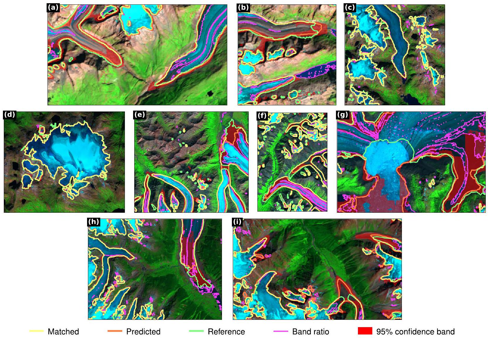
يوفر الشكل 2 عرضًا أكثر تفصيلًا لنتائج التصنيف لبيانات اختبار الاستحواذ المستقلة كما تم اشتقاقها باستخدام استراتيجية ترميز المنطقة وتحسين التحيز التي أظهرت أفضل أداء. بالنسبة لجبال الألب (الشكل 2أ، ب)، أظهر النموذج دقة عالية في إعادة بناء مواقع نهايات الأنهار الجليدية مع انحرافات صغيرة عن بيانات المرجع. بالنسبة لجنوب النرويج (الشكل 2ج، د)، اقتربت التنبؤات من الكمال، ويرجع ذلك إلى حد كبير إلى انتشار الجليد النظيف في المنطقة. بالنسبة لألاسكا، فشل في تصنيف مزيج الجليد بدقة وتحديد واجهات الانهيار (الشكل 2و)، على الرغم من أن النموذج نجح في رسم خريطة لجزء كبير من المناطق المغطاة بالحطام (الشكل 2هـ، و). بالنسبة لجنوب كندا، أظهر النموذج أداءً قويًا في تصنيف الجليد المغطى بالحطام (الشكل 2ي، نشك في وجود أخطاء في بيانات المرجع في الجانب السفلي من ي، ويبدو أن نموذجنا يحدد نهاية الجليد الفعلية بشكل أفضل)، على الرغم من أن بعض أجزاء الحطام ظلت غير مكتشفة (الشكل 2ز).

أظهرت أداء الاستراتيجيات اتجاهًا مميزًا مقارنةً بالنتائج السابقة المستندة إلى مجموعة البيانات المعتمدة على البلاط. تقدم اختبارات الاستحواذ المستقلة سيناريوهات أكثر تحديًا تتميز بتحولات أكبر في المجال بسبب اختلاف المستشعرات وظروف التصوير وميزات التضاريس. لذلك، فإن تقديرات الدقة المستمدة من هذه الاختبارات أكثر موثوقية وتصور بشكل أفضل الأداء المتوقع الفعلي للاستراتيجيات في التطبيقات العالمية متعددة الزمن.

كما استخدمنا مجموعة بيانات اختبار الاستحواذ المستقلة لإجراء مقارنات إضافية والتحقق من الصحة. أولاً، قمنا بمقارنة النتائج المستمدة من GlaViTU مع طريقة نسبة النطاق. لهذا، استخدمنا طريقة نسبة النطاق المعترف بها على نطاق واسع – الأحمر / SWIR. ث وأزرق القيم الحدية المثلى ) تم العثور عليها من خلال تعظيم IoU على بيانات التدريب من مجموعة البيانات المعتمدة على البلاط. يتفوق GlaViTU على نسبة الطيف، التي لا تستطيع تصنيف الجليد المغطى بالحطام وتنتج العديد من الإيجابيات الكاذبة للمسطحات المائية في جميع المناطق (الشكل 2 والجدول 1). في جنوب النرويج، الذي يهيمن عليه الجليد النظيف، تقترب نسبة الطيف من أداء GlaViTU (loU مقابل 0.933).

علاوة على ذلك، لاحظنا أن GlaViTU حقق نتائج غير متسقة بالنسبة للأنهار الجليدية الصغيرة. للحصول على رؤى حول أدائه عبر الأنهار الجليدية

الشكل 2 | نتائج تقسيم المعاني لبيانات اختبار الاستحواذ المستقلة كما تم اشتقاقها باستخدام GlaViTU مع الترميز الإقليمي وتحسين التحيز.
جبال الألب السويسرية، ج، د جنوب النرويج، هـ-ز ألاسكا و ح، ط جنوب كندا. الـ
تُعرض صور الأقمار الصناعية في تركيبة ألوان زائفة (R: SWIR ، G: NIR، B: R). صور لاندسات مقدمة من المسح الجيولوجي الأمريكي. بيانات كوبرنيكوس سنتينل 2019.
لتقييم دقة الكشف عن تباين المقياس، قمنا بتقييم دقته للكشف عن أحجام الأنهار الجليدية المختلفة (الجدول التكميلي 5). أظهر النموذج أداءً عاليًا في الكشف عن الأنهار الجليدية ودقة محدودة للأنهار الجليدية قمنا بأخذ 17 نهر جليدي تمثل أحجامًا مختلفة وتغطيها الحطام من مجموعة بيانات اختبار الاستحواذ المستقل وقمنا بتقييم جودة المخططات من حيث انحرافات المساحة والمسافة (الجدول التكميلي 6). تراوحت انحرافات المساحة من إلى باستثناء براتبرين ( ) وجليد السيف ، تضمن السابق البقعة التي فاتت من قبل النموذج وقد فاتت الأخيرة نسبة كبيرة من الجليد المغطى بالحطام بجوار التلال الجانبية في المرجع؛ كانت انحراف المسافة الوسيطة تقارب حجم بكسل مستشعر التصوير (10 م لـ Sentinel-2 و30 م لـ Landsat) مع وصول النسب المئوية الـ 95 إلى 300 م، وهو ضمن عدم اليقين الذي أبلغ عنه الخبراء البشريين في الأدبيات. .

قمنا بتقييم تأثير المسارات الثلاثة للبيانات على أداء نموذج رسم الخرائط الجليدية عبر مناطق فرعية مختلفة. لاختباراتنا، استخدمنا الاستراتيجية العالمية. تم تلخيص النتائج في الجدول التكميلي 7. لم يوفر إضافة البيانات الحرارية إلى النموذج تحسينات كبيرة، بل أدى ذلك إلى انخفاض الأداء في حوالي نصف المناطق الفرعية مقارنةً بالبيانات البصرية وبيانات DEM فقط (المتوسط للنفس المناطق الفرعية). على النقيض من ذلك، فإن دمج بيانات InSAR عزز بدقة نموذج الأداء عبر جميع المناطق الفرعية حيث كانت متاحة (0.891 مقابل 0.861)، مع أكبر تحسين لجبال الألب (0.873 مقابل 0.844)، والجبال الأنديز الجنوبية (SAN1، 0.890 مقابل 0.874) واسكندنافيا (SCA2، 0.909 مقابل 0.836).

يوفر الشكل التكميلي 12 توضيحًا نوعيًا لتأثيرات إضافة النطاق الحراري ويبرز الحالات التي تضررت فيها الأداء بسبب إضافة بيانات حرارية، خاصة في تصنيف الجليد المغطى بالحطام (الشكل التكميلي 12a-f)، وأدى إلى زيادة الإيجابيات الكاذبة في مزيج الجليد (الشكل التكميلي 12g). على العكس، يظهر الشكل التكميلي 7 مزايا دمج بيانات InSAR. أدى إضافة تشتت SAR وتماسك InSAR إلى تحسين دقة رسم خرائط نهايات الأنهار الجليدية (الشكل التكميلي 7a)، وتمكن من رسم خرائط للجليد الذي تم حظره جزئيًا بواسطة سحب رقيقة (الشكل التكميلي 7b) وحل جزئي للمشكلات المتعلقة بالعيوب على طول السواحل (الشكل التكميلي 7c).

باختصار، كشفت التقييمات أنه في تصميمنا التجريبي، كانت إضافة البيانات الحرارية لها فوائد محدودة، وفي حوالي نصف الحالات، حتى أدت إلى تدهور أداء النموذج. كان دمج بيانات InSAR يعزز أداء النموذج باستمرار عبر جميع المناطق المختبرة.

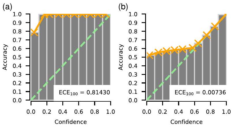
استفدنا من إسقاط مونت كارلو ودرجات السوفتمكس العادية لاشتقاق احتمالات الفئات المتوقعة واستخدمناها لإنتاج تقديرات ثقة التصنيف. في البداية، عند استخدام إسقاط مونت كارلو قبل معايرة ثقة التنبؤ، وجدنا أن النموذج كان يميل إلى إظهار عدم ثقة كبير كما يتضح من خطأ المعايرة المتوقع العالي. . تسلط هذه النتيجة، كما هو موضح في الشكل 3a، الضوء على الحاجة إلى مزيد من المعايرة لتعزيز موثوقية هذه التقديرات لعدم اليقين. أدت معايرة الثقة إلى تقليل ملحوظ في خطأ المعايرة المتوقع إلى . يظهر الشكل 3b التحسين

بعد معايرة الثقة. من المثير للاهتمام، وجدنا أن تقديرات الثقة المستمدة فقط من درجات السوفتمكس العادية أسفرت عن نتائج شبه مطابقة لتلك التي تم الحصول عليها من إسقاط مونت كارلو قبل المعايرة و بعد . علاوة على ذلك، كانت التقديرات المعايرة المستمدة من إسقاط مونت كارلو ودرجات السوفتمكس مرتبطة ارتباطًا وثيقًا، حيث كان معامل الارتباط بيرسون يتراوح بين 0.873 و0.884 (تم الإبلاغ عنها كالنسب المئوية 2.5 و97.5 التي تم الحصول عليها من التمهيد). ومن ثم، نقترح أن الثقة المستمدة من درجات السوفتمكس وحدها يمكن أن تحل محل إسقاط مونت كارلو كوسيلة موثوقة لتقدير عدم اليقين التنبؤي، مما يوفر تكاليف حسابية أقل مطلوبة للاستدلال.

توفر الأشكال التكملية 3 و6 تصورات لخرائط الثقة للقطع التمثيلية، مما يقدم رؤى حول كيفية توزيع هذه التقديرات عبر ميزات التضاريس المختلفة. كانت الثقة تميل إلى أن تكون منخفضة باستمرار للجليد المغطى بالحطام بغض النظر عما إذا كان قد تم رسمه بشكل صحيح أم لا (الأشكال التكملية 3a-d و ). كانت الثقة أيضًا منخفضة في المناطق المظللة حيث فشل النموذج في اكتشاف بكسلات الجليد (الشكل التكميلي 6c). بالنسبة لمزيج الجليد الذي تم التنبؤ به بشكل صحيح، منح نموذجنا درجات ثقة عالية (الشكل التكميلي 3g). بالنسبة لمناطق مزيج الجليد التي تم تصنيفها بشكل خاطئ، أظهرت تقديرات الثقة تباينًا، حيث كانت منخفضة في إعدادات معينة (الشكل التكميلي 6d) ومرتفعة في أخرى (الشكل التكميلي 6e). كما أبلغنا عن -نطاقات الثقة لنتائج التقسيم الدلالي لبيانات اختبار الاستحواذ المستقلة لاختبارات التعميم في الشكل 2. أظهرت نطاقات الثقة أنماطًا مشابهة للمناطق المغطاة بالحطام والمظللة. في المجموع، من البكسلات المصنفة بشكل خاطئ تم تضمينها في نطاقات الثقة، و على بيانات اختبار الاستحواذ المستقلة. من الجدير بالذكر أن الأجزاء المصنفة بشكل خاطئ من الجليد المغطى بالحطام كانت في الغالب ضمن نطاقات الثقة المبلغ عنها، على عكس مزيج الجليد الذي تم تصنيفه بشكل خاطئ على أنه أنهار جليدية بثقة عالية.

تحقق GlaViTU دقة عالية بشكل عام وغالبًا ما يلغي الحاجة إلى تصحيحات يدوية، مما يقدم تحسينًا كبيرًا على طرق نسبة النطاقات المعروفة التي تشكل العمود الفقري لمعظم عمليات الرقمنة شبه الآلية، بما في ذلك تلك المستخدمة في GLIMS وRGI، بالإضافة إلى نماذج التعلم العميق الأخرى (انظر الملاحظات التكميلية). قارننا نتائج GlaViTU مع عدم اليقين لدى الخبراء البشريين المقدم في الأدبيات،
لا سيما العمل الذي قام به بول وآخرون. وتجارب مقارنة تحليل GLIMS (GLACE) . شمل تحليلنا مجموعة متنوعة من 17 نهرًا جليديًا، تتفاوت في الحجم وتغطية الحطام، من مجموعة بيانات اختبار الاستحواذ المستقلة. كانت التقييمات تستند إلى انحرافات المساحة والمسافة، حيث أظهرت معظم الأنهار الجليدية انحرافات ضمن ، مما يتماشى عن كثب مع عدم اليقين في تحديدات الخبراء البشريين. بينما كانت انحرافات المسافة الوسيطة على قدم المساواة مع حجم بكسل أجهزة استشعار التصوير Sentinel-2 وLandsat، مع النسب المئوية 95 ضمن نطاق عدم اليقين للخبراء، هناك اعتبارات أساسية يجب أخذها في الاعتبار. أبلغت تجارب GLACE وبول وآخرون عن عدم اليقين البشري للأنهار الجليدية النظيفة في الغالب، مستبعدين الأجزاء الكبيرة المغطاة بالحطام أو المناطق المظللة الواسعة التي تعد مصادر كبيرة للأخطاء في الجرد. علاوة على ذلك، تركزت دراسات مثل هذه عادةً على مجموعة صغيرة من الأنهار الجليدية، والتي قد لا تعكس التنوع الموجود في مجموعات البيانات الأكبر، وقد تعطي آراء إيجابية بشكل مفرط حول دقة الخبراء نظرًا لأن الخبراء على علم بأن عملهم يتم مقارنته ببعضهم البعض. في الإعدادات العملية، غالبًا ما يكون عدم اليقين في رسم الخرائط اليدوية أعلى بكثير مما تم الإبلاغ عنه في الدراسات المنضبطة. لقد وجدنا تباينات حيث تجاوز عدم اليقين لدى الخبراء الأرقام المبلغ عنها بمقدار خمسة إلى عشرة أضعاف، خاصة في السيناريوهات المعقدة التي تتضمن الحطام (على سبيل المثال، كما هو موضح في الشكل 2i والشكل التكميلي 11d). تشير هذه الملاحظات إلى فجوة معرفية كبيرة في رسم الخرائط اليدوية على نطاق واسع وتؤكد فعالية طريقتنا الآلية عبر المناظر الجليدية المتنوعة بينما تكون قابلة للتوسع وقابلة للتكرار بالكامل، على عكس الخبراء البشر.

لا تزال التحديات قائمة، على سبيل المثال، فإن تحديد الألسنة المغطاة بالحطام لا يزال مهمة معقدة بسبب تشابهها الطيفي مع الصخور المحيطة. يواجه GlaViTU أيضًا مشكلات في تصنيف الجليد المظلل بدقة واكتشاف الأنهار الجليدية الصغيرة. يمكن أن يُعزى الأداء المحدود في الكشف عن الأنهار الجليدية الصغيرة ( ) جزئيًا أيضًا إلى عدم اليقين الموروث في الجردات المستمدة من البشر، والتي تنشأ من القرارات الذاتية بشأن الحد الأدنى من مساحة الجليد التي يجب تضمينها، مع قيم نموذجية تتراوح من إلى 0.05 . بالنسبة لمزيج الجليد الكثيف، تظهر نماذجنا عددًا كبيرًا من الإيجابيات الكاذبة لأن توقيعها الطيفي مشابه لذلك الخاص بالجليد النظيف وهي ممثلة تمثيلاً ناقصًا في مجموعات البيانات لدينا. علاوة على ذلك، تحدث أحيانًا آثار غير متوقعة على السواحل، على الأرجح بسبب انعكاس المياه المنخفضة المشابه للجليد في نطاق الأشعة تحت الحمراء القصيرة وانحدارات صفرية في نموذج الارتفاع الرقمي للمحيط المظلل. وهذا يستدعي الحاجة إلى مزيد من تحسين النموذج أو الخوارزمية. على سبيل المثال، خلال تدريب النموذج، قد تكون استراتيجية العينة التكيفية التي تزود النموذج بعينات أكثر تحديًا مفيدة لتحسين الأداء على الأهداف التي يصعب تصنيفها. بدلاً من ذلك، يمكن معالجة بعض الأهداف بطريقة خاصة. على سبيل المثال، يمكن رسم واجهات الانفصال باستخدام الطرق المقترحة من قبل وو وآخرون. أو هايدلر وآخرون. . يمكن تطبيق المعالجة اللاحقة للتخلص من بعض المشكلات. على سبيل المثال، يمكن تصفية مضلعات الشظايا على المورينات الوسطى للأنهار الجليدية بناءً على أوصاف الشكل، ويمكن إزالة الآثار على السواحل باستخدام أقنعة تشير إلى غياب الجليد بناءً على المعرفة السابقة. أيضًا، تقدم نطاقات الثقة فرصة لتحسين رسم خرائط الأنهار الجليدية الصغيرة وتغطية الحطام كما هو موضح أدناه.

مع النموذج، قدمنا خمس استراتيجيات لتحقيق رسم خرائط الأنهار الجليدية على نطاق عالمي. قمنا بتقييم هذه الاستراتيجيات بطريقتين مختلفتين – باستخدام مجموعة اختبار قائمة على البلاط ومع بيانات اختبار الاستحواذ المستقلة التي تم تجميعها لاختبار التعميم. تباينت نتائج التقييمين. وفقًا للتقييم القائم على البلاط، فإن الاستراتيجيات الإقليمية واستراتيجيات الضبط الدقيق تتفوق على غيرها. على العكس، وفقًا للتقييم القائم على البيانات المفصولة تمامًا في الوقت أو المكان، أظهرت استراتيجية ترميز المنطقة مع تحسين التحيز أفضل النتائج، على الرغم من أن الفروق مع الاستراتيجية العالمية كانت طفيفة.

من الناحية الفنية، يمكن تنفيذ طريقة تحسين التحيز لأي نموذج. في تصميمنا التجريبي، ومع ذلك، فإنها تكمل بشكل طبيعي استراتيجيات ترميز الموقع التي تحتوي بالفعل على كتلة خاصة لإدخال التحيز. فشلت استراتيجية ترميز الإحداثيات عند تصنيف بيانات غير مرئية تمامًا مما قد يشير إلى ميلها إلى الإفراط في التكيف، قد تحقق الأبحاث المستقبلية طرق تنظيم لهذه الاستراتيجية. نظرًا لأن طريقة التقييم الثانية أقل تحيزًا، نؤكد أن تقديرات الدقة التي حصلنا عليها خلال هذه الاختبارات الزمنية والمكانية للتعميم أكثر موثوقية في ضوء نشر النموذج لرسم خرائط متعددة الأوقات على مستوى عالمي، مما يتطلب التعميم في الفضاء والزمان وخصائص المستشعر. لا يزال يمكن أن تكون طريقة التقييم الأولى متحيزة تجاه مستشعرات الأقمار الصناعية، وظروف التصوير أو الإجراءات المستخدمة لإنتاج بيانات مرجعية (مثل تصفية أكوام الثلج الصغيرة بناءً على عتبة المساحة). من الجدير بالذكر أن التقييم القائم على البلاط معتمد على نطاق واسع , مما قد يشير إلى أداء النموذج المتفائل المفرط الذي يتم الإبلاغ عنه غالبًا في الأدبيات، وبالتالي، يجب التعامل مع مثل هذه التقييمات بحذر، خاصة عند البحث عن نموذج بقدرة تعميم عالية للتطبيقات التشغيلية على نطاق واسع. ومع ذلك، يمكن أن تحقق استراتيجيات أخرى نتائج أفضل في بعض الإعدادات. على سبيل المثال، يمكن أن تؤدي النماذج الإقليمية أداءً استثنائيًا عند تطبيقها على نفس بيانات المستشعر والظروف المماثلة لتلك الموجودة في مجموعة بيانات التدريب لمنطقة معينة. بشكل عام، تحقق نماذجنا دقة وقوة كافية لملاحظة تغييرات كبيرة في مساحة الأنهار الجليدية على مدى عقود كما هو موضح في تحليلنا المفصل في الملاحظات التكميلية. يثبت هذا التحليل قدرة GlaViTU على مراقبة التغيرات طويلة الأجل في امتدادات الأنهار الجليدية ويؤكد فائدة النموذج في الدراسات متعددة الأوقات. علاوة على ذلك، يوفر التحقق الإضافي ضد مجموعة بيانات مستقلة تمامًا، وهي جرد الأنهار الجليدية السويسرية , رؤى إضافية حول فعالية وقوة GlaViTU، كما هو مفصل في الملاحظات التكميلية. هذا التحقق أمر حاسم لأنه يستخدم بيانات بدقة بكسل أقل من متر، والتي تعتبر المعيار الذهبي بسبب دقتها الأعلى، على الرغم من أنها ليست قابلة للتطبيق عالميًا وتحتوي أيضًا على تحيزات ذاتية.

يوفر مقارنة مسارات البيانات المختلفة ضمن إطار رسم خرائط الأنهار الجليدية لدينا رؤى قيمة حول دور مدخلات الاستشعار عن بعد المختلفة في تحسين أداء النموذج. أولاً، تشير نتائجنا إلى أن إضافة البيانات الحرارية، على الرغم من أنها واعدة في البداية بسبب قدرتها على التمييز بين الصخور المحيطة والجليد المغطى بالحطام , لا تعزز الأداء بشكل موثوق في تجاربنا. في الواقع، يؤدي ذلك إلى انخفاض في الدقة في حوالي نصف المناطق الفرعية. تشير هذه النتيجة إلى أن البيانات الحرارية تقدم تعقيدات أو عدم يقين يكافح نموذجنا للتكيف معها، خاصة في المناطق المغطاة بالحطام. قد تشبع النطاق الحراري، كمتنبئ قوي للجليد النظيف والثلج، الشبكة العصبية خلال المراحل المبكرة من التدريب. علاوة على ذلك، يمكن أن تؤدي الدقة المكانية المنخفضة للنطاقات الحرارية (120 م للاقمار الصناعية لاندسات للاقمار الصناعية لاندسات 7 ETM + و100 م للاقمار الصناعية لاندسات 8 TIRS) إلى تشويش الميزات المهمة اللازمة لرسم خرائط الأنهار الجليدية بدقة، خاصة في المناطق المغطاة بالجليد حيث تكون التفاصيل الأكثر دقة مطلوبة للتمييز بين الحطام والصخور. أيضًا، تنخفض قيمة الصور الحرارية مع اقتراب سمك طبقة الحطام من 0.5 م، مما يعزل الجليد تحتها ويخفي توقيعها الحراري . لذلك، قد يؤدي الدمج المباشر للبيانات الحرارية إلى فقدان الأداء ويجب التعامل معه بحذر. على النقيض من ذلك، يبرز التأثير الإيجابي لإضافة بيانات InSAR عبر جميع المناطق الفرعية حيث كانت متاحة أهميتها لرسم خرائط الأنهار الجليدية. إنه يحسن الدقة العامة ويعالج تحديات محددة، مثل رسم الخرائط الدقيقة للنهايات أو الحجب الجزئي للجليد مع سحب رقيقة. من المحتمل أن تكون هذه التحسينات بسبب قدرة SAR على اختراق السحب وقدرة InSAR على اكتشاف تشوهات بمقياس السنتيمتر مما يمكّن من تمييز أكثر دقة بين الجليد والأرض المستقرة. ومع ذلك، فإن بيانات SAR المتسقة والعالمية يصعب جمعها للفترات التي تسبق عام 2015. لذلك، من المعقول التركيز على
تطوير مسار Optical+DEM لرسم خرائط الأنهار الجليدية قبل عام 2015 ومسار Optical+DEM+InSAR بعد عام 2015 عندما أصبحت بيانات Sentinel-1 متاحة عالميًا.

كشف تقدير عدم اليقين ضمن نماذج تقسيمنا الدلالي عن بعض النتائج الملحوظة. قبل معايرة الثقة، أظهرت النماذج ميلاً نحو عدم الثقة، والذي يمكن أن يرتبط جزئيًا باستخدام تنعيم التسمية . أيضًا، وجدنا أن درجات softmax العادية، التي تكون فعالة حسابيًا وسهلة الحصول عليها، تعطي تقديرات ثقة قابلة للمقارنة مع تلك التي تم الحصول عليها من إسقاط مونت كارلو، على عكس بعض التقارير في الأدبيات. في الواقع، سلطت العديد من الدراسات الضوء على الإفراط في الثقة لنماذج التعلم العميق وقيود استخدام درجات softmax كتقديرات موثوقة لعدم اليقين . بشكل مدهش، أشارت نتائجنا إلى أن درجات softmax العادية يمكن أن تكون موردًا قيمًا لتقدير عدم اليقين التنبؤي في سياق رسم خرائط الأنهار الجليدية لدينا.

تقدم التصورات الخاصة بالثقة التنبؤية نظرة ثاقبة على توزيع الثقة عبر ميزات التضاريس المختلفة وتوفر سياقًا إضافيًا لتحسين نماذجنا وفهم قيودها. يمكن أن تكون أيضًا بمثابة إرشادات للتصحيحات اليدوية، واختيار العينات الأكثر معلوماتية للتسمية ضمن حلقة التعلم النشط أو كجزء من أنظمة شبه آلية تفاعلية. علاوة على ذلك، فإن درجات الثقة المتوقعة لديها القدرة على أن تُدمج في خوارزميات ما بعد المعالجة لتحسين دقة نتائج الخرائط بشكل أكبر. بالإضافة إلى ذلك، يمكن ربط الثقة التنبؤية بشكل أكبر مع IoU كمقياس لأداء النموذج في غياب بيانات مرجعية (انظر الملاحظات التكميلية).

في هذه الورقة، قدمنا GlaViTU، وهو نموذج هجين من الشبكات العصبية التلافيفية والمحولات لرسم خرائط الأنهار الجليدية من بيانات الأقمار الصناعية متعددة الأنماط المفتوحة. كما نشرنا مجموعة بيانات مرجعية لرسم خرائط الأنهار الجليدية على نطاق عالمي. يتفوق GlaViTU باستمرار على نماذج التعلم العميق الأخرى (انظر الملاحظات التكميلية) عبر مناطق مختلفة، مما ينتج عنه نتائج عالية الجودة لمعظم الصور، تقترب من عدم اليقين لدى الخبراء البشر. على الرغم من نجاحاته، لا تزال التحديات قائمة، خاصة في تحديد الألسنة المغطاة بالحطام، وتصنيف الجليد المظلل والتعامل مع مزيج الجليد. قدمنا خمس استراتيجيات لتحقيق تعميم عالي لرسم خرائط الأنهار الجليدية عبر المناطق وعلى مر الزمن. بشكل عام، تعتبر استراتيجية ترميز المنطقة الم coupled with تحسين التحيز هي أفضل استراتيجية تسمح بتحقيق قيم IoU تتجاوز 0.85 للصور التي لم يتم ملاحظتها سابقًا في المتوسط. للكسارات الغنية بالركام للمناطق ذات الجليد النظيف). تكشف دراستنا أن كل من أسلوب مونت كارلو للتخلي والدرجات العادية للسوفت ماكس يمكن أن توفر تقديرات موثوقة للثقة في توقعات النموذج بعد المعايرة، حيث تعتبر درجات السوفت ماكس العادية خيارًا أكثر فعالية من حيث الحوسبة. يمكن أن تكون هذه التقديرات مفيدة في المعالجة اللاحقة وفهم قيود النموذج. في الأبحاث المستقبلية، يمكن أن يتضمن ذلك طرق الذكاء الاصطناعي القابلة للتفسير، مثل التدرجات المتكاملة. يمكن أن تعزز الشفافية في النموذج وتساعد في معالجة التحديات المتبقية. اقترحنا علاقة لتقدير IoU في غياب بيانات مرجعية بناءً على الثقة التنبؤية، مما يظهر ارتباطًا قويًا بين القيم المقدرة والفعلية لـ IoU المحلي (انظر الملاحظات التكميلية). تشمل أعمالنا أيضًا نهجًا آليًا لاشتقاق حدود الجليد من DEM كما اقترح كينهلوز وآخرون. (انظر الملاحظات التكميلية)، مما يجعل سير عمل شامل لتوليد مخططات الأنهار الجليدية.

تقدم هذه الدراسة أيضًا رؤى علمية أوسع حول مراقبة الأرض وتعلم الآلة تتجاوز رسم خرائط الأنهار الجليدية. تؤكد هذه الورقة على أهمية تقدير عدم اليقين في توقعات النماذج، وهو ما يتم تجاهله غالبًا في دراسات الاستشعار عن بعد وتعلم الآلة، مما يوفر طريقًا لتطبيقات الذكاء الاصطناعي الأكثر شفافية وقابلية للتفسير في علوم الأرض. يمكن للتقنيات المقدمة هنا التعامل مع بيانات مراقبة الأرض من أوقات مختلفة و
تعد المستشعرات قابلة للتكيف لدراسة ظواهر بيئية متنوعة وتوفر أدوات قيمة لمجتمع مراقبة الأرض لتحسين رصد ومعالجة التغيرات البيئية على نطاق واسع. متفوقة على نماذج الأساس الأخرى، نقترح تطبيق GlaViTU في مجالات الاستشعار عن بعد المختلفة، مثل رسم خرائط استخدام الأراضي وتغطية الأراضي ومراقبة الغطاء النباتي والغابات والجليد البحري والصفائح الجليدية.

في الختام، تمثل دراستنا تقدمًا في الجهود نحو رسم خرائط الأنهار الجليدية على نطاق عالمي بشكل آلي بالكامل، حيث تقدم دقة وكفاءة محسنتين، وتمكن من إنشاء قوائم جليدية عالمية محدثة بانتظام وتحليل تغييرات مساحة الأنهار الجليدية على المدى الطويل. هذه التقدمات أساسية لتحسين جودة التحليلات اللاحقة، بما في ذلك، على سبيل المثال، قياسات ونمذجة سرعة سطح الجليد، والتوازن الكتلي، وتطور الأنهار الجليدية. ومع ذلك، لا تزال هناك تحديات، وهناك حاجة إلى مزيد من تحسينات النماذج والخوارزميات. نشجع المجتمع على استخدام كودنا مفتوح المصدر ومجموعات البيانات المرجعية بنشاط لتطوير النماذج المستقبلية للمساعدة في التغلب على هذه التحديات. مع الأساليب والنتائج من هذا البحث، نحن مستعدون لإطلاق مبادرة شاملة لرسم خرائط الأنهار الجليدية العالمية تعتمد على الذكاء الاصطناعي، والتي ستتتبع تغييرات الأنهار الجليدية على مدى الثلاثين عامًا الماضية وفي المستقبل.

قمنا بجمع مجموعتين من البيانات – مجموعة بيانات قائمة على البلاط تشمل أنواعًا متنوعة من الأنهار الجليدية عبر عدة مناطق في جميع أنحاء العالم، ومجموعة بيانات اختبار مستقلة تُستخدم بشكل خاص لتقييم النماذج على بيانات متباينة مكانيًا وزمنيًا عن مجموعة البيانات القائمة على البلاط، بالإضافة إلى بيانات من مستشعرات وظروف تصوير مختلفة. تجمع مجموعة البيانات القائمة على البلاط بيانات بصرية وبيانات رادارية (SAR) وبيانات نمذجة الارتفاع (DEM) متاحة للجمهور لـ 11 منطقة (23 منطقة فرعية) في جميع أنحاء العالم – جبال الألب الأوروبية (ALP)، القارة القطبية الجنوبية (ANT)، ألاسكا وغرب أمريكا (AWA)، القوقاز (CAU)، محيط غرينلاند (GRL)، جبال آسيا العالية (HMA)، المناطق المنخفضة (TRP)، نيوزيلندا (NZL)، جبال الأنديز الجنوبية (SAN)، الدول الاسكندنافية (SCA) وسفالبارد (SVAL). صممنا مجموعة البيانات لتشمل طيفًا متنوعًا من الأنهار الجليدية، بما في ذلك، على سبيل المثال، الأنهار الجليدية النظيفة، المغطاة بالحطام والمغطاة بالنباتات، الموجودة في بيئات متنوعة مثل البيئات الجبلية، القطبية والاستوائية، بالإضافة إلى البيئات البحرية والقارية. سمح لنا هذا الاختيار التصميمي بمعالجة الحاجة إلى رسم خرائط قوية للأنهار الجليدية عبر مناخات وتضاريس مختلفة. تغطي مجموعة البيانات تقريبًا أو 19,000 من الأنهار الجليدية في جميع أنحاء العالم وتمثل حوالي من المنطقة الجليدية باستثناء صفائح الجليد في غرينلاند والقارة القطبية الجنوبية. أقدم بيانات مرجعية هي من المنطقة القطبية الجنوبية في بينما أحدث البيانات تأتي من سفالبارد في .

تتضمن مجموعة البيانات المعتمدة على البلاط بيانات من مصادر متنوعة. بالنسبة للبيانات البصرية، استخدمنا قيم الانعكاس عند قمة الغلاف الجوي لستة نطاقات، وهي: الأزرق، والأخضر، والأحمر، والأشعة تحت الحمراء القريبة، ونطاقين من الأشعة تحت الحمراء القصيرة. و ) من لاندسات 5 و 7 و 8 وسينتينل-2. كميزات SAR، تم استخدام صور السعة المعايرة التي تم الحصول عليها من ENVISAT و Sentinel-1 من كلا المسارين المداريين الصاعدين والنازلين. بالإضافة إلى السعة، تم استخدام صور تماسك SAR التداخلي (InSAR) إذا كانت متاحة. تم استخدام نموذج الارتفاع من مهمة رادار توبوغرافيا المكوك (SRTM) ونموذج الارتفاع العالمي ALOS 3D 30 م (AW3D30) ونموذج الارتفاع Copernicus GLO-30 (Cop30DEM) لتمثيل بيانات الارتفاع وانحدارات التضاريس. استخدمنا جردًا إقليميًا لحدود الأنهار الجليدية في جبال الألب. نيوزيلندا شمال اسكندنافيا وسفالبارد (لقد تلقينا نسخة أولية من مجموعة البيانات من المؤلفين)، بينما GLIMS تم توفير بيانات مرجعية مباشرة للمناطق المتبقية، مع وجود عدد قليل فقط من المراجع الأصلية الموجودة في البيانات الوصفية تم اختيار الصور البصرية لتتناسب مع التواريخ المحددة بدقة في بيانات جرد الأنهار الجليدية، مع التركيز بشكل خاص على acquisitions في أواخر الصيف في نهاية موسم الذوبان قبل أول حدث ثلجي كبير لضمان الحد الأدنى من الثلوج الموسمية.
غطاء. بالنسبة لبيانات SAR و DEM، حيث لم يكن من الممكن مطابقة التواريخ بدقة، اخترنا الصور ضمن نافذة زمنية محدودة تصل إلى شهر لبيانات SAR وسبع سنوات لبيانات DEM، باستثناء القارة القطبية الجنوبية وغرينلاند التي لا تغطيها SRTM حيث استخدمنا AW3D30. تم إعادة عينة جميع الصور إلى دقة 10 م لتتناسب مع أعلى دقة مكانية لـ Sentinel-2، وتم تطبيق طريقة الجوار الأقرب على النطاقات الضوئية، بينما تم استخدام طريقة الاستيفاء الثنائي لإعادة عينة بقية البيانات. وفقًا لممارسة مقبولة على نطاق واسع في دراسات الاستشعار عن بعد، قمنا بتقسيم جميع المناطق إلى بلاطات قريبة من المربعات بحجم تقريبي من ، وتم اختيار حوالي بلاط للتدريب، للتأكيد و للاختبار. الشكل 1 يوضح نظرة عامة على مجموعة البيانات المعتمدة على البلاط ومناطق الدراسة، والجدول 2 يقدم ملخصًا لها.

للتعامل مع مجموعات الميزات المتنوعة عبر المناطق الفرعية المختلفة، حددنا ثلاثة مسارات بيانات متميزة لاستخدامها في التجارب اللاحقة. هذه المسارات هي كما يلي:

تتكون مجموعة بيانات اختبار الاستحواذ المستقل من بيانات من GLIMS لتقييم تعميم النماذج على اكتسابات جديدة في سياقات زمنية ومكانية مختلفة. إن دمج هذه البيانات المستقلة للاختبار يوفر رؤى حول أداء الخرائط عبر مناطق متنوعة ومقاييس زمنية غير موجودة في مجموعة البيانات المعتمدة على البلاط، مما يتماشى مع هدفنا طويل الأمد في أتمتة رسم الخرائط الجليدية العالمية ومتعددة الأوقات باستخدام مستشعرات تصوير مختلفة. لتقييم التعميم الزمني، حصلنا على بيانات من جبال الألب السويسرية (259 نهر جليدي تغطي )، مجموعة فرعية من ALP، منذ عام 1998، ومن جنوب اسكندنافيا ( 1508 نهر جليدي، )، نفس المنطقة مثل SCA1، من تتميز جبال الألب السويسرية بألسنة مغطاة بالحطام والجليد في الظل، بينما تتميز جنوب اسكندنافيا بشكل رئيسي بالجليد النظيف. كما أن اختبارات التعميم الزمني عملت أيضًا كاختبارات تعميم عبر المستشعرات وعبر نماذج الارتفاع الرقمية (DEM) حيث كانت المستشعرات البصرية ونماذج الارتفاع الرقمية المستخدمة في هذه الاختبارات مختلفة تمامًا عن تلك الموجودة في مجموعة البيانات المعتمدة على البلاط. تتكون مجموعة البيانات المعتمدة على البلاط من صور Sentinel-2 وبلاطات Cop30DEM لجبال الألب السويسرية، بينما تعتمد البيانات الإضافية على Landsat 5 وSRTM. وبالمثل، استخدم SCA1 من مجموعة البيانات المعتمدة على البلاط Landsat 5 وAW3D30، بينما استخدمنا Sentinel-2 وCop30DEM للاختبار. بالنسبة لاختبارات التعميم المكاني، اخترنا منطقة في ألاسكا (1108 جليدًا، ، 2009، لاندسات 5 و AW3D30) ومنطقة في جنوب كندا (980 نهر جليدي، 2005، لاندسات 5 و AW3D30). تتميز كلا المنطقتين بألسنة جليدية تغطيها حطام بارز. علاوة على ذلك، تشمل منطقة ألاسكا الأنهار الجليدية التي تنتهي بالماء مع مزيج من الجليد، مما يشكل تحديًا كبيرًا لرسم الخرائط بدقة. تم استخدام بيانات اختبار الاستحواذ المستقلة هذه فقط لتقييم النماذج المدربة على بلاطات التدريب من مجموعة البيانات المعتمدة على البلاطات ولم يتم استخدامها للتدريب. الشكل التكميلي 13 يوضح المناطق الإضافية لاختبارات التعميم الزمني والمكاني.

الجدول 2 | ملخص مجموعة البيانات المعتمدة على البلاط

تغطية الحطام مأخوذة من هيرريد وبيليتشيوتي .

قمنا بتوسيع عملنا السابق ، حيث اقترحنا نسخة أولية من GlaViTU (الشكل التوضيحي التكميلي 10)، وهو مزيج من شبكة التلافيف ومحولات لتخطيط الأنهار الجليدية على نطاق واسع. يتضمن كتل بناء مبسطة من SEgmentation TRansformer (SETR) مع وحدة فك ترميز ذات تصعيد تدريجي (PUP). و U-Net مع الاتصالات المتبقية من خلال وضع الشبكات الفرعية المحولة والتلافيفية بشكل متتابع، تضمن GlaViTU أن يتم تعلم السياق العالمي للصورة في البداية، تليها استخراج الميزات الدقيقة باستخدام الشبكة الفرعية التلافيفية. يستند هذا الاختيار التصميمي إلى الملاحظة أن النماذج المعتمدة فقط على المحولات تواجه تحديات في تقديم توقعات كثيفة ومفصلة. من خلال دمج نقاط القوة في نماذج الالتفاف ونماذج المحولات، تلتقط GlaViTU بفعالية كل من الميزات على المستوى المحلي والمستوى العالمي في بيانات الاستشعار عن بعد المتعددة المصادر وغير المتجانسة، مما يمكّن من إنتاج جرد دقيق للأنهار الجليدية وتحسين التعميم. يقدم هذا البحث نسخة معدلة من GlaViTU مع كتلة دمج بيانات محسّنة وروتين تدريب أكثر تقدمًا. توضح الشكل التوضيحي الإضافي 8 كتلة دمج البيانات المعدلة لحالة المدخلات الثلاثة. مستلهمًا من Hu وآخرين. قمنا بإضافة كتلة ضغط وتحفيز واحدة في كل فرع تلافيفي لدمج المزيد من التفاعلات عبر القنوات وإضافة وزن للميزات قبل دمج المدخلات متعددة المصادر.

تم تدريب النماذج باستخدام قطع صور بحجم بكسلات مستخرجة عشوائيًا من مجموعة بيانات التدريب. استخدمنا مُحسِّن آدم. لإيجاد معلمات النموذج من خلال تقليل الخسارة البؤرية مع تعيين المعامل البؤري إلى . أضفنا فرع إشراف عميق مع دالة خسارة متطابقة مباشرة بعد شبكة التحويل (الشكل التوضيحي 10). لتعزيز عملية التدريب بشكل أكبر، طبقنا تلطيف التسميات مع معامل التلطيف لتعديل معدل التعلم بشكل ديناميكي، استخدمنا جدول تناقص جيبي مع إعادة تشغيل دافئة كما اقترح لوشتشيلوف وهوتير. لتجنب الحد الأدنى المحلي والمناطق الواسعة من الهضاب في مشهد الخسارة. معدل التعلم الابتدائي هو تم تقسيم التدريب إلى أربع دورات، كل منها تتكون من ، و 80 دورة، على التوالي. بعد كل دورة، تم إعادة تعيين معدل التعلم إلى قيمته الأولية. في نهاية كل دورة، تم تقييم النماذج على مجموعة التحقق. فقط النماذج التي أظهرت أفضل أداء على مجموعة التحقق تم حفظها واختيارها لمزيد من التقييم والتحليل. لتعزيز بيانات التدريب وتحسين التعميم، تم تطبيق تقنيات تعزيز البيانات أثناء التدريب. شملت هذه التقنيات تقلبات عمودية وأفقية عشوائية، والتدوير، والقص وإعادة تحجيم قطع الصور. بالإضافة إلى ذلك، استخدمنا تعديلات عشوائية على التباين، وضوضاء غاوسية على مستوى القناة والبكسل، وحجب الميزات، وهو إسقاط مناطق مستطيلة من المدخلات أثناء التدريب.

لتحقيق رسم خرائط الجليد العالمي، استكشفنا استراتيجيات مختلفة تشمل كل من طرق التدريب التقليدية وتقنيات ترميز المواقع. نقدم الاستراتيجيات الخمس التالية:

أين هو متجه التحيزات المحسّنة، هو متجه الاحتمالات المتوقعة للعينة هو نموذج التعيين، هي ميزات صورة الاختبار، هو متجه المنطقة، و عدد العينات وعدد الفئات، على التوالي، و يدل على اللوغاريتم ذو الأساس تم إدخال متجهات المناطق المعدلة في نموذج التعيين لإجراء استدلال عادي بدلاً من متجهات المناطق ذات التشفير الأحادي. قمنا بحل هذه المشكلة التحسينية لمشهد كامل باستخدام مُحسِّن آدم. ومعدل تعلم ثابت لمدة 100 عصر أو حتى التقاء.
5. ترميز الإحداثيات: قمنا بترميز خط العرض ( ) وخط الطول ( ) تم ترميز مركز البقعة كمتجه رباعي الأبعاد: ( ). هذا الترميز يحل بشكل طبيعي مشاكل تطبيع البيانات والانقطاع حول خط الطول 180. من خلال دمج معلومات الإحداثيات مباشرة في الشبكات، كان من المتوقع أن تتمكن النماذج من تعلم العلاقات المكانية والميزات الخاصة بالمناطق في القطع بناءً على مواقعها الجغرافية.

توضح الشكل التوضيحي التكميلي 9 كتلة الاندماج المعدلة المستخدمة في استراتيجيات ترميز المنطقة والإحداثيات، والتي مكنت من دمج معلومات الموقع في بنية الشبكة. قبل دمج المدخلات، تم معالجة متجهات الموقع باستخدام شبكة تغذية أمامية بسيطة. بعد ذلك، تم إضافتها إلى الميزات منخفضة المستوى المستخرجة من الصور مما أدخل تحيزات محددة للموقع. تم تدريب كتلة الاندماج بشكل مشترك مع بقية النموذج.

تم معالجة تقدير عدم اليقين لمهام التنبؤ الكثيف باستخدام الشبكات العصبية البايزية أو تقريباتها طرق حتمية تجميع النماذج وطرق أخرى . ومع ذلك، فإن معظم الدراسات تتجاهل معايرة عدم اليقين التي قد تؤثر على موثوقية وقابلية تفسير تقديرات عدم اليقين.

تقدم هذه الدراسة معايرة عدم اليقين في سياق رسم الخرائط الجليدية.

خطوة ضرورية في تقييم عدم اليقين في الخرائط هي تقدير دقيق لاحتمالات الفئات. للقيام بذلك، استخدمنا طريقتين:

كإجراء لقياس الثقة، استخدمنا مقياس يعتمد على إنتروبيا شانون:

أين هو متجه احتمالية الفئة، هو عدد الفصول، و يدل على اللوغاريتم ذو الأساس .

قد تتعارض الثقة المقدرة مع الدقة الفعلية. لذلك، من المهم معايرة الثقة المستمدة لضمان تقديرات عدم اليقين الدقيقة والمعنوية. للقيام بذلك، بحثنا عن نموذج لمعايرة الثقة. الذي يلبي التعبير التالي بأقرب شكل ممكن لـ كـ :

أين هو ثقة، هو عدد العينات، هو تسمية مرجعية مشفرة بطريقة واحدة هي احتمالات الفئات المتوقعة، و يمثل دالة المؤشر. الجانب الأيسر من المعادلة 4 يمثل دقة النموذج العامة للتوقعات بمستوى الثقة ، والغرض من معايرة النموذج هو مواءمة الثقة المتوقعة، conf ، مع هذه الدقة. قمنا بنمذجة مع الانحدار الجبهي النواة وقمنا بتطبيقه على تقديرات الثقة والدقة المستمدة من مجموعة التحقق.

تم تقييم جودة تقديرات الثقة باستخدام مخططات الموثوقية، التي تُظهر مجموعات من الثقة المتوقعة مقابل الدقة الفعلية ضمن هذه المجموعات، وخطأ المعايرة المتوقع المعطى كالتالي:

أين هو عدد صناديق الثقة المتساوية المسافة، الدقة هو الدقة العامة في الحاوية هو متوسط الثقة المتوقعة في الحاوية ، و هو كسر العينات في الصندوق .

قمنا بتقييم أداء التصنيف باستخدام IoU كمقياس على مستوى البكسل:

أين و هي بكسلات الجليد المرجعية والمتوقعة، على التوالي.

لتقييم أداء الكشف، استخدمنا الدقة والاسترجاع و الدرجة المعطاة هي:

أين و هي مجموعات الأنهار الجليدية المرجعية والمكتشفة، على التوالي. تم اعتبار أن الجليد المتوقع يتطابق مع الجليد المرجعي إذا كانت منطقة تقاطعهم تتكون من أكثر من 50% من كل منهما بشكل فردي.

تم تقييم انحرافات المنطقة من حيث القيم المطلقة والنسبية على النحو التالي:

أين هو منطقة جليدية متوقعة، و هي منطقة مرجعية. تم تقدير انحرافات المسافة باستخدام مقياس PoLiS الذي يقيس الاختلاف بين شكلين هندسيين عن طريق تقييم المسافة المتوسطة من كل نقطة في أحد الشكلين إلى أقرب نقطة على حدود الشكل الآخر والعكس صحيح:

أين هو نقطة من الحدود، وref وpred هما الحدود المرجعية والمتوقعة، على التوالي، و يمثل المسافة الإقليدية. قمنا بأخذ عينات من عقد المضلع كل 10 أمتار على طول الحدود لحساب هذه المقياس. كما أبلغنا عن القيم المتوسطة وقيم النسبة المئوية 95 بالإضافة إلى القيم المتوسطة لتوفير تقييم أكثر تفصيلاً لتوزيع انحراف المسافة.

قمنا بتدريب ونشر النماذج على خوادم سحابية مزودة بوحدات معالجة الرسوميات NVIDIA RTXA6000، ومعالجات مركزية 16-core بتردد 2.3 جيجاهرتز وذاكرة وصول عشوائي 110 جيجابايت. استغرق تدريب نموذج واحد على مجموعة بيانات قائمة على البلاط حوالي أسبوعين، حيث كانت عمليات الإدخال والإخراج من القرص الصلب هي على الأرجح عنق الزجاجة الرئيسي في الأداء. تراوحت مدة تدريب النماذج الإقليمية من يوم إلى يومين حسب حجم العينة. استغرق ضبط نموذج ما من بضع ساعات إلى يوم. عادةً ما استغرق تطبيق النماذج على بيانات اختبار الاستحواذ المستقلة لاختبارات التعميم بضع دقائق فقط. عند استخدام تحسين التحيز، قد يستغرق الأمر عدة دقائق إلى ساعتين كحد أقصى، اعتمادًا على حجم منطقة الاهتمام.

تم إيداع البيانات التي تم جمعها وتحليلها في هذه الدراسة في قاعدة بيانات NIRD تحت رمز الوصولhttps://doi.org/10.11582/2024.00168. تم توفير بيانات المصدر مع هذه الورقة.

قاعدة الشيفرة والنماذج المدربة مسبقًا متاحة على https:// github.com/konstantin-a-maslov/scalable_glacier_mapping/tree/v1.0.

Requirements (GCOS 245). https://library.wmo.int/idurl/4/ 58111 (2022).
2. Hock, R. et al. High Mountain Areas. IPCC Special Report on the Ocean and Cryosphere in a Changing Climate, 131-202. https:// www.ipcc.ch/srocc/chapter/chapter-2/ (2019).
3. Meredith, M. et al. Polar Regions. IPCC Special Report on the Ocean and Cryosphere in a Changing Climate, 203-320. https://www. ipcc.ch/srocc/chapter/chapter-3-2/ (2019).
4. Rounce, D. R. et al. Global glacier change in the 21st century: every increase in temperature matters. Science 379, 78-83 (2023).
5. Zemp, M. et al. Global glacier mass changes and their contributions to sea-level rise from 1961 to 2016. Nature 568, 382-386 (2019).
6. Hugonnet, R. et al. Accelerated global glacier mass loss in the early twenty-first century. Nature 592, 726-731 (2021).
7. Huss, M. & Hock, R. Global-scale hydrological response to future glacier mass loss. Nat. Clim. Change 8, 135-140 (2018).
8. Gascoin, S. A call for an accurate presentation of glaciers as water resources. WIREs Water 11, e1705 (2024).
9. Laghari, J. R. Climate change: melting glaciers bring energy uncertainty. Nature 502, 617-618 (2013).
10. Fortner, S. K., Lyons, W. B., Fountain, A. G., Welch, K. A. & Kehrwald, N. M. Trace element and major ion concentrations and dynamics in glacier snow and melt: Eliot Glacier, Oregon cascades. Hydrol. Process. 23, 2987-2996 (2009).
11. Cauvy-Fraunié, S. & Dangles, O. A global synthesis of biodiversity responses to glacier retreat. Nat. Ecol. Evol. 3, 1675-1685 (2019).
12. Emmer, A. Glacier retreat and glacial lake outburst floods (GLOFs). Oxford Research Encyclopedia of Natural Hazard Science. https:// oxfordre.com/naturalhazardscience/view/10.1093/acrefore/ 9780199389407.001.0001/acrefore-9780199389407-e-275 (2017).
13. Veh, G. et al. Less extreme and earlier outbursts of ice-dammed lakes since 1900. Nature 614, 701-707 (2023).
14. Millan, R., Mouginot, J., Rabatel, A. & Morlighem, M. Ice velocity and thickness of the world’s glaciers. Nat. Geosci. 15, 124-129 (2022).
15. RGI Consortium. Randolph Glacier Inventory-A Dataset of Global Glacier Outlines, Version 7 (National Snow and Ice Data Center (NSIDC), 2023).
16. GLIMS Consortium. GLIMS Glacier Database, Version 1 (NASA National Snow and Ice Data Center Distributed Active Archive Center, 2015).
17. Paul, F., Winsvold, S. H., Kääb, A., Nagler, T. & Schwaizer, G. Glacier remote sensing using Sentinel-2. Part II: Mapping glacier extents and surface facies, and comparison to Landsat 8. Remote Sens. 8, 575 (2016).
18. Mölg, N., Bolch, T., Rastner, P., Strozzi, T. & Paul, F. A consistent glacier inventory for Karakoram and Pamir derived from Landsat data: distribution of debris cover and mapping challenges. Earth Syst. Sci. Data 10, 1807-1827 (2018).
19. Andreassen, L. M. et al. Monitoring Glaciers in Mainland Norway and Svalbard Using Sentinel. NVE Rapport. https://publikasjoner. nve.no/rapport/2021/rapport2021_03.pdf (2021).
20. Winsvold, S. H., Kääb, A. & Nuth, C. Regional glacier mapping using optical satellite data time series. IEEE J. Sel. Top. Appl. Earth Obs. Remote Sens. 9, 3698-3711 (2016).
21. Racoviteanu, A. E., Paul, F., Raup, B., Khalsa, S. J. S. & Armstrong, R. Challenges and recommendations in mapping of glacier parameters from space: results of the 2008 Global Land Ice Measurements from Space (GLIMS) Workshop, Boulder, Colorado, USA. Ann. Glaciol. 50, 53-69 (2009).
22. Taschner, S. & Ranzi, R. Comparing the opportunities of Landsat-TM and Aster data for monitoring a debris covered glacier in the Italian Alps within the GLIMS project. Int. Geosci. Remote Sens. Symp. 2, 1044-1046 (2002).
23. Falk, U., Gieseke, H., Kotzur, F. & Braun, M. Monitoring snow and ice surfaces on King George Island, Antarctic Peninsula, with highresolution TerraSAR-X time series. Antarct. Sci. 28, 135-149 (2016).
24. Lippl, S., Vijay, S. & Braun, M. Automatic delineation of debriscovered glaciers using InSAR coherence derived from X-, C- and L-band radar data: a case study of Yazgyl Glacier. J. Glaciol. 64, 811-821 (2018).
25. Zhang, B. et al. Semi-automated mapping of complex-terrain mountain glaciers by integrating L-band SAR amplitude and interferometric coherence. Remote Sens. 14, 1993 (2022).
26. Alifu, H., Vuillaume, J. F., Johnson, B. A. & Hirabayashi, Y. Machinelearning classification of debris-covered glaciers using a combination of Sentinel-1/-2 (SAR/optical), Landsat 8 (thermal) and digital elevation data. Geomorphology 369, 107365 (2020).
27. Badrinarayanan, V., Kendall, A. & Cipolla, R. Segnet: a deep convolutional encoder-decoder architecture for image segmentation. IEEE Trans. Pattern Anal. Mach. Intell. 39, 2481-2495 (2015).
28. Xie, Z. et al. Glaciernet: a deep-learning approach for debriscovered glacier mapping. IEEE Access 8, 83495-83510 (2020).
29. Xie, Z., Asari, V. K. & Haritashya, U. K. Evaluating deep-learning models for debris-covered glacier mapping. Appl. Comput. Geosci. 12, 100071 (2021).
30. Chen, L. C., Zhu, Y., Papandreou, G., Schroff, F. & Adam, H. Encoder-decoder with atrous separable convolution for semantic image segmentation. Lect. Notes Comput. Sci. 11211, 833-851 (2018).
31. Yan, S. et al. Glacier classification from Sentinel-2 imagery using spatial-spectral attention convolutional model. Int. J. Appl. Earth Obs. Geoinf. 102, 102445 (2021).
32. Ronneberger, O., Fischer, P. & Brox, T. U-Net: convolutional networks for biomedical image segmentation. Lect. Notes Comput. Sci. 9351, 234-241 (2015).
33. Dosovitskiy, A. et al. An image is worth words: transformers for image recognition at scale. Preprint at https://arxiv.org/abs/ 2010.11929v2 (2020).
34. Zheng, S. et al. Rethinking semantic segmentation from a sequence-to-sequence perspective with transformers. In Proc. IEEE/CVF Conference on Computer Vision and Pattern Recognition (CVPR), 6877-6886 (2021).
35. Strudel, R., Garcia, R., Laptev, I. & Schmid, C. Segmenter: transformer for semantic segmentation. In Proc. IEEE/CVF International Conference on Computer Vision (ICCV), 7242-7252 (2021).
36. Xie, E. et al. Segformer: simple and efficient design for semantic segmentation with transformers. Adv. Neural Inf. Process. Syst. 15, 12077-12090 (2021).
37. Wang, L., Fang, S., Li, R. & Meng, X. Building extraction with vision transformer. IEEE Trans. Geosci. Remote Sens. 60, 1-11 (2021).
38. Chen, K., Zou, Z. & Shi, Z. Building extraction from remote sensing images with sparse token transformers. Remote Sens. 13, 4441 (2021).
39. Peng, Y. et al. Automated glacier extraction using a transformer based deep learning approach from multi-sensor remote sensing imagery. ISPRS J. Photogramm. Remote Sens. 202, 303-313 (2023).
40. Paul, F. et al. Glacier shrinkage in the Alps continues unabated as revealed by a new glacier inventory from Sentinel-2. Earth Syst. Sci. Data 12, 1805-1821 (2020).
41. Carrivick, J. L., James, W. H., Grimes, M., Sutherland, J. L. & Lorrey, A. M. Ice thickness and volume changes across the Southern Alps, New Zealand, from the Little Ice Age to present. Sci. Rep. 10, 1-10 (2020).
42. Andreassen, L. M., Nagy, T., Kjollmoen, B. & Leigh, J. R. An inventory of Norway’s glaciers and ice-marginal lakes from 2018-19 Sentinel-2 data. J. Glaciol. 68, 1085-1106 (2022).
43. Lith, A., Moholdt, G. & Kohler, J. Svalbard glacier inventory based on Sentinel-2 imagery from summer 2020. https://doi.org/10.21334/ npolar.2021.1b8631bf (2021).
44. Gal, Y. & Ghahramani, Z. Dropout as a Bayesian approximation: representing model uncertainty in deep learning. In Proc. The 33rd International Conference on Machine Learning 48, 1050-1059 (2016).
45. Goodfellow, I., Bengio, Y. & Courville, A. Deep Learning (MIT Press, 2016).
46. Paul, F. et al. On the accuracy of glacier outlines derived from remote-sensing data. Ann. Glaciol. 54, 171-182 (2013).
47. Raup, B. H. et al. Quality in the GLIMS glacier database. Global Land Ice Measurements from Space, 163-182 (Springer, 2014).
48. Paul, F. et al. Recommendations for the compilation of glacier inventory data from digital sources. Ann. Glaciol. 50, 119-126 (2009).
49. Liu, X., An, L., Hai, G., Xie, H. & Li, R. Updating glacier inventories on the periphery of Antarctica and Greenland using multi-source data. Ann. Glaciol. 64, 352-369 (2024).
50. Wu, F. et al. AMD-HookNet for glacier front segmentation. IEEE Trans. Geosci. Remote Sens. 61, 1-12 (2023).
51. Heidler, K., Mou, L., Baumhoer, C., Dietz, A. & Zhu, X. X. HED-UNet: combined segmentation and edge detection for monitoring the Antarctic coastline. IEEE Trans. Geosci. Remote Sens. 60, 1-14 (2022).
52. Li, R. et al. Multiattention network for semantic segmentation of fine-resolution remote sensing images. IEEE Trans. Geosci. Remote Sens. 60, 1-13 (2022).
53. Sertel, E., Ekim, B., Osgouei, P. E. & Kabadayi, M. E. Land use and land cover mapping using deep learning based segmentation approaches and VHR Worldview-3 images. Remote Sens. 14, 4558 (2022).
54. Linsbauer, A. et al. The new Swiss Glacier Inventory SGI2O16: from a topographical to a glaciological dataset. Front. Earth Sci. 9, 704189 (2021).
55. Karimi, N., Farokhnia, A., Karimi, L., Eftekhari, M. & Ghalkhani, H. Combining optical and thermal remote sensing data for mapping debris-covered glaciers (Alamkouh Glaciers, Iran). Cold Reg. Sci. Technol. 71, 73-83 (2012).
56. Shukla, A., Arora, M. & Gupta, R. Synergistic approach for mapping debris-covered glaciers using optical-thermal remote sensing data with inputs from geomorphometric parameters. Remote Sens. Environ. 114, 1378-1387 (2010).
57. Müller, R., Kornblith, S. & Hinton, G. When does label smoothing help? In Proc. The 33rd International Conference on Neural Information Processing Systems, 4694-4703 (2019).
58. Guo, C., Pleiss, G., Sun, Y. & Weinberger, K. Q. On calibration of modern neural networks. In Proc. The 34th International Conference on Machine Learning, 70, 1321-1330 (2017).
59. Demir, B., Persello, C. & Bruzzone, L. Batch-mode active-learning methods for the interactive classification of remote sensing images. IEEE Trans. Geosci. Remote Sens. 49, 1014-1031 (2011).
60. Sundararajan, M., Taly, A. & Yan, Q. Axiomatic attribution for deep networks. In Proc. The 34th International Conference on Machine Learning, 70, 3319-3328 (2017).
61. Kienholz, C., Hock, R. & Arendt, A. A new semi-automatic approach for dividing glacier complexes into individual glaciers. J. Glaciol. 59, 925-937 (2013).
62. Davies, B. J., Carrivick, J. L., Glasser, N. F., Hambrey, M. J. & Smellie, J. L. Variable glacier response to atmospheric warming, northern Antarctic Peninsula, 1988-2009. Cryosphere 6, 1031-1048 (2012).
63. Tielidze, L. G. & Wheate, R. D. The greater Caucasus glacier inventory (Russia, Georgia and Azerbaijan). Cryosphere 12, 81-94 (2018).
64. Winsvold, S. H., Andreassen, L. M. & Kienholz, C. Glacier area and length changes in Norway from repeat inventories. Cryosphere 8, 1885-1903 (2014).
65. Maslov, K. A., Persello, C., Schellenberger, T. & Stein, A. GLAVITU: a hybrid CNN-transformer for multi-regional glacier mapping from multi-source data. In Proc. (IGARSS 2023) 2023 IEEE International Geoscience and Remote Sensing Symposium, 1233-1236 (2023).
66. He, K., Zhang, X., Ren, S. & Sun, J. Deep residual learning for image recognition. In Proc. IEEE Conference on Computer Vision and Pattern Recognition (CVPR), 770-778 (2016).
67. Hu, J., Shen, L., Albanie, S., Sun, G. & Wu, E. Squeeze-and-excitation networks. IEEE Trans. Pattern Anal. Mach. Intell. 42, 2011-2023 (2017).
68. Kingma, D. P. & Ba, J. L. Adam: a method for stochastic optimization. Preprint at https://arxiv.org/abs/1412.6980v9 (2014).
69. Lin, T. Y., Goyal, P., Girshick, R., He, K. & Dollar, P. Focal loss for dense object detection. IEEE Trans. Pattern Anal. Mach. Intell. 42, 318-327 (2017).
70. Szegedy, C., Vanhoucke, V., loffe, S., Shlens, J. & Wojna, Z. Rethinking the inception architecture for computer vision. In Proc. IEEE Conference on Computer Vision and Pattern Recognition (CVPR), 2818-2826 (2016).
71. Loshchilov, I. & Hutter, F. SGDR: stochastic gradient descent with warm restarts. Preprint at https://arxiv.org/abs/1608.03983v5 (2016).
72. Ma, Y., Zhang, Z., Kang, Y. & Özdoğan, M. Corn yield prediction and uncertainty analysis based on remotely sensed variables using a Bayesian neural network approach. Remote Sens. Environ. 259, 112408 (2021).
73. Dechesne, C., Lassalle, P. & Lefèvre, S. Bayesian U-Net: estimating uncertainty in semantic segmentation of earth observation images. Remote Sens. 13, 3836 (2021).
74. Holder, C. J. & Shafique, M. Efficient uncertainty estimation in semantic segmentation via distillation. In Proc. IEEE International Conference on Computer Vision, 3080-3087 (Institute of Electrical and Electronics Engineers Inc., 2021).
75. Singh, R. & Principe, J. C. Quantifying model uncertainty for semantic segmentation using operators in the RKHS. Preprint at https://arxiv.org/abs/2211.01999v1 (2022).
76. Gawlikowski, J. et al. A survey of uncertainty in deep neural networks. Artif. Intell. Rev. 56, 1513-1589 (2023).
77. Kuleshov, V., Fenner, N. & Ermon, S. Accurate uncertainties for deep learning using calibrated regression. In Proc. The 35th International Conference on Machine Learning, 80, 2796-2804 (2018).
78. Avbelj, J., Müller, R. & Bamler, R. A metric for polygon comparison and building extraction evaluation. IEEE Geosci. Remote Sens. Lett. 12, 170-174 (2015).
79. Herreid, S. & Pellicciotti, F. The state of rock debris covering Earth’s glaciers. Nat. Geosci. 13, 621-627 (2020).

تم تمويل هذا البحث من قبل مجلس البحث النرويجي تحت “مشروع الباحث للتجديد العلمي” (المشروع MASSIVE، رقم 315971) الممنوح لـ T.S. و C.P. و A.S. و K.A.M. تم تقديم دعم إضافي من قبل السحب المفتوحة لبيئات البحث تحت برنامج الاتحاد الأوروبي H2020 (المشروع MATS_CLOUD، رقم 824079) للوصول إلى منصة الحوسبة السحابية CREODIAS، الممنوحة لـ C.P. و T.S. و K.A.M.

K.A.M. و C.P. و T.S. صمموا الدراسة. K.A.M. نفذ الطرق وأجرى التحليل. K.A.M. و C.P. و T.S. و A.S. ناقشوا النتائج بشكل موسع. كانت فكرة المشروع لـ T.S. وقاد المشروع مع C.P. كتب K.A.M. المخطوطة. راجع C.P. و T.S. و A.S. المخطوطة.

يعلن المؤلفون عدم وجود مصالح متنافسة.

مواد تكميلية متاحة على
https://doi.org/10.1038/s41467-024-54956-x.

يجب توجيه المراسلات وطلبات المواد إلى كونستانتين أ. ماسلوف.

معلومات مراجعة الأقران تشكر Nature Communications جوناثان بامبر، وجوردي بوليبار ورومان هوجونيت على مساهمتهم في مراجعة الأقران لهذا العمل. يتوفر ملف مراجعة الأقران.

معلومات إعادة الطبع والتصاريح متاحة على
http://www.nature.com/reprints

ملاحظة الناشر تظل Springer Nature محايدة فيما يتعلق بالمطالبات القضائية في الخرائط المنشورة والانتماءات المؤسسية.

الوصول المفتوح هذه المقالة مرخصة بموجب رخصة المشاع الإبداعي للاستخدام والمشاركة والتكيف والتوزيع وإعادة الإنتاج في أي وسيلة أو صيغة، طالما أنك تعطي الائتمان المناسب للمؤلفين الأصليين والمصدر، وتوفر رابطًا لرخصة المشاع الإبداعي، وتوضح ما إذا كانت هناك تغييرات قد تم إجراؤها. الصور أو المواد الأخرى من طرف ثالث في هذه المقالة مشمولة في رخصة المشاع الإبداعي للمقالة، ما لم يُشار إلى خلاف ذلك في سطر الائتمان للمواد. إذا لم تكن المادة مشمولة في رخصة المشاع الإبداعي للمقالة واستخدامك المقصود غير مسموح به بموجب اللوائح القانونية أو يتجاوز الاستخدام المسموح به، ستحتاج إلى الحصول على إذن مباشرة من صاحب حقوق الطبع والنشر. لعرض نسخة من هذه الرخصة، قم بزيارةhttp://creativecommons.org/licenses/by/4.0/.
(ج) المؤلفون 2024

Received: 6 December 2023
Accepted: 25 November 2024
Published online: 02 January 2025
Check for updates

Konstantin A. Maslov ®, Claudio Persello , Thomas Schellenberger (D²) Alfred Stein (D)

Accurate global glacier mapping is critical for understanding climate change impacts. Despite its importance, automated glacier mapping at a global scale remains largely unexplored. Here we address this gap and propose Glacier-VisionTransformer-U-Net (GlaViTU), a convolutional-transformer deep learning model, and five strategies for multitemporal global-scale glacier mapping using open satellite imagery. Assessing the spatial, temporal and cross-sensor generalisation shows that our best strategy achieves intersection over union >0.85 on previously unobserved images in most cases, which drops to >0.75 for debris-rich areas such as High-Mountain Asia and increases to for regions dominated by clean ice. A comparative validation against human expert uncertainties in terms of area and distance deviations underscores GlaViTU performance, approaching or matching expert-level delineation. Adding synthetic aperture radar data, namely, backscatter and interferometric coherence, increases the accuracy in all regions where available. The calibrated confidence for glacier extents is reported making the predictions more reliable and interpretable. We also release a benchmark dataset that covers of glaciers worldwide. Our results support efforts towards automated multitemporal and global glacier mapping.

Glaciers are highly sensitive to alterations in temperature and precipitation, making them important indicators of climate change, and recognised as an essential climate variable within the Global Climate Observing System (GCOS) programme . In the last decades, the vast majority of glaciers worldwide have diminished in size and are expected to continue retreating, and of glaciers are likely to disappear by 2100 regardless of the greenhouse gas emission scenario . This loss in glacier mass contributes significantly to rising sea levels, accounting for approximately of the observed increase since 1961, with regions such as Alaska, the Canadian Arctic, the periphery of Greenland, the Southern Andes, the Russian Arctic and Svalbard having the greatest shares . The projected rise in sea level from glaciers ( to millimetres sea level equivalent) poses a severe threat to millions of households predicted to be below
high-tide lines by the end of the century . In addition, glacier run-off can compensate for seasons of low flow and offset water shortages during droughts . Glacier retreat affects hydroelectric power generation , drinking water quality, agricultural productivity , ecosystems and biodiversity and is related to glacial lake outburst floods with possibly devastating consequences , though their severity tends to diminish over time .

Regularly updated glacier inventories, which track glacier area as one of the GCOS essential climate variable products , provide valuable information to measure, predict, mitigate or adapt to these challenges. Yet currently, the GSOC standards for estimating regional glacier area change in most glacierised regions on a decadal scale are not fulfilled . Furthermore, existing glacier inventories currently have several limitations. Regional and sub-regional inventories have restricted spatial

coverage and lack consistency in the methods and principles employed for deriving glacier outlines. The global Randolph Glacier Inventory (RGI) has a limited temporal coverage with most glacier outlines mapped around the year 2000. It serves as a baseline dataset in many glaciological studies , but its use is limited when trying to understand temporal evolution and more recent changes . Similarly to the regional inventories, the Global Land Ice Measurements from Space (GLIMS) database, the largest inventory database and a superset of RGI, despite being global and multitemporal, suffers from data quality issues as it comprises a compilation of regional inventories with varying levels of accuracy and consistency. This makes it challenging to obtain a comprehensive and reliable view of glaciers worldwide at a multitemporal level . These limitations have significant scientific effects. Glaciologists who derive critical glacier products, such as ice surface velocities, ice thickness and geodetic mass balance, depend on accurate glacier outlines . Any inaccuracies in these outlines may propagate errors to downstream tasks affecting subsequent analyses and applications, e.g., global mass balance modelling studies . Moreover, glacier outlines serve as essential inputs for modelling efforts, allowing scientists to make informed assumptions about physical processes and to forecast the evolution of glaciers. The availability of consistent, multitemporal glacier outlines, given they match or exceed the quality of existing inventories, would not only improve the accuracy of future glacier datasets and studies but would also offer a more reliable basis for calibrating glacier models to past periods. They will also lead to enhancements in glacier evolution model development, e.g., allowing for the incorporation of regularly updated glacier geometries into glacier dynamics models as well as the incorporation of calving dynamics of marine-terminating glaciers and a better representation of extreme changes in areas, e.g., via advances through glacier surges. Overall, we expect multiple methodological innovations which will enhance our ability to better constrain past and predict future glacier evolution. Producing consistent inventories, however, is a highly challenging and time-consuming task often requiring extensive visual interpretation and manual digitisation of satellite images by experts. Thus, a crucial long-term goal is to automate glacier mapping globally and across multiple time periods in a consistent manner.

Simple thresholds of optical band ratios are effective methods to map clean-ice glaciers on different scales . The choice of threshold values, however, can vary for different imaging conditions and within a scene . Moreover, threshold-based methods ignore spatial patterns and textural information and, thus, fail to classify complex glacier parts such as debris- or vegetation-covered ice requiring labour-consuming manual corrections or application of more sophisticated methods . To overcome some of these limitations, researchers have focused on incorporating additional data to optical imagery such as thermalinfrared bands , interferometric synthetic aperture radar (SAR) data as well as SAR amplitude time series . Alifu et al. applied machine learning to multi-source data combining optical, SAR, thermal data and a digital elevation model (DEM) and found random forests to have good correspondence with manually derived outlines.

In recent years, deep learning has been applied to glacier mapping. GlacierNet, a modification of SegNet , was utilised in the Karakoram and Nepal Himalayas leveraging both optical and topographical features . Subsequently, Xie et al. compared GlacierNet with other convolutional models, where DeepLabv3+30 demonstrated superior performance. Yan et al. proposed a spatiospectral attention module and combined it with U-Net to map glaciers on a sub-regional scale in the Nyainqentanglha Range, China. Recently, following the introduction of vision transformers (ViTs) , which are capable of extracting long-range dependencies in images due to the global attention mechanism, transformers were adapted for different computer vision tasks including semantic image segmentation . They were also applied in remote sensing often introducing hybrid convolutional-transformer models that aim at
leveraging the advantages of both types of architectures . One such hybrid model for ice mapping was tested in the Qilian mountains, China . Despite the variety of methods, none of them have been applied and validated in mapping glaciers on a large or global scale, thus limiting their transferability in time and space.

Mapping glaciers on a global scale presents unique challenges, particularly in achieving model generalisation across diverse environmental conditions, time ranges and satellite sensors. While it may be relatively straightforward to map glaciers in a single region and year, extending this to a worldwide scale adds multiple dimensions of complexity. First, the sheer volume of data necessitates efficient data engineering and management. Second, reaching global generalisation highlights critical aspects of data preparation and quality as well as their representativeness. Furthermore, no attempt has been made to quantify the automated mapping uncertainty of the glacier outlines despite its crucial role in enhancing map reliability, facilitating time series analysis and enabling transparent communication of results generated with artificial intelligence (AI) to stakeholders and decisionmakers. Additionally, as we will show, uncertainty quantification can be used to estimate mapping quality in the absence of reference data. We address these gaps in this paper.

This study makes several contributions to the field of global glacier mapping. We introduce a convolutional-transformer deep learning model and release a comprehensive multimodal dataset (approximately 400 GB ) leveraging the potential of using open optical and SAR satellite data in a single semantic segmentation framework. The dataset spans diverse glacierised environments with of all glaciers worldwide included. We explore five deep learning-based strategies that aim to achieve high generalisation across regions, satellite sensors and through time. Our results suggest that one can expect an intersection over union ( IoU , where and are the reference and predicted areas, respectively) score of 0.85 or higher on previously unobserved satellite imagery on average. This, however, might drop to for debris-rich and increase to for clean-ice-dominated areas. Comparing the proposed deep learning approach to human expert uncertainty in terms of area and distance shows it approaches or matches expert delineation in most cases while ensuring objective, scalable and reproducible results, which are necessary for quantifying glacier area changes over decades. Additionally, our predicted confidence analysis reveals valuable insights into the model behaviour and limitations, enhancing the reliability of the predictions as well as providing a means to correct the outlines for glaciers of specific interest. While challenges persist, such as the identification of debris-covered tongues, ice mélange, snow patches and glaciers in mountain shadows, our findings represent a significant step forward towards automated global glacier mapping, offering improved accuracy and more efficient glacier inventory generation.

We compiled two comprehensive datasets from publicly accessible satellite images and glacier inventories-a tile-based dataset and an independent acquisition test dataset. The tile-based dataset (Fig. 1), primarily used for the development and preliminary testing of the model, covers 11 diverse regions globally and spans from 1988 to 2020. It is structured into non-overlapping near-squared tiles. The tiles were randomly split into training, validation and testing subsets. This dataset contains a broad spectrum of glacier types across different environmental settings and includes optical, SAR and DEM features and reference data from GLIMS , RGI and regional inventories for both training and accuracy estimation. The data were organised into three tracks-(1) Optical+DEM, (2) Optical+DEM +thermal and (3) Optical+DEM+InSAR-to investigate the influence of different feature sets on the classification performance. The independent acquisition test dataset is specifically used to test the generalisation of our model over different satellite image acquisitions in a

Fig. 1 | Tile-based dataset and results overview. Region abbreviations: ALP (the Alps), ANT (Antarctica), AWA (Alaska and Western America), CAU (Caucasus), GRL (Greenland), HMA (High-Mountain Asia), TRP (low latitudes), NZL (New Zealand), SAN (the Southern Andes), SCA (Scandinavia), SVAL (Svalbard). The glacier outlines and tidewater glacier areas are based on RGI7.0 . Debris coverage is adapted
from Herreid and Pellicciotti . The intersection over union (IoU) values are presented for the GlaViTU model trained globally with Optical+DEM data. The statistics for Central, South West and South East Asia are aggregated. Source data are provided as a Source Data file.
“real-world” application scenario and includes data from the Swiss Alps, Scandinavia, Alaska and Southern Canada. This test dataset enabled more challenging temporal and spatial generalisation assessments of the models trained solely on the tile-based dataset. For more details on the data, please see the “Study areas and datasets” subsection.

We propose Glacier-VisionTransformer-U-Net (GlaViTU, Supplementary Fig. 10), a deep learning model, which is designed to capture both global and local image patterns (see the details in the “GlaViTU” subsection) and trained it on the tile-based dataset. Five strategies to achieve high generalisation were explored: (1) a global strategy that implies one model trained over all regions, (2) a regional strategy that trains one model per one region or a group of regions (e.g., sharing similar characteristics such as debris cover percentage), (3) a finetuning strategy in which the global model is finetuned for every region (or a group of regions) individually and (4) region encoding and (5) coordinate encoding strategies where we feed location data, respectively, one-hot encoded regions and geographical coordinates, directly into the model. Coupled with the region encoding strategy, we also implemented bias optimisation that aimed at reducing the domain shift by adjusting biases introduced by the location data during inference (see the details in the “Strategies towards global glacier mapping” subsection). We tested these strategies on both the tile-based and independent acquisition test datasets. In addition, we derived predictive confidence from Monte-Carlo dropout and plain softmax scores , performed
calibration to better align confidence with actual accuracy for more reliable interpretation and compared those, as well as explored which targets exhibit low confidence scores (see the details in the “Uncertainty quantification” subsection). For a detailed description of what metrics we used to evaluate our results, please see the “Accuracy assessment” subsection.

GlaViTU, trained globally on Optical+DEM data, achieved a high accuracy with an average loU of 0.894 (Supplementary Table 2). The model performed very well for regions with predominantly snow and ice conditions such as the Southern Andes (IoU = 0.952), Antarctica (0.949), Greenland (0.937) and Svalbard (0.936). A drop in performance is seen for areas with significant debris cover, with the worst performance in High-Mountain Asia (0.774), but also for Caucasus (0.862) and the Alps (0.844). Several classified tiles are shown in Supplementary Fig. 2.

GlaViTU still faced challenges in certain scenarios (Supplementary Fig. 5). For instance, identifying some debris-covered tongues could be challenging in some cases, the model tended to overpredict debris (Supplementary Fig. 5a) and to miss it in other cases (Supplementary Fig. 5b). Also, GlaViTU struggled with shadowed ice, sometimes failing to classify it accurately (Supplementary Fig. 5c). In situations of dense ice mélange, GlaViTU yielded a significant amount of false positives (Supplementary Fig. 5d, e). Also, there could be unexpected artefacts on coastlines (Supplementary Fig. 5f).

Parentheses specify the regions used for regional/finetuned models and the flags for region encoding: ALP (the Alps), AWA (Alaska and Western America), CAU (Caucasus) and SCA (Scandinavia).
The best loU values are in bold.
The use of bias optimisation.

To sum up, GlaViTU showed high performance in various settings of glacier mapping. Challenges still remain such as debris-covered tongue identification, shadowed ice detection, errors in dense ice mélange regions and artefacts at coastlines.

We tested five strategies towards global glacier mapping and evaluated their performance. Supplementary Table 4 provides an overview of the results. Overall, the regional and finetuning strategies emerged as the most promising with average IoUs of 0.902 and 0.901 , respectively, delivering the best models for all but two regions. The region encoding strategy performed slightly worse on average ( ). It showed a slight performance gain as compared to the global strategy ( ) and performed better in all but one region. The coordinate encoding strategy had the lowest average IoU of 0.893 and did not perform best in any of the regions. Although, on average, the differences are minor, and it outperformed some of the other strategies in some regions, it generally does not offer performance gains for global glacier mapping.

A qualitative analysis of the performance of the five strategies in different scenarios allowed the identification of several patterns. Some classification results derived with different strategies are shown in Supplementary Fig. 11. Across strategies, the results for clean ice classification were almost identical (Supplementary Fig. 11a, b), while the regional and finetuning strategies were superior in locating glacier tongues in more challenging settings (Supplementary Fig. 11c, d). Both regional and finetuning strategies tended to produce fewer false positives for ice mélange (Supplementary Fig. 11e, f) and solved the issues with the coastline artefacts (Supplementary Fig. 11g), further enhancing the reliability and precision of the mapping outcomes.

In summary, when tested on the tile-based dataset, the regional and finetuning strategies provided the best mapping accuracy with notable improvements in challenging settings.

When assessing the strategies in terms of their temporal and spatial generalisation performance using the independent acquisition test data, the results diverged from the initial findings, as shown in Table 1. For instance, the region encoding strategy coupled with bias optimisation yielded the best mapping quality on average ( ), while the achieved performance gain remained relatively modest when compared to the global strategy ( ). The regional and finetuning strategies did not maintain their superiority in these tests. The only exception was Southern Canada, where the finetuning strategy
marginally outperformed the other strategies, but we consider this difference of minor importance. On average, the finetuned models exhibited noticeable improvements as compared to the regional models. Additionally, training and finetuning models for clusters of regions with similar characteristics yielded an overall enhancement in performance as compared to a single region. The coordinate encoding strategy delivered inconsistent and occasionally unsatisfactory results, especially for the Swiss Alps and Alaska, raising concerns about its potential overfitting.

Figure 2 provides a more detailed view of the classification results of the independent acquisition test data as derived with the region encoding strategy and bias optimisation as showing the best performance. For the Alps (Fig. 2a, b), the model demonstrated high accuracy in reconstructing the positions of glacier termini with small deviations from the reference data. For Southern Norway (Fig. 2c, d), the predictions approached near-perfection, largely due to the prevalence of clean ice in the region. For Alaska, it failed to accurately classify ice mélange and to identify the calving fronts (Fig. 2g), although the model successfully mapped a significant portion of debris-covered areas (Fig. 2e, f). For Southern Canada, the model exhibited robust performance in classifying debris-covered ice (Fig. 2i, we suspect errors in the reference data on the bottom side of i , and our model seems to outline the actual glacier terminus better), although some debris parts remained undetected (Fig. 2h).

The performance of the strategies exhibited a distinct trend as compared to the previous results based on the tile-based dataset. The independent acquisition tests present more challenging scenarios marked by larger domain shifts due to different sensors, imaging conditions and terrain features. Therefore, accuracy estimates derived from these tests are more reliable and better depict the actual expected performance of the strategies in global multitemporal applications.

We also utilised the independent acquisition test dataset for additional comparisons and validation. First, we compared the results derived with GlaViTU with a band ratio method. For this, we used a widely accepted band ratio method-Red/SWIR th and Blue . The optimal threshold values ( ) were found by maximising IoU on the training data from the tile-based dataset. GlaViTU outperforms the band ratio, which is not capable of classifying debris-covered ice and produces many false positives for water bodies in all regions (Fig. 2 and Table 1). In Southern Norway, dominated by clean ice, the band ratio approaches the performance of GlaViTU (loU vs. 0.933).

Moreover, we observed that GlaViTU yielded inconsistent results for small glaciers. To gain insights into its performance across glacier

Fig. 2 | Semantic segmentation results for the independent acquisition test data as derived using GlaViTU with regional encoding and bias optimisation.
The Swiss Alps, c, d Southern Norway, e-g Alaska and h, i Southern Canada. The
satellite images are presented in a false colour composition (R: SWIR , G: NIR, B: R). Landsat images courtesy of the U.S. Geological Survey. Copernicus Sentinel data 2019.
scale variability, we evaluated its detection accuracy for different glacier sizes (Supplementary Table 5). The model showed high detection performance for glaciers and limited accuracy for glaciers . We took 17 representative glaciers of varying sizes and debris cover from the independent acquisition test dataset and assessed the quality of the outlines in terms of area and distance deviations (Supplementary Table 6). The area deviation ranged from to , except Brattbreen ( ) and Scimitar glacier , the former included a patch that was missed by the model and the latter missed a large fraction of debriscovered ice next to the lateral moraines in the reference; the median distance deviation approximately equalled the pixel size of the imaging sensor ( 10 m for Sentinel- 2 and 30 m for Landsat) with 95th percentiles reaching 300 m , which is within the human expert uncertainty reported in the literature .

We evaluated the impact of the three data tracks on the glacier mapping model performance across various subregions. For these tests, we used the global strategy. The results are summarised in Supplementary Table 7. Adding thermal data to the model did not provide substantial improvements and even led to decreased performance for about half of the subregions as compared to optical and DEM data alone (average for the same subregions). In contrast, incorporating InSAR data consistently enhanced the model accuracy across all subregions where it was available ( 0.891 vs. 0.861 ), with the largest improvement for the Alps (0.873 vs. 0.844), the Southern Andes (SAN1, 0.890 vs. 0.874 ) and Scandinavia (SCA2, 0.909 vs. 0.836 ).

Supplementary Fig. 12 provides a qualitative illustration of the effects of adding the thermal band and highlights instances where adding thermal data harmed performance, particularly in the classification of debris-covered ice (Supplementary Fig. 12a-f), and led to increased false positives in ice mélange (Supplementary Fig. 12g). Conversely, Supplementary Fig. 7 demonstrates the advantages of incorporating InSAR data. Adding SAR backscatter and InSAR coherence improved the accuracy of glacier termini mapping (Supplementary Fig. 7a), enabled mapping of ice partially occluded by thin clouds (Supplementary Fig. 7b) and partially resolved the issues related to artefacts along coastlines (Supplementary Fig. 7c).

In summary, the evaluation revealed that in our experimental design, the addition of thermal data had limited benefits and, for about half the cases, even degraded model performance. The inclusion of InSAR data consistently enhanced the model performance across all tested regions.

We leveraged Monte-Carlo dropout and plain softmax scores to derive predicted class probabilities and used them to produce classification confidence estimates. Initially, when using Monte-Carlo dropout before predictive confidence calibration, we found that the model tended to exhibit significant underconfidence evidenced by high expected calibration error . This finding, as illustrated in Fig. 3a, highlights the need for further calibration to enhance the reliability of these uncertainty estimates. Confidence calibration resulted in a remarkable reduction in the expected calibration error to . Figure 3b shows the improvement

after confidence calibration. Interestingly, we found that confidence estimates derived solely from plain softmax scores yielded outcomes almost identical to those obtained from Monte-Carlo dropout before calibration and after . Moreover, the calibrated estimates derived from Monte-Carlo dropout and softmax scores were highly correlated, with the Pearson correlation coefficient lying between 0.873 and 0.884 (reported as the 2.5th and 97.5th percentiles obtained from bootstrapping). Hence, we suggest that confidence derived from softmax scores alone can replace Monte-Carlo dropout as a reliable means of estimating predictive uncertainty, providing lower computational costs required for inference.

Supplementary Figs. 3 and 6 provide visualisations of confidence rasters for representative tiles, offering insights into how these confidence estimates are distributed across different terrain features. Confidence tended to be consistently low for debris-covered ice no matter whether it was mapped correctly or not (Supplementary Figs. 3a-d and ). Confidence was also low for shadowed areas where the model failed to detect glacier pixels (Supplementary Fig. 6c). For correctly predicted ice mélange, our model assigned high confidence scores (Supplementary Fig. 3g). For misclassified ice mélange areas, confidence estimates exhibited variability, being low in certain settings (Supplementary Fig. 6d) and high in others (Supplementary Fig. 6e). We also reported -confidence bands for the semantic segmentation results of the independent acquisition test data for generalisation tests in Fig. 2. The confidence bands exhibited similar patterns for debris and shadowed areas. In total, of the misclassified pixels were included in the confidence bands, and on the independent acquisition test data. Notably, the misclassified parts of the debris-covered ice were mostly within the reported confidence bands, unlike ice mélange which was wrongly classified as glaciers with high confidence.

GlaViTU achieves high overall accuracy and often eliminates the need for manual corrections, offering a substantial improvement over wellestablished band ratio methods that form the backbone of the majority of semi-automated digitisation processes, including those used in GLIMS and RGI, as well as other deep learning models (see Supplementary Notes). We compared the results of GlaViTU against the human expert uncertainty presented in the literature,
notably the work by Paul et al. and the GLIMS Analysis Comparison Experiments (GLACE) experiments . Our analysis included a diverse subset of 17 glaciers, varying in size and debris cover, from the independent acquisition test dataset. The assessment was based on area and distance deviations, with most glaciers exhibiting deviations within , aligning closely with the uncertainties of human expert delineations. While the median distance deviations were on par with the pixel size of Sentinel-2 and Landsat imaging sensors, with 95th percentiles within the range of expert uncertainty, there are essential considerations to account for. The GLACE experiments and Paul et al. reported human uncertainties for mostly clean glaciers, excluding large debris-covered parts or extensive shadow areas which are significant sources of errors in inventories. Furthermore, studies such as these typically focus on a small selection of glaciers, which might not reflect the variety found in larger datasets, and they may give overly positive views of expert accuracy since the experts are aware their work is being compared against each other. In practical settings, manual mapping uncertainty is often much higher than reported in controlled studies. We have found discrepancies where expert uncertainty exceeded reported figures by a factor of five to ten, particularly in complex scenarios involving debris (e.g., seen in Fig. 2i and Supplementary Fig. 11d). These observations point to a substantial knowledge gap in manual mapping at scale and underscore the effectiveness of our automated method across diverse glacial landscapes while being scalable and fully reproducible, unlike human experts.

Challenges still persist, for instance, identifying debris-covered tongues remains a complex task due to their spectral similarity to surrounding rocks. GlaViTU also faces issues in accurately classifying shadowed ice and detecting small glaciers. The limited detection performance for smaller glaciers ( ) can also be partially attributed to the uncertainties inherited in human-derived inventories, which arise from subjective decisions regarding the minimum glacier area to include, with typical values ranging from to 0.05 . For dense ice mélange, our models exhibit a significant number of false positives because its spectral signature is similar to that of clean ice and it is underrepresented in our datasets. Furthermore, unexpected artefacts occasionally occur on coastlines, likely caused by similar-to-ice low water body reflectance in the shortwave-infrared range and zero slopes in the DEM for the masked ocean. It implicates the need for further model or algorithm refinement. For example, during model training, an adaptive sample strategy that feeds to the model more challenging samples could be beneficial to improve the performance on the difficult-to-classify targets. Alternatively, some of the targets could be treated in a special manner. For instance, calving fronts could be mapped with methods proposed by Wu et al. or Heidler et al. . Post-processing could be applied to eliminate some of the problems. For instance, sliver polygons on the medial moraines of glaciers could be filtered out based on shape descriptors, and artefacts at coastlines could be removed using masks that indicate glacier absence based on a priori knowledge. Also, the confidence bands present an opportunity to improve small glacier and debris cover mapping as discussed below.

Together with the model, we introduced five strategies to achieve global-scale glacier mapping. We evaluated these strategies in two different ways-with the tile-based test subset and with the independent acquisition test data that was compiled to test the generalisation. The outcomes of the two evaluations diverged. According to the tilebased evaluation, the regional and finetuning strategies are superior to others. Conversely, according to the evaluation based upon the data completely separated in either time or space, the region encoding strategy coupled with bias optimisation showed the best results, although the differences with the global strategy were minor.

Technically, the bias optimisation method can be implemented for any model. In our experimental design, however, it naturally complements the location encoding strategies that already contain a special block for bias introduction. The coordinate encoding strategy failed when classifying completely unseen data which may indicate its proneness to overfitting, further research might investigate regularisation methods for this strategy. As the second evaluation method is less biased, we assert that the accuracy estimates that we obtained during these temporal and spatial generalisation tests are more reliable in view of deploying the model to global multitemporal mapping, requiring generalisation in space, time and sensor characteristics. The first evaluation method can still be biased towards satellite sensors, imaging conditions or the procedures used to produce reference data (e.g., filtering out small snowpacks based on an area threshold). Notably, the tile-based evaluation is widely adopted , which may indicate overoptimistic model performances often reported in the literature, and thus, such evaluations should be approached with caution, particularly when seeking a model with high generalisation ability for largescale operational applications. Still, other strategies can yield better results in some settings. For instance, regional models can perform exceptionally well when applied to the same sensor data and similar conditions as those present in the training dataset for a particular region. Overall, our models achieve accuracy and robustness high enough to observe significant decadal glacier area change as shown in our analysis detailed in Supplementary Notes. This analysis proves the capability of GlaViTU to monitor long-term changes in glacier extents and validates the model’s utility in multitemporal studies. Furthermore, additional validation against a completely independent dataset, the Swiss Glacier Inventory , provides further insights into the effectiveness and robustness of GlaViTU, as detailed in Supplementary Notes. This validation is crucial as it utilises data from sub-metre pixel resolution, considered the golden standard due to its higher accuracy, though it is not applicable globally and also includes subjective biases.

The comparison of different data tracks within our glacier mapping framework provides valuable insights into the role of various remote sensing inputs in improving model performance. Firstly, our results suggest that the addition of thermal data, while initially promising due to its potential for distinguishing between surrounding bedrock and debris-covered ice , does not reliably enhance performance in our experiments. In fact, it leads to a decrease in accuracy in about half of the subregions. This outcome suggests that thermal data introduces complexities or uncertainties that our model struggles to adapt to, particularly in regions with debris cover. The thermal band, as a powerful predictor for clean ice and snow, may saturate the neural network during the early stages of training. Moreover, the lower spatial resolution of thermal bands ( 120 m for Landsat for Landsat 7 ETM + and 100 m for Landsat 8 TIRS) can blur important features necessary for accurate glacier mapping, particularly in regions with debris-covered ice where more subtle details are needed to differentiate between debris and bedrock. Also, the value of thermal images decreases as the thickness of the debris layer approaches 0.5 m , effectively insulating the ice beneath and obscuring its thermal signature . Therefore, the straightforward incorporation of thermal data may result in performance loss and should be approached with caution. In contrast, the positive impact of adding InSAR data across all subregions where it was available highlights its importance for glacier mapping. It improves overall accuracy and addresses specific challenges, such as accurate termini mapping or partial occlusion of ice with thin clouds. These improvements are likely due to the SAR’s ability to penetrate clouds and InSAR’s capacity to detect centimetrescale deformations enabling more precise differentiation between ice and stable land. Consistent and global SAR data, however, are difficult to collect for the periods before 2015. Thus, it is reasonable to focus on
developing further the Optical+DEM track to map glaciers before 2015 and the Optical+DEM+InSAR track after 2015 when Sentinel-1 data became globally available.

Uncertainty quantification within our semantic segmentation models revealed some noteworthy findings. Before confidence calibration, the models exhibited a tendency towards underconfidence, which can be partially related to the use of label smoothing . Also, we found plain softmax scores, which are computationally efficient and straightforward to obtain, yield confidence estimates comparable to those obtained from Monte-Carlo dropout, contrary to some reports in the literature. Indeed, several studies have highlighted the overconfidence of deep learning models and the limitations of using softmax scores as reliable uncertainty estimates . Surprisingly, our findings indicated that plain softmax scores can be a valuable resource for estimating predictive uncertainty in our glacier mapping context.

The visualisations of predictive confidence offer insight into the distribution of confidence across different terrain features and provide additional context for refining our models and understanding their limitations. They can also serve as guidance for manual corrections, choosing the most informative samples to label within an active learning loop or as a part of interactive semi-automated systems. Moreover, predicted confidence scores have the potential to be integrated into post-processing algorithms for further improving the accuracy of the mapping results. Additionally, the predictive confidence can be further linked with IoU as a measure of the model performance in the absence of reference data (see Supplementary Notes).

In this paper, we presented GlaViTU, a hybrid convolutionaltransformer model for glacier mapping from open multimodal satellite data. Also, we published a benchmark dataset for global-scale glacier mapping. GlaViTU consistently outperforms other deep learning models (see Supplementary Notes) across various regions, producing high-quality results for the majority of the images, approaching human expert uncertainty. Despite its successes, challenges persist, particularly in identifying debris-covered tongues, classifying shadowed ice and dealing with ice mélange. We introduced five strategies to achieve high generalisation for glacier mapping across regions and through time. Overall, the region encoding strategy coupled with bias optimisation is the best strategy allowing achieving IoU values above 0.85 for previously unobserved images on average ( for debrisrich and for clean-ice regions). Our study reveals that both Monte-Carlo dropout and plain softmax scores can provide reliable confidence estimates for the model predictions after calibration, with plain softmax scores being a more computationally effective choice. These estimates can be instrumental for post-processing and understanding model limitations. In future research, the incorporation of explainable AI methods, e.g., integrated gradients , can further enhance model transparency and aid in addressing the remaining challenges. We proposed a relation for IoU estimation in the absence of reference data based upon predictive confidence, showcasing a strong correlation between estimated and actual local IoU values (see Supplementary Notes). Our work also includes an automated approach to derive ice divides from DEM as proposed by Kienholz et al. (see Supplementary Notes), making an end-to-end workflow for the generation of glacier outlines.

This work also offers broader scientific insights into Earth observation and machine learning that go beyond glacier mapping. This paper underscores the importance of uncertainty quantification in model predictions, often overlooked in remote sensing and machine learning studies, providing a pathway for more transparent and interpretable AI applications in Earth sciences. The techniques introduced here can handle Earth observation data from different times and
sensors, are adaptable for studying various environmental phenomena and provide valuable tools for the Earth observation community to better monitor and address large-scale environmental changes. Outperforming other baseline models, we suggest the application of GlaViTU in various remote sensing domains, e.g., land-use and land-cover mapping and the monitoring of vegetation, forests, sea ice and ice sheets.

In conclusion, our study represents an advancement in the efforts towards fully automated global-scale glacier mapping, offering improved accuracy and efficiency, and enabling the generation of regularly updated global glacier inventories and long-term glacier area change analysis. These advances are key to improving the quality of downstream analyses, including, e.g., measurements and modelling of ice surface velocity, mass balance and glacier evolution. Challenges, however, remain, and further model and algorithm refinements are needed. We encourage the community to actively use our open-source code and benchmark datasets for future model development to help overcome these challenges. With the approaches and findings from this research, we are ready to launch a comprehensive, AI-based global glacier mapping initiative that will track glacier changes from the past thirty years and well into the future.

We collected two datasets-a tile-based dataset that includes diverse glacier types across several regions worldwide and an independent acquisition test dataset that is specifically used to evaluate models on data spatially and temporally disjoint from the tile-based dataset as well as across different sensors and imaging conditions. The tile-based dataset combines publicly available optical, SAR and DEM data for 11 regions (23 subregions) worldwide-the European Alps (ALP), Antarctica (ANT), Alaska and Western America (AWA), Caucasus (CAU), the periphery of Greenland (GRL), High-Mountain Asia (HMA), low latitudes (TRP), New Zealand (NZL), the Southern Andes (SAN), Scandinavia (SCA) and Svalbard (SVAL). We designed the dataset to encompass a diverse spectrum of glaciers, including, e.g., clean-ice, debris-covered and vegetation-covered, situated in various surroundings such as alpine, polar and tropical as well as maritime and continental environments. This design choice allowed us to address the need for robust glacier mapping across various climates and terrains. The dataset covers approximately or 19,000 of glaciers worldwide and represents about of the glacierised area excluding the Greenland and Antarctic ice sheets. The earliest reference data are from the Antarctic region in , while the most recent data are from Svalbard in .

The tile-based dataset incorporates data from diverse sources. For optical data, we used top-of-atmosphere reflectance values of six bands, namely, blue, green, red, near-infrared and two shortwaveinfrared bands ( and ) from Landsat 5, 7, 8 and Sentinel-2. As SAR features, -calibrated amplitude images acquired by ENVISAT and Sentinel-1 from both ascending and descending orbital paths were employed. In addition to the amplitude, interferometric SAR (InSAR) coherence images were used if available. Shuttle Radar Topography Mission DEM (SRTM), ALOS World 3D 30 m (AW3D30) and Copernicus GLO-30 DEM (Cop30DEM) were used to represent elevation data and terrain slopes. We employed regional inventories for glacier outlines in the Alps , New Zealand , Northern Scandinavia and Svalbard (we received a preliminary version of the dataset from the authors), while GLIMS directly provided reference data for the remaining regions, with only a few original references found in the metadata . Optical imagery was chosen to match the exact dates specified in glacier inventory metadata, particularly focusing on late summer acquisitions at the end of the ablation season before the first major snow event to ensure minimal seasonal snow
cover. For SAR and DEM data, where exact date matching was not feasible, we selected images within a constrained temporal windowup to a month for SAR and seven years for DEM, except Antarctica and Greenland which are not covered by SRTM and where we used AW3D30. All images were resampled to 10 m resolution to match with the highest spatial resolution of Sentinel-2, nearest neighbour interpolation was applied to the optical bands, while bilinear interpolation was used for resampling the rest of the data. Following a widely accepted practice in remote sensing studies, we divided all regions into near-squared tiles of an approximate size of , and randomly selected approximately tiles for training, for validation and for testing. Figure 1 shows an overview of the tile-based dataset and study areas, and Table 2 provides its summary.

To deal with the varying feature sets across different subregions, we identified three distinct data tracks for use in the subsequent experiments. These tracks are as follows:

The independent acquisition test dataset comprises data from GLIMS to assess the generalisation of the models to new acquisitions in different temporal and spatial contexts. Incorporating these independent acquisition test data provides insights into mapping performance across diverse regions and temporal scales not present in the tile-based dataset, thus aligning with our long-term goal of automating global and multitemporal glacier mapping with different imaging sensors. To evaluate temporal generalisation, we obtained data from the Swiss Alps ( 259 glaciers covering ), a subset of ALP, from 1998, and from Southern Scandinavia ( 1508 glaciers, ), the same area as SCA1, from . The Swiss Alps are characterised by debris-covered tongues and ice in shadow, while Southern Scandinavia predominantly features clean ice. The temporal generalisation tests also served as cross-sensor and cross-DEM generalisation tests as both the optical sensors and DEMs used in these tests were completely different from those in the tile-based dataset. The tile-based dataset consists of Sentinel-2 imagery and Cop30DEM tiles for the Swiss Alps, while additional data rely on Landsat 5 and SRTM. Similarly, SCA1 from the tile-based dataset utilised Landsat 5 and AW3D30, whereas we employed Sentinel-2 and Cop30DEM for the test. For spatial generalisation tests, we selected an area in Alaska ( 1108 glaciers, , 2009, Landsat 5 and AW3D30) and an area in Southern Canada ( 980 glaciers, , 2005, Landsat 5 and AW3D30). Both areas are characterised by glacier tongues with prominent debris cover. Furthermore, the Alaska region includes water-terminating glaciers with ice mélange, presenting a considerable challenge for accurate mapping. These independent acquisition test data were only used to evaluate the models trained on the training tiles from the tile-based dataset and were not utilised for training. Supplementary Fig. 13 shows the additional areas for temporal and spatial generalisation tests.