تساهم الفئات ذات الدخل المرتفع بشكل غير متناسب في التغيرات المناخية المتطرفة على مستوى العالم High-income groups disproportionately contribute to climate extremes worldwide

المجلة: Nature Climate Change، المجلد: 15، العدد: 6
DOI: https://doi.org/10.1038/s41558-025-02325-x
تاريخ النشر: 2025-05-07

تساهم الفئات ذات الدخل المرتفع بشكل غير متناسب في التغيرات المناخية المتطرفة على مستوى العالم

تاريخ الاستلام: 8 نوفمبر 2024
تم القبول: 24 مارس 2025
نُشر على الإنترنت: 7 مايو 2025
(أ) التحقق من التحديثات

سارة شونغارت زبدة نيكولز رومان هوفمان سيتو بيلز (1) وكارل-فريدريش شلاوسنر (1)

الملخص

تستمر الظلم المناخي حيث يتحمل الأقل مسؤولية غالبًا أكبر الآثار، سواء بين الدول أو داخلها. هنا نوضح كيف أن انبعاثات غازات الدفيئة الناتجة عن الاستهلاك والاستثمارات المنسوبة إلى أغنى فئات السكان قد أثرت بشكل غير متناسب على تغير المناخ الحالي. نربط عدم المساواة في الانبعاثات خلال الفترة من 1990 إلى 2020 بالظواهر المناخية الإقليمية باستخدام إطار قائم على المحاكاة. نجد أن ثلثي (خمس) الاحترار يُعزى إلى الأغنى. ، مما يعني أن المساهمات الفردية هي 6.5 (20) مرة من المتوسط ​​لكل فرد. بالنسبة للأحداث المتطرفة، فإن الأعلى ساهمت 7 (26) مرة في المتوسط في الزيادات في درجات الحرارة القصوى التي تحدث مرة واحدة كل 100 عام على مستوى العالم و6 (17) مرات أكثر في جفاف الأمازون. أدت انبعاثات أغنى 10% في الولايات المتحدة والصين إلى زيادة تتراوح بين مرتين إلى ثلاث مرات في درجات الحرارة القصوى عبر المناطق المعرضة للخطر. يمكن أن يساعد قياس العلاقة بين الفوارق في الثروة وتأثيرات المناخ في النقاش حول العدالة والمساواة المناخية.

على مدى العقدين الماضيين، أدت الأحداث المتطرفة الناتجة عن تغير المناخ إلى متوسط سنوي قدره مليار في الأضرار كيف يمكن ويجب تغطية هذه التكاليف – سواء بين الدول أو داخلها – هو موضوع نقاش. في صميم هذا النقاش تكمن الفجوة الواضحة بين أولئك المسؤولين عن الانبعاثات وأولئك المتأثرين بتداعياتها. الأغنياء من السكان العالميين شكلوا ما يقرب من نصف الانبعاثات العالمية في عام 2019 من خلال الاستهلاك الخاص والاستثمارات، في حين أن الأفقر مثل فقط عُشر الانبعاثات العالمية في الوقت نفسه، فإن المناطق ذات الانبعاثات التاريخية المنخفضة ومستويات الدخل المنخفضة تتعرض عادةً بشكل أكثر تكرارًا وشدةً لتأثيرات المناخ. ولديهم موارد محدودة للتكيف هذا الظلم الناتج عن السبب والنتيجة معترف به على نطاق واسع ومع ذلك، فإن هناك نقصًا في تحديد كيفية ترجمة عدم المساواة في الانبعاثات إلى عدم المساواة في المساءلة عن مستويات درجات الحرارة العالمية الناتجة والأحداث المناخية المتطرفة. يجب أن تأخذ هذه الترجمة في الاعتبار المساهمات الفردية في الاحترار الناتجة عن انبعاثات غير… غازات الدفيئة، مثل الميثان نظرًا لدورها الرئيسي في الاحترار الأخير .
في هذه الدراسة، نجمع بين تقييمات عدم المساواة في الكربون المستندة إلى الثروة مع إطار نمذجة المناخ القائم على المحاكاة إلى
نُعزى بشكل منهجي التغيرات في مستويات درجة الحرارة العالمية المتوسطة (GMT) والتغيرات المناخية على مستوى خلايا الشبكة إلى الانبعاثات من مجموعات الثروة المختلفة. نستخدم نموذج تقييم تغير المناخ الناتج عن غازات الدفيئة (MAGICC). نموذج مناخي بسيط، بالتعاون مع محاكي نموذج نظام الأرض المعياري لدرجة الحرارة الشهرية والهطول (MESMER-M-TP) نموذج قادر على توليد مجموعات كبيرة من بيانات درجة الحرارة وهطول الأمطار الشهرية المحددة مكانيًا والتي تشبه إلى حد كبير تلك الخاصة بنماذج النظام الأرضي المعقدة بتكلفة أقل بكثير.
نستخدم أطر علم الإسناد لربط انبعاثات غازات الدفيئة الناتجة عن الإنسان بالتغيرات في تكرار وشدة الظواهر المتطرفة المودلّة. . تم تطوير هذه الأطر في الأصل لتحديد التغيرات في إجمالي انبعاثات البشر اليوم، يتم تطبيقها بشكل متزايد لتحديد مصدر الانبعاثات؛ أي، لقياس المساهمات النسبية لمجموعات الم emitters الفردية، مثل الشركات أو الدول. عند نسب التأثيرات بين عدة مصادر انبعاث، توجد طرق متنوعة تخدم أغراضًا مختلفة. . هنا نقيم التغيرات في خصائص extremes الشهرية ولكن بالنسبة للانبعاثات المنسوبة إلى مجموعة محددة من المنبعثين .
الشكل 1| نظرة عامة على إطار النمذجة باستخدام مثال تخطيطي. تم تحويل الانبعاثات المضادة للواقع إلى درجة حرارة الأرض العالمية باستخدام نموذج المناخ البسيط MAGICC، ثم تم ترجمتها إلى تجسيدات على مستوى خلايا الشبكة للمتغيرات المناخية باستخدام MESMER-M-TP. أ، مسارات انبعاثات ثاني أكسيد الكربون المضادة للواقع. الانبعاثات التاريخية مع وبدون مساهمات من مختارين
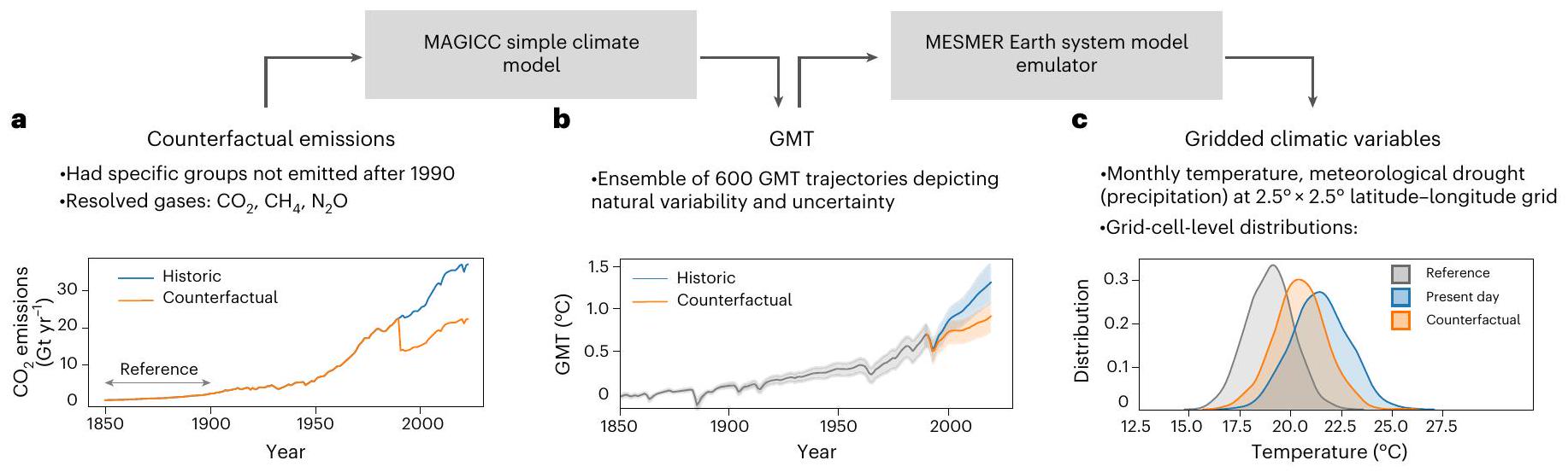
مجموعات المنبع بعد عام 1990 (برتقالي). ب، مستويات متوسط درجة الحرارة العالمية للانبعاثات التاريخية والافتراضية (الخطوط الصلبة) جنبًا إلى جنب مع فترات الثقة من 5 إلى 95 (الأغلفة المظللة) المستمدة من 600 عضو في المجموعة. ج، التوزيعات المرجعية والحالية والافتراضية في خلية شبكة واحدة باستخدام درجة الحرارة كمثال.
نقوم بتوليد مسارات انبعاثات مضادة للواقع من خلال طرح انبعاثات مجموعات الم emitters المحددة من 1990 إلى 2019، وهي الأغنى. و على مستوى العالم، وكذلك في الولايات المتحدة، والاتحاد الأوروبي 27، والهند والصين (الشكل 1ب). تم جمع بيانات الانبعاثات من المرجع 3 وتشمل الانبعاثات الناتجة عن الاستهلاك المحلي، والاستثمارات العامة والخاصة، والتجارة. تُنسب هذه الانبعاثات بشكل أساسي إلى المستهلكين، باستثناء الانبعاثات الناتجة عن تكوين رأس المال في قطاعات الإنتاج، والتي تُنسب إلى مالكي الشركات. تُبلغ الانبعاثات كحزمة من غازات الدفيئة مع التعبير عن الاحترار في المعادلات. نحن نحول هذه المسارات الافتراضية إلى مستويات GMT ومتغيرات مناخية موزعة على الشبكة (الشكل 1أ)، مما يسمح لنا بمقارنة مناخ عام 2020 مع الحالة المناخية الافتراضية لعام 2020 التي كنا سنلاحظها إذا لم تكن هذه المجموعات قد انبعثت. على وجه التحديد، نحن ننسب مستويات GMT والتغيرات في احتمالية وشدة الأشهر الحارة والجافة للغاية (الشكل 1ج). يشكل الحر الشديد عبئًا كبيرًا على صحة الإنسان. وتؤدي العجز المستمر في هطول الأمطار إلى تدهور إنتاج المحاصيل وتهدد موارد المياه مما يعني أن كلا من التطرفات المناخية ذات صلة كبيرة في دفع تأثيرات المناخ. نقيس الجفاف الجوي باستخدام مؤشر الهطول القياسي المحسوب على فترات مدتها 3 أشهر (SPI-3). .
نحن نقوم بت quantifying تأثيرات المناخ المرتبطة بالمنبعثين الأثرياء ونقارنها بالمعدل العالمي للإسهام لكل فرد. نحن لا نقيم ما الذي يمكن أن يشكل انبعاثات عادلة أو منصفة، ولا نحدد المسؤولية المباشرة عن التأثيرات الناتجة. للتوضيح، نقدم أيضًا نتائج الاحترار الافتراضية بناءً على إعادة قياس الانبعاثات العالمية وفقًا لملف الدخل الفردي لكل نسبة مئوية.

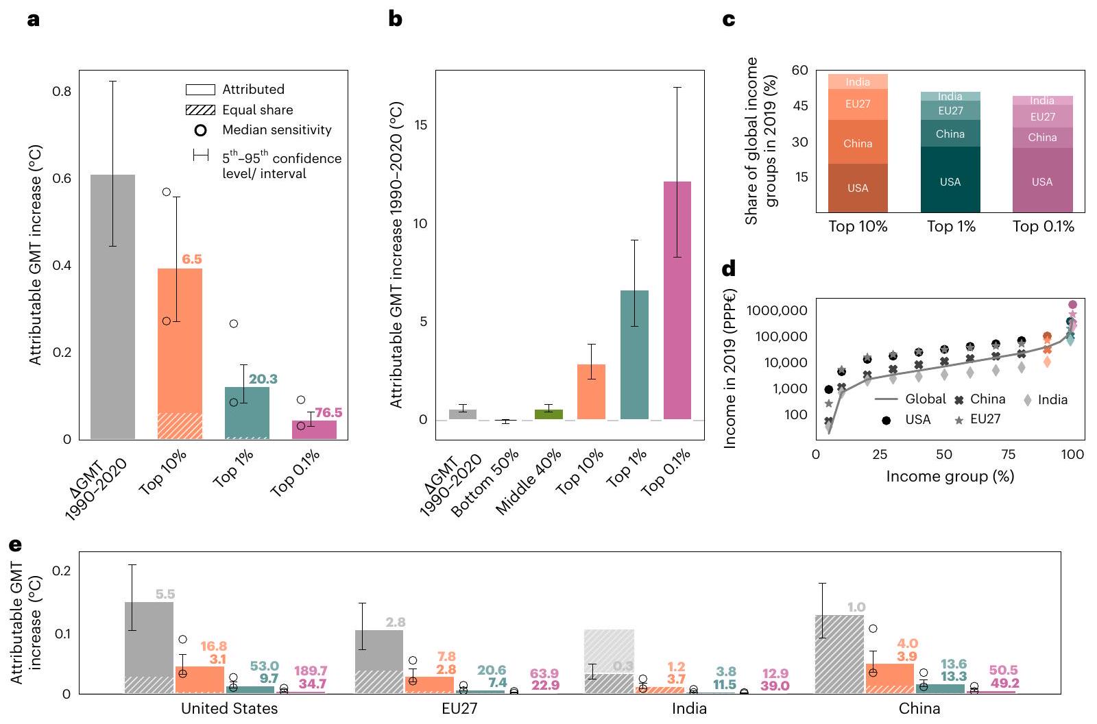
عدم المساواة في المساهمات المنسوبة للاحتباس الحراري العالمي

إطار نمذجة لدينا يصور التباين الطبيعي وعدم اليقين في الاستجابة العالمية لتغيرات الانبعاثات (الطرق). ما لم يُذكر خلاف ذلك، نقدم النتائج الوسيطة مع فترات الثقة من 5 إلى 95 في المئة بين قوسين. جميع النتائج ذات دلالة إحصائية (تم إثباتها من خلال اختبار عينة واحدة -الاختبارات، الطرق) ما لم يتم الإشارة إلى خلاف ذلك بشكل صريح. حيث أن قاعدة بياناتنا توفر فقط انبعاثات السلة، استنتجنا النتائج الرئيسية من خلال افتراض أن الانبعاثات لكل غاز دفيئة تتناسب بشكل نسبي مع الانبعاثات العالمية المجمعة (الطرق). نستكشف الحساسية لهذا الافتراض في القسم التكميلي 2.
التوقيت العالمي المنسق في عام 2020 هو أعلى من عام 1990. وجدنا أن حوالي هذا الارتفاع يُعزى إلى القمة العالمية إلى القمة و إلى أعلى 0.1% (الشكل 2أ والجدول التكميلي 3). هذه المساهمات في الاحترار أعلى (بنحو
واحد من خمسة) من مساهمات المجموعة المعنية في انبعاثات غازات الدفيئة المجمعة (الجدول التكميلي 2)، مما يبرز أهمية غير- (انظر أيضًا القسم التكميلية 2).
لوضع هذه الأرقام في سياقها، قمنا بتعريف الحصة المتساوية لمجموعة ما على أنها المساهمة في الاحترار التي ستتحقق إذا كان تأثيرها لكل فرد يتناسب مع المتوسط العالمي. لذلك، قمنا بتعديل الزيادة الإجمالية في درجة حرارة الأرض وفقًا لحصة المجموعة من السكان العالميين (على سبيل المثال، الحصة المتساوية لأعلى مجموعة عالمية) سيكون من الكاملة زيادة). ثم استخلصنا عوامل عدم المساواة المناخية (CIFs) كالمساهمة الفعلية للمجموعة في الاحتباس الحراري العالمي بالنسبة لحصتها المتساوية. تزداد عوامل عدم المساواة المناخية من 6.5 لأعلى إلى 20 (77) للأعلى ، مما يشير إلى تضخيم عدم المساواة المناخية مع زيادة الثروة.
تظهر عمق التفاوت في المساهمات في مستوى GMT بشكل ملموس عندما يتم إعادة قياس الانبعاثات العالمية وفقًا لملف نصيب الفرد من مجموعات الدخل العالمية (الشكل 2ب). إذا كانت جميع سكان العالم قد انبعثوا مثل الأدنى ، لكان هناك ارتفاع طفيف في درجات الحرارة منذ عام 1990. ومع ذلك، إذا كانت جميع سكان العالم قد انبعثوا مثل الأعلى أو ، كان من المفترض أن يكون الزيادة في التوقيت العالمي المنسق منذ عام 1990 أو .
بين عامي 1990 و2020، نشأت الانبعاثات من أعلى 10% على مستوى العالم بشكل أساسي في أعلى الدول المصدرة للانبعاثات: الولايات المتحدة، والاتحاد الأوروبي 27، والصين، والهند (الشكل 2c). لاحظ أن تركيبة أعلى 10% على مستوى العالم تتغير مع مرور الوقت (الشكل التوضيحي 1)، وعلى الرغم من أن تركيزنا هو على الأفراد الأثرياء من أكبر اقتصادات العالم، فإن الأفراد من الدول الأصغر (الأثرياء، وكذلك الأقل ثراءً) يساهمون أيضًا بشكل غير متناسب. تختلف مستويات الدخل من أكبر الملوثين الإقليميين عن نظرائهم العالميين: حيث أن أعلى 10% و1% في الولايات المتحدة والاتحاد الأوروبي 27 (الهند والصين) أغنى (أفقر) من الأغنى عالمياً. و (الشكل 2د).
تجمع الأسهم المنسوبة إلى مجموعات المصدرين الإقليميين بين عدم المساواة داخل المنطقة وبين المناطق. في الولايات المتحدة (EU27)، الأعلى يساهمون بمعدل 3.1 (2.8) مرات أكثر في الاحتباس الحراري مقارنة بالمواطن العادي، ولكن 17 (8) مرة أكثر من المتوسط العالمي. بالنسبة للولايات المتحدة، فإن مساهمة الأثرياء تفوق وحده الحصة المتساوية لكامل البلاد. هذه اللامساواة النسبية تزداد مع زيادة الثروة: حيث يساهم أعلى 1% في الولايات المتحدة (EU27) بمعدل 53 (21) مرة من حصصهم المتساوية، ويساهم أعلى 0.1% بمعدل 190 (64) مرة من حصصهم المتساوية. في الصين، حيث يكون CIF العام قريبًا من 1، يساهم الأعلى و يصدرون 4.13 و50 مرة من حصصهم المتساوية، مما يظهر تأثيرًا إقليميًا أكبر من النخب الاجتماعية. وبالمثل، في الهند، حيث يبلغ مؤشر CIF الوطني 0.3 (مما يعني أن متوسط انبعاثات الفرد في البلاد أقل من المتوسط العالمي)، فإن أعلى و ت emit 1.2 و 4 و 10 مرات من المتوسط العالمي.
الشكل 2 | الزيادات المنسوبة لدرجة حرارة الأرض العالمية (GMT) من 1990 إلى 2020 حسب مجموعة المنبع. أ، الزيادة المتوسطة في GMT خلال الفترة من 1990 إلى 2020 والنسب المنسوبة لأعلى 10% و1% على مستوى العالم و تشير المناطق المظللة إلى الاحترار لكل مجموعة بناءً على مساهمة متساوية للفرد في الاحترار. تُعطى مؤشرات CIF لمساهمة المجموعة في الاحترار العالمي بالنسبة للمساهمة المتوسطة فوق الأعمدة. تمثل الخطوط العمودية فترات الثقة من 5 إلى 95 من التباين الطبيعي وعدم اليقين في استجابة درجة الحرارة العالمية. تبرز الدوائر القيم المتوسطة من تحليل الحساسية (الطرق؛ الدائرة السفلية هي الانبعاثات القائمة على – والدائرة العليا غير – -الانبعاثات المستندة إلى). التقديرات تستند إلى 600 عضو في المجموعة. ب، الزيادة المتوسطة في درجة حرارة الأرض الافتراضية من 1990-2020 إذا كان الجميع ينفث مثل المجموعات الدخل المعطاة، مع النسبة المئوية 5-95
فترات الثقة ممثلة كخطوط عمودية. التقديرات تستند إلى 600 عضو في المجموعة. ج، التحليل الإقليمي لأفضل النتائج العالمية و في عام 2019. د، التوزيعات العالمية (الخط الصلب) والإقليمية (الرموز) للدخل في عام 2019. هـ، نفس ما هو في أ ولكن بالنسبة لأعلى الإقليم. و في الولايات المتحدة، والاتحاد الأوروبي 27، والهند، والصين. تبرز الأشرطة الرمادية الزيادة المتوسطة في درجة حرارة الأرض الناتجة عن كل منطقة ككل. يتم تقديم قيمتين لمؤشر CIF: القيمة الأفتح (الأغمق) تتعلق بحصة البلاد المتساوية (الانبعاثات الفعلية) وتقيس عدم المساواة العالمية (الإقليمية). تمثل الخطوط العمودية فترات الثقة من 5 إلى 95 من التباين الطبيعي وعدم اليقين في استجابة درجة حرارة الأرض العالمية. تبرز الدوائر القيم المتوسطة من تحليل الحساسية. التقديرات تستند إلى 600 عضو في المجموعة.

فروقات كبيرة في الظروف القصوى المنسوبة على مستوى العالم

نُعزى الزيادات الإقليمية في تكرار الأشهر الحارة (الجافة) بشكلٍ استثنائي، هنا تُعرف بأنها أحداث تحدث مرة واحدة كل 100 عام في مناخ ما قبل الصناعة، إلى انبعاثات أعلى 10% على مستوى العالم (الشكل 3أ)، لذا فإن المصطلحات المستخدمة في هذه المقالة تشير إلى الأحداث المتطرفة أو الشديدة التي تعني أن الشهر كان على الأقل بنفس حرارة (جفاف) الشهر الأكثر حرارة (جفاف). من الأشهر في مناخ ما قبل الصناعة. نحن نعرض نتائج النسبة كأعداد أحداث إضافية على مدى فترة 100 عام نموذجية من ظروف المناخ الحالية مقارنة بتلك في عام 1990 (الطرق). على سبيل المثال، تشير 10 أحداث إضافية قابلة للنسبة إلى أن حدثًا يحدث مرة واحدة كل 100 عام في فترة ما قبل الصناعة يحدث 10 مرات إضافية خلال 100 عام، مما يعني أن احتماليته قد زادت بمقدار عشرة أضعاف.
بالنسبة لدرجات الحرارة القصوى، تكون التغيرات الأكثر (الأقل) وضوحًا في أغسطس (فبراير)، حيث يُعزى 11.5 [8.5-15.4] (3.5 [2.4-4.3]) حدثًا إضافيًا إلى القمة العالمية. . تشير هذه التغييرات إلى الوسيط العالمي على اليابسة الذي يقع بشكل أساسي في نصف الكرة الشمالي. تواجه المناطق في المناطق المتأثرة بشدة، مثل منطقة الأمازون وجنوب شرق آسيا أو وسط أفريقيا، أشهرًا تصل فيها احتمالات الزيادة إلى 30 ضعفًا (انظر أيضًا الأشكال التكميلية 5-8).
لتفسير الفروق في الموسمية بين نصف الكرة الشمالي ونصف الكرة الجنوبي، قمنا بتقييم حالات الحرارة القصوى خلال الشهر الذي يشهد أعلى درجات الحرارة (الشكل التكميلي 4). أدت الانبعاثات من 1990 إلى 2020 إلى زيادة بمقدار 12.3 مرة (9.7-17.9) في احتمال حدوث حالات الحرارة القصوى في شهر ذروة درجات الحرارة.
القمة يساهم أضعاف المتوسط العالمي إلى هذا (الأشكال التكميلية 9-13e). بالإضافة إلى ذلك، زادت شدة هذه extremes بمقدار ( منذ عام 1990. من هذه الزيادة، يعود إلى القمة مما يشير إلى أن مساهمتهم أعلى بمقدار 6.7 (21.1) مرة من المتوسط العالمي (الأشكال التكميلية 9-13).
نتائج النسبة المئوية للجفاف المناخي تعتمد بشكل كبير على المنطقة والشهر، حيث تم العثور على جفاف قوي بشكل رئيسي في أمريكا الوسطى، والأمازون، وحوض البحر الأبيض المتوسط، وجنوب أفريقيا، وشمال أستراليا (الشكل 3د والأشكال التكميلية 5-8). وهذا متوقع، نظرًا للاختلاف الكبير بين النماذج وعدم اليقين الكبير في توقعات هطول الأمطار الإقليمية. وجدنا أقوى اتجاه جفاف يمكن نسبه في منطقة الأمازون في أكتوبر. بشكل عام، تواجه المنطقة زيادة ثلاثية في احتمالية الظروف القاسية (1.7-4.2) مقارنة بعام 1990 (الشكل 3ب). تساهم أعلى 10% (1%) بمعدل 6.1 (16.7) مرة من المتوسط العالمي في هذه الزيادة. تعتبر منطقة الأمازون ذات أهمية عالمية، نظرًا لنظامها الفريد من نوعه في التنوع البيولوجي ودورها الرئيسي في دورة الكربون العالمية. لقد أثرت أحداث الجفاف على مدى القرن الماضي سلبًا على تخزين الكربون في غابات الأمازون المطيرة. .
بشكل عام، تشير الفجوة المكانية في التغيرات المنسوبة على مستوى خلايا الشبكة (الشكل 3 والأشكال التكميلية 5-13) إلى أن المناطق التي تساهم بشكل غير متناسب في انبعاثات الأعلى (على سبيل المثال، الاتحاد الأوروبي 27 والولايات المتحدة؛ الشكل 2) تواجه زيادات أصغر من المناطق التي ساهمت قليلاً جداً (على سبيل المثال،
الشكل 3 | تغيير التردد لظواهر الحرارة والجفاف الجوي الشهرية التي تحدث مرة كل 100 عام والتي تعزى إلى أكبر الدول المصدرة. أ، ب، التوزيعات الشهرية لظواهر الحرارة القصوى (أ) وظواهر الجفاف القصوى في الأمازون (ب) عبر خلايا الشبكة التي تعزى إلى أكبر الدول المصدرة العالمية. . تم اشتقاق التوزيعات من خلال حساب نتائج النسبة المئوية الوسيطة في كل خلية شبكية (مقدرة من 15,000 عضو في المجموعة لكل منها) ثم حساب الإحصائيات عبر جميع 2,652 خلية شبكية. تظليل الألوان نوعي. ج، د، التوزيع المكاني للعدد الوسيط من حالات الحرارة (ج) والجفاف (د) خلال أشهر ذروة درجات الحرارة المنسوبة إلى القمة العالمية تستند التقديرات المتوسطة إلى 15,000 عضو من المجموعة.
تشير المناطق المظللة إلى نتائج غير مهمة و/أو عدم توافق كافٍ للنموذج. هـ، العدد الوسيط لظواهر الحرارة الإضافية (هـ) والجفاف (و) حسب المنطقة (المميزة على الخرائط في و ). تشير CIFs إلى مساهمة المجموعة في التطرف بالنسبة للمساهمة المتوسطة الموضحة فوق الأعمدة. تتوافق الخطوط العمودية مع فترات الثقة من 5 إلى 95. نحن نتجنب عرض تقديرات الجفاف العالمية بسبب عدم كفاية الاتفاق بين خلايا الشبكة. تم اشتقاق التوزيعات من خلال حساب نتائج النسبة المئوية الوسيطة في كل خلية شبكة (المقدرة من 15,000 عضو في المجموعة لكل منها) ثم حساب الإحصائيات عبر جميع خلايا الشبكة داخل كل منطقة.
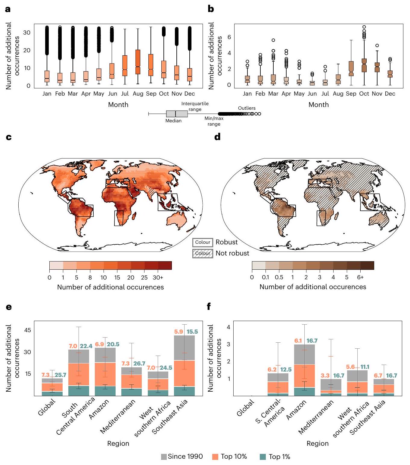
شمال غرب أمريكا وأوروبا الغربية والوسطى مقارنةً بمنطقة الأمازون وغرب وجنوب أفريقيا في الشكل 3c، d).
التغيرات الصغيرة نسبيًا (التي يمكن نسبها) في الهند وأجزاء من الصين والاختلاف العالي في النماذج في الوقت نفسه تستحق الملاحظة، نظرًا لأنها تتعارض مع العدد المتزايد من الكوارث المتعلقة بالمناخ التي تواجهها الهند بالفعل. نفترض أن هذا مرتبط بتأثيرات المناخ الناتجة عن تلوث الهواء، والتي نناقشها بمزيد من التفصيل في القسم التكميلي 3.

نسبة التأثيرات العابرة للحدود الناتجة عن الانبعاثات الإقليمية

تتجاوز الفجوة في مساهمات الاحترار من المجموعات الثرية في المناطق ذات الانبعاثات العالية الفجوة في مساهماتهم العالمية.
نظائرها (الشكل 2). تظهر هذه الفجوة أيضًا على مستوى خلايا الشبكة: في الوسيط العالمي، تنبعث الانبعاثات من الأعلى في الولايات المتحدة مرتبطة بـ أحداث حرارة إضافية تحدث مرة واحدة كل 100 عام خلال أشهر ذروة الحرارة. يمثل هذا التأثير 23 (60) مرة من المساهمة العالمية المتوسطة وحوالي 3 (2) مرات من المساهمة النسبية لأعلى مستوى عالمي. (1%) (الشكل 3). زيادة الحرارة الشديدة غير موزعة بالتساوي عبر المناطق. على سبيل المثال، في المناطق المتأثرة بالحرارة مثل الأمازون وجنوب شرق أفريقيا، فإن الانبعاثات من الأعلى في الصين (الولايات المتحدة) مرتبطة بـ 2.7 (1.9-3.2) (2.5(1.7-2.8)) و حدوثات إضافية من الحرارة الشديدة خلال الأشهر التي تشهد درجات حرارة قصوى (الشكل 4). في هذه المناطق، يمكننا أيضًا أن ننسب بشكل قوي الظواهر الحرارية الشديدة إلى القمة الإقليمية. في الأمازون، الحرارة الشديدة الإضافية هي
الشكل 4 | زيادة في تكرار ذروة حرارة الصيف الشديدة التي تحدث مرة كل 100 عام في مناطق مختارة تعزى إلى القمة و للمصدرين. اليسار: العدد الوسيط للحرارة الشديدة الإضافية في المناطق المختارة التي تعزى إلى أعلى 10% من المصدرين في الصين والولايات المتحدة والاتحاد الأوروبي 27 والهند. اليمين: نفس ما هو موجود على اليسار ولكن لأعلى من المنبعثين. تشير القضبان الأوسع إلى أن المزيد
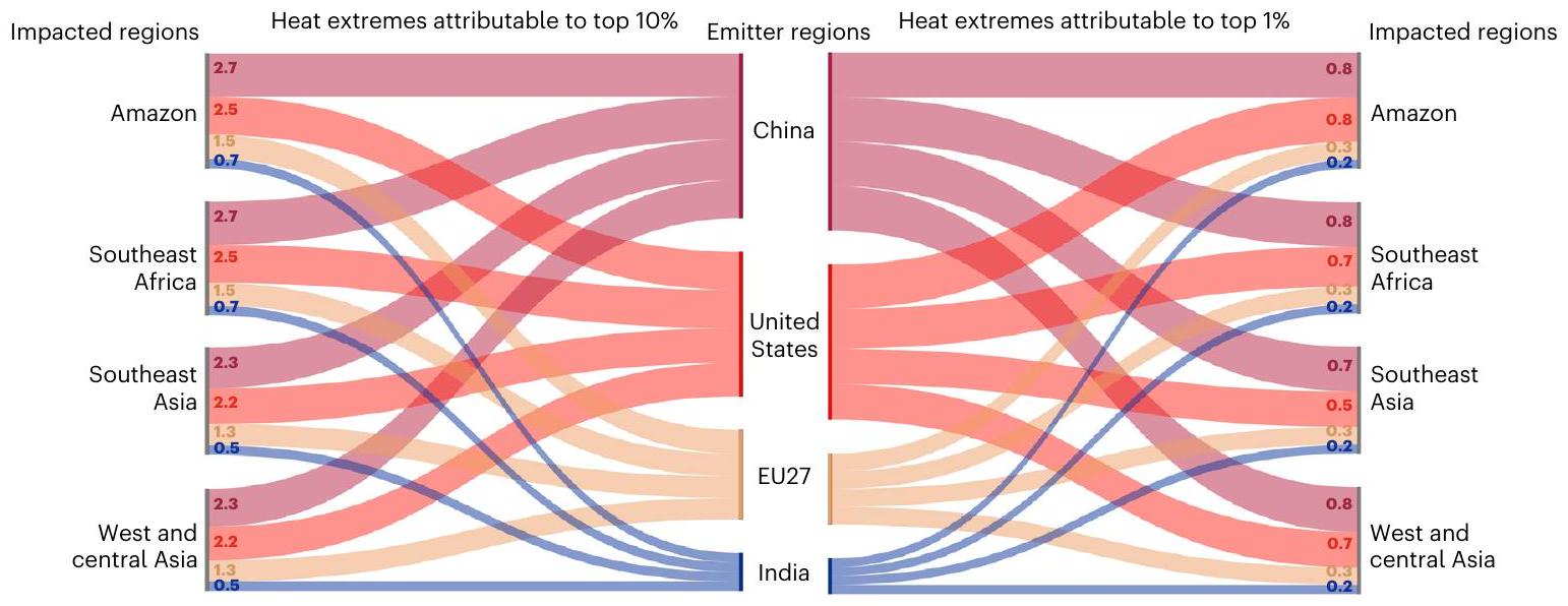
الأحداث تُنسب إلى مجموعة معينة من المنبعين. القيم في الأعمدة تشير إلى الأعداد الإضافية من الأحداث على مدار 100 عام. تم اشتقاق التقديرات الوسيطة من خلال حساب نتائج النسبة الوسيطة في كل خلية شبكية (مُقدرة من 15,000 عضو في المجموعة لكل منها) ثم حساب الإحصائيات عبر الخلايا الشبكية داخل كل منطقة.
ناتج عن القمة في الصين. وهذا يتوافق مع زيادة في تكرار الحدوث لـ .
يصبح من الصعب بشكل متزايد نسب التغيرات في الأحداث المتطرفة إلى مجموعات الملوثين الأثرياء المحددة في كل بلد، حيث أن حجم هذه المجموعات من الملوثين يقل في نصيب الفرد، مما يعني أن انبعاثاتهم التراكمية تنخفض حتى لو زادت مساهماتهم النسبية في الانبعاثات. تتميز توزيعات درجات الحرارة المتوقعة بتغيرات قوية في الاتجاه وبتناسق عبر النماذج، مما يسمح بنتائج نسب موثوقة حتى لكميات الانبعاثات التي تبدو صغيرة، لا سيما في المناطق المتأثرة بشدة. تعتمد magnitude على تعريف extremes، حيث تشهد المخاطر في الأطراف أقوى زيادة (الأشكال التكميلية 18-21). بالنسبة للجفاف، فإن الوضع أكثر تعقيدًا. يهيمن على إشارة SPI-3 التباين وعدم الاتفاق الكبير بين النماذج، مما حال دون اشتقاق نتائج نسب موثوقة عندما تكون الانبعاثات صغيرة.

نقاش

تقدم هذه الدراسة إطارًا لربط الانبعاثات المستندة إلى الثروة بالتغيرات في درجة حرارة الأرض العالمية والتغيرات في extremes الحرارة الشهرية والجفاف الجوي الإقليمي. وجدنا أن أغنى ساهمت بـ 6.5 مرات أكثر في الاحتباس الحراري العالمي من المتوسط، مع أعلى و مساهمين بمعدل 20 و76 مرة أكثر، على التوالي. بالنسبة للحرارة، فإن هذا الاختلال يكون أكثر وضوحًا على مستوى خلايا الشبكة: الأغنياء و ساهمت بأكثر من 7 و 25 مرة مقارنة بالمتوسط العالمي في زيادة تكرار درجات الحرارة القصوى التي تحدث مرة كل 100 عام قبل العصر الصناعي خلال الأشهر التي تشهد أعلى درجات حرارة صيفية. ترتبط مساهمات الأثرياء بتأثيرات عبر الحدود كبيرة – على سبيل المثال، مساهمات الأغنياء. داخل الولايات المتحدة والصين أدى إلى زيادة تتراوح بين مرتين إلى ثلاث مرات في حالات الحرارة القصوى عبر المناطق الضعيفة مثل الأمازون وجنوب شرق آسيا وجنوب شرق أفريقيا. إن نسبة إشارات الجفاف بشكل موثوق أكثر تعقيدًا. وجدنا أقوى الإشارات في منطقة الأمازون في أكتوبر، حيث انبعاثات أعلى مستوى عالمي أدى إلى زيادة بمقدار 2.3 مرة (0.8 مرة) في تكرار الجفاف الشديد.
تحليلنا يبرز أيضًا الدور الحاسم لـ الانبعاثات في الاحترار على المدى القريب (الشكل التوضيحي 2) ويدعو إلى أبحاث جديدة لفك ارتباط الانبعاثات المعتمدة على الدخل على مستوى الغازات الفردية. تقليل يمكن أن تؤدي الانبعاثات المتوافقة مع مسارات اتفاق باريس إلى تخفيضات فورية في درجات الحرارة العالمية والتقلبات المناخية. .
نلاحظ أن دراستنا تركز على الحرارة الشديدة الشهرية (أي الأشهر شديدة الحرارة)، مما يعني أن موجات الحرارة – التي تُعرف بأنها فترات طويلة من درجات الحرارة المرتفعة بشكل غير طبيعي تستمر من يومين إلى عدة أشهر. -لا تتعلق مباشرة بمقياسنا. ومع ذلك، فإن احتمال درجات الحرارة اليومية القصوى يتزايد خلال الأشهر الحارة للغاية. مما يوحي بأن النتائج القابلة للنسب لفترات الحرارة القصيرة قد تكون أكثر وضوحًا. هناك حاجة لمزيد من البحث لاستكشاف هذه العلاقة بشكل صريح.
تشمل انبعاثات الثروة الاستهلاك الخاص والاستثمار في تشكيل رأس المال عبر القطاعات الإنتاجية التي تزود المجتمع بالسلع والخدمات. يمكن أن يساعد التعرف على المساهمات غير المتكافئة في الاحترار في توجيه التدخلات السياسية. على سبيل المثال، يمكن أن تستند المناقشات حول فرض ضريبة عالمية منسقة على الثروة إلى هذا العمل، موضحة الفوائد المناخية المترتبة على تقليل الفجوات الكبيرة في المسؤوليات المتعلقة بتأثير المناخ بناءً على الثروة. تُبرز التأثيرات العابرة للحدود التي نحددها كيف يساهم الأفراد ذوو الانبعاثات العالية في تفاقم الظروف المتطرفة، حتى في المناطق البعيدة. وبالمثل، فإن الاحترار الناتج عن استثمارات الأثرياء يسلط الضوء على الحاجة إلى إعادة توجيه التدفقات المالية لتحقيق الأهداف المناخية العالمية. . هذا مهم بشكل خاص للأغنياء و التي تساهم عبر الحدود في تفاقم الظروف المحلية المتطرفة تنشأ بشكل أساسي من خلال الاستثمارات، بدلاً من الاستهلاك. يجب أن تأخذ الجهود الرامية إلى إعادة توجيه هذه التدفقات المالية في الاعتبار أيضًا المسؤوليات المشتركة للحكومات لتسريع التغييرات النظامية في الهياكل المالية والتنظيمية. .
تحليلنا التفصيلي للأثر يظهر أن المناطق ذات الدخل المنخفض تتحمل العبء الأكبر من الأضرار الناجمة عن الانبعاثات المركزة بين السكان الأثرياء في جميع أنحاء العالم. من منظور التكيف والخسائر والأضرار، يوفر هذا أساسًا للمناقشات السياسية حول المساهمات في التدابير التعويضية والوقائية. المبالغ المخصصة حاليًا لتمويل التكيف والخسائر والأضرار ضئيلة مقارنة بالاحتياجات المقدرة. يحفز عملنا أدوات سياسة مبتكرة تستهدف الأفراد الأثرياء لسد هذه الفجوات المالية الواضحة. يمكن أن تحسن مثل هذه السياسات أيضًا من تصورات العدالة المناخية، وهو عامل حيوي في تعزيز القبول الاجتماعي للعمل المناخي. التحرك نحو سياسات قائمة على الأدلة وموجهة تعكس مبادئ دفع الملوثين، بما في ذلك على المستوى المحلي من حيث المساهمات الفردية، قد يكون بالتالي حجر الزاوية المهم لتعزيز الدعم السياسي للعمل المناخي بشكل عام.
ومع ذلك، يجب أن تأخذ الاعتبارات المتعلقة بنتائجنا في المناقشات السياسية في الاعتبار التحديات المفاهيمية والأحكام القيمية في نهجنا وتنفيذه. أولاً، يعتمد تحليلنا على حساب انبعاثات قائمة على الاستهلاك، حيث يتم تخصيص الانبعاثات بين المستهلكين والمساهمين من خلال الملكية المشتركة (انظر المرجع 3). يتناقض نهجنا مع الأساليب القائمة على الإنتاج المستخدمة لتحديد مسؤوليات المنتجين. استكشاف أطر المحاسبة المتنوعة هو مفتاح لتطوير آليات السياسات التي تعالج أبعادًا متعددة، ولكنه يتطلب العناية في تحديد المسؤولية. ثانيًا، نستخدم طريقة النسبة ‘لكن من أجل’ في النسبة. هذا النهج يربط مباشرة بين الانبعاثات والتغير المناخي الملحوظ مع الأخذ في الاعتبار توقيت الانبعاثات وآثارها. ومع ذلك، فهو حساس لتسلسل إزالة الانبعاثات وتصميم السيناريوهات المضادة للواقع. ثالثًا، نهجنا محدود بالتغيرات في مخاطر المناخ فقط، ولا يأخذ في الاعتبار نقاط الضعف والتعرض على الأرض، والتي غالبًا ما تكون مفتاحًا لدفع التأثير النهائي للأحداث المناخية المتطرفة. إن دمج عوامل سببية أخرى في تحليل نسبة الأحداث المتطرفة يتيح لنا بشكل متزايد معالجة تلك القيود. في خطوة نحو استخدام نسبة الأحداث المتطرفة لإبلاغ النقاش حول الخسائر والأضرار في الوقت نفسه، تعتبر مستويات الثروة عاملاً رئيسياً لتحديد القدرة على التكيف والضعف في مواجهة تغير المناخ، لا سيما على مستوى الأسر والأفراد. لذا نتوقع أن تؤدي العوامل المتعلقة بالثروة التي تؤثر على الضعف والتعرض إلى تفاقم الفجوات في المسؤوليات وتجربة آثار المخاطر المناخية التي درسناها هنا.
جميع التقديرات الكمية مرتبطة بهذه الافتراضات الثلاثة، ويجب علينا أن ندرك الخيارات والأحكام القيمية المتضمنة في التحليل عند تقييم الآثار الأخلاقية والقانونية لنتائجنا.
تحليلنا محدود أيضًا بسبب نقص البيانات حول كيفية اختلاف تركيبات انبعاثات غازات الدفيئة مع الدخل والثروة. هذا يحد من دقة نتائجنا، نظرًا لدور غازات الدفيئة غير ثاني أكسيد الكربون في الاحترار الأخير. بالإضافة إلى ذلك، فإن مؤشر الجفاف لدينا يأخذ في الاعتبار فقط هطول الأمطار، مما قد يؤدي إلى تقديرات منخفضة لمخاطر الجفاف. أخيرًا، تحليلنا يعتمد على بيانات نموذجية، والتي قد تختلف عن الملاحظات. .
وبناءً عليه، فإن تحليلنا لا يحدد بشكل صريح المسؤولية الكاملة عن آثار المناخ الناتجة، كما أنه لا يحدد مستويات الانبعاثات العادلة لأي مجموعة دخل. تتطلب مثل هذه التحديدات رؤية متكاملة للعدالة والإنصاف والعوامل الاجتماعية والاقتصادية. مع نقاط مرجعية مختلفة للمجتمعات عند مستويات مختلفة من التنمية.
في الختام، تُظهر نتائجنا كيف ساهمت مجموعات المنبع الفردية في زيادة التطرف الإقليمي على مستوى العالم. في أوقات تزايد الفوارق الاقتصادية والمناخية، يمكن أن تُسهم الأطر المتقدمة لنسب الانبعاثات إلى المنبعين الفرديين في توجيه العمل المناخي العالمي وتعزيز العدالة المناخية.

المحتوى عبر الإنترنت

أي طرق، مراجع إضافية، ملخصات تقارير Nature Portfolio، بيانات المصدر، بيانات موسعة، معلومات تكميلية، شكر وتقدير، معلومات مراجعة الأقران؛ تفاصيل مساهمات المؤلفين والمصالح المتنافسة؛ وبيانات توفر البيانات والرموز متاحة علىhttps://doi.org/10.1038/s41558-025-02325-x.

References

  1. Newman, R. & Noy, I. The global costs of extreme weather that are attributable to climate change. Nat. Commun. 14, 6103 (2023).
  2. Warner, K. & Weisberg, M. A funding mosaic for loss and damage. Science 379, 219-219 (2023).
  3. Chancel, L. Global carbon inequality over 1990-2019. Nat. Sustain. 5, 931-938 (2022).
  4. Wallemacq, P., Below, R. & McClean, D. Economic Losses, Poverty and Disasters: 1998-2017 (United Nations Office for Disaster Risk Reduction, 2018); https://www.preventionweb.net/files/61119_ credeconomiclosses.pdf
  5. Diffenbaugh, N. S. & Burke, M. Global warming has increased global economic inequality. Proc. Natl Acad. Sci. USA 116, 9808-9813 (2019).
  6. Hallegatte, S. & Rozenberg, J. Climate change through a poverty lens. Nat. Clim. Change 7, 250-256 (2017).
  7. Dhakal, S. et al. in Climate Change 2022: Mitigation of Climate Change (eds Shukla, P. R. et al.) 215-294 (IPCC, Cambridge Univ. Press, 2023).
  8. Mar, K. A., Unger, C., Walderdorff, L. & Butler, T. Beyond CO2 equivalence: the impacts of methane on climate, ecosystems, and health. Environ. Sci. Policy 134, 127-136 (2022).
  9. Beusch, L., Gudmundsson, L. & Seneviratne, S. I. Emulating Earth system model temperatures with MESMER: from global mean temperature trajectories to grid-point-level realizations on land. Earth Syst. Dynam. 11, 139-159 (2020).
  10. Meinshausen, M., Raper, S. C. & Wigley, T. M. Emulating coupled atmosphere-ocean and carbon cycle models with a simpler model, MAGICC6 – part 1: model description and calibration. Atmos. Chem. Phys. 11, 1417-1456 (2011).
  11. Schöngart, S. Introducing the MESMER-M-TPv0.1.0 module: spatially explicit Earth system model emulation for monthly precipitation and temperature. EGUsphere 2024, 8283-8320 (2024).
  12. Otto, F. E. Attribution of extreme events to climate change. Annu. Rev. Environ. Resour. 48, 813-828 (2023).
  13. Stott, P. A., Stone, D. A. & Allen, M. R. Human contribution to the European heatwave of 2003. Nature 432, 610-614 (2004).
  14. Van Oldenborgh, G. J. et al. Pathways and pitfalls in extreme event attribution. Climatic Change 166, 13 (2021).
  15. Beusch, L. et al. Responsibility of major emitters for country-level warming and extreme hot years. Commun. Earth Environ. 3, 7 (2022).
  16. Callahan, C. W. & Mankin, J. S. National attribution of historical climate damages. Climatic Change 172, 40 (2022).
  17. Trudinger, C. & Enting, I. Comparison of formalisms for attributing responsibility for climate change: non-linearities in the brazilian proposal approach. Climatic Change 68, 67-99 (2005).
  18. Otto, F. E., Skeie, R. B., Fuglestvedt, J. S., Berntsen, T. & Allen, M. R. Assigning historic responsibility for extreme weather events. Nat. Clim. Change 7, 757-759 (2017).
  19. De Polt, K. et al. Quantifying impact-relevant heatwave durations. Environ. Res. Lett. 18, 104005 (2023).
  20. Seneviratne, S. et al. 2021: Weather and climate extreme events in a changing climate. in Climate Change 2021: The Physical Science Basis. Contribution of Working Group I to the Sixth Assessment Report of the Intergovernmental Panel on Climate Change (eds Masson-Delmotte, V. et al.), 1513-1766 (IPCC, Cambridge Univ. Press 2021).
  21. Allen, M. R. et al. Indicate separate contributions of long-lived and short-lived greenhouse gases in emission targets. npj Clim. Atmos. Sci. 5, 5 (2022).
  22. Cook, B.I. et al. Twenty-first century drought projections in the CMIP6 forcing scenarios. Earth Future 8, e2019EF001461 (2020).
  23. Wu, Y. et al. Hydrological projections under CMIP5 and CMIP6: sources and magnitudes of uncertainty. Bull. Am. Meteorol. Soc. 105, E59-E74 (2024).
  24. Chen, D. et al. 2021: Framing, context, and methods. in Climate Change 2021: The Physical Science Basis. Contribution of Working Group I to the Sixth Assessment Report of the Intergovernmental Panel on Climate Change (eds Masson-Delmotte, V. et al.) 147-286 (IPCC, Cambridge Univ. Press, 2021).
  25. Yao, Y., Ciais, P., Viovy, N., Joetzjer, E. & Chave, J. How drought events during the last century have impacted biomass carbon in amazonian rainforests. Glob. Change Biol. 29, 747-762 (2023).
  26. Kumar, N. et al. Joint behaviour of climate extremes across India: past and future. J. Hydrol. 597, 126185 (2021).
  27. McKenna, C. M., Maycock, A. C., Forster, P. M., Smith, C. J. & Tokarska, K. B. Stringent mitigation substantially reduces risk of unprecedented near-term warming rates. Nat. Clim. Change 11, 126-131 (2021).
  28. IPCC Climate Change 2022: Impacts, Adaptation and Vulnerability (eds Pörtner, H.-O. et al.) (Cambridge Univ. Press, 2023).
  29. Zeppetello, L. R. V., Battisti, D. S. & Baker, M. B. The physics of heat waves: what causes extremely high summertime temperatures? J. Clim. 35, 2231-2251 (2022).
  30. Chancel, L., Bothe, P. & Voituriez, T. The potential of wealth taxation to address the triple climate inequality crisis. Nat. Clim. Change 14, 5-7 (2024).
  31. Zucman, G. A Blueprint for a Coordinated Minimum Effective Taxation Standard for Utra-High-Net-Worth Individuals (Tax Observatory, 2024); https://www.taxobservatory.eu/www-site/ uploads/2024/06/report-g20-24_06_24.pdf
  32. Pachauri, S. et al. Fairness considerations in global mitigation investments. Science 378, 1057-1059 (2022).
  33. Bhattacharya, A., Songwe, V., Soubeyran, E. & Stern, N. Raising Ambition and Accelerating Delivery of Climate Finance (Grantham Research Institute on Climate Change and the Environment, 2024); https://www.lse.ac.uk/granthaminstitute/wp-content/ uploads/2024/11/Raising-ambition-and-accelerating-delivery-of-climate-finance_Third-IHLEG-report.pdf
  34. Dibley, A. et al. Biases in ‘sustainable finance’ metrics could hinder lending to those that need it most. Nature 634, 294-297 (2024).
  35. Serdeczny, O. & Lissner, T. Research agenda for the loss and damage fund. Nat. Clim. Change 13, 412-412 (2023).
  36. Ogunbode, C. A. et al. Climate justice beliefs related to climate action and policy support around the world. Nat. Clim. Change 14, 1144-1150 (2024).
  37. Berger, J. & Liebe, U. Effective climate action must address both social inequality and inequality aversion. npj Clim. Action 4, 1 (2025).
  38. Jézéquel, A. et al. Broadening the scope of anthropogenic influence in extreme event attribution. Environ. Res. Clim. 3, 042003 (2024).
  39. Perkins-Kirkpatrick, S. E. et al. Frontiers in attributing climate extremes and associated impacts. Front. Clim. 6, 1455023 (2024).
  40. Noy, I. et al. Event attribution is ready to inform loss and damage negotiations. Nat. Clim. Change 13, 1279-1281 (2023).
  41. King, A. D., Grose, M. R., Kimutai, J., Pinto, I. & Harrington, L. J. Event attribution is not ready for a major role in loss and damage. Nat. Clim. Change 13, 415-417 (2023).
  42. Andrijevic, M. et al. Towards scenario representation of adaptive capacity for global climate change assessments. Nat. Clim. Change 13, 778-787 (2023).
  43. Smiley, K. T. et al. Social inequalities in climate change-attributed impacts of hurricane Harvey. Nat. Commun. 13, 3418 (2022).
  44. Jensen, L., Gerdener, H., Eicker, A., Kusche, J. & Fiedler, S. Observations indicate regionally misleading wetting and drying trends in CMIP6. npj Clim. Atmos. Sci. 7, 249 (2024).
  45. Kim, Y.-H., Min, S.-K., Zhang, X., Sillmann, J. & Sandstad, M. Evaluation of the CMIP6 multi-model ensemble for climate extreme indices. Weather Clim. Extremes 29, 100269 (2020).
  46. Zimm, C. et al. Justice considerations in climate research. Nat. Clim. Change 14, 22-30 (2024).
  47. Kikstra, J. S., Mastrucci, A., Min, J., Riahi, K. & Rao, N. D. Decent living gaps and energy needs around the world. Environ. Res. Lett. 16, 095006 (2021).
Publisher’s note Springer Nature remains neutral with regard to jurisdictional claims in published maps and institutional affiliations.
Open Access This article is licensed under a Creative Commons Attribution 4.0 International License, which permits use, sharing, adaptation, distribution and reproduction in any medium or format, as long as you give appropriate credit to the original author(s) and the source, provide a link to the Creative Commons licence, and indicate if changes were made. The images or other third party material in this article are included in the article’s Creative Commons licence, unless indicated otherwise in a credit line to the material. If material is not included in the article’s Creative Commons licence and your intended use is not permitted by statutory regulation or exceeds the permitted use, you will need to obtain permission directly from the copyright holder. To view a copy of this licence, visit http://creativecommons. org/licenses/by/4.0/.
© The Author(s) 2025, corrected publication 2025

طرق

قمنا بتحديد التغيرات في الشدة والتكرار في الأشهر الحارة جداً (الجافة) المنسوبة إلى مجموعات محددة من المنبعثات. يعتمد الإطار المنهجي على ثلاث خطوات (الشكل 1): أولاً، قمنا ببناء مسارات انبعاثات مضادة للحقائق (أي، مسارات انبعاثات مع وبدون انبعاثات المجموعات السكانية المختارة)؛ ثانياً، قمنا بترجمة الانبعاثات إلى بيانات درجة الحرارة، والهطول، والجفاف المحتمل الموزعة على الشبكة عبر سلسلة من المحاكيات الفعالة حسابياً؛ وثالثاً، قمنا بالاستناد إلى إطار نسبة الأحداث المتطرفة لتحديد التغيرات في توزيعات المتغيرات المناخية على مستوى خلايا الشبكة.
اعتمدنا على مؤشر SPI-3 لتحديد الجفاف المناخي. . يتم حساب SPI-3 من بيانات الهطول فقط، مما يعني أنه لا يأخذ في الاعتبار التغيرات في احتياجات المياه المستندة إلى التربة والنباتات. حيث تهيمن التغيرات المناخية المدفوعة بالهطول على التباين الطبيعي واختلاف النماذج. من المحتمل أن تكون الاتجاهات المستندة إلى تغير المناخ في مؤشر الجفاف لدينا تقديرًا متحفظًا للتغيرات الفعلية. . لذلك، قمنا أيضًا بحساب SPEI-3 . يأخذ مؤشر الجفاف SPEI-3 في الاعتبار التغيرات في الطلبات المائية من خلال التبخر والنتح المحتمل (PET). من الناحية المثالية، يتم تقدير PET من درجات الحرارة، والإشعاع، وسرعة الرياح، والرطوبة من خلال معادلة بنمان-مونتيث. نظرًا لأن إطار المحاكاة لدينا يصور فقط درجة الحرارة وهطول الأمطار، اعتمدنا على طريقة ثورنثويت لحساب PET استنادًا إلى بيانات درجة الحرارة فقط. ومع ذلك، فإن تقديرات التبخر والنتح المحتمل باستخدام طريقة ثورنثويت عرضة للتقديرات المبالغ فيها من حيث الحجم والاتجاهات الزمنية. . هذا ترك لنا مؤشراً للجفاف المناخي (SPI-3) الذي من المحتمل أن يقلل من تقديرات مخاطر الجفاف ومؤشراً إضافياً للجفاف المحتمل (SPEI-3 عبر طريقة ثورنثويت) الذي من المحتمل أن يقدم تقديراً مبالغاً فيه. استخدمنا التقديرات المحافظة في الجزء الرئيسي من تحليلنا ونظهر مخاطر الجفاف المحتملة في القسم التكميلية 5.

مسارات الانبعاثات المضادة للواقع

قمنا بتقييم كيف ستبدو مناخنا اليوم إذا كان الأغنياء و على مستوى العالم، وكذلك في الولايات المتحدة، والاتحاد الأوروبي 27، والهند والصين، لم تساهم في الانبعاثات العالمية بين عامي 1990 و2019. اتبعنا المرجع 52 لبناء سلسلة زمنية من الانبعاثات الأساسية التاريخية من 1850-2019 مفصلة حسب الغاز. بعد ذلك، قمنا بإزالة المساهمات المحددة للمنبع من هذه الانبعاثات الأساسية (الشكل 1). للقيام بذلك، اعتمدنا على مجموعة بيانات قائمة على الاستهلاك الانبعاثات المصنفة حسب البلد ودرجات الدخل بين عامي 1990 و . تتعلق التقديرات بجميع الانبعاثات باستثناء تلك الناتجة عن الزراعة والغابات واستخدام الأراضي الأخرى. تطلب تحليلنا منا إجراء افتراضات حول كيفية تفكيك الانبعاثات المبلغ عنها إلى غازات فردية. ركزنا على تحليل الانبعاثات إلى أكسيد النيتروجين ( ) و تتكون هذه الغازات الثلاثة من من إجمالي انبعاثات غازات الدفيئة العالمية (باستثناء الزراعة والغابات واستخدام الأراضي الأخرى) تتفاوت تركيبة انبعاثات غازات الدفيئة من جانب الإنتاج بشكل كبير حسب البلد، حيث تتراوح من أساساً انبعاثات قائمة على (على سبيل المثال، سنغافورة) إلى حصص متساوية تقريبًا من و (على سبيل المثال، قطر) وفي البلدان ذات الدخل المنخفض بشكل خاص، بشكل أساسي (على سبيل المثال، تشاد) تستخدم مجموعة بيانات عدم المساواة في الكربون من المرجع 3 جداول المدخلات والمخرجات التي تعيد توزيع انبعاثات الإنتاج على المستهلكين عبر الدول. حوالي نصف انبعاثات الميثان العالمية متجسدة في التجارة العالمية، حيث تهيمن استهلاك الأسر على فئة الطلب النهائي. . بالنظر إلى هذه الاعتبارات، وغياب البيانات البديلة، اخترنا تطبيق نفس افتراضات التحليل عبر البلدان ومجموعات المنبعثين. بالنسبة لتقديرنا المركزي، افترضنا أن انبعاثات كل غاز دفيئة تتناسب بشكل نسبي مع الانبعاثات العالمية المجمعة. اختبرنا حساسية هذا الافتراض من خلال تقديم حالتين متطرفتين حيث يقوم المنبعثون الأثرياء (1) بإصدار الكربون فقط ( حالة) أو (2) تصدر فقط و (غير- الحالة). لاحظ أنه في غير الـ الحالة، الانبعاثات المرتبطة بأعلى مستوى عالمي أكبر من الإجمالي العالمي و الانبعاثات مجتمعة، وقد أزلنا الانبعاثات الزائدة
من سلاسل زمنية. قمنا بالتحويل بين غازات الدفيئة الفردية و باستخدام إمكانات الاحترار العالمي 100.

نهج النمذجة القائم على المحاكي

قمنا بتحويل الانبعاثات الافتراضية إلى توزيعات درجة الحرارة والهطول على مستوى خلايا الشبكة باستخدام المحاكيات، ومن ثم قمنا بحساب مقاييس الجفاف من البيانات المحاكية. كانت عملية المحاكاة تتكون من خطوتين: أولاً، تحويل الانبعاثات إلى درجة حرارة الأرض العالمية؛ وثانياً، ترجمة درجة حرارة الأرض العالمية إلى توزيعات درجة الحرارة والهطول الشهرية على مستوى خلايا الشبكة (الشكل 1). تم تنفيذ خطوة الترجمة الأولى باستخدام MAGICC. ماجيك هو نموذج مناخي بسيط وفعال حسابياً لمؤشرات المناخ العالمية. تم حساب نتائج درجات الحرارة لدينا باستخدام ماجيك الإصدار 7.5 في إطار احتمالي يعكس نطاقات عدم اليقين المقدرة من تقرير التقييم السادس للهيئة الحكومية الدولية المعنية بتغير المناخ. قمنا بإنشاء 600 مسار GMT لكل سيناريو. تم تنفيذ خطوة الترجمة الثانية باستخدام MESMER-M-TP. .يجمع MESMER-M-TP بين الأساليب البارامترية وأخذ العينات العشوائية لتقريب سلوك نماذج المناخ الفردية. بالنسبة لأي نموذج مناخي، يمكن معايرة المحاكي باستخدام مجموعة صغيرة من بيانات نموذج المناخ الفعلية ثم استخدامه لتوليد بيانات درجة حرارة وهطول أمطار موزعة على شبكة تشبه إحصائيًا بيانات نموذج المناخ. هنا قمنا بمعايرة MESMER-M-TP باستخدام 24 نموذجًا مختلفًا من المرحلة السادسة لمشروع المقارنة بين النماذج المتصلة (الجدول التكميلي 4). بعد ذلك، قمنا بتحويل كل مسار GMT إلى سلسلة زمنية موزعة على شبكة واحدة من درجة الحرارة وهطول الأمطار. قمنا بحساب مؤشر SPI-3/SPEI-3 وفقًا للمرجع 48 واستخدمنا توزيع غاما للتطبيع. وقد وفر لنا ذلك مجموعة بيانات تحتوي على 4 متغيرات. إدراكات نقاط الشبكة سنوات شهور لكل سيناريو.

إطار النسبة

تهدف دراسات النسبة التقليدية عادةً إلى فهم كيف غيّر تغير المناخ إحصائيات حدث متطرف محدد تم ملاحظته. دراستنا تنحرف عن هذا النهج. كنا مهتمين بفهم مدى إمكانية ربط التغيرات في فئة واسعة من الأحداث التاريخية المتطرفة بانبعاثات من مجموعات محددة من الملوثين. لذلك استخدمنا إطار عمل نسبة الأحداث كدليل. لكننا عدلنا ذلك وفقًا لأسئلة بحثنا. والأهم من ذلك، أن تحليلنا اعتمد بالكامل على البيانات النموذجية، مما يعني أننا لم نأخذ البيانات الملاحظة في الاعتبار. وبالتالي، تم تقليل إطار نسبة الأحداث إلى ثلاث خطوات أساسية: أولاً، قمنا بتعريف الأحداث المتطرفة؛ ثانيًا، أجرينا تحليلًا باستخدام بيانات محاكاة (نموذج المناخ)؛ وثالثًا، قمنا بتجميع المخاطر في بيان النسبة.

تعريف الحدث المتطرف

حددنا الأحداث المتطرفة بالنسبة لفترة المرجع 1850-1900 وركزنا على أحداث 1 في 100 عام (النص الرئيسي) و1 في 50/1 في 10,000 عام (المعلومات التكميلية).

تحليل نماذج المناخ وتوليف المخاطر

في الخطوة الأولى، اختبرنا ما إذا كانت التغيرات في توزيع متغير مناخي على مستوى خلايا الشبكة تحت سيناريو مضاد معين تختلف بشكل كبير عن توزيعه في الوقت الحاضر. لهذا الغرض، قمنا بحساب الفروقات بين التوزيعات الحالية وتوزيعات السيناريو المضاد الحالية واستخدمنا اختبار ستودنت. -اختبار للتحقق من أن التوزيع كان مختلفًا بشكل كبير عن الصفر. إذا كان هذا هو الحال، تابعنا مع النسبة الفعلية. استخدمنا التوزيع النموذجي للمتغيرات المناخية خلال فترة المرجع لاشتقاق عتبات شدة محددة لكل خلية شبكية لفعالياتنا المحددة. لتقييم تغييرات التردد، قمنا بعدّ عدد المرات التي تم فيها تجاوز عتبة الشدة المرجعية في مناخ اليوم الحالي (2020) وفي مناخ مضاد للواقع لعام 2020، ونسبنا الفرق إلى مجموعة محددة من المنبعثين. وبالمثل، نقوم بتحديد تغييرات الشدة من خلال تقييم مدى حرارة (جفاف) حدث متطرف معين في الوقت الحاضر.
المناخ مقارنة بمناخ افتراضي، ونسبة الفرق في القيم.

ملخص التقرير

معلومات إضافية حول تصميم البحث متاحة في ملخص تقارير مجموعة ناتشر المرتبط بهذه المقالة.

توفر البيانات

البيانات التي تم توليدها لهذه الدراسة متاحة عبر زينودو علىhttps://doi. org/10.5281/zenodo.14860538 (مرجع 58). يمكن إعادة إنتاج النتائج باستخدام سجلات البيانات العامة. كانت نقطة انطلاق تحليلنا هي السلاسل الزمنية للناتج المحلي الإجمالي للفرد. انبعاثات من المرجع 3. كما استخدمنا بيانات الانبعاثات التاريخية المتاحة في المرجع 52. استخدمنا MAGICC v7.5 (المراجع 10، 56) لترجمة بيانات الإدخال الخاصة بنا إلى مستويات GMT وMESMER-M-TPv0.1.0 (المراجع 11، 59) لتوليد مجموعة كبيرة من بيانات درجة الحرارة وهطول الأمطار.

توفر الشيفرة

كودنا متاح للجمهور عبر GitHub علىhttps://github.com/sarasita/attribution.git. النسخة الدقيقة المستخدمة لإنتاج هذه الدراسة متاحة عبر زينودو علىhttps://doi.org/10.5281/zenodo.15011461 (المرجع 60). لاحظ أن أجزاء من كودنا تعتمد على معالجة البيانات وفقًا للمرجع 60.

References

  1. Tirivarombo, S., Osupile, D. & Eliasson, P. Drought monitoring and analysis: standardised precipitation evapotranspiration index (SPEI) and standardised precipitation index (SPI). Phys. Chem. Earth, Parts A/B/C. 106, 1-10 (2018).
  2. Vicente-Serrano, S. M., Van der Schrier, G., Beguería, S., Azorin-Molina, C. & Lopez-Moreno, J.-I. Contribution of precipitation and reference evapotranspiration to drought indices under different climates. J. Hydrol. 526, 42-54 (2015).
  3. Santos, C. N. et al. Monthly potential evapotranspiration estimated using the Thornthwaite method with gridded climate datasets in southeastern brazil. Theor. Appl. Climatol. 155, 3739-3756 (2024).
  4. Sheffield, J., Wood, E. F. & Roderick, M. L. Little change in global drought over the past 60 years. Nature 491, 435-438 (2012).
  5. Nicholls, Z. R. J. et al. Reduced complexity model intercomparison project phase 1: introduction and evaluation of global-mean temperature response. Geosci. Model Dev. 13, 5175-5190 (2020).
  6. IPCC: Summary for policymakers. In Climate Change 2022: Mitigation of Climate Change (eds Shukla, P. R. et al.) (Cambridge Univ. Press, 2023).
  7. Gütschow, J. et al. The PRIMAP-hist national historical emissions time series. Earth Syst. Sci. Data 8, 571-603 (2016).
  8. Zhang, B. et al. Consumption-based accounting of global anthropogenic emissions. Earth Future 6, 1349-1363 (2018).
  9. Meinshausen, M. et al. Greenhouse-gas emission targets for limiting global warming to . Nature 458, 1158-1162 (2009).
  10. Büning, H. & Trenkler, G. Nichtparametrische Statistische Methoden (Walter de Gruyter, 2013).
  11. Schoengart, S. Data accompanying publication “High-Income Groups Disproportionately Contribute to Climate Extremes Worldwide.”. Zenodo https://doi.org/10.5281/zenodo. 14860538 (2025).
  12. Schöngart, S. sarasita/mesmer-m-tp: MESMER-M-TP v0.1.0 – GMD Submission. Zenodo https://doi.org/10.5281/zenodo. 11086167 (2024).
  13. Schöngart, S. sarasita/attribution: code version accompanying publication “High-Income Groups Disproportionately Contribute to Climate Extremes Worldwide.”. Zenodo https://doi.org/10.5281/ zenodo. 15011461 (2025).

شكر وتقدير

يقر S.S. بالدعم من مؤسسة البيئة الفيدرالية الألمانية (DBU). يقر S.S. و C.F.S. بالتمويل من برنامج أفق 2020 للبحث والابتكار التابع للاتحاد الأوروبي تحت رقم المنحة 101003687 (PROVIDE). يقر C.F.S. بالتمويل من برنامج أفق أوروبا التابع للاتحاد الأوروبي تحت رقم المنحة 101081369 (SPARCCLE). يقر Z.N. بالدعم من برنامج تمويل البحث والابتكار التابع للاتحاد الأوروبي أفق 2020 (رقم المنحة 101003536، نماذج نظام الأرض للمستقبل، ESM2O25). يقر R.H. بالتمويل من برنامج أفق أوروبا التابع للاتحاد الأوروبي تحت رقم اتفاقية المنحة 101094551 (SPES) ورقم اتفاقية المنحة 101162653 (2C-RISK) المدعوم من المجلس الأوروبي للبحث. يقر S.P. بالتمويل من برنامج أفق أوروبا للبحث والابتكار التابع للاتحاد الأوروبي تحت رقم المنحة 101056873 (ELEVATE). كما نقر بامتنان بالتمويل من IIASA ومنظمات الأعضاء الوطنية التي تدعم المعهد. الآراء والأفكار المعبر عنها هي آراء المؤلف (المؤلفين) فقط ولا تعكس بالضرورة آراء الاتحاد الأوروبي أو الوكالة التنفيذية للمجلس الأوروبي للبحث. لا يمكن تحميل الاتحاد الأوروبي أو الجهة المانحة المسؤولية عنها.

مساهمات المؤلفين

قام S.S. و Z.N. و R.H. و S.P. و C.-F.S. بتصميم الدراسة. قام S.S. بإجراء تحليل البيانات بمساهمات من Z.N. كتب S.S. المخطوطة بمساهمات من Z.N. و R.H. و S.P. و C.-F.S. قرأ S.S. و Z.N. و R.H. و S.P. و C.-F.S. ووافقوا على النسخة المنشورة من المخطوطة.

تمويل

تمويل الوصول المفتوح مقدم من المعهد الفيدرالي السويسري للتكنولوجيا في زيورخ

المصالح المتنافسة

يعلن المؤلفون عدم وجود مصالح متنافسة.

معلومات إضافية

معلومات إضافية النسخة الإلكترونية تحتوي على مواد إضافية متاحة علىhttps://doi.org/10.1038/s41558-025-02325-x.
يجب توجيه المراسلات والطلبات للحصول على المواد إلى سارة شونغارت.
تُعرب مجلة نيتشر لتغير المناخ عن شكرها لكريستوفر كالهان والمراجعين الآخرين المجهولين على مساهمتهم في مراجعة الأقران لهذا العمل.
معلومات إعادة الطباعة والتصاريح متاحة علىwww.nature.com/reprints.

محفظة الطبيعة

المؤلف(المؤلفون) المراسلون: سارة شونغارت
آخر تحديث بواسطة المؤلفين: 13/03/2025

ملخص التقرير

تسعى Nature Portfolio إلى تحسين إمكانية تكرار العمل الذي ننشره. يوفر هذا النموذج هيكلًا للاتساق والشفافية في التقرير. لمزيد من المعلومات حول سياسات Nature Portfolio، يرجى الاطلاع على سياسات التحرير وقائمة مراجعة سياسة التحرير.

الإحصائيات

لجميع التحليلات الإحصائية، تأكد من أن العناصر التالية موجودة في أسطورة الشكل، أسطورة الجدول، النص الرئيسي، أو قسم الطرق.
غير متوفر | مؤكد
□ حجم العينة بالضبط لكل مجموعة/شرط تجريبي، معطاة كرقم منفصل ووحدة قياس
بيان حول ما إذا كانت القياسات قد أُخذت من عينات متميزة أو ما إذا كانت نفس العينة قد تم قياسها عدة مرات
□ الاختبار الإحصائي المستخدم وما إذا كان ذو جانب واحد أو جانبين
يجب أن تُوصف الاختبارات الشائعة فقط بالاسم؛ واصفًا التقنيات الأكثر تعقيدًا في قسم الطرق.
□ وصف لجميع المتغيرات المرافقة التي تم اختبارها
□ وصف لأي افتراضات أو تصحيحات، مثل اختبارات الطبيعية والتعديل للمقارنات المتعددة

□ وصف كامل للمعلمات الإحصائية بما في ذلك الاتجاه المركزي (مثل المتوسطات) أو تقديرات أساسية أخرى (مثل معامل الانحدار) وَ التباين (مثل الانحراف المعياري) أو تقديرات مرتبطة بعدم اليقين (مثل فترات الثقة)
□ لاختبار الفرضية الصفرية، إحصائية الاختبار (على سبيل المثال، ) مع فترات الثقة، أحجام التأثير، درجات الحرية و قيمة ملحوظة أعطِ قيم كقيم دقيقة كلما كان ذلك مناسبًا.
□ لتحليل بايزي، معلومات حول اختيار الأوليات وإعدادات سلسلة ماركوف مونت كارلو
□ للتصاميم الهرمية والمعقدة، تحديد المستوى المناسب للاختبارات والتقارير الكاملة للنتائج
□ تقديرات أحجام التأثير (مثل حجم كوهين , حجم بيرسون )، موضحًا كيف تم حسابها
تحتوي مجموعتنا على الإنترنت حول الإحصائيات لعلماء الأحياء على مقالات حول العديد من النقاط المذكورة أعلاه.

البرمجيات والرموز

معلومات السياسة حول توفر كود الكمبيوتر
جمع البيانات
تحليل البيانات
البيانات التي تم توليدها لهذه الدراسة متاحة على https://zenodo.org/records/14860538. يمكن إعادة إنتاج النتائج باستخدام سجلات البيانات العامة. انبعاثات CO2-e للفرد متاحة من https://lucaschancel.com/global-carbon-inequality-1990-2019/. نحن نأخذ الانبعاثات التاريخية من https://gmd.copernicus.org/articles/13/5175/2020/ والمراجع هناك.
نحن نعتمد على MAGICC v7.5 (https://magicc.org/download/magicc7) لترجمة بيانات الإدخال الخاصة بنا إلى مستويات GMT. ثم نعتمد على MESMER-MTPv0.1.0 (https://github.com/sarasita/mesmer-m-tp.git) لتوليد مجموعة كبيرة من بيانات درجة الحرارة وهطول الأمطار. كودنا متاح على https://github.com/sarasita/attribution.git ومؤرشف على https://zenodo.org/records/15011461.
بالنسبة للمخطوطات التي تستخدم خوارزميات أو برمجيات مخصصة تكون مركزية للبحث ولكن لم يتم وصفها بعد في الأدبيات المنشورة، يجب أن تكون البرمجيات متاحة للمحررين والمراجعين. نشجع بشدة على إيداع الكود في مستودع مجتمعي (مثل GitHub). انظر إرشادات Nature Portfolio لتقديم الكود والبرمجيات لمزيد من المعلومات.
nature portfolio | ملخص التقرير مارس 2021

البيانات

معلومات السياسة حول توفر البيانات

يجب أن تتضمن جميع المخطوطات بيانًا حول توفر البيانات. يجب أن يوفر هذا البيان المعلومات التالية، حيثما كان ذلك مناسبًا:
  • رموز الوصول، معرفات فريدة، أو روابط ويب لمجموعات البيانات المتاحة للجمهور
  • وصف لأي قيود على توفر البيانات
  • بالنسبة لمجموعات البيانات السريرية أو بيانات الطرف الثالث، يرجى التأكد من أن البيان يتماشى مع سياستنا
البيانات التي تم توليدها لهذه الدراسة متاحة في المرجع [34] (https://doi.org/10.5281/zenodo.14039672). يمكن إعادة إنتاج النتائج باستخدام سجلات البيانات العامة كما هو موضح في الورقة.

المشاركون في البحث البشري

معلومات السياسة حول الدراسات التي تشمل المشاركين في البحث البشري والجنس والنوع في البحث.
التقارير حول الجنس والنوع غير متاح
خصائص السكان غير متاح
التوظيف
غير متاح
الإشراف الأخلاقي غير متاح
لاحظ أنه يجب أيضًا تقديم معلومات كاملة حول الموافقة على بروتوكول الدراسة في المخطوطة.

التقارير الخاصة بالمجال

يرجى اختيار الخيار أدناه الذي يناسب بحثك بشكل أفضل. إذا لم تكن متأكدًا، اقرأ الأقسام المناسبة قبل اتخاذ قرارك.
□ علوم الحياة □ العلوم السلوكية والاجتماعية
  • العلوم البيئية والتطورية والبيئية
لنسخة مرجعية من الوثيقة مع جميع الأقسام، انظر nature.com/documents/nr-reporting-summary-flat.pdf

تصميم دراسة العلوم البيئية والتطورية والبيئية

يجب على جميع الدراسات الإفصاح عن هذه النقاط حتى عندما يكون الإفصاح سلبيًا.
وصف الدراسة
عينة البحث
استراتيجية العينة
جمع البيانات
التوقيت والنطاق المكاني
استبعاد البيانات
إمكانية إعادة الإنتاج
العشوائية
التعمية
نحن نولد مسارات انبعاثات مضادة من خلال طرح انبعاثات مجموعات الم emitters المحددة من 1990-2019، وهي الأغنى عالميًا، وكذلك في الولايات المتحدة، والاتحاد الأوروبي 27، والهند، والصين. ثم نقوم بتحويل هذه المسارات المضادة إلى مستويات GMT ومتغيرات مناخية مصفوفة، مما يسمح لنا بمقارنة مناخ 2020 مع حالة المناخ الافتراضية لعام 2020 التي كنا سنلاحظها، إذا لم تكن هذه المجموعات قد انبعثت. على وجه التحديد، ننسب مستويات GMT والتغيرات في احتمال وشدة درجات الحرارة الشهرية وذروة الجفاف الجوي إلى مجموعات الم emitters المحددة.
نحن نعتمد على نهج نمذجة قائم على المحاكي يقارب سلوك 24 نموذجًا مختلفًا لنظام الأرض. لكل مسار انبعاث (مضاد) نولد مجموعة من 600 إدراك لدرجات الحرارة ومحتملات الجفاف بدقة شهرية.
تم اختيار حجم العينة بما يتماشى مع نطاقات عدم اليقين AR6 لـ IPCC من MAGICC v7.5.
جمع Sa.S. البيانات من خلال مستودعات عامة.
بيانات درجة الحرارة، والهطول، والجفاف بدقة شهرية وتغطي شبكة خطوط العرض والطول.
لم يتم استبعاد أي بيانات من التحليل.
النتائج قابلة لإعادة الإنتاج باستخدام مستودعات البيانات العامة والكود الذي نقدمه (https://github.com/sarasita/attribution.git). قمنا بتخزين البذور العشوائية كلما اعتمد نهجنا على العمليات العشوائية. يمكن توفيرها عند الطلب. غير متاح
n/a
nature portfolio | ملخص التقرير مارس 2021

التقارير للمواد والأنظمة والأساليب المحددة

نحتاج إلى معلومات من المؤلفين حول بعض أنواع المواد والأنظمة التجريبية والأساليب المستخدمة في العديد من الدراسات. هنا، حدد ما إذا كانت كل مادة أو نظام أو طريقة مدرجة ذات صلة بدراستك. إذا لم تكن متأكدًا مما إذا كان عنصر القائمة ينطبق على بحثك، اقرأ القسم المناسب قبل اختيار رد.
المواد والأنظمة التجريبية الأساليب
غير متاح المشاركة في الدراسة غير متاح المشاركة في الدراسة
X
X X
X
X
V

  1. المعهد الدولي لتحليل النظم التطبيقية (IIASA)، لاكسنبورغ، النمسا. معهد علوم الغلاف الجوي والمناخ، ETH زيورخ، زيورخ، سويسرا. IRIThesys، جامعة هومبولت في برلين، برلين، ألمانيا. موارد المناخ، ملبورن، فيكتوريا، أستراليا. مدرسة الجغرافيا، علوم الأرض والغلاف الجوي، جامعة ملبورن، ملبورن، فيكتوريا، أستراليا. البريد الإلكتروني: sarah.schoengart@env.ethz.ch

Journal: Nature Climate Change, Volume: 15, Issue: 6
DOI: https://doi.org/10.1038/s41558-025-02325-x
Publication Date: 2025-05-07

High-income groups disproportionately contribute to climate extremes worldwide

Received: 8 November 2024
Accepted: 24 March 2025
Published online: 7 May 2025
(A) Check for updates

Sarah Schöngart , Zebedee Nicholls , Roman Hoffmann , Setu Pelz (1) & Carl-Friedrich Schleussner (1)

Abstract

Climate injustice persists as those least responsible often bear the greatest impacts, both between and within countries. Here we show how GHG emissions from consumption and investments attributable to the wealthiest population groups have disproportionately influenced present-day climate change. We link emissions inequality over the period 1990-2020 to regional climate extremes using an emulator-based framework. We find that two-thirds (one-fifth) of warming is attributable to the wealthiest , meaning that individual contributions are 6.5 (20) times the average per capita contribution. For extreme events, the top contributed 7 (26) times the average to increases in monthly 1-in-100-year heat extremes globally and 6 (17) times more to Amazon droughts. Emissions from the wealthiest 10% in the United States and China led to a two- to threefold increase in heat extremes across vulnerable regions. Quantifying the link between wealth disparities and climate impacts can assist in the discourse on climate equity and justice.

Over the past two decades, extreme events attributable to climate change resulted in an annual average of US billion in damages . How these costs could and should be covered-both between and within countries-is a matter of debate . Central to this debate is the stark disparity between those responsible for emissions and those affected by their impacts. The wealthiest of the global population accounted for nearly half of global emissions in 2019 through private consumption and investments, whereas the poorest accounted for only one-tenth of global emissions . At the same time, regions with low historic emissions and income levels are typically more frequently and severely exposed to climate impacts and have limited resources for adaptation . This cause-and-effect injustice is widely acknowledged , yet a quantification of how emissions inequality translates into unequal accountability for the resulting global temperature levels and extreme climate events is missing. This translation should account for the individual warming contributions of emissions of non- GHGs, such as methane , given their major role in recent warming .
In this study we combine wealth-based carbon inequality assessments with an emulator-based climate modelling framework to
systematically attribute changes in global mean temperature (GMT) levels and grid-cell-level climate extremes to emissions from different wealth groups. We use the Model for the Assessment of the Greenhouse Gas Induced Climate Change (MAGICC) , a simple climate model, in conjunction with the Modular Earth System Model Emulator for Monthly Temperature and Precipitation (MESMER-M-TP) , a model that is able to generate large ensembles of spatially explicit monthly temperature and precipitation data that closely resemble those of complex Earth system models at a fraction of the cost.
We use attribution science frameworks to link human-induced GHG emissions to changes in the modelled frequency and intensity of extremes . These frameworks were originally developed to attribute changes in total human emissions . Today, they are increasingly applied for source attribution; that is, to quantify the relative contributions of individual emitter groups, such as companies or countries . When attributing impacts among multiple emitters, various approaches exist and serve distinct purposes . Here we assess the changes in the characteristics of monthly extremes but for the emissions attributable to a specific emitter group .
Fig. 1| Overview of the modelling framework using a schematic example. Counterfactual emissions were converted into GMT using the simple climate model MAGICC and subsequently translated into grid-cell-level realizations of climatic variables using MESMER-M-TP. a, Counterfactual CO2 emissions pathways. Historic emissions with and without contributions from selected
emitter groups after 1990 (orange).b, Median GMT levels for historic and counterfactual emissions pathways (solid lines) along with 5th-95th confidence intervals (shaded envelopes) derived from 600 ensemble members. c, Reference, present-day and counterfactual distributions at a single grid-cell using temperature as an example.
We generate counterfactual emission pathways by subtracting the 1990-2019 emissions of specific emitter groups, namely the wealthiest and globally, as well as in the United States, EU27, India and China (Fig. 1b). Emissions data are drawn from ref. 3 and include emissions from domestic consumption, public and private investments and trade. These emissions are attributed primarily to consumers, except emissions from capital formation in production sectors, which are attributed to firm owners .Emissions are reported as a basket of GHGs with warming expressed in equivalents. We convert these counterfactual pathways into GMT levels and gridded climatic variables (Fig. 1a), allowing us to compare the 2020 climate against the hypothetical 2020 climate state that we would observe if these groups had not emitted. Specifically, we attribute GMT levels and changes in the probability and intensity of extremely hot and dry months (Fig.1c). Prolonged heat poses a significant burden on human health and sustained precipitation deficits impair crop yields and threaten water resources , meaning that both climate extremes are highly relevant in driving climate impacts. We measure meteorological droughts with the standardized precipitation index computed over 3-month periods (SPI-3) .
We quantify climate impacts associated with wealthy emitters and compare them to the global average per capita contribution. We do not assess what would constitute fair or just emissions, nor do we assign direct responsibility for the resulting impacts. For illustration, we also provide counterfactual warming outcomes based on rescaling global emissions according to the per capita profile of individual income percentiles.

Inequality in attributed global warming contributions

Our modelling framework depicts natural variability and uncertainty in the global response to emission changes (Methods). Unless mentioned otherwise, we provide median results with the 5th-95th confidence intervals in parentheses. All results are statistically significant (established via a one-sample -tests, Methods) unless explicitly marked otherwise. As our database provides only basket emissions, we derived the main results by assuming that emissions for each GHG scale proportionally with the globally aggregated emissions (Methods). We explore the sensitivity to this assumption in Supplementary Section 2.
GMT in 2020 is higher than in 1990. We found that about of this increase is attributable to the global top to the top and to the top 0.1% (Fig. 2a and Supplementary Table 3). These warming contributions are higher (by about
one-fifth) than the respective group’s contributions to aggregated GHG basket emissions (Supplementary Table 2), underscoring the importance of non- (see also Supplementary Section 2).
To put these numbers into perspective, we defined a group’s equal share as the contribution to warming they would have if their per capita impact matched the global average. Therefore, we scaled the total GMT increase according to the group’s share of the global population (for example, the equal share of the global top would be of the full increase). We then derived climate inequality factors (CIFs) as the group’s actual contribution to global warming relative to their equal share. CIFs increase from 6.5 for the top to 20 (77) for the top , indicating an amplification of climate inequality with increasing wealth.
The full depth of the disproportion in contributions to GMT level becomes tangible when global emissions are rescaled according to the per capita profile of global income groups (Fig. 2b). If the entire world population had emitted like the bottom , there would have been minimal additional warming since 1990. However, if the entire world population had emitted like the top or , the GMT increase since 1990 would have been or .
Between 1990 and 2020, emissions from the global top 10% arose primarily in the world’s highest emitting countries: the United States, the EU27, China and India (Fig. 2c). Note that the composition of the global top 10% shifts over time (Supplementary Fig.1), and while our focus is on wealthy individuals from the world’s largest economies, those from smaller (wealthier, as well as less wealthy) countries also contribute disproportionately . Income levels from regional top emitters deviate from their global counterparts: the top 10% and 1% in the United States and the EU27 (India and China) are wealthier (poorer) than the globally wealthiest and (Fig. 2d).
Attributed GMT shares by regional emitter groups combine within- and between-region inequality. In the United States (EU27), the top contribute 3.1 (2.8) times more to global warming than the average citizen, but 17 (8) times more than the global average. For the United States, the contribution of the top alone exceedes the entire country’s equal share. This relative inequality increases with increasing wealth: the top 1% in the United States (EU27) contribute 53 (21) times their equal shares, and the top 0.1% contribute 190 (64) times their equal shares. In China, where the overall CIF is near 1, the top and emit 4,13 and 50 times their equal shares, showing even greater regional influence from societal elites. Similarly, in India, where the national CIF is 0.3 (implying that the countries per capita average emissions are below the global average), the top and emit 1.2, 4 and 10 times the global average.
Fig. 2 | Attributed 1990-2020 GMT increases by emitter group. a, Median GMT increase over 1990-2020 and the shares attributed to global top 10%, 1% and . Hatched areas indicate the warming for each group based on an equal per capita contribution to warming. CIFs indicating the group’s contribution to global warming relative to the average contribution are given above the bars. Vertical lines represent the 5th-95th confidence intervals from natural variability and uncertainty in the global temperature response. Circles highlight median values from the sensitivity analysis (Methods; the lower circle is -based emissions and the upper circle is non- -based emissions). Estimates are based on 600 ensemble members each.b, Median hypothetical GMT increase from 1990-2020 if everyone emitted like the given income groups, with the 5th-95th
confidence intervals represented as vertical lines. Estimates are based on 600 ensemble members. c, Regional breakdown of the global top and in 2019. d, Global (solid line) and regional (symbols) income distributions in 2019. e, Same as a but for the regional top and in the United States, the EU27, India and China. Grey bars highlight the median GMT increase attributable to each region as a whole. Two CIFs are given: the lighter (darker) value is relative to the country’s equal share (actual emissions) and measures global (regional) inequality. Vertical lines represent the 5th-95th confidence intervals from natural variability and uncertainty in the global temperature response. Circles highlight median values from the sensitivity analysis. Estimates are based on 600 ensemble members each.

Major disparities in attributable extremes worldwide

We attribute regional increases in the frequency of extremely hot (dry) months, here defined as 1-in-100-year events in a pre-industrial climate, to the emissions of the global top 10% (Fig. 3a), so throughout this Article extremes or extreme events refer to a month being at least as hot (dry) as the hottest (driest) of months in a pre-industrial climate. We state attribution results as additional event counts over a modelled 100-year period of current climate conditions compared with those in 1990 (Methods). For example, 10 additional attributable events indicate that a pre-industrial 1-in-100-year event happens an additional 10 times within 100 years, meaning that its probability has increased tenfold.
For heat extremes, changes are most (least) pronounced in August (February), where 11.5 [8.5-15.4] (3.5 [2.4-4.3]) additional events are attributable to the global top . These changes refer to the global median over land that is predominantly located on the Northern Hemisphere. Areas in strongly affected regions, such as the Amazon region, Southeast Asia or central Africa, face months with up to 30 -fold increases in probability (see also Supplementary Figs.5-8).
To account for differences in seasonality between the Northern Hemisphere and Southern Hemisphere, we assessed heat extremes during the month with peak temperatures (Supplementary Fig. 4). Emissions from 1990-2020 led to a 12.3-fold (9.7-17.9) increase in the probability of heat extremes in the peak temperature month.
The top contribute times the global average to this (Supplementary Figs. 9-13e). In addition, the intensities of these extremes increased by ( ) since 1990. Of this increase, is attributable to the top , suggesting that their contribution is 6.7 (21.1) times higher than the global average (Supplementary Figs. 9-13).
Attribution results for mete or ological drought extremes strongly depend on region and month, with robust drying found mainly in Central America, the Amazon, the Mediterranean, southern Africa and northern Australia (Fig. 3d and Supplementary Figs. 5-8). This is expected, given the considerable intermodel disagreement and large uncertainties in regional precipitation projections . We found the strongest attributable drying trend in the Amazon region in October. Overall, the region faces a threefold increase (1.7-4.2) in extreme probability compared with 1990 (Fig. 3b). The top 10% (1%) contribute 6.1 (16.7) times the global average to this increase. The Amazon region is of global importance, given its uniquely biodiverse system and its major role in the global carbon cycle. Drought events over the past century have already negatively impacted carbon storage in Amazonian rainforests .
Overall, the spatial disparity in attributable changes at the grid-cell-level (Fig. 3 and Supplementary Figs. 5-13) implies that the regions that disproportionately contribute to the emissions of the top (for example, the EU27 and the United States; Fig. 2) face smaller increases than regions that have contributed very little (for example,
Fig. 3 | Frequency change of 1-in-100-year monthly heat and meteorological drought events attributable to global top emitters. a,b, Monthly distributions of heat extremes (a) and drought extremes in the Amazon (b) across grid cells attributable to the global top . Distributions were derived by first computing the median attribution results at each grid cell (estimated from 15,000 ensemble members each) and then computing statistics across all 2,652 grid cells. Colour shading is qualitative. c,d, Spatial distribution of the median number of heat (c) and drought (d) extremes during peak temperature months attributable to the global top . Median estimates are derived from 15,000 ensemble members.
Hatched regions indicate insignificant results and/or insufficient model agreement.e,f, Median number of additional heat (e) and drought (f) extremes by region (highlighted on the maps in and ). CIFs indicating the group’s contribution to extremes relative to the average contribution are given above the bars. Vertical lines correspond to 5th-95th confidence intervals. We omit showing global drought estimates because of insufficient agreement among grid-cells. Distributions were derived by first computing median attribution results at each grid cell (estimated from 15,000 ensemble members each) and then computing statistics across all grid cells within each region.
western North America and west and central Europe compared with the Amazon region and west southern Africa in Fig. 3c,d).
The relatively small (attributable) changes over India and parts of China and the simultaneously high intermodel disagreement are worth noting, given that they are inconsistent with the increasing number of climate-related disasters India is already facing . We assume that this is related to the climate effects of air pollution, which we discuss in greater detail in Supplementary Section 3.

Attributing transboundary impacts of regional emissions

The inequality in warming contributions from affluent groups in high-emitting regions exceeds the inequality in their global
counterparts (Fig. 2). This disparity also appears at the grid-cell-level: in the global median, emissions from the top in the United States are associated with additional 1-in-100-year heat events during peak temperature months. This impact represents 23 (60) times the global average contribution and about 3 (2) times the relative contribution of the global top (1%) (Fig. 3). The increase in extreme heat is unevenly distributed across regions. For example, in heat-affected areas such as the Amazon and southeast Africa, emissions from the top in China (the United States) are linked to 2.7 (1.9-3.2) (2.5(1.7-2.8)) and additional occurrences of extreme heat during months with peak temperatures (Fig. 4). In these areas, we can also robustly attribute heat extremes to the regional top . In the Amazon, additional heat extremes are
Fig. 4 | Increase in the frequency of 1-in-100-year peak summer heat extremes in selected regions attributable to the top and of emitters. Left: median number of additional heat extremes in selected regions that are attributable to the top 10% of emitters in China, the United States, the EU27 and India. Right: same as on the left but for the top of emitters. Wider bars indicate that more
events are attributable to a given emitter group. The values in the bars indicate the additional numbers of events over the course of 100 years. Median estimates were derived by first computing median attribution results at each grid cell (estimated from 15,000 ensemble members for each) and then computing statistics across grid cells within each region.
attributable to the top in China. This corresponds to an increase in occurrence frequency of .
Attributing changes in extreme events to country-specific wealthy emitter groups becomes increasingly challenging as emitter groups decrease in per capita size, meaning that their cumulative emissions decrease even if their relative emissions contributions increase. Projected temperature distributions are characterized by strong changes in the trend and by consistency across models, allowing robust attribution results even for seemingly small emission amounts, particularly in highly affected regions. The magnitude depends on the definition of extremes, with tail risks seeing the strongest increase (Supplementary Figs. 18-21). For droughts, the situation is more complex. The SPI-3 signal is dominated by variability and considerable intermodel disagreement, which prevented us from deriving robust attribution results when emissions are small.

Discussion

This study introduces a framework to link wealth-based emissions to shifts in GMT and to changes in regional monthly heat and meteorological drought extremes. We found that the wealthiest contributed 6.5 times more to global warming than the average, with the top and contributing 20 and 76 times more, respectively. For heat, this imbalance is more pronounced at the grid-cell-level: the wealthiest and contributed over 7 and 25 times more than the global average to the increase in frequency of pre-industrial 1-in-100-year heat extremes during months with peak summer temperatures. The warming contributions of the wealthy are associated with considerable transboundary effects-for example, the contributions of the wealthiest within the United States and China led to a two- to threefold increase in heat extremes across vulnerable regions such as the Amazon, Southeast Asia and southeast Africa. The robust attribution of drought signals is more complex. We found the strongest signals in the Amazon region in October, where the emissions of the global top led to a 2.3 -fold ( 0.8 -fold) increase in the frequency of extreme droughts.
Our analysis also underscores the critical role of emissions in near-term warming (Supplementary Fig. 2) and calls for new research to disentangle income-based emissions at the level of individual gases. Reducing emissions in line with Paris Agreement-compatible pathways could yield immediate reductions in global temperatures and climate extremes .
We note that our study focuses on monthly extreme heat (that is, extremely hot months), meaning that heatwaves-defined as prolonged periods of abnormally high temperatures lasting from two days to months -do not directly relate to our metric. However, the probability of extreme daily temperatures is amplified during extremely hot months , implying that attributable results for short-duration heatwaves might be even more pronounced. Further research is needed to explicitly explore this relationship.
Wealth-based emissions comprise private consumption and investment in capital formation across production sectors that supply goods and services consumed by society. Recognizing the associated unequal warming contributions can inform policy interventions. For example, deliberation over a coordinated global wealth tax can draw on this work, illustrating the climate co-benefits of attenuating stark wealth-based disparities in climate impact responsibilities . The transboundary impacts we identify highlight how high-emitting individuals contribute to intensified extremes, even in distant regions. Similarly, the warming attributable to the investments of the wealthy underscores the need to realign financial flows to meet global climate goals . This is particularly relevant for the wealthiest and , whose transboundary contributions to worsening local extremes arise primarily through investments, rather than consumption. Efforts to redirect these financial flows should also consider the shared responsibilities of governments to expedite systemic changes in financial and regulatory structures .
Our granular impact analysis shows that low-income regions incur the brunt of the harm caused by emissions concentrated among wealthier populations worldwide. From an adaptation and loss-and-damage perspective, this provides a basis for policy discussions around contributions to compensatory and preventative measures. The amounts of adaptation and loss-and-damage finance provided currently are minuscule compared with the assessed needs . Our work motivates innovative policy instruments targeted at wealthy individuals to bridge these glaring finance gaps . Such policies can also improve perceptions of climate justice, a vital factor in fostering social acceptance of climate action . Moving towards evidence-based and targeted policies that reflect polluter-pays principles, including on the domestic level in terms of individual contributions, may therefore be an important cornerstone to enhance policy support for climate action in general.
Considerations of our results in policy debates must, however, recognize the conceptual challenges and value judgements in our approach and implementation. First, our attribution relies on consumption-based emissions accounting, allocating emissions between consumers and shareholders through shared ownership (see ref. 3). Our approach contrasts with production-based approaches used to quantify the responsibilities of producers . Exploring diverse accounting frameworks is key to developing policy mechanisms that address multiple dimensions, but requires care in determining responsibility. Second, we employ the ‘but for’ attribution method. This approach directly links emissions to observed climate change while accounting for the timing of emissions and impacts. However, it is sensitive to the sequence of emissions removal and the design of the counterfactual scenarios . Third, our approach is limited to changes in climate hazards only, and does not account for on-the-ground vulnerabilities and exposure, which are often key to driving the eventual impact of extreme climate events . Integrating other causal drivers into extreme event attribution analysis increasingly allows us to address those limitations in a step towards using extreme event attribution to inform the discourse on loss and damage . At the same time, wealth levels are a key determinant for adaptive capacity and vulnerability in the face of climate change, particularly at the levels of households and individuals . We would therefore expect wealth-related drivers of vulnerability and exposure to further exacerbate the inequalities in responsibilities and experience of the impacts of the climate hazards we studied here.
All quantitative estimates are tied to these three assumptions, and we must recognize the choices and value judgements involved in the analysis when evaluating the ethical and legal implications of our findings.
Our analysis is further limited by the lack of data on how GHG emission compositions vary with income and wealth. This limits the accuracy of our results, given the role of non-CO2 GHGs in recent warming. In addition, our drought indicator only considers precipitation, which may lead to underestimations in drought risks . Finally, our analysis is based on modelled data, which may deviate from observations .
Accordingly, our analysis does not explicitly assign full responsibility for resulting climate impacts, nor does it determine fair emission levels for any income group. Such determinations require an integrated view of fairness, justice and socio-economic factors , with different reference points for societies at varying levels of development.
In conclusion, our findings demonstrate how individual emitter groups have contributed to increases in regional extremes globally. In times of growing economic and climate inequalities, advancing frameworks for attributing emissions to individual emitters can inform global climate action and enhance climate justice.

Online content

Any methods, additional references, Nature Portfolio reporting summaries, source data, extended data, supplementary information, acknowledgements, peer review information; details of author contributions and competing interests; and statements of data and code availability are available at https://doi.org/10.1038/s41558-025-02325-x.

References

  1. Newman, R. & Noy, I. The global costs of extreme weather that are attributable to climate change. Nat. Commun. 14, 6103 (2023).
  2. Warner, K. & Weisberg, M. A funding mosaic for loss and damage. Science 379, 219-219 (2023).
  3. Chancel, L. Global carbon inequality over 1990-2019. Nat. Sustain. 5, 931-938 (2022).
  4. Wallemacq, P., Below, R. & McClean, D. Economic Losses, Poverty and Disasters: 1998-2017 (United Nations Office for Disaster Risk Reduction, 2018); https://www.preventionweb.net/files/61119_ credeconomiclosses.pdf
  5. Diffenbaugh, N. S. & Burke, M. Global warming has increased global economic inequality. Proc. Natl Acad. Sci. USA 116, 9808-9813 (2019).
  6. Hallegatte, S. & Rozenberg, J. Climate change through a poverty lens. Nat. Clim. Change 7, 250-256 (2017).
  7. Dhakal, S. et al. in Climate Change 2022: Mitigation of Climate Change (eds Shukla, P. R. et al.) 215-294 (IPCC, Cambridge Univ. Press, 2023).
  8. Mar, K. A., Unger, C., Walderdorff, L. & Butler, T. Beyond CO2 equivalence: the impacts of methane on climate, ecosystems, and health. Environ. Sci. Policy 134, 127-136 (2022).
  9. Beusch, L., Gudmundsson, L. & Seneviratne, S. I. Emulating Earth system model temperatures with MESMER: from global mean temperature trajectories to grid-point-level realizations on land. Earth Syst. Dynam. 11, 139-159 (2020).
  10. Meinshausen, M., Raper, S. C. & Wigley, T. M. Emulating coupled atmosphere-ocean and carbon cycle models with a simpler model, MAGICC6 – part 1: model description and calibration. Atmos. Chem. Phys. 11, 1417-1456 (2011).
  11. Schöngart, S. Introducing the MESMER-M-TPv0.1.0 module: spatially explicit Earth system model emulation for monthly precipitation and temperature. EGUsphere 2024, 8283-8320 (2024).
  12. Otto, F. E. Attribution of extreme events to climate change. Annu. Rev. Environ. Resour. 48, 813-828 (2023).
  13. Stott, P. A., Stone, D. A. & Allen, M. R. Human contribution to the European heatwave of 2003. Nature 432, 610-614 (2004).
  14. Van Oldenborgh, G. J. et al. Pathways and pitfalls in extreme event attribution. Climatic Change 166, 13 (2021).
  15. Beusch, L. et al. Responsibility of major emitters for country-level warming and extreme hot years. Commun. Earth Environ. 3, 7 (2022).
  16. Callahan, C. W. & Mankin, J. S. National attribution of historical climate damages. Climatic Change 172, 40 (2022).
  17. Trudinger, C. & Enting, I. Comparison of formalisms for attributing responsibility for climate change: non-linearities in the brazilian proposal approach. Climatic Change 68, 67-99 (2005).
  18. Otto, F. E., Skeie, R. B., Fuglestvedt, J. S., Berntsen, T. & Allen, M. R. Assigning historic responsibility for extreme weather events. Nat. Clim. Change 7, 757-759 (2017).
  19. De Polt, K. et al. Quantifying impact-relevant heatwave durations. Environ. Res. Lett. 18, 104005 (2023).
  20. Seneviratne, S. et al. 2021: Weather and climate extreme events in a changing climate. in Climate Change 2021: The Physical Science Basis. Contribution of Working Group I to the Sixth Assessment Report of the Intergovernmental Panel on Climate Change (eds Masson-Delmotte, V. et al.), 1513-1766 (IPCC, Cambridge Univ. Press 2021).
  21. Allen, M. R. et al. Indicate separate contributions of long-lived and short-lived greenhouse gases in emission targets. npj Clim. Atmos. Sci. 5, 5 (2022).
  22. Cook, B.I. et al. Twenty-first century drought projections in the CMIP6 forcing scenarios. Earth Future 8, e2019EF001461 (2020).
  23. Wu, Y. et al. Hydrological projections under CMIP5 and CMIP6: sources and magnitudes of uncertainty. Bull. Am. Meteorol. Soc. 105, E59-E74 (2024).
  24. Chen, D. et al. 2021: Framing, context, and methods. in Climate Change 2021: The Physical Science Basis. Contribution of Working Group I to the Sixth Assessment Report of the Intergovernmental Panel on Climate Change (eds Masson-Delmotte, V. et al.) 147-286 (IPCC, Cambridge Univ. Press, 2021).
  25. Yao, Y., Ciais, P., Viovy, N., Joetzjer, E. & Chave, J. How drought events during the last century have impacted biomass carbon in amazonian rainforests. Glob. Change Biol. 29, 747-762 (2023).
  26. Kumar, N. et al. Joint behaviour of climate extremes across India: past and future. J. Hydrol. 597, 126185 (2021).
  27. McKenna, C. M., Maycock, A. C., Forster, P. M., Smith, C. J. & Tokarska, K. B. Stringent mitigation substantially reduces risk of unprecedented near-term warming rates. Nat. Clim. Change 11, 126-131 (2021).
  28. IPCC Climate Change 2022: Impacts, Adaptation and Vulnerability (eds Pörtner, H.-O. et al.) (Cambridge Univ. Press, 2023).
  29. Zeppetello, L. R. V., Battisti, D. S. & Baker, M. B. The physics of heat waves: what causes extremely high summertime temperatures? J. Clim. 35, 2231-2251 (2022).
  30. Chancel, L., Bothe, P. & Voituriez, T. The potential of wealth taxation to address the triple climate inequality crisis. Nat. Clim. Change 14, 5-7 (2024).
  31. Zucman, G. A Blueprint for a Coordinated Minimum Effective Taxation Standard for Utra-High-Net-Worth Individuals (Tax Observatory, 2024); https://www.taxobservatory.eu/www-site/ uploads/2024/06/report-g20-24_06_24.pdf
  32. Pachauri, S. et al. Fairness considerations in global mitigation investments. Science 378, 1057-1059 (2022).
  33. Bhattacharya, A., Songwe, V., Soubeyran, E. & Stern, N. Raising Ambition and Accelerating Delivery of Climate Finance (Grantham Research Institute on Climate Change and the Environment, 2024); https://www.lse.ac.uk/granthaminstitute/wp-content/ uploads/2024/11/Raising-ambition-and-accelerating-delivery-of-climate-finance_Third-IHLEG-report.pdf
  34. Dibley, A. et al. Biases in ‘sustainable finance’ metrics could hinder lending to those that need it most. Nature 634, 294-297 (2024).
  35. Serdeczny, O. & Lissner, T. Research agenda for the loss and damage fund. Nat. Clim. Change 13, 412-412 (2023).
  36. Ogunbode, C. A. et al. Climate justice beliefs related to climate action and policy support around the world. Nat. Clim. Change 14, 1144-1150 (2024).
  37. Berger, J. & Liebe, U. Effective climate action must address both social inequality and inequality aversion. npj Clim. Action 4, 1 (2025).
  38. Jézéquel, A. et al. Broadening the scope of anthropogenic influence in extreme event attribution. Environ. Res. Clim. 3, 042003 (2024).
  39. Perkins-Kirkpatrick, S. E. et al. Frontiers in attributing climate extremes and associated impacts. Front. Clim. 6, 1455023 (2024).
  40. Noy, I. et al. Event attribution is ready to inform loss and damage negotiations. Nat. Clim. Change 13, 1279-1281 (2023).
  41. King, A. D., Grose, M. R., Kimutai, J., Pinto, I. & Harrington, L. J. Event attribution is not ready for a major role in loss and damage. Nat. Clim. Change 13, 415-417 (2023).
  42. Andrijevic, M. et al. Towards scenario representation of adaptive capacity for global climate change assessments. Nat. Clim. Change 13, 778-787 (2023).
  43. Smiley, K. T. et al. Social inequalities in climate change-attributed impacts of hurricane Harvey. Nat. Commun. 13, 3418 (2022).
  44. Jensen, L., Gerdener, H., Eicker, A., Kusche, J. & Fiedler, S. Observations indicate regionally misleading wetting and drying trends in CMIP6. npj Clim. Atmos. Sci. 7, 249 (2024).
  45. Kim, Y.-H., Min, S.-K., Zhang, X., Sillmann, J. & Sandstad, M. Evaluation of the CMIP6 multi-model ensemble for climate extreme indices. Weather Clim. Extremes 29, 100269 (2020).
  46. Zimm, C. et al. Justice considerations in climate research. Nat. Clim. Change 14, 22-30 (2024).
  47. Kikstra, J. S., Mastrucci, A., Min, J., Riahi, K. & Rao, N. D. Decent living gaps and energy needs around the world. Environ. Res. Lett. 16, 095006 (2021).
Publisher’s note Springer Nature remains neutral with regard to jurisdictional claims in published maps and institutional affiliations.
Open Access This article is licensed under a Creative Commons Attribution 4.0 International License, which permits use, sharing, adaptation, distribution and reproduction in any medium or format, as long as you give appropriate credit to the original author(s) and the source, provide a link to the Creative Commons licence, and indicate if changes were made. The images or other third party material in this article are included in the article’s Creative Commons licence, unless indicated otherwise in a credit line to the material. If material is not included in the article’s Creative Commons licence and your intended use is not permitted by statutory regulation or exceeds the permitted use, you will need to obtain permission directly from the copyright holder. To view a copy of this licence, visit http://creativecommons. org/licenses/by/4.0/.
© The Author(s) 2025, corrected publication 2025

Methods

We quantified intensity and frequency changes in extremely hot (dry) months attributable to specific emitter groups. The methodological framework relies on three steps (Fig. 1): first, we constructed counterfactual emissions pathways (that is, emissions pathways with and without the emissions of selected population groups); second, we translated emissions into gridded temperature, precipitation and potential drought data via a chain of computationally efficient emulators; and third, we built on the framework of extreme event attribution to quantify changes in the grid-cell-level distributions of the climatic variables.
We relied on the SPI-3 to identify meteorological droughts . The SPI-3 is computed from precipitation data only, meaning that it does not account for changes in soil- and plant-based water demands. As climate-driven precipitation signals are dominated by natural variability and intermodel disagreement , climate change-induced trends in our drought indicator are probably a conservative estimate of actual changes . Therefore, we also computed the SPEI-3 . The SPEI-3 takes changes in water demands via potential evapotranspiration (PET) into account. Ideally, PET is estimated from temperatures, radiation, wind speed and humidity via the Penman-Monteith equation . Given that our emulation framework only depicts temperature and precipitation, we relied on the Thornthwaite method to compute PET from temperature data only . However, PET estimates via the Thornthwaite method are prone to overestimations in terms of magnitude and temporal trends . This left us with an indicator for meteorological droughts (SPI-3) that probably underestimates drought risks and an additional indicator for potential droughts (SPEI-3 via the Thornthwaite method) that probably provides an overestimation. We used the conservative estimates in the main part of our analysis and show potential drought risks in Supplementary Section 5.

Counterfactual emissions pathways

We assessed what our climate today would look like if the wealthiest and globally, as well as in the United States, EU27, India and China, had not contributed to global emissions between 1990 and 2019. We followed ref. 52 to construct a time series of historic baseline emissions from 1850-2019 resolved by gas. Next, we removed emitter-specific contributions from these baseline emissions (Fig.1). To do so, we relied on a dataset of consumption-based emissions categorized by country and income decile between 1990 and . The estimates relate to all emissions except those from agriculture, forestry and other land use. Our analysis required us to make assumptions about how to disaggregate the reported basket emissions into individual gases. We focused on decomposing emissions into , nitrogen oxide ( ) and . These three gases make up of the total global GHG emissions (excluding agriculture, forestry and other land use) . The composition of production-side GHG emissions varies strongly by country, ranging from primarily -based emissions (for example, Singapore) to almost equal shares of and (for example, Qatar) and, in low-income countries in particular, primarily (for example, Chad) . The carbon inequality dataset from ref. 3 employs input-output tables that redistribute production-side emissions to consumers across countries. About one-half of global CH4 emissions are embodied in global trade, with household consumption dominating the final demand category . Given these considerations, and a lack of alternative data, we chose to apply the same decomposition assumptions across countries and emitter groups. For our central estimate, we assumed that emissions for each GHG scale proportionally with the globally aggregated emissions. We tested the sensitivity to this assumption by providing two extreme cases in which the wealthy emitters (1) solely emit carbon ( case) or (2) solely emit and (non- case). Note that in the non- case, the emissions associated with the global top are larger than the total global and emissions combined, and we removed the excessive emissions
from the time series. We converted between individual GHGs and using the Global Warming Potential 100.

Emulator-based modelling approach

We transformed counterfactual emissions into grid-cell-level distributions of temperature and precipitation using emulators and subsequently computed drought measures from the emulated data. The emulation consisted of two steps: first, converting emissions into GMT; and second, translating GMT into grid-cell-level monthly mean temperature and precipitation distributions (Fig.1). The first translation step was carried out with MAGICC . MAGICC is a simple, computationally efficient climate model for global climate indicators. Our temperature outcomes were calculated with MAGICC v7.5 in a probabilistic setting that reflects the assessed uncertainty ranges from the IPCC’s Sixth Assessment Report . We generated 600 GMT trajectories for each scenario. The second translation step was carried out using MESMER-M-TP .MESMER-M-TP combines parametric approaches and stochastic sampling to approximate the behaviour of individual climate models. For any climate model, the emulator can be calibrated with a small set of actual climate model data and then used to generate gridded temperature and precipitation data that statistically resemble the climate model data. Here we calibrated MESMER-M-TP with 24 different models from the Phase Six of the Coupled Model Intercomparison Project (Supplementary Table 4). Subsequently, we converted each GMT trajectory into a single gridded time series of temperature and precipitation. We computed the SPI-3/SPEI-3 indicator following ref. 48 and used the gamma distribution for normalization. This provided us with a dataset containing 4 variables realizations grid points years months for each scenario.

Attribution framework

Traditional attribution studies typically aim to understand how climate change altered the statistics of a specified observed extreme. Our study deviates from this approach. We were interested in understanding the extent to which changes in a broad class of historic extremes can be related to emissions from specific emitter groups. We therefore used the framework for event attribution as a guideline but modified it according to our research questions. Most importantly, our analysis fully relied on modelled data, meaning that we were not taking observational data into account. Hence, the event attribution framework was reduced to three essential steps: first, we defined extreme events; second, we performed an analysis using emulated (climate model) data; and third, we synthesized the hazards into an attribution statement.

Extreme event definition

We defined extreme events relative to the reference period 1850-1900 and focused on1-in-100-year (main text) and1-in-50/1-in-10,000-year (Supplementary Information) events.

Climate model analysis and hazard synthesis

In a first step, we tested whether changes in the grid-cell-level distribution of a climatic variable under a given counterfactual scenario were significantly different from its present-day distribution. To this end, we computed the differences between the present-day and counterfactual present-day distributions and employed a Student’s -test to verify that the distribution was significantly different from zero. If this was the case, we proceeded with the actual attribution. We used the modelled distribution of climatic variables over the reference period to derive grid-cell-specific intensity thresholds for our defined events. To assess frequency changes, we counted how many times the reference intensity threshold was exceeded in a present-day (2020) climate and in a counterfactual 2020 climate, and attributed the difference to a specific emitter group. Similarly, we quantify intensity changes by assessing how hot (dry) a specific extreme would be in a present-day
climate as compared to a counterfactual climate, and attribute the difference in values.

Reporting summary

Further information on research design is available in the Nature Portfolio Reporting Summary linked to this article.

Data availability

The data generated for this study are available via Zenodo at https://doi. org/10.5281/zenodo.14860538 (ref. 58). The results can be reproduced using public data records. The starting point of our analysis was time series of per capita emissions from ref. 3. We also used historic emissions data available in ref. 52 . We used MAGICC v7.5 (refs. 10,56) to translate our input data into GMT levels and MESMER-M-TPv0.1.0 (refs. 11,59) to generate a large ensemble of temperature and precipitation data.

Code availability

Our code is publicly available via GitHub at https://github.com/sarasita/ attribution.git. The exact version used to produce this study is available via Zenodo at https://doi.org/10.5281/zenodo.15011461 (ref. 60). Note, parts of our code rely on processing data according to ref. 60.

References

  1. Tirivarombo, S., Osupile, D. & Eliasson, P. Drought monitoring and analysis: standardised precipitation evapotranspiration index (SPEI) and standardised precipitation index (SPI). Phys. Chem. Earth, Parts A/B/C. 106, 1-10 (2018).
  2. Vicente-Serrano, S. M., Van der Schrier, G., Beguería, S., Azorin-Molina, C. & Lopez-Moreno, J.-I. Contribution of precipitation and reference evapotranspiration to drought indices under different climates. J. Hydrol. 526, 42-54 (2015).
  3. Santos, C. N. et al. Monthly potential evapotranspiration estimated using the Thornthwaite method with gridded climate datasets in southeastern brazil. Theor. Appl. Climatol. 155, 3739-3756 (2024).
  4. Sheffield, J., Wood, E. F. & Roderick, M. L. Little change in global drought over the past 60 years. Nature 491, 435-438 (2012).
  5. Nicholls, Z. R. J. et al. Reduced complexity model intercomparison project phase 1: introduction and evaluation of global-mean temperature response. Geosci. Model Dev. 13, 5175-5190 (2020).
  6. IPCC: Summary for policymakers. In Climate Change 2022: Mitigation of Climate Change (eds Shukla, P. R. et al.) (Cambridge Univ. Press, 2023).
  7. Gütschow, J. et al. The PRIMAP-hist national historical emissions time series. Earth Syst. Sci. Data 8, 571-603 (2016).
  8. Zhang, B. et al. Consumption-based accounting of global anthropogenic emissions. Earth Future 6, 1349-1363 (2018).
  9. Meinshausen, M. et al. Greenhouse-gas emission targets for limiting global warming to . Nature 458, 1158-1162 (2009).
  10. Büning, H. & Trenkler, G. Nichtparametrische Statistische Methoden (Walter de Gruyter, 2013).
  11. Schoengart, S. Data accompanying publication “High-Income Groups Disproportionately Contribute to Climate Extremes Worldwide.”. Zenodo https://doi.org/10.5281/zenodo. 14860538 (2025).
  12. Schöngart, S. sarasita/mesmer-m-tp: MESMER-M-TP v0.1.0 – GMD Submission. Zenodo https://doi.org/10.5281/zenodo. 11086167 (2024).
  13. Schöngart, S. sarasita/attribution: code version accompanying publication “High-Income Groups Disproportionately Contribute to Climate Extremes Worldwide.”. Zenodo https://doi.org/10.5281/ zenodo. 15011461 (2025).

Acknowledgements

S.S. acknowledges support from the German Federal Environmental Foundation (DBU). S.S. and C.F.S. acknowledge funds from the European Union’s Horizon 2020 Research and Innovation Programme under grant number 101003687 (PROVIDE). C.F.S. acknowledges funds from the European Union’s Horizon Europe Programme under grant number 101081369 (SPARCCLE). Z.N. acknowledges support from the European Union’s Horizon 2020 Research and Innovation Funding Programme (grant number 101003536, Earth System Models for the Future, ESM2O25). R.H. acknowledges funding from the European Union’s Horizon Europe Programme under grant agreement number 101094551 (SPES) and grant agreement number 101162653 (2C-RISK) supported by the European Research Council. S.P. acknowledges funding from the European Union’s Horizon Europe Research and Innovation Programme under grant number 101056873 (ELEVATE). We also gratefully acknowledge funding from IIASA and the National Member Organizations that support the institute. Views and opinions expressed are those of the author(s) only and do not necessarily reflect those of the European Union or the European Research Council Executive Agency. Neither the European Union nor the granting authority can be held responsible for them.

Author contributions

S.S., Z.N., R.H., S.P. and C.-F.S. conceived the study. S.S. performed the data analysis with contributions from Z.N. S.S. wrote the manuscript with contributions from Z.N., R.H., S.P. and C.-F.S. S.S., Z.N., R.H., S.P. and C.-F.S. have read and agreed to the published version of the manuscript.

Funding

Open access funding provided by Swiss Federal Institute of Technology Zurich

Competing interests

The authors declare no competing interests.

Additional information

Supplementary information The online version contains supplementary material available at https://doi.org/10.1038/s41558-025-02325-x.
Correspondence and requests for materials should be addressed to Sarah Schöngart.
Peer review information Nature Climate Change thanks Christopher Callahan and the other, anonymous, reviewer(s) for their contribution to the peer review of this work.
Reprints and permissions information is available at www.nature.com/reprints.

natureportfolio

Corresponding author(s): Sarah Schöngart
Last updated by author(s): 13/03/2025

Reporting Summary

Nature Portfolio wishes to improve the reproducibility of the work that we publish. This form provides structure for consistency and transparency in reporting. For further information on Nature Portfolio policies, see our Editorial Policies and the Editorial Policy Checklist.

Statistics

For all statistical analyses, confirm that the following items are present in the figure legend, table legend, main text, or Methods section.
n/a |Confirmed
□ 【 The exact sample size for each experimental group/condition, given as a discrete number and unit of measurement
X A statement on whether measurements were taken from distinct samples or whether the same sample was measured repeatedly
□ The statistical test(s) used AND whether they are one- or two-sided
Only common tests should be described solely by name; describe more complex techniques in the Methods section.
□ A description of all covariates tested
□ A description of any assumptions or corrections, such as tests of normality and adjustment for multiple comparisons

□ A full description of the statistical parameters including central tendency (e.g. means) or other basic estimates (e.g. regression coefficient) AND variation (e.g. standard deviation) or associated estimates of uncertainty (e.g. confidence intervals)
□ For null hypothesis testing, the test statistic (e.g. ) with confidence intervals, effect sizes, degrees of freedom and value noted Give values as exact values whenever suitable.
□ For Bayesian analysis, information on the choice of priors and Markov chain Monte Carlo settings
□ For hierarchical and complex designs, identification of the appropriate level for tests and full reporting of outcomes
□ Estimates of effect sizes (e.g. Cohen’s , Pearson’s ), indicating how they were calculated
Our web collection on statistics for biologists contains articles on many of the points above.

Software and code

Policy information about availability of computer code
Data collection
Data analysis
The data generated for this study is available at https://zenodo.org/records/14860538. The results can be reproduced using public data records. CO2-e per capita emissions are available from https://lucaschancel.com/global-carbon-inequality-1990-2019/. We take historic emissions from https://gmd.copernicus.org/articles/13/5175/2020/ and references therein.
We rely on MAGICC v7.5 (https://magicc.org/download/magicc7) to translate our input data into GMT levels. We then rely on MESMER-MTPv0.1.0 (https://github.com/sarasita/mesmer-m-tp.git) to generate a large-ensemble of temperature and precipitation data. Our code is available at https://github.com/sarasita/attribution.git and archived at https://zenodo.org/records/15011461.
For manuscripts utilizing custom algorithms or software that are central to the research but not yet described in published literature, software must be made available to editors and reviewers. We strongly encourage code deposition in a community repository (e.g. GitHub). See the Nature Portfolio guidelines for submitting code & software for further information.
nature portfolio | reporting summary March 2021

Data

Policy information about availability of data

All manuscripts must include a data availability statement. This statement should provide the following information, where applicable:
  • Accession codes, unique identifiers, or web links for publicly available datasets
  • A description of any restrictions on data availability
  • For clinical datasets or third party data, please ensure that the statement adheres to our policy
The data generated for this study is available at ref. [34] (https://doi.org/10.5281/zenodo.14039672). The results can be reproduced using public data records as outlined in the paper.

Human research participants

Policy information about studies involving human research participants and Sex and Gender in Research.
Reporting on sex and gender n/a
Population characteristics n/a
Recruitment
n/a
Ethics oversight n/a
Note that full information on the approval of the study protocol must also be provided in the manuscript.

Field-specific reporting

Please select the one below that is the best fit for your research. If you are not sure, read the appropriate sections before making your selection.
□ Life sciences □ Behavioural & social sciences
  • Ecological, evolutionary & environmental sciences
For a reference copy of the document with all sections, see nature.com/documents/nr-reporting-summary-flat.pdf

Ecological, evolutionary & environmental sciences study design

All studies must disclose on these points even when the disclosure is negative.
Study description
Research sample
Sampling strategy
Data collection
Timing and spatial scale
Data exclusions
Reproducibility
Randomization
Blinding
We generate counterfactual emission pathways by subtracting the 1990-2019 emissions of specific emitter groups, namely the wealthiest globally, as well as in the US, the EU27, India, and China. We then convert these counterfactual pathways into GMT levels and gridded climatic variables, allowing us to compare the 2020 climate against the hypothetical 2020 climate state that we would observe, if these groups had not emitted. Specifically, we attribute GMT levels and changes in the probability and intensity of monthly temperature and meteorological drought extremes to the specified emitter groups.
We rely on an emulator based modeling approach that approximates the behavior of 24 different Earth System Models. For each (counterfactual) emission pathway we generate an ensemble of 600 gridded temperature and potential drought realizations at monthly resolution.
Sample size was chosen in consistency with IPCC’s AR6 uncertainty ranges from MAGICC v7.5.
Sa.S. collected the data through public repositories.
Temperature, precipitation and drought data is at monthly resolution and covers a latitude-longitude grid.
No data was excluded from the analysis.
Results are reproducible using public data repositories and the code we provide (https://github.com/sarasita/attribution.git). We stored random seeds whenever our approach relied on stochastic processes. These can be made available upon request.n/a
n/a
nature portfolio | reporting summary March 2021

Reporting for specific materials, systems and methods

We require information from authors about some types of materials, experimental systems and methods used in many studies. Here, indicate whether each material, system or method listed is relevant to your study. If you are not sure if a list item applies to your research, read the appropriate section before selecting a response.
Materials & experimental systems Methods
n/a Involved in the study n/a Involved in the study
X
X X
X
X
V

  1. International Institute for Applied Systems Analysis (IIASA), Laxenburg, Austria. Institute for Atmospheric and Climate Science, ETH Zürich, Zurich, Switzerland. IRIThesys, Humboldt-Universität zu Berlin, Berlin, Germany. Climate Resource, Melbourne, Victoria, Australia. School of Geography, Earth and Atmospheric Sciences, The University of Melbourne, Melbourne, Victoria, Australia. e-mail: sarah.schoengart@env.ethz.ch