DOI: https://doi.org/10.1038/s44221-023-00181-7
تاريخ النشر: 2024-01-15
تقييم دقة بيانات التبخر والنتح المستندة إلى الأقمار الصناعية من OpenET لدعم تطبيقات إدارة الموارد المائية والأراضي
تم القبول: 30 نوفمبر 2023
نُشر على الإنترنت: 15 يناير 2024
الملخص
جون م. فولك ©
الملخص
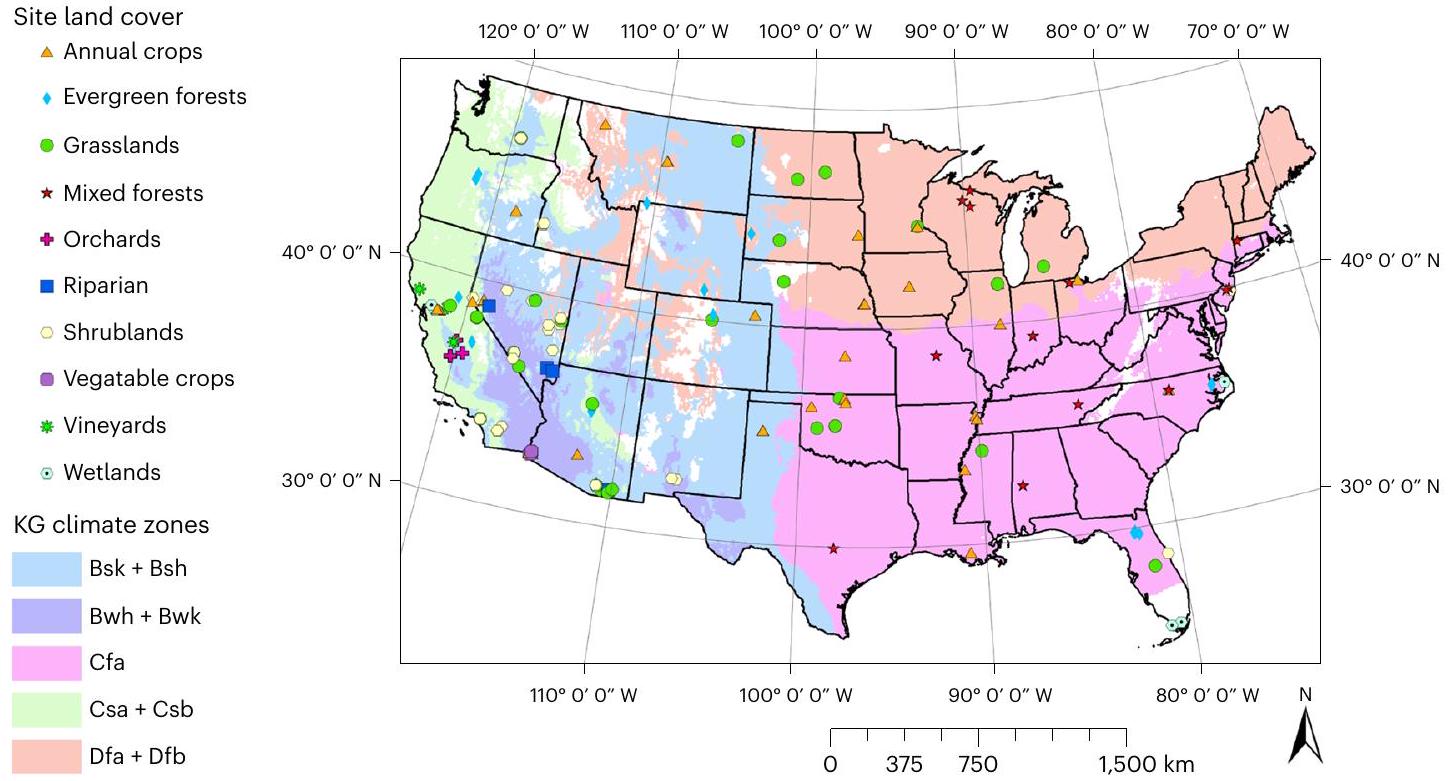
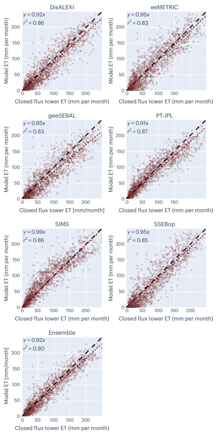
تقدم بيانات التبخر والنتح المستشعرة عن بُعد (ET) إمكانيات قوية لدعم الأساليب المعتمدة على البيانات لإدارة المياه المستدامة. ومع ذلك، يحتاج الممارسون إلى تقييمات دقيقة وصارمة لمدى دقة هذه البيانات. تم تطوير نظام OpenET، الذي يتضمن مجموعة من ستة نماذج استشعار عن بُعد، لزيادة الوصول إلى بيانات ET على مستوى الحقل (30 م) للولايات المتحدة المتجاورة. هنا نقارن مخرجات OpenET ضد بيانات من 152 محطة في الموقع، تتكون أساسًا من أبراج تدفق التباين الدوامي، المنتشرة عبر الولايات المتحدة المتجاورة. متوسط الخطأ المطلق في مواقع الأراضي الزراعية لقيمة مجموعة OpenET هو 15.8 مم في الشهر (
العديد من المياه الجوفية وخزانات المياه في غرب الولايات المتحدة عند أدنى مستوياتها على الإطلاق
نهج الانحراف (MAD)
| نوع تغطية الأرض | إحصائية | مجموعة | ديزاكسي | eeMETRIC | جي سيبال | PT-JPL | سيمز | SSEBop |
|
|
| جميع المحاصيل، متوسط ET للمحطة 91 (مم في الشهر) | منحدر | 0.92 | 0.92 | 0.95 | 0.85 | 0.91 | 0.99 | 0.95 | 53 | 1,652 |
| MBE (مم) | -5.27 (-5.8%) | -7.72 (-8.4%) | -2.44 (-2.7%) | -12.18 (-13.3%) | -2.9 (-3.2%) | 4.32 (4.7%) | -6.08 (-6.7%) | ٤٤ | 1,638 | |
| MAE (مم) | 15.84 (17.3%) | 19.91 (21.8%) | 21.23 (23.2%) | 22.69 (24.8%) | 18.12 (19.8%) | 17.93 (19.6%) | 22.4 (24.5%) | ٤٤ | 1,638 | |
| جذر متوسط مربع الخطأ (مم) | 20.44 (22.4%) | 25.35 (27.7%) | ٢٦.٩٧ (٢٩.٥٪) | ٢٩.٠٥ (٣١.٨٪) | 23.67 (25.9%) | 23.1 (25.3%) | 27.72 (30.3%) | ٤٤ | 1,638 | |
|
|
0.9 | 0.86 | 0.83 | 0.83 | 0.87 | 0.86 | 0.85 | 53 | 1,652 | |
| المحاصيل السنوية، متوسط ET للمحطة 85 (مم في الشهر) | منحدر | 0.93 | 0.92 | 0.98 | 0.85 | 0.9 | 1.01 | 0.92 | 42 | ١٤٤٦ |
| MBE (مم) | -5.11 (-6.0%) | -8.18 (-9.6%) | 0.23 (0.3%) | -12.38 (-14.6%) | -3.77 (-4.4%) | 6.27 (7.4%) | -9.13 (-10.7%) | ٣٦ | ١٤٣٦ | |
| MAE (مم) | 15.26 (17.9%) | ٢٠.٠٩ (٢٣.٦٪) | 20.44 (24.0%) | 22.52 (26.5%) | 17.0 (20.0%) | 17.48 (20.5%) | 21.93 (25.8%) | ٣٦ | ١٤٣٦ | |
| جذر متوسط مربع الخطأ (مم) | 19.71 (23.2%) | 25.68 (30.2%) | ٢٦.١٧ (٣٠.٨٪) | 28.67 (33.7%) | 22.31 (26.2%) | 22.49 (26.4%) | 27.14 (31.9%) | ٣٦ | ١٤٣٦ | |
|
|
0.9 | 0.84 | 0.83 | 0.82 | 0.87 | 0.85 | 0.84 | 42 | ١٤٤٦ | |
| البساتين، متوسط محطة ET هو 126 (مم في الشهر) | منحدر | 0.87 | 0.88 | 0.81 | 0.84 | 0.88 | 0.93 | 0.97 | ٥ | 141 |
| MBE (مم) | -11.9 (-9.4%) | -11.02 (-8.7%) | -20.66 (-16.4%) | -15.11 (-12.0%) | -7.39 (-5.8%) | -3.47 (-2.7%) | -3.69 (-2.9%) | ٥ | 141 | |
| MAE (مم) | 21.18 (16.8%) | 22.2 (17.6%) | 28.19 (22.3%) | 24.9 (19.7%) | 24.43 (19.3%) | 22.95 (18.2%) | 20.18 (16.0%) | ٥ | 141 | |
| جذر متوسط مربع الخطأ (مم) | 27.89 (22.1%) | 27.86 (22.1%) | 35.26 (27.9%) | 32.77 (25.9%) | 31.67 (25.1%) | 30.49 (24.1%) | 27.26 (21.6%) | ٥ | 141 | |
|
|
0.91 | 0.89 | 0.89 | 0.88 | 0.88 | 0.86 | 0.89 | ٥ | 141 | |
| كروم العنب، متوسط المحطة ET هو 112 (مم في الشهر) | منحدر | 1.02 | 1.02 | 0.95 | 0.95 | 1.09 | 0.92 | 1.25 | ٣ | 61 |
| MBE (مم) | 5.27 (4.7%) | 4.99 (4.5%) | -4.62 (-4.1%) | -3.76 (-3.4%) | 17.95 (16.0%) | -7.71 (-6.9%) | 31.88 (28.5%) | ٣ | 61 | |
| MAE (مم) | 13.66 (12.2%) | 13.01 (11.6%) | 18.73 (16.7%) | 20.72 (18.5%) | 21.53 (19.2%) | 14.43 (12.9%) | 33.22 (29.7%) | ٣ | 61 | |
| جذر متوسط مربع الخطأ (مم) | 16.23 (14.5%) | 15.87 (14.2%) | 22.1 (19.7%) | 27.2 (24.3%) | 27.19 (24.3%) | 17.34 (15.5%) | ٣٦.٥٦ (٣٢.٦٪) | ٣ | 61 | |
|
|
0.9 | 0.9 | 0.81 | 0.73 | 0.83 | 0.88 | 0.84 | ٣ | 61 |
 من متوسط التدفق المغلق للبرج المثقل ET. لاحظ أنه كان هناك ثلاثة مواقع إضافية لمحاصيل الخضروات مدرجة في مجموعة المحاصيل المجمعة، والتي بمفردها لم تستوفِ متطلبات بياناتنا للتحليلات الإحصائية.
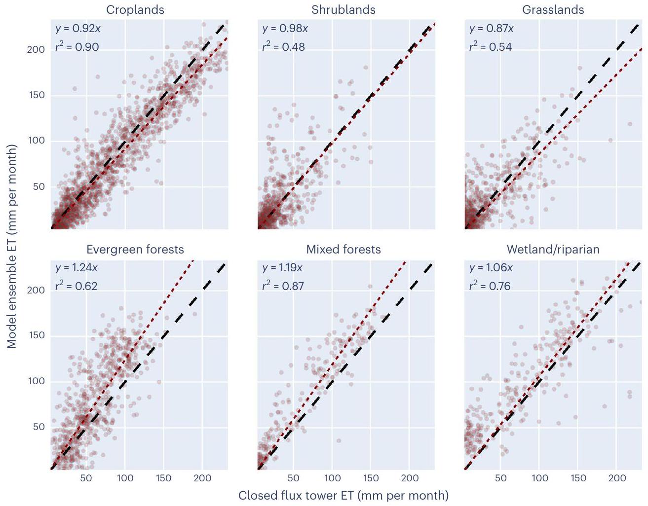
على المقياس الزمني الشهري (مقارنةً باليومي)، يوفر OpenET مباشرةً ET اليومية والشهرية، بالإضافة إلى خدمات البيانات التي تتيح للمستخدمين حساب ET في فترات تجميع أخرى. يتم تقديم نتائج الدقة لفترات زمنية يومية وشهرية وموسمية وسنوية في الجداول التكميلية 2-6، وينبغي استشارة مقاييس الدقة لفترات زمنية يومية لتطبيقات بيانات ET في فترات زمنية تتراوح بين 1-15 يومًا. تم استخدام خمسة مقاييس إحصائية معروفة لتقييم دقة OpenET (للمعادلات، انظر الطرق): ميل الانحدار الخطي المفروض من خلال الأصل الذي يقيس التحيز (الميل)، خطأ التحيز المتوسط (MBE)، خطأ القيمة المطلقة المتوسطة (MAE)، خطأ الجذر التربيعي المتوسط (RMSE) ومعامل التحديد.
الأداء عبر جميع مواقع تدفق الزراعة
ET المقاسة بواسطة النموذج لتوليد المناخيات الشهرية لتصنيفات الغطاء الأرضي الرئيسية (الشكل 3 والأشكال البيانية الموسعة 1-5). النطاق بين ECET غير المغلق والمغلق يوفر مقياسًا واحدًا لعدم اليقين في البيانات الميدانية.
أثر فترة العينة على أداء النموذج
الأداء بين المحاصيل السنوية والدائمة
| نوع تغطية الأرض | إحصاء | مجموعة | ديزاكسي | eeMETRIC | جي سيبال | PT-JPL | سيمز | SSEBop |
|
|
| بسك + بش (سافانا شبه جافة باردة وحارة)، متوسط تبخر المحطة 133 (مم في الشهر) | منحدر | 0.9 | 0.85 | 0.91 | 0.82 | 0.88 | 0.97 | 1 | 11 | 246 |
| MBE (مم) | -6.94 (-5.2%) | -15.17 (-11.4%) | -4.65 (-3.5%) | -18.09 (-13.6%) | -7.55 (-5.7%) | 2.71 (2.0%) | 2.89 (2.2%) | 11 | 246 | |
| MAE (مم) | 20.74 (15.6%) | ٢٦.٩٣ (٢٠.٣٪) | ٢٦.٩٤ (٢٠.٣٪) | 30.31 (22.8%) | 25.7 (19.3%) | 22.99 (17.3%) | ٢٤.٢٣ (١٨.٢٪) | 11 | 246 | |
| جذر متوسط مربع الخطأ (مم) | ٢٦.٣٨ (١٩.٨٪) | ٣٤.٥٥ (٢٦.٠٪) | 33.4 (25.1%) | ٣٨.٠ (٢٨.٦٪) | 32.49 (24.4%) | 28.97 (21.8%) | 30.99 (23.3%) | 11 | 246 | |
|
|
0.89 | 0.81 | 0.8 | 0.8 | 0.84 | 0.84 | 0.84 | 11 | 246 | |
| بوه + بوك (صحراء حارة وباردة)، متوسط محطة ET يبلغ 110 (مم في الشهر) | منحدر | 0.91 | 0.85 | 1.02 | 0.92 | 0.86 | 0.92 | 0.88 | 10 | 53 |
| MBE (مم) | -6.78 (-6.1%) | -15.63 (-14.2%) | 9.63 (8.7%) | -8.19 (-7.4%) | -7.77 (-7.0%) | -3.2 (-2.9%) | -12.34 (-11.2%) | ٧ | ٤٩ | |
| MAE (مم) | 13.24 (12.0%) | 21.21 (19.2%) | 18.92 (17.1%) | 19.13 (17.3%) | 19.21 (17.4%) | 13.62 (12.3%) | 19.59 (17.8%) | ٧ | ٤٩ | |
| جذر متوسط مربع الخطأ (مم) | 17.02 (15.4%) | 25.78 (23.4%) | 23.92 (21.7%) | 23.51 (21.3%) | 23.81 (21.6%) | 16.07 (14.6%) | 22.95 (20.8%) | ٧ | ٤٩ | |
|
|
0.91 | 0.85 | 0.88 | 0.87 | 0.83 | 0.94 | 0.89 | 10 | 53 | |
| Cfa (رطب شبه استوائي)، متوسط ET للمحطة 75 (مم في الشهر) | منحدر | 1 | 1.03 | 1.03 | 0.99 | 0.93 | 1.15 | 0.91 | 11 | 232 |
| MBE (مم) | 2.15 (2.9%) | 4.49 (6.0%) | 3.65 (4.9%) | 0.97 (1.3%) | -0.88 (-1.2%) | 14.98 (19.9%) | -3.84 (-5.1%) | ٨ | 228 | |
| MAE (مم) | 17.51 (23.3%) | 20.17 (26.8%) | 24.01 (31.9%) | 20.06 (26.7%) | 17.79 (23.6%) | 22.71 (30.2%) | 21.97 (29.2%) | ٨ | 228 | |
| جذر متوسط مربع الخطأ (مم) | 23.76 (31.6%) | ٢٦.١٨ (٣٤.٨٪) | 31.88 (42.4%) | 28.39 (37.7%) | 23.62 (31.4%) | 30.23 (40.2%) | 28.76 (38.2%) | ٨ | 228 | |
|
|
0.75 | 0.72 | 0.62 | 0.69 | 0.76 | 0.72 | 0.64 | 11 | 232 | |
| CSA + CSB (المتوسطات المناخية للبحر الأبيض المتوسط ذات الصيف الحار والدافئ)، متوسط ET للمحطة هو 94 (ملم في الشهر) | منحدر | 0.95 | 0.96 | 0.99 | 0.81 | 1.01 | 0.93 | 0.99 | ٨ | ٢٩٢ |
| MBE (مم) | -4.37 (-4.7%) | -6.32 (-6.7%) | -1.72 (-1.8%) | -20.92 (-22.3%) | 7.37 (7.9%) | -1.34 (-1.4%) | -2.9 (-3.1%) | ٨ | ٢٩٢ | |
| MAE (مم) | 13.32 (14.2%) | 18.65 (19.9%) | 17.14 (18.3%) | 25.9 (27.6%) | 17.17 (18.3%) | 14.04 (15.0%) | 23.94 (25.6%) | ٨ | ٢٩٢ | |
| جذر متوسط مربع الخطأ (مم) | 16.52 (17.6%) | 22.75 (24.3%) | 21.48 (22.9%) | 31.31 (33.4%) | 21.97 (23.5%) | 18.27 (19.5%) | 27.92 (29.8%) | ٨ | ٢٩٢ | |
|
|
0.93 | 0.87 | 0.88 | 0.85 | 0.87 | 0.88 | 0.84 | ٨ | ٢٩٢ | |
| دي إف إيه + دي إف بي (قاري رطب صيف حار وصيف دافئ)، متوسط ET للمحطة 67 (مم في الشهر) | منحدر | 0.9 | 0.93 | 0.94 | 0.86 | 0.87 | 1.02 | 0.9 | ١٣ | 829 |
| MBE (مم) | -8.0 (-11.9%) | -8.07 (-12.0%) | -6.74 (-10.0%) | -10.55 (-15.7%) | -5.72 (-8.5%) | 4.88 (7.3%) | -13.58 (-20.2%) | 10 | ٨٢٣ | |
| MAE (مم) | 13.8 (20.5%) | 15.68 (23.3%) | 18.93 (28.2%) | 17.88 (26.6%) | 13.67 (20.3%) | 15.35 (22.8%) | 21.09 (31.4%) | 10 | ٨٢٣ | |
| جذر متوسط مربع الخطأ (مم) | 17.85 (26.6%) | 20.36 (30.3%) | ٢٤.١ (٣٥.٨٪) | 23.36 (34.7%) | 18.89 (28.1%) | 19.94 (29.7%) | 25.9 (38.5%) | 10 | ٨٢٣ | |
|
|
0.91 | 0.9 | 0.83 | 0.86 | 0.89 | 0.86 | 0.86 | ١٣ | 829 |
 متوسط الوزن لإنتاجية التبخر من برج التدفق المغلق.
الأغصان المتجمعة بقوة، خاصة بالنسبة للنماذج التي تعتمد بشكل كبير على مدخلات درجة حرارة سطح الأرض. كانت القيمة الجماعية تحمل انحيازًا سلبيًا بمتوسط ميل قدره
تباين أداء النموذج عبر المناطق المناخية
الأداء في النظم البيئية الطبيعية
لا يتم تصميمه حاليًا وتنفيذه في أنواع تغطية الأراضي غير الزراعية؛ بالنسبة لهذه البكسلات، يتكون التجميع من خمسة نماذج مع إمكانية إزالة نقطة شاذة واحدة (الطرق). كان خطأ النموذج المنهجي والتباين لمواقع غير الزراعية أعلى من مواقع الأراضي الزراعية (الشكل 5).
إزالة القيم الشاذة من المجموعة والتباين المكاني بين النماذج
نقاش
الاستنتاجات
المستخدمون المحتملون لـ OpenET بسبب الصرامة العالية والشفافية في الأساليب التي تم استخدامها.
طرق
معالجة بيانات التدفق وأخذ عينات البصمة
المواقع المجهزة، التي تقيس ET في الغالب في أراضي الشجيرات الفرياطية في نيفادا
بيانات النموذج
(1) تم حساب ET اليومي من eeMETRIC وSIMS وSSEBop للمواقع خارج كاليفورنيا من خلال ضرب وحدات EToF اليومية المأخوذة من النماذج في الوزن اليومي لكل وحدة تدفق للحصول على وحدات EToF اليومية الموزونة، وجمع جميع وحدات EToF اليومية الموزونة للحصول على متوسط EToF اليومي الموزون، وتطبيع متوسط EToF اليومي الموزون من خلال مجموع الأوزان لمراعاة الأوقات التي لم يساوي فيها مجموع الأوزان 1 (على سبيل المثال، بسبب حجب السحب لوحدات البكسل)، ثم ضرب متوسط EToF اليومي الموزون في متوسط ETo اليومي المصحح من bias من gridMET (الذي تم استبداله للمواقع داخل كاليفورنيا باستخدام ETo اليومي من CIMIS);
(2) تم حساب ET اليومي من PT-JPL و geeSEBAL و ALEXI/DisALEXI لجميع المواقع عن طريق ضرب بكسلات ET اليومية في أوزان بصمة التدفق اليومية للحصول على بكسلات ET اليومية الموزونة، وجمع جميع بكسلات ET اليومية الموزونة للحصول على ET اليومي الموزون المتوسط، ثم تطبيع ET اليومي الموزون المتوسط بواسطة مجموع الأوزان، و
(3) تم حساب ET الشهري من جميع نماذج RSET للمواقع خارج كاليفورنيا من خلال ضرب بكسلات EToF الشهرية بـ
تُستخدم أوزان بصمة التدفق الشهرية للحصول على بكسلات EToF الشهرية الموزونة، من خلال جمع جميع بكسلات EToF الشهرية الموزونة للحصول على متوسط EToF الشهري الموزون، ثم يتم تطبيع متوسط EToF الشهري الموزون بواسطة مجموع الأوزان، وبعد ذلك يتم ضرب متوسط EToF الشهري الموزون في متوسط ETo المصحح بالتحيز من شبكة gridMET (الذي تم استبداله للمواقع داخل كاليفورنيا باستخدام ETo الشهري من CIMIS).
حساب جماعي
التحليلات الإحصائية
كانت ملاحظات الأزواج دائمًا هي نفسها بين النماذج لجميع التحليلات الإحصائية.
ملخص التقرير
توفر البيانات
خلال الدراسة الحالية متاحة في مستودع زينودو، مع المعرفhttps://doi.org/10.5281/zenodo.10119477.
توفر الشيفرة
References
- Fisher, J. B. et al. The future of evapotranspiration: global requirements for ecosystem functioning, carbon and climate feedbacks, agricultural management, and water resources. Water Resour. Res. 53, 2618-2626 (2017).
- Dieter, C. A. et al. Estimated use of water in the United States in 2015. Circular 1411 https://pubs.usgs.gov/publication/cir1441 (2018).
- Cook, B. I., Ault, T. R. & Smerdon, J. E. Unprecedented 21st century drought risk in the American Southwest and Central Plains. Sci. Adv. 1, e1400082 (2015).
- Liu, P.-W. et al. Groundwater depletion in California’s Central Valley accelerates during megadrought. Nat. Commun. 13, 7825 (2022).
- Melton, F. S. et al. OpenET: filling a critical data gap in water management for the western United States. J. Am. Water Resour. Assoc. 58, 971-994 (2022).
- Chen, J. M. & Liu, J. Evolution of evapotranspiration models using thermal and shortwave remote sensing data. Remote Sens. Environ. 237, 111594 (2020).
- Anderson, M. et al. Field-scale assessment of land and water use change over the California Delta using remote sensing. Remote Sens. 10, 889 (2018).
- Allen, R. G., Tasumi, M. & Trezza, R. Satellite-based energy balance for mapping evapotranspiration with internalized calibration (METRIC)-Model. J. Irrig. Drain. Eng. 133, 380-394 (2007).
- Laipelt, L. et al. Long-term monitoring of evapotranspiration using the SEBAL algorithm and Google Earth Engine cloud computing. ISPRS J. Photogramm. Remote Sens. 178, 81-96 (2021).
- Fisher, J. B., Tu, K. P. & Baldocchi, D. D. Global estimates of the land-atmosphere water flux based on monthly AVHRR and ISLSCP-II data, validated at 16 FLUXNET sites. Remote Sens. Environ. 112, 901-919 (2008).
- Pereira, L. S. et al. Prediction of crop coefficients from fraction of ground cover and height. Background and validation using ground and remote sensing data. Agric. Water Manag. 241, 106197 (2020).
- Melton, F. S. et al. Satellite irrigation management support with the terrestrial observation and prediction system: a framework for integration of satellite and surface observations to support improvements in agricultural water resource management. IEEE J. Sel. Top. Appl. Earth Obs. Remote Sens. 5, 1709-1721 (2012).
- Senay, G. B. et al. Improving the operational simplified surface energy balance evapotranspiration model using the forcing and normalizing operation. Remote Sens. 15, 260 (2023).
- Gorelick, N. et al. Google Earth Engine: planetary-scale geospatial analysis for everyone. Remote Sens. Environ. 202, 18-27 (2017).
- Allen, R. G. et al. Satellite-based energy balance for mapping evapotranspiration with internalized calibration (METRIC)Applications. J. Irrig. Drain. Eng. 133, 395-406 (2007).
- Knipper, K. R. et al. Using high-spatiotemporal thermal satellite ET retrievals for operational water use and stress monitoring in a California vineyard. Remote Sens. 11, 2124 (2019).
- Senay, G. B., Friedrichs, M., Singh, R. K. & Velpuri, N. M. Evaluating Landsat 8 evapotranspiration for water use mapping in the Colorado River Basin. Remote Sens. Environ. 185, 171-185 (2016).
- Foster, T., Mieno, T. & Brozović, N. Satellite-based monitoring of irrigation water use: assessing measurement errors and their implications for agricultural water management policy. Water Resour. Res. 56, e2020WRO28378 (2020).
- Volk, J. M. et al. Development of a benchmark eddy flux evapotranspiration dataset for evaluation of satellite-driven evapotranspiration models over the CONUS. Agric. For. Meteorol. 331, 109307 (2023).
- Volk, J. M. et al. Post-processed data and graphical tools for a CONUS-wide eddy flux evapotranspiration dataset. Data Brief https://doi.org/10.1016/j.dib.2023.109274 (2023).
- Baldocchi, D. Measuring fluxes of trace gases and energy between ecosystems and the atmosphere-the state and future of the eddy covariance method. Glob. Change Biol. 20, 3600-3609 (2014).
- Baldocchi, D. et al. FLUXNET: a new tool to study the temporal and spatial variability of ecosystem-scale carbon dioxide, water vapor, and energy flux densities. Bull. Am. Meteorol. Soc. 82, 2415-2434 (2001).
- Hampel, F. R. The influence curve and its role in robust estimation. J. Am. Stat. Assoc. 69, 383-393 (1974).
- Leys, C., Ley, C., Klein, O., Bernard, P. & Licata, L. Detecting outliers: do not use standard deviation around the mean, use absolute deviation around the median. J. Exp. Soc. Psychol. 49, 764-766 (2013).
- Thompson, P. D. How to improve accuracy by combining independent forecasts. Mon. Weather Rev. 105, 228-229 (1977).
- Kirtman, B. P. et al. The North American multimodel ensemble: phase-1 seasonal-to-interannual prediction; phase-2 toward developing intraseasonal prediction. Bull. Am. Meteorol. Soc. 95, 585-601 (2014).
- Bai, Y. et al. On the use of machine learning based ensemble approaches to improve evapotranspiration estimates from croplands across a wide environmental gradient. Agric. For. Meteorol. 298, 108308 (2021).
- Novick, K. A. et al. The AmeriFlux network: a coalition of the willing. Agric. For. Meteorol. 249, 444-456 (2018).
- Pastorello, G. et al. The FLUXNET2O15 dataset and the ONEFlux processing pipeline for eddy covariance data. Sci. Data 7, 1-27 (2020).
- Mauder, M., Foken, T. & Cuxart, J. Surface-energy-balance closure over land: a review. Bound. Layer Meteorol. 177, 395-426 (2020).
- Ingwersen, J., Imukova, K., Högy, P. & Streck, T. On the use of the post-closure methods uncertainty band to evaluate the performance of land surface models against eddy covariance flux data. Biogeosciences 12, 2311-2326 (2015).
- Knipper, K. R. et al. Evapotranspiration estimates derived using thermal-based satellite remote sensing and data fusion for irrigation management in California vineyards. Irrig. Sci. 37, 431-449 (2019).
- Bambach, N. et al. Evapotranspiration uncertainty at micrometeorological scales: the impact of the eddy covariance energy imbalance and correction methods. Irrig. Sci. 40, 445-461 (2022).
- Rubel, F., Brugger, K., Haslinger, K. & Auer, I. The climate of the European Alps: shift of very high resolution Köppen-Geiger climate zones 1800-2100. Meteorol. Z. 26, 115-125 (2017).
- Yang, Y. et al. Studying drought-induced forest mortality using high spatiotemporal resolution evapotranspiration data from thermal satellite imaging. Remote Sens. Environ. 265, 112640 (2021).
- Isaacson, B. N., Yang, Y., Anderson, M. C., Clark, K. L. & Grabosky, J. C. The effects of forest composition and management on evapotranspiration in the New Jersey pinelands. Agric. For. Meteorol. 339, 109588 (2023).
- Qian, Y. et al. Neglecting irrigation contributes to the simulated summertime warm-and-dry bias in the central United States. Npj Clim. Atmos. Sci. 3, 31 (2020).
- Lei, F., Crow, W. T., Holmes, T. R., Hain, C. & Anderson, M. C. Global investigation of soil moisture and latent heat flux coupling strength. Water Resour. Res. 54, 8196-8215 (2018).
- Dong, J., Lei, F. & Crow, W. T. Land transpiration-evaporation partitioning errors responsible for modeled summertime warm bias in the central United States. Nat. Commun. 13, 336 (2022).
- Abolafia-Rosenzweig, R., Pan, M., Zeng, J. & Livneh, B. Remotely sensed ensembles of the terrestrial water budget over major global river basins: an assessment of three closure techniques. Remote Sens. Environ. 252, 112191 (2021).
- Wang, Q. et al. Land surface models significantly underestimate the impact of land-use changes on global evapotranspiration. Environ. Res. Lett. 16, 124047 (2021).
- Allen, R. G., Pereira, L. S., Howell, T. A. & Jensen, M. E. Evapotranspiration information reporting: I. Factors governing measurement accuracy. Agric. Water Manag. 98, 899-920 (2011).
- Adu, M. O., Yawson, D. O., Armah, F. A., Asare, P. A. & Frimpong, K. A. Meta-analysis of crop yields of full, deficit, and partial root-zone drying irrigation. Agric. Water Manag. 197, 79-90 (2018).
- Xue, J. et al. Improving the spatiotemporal resolution of remotely sensed ET information for water management through Landsat, Sentinel-2, ECOSTRESS and VIIRS data fusion. Irrig. Sci. 40, 609-634 (2022).
- Gao, F. & Zhang, X. Mapping crop phenology in near real-time using satellite remote sensing: challenges and opportunities. J. Remote Sens. 2021, 8379391 (2021).
- Müller, M. Dynamic time warping. in Information Retrieval for Music and Motion. 69-84 (Springer, 2007).
- Bambach, N. et al. The Tree-crop Remote sensing of Evapotranspiration eXperiment (T-REX): a science-based path for sustainable water management and climate mitigation. Bull. Am. Meteorol. Soc. In the press (2023).
- Fisher, J. B. Hydrosat: towards daily, field-scale, global evapotranspiration from space. (2022).
- Polhamus, A., Fisher, J. B. & Tu, K. P. What controls the error structure in evapotranspiration models? Agric. For. Meteorol. 169, 12-24 (2013).
- Blankenau, P. A., Kilic, A. & Allen, R. An evaluation of gridded weather data sets for the purpose of estimating reference evapotranspiration in the United States. Agric. Water Manag. 242, 106376 (2020).
- Doherty, C. T. et al. Effects of meteorological and land surface modeling uncertainty on errors in winegrape ET calculated with SIMS. Irrig. Sci. 40, 515-530 (2022).
- Purdy, A., Fisher, J., Goulden, M. & Famiglietti, J. Ground heat flux: an analytical review of 6 models evaluated at 88 sites and globally. J. Geophys. Res. Biogeosci. 121, 3045-3059 (2016).
- Allen, R. G. et al. A recommendation on standardized surface resistance for hourly calculation of reference ETo by the FAO56 Penman-Monteith method. Agric. Water Manag. 81, 1-22 (2006).
- Jung, M. et al. The FLUXCOM ensemble of global landatmosphere energy fluxes. Sci. Data 6, 74 (2019).
- Reitz, M., Senay, G. B. & Sanford, W. E. Combining remote sensing and water-balance evapotranspiration estimates for the conterminous United States. Remote Sens. 9, 1181 (2017).
- Volk, J. et al. flux-data-qaqc: a Python package for energy balance closure and post-processing of eddy flux. Data. 6, 1-5 (2021).
- Evett, S. R. et al. The Bushland weighing lysimeters: a quarter century of crop ET investigations to advance sustainable irrigation. Trans. ASABE 59, 163-179 (2016).
- Abatzoglou, J. T. Development of gridded surface meteorological data for ecological applications and modelling. Int. J. Climatol. 33, 121-131 (2013).
- Kljun, N., Calanca, P., Rotach, M. W. & Schmid, H. P. A simple twodimensional parameterisation for Flux Footprint Prediction (FFP). Geosci. Model Dev. 8, 3695-3713 (2015).
- Xia, Y. et al. Continental-scale water and energy flux analysis and validation for the North American Land Data Assimilation System project phase 2 (NLDAS-2): 1. Intercomparison and application of model products. J. Geophys. Res. Atmos. 117, DO31O9 (2012).
- Foga, S. et al. Cloud detection algorithm comparison and validation for operational Landsat data products. Remote Sens. Environ. 194, 379-390 (2017).
- Rousseeuw, P. J. & Croux, C. Alternatives to the median absolute deviation. J. Am. Stat. Assoc. 88, 1273-1283 (1993).
- Harris, C. R. et al. Array programming with NumPy. Nature 585, 357-362 (2020).
- Seabold, S. & Perktold, J. Statsmodels: econometric and statistical modeling with Python. In Proc. 9th Python in Science Conference vol. 57 10-25080 (SciPy, 2010).
- Obrecht, N. A. Sample size weighting follows a curvilinear function. J. Exp. Psychol. Learn. Mem. Cogn. 45, 614 (2019).
شكر وتقدير
https://doi.org/10.17190/AMF/1246070، https://doi.org/10.17190/AMF/1660346،https://doi.org/10.17190/AMF/1246074، https://doi. org/10.17190/AMF/1246076، https://doi.org/10.17190/AMF/1246079، https://doi.org/10.17190/AMF/1246128، https://doi.org/10.17190/AMF/1617715،https://doi.org/10.17190/AMF/1617716، “https://doi. org/10.17190/AMF/1246080، https://doi.org/10.17190/AMF/1246081، https://doi.org/10.17190/AMF/1246083، https://doi.org/10.17190/AMF/1419506،https://doi.org/10.17190/AMF/1480314، https://doi. org/10.17190/AMF/1246084، https://doi.org/10.17190/AMF/1246085، https://doi.org/10.17190/AMF/1246086، https://doi.org/10.17190/AMF/1246088،https://doi.org/10.17190/AMF/1246089، https://doi. org/10.17190/AMF/1246092، https://doi.org/10.17190/AMF/1418683، https://doi.org/10.17190/AMF/1246093، https://doi.org/10.17190/AMF/1419507،https://doi.org/10.17190/AMF/1419508، https://doi. org/10.17190/AMF/1419509، https://doi.org/10.17190/AMF/1617721، https://doi.org/10.17190/AMF/1617724، https://doi.org/10.17190/AMF/1375201،https://doi.org/10.17190/AMF/1419502، https://doi. org/10.17190/AMF/1419501، https://doi.org/10.17190/AMF/1419504، https://doi.org/10.17190/AMF/1246136، https://doi.org/10.17190/AMF/1246105،https://doi.org/10.17190/AMF/1246096، https://doi. org/10.17190/AMF/1418684، https://doi.org/10.17190/AMF/1246097، https://doi.org/10.17190/AMF/1246098، https://doi.org/10.17190/AMF/1246099،https://doi.org/10.17190/AMF/1246101، https://doi. org/10.17190/AMF/1246102، https://doi.org/10.17190/AMF/1246127، https://doi.org/10.17190/AMF/1246154، “https://doi.org/10.17190/AMF/1246104،https://doi.org/10.17190/AMF/1418685، https://doi. org/10.17190/AMF/1660351، https://doi.org/10.17190/AMF/1246148، https://doi.org/10.17190/AMF/1246149، https://doi.org/10.17190/AMF/1246140،https://doi.org/10.17190/AMF/1245984، https://doi. org/10.17190/AMF/1246109، https://doi.org/10.17190/AMF/1246111، https://doi.org/10.17190/AMF/1246112، https://doi.org/10.17190/AMF/1617728،https://doi.org/10.17190/AMF/1579721، https://doi. org/10.17190/AMF/1617732، https://doi.org/10.17190/AMF/1579723، https://doi.org/10.17190/AMF/1617735، https://doi.org/10.17190/AMF/1617737،https://doi.org/10.17190/AMF/1617741, https://doi. org/10.3133/sir20095079، https://doi.org/10.3133/sir20095079، https://doi.org/10.3133/sir20055288، https://doi.org/10.3133/سير20055288،https://doi.org/10.3133/sir20085116، https://doi. org/10.3133/sir20095079، https://doi.org/10.3133/sir20085116، https:// doi.org/10.5066/F7R49NZN، https://doi.org/10.5066/F7R49NZN، https://doi.org/10.5066/F79C6WM9, https://doi.org/10.5066/F79C6WM9https://doi.org/10.3133/pp1805، https://doi.org/10.5066/ P9NZ9XSP، https://doi.org/10.5066/P9NZ9XSP، https://doi. org/10.5066/P9NZ9XSP، https://doi.org/10.3133/sir20075078، https:// doi.org/10.3133/sir20075078، https://doi.org/10.3133/sir20085116، https://doi.org/10.3133/sir20075078 و https://doi.org/10.3133/السير 20075078. تم توفير التمويل لموارد بيانات أمري فلوكس من قبل مكتب العلوم بوزارة الطاقة الأمريكية. أي استخدام لأسماء التجارة أو الشركات أو المنتجات هو لأغراض وصفية فقط ولا يعني تأييدًا من الحكومة الأمريكية.
مساهمات المؤلفين
المصالح المتنافسة
معلومات إضافية
https://doi.org/10.1038/s44221-023-00181-7.
معلومات إضافية النسخة الإلكترونية تحتوي على مواد إضافية متاحة فيhttps://doi.org/10.1038/s44221-023-00181-7.
الغابات دائمة الخضرة
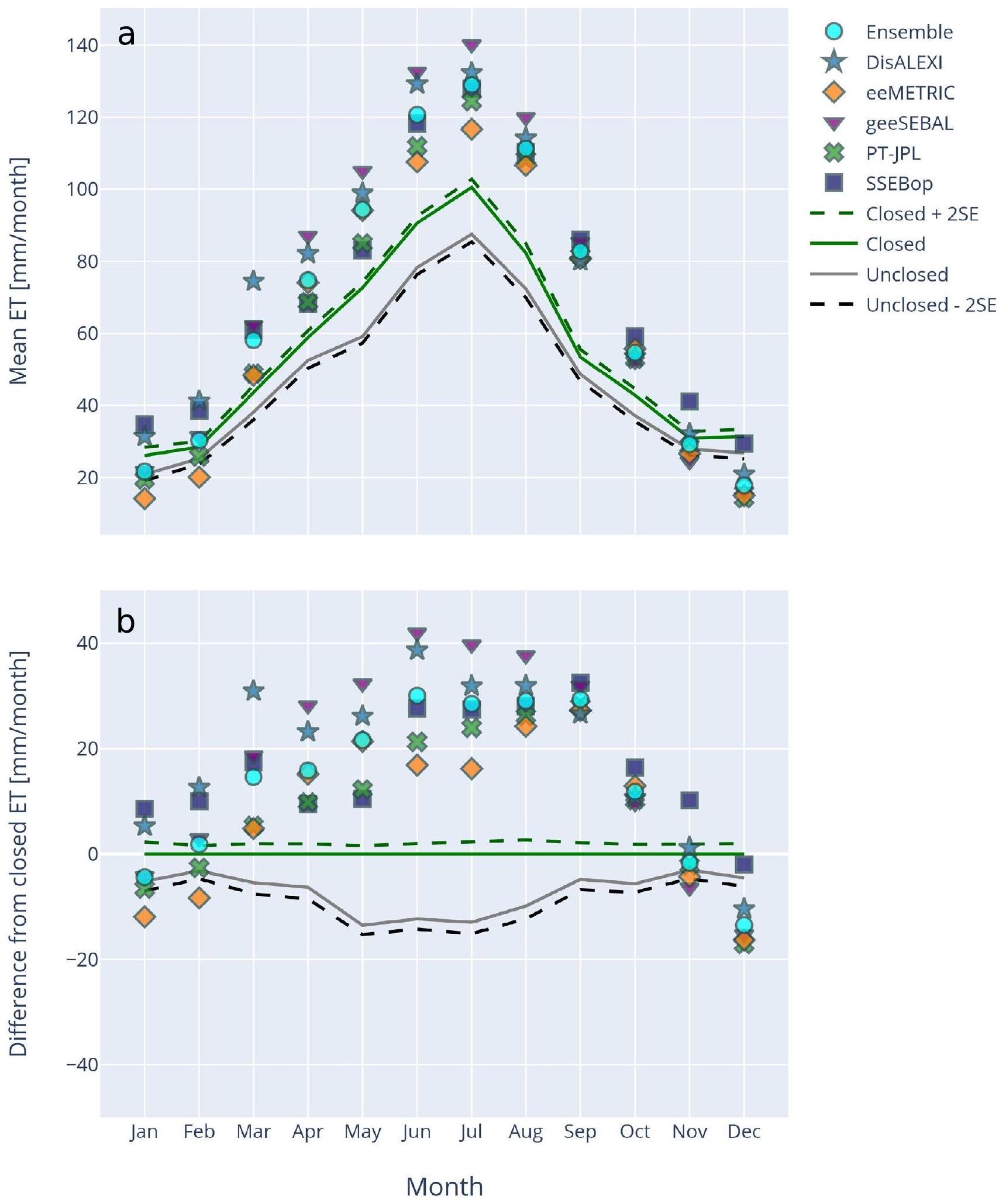
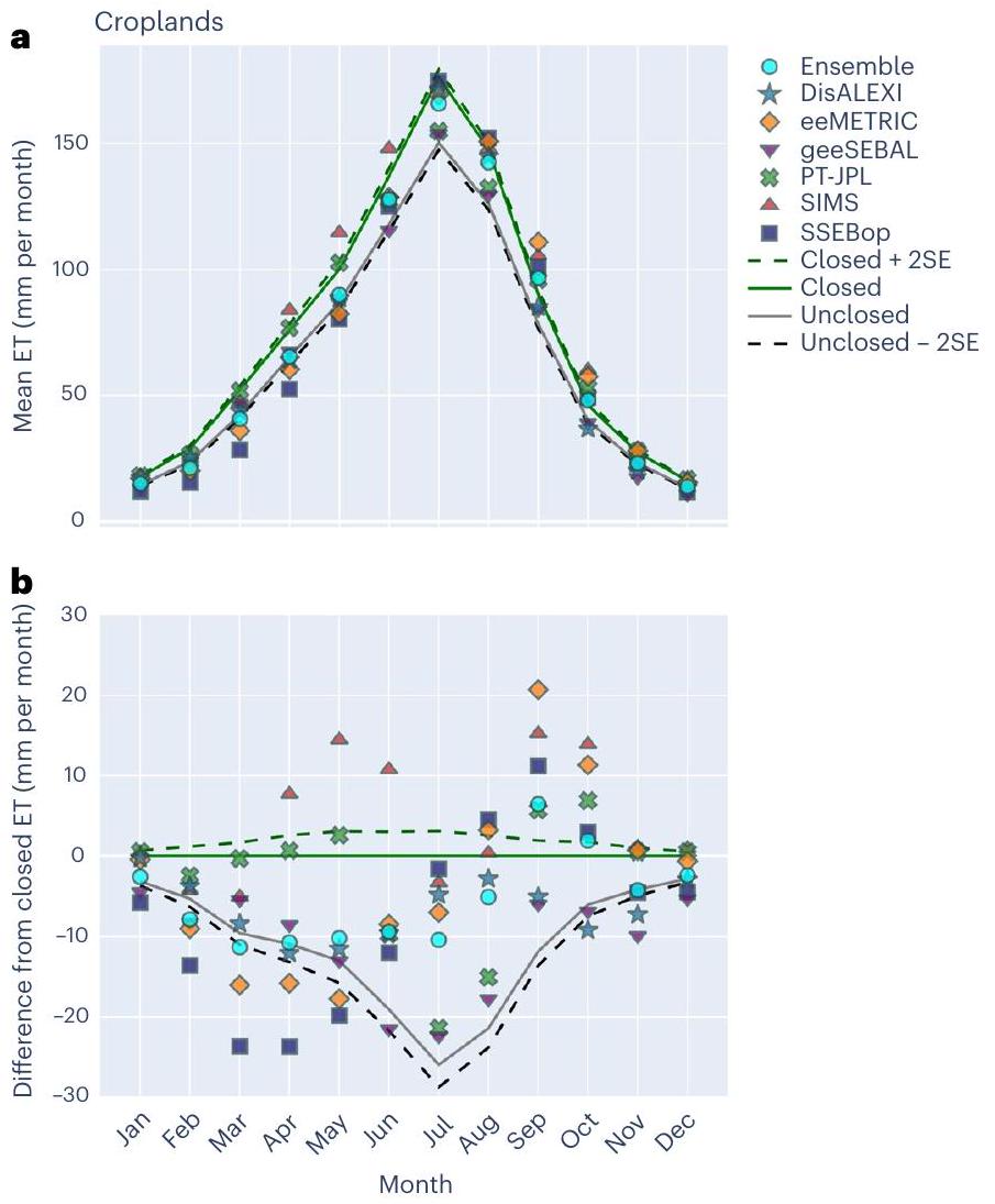
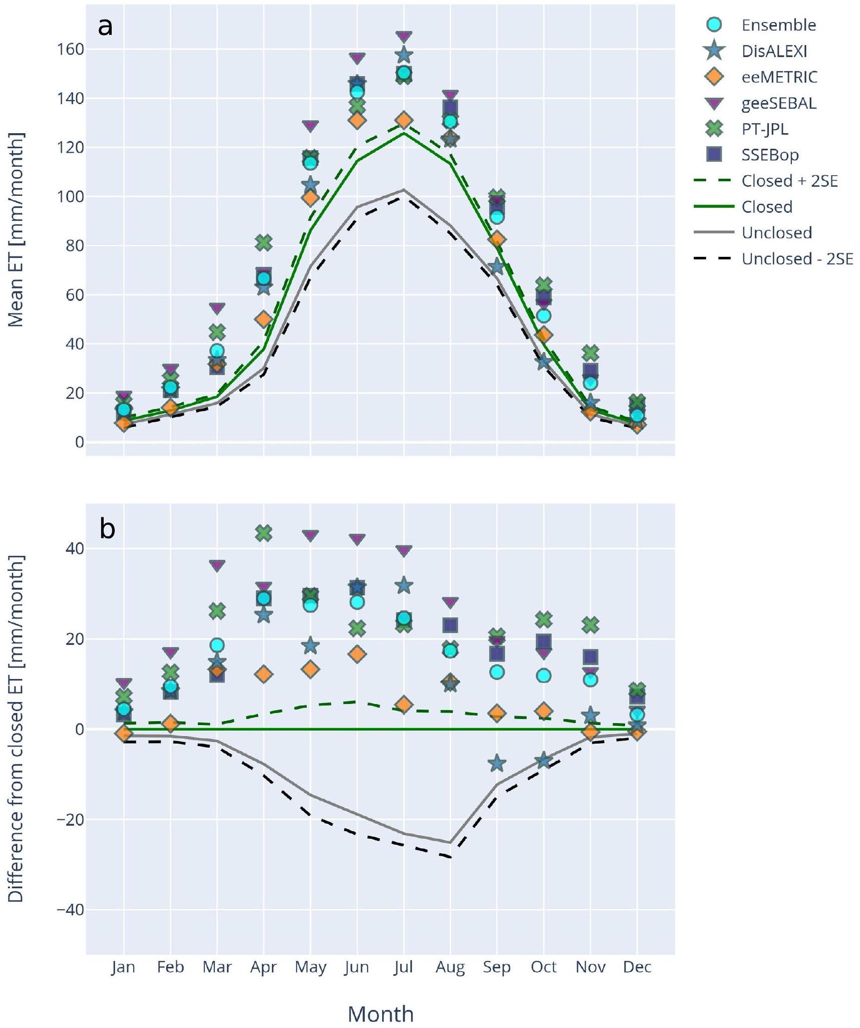
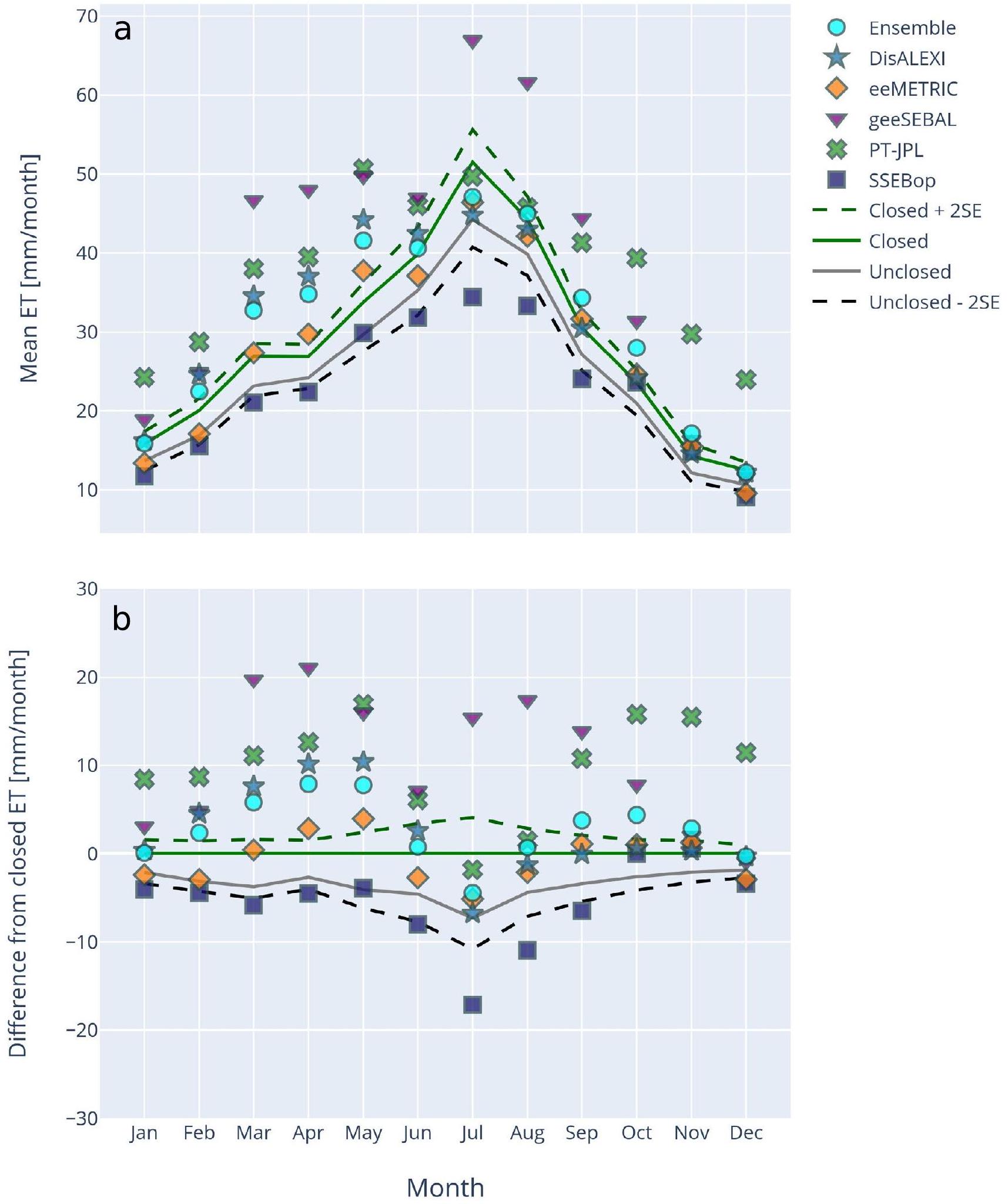
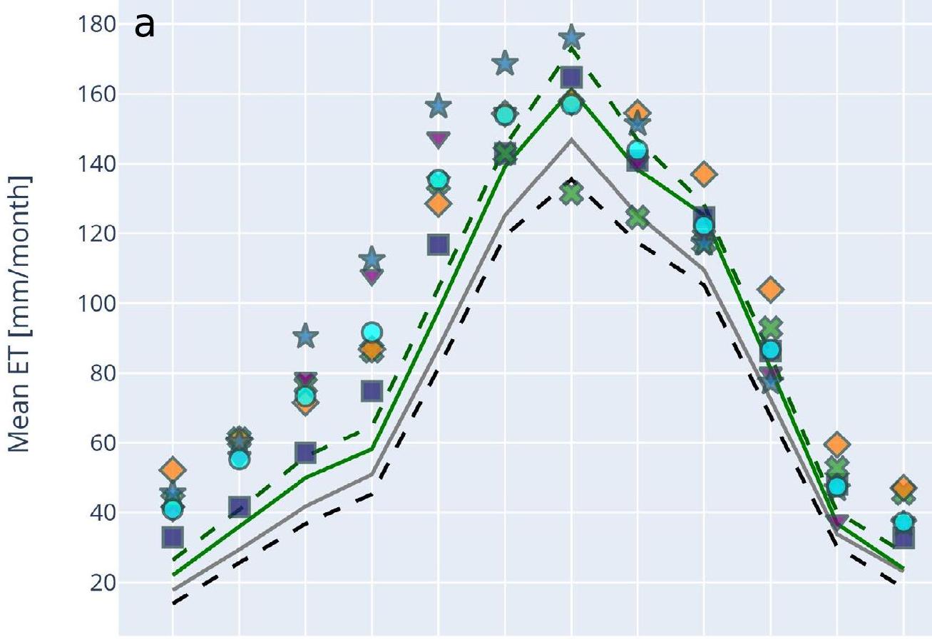
تشير التسميات المغلقة وغير المغلقة إلى تدفق برج ET قبل وبعد تصحيح توازن الطاقة. تمثل الخطوط المتقطعة متوسط تدفق ET المغلق زائد اثنين من الأخطاء المعيارية للمتوسط ومتوسط تدفق ET غير المغلق ناقص اثنين من الأخطاء المعيارية للمتوسط.
الغابات المختلطة
تشير التسميات المغلقة وغير المغلقة إلى تدفق برج ET قبل وبعد تصحيح توازن الطاقة. تمثل الخطوط المتقطعة متوسط تدفق ET المغلق زائد اثنين من الأخطاء المعيارية للمتوسط ومتوسط تدفق ET غير المغلق ناقص اثنين من الأخطاء المعيارية للمتوسط.
المراعي
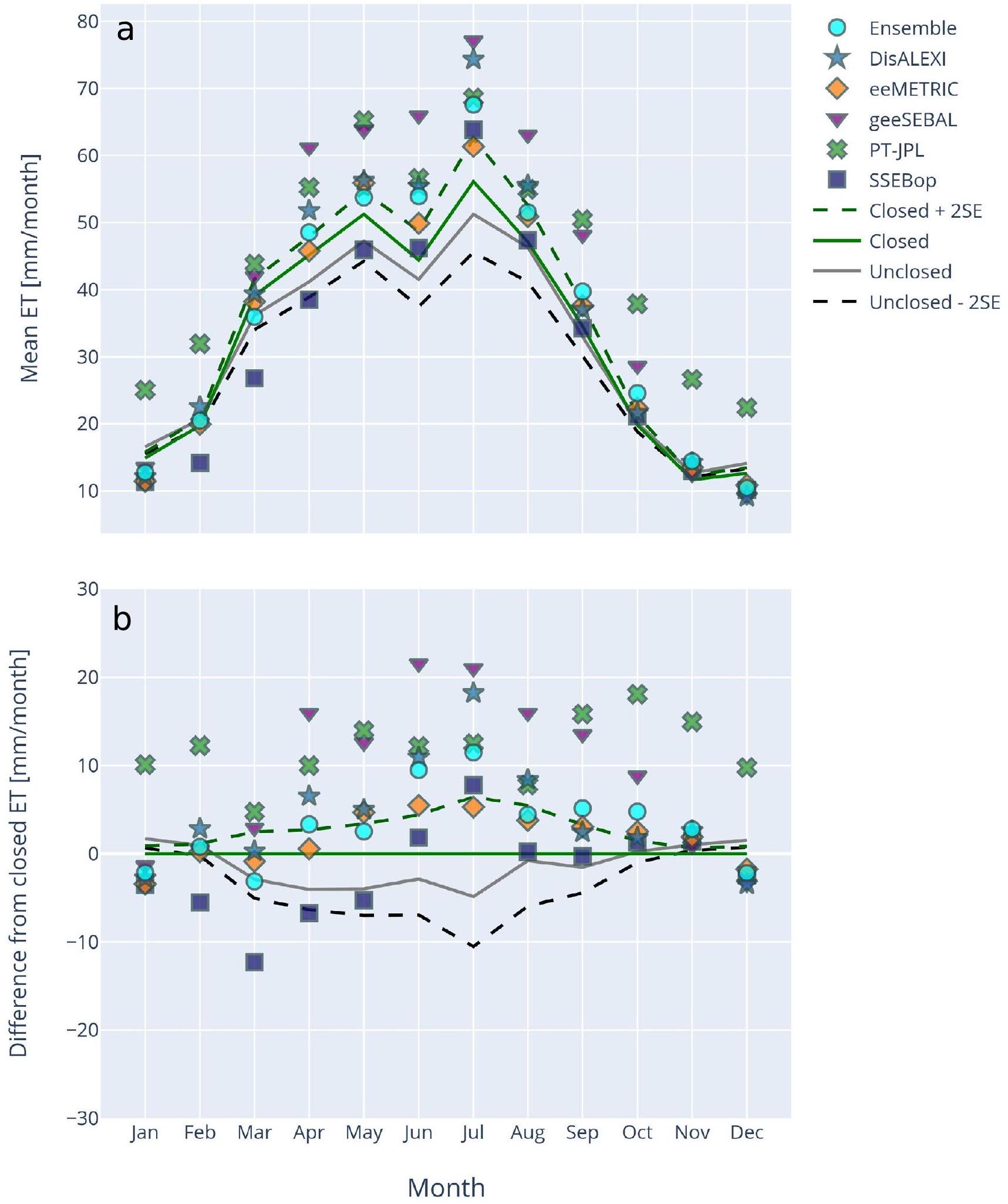
ET لمواقع المراعي. توضح الفقرة (أ) المناخ الشهري لبيانات OpenET المزدوجة
تشير التسميات المغلقة وغير المغلقة إلى تدفق برج ET قبل وبعد تصحيح توازن الطاقة. تمثل الخطوط المتقطعة متوسط تدفق ET المغلق زائد اثنين من الأخطاء المعيارية للمتوسط ومتوسط تدفق ET غير المغلق ناقص اثنين من الأخطاء المعيارية للمتوسط.
الأراضي الشجرية
ET لمواقع الشجيرات. يوضح الرسم الفرعي (أ) المناخ الشهري لبيانات OpenET المزدوجة
تشير التسميات المغلقة وغير المغلقة إلى تدفق برج ET قبل وبعد تصحيح توازن الطاقة. تمثل الخطوط المتقطعة متوسط تدفق ET المغلق زائد اثنين من الأخطاء المعيارية للمتوسط ومتوسط تدفق ET غير المغلق ناقص اثنين من الأخطاء المعيارية للمتوسط.
الأراضي الرطبة/المناطق الساحلية
|
|
مجموعة |
| ديزاكسي | eeMETRIC |
| جي سيبال | |
| PT-JPL | |
| – | SSEBop |
| – | مغلق + 2SE |
| – | مغلق |
| – | غير مغلق |
| – – غير مغلق – 2SE |
شهر
لبناء الخريطة. يظهر الرسم الفرعي (ب) متوسط عدد النماذج المستخدمة في المجموعة بعد إزالة القيم الشاذة باستخدام جميع بيانات الأشهر لفترة النمو لبكسلات الأراضي الزراعية. تشير القيمة ستة إلى أنه لم يتم تحديد أي نموذج كقيمة شاذة، بينما أربعة هي الحد الأدنى حيث تم إزالة نموذجين كحد أقصى كقيم شاذة قبل أخذ المتوسط الجماعي.
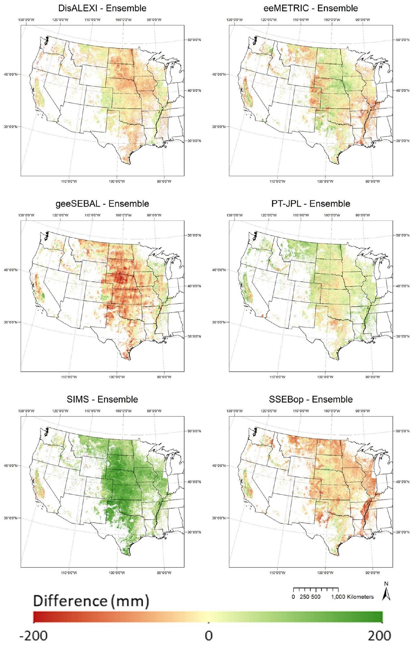
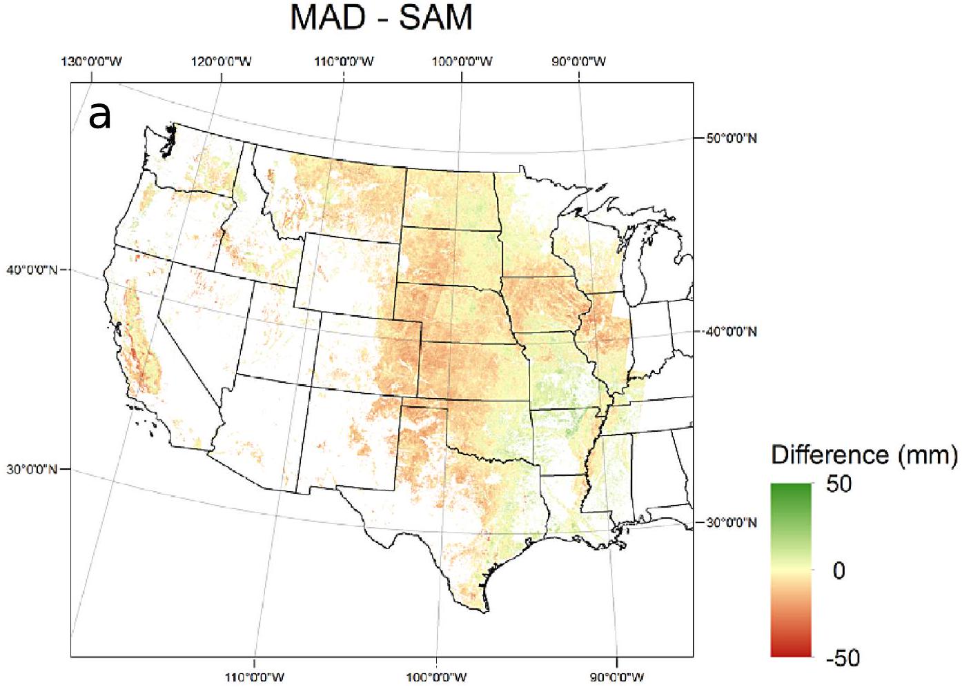
ناقص المتوسط الجماعي باستخدام جميع بيانات الأشهر من جميع البكسلات التي تم تصنيفها كأراضي زراعية لكل عام من 2016-2022. انظر المناقشة التكميلية 4 لمناقشة خطوط Landsat المعروضة بواسطة geeSEBAL.
natureportfolio
جون فوك
آخر تحديث من قبل المؤلف(ين): 27 نوفمبر 2023
ملخص التقرير
الإحصائيات
تم التأكيد
يجب وصف الاختبارات الشائعة فقط بالاسم؛ وصف تقنيات أكثر تعقيدًا في قسم الطرق.
تحتوي مجموعتنا على الإنترنت حول الإحصائيات لعلماء الأحياء على مقالات حول العديد من النقاط أعلاه.
البرمجيات والرموز
معلومات السياسة حول توفر كود الكمبيوتر
تم معالجة بيانات التبخر والنتح المقاسة في الموقع التي تم تحليلها خلال الدراسة الحالية باستخدام حزمة بايثون “flux-data-qaqc”، الإصدار 0.1.6 (https://github.com/Open-ET/flux-data-qaqc).
تم استخدام حزمة بايثون “flux-data-footprint” لإنشاء بصمات تدفق ديناميكية زمنية لعينات بيانات ET اليومية والشهرية (https://github.com/Open-ET/flux-data-footprint). تم استخدام حزم بايثون Numpy (الإصدار 1.17.2) وstatsmodels (الإصدار 0.12.1) لتحليل البيانات خلال الدراسة الحالية.
البيانات
يجب أن تتضمن جميع المخطوطات بيانًا حول توفر البيانات. يجب أن يوفر هذا البيان المعلومات التالية، حيثما ينطبق:
- رموز الوصول، معرفات فريدة، أو روابط ويب لمجموعات البيانات المتاحة للجمهور
- وصف لأي قيود على توفر البيانات
- بالنسبة لمجموعات البيانات السريرية أو بيانات الطرف الثالث، يرجى التأكد من أن البيان يتماشى مع سياستنا
المشاركون في البحث البشري
| التقرير عن الجنس والنوع | لم تتضمن الدراسة الحالية مشاركين بشريين، بياناتهم، أو موادهم البيولوجية. |
| خصائص السكان | لم تتضمن الدراسة الحالية مشاركين بشريين، بياناتهم، أو موادهم البيولوجية. |
| التجنيد | لم تتضمن الدراسة الحالية مشاركين بشريين، بياناتهم، أو موادهم البيولوجية. |
| الإشراف الأخلاقي | لم تتضمن الدراسة الحالية مشاركين بشريين، بياناتهم، أو موادهم البيولوجية. |
التقارير الخاصة بالمجال
علوم الحياة العلوم السلوكية والاجتماعية
العلوم البيئية والتطورية والبيئية
لنسخة مرجعية من الوثيقة مع جميع الأقسام، انظر nature.com/documents/nr-reporting-summary-flat.pdf
تصميم دراسة العلوم البيئية والتطورية والبيئية
| وصف الدراسة | تركز الدراسة الحالية على المقارنات واحد لواحد بين بيانات التبخر والنتح كما تم نمذجتها بواسطة طرق الاستشعار عن بعد وكما تم قياسها على الأرض؛ تم استخدام مقاييس جودة الملاءمة المعروفة لتقييم بيانات النموذج مقابل البيانات المقاسة. تم ربط البيانات النمذجة والمقاسة بناءً على سجلات متداخلة زمنياً في محطات قياس متعددة. تم تجميع نتائج مقاييس الدقة حسب خصائص مشتركة مختلفة للمحطات، باستخدام المتوسط المرجح. تم رسم بيانات النموذج طويلة الأجل للموديلات الفردية وتم طرحها من المتوسط الجماعي للنموذج. |
| عينة البحث | جاءت بيانات التبخر والنتح اليومية والشهرية المقاسة في الدراسة الحالية من مجموعة بيانات عامة متاحة هنا: http://dx.doi.org/10.5281/zenodo.7636781. تم جمع القياسات المستخدمة بين 1995-2021. تم إنشاء بيانات نموذج OpenET وتم ربطها بالقياسات اليومية والشهرية، ومع ذلك لم تكن بيانات النموذج متاحة قبل عام 2001. كان العدد الإجمالي للمحطات التي تحتوي على بيانات مرتبطة 152، ومن بينها كان هناك 16,444 يومًا و4,107 أشهر من البيانات المرتبطة. |
| استراتيجية العينة | كإجراء احترازي، طلبنا حدًا أدنى من 3 أشهر من البيانات المرتبطة لكل محطة قياس ليتم تضمينها في مقاييس دقة المتوسط المرجح. لتجنب تحريف مقاييس المتوسطات المجمعة، قمنا بوزن كل محطة بجذر عدد البيانات المرتبطة. |
| جمع البيانات | تمت معالجة بيانات ET المقاسة مسبقًا وأرشفتها علنًا على Zenodo (http://dx.doi.org/10.5281/zenodo.7636781). تم إنشاء بيانات ET للنموذج للدراسة باستخدام الإصدار الحالي من OpenET. |
| التوقيت والنطاق المكاني | تم جمع البيانات المقاسة بشكل أساسي من أنظمة تباين الإدي وجرى معالجتها لاحقًا إلى فترات مجمعة يومية وشهرية. تم أخذ عينات من بيانات ET للنموذج على فترات يومية (تاريخ مرور القمر الصناعي) وشهرية في محطات القياس باستخدام بصمات بكسل تم تحديدها إما من اتجاه الرياح طويل الأجل أو من نموذج توقع بصمة التدفق القائم على الفيزياء. نادرًا ما تجاوزت بصمات التدفق حجم شبكة
|
| استبعاد البيانات | لا توجد بيانات متاحة لنا تم استبعادها من التحليلات خلال الدراسة الحالية. |
| إعادة الإنتاجية | تم جعل خطوات معالجة البيانات لكل من البيانات المودلة والمقاسة المستخدمة في الدراسة الحالية قابلة لإعادة الإنتاج من خلال استخدامنا لبرامج مفتوحة المصدر موثقة جيدًا. قمنا بتطوير كود بايثون لمعالجة بيانات التبادل الحراري وتطوير البصمة. وبالمثل، تم توليد بيانات OpenET المودلة باستخدام النماذج التشغيلية التي هي مفتوحة المصدر وبياناتها متاحة أيضًا للجمهور من خلال آليات مختلفة بما في ذلك واجهة برمجة تطبيقات OpenET وكاتالوج بيانات Google Earth Engine. كانت الطرق الإحصائية المستخدمة في الدراسة محدودة بتقنيات بسيطة، وتم اختبار النتائج بشكل مستقل من قبل عدة أعضاء من مجموعة OpenET باستخدام حزم إحصائية مختلفة مثل بايثون ومايكروسوفت إكسل. |
| العشوائية | لم يكن من الممكن تطبيق عشوائية البيانات إلى مجموعات حيث تم تعريف المجموعات بواسطة الخصائص البيوفيزيائية مثل المناخ ونوع تغطية الأرض. |
| التعمية | لم تستخدم هذه الدراسة تعمية البيانات بسبب الكمية المحدودة من بيانات التبخر والنتح المقاسة عالية الجودة المتاحة لنا. ومع ذلك، تم الاحتفاظ ببيانات إضافية لم تتم مقارنتها بعد مع نماذج OpenET خارج هذه الدراسة من أجل مقارنة عمياء مستقبلية وتقييم دقة OpenET. |
التقارير عن مواد وأنظمة وطرق محددة
| المواد والأنظمة التجريبية | الطرق | ||
| غير متاح | المشاركة في الدراسة | غير متاح | المشاركة في الدراسة |
 |
الأجسام المضادة | |
ChIP-seq |
|
|
||
|
علم الحفريات وعلم الآثار | |
|
|
|||
|
|
||
|
|
||
- بيانات التبخر والنتح المقاسة في الموقع التي تم تحليلها خلال الدراسة الحالية متاحة في مستودع Zenodo، مع المعرف http://dx.doi.org/10.5281/
DOI: https://doi.org/10.1038/s44221-023-00181-7
Publication Date: 2024-01-15
Assessing the accuracy of OpenET satellite-based evapotranspiration data to support water resource and land management applications
Accepted: 30 November 2023
Published online: 15 January 2024
Abstract
John M. Volk ©
Abstract
Remotely sensed evapotranspiration (ET) data offer strong potential to support data-driven approaches for sustainable water management. However, practitioners require robust and rigorous accuracy assessments of such data. The OpenET system, which includes an ensemble of six remote sensing models, was developed to increase access to field-scale ( 30 m ) ET data for the contiguous United States. Here we compare OpenET outputs against data from 152 in situ stations, primarily eddy covariance flux towers, deployed across the contiguous United States. Mean absolute error at cropland sites for the OpenET ensemble value is 15.8 mm per month (
many aquifers and water reservoirs in the western United States at all-time-low levels
deviation (MAD) approach
| Land cover type | Statistic | Ensemble | DisALEXI | eeMETRIC | geeSEBAL | PT-JPL | SIMS | SSEBop |
|
|
| All crops, mean station ET of 91 (mm per month) | Slope | 0.92 | 0.92 | 0.95 | 0.85 | 0.91 | 0.99 | 0.95 | 53 | 1,652 |
| MBE (mm) | -5.27 (-5.8%) | -7.72 (-8.4%) | -2.44 (-2.7%) | -12.18 (-13.3%) | -2.9 (-3.2%) | 4.32 (4.7%) | -6.08 (-6.7%) | 44 | 1,638 | |
| MAE (mm) | 15.84 (17.3%) | 19.91 (21.8%) | 21.23 (23.2%) | 22.69 (24.8%) | 18.12 (19.8%) | 17.93 (19.6%) | 22.4 (24.5%) | 44 | 1,638 | |
| RMSE (mm) | 20.44 (22.4%) | 25.35 (27.7%) | 26.97 (29.5%) | 29.05 (31.8%) | 23.67 (25.9%) | 23.1 (25.3%) | 27.72 (30.3%) | 44 | 1,638 | |
|
|
0.9 | 0.86 | 0.83 | 0.83 | 0.87 | 0.86 | 0.85 | 53 | 1,652 | |
| Annual crops, mean station ET of 85 (mm per month) | Slope | 0.93 | 0.92 | 0.98 | 0.85 | 0.9 | 1.01 | 0.92 | 42 | 1,446 |
| MBE (mm) | -5.11 (-6.0%) | -8.18 (-9.6%) | 0.23 (0.3%) | -12.38 (-14.6%) | -3.77 (-4.4%) | 6.27 (7.4%) | -9.13 (-10.7%) | 36 | 1,436 | |
| MAE (mm) | 15.26 (17.9%) | 20.09 (23.6%) | 20.44 (24.0%) | 22.52 (26.5%) | 17.0 (20.0%) | 17.48 (20.5%) | 21.93 (25.8%) | 36 | 1,436 | |
| RMSE (mm) | 19.71 (23.2%) | 25.68 (30.2%) | 26.17 (30.8%) | 28.67 (33.7%) | 22.31 (26.2%) | 22.49 (26.4%) | 27.14 (31.9%) | 36 | 1,436 | |
|
|
0.9 | 0.84 | 0.83 | 0.82 | 0.87 | 0.85 | 0.84 | 42 | 1,446 | |
| Orchards, mean station ET of 126 (mm per month) | Slope | 0.87 | 0.88 | 0.81 | 0.84 | 0.88 | 0.93 | 0.97 | 5 | 141 |
| MBE (mm) | -11.9 (-9.4%) | -11.02 (-8.7%) | -20.66 (-16.4%) | -15.11 (-12.0%) | -7.39 (-5.8%) | -3.47 (-2.7%) | -3.69 (-2.9%) | 5 | 141 | |
| MAE (mm) | 21.18 (16.8%) | 22.2 (17.6%) | 28.19 (22.3%) | 24.9 (19.7%) | 24.43 (19.3%) | 22.95 (18.2%) | 20.18 (16.0%) | 5 | 141 | |
| RMSE (mm) | 27.89 (22.1%) | 27.86 (22.1%) | 35.26 (27.9%) | 32.77 (25.9%) | 31.67 (25.1%) | 30.49 (24.1%) | 27.26 (21.6%) | 5 | 141 | |
|
|
0.91 | 0.89 | 0.89 | 0.88 | 0.88 | 0.86 | 0.89 | 5 | 141 | |
| Vineyards, mean station ET of 112 (mm per month) | Slope | 1.02 | 1.02 | 0.95 | 0.95 | 1.09 | 0.92 | 1.25 | 3 | 61 |
| MBE (mm) | 5.27 (4.7%) | 4.99 (4.5%) | -4.62 (-4.1%) | -3.76 (-3.4%) | 17.95 (16.0%) | -7.71 (-6.9%) | 31.88 (28.5%) | 3 | 61 | |
| MAE (mm) | 13.66 (12.2%) | 13.01 (11.6%) | 18.73 (16.7%) | 20.72 (18.5%) | 21.53 (19.2%) | 14.43 (12.9%) | 33.22 (29.7%) | 3 | 61 | |
| RMSE (mm) | 16.23 (14.5%) | 15.87 (14.2%) | 22.1 (19.7%) | 27.2 (24.3%) | 27.19 (24.3%) | 17.34 (15.5%) | 36.56 (32.6%) | 3 | 61 | |
|
|
0.9 | 0.9 | 0.81 | 0.73 | 0.83 | 0.88 | 0.84 | 3 | 61 |
of the weighted mean closed flux tower ET. Note, there were three additional vegetable crop sites included in the combined crop group, which alone did not meet our data requirements for statistical analyses
at the monthly (compared with daily) timescale, and OpenET directly provides daily and monthly ET, along with data services that allow users to compute ET at other aggregation periods. Accuracy results are provided for daily, monthly, seasonal and annual timesteps in Supplementary Tables 2-6, and accuracy metrics for daily timesteps should be consulted for applications of ET data at timesteps of 1-15 days. Five well-known statistical metrics were used to evaluate OpenET accuracy (for equations, see Methods): the linear regression slope forced through the origin which measures bias (Slope), mean bias error (MBE), mean absolute error (MAE), root-mean-square error (RMSE) and the coefficient of determination (
Performance over all agricultural flux sites
(model-measured) ET to generate monthly climatologies for major land cover classifications (Fig. 3 and Extended Data Figs. 1-5). The range between unclosed and closed ECET provides one measure of the uncertainty in the in situ data
Impact of sampling interval on model performance
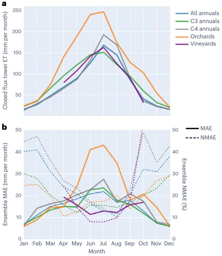
Performance among annual and perennial crops
| Land cover type | Statistic | Ensemble | DisALEXI | eeMETRIC | geeSEBAL | PT-JPL | SIMS | SSEBop |
|
|
| Bsk + Bsh (cold and hot semi-arid steppe), mean station ET of 133 (mm per month) | Slope | 0.9 | 0.85 | 0.91 | 0.82 | 0.88 | 0.97 | 1 | 11 | 246 |
| MBE (mm) | -6.94 (-5.2%) | -15.17 (-11.4%) | -4.65 (-3.5%) | -18.09 (-13.6%) | -7.55 (-5.7%) | 2.71 (2.0%) | 2.89 (2.2%) | 11 | 246 | |
| MAE (mm) | 20.74 (15.6%) | 26.93 (20.3%) | 26.94 (20.3%) | 30.31 (22.8%) | 25.7 (19.3%) | 22.99 (17.3%) | 24.23 (18.2%) | 11 | 246 | |
| RMSE (mm) | 26.38 (19.8%) | 34.55 (26.0%) | 33.4 (25.1%) | 38.0 (28.6%) | 32.49 (24.4%) | 28.97 (21.8%) | 30.99 (23.3%) | 11 | 246 | |
|
|
0.89 | 0.81 | 0.8 | 0.8 | 0.84 | 0.84 | 0.84 | 11 | 246 | |
| Bwh + Bwk (hot and cold desert), mean station ET of 110 (mm per month) | Slope | 0.91 | 0.85 | 1.02 | 0.92 | 0.86 | 0.92 | 0.88 | 10 | 53 |
| MBE (mm) | -6.78 (-6.1%) | -15.63 (-14.2%) | 9.63 (8.7%) | -8.19 (-7.4%) | -7.77 (-7.0%) | -3.2 (-2.9%) | -12.34 (-11.2%) | 7 | 49 | |
| MAE (mm) | 13.24 (12.0%) | 21.21 (19.2%) | 18.92 (17.1%) | 19.13 (17.3%) | 19.21 (17.4%) | 13.62 (12.3%) | 19.59 (17.8%) | 7 | 49 | |
| RMSE (mm) | 17.02 (15.4%) | 25.78 (23.4%) | 23.92 (21.7%) | 23.51 (21.3%) | 23.81 (21.6%) | 16.07 (14.6%) | 22.95 (20.8%) | 7 | 49 | |
|
|
0.91 | 0.85 | 0.88 | 0.87 | 0.83 | 0.94 | 0.89 | 10 | 53 | |
| Cfa (humid subtropical), mean station ET of 75 (mm per month) | Slope | 1 | 1.03 | 1.03 | 0.99 | 0.93 | 1.15 | 0.91 | 11 | 232 |
| MBE (mm) | 2.15 (2.9%) | 4.49 (6.0%) | 3.65 (4.9%) | 0.97 (1.3%) | -0.88 (-1.2%) | 14.98 (19.9%) | -3.84 (-5.1%) | 8 | 228 | |
| MAE (mm) | 17.51 (23.3%) | 20.17 (26.8%) | 24.01 (31.9%) | 20.06 (26.7%) | 17.79 (23.6%) | 22.71 (30.2%) | 21.97 (29.2%) | 8 | 228 | |
| RMSE (mm) | 23.76 (31.6%) | 26.18 (34.8%) | 31.88 (42.4%) | 28.39 (37.7%) | 23.62 (31.4%) | 30.23 (40.2%) | 28.76 (38.2%) | 8 | 228 | |
|
|
0.75 | 0.72 | 0.62 | 0.69 | 0.76 | 0.72 | 0.64 | 11 | 232 | |
| Csa + Csb (hot- and warm-summer Mediterranean), mean station ET of 94 (mm per month) | Slope | 0.95 | 0.96 | 0.99 | 0.81 | 1.01 | 0.93 | 0.99 | 8 | 292 |
| MBE (mm) | -4.37 (-4.7%) | -6.32 (-6.7%) | -1.72 (-1.8%) | -20.92 (-22.3%) | 7.37 (7.9%) | -1.34 (-1.4%) | -2.9 (-3.1%) | 8 | 292 | |
| MAE (mm) | 13.32 (14.2%) | 18.65 (19.9%) | 17.14 (18.3%) | 25.9 (27.6%) | 17.17 (18.3%) | 14.04 (15.0%) | 23.94 (25.6%) | 8 | 292 | |
| RMSE (mm) | 16.52 (17.6%) | 22.75 (24.3%) | 21.48 (22.9%) | 31.31 (33.4%) | 21.97 (23.5%) | 18.27 (19.5%) | 27.92 (29.8%) | 8 | 292 | |
|
|
0.93 | 0.87 | 0.88 | 0.85 | 0.87 | 0.88 | 0.84 | 8 | 292 | |
| Dfa + Dfb (hot- and warm-summer humid continental), mean station ET of 67 (mm per month) | Slope | 0.9 | 0.93 | 0.94 | 0.86 | 0.87 | 1.02 | 0.9 | 13 | 829 |
| MBE (mm) | -8.0 (-11.9%) | -8.07 (-12.0%) | -6.74 (-10.0%) | -10.55 (-15.7%) | -5.72 (-8.5%) | 4.88 (7.3%) | -13.58 (-20.2%) | 10 | 823 | |
| MAE (mm) | 13.8 (20.5%) | 15.68 (23.3%) | 18.93 (28.2%) | 17.88 (26.6%) | 13.67 (20.3%) | 15.35 (22.8%) | 21.09 (31.4%) | 10 | 823 | |
| RMSE (mm) | 17.85 (26.6%) | 20.36 (30.3%) | 24.1 (35.8%) | 23.36 (34.7%) | 18.89 (28.1%) | 19.94 (29.7%) | 25.9 (38.5%) | 10 | 823 | |
|
|
0.91 | 0.9 | 0.83 | 0.86 | 0.89 | 0.86 | 0.86 | 13 | 829 |
weighted mean closed flux tower ET.strongly clumped canopies, particularly for models that are strongly dependent on LST inputs. The ensemble value had a negative bias with mean slope of
Variation of model performance across climate regions
Performance in natural ecosystems
is currently not designed for and implemented in non-agricultural land-cover types; for these pixels, the ensemble consists of five models with the possibility of removing a single outlier (Methods). Systematic model error and variability for non-agricultural sites was higher than cropland sites (Fig. 5).
Ensemble outlier removal and spatial inter-model variability
Discussion
Conclusions
potential users of OpenET due to the high rigour and transparency of methods that were employed.
Methods
Flux data processing and footprint sampling
instrumented sites, which measure ET in predominantly phreatophyte shrublands in Nevada
Model data
(1) daily ET from eeMETRIC, SIMS and SSEBop for sites outside of California was calculated by first multiplying the sampled daily EToF pixels produced by the models in the footprint by each daily flux footprint weight to obtain daily weighted EToF pixels, and summing all daily weighted EToF pixels to obtain mean daily weighted EToF, normalizing the mean daily weighted EToF by the sum of weights to account for times when the sum of weights did not equal 1 (for example, caused by cloud masking of pixels), and then multiplying the mean daily weighted EToF by the mean daily bias corrected gridMET ETo (replaced for sites within California using the daily CIMIS ETo);
(2) daily ET from PT-JPL, geeSEBAL and ALEXI/DisALEXI for all sites was calculated by multiplying the daily ET pixels by the daily flux footprint weights to obtain daily weighted ET pixels, summing all daily weighted ET pixels to obtain mean daily weighted ET, and then normalizing the mean daily weighted ET by the sum of weights, and
(3) monthly ET from all RSET models for sites outside of California was calculated by first multiplying the monthly EToF pixels by
the monthly flux footprint weights to obtain monthly weighted EToF pixels, summing all monthly weighted EToF pixels to obtain mean monthly weighted EToF, normalizing the mean monthly weighted EToF by the sum of weights, and then multiplying the mean monthly weighted EToF by the mean monthly bias-corrected gridMET ETo (replaced for sites within California using the monthly CIMIS ETo).
Ensemble computation
Statistical analyses
of paired observations was always the same among models for all statistical analyses.
Reporting summary
Data availability
during the current study are available in the Zenodo repository, with identifier https://doi.org/10.5281/zenodo.10119477.
Code availability
References
- Fisher, J. B. et al. The future of evapotranspiration: global requirements for ecosystem functioning, carbon and climate feedbacks, agricultural management, and water resources. Water Resour. Res. 53, 2618-2626 (2017).
- Dieter, C. A. et al. Estimated use of water in the United States in 2015. Circular 1411 https://pubs.usgs.gov/publication/cir1441 (2018).
- Cook, B. I., Ault, T. R. & Smerdon, J. E. Unprecedented 21st century drought risk in the American Southwest and Central Plains. Sci. Adv. 1, e1400082 (2015).
- Liu, P.-W. et al. Groundwater depletion in California’s Central Valley accelerates during megadrought. Nat. Commun. 13, 7825 (2022).
- Melton, F. S. et al. OpenET: filling a critical data gap in water management for the western United States. J. Am. Water Resour. Assoc. 58, 971-994 (2022).
- Chen, J. M. & Liu, J. Evolution of evapotranspiration models using thermal and shortwave remote sensing data. Remote Sens. Environ. 237, 111594 (2020).
- Anderson, M. et al. Field-scale assessment of land and water use change over the California Delta using remote sensing. Remote Sens. 10, 889 (2018).
- Allen, R. G., Tasumi, M. & Trezza, R. Satellite-based energy balance for mapping evapotranspiration with internalized calibration (METRIC)-Model. J. Irrig. Drain. Eng. 133, 380-394 (2007).
- Laipelt, L. et al. Long-term monitoring of evapotranspiration using the SEBAL algorithm and Google Earth Engine cloud computing. ISPRS J. Photogramm. Remote Sens. 178, 81-96 (2021).
- Fisher, J. B., Tu, K. P. & Baldocchi, D. D. Global estimates of the land-atmosphere water flux based on monthly AVHRR and ISLSCP-II data, validated at 16 FLUXNET sites. Remote Sens. Environ. 112, 901-919 (2008).
- Pereira, L. S. et al. Prediction of crop coefficients from fraction of ground cover and height. Background and validation using ground and remote sensing data. Agric. Water Manag. 241, 106197 (2020).
- Melton, F. S. et al. Satellite irrigation management support with the terrestrial observation and prediction system: a framework for integration of satellite and surface observations to support improvements in agricultural water resource management. IEEE J. Sel. Top. Appl. Earth Obs. Remote Sens. 5, 1709-1721 (2012).
- Senay, G. B. et al. Improving the operational simplified surface energy balance evapotranspiration model using the forcing and normalizing operation. Remote Sens. 15, 260 (2023).
- Gorelick, N. et al. Google Earth Engine: planetary-scale geospatial analysis for everyone. Remote Sens. Environ. 202, 18-27 (2017).
- Allen, R. G. et al. Satellite-based energy balance for mapping evapotranspiration with internalized calibration (METRIC)Applications. J. Irrig. Drain. Eng. 133, 395-406 (2007).
- Knipper, K. R. et al. Using high-spatiotemporal thermal satellite ET retrievals for operational water use and stress monitoring in a California vineyard. Remote Sens. 11, 2124 (2019).
- Senay, G. B., Friedrichs, M., Singh, R. K. & Velpuri, N. M. Evaluating Landsat 8 evapotranspiration for water use mapping in the Colorado River Basin. Remote Sens. Environ. 185, 171-185 (2016).
- Foster, T., Mieno, T. & Brozović, N. Satellite-based monitoring of irrigation water use: assessing measurement errors and their implications for agricultural water management policy. Water Resour. Res. 56, e2020WRO28378 (2020).
- Volk, J. M. et al. Development of a benchmark eddy flux evapotranspiration dataset for evaluation of satellite-driven evapotranspiration models over the CONUS. Agric. For. Meteorol. 331, 109307 (2023).
- Volk, J. M. et al. Post-processed data and graphical tools for a CONUS-wide eddy flux evapotranspiration dataset. Data Brief https://doi.org/10.1016/j.dib.2023.109274 (2023).
- Baldocchi, D. Measuring fluxes of trace gases and energy between ecosystems and the atmosphere-the state and future of the eddy covariance method. Glob. Change Biol. 20, 3600-3609 (2014).
- Baldocchi, D. et al. FLUXNET: a new tool to study the temporal and spatial variability of ecosystem-scale carbon dioxide, water vapor, and energy flux densities. Bull. Am. Meteorol. Soc. 82, 2415-2434 (2001).
- Hampel, F. R. The influence curve and its role in robust estimation. J. Am. Stat. Assoc. 69, 383-393 (1974).
- Leys, C., Ley, C., Klein, O., Bernard, P. & Licata, L. Detecting outliers: do not use standard deviation around the mean, use absolute deviation around the median. J. Exp. Soc. Psychol. 49, 764-766 (2013).
- Thompson, P. D. How to improve accuracy by combining independent forecasts. Mon. Weather Rev. 105, 228-229 (1977).
- Kirtman, B. P. et al. The North American multimodel ensemble: phase-1 seasonal-to-interannual prediction; phase-2 toward developing intraseasonal prediction. Bull. Am. Meteorol. Soc. 95, 585-601 (2014).
- Bai, Y. et al. On the use of machine learning based ensemble approaches to improve evapotranspiration estimates from croplands across a wide environmental gradient. Agric. For. Meteorol. 298, 108308 (2021).
- Novick, K. A. et al. The AmeriFlux network: a coalition of the willing. Agric. For. Meteorol. 249, 444-456 (2018).
- Pastorello, G. et al. The FLUXNET2O15 dataset and the ONEFlux processing pipeline for eddy covariance data. Sci. Data 7, 1-27 (2020).
- Mauder, M., Foken, T. & Cuxart, J. Surface-energy-balance closure over land: a review. Bound. Layer Meteorol. 177, 395-426 (2020).
- Ingwersen, J., Imukova, K., Högy, P. & Streck, T. On the use of the post-closure methods uncertainty band to evaluate the performance of land surface models against eddy covariance flux data. Biogeosciences 12, 2311-2326 (2015).
- Knipper, K. R. et al. Evapotranspiration estimates derived using thermal-based satellite remote sensing and data fusion for irrigation management in California vineyards. Irrig. Sci. 37, 431-449 (2019).
- Bambach, N. et al. Evapotranspiration uncertainty at micrometeorological scales: the impact of the eddy covariance energy imbalance and correction methods. Irrig. Sci. 40, 445-461 (2022).
- Rubel, F., Brugger, K., Haslinger, K. & Auer, I. The climate of the European Alps: shift of very high resolution Köppen-Geiger climate zones 1800-2100. Meteorol. Z. 26, 115-125 (2017).
- Yang, Y. et al. Studying drought-induced forest mortality using high spatiotemporal resolution evapotranspiration data from thermal satellite imaging. Remote Sens. Environ. 265, 112640 (2021).
- Isaacson, B. N., Yang, Y., Anderson, M. C., Clark, K. L. & Grabosky, J. C. The effects of forest composition and management on evapotranspiration in the New Jersey pinelands. Agric. For. Meteorol. 339, 109588 (2023).
- Qian, Y. et al. Neglecting irrigation contributes to the simulated summertime warm-and-dry bias in the central United States. Npj Clim. Atmos. Sci. 3, 31 (2020).
- Lei, F., Crow, W. T., Holmes, T. R., Hain, C. & Anderson, M. C. Global investigation of soil moisture and latent heat flux coupling strength. Water Resour. Res. 54, 8196-8215 (2018).
- Dong, J., Lei, F. & Crow, W. T. Land transpiration-evaporation partitioning errors responsible for modeled summertime warm bias in the central United States. Nat. Commun. 13, 336 (2022).
- Abolafia-Rosenzweig, R., Pan, M., Zeng, J. & Livneh, B. Remotely sensed ensembles of the terrestrial water budget over major global river basins: an assessment of three closure techniques. Remote Sens. Environ. 252, 112191 (2021).
- Wang, Q. et al. Land surface models significantly underestimate the impact of land-use changes on global evapotranspiration. Environ. Res. Lett. 16, 124047 (2021).
- Allen, R. G., Pereira, L. S., Howell, T. A. & Jensen, M. E. Evapotranspiration information reporting: I. Factors governing measurement accuracy. Agric. Water Manag. 98, 899-920 (2011).
- Adu, M. O., Yawson, D. O., Armah, F. A., Asare, P. A. & Frimpong, K. A. Meta-analysis of crop yields of full, deficit, and partial root-zone drying irrigation. Agric. Water Manag. 197, 79-90 (2018).
- Xue, J. et al. Improving the spatiotemporal resolution of remotely sensed ET information for water management through Landsat, Sentinel-2, ECOSTRESS and VIIRS data fusion. Irrig. Sci. 40, 609-634 (2022).
- Gao, F. & Zhang, X. Mapping crop phenology in near real-time using satellite remote sensing: challenges and opportunities. J. Remote Sens. 2021, 8379391 (2021).
- Müller, M. Dynamic time warping. in Information Retrieval for Music and Motion. 69-84 (Springer, 2007).
- Bambach, N. et al. The Tree-crop Remote sensing of Evapotranspiration eXperiment (T-REX): a science-based path for sustainable water management and climate mitigation. Bull. Am. Meteorol. Soc. In the press (2023).
- Fisher, J. B. Hydrosat: towards daily, field-scale, global evapotranspiration from space. (2022).
- Polhamus, A., Fisher, J. B. & Tu, K. P. What controls the error structure in evapotranspiration models? Agric. For. Meteorol. 169, 12-24 (2013).
- Blankenau, P. A., Kilic, A. & Allen, R. An evaluation of gridded weather data sets for the purpose of estimating reference evapotranspiration in the United States. Agric. Water Manag. 242, 106376 (2020).
- Doherty, C. T. et al. Effects of meteorological and land surface modeling uncertainty on errors in winegrape ET calculated with SIMS. Irrig. Sci. 40, 515-530 (2022).
- Purdy, A., Fisher, J., Goulden, M. & Famiglietti, J. Ground heat flux: an analytical review of 6 models evaluated at 88 sites and globally. J. Geophys. Res. Biogeosci. 121, 3045-3059 (2016).
- Allen, R. G. et al. A recommendation on standardized surface resistance for hourly calculation of reference ETo by the FAO56 Penman-Monteith method. Agric. Water Manag. 81, 1-22 (2006).
- Jung, M. et al. The FLUXCOM ensemble of global landatmosphere energy fluxes. Sci. Data 6, 74 (2019).
- Reitz, M., Senay, G. B. & Sanford, W. E. Combining remote sensing and water-balance evapotranspiration estimates for the conterminous United States. Remote Sens. 9, 1181 (2017).
- Volk, J. et al. flux-data-qaqc: a Python package for energy balance closure and post-processing of eddy flux. Data. 6, 1-5 (2021).
- Evett, S. R. et al. The Bushland weighing lysimeters: a quarter century of crop ET investigations to advance sustainable irrigation. Trans. ASABE 59, 163-179 (2016).
- Abatzoglou, J. T. Development of gridded surface meteorological data for ecological applications and modelling. Int. J. Climatol. 33, 121-131 (2013).
- Kljun, N., Calanca, P., Rotach, M. W. & Schmid, H. P. A simple twodimensional parameterisation for Flux Footprint Prediction (FFP). Geosci. Model Dev. 8, 3695-3713 (2015).
- Xia, Y. et al. Continental-scale water and energy flux analysis and validation for the North American Land Data Assimilation System project phase 2 (NLDAS-2): 1. Intercomparison and application of model products. J. Geophys. Res. Atmos. 117, DO31O9 (2012).
- Foga, S. et al. Cloud detection algorithm comparison and validation for operational Landsat data products. Remote Sens. Environ. 194, 379-390 (2017).
- Rousseeuw, P. J. & Croux, C. Alternatives to the median absolute deviation. J. Am. Stat. Assoc. 88, 1273-1283 (1993).
- Harris, C. R. et al. Array programming with NumPy. Nature 585, 357-362 (2020).
- Seabold, S. & Perktold, J. Statsmodels: econometric and statistical modeling with Python. In Proc. 9th Python in Science Conference vol. 57 10-25080 (SciPy, 2010).
- Obrecht, N. A. Sample size weighting follows a curvilinear function. J. Exp. Psychol. Learn. Mem. Cogn. 45, 614 (2019).
Acknowledgements
https://doi.org/10.17190/AMF/1246070, https://doi.org/10.17190/ AMF/1660346, https://doi.org/10.17190/AMF/1246074, https://doi. org/10.17190/AMF/1246076, https://doi.org/10.17190/AMF/1246079, https://doi.org/10.17190/AMF/1246128, https://doi.org/10.17190/ AMF/1617715, https://doi.org/10.17190/AMF/1617716, https://doi. org/10.17190/AMF/1246080, https://doi.org/10.17190/AMF/1246081, https://doi.org/10.17190/AMF/1246083, https://doi.org/10.17190/ AMF/1419506, https://doi.org/10.17190/AMF/1480314, https://doi. org/10.17190/AMF/1246084, https://doi.org/10.17190/AMF/1246085, https://doi.org/10.17190/AMF/1246086, https://doi.org/10.17190/ AMF/1246088, https://doi.org/10.17190/AMF/1246089, https://doi. org/10.17190/AMF/1246092, https://doi.org/10.17190/AMF/1418683, https://doi.org/10.17190/AMF/1246093, https://doi.org/10.17190/ AMF/1419507, https://doi.org/10.17190/AMF/1419508, https://doi. org/10.17190/AMF/1419509, https://doi.org/10.17190/AMF/1617721, https://doi.org/10.17190/AMF/1617724, https://doi.org/10.17190/ AMF/1375201, https://doi.org/10.17190/AMF/1419502, https://doi. org/10.17190/AMF/1419501, https://doi.org/10.17190/AMF/1419504, https://doi.org/10.17190/AMF/1246136, https://doi.org/10.17190/ AMF/1246105, https://doi.org/10.17190/AMF/1246096, https://doi. org/10.17190/AMF/1418684, https://doi.org/10.17190/AMF/1246097, https://doi.org/10.17190/AMF/1246098, https://doi.org/10.17190/ AMF/1246099, https://doi.org/10.17190/AMF/1246101, https://doi. org/10.17190/AMF/1246102, https://doi.org/10.17190/AMF/1246127, https://doi.org/10.17190/AMF/1246154, https://doi.org/10.17190/ AMF/1246104, https://doi.org/10.17190/AMF/1418685, https://doi. org/10.17190/AMF/1660351, https://doi.org/10.17190/AMF/1246148, https://doi.org/10.17190/AMF/1246149, https://doi.org/10.17190/ AMF/1246140, https://doi.org/10.17190/AMF/1245984, https://doi. org/10.17190/AMF/1246109, https://doi.org/10.17190/AMF/1246111, https://doi.org/10.17190/AMF/1246112, https://doi.org/10.17190/ AMF/1617728, https://doi.org/10.17190/AMF/1579721, https://doi. org/10.17190/AMF/1617732, https://doi.org/10.17190/AMF/1579723, https://doi.org/10.17190/AMF/1617735, https://doi.org/10.17190/ AMF/1617737, https://doi.org/10.17190/AMF/1617741, https://doi. org/10.3133/sir20095079, https://doi.org/10.3133/sir20095079, https://doi.org/10.3133/sir20055288, https://doi.org/10.3133/ sir20055288, https://doi.org/10.3133/sir20085116, https://doi. org/10.3133/sir20095079, https://doi.org/10.3133/sir20085116, https:// doi.org/10.5066/F7R49NZN, https://doi.org/10.5066/F7R49NZN, https://doi.org/10.5066/F79C6WM9, https://doi.org/10.5066/ F79C6WM9, https://doi.org/10.3133/pp1805, https://doi.org/10.5066/ P9NZ9XSP, https://doi.org/10.5066/P9NZ9XSP, https://doi. org/10.5066/P9NZ9XSP, https://doi.org/10.3133/sir20075078, https:// doi.org/10.3133/sir20075078, https://doi.org/10.3133/sir20085116, https://doi.org/10.3133/sir20075078 and https://doi.org/10.3133/ sir20075078. Funding for AmeriFlux data resources was provided by the US Department of Energy Office of Science. Any use of trade, firm or product names is for descriptive purposes only and does not imply endorsement by the US Government.
Author contributions
Competing interests
Additional information
https://doi.org/10.1038/s44221-023-00181-7.
Supplementary information The online version contains supplementary material available at https://doi.org/10.1038/s44221-023-00181-7.
Evergreen Forests
and closed labels refer to flux tower ET before and after energy balance closure correction. Dashed lines represent the closed flux ET mean plus two standard errors of the mean and unclosed flux ET mean minus two standard errors of the mean.
Mixed Forests
and closed labels refer to flux tower ET before and after energy balance closure correction. Dashed lines represent the closed flux ET mean plus two standard errors of the mean and unclosed flux ET mean minus two standard errors of the mean.
Grasslands
ET for grassland sites. Subplot (a) shows monthly climatology of paired OpenET
and closed labels refer to flux tower ET before and after energy balance closure correction. Dashed lines represent the closed flux ET mean plus two standard errors of the mean and unclosed flux ET mean minus two standard errors of the mean.
Shrublands
ET for shrubland sites. Subplot (a) shows monthly climatology of paired OpenET
and closed labels refer to flux tower ET before and after energy balance closure correction. Dashed lines represent the closed flux ET mean plus two standard errors of the mean and unclosed flux ET mean minus two standard errors of the mean.
Wetland/Riparian
|
|
Ensemble |
| DisALEXI | eeMETRIC |
| geeSEBAL | |
| PT-JPL | |
| – | SSEBop |
| – | Closed + 2SE |
| – | Closed |
| – | Unclosed |
| – – Unclosed – 2SE |
Month
was used to build the map. Subplot (b) shows the average count of models used in the ensemble after outlier removal using all growing season monthly data for cropland pixels. A value of six indicates that no model was identified as an outlier, while four is the lower limit where a maximum of two models were removed as outliers before taking the ensemble mean.
model minus the ensemble mean using all monthly data from all pixels that were classified as croplands for each year from 2016-2022. See Supplementary Discussion 4 for a discussion of the Landsat striping exhibited by geeSEBAL.
natureportfolio
John Volk
Last updated by author(s): Nov 27, 2023
Reporting Summary
Statistics
Confirmed
Only common tests should be described solely by name; describe more complex techniques in the Methods section.
Our web collection on statistics for biologists contains articles on many of the points above.
Software and code
Policy information about availability of computer code
The in situ measured evapotranspiration data analysed during the current study were processed using the “flux-data-qaqc” Python package, version 0.1.6 (https://github.com/Open-ET/flux-data-qaqc).
The “flux-data-footprint” Python package was used to generate temporally dynamic flux footprints for sampling of of daily and monthly model ET data (https://github.com/Open-ET/flux-data-footprint). The Numpy (version 1.17.2) and statsmodels (version 0.12.1) Python packages were used for data analyses during the current study.
Data
All manuscripts must include a data availability statement. This statement should provide the following information, where applicable:
- Accession codes, unique identifiers, or web links for publicly available datasets
- A description of any restrictions on data availability
- For clinical datasets or third party data, please ensure that the statement adheres to our policy
Human research participants
| Reporting on sex and gender | The current study did not involve human participants, their data, or their biological material. |
| Population characteristics | The current study did not involve human participants, their data, or their biological material. |
| Recruitment | The current study did not involve human participants, their data, or their biological material. |
| Ethics oversight | The current study did not involve human participants, their data, or their biological material. |
Field-specific reporting
Life sciences Behavioural & social sciences
Ecological, evolutionary & environmental sciences
For a reference copy of the document with all sections, see nature.com/documents/nr-reporting-summary-flat.pdf
Ecological, evolutionary & environmental sciences study design
| Study description | The current study is focused on one-to-one comparisons between evapotranspiration data as modeled by remote-sensing methods and as measured on the ground; well known goodness-of-fit metrics were used to evaluate model data against measured data. Modeled and measured data were paired based on temporally overlapping records at multiple measurement stations. Accuracy metric results were grouped by different shared characteristics of the stations, using weighted averaging. Spatial long-term model data were mapped for individual models and differenced from the model ensemble average. |
| Research sample | The measured daily and monthly evapotranspiration data in the current study came from a public dataset that is available here: http://dx.doi.org/10.5281/zenodo.7636781. The measurements used were collected between 1995-2021. OpenET model data were generated and paired to the daily and monthly measurements, however model data was not available prior to 2001. The total number of stations with paired data was 152, and among them there were 16,444 days and 4,107 months of paired data. |
| Sampling strategy | As a conservative measure, we required a minimum of 3 months of paired data per measurement station to be included in weighted average accuracy metrics. In order to avoid skewing grouped average metrics, we weighted each station by the square root of the number of paired data. |
| Data collection | Measured ET data was previously curated and publicly archived on Zenodo (http://dx.doi.org/10.5281/zenodo.7636781). Model ET data was generated for the study using the current OpenET version. |
| Timing and spatial scale | Measured data was collected primarily from eddy covariance systems and post-processed to daily and monthly aggregated periods. Model ET was sampled at daily (the dates of satellite overpass) and monthly intervals at the measurement stations using pixel footprints which were determined by either long-term wind direction or from a physically based flux footprint prediction model. Flux footprints rarely exceeded the size of a
|
| Data exclusions | No data available to us were excluded from the analyses during the current study. |
| Reproducibility | Data processing steps for both modeled and measured data used in the current study were made reproducible by our use of well-documented open source software. We developed Python code for eddy covariance data processing and footprint development. Similarly, the OpenET modeled data was generated using the operational models which are open source and their data are also publicly available through various mechanisms including the OpenET API and the Google Earth Engine Data Catalog. The statistical methods used in the study were limited to simple techniques, and the results were independently tested by multiple members of the OpenET group using different statistical packages such as Python and Microsoft Excel. |
| Randomization | Randomization of data into groups was not applicable as groups were defined by biophysical characteristics such as climate and land cover type. |
| Blinding | This study did not employ blinding of data due to the limited amount of high quality measured evapotranspiration data available to us. However, additional data that has not yet been compared against OpenET models was held out of this study for a future blind intercomparison and accuracy assessment of OpenET. |
Reporting for specific materials, systems and methods
| Materials & experimental systems | Methods | ||
| n/a | Involved in the study | n/a | Involved in the study |
|
Antibodies | |
ChIP-seq |
|
|
||
|
Palaeontology and archaeology | |
|
|
|||
|
|
||
|
|
||
- The in situ measured evapotranspiration data analysed during the current study are available in the Zenodo repository, with identifier http://dx.doi.org/10.5281/