DOI: https://doi.org/10.1038/s41598-025-91329-w
PMID: https://pubmed.ncbi.nlm.nih.gov/40000767
تاريخ النشر: 2025-02-25
تقارير علمية
افتح
تقييم فعالية الذاكرة طويلة وقصيرة المدى والشبكة العصبية الاصطناعية في التنبؤ بتركيزات الأوزون اليومية في مدينة لياوتشينغ
الملخص
تؤثر تلوث الأوزون على إنتاج الغذاء وصحة الإنسان وحياة الأفراد. بسبب التصنيع السريع والتحضر، شهدت لياوتشينغ زيادة في تركيز الأوزون على مدى عدة سنوات. لذلك، أصبح الأوزون مشكلة بيئية رئيسية في مدينة لياوتشينغ. تم إنشاء نماذج الذاكرة طويلة الأمد (LSTM) والشبكة العصبية الاصطناعية (ANN) للتنبؤ بتركيزات الأوزون في مدينة لياوتشينغ من 2014 إلى 2023. تظهر النتائج تحسنًا عامًا في دقة نموذج LSTM مقارنة بنموذج ANN. مقارنةً بـ ANN، شهد نموذج LSTM زيادة في معامل التحديد.
تؤثر تلوث الهواء على تغير المناخ وإنتاج الغذاء وحياة الإنسان
الأعمال ذات الصلة
توقع تركيزات الأوزون بدقة، مع أداء قوي (مؤشر الاتفاق (IOA) أكبر من 0.85 لـ 19 من 21 محطة)
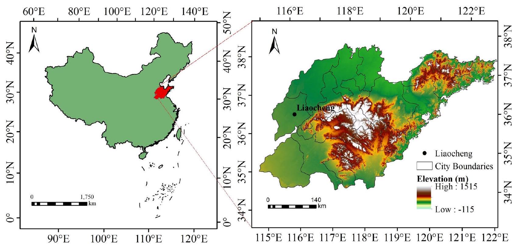
منطقة الدراسة والبيانات
منطقة الدراسة
بيانات
المنهجية
الشبكة العصبية الاصطناعية (ANN)
معدل التعلم، الزخم التكيفي، الانتشار العكسي المرن، كوازى-نيوتن، التدرج المترافق، والتقنين البايزي. نقارن 13 خوارزمية تدريب رئيسية لتحسين أداء الشبكات العصبية الاصطناعية، تحديدًا من حيث الدقة في الجدول 1. يتم تحديد أفضل خوارزمية تدريب من خلال نهج التجربة والخطأ.
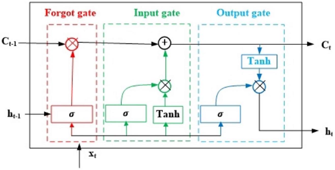
ذاكرة طويلة قصيرة المدى (LSTM)
| وظائف التدريب | خوارزمية التدريب | فئة |
| ترينبر | الانتشار العكسي مع تنظيم بايزي (BR) | التنظيم البايزي |
| تدريب | خوارزمية ليفنبرغ-ماركوات (LM) للتراجع العكسي | كوازى-نيوتن |
| تراينغديكس | انحدار التدرج مع الزخم ومعدل التعلم التكيفي في الانتشار العكسي (GDX) | معدل التعلم الذاتي التكيف |
| تدريب | الانحدار التدرجي عبر الانتشار العكسي (GD) | الزخم التكيفي |
| ترينغدم | انحدار التدرج مع دالة الزخم (GDM) | الزخم التكيفي |
| ترينغدا | انحدار التدرج مع معدل تعلم تكيفي (GDA) | معدل تعلم ذاتي التكيف |
| تدريب | الانتشار العكسي المرن (RP) | الانتشار العكسي المرن |
| ترين سي جي بي | الانتشار العكسي بتدرج مترافق مع تحديثات بولاك-ريبيير (CGP) | خوارزميات التدرج المترافق |
| تدريب | الانتشار العكسي باستخدام تدرج مترافق مع فليتشر-ريفز (CGF) | التدرج المترافق |
| ترين سي جي بي | الانتشار العكسي بتدرج مترافق مع إعادة تشغيل باول-بييل (CGB) | التدرج المترافق |
| تدريب | الانتشار العكسي بتدرج مترافق مقاس (SCG) | خوارزميات التدرج المترافق |
| تدريب بي إف جي | الانتشار العكسي بطريقة BFGS كوانتي-نيوتن (BFGS) | كوازى-نيوتن |
| ترينوس | الانتشار العكسي باستخدام القاطع بخطوة واحدة (OSS) | كوازى-نيوتن |
التطبيع
معايير الأداء
التحقق المتقاطع
النتائج
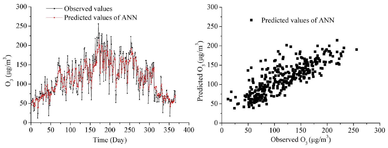
تحليل نتائج التنبؤ للشبكة العصبية الاصطناعية
| أيام |
|
جذر متوسط مربع الخطأ (RMSE)
|
ماي
|
||||||
| تدريب | التحقق | التنبؤ | تدريب | التحقق | التنبؤ | تدريب | التحقق | التنبؤ | |
| 1 | 0.7199 | 0.6704 | 0.6746 | 28.9068 | ٢٨.٧٥١٦ | ٢٨.٤٧٥٣ | ٢٢.١١١٢ | ٢٢.٧٢٥٠ | 21.7433 |
| 2 | 0.7194 | 0.6699 | 0.6767 | 30.2199 | 30.1252 | 30.1126 | 23.0106 | ٢٣.٦٧٢٥ | ٢٤٫٠٩٠٥ |
| ٣ | 0.7201 | 0.6708 | 0.6752 | ٢٩.٠٣٩٤ | ٢٨.٨٨٠٩ | ٢٨.٧٦٢٠ | 22.2106 | ٢٢.٦٤٨١ | ٢٢٫٦٠٨٦ |
| ٤ | 0.7194 | 0.6688 | 0.6738 | 30.5321 | 30.5937 | 30.3191 | ٢٣.٣١٠١ | ٢٣.٥٠٥٧ | ٢٢.١٧٧٠ |
| ٥ | 0.7202 | 0.6681 | 0.6742 | ٢٩.٢٣٧٢ | ٢٩.٢٤٦١ | ٢٩.٠٢٧٩ | 22.3948 | ٢٣.٠٤٧٥ | 22.8921 |
| ٦ | 0.7207 | 0.6636 | 0.6743 | ٢٩.٥٨٧٤ | ٢٩.٦٧٢٠ | ٢٩.٠٦١٠ | 23.2021 | ٢٣.٧٦٥٦ | 23.0427 |
| ٧ | 0.7185 | 0.6740 | 0.6679 | ٢٩.٢٩٧٩ | ٢٩.٦٢٣٧ | ٢٩.٢٥٦٨ | 22.3965 | ٢٣٫٢٤٥٧ | ٢٣.١٨٢٥ |
| ٨ | 0.7209 | 0.6753 | 0.6726 | ٢٩.٠٥٢١ | ٢٩.٠٧٨٩ | ٢٨.٨٢٤٨ | 22.2262 | 22.3580 | 21.7427 |
| 9 | 0.7217 | 0.6752 | 0.6759 | ٢٨.٥٥٠٥ | ٢٨.٥٤٠٩ | ٢٨.٠٢٦٩ | 21.8588 | ٢٢.٩٥٧٧ | 21.7169 |
| 10 | 0.7206 | 0.6750 | 0.6733 | ٢٨.٥٢٧٣ | ٢٨.٦٣٢٧ | ٢٨.٢٨١١ | 21.8717 | 22.3195 | ٢١.٧١١٩ |
| 11 | 0.7213 | 0.6751 | 0.6705 | ٢٨.٥٤٥٦ | ٢٨.٥٦٧٤ | ٢٨.٣٤٥٣ | 21.8699 | 21.9867 | 21.7381 |
| 12 | 0.7340 | 0.6714 | 0.6698 | ٢٩.٦٩٩٠ | 30.1861 | ٢٩.٥٠٦٨ | ٢٢.٦٥٠٤ | 22.8725 | 21.9138 |
| ١٣ | 0.7338 | 0.6767 | 0.6759 | ٢٨.٥٤٣١ | ٢٨.٥٩٨٨ | ٢٨.١١٦٢ | 21.8645 | 21.9931 | 21.7150 |
| 14 | 0.7322 | 0.6792 | 0.6721 | ٢٨.٩٥٠٤ | ٢٨.٨٦٩٧ | ٢٨.٤٧٣٧ | 22.0829 | ٢٢.٦٣١٦ | 22.3236 |
| 15 | 0.7357 | 0.6800 | 0.6722 | ٢٨.٥٧٠٢ | ٢٨.٦٢٥٨ | ٢٨.٣٧٨٣ | ٢١.٧٨٦٧ | 22.3737 | ٢٢.٠٥٥٨ |
| 16 | 0.7344 | 0.6675 | 0.6647 | ٢٨.٧٥٠٥ | ٢٩.٣٣١٠ | ٢٨.٦٦٤٩ | 21.9436 | ٢٢.٦٣٤٧ | 21.8948 |
| 17 | 0.7362 | 0.6806 | 0.6714 | ٢٨.٦٥٠٤ | ٢٨.٢٣٧٨ | ٢٨.٢٣٣٧ | 21.8700 | 21.7673 | 21.7461 |
| ١٨ | 0.7365 | 0.6816 | 0.6779 | ٢٨.٥٠٩٥ | ٢٨.٥٥١٤ | ٢٧.٩٨٩٥ | ٢١.٧٦٤٩ | ٢٢.٢١٩٤ | 21.6919 |
| 19 | 0.7298 | 0.6558 | 0.6609 | ٢٩٫٠٩٠١ | ٢٩.٨٦٣٠ | 28.9438 | 22.3889 | ٢٣.٦٨١٢ | ٢٢.٩٩٧٤ |
| 20 | 0.7347 | 0.6804 | 0.6770 | 28.8931 | ٢٩.٠٥٧٥ | ٢٨.٤٣٦٥ | ٢٢.٠١٧٦ | ٢٢.٢٩٩٢ | 21.7366 |
| 21 | 0.7356 | 0.6728 | 0.6722 | 31.7804 | ٣٢.٠٩٥٦ | 31.6421 | ٢٤.٨٤١٧ | ٢٦.٠٢٤٨ | 25.9455 |
| وظائف التدريب |
|
جذر متوسط مربع الخطأ (RMSE)
|
ماي
|
||||||
| تدريب | التحقق | التنبؤ | تدريب | التحقق | التنبؤ | تدريب | التحقق | التنبؤ | |
| ترينبر | 0.7365 | 0.6816 | 0.6779 | ٢٨.٥٠٩٥ | ٢٨.٥٥١٤ | ٢٧.٩٨٩٥ | ٢١.٧٦٤٩ | ٢٢.٢١٩٤ | 21.6919 |
| تدريب | 0.7175 | 0.6695 | 0.6616 | ٢٨.٦١٥٨ | ٢٨.٧٥١٧ | 28.4215 | ٢٢.٢٦٧٦ | ٢٢.٩١٨٢ | 22.2838 |
| تراينغديكس | 0.5898 | 0.5118 | 0.4879 | ٤٥٫٠٨٨٥ | 41.8351 | 41.8636 | 37.7704 | ٣٤.٦٥٩٨ | ٣٥.٠٦٩١ |
| تدريب | 0.6393 | 0.5572 | 0.5163 | 51.6911 | ٤٧.٦٢٥٢ | ٤٧.٤٩٥٣ | ٤٣.٣٠٣٩ | ٣٩.٠٦٨٤ | ٣٩.٥٣٨١ |
| ترينغدم | 0.6970 | 0.6258 | 0.5978 | 30.5444 | 30.9063 | ٣١.١٩٧٧ | ٢٣.٣٨٠٧ | ٢٤.١٣٢٣ | ٢٤.٦٣٨٣ |
| ترينغدا | 0.6970 | 0.6258 | 0.5978 | 30.5444 | 30.9063 | 31.1977 | ٢٣.٣٨٠٧ | ٢٤.١٣٢٣ | ٢٤.٦٣٨٣ |
| تدريب دور | 0.7277 | 0.6709 | 0.6762 | 28.9446 | ٢٩.٠١٩٦ | ٢٨.٠٦٧٢ | ٢٢.٣٠٠٠ | ٢٢.٨٢٧١ | 22.1916 |
| ترين سي جي بي | 0.7243 | 0.6722 | 0.6616 | 28.8725 | ٢٨.٦٧٥٨ | ٢٨.٩٠٨٢ | ٢٢.٤٥٣٤ | ٢٢.٨٣٠٠ | ٢٢.٢٢٩٩ |
| تدريب | 0.7255 | 0.6702 | 0.6775 | ٢٨.٨٠٧٢ | ٢٨.٦٦٨١ | 28.9245 | 22.4128 | ٢٢.٩٥٧٧ | ٢٢.٢٥٨٢ |
| ترين سي جي بي | 0.7238 | 0.6734 | 0.6666 | ٢٨.٩٠١٤ | ٢٨.٧١٢١ | ٢٨.٦٨٤٣ | ٢٢.٤٩٩٤ | 22.8450 | ٢٢.٢٠٩٣ |
| تدريب | 0.7239 | 0.6678 | 0.6638 | ٢٨.٩٩٥٦ | ٢٨.٨٣٧٥ | ٢٨.٨٠٦٦ | ٢٢.٤٧٨٧ | ٢٣.٠٣٦٤ | ٢٢.١١٨٩ |
| تدريب بي إف جي | 0.7275 | 0.6698 | 0.6667 | ٢٨.٩٩٨٨ | ٢٨.٩٢٩١ | 28.6813 | ٢٢.٣٥٣٢ | 22.9733 | ٢٢٫٢٠٥٦ |
| ترينوس | 0.7219 | 0.6651 | 0.6653 | ٢٩.٣٠٩٤ | ٢٨.٩٤٩٩ | 28.7389 | ٢٢.٥٢٩٤ | ٢٣.١١٢٨ | ٢٢.٠٣٨١ |
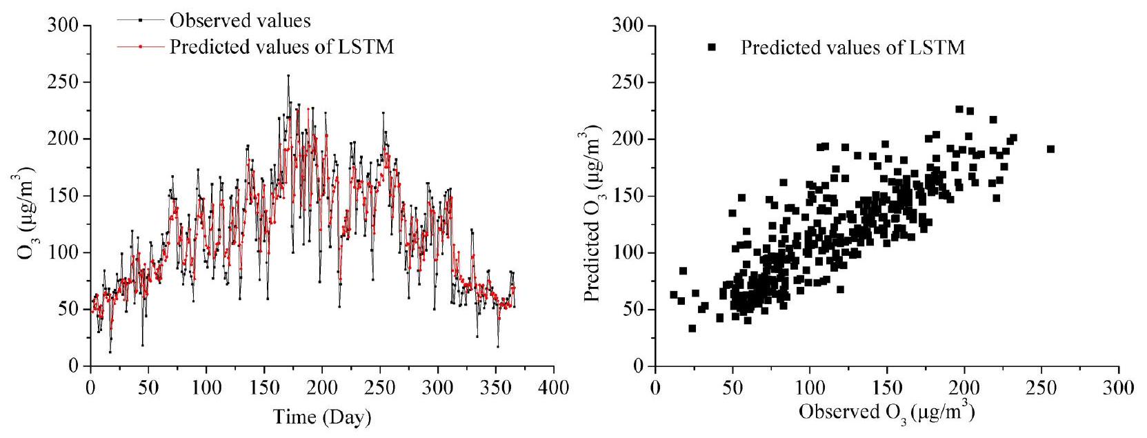
تحليل نتائج LSTM
| دالة النقل |
|
جذر متوسط مربع الخطأ | ماي | ||||||
| تدريب | التحقق | التنبؤ | تدريب | التحقق | التنبؤ | تدريب | التحقق | التنبؤ | |
| تا-بو | 0.7261 | 0.6651 | 0.6613 | ٢٩.١٠٩٨ | ٢٨.٧٥٩٧ | ٢٨.٢٦٦٦ | 21.8107 | ٢٢.٤٣٣٦ | 21.9249 |
| تا-لو | 0.7312 | 0.6666 | 0.6705 | ٢٨.٧٤٥٤ | ٢٨.٦٠٨٨ | ٢٨.٢٨٠٣ | 21.9803 | 22.4058 | ٢٢.٣٢٨٤ |
| وداعاً | 0.7240 | 0.6563 | 0.6605 | ٢٩.٢٣٣١ | ٢٩.٤٠٣٣ | ٢٨.٦٧٢٢ | 21.8764 | ٢٢.٥٢١٦ | 22.2328 |
| لو-بو | 0.7365 | 0.6816 | 0.6779 | ٢٨.٥٠٩٥ | ٢٨.٥٥١٤ | ٢٧.٩٨٩٥ | 21.7649 | ٢٢.٢١٩٤ | 21.6919 |
| لو-تا | 0.7240 | 0.6626 | 0.6605 | ٢٩.٢٣٧٥ | ٢٩.٤٢٠٩ | 28.6688 | 21.8794 | ٢٣٫٢٤٦٠ | 22.2513 |
| لو-لو | 0.7229 | 0.6612 | 0.6610 | ٢٩.٣٠٧٠ | ٢٩.٠٧٣٣ | ٢٨.٤٤٤٦ | ٢١.٩٥٠٠ | 22.8055 | 22.7744 |
| بو-تا | 0.7143 | 0.6600 | 0.6703 | ٢٩.٧٤٣٩ | ٢٨.٦١٤٦ | ٢٨.٢٨٣٨ | ٢١.٩٨٣٢ | 22.4110 | ٢٢.٣٣٦٤ |
| بيو-لو | 0.7178 | 0.6615 | 0.6605 | ٢٩.٥٩٨٠ | ٢٨.٩٢٥٨ | ٢٨.٦٧٧٧ | ٢٢.١٧٥٤ | ٢٢.٦٦٣٨ | ٢٢.٧٤٥٨ |
| بيو-بيو | 0.7216 | 0.6606 | 0.6595 | ٢٩.٣٣٤١ | ٢٩.٣٣٩٣ | ٢٨.٠٥٧٨ | ٢٢.٥٧١٨ | ٢٣.٠٩٣٦ | 22.3539 |
| تا-بو | 0.7077 | 0.6619 | 0.6607 | 29.2008 | ٢٨.٧١٨٦ | ٢٨.٥٥٥٦ | ٢٢.٨٩٥٤ | ٢٢.٥٦٦٤ | ٢٢.١٣٧٥ |
| لو-بو | 0.7195 | 0.6611 | 0.6615 | ٢٩.٤٩٣٨ | ٢٩.٠٩٤٢ | 28.1946 | ٢٢٫٠٣٨٧ | 22.8510 | 22.7705 |
| بو-بو | 0.7209 | 0.6618 | 0.6619 | ٢٩.٤١٤٠ | ٢٩.٧٩٣٧ | ٢٨.٩٨٦٨ | 22.9791 | ٢٢.٥١٤٦ | 22.7470 |
| PU-PO | 0.7166 | 0.6609 | 0.6608 | ٢٩.٧٦٨٩ | ٢٩.٢٢٥٢ | ٢٨.٥٢١١ | 22.2734 | 22.9010 | ٢٢.١٥٤٦ |
| بو-لو | 0.7169 | 0.6612 | 0.6604 | ٢٩.٦٢٠٧ | ٢٩.٠٨٢٣ | 28.6772 | ٢٢.٠٩٠١ | 22.6724 | ٢٢.٢٥٣٢ |
| بو-بو | 0.7170 | 0.6618 | 0.6610 | ٢٩.٥٤٢١ | ٢٩.٧٦١١ | ٢٨.٤٠٦٦ | ٢٢٫٠٦٤١ | ٢٢.٥٢٥١ | 22.7511 |
| بو-تا | 0.7174 | 0.6612 | 0.6619 | ٢٩.٣٥٣٢ | ٢٩.٠٨٩١ | ٢٨.٠١٢٦ | ٢٢.٠٠٨٠ | 22.7055 | ٢٢.٦٢٠٠ |
| أيام |
|
جذر متوسط مربع الخطأ (RMSE)
|
ماي
|
||||||
| تدريب | التحقق | التنبؤ | تدريب | التحقق | التنبؤ | تدريب | التحقق | التنبؤ | |
| 1 | 0.7074 | 0.6530 | 0.6535 | ٢٩٫٩٧٠١ | ٢٩.٧٨١٤ | ٢٨.٩٩٨٢ | 22.8702 | 22.8105 | ٢٢.١٦٧٣ |
| 2 | 0.7189 | 0.6545 | 0.6566 | ٢٩.٣٧٦٨ | ٢٩.٧٠١٧ | 28.8565 | 22.3821 | ٢٢.٧١٠٤ | ٢٢.٠٤٧٣ |
| ٣ | 0.7263 | 0.6705 | 0.6672 | 28.9846 | ٢٨.٩٩٠٥ | ٢٨.٣٩٠٨ | ٢٢.٠٥٤٣ | ٢٢.٢٠٤٤ | ٢١.٩٨٩٤ |
| ٤ | 0.7320 | 0.6726 | 0.6662 | ٢٨.٦٨٣٣ | ٢٨.٨٩٨٩ | ٢٨.٤٢٧١ | 21.7966 | ٢٢.٠٩٧١ | 21.7849 |
| ٥ | 0.7379 | 0.6682 | 0.6761 | ٢٨.٣٦٦٣ | ٢٩.١٠٠٨ | 27.9928 | 21.6099 | ٢٢.٣٠٥١ | ٢١.٤٣١٤ |
| ٦ | 0.7384 | 0.6705 | 0.6767 | ٢٨.٣٣٦٦ | ٢٨.٩٩٧٨ | 27.9644 | ٢١.٥٣٧٧ | 22.2521 | 21.1804 |
| ٧ | 0.7423 | 0.6694 | 0.6842 | ٢٨.١٢٦٠ | ٢٩.٠٤٣٠ | 27.6338 | ٢١.٤٢٩١ | ٢٢.٣١٣٣ | ٢١.٠٣٥٣ |
| ٨ | 0.7427 | 0.6784 | 0.6831 | ٢٨.١٠٥٦ | ٢٨.٦٤٠٨ | ٢٧.٦٨٧١ | 21.4157 | 21.9549 | 21.2736 |
| 9 | 0.7460 | 0.6815 | 0.6829 | 27.9226 | ٢٨.٥٠٩٠ | 27.7014 | 21.2723 | 21.9219 | 21.3349 |
| 10 | 0.7482 | 0.6811 | 0.6855 | 27.8022 | ٢٨.٥٣٦٤ | ٢٧.٥٨١٧ | 21.1620 | 21.9089 | 21.1191 |
| 11 | 0.7491 | 0.6840 | 0.6826 | ٢٧.٧٥٥٦ | ٢٨.٣٩٤٥ | 27.7119 | ٢١.٠٦٤٣ | 21.8384 | 21.2267 |
| 12 | 0.7484 | 0.6824 | 0.6833 | ٢٧.٧٩٠٠ | ٢٨.٤٧٠٨ | 27.6793 | ٢١.٠٩٥٦ | 21.8943 | ٢١.١٨٢٨ |
| ١٣ | 0.7490 | 0.6878 | 0.6876 | 27.7566 | ٢٨.٢٢٦٦ | ٢٧.٤٩٤٩ | ٢١.١٣٩٠ | 21.7223 | 21.0147 |
| 14 | 0.7533 | 0.6906 | 0.6921 | 27.5190 | ٢٨٫٠٩٠٤ | 27.2943 | ٢١.٠٠٤٩ | 21.8952 | 20.8469 |
| 15 | 0.7547 | 0.6930 | 0.6879 | 27.4405 | 27.9839 | 27.4774 | ٢٠.٩٣٣٣ | 21.7072 | 21.1297 |
| 16 | 0.7563 | 0.6964 | 0.6807 | ٢٧.٣٥٠٠ | 27.8272 | 27.8038 | 20.9849 | ٢١.٦٦٦٥ | ٢١.٢٨٥٥ |
| 17 | 0.7561 | 0.6975 | 0.6829 | 27.3652 | 27.7974 | 27.7057 | 20.9517 | ٢١.٦٤٧٨ | ٢١.٢٤٣٩ |
| ١٨ | 0.7577 | 0.6989 | 0.6939 | 27.2747 | 27.7139 | 27.2140 | 20.9027 | 21.6309 | 20.8825 |
| 19 | 0.7574 | 0.6975 | 0.6932 | ٢٧.٣٦٥٨ | 27.7230 | ٢٧.٢٤٧٣ | 20.9553 | 21.6801 | 20.8978 |
| 20 | 0.7572 | 0.6952 | 0.6899 | ٢٧.٣٠٣٤ | 27.8852 | ٢٧.٣٨٩٣ | 20.9360 | 21.6827 | 21.1164 |
| 21 | 0.7567 | 0.6919 | 0.6930 | 27.3311 | ٢٨.٠٣٢٦ | 27.2583 | 20.9318 | ٢١.٦٢٦٦ | 20.9265 |
تحليل نتائج LSTM و ANN لعملية التحقق المتقاطع بعشر طيات
| نماذج | R2 | جذر متوسط مربع الخطأ
|
ماي
|
|||
| تدريب | التحقق | تدريب | التحقق | تدريب | التحقق | |
| LSTM | 0.738004 | 0.68879 | 27.87386 | ٢٧.٤٦٥٦٩ | 21.35167 | 21.38393 |
| إيه إن إن | 0.725225 | 0.673961 | ٢٨.٧٢١٢١ | 28.61427 | ٢٢.٢٩٥٥٤ | 22.37229 |
نقاش
الاستنتاجات
توفر البيانات
تاريخ الاستلام: 24 أبريل 2024؛ تاريخ القبول: 19 فبراير 2025
نُشر على الإنترنت: 25 فبراير 2025
References
-
. et al. A quantitative assessment and process analysis of the contribution from meteorological conditions in an O 3 pollution episode in Guangzhou. China Atmos. Environ. 303, 119757. https://doi.org/10.1016/j.atmosenv.2023.119757 (2023). - Wang, L., Zhao, B., Zhang, Y. & Hu, H. Correlation between surface PM2.5 and O3 in eastern China during 2015-2019: Spatiotemporal variations and meteorological impacts. Atmos. Environ. 294, 119520. https://doi.org/10.1016/j.atmosenv.2022.11 9520 (2023).
- Qi, Q., Wang, S., Zhao, H., Kota, S. H. & Zhang, H. Rice yield losses due to O3 pollution in China from 2013 to 2020 based on the WRF-CMAQ model. J. Clean. Prod. https://doi.org/10.1016/j.jclepro.2023.136801 (2023).
- Mo, S. et al. Sex disparity in cognitive aging related to later-life exposure to ambient air pollution. Sci. Total Environ. 886, 163980. https://doi.org/10.1016/j.scitotenv.2023.163980 (2023).
- Lyu, Y. et al. Tracking long-term population exposure risks to PM2.5 and ozone in urban agglomerations of China 2015-2021. Sci. Total Environ. 854, 158599. https://doi.org/10.1016/j.scitotenv.2022.158599 (2023).
- Guo, Q., He, Z. & Wang, Z. Long-term projection of future climate change over the twenty-first century in the Sahara region in Africa under four Shared Socio-Economic Pathways scenarios. Environ. Sci. Pollut. Res. 30, 22319-22329. https://doi.org/10.100 7/s11356-022-23813-z (2023).
- Guo, Q., He, Z. & Wang, Z. The characteristics of air quality changes in Hohhot City in China and their relationship with meteorological and socio-economic factors. Aerosol Air Qual. Res. 24, 230274. https://doi.org/10.4209/aaqr. 230274 (2024).
- Guo, Q., He, Z. & Wang, Z. Change in air quality during 2014-2021 in Jinan City in China and its influencing factors. Toxics 11, 210. https://doi.org/10.3390/toxics11030210 (2023).
- Shams, S. R. et al. Assessing the effectiveness of artificial neural networks (ANN) and multiple linear regressions (MLR) in forcasting AQI and PM10 and evaluating health impacts through AirQ+ (case study: Tehran). Environ. Pollut. 338, 122623. https://doi.org/10.1016/j.envpol.2023.122623 (2023).
- Xue, T. et al. Estimating the exposure-response function between long-term ozone exposure and under- 5 mortality in 55 lowincome and middle-income countries: a retrospective, multicentre, epidemiological study. Lancet Planet. Health 7, e736-e746. https://doi.org/10.1016/S2542-5196(23)00165-1 (2023).
- Chu, Y. et al. Three-hourly PM25 and O3 concentrations prediction based on time series decomposition and LSTM model with attention mechanism. Atmos. Pollut. Res. 14, 101879. https://doi.org/10.1016/j.apr.2023.101879 (2023).
- Huang, C. et al. Study on the assimilation of the sulphate reaction rates based on WRF-Chem/DART. Sci. China Earth Sci. 66, 2239-2253. https://doi.org/10.1007/s11430-023-1153-9 (2023).
- Wang, Y. et al. Ultra-high-resolution mapping of ambient fine particulate matter to estimate human exposure in Beijing. Commun. Earth Environ. 4, 451. https://doi.org/10.1038/s43247-023-01119-3 (2023).
- Mirzavand Borujeni, S., Arras, L., Srinivasan, V. & Samek, W. Explainable sequence-to-sequence GRU neural network for pollution forecasting. Sci. Rep. 13, 9940. https://doi.org/10.1038/s41598-023-35963-2 (2023).
- Guo, Q., He, Z. & Wang, Z. Simulating daily PM2.5 concentrations using wavelet analysis and artificial neural network with remote sensing and surface observation data. Chemosphere 340, 139886. https://doi.org/10.1016/j.chemosphere.2023.139886 (2023).
- Guo, Q., He, Z. & Wang, Z. Prediction of Hourly PM2.5 and PM10 Concentrations in Chongqing City in China Based on Artificial Neural Network. Aerosol Air Qual. Res. 23, 220448. https://doi.org/10.4209/aaqr. 220448 (2023).
- Guo, Q., He, Z. & Wang, Z. Predicting of daily PM2.5 concentration employing wavelet artificial neural networks based on meteorological elements in Shanghai China. Toxics 11, 51. https://doi.org/10.3390/toxics11010051 (2023).
- He, Z., Guo, Q., Wang, Z. & Li, X. Prediction of monthly PM2.5 concentration in Liaocheng in China employing artificial neural network. Atmosphere 13, 1221. https://doi.org/10.3390/atmos13081221 (2022).
- Guo, Q. et al. Air pollution forecasting using artificial and wavelet neural networks with meteorological conditions. Aerosol Air Qual. Res. 20, 1429-1439. https://doi.org/10.4209/aaqr.2020.03.0097 (2020).
- Kapadia, D. & Jariwala, N. Prediction of tropospheric ozone using artificial neural network (ANN) and feature selection techniques. Model. Earth Syst. Environ. 8, 2183-2192. https://doi.org/10.1007/s40808-021-01220-6 (2022).
- Guo, Q., He, Z. & Wang, Z. Prediction of monthly average and extreme atmospheric temperatures in Zhengzhou based on artificial neural network and deep learning models. Front. Forests Glob. Change 6, 1249300. https://doi.org/10.3389/ffgc.2023.1249300 (2023).
- He, Z. & Guo, Q. Comparative analysis of multiple deep learning models for forecasting monthly ambient PM2.5 concentrations: A case study in Dezhou City, China. Atmosphere 15, 1432. https://doi.org/10.3390/atmos15121432 (2024).
- Guo, Q. et al. A performance comparison study on climate prediction in Weifang city using different deep learning models. Water 16, 2870. https://doi.org/10.3390/w16192870 (2024).
- Guo, Q., He, Z. & Wang, Z. Monthly climate prediction using deep convolutional neural network and long short-term memory. Sci. Rep. 14, 17748. https://doi.org/10.1038/s41598-024-68906-6 (2024).
- Zhang, Y. et al. Prediction and cause investigation of ozone based on a double-stage attention mechanism recurrent neural network. Front. Environ. Sci. Eng. 17, 21. https://doi.org/10.1007/s11783-023-1621-4 (2022).
- Barthwal, A. & Goel, A. K. Advancing air quality prediction models in urban India: a deep learning approach integrating DCNN and LSTM architectures for AQI time-series classification. Model. Earth Syst. Environ. 10, 2935-2955. https://doi.org/10.1007/s4 0808-023-01934-9 (2024).
- Ding, W. & Sun, H. Prediction of PM2.5 concentration based on the weighted RF-LSTM model. Earth Sci. Inform. 16, 3023-3037. https://doi.org/10.1007/s12145-023-01111-7 (2023).
- Xu, S., Li, W., Zhu, Y. & Xu, A. A novel hybrid model for six main pollutant concentrations forecasting based on improved LSTM neural networks. Sci. Rep. 12, 14434. https://doi.org/10.1038/s41598-022-17754-3 (2022).
- Duan, J., Gong, Y., Luo, J. & Zhao, Z. Air-quality prediction based on the ARIMA-CNN-LSTM combination model optimized by dung beetle optimizer. Sci. Rep. 13, 12127. https://doi.org/10.1038/s41598-023-36620-4 (2023).
- Zhu, L., Husny, Z. J. B. M., Samsudin, N. A., Xu, H. & Han, C. Deep learning method for minimizing water pollution and air pollution in urban environment. Urban Clim. 49, 101486. https://doi.org/10.1016/j.uclim.2023.101486 (2023).
- Navares, R. & Aznarte, J. L. Predicting air quality with deep learning LSTM: Towards comprehensive models. Ecol. Inform. 55, 101019. https://doi.org/10.1016/j.ecoinf.2019.101019 (2020).
- Masood, A. & Ahmad, K. A review on emerging artificial intelligence (AI) techniques for air pollution forecasting: Fundamentals, application and performance. J. Clean. Prod. 322, 129072. https://doi.org/10.1016/j.jclepro.2021.129072 (2021).
- Cabaneros, S. M., Calautit, J. K. & Hughes, B. R. A review of artificial neural network models for ambient air pollution prediction. Environ. Model. Softw. 119, 285-304. https://doi.org/10.1016/j.envsoft.2019.06.014 (2019).
- Pan, Q., Harrou, F. & Sun, Y. A comparison of machine learning methods for ozone pollution prediction. J. Big Data 10, 63. https://doi.org/10.1186/s40537-023-00748-x (2023).
- Zhang, B., Zhang, Y. & Jiang, X. Feature selection for global tropospheric ozone prediction based on the BO-XGBoost-RFE algorithm. Sci. Rep. 12, 9244. https://doi.org/10.1038/s41598-022-13498-2 (2022).
- Zhang, W. et al. Parsimonious estimation of hourly surface ozone concentration across China during 2015-2020. Sci. Data 11, 492. https://doi.org/10.1038/s41597-024-03302-3 (2024).
- Chen, Y. et al. Seasonal predictability of the dominant surface ozone pattern over China linked to sea surface temperature.
Clim. Atmos. Sci. 7, 17. https://doi.org/10.1038/s41612-023-00560-7 (2024). - Liao, Q. et al. Deep learning for air quality forecasts: A review. Curr. Pollut. Rep. https://doi.org/10.1007/s40726-020-00159-z (2020).
- Malhotra, M., Walia, S., Lin, C.-C., Aulakh, I. K. & Agarwal, S. A systematic scrutiny of artificial intelligence-based air pollution prediction techniques, challenges, and viable solutions. J. Big Data 11, 142. https://doi.org/10.1186/s40537-024-01002-8 (2024).
- Kaur, M. et al. Computational deep air quality prediction techniques: a systematic review. Artif. Intell. Rev. 56, 2053-2098. https: //doi.org/10.1007/s10462-023-10570-9 (2023).
- Chaloulakou, A., Saisana, M. & Spyrellis, N. Comparative assessment of neural networks and regression models for forecasting summertime ozone in Athens. Sci. Total Environ. 313, 1-13. https://doi.org/10.1016/S0048-9697(03)00335-8 (2003).
- Hrust, L., Klaić, Z. B., Križan, J., Antonić, O. & Hercog, P. Neural network forecasting of air pollutants hourly concentrations using optimised temporal averages of meteorological variables and pollutant concentrations. Atmos. Environ. 43, 5588-5596. https://doi.org/10.1016/j.atmosenv.2009.07.048 (2009).
- Mahapatra, A. Prediction of daily ground-level ozone concentration maxima over New Delhi. Environ. Monit. Assess. 170, 159170. https://doi.org/10.1007/s10661-009-1223-z (2010).
- Chattopadhyay, G., Chattopadhyay, S. & Chakraborthy, P. Principal component analysis and neurocomputing-based models for total ozone concentration over different urban regions of India. Theor. Appl. Climatol. 109, 221-231. https://doi.org/10.1007/s00 704-011-0569-7 (2012).
- Luna, A. S., Paredes, M. L. L., de Oliveira, G. C. G. & Corrêa, S. M. Prediction of ozone concentration in tropospheric levels using artificial neural networks and support vector machine at Rio de Janeiro, Brazil. Atmos. Environ. 98, 98-104. https://doi.org/10.10 16/j.atmosenv.2014.08.060 (2014).
- Božnar, M. Z., Grašič, B., Mlakar, P., Gradišar, D. & Kocijan, J. Nonlinear data assimilation for the regional modeling of maximum ozone values. Environ. Sci. Pollut. Res. 24, 24666-24680. https://doi.org/10.1007/s11356-017-0059-2 (2017).
- Gao, M., Yin, L. & Ning, J. Artificial neural network model for ozone concentration estimation and Monte Carlo analysis. Atmos. Environ. https://doi.org/10.1016/j.atmosenv.2018.03.027 (2018).
- Sayahi, T. et al. Long-term calibration models to estimate ozone concentrations with a metal oxide sensor. Environ. Pollut. 267, 115363. https://doi.org/10.1016/j.envpol.2020.115363 (2020).
- Mo, Y. et al. A novel framework for daily forecasting of ozone mass concentrations based on cycle reservoir with regular jumps neural networks. Atmos. Environ. 220, 117072. https://doi.org/10.1016/j.atmosenv.2019.117072 (2020).
- Agarwal, S. et al. Air quality forecasting using artificial neural networks with real time dynamic error correction in highly polluted regions. Sci. Total Environ. 735, 139454. https://doi.org/10.1016/j.scitotenv.2020.139454 (2020).
- Malinović-Milićević, S. et al. Prediction of tropospheric ozone concentration using artificial neural networks at traffic and background urban locations in Novi Sad, Serbia. Environ. Monit. Assess. 193, 84. https://doi.org/10.1007/s10661-020-08821-1 (2021).
- Antanasijević, D., Pocajt, V., Perić-Grujić, A. & Ristić, M. Urban population exposure to tropospheric ozone: A multi-country forecasting of SOMO35 using artificial neural networks. Environ. Pollut. 244, 288-294. https://doi.org/10.1016/j.envpol.2018.10. 051 (2019).
- Feng, Y., Zhang, W., Sun, D. & Zhang, L. Ozone concentration forecast method based on genetic algorithm optimized back propagation neural networks and support vector machine data classification. Atmos. Environ. 45, 1979-1985. https://doi.org/10. 1016/j.atmosenv.2011.01.022 (2011).
- Meda, B. N. M., Mathew, A., Sarwesh, P., Shekar, P. R. & Sharma, K. V. Machine learning-based modeling of ground level ozone formation in Bangalore and New Delhi cities in India. Stochastic Environ. Res. Risk Assess. https://doi.org/10.1007/s00477-024-0 2845-6 (2024).
- Yafouz, A. et al. Comprehensive comparison of various machine learning algorithms for short-term ozone concentration prediction. Alex. Eng. J. 61, 4607-4622. https://doi.org/10.1016/j.aej.2021.10.021 (2022).
- Balram, D., Lian, K.-Y. & Sebastian, N. A novel soft sensor based warning system for hazardous ground-level ozone using advanced damped least squares neural network. Ecotoxicol. Environ. Saf. 205, 111168. https://doi.org/10.1016/j.ecoenv.2020.111168 (2020).
- Jia, B., Dong, R. & Du, J. Ozone concentrations prediction in Lanzhou, China, using chaotic artificial neural network. Chemometr. Intell. Lab. Syst. 204, 104098. https://doi.org/10.1016/j.chemolab.2020.104098 (2020).
- AlOmar, M. K., Hameed, M. M. & AlSaadi, M. A. Multi hours ahead prediction of surface ozone gas concentration: Robust artificial intelligence approach. Atmos. Pollut. Res. 11, 1572-1587. https://doi.org/10.1016/j.apr.2020.06.024 (2020).
- Dunea, D., Pohoata, A. & Iordache, S. Using wavelet-feedforward neural networks to improve air pollution forecasting in urban environments. Environ. Monit. Assess. 187, 477. https://doi.org/10.1007/s10661-015-4697-x (2015).
- Braik, M., Sheta, A. & Al-Hiary, H. Hybrid neural network models for forecasting ozone and particulate matter concentrations in the Republic of China. Air Qual. Atmos. Health 13, 839-851. https://doi.org/10.1007/s11869-020-00841-7 (2020).
- Park, J. Efficient ozone concentration trend prediction using ANN and K-means clustering. Earth Sci. Inform. 18, 163. https://do i.org/10.1007/s12145-024-01676-x (2025).
- Braik, M. et al. Predicting surface ozone levels in eastern Croatia: Leveraging recurrent fuzzy neural networks with grasshopper optimization algorithm. Water Air Soil Pollut. 235, 655. https://doi.org/10.1007/s11270-024-07378-w (2024).
- Gorai, A. K. & Mitra, G. A comparative study of the feed forward back propagation (FFBP) and layer recurrent (LR) neural network model for forecasting ground level ozone concentration. Air Qual. Atmos. Health 10, 213-223. https://doi.org/10.1007/s 11869-016-0417-0 (2017).
- Mu, L., Bi, S., Ding, X. & Xu, Y. Transformer-based ozone multivariate prediction considering interpretable and priori knowledge: A case study of Beijing, China. J. Environ. Manag. 366, 121883. https://doi.org/10.1016/j.jenvman.2024.121883 (2024).
- Zhou, J., Zhou, L., Cai, C. & Zhao, Y. Multi-step ozone concentration prediction model based on improved secondary decomposition and adaptive kernel density estimation. Process Saf. Environ. Prot. 190, 386-404. https://doi.org/10.1016/j.psep. 2 024.08.044 (2024).
- Wang, S. et al. A deep learning model integrating a wind direction-based dynamic graph network for ozone prediction. Sci. Total Environ. 946, 174229. https://doi.org/10.1016/j.scitotenv.2024.174229 (2024).
- Sayeed, A. et al. Using a deep convolutional neural network to predict 2017 ozone concentrations, 24 hours in advance. Neural Netw. 121, 396-408. https://doi.org/10.1016/j.neunet.2019.09.033 (2020).
- Eslami, E., Choi, Y., Lops, Y. & Sayeed, A. A real-time hourly ozone prediction system using deep convolutional neural network. Neural Comput. Appl. 32, 8783-8797. https://doi.org/10.1007/s00521-019-04282-x (2020).
- Feng, R. et al. Unveiling tropospheric ozone by the traditional atmospheric model and machine learning, and their comparison: A case study in hangzhou, China. Environ. Pollut. 252, 366-378. https://doi.org/10.1016/j.envpol.2019.05.101 (2019).
- Biancofiore, F. et al. Analysis of surface ozone using a recurrent neural network. Sci. Total Environ. 514, 379-387. https://doi.org /10.1016/j.scitotenv.2015.01.106 (2015).
- Hu, F., Zhu, Y., Liu, J. & Li, L. An efficient Long Short-Term Memory model based on Laplacian Eigenmap in artificial neural networks. Appl. Soft Comput. 91, 106218. https://doi.org/10.1016/j.asoc.2020.106218 (2020).
- Pak, U., Kim, C., Ryu, U., Sok, K. & Pak, S. A hybrid model based on convolutional neural networks and long short-term memory for ozone concentration prediction. Air Qual. Atmos. Health 11, 883-895. https://doi.org/10.1007/s11869-018-0585-1 (2018).
- Wang, H.-W. et al. Regional prediction of ground-level ozone using a hybrid sequence-to-sequence deep learning approach.
. Clean. Prod. 253, 119841. https://doi.org/10.1016/j.jclepro.2019.119841 (2020). - Chen, Y., Chen, X., Xu, A., Sun, Q. & Peng, X. A hybrid CNN-Transformer model for ozone concentration prediction. Air Qual. Atmos. Health 15, 1533-1546. https://doi.org/10.1007/s11869-022-01197-w (2022).
- Jiménez-Navarro, M. J., Martínez-Ballesteros, M., Martínez-Álvarez, F. & Asencio-Cortés, G. Explaining deep learning models for ozone pollution prediction via embedded feature selection. Appl. Soft Comput. 157, 111504. https://doi.org/10.1016/j.asoc. 20 24.111504 (2024).
- Chen, M. et al. Air Pollution prediction based on optimized deep learning neural networks: PSO-LSTM. Atmos. Pollut. Res. 16, 102413. https://doi.org/10.1016/j.apr.2025.102413 (2025).
- Tian, W., Ge, Z. & He, J. OzoneNet: A spatiotemporal information attention encoder model for ozone concentrations prediction with multi-source data. Air Qual. Atmos. Health 17, 2223-2234. https://doi.org/10.1007/s11869-024-01568-5 (2024).
- Lin, G., Zhao, H. & Chi, Y. A comprehensive evaluation of deep learning approaches for ground-level ozone prediction across different regions. Ecol. Inform. 86, 103024. https://doi.org/10.1016/j.ecoinf.2025.103024 (2025).
- Guo, Q. et al. Changes in Air Quality from the COVID to the Post-COVID Era in the Beijing-Tianjin-Tangshan Region in China. Aerosol Air Qual. Res. 21, 210270. https://doi.org/10.4209/aaqr. 210270 (2021).
- Goudarzi, G., Hopke, P. K. & Yazdani, M. Forecasting PM2.5 concentration using artificial neural network and its health effects in Ahvaz, Iran. Chemosphere 283, 131285. https://doi.org/10.1016/j.chemosphere.2021.131285 (2021).
- Nunnari, G. et al. Modelling SO2 concentration at a point with statistical approaches. Environ. Model. Softw. 19, 887-905. https:/ /doi.org/10.1016/j.envsoft.2003.10.003 (2004).
- Lim, C. E. et al. Predicting microbial fuel cell biofilm communities and power generation from wastewaters with artificial neural network. Int. J. Hydrogen Energy 52, 1052-1064. https://doi.org/10.1016/j.ijhydene.2023.08.290 (2024).
- Chinatamby, P. & Jewaratnam, J. A performance comparison study on PM2.5 prediction at industrial areas using different training algorithms of feedforward-backpropagation neural network (FBNN). Chemosphere 317, 137788. https://doi.org/10.1016/j.chem osphere.2023.137788 (2023).
- Khoshraftar, Z. Modeling of CO2 solubility and partial pressure in blended diisopropanolamine and 2-amino-2-methylpropanol solutions via response surface methodology and artificial neural network. Sci. Rep. 15, 1800. https://doi.org/10.1038/s41598-02 5-86144-2 (2025).
- Rene, E. R., Estefanía López, M., Veiga, M. C. & Kennes, C. Neural network models for biological waste-gas treatment systems. New Biotechnol. 29, 56-73. https://doi.org/10.1016/j.nbt.2011.07.001 (2011).
- Luo, J. & Gong, Y. Air pollutant prediction based on ARIMA-WOA-LSTM model. Atmos. Pollut. Res. 14, 101761. https://doi.org /10.1016/j.apr.2023.101761 (2023).
- Ma, J., Ding, Y., Cheng, J. C. P., Jiang, F. & Wan, Z. A temporal-spatial interpolation and extrapolation method based on geographic Long Short-Term Memory neural network for PM2.5. J. Clean. Prod. 237, 117729. https://doi.org/10.1016/j.jclepro.2019.117729 (2019).
- Mathivanan, S. K., Rajadurai, H., Cho, J. & Easwaramoorthy, S. V. A multi-modal geospatial-temporal LSTM based deep learning framework for predictive modeling of urban mobility patterns. Sci. Rep. 14, 31579. https://doi.org/10.1038/s41598-024-74237-3 (2024).
- Al Mehedi, M. A. et al. Predicting the performance of green stormwater infrastructure using multivariate long short-term memory (LSTM) neural network. J. Hydrol. 625, 130076. https://doi.org/10.1016/j.jhydrol.2023.130076 (2023).
- Toh, S. C., Lai, S. H., Mirzaei, M., Soo, E. Z. X. & Teo, F. Y. Sequential data processing for IMERG satellite rainfall comparison and improvement using LSTM and ADAM optimizer. Appl. Sci. 13, 7237. https://doi.org/10.3390/app13127237 (2023).
- Chang, Z., Zhang, Y. & Chen, W. Electricity price prediction based on hybrid model of adam optimized LSTM neural network and wavelet transform. Energy 187, 115804. https://doi.org/10.1016/j.energy.2019.07.134 (2019).
- Zhang, J. & Li, S. Air quality index forecast in Beijing based on CNN-LSTM multi-model. Chemosphere 308, 136180. https://doi. org/10.1016/j.chemosphere.2022.136180 (2022).
- Wang, Z. et al. Enhanced RBF neural network metamodelling approach assisted by sliced splitting-based K-fold cross-validation and its application for the stiffened cylindrical shells. Aerosp. Sci. Technol. 124, 107534. https://doi.org/10.1016/j.ast.2022.107534 (2022).
- Sejuti, Z. A. & Islam, M. S. A hybrid CNN-KNN approach for identification of COVID-19 with 5-fold cross validation. Sensors Int. 4, 100229. https://doi.org/10.1016/j.sintl.2023.100229 (2023).
- Hong, F., Ji, C., Rao, J., Chen, C. & Sun, W. Hourly ozone level prediction based on the characterization of its periodic behavior via deep learning. Process Saf. Environ. Prot. 174, 28-38. https://doi.org/10.1016/j.psep.2023.03.059 (2023).
- Zhang, B., Song, C., Li, Y. & Jiang, X. Spatiotemporal prediction of O3 concentration based on the KNN-Prophet-LSTM model. Heliyon 8, e11670. https://doi.org/10.1016/j.heliyon.2022.e11670 (2022).
- Ehteram, M., Najah Ahmed, A., Khozani, Z. S. & El-Shafie, A. Graph convolutional network – Long short term memory neural network- multi layer perceptron- Gaussian progress regression model: A new deep learning model for predicting ozone concertation. Atmos. Pollut. Res. 14, 101766. https://doi.org/10.1016/j.apr.2023.101766 (2023).
- Suraboyina, S., Allu, S. K., Anupoju, G. R. & Polumati, A. A comparative predictive analysis of back-propagation artificial neural networks and non-linear regression models in forecasting seasonal ozone concentrations. J. Earth Syst. Sci. 131, 189. https://doi. org/10.1007/s12040-022-01912-2 (2022).
- Zhou, Z., Qiu, C. & Zhang, Y. A comparative analysis of linear regression, neural networks and random forest regression for predicting air ozone employing soft sensor models. Sci. Rep. 13, 22420. https://doi.org/10.1038/s41598-023-49899-0 (2023).
- Zhang, X. et al. Estimation of lower-stratosphere-to-troposphere ozone profile using long short-term memory (LSTM). Remote Sens. https://doi.org/10.3390/rs13071374 (2021).
- Seng, D., Zhang, Q., Zhang, X., Chen, G. & Chen, X. Spatiotemporal prediction of air quality based on LSTM neural network. Alex. Eng. J. 60, 2021-2032. https://doi.org/10.1016/j.aej.2020.12.009 (2021).
- Ekinci, E., İlhan Omurca, S. & Özbay, B. Comparative assessment of modeling deep learning networks for modeling ground-level ozone concentrations of pandemic lock-down period. Ecol. Model. 457, 109676. https://doi.org/10.1016/j.ecolmodel.2021.109676 (2021).
- Cheng, Y., Zhu, Q., Peng, Y., Huang, X.-F. & He, L.-Y. Multiple strategies for a novel hybrid forecasting algorithm of ozone based on data-driven models. J. Clean. Prod. 326, 129451. https://doi.org/10.1016/j.jclepro.2021.129451 (2021).
شكر وتقدير
مساهمات المؤلفين
الإعلانات
المصالح المتنافسة
معلومات إضافية
معلومات إعادة الطبع والتصاريح متاحة علىwww.nature.com/reprints.
ملاحظة الناشر: تظل شركة سبرينجر ناتشر محايدة فيما يتعلق بالمطالبات القضائية في الخرائط المنشورة والانتماءات المؤسسية.
© المؤلفون 2025
كلية الجغرافيا والبيئة، جامعة لياوتشينغ، لياوتشينغ 252000، الصين. معهد دراسات هوانغهي، جامعة لياوتشينغ، لياوتشينغ 252000، الصين. المختبر الوطني الرئيسي للتربة والجيولوجيا الرباعية، معهد بيئة الأرض، الأكاديمية الصينية للعلوم، شيآن 710061، الصين. المختبر الرئيسي للكيمياء الجوية، الإدارة الوطنية للأرصاد الجوية، بكين 100081، الصين. المختبر الرئيسي لمراقبة ونمذجة شبكة النظام البيئي، معهد علوم الجغرافيا والموارد الطبيعية، مركز بيانات علوم النظام البيئي الوطني، الأكاديمية الصينية للعلوم، بكين 100101، الصين. البريد الإلكتروني: guoqingchun@lcu.edu.cn
DOI: https://doi.org/10.1038/s41598-025-91329-w
PMID: https://pubmed.ncbi.nlm.nih.gov/40000767
Publication Date: 2025-02-25
scientific reports
OPEN
Assessing the effectiveness of long short-term memory and artificial neural network in predicting daily ozone concentrations in Liaocheng City
Abstract
Ozone pollution affects food production, human health, and the lives of individuals. Due to rapid industrialization and urbanization, Liaocheng has experienced increasing of ozone concentration over several years. Therefore, ozone has become a major environmental problem in Liaocheng City. Long short-term memory (LSTM) and artificial neural network (ANN) models are established to predict ozone concentrations in Liaocheng City from 2014 to 2023. The results show a general improvement in the accuracy of the LSTM model compared to the ANN model. Compared to the ANN, the LSTM has an increase in determination coefficient
Air pollution affects climate change, food production, and human life
Related works
accurately predict ozone concentrations, with a strong performance (index of agreement (IOA) greater than 0.85 for 19 of 21 stations)
Study area and data
Study area
Data
Methodology
Artificial neural network (ANN)
learning rate, adaptive momentum, resilient backpropagation, quasi-Newton, conjugate gradient, and Bayesian regularization. we compare 13 key training algorithms for improving ANN performance, specifically in terms of accuracy in Table 1. The best training algorithm is determined through a trial-and-error approach
Long short-term memory (LSTM)
| Training functions | Training algorithm | Category |
| Trainbr | Bayesian regularization backpropagation (BR) | Bayesian Regularization |
| Trainlm | Levenberg-Marquardt backpropagation (LM) | Quasi-Newton |
| Traingdx | Gradient descent with momentum and adaptive learning rate backpropagation (GDX) | Self-Adaptive Learning Rate |
| Traingd | Gradient descent backpropagation (GD) | Adaptive Momentum |
| Traingdm | Gradient descent with momentum backpropagation (GDM) | Adaptive Momentum |
| Traingda | Gradient descent with adaptive learning rate (GDA) | self-adaptive learning rate |
| Trainrp | Resilient backpropagation (RP) | Resilient Backpropagation |
| Traincgp | Conjugate gradient backpropagation with Polak-Ribiére updates (CGP) | Conjugate Gradient Algorithms |
| Traincgf | Conjugate gradient backpropagation with Fletcher-Reeves (CGF) | Conjugate Gradient |
| Traincgb | Conjugate gradient backpropagation with Powell-Beale restarts (CGB) | Conjugate Gradient |
| Trainscg | Scaled conjugate gradient backpropagation (SCG) | Conjugate Gradient Algorithms |
| Trainbfg | BFGS quasi-Newton backpropagation (BFGS) | Quasi-Newton |
| Trainoss | One-step secant backpropagation (OSS) | Quasi-Newton |
Normalization
Performance criteria
Cross-validation
Results
Prediction result analysis of ANN
| Days |
|
RMSE (
|
MAE (
|
||||||
| Training | Verification | Predicting | Training | Verification | Predicting | Training | Verification | Predicting | |
| 1 | 0.7199 | 0.6704 | 0.6746 | 28.9068 | 28.7516 | 28.4753 | 22.1112 | 22.7250 | 21.7433 |
| 2 | 0.7194 | 0.6699 | 0.6767 | 30.2199 | 30.1252 | 30.1126 | 23.0106 | 23.6725 | 24.0905 |
| 3 | 0.7201 | 0.6708 | 0.6752 | 29.0394 | 28.8809 | 28.7620 | 22.2106 | 22.6481 | 22.6086 |
| 4 | 0.7194 | 0.6688 | 0.6738 | 30.5321 | 30.5937 | 30.3191 | 23.3101 | 23.5057 | 22.1770 |
| 5 | 0.7202 | 0.6681 | 0.6742 | 29.2372 | 29.2461 | 29.0279 | 22.3948 | 23.0475 | 22.8921 |
| 6 | 0.7207 | 0.6636 | 0.6743 | 29.5874 | 29.6720 | 29.0610 | 23.2021 | 23.7656 | 23.0427 |
| 7 | 0.7185 | 0.6740 | 0.6679 | 29.2979 | 29.6237 | 29.2568 | 22.3965 | 23.2457 | 23.1825 |
| 8 | 0.7209 | 0.6753 | 0.6726 | 29.0521 | 29.0789 | 28.8248 | 22.2262 | 22.3580 | 21.7427 |
| 9 | 0.7217 | 0.6752 | 0.6759 | 28.5505 | 28.5409 | 28.0269 | 21.8588 | 22.9577 | 21.7169 |
| 10 | 0.7206 | 0.6750 | 0.6733 | 28.5273 | 28.6327 | 28.2811 | 21.8717 | 22.3195 | 21.7119 |
| 11 | 0.7213 | 0.6751 | 0.6705 | 28.5456 | 28.5674 | 28.3453 | 21.8699 | 21.9867 | 21.7381 |
| 12 | 0.7340 | 0.6714 | 0.6698 | 29.6990 | 30.1861 | 29.5068 | 22.6504 | 22.8725 | 21.9138 |
| 13 | 0.7338 | 0.6767 | 0.6759 | 28.5431 | 28.5988 | 28.1162 | 21.8645 | 21.9931 | 21.7150 |
| 14 | 0.7322 | 0.6792 | 0.6721 | 28.9504 | 28.8697 | 28.4737 | 22.0829 | 22.6316 | 22.3236 |
| 15 | 0.7357 | 0.6800 | 0.6722 | 28.5702 | 28.6258 | 28.3783 | 21.7867 | 22.3737 | 22.0558 |
| 16 | 0.7344 | 0.6675 | 0.6647 | 28.7505 | 29.3310 | 28.6649 | 21.9436 | 22.6347 | 21.8948 |
| 17 | 0.7362 | 0.6806 | 0.6714 | 28.6504 | 28.2378 | 28.2337 | 21.8700 | 21.7673 | 21.7461 |
| 18 | 0.7365 | 0.6816 | 0.6779 | 28.5095 | 28.5514 | 27.9895 | 21.7649 | 22.2194 | 21.6919 |
| 19 | 0.7298 | 0.6558 | 0.6609 | 29.0901 | 29.8630 | 28.9438 | 22.3889 | 23.6812 | 22.9974 |
| 20 | 0.7347 | 0.6804 | 0.6770 | 28.8931 | 29.0575 | 28.4365 | 22.0176 | 22.2992 | 21.7366 |
| 21 | 0.7356 | 0.6728 | 0.6722 | 31.7804 | 32.0956 | 31.6421 | 24.8417 | 26.0248 | 25.9455 |
| Training functions |
|
RMSE (
|
MAE (
|
||||||
| Training | Verification | Predicting | Training | Verification | Predicting | Training | Verification | Predicting | |
| Trainbr | 0.7365 | 0.6816 | 0.6779 | 28.5095 | 28.5514 | 27.9895 | 21.7649 | 22.2194 | 21.6919 |
| Trainlm | 0.7175 | 0.6695 | 0.6616 | 28.6158 | 28.7517 | 28.4215 | 22.2676 | 22.9182 | 22.2838 |
| Traingdx | 0.5898 | 0.5118 | 0.4879 | 45.0885 | 41.8351 | 41.8636 | 37.7704 | 34.6598 | 35.0691 |
| Traingd | 0.6393 | 0.5572 | 0.5163 | 51.6911 | 47.6252 | 47.4953 | 43.3039 | 39.0684 | 39.5381 |
| Traingdm | 0.6970 | 0.6258 | 0.5978 | 30.5444 | 30.9063 | 31.1977 | 23.3807 | 24.1323 | 24.6383 |
| Traingda | 0.6970 | 0.6258 | 0.5978 | 30.5444 | 30.9063 | 31.1977 | 23.3807 | 24.1323 | 24.6383 |
| Trainrp | 0.7277 | 0.6709 | 0.6762 | 28.9446 | 29.0196 | 28.0672 | 22.3000 | 22.8271 | 22.1916 |
| Traincgp | 0.7243 | 0.6722 | 0.6616 | 28.8725 | 28.6758 | 28.9082 | 22.4534 | 22.8300 | 22.2299 |
| Traincgf | 0.7255 | 0.6702 | 0.6775 | 28.8072 | 28.6681 | 28.9245 | 22.4128 | 22.9577 | 22.2582 |
| Traincgb | 0.7238 | 0.6734 | 0.6666 | 28.9014 | 28.7121 | 28.6843 | 22.4994 | 22.8450 | 22.2093 |
| Trainscg | 0.7239 | 0.6678 | 0.6638 | 28.9956 | 28.8375 | 28.8066 | 22.4787 | 23.0364 | 22.1189 |
| Trainbfg | 0.7275 | 0.6698 | 0.6667 | 28.9988 | 28.9291 | 28.6813 | 22.3532 | 22.9733 | 22.2056 |
| Trainoss | 0.7219 | 0.6651 | 0.6653 | 29.3094 | 28.9499 | 28.7389 | 22.5294 | 23.1128 | 22.0381 |
Result analysis of LSTM
| Transfer function |
|
RMSE | MAE | ||||||
| Training | Verification | Predicting | Training | Verification | Predicting | Training | Verification | Predicting | |
| TA-PU | 0.7261 | 0.6651 | 0.6613 | 29.1098 | 28.7597 | 28.2666 | 21.8107 | 22.4336 | 21.9249 |
| TA-LO | 0.7312 | 0.6666 | 0.6705 | 28.7454 | 28.6088 | 28.2803 | 21.9803 | 22.4058 | 22.3284 |
| TA-TA | 0.7240 | 0.6563 | 0.6605 | 29.2331 | 29.4033 | 28.6722 | 21.8764 | 22.5216 | 22.2328 |
| LO-PU | 0.7365 | 0.6816 | 0.6779 | 28.5095 | 28.5514 | 27.9895 | 21.7649 | 22.2194 | 21.6919 |
| LO-TA | 0.7240 | 0.6626 | 0.6605 | 29.2375 | 29.4209 | 28.6688 | 21.8794 | 23.2460 | 22.2513 |
| LO-LO | 0.7229 | 0.6612 | 0.6610 | 29.3070 | 29.0733 | 28.4446 | 21.9500 | 22.8055 | 22.7744 |
| PU-TA | 0.7143 | 0.6600 | 0.6703 | 29.7439 | 28.6146 | 28.2838 | 21.9832 | 22.4110 | 22.3364 |
| PU-LO | 0.7178 | 0.6615 | 0.6605 | 29.5980 | 28.9258 | 28.6777 | 22.1754 | 22.6638 | 22.7458 |
| PU-PU | 0.7216 | 0.6606 | 0.6595 | 29.3341 | 29.3393 | 28.0578 | 22.5718 | 23.0936 | 22.3539 |
| TA-PO | 0.7077 | 0.6619 | 0.6607 | 29.2008 | 28.7186 | 28.5556 | 22.8954 | 22.5664 | 22.1375 |
| LO-PO | 0.7195 | 0.6611 | 0.6615 | 29.4938 | 29.0942 | 28.1946 | 22.0387 | 22.8510 | 22.7705 |
| PO-PO | 0.7209 | 0.6618 | 0.6619 | 29.4140 | 29.7937 | 28.9868 | 22.9791 | 22.5146 | 22.7470 |
| PU-PO | 0.7166 | 0.6609 | 0.6608 | 29.7689 | 29.2252 | 28.5211 | 22.2734 | 22.9010 | 22.1546 |
| PO-LO | 0.7169 | 0.6612 | 0.6604 | 29.6207 | 29.0823 | 28.6772 | 22.0901 | 22.6724 | 22.2532 |
| PO-PU | 0.7170 | 0.6618 | 0.6610 | 29.5421 | 29.7611 | 28.4066 | 22.0641 | 22.5251 | 22.7511 |
| PO-TA | 0.7174 | 0.6612 | 0.6619 | 29.3532 | 29.0891 | 28.0126 | 22.0080 | 22.7055 | 22.6200 |
| Days |
|
RMSE (
|
MAE (
|
||||||
| Training | Verification | Predicting | Training | Verification | Predicting | Training | Verification | Predicting | |
| 1 | 0.7074 | 0.6530 | 0.6535 | 29.9701 | 29.7814 | 28.9982 | 22.8702 | 22.8105 | 22.1673 |
| 2 | 0.7189 | 0.6545 | 0.6566 | 29.3768 | 29.7017 | 28.8565 | 22.3821 | 22.7104 | 22.0473 |
| 3 | 0.7263 | 0.6705 | 0.6672 | 28.9846 | 28.9905 | 28.3908 | 22.0543 | 22.2044 | 21.9894 |
| 4 | 0.7320 | 0.6726 | 0.6662 | 28.6833 | 28.8989 | 28.4271 | 21.7966 | 22.0971 | 21.7849 |
| 5 | 0.7379 | 0.6682 | 0.6761 | 28.3663 | 29.1008 | 27.9928 | 21.6099 | 22.3051 | 21.4314 |
| 6 | 0.7384 | 0.6705 | 0.6767 | 28.3366 | 28.9978 | 27.9644 | 21.5377 | 22.2521 | 21.1804 |
| 7 | 0.7423 | 0.6694 | 0.6842 | 28.1260 | 29.0430 | 27.6338 | 21.4291 | 22.3133 | 21.0353 |
| 8 | 0.7427 | 0.6784 | 0.6831 | 28.1056 | 28.6408 | 27.6871 | 21.4157 | 21.9549 | 21.2736 |
| 9 | 0.7460 | 0.6815 | 0.6829 | 27.9226 | 28.5090 | 27.7014 | 21.2723 | 21.9219 | 21.3349 |
| 10 | 0.7482 | 0.6811 | 0.6855 | 27.8022 | 28.5364 | 27.5817 | 21.1620 | 21.9089 | 21.1191 |
| 11 | 0.7491 | 0.6840 | 0.6826 | 27.7556 | 28.3945 | 27.7119 | 21.0643 | 21.8384 | 21.2267 |
| 12 | 0.7484 | 0.6824 | 0.6833 | 27.7900 | 28.4708 | 27.6793 | 21.0956 | 21.8943 | 21.1828 |
| 13 | 0.7490 | 0.6878 | 0.6876 | 27.7566 | 28.2266 | 27.4949 | 21.1390 | 21.7223 | 21.0147 |
| 14 | 0.7533 | 0.6906 | 0.6921 | 27.5190 | 28.0904 | 27.2943 | 21.0049 | 21.8952 | 20.8469 |
| 15 | 0.7547 | 0.6930 | 0.6879 | 27.4405 | 27.9839 | 27.4774 | 20.9333 | 21.7072 | 21.1297 |
| 16 | 0.7563 | 0.6964 | 0.6807 | 27.3500 | 27.8272 | 27.8038 | 20.9849 | 21.6665 | 21.2855 |
| 17 | 0.7561 | 0.6975 | 0.6829 | 27.3652 | 27.7974 | 27.7057 | 20.9517 | 21.6478 | 21.2439 |
| 18 | 0.7577 | 0.6989 | 0.6939 | 27.2747 | 27.7139 | 27.2140 | 20.9027 | 21.6309 | 20.8825 |
| 19 | 0.7574 | 0.6975 | 0.6932 | 27.3658 | 27.7230 | 27.2473 | 20.9553 | 21.6801 | 20.8978 |
| 20 | 0.7572 | 0.6952 | 0.6899 | 27.3034 | 27.8852 | 27.3893 | 20.9360 | 21.6827 | 21.1164 |
| 21 | 0.7567 | 0.6919 | 0.6930 | 27.3311 | 28.0326 | 27.2583 | 20.9318 | 21.6266 | 20.9265 |
Result analysis of LSTM and ANN for tenfold-cross-validation
| Models | R2 | RMSE
|
MAE
|
|||
| Training | Verification | Training | Verification | Training | Verification | |
| LSTM | 0.738004 | 0.68879 | 27.87386 | 27.46569 | 21.35167 | 21.38393 |
| ANN | 0.725225 | 0.673961 | 28.72121 | 28.61427 | 22.29554 | 22.37229 |
Discussion
Conclusions
Data availability
Received: 24 April 2024; Accepted: 19 February 2025
Published online: 25 February 2025
References
-
. et al. A quantitative assessment and process analysis of the contribution from meteorological conditions in an O 3 pollution episode in Guangzhou. China Atmos. Environ. 303, 119757. https://doi.org/10.1016/j.atmosenv.2023.119757 (2023). - Wang, L., Zhao, B., Zhang, Y. & Hu, H. Correlation between surface PM2.5 and O3 in eastern China during 2015-2019: Spatiotemporal variations and meteorological impacts. Atmos. Environ. 294, 119520. https://doi.org/10.1016/j.atmosenv.2022.11 9520 (2023).
- Qi, Q., Wang, S., Zhao, H., Kota, S. H. & Zhang, H. Rice yield losses due to O3 pollution in China from 2013 to 2020 based on the WRF-CMAQ model. J. Clean. Prod. https://doi.org/10.1016/j.jclepro.2023.136801 (2023).
- Mo, S. et al. Sex disparity in cognitive aging related to later-life exposure to ambient air pollution. Sci. Total Environ. 886, 163980. https://doi.org/10.1016/j.scitotenv.2023.163980 (2023).
- Lyu, Y. et al. Tracking long-term population exposure risks to PM2.5 and ozone in urban agglomerations of China 2015-2021. Sci. Total Environ. 854, 158599. https://doi.org/10.1016/j.scitotenv.2022.158599 (2023).
- Guo, Q., He, Z. & Wang, Z. Long-term projection of future climate change over the twenty-first century in the Sahara region in Africa under four Shared Socio-Economic Pathways scenarios. Environ. Sci. Pollut. Res. 30, 22319-22329. https://doi.org/10.100 7/s11356-022-23813-z (2023).
- Guo, Q., He, Z. & Wang, Z. The characteristics of air quality changes in Hohhot City in China and their relationship with meteorological and socio-economic factors. Aerosol Air Qual. Res. 24, 230274. https://doi.org/10.4209/aaqr. 230274 (2024).
- Guo, Q., He, Z. & Wang, Z. Change in air quality during 2014-2021 in Jinan City in China and its influencing factors. Toxics 11, 210. https://doi.org/10.3390/toxics11030210 (2023).
- Shams, S. R. et al. Assessing the effectiveness of artificial neural networks (ANN) and multiple linear regressions (MLR) in forcasting AQI and PM10 and evaluating health impacts through AirQ+ (case study: Tehran). Environ. Pollut. 338, 122623. https://doi.org/10.1016/j.envpol.2023.122623 (2023).
- Xue, T. et al. Estimating the exposure-response function between long-term ozone exposure and under- 5 mortality in 55 lowincome and middle-income countries: a retrospective, multicentre, epidemiological study. Lancet Planet. Health 7, e736-e746. https://doi.org/10.1016/S2542-5196(23)00165-1 (2023).
- Chu, Y. et al. Three-hourly PM25 and O3 concentrations prediction based on time series decomposition and LSTM model with attention mechanism. Atmos. Pollut. Res. 14, 101879. https://doi.org/10.1016/j.apr.2023.101879 (2023).
- Huang, C. et al. Study on the assimilation of the sulphate reaction rates based on WRF-Chem/DART. Sci. China Earth Sci. 66, 2239-2253. https://doi.org/10.1007/s11430-023-1153-9 (2023).
- Wang, Y. et al. Ultra-high-resolution mapping of ambient fine particulate matter to estimate human exposure in Beijing. Commun. Earth Environ. 4, 451. https://doi.org/10.1038/s43247-023-01119-3 (2023).
- Mirzavand Borujeni, S., Arras, L., Srinivasan, V. & Samek, W. Explainable sequence-to-sequence GRU neural network for pollution forecasting. Sci. Rep. 13, 9940. https://doi.org/10.1038/s41598-023-35963-2 (2023).
- Guo, Q., He, Z. & Wang, Z. Simulating daily PM2.5 concentrations using wavelet analysis and artificial neural network with remote sensing and surface observation data. Chemosphere 340, 139886. https://doi.org/10.1016/j.chemosphere.2023.139886 (2023).
- Guo, Q., He, Z. & Wang, Z. Prediction of Hourly PM2.5 and PM10 Concentrations in Chongqing City in China Based on Artificial Neural Network. Aerosol Air Qual. Res. 23, 220448. https://doi.org/10.4209/aaqr. 220448 (2023).
- Guo, Q., He, Z. & Wang, Z. Predicting of daily PM2.5 concentration employing wavelet artificial neural networks based on meteorological elements in Shanghai China. Toxics 11, 51. https://doi.org/10.3390/toxics11010051 (2023).
- He, Z., Guo, Q., Wang, Z. & Li, X. Prediction of monthly PM2.5 concentration in Liaocheng in China employing artificial neural network. Atmosphere 13, 1221. https://doi.org/10.3390/atmos13081221 (2022).
- Guo, Q. et al. Air pollution forecasting using artificial and wavelet neural networks with meteorological conditions. Aerosol Air Qual. Res. 20, 1429-1439. https://doi.org/10.4209/aaqr.2020.03.0097 (2020).
- Kapadia, D. & Jariwala, N. Prediction of tropospheric ozone using artificial neural network (ANN) and feature selection techniques. Model. Earth Syst. Environ. 8, 2183-2192. https://doi.org/10.1007/s40808-021-01220-6 (2022).
- Guo, Q., He, Z. & Wang, Z. Prediction of monthly average and extreme atmospheric temperatures in Zhengzhou based on artificial neural network and deep learning models. Front. Forests Glob. Change 6, 1249300. https://doi.org/10.3389/ffgc.2023.1249300 (2023).
- He, Z. & Guo, Q. Comparative analysis of multiple deep learning models for forecasting monthly ambient PM2.5 concentrations: A case study in Dezhou City, China. Atmosphere 15, 1432. https://doi.org/10.3390/atmos15121432 (2024).
- Guo, Q. et al. A performance comparison study on climate prediction in Weifang city using different deep learning models. Water 16, 2870. https://doi.org/10.3390/w16192870 (2024).
- Guo, Q., He, Z. & Wang, Z. Monthly climate prediction using deep convolutional neural network and long short-term memory. Sci. Rep. 14, 17748. https://doi.org/10.1038/s41598-024-68906-6 (2024).
- Zhang, Y. et al. Prediction and cause investigation of ozone based on a double-stage attention mechanism recurrent neural network. Front. Environ. Sci. Eng. 17, 21. https://doi.org/10.1007/s11783-023-1621-4 (2022).
- Barthwal, A. & Goel, A. K. Advancing air quality prediction models in urban India: a deep learning approach integrating DCNN and LSTM architectures for AQI time-series classification. Model. Earth Syst. Environ. 10, 2935-2955. https://doi.org/10.1007/s4 0808-023-01934-9 (2024).
- Ding, W. & Sun, H. Prediction of PM2.5 concentration based on the weighted RF-LSTM model. Earth Sci. Inform. 16, 3023-3037. https://doi.org/10.1007/s12145-023-01111-7 (2023).
- Xu, S., Li, W., Zhu, Y. & Xu, A. A novel hybrid model for six main pollutant concentrations forecasting based on improved LSTM neural networks. Sci. Rep. 12, 14434. https://doi.org/10.1038/s41598-022-17754-3 (2022).
- Duan, J., Gong, Y., Luo, J. & Zhao, Z. Air-quality prediction based on the ARIMA-CNN-LSTM combination model optimized by dung beetle optimizer. Sci. Rep. 13, 12127. https://doi.org/10.1038/s41598-023-36620-4 (2023).
- Zhu, L., Husny, Z. J. B. M., Samsudin, N. A., Xu, H. & Han, C. Deep learning method for minimizing water pollution and air pollution in urban environment. Urban Clim. 49, 101486. https://doi.org/10.1016/j.uclim.2023.101486 (2023).
- Navares, R. & Aznarte, J. L. Predicting air quality with deep learning LSTM: Towards comprehensive models. Ecol. Inform. 55, 101019. https://doi.org/10.1016/j.ecoinf.2019.101019 (2020).
- Masood, A. & Ahmad, K. A review on emerging artificial intelligence (AI) techniques for air pollution forecasting: Fundamentals, application and performance. J. Clean. Prod. 322, 129072. https://doi.org/10.1016/j.jclepro.2021.129072 (2021).
- Cabaneros, S. M., Calautit, J. K. & Hughes, B. R. A review of artificial neural network models for ambient air pollution prediction. Environ. Model. Softw. 119, 285-304. https://doi.org/10.1016/j.envsoft.2019.06.014 (2019).
- Pan, Q., Harrou, F. & Sun, Y. A comparison of machine learning methods for ozone pollution prediction. J. Big Data 10, 63. https://doi.org/10.1186/s40537-023-00748-x (2023).
- Zhang, B., Zhang, Y. & Jiang, X. Feature selection for global tropospheric ozone prediction based on the BO-XGBoost-RFE algorithm. Sci. Rep. 12, 9244. https://doi.org/10.1038/s41598-022-13498-2 (2022).
- Zhang, W. et al. Parsimonious estimation of hourly surface ozone concentration across China during 2015-2020. Sci. Data 11, 492. https://doi.org/10.1038/s41597-024-03302-3 (2024).
- Chen, Y. et al. Seasonal predictability of the dominant surface ozone pattern over China linked to sea surface temperature.
Clim. Atmos. Sci. 7, 17. https://doi.org/10.1038/s41612-023-00560-7 (2024). - Liao, Q. et al. Deep learning for air quality forecasts: A review. Curr. Pollut. Rep. https://doi.org/10.1007/s40726-020-00159-z (2020).
- Malhotra, M., Walia, S., Lin, C.-C., Aulakh, I. K. & Agarwal, S. A systematic scrutiny of artificial intelligence-based air pollution prediction techniques, challenges, and viable solutions. J. Big Data 11, 142. https://doi.org/10.1186/s40537-024-01002-8 (2024).
- Kaur, M. et al. Computational deep air quality prediction techniques: a systematic review. Artif. Intell. Rev. 56, 2053-2098. https: //doi.org/10.1007/s10462-023-10570-9 (2023).
- Chaloulakou, A., Saisana, M. & Spyrellis, N. Comparative assessment of neural networks and regression models for forecasting summertime ozone in Athens. Sci. Total Environ. 313, 1-13. https://doi.org/10.1016/S0048-9697(03)00335-8 (2003).
- Hrust, L., Klaić, Z. B., Križan, J., Antonić, O. & Hercog, P. Neural network forecasting of air pollutants hourly concentrations using optimised temporal averages of meteorological variables and pollutant concentrations. Atmos. Environ. 43, 5588-5596. https://doi.org/10.1016/j.atmosenv.2009.07.048 (2009).
- Mahapatra, A. Prediction of daily ground-level ozone concentration maxima over New Delhi. Environ. Monit. Assess. 170, 159170. https://doi.org/10.1007/s10661-009-1223-z (2010).
- Chattopadhyay, G., Chattopadhyay, S. & Chakraborthy, P. Principal component analysis and neurocomputing-based models for total ozone concentration over different urban regions of India. Theor. Appl. Climatol. 109, 221-231. https://doi.org/10.1007/s00 704-011-0569-7 (2012).
- Luna, A. S., Paredes, M. L. L., de Oliveira, G. C. G. & Corrêa, S. M. Prediction of ozone concentration in tropospheric levels using artificial neural networks and support vector machine at Rio de Janeiro, Brazil. Atmos. Environ. 98, 98-104. https://doi.org/10.10 16/j.atmosenv.2014.08.060 (2014).
- Božnar, M. Z., Grašič, B., Mlakar, P., Gradišar, D. & Kocijan, J. Nonlinear data assimilation for the regional modeling of maximum ozone values. Environ. Sci. Pollut. Res. 24, 24666-24680. https://doi.org/10.1007/s11356-017-0059-2 (2017).
- Gao, M., Yin, L. & Ning, J. Artificial neural network model for ozone concentration estimation and Monte Carlo analysis. Atmos. Environ. https://doi.org/10.1016/j.atmosenv.2018.03.027 (2018).
- Sayahi, T. et al. Long-term calibration models to estimate ozone concentrations with a metal oxide sensor. Environ. Pollut. 267, 115363. https://doi.org/10.1016/j.envpol.2020.115363 (2020).
- Mo, Y. et al. A novel framework for daily forecasting of ozone mass concentrations based on cycle reservoir with regular jumps neural networks. Atmos. Environ. 220, 117072. https://doi.org/10.1016/j.atmosenv.2019.117072 (2020).
- Agarwal, S. et al. Air quality forecasting using artificial neural networks with real time dynamic error correction in highly polluted regions. Sci. Total Environ. 735, 139454. https://doi.org/10.1016/j.scitotenv.2020.139454 (2020).
- Malinović-Milićević, S. et al. Prediction of tropospheric ozone concentration using artificial neural networks at traffic and background urban locations in Novi Sad, Serbia. Environ. Monit. Assess. 193, 84. https://doi.org/10.1007/s10661-020-08821-1 (2021).
- Antanasijević, D., Pocajt, V., Perić-Grujić, A. & Ristić, M. Urban population exposure to tropospheric ozone: A multi-country forecasting of SOMO35 using artificial neural networks. Environ. Pollut. 244, 288-294. https://doi.org/10.1016/j.envpol.2018.10. 051 (2019).
- Feng, Y., Zhang, W., Sun, D. & Zhang, L. Ozone concentration forecast method based on genetic algorithm optimized back propagation neural networks and support vector machine data classification. Atmos. Environ. 45, 1979-1985. https://doi.org/10. 1016/j.atmosenv.2011.01.022 (2011).
- Meda, B. N. M., Mathew, A., Sarwesh, P., Shekar, P. R. & Sharma, K. V. Machine learning-based modeling of ground level ozone formation in Bangalore and New Delhi cities in India. Stochastic Environ. Res. Risk Assess. https://doi.org/10.1007/s00477-024-0 2845-6 (2024).
- Yafouz, A. et al. Comprehensive comparison of various machine learning algorithms for short-term ozone concentration prediction. Alex. Eng. J. 61, 4607-4622. https://doi.org/10.1016/j.aej.2021.10.021 (2022).
- Balram, D., Lian, K.-Y. & Sebastian, N. A novel soft sensor based warning system for hazardous ground-level ozone using advanced damped least squares neural network. Ecotoxicol. Environ. Saf. 205, 111168. https://doi.org/10.1016/j.ecoenv.2020.111168 (2020).
- Jia, B., Dong, R. & Du, J. Ozone concentrations prediction in Lanzhou, China, using chaotic artificial neural network. Chemometr. Intell. Lab. Syst. 204, 104098. https://doi.org/10.1016/j.chemolab.2020.104098 (2020).
- AlOmar, M. K., Hameed, M. M. & AlSaadi, M. A. Multi hours ahead prediction of surface ozone gas concentration: Robust artificial intelligence approach. Atmos. Pollut. Res. 11, 1572-1587. https://doi.org/10.1016/j.apr.2020.06.024 (2020).
- Dunea, D., Pohoata, A. & Iordache, S. Using wavelet-feedforward neural networks to improve air pollution forecasting in urban environments. Environ. Monit. Assess. 187, 477. https://doi.org/10.1007/s10661-015-4697-x (2015).
- Braik, M., Sheta, A. & Al-Hiary, H. Hybrid neural network models for forecasting ozone and particulate matter concentrations in the Republic of China. Air Qual. Atmos. Health 13, 839-851. https://doi.org/10.1007/s11869-020-00841-7 (2020).
- Park, J. Efficient ozone concentration trend prediction using ANN and K-means clustering. Earth Sci. Inform. 18, 163. https://do i.org/10.1007/s12145-024-01676-x (2025).
- Braik, M. et al. Predicting surface ozone levels in eastern Croatia: Leveraging recurrent fuzzy neural networks with grasshopper optimization algorithm. Water Air Soil Pollut. 235, 655. https://doi.org/10.1007/s11270-024-07378-w (2024).
- Gorai, A. K. & Mitra, G. A comparative study of the feed forward back propagation (FFBP) and layer recurrent (LR) neural network model for forecasting ground level ozone concentration. Air Qual. Atmos. Health 10, 213-223. https://doi.org/10.1007/s 11869-016-0417-0 (2017).
- Mu, L., Bi, S., Ding, X. & Xu, Y. Transformer-based ozone multivariate prediction considering interpretable and priori knowledge: A case study of Beijing, China. J. Environ. Manag. 366, 121883. https://doi.org/10.1016/j.jenvman.2024.121883 (2024).
- Zhou, J., Zhou, L., Cai, C. & Zhao, Y. Multi-step ozone concentration prediction model based on improved secondary decomposition and adaptive kernel density estimation. Process Saf. Environ. Prot. 190, 386-404. https://doi.org/10.1016/j.psep. 2 024.08.044 (2024).
- Wang, S. et al. A deep learning model integrating a wind direction-based dynamic graph network for ozone prediction. Sci. Total Environ. 946, 174229. https://doi.org/10.1016/j.scitotenv.2024.174229 (2024).
- Sayeed, A. et al. Using a deep convolutional neural network to predict 2017 ozone concentrations, 24 hours in advance. Neural Netw. 121, 396-408. https://doi.org/10.1016/j.neunet.2019.09.033 (2020).
- Eslami, E., Choi, Y., Lops, Y. & Sayeed, A. A real-time hourly ozone prediction system using deep convolutional neural network. Neural Comput. Appl. 32, 8783-8797. https://doi.org/10.1007/s00521-019-04282-x (2020).
- Feng, R. et al. Unveiling tropospheric ozone by the traditional atmospheric model and machine learning, and their comparison: A case study in hangzhou, China. Environ. Pollut. 252, 366-378. https://doi.org/10.1016/j.envpol.2019.05.101 (2019).
- Biancofiore, F. et al. Analysis of surface ozone using a recurrent neural network. Sci. Total Environ. 514, 379-387. https://doi.org /10.1016/j.scitotenv.2015.01.106 (2015).
- Hu, F., Zhu, Y., Liu, J. & Li, L. An efficient Long Short-Term Memory model based on Laplacian Eigenmap in artificial neural networks. Appl. Soft Comput. 91, 106218. https://doi.org/10.1016/j.asoc.2020.106218 (2020).
- Pak, U., Kim, C., Ryu, U., Sok, K. & Pak, S. A hybrid model based on convolutional neural networks and long short-term memory for ozone concentration prediction. Air Qual. Atmos. Health 11, 883-895. https://doi.org/10.1007/s11869-018-0585-1 (2018).
- Wang, H.-W. et al. Regional prediction of ground-level ozone using a hybrid sequence-to-sequence deep learning approach.
. Clean. Prod. 253, 119841. https://doi.org/10.1016/j.jclepro.2019.119841 (2020). - Chen, Y., Chen, X., Xu, A., Sun, Q. & Peng, X. A hybrid CNN-Transformer model for ozone concentration prediction. Air Qual. Atmos. Health 15, 1533-1546. https://doi.org/10.1007/s11869-022-01197-w (2022).
- Jiménez-Navarro, M. J., Martínez-Ballesteros, M., Martínez-Álvarez, F. & Asencio-Cortés, G. Explaining deep learning models for ozone pollution prediction via embedded feature selection. Appl. Soft Comput. 157, 111504. https://doi.org/10.1016/j.asoc. 20 24.111504 (2024).
- Chen, M. et al. Air Pollution prediction based on optimized deep learning neural networks: PSO-LSTM. Atmos. Pollut. Res. 16, 102413. https://doi.org/10.1016/j.apr.2025.102413 (2025).
- Tian, W., Ge, Z. & He, J. OzoneNet: A spatiotemporal information attention encoder model for ozone concentrations prediction with multi-source data. Air Qual. Atmos. Health 17, 2223-2234. https://doi.org/10.1007/s11869-024-01568-5 (2024).
- Lin, G., Zhao, H. & Chi, Y. A comprehensive evaluation of deep learning approaches for ground-level ozone prediction across different regions. Ecol. Inform. 86, 103024. https://doi.org/10.1016/j.ecoinf.2025.103024 (2025).
- Guo, Q. et al. Changes in Air Quality from the COVID to the Post-COVID Era in the Beijing-Tianjin-Tangshan Region in China. Aerosol Air Qual. Res. 21, 210270. https://doi.org/10.4209/aaqr. 210270 (2021).
- Goudarzi, G., Hopke, P. K. & Yazdani, M. Forecasting PM2.5 concentration using artificial neural network and its health effects in Ahvaz, Iran. Chemosphere 283, 131285. https://doi.org/10.1016/j.chemosphere.2021.131285 (2021).
- Nunnari, G. et al. Modelling SO2 concentration at a point with statistical approaches. Environ. Model. Softw. 19, 887-905. https:/ /doi.org/10.1016/j.envsoft.2003.10.003 (2004).
- Lim, C. E. et al. Predicting microbial fuel cell biofilm communities and power generation from wastewaters with artificial neural network. Int. J. Hydrogen Energy 52, 1052-1064. https://doi.org/10.1016/j.ijhydene.2023.08.290 (2024).
- Chinatamby, P. & Jewaratnam, J. A performance comparison study on PM2.5 prediction at industrial areas using different training algorithms of feedforward-backpropagation neural network (FBNN). Chemosphere 317, 137788. https://doi.org/10.1016/j.chem osphere.2023.137788 (2023).
- Khoshraftar, Z. Modeling of CO2 solubility and partial pressure in blended diisopropanolamine and 2-amino-2-methylpropanol solutions via response surface methodology and artificial neural network. Sci. Rep. 15, 1800. https://doi.org/10.1038/s41598-02 5-86144-2 (2025).
- Rene, E. R., Estefanía López, M., Veiga, M. C. & Kennes, C. Neural network models for biological waste-gas treatment systems. New Biotechnol. 29, 56-73. https://doi.org/10.1016/j.nbt.2011.07.001 (2011).
- Luo, J. & Gong, Y. Air pollutant prediction based on ARIMA-WOA-LSTM model. Atmos. Pollut. Res. 14, 101761. https://doi.org /10.1016/j.apr.2023.101761 (2023).
- Ma, J., Ding, Y., Cheng, J. C. P., Jiang, F. & Wan, Z. A temporal-spatial interpolation and extrapolation method based on geographic Long Short-Term Memory neural network for PM2.5. J. Clean. Prod. 237, 117729. https://doi.org/10.1016/j.jclepro.2019.117729 (2019).
- Mathivanan, S. K., Rajadurai, H., Cho, J. & Easwaramoorthy, S. V. A multi-modal geospatial-temporal LSTM based deep learning framework for predictive modeling of urban mobility patterns. Sci. Rep. 14, 31579. https://doi.org/10.1038/s41598-024-74237-3 (2024).
- Al Mehedi, M. A. et al. Predicting the performance of green stormwater infrastructure using multivariate long short-term memory (LSTM) neural network. J. Hydrol. 625, 130076. https://doi.org/10.1016/j.jhydrol.2023.130076 (2023).
- Toh, S. C., Lai, S. H., Mirzaei, M., Soo, E. Z. X. & Teo, F. Y. Sequential data processing for IMERG satellite rainfall comparison and improvement using LSTM and ADAM optimizer. Appl. Sci. 13, 7237. https://doi.org/10.3390/app13127237 (2023).
- Chang, Z., Zhang, Y. & Chen, W. Electricity price prediction based on hybrid model of adam optimized LSTM neural network and wavelet transform. Energy 187, 115804. https://doi.org/10.1016/j.energy.2019.07.134 (2019).
- Zhang, J. & Li, S. Air quality index forecast in Beijing based on CNN-LSTM multi-model. Chemosphere 308, 136180. https://doi. org/10.1016/j.chemosphere.2022.136180 (2022).
- Wang, Z. et al. Enhanced RBF neural network metamodelling approach assisted by sliced splitting-based K-fold cross-validation and its application for the stiffened cylindrical shells. Aerosp. Sci. Technol. 124, 107534. https://doi.org/10.1016/j.ast.2022.107534 (2022).
- Sejuti, Z. A. & Islam, M. S. A hybrid CNN-KNN approach for identification of COVID-19 with 5-fold cross validation. Sensors Int. 4, 100229. https://doi.org/10.1016/j.sintl.2023.100229 (2023).
- Hong, F., Ji, C., Rao, J., Chen, C. & Sun, W. Hourly ozone level prediction based on the characterization of its periodic behavior via deep learning. Process Saf. Environ. Prot. 174, 28-38. https://doi.org/10.1016/j.psep.2023.03.059 (2023).
- Zhang, B., Song, C., Li, Y. & Jiang, X. Spatiotemporal prediction of O3 concentration based on the KNN-Prophet-LSTM model. Heliyon 8, e11670. https://doi.org/10.1016/j.heliyon.2022.e11670 (2022).
- Ehteram, M., Najah Ahmed, A., Khozani, Z. S. & El-Shafie, A. Graph convolutional network – Long short term memory neural network- multi layer perceptron- Gaussian progress regression model: A new deep learning model for predicting ozone concertation. Atmos. Pollut. Res. 14, 101766. https://doi.org/10.1016/j.apr.2023.101766 (2023).
- Suraboyina, S., Allu, S. K., Anupoju, G. R. & Polumati, A. A comparative predictive analysis of back-propagation artificial neural networks and non-linear regression models in forecasting seasonal ozone concentrations. J. Earth Syst. Sci. 131, 189. https://doi. org/10.1007/s12040-022-01912-2 (2022).
- Zhou, Z., Qiu, C. & Zhang, Y. A comparative analysis of linear regression, neural networks and random forest regression for predicting air ozone employing soft sensor models. Sci. Rep. 13, 22420. https://doi.org/10.1038/s41598-023-49899-0 (2023).
- Zhang, X. et al. Estimation of lower-stratosphere-to-troposphere ozone profile using long short-term memory (LSTM). Remote Sens. https://doi.org/10.3390/rs13071374 (2021).
- Seng, D., Zhang, Q., Zhang, X., Chen, G. & Chen, X. Spatiotemporal prediction of air quality based on LSTM neural network. Alex. Eng. J. 60, 2021-2032. https://doi.org/10.1016/j.aej.2020.12.009 (2021).
- Ekinci, E., İlhan Omurca, S. & Özbay, B. Comparative assessment of modeling deep learning networks for modeling ground-level ozone concentrations of pandemic lock-down period. Ecol. Model. 457, 109676. https://doi.org/10.1016/j.ecolmodel.2021.109676 (2021).
- Cheng, Y., Zhu, Q., Peng, Y., Huang, X.-F. & He, L.-Y. Multiple strategies for a novel hybrid forecasting algorithm of ozone based on data-driven models. J. Clean. Prod. 326, 129451. https://doi.org/10.1016/j.jclepro.2021.129451 (2021).
Acknowledgements
Author contributions
Declarations
Competing interests
Additional information
Reprints and permissions information is available at www.nature.com/reprints.
Publisher’s note Springer Nature remains neutral with regard to jurisdictional claims in published maps and institutional affiliations.
© The Author(s) 2025
School of Geography and Environment, Liaocheng University, Liaocheng 252000, China. Institute of Huanghe Studies, Liaocheng University, Liaocheng 252000, China. State Key Laboratory of Loess and Quaternary Geology, Institute of Earth Environment, Chinese Academy of Sciences, Xi’an 710061, China. Key Laboratory of Atmospheric Chemistry, China Meteorological Administration, Beijing 100081, China. Key Laboratory of Ecosystem Network Observation and Modeling, Institute of Geographic Sciences and Natural Resources Research, National Ecosystem Science Data Center, Chinese Academy of Sciences, Beijing 100101, China. email: guoqingchun@lcu.edu.cn