تنبؤ هيكل البروتين في مجال واحد ومتعدد المجالات باستخدام D-I-TASSER المعتمد على التعلم العميق Deep-learning-based single-domain and multidomain protein structure prediction with D-I-TASSER
لقد تحدى النجاح السائد لتقنيات التعلم العميق في توقع بنية البروتين الحاجة وفائدة محاكاة الطي التقليدية المعتمدة على مجالات القوة. اقترحنا نهجًا هجينًا، وهو تحسين تجميع الخيوط التكراري القائم على التعلم العميق (D-I-TASSER)، الذي يقوم ببناء نماذج بنيوية للبروتين على المستوى الذري من خلال دمج إمكانيات التعلم العميق متعددة المصادر مع محاكاة تجميع الشظايا التكرارية. يقدم D-I-TASSER بروتوكول تقسيم وتجميع المجالات للنمذجة الآلية للهياكل البروتينية الكبيرة متعددة المجالات. تظهر اختبارات المعايير والتقييم النقدي الأخير لتوقع بنية البروتين، في 15 تجربة، أن D-I-TASSER يتفوق على AlphaFold2 وAlphaFold3 في كل من البروتينات أحادية المجال ومتعددة المجالات. تظهر تجارب الطي على نطاق واسع أيضًا أن D-I-TASSER يمكنه طي 81% من مجالات البروتين و73% من تسلسلات السلاسل الكاملة في البروتين البشري، مع نتائج تكمل بشكل كبير النماذج التي أصدرتها AlphaFold2 مؤخرًا. تسلط هذه النتائج الضوء على طريق جديد لدمج التعلم العميق مع محاكاة الطي المعتمدة على الفيزياء التقليدية لتوقعات دقيقة للغاية لبنية البروتين ووظيفته التي يمكن استخدامها في التطبيقات على مستوى الجينوم.
تمت ملاحظة تقدم كبير في توقع الهيكل ثلاثي الأبعاد (3D) للبروتين من خلال التقييم النقدي الشامل لتجارب توقع هيكل البروتين (CASP).حدثت أول علامة فارقة في هذا المجال عندما تم استخدام التعلم العميق للتنبؤ بميزات الهيكل المحلي.مثل خرائط الاتصال والمسافةرابطة الهيدروجينوزوايا الالتواء/الزاوية الثنائيةثم تم بناء نماذج ثلاثية الأبعاد كاملة الطول من خلال تلبية توقعات الهندسة بشكل مثالي، عادةً من خلال تقليل كوازى نيوتن.تبع عن طريق الاسترخاء الكامل للذراتأو نظام البلورات والرنين المغناطيسي النوويتُقود موجة أخرى من التنبؤات بروتوكول التعلم من البداية إلى النهاية، AlphaFold2 (المرجع 12)، الذي تم تطويره لتحسين طرق النمذجة المعتمدة على القيود ذات المرحلتين. مؤخرًا، وجدت AlphaFold3 (المرجع 13) أن فعالية وعمومية التعلم من البداية إلى النهاية يمكن تعزيزها بشكل أكبر من خلال دمج عينات الانتشار. أظهرت هذه الأساليب في التعلم العميق أداءً أكثر دقة مقارنةً بأساليب الطي الهيكلي التقليدية.
طرق مبنية على محاكاة واسعة النطاق تعتمد على مجالات القوة الفيزيائية، مثل I-TASSERروزا وكوارك على الرغم من أن الطرق المعتمدة على الفيزياء تحتفظ باستخدامها لدراسة مبادئ وطرق طي البروتين، مثل تتبع مسارات المحاكاة، فإن نتائج CASP أثارت سؤالًا مهمًا حول ضرورة وفائدة الأساليب المعتمدة على الفيزياء في التنبؤ بهياكل البروتين بدقة عالية..
علاوة على ذلك، فإن أحد القيود المهمة الموجودة في هذا المجال هو أن معظم الطرق المتقدمة تركز على نمذجة الهياكل على مستوى المجال، والتي تشكل الوحدات الأساسية للطي والوظيفة داخل الهياكل الثلاثية المعقدة للبروتينات. ومع ذلك، فإن ثلثي البروتينات بدائية النواة وأربعة أخماس البروتينات حقيقية النواة تحتوي على مجالات متعددة. وتنفيذ وظائف على مستوى أعلى من خلال التفاعلات بين المجالات تفتقر معظم الطرق لنمذجة البروتينات متعددة المجالات، بما في ذلك الأساليب القائمة على الفيزياء والتعلم العميق، إلى وحدة معالجة متعددة المجالات.وبالتالي، فإن النمذجة الدقيقة والفعالة للبروتينات متعددة المجالات لا تزال تمثل تحديًا في هذا المجال.
نقدم خط أنابيب هجين، يعتمد على التعلم العميق في تحسين تجميع الخيوط التكراري (D-I-TASSER)، والذي يجمع بين ميزات التعلم العميق متعددة المصادر، بما في ذلك خرائط الاتصال/المسافة وشبكات الروابط الهيدروجينية، مع محاكاة تجميع الخيوط التكرارية المتطورة.لنمذجة الهيكل الثانوي للبروتين على المستوى الذري. يختلف عن خوارزمية تقليل كوازي-نيوتن، التي تتطلب قابلية التفاضل للدالة الهدف، فإن محاكاة مونت كارلو التي أجراها D-I-TASSER تسمح بتنفيذ النسخة الكاملة من مجال القوة القائم على الفيزياء لـ I-TASSER من أجل تحسين الهيكل وتنقيحه عند اقترانها بنماذج التعلم العميق. بالإضافة إلى ذلك، تم تقديم وحدة جديدة لتقسيم وإعادة تجميع النطاقات للنمذجة الآلية للهياكل البروتينية الكبيرة متعددة النطاقات. أظهرت كل من اختبارات المعايير والتجربة العمياء الأخيرة CASP15 أن خط أنابيب D-I-TASSER الهجين يتفوق على طرق سلسلة I-TASSER التقليدية ويتفوق على أحدث أساليب التعلم العميق AlphaFold2 (المرجع 12) و AlphaFold3 (المرجع 13). كمثال على التطبيق على نطاق واسع، تم تطبيق D-I-TASSER على النمذجة الهيكلية للبروتينات البشرية بالكامل وأسفر عن تغطية أكبر من التسلسلات القابلة للطي مقارنة بقاعدة بيانات هيكل AlphaFold التي تم إصدارها مؤخرًا.تم إتاحة برامج D-I-TASSER ونتائج النمذجة على مستوى الجينوم مجانًا للمجتمع من خلالhttps://zhanggroup.org/D-I-TASSER/جميع مجموعات البيانات المرجعية والحزمة المستقلة متاحة علىhttps://zhanggroup.org/D-I-TASSER/download/للاستخدام الأكاديمي.
النتائج
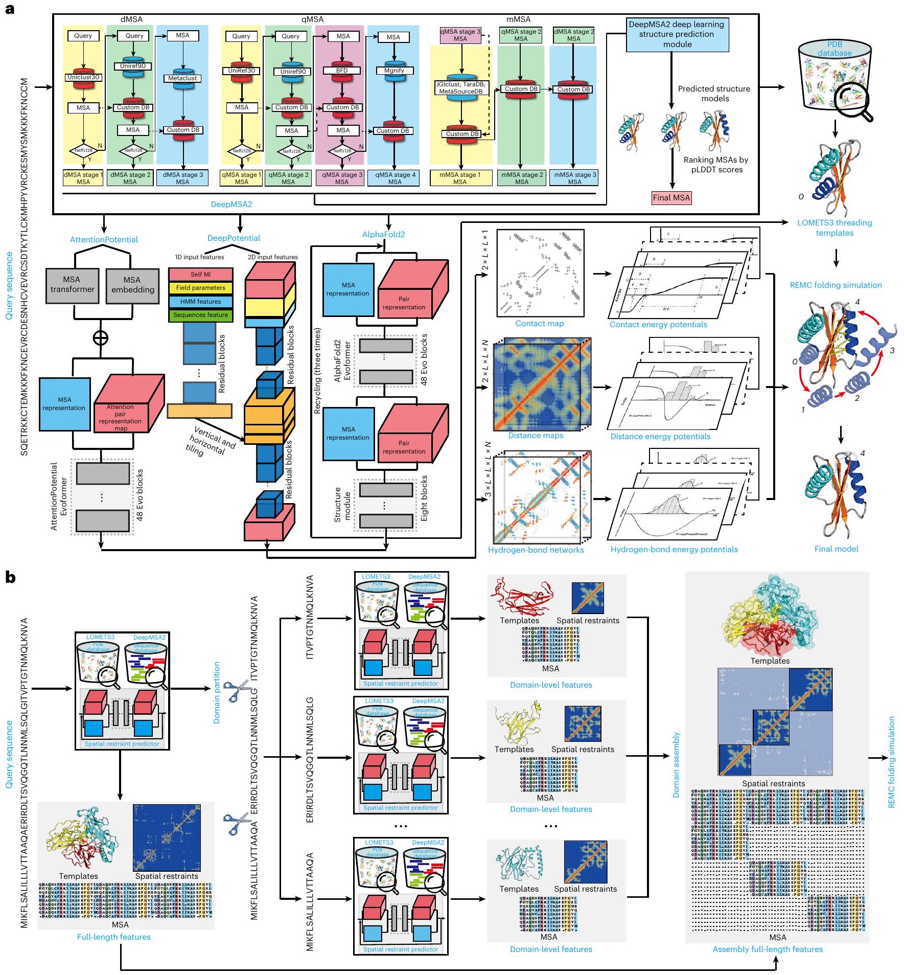
D-I-TASSER مصمم لنمذجة هيكل البروتين القائم على تجميع الشظايا العميقة والتعلم الهجين مع التركيز على البروتينات غير المتجانسة ومتعددة المجالات. كما هو موضح في الشكل 1a، يقوم D-I-TASSER أولاً بإنشاء محاذاة تسلسلية متعددة عميقة (MSAs) من خلال البحث المتكرر في قواعد بيانات التسلسل الجينومي والميتابيوتي، ويختار أفضل MSA من خلال عملية توقع سريعة موجهة بالتعلم العميق. ثم يقوم الخط الأنبوبي بإنشاء قيود هيكلية مكانية بواسطة DeepPotential.، AttentionPotential و AlphaFold2 (المرجع 12)، اللذان يعملان بواسطة الشبكات العصبية التلافيفية العميقة المتبقية، ومحول الانتباه الذاتي، والشبكات العصبية من النهاية إلى النهاية، على التوالي. ثم يتم بناء النماذج الكاملة من خلال تجميع قطع القالب من محاذاة متعددة باستخدام خادم LOcal MEta-Threading (LOMETS3).من خلال محاكاة مونت كارلو لتبادل النسخ (REMC)تحت إشراف مجال قوة قائم على التعلم العميق والمعرفة تم تحسينه بشكل كبير. لمواجهة تعقيد نمذجة الهيكل متعدد المجالات، دمج D-I-TASSER وحدة جديدة لتقسيم وتجميع المجالات، حيث يتم إنشاء تقسيم حدود المجال، وMSAs على مستوى المجال، والمحاذاة الخيطية والقيود المكانية بطريقة تكرارية، حيث يتم إنشاء نماذج هيكلية متعددة المجالات من خلال محاكاة تجميع I-TASSER لكامل السلسلة كما هو موجه بواسطة القيود المكانية على مستوى المجال والقيود بين المجالات (الشكل 1ب). وصف تفصيلي لـ تم تقديم خط أنابيب D-I-TASSER، بما في ذلك مجالات القوة والبروتوكولات المختلفة، في القسم الخاص بالطرق.
معيار D-I-TASSER على البروتينات أحادية المجال
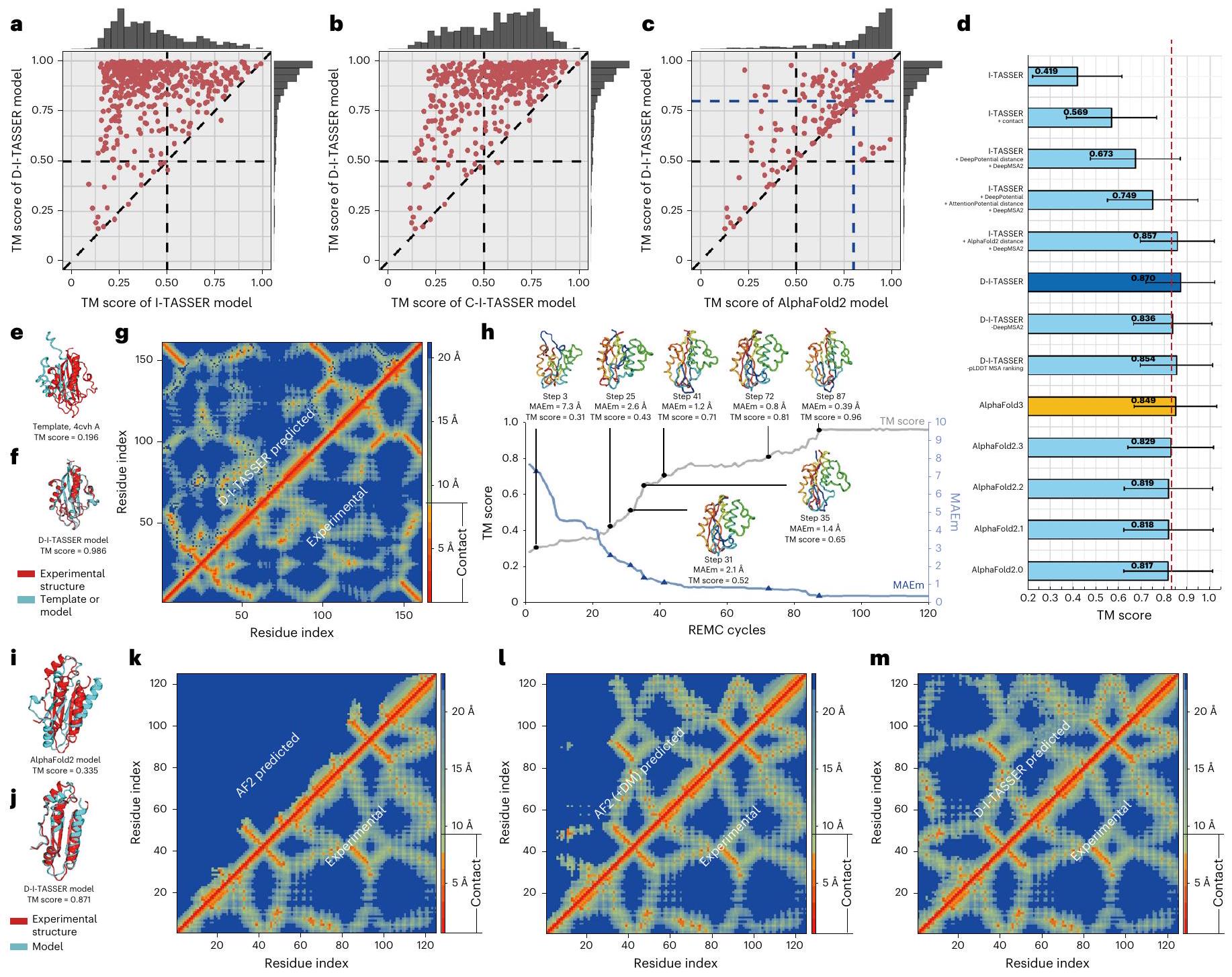
النمذجة الهيكلية للبروتينات ذات النطاق الواحد أساسية لتوقع هيكل البروتينات باستخدام الحاسوب. لاختبار أداء خط أنابيبنا، قمنا أولاً باختبار D-I-TASSER على مجموعة من 500 نطاق ‘صعب’ غير متكرر تم جمعها من تصنيف البروتينات الهيكلية (SCOPe) ومكتبة بيانات البروتين (PDB) وتجارب CASP 8-14، والتي لا يمكن اكتشاف قوالب مهمة لها بواسطة LOMETS3 من PDB بعد استبعاد الهياكل المتجانسة ذات هوية تسلسلية.إلى تسلسل الاستعلامات (انظر ‘جمع مجموعة البيانات المرجعية’). كما هو مدرج في الجدول التكميلي 1، حقق D-I-TASSER متوسط درجة نمذجة القالب (TM) قدرها 0.870، وهو أعلى بنسبة 108% و53% من خطوط الأنابيب السابقة المعتمدة على I-TASSER، بما في ذلك I-TASSER (متوسط درجة TM )، الذي يستخدم معلومات القالب فقط لطي البروتينات “، و C-I-TASSER (متوسط درجة TM )، الذي يستخدم قيود الاتصال المتوقعة بواسطة التعلم العميق. الفروق بين الطريقتين ذات دلالة كبيرة جداً مع قيم من و ، على التوالي، باستخدام اختبار ستودنت ذو الجانبين المزدوجين الاختبارات. الشكل 2أ، ب يوضح تطور سلالة I-TASSER من خلال المقارنات المباشرة بين الطرق الثلاث، حيث يتمتع D-I-TASSER بدرجة TM أعلى في 99% و 98% من الحالات مقارنةً بـ I-TASSER و C-I-TASSER على التوالي. إذا قمنا بحساب الحالات التي تحتوي على طية صحيحة (أي، درجة TM > 0.5) قامت D-I-TASSER بطي 480 هدفًا، وهو عدد أعلى بمقدار 3.3 و1.5 مرة من I-TASSER (145) وC-I-TASSER (329) على التوالي (الجدول التكميلي 1).
في الشكل 2c، قمنا بمقارنة إضافية بين D-I-TASSER وطريقة AlphaFold2 المتطورة (الإصدار 2.3)حيث أن متوسط درجة TM لنماذج D-I-TASSER (0.870) هوأعلى من ذلك لـ AlphaFold2 (; الجدول التكميلية 1). بالإضافة إلى ذلك، أنتج D-I-TASSER نماذج أفضل مع درجة TM أعلى من AlphaFold2 لـمن الأهداف، مما يدل على أن D-I-TASSER يتفوق باستمرار على AlphaFold2. من الجدير بالذكر أن الفرق بين الاثنين جاء بشكل رئيسي من المجالات الصعبة. بالنسبة لـ 352 مجالًا حيث حقق كل من D-I-TASSER و AlphaFold2 درجة TMعلى سبيل المثال، فإن متوسط درجة TM قريب جداً (0.938 مقابل 0.925 لـ D-I-TASSER و AlphaFold2، على التوالي). ومع ذلك، بالنسبة لـ 148 مجالاً أكثر صعوبة، حيث أدت إحدى الطرق على الأقل أداءً ضعيفاً، فإن فرق درجة TM يكون كبيراً (0.707 لـ D-I-TASSER مقابل 0.598 لـ AlphaFold2، مع من جانب واحد لطالباختبار). من بين 148 مجالًا صعبًا، يقوم D-I-TASSER ببناء نماذج ذات درجات TM أعلى من AlphaFold2 بفارق لا يقل عن 0.1 في 63 مجالًا، بينما يتمتع AlphaFold2 بدرجة TM أعلى بكثير من نموذج D-I-TASSER في واحد فقط منها.
هنا كانت مقارنة المعايير لدينا بشكل رئيسي ضد AlphaFold2.3. ومع ذلك، لاحظنا اختلافات طفيفة بين الإصدارات المختلفة من AlphaFold، بما في ذلك AlphaFold2.0 وAlphaFold2.1 وAlphaFold2.2 وAlphaFold2.3 وAlphaFold3، التي تم تشغيلها على جميع المجالات الاختبارية الـ 500 (الشكل 2d). ومن الجدير بالذكر أن متوسط درجة TM لـ D-I-TASSER (=0.870) أعلى بكثير من جميع إصدارات AlphaFold، أي درجة TM.لـ AlphaFold2.0، درجة TMلـ AlphaFold2.1، درجة TMلـ AlphaFold2.2، درجة TMلـ AlphaFold2.3 ودرجة TMلـ AlphaFold3، معالقيم أدناهلجميع المقارنات (الجدول التكميلي 2). نظرًا لاختلاف بيانات التدريب المستخدمة من قبل إصدارات مختلفة من AlphaFold، وللتعامل بشكل أكبر مع القلق بشأن الإفراط في التدريب، جمعنا مجموعة فرعية من 176 هدفًا من 500 هدف صعب، تم إصدار هياكلها بعد 1 مايو 2022، وهو وقت بعد تاريخ تدريب جميع برامج AlphaFold. أظهرت النتائج على هذه المجموعة الفرعية من البروتينات مرة أخرى أن D-I-TASSER (مع درجة TM ) تفوقت بشكل ملحوظ على جميع النسخ الخمسة من برامج AlphaFold (مع درجة TM = 0.734 لـ AlphaFold2.0، درجة TM = 0.728 لـ AlphaFold2.1، درجة TM = 0.727 لـ AlphaFold2.2، درجة TM = 0.739 لـ AlphaFold2.3 ودرجة TM لـ AlphaFold3)، معقيم أقل منفي جميع الحالات (الجدول التكميلي 3).
الشكل 1 | مخططات انسيابية لتوقع بنية بروتين D-I-TASSER. أ، تتكون عملية D-I-TASSER من أربع خطوات تشمل توليد MSA عميق، واكتشاف القوالب بواسطة خادم الميتا-threading، وتوقع القيود المكانية المعتمد على التعلم العميق، وبناء نموذج كامل الطول مع تجزئة REMC التكرارية. محاكاة التجميع.خط أنابيب نموذج النمذجة الهيكلية متعددة المجالات الذي يتكون من تحديد حدود المجالات، وخياطة على مستوى المجال، وجمع MSA وتجميع الميزات بين المجالات.
نحن نعزو الأداء الدقيق للغاية لـ D-I-TASSER إلى تركيبه الأمثل لمصادر مختلفة من قيود التعلم العميق. في الشكل 2d، نعرض مقارنة درجة TM لمحاكاة I-TASSER مع قيود مختلفة. بينما حسنت خرائط الاتصال الناتجة عن التعلم العميق بواسطة C-I-TASSER درجة TM لـ I-TASSER بـتزيد الإضافات التدريجية للقيود المسافة الإضافية من DeepPotential وAttentionPotential وAlphaFold2 من النطاق تحسينات على و على التوالي (الجدول التكميلي 2). من الجدير بالذكر أنه عند استخدام قيود المسافة من AlphaFold2 فقط، فإن متوسط درجة TM للنموذج النهائي هو 0.857، وهو رقم أعلى قليلاً (لكن بشكل ملحوظ، من حيث أقل من درجة TM البالغة 0.870 التي حققتها النماذج التي تتضمن قيودًا من DeepPotential وAttentionPotential وAlphaFold2، مما يبرز الفوائد التي توفرها دمج مصادر مختلفة من قيود التعلم العميق. في الشكل 2e،
الشكل 2 | نتائج نمذجة D-I-TASSER على 500 مجال صلب غير متكرر.درجات TM للنماذج الأولى التي تم بناؤها بواسطة D-I-TASSER مقابل تلك الخاصة بـ I-TASSER (أ)، C-I-TASSER (ب) و AlphaFold2 (ج). د، مقارنات درجات TM لـ I-TASSER مع إمكانيات التعلم العميق المختلفة وإصدارات AlphaFold2، حيث ‘I-TASSER + DeepPotential + AttentionPotential + مسافات AlphaFold2’ تعادل D-I-TASSER. ارتفاع الرسم البياني يشير إلى القيمة المتوسطة، وشريط الخطأ يمثل الانحراف المعياري. هـ، تراكب الهيكل لأفضل نموذج LOMETS (معرف PDB: 4 cvhA) فوق الهيكل المستهدف (معرف PDB: 3 fpiA). و، تراكب الهيكل للنموذج الأول من D-I-TASSER مع الهيكل المستهدف. مقارنة خريطة المسافة بين البقايا المتوقعة من التعلم العميق نماذج (مثلث علوي) وخريطة المسافة المحسوبة من الهيكل المستهدف (مثلث سفلي) لرقم PDB: 3fpiA.h، مسار درجات TM وMAEخلال دورات REMC للنسخة التي تبدأ بقالب PDB ID: 4 cvhA. الهياكل هي نماذج خداعية مأخوذة من خطوات محاكاة مختلفة. i، تراكب الهيكل لنموذج AlphaFold2 فوق الهيكل المستهدف (PDB ID: 4jgnA).تراكب الهيكل لنموذج D-I-TASSER مع الهيكل المستهدف (معرف PDB: 4jgnA). k-m، مقارنات خريطة المسافة بين البقايا من الهيكل المستهدف (مثلث سفلي) لمعرف PDB: 4jgnA مقابل خرائط المسافة المتوقعة (مثلث سفلي) بواسطة AlphaFold2 القياسي (k)، وAlphaFold2 مع MSA DeepMSA2 (I) وتجميع D-I-TASSER (m). نقدم مثالاً من Yersinia pestis 2-C-methyl-d-erythritol 2,4-cyclodiphosphate synthase (معرف PDB: 3 fpiA)، حيث فشلت LOMETS في تحديد قوالب معقولة وأفضل قالب (معرف PDB: 4 cvhA) لديه درجة TM تبلغ 0.196. على الرغم من أن النسخة الكلاسيكية من I-TASSER قد حسنت بشكل كبير من جودة القالب من خلال محاكاة تجميع الشظايا المتعددة، إلا أن النموذج لا يزال لديه طي غير صحيح مع درجة TM. (الشكل التوضيحي 1ب). بفضل توجيه قيود التعلم العميق، قامت D-I-TASSER بتجميع نموذج ممتاز بتقييم TM قدره 0.986 (الشكل 2ف). يُعزى التحسن بشكل رئيسي إلى الدقة العالية للقيود المكانية، حيث كان هناك خطأ مطلق متوسط (MAE) منخفض جداً في توقع خريطة المسافة بالنسبة للنموذج الأصلي (MAEتم تحقيق المعادلة (13) (الشكل 2g). يوضح الشكل 2h مسارات الطي لمحاكاة D-I-TASSER التي تبدأ من هيكل القالب 4 cvhA. مسترشدًا بإمكانات التعلم العميق المصممة حديثًا من D-I-TASSER (المعادلات (25-31))، كانت MAE للتنبؤات المسافات بالنسبة لنموذج الطُعم (; المعادلة (14) تنخفض بسرعة من 7.7 إلى في أول 40 دورة REMC، حيث زادت درجات TM للتمويه من 0.31 إلى 0.71. بعد 100 عملية مسح REMC،ظل مستقرًا عند حوالي، مما أدى إلى تحقيق درجة TM مستقرة تبلغ حوالي 0.96. أظهرت هذه البيانات وجود ارتباط قوي بين دقة نمذجة D-I-TASSER وقدرتها على إنشاء وتنفيذ القيود المكانية عالية الجودة بشكل مثالي.
مساهم آخر مهم في أداء D-I-TASSER هو MSAs عالية الجودة التي تنتجها DeepMSA2. على سبيل المثال، إذا قمنا بإزالة وحدة DeepMSA2 من خط أنابيب D-I-TASSER، فإن متوسط درجة TM لنماذجه ينخفض إلى 0.836 (الجدول التكميلي 2)، وهو أقل بكثير من ذلك الخاص بخط أنابيب D-I-TASSER الكامل (0.870)، مما يتوافق معاستخدام اختبار ستودنت ذو الجانبين المزدوجالاختبارات. يساهم DeepMSA2 في D-I-TASSER بشكل رئيسي في الجانبين التاليين: قواعد بياناته الواسعة في الميتاجينوميات و خوارزمية تصنيف MSA المستمدة من التعلم العميق. لإثبات ذلك، إذا قام D-I-TASSER ببناء نماذج باستخدام MSA النهائي فقط من DeepMSA2 دون التصنيف المستمد من التعلم العميق، فإن متوسط درجة TM هو 0.854، وهو أعلى من درجة D-I-TASSER بدون DeepMSA2. هذه النتيجة تبرز أهمية قواعد بيانات الميتاجينوميات. ومع ذلك، فإن هذه الأداء لا يزال أسوأ بكثير من أداء خط أنابيب D-I-TASSER الكامل. )، مع تسليط الضوء على مساهمة آلية تصنيف MSA. ومع ذلك، فإن الأداء المتفوق لـ D-I-TASSER لا يُعزى فقط إلى DeepMSA2. قمنا بإجراء تجربة منفصلة حيث قمنا بتشغيل AlphaFold2 باستخدام MSAs من أداة توليد MSA المتطورة DeepMSA2. كما هو موضح في الجدول التكميلي 1، فإن AlphaFold2 + DeepMSA2 بالفعل يحسن باستمرار نماذج AlphaFold2 مع MSA الافتراضي (0.819 مقابل 0.841). ومع ذلك، لا يزال D-I-TASSER يتفوق بشكل كبير على AlphaFold2 + DeepMSA2 في متوسط درجة TM (0.870 مقابل 0.841)، مما يتوافق مع قيمة لـفي اختبار ستودنت ذو الجانبين المزدوجيناختبار. إن تحسين درجة TM لـ D-I-TASSER مقارنة بـ AlphaFold2، المبني على نفس MSAs DeepMSA2، ينشأ بشكل أساسي من قدرة D-I-TASSER على دمج قيود التعلم العميق متعددة المصادر مع حقل قوة قائم على المعرفة، مما يمكّن من إعادة تجميع وتحسين التوافقات الهيكلية.
في الشكل 2i-m، نقدم مثالًا آخر من مثبطات RNA الصامت p19 لفيروس قزم الطماطم (معرف PDB: 4jgnA)، حيث تفوقت D-I-TASSER بشكل كبير على AlphaFold2. بالنسبة لهذا البروتين، أنشأ AlphaFold2 نموذجًا ضعيفًا مع TMscore (الشكل 2i)، ربما بسبب جمع MSA الضحل (مع عدد منخفض من التسلسلات الفعالة،; المعادلة (1))، مما أدى إلى خطأ نسبي مرتفع في خريطة المسافة مع (الشكل 2 ك). بالمقابل، من خلال البناء على عمليات البحث التكرارية لـ DeepMSA2 عبر قواعد بيانات التسلسل الجينومي والميتابايوتي، قامت D-I-TASSER بإنشاء MSA أعمق بمقدار 6.75 مرة مع تظهر الشكل 21 خريطة المسافة لـ AlphaFold2 مع MSA الجديدة من DeepMSA2، والتي أدت إلى تحسين كبير. ومع ذلك، لا تزال خريطة المسافة هذه من AlphaFold2 تفتقر إلى معلومات المسافة بين الطرف N ومناطق أخرى، بينما أدى دمج نماذج DeepPotential وAttentionPotential إلى تحسين كبير في دقة المسافة مع Å الذي يغطي منطقة التسلسل بالكامل (الشكل 2 م). مسترشدًا بهذه الخريطة المركبة للمسافة، أنشأ D-I-TASSER في النهاية نموذج هيكل عالي الجودة مع درجة TM (الشكل 2j). تسلط هذه الحالة الضوء على أهمية DeepMSA2 لجمع بيانات MSA أعمق وملفات التعايش التطوري الأكثر شمولاً، مما يساعد بشكل كبير في تحسين التغطية والدقة لقيود التعلم العميق وبالتالي جودة محاكاة تجميع الهيكل النهائي D-I-TASSER.
على الرغم من أن الهدف الأساسي من نماذج التعلم العميق كان طي المجالات الصعبة غير المتجانسة، فإنه من المثير للاهتمام فحص ما إذا كانت القيود الناتجة عن التعلم العميق دقيقة بما يكفي للمساعدة في تحسين المجالات السهلة التي تحتوي على قوالب متجانسة. لهذا، جمعنا 762 مجالًا غير متكرر من SCOPe2.06، وPDB وCASP 8-14، والتي تمكنت برامج LOMETS من اكتشاف قالب واحد أو أكثر لها مع المعايير المعيارية.نتيجة (الملاحظة التكميلية 3 – المعادلة (1)). كما هو ملخص في الجدول التكميلية 1، فإن درجة TM لـ I-TASSER للنطاقات السهلة (0.729) أعلى بشكل ملحوظ من تلك للنطاقات الصعبة (0.419)، وذلك بفضل مساعدة القوالب المتجانسة. ومع ذلك، فإن درجة TM لـ D-I-TASSER (0.936) لا تزال أعلى بشكل ملحوظ من تلك لـ I-TASSER و C-I-TASSER و AlphaFold2 و AlphaFold2 + DeepMSA2، مع قيم من و على التوالي، في اختبار ستودنت ذو الجانبين المقترنيناختبارات، تُظهر أن دقة قيود التعلم العميق تصل إلى مستوى مكمل لذلك الخاص بقوالب الخياطة وبالتالي تحسن محاكاة D-I-TASSER للأهداف المتجانسة.
بينما تم إثبات أن D-I-TASSER ينتج نماذج عالية الجودة للمناطق المنظمة للبروتينات التي تم تحديدها تجريبيًا، لا يزال نمذجة المناطق غير المنظمة تمثل تحديًا. المناطق غير المنظمة هي مقاطع من سلسلة البوليببتيد تفتقر إلى استقرار محدد جيدًا.
هيكل ثلاثي الأبعاد تحت ظروف فسيولوجية، ولا يوجد حاليًا توافق حول النهج الصحيح للنمذجة بسبب غياب البيانات الهيكلية التجريبية لهذه المناطق. نظرًا لأن المناطق غير المرتبة غالبًا ما تكون أكثر مرونة، قد يكون من المفيد لطرق التنبؤ بالهيكل نمذجة هذه المناطق مع تكوينات متعددة. أظهر تحليل لـ 1,262 بروتينًا من Benchmark-I مع هياكل تم حلها تجريبيًا في PDB أن D-I-TASSER يولد أفضل خمسة نماذج مع تباين أكبر في المناطق غير المرتبة مقارنة بـ AlphaFold2، مع متوسط انحرافات الجذر التربيعي (RMSDs) لـ ضد تشير هذه البيانات إلى أن الأساليب المعتمدة على الفيزياء مثل D-I-TASSER، التي تقوم بنمذجة التجمعات التوافقية من خلال محاكاة REMC وتستكشف مساحة توافقية أوسع، قد تكون لها مزايا محتملة على الأساليب المعتمدة فقط على التعلم العميق مثل AlphaFold2 في نمذجة الهياكل غير المرتبة.
أداء D-I-TASSER على البروتينات متعددة المجالات
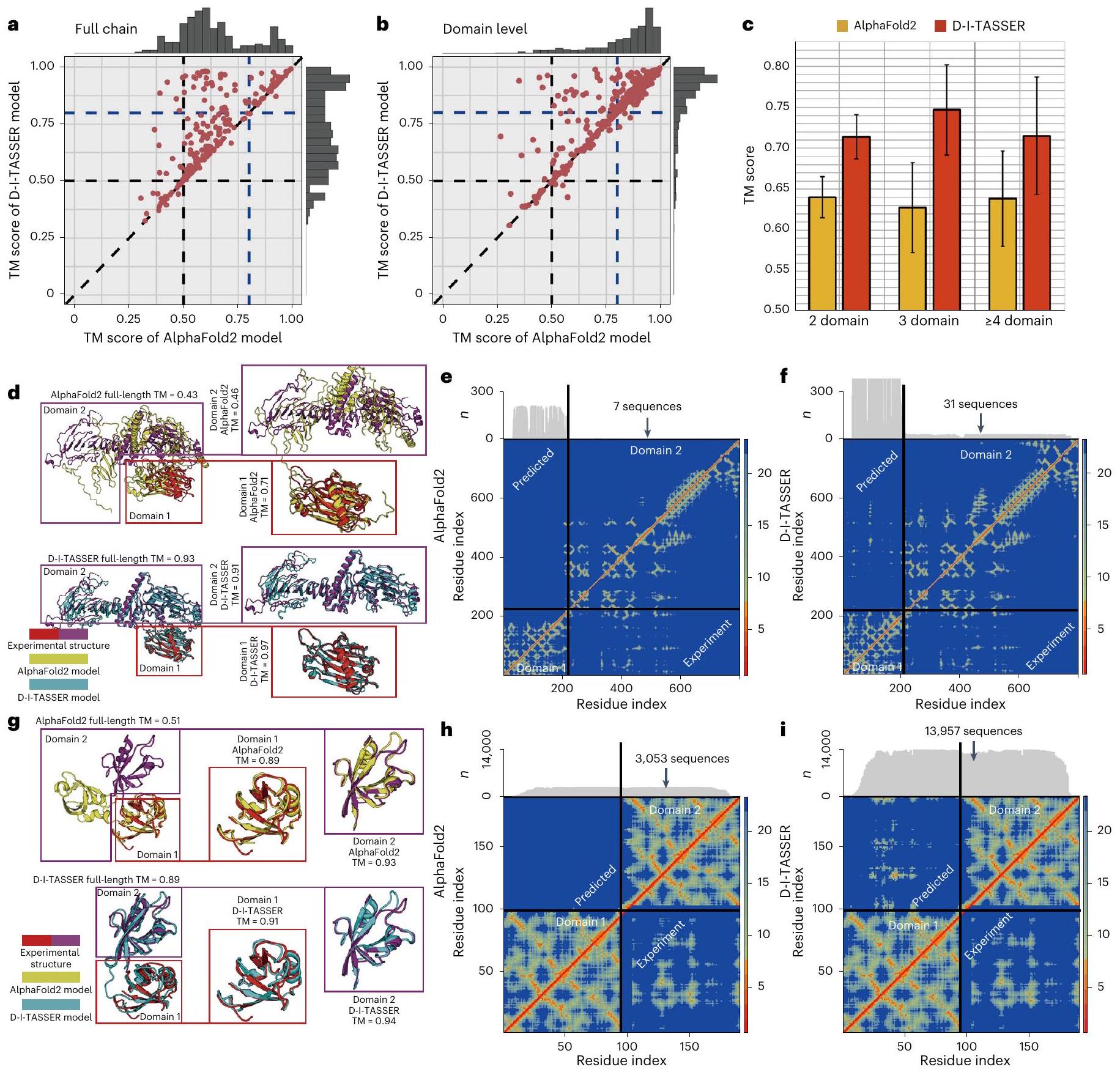
لفحص قدرة D-I-TASSER على التنبؤ الهيكلي متعدد المجالات، جمعنا مجموعة من 230 بروتين غير متكرر من PDB تتكون من مجالين إلى سبعة مجالات، مع تغطية إجمالية تبلغ 557 مجالًا فرديًا (انظر ‘جمع مجموعة بيانات المعايير’). تلخص الأشكال 3a و3b مقارنة الأداء بين D-I-TASSER وAlphaFold2 في التنبؤات الهيكلية على مستوى السلسلة الكاملة والمجال، على التوالي. وقد أظهر أن D-I-TASSER أنشأ نماذج على مستوى السلسلة الكاملة والمجال مع درجات TM تبلغ 0.720 و0.858، والتي هي و أعلى من تلك الخاصة بنماذج AlphaFold2 (0.638 و 0.835) على التوالي.القيم بواسطة اختبار ستودنت أحادي الجانبالاختبار بين الطريقتين هو و للسلاسل الكاملة والمجالات الفردية، على التوالي (الجداول التكميلية 4 و 5)، مما يشير إلى أن الفروق ذات دلالة إحصائية.
بشكل عام، يتمتع D-I-TASSER بدرجة TM أعلى من AlphaFold2 فيللبروتينات ذات السلسلة الكاملة وفي 63% من الحالات على مستوى النطاق. مرة أخرى، يحدث التحسن في البروتينات متعددة النطاقات بشكل رئيسي على الأهداف الصعبة، حيث تكون تحسينات درجة TM لـ D-I-TASSER مقارنة بـ AlphaFold2 هي و 9.9%، على التوالي، لحالات السلسلة الكاملة البالغ عددها 185 وحالات مستوى المجال البالغ عددها 166، حيث أدت على الأقل طريقة واحدة بشكل ضعيف مع درجة TM أقل من 0.8. يوضح الشكل 3c مقارنة درجات TM بين D-I-TASSER و AlphaFold2 على البروتينات التي تحتوي على أعداد مختلفة من المجالات. تظهر البيانات أداءً متسقًا إلى حد كبير لـ D-I-TASSER عبر أعداد المجالات المختلفة، مع درجات TM تبلغ 0.714 و 0.747 و 0.715 للبروتينات ذات المجالين، وثلاثة مجالات، والبروتينات عالية الترتيب، على التوالي. جميعها أعلى بكثير من تلك الخاصة بـ AlphaFold2، التي تتراوح بين 0.62 و 0.65، مع القيم بواسطة اختبار ستودنت أحادي الجانباختبار أدناهفي جميع الحالات (الجدول التكميلي 4).
كنموذج دراسي، نعرض في الشكل 3d مثالاً من بروتين الشوكة الشعاعية لذيل الكلادوموناس رينهاردتي (معرف PDB: 7jtkB)، وهو بروتين ذو مجالين يتكون من 801 بقايا مع تعريف حدود المجال كـ ‘1-202 و203-801’. أنشأ AlphaFold2 نموذج سلسلة كاملة بجودة منخفضة مع درجة TM منخفضة = 0.425 (الشكل 3d، الأعلى)، حيث أن السبب المحتمل هو أن MSA الخاص بـ AlphaFold2 اكتشف عددًا قليلًا جدًا من التسلسلات المتجانسة مع، مما أدى إلى توقعات ضعيفة لكل من المجالات البينية (MAE ) وداخل النطاق ( MAE و للمجالين، على التوالي) خرائط المسافة (الشكل 3e). بالمقابل، اكتشف D-I-TASSER MSAs كاملة السلسلة مع . بشكل خاص، يسمح عملية تقسيم النطاقات لـ DeepMSA2 بالكشف عن 688 و 15 تسلسل متجانس إضافي للنطاقين 1 و 2، على التوالي، مما ساعد نماذج التعلم العميق على استنتاج معلومات تطورية أكثر موثوقية. ونتيجة لذلك، تصبح خرائط المسافات أكثر دقة بكثير، مع كون MAEn لسلسلة كاملة،للنطاق 1 وللنطاق 2 (الشكل 3f). مسترشدًا بالقيود المشتركة داخل النطاقات وبين النطاقات، أنشأ D-I-TASSER نموذجًا هيكليًا ممتازًا مع درجة TM كاملة تبلغ 0.934 ودرجات TM على مستوى النطاق تبلغ 0.971 و0.910 على التوالي، وهي أعلى بكثير من تلك الخاصة بـ AlphaFold2.
الشكل 3 | نتائج نمذجة D-I-TASSER على 230 بروتين متعدد المجالات. أ، ب، مقارنات مباشرة لدرجة TM بين D-I-TASSER و AlphaFold2 في نمذجة السلسلة الكاملة (أ) ونمذجة مستوى المجال (ب). ج، مقارنة درجة TM بين D-I-TASSER و AlphaFold2 على بروتينات ذات مجالين، ثلاثة مجالات وبروتينات ذات مجالات عالية الترتيب. ارتفاع المدرج البياني يشير إلى القيمة المتوسطة وشريط الخطأ يمثل الانحراف المعياري. د، نماذج D-I-TASSER و AlphaFold2 لبروتين الشوكة الشعاعية للذيل في C. reinhardtii (معرف PDB: 7jtkB) متراكبة مع الهيكل المستهدف، حيث يتم تلوين مجالين من الهيكل المستهدف بألوان مختلفة. خريطة المسافة بين البقايا (خريطة الحرارة) جنبًا إلى جنب مع عدد البقايا المتراصة لكل موقع، الموضح في الهوامش) المتوقع من AlphaFold2 (مثلث علوي) مقابل ما تم حسابه من الهيكل المستهدف (مثلث سفلي) لرقم PDB: 7jtkB.f، كما في e، ولكن تم نمذجته باستخدام D-I-TASSER.g، نماذج D-I-TASSER و AlphaFold2 لبروتين الإنسان InaD-like (رقم PDB: 6irdC) متراكبة مع الهيكل المستهدف، حيث يتم تلوين مجالين من الهيكل المستهدف بألوان مختلفة. h,i، معادلة لـ e,f، على التوالي، ولكن لرقم PDB: 6irdC.
الشكل 3 ج يظهر مثالاً آخر من بروتين شبيه InaD البشري (معرف PDB: 6irdC)، وهو بروتين متوسط الحجم ذو مجالين مع تعريف حدود المجال كالتالي ‘1-93;94-190’. على الرغم من أن AlphaFold2 أنتج نماذج عالية الجودة على مستوى المجال مع درجات TM تبلغ 0.894 و 0.930، إلا أن اتجاه المجالات في نموذج AlphaFold2 خاطئ تمامًا، مما أدى إلى درجة TM منخفضة لسلسلة البروتين الكاملة تبلغ 0.503 (الشكل 3ج، الأعلى). في الواقع، يظهر مخطط مسافة النقاط في الشكل 3ح أن AlphaFold2 يعاني من دقة منخفضة جدًا بالنسبة للقيود بين المجالات مع بسبب سلسلة MSA الكاملة الضحلة نسبيًا. لنفس البروتين، أنشأ D-I-TASSER سلسلة MSA كاملة أعمق بكثير تحتوي على 13,957 تسلسلًا. )، مما يؤدي إلى توقع عالي الدقة لكل من النطاق الداخليللنطاقات 1 وللنطاق 2) وبين النطاقات (MAEخرائط المسافة (الشكل 3i)، ومن ثم نموذج كامل السلسلة المحسن بشكل كبير مع درجة TM تبلغ 0.890. تظهر هذه النتائج أن عملية تقسيم المجال والتجميع في الوحدة متعددة المجالات التي تم تقديمها حديثًا تساعد في الكشف عن معلومات تطورية أكثر شمولاً على مستوى النطاق، وبالتالي قيود أكثر دقة بين النطاقات وداخل النطاقات، مما يمكّن D-I-TASSER من إنشاء هياكل متعددة النطاقات بدقة أكبر مقارنةً بطريقة AlphaFold2 المستخدمة على نطاق واسع.
بالمثل، فإن تحسين D-I-TASSER مقارنة بـ AlphaFold2 في أداء نمذجة متعدد المجالات لا يعتمد فقط على DeepMSA2. كدليل، نعرض مقارنة بين D-I-TASSER وإصدار معدل من AlphaFold2 باستخدام MSAs من DeepMSA2 في الجداول التكميلية 4 و 5، على التوالي، للـ 230 هيكل كامل السلسلة و557 هيكل على مستوى المجال. وقد أظهرت النتائج أن متوسط درجات TM لنماذج D-I-TASSER هو و أعلى من تلك الخاصة بـ AlphaFold2 + DeepMSA2 لسلسلة كاملة والمجالات الفردية، على التوالي، معقيم من و في اختبار ستودنت ذو الجانبين المزدوجيناختبار. من الجدير بالذكر أن تغييرات درجة TM للطريقتين أكثر أهمية بكثير لسلاسل كاملة مقارنة بمستوى المجال، مما يشير إلى أن تحسين D-I-TASSER على AlphaFold2 + DeepMSA2 يتمحور بشكل أساسي حول نمذجة توجيه المجال من خلال محاكاة تجميع الهيكل الموجهة بواسطة قيود متعددة المصادر.
من المهم أن نلاحظ أن البروتينات متعددة المجالات غالبًا ما تتبنى أشكالًا متنوعة، لا سيما في اتجاه المجالات، لتلبية المتطلبات الوظيفية. مدفوعةً بحقل قوى مركب يدمج التعلم العميق مع مصطلحات الطاقة المعتمدة على الفيزياء، تولد محاكاة I-TASSER REMC مجموعات واسعة من النماذج الشكلية المتنوعة، مما يوفر إمكانيات قوية لنمذجة البروتينات ذات الحالات الشكلية المتعددة. في الشكل التوضيحي التكميلي 3، نقدم دراسة حالة عن بروتين السنبلة SARS-CoV-2، الذي يشكل ثلاثيًا مع سلاسل موجودة في كل من حالات الشكل المفتوح والمغلق (الشكل التوضيحي التكميلي 3أ). الفرق بين هاتين الحالتين، اللتين همابعيدًا عن بعضهما البعض، يرجع أساسًا إلى الاتجاه المميز لمنطقة ارتباط المستقبل C-terminal بالنسبة إلى المجالات الأخرى. نجح D-I-TASSER في التنبؤ بنماذج لكلتا الحالتين (الشكل التكميلي 3b)، حيث يمثل النموذج الأول الحالة المغلقة (درجة TM ) والثاني يمثل الحالة المفتوحة (درجة TM كما هو موضح في الشكل التكميلي 3c، يتم عادةً تصنيف خدع محاكاة D-I-TASSER إلى الفئات الثلاث التالية: الحالات المفتوحة، المغلقة والمتوسطة، والتي يتم تجميعها بشكل أكبر في خمسة تجمعات بواسطة SPICKER.، حيث يظهر النموذج الأول (الحالة المغلقة) من أكبر مجموعة، ويظهر النموذج الثاني (الحالة المفتوحة) من ثاني أكبر مجموعة. وبالتالي، على عكس الأساليب القائمة على التعلم العميق البحت، التي يتم تدريبها على الهياكل البلورية وعادة ما تنتج نموذجًا ثابتًا واحدًا، تؤكد هذه النتائج القدرة الجوهرية لخوارزميات التنبؤ بالهياكل المعتمدة على الفيزياء، مثل D-I-TASSER، على نمذجة البروتينات عبر حالات تكوينية متعددة.
أداء D-I-TASSER في اختبار CASP15 الأعمى
كاختبار أعمى، شارك خط أنابيب D-I-TASSER في تجربة CASP15 التي أقيمت في عام 2022 لتوقع بنية البروتين الثلاثية. أصدرت تجربة CASP15 77 هدفًا بروتينيًا، بما في ذلك 55 هدفًا أحادي النطاق و22 هدفًا متعدد النطاقات. يمكن تقسيم هذه الأهداف إلى 62 نطاقًا قائمًا على النماذج (TBM) و50 نطاقًا للنمذجة الحرة (FM)، حيث تم دمج النطاقات ‘TBM-easy’ و’TBM-hard’ في ‘TBM’ وتم دمج ‘FM/TBM’ و’FM’ في ‘FM’ لتبسيط التحليلات. بشكل عام، أنشأ D-I-TASSER نماذج بأشكال صحيحة (درجة TM > 0.5) لـ 95% (=106/112) من النطاقات، مع متوسط درجة TM قدره 0.878 لـ 112 نطاقًا (الجدول التكميلي 6). عند النظر في مجموعة الأهداف على مستوى السلسلة الكاملة، أنشأ D-I-TASSER أشكالًا صحيحة لـ 94% من الحالات (=72/77)، مع متوسط درجة TM قدره 0.851 (الجدول التكميلي 7).
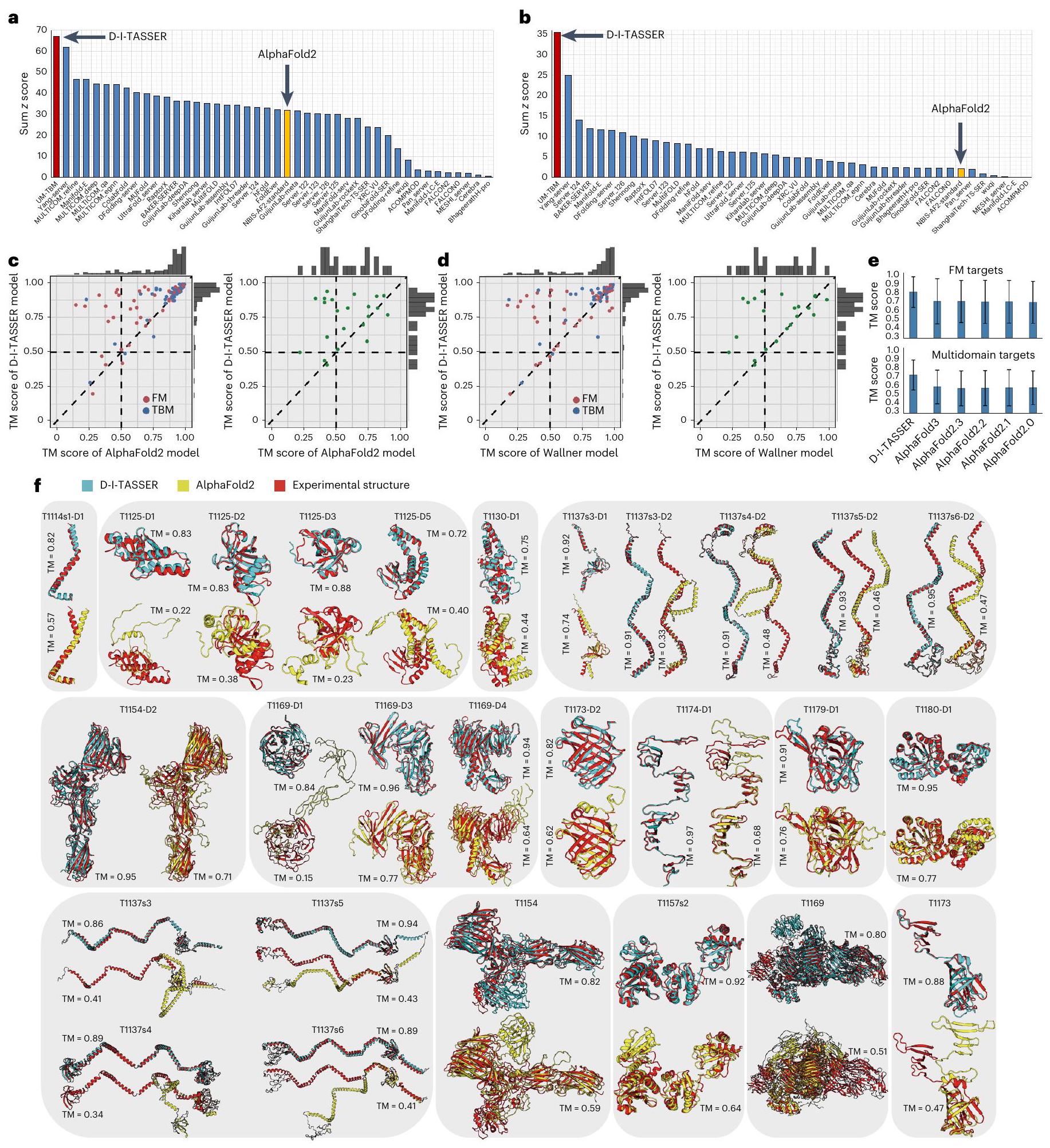
في الشكل 4أ، ب، نقوم بإدراج مقارنة بين D-I-TASSER (المسمى ‘UB-TBM’) و 44 مجموعة خوادم أخرى شاركت في أقسام ‘النمذجة العادية’ و ‘نمذجة المجالات المتداخلة’ في CASP15، والتي تت correspond إلى الهياكل أحادية المجال ومتعددة المجالات، على التوالي. تفوق D-I-TASSER على جميع المجموعات الأخرى من حيث مجموعاتالنتائج, تم حسابها من قبل مقيمي CASP استنادًا إلى درجة اختبار المسافة العالمية – الدقة العالية (GDT-HA) لنمذجة المجالات واختبار الفرق في المسافة المحلية (LDDT) لنمذجة المجالات البينية، على التوالي. بشكل عام، حقق D-I-TASSER تراكمًادرجات 67.20 و 35.53، والتي كانت أعلى بمقدار 2 و 16 مرة من أداء مجموعة ‘NBIS-AF2-standard’ (أي النسخة العامة 2.2.0 من AlphaFold2 التي تم تشغيلها بواسطة مختبر إلوفسون على أهداف CASP15، والتي حققت مجموعيدرجات 32.05 و 2.11) للمجالات والأهداف متعددة المجالات، على التوالي. يجب ملاحظة أن CASP15 شمل القسمين التاليين: قسم ‘الخادم’، حيث يتم إنشاء النماذج تلقائيًا خلال 72 ساعة، وقسم ‘البشر’، الذي يسمح بتدخل الخبراء البشر ويسمح بـ 3 أسابيع لكل هدف. توفر الجداول التكميلية 8 و 9 قائمة شاملة بالنتائج من جميع المجموعات في كل من قسم الخادم وقسم البشر. تظهر النتائج أنه حتى مع المجموعات البشرية، لا يزال خادم D-I-TASSER يحقق المركز الثاني (أو الأول) لأهداف ‘النمذجة العادية’ بناءً على صيغ المقيمين لـدرجة > -2.0 (أو > 0.0). علاوة على ذلك، فإن خادم D-I-TASSER تفوق بوضوح على جميع المجموعات، بما في ذلك المجموعات البشرية، في ‘نمذجة المجالات المتداخلة’، حيث أن المجموع التراكميكانت نتيجة خادم D-I-TASSER أعلى بنسبة 42.3% من المجموعة الثانية الأفضل (24.96) في هذه الفئة.
الشكل 4c و d يظهران المزيد من المقارنات المباشرة بين D-I-TASSER ونماذج AlphaFold2 و Wallner على 112 هدفًا على مستوى المجال و 22 هدفًا متعدد المجالات، حيث تعتبر مجموعة Wallner مجموعة قوية أخرى للتنبؤ من CASP15، تعتمد بشكل كبير على العينة الضخمة باستخدام AlphaFold2 (المرجع 31). بالنسبة لـ 112 مجالًا، لاحظنا أن النماذج المتنبأ بها بواسطة D-I-TASSER كانت ذات درجة TM أعلى من AlphaFold2 و Wallner لـ و ( ) من الحالات، على التوالي. بالنسبة لأهداف FM، فإن متوسط درجة TM لنماذج D-I-TASSER ( 0.833 ) هو و أعلى من نموذج AlphaFold2 (0.701) ونموذج Wallner (0.726)، معقيم من و باستخدام اختبار ستودنت ذو الجانبين المزدوجيناختبار، على التوالي. عند النظر في 22 هدفًا متعدد المجالات، أنشأ D-I-TASSER نماذج ذات درجة TM أعلى من نماذج AlphaFold2 وWallner على و من الأهداف، حيث كان متوسط درجة TM لنماذج D-I-TASSER (0.747) هو و أعلى من نموذج AlphaFold2 (0.578) ونموذج Wallner (0.602)، معقيم من و بواسطة اختبار ستودنت ذو الجانبين المزدوجيناختبار، على التوالي. هذه النتائج المقارنة مع AlphaFold2 تتماشى إلى حد كبير مع نتائج المعايير الملخصة في الأشكال 2 و 3.
في الشكل 4e، نعرض أيضًا مقارنة بين D-I-TASSER وإصدارات مختلفة من برامج AlphaFold على 50 مجال FM التي تفتقر إلى قوالب متجانسة و20 هدفًا متعدد المجالات. بينما كانت الفروق في الأداء بين إصدارات AlphaFold ضئيلة، حقق D-I-TASSER درجات TM أعلى بشكل ملحوظ (0.833 لمجالات FM و0.742 للأهداف متعددة المجالات) من جميع إصدارات AlphaFold، أي درجات TM.و 0.599 لـ AlphaFold2.0، درجات TMو0.598 لـ AlphaFold2.1، درجات TM = 0.721 و0.595 لـ AlphaFold2.2، درجات TMو0.592 لـ AlphaFold2.3 ودرجات TMو0.609 لـ AlphaFold3، مع القيم في اختبار ستودنت ذو الجانبين المقترنيناختبارات جميع ما يليلأهداف FM/متعددة المجالات، على التوالي (الجدول التكميلي 10).
كأمثلة، توضح الشكل 4 ف نماذج هيكلية لـ 19 مجالًا و8 أهداف متعددة المجالات، حيث كانت تحسينات درجة TM بواسطة D-I-TASSER أعلى من 0.15 مقارنة بـ AlphaFold2. وتشمل هذه بعض أهداف البروتينات متعددة المجالات الكبيرة جدًا معبقايا (على سبيل المثال، T1169 مع 3,364 بقايا ودرجة TM )، مما يمثل تقدمًا مهمًا في نمذجة الهياكل البروتينية الكبيرة باستخدام قيود التعلم العميق – وهو تحدٍ طويل الأمد لأساليب نمذجة الهياكل التقليدية .
نلاحظ أيضًا أنه على الرغم من النتائج الواعدة، فإن متوسط درجة TM للأهداف متعددة المجالات لا يزال أقل بكثير من درجة TM للأهداف أحادية المجال (0.747 مقابل 0.893، كما هو موضح في الجدول التكميلي 7)، مما يشير إلى أن توجيه المجالات المتداخلة لا يزال قضية صعبة في توقع بنية البروتين. ومع ذلك، فإن الفجوة في درجة TM بين الأهداف أحادية المجال و
الشكل 4 | نتائج نمذجة D-I-TASSER في CASP15. أ، ب، مجموعالدرجات لمجموعات الخوادم المسجلة البالغ عددها 45 في أقسام ‘النمذجة العادية’ (أ) و’النمذجة بين المجالات’ (ب). تم تمييز D-I-TASSER (المسجل كـ ‘UM-TBM’) والإصدار العام 2.2.0 من خادم AlphaFold2 (المسجل كـ ‘NBIS-AF2-standard’) باللونين الأحمر والأصفر، على التوالي. ج، د، تُظهر المقارنات المباشرة بين D-I-TASSER وAlphaFold2 (ج) أو نماذج Wallner (د) على 112 مجالًا فرديًا و22 هدفًا متعدد المجالات، حيث تم تلوين مجالات FM وTBM والأهداف متعددة المجالات باللون الأحمر والأزرق والأخضر، على التوالي. هـ، مقارنات درجات TM
من D-I-TASSER وإصدارات AlphaFold المختلفة على 50 مجال FM و20 هدف متعدد المجالات مع هياكل تجريبية تم إصدارها. ارتفاع المدرج البياني يشير إلى القيمة المتوسطة، وبار الخطأ يمثل الانحراف المعياري. f، تم تراكب النماذج الأولى التي أنتجها D-I-TASSER (سماوي) وAlphaFold2 (أصفر) على الهياكل المستهدفة (أحمر) لـ 19 مجالًا (الصفين العلويين) و8 أهداف متعددة المجالات (الصف السفلي)، حيث كانت تحسينات درجة TM بواسطة D-I-TASSER أعلى من 0.15 مقارنة بـ AlphaFold2. بروتينات متعددة المجالات بواسطة D-I-TASSER (0.146) أقل بكثير من تلك الخاصة بـ AlphaFold2يعكس فعالية وحدة تقسيم المجالات المحددة والتجميع التي تم تقديمها لـ D-I-TASSER لنمذجة الأهداف متعددة المجالات وشرح الأداء الرائد لـ D-I-TASSER في التفاعلات بين المجالات في CASP15.
تحدٍ آخر للإصدار الحالي من D-I-TASSER هو أداؤه في نمذجة البروتينات اليتيمة، التي تحتوي على عدد قليل جداً من التسلسلات المتماثلة. توضح الشكل التوضيحي 4a العلاقة بين درجة TM ومن MSAs. للأهداف التي تحتوي علىتحقق D-I-TASSER متوسط درجة TM قدرها 0.67، والتي، على الرغم من كونها أعلى من معظم المجموعات الأخرى، إلا أنها أقل بكثير من درجة TM الخاصة بها (0.91) للأهداف مع، مما يبرز اعتماد نتائج النمذجة على جودة MSAs. ومن الجدير بالذكر أنه بالنسبة للأهداف T1122-D1 و T1131-D1 (الشكل التكميلي 4b)، توقعت D-I-TASSER طيات غير صحيحة، مع درجات TM تبلغ 0.42 و 0.20 على التوالي، وهو ما يمكن أن يُعزى إلى الجودة الضعيفة لـ MSAs التي لديها الأدنىو 0.08، على التوالي). من المهم التأكيد على أن هذه التحديات في نمذجة البروتينات اليتيمة ليست فريدة من نوعها بالنسبة لـ D-I-TASSER، حيث لم ينجح أي من المشاركين في CASP15 في توليد نماذج صحيحة لهذين الهدفين؛ بل تمثل تحديًا مستمرًا في الحصول على معلومات تطورية كافية لدفع توقعات الهيكل المعتمدة على التعلم العميق للبروتينات اليتيمة، على الرغم من التقدم الكبير في الأساليب في هذا المجال.
نمذجة الهيكل والوظيفة للبروتيوم البشري
استنادًا إلى يوني بروتيحتوي البروتين البشري على أكثر من 20,000 بروتين تتراوح أطوالها من 2 إلى 34,350 حمض أميني. على الرغم منلدى البروتينات البشرية معلومات هيكلية تجريبية جزئية على الأقل في قاعدة بيانات البروتينات (PDB)، وعادةً ما تكون أطوال الهياكل المحلولة أقصر من التسلسلات الكاملة، حيث فقطبروتينات بشرية ذات هياكل تجريبية تغطيمن التسلسل (الشكل التوضيحي التكميلي 5). لفحص الاستخدام العملي لنمذجة الهيكل على مستوى الجينوم، قمنا بتطبيق D-I-TASSER على التسلسلات التي تتراوح أطوالها من 40 إلى 1500 بقايا، والتي تشمل 19,512 بروتينًا فرديًا، تغطي تقريبًاللبروتينات البشرية. استنادًا إلى نموذج هجين من النمذجة القائمة على الخيوط (ThreaDom ) ومرتبط بالاتصال (FUpred ) التنبؤات (انظر ‘بروتوكولات تقسيم المجال وتجميع الهيكل متعدد المجالات’)، تحتوي 19,512 تسلسلًا على 12,236 بروتينًا أحادي المجال و7,276 بروتينًا متعدد المجالات، حيث يمكن تقسيم المجموعة الأخيرة إلى 22,732 مجالًا. يتم تقديم تحليل مفصل لمجموعة بيانات البروتينات البشرية في الشكل التوضيحي 6 والمجموعة البيانات الخاصة بالبروتينات البشرية. قمنا أولاً بتطبيق D-I-TASSER لإنشاء نماذج كاملة السلسلة لجميع البروتينات في البروتينات البشرية. بالنسبة للبروتينات متعددة المجالات، بالإضافة إلى نماذج السلسلة الكاملة، يتم أيضًا إنشاء 22,732 نموذجًا على مستوى المجال بواسطة D-I-TASSER. هذه النتائج تؤدي إلى نماذج على مستوى المجال و19,512نماذج نهائية على مستوى سلسلة كاملة.
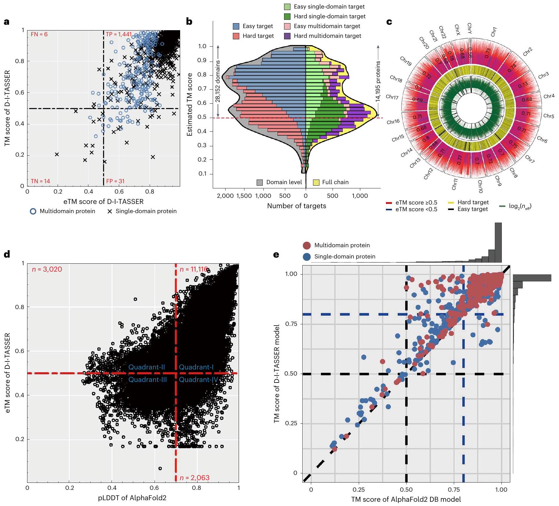
نظرًا لأن الهياكل التجريبية غير معروفة لمعظم البروتينات البشرية، تم تصميم تقدير درجة TM (درجة eTM) لتقييم جودة نماذج D-I-TASSER بشكل كمي. كما هو موضح في المعادلة (33) في ‘التقدير العالمي لجودة توقعات هيكل D-I-TASSER’، يتم تقدير درجة eTM من تركيبة خطية من خمسة عوامل تتعلق بأهمية محاذاة LOMETS، ومعدلات الرضا عن خرائط الاتصال والمسافة المتوقعة، والتقارب الهيكلي لمحاكاة D-I-TASSER ودرجة LDDT المتوقعة (pLDDT) من النموذج الأول من AlphaFold2. استنادًا إلى 1,492 هدف اختبار في مجموعات البيانات المرجعية، كانت درجة eTM لها معامل ارتباط بيرسون (PCC) قدره 0.79 مع درجة TM الحقيقية للنموذج الأصلي (الشكل 5a). عند أخذ حد درجة eTM عند 0.5 لتصنيف نموذج على أنه قابل للطي مقابل غير قابل، وصل معامل ارتباط ماثيوز (MCC) في مجموعة البيانات المرجعية إلى حد أقصى قدره 0.46 مع معدل اكتشاف خاطئ من.
في الشكل 5ب، نعرض توزيعات درجات eTM لنماذج D-I-TASSER لكل من البروتينات البشرية على مستوى المجال والسلسلة الكاملة. بالنسبة لـ 34,968 بروتين بشري على مستوى المجال،من الـ
من المتوقع أن تحتوي نماذج D-I-TASSER على طية صحيحة مع درجات eTMبينما بالنسبة لـ 19,512 بروتين كامل السلسلة،تم طيها بشكل صحيح بواسطة D-I-TASSER مع درجات eTMمن المثير للاهتمام أن هناك ذروتين تظهران عند درجة eTM حوالي 0.55 و 0.80، على التوالي، لكل من بروتينات الإنسان على مستوى المجال والسلسلة الكاملة (الشكل 5ب)، والتي ربما تت correspond إلى الفئتين من الأهداف الصعبة والسهلة.
في الشكل 5c، نرسم درجات eTM (المسار الخارجي)، نوع الهدف (سهل أو صعب؛ المسار الأوسط) وقيم (المسار الداخلي) لنماذج السلسلة الكاملة الموجودة في كل كروموسوم. وجدنا أن هذه المؤشرات كانت لها توزيع شبه متساوٍ بين الكروموسومات المختلفة، مما يشير إلى أن جودة النموذج تعتمد إلى حد كبير على الموقع الكروموسومي للجين. ومع ذلك، بالنسبة للكروموسوم 17، هناك منطقة صغيرة تظهر وادٍ كبير من درجات eTM، والتي تتوافق مع منطقة تجمع بروتينات الكيراتين والبروتينات المرتبطة بالكيراتين. هذه الأنواع من البروتينات توجد في الغالب في الفقاريات.، حيث لا يمكن لقواعد بيانات الميتاجينوميات المساعدة في تكميل التسلسلات المتجانسة في MSAs، مما يؤدي إلى انخفاض النسبيالقيم. في الوقت نفسه، فإن ألياف الكيراتين عمومًا صعبة الذوبان والتبلور.، ونقص القوالب المتجانسة يجعل معظم تسلسلات الكروموسوم 17 أهدافًا صعبة. هناك أيضًا بعض قمم درجات eTM في الكروموسومات 2 و7 و11 و14 و22، والتي تتوافق جميعها مع تجمعات من الأهداف السهلة ذات النسب العالية نسبيًا.القيم. تعكس هذه البيانات تأثير نماذج الخياطة وقيود التعلم العميق على محاكاة D-I-TASSER.
في دراسة حديثة، أصدرت DeepMind نماذج البروتين البشري التي تم بناؤها بواسطة AlphaFold2 (المرجع 23). من خلال فحص نماذج البروتين البشري من D-I-TASSER وAlphaFold2، وجدنا أن البرنامجين مكملان للغاية بسبب الاستراتيجيات المختلفة المتبعة لنمذجة الهياكل. تقدم الشكل 5d مقارنة مباشرة بين pLDDT الخاص بـ AlphaFold2 مقابل درجة eTM الخاصة بـ D-I-TASSER على 19,488 بروتينًا تم التنبؤ بها بواسطة كلا البرنامجين. هنا، مثل درجة eTM، كانت pLDDT مقياسًا استخدمه AlphaFold2 لتقييم جودة التنبؤ على مستوى البقايا مع pLDDT.مؤشرًا على طي العمود الفقري الصحيح. بينما حول تُطوى التسلسلات عادةً بواسطة كلا الطريقتين مع pLDDT ودرجة eTM (الربع الأول)، منها قابلة للطي بأي من الطريقتين، بما في ذلك 3,020 بواسطة D-I-TASSER فقط (الربع الثاني) و2,063 بواسطة AlphaFold2 فقط (الشكل 5د، الربع الرابع).
من بين 19,512 بروتين بشري كامل السلسلة، تم حل هيكل تجريبي لـ 1,907 منها في قاعدة بيانات البروتينات (PDB)، والتي تغطي أكثر من 90% من أطوال تلك التسلسلات (الشكل التوضيحي 5)، وتحتوي على 1,147 بروتين أحادي النطاق و760 بروتين متعدد النطاقات. بالنسبة لهذه البروتينات، حقق D-I-TASSER درجة TM أعلى (0.931) من AlphaFold2 (0.916) معقيمة (الجدول التكميلي 11). الفرق النسبي الصغير في درجة TM بين D-I-TASSER و AlphaFold2 يعود بشكل رئيسي إلى أن معظم الأهدافمن 1,907) هي أهداف سهلة، حيث يمكن لكلا البرنامجين توليد نماذج عالية الجودة مع درجة TM (أي أن متوسط درجات TM لهذه الأهداف هو 0.966 و0.958 لـ D-I-TASSER وAlphaFold2، على التوالي؛ الجدول التكميلي 12). ولكن بالنسبة لبقية 248 بروتينًا صعبًا نسبيًا، حيث أدت إحدى الطرق على الأقل بشكل ضعيف (درجة TM < 0.8)، تصبح الفجوة في درجات TM أكثر أهمية مع متوسط درجات TM تبلغ 0.699 مقابل 0.633 بواسطة D-I-TASSER وAlphaFold2، على التوالي، مع قيمةمن جانب واحد لطالباختبار. الشكل 5e يقدم مقارنة مباشرة بين D-I-TASSER و AlphaFold2، حيث أن D-I-TASSER لديه درجة TM أعلى من AlphaFold2 في 79% من الحالات ( ). إذا استخدمنا درجة TM للدلالة على طية صحيحة، فإن MCC هو 0.52 و 0.47 لدرجة eTM في D-I-TASSERو AlphaFold2 pLDDTعلى التوالي، مما يظهر أن كلاهما يمكن استخدامه كعتبة معقولة لتقدير قابلية الطي للنماذج المتوقعة.
وفقًا لنموذج التسلسل إلى الهيكل إلى الوظيفة، قمنا أيضًا بتطبيق بروتوكول COFACTOR المعروف جيدًالتعليق الوظائف البيولوجية للجينوم البشري استنادًا إلى النماذج المتوقعة بواسطة D-I-TASSER. بينما تكون وظائف البروتينات غالبًا متعددة الأوجه، نركز على ثلاثة جوانب رئيسية لموقع ارتباط الليغاند (LBS) ورقم لجنة الإنزيمات (EC) وعلم الأحياء الجيني (GO)، حيث يتم توسيع GO بشكل أكبر.
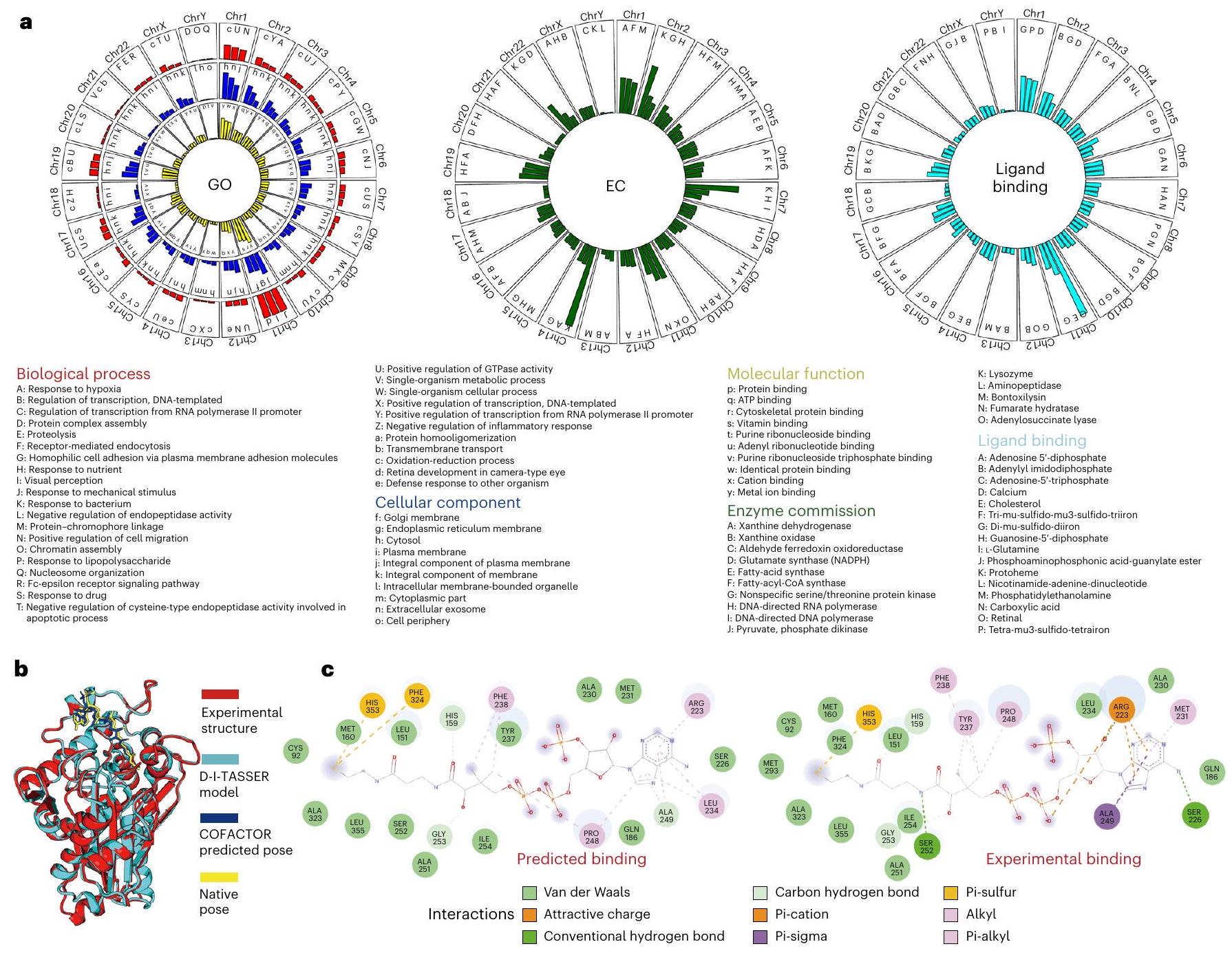
الشكل 5 | نتائج نمذجة الهيكل باستخدام D-I-TASSER على البروتينات البشرية. أ، درجة TM مقابل درجة eTM على مجموعة البيانات المرجعية المكونة من 1,492 بروتين مختلط. تمثل الدوائر الزرقاء البروتينات متعددة المجالات، وتمثل الصلبان السوداء البروتينات أحادية المجال. ب، توزيع درجات eTM للبروتينات البشرية. يسارًا، النتائج على 34,968 مجالًا فرديًا في البروتينات البشرية، حيث تمثل الأعمدة الزرقاء الأهداف السهلة، وتمثل الأعمدة الحمراء الأهداف الصعبة، ويعرض الرسم البياني الرمادي التوزيع العام. يمينًا، يتوافق مع النتائج على 19,512 بروتين بشري كامل السلسلة، حيث تمثل الأعمدة الخضراء الفاتحة الأهداف السهلة أحادية المجال، وتمثل الأعمدة الخضراء الداكنة الأهداف الصعبة أحادية المجال، وتمثل الأعمدة الأرجوانية الفاتحة الأهداف السهلة متعددة المجالات، وتمثل الأعمدة الأرجوانية الداكنة الأهداف الصعبة. أهداف متعددة المجالات ومخطط الكمان الأصفر يعرض التوزيع العام. ج، تحليلات على مستوى الكروموسوم حول توزيعات درجات eTM (المسار الخارجي)، أنواع الأهداف (سهلة أو صعبة؛ المسار الأوسط) واللوغاريتم لـالقيم (المسار الداخلي). د، مقارنة درجات الثقة بين نماذج D-I-TASSER و AlphaFold2 على 19,488 بروتين بشري. تُستخدم درجات eTM و pLDDT كمعايير من قبل D-I-TASSER و AlphaFold2 لتقدير دقة النمذجة، حيث تشير درجات eTM > 0.5 و pLDDT > 0.7 إلى الطي الصحيح من قبل البرنامجين، على التوالي. هـ، مقارنة درجات TM بين نماذج D-I-TASSER و AlphaFold2 لـ 1,907 بروتينات من البروتينات البشرية التي تم حلها تجريبيًا، بما في ذلك 1,147 بروتين أحادي النطاق (أزرق) و 760 بروتين متعدد النطاقات (أحمر). مصنفة إلى ثلاثة جوانب فرعية من الوظيفة الجزيئية (MF) والعملية البيولوجية (BP) والمكون الخلوي (CC)في الشكل التوضيحي الإضافي 7 والجدول الإضافي 13، قمنا بإدراج أعلى 20 وظيفة تم تعيينها بشكل متكرر في كل جانب من جوانب الوظيفة. لضمان تعليقات وظيفية عالية الثقة، هنا نأخذ في الاعتبار فقط توقع البروتينات البشرية التي يمكن طيها بواسطة D-I-TASSER مع درجة eTM.. بشكل عام، وُجد أن البروتينات البشرية تتسم بأعلى تركيز في ‘عملية الأكسدة والاختزال’ في BP، و’السيتوسول’ و’الإكسوزوم خارج الخلية’ في CC، و’ارتباط أيون المعدن’ في MF و’الليزوزيم’ في EC، وتربط بشكل متكرر مع ‘أدينيل إيميدوديفوسفات’ (وبالتالي ATP في السياق الخلوي) و ‘دي-مو-سولفيدو-دي-حديد’ (وبالتالي مجموعات الحديد-الكبريت في الجسم الحي). في الشكل 6أ، نقدم قائمة بنماذج وظائف D-I-TASSER/COFACTOR بناءً على الكروموسومات، حيث يتم اختيار أفضل ثلاث وظائف لكل كروموسوم. توجد قائمة مماثلة من الوظائف الغنية لمعظم الكروموسومات، ولكن هناك استثناء واضح في الكروموسوم 11، الذي يحتوي على غنى كبير في التوصيفات المتعلقة بالعيون، مثل ‘الإدراك البصري’ و ‘تطور الشبكية في العين من نوع الكاميرا’ من BP، و ‘الشبكية’ من تفاعل ربط الليغاند. هذا يتماشى مع
الشكل 6|ت annotations الوظائف المستندة إلى D-I-TASSER للبروتينات البشرية. أ، توزيع هيستوجرام للبروتينات مع مصطلحات وظيفة محددة من BP وCC وMF وEC و ligand غير الببتيد، حيث يتم عرض فقط الثلاثة مصطلحات الوظيفة الأكثر تكرارًا، التي تم ذكر أسمائها أسفل الرسوم البيانية، لكل كروموسوم. ب، دراسة حالة لإنزيم أسيتيل-CoA أسيتيل ترانسفيراز (معرف يوني بروت: Q9BWD1) يرتبط بجزيء CoA، مع رموز ألوان مختلفة تبرز الهياكل ومواقع الربط من التجربة، D-I-TASSER و COFACTOR2، على التوالي. ج، مقارنة جيب الربط الذي هوإلى جزيء CoA بواسطة COFACTOR2 (يسار) والتجربة (يمين) لإنزيم أسيتيل-CoA أسيتيل ترانسفيراز. الدراسات التجريبية السابقة، التي اقترحت أن الكروموسوم البشري 11 مرتبط بمختلف الأمراض العينية البشرية.
في الشكل 6ب، ج، نقدم مثالًا توضيحيًا للتنبؤ الآلي باستخدام LBS لإنزيم أسيتيل-كوإنزيم A (CoA) أسيتيل ترانسفيراز (معرف UniProt: Q9BWD1)، حيث يتمتع نموذج D-I-TASSER بدرجة TM عالية تبلغ 0.99 مقارنةً بالهيكل الذي تم حله تجريبيًا. تم التنبؤ بأن هذا الهدف يرتبط بجزيء CoA، حيث أن RMSD بين الوضع المتوقع لجزيء CoA والهيكل الأصلي المحسوب من الهيكل التجريبي 1 و 14 هو، مما يشير إلى توقع دقيق للغاية لموقع الارتباط. من بين 23 بقايا تحت 4 Å ترتبط بجزيء CoA في الهيكل التجريبي، تم التنبؤ بشكل صحيح بـ 22 بقايا مرتبطة بالليغاند بواسطة COFACTOR (الشكل 6c).
نقاش
لقد طورنا خط أنابيب هجين، D-I-TASSER، لبناء نماذج هياكل البروتين على المستوى الذري من خلال دمج إمكانيات التعلم العميق المتعددة مع محاكاة تجميع الخيوط التكرارية وتقديم بروتوكول تقسيم وتجميع المجالات لنمذجة الهياكل البروتينية الكبيرة متعددة المجالات بشكل آلي.
تم اختبار خط الأنابيب أولاً على مجموعتين كبيرتين من البيانات المرجعية. بالنسبة لمجموعة البيانات التي تتكون من 500 بروتين أحادي المجال نظرًا لعدم وجود قوالب متجانسة في قاعدة بيانات PDB، يقوم D-I-TASSER بإنشاء نماذج عالية الجودة مع متوسط درجة TMأعلى من تلك الناتجة عن خط أنابيب I-TASSER الكلاسيكي، مما يظهر تأثيرًا كبيرًا لإمكانات التعلم العميق على طي الهياكل غير المتجانسة. في مجموعة البيانات الثانية المكونة من 230 بروتين متعدد المجالات، يقوم D-I-TASSER بإنشاء نماذج كاملة السلسلة بمتوسط درجة TMأعلى من ذلك من AlphaFold2 (V2.3)، واحدة من الطرق الرائدة في التعلم العميق في هذا المجال، معقيمةفي اختبار ستودنت ذو الجانبين المقترنيناختبار. أظهرت تحليلات البيانات التفصيلية ميزة كبيرة لبروتوكول تقسيم المجالات وإعادة التجميع الجديد، الذي يسمح باشتقاق معلومات تطورية على مستوى المجال بشكل أكثر شمولاً وتطوير نماذج التعلم العميق المتوازنة داخل المجال وبين المجالات، وبالتالي تجميع هيكلي متعدد المجالات أكثر دقة.
تم اختبار الأنبوب أيضًا (باسم ‘UM-TBM’) في أحدث تجربة شاملة للمجتمع CASP15، حيث حقق D-I-TASSER أعلى دقة في النمذجة في فئتي التنبؤ بالهياكل أحادية المجال ومتعددة المجالات، مع متوسط درجات TM. و أعلى من النسخة العامة مارس-2022 v.2.2.0 من خادم AlphaFold2 الذي تديره مختبر إلوفسون (المسجل كـ ‘NBIS-AF2-standard’)، على مجالات FM والبروتينات متعددة المجالات، على التوالي. تعزز هذه النتائج الإمكانية والفعالية للهيكل القائم على الفيزياء. محاكاة التجميع، عند اقترانها بتقنيات التعلم العميق المتقدمة، لتوقعات عالية الجودة لهيكل البروتين الثلاثي..
كأحد التطبيقات العملية على نطاق واسع، تم استخدام D-I-TASSER لتوليد توقعات البنية لجميع 19,512 تسلسلًا من البروتينات البشرية، حيثسلاسل كاملةمن المجالات) قابلة للطي باستخدام D-I-TASSER، مما يوفر معلومات تتكامل بشكل كبير مع نماذج البروتينات البشرية التي تم إصدارها مؤخرًا والتي تم بناؤها بواسطة برنامج AlphaFold2.تعتبر هذه النماذج ذات صلة كبيرة بالتعليق القائم على الهيكل لوظائف متعددة الجوانب للبروتينات في الجينوم البشري.
على الرغم من النجاح، لا تزال هناك العديد من التحديات في هذا المجال. على سبيل المثال، على الرغم من دمج DeepMSA2 مع قواعد بيانات الميتاجينوم الواسعة، لا تزال هناك MSAs ضحلة لبعض البروتينات، خاصة بالنسبة للبروتينات من الجينوم الفيروسي، حيث تؤدي التطورات السريعة للفيروسات والتوزيع الضريبي الواسع إلى ندرة التسلسلات المتجانسة مقارنة بالمجموعات الضريبية الأخرى. علاوة على ذلك، لا تتناول هذه الدراسة تحدي توقع بنية معقدات البروتين-بروتين، وهي مشكلة كبيرة تفتقر إلى حل فعال. ومع ذلك، أظهر خط الأنابيب المقدم مزايا في نمذجة الأهداف الصعبة والبروتينات متعددة المجالات عند مقارنتها بالخوارزميات الحديثة المتطورة. تشير هذه النجاحات إلى إمكانيات واعدة لتوسيع البروتوكول الحالي، المبني على دمج تقنيات التعلم العميق المتقدمة مع محاكاة الطي القائمة على الفيزياء، لمعالجة التحديات المستمرة في كل من توقع بنية البروتين اليتيم وبنية معقدات البروتين.
المحتوى عبر الإنترنت
أي طرق، مراجع إضافية، ملخصات تقارير Nature Portfolio، بيانات المصدر، بيانات موسعة، معلومات تكميلية، شكر وتقدير، معلومات مراجعة الأقران؛ تفاصيل مساهمات المؤلفين والمصالح المتنافسة؛ وبيانات توفر البيانات والرموز متاحة علىhttps://doi.org/10.1038/s41587-025-02654-4.
References
Kryshtafovych, A., Schwede, T., Topf, M., Fidelis, K. & Moult, J. Critical assessment of methods of protein structure prediction (CASP)-round XIV. Proteins 89, 1607-1617 (2021).
Kryshtafovych, A., Schwede, T., Topf, M., Fidelis, K. & Moult, J. Critical assessment of methods of protein structure prediction (CASP)-round XV. Proteins 91, 1539-1549 (2023).
Pearce, R. & Zhang, Y. Deep learning techniques have significantly impacted protein structure prediction and protein design. Curr. Opin. Struct. Biol. 68, 194-207 (2021).
Mortuza, S. M. et al. Improving fragment-based ab initio protein structure assembly using low-accuracy contact-map predictions. Nat. Commun. 12, 5011 (2021).
Senior, A. W. et al. Improved protein structure prediction using potentials from deep learning. Nature 577, 706-710 (2020).
Greener, J. G., Kandathil, S. M. & Jones, D. T. Deep learning extends de novo protein modelling coverage of genomes using iteratively predicted structural constraints. Nat. Commun. 10, 3977 (2019).
Li, Y., Zhang, C., Yu, D. J. & Zhang, Y. Deep learning geometrical potential for high-accuracy ab initio protein structure prediction. iScience 25, 104425 (2022).
Yang, J. et al. Improved protein structure prediction using predicted interresidue orientations. Proc. Natl Acad. Sci. USA 117, 1496-1503 (2020).
Liu, D. C. & Nocedal, J. On the limited memory BFGS method for large scale optimization. Math. Program. 45, 503-528 (1989).
Rohl, C., Strauss, C., Misura, K. & Baker, D. Protein structure prediction using Rosetta. Methods Enzymol. 383, 66-93 (2004).
Brunger, A. T. et al. Crystallography & NMR system: a new software suite for macromolecular structure determination. Acta Crystallogr. D. Biol. Crystallogr. 54, 905-921 (1998).
Jumper, J. et al. Highly accurate protein structure prediction with AlphaFold. Nature 596, 583-589 (2021).
Abramson, J. et al. Accurate structure prediction of biomolecular interactions with AlphaFold3. Nature 630, 493-500 (2024).
Zhang, Y. & Skolnick, J. Automated structure prediction of weakly homologous proteins on a genomic scale. Proc. Natl Acad. Sci. USA 101, 7594-7599 (2004).
Roy, A., Kucukural, A. & Zhang, Y. I-TASSER: a unified platform for automated protein structure and function prediction. Nat. Protoc. 5, 725-738 (2010).
Xu, D. & Zhang, Y. Ab initio protein structure assembly using continuous structure fragments and optimized knowledge-based force field. Proteins 80, 1715-1735 (2012).
Pearce, R. & Zhang, Y. Toward the solution of the protein structure prediction problem. J. Biol. Chem. 297, 100870 (2021).
Chothia, C., Gough, J., Vogel, C. & Teichmann, S. A. Evolution of the protein repertoire. Science 300, 1701-1703 (2003).
Han, J.-H., Batey, S., Nickson, A. A., Teichmann, S. A. & Clarke, J. The folding and evolution of multidomain proteins. Nat. Rev. Mol. Cell Biol. 8, 319-330 (2007).
Kryshtafovych, A. & Rigden, D. J. To split or not to split: CASP15 targets and their processing into tertiary structure evaluation units. Proteins 91, 1558-1570 (2023).
Ozden, B., Kryshtafovych, A. & Karaca, E. The impact of AI-based modeling on the accuracy of protein assembly prediction: insights from CASP15. Proteins 91, 1636-1657(2023).
Yang, J. et al. The I-TASSER Suite: protein structure and function prediction. Nat. Methods 12, 7-8 (2015).
Tunyasuvunakool, K. et al. Highly accurate protein structure prediction for the human proteome. Nature 596, 590-596 (2021).
Mirdita, M. et al. ColabFold: making protein folding accessible to all. Nat. Methods 19, 679-682 (2022).
Li, Y. et al. Protein inter-residue contact and distance prediction by coupling complementary coevolution features with deep residual networks in CASP14. Proteins 89, 1911-1921 (2021).
Zheng, W. et al. LOMETS3: integrating deep learning and profile alignment for advanced protein template recognition and function annotation. Nucleic Acids Res 50, W454-W464 (2022).
Swendsen, R. H. & Wang, J. S. Replica Monte Carlo simulation of spin glasses. Phys. Rev. Lett. 57, 2607-2609 (1986).
Zhang, Y. & Skolnick, J. Scoring function for automated assessment of protein structure template quality. Proteins 57, 702-710 (2004).
Xu, J. & Zhang, Y. How significant is a protein structure similarity with TM-score = 0.5? Bioinformatics 26, 889-895 (2010).
Zhang, Y. & Skolnick, J. SPICKER: a clustering approach to identify near-native protein folds. J. Comput. Chem. 25, 865-871 (2004).
Wallner, B. Improved multimer prediction using massive sampling with AlphaFold in CASP15. Proteins 91, 1734-1746 (2023).
Moult, J. A decade of CASP: progress, bottlenecks and prognosis in protein structure prediction. Curr. Opin. Struct. Biol. 15, 285-289 (2005).
Zhang, Y. Progress and challenges in protein structure prediction. Curr. Opin. Struct. Biol. 18, 342-348 (2008).
UniProt Consortium. UniProt: the universal protein knowledgebase in 2021. Nucleic Acids Res. 49, D480-D489 (2021).
Xue, Z., Xu, D., Wang, Y. & Zhang, Y. ThreaDom: extracting protein domain boundary information from multiple threading alignments. Bioinformatics 29, i247-i256 (2013).
Zheng, W. et al. FUpred: detecting protein domains through deep-learning-based contact map prediction. Bioinformatics 36, 3749-3757 (2020).
Wang, B., Yang, W., McKittrick, J. & Meyers, M. A. Keratin: structure, mechanical properties, occurrence in biological organisms, and efforts at bioinspiration. Prog. Mater. Sci. 76, 229-318 (2016).
Parry, D. A. D., Strelkov, S. V., Burkhard, P., Aebi, U. & Herrmann, H. Towards a molecular description of intermediate filament structure and assembly. Exp. Cell. Res. 313, 2204-2216 (2007).
Zhang, Y. Protein structure prediction: when is it useful? Curr. Opin. Struct. Biol. 19, 145-155 (2009).
Zhang, C., Freddolino, P. L. & Zhang, Y. COFACTOR: improved protein function prediction by combining structure, sequence and protein-protein interaction information. Nucleic Acids Res 45, W291-W299 (2017).
Ashburner, M. et al. Gene ontology: tool for the unification of biology. The Gene Ontology Consortium. Nat. Genet. 25, 25-29 (2000).
Mets, M. B. & Maumenee, I. H. The eye and the chromosome. Surv. Ophthalmol. 28, 20-32 (1983).
Gilbert, F. Chromosome 11. Genet. Test. 4, 409-426 (2000).
Jumper, J. et al. Applying and improving AlphaFold at CASP14. Proteins 89, 1711-1721 (2021).
Publisher’s note Springer Nature remains neutral with regard to jurisdictional claims in published maps and institutional affiliations.
Open Access This article is licensed under a Creative Commons Attribution-NonCommercial-NoDerivatives 4.0 International License, which permits any non-commercial use, sharing, distribution and reproduction in any medium or format, as long as you give appropriate credit to the original author(s) and the source, provide a link to the Creative Commons licence, and indicate if you modified the licensed material. You do not have permission under this licence to share adapted material derived from this article or parts of it. The images or other third party material in this article are included in the article’s Creative Commons licence, unless indicated otherwise in a credit line to the material. If material is not included in the article’s Creative Commons licence and your intended use is not permitted by statutory regulation or exceeds the permitted use, you will need to obtain permission directly from the copyright holder. To view a copy of this licence, visit http://creativecommons.org/licenses/by-nc-nd/4.0/.
(c) The Author(s) 2025
طرق
مجموعات البيانات
جمع مجموعة بيانات المعايير. لاختبار طرقنا، تم جمع البروتينات أحادية المجال في مجموعة بيانات المعايير (Benchmark-I) من قاعدة بيانات SCOPe 2.06. ( 717 هدفًا)، PDB ( 257 هدفًا تم إصدارها بعد 1 مايو 2022) وأهداف FM و FM/TBM من CASP 8-14 (المراجع 46-50؛ 288 هدفًا). ثم تم إزالة التكرار باستخدام حد هوية تسلسل ثنائي.، وتم الاحتفاظ فقط بالتسلسلات التي تتراوح أطوالها بين 30 و 850 حمضًا أمينيًا في مجموعة بيانات المعايير. علاوة على ذلك، تم إزالة الأهداف غير المتصلة إذا لم تكن مؤشرات البقايا متتالية أو إذا كانت المسافة بين بقايا متتالية كانت أكبر من. في المجموع، كان هناك 1,262 هدفًا تتكون من بروتيناتالبروتينات و أو البروتينات في مجموعة البيانات المرجعية، والتي يمكن تصنيفها إلى 211 بسيط (TBM-easy)، 551 سهل (TBM-hard)، 383 صعب (FM/TBM) و117 صعب جداً (FM) (انظر ‘وحدة التعلم العميق لتوقع خريطة الاتصال، خريطة المسافة وشبكة الروابط الهيدروجينية’) بناءً على LOMETS3 (المراجع 26، 51، 52). في تحليل المرجع، تم دمج الأهداف ‘البسيطة’ و’السهل’ في مجموعة واحدة تسمى ‘الأهداف السهلة’ (762)، بينما تم دمج الأهداف ‘الصعبة’ و’الصعبة جداً’ في مجموعة واحدة تسمى ‘الأهداف الصعبة’ (500).
تم الحصول على البروتينات متعددة المجالات المعروضة في مجموعة البيانات المرجعية، المعروفة باسم Benchmark-II، من قاعدة بيانات PDB.لإزالة التكرار، تم تحديد حد أدنى لهوية التسلسل الثنائي أقل منتم استخدامه. في المجموع، تم اختيار 230 هدفًا بطول يتراوح بين 80 إلى 1,250 حمض أميني. تغطي هذه الأهداف 557 مجالًا ويمكن تقسيمها إلى 167 هدفًا ثنائي المجال، و37 هدفًا ثلاثي المجال و26 هدفًا عالي المجال.الأهداف (المجالات). ومن الجدير بالذكر أن 43 من الأهداف ضمن Benchmark-II تحتوي على مجال غير متصل واحد على الأقل. هنا يتم تعريف المجال غير المتصل على أنه مجال يحتوي على شريحتين أو أكثر من مناطق منفصلة من تسلسل البروتين.
يرجى ملاحظة أنه عند تنفيذ خيوط LOMETS3، تم استخدام جميع القوالب المتجانسة التي تحمل هوية تسلسليةتم استبعاد الهدف.
مجموعة بيانات البروتينات البشرية. تحتوي مجموعة بيانات البروتينات البشرية على 20,595 بروتينًا بأطوال تتراوح بين 2 و34,350 حمض أميني تم جمعها من UniProt. لتلبية قابلية التوسع لـ D-I-TASSER (3.0)، احتفظنا فقط بالبروتينات ذات الأطوال. بالإضافة إلى ذلك، قمنا بإزالة البروتينات التي تقل أطوالها عن 40 لأن البروتينات التي تقل عن 40 حمض أميني عادةً ما تشكل هياكل حلزونية بسيطة أو لولبية، والتي لا تفيد في التنبؤ. في المجموع، تم التنبؤ بـ 19,512 بروتين بشري من خلال هذا العمل. الناتج هو 19,512تحتوي البروتينات على 12,236 بروتين أحادي النطاق و7,276 بروتين متعدد النطاق كما تم تصنيفه بواسطة FUpred.أو ثريدام (الإصدار 1.0؛ انظر ‘بروتوكولات تقسيم المجال وتجميع الهياكل متعددة المجالات’). يمكن تقسيم 7,276 بروتين متعدد المجالات إلى 22,732 مجالًا. وبالتالي، هناك في المجموع 34,968 ( ) المجالات لنمذجة مستوى المجال D-I-TASSER.
كما هو محدد بواسطة LOMETS (الإصدار 3.0)، لعدد 19,512 بروتين كامل السلسلة،تم تحديدها كأهداف سهلة/صعبة، بينما بالنسبة لـ 34,968 بروتين على مستوى المجال، كانت نسبة الأهداف السهلة أعلى، مع نسبة 65:35 للأهداف السهلة والصعبة (الشكل التوضيحي التكميلي 8a). في الوقت نفسه، كان المتوسطمن MSAs للبروتينات على مستوى النطاق (501) هو أكثر من ضعف عدد بروتينات السلسلة الكاملة (238؛ الشكل التوضيحي 8b). تشير هذه البيانات إلى ميزة توقعات الهيكل على مستوى النطاق لأن المزيد من القوالب المتجانسة توفر تكوينًا ابتدائيًا أفضل، وارتفاعتحتوي MSAs على معلومات تطور مشترك أكثر اكتمالاً، مما يساعد AlphaFold2 (المرجع 12) وAttentionPotential وDeepPotential على إنشاء قيود أفضل لدعم محاكاة D-I-TASSER.
خط أنابيب D-I-TASSER
D-I-TASSER هو نهج هجين لتوقع بنية البروتينات ذات المجال الواحد والمجالات المتعددة بشكل موحد، يجمع بين التعلم العميق ومحاكاة تجميع الخيوط. تتكون سلسلة العمليات من ست خطوات التالية: (1) توليد MSA عميق، (2) تحديد قالب الخيوط، (3) توقع قيود بين البقايا، (4) تقسيم وتجميع حدود المجال، (5) محاكاة تجميع الهيكل التكراري و(6) تحسين الهيكل على المستوى الذري وتقدير جودة النموذج (الشكل 1).
DeepMSA2 لتوليد MSA. لتوليد عدد كافٍ من التسلسلات المتجانسة في MSA، قمنا بتوسيع طريقة توليد MSA السابقة لدينا، DeepMSA. (الإصدار 1.0) إلى DeepMSA2 (المراجع 54،55؛ الإصدار 2.0، https://zhanggroup.org/DeepMSA2)، الذي يستخدم HHblits (الإصدار 2.0.15)، جاكهامر (3.1b2) و HMMsearch (3.1b2) للبحث بشكل تكراري في ثلاثة قواعد بيانات تسلسل الجينوم الكامل، بما في ذلك Uniclust30 (المرجع 58)، وUniRef30 (المرجع 58) وUniRef90 (المرجع 59)، وستة قواعد بيانات تسلسل الميتاجينوم، بما في ذلك Metaclust، مجنفيتارا دي بيقاعدة بيانات ميتا سورس وJGIclust (الشكل التوضيحي التكميلي 9). نظرًا لأن قواعد بيانات الميتاجينوميات تحتوي على معلومات تسلسل أكثر بكثير من قواعد بيانات الجينوم العادية، فإن تضمينها قد يساعد في تحسين جودة MSA. يمكن العثور على الوصف التفصيلي لهذه القواعد البيانية للجينوم والميتاجينوم في الملاحظة التكميلية 1. كما هو موضح في الشكل التوضيحي التكميلي 9، يحتوي DeepMSA2 على ثلاثة خطوط أنابيب: dMSA و qMSA و mMSA (انظر التفاصيل في الملاحظة التكميلية 2). يتم تصنيف MSAs الناتجة من dMSA و qMSA و mMSA بواسطة نسخة مبسطة من AlphaFold2، حيث يتم تعطيل وحدة اكتشاف القالب، ويتم تعيين معلمة التضمين إلى واحد لتسريع عملية توليد النموذج. هنا يتم الحصول على ما يصل إلى عشرة MSAs من خطوة توليد MSA، ويتم استخدام كل من هذه MSAs كمدخلات لبرنامج AlphaFold2 المبسط، مما يؤدي إلى إنشاء خمسة نماذج هيكلية. من بين هذه النماذج، يتم تعيين أعلى درجة pLDDT كدرجة تصنيف لذلك MSA المحدد. في النهاية، يتم اختيار MSA الذي يحمل أعلى درجة تصنيف من بين جميع MSAs الناتجة كـ MSA النهائي، مما يمثل تحسينًا لمحتوى المعلومات المساهم في عملية الطي.
لتحديد تنوع MSA، نحدد عدد التسلسلات الفعالة ( ) بواسطة
أين هو طول بروتين الاستعلام، هو عدد التسلسلات في MSA، هو هوية التسلسل بين ث” و ” تسلسلات و/[] تمثل قوس إيفرسون، الذي يأخذ القيمةإذا، و0 خلاف ذلك.
خط أنابيب LOMETS3 لخيوط الخادم الميتا. LOMETS3 (https:// zhanggroup.org/LOMETS) هو خادم خيوط ميتا لتعرف الطيات السريع القائم على القوالب وتوقع بنية البروتين. يدمج البرامج الحادية عشر المتطورة التالية: خمسة برامج خيوط قائمة على الاتصال، وهي CEthreader (الإصدار 1.0)، هجين-CEthreader (الإصدار 1.0)، MapAlign (الإصدار 1.0)، ديسكوفير (الإصدار 1.0) و EigenThreader (الإصدار 1.0)، وستة برامج خيوط قائمة على الملف الشخصي، وهي HHpred (الإصدار 1.0)، (2.0.15)، FFAS3D (الإصدار 1.0)، موستَر (الإصدار 1.0) و Sparks (v1.0) ، للمساعدة في تحسين جودة نتائج التداخل الميتا. جميع طرق التداخل الفردية مثبتة محليًا وتعمل على مجموعة الحواسيب لدينا لضمان توليد سريع لمحاذاة التداخل الأولية. كما يتم تحديث مكتبات القوالب أسبوعيًا. حاليًا، تحتوي مكتبة القوالب على 106,803 نطاقات/سلاسل مع هوية تسلسلية ثنائية.. بالنسبة لسلسلة البروتين التي تتكون من عدة مجالات، يتم تضمين هياكل السلسلة الكاملة والهياكل الفردية للمجالات في المكتبة. نظرًا لسرعته ودقته، يتم استخدام LOMETS3 كخطوة أولى في D-I-TASSER لتحديد القوالب الهيكلية وإنشاء محاذاة الاستعلام-القالب.
يتكون خط أنابيب LOMETS3 من الخطوات الثلاث المتتالية التالية: توليد ملفات التسلسل، التعرف على الطيات من خلال برامج الخياطة المكونة له، وتصنيف القوالب واختيارها.
توليد ملفات التسلسل. بدءًا من تسلسل بروتين مستهدف، يتم استخدام طريقة DeepMSA2 (المراجع 54، 55) (انظر ‘خط أنابيب LOMETS3 لخدمة الخيوط الميتا’) لتوليد MSAs عميقة من خلال بحث متكرر عن التشابه التسلسلي عبر قواعد بيانات تسلسلات متعددة. يتم حساب الملفات العميقة من MSAs في شكل ملفات تسلسل أو نماذج ماركوف المخفية (HMMs)، والتي تعتبر متطلبات مسبقة لبرامج الخيوط الفردية المختلفة. كما تُستخدم MSAs للتنبؤ بالاتصالات بين البقايا، والمسافات، وهندسة الروابط الهيدروجينية (HB) التي تستخدمها برامج الخيوط المعتمدة على الاتصال الخمسة وتصنيف القوالب.
التعرف على الطي من خلال برامج خياطة المكونات. تُستخدم الملفات الشخصية التي تم إنشاؤها في الخطوة الأولى بواسطة 11 برنامج خياطة LOMETS3 لتحديد هياكل القوالب من مكتبة القوالب، حيث يتم بناء الملفات الشخصية مسبقًا لكل قالب.
تصنيف واختيار القوالب. بالنسبة لهدف معين، يتم إنشاء 220 قالبًا بواسطة 11 خادمًا مكونًا، حيث يقوم كل خادم بإنشاء 20 قالبًا رئيسيًا يتم ترتيبها حسب الدرجات لكل خوارزمية خيوط. يتم اختيار أفضل عشرة قوالب أخيرًا من بين 220 قالبًا بناءً على دالة الدرجات التالية التي تدمج درجة – درجة تمثل الثقة في كل طريقة – وهوية التسلسل بين القوالب المحددة وتسلسل الاستعلام:
حيث seqid هو هوية التسلسل بين الاستعلام و القالب لـ البرنامج، و تأكيد هو درجة الثقة لـ تم حساب البرنامج من خلال تحديد متوسط درجات TM على النماذج الأولى للهياكل الأصلية في مجموعة تدريب مكونة من 243 بروتين هدف غير متكرر.التعريف المفصل لـنتيجةيمكن العثور عليه في الملاحظة التكميلية 3، التي تتضمن ثلاثة مصطلحات تقييم من الاتصالات، والمسافات، والهندسات الهيدروجينية المتوقعة بواسطة AttentionPotential (الإصدار 1.0) وDeepPotential (الإصدار 1.0)، ومصطلح تقييم واحد من ملف التسلسل الأصلي القائم على طرق الخياطة. هو -حد النقاط لتحديد القوالب الجيدة/السيئة لـ البرنامج، الذي تم تحديده من خلال تعظيم MCC لتمييز نموذج جيد (مع درجة TM ) من نموذج سيء (درجة TM <0.5) على نفس مجموعة التدريب. ونتيجة لذلك، فإن المعلمات (و تأكيد ) هي 6.1(0.495)، 7.8(0.478)، 6.0 (0.472)، 22.0 (0.471)، و 83.0 (0.389) لـ Hybrid-CEthreader، SparksX، CEthreader (https:// zhanggroup.org/CEthreader“), HHsearch، MapAlign، MUSTER (https://zhanggroup.org/MUSTER), MRFsearch، DisCovER، FFAS3D، EigenThreader و HHpred، على التوالي.
استنادًا إلى جودة وعدد محاذاة الخيوط من LOMETS3، يمكن تصنيف أهداف البروتين على أنها ‘تافهة’، ‘سهلة’، ‘صعبة’ أو ‘صعبة جدًا’. تم أخذ تصنيف الأهداف في الاعتبار في أقسام توقع الاتصال ومحاكاة REMC في D-I-TASSER لتدريب المعلمات والأوزان فيما يتعلق بأنواع الأهداف المختلفة. الإجراء التفصيلي لتصنيف الأهداف موضح كما يلي:
لكل هدف بروتيني، نقوم أولاً باختيار أفضل نموذج لكل من الطرق الـ 11 في LOMETS3. استنادًا إلى النماذج المختارة،المتوسط المعدلالنتيجة (مقسومة على ) يتم حسابه لطرق الخياطة الـ 11. نقوم أيضًا بحساب درجات TM الزوجية بين الـ 11 نموذجًا المختارة بواسطة طرق الخياطة الـ 11. هناك أزواج قوالب متميزة ودرجات TM المقابلة. نحن نعرف TM1 وTM2 وTM3 وTM4 كمتوسط درجات TM عبر الأرباع لأزواج القوالب المصنفة حسب درجات TM الخاصة بها (بدءًا من الأعلى تصنيفًا). وبالتالي، نحصل على مجموعة من تسع درجات، أي، TM1، TM2، TM3، TM4،TM1TM2،TM3TM4} . بناءً على المجموعةيمكن تصنيف الهدف وفقًا للقواعد التالية:
أين القطع 1، وقطع2، 0.209 }. هنا | . hellips;}.
لتبسيط منطق التحليلات في المخطوطة، قمنا بإعادة تعريف تصنيف الأهداف إلى مجموعتين من الأهداف: الأهداف السهلة والأهداف الصعبة، حيث تشمل الأهداف السهلة هنا كلا من الأنواع ‘التافهة’ و ‘السهلة’، بينما الأهداف الصعبة هي مزيج من مجموعتي ‘الصعبة’ و ‘الصعبة جداً’. ومع ذلك، بالنسبة لتحديد المعلمات، لا نزال نحتفظ بأربع مجموعات تصنيف.
وحدة التعلم العميق لتوقع خريطة الاتصال، خريطة المسافة وشبكة الروابط الهيدروجينية. تحتوي وحدة التعلم العميق على DeepPotential وAttentionPotential وAlphaFold2 وخمسة متنبئين بالاتصالات، والتي تم تصميمها لتوقع القيود المكانية لاستخدامها في محاكاة طي D-I-TASSER، بما في ذلك الاتصالات والمسافات وشبكات الروابط الهيدروجينية.
أولاً، يتم عرض تعريفات الاتصال، المسافة و HB في الأقسام التالية.
الاتصال بين البقايا. يُعرف الاتصال بأنه زوج من البقايا حيث المسافة بينهما أو الذرات أقل من أو تساوي شرط أن تكون مفصولة بمسافة لا تقل عن خمسة بقايا في التسلسل. يتم تعريف الاتصالات بعيدة المدى والمتوسطة والقصيرة المدى من خلال فصل التسلسل و ، على التوالي.
مسافة بين البقايا. تُعرف المسافة بأنها أو المسافة بين زوج من البقايا.
بين البقاياتُعرَّف الـ HBs المستخدمة في D-I-TASSER على أنها ناتج الضرب الداخلي لنظامي إحداثيات كارتيسية محليين يتكونان من زوج من البقايا. و . كما هو موضح في الشكل التوضيحي 10، بالنسبة لبقاياثلاثة متجهات اتجاهية و تُستخدم لتعريف نظام الإحداثيات المحلي لوصف اتجاه الهيدروجين. هنا هو متجه الاتجاه للطائرة المكونة من ثلاثة ذرات مجاورة، و بينما و هي متجهات متعامدة تقع في المستوى. معادلات و موضحة في المعادلات (16-18) على التوالي. بالنسبة لبقايا اثنين و يمكننا تعريف الـ و CC كحاصل ضرب داخلي لـ و ، على التوالي. و CC تُستخدم لتمثيل الروابط الهيدروجينية بين اثنين من البقايا، والتي تساعد في تصحيح الهياكل الثانوية في محاكاة النمذجة. معادلات و CC موضحة في المعادلات (19-21) على التوالي.
ثانيًا، نقوم بإدراج المتنبئات المستخدمة في وحدة التعلم العميق.
خط أنابيب DeepPotential. يتم استخدام خط أنابيب DeepPotential للتنبؤ بالاتصالات والمسافات وشبكات الروابط الهيدروجينية. في DeepPotential (https://zhanggroup. org/DeepPotential)، يتم استخراج مجموعة من الميزات التعاونية من MSA التي تم الحصول عليها بواسطة DeepMSA2. تعتبر معلمات الاقتران الخام من نموذج بوتس ذو 22 حالة الذي تم تعظيم الاحتمالية الزائفة (PLM) ومصفوفة المعلومات المتبادلة (MI) الخام هما الميزتان الرئيسيتان ثنائيتا الأبعاد في DeepPotential. تمثل الـ 22 حالة هنا 20 حمضًا أمينيًا قياسيًا، ونوع الحمض الأميني غير القياسي وحالة الفجوة. هنا، تقوم ميزة PLM بتقليل دالة الخسارة التالية:
أين هو بواسطةمصفوفة تمثل MSA. و هي معلمات المجال والتزاوج لنموذج بوتس، على التوالي؛ و هي معاملات الانتظام لـ و ; و هو طول التسلسل. ميزة MI للمتبقي و يتم تعريفه على النحو التالي:
هناهو تردد نوع بقايافي الموضعمن MSA،هو التواجد المشترك لنوعين من البقايا و في المناصب و .
لسلسلة معينة،المعلمات المقابلة لكل زوج من البقايا في مصفوفات PLM و MI، و تُستخرج أيضًا كميزات إضافية تقيس المعلومات التفاعلية الخاصة بالاستعلام في MSA، حيثتشير إلى نوع البقايا في الموضعمن تسلسل الاستعلام. معلمات الحقلوالتبادل الذاتيتعتبر المعلومات ميزات أحادية البعد، مدمجة مع ميزات HMM. كما يتم أخذ التمثيل الأحادي الساخن لـ MSA ووصفيات أخرى، مثل عدد التسلسلات في MSA، بعين الاعتبار. يتم إدخال الميزات الأحادية البعد والميزات ثنائية البعد في شبكات عصبية عميقة تلافيفية بشكل منفصل، حيث يتم تمرير كل منها عبر مجموعة من عشرة كتل متبقية أحادية البعد وثنائية البعد، على التوالي، ثم يتم تجميعها معًا. تعتبر تمثيلات الميزات مدخلات لشبكة عصبية متبقية بالكامل تحتوي على 402 كتلة متبقية، والتي تنتج عدة مصطلحات تفاعل بين البقايا (الشكل 1أ، اليسار، العمود 2).
نموذج AttentionPotential. نموذج AttentionPotential هو نموذج محسّن يمكنه التنبؤ بمختلف إمكانيات هندسة التفاعلات بين البقايا، بما في ذلك الاتصالات، والمسافات، وشبكات الروابط الهيدروجينية. في نموذج AttentionPotential (الشكل 1a، اليسار، العمود 1)، يتم استخراج المعلومات التعاونية مباشرة باستخدام آلية المحول الانتباهي التي يمكنها نمذجة التفاعلات بين البقايا بدلاً من المعاملات التطورية المحسوبة مسبقًا المستخدمة في DeepPotential. بدءًا من MSAمعتسلسلات متوافقة وتم تطبيق وحدة InputEmbedder للحصول على تمثيل MSA المدمجوتمثيل الأزواج. بالإضافة إلى ذلك، تمثيلات MSA وخرائط الانتباه من محول MSA، أي، و ، تم إسقاطها خطيًا وإضافتها إلى و ، على التوالي. يرجى ملاحظة أن هو تمثيل الطبقة المخفية الأخيرة في MSA و يكدس خرائط الانتباه لكل طبقة مخفية في محول MSA. ثم يتم إدخال التمثيلات الناتجة في نموذج Evoformer الذي يتكون من 48 كومة Evoformer. المعادلات التي تحدد العملية هي كما يلي:
أين و هما وحدة InputEmbedder ومحول MSA، على التوالي. و هل هي أجهزة العرض لـ و ، على التوالي. يحدد Evoformer، الذي هو الشبكة الأساسية لـ AttentionPotential. كانت توقعات هندسة التفاعلات بين البقايا مستندة إلىفي شكل تعلم متعدد المهام. يتم توقع كل من مصطلحات الهندسة من خلال إسقاطها المنفصل، تليها طبقة سوفتماكس، التي يمكن أن تنتج توزيع متعدد الحدود لكل زوج من البقايا.
قمنا بتنفيذ وتدريب AttentionPotential باستخدام PyTorch (1.7.0). بالنسبة لمحول MSA، يتم تهيئة الأوزان باستخدام النموذج المدرب مسبقًا.وظلت ثابتة أثناء التدريب والاستدلال. لجعل نموذج التعلم العميق قابلاً للتدريب على موارد محدودة، أي على وحدة معالجة الرسوميات V100 واحدة، تم تحديد أحجام القنوات لتمثيلات الزوج وMSA في
تم تعيين كتل Evoformer إلى 64. تم تعيين عدد الرؤوس وحجم القناة في الانتباه على مستوى الصف والعمود إلى 8. يرجى ملاحظة أنه لم يتم تنفيذ طبقات الإسقاط على مستوى الصف أو العمود حيث يعتبر النموذج على نطاق صغير.
الجهات الاتصال،جهات الاتصال،المسافات،المسافات وتعتبر أوصاف هندسة الشبكة الهيدروجينية المستندة إلى – بين البقايا كعوامل تنبؤية. يتم تحويل قيم الاتصال، المسافة، الاتجاهات وهندسة الروابط الهيدروجينية إلى أوصاف ثنائية، وتم تدريب الشبكات العصبية باستخدام خسارة الانتروبيا المتقاطعة.
خط أنابيب AlphaFold2. تم استخدام خط أنابيب AlphaFold2 للتنبؤ بخريطة الاتصال وقيود المسافة لـ D-I-TASSER عبر جميع المعايير المقدمة في هذه الدراسة. تم تطوير طريقة AlphaFold2 في الأصل بواسطة DeepMind، حيث يتم تنفيذ بنية شبكة شاملة للتنبؤ بالهيكل ثلاثي الأبعاد للبروتينات الأحادية من MSA والقوالب المتجانسة.. في D-I-TASSER، تم استخدام نسخة معدلة قليلاً من برنامج AlphaFold2 للتنبؤ بالنماذج الهيكلية المرتبطة بـ قيود المسافة، حيث يتم استبدال إدخال MSA الافتراضي بـ DeepMSA2 MSA، ويتم استبدال القوالب الافتراضية بقوالب LOMETS3. أخيرًا، يقوم AlphaFold2 بإنشاء خمسة نماذج. يتم استخدام الناتج عن المسافة من النموذج الذي لديه أعلى درجة pLDDT لتوجيه محاكاة طي D-I-TASSER مع قيود المسافة من خطوط أنابيب DeepPotential وAttentionPotential.
خمسة متنبئات للتواصل. بالإضافة إلى توقعات التواصل من AttentionPotential وDeepPotential وAlphaFold2، يستخدم D-I-TASSER أيضًا معلومات خريطة التواصل من TripletRes. (الإصدار 1.0)، ResTriplet (الإصدار 1.0)، ونيبكونالطرق التي تم توضيحها في الملاحظة التكميلية 4.
اختيار الاتصال وإعادة الترتيب. نظرًا لاختلاف أنظمة التقييم المستخدمة من قبل متنبئي الاتصال المختلفين، اخترنا حدود درجات الثقة المختلفة لمتنبئين مختلفين تتوافق مع دقة الاتصال لا تقل عن 0.5 لمجالات مختلفة، بما في ذلك الاتصالات بعيدة المدى والمتوسطة والقصيرة مع فواصل تسلسلية.، و ، على التوالي. لكل متنبئ اتصال فردي، نقوم أولاً بترتيب جميع أزواج البقايا في ترتيب تنازلي بناءً على درجات الثقة التي يتنبأ بها المتنبئ. زوج البقايايتم اختيارها كجهة الاتصال المتوقعة إذا، حيث هو درجة الثقة لزوج البقايا-البقاياتنبأ به المتنبئ، و هو حد درجة الثقة للمؤشرنوع النطاق (قصير، متوسط وطويل المدى) أو أينهو العدد الحالي المحدد من جهات الاتصال بواسطة المتنبئ و هو الحد الأدنى لعدد جهات الاتصال المختارة بواسطة المتنبئمن المهم أن نلاحظ أن جميع حدود الثقة ومجموعات المعلمات تم تحديدها على مجموعة منفصلة من 243 بروتين تدريب.لكل متنبئ; تأكيد (نطاق قصير) و 0.512 ; تأكيد نطاق متوسط و 0.652 ; تأكيد مدى طويل0.849 و 0.906 لـ AttentionPotential و DeepPotential و TripletRes و ResTriplet و ResPRE و ResPLM و NeBconB و NeBconA، على التوالي.
بعد اختيار جهات الاتصال من كل متنبئ للاتصال، نقوم بتطبيع نتائج توقع الاتصال من المتنبئين المختلفين. لكل من جهات الاتصال المتوقعة ( )، يتم حساب درجات الثقة العادية الجديدة عبر مختلف متنبئي الاتصال على النحو التالي:
أين هو عدد المتنبئين. تأكيد هو درجة ثقة الاتصال لزوج البقاياتنبأ به المتنبئ، و هو حد درجة ثقة الاتصال للمؤشرفي نوع النطاق (قصير، متوسط وطويل المدى)، كما هو موضح أعلاه.و 5 لأنواع الأهداف التافهة، السهلة، الصعبة، والصعبة جداً، على التوالي، عندمابينماو 3.75 وفقًا لذلك، عندما.
اختيار المسافة. من أجل المسافات والمسافات، أربعة حدود عليا، بما في ذلك و ، تم استخدامها. بالنظر إلى أن كل من AttentionPotential و DeepPotential تميلان إلى أن تكون لهما ثقة أعلى لنماذج المسافة ذات حدود المسافة الأقصر، تم إنشاء أربع مجموعات من ملفات المسافة لكل طريقة مع نطاقات المسافة من و ، حيث تم تقسيم النطاقات الأربعة إلى 18 و 24 و 30 و 38 حاوية مسافة، على التوالي؛ تم اختيار ملفات المسافة فقط من الحدود الدنيا للمسافة، أي، تم اختيار المسافات من [2-10) Å من مجموعة النموذج 1، والمسافات من [10-13) Å من المجموعة 2، و [13-16) Å من المجموعة 3 و [16-20] Å من المجموعة 4. بالمقابل، توقع AlphaFold2 تتراوح المسافات من 2 Å إلى 22 Å، وتم تقسيم المسافات إلى 64 حاوية. يتم اختيار قيد مسافة واحد فقط من نماذج AlphaFold2 وAttentionPotential وDeepPotential لزوج معين.استنادًا إلى القيمة الأعلى لـ
أينهي الاحتمالية لزوج من البقاياتقع في الث bin، هو عدد الصناديق، هو الانحراف المعياري لتوزيع المسافة لزوج من البقايا. بعد اختيار لكلبين نماذج AlphaFold2 وAttentionPotential وDeepPotential، يتم إجراء جولة ثانية من الاختيار لاختيار مجموعة القيود المسافة التي لها أعلى قيمة من. للأهداف التافهة والسهلة، الأعلى ، و تم اختيار المسافات من القصير (الفصل )، المدى المتوسط والطويل، على التوالي، بينما بالنسبة للأهداف الصعبة جدًا والصعبة للغاية، فإن القمة و تم اختيار المسافات من القصير (الفصلتم تحويل المسافات المجمعة بعد ذلك إلى دالة بأسلوب اللوغاريتم السالب تُستخدم كإمكانات المسافة (المعادلة (27)).
اختيار HB. بالنسبة لـ HBs، تتنبأ خطوط أنابيب AttentionPotential و DeepPotential بالزوايا بين المتجهات الوحدوية المقابلة للبقايا.وبقايا (أي، و ) إذا كانت المسافة بين و أدناه، والذي يتم تقييمه باستخدام مجموع الاحتمالية التنبؤية تحت الحد الأدنى ( ). يرجى ملاحظة أنه لكل زوج من بقايا ( )، سيتم اختيار مجموعة واحدة فقط من HBs من AttentionPotential أو DeepPotential، بناءً على أيهما لديه أكبر مجموع من الاحتمالية التنبؤية. أخيرًا، أعلى تُختار الزوايا المتوقعة وتُرتب حسب الاحتمالات المتوقعة. ثم يتم تحويل توزيع الاحتمالات المتوقعة للزوايا إلى طاقة هارمونية بصرية (HB) بشكل مشابه لطاقة المسافة.
قياسات تقييم المسافة. لتقييم دقة توقعات المسافة باستخدام التعلم العميق، استخدمنا المقياسكخطأ المسافة المطلقة المتوسطة بين الأعلىالمسافات المتوقعة والمسافات المقابلة المحسوبة من الهياكل التي تم حلها تجريبيًا. المعادلة هي كما يلي:
أين هو (أو ) المسافة بين البقايا و في الهيكل التجريبي، و هو المتوقع (أو ) المسافة بين البقايا و تنبأت به AlphaFold2، AttentionPotential أو DeepPotential. لأن AlphaFold2،
انتباه محتمل و ) أو DeepPotential ( و توقع توزيع الاحتمالات لكل زوج من البقايا )، تم تصنيف توزيعات المسافات أولاً حسب احتمال الذروة (فقط المسافات تم اعتبار Å أو 22 Å لـ AlphaFold2). ثم، أعلىتم استخدام توزيعات المسافات المرتبة لحساب MAE، حيث تم تقديرها كقيمة متوسطة للصندوق الذي كانت فيه أعلى احتمالية. على وجه الخصوص، استخدمنا الأعلىمرتبة طويلة المدىالمسافات من النماذج المدمجة AlphaFold2 وAttentionPotential وDeepPotential لحساب MAEلأننا وجدنا أنه كان لديه أعلى قيمة لمؤشر PCC مع درجات TM من النماذج المتوقعة.
لتحديد مدى توافق النماذج المتوقعة مع المسافات المتوقعة من نماذج التعلم العميق، قمنا بتعريف مقياس آخركخطأ المسافة المطلقة المتوسطة بين الأعلى (حيث هو طول البروتين) المسافات المتوقعة والمسافات المقابلة المحسوبة من نماذج D-I-TASSER. المعادلة هي كما يلي:
بالمثل لـالأعلىمرتبة طويلة المدىتم استخدام المسافات الناتجة عن دمج AlphaFold2 وAttentionPotential وDeepPotential لحساب هو المسافة بين البقايا و في هيكل النموذج المتوقع.
بروتوكولات تقسيم النطاق والتجميع الهيكلي متعدد النطاقات. لنمذجة البروتينات متعددة النطاقات، قدمنا وحدة جديدة لتقسيم النطاق والتجميع الهيكلي في خط أنابيب D-I-TASSER. على عكس وحدة معالجة النطاق السابقة التي استخدمناها في CASP14، والتي حاولت توصيل نماذج النطاق على مستوى النطاق بنماذج السلسلة الكاملة، تقوم الوحدة الجديدة بإنشاء نماذج السلسلة الكاملة مباشرة من محاكاة تجميع D-I-TASSER على مستوى السلسلة الكاملة تحت إشراف قيود مستوى النطاق المركب وقيود مستوى السلسلة الكاملة من LOMETS ونماذج التعلم العميق. تتكون وحدة تقسيم النطاق والتجميع الهيكلي الجديدة من الخطوات الخمس التالية: توقع حدود النطاق، توقع القالب والقيود على مستوى النطاق، جمع القيود على مستوى السلسلة الكاملة، جمع MSA على مستوى السلسلة الكاملة وإنشاء القيود المكانية وتجميع D-I-TASSER الهيكلي على مستوى السلسلة الكاملة.
تنبؤ حدود النطاق. يتم توقع حدود النطاق لتسلسل الاستعلام بواسطة برنامجين تكميليين..
أولاً، ثريا دوم(https://zhanggroup.org/ThreaDom) هو خوارزمية قائمة على القوالب لتوقع حدود نطاق البروتين مستمدة من محاذاة الخيوط. عند إعطاء تسلسل بروتين، يقوم ThreaDom أولاً بتمرير الهدف عبر مكتبة PDB لتحديد قوالب البروتين ذات الطيات الهيكلية المماثلة. ثم يتم حساب درجة الحفاظ على النطاق (DCS) لكل بقايا، والتي تجمع المعلومات من هياكل نطاق القالب، والفجوات الطرفية والداخلية والإضافات. أخيرًا، يتم اشتقاق معلومات حدود النطاق من توزيع ملف DCS. تم تصميم ThreaDom لتوقع النطاقات المستمرة وغير المستمرة. يتم الحصول على القوالب المستخدمة في ThreaDom باستخدام LOMETS3 (انظر ‘خط أنابيب LOMETS3 لخدمة الخيوط الميتا’) مع تسلسل الاستعلام الكامل كمدخل.
ثانياً، FUpred (https://zhanggroup.org/FUpred) هي طريقة جديدة تم تطويرها للتنبؤ بالحدود النطاقية تستخدم استراتيجية تكرارية للكشف عن حدود النطاقات بناءً على خرائط الاتصال المتوقعة ومعلومات الهيكل الثانوي. الفكرة الأساسية للخوارزمية هي التنبؤ بمواقع حدود النطاقات من خلال زيادة عدد الاتصالات داخل النطاق وتقليل عدد الاتصالات بين النطاقات من خرائط الاتصال. حققت FUpred أداءً متفوقًا في الكشف عن حدود النطاقات، خاصة بالنسبة للنطاقات غير المتصلة.خريطة الاتصال المستخدمة في FUpred يتم التنبؤ بها بواسطة وحدة التعلم العميق (انظر ‘وحدة التعلم العميق لتنبؤ خريطة الاتصال، خريطة المسافة وشبكة الروابط الهيدروجينية’) مع تسلسل الاستعلام الكامل وسلسلة متعددة من الترتيب العميق كمدخلات.
اعتمادًا على تعريف LOMETS لفئة الهدف، يتم أخذ نماذج الحدود النهائية من ThreaDom (إذا كانت الاستعلام هدفًا سهلًا) أو FUpred (إذا كانت الاستعلام هدفًا صعبًا).
تعدد الخيوط على مستوى النطاق وتوليد القيود. بعد اكتشاف حدود النطاق، يتم تقسيم سلسلة الاستعلام الكاملة إلى سلاسل على مستوى النطاق. بعد ذلك، يتم إدخال سلسلة كل نطاق فردي إلى DeepMSA2 لبناء MSA على مستوى النطاق، وإلى LOMETS3 لاكتشاف القوالب على مستوى النطاق، وإلى وحدة التعلم العميق لتوقع القيود المكانية على مستوى النطاق.
جمع مستوى MSA على مستوى السلسلة الكاملة وإنشاء قيود مكانية. يتم استخدام MSAs على مستوى المجال و MSA السلسلة الكاملة الأولية من DeepMSA2 لتجميع MSA جديدة على طراز رقعة الشطرنج، حيث يتم أولاً وضع التسلسلات المتجانسة للسلسلة الكاملة في MSA السلسلة الكاملة الأولية في MSA الجديدة، تليها وضع تسلسلات مستوى المجال لكل مجال مع حشو الفجوات لجميع المجالات الأخرى (الشكل 1b). يتم تغذية MSA المجمعة حديثًا مرة أخرى إلى وحدة التعلم العميق للتنبؤ بمجموعة جديدة من القيود المكانية على مستوى السلسلة الكاملة (انظر “وحدة التعلم العميق لرسم خرائط الاتصال، ورسم الخرائط البعيدة وشبكة HB”). تتكون مجموعة القيود النهائية من قيود التعلم العميق على مستوى السلسلة الكاملة بالإضافة إلى القيود المحولة من قيود التعلم العميق على مستوى المجال مع إعادة ترتيب فهارس البقايا.
مجموعة قوالب مستوى السلسلة الكاملة. يتم تجميع قوالب الخيوط على مستوى المجال في قوالب ‘سلسلة كاملة’ باستخدام DEMO2 (المرجع 79؛ الإصدار 2.0،https://zhanggroup.org/DEMO“). هنا، بدءًا من قوالب LOMETS على مستوى النطاق، يقوم DEMO2 بتحديد مجموعة من عشرة هياكل قوالب عالمية مماثلة تغطي أكبر عدد ممكن من النطاقات من مكتبة هياكل البروتين متعددة النطاقات غير المتكررة من خلال مطابقة كل قالب نطاق مع هياكل القوالب متعددة النطاقات باستخدام TM-align. (22 أغسطس 2019). يتم بعد ذلك إجراء تحسين باستخدام خوارزمية Broyden-Fletcher-Goldfarb-Shanno ذات الذاكرة المحدودة (L-BFGS) بدءًا من القوالب العالمية الأولية لاكتشاف متجهات الترجمة المثلى وزوايا الدوران لكل مجال. يتم توجيه عملية التحسين بواسطة دالة طاقة شاملة تتضمن طاقة قائمة على المعرفة، وطاقة قائمة على القوالب، والقيود المكانية بين المجالات من وحدة التعلم العميق. يتم اختيار متجهات الترجمة وزوايا الدوران ذات الطاقة الأقل لبناء مجموعة من القوالب المجمعة ‘الكاملة السلسلة’. تتكون مجموعة القوالب النهائية من قوالب DEMO2 المجمعة الكاملة السلسلة بالإضافة إلى قوالب LOMETS على مستوى السلسلة الكاملة.
بناء الهياكل متعددة المجالات بواسطة D-I-TASSER. بدءًا من قوالب السلسلة الكاملة، يتم إعادة تجميع نماذج الهياكل متعددة المجالات من خلال محاكاة D-I-TASSER، التي يتم توجيهها بواسطة القيود المكانية للسلسلة الكاملة التي تم جمعها أعلاه. تقنيًا، يتم التحكم في طي الهياكل على مستوى المجال بشكل رئيسي بواسطة الخياطة على مستوى المجال ونمذجة التعلم العميق، بينما يتم توجيه اتجاهات المجالات المتداخلة بواسطة قيود التعلم العميق على مستوى السلسلة الكاملة ومحاذاة الخياطة العالمية، جنبًا إلى جنب مع مجال القوة المعتمد على المعرفة الخاص بـ D-I-TASSER. يتم تقديم وصف مفصل لتجميع الهياكل الموحد لـ D-I-TASSER واختيار النماذج لكل من البروتينات أحادية المجال ومتعددة المجالات في الطرق (انظر ‘بروتوكول REMC في D-I-TASSER’، ‘مجال القوة لـ D-I-TASSER’، ‘اختيار النموذج وتوليد الهيكل الذري’ و ‘تقدير الجودة العالمية لتوقعات هياكل D-I-TASSER’).
بروتوكول REMC في D-I-TASSER. D-I-TASSER هو امتداد لخط أنابيب I-TASSER المعتمد.لعمليات محاكاة تجميع هيكل بروتين REMC. جاءت التشكيلات الأولية المستخدمة في محاكاة REMC من قوالب خياطة LOMETS3، جنبًا إلى جنب مع النماذج الكاملة التي تم بناؤها بواسطة AlphaFold2 وDeepFold (الإصدار 1.0، https:// zhanggroup.org/DeepFold) مع القيود المكانية. في خطوة توليد التكوين الأولي، يتم إنشاء ما مجموعه عشرة نماذج كاملة الطول. تم إنشاؤه بواسطة نظام الطي L-BFGS من DeepFold باستخدام قيود مكانية تم جمعها من قوالب LOMETS3 (انظر ‘خط أنابيب LOMETS3 لخدمة الخيوط الميتا’) وتنبؤ به بواسطة DeepPotential أو AttentionPotential (انظر ‘وحدة التعلم العميق لتوقع خريطة الاتصال، خريطة المسافة وشبكة الروابط الهيدروجينية’). لمساعدة عملية الطي L-BFGS، يتم تحويل احتمالات مصطلحات المسافة لكل زوج من البقايا إلى إمكانيات سلسة لنظام طي البروتين القائم على الانحدار. ثم يتم استيفاء السجل السالب للتوزيع الاحتمالي الخام باستخدام منحنى مكعب لاشتقاق الإمكانيات. بالنسبة لتوزيع الاحتمالات لمسافة زوج البقايا و احتمالية،هو احتمال دمج يجمع بين الاحتمال الخامالمتنبأ به من DeepPotential (أو AttentionPotential) والاحتمالية الإحصائيةمشتق من LOMETS3 الأعلىقوالب مرتبة مع تغطيات المحاذاةللهدفين ‘السهلين’ وتغطيات المحاذاةللهدف ‘الصعب’. هنا هو 50 لهدف ‘سهل’، و هو 30 لهدف ‘صعب’. احتمال الاندماجيمكن حسابه على النحو التالي:
أينهو وزن ويعادل 0.8. تم إنشاء خمسة نماذج باستخدام DeepFold، مع بذور عشوائية مختلفة، باستخدام قيود من إما DeepPotential أو AttentionPotential بالاشتراك مع قوالب LOMETS3. وبالتالي، تم جمع ما مجموعه 15 نموذجًا كامل الطول، بما في ذلك خمسة نماذج AlphaFold2، وخمسة نماذج تعتمد على AttentionPotential، وخمسة نماذج تعتمد على DeepPotential، من وحدة التعلم العميق. تم دمج هذه النماذج مع 220 قالبًا من قوالب LOMETS3 ذات الترتيب الأعلى لتوفير التكوينات الأولية لمحاكاة طي D-I-TASSER REMC.
لتقليل مساحة البحث التوافقي، فقطيتم التعامل مع ذرة كل بقايا بشكل صريح من خلال تقييدتتبع إلى نظام شبكة مكعب ثلاثي الأبعاد مع شبكة شبكية من (الشكل التوضيحي التكميلي 11a). يُسمح لطول العمود الفقري للنموذج الهيكلي بالتقلب من 3.26 Å إلى (أي، المسافة الفعلية من إلىمطلوب أن يكون في النطاقفي الشكل التوضيحي الإضافي 11a) للحفاظ على مرونة كافية للحركات التوافقية والوفاء الهندسي لتمثيل الهيكل. لذلك، يمكن استخدام 312 متجهًا أساسيًا لتمثيل الافتراضي والمعقول. الروابط. متوسط طول المتجه حوالي ، متسق مع قيمة البروتينات الحقيقية. علاوة على ذلك، فإن زاوية الرابطة مقيدة بالنطاق التجريبي [ ] لتقليل الإنتروبيا التكوينية. يرجى ملاحظة أن جميع تم حساب تركيبات الروابط مسبقًا.
مواقع ثلاثة متتاليةتحدد الذرات نظام الإحداثيات المحلي، والذي يُستخدم بدوره لتحديد وحدتي التفاعل المتبقيتين-الكربون (؛ باستثناء الجلايسين) ومركز ذرات المجموعة الجانبية الثقيلة (SG؛ باستثناء الجلايسين والألانين). كما هو موضح في الشكل التوضيحي 10b، دع كن المتجه منإلى و كن متجه الوحدة لـوبالتالي، يمكن تمثيل نظام الإحداثيات الكارتيزية المحلي في شكل
هناهو أيضًا اتجاه الـ HB. علاوة على ذلك، يمكننا استخدام ثلاثة نواتج داخلية، و CC (انظر أدناه) لتمثيل الروابط الهيدروجينية.
دعكن في موقعث الذرة، و SG(i) تكون موضع مركز ذرات المجموعة الجانبية الثقيلة. لذلك، فإن المتجهات المقابلة بالنسبة إلىيمكن تمثيله كما يلي:
حيث المعلمات و هي قيم إحصائية تعتمد على نوع الأحماض الأمينية تم استخراجها من قاعدة بيانات البروتينات (PDB).
يتم إعادة تجميع الهيكل في D-I-TASSER من خلال محاكاة REMC، التي تستخدم الأنواع الستة التالية من الحركات التشكيلية (الشكل التكميلي 11c): (1) مسار متجه ذو رابطتين، (2) مسار متجه ذو ثلاث روابط، (3) مسار متجه ذو أربع روابط، (4) مسار متجه ذو خمس روابط، (5) مسار متجه ذو ست روابط و(6) مسار عشوائي من الطرف N أو الطرف C. لتسريع المحاكاة، يتم حساب التغيرات التشكيلية ذات الرابطتين وثلاث الروابط – المشار إليها بالحركات (1) و(2) – مسبقًا وتطبيقها بسرعة باستخدام جدول بحث. يمكن أيضًا تنفيذ الحركات (3)-(5) بسرعة من خلال إجراء تركيبات من الحركات (1) و(2) بشكل متكرر.
وفقًا لبروتوكول REMC القياسي، هناكنسخ المحاكاة التي يتم تنفيذها بالتوازي، مع درجة حرارة الـالنسخة المتماثلة تكون
أين و هي درجات حرارة النسخ الأولى والأخيرة، على التوالي. و ، اعتمادًا على حجم البروتين. البروتينات الأكبر حجمًا لديها المزيد من النسخ ودرجات حرارة أعلى. يمكن أن تؤدي إعدادات هذه المعلمات إلى معدل قبوللأدنى درجة حرارة للنسخة ولنسخة أعلى درجة حرارة لبروتينات بأحجام مختلفة.
كما هو موضح في الشكل التكميلي 11d، بعد كلالحركات التوافقية المحلية، حيثيمثل طول البروتين، ويتم محاولة حركة تبادل عالمية بين كل زوج من النسخ المجاورة وفقًا لمعيار ميتروبوليس القياسي مع احتمال، حيث هو ثابت وتوزيع درجة الحرارة موضح في المعادلة (24). تؤدي هذه الإعدادات للمعامل إلى تقريب معدل القبول لحركة التبادل بين كل نسخة مجاورة.
مجال القوة D-I-TASSER. تحكم محاكاة D-I-TASSER مصطلحات طاقة مختلفة تحقق تأثيرات متنوعة على توليد حالات مشابهة للحالات الأصلية. المجال العام المستخدم في D-I-TASSER هو كما يلي:
هناك 24 مصطلح طاقة في مجال القوة D-I-TASSER، والتي يمكن تصنيفها إلى سبع مجموعات طاقة (أو مجموعات E)، بما في ذلك (مجموعة E 1) قيود هندسية مكانية قائمة على التعلم العميق، (مجموعة E 2) قيود قائمة على نماذج الخيوط، (مجموعة E 3) قيود تفاعل الدفن، (مجموعة E 4) قيود قائمة على الهيكل الثانوي، (مجموعة E 5) إمكانيات زوجية إحصائية، (مجموعة E 6) قيود HB و(مجموعة E 7) قيود إحصائية من مكتبة PDB. أدناه، نشرح بالتفصيل المصطلحات الجديدة لمجموعة E 1 المبنية على قيود التعلم العميق، بينما يتم شرح المجموعات الستة الأخرى الممتدة من مجالات القوة الكلاسيكية I-TASSER في الملاحظة التكميلية 5.
المجموعة E 1: قيود هندسية مكانية قائمة على التسلسل في التعلم العميق
تم تنفيذ هذه المجموعة، بما في ذلك قيود المسافة، وقيود HB، وقيود الاتصال المتوقعة، حديثًا لتوجيه محاكاة الطي بناءً على توقعات التعلم العميق في D-I-TASSER.
قيود المسافة. يتم توقع المسافات المعتمدة على التسلسل من AlphaFold2 وAttentionPotential وDeepPotential؛ يتم اختيار قيد مسافة واحد فقط من نماذج AlphaFold2 وAttentionPotential وDeepPotential لزوج معين.استنادًا إلى القيمة الأعلى لـ يتم تعريف الدرجة في المعادلة (12). يتم اختيار مجموعة من قيود المسافة ذات الثقة العالية عن طريق فرز القيم (انظر ‘اختيار المسافة’). تم تحويل المسافات المختارة إلى دالة بأسلوب اللوغاريتم السالب تُستخدم كإمكان المسافة كما هو موضح أدناه:
أينهو المسافة بين زوج البقايا و ، الذي يتبع توزيع احتمالي متوقع. هو احتمال أن تكون المسافة موجودة في ، و هو احتمال أن تكون آخر حاوية مسافة تحت العتبة العليا (أي، و كما هو موضح في ‘اختيار المسافة’). يتم عرض توضيح قيود المسافة في الشكل التكميلية 12a.
قيود HB. يتم تحويل توزيع الاحتمالات المتوقع للزوايا إلى طاقة محتملة بشكل مشابه لطاقة المسافة، حيث يتم وصف الطاقة المحتملة كما يلي:
أينهو زاوية الهيدروجين بين زوج البقايا و ، أي الزاوية بين المتجه و ، الذي يتبع توزيع احتماليالمتنبأ به بواسطة AttentionPotential أو DeepPotential، هو احتمال أن يكون الزاوية موجودة في و ” هو عدد زائف تم تقديمه لتجنب لوغاريتم الصفر. يتم توضيح قيود HB في الشكل التوضيحي 12b. هنا لكل زوج من البقايا ( )، سيتم اختيار مجموعة واحدة فقط من HBs من AttentionPotential أو DeepPotential، بناءً على أيهما لديه أكبر مجموع من الاحتمالية التنبؤية تحت العتبة من (انظر ‘اختيار HB’).
قيود الاتصال. تم تطوير هذا المصطلح الطاقي لأخذ القيود الناتجة عن الاتصالات المتوقعة في الاعتبار، حيث يتم النظر في كل زوج من البقايا.، التوقعات المتعلقة بالاتصالات من مختلف نماذج التعلم العميق هي مجمعة باستخدام المعادلتين (10) و(11) كما هو موضح في ‘وحدة التعلم العميق لتوقع خريطة الاتصال، خريطة المسافة وشبكة الروابط الهيدروجينية’. نحن نعرفها على أنها إمكانات الاتصال ثلاثية التدرج، التي تأخذ الشكل التالي لكلا و ذرات:
أين هو أو المسافة بينث” و ” بقايا النموذج، ويتم حسابه بواسطة المعادلة (10). و أين هو عرض البئر للحد الأول من دالة الجيب و 80-D هو عرض البئر للحد الثاني من دالة الجيب. عرض البئر ( ) هو معلم حاسم لتحديد المعدل الذي يتم به جذب البقايا التي يُتوقع أن تكون في اتصال معًا، وقد تم ضبطه بناءً على طول البروتينات التدريبية.
اختيار النموذج وتوليد الهيكل الذري. يتم تجميع الهياكل الوهمية التي تم إنشاؤها من محاكاة REMC لـ D-I-TASSER بواسطة SPICKER (الإصدار 3.0) مع إضافة ذرات العمود الفقري بواسطة REMO (الإصدار 1.0) وإعادة تعبئة السلاسل الجانبية بواسطة FASPR (الإصدار 1.0) لإزالة التصادمات الفراغية. أخيرًا، يتم استخدام خط أنابيب تحسين الديناميات الجزيئية الموجهة بالقطع (FG-MD) لاشتقاق نماذج هيكلية على المستوى الذري.
سباكر (https://zhanggroup.org/SPICKER“) هو خوارزمية تجميع لتحديد النماذج القريبة من الأصل من مجموعة من نماذج هياكل البروتين. يتم اختيار التشكيلات الأكثر تكرارًا في محاكاة تجميع هياكل D-I-TASSER بواسطة برنامج تجميع SPICKER. تتوافق هذه التشكيلات مع النماذج ذات أدنى حالات الطاقة الحرة في محاكاة مونت كارلو لأن عدد النماذج المزيفة في كل مجموعة تشكليةيتناسب مع دالة التقسيمأي، . وبالتالي، فإن لوغاريتم حجم العنقود المُعَدل مرتبط بالطاقة الحرة للمحاكاة، أي أن أين هو العدد الإجمالي للتمويهات المقدمة للتجميع. بعد أن يقوم SPICKER بتجميع التمويهات الهيكلية الناتجة عن الجولة الأولى من المحاكاة، يتم توليد مراكز التجمع عن طريق متوسط جميع الهياكل المجمعة بعد التراكب. نظرًا لأن نماذج المركز غالبًا ما تحتوي على تصادمات ستيرية، يتم إجراء جولة ثانية من محاكاة التجميع بواسطة D-I-TASSER لإزالة التصادمات المحلية ولتحسين الط topology العالمية بشكل أكبر. بدءًا من توافقيات مركز التجمع، يتم إجراء محاكاة REMC مرة أخرى. يتم أخذ قيود المسافة والاتصال في الجولة الثانية من محاكاة D-I-TASSER من مزيج الهياكل المركزية وهياكل PDB التي تم البحث عنها بواسطة برنامج محاذاة الهياكل TM-align.استنادًا إلى مراكز التجمع. يتم اختيار التكوين الذي يمتلك أقل طاقة في الجولة الثانية. أخيرًا، REMO (https://zhanggroup.org/ريمويستخدم لإضافة ذرات العمود الفقري ( و O )، و FASPR (https://zhanggroup.org/FASPR) يستخدم لبناء الروتامرات الجانبية.
FG-MD بروتوكول (https://zhanggroup.org/FG-MD) هو خوارزمية قائمة على الديناميكا الجزيئية (MD) لتكرير بنية البروتين على المستوى الذري. بدءًا من بنية البروتين المستهدفة، يتم تقسيم التسلسل إلى عناصر بنية ثانوية منفصلة (SSEs). تُستخدم البنى الفرعية لكل ثلاثة عناصر SSE متتالية، جنبًا إلى جنب مع بنية السلسلة الكاملة، كأدلة للبحث في مكتبة PDB غير المتكررة بواسطة TM-align.لأجزاء الهيكل الأقرب إلى الهدف. أعلى 20 هيكل قالب بأعلى TM الدرجاتتُستخدم لجمع القيود المكانية. ثم تُجرى محاكاة الديناميكا الجزيئية باستخدام التبريد المحاكى باستخدام نسخة معدلة من LAMMPS. (9 يناير 2009)، والذي يستند إلى أربعة مصطلحات طاقة محتملة التالية: قيود خريطة المسافة، الروابط الهيدروجينية الصريحة، طاقة طاردة وحقول القوة AMBER99تم اختيار النماذج النهائية المكررة بناءً على مجموع الـنتيجة الـ HBs،درجة عدد الاصطدامات الفراغية ودرجة طاقة FG-MD.
التقدير العالمي لجودة توقعات هياكل D-I-TASSER. يتم عادةً تقييم الجودة العالمية لنموذج هيكلي بواسطة درجة TMhttps://zhanggroup.org/TM-score) بين النموذج والبنية التجريبية:
أين هو عدد البقايا، هو المسافة بين البقايا المتراصة و هو عامل مقياس. تتراوح درجات TM بين 0 و 1 ، مع درجات TM مما يدل على أن النماذج الهيكلية لديها طوبولوجيات عالمية صحيحة. أظهرت الإحصائيات الصارمة أن درجة TM يتوافق مع تشابه بين هياكلين لهما نفس الطي المحدد في SCOP/CATH.
يرجى ملاحظة أن درجة TM قد تكون متباينة مع RMSD المستخدم على نطاق واسع لبعض أزواج هياكل البروتين. من ناحية، فإن RMSDيتم حسابه كمتوسط لخطأ المسافةبوزن متساوٍ على جميع أزواج البقايا. لذلك، قد يؤدي خطأ محلي كبير في بعض أزواج البقايا إلى نتيجة RMSD كبيرة جدًا. من ناحية أخرى، من خلال وضعفي المقام، يزن مؤشر TM بشكل طبيعي أكثر للأخطاء في المسافات الصغيرة مقارنة بالأخطاء في المسافات الكبيرة، مما يؤدي إلى أن تكون قيمة مؤشر TM أكثر حساسية للتشابه الهيكلي العالمي بدلاً من الأخطاء الهيكلية المحلية، مقارنةً بـ RMSD. ميزة أخرى لمؤشر TM هي إدخال المقياسمما يجعل مقدار درجة TM غير معتمد على الطول لزوج الهياكل العشوائية، بينما RMSD هو مقياس يعتمد على الطولنظرًا لهذه الأسباب، فإن مناقشتنا لنتائج النمذجة تعتمد بشكل أساسي على درجة TM. ومع ذلك، نظرًا لأن RMSD أكثر ألفة بشكل بديهي لمعظم القراء، فإننا نذكر أيضًا قيم RMSD عند الضرورة.
لتوقع بنية البروتين في العالم الحقيقي، عندما لا تكون الهياكل التجريبية متاحة، فإن تقدير دقة النمذجة أمر ضروري للمستخدمين ليقرروا كيفية استخدام النماذج في أبحاثهم الخاصة. في هذه الدراسة، نستخدم درجة eTM لمحاكاة تجميع الهياكل لتقييم الدقة المتوقعة لنماذج D-I-TASSER الهيكلية:
أين هو العدد الإجمالي للتشكيلات الخادعة المستخدمة للتجميع، هو عدد الطُعم في الكتلة العليا و <RMSD> هو متوسط RMSD بين الطُعم في نفس الكتلة. تصف هذه المصطلحات الثلاثة مدى تقارب محاكاة تجميع الهيكل. هو نتيجة القالب الأعلى بطريقة الخيوط، ، و هو حد أعلى يُعتبر فوقه القوالب موثوقة/ جيدة. هذه تصف التدابير المتعلقة بالنتيجة أهمية الـ
قوالب وخطوط خياطة LOMETS3. هو عدد الاتصالات المتوقعة المستخدمة لتوجيه محاكاة REMC، و هو عدد الاتصالات المتداخلة بين النموذج النهائي والاتصالات المتوقعة. هذه المصطلحات الثلاثة تمثل معدل رضا الاتصال. هو المسافة بين البقايا و مستخرج من النموذج الهيكلي D-I-TASSER، هو المتوقع المسافة بين البقايا و من مزيج من AlphaFold2 وAttentionPotential وDeepPotential ويتم حسابه بواسطة المعادلة (1). pLDDT هو درجة pLDDT من AlphaFold2. و هي معلمات حرة حصلنا عليها من خلال الانحدار الخطي.
قمنا بتحليل تأثير درجة eTM على تقييم جودة النموذج، كما هو موضح في الشكل 5a. قمنا بحساب درجات TM الحقيقية بين النماذج والهياكل التجريبية ودرجات eTM للنماذج المتوقعة لـ 1,492.بروتينات مختلطة (نطاق واحد + 230 نطاق متعدد) في مجموعات البيانات المرجعية. وجدنا أن درجة eTM كانت لها علاقة قوية مع درجة TM الحقيقية، مع معاملات ارتباط بيرسون تبلغ 0.79 لمجموعة البيانات.
COFACTOR لتوضيح الوظيفة. COFACTOR (الإصدار 2.0،https://zhanggroup.org/COFACTOR) هو طريقة تعتمد على الهيكل والتسلسل وتفاعل البروتينات (PPI) لتوصيف الوظيفة البيولوجية لجزيئات البروتين. بدءًا من النموذج الهيكلي ثلاثي الأبعاد، سيقوم COFACTOR بتمرير الاستعلام عبر BioLiP (https://zhanggroup.org/قاعدة بيانات وظيفة البروتين BioLiP من خلال مطابقة الهياكل المحلية والعالمية لتحديد المواقع الوظيفية والتشابهات. سيتم اشتقاق الرؤى الوظيفية، بما في ذلك GO و EC و LBSs، من أفضل قوالب التشابه الوظيفي.
تنبؤ مصطلح GO. MetaGO (الإصدار 1.0،https://zhanggroup.org/MetaGO) يستخدم لتوقع مصطلحات GO للبروتينات. يتكون من ثلاثة خطوط أنابيب للكشف عن المتجانسات الوظيفية من خلال (1) محاذاة الهيكل المحلي والعالمي، (2) مقارنة التسلسل وملف التسلسل و(3) رسم خرائط تفاعلات البروتينات المعتمدة على المتجانسة الشريكة. التوقعات النهائية للوظائف هي مزيج من الخطوط الثلاثة التالية عبر الانحدار اللوجستي: (1) خط أنابيب قائم على الهيكل، (2) خط أنابيب قائم على التسلسل و(3) خط أنابيب قائم على تفاعلات البروتينات.
في خط الأنابيب القائم على الهيكل، يتم مقارنة هيكل الاستعلام بمجموعة غير متكررة من البروتينات المعروفة في مكتبة BioLiP.من خلال مجموعتين من المحاذاة الهيكلية المحلية والعالمية استنادًا إلى TM-alignhttps://zhanggroup.org/TM-align/خوارزمية، لاكتشاف التطابقات الوظيفية. هنا، تعتبر BioLiP قاعدة بيانات هيكل-وظيفة مُنقحة يدويًا جزئيًا تحتوي على ارتباطات معروفة للهياكل التي تم حلها تجريبيًا والوظائف البيولوجية للبروتينات من حيث مصطلحات GO، ورقم EC، وLBSs. تحتوي النسخة الحالية من BioLiP على 35,238 إدخالًا مُعَلَّمًا بـ الشروط.
في خط الأنابيب القائم على التسلسل، يتم البحث عن استعلام ضد UniProt-GOA باستخدام BLAST (2.5.0+) مع تم تحديد حد القيمة 0.01 لتحديد المتجانسات التسلسلية، حيث يتم استبعاد التعليقات غير المراجعة المستنتجة من التعليق الإلكتروني أو التي لا تتوفر لها بيانات بيولوجية. وبالمثل، يتم إجراء بحث PSI-BLAST ثلاثي التكرار للاستعلام من خلال قاعدة بيانات UniRef90 (المرجع 59) لإنشاء ملف تسلسلي، والذي يُستخدم لبدء بحث PSI-BLAST بتكرار واحد (2.5.0+) من خلال UniProt-GOA.
في خط أنابيب المعتمد على PPI، يتم أولاً ربط الاستعلام بـ STRINGقاعدة بيانات PPI بواسطة BLAST؛ فقط نتيجة BLAST الأكثر دلالةتُعتبر القيم لاحقًا. يتم جمع مصطلحات GO لشركاء التفاعل، كما هو موضح في قاعدة بيانات STRING، ثم تُخصص لبروتين الاستعلام. الفرضية الأساسية هي أن شركاء البروتين المتفاعلين يميلون إلى المشاركة في نفس المسار البيولوجي في نفس الموقع الخلوي، وبالتالي، قد يكون لديهم مصطلحات GO مشابهة.
تنبؤ رقم EC. إن خط أنابيب تنبؤ رقم EC مشابه للطريقة المعتمدة على الهيكل والتشابه المستخدمة في تنبؤ GO.
تم تحديد المتجانسات الإنزيمية من خلال محاذاة الهيكل المستهدف، باستخدام TM-align، مع مكتبة تحتوي على 8,392 هيكل إنزيمي من مكتبة BioLiP، مع رسم بقايا الموقع النشط من قاعدة بيانات أطلس المواقع التحفيزية..
تنبؤ LBS. يتكون تنبؤ ارتباط الجزيئات في COFACTOR من الخطوات الثلاث التالية:
أولاً، يتم تحديد التماثلات الوظيفية من خلال مطابقة الهيكل الاستعلامي عبر مجموعة غير متكررة من مكتبة BioLiP، التي تحتوي حالياً على 58,416 نموذج هيكلي يحتوي على إجمالي 76,679 موقع ربط للتفاعل بين بروتينات المستقبلات والمركبات الصغيرة، والببتيدات القصيرة والأحماض النووية. ثم يتم رسم مواقع الربط الأولية إلى الاستعلام من النماذج الفردية بناءً على المحاذاة الهيكلية.
بعد ذلك، يتم تراكب الجزيئات من كل نموذج فردي على مواقع الربط المتوقعة في الهيكل الاستفساري باستخدام مصفوفات التراكب من محاذاة محلية لمواقع الربط في الاستفسار والنموذج. لحل التصادمات الذرية، يتم تحسين وضعيات الجزيئات من خلال محاكاة قصيرة باستخدام طريقة ميتروبوليس مونت كارلو تحت دوران وترجمة الجسم الصلب.
أخيرًا، يتم الحصول على مواقع التوافق الملزمة من خلال تجميع جميع الروابط التي تم تراكبها على الهيكل الاستعلام، استنادًا إلى مسافات مراكز الكتلة للروابط باستخدام حد قطع. يتم تجميع الروابط المختلفة داخل نفس جيب الربط بشكل إضافي بواسطة تجميع الربط المتوسط مع التشابه الكيميائي، باستخدام معامل تاني موتو مع حد أدنى قدره 0.7. يتم اختيار النموذج الذي لديه أعلى درجة ثقة في ربط الروابط بين جميع المجموعات.
متطلبات الموارد. النسخة المستقلة من D-I-TASSER متاحة للتنزيل على https://zhanggroup.org/D-I-TASSER/download/ ويمكن تثبيتها على أي جهاز يعمل بنظام لينكس، بدءًا من أجهزة الكمبيوتر المحمولة إلى مجموعات الحوسبة عالية الأداء. تتطلب الحزمة نفسها حوالي 15 جيجابايت من مساحة القرص الصلب، مع حاجة إضافية تتراوح بين 200 جيجابايت إلى 3 تيرابايت للمكتبة، اعتمادًا على ما إذا كانت قواعد بيانات DeepMSA2 مشمولة. لقد اختبرنا حزمة D-I-TASSER المستقلة على 645 بروتينًا، مع أطوال تسلسلية تتراوح بين 30 إلى 350 حمضًا أمينيًا، باستخدام عشرة وحدات معالجة مركزية، مع تقديم مقارنات مفصلة لوقت التشغيل في الشكل التكميلي 13. في المتوسط، ينتج D-I-TASSER خمسة نماذج خلال 8.2 ساعة، ويتطلب حوالي 20 جيجابايت من الذاكرة. بينما هذه المتطلبات من الموارد وأوقات التشغيل أعلى قليلاً من تلك الخاصة بـ AlphaFold2 (1.2 ساعة و60 جيجابايت من الذاكرة)، فإن الأداء المحسن للنمذجة لـ D-I-TASSER يبرر الزيادة المتواضعة في الطلب الحوسبي، خاصة عند النظر في الكمية الكبيرة من الجهد التجريبي والنفقات التي من المحتمل أن تكون مدفوعة بالتنبؤات.
تقييم جودة النموذج وتحليل البيانات. يتم استخدام برنامج TM score (22 أغسطس 2019) في العمل لتقييم جودة النموذج، ويتم إجراء جميع التحليلات الإحصائية للبيانات بواسطة (v4.4.2).
ملخص التقرير
معلومات إضافية حول تصميم البحث متاحة في ملخص تقرير Nature Portfolio المرتبط بهذه المقالة.
Chandonia, J.-M., Fox, N. K. & Brenner, S. E. SCOPe: classification of large macromolecular structures in the structural classification of proteins-extended database. Nucleic Acids Res 47, D475-D481 (2018).
J. Moult, K., Fidelis, A., Kryshtafovych, B. & Rost, A. Tramontano Critical assessment of methods of protein structure predictionround VIII. Proteins 77, 1-4 (2009).
Moult, J., Fidelis, K., Kryshtafovych, A., Schwede, T. & Tramontano, A. Critical assessment of methods of protein structure prediction (CASP)-round XII. Proteins 86, 7-15 (2018).
Moult, J., Fidelis, K., Kryshtafovych, A., Schwede, T. & Tramontano, A. Critical assessment of methods of protein structure prediction: progress and new directions in round XI. Proteins 84, 4-14 (2016).
Moult, J., Fidelis, K., Kryshtafovych, A., Schwede, T. & Tramontano, A. Critical assessment of methods of protein structure prediction (CASP)-round x. Proteins 82, 1-6 (2014).
Moult, J., Fidelis, K., Kryshtafovych, A. & Tramontano, A. Critical assessment of methods of protein structure prediction (CASP)round IX. Proteins 79, 1-5 (2011).
Wu, S. & Zhang, Y. LOMETS: a local meta-threading-server for protein structure prediction. Nucleic Acids Res 35, 3375-3382 (2007).
Zheng, W. et al. LOMETS2: improved meta-threading server for fold-recognition and structure-based function annotation for distant-homology proteins. Nucleic Acids Res 47, W429-W436 (2019).
Berman, H. M. et al. The Protein Data Bank. Nucleic Acids Res 28, 235-242 (2000).
Zhang, C., Zheng, W., Mortuza, S. M., Li, Y. & Zhang, Y. DeepMSA: constructing deep multiple sequence alignment to improve contact prediction and fold-recognition for distant-homology proteins. Bioinformatics 36, 2105-2112 (2019).
Zheng, W. et al. Improving deep learning protein monomer and complex structure prediction using DeepMSA2 with huge metagenomics data. Nat. Methods 21, 279-289 (2024).
Remmert, M., Biegert, A., Hauser, A. & Söding, J. HHblits: lightning-fast iterative protein sequence searching by HMM-HMM alignment. Nat. Methods 9, 173-175 (2012).
Eddy, S. R. Profile hidden Markov models. Bioinformatics 14, 755-763 (1998).
Mirdita, M. et al. Uniclust databases of clustered and deeply annotated protein sequences and alignments. Nucleic Acids Res 45, D170-D176 (2017).
Suzek, B. E. et al. UniRef clusters: a comprehensive and scalable alternative for improving sequence similarity searches. Bioinformatics 31, 926-932 (2014).
Steinegger, M. & Söding, J. Clustering huge protein sequence sets in linear time. Nat. Commun. 9, 2542 (2018).
Steinegger, M., Mirdita, M. & Söding, J. Protein-level assembly increases protein sequence recovery from metagenomic samples manyfold. Nat. Methods 16, 603-606 (2019).
Mitchell, A. L. et al. MGnify: the microbiome analysis resource in 2020. Nucleic Acids Res 48, D570-D578 (2020).
Wang, Y. et al. Fueling ab initio folding with marine metagenomics enables structure and function predictions of new protein families. Genome Biol. 20, 229 (2019).
Yang, P., Zheng, W., Ning, K. & Zhang, Y. Decoding the link of microbiome niches with homologous sequences enables accurately targeted protein structure prediction. Proc. Natl Acad. Sci. USA 118, e2110828118 (2021).
Nordberg, H. et al. The genome portal of the Department of Energy Joint Genome Institute: 2014 updates. Nucleic Acids Res 42, D26-D31 (2014).
Zheng, W. et al. Detecting distant-homology protein structures by aligning deep neural-network based contact maps. PLoS Comput. Biol. 15, e1007411 (2019).
Ovchinnikov, S. et al. Protein structure determination using metagenome sequence data. Science 355, 294 (2017).
S. Bhattacharya, R. & Roche, D. Bhattacharya DisCovER: distanceand orientation-based covariational threading for weakly homologous proteins. Proteins 90, 579-588 (2021).
Buchan, D. W. A. & Jones, D. T. EigenTHREADER: analogous protein fold recognition by efficient contact map threading. Bioinformatics 33, 2684-2690 (2017).
Meier, A. & Söding, J. Automatic prediction of protein 3D structures by probabilistic multi-template homology modeling. PLoS Comput. Biol. 11, e1004343 (2015).
Söding, J. Protein homology detection by HMM-HMM comparison. Bioinformatics 21, 951-960 (2005).
Xu, D., Jaroszewski, L., Li, Z. & Godzik, A. FFAS-3D: improving fold recognition by including optimized structural features and template re-ranking. Bioinformatics 30, 660-667(2013).
Wu, S. & Zhang, Y. MUSTER: improving protein sequence profile-profile alignments by using multiple sources of structure information. Proteins 72, 547-556 (2008).
Yang, Y., Faraggi, E., Zhao, H. & Zhou, Y. Improving protein fold recognition and template-based modeling by employing probabilistic-based matching between predicted one-dimensional structural properties of query and corresponding native properties of templates. Bioinformatics 27, 2076-2082 (2011).
Rao, R. et al. MSA transformer. Preprint at bioRxiv https://doi.org/ 10.1101/2021.02.12.430858 (2021).
Li, Y. et al. Deducing high-accuracy protein contact-maps from a triplet of coevolutionary matrices through deep residual convolutional networks. PLoS Comput. Biol. 17, e1008865 (2021).
Zheng, W. et al. Deep-learning contact-map guided protein structure prediction in CASP13. Proteins 87, 1149-1164 (2019).
He, B., Mortuza, S. M., Wang, Y., Shen, H.-B. & Zhang, Y. NeBcon: protein contact map prediction using neural network training coupled with naïve Bayes classifiers. Bioinformatics 33, 2296-2306 (2017).
Zhou, X. et al. DEMO2: assemble multi-domain protein structures by coupling analogous template alignments with deep-learning inter-domain restraint prediction. Nucleic Acids Res 50, W235-W245 (2022).
Zhang, Y. & Skolnick, J. TM-align: a protein structure alignment algorithm based on the TM-score. Nucleic Acids Res 33, 2302-2309 (2005).
Pearce, R., Li, Y., Omenn, G. S. & Zhang, Y. Fast and accurate ab initio protein structure prediction using deep learning potentials. PLoS Comput. Biol. 18, e1010539 (2022).
Li, Y. & Zhang, Y. REMO: a new protocol to refine full atomic protein models from traces by optimizing hydrogen-bonding networks. Proteins 76, 665-676 (2009).
Huang, X., Pearce, R. & Zhang, Y. FASPR: an open-source tool for fast and accurate protein side-chain packing. Bioinformatics 36, 3758-3765 (2020).
Zhang, J., Liang, Y. & Zhang, Y. Atomic-level protein structure refinement using fragment-guided molecular dynamics conformation sampling. Structure 19, 1784-1795 (2011).
Plimpton, S. Fast parallel algorithms for short-range molecular dynamics. J. Comput. Phys. 117, 1-19 (1995).
Ponder D, J. W. A. Case Force fields for protein simulations. Adv. Protein Chem. 66, 27-85 (2003).
Zhang, C., Zheng, W., Freddolino, P. L. & Zhang, Y. MetaGO: predicting gene ontology of non-homologous proteins through low-resolution protein structure prediction and protein-protein network mapping. J. Mol. Biol. 430, 2256-2265 (2018).
Yang, J., Roy, A. & Zhang, Y. BioLiP: a semi-manually curated database for biologically relevant ligand-protein interactions. Nucleic Acids Res 41, D1096-D1103 (2013).
Szklarczyk, D. et al. STRING v10: protein-protein interaction networks, integrated over the tree of life. Nucleic Acids Res 43, D447-D452 (2015).
Furnham, N. et al. The Catalytic Site Atlas 2.0: cataloging catalytic sites and residues identified in enzymes. Nucleic Acids Res 42, D485-D489 (2014).
Rogers, D. J. & Tanimoto, T. T. A computer program for classifying plants. Science 132, 1115-1118 (1960).
Zheng, W. et al. Deep learning-based single- and multi-domain protein structure prediction with D-I-TASSER. Datasets. Zenodo https://zhanggroup.org/HPmod/ (2025).
Zheng, W., et al. Deep learning-based single- and multi-domain protein structure prediction with D-I-TASSER. Source code. Zenodo https://zhanggroup.org/D-I-TASSER/download/ (2025).
الشكر والتقدير
يدعم هذا العمل جزئيًا من قبل المعهد الوطني للعلوم الطبية العامة (GM136422 و S10OD026825 إلى Y.Z.)، والمعهد الوطني للحساسية والأمراض المعدية (Al134678 إلى L.F.)، ومؤسسة العلوم الوطنية (IIS1901191 و DBI2030790 إلى Y.Z.; MTM2O25426 إلى L.F.)، ومؤسسة العلوم الطبيعية الوطنية في الصين (12426303 إلى W.Z.)، وبرنامج العلوم والتكنولوجيا في تيانجين (24ZXZSSS00320 إلى W.Z.) وصندوق البحث الأساسي للجامعات المركزية (054-63253109 إلى W.Z.). لم يكن للجهات الممولة دور في تصميم الدراسة، جمع البيانات وتحليلها، اتخاذ القرار للنشر أو إعداد المخطوطة. تم إجراء جزء من الدراسة باستخدام موارد البنية التحتية السيبرانية المتقدمة
نظام التنسيق: الخدمات والدعم (ACCESS)/Expanse و ACCESS/Delta من خلال التخصيصات MCB160101 و MCB160124 من برنامج ACCESS، الذي تدعمه مؤسسة العلوم الوطنية الأمريكية (المنح 2138259، 2138286، 2138307، 2137603 و 2138296).
مساهمات المؤلفين
Y.Z. و L.F. تصوروا المشروع وصمموا التجارب. طور Y.Z. و W.Z. و Q.W. الطرق وأجروا التجارب. قام W.Z. و Q.W. و X.Z. بتحليل البيانات. جمع W.Z. و Q.W. و C.P. مجموعات البيانات وساعدوا في بناء MSA. طور Y.L. طرق التعلم الآلي. طور X.Z. DEMO لتجميع البروتينات متعددة المجالات. بنى W.Z. و Q.L. حزمة D-I-TASSER المستقلة. جمع Y.H.Z. بيانات الوظيفة. أدار L.F. و Y.Z. المشروع. كتب W.Z. و Q.W. و L.F. و Y.Z. المخطوطة. قام جميع المؤلفين بمراجعة المخطوطة النهائية والموافقة عليها.
تتمنى Nature Portfolio تحسين قابلية إعادة إنتاج العمل الذي ننشره. يوفر هذا النموذج هيكلًا للاتساق والشفافية في التقرير. لمزيد من المعلومات حول سياسات Nature Portfolio، انظر سياسات التحرير وقائمة مراجعة سياسة التحرير.
الإحصائيات
لجميع التحليلات الإحصائية، تأكد من أن العناصر التالية موجودة في أسطورة الشكل، أسطورة الجدول، النص الرئيسي، أو قسم الطرق.
n/a
□
□
□ X
□ وصف لجميع المتغيرات التي تم اختبارها
□
□ X
□ لمعلومات تحليل بايزي، معلومات حول اختيار الأوليات وإعدادات سلسلة ماركوف مونت كارلو
□ للتصاميم الهرمية والمعقدة، تحديد المستوى المناسب للاختبارات والتقارير الكاملة للنتائج
□ تقديرات أحجام التأثير (مثل كوهين’s , Pearson’s r)، تشير إلى كيفية حسابها
تم التأكيد
حجم العينة الدقيقة لكل مجموعة/شرط تجريبي، معطاة كرقم منفصل ووحدة قياس
بيان حول ما إذا كانت القياسات قد تم أخذها من عينات متميزة أو ما إذا كانت نفس العينة قد تم قياسها عدة مرات
الاختبار(الاختبارات) الإحصائية المستخدمة وما إذا كانت أحادية الجانب أو ثنائية الجانب
يجب وصف الاختبارات الشائعة فقط بالاسم؛ وصف تقنيات أكثر تعقيدًا في قسم الطرق.
□ وصف لأي افتراضات أو تصحيحات، مثل اختبارات الطبيعية والتعديل لمقارنات متعددة
وصف كامل للمعلمات الإحصائية بما في ذلك الاتجاه المركزي (مثل المتوسطات) أو تقديرات أساسية أخرى (مثل معامل الانحدار) و التباين (مثل الانحراف المعياري) أو تقديرات عدم اليقين المرتبطة (مثل فترات الثقة)
لإجراء اختبار الفرضية الصفرية، إحصائية الاختبار (مثل ) مع فترات الثقة، أحجام التأثير، درجات الحرية و القيمة المذكورة. أعطِ القيم كقيم دقيقة كلما كان ذلك مناسبًا.
□ مجموعتنا على الويب حول الإحصائيات لعلماء الأحياء تحتوي على مقالات حول العديد من النقاط المذكورة أعلاه.
البرمجيات والكود
معلومات السياسة حول توفر كود الكمبيوتر
جمع البيانات لم يتم استخدام أي برنامج لجمع البيانات. جميع البيانات تم تنزيلها من SCOPe، PDB.
تحليل البيانات
للمخطوطات التي تستخدم خوارزميات أو برامج مخصصة تعتبر مركزية للبحث ولكن لم يتم وصفها بعد في الأدبيات المنشورة، يجب أن تكون البرمجيات متاحة للمحررين والمراجعين. نشجع بشدة على إيداع الكود في مستودع مجتمعي (مثل GitHub). انظر إرشادات Nature Portfolio لتقديم الكود والبرمجيات لمزيد من المعلومات.
البيانات
معلومات السياسة حول توفر البيانات
يجب أن تتضمن جميع المخطوطات بيان توفر البيانات. يجب أن يوفر هذا البيان المعلومات التالية، حيثما ينطبق:
رموز الوصول، معرفات فريدة، أو روابط ويب لمجموعات البيانات المتاحة للجمهور
وصف لأي قيود على توفر البيانات
بالنسبة لمجموعات البيانات السريرية أو بيانات الطرف الثالث، يرجى التأكد من أن البيان يتماشى مع سياستنا
البحث الذي يشمل المشاركين البشريين، بياناتهم، أو المواد البيولوجية
معلومات السياسة حول الدراسات التي تشمل المشاركين البشريين أو البيانات البشرية. انظر أيضًا معلومات السياسة حول الجنس، الهوية/العرض، والتوجه الجنسي والعرق، الإثنية والعنصرية.
التقارير عن الجنس والنوع الاجتماعي
غير متوفر
التقارير عن العرق أو الإثنية أو غيرها من المجموعات الاجتماعية ذات الصلة
غير متوفر
خصائص السكان
غير متوفر
التوظيف
غير متوفر
غير متوفر
يرجى ملاحظة أنه يجب أيضًا تقديم معلومات كاملة حول الموافقة على بروتوكول الدراسة في المخطوطة.
التقارير المتخصصة في المجال
يرجى اختيار الخيار أدناه الذي يناسب بحثك بشكل أفضل. إذا لم تكن متأكدًا، اقرأ الأقسام المناسبة قبل اتخاذ قرارك. علوم الحياة العلوم السلوكية والاجتماعية □ العلوم البيئية والتطورية والبيئية لنسخة مرجعية من الوثيقة بجميع الأقسام، انظرnature.com/documents/nr-reporting-summary-flat.pdf
تصميم دراسة العلوم الحياتية
يجب على جميع الدراسات الإفصاح عن هذه النقاط حتى عندما يكون الإفصاح سلبياً.
حجم العينة
يتضمن المخطوط 1,262 هدفًا أحادي النطاق و230 هدفًا متعدد النطاقات في مجموعة المعايير. كانت مجموعة بيانات CASP من التجارب المجتمعية؛ وتم جمع مجموعة المعايير من قاعدة بيانات PDB. كما تم توفير نماذج D-I-TASSER لبروتينات الجينوم البشري بالكامل التي يقل طولها عن 1,500 بقايا في هذا المخطوط. لم يتم جمع أو إنشاء أي عينات، جميع البيانات تم تنزيلها من قواعد البيانات المتاحة للجمهور. لا توجد طريقة إحصائية مستخدمة لتحديد حجم العينة، ولكن أعداد الأهداف في كل مجموعة معايير كافية لاختبار T لستودنت (أي، ).
استثناءات البيانات
تم استبعاد البروتينات المتجانسة مع مجموعة البيانات المرجعية من مكتبة القوالب لتجنب التلوث المتجانس.
التكرار
يمكن إعادة إنتاج جميع النتائج بواسطة خادمنا وحزمة التشغيل المستقلة، أو استنادًا إلى المعلومات المقدمة في الملحق.
التوزيع العشوائي
تم اختيار البروتينات المرجعية عشوائيًا من قاعدة بيانات البروتينات (PDB) وCASP8-14، بعد أخذ استبعاد التشابه في الاعتبار.
مُعَمي
لم يكن هناك مجموعة عمياء أو تحليل في أقسام المعايير في هذه المخطوطة، ولكن بالنسبة لأقسام CASP15، عندما شارك خادم D-I-TASSER في CASP15، لم نكن نعرف الهياكل التجريبية، لذا يمكن اعتبار نتائج CASP15 كنتائج اختبار عمياء.
التقارير عن مواد وأنظمة وطرق محددة
نحتاج إلى معلومات من المؤلفين حول بعض أنواع المواد والأنظمة التجريبية والأساليب المستخدمة في العديد من الدراسات. هنا، يرجى الإشارة إلى ما إذا كانت كل مادة أو نظام أو طريقة مدرجة ذات صلة بدراستك. إذا لم تكن متأكدًا مما إذا كان عنصر القائمة ينطبق على بحثك، يرجى قراءة القسم المناسب قبل اختيار رد.
المواد والأنظمة التجريبية
طرق
غير متوفر
مشارك في الدراسة
غير متوفر
مشارك في الدراسة
إكس
□
–
□
–
□
–
□
إكس
□
إكس
□
إكس
□
إكس
□
إكس
إكس
□
نباتات
مخزونات البذور
أنماط جينية نباتية جديدة
المصادقة
غير متوفر
غير متوفر
غير متوفر
نظام المعلومات والتكنولوجيا في التعليم، كلية الإحصاء وعلوم البيانات، AAIS، LPMC وKLMDASR، جامعة نانكاي، تيانجين، الصين.قسم الطب الحسابي والمعلوماتية الحيوية، جامعة ميتشيغان، آن آربر، ميشيغان، الولايات المتحدة الأمريكية.قسم علوم الحاسوب والهندسة، جامعة ولاية ميتشيغان، إيست لانسنغ، ميشيغان، الولايات المتحدة الأمريكية.معهد علوم السرطان في سنغافورة، الجامعة الوطنية في سنغافورة، سنغافورة، سنغافورة.قسم الكيمياء الحيوية، جامعة ميتشيغان، آن آربر، ميشيغان، الولايات المتحدة الأمريكية.قسم علوم الحاسوب، كلية الحوسبة، الجامعة الوطنية في سنغافورة، سنغافورة، سنغافورة.قسم الكيمياء الحيوية، مدرسة يونغ لوو لين للطب، الجامعة الوطنية في سنغافورة، سنغافورة، سنغافورة.ساهم هؤلاء المؤلفون بالتساوي: وي تشنغ، كيتشجي وويون، يانغ لي. □ البريد الإلكتروني: lydsf@umich.edu; zhang@zhanggroup.org
Deep-learning-based single-domain and multidomain protein structure prediction with D-I-TASSER
Received: 13 April 2024
Accepted: 26 March 2025
Published online: 23 May 2025
Check for updates
Wei Zheng , Qiqige Wuyun , Yang Li , Quancheng Liu , Xiaogen Zhou , Chunxiang Peng , Yiheng Zhu , Lydia Freddolino & Yang Zhang .
The dominant success of deep learning techniques on protein structure prediction has challenged the necessity and usefulness of traditional force field-based folding simulations. We proposed a hybrid approach, deep-learning-based iterative threading assembly refinement (D-I-TASSER), which constructs atomic-level protein structural models by integrating multisource deep learning potentials with iterative threading fragment assembly simulations. D-I-TASSER introduces a domain splitting and assembly protocol for the automated modeling of large multidomain protein structures. Benchmark tests and the most recent critical assessment of protein structure prediction, 15 experiments demonstrate that D-I-TASSER outperforms AlphaFold2 and AlphaFold3 on both single-domain and multidomain proteins. Large-scale folding experiments further show that D-I-TASSER could fold 81% of protein domains and 73% of full-chain sequences in the human proteome with results highly complementary to recently released models by AlphaFold2. These results highlight a new avenue to integrate deep learning with classical physics-based folding simulations for high-accuracy protein structure and function predictions that are usable in genome-wide applications.
Substantial progress in protein three-dimensional (3D) structure prediction has been witnessed by the community-wide critical assessment of protein structure prediction (CASP) experiments . A first milestone in the field occurred when deep learning was used to predict local structure features , such as contact and distance maps , hydrogen bonding and torsion/dihedral angles , and full-length 3D models was then constructed by optimally satisfying the geometry predictions, typically through quasi-Newton minimization followed
by full-atom relax or the crystallography and nuclear magnetic resonance system . Another wave of predictions is led by an end-to-end learning protocol, AlphaFold2 (ref. 12), which was developed to further improve the two-stage restraint-based modeling methods. Most recently, AlphaFold3 (ref.13) found that the effectiveness and generality of the end-to-end learning can be further enhanced by the integration of the diffusion samples. These deep learning approaches demonstrated more accurate performance over the traditional structural folding
methods built on extensive physical force field-based simulations, such as I-TASSER , Rosetta and QUARK . Although physics-based methods retain their use for studying protein folding principles and pathways, such as through tracking simulation trajectories, the CASP results raised an important question about the necessity and usefulness of physics-based approaches to high-accuracy protein structure prediction .
Furthermore, an important existing limitation in the field is that most advanced methods emphasize the modeling of domain-level structures, which constitute the fundamental folding and functional units within the complicated protein tertiary structures. Nevertheless, two-thirds of prokaryotic proteins and four-fifths of eukaryotic proteins incorporate multiple domains and execute higher-level functions through domain-domain interactions . Most methods for modeling multidomain proteins, including both physics and deep-learning-based approaches, lack a multidomain processing module . Consequently, the accurate and efficient modeling of multidomain proteins remains a challenge in the field.
We present a hybrid pipeline, deep-learning-based iterative threading assembly refinement (D-I-TASSER), which couples multisource deep learning features, including contact/distance maps and hydrogen-bonding networks, with cutting-edge iterative threading assembly simulations for atomic-level protein tertiary structure modeling. Different from the quasi-Newton minimization algorithm, which requires the differentiability of the objective function, Monte Carlo simulations performed by D-I-TASSER allow for the implementation of the full version physics-based force field of I-TASSER for structural optimization and refinement when coupled with the deep learning models. In addition, a new domain-splitting and reassembly module is introduced for the automated modeling of large multidomain protein structures. Both benchmark tests and the most recent blind CASP15 experiment showed that the hybrid D-I-TASSER pipeline surpasses traditional I-TASSER series methods and outperforms the state-of-the-art deep learning approaches AlphaFold2 (ref.12) and AlphaFold3 (ref.13). As an illustration of large-scale application, D-I-TASSER was applied to the structural modeling of the entire human proteome and resulted in a larger coverage of foldable sequences compared to the recently released AlphaFold Structure Database . The D-I-TASSER programs and the genome-wide modeling results have been made freely accessible to the community through https://zhanggroup.org/D-I-TASSER/. All benchmark datasets and the standalone package are available at https://zhanggroup.org/D-I-TASSER/download/ for academic use.
Results
D-I-TASSER is designed for hybrid deep learning and threading fragment assembly-based protein structure modeling with a focus on nonhomologous and multidomain proteins. As shown in Fig. 1a, D-I-TASSER first constructs deep multiple sequence alignments (MSAs) by iteratively searching genomic and metagenomic sequence databases and selects the optimal MSA through a rapid deep-learning-guided prediction process. The pipeline then creates spatial structural restraints by DeepPotential , AttentionPotential and AlphaFold2 (ref.12), which are driven by deep residual convolutional, self-attention transformer and end-to-end neural networks, respectively. Full-length models are then constructed by assembling template fragments from multiple threading alignments by LOcal MEta-Threading Server (LOMETS3) through replica-exchange Monte Carlo (REMC) simulations , under the guidance of a highly optimized deep learning and knowledge-based force field. To tackle the complexity of multidomain structural modeling, D-I-TASSER incorporated a new domain partition and assembly module, in which domain boundary splitting, domain-level MSAs, threading alignments and spatial restraints are created in an iterative mode, where the multidomain structural models are created by full-chain I-TASSER assembly simulations as guided by the hybrid domain-level and interdomain spatial restraints (Fig. 1b). A detailed description of
the D-I-TASSER pipeline, including force fields and various protocols, is given in the Methods.
Benchmark of D-I-TASSER on single-domain proteins
Structural modeling of single-domain proteins is fundamental for computational protein structure prediction. To examine the performance of our pipeline, we first tested D-I-TASSER on a set of 500 nonredundant ‘Hard’ domains collected from the Structural Classification of Proteins (SCOPe), Protein Data Bank (PDB) and the CASP 8-14 experiments, for which no significant templates can be detected by LOMETS3 from the PDB after excluding homologous structures with a sequence identity to the query sequences (see ‘Benchmark dataset collection’). As listed in Supplementary Table 1, D-I-TASSER achieved an average template modeling (TM) score of 0.870 , which is 108% and 53% higher than the previous I-TASSER-based pipelines, including I-TASSER (average TM score ), which solely uses template information to fold proteins , and C-I-TASSER (average TM score ), which uses deep-learning-predicted contact restraints. The differences between both methods are highly significant with values of and , respectively, using paired one-sided Student’s tests. Figure 2a,b shows the evolution of the I-TASSER lineage through head-to-head comparisons between the three methods, where D-I-TASSER has a higher TM score in 99% and 98% of the cases than I-TASSER and C-I-TASSER, respectively. If we count the cases with a correct fold (that is, TM score > 0.5) , D-I-TASSER folded 480 targets, a count 3.3 and 1.5 times higher than I-TASSER (145) and C-I-TASSER (329), respectively (Supplementary Table 1).
In Fig. 2c, we made a further comparison of D-I-TASSER with the cutting-edge AlphaFold2 method (v.2.3) , where the average TM score of D-I-TASSER models ( 0.870 ) is higher than that of AlphaFold2 ( ; Supplementary Table 1). In addition, D-I-TASSER generated better models with a higher TM score than AlphaFold2 for of the targets, demonstrating that D-I-TASSER consistently outperforms AlphaFold2. It is notable that the difference between the two mainly came from difficult domains. For the 352 domains where both D-I-TASSER and AlphaFold2 achieved a TM score , for example, the average TM score is very close ( 0.938 versus 0.925 for D-I-TASSER and AlphaFold2, respectively). However, for the remaining 148 more difficult domains, where at least one of the methods performed poorly, the TM score difference is dramatic ( 0.707 for D-I-TASSER versus 0.598 for AlphaFold2, with a by one-sided Student’s test). Among the 148 difficult domains, D-I-TASSER builds models with TM scores higher than AlphaFold2 by a difference of at least 0.1 in 63 domains, whereas AlphaFold2 has a TM score substantially higher than the D-I-TASSER model for only one of them.
Here our benchmark comparison was mainly against AlphaFold2.3. Nevertheless, we observed minimal differences between the various versions of AlphaFold, including AlphaFold2.0, AlphaFold2.1, AlphaFold2.2, AlphaFold2.3 and AlphaFold3, which were run on all 500 test domains (Fig. 2d). Notably, the average TM score of D-I-TASSER (=0.870) is significantly higher than that of all AlphaFold versions, that is, TM score for AlphaFold2.0, TM score for AlphaFold2.1, TM score for AlphaFold2.2, TM score for AlphaFold2.3 and TM score for AlphaFold3, with values below for all comparisons (Supplementary Table 2). Given that the training data used by different versions of AlphaFold vary and to further address the concern of over-training, we collected a subset of 176 targets from the 500 hard targets, whose structures were released after 1 May 2022, a time after the training date of all AlphaFold programs. The results on this subset of proteins showed again that D-I-TASSER (with TM score ) significantly outperformed all five versions of AlphaFold programs (with TM score = 0.734 for AlphaFold2.0, TM score = 0.728 for AlphaFold2.1, TM score = 0.727 for AlphaFold2.2, TM score = 0.739 for AlphaFold2.3 and TM score for AlphaFold3), with values less than in all cases (Supplementary Table 3).
Fig. 1 | Flowcharts for D-I-TASSER protein structure prediction. a, The D-I-TASSER pipeline consists of four steps of deep MSA generation, template detection by meta-threading server, deep-learning-based spatial restraint prediction and full-length model construction with iterative REMC fragment
assembly simulations. , The pipeline of the multidomain structural modeling module consisting of domain boundary identification, domain-level threading and MSA collections and interdomain feature assembly.
We attribute the highly accurate performance of D-I-TASSER to its optimal combination of different sources of deep learning restraints. In Fig. 2d, we show a TM score comparison of I-TASSER simulations with different restraints. While the deep learning contact maps by C-I-TASSER improved the TM score of I-TASSER by , the incremental incorporations of additional distance restraints from DeepPotential, AttentionPotential and AlphaFold2 further increase the extent
of improvements to and , respectively (Supplementary Table 2). Notably, when only distance restraints from AlphaFold2 are used, the average TM score of the final model is 0.857 , which is slightly (but significantly, in terms of ) lower than the TM score of 0.870 achieved by models incorporating restraints from DeepPotential, AttentionPotential and AlphaFold2, highlighting the benefits provided by integrating different sources of deep learning restraints. In Fig. 2e,
Fig. 2 |D-I-TASSER modeling results on 500 hard nonredundant domains. , TM scores of the first-rank models built by D-I-TASSER versus those of I-TASSER (a), C-I-TASSER (b) and AlphaFold2 (c). d, TM score comparisons of I-TASSER with different deep learning potentials and Alphafold2 versions, where ‘I-TASSER + DeepPotential + AttentionPotential + AlphaFold2 distances’ is equivalent to D-I-TASSER. The height of the histogram indicates the mean value, and the error bar depicts s.d. e, Structure superposition of the best LOMETS template (PDB ID: 4 cvhA ) over the target structure (PDB ID: 3 fpiA ). f, Structure superposition of the first D-I-TASSER model with the target structure.
g, Comparison of inter-residue distance map predicted from deep learning
models (upper triangle) and the distance map calculated from the target structure (lower triangle) for PDB ID: 3fpiA.h, Trajectory of TM scores and MAE during the REMC cycles of the replica that starts with template PDB ID: 4 cvhA . The structures are decoy models taken from different simulation steps. i, Structure superposition of the AlphaFold2 model over the target structure (PDB ID: 4jgnA). , Structure superposition of the D-I-TASSER model with the target structure (PDB ID: 4jgnA). k-m, Comparisons of inter-residue distance map from the target structure (lower triangle) for PDB ID: 4jgnA versus the predicted distance maps (lower triangle) by standard AlphaFold2 (k), AlphaFold2 with DeepMSA2 MSA (I) and D-I-TASSER assembly (m).
we present an example from Yersinia pestis 2-C-methyl-d-erythritol 2,4-cyclodiphosphate synthase (PDB ID: 3 fpiA ), in which LOMETS failed to identify reasonable templates and the best template (PDB ID: 4 cvhA ) has a TM score of 0.196 . Although the classical version of I-TASSER considerably refined the template quality by multiple fragment assembly simulations, the model still has an incorrect fold with TM score (Supplementary Fig. 1b). With the guidance of deep learning restraints, D-I-TASSER assembled an excellent model with a TM score of 0.986 (Fig. 2f). The improvement is mainly attributed to the high accuracy of spatial restraints, where a very low mean absolute error (MAE) for the distance-map prediction relative to the native ( MAE , equation (13)) was achieved (Fig. 2g). Figure 2h shows the folding trajectories of D-I-TASSER simulations starting from the template structure 4 cvhA . Guided by D-I-TASSER’s newly designed deep learning potentials (equations (25-31)), the MAE of predicted
distances relative to the decoy model ( ; equation (14)) reduces rapidly from 7.7 to in the first 40 REMC cycles, where TM scores of the decoys increased from 0.31 to 0.71 . After 100 REMC sweeps, the remained stable at around , resulting in a stable TM score of roughly 0.96 . These data demonstrated a strong correlation between the D-I-TASSER modeling accuracy and its ability to create and optimally implement the high-quality spatial restraints.
Another important contributor to D-I-TASSER’s performance is the high-quality MSAs generated by DeepMSA2. For example, if we remove the DeepMSA2 module from the D-I-TASSER pipeline, the average TM score of its models reduces to 0.836 (Supplementary Table 2), which is significantly lower than that of the full D-I-TASSER pipeline ( 0.870 ), corresponding to a using paired one-sided Student’s tests. DeepMSA2 contributes to D-I-TASSER mainly in the following two aspects: its extensive metagenomics databases and the
deep-learning-derived MSA ranking algorithm. To demonstrate this, if D-I-TASSER builds models solely using the final MSA from DeepMSA2 without the deep-learning-derived ranking, the average TM score is 0.854, which is higher than that of D-I-TASSER without DeepMSA2. This finding underscores the importance of the metagenomics databases. However, this performance is still significantly worse than that of the full D-I-TASSER pipeline ( ), highlighting the contribution of the MSA ranking mechanism. Nevertheless, the superior performance of D-I-TASSER is not solely attributable to DeepMSA2. We performed a separate experiment where we ran AlphaFold2 using MSAs from the state-of-the-art MSA generation tool DeepMSA2. As shown in Supplementary Table 1, AlphaFold2 + DeepMSA2 indeed consistently improves the models of AlphaFold2 with the default MSA ( 0.819 versus 0.841). However, D-I-TASSER still significantly outperforms AlphaFold2 + DeepMSA2 in the average TM score (0.870 versus 0.841), corresponding to a value of in the paired one-sided Student’s test. The TM score improvement of D-I-TASSER over AlphaFold2, built on the same DeepMSA2 MSAs, primarily arises from D-I-TASSER’s capability to integrate multisource deep learning restraints with a knowledge-based force field, enabling reassembly and refinement of structural conformations.
In Fig. 2i-m, we present another example from RNA silencing suppressor p19 of tomato bushy stunt virus (PDB ID: 4jgnA), in which D-I-TASSER significantly outperformed AlphaFold2. For this protein, AlphaFold2 created a poor model with TMscore (Fig.2i), probably due to the shallow MSA collection (with a low number of effective sequences, ; equation (1)), which resulted in a relatively high distance map error with (Fig. 2 k ). In contrast, by building on the iterative DeepMSA2 searches through multiple genomics and metagenomics sequence databases (see ‘DeepMSA2 for MSA generation’), D-I-TASSER constructed a 6.75-fold deeper MSA with . Figure 21 shows the distance map of AlphaFold2 with the new MSA from DeepMSA2, which resulted in a considerably improved . Nevertheless, this distance map from AlphaFold2 still lacks the distance information between the N-terminus and other regions, while the incorporation of the DeepPotential and AttentionPotential models resulted in a much-improved distance accuracy with Å that covers the entire sequence region (Fig. 2 m ). Guided by this composite distance map, D-I-TASSER finally created a high-quality structure model with a TM score (Fig. 2j). This case highlights the importance of DeepMSA2 for deeper MSA and more comprehensive co-evolutionary profile collections, which help significantly improve the coverage and accuracy of deep learning restraints and therefore the quality of final D-I-TASSER structural assembly simulations.
Although the primary goal of the deep learning models was to fold nonhomologous hard domains, it is of interest to examine whether the deep learning restraints are accurate enough to help improve the easy domains that have homologous templates. For this, we collected 762 nonredundant domains from SCOPe2.06, the PDB and CASP 8-14, for which LOMETS programs could detect one or more templates with the normalized score (Supplementary Note 3-equation (1)). As summarized in Supplementary Table 1, the TM score of I-TASSER for easy domains (0.729) is dramatically higher than that for hard domains (0.419), due to the help of homologous templates. Nevertheless, the TM score of D-I-TASSER (0.936) is still significantly higher than that of I-TASSER, C-I-TASSER, AlphaFold2 and AlphaFold2 + DeepMSA2, with values of and , respectively, in paired one-sided Student’s tests, demonstrating that the accuracy of deep learning restraints reaches a level complementary to that of the threading templates and therefore improves D-I-TASSER simulations for the homologous targets.
While D-I-TASSER has been shown to produce high-quality models for the structured regions of experimentally determined proteins, modeling disordered regions remains challenging. Disordered regions are segments of the polypeptide chain that lack a stable, well-defined
3D structure under physiological conditions, and there is currently no consensus on the correct modeling approach due to the absence of experimental structural data for these regions. Because disordered regions are often more flexible, it may be advantageous for structure prediction methods to model these regions with multiple conformations. An analysis of 1,262 proteins from Benchmark-I with experimentally solved structures in the PDB revealed that D-I-TASSER generates the top five models with greater variation in the disordered regions than AlphaFold2, with average root mean square deviations (RMSDs) of versus , respectively (Supplementary Fig. 2). This data suggest that physics-based approaches like D-I-TASSER, which model conformational assemblies through REMC simulations and explore a broader conformational space, may have potential advantages over purely deep-learning-based methods such as AlphaFold2 in modeling disordered structures.
Performance of D-I-TASSER on multidomain proteins
To examine the capacity of D-I-TASSER on multidomain structural prediction, we collected a set of 230 nonredundant proteins from the PDB that consists of two to seven domains, with a total coverage of 557 individual domains (see ‘Benchmark dataset collection’). Figure 3a,b summarize the performance comparison between D-I-TASSER and AlphaFold2 on full-chain and domain-level structural predictions, respectively. It was shown that D-I-TASSER created full-chain and domain-level models with TM scores of 0.720 and 0.858 , which are and higher than those of the AlphaFold2 models ( 0.638 and 0.835 ), respectively. The values by one-sided Student’s test between the two methods are and for full-chain and individual domains, respectively (Supplementary Tables 4 and 5), indicating that the differences are statistically significant.
Overall, D-I-TASSER has a higher TM score than AlphaFold2 in of full-chain proteins and in 63% of domain-level cases. Again, the improvement on multidomain proteins mainly occurs on the difficult targets, where the TM score improvements of D-I-TASSER over AlphaFold2 are and 9.9%, respectively, for the 185 full-chain and 166 domain-level cases for which at least one method performed poorly with a TM score<0.8. Figure 3c further lists the TM score comparison of D-I-TASSER and AlphaFold2 on proteins that contain different numbers of domains. The data show a quite consistent performance of D-I-TASSER across different domain counts, with TM scores of 0.714, 0.747 and 0.715 for two-domain, three-domain and high-order proteins, respectively. They are all significantly higher than those of AlphaFold2, which range from 0.62 to 0.65 , with values by one-sided Student’s test below in all cases (Supplementary Table 4).
As a case study, we show in Fig. 3d an example from the Chlamydomonas reinhardtii flagellar radial spoke protein (PDB ID: 7jtkB), which is a two-domain protein consisting of 801 residues with a domain boundary definition as ‘1-202 and 203-801’. AlphaFold2 created a poor-quality full-chain model with a low TM score = 0.425 (Fig. 3d, top), where a likely cause is that the AlphaFold2 MSA detected too few homologous sequences with , which led to poor predictions of both interdomain ( MAE ) and intradomain ( MAE and for two domains, respectively) distance maps (Fig. 3e). In contrast, D-I-TASSER detected full-chain MSAs with a slightly higher . Especially, the domain-splitting process allows DeepMSA2 to detect 688 and 15 additional homologous sequences for domains 1 and 2, respectively, which helped the deep learning models to derive more reliable evolutionary information. As a result, the distance maps become much more accurate, with MAEn being for full chain, for domain 1 and for domain 2 (Fig. 3f). Guided by the combined intradomain and interdomain restraints, D-I-TASSER generated an excellent structural model with a full-chain TM score of 0.934 and domain-level TM scores of 0.971 and 0.910 , respectively, which are substantially higher than that of AlphaFold2.
Fig. 3 | D-I-TASSER modeling results on 230 multidomain proteins. a,b, Head-to-head TM score comparisons between the D-I-TASSER and AlphaFold2 on fullchain modeling (a) and domain-level modeling (b). c, TM score comparison of D-I-TASSER and AlphaFold2 on two-domain, three-domain and high-order domain proteins. The height of the histogram indicates the mean value and the error bar depicts s.d. d, D-I-TASSER and AlphaFold2 models for C. reinhardtii flagellar radial spoke protein (PDB ID: 7jtkB) superposed with the target structure, where two domains of the target structure are colored differently.
e, The residue-residue distance map (heat map) along with the number of aligned residues per site ( , shown in margins) predicted from AlphaFold2 (upper triangle) versus that calculated from the target structure (lower triangle) for PDB ID: 7jtkB.f, As in e, but modeled with D-I-TASSER.g, D-I-TASSER and AlphaFold2 models for human InaD-like protein (PDB ID: 6irdC) superposed with the target structure, where two domains of the target structure are colored differently. h,i, Equivalent to e,f, respectively, but for PDB ID: 6irdC.
Figure 3 g shows another example from human InaD-like protein (PDB ID: 6irdC), which is a medium-sized two-domain protein with domain boundary definition as ‘1-93;94-190’. Although AlphaFold2 generated good-quality domain-level models with TM scores of 0.894 and 0.930 , the interdomain orientation of the AlphaFold2 model is completely wrong, resulting in a poor full-chain TM score of 0.503 (Fig. 3g, top). The distance-map plot in Fig. 3h indeed shows that AlphaFold2 suffers from a very low accuracy for the interdomain restraints with Å due to the relatively shallow full-chain MSA. For the same protein, D-I-TASSER created a much deeper full-chain MSA with 13,957 sequences ( ), which results in a high-accuracy prediction for both intradomain for domains 1 and for domain 2) and interdomain ( MAE ) distance maps (Fig. 3i), and subsequently a significantly improved full-chain model with a TM score of 0.890 . These results show that the domain-splitting and assembly process in the newly introduced multidomain module helps detect
more comprehensive domain-level evolutionary information and, therefore, more accurate interdomain and intradomain restraints, which enables D-I-TASSER to create more accurate multidomain structures relative to the widely used AlphaFold2 method.
Similarly to single-domain protein modeling, the improvement of D-I-TASSER relative to AlphaFold2 in multidomain modeling performance is not solely based on DeepMSA2. As proof, we list a comparison of D-I-TASSER and a modified version of AlphaFold2 using MSAs from DeepMSA2 in Supplementary Tables 4 and 5, respectively, for the 230 full-chain and 557 domain-level structures. It is shown that the average TM scores of D-I-TASSER models are and higher than those of AlphaFold2 + DeepMSA2 for full-chain and individual domains, respectively, with values of and in paired one-sided Student’s test. It is notable that the TM score changes of the two methods are much more significant for full chains than at the domain level, indicating that the improvement of D-I-TASSER over AlphaFold2 + DeepMSA2 is mainly on the domain-orientation modeling through the multisource restraint-guided structure assembly simulations.
It is important to note that multidomain proteins often adopt varied conformations, particularly in domain orientation, to meet functional requirements. Driven by a composite force field that integrates deep learning with physics-based energy terms, the I-TASSER REMC simulations generate extensive sets of diverse conformational decoys, offering robust potential for modeling proteins with multiple conformational states. In Supplementary Fig. 3, we present a case study on the SARS-CoV-2 spike protein complex, which forms a trimer with chains existing in both open and closed conformation states (Supplementary Fig. 3a). The difference between these two states, which are away from each other, is primarily due to the distinct orientation of the C-terminal receptor-binding domain relative to other domains. D-I-TASSER successfully predicted models for both states (Supplementary Fig. 3b), with the first model representing the closed state (TM score ) and the second representing the open state (TM score ). As shown in Supplementary Fig. 3c, the D-I-TASSER simulation decoys are generally grouped into the following three categories: open, closed and intermediate states, which are further clustered into five clusters by SPICKER , with the first model (closed state) emerging from the largest cluster and the second model (open state) from the second-largest cluster. Thus, in contrast to pure deep learning approaches, which are trained on crystal structures and typically produce a single static model, these results underscore the intrinsic capability of physics-based structure prediction algorithms, like D-I-TASSER, to model proteins across multiple conformational states.
D-I-TASSER performance in CASP15 blind test
As a blind test, the D-I-TASSER pipeline participated in the community-wide CASP15 experiment held in 2022 for protein tertiary structure prediction. The CASP15 experiment released 77 protein targets, including 55 single-domain and 22 multidomain targets. These targets can be further divided into 62 template-based modeling (TBM) domains and 50 free modeling (FM) domains, where ‘TBM-easy’ and ‘TBM-hard’ domains have been merged into ‘TBM’ and ‘FM/TBM’ and ‘FM’ domains have been merged into ‘FM’ domains to simplify the analyses. Overall, D-I-TASSER created models with correct fold (TM score > 0.5) for 95% (=106/112) of domains, with an average TM score of 0.878 for the 112 domains (Supplementary Table 6). When considering the full-chain level target set, D-I-TASSER generated correct folds for 94% of cases (=72/77), with an average TM score of 0.851 (Supplementary Table 7).
In Fig. 4a,b, we list a comparison of D-I-TASSER (named as ‘UB-TBM’) with 44 other server groups that participated in the CASP15 ‘regular modeling’ and ‘interdomain modeling’ sections, which correspond to single-domain and multidomain structures, respectively. D-I-TASSER outperformed all other groups in terms of the sums of scores,
calculated by the CASP assessors based on the global distance test-high accuracy (GDT-HA) score for domain modeling and local distance difference Test (LDDT) for interdomain modeling, respectively. Overall, D-I-TASSER achieved cumulative scores of 67.20 and 35.53 , which were 2- and 16-fold higher than the performance of the ‘NBIS-AF2-standard’ group (that is, the public version 2.2.0 of the AlphaFold2 run by the Elofsson Lab on CASP15 targets, which achieved cumulative scores of 32.05 and 2.11) for the domains and multidomain targets, respectively. It should be noted that the CASP15 included the following two sections: the ‘server’ section, where models are automatically generated within 72 h , and the ‘human’ section, which allows for human expert intervention and permits 3 weeks per target. Supplementary Tables 8 and 9 provide a comprehensive list of results from all groups in both the server and human sections. The results show that even with human groups, the D-I-TASSER server still achieved the second (or first) place for ‘regular modeling’ targets based on the assessors’ formulae for score > -2.0 (or > 0.0). Furthermore, the D-I-TASSER server clearly outperformed all groups, including the human groups, in ‘interdomain modeling’, where the cumulative score of the D-I-TASSER server was 42.3 % higher than the second-best group (24.96) in this category.
Figure 4c,d further show head-to-head comparisons between D-I-TASSER and the AlphaFold2 and Wallner models on the 112 domain-level and 22 multidomain targets, respectively, where the Wallner group is another strong prediction group from CASP15, based largely on massive sampling using AlphaFold2 (ref. 31). For the 112 domains, we observed that D-I-TASSER-predicted models with a higher TM score than AlphaFold2 and Wallner for and ( ) of the cases, respectively. For the FM targets, the average TM score of the D-I-TASSER models ( 0.833 ) is and higher than that of the AlphaFold2 ( 0.701 ) and Wallner ( 0.726 ) models, with values of and by paired one-sided Student’s test, respectively. When considering the 22 multidomain targets, D-I-TASSER created models with a higher TM score than AlphaFold2 and Wallner models on and of the targets, where the average TM score of the D-I-TASSER models ( 0.747 ) was and higher than that of AlphaFold2 ( 0.578 ) and Wallner ( 0.602 ) models, with values of and by paired one-sided Student’s test, respectively. These comparison results with AlphaFold2 are largely consistent with the benchmark results summarized in Figs. 2 and 3.
In Fig. 4e, we also show a comparison of D-I-TASSER with different versions of AlphaFold programs on the 50 FM domains that lack homologous templates and 20 multidomain targets. While performance differences among the AlphaFold versions are minimal, D-I-TASSER achieved significantly higher TM scores ( 0.833 for FM domains and 0.742 for multidomain targets) than all AlphaFold versions, that is, TM scores and 0.599 for AlphaFold2.0, TM scores and 0.598 for AlphaFold2.1, TM scores = 0.721 and 0.595 for AlphaFold2.2, TM scores and 0.592 for AlphaFold2.3 and TM scores and 0.609 for AlphaFold3, with the values in paired one-sided Student’s tests all below for FM/multidomain targets, respectively (Supplementary Table 10).
As illustrations, Fig. 4 f lists structural models of 19 domains and 8 multidomain targets, in which the TM score improvements by D-I-TASSER were higher than 0.15 compared with AlphaFold2. These include some very large multidomain protein targets with residues (for example, T1169 with 3,364 residues and TM score ), marking important progress in modeling large protein structures using deep learning restraints-a long-term challenge for traditional structure modeling approaches .
We also note that despite the promising results, the average TM score of the multidomain targets is still substantially lower than the TM score of the corresponding single-domain targets ( 0.747 versus 0.893, as shown in Supplementary Table 7), suggesting that interdomain orientation is still a challenging issue in protein structure prediction. Nevertheless, the TM score gap between single-domain and
Fig. 4 |D-I-TASSER modeling results in CASP15. a,b, Sum of scores for the 45 registered server groups in ‘regular modeling’ (a) and ‘interdomain modeling’ (b) sections. D-I-TASSER (registered as ‘UM-TBM’) and the public version 2.2.0 of the AlphaFold2 server (registered as ‘NBIS-AF2-standard’) are marked in red and yellow, respectively. c,d, Head-to-head comparisons between D-I-TASSER and AlphaFold2 (c) or Wallner (d) models are shown on the 112 individual domains and 22 multidomain targets, where FM and TBM domains and multidomain targets are colored red, blue and green, respectively. e, TM score comparisons
of D-I-TASSER and different AlphaFold versions on the 50 FM domains and 20 multidomain targets with released experimental structures. The height of the histogram indicates the mean value, and the error bar depicts s.d. f, The first models produced by D-I-TASSER (cyan) and AlphaFold2 (yellow) are superposed on the target structures (red) for 19 domains (top two rows) and 8 multidomain targets (bottom row), for which the TM score improvements by D-I-TASSER are higher than 0.15 over AlphaFold2.
multidomain proteins by D-I-TASSER ( 0.146 ) is considerably lower than that of AlphaFold2 , reflecting the effectiveness of the specific domain-splitting and assembly module introduced to D-I-TASSER for modeling multidomain targets and explaining the leading performance of D-I-TASSER on interdomain interactions in CASP15.
Another challenge for the current version of D-I-TASSER is its performance in modeling orphan proteins, which have very few homologous sequences. Supplementary Fig. 4a illustrates the correlation between the TM score and of the MSAs. For targets with , D-I-TASSER achieves an average TM score of 0.67, which, although higher than that of most of the other groups, is significantly lower than its TM score (0.91) for targets with , highlighting the dependence of the modeling results on the quality of MSAs. Notably, for targets T1122-D1 and T1131-D1 (Supplementary Fig. 4b), D-I-TASSER-predicted incorrect folds, with TM scores of 0.42 and 0.20 , respectively, which can be attributed to the poor quality of the MSAs that have the lowest and 0.08 , respectively). It is important to emphasize that this challenge in modeling orphan proteins is not unique to D-I-TASSER, as none of the CASP15 participants succeeded in generating correct models for these two targets; rather, it represents an ongoing challenge in obtaining sufficient co-evolutionary information to drive deep-learning-based structure predictions for the orphan proteins, despite the significant advancement of the approaches in the field.
Structure and function modeling of human proteome
Based on UniProt ,the human proteome contains over 20,000 proteins with lengths from 2 to 34,350 amino acids. Although of human proteins have at least partial experimental structure information in the PDB, the lengths of the solved structures are generally shorter than the complete sequences, where only human proteins with experimental structures cover of the sequence (Supplementary Fig. 5). To examine the practical use of genome-wide structure modeling, we applied D-I-TASSER on the sequences with lengths from 40 to1,500 residues, which include 19,512 individual proteins, covering approximately of the human proteome. Based on a hybrid model from threading-based (ThreaDom ) and contact-based (FUpred ) predictions (see ‘Protocols for domain partition and multidomain structural assembly’), the 19,512 sequences contain 12,236 single-domain and 7,276 multidomain proteins, where the latter group can be further split into 22,732 domains. A detailed breakdown of the human proteome data collection is provided in Supplementary Fig. 6 and ‘Human proteome dataset’. We first applied D-I-TASSER to generate full-chain models for all proteins in the human proteome. For the multidomain proteins, in addition to the full-chain models, 22,732 domain-level models are also created by D-I-TASSER. These result in domain-level models and 19,512 full-chain-level final models.
Because the experimental structures are unknown for most human proteins, an estimated TM score (eTM score) has been designed to quantitatively evaluate the quality of the D-I-TASSER models. As shown in equation (33) in ‘Global quality estimation of D-I-TASSER structure predictions’, the eTM score is estimated from a linear combination of five factors from the significance of LOMETS threading alignments, the satisfaction rates of predicted contact and distance maps, the structural convergence of D-I-TASSER simulations and the predicted LDDT (pLDDT) score from AlphaFold2 first-ranked model. Based on the 1,492 test targets in the benchmark datasets, the eTM score had a Pearson correlation coefficient (PCC) of 0.79 with the true TM score to the native (Fig. 5a). When taking an eTM score cutoff at 0.5 for classifying a model as foldable versus not, the Matthews correlation coefficient (MCC) on the benchmark dataset reached a maximum of 0.46 with a false discovery rate of .
In Fig. 5b, we show the distributions of eTM scores of the D-I-TASSER models for both domain-level and full-chain human proteins. For the 34,968 domain-level human proteins, of the
D-I-TASSER models are predicted to have a correct fold with eTM scores , while for the 19,512 full-chain proteins, are correctly folded by D-I-TASSER with eTM scores . Interestingly, two peaks appear at the eTM score of around 0.55 and 0.80 , respectively, for both domain-level and full-chain human proteins (Fig. 5b), which probably corresponds to the two categories of hard and easy targets.
In Fig. 5c, we plot the eTM scores (outer track), target type (easy or hard; middle track) and values (inner track) of full-chain models located in each chromosome. We found that these indices had a nearly even distribution among different chromosomes, suggesting that the model quality is largely independent of the chromosomal location of a gene. For chromosome 17, however, there is a small region showing a significant valley of eTM scores, which corresponds to the region of a cluster of keratin and keratin-associated proteins. These types of proteins are mostly found in vertebrates , for which the metagenomics databases cannot help to supplement homologous sequences in MSAs, resulting in the relatively low values. Meanwhile, keratin fibers are generally difficult to solubilize and crystallize , and the lack of homologous templates renders most of the chromosome 17 sequences as hard targets. There are also some eTM score peaks in chromosomes 2,7,11,14 and 22, which all correspond to clusters of easy targets with relatively high values. This data reflects the impact of threading templates and deep learning restraints on the D-I-TASSER simulations.
In a recent study, DeepMind released the human proteome models built by AlphaFold2 (ref. 23). By examining the D-I-TASSER and AlphaFold2 human proteome models, we found that the two programs are highly complementary due to the different strategies taken to model the structures. Figure 5d presents a head-to-head comparison of the pLDDT of AlphaFold2 versus the eTM score of D-I-TASSER on 19,488 proteins that are predicted by both programs. Here like eTM score, pLDDT was a scale used by AlphaFold2 to evaluate the residue-level prediction quality with pLDDT , indicating a correct backbone fold . While around of sequences are commonly folded by both methods with pLDDT and eTM score (Quadrant-I), of them are foldable by either method, including 3,020 by D-I-TASSER only (Quadrant-II) and 2,063 by AlphaFold2 only (Fig. 5d, Quadrant-IV).
Of the 19,512 full-chain human proteins,1,907 have an experimental structure solved in the PDB, which covers >90% of the lengths of those sequences (Supplementary Fig. 5), containing 1,147 single-domain and 760 multidomain proteins. For these proteins, D-I-TASSER achieved a higher TM score (0.931) than AlphaFold2 (0.916) with a value (Supplementary Table 11). The relatively small TM score difference between D-I-TASSER and AlphaFold2 is mainly because most of the targets of 1,907 ) are easy targets, where both programs can generate high-quality models with TM score (that is, the average TM scores for these targets are 0.966 and 0.958 for D-I-TASSER and AlphaFold2, respectively; Supplementary Table 12). But for the remaining 248 relatively difficult proteins, where at least one of the methods performed poorly (TM score < 0.8), the TM score difference becomes more significant with average TM scores of 0.699 versus 0.633 by D-I-TASSER and AlphaFold2, respectively, with a value by one-sided Student’s test. Figure 5e presents a head-to-head comparison of D-I-TASSER and AlphaFold2, where D-I-TASSER has a higher TM score than AlphaFold2 in 79% of cases ( ). If we use a TM score to denote a correct fold, the MCC is 0.52 and 0.47 for D-I-TASSER eTM score and AlphaFold2 pLDDT , respectively, showing that both can be used as a reasonable threshold for estimating the foldability of the predicted models.
Following the sequence-to-structure-to-function paradigm , we further applied the well-established COFACTOR protocol to annotate biological functions of the human genome based on the D-I-TASSER-predicted models. While protein functions are often multifold, we focus on three major aspects of ligand-binding site (LBS), enzyme commission (EC) and gene ontology (GO), where GO is further
Fig.5|D-I-TASSER structural modeling results on the human proteome. a, TM score versus eTM score on the 1,492 mixed protein benchmark dataset. The blue circles represent the multidomain proteins, and the black crosses represent the single-domain proteins. b, Distribution of eTM scores for the human proteome. Left, the results on 34,968 individual domains in the human proteome, where blue bars represent the easy targets, red bars represent the hard targets and the gray violin plot displays the overall distribution. Right, corresponds to the results on the 19,512 full-chain human proteins, where the light green bars are easy single-domain targets, the dark green bars are hard single-domain targets, the light purple bars are easy multidomain targets, the dark purple bars are hard
multidomain targets and the yellow violin plot displays the overall distribution. c, Chromosome-level analyses on distributions of eTM scores (outer track), target types (easy or hard; middle track) and logarithm of values (inner track). d, Comparison of confidence scores between the D-I-TASSER and AlphaFold2 models on the 19,488 human proteins. eTM score and pLDDT are scales used by D-I-TASSER and AlphaFold2 to estimate the modeling accuracy, where eTM score > 0.5 and pLDDT > 0.7 indicate correct fold by the two programs, respectively. e, Head-to-head TM score comparison between the D-I-TASSER and AlphaFold2 models for 1,907 experimentally solved human proteome proteins, including 1,147 single-domain proteins (blue) and 760 multidomain proteins (red).
categorized into three subaspects of molecular function (MF), biological process (BP) and cellular component (CC) . In Supplementary Fig. 7 and Supplementary Table 13, we listed the top 20 most frequently assigned functions in each function aspect. To ensure high-confidence function annotations, here we only consider the prediction of human proteins that are foldable by D-I-TASSER with an eTM score . Overall, it is found that human proteins are most enriched for ‘oxidationreduction process’ in BP, ‘cytosol’ and ‘extracellular exosome’ in CC, ‘metal ion binding’ in MF and ‘lysozyme’ in EC, and most frequently bind
with ‘adenylyl imidodiphosphate’ (and thus ATP in the cellular context) and ‘Di-mu-sulfido-diiron’ (and thus iron-sulfur clusters in vivo). In Fig. 6a, we present a list of D-I-TASSER/COFACTOR function models on the base of chromosomes, where the top three functions are selected for each chromosome. A similar list of enriched functions is found for most chromosomes, but a clear exception occurs in chromosome 11, which has significant enrichment for ophthalmic-related annotations, such as ‘visual perception’ and ‘retina development in camera-type eye’ of BP, and ‘retinal’ of ligand-binding interaction. This is consistent with
Fig. 6|D-I-TASSER-based function annotations for the human proteome. a, Histogram distribution of proteins with specific function terms of BP, CC, MF, EC and nonpeptide ligand, where only the three most frequently occurring function terms, whose names are listed below the graphs, are shown for each chromosome.b, A case study for acetyl-CoA acetyltransferase
(UniProt ID: Q9BWD1) binding to a CoA molecule, with different color codes highlighting the structures and binding sites from experiment, D-I-TASSER and COFACTOR2, respectively. c, Comparison of the binding pocket that is to the CoA molecule by COFACTOR2 (left) and experiment (right) for acetyl-CoA acetyltransferase.
previous experimental studies, which suggested that human chromosome 11 is related to various human ophthalmic diseases .
In Fig. 6b,c, we present an illustrative example of the automated LBS prediction for acetyl-coenzyme-A ( CoA ) acetyltransferase (UniProt ID: Q9BWD1), for which the D-I-TASSER model has a high TM score of 0.99 to the experimentally solved structure. This target has been predicted to bind with the CoA molecule, where the RMSD between the predicted pose of CoA and the native calculated from experimental structure 1 w 14 is , indicating a highly accurate binding position prediction. Among the 23 residues under 4 Å binding to the CoA molecule in the experimental structure, 22 ligand-binding residues are correctly predicted by COFACTOR (Fig. 6c).
Discussion
We have developed a hybrid pipeline, D-I-TASSER, to construct atomic-level protein structure models by integrating multiple deep learning potentials with iterative threading assembly simulations and introducing a domain splitting and assembly protocol for the automated modeling of large multidomain protein structures.
The pipeline was first tested on two large-scale benchmark datasets. For the dataset consisting of 500 single-domain proteins
lacking homologous templates in the PDB, D-I-TASSER generates high-quality models with the average TM score higher than those from the classic I-TASSER pipeline , showing a significant impact of deep learning potentials on nonhomologous structure folding. On the second dataset of 230 multidomain proteins, D-I-TASSER creates full-chain models with an average TM score higher than that from AlphaFold2 (V2.3), one of the leading deep learning methods in the field, with value in a paired one-sided Student’s test. Detailed data analyses demonstrated a significant advantage of the new domain-splitting and reassembly protocol, which allows more comprehensive domain-level evolutionary information derivation and balanced intradomain and interdomain deep learning model developments, and therefore more accurate multidomain structural assembly.
The pipeline was also tested (as ‘UM-TBM’) in the most recent community-wide CASP15 experiment, where D-I-TASSER achieved the highest modeling accuracy in both single-domain and multidomain structure prediction categories, with average TM scores and higher than the public March-2022 v.2.2.0 of the AlphaFold2 server run by the Elofsson Lab (registered as ‘NBIS-AF2-standard’), on FM domains and multidomain proteins, respectively. These results reinforce the potential and effectiveness of physics-based structural
assembly simulations, when coupled with the advanced deep learning techniques, for high-quality protein tertiary structure predictions .
As a large-scale practical application, D-I-TASSER was used to generate structure predictions for all 19,512 sequences of the human proteome, where of full-chain sequences (or of domains) are foldable using D-I-TASSER, providing information that is highly complementary to the recently released human protein models built by the AlphaFold2 program . These models are found highly relevant for structure-based annotation of multi-aspect functions of the proteins in the human genome.
Despite the success, many challenges remain in the field. For example, despite the incorporation of DeepMSA2 with extensive metagenomics databases, shallow MSAs persist for some proteins, especially for proteins from viral genomics, where the viral rapid evolution and wide taxonomic distribution result in a scarcity of homologous sequences compared to other taxonomic groups. Moreover, this study does not delve into the challenge of protein-protein complex structure prediction, a significant problem lacking an effective solution. Nevertheless, the presented pipeline demonstrated advantages in modeling challenging targets and multidomain proteins when compared to the current state-of-the-art algorithms. These successes suggest a promising potential for extending the current protocol, built on the integration of advanced deep learning techniques with cutting-edge physics-based folding simulations, to address the persisting challenges in both orphan protein and protein complex structure prediction.
Online content
Any methods, additional references, Nature Portfolio reporting summaries, source data, extended data, supplementary information, acknowledgements, peer review information; details of author contributions and competing interests; and statements of data and code availability are available at https://doi.org/10.1038/s41587-025-02654-4.
References
Kryshtafovych, A., Schwede, T., Topf, M., Fidelis, K. & Moult, J. Critical assessment of methods of protein structure prediction (CASP)-round XIV. Proteins 89, 1607-1617 (2021).
Kryshtafovych, A., Schwede, T., Topf, M., Fidelis, K. & Moult, J. Critical assessment of methods of protein structure prediction (CASP)-round XV. Proteins 91, 1539-1549 (2023).
Pearce, R. & Zhang, Y. Deep learning techniques have significantly impacted protein structure prediction and protein design. Curr. Opin. Struct. Biol. 68, 194-207 (2021).
Mortuza, S. M. et al. Improving fragment-based ab initio protein structure assembly using low-accuracy contact-map predictions. Nat. Commun. 12, 5011 (2021).
Senior, A. W. et al. Improved protein structure prediction using potentials from deep learning. Nature 577, 706-710 (2020).
Greener, J. G., Kandathil, S. M. & Jones, D. T. Deep learning extends de novo protein modelling coverage of genomes using iteratively predicted structural constraints. Nat. Commun. 10, 3977 (2019).
Li, Y., Zhang, C., Yu, D. J. & Zhang, Y. Deep learning geometrical potential for high-accuracy ab initio protein structure prediction. iScience 25, 104425 (2022).
Yang, J. et al. Improved protein structure prediction using predicted interresidue orientations. Proc. Natl Acad. Sci. USA 117, 1496-1503 (2020).
Liu, D. C. & Nocedal, J. On the limited memory BFGS method for large scale optimization. Math. Program. 45, 503-528 (1989).
Rohl, C., Strauss, C., Misura, K. & Baker, D. Protein structure prediction using Rosetta. Methods Enzymol. 383, 66-93 (2004).
Brunger, A. T. et al. Crystallography & NMR system: a new software suite for macromolecular structure determination. Acta Crystallogr. D. Biol. Crystallogr. 54, 905-921 (1998).
Jumper, J. et al. Highly accurate protein structure prediction with AlphaFold. Nature 596, 583-589 (2021).
Abramson, J. et al. Accurate structure prediction of biomolecular interactions with AlphaFold3. Nature 630, 493-500 (2024).
Zhang, Y. & Skolnick, J. Automated structure prediction of weakly homologous proteins on a genomic scale. Proc. Natl Acad. Sci. USA 101, 7594-7599 (2004).
Roy, A., Kucukural, A. & Zhang, Y. I-TASSER: a unified platform for automated protein structure and function prediction. Nat. Protoc. 5, 725-738 (2010).
Xu, D. & Zhang, Y. Ab initio protein structure assembly using continuous structure fragments and optimized knowledge-based force field. Proteins 80, 1715-1735 (2012).
Pearce, R. & Zhang, Y. Toward the solution of the protein structure prediction problem. J. Biol. Chem. 297, 100870 (2021).
Chothia, C., Gough, J., Vogel, C. & Teichmann, S. A. Evolution of the protein repertoire. Science 300, 1701-1703 (2003).
Han, J.-H., Batey, S., Nickson, A. A., Teichmann, S. A. & Clarke, J. The folding and evolution of multidomain proteins. Nat. Rev. Mol. Cell Biol. 8, 319-330 (2007).
Kryshtafovych, A. & Rigden, D. J. To split or not to split: CASP15 targets and their processing into tertiary structure evaluation units. Proteins 91, 1558-1570 (2023).
Ozden, B., Kryshtafovych, A. & Karaca, E. The impact of AI-based modeling on the accuracy of protein assembly prediction: insights from CASP15. Proteins 91, 1636-1657(2023).
Yang, J. et al. The I-TASSER Suite: protein structure and function prediction. Nat. Methods 12, 7-8 (2015).
Tunyasuvunakool, K. et al. Highly accurate protein structure prediction for the human proteome. Nature 596, 590-596 (2021).
Mirdita, M. et al. ColabFold: making protein folding accessible to all. Nat. Methods 19, 679-682 (2022).
Li, Y. et al. Protein inter-residue contact and distance prediction by coupling complementary coevolution features with deep residual networks in CASP14. Proteins 89, 1911-1921 (2021).
Zheng, W. et al. LOMETS3: integrating deep learning and profile alignment for advanced protein template recognition and function annotation. Nucleic Acids Res 50, W454-W464 (2022).
Swendsen, R. H. & Wang, J. S. Replica Monte Carlo simulation of spin glasses. Phys. Rev. Lett. 57, 2607-2609 (1986).
Zhang, Y. & Skolnick, J. Scoring function for automated assessment of protein structure template quality. Proteins 57, 702-710 (2004).
Xu, J. & Zhang, Y. How significant is a protein structure similarity with TM-score = 0.5? Bioinformatics 26, 889-895 (2010).
Zhang, Y. & Skolnick, J. SPICKER: a clustering approach to identify near-native protein folds. J. Comput. Chem. 25, 865-871 (2004).
Wallner, B. Improved multimer prediction using massive sampling with AlphaFold in CASP15. Proteins 91, 1734-1746 (2023).
Moult, J. A decade of CASP: progress, bottlenecks and prognosis in protein structure prediction. Curr. Opin. Struct. Biol. 15, 285-289 (2005).
Zhang, Y. Progress and challenges in protein structure prediction. Curr. Opin. Struct. Biol. 18, 342-348 (2008).
UniProt Consortium. UniProt: the universal protein knowledgebase in 2021. Nucleic Acids Res. 49, D480-D489 (2021).
Xue, Z., Xu, D., Wang, Y. & Zhang, Y. ThreaDom: extracting protein domain boundary information from multiple threading alignments. Bioinformatics 29, i247-i256 (2013).
Zheng, W. et al. FUpred: detecting protein domains through deep-learning-based contact map prediction. Bioinformatics 36, 3749-3757 (2020).
Wang, B., Yang, W., McKittrick, J. & Meyers, M. A. Keratin: structure, mechanical properties, occurrence in biological organisms, and efforts at bioinspiration. Prog. Mater. Sci. 76, 229-318 (2016).
Parry, D. A. D., Strelkov, S. V., Burkhard, P., Aebi, U. & Herrmann, H. Towards a molecular description of intermediate filament structure and assembly. Exp. Cell. Res. 313, 2204-2216 (2007).
Zhang, Y. Protein structure prediction: when is it useful? Curr. Opin. Struct. Biol. 19, 145-155 (2009).
Zhang, C., Freddolino, P. L. & Zhang, Y. COFACTOR: improved protein function prediction by combining structure, sequence and protein-protein interaction information. Nucleic Acids Res 45, W291-W299 (2017).
Ashburner, M. et al. Gene ontology: tool for the unification of biology. The Gene Ontology Consortium. Nat. Genet. 25, 25-29 (2000).
Mets, M. B. & Maumenee, I. H. The eye and the chromosome. Surv. Ophthalmol. 28, 20-32 (1983).
Gilbert, F. Chromosome 11. Genet. Test. 4, 409-426 (2000).
Jumper, J. et al. Applying and improving AlphaFold at CASP14. Proteins 89, 1711-1721 (2021).
Publisher’s note Springer Nature remains neutral with regard to jurisdictional claims in published maps and institutional affiliations.
Open Access This article is licensed under a Creative Commons Attribution-NonCommercial-NoDerivatives 4.0 International License, which permits any non-commercial use, sharing, distribution and reproduction in any medium or format, as long as you give appropriate credit to the original author(s) and the source, provide a link to the Creative Commons licence, and indicate if you modified the licensed material. You do not have permission under this licence to share adapted material derived from this article or parts of it. The images or other third party material in this article are included in the article’s Creative Commons licence, unless indicated otherwise in a credit line to the material. If material is not included in the article’s Creative Commons licence and your intended use is not permitted by statutory regulation or exceeds the permitted use, you will need to obtain permission directly from the copyright holder. To view a copy of this licence, visit http://creativecommons.org/licenses/by-nc-nd/4.0/.
(c) The Author(s) 2025
Methods
Datasets
Benchmark dataset collection. To test our methods, the singledomain proteins in the benchmark dataset (Benchmark-I) were collected from the SCOPe 2.06 database ( 717 targets), PDB ( 257 targets released after 1 May 2022) and the FM and FM/TBM targets from CASP 8-14 (refs. 46-50; 288 targets). Then, redundancy was removed using a pairwise sequence identity cutoff of , and only sequences with lengths between 30 and 850 amino acids were kept in the benchmark dataset. Furthermore, discontinuous targets were removed if the residue indices were not consecutive or the distance between two consecutive residues was greater than . In total, there were 1,262 targets consisting of proteins, proteins and or proteins in the benchmark dataset, which can be classified as 211 trivial (TBM-easy), 551 easy (TBM-hard), 383 hard (FM/TBM) and 117 very hard (FM) targets (see ‘Deep learning module for contact map, distance map and HB network prediction’) based on LOMETS3 (refs. 26,51,52). In the benchmark analysis, the ‘trivial’ and ‘easy’ targets were combined into one group called ‘easy targets’ (762), while the ‘hard’ and ‘very hard’ targets were integrated into one group called ‘hard targets’ (500).
The multidomain proteins presented in the benchmark dataset, known as Benchmark-II, were sourced from the PDB database . To eliminate redundancy, a pairwise sequence identity cutoff of less than was used. In total, 230 targets within a length ranging from 80 to 1,250 amino acids were chosen. These targets cover 557 domains and can be divided into 167 two-domain targets, 37 three-domain targets and 26 high-order domain ( domains) targets. Notably, 43 of the targets within Benchmark-II contain at least one discontinuous domain. Here a discontinuous domain is defined as a domain that contains two or more segments from separate regions of the protein sequence.
Please note that when LOMETS3 threading was performed, all homologous templates with a sequence identity to the target were excluded.
Human proteome dataset. The human proteome dataset contains 20,595 proteins with lengths between 2 and 34,350 amino acids collected from UniProt. To meet the scalability of D-I-TASSER (3.0), we only kept proteins with lengths . Additionally, we removed proteins with lengths < 40 because proteins shorter than 40 amino acids generally form simple helix or coil structures, which are useless to predict. In total, 19,512 human proteins are predicted by this work. The resulting 19,512 proteins contain 12,236 single-domain proteins and 7,276 multidomain proteins as classified by FUpred or ThreaDom (v1.0; see ‘Protocols for domain partition and multidomain structural assembly’). The 7,276 multidomain proteins can be further split into 22,732 domains. Consequently, in total, there are 34,968 ( ) domains for D-I-TASSER domain-level modeling.
As defined by LOMETS (v3.0), for the 19,512 full-chain proteins, were identified as easy/hard targets, while for the 34,968 domain-level proteins, the proportion of easy targets was higher, with a ratio of 65:35 for easy and hard targets (Supplementary Fig. 8a). Meanwhile, the average of the MSAs for the domain-level proteins (501) is more than two times higher than that of the full-chain proteins (238; Supplementary Fig. 8b). These data suggested the advantage of domain-level structure predictions because more homologous templates provide a better starting conformation, and higher MSAs contain more complete co-evolution information, thus helping AlphaFold2 (ref. 12), AttentionPotential and DeepPotential to create better restraints to assist D-I-TASSER simulations.
D-I-TASSER pipeline
The D-I-TASSER is a hybrid approach for uniform single-domain and multidomain protein structure prediction, coupling deep learning and threading assembly simulations. The pipeline consists of the
following six steps: (1) deep MSA generation, (2) threading template identification, (3) inter-residue constraint prediction, (4) domain boundary partition and assembly, (5) iterative structure assembly simulation and (6) atomic-level structure refinement and model quality estimation (Fig.1).
DeepMSA2 for MSA generation. To generate a sufficient number of homologous sequences in an MSA, we extended our previous MSA generation method, DeepMSA (v1.0) to DeepMSA2 (refs. 54,55; v2.0, https://zhanggroup.org/DeepMSA2), which uses HHblits (v2.0.15), Jackhmmer (3.1b2) and HMMsearch (3.1b2) to iteratively search three whole-genome sequence databases, including Uniclust30 (ref.58), UniRef30 (ref.58) and UniRef90 (ref.59), and six metagenome sequence databases, including Metaclust , , Mgnify , TaraDB , MetaSourceDB andJGIclust (Supplementary Fig. 9). Because the metagenomics databases include a lot more sequence information than normal genome databases, their inclusion may help improve the MSA quality. The detailed descriptions of these genome and metagenome databases can be found in Supplementary Note 1. As shown in Supplementary Fig. 9, DeepMSA2 contains the following three pipelines: dMSA, qMSA and mMSA (see details in Supplementary Note 2). The MSAs generated from dMSA, qMSA and mMSA are ranked by a simplified version of AlphaFold2, in which the template detection module is deactivated, and the embedding parameter is set to one to expedite the model generation process. Here up to ten MSAs are obtained from the MSA generation step, and each of these MSAs is used as input for the simplified AlphaFold2 program, resulting in the creation of five structural models. Among these models, the highest pLDDT score is assigned as the ranking score for that specific MSA. Ultimately, the MSA with the highest-ranking score among all generated MSAs is selected as the final MSA, representing an optimization of the information content contributing to the folding process.
To quantify the diversity of an MSA, we define the number of effective sequences ( ) by
where is the length of a query protein, is the number of sequences in the MSA, is the sequence identity between the th and th sequences and/[] represents the Iverson bracket, which takes the value if , and 0 otherwise.
LOMETS3 pipeline for meta-server threading. LOMETS3 (https:// zhanggroup.org/LOMETS) is a meta-threading server for quick template-based fold recognition and protein structure prediction. It integrates the following 11 state-of-the-art threading programs: five contact-based threading programs, namely CEthreader (v1.0), Hybrid-CEthreader (v1.0), MapAlign (v1.0), DisCovER (v1.0) and EigenThreader (v1.0), and six profile-based threading programs, namely HHpred (v1.0), (2.0.15), FFAS3D (v1.0), MUSTER (v1.0) and Sparks (v1.0), to help improve the quality of the meta-threading results. All individual threading methods are locally installed and run on our computer cluster to ensure the quick generation of initial threading alignments. Also, template libraries are updated weekly. Currently, the template library contains 106,803 domains/chains with a pairwise sequence identity of . For a protein chain that consists of multiple domains, both the whole-chain and individual domain structures are included in the library. Due to its speed and accuracy, LOMETS3 is used as the initial step of D-I-TASSER to identify structural templates and generate query-template alignments.
The LOMETS3 pipeline consists of the following three consecutive steps: generation of sequence profiles, fold recognition through its component threading programs and template ranking and selection.
Generation of sequence profiles. Starting from a target protein sequence, the DeepMSA2 (refs. 54,55) method (see ‘LOMETS3 pipeline for meta-server threading’) is used to generate deep MSAs by iterative sequence homology searches through multiple sequence databases. The deep profiles are calculated from the MSAs in the form of sequence profiles or profile hidden Markov models (HMMs), which are prerequisites for the different individual threading programs. The MSAs are also used to predict residue-residue contacts, distances and hydrogen bond (HB) geometries that are used by the five contact-based threading programs and template ranking.
Fold recognition through the component threading programs. The profiles generated in the first step are used by the 11 LOMETS3 threading programs to identify template structures from the template library, where profiles are prebuilt for each template.
Template ranking and selection. For a given target, 220 templates are generated by the 11 component servers, where each server generates 20 top templates that are sorted by their scores for each threading algorithm. The top ten templates are finally selected from the 220 templates based on the following scoring function that integrates the score-a score representing confidence in each method-and the sequence identity between the identified templates and query sequence:
where seqid is the sequence identity between the query and the th template for the th program, and conf is the confidence score for the th program, which was calculated by determining the average TM scores over the first templates to the native structures on a training set of 243 nonredundant target proteins . The detailed definition of score can be found in Supplementary Note3, which includes three score terms from contacts, distances and HB geometries predicted by AttentionPotential (v1.0) and DeepPotential (v1.0), and one sequence profile score term from the original profile-based threading methods. is the -score cutoff for defining good/bad templates for the th program, which was determined by maximizing the MCC for distinguishing a good template (with a TM score ) from a bad template (TM score <0.5) on the same training set. As a result, the parameters (and conf ) are 6.1(0.495), 7.8(0.478), 6.0 (0.472), 22.0 (0.471), and 83.0 (0.389) for Hybrid-CEthreader,SparksX, CEthreader (https:// zhanggroup.org/CEthreader), HHsearch, MapAlign, MUSTER (https:// zhanggroup.org/MUSTER), MRFsearch, DisCovER, FFAS3D, EigenThreader and HHpred, respectively.
Based on the quality and number of threading alignments from LOMETS3, protein targets can be classified as ‘trivial’, ‘easy’, ‘hard’ or ‘very hard’. The classification of targets was considered in the contact prediction and REMC simulation sections of D-I-TASSER to train the parameters and weights with regard to different target types. The detailed procedure of target classification is shown as follows:
For each protein target, we first select the top template for each of the 11 threading methods in LOMETS3. Based on the selected templates, , the average normalized score (divided by ) is calculated for the 11 threading methods. We further calculate the pairwise TM scores among the 11 templates selected by the 11 threading methods. There are distinct template-template pairs and corresponding TM scores. We define TM1, TM2, TM3 and TM4 as the average TM scores over the quartiles of the template pairs ranked by their TM scores (beginning with the top ranker). Thus, we get a set of nine scores, that is, , TM1, TM2, TM3, TM4, TM1, TM2, TM3, TM4} . Based on set , the target can be classified by the following rule:
where cut1 , and cut2 , 0.209 }. Here | . hellips;}.
To simplify the logic of the analyses in the manuscript, we redefined target classification as the following two groups of targets: easy targets and hard targets, where easy targets here include both ‘trivial’ and ‘easy’ types, while hard targets are a combination of both the ‘hard’ and ‘very hard’groups. However, for the parameter determination, we still keep the four classification groups.
Deep learning module for contact map, distance map and HB network prediction. The deep learning module contains DeepPotential, AttentionPotential, AlphaFold2 and five contact predictors, which are designed for predicting spatial restraints for use in D-I-TASSER folding simulation, including contacts, distances and HB networks.
First, the definitions of contact, distance and HB are shown in the following sections.
Inter-residue contact. A contact is defined as a pair of residues where the distance between their or atoms is less than or equal to , provided that they are separated by at least five residues in the sequence. The long-, medium- and short-range contacts are defined by sequence separation and , respectively.
Inter-residue distance. A distance is defined as the or distance between a pair of residues.
Inter-residue . The HBs used in D-I-TASSER are defined as the inner cross products of two local Cartesian coordinate systems formed by a residue pair and . As shown in Supplementary Fig. 10, for residue , three unit direction vectors, and , are used to define the local coordinate system to describe the hydrogen direction. Here is the direction vector of the plane formed by three neighboring atoms, and , while and are mutually perpendicular vectors located in the plane. The equations of and are shown in equations (16-18), respectively. For two residues and , we can define the and CC as the inner product of and , respectively. and CC are used to represent the HBs between two residues, which are helpful to correct the secondary structures in the modeling simulations. The equations of and CC are shown in equations (19-21), respectively.
Second, we list the predictors used in the deep learning module.
DeepPotential pipeline. DeepPotential pipeline is used to predict contacts, distances and HB networks. In DeepPotential (https://zhanggroup. org/DeepPotential), a set of co-evolutionary features are extracted from the MSA obtained by DeepMSA2. The raw coupling parameters from the pseudo-likelihood maximized (PLM) 22-state Potts model and the raw mutual information (MI) matrix are the two major two-dimensional features in DeepPotential. Here the 22 states represent the 20 standard amino acids, the nonstandard amino acid type and the gap state. Here the PLM feature minimizes the following loss function:
where is the by matrix representing the MSA. and are the field and coupling parameters of the Potts model, respectively; and are the regularization coefficients for and ; and is the sequence length. The MI feature of residue and is defined as follows:
Here is the frequency of a residue type at position of the MSA, is the co-occurrence of two residue types and at positions and .
For a given sequence, , the corresponding parameters for each residue pair in the PLM and MI matrices, and , are also extracted as additional features that measure query-specific co-evolutionary information in an MSA, where indicates the residue type of position of the query sequence. The field parameters and the self-mutual information are considered as one-dimensional features, incorporated with HMM features. The one-hot representation of the MSA and other descriptors, such as the number of sequences in the MSA, are also considered. The one-dimensional features and two-dimensional features are fed into deep convolutional neural networks separately, where each of them is passed through a set of ten one-dimensional and two-dimensional residual blocks, respectively, and are then tiled together. The feature representations are considered as the inputs of another fully residual neural network containing 402D residual blocks, which output several inter-residue interaction terms (Fig. 1a, left, column 2).
AttentionPotential pipeline. AttentionPotential pipeline is an improved model that can predict various inter-residue geometry potentials, including contacts, distances and HB networks. In the AttentionPotential model (Fig. 1a, left, column 1), the co-evolutionary information is directly extracted using the attention transformer mechanism that can model the interactions between residues instead of the precomputed evolutionary coefficients used in DeepPotential. Starting from an MSA , with aligned sequences and positions, the InputEmbedder module was applied to get the embedded MSA representation and the pairwise representation . Additionally, the MSA embeddings and attention maps from MSA transformer, that is, and , were linearly projected and added to and , respectively. Please note that is the MSA representation of the last hidden layer and stacks the attention maps of each hidden layer in the MSA transformer. The obtained representations are then fed into the Evoformer model consisting of 48 Evoformer stacks. The equations that define the process are as follows:
where and are the InputEmbedder module and MSA transformer, respectively. and are the projectors for and , respectively. defines the Evoformer, which is the backbone network of AttentionPotential. The inter-residue geometry prediction was based on in the form of multitask learning. Each of the geometry terms is predicted by its separate projection of , followed by a softmax layer, which can produce a multinomial distribution for each residue pair.
We implemented and trained AttentionPotential with PyTorch (1.7.0). For the MSA transformer, the weights are initialized with the pretrained model and kept fixed during the training and inference. To make the deep learning model trainable on limited resources, that is, a single V100 GPU, the channel sizes of pair and MSA representations in
Evoformer blocks were set to 64. The number of heads and the channel size in MSA row- and column-wise attention were set to 8 . Please note that the row- or column-wise dropout layers were not implemented as the model is considered at a small scale.
The contacts, contacts, distances, distances and -based HB network geometry descriptors between residues are considered as prediction terms. The contact, distance, orientations and HB geometry values are discretized into binary descriptions, and the neural networks were trained using cross-entropy loss.
AlphaFold2pipeline. The AlphaFold2 pipeline was used to predict contact maps and distance restraints for D-I-TASSER across all benchmarks presented in this study. The AlphaFold2 method was originally developed by DeepMind, where an end-to-end network architecture is implemented to predict the 3D structure of monomeric proteins from an MSA and homologous templates . In D-I-TASSER, a slightly modified version of the AlphaFold2 program has been used to predict the structural models associated with the distance restraints, in which the default input MSA is replaced by the DeepMSA2 MSA, and the default templates are replaced by LOMETS3 templates. Finally, AlphaFold2 generates five models. The distance output from the model with the highest pLDDT score is used for guiding D-I-TASSER folding simulation together with distance restraints from DeepPotential and AttentionPotential pipelines.
Five contact predictors. In addition to contact predictions from AttentionPotential, DeepPotential and AlphaFold2, D-I-TASSER also uses contact map information from TripletRes (v1.0), ResTriplet (v1.0), and NeBcon , the methods of which are outlined in Supplementary Note 4.
Finally, we show the selection strategies for contact, distance and HB in the following sections.
Contact selection and reranking. Due to the variation of scoring schemes used by different contact predictors, we chose different confidence score cutoffs for different predictors that correspond to a contact precision of at least 0.5 for different ranges, including long-, medium- and short-range contacts with sequence separations , and , respectively. For each individual contact predictor , we first rank all of the residue-residue pairs in descending order of confidence scores predicted by the predictor. A residue-residue pair is selected as the predicted contact if , where is the confidence score of the residue-residue pair predicted by predictor , and is the confidence score cutoff for the predictor at range type (short, medium and long range) or where is the currently selected number of contacts by predictor and is the cutoff for the minimum number of selected contacts by predictor . It is important to note that all the confidence cutoffs and parameter sets were determined on a separate set of 243 training proteins for all predictor ; conf (short range) and 0.512 ; conf medium range and 0.652 ; conf long range , 0.849 and 0.906 for AttentionPotential, DeepPotential, TripletRes, ResTriplet, ResPRE, ResPLM, NeBconB and NeBconA, respectively.
After the contacts have been selected from each contact predictor, we normalize the contact prediction results from different predictors. For each of the predicted contacts ( ), the new normalized confidence scores over different contact predictors are calculated as follows:
where is the number of predictors. conf is the contact confidence score of the residue-residue pair predicted by predictor , and is the contact confidence score cutoff for predictor at range type (short, medium and long range), which is given above. and 5 for trivial, easy, hard and very hard target types, respectively, when , while and 3.75 accordingly, when .
Distance selection. For the distances and distances, four upper thresholds, including and , were used. Considering that both AttentionPotential and DeepPotential tend to have a higher confidence for distance models with shorter distance cutoffs, four sets of distance profiles for each method were generated with distance ranges from and , where the four ranges were divided into 18, 24, 30 and 38 distance bins, respectively; only the distance profiles from the lower distance cutoffs were selected, that is, distances from [2-10) Å were selected from model set 1, distances from [10-13) Å from set 2, [13-16) Å from set 3 and [16-20] Å from set 4 . In contrast, AlphaFold2 predicted the distances ranging from 2 Å to 22 Å, and the distances were divided into 64 bins. Only one distance restraint is selected from the AlphaFold2, AttentionPotential and DeepPotential models for a given pair based on the higher value of
where is the probability for a residue pair located in the th bin, is the number of bins, is the s.d. of the distance distribution for a residue pair . After the selection of for each between AlphaFold2, AttentionPotential and DeepPotential models, a second round of selection is performed to select the set of distance restraints that have the highest value of . For trivial and easy targets, the top , and distances are selected from the short (separation ), medium and long range, respectively, while for hard and very hard targets, the top and distances are selected from the short (separation ), medium and long range, respectively. The combined distances were then converted into a negative logarithm-style function used as the distance potential (equation (27)).
HB selection. For HBs, the AttentionPotential and DeepPotential pipelines predict the angles between the corresponding unit vectors of residue and residue (that is, and ) if the distance between and is below , which is assessed using the sum of the predictive probability below the cutoff ( ). Please note that for each residue pair ( ), only one set of HBs will be selected from AttentionPotential or DeepPotential, based on whichever has the largest sum of the predictive probability. Finally, the top predicted angles are selected and sorted by the predicted probabilities. The predicted probability distribution of angles is then converted into an HB energy potential with a similar form as the distance energy.
Distance assessment measures. To assess the accuracy of the deep learning distance predictions, we used the measure as the mean absolute distance error between the top predicted distances and the corresponding distances calculated from the experimentally solved structures. The equation is as follows:
where is the (or ) distance between residue and in the experimental structure, and is the predicted (or ) distance between residue and predicted by AlphaFold2, AttentionPotential or DeepPotential. Because AlphaFold2 ,
AttentionPotential ( and ) or DeepPotential ( and ) predict the probability distribution for each residue pair ( ), the distance distributions were first ranked by their peak probability (only distances Å were considered, or 22 Å for AlphaFold2). Then, the top -ranked distance distributions were used to calculate MAE , where was estimated as the middle value of the bin where the highest probability was located. In particular, we used the top -ranked long-range distances from the combined AlphaFold2, AttentionPotential and DeepPotential models to calculate MAE because we found it had the maximal PCC with TM scores from the predicted models.
To quantify how well the predicted models fit with the predicted distances from the deep learning models, we defined another measure as the mean absolute distance error between the top (where is the protein length) predicted distances and the corresponding distances calculated from the D-I-TASSER models. The equation is as follows:
Similarly to , the top -ranked long-range distances from the combination of AlphaFold2, AttentionPotential and DeepPotential were used to calculate the is the distance between residues and in the predicted model structure.
Protocols for domain partition and multidomain structural assembly. To model multidomain proteins, we introduced a new domain partition and structural assembly module into the D-I-TASSER pipeline. In contrast to our previous domain handling module used in CASP14, which attempted to dock the domain-level models into full-chain models, the new module creates full-chain models directly from the full-chain level D-I-TASSER assembly simulations under the guidance of the composite domain-level and whole-chain-level restraints from LOMETS and deep learning models. The new domain partition and structural assembly module consists of the following five steps: domain boundary prediction, domain-level template and restraint prediction, full-chain level restraint collection, full-chain level MSA collection and spatial restraint creation and full-chain level D-I-TASSER structural assembly.
Domain boundary prediction. The domain boundaries of the query sequence are predicted by two complementary programs .
First, ThreaDom(https://zhanggroup.org/ThreaDom) is a templatebased algorithm for protein domain boundary prediction derived from threading alignments. Given a protein sequence, ThreaDom first threads the target through the PDB library to identify protein templates with similar structural folds. A domain conservation score (DCS) is then calculated for each residue, which combines information from the template domain structures, terminal and internal gaps and insertions. Finally, the domain boundary information is derived from the DCS profile distribution. ThreaDom is designed to predict both continuous and discontinuous domains. The templates used in ThreaDom are obtained using LOMETS3 (see ‘LOMETS3 pipeline for meta-server threading’) with the full-chain query sequence as input.
Second, FUpred (https://zhanggroup.org/FUpred) is a newly developed domain prediction method that uses a recursive strategy to detect domain boundaries based on predicted contact maps and secondary structure information. The core idea of the algorithm is to predict domain boundary locations by maximizing the number of intradomain contacts while minimizing the number of interdomain contacts from the contact maps. FUpred achieved state-of-the-art performance on domain boundary detection, especially for discontinuous domains . The contact map used in FUpred is predicted by the deep learning module (see ‘Deep learning module for contact map, distance map and HB network prediction’) with the full-chain query sequence and deep MSA as input.
Depending on the LOMETS definition of the target class, the final boundary models are taken from ThreaDom (if the query is an easy target) or FUpred (if the query is a hard target).
Domain-level threading and restraintgeneration. After domain boundaries have been detected, the full-chain query sequence is divided into domain-level sequences. Subsequently, the sequence of each individual domain is input to DeepMSA2 for domain-level MSA construction, to LOMETS3 for domain-level template detection and to the deep learning module for domain-level spatial restraint prediction.
Full-chain level MSA collection and spatial restraint creation. The domain-level MSAs and the initial full-chain MSA from DeepMSA2 are used for assembling a new checkerboard-style full-chain MSA, in which the full-chain homologous sequences in the initial full-chain MSA are first put into the new MSA, followed by the placement of domain-level sequences of each domain with gap padding to all other domains (Fig. 1b). This newly assembled MSA is again fed to the deep learning module to predict a new set of full-chain-level spatial restraints (see ‘Deep learning module for contact map, distance map and HB network prediction’). The final restraint set consists of the full-chain-level deep learning restraints plus the restraints converted from domain-level deep learning restraints with reordered residue indexes.
Full-chain level template collection. The domain-level threading templates are assembled into ‘full-chain’ templates using DEMO2 (ref. 79; v2.0, https://zhanggroup.org/DEMO). Here starting from domain-level LOMETS templates, DEMO2 identifies a set of ten analogous global template structures that cover as many domains as possible from a nonredundant multidomain protein structure library by matching each domain template to the multidomain template structures using TM-align (22 August 2019). A limited-memory Broyden-Fletcher-Goldfarb-Shanno (L-BFGS) optimization is then performed starting from initial global templates to detect each domain’s optimal translation vectors and rotation angles. The optimization is guided by a comprehensive energy function that includes a knowledge-based potential, a template-based potential and the interdomain spatial restraints from the deep learning module. The translation vectors and rotation angles with the lowest energy are selected to construct a set of assembled ‘full-chain’ templates. The final template set consists of the DEMO2 assembled full-chain templates plus the full-chain-level LOMETS threading templates.
Multidomain structure construction by D-I-TASSER. Starting with the full-chain templates, full-chain multidomain structural models are reassembled D-I-TASSER simulations, which are guided by the above-collected full-chain spatial restraints. Technically, the domain-level structural folding is mainly controlled by the domain-level threading and deep learning modeling, while the interdomain orientations are guided by the full-chain-level deep learning restraints and global threading alignments, together with the inherent knowledge-based D-I-TASSER force field. A detailed description of the unified D-I-TASSER structural assembly and model selection for both single-domain and multidomain proteins is given in Methods (see ‘REMC protocol in D-I-TASSER’, ‘D-I-TASSER force field’, ‘Model selection and atomic structure generation’ and ‘Global quality estimation of D-I-TASSER structure predictions’).
REMC protocol in D-I-TASSER. D-I-TASSER is an extension of the established I-TASSER pipeline for REMC protein structure assembly simulations. The initial conformations used in the REMC simulation came from LOMETS3 threading templates, together with the full-length models built by AlphaFold2 and DeepFold (v1.0, https:// zhanggroup.org/DeepFold) with the spatial restraints. In the initial conformation generation step, a total of ten full-length models are
created by DeepFold L-BFGS folding system using spatial restraints collected from LOMETS3 templates (see ‘LOMETS3 pipeline for meta-server threading’) and predicted by the DeepPotential or AttentionPotential (see ‘Deep learning module for contact map, distance map and HB network prediction’). To assist the L-BFGS folding process, the probabilities of distance terms for each pair of residues are converted into smooth potentials for the gradient-descent-based protein folding system. The negative log of the raw probability histogram is then interpolated using a cubic spline to derive the potentials. For distance probability histogram of residue pair and , the probability, , is a fusion probability combining the raw probability predicted from DeepPotential (or AttentionPotential) and the statistical probability derived from LOMETS3 top ranked templates with alignment coverages for ‘easy’ targets and alignment coverages for ‘hard’ targets. Here is 50 for an ‘easy’ target, and is 30 for a ‘hard’ target. The fusion probability can be calculated as follows:
where is a weight and equals to 0.8 . Five models were generated using DeepFold, with varying random seeds, using restraints from either DeepPotential or AttentionPotential combined with LOMETS3 templates. Thus, a total of 15 full-length models, including five AlphaFold2 models, five AttentionPotential-based models and five DeepPotential-based models, are collected from the deep learning module. These models are merged with 220 top-ranked LOMETS3 threading templates to provide initial conformations for D-I-TASSER REMC folding simulations.
To reduce the conformational search space, only the atom of each residue is treated explicitly by restricting the trace to a 3D underlying cubic lattice system with a lattice grid of (Supplementary Fig. 11a). The backbone length of the structural model is allowed to fluctuate from 3.26 Å to (that is, the actual distance from to is required to be in the range in Supplementary Fig. 11a) to preserve sufficient flexibility for the conformational movements and geometric fidelity of the structure representation. Therefore, 312 basic vectors can be used to represent the virtual and reasonable bonds. The average vector length is about , consistent with the value of real proteins. Furthermore, the reasonable bond angle is restricted to the experimental range [ ] to reduce the configurational entropy. Please note that all of the allowable bond combinations are precalculated.
The positions of three consecutive atoms define the local coordinate system, which in turn is used to determine the remaining two interaction units-the carbon ( ; except glycine) and the center of side-group heavy atoms (SG; except glycine and alanine). As shown in Supplementary Fig. 10b, let be the vector from to and be the unit vector for . Thus, the local Cartesian coordinate system can be represented in the form of
Here is also the direction of the HB. Furthermore, we can use three inner products, and CC (see below), to represent the hydrogen bonds.
Let be the position of the th atom, and SG(i) be the position of the th center of the side-group heavy atoms. Therefore, the corresponding vectors relative to can be represented as follows:
where the parameters and are amino acid type-dependent statistical values that were extracted from the PDB.
The structure reassembly in D-I-TASSER is conducted by REMC simulations, which make use of the following six types of conformational movements (Supplementary Fig. 11c): (1) two-bond vector walk, (2) three-bond vector walk, (3) four-bond vector walk, (4) five-bond vector walk, (5) six-bond vector walk and (6) N- or C-terminal random walk. To speed up the simulations, the two-bond and three-bond conformational changes-referred to as movements (1) and (2)-for any given distance vector within the moving window are precalculated and rapidly applied using a look-up table. Movements (3)-(5) can also be performed rapidly by recursively conducting combinations of movements (1) and (2).
Following the standard REMC protocol, there are simulation replicas that are implemented in parallel, with the temperature of the th replica being
where and are the temperatures of the first and the last replicas, respectively. and , depending on the protein size. Larger proteins have more replicas and higher temperatures. These parameter settings can result in an acceptance rate of for the lowest-temperature replica and for the highest-temperature replica for different-sized proteins.
As shown in Supplementary Fig.11d, after every local conformational movements, where represents the protein length, a global swap movement between each pair of neighboring replicas is attempted following the standard Metropolis criterion with a probability of , where is a constant and the temperature distribution is shown in equation (24). This parameter setting results in an approximate acceptance rate for the swap movement between each neighboring replica.
D-I-TASSER force field. The D-I-TASSER simulations are governed by different energy terms that achieve various effects on the generation of native-like states. The overall force field used in D-I-TASSER is as follows:
There are 24 energy terms in the D-I-TASSER force field, which can be categorized into seven energy groups (or E groups), including (E group 1) deep learning sequence-based spatial geometric restraints, (E group 2) threading template-based restraints, (E group 3) burial interaction restraints, (Egroup 4) secondary structure-based restraints, (E group 5) statistical pairwise potentials, (E group 6) HB restraints and (Egroup 7) statistical restraints from the PDB library. Below, we explain in detail the newly developed E group 1 terms built on the deep learning restraints, while the other six E groups extended from the classical I-TASSER force fields are explained in Supplementary Note 5.
E group 1: deep-learning sequence-based spatial geometric restraints
This group, including distance restraints, HB restraints and contact restraints predicted, is newly implemented to guide the folding simulations based on deep learning predictions in D-I-TASSER.
Distance restraints. Sequence-based distances are predicted from AlphaFold2, AttentionPotential and DeepPotential; only one distance restraint is selected from the AlphaFold2, AttentionPotential and DeepPotential models for a given pair ( ) based on the higher value of score defined in equation (12). A set of high-confidence distance restraints is selected by sorting the values (see ‘Distance selection’). The selected distances were converted into a negative logarithm-style function used as the distance potential as described below:
where is the distance between residue pair and , which follows a predicted probability distribution . is the probability that the distance is located at , and is the probability of the last distance bin below the upper threshold (that is, and as described in the ‘Distance selection’). The illustration of the distance restraints is shown in Supplementary Fig. 12a.
HB restraints. The predicted probability distribution of angles is converted into an energy potential with a similar form as the distance energy, where the potential is described as follows:
where is the hydrogen angle between residue pair and , that is, the angle between vector and , which follows a probability distribution predicted by AttentionPotential or DeepPotential, is the probability that the angle is located at and is a pseudo count introduced to avoid the logarithm of zero. The illustration of the HB restraints is shown in Supplementary Fig. 12b. Here for each residue pair ( ), only one set of HBs will be selected from AttentionPotential or DeepPotential, based on whichever has the largest sum of the predictive probability under the threshold of (see ‘HB selection’).
Contact restraints. This energy term was developed to account for the restraints from the predicted contacts, where for each residue pair , the predicted contacts from different deep learning predictors are
combined using equations (10) and (11) as described in ‘Deep learning module for contact map, distance map and HB network prediction’. We define it as the three-gradient contact potential, which has the following form for both and atoms:
where is the or distance between the th and th residues of the model, and is calculated by equation (10). and where is the well width of the first sine function term and 80-D is the well width of the second sine function term. The well width ( ) is a crucial parameter to determine the rate at which residues that are predicted to be in contact are drawn together, and it was tuned based on the length of the training proteins.
Model selection and atomic structure generation. Decoy structures generated from the REMC simulations of D-I-TASSER are then clustered by SPICKER (v3.0) with the backbone atoms added by REMO (v1.0) and the side chains repacked by FASPR(v1.0) to remove steric clashes. Finally, the fragment-guided molecular dynamics (FG-MD) refinement pipeline is used to derive the atomic-level structural models.
SPICKER (https://zhanggroup.org/SPICKER) is a clustering algorithm to identify near-native models from a pool of protein structure decoys. The most frequently occurring conformations in the D-I-TASSER structure assembly simulations are selected by the SPICKER clustering program. These conformations correspond to the models with the lowest free energy states in the Monte Carlo simulations because the number of decoys at each conformational cluster is proportional to the partition function , that is, . Thus, the logarithm of the normalized cluster size is related to the free energy of the simulation, that is, where is the total number of decoys submitted for clustering. After SPICKER clusters the structure decoys produced by the first round of simulations, the cluster centroids are generated by averaging all the clustered structures after superposition. Because the centroid models often contain steric clashes, a second round of assembly simulations is conducted by D-I-TASSER to remove the local clashes and to further refine the global topology. Starting from the cluster centroid conformations, the REMC simulations are performed again. The distance and contact restraints in the second round of the D-I-TASSER simulations are taken from the combination of the centroid structures and the PDB structures searched by the structure alignment program TM-align based on the cluster centroids. The conformation with the lowest energy in the second round is selected. Finally, REMO (https://zhanggroup.org/ REMO) is used to add backbone atoms ( and O ), and FASPR (https://zhanggroup.org/FASPR) is used to build side-chain rotamers.
The FG-MD protocol (https://zhanggroup.org/FG-MD) is a molecular dynamics (MD)-based algorithm for atomic-level protein structure refinement. Starting from a target protein structure, the sequence is split into separate secondary structure elements (SSEs). The substructures of every three consecutive SSEs, together with the full-chain structure, are used as probes to search through a nonredundant PDB library by TM-align for structure fragments closest to the target. The top 20 template structures with the highest TM
scores are used to collect spatial restraints. Simulated annealing MD simulations are then carried out using a modified version of LAMMPS (9 January 2009), which is guided by the following four energy potential terms: distance map restraints, explicit hydrogen bonding, a repulsive potential and the AMBER99 force field . The final refined models are selected on the basis of the sum of the score of the HBs, score of the number of steric clashes and score of the FG-MD energy.
Global quality estimation of D-I-TASSER structure predictions. The global quality of a structural model is usually assessed by the TM score (https://zhanggroup.org/TM-score) between the model and the experimental structure:
where is the number of residues, is the distance between the th aligned residue and is a scaling factor. The TM score ranges between 0 and 1 , with TM scores indicating that the structural models have correct global topologies. Stringent statistics showed that a TM score corresponds to a similarity with two structures having the same fold defined in SCOP/CATH .
Please note that the TM score can be discrepant with the widely used RMSD for some protein structure pairs. On the one hand, RMSD is calculated as an average of distance error with equal weight over all residue pairs. Therefore, a large local error on a few residue pairs may result in a quite large RMSD. On the other hand, by putting in the denominator, the TM score naturally weighs more for smaller distance errors than larger distance errors, resulting in the TM score value being more sensitive to the global structural similarity rather than to the local structural errors, compared to RMSD. Another advantage of the TM score is the introduction of the scale , which makes the magnitude of TM score length independent for random structure pairs, while RMSD is a length-dependent metric . Due to these reasons, our discussion of modeling results is mainly based on the TM score. Because RMSD is intuitively more familiar to most readers, however, we also list RMSD values when necessary.
For real-world protein structure prediction, when experimental structures are not available, an estimation of the modeling accuracy is essential for users to decide how to use the models in their own research. In this study, we make use of the eTM score of the structure assembly simulations to assess the expected accuracy of the D-I-TASSER structural models:
where is the total number of decoy conformations used for clustering, is the number of decoys in the top cluster and <RMSD> is the average RMSD among decoys in the same cluster. These three terms describe the extent of convergence of the structure assembly simulations. is the score of the top template by the threading method, , and is a cutoff above which templates are considered reliable/ good. These -score-related measures describe the significance of the
LOMETS3 threading templates and alignments. is the number of predicted contacts used to guide the REMC simulation, and is the number of overlapped contacts between the final model and the predicted contacts. These three terms account for the contact satisfaction rate. is the distance between residue and extracted from the D-I-TASSER structural model, is the predicted distance between residue and from a combination of AlphaFold2, AttentionPotential and DeepPotential and the is calculated by equation (1). pLDDT is the pLDDT score from AlphaFold2. and are free parameters that we obtained by linear regression.
We analyzed the effect of the eTM score on evaluating the model quality, as shown in Fig. 5a. We calculated the true TM scores between models and experimental structures and the eTM scores for the predicted models for 1,492( single domain + 230 multidomain) mixed proteins in benchmark datasets. We found that the eTM score had a strong correlation with the real TM score, with PCCs of 0.79 for the dataset.
COFACTOR for function annotation. COFACTOR (v2.0, https://zhanggroup.org/COFACTOR) is a structure, sequence and protein-protein interaction (PPI) based method for biological function annotation of protein molecules. Starting from the 3D structural model, COFACTOR will thread the query through the BioLiP (https://zhanggroup.org/ BioLiP) protein function database by local and global structure matches to identify functional sites and homologies. Functional insights, including GO, EC and LBSs, will be derived from the best functional homology templates.
GO term prediction. MetaGO(v1.0, https://zhanggroup.org/MetaGO) is used for predicting the GO terms of proteins. It consists of three pipelines to detect functional homologs through (1) local and global structure alignments, (2) sequence and sequence profile comparison and (3) partner-homology-based PPI mapping. The final function predictions are a combination of the following three pipelines via logistic regression: (1) structure-based pipeline, (2) sequence-based pipeline and (3) PPI-based pipeline.
In the structure-based pipeline, the query structure is compared to a nonredundant set of known proteins in the BioLiP library through two sets of local and global structural alignments based on the TM-align (https://zhanggroup.org/TM-align/) algorithm , for functional homology detections. Here BioLiP is a semi-manually curated structure-function database containing known associations of experimentally solved structures and biological functions of proteins in terms of GO terms, EC number and LBSs. The current version of BioLiP contains 35,238 entries annotated with terms.
In the sequence-based pipeline, a query is searched against the UniProt-GOA by BLAST (2.5.0+) with an value cutoff of 0.01 to identify sequence homologs, where unreviewed annotations inferred from electronic annotation or no biological data available evidence codes are excluded. Similarly, a three-iteration PSI-BLAST search is performed for the query through the UniRef90 (ref. 59) database to create a sequence profile, which is used to jump-start a one-iteration PSI-BLAST (2.5.0+) search through UniProt-GOA.
In the PPI-based pipeline, the query is first mapped to the STRING PPI database by BLAST; only the BLAST hit with the most significant values is subsequently considered. GO terms of the interaction partners, as annotated in the STRING database, are then collected and assigned to the query protein. The underlying assumption is that interacting protein partners tend to participate in the same biological pathway at the same subcellular location and, therefore, may have similar GO terms.
ECnumberprediction. The pipeline of EC number prediction is similar to the structure-homology-based method used in GO prediction.
Enzymatic homologs are identified by aligning the target structure, using TM-align, to a library of 8,392 enzyme structures from the BioLiP library, with the active site residues mapped from the Catalytic Site Atlas database .
LBS prediction. Ligand-binding prediction in COFACTOR consists of the following three steps:
First, functional homologies are identified by matching the query structure through a nonredundant set of the BioLiP library, which currently contains 58,416 structure templates harboring a total of 76,679 LBSs for interaction between receptor proteins and small molecule compounds, short peptides and nucleic acids. The initial binding sites are then mapped to the query from the individual templates based on the structural alignments.
Next, the ligands from each individual template are superposed to the predicted binding sites on the query structure using superposition matrices from a local alignment of the query and template binding sites. To resolve atomic clashes, the ligand poses are refined by a short Metropolis Monte Carlo simulation under rigid-body rotation and translation.
Finally, the consensus binding sites are obtained by clustering all ligands that are superposed to the query structure, based on distances of the centers of mass of the ligands using a cutoff of . Different ligands within the same binding pocket are further grouped by the average linkage clustering with chemical similarity, using the Tanimoto coefficient with a cutoff of 0.7. The model with the highest ligand-binding confidence score among all the clusters is selected.
Resource requirement. The standalone version of D-I-TASSER is available for download at https://zhanggroup.org/D-I-TASSER/download/ and can be installed on any Linux-based machine, ranging from laptops to high-performance computing clusters. The package itself requires approximately 15 GB of hard disk space, with an additional 200 GB to 3 TB needed for the library, depending on whether the DeepMSA2 databases are included. We tested the D-I-TASSER standalone package on 645 proteins, with sequence lengths ranging from 30 to 350 amino acids, using ten CPUs, with detailed running time comparisons provided in Supplementary Fig. 13. On average, D-I-TASSER generates five models within 8.2 h , requiring approximately 20 GB of memory. While these resource requirements and running times are slightly higher than those of AlphaFold2 ( 1.2 h and 60 GB of memory), the improved modeling performance of D-I-TASSER justifies the modest increase in computational demand, particularly when considering the substantial amount of experimental effort and expense likely to be driven by the predictions.
Model quality assessment and data analysis. TM score (22 August 2019) program is used in the work to assess the model quality, and all data statistical analyses are done by (v4.4.2).
Reporting summary
Further information on research design is available in the Nature Portfolio Reporting Summary linked to this article.
Chandonia, J.-M., Fox, N. K. & Brenner, S. E. SCOPe: classification of large macromolecular structures in the structural classification of proteins-extended database. Nucleic Acids Res 47, D475-D481 (2018).
J. Moult, K., Fidelis, A., Kryshtafovych, B. & Rost, A. Tramontano Critical assessment of methods of protein structure predictionround VIII. Proteins 77, 1-4 (2009).
Moult, J., Fidelis, K., Kryshtafovych, A., Schwede, T. & Tramontano, A. Critical assessment of methods of protein structure prediction (CASP)-round XII. Proteins 86, 7-15 (2018).
Moult, J., Fidelis, K., Kryshtafovych, A., Schwede, T. & Tramontano, A. Critical assessment of methods of protein structure prediction: progress and new directions in round XI. Proteins 84, 4-14 (2016).
Moult, J., Fidelis, K., Kryshtafovych, A., Schwede, T. & Tramontano, A. Critical assessment of methods of protein structure prediction (CASP)-round x. Proteins 82, 1-6 (2014).
Moult, J., Fidelis, K., Kryshtafovych, A. & Tramontano, A. Critical assessment of methods of protein structure prediction (CASP)round IX. Proteins 79, 1-5 (2011).
Wu, S. & Zhang, Y. LOMETS: a local meta-threading-server for protein structure prediction. Nucleic Acids Res 35, 3375-3382 (2007).
Zheng, W. et al. LOMETS2: improved meta-threading server for fold-recognition and structure-based function annotation for distant-homology proteins. Nucleic Acids Res 47, W429-W436 (2019).
Berman, H. M. et al. The Protein Data Bank. Nucleic Acids Res 28, 235-242 (2000).
Zhang, C., Zheng, W., Mortuza, S. M., Li, Y. & Zhang, Y. DeepMSA: constructing deep multiple sequence alignment to improve contact prediction and fold-recognition for distant-homology proteins. Bioinformatics 36, 2105-2112 (2019).
Zheng, W. et al. Improving deep learning protein monomer and complex structure prediction using DeepMSA2 with huge metagenomics data. Nat. Methods 21, 279-289 (2024).
Remmert, M., Biegert, A., Hauser, A. & Söding, J. HHblits: lightning-fast iterative protein sequence searching by HMM-HMM alignment. Nat. Methods 9, 173-175 (2012).
Eddy, S. R. Profile hidden Markov models. Bioinformatics 14, 755-763 (1998).
Mirdita, M. et al. Uniclust databases of clustered and deeply annotated protein sequences and alignments. Nucleic Acids Res 45, D170-D176 (2017).
Suzek, B. E. et al. UniRef clusters: a comprehensive and scalable alternative for improving sequence similarity searches. Bioinformatics 31, 926-932 (2014).
Steinegger, M. & Söding, J. Clustering huge protein sequence sets in linear time. Nat. Commun. 9, 2542 (2018).
Steinegger, M., Mirdita, M. & Söding, J. Protein-level assembly increases protein sequence recovery from metagenomic samples manyfold. Nat. Methods 16, 603-606 (2019).
Mitchell, A. L. et al. MGnify: the microbiome analysis resource in 2020. Nucleic Acids Res 48, D570-D578 (2020).
Wang, Y. et al. Fueling ab initio folding with marine metagenomics enables structure and function predictions of new protein families. Genome Biol. 20, 229 (2019).
Yang, P., Zheng, W., Ning, K. & Zhang, Y. Decoding the link of microbiome niches with homologous sequences enables accurately targeted protein structure prediction. Proc. Natl Acad. Sci. USA 118, e2110828118 (2021).
Nordberg, H. et al. The genome portal of the Department of Energy Joint Genome Institute: 2014 updates. Nucleic Acids Res 42, D26-D31 (2014).
Zheng, W. et al. Detecting distant-homology protein structures by aligning deep neural-network based contact maps. PLoS Comput. Biol. 15, e1007411 (2019).
Ovchinnikov, S. et al. Protein structure determination using metagenome sequence data. Science 355, 294 (2017).
S. Bhattacharya, R. & Roche, D. Bhattacharya DisCovER: distanceand orientation-based covariational threading for weakly homologous proteins. Proteins 90, 579-588 (2021).
Buchan, D. W. A. & Jones, D. T. EigenTHREADER: analogous protein fold recognition by efficient contact map threading. Bioinformatics 33, 2684-2690 (2017).
Meier, A. & Söding, J. Automatic prediction of protein 3D structures by probabilistic multi-template homology modeling. PLoS Comput. Biol. 11, e1004343 (2015).
Söding, J. Protein homology detection by HMM-HMM comparison. Bioinformatics 21, 951-960 (2005).
Xu, D., Jaroszewski, L., Li, Z. & Godzik, A. FFAS-3D: improving fold recognition by including optimized structural features and template re-ranking. Bioinformatics 30, 660-667(2013).
Wu, S. & Zhang, Y. MUSTER: improving protein sequence profile-profile alignments by using multiple sources of structure information. Proteins 72, 547-556 (2008).
Yang, Y., Faraggi, E., Zhao, H. & Zhou, Y. Improving protein fold recognition and template-based modeling by employing probabilistic-based matching between predicted one-dimensional structural properties of query and corresponding native properties of templates. Bioinformatics 27, 2076-2082 (2011).
Rao, R. et al. MSA transformer. Preprint at bioRxiv https://doi.org/ 10.1101/2021.02.12.430858 (2021).
Li, Y. et al. Deducing high-accuracy protein contact-maps from a triplet of coevolutionary matrices through deep residual convolutional networks. PLoS Comput. Biol. 17, e1008865 (2021).
Zheng, W. et al. Deep-learning contact-map guided protein structure prediction in CASP13. Proteins 87, 1149-1164 (2019).
He, B., Mortuza, S. M., Wang, Y., Shen, H.-B. & Zhang, Y. NeBcon: protein contact map prediction using neural network training coupled with naïve Bayes classifiers. Bioinformatics 33, 2296-2306 (2017).
Zhou, X. et al. DEMO2: assemble multi-domain protein structures by coupling analogous template alignments with deep-learning inter-domain restraint prediction. Nucleic Acids Res 50, W235-W245 (2022).
Zhang, Y. & Skolnick, J. TM-align: a protein structure alignment algorithm based on the TM-score. Nucleic Acids Res 33, 2302-2309 (2005).
Pearce, R., Li, Y., Omenn, G. S. & Zhang, Y. Fast and accurate ab initio protein structure prediction using deep learning potentials. PLoS Comput. Biol. 18, e1010539 (2022).
Li, Y. & Zhang, Y. REMO: a new protocol to refine full atomic protein models from traces by optimizing hydrogen-bonding networks. Proteins 76, 665-676 (2009).
Huang, X., Pearce, R. & Zhang, Y. FASPR: an open-source tool for fast and accurate protein side-chain packing. Bioinformatics 36, 3758-3765 (2020).
Zhang, J., Liang, Y. & Zhang, Y. Atomic-level protein structure refinement using fragment-guided molecular dynamics conformation sampling. Structure 19, 1784-1795 (2011).
Plimpton, S. Fast parallel algorithms for short-range molecular dynamics. J. Comput. Phys. 117, 1-19 (1995).
Ponder D, J. W. A. Case Force fields for protein simulations. Adv. Protein Chem. 66, 27-85 (2003).
Zhang, C., Zheng, W., Freddolino, P. L. & Zhang, Y. MetaGO: predicting gene ontology of non-homologous proteins through low-resolution protein structure prediction and protein-protein network mapping. J. Mol. Biol. 430, 2256-2265 (2018).
Yang, J., Roy, A. & Zhang, Y. BioLiP: a semi-manually curated database for biologically relevant ligand-protein interactions. Nucleic Acids Res 41, D1096-D1103 (2013).
Szklarczyk, D. et al. STRING v10: protein-protein interaction networks, integrated over the tree of life. Nucleic Acids Res 43, D447-D452 (2015).
Furnham, N. et al. The Catalytic Site Atlas 2.0: cataloging catalytic sites and residues identified in enzymes. Nucleic Acids Res 42, D485-D489 (2014).
Rogers, D. J. & Tanimoto, T. T. A computer program for classifying plants. Science 132, 1115-1118 (1960).
Zheng, W. et al. Deep learning-based single- and multi-domain protein structure prediction with D-I-TASSER. Datasets. Zenodo https://zhanggroup.org/HPmod/ (2025).
Zheng, W., et al. Deep learning-based single- and multi-domain protein structure prediction with D-I-TASSER. Source code. Zenodo https://zhanggroup.org/D-I-TASSER/download/ (2025).
Acknowledgements
This work is supported in part by the National Institute of General Medical Sciences (GM136422 and S10OD026825 to Y.Z.), the National Institute of Allergy and Infectious Diseases (Al134678 to L.F.), the National Science Foundation (IIS1901191 and DBI2030790 to Y.Z.; MTM2O25426 to L.F.), the National Natural Science Foundation of China (12426303 to W.Z.), the Tianjin Science and Technology Program (24ZXZSSS00320 to W.Z.) and the Fundamental Research Funds for the Central Universities (054-63253109 to W.Z.). The funders had no role in study design, data collection and analysis, decision to publish or preparation of the manuscript. Part of the study has been performed using the resource of Advanced Cyberinfrastructure
Coordination Ecosystem: Services & Support (ACCESS)/Expanse and ACCESS/Delta through allocations MCB160101 and MCB160124 from the ACCESS program, which is supported by the US National Science Foundation (grants 2138259, 2138286, 2138307, 2137603 and 2138296).
Author contributions
Y.Z. and L.F. conceived the project and designed the experiments. Y.Z., W.Z. and Q.W. developed methods and performed experiments. W.Z., Q.W. and X.Z. analyzed the data. W.Z., Q.W. and C.P. collected datasets and helped with MSA construction. Y.L. developed machine-learning methods. X.Z. developed DEMO for multidomain protein assembly. W.Z. and Q.L. built the D-I-TASSER standalone package. Y.H.Z. collected function data. L.F. and Y.Z. directed the project. W.Z., Q.W., L.F. and Y.Z. wrote the manuscript. All authors proofread and approved the final manuscript.
Correspondence and requests for materials should be addressed to Lydia Freddolino or Yang Zhang.
Peer review information Nature Biotechnology thanks Arne Elofsson and the other, anonymous, reviewer(s) for their contribution to the peer review of this work.
Nature Portfolio wishes to improve the reproducibility of the work that we publish. This form provides structure for consistency and transparency in reporting. For further information on Nature Portfolio policies, see our Editorial Policies and the Editorial Policy Checklist.
Statistics
For all statistical analyses, confirm that the following items are present in the figure legend, table legend, main text, or Methods section.
n/a
□
□
□ X
□ A description of all covariates tested
□
□ X
□ For Bayesian analysis, information on the choice of priors and Markov chain Monte Carlo settings
□ For hierarchical and complex designs, identification of the appropriate level for tests and full reporting of outcomes
□ Estimates of effect sizes (e.g. Cohen’s , Pearson’s r ), indicating how they were calculated
Confirmed
The exact sample size for each experimental group/condition, given as a discrete number and unit of measurement
A statement on whether measurements were taken from distinct samples or whether the same sample was measured repeatedly
The statistical test(s) used AND whether they are one- or two-sided
Only common tests should be described solely by name; describe more complex techniques in the Methods section.
□ A description of any assumptions or corrections, such as tests of normality and adjustment for multiple comparisons
A full description of the statistical parameters including central tendency (e.g. means) or other basic estimates (e.g. regression coefficient) AND variation (e.g. standard deviation) or associated estimates of uncertainty (e.g. confidence intervals)
For null hypothesis testing, the test statistic (e.g. ) with confidence intervals, effect sizes, degrees of freedom and value noted Give values as exact values whenever suitable.
□ Our web collection on statistics for biologists contains articles on many of the points above.
Software and code
Policy information about availability of computer code
Data collection No software was used to collect data. All data are downloaded from SCOPe, PDB.
Data analysis
For manuscripts utilizing custom algorithms or software that are central to the research but not yet described in published literature, software must be made available to editors and reviewers. We strongly encourage code deposition in a community repository (e.g. GitHub). See the Nature Portfolio guidelines for submitting code & software for further information.
Data
Policy information about availability of data
All manuscripts must include a data availability statement. This statement should provide the following information, where applicable:
Accession codes, unique identifiers, or web links for publicly available datasets
A description of any restrictions on data availability
For clinical datasets or third party data, please ensure that the statement adheres to our policy
Research involving human participants, their data, or biological material
Policy information about studies with human participants or human data. See also policy information about sex, gender (identity/presentation), and sexual orientation and race, ethnicity and racism.
Reporting on sex and gender
NA
Reporting on race, ethnicity, or other socially relevant groupings
NA
Population characteristics
NA
Recruitment
NA
NA
Note that full information on the approval of the study protocol must also be provided in the manuscript.
Field-specific reporting
Please select the one below that is the best fit for your research. If you are not sure, read the appropriate sections before making your selection.
Life sciences
Behavioural & social sciences □ Ecological, evolutionary & environmental sciences
For a reference copy of the document with all sections, see nature.com/documents/nr-reporting-summary-flat.pdf
Life sciences study design
All studies must disclose on these points even when the disclosure is negative.
Sample size
The manuscript includes 1,262 single-domain targets and 230 multi-domain targets in benchmark set. The CASP dataset was from the community-wide experiments; the benchmark set was collected from the PDB database. The D-I-TASSER models for the whole human genome proteins with length less that 1,500 residues are also provided in this manuscript. No samples are collected or created, all data are download from the public available databases. There is no statistical method used for deciding the sample size, but the target numbers of each benchmark set are sufficient for the Student’s T-test (i.e., ).
Data exclusions
The proteins homologous to the benchmark dataset were excluded from the template library to avoid homologous contamination.
Replication
All results could be reproduced by our server and standalone package, or based on the information provided in SI.
Randomization
The benchmark proteins were selected randomly from the PDB and CASP8-14, after the consideration of homology exclusion.
Blinding
There was no blinding group or analysis in the benchmark sections of this manuscript, but for the CASP15 sections, when D-I-TASSER server participate the CASP15, we do not know the experimental structures, so the results of the CASP15 could be treated as Blinding test results.
Reporting for specific materials, systems and methods
We require information from authors about some types of materials, experimental systems and methods used in many studies. Here, indicate whether each material, system or method listed is relevant to your study. If you are not sure if a list item applies to your research, read the appropriate section before selecting a response.
Materials & experimental systems
Methods
n/a
Involved in the study
n/a
Involved in the study
X
□
–
□
–
□
–
□
X
□
X
□
X
□
X
□
X
X
□
Plants
Seed stocks
Novel plant genotypes
Authentication
NA
NA
NA
NITFID, School of Statistics and Data Science, AAIS, LPMC and KLMDASR, Nankai University, Tianjin, China. Department of Computational Medicine and Bioinformatics, University of Michigan, Ann Arbor, MI, USA. Department of Computer Science and Engineering, Michigan State University, East Lansing, MI, USA. Cancer Science Institute of Singapore, National University of Singapore, Singapore, Singapore. Department of Biological Chemistry, University of Michigan, Ann Arbor, MI, USA. Department of Computer Science, School of Computing, National University of Singapore, Singapore, Singapore. Department of Biochemistry, Yong Loo Lin School of Medicine, National University of Singapore, Singapore, Singapore. These authors contributed equally: Wei Zheng, Qiqige Wuyun, Yang Li. □ e-mail: lydsf@umich.edu; zhang@zhanggroup.org