المجلة: Scientific Reports، المجلد: 15، العدد: 1
DOI: https://doi.org/10.1038/s41598-025-87047-y
PMID: https://pubmed.ncbi.nlm.nih.gov/39843615
تاريخ النشر: 2025-01-22
DOI: https://doi.org/10.1038/s41598-025-87047-y
PMID: https://pubmed.ncbi.nlm.nih.gov/39843615
تاريخ النشر: 2025-01-22
تقارير علمية
مفتوح
توقع التغيرات في غلات الزراعة تحت سيناريوهات تغير المناخ وآثارها على الأمن الغذائي العالمي
لتغير المناخ آثار مباشرة على الإنتاجية الزراعية الحالية والمستقبلية. يمكن استخدام نماذج التحليل الإحصائي لتوليد توقعات استجابة غلة المحاصيل للعوامل المناخية من خلال تجميع البيانات من التجارب المنضبطة. ومع ذلك، فإن التحديات المنهجية في إجراء هذه التحليلات الميتا، جنبًا إلى جنب مع عدم اليقين المدمج من مصادر مختلفة، تجعل من الصعب التحقق من صحة نتائج النماذج. نقدم تحديثات للتقديرات المنشورة لاستجابة غلة المحاصيل لدرجات الحرارة المتوقعة، وهطول الأمطار، وأنماط ثاني أكسيد الكربون، ونظهر أن نماذج التأثيرات المختلطة تؤدي بشكل أفضل من نماذج OLS المجمعة من حيث خطأ الجذر التربيعي المتوسط (RMSE) والانحراف المفسر، على الرغم من الاستخدام الشائع لنماذج OLS المجمعة في التحليلات الميتا السابقة. بناءً على تحليلنا، قد يؤدي استخدام نماذج OLS المجمعة إلى تقدير خسائر الغلة بشكل أقل. نستخدم أيضًا نهج البلوك-بوتستراب لتحديد عدم اليقين عبر أبعاد متعددة، بما في ذلك اختيارات النماذج، وتوقعات المناخ من مشروع المقارنة بين النماذج المتصلة السادس (CMIP6)، وسيناريوهات الانبعاثات من المسارات الاجتماعية والاقتصادية المشتركة (SSP). تظهر تقديراتنا استجابات غلة متوقعة تبلغ –
من المتوقع أن يؤثر تغير المناخ بشكل مباشر على الإنتاج الزراعي من خلال تقليل كل من غلة المحاصيل والجودة عبر تغيير أنماط درجات الحرارة والمياه والغازات والمواد الغذائية. علاوة على ذلك، يمكن أن يكون لتغير المناخ أيضًا آثار غير مباشرة على الغلات من خلال تغيير التأثيرات الناتجة عن الآفات والأمراض والأعشاب الضارة. يمكن تقدير نماذج الاستجابة لغلة المحاصيل لتغير المناخ باستخدام بيانات من التجارب المنضبطة. يمكن استخدام هذه النماذج لتوليد توقعات لتأثيرات المناخ في بيئات جديدة مثل الفترات الزمنية المستقبلية أو الجغرافيا التي تفتقر نسبيًا إلى الدراسات الأولية.
أن يوضح المودلون هذه الغموض، وهو ما نقوم به في هذه الدراسة. للذهاب أبعد من ذلك، غالبًا ما يُشار إلى مسار التنمية الاقتصادية العالمية وتأثير انبعاثات البشر على أنظمة الأرض والمناخ على أنه غير قابل للاختزال، حيث قد لا تقلل المزيد من المعلومات بالضرورة من هذا عدم اليقين.
لدراستنا ثلاثة أهداف: (1) تحسين تقدير استجابات الغلة للعوامل المناخية مثل درجة الحرارة، وهطول الأمطار وثاني أكسيد الكربون، باستخدام بيانات من قاعدة بيانات استجابة غلة المحاصيل المعتمدة (بيانات CGIAR)، (2) تحليل نطاق عدم اليقين في التوقعات الناتجة إلى مصادرها المنفصلة، و (3) تقديم تقديرات ذات صلة بالسياسة تتعلق بالأمن الغذائي العالمي. كان هدفنا هو تقديم تقدير شامل ولكنه محدث لاستجابات غلة المناخ العالمية مع مراعاة الآثار على الأمن الغذائي وعدم اليقين المرتبط تحت مجموعة أكبر من سيناريوهات الانبعاثات والفترات الزمنية. أولاً، افترضنا أن ملاءمة النماذج المختلطة لبيانات CGIAR ستساعد في حساب الارتباط داخل الدراسة بين تقديرات متعددة في مجموعة البيانات، مما يؤدي إلى أداء أفضل للنموذج الإحصائي مقارنة بنماذج OLS المجمعة المستخدمة في التحليلات الميتا السابقة لنفس مجموعة البيانات.
النتائج
وظائف استجابة الغلة المودلة
بدأنا بتحديث قاعدة بيانات CGIAR من خلال فحص وتقدير البيانات المفقودة.
نقوم بتطبيق نماذج إحصائية لكل محصول على حدة (انظر قسم “الطرق” للحصول على المواصفات الكاملة). نماذجنا الخمسة المرشحة هي: (1) نموذج المربعات الصغرى العادية (OLS) المجمعة، (2) نموذج مختلط خطي عام (GLMM) مع تقاطعات عشوائية، (3) GLMM مع تقاطعات عشوائية ومنحدرات عشوائية، (4) نموذج مختلط إضافي عام (GAMM) مع تقاطعات عشوائية و(5) GAMM مع تقاطعات عشوائية ومنحدرات عشوائية، كما هو موضح في الشكل 1. النموذج 1 هو نموذج OLS مجمع يعامل التقديرات النقطية من نفس الدراسة والدولة كما لو كانت مستقلة، وهو مشابه لنماذج OLS المستخدمة في التحليل التلوي المنشور سابقًا على نفس مجموعة بيانات CGIAR،
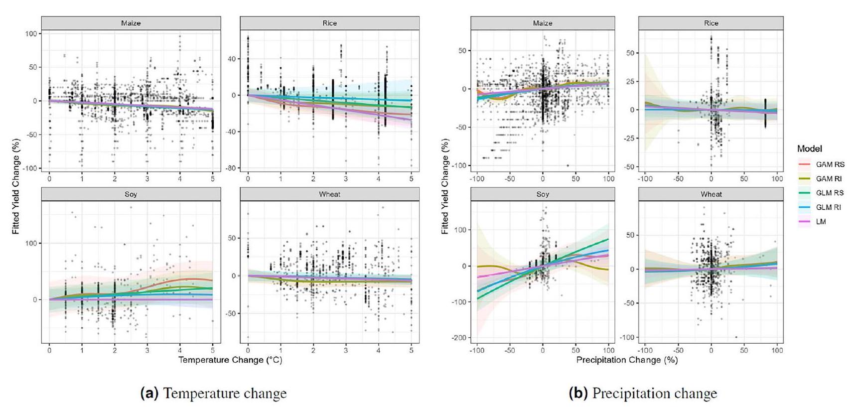
وجدنا أن دوال الاستجابة لدرجة الحرارة والعائد تميل إلى الانحدار لأسفل للذرة، الأرز والقمح، مما يشير إلى أن تأثيرات درجة الحرارة بمفردها تميل إلى أن يكون لها تأثير مخفض على العائدات (الشكل 1أ). لا يُرى هذا الاستجابة في فول الصويا. تصف دوال الاستجابة للهطول علاقة إيجابية بين التغيرات في الأمطار والعائدات لجميع المحاصيل باستثناء الأرز، وقد يكون ذلك بسبب أن الأرز يُروى في الغالب (الشكل 1ب). لأغراض التصوير، تُظهر هذه الرسوم البيانية دوال الاستجابة عند مستويات خط الأساس المتوسطة من درجة الحرارة والهطول، لكنها لا تُظهر التفاعلات بين التغيرات في درجة الحرارة والهطول، أو تركيبات من مستويات خط الأساس المختلفة مع التغيرات. ما يمكن أيضًا رؤيته من نقاط البيانات المرسومة هو تقديرات متعددة من نفس الدراسة، والتي قد تمثل تجارب فريدة تختبر الاستجابات لتركيبات من
الشكل 1. دوال الاستجابة المتوسطة الهامشية (
| محصول | نموذج | عينة | نماذج المناخ العالمية | البيانات المفقودة | مجموعة |
| ذرة | 10.9 | 8.67 | 4.52 | 8.58 | 32.7 |
| أرز | 19.3 | 12.0 | 9.46 | 12.4 | 53.1 |
| فول | 51.1 | 48.2 | 18.6 | 47.5 | 165.0 |
| قمح | 15.3 | 8.57 | 6.08 | 8.64 | 38.6 |
الجدول 1. مصادر عدم اليقين الناتجة عن اختيار النموذج، العينة، نماذج المناخ العالمية ومجموعات البيانات المعززة (البيانات المفقودة)، كما تم قياسها بواسطة متوسط الانحراف المعياري لتغير العائدات العالمية الموزونة (%). عدم اليقين المجمّع لا يضيف إلى
درجة الحرارة، والهطول وثاني أكسيد الكربون. تثير هذه الدراسات متعددة التقديرات الحاجة إلى نمذجة التأثيرات المختلطة لأخذ في الاعتبار انحياز الارتباط داخل الدراسة.
مصادر عدم اليقين
قمنا بتحديد عدم اليقين بشكل منهجي من خلال أخذ 100 عينة من البيانات باستخدام طريقة البلوك-بووتستراب ومقارنة متوسط الانحراف المعياري الناتج للاستجابات العالمية المقدرة عبر خمسة أبعاد. تشمل هذه الأبعاد: (1) 100 عينة من البلوك-بووتستراب، مع حجب حسب الدراسة حيث يتم اختيار مجموعة مختلفة من الدراسات في كل عينة (أي عدم اليقين بشأن استراتيجية العينة لتجميع مجموعة بيانات CGIAR)، (2) خمس تعويضات مختلفة لمجموعة بيانات CGIAR لملء القيم المفقودة، باستخدام معادلات التعويض المتعددة المتسلسلة (MICE، انظر قسم “الطرق”) (أي عدم اليقين بشأن معالجة البيانات المفقودة)، (3) خمسة نماذج إحصائية (أي عدم اليقين بشأن المواصفة الاقتصادية)، (4) 23 مجموعة من بيانات المدخلات لدرجة الحرارة، والهطول وثاني أكسيد الكربون من مجموعة CMIP6 من 23 نموذج مناخ عالمي، لكل من ثلاثة سيناريوهات انبعاثات (أي عدم اليقين بشأن تأثير انبعاثات الإنسان على نظام المناخ) (انظر قسم “الطرق”).
وجدنا أن عدم اليقين الناتج عن اختيار النموذج يساوي بين 10 و
الشكل 2. توزيعات التغير المتوقع في العائدات العالمية الموزونة في 2081-2100 من 575 مجموعة نماذج لكل محصول (5 مواصفات نموذجية
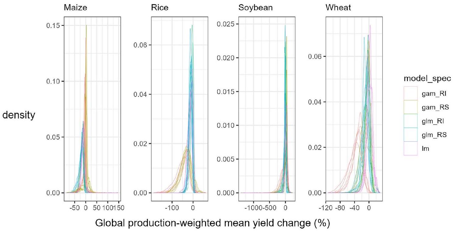
يولد نموذج OLS المجمّع توزيعًا أضيق للاستجابات المقدرة مقارنةً بكل من GLMMs للذرة، فول الصويا والقمح، ومقارنةً بنماذج GAM للأرز. وهذا يشير إلى أن عدم أخذ الارتباطات المتعلقة بالدراسة والدولة في البيانات في الاعتبار قد يؤدي إلى تقديرات منخفضة لعدم اليقين في التنبؤ.
أداء النموذج
قمنا بتقييم أداء النموذج التنبؤي من خلال إجراء اختبار التحقق المتقاطع k-fold مع عشرة طيات. وجدنا أن GAMM وGLMM مع تقاطعات عشوائية ومنحدرات عشوائية أدت أفضل أداء كما تم قياسه بواسطة الجذر التربيعي لمتوسط الخطأ (RMSE)، وأدى نموذج OLS المجمّع أسوأ أداء. الشكل 3 يُظهر ذلك جنبًا إلى جنب مع الانحراف المفسر لكل من المواصفات الخمس للنموذج (كل منها مجمعة عبر خمس تقديرات ملائمة معززة). كان أداء نموذج OLS المجمّع هو الأسوأ، مع أعلى متوسط RMSE للنموذج وأقل انحراف مفسر عبر جميع المواصفات الخمس للنموذج.
أداء نماذج GLMM و GAMM مع تقاطعات وانحدارات عشوائية أفضل مقارنة بجميع نماذج GLMM و GAMM مع تقاطعات عشوائية فقط. وهذا ليس مفاجئًا نظرًا للاختلاف الهيكلي في الدراسات عبر قاعدة بيانات CGIAR؛ مما يسمح بمتغيرات المناخ (درجة الحرارة، هطول الأمطار و
تغيرات العائد المتوقع على المستوى العالمي
استخدمنا التقديرات الملائمة من النموذج المفضل (نموذج الانحدار الخطي العام مع تقاطعات وانحدارات عشوائية) لتقدير التغيرات المستقبلية المتوقعة في العائد على
نظهر توقعات عالمية مجمعة من CMIP6 للنموذج المفضل لـ SSP5-8.5 في الشكل 4 ولـ SSP12.6 و SSP2-4.5 في الشكلين التكميلين 5 و 6. أكبر تخفيضات في العائدات تُلاحظ في الذرة، مع خسائر قدرها
الشكل 3. متوسط خطأ الجذر التربيعي للنموذج (RMSE) من التحقق المتقاطع بعشر طيات (الأعلى) والانحراف المفسر بواسطة كل نموذج (الأسفل) عبر 5 تقديرات لمجموعات البيانات المدخلة. الدوائر السوداء تظهر متوسط RMSE والانحراف المفسر الخاص بالنموذج، المحسوب عبر مجموعات البيانات المدخلة. الأسطورة: GLM RI، نموذج خطي مختلط عام (GLMM) مع تقاطعات عشوائية؛ GLM RS، GLMM مع تقاطعات ومنحدرات عشوائية؛ GAM RI، نموذج مختلط إضافي عام (GAMM) مع تقاطعات عشوائية؛ GAM RS، GAMM مع تقاطعات ومنحدرات عشوائية؛ LM، نموذج OLS مجمع.
الشرق الأوسط، أمريكا الجنوبية، وجنوب/جنوب شرق آسيا، تتفاقم على مدار القرن مع خسارة متوسطة عالمية مرجحة في العائد قدرها
الفجوة العالمية المتوقعة في سعرات الطعام
قمنا بتحويل تقديرات التغير في العائد العالمي المتوقع إلى إمدادات السعرات الحرارية الوطنية وقارناها بتقديرات الطلب الوطني على السعرات الحرارية باستخدام بيانات من منظمة الأغذية والزراعة (الفاو) وأدبيات أخرى.
قمنا أيضًا بإعادة إنتاج خرائط فجوة السعرات الحرارية باستخدام نموذج OLS المجمّع (الشكل التوضيحي 7b، d). يُظهر هذا أن العديد من البلدان تعاني من تخفيضات أقل حدة في السعرات الحرارية تحدث في وقت لاحق من القرن مقارنةً بنموذج GLMM المفضل مع تقاطعات وانحدارات عشوائية. قد يكون ذلك بسبب الدراسات متعددة التقديرات التي تحتوي على عائدات أقل حدة.
الشكل 4. التغيرات المتوقعة في العائد المستمدة من نموذج الانحدار الخطي المختلط العام (GLMM) مع تقاطعات وانحدارات عشوائية مجمعة عبر 5 نماذج تعويض و23 مجموعة بيانات توقعات GCM لنموذج SSP5-8.5، حيث تشير التظليل إلى التوزيع المكاني لإنتاج المحاصيل.
تؤثر الاستجابات على نتائج OLS المجمعة، أو لأن الاستجابات السلبية للعائدات واضحة ضمن الدراسات الفردية، ولكنها خافتة عند دمج البيانات من تلك الدراسات (أي مفارقة سيمبسون).
نقاش
نقدم مراجعة موجزة لنتائجنا في سياق الأدبيات العلمية الواسعة والعميقة التي تغطي تغير الفينولوجيا لمحاصيل الحبوب استجابةً لارتفاع درجات الحرارة وظروف الجفاف.
| محصول | سيناريو | 2021-2040 | 2041-2060 | 2061-2080 | ٢٠٨١-٢١٠٠ |
| ذرة | SSP1-2.6 | – 1.6 [- 9.0, 5.7] | – 3.3 [- 10.5, 4.0] | -4.0 [-11.2, 3.3] | -3.8 [- 11.1, 3.6] |
| SSP2-4.5 | -1.6 [-9.0, 5.7] | – 4.6 [- 11.9, 2.7] | -7.2 [-14.8, 0.4] | – 13.4 [- 17.0, – 1.2] | |
| SSP5-8.5 | – 2.0 [- 9.3, 5.3] | -6.8 [-14.3, 0.8] | -12.9 [-22.3, -4.5] | -22.2 [-34.3, -10.1] | |
| أرز | SSP1-2.6 | 0.5 [- 9.1, 10.0] | – 1.2 [- 10.8, 8.4] | – 2.2 [- 12.0, 7.5] | – 2.7 [- 12.5, 7.1] |
| SSP2-4.5 | 1.0 [- 8.5, 10.5] | – 0.9 [- 10.8, 9.0] | – 2.7 [- 13.5, 8.0] | – 4.3 [- 15.9, 7.2] | |
| SSP5-8.5 | 1.2 [- 8.4, 10.7] | – 1.8 [- 12.5, 8.9] | – 5.8 [- 19.2, 7.7] | -9.0 [-26.8, 8.8] | |
| صويا | SSP1-2.6 | 2.9 [-21.3، 27.0] | 3.3 [-20.5, 27.1] | 2.4 [- 21.5, 26.3] | 1.4 [- 22.7, 25.5] |
| SSP2-4.5 | 3.5 [-20.5, 27.5] | 5.3 [- 19.3, 30.0] | 4.4 [- 22.4, 31.2] | 2.6 [- 26.1, 31.4] | |
| SSP5-8.5 | 4.5 [- 19.7, 28.6] | 5.5 [- 21.4, 32.3] | -0.6 [-36.0, 34.8] | – 15.4 [- 69.2, 38.5] | |
| قمح | SSP1-2.6 | 1.3 [- 11.0, 13.6] | -0.4 [-12.3, 11.5] | – 1.3 [- 13.2, 10.6] | – 1.5 [- 13.5, 10.5] |
| SSP2-4.5 | 1.7 [-10.6، 13.9] | -0.7 [-12.6, 11.1] | – 3.1 [- 15.1, 9.0] | -4.9 [-17.3, 7.5] | |
| SSP5-8.5 | 1.6 [-10.6, 13.7] | – 2.4 [- 14.4, 9.7] | – 7.8 [- 21.5, 6.0] | – 14.1 [- 32.6, 4.3] |
الجدول 2. توقعات التغير في متوسط العائد الموزون عالميًا (%) من نموذج الانحدار الخطي العام المختلط (GLMM) لـ SSP1-2.6 (الأعلى)، SSP2-4.5 (الوسط) و SSP5-8.5 (الأسفل)، التقديرات المركزية بالخط العريض [فترة الثقة 95%]. الوزن بناءً على قيم إنتاج المحاصيل الموزعة على الشبكة. التقديرات تتجاهل التغيرات في المناطق غير المزروعة حاليًا.
| محصول | أكبر المنتجين | SSP1-2.6 | SS2-4.5 | SSP5-8.5 |
| ذرة | الولايات المتحدة | -6.5 [-13.3, 0.3] | – 12.6 [- 20.5, – 4.6] | -26.0 [-39.3، -12.7] |
| الصين | -4.7 [-11.7, 2.2] | – 10.1 [- 17.8, – 2.4] | -24.7 [-37.2, -12.1] | |
| البرازيل | 1.0 [- 7.5, 9.5] | – 3.0 [- 10.7, 4.7] | – 13.1 [- 22.6, – 3.7] | |
| الأرجنتين | – 0.9 [- 8.3, 6.5] | – 4.3 [- 11.6, 3.1] | – 12.1 [- 20.8, – 3.5] | |
| أرز | الصين | -5.6 [- 13.0, 1.8] | -6.1 [-15.1, 3.0] | – 9.8 [- 24.6, 5.0] |
| الهند | -7.2 [-14.1، -0.3] | – 10.2 [- 18.6, – 1.7] | – 21.3 [- 35.0, – 7.6] | |
| إندونيسيا | 7.4 [- 8.2, 23.0] | 3.7 [- 11.7, 19.1] | -6.5 [-22.5, 9.6] | |
| بنغلاديش | – 10.3 [- 19.8, – 0.7] | – 11.9 [- 22.6, – 1.2] | – 21.6 [- 36.4, – 6.9] | |
| فول الصويا | البرازيل | 0.4 [- 28.4, 29.1] | 5.4 [-20.0، 30.9] | -5.6 [-45.9, 34.8] |
| الولايات المتحدة | – 3.5 [- 22.7, 15.8] | – 6.0 [- 32.6, 20.7] | – 30.9 [- 89.1, 27.3] | |
| الصين | 1.4 [-20.7، 23.5] | 2.1 [- 25.6, 29.7] | – 17.2 [- 73.4, 39.0] | |
| الأرجنتين | 2.9 [- 17.5, 23.3] | 7.7 [- 14.0, 29.4] | 2.9 [- 28.1, 33.8] | |
| قمح | الصين | -4.0 [-12.9, 4.8] | – 5.7 [- 15.3, 3.9] | – 12.7 [- 29.2, 3.9] |
| الهند | -4.6 [-16.3, 7.1] | – 8.5 [- 20.8, 3.8] | – 21.7 [- 39.9, – 3.6] | |
| روسيا | – 1.9 [- 14.3, 10.5] | -4.9 [-17.6, 7.7] | – 13.3 [- 33.1, 6.4] | |
| الولايات المتحدة | -4.3 [-14.5, 6.0] | -7.2 [-18.1, 3.8] | – 14.4 [- 32.5, 3.6] | |
| كندا | -2.1 [- 13.0, 8.9] | -3.4 [-15.5, 8.8] | -8.1 [-31.0, 14.8] |
الجدول 3. توقعات التغير في متوسط العائد الموزون بالإنتاج للفترة 2081-2100 من نموذج الانحدار الخطي المختلط العام (GLMM) مع تقاطعات وانحدارات عشوائية لأكبر المنتجين (%) لسيناريوهات SSP1-2.6 وSSP2-4.5 وSSP5-8.5، التقديرات المركزية بالخط العريض [فترة الثقة 95%]. الوزن بقيم إنتاج المحاصيل الموزعة على الشبكة يتجاهل التغيرات في المناطق غير المزروعة حاليًا. انظر البيانات التكميلية لجميع البلدان.
مقارنةً بالتحليلات الميتا السابقة لنفس مجموعة بيانات CGIAR
تتوافق الخسائر النسبية الأكثر حدة في العائدات للذرة مقارنة بالقمح مع تحليلات مقارنة أخرى في الأدبيات.
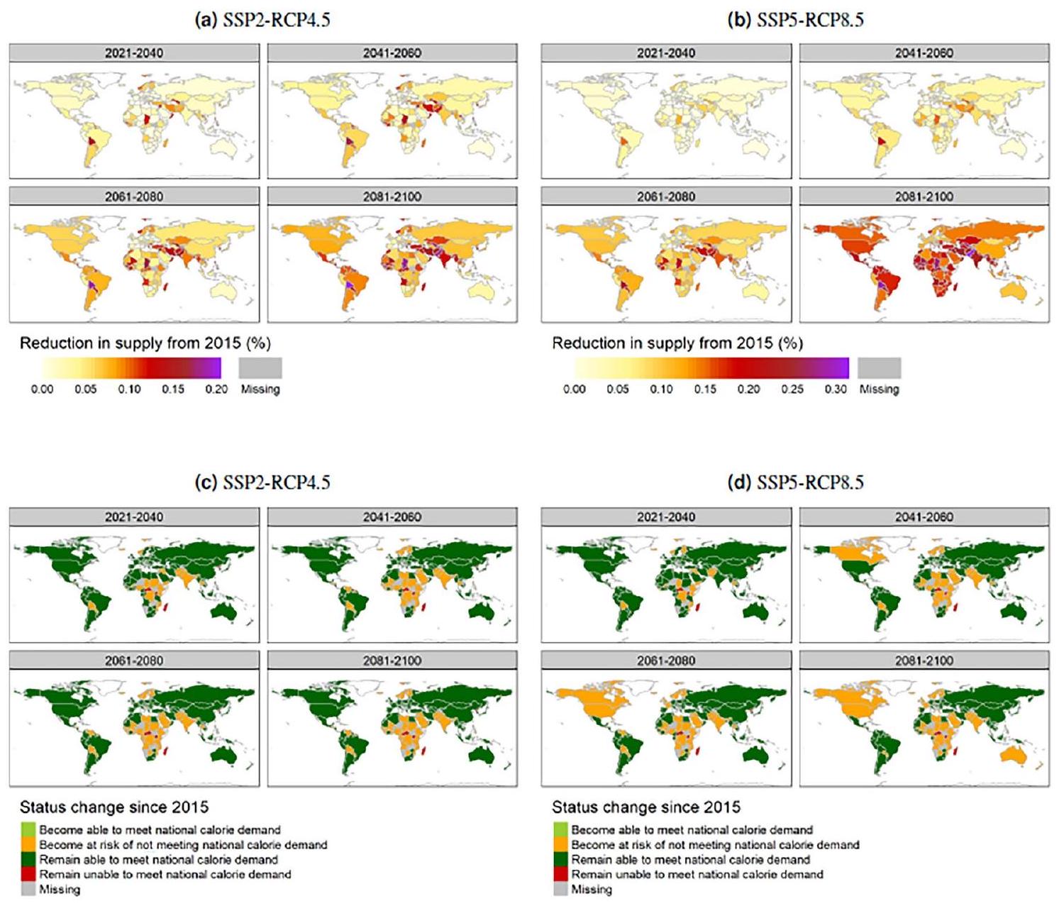
الشكل 5. الآثار المترتبة على الأمن الغذائي المقدرة من نموذج الانحدار الخطي العام المختلط (GLMM) مع تقاطعات وانحدارات عشوائية. الأعلى: انخفاض في إجمالي إمدادات الغذاء بالسعرات الحرارية بالنسبة لخط الأساس لعام 2015 (%) لـ SSP24.5 (أ) و SSP5-8.5 (ب). الأسفل: تغيير في خطر عدم تلبية الطلب الوطني على السعرات الحرارية من الإنتاج والواردات لـ SSP2-4.5 (ج) و SSP5-8.5 (د). الخرائط لـ SSP1-2.6 موجودة في الشكل التكميلية 7.
أصول الذرة في مناطق أقل محدودية بالمياه مقارنة بالقمح الذي نشأ في المناطق الجافة. وبالتالي، اكتسب القمح صفات التكيف بما في ذلك تأخير الشيخوخة، والتي يمكن أن تكون مفيدة في الجفاف المتأخر في الموسم، بالإضافة إلى أنظمة جذرية أعمق للوصول إلى مياه التربة تحت السطحية.
خسائر محصول الأرز أكبر مما تم تقديره في التحليلات الميتا السابقة باستخدام نفس مجموعة بيانات CGIAR، ومن المتوقع هنا أن تنخفض الغلات في أفريقيا وأمريكا الجنوبية وأستراليا حتى نهاية القرن استجابةً لارتفاع درجات الحرارة. وهذا يتماشى مع الفهم العلمي لتأثير إجهاد درجات الحرارة العالية على حبوب لقاح الأرز، والخصوبة، وغلة الحبوب.
تحمل الإجهاد الحراري حول الإزهار (مقارنة بالذرة والقمح) ولكن أيضًا تحملها لدرجات الحرارة المنخفضة. يمكن رؤية ذلك في دراسات مماثلة تتنبأ بوجود مناطق عديدة ذات غلات منخفضة كما هو الحال مع المناطق ذات الغلات المرتفعة، لا سيما في الولايات المتحدة والبرازيل.
تحمل الإجهاد الحراري حول الإزهار (مقارنة بالذرة والقمح) ولكن أيضًا تحملها لدرجات الحرارة المنخفضة. يمكن رؤية ذلك في دراسات مماثلة تتنبأ بوجود مناطق عديدة ذات غلات منخفضة كما هو الحال مع المناطق ذات الغلات المرتفعة، لا سيما في الولايات المتحدة والبرازيل.
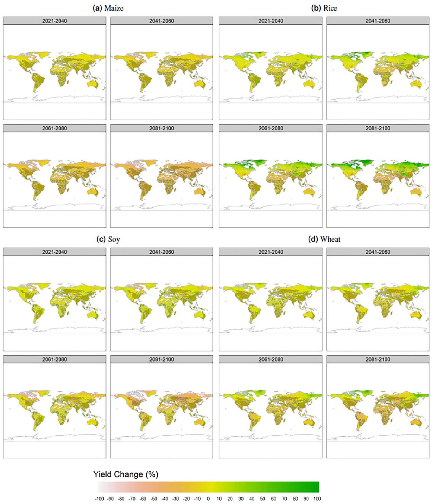
تظهر خرائطنا للتغيرات المتوقعة في غلة المحاصيل العالمية الموزعة على الشبكة زيادة في ملاءمة زراعة الأرز والقمح في خطوط العرض والارتفاعات الشمالية، وانخفاض في الملاءمة تقريبًا في كل مكان آخر (انظر الشكل 4). وهذا يتماشى مع دراسات أخرى تظهر زيادة الملاءمة في شمال أوروبا لمحاصيل القمح المعتمدة على الأمطار بسبب التغيرات في هطول الأمطار ودرجة الحرارة.
تسلط نتائجنا الضوء على تغير توزيع المحاصيل بسبب تغير أنماط درجات الحرارة وهطول الأمطار، ومع ذلك فإنها تغفل آثار ارتفاع مستوى سطح البحر، والملوحة، وضغط المياه الناتج عن استخدامات الأراضي المتنافسة
تقديراتنا، التي تأخذ في الاعتبار التغيرات في المعايير متعددة العقود، لا تلتقط أيضًا بالكامل آثار درجات الحرارة المتغيرة والمتطرفة وأحداث هطول الأمطار. هناك أدلة تشير إلى أن المحاصيل قد تكون أكثر حساسية لمناخ متغير بشكل كبير على كوكب أكثر دفئًا في المتوسط مقارنة بمناخ يتغير تدريجيًا
لقد وجدنا أن تخفيضات في إمدادات السعرات الحرارية تتراوح بين 15 و
من المحتمل أن تتأثر جودة المغذيات بتغير المناخ، ولكن لم يكن من الممكن تضمينها في هذا التحليل. تظهر الأبحاث آثارًا مختلطة لزيادة CO2، ودرجات الحرارة، والملوحة، والفيضانات، وضغط الجفاف على تراكم المغذيات في التربة، حيث تعتمد الآثار بشكل كبير على المغذيات، ونبات المحاصيل، ومستوى شدة التغيير
أخيرًا، قمنا بالتحقيق في مصادر عدم اليقين التي تساهم في التباين حول استجابات الغلة العالمية المقدرة. وجدنا أن عدم اليقين الناتج عن اختيار النموذج هو الأكثر أهمية مقارنة بعدم اليقين الناتج عن العينة، والبيانات المفقودة، ونماذج المناخ العالمية. فيما يتعلق بعدم اليقين الناتج عن اختيار النموذج، قد لا تكون توقعات نماذج التجميع هي أفضل طريقة لتمثيل هذا التباين حيث أظهرت بعض النماذج أنها تتفوق على الأخرى. لقد اخترنا مواصفة نموذج التأثيرات المختلطة التي نعتقد أنها تحقق أفضل توازن بين الأداء التنبؤي والتكيف المفرط مع البيانات. نشعر بالراحة لرؤية توافق كامل للنموذج عبر العديد من المناطق في متوسط علامة توقعات الغلة المستقبلية لجميع المحاصيل باستثناء فول الصويا، على الرغم من أن هذه المناطق من التوافق لا تتداخل بالضرورة مع الأماكن التي تزرع فيها المحاصيل حاليًا (الشكل التكميلي 9). يعكس عدم اليقين الناتج عن نماذج المناخ العالمية عدم اليقين بشأن تأثير انبعاثات البشر على نظام المناخ. بينما يمكن توضيح هذا عدم اليقين العميق من خلال تضمين مجموعة من نماذج CMIP6 كمدخلات لنمذجة تأثير المناخ، قد لا تمثل مجموعات النماذج العينة الكاملة أو النظامية لاستجابة المناخ
(على الرغم من أن عدم اليقين الناتج عن نماذج المناخ العالمية لا يزال مهمًا)
(على الرغم من أن عدم اليقين الناتج عن نماذج المناخ العالمية لا يزال مهمًا)
تظل تحذيرات كبيرة بشأن النهج الذي اتخذناه في النمذجة الإحصائية هنا. ربما الأهم من ذلك، أن نقل الوظيفة يفترض ضمنيًا أن معلمات الوظيفة المقدرة في مواقع الدراسة تنتقل عبر الزمن والمكان
الخاتمة
في هذه الدراسة، استخدمنا التحليل الإحصائي الشامل لتناسب نماذج التأثيرات المختلطة لاستجابة إنتاج المحاصيل لتغير المناخ باستخدام قاعدة بيانات معتمدة. قمنا بتناسب خمسة مواصفات نموذجية وقدمنا تقديرات لتغيرات الإنتاج المستقبلية باستخدام توقعات درجات الحرارة وهطول الأمطار حتى عام 2100 من مجموعة CMIP6 المكونة من 23 نموذجًا من نماذج المناخ العالمية. استخدمنا هذه التقديرات لحساب إمدادات السعرات الحرارية الوطنية وقارناها بمقاييس الطلب على السعرات الحرارية لفهم آثارها على الأمن الغذائي العالمي. يقدر نموذجنا المفضل أن الإنتاج العالمي قد يتغير عن مستويات عام 2015 بـ
طرق
الأهداف والنطاق
قمنا بإجراء تحليل ميتا إحصائي لفهم التأثيرات المحتملة للمناخ على غلات المحاصيل وبالتالي الحصول على تقديرات للعجز المحتمل في السعرات الحرارية تحت ثلاثة سيناريوهات انبعاثات حتى نهاية القرن. للقيام بذلك، قمنا بتطبيق خمسة نماذج مختلفة بما في ذلك نماذج التأثيرات المختلطة لأخذ الارتباطات داخل وبين الدراسات في الاعتبار، وقمنا بتحديد الحجم النسبي لعدم اليقين الناتج عن اختيار النموذج، والعينة، والبيانات المفقودة، ونماذج المناخ العالمية من مجموعة CMIP6. قمنا بتحويل التغير المتوقع في الغلة الذي تم تقديره بواسطة النموذج المختلط المفضل إلى مقاييس للإمداد الوطني من السعرات الحرارية وقارناها بمقاييس الطلب على السعرات الحرارية لفهم التأثيرات المستقبلية على الأمن الغذائي.
البيانات، الاستخراج والفحص
تشمل بيانات CGIAR 13,890 تقديرًا نقطيًا لتغير العائد، وتغير درجة الحرارة،
تم إدخالها بشكل خاطئ، واستبدلناها بالقيم الصحيحة من الدراسات. كما تحققنا من أن أي قيم مفقودة مسجلة في مجموعة بيانات CGIAR كانت قيمًا مفقودة حقيقية (أي ليست قيم صفرية).
تم إدخالها بشكل خاطئ، واستبدلناها بالقيم الصحيحة من الدراسات. كما تحققنا من أن أي قيم مفقودة مسجلة في مجموعة بيانات CGIAR كانت قيمًا مفقودة حقيقية (أي ليست قيم صفرية).
درجات الحرارة وهطول الأمطار خلال موسم النمو الأساسي
لتقدير درجات حرارة موسم النمو الأساسية المحددة بالموقع، اعتمدنا على البيانات الشهرية العالمية
تقدير البيانات
من بين 8846 تقديرًا نقطيًا في بيانات CGIAR، كانت هناك العديد من القيم للمتغيرات الرئيسية التي كانت مهمة نظريًا لنمذجة استجابة محصول المحاصيل لتغير درجة الحرارة مفقودة. وشملت هذه التغير في درجة الحرارة، وتغير هطول الأمطار،
توافق النموذج
قمنا بتناسب 5 نماذج مرشحة لكل محصول على حدة مع تغيير نسبة العائد كمتغير استجابة: نموذج OLS، ونموذجان GLMM، ونموذجان GAMM، كل منهما تم تناسبه مع تقاطعات عشوائية فقط (RI) ومع تقاطعات ومنحدرات عشوائية (RS).
أكثر نماذج التحديد تعقيدًا (التي تشمل تقاطعات وانحدارات عشوائية) تسمح بتغير درجة الحرارة، وتغير هطول الأمطار و
المعلمات المضمنة:
قمنا بتشغيل هذه النماذج الخمسة المختلفة على كل من مجموعات البيانات الخمسة المعوضة، مما أسفر عن 25 مجموعة من التقديرات الملائمة لكل محصول. ثم قمنا بتطبيقها على 23 مجموعة من بيانات التنبؤ التي تحتوي على جميع مصطلحات النموذج، بما في ذلك درجة الحرارة، والهطول و
تنبؤ النموذج
قمنا بإنشاء بيانات التنبؤ لكل من مصطلحات النموذج. تم تقدير درجات حرارة موسم النمو الأساسية وهطول الأمطار باستخدام نفس النهج المستخدم لحساب المتغير في مجموعة البيانات الرئيسية، ولكن لعام 2015 (الشكل التوضيحي 4). تم استرجاع قيم درجات الحرارة وهطول الأمطار الموزعة على الشبكة للفترات 2021-2040، 2041-2060، 2061-2080 و2081-2100 من 23 مجموعة بيانات GCM المصححة من الانحياز من WorldClim لنماذج SSP1-2.6، SSP2-4.5 وSSP5-8.5 عند
للعالمية
توقعنا تأثيرات العائدات العالمية الموزعة عبر كل من الفترات الزمنية الأربع باستخدام 5 تقديرات ملائمة مستنتجة.
لا تتطلب دوال الاستجابة المودلة وتقديرات الملاءمة المتوقعة أن تمر عبر الأصل (مما يعني وجود تقاطع غير صفري)، ومع ذلك تتطلب النظرية عدم وجود تغيير في العائد مع عدم وجود تغيير في درجة الحرارة.
تقييم عدم اليقين
قمنا بتحديد أربعة مصادر مختلفة من عدم اليقين الناشئة عن اختيار النموذج، وأخذ العينات، والبيانات المفقودة، وتنوع النماذج المتعددة في CMIP6 عبر نماذج GCM، وفقًا للنهج في المرجع.
قمنا بتوصيف عدم اليقين الناتج عن اختيار النموذج من خلال تثبيت مجموعة البيانات المعززة بالتعويض، وعينة البوتستراب، وبيانات مخرجات نموذج المناخ العالمي المستخدمة، مع تغيير مواصفات النموذج وحساب متوسط الانحراف المعياري في التغير العالمي في العائدات الموزونة عبر مواصفات النموذج. قمنا بتوصيف المصادر الأخرى لعدم اليقين بنفس الطريقة.
فجوة السعرات الحرارية في الغذاء
قمنا بتقدير إمدادات السعرات الحرارية وطلب السعرات الحرارية باستخدام بيانات منظمة الأغذية والزراعة حول إنتاج الدول على نطاق واسع، وكميات الاستيراد والتصدير، ونسبة المحاصيل المخصصة للغذاء، ومتطلبات الطاقة اليومية المتوسطة، والسعرات الحرارية من الطاقة المقدمة إلى نظام الغذاء حسب المحصول والدولة، وأنماط التجارة التفصيلية (انظر قسم “الطرق”).
لتقدير الإنتاج الأساسي في عام 2015 من الذرة والأرز وفول الصويا والقمح بالأطنان حسب البلد، قمنا بضرب المساحات المحصودة (هكتار) في الغلات المحصودة (طن/هكتار) في مجموعة بيانات مكانية بدقة 5 دقائق.
تفترض هذه الخطوات أن حصة الصادرات من إنتاج البلاد وحصة الشركاء في التصدير تظل ثابتة في المستقبل. نستخدم بيانات عن مساحة الأراضي المحصودة.
لتقدير الطلب الأساسي على السعرات الحرارية في عام 2015 حسب البلد، ضربنا متوسط الاحتياجات اليومية من الطاقة لكل فرد (ADER) على مدار 2014-2016 في أرقام السكان من FAOSTAT.
توفر البيانات
البيانات والرموز المستخدمة في هذا التحليل متاحة علىhttps://github.com/christineklli/global-yield-impacts. تم تقديم تأثيرات العائدات المودلة للبلدان كبيانات تكملية.
تاريخ الاستلام: 22 مايو 2023؛ تاريخ القبول: 15 يناير 2025
تم النشر عبر الإنترنت: 22 يناير 2025
تم النشر عبر الإنترنت: 22 يناير 2025
References
- Roson, R. & Sartori, M. Estimation of climate change damage functions for 140 regions in the GTAP 9 data base. J. Glob. Econ. Anal. 1(2), 78-115 (2016).
- Newell, R. G., Prest, B. C. & Sexton, S. E. The GDP-temperature relationship: Implications for climate change damages. J. Environ. Econ. Manag. 108, 102445 (2021).
- Liu, B. et al. Similar estimates of temperature impacts on global wheat yield by three independent methods. Nat. Clim. Change 6, 1130-1136 (2016).
- Challinor, A. J. et al. A meta-analysis of crop yield under climate change and adaptation. Nat. Clim. Change 4, 287-291 (2014).
- Kopp, R., Hsiang, S. & Oppenheimer, M. Empirically calibrating damage functions and considering stochasticity when integrated assessment models are used as decision tools. Impacts World 2013, International Conference on Climate Change Effects 12 (2013).
- Tol, R. S. J. The economic effects of climate change. J. Econ. Perspect. 23, 29-51 (2009).
- Tol, R. S. J. Correction and update: The economic effects of climate change. J. Econ. Perspect. 28, 221-226 (2014).
- Wang, X. et al. Emergent constraint on crop yield response to warmer temperature from field experiments. Nat. Sustain. 3, 908-916 (2020).
- Whetton, P. H., Grose, M. R. & Hennessy, K. J. A short history of the future: Australian climate projections 1987-2015. Clim. Serv. 2-3, 1-14 (2016).
- Nelson, J. P. & Kennedy, P. E. The use (and abuse) of meta-analysis in environmental and natural resource economics: An assessment. Environ. Resour. Econ. 42, 345-377 (2009).
- Howard, P. H. & Sterner, T. Few and not so far between: A meta-analysis of climate damage estimates. Environ. Resour. Econ. 68, 197-225 (2017).
- Moore, F. C., Baldos, U. L. C., Hertel, T. W. & Diaz, D. New science of climate change impacts on agriculture implies higher social cost of carbon. Nat. Commun. 9, 1 (2017).
- CGIAR. Agriculture Impacts. https://web.archive.org/web/20211204202518/; http://www.ag-impacts.org/ (2021).
- FAOSTAT. Food Balance Sheets. https://www.fao.org/faostat/en/#data/FBS (2023).
- Bell, A., Fairbrother, M. & Jones, K. Fixed and random effects models: Making an informed choice. Qual. Quant. 53, 1051-1074 (2019).
- Asseng, S., Foster, I. & Turner, N. C. The impact of temperature variability on wheat yields. Glob. Change Biol. 17, 997-1012 (2011).
- Porter, J. R. & Semenov, M. A. Crop responses to climatic variation. Philos. Trans. R. Soc. B Biol. Sci. 360, 2021-2035 (2005).
- Semenov, M. & Porter, J. Climatic variability and the modelling of crop yields. Agric. For. Meteorol. 73, 265-283 (1995).
- Moriondo, M., Giannakopoulos, C. & Bindi, M. Climate change impact assessment: The role of climate extremes in crop yield simulation. Clim. Change 104, 679-701 (2011).
- Springer, C. J. & Ward, J. K. Flowering time and elevated atmospheric CO 2. New Phytol. 176, 243-255 (2007).
- Wheeler, T. R., Craufurd, P. Q., Ellis, R. H., Porter, J. R. & Vara Prasad, P. Temperature variability and the yield of annual crops. Agric. Ecosyst. Environ. 82, 159-167 (2000).
- Rosenzweig, C., Iglesius, A., Yang, X. B., Epstein, P. & Chivian, E. Climate Change and Extreme Weather Events-Implications for Food Production, Plant Diseases, and Pests (NASA Publications, 2001).
- Hatfield, J. L. & Prueger, J. H. Temperature extremes: Effect on plant growth and development. Weather Clim. Extremes 10, 4-10 (2015).
- Craufurd, P. Q. & Wheeler, T. R. Climate change and the flowering time of annual crops. J. Exp. Bot. 60, 2529-2539 (2009).
- Lobell, D. B., Sibley, A. & Ivan Ortiz-Monasterio, J. Extreme heat effects on wheat senescence in India. Nat. Clim. Change 2, 186-189 (2012).
- Lobell, D. B., Baldos, U. L. C. & Hertel, T. W. Climate adaptation as mitigation: The case of agricultural investments. Environ. Res. Lett. 8, 015012 (2013).
- Masson-Delmotte, V. et al. IPCC, 2021: Summary for policymakers. In Climate Change 2021: The Physical Science Basis. Contribution of Working Group I to the Sixth Assessment Report of the Intergovernmental Panel on Climate Change (2021).
- Riahi, K. et al. The shared socioeconomic pathways and their energy, land use, and greenhouse gas emissions implications: An overview. Glob. Environ. Change 42, 153-168 (2017).
- FAOSTAT. Detailed Trade Matrix. https://www.fao.org/faostat/en/#data/TM (2023).
- Cassidy, E. S., West, P. C., Gerber, J. S. & Foley, J. A. Redefining agricultural yields: From tonnes to people nourished per hectare. Environ. Res. Lett. 8, 034015 (2013).
- Grogan, D., Frolking, S., Wisser, D., Prusevich, A. & Glidden, S. Global gridded crop harvested area, production, yield, and monthly physical area data circa 2015. Sci. Data 9, 15 (2022).
- Kc, S. & Lutz, W. The human core of the shared socioeconomic pathways: Population scenarios by age, sex and level of education for all countries to 2100. Glob. Environ. Change 42, 181-192 (2017).
- Tilman, D., Balzer, C., Hill, J. & Befort, B. L. Global food demand and the sustainable intensification of agriculture. Proc. Natl. Acad. Sci. 108, 20260-20264 (2011).
- Ivanovich, C. C., Sun, T., Gordon, D. R. & Ocko, I. B. Future warming from global food consumption. Nat. Clim. Change 1, 1-6 (2023).
- Ray, D. K. & Foley, J. A. Increasing global crop harvest frequency: Recent trends and future directions. Environ. Res. Lett. 8, 044041 (2013).
- Fahad, S. et al. Crop production under drought and heat stress: Plant responses and management options. Front. Plant Sci. 8, 1 (2017).
- Daryanto, S., Wang, L. & Jacinthe, P.-A. Global synthesis of drought effects on maize and wheat production. PLoS ONE 11, e0156362 (2016).
- Marothia, D. et al. Abiotic Stress in Plants (IntechOpen, 2020).
- Costa, M. V. J. D. et al. Combined drought and heat stress in rice: Responses, phenotyping and strategies to improve tolerance. Rice Sci. 28, 233-242 (2021).
- Hussain, H. A. et al. Interactive effects of drought and heat stresses on morpho-physiological attributes, yield, nutrient uptake and oxidative status in maize hybrids. Sci. Rep. 9, 3890 (2019).
- Jumrani, K. & Bhatia, V. S. Interactive effect of temperature and water stress on physiological and biochemical processes in soybean. Physiol. Mol. Biol. Plants 25, 667-681 (2019).
- Ostmeyer, T. et al. Impacts of heat, drought, and their interaction with nutrients on physiology, grain yield, and quality in field crops. Plant Physiol. Rep. 25, 549-568 (2020).
- Iqbal, M. M., Arif, M. & Khan, A. M. Climate Change Aspersions on Food Security of Pakistan 11 (2009).
- Lobell, D. B. & Burke, M. B. Why are agricultural impacts of climate change so uncertain? The importance of temperature relative to precipitation. Environ. Res. Lett. 3, 034007 (2008).
- Hausfather, Z. Explainer: What climate models tell us about future rainfall. Carbon Brief. https://www.carbonbrief.org/explaine r-what-climate-models-tell-us-about-future-rainfall/ (2022).
- Deryng, D., Conway, D., Ramankutty, N., Price, J. & Warren, R. Global crop yield response to extreme heat stress under multiple climate change futures. Environ. Res. Lett. 9, 034011 (2014).
- Hatfield, J. L. et al. Climate impacts on agriculture: Implications for crop production. Agron. J. 103, 351-370 (2011).
- FAOSTAT. Crops and Livestock Products. https://www.fao.org/faostat/en/#data/QCL (2023).
- Fahad, S. et al. Consequences of high temperature under changing climate optima for rice pollen characteristics-concepts and perspectives. Arch. Agron. Soil Sci. 64, 1473-1488 (2018).
- Fahad, S. et al. A combined application of biochar and phosphorus alleviates heat-induced adversities on physiological, agronomical and quality attributes of rice. Plant Physiol. Biochem. 103, 191-198 (2016).
- Bradford, J. B. et al. Future soil moisture and temperature extremes imply expanding suitability for rainfed agriculture in temperate drylands. Sci. Rep. 7, 12923 (2017).
- Tuninetti, M., Ridolfi, L. & Laio, F. Ever-increasing agricultural land and water productivity: A global multi-crop analysis. Environ. Res. Lett. 15, 09402 (2020).
- Gerten, D. et al. Global water availability and requirements for future food production. J. Hydrometeorol. 12, 885-899 (2011).
- Billen, G. et al. Reshaping the European agro-food system and closing its nitrogen cycle: The potential of combining dietary change, agroecology, and circularity. One Earth 4, 839-850 (2021).
- World-Bank. Water in Agriculture World Bank. https://www.worldbank.org/en/topic/water-in-agriculture (2023).
- Elliott, J. et al. Constraints and potentials of future irrigation water availability on agricultural production under climate change. Proc. Natl. Acad. Sci. 111, 3239-3244 (2014).
- Rosa, L. et al. Potential for sustainable irrigation expansion in a
C warmer climate. Proc. Natl. Acad. Sci. 117, 29526-29534 (2020). - Wisser, D. et al. Global irrigation water demand: Variability and uncertainties arising from agricultural and climate data sets. Geophys. Res. Lett. 35, 1 (2008).
- Ortiz-Bobea, A., Ault, T. R., Carrillo, C. M., Chambers, R. G. & Lobell, D. B. Anthropogenic climate change has slowed global agricultural productivity growth. Nat. Clim. Change 11, 306-312 (2021).
- WRI. Resource Watch Aqueduct Stress Projections. https://resourcewatch.org/data/explore (2023).
- Luck, M., Landis, M. & Gassert, F. Aqueduct Water Stress Projections: Decadal Projections of Water Supply and Demand Using CMIP5 GCMs 20 (2015).
- Puy, A., LoPiano, S. & Saltelli, A. Current models underestimate future irrigated areas. Geophys. Res. Lett. 47, e2020087360 (2020).
- Vanschoenwinkel, J. & Van Passel, S. Climate response of rainfed versus irrigated farms: The bias of farm heterogeneity in irrigation. Clim. Change 147, 225-234 (2018).
- Kompas, T., Che, T. N. & Grafton, R. Q. The Impact of Water and Heat Stress from Global Warming on Agricultural Productivity and Food Security (Global Commission on the Economics of Water, 2023).
- Roy, S., Chowdhury, N., Roy, S. & Chowdhury, N. Abiotic Stress in Plants (IntechOpen, 2020).
- Uçarlı, C. Abiotic Stress in Plants (IntechOpen, 2020).
- Fahad, S. et al. Phytohormones and plant responses to salinity stress: A review. Plant Growth Regul. 75, 391-404 (2015).
- Lal, M. Implications of climate change in sustained agricultural productivity in South Asia. Reg. Environ. Change 11, 79-94 (2011).
- Soares, J. C., Santos, C. S., Carvalho, S. M. P., Pintado, M. M. & Vasconcelos, M. W. Preserving the nutritional quality of crop plants under a changing climate: Importance and strategies. Plant Soil 443, 1-26 (2019).
- De Vries, W., Kros, J., Kroeze, C. & Seitzinger, S. P. Assessing planetary and regional nitrogen boundaries related to food security and adverse environmental impacts. Curr. Opin. Environ. Sustain. 5, 392-402 (2013).
- MacDonald, G. K., Bennett, E. M., Potter, P. A. & Ramankutty, N. Agronomic phosphorus imbalances across the world’s croplands. Proc. Natl. Acad. Sci. 108, 3086-3091 (2011).
- Zhang, C. et al. The role of nitrogen management in achieving global sustainable development goals. Resour. Conserv. Recycl. 201, 107304 (2024).
- Gu, B. et al. Cost-effective mitigation of nitrogen pollution from global croplands. Nature 613, 77-84 (2023).
- Qiao, L. et al. Assessing the contribution of nitrogen fertilizer and soil quality to yield gaps: A study for irrigated and rainfed maize in China. Field Crops Res. 273, 108304 (2021).
- Vanlauwe, B. & Dobermann, A. Sustainable intensification of agriculture in sub-Saharan Africa: First things first. Front. Agric. Sci. Eng. 7, 376-382 (2020).
- Cassman, K. G. & Dobermann, A. Nitrogen and the future of agriculture: 20 years on. Ambio 51, 17-24 (2022).
- Zhang, X. et al. Managing nitrogen for sustainable development. Nature 528, 51-59 (2015).
- Zhang, X. et al. Quantifying nutrient budgets for sustainable nutrient management. Glob. Biogeochem. Cycles 34, e2018006060 (2020).
- Juroszek, P. & von Tiedemann, A. Linking plant disease models to climate change scenarios to project future risks of crop diseases: A review. J. Plant Dis. Prot. 122, 3-15 (2015).
- Bradshaw, C. et al. Climate change in pest risk assessment: Interpretation and communication of uncertainties. EPPO Bull. 54, 4-19 (2024).
- Giorgi, F. Thirty years of regional climate modeling: Where are we and where are we going next? J. Geophys. Res. Atmos. 124, 5696-5723 (2019).
- Hawkins, E. & Sutton, R. The potential to narrow uncertainty in regional climate predictions. Bull. Am. Meteorol. Soc. 90, 10951108 (2009).
- Czajkowski, M. & ŠčasnÃý, M. Study on benefit transfer in an international setting. How to improve welfare estimates in the case of the countries’ income heterogeneity? Ecol. Econ. 69, 2409-2416 (2010).
- Muleke, A., Harrison, M. T., Yanotti, M. & Battaglia, M. Yield gains of irrigated crops in Australia have stalled: The dire need for adaptation to increasingly volatile weather and market conditions. Curr. Res. Environ. Sustain. 4, 100192 (2022).
- Ciscar, J.-C., Fisher-Vanden, K. & Lobell, D. B. Synthesis and review: An inter-method comparison of climate change impacts on agriculture. Environ. Res. Lett. 13, 070401 (2018).
- Lobell, D. B., Thau, D., Seifert, C., Engle, E. & Little, B. A scalable satellite-based crop yield mapper. Remote Sens. Environ. 164, 324-333 (2015).
- Roberts, M. J., Braun, N. O., Sinclair, T. R., Lobell, D. B. & Schlenker, W. Comparing and combining process-based crop models and statistical models with some implications for climate change. Environ. Res. Lett. 12, 095010 (2017).
- Moore, F. C., Baldos, U. L. C. & Hertel, T. Economic impacts of climate change on agriculture: A comparison of process-based and statistical yield models. Environ. Res. Lett. 12, 065008 (2017).
- Harris, I., Osborn, T. J., Jones, P. & Lister, D. Version 4 of the CRU TS monthly high-resolution gridded multivariate climate dataset. Sci. Data 7, 109 (2020).
- Sacks, W. J., Deryng, D., Foley, J. A. & Ramankutty, N. Crop planting dates: An analysis of global patterns. Glob. Ecol. Biogeogr. 19, 607-620 (2010).
- Portmann, F. T., Siebert, S. & Döll, P. MIRCA2000-Global monthly irrigated and rainfed crop areas around the year 2000: A new high-resolution data set for agricultural and hydrological modeling. Glob. Biogeochem. Cycles 24, 1 (2010).
- Monfreda, C., Ramankutty, N. & Foley, J. A. Farming the planet: 2. Geographic distribution of crop areas, yields, physiological types, and net primary production in the year 2000. Glob. Biogeochem. Cycles 22, 1 (2008).
- Graham, J. W. Missing data analysis: Making it work in the real world. Annu. Rev. Psychol. 60, 549-576 (2009).
- Schafer, J. L. & Graham, J. W. Missing data: Our view of the state of the art. Missing Data 31, 1 (2002).
- Van Buuren, S. & Groothuis-Oudshoorn, K. Mice: Multivariate imputation by chained equations in R. J. Stat. Softw. 67, 1 (2011).
- Yucel, R. M. Multiple imputation inference for multivariate multilevel continuous data with ignorable non-response. Philos. Trans. Ser. A Math. Phys. Eng. Sci. 366, 2389-2403 (2008).
- Heymans, M. W. & Eekhout, I. Applied Missing Data Analysis with SPSS and (R)Studio (2019).
- Schomaker, M. & Heumann, C. Model selection and model averaging after multiple imputation. Comput. Stat. Data Anal. 71, 758-770 (2014).
- Wood, S. N. Generalized Additive Models: An introduction with R 397 (2017).
- Harrer, M., Cuijpers, P., Furukawa, T. A. & Ebert, D. D. Doing Meta-analysis in R (2021).
- WorldClim. Future Climate, 10 Minutes Spatial Resolution—WorldClim 1 Documentation. https://www.worldclim.org/data/cmip 6/cmip6_clim10m.html (2023).
- KNMI, C.E. Monthly CMIP5 Scenario Runs. https://climexp.knmi.nl/start.cgi (2023).
- US Department of Commerce, N. Global Monitoring Laboratory—Carbon Cycle Greenhouse Gases. https://gml.noaa.gov/ccgg/tre nds/data.html (2023).
- White, I. R., Royston, P. & Wood, A. M. Multiple imputation using chained equations: Issues and guidance for practice. Stat. Med. 30, 377-399 (2011).
- Rubin, D. B. & Schenker, N. Multiple Imputation for Interval Estimation from Simple Random Samples with Ignorable Nonresponse 10 (1986).
- Fischer, E. M., Sedláěek, J., Hawkins, E. & Knutti, R. Models agree on forced response pattern of precipitation and temperature extremes. Geophys. Res. Lett. 41, 8554-8562 (2014).
- Wilcox, J. & Makowski, D. A meta-analysis of the predicted effects of climate change on wheat yields using simulation studies. Field Crop Res. 156, 180-190 (2014).
الشكر والتقدير
تم تمويل C.L. من قبل مركز التميز لتحليل مخاطر الأمن الحيوي. نشكر J. Baumgartner على تقديم نصائح برمجية.
مساهمات المؤلفين
A.R. وC.L. وJ.C. وT.K. تصوروا التحليل، قامت C.L. بإجراء التحليل وكتبت المسودة الأصلية. راجع جميع المؤلفين وحرروا المخطوطة.
الإعلانات
المصالح المتنافسة
يعلن المؤلفون عدم وجود مصالح متنافسة.
معلومات إضافية
المعلومات التكميلية النسخة عبر الإنترنت تحتوي على مواد تكميلية متاحة علىhttps://doi.org/1
يجب توجيه المراسلات وطلبات المواد إلى C.L.
معلومات إعادة الطبع والتصاريح متاحة علىwww.nature.com/reprints.
ملاحظة الناشر تظل Springer Nature محايدة فيما يتعلق بالمطالبات القضائية في الخرائط المنشورة والانتماءات المؤسسية.
يجب توجيه المراسلات وطلبات المواد إلى C.L.
معلومات إعادة الطبع والتصاريح متاحة علىwww.nature.com/reprints.
ملاحظة الناشر تظل Springer Nature محايدة فيما يتعلق بالمطالبات القضائية في الخرائط المنشورة والانتماءات المؤسسية.
الوصول المفتوح هذه المقالة مرخصة بموجب رخصة المشاع الإبداعي للاستخدام غير التجاري، والتي تسمح بأي استخدام غير تجاري، ومشاركة، وتوزيع، وإعادة إنتاج في أي وسيلة أو صيغة، طالما أنك تعطي الائتمان المناسب للمؤلفين الأصليين والمصدر، وتوفر رابطًا لرخصة المشاع الإبداعي، وتوضح إذا قمت بتعديل المادة المرخصة. ليس لديك إذن بموجب هذه الرخصة لمشاركة المواد المعدلة المشتقة من هذه المقالة أو أجزاء منها. الصور أو المواد الأخرى من طرف ثالث في هذه المقالة مشمولة في رخصة المشاع الإبداعي للمقالة، ما لم يُذكر خلاف ذلك في سطر ائتمان للمادة. إذا لم تكن المادة مشمولة في رخصة المشاع الإبداعي للمقالة واستخدامك المقصود غير مسموح به بموجب اللوائح القانونية أو يتجاوز الاستخدام المسموح به، ستحتاج إلى الحصول على إذن مباشرة من صاحب حقوق الطبع والنشر. لعرض نسخة من هذه الرخصة، قم بزيارةhttp://creativecommo ns.org/licenses/by-nc-nd/4.0/.
© المؤلفون 2025
© المؤلفون 2025
مدرسة العلوم الحيوية، مركز التميز لتحليل مخاطر الأمن الحيوي، جامعة ملبورن، ملبورن 3010، أستراليا. مدرسة الرياضيات والإحصاء، جامعة ملبورن، ملبورن 3010، أستراليا. مدرسة الزراعة، علوم الغذاء والبيئة، جامعة ملبورن، ملبورن 3010، أستراليا. البريد الإلكتروني:christinel3@unimelb.edu.au
Journal: Scientific Reports, Volume: 15, Issue: 1
DOI: https://doi.org/10.1038/s41598-025-87047-y
PMID: https://pubmed.ncbi.nlm.nih.gov/39843615
Publication Date: 2025-01-22
DOI: https://doi.org/10.1038/s41598-025-87047-y
PMID: https://pubmed.ncbi.nlm.nih.gov/39843615
Publication Date: 2025-01-22
scientific reports
OPEN
Predicting changes in agricultural yields under climate change scenarios and their implications for global food security
Climate change has direct impacts on current and future agricultural productivity. Statistical metaanalysis models can be used to generate expectations of crop yield responses to climatic factors by pooling data from controlled experiments. However, methodological challenges in performing these meta-analyses, together with combined uncertainty from various sources, make it difficult to validate model results. We present updates to published estimates of crop yield responses to projected temperature, precipitation, and CO2 patterns and show that mixed effects models perform better than pooled OLS models on root mean squared error (RMSE) and explained deviance, despite the common usage of pooled OLS in previous meta-analyses. Based on our analysis, the use of pooled OLS may underestimate yield losses. We also use a block-bootstrapping approach to quantify uncertainty across multiple dimensions, including modeler choices, climate projections from the sixth Coupled Model Intercomparison Project (CMIP6), and emissions scenarios from Shared Socioeconomic Pathways (SSP). Our estimates show projected yield responses of –
Climate change is expected to directly impact agricultural production by reducing both crop yield and quality via changing patterns in temperature, water, gases and nutrients. Moreover, changing climate can also have indirect impacts on yields by altering impacts caused by pests, diseases and weeds. Statistical models of crop yield response to climate change can be estimated using data from controlled experiments. These models can be used to generate expectations of climate impacts in new settings such as future time periods or geographies with relatively scarce primary studies
helpful for modellers to clarify these ambiguities, which we do in this study. Going further, the trajectory of global economic development and the effect of human emissions on earth systems and climate is often referred to as irreducibly uncertain, where more information may not necessarily reduce this uncertainty
Our study has three objectives: (1) to improve the estimation of yield responses to climatic factors such as temperature, precipitation and CO2, using data from an established crop yield response database (CGIAR data), (2) to decompose the range of uncertainty in resulting predictions into its separate sources, and (3) to provide policy-relevant estimates related to global food security. Our goal was to provide a comprehensive yet up to date estimation of global climate yield responses while also considering implications for food security and associated uncertainty under a greater set of emissions scenarios and time periods. First, we hypothesised that fitting mixed models to the CGIAR dataset would help to account for within-study correlation between multiple estimates in the dataset, resulting in better statistical model performance compared to pooled OLS models used in previous meta-analyses of the same dataset
Results
Modelled yield response functions
We began by refreshing the CGIAR database with screening and imputation of missing data
We fit statistical models for each crop separately (see “Methods” section for full specifications). Our five candidate models are: (1) Ordinary Least Squares (OLS) pooled model, (2) Generalised Linear Mixed Model (GLMM) with random intercepts, (3) GLMM with random intercepts and random slopes, (4) Generalised Additive Mixed Model (GAMM) with random intercepts and (5) GAMM with random intercepts and random slopes, plotted in Fig. 1. Model 1 is a pooled OLS model which treats point estimates from the same study and country as though they are independent, and are similar to the OLS models used in previous published metaanalysis on the same CGIAR dataset
We found that fitted temperature-yield response functions are downward sloping for maize, rice and wheat, suggesting that temperature effects in isolation tend to have a yield-reducing effect on crops (Fig. 1a). This response is not seen in soybean. Precipitation-response functions describe a positive relationship between changes in rainfall and yields for all crops except rice, the latter may be due to rice being mostly irrigated (Fig. 1b). For visualisation purposes, these plots show response functions at the median baseline levels of temperature and precipitation, but do not show interactions between changes in temperature and precipitation, or combinations of different baseline levels with changes. What can also be seen from the plotted data points are multiple estimates from the same study, which may represent unique experiments testing responses to combinations of
Fig. 1. Marginal mean response functions (
| Crop | Model | Sampling | GCMs | Missing data | Combined |
| Maize | 10.9 | 8.67 | 4.52 | 8.58 | 32.7 |
| Rice | 19.3 | 12.0 | 9.46 | 12.4 | 53.1 |
| Soy | 51.1 | 48.2 | 18.6 | 47.5 | 165.0 |
| Wheat | 15.3 | 8.57 | 6.08 | 8.64 | 38.6 |
Table 1. Sources of uncertainty attributable to model choice, sampling, GCMs and imputation-augmented datasets (missing data), as measured by the average standard deviation of global production-weighted yield change (%). Combined uncertainty does not add to
temperature, precipitation and CO2. These multi-estimate studies raise the need for mixed effects modelling to account for correlation bias within-study.
Sources of uncertainty
We systematically quantified uncertainty by block-bootstrapping 100 samples of the data and comparing the resulting average standard deviation of estimated global yield responses across five dimensions. These dimensions span: (1) 100 block-bootstrap samples, blocking by study where a different set of studies are selected in each sample (i.e. uncertainty regarding the sampling strategy to compile the CGIAR dataset), (2) five different imputations of the CGIAR dataset to fill in missing values, using Multiple Imputation Chained Equations (MICE, see “Methods” section) (i.e. uncertainty regarding treatment of missing data), (3) five statistical models (i.e. uncertainty regarding the econometric specification), (4) 23 sets of temperature, precipitation and CO2 input data from the CMIP6 ensemble of 23 GCMs, for each of three emissions scenario (i.e. uncertainty regarding the effect of human emissions on the climate system) (see “Methods” section).
We found that uncertainty from model choice is equal to between 10 and
Fig. 2. Distributions of predicted global production-weighted mean yield change in 2081-2100 from 575 model combinations for each crop ( 5 model specifications
The pooled OLS model generates a narrower distribution of estimated responses compared to both GLMMs for maize, soy and wheat, and compared to GAM models for rice. This suggests that not accounting for study- and country-related correlations in the data may result in underestimates of prediction uncertainty.
Model performance
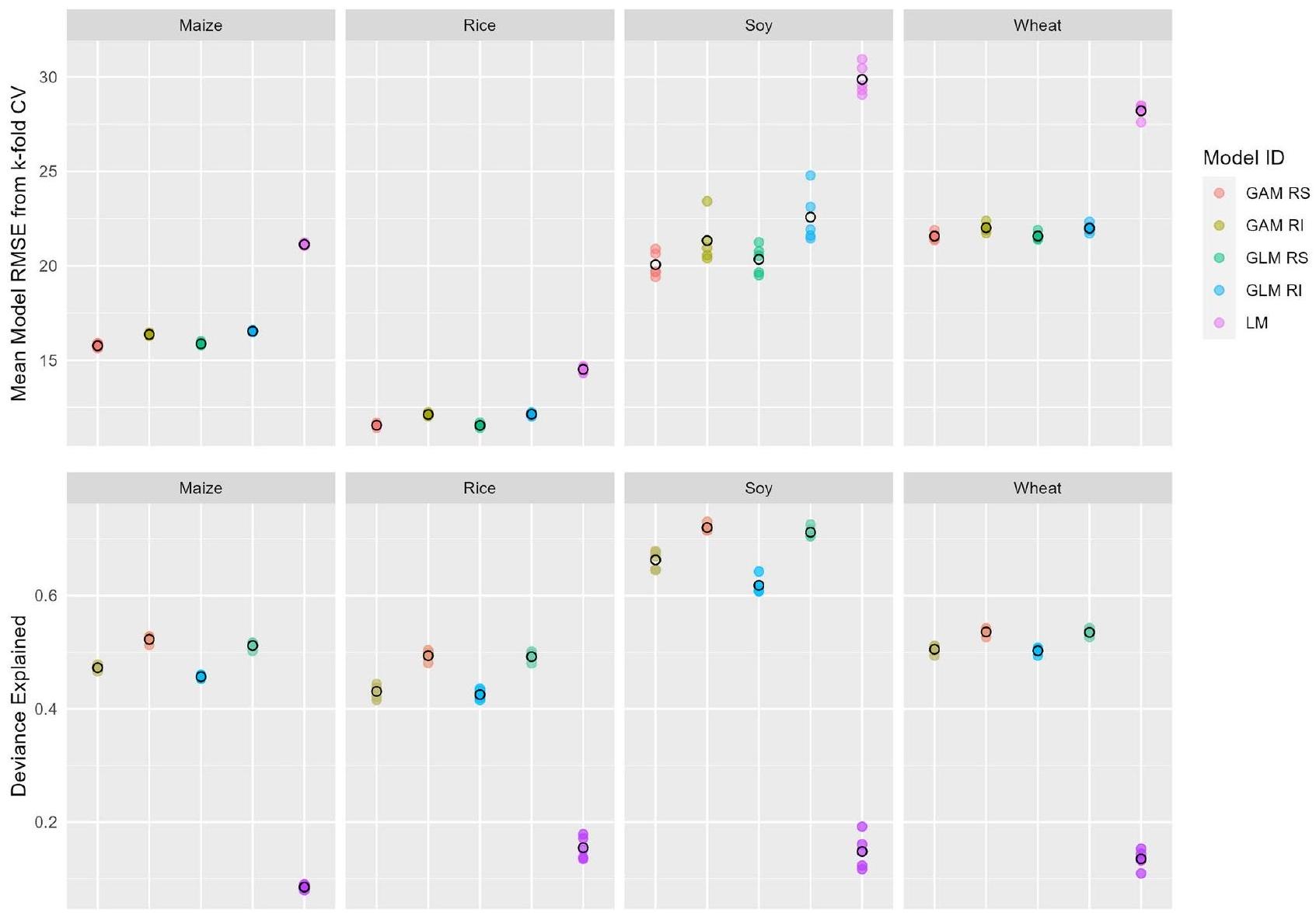
We evaluated model predictive performance by running k -fold cross validation with tenfolds. We found the GAMM and GLMM with random intercepts and random slopes performed best as measured by Root Mean Squared Error (RMSE), and the pooled OLS model performed the worst. Figure 3 shows this alongside explained deviance for each of the five model specifications (each pooled across five imputed fit estimates). The pooled OLS model fit performed the worst, with the highest mean model RMSE and least explained deviance across all five model specifications.
GLMM and GAMM models with random intercepts and slopes performed better compared to all the GLMM and GAMM models with random intercepts only. This is unsurprising given the structural variation in studies across the CGIAR database; allowing climate variables (temperature, precipitation and
Global future projected yield changes
We used fitted estimates from the preferred model (GLMM with random intercepts and slopes) to estimate future projected yield changes on a
We show CMIP6-ensembled global predictions for the preferred model for SSP5-8.5 in Fig. 4 and for SSP12.6 and SSP2-4.5 in Supp. Fig. 5 and 6. The largest yield reductions are seen in maize, with losses of
Fig. 3. Model root mean squared error (RMSE) from tenfold cross validation (top) and deviance explained by each model (bottom) across 5 imputed dataset fit estimates. Black circles show model-specific mean RMSE and explained deviance, calculated across imputed datasets. Legend: GLM RI, Generalised Linear Mixed Model (GLMM) with random intercepts; GLM RS, GLMM with random intercepts and slopes; GAM RI, Generalised Additive Mixed Model (GAMM) with random intercepts; GAM RS, GAMM with random intercepts and slopes; LM, pooled OLS model.
the Middle East, South America, and South/South East Asia, worsening over the century with a global weighted mean yield loss of
Global projected food calorie gap
We converted projected global yield change estimates into national calorie supply and compared them to estimates of national calorie demand using data from the FAO and other literature
We also replicated calorie gap maps using the pooled OLS model (Supp. Fig. 7b,d). This shows many countries experiencing less severe calorie reductions occurring later in the century compared to the preferred GLMM model with random intercepts and slopes. This could be because multi-estimate studies with less severe yield
Fig. 4. Predicted yield changes derived from Generalised Linear Mixed Model (GLMM) with random intercepts and slopes pooled across 5 imputation models and 23 GCM prediction datasets for SSP5-8.5, shading indicates spatial distribution of crop production c.
responses are biasing the pooled OLS results, or because negative yield responses are apparent within individual studies, but muted when data from those studies are combined (i.e. Simpson’s paradox).
Discussion
We offer a brief review of our results in the context of the broad and deep scientific literature covering the changing phenology of grain crops in response to elevated heat and drought conditions
| Crop | Scenario | 2021-2040 | 2041-2060 | 2061-2080 | 2081-2100 |
| Maize | SSP1-2.6 | – 1.6 [- 9.0, 5.7] | – 3.3 [- 10.5, 4.0] | -4.0 [- 11.2, 3.3] | -3.8 [- 11.1, 3.6] |
| SSP2-4.5 | -1.6 [-9.0, 5.7] | – 4.6 [- 11.9, 2.7] | -7.2 [-14.8, 0.4] | – 13.4 [- 17.0, – 1.2] | |
| SSP5-8.5 | – 2.0 [- 9.3, 5.3] | -6.8 [- 14.3, 0.8] | -12.9 [-22.3, -4.5] | -22.2 [- 34.3, – 10.1] | |
| Rice | SSP1-2.6 | 0.5 [- 9.1, 10.0] | – 1.2 [- 10.8, 8.4] | – 2.2 [- 12.0, 7.5] | – 2.7 [- 12.5, 7.1] |
| SSP2-4.5 | 1.0 [- 8.5, 10.5] | – 0.9 [- 10.8, 9.0] | – 2.7 [- 13.5, 8.0] | – 4.3 [- 15.9, 7.2] | |
| SSP5-8.5 | 1.2 [- 8.4, 10.7] | – 1.8 [- 12.5, 8.9] | – 5.8 [- 19.2, 7.7] | -9.0 [- 26.8, 8.8] | |
| Soy | SSP1-2.6 | 2.9 [- 21.3, 27.0] | 3.3 [- 20.5, 27.1] | 2.4 [- 21.5, 26.3] | 1.4 [- 22.7, 25.5] |
| SSP2-4.5 | 3.5 [- 20.5, 27.5] | 5.3 [- 19.3, 30.0] | 4.4 [- 22.4, 31.2] | 2.6 [- 26.1, 31.4] | |
| SSP5-8.5 | 4.5 [- 19.7, 28.6] | 5.5 [- 21.4, 32.3] | -0.6 [-36.0, 34.8] | – 15.4 [- 69.2, 38.5] | |
| Wheat | SSP1-2.6 | 1.3 [- 11.0, 13.6] | -0.4 [-12.3,11.5] | – 1.3 [- 13.2, 10.6] | – 1.5 [- 13.5, 10.5] |
| SSP2-4.5 | 1.7 [- 10.6, 13.9] | -0.7 [-12.6,11.1] | – 3.1 [- 15.1, 9.0] | -4.9 [- 17.3, 7.5] | |
| SSP5-8.5 | 1.6 [- 10.6, 13.7] | – 2.4 [- 14.4, 9.7] | – 7.8 [- 21.5, 6.0] | – 14.1 [- 32.6, 4.3] |
Table 2. Global production-weighted mean yield change (%) projections from Generalised Linear Mixed Model (GLMM) for SSP1-2.6 (top), SSP2-4.5 (middle) and SSP5-8.5 (bottom), central estimates bolded [95% confidence interval]. Weighting by gridded crop production values. Estimates ignore changes in areas not currently under cultivation.
| Crop | Largest producers | SSP1-2.6 | SS2-4.5 | SSP5-8.5 |
| Maize | US | -6.5 [-13.3, 0.3] | – 12.6 [- 20.5, – 4.6] | -26.0 [-39.3, -12.7] |
| China | -4.7 [- 11.7, 2.2] | – 10.1 [- 17.8, – 2.4] | -24.7 [- 37.2, – 12.1] | |
| Brazil | 1.0 [- 7.5, 9.5] | – 3.0 [- 10.7, 4.7] | – 13.1 [- 22.6, – 3.7] | |
| Argentina | – 0.9 [- 8.3, 6.5] | – 4.3 [- 11.6, 3.1] | – 12.1 [- 20.8, – 3.5] | |
| Rice | China | -5.6 [- 13.0, 1.8] | -6.1 [- 15.1, 3.0] | – 9.8 [- 24.6, 5.0] |
| India | -7.2 [- 14.1, – 0.3] | – 10.2 [- 18.6, – 1.7] | – 21.3 [- 35.0, – 7.6] | |
| Indonesia | 7.4 [- 8.2, 23.0] | 3.7 [- 11.7, 19.1] | -6.5 [- 22.5, 9.6] | |
| Bangladesh | – 10.3 [- 19.8, – 0.7] | – 11.9 [- 22.6, – 1.2] | – 21.6 [- 36.4, – 6.9] | |
| Soybean | Brazil | 0.4 [- 28.4, 29.1] | 5.4 [- 20.0, 30.9] | -5.6 [- 45.9, 34.8] |
| US | – 3.5 [- 22.7, 15.8] | – 6.0 [- 32.6, 20.7] | – 30.9 [- 89.1, 27.3] | |
| China | 1.4 [- 20.7, 23.5] | 2.1 [- 25.6, 29.7] | – 17.2 [- 73.4, 39.0] | |
| Argentina | 2.9 [- 17.5, 23.3] | 7.7 [- 14.0, 29.4] | 2.9 [- 28.1, 33.8] | |
| Wheat | China | -4.0 [- 12.9, 4.8] | – 5.7 [- 15.3, 3.9] | – 12.7 [- 29.2, 3.9] |
| India | -4.6 [- 16.3, 7.1] | – 8.5 [- 20.8, 3.8] | – 21.7 [- 39.9, – 3.6] | |
| Russia | – 1.9 [- 14.3, 10.5] | -4.9 [- 17.6, 7.7] | – 13.3 [- 33.1, 6.4] | |
| US | -4.3 [- 14.5, 6.0] | -7.2 [- 18.1, 3.8] | – 14.4 [- 32.5, 3.6] | |
| Canada | -2.1 [- 13.0, 8.9] | -3.4 [- 15.5, 8.8] | -8.1 [- 31.0, 14.8] |
Table 3. Production-weighted mean yield change projections for 2081-2100 from generalised linear mixed model (GLMM) random intercepts and slopes model for largest producers (%) for SSP1-2.6, SS2-4.5 and SS5-8.5, central estimates bolded [95% confidence interval]. Weighting by gridded crop production values ignores changes in areas not currently under cultivation. See supplementary data for all countries.
Compared to previous meta-analyses of the same CGIAR dataset
The relatively more severe yield losses for maize compared to wheat aligns with other comparative analyses in the literature. Reference
Fig. 5. Food security implications estimated from Generalised Linear Mixed Model (GLMM) with random intercepts and slopes. Top: Reduction in total supply of food in calories relative to 2015 baseline (%) for SSP24.5 (a) and SSP5-8.5 (b). Bottom: Change in risk of not meeting national calorie demand from production and imports for SSP2-4.5 (c) and SSP5-8.5 (d). Maps for SSP1-2.6 are in Supp. Fig. 7.
origins of maize in less water-limited regions compared to wheat originating in dryland regions. Wheat has thus acquired adaptability traits including delayed senescence which can be useful for late-season drought, as well as deeper root systems to access sub-surface soil water
Rice yield losses are larger than what has been estimated in previous meta-analyses using the same CGIAR dataset, and here yields are expected to decline in Africa, South America and Australia through to the end of the century in response to higher temperatures. This aligns with scientific understanding of the impact of high temperature stress on rice pollen, fertility and grain yield
tolerance to heat stress around anthesis (compared to maize and wheat) but also its lower limit temperature tolerance. This can be seen in similar studies predicting as many areas with decreased yields as there are with increased yields, particularly in the USA and Brazil
tolerance to heat stress around anthesis (compared to maize and wheat) but also its lower limit temperature tolerance. This can be seen in similar studies predicting as many areas with decreased yields as there are with increased yields, particularly in the USA and Brazil
Our maps of projected global gridded yield changes show expanding suitability for rice and wheat in the northern latitudes and elevations and declining suitability nearly everywhere else (see Fig. 4). This accords with other studies showing growing suitability in northern Europe for rainfed wheat crops due to changes in rainfall and temperature
Our results shed light on shifting crop distributions due to changing temperature and precipitation patterns, however it misses the effects of sea level rise, salinity and water stress from competing land uses
Our estimates, which consider changes in multi-decadal norms, also do not fully capture the effects of variable and extreme temperatures and rainfall events. There is evidence suggesting that crops may be more sensitive to a highly variable climate on a warmer planet on average than to a climate that changes gradually
We have found that reductions in calorie supply of between 15 and
Nutrient quality is highly likely to be affected by climate change, but was not possible to include in this analysis. Research shows mixed effects of elevated CO2, temperature, salinity, waterlogging and drought stress on nutrient accumulation in soils, with effects being highly dependent on the nutrient, crop plant and intensity level of change
Finally, we have interrogated the sources of uncertainty contributing to variance around estimated global yield responses. We found that uncertainty from model choice is most significant compared to uncertainty from sampling, missing data and GCMs. Regarding model choice uncertainty, ensembling model predictions may not be the best way to represent this variation since some models were shown to outperform others. We have chosen the mixed effects model specification that we believe best achieves the trade-off between predictive performance and over-fitting the data. We are comforted by seeing full model agreement across many regions in the mean sign of future yield projections for all crops except for soy, though these areas of agreement do not necessarily overlap with where crops are currently grown (Supp. Fig. 9). Uncertainty from GCMs reflects uncertainty about the effect of human emissions on the climate system. While this deep uncertainty can be clarified by including a range of CMIP6 models as inputs to climate impact modelling, model ensembles may not represent the complete or systematic sample of the climate response
dominates (though GCM uncertainty remains significant)
dominates (though GCM uncertainty remains significant)
Significant caveats remain on the approach we have taken to statistical modelling here. Perhaps most significantly, function transfer implicitly assumes that estimated function parameters at study sites transfer across time and space
Conclusion
In this study, we used statistical meta-analysis to fit mixed effects models of crop yield responses to climate change using an established database. We fit five model specifications and estimated future yield changes using temperature and precipitation projections to 2100 from a CMIP6 ensemble of 23 GCMs. We used these estimates to calculate national calorie supply and compared them to measures of calorie demand to understand their implications for global food security. Our preferred model estimates that global yields may change from 2015 levels by
Methods
Objectives and scope
We performed statistical meta-analysis to understand potential climate impacts on crop yields and thus obtain estimates of potential calorie deficits under three emissions scenarios to the end of the century. To do this we fitted five model specifications including mixed effects models to account for correlation within and between studies, and quantified the relative magnitude of uncertainty attributable to model choice, sampling, missing data and GCMs from the CMIP6 ensemble. We converted projected yield change estimated by the preferred mixed model into measures of national calorie supply and compared them against measures of calorie demand to understand future impacts on food security.
Data, extraction and screening
CGIAR data includes 13,890 point estimates of yield change, temperature change,
mis-entered, and replaced them with correct values from the studies. We also verified that any missing values recorded in the CGIAR dataset were true missing values (i.e., not zero values).
mis-entered, and replaced them with correct values from the studies. We also verified that any missing values recorded in the CGIAR dataset were true missing values (i.e., not zero values).
Baseline growing-season temperatures and precipitation
To estimate location-specific baseline growing-season temperatures, we drew on global monthly
Data imputation
Of the 8846 point estimates in the CGIAR data, many values for key variables that were theoretically important for modelling crop yield responses to temperature change were missing. These included temperature change, precipitation change,
Model fitting
We fit 5 candidate models for each crop separately with percentage yield change as the response variable: OLS model, two GLMM and two GAMM models each fit with random intercepts only (RI) and with random intercepts and slopes (RS)
The most complex model specification (that includes random intercepts and slopes) allows temperature change, precipitation change and
Included parameters:
We ran these five different model specifications on each of the five imputed datasets, yielding 25 combinations of fitted estimates per crop. We then fit these to 23 sets of prediction data containing all model terms, including temperature, precipitation and
Model prediction
We created prediction data for each of the model terms. Baseline growing-season temperatures and precipitation were estimated using the same approach used to calculate the variable in the main data set, but for 2015 (Supp. Fig. 4). Gridded temperature and precipitation values for 2021-2040, 2041-2060, 2061-2080 and 2081-2100 were retrieved from 23 WorldClim bias-corrected CMIP6 GCM datasets for SSP1-2.6, SSP2-4.5 and SSP5-8.5 at a
For global
We predicted global gridded yield impacts across each of the four time periods using 5 imputed fit estimates
Modelled response functions and predicted fit estimates do not necessarily go through the origin (meaning a non-zero intercept exists), yet theory requires zero yield change with zero temperature change
Evaluating uncertainty
We quantified four different sources of uncertainty arising from model choice, sampling, missing data and CMIP6 multi-model variation across GCMs, following the approach in Ref.
We characterised uncertainty from model choice by holding constant the imputation-augmented dataset, bootstrap sample and GCM output data used, varying the model specification and calculating the average standard deviation in global weighted yield change across model specifications. We characterised the other sources of uncertainty in the same way.
Food calorie gap
We estimated calorie supply and calorie demand using FAO data on country-scale production, import and export quantities and the share of crops allocated to food, average daily energy requirements, calories of energy supplied to the food system by crop and country, and detailed trade patterns (see “Methods” section)
To estimate baseline production in the year 2015 of maize, rice, soy and wheat in tons by country, we multiplied gridded hectares harvested (ha) by gridded yields (t/ha) in a spatial dataset with 5 -min resolution
These steps assume that the export share of country production and export partner share remain fixed in the future. We use data on harvested area data c.
To estimate baseline calorie demand in the year 2015 by country, we multiplied annual per capita average daily energy requirements (ADER) averaged over 2014-2016 by population figures from FAOSTAT
Data availability
Data and code used for this analysis are provided at https://github.com/christineklli/global-yield-impacts. Mod elled country yield impacts are provided as Supplementary Data.
Received: 22 May 2023; Accepted: 15 January 2025
Published online: 22 January 2025
Published online: 22 January 2025
References
- Roson, R. & Sartori, M. Estimation of climate change damage functions for 140 regions in the GTAP 9 data base. J. Glob. Econ. Anal. 1(2), 78-115 (2016).
- Newell, R. G., Prest, B. C. & Sexton, S. E. The GDP-temperature relationship: Implications for climate change damages. J. Environ. Econ. Manag. 108, 102445 (2021).
- Liu, B. et al. Similar estimates of temperature impacts on global wheat yield by three independent methods. Nat. Clim. Change 6, 1130-1136 (2016).
- Challinor, A. J. et al. A meta-analysis of crop yield under climate change and adaptation. Nat. Clim. Change 4, 287-291 (2014).
- Kopp, R., Hsiang, S. & Oppenheimer, M. Empirically calibrating damage functions and considering stochasticity when integrated assessment models are used as decision tools. Impacts World 2013, International Conference on Climate Change Effects 12 (2013).
- Tol, R. S. J. The economic effects of climate change. J. Econ. Perspect. 23, 29-51 (2009).
- Tol, R. S. J. Correction and update: The economic effects of climate change. J. Econ. Perspect. 28, 221-226 (2014).
- Wang, X. et al. Emergent constraint on crop yield response to warmer temperature from field experiments. Nat. Sustain. 3, 908-916 (2020).
- Whetton, P. H., Grose, M. R. & Hennessy, K. J. A short history of the future: Australian climate projections 1987-2015. Clim. Serv. 2-3, 1-14 (2016).
- Nelson, J. P. & Kennedy, P. E. The use (and abuse) of meta-analysis in environmental and natural resource economics: An assessment. Environ. Resour. Econ. 42, 345-377 (2009).
- Howard, P. H. & Sterner, T. Few and not so far between: A meta-analysis of climate damage estimates. Environ. Resour. Econ. 68, 197-225 (2017).
- Moore, F. C., Baldos, U. L. C., Hertel, T. W. & Diaz, D. New science of climate change impacts on agriculture implies higher social cost of carbon. Nat. Commun. 9, 1 (2017).
- CGIAR. Agriculture Impacts. https://web.archive.org/web/20211204202518/; http://www.ag-impacts.org/ (2021).
- FAOSTAT. Food Balance Sheets. https://www.fao.org/faostat/en/#data/FBS (2023).
- Bell, A., Fairbrother, M. & Jones, K. Fixed and random effects models: Making an informed choice. Qual. Quant. 53, 1051-1074 (2019).
- Asseng, S., Foster, I. & Turner, N. C. The impact of temperature variability on wheat yields. Glob. Change Biol. 17, 997-1012 (2011).
- Porter, J. R. & Semenov, M. A. Crop responses to climatic variation. Philos. Trans. R. Soc. B Biol. Sci. 360, 2021-2035 (2005).
- Semenov, M. & Porter, J. Climatic variability and the modelling of crop yields. Agric. For. Meteorol. 73, 265-283 (1995).
- Moriondo, M., Giannakopoulos, C. & Bindi, M. Climate change impact assessment: The role of climate extremes in crop yield simulation. Clim. Change 104, 679-701 (2011).
- Springer, C. J. & Ward, J. K. Flowering time and elevated atmospheric CO 2. New Phytol. 176, 243-255 (2007).
- Wheeler, T. R., Craufurd, P. Q., Ellis, R. H., Porter, J. R. & Vara Prasad, P. Temperature variability and the yield of annual crops. Agric. Ecosyst. Environ. 82, 159-167 (2000).
- Rosenzweig, C., Iglesius, A., Yang, X. B., Epstein, P. & Chivian, E. Climate Change and Extreme Weather Events-Implications for Food Production, Plant Diseases, and Pests (NASA Publications, 2001).
- Hatfield, J. L. & Prueger, J. H. Temperature extremes: Effect on plant growth and development. Weather Clim. Extremes 10, 4-10 (2015).
- Craufurd, P. Q. & Wheeler, T. R. Climate change and the flowering time of annual crops. J. Exp. Bot. 60, 2529-2539 (2009).
- Lobell, D. B., Sibley, A. & Ivan Ortiz-Monasterio, J. Extreme heat effects on wheat senescence in India. Nat. Clim. Change 2, 186-189 (2012).
- Lobell, D. B., Baldos, U. L. C. & Hertel, T. W. Climate adaptation as mitigation: The case of agricultural investments. Environ. Res. Lett. 8, 015012 (2013).
- Masson-Delmotte, V. et al. IPCC, 2021: Summary for policymakers. In Climate Change 2021: The Physical Science Basis. Contribution of Working Group I to the Sixth Assessment Report of the Intergovernmental Panel on Climate Change (2021).
- Riahi, K. et al. The shared socioeconomic pathways and their energy, land use, and greenhouse gas emissions implications: An overview. Glob. Environ. Change 42, 153-168 (2017).
- FAOSTAT. Detailed Trade Matrix. https://www.fao.org/faostat/en/#data/TM (2023).
- Cassidy, E. S., West, P. C., Gerber, J. S. & Foley, J. A. Redefining agricultural yields: From tonnes to people nourished per hectare. Environ. Res. Lett. 8, 034015 (2013).
- Grogan, D., Frolking, S., Wisser, D., Prusevich, A. & Glidden, S. Global gridded crop harvested area, production, yield, and monthly physical area data circa 2015. Sci. Data 9, 15 (2022).
- Kc, S. & Lutz, W. The human core of the shared socioeconomic pathways: Population scenarios by age, sex and level of education for all countries to 2100. Glob. Environ. Change 42, 181-192 (2017).
- Tilman, D., Balzer, C., Hill, J. & Befort, B. L. Global food demand and the sustainable intensification of agriculture. Proc. Natl. Acad. Sci. 108, 20260-20264 (2011).
- Ivanovich, C. C., Sun, T., Gordon, D. R. & Ocko, I. B. Future warming from global food consumption. Nat. Clim. Change 1, 1-6 (2023).
- Ray, D. K. & Foley, J. A. Increasing global crop harvest frequency: Recent trends and future directions. Environ. Res. Lett. 8, 044041 (2013).
- Fahad, S. et al. Crop production under drought and heat stress: Plant responses and management options. Front. Plant Sci. 8, 1 (2017).
- Daryanto, S., Wang, L. & Jacinthe, P.-A. Global synthesis of drought effects on maize and wheat production. PLoS ONE 11, e0156362 (2016).
- Marothia, D. et al. Abiotic Stress in Plants (IntechOpen, 2020).
- Costa, M. V. J. D. et al. Combined drought and heat stress in rice: Responses, phenotyping and strategies to improve tolerance. Rice Sci. 28, 233-242 (2021).
- Hussain, H. A. et al. Interactive effects of drought and heat stresses on morpho-physiological attributes, yield, nutrient uptake and oxidative status in maize hybrids. Sci. Rep. 9, 3890 (2019).
- Jumrani, K. & Bhatia, V. S. Interactive effect of temperature and water stress on physiological and biochemical processes in soybean. Physiol. Mol. Biol. Plants 25, 667-681 (2019).
- Ostmeyer, T. et al. Impacts of heat, drought, and their interaction with nutrients on physiology, grain yield, and quality in field crops. Plant Physiol. Rep. 25, 549-568 (2020).
- Iqbal, M. M., Arif, M. & Khan, A. M. Climate Change Aspersions on Food Security of Pakistan 11 (2009).
- Lobell, D. B. & Burke, M. B. Why are agricultural impacts of climate change so uncertain? The importance of temperature relative to precipitation. Environ. Res. Lett. 3, 034007 (2008).
- Hausfather, Z. Explainer: What climate models tell us about future rainfall. Carbon Brief. https://www.carbonbrief.org/explaine r-what-climate-models-tell-us-about-future-rainfall/ (2022).
- Deryng, D., Conway, D., Ramankutty, N., Price, J. & Warren, R. Global crop yield response to extreme heat stress under multiple climate change futures. Environ. Res. Lett. 9, 034011 (2014).
- Hatfield, J. L. et al. Climate impacts on agriculture: Implications for crop production. Agron. J. 103, 351-370 (2011).
- FAOSTAT. Crops and Livestock Products. https://www.fao.org/faostat/en/#data/QCL (2023).
- Fahad, S. et al. Consequences of high temperature under changing climate optima for rice pollen characteristics-concepts and perspectives. Arch. Agron. Soil Sci. 64, 1473-1488 (2018).
- Fahad, S. et al. A combined application of biochar and phosphorus alleviates heat-induced adversities on physiological, agronomical and quality attributes of rice. Plant Physiol. Biochem. 103, 191-198 (2016).
- Bradford, J. B. et al. Future soil moisture and temperature extremes imply expanding suitability for rainfed agriculture in temperate drylands. Sci. Rep. 7, 12923 (2017).
- Tuninetti, M., Ridolfi, L. & Laio, F. Ever-increasing agricultural land and water productivity: A global multi-crop analysis. Environ. Res. Lett. 15, 09402 (2020).
- Gerten, D. et al. Global water availability and requirements for future food production. J. Hydrometeorol. 12, 885-899 (2011).
- Billen, G. et al. Reshaping the European agro-food system and closing its nitrogen cycle: The potential of combining dietary change, agroecology, and circularity. One Earth 4, 839-850 (2021).
- World-Bank. Water in Agriculture World Bank. https://www.worldbank.org/en/topic/water-in-agriculture (2023).
- Elliott, J. et al. Constraints and potentials of future irrigation water availability on agricultural production under climate change. Proc. Natl. Acad. Sci. 111, 3239-3244 (2014).
- Rosa, L. et al. Potential for sustainable irrigation expansion in a
C warmer climate. Proc. Natl. Acad. Sci. 117, 29526-29534 (2020). - Wisser, D. et al. Global irrigation water demand: Variability and uncertainties arising from agricultural and climate data sets. Geophys. Res. Lett. 35, 1 (2008).
- Ortiz-Bobea, A., Ault, T. R., Carrillo, C. M., Chambers, R. G. & Lobell, D. B. Anthropogenic climate change has slowed global agricultural productivity growth. Nat. Clim. Change 11, 306-312 (2021).
- WRI. Resource Watch Aqueduct Stress Projections. https://resourcewatch.org/data/explore (2023).
- Luck, M., Landis, M. & Gassert, F. Aqueduct Water Stress Projections: Decadal Projections of Water Supply and Demand Using CMIP5 GCMs 20 (2015).
- Puy, A., LoPiano, S. & Saltelli, A. Current models underestimate future irrigated areas. Geophys. Res. Lett. 47, e2020087360 (2020).
- Vanschoenwinkel, J. & Van Passel, S. Climate response of rainfed versus irrigated farms: The bias of farm heterogeneity in irrigation. Clim. Change 147, 225-234 (2018).
- Kompas, T., Che, T. N. & Grafton, R. Q. The Impact of Water and Heat Stress from Global Warming on Agricultural Productivity and Food Security (Global Commission on the Economics of Water, 2023).
- Roy, S., Chowdhury, N., Roy, S. & Chowdhury, N. Abiotic Stress in Plants (IntechOpen, 2020).
- Uçarlı, C. Abiotic Stress in Plants (IntechOpen, 2020).
- Fahad, S. et al. Phytohormones and plant responses to salinity stress: A review. Plant Growth Regul. 75, 391-404 (2015).
- Lal, M. Implications of climate change in sustained agricultural productivity in South Asia. Reg. Environ. Change 11, 79-94 (2011).
- Soares, J. C., Santos, C. S., Carvalho, S. M. P., Pintado, M. M. & Vasconcelos, M. W. Preserving the nutritional quality of crop plants under a changing climate: Importance and strategies. Plant Soil 443, 1-26 (2019).
- De Vries, W., Kros, J., Kroeze, C. & Seitzinger, S. P. Assessing planetary and regional nitrogen boundaries related to food security and adverse environmental impacts. Curr. Opin. Environ. Sustain. 5, 392-402 (2013).
- MacDonald, G. K., Bennett, E. M., Potter, P. A. & Ramankutty, N. Agronomic phosphorus imbalances across the world’s croplands. Proc. Natl. Acad. Sci. 108, 3086-3091 (2011).
- Zhang, C. et al. The role of nitrogen management in achieving global sustainable development goals. Resour. Conserv. Recycl. 201, 107304 (2024).
- Gu, B. et al. Cost-effective mitigation of nitrogen pollution from global croplands. Nature 613, 77-84 (2023).
- Qiao, L. et al. Assessing the contribution of nitrogen fertilizer and soil quality to yield gaps: A study for irrigated and rainfed maize in China. Field Crops Res. 273, 108304 (2021).
- Vanlauwe, B. & Dobermann, A. Sustainable intensification of agriculture in sub-Saharan Africa: First things first. Front. Agric. Sci. Eng. 7, 376-382 (2020).
- Cassman, K. G. & Dobermann, A. Nitrogen and the future of agriculture: 20 years on. Ambio 51, 17-24 (2022).
- Zhang, X. et al. Managing nitrogen for sustainable development. Nature 528, 51-59 (2015).
- Zhang, X. et al. Quantifying nutrient budgets for sustainable nutrient management. Glob. Biogeochem. Cycles 34, e2018006060 (2020).
- Juroszek, P. & von Tiedemann, A. Linking plant disease models to climate change scenarios to project future risks of crop diseases: A review. J. Plant Dis. Prot. 122, 3-15 (2015).
- Bradshaw, C. et al. Climate change in pest risk assessment: Interpretation and communication of uncertainties. EPPO Bull. 54, 4-19 (2024).
- Giorgi, F. Thirty years of regional climate modeling: Where are we and where are we going next? J. Geophys. Res. Atmos. 124, 5696-5723 (2019).
- Hawkins, E. & Sutton, R. The potential to narrow uncertainty in regional climate predictions. Bull. Am. Meteorol. Soc. 90, 10951108 (2009).
- Czajkowski, M. & ŠčasnÃý, M. Study on benefit transfer in an international setting. How to improve welfare estimates in the case of the countries’ income heterogeneity? Ecol. Econ. 69, 2409-2416 (2010).
- Muleke, A., Harrison, M. T., Yanotti, M. & Battaglia, M. Yield gains of irrigated crops in Australia have stalled: The dire need for adaptation to increasingly volatile weather and market conditions. Curr. Res. Environ. Sustain. 4, 100192 (2022).
- Ciscar, J.-C., Fisher-Vanden, K. & Lobell, D. B. Synthesis and review: An inter-method comparison of climate change impacts on agriculture. Environ. Res. Lett. 13, 070401 (2018).
- Lobell, D. B., Thau, D., Seifert, C., Engle, E. & Little, B. A scalable satellite-based crop yield mapper. Remote Sens. Environ. 164, 324-333 (2015).
- Roberts, M. J., Braun, N. O., Sinclair, T. R., Lobell, D. B. & Schlenker, W. Comparing and combining process-based crop models and statistical models with some implications for climate change. Environ. Res. Lett. 12, 095010 (2017).
- Moore, F. C., Baldos, U. L. C. & Hertel, T. Economic impacts of climate change on agriculture: A comparison of process-based and statistical yield models. Environ. Res. Lett. 12, 065008 (2017).
- Harris, I., Osborn, T. J., Jones, P. & Lister, D. Version 4 of the CRU TS monthly high-resolution gridded multivariate climate dataset. Sci. Data 7, 109 (2020).
- Sacks, W. J., Deryng, D., Foley, J. A. & Ramankutty, N. Crop planting dates: An analysis of global patterns. Glob. Ecol. Biogeogr. 19, 607-620 (2010).
- Portmann, F. T., Siebert, S. & Döll, P. MIRCA2000-Global monthly irrigated and rainfed crop areas around the year 2000: A new high-resolution data set for agricultural and hydrological modeling. Glob. Biogeochem. Cycles 24, 1 (2010).
- Monfreda, C., Ramankutty, N. & Foley, J. A. Farming the planet: 2. Geographic distribution of crop areas, yields, physiological types, and net primary production in the year 2000. Glob. Biogeochem. Cycles 22, 1 (2008).
- Graham, J. W. Missing data analysis: Making it work in the real world. Annu. Rev. Psychol. 60, 549-576 (2009).
- Schafer, J. L. & Graham, J. W. Missing data: Our view of the state of the art. Missing Data 31, 1 (2002).
- Van Buuren, S. & Groothuis-Oudshoorn, K. Mice: Multivariate imputation by chained equations in R. J. Stat. Softw. 67, 1 (2011).
- Yucel, R. M. Multiple imputation inference for multivariate multilevel continuous data with ignorable non-response. Philos. Trans. Ser. A Math. Phys. Eng. Sci. 366, 2389-2403 (2008).
- Heymans, M. W. & Eekhout, I. Applied Missing Data Analysis with SPSS and (R)Studio (2019).
- Schomaker, M. & Heumann, C. Model selection and model averaging after multiple imputation. Comput. Stat. Data Anal. 71, 758-770 (2014).
- Wood, S. N. Generalized Additive Models: An introduction with R 397 (2017).
- Harrer, M., Cuijpers, P., Furukawa, T. A. & Ebert, D. D. Doing Meta-analysis in R (2021).
- WorldClim. Future Climate, 10 Minutes Spatial Resolution—WorldClim 1 Documentation. https://www.worldclim.org/data/cmip 6/cmip6_clim10m.html (2023).
- KNMI, C.E. Monthly CMIP5 Scenario Runs. https://climexp.knmi.nl/start.cgi (2023).
- US Department of Commerce, N. Global Monitoring Laboratory—Carbon Cycle Greenhouse Gases. https://gml.noaa.gov/ccgg/tre nds/data.html (2023).
- White, I. R., Royston, P. & Wood, A. M. Multiple imputation using chained equations: Issues and guidance for practice. Stat. Med. 30, 377-399 (2011).
- Rubin, D. B. & Schenker, N. Multiple Imputation for Interval Estimation from Simple Random Samples with Ignorable Nonresponse 10 (1986).
- Fischer, E. M., Sedláěek, J., Hawkins, E. & Knutti, R. Models agree on forced response pattern of precipitation and temperature extremes. Geophys. Res. Lett. 41, 8554-8562 (2014).
- Wilcox, J. & Makowski, D. A meta-analysis of the predicted effects of climate change on wheat yields using simulation studies. Field Crop Res. 156, 180-190 (2014).
Acknowledgements
C.L. was funded by the Centre of Excellence for Biosecurity Risk Analysis. We thank J. Baumgartner for providing programming advice.
Author contributions
A.R., C.L., J.C., and T.K. conceived the analysis, C.L. conducted the analysis and wrote the original draft. All authors reviewed and edited the manuscript.
Declarations
Competing interests
The authors declare no competing interests.
Additional information
Supplementary Information The online version contains supplementary material available at https://doi.org/1
Correspondence and requests for materials should be addressed to C.L.
Reprints and permissions information is available at www.nature.com/reprints.
Publisher’s note Springer Nature remains neutral with regard to jurisdictional claims in published maps and institutional affiliations.
Correspondence and requests for materials should be addressed to C.L.
Reprints and permissions information is available at www.nature.com/reprints.
Publisher’s note Springer Nature remains neutral with regard to jurisdictional claims in published maps and institutional affiliations.
Open Access This article is licensed under a Creative Commons Attribution-NonCommercial-NoDerivatives 4.0 International License, which permits any non-commercial use, sharing, distribution and reproduction in any medium or format, as long as you give appropriate credit to the original author(s) and the source, provide a link to the Creative Commons licence, and indicate if you modified the licensed material. You do not have permission under this licence to share adapted material derived from this article or parts of it. The images or other third party material in this article are included in the article’s Creative Commons licence, unless indicated otherwise in a credit line to the material. If material is not included in the article’s Creative Commons licence and your intended use is not permitted by statutory regulation or exceeds the permitted use, you will need to obtain permission directly from the copyright holder. To view a copy of this licence, visit http://creativecommo ns.org/licenses/by-nc-nd/4.0/.
© The Author(s) 2025
© The Author(s) 2025
School of BioSciences, Centre of Excellence for Biosecurity Risk Analysis, University of Melbourne, Melbourne 3010, Australia. School of Mathematics and Statistics, University of Melbourne, Melbourne 3010, Australia. School of Agriculture, Food and Ecosystem Sciences, University of Melbourne, Melbourne 3010, Australia. email: christinel3@unimelb.edu.au