المحرر المعالج: إيزابيل سوارس

محاصيل الطاقة
تنبؤ التقلبات
التحولات المفاجئة في التباين
نماذج MSGARCH
SV
الانقطاعات الهيكلية

لقد حظي نمذجة وتنبؤ أسعار وتقلبات السلع الزراعية المتجددة للطاقة باهتمام كبير في السنوات الأخيرة (انظر على سبيل المثال المراجع [13،20،54] لأن هذه المحاصيل تمثل جزءًا كبيرًا من إنتاج الوقود الحيوي واستهلاك الأسر. لقد وضعت العديد من الدول في جميع أنحاء العالم أهدافًا لاستبدال الوقود الأحفوري بالوقود الحيوي، استجابةً بشكل أساسي للقلق بشأن تغير المناخ [13]. يوفر إنتاج واستخدام الوقود الحيوي إمكانيات لتخفيف انبعاثات غازات الدفيئة (GHG) وتعزيز أمن الطاقة (انظر على سبيل المثال المرجع [14].

لقد كان تركيزنا على محاصيل الوقود الحيوي ذات أعلى أحجام إنتاج في جميع أنحاء العالم. تستخدم مصانع الوقود الحيوي (في أجزاء من آسيا والبرازيل) بشكل أساسي الذرة وزيت النخيل كمواد خام [67]، بينما يعتمد إنتاج الوقود الحيوي في السوق الأمريكية بشكل أساسي على فول الصويا [23]. وفقًا لإدارة معلومات الطاقة (EIA)، في عام 2020، بلغ إنتاج الديزل الحيوي في الولايات المتحدة 1.8 مليار جالون؛ مثل زيت فول الصويا حوالي من المواد الخام النباتية المستخدمة في إنتاجه. لقد تم دفع نمو صناعة الديزل الحيوي، جزئيًا، بواسطة معيار الوقود المتجدد، وهو برنامج
أنشأته وكالة حماية البيئة الأمريكية (EPA) التي تحدد أهدافًا سنوية لاستخدام الوقود الحيوي، بما في ذلك الديزل الحيوي، في قطاع النقل الأمريكي.

وفقًا لـ EBB [22]، يحتفظ زيت اللفت بمكانته كالمادة الخام الرئيسية لإنتاج الديزل الحيوي في الاتحاد الأوروبي، حيث يمثل حوالي من إجمالي حجم الإنتاج. بينما كان هناك نمو مؤخر في استخدام المواد الخام البديلة، مثل الزيوت والدهون المستعملة، لا يزال زيت اللفت هو المادة الخام الأكثر استخدامًا بسبب توفره السهل، وتكلفته المنخفضة، وملفه الشخصي المستدام المفضل. لا يزال زيت النخيل هو المساهم الأكثر أهمية في إنتاج الزيوت النباتية العالمية، حيث يمثل حوالي ثلث الحجم الإجمالي (USDA) [71]. هناك أدبيات واسعة تؤكد على أهمية نمذجة وتنبؤ تقلبات السوق في الأسواق المالية والسلعية. إن القيام بذلك يعزز إدارة المخاطر الفعالة، والتحوط المستنير، وتحسين المحفظة، وتقييم المشتقات بدقة. تدعم نمذجة وتنبؤ التقلبات أيضًا تطبيقات اتخاذ القرار المختلفة.
[69] يشير إلى أنه، مقارنة بمستويات الأسعار، تحمل صدمات الأسعار عمومًا معلومات أساسية للمنتج أو المستهلك – حيث أن التقلبات السعرية المفرطة

والمتكررة تهدد كلاهما. قد يؤدي التقلب في أسعار المحاصيل الحيوية إلى خلق عدم اليقين الاقتصادي، ويعيق الإنتاج طويل الأجل للمنتجين، ويؤثر على قرارات الاستثمار. بالإضافة إلى ذلك، قد يزيد التقلب السعري العالي من تكاليف التعامل مع المخاطر المرتبطة ويقلل من الدخل (انظر على سبيل المثال المرجع [29]. [29] يشير إلى أن تقلب الأسعار يعيق الميزانية طويلة الأجل للمستهلكين ذوي الدخل المنخفض ويهدد جهود الحد من الفقر. وبالتالي، فإن تحليل تقلب الأسعار أمر ضروري لتحقيق أهداف التنمية المستدامة للأمم المتحدة (SDGs)، وخاصة الهدف 1 (لا فقر) والهدف 2 (لا جوع) [7].

تركز الأدبيات المتعلقة بنمذجة وتنبؤ التقلبات في أسواق السلع بشكل رئيسي على السلع، بما في ذلك مصادر الطاقة غير المتجددة والمعادن غير الحديدية (انظر على سبيل المثال المراجع [13،15،25،32،35،42،43،47،50-52،56،62،63]. ومع ذلك، كانت هناك أبحاث محدودة حول نمذجة وتنبؤ تقلبات أسواق المواد الخام الحيوية، على الرغم من تقلباتها المتزايدة والسياسات التي تدعم الوقود الحيوي في جميع أنحاء العالم؛ الاستثناءات الملحوظة هي [12،21،34]. [12،21] تعتمد على عدد محدود من النماذج وإطار زمني واحد للتنبؤ بالتقلبات في أسواق الإيثانول والمواد الخام الحيوية. على العكس من ذلك، يستكشف حسنوف وآخرون [34] نماذج مختلفة من فئة GARCH للتنبؤ بالتقلبات في سوق المحاصيل الطاقية ولكن لا يفحصون أي نماذج تتجاوز هذه الفئة.

في الدراسة الحالية، نقدم تقييمًا شاملاً لأداء التنبؤ لمجموعة متنوعة من النماذج من فئات مختلفة ضمن إطار عمل مخطط نافذة متحركة مع وبدون دمج التغيرات الهيكلية. حافز كبير للتحقيق في هذه السلع هو ماليتها، التي أصبحت أكثر انتشارًا بعد الأزمة المالية العالمية [17].

تجد الدراسات الحالية أن تجاهل الانقطاعات الهيكلية في نماذج التقلبات قد يؤدي إلى تقدير مفرط لمعاملات النموذج، مما يؤدي إلى توقعات تقلب غير دقيقة (انظر على سبيل المثال المراجع [12،45،56]. في السنوات الأخيرة، أثرت الظروف الجوية المتطرفة، وجائحة، والعديد من الأحداث الاقتصادية والمالية والسياسية العالمية بشكل كبير على الأسواق المالية وأسواق السلع، بما في ذلك أسواق المحاصيل الحيوية. عادةً ما أدت هذه الأحداث إلى تحولات أو انقطاعات كبيرة (انظر على سبيل المثال المرجع [70]، في السوق. إن الأخذ في الاعتبار المعلومات حول التقلبات المفاجئة أو الانقطاعات الهيكلية في النمذجة أمر ضروري [60] لتنبؤ التقلبات في أسواق المواد الخام للوقود الحيوي [12،34،60]. كما يبرز [57]، أن تفشي COVID-19 أدى إلى تحول هيكلي كبير (انظر الشكل 1). نتيجة لذلك، كان هناك تضخيم للاهتمام بالانقطاعات الهيكلية في نمذجة وتنبؤ تقلبات سوق المحاصيل الحيوية.

نستخدم العديد من النماذج لاستيعاب التغيرات الهيكلية. أولاً، تستخدم مجموعة فرعية من النماذج خوارزمية اكتشاف الانقطاع: تقنية المجموع التراكمي المعدلة (ICSS) التي يقترحها [64] لضبط أطوال النوافذ (ICSS المعدلة، من الآن فصاعدًا). هذه الإجراء لتوليد توقعات التقلبات مشابه لعمليات من نوع GARCH المستخدمة من قبل المرجع [61]. المساهمة الجديدة لهذه الدراسة هي أننا نتجاوز فئة GARCH ونحقق في دقة التنبؤ للنموذج التاريخي (HM) ونماذج التنعيم الأسي (ES) والتقلب العشوائي (SV) بموجب هذا الإجراء.

نستخدم نهجًا جديدًا آخر لحساب توقعات التقلب من خلال تضمين المتغيرات الثنائية في عدة نماذج تباين من نوع GARCH. حسب علمنا، فإن دراستنا هي واحدة من أولى المحاولات لتوقع التقلب اليومي لأسواق المواد الخام للوقود الحيوي من خلال دمج المتغيرات النظامية في نماذج من فئة GARCH ضمن إطار نافذة متحركة. كما نأخذ في الاعتبار نماذج التحول ماركوف (MSGARCH) التي تظهر في المرجع [28] مع عدة نماذج تباين شرطي تحت افتراضات توزيع مختلفة. هذه الدراسة هي واحدة من عدد محدود من الدراسات التي تقيم أداء التوقعات للنماذج التي تتضمن انقطاعات تم اكتشافها بشكل داخلي ونماذج التحول ماركوف. كما نقيم قدرات النماذج التنبؤية على مدى آفاق زمنية مختلفة، بما في ذلك الأجل القصير (خطوة واحدة وخمس خطوات) والأجل الطويل (عشرون وأربعون خطوة).

في هذه الدراسة، نستخدم مجموعة ثقة النموذج (MCS) المقترحة في المرجع [30] لتقييم القدرة التنبؤية للنماذج قيد البحث، مستندين إلى الأبحاث الحديثة في هذا المجال (مثل المراجع [8، 16، 35،

65]. وضعنا على الأقل هدفين بحثيين. هدفنا الأول هو التحقيق في أفضل الطرق لاستخدام معلومات الانكسار الهيكلي (أي، مع فترة الانكسار الأخيرة ودمى النظام). لتحسين دقة التنبؤ للأسواق قيد الدراسة. ثانيًا، نسعى لتحديد ما إذا كانت دقة التنبؤ لنماذج HM وES وSV، عند دمجها مع الفواصل (أي، مع آخر فترة فاصل)، تتجاوز عمليات GARCH من النوعين مع أو بدون فواصل أو تغييرات في النظام. من المهم التأكيد على أنه لا يزال هناك حاجة واضحة لإيجاد طريقة واعدة لدمج معلومات الفواصل الهيكلية في النماذج لتوليد توقعات أكثر دقة للتقلبات خارج العينة.

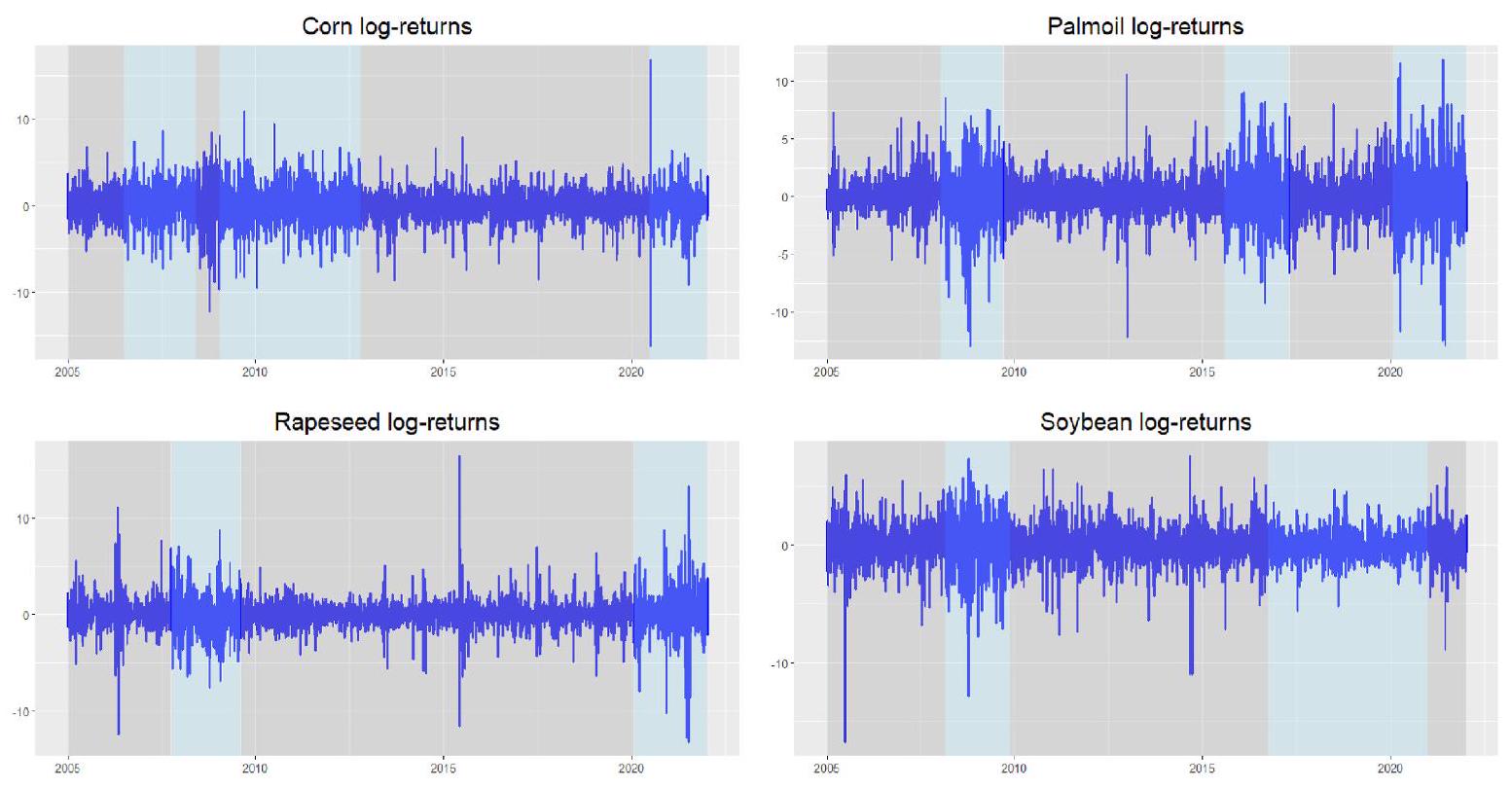
الأقسام المتبقية من هذه الدراسة منظمة على النحو التالي. في القسم 2، نقدم لمحة عامة عن البيانات والإحصاءات الوصفية. نعرض نماذجنا في القسم 3 ونصف الإجراء المستخدم لتحليل التنبؤ خارج العينة. في القسم 4، نقدم نتائج التنبؤ ونناقش نتائجنا. أخيرًا، في القسم 5، نختم بتلخيص الرؤى الرئيسية وتسليط الضوء على الآثار العملية للنتائج.

نجمع بيانات يومية لأسعار أربع مواد خام للوقود الحيوي: الذرة (دولار أمريكي لكل بوشل، رقم 2 أصفر)، زيت اللفت (يورو لكل طن متري، هولندي FOB NWE)، زيت النخيل (دولار أمريكي لكل طن متري، ماليزي CIF)، وفول الصويا (دولار أمريكي لكل بوشل، رقم 1 أصفر). نسترجع جميع البيانات من قاعدة بيانات Refinitive Eikon. تمتد فترات عينتنا من 31 ديسمبر 2004 إلى 7 يناير 2022 للذرة وزيت اللفت وفول الصويا، وإلى 6 يناير 2022 لزيت النخيل.

تقرير الجدول 1 الإحصائيات الوصفية لعوائد أسعار جميع السلع الحيوية (الشكل 1). نحن نحسب الإحصائيات لفترة العينة الكاملة. سلسلة العوائد تميل إلى السلبية لجميع السلع باستثناء زيت بذور اللفت. جميع عوائد السلع تظهر خصائص لبتوكورتيك، مما يشير إلى أن توزيعاتها تحتوي على قمم أعلى حول المتوسط مقارنة بالتوزيع الغاوسي. وبالتالي، نلاحظ ذيولًا ثقيلة على كلا الجانبين من توزيعات عوائد السلع ونرفض فرضية العدم للانتظام عند مستوى لعوائد جميع السلع، وفقًا لإحصائيات جاركي-بيرا. تكشف إحصائيات ليونغ-بوكس عن وجود ارتباط تسلسلي واضح في العوائد المربعة لجميع السلع. يوفر اختبار ARCH (التباين الشرطي الذاتي الانحدار) [24] دليلًا قويًا على التباين غير المتجانس، ويتم رفض الفرضية الصفرية لعدم وجود تباين غير متجانس عند مستوى الدلالة.

لإجراء تقديرات ذات مغزى لنماذج GARCH ونماذج SV وغيرها من نماذج التقلب، من الضروري افتراض أن تباين المتغيرات محدود. وبالتالي، باستخدام طريقة هيل [37]، نقوم بحساب مؤشرات الذيل (أي، لكل العوائد قيد الدراسة. في مستوى الدلالة، نرفض الفرضية الصفرية، ، لصالح بينما لا نرفض لصالح لكل سلاسل العوائد. تشير النتائج أعلاه إلى أن تبايناتها محدودة، وقد لا يكون الانحراف غير محدود.

نحن نقوم بتقدير عدة نماذج لكل سلعة من الوقود الحيوي: نماذج GARCH وSV ذات النظام الواحد (مع أحجام نوافذ كاملة ونصف وربع)، نماذج GARCH من نوع ICSS (مع فترة الكسر الأخيرة ودمى النظام)، نماذج SV من نوع ICSS (مع فترة الكسر الأخيرة)، نماذج GARCH ذات التحويل ماركوف، ونماذج HM وES. (مع نوافذ كاملة ونصف وربع)، و HM و ES في ICSS آخر كسر

يتم استخدام اختبار جاركي-بيرا (J-B) لتقييم التوزيع الطبيعي. Q(10) و Q2(10) تمثل اختبار ليونغ-بوكس. إحصائيات الاختبار للعوائد والعوائد المربعة، على التوالي، حتى التأخر 10 [37]. يتم استخدام الإجراء لتقدير مؤشرات الذيل. تُقدم حدود الثقة بين قوسين.
نماذج. نحن نقدر نماذج GARCH-class وSV تحت افتراضات توزيع مختلفة. الجدول A في الملحق يصف تفاصيل النماذج المستخدمة في هذه الدراسة.

لقد استخدمت الدراسات الحديثة بشكل متزايد نماذج التقلبات المحققة للتنبؤ أو تقدير التقلبات بعد حدوثها، مستفيدة من توفر بيانات عالية التردد داخل اليوم (انظر المراجع [49-51]؛ من بين آخرين). ومع ذلك، في هذه الدراسة، نختار عدم النظر في نماذج ومقاييس التقلبات المحققة بسبب محدودية قابليتها للتطبيق خارج مجال المالية.

بدلاً من ذلك، نركز على نماذج التقلبات التي تستخدم بيانات ذات تردد منخفض (أي يومية) وتكون أكثر ملاءمة لتحليل المواد الخام للوقود الحيوي من الجيل الثاني. حيث تكون بيانات التردد العالي نادرة. يمكن تطبيق النماذج التي نقترحها بشكل ملائم على الأسواق الخاصة بالمواد الخام للوقود الحيوي من الجيل الثاني مثل أصناف الذرة الحلوة، والطحالب، والسكريات السليلوزية، وغيرها. علاوة على ذلك، بينما تشير بعض الدراسات إلى أن النماذج التي تتضمن بيانات داخل اليوم قد توفر توقعات مخاطر محسنة مقارنة بتلك المعتمدة فقط على العوائد اليومية (مثل المراجع [53،73])، تشير أبحاث أخرى إلى أن نماذج التقلبات ذات التردد العالي قد تقدم توقعات أفضل على المدى القصير، على الرغم من أن النماذج ذات التردد العالي والمنخفض تنتج نتائج مشابهة لفترات التوقع الأطول [53].

يمكن وصف مواصفات GARCH(1,1) القياسية وGJR-GARCH(1,1) وEGARCH(1,1) في المراجع [10،27] و[55]، على التوالي، بنموذج متوسط في شكل ARMA( الأمثل. ) عملية باستخدام المعادلات التالية.

أين و ، هل معادلة المتوسط و و هي معلمات معادلة التباين.

أين إذا وإلا، فإن المعاملات، و هي معلمات نموذج التباين.

أين .
نستخدم أيضًا نموذج Beta-t-skew-EGARCH في المرجع [32]؛ الذي نوجه القراء المهتمين لمزيد من التفاصيل.

يمكن صياغة نموذج SV التقليدي، بافتراض توزيع طبيعي، على النحو التالي:

بالإضافة إلى ذلك، ندمج نموذج SV، الذي يفترض توزيع ستودنت الشرطي -التوزيع في المرجع [31].

أين ، هو الطالب’s -توزيع مع درجات الحرية، تباين الوحدة، ومتوسط صفر. كما نقوم بتقدير نموذج SV التالي، الذي يتضمن تأثير الرفع:

مصفوفة الارتباط لـ يُعرَّف بأنه كما يلي:

نفترض أن العمليات و مستقلون. يتم الإشارة إلى عملية لوغاريتم التباين بـ المتجه، يمثل مجموعة من المتغيرات المستقلة، و يمثل متجه المعاملات. يتم تمثيل معلمات النماذج بواسطة ، و . نحصل على المتبقيات من نموذج ARMA الأمثل ( ) نماذج لتقدير نماذج SV؛ هذا مشابه للعملية المتبعة للحصول على متوسط نماذج فئة GARCH. نحن نعتبر بدائل نماذج من خلال السماح بالمعلمات و لتتفاوت ضمن نطاق لكل نافذة متحركة. وفقًا للمرجع [35]؛ فإن النماذج التي تتضمن المتوسط الأمثل تتفوق على النماذج التي تتجاهل الأمثلية في نموذج المتوسط.

نأخذ في الاعتبار التغيرات الهيكلية المكتشفة داخليًا في نماذج GARCHclass وSV. أولاً، نستخدم آخر فترة بعد الكسر كعينة داخلية (أي، نماذج الكسر الأخير) وفقًا لـ [34،61]. تستخدم نماذج الكسر الأخير إجراء ICSS المعدل للعثور على نوافذ التقدير. نعتمد على اختبار (انظر المرجع [64] للحصول على التفاصيل) لتكون متاحة من الملاحظات المتاحة في العينة من واحد إلى . إذا استطعنا تحديد أدلة إحصائية كبيرة على تغيير النظام وتحديد اللحظة النهائية التي حدث فيها الانفصال ثم يمكننا تقدير جميع النماذج قيد الدراسة من إلى لحساب تقدير لـ . نحن نطبق نفس التقنية على نماذج HM و ES. واحدة من القيود المحتملة لهذا

الطريقة هي أنه قد يكون هناك حجم عينة محدود نسبيًا لتقدير معلمات النموذج في نوافذ محددة، خاصة عندما تكشف الإجراء عن انقطاع بالقرب من تاريخ التنبؤ.

نحن أيضًا نستوعب التغيرات المفاجئة غير المشروطة في التباين التي تم تحديدها من خلال ICSS المعدل في نماذج GARCH من خلال إضافة متغيرات وهمية في نماذج التباين. تستخدم العديد من الدراسات هذا النهج لتحليل تأثيرات التحولات المفاجئة في التباين غير المشروط على التقلب الشرطي للمتغيرات الاقتصادية والمالية (انظر، من بين آخرين، [1،3،25،36،41،46]. ومع ذلك، فإن استخدام هذا النهج محدود إلى حد ما في أدبيات توقع التقلبات. نحن نضيف متغيرات ثنائية لفترات الانكسار في معادلات التباين في نماذج GARCH المعطاة في المعادلات (1)-(3) ونحصل على النماذج المعززة التالية.

نحن نقدر النماذج المذكورة أعلاه تحت افتراضات توزيع بديلة. نحن نعرف المتغيرات الوهمية، dum التي تأخذ قيمة واحد لكل نقطة من نقاط التغير المفاجئ في التباين وما بعدها وصفر بخلاف ذلك، وفقًا للدراسات السابقة (مثل المراجع [3،41]. نقوم بتقدير هذه النماذج من خلال النوافذ المتحركة. بشكل أكثر تحديدًا، نبدأ باختيار النافذة الأولى وتحديد نقاط الانكسار. ثم ننتقل إلى النافذة التالية، مرة أخرى نجري الاختبار لنقاط الانكسار المفاجئة. تتكرر هذه العملية حتى نصل إلى النافذة النهائية. نقوم بتضمين المتغيرات الوهمية المعرفة أعلاه في نوافذها المعنية ونقدر النماذج المحددة في المعادلات (7)-(9) للحصول على التوقعات.

بالإضافة إلى النماذج الموضحة في الأقسام 3.1 و3.2 و3.3، نستخدم نموذج MSGARCH في المرجع [28]؛ مع الأخذ في الاعتبار افتراضات توزيع متنوعة (أي، غاوسي، سكيون ستودنت وطالب يمكن تحديد نموذج MSGARCH على النحو التالي:

أين يمثل دالة توزيع بمتوسط صفر وتقلب شرطي متغير مع الزمن، ، في النظام . المتجه يشمل معلمات إضافية، مثل معلمات الذيل والانحراف. الرمز يمثل مجموعة المعلومات والمتغير الحالى يتبع سلسلة ماركوف متجانسة من الدرجة الأولى مع الدول. نحن نعتبر ثلاثة مواصفات لتباين الشرط: GARCH القياسي، GJR-GARCH، وEGARCH تحت نماذج MSGARCH. نحن نقدر تسعة نماذج MSGARCH لكل نافذة متحركة وعائدات المحاصيل الحيوية للحصول على توقعات فردية ومتعددة الخطوات. وفقًا للنهج في الدراسات الحالية، نقوم بإزالة التأثيرات الذاتية والانحدار المتحرك داخل كل نافذة متحركة (على سبيل المثال، انظر المراجع [5،35]. ننجز هذه العملية من خلال تطبيق تصفية البيانات، مما يسمح

لنجري نماذج التحويل ماركوف على المتبقيات الناتجة.

أحد أهدافنا هو دراسة أهمية أحجام النوافذ في التنبؤ بالتقلبات. مثل [61]؛ نقوم بتعديل نافذة التقدير لاستيعاب التغيرات المحتملة في التباين غير المشروط للعوائد. نقوم بتقدير نماذج GARCH، SV، HM و ES باستخدام أحجام نوافذ تساوي و طول فترة العينة. من خلال استخدام نافذة تقدير أقصر (أي، و من العينة المستخدمة)، تستخدم النماذج عددًا أقل من الملاحظات المتاحة لتقدير معلمات النموذج [61]. لاحظ أن إعداد هذه النافذة يقلل من احتمال استخدام العوائد من أنظمة متميزة.

نقوم بحساب توقعات التقلبات اليومية لخطوات واحدة، وخمس، وعشرون، وأربعون للأمام لأربعة سلع. نحدد فترة الاختبار الخارجي لتغطي آخر 1000 عائد من العينة الكلية. نستمر في تحريك تواريخ البدء والانتهاء لفترة تقدير العينة إلى يوم واحد، خمسة أيام، عشرين يومًا، وأربعين يومًا حتى نهاية فترة الاختبار الخارجي. نستمر في تنفيذ هذه العملية حتى نصل إلى نهاية فترة الاختبار الخارجي المتاحة. نعتمد على اختبار MCS. لتصنيف النماذج وفقًا لأدائها في التنبؤ، تماشيًا مع الدراسات الحديثة (مثل، المراجع. نستخدم إحصائيات قائمة على النطاق، يتم حسابها عند مستوى الثقة، وفقًا لـ [2,30].

تُستخدم تقديرات المعاملات لجميع النماذج المدروسة في الجدول A في الملحق لحساب التنبؤات اليومية للأحجام الشرطية على المدى القصير والطويل. تُبلغ الجداول 2-5 عن نتائج MCS للأسواق (أي الذرة، والنخيل، وبذور اللفت، وفول الصويا) لأربعة مقاييس خسارة: MAE، HMAE، HMSE، وQLIKE.



QLIKE
في مقاييس الخسارة، نشير إلى وكيل للتقلبات اللاحقة (أي العوائد المربعة) بـ وتوقعات بواسطة .

تستحق بعض نتائجنا التأكيد. أولاً، تشير نتائجنا إلى أنه لا يوجد نموذج واحد يتفوق على الآخرين لجميع سلع المواد الخام للوقود الحيوي. وهذا يؤكد نتائج العديد من الدراسات السابقة (على سبيل المثال، المراجع [33،65]). ثانياً، عندما نتحدث عن أنظمة MCS العامة (النماذج مع -قيم أكبر من 0.10)، فإن النماذج التي تقدم أفضل توقعات للتقلبات للأسواق المدروسة هي غالبًا نماذج GARCH التي تأخذ في الاعتبار الانقطاعات الهيكلية الذاتية (الانقطاعات المستندة إلى ICSS والعيّنات الفرعية للانقطاع الأخير)، تليها نماذج MSGARCH. بشكل أوضح، تظهر هذه النماذج غالبًا في MCSs عبر جميع مقاييس الخسارة وآفاق التوقع مقارنة بالنماذج ذات النظام الواحد المقدرة من خلال النوافذ الكاملة، والنصف، والربع.

الآن، نعتبر النماذج ذات الأداء الاستثنائي في جميع معايير الخسارة مع -قيمة الوحدة. هناك أربعة وستون نموذجًا مع قيمة الوحدة في جميع السلع عبر أربعة معايير خسارة وجميع آفاق التنبؤ. لم تتمكن نماذج CARCH-class وSV ذات النظام الواحد المقدرة باستخدام نوافذ كاملة ونصف وربع من التفوق على نماذج MSGARCH ونماذج الانكسار الهيكلي المعتمدة على ICSS. من الجدير بالذكر أننا لم نجد أي نموذج واحد (حجم النافذة الكاملة) من بين النماذج ذات الأداء الأفضل. وفقًا للمرجع [59]؛ إذا كانت هناك انكسارات هيكلية في سلسلة العوائد، فإن الاعتماد على سلسلة العوائد المتاحة بالكامل لتقدير النموذج قد يؤدي إلى توقعات غير دقيقة، حتى لو أدى ذلك إلى تقليل التباين. ومع ذلك، إذا تم اعتبار فقط مواصفات GARCH من نوع النوافذ الكاملة والنصف والربع، فإن النماذج التي تستخدم نوافذ نصفية تكون أفضل قليلاً من تلك التي تستخدم النوافذ الكاملة والربع. إلى حد ما، تأخذ هذه النماذج (تحديدًا تلك التي تحتوي على نوافذ نصف وربع) في الاعتبار التحولات الهيكلية المفاجئة في العوائد، حيث أن تعديل حجم النافذة يقلل من فرص دمج العوائد من أنظمة مختلفة.

مقارنةً بالنماذج الأخرى في هذه الدراسة، لا تبدو نماذج SV و ES المعتمدة على ICSS واعدة. ومن المثير للاهتمام، أننا نجد أن نموذج HM يظهر إمكانيات كنموذج لسوق الذرة؛ حيث يظهر بشكل متكرر في مجموعات النماذج المتفوقة عبر تقريبًا جميع معايير الخسارة وآفاق التنبؤ. تُظهر الجدول 2 أنه تحت HMAE و HMSE، يُظهر نموذج HM ذو النظام الواحد للذرة الأداء الأكثر دقة في التنبؤ بناءً على -القيم المحسوبة في اختبارات MCS التسلسلية في آفاق التنبؤ 5 و20 و40 خطوة للأمام. ومع ذلك، فإن اختبار اتجاه التغيير (DoC) لا يدعم هذه النتيجة (انظر القسم 4.4). يستبعد اختبار MCS نموذج HM من نماذج SSMs تحت جميع مقاييس الخسارة وآفاق التنبؤ لسوق بذور اللفت، مما يشير إلى أن هذا النموذج غير كافٍ لالتقاط التقلبات المستقبلية.

نحن نفحص أهمية دوال التوزيع في التنبؤ بالأداء ونجد أن تأثيرها على التوقعات خارج العينة عمومًا مختلط (على سبيل المثال، المراجع [33،34]. تكشف نتائجنا أنه لا يوجد توزيع سائد لجميع أسواق المواد الخام للوقود الحيوي، مما يعزز دقة التنبؤ. النماذج التي تستخدم التوزيع الطبيعي، توزيع ستودنت وانحراف الطالب -التوزيعات تميل إلى الأداء الأفضل؛ تم تضمين هنا تلك النماذج التي لديها قيمة p تساوي الواحد، مقارنةً بـ GHYP عبر وظائف خسارة مختلفة وأسواق المواد الخام للوقود الحيوي. تتوافق هذه النتيجة مع وجهة نظر [18] التي تشير إلى أن التوزيع المعقد لا يتفوق باستمرار على التوزيع الأبسط، ربما بسبب مخاوف من الإفراط في التكيف في اختبارات دقة خارج العينة. بالإضافة إلى ذلك، نلاحظ أنه، مقارنةً بنموذج SV البسيط مع التوزيع الطبيعي، فإن نماذج SV التي تستخدم توزيع ستودنت -التوزيع يظهر أداءً متفوقًا عبر جميع دوال الخسارة وآفاق التنبؤ.

نقوم بتقييم دقة التنبؤ لنماذجنا من خلال فحص الآفاق القصيرة الأجل (خطوتين و5 خطوات) والآفاق الطويلة الأجل (20 و40 خطوة). يتضمن ذلك تقييم تكرار النماذج في MCSs لهذه الآفاق التنبؤية. عبر جميع السلع ومقاييس الخسارة التي تم فحصها، نجد أنه بالنسبة للآفاق القصيرة والطويلة الأجل، فإن نماذج GARCH-class التي

تعرض الجدول نتائج MCS، بما في ذلك الإحصائيات المستندة إلى النطاق والقيم p المقابلة، لأربعة معايير خسارة مختلفة مع آفاق توقع تبلغ s. ، و 40، استنادًا إلى فترة خارج العينة من . تمثل قيم p المميزة بالأحرف الغامقة أعلى قيمة p لكل أفق توقع ومعيار خسارة. يتم إجراء MCS بمستوى ثقة . المصطلح، Last-BR، يعني نموذج الكسر الأخير، Skt يدل على الانحراف ، وتشير نماذج EGARCH ذات المكون الواحد والمكونين إلى نماذج Beta t EGARCH ذات المكون الواحد والمكونين. التوزيعات الشرطية المستخدمة في تقديرات نماذج GARCH هي (i) توزيع ستاندرد ستودنت t (STD)، (ii) توزيع طبيعي قياسي (N)، (iii) توزيع ستاندرد سكيوا ستودنت t (SSTD)، و(vii) توزيع هايبروليك العام (GHYP). نقوم بتقدير نماذج GARCH ذات التحويل ماركوف بافتراض التوزيع الطبيعي، وتوزيع ستودنت t، وتوزيع ستودنت السكيوا. -التوزيعات. تفترض نماذج SV توزيعات طبيعية (N) وتوزيعات ستودنت (ST). نشير إلى النماذج التي تستخدم حجم نافذة يساوي ، و طول فترة العينة عن طريق إضافة 0.25 أمام أسماء النماذج.
تأخذ في الاعتبار الانكسارات الهيكلية الذاتية (باستخدام دمى الانكسار المعتمدة على ICSS والعينة الفرعية الأخيرة) وتؤدي بشكل جيد؛ يليها في الأداء نماذج GARCH ذات التحول ماركوف. ثم نركز على أداء نماذج النظام الواحد المقدرة باستخدام نوافذ كاملة ونصف وربع الحجم على المدى القصير والطويل. نجد أن نماذج GARCH ذات النظام الواحد مع نافذة كاملة تؤدي بشكل أفضل على المدى القصير مقارنةً بالمدى الطويل، بينما تظهر نماذج النظام الواحد ذات أحجام النوافذ نصف وربع أداءً مشابهًا على الآفاق القصيرة والطويلة.

نموذج SV مع تأثيرات الرفع يتم تضمينه بشكل أكثر تكرارًا في مجموعات ثقة النموذج عبر جميع مقاييس الخسارة لفترات زمنية أطول؛ نموذج SV مع -التوزيع يظهر أداءًComparable في الآفاق القصيرة والطويلة. نموذج SV مع الانقطاعات المحددة بشكل داخلي يؤدي بشكل مشابه عبر كلا الأفقين. أخيرًا، تظهر نماذج HM و ES أداءً متفوقًا قليلاً في الآفاق الأطول.

باختصار، تميل نماذج MSGARCH والنماذج التي تتضمن انقطاعات محددة داخليًا إلى الأداء بشكل أفضل من النماذج الأخرى على المدى القصير والطويل. تتماشى نتائجنا مع تلك الواردة في [66، 72]؛ و [74]؛ حيث تكشف هذه الدراسات عن فعالية نماذج تغيير الأنظمة في التقاط التحولات في أسواق المواد الخام للوقود الحيوي. تحمل النتائج أهمية وتعزز المعرفة الحالية بشأن توقع التقلبات في أسواق السلع [50]. توضح أن استخدام مواصفات تغيير الأنظمة يتضمن معلومات قيمة موجودة مسبقًا تتعلق بالتقلبات المستقبلية، خاصة عند توقع التقلبات على المدى المتوسط والطويل.

عند توقع تقلبات المواد الخام للوقود الحيوي على المدى القصير والطويل، من الضروري اختيار نماذج تنبؤية تأخذ في الاعتبار الانقطاعات الهيكلية والأنظمة ذات الصلة. علاوة على ذلك، يساعد استخدام الوقود الحيوي والطاقة المتجددة في الجهود المبذولة للحد من تلوث الكربون وتحقيق أهداف خفض الانبعاثات العالمية (على سبيل المثال، المرجع [4]). نتيجة لذلك، من المتوقع أن تقوم الحكومات بوضع سياسات إضافية لتعزيز نمو صناعات الطاقة المتجددة وأن تخصص الشركات المزيد من الموارد نحو البحث وإنتاج المنتجات المتعلقة بالوقود الحيوي.

استنادًا إلى الدراسات الحالية، نقوم أيضًا بحساب اختبار DoC (على سبيل المثال، المراجع [19،58]، التي تشير إلى نسبة التوقعات التي تتنبأ بدقة باتجاه (إما صعودي أو هبوطي) للتقلب.

وثيقة

انظر الملاحظات في الجدول 2.

انظر الملاحظات في الجدول 2.

نحسب قيمة DoC لجميع النماذج وتُعرض النتائج في الجدول A في الملحق. كما نقوم بترتيب النماذج وفقًا لقيم DoC ونأخذ في الاعتبار أفضل خمسة عشر نموذجًا في التحليل. تؤكد هذه الاختبار أن النماذج التي تحتوي على انقطاعات تم اكتشافها بشكل داخلي، تليها نموذج GARCH من الفئة 0.25 (مع حجم نافذة ربع سنوية)، تتفوق بشكل كبير على النماذج الأخرى لجميع السلع الحيوية للطاقة التي تم النظر فيها. على وجه الخصوص، تتفوق نماذج الانقطاع الأخير (انظر القسم 3.3) على جميع النماذج الأخرى في هذا الاختبار. عند دمج الانقطاعات،

يتضح أنه بالنسبة للذرة، فإن EGARCH (مع درجة حرية) في الخطوة 5) و Beta-t-skew-EGARCH (مع درجة من الحرية في الخطوة 20) تقدم أفضل دقة في توقع تحركات التقلبات.

وبالمثل، بالنسبة لزيت النخيل، Beta-t-skew-EGARCH (مع قيم DoC من في الخطوة 1 و في الخطوة 40) و EGARCH (مع نسب DoC من في الخطوة 5 و في الخطوة 20) تظهر أداءً تنبؤيًا متفوقًا في التقاط اتجاه التقلبات. كما نلاحظ نتائج مشابهة في DoC لبذور اللفت وفول الصويا. على الرغم من أن نموذج SV مع الانقطاعات في الخطوتين 5 و20 يوفر توقعات اتجاهية متفوقة، إلا أن نموذج Beta-t-skew-EGARCH وES مع الانقطاعات يقدمون أكثر التوقعات دقة لبذور اللفت في الخطوتين 1 و40. أفضل نماذج توقع الاتجاه لبذور فول الصويا هي Beta-t-skew-EGARCH وEGARCH (بالإضافة إلى

انظر الملاحظات في الجدول 2.
الانقطاعات) عبر جميع آفاق التنبؤ المعنية.
وفقًا لنتائج MCS، فإن النماذج التي تتجاهل عدم الاستقرار (مثل النماذج ذات النظام الواحد) تظهر دقة تنبؤ أقل فيما يتعلق بحركات التقلب. علاوة على ذلك، فإن النماذج ضمن فئة GARCH التي تدمج متغيرات كسر قائمة على ICSS ونماذج MS-GARCH لا تقدم تنبؤات جيدة لاتجاه التقلب. كما نلاحظ أنه عند دمجها مع الكسور، فإن نماذج ES لبعض خطوات التنبؤ تتنبأ بدقة بتقلبات الذرة الصاعدة والهابطة. لخطوة 1) وتلك الخاصة بزيت اللفت (مع DoC للخطوة 40).

تشير هذه النتائج إلى أن دمج الانقطاعات المكتشفة داخليًا في النموذج المستخدم أمر ضروري في التوقعات النقطية والاتجاهية.

لقد تأثرت أسواق المواد الخام للوقود الحيوي بشدة بالجائحات، والطقس القاسي، وغيرها من الأحداث الاقتصادية والمالية والسياسية العالمية. وقد أدت هذه الأحداث إلى حدوث تغييرات كبيرة أو انقطاعات في التباين في الأسواق المعنية. تشير الدراسات الحالية إلى أن تجاهل الانقطاعات الهيكلية في نماذج التقلبات قد يؤدي إلى تقدير مفرط لمعاملات النموذج، مما يؤدي إلى توقعات غير دقيقة. لذلك، تقوم هذه الدراسة بفحص شامل لعدة نماذج مع وبدون احتساب التغيرات الهيكلية على مدى آفاق متعددة باستخدام إجراء نافذة متحركة.

تظهر نتائج MCS تفضيلًا قويًا للنماذج التي تأخذ في الاعتبار الانقطاعات الهيكلية على نماذج GARCH ذات النظام الواحد، بغض النظر عن حجم النافذة. ومع ذلك، فإن استيعاب الانقطاعات في نماذج SV لا يزيد بشكل كبير من دقتها التنبؤية. لا نجد أي نموذج شامل بين النماذج ذات الأداء الأفضل. عند النظر فقط في مواصفات GARCH من نوع النوافذ الكاملة، ونصف النافذة، وربع النافذة، فإن النماذج التي تستخدم نوافذ نصفية أفضل قليلاً من النماذج ذات النوافذ الكاملة والربع. بالمقارنة مع الآخرين، لا تبدو نماذج SV وES المعتمدة على ICSS واعدة. ومن المثير للاهتمام، أننا نجد أن نموذج HM هو نموذج واعد لسوق الذرة حيث يظهر بشكل متكرر في مجموعات النماذج المتفوقة عبر جميع معايير الخسارة وآفاق التنبؤ.

الاختبار الإضافي، DoC، يؤكد أن النماذج المدمجة مع الانقطاعات المكتشفة داخليًا تليها GARCH-class 0.25 (مع نوافذ ربع سنوية) تتفوق بشكل كبير على النماذج الأخرى.
عبر جميع آفاق التنبؤ لجميع السلع الحيوية المعتمدة. على وجه الخصوص، تتفوق نماذج آخر فترة على جميع النماذج الأخرى في هذا الاختبار. وفقًا لنتائج MCS، تظهر النماذج التي تتجاهل عدم الاستقرار (مثل نماذج النظام الواحد) دقة تنبؤ أقل لحركات التقلب.

من الضروري أخذ اعتبارات الانكسارات الهيكلية ونماذج التحول النظامي في الاعتبار عند نمذجة التقلبات في أسواق المحاصيل الحيوية. إن نتائجنا لها تداعيات كبيرة على اتخاذ القرارات من قبل مختلف المشاركين في سوق المحاصيل الحيوية، بما في ذلك المصنعين والمتداولين الماليين وصانعي السياسات. على وجه الخصوص، فإن دمج الانكسارات المكتشفة بشكل داخلي ونماذج التحول ماركوف يمكّن المشاركين من تطوير خطط إدارة مخاطر أكثر دقة على المدى القصير والطويل.

نتائجنا مهمة للمستثمرين وصانعي السياسات. على وجه التحديد، يمكن للمستثمرين إجراء توقعات دقيقة حول تقلبات عوائد المواد الخام للوقود الحيوي من خلال دمج معلومات الانكسار الهيكلي. وهذا بدوره يمكّن المستثمرين من إنشاء محافظ لتقليل المخاطر المرتبطة بالأصول المالية الأخرى [63]. نظرًا لأن تقلب أسعار المواد الخام للوقود الحيوي يعكس عدم اليقين الاقتصادي، فقد يعيق ذلك قرارات الإنتاج والاستثمار طويلة الأجل للمنتجين. علاوة على ذلك، وفقًا للمرجع [29]؛ يمكن أن تتداخل تقلبات الأسعار مع جهود المستهلكين ذوي الدخل المنخفض لوضع ميزانية على المدى الطويل وتعرضهم لمخاطر الفقر. لهذا السبب، فإن تحليل تقلب الأسعار أمر بالغ الأهمية لتحقيق أهداف التنمية المستدامة للأمم المتحدة (SDGs)، وبشكل خاص الهدف 1 (لا فقر) والهدف 2 (لا جوع)، كما تم تسليط الضوء عليه في المرجع [7]. يمكن استيعاب معلومات الانكسار في النماذج لإنتاج توقعات لأسواق زراعية متنوعة، مما يسهل صياغة استجابات سياسية مناسبة لمنع الانكماش الاقتصادي.

أكرم شافكاتوفيتش حسنوف: التصور، تنظيم البيانات، التحليل الرسمي، التحقيق، المنهجية، إدارة المشروع، الموارد، البرمجيات، الإشراف، التحقق، الكتابة – المسودة الأصلية، الكتابة – المراجعة والتحرير. أكتام عثمانوفيتش بورخانوف: الحصول على التمويل، إدارة المشروع، الإشراف، التحقق. بونيود أوزمونوف: تنظيم البيانات، التحقيق، البرمجيات، التحقق. نيزومجون شكر الله فيتش خاجيموراتوف: إدارة المشروع، الموارد، الإشراف. مادينا منصور قزي خوراموفا: البيانات.
تنسيق، تحقيق، برمجيات، تحقق.

خلال إعداد هذا العمل، استخدم المؤلفون ChatGPT لإعادة صياغة بعض النصوص في المخطوطة لزيادة الوضوح وسهولة القراءة. بعد استخدام هذه الأداة، قام المؤلفون بمراجعة وتحرير المحتوى حسب الحاجة ويتحملون المسؤولية الكاملة عن محتوى النشر.

يعلن المؤلفون أنهم ليس لديهم أي تضارب مالي معروف
المصالح أو العلاقات الشخصية التي قد تبدو أنها تؤثر على العمل المبلغ عنه في هذه الورقة.

ستكون البيانات متاحة عند الطلب.

يُعبر المؤلف، أكرم شافكاتوفيتش حسنوف، عن تقديره وامتنانه للدعم المالي الذي تم تلقيه من جامعة موناش، ماليزيا من خلال منحة البذور (B-2-2020).

الجدول أ
النماذج الاقتصاد قياسية

1 Single regime with whole window size GARCH-class models
1.0-GARCH-ST, 1.0-GARCH-N, 1.0-GARCH-SST, 1.0-GJR-GARCH-N, 1.0-GARCH-GHYP, 1.0-GJR-GARCH-ST, 1.0-GJR-
GARCH-GHYP, 1.0-GJR-GARCH-SST, 1.0-EGARCH-ST, 1.0-EGARCH-N, 1.0-EGARCH-SST, 1.0-EGARCH-GHYP, 1.0-two-
comp-Beta-t-EGARCH, 1.0-one-comp-Beta-t-EGARCH
2 Single regime with half window size GARCH-class models
0.5-GARCH-ST, 0.5-GARCH-N, 0.5-GARCH-SST, 0.5-GARCH-GHYP, 0.5-GJR-GARCH-ST, 0.5-GJR-GARCH-N, 0.5-GJR-
GARCH-SST, 0.5-GJR-GARCH-GHYP, 0.5-EGARCH-ST, 0.5-EGARCH-N, 0.5-EGARCH-SST, 0.5-EGARCH-GHYP, 0.5-two-
comp-Beta-t-EGARCH, 0.5-one-comp-Beta-t-EGARCH
3 Single regime with quarter window size GARCH-class models
0.25-GARCH-ST, 0.25-GARCH-N, 0.25-GARCH-SST, 0.25-GARCH-GHYP, 0.25-GJR-GARCH-ST, 0.25-GJR-GARCH-N,
0.25-GJR-GARCH-SST, 0.25-GJR-GARCH-GHYP, 0.25-EGARCH-ST, 0.25-EGARCH-N, 0.25-EGARCH-SST, 0.25-EGARCH-
GHYP, 0.25-two-comp-Beta-t-EGARCH, 0.25-one-comp-Beta-t-EGARCH
4 Single regime with full window size SV models
1.0-SVT, 1.0-SV, 1.0-SV-lev
5 text { Single regime with half window size SV models }
0.5-SVT, 0.5-SV, 0.5-SV-lev
6 Single regime with quarter window size SV models
0.25-SVT, 0.25-SV, 0.25-SV-lev
7 text { ICSS regime dummy GARCH-class models }
ICSS-GARCH-ST, ICSS-GARCH-N, ICSS-GARCH-SST, ICSS-GARCH-GHYP, ICSS-GJR-GARCH-ST, ICSS-GJR-GARCH-N,
ICSS-GJR-GARCH-SST, ICSS-GJR-GARCH-GHYP, ICSS-EGARCH-ST, ICSS-EGARCH-N, ICSS-EGARCH-SST, ICSS-EGARCH-
GHYP
8 ICSS last break period GARCH-class models
ICSS-Last-BR-GARCH-ST, ICSS-Last-BR-GARCH-N, ICSS-Last-BR-GARCH-SST, ICSS-Last-BR-GARCH-GHYP, ICSS-Last-BR-
GJR-GARCH-ST, ICSS-Last-BR-GJR-GARCH-N, ICSS-Last-BR-GJR-GARCH-SST, ICSS-Last-BR-GJR-GARCH-GHYP, ICSS-
Last-BR-EGARCH-ST, ICSS-Last-BR-EGARCH-N, ICSS-Last-BR-EGARCH-SST, ICSS-Last-BR-EGARCH-GHYP, ICSS-Last-BR-
two-comp-Beta-t-EGARCH, ICSS-Last-BR-one-comp-Beta-t-EGARCH
9 ICSS last break period SV models
ICSS-Last-BR-SVT, ICSS-Last-BR-SV, ICSS-Last-BR-SV-lev
10 Markov-switching GARCH models
MS-GARCH-ST, MS-GARCH-N, MS-GARCH-SST, MS-GJR-GARCH-ST, MS-GJR-GARCH-N, GJR-MS-GARCH-SST, MS-
EGARCH-ST, MS-EGARCH-N, MS-EGARCH-SST
11 Full, half, and quarter window size single regime HM, ES models
1.0-ES, 1.0-HM, 0.5-ES, 0.5-HM, 0.25-ES, 0.25.0-HM
12 ICSS last break period HM and ES models
ICSS-Last-BR-ES, ICSS-Last-BR-HM

نقوم بتحسين معادلة المتوسط لنموذج GARCH من خلال AIC المصحح في كل نافذة. نقوم بإزالة التأثيرات الذاتية والانزلاقية في كل نافذة متحركة عن طريق تشغيل ARMA الأمثل( ) تصفية قبل تقدير نماذج SV ونماذج التحويل ماركوف على المتبقيات. التوزيعات الشرطية المستخدمة في تقديرات الاحتمال الأقصى شبه لنماذج GARCH هي (i) توزيع طبيعي قياسي (N)، (ii) توزيع ستودنت الموحد (STD)، (iii) توزيع ستودنت المنحرف القياسي (SSTD)، و (vii) توزيع هايبرولي عمومي (GHYP). نقوم بتقدير نماذج GARCH ذات التحويل ماركوف بافتراض التوزيع الطبيعي، توزيع ستودنت وتحريف طالب التوزيعات. تفترض نماذج SV التوزيع الطبيعي وتوزيع ستودنت -التوزيعات.

[1] Aggarwal R, Inclán C, Leal R. Volatility in emerging stock markets. J Financ Quant Anal 1999;34:33-55.
[2] Amendola A, Braione M, Candila V, Storti G. A Model Confidence Set approach to the combination of multivariate volatility forecasts. Int Forecast 2020;36:873-91. https://doi.org/10.1016/j.ijforecast.2019.10.001.
[3] Anjum H, Malik F. Forecasting risk in the US Dollar exchange rate under volatility shifts. N Am J Econ Finance 2020;54:101257. https://doi.org/10.1016/j. najef.2020.101257.
[4] Apergis N, Payne JE, Menyah K, Wolde-Rufael Y. On the causal dynamics between emissions, nuclear energy, renewable energy, and economic growth. Ecol Econ 2010;69:2255-60. https://doi.org/10.1016/j.ecolecon.2010.06.014.
[5] Ardia D, Bluteau K, Boudt K, Catania L. Forecasting risk with Markov-switching GARCH models: a large-scale performance study. Int J Forecast 2018;34:733-47.
[6] Ardia D, Bluteau K, Boudt K, Catania L, Trottier D-A. Markov-switching GARCH models in R : the MSGARCH package. J Stat Software 2019;91. https://doi.org/ 10.18637/jss.v091.i04.
[7] Berger J, Dalheimer B, Brümmer B. Effects of variable EU import levies on corn price volatility. Food Pol 2021;102:102063. https://doi.org/10.1016/j. foodpol.2021.102063.
[8] Bergsli Lø, Lind AF, Molnár P, Polasik M. Forecasting volatility of bitcoin. Res Int Bus Finance 2022;59:101540. https://doi.org/10.1016/j.ribaf.2021.101540.
[9] Bergtold JS, Shanoyan A, Fewell JE, Williams JR. Annual bioenergy crops for biofuels production: farmers’ contractual preferences for producing sweet sorghum. Energy 2017;119:724-31. https://doi.org/10.1016/j. energy.2016.11.032.
[10] Bollerslev T. Generalized autoregressive conditional heteroskedasticity. J Economtrics 1986;31:307-27.
[11] Bollerslev T. The story of GARCH: a personal odyssey. J Econom 2023;234:96-100.
[12] Bouri E, Dutta A, Saeed T. Forecasting ethanol price volatility under structural breaks. Biofuels, Bioprod. Bioref. 2021;15:250-6. https://doi.org/10.1002/ bbb. 2158.
[13] Carpio LGT. The effects of oil price volatility on ethanol, gasoline, and sugar price forecasts. Energy 2019;181:1012-22. https://doi.org/10.1016/j. energy.2019.05.067.
[14] Chang T-H, Su H-M. The substitutive effect of biofuels on fossil fuels in the lower and higher crude oil price periods. Energy 2010;35:2807-13.
[15] Charfeddine L. True or spurious long memory in volatility: further evidence on the energy futures markets. Energy Pol 2014;71:76-93. https://doi.org/10.1016/j. enpol.2014.04.027.
[16] Charles A, Darné O. Forecasting crude-oil market volatility: further evidence with jumps. Energy Econ 2017;67:508-19. https://doi.org/10.1016/j. eneco.2017.09.002.
[17] Cheng IH, Xiong W. Financialization of commodity markets. Annu Rev Financ Econ 2014;6:419-41.
[18] Chuang I-Y, Lu J-R, Lee P-H. Forecasting volatility in the financial markets: a comparison of alternative distributional assumptions. Appl Financ Econ 2007;17: 1051-60. https://doi.org/10.1080/09603100600771000.
[19] Degiannakis S, Filis G. Forecasting oil price realized volatility using information channels from other asset classes. J Int Money Finance 2017;76:28-49. https://doi. org/10.1016/j.jimonfin.2017.05.006.
[20] Degiannakis S, Filis G, Klein T, Walther T. Forecasting realized volatility of agricultural commodities. Int J Forecast 2022;38:74-96. https://doi.org/10.1016/ j.ijforecast.2019.08.011.
[21] Dutta A, Junttila J, Uddin GS. Forecasting the volatility of biofuel feedstock prices: the US Evidence. Biofuels Bioprod Bioref 2019;13:912-9.
[22] EBB. About biodiesel. European Biodiesel Board. https://ebb-eu.org/(accessed 21 February 2023)..
[23] EIA. Monthly biodiesel production report. U.S. Energy Information Administration; 2020. https://www.eia.gov/biofuels/biodiesel/production/. [Accessed 21 February 2023].
[24] Engle RF. Autoregressive conditional heteroscedasticity with estimates of the variance of U.K. inflation. Econometrica 1982;50:987-1008.
[25] Ewing BT, Malik F. Estimating volatility persistence in oil prices under structural breaks. Financ Rev 2010;45:1011-23. https://doi.org/10.1111/j.15406288.2010.00283.x.
[26] Galanos A. Rugarch: univariate GARCH models. 2022. https://cran.r-project.org/ web/packages/rugarch/rugarch.pdf.
[27] Glosten LR, Jagannathan R, Runkle D. On the relation between the expected value and the volatility of the nominal excess return on stocks. J Finance 1993;XLVIII.
[28] Haas M, Mittnik S, Paolella M. A new approach to Markov-switching GARCH models. J Financ Econom 2004;2:493-530.
[29] Hajkowicz S, Negra C, Barnett P, Clark M, Harch B, Keating B. Food price volatility and hunger alleviation – can Cannes work? Agric Food Secur 2012;1. https://doi. org/10.1186/2048-7010-1-8.
[30] Hansen PR, Lunde A, Nason JM. The model confidence set. Econometrica 2011;79: 453-97.
[31] Harvey A, Ruiz E, Shephard N. Multivariate stochastic variance models. Rev Econ Stud 1994;61:247-64.
[32] Harvey A, Sucarrat G. EGARCH models with fat tails, skewness and leverage. Comput Stat Data Anal 2014;76:320-38. https://doi.org/10.1016/j. csda.2013.09.022.
[33] Hasanov AS, Avazkhodjaev SS. Stochastic volatility models with endogenous breaks in volatility forecasting. In: Terzioglu MK, editor. Advances in econometrics, operational research, data science and actuarial studies. Cham: Springer International Publishing; 2022. p. 81-97.
[34] Hasanov AS, Poon WC, Al-Freedi A, Heng ZY. Forecasting volatility in the biofuel feedstock markets in the presence of structural breaks: a comparison of alternative distribution functions. Energy Econ 2018;70:307-33. https://doi.org/10.1016/j. eneco.2018.01.011.
[35] Hasanov AS, Shaiban MS, Al-Freedi A. Forecasting volatility in the petroleum futures markets: a re-examination and extension. Energy Econ 2020;86:104626. https://doi.org/10.1016/j.eneco.2019.104626.
[36] Hasanov AS, Shitan M. Modeling inflation volatility: evidence from two post-Soviet economies. Int J Stat Sci 2012;12:9-27.
[37] Hill BM. A simple general approach to inference about the tail of a distribution. Ann Stat 1975;3:1163-74. https://doi.org/10.1214/aos/1176343247.
[38] Hosszejni D, Kastner G. Efficient bayesian inference for stochastic volatility (SV). The “stochvol” R package version 3.2.0 2022. https://cran.r-project.org/web/p ackages/stochvol/stochvol.pdf.
[39] Hyndman R, Athanasopoulos G, Bergmeir C, Caceres G, Chhay L, Kuroptev K, O’Hara-Wild M, Petropoulos F, Razbash S, Wang E, Yasmeen F. Forecast:
forecasting functions for time series and linear models. 2022. https://cran.r-project .org/web/packages/forecast/forecast.pdf.
[40] Inclán C, Tiao GC. Use of cumulative sums of squares for retrospective detection of changes of variance. J Am Stat Assoc 1994;89:913-23.
[41] Kang SH, Cheong C, Yoon S-M. Structural changes and volatility transmission in crude oil markets. Phys Stat Mech Appl 2011;390:4317-24. https://doi.org/ 10.1016/j.physa.2011.06.056.
[42] Kang SH, Kang S-M, Yoon S-M. Forecasting volatility of crude oil markets. Energy Econ 2009;31:119-25. https://doi.org/10.1016/j.eneco.2008.09.006.
[43] Klein T, Walther T. Oil price volatility forecast with mixture memory GARCH. Energy Econ 2016;58:46-58. https://doi.org/10.1016/j.eneco.2016.06.004.
[44] Kumar D, Maheswaran S. Modelling asymmetry and persistence under the impact of sudden changes in the volatility of the Indian stock market. IIMB Manage Rev 2012;24:123-36.
[45] Lamoureux CG, Lastrapes WD. Persistence in variance, structural change, and the GARCH model. J Bus Econ Stat 1990;8:225. https://doi.org/10.2307/1391985.
[46] Law SH. Has stock market volatility in the Kuala Lumpur Stock Exchange returned to pre-Asian financial crisis levels? ASEAN Econ Bull 2006;23:212-29.
[47] Li X, Guo Q, Liang C, Umar M. Forecasting gold volatility with geopolitical risk indices. Res Int Bus Finance 2023;64:101857. https://doi.org/10.1016/j. ribaf.2022.101857.
[48] Li Y, Liang C, Ma F, Wang J. The role of the IDEMV in predicting European stock market volatility during the COVID-19 pandemic. Finance Res Lett 2020;36: 101749. https://doi.org/10.1016/j.frl.2020.101749.
[49] Liu J, Wei Y, Ma F, Wahab M. Forecasting the realized range-based volatility using dynamic model averaging approach. Econ Modell 2017;61:12-26. https://doi.org/ 10.1016/j.econmod.2016.11.020.
[50] Liu Y, Niu Z, Suleman MT, Yin L, Zhang H. Forecasting the volatility of crude oil futures: the role of oil investor attention and its regime switching characteristics under a high-frequency framework. Energy 2022;238:121779. https://doi.org/ 10.1016/j.energy.2021.121779.
[51] Lyócsa S, Molnár P. Exploiting dependence: day-ahead volatility forecasting for crude oil and natural gas exchange-traded funds. Energy 2018;155:462-73. https://doi.org/10.1016/j.energy.2018.04.194.
[52] Lyócsa S, Molnár P, Todorova N. Volatility forecasting of non-ferrous metal futures: covariances, covariates or combinations? J Int Financ Mark Inst Money 2017;51: 228-47. https://doi.org/10.1016/j.intfin.2017.08.005.
[53] Lyócsa S, Molnár P, Výrost T. Stock market volatility forecasting: do we need highfrequency data? Int J Forecast 2021;37:1092-110.
[54] Mei D, Xie Y. U.S. grain commodity futures price volatility: does trade policy uncertainty matter? Finance Res Lett 2022;48:103028. https://doi.org/10.1016/j. frl.2022.103028.
[55] Nelson DB. Conditional heteroskedasticity in asset returns: a new approach. Econometrica 1991;59:347-70.
[56] Nomikos NK, Pouliasis PK. Forecasting petroleum futures markets volatility: the role of regimes and market conditions. Energy Econ 2011;33:321-37. https://doi. org/10.1016/j.eneco.2010.11.013.
[57] Park B-J. The COVID-19 pandemic, volatility, and trading behavior in the bitcoin futures market. Res Int Bus Finance 2022;59:101519. https://doi.org/10.1016/j. ribaf.2021.101519.
[58] Peng L, Liang C. Sustainable development during the post-COVID-19 period: role of crude oil. Resour Pol 2023;85:103843. https://doi.org/10.1016/j. resourpol.2023.103843.
[59] Pesaran MH, Timmermann A. Selection of estimation window in the presence of structural breaks. J Econom 2007;137:134-61.
[60] Qian L, Wang J, Ma F, Li Z. Bitcoin volatility predictability-The role of jumps and regimes. Finance Res Lett 2022;47:102687. https://doi.org/10.1016/j. frl.2022.102687.
[61] Rapach DE, Strauss JK. Structural breaks and GARCH models of exchange rate volatility. J Appl Econ 2008;23:65-90. https://doi.org/10.1002/jae.976.
[62] Sadorsky P. Modeling and forecasting petroleum futures volatility. Energy Econ 2006;28:467-88. https://doi.org/10.1016/j.eneco.2006.04.005.
[63] Salisu AA, Gupta R, Bouri E, Ji Q. The role of global economic conditions in forecasting gold market volatility: evidence from a GARCH-MIDAS approach. Res Int Bus Finance 2020;54:101308. https://doi.org/10.1016/j.ribaf.2020.101308.
[64] Sansó A, Arragó V, Carrion JL. Testing for change in the unconditional variance of financial time series. Rev Econ Financ 2004;4:32-53.
[65] Segnon M, Bekiros S. Forecasting volatility in bitcoin market. Ann Finance 2020; 16:435-62. https://doi.org/10.1007/s10436-020-00368-y.
[66] Segnon M, Gupta R, Wilfling B. Forecasting stock market volatility with regimeswitching GARCH-MIDAS: the role of geopolitical risks. Int J Forecast 2023. https://doi.org/10.1016/j.ijforecast.2022.11.007.
[67] Serra T. Volatility spillovers between food and energy markets: a semiparametric approach. Energy Econ 2011;33:1155-64. https://doi.org/10.1016/j. eneco.2011.04.003.
[68] Sucarrat G. Betategarch: simulation, estimation and forecasting of beta-skew-tEGARCH models. 2022. https://cran.r-project.org/web/packages/betategarch/be tategarch.pdf.
[69] Swinnen J, Squicciarini P. Mixed messages on prices and food security. Science 2012;335:405-6.
[70] Umar M, Su C-W, Rizvi SKA, Shao X-F. Bitcoin: a safe haven asset and a winner amid political and economic uncertainties in the US? Technol Forecast Soc Change 2021;167:120680.
[71] USDA. Oilseeds: world markets and trade. United States Department of Agriculture; 2023. https://apps.fas.usda.gov/psdonline/circulars/oilseeds.pdf. [Accessed 21 February 2023].
[72] Wang L, Wu J, Cao Y, Hong Y. Forecasting renewable energy stock volatility using short and long-term Markov switching GARCH-MIDAS models: either, neither or both? Energy Econ 2022;111:106056. https://doi.org/10.1016/j. eneco.2022.106056.
[73] Wong ZY, Chin WC, Tan SH. Daily value-at-risk modeling and forecast evaluation: the realized volatility approach. J Finance Data Sci 2016;2:171-87. https://doi. org/10.1016/j.jfds.2016.12.001.
[74] Yahya M, Kanjilal K, Dutta A, Uddin GS, Ghosh S. Can clean energy stock price rule oil price? New evidences from a regime-switching model at first and second moments. Energy Econ 2021;95:105116. https://doi.org/10.1016/j. eneco.2021.105116.

Handling Editor: Isabel Soares

Energy crops
Volatility forecasting
Sudden variance shifts
MSGARCH models
SV
Structural breaks

Modeling and forecasting the agricultural renewable-energy-crop commodity price and volatility has received considerable attention in recent years (e.g., see Refs. [13,20,54] because these crops represent a significant portion of biofuel production and household consumption. Many countries across the globe have established targets to substitute fossil fuels with biofuels, primarily in response to concerns about climate change [13]. The production and use of biofuels offer possibilities for mitigating greenhouse gas (GHG) emissions and enhancing energy security (e.g., Ref. [14].

Our focus has been on the biofuel crops with the highest production volumes worldwide. Biofuel plants (in parts of Asia and Brazil) predominantly use corn and palm oil as feedstock [67], whereas biofuel production in the US market primarily employs soybean [23]. According to the EIA, in 2020, biodiesel production in the US reached 1.8 billion gallons; soybean oil accounted for approximately of the vegetable feedstock used in its production. The growth of the biodiesel industry has been driven, in part, by the Renewable Fuel Standard, a program
established by the US Environmental Protection Agency (EPA) that sets annual targets for the use of biofuels, including biodiesel, in the US transportation sector.

According to the EBB [22], rapeseed oil maintains its status as the primary feedstock for biodiesel production in the European Union, representing around of overall production volume. While there has been recent growth in the use of alternative feedstocks, such as waste oils and fats, rapeseed oil remains the most commonly used feedstock due to its ready availability, low cost, and favorable sustainability profile. Palm oil remains the most significant contributor to global vegetable oil production, accounting for approximately one-third of the total volume (USDA) [71]. There is extensive literature emphasizing the significance of modeling and predicting market volatility in financial and commodity markets. Doing so promotes effective risk management, informed hedging, portfolio optimization, and accurate derivative valuation. Modeling and volatility predictions also support various decision-making applications.
[69] note that, compared to price levels, price shocks generally carry information that is essential for the producer or the consumer- excessive

and frequent price fluctuations threaten both. Volatility in bioenergy-crop prices may generate economic uncertainty, hamper producers’ long-term production, and affect investment decisions. In addition, high price volatility may increase the costs of handling associated risks and reduce income (e.g. Ref. [29]. [29], note that price volatility hampers the long-term budgeting of low-income consumers and threatens poverty-reduction efforts. Analyzing price volatility is thus essential for achieving the UN’s Sustainable Development Goals (SDGs), in particular SDG 1 (no poverty) and SDG 2 (zero hunger) [7].

The literature concerning the modeling and forecasting of volatility in commodity markets has mainly concentrated on commodities, including non-renewable energy sources and non-ferrous metals (e.g., Refs. [13,15,25,32,35,42,43,47,50-52,56,62,63]. However, there has been limited research on modeling and predicting the volatility of bioenergy feedstock markets, despite their growing volatility and policies supporting biofuels worldwide; the notable exceptions are [12,21,34]. [12,21] rely on a limited number of models and a single time frame to predict volatility in the ethanol and biofuel feedstock markets. Conversely, Hasanov et al. [34] explore various GARCH-class models to forecast volatility in the market for energy crops but examine no models beyond this class.

In the current study, we offer a comprehensive assessment of the forecasting performance of a diverse array of models from different classes within the framework of a rolling-window scheme with and without the incorporation of structural changes. A significant incentive for investigating these commodities is their financialization, which has become increasingly prevalent following the global financial crisis [17].

Existing studies find that disregarding structural breaks in volatility models may result in an overestimation of the model parameters, leading to imprecise volatility forecasts (e.g., Refs. [12,45,56]. In recent years, extreme weather, a pandemic, and several global economic, financial, and political events have severely impacted the financial and commodity markets, including bioenergy crop markets. Typically, these events have led to substantial shifts or breaks (e.g. Ref. [70], in the market. Accounting for information on sudden fluctuations or structural breaks in modeling is essential [60] for predicting volatility in the markets for biofuel feedstock [12,34,60]. As [57] highlights, the outbreak of COVID-19 brought about a significant structural shift (see Fig. 1). As a result, there has been an amplification of interest in structural breaks in modeling and forecasting the bioenergy-crop market volatility.

We employ numerous models to accommodate structural changes. First, a subset of models uses a break-detection algorithm: the adjusted iterative, cumulative sum of squares (ICSS) technique that [64] propose to adjust the window lengths (adj. ICSS, hereafter). This procedure to generate volatility forecasts is similar to the GARCH-type processes used by Ref. [61]. The novel contribution of this study is that we go beyond the GARCH class and investigate the predictive accuracy of the historical model (HM) and of the exponential smoothing (ES) and stochastic volatility (SV) models under this procedure.

We employ another novel approach to volatility-forecast computation by including the binary variables in several GARCH-type variance models. To the best of our knowledge, ours is one of the first attempts to predict the daily volatility of biofuel-feedstock markets by incorporating the regime dummies in GARCH-class models within a rolling-window framework. We also consider the Markov-switching (MSGARCH) models that appear in Ref. [28] with several conditional variance models under various distributional assumptions. This study is one of a limited number of studies to evaluate the forecasting performance of models incorporating endogenously detected breaks and Markov-switching models. We also assess the models’ predictive capabilities over different time horizons, including the short (one and five steps) and long (twenty and forty steps) terms.

In this study, we utilize the model confidence set (MCS) proposed by Ref. [30] to assess the predictive capability of the models under investigation, building upon recent research in this area (e.g., Refs. [8,16,35,

65]. We set at least two research objectives. Our first objective is to investigate the best ways to use structural break information (i.e., with the last break period and regime dummies) to improve the forecasting accuracy for the markets under investigation. Second, we seek to ascertain whether the forecasting accuracy of HM, ES, and SV models, when combined with breaks (i.e., with the last break period), surpasses GARCH-type processes with or without breaks or regime shifts. It is worth emphasizing that there remains a clear need to find a promising way to incorporate structural-break information into models to generate more accurate out-of-sample volatility forecasts.

The remaining sections of this study are structured as follows. In Section 2, we present an overview of the data and descriptive statistics. We outline our models in Section 3 and describe the procedure employed for out-of-sample forecasting analysis. In Section 4, we present the forecasting results and discuss our findings. Finally, in Section 5, we conclude by summarizing key insights and highlighting the findings’ practical implications.

We collect daily data for four biofuel feedstock spot prices: corn (USD per bushel, no. 2 yellow), rapeseed oil (Euro per metric ton, Dutch FOB NWE), palm oil (USD per metric ton, Malaysian Crude CIF), and soybean (USD per bushel, no. 1 yellow). We retrieve all data from the Refinitive Eikon database. Our sample periods extend from December 31, 2004, to January 7, 2022, for corn, rapeseed oil, and soybean and to January 6, 2022, for palm oil.

Table 1 reports the descriptive statistics for the price returns of all bioenergy feedstock commodities (Fig. 1). We compute the statistics for the whole sample period. The return series is negatively skewed for all commodities except rapeseed oil. All commodity returns exhibit leptokurtic characteristics, indicating that their distributions have higher peaks around the mean than a Gaussian distribution. Consequently, we observe heavy tails on both sides of the commodity-return distributions and reject the null hypothesis of normality at a level for all commodity returns, according to the Jarque-Bera statistics. The Ljung-Box statistics reveal evident serial correlation in the squared returns of all commodities. The ARCH (autoregressive conditional heteroskedasticity) test [24] provides compelling evidence of heteroskedasticity, and the null hypothesis of no heteroskedasticity is rejected at the significance level.

For meaningful estimations of GARCH-type, SV, and other volatility models, it is essential to assume that the variance of the variables is finite. Hence, using Hill’s method [37], we compute the tail indexes (i.e., for all returns under study. At a significance level, we reject the null hypothesis, , in favor of , while we do not reject in favor of for all return series. The above results indicate that their variances are finite, and skewness may not be finite.

We estimate several models for each biofuel commodity: singleregime GARCH and SV models (with whole-, one-half-, and onequarter window sizes), ICSS-based GARCH-class (with the last-break period and regime dummies), ICSS-based SV (with the last-break period), Markov-switching GARCH, HM and ES models (with whole, one-half, and one-quarter windows), and ICSS last-break HM and ES

The Jarque-Bera test (J-B) is employed to assess normality. Q(10) and Q2(10) represent the Ljung-Box test statistics for returns and squared returns, respectively, up to lag 10 [37]. procedure is utilized to estimate tail indexes. The confidence bounds are provided in brackets.
models. We estimate the GARCH-class and SV models under various distributional assumptions. Table A in the Appendix describes the details of the models employed in this study.

Recent studies have increasingly employed realized-volatility models to forecast or estimate ex post volatility, taking advantage of the availability of high-frequency intra-daily data (see Refs. [49-51]; among others). However, in this study, we opt not to consider realized volatility models and measures due to their limited applicability beyond finance

[11]. Instead, we focus on volatility models that utilize lower-frequency data (i.e., daily) and are more suitable for analyzing second-generation biofuel feedstocks where high-frequency data are scarce. The models we propose can be conveniently applied to markets for second-generation biofuel feedstocks such as sweet sorghum varieties, algae, cellulosic sugars, and others. Furthermore, while some studies suggest that models incorporating intraday data may provide improved risk forecasts compared to those based solely on daily returns (e.g. Refs. [53,73], other research indicates that high-frequency volatility models might offer better short-term predictions, though high- and low-frequency models produce similar results for more extended forecast periods [53].

The standard GARCH(1,1), the GJR-GARCH(1,1), and EGARCH(1,1) specifications in Refs. [10,27]; and [55]; respectively, can be described with a mean model in the form of an optimal ARMA( ) process using the following equations.

where and , are the mean equation and and , are the variance equation parameters.

where if otherwise, the coefficients, and , are the variance model parameters.

where .
We also employ the Beta-t-skew-EGARCH model in Ref. [32]; to which we refer interested readers for further details.

The conventional SV model, assuming a normal distribution, can be formulated as follows:

Additionally, we incorporate the SV model, which assumes the conditional Student’s -distribution in Ref. [31].

where , is the Student’s -distribution with degrees of freedom, unit variance, and zero mean. We also estimate the following SV model, which incorporates the leverage effect:

The correlation matrix of is defined as follows:

We assume that the processes and are independent. The logvariance process is denoted by , the vector, , represents a set of regressors, and represents a vector of coefficients. The parameters of the models are represented by , and . We obtain the residuals from the optimal ARMA ( ) models to estimate SV models; this is similar to the process followed to obtain the mean of the GARCH-class models. We consider alternative models by allowing the parameters and to vary within the range of for each rolling window. According to Ref. [35]; the models that incorporate optimal mean outperform models that disregard optimality in the mean model.

We account for endogenously detected structural changes in GARCHclass and SV models. First, we utilize the last post-break period as an insample (i.e., last-break models) following [34,61]. The last-break models employ the adj. ICSS procedure to find the estimation windows. We rely on the test (see Ref. [64] for details) to available in-sample observations from one through . If we ascertain statistically substantial evidence of regime change and identify the final break occurred at a time , then we can estimate all models under study from to to compute an estimate of . We implement the same technique for the HM and ES models. One potential limitation of this

method is that there may be a relatively limited sample size for estimating the model parameters in specific windows, primarily when the procedure detects a break near the forecast date [61].

We also accommodate sudden unconditional changes in variance identified through the adjusted ICSS in the GARCH-class models by adding dummy variables in the variance models. Several studies employ this approach to analyze the impacts of sudden shifts in unconditional variance on conditional volatility of economic and financial variables (see, among others, [1,3,25,36,41,46]. However, the use of this approach is somewhat limited in the volatility forecasting literature. We augment binary variables for the break periods in variance equations in the GARCH-class models given in Eqs. (1)-(3) and obtain the following augmented models.

We estimate the above models under alternative distribution assumptions. We define the dummy variables, dum , which take the value of one for each point of a sudden change of variance onwards and zero otherwise, following the earlier studies (e.g., Refs. [3,41]. We estimate these models through the rolling windows. More specifically, we begin by selecting the first window and identifying the breakpoints. We then proceed to the next window, again conducting the test for sudden break points. This process is repeated until we reach the final window. We include the above-defined dummy variables in their respective windows and estimate the models specified in Eqs. (7)-(9) to obtain the forecasts.

Alongside the models outlined in Sections 3.1, 3.2, and 3.3, we employ the MSGARCH model in Ref. [28]; considering various distribution assumptions (i.e., Gaussian, skew Student , and Student ). The MSGARCH model can be specified as follows:

where represents a distribution function with a mean of zero and time-varying conditional volatility, , in regime . The vector encompasses additional parameters, such as tail and skew parameters. The symbol denotes the information set and the state variable follows a first-order homogeneous Markov chain with states. We consider three conditional variance specifications: the standard GARCH, GJR-GARCH, and EGARCH under MSGARCH models. We estimate nine MSGARCH models for each moving window and bioenergy crop return to obtain single and multi-step forecasts. Following the approach in existing studies, we remove autoregressive and moving average effects within each rolling window (e.g., see Refs. [5,35]. We accomplish this procedure by applying an optimal filter to the data, allowing

us to fit the Markov-switching models on the resulting residuals.

One of our objectives is to study the relevance of window sizes in volatility forecasting. Like [61]; we adjust the estimation window to accommodate potential changes in the unconditional variance of returns. We estimate the GARCH-class, SV, HM and ES models using window sizes equal to and of the length of the in-sample period. By employing a shorter estimation window (i.e., and of the in-sample), the models utilize fewer available observations to estimate the model parameters [61]. note that this window setting minimizes the likelihood of utilizing the returns from distinct regimes.

We compute daily one-, five-, twenty-, and forty-step-ahead volatility forecasts for the four commodities. We set the out-of-sample period to cover the last 1000 returns of the total sample. We keep moving the start and end dates of the in-sample estimation period to one, five, twenty, and forty days until the end of the out-of-sample period. We continue to execute this procedure until we reach the end of the available out-ofsample period. We rely on the MCS test to rank the models according to their forecasting performance, in line with recent studies (e.g., Refs. We utilize range-based statistics, computed at a confidence level, following [2,30].

The coefficient estimates of all models considered in Table A in the Appendix are used to compute daily single and multi-step-ahead predictions for conditional variances. Tables 2-5 report the MCS results for the markets (i.e., corn, palm, rapeseed, and soybean) for the four loss metrics: MAE, HMAE, HMSE, and QLIKE.



QLIKE
In the loss measures, we denote a proxy for ex post volatility (i.e., squared returns) by and forecasts by .