زيادة امتصاص ثاني أكسيد الكربون في المحيط الساحلي تهيمن عليه عملية تثبيت الكربون البيولوجي Enhanced CO2 uptake of the coastal ocean is dominated by biological carbon fixation
تشير إعادة البناء الملاحظ إلى زيادة معاصرة في المحيط الساحليالامتصاص. ومع ذلك، تظل الآليات وأهميتها النسبية في دفع هذا الامتصاص المتزايد عالميًا غير واضحة. هنا نقوم بدمج ديناميات الكربون الساحلي في نموذج عالمي من خلال تحسين الشبكة الإقليمية وتعزيز تمثيل العمليات. نجد أن الساحل المتزايديتم تحفيزه بشكل أساسي من خلال الاستجابات البيولوجية للتغيرات الناتجة عن المناخ في الدورة الدموية ) وزيادة أحمال المغذيات في الأنهار (23%)، مما يتجاوز المحيطمضخة الذوبانيةيتم التوسط في تأثير الأنهار من خلال زيادة تصدير الكربون العضوي عبر حافة الرف، مما يضيف إلى إثراء الكربون في المحيط المفتوح. تزداد مساهمة تثبيت الكربون البيولوجي مع زيادة قدرة مياه البحر على الاحتفاظتنخفض تحت تغير المناخ المستمر وتحمض المحيطات. تعزز تكاملنا السلس للمحيط الساحلي واقعية نماذج دورة الكربون، وهو ما يتعلق بمعالجة آثار جهود التخفيف من تغير المناخ.
المحيط الساحلي هو مصب غير متناسب للغلاف الجوي، مع تغطية الرفوف البحرية والبحار الهامشية فقطمن سطح محيطات العالم ولكن تشغل المزيد منلكل منطقة أكثر من المحيط المفتوحوفقًا للمنتجات الرصدية، فإن المحيط الساحلي العالمي يمتص حاليًامنمن الغلاف الجوي (باستثناء المصبات والموائل الساحلية المتغيرة)علاوة على ذلك، فإن إعادة بناء المحيطات العالميةالضغط الجزئي ) تشير إلى أنه بينما كل من المحيط المفتوح والساحلي لقد زادت أحواض الغمر خلال العقود الأخيرة، مع زيادة أسرع في المحيط-الغلاف الجويتدرجات ( يحدث في المحيط الساحلي ومع ذلك، فإن التقديرات المستندة إلى النمذجة المفاهيمية والديناميكية تختلف بسبب التبسيطات والافتراضات المتعلقة بتمثيل العمليات والتباين المكاني الزمني في تدفقات الكربون الساحلية.الأدوار التي تلعبها العوامل الأرضية والغلاف الجوي والمحيط المفتوح في تفسير الت intensification العالمي المتزايدتظل امتصاصات المياه الساحلية غامضة، خاصة من حيث الكمية. تسلط الدراسات الحديثة حول ميزانية الكربون العالمية الضوء على أن هوامش المحيطات ومناطق الانتقال بين اليابسة والمحيط هي مناطق حيوية حيث تحتاج المزيد من الأبحاث لتحسين تقديرات خزانات الكربون في المحيط..
تتأثر ديناميات الكربون في المحيط الساحلي بعدد من العوامل التي تؤثر في النهاية على حجم الساحلغمر. توازن مياه البحر مع زيادة الغلاف الجويتؤثر مستويات التغيرات المناخية في الدورة على تصدير الكربون الفيزيائي إلى المحيط المفتوح، مما يثير تساؤلاً حول ما إذا كانت النقل الجانبي خارج الرف لا يزال يؤدي إلى تقليل ملحوظ في المحيط.أو ما إذا كانت هذه المساهمة أصبحت غير ملحوظةلقد أثرت الأسمدة الزراعية ومعالجة مياه الصرف الصحي على مدخلات المغذيات من اليابسة، مما يعزز بدوره تثبيت الكربون البيولوجي في المحيط الساحلي.. هذا يثير تساؤلًا حول ما إذا كانت عملية احتجاز الكربون البيولوجي الإضافية، تحت تأثيرات المياه العذبة النهرية وإمدادات الكربون الأرضية على السطحيمكن أن يبطئ بشكل كبير تراكم الكربون غير العضوي المذاب (DIC) في المياه الساحلية، مما يعزز امتصاصمن الغلاف الجوي. علاوة على ذلك، فإن تعزيز الطبقية بسبب ارتفاع درجة حرارة الغلاف الجوي يضعف الإمداد العمودي بالعناصر الغذائية للإنتاجية البيولوجية.أخفضذوبانية كتل المياه الأكثر دفئًا مرتبطة بارتفاع (المرجع 13)، وزيادة درجة حرارة مياه البحر تقلل من سعة العازل، مما يحد من امتصاص المزيد منمن الغلاف الجوي.
الجدول 1 | نظرة عامة على محاكاة ICON-Coast المنفذة مع مزيد من المعلومات حول الغلاف الجوي المحددحقول القوة الجوية وأحمال المغذيات النهرية
تجربة
فترة
جوي
الضغط الجوي
أحمال المغذيات النهرية
تحكم:
211 سنة
ثابت 296 جزء في المليون
مكرر 1900-1919
مكرر 1900-1919
تشغيل التحكم
(سنة 1900)
تاريخ:
1900-2010
عابر
عابر
زيادة خطية
تشغيل كامل للتنبؤ العكسي
(1900-2010)
(1900-2010)
وريف:
1900-2010
عابر
عابر
مكرر 1900-1919
تاريخ بدون زيادة المدخلات الغذائية من الأرض
(1900-2010)
(1900-2010)
تاريخ :
100 سنة
ثابت 390 جزء في المليون
مكرر 1991-2010
مكرر 1991-2010
استمرار الهست مع جو ثابت
(سنة 2010)
وريف :
100 سنة
ثابت 390 جزء في المليون
مكرر 1991-2010
مكرر 1900-1919
استمرار العمل مع الغلاف الجوي الثابت
(سنة 2010)
وريف
40 سنة
RCP8.5 العابر
مكرر 1991-2010
مكرر 1900-1919
استمرار العمل مع زيادة الغلاف الجوي
(2011-2050)
يعني الضغط المتكرر أن شروط الضغط لفترة فرعية محدودة تتكرر باستمرار على مدى وقت تكامل النموذج بأكمله للحفاظ على الظروف طويلة الأمد مستقرة مع الحفاظ على التغيرات الطبيعية عالية التردد. بالمقابل، يعني الضغط العابر أن شروط الضغط تتبع تطورها الزمني الخاص بها خلال تكامل النموذج. انظر الشكل 2 في البيانات الموسعة لمزيد من المعلومات حول الغلاف الجوي المحدد.وقسم ‘تصميم التجربة’ لمزيد من التفاصيل.
تواجه الدراسات القائمة على الملاحظة حول تدفقات الكربون في المحيطات الساحلية عدم يقين كبير بسبب ندرة البيانات العامة. على وجه الخصوص، تعيق التغيرات الطبيعية العالية في التحولات البيوجيوكيميائية وتدفقات التبادل اكتشاف الاتجاهات طويلة الأمد.تقدم أساليب النمذجة الديناميكية العالمية، على النقيض من ذلك، مجالات متغيرة كاملة من حيث المكان والزمان، لكنها تواجه صعوبة في تمثيل العمليات الفيزيائية والبيوجيوكيميائية ذات الصلة بدورة الكربون الساحلية، ولا تلتقط دقتها الحالية الخشنة ميزات الدوران الإقليمية المميزة..
هنا نطبق نموذج المحيطات والبيوجيوكيمياء العالمي ICON-Coastلاشتقاق فهم كمي للتغيرات الناتجة عن الأنشطة البشرية فيكفاءة امتصاص الكربون في المحيط الساحلي. يضيف ICON-Coast قيمة إلى نمذجة الكربون الساحلي (كما هو موضح في الشكل البياني الممتد 1) من خلال تطبيق تكوين شبكة غير منظمة مع زيادة في الدقة الأفقية في المناطق الساحلية وتمثيل موسع للعمليات الفيزيائية والبيوجيوكيميائية لتحسين حساب التحولات والنقل والتخزين الخاصة بالرفوف. بشكل خاص، يتضمن ICON-Coast تيارات المد والجزر بما في ذلك تأثيرات سحب القاع ويأخذ في الاعتبار بشكل صريح إعادة تعليق الرواسب، وإعادة التمعدن المعتمدة على درجة الحرارة، والذوبان في عمود الماء والرواسب، وتدفقات المواد النهرية من اليابسة بما في ذلك الكربون العضوي البري، وسرعة الغرق المتغيرة للمواد الجسيمية المجمعة. من خلال هذا النهج، يوفر النموذج تمثيلاً سلساً لدورة الكربون البحرية العالمية، بما في ذلك التبادل الثنائي الاتجاه بين تدفقات المحيط المفتوح والمناطق الساحلية المنتجة بيولوجياً.
قمنا بإجراء محاكاة على الفترة التاريخية من 1900 إلى 2010، والتي تأخذ في الاعتبار التغيرات الجوية في المناخ، وزيادة الغلاف الجويتركيزات وزيادة المدخلات الغذائية البشرية من اليابسة (الجدول 1 والشكل البياني الموسع 2). على الرفوف القارية وفي منطقة الانتقال إلى المحيط المفتوح المجاور، تكون دقة الشبكة 20 كم، والتي هيأكثر دقة بمئات المرات مما يمكن تحقيقه من خلال الدراسات السابقة. نحن نحقق في مدى قدرة العمليات التي تتحكم في تثبيت الكربون الصافي في المحيط الساحلي على مواكبة الارتفاع السريعفي الغلاف الجوي، مما يساهم في كفاءةنقل من الغلاف الجوي إلى المحيط العالمي. نقوم بتحديد ميزانية الكربون الساحلية وتحديد العوامل الرئيسية التي تؤثر على الدفن والنقل وتبادل الغاز بين الهواء والبحر خلال القرن العشرين.
الاتجاهات في المحيطات العالميةامتصاص
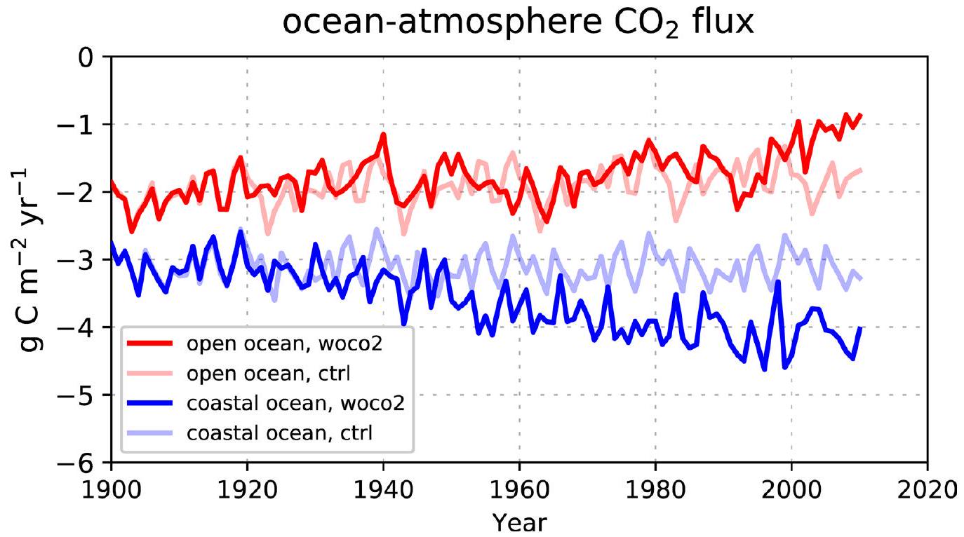
المحيط-الغلاف الجويتدفق ( ) يظهر تغييرًا واضحًا نحو صافي أقوى غرق خلال فترة 1900-2010 (أكثر سلبيةفي الشكل 1). هذه النزعة تنطبق على كل من المحيط المفتوح والساحلي، وتعكس التغيرات في (الشكل البياني الموسع 3). منذ الخمسينيات، يزيد بمقدارفي المحيط الساحلي، تفوق علىزيادة في المحيط المفتوح (الاتجاه الخطي، ). الإشارة الأقوى في المحيط الساحلي تتماشى مع الدراسة الرصدية في المرجع 7. ومع ذلك، فإن معدلات الزيادة في محاكاة لدينا تكون عمومًا أضعف بعوامل 2 و 4 في المحيط المفتوح والساحلي على التوالي، وتظل أضعف عند المقارنة بنفس الفترة الزمنية (اتجاهات الشتاء منذ الثمانينيات) والتغطية المكانية (باستثناء الرفوف القطبية والجنوبية الشرقية لآسيا). ومع ذلك، فإن الاتجاهات المستمدة في المرجع 7 تظهر عدم يقين كبير، حيث أن التباينات ( في بياناتهم المستندة إلى المحطات، تكون القيم 10 و 4 مرات أكبر من القيم المتوسطة العالمية المقابلة. هذه الشكوك العالية تتأكد أكثر من خلال دراسة المرجع 17، التي استخدمت نسخة مبكرة من أطلس SOCAT.لكن لم يجدوا اتجاهًا ملحوظًا في السواحل.
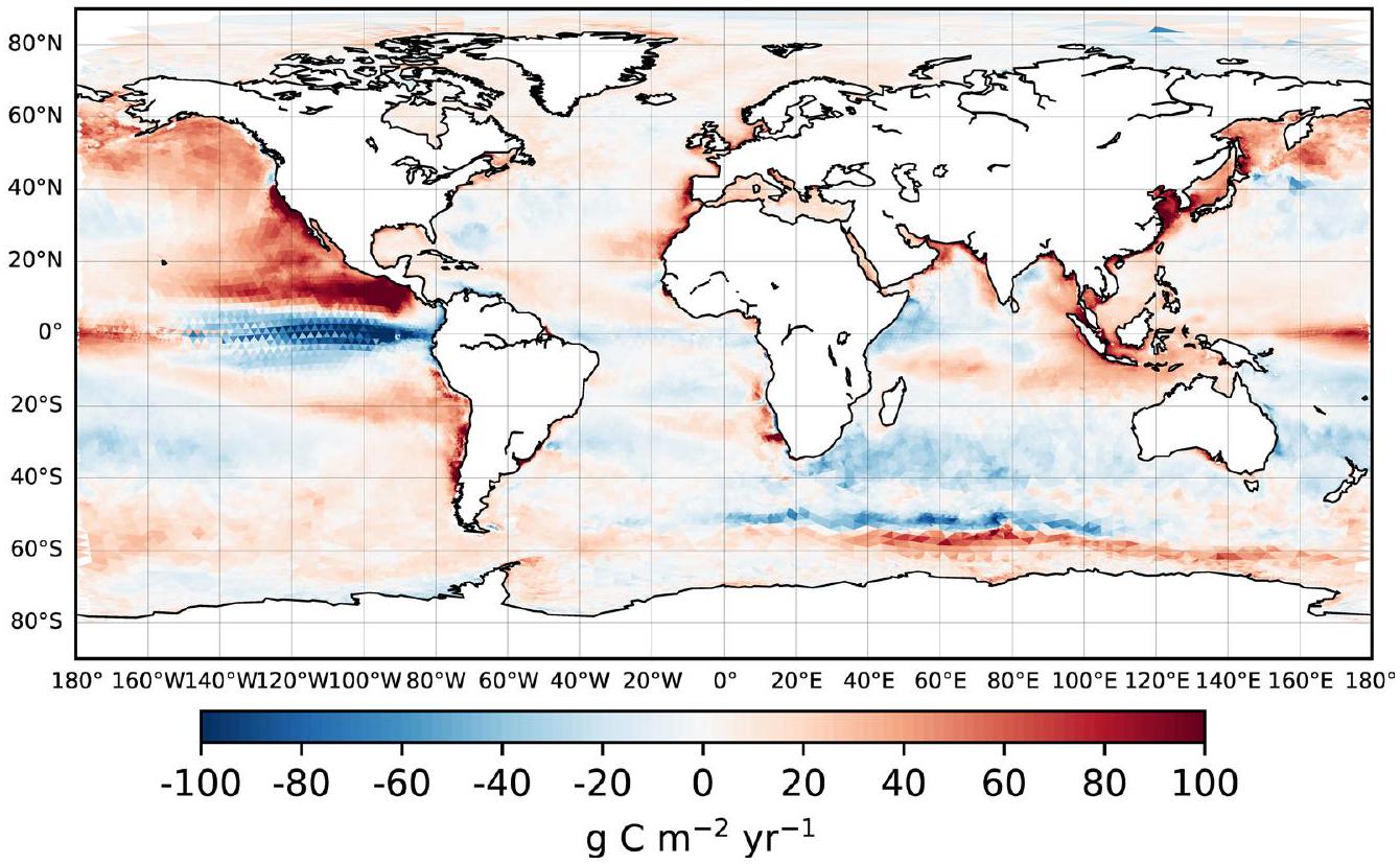
التوزيع المكاني للمحاكاةالإشارة (الشكل 2) تعكس الاتجاه العام في اتجاه التدفق الهابط، بسبب الانخفاض السائد فيزيادة المعدلات في المحيط أكثر من الغلاف الجوي (يمثلها تغيير سلبي في ). الاستثناءات توجد بشكل رئيسي في المحيط الجنوبي وعلى الرفوف القطبية، حيث يحدث ارتفاع في درجة حرارة السطح (بمقدار يصل إلى يحفزتغيرات في الاتجاه المعاكس. على المتوسط العالمي، الناتج الصافيالامتصاص له كثافة أعلى بشكل عام (بـ ) في المحيط الساحلي أكثر من المحيط المفتوح (الشكل 1).
المحيط الساحلي كمنطقة لتحويل الكربون
المحيط الساحلي هو منطقة ذات نشاط بيولوجي مرتفع. يتم محاكاة الإنتاج الأولي الصافي المتكامل (NPP) ليكونللفترة من 1991 إلى 2010 (تاريخي)، أو 11% من الإنتاج الأولي البحري العالمي. يتم إعادة تَحَجُّر الغالبية العظمى من هذا الكربون المرتبط بيولوجيًا مرة أخرى على الرفوف القارية (87%). من الكربون العضوي وغير العضوي الجسيمي المتبقي،يتم دفنه في رواسب الرف، بينماالكربون العضوي المذاب (DOC) والكربون العضوي الجزيئي (POC) يتم نقلهما بعيدًا عن الرف إلى المحيط المفتوح (الشكل 3). حيث تتجاوز هذه التدفقات التصديرية صافي الوارد من
الشكل 1 | سلسلة زمنية لمحاكاة المحيط-الغلاف الجويكثافة التدفق. متوسطات فوق المحيط المفتوح (أ) والمحيط الساحلي (ب). تم تمديد كلا المحاكاة woriv و hist لفترة 1900-2010 لمدة 100 عام أخرى بواسطة الغلاف الجوي الثابت.سنة 2010 (تاريخووريفعلى التوالي)، في حين تم تمديد woriv لمدة 40 عامًا إضافية من خلال زيادة الغلاف الجوي بشكل مستمرسيناريو الانبعاثات التالي RCP8.5ما عدا الغلاف الجويتم دفع الفترات الممتدة بواسطة قوى متكررة من الفترة 1991-2010 (انظر ‘تصميم التجربة’). الخط العمودي الرمادي يحدد الانتقال إلى الفترات الممتدة. تشير العلامة السلبية إلىتدفق إلى المحيط.
عبر الأنهار و DIC عبر كتل المياه في المحيط المفتوح، يتم تعويض العجز الناتج في المياه الساحلية بواسطة صافياستيعابمن الغلاف الجوي. وبالتالي، يشكل المحيط الساحلي دورة الكربون البحرية من خلال تحويل الكربون غير العضوي (IC) المقدم من اليابسة والغلاف الجوي والمحيط المفتوح إلى كربون عضوي (OC).
تمت محاكاة التحول الصافي من IC إلى OC في المحيط الساحلي منذ بداية القرن العشرين (ctrl)، مع امتصاص صافي ضعيف للغلاف الجوي.من (الشكل 3). تؤكد هذه المصيدة الكربونية الساحلية المبكرة التقييمات الأولى لحالة المحيط قبل الصناعة، مما يشير إلى ساحل ضعيف امتصاص 40 و للمراجع 4 و 22، على التوالي، على الرغم من صافيإطلاق من المحيط العالمي. وفقًا لمحاكياتنا، فإن التأثير التراكمي الناتج عن الأنشطة البشرية خلال القرن العشرين يؤدي إلى أكثر من ضعف المحيط الساحلي.يغرق. من خلال افتراض أن النقل الجاهز للـ POC يتم تمريره إلى المحيط العميق ويتم إزالة DOC من المحيط العلوي عبر إنتاج تصدير جديديمكننا التحقق من خزانات الكربون حيث تم امتصاص الكمية الإضافيةيبقى:يعيش في المياه الساحلية،يتم دفنه في رواسب الرفوف،يتم تصديره إلى المحيط المفتوح العلوي ويتم نقله إلى المحيط العميق.
ضوابط الزيادةحفرة المحيط الساحلي
الساحليتُعزز المصب من خلال زيادة الارتفاع في أنظمة الارتفاع الحدودية الشرقية عالية الإنتاج (EBUS) ومن خلال البحر تراجع لطيف في العروض العليا، ناتج عن التغيرات المناخية التي تسببها الأنشطة البشرية.
تغيرات في نمط الرياح القريبة من السطح (الشكل التكميلي 1) تعكس هجرة قطبية عالمية لحقول الضغط الجوي العالي على نطاق واسع، والتي تُسمى التوسع الاستوائي.. في نظام EBUS الساحلي المجاور للمحيط الهادئ والأطلسي (انظر ‘التحليل’)، يتعزز تدفق المحيط المفتوح إلى الرفوف بشكل ومعناهايزداد التركيز بمقدار 0.6 مليمول نيتروجين لكل متر خلال القرن العشرين. زادت الدورة المكثفة والإنتاجية المحسّنة، الشكل التوضيحي الإضافي 2) تسبب زيادة في تصدير OC إلى المحيط المفتوح بواسطةوتغيير نحو الأسفل فيبـ 31 جزء في المليون، مما يزيد من الساحلي امتصاص بواسطة .
في المحيط الساحلي في العروض العليا، تتوسع المناطق الخالية من الجليد (الربيع القطبي الشماليالقطب الجنوبي، الشكل 4 من البيانات الموسعة) يعزز الشبكة امتصاص بواسطة على الرفوف القطبية الشمالية وفي المناطق الساحلية في القارة القطبية الجنوبية. تؤدي المناطق المفتوحة الأكبر والأطول عمراً إلى زيادة الذوبانية وضخ الكائنات الحية (الربيع NPP القطب الشماليالقطب الجنوبي )، مع وجود علاقة بين إنتاجية ازدهار الربيع وغطاء الجليد البحري ( ). التغيرات في القطب الشمالي تخفف من خلال ارتفاع درجات الحرارة فوق المعدل بمقدار يصل إلى ، الذي يعوض أيضًا تأثير التخفيف المعزز (الملوحة-0.2 وحدة عملية،بسبب غزو مياه الذوبان من اليابسة (الجريان السطحي) ) وجليد البحر. تأثير درجة الحرارة يتناقص إقليمياً (الشكل 2)، ولكن بشكل عام، الساحليمن الواضح أن الامتصاص قد زاد بشكل ملحوظ (الشكل 4). بسبب اختلاف مناطق التغطية، فإن المساهمة الإجمالية للرفوف القطبية الشمالية تساهم في زيادة امتصاص CO2 بواسطة، وهو أكبر بكثير من الرفوف القطبية الجنوبية الضيقة نسبياً ( ).
لتحقيق تأثير ارتفاع الغلاف الجويواصلنا التجارب التاريخية والعمل مع الغلاف الجويثابت (تاريخ)ووريف ). هذا يسمح لنا بتمييز الإجمالي إشارة إلى مضخة الذوبان، مدفوعة بعملية ذوبان الغلاف الجويفي المحيط، ومضخة البيولوجية، المدفوعة بامتصاص DIC بسبب نمو العوالق النباتية (انظر قسم ‘التحليل’)، وقياس تدفقات الاستيراد والتصدير لميزانية الكربون الساحلية (البيانات الموسعة الجدول 1) التي تدعم هذهالمساهمات (الشكل 5). مناقشة إضافية حول استجابة المحيطتُقدم الغوص في هذا السيناريو المثالي لحياد المناخ في القسم ‘استجابة المحيط الساحلي’.الاستيعاب نحو الحياد المناخي.
في المحاكاة دون زيادة مدخلات المغذيات من الأنهار (woriv)، كانت المساهمة في إشارة الامتصاص بواسطة مضخة الذوبان; الشكل 5أ) أكبر من مساهمة المضخة البيولوجية (; الشكل 5ب). الإضافي إزالة من الغلاف الجوي إما تزيد من مخزون الكربون غير العضوي في السواحل (55%) أو يتم نقلها خارج الرف الساحلي ( )، مما يضعف تدفق DIC الصافي من المحيط المفتوح (الشكل 5أ، تغيير إيجابي في التدفق الحراري للـ IC). الإنتاجية البيولوجية الأعلى بسبب زيادة الارتفاع وذوبان الجليد البحري (NPPيؤدي إلى زيادة تصدير الكربون العضوي عن طريق الحمل ولكن أيضًا التنفس، مما يقلل من استهلاك DIC في المحيط المفتوح بمقدار مماثل (الشكل 5ب، تغيير إيجابي في التدفق الإيجابي لـ IC).
الإمداد المعزز بالعناصر الغذائية من الأنهار (التاريخ) يعزز بشكل كبير نمو العوالق النباتية في المحيط الساحلي (الإنتاج الأولي الصافي) ). إن زيادة تثبيت الكربون البيولوجي الأعلى تعزز المساهمة البيولوجية في السواحل (إلى ; الشكل 5د) ويحول هذاإلى المادة العضوية (الشكل 5ج، تدفق الكربون العضوي). الزيادة الناتجة عن النهر في الإنتاجية البيولوجية تزيد من تصدير الكربون العضوي (إلى المحيط المفتوح والرواسب)، واستيراد الكربون غير العضوي التدفق (الشكل 5د، التغير السلبي في تدفق الكربون غير العضوي) وامتصاص من الغلاف الجوي، ولا يزال يؤدي إلى تراكم أقل من DIC (مخزون IC) في المياه الساحلية (جميعها مقارنة بـ woriv،تشير الزيادة في صافي استيراد الكربون غير العضوي من المحيط المفتوح (البيانات الموسعة الجدول 1، متوسط سالب وتغير سالب في تدفق الكربون غير العضوي) إلى أن المحيط الساحلي قد يعمل على إضعاف الزيادة العامة في الكربون غير العضوي في المحيط المفتوح، حيث يتم استهلاك المزيد من الكربون غير العضوي في المحيط المفتوح من قبل الإنتاجية البيولوجية أكثر من التنفس.وتم نقل أحمال DIC النهرية خارج الرف. في نهاية القرن العشرين، كانت هذه الصافي
الشكل 2 | إشارة التغيير المحاكية للمحيط-الغلاف الجويخلال القرن العشرين (1991-2010 من التاريخ ناقص التحكم). التغيرات السلبية (باللون الأزرق) تشير إلى أنتغير في اتجاه هابط، أي نحو المزيد من امتصاص أقل وانبعاث غازات أقل. تمثل المناطق البيضاء المظللة في القطب الشمالي غطاء الجليد البحري الدائم، مما يعيق تبادل الغازات عند سطح البحر. تشير المناطق المنقطة إلى تغييرات بأقل منثقة قائمة على جانبين-اختبار.
استيراد DIC من المحيط المفتوح هوالذي تُنسب إلى تأثير زيادة المدخلات الغذائية من اليابسة (الشكل 3). عندما نطرح مصدر DIC من بسبب التمعدن المحاكى للمياه العضوية الأرضية في المحيط المفتوح، يعتبر المحيط الساحلي مصدراً ضعيفاً لامتصاص الكربون العضوي المذاب.للمحيط المفتوح. وبالتالي، تحت تأثير زيادة التخصيب، فإن المحيط الساحلي ليس فقط مصبًا متزايدًا للغلاف الجوي، ولكن أيضًا لثاني أكسيد الكربون الذائب في المياه العليا، مما يعززامتصاص في المحيط المفتوح.
عند أخذ زيادة الإثراء الغذائي في الاعتبار (التاريخ)، فإن المساهمة البيولوجية ( ) يتجاوز بوضوح مساهمة الذوبانية ( )، مما يجعل تثبيت الكربون البيولوجي العملية السائدة التي تعزز السواحل الامتصاص خلال القرن العشرين. يتم التوسط في هذا التغيير من خلال زيادة تصدير الكربون العضوي إلى المحيط المفتوح، الذي يتم استبعاده من تبادل الغاز مع الغلاف الجوي، مما يضيف المزيد إلى إثراء الكربون في المحيط المفتوح.
يمكننا الآن قياس العوامل الرئيسية للزيادة المعاصرةالامتصاص في المحيط الساحلي (انظر قسم ‘التحليل’). يتم تمثيل مساهمة الذوبانية من خلال الانخفاض فيالامتصاص من تاريخ إلى تاريخ (الشكل 1) ويعبر عن من الإجماليإشارة خلال القرن العشرين. تمثل النسبة المتبقية 59% المساهمة البيولوجية، والتي يمكن أن تُعزى بشكل أكبر إلى مكون ناتج عن المناخ.مدفوع أساسًا بزيادة الارتفاع البحري وتراجع الجليد البحري، ومكون ناتج عن تحميل الأنهاريمثل الفرق بين hist و woriv. ومع ذلك، تتضمن هذه التقسيمات تأثير التغيرات في درجة حرارة سطح البحر وسرعة الرياح على (المرجع 27)، بالإضافة إلى تأثير الانخفاض في سعة العازلة لمياه البحر بسبب حموضة المحيطأخفضالذوبانية وسرعة المكبس الأعلى بسبب زيادة درجة حرارة الماء كلاهما يتغيران بأقل منوبالتالي تلغي بشكل عادل تأثيرها على. عادةً ما تكون سرعات الرياح الأعلى (بنحو )، ومع ذلك، تؤدي إلى أقوى تبادل التدفقات (عن طريق )، مما يزيد بشكل متساوٍ من قابلية الذوبان ومضخات الكربون البيولوجية. علاوة على ذلك، فإن متوسط تركيز الكربون غير العضوي الذائب في السطح المحاكي في المحيط الساحلي يزيد خلال القرن العشرين بمقدار ، مما أدى إلى زيادة عامل ريفيل من 10.1 إلى 10.7 (انظر “التحليل”). هذا يعني أن يصبح أكثر حساسية للتغيرات في DIC ونتيجة لذلك، فإن التغيرات في عمليات تثبيت الكربون والتصدير لها تأثير أكبر على و تبادل الغازات.
الشكل 3 | ميزانية الكربون للمحيط الساحلي العالمي، المستمدة من التجارب ctrl و woriv و hist للفترة من 1991 إلى 2010. جميع الأرقام مقدمة في. *، نهريةتم وصف المدخلات ويفترض أنها ثابتة على مدار فترة المحاكاة. **، تراكم DIC الصافي في التشغيل الضابط ناتج عن انحراف النموذج على المدى الطويل. DOCt، الكربون العضوي الذائب الأرضي؛ PIC، الكربون غير العضوي الجزيئي.
عندما نكرر محاكاة التاريخ دون الارتفاع التاريخي في الغلاف الجوي (الشكل 5 من البيانات الموسعة)، نجد أن الزيادة في المحيط الساحليالاستهلاك أضعف بمقدار يصل إلى
الشكل 4 | إشارة التغيير المحاكية للمحيط-الغلاف الجويالتدفق خلال القرن العشرين (1991-2010 من التاريخ ناقص التحكم)، موضحًا للمحيط الساحلي. القيم السلبية تشير إلى تغييرات نحو المزيد منامتصاص أقل وإطلاق غازات أقل.
الشكل 5|تقسيم المحيط الساحليإشارة إلى التغيرات في الذوبانية ومضخات الكربون البيولوجية. أ-د، الذوبانية (أ، ج) والمساهمات البيولوجية (ب، د) لتجربة ووريف (أ، ب) (باستثناء الزيادات في مدخلات المغذيات من اليابسة) والمحاكاة التاريخية (ج، د). مجموع الذوبانية والمساهمات البيولوجية (سماوي) يتوافق مع الإجماليشذوذ بالنسبة للتحكم. يتم اشتقاق الذوبانية والإشارات البيولوجية بالإضافة إلى تدفقات الاستيراد والتصدير الصافية المستدامة من ميزانية الكربون للفترة من 1991 إلى 2010 (رمادي
المساحة المظللة والقيم في هوامش الشكل الأيمن) من خلال افتراض مساهمات نسبية ثابتة على مدار فترة المحاكاة بأكملها. التغيرات السلبية فيتشير إلى الزيادة امتصاص النقل الانتقالي الصافي للكربون العضوي/غير العضوي إلى المحيط المفتوح؛الرواسب، الإيداع الصافي للكربون العضوي/غير العضوي في رواسب الرف؛ محلول/بيولوجيالذوبانية الصافية/ البيولوجيةالتدفق عند سطح البحر؛ مخزون الكربون غير العضوي، تخزين الكربون غير العضوي في مياه الرفوف. ( 1.1 بدلاً من )، في حين أن معدل تثبيت الكربون البيولوجي يبقى كما هو. وهذا يعني أن المساهمة البيولوجية لـ إشارة ( ) هو مدفوعًا بتأثير العازل )، حيث أن استيعاب DIC من خلال نمو العوالق النباتية يؤدي إلى أكبرانخفاض عندماسعة العازلة منخفضة. لقد أظهر تأثير الحموضة هذا أنه يعزز بشكل كبير التأثير البيولوجي المحفز على الهواء والبحر.تدرجوهنا يتم تعميمه ليشمل هوامش المحيط. في المحيط المفتوح، دون تأثير العازل (موسع
بيانات الشكل 5)، تأثير الاحترار على ستفوق القابلية للذوبان حتى على تحسين احتجاز الكربون البيولوجي، مما يؤدي إلى تقليل صافي في امتصاص بواسطة . وبالمثل، في المحيط الساحلي، حددنا تأثير العازل كونه السيطرة السائدة ( ) من البيولوجي الإشارة. وبالتالي، فإن تثبيت الكربون البيولوجي يساهم بشكل كبير أكثر فيالامتصاص مع انخفاض سعة العازلة تحت تغير المناخ المستمر.
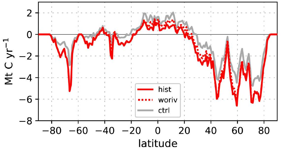
خلال القرن العشرين، كانت هناك تغييرات في تُظهر تدفقات السطح نحو مزيد من الامتصاص أو أقل من انبعاث الغازات في 93% من منطقة المحيط الساحلي (الشكل 4). هذه الاتجاه العام مرئي في جميع خطوط العرض، بينما تقتصر تأثيرات إشارة الإثراء الغذائي بشكل رئيسي على نصف الكرة الشمالي (الشكل البياني الممتد 6، الفرق بين woriv و hist) بسبب عدم التماثل في التوزيع المكاني للكتل الأرضية، وتصريف الأنهار، ومدخلات المغذيات المرتبطة بها..
مقارنةً بـامتصاص المحيط المفتوح
وفقًا لمحاكياتنا، زادت الإنتاجية الأولية للنباتات البحرية العالمية (الشكل البياني الإضافي 7) خلال القرن العشرين من 44.6 إلى 46.7 بيغاغرام كربون في السنة. )، مع مساهمة سطحية من في المحيط المفتوح وإشارة أقوى بخمس مرات منفي المحيط الساحلي بسبب تأثيرات زيادة الارتفاع، وتراجع الجليد البحري، والتغذية الزائدة (انظر ‘الزيادة العالمية في الإنتاج الأولي الصافي الساحلي’). بينما أظهرنا أن هذه الاستجابة البيولوجية تؤثر بشكل كبير علىالامتصاص على الرفوف، التغيير الناتج في تصدير POC العمودي في المحيط المفتوحيساهم فقطإلى الشبكة المعززة امتصاص ). هذه المساهمة البيولوجية الطفيفة تتماشى مع التقدير المقدم في المرجع 31، الذي حلل استخدام الأكسجين الظاهر كبديل للإنتاجية البيولوجية وخلص إلى أن تعزيز المحيط المفتوحالغرق خلال العقود الأخيرة كان مدفوعًا إلى حد كبير بالعمليات الفيزيائية والكيميائية. منانخفاض في تاريخ التجربةنحصل على مكون مدفوع كيميائيًا منيترككالمساهمة المتبقية المدفوعة بالدوران الفيزيائي لـإشارة في المحيط المفتوح.
نموذجنا من الجيل التالي ICON-Coast يكشف أن المحيط الساحلي هو أكثر كفاءةأعمق من المحيط المفتوح (الشكل 1)، كونه النموذج الأول الذي يظهر توافقًا مع هذا الاستنتاج الذي تم استنتاجه أولاً من المنتجات الرصدية.نجد أكبر الفروقات بين السواحل والمحيط المفتوحكثافات التدفق في خطوط العرض المنخفضة بين و . في هذه المناطق، يؤدي تثبيت الكربون البيولوجي إلى تقليل السواحلإطلاق الغازات وزيادة الامتصاص بمقدار 2.7 وعلى التوالي، في حين أن في خطوط العرض المتوسطة والعالية، الساحليةكثافات التدفق لا تتجاوز قيم المحيط المفتوح. المتباينتكون أسعار الصرف في خطوط العرض المنخفضة مدعومة جيدًا للمنطقة الاستوائية منمن خلال الدراسة الرصدية في المرجع 3، بينما بالنسبة للأجزاء المتبقية، فإن هذا أقل وضوحًا، على الرغم من أنه يتماشى مع نطاق عدم اليقين لديهم.
التباين بين السواحل والمحيط المفتوحتُعزَّز كثافات التدفق بهيمنة المناطق تحت القطبية والقطبيةتغمر في توزيع المنطقة للمحيط الساحلي العالميومع ذلك، ستظل كفاءة الامتصاص الأعلى للمحيط الساحلي محفوظة إذا تم توزيع نسبة المساحة العرضية بشكل متساوٍ، حيث أن الناتج الصافي الناتجاستيعابفي المحيط الساحلي لا يزال يتجاوز الـالمحيط المفتوح. وهذا يشير إلى أن هناك عاملاً رئيسياً آخر يتحكم في عدم التناسبغمر المحيط الساحلي هو تثبيت الكربون البيولوجي العالي في خطوط العرض المنخفضة.
نموذجنا يظهر المحيط الساحلي كنقطة ساخنة لعمليات تحويل الكربون، مما يؤدي إلى “بيولوجيغرق خلال القرن العشرين. بينما تم اقتراح مثل هذا المحيط التلقائي في دراسات سابقة قائمة على النماذجتكون التغيرات في تدفقات تبادل الكربون العمودية والأفقية عمومًا أقوى بعوامل منفي نموذجنا المحدد للساحل. إن هذه التدفقات أكبر مما كان يُفترض سابقًا، مما له تداعيات على الحلقة المفقودة في المحيط الساحلي.التدفق في الميزانية العالمية للكربونمصدر OC للمحيط المفتوح، بالإضافة إلى التأثيرات البيولوجية المتعلقة بزيادة تكوين المركبات العضوية المتطايرةمن المحتمل أن تواجه تدفقات الكربون الكثيفة في المحيط الساحلي معدلات متزايدة مع الانبعاثات المركبة القادمة من الوقود الأحفوري، وتغير المناخ، والاضطرابات البشرية في أنظمة المياه العذبة. وبالتالي، توفر دراستنا خطوة حيوية لتقييم التطورات التاريخية والمستقبلية لدورة الكربون الساحلية.
المحتوى عبر الإنترنت
أي طرق، مراجع إضافية، ملخصات تقارير Nature Portfolio، بيانات المصدر، بيانات موسعة، معلومات تكميلية، شكر وتقدير، معلومات مراجعة الأقران؛ تفاصيل مساهمات المؤلفين والمصالح المتنافسة؛ وبيانات توفر البيانات والرموز متاحة علىhttps://doi.org/10.1038/s41558-024-01956-w.
References
Liu, K. K., Atkinson, L., Quiñones, R. & Talaue-McManus, L. in Carbon and Nutrient Fluxes in Continental Margins: A Global Synthesis (eds Liu, K. K. et al.) 3-24 (Springer, 2010).
Bauer, J. E. et al. The changing carbon cycle of the coastal ocean. Nature 504, 61-70 (2013).
Roobaert, A. et al. The spatiotemporal dynamics of the sources and sinks of in the global coastal ocean. Global Biogeochem. Cycles 33, 1693-1714 (2019).
Regnier, P., Resplandy, L., Najjar, R. G. & Ciais, P. The land-to-ocean loops of the global carbon cycle. Nature 603, 401-410 (2022).
Laruelle, G. G., Lauerwald, R., Pfeil, B. & Regnier, P. Regionalized global budget of the exchange at the air-water interface in continental shelf seas. Global Biogeochem. Cycles 28, 1199-1214 (2014).
Dai, M. et al. Carbon fluxes in the coastal ocean: synthesis, boundary processes, and future trends. Annu. Rev. Earth Planet. Sci. 50, 593-626 (2022).
Laruelle, G. G. et al. Continental shelves as a variable but increasing global sink for atmospheric carbon dioxide. Nat. Commun. 9, 454 (2018).
Hauck, J. et al. Consistency and challenges in the ocean carbon sink estimate for the global carbon budget. Front. Mar. Sci. 7, 22 (2020).
Brewin, R. J. W. et al. Ocean carbon from space: current status and priorities for the next decade. Earth Sci. Rev. 240, 104386 (2023).
Bourgeois, T. et al. Coastal-ocean uptake of anthropogenic carbon. Biogeosciences 13, 4167-4185 (2016).
Lacroix, F., Ilyina, T., Mathis, M., Laruelle, G. G. & Regnier, P. Historical increases in land-derived nutrient inputs may alleviate effects of a changing physical climate on the oceanic carbon cycle. Global Change Biol. 27, 5491-5513 (2021).
Mathis, M., Elizalde, A. & Mikolajewicz, U. The future regime of Atlantic nutrient supply to the Northwest European Shelf. J. Mar. Syst. 189, 98-115 (2019).
Takahashi, T. et al. Global sea-air flux based on climatological surface ocean , and seasonal biological and temperature effects. Deep Sea Res. II 49, 1601-1622 (2002).
Sundquist, E. T., Plummer, L. N. & Wigley, T. M. L. Carbon dioxide in the ocean surface: the homogeneous buffer factor. Science 204, 1203-1205 (1979).
Takahashi, T. et al. Climatological mean and decadal change in surface ocean , and net sea-air flux over the global oceans. Deep Sea Res. II 56, 554-577 (2009).
McKinley, G. et al. Timescales for detection of trends in the ocean carbon sink. Nature 530, 469-472 (2016).
Wang, H., Hu, X., Cai, W. J. & Sterba-Boatwright, B. Decadal trends in global ocean margins and adjacent boundary current-influenced areas. Geophys. Res. Lett. 44, 8962-8970 (2017).
Ward, N. D. et al. Representing the function and sensitivity of coastal interfaces in Earth system models. Nat. Commun. 11, 2458 (2020).
Roobaert, A., Resplandy, L., Laruelle, G. G., Liao, E. & Regnier, P. A framework to evaluate and elucidate the driving mechanisms of coastal sea surface seasonality using an ocean general circulation model (MOM6-COBALT). Ocean Sci. 18, 67-88 (2022).
Mathis, M. et al. Seamless integration of the coastal ocean in global marine carbon cycle modeling. J. Adv. Model. Earth Syst. 14, e2021MS002789 (2022).
Bakker, D. C. E. et al. A multi-decade record of high-quality data in version 3 of the Surface Ocean CO2 Atlas (SOCAT). Earth Syst. Sci. Data 8, 383-413 (2016).
Lacroix, F., Ilyina, T., Laruelle, G. G. & Regnier, P. Reconstructing the preindustrial coastal carbon cycle through a global ocean circulation model: was the global continental shelf already both autotrophic and a sink? Global Biogeochem. Cycles 35, e2020GB006603 (2021).
DeVries, T. & Weber, T. The export and fate of organic matter in the ocean: new constraints from combining satellite and oceanographic tracer observations. Global Biogeochem. Cycles 31, 535-555 (2017).
Daloz, A. S. & Camargo, S. J. Is the poleward migration of tropical cyclone maximum intensity associated with a poleward migration of tropical cyclone genesis? Clim. Dyn. 50, 705-715 (2018).
Yang, H. et al. Poleward shift of the major ocean gyres detected in a warming climate. Geophys. Res. Lett. 47, e2019GL085868 (2020).
Yang, H. et al. Tropical expansion driven by poleward advancing midlatitude meridional temperature gradients. J. Geophys. Res. Atmos. 125, e2020JD033158 (2020).
Wanninkhof, R. Relationship between wind speed and gas exchange over the ocean revisited. Limnol. Oceanogr. Methods 12, 351-362 (2014).
Sarmiento, J. L. & Gruber, N. Ocean Biogeochemical Dynamics (Princeton Univ. Press, 2006).
Hauck, J. & Völker, C. Rising atmospheric leads to large impact of biology on Southern Ocean uptake via changes of the Revelle factor. Geophys. Res. Lett. 42, 1459-1464 (2015).
Lacroix, F., Ilyina, T. & Hartmann, J. Oceanic outgassing and biological production hotspots induced by pre-industrial river loads of nutrients and carbon in a global modeling approach. Biogeosciences 17, 55-88 (2020).
Koeve, W., Kähler, P. & Oschlies, A. Does export production measure transient changes of the biological carbon pump’s feedback to the atmosphere under global warming? Geophys. Res. Lett. 47, e2020GL089928 (2020).
Friedlingstein, P. et al. Global carbon budget 2020. Earth Syst. Sci. Data 12, 3269-3340 (2020).
Breitburg, D. et al. Declining oxygen in the global ocean and coastal waters. Science 359, eaam7240 (2018).
Publisher’s note Springer Nature remains neutral with regard to jurisdictional claims in published maps and institutional affiliations.
Open Access This article is licensed under a Creative Commons Attribution 4.0 International License, which permits use, sharing, adaptation, distribution and reproduction in any medium or format, as long as you give appropriate credit to the original author(s) and the source, provide a link to the Creative Commons licence, and indicate if changes were made. The images or other third party material in this article are included in the article’s Creative Commons licence, unless indicated otherwise in a credit line to the material. If material is not included in the article’s Creative Commons licence and your intended use is not permitted by statutory regulation or exceeds the permitted use, you will need to obtain permission directly from the copyright holder. To view a copy of this licence, visit http://creativecommons. org/licenses/by/4.0/.
(c) The Author(s) 2024
طرق
وصف النموذج
نموذج الكيمياء الحيوية المحيطية ICON-Coast هو تطور لمكون المحيط ICON-Oنموذج نظام الأرض هامبورغ ICON-ESMيتكون تكيفه لدمج ميزات الدورة الساحلية وديناميات الكربون من تطوير على مرحلتين. أولاً، تم تقييد تحسين دقة الشبكة الأفقية على الهوامش القارية والرفوف الضحلة، بما في ذلك منطقة الانتقال إلى أحواض المحيط العميق المجاورة.ثانيًا، مكون الكيمياء الحيوية HAMOCCتم تمديده ليأخذ في الاعتبار بشكل أفضل عمليات تحويل الكربون الخاصة بالرفوفبما في ذلك تيارات المد والجزر وتأثيرات سحب القاعإعادة تعليق الرواسبإعادة التمعدن المعتمدة على درجة الحرارة في عمود الماء والرواسب سرعات الغرق المتغيرة لمكونات الكربون الجزيئي والمعادن المجمعةوتدفقات المواد من اليابسة، بما في ذلك أحمال الأنهار من الكربون الأرضي والمواد المغذيةبالإضافة إلى ترسيب الغبار من الغلاف الجويوالنيتروجين.
تعتمد ديناميات النموذج على معادلات بوسينسكي الهيدروستاتيكية، التي تم حلها على شبكة مثلثية مع تداخل من نوع أراكوا C. في التكوين المقدم هنا، استخدمنا إغلاق سرعة تحت الشبكة من نوع بيهارموني مع معامل لزوجة يعتمد على المقياس لأخذ في الاعتبار الدقة الأفقية المتغيرة. تم تهيئة الخلط العمودي بواسطة معادلة تنبؤية لطاقة الحركة المضطربة. تم محاكاة ديناميات الجليد البحري بواسطة نموذج الجليد البحري FESIM.تم نقل المؤشرات البيوجيوكيميائية في عمود الماء بواسطة أنظمة النقل الفيزيائي والتشتت. تبعت النشاطات البيولوجية نهجًا موسعًا للمواد الغذائية، والطحالب العائمة، والزوائد العائمة، والمواد العضوية المتحللة (NPZD) مع نسبة ثابتة من العناصر الغذائية وتحديد مشترك للعناصر الغذائية الفوسفات، والنيترات، والسيليكات، والحديد. تم فصل الإنتاج المصدر إلىومادة قشرة الأوبال. تم تمثيل العمليات الرسوبية بـ 12 طبقة نشطة بيولوجيًا، مما يعكس تحلل ودفن المواد العضوية وغير العضوية الجسيمية، بما في ذلك انتشار مياه المسام.
لعمليات المحاكاة لدينا هنا، استخدمنا نفس تكوين الشبكة المستخدم في تجارب الكيمياء الحيوية في ورقة تقديم النموذج.. تراوحت المسافة الأفقية للشبكة من 160 كم في المحيط المفتوح إلى 20 كم بالقرب من السواحل وعلى طول التدرجات الطبوغرافية. وتم تمثيل العمق بـ 40 مستوى على -الإحداثيات، مع سمك طبقة يبلغ 10 م في أعلى 100 م من عمود الماء (باستثناء الطبقة العليا التي تبلغ 16 م مع ارتفاع سطح حر لتسهيل سعة المد والجزر وسماكة الجليد البحري) وزيادة المسافة في الأسفل. كانت خطوة الوقت في النموذج في الإعداد المقدم 720 ثانية.
تصميم التجربة
تم تشغيل محاكاة المحيطات لدينا باستخدام ICON-Coast مع عدد من شروط الحدود المحددة. كحقول قوى جوية، استخدمنا بيانات إعادة التحليل ERA-20C كل ثلاث ساعات.المتوسط السنوي للغلاف الجويتبع السجل التاريخي أو سيناريو ارتفاع الانبعاثات للاحترار العالمي RCP8.5، كما تم تطويره للتقرير التقييمي الخامس للهيئة الحكومية الدولية المعنية بتغير المناخ (AR5). جريان الأنهار منتم إعادة بناء مناطق التجميع بواسطة نموذج التصريف الهيدرولوجي العالمي HDتم اشتقاق تدفقات المادة من DIP و DIN و DSi و DFe و DIC والقلوية والمادة العضوية الجسيمية والمادة العضوية المذابة الأرضية في المراجع 11 و 30 لأكبر حوالي 850 نهرًا. تم تقدير زيادة الأحمال الغذائية من DIN و DIP تاريخيًا من خلال زيادة خطية خلال فترة التنبؤ العكسي 1900-2010 (الشكل التكميلي 3). تبعت ترسيب النيتروجين والغبار الهوائي كمصادر إضافية للمواد الغذائية غير العضوية المراجع 40 و 42، على التوالي. هنا، فقطحدثت ترسيبات النيتروجين في المحيط الساحلي، بينماتم تصريف مدخلات النهر على الرفوف (الشكل التكميلي 3). وعند تجميعها على منطقة المحيط الساحلي، كانت الحمولة الإجمالية الناتجة من المغذيات من اليابسة تتكون أساسًا من مدخلات النهر. لذلك، في تحليلنا ومناقشتنا للمحيط الساحلي، نشير بشكل رئيسي إلى تدفقات المغذيات من اليابسة كحمولات نهرية.
قمنا بتهيئة إجراء الدوران الخاص بنا بحالة المحيط من عام 1900 من محاكاة تاريخية لنموذج نظام الأرض.
تم استخدام MPI-ESM-HR كجزء من المشروع السادس لمقارنة النماذج المتصلة (CMIP6). ثم تم تشغيل ICON-Coast في وضع الفيزياء فقط لمدة 200 عام باستخدام ظروف فرضية متكررة من الفترة 1900-1919 للسماح لدورة المحيطات بالتكيف مع مواصفات النموذج وتكوين الشبكة. ثم تم تضمين مكون الكيمياء الحيوية لمدة 100 عام أخرى. تم استخدام نهاية هذه الفترة التمهيدية لتهيئة عمليات الإنتاج لدينا مع فرضيات متغيرة، بالإضافة إلى تشغيل التحكم كاستمرار للفترة التمهيدية مع فرضيات متكررة.
النموذج الأساسي لهذه الدراسة هو تشغيل استرجاعي (hist) خلال الفترة التاريخية 1900-2010، مدفوعًا بشروط القوة الموضحة في الجدول 1. للتحقيق في تأثيرات أحمال المغذيات من الأنهار وإشارة الإثراء الناتجة في المحيط الساحلي، قمنا بمقارنة هذا النموذج مع تجربة حيث تم استبعاد الزيادة في مدخلات المغذيات من اليابسة (woriv).
لفك تشابك إشارات التغيير بشكل أكبر فيتدفق السطح بالنسبة للمساهمات من اتجاه نشط لأسفلضخ بواسطة الغلاف الجوي أو سلبيةتدفق الامتصاص الذي يوازن بين احتجاز الكربون البيولوجي، تم تمديد هذه المحاكاة لمدة 100 عام أخرى من خلال الحفاظ علىفي الغلاف الجوي عند مستوى ثابت (الشكل البياني الممتد 2) وبخلاف ذلك باستخدام ظروف فرضية متكررة على مدى 1991-2010 (التاريخووريف ). في هذه التجارب، قمنا بتشغيل النموذج إلى حالة شبه توازن في الجزء العلوي من المحيط، كما يتضح من استواء الـتدفق السطح (الشكل 1). وهذا أتاح لنا أيضًا تقدير استجابة المحيطيغمر إذا كنا سنحقق الحياد المناخي العالمي، أو في حالتنا إذا كنا قد أسسنا الحياد المناخي منذ عام 2010. لمقارنة هذا الرد، قمنا أيضًا بإعداد تجربة مضادة مماثلة مع زيادة مستمرةسيناريو الانبعاثات التالي RCP8.5 ).
زيادةالامتصاص بواسطة المحيط مرتبط بانخفاض قدرة مياه البحر على امتصاص أي شيء إضافي.، مما يعني أن التغيرات في تركيزات DIC ستؤدي إلى تغييرات أقوى في ومن ثم في تبادل الغاز. لقياس تأثير هذا التأثير العازل على البيولوجياالامتصاص، أجرينا تجربة، وهو نفس تاريخ التنبؤ السابق ولكن مع الحفاظ على الغلاف الجويعلى مستوى عام 1900 (بالنسبة للتشغيل الضابط ctrl). حيث أننا لم نقم بتحليل هذه التجربة بشكل أعمق، فهي معروضة فقط في الشكل البياني الممتد 5.
تقييم النموذج
لتقييم نتائج نموذجنا، قمنا بمقارنة السنوات العشر الأخيرة (2001-2010) من محاكاة التنبؤ العكسي hist مع أفضل التقديرات المستندة إلى الملاحظات. الحقول العالمية للإنتاج الأولي الصافي (NPP) والسطحتم عرض التدفقات في الشكل التكميلية 4، مع إنتاجية إجمالية محاكاة لـوشبكةاستيعاب. هذه القيم العالمية تتماشى مع النطاقات الملاحظة المعاصرة لـلـ NPP و لـالامتصاص خلال الفترة من 1994 إلى 2007تحيزات في العناصر الغذائية السطحية (النتراتوفوسفات ) مقارنة مع أطلس المحيطات العالمي توجد بشكل رئيسي في المحيط الجنوبي (الشكل التوضيحي التكميلي 4c)، ربما بسبب تقدير غير كافٍ لحدود الحديد في استهلاك المغذيات البيولوجية.
سطح محاكىيظهر توزيعًا نوعيًا متسقًا مع إعادة البناء في المرجع 53 استنادًا إلى بيانات SOCAT للفترة من 1998 إلى 2015 (الشكل التوضيحي التكميلي 5)، ولكن القيم عمومًا مبالغ فيها بمتوسط انحياز قدره +16 جزء في المليون في المحيط الساحلي و +11 جزء في المليون في المحيط المفتوح. للحصول على المتوسط المحليتوافقًا مع الملاحظات، قمنا بتطبيق تصحيح انحياز خطي لمحاكاةضد المرجع 53 من خلال طرح الفروقات المناخية للفترة 2001-2010 في كل خلية شبكية. وقد أدى ذلك إلى انحراف في المحاكاةسلسلة زمنية، بينما ظلت الموسمية المحاكية أو الاتجاه طويل الأجل للسلسلة الزمنية غير متأثرة.التدفقات عند سطح البحر، ومع ذلك، لم يتم تعديلها لضمان توازن كتلة مغلق. الإشارة البشرية في المحيط العالميوبالتالي، بدا أن الامتصاص (الشكل التوضيحي الإضافي 6) أضعف قليلاً مقارنةً بأفضل التقديرات من الميزانية العالمية للكربون.لكنها لا تزال تقع ضمن نطاق عدم اليقين.
تم التقاط الإنتاج الأولي الصافي بشكل جيد بشكل خاص في المحيط الساحلي (الشكل البياني الإضافي 1)، مما يوضح بشكل أفضل القيمة المضافة لنموذج ICON-Coast مقارنة بالنماذج العالمية التقليدية التي تم تصميمها لبيولوجيا كيمياء المحيط المفتوح. كان ميزان الكربون الساحلي الذي قمنا بمحاكاته للفترة من 2001 إلى 2010 يتميز بتصدير الكربون الجانبي من مياه الرف القاري إلى المحيط المفتوح منالذي يمكن مقارنته بالنطاق القائم على الملاحظة لـ (المراجع 2، 4). تم محاكاة دفن الكربون في رواسب الرف البحري ليكون وتراكم DIC في عمود الماء ليكونالذي تم تقديره في المجموع بـفي المرجع 4. أدت تدفقات تصدير الكربون إلى صافي محاكاةاستيعابمن الغلاف الجوي، بما يتماشى جيدًا مع التقديرات الرصدية لـ.
يمكن العثور على تقييم إضافي لأداء النموذج في تمثيل ديناميات الكربون الساحلي في المرجع 20. معلمات النموذج وتكوين الشبكة التي نستخدمها هنا متطابقة مع الإعداد في المرجع 20 المستخدم في المحاكاة بما في ذلك الكيمياء الحيوية للمحيطات. لذلك، فإن الاختلافات تكمن فقط في القوة الخارجية المفروضة، حيث تغطي محاكياتنا القرن العشرين بأكمله بدلاً من فترة التقييم فقط من 2000 إلى 2010. استخدمنا إعادة تحليل ERA-20C للقوة الجوية بدلاً من ERA-Interim، واستخدمنا الغلاف الجوي المتغير.بالإضافة إلى أحمال المغذيات النهرية، التي تم الاحتفاظ بها ثابتة في المرجع 20.
نظرًا للقيود في الموارد الحاسوبية، تم بدء المحاكاة المقدمة هنا من حالة محيط عالمية لم تكن في توازن داخلي للنموذج. يتم عكس الانجراف طويل الأمد المتبقي بعد فترة التشغيل من خلال تعديل مستمر للعلامات البيوجيوكيميائية على سطح البحر، على سبيل المثال، منفوسفات والسيليكات، مما يؤدي إلى زيادة في تخزين الكربون العضوي الذائب في السواحل في التشغيل الضابط لـ (أسهم IC في الجدول الإضافي 1). لأخذ انحراف النموذج في تحليلنا بعين الاعتبار، قمنا بتحديد إشارات التغيير خلال فترة المحاكاة بالنسبة للتشغيل المرجعي (انظر القسم التالي).
تحليل
تظهر المناطق الساحلية غالبًا تدرجات مكانية قوية في خصائص كتل المياه بين المنطقة القريبة الضحلة ومناطق الرف الخارجي بعمق مياه يصل إلى 500 متر على طول الهامش القاري. هذه المناطق الأعمق تتأثر أقل بالخلط المدّي وتعزز تدفقات عمودية واسعة من الكربون والمواد المغذية خارج الطبقات السطحية المنتجة بيولوجيًا، مما يلعب دورًا تكامليًا في وظيفة مضخة الكربون في الرف.لذا، استخدمنا في تعريفنا للمحيط الساحلي المنطقة التي تمتد من الساحل إلى عمق 500 متر لتضمين الرفوف الأعمق مثل بحر بارنتس، ورف غرينلاند، أو الجزء الخارجي من رف باتاغونيا..
الـ EBUS الذي نشير إليه يتضمن كاليفورنيا ( ) وهومبولت ( أنظمة الارتفاع في المحيط الهادئ الشرقي، وجزر الكناري ) وبنغويلا ( أنظمة الارتفاع في المحيط الأطلسي الشرقي.
تشير الإشارات الناتجة عن التأثيرات البشرية خلال فترة المحاكاة من 1900 إلى 2010 إلى التغيرات التي تحدث نتيجة الاضطرابات البشرية، هنا زيادة في الغلاف الجويوأحمال المغذيات النهرية. تم تقييم هذه التغييرات بالنسبة لخلفية التباين الطبيعي، التي تم تصورها من خلال تجربة التحكم لظروف القوة المستقرة بين 1900-1919. وبالتالي، لا تشمل نتائجنا التغيرات في ميزانية الكربون البحرية خلال فترة التصنيع المبكر بين 1750 و1900. تم حساب إشارات التغيير خلال القرن العشرين كمتوسطات على فترة 1991-2010 لمحاكاة معينة مطروحًا منها نفس الفترة من تشغيل التحكم ctrl، مما يزيل المساهمات الناتجة عن انحراف النموذج على المدى الطويل. علاوة على ذلك، تم اختبار إشارات التغيير عند مستوى الثقة لأخذ تأثيرات التغيرات العقدية في الاعتبار. تم تقييم التغيرات ذات التردد المنخفض في السلاسل الزمنية من خلال تحليل الارتباط الذاتي. بالنسبة لتدفقات الواردات والصادرات من ميزانية الكربون الساحلية (البيانات الموسعة الجدول 1)، تم حساب معاملات الارتباط الذاتي لفترات تأخير تتراوح بين 1-50 سنة وكانت عمومًا أقل من.
يتم استخدام عامل ريفيل لت quantifying سعة العازلة لمياه البحر. هذه مقياس لمدى كمية الغلاف الجويالذي يمكن أن تأخذه المحيطات. قمنا بحساب عامل ريفيل كالنسبة بين التغيرات الجزئية في المحيط و DIC .
في تجاربنا، اعتبرنا ثلاثة اضطرابات خارجية يمكن أن تغير الـالتبادل عند سطح البحر (انظر ‘تصميم التجربة’). تؤثر القوة الجوية (1) على المناخ الفيزيائي الذي يؤثر بشكل أساسي على درجة حرارة المياه وتراصف المحيط العلوي، بالإضافة إلى دوران المحيط. لذلك، فإن التغيرات في هذه القوة تؤثر علىذوبانية مياه البحر وتدفقات التبادل الجانبي للكربون بين الرفوف القارية والمحيط المفتوح المجاور. الغلاف الجوييؤثر على المحيط والجوالتدرج وبالتالي القوة الديناميكية الحرارية لـالتدفق. المدخلات الغذائية من اليابسة (3) تغذي الإنتاج الأولي البحري وبالتالي تؤثر على تركيزات الكربون غير العضوي المذاب.على سطح البحر.
تقديرنا للمساهمات الرئيسية في الزيادةكان امتصاص المحيط الساحلي مستندًا إلى المحاكاة المطولة مع الغلاف الجوي الثابتوقوة جوية مستقرة (تاريخيةووريف ). تصف حالة التوازن في هذه التجارب ميزانية الكربون في نهاية القرن العشرين التي تم حرمانها من الزيادة السريعة في الغلاف الجوي ، والانخفاض الناتج فيالامتصاص (الشكل 1) يمثل مساهمة الذوبانية في التاريخإشارة ناتجة عنضخ من الغلاف الجوي. في التاريخ، هذه المساهمة في الذوبانية هيمن الإجماليإشارة (المساهمة المتبقية منيتم دفعه في الاتجاه العكسي للسبب، أي، يتم امتصاصه بواسطة المحيط بسبب تثبيت الكربون البيولوجي، مما يعوض عن تأثيرات الاحترار على نطاق عالمي التي تضعف الامتصاص، مثل الانخفاض فيالذوبانية أو زيادة وتكثيف الطبقات (التغيرات العالمية المتوسطة في عمق الطبقة المختلطة في فصل الشتاء – 23 مترًا والطبقية ). حيث وجدنا أن حجم النقل في الرفوف البحرية لم يتغير بشكل كبير، في المحيط الساحلي، فإن هذه المساهمة غير الكيميائية في التاريخ لذلك، فإن الإشارة (الشكل 1) تهيمن عليها تدفقات الكربون المعززة بيولوجيًا، مما يسمح لنا بالإشارة هنا بشكل شائع إلى المساهمة البيولوجية. تجربة العملسمح لنا بتعزيز نسبة المساهمة البيولوجية في عنصر ناتج عن تغير المناخومكون مستحث بواسطة حمولة النهر. علاوة على ذلك، حيث تم الاحتفاظ بالتغيرات الناتجة عن المناخ في الجولات الممتدة بسبب القوة الجوية المستقرة، كانت تدفقات الكربون المتعلقة بالإنتاجية البيولوجية أيضًا تمثل نظيراتها في نهاية التجارب الأصلية hist و woriv، مع اختلاف بسيط فقط في NPP و في تصدير الكربون العضوي (OC) عن طريق النقل إلى المحيط المفتوح وتصدير الكربون العضوي وغير العضوي (IC) عمودياً إلى الرواسب. في الجولات الممتدة، أغلق تدفق الكربون غير العضوي (IC) الناتج عن النقل بالتالي التوازن بين جميع تدفقات التصدير المحيطية (الأفقية والعمودية) المدفوعة بيولوجياً.الامتصاص من الغلاف الجوي. ومن ثم، من خلال مقارنة ميزانيات الكربون في المحاكاة الأصلية والموسعة، يمكننا استنتاج كيفية مساهمة الذوبانية والمساهمات البيولوجية في التغير فيتتوازن تدفقات السطح بواسطة تدفقات الاستيراد والتصدير عبر حدود الرواسب والمحيط المفتوح (الشكل 5).
عندما تم استبعاد زيادة المدخلات الغذائية من الأرض من القوة (woriv)، فإنإشارة التغيير لـ (الجدول البياني الموسع 1) مقسم إلى مساهمة بيولوجية من (التوازنفي ووريف ) ومساهمة ذوبانية أكبر قليلاً من بسبب الضخ الجوي (الـسقوط من ووريف إلى ووريف ). علاوة على ذلك، يحتوي المحيط الساحلي على المزيد من التنفس (الشكل 5ب)، ممثلة بتغير في تدفق IC الناقل لـفي تجربة ووريف (بالنسبة إلى ctrl). في تشغيل woriv الأصلي، ومع ذلك، تغير تدفق IC العكسي بـ (الجدول البياني الموسع 1)، مما يعني أن هناك آخر يتكون هذا الضعف في واردات الدوائر المتكاملة من إضافاتتم توصيله بواسطة الغلاف الجوي. حيث أن هذا المصطلح يوازن جميع التغيرات في تدفقات التصدير، المتبقيةمن الإجماليالمقدمة من الضخ الجوي تتراكم في عمود الماء، مما ينعكس في زيادة الكربون غير العضوي المذاب المتكامل على العمق (مخزون الكربون غير العضوي في الجدول البياني الممتد 1).
الإمداد الإضافي من المغذيات من الأنهار عزز بشكل كبير نمو العوالق النباتية في المحيط الساحلي (NPP ) وحفزت المنتجين الأساسيين على استخدام الغلاف الجوي ضخ كمصدر للكربون. في محاكاة التنبؤ العكسي التاريخي، الـإشارة التغيير لـتضمن مساهمة في الذوبانية منلكن مساهمة بيولوجية أكبر منبسبب الإثراء الغذائي (الشكل 5ج). كما أثر ارتفاع إنتاج المواد العضوية على معدلات تصدير الكربون، مقارنةً بـ woriv. في التاريخ، كان التغيير في تدفق IC الناقل هو (بالنسبة إلى التحكم)، والذي يمثل صافي استيراد DIC الإضافي من المحيط المفتوح الذي سيكون مطلوبًا لتوفير ما يكفي من IC للزيادة الملحوظة في إنتاج المادة العضوية، إذا كان لدينا ثباتفي الغلاف الجوي (ومن ثم لا مزيد من التفاعل الكيميائي الضخ كمصدر لـ IC). ومع ذلك، كانت التغيرات الواقعية في صافي واردات IC من المحيط المفتوح في التاريخ فقط (IC الإضافي في الجدول البياني 1). تشير هذه الفجوة إلى أن الإنتاج البيولوجي المعزز في الهيست يستهلك أيضًا من الإضافيمضخًّا من الغلاف الجوي. هذا قد يحد من التأثير البيولوجي على الإجماليإشارة (بالنسبة إلى woriv)؛ ومع ذلك، فإنها تقضي على مصدر كبير لمصطلح DIC للمحيط المفتوح. حيث أن هذه المساهمة مرة أخرى توازن جميع التغيرات في تدفقات تصدير الكربون، فإن المتبقيالجوّيتتراكم المضخات في عمود الماء (مخزون IC في الجدول الإضافي 1).
قيود النموذج وعدم اليقين
نهجنا في نمذجة السواحل على نطاق عالمي يفتح إمكانية تضمين المزيد من العمليات ذات الصلة التي لم تؤخذ بعين الاعتبار بعد في محاكياتنا. نوضح أن تعزيز تثبيت الكربون البيولوجي بسبب المدخلات الغذائية من الأنهار يعزز الـغمر المحيط الساحلي بالإضافة إلى نقل المواد العضوية من الرف. ومع ذلك، في تحميلات الأنهار لدينا، تجاهلنا الزيادة غير المؤكدة بعد في نقل المواد العضوية إلى المحيط، والتي تم تقديرها بـمنذ العصور ما قبل الصناعية (المرجع 4 والاستشهادات الواردة فيه). كانت تركيزات DOC في النموذج عمومًا منخفضة، حيث وصلت إلىفي المناطق الساحلية ذات الإنتاجية العالية مثل رف شرق الصين، في حين تتراوح القياسات بين 100 و (المرجع 59). حيث أن المادة العضوية الأرضية عادة ما تسبب المصدر الذي يتبع التمعدن في المحيط، قد يؤدي زيادة المدخلات العضوية الكربونية من اليابسة إلى إضعاف الصافيامتصاص في المحيط الساحلي. في نهجنا،الزيادة ستتوافق مع إدخال إضافي لـمع الأخذ في الاعتبار أن جزءًا منيتم تمعدنه في المحيط الساحلي، كما هو مقترح في الأدبيات المنشورة وتم تأكيد هنا، قد يت weakened uptake بواسطةمن خلال زيادة مدخلات الكربون العضوي. كما افترضنا أن تصدير الكربون العضوي عن طريق النقل إلى المحيط المفتوح سيرتفع بنفس القدر. بالنظر إلى أن الفرق فيالامتصاص بين التجارب hist و woriv هوالزيادات الناتجة عن النهر في صافيستظل الاستفادة تتجاوز ما قد يكون أضعفالامتصاص الناتج عن زيادة مدخلات OC.
ومع ذلك، فإن دمج مصادر أخرى من الأحمال المشتقة من اليابسة سيقيد بشكل أكبر تأثيرها الكمي على السواحل.تساعد على تقدير الاستجابات لتغير المناخ في المستقبل. يوفر تصريف المياه الجوفية مدخلات بارزة إقليمياً من الكربون القابل للذوبان والمواد المغذية إلى المحيط الساحلي تصل إلى 25% من تدفقات الأنهار.تتقلص خزانات الكربون في السهول المدية والأراضي الرطبة بين المد والجزر بسبب ارتفاع مستوى سطح البحر، مما يؤدي إلى تدفقات صافية من الكربون إلى المحيط والغلاف الجوي. (المرجع 61). على الرفوف القطبية، فإن الإمداد الإضافي من الكربون والمغذيات بسبب تآكل السواحل هو أعلى من المدخلات المائيةومن المتوقع أن تزداد بشكل أكبر مع الاحترار العالمي. الـقد يصبح الامتصاص في العروض العليا الشمالية أضعف بشكل عام عندما تؤخذ آثار تآكل السواحل في الاعتبار. ومع ذلك، فإن العوامل المحركة للإنتاجية الأولية والمرتبطة بها تم إظهار أن تدفقات الكربون في منطقة القطب الشمالي المتغيرة بشكل كبير تعتمد على عمليات وأحداث وميزات مختلفة عبر مقاييس مكانية وزمنية متنوعة.لذا قد تكون نتائج نموذجنا للقطب الشمالي مرتبطة بقدر كبير من عدم اليقين.
وفقًا لمحاكياتنا، فإن المحيط الساحلي هو أكثر كفاءةغرق أكثر من المحيط المفتوح. قد يتم تعويض كثافات التدفق المبالغ فيها المحتملة في المناطق الساحلية القطبية بسبب نقص مدخلات الكربون من خلال ارتفاع مستويات المحيط.بشكل خاص في القطاع الكندي (الشكل التوضيحي 5)، مما يضعف على الأرجح الصافي المحاكىامتصاص شمال. في خطوط العرض المنخفضة، المتباينتدعم دراسة الملاحظة في المرجع 3 بشكل جيد أسعار الصرف بين السواحل والمحيط المفتوح.
تركيزات الأكسجين المحاكاة على الرفوف عادة ما تكون أعلى من، ومن ثم فإن النموذج لا يلتقط الظروف اللاهوائية في المناطق الساحلية الضحلة. في تكوين النموذج الحالي، يجب تمثيل عمود الماء في النموذج بواسطة طبقتين عموديتين على الأقل. في تكوين الشبكة المستخدم هنا، تأتي الحد الأدنى من الدقة العمودية البالغة 10 أمتار مع قيود في تمثيل التراصف الضحل الذي قد يحد من تهوية الكتل المائية تحت السطح، فضلاً عن إعادة تزويد العناصر الغذائية إلى سطح البحر. علاوة على ذلك، فإن النموذج الحالي يفتقر إلى تأثير عكارة الماء على الإشعاع وعمق اختراق الضوء كعامل تحكم في ديناميات الكربون الساحلي. وهذا ذو صلة خاصة في المناطق التي تسبب فيها التيارات المدية القوية إعادة تعليق الرواسب، فضلاً عن المناطق ذات المدخلات العالية من الأنهار للمواد الجسيمية.
قد تحدد الدقة الرأسية الخشنة أيضًا تمثيل حالات تشبع الأراجونيت/الكالسيت المنخفضة في المياه الساحلية، بما في ذلك مياه مسام الرواسب.لذا فإن الزيادة المحاكاة في ترسيب الجسيمات الدقيقة ربما تكون مبالغًا فيها. ومع ذلك، فإن معدل الترسيب لـفي الفترة من 1991 إلى 2010 لا يزال منخفضًا نسبيًا، حيث أن النموذج لا يشمل المساهمات من الشعاب المرجانية والمناطق البحرية التي تهيمن عليها الأعشاب البحرية، والتي يُقدّر أنها تمثلمن إجمالي دفن الكربوناتفي المحيط الساحلي (المرجع 67).
في محاكياتنا، يرتبط تعزيز الارتفاع في أنظمة الارتفاع على الحدود الشرقية بمزيد منالامتصاص، المدفوع بزيادة تثبيت الكربون البيولوجي الذي يعوض عن تأثير تركيزات DIC الأعلى في كتل المياه الصاعدة على السطح. من وجهة نظر رصدية، ومع ذلك، فإن التأثير الصافي للازدياد في الارتفاع على في المناطق الحدودية الشرقية لا يزال غير واضح. يمكن أن تؤثر كتل المياه الباردة من الأعماق المتوسطة على استدامة الاحتباس الحراري وقد تؤدي حتى إلى انخفاض درجة حرارة سطح البحر. و (المرجع 13)، بينما تحليلات الاتجاهات لنظام الارتفاع في كاليفورنيا على فترات زمنية أقصربدلاً من ذلك، اقترحزيادة في المحيط تتجاوز معدل التغير في الغلاف الجوي.
أدق دقة شبكية أفقية تبلغ 20 كم المستخدمة في المحاكاة المقدمة هنا تمثل تحسينًا كبيرًا في الأساليب العالمية لنمذجة ديناميات المحيطات الساحلية. ومع ذلك، فإن تباعد الشبكةمطلوب لحل المقاييس المكانية المميزة على معظم الرفوف الضحلةالعمليات المتعلقة بالدوائر التي تتميز بأصغر منلذلك لا يزالون ممثلين تمثيلاً ناقصاً في نتائجنا. هذا قد يؤثر، على سبيل المثال، على تشكيل الجبهات المدية وتبادل العبور عبر الجبهاتالخلط العمودي بسبب الموجات الداخليةونقل الحرارة والمتتبعات البيوجيوكيميائية بواسطة الدوامات الصغيرة والمتوسطة الحجمنظرًا لأن نمذجة نظام الأرض عالية الدقة لا تزال في مراحلها الأولى، فإنه من غير المعروف كيف ستعدل هذه العمليات تدفقات الكربون في المحيط الساحلي العالمي وتتفاعل مع الديناميات الأكبر للمحيط والغلاف الجوي.
تم اشتقاق نتائجنا من محاكاة واحدة عالمية لبيوكيمياء المحيطات. وبالتالي، نحن غير قادرين على تقييم حساسية نتائجنا للإعدادات المحددة للمعلمات المستخدمة هنا وللشكوك العامة في النموذج. نظرًا للاختلاف الكبير في السيطرة الفيزيائية والبيوكيميائية السائدة على الديناميات الكربونية الإقليمية، فإن هذا القيد له أهمية خاصة حيث أن حساب ميزانية الكربون الساحلي ينشأ من توازن كبير عبر الرفوف. نقل الحجم في حدودتسلط هذه القيود الضوء على الحاجة الملحة لمزيد من التطوير في تمثيل ديناميات الكربون الساحلي في النماذج العالمية من أجل تقليل عدم اليقين في نتائجنا، مما سيساعد على تعميق الفهم الكمي لدور منطقة الانتقال بين اليابسة والمحيط في دورة الكربون العالمية.
استجابة المحيط الساحليالتحول نحو الحياد المناخي
تشير ميزانية الكربون الساحلية لدينا إلى أن تراكم الكربون غير العضوي الذائب في مياه الرفوف خلال العقود الماضية كان عملية مدفوعة كيميائيًا (احتياطي الكربون غير العضوي في الشكل 5أ، ج). وبناءً عليه، كما أن الغلاف الجوياستمر في الزيادة في تجربة العمل، الـاستمرار امتصاص المحيط في النمو دون انقطاع ملحوظ (الشكل 1). في سيناريو مثالي للحياد المناخي مع الغلاف الجويوتم الحفاظ على مجالات القوة الجوية مستقرة (تجارب ووريفوهيستبالمقابل،بدأت الاستجابة تضعف بشكل كبير مع تأخير قصير منسنوات. الوقت اللازم للاسترخاء لكي يتوازن المحيط العلوي كيميائيًا مع الغلاف الجوي كانسنوات لكل من السواحل والمحيط المفتوح. ومع ذلك، كانت التقدم له شكل تقاربي، حيث نصف الـحدث انخفاض في العقود 1-2 الأولى. في المحيط الساحلي،استرخاء الهيستتجربة متبوعة worivمع انحراف مستقر بشكل ملحوظ من (الشكل التوضيحي 7)، الناتج عن مدخلات المغذيات المشتقة من اليابسة. وبالتالي، على الرغم من أن هذين التجربتين اختلفتا بشكل واضح في تدفقات الكربون البيولوجية، إلا أن البيولوجيا لم يكن لها تأثير يذكر على عملية التوازن. التأثير الصافي لاحتجاز الكربون البيولوجي لا يسرع من عملية التوازن بسبب زيادة السطحالتدفق، ولا إبطاء التوازن عن طريق الإزالة المستمرةالذي تم امتصاصه من الغلاف الجوي. هذه النتيجة تتماشى مع الاكتشاف الذي يشير إلى أن التنفسلا يتراكم على الرفوف (IC العددي في الشكل 5ب)، مما يعزز الهيمنة الكيميائية أيضًا في آلية التوازن.
مماثل للاستجابة في المحيط الساحلي،استمرار زيادة الامتصاص في المحيط المفتوح مع زيادة أخرى في الغلاف الجوي (وريف ) ولكن انهار بشكل كبير بمجرد أن أصبحت الأجواء استقر (الشكل 1أ)، مع وقت توازن قابل للمقارنة بـسنوات. في المحيط المفتوح، ومع ذلك، ستتأثر هذه المدة بعمق الطبقة المختلطة، واستقرار التراص، وشدة الخلط العمودي. نظرًا لأن النطاق في الهيكل العمودي لعمود الماء كما تم محاكاته بواسطة نماذج عالمية مختلفة مرتفع نسبيًا.نتوقع وجود عدم يقين مشابه فيوقت استرخاء التدفق. باستخدام نموذج نظام الأرض في جامعة فيكتوريا كمثال، حصل المرجع 77 على انخفاض مفاجئ مماثل في المحيط العالمي.الامتصاص بعد الغلاف الجويتوقف عن الارتفاع، ولكن زمن الاسترخاء الأطول بشكل ملحوظ يبلغ حوالي 200-300 سنة لظروف المناخ الحالية.
ومع ذلك، تحدد التدفقات البيولوجية مستوى التوازن لـالامتصاص، كماالتبادل مع الغلاف الجوي يوازن ديناميكياً بين المصادر والمصارف البحرية للكربون غير العضوي. في المحيط الساحلي، تعزز الإنتاجية البيولوجية الأعلى المدفوعة بزيادة المدخلات الغذائية من الأنهار.أدى إلى زيادة إجمالية في المساهمة البيولوجية فيمن. بسبب الإشارة البيولوجية المتغيرة بشكل أكبر بكثير في المحيط الساحلي مقارنة بالمحيط المفتوح (انظر ‘التباين بين امتصاص المحيط المفتوح’) ، وجدنا أن النسبة سقوط تحت ضغط جوي ثابت ( تاريخ كان أضعف في المحيط الساحلي بواسطة (الشكل 1) والتوازنكان أعلى بعامل 2 (المحيط الساحليالمحيط المفتوح ). هذا يعني أنه في سيناريو الحياد المناخي، المحيط العالمي يضعف الحوض بواسطة (الجدول التكميلي 1)، لكن المحيط الساحلي يكتسب أهمية حيث تزداد مساهمته في إجمالي الامتصاص المحيطي من المستوى الحالي (نهاية التاريخ) إلى .
ومع ذلك، يجب ملاحظة أن هذا السيناريو ليس توقعًا مستقبليًا متسقًا، حيث نفتقر إلى الاستجابة الفيزيائية لنظام المناخ المرتبط بالمحيط والغلاف الجوي، بالإضافة إلى التغيرات الطبيعية في الغلاف الجوي.. ومع ذلك، فإن استجابتنا المحاكاة للمحيط لـ جويالتسوية تتماشى مع محاكاة النماذج العالمية السابقةوهنا يتم إثبات أنها تشمل الرفوف القارية، على الرغم من عمليات تحويل الكربون وتبادله الأكثر كثافة بشكل عام. ومع ذلك، فإن الساحل الأعلى يتم الحفاظ على الامتصاص من خلال تعزيز تثبيت الكربون البيولوجي. بموجب سياسة فعالة لتقليل الانبعاثات، ستظل المحيطات الساحلية بالتالي أقوى غمر أكثر من المحيط المفتوح (لكل وحدة مساحة)، مما يدعم تدرج الرف البحري المتزايد فيكثافة التدفق. وهذا يعني أن المستقبلتأثير المحيط الساحلي يتأثر بشكل حاسم بمعدلات نمو تركيزات غازات الدفيئة في الغلاف الجوي وتدفقات المواد من اليابسة.
زيادة عالمية في الإنتاج الأولي الصافي الساحلي
تشير نتائج نموذجنا إلى أن تثبيت الكربون البيولوجي قدم مساهمة أساسية في الزيادة في المحيطات الساحلية.الزيادة خلال القرن الماضي. لتقييم الزيادة المحاكاة في الإنتاج الأولي الساحلي، قمنا هنا بمقارنة نتائج نموذجنا مع التقديرات الملاحظة المستمدة من منتجات الأقمار الصناعية.
الزيادة المحاكاة في متوسط الإنتاج الأولي الساحلي هي. يتم دفع هذه الإشارة بشكل رئيسي من خلال زيادة المدخلات الغذائية من اليابسة ( )، زيادة الارتفاع في أنظمة الارتفاع على الحدود الشرقية (10%) وزيادة مناطق المياه المفتوحة في العروض العليا بسبب تراجع الجليد البحري (4%). المدخلات الغذائية من الأنهار تغذي مباشرة الإنتاج الأولي الصافي في المناطق القريبة من الشاطئ لأنظمة الأنهار الكبيرة تعمل التيارات الصاعدة على خلط كتل المياه الغنية بالمغذيات من الأعماق المتوسطة إلى منطقة الإضاءة.، وانحسار الجليد البحري يؤدي إلى مناطق مياه مفتوحة أكبر وأطول مدة، مما يعزز الإنتاجية الأولية الصافية من خلال ظروف ضوء أكثر ملاءمة .
الأثر الفوري لثبات الكربون البيولوجي على المحيطوتبادل الغاز بين الهواء والبحر يعتمد على قدرة مياه البحر على الاحتفاظ بـ (المرجع 28). تضعف سعة هذا العازل مع زيادة تركيزات الكربونات العضوية الذائبة في المحيط في سياق ارتفاعالانبعاثات إلى الغلاف الجوي، مما يؤدي إلى زيادة حساسية مياه البحرلتغييرات DIC. في المحيط الساحلي العالمي، وجدنا أن تأثير العازل يمثل 60% من الزيادة في مضخة الكربون البيولوجية (انظر الجزء الرئيسي). نظرًا لأن كيمياء مياه البحر تتأثر بشكل أكبر بدرجة الحرارة، فإن هذا التأثير يتعزز نحو الأقطاب.في خطوط العرض العالية، فإن عملية تثبيت الكربون البيولوجي تتحول بالتالي إلىسقوط أكبر من المناطق ذات العرض الجغرافي المنخفض، مما يؤدي إلى تحكم بيولوجي أكبر في المحيط-الغلاف الجويتدرج وبالتاليالتبادل. على الرفوف القطبية الواسعة، تساهم تأثير العازل في الجانب البيولوجيالإشارة زوجية.
قمنا بتحليل السلاسل الزمنية لـ 11 منتجًا فضائيًا لنمو الإنتاجية الصافية (NPP) المقدمة من مشروع إنتاجية المحيطات.http://sites.science.oregonstate.edu/ocean.productivity/custom.php، تم الوصول إليه في 18 ديسمبر 2023). تغطي البيانات فترات تتراوح بين 10 و 20 عامًا فقط (MODIS 20 عامًا، SeaWiFS 10 أعوام، VIIRS 10 أعوام)، مما يعيق تقييم الاتجاهات طويلة الأجل. ومع ذلك، تُظهر الغالبية العظمى من الاتجاهات العقدية المحسوبة زيادة متسقة للمحيط الساحلي العالمي، وكذلك للمناطق الفرعية من أنظمة الارتفاع على الحدود الشرقية والرفوف القطبية (الجدول التكميلي 2). علاوة على ذلك، فإن الاتجاهات المتزايدة عمومًا أكبر للمحيط الساحلي مقارنة بالمحيط المفتوح (بمعدل 5-10 مرات)، بما يتماشى مع نتائج نموذجنا. قد تشير الاتجاهات المنخفضة المحتملة في إنتاجية القطب الشمالي إلى أن التأثير المحاكى لمضخة الكربون البيولوجية على قد يتم التقليل من تقدير الامتصاص في خطوط العرض العالية. للتوضيح، تم توحيد جميع السلاسل الزمنية (الشكل التوضيحي 8) لأخذ في الاعتبار عدم اليقين العالي في الناتج الأولي الأولي المستمد من الأقمار الصناعية..
توفر البيانات
النموذج الأساسي المستخدم لإنشاء الأشكال المعروضة هنا متاح مجانًا على أرشيف زينودو.
Korn, P. Formulation of an unstructured grid model for global ocean dynamics. J. Comput. Phys. 339, 525-552 (2017).
Korn, P. & Linardakis, L. A conservative discretization of the shallow-water equations on triangular grids. J. Comput. Phys. 375, 871-900 (2018).
Jungclaus, J. H. et al. The ICON Earth System Model version 1.0. J. Adv. Model. Earth Syst. 14, e2021MS002813 (2022).
Logemann, K., Linardakis, L., Korn, P. & Schrum, C. Global tide simulations with ICON-O: testing the model performance on highly irregular meshes. Ocean Dyn. 71, 43-57 (2021).
Ilyina, T. et al. The global ocean biogeochemistry model HAMOCC: model architecture and performance as component of the MPI-Earth System Model in different CMIP5 experimental realizations. J. Adv. Model. Earth Syst. 5, 287-315 (2013).
Paulsen, H., Ilyina, T., Six, K. D. & Stemmler, I. Incorporating a prognostic representation of marine nitrogen fixers into the global ocean biogeochemical model HAMOCC. J. Adv. Model. Earth Syst. 9, 438-464 (2017).
Mauritsen, T. et al. Developments in the MPI-M Earth System Model version 1.2 (MPI-ESM1.2) and its response to increasing . J. Adv. Model. Earth Syst. 11, 998-1038 (2019).
Maerz, J., Six, K. D., Stemmler, I., Ahmerkamp, S. & Ilyina, T. Microstructure and composition of marine aggregates as co-determinants for vertical particulate organic carbon transfer in the global ocean. Biogeosciences 17, 1765-1803 (2020).
Mahowald, N. et al. Climate response and radiative forcing from mineral aerosols during the last glacial maximum, pre-industrial, current and doubled-carbon dioxide climates. Geophys. Res. Lett. 33, L20705 (2006).
Danilov, S. et al. Finite-element sea ice model (FESIM), version 2. Geosci. Model. Dev. 8, 1747-1761 (2015).
Poli, P. et al. The Data Assimilation System and Initial Performance Evaluation of the ECMWF Pilot Reanalysis of the 20th-century Assimilating Surface Observations Only (ERA-20C) ERA Report Series 14 (ECMWF, 2013).
Poli, P. et al. ERA-20C Deterministic ERA Report Series 20 (ECMWF, 2015).
Hagemann, S., Stacke, T. & Ho-Hagemann, H. T. M. High resolution discharge simulations over Europe and the Baltic Sea catchment. Front. Earth Sci. 8, 12 (2020).
Buitenhuis, E. T., Hashioka, T. & Quéré, C. L. Combined constraints on global ocean primary production using observations and models. Global Biogeochem. Cycles 27, 847-858 (2013).
Richardson, K. & Bendtsen, J. Vertical distribution of phytoplankton and primary production in relation to nutricline depth in the open ocean. Mar. Ecol. Progr. Ser. 620, 33-46 (2019).
Kulk, G. et al. Primary production, an index of climate change in the ocean: satellite-based estimates over two decades. Remote Sens. 12, 826 (2020).
Gruber, N. et al. The oceanic sink for anthropogenic from 1994 to 2007. Science 363, 1193-1199 (2019).
Watson, A. J. et al. Revised estimates of ocean-tmosphere flux are consistent with ocean carbon inventory. Nat. Commun. 11, 4422 (2020).
Garcia, H. E. et al. World Ocean Atlas 2013, Volume 4, Dissolved Inorganic Nutrients (Phosphate, Nitrate, Silicate) NOAA Atlas NESDIS 76 (NOAA, 2014).
Landschützer, P., Laruelle, G. G., Roobaert, A. & Regnier, P. A uniform climatology combining open and coastal oceans. Earth Syst. Sci. Data 12, 2537-2553 (2020).
Holt, J. et al. Modelling the global coastal ocean. Philos. Trans. A: Math Phys. Eng. Sci. 367, 939-951 (2009).
Tsunogai, S., Watanabe, S. & Sato, T. Is there a ‘continental shelf pump’ for the absorption of atmospheric ? Tellus B 51, 701-712 (1999).
Thomas, H., Bozec, Y., Elkalay, K. & de Baar, H. J. W. Enhanced open ocean storage of from shelf sea pumping. Science 304, 1005-1008 (2004).
Bates, N. R. Air-sea fluxes and the continental shelf pump of carbon in the Chukchi Sea adjacent to the Arctic Ocean. J. Geophys. Res. 111, C10013 (2006).
Laruelle, G. G. et al. Global multi-scale segmentation of continental and coastal waters from the watersheds to the continental margins. Hydrol. Earth Syst. Sci. 17, 2029-2051 (2013).
Barrón, C. & Duarte, C. M. Dissolved organic carbon pools and export from the coastal ocean. Global Biogeochem. Cycles 29, 1725-1738 (2015).
Luijendijk, E., Gleeson, T. & Moosdorf, N. Fresh groundwater discharge insignificant for the world’s oceans but important for coastal ecosystems. Nat. Commun. 11, 1260 (2020).
Chen, Z. L. & Lee, S. Y. Tidal flats as a significant carbon reservoir in global coastal ecosystems. Front. Mar. Sci. https://doi.org/ 10.3389/fmars.2022.900896 (2022).
Vonk, J. E. et al. Activation of old carbon by erosion of coastal and subsea permafrost in Arctic Siberia. Nature 489, 137-140 (2012).
Terhaar, J., Lauerwald, R., Regnier, P., Gruber, N. & Bopp, L. Around one third of current Arctic Ocean primary production sustained by rivers and coastal erosion. Nat. Commun. 12, 169 (2021).
Nielsen, D. M. et al. Increase in Arctic coastal erosion and its sensitivity to warming in the twenty-first century. Nat. Clim. Change 12, 263-270 (2022).
Frey, K. E. et al. Arctic Ocean Primary Productivity: The Response of Marine Algae to Climate Warming and Sea Ice Decline NOAA Technical Report OAR ARC22-08 (NOAA, 2022).
Eyre, B. D. et al. Coral reefs will transition to net dissolving before end of century. Science 359, 908-911 (2018).
O’Mara, N. A. & Dunne, J. P. Hot spots of carbon and alkalinity cycling in the coastal oceans. Sci. Rep. 9, 4434 (2019).
Santos, F., Gomez-Gesteira, M., deCastro, M. & Alvarez, I. Differences in coastal and oceanic SST trends due to the strengthening of coastal upwelling along the Benguela current system. Cont. Shelf Res. 34, 79-86 (2012).
Jacox, M. G., Moore, A. M., Edwards, C. A. & Fiechter, J. Spatially resolved upwelling in the California Current System and its connections to climate variability. Geophys. Res. Lett. 41, 3189-3196 (2014).
Hallberg, R. Using a resolution function to regulate parameterizations of oceanic mesoscale eddy effects. Ocean Model. 72, 92-103 (2013).
Moum, J. N., Nash, J. D. & Klymak, J. M. Small-scale processes in the coastal ocean. Oceanography 21, 22-33 (2008).
Timko, P. G. et al. Assessment of shelf sea tides and tidal mixing fronts in a global ocean model. Ocean Model. 136, 66-84 (2019).
Kossack, J., Mathis, M., Daewel, U., Zhang, Y. J. & Schrum, C. Barotropic and baroclinic tides increase primary production on the Northwest European Shelf. Front. Mar. Sci. https://doi.org/ 10.3389/fmars.2023.1206062 (2023).
Brearley, J. A., Moffat, C., Venables, H. J., Meredith, M. P. & Dinniman, M. S. The role of eddies and topography in the export of shelf waters from the West Antarctic Peninsula Shelf. J. Geophys. Res. Oceans 124, 7718-7742 (2019).
Robinson, A. R., Brink, K. H., Ducklow, H. W., Jahnke, R. A. & Rothschild, B. J. in The Sea: The Global Coastal Ocean: Multiscale Interdisciplinary Processes Vol. 13 (eds Robinson, A. R. & Brink, K. H.) 3-35 (Harvard Univ. Press, 2005).
Heuzé, C. North Atlantic deep water formation and AMOC in CMIP5 models. Ocean Sci. 13, 609-622 (2017).
Zheng, M. D. & Cao, L. Simulation of global ocean acidification and chemical habitats of shallow- and cold-water coral reefs. Adv. Clim. Change Res. 5, 189-196 (2014).
Cotrim da Cunha, L., Buitenhuis, E. T., Quéré, C. L., Giraud, X. & Ludwig, W. Potential impact of changes in river nutrient supply on global ocean biogeochemistry. Global Biogeochem. Cycles 21, GB4007 (2007).
Fréon, P., Barange, M. & Arístegui, J. Eastern Boundary Upwelling Ecosystems: integrative and comparative approaches. Progr. Oceanogr. 83, 1-14 (2009).
Arrigo, K. R. & van Dijken, G. L. Continued increases in Arctic Ocean primary production. Progr. Oceanogr. 136, 60-70 (2015).
Jiang, L. Q., Carter, B. R., Feely, R. A., Lauvset, S. K. & Olsen, A. Surface ocean pH and buffer capacity: past, present and future. Sci. Rep. 9, 18624 (2019).
Westberry, T. K., Silsbe, G. M. & Behrenfeld, M. J. Gross and net primary production in the global ocean: an ocean color remote sensing perspective. Earth Sci. Rev. 237, 104322 (2023).
Mathis, M. ICON-Coast model output for a study on increasing uptake of the coastal ocean. Zenodo https://doi.org/10.5281/ zenodo. 7964987 (2023).
ساهم هذا العمل في المشروع الفرعي ‘A5 – منطقة الانتقال بين اليابسة والمحيط’ ضمن استراتيجية التميز الألمانية EXC 2037 ‘CLICCS – المناخ، التغير المناخي، والمجتمع’ برقم المشروع 390683824، الممول من قبل مؤسسة الأبحاث الألمانية (DFG). تم توفير الموارد الحاسوبية من قبل مركز الحوسبة المناخية الألماني (DKRZ) من خلال الدعم. من وزارة التعليم والبحث الفيدرالية الألمانية (BMBF). تم دعم T.I. من قبل برنامج البحث والابتكار التابع للاتحاد الأوروبي Horizon 2020 بموجب اتفاقية المنحة رقم 101003536 (ESM2O25 – نماذج النظام الأرضي للمستقبل). تم توفير تمويل الوصول المفتوح من قبل Helmholtz-Zentrum هنا.
مساهمات المؤلفين
قام م.م.، ت.إ. و س.س. بالتخطيط والتنسيق للدراسة وتصميم التجارب النموذجية. قدم م.م. و س.ح. بيانات القوة. ساهم م.م. في تطوير النموذج وأجرى التجارب. قام م.م.، د.م.ن. و ف.ل. بتحليل مخرجات النموذج ومناقشة تفسير النتائج. كتب م.م. المخطوطة بمساهمات من جميع المؤلفين المشاركين.
تمويل
تم توفير تمويل الوصول المفتوح من قبل هيلم هولتز-زنترووم هيريون GmbH (4216).
البيانات الموسعة الجدول 1 | تدفقات الكربون في المحيط الساحلي
ميزانية الكربون في المحيط الساحلي
وريف
تاريخ
وريف
تاريخ
NPP
145
150
166
+5
+21
OC تذكير
127.1
131.3
143.7
+4.2
+16.6
تدفقات التصدير:
التدفق الحراري OC
+22.1
+23.1
+25.9
+1.0
+3.8
IC الجرف
-3.3
-1.4
-4.1
+1.9
-0.8
رواسب OC
+6.4
+6.2
+7.0
-0.2
+0.6
رواسب IC
+0.1
+0.1
+0.3
–
+0.2
FCO2
-3.1
-6.9
-7.9
-3.8
-4.8
أنهار OC
-10.6
-10.6
-10.6
–
–
أنهار IC
-12.2
-12.2
-12.2
–
–
تدفقات التخزين:
أسهم IC
+0.6
+1.7
+1.6
+1.1
+1.0
أسهم OC
–
–
–
–
–
ميزانية الكربون للمحيط الساحلي العالمي، المستمدة من التجارب ctrl و woriv و hist للفترة من 1991 إلى 2010، بالإضافة إلى إشارات التغييروريف (وريف ناقص التحكم) والتاريخ (التاريخ ناقص التحكم). يتم تقريب القيم إلى رقم واحد بعد الفاصلة العشرية، وبالتالي يتم استبعادها إذا كانت أقل من 0.05. تتوافق التدفقات الإيجابية مع تدفقات الصادرات الصافية من الرف إلى المحيط المفتوح أو الرواسب أو الغلاف الجوي. تتوافق التدفقات الإيجابية للتخزين مع معدلات التراكم الصافية في عمود الماء. تشير إشارات التغيير المعطاة بالخط العريض إلى أنها ذات دلالة إحصائية عندمستوى الثقة، بناءً على جانبين-اختبار. NPP: الإنتاج الأولي الصافي؛ OC remin: إعادة التمعدن للكربون العضوي الكلي في مياه الرف القاري؛ OC/IC advective: الصادرات الصافية للكربون العضوي الكلي/ من المحيط إلى الغلاف الجوي؛الأنهار: إجمالي إمدادات الكربون العضوي/غير العضوي عبر تصريف الأنهار (لا تؤخذ الاتجاهات في مدخلات الكربون النهرية بعين الاعتبار؛ انظر قسم الطرق); في الشكل 3.
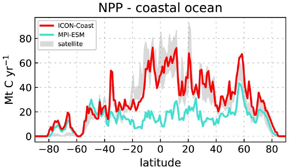
الشكل البياني الموسع 1 | التوزيع العرضي للإنتاج الأولي البحري. مقارنة للإنتاج الأولي الصافي المتكامل زونياً (لكلحزام عرضي) في المحيط الساحلي بين ICON-Coast، نموذج النظام الأرضي العالمي MPI-ESM-LR، ونطاق منتجين قائمين على الأقمار الصناعية (MODIS-CAFE و
VIIRS-CBPM). الفروق أقل وضوحًا في العروض العليا حيث يتأثر الناتج الأولي البيولوجي بشدة بتوفر الضوء وغطاء الجليد البحري، ومدخلات المغذيات من الأنهار (التي يتم تجاهلها من قبل MPI-ESM) أقل بكثير مما هي عليه في العروض الدنيا.
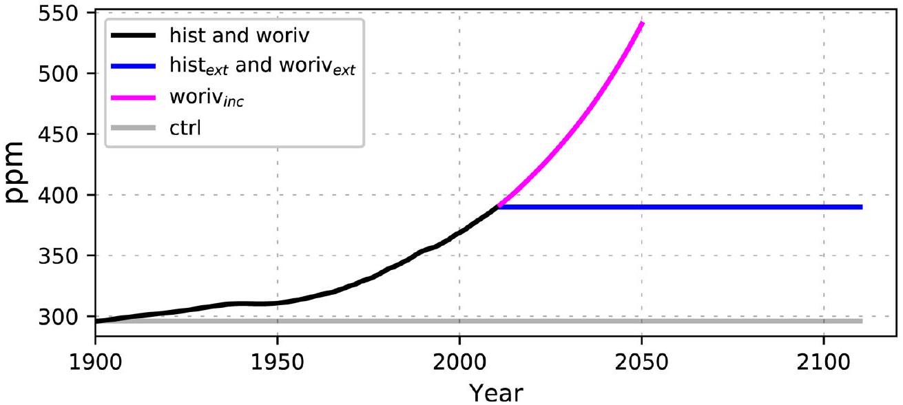
جوي
الشكل البياني الموسع 2 | الغلاف الجويفي تجارب النماذج. نظرة عامة على الغلاف الجوي المحددمستخدم في تجارب النماذج المختلفة. الأسود: تاريخيسجل (يستخدم للتاريخ والعمل)؛ ماجنتا: افتراضي وفقًا لسيناريو الانبعاثات RCP8.5 (المستخدم للتاريخ ); الأزرق: ثابت سنة 2010 (يستخدم للتاريخووريف ); رمادي: ثابت سنة 1900 (يستخدم لـتُعطى معلومات إضافية عن شروط القوة في الجدول 1.
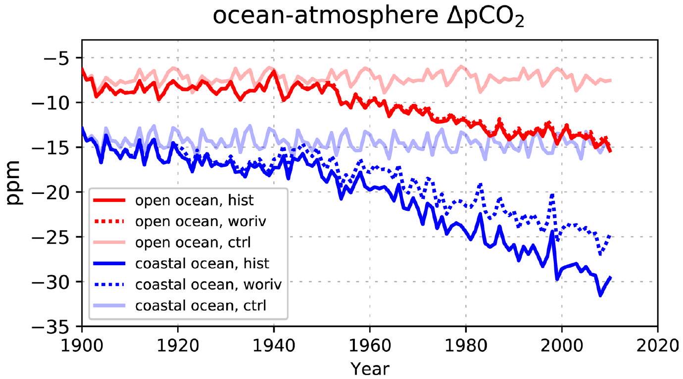
الشكل البياني الموسعفي المحيط المفتوح والساحلي. سلاسل زمنية لمحاكاة المحيط-الغلاف الجويللمحيط المفتوح (الأحمر) والمحيط الساحلي (الأزرق). سالبتشير إلى نقص التشبع في المحيط. hist: توقع تاريخي، woriv: نفس الشيء مثل hist ولكن بدون زيادة أحمال المغذيات من اليابسة، ctrl: تشغيل تحكم مع قوة ثابتة.
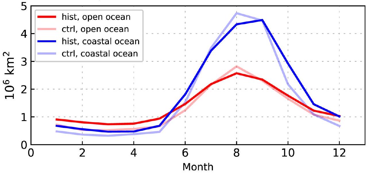
منطقة المياه المفتوحة – المحيط القطبي الشمالي
الشكل 4 من البيانات الموسعة | منطقة المياه المفتوحة في القطب الشمالي. الدورة الموسمية لمنطقة المياه المفتوحة المحاكاة في المحيط القطبي الشمالي (شمال )، مفصولة للمحيط المفتوح (الأحمر) والمحيط الساحلي (الأزرق). تُعتبر خلايا الشبكة في حالة مياه مفتوحة إذا كان تغطية الجليد البحري فيها أقل من .
الشكل البياني الموسع |حذف زيادة الغلاف الجويسلاسل زمنية لمحاكاة المحيط-الغلاف الجويالتدفق للمحيط المفتوح (الأحمر) والمحيط الساحلي (الأزرق). القيم السلبية تشير إلى المحيطامتصاص. ووكو : نفس ما هو موجود في السجل التاريخي ولكن دون زيادة في الغلاف الجويالتحكم: التشغيل مع قوة ثابتة.
لا محيط-غلاف جوي – المحيط الساحلي
الشكل البياني الموسع 6 | التوزيع العرضي لـتدفق السطح. متكامل زونياًتدفق السطح (لكلحزام عرضي) في المحيط الساحلي، موضحًا لعملية التحكم (باللون الرمادي) بالإضافة إلى المتوسطات من 1991-2010 من التنبؤ التاريخي (باللون الأحمر الصلب) والتجربة حيث تم استبعاد زيادة المدخلات الغذائية من اليابسة (باللون الأحمر المتقطع). تشير التدفقات الإيجابية إلىإطلاق الغازات.
تغيير في العمق – الناتج الأولي الصافي
الشكل 7 من البيانات الموسعة | التغيرات في الإنتاج الأولي البحري. إشارة التغير المحاكية للإنتاج الأولي الصافي المتكامل على العمق خلالقرن (تجربة تاريخية).
معهد الأنظمة الساحلية، مركز هيلمهولتز هيرون، غيستهاخت، ألمانيا.فيزياء المناخ والبيئة، جامعة برن، برن، سويسرا.مركز أوشجر لبحوث تغير المناخ، جامعة برن، برن، سويسرا.معهد ماكس بلانك للأرصاد الجوية، هامبورغ، ألمانيا.معهد المحيطات، جامعة هامبورغ، هامبورغ، ألمانيا.البريد الإلكتروني: moritz.mathis@hereon.de
Observational reconstructions indicate a contemporary increase in coastal ocean uptake. However, the mechanisms and their relative importance in driving this globally intensifying absorption remain unclear. Here we integrate coastal carbon dynamics in a global model via regional grid refinement and enhanced process representation. We find that the increasing coastal is primarily driven by biological responses to climate-induced changes in circulation ( ) and increasing riverine nutrient loads (23%), together exceeding the ocean solubility pump . The riverine impact is mediated by enhanced export of organic carbon across the shelf break, thereby adding to the carbon enrichment of the open ocean. The contribution of biological carbon fixation increases as the seawater capacity to hold decreases under continuous climate change and ocean acidification. Our seamless coastal ocean integration advances carbon cycle model realism, which is relevant for addressing impacts of climate change mitigation efforts.
The coastal ocean is a disproportionate sink for atmospheric , with shelf and marginal seas covering only of the world’s ocean surface but taking up more per area than the open ocean . According to observational products, the global coastal ocean is currently absorbing of from the atmosphere (excluding estuaries and intertidal wetlands) . Moreover, reconstructions of global ocean partial pressure ( ) suggest that while both the open and coastal ocean sinks have been increasing during the last decades, a faster increase in ocean-atmosphere gradients ( ) is occurring in the coastal ocean . Estimates from conceptual and dynamical modelling, however, disagree due to simplifications and assumptions regarding process representation and spatio-temporal heterogeneity in coastal carbon fluxes . The roles that terrestrial, atmospheric and open ocean drivers have in explaining the globally intensifying absorption by coastal waters remain enigmatic, especially in quantitative terms. Recent global carbon budgeting studies highlight that ocean margins and land-ocean transition zones are critical areas where further research is needed to improve ocean carbon sink estimates .
Carbon dynamics in the coastal ocean are affected by a multitude of drivers that ultimately influence the magnitude of the coastal sink. The equilibration of sea waters to increasing atmospheric levels and climate-induced changes in circulation affect the physical carbon export to the open ocean, raising the question of whether lateral off-shelf transport still induces a notable reduction in oceanic or whether this contribution is becoming negligible . Agricultural fertilization and wastewater treatment have affected nutrient inputs from land, which in turn promote biological carbon fixation in the coastal ocean . This raises the question of whether the additional biological carbon sequestration, under the influences of riverine freshwater and terrestrial carbon supplies on surface , can substantially slow down the accumulation of dissolved inorganic carbon (DIC) in coastal waters, thus enhancing the uptake of from the atmosphere. Furthermore, enhanced stratification due to atmospheric warming weakens the vertical nutrient supply for biological productivity , lower solubility of warmer water masses is associated with higher (ref. 13), and increasing sea water temperature reduces its buffer capacity , limiting further absorption of from the atmosphere.
Table 1 | Overview of the conducted ICON-Coast simulations with further information on the prescribed atmospheric , meteorological forcing fields and riverine nutrient loads
Experiment
Period
Atmospheric
Meteorological forcing
Riverine nutrient loads
ctrl:
211 yr
constant 296ppm
looped 1900-1919
looped 1900-1919
Control run
(year 1900)
hist:
1900-2010
transient
transient
linear increase
Full hindcast run
(1900-2010)
(1900-2010)
woriv:
1900-2010
transient
transient
looped 1900-1919
hist without increasing nutrient inputs from land
(1900-2010)
(1900-2010)
hist :
100 yr
constant 390ppm
looped 1991-2010
looped 1991-2010
Continuation of hist with constant atmospheric
(year 2010)
woriv :
100 yr
constant 390ppm
looped 1991-2010
looped 1900-1919
Continuation of woriv with constant atmospheric
(year 2010)
woriv
40 yr
transient RCP8.5
looped 1991-2010
looped 1900-1919
Continuation of woriv with increasing atmospheric
(2011-2050)
A looped forcing means that forcing conditions of a limited subperiod is continuously repeated over the whole model integration time to keep long-term conditions stable while still maintaining natural high-frequency variations. In contrast, a transient forcing means that forcing conditions follow their own specific temporal evolution over the model integration. See Extended Data Fig. 2 for further information on the prescribed atmospheric and the ‘Experiment design’ section for more details.
Observation-based studies on coastal ocean carbon fluxes are fraught with large uncertainty due to general data scarcity. In particular, the detection of long-term trends is impeded by high natural variability of biogeochemical transformation and exchange fluxes . Global dynamic modelling approaches, by contrast, provide spatially and temporally complete variable fields but struggle to represent physical and biogeochemical processes relevant to the coastal carbon cycle, and their current coarse resolutions do not capture distinct regional circulation features .
Here we apply the global ocean-biogeochemistry model ICON-Coast to derive a quantitative understanding of anthropogenic alterations in the uptake efficiency of the coastal ocean. ICON-Coast adds value to coastal carbon modelling (exemplified in Extended Data Fig. 1) by applying an unstructured grid configuration with increased horizontal resolution in coastal areas and an extended representation of physical and biogeochemical processes to better account for shelf-specific carbon transformation, transport and storage dynamics. Particularly, ICON-Coast incorporates tidal currents including bottom drag effects and explicitly accounts for sediment resuspension, temperature-dependent remineralization and dissolution in the water column and sediment, riverine matter fluxes from land including terrestrial organic carbon, and variable sinking speed of aggregated particulate matter. With this approach, the model provides a seamless representation of the global marine carbon cycle, including two-way exchange between flows of the open ocean and the biologically productive coastal areas.
We conducted simulations over the historical period 1900-2010, which consider atmospheric changes in climate, increasing atmospheric concentrations and the increase in anthropogenic nutrient inputs from land (Table 1 and Extended Data Fig. 2). On continental shelves and in the transition zone to the adjacent open ocean, the grid resolution is 20 km , which is times finer than what could be achieved by earlier studies . We investigate to what extent the processes controlling net carbon fixation in the coastal ocean can keep up with the rapidly rising in the atmosphere, thus contributing to an efficient transfer from the atmosphere to the global ocean. We quantify the coastal carbon budget and identify key drivers altering burial, transport and air-sea gas exchange during the twentieth century.
Trends in global ocean uptake
The ocean-atmosphere flux ( ) shows a clear change towards a stronger net sink over the 1900-2010 period (more negative in Fig. 1). This tendency holds for both the open and coastal ocean, and reflects changes in (Extended Data Fig.3). Since the 1950s, increases by in the coastal ocean, outweighing the increase in the open ocean (linear trend, ). The stronger signal in the coastal ocean is in line with the observational study of ref. 7. In our simulations, however, the increase rates are generally weaker by factors of 2 and 4 in the open and coastal ocean, respectively, and remain weaker when comparing to the same temporal period (winter trends since the 1980s) and spatial coverage (excluding Arctic and south-east Asian shelves). Yet, the trends derived in ref. 7 show substantial uncertainty, as the spreads ( ) in their station-based data are 10 and 4 times larger than the corresponding globally averaged values. This high uncertainty is further underlined by the study of ref. 17, which utilized an early version of the SOCAT atlas but did not find a notable trend in coastal .
The spatial distribution of the simulated signal (Fig. 2) mirrors the general trend in a downward flux direction, owing to predominantly lower increase rates in the ocean than in the atmosphere (represented by a negative change in ). Exceptions are found mainly in the Southern Ocean and on Arctic shelves, where surface warming (by up to ) induces changes in the opposite direction. On a global average, the resulting net uptake has a generally higher density (by ) in the coastal ocean than in the open ocean (Fig. 1).
The coastal ocean as a zone of carbon transformation
The coastal ocean is an area of high biological activity. Integrated net primary production (NPP) is simulated to be for 1991-2010 (hist), or 11% of global marine NPP. The majority of this biogenically bound carbon is remineralized again on the continental shelves (87%). Of the remaining particulate organic and inorganic carbon, gets buried in the shelf sediments, whereas of dissolved (DOC) and particulate organic carbon (POC) is advected off-shelf to the open ocean (Fig.3). As these export fluxes exceed the net import of
Fig. 1 | Time series of simulated ocean-atmosphere flux density. , Averages over the open (a) and the coastal (b) ocean. Both simulations woriv and hist of the period 1900-2010 were extended for another 100 years by constant atmospheric of the year 2010 ( hist and woriv , respectively), whereas woriv was additionaly extended for 40 years by continuously increasing atmospheric following emission scenario RCP8.5 (woriv ). Except for atmospheric , the extended runs were driven by looped forcings of the period 1991-2010 (see ‘Experiment design’). The grey vertical line marks the transition to the extended runs. A negative sign indicates flux into the ocean.
via rivers and DIC via open ocean water masses, the resulting carbon deficit in coastal waters is balanced by net uptake of from the atmosphere. The coastal ocean thus shapes the marine carbon cycle by transforming inorganic carbon (IC) supplied by the land, atmosphere and open ocean into organic carbon (OC).
The net transformation of IC to OC in the coastal ocean is already simulated from the beginning of the twentieth century (ctrl), with a weak net uptake of atmospheric of (Fig. 3). This early coastal carbon sink confirms first evaluations of the preindustrial ocean state , which suggest a weak coastal uptake of 40 and for refs. 4 and 22, respectively, despite a net release from the global ocean. According to our simulations, the cumulative anthropogenic impact during the twentieth century leads to more than a doubling of the coastal ocean sink. By assuming that the off-shelf transport of POC is passed to the deep ocean and of the DOC transport is removed from the upper ocean via new export production , we can verify the carbon reservoirs where the additionally absorbed remains: resides in shelf waters, gets buried in shelf sediments, is exported to the upper open ocean and is transferred to the deep ocean.
Controls of the increasing sink of the coastal ocean
The coastal sink is enhanced by increased upwelling in the highly productive eastern boundary upwelling systems (EBUS) and by sea
ice retreat in high latitudes, both caused by human-induced changes to the physical climate.
Changes in the near-surface wind pattern (Supplementary Fig. 1) reflect a global poleward migration of the large-scale atmospheric high-pressure fields, termed tropical expansion . In the adjacent coastal EBUS of the Pacific and Atlantic (see ‘Analysis’), the simulated open ocean inflow to the shelves strengthens by and its mean concentration increases by 0.6 mmol N m during the twentieth century. The intensified circulation and enhanced productivity ( , Supplementary Fig. 2) cause an increase in OC export to the open ocean by and a downward change in by 31 ppm , increasing the coastal uptake by .
In the coastal ocean of high latitudes, expanding ice-free areas (springtime Arctic , Antarctic , Extended Data Fig. 4) strengthens the net uptake by on the Arctic shelves and in the Antarctic coastal areas. Larger and longer-lasting open water areas give rise to both enhanced solubility and biological pumping (spring NPP Arctic , Antarctic ), with a correlation between spring bloom productivity and sea ice cover of ( ). Changes in the Arctic are alleviated by above-average warming by up to , which also compensates the effect of enhanced dilution (salinity-0.2 psu, ) due to meltwater invasion from land (run-off ) and sea ice. The temperature effect decreases regionally (Fig. 2), but overall, the coastal uptake is clearly enhanced (Fig. 4). Because of the different area covers, the total contribution of the Arctic shelves integrates to an increase in CO2 absorption by , which is much larger than for the comparatively narrow Antarctic shelves ( ).
To investigate the impact of the rising atmospheric , we continued experiments hist and woriv with atmospheric held constant ( hist and woriv ). This allows us to differentiate the total signal into the solubility pump, driven by the dissolution of atmospheric in the ocean, and the biological pump, driven by DIC assimilation due to phytoplankton growth (see ‘Analysis’ section), and quantify the import and export fluxes of the coastal carbon budget (Extended Data Table 1) sustaining these contributions (Fig. 5). Further discussion on the response of the ocean sink to this idealized climate neutrality scenario is provided in section ‘The response of the coastal ocean uptake to climate neutrality’.
In the simulation without increasing nutrient input from rivers (woriv), the contribution to the uptake signal by the solubility pump ( ; Fig. 5a) is larger than the contribution by the biological pump ( ; Fig. 5b). The additional removed from the atmosphere either increases the coastal DIC inventory (55%) or is advected off-shelf ( ), thus weakening the net DIC flux from the open ocean (Fig. 5a, positive change in IC advective). The higher biological productivity due to enhanced upwelling and sea ice retreat (NPP ) results in higher advective export of OC but also respiratory , further reducing the net consumption of open ocean DIC by a similar amount (Fig. 5b, positive change in IC advective).
The enhanced nutrient supply from rivers (hist) strongly promotes phytoplankton growth in the coastal ocean (NPP ). The higher biological carbon fixation increases the biological contribution to the coastal (to ; Fig. 5d) and transforms this into organic matter (Fig. 5c, OC advective). The river-induced boost in biological productivity increases the OC export (to the open ocean and sediments), the advective IC import (Fig. 5d, negative change in IC advective) and the uptake from the atmosphere, and still leads to less DIC accumulation (IC stock) in coastal waters (all compared to woriv, ). The increasing net import of IC from the open ocean (Extended Data Table 1, negative mean and negative change in IC advective) indicates that the coastal ocean might act to weaken the general DIC increase in the open ocean, since more open ocean DIC is consumed by biological productivity than respiratory and riverine DIC loads are transported off-shelf. At the end of the twentieth century, this net
Fig. 2 | Simulated change signal of ocean-atmosphere during the twentieth century (1991-2010 of hist minus ctrl). Negative (blue) changes indicate that changed in a downward direction, that is, towards more
uptake and less outgassing. White masked areas in the Arctic represent permanent sea ice cover, suppressing gas exchange at the sea surface. Dotted areas indicate changes with less than confidence based on a 2 -sided -test.
DIC import from the open ocean is , of which are attributed to the impact of enhanced nutrient inputs from land (Fig.3). When we subtract the DIC source of due to simulated open ocean mineralization of terrestrial DOC, the coastal ocean is a weak net DIC sink of for the open ocean. Thus, under the influence of increasing eutrophication, the coastal ocean is not only a growing sink for atmospheric , but also for upper ocean DIC, enhancing uptake in the open ocean.
When increasing eutrophication is taken into account (hist), the biological contribution ( ) clearly exceeds the solubility contribution ( ), making biological carbon fixation the predominant process that intensifies the coastal absorption during the twentieth century. This change is mediated by an enhanced export of OC to the open ocean, which is excluded from the gas exchange with the atmosphere, thus further adding to the carbon enrichment of the open ocean.
We can now quantify the main controls of the contemporary increasing uptake in the coastal ocean (see ‘Analysis’ section). The solubility contribution is represented by the drop in the uptake from hist to hist (Fig. 1) and accounts for of the total signal during the twentieth century. The remaining 59% represents the biological contribution, which can be further attributed to a climate-induced component of primarily driven by enhanced upwelling and sea ice retreat, and a river load-induced component of represented by the difference between hist and woriv. This partitioning, however, includes the influence of changes in sea surface temperature and wind speed on (ref. 27), as well as the effect of the reduced buffer capacity of sea water due to ocean acidification . Lower solubility and higher piston velocity due to increased water temperature both change by less than and thus fairly cancel in their impact on . Generally higher wind speeds (by about ), however, lead to stronger exchange fluxes (by ), equally intensifying the solubility and biological carbon pumps. Moreover, simulated mean surface DIC concentration in the coastal ocean increases during the twentieth century by , resulting in an increase of the Revelle factor from 10.1 to 10.7 (see ‘Analysis’). This means that the gets more sensitive to changes in DIC and as a consequence, changes in carbon fixation and export processes have a higher impact on the and gas exchange.
Fig. 3 | Carbon budget of the global coastal ocean, derived from experiments ctrl, woriv and hist for the period 1991-2010. All numbers are given in . *, riverine inputs are prescribed and assumed to be constant over the simulation period.**, net DIC accumulation in the control run is due to long-term model drift. DOCt, terrestrial dissolved organic carbon; PIC, particulate inorganic carbon.
When we repeat the hist simulation without the historical rise in atmospheric (Extended Data Fig. 5), we find that the increase in coastal ocean uptake is weaker by as much as
Fig. 4 | Simulated change signal of ocean-atmosphere flux during the twentieth century (1991-2010 of hist minus ctrl), shown for the coastal ocean. Negative values indicate changes towards more uptake and less outgassing.
Fig. 5|Partitioning of the coastal ocean signal into changes in the solubility and biological carbon pumps. a-d, Solubility (a,c) and biological contributions (b,d) for experiment woriv (a,b) (excluding increases in nutrient inputs from land) and the hindcast simulation hist (c,d). The sum of the solubility and biological contributions (cyan) corresponds to the total anomaly relative to ctrl. The solubility and biological signals as well as their sustaining net import and export fluxes are derived from the carbon budget of 1991-2010 (grey
shaded area and values in the right figure margins) by assuming constant relative contributions over the whole simulation period. Negative changes in indicate increasing uptake. advective, net advective transport of organic/inorganic carbon to the open ocean; sediment, net deposition of organic/inorganic carbon in shelf sediments; sol/bio , net solubility/ biological flux at the sea surface; IC stock, storage of inorganic carbon in shelf waters.
( 1.1 instead of ), whereas the biological carbon fixation rate remains the same. This means that the biological contribution of the signal ( ) is driven by the buffer effect ( ), as DIC assimilation by phytoplankton growth results in a
larger decline when the buffer capacity is low. This acidification impact has been shown to considerably enhance the biologically induced air-sea gradient and is here generalized to include the ocean margins. In the open ocean, without the buffer effect (Extended
Data Fig. 5), the warming impact on the solubility would even outweigh the enhanced biological carbon sequestration, leading to a net reduction in uptake by . Similarly, in the coastal ocean we identified the buffer effect as being the dominating control ( ) of the biological signal. The biological carbon fixation thus contributes substantially more to the uptake as the buffer capacity decreases under continuous climate change.
During the twentieth century, changes in the surface flux towards more uptake or less outgassing are represented in 93% of the coastal ocean area (Fig. 4). This general trend is visible in all latitudes, while impacts of the eutrophication signal are mainly restricted to the northern hemisphere (Extended Data Fig. 6, difference between woriv and hist) owing to the asymmetries in the spatial distribution of land masses, river run-off and associated nutrient inputs .
Contrasting the uptake of the open ocean
According to our simulations, global oceanic NPP (Extended Data Fig. 7) increased through the twentieth century from 44.6 to 46.7 PgC yr-1 ( ), with an areal contribution of in the open ocean and a 5 -times stronger signal of in the coastal ocean due to the impacts of enhanced upwelling, sea ice retreat and eutrophication (see ‘Global increase in coastal net primary production’). While we have shown that this biological response substantially impacts the absorption on the shelves, the resulting change in open ocean vertical POC export ( ) contributes only to the enhanced net uptake ( ). This minor biological contribution is consistent with the estimate provided in ref. 31, which analysed apparent oxygen utilization as a proxy for biological productivity and concluded that of the strengthening of the open ocean sink during the recent decades was rather driven by physical and chemical processes. From the decline in experiment hist , we obtain a chemically driven component of , leaving as the remaining physical circulation-driven contribution of the signal in the open ocean.
Our next-generation model ICON-Coast reveals that the coastal ocean is a more efficient sink than the open ocean (Fig. 1), being the first model to show agreement with this conclusion first deduced from observational products . We find the largest differences in coastal versus open ocean flux densities in low latitudes between and . In these regions, biological carbon fixation leads to less coastal outgassing and more uptake by 2.7 and , respectively, whereas in middle and high latitudes, coastal flux densities do not exceed open ocean values. The divergent exchange rates in low latitudes are well supported for the equatorial band of by the observational study of ref. 3, whereas for the remaining parts, this is less clear, albeit consistent with their uncertainty range.
The contrast between the coastal and open ocean flux densities is strengthened by the dominance of subpolar and polar sinks in the area distribution of the global coastal ocean . The higher uptake efficiency of the coastal ocean, however, would also be maintained if the latitudinal area fraction was equally distributed, as the resulting net uptake of in the coastal ocean would still exceed the of the open ocean. This suggests that another key factor controlling the disproportional sink of the coastal ocean is high biological carbon fixation in low latitudes.
Our model shows the coastal ocean as a hotspot of carbon transformation processes, resulting in a biological sink over the twentieth century. While such an autotrophic ocean has been put forward in previous model-based studies , changes in vertical and lateral carbon exchange fluxes are generally stronger by factors of in our coast-specific model. That these fluxes are larger than previously assumed has implications for the missing link of the coastal ocean flux in the global carbon budget , the source of OC for the open ocean ,
as well as biological impacts related to increased OC formation . The dense carbon fluxes of the coastal ocean will probably face accelerating rates with forthcoming compound fossil emissions, climate change and human perturbations of freshwater systems. Our study thus provides a vital step for the assessment of historical and prospective evolutions of the coastal carbon cycle.
Online content
Any methods, additional references, Nature Portfolio reporting summaries, source data, extended data, supplementary information, acknowledgements, peer review information; details of author contributions and competing interests; and statements of data and code availability are available at https://doi.org/10.1038/s41558-024-01956-w.
References
Liu, K. K., Atkinson, L., Quiñones, R. & Talaue-McManus, L. in Carbon and Nutrient Fluxes in Continental Margins: A Global Synthesis (eds Liu, K. K. et al.) 3-24 (Springer, 2010).
Bauer, J. E. et al. The changing carbon cycle of the coastal ocean. Nature 504, 61-70 (2013).
Roobaert, A. et al. The spatiotemporal dynamics of the sources and sinks of in the global coastal ocean. Global Biogeochem. Cycles 33, 1693-1714 (2019).
Regnier, P., Resplandy, L., Najjar, R. G. & Ciais, P. The land-to-ocean loops of the global carbon cycle. Nature 603, 401-410 (2022).
Laruelle, G. G., Lauerwald, R., Pfeil, B. & Regnier, P. Regionalized global budget of the exchange at the air-water interface in continental shelf seas. Global Biogeochem. Cycles 28, 1199-1214 (2014).
Dai, M. et al. Carbon fluxes in the coastal ocean: synthesis, boundary processes, and future trends. Annu. Rev. Earth Planet. Sci. 50, 593-626 (2022).
Laruelle, G. G. et al. Continental shelves as a variable but increasing global sink for atmospheric carbon dioxide. Nat. Commun. 9, 454 (2018).
Hauck, J. et al. Consistency and challenges in the ocean carbon sink estimate for the global carbon budget. Front. Mar. Sci. 7, 22 (2020).
Brewin, R. J. W. et al. Ocean carbon from space: current status and priorities for the next decade. Earth Sci. Rev. 240, 104386 (2023).
Bourgeois, T. et al. Coastal-ocean uptake of anthropogenic carbon. Biogeosciences 13, 4167-4185 (2016).
Lacroix, F., Ilyina, T., Mathis, M., Laruelle, G. G. & Regnier, P. Historical increases in land-derived nutrient inputs may alleviate effects of a changing physical climate on the oceanic carbon cycle. Global Change Biol. 27, 5491-5513 (2021).
Mathis, M., Elizalde, A. & Mikolajewicz, U. The future regime of Atlantic nutrient supply to the Northwest European Shelf. J. Mar. Syst. 189, 98-115 (2019).
Takahashi, T. et al. Global sea-air flux based on climatological surface ocean , and seasonal biological and temperature effects. Deep Sea Res. II 49, 1601-1622 (2002).
Sundquist, E. T., Plummer, L. N. & Wigley, T. M. L. Carbon dioxide in the ocean surface: the homogeneous buffer factor. Science 204, 1203-1205 (1979).
Takahashi, T. et al. Climatological mean and decadal change in surface ocean , and net sea-air flux over the global oceans. Deep Sea Res. II 56, 554-577 (2009).
McKinley, G. et al. Timescales for detection of trends in the ocean carbon sink. Nature 530, 469-472 (2016).
Wang, H., Hu, X., Cai, W. J. & Sterba-Boatwright, B. Decadal trends in global ocean margins and adjacent boundary current-influenced areas. Geophys. Res. Lett. 44, 8962-8970 (2017).
Ward, N. D. et al. Representing the function and sensitivity of coastal interfaces in Earth system models. Nat. Commun. 11, 2458 (2020).
Roobaert, A., Resplandy, L., Laruelle, G. G., Liao, E. & Regnier, P. A framework to evaluate and elucidate the driving mechanisms of coastal sea surface seasonality using an ocean general circulation model (MOM6-COBALT). Ocean Sci. 18, 67-88 (2022).
Mathis, M. et al. Seamless integration of the coastal ocean in global marine carbon cycle modeling. J. Adv. Model. Earth Syst. 14, e2021MS002789 (2022).
Bakker, D. C. E. et al. A multi-decade record of high-quality data in version 3 of the Surface Ocean CO2 Atlas (SOCAT). Earth Syst. Sci. Data 8, 383-413 (2016).
Lacroix, F., Ilyina, T., Laruelle, G. G. & Regnier, P. Reconstructing the preindustrial coastal carbon cycle through a global ocean circulation model: was the global continental shelf already both autotrophic and a sink? Global Biogeochem. Cycles 35, e2020GB006603 (2021).
DeVries, T. & Weber, T. The export and fate of organic matter in the ocean: new constraints from combining satellite and oceanographic tracer observations. Global Biogeochem. Cycles 31, 535-555 (2017).
Daloz, A. S. & Camargo, S. J. Is the poleward migration of tropical cyclone maximum intensity associated with a poleward migration of tropical cyclone genesis? Clim. Dyn. 50, 705-715 (2018).
Yang, H. et al. Poleward shift of the major ocean gyres detected in a warming climate. Geophys. Res. Lett. 47, e2019GL085868 (2020).
Yang, H. et al. Tropical expansion driven by poleward advancing midlatitude meridional temperature gradients. J. Geophys. Res. Atmos. 125, e2020JD033158 (2020).
Wanninkhof, R. Relationship between wind speed and gas exchange over the ocean revisited. Limnol. Oceanogr. Methods 12, 351-362 (2014).
Sarmiento, J. L. & Gruber, N. Ocean Biogeochemical Dynamics (Princeton Univ. Press, 2006).
Hauck, J. & Völker, C. Rising atmospheric leads to large impact of biology on Southern Ocean uptake via changes of the Revelle factor. Geophys. Res. Lett. 42, 1459-1464 (2015).
Lacroix, F., Ilyina, T. & Hartmann, J. Oceanic outgassing and biological production hotspots induced by pre-industrial river loads of nutrients and carbon in a global modeling approach. Biogeosciences 17, 55-88 (2020).
Koeve, W., Kähler, P. & Oschlies, A. Does export production measure transient changes of the biological carbon pump’s feedback to the atmosphere under global warming? Geophys. Res. Lett. 47, e2020GL089928 (2020).
Friedlingstein, P. et al. Global carbon budget 2020. Earth Syst. Sci. Data 12, 3269-3340 (2020).
Breitburg, D. et al. Declining oxygen in the global ocean and coastal waters. Science 359, eaam7240 (2018).
Publisher’s note Springer Nature remains neutral with regard to jurisdictional claims in published maps and institutional affiliations.
Open Access This article is licensed under a Creative Commons Attribution 4.0 International License, which permits use, sharing, adaptation, distribution and reproduction in any medium or format, as long as you give appropriate credit to the original author(s) and the source, provide a link to the Creative Commons licence, and indicate if changes were made. The images or other third party material in this article are included in the article’s Creative Commons licence, unless indicated otherwise in a credit line to the material. If material is not included in the article’s Creative Commons licence and your intended use is not permitted by statutory regulation or exceeds the permitted use, you will need to obtain permission directly from the copyright holder. To view a copy of this licence, visit http://creativecommons. org/licenses/by/4.0/.
(c) The Author(s) 2024
Methods
Model description
The ocean-biogeochemistry model ICON-Coast is an advancement of the ocean component ICON-O of the Hamburg Earth system model ICON-ESM . Its adaptation to integrate coastal circulation features and carbon dynamics consists of a two-step development. First, a refinement of the horizontal grid resolution was confined to the continental margins and shallow shelves, including the transition zone to the adjacent deep ocean basins . Second, the biogeochemistry component HAMOCC was extended to better account for shelf-specific carbon transformation processes , including tidal currents and bottom drag effects , sediment resuspension , temperature-dependent remineralization in the water column and sediment , variable sinking speeds of aggregated particulate carbon and mineral components , and matter fluxes from land, including river loads of terrestrial carbon and nutrients as well as atmospheric deposition of dust and nitrogen .
The dynamics of the model is based on the hydrostatic Boussinesq equations, which are solved on a triangular grid with Arakawa C-type staggering. In the configuration presented here, we used a biharmonic subgrid scale velocity closure with a scale-dependent viscosity coefficient to account for the variable horizontal resolution. Vertical mixing was parameterized by a prognostic equation for turbulent kinetic energy. Sea-ice dynamics were simulated by the sea-ice model FESIM . Biogeochemical tracers in the water column were transported by the physical advection and diffusion schemes. Biological activity followed an extended nutrient, phytoplankton, zooplankton and detritus (NPZD) approach with a fixed stoichiometry and nutrient co-limitation of phosphate, nitrate, silicate and iron. Export production was separated into and opal shell material. Sedimentary processes were represented by 12 biologically active layers, accounting for degradation and burial of organic and inorganic particulate matter, including pore water diffusion.
For our simulations here, we applied the same grid configuration used for the biogeochemistry runs in the model introduction paper . The horizontal mesh spacing ranged from 160 km in the open ocean to 20 km near the coasts and along topographic gradients. The vertical was represented by 40 levels on -coordinates, with a layer thickness of 10 m in the upper 100 m of the water column (except for the 16 m top layer with free surface elevation to facilitate tidal amplitudes and sea-ice draft) and increasing spacing below. The model time step in the presented setup was 720 s.
Experiment design
Our ocean simulations with ICON-Coast were driven with a number of prescribed boundary conditions. As atmospheric forcing fields, we used 3-hourly ERA-20C reanalysis data . Annual mean atmospheric followed the historical record or the high-emissions global warming scenario RCP8.5, both as developed for the fifth IPCC Assessment Report (AR5). River run-off from catchment areas was reconstructed by the global hydrological discharge model HD . Matter fluxes of DIP, DIN, DSi, DFe, DIC, Alkalinity, particulate organic matter and terrestrial dissolved organic matter were derived in refs. 11,30 for about the largest 850 rivers. Historically increasing nutrient loads of DIN and DIP were approximated by a linear increase during the hindcast period 1900-2010 (Supplementary Fig. 3). Atmospheric deposition of nitrogen and aeolian dust as further sources of inorganic nutrients followed refs. 40,42 , respectively. Here, only of the N deposition occurred in the coastal ocean, whereas of the river inputs were discharged on the shelves (Supplementary Fig. 3). Aggregated over the coastal ocean area, the resulting total nutrient load from land thus primarily consisted of river inputs. In our analysis and discussion of the coastal ocean, we therefore mainly refer to the nutrient fluxes from land as river loads.
We initialized our spin-up procedure with an ocean state of the year 1900 from a historical simulation of the Earth system model
MPI-ESM-HR as it contributed to the sixth Coupled Model Intercomparison Project (CMIP6). ICON-Coast was then run in physics-only mode for 200 years using looped forcing conditions of the period 1900-1919 to allow the ocean circulation to adjust to the model specifications and grid configuration. The biogeochemistry component was then included for another 100 years. The end of this spin-up run was used to initialize our production runs with transient forcing, as well as the control run as the continuation of the spinup with looped forcing.
The core simulation of this study is a hindcast run (hist) over the historical period 1900-2010, driven with the forcing conditions described in Table 1. To investigate the impacts of nutrient loads from rivers and the induced eutrophication signal in the coastal ocean, we contrasted this simulation with an experiment where the increase in nutrient inputs from land is excluded (woriv).
To further disentangle change signals in the surface flux with respect to contributions from an active downward pumping by the atmosphere or a passive uptake flux that balances biological carbon sequestration, these simulations were extended for another 100 years by keeping the in the atmosphere at a constant level (Extended Data Fig. 2) and otherwise using looped forcing conditions over 1991-2010 ( hist and woriv ). In these experiments, we ran the model into quasi-equilibrium of the upper ocean, indicated by a leveling of the surface flux (Fig. 1). This additionally allowed us to estimate the response of the ocean sink if we were to achieve global climate neutrality, or in our case if we had established climate neutrality since the year 2010. To contrast this response, we also set up an analogous counter experiment with continuously increasing following emission scenario RCP8.5 (woriv ).
Increasing uptake by the ocean is associated with a decrease in the ability of the sea water to further absorb any additional , which means that changes in DIC concentrations would induce stronger changes in and hence in gas exchange. To quantify the impact of this buffer effect on the biological uptake, we conducted experiment , which is the same as the hindcast hist but keeping atmospheric at the level of the year 1900 (as for the control run ctrl). As we have not analysed this experiment further, it is only shown in Extended Data Fig. 5.
Model evaluation
To evaluate our model results, we compared the last 10 years (2001-2010) of the hindcast simulation hist with best estimates from observation-based upscalings. Global fields of NPP and surface flux are shown in Supplementary Fig. 4, with a simulated total productivity of and a net uptake of . These global values are consistent with the contemporary observational ranges of for NPP and for absorption during the period 1994-2007 . Biases in surface nutrients (nitrate and phosphate ) compared with the World Ocean Atlas are mainly found in the Southern Ocean (Supplementary Fig. 4c), probably related to underestimated iron limitation in the biological nutrient consumption.
Simulated surface shows a qualitative distribution consistent with the reconstruction in ref. 53 based on SOCAT data of the period 1998-2015 (Supplementary Fig. 5), but values are generally overestimated with a mean bias of +16 ppm in the coastal ocean and +11 ppm in the open ocean. To get the local mean in agreement with observations, we applied a linear bias correction of simulated against ref. 53 by subtracting the climatological differences of the period 2001-2010 at every grid cell. This resulted in an offset of the simulated time series, while the simulated seasonality or the long-term trend of the time series remained unaffected. fluxes at the sea surface, however, were not adjusted to ensure a closed mass balance. The anthropogenic signal of the global ocean uptake (Supplementary Fig. 6) thus seemed to be slightly weaker compared with best estimates by the Global Carbon Budget , but still lay within the range of uncertainty.
Net primary production was particularly well captured in the coastal ocean (Extended Data Fig. 1), best demonstrating the added value of ICON-Coast compared with conventional global models that are designed for open ocean biogeochemistry. Our simulated coastal carbon budget for the period 2001-2010 was characterized by a lateral carbon export from continental shelf waters to the open ocean of , which is comparable to the observation-based range of (refs. 2,4). Carbon burial in the shelf sediments was simulated to be and DIC accumulation in the water column to be , which in total was estimated to be in ref. 4. The carbon export fluxes induced a simulated net uptake of from the atmosphere, in good agreement with observational estimates of .
Further evaluation of the model performance in representing coastal carbon dynamics can be found in ref. 20. The model parameters and grid configuration we use here are identical to the setup in ref. 20 used for the simulation including ocean biogeochemistry. The differences are therefore only in the prescribed external forcing, as our simulations cover the entire twentieth century rather than just the evaluation period 2000-2010. We used ERA-20C reanalysis for the meteorological forcing instead of ERA-Interim, and we used transient atmospheric as well as riverine nutrient loads, which were held constant in ref. 20.
Due to limitations in computational resources, the simulations presented here were initialized from a global ocean state that was not in internal model equilibrium. The remaining long-term drift after spinup is reflected by an ongoing adjustment of biogeochemical tracers at the sea surface, for example, of phosphate and silicate, leading to an increase in coastal DIC storage in the control run of (IC stock in Extended Data Table1). To account for the model drift in our analysis, we determined change signals through the simulation period relative to the control run (see next section).
Analysis
Coastal regions often show strong spatial gradients in water mass characteristics between the shallow proximal zone and the outer shelf areas with water depths reaching 500 m along the continental margin. These deeper regions are less affected by tidal mixing and promote extensive vertical fluxes of carbon and nutrients out of the biologically productive surface layers, thus playing an integrative role in the functioning of the shelf carbon pump . For our definition of the coastal ocean, we therefore used the area spanning from the coastline to the 500 m isobath to properly include the deeper shelves such as the Barents Sea, the Greenland Shelf or the outer part of the Patagonian Shelf .
The EBUS we are referring to comprise the California ( ) and Humboldt ( ) upwelling systems in the eastern Pacific, and the Canary ( ) and Benguela ( ) upwelling systems in the eastern Atlantic.
Anthropogenically forced signals during the simulation period 1900-2010 refer to changes that are induced by anthropogenic perturbations, here increasing atmospheric and riverine nutrient loads. These changes were evaluated relative to the background of natural variability, which is idealized by the control experiment of stable 1900-1919 forcing conditions. Our results thus do not include alterations in the marine carbon budget during early industrialization between 1750 and 1900. Change signals through the twentieth century were calculated as means over the period 1991-2010 of a particular simulation minus the same period of the control ctrl run, thus removing contributions due to long-term model drift. Moreover, the change signals were tested at the confidence level to account for influences of decadal variability. Further low-frequency variations in time series were evaluated by autocorrelation analysis. For the import and export fluxes of the coastal carbon budget (Extended Data Table1),
autocorrelation coefficients calculated for lags of 1-50 years were generally lower than .
The Revelle factor is used to quantify the buffer capacity of sea water. This is a measure of the amount of atmospheric that can be taken up by the ocean. We calculated the Revelle factor as the ratio between fractional changes in ocean and DIC .
In our experiments, we considered three external perturbations that can alter the exchange at the sea surface (see ‘Experiment design’). The meteorological forcing (1) determines the physical climate that primarily affects the water temperature and stratification of the upper ocean, as well as the ocean circulation. Changes in this forcing therefore impact the solubility of sea water and the lateral exchange fluxes of carbon between the continental shelves and the adjacent open ocean. The atmospheric impacts the oceanatmosphere gradient and therefore the thermodynamic force of the flux. Nutrient inputs from land (3) fuel marine primary production and thus impact DIC concentrations and at the sea surface.
Our quantification of the main contributions to the increasing uptake in the coastal ocean was based on the extended simulations with constant atmospheric and stable meteorological forcing ( hist and woriv ). The equilibrium state of these experiments describes an end-of-twentieth-century carbon budget that has been deprived by the rapid increase in atmospheric , and the resulting drop in uptake (Fig. 1) represents the solubility contribution to the historical signal caused by pumping from the atmosphere. In hist , this solubility contribution is of the total signal ( ). The remaining contribution of is driven in the reversed causal direction, that is, being sucked up by the ocean due to biological carbon fixation, compensating uptake-weakening physical effects of global-scale warming, such as reduced solubility or a shoaling and strengthening of the stratification (global mean changes in winter-time mixed-layer depth-23m and stratification ). As we found that ocean-shelf volume transports did not significantly change, in the coastal ocean this non-chemical contribution to the historical signal (Fig. 1) is therefore dominated by biologically enhanced carbon fluxes, allowing us to commonly refer here to the biological contribution. Experiment woriv allowed us to further attribute the biological contribution to a climate-induced component of and a river load-induced component of . Furthermore, as the climate-induced changes were retained in the extended runs due to the stable meteorological forcing, the carbon fluxes related to biological productivity were also representative for their correlates at the end of the original experiments hist and woriv, differing by only in NPP and in the advective OC export to the open ocean and the vertical OC and IC exports to the sediment. In the extended runs, the advective IC flux thus closed the balance between all oceanic export fluxes (lateral and vertical) and the biologically driven uptake from the atmosphere. Hence, by comparing the carbon budgets of the original and extended simulations, we can derive how the solubility and biological contributions to the change in the surface flux are balanced by the import and export fluxes through the sediment and open ocean boundaries (Fig. 5).
When increasing nutrient inputs from land were excluded from the forcing (woriv), the change signal of (Extended Data Table 1) divided into a biological contribution of (the equilibrium in woriv ) and a slightly larger solubility contribution of due to atmospheric pumping (the drop from woriv to woriv ). Moreover, the coastal ocean contains more respiratory (Fig. 5b), represented by a change in the advective IC flux of in experiment woriv (relative to ctrl). In the original woriv run, however, the advective IC flux changed by (Extended Data Table 1), which means that another of this weakening net IC import consists of additional delivered by the atmosphere. As this term balanced all changes in
the export fluxes, the remaining of the total provided by atmospheric pumping are accumulating in the water column, reflected by the increase in depth-integrated DIC (IC stock in Extended Data Table 1).
The additional nutrient supply from rivers strongly promoted phytoplankton growth in the coastal ocean (NPP ) and induced primary producers to utilize atmospheric pumping as a carbon source. In the hindcast simulation hist, the change signal of contained a solubility contribution of but a larger biological contribution of due to eutrophication (Fig. 5c). The higher organic matter production also affected the carbon export rates, compared with woriv. In hist , the change in the advective IC flux was (relative to ctrl), which represents the additional net DIC import from the open ocean that would be required to provide enough IC for the marked increase in organic matter production, if we had constant in the atmosphere (and hence no further chemical pumping as a source of IC). The factual change in net open ocean IC import in hist, however, was only (IC advective in Extended Data Table 1). This discrepancy indicates that the enhanced biological production in hist also consumes of the additional pumped in from the atmosphere. This potentially limits the biological impact on the total signal (relative to woriv); however, it eliminates a considerable source term of DIC for the open ocean. As this contribution again balanced all changes in the carbon export fluxes, the remaining of the atmospheric pumping are accumulating in the water column (IC stock in Extended Data Table1).
Model limitations and uncertainties
Our approach in global-scale coastal modelling opens the possibility to include more relevant processes that have not yet been taken into account in our simulations. We show that enhanced biological carbon fixation due to riverine nutrient inputs strengthens the sink of the coastal ocean as well as the off-shelf transport of organic matter. In our river loadings, however, we neglected the still uncertain augmentation of OC transports to the ocean, which was estimated at since preindustrial times (ref. 4 and citations therein). DOC concentrations in the model were generally low, reaching in highly productive coastal areas such as the East China Shelf, whereas measurements range between 100 and (ref. 59). As terrestrial organic matter typically causes a source following mineralization in the ocean, increased OC inputs from land could potentially weaken the net uptake in the coastal ocean. In our approach, a increase would correspond to an additional input of . Taking into account that a fraction of is mineralized in the coastal ocean, as suggested in published literature and confirmed here, the uptake could be weakened by by increasing OC inputs. We also assumed that the advective OC export to the open ocean would rise by a similar amount. Considering that the difference in uptake between experiments hist and woriv is , the river-induced increases in net uptake would still override a potentially weaker uptake caused by rising OC inputs.
The incorporation of other sources of land-derived matter loadings, however, would further constrain their quantitative impact on coastal uptake and help estimate responses to future climate change. Groundwater discharge provides regionally eminent inputs of soluble carbon and nutrients to the coastal ocean of up to 25% of the river fluxes . Carbon reservoirs in tidal flats and intertidal wetlands are shrinking due to sea level rise, resulting in net carbon fluxes to the ocean and atmosphere of (ref. 61). On the Arctic shelves, additional carbon and nutrient supply due to coastal erosion is higher than fluvial inputs and is expected to further increase with global warming . The uptake in the northern high latitudes might thus become generally weaker when effects of coastal erosion are taken into account. Nevertheless, drivers of primary productivity and related
carbon fluxes in a widely changing Arctic were shown to depend on various processes, events and features across different spatial and temporal scales . Our model results for the Arctic may therefore be associated with comparatively high uncertainty.
According to our simulations, the coastal ocean is a more efficient sink than the open ocean. The potentially overestimated flux densities in the Arctic coastal regions due to missing carbon inputs might be compensated by too high ocean in particular in the Canadian sector (Supplementary Fig. 5), which probably weakens the simulated net absorption north of . In the low latitudes, the divergent exchange rates between the coastal and open ocean are well supported by the observational study of ref. 3 .
Simulated oxygen concentrations on the shelves are generally higher than , hence the model does not capture anoxic conditions in shallow coastal areas. In the current model configuration, the water column has to be represented in the model by at least two vertical layers. In the grid configuration used here, the minimum vertical resolution of 10 m comes with limitations in representing shallow stratification that would limit the ventilation of subsurface water masses, as well as the resupply of nutrients to the sea surface. Moreover, the model currently misses the impact of water turbidity on irradiance and light penetration depth as a control factor of coastal carbon dynamics. This is particularly relevant in areas where strong tidal currents induce sediment resuspension, as well as in regions with high river inputs of particulate matter.
The coarse vertical resolution may also limit the representation of low aragonite/calcite saturation states of coastal waters, including sediment pore water . The simulated increase in particulate IC sedimentation is therefore probably overestimated. Nevertheless, the sedimentation rate of in 1991-2010 is still comparatively low, as the model does not include contributions from coral reefs and seagrass-dominated embayments, which are estimated to account for of the total carbonate burial of in the coastal ocean (ref. 67).
In our simulations, enhanced upwelling in eastern boundary upwelling systems is associated with more uptake, driven by increased biological carbon fixation that compensates for the impact of higher DIC concentrations of upwelled water masses on surface . From an observational point of view, however, the net effect of intensified upwelling on in eastern boundary regions is still unclear. The influence of cold water masses from intermediate depths could sustain global warming and even lead to lower sea surface temperature and (ref. 13), while trend analyses of the California upwelling system over shorter time periods rather suggest a increase in the ocean that exceeds the rate of change in the atmosphere.
The finest horizontal grid resolution of 20 km used in the simulations presented here is a considerable improvement in global modelling approaches on coastal ocean dynamics. Yet, a mesh spacing of is required to resolve the characteristic spatial scales on most shallow shelves . Processes related to circulation features smaller than are therefore still underrepresented in our results . This potentially affects, for instance, the formation of tidal fronts and cross-frontal exchange , vertical mixing due to internal waves , and the transport of heat and biogeochemical tracers by small-scale and meso-scale eddies . As high-resolution Earth system modelling is still in its infancy, it is unknown how these processes would modify the carbon fluxes in the global coastal ocean and interact with the larger-scale dynamics of the ocean and atmosphere.
Our results were derived from a single global oceanbiogeochemistry simulation. We are thus unable to evaluate the sensitivity of our findings to the specific parameter setup used here and to general model uncertainties. In view of the high heterogeneity in the dominating physical and biogeochemical controls on regional carbon dynamics, this constraint is of particular relevance as the calculation of the coastal carbon budget ensues from the balance of huge cross-shelf
volume transports in the order of . These limitations underline the urgent need for further development on the representation of coastal carbon dynamics in global modelling approaches to better constrain uncertainties in our findings, which would help deepen a quantitative understanding of the role of the land-ocean transition zone in the global carbon cycle.
The response of the coastal ocean uptake to climate neutrality
Our coastal carbon budget suggests that the DIC accumulation in the shelf waters during the past decades was a chemically driven process (IC stock in Fig. 5a,c). Accordingly, as atmospheric continued to increase in experiment woriv , the uptake of the ocean kept growing without discernible disruption (Fig.1). In an idealized climate neutrality scenario with atmospheric and meteorological forcing fields held stable (experiments woriv and hist ), by contrast, the uptake started to weaken dramatically with a short delay of years. The relaxation time needed for the upper ocean to chemically equilibrate with the atmosphere was years for both the coastal and open ocean. The progression, however, had an asymptotic shape, where half of the drop occurred in the first 1-2 decades. In the coastal ocean, the relaxation of hist followed experiment woriv with a remarkably stable offset of (Supplementary Fig. 7), resulting from land-derived nutrient inputs. Thus, although these two experiments distinctly differed in their biological carbon fluxes, the biology had hardly any influence on the equilibration process. The net impact of biological carbon sequestration is neither speeding up equilibration due to an increased surface flux, nor retarding equilibration by continuously removing that has been absorbed from the atmosphere. This result is consistent with the finding that respiratory does not accumulate on the shelves (IC advective in Fig. 5b), reinforcing chemical dominance also in the equilibration mechanism.
Similar to the response in the coastal ocean, the uptake in the open ocean continued to increase with further increasing atmospheric (woriv ) but broke down drastically as soon as atmospheric levelled off (Fig. 1a), with a comparable equilibration time of years. In the open ocean, however, this time scale would be influenced by the depth of the mixed layer, the stability of the stratification and the intensity of vertical mixing. Since the range in the vertical structure of the water column as simulated by different global models is relatively high , we expect a similar model uncertainty in the flux relaxation time. Using the UVic Earth System Model for example, ref. 77 obtained a comparable sudden drop in the global ocean uptake after atmospheric stopped rising, but a distinctly longer relaxation time of ~200-300 years for present-day climate conditions.
The biological fluxes, however, determine the equilibrium level of the uptake, as the exchange with the atmosphere dynamically balances the oceanic sources and sinks of inorganic carbon. In the coastal ocean, the higher biological productivity fuelled by increasing riverine nutrient inputs (experiments hist and hist ) led to a total increase in the biological contribution to of . Because of the much higher biological change signal in the coastal ocean compared with the open ocean (see ‘Contrasting the uptake of the open ocean’), we found that the relative drop under constant atmospheric ( hist ) was weaker in the coastal ocean by (Fig.1) and the equilibrium was higher by a factor of 2 (coastal ocean , open ocean ). This means that in a climate neutrality scenario, the global ocean sink weakens by (Supplementary Table 1), but the coastal ocean gains relevance as its contribution to the total oceanic uptake increases from the currently (end of hist) to .
Note, however, that this scenario is not a consistent future projection, as we are missing the physical response of the coupled ocean-atmosphere climate system, as well as natural variations in atmospheric . Nevertheless, our simulated oceanic response to
atmospheric levelling is consistent with previous global model simulations and is here demonstrated to include the continental shelves, despite their generally more intense carbon transformation and exchange processes. Yet, a higher coastal uptake is maintained by enhanced biological carbon fixation. Under an effective emissions reduction policy, the coastal ocean would thus remain a stronger sink than the open ocean (per unit area), sustaining an increased ocean-shelf gradient in flux density. This implies that the future uptake of the coastal ocean is crucially influenced by the growth rates of atmospheric greenhouse gas concentrations and matter fluxes from land.
Global increase in coastal net primary production
Our model results suggest that biological carbon fixation provided an essential contribution to the increase in coastal ocean uptake during the past century. To evaluate the simulated increase in coastal NPP, we here compared our model results with observational estimates derived from satellite products.
The simulated increase in mean coastal NPP is . This signal is mainly driven by increasing nutrient inputs from land ( ), enhanced upwelling in eastern boundary upwelling systems (10%) and growing open water areas in high latitudes due to sea ice retreat (4%). Riverine nutrient inputs directly fuel NPP in near-shore areas of large river systems , upwelling mixes nutrient-rich water masses from intermediate depths to the euphotic zone , and sea ice retreat leads to larger and longer-lasting open water areas, promoting NPP via more favourable light conditions .
The immediate impact of biological carbon fixation on ocean and air-sea gas exchange is dependent on the sea water capacity to hold (ref. 28). This buffer capacity weakens with increasing DIC concentrations in the ocean in the course of rising emissions to the atmosphere, leading to a higher sensitivity of sea water to DIC changes. In the global coastal ocean, we found that the buffer effect accounts for 60% of the increase in the biological carbon pump (see main part). Because sea water chemistry is further influenced by temperature, this impact is intensified towards the poles . In high latitudes, the process of biological carbon fixation therefore translates into a drop that is larger than in low latitudes, resulting in a larger biological control of the ocean-atmosphere gradient and thus exchange. On the broad Arctic shelves, the contribution of the buffer effect to the biological signal is even .
We analysed the time series of 11 satellite products for NPP provided by the Ocean Productivity project (http://sites.science.oregonstate.edu/ocean.productivity/custom.php, accessed 18 December 2023). The data cover periods that range between 10 and 20 years only (MODIS 20 years, SeaWiFS 10 years, VIIRS 10 years), impeding an evaluation of long-term trends. Nevertheless, the majority of the calculated decadal trends show a consistent increase for the global coastal ocean, as well as for subareas of the eastern boundary upwelling systems and the Arctic shelves (Supplementary Table 2). Moreover, the increasing trends are generally larger for the coastal ocean than for the open ocean (by factors of 5-10), in line with our model results. The potentially too-low trend in Arctic productivity may indicate that the simulated impact of the biological carbon pump on the uptake in high latitudes might be underestimated. For illustration, all time series have been standardized (Supplementary Fig. 8) to account for the high uncertainty in satellite-derived NPP .
Data availability
Primary model output used for creating the figures shown here is freely accessible on the Zenodo archive .
Code availability
The model code of ICON-Coast is available to individuals under licences (https://mpimet.mpg.de/en/science/modeling-with-icon/
code-availability). By downloading the ICON-Coast source code, the user accepts the licence agreement. The source code of ICON-Coast used in this study can be obtained from the Zenodo archive . Climate Data Operators were used for analyses (https://code.mpimet.mpg.de/ projects/cdo/). Figures including maps were made with Natural Earth and Cartopy (https://scitools.org.uk/cartopy).
References
Korn, P. Formulation of an unstructured grid model for global ocean dynamics. J. Comput. Phys. 339, 525-552 (2017).
Korn, P. & Linardakis, L. A conservative discretization of the shallow-water equations on triangular grids. J. Comput. Phys. 375, 871-900 (2018).
Jungclaus, J. H. et al. The ICON Earth System Model version 1.0. J. Adv. Model. Earth Syst. 14, e2021MS002813 (2022).
Logemann, K., Linardakis, L., Korn, P. & Schrum, C. Global tide simulations with ICON-O: testing the model performance on highly irregular meshes. Ocean Dyn. 71, 43-57 (2021).
Ilyina, T. et al. The global ocean biogeochemistry model HAMOCC: model architecture and performance as component of the MPI-Earth System Model in different CMIP5 experimental realizations. J. Adv. Model. Earth Syst. 5, 287-315 (2013).
Paulsen, H., Ilyina, T., Six, K. D. & Stemmler, I. Incorporating a prognostic representation of marine nitrogen fixers into the global ocean biogeochemical model HAMOCC. J. Adv. Model. Earth Syst. 9, 438-464 (2017).
Mauritsen, T. et al. Developments in the MPI-M Earth System Model version 1.2 (MPI-ESM1.2) and its response to increasing . J. Adv. Model. Earth Syst. 11, 998-1038 (2019).
Maerz, J., Six, K. D., Stemmler, I., Ahmerkamp, S. & Ilyina, T. Microstructure and composition of marine aggregates as co-determinants for vertical particulate organic carbon transfer in the global ocean. Biogeosciences 17, 1765-1803 (2020).
Mahowald, N. et al. Climate response and radiative forcing from mineral aerosols during the last glacial maximum, pre-industrial, current and doubled-carbon dioxide climates. Geophys. Res. Lett. 33, L20705 (2006).
Danilov, S. et al. Finite-element sea ice model (FESIM), version 2. Geosci. Model. Dev. 8, 1747-1761 (2015).
Poli, P. et al. The Data Assimilation System and Initial Performance Evaluation of the ECMWF Pilot Reanalysis of the 20th-century Assimilating Surface Observations Only (ERA-20C) ERA Report Series 14 (ECMWF, 2013).
Poli, P. et al. ERA-20C Deterministic ERA Report Series 20 (ECMWF, 2015).
Hagemann, S., Stacke, T. & Ho-Hagemann, H. T. M. High resolution discharge simulations over Europe and the Baltic Sea catchment. Front. Earth Sci. 8, 12 (2020).
Buitenhuis, E. T., Hashioka, T. & Quéré, C. L. Combined constraints on global ocean primary production using observations and models. Global Biogeochem. Cycles 27, 847-858 (2013).
Richardson, K. & Bendtsen, J. Vertical distribution of phytoplankton and primary production in relation to nutricline depth in the open ocean. Mar. Ecol. Progr. Ser. 620, 33-46 (2019).
Kulk, G. et al. Primary production, an index of climate change in the ocean: satellite-based estimates over two decades. Remote Sens. 12, 826 (2020).
Gruber, N. et al. The oceanic sink for anthropogenic from 1994 to 2007. Science 363, 1193-1199 (2019).
Watson, A. J. et al. Revised estimates of ocean-tmosphere flux are consistent with ocean carbon inventory. Nat. Commun. 11, 4422 (2020).
Garcia, H. E. et al. World Ocean Atlas 2013, Volume 4, Dissolved Inorganic Nutrients (Phosphate, Nitrate, Silicate) NOAA Atlas NESDIS 76 (NOAA, 2014).
Landschützer, P., Laruelle, G. G., Roobaert, A. & Regnier, P. A uniform climatology combining open and coastal oceans. Earth Syst. Sci. Data 12, 2537-2553 (2020).
Holt, J. et al. Modelling the global coastal ocean. Philos. Trans. A: Math Phys. Eng. Sci. 367, 939-951 (2009).
Tsunogai, S., Watanabe, S. & Sato, T. Is there a ‘continental shelf pump’ for the absorption of atmospheric ? Tellus B 51, 701-712 (1999).
Thomas, H., Bozec, Y., Elkalay, K. & de Baar, H. J. W. Enhanced open ocean storage of from shelf sea pumping. Science 304, 1005-1008 (2004).
Bates, N. R. Air-sea fluxes and the continental shelf pump of carbon in the Chukchi Sea adjacent to the Arctic Ocean. J. Geophys. Res. 111, C10013 (2006).
Laruelle, G. G. et al. Global multi-scale segmentation of continental and coastal waters from the watersheds to the continental margins. Hydrol. Earth Syst. Sci. 17, 2029-2051 (2013).
Barrón, C. & Duarte, C. M. Dissolved organic carbon pools and export from the coastal ocean. Global Biogeochem. Cycles 29, 1725-1738 (2015).
Luijendijk, E., Gleeson, T. & Moosdorf, N. Fresh groundwater discharge insignificant for the world’s oceans but important for coastal ecosystems. Nat. Commun. 11, 1260 (2020).
Chen, Z. L. & Lee, S. Y. Tidal flats as a significant carbon reservoir in global coastal ecosystems. Front. Mar. Sci. https://doi.org/ 10.3389/fmars.2022.900896 (2022).
Vonk, J. E. et al. Activation of old carbon by erosion of coastal and subsea permafrost in Arctic Siberia. Nature 489, 137-140 (2012).
Terhaar, J., Lauerwald, R., Regnier, P., Gruber, N. & Bopp, L. Around one third of current Arctic Ocean primary production sustained by rivers and coastal erosion. Nat. Commun. 12, 169 (2021).
Nielsen, D. M. et al. Increase in Arctic coastal erosion and its sensitivity to warming in the twenty-first century. Nat. Clim. Change 12, 263-270 (2022).
Frey, K. E. et al. Arctic Ocean Primary Productivity: The Response of Marine Algae to Climate Warming and Sea Ice Decline NOAA Technical Report OAR ARC22-08 (NOAA, 2022).
Eyre, B. D. et al. Coral reefs will transition to net dissolving before end of century. Science 359, 908-911 (2018).
O’Mara, N. A. & Dunne, J. P. Hot spots of carbon and alkalinity cycling in the coastal oceans. Sci. Rep. 9, 4434 (2019).
Santos, F., Gomez-Gesteira, M., deCastro, M. & Alvarez, I. Differences in coastal and oceanic SST trends due to the strengthening of coastal upwelling along the Benguela current system. Cont. Shelf Res. 34, 79-86 (2012).
Jacox, M. G., Moore, A. M., Edwards, C. A. & Fiechter, J. Spatially resolved upwelling in the California Current System and its connections to climate variability. Geophys. Res. Lett. 41, 3189-3196 (2014).
Hallberg, R. Using a resolution function to regulate parameterizations of oceanic mesoscale eddy effects. Ocean Model. 72, 92-103 (2013).
Moum, J. N., Nash, J. D. & Klymak, J. M. Small-scale processes in the coastal ocean. Oceanography 21, 22-33 (2008).
Timko, P. G. et al. Assessment of shelf sea tides and tidal mixing fronts in a global ocean model. Ocean Model. 136, 66-84 (2019).
Kossack, J., Mathis, M., Daewel, U., Zhang, Y. J. & Schrum, C. Barotropic and baroclinic tides increase primary production on the Northwest European Shelf. Front. Mar. Sci. https://doi.org/ 10.3389/fmars.2023.1206062 (2023).
Brearley, J. A., Moffat, C., Venables, H. J., Meredith, M. P. & Dinniman, M. S. The role of eddies and topography in the export of shelf waters from the West Antarctic Peninsula Shelf. J. Geophys. Res. Oceans 124, 7718-7742 (2019).
Robinson, A. R., Brink, K. H., Ducklow, H. W., Jahnke, R. A. & Rothschild, B. J. in The Sea: The Global Coastal Ocean: Multiscale Interdisciplinary Processes Vol. 13 (eds Robinson, A. R. & Brink, K. H.) 3-35 (Harvard Univ. Press, 2005).
Heuzé, C. North Atlantic deep water formation and AMOC in CMIP5 models. Ocean Sci. 13, 609-622 (2017).
Zheng, M. D. & Cao, L. Simulation of global ocean acidification and chemical habitats of shallow- and cold-water coral reefs. Adv. Clim. Change Res. 5, 189-196 (2014).
Cotrim da Cunha, L., Buitenhuis, E. T., Quéré, C. L., Giraud, X. & Ludwig, W. Potential impact of changes in river nutrient supply on global ocean biogeochemistry. Global Biogeochem. Cycles 21, GB4007 (2007).
Fréon, P., Barange, M. & Arístegui, J. Eastern Boundary Upwelling Ecosystems: integrative and comparative approaches. Progr. Oceanogr. 83, 1-14 (2009).
Arrigo, K. R. & van Dijken, G. L. Continued increases in Arctic Ocean primary production. Progr. Oceanogr. 136, 60-70 (2015).
Jiang, L. Q., Carter, B. R., Feely, R. A., Lauvset, S. K. & Olsen, A. Surface ocean pH and buffer capacity: past, present and future. Sci. Rep. 9, 18624 (2019).
Westberry, T. K., Silsbe, G. M. & Behrenfeld, M. J. Gross and net primary production in the global ocean: an ocean color remote sensing perspective. Earth Sci. Rev. 237, 104322 (2023).
Mathis, M. ICON-Coast model output for a study on increasing uptake of the coastal ocean. Zenodo https://doi.org/10.5281/ zenodo. 7964987 (2023).
This work contributed to the subproject ‘A5 – The Land-Ocean Transition Zone’ of Germany’s Excellence Strategy EXC 2037 ‘CLICCS – Climate, Climatic Change, and Society’ with project no. 390683824, funded by the Deutsche Forschungsgemeinschaft (DFG, German Research Foundation). Computational resources were made available by the German Climate Computing Center (DKRZ) through support
from the German Federal Ministry of Education and Research (BMBF). T.I. was supported by the European Union’s Horizon 2020 research and innovation programme under grant agreement no. 101003536 (ESM2O25 – Earth System Models for the Future). Open-access funding was provided by Helmholtz-Zentrum hereon GmbH.
Author contributions
M.M., T.I. and C.S. planned and coordinated the study and designed the model experiments. M.M. and S.H. provided forcing data. M.M. contributed to the model development and performed the experiments. M.M., D.M.N. and F.L. analysed the model output and discussed the interpretation of the results. M.M. wrote the manuscript with contributions from all co-authors.
Funding
Open access funding provided by Helmholtz-Zentrum hereon GmbH (4216).
Correspondence and requests for materials should be addressed to Moritz Mathis.
Peer review information Nature Climate Change thanks Laure Resplandy, Tim Rixen and Raphaël Savelli for their contribution to the peer review of this work.
Extended Data Table 1 | Coastal ocean carbon fluxes
Coastal ocean carbon budget
woriv
hist
woriv
hist
NPP
145
150
166
+5
+21
OC remin
127.1
131.3
143.7
+4.2
+16.6
Export fluxes:
OC advective
+22.1
+23.1
+25.9
+1.0
+3.8
IC advective
-3.3
-1.4
-4.1
+1.9
-0.8
OC sediment
+6.4
+6.2
+7.0
-0.2
+0.6
IC sediment
+0.1
+0.1
+0.3
–
+0.2
FCO2
-3.1
-6.9
-7.9
-3.8
-4.8
OC rivers
-10.6
-10.6
-10.6
–
–
IC rivers
-12.2
-12.2
-12.2
–
–
Storage fluxes:
IC stock
+0.6
+1.7
+1.6
+1.1
+1.0
OC stock
–
–
–
–
–
Carbon budget of the global coastal ocean, derived from experiments ctrl, woriv and hist for the period 1991-2010, as well as change signals woriv (woriv minus ctrl) and hist (hist minus ctrl). Values are rounded to one digit after the decimal point, and thus excluded if smaller than 0.05. Positive exchange fluxes correspond to net export fluxes from the shelf to the open ocean, sediment or atmosphere. Positive storage fluxes correspond to net accumulation rates in the water column. Change signals given in bold are statistically significant at the confidence level, based on a 2 -sided -test. NPP: net primary production; OC remin: remineralization of total organic carbon in continental shelf waters; OC/IC advective: net export of total organic/ from the ocean to the atmosphere); rivers: total organic/inorganic carbon supply via river discharge (trends in riverine carbon inputs are not considered; see Methods section); in Fig. 3.
Extended Data Fig. 1 | Latitudinal distribution of marine primary production. Comparison of zonally integrated net primary production (per latitudinal band) in the coastal ocean between ICON-Coast, the global Earth system model MPI-ESM-LR, and the range of two satellite-based products (MODIS-CAFE and
VIIRS-CBPM). Differences are less pronounced in high latitudes as here NPP is strongly influenced by light availability and sea ice cover, and riverine nutrient inputs (which are neglected by MPI-ESM) are much lower than in low latitudes.
atmospheric
Extended Data Fig. 2 | Atmospheric in model experiments. Overview of prescribed atmospheric used in the different model experiments. Black: historical record (used for hist and woriv); magenta: hypothetical
according to emission scenario RCP8.5 (used for hist ); blue: constant of the year 2010 (used for hist and woriv ); grey: constant of the year 1900 (used for ). Further information on the forcing conditions is given in Table 1.
Extended Data Fig. in the open and coastal ocean. Time series of simulated ocean-atmosphere for the open (red) and coastal (blue) ocean. Negative indicates ocean undersaturation. hist: historical hindcast, woriv: same as hist but without increasing nutrient loads from land, ctrl: control run with constant forcing.
open water area – Arctic Ocean
Extended Data Fig. 4 | Arctic open-water area. Seasonal cycle of simulated open-water area in the Arctic Ocean (north of ), separated for the open (red) and coastal (blue) ocean. Grid cells are considered as open-water condition if their areal sea ice cover is less than .
Extended Data Fig. |Omitting increasing atmospheric . Time series of simulated ocean-atmosphere flux for the open (red) and coastal (blue) ocean. Negative values indicate ocean uptake. woco : same as the hindcast hist but without increasing atmospheric , ctrl: control run with constant forcing.
ocean-atmosphere – coastal ocean
Extended Data Fig. 6 | Latitudinal distribution of surface flux. Zonally integrated surface flux ( per latitudinal band) in the coastal ocean, shown for the control run (grey) as well as means over 1991-2010 of the hindcast hist (solid red) and experiment woriv where increasing nutrient inputs from land were excluded (dashed red). Positive fluxes indicate outgassing.
change in depth-int NPP
Extended Data Fig. 7 | Changes in marine primary production. Simulated change signal of depth-integrated net primary production during the century (experiment hist).
Institute of Coastal Systems, Helmholtz-Zentrum Hereon, Geesthacht, Germany. Climate and Environmental Physics, University of Bern, Bern, Switzerland. Oeschger Centre for Climate Change Research, University of Bern, Bern, Switzerland. Max-Planck-Institute for Meteorology, Hamburg, Germany. Institute of Oceanography, University of Hamburg, Hamburg, Germany. e-mail: moritz.mathis@hereon.de
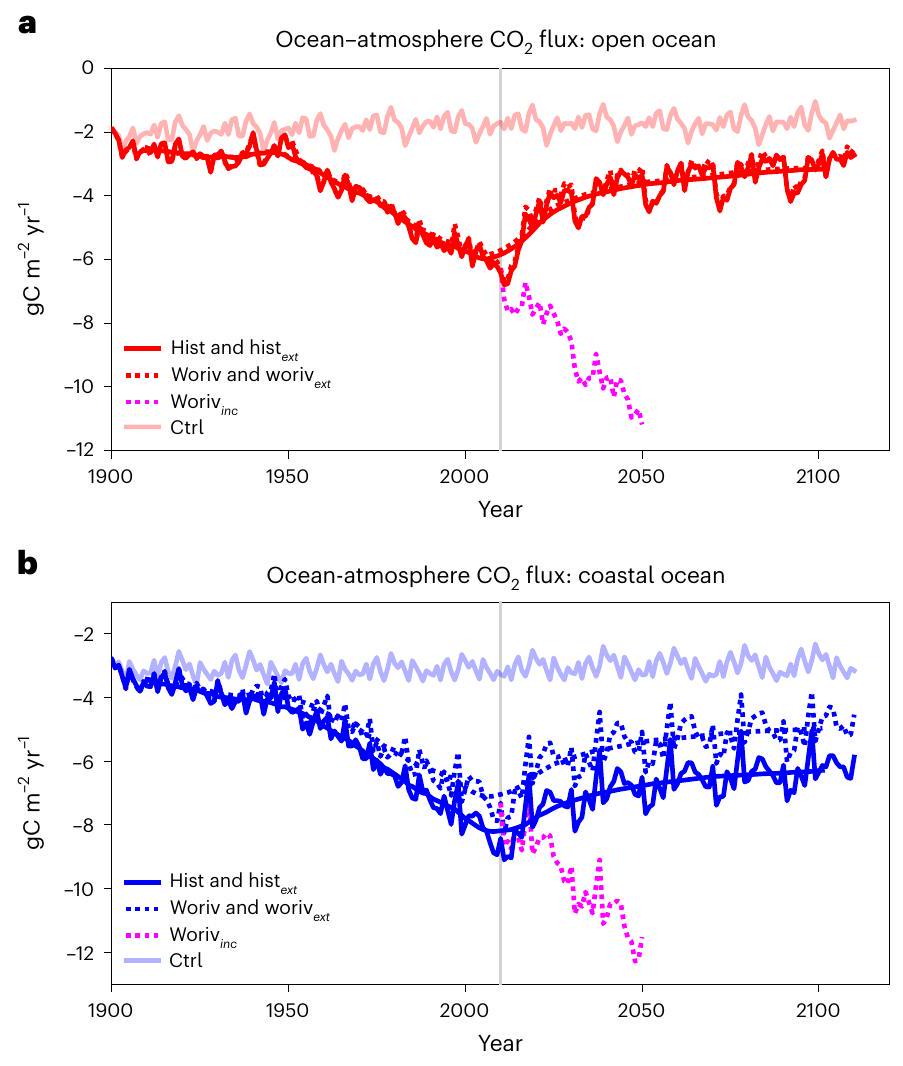
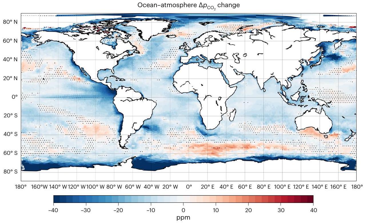
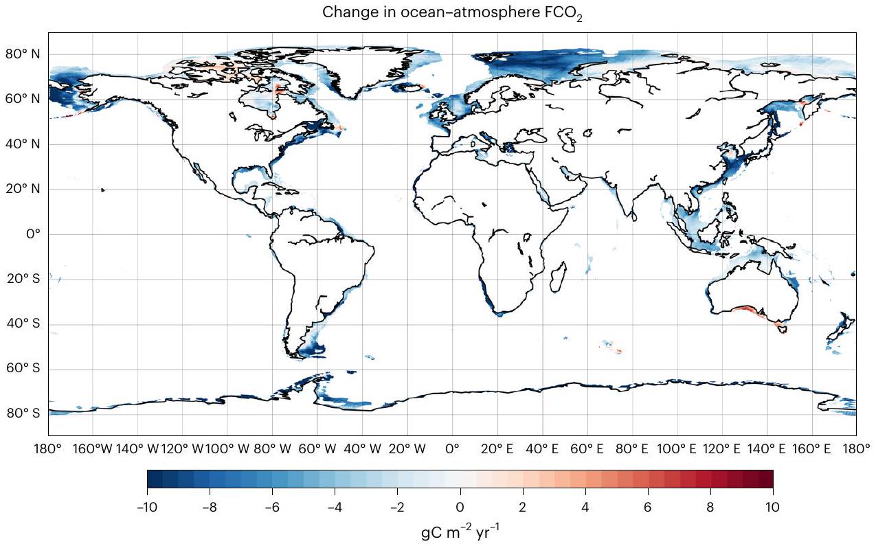
 من المحيط إلى الغلاف الجوي؛