DOI: https://doi.org/10.1038/s41586-024-07147-z
PMID: https://pubmed.ncbi.nlm.nih.gov/38480894
تاريخ النشر: 2024-03-13
سلاسل الإمداد العالمية تعزز التكاليف الاقتصادية لمخاطر الحرارة الشديدة المستقبلية
تاريخ الاستلام: 16 أغسطس 2022
تم القبول: 1 فبراير 2024
نُشر على الإنترنت: 13 مارس 2024
الوصول المفتوح
(أ) التحقق من التحديثات
الملخص
تظهر الأدلة زيادة مستمرة في تكرار وشدة موجات الحرارة العالمية
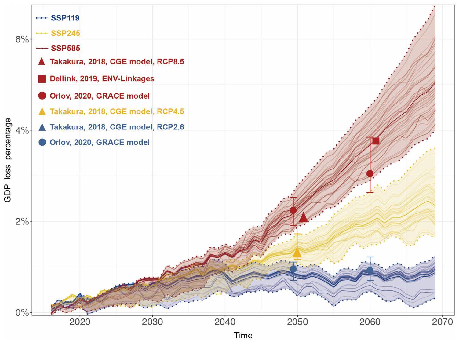
الاتجاه غير الخطي لنمو الخسائر العالمية المرتبطة بالحرارة
خسارة)، بقيمة حوالي الولايات المتحدة
حساسيات مختلفة تجاه الإجهاد الحراري عبر البلدان
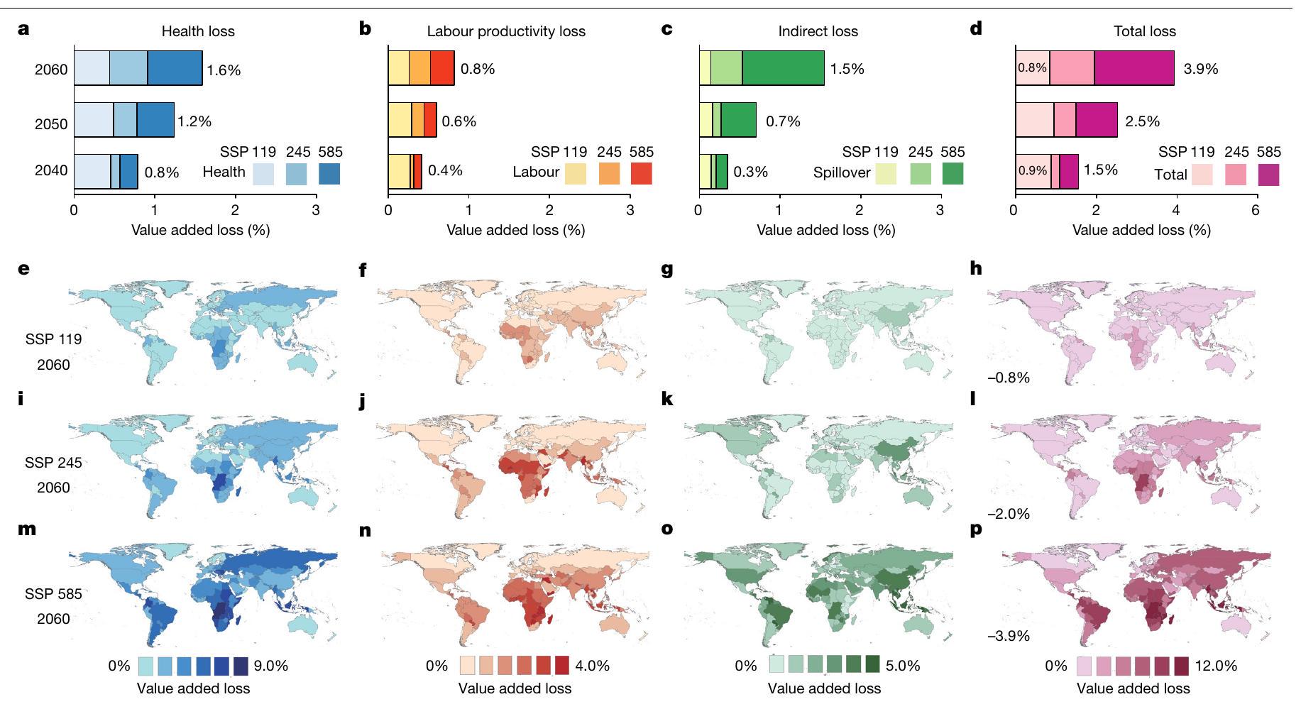
عبر العالم. أ-د، الاتجاهات التطورية لأنواع الخسائر الأربعة من 2040 إلى 2060 تحت سيناريوهات مختلفة (خسارة الصحة (أ)؛ خسارة إنتاجية العمل (ب)؛ الخسارة غير المباشرة (اضطرابات سلسلة التوريد) (ج)؛ وإجمالي الخسائر (د)). تمثل الألوان من الفاتح إلى الداكن الخسائر الاقتصادية من الثلاثة
مقدار القدرة التكيفية. على سبيل المثال، تعاني هنغاريا وكرواتيا من خسائر صحية كبيرة، على الرغم من أن المناخ في هذين البلدين أكثر برودة من المناخ في الشرق الأوسط وشمال أفريقيا. على عكس خسائر العمل، التي تحدث في المناطق ذات درجات الحرارة والرطوبة العالية جداً، تعتمد الخسائر الصحية إلى حد كبير على التباين والتغيرات المفاجئة في درجات حرارة الصيف. مع تغير المناخ، ستؤدي موجات الحرارة الأكثر تكراراً وشدة إلى فقدان كبير في الأرواح في المناطق ذات المناخ الأكثر برودة إذا لم تتماشى القدرة التكيفية مع التغيرات المفاجئة والسريعة.
تأثرت (الشكل 2ج). عانت بورتو ريكو من أعلى الخسائر، التي تقدر بـ
مع المثلثات السوداء تم تصنيفها حديثًا من بين أكثر البلدان عرضة للخطر في عام 2060 تحت سيناريو SSP 585 مقارنةً بـ SSP 119. القيم المعروضة هي متوسطات لعشر سنوات. تمثل أشرطة الخطأ انحرافًا معياريًا واحدًا عن المتوسط لبيانات العقد. تشير الحدود العليا والسفلى إلى المتوسط + انحراف معياري والمتوسط – انحراف معياري، على التوالي. TTO، ترينيداد وتوباغو.
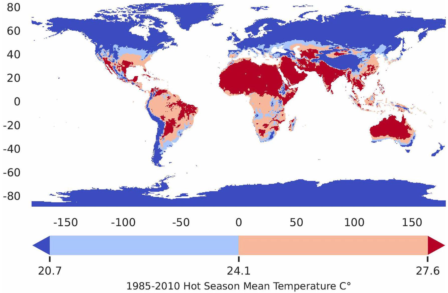
من الناتج المحلي الإجمالي لها، في حين أن اقتصادات ناشئة أخرى مثل باراغواي وإندونيسيا تخسر حوالي 3.3% من ناتجها المحلي الإجمالي. أظهرت هذه النتائج أن النمو السريع في الدخل واختراق تكييف الهواء في الاقتصادات الناشئة تحت سيناريو SSP 585 لا يكفي لمواجهة التأثير الهائل لتغير المناخ على اقتصاداتها.
آثار غير متكافئة للإجهاد الحراري على سلاسل الإمداد العالمية
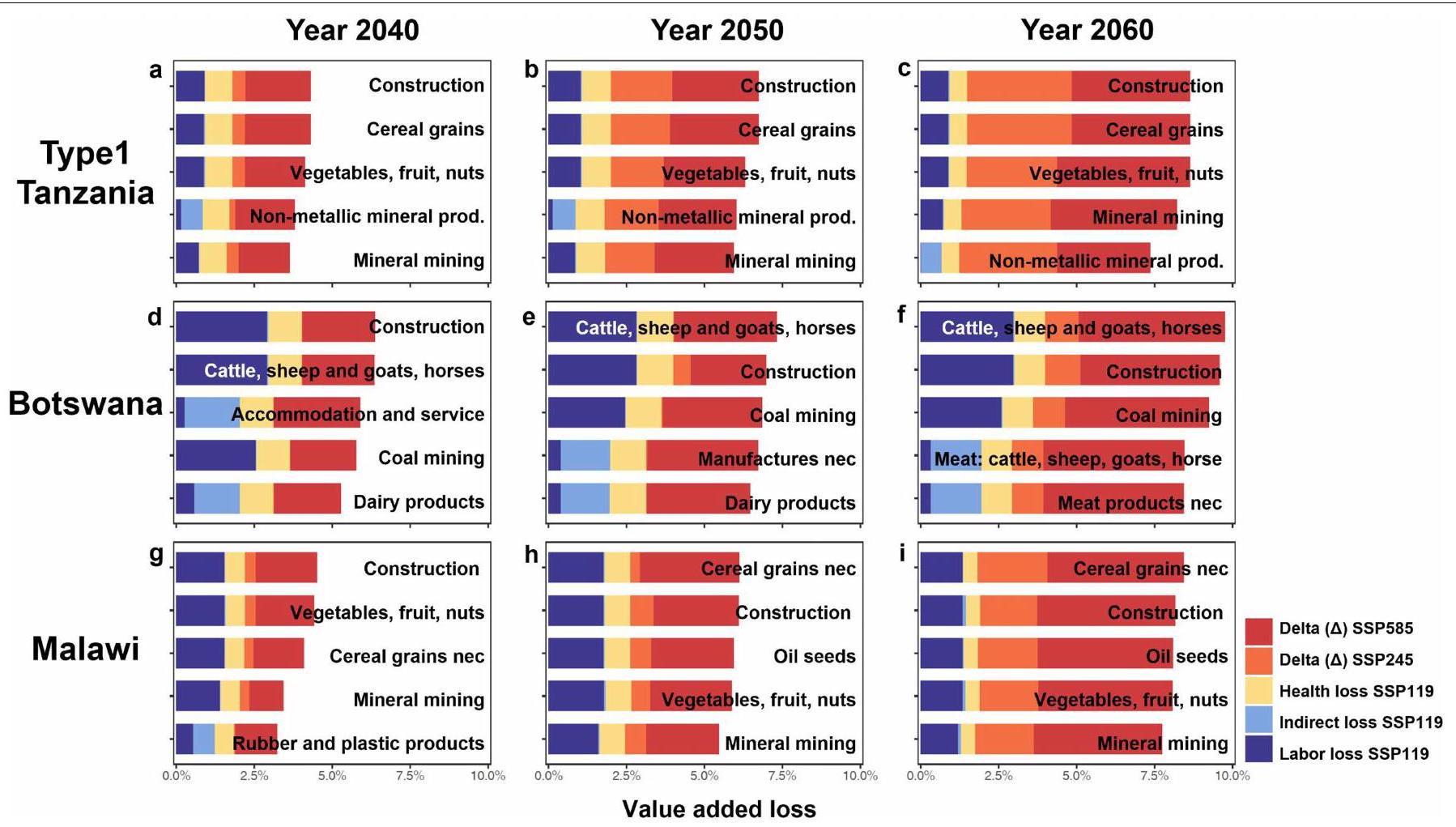
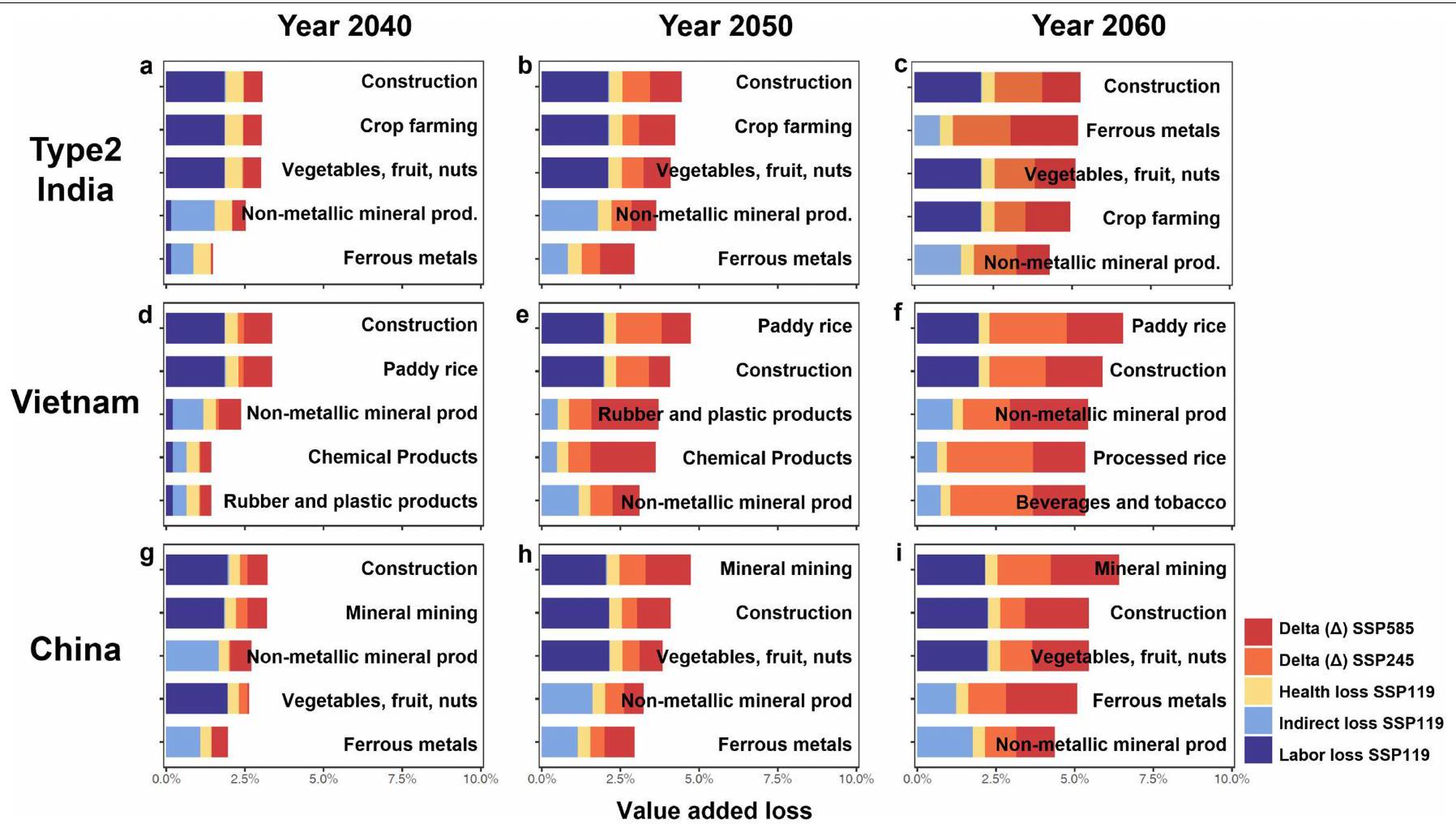
تؤدي الإنتاجية في صناعات البناء والزراعة المحلية مباشرةً إلى خسائر اقتصادية كبيرة في سلاسل القيمة المرتبطة في البلاد. كما هو موضح في الشكل 10 من البيانات الموسعة، تظهر الدول الواقعة في خطوط العرض المنخفضة والمتوسطة، مثل الصين وفيتنام، أنماط خسارة مشابهة.
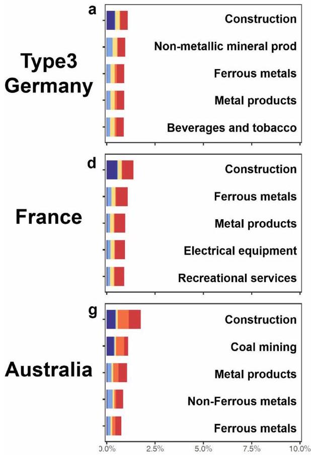
تتعرض الصناعات الخفيفة، بما في ذلك المنتجات المعدنية، والمنتجات المطاطية والبلاستيكية، ومعالجة الأغذية والمشروبات والتبغ، لتأثيرات غير مباشرة بسبب نقص إمدادات المواد الخام، مثل المعادن، والمعادن، والمحاصيل، وزيوت البذور والخضروات. على سبيل المثال، في سيناريو SSP 119، تخسر صناعة المنتجات المعدنية وصناعة التبغ والمشروبات في ألمانيا حوالي
فقط في قطاع البناء أو التعدين، بينما تكون الخسائر غير المباشرة أعلى في قطاع التصنيع المتعلق بالمعادن بسبب نقص الإمدادات من الشركاء التجاريين الأجانب.
| المنبع | |||||
| أ | ماليزيا – الزيوت والدهون النباتية | -1.8% | |||
| البرازيل – السكر | -2.3% | ||||
| 2040 | البرازيل – الزيوت والدهون النباتية | -1.7% | |||
| الصين – الخضروات والفواكه والمكسرات | -1.7% | ||||
| إندونيسيا – الفحم | -2.5% | ||||
| ج | |||||
| إندونيسيا – الزيوت والدهون النباتية | -4.9% | ||||
| 2060 | البرازيل – السكر | -4.8% | |||
| كوت ديفوار – الخضروات والفواكه والمكسرات -6.2% | |||||
| ماليزيا – المنتجات الكيميائية | -5.4% | ||||
| هـ | جمهورية الدومينيكان – الكهرباء | -1.7% | |||
| الولايات المتحدة – التأمين | -1.4% | ||||
| 2040 | الصين – المعدات الكهربائية | -1.6% | |||
| الصين – المنتجات الإلكترونية والبصرية | -1.8% | ||||
| جمهورية الدومينيكان – المركبات وأجزائها | -1.9% | ||||
| ز | جمهورية الدومينيكان – خدمات الأعمال -4.5% | ||||
| الولايات المتحدة – التأمين | -4.7% | ||||
| 2060 | الصين – المعدات الكهربائية | -4.2% | |||
| الصين – المنتجات الإلكترونية والبصرية | -4.2% | 0 | |||
| الولايات المتحدة – الخدمات المالية nec | -4.3% | ||||
| -10 | تغيير تدفق التجارة (%) | 0 | |||
القطاعات) ويمثل الطول النسبة المئوية للانخفاض في تدفق المنتجات مقارنة بالفترة الأساسية لعام 2014. تمثل ألوان الأعمدة مستوى التماسك للقطاع المعين مع قطاع إنتاج الغذاء الهندي من الأزرق (ضعيف) إلى الأحمر (قوي)، والذي يتم قياسه من خلال حجم التجارة بين القطاع المعين وقطاع إنتاج الغذاء الهندي. nec، غير مصنف في مكان آخر.
الموجودة في خطوط العرض العالية، مثل النرويج والمملكة المتحدة، تتميز بأنماط خسائر مشابهة.
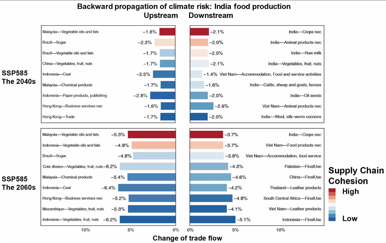
نحن أيضًا نحلل الآلية التي تنتشر من خلالها الخسائر غير المباشرة الناتجة عن الاضطرابات في تدفقات التجارة الدولية عبر سلاسل الإمداد الوطنية لقطاعات معينة. يوضح الشكل 4 كيف ينتشر خطر المناخ عبر سلسلتين من الإمداد، وهما إنتاج الغذاء في الهند وقطاع السياحة في جمهورية الدومينيكان، على التوالي (انظر الشكل البياني الممتد 8 لسلاسل الإمداد النموذجية الأخرى). كل من هذه القطاعات مهمة للاقتصادات المعنية في الهند (
تعتمد سلسلة الإمداد لصناعة إنتاج الغذاء في الهند بشكل كبير على مورديها العلويين، قطاعات الزيوت والدهون في إندونيسيا وماليزيا، ونتيجة لذلك فهي معرضة لدرجات حرارة أعلى. يؤدي الاحترار غير المهدد تحت سيناريو SSP 585 إلى تفاقم نقص المواد الخام. بحلول عام 2060، تنخفض إمدادات زيت النخيل من ماليزيا وإندونيسيا بنسبة
البنية التحتية السياحية وتوريد المنتجات الداعمة للسياحة، مما يشكل مخاطر كبيرة على استثمار السياحة.
تداعيات على حوكمة المخاطر المستهدفة والتعاون الإقليمي
تظهر نتائجنا أن سلاسل الإمداد تضخم خطر الضغط الحراري المستقبلي من خلال التسبب في خسائر اقتصادية غير خطية على مستوى العالم. بعبارة أخرى، لا يمكن تجاهل التأثيرات السلبية الكبيرة غير المباشرة للضغط الحراري عبر الأسواق المترابطة. تسلط الخسائر غير المباشرة للضغط الحراري الضوء على الحاجة إلى تعزيز التعاون بين الدول عبر أصحاب المصلحة المعنيين في سلاسل الإمداد العالمية لتحقيق تكيف ناجح مع الضغط الحراري. على سبيل المثال، تظهر نتائجنا أن تأثير موجة الحرارة على صناعة الزراعة وإنتاج الغذاء في الهند يمكن أن يؤدي إلى
نحن أيضًا نوضح حساسية الدول والقطاعات المختلفة تجاه الأنواع الثلاثة من الخسائر الناتجة عن الإجهاد الحراري. على سبيل المثال، من المرجح أن تعاني دول الكاريبي وأفريقيا الوسطى من خسائر صحية، بينما من المرجح أن تعاني الدول ذات الدخل المنخفض في أفريقيا وجنوب شرق آسيا من خسائر في العمل. بالمقابل، فإن الاقتصادات الصغيرة إلى المتوسطة التي تعتمد على التجارة الدولية، مثل بروناي، تكون أكثر تعرضًا للخسائر غير المباشرة. الطريقة التي تظهر بها تكاليف الإجهاد الحراري توضح كيف تنتشر التأثيرات الواسعة والمتنوعة الناتجة عن الإجهاد الحراري عبر سلاسل التوريد العالمية، مما يؤدي إلى خسائر اقتصادية لدولة أو قطاع قد لا تكون واضحة على الفور. توفر نتائجنا الكمية معلومات قيمة لتصميم استراتيجيات تكيف أكثر استهدافًا وفعالية تجاه الإجهاد الحراري.
نموذجنا المطور والتقديرات الخاصة بنا عرضة لعدم اليقين والقيود (وصف مفصل في قسم المعلومات التكميلية 1.1-1.3). على سبيل المثال، على الرغم من أن وحدة بصمة الكارثة تُستخدم على نطاق واسع وتؤدي بشكل جيد في تحليلات الدول الفردية/المناطق الفردية، فإن قابلية استبدال المنتجات في سيناريو متعدد الدول تتطلب مزيدًا من المناقشة لضمان القوة. لت quantifying بعض من عدم اليقين، أجرينا تحليل حساسية شامل، مع تفاصيل متاحة في قسم الطرق والمعلومات التكميلية 1. على وجه التحديد، استخدمنا سنوات وإصدارات مختلفة من قاعدة بيانات المدخلات والمخرجات للمقارنة لتحليل عدم اليقين في هياكل الإنتاج والتجارة (الشكل 4 من البيانات الموسعة).
على المستوى العالمي، فإن تقدير إجمالي مقدار الخسائر غير المباشرة قوي أمام التغيرات في البيانات المستخدمة (GTAP 2011 وGTAP 2014) لفترة الأساس. تختلف نتائج تقييم الخسائر على المستوى العالمي بأقل من
إحصائيات (https://www.singstat.gov.sg/) وقاعدة بيانات إحصاءات تجارة السلع التابعة للأمم المتحدة (https://comtrade.un.orgأصبحت الصين أكبر شريك تجاري لسنغافورة في عام 2014، بعد أن كانت في المرتبة الرابعة في عام 2011، بينما ارتفعت فيتنام إلى المرتبة الثالثة عشرة في عام 2014، بعد أن كانت في المرتبة العشرين في عام 2011. وعلى العكس من ذلك، انخفضت حصة التجارة الإجمالية لسنغافورة مع الاتحاد الأوروبي والولايات المتحدة قليلاً خلال نفس الفترة. وبالمثل، طورت اليابان وكوريا وميانمار علاقات تجارية أقرب مع الأسواق الناشئة مثل الصين والهند وفيتنام.
على الرغم من الشكوك، فإن استنتاجنا بأن التغير المناخي المتوقع سيستمر في زيادة المخاطر المرتبطة بالحرارة على مستوى العالم في العقود القادمة، وأن سلاسل الإمداد العالمية ستعزز الخسائر الاقتصادية من خلال نشر الخسائر غير المباشرة إلى مناطق أوسع، يبقى قويًا. لذلك، يجب أن تتحول تنظيم سلاسل الإمداد العالمية في المستقبل تدريجياً من التركيز الحصري على الكفاءة إلى التركيز المتساوي على الكفاءة والمرونة. لن تؤدي استراتيجية عالمية منسقة لتقليل الانبعاثات إلى حماية العديد من الناس في الاقتصادات النامية من الخسائر الاقتصادية المباشرة الناتجة عن الإجهاد الحراري فحسب، بل ستساهم أيضًا في الحفاظ على سلاسل إمداد عالمية مرنة وفعالة وتساهم في التنمية السليمة والطويلة الأجل للاقتصاد العالمي.
المحتوى عبر الإنترنت
- كاليندار، ج. س. الإنتاج الصناعي لثاني أكسيد الكربون وتأثيره على درجة الحرارة. مجلة الجمعية الملكية للأرصاد الجوية 64، 223-240 (1938).
- سيني فيراتني، س. آي. وآخرون في تغير المناخ 2021: الأساس العلمي الفيزيائي (تحرير ماسون-ديلموت، ف. وآخرون) 1513-1766 (مطبعة جامعة كامبريدج، 2021).
- كالاهان، سي. دبليو. ومانكين، جي. إس. التأثير غير المتساوي عالميًا للحرارة الشديدة على النمو الاقتصادي. ساينس أدفانس. 8، eadd3726 (2022).
- لينتون، ت. م. وآخرون. قياس التكلفة البشرية للاحتباس الحراري. نات. سستين. 6، 1237-1247 (2023).
- كاي، و. وآخرون. تقرير الصين لعام 2020 من عداد لانست حول الصحة وتغير المناخ. لانست للصحة العامة 6، e64-e81 (2021).
- غاسباريني، أ. وآخرون. خطر الوفاة الناتج عن درجات الحرارة العالية والمنخفضة: دراسة رصدية متعددة البلدان. لانسيت 386، 369-375 (2015).
- فلوريس، أ. د. وآخرون. صحة العمال وإنتاجيتهم تحت ضغط الحرارة المهنية: مراجعة منهجية وتحليل تلوي. لانسيت كوكب. الصحة 2، e521-e531 (2018).
- ريفش، ب. وشابوشنيكوف، د. الوفيات الزائدة خلال موجات الحر والبرد في موسكو، روسيا. الطب المهني والبيئي 65، 691-696 (2008).
- كييلستروم، ت. وكرو، ج. تغير المناخ، التعرض لحرارة مكان العمل والصحة المهنية والإنتاجية في أمريكا الوسطى. المجلة الدولية للصحة المهنية والبيئة 17، 270-281 (2011).
مقالة
- كووان، ت. وآخرون. موجات حرارية أكثر تكرارًا، وأطول، وأكثر حرارة لأستراليا في القرن الحادي والعشرين. مجلة المناخ 27، 5851-5871 (2014).
- أحمدليبور، أ. ومورادخاني، ح. زيادة خطر الوفاة بسبب الإجهاد الحراري نتيجة للاحتباس الحراري في الشرق الأوسط وشمال أفريقيا (MENA). البيئة الدولية 117، 215-225 (2018).
- كريستيديس، ن.، جونز، ج. س. وستوت، ب. أ. زيادة كبيرة في فرصة حدوث صيف شديد الحرارة منذ موجة الحر الأوروبية عام 2003. نات. مناخ. تغيير 5، 46-50 (2015).
- دون، ج. ب.، ستوفر، ر. ج. وجون، ج. ج. تخفيضات في القدرة على العمل بسبب الإجهاد الحراري تحت ارتفاع درجات الحرارة المناخية. نات. مناخ. تغيير 3، 563-566 (2013).
- كييلستروم، ت.، فريبرغ، ج.، ليمكي، ب.، أوتو، م. & بريغز، د. تقدير تعرض السكان للحرارة وتأثيراته على العمال بالتزامن مع تغير المناخ. المجلة الدولية لعلم الأرصاد الحيوية 62، 291-306 (2018).
- لي، س.-و.، لي، ك. وليم، ب. آثار الإجهاد الحراري المرتبط بتغير المناخ على إنتاجية العمل في كوريا الجنوبية. المجلة الدولية لعلم المناخ الحيوي 62، 2119-2129 (2018).
- ننفام، ف. ف.، أدويسي-أسانتي، ك.، فريمبونغ، ك.، فان إيتن، إ. ج. وأوستهايزن، ج. الحواجز أمام التكيف مع مخاطر الإجهاد الحراري المهني لعمال المناجم في غانا. المجلة الدولية لعلم المناخ الحيوي 64، 1085-1101 (2020).
- بورغ، م. أ. وآخرون. الإجهاد الحراري المهني والعبء الاقتصادي: مراجعة للأدلة العالمية. البحث البيئي. 195، 110781 (2021).
- كييلستروم، ت.، كوفاتس، ر. س.، لويد، س. ج.، هولت، ت. وتول، ج. س. ر. الأثر المباشر لتغير المناخ على إنتاجية العمل الإقليمية. أرشيف الصحة البيئية والمهنية 64، 217-227 (2009).
- هاسيغاوا، ت. وآخرون. تقييم تأثير وتكيف تغير المناخ على استهلاك الغذاء باستخدام إطار سيناريو جديد. علوم البيئة والتكنولوجيا 48، 438-445 (2014).
- وينز، ل. وليفرمان، أ. تعزيز الاتصال الاقتصادي لتخفيف الخسائر المرتبطة بالإجهاد الحراري. ساينس أدفانس 2، e1501026-e1501026 (2016).
- شيا، ي. وآخرون. تقييم الآثار الاقتصادية لموجات الحرارة: دراسة حالة نانجينغ، الصين. مجلة الإنتاج النظيف 171، 811-819 (2018).
- تشاو، م.، لي، ج. ك. و.، كيلستروم، ت. & كاي، و. تقييم الأثر الاقتصادي لفقدان إنتاجية العمل المرتبطة بالحرارة: مراجعة منهجية. تغير المناخ 167، 22 (2021).
- شيا، و. وآخرون. انخفاضات في إمدادات البيرة العالمية بسبب الجفاف الشديد والحرارة. نات. بلانتس 4، 964-973 (2018).
- ليما، سي. زد. وآخرون. الإجهاد الحراري على العمال الزراعيين يزيد من تأثيرات تغير المناخ على المحاصيل. رسائل البحث البيئي 16، 044020 (2021).
- هيرتل، ت. و روش، س. د. تغير المناخ والزراعة والفقر. وجهات نظر السياسة الاقتصادية التطبيقية 32، 355-385 (2010).
- شيا، و.، كوي، ق. وعلي، ت. دور وكلاء السوق في التخفيف من آثار تغير المناخ على اقتصاد الغذاء. المخاطر الطبيعية 99، 1215-1231 (2019).
- بيرس، ر. ج. الاستقلال الطاقي والاحترار العالمي. الموارد الطبيعية والبيئة 21، 68-71 (2007).
- بلايشفيتس، ر. الموارد المعدنية في عصر التكيف مع المناخ والمرونة. مجلة البيئة الصناعية 24، 291-299 (2020).
- وانغ، د. وآخرون. الأثر الاقتصادي لحرائق الغابات في كاليفورنيا في عام 2018. الطبيعة. الاستدامة. 4، 252-260 (2021).
- شيا، ي. وآخرون. تقييم الآثار الاقتصادية لإيقاف خدمات تكنولوجيا المعلومات خلال فيضان يورك عام 2015 في المملكة المتحدة. محاضر الجمعية الملكية أ 475، 20180871 (2019).
- غارسيا-ليون، د. وآخرون. التأثيرات الاقتصادية الإقليمية الحالية والمتوقعة لموجات الحر في أوروبا. نات. كوم. 12، 5807 (2021).
- كنيتل، ن.، جوري، م. و.، بدنار-فريدل، ب.، باخنر، ج. وستاينر، أ. ك. تحليل عالمي لفقدان إنتاجية العمل المرتبطة بالحرارة تحت تغير المناخ – الآثار على التجارة الخارجية لألمانيا. تغير المناخ 160، 251-269 (2020).
- تاكاجورا، ج. وآخرون. الدور المحدود لتغيير وقت العمل في تعويض الزيادة في تكاليف الصحة المهنية الناتجة عن التعرض للحرارة. مستقبل الأرض 6، 1588-1602 (2018).
- إيرينغ، ف. وآخرون. نظرة عامة على تصميم التجارب وتنظيم مشروع المقارنة بين النماذج المتصلة المرحلة 6 (CMIP6). تطوير نماذج علوم الأرض 9، 1937-1958 (2016).
- فاسولو، ج. ت. تقييم أنماط المناخ المحاكية من أرشيفات CMIP باستخدام بيانات الأقمار الصناعية وإعادة التحليل باستخدام أداة تقييم نماذج المناخ (CMATv1). تطوير نماذج علوم الأرض 13، 3627-3642 (2020).
- Guo، Y. وآخرون. موجة حر والموت: دراسة متعددة البلدان والمجتمعات. وجهات نظر الصحة البيئية 125، 087006 (2017).
- رياحي، ك. وآخرون. المسارات الاجتماعية والاقتصادية المشتركة وآثارها على الطاقة واستخدام الأراضي وانبعاثات غازات الدفيئة: نظرة عامة. التغيير البيئي العالمي 42، 153-168 (2017).
- فريكو، أ. وآخرون. قياس المؤشرات لمسار التنمية الاجتماعية والاقتصادية المشترك 2: سيناريو وسط الطريق للقرن الحادي والعشرين. التغيير البيئي العالمي 42، 251-267 (2017).
- أورلوف، أ.، سيلمان، ج.، أونان، ك.، كيلستروم، ت. وآهيم، أ. التكاليف الاقتصادية لانخفاض إنتاجية العمال بسبب الحرارة الناتجة عن الاحتباس الحراري. التغيير البيئي العالمي 63، 102087 (2020).
- تاكاجورا، ج. وآخرون. تكلفة الوقاية من الأمراض المرتبطة بالحرارة في مكان العمل من خلال فترات استراحة العمال وفائدة التخفيف من آثار تغير المناخ. رسائل البحث البيئي 12، 064010 (2017).
- واتس، ن. وآخرون. تقرير 2019 من لانسيت كاونتداون حول الصحة وتغير المناخ: ضمان أن صحة الطفل المولود اليوم لا تتحدد بتغير المناخ. لانسيت 394، 1836-1878 (2019).
- مؤشرات التنمية العالمية،https://databank.worldbank.org/source/world-developmentindicators (البنك الدولي، 2022).
- شيانغ، س. م. درجات الحرارة والأعاصير مرتبطة ارتباطًا قويًا بالإنتاج الاقتصادي في منطقة الكاريبي وأمريكا الوسطى. وقائع الأكاديمية الوطنية للعلوم في الولايات المتحدة الأمريكية 107، 15367-15372 (2010).
- كولاستيو، ر.، هوفمان، ب. وفان، ت. درجة الحرارة والنمو: تحليل بانل للولايات المتحدة. مجلة المال والائتمان والبنك. 51، 313-368 (2019).
- EM-DAT،www.emdat.be/ (CRED، تم الوصول إليه في 1 فبراير 2023).
- السكان الموزعين على الشبكة في العالم، الإصدار 4 (GPWv4): عدد السكان، المراجعة 11،https://doi.org/10.7927/H4JW8BX5 (CIESIN، 2018).
- التكلفة البشرية للكوارث: نظرة عامة على آخر 20 عامًا (2000-2019)، www.undrr.org/publication/human-cost-disasters-overview-last-20-years-2000-2019 (UNDRR، 2020).
- دلينك، ر.، لانزي، إ. وشاتو، ج. العواقب الاقتصادية القطاعية والإقليمية لتغير المناخ حتى عام 2060. البحث البيئي والاقتصاد 72، 309-363 (2019).
(ج) المؤلف(ون) 2024
طرق
وحدة المناخ
تستخدم بعد عام 2015). يساعد استخدام عتبة ديناميكية تستند إلى كل من البيانات التاريخية وبيانات التوقعات المناخية في دمج تكيف الإنسان مع ضغط الحرارة في سيناريو الاحترار على المدى الطويل، كما تم الإبلاغ عنه في دراسات حديثة
تكاليف الصحة المتعلقة بالتعرض للحرارة
وظيفة التعرض لإنتاجية العمل
المعلمات متنوعة في دراسات مختلفة. تشمل وظائف الفقد المستخدمة في الأبحاث السائدة الدالة الأسية
الذي يحدد الإطار الزمني لحساب خسائر إنتاجية العمل كالموسم الدافئ (يونيو إلى 30 سبتمبر في نصف الكرة الشمالي وديسمبر إلى 30 مارس في نصف الكرة الجنوبي) لتعديل التقدير المفرط لمخاطر درجات الحرارة الحارة المعتدلة، حيث أن النموذج أكثر قابلية للتطبيق على الصدمات المفاجئة والقوية بدلاً من التغيرات المعتدلة على مدار العام.
وحدة تحليل بصمة الكارثة العالمية
وحدة الإنتاج
والمدخلات الأساسية لإنتاج السلع والخدمات لتلبية الطلب من عملائهم. بعد الكارثة، سينخفض الإنتاج. من منظور الإنتاج، هناك بشكل رئيسي القيود التالية.
وحدة التخصيص
وحدة الطلب
وحدة المحاكاة
تخطط الشركات وتنفيذ إنتاجها بناءً على ثلاثة عوامل: (1) مخزونات المنتجات الوسيطة التي لديها، (2) عرض المدخلات الأساسية و(3) الطلبات من عملائها. ستقوم الشركات بزيادة إنتاجها تحت هذه القيود.
تصدر الشركات والأسر طلبات لمورديها للخطوة الزمنية التالية. تقوم الشركات بتقديم الطلبات لمورديها بناءً على الفجوات في مخزونها (مستوى المخزون المستهدف ناقص مستوى المخزون الحالي). تقدم الأسر طلبات لمورديها بناءً على طلبها. عندما يأتي منتج من عدة موردين، يتم تعديل تخصيص الطلبات وفقًا لسعة الإنتاج لكل مورد.
البصمة الاقتصادية
الشركة المتأثرة مباشرة بالصدمة السلبية الخارجية، تشمل خسارتها جزئين: (1) انخفاض القيمة المضافة الناتج عن القيود الخارجية و(2) انخفاض القيمة المضافة الناتج عن الانتشار. الأول هو الخسارة المباشرة، بينما الأخير هو الخسارة غير المباشرة. البصمة الاقتصادية الإجمالية للصدمة السلبية (TEF
شبكة سلسلة التوريد العالمية
تم اعتبار الاستبدال المحتمل للعمالة برأس المال الناتج عن التقدم التكنولوجي، مثل الميكنة. تتجاهل تحليلاتنا مستويات الانفتاح التجاري والعولمة المختلفة بين روايات SSP، فضلاً عن دور العوامل الديناميكية مثل التكنولوجيا والأسعار. مرة أخرى، على الرغم من أننا أجرينا اختبارات موثوقية لدرجات مختلفة من قابلية استبدال التجارة، فإن المعامل المعني يتم تعيينه عشوائيًا في محاكاة مونت كارلو بدلاً من أن يتم اشتقاقه من خلال نموذج التوازن العام. لذلك يجب تفسير النتائج بحذر على أنها تشير إلى مخاطر تغير المناخ المحتملة على الاقتصاد القائم بدلاً من أن تكون توقعات كمية، نظرًا لأن التمثيل الثابت للهيكل الاقتصادي في نموذجنا يشوه حتمًا التقييم على المدى الطويل.
توفر البيانات
توفر الشيفرة
49. لانج، س. وبوشنر، م. بيانات المدخلات المناخية الجوية المعدلة للانحياز ISIMIP3b الثانوية (الإصدار 1.1)،https://doi.org/10.48364/ISIMIP.581124.1 (مستودع ISIMIP، 2022).
50. وارسوفسكي، ل. وآخرون. مشروع مقارنة نماذج التأثير بين القطاعات (ISI-MIP): إطار المشروع. وقائع الأكاديمية الوطنية للعلوم في الولايات المتحدة الأمريكية 111، 3228-3232 (2014).
51. هيرسباخ، هـ. وآخرون. إعادة التحليل العالمية ERA5. مجلة الجمعية الملكية للأرصاد الجوية 146، 1999-2049 (2020).
52. كاسانويفا، أ. وآخرون. توقعات المناخ لمؤشر إجهاد الحرارة المتعدد المتغيرات: دور التخفيف وتصحيح الانحياز. تطوير نماذج علوم الأرض 12، 3419-3438 (2019).
53. لمكي، ب. وكيلستروم، ت. حساب WBGT في مكان العمل من البيانات المناخية: أداة لتقييم تغير المناخ. الصحة الصناعية 50، 267-278 (2012).
54. تونغ، س.، وانغ، إكس. واي. وبارنيت، أ. ج. تقييم آثار الصحة المرتبطة بالحرارة في بريسبان، أستراليا: مقارنة بين تعريفات موجات الحرارة المختلفة. PLoS ONE 5، e12155 (2010).
55. شو، ز.، فيتزجيرالد، ج.، قوه، ي.، جلال الدين، ب. وتونغ، س. تأثير موجات الحر على الوفيات تحت تعريفات مختلفة لموجات الحر: مراجعة منهجية وتحليل تلوي. البيئة الدولية 89-90، 193-203 (2016).
56. صن، إكس. وآخرون. تأثير موجة الحرارة على الوفيات في منطقة بودونغ الجديدة، الصين في 2013. العلوم. البيئة الكاملة 493، 789-794 (2014).
57. سيتشل، هـ. إعادة تحليل ECMWF v5، www.ecmwf.int/en/forecasts/dataset/ecmwf-reanalysis-v5 (ECMWF، 2020).
58. نيرن، ج.، فوسيت، ر. وراي، د. تعريف وتوقع أحداث الحرارة المفرطة، نظام وطني (CAWCR، 2009).
59. تونغ، س.، وانغ، إكس. واي.، يو، و.، تشين، د. ووانغ، إكس. تأثير موجات الحر على الوفيات في أستراليا: دراسة متعددة المدن. BMJ Open 4، e003579 (2014).
60. قوه، إكس. وآخرون. التهديد الذي تشكله موجات الحرارة البحرية على النظم البيئية البحرية الكبيرة القابلة للتكيف في نموذج يحل الدوامات. نات. مناخ. تغيير 12، 179-186 (2022).
61. أسترم، د. أ.، تورنيفي، أ.، إيبي، ك. ل.، روكلوف، ج. وفورسبيرغ، ب. تطور درجة حرارة الحد الأدنى للوفيات في ستوكهولم، السويد، 1901-2009. وجهات نظر الصحة البيئية 124، 740-744 (2016).
62. ين، ق.، وانغ، ج.، رين، ز.، لي، ج. وغو، ي. رسم خرائط درجات الحرارة الدنيا المتزايدة للوفيات في سياق التغير المناخي العالمي. نات. كوميونيك. 10، 4640 (2019).
63. تود، ن. وفاليرون، أ.-ج. التغاير الزمني المكاني للوفيات مع درجة الحرارة: دراسة منهجية للوفيات في فرنسا، 1968-2009. وجهات نظر الصحة البيئية 123، 659-664 (2015).
64. فولكيرتس، م. أ. وآخرون. التكيف طويل الأمد مع الإجهاد الحراري: التحولات في درجة حرارة الحد الأدنى للوفيات في هولندا. فرونت. فيزيول. 11، 225 (2020).
65. أندرسون، ب. ج. وبل، م. ل. الوفيات المرتبطة بالطقس. علم الأوبئة 20، 205-213 (2009).
66. قوه، ي. وآخرون. التباين العالمي في تأثيرات درجة الحرارة المحيطة على الوفيات: تقييم منهجي. علم الأوبئة 25، 781-789 (2014).
67. قوه، ي. وآخرون. قياس الوفيات الزائدة المرتبطة بموجات الحرارة تحت سيناريوهات تغير المناخ: دراسة نمذجة زمنية متعددة البلدان. PLoS Med. 15، e1002629 (2018).
68. سيرا، ف. وآخرون. تكييف الهواء والوفيات المرتبطة بالحرارة: دراسة طولية متعددة البلدان. علم الأوبئة 31، 779 (2020).
69. بنمرهانية، ت. وآخرون. نهج الفرق في الفروق لتقييم تأثير خطة العمل المتعلقة بالحرارة على الوفيات المرتبطة بالحرارة والاختلافات في الفعالية وفقًا للجنس والعمر والحالة الاجتماعية والاقتصادية (مونتريال، كيبك). وجهات نظر الصحة البيئية 124، 1694-1699 (2016).
70. تشنغ، ج. وآخرون. موجات الحرارة ووفيات المسنين: تقييم عبء الوفيات وتكاليف الصحة مع الأخذ في الاعتبار إزاحة الوفيات على المدى القصير. البيئة الدولية 115، 334-342 (2018).
71. ووندماجن، ب. ي. وآخرون. تأثير شدة موجات الحرارة باستخدام عامل الحرارة الزائدة على حالات الطوارئ وتكاليف الرعاية الصحية ذات الصلة في أديلايد، جنوب أستراليا. العلوم. البيئة الكاملة. 781، 146815 (2021).
72. زانغ، ل. وآخرون. تأثيرات الوفيات الناتجة عن موجات الحرارة تختلف حسب العمر والمنطقة: دراسة متعددة المناطق في الصين. الصحة البيئية 17، 54 (2018).
73. بنمرهانية، ت.، دقوين، س.، كوفمان، ج. س. وسمارجياسي، أ. Vulnerability to heat-related mortality: a systematic review, meta-analysis and meta-regression analysis. Epidemiology 26, 781 (2015).
74. جونز، ب. وأونيل، ب. ج. سيناريوهات سكانية عالمية محددة مكانيًا تتماشى مع المسارات الاجتماعية والاقتصادية المشتركة. رسائل البحث البيئي 11، 084003 (2016).
75. معدل الوفيات الخام (لكل 1,000 شخص) | البيانات،https://data.worldbank.org/indicator/SP.DYN. سي دي آر تي.إن (البنك الدولي، 2021).
76. السكان والديموغرافيا – قاعدة بيانات يوروستات،https://ec.europa.eu/eurostat/web/السكان – الديموغرافيا / الديموغرافيا – توازن مخزون السكان / قاعدة البيانات (الاتحاد الأوروبي، تم الوصول إليها في 8 سبتمبر 2023).
77. قاعدة بيانات الخصوبة والوفيات الروسية (RusFMD) (مركز الأبحاث السكانية، 2022).
78. الكتاب الإحصائي الصيني 2019 (المكتب الوطني للإحصاء، 2019).
79. جدول الوفيات في الولايات المتحدة حسب الولاية | بوابة بيانات HDPulsehttps://hdpulse.nimhd.nih.gov/بيانات-البوابة/الوفيات (NIH، تاريخ الوصول 8 سبتمبر 2023).
80. معدل الوفيات العام،ftp.ibge.gov.br/Tabuas_Completas_de_Mortalidade/Tabuas_Completas_de_Mortalidade_2016/tabua_de_mortalidade_2016_analise.pdf (المعهد البرازيلي للجغرافيا والإحصاء – IBGE، 2017).
81. معدلات الوفيات، حسب الفئة العمرية،www.statcan.gc.ca/ar/subjects-start/health/life_expectancy_والوفيات (حكومة كندا، 2021).
82. الوفيات، أستراليا، 2019،www.abs.gov.au/statistics/people/population/deaths-australia/2019 (المكتب الأسترالي للإحصاءات، 2020).
83. المسح الاقتصادي،www.indiabudget.gov.in/economicsurvey/ (حكومة الهند، تم الوصول إليها في 8 سبتمبر 2023).
84. فيسكو، و. ك. تسعير المخاطر الصحية العالمية لجائحة COVID-19. مجلة المخاطر وعدم اليقين. 61، 101-128 (2020).
85. ألكاير، ب. س.، بيترز، أ. و.، شرايم، م. ج. وميرا، ج. ج. العواقب الاقتصادية للوفيات القابلة للتجنب من خلال الرعاية الصحية عالية الجودة في البلدان ذات الدخل المنخفض والمتوسط. شؤون الصحة 37، 988-996 (2018).
86. هاميت، ج. ك. وروبنسون، ل. أ. مرونة الدخل لقيمة الحياة الإحصائية: نقل التقديرات بين السكان ذوي الدخل المرتفع والمنخفض. تحليل الفوائد والتكاليف. 2، 1-29 (2011).
87. نارين، يو. وسال، سي. منهجية لتقييم آثار تلوث الهواء على الصحة: مناقشة التحديات والحلول المقترحة،https://openknowledge.worldbank. org/handle/10986/24440 (البنك الدولي، 2016).
88. بروده، ب.، فيالا، د.، ليمكي، ب. وكيلستروم، ت. القدرة على العمل المقدرة في البيئات الخارجية الدافئة تعتمد على مقياس تقييم إجهاد الحرارة المختار. المجلة الدولية لعلم الأرصاد الحيوية 62، 331-345 (2018).
89. واتس، ن. وآخرون. تقرير 2020 من لانسيت حول الصحة وتغير المناخ: الاستجابة للأزمات المتقاربة. لانسيت 397، 129-170 (2021).
90. رومانيلو، م. وآخرون. تقرير 2021 من عدّاد لانست حول الصحة وتغير المناخ: إنذار أحمر لمستقبل صحي. لانست 398، 1619-1662 (2021).
91. بارسونز، ل. أ.، شيندل، د.، تيغشيلار، م.، زانغ، ي. وسبكتور، ج. ت. زيادة خسائر العمل وانخفاض إمكانيات التكيف في عالم أكثر حرارة. نات. كوميونيك. 12، 7286 (2021).
92. بافانيلي، ف. وآخرون. تكييف الهواء وعجز التكيف في التبريد في الاقتصادات الناشئة. نات. كوميونيك. 12، 6460 (2021).
93. مستقبل التبريد – تحليل،https://www.iea.org/reports/the-future-of-cooling (الوكالة الدولية للطاقة، 2018).
94. هاليغاتي، س. نموذج إدخال-إخراج إقليمي تكيفي وتطبيقه في تقييم التكلفة الاقتصادية لكاترينا. تحليل المخاطر. 28، 779-799 (2008).
95. هاليغاتي، س. نمذجة دور المخزونات والتنوع في تقييم التكاليف الاقتصادية للكوارث الطبيعية: نمذجة دور المخزونات والتنوع. تحليل المخاطر. 34، 152-167 (2014).
96. كوكز، إ. إ. وثيسن، م. نموذج تقييم تأثير متعدد المناطق لتحليل الكوارث. بحوث الأنظمة الاقتصادية 28، 429-449 (2016).
97. لي، ج.، كراوفورد-براون، د.، سيدال، م. وغوان، د. نمذجة التعافي الاقتصادي غير المتوازن بعد كارثة طبيعية باستخدام تحليل المدخلات والمخرجات: نمذجة التعافي الاقتصادي غير المتوازن. تحليل المخاطر 33، 1908-1923 (2013).
98. أوكوياما، ي. وسانتوس، ج. ر. تأثير الكوارث وتحليل المدخلات والمخرجات. بحوث الأنظمة الاقتصادية 26، 1-12 (2014).
99. إينو، هـ. وتودو، ي. انتشار الصدمات على مستوى الشركات من خلال شبكات سلسلة التوريد. نات. سستين. 2، 841-847 (2019).
مقالة
- باردازي، ر. وجيزي، ل. صدمات متعددة الجنسيات على نطاق واسع والتجارة الدولية: لعبة غير صفرية. بحوث نظم الاقتصاد 34، 383-409 (2022).
- تشانغ، ز.، لي، ن.، شو، هـ. وتشين، إكس. تحليل تأثير الاقتصاد المتزايد للولايات المتحدة على العالم بسبب تغير المناخ المستقبلي. مستقبل الأرض 6، 828-840 (2018).
- إنوي، هـ. وتودو، ي. انتشار الصدمات السلبية عبر الشبكات الوطنية للشركات. PLoS ONE 14، e0213648 (2019).
- ميلر، ر. إ. وبلير، ب. د. تحليل المدخلات والمخرجات: الأسس والتوسعات (مطبعة جامعة كامبريدج، 2009).
- كوكز، إ. إ. وآخرون. تحليل تأثير الكوارث الإقليمية: مقارنة نماذج المدخلات والمخرجات ونماذج التوازن العام القابل للحساب. علوم الأرض والظواهر الطبيعية 16، 1911-1924 (2016).
- ليو، إكس. وآخرون. تقييم الخسائر الاقتصادية غير المباشرة لكوارث الجليد البحري: نهج نمذجة المدخلات والمخرجات الإقليمية التكيفية. المجلة الدولية للهندسة القطبية البحرية 29، 415-420 (2019).
- ماتسوو، هـ. تداعيات زلزال توهوكو على آلية تنسيق تويوتا: اضطراب سلسلة الإمداد لرقائق السيارات. المجلة الدولية للاقتصاد الإنتاجي 161، 217-227 (2015).
- ستينج، أ. إ. وبوكاريوفا، م. التفكير في الاختلالات في اقتصادات ما بعد الكارثة: اقتراح قائم على المدخلات والمخرجات. بحوث نظم الاقتصاد 19، 205-223 (2007).
- بناسّي، ج.-ب. الأسواق غير المصفاة: مفاهيم ميكرو اقتصادية وتطبيقات ماكرو اقتصادية. الأدب الاقتصادي. 31، 732-761 (1993).
- أغويار، أ.، تشيبيلييف، م.، كورونغ، إ. ومكدوجال، ر. قاعدة بيانات GTAP: النسخة 10. مجلة التحليل الاقتصادي العالمي 4، 27 (2019).
- أغيار، أ.، نارايانان، ب. ومكدوجال، ر. نظرة عامة على قاعدة بيانات GTAP 9. مجلة التحليل الاقتصادي العالمي 1، 181-208 (2016).
- هوا، ج. وآخرون. جدول المدخلات والمخرجات متعدد المناطق على نطاق كامل، قريب من الوقت الحقيقي للاقتصادات الناشئة العالمية (EMERGING). مجلة البيئة الصناعية 26، 1218-1232 (2022).
- بريتز، و. & روزون، ر. نموذج G-RDEM: نموذج CGE ديناميكي تكراري قائم على GTAP لتوليد وتحليل الأساس طويل الأجل. مجلة التحليل الاقتصادي العالمي 4، 50-96 (2019).
- لينزن، م. تجميع أنظمة المدخلات والمخرجات بأقل خطأ. بحوث الأنظمة الاقتصادية 31، 594-616 (2019).
- أرا، ك. مشكلة التجميع في تحليل المدخلات والمخرجات. إيكوميتريكا 27، 257-262 (1959).
- في، ج. سي.-إتش. نظرية أساسية لمشكلة التجميع في تحليل المدخلات والمخرجات. إيكوميتريكا 24، 400-412 (1956).
- ليندر، س.، ليغو، ج. وغوان، د. تفكيك قطاع الكهرباء في جدول المدخلات والمخرجات في الصين من أجل تحسين تقييم دورة الحياة البيئية. بحوث نظم الاقتصاد 25، 300-320 (2013).
- ليندر، س.، ليغو، ج. وغوان، د. تفكيك نماذج المدخلات والمخرجات بمعلومات غير مكتملة. بحوث الأنظمة الاقتصادية 24، 329-347 (2012).
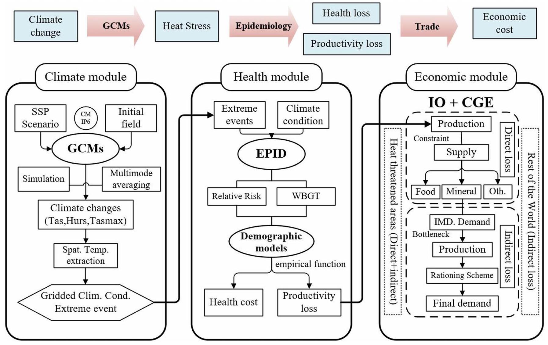
- هان، ق.، سون، س.، ليو، ز.، شو، و. & شي، ب. تسارع تفاقم موجات الحرارة الشديدة العالمية تحت سيناريوهات الاحترار. المجلة الدولية لعلم المناخ. 42، 5430-5441 (2022).
- شيانغ، س. وآخرون. تقدير الأضرار الاقتصادية الناتجة عن تغير المناخ في الولايات المتحدة. ساينس 356، 1362-1369 (2017).
معلومات إضافية
يجب توجيه المراسلات والطلبات للحصول على المواد إلى دابو جوان.
تُعرب Nature عن شكرها لبيرجيت بدنار-فريدل، أندرياس فلوريس، جي. جيسون جولي، إلكو كوكز وفكي ثومبسون على مساهمتهم في مراجعة الأقران لهذا العمل. تقارير مراجعي الأقران متاحة.
معلومات إعادة الطباعة والتصاريح متاحة علىhttp://www.nature.com/reprints.
مقالة
تصنيف المناخ
درجة حرارة الموسم الحار:
مقالة
الخسائر تحت هياكل التجارة المرجعية المختلفة في كل منطقة. يقيس المحور الأفقي الخسائر غير المباشرة كنسبة مئوية من الناتج المحلي الإجمالي باستخدام هيكل التجارة GTAP2014، بينما يقيس المحور العمودي الخسائر غير المباشرة كنسبة مئوية من الناتج المحلي الإجمالي باستخدام هيكل التجارة GTAP2011. يمكن التحقق من تفاصيل الشكل الإضافي 4d في الشكل التكميلية 6.
مقالة
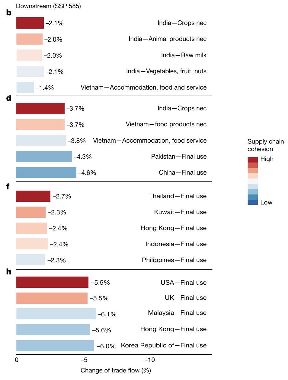
انخفاض في تدفق المنتجات مقارنة بالفترة الأساسية لعام 2014. تمثل ألوان الأعمدة مستوى التماسك للقطاع المعني مع قطاع إنتاج الغذاء الهندي من الأزرق (ضعيف) إلى الأحمر (قوي)، والذي يتم قياسه من خلال حجم التجارة بين القطاع المعني وقطاع إنتاج الغذاء الهندي.
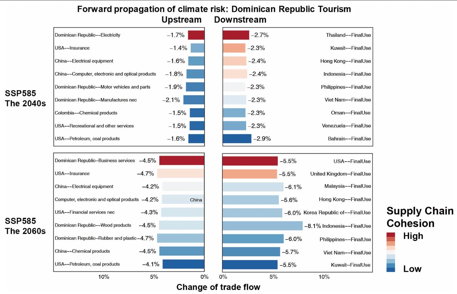
نسبة الانخفاض في تدفق المنتجات مقارنة بالفترة الأساسية لعام 2014. تمثل ألوان الأعمدة مستوى التماسك للقطاع المعين مع قطاع السياحة في جمهورية الدومينيكان من الأزرق (ضعيف) إلى الأحمر (قوي)، والذي يتم قياسه من خلال حجم التجارة بين القطاع المعين وقطاع السياحة في جمهورية الدومينيكان.
مقالة
الخسائر (الأعمدة الصفراء)، خسائر إنتاجية العمل (الأعمدة الزرقاء) وخسائر اضطراب سلسلة التوريد (الأعمدة الخضراء). تمثل الأعمدة البرتقالية والحمراء الزيادات الإجمالية في الخسائر لسيناريو SSP245 و SSP585 (دون تمييز بين أنواع الخسائر في هذا الجزء)، على التوالي. تشير الخطوط الحمراء المتقطعة إلى القيمة المتوسطة للخسائر لجميع القطاعات في سيناريو SSP585.
مقالة
خسائر إنتاجية العمل (الأعمدة الزرقاء) وخسائر اضطراب سلسلة التوريد (الأعمدة الخضراء). تمثل الأعمدة البرتقالية والحمراء إجمالي زيادات الخسائر لـ SSP245 و SSP585 (دون تمييز بين أنواع الخسائر في هذا الجزء)، على التوالي. تشير الخطوط الحمراء المتقطعة إلى القيمة المتوسطة للخسائر لجميع القطاعات في سيناريو SSP585.
الخسائر (الأعمدة الصفراء)، خسائر إنتاجية العمل (الأعمدة الزرقاء) وخسائر اضطراب سلسلة التوريد (الأعمدة الخضراء). تمثل الأعمدة البرتقالية والحمراء الزيادات الإجمالية في الخسائر لسيناريو SSP245 وSSP585 (دون تمييز بين أنواع الخسائر في هذا الجزء)، على التوالي. تشير الخطوط الحمراء المتقطعة إلى القيمة المتوسطة للخسائر لجميع القطاعات في سيناريو SSP585.
مقالة
خسائر الصحة (الأعمدة الصفراء)، خسائر إنتاجية العمل (الأعمدة الزرقاء) وخسائر اضطراب سلسلة التوريد (الأعمدة الخضراء). تمثل الأعمدة البرتقالية والحمراء إجمالي زيادات الخسائر لـ SSP245 و SSP585 (دون تمييز بين أنواع الخسائر في هذا الجزء)، على التوالي. تشير الخطوط الحمراء المتقطعة إلى القيمة المتوسطة للخسائر لجميع القطاعات في سيناريو SSP585.
| نماذج المناخ | معهد بحثي |
| CAMS-CSM1 | الأكاديمية الصينية لعلوم الأرصاد الجوية (بكين، الصين) |
| CanESM5 | المركز الكندي لنمذجة المناخ والتحليل (فيكتوريا، كولومبيا البريطانية، كندا) |
| CESM2 | المركز الوطني لأبحاث الغلاف الجوي (بولدر، كولورادو، الولايات المتحدة الأمريكية) |
| CNRM-CM6-1 | المركز الوطني لأبحاث الأرصاد الجوية (ميتيو-فرانس، تولوز، فرنسا) |
| CNRM-ESM2-1 | المركز الوطني لأبحاث الأرصاد الجوية (ميتيو-فرانس، تولوز، فرنسا) |
| EC-Earth3 | الاتحاد الأوروبي للخدمات الوطنية للأرصاد الجوية ومعاهد البحث. |
| جي إف دي إل – إسم 4 | مختبر ديناميات السوائل الجيوفيزيائية (برينستون، نيو جيرسي، الولايات المتحدة الأمريكية) |
| هادجم3-جي سي 31-إم إم | مكتب الأرصاد الجوية، مركز هادلي (إكستر، المملكة المتحدة) |
| IPSL-CM6A-LR | معهد بيير-سيمون لابلاس (باريس، فرنسا) |
| MIROC6 | وكالة اليابان لعلوم البحار والأرض، معهد أبحاث الغلاف الجوي والمحيطات (طوكيو، جامعة طوكيو)، والمعهد الوطني للدراسات البيئية (تسوكوبا، اليابان) |
| MPI-ESM1-2-HR | معهد ماكس بلانك للأرصاد الجوية (هامبورغ، ألمانيا) |
| إم آر آي – إي إس إم 2 | معهد الأبحاث الجوية (تسوكوبا، اليابان) |
| NORESM2-MM | المركز النرويجي للمناخ (برغن، النرويج) |
| يوكسم1 | مكتب الأرصاد الجوية – مركز هادلي (إكستر، المملكة المتحدة) ومجلس الأبحاث البيئية الطبيعية (المملكة المتحدة) |
مقالة
| منطقة المناخ | تقدير منخفض لمعدل العائد | تقدير متوسط معدل الاستجابة | تقدير RR مرتفع |
| بارد | 1.04467 | 1.05866 | 1.07282 |
| برد معتدل | 1.06919 | 1.08826 | 1.10751 |
| حار معتدل | 1.05357 | 1.06955 | 1.08571 |
| ساخن | 1.0345 | 1.04794 | 1.06174 |
|
|
|
||||||
| ٢٠٠ | ٣٥.٥٣ | 3.94 | ||||||
| ٣٠٠ | ٣٣.٤٩ | 3.94 | ||||||
| ٤٠٠ | ٣٢.٤٧ | ٤.١٦ |
قسم علوم نظام الأرض، وزارة التعليم، المختبر الرئيسي لنمذجة نظام الأرض، معهد دراسات التغير العالمي، جامعة تسينغhua، بكين، الصين. قسم علوم الغلاف الجوي، كلية علوم الأرض، جامعة تشجيانغ، هانغتشو، الصين. برنامج الطاقة والطاقة المتقدمة، جامعة كاليفورنيا إيرفين، إيرفين، كاليفورنيا، الولايات المتحدة الأمريكية. قسم الجغرافيا، كلية كينغز لندن، لندن، المملكة المتحدة. مركز التفاعل المناخي، قسم علوم الحاسوب والتكنولوجيا، جامعة كامبريدج، كامبريدج، المملكة المتحدة. المفتاح الرئيسي
 مركز البحوث المشترك للتخطيط الذكي من الجيل التالي في معهد شيان للمسح ورسم الخرائط، بكين، الصين.
قسم الاقتصاد، جامعة جنوب كاليفورنيا، لوس أنجلوس، كاليفورنيا، الولايات المتحدة الأمريكية. قسم الاقتصاد، جامعة واترلو، واترلو، أونتاريو، كندا. مدرسة الإدارة والاقتصاد، معهد بكين للتكنولوجيا، بكين، الصين. مدرسة الاقتصاد والإدارة، جامعة جنوب شرق، نانجينغ، الصين. كلية البيئة الحضرية، جامعة بكين، بكين، الصين. مدرسة بارلت للبناء المستدام، كلية لندن الجامعية، لندن، المملكة المتحدة. ساهم هؤلاء المؤلفون بالتساوي: ييدا سون، شوبينغ تشو، داوبينغ وانغ. البريد الإلكتروني:guandabo@tsinghua.edu.cn
DOI: https://doi.org/10.1038/s41586-024-07147-z
PMID: https://pubmed.ncbi.nlm.nih.gov/38480894
Publication Date: 2024-03-13
Global supply chains amplify economic costs of future extreme heat risk
Received: 16 August 2022
Accepted: 1 February 2024
Published online: 13 March 2024
Open access
(A) Check for updates
Abstract
Evidence shows a continuing increase in the frequency and severity of global heatwaves
Nonlinear growth trend of global heat-related losses
loss), with a value of about US
Different sensitivities to heat stress across countries
across the world. a-d, Evolutionary trends of the four types of losses from 2040 to 2060 under different scenarios (health loss (a); labour productivity loss (b); indirect loss (supply-chain disruptions) (c); and the total losses (d)). The colours from light to dark, represent the economic losses from the three
the amount of adaptive capacity. For example, Hungary and Croatia suffer considerable health losses, even though in these countries the climate is cooler than in the Middle East and North Africa. Unlike labour losses, which occur in regions with very high average temperature and humidity, health losses depend largely on the variance and abrupt changes in summer temperatures. As climate change will lead to more frequent and intense heatwaves, populations in cooler climatic zones will experience considerable loss of life if the adaptive capacity does not keep pace with the abrupt and sudden changes.
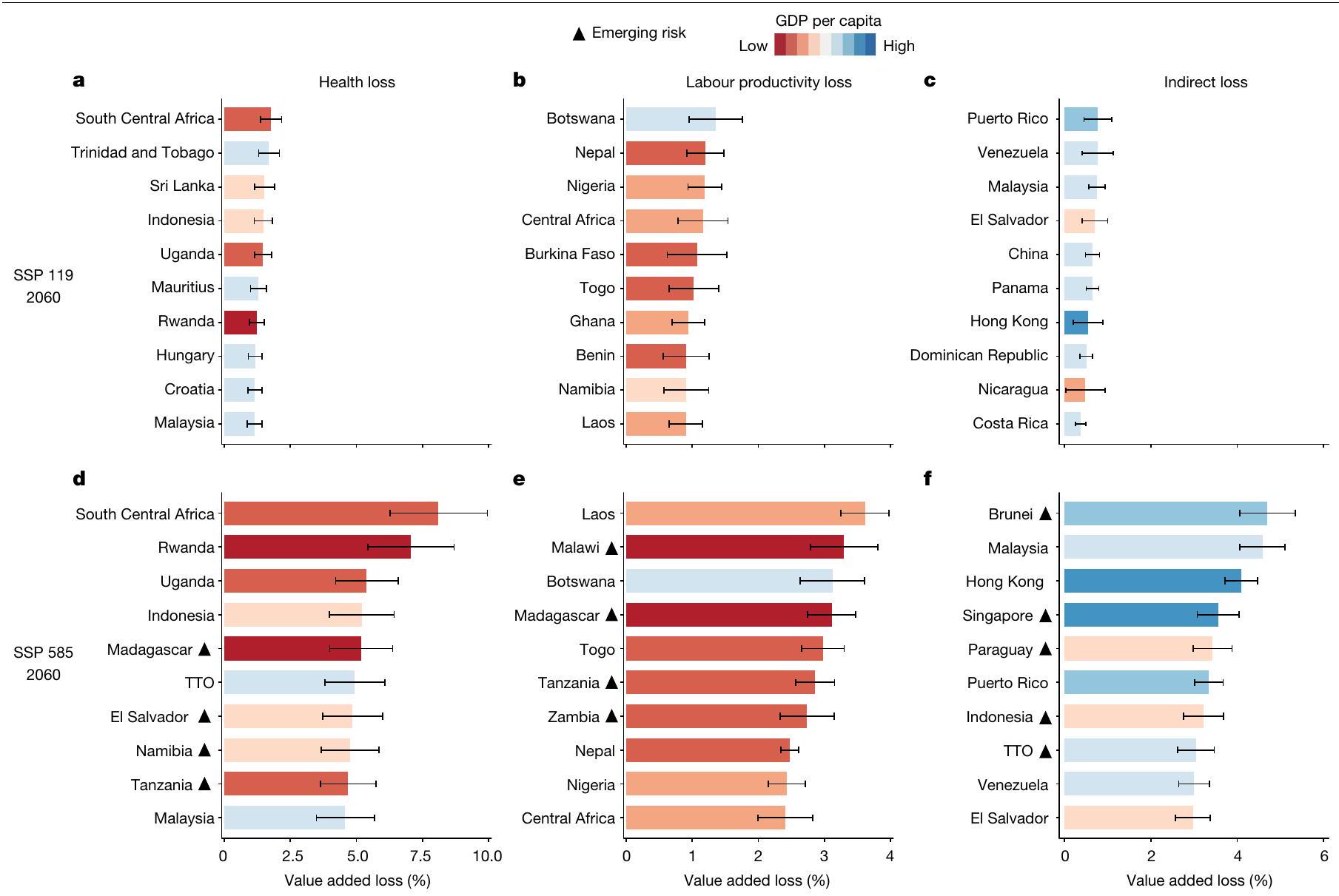
affected (Fig. 2c). Puerto Rico suffered the highest losses, estimated at
with black triangles are newly ranked among the most vulnerable countries in 2060 under the SSP 585 scenario compared with SSP 119. The values shown are 10 -year averages. Error bars represent 1 s.d. from the mean of decadal data. Upper and lower limits indicate mean + s.d. and mean – s.d., respectively. TTO, Trinidad and Tobago.
of its GDP, whereas other emerging economies like Paraguay and Indonesia lose around 3.3% of their GDP. These findings demonstrated that the rapid growth of income and air-conditioning penetration in emerging economies under the SSP 585 scenario falls short of counteracting the immense impact of climate change on their economies.
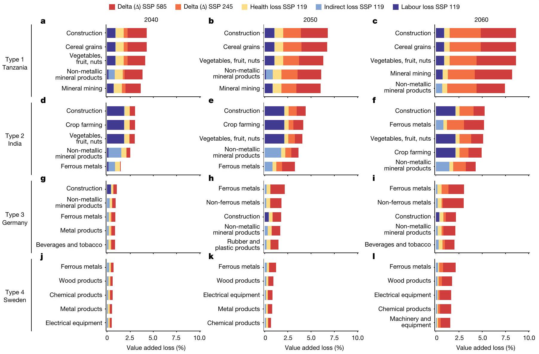
Asymmetric effects of heat stress on global supply chains
productivity in the domestic construction and plantation industries leads directly to high economic losses in the country’s related value chains. As shown in Extended Data Fig. 10, countries located at low and middle latitudes, such as China and Vietnam, exhibit similar patterns of loss.
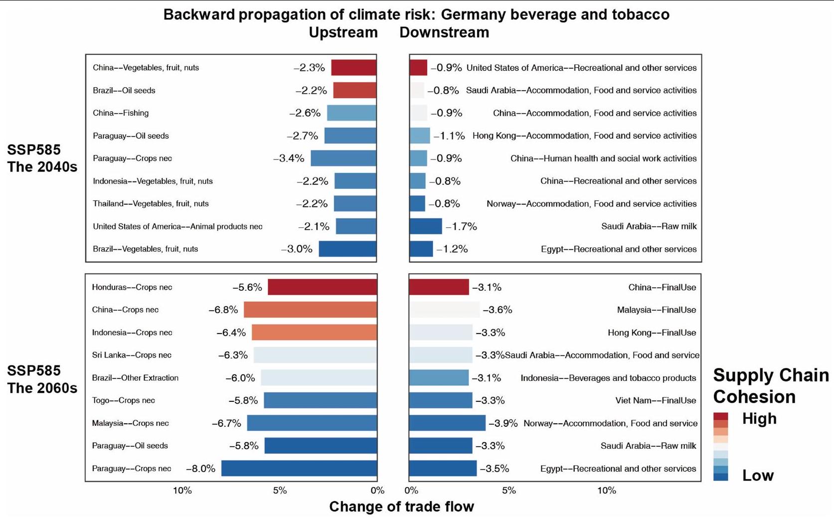
Light manufacturing, including metal products, rubber and plastic products, food processing and beverages and tobacco, are vulnerable to indirect effects because of a lack of raw materials supply, such as minerals, metals, crops, oil seeds and vegetables. For example, under the SSP 119 scenario, metal products and tobacco and beverage manufacturing in Germany lose around
only in the construction or mining sector, whereas indirect losses are higher in the metal-related manufacturing sector because of insufficient supply from foreign trading partners.
| Upstream | |||||
| a | Malaysia—Vegetable oils and fats | -1.8% | |||
| Brazil-Sugar | -2.3% | ||||
| 2040 | Brazil-Vegetable oils and fats | -1.7% | |||
| China-Vegetables, fruit, nuts | -1.7% | ||||
| Indonesia-Coal | -2.5% | ||||
| c | |||||
| Indonesia-Vegetable oils and fats | -4.9% | ||||
| 2060 | Brazil-Sugar | -4.8% | |||
| Côte d’Ivoire-Vegetables, fruit, nuts -6.2% | |||||
| Malaysia-Chemical products | -5.4% | ||||
| e | Dominican Republic-Electricity | -1.7% | |||
| USA-Insurance | -1.4% | ||||
| 2040 | China-Electrical equipment | -1.6% | |||
| China-Computer, electronic and optical products | -1.8% | ||||
| Dominican Republic-Motor vehicles and parts | -1.9% | ||||
| g | Dominican Republic-Business services -4.5% | ||||
| USA-Insurance | -4.7% | ||||
| 2060 | China-Electrical equipment | -4.2% | |||
| China-Electronic and optical products | -4.2% | 0 | |||
| USA-Financial services nec | -4.3% | ||||
| -10 | Change of trade flow (%) | 0 | |||
sectors) and the length represents the percentage decrease in product flow compared to the base period of 2014. The colours of the bars represent the cohesion level of the particular sector to the Indian food production sector from blue (weak) to red (strong), which is measured by the trade volume between the particular sector and the Indian food production sector. nec, not elsewhere classified.
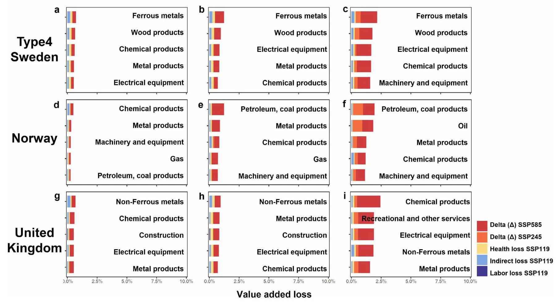
located at high latitudes, such as Norway and the UK, are characterized by similar loss patterns.
We also analyse the mechanism through which indirect losses from disruptions in international trade flows propagate through national supply chains of specific sectors. Figure 4 illustrates how climate risk propagates through two supply chains, the Indian food production and the Dominican Republic tourism sectors, respectively (see Extended Data Fig. 8 for other typical supply chains). Each of these sectors is important to the respective economies of India (
The supply chain of the Indian food production industry relies heavily on its upstream suppliers, the oil and fat sectors of Indonesia and Malaysia, and as a result it is vulnerable to higher temperatures. The unmitigated warming under the SSP 585 scenario exacerbates the shortage of raw materials. By 2060, palm oil supplies from Malaysia and Indonesia fall by
tourism infrastructure and the supply of tourism supporting products, posing considerable risks for tourism investment.
Implication for targeted risk governance and regional cooperation
Our findings show that supply chains amplify the risk of future heat stress by causing nonlinear economic losses worldwide. In other words, the considerable adverse indirect effects of heat stress across interconnected markets cannot be overlooked. The indirect losses of heat stress highlight the need for countries to strengthen collaboration across global relevant supply-chain stakeholders to achieve successful heat stress adaptation. For instance, our results demonstrate that the impact of a heatwave on the agriculture and food manufacturing industry in India can further lead to a
We also illustrate the sensitivity of different countries and sectors to the three types of losses caused by heat stress. For example, Caribbean and Central African countries are more likely to suffer health losses, whereas for low-income countries in Africa and Southeast Asia labour losses are more likely. By contrast, small to medium-sized economies dependent on international trade, such as Brunei, are more exposed to indirect losses. The way heat stress-related costs emerge demonstrates how extensive and diverse impacts from heat stress are propagated through global supply chains, resulting in economic losses to a country or sector that may not be immediately apparent. Our quantitative results provide valuable information for designing more targeted and effective heat stress adaptation strategies.
Our developed model and estimations are subject to uncertainties and limitation (detailed description in Supplementary Information sections 1.1-1.3). For example, although the disaster footprint module is widely used and performs well for single-country/single-region analyses, the substitutability of products in a multicountry scenario requires further discussion to ensure robustness. To quantify some of the uncertainties, we conducted a comprehensive sensitivity analysis, with details available in the Methods and Supplementary Information section 1 . Specifically, we used different years and versions of the input-output database for comparison to analyse the uncertainty in production and trade structures (Extended Data Fig. 4).
Globally, the estimate of the total amount of indirect losses is robust to changes in the data used (GTAP 2011 and GTAP 2014) for the base period. The results of the loss assessment at global scale differ by less than
of Statistics (https://www.singstat.gov.sg/) and the United Nations Commodity Trade Statistics Database (https://comtrade.un.org), China became the largest trading partner of Singapore in 2014, up from fourth place in 2011, whereas Vietnam rose to the 13th largest partner in 2014, from the 20th place in 2011. Conversely, Singapore’s total trade share with the EU and the USA decreased slightly over the same period. Similarly,Japan,Korea and Myanmar developed closer trade relationships with emerging markets such as China, India and Vietnam.
Despite the uncertainties, our conclusion that projected climate change will continue to increase heat-related risks globally in the coming decades and that global supply chains will amplify economic losses by spreading indirect losses to wider regions, remain robust. Therefore, in the future, the organization of global supply chains should gradually shift from an exclusive focus on efficiency to one that places equal emphasis on efficiency and resilience. A concerted global strategy to reduce emissions will not only directly protect many people in developing economies from direct economic losses of heat stress but will also maintain resilient and efficient global supply chains and contribute to the long-term, sound development of the global economy.
Online content
- Callendar, G. S. The artificial production of carbon dioxide and its influence on temperature. Q. J. R. Meteorolog. Soc. 64, 223-240 (1938).
- Seneviratne, S. I. et al. in Climate Change 2021: The Physical Science Basis (eds Masson-Delmotte, V. et al.) 1513-1766 (Cambridge Univ. Press, 2021).
- Callahan, C. W. & Mankin, J. S. Globally unequal effect of extreme heat on economic growth. Sci. Adv. 8, eadd3726 (2022).
- Lenton, T. M. et al. Quantifying the human cost of global warming. Nat. Sustain. 6, 1237-1247 (2023).
- Cai, W. et al. The 2020 China report of the Lancet Countdown on health and climate change. Lancet Public Health 6, e64-e81 (2021).
- Gasparrini, A. et al. Mortality risk attributable to high and low ambient temperature: a multicountry observational study. Lancet 386, 369-375 (2015).
- Flouris, A. D. et al. Workers’ health and productivity under occupational heat strain: a systematic review and meta-analysis. Lancet Planet. Health 2, e521-e531 (2018).
- Revich, B. & Shaposhnikov, D. Excess mortality during heat waves and cold spells in Moscow, Russia. Occup. Environ. Med. 65, 691-696 (2008).
- Kjellstrom, T. & Crowe, J. Climate change, workplace heat exposure and occupational health and productivity in Central America. Int. J. Occup. Environ. Health 17, 270-281 (2011).
Article
- Cowan, T. et al. More frequent, longer and hotter heat waves for Australia in the twenty-first century. J. Clim. 27, 5851-5871 (2014).
- Ahmadalipour, A. & Moradkhani, H. Escalating heat-stress mortality risk due to global warming in the Middle East and North Africa (MENA). Environ. Int. 117, 215-225 (2018).
- Christidis, N., Jones, G. S. & Stott, P. A. Dramatically increasing chance of extremely hot summers since the 2003 European heatwave. Nat. Clim. Change 5, 46-50 (2015).
- Dunne, J. P., Stouffer, R. J. & John, J. G. Reductions in labour capacity from heat stress under climate warming. Nat. Clim. Change 3, 563-566 (2013).
- Kjellstrom, T., Freyberg, C., Lemke, B., Otto, M. & Briggs, D. Estimating population heat exposure and impacts on working people in conjunction with climate change. Int. J. Biometeorol. 62, 291-306 (2018).
- Lee, S.-W., Lee, K. & Lim, B. Effects of climate change-related heat stress on labor productivity in South Korea. Int. J. Biometeorol. 62, 2119-2129 (2018).
- Nunfam, V. F., Adusei-Asante, K., Frimpong, K., Van Etten, E. J. & Oosthuizen, J. Barriers to occupational heat stress risk adaptation of mining workers in Ghana. Int. J. Biometeorol. 64, 1085-1101 (2020).
- Borg, M. A. et al. Occupational heat stress and economic burden: a review of global evidence. Environ. Res. 195, 110781 (2021).
- Kjellstrom, T., Kovats, R. S., Lloyd, S. J., Holt, T. & Tol, J. S. R. The direct impact of climate change on regional labor productivity. Arch. Environ. Occup. Health 64, 217-227 (2009).
- Hasegawa, T. et al. Climate change impact and adaptation assessment on food consumption utilizing a new scenario framework. Environ. Sci. Technol. 48, 438-445 (2014).
- Wenz, L. & Levermann, A. Enhanced economic connectivity to foster heat stress-related losses. Sci. Adv. 2, e1501026-e1501026 (2016).
- Xia, Y. et al. Assessment of the economic impacts of heat waves: a case study of Nanjing, China. J. Clean. Prod. 171, 811-819 (2018).
- Zhao, M., Lee, J. K. W., Kjellstrom, T. & Cai, W. Assessment of the economic impact of heat-related labor productivity loss: a systematic review. Clim. Change 167, 22 (2021).
- Xie, W. et al. Decreases in global beer supply due to extreme drought and heat. Nat. Plants 4, 964-973 (2018).
- Lima, C. Zde et al. Heat stress on agricultural workers exacerbates crop impacts of climate change. Environ. Res. Lett. 16, 044020 (2021).
- Hertel, T. W. & Rosch, S. D. Climate change, agriculture and poverty. Appl. Econ. Perspect. Policy 32, 355-385 (2010).
- Xie, W., Cui, Q. & Ali, T. Role of market agents in mitigating the climate change effects on food economy. Nat. Hazards 99, 1215-1231 (2019).
- Pierce, R. J. Energy independence and global warming. Nat. Res. Environ. 21, 68-71 (2007).
- Bleischwitz, R. Mineral resources in the age of climate adaptation and resilience. J. Ind. Ecol. 24, 291-299 (2020).
- Wang, D. et al. Economic footprint of California wildfires in 2018. Nat. Sustain. 4, 252-260 (2021).
- Xia, Y. et al. Assessing the economic impacts of IT service shutdown during the York flood of 2015 in the UK. Proc. R. Soc. A 475, 20180871 (2019).
- García-León, D. et al. Current and projected regional economic impacts of heatwaves in Europe. Nat. Commun. 12, 5807 (2021).
- Knittel, N., Jury, M. W., Bednar-Friedl, B., Bachner, G. & Steiner, A. K. A global analysis of heat-related labour productivity losses under climate change-implications for Germany’s foreign trade. Clim. Change 160, 251-269 (2020).
- Takakura, J. et al. Limited role of working time shift in offsetting the increasing occupational-health cost of heat exposure. Earth’s Future 6, 1588-1602 (2018).
- Eyring, V. et al. Overview of the Coupled Model Intercomparison Project Phase 6 (CMIP6) experimental design and organization. Geosci. Model Dev. 9, 1937-1958 (2016).
- Fasullo, J. T. Evaluating simulated climate patterns from the CMIP archives using satellite and reanalysis datasets using the Climate Model Assessment Tool (CMATv1). Geosci. Model Dev. 13, 3627-3642 (2020).
- Guo, Y. et al. Heat wave and mortality: a multicountry, multicommunity study. Environ. Health Perspect. 125, 087006 (2017).
- Riahi, K. et al. The Shared Socioeconomic Pathways and their energy, land use and greenhouse gas emissions implications: an overview. Glob. Environ. Change 42, 153-168 (2017).
- Fricko, O. et al. The marker quantification of the Shared Socioeconomic Pathway 2: a middle-of-the-road scenario for the 21st century. Glob. Environ. Change 42, 251-267 (2017).
- Orlov, A., Sillmann, J., Aunan, K., Kjellstrom, T. & Aaheim, A. Economic costs of heatinduced reductions in worker productivity due to global warming. Glob. Environ. Change 63, 102087 (2020).
- Takakura, J. et al. Cost of preventing workplace heat-related illness through worker breaks and the benefit of climate-change mitigation. Environ. Res. Lett. 12, 064010 (2017).
- Watts, N. et al. The 2019 report of The Lancet Countdown on health and climate change: ensuring that the health of a child born today is not defined by a changing climate. Lancet 394, 1836-1878 (2019).
- World Development Indicators, https://databank.worldbank.org/source/world-developmentindicators (World Bank, 2022).
- Hsiang, S. M. Temperatures and cyclones strongly associated with economic production in the Caribbean and Central America. Proc. Natl Acad. Sci. USA 107, 15367-15372 (2010).
- Colacito, R., Hoffmann, B. & Phan, T. Temperature and growth: a panel analysis of the United States. J. Money Credit Bank. 51, 313-368 (2019).
- EM-DAT, www.emdat.be/ (CRED, accessed 1 February 2023).
- Gridded Population of the World, Version 4 (GPWv4): Population Count, Revision 11, https://doi.org/10.7927/H4JW8BX5 (CIESIN, 2018).
- The Human Cost of Disasters: An Overview of the Last 20 Years (2000-2019), www.undrr. org/publication/human-cost-disasters-overview-last-20-years-2000-2019 (UNDRR, 2020).
- Dellink, R., Lanzi, E. & Chateau, J. The sectoral and regional economic consequences of climate change to 2060. Environ. Res. Econ. 72, 309-363 (2019).
(c) The Author(s) 2024
Methods
Climate module
projection data are used after 2015). The use of a dynamic threshold based on both historical and climate projections data helps to incorporate the human adaptation of heat stress in a long-term warming scenario, as reported in recent studies
Health costs related to heat exposure
Expose function of labour productivity
parameters are various in different studies. The loss functions used in mainstream research include exponential function
which defines the timeframe for computing labour productivity losses as the warm season (June to 30 September in the Northern Hemisphere and December to 30 March in the Southern Hemisphere) to adjust the overestimation of the risk of moderate hot temperature, as the model is more applicable to sudden and strong shocks rather than moderate changes throughout the year.
Global disaster footprint analysis module
Production module
products and primary inputs to produce goods and services to satisfy demand from their clients. After a disaster, output will decline. From a production perspective, there are mainly the following constraints.
Allocation module
Demand module
Simulation module
Firms plan and execute their production on the basis of three factors: (1) inventories of intermediate products they have, (2) supply of primary inputs and (3) orders from their clients. Firms will maximize their output under these constraints.
Firms and households issue orders to their suppliers for the next time step. Firms place orders with their suppliers on the basis of the gaps in their inventories (target inventory level minus existing inventory level). Households place orders with their suppliers on the basis of their demand. When a product comes from several suppliers, the allocation of orders is adjusted according to the production capacity of each supplier.
Economic footprint
firm directly affected by exogenous negative shocks, its loss includes two parts: (1) the VA decrease caused by exogenous constraints and (2) the VA decrease caused by propagation. The former is the direct loss, whereas the latter is the indirect loss. A negative shock’s total economic footprint ( TEF
Global supply-chain network
considered the potential substitution of labour with capital resulting from technological advances, such as mechanization. Our analysis ignores the different levels of trade openness and globalization among SSP narratives, as well as the role of dynamic factors such as technology and price. Again, although we have conducted robustness tests for different degrees of trade substitutability, the relevant parameter is set randomly in the Monte Carlo simulation rather than derived through a general equilibrium model. The results should therefore be interpreted with caution as indicating potential future climate change risks to the existing economy rather than as quantitative predictions, given that the static representation of the economic structure in our model inevitably skews the assessment in the long run.
Data availability
Code availability
49. Lange, S. & Büchner, M. Secondary ISIMIP3b Bias-Adjusted Atmospheric Climate Input Data (v1.1), https://doi.org/10.48364/ISIMIP.581124.1 (ISIMIP Repository, 2022).
50. Warszawski, L. et al. The Inter-Sectoral Impact Model Intercomparison Project (ISI-MIP): project framework. Proc. Natl Acad. Sci. USA 111, 3228-3232 (2014).
51. Hersbach, H. et al. The ERA5 global reanalysis. Q. J. R. Meteorolog. Soc. 146, 1999-2049 (2020).
52. Casanueva, A. et al. Climate projections of a multivariate heat stress index: the role of downscaling and bias correction. Geosci. Model Dev. 12, 3419-3438 (2019).
53. Lemke, B. & Kjellstrom, T. Calculating workplace WBGT from meteorological data: a tool for climate change assessment. Indust. Health 50, 267-278 (2012).
54. Tong, S., Wang, X. Y. & Barnett, A. G. Assessment of heat-related health impacts in Brisbane, Australia: comparison of different heatwave definitions. PLoS ONE 5, e12155 (2010).
55. Xu, Z., FitzGerald, G., Guo, Y., Jalaludin, B. & Tong, S. Impact of heatwave on mortality under different heatwave definitions: a systematic review and meta-analysis. Environ. Int. 89-90, 193-203 (2016).
56. Sun, X. et al. Heat wave impact on mortality in Pudong New Area, China in 2013. Sci. Total Environ. 493, 789-794 (2014).
57. Setchell, H. ECMWF Reanalysis v5, www.ecmwf.int/en/forecasts/dataset/ecmwf-reanalysis-v5 (ECMWF, 2020).
58. Nairn, J., Fawcett, R. & Ray, D. Defining and Predicting Excessive Heat Events, a National System (CAWCR, 2009).
59. Tong, S., Wang, X. Y., Yu, W., Chen, D. & Wang, X. The impact of heatwaves on mortality in Australia: a multicity study. BMJ Open 4, e003579 (2014).
60. Guo, X. et al. Threat by marine heatwaves to adaptive large marine ecosystems in an eddy-resolving model. Nat. Clim. Change 12, 179-186 (2022).
61. Åström, D. O., Tornevi, A., Ebi, K. L., Rocklöv, J. & Forsberg, B. Evolution of minimum mortality temperature in Stockholm, Sweden, 1901-2009. Environ. Health Perspect. 124, 740-744 (2016).
62. Yin, Q., Wang, J., Ren, Z., Li, J. & Guo, Y. Mapping the increased minimum mortality temperatures in the context of global climate change. Nat. Commun. 10, 4640 (2019).
63. Todd, N. & Valleron, A.-J. Space-time covariation of mortality with temperature: a systematic study of deaths in France, 1968-2009. Environ. Health Perspect. 123, 659-664 (2015).
64. Folkerts, M. A. et al. Long term adaptation to heat stress: shifts in the minimum mortality temperature in the Netherlands. Front. Physiol. 11, 225 (2020).
65. Anderson, B. G. & Bell, M. L. Weather-related mortality. Epidemiology 20, 205-213 (2009).
66. Guo, Y. et al. Global variation in the effects of ambient temperature on mortality: a systematic evaluation. Epidemiology 25, 781-789 (2014).
67. Guo, Y. et al. Quantifying excess deaths related to heatwaves under climate change scenarios: a multicountry time series modelling study. PLoS Med. 15, e1002629 (2018).
68. Sera, F. et al. Air conditioning and heat-related mortality: a multi-country longitudinal study. Epidemiology 31, 779 (2020).
69. Benmarhnia, T. et al. A difference-in-differences approach to assess the effect of a heat action plan on heat-related mortality and differences in effectiveness according to sex, age and socioeconomic status (Montreal, Quebec). Environ. Health Perspect. 124, 1694-1699 (2016).
70. Cheng, J. et al. Heatwave and elderly mortality: an evaluation of death burden and health costs considering short-term mortality displacement. Environ. Int. 115, 334-342 (2018).
71. Wondmagegn, B. Y. et al. Impact of heatwave intensity using excess heat factor on emergency department presentations and related healthcare costs in Adelaide, South Australia. Sci. Total Environ. 781, 146815 (2021).
72. Zhang, L. et al. Mortality effects of heat waves vary by age and area: a multi-area study in China. Environ. Health 17, 54 (2018).
73. Benmarhnia, T., Deguen, S., Kaufman, J. S. & Smargiassi, A. Vulnerability to heat-related mortality: a systematic review, meta-analysis and meta-regression analysis. Epidemiology 26, 781 (2015).
74. Jones, B. & O’Neill, B. C. Spatially explicit global population scenarios consistent with the Shared Socioeconomic Pathways. Environ. Res. Lett. 11, 084003 (2016).
75. Death Rate, Crude (per 1,000 People) | Data, https://data.worldbank.org/indicator/SP.DYN. CDRT.IN (World Bank, 2021).
76. Population and Demography-Eurostat Database, https://ec.europa.eu/eurostat/web/ population-demography/demography-population-stock-balance/database (European Union, accessed 8 September 2023).
77. The Russian Fertility and Mortality Database (RusFMD) (Center for Demographic Research, 2022).
78. China Statistical Yearbook 2019 (NBSC, 2019).
79. Mortality Table for US by State | HDPulse Data Portal, https://hdpulse.nimhd.nih.gov/ data-portal/mortality (NIH, date accessed 8 September 2023).
80. Taxa de Mortalidade Geral, ftp.ibge.gov.br/Tabuas_Completas_de_Mortalidade/Tabuas_ Completas_de_Mortalidade_2016/tabua_de_mortalidade_2016_analise.pdf (Instituto Brasileiro de Geografia e Estatística – IBGE, 2017).
81. Mortality Rates, by Age Group, www.statcan.gc.ca/en/subjects-start/health/life_expectancy_ and_deaths (Government of Canada, 2021).
82. Deaths, Australia, 2019, www.abs.gov.au/statistics/people/population/deaths-australia/ 2019 (Australian Bureau of Statistics, 2020).
83. Economic Survey, www.indiabudget.gov.in/economicsurvey/ (Government of India, accessed 8 September 2023).
84. Viscusi, W. K. Pricing the global health risks of the COVID-19 pandemic. J. Risk Uncertain. 61, 101-128 (2020).
85. Alkire, B. C., Peters, A. W., Shrime, M. G. & Meara, J. G. The economic consequences of mortality amenable to high-quality health care in low- and middle-income countries. Health Affairs 37, 988-996 (2018).
86. Hammitt, J. K. & Robinson, L. A. The income elasticity of the value per statistical life: transferring estimates between high and low income populations. J. Benefit-Cost Anal. 2, 1-29 (2011).
87. Narain, U. & Sall, C. Methodology for Valuing the Health Impacts of Air Pollution: Discussion of Challenges and Proposed Solutions, https://openknowledge.worldbank. org/handle/10986/24440 (World Bank, 2016).
88. Bröde, P., Fiala, D., Lemke, B. & Kjellstrom, T. Estimated work ability in warm outdoor environments depends on the chosen heat stress assessment metric. Int. J. Biometeorol. 62, 331-345 (2018).
89. Watts, N. et al. The 2020 report of The Lancet Countdown on health and climate change: responding to converging crises. Lancet 397, 129-170 (2021).
90. Romanello, M. et al. The 2021 report of the Lancet Countdown on health and climate change: code red for a healthy future. Lancet 398, 1619-1662 (2021).
91. Parsons, L. A., Shindell, D., Tigchelaar, M., Zhang, Y. & Spector, J. T. Increased labor losses and decreased adaptation potential in a warmer world. Nat. Commun. 12, 7286 (2021).
92. Pavanello, F. et al. Air-conditioning and the adaptation cooling deficit in emerging economies. Nat. Commun. 12, 6460 (2021).
93. The Future of Cooling-Analysis, https://www.iea.org/reports/the-future-of-cooling (IEA, 2018).
94. Hallegatte, S. An adaptive regional input-output model and its application to the assessment of the economic cost of Katrina. Risk Anal. 28, 779-799 (2008).
95. Hallegatte, S. Modeling the role of inventories and heterogeneity in the assessment of the economic costs of natural disasters: modeling the role of inventories and heterogeneity. Risk Anal. 34, 152-167 (2014).
96. Koks, E. E. & Thissen, M. A multiregional impact assessment model for disaster analysis. Econ. Syst. Res. 28, 429-449 (2016).
97. Li, J., Crawford-Brown, D., Syddall, M. & Guan, D. Modeling imbalanced economic recovery following a natural disaster using input-output analysis: modeling imbalanced economic recovery. Risk Anal. 33, 1908-1923 (2013).
98. Okuyama, Y. & Santos, J. R. Disaster impact and input-output analysis. Econ. Syst. Res. 26, 1-12 (2014).
99. Inoue, H. & Todo, Y. Firm-level propagation of shocks through supply-chain networks. Nat. Sustain. 2, 841-847 (2019).
Article
- Bardazzi, R. & Ghezzi, L. Large-scale multinational shocks and international trade: a non-zero-sum game. Econ. Syst. Res. 34, 383-409 (2022).
- Zhang, Z., Li, N., Xu, H. & Chen, X. Analysis of the economic ripple effect of the United States on the world due to future climate change. Earth’s Future 6, 828-840 (2018).
- Inoue, H. & Todo, Y. Propagation of negative shocks across nationwide firm networks. PLoS ONE 14, e0213648 (2019).
- Miller, R. E. & Blair, P. D. Input-Output Analysis: Foundations and Extensions (Cambridge Univ. Press, 2009).
- Koks, E. E. et al. Regional disaster impact analysis: comparing input-output and computable general equilibrium models. Nat. Hazards Earth Syst. Sci. 16, 1911-1924 (2016).
- Liu, X. et al. Assessing the indirect economic losses of sea ice disasters: an adaptive regional input-output modeling approach. Int. J. Offshore Polar Eng. 29, 415-420 (2019).
- Matsuo, H. Implications of the Tohoku earthquake for Toyota’s coordination mechanism: supply chain disruption of automotive semiconductors. Int. J. Prod. Econ. 161, 217-227 (2015).
- Steenge, A. E. & Bočkarjova, M. Thinking about imbalances in post-catastrophe economies: an input-output based proposition. Econ. Syst. Res. 19, 205-223 (2007).
- Bénassy, J.-P. Nonclearing markets: microeconomic concepts and macroeconomic applications. J. Econ. Lit. 31, 732-761 (1993).
- Aguiar, A., Chepeliev, M., Corong, E. & Mcdougall, R. The GTAP data base: version 10. J. Glob. Econ. Anal. 4, 27 (2019).
- Aguiar, A., Narayanan, B. & McDougall, R. An overview of the GTAP 9 data base. J. Glob. Econ. Anal. 1, 181-208 (2016).
- Huo, J. et al. Full-scale, near real-time multi-regional input-output table for the global emerging economies (EMERGING). J. Ind. Ecol. 26, 1218-1232 (2022).
- Britz, W. & Roson, R. G-RDEM: a GTAP-based recursive dynamic CGE model for long-term baseline generation and analysis. J. Glob. Econ. Anal. 4, 50-96 (2019).
- Lenzen, M. Aggregating input-output systems with minimum error. Econ. Syst. Res. 31, 594-616 (2019).
- Ara, K. The aggregation problem in input-output analysis. Econometrica 27, 257-262 (1959).
- Fei, J. C.-H. A fundamental theorem for the aggregation problem of input-output analysis. Econometrica 24, 400-412 (1956).
- Lindner, S., Legault, J. & Guan, D. Disaggregating the electricity sector of China’s inputoutput table for improved environmental life-cycle assessment. Econ. Syst. Res. 25, 300-320 (2013).
- Lindner, S., Legault, J. & Guan, D. Disaggregating input-output models with incomplete information. Econ. Syst. Res. 24, 329-347 (2012).
- Han, Q., Sun, S., Liu, Z., Xu, W. & Shi, P. Accelerated exacerbation of global extreme heatwaves under warming scenarios. Int. J. Climatol. 42, 5430-5441 (2022).
- Hsiang, S. et al. Estimating economic damage from climate change in the United States. Science 356, 1362-1369 (2017).
Additional information
Correspondence and requests for materials should be addressed to Dabo Guan.
Peer review information Nature thanks Birgit Bednar-Friedl, Andreas Flouris, G. Jason Jolley, Elco Koks and Vikki Thompson for their contribution to the peer review of this work. Peer reviewer reports are available.
Reprints and permissions information is available at http://www.nature.com/reprints.
Article
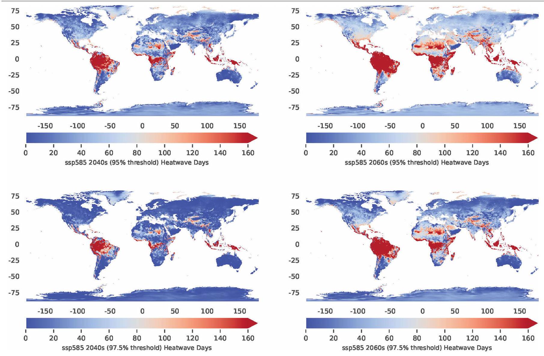
Climate Classification
temperature of hot season:
Article
losses under different benchmark trade structures in each region. The horizontal axis measures the indirect losses as a percentage of GDP using the GTAP2014 trade structure and the vertical axis measures the indirect losses as a percentage of GDP using the GTAP2011 trade structure. Details of Extended Data Fig. 4d can be checked in Supplementary Fig. 6.
Article
decrease in product flow compared to the base period of 2014. The colours of the bars represent the cohesion level of the particular sector to the Indian food production sector from blue (weak) to red (strong), which is measured by the trade volume between the particular sector and the Indian food production sector.
percentage decrease in product flow compared to the base period of 2014. The colours of the bars represent the cohesion level of the particular sector to the Dominican Republic’s tourism sector from blue (weak) to red (strong), which is measured by the trade volume between the particular sector and the Dominican Republic’s tourism sector.
Article
losses (Yellow bars), labour productivity losses (Blue bars) and supply-chain disruption losses (Green bars). The orange and red bars represent total loss increments for SSP245 and SSP585 (no distinction between types of loss in this part), respectively. The red dashed line indicates the mean value of losses for all sectors in the SSP585 scenario.
Article
bars), labour productivity losses (Blue bars) and supply-chain disruption losses (Green bars). The orange and red bars represent total loss increments for SSP245 and SSP585 (no distinction between types of loss in this part), respectively. The red dashed line indicates the mean value of losses for all sectors in the SSP585 scenario.
losses (Yellow bars), labour productivity losses (Blue bars) and supply-chain disruption losses (Green bars). The orange and red bars represent total loss increments for SSP245 and SSP585 (no distinction between types of loss in this part), respectively. The red dashed line indicates the mean value of losses for all sectors in the SSP585 scenario.
Article
health losses (Yellow bars), labour productivity losses (Blue bars) and supplychain disruption losses (Green bars). The orange and red bars represent total loss increments for SSP245 and SSP585 (no distinction between types of loss in this part), respectively. The red dashed line indicates the mean value of losses for all sectors in the SSP585 scenario.
| Climate models | Research institute |
| CAMS-CSM1 | Chinese Academy of Meteorological Sciences (Beijing, China) |
| CanESM5 | Canadian Centre for Climate Modelling and Analysis (Victoria, British Columbia, Canada) |
| CESM2 | National Center for Atmospheric Research (Boulder, Colorado, USA) |
| CNRM-CM6-1 | Centre National de Recherches Météorologiques (Météo-France, Toulouse, France) |
| CNRM-ESM2-1 | Centre National de Recherches Météorologiques (Météo-France, Toulouse, France) |
| EC-Earth3 | European consortium of national meteorological services and research institutes. |
| GFDL-esm4 | Geophysical Fluid Dynamics Laboratory (Princeton, NJ, USA) |
| HadGEM3-GC31-MM | Met Office, Hadley Centre (Exeter, United Kingdom) |
| IPSL-CM6A-LR | Institute Pierre-Simon Laplace (Paris, France) |
| MIROC6 | Japan Agency for Marine-Earth Science and Technology, Atmosphere and Ocean Research Institute (Tokyo, The University of Tokyo), and National Institute for Environmental Studies (Tsukuba, Japan) |
| MPI-ESM1-2-HR | Max Planck Institute for Meteorology (Hamburg, Germany) |
| MRI-ESM2 | Meteorological Research Institute (Tsukuba, Japan) |
| NORESM2-MM | Norwegian Climate Centre (Bergen, Norway) |
| UKESM1 | Met Office Hadley Centre (Exeter, United Kingdom) and NERC (Natural Environment Research Council, United Kingdom) |
Article
| Climate Zone | Low RR estimate | Middle RR estimate | High RR estimate |
| Cold | 1.04467 | 1.05866 | 1.07282 |
| Moderate Cold | 1.06919 | 1.08826 | 1.10751 |
| Moderate Hot | 1.05357 | 1.06955 | 1.08571 |
| Hot | 1.0345 | 1.04794 | 1.06174 |
|
|
|
||||||
| 200 | 35.53 | 3.94 | ||||||
| 300 | 33.49 | 3.94 | ||||||
| 400 | 32.47 | 4.16 |
Department of Earth System Science, Ministry of Education Key Laboratory for Earth System Modeling, Institute for Global Change Studies, Tsinghua University, Beijing, China. Department of Atmospheric Sciences, School of Earth Sciences, Zhejiang University, Hangzhou, China. Advanced Power and Energy Program, University of California Irvine, Irvine, CA, USA. Department of Geography, King’s College London, London, UK. Centre for Climate Engagement, Department of Computer Science and Technology, University of Cambridge, Cambridge, UK. State Key
Xi’an Institute of Surveying and Mapping Joint Research Center for Next-Generation Smart Mapping, Beijing, China.
Department of Economics, University of Southern California, Los Angeles, CA, USA. Department of Economics, University of Waterloo, Waterloo, Ontario, Canada. School of Management and Economics, Beijing Institute of Technology, Beijing, China. School of Economics and Management, Southeast University, Nanjing, China. College of Urban Environment, Peking University, Beijing, China. The Bartlett School of Sustainable Construction, University College London, London, UK. These authors contributed equally: Yida Sun, Shupeng Zhu, Daoping Wang. e-mail: guandabo@tsinghua.edu.cn