DOI: https://doi.org/10.1103/physrevlett.132.166001
PMID: https://pubmed.ncbi.nlm.nih.gov/38701475
تاريخ النشر: 2024-04-15
مسار قابل للتطبيق نحو الموصلية الفائقة للهيدريدات عند درجات حرارة مرتفعة وضغط جوي عادي
الملخص
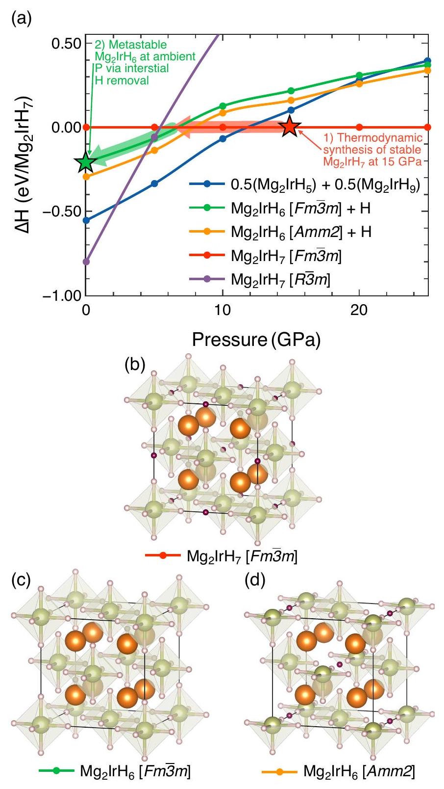
تُعتبر إيجاد الموصلات الفائقة عند درجات حرارة مرتفعة من التحديات الرئيسية في اكتشاف المواد. لقد تم اعتبار مواد الهيدروجين والهيدريد لفترة طويلة مواد واعدة تُظهر موصلية فائقة تقليدية تعتمد على الفونونات. ومع ذلك، فإن الضغوط العالية المطلوبة لتثبيت هذه المواد قد قيدت تطبيقها. هنا، نقدم نتائج من حسابات عالية الإنتاجية، مع الأخذ في الاعتبار مجموعة واسعة من الهيدريدات الثلاثية ذات التناظر العالي من جميع أنحاء الجدول الدوري تحت ضغط محيط. ثم يتم تقليل هذه المساحة الكبيرة من التركيب من خلال النظر في الاستقرار الديناميكي والحراري والمغناطيسي، قبل التقديرات المباشرة لدرجة الحرارة الحرجة للموصلية الفائقة. وقد كشفت هذه الطريقة عن موصل فائق هيدريد مستقر عند الضغط المحيط.
والاستقرار الحركي. يشير الاستقرار الديناميكي الحراري إلى القدرة على التحول إلى مراحل أخرى أو إلى التحلل إلى مكونات أساسية، مما يعني أن الهيكل موجود عند الحد الأدنى العالمي للطاقة.
قم بإجراء عملية فحص متعددة المراحل وعالية الإنتاجية لاختبار الاستقرار الديناميكي والحراري والمغناطيسي. أولاً، بالنسبة للاستقرار الحراري، قمنا بحساب الأصداف المحدبة الثلاثية لجميع التباديل لـ
تقسيم
- cjp20@cam.ac.uk
[1] هـ. ك. أونيس، مجلة مختبر الفيزياء، جامعة لايدن 122 (1911).
[2] إ. زوريك، تعليقات على الكيمياء غير العضوية 37، 78 (2017).
[3] سي. جي. بيكارد، آي. إيرريا، و م. آي. إيريميتس، المراجعة السنوية لفيزياء المادة المكثفة 11، 57 (2020).
[4] ل. بويري، ر. هينينغ، ب. هيرشفيليد، ج. بروفيتا، أ. سانا، إ. زوريك، و. إ. بيكيت، م. أملسر، ر. دياز، م. إ. إيريميتس، ج. هايل، ر. ج. هيملي، هـ. ليو، ي. ما، ج. بييرليوني، أ. ن. كولموغوروف، ن. ريبين، د. نوفوسيلوف، ف. أنيسيموف، أ. ر. أوجانوف، ج. ج. بيكارد، ت. بي، ر. أريتا، إ. إرييا، ج. بيليجريني، ر. ريكويست، إ. ك. أ. غروس، إ. ر. مارغين، س. ر. شيا، ي. كوان، أ. هير، ل. فanfاريلو، ج. ر. ستيوارت، ج. ج. هاملين، ف. ستانيف، ر. س. غونيللي، إ. بياتي، د. رومانين، د. داغهيرو، ور. فالينتي، مجلة الفيزياء: المادة المكثفة 34، 183002 (2022).
[5] سي. جي. بيكارد ور. جي. نيدز، فيزيكال ريفيو ليترز 97، 045504 (2006).
[6] سي. جي. بيكارد ور. جي. نيدز، مراجعة الفيزياء ب 76، 144114 (2007).
[7] د. دوآن، ي. ليو، ف. تيان، د. لي، خ. هوانغ، ز. تشاو، هـ. يو، ب. ليو، و. تيان، و ت. كوي، التقارير العلمية 4، 6968 (2014).
[8] أ. م. شيبلي، م. ج. هاتشون، ر. ج. نيدز، و ج. ج. بيكارد، مراجعة الفيزياء ب 104، 054501 (2021).
[9] ب. تشين، ل. ج. كونواي، و. صن، إكس. كوانغ، سي. لو، وأ. هيرمان، فيز. ريف. ب 103، 1 (2021).
[10] س. سها، س. دي كاتالدو، ف. جيانيسي، أ. كوتشيارى، و. فون دير ليندن، و ل. بويري، مراجعة المواد الفيزيائية 7، 054806 (2023).
[11] م. ج. هاتشون، أ. م. شيبلي، و ر. ج. نيدز، مراجعة الفيزياء ب 101، 144505 (2020).
[12] ت. ف. ت. سيركويرا، أ. سانا، و م. أ. ل. ماركيس، “استكشاف كامل مساحة المواد للمواد فائقة التوصيل التقليدية،” (2023)، arxiv:2307.10728 [cond-mat].
[13] س. ر. شي، ي. كوان، أ. س. هير، ب. دينغ، ج. م. ديستيفانو، إ. ساليناس، أ. س. شاه، ل. فanfاريلو، ج. ليم، ج. كيم، ج. ر. ستيوارت، ج. ج. هاملين، ب. ج. هيرشفيليد، ور. ج. هينغ، npj مواد الحوسبة 8، 14 (2022).
[14] هـ. تران و ت. ن. فو، مراجعة المواد الفيزيائية 7، 054805 (2023).
[15] أ. ب. دروزدوف، م. إ. إيريميتس، إ. أ. ترويان، ف. كسينوفونتوف، و س. إ. شيلين، ناتشر 525، 73 (2015).
[16] أ. ب. دروزدوف، ب. ب. كونغ، ف. س. مينكوف، س. ب. بيسيدين، م. أ. كوزوفنيكوف، س. موزافاري، ل. باليكس، ف. ف. بالاكيريف، د. إ. غراف، ف. ب. براكابينكا، إ. غرينبرغ، د. أ. كنيازيف، م. تكاتس، وم. إ. إيريميتس، ناتشر 569، 528 (2019).
[17] I. A. ترويان، D. V. سيمينوك، A. G. كفاشنين، A. V. ساداكوف، O. A. سوبوليفسكي، V. M. بودالوف، A. G. إيفانوفا، V. B. براكابينكا، E. غرينبرغ، A. G. غافريليوك، I. S. ليوبوتين، V. V. ستروزكين، A. بيرغارا، I. إيريا، R. بيانكو، M. كالاندرا، F. موري، L. موناكيلي، R. أكاشي، و A. R. أوجانوف، مواد متقدمة 33، 2006832 (2021).
[18] ب. كونغ، ف. س. مينكوف، م. أ. كوزوفنيكوف، أ. ب. دروزدوف، س. ب. بيسيدين، س. موزافاري، ل. باليكس، ف. ف. بالاكيريف، ف. ب. براكابينكا، س. تشاريتون، د. أ. كنيازيف، إ. غرين-
برغ، و م. إ. إيريميتس، اتصالات الطبيعة 12، 5075 (2021).
[19] و. تشين، د. ف. سيمينوك، إكس. هوانغ، هـ. شو، إكس. لي، د. دوان، ت. كوي، وأ. ر. أوجانوف، رسائل المراجعة الفيزيائية 127، 117001 (2021).
[20] ل. ما، ك. وانغ، ي. شيا، إكس. يانغ، ي. وانغ، م. تشو، هـ. ليو، إكس. يو، ي. تشاو، هـ. وانغ، ج. ليو، وي. ما، رسائل مراجعة الفيزياء 128، 167001 (2022).
[21] سي. جي. بيكارد ور. جي. نيدز، مجلة الفيزياء: المادة المكثفة 23، 053201 (2011).
[22] و. صن، س. ت. داسيك، س. ب. أونغ، ج. هاوتيير، أ. جاين، و. د. ريتشاردز، أ. س. غامست، ك. أ. بيرسون، وج. سيدر، تقدم العلوم 2، e1600225 (2016).
[23] س. دي كاتالدو، ج. هايل، و. فون دير ليندن، و ل. بويري، مراجعة الفيزياء B 104، L020511 (2021).
[24] ر. لوكريزي، س. دي كاتالدو، و. فون دير ليندن، ل. بويري، و ج. هايل، npj مواد الحوسبة 8، 119 (2022).
[25] ف. بيلي وإ. إيريا، مراجعة الفيزياء ب 106، 134509 (2022).
[26] هـ. وانغ، ب. ت. سالزبريتنر، إ. إيريا، ف. بينغ، ز. لو، هـ. ليو، ل. زو، ج. ج. بيكارد، وي. ياو، اتصالات الطبيعة 14، 1674 (2023).
[27] م. كوسيه، ج. جينست، و ب. لوبيير، مراجعة الفيزياء B 107، L060301 (2023).
[28] كانت اللوحة تحتوي على؛، Cu، Zn، Ga، Ge، As، Se، Br، Rb، Sr، Y، Zr، Nb، Mo، Tc، Ru، Rh، Pd، Ag، Cd، In، Sn، Sb، Te، I، Cs، Ba، La، Ce، Lu، Hf، Ta، W، Re، Os، Ir، Pt، Au، Hg، Tl، Pb، Bi، و Po.
[29] المجموعات الفراغية التالية تحتوي على 24 أو 48 عملية تناظر:، ، ، ، ، و .
[30] س. ج. كلارك، م. د. سيجال، ج. ج. بيكارد، ب. ج. هاسنيب، م. آي. ج. بروبرت، ك. ريفسون، و م. س. باين، مجلة بلورات – المواد البلورية 220، 567 (2005).
[31] ج. ب. بيرديو، ك. بورك، و م. إرنزرهوف، فيز. ريف. ليت. 77، 3865 (1996).
[32] ب. جيانوزي، أ. باسيجيو، ب. بونفّا، د. بروناتو، ر. كار، إ. كارنيمايو، ج. كافازوني، س. دي جيرونكولي، ب. ديلوجاس، ف. فيراري روفينو، أ. فيريتي، ن. مارزاري، إ. تيمروف، أ. أورو، وس. باروني، مجلة الفيزياء الكيميائية 152، 154105 (2020).
[33] انظر المواد التكميلية في الصفحة اللاحقة، والتي تتضمن المراجع [34-46]، لمزيد من المعلومات حول المناقشة التفصيلية لطرق الحساب، وحسابات العيوب، وتشتت الفونونات غير التوافقية، وطيف رامان وطيف الأشعة السينية المحسوب، والهياكل البلورية، وقبة كاملة للمجموعة.نظام، خصائص مرنة وخشنة . الحسابات.
[34] س. باروني، س. دي جيرونكولي، أ. دال كورسو، و ب. جيانوزي، ريف. مود. فيز. 73، 515 (2001).
[35] ك. ف. غاريتي، ج. و. بينيت، ك. م. رابي، و د. فاندربيلت، علوم المواد الحاسوبية 81، 446 (2014).
[36] م. ميثفيسل و أ. ت. باكستون، فيزيكس ريفيو ب 40، 3616 (1989).
[37] س. بونس، إ. مارغين، ج. فيردي، و ف. جيوستينو، اتصالات الفيزياء الحاسوبية 209، 116 (2016).
[38] أ. داملي، ل. لين، و ل. يينغ، مجلة النظرية الكيميائية والحساب 11، 1463 (2015).
[39] إ. ر. مارغين وف. جيوستينو، مراجعة الفيزياء ب 87، 024505 (2013).
[40] ل. موناكلي، ر. بيانكو، م. شيروبيني، م. كالاندرا، إ. إيريا، و ف. موري، مجلة الفيزياء: المادة المكثفة 33، 363001 (2021).
حجم العينة الفعّال يُحسب على أنه، حيث تمثل عوامل وزن أخذ العينات الهامة.
[42] أ. توغو، مجلة الجمعية الفيزيائية اليابانية 92، 012001 (2023).
[43] سي. جي. بيكارد، مراجعة الفيزياء ب 106، 014102 (2022).
[44] ب. ت. سالزبريتنر، س. هـ. جو، ل. ج. كونواي، ب. آي. سي. كوك، ب. زهو، م. ب. ماترازيك، و. ج. ويت، و س. ج. بيكارد، مجلة الفيزياء الكيميائية 159، 144801 (2023).
[45] م. كوكوتشوني و س. دي جيرونكولي، فيز. ريف. ب 71، 035105 (2005).
[46] م. بورن، وقائع الرياضيات لجمعية كامبريدج الفلسفية 36، 160-172 (1940).
[47] ب. ج. إيوينغ و ل. باولينغ، مجلة بلورات – المواد البلورية 68، 223 (1928).
[48] ب. هوانغ، ف. بونهوم، ب. سيلفام، ك. إيفون، و ب. فيشر، مجلة المعادن الأقل شيوعًا 171، 301 (1991).
[49] س. ساي رامان، د. ديفيدسون، ج.-ل. بوبت، وأو. سريفاستافا، مجلة السبائك والمركبات 333، 282 (2002).
[50] و. زيدي، ج.-ب. بونيت، ج. زانغ، ف. كويفاس، م. لاتروش، س. كويلاود، ج.-ل. بوبت، م. سوغراتي، ج.-س. جوماس، و ل. أيمار، المجلة الدولية لطاقة الهيدروجين 38، 4798 (2013).
[51] هـ. شيا، ت. ليانغ، ت. كوي، إكس. فنغ، هـ. سونغ، د. لي، ف. تيان، س. أ. ت. ريدفيرن، ج. ج. بيكارد، ود. دوان، الكيمياء الفيزيائية والفيزياء الكيميائية 24، 13033 (2022).
[52] ب. ب. فيريرا، ل. ج. كونواي، أ. كوتشيارى، س. دي كاتالدو، ف. جيانيسي، إ. كوجلر، ل. ت. ف. إيلينو، ج. ج. بيكارد، ج. هايل، ول. بويري، اتصالات الطبيعة 14، 5367 (2023).
[53] أ. جاين، س. ب. أونغ، ج. هاوتيير، و. تشين، و. د. ريتشاردز، س. داسيك، س. تشوليا، د. غونتر، د. سكينر، ج. سيدر، و ك. أ. بيرسون، APL Mater. 1، 011002 (2013).
[54] ف. جيوستينو، م. ل. كوهين، و س. ج. لوي، مراجعة الفيزياء ب 76، 165108 (2007).
[55] ر. لوكريزي، إ. كوجلر، س. دي كاتالدو، م. آيشهورن، ل. بويري، و ج. هايل، “ديناميات الشبكة الكمومية وأهميتها في الكلاترات الثلاثية السوبرهايدريدية،” (2022)، arxiv:2212.09789 [cond-mat].
[56] أ. د. بيك وك. إ. إيدجكومب، مجلة الفيزياء الكيميائية 92، 5397 (1990).
[57] أ. سانا، ت. ف. ت. سيركيرا، ي.-و. فانغ، إ. إيريا، أ. لودفيغ، و م. أ. ل. ماركيس، npj مواد الحوسبة 10، 44 (2024).
المواد التكميلية لـ “مسار قابل للتطبيق نحو الموصلية الفائقة للهيدريدات عند درجات حرارة مرتفعة وضغط محيط”
- طرق حسابية
- معلمات ‘خشنة’ المستخدمة في حسابات DFPT للبحث عالي الإنتاجية
- معايير ‘قوية’ مستخدمة في
حسابات لـ - حسابات فجوة الموصلية الفائقة غير المتجانسة
- حسابات الفونونات غير التوافقية
- حسابات الطاقة الحرة شبه التوافقية
- حسابات رامان
- ديناميكا الجزيئات
- أنماط حيود الأشعة السينية المحاكاة
- محاكاة الديناميكا الجزيئية
- حسابات العيوب
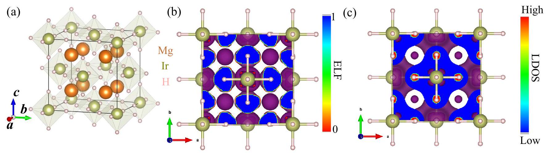
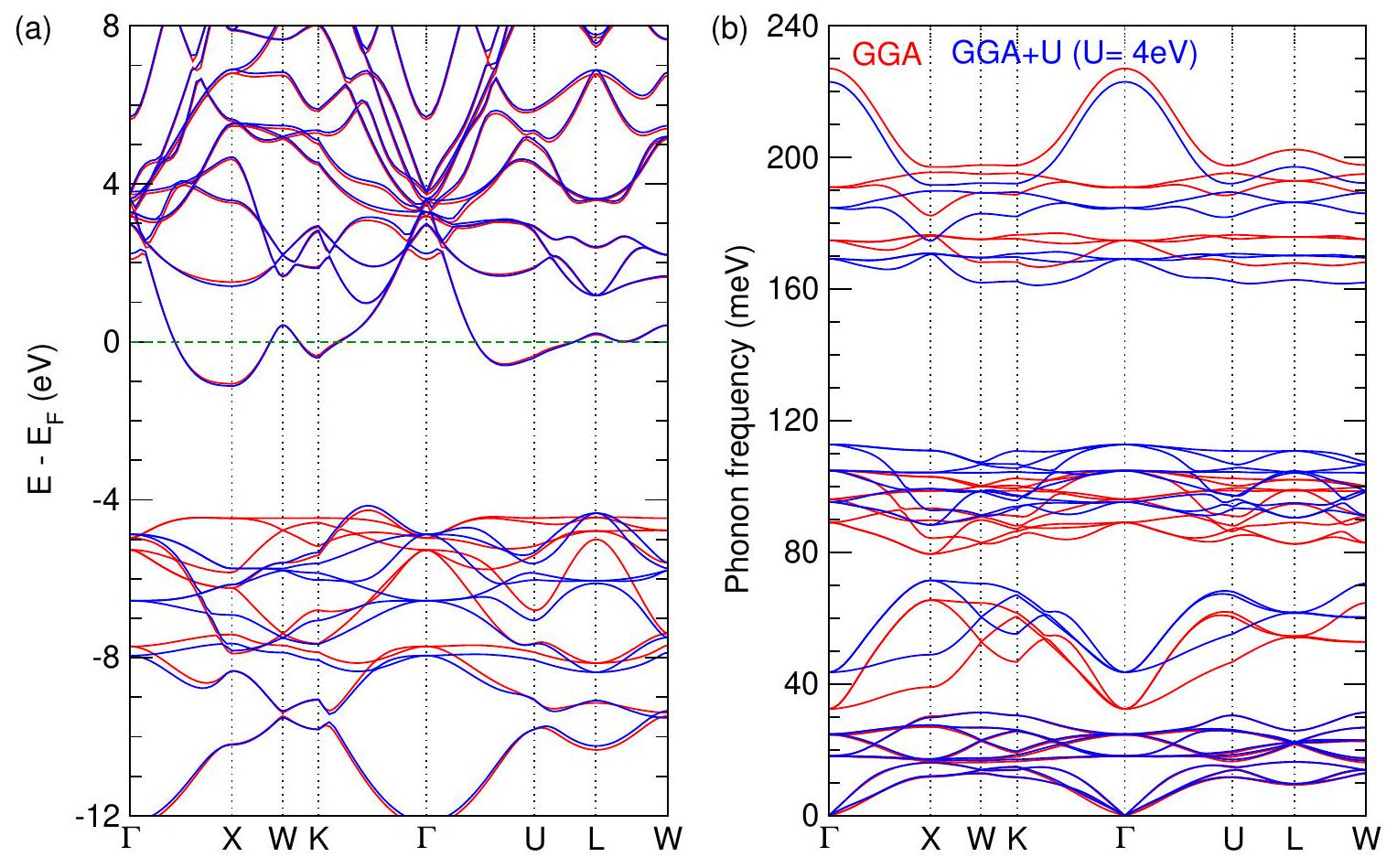
- الهياكل الإلكترونية لـ
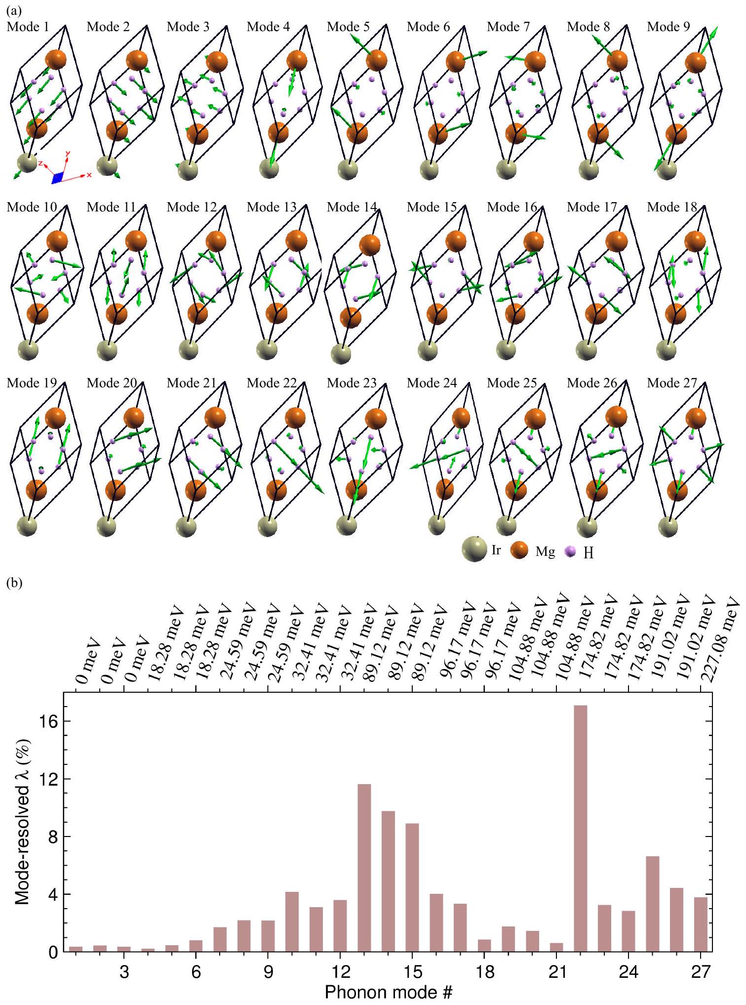
و مراحل - وضع الفونون المحلّل
- حساب انتشار الإلكترونات والفونونات باستخدام نظرية الكثافة
- حسابات الطاقة الحرة
- رامان المحاكي
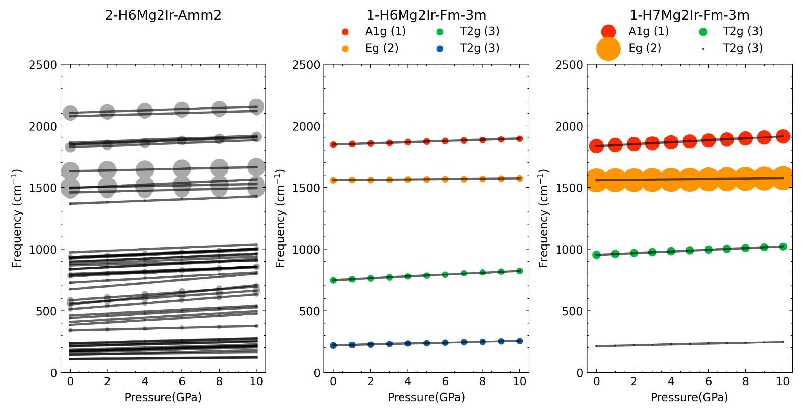
- انتشار الفونونات غير التوافقية
- الهياكل البلورية
- الغلاف المحدب الكامل
- ثوابت المرونة
- خشن
حسابات - بحث عن التناظر العالي
الفحص عالي الإنتاجية
طرق حسابية
معلمات ‘خشنة’ المستخدمة في حسابات DFPT للبحث عالي الإنتاجية
المعلمات ‘القوية’ المستخدمة في
حسابات فجوة الموصلية الفائقة غير المتجانسة
حسابات الفونونات غير التوافقية
حسابات الطاقة الحرة شبه التوافقية
حسابات رامان
ديناميكا الجزيئات
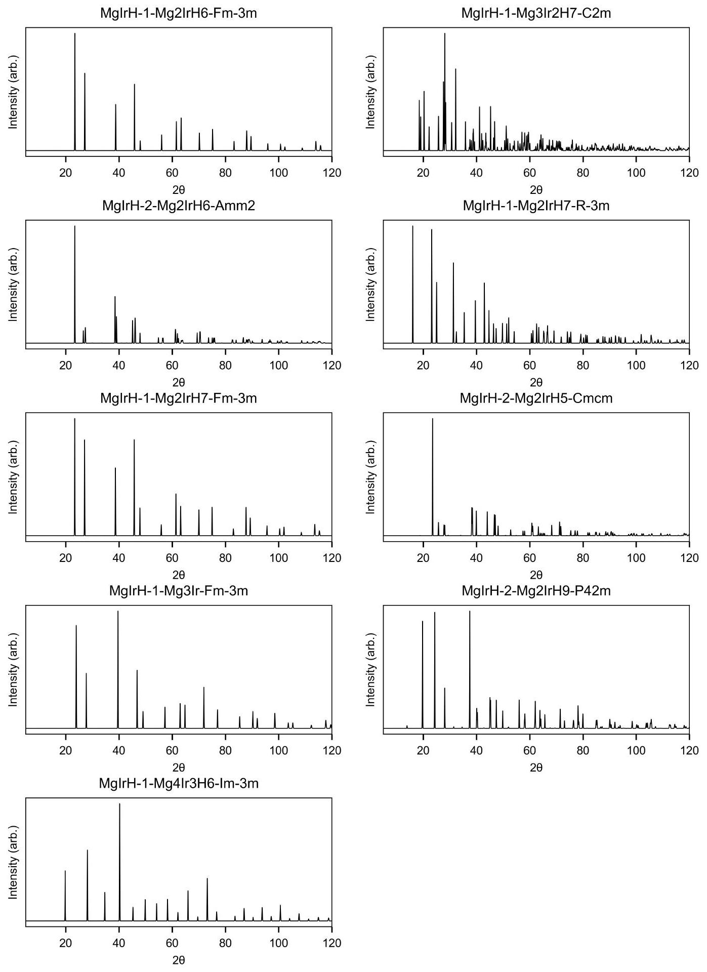
أنماط حيود الأشعة السينية المحاكاة
محاكاة الديناميكا الجزيئية
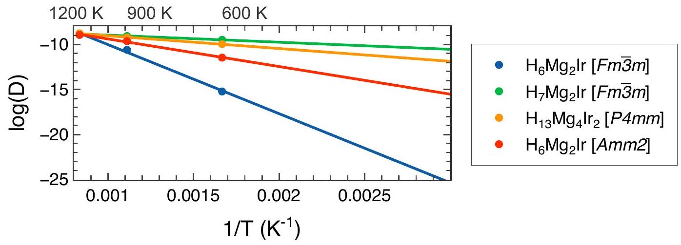
| هيكل | طاقة التنشيط |
| 1-H6Mg2Ir-Fm-3m | 0.56 إلكترون فولت |
| 1-H7Mg2Ir-Fm-3m | 0.06 إلكترون فولت |
| 2-H13Mg4Ir2-P4mm | 0.11 إلكترون فولت |
| 2-H6Mg2Ir-Amm2 | 0.26 إلكترون فولت |
حسابات العيوب
| صيغة | وظائف شاغرة | الهياكل | الهياكل غير المتكافئة بشكل متماثل |
|
|
0 | 1 | 1 |
|
|
1 | ٢٨ | 2 |
|
|
٢ | 378 | 12 |
|
|
٣ | 3,276 | 53 |
|
|
٤ | ٢٠٤٧٥ | ٢٥٢ |
|
|
٥ | ٩٨٢٨٠ | 927 |
|
|
٦ | ٣٧٦,٧٤٠ | 3,158 |
|
|
٧ | 1,184,040 | 8,875 |
|
|
٨ | ٣,١٠٨,١٠٥ | ٢١,٨٩٩ |
وضع الصوت – المحلول
حساب انتشار الإلكترونات والفونونات باستخدام نظرية الكثافة الوظيفية
حسابات الطاقة المجانية
رامان المحاكي
حسابات الفونونات غير التوافقية
الهياكل البلورية [.صيغة RES]
TITL MgIrH-1-Mg2IrH6-Fm-3m 0.084500000000 71.835913608101-15487.932800000000 0.00 0.00 9 (Fm-3m)
    n - 1
REM Functional PBE for solids (2008) Relativity Koelling-Harmon Dispersion off
REM Cut-off 600.0000 eV Grid scale 1.7500 Gmax 21.9610 1/A FBSC none
REM Offset 0.000 0.000 0.000 No. kpts 250 Spacing 0.03
REM MgIrH_Op0.cell (335d2f979913d52602ffaf9ace29feca)
REM Mg 3|1.8|7|8|9|20U:30:21:32
REM Ir 3|2.4|9|10|11|50U:60:51:52:43(qc=6)
REM H 1|0.6|13|15|17|10( qc=8)
CELL 1.54180 4.66608 4.66608 4.66608 60.00000 60.00000 60.00000
LATT -1
SFAC H Mg Ir

begin{tabular}{|l|l|l|l|l|l|}
hline H & 1 & 0.2398024272600 & 0.2398024272600 & 0.7601975727400 & 1.0 \
hline H & 1 & 0.2398024272600 & 0.7601975727400 & 0.7601975727400 & 1.0 \
hline H & 1 & 0.7601975727400 & 0.2398024272600 & 0.7601975727400 & 1.0 \
hline H & 1 & 0.7601975727400 & 0.7601975727400 & 0.2398024272600 & 1.0 \
hline H & 1 & 0.7601975727400 & 0.2398024272600 & 0.2398024272600 & 1.0 \
hline H & 1 & 0.2398024272600 & 0.7601975727400 & 0.2398024272600 & 1.0 \
hline Mg & 2 & 0.7500000000000 & 0.7500000000000 & 0.7500000000000 & 1.0 \
hline Mg & 2 & 0.2500000000000 & 0.2500000000000 & 0.2500000000000 & 1.0 \
hline Ir & 3 & 0.5000000000000 & 0.5000000000000 & 0.5000000000000 & 1.0 \
hline
end{tabular}
END
TITL MgIrH-1-Mg2IrH7-Fm-3m 0.022400000000 72.344217934844-15503.340800000000 0.00 0.00 10 (Fm-3m)
    n - 1
REM Functional PBE for solids (2008) Relativity Koelling-Harmon Dispersion off
REM Cut-off 600.0000 eV Grid scale 1.7500 Gmax 21.9610 1/A FBSC none
REM MP grid 9 9 9 Offset 0.000 0.000 0.000 No. kpts 35 Spacing 0.03
REM MgIrH_0p0.cell (335d2f979913d52602ffaf9ace29feca)
REM Mg 3|1.8|7|8|9|20U:30:21:32
REM Ir 3|2.4|9|10|11|50U:60:51:52:43(qc=6)
REM H 1|0.6|13|15|17|10( qc=8)
CELL 1.54180 4.67706 4.67706 4.67706 60.00000 60.00000 60.00000
LATT -1
SFAC H Mg Ir

begin{tabular}{|l|l|l|l|l|l|}
hline H & 1 & 0.2409774004889 & 0.7590225995111 & 0.2409774004889 & 1.0 \
hline H & 1 & 0.2409774004889 & 0.2409774004889 & 0.7590225995111 & 1.0 \
hline H & 1 & 0.7590225995111 & 0.2409774004889 & 0.2409774004889 & 1.0 \
hline H & 1 & 0.7590225995111 & 0.2409774004889 & 0.7590225995111 & 1.0 \
hline H & 1 & 0.7590225995111 & 0.7590225995111 & 0.2409774004889 & 1.0 \
hline H & 1 & 0.2409774004889 & 0.7590225995111 & 0.7590225995111 & 1.0 \
hline H & 1 & 0.0000000000000 & 0.0000000000000 & 0.0000000000000 & 1.0 \
hline Mg & 2 & 0.2500000000000 & 0.2500000000000 & 0.2500000000000 & 1.0 \
hline Mg & 2 & 0.7500000000000 & 0.7500000000000 & 0.7500000000000 & 1.0 \
hline Ir & 3 & 0.5000000000000 & 0.5000000000000 & 0.5000000000000 & 1.0 \
hline
end{tabular}
END
TITL MgIrH-1-Mg2IrH7-R-3m 0.025500000000 100.588817128868-15504.146900000000 0.00 0.00 10 (R-3m)
    n - 1
REM Functional PBE for solids (2008) Relativity Koelling-Harmon Dispersion off
REM Cut-off 600.0000 eV Grid scale 1.7500 Gmax 21.9610 1/A FBSC none
REM MP grid 9 9 7 Offset 0.000 0.000 0.000 No. kpts 160 Spacing 0.03
REM MgIrH_0p0.cell (335d2f979913d52602ffaf9ace29feca)
REM Mg 3|1.8|7|8|9|20U:30:21:32
REM Ir 3|2.4|9|10|11|50U:60:51:52:43(qc=6)
REM H 1|0.6|13|15|17|10( qc=8)
CELL 1.54180 6.14379 6.14379 6.14379 43.72909 43.72909 43.72909
LATT -1
SFAC H Mg Ir
H 1 0.1026868854988 0.1026868854988 0.6090901528379 1.0
H 1 0.5000000000000 0.5000000000000 0.5000000000000 1.0
H 1 0.8973131145012 0.8973131145012 0.3909098471621 1.0
H 1 0.1026868854988 0.6090901528379 0.1026868854988 1.0
H 1 0.8973131145012 0.3909098471621 0.8973131145012 1.0
H 1 0.6090901528379 0.1026868854988 0.1026868854988 1.0
H 1 0.3909098471621 0.8973131145012 0.8973131145012 1.0
Mg 2 0.3923887698750 0.3923887698750 0.3923887698750 1.0
Mg 2 0.6076112301250 0.6076112301250 0.6076112301250 1.0
Ir 3 -0.0000000000000 -0.0000000000000 0.0000000000000 1.0
END
TITL MgIrH-1-Mg3Ir-Fm-3m -0.003400000000 67.568564974623 -17079.898949999999 0.00 0.00 4 (Fm-3m) n
    - 1
REM Functional PBE for solids (2008) Relativity Koelling-Harmon Dispersion off
REM Cut-off 600.0000 eV Grid scale 1.7500 Gmax 21.9610 1/A FBSC none
REM MP grid 9 10 5 Offset 0.000 0.000 0.000 No. kpts 225 Spacing 0.03
REM MgIrH_0p0.cell (335d2f979913d52602ffaf9ace29feca)
REM Mg 3|1.8|7|8|9|20U:30:21:32
REM Ir 3|2.4|9|10|11|50U:60:51:52:43(qc=6)
CELL 1.54180 4.57179 4.57179 4.57179 60.00000 60.00000 60.00000
LATT -1
SFAC Mg Ir

begin{tabular}{llllll}
Mg & 1 & 0.7500000000000 & 0.7500000000000 & 0.7500000000000 & 1.0 \
Mg & 1 & 0.2500000000000 & 0.2500000000000 & 0.2500000000000 & 1.0 \
Mg & 1 & 0.5000000000000 & 0.5000000000000 & 0.5000000000000 & 1.0 \
Ir & 2 & 0.0000000000000 & 0.0000000000000 & 0.0000000000000 & 1.0
end{tabular}
END
TITL MgIrH-1-Mg3Ir2H7-C2m 0.067700000000 106.193022460744-29209.100200000001 0.00 0.00 12 (C2/m)
    n - 1
REM Functional PBE for solids (2008) Relativity Koelling-Harmon Dispersion off
REM Cut-off 600.0000 eV Grid scale 1.7500 Gmax 21.9610 1/A FBSC none
REM Offset 0.000 0.000 0.000 No. kpts 297 Spacing 0.03
REM MgIrH_0p0.cell (335d2f979913d52602ffaf9ace29feca)
REM Mg 3|1.8|7|8|9|20U:30:21:32
REM Ir 3|2.4|9|10|11|50U:60:51:52:43(qc=6)
REM H 1|0.6|13|15|17|10( qc=8)
CELL 1.54180 4.69978 4.69978 5.61738 91.74118 91.74118 58.91363
LATT -1
SFAC H Mg Ir
H 1 0.3468593555633 0.8415574556774 0.6641452764272 1.0
H 1 0.3535461939612 0.3535461939612 0.6782277793160 1.0
H 1 0.0000000000000 0.0000000000000 0.0000000000000 1.0
H 1 0.8415574556774 0.3468593555633 0.6641452764272 1.0
H 1 0.6464538060388 0.6464538060388 0.3217722206840 1.0
H 1 0.1584425443226 0.6531406444367 0.3358547235728 1.0
H 1 0.6531406444367 0.1584425443226 0.3358547235728 1.0
Mg 2 0.1683588134073 0.1683588134073 0.3292901708938 1.0
Mg 2 0.8316411865927 0.8316411865927 0.6707098291062 1.0
Mg 2 0.5000000000000 0.5000000000000 0.0000000000000 1.0
Ir 3 0.1822869262993 0.1822869262993 0.8319899301768 1.0
Ir 3 0.8177130737007 0.8177130737007 0.1680100698232 1.0
END
TITL MgIrH-1-Mg4Ir3H6-Im-3m -0.048200000000 129.091873959026 -42897.715199999999 0.00 0.00 13 (Im
    -3m) n - 1
REM Functional PBE for solids (2008) Relativity Koelling-Harmon Dispersion off
REM Cut-off 600.0000 eV Grid scale 1.7500 Gmax 21.9610 1/A FBSC none
REM MP grid 8 8 8 Offset 0.000 0.000 0.000 No. kpts 26 Spacing 0.03
REM MgIrH_0p0.cell (335d2f979913d52602ffaf9ace29feca)
REM Mg 3|1.8|7|8|9|20U:30:21:32
REM Ir 3|2.4|9|10|11|50U:60:51:52:43(qc=6)
REM H 1|0.6|13|15|17|10( qc=8)
CELL 1.54180 5.51451 5.51451 5.51451 109.47122 109.47122 109.47122
LATT -1
SFAC H Mg Ir

begin{tabular}{|l|l|l|l|l|l|}
hline H & 1 & 0.7600830742351 & 0.7600830742351 & 0.0000000000000 & 1.0 \
hline H & 1 & 0.7600830742351 & 0.0000000000000 & 0.7600830742351 & 1.0 \
hline H & 1 & 0.2399169257649 & 0.2399169257649 & 0.0000000000000 & 1.0 \
hline H & 1 & 0.0000000000000 & 0.2399169257649 & 0.2399169257649 & 1.0 \
hline H & 1 & 0.0000000000000 & 0.7600830742351 & 0.7600830742351 & 1.0 \
hline H & 1 & 0.2399169257649 & 0.0000000000000 & 0.2399169257649 & 1.0 \
hline Mg & 2 & 0.5000000000000 & 0.5000000000000 & 0.5000000000000 & 1.0 \
hline Mg & 2 & 0.0000000000000 & 0.5000000000000 & 0.0000000000000 & 1.0 \
hline Mg & 2 & 0.0000000000000 & 0.0000000000000 & 0.5000000000000 & 1.0 \
hline Mg & 2 & 0.5000000000000 & 0.0000000000000 & 0.0000000000000 & 1.0 \
hline Ir & 3 & 0.5000000000000 & 0.5000000000000 & 0.0000000000000 & 1.0 \
hline Ir & 3 & 0.5000000000000 & 0.0000000000000 & 0.5000000000000 & 1.0 \
hline Ir & 3 & 0.0000000000000 & 0.5000000000000 & 0.5000000000000 & 1.0 \
hline
end{tabular}
END
TITL MgIrH-2-Mg2IrH5-Cmcm -0.076100000000 143.333691455769 -30945.621200000001 0.00 0.00 16 (Cc) n
    - 1
REM Functional PBE for solids (2008) Relativity Koelling-Harmon Dispersion off
REM Cut-off 600.0000 eV Grid scale 1.7500 Gmax 21.9610 1/A FBSC none
REM MP grid 8 8 6 Offset 0.000 0.000 0.000 No. kpts 108 Spacing 0.03
REM MgIrH_Op0.cell (335d2f979913d52602ffaf9ace29feca)
REM Mg 3|1.8|7|8|9|20U:30:21:32
REM Ir 3|2.4|9|10|11|50U:60:51:52:43(qc=6)
REM H 1|0.6|13|15|17|10( qc=8)
CELL 1.54180 4.74533 4.74533 6.38388 90.00666 90.00666 94.37834
LATT -1
SFAC H Mg Ir
H 1 0.2468522548024 0.2464521516470 0.7325950185302 1.0
H 1 0.2464521516470 0.2468522548024 0.2325950185302 1.0
H 1 0.4913546118048 0.9897566895505 0.9729166541177 1.0
H 1 0.9897566895505 0.4913546118048 0.4729166541177 1.0
H 1 0.4929055126189 0.9915437222381 0.4927685234535 1.0
H 1 0.9915437222381 0.4929055126189 0.9927685234535 1.0
H 1 0.2374952057684 0.7588304057632 0.7320830804846 1.0
H 1 0.7588304057632 0.2374952057684 0.2320830804846 1.0
H 1 0.7339803669797 0.2347279796414 0.7336850529610 1.0
H 1 0.2347279796414 0.7339803669797 0.2336850529610 1.0
Mg 2 0.9780943536533 0.9780914936485 0.4829233849779 1.0
Mg 2 0.9780914936485 0.9780943536533 0.9829233849779 1.0
Mg 2 0.5060649297031 0.5059498875726 0.9830398256762 1.0
Mg 2 0.5059498875726 0.5060649297031 0.4830398256762 1.0
Ir 3 0.4824950418691 0.0007279927391 0.2328381597988 1.0
Ir 3 0.0007279927391 0.4824950418691 0.7328381597988 1.0
END
TITL MgIrH-2-Mg2IrH6-Amm2 0.007200000000 144.379851302026 -30976.059300000001 0.00 0.00 18 (Amm2)
    n - 1
REM Functional PBE for solids (2008) Relativity Koelling-Harmon Dispersion off
REM Cut-off 600.0000 eV Grid scale 1.7500 Gmax 21.9610 1/A FBSC none
REM MP grid 6 6 6 Offset 0.000 0.000 0.000 No. kpts 54 Spacing 0.03
REM MgIrH.cell (335d2f979913d52602ffaf9ace29feca)
REM Mg 3|1.8|7|8|9|20U:30:21:32
REM Ir 3|2.4|9|10|11|50U:60:51:52:43(qc=6)
REM H 1|0.6|13|15|17|10( qc=8)
CELL 1.54180 6.56232 4.69156 4.69156 88.32611 90.00000 90.00000
LATT -1
SFAC H Mg Ir
H 1 0.5000000000000 0.7560855173187 0.2485385147120 1.0
H 1 0.7597352680519 0.4997875636871 0.4997875636871 1.0
H 1 0.5000000000000 0.2408220253033 0.2408220253033 1.0
H 1 0.5000000000000 0.2485385147120 0.7560855173187 1.0
H 1 0.7464616102291 0.0036899515095 0.0036899515095 1.0
H 1 0.0000000000000 0.2554796300315 0.2554796300315 1.0
H 1 0.0000000000000 0.2647507829720 0.7376982665770 1.0
H 1 0.2535383897709 0.0036899515095 0.0036899515095 1.0
H 1 0.0000000000000 0.7473689432757 0.7473689432757 1.0
H 1 0.0000000000000 0.7376982665770 0.2647507829720 1.0
H 1 0.2402647319481 0.4997875636871 0.4997875636871 1.0
H 1 0.0000000000000 0.5068998641674 0.5068998641674 1.0
Mg 2 0.7429833434990 0.9881309589843 0.5050406993662 1.0
Mg 2 0.7429833434990 0.5050406993662 0.9881309589843 1.0
Mg 2 0.2570166565010 0.5050406993662 0.9881309589843 1.0
Mg 2 0.2570166565010 0.9881309589843 0.5050406993662 1.0
Ir 3 0.5000000000000 0.4891841959690 0.4891841959690 1.0
Ir 3 0.0000000000000 0.0021392434802 0.0021392434802 1.0
END
TITL MgIrH-2-Mg2IrH9-P42m -0.009200000000 183.563587013802-31069.982700000000 0.00 0.00 24 (P42/m
    ) n - 1
REM Functional PBE for solids (2008) Relativity Koelling-Harmon Dispersion off
REM Cut-off 600.0000 eV Grid scale 1.7500 Gmax 21.9610 1/A FBSC none
REM MP grid 8 6 6 Offset 0.000 0.000 0.000 No. kpts 36 Spacing 0.03
REM MgIrH_0p0.cell (335d2f979913d52602ffaf9ace29feca)
REM Mg 3|1.8|7|8|9|20U:30:21:32
REM Ir 3|2.4|9|10|11|50U:60:51:52:43(qc=6)
REM H 1|0.6|13|15|17|10( qc=8)
CELL 1.54180 6.39037 6.39037 4.49505 90.00000 90.00000 90.00000
LATT -1
SFAC H Mg Ir
H 1 0.0580813378979 0.9842036057895 0.5000000000000 1.0
H 1 0.9419186621021 0.0157963942105 0.5000000000000 1.0
H 1 0.9842036057895 0.9419186621021 0.0000000000000 1.0
H 1 0.0157963942105 0.0580813378979 0.0000000000000 1.0
H 1 0.6742339054048 0.1921793668453 0.5000000000000 1.0
H 1 0.3257660945952 0.8078206331547 0.5000000000000 1.0
H 1 0.1921793668453 0.3257660945952 0.0000000000000 1.0
H 1 0.8078206331547 0.6742339054048 0.0000000000000 1.0
H 1 0.3470353706737 0.1034854487123 0.7604983732390 1.0
H 1 0.6529646293263 0.8965145512877 0.7604983732390 1.0
H 1 0.1034854487123 0.6529646293263 0.2604983732390 1.0
H 1 0.8965145512877 0.3470353706737 0.2604983732390 1.0
H 1 0.3470353706737 0.1034854487123 0.2395016267610 1.0
H 1 0.6529646293263 0.8965145512877 0.2395016267610 1.0
H 1 0.1034854487123 0.6529646293263 0.7395016267610 1.0
H 1 0.8965145512877 0.3470353706737 0.7395016267610 1.0
H 1 0.5000000000000 0.5000000000000 0.2500000000000 1.0
H 1 0.5000000000000 0.5000000000000 0.7500000000000 1.0
Mg 2 0.2611733307333 0.3824267486473 0.5000000000000 1.0
Mg 2 0.7388266692667 0.6175732513527 0.5000000000000 1.0
Mg 2 0.3824267486473 0.7388266692667 0.0000000000000 1.0
Mg 2 0.6175732513527 0.2611733307333 0.0000000000000 1.0
Ir 3 0.5000000000000 0.0000000000000 0.5000000000000 1.0
Ir 3 0.0000000000000 0.5000000000000 0.0000000000000 1.0
END
الغلاف المحدب الكامل
ثوابت المرونة
|
|
|
|
|
|
|
|
|
تي粗
بحث عن التناظر العالي
| تركيب | مجموعة الفضاء | نموذج أولي |
|
|
|
|
|
|
Fm-3m |
|
١٣٤.١٠٣ | ٢٨.٩١٧ | -0.263 | 0.000 |
|
|
Fm-3m |
|
٨٩.١٦٨ | ١٤.٥١٧ | 0.030 | 0.080 |
|
|
بي إم – 3 م | بيروفسكايت مكعب | 65.027 | ٤.٠٤٧ | -0.224 | 0.026 |
| HNSc | F-43م | نصف هيوسلر | ٣٨.٧٦٥ | 19.333 | -0.790 | 0.000 |
|
|
بي إم – 3 م | البيروفسكايت المكعب | ٣٥.٥٠٣ | 21.422 | -0.270 | 0.100 |
|
|
Fm-3 | فلوريت
|
٢٩.٤٢١ | ٢٢.٥٣٧ | -0.248 | 0.075 |
|
|
بي إم – 3 م | البيروفسكايت المكعب | 27.011 | 10.822 | -0.146 | 0.000 |
|
|
بي إم – 3 م | البيروفسكايت المكعب | 25.369 | ١٤٫٥٣٩ | -0.281 | 0.000 |
|
|
بي إم – 3 م |
|
12.871 | 10.292 | -0.595 | 0.000 |
|
|
بي إم – 3 م | بيروفسكايت مكعب | 9.329 | 2.117 | -0.117 | 0.031 |
|
|
بي إم – 3 م |
|
8.782 | 5.338 | -1.854 | 0.000 |
|
|
بي إم – 3 م | البيروفسكايت المكعب | 8.442 | ٥.٢٦٦ | -0.050 | 0.000 |
|
|
بي إم – 3 م | بيروفسكايت مكعب | 6.821 | 0.007 | -0.452 | 0.000 |
|
|
بي إم – 3 م | بيروفسكايت مكعب | ٦.٤١٥ | ٣.٦٨٢ | -0.044 | 0.000 |
|
|
بي إم – 3 م | بيروفسكايت مكعب | ٤.٣٥٠ | ٤.٥٦٣ | 0.085 | 0.085 |
|
|
بي إم – 3 م | البيروفسكايت المكعب | ٤.٣٠٩ | 0.781 | -0.146 | 0.000 |
|
|
بي إم – 3 م | البيروفسكايت المكعب | ٣.٧٤٣ | 1.803 | -0.350 | 0.000 |
|
|
بي إم – 3 م | بيروفسكايت مكعب | ٢.١٤٦ | 1.465 | -0.287 | 0.000 |
|
|
بي إم – 3 م |
|
2.118 | ٤.١٥٣ | -0.491 | 0.000 |
|
|
بي إم – 3 م | البيروفسكايت المكعب | 2.015 | 1.415 | -0.122 | 0.026 |
|
|
بي إم – 3 م | البيروفسكايت المكعب | 1.222 | 1.000 | -0.199 | 0.000 |
|
|
بي إم – 3 م | البيروفسكايت المكعب | 0.639 | 0.038 | -0.277 | 0.000 |
|
|
بي إم – 3 م | بيروفسكايت مكعب | 0.000 | 3.114 | -0.147 | 0.000 |
TITL th - 1-HNSc-F-43m 0.983600000000 30.077721864843 -1567.067620000000 0.00 0.00 3 (F-43m) n - 1
CELL 1.54180 3.49076 3.49076 3.49076 60.00000 60.00000 60.00000
LATT -1
SFAC H N Sc

begin{tabular}{llllll}
H & 1 & 0.2500000000000 & 0.2500000000000 & 0.2500000000000 & 1.0 \
N & 2 & 0.7500000000000 & 0.7500000000000 & 0.7500000000000 & 1.0 \
Sc & 3 & 0.5000000000000 & 0.5000000000000 & 0.5000000000000 & 1.0
end{tabular}
END
TITL th-1-HN3Mo3-Pm-3m 1.010800000000 69.750856277710 -6443.849310000000 0.00 0.00 7(Pm-3m) n - 1
CELL 1.54180 4.11639 4.11639 4.11639 90.00000 90.00000 90.00000
LATT -1
SFAC H N Mo

begin{tabular}{|l|l|l|l|l|l|}
hline H & 1 & 0.5000000000000 & 0.5000000000000 & 0.5000000000000 & 1.0 \
hline N & 2 & 0.5000000000000 & 0.0000000000000 & 0.0000000000000 & 1.0 \
hline N & 2 & 0.0000000000000 & 0.0000000000000 & 0.5000000000000 & 1.0 \
hline N & 2 & 0.0000000000000 & 0.5000000000000 & 0.0000000000000 & 1.0 \
hline Mo & 3 & 0.5000000000000 & 0.0000000000000 & 0.5000000000000 & 1.0 \
hline Mo & 3 & 0.5000000000000 & 0.5000000000000 & 0.0000000000000 & 1.0 \
hline Mo & 3 & 0.0000000000000 & 0.5000000000000 & 0.5000000000000 & 1.0 \
hline
end{tabular}
END
TITL th-1-H12Lu2Ta-Fm-3 1.051200000000 114.705611487894-22614.203699999998 0.00 0.00 15 (Fm-3) n
    - 1
CELL 1.54180 5.45381 5.45381 5.45381 60.00000 60.00000 60.00000
LATT -1
SFAC H Lu Ta
H 1 0.5900714906738 0.1548830550478 0.8451169449522 1.0
H 1 0.1548830550478 0.8451169449522 0.5900714906738 1.0
H 1 0.5900714906738 0.4099285093262 0.1548830550478 1.0
H 1 0.4099285093262 0.8451169449522 0.1548830550478 1.0
H 1 0.8451169449522 0.1548830550478 0.4099285093262 1.0
H 1 0.4099285093262 0.5900714906738 0.8451169449522 1.0
H 1 0.8451169449522 0.5900714906738 0.1548830550478 1.0
H 1 0.1548830550478 0.4099285093262 0.8451169449522 1.0
H 1 0.1548830550478 0.5900714906738 0.4099285093262 1.0
H 1 0.8451169449522 0.4099285093262 0.5900714906738 1.0
H 1 0.4099285093262 0.1548830550478 0.5900714906738 1.0
H 1 0.5900714906738 0.8451169449522 0.4099285093262 1.0
Lu 2 0.7500000000000 0.7500000000000 0.7500000000000 1.0
Lu 2 0.2500000000000 0.2500000000000 0.2500000000000 1.0
Ta 3 0.5000000000000 0.5000000000000 0.5000000000000 1.0
END
| أ | ب في
|
|
|
|
|
| مغنيسيوم | إير | ١٣٤٫٣٨٦ | ٢٩.٣٥٣ | -0.263 | 0.000 |
| مغ | نقطة | ١٠٥.٥٣٣ | 86.189 | -0.084 | 0.088 |
| ال | إعادة | ١٠٥.١١٩ | 30.859 | 0.001 | 0.001 |
| مغنيسيوم | ر | ١٠٢.٢٥٥ | ٣١.٠٢٩ | -0.248 | 0.000 |
| لا | فضة | 99.590 | ٣٧.٨١٤ | 0.163 | 0.264 |
| ال | من | ٨٩.٣٩٥ | 18.447 | -0.011 | 0.000 |
| نا | أو | ٧٧.٨٢٣ | ٢٦.٢٥١ | -0.012 | 0.089 |
| في | إعادة | ٥٩.٨٣٧ | 18.892 | 0.165 | 0.165 |
| كا | فضة | ٥٨.٠٩٨ | 31.324 | -0.193 | 0.197 |
| في | تي سي | ٥٧.٩٣٣ | ٢٠.٢٩٦ | 0.133 | 0.143 |
| سير | فضة | ٤٨.٧٣٥ | 18.795 | -0.223 | 0.156 |
| با | فضة | 41.980 | ١٦٫١٤٢ | -0.233 | 0.101 |
| لا | ب | 41.031 | ٢٤.٣٠١ | 0.117 | 0.218 |
| لا | زن | ٣٩.٧٨٥ | 44.523 | 0.808 | 0.909 |
| كا | نحاس | ٣٦.١٦٤ | 6.794 | -0.321 | 0.069 |
| لا | ال | ٣٥.١٢٨ | ٢٣.٣٩٨ | 0.052 | 0.155 |
| كا | Pd | ٣٤.٠٣٨ | 11.898 | -0.427 | 0.081 |
| نا | غا | ٣١.٥٥٠ | 25.716 | 0.126 | 0.227 |
| لو | تي سي | ٢٩.٣٠٢ | 1.658 | -0.528 | 0.000 |
| سير | نحاس | ٢٦.٦٧٠ | ٤.٦٠٥ | -0.329 | 0.051 |
| سير | Pd | ٢٦.٤٩٨ | 7.773 | -0.437 | 0.000 |
| با | لا | 25.671 | 12.309 | -0.102 | 0.283 |
| ي | نحاس | ٢٤.٤٧٨ | 9.846 | -0.364 | 0.182 |
| لو | إعادة | ٢٣.٧٠٣ | ٣.٠٧٩ | -0.474 | 0.023 |
| كا | غا | 23.306 | 17.366 | -0.179 | 0.211 |
| نب | ني | ٢٢.٩٧٤ | ٢٠.٨٩٨ | -0.042 | 0.148 |
| لو | إير | 21.524 | ١٤.٥٧٦ | -0.385 | 0.119 |
| Rb | فضة | 21.292 | 10.443 | 0.098 | 0.213 |
| سي إس | فضة | ١٩٫٢٩٠ | 9.751 | 0.081 | 0.209 |
| سير | غا | 15.155 | 9.076 | -0.230 | 0.149 |
| ك | أو | 13.937 | ٤.٤٦٢ | -0.095 | 0.067 |
DOI: https://doi.org/10.1103/physrevlett.132.166001
PMID: https://pubmed.ncbi.nlm.nih.gov/38701475
Publication Date: 2024-04-15
Feasible route to high-temperature ambient-pressure hydride superconductivity
Abstract
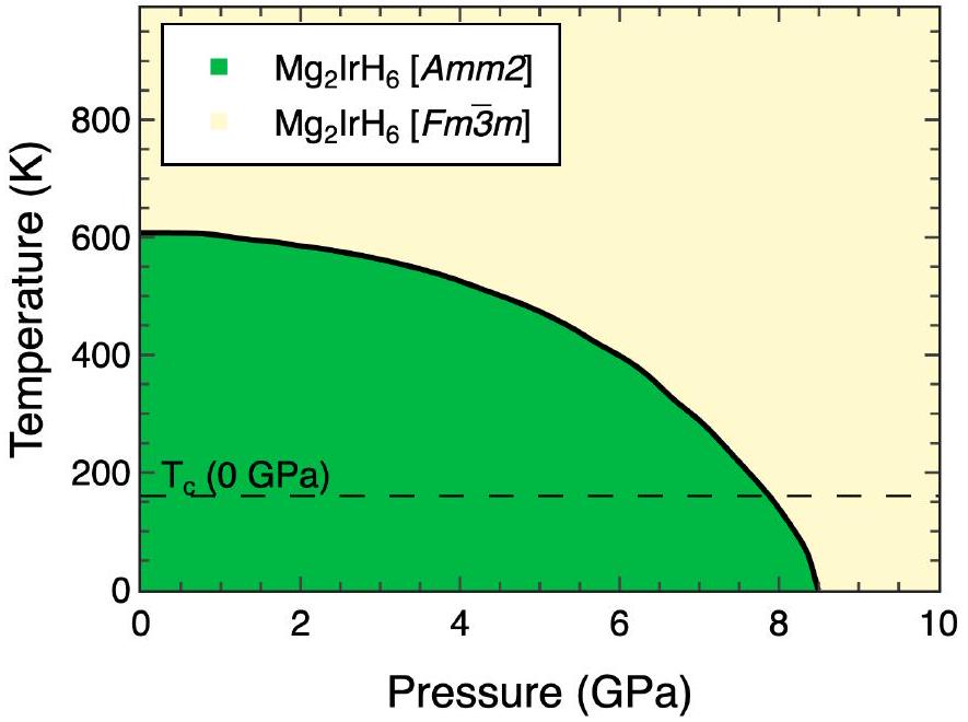
A key challenge in materials discovery is to find high-temperature superconductors. Hydrogen and hydride materials have long been considered promising materials displaying conventional phononmediated superconductivity. However, the high pressures required to stabilize these materials have restricted their application. Here, we present results from high-throughput computation, considering a wide range of high-symmetry ternary hydrides from across the periodic table at ambient pressure. This large composition space is then reduced by considering thermodynamic, dynamic, and magnetic stability, before direct estimations of the superconducting critical temperature. This approach has revealed a metastable ambient-pressure hydride superconductor,
and kinetic stability. Thermodynamic stability indicates a resilience to transformation into other phases or to decomposition into constituent species, implying the structure exists at a global energy minimum.
perform a multi-stage, high-throughput screening process to test for thermodynamic, dynamic, and magnetic instabilities. Firstly, for thermodynamic stability, we calculated ternary convex hulls for all permutations of
splitting of
- cjp20@cam.ac.uk
[1] H. K. Onnes, Comm. Phys. Lab. Univ. Leiden 122 (1911).
[2] E. Zurek, Comments on Inorganic Chemistry 37, 78 (2017).
[3] C. J. Pickard, I. Errea, and M. I. Eremets, Annual Review of Condensed Matter Physics 11, 57 (2020).
[4] L. Boeri, R. Hennig, P. Hirschfeld, G. Profeta, A. Sanna, E. Zurek, W. E. Pickett, M. Amsler, R. Dias, M. I. Eremets, C. Heil, R. J. Hemley, H. Liu, Y. Ma, C. Pierleoni, A. N. Kolmogorov, N. Rybin, D. Novoselov, V. Anisimov, A. R. Oganov, C. J. Pickard, T. Bi, R. Arita, I. Errea, C. Pellegrini, R. Requist, E. K. U. Gross, E. R. Margine, S. R. Xie, Y. Quan, A. Hire, L. Fanfarillo, G. R. Stewart, J. J. Hamlin, V. Stanev, R. S. Gonnelli, E. Piatti, D. Romanin, D. Daghero, and R. Valenti, Journal of Physics: Condensed Matter 34, 183002 (2022).
[5] C. J. Pickard and R. J. Needs, Phys. Rev. Lett. 97, 045504 (2006).
[6] C. J. Pickard and R. J. Needs, Physical Review B 76, 144114 (2007).
[7] D. Duan, Y. Liu, F. Tian, D. Li, X. Huang, Z. Zhao, H. Yu, B. Liu, W. Tian, and T. Cui, Scientific Reports 4, 6968 (2014).
[8] A. M. Shipley, M. J. Hutcheon, R. J. Needs, and C. J. Pickard, Physical Review B 104, 054501 (2021).
[9] B. Chen, L. J. Conway, W. Sun, X. Kuang, C. Lu, and A. Hermann, Phys. Rev. B 103, 1 (2021).
[10] S. Saha, S. Di Cataldo, F. Giannessi, A. Cucciari, W. Von Der Linden, and L. Boeri, Physical Review Materials 7, 054806 (2023).
[11] M. J. Hutcheon, A. M. Shipley, and R. J. Needs, Physical Review B 101, 144505 (2020).
[12] T. F. T. Cerqueira, A. Sanna, and M. A. L. Marques, “Sampling the Whole Materials Space for Conventional Superconducting Materials,” (2023), arxiv:2307.10728 [cond-mat].
[13] S. R. Xie, Y. Quan, A. C. Hire, B. Deng, J. M. DeStefano, I. Salinas, U. S. Shah, L. Fanfarillo, J. Lim, J. Kim, G. R. Stewart, J. J. Hamlin, P. J. Hirschfeld, and R. G. Hennig, npj Computational Materials 8, 14 (2022).
[14] H. Tran and T. N. Vu, Physical Review Materials 7, 054805 (2023).
[15] A. P. Drozdov, M. I. Eremets, I. A. Troyan, V. Ksenofontov, and S. I. Shylin, Nature 525, 73 (2015).
[16] A. P. Drozdov, P. P. Kong, V. S. Minkov, S. P. Besedin, M. A. Kuzovnikov, S. Mozaffari, L. Balicas, F. F. Balakirev, D. E. Graf, V. B. Prakapenka, E. Greenberg, D. A. Knyazev, M. Tkacz, and M. I. Eremets, Nature 569, 528 (2019).
[17] I. A. Troyan, D. V. Semenok, A. G. Kvashnin, A. V. Sadakov, O. A. Sobolevskiy, V. M. Pudalov, A. G. Ivanova, V. B. Prakapenka, E. Greenberg, A. G. Gavriliuk, I. S. Lyubutin, V. V. Struzhkin, A. Bergara, I. Errea, R. Bianco, M. Calandra, F. Mauri, L. Monacelli, R. Akashi, and A. R. Oganov, Advanced Materials 33, 2006832 (2021).
[18] P. Kong, V. S. Minkov, M. A. Kuzovnikov, A. P. Drozdov, S. P. Besedin, S. Mozaffari, L. Balicas, F. F. Balakirev, V. B. Prakapenka, S. Chariton, D. A. Knyazev, E. Green-
berg, and M. I. Eremets, Nature Communications 12, 5075 (2021).
[19] W. Chen, D. V. Semenok, X. Huang, H. Shu, X. Li, D. Duan, T. Cui, and A. R. Oganov, Physical Review Letters 127, 117001 (2021).
[20] L. Ma, K. Wang, Y. Xie, X. Yang, Y. Wang, M. Zhou, H. Liu, X. Yu, Y. Zhao, H. Wang, G. Liu, and Y. Ma, Physical Review Letters 128, 167001 (2022).
[21] C. J. Pickard and R. J. Needs, Journal of Physics: Condensed Matter 23, 053201 (2011).
[22] W. Sun, S. T. Dacek, S. P. Ong, G. Hautier, A. Jain, W. D. Richards, A. C. Gamst, K. A. Persson, and G. Ceder, Science Advances 2, e1600225 (2016).
[23] S. Di Cataldo, C. Heil, W. von der Linden, and L. Boeri, Physical Review B 104, L020511 (2021).
[24] R. Lucrezi, S. Di Cataldo, W. von der Linden, L. Boeri, and C. Heil, npj Computational Materials 8, 119 (2022).
[25] F. Belli and I. Errea, Physical Review B 106, 134509 (2022).
[26] H. Wang, P. T. Salzbrenner, I. Errea, F. Peng, Z. Lu, H. Liu, L. Zhu, C. J. Pickard, and Y. Yao, Nature Communications 14, 1674 (2023).
[27] M. Caussé, G. Geneste, and P. Loubeyre, Physical Review B 107, L060301 (2023).
[28] The palette contained;, , Cu, Zn, Ga, Ge, As, Se, Br, Rb, Sr, Y, Zr, Nb, Mo, Tc, Ru, Rh, Pd, Ag, Cd, In, Sn, Sb, Te, I, Cs, Ba, La, Ce, Lu, Hf, Ta, W, Re, Os, Ir, Pt, Au, Hg, Tl, Pb, Bi, and Po.
[29] The following space groups have 24 or 48 symmetry operations:, , , , , and .
[30] S. J. Clark, M. D. Segall, C. J. Pickard, P. J. Hasnip, M. I. J. Probert, K. Refson, and M. C. Payne, Zeitschrift für Kristallographie – Crystalline Materials 220, 567 (2005).
[31] J. P. Perdew, K. Burke, and M. Ernzerhof, Phys. Rev. Lett. 77, 3865 (1996).
[32] P. Giannozzi, O. Baseggio, P. Bonfà, D. Brunato, R. Car, I. Carnimeo, C. Cavazzoni, S. de Gironcoli, P. Delugas, F. Ferrari Ruffino, A. Ferretti, N. Marzari, I. Timrov, A. Urru, and S. Baroni, The Journal of Chemical Physics 152, 154105 (2020).
[33] See Supplemental Material in the later page, which includes Refs. [34-46], for additional information about the detailed discussion of the computational methods, defect calculations, Anharmonic phonon dispersion, calculated Raman and XRD spectra, crystal structures, a full convex hull for thesystem, elastic properties and coarse . calculations.
[34] S. Baroni, S. de Gironcoli, A. Dal Corso, and P. Giannozzi, Rev. Mod. Phys. 73, 515 (2001).
[35] K. F. Garrity, J. W. Bennett, K. M. Rabe, and D. Vanderbilt, Computational Materials Science 81, 446 (2014).
[36] M. Methfessel and A. T. Paxton, Phys. Rev. B 40, 3616 (1989).
[37] S. Poncé, E. Margine, C. Verdi, and F. Giustino, Computer Physics Communications 209, 116 (2016).
[38] A. Damle, L. Lin, and L. Ying, Journal of Chemical Theory and Computation 11, 1463 (2015).
[39] E. R. Margine and F. Giustino, Physical Review B 87, 024505 (2013).
[40] L. Monacelli, R. Bianco, M. Cherubini, M. Calandra, I. Errea, and F. Mauri, Journal of Physics: Condensed Matter 33, 363001 (2021).
[41] The effective sample size is computed as, where represents the importance sampling weighting factors.
[42] A. Togo, Journal of the Physical Society of Japan 92, 012001 (2023).
[43] C. J. Pickard, Physical Review B 106, 014102 (2022).
[44] P. T. Salzbrenner, S. H. Joo, L. J. Conway, P. I. C. Cooke, B. Zhu, M. P. Matraszek, W. C. Witt, and C. J. Pickard, The Journal of Chemical Physics 159, 144801 (2023).
[45] M. Cococcioni and S. de Gironcoli, Phys. Rev. B 71, 035105 (2005).
[46] M. Born, Mathematical Proceedings of the Cambridge Philosophical Society 36, 160-172 (1940).
[47] P. J. Ewing and L. Pauling, Zeitschrift für Kristallographie – Crystalline Materials 68, 223 (1928).
[48] B. Huang, F. Bonhomme, P. Selvam, K. Yvon, and P. Fischer, Journal of the Less Common Metals 171, 301 (1991).
[49] S. Sai Raman, D. Davidson, J.-L. Bobet, and O. Srivastava, Journal of Alloys and Compounds 333, 282 (2002).
[50] W. Zaïdi, J.-P. Bonnet, J. Zhang, F. Cuevas, M. Latroche, S. Couillaud, J.-L. Bobet, M. Sougrati, J.-C. Jumas, and L. Aymard, International Journal of Hydrogen Energy 38, 4798 (2013).
[51] H. Xie, T. Liang, T. Cui, X. Feng, H. Song, D. Li, F. Tian, S. A. T. Redfern, C. J. Pickard, and D. Duan, Physical Chemistry Chemical Physics 24, 13033 (2022).
[52] P. P. Ferreira, L. J. Conway, A. Cucciari, S. Di Cataldo, F. Giannessi, E. Kogler, L. T. F. Eleno, C. J. Pickard, C. Heil, and L. Boeri, Nature Communications 14, 5367 (2023).
[53] A. Jain, S. P. Ong, G. Hautier, W. Chen, W. D. Richards, S. Dacek, S. Cholia, D. Gunter, D. Skinner, G. Ceder, and K. A. Persson, APL Mater. 1, 011002 (2013).
[54] F. Giustino, M. L. Cohen, and S. G. Louie, Physical Review B 76, 165108 (2007).
[55] R. Lucrezi, E. Kogler, S. Di Cataldo, M. Aichhorn, L. Boeri, and C. Heil, “Quantum lattice dynamics and their importance in ternary superhydride clathrates,” (2022), arxiv:2212.09789 [cond-mat].
[56] A. D. Becke and K. E. Edgecombe, The Journal of Chemical Physics 92, 5397 (1990).
[57] A. Sanna, T. F. T. Cerqueira, Y.-W. Fang, I. Errea, A. Ludwig, and M. A. L. Marques, npj Computational Materials 10, 44 (2024).
Supplemental Material for “Feasible route to high-temperature ambient-pressure hydride superconductivity”
- Computational Methods
- ‘Coarse’ parameters used in DFPT calculations for high-throughput search
- ‘Robust’ parameters used in
calculations for - Anisotropic superconducting gap calculations
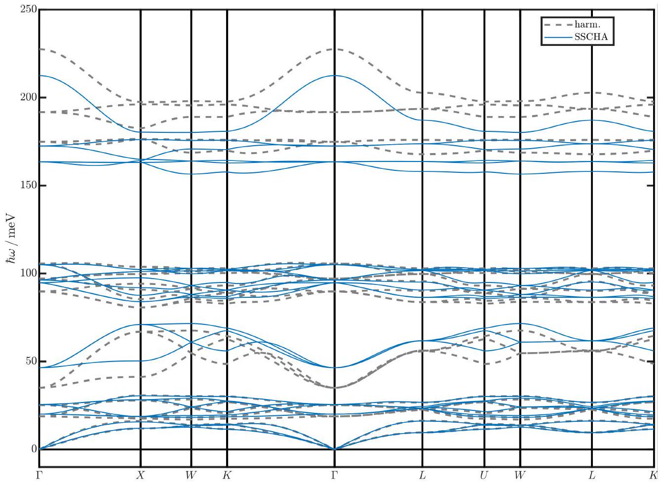
- Anharmonic phonon calculations
- Quasiharmonic free energy calculations
- Raman Calculations
- Molecular Dynamics
- Simulated X-ray diffraction patterns
- Molecular dynamics simulation
- Defect calculations
- Electronic structures of
and phases of - Phonon mode-resolved
- Electronic and phonon dispersion calculation using DFT
- Free energy calculations
- Simulated Raman
- Anharmonic phonon dispersion
- Crystal Structures
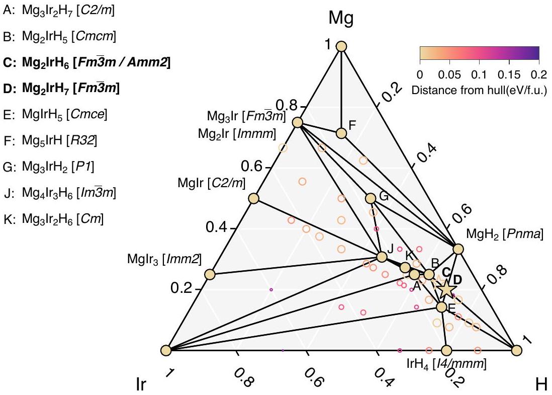
- Full Convex Hull
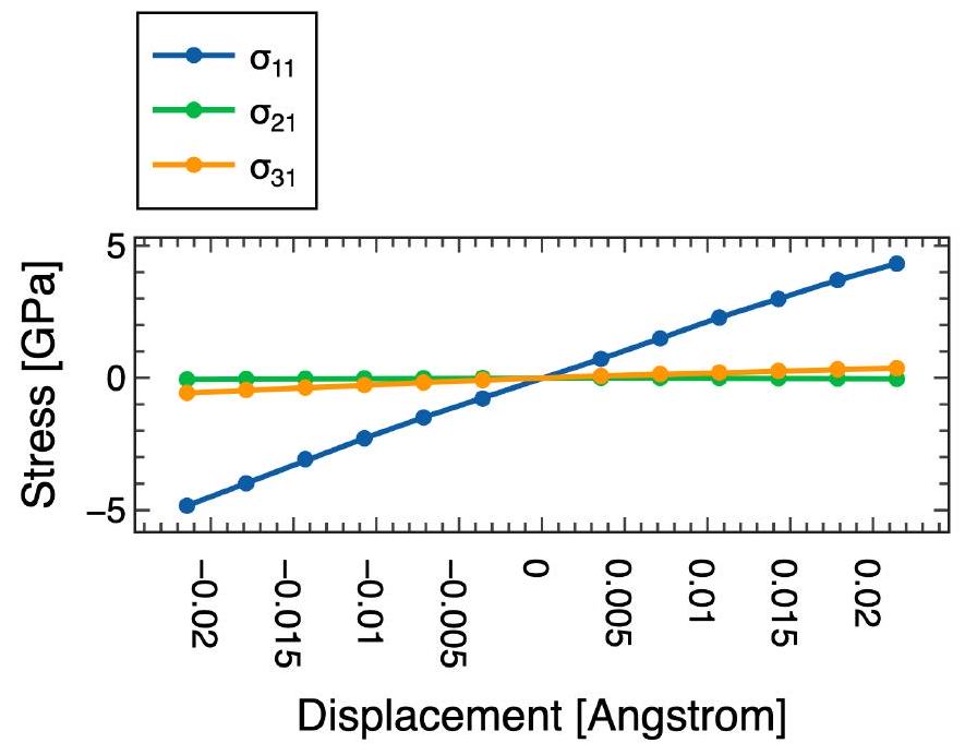
- Elastic constants
- Coarse
calculations - High symmetry search
high throughput Screening
COMPUTATIONAL METHODS
‘Coarse’ parameters used in DFPT calculations for high-throughput search
‘Robust’ parameters used in
Anisotropic superconducting gap calculations
Anharmonic phonon calculations
Quasiharmonic free energy calculations
Raman Calculations
Molecular Dynamics
SIMULATED X-RAY DIFFRACTION PATTERNS
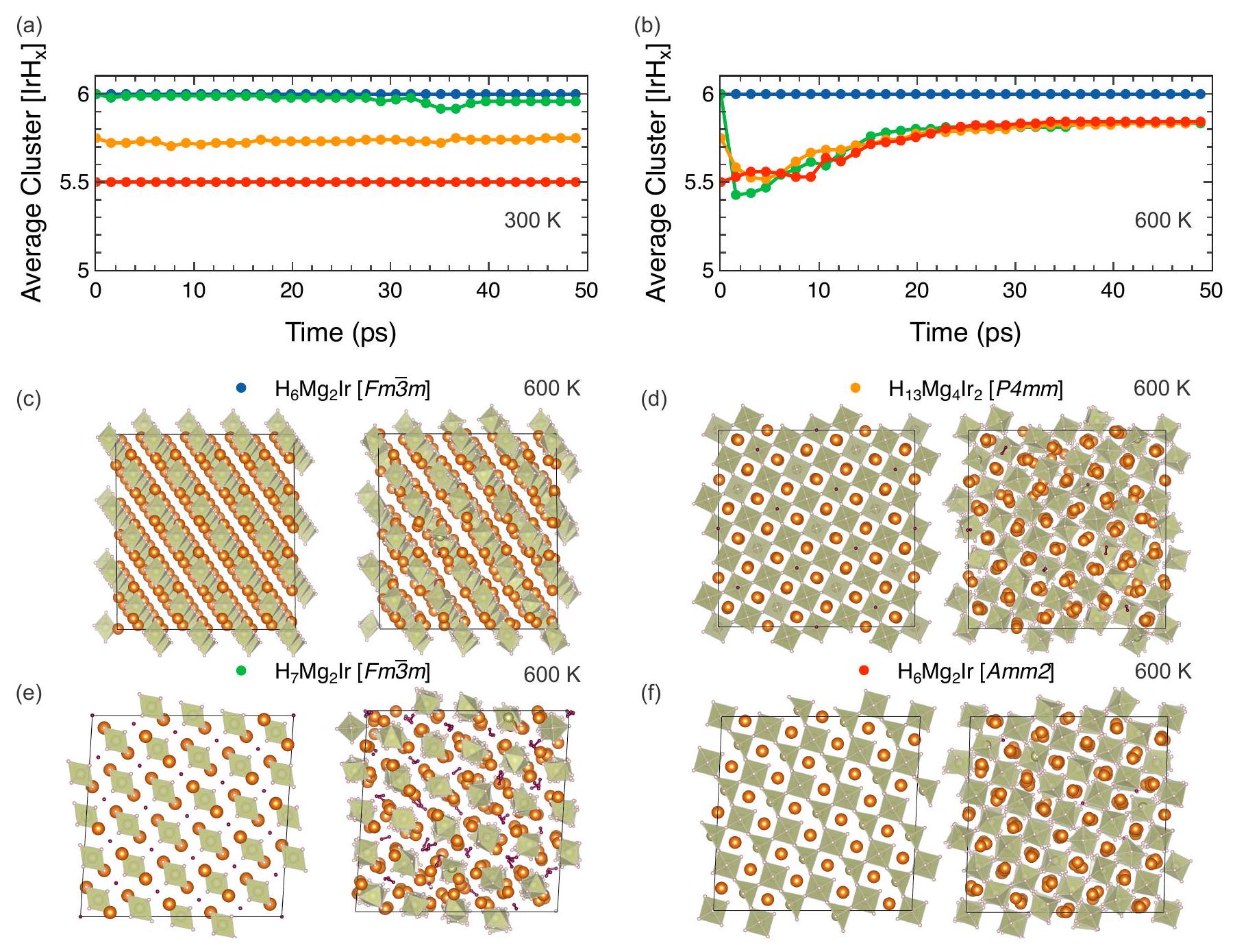
MOLECULAR DYNAMICS SIMULATIONS
| Structure | Activation Energy |
| 1-H6Mg2Ir-Fm-3m | 0.56 eV |
| 1-H7Mg2Ir-Fm-3m | 0.06 eV |
| 2-H13Mg4Ir2-P4mm | 0.11 eV |
| 2-H6Mg2Ir-Amm2 | 0.26 eV |
DEFECT CALCULATIONS
| Formula | Vacancies | Structures | Symmetrically Inequivalent Structures |
|
|
0 | 1 | 1 |
|
|
1 | 28 | 2 |
|
|
2 | 378 | 12 |
|
|
3 | 3,276 | 53 |
|
|
4 | 20,475 | 252 |
|
|
5 | 98,280 | 927 |
|
|
6 | 376,740 | 3,158 |
|
|
7 | 1,184,040 | 8,875 |
|
|
8 | 3,108,105 | 21,899 |
PHONON MODE-RESOLVED
ELECTRONIC AND PHONON DISPERSION CALCULATION USING DFT
FREE ENERGY CALCULATIONS
SIMULATED RAMAN
ANHARMONIC PHONON CALCULATIONS
CRYSTAL STRUCTURES [.RES FORMAT]
TITL MgIrH-1-Mg2IrH6-Fm-3m 0.084500000000 71.835913608101-15487.932800000000 0.00 0.00 9 (Fm-3m)
    n - 1
REM Functional PBE for solids (2008) Relativity Koelling-Harmon Dispersion off
REM Cut-off 600.0000 eV Grid scale 1.7500 Gmax 21.9610 1/A FBSC none
REM Offset 0.000 0.000 0.000 No. kpts 250 Spacing 0.03
REM MgIrH_Op0.cell (335d2f979913d52602ffaf9ace29feca)
REM Mg 3|1.8|7|8|9|20U:30:21:32
REM Ir 3|2.4|9|10|11|50U:60:51:52:43(qc=6)
REM H 1|0.6|13|15|17|10( qc=8)
CELL 1.54180 4.66608 4.66608 4.66608 60.00000 60.00000 60.00000
LATT -1
SFAC H Mg Ir

begin{tabular}{|l|l|l|l|l|l|}
hline H & 1 & 0.2398024272600 & 0.2398024272600 & 0.7601975727400 & 1.0 \
hline H & 1 & 0.2398024272600 & 0.7601975727400 & 0.7601975727400 & 1.0 \
hline H & 1 & 0.7601975727400 & 0.2398024272600 & 0.7601975727400 & 1.0 \
hline H & 1 & 0.7601975727400 & 0.7601975727400 & 0.2398024272600 & 1.0 \
hline H & 1 & 0.7601975727400 & 0.2398024272600 & 0.2398024272600 & 1.0 \
hline H & 1 & 0.2398024272600 & 0.7601975727400 & 0.2398024272600 & 1.0 \
hline Mg & 2 & 0.7500000000000 & 0.7500000000000 & 0.7500000000000 & 1.0 \
hline Mg & 2 & 0.2500000000000 & 0.2500000000000 & 0.2500000000000 & 1.0 \
hline Ir & 3 & 0.5000000000000 & 0.5000000000000 & 0.5000000000000 & 1.0 \
hline
end{tabular}
END
TITL MgIrH-1-Mg2IrH7-Fm-3m 0.022400000000 72.344217934844-15503.340800000000 0.00 0.00 10 (Fm-3m)
    n - 1
REM Functional PBE for solids (2008) Relativity Koelling-Harmon Dispersion off
REM Cut-off 600.0000 eV Grid scale 1.7500 Gmax 21.9610 1/A FBSC none
REM MP grid 9 9 9 Offset 0.000 0.000 0.000 No. kpts 35 Spacing 0.03
REM MgIrH_0p0.cell (335d2f979913d52602ffaf9ace29feca)
REM Mg 3|1.8|7|8|9|20U:30:21:32
REM Ir 3|2.4|9|10|11|50U:60:51:52:43(qc=6)
REM H 1|0.6|13|15|17|10( qc=8)
CELL 1.54180 4.67706 4.67706 4.67706 60.00000 60.00000 60.00000
LATT -1
SFAC H Mg Ir

begin{tabular}{|l|l|l|l|l|l|}
hline H & 1 & 0.2409774004889 & 0.7590225995111 & 0.2409774004889 & 1.0 \
hline H & 1 & 0.2409774004889 & 0.2409774004889 & 0.7590225995111 & 1.0 \
hline H & 1 & 0.7590225995111 & 0.2409774004889 & 0.2409774004889 & 1.0 \
hline H & 1 & 0.7590225995111 & 0.2409774004889 & 0.7590225995111 & 1.0 \
hline H & 1 & 0.7590225995111 & 0.7590225995111 & 0.2409774004889 & 1.0 \
hline H & 1 & 0.2409774004889 & 0.7590225995111 & 0.7590225995111 & 1.0 \
hline H & 1 & 0.0000000000000 & 0.0000000000000 & 0.0000000000000 & 1.0 \
hline Mg & 2 & 0.2500000000000 & 0.2500000000000 & 0.2500000000000 & 1.0 \
hline Mg & 2 & 0.7500000000000 & 0.7500000000000 & 0.7500000000000 & 1.0 \
hline Ir & 3 & 0.5000000000000 & 0.5000000000000 & 0.5000000000000 & 1.0 \
hline
end{tabular}
END
TITL MgIrH-1-Mg2IrH7-R-3m 0.025500000000 100.588817128868-15504.146900000000 0.00 0.00 10 (R-3m)
    n - 1
REM Functional PBE for solids (2008) Relativity Koelling-Harmon Dispersion off
REM Cut-off 600.0000 eV Grid scale 1.7500 Gmax 21.9610 1/A FBSC none
REM MP grid 9 9 7 Offset 0.000 0.000 0.000 No. kpts 160 Spacing 0.03
REM MgIrH_0p0.cell (335d2f979913d52602ffaf9ace29feca)
REM Mg 3|1.8|7|8|9|20U:30:21:32
REM Ir 3|2.4|9|10|11|50U:60:51:52:43(qc=6)
REM H 1|0.6|13|15|17|10( qc=8)
CELL 1.54180 6.14379 6.14379 6.14379 43.72909 43.72909 43.72909
LATT -1
SFAC H Mg Ir
H 1 0.1026868854988 0.1026868854988 0.6090901528379 1.0
H 1 0.5000000000000 0.5000000000000 0.5000000000000 1.0
H 1 0.8973131145012 0.8973131145012 0.3909098471621 1.0
H 1 0.1026868854988 0.6090901528379 0.1026868854988 1.0
H 1 0.8973131145012 0.3909098471621 0.8973131145012 1.0
H 1 0.6090901528379 0.1026868854988 0.1026868854988 1.0
H 1 0.3909098471621 0.8973131145012 0.8973131145012 1.0
Mg 2 0.3923887698750 0.3923887698750 0.3923887698750 1.0
Mg 2 0.6076112301250 0.6076112301250 0.6076112301250 1.0
Ir 3 -0.0000000000000 -0.0000000000000 0.0000000000000 1.0
END
TITL MgIrH-1-Mg3Ir-Fm-3m -0.003400000000 67.568564974623 -17079.898949999999 0.00 0.00 4 (Fm-3m) n
    - 1
REM Functional PBE for solids (2008) Relativity Koelling-Harmon Dispersion off
REM Cut-off 600.0000 eV Grid scale 1.7500 Gmax 21.9610 1/A FBSC none
REM MP grid 9 10 5 Offset 0.000 0.000 0.000 No. kpts 225 Spacing 0.03
REM MgIrH_0p0.cell (335d2f979913d52602ffaf9ace29feca)
REM Mg 3|1.8|7|8|9|20U:30:21:32
REM Ir 3|2.4|9|10|11|50U:60:51:52:43(qc=6)
CELL 1.54180 4.57179 4.57179 4.57179 60.00000 60.00000 60.00000
LATT -1
SFAC Mg Ir

begin{tabular}{llllll}
Mg & 1 & 0.7500000000000 & 0.7500000000000 & 0.7500000000000 & 1.0 \
Mg & 1 & 0.2500000000000 & 0.2500000000000 & 0.2500000000000 & 1.0 \
Mg & 1 & 0.5000000000000 & 0.5000000000000 & 0.5000000000000 & 1.0 \
Ir & 2 & 0.0000000000000 & 0.0000000000000 & 0.0000000000000 & 1.0
end{tabular}
END
TITL MgIrH-1-Mg3Ir2H7-C2m 0.067700000000 106.193022460744-29209.100200000001 0.00 0.00 12 (C2/m)
    n - 1
REM Functional PBE for solids (2008) Relativity Koelling-Harmon Dispersion off
REM Cut-off 600.0000 eV Grid scale 1.7500 Gmax 21.9610 1/A FBSC none
REM Offset 0.000 0.000 0.000 No. kpts 297 Spacing 0.03
REM MgIrH_0p0.cell (335d2f979913d52602ffaf9ace29feca)
REM Mg 3|1.8|7|8|9|20U:30:21:32
REM Ir 3|2.4|9|10|11|50U:60:51:52:43(qc=6)
REM H 1|0.6|13|15|17|10( qc=8)
CELL 1.54180 4.69978 4.69978 5.61738 91.74118 91.74118 58.91363
LATT -1
SFAC H Mg Ir
H 1 0.3468593555633 0.8415574556774 0.6641452764272 1.0
H 1 0.3535461939612 0.3535461939612 0.6782277793160 1.0
H 1 0.0000000000000 0.0000000000000 0.0000000000000 1.0
H 1 0.8415574556774 0.3468593555633 0.6641452764272 1.0
H 1 0.6464538060388 0.6464538060388 0.3217722206840 1.0
H 1 0.1584425443226 0.6531406444367 0.3358547235728 1.0
H 1 0.6531406444367 0.1584425443226 0.3358547235728 1.0
Mg 2 0.1683588134073 0.1683588134073 0.3292901708938 1.0
Mg 2 0.8316411865927 0.8316411865927 0.6707098291062 1.0
Mg 2 0.5000000000000 0.5000000000000 0.0000000000000 1.0
Ir 3 0.1822869262993 0.1822869262993 0.8319899301768 1.0
Ir 3 0.8177130737007 0.8177130737007 0.1680100698232 1.0
END
TITL MgIrH-1-Mg4Ir3H6-Im-3m -0.048200000000 129.091873959026 -42897.715199999999 0.00 0.00 13 (Im
    -3m) n - 1
REM Functional PBE for solids (2008) Relativity Koelling-Harmon Dispersion off
REM Cut-off 600.0000 eV Grid scale 1.7500 Gmax 21.9610 1/A FBSC none
REM MP grid 8 8 8 Offset 0.000 0.000 0.000 No. kpts 26 Spacing 0.03
REM MgIrH_0p0.cell (335d2f979913d52602ffaf9ace29feca)
REM Mg 3|1.8|7|8|9|20U:30:21:32
REM Ir 3|2.4|9|10|11|50U:60:51:52:43(qc=6)
REM H 1|0.6|13|15|17|10( qc=8)
CELL 1.54180 5.51451 5.51451 5.51451 109.47122 109.47122 109.47122
LATT -1
SFAC H Mg Ir

begin{tabular}{|l|l|l|l|l|l|}
hline H & 1 & 0.7600830742351 & 0.7600830742351 & 0.0000000000000 & 1.0 \
hline H & 1 & 0.7600830742351 & 0.0000000000000 & 0.7600830742351 & 1.0 \
hline H & 1 & 0.2399169257649 & 0.2399169257649 & 0.0000000000000 & 1.0 \
hline H & 1 & 0.0000000000000 & 0.2399169257649 & 0.2399169257649 & 1.0 \
hline H & 1 & 0.0000000000000 & 0.7600830742351 & 0.7600830742351 & 1.0 \
hline H & 1 & 0.2399169257649 & 0.0000000000000 & 0.2399169257649 & 1.0 \
hline Mg & 2 & 0.5000000000000 & 0.5000000000000 & 0.5000000000000 & 1.0 \
hline Mg & 2 & 0.0000000000000 & 0.5000000000000 & 0.0000000000000 & 1.0 \
hline Mg & 2 & 0.0000000000000 & 0.0000000000000 & 0.5000000000000 & 1.0 \
hline Mg & 2 & 0.5000000000000 & 0.0000000000000 & 0.0000000000000 & 1.0 \
hline Ir & 3 & 0.5000000000000 & 0.5000000000000 & 0.0000000000000 & 1.0 \
hline Ir & 3 & 0.5000000000000 & 0.0000000000000 & 0.5000000000000 & 1.0 \
hline Ir & 3 & 0.0000000000000 & 0.5000000000000 & 0.5000000000000 & 1.0 \
hline
end{tabular}
END
TITL MgIrH-2-Mg2IrH5-Cmcm -0.076100000000 143.333691455769 -30945.621200000001 0.00 0.00 16 (Cc) n
    - 1
REM Functional PBE for solids (2008) Relativity Koelling-Harmon Dispersion off
REM Cut-off 600.0000 eV Grid scale 1.7500 Gmax 21.9610 1/A FBSC none
REM MP grid 8 8 6 Offset 0.000 0.000 0.000 No. kpts 108 Spacing 0.03
REM MgIrH_Op0.cell (335d2f979913d52602ffaf9ace29feca)
REM Mg 3|1.8|7|8|9|20U:30:21:32
REM Ir 3|2.4|9|10|11|50U:60:51:52:43(qc=6)
REM H 1|0.6|13|15|17|10( qc=8)
CELL 1.54180 4.74533 4.74533 6.38388 90.00666 90.00666 94.37834
LATT -1
SFAC H Mg Ir
H 1 0.2468522548024 0.2464521516470 0.7325950185302 1.0
H 1 0.2464521516470 0.2468522548024 0.2325950185302 1.0
H 1 0.4913546118048 0.9897566895505 0.9729166541177 1.0
H 1 0.9897566895505 0.4913546118048 0.4729166541177 1.0
H 1 0.4929055126189 0.9915437222381 0.4927685234535 1.0
H 1 0.9915437222381 0.4929055126189 0.9927685234535 1.0
H 1 0.2374952057684 0.7588304057632 0.7320830804846 1.0
H 1 0.7588304057632 0.2374952057684 0.2320830804846 1.0
H 1 0.7339803669797 0.2347279796414 0.7336850529610 1.0
H 1 0.2347279796414 0.7339803669797 0.2336850529610 1.0
Mg 2 0.9780943536533 0.9780914936485 0.4829233849779 1.0
Mg 2 0.9780914936485 0.9780943536533 0.9829233849779 1.0
Mg 2 0.5060649297031 0.5059498875726 0.9830398256762 1.0
Mg 2 0.5059498875726 0.5060649297031 0.4830398256762 1.0
Ir 3 0.4824950418691 0.0007279927391 0.2328381597988 1.0
Ir 3 0.0007279927391 0.4824950418691 0.7328381597988 1.0
END
TITL MgIrH-2-Mg2IrH6-Amm2 0.007200000000 144.379851302026 -30976.059300000001 0.00 0.00 18 (Amm2)
    n - 1
REM Functional PBE for solids (2008) Relativity Koelling-Harmon Dispersion off
REM Cut-off 600.0000 eV Grid scale 1.7500 Gmax 21.9610 1/A FBSC none
REM MP grid 6 6 6 Offset 0.000 0.000 0.000 No. kpts 54 Spacing 0.03
REM MgIrH.cell (335d2f979913d52602ffaf9ace29feca)
REM Mg 3|1.8|7|8|9|20U:30:21:32
REM Ir 3|2.4|9|10|11|50U:60:51:52:43(qc=6)
REM H 1|0.6|13|15|17|10( qc=8)
CELL 1.54180 6.56232 4.69156 4.69156 88.32611 90.00000 90.00000
LATT -1
SFAC H Mg Ir
H 1 0.5000000000000 0.7560855173187 0.2485385147120 1.0
H 1 0.7597352680519 0.4997875636871 0.4997875636871 1.0
H 1 0.5000000000000 0.2408220253033 0.2408220253033 1.0
H 1 0.5000000000000 0.2485385147120 0.7560855173187 1.0
H 1 0.7464616102291 0.0036899515095 0.0036899515095 1.0
H 1 0.0000000000000 0.2554796300315 0.2554796300315 1.0
H 1 0.0000000000000 0.2647507829720 0.7376982665770 1.0
H 1 0.2535383897709 0.0036899515095 0.0036899515095 1.0
H 1 0.0000000000000 0.7473689432757 0.7473689432757 1.0
H 1 0.0000000000000 0.7376982665770 0.2647507829720 1.0
H 1 0.2402647319481 0.4997875636871 0.4997875636871 1.0
H 1 0.0000000000000 0.5068998641674 0.5068998641674 1.0
Mg 2 0.7429833434990 0.9881309589843 0.5050406993662 1.0
Mg 2 0.7429833434990 0.5050406993662 0.9881309589843 1.0
Mg 2 0.2570166565010 0.5050406993662 0.9881309589843 1.0
Mg 2 0.2570166565010 0.9881309589843 0.5050406993662 1.0
Ir 3 0.5000000000000 0.4891841959690 0.4891841959690 1.0
Ir 3 0.0000000000000 0.0021392434802 0.0021392434802 1.0
END
TITL MgIrH-2-Mg2IrH9-P42m -0.009200000000 183.563587013802-31069.982700000000 0.00 0.00 24 (P42/m
    ) n - 1
REM Functional PBE for solids (2008) Relativity Koelling-Harmon Dispersion off
REM Cut-off 600.0000 eV Grid scale 1.7500 Gmax 21.9610 1/A FBSC none
REM MP grid 8 6 6 Offset 0.000 0.000 0.000 No. kpts 36 Spacing 0.03
REM MgIrH_0p0.cell (335d2f979913d52602ffaf9ace29feca)
REM Mg 3|1.8|7|8|9|20U:30:21:32
REM Ir 3|2.4|9|10|11|50U:60:51:52:43(qc=6)
REM H 1|0.6|13|15|17|10( qc=8)
CELL 1.54180 6.39037 6.39037 4.49505 90.00000 90.00000 90.00000
LATT -1
SFAC H Mg Ir
H 1 0.0580813378979 0.9842036057895 0.5000000000000 1.0
H 1 0.9419186621021 0.0157963942105 0.5000000000000 1.0
H 1 0.9842036057895 0.9419186621021 0.0000000000000 1.0
H 1 0.0157963942105 0.0580813378979 0.0000000000000 1.0
H 1 0.6742339054048 0.1921793668453 0.5000000000000 1.0
H 1 0.3257660945952 0.8078206331547 0.5000000000000 1.0
H 1 0.1921793668453 0.3257660945952 0.0000000000000 1.0
H 1 0.8078206331547 0.6742339054048 0.0000000000000 1.0
H 1 0.3470353706737 0.1034854487123 0.7604983732390 1.0
H 1 0.6529646293263 0.8965145512877 0.7604983732390 1.0
H 1 0.1034854487123 0.6529646293263 0.2604983732390 1.0
H 1 0.8965145512877 0.3470353706737 0.2604983732390 1.0
H 1 0.3470353706737 0.1034854487123 0.2395016267610 1.0
H 1 0.6529646293263 0.8965145512877 0.2395016267610 1.0
H 1 0.1034854487123 0.6529646293263 0.7395016267610 1.0
H 1 0.8965145512877 0.3470353706737 0.7395016267610 1.0
H 1 0.5000000000000 0.5000000000000 0.2500000000000 1.0
H 1 0.5000000000000 0.5000000000000 0.7500000000000 1.0
Mg 2 0.2611733307333 0.3824267486473 0.5000000000000 1.0
Mg 2 0.7388266692667 0.6175732513527 0.5000000000000 1.0
Mg 2 0.3824267486473 0.7388266692667 0.0000000000000 1.0
Mg 2 0.6175732513527 0.2611733307333 0.0000000000000 1.0
Ir 3 0.5000000000000 0.0000000000000 0.5000000000000 1.0
Ir 3 0.0000000000000 0.5000000000000 0.0000000000000 1.0
END
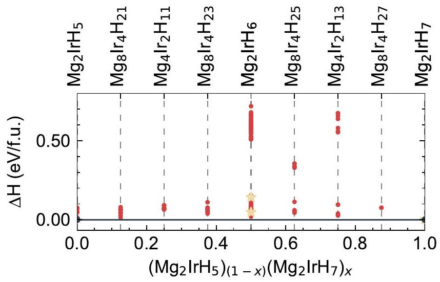
FULL CONVEX HULL
ELASTIC CONSTANTS
|
|
|
|
|
|
|
|
|
COARSE T
High Symmetry Search
| Composition | Space Group | Prototype |
|
|
|
|
|
|
Fm-3m |
|
134.103 | 28.917 | -0.263 | 0.000 |
|
|
Fm-3m |
|
89.168 | 14.517 | 0.030 | 0.080 |
|
|
Pm-3m | Cubic Perovskite | 65.027 | 4.047 | -0.224 | 0.026 |
| HNSc | F-43m | Half-Heusler | 38.765 | 19.333 | -0.790 | 0.000 |
|
|
Pm-3m | Cubic Perovskite | 35.503 | 21.422 | -0.270 | 0.100 |
|
|
Fm-3 | Fluorite
|
29.421 | 22.537 | -0.248 | 0.075 |
|
|
Pm-3m | Cubic Perovskite | 27.011 | 10.822 | -0.146 | 0.000 |
|
|
Pm-3m | Cubic Perovskite | 25.369 | 14.539 | -0.281 | 0.000 |
|
|
Pm-3m |
|
12.871 | 10.292 | -0.595 | 0.000 |
|
|
Pm-3m | Cubic Perovskite | 9.329 | 2.117 | -0.117 | 0.031 |
|
|
Pm-3m |
|
8.782 | 5.338 | -1.854 | 0.000 |
|
|
Pm-3m | Cubic Perovskite | 8.442 | 5.266 | -0.050 | 0.000 |
|
|
Pm-3m | Cubic Perovskite | 6.821 | 0.007 | -0.452 | 0.000 |
|
|
Pm-3m | Cubic Perovskite | 6.415 | 3.682 | -0.044 | 0.000 |
|
|
Pm-3m | Cubic Perovskite | 4.350 | 4.563 | 0.085 | 0.085 |
|
|
Pm-3m | Cubic Perovskite | 4.309 | 0.781 | -0.146 | 0.000 |
|
|
Pm-3m | Cubic Perovskite | 3.743 | 1.803 | -0.350 | 0.000 |
|
|
Pm-3m | Cubic Perovskite | 2.146 | 1.465 | -0.287 | 0.000 |
|
|
Pm-3m |
|
2.118 | 4.153 | -0.491 | 0.000 |
|
|
Pm-3m | Cubic Perovskite | 2.015 | 1.415 | -0.122 | 0.026 |
|
|
Pm-3m | Cubic Perovskite | 1.222 | 1.000 | -0.199 | 0.000 |
|
|
Pm-3m | Cubic Perovskite | 0.639 | 0.038 | -0.277 | 0.000 |
|
|
Pm-3m | Cubic Perovskite | 0.000 | 3.114 | -0.147 | 0.000 |
TITL th - 1-HNSc-F-43m 0.983600000000 30.077721864843 -1567.067620000000 0.00 0.00 3 (F-43m) n - 1
CELL 1.54180 3.49076 3.49076 3.49076 60.00000 60.00000 60.00000
LATT -1
SFAC H N Sc

begin{tabular}{llllll}
H & 1 & 0.2500000000000 & 0.2500000000000 & 0.2500000000000 & 1.0 \
N & 2 & 0.7500000000000 & 0.7500000000000 & 0.7500000000000 & 1.0 \
Sc & 3 & 0.5000000000000 & 0.5000000000000 & 0.5000000000000 & 1.0
end{tabular}
END
TITL th-1-HN3Mo3-Pm-3m 1.010800000000 69.750856277710 -6443.849310000000 0.00 0.00 7(Pm-3m) n - 1
CELL 1.54180 4.11639 4.11639 4.11639 90.00000 90.00000 90.00000
LATT -1
SFAC H N Mo

begin{tabular}{|l|l|l|l|l|l|}
hline H & 1 & 0.5000000000000 & 0.5000000000000 & 0.5000000000000 & 1.0 \
hline N & 2 & 0.5000000000000 & 0.0000000000000 & 0.0000000000000 & 1.0 \
hline N & 2 & 0.0000000000000 & 0.0000000000000 & 0.5000000000000 & 1.0 \
hline N & 2 & 0.0000000000000 & 0.5000000000000 & 0.0000000000000 & 1.0 \
hline Mo & 3 & 0.5000000000000 & 0.0000000000000 & 0.5000000000000 & 1.0 \
hline Mo & 3 & 0.5000000000000 & 0.5000000000000 & 0.0000000000000 & 1.0 \
hline Mo & 3 & 0.0000000000000 & 0.5000000000000 & 0.5000000000000 & 1.0 \
hline
end{tabular}
END
TITL th-1-H12Lu2Ta-Fm-3 1.051200000000 114.705611487894-22614.203699999998 0.00 0.00 15 (Fm-3) n
    - 1
CELL 1.54180 5.45381 5.45381 5.45381 60.00000 60.00000 60.00000
LATT -1
SFAC H Lu Ta
H 1 0.5900714906738 0.1548830550478 0.8451169449522 1.0
H 1 0.1548830550478 0.8451169449522 0.5900714906738 1.0
H 1 0.5900714906738 0.4099285093262 0.1548830550478 1.0
H 1 0.4099285093262 0.8451169449522 0.1548830550478 1.0
H 1 0.8451169449522 0.1548830550478 0.4099285093262 1.0
H 1 0.4099285093262 0.5900714906738 0.8451169449522 1.0
H 1 0.8451169449522 0.5900714906738 0.1548830550478 1.0
H 1 0.1548830550478 0.4099285093262 0.8451169449522 1.0
H 1 0.1548830550478 0.5900714906738 0.4099285093262 1.0
H 1 0.8451169449522 0.4099285093262 0.5900714906738 1.0
H 1 0.4099285093262 0.1548830550478 0.5900714906738 1.0
H 1 0.5900714906738 0.8451169449522 0.4099285093262 1.0
Lu 2 0.7500000000000 0.7500000000000 0.7500000000000 1.0
Lu 2 0.2500000000000 0.2500000000000 0.2500000000000 1.0
Ta 3 0.5000000000000 0.5000000000000 0.5000000000000 1.0
END
| A | B in
|
|
|
|
|
| Mg | Ir | 134.386 | 29.353 | -0.263 | 0.000 |
| Mg | Pt | 105.533 | 86.189 | -0.084 | 0.088 |
| Al | Re | 105.119 | 30.859 | 0.001 | 0.001 |
| Mg | Rh | 102.255 | 31.029 | -0.248 | 0.000 |
| Na | Ag | 99.590 | 37.814 | 0.163 | 0.264 |
| Al | Mn | 89.395 | 18.447 | -0.011 | 0.000 |
| Na | Au | 77.823 | 26.251 | -0.012 | 0.089 |
| In | Re | 59.837 | 18.892 | 0.165 | 0.165 |
| Ca | Ag | 58.098 | 31.324 | -0.193 | 0.197 |
| In | Tc | 57.933 | 20.296 | 0.133 | 0.143 |
| Sr | Ag | 48.735 | 18.795 | -0.223 | 0.156 |
| Ba | Ag | 41.980 | 16.142 | -0.233 | 0.101 |
| Na | B | 41.031 | 24.301 | 0.117 | 0.218 |
| Na | Zn | 39.785 | 44.523 | 0.808 | 0.909 |
| Ca | Cu | 36.164 | 6.794 | -0.321 | 0.069 |
| Na | Al | 35.128 | 23.398 | 0.052 | 0.155 |
| Ca | Pd | 34.038 | 11.898 | -0.427 | 0.081 |
| Na | Ga | 31.550 | 25.716 | 0.126 | 0.227 |
| Lu | Tc | 29.302 | 1.658 | -0.528 | 0.000 |
| Sr | Cu | 26.670 | 4.605 | -0.329 | 0.051 |
| Sr | Pd | 26.498 | 7.773 | -0.437 | 0.000 |
| Ba | Na | 25.671 | 12.309 | -0.102 | 0.283 |
| Y | Cu | 24.478 | 9.846 | -0.364 | 0.182 |
| Lu | Re | 23.703 | 3.079 | -0.474 | 0.023 |
| Ca | Ga | 23.306 | 17.366 | -0.179 | 0.211 |
| Nb | Ni | 22.974 | 20.898 | -0.042 | 0.148 |
| Lu | Ir | 21.524 | 14.576 | -0.385 | 0.119 |
| Rb | Ag | 21.292 | 10.443 | 0.098 | 0.213 |
| Cs | Ag | 19.290 | 9.751 | 0.081 | 0.209 |
| Sr | Ga | 15.155 | 9.076 | -0.230 | 0.149 |
| K | Au | 13.937 | 4.462 | -0.095 | 0.067 |