نماذج الغلاف الجوي تحت النجمي في سونورا. IV. بومة الجان: الخلط الجوي وعدم التوازن الكيميائي مع تباين نسبة المعادن ونسبة الكربون إلى الأكسجين The Sonora Substellar Atmosphere Models. IV. Elf Owl: Atmospheric Mixing and Chemical Disequilibrium with Varying Metallicity and C/O Ratios
نماذج الغلاف الجوي تحت النجمي في سونورا. IV. بومة الجان: الخلط الجوي وعدم التوازن الكيميائي مع تباين نسبة المعادن ونسبة الكربون إلى الأكسجين
سانجيك موكيرجي (D)، جوناثان ج. فورتني (D)، كارولين ف. مورلي (D)، ناتاشا إ. باتالها (D)، مارك س. مارلي (D)، ثيودورا كاراليدي (D)، تشانون فيشر (D)، روكسانا لوبي, ريتشارد فريدمان, إحسان غريب نژاد (D) قسم علم الفلك والفيزياء الفلكية، جامعة كاليفورنيا، سانتا كروز، CA 95064، الولايات المتحدة الأمريكية قسم علم الفلك، جامعة تكساس في أوستن، أوستن، TX 78712، الولايات المتحدة الأمريكية مركز أبحاث ناسا أيمس، MS 245-3، ميدان موفيت، CA 94035، الولايات المتحدة الأمريكية مختبر القمر والكواكب، جامعة أريزونا، توكسون، AZ 85721، الولايات المتحدة الأمريكية قسم الفيزياء، جامعة وسط فلوريدا، 4111 ليبرا درايف، أورلاندو، FL 32816، الولايات المتحدة الأمريكية الكيمياء وعلوم الكواكب، جامعة دوردت، سيوكس سنتر، IA 51250، الولايات المتحدة الأمريكية مركز الأنظمة الكوكبية الخارجية، معهد علوم الفضاء، بولدر، CO 80301، الولايات المتحدة الأمريكية يوريكا ساينتيفيك، إنك، أوكلاند، CA 94602 معهد SETI، مركز أبحاث ناسا أيمس، ميدان موفيت، CA 94035نسخة مسودة 2 فبراير 2024
ملخص
الكيمياء غير المتوازنة بسبب الخلط العمودي في الغلاف الجوي للعديد من الأقزام البنية والكواكب الخارجية العملاقة مثبتة جيدًا. نماذج الغلاف الجوي لهذه الأجسام عادة ما تضع معلمات الخلط مع المعامل غير المؤكد بشدة معامل الانتشار. تم استكشاف دور الخلط في تغيير وفرة الجزيئات الحاوية على C-N-O بشكل أساسي للغلاف الجوي بتكوين شمسي. ومع ذلك، فإن المعدنية الجوية و النسبة تؤثر أيضًا على الكيمياء الجوية. لذلك، نقدم شبكة بومة الجان سونورا من نماذج الغلاف الجوي المتسقة ذاتيًا الخالية من السحب لنماذج التوازن الإشعاعي-الحمل الحراري 1D لملاحظات JWST، والتي تشمل تباينًا في عبر عدة أوامر من حيث الحجم وتشمل أيضًا معدنيات دون الشمس إلى فوق الشمس و النسب. نجد أن تأثير على الملف والطيف هو دالة قوية لكل من والمعدنية. بالنسبة للأجسام الفقيرة بالمعادن، فإن له تأثيرات كبيرة على الغلاف الجوي عند أعلى بكثير مقارنةً بالغلاف الجوي الغني بالمعادن حيث يُرى تأثير ليحدث عند أقل. نحدد تدهورات طيفية كبيرة بين والمعدنية في نوافذ الطول الموجي المتعددة، لا سيما عند 3-5. نستخدم شبكة الغلاف الجوي لبومة الجان سونورا لتناسب الأطياف المرصودة لعينة من 9 أجسام من النوع T المبكر إلى المتأخر من. نجد أدلة على خلط عمودي غير فعال جدًا في هذه الأجسام مع قيم المستنتجة تقع في النطاق بين. باستخدام نماذج متسقة ذاتيًا، نجد أن هذا الخلط العمودي البطيء ناتج عن الملاحظات التي تستكشف الخلط في المنطقة الإشعاعية العميقة المنفصلة في هذه الأجواء.
الكلمات الرئيسية: الأقزام البنية، الأقزام T، الأقزام Y، التركيب الجوي، الكواكب الغازية الخارجية
1. المقدمة
تكون أجواء الكواكب الخارجية والأقزام البنية في الغالب جزيئية بسبب درجات حرارتها المنخفضة وضغوطها العالية. يتم تحديد التركيب الكيميائي لهذه الأجواء من خلال التفاعل بين التفاعلات الكيميائية المعتمدة على درجة الحرارة والضغط وعمليات الخلط الديناميكية الجوية. تتأثر معدلات التفاعلات الجزيئية بهيكل ضغط درجة الحرارة الجوي ومخزون العناصر الكيميائية في الغلاف الجوي. يُقال إن الغلاف الجوي في حالة توازن كيميائي إذا كانت كيميائه تحددها التفاعلات الحرارية الكيميائية بناءً على ظروف الضغط ودرجة الحرارة المحلية. ولكن العمليات مثل الخلط الديناميكي يمكن أن تتسبب في انحراف الأجواء الفرعية عن التوازن الكيميائي (فيغلي ولودرس 1996؛ نول وآخرون 1997؛ موسى وآخرون 2011؛ زاهنل ومارلي 2014؛ تسائي
وآخرون 2021؛ لي وآخرون 2023) إذا كانت أوقات الخلط أسرع من أوقات التفاعلات الكيميائية. ومع ذلك، لا يزال الخلط الديناميكي أحد أكثر الجوانب غير المؤكدة وغير المفهومة في الأجواء الفرعية.
يعد الخلط الديناميكي وتأثيراته على الكيمياء الجوية عملية مدروسة جيدًا في أجواء الكواكب في النظام الشمسي (على سبيل المثال، برين وبارشاي 1977؛ يونغ وآخرون 1988؛ بيوركر وآخرون 1986؛ زانغ وشومان 2018a؛ زانغ وآخرون 2012؛ ألين وآخرون 1981؛ ناير وآخرون 1994؛ موسى وآخرون 2005؛ لي وآخرون 2014؛ فيشر وآخرون 2010؛ فيشر وموسى 2011؛ وونغ وآخرون 2017). ومع ذلك، نظرًا لأن معظم الأقزام البنية والكواكب الخارجية المعرضة بشدة تنتمي إلى نظام ضغط-درجة حرارة مختلف تمامًا، لا تزال العمليات الديناميكية في أجوائها غير مفهومة جيدًا.
1.1. لماذا يعتبر تقييد مهمًا؟
يمكن أن تنقل الديناميات الجوية الغازات والجسيمات السحابية/الغبار عبر عدة مقاييس ضغط في الاتجاه الشعاعي للأجواء الفرعية (على سبيل المثال، بارمنتير وآخرون 2013؛ تان 2022؛ فريتاغ وآخرون 2010). تُسمى هذه العملية غالبًا بالخلط العمودي. تحت هذا الافتراض بأن هذا الخلط يمكن نمذجته كعملية انتشار، يتم عادةً وضعه في معلمات بواسطة معامل الانتشار العمودي يتأثر بمعدل دوران الغلاف الجوي ويمكن فهمه بشكل حدسي كمنتج لطول المقياس الذي يحدث فيه الخلط وسرعة الخلط (تشامبرلين وهونتن 1987). تمثل قيمة عالية من غلافًا جويًا نشطًا ديناميكيًا للغاية، بينما تمثل القيمة المنخفضة سيناريو بخلط بطيء وغير فعال. في الأجزاء الحملية من الغلاف الجوي، من المتوقع أن يرتبط معدل الخلط بتدفق الطاقة الحملية، وفي الواقع، توفر نظرية طول الخلط (MLT) تقديرات لـ (على سبيل المثال، جيراش وكونراث 1985؛ أكرمان ومارلي 2001). في الأجواء الإشعاعية، يمكن أن تتحكم عمليات ديناميكية أخرى، مثل كسر الموجات الجوية، في الخلط وبالتالي تؤثر على قيمة.
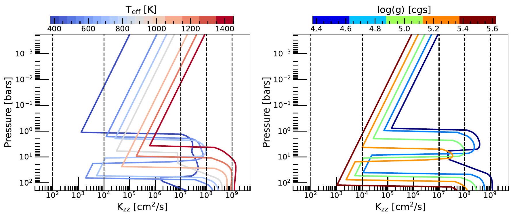
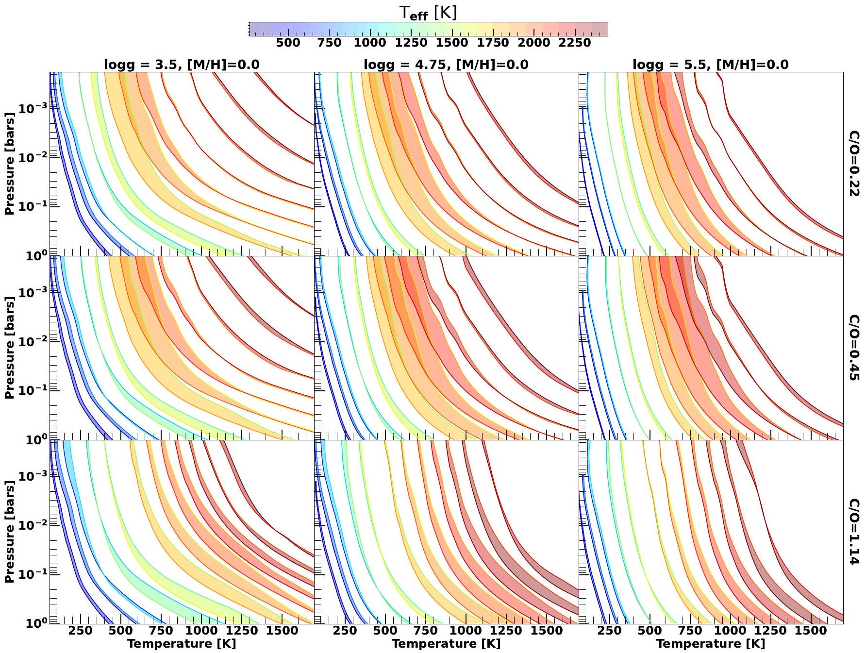
يتطلب الفهم الكامل للخلط الديناميكي الجوي قيودًا على في كل من الأجزاء الحملية والإشعاعية من الغلاف الجوي. حاليًا، في أجواء الأقزام البنية والكواكب الخارجية لا يزال غير مؤكد بأكثر من مليون مرة (لاسي وبيروز 2023؛ موكيرجي وآخرون 2022؛ كاراليدي وآخرون 2021؛ فيليبس وآخرون 2020؛ فورتني وآخرون 2020؛ زاهنل ومارلي 2014؛ هوبيني وبيروز 2007؛ بارمان وآخرون 2015). تُظهر التقديرات النظرية لملفات لسلسلة من أجواء الأقزام البنية مع تغير من موكيرجي وآخرون (2022) في الشكل 1، اللوحة اليسرى. تُظهر اللوحة اليمنى من الشكل 1 اعتماد ملفات النظرية على. تُظهر هذه التقديرات النظرية أن يمكن أن تتغير بأوامر من حيث الحجم بسبب التغيرات في كلا هذين المعاملين. علاوة على ذلك، في نفس الغلاف الجوي، يمكن أن يتغير بعدة أوامر من حيث الحجم اعتمادًا على ما إذا كانت جزء معين من الغلاف الجوي إشعاعي أو حمل حراري. يُرى مثل هذا التغير في عبر المناطق الإشعاعية أو الحملية أيضًا في النماذج النجمية (على سبيل المثال، فارغيس وآخرون 2023). يُظهر الشكل 1 أيضًا أن موقع المناطق الحملية والإشعاعية يمكن أن يكون أيضًا دالة قوية لكل من و.
يعد تقييد أمرًا حيويًا لفهم الطبيعة الفيزيائية للديناميات الجوية التي تعمل في الأجواء العميقة للأقزام البنية والكواكب الخارجية، فضلاً عن الآثار المترتبة على الكيمياء الجوية والسحب، وكلاهما له بصمات كبيرة على الأطياف المرصودة لهذه الأجسام. يقوم الخلط الجوي بسحب الغازات من الغلاف الجوي العميق إلى الغلاف الجوي العلوي المرئي. إذا تم تدمير هذه الغازات كيميائيًا بشكل أسرع من المقياس الزمني النموذجي للخلط، فإن الغلاف الجوي يبقى في حالة توازن حراري كيميائي. ومع ذلك، إذا كانت عملية الخلط أسرع من أوقات التفاعلات الكيميائية، فإن الغلاف الجوي العلوي لم يعد يبقى في حالة توازن حراري كيميائي (موسى وآخرون 2011؛ تسائي وآخرون 2017، 2021؛ زاهنل ومارلي 2014؛ فيشر وفغلي 2005؛ فيشر وآخرون 2006؛ فيشر وموسى 2011). يتسبب ذلك في تغييرات كبيرة في التركيب الكيميائي وعمق البصريات للغلاف الضوئي القابل للرصد، مما يغير الطيف القابل للرصد للجسم (على سبيل المثال، فيليبس وآخرون 2020؛ تريمبلين وآخرون 2015؛ لاسي وبيروز 2023؛ كاراليدي وآخرون 2021؛ موكيرجي وآخرون 2022؛ هوبيني وبيروز
2007؛ لي وآخرون 2023). يمكن أن ينقل الخلط العمودي أيضًا بخار الغاز من الغلاف الجوي الأعمق إلى الغلاف الجوي الأبرد حيث يمكن أن يتكثف ويشكل السحب (مثل سحب الماء في الأقزام Y، وسحب الحديد في الأقزام L) (مثل، أكرمان ومارلي 2001؛ مورلي وآخرون 2014أ، 2012؛ صومون ومارلي 2008؛ وويتكي وآخرون 2020؛ لايسي وبيروز 2023؛ فريتاغ وآخرون 2010؛ ألارد وآخرون 2012؛ هيلينغ وآخرون 2017؛ لي وآخرون 2016؛ قاو وبينيك 2018؛ تشارني وآخرون 2018؛ كوبر وآخرون 2003؛ هيلينغ وآخرون 2001). علاوة على ذلك، يمكن أن يحافظ الخلط على هذه الجسيمات السحابية مرتفعة في الفوتوسفير من خلال مقاومة استقرارها الجاذبي. هذه الجسيمات السحابية المرتفعة “تُحمر” طيف الأجسام تحت النجمين بفضل امتصاصها وشفافيتها المتناثرة، وتميل أيضًا إلى تسخين الغلاف الجوي الأعمق من خلال امتصاص إشعاع حراري إضافي (مثل، صومون ومارلي 2008؛ مورلي وآخرون 2012، 2014أ؛ لونا ومورلي 2021؛ قاو وآخرون 2020؛ مانغ وآخرون 2022؛ لي وآخرون 2016؛ تان 2022). على الرغم من أنه غير مؤكد للغاية،يلعب دورًا رئيسيًا في التأثير على المكونات الجوية الرئيسية للأجسام تحت النجمية مثل الكيمياء الجوية، والسحب، ودرجة الحرارة-الضغط ) الهيكل (على سبيل المثال، دروموند وآخرون 2016). مع أدوات حساسة ومستقرة للغاية مثل أظهرت الدراسات السابقة أن اعتماد الكيمياء الجوية والسحب علىيمكن الاستفادة منه لتقييدنفسه (على سبيل المثال، مايلز وآخرون 2020؛ كاراليدي وآخرون 2021؛ موكيرجي وآخرون 2022؛ فيليبس وآخرون 2020).
لقد درست النماذج النظرية آثارعلى الكيمياء الجوية والطيف السابق للأقزام البنية والكواكب المصورة مباشرةً ذات التركيب الجوي الشمسي. قام كاراليدي وآخرون (2021) وهوبيني وبوروز (2007) بدراسة هذه التأثيرات باستخدام ثوابت غير معتمدة على الضغط.ملفات تعريف للغلاف الجوي تحت النجمي لتكوين الشمس، في حين أن فيليبس وآخرون (2020) قد درسوا هذه التأثيرات عند معدنية شمسية مع اعتماد الضغط ولكن اعتماد على الجاذبية.الملفات الشخصية.في المناطق الإشعاعية يمكن أن تختلف بشكل كبير عنفي المناطق الحملية بسبب آليات الدوران المنفصلة تمامًا التي تعمل في كل نظام. استكشف موكيرجي وآخرون (2022) فضاء المعلمات لجو الأقزام البنية ذات التركيب الشمسي وحدد طرق القياسفي الغلاف الجوي الإشعاعي وكذلك الحمل الحراري لهذه الأجسام معاستكشفت لاسي وبوروز (2023) معالجة ذاتية التناسق لكل من سحب الماء وكيمياء عدم التوازن بسبب الخلط لنجوم Y ذات المعادن الشمسية وأقل أو أكثر قليلاً من الشمس. باستخدام الملاحظات الطيفية الأرضية ونماذج الغلاف الجوي ذات التركيب الشمسي، قام مايلز وآخرون (2020) بقياسفي سلسلة من الأقزام المتأخرة من النوع T – والأقزام المبكرة من النوع Y – لوحظت زيادة حادة فيفيتم الافتراض في دراسة مايلز وآخرون (2020) أن هذا الانتقال من المنخفض إلى المرتفعالانتقال ناتج عن وجود مناطق إشعاعية “مُحاطة” في الأجواء العميقة للأجسام التي تحتوي علىبين، والذي تم تأكيده لاحقًا نظريًا في موكيرجي وآخرون (2022). كانت هذه عرضًا رائعًا لكيفية تقييد عدم اليقين يمكن أن تساعدنا في الحصول على رؤى أساسية حول أجواء الأقزام البنية والكواكب. ومع ذلك، لا يُتوقع أن تكون جميع أجواء الأقزام البنية من تركيب شمسي (على سبيل المثال، لاين وآخرون 2017؛ زالسكي وآخرون 2019؛ زالسكي وآخرون 2022؛ ميسنر وآخرون 2023؛ بيلر وآخرون 2023؛ هوخ وآخرون 2023)، وأن الكيمياء الناتجة عن الاختلاط غير المتوازنة-
الشكل 1. اللوحة اليسرى تظهر الحسابات الذاتية المتسقةالملفات كدالة للضغط لسلسلة من نماذج الغلاف الجوي بتكوين شمسي معمن 1500 ك إلى 400 ك و. الـفي المنطقة الحملية تم حسابها باستخدام نظرية طول الخلط بينمافي الغلاف الجوي الإشعاعي يتبع التوصيف في موسى وآخرون (2021). تُظهر اللوحة اليمنى ملفات تعريف لنموذج 700 ك مع تباينبين 4.5 و 5.5. الخطوط المنقطة السوداء تمثل الثابتالملفات المستخدمة في هذا العمل لأخذ عينات من نطاقات متعددة من الأوامرالقيم التي تغطيها هذه الحسابات النموذجية. بعض النماذج الأكثر برودة في اللوحة اليسرى معبينيظهر انخفاضًا حادًا وارتفاعًا فيفي الغلاف الجوي العميق الذي يدل على وجود منطقة إشعاعية منفصلة في غلافها الجوي. سلوك مشابه موجود أيضًا في نماذج الجاذبية المنخفضة الموضحة في اللوحة اليمنى.
لم يتم استكشاف الكيمياء في الأجواء غير الشمسية بشكل كافٍ.
1.2. المعدنية،نسبة، و
أظهرت دراسات الاسترجاع البايزية لسكان متزايد من الأقزام البنية أجواءً غير شمسية التركيب. تتراوح هذه الأجواء من أجواء فقيرة جداً بالمعادن (مثل، ميسنر وآخرون 2023؛ زانغ وآخرون 2021؛ لاين وآخرون 2017؛ زالسكي وآخرون 2019؛ زالسكي وآخرون 2022؛ بورغاسر وآخرون 2023) إلى أجسام ذات معدلات معدنية جوية مرتفعة (مثل، زانغ وآخرون 2021؛ لاين وآخرون 2017؛ زالسكي وآخرون 2022؛ زالسكي وآخرون 2019؛ زانغ وآخرون 2023). كما تم إثبات تباين كبير في نسبة الكربون إلى الأكسجين (C/O) من قيم دون الشمس إلى قيم فوق الشمس في الأدبيات (مثل، كالماري وآخرون 2022؛ زالسكي وآخرون 2022؛ زالسكي وآخرون 2019؛ لاين وآخرون 2017؛ هوش وآخرون 2023). تكشف الملاحظات المنشورة من تلسكوب جيمس ويب الفضائي لأجسام مثل VHS 1256b و HD 19467b بالفعل عن توقيعات قوية لعدم التوازن الكيميائي (مايلز وآخرون 2022؛ غرينباوم وآخرون 2023؛ بيلر وآخرون 2023) بالإضافة إلى الملاحظات الأرضية والفضائية للأقزام البنية التي تم الحصول عليها في العقدين الماضيين (مثل، نول وآخرون 1997؛ أوبنهايمر وآخرون 1998؛ سوراهانا ويامامورا 2012؛ مايلز وآخرون 2020؛ مادورويتز وآخرون 2023). المتاحة والقادمةمن المتوقع أن تُظهر البيانات من الأقزام البنية والكواكب الملتقطة مباشرة وجود كل من الكيمياء غير المتوازنة الناتجة عن الخلط العمودي والانحرافات عن الغلاف الجوي ذو التركيب الشمسي.
الخلط العمودي يؤدي إلى تغييرات كبيرة في وفرة الغازات في الطبقة الضوئية مثل، ، و عن طريق إخماد وفرتها في الأجواء الأعمق. تتأثر هذه الغازات بشكل خاص بسبب الخلط العمودي لأنها تمتلك أوقات تفاعل كيميائي طويلة جدًا. على سبيل المثال، تحويلإلى أو CO إلى يتطلب الكسر روابط جزيئية قوية. ومع ذلك، فإن وفرة جميع هذه الغازات حساسة أيضًا لوجود المعادن في الغلاف الجوي ونسبة الكربون إلى الأكسجين. يؤدي ارتفاع وجود المعادن في الغلاف الجوي إلى زيادة في جميع هذه الغازات في الغلاف الجوي بدرجات متفاوتة، وخاصة بالنسبة للجزيئات “المسيطرة على المعادن” مثل CO و. الـنسبة تغير الوفرة النسبية لمختلف الغازات التي تحتوي على الكربون والأكسجين (على سبيل المثال، مادوسودان 2012؛ موسى وآخرون 2013). على سبيل المثال، نسبة عاليةنسبة تزيد منالوفرة وتقلل من وفرة الغازات الحاملة للأكسجين مثلفي الغلاف الجوي. بخلاف تغيير الكيمياء الجوية، فإن المعدنية،نسبة، وكما أن لها تأثيرات على الغلاف الجويالملف بسبب الأعماق البصرية الجوية المعززة أو المنقوصة. لذلك، من أجل تقييد المعدنية، نسبة الكربون إلى الأكسجين، وفي نفس الوقت منملاحظات على الأقزام البنية والكواكب الخارجية التي تم تصويرها مباشرة، نماذج إشعاعية-حمل حراري “متسقة ذاتياً” نظرية تشمل التغيرات فيالمعدنية، ونسب مطلوبة. تعتبر هذه النماذج الجوية ضرورية لهذا الغرض حيث تؤثر هذه المعلمات الثلاثة على الغلاف الجوي.الملف الشخصي. يمكن التقاط ذلك فقط بواسطة نماذج جوية إشعاعية-حرارية متسقة ذاتيًا تحسب الكيمياء، والنقل الإشعاعي، وملف تعريف الغلاف الجوي في الوقت نفسه من خلال أخذ جميع الروابط الفيزيائية بين هذه العمليات في الاعتبار (على سبيل المثال، موكيرجي وآخرون 2023؛ فيليبس وآخرون 2020؛ بارمان وآخرون 2001، 2011؛ هوبيني وبوروز 2007؛ لايسي وبوروز 2023).
في هذا العمل، استخدمنا برنامج PICASO مفتوح المصدرنموذج جوي (موخيرجي وآخرون 2022؛ باتالها وآخرون 2019) لمحاكاة شبكة بومة سونورا إلف من نماذج جوية خالية من السحب متسقة ذاتيًا مع اختلال كيميائي ناتج عن الخلط العمودي من أجل مباشرة…
الكواكب القديمة والأقزام البنية. بخلاف النطاق في و القيم الملتقطة ضمن الشبكة، تشمل التباين فيعبر 7 أوامر من الحجم، التغير في المعدنية الجوية منالطاقة الشمسية إلىالقيم الشمسية، وتنوع مننسبة من 0.22 إلى 1.14. نطاق التغير فيالقيم مدفوعة بالتغيير الكبير فيتقديرات من النماذج النظرية بين المناطق الإشعاعية والمناطق الحملية في الغلاف الجوي وأيضًا التباين الكبير في النظرياتتقديرات مع كليهما و (الشكل 1).
باستخدام هذه الشبكة من النماذج ومن خلال مقارنتها مع بيانات المراقبة الفضائية الموجودة من 9 مصادر، نتناول الأسئلة التالية في هذا العمل:
ما هو تأثيرعلىملف الكواكب المصورة مباشرة والأقزام البنية عند معدلات معدنية مختلفةنسب؟
كيفكيف تؤثر الطيفيات للأجسام من النوع L والنوع T والنوع Y عند معدلات المعادن تحت الشمسية والشمسية وفوق الشمسية ونسب الكربون إلى الأكسجين؟
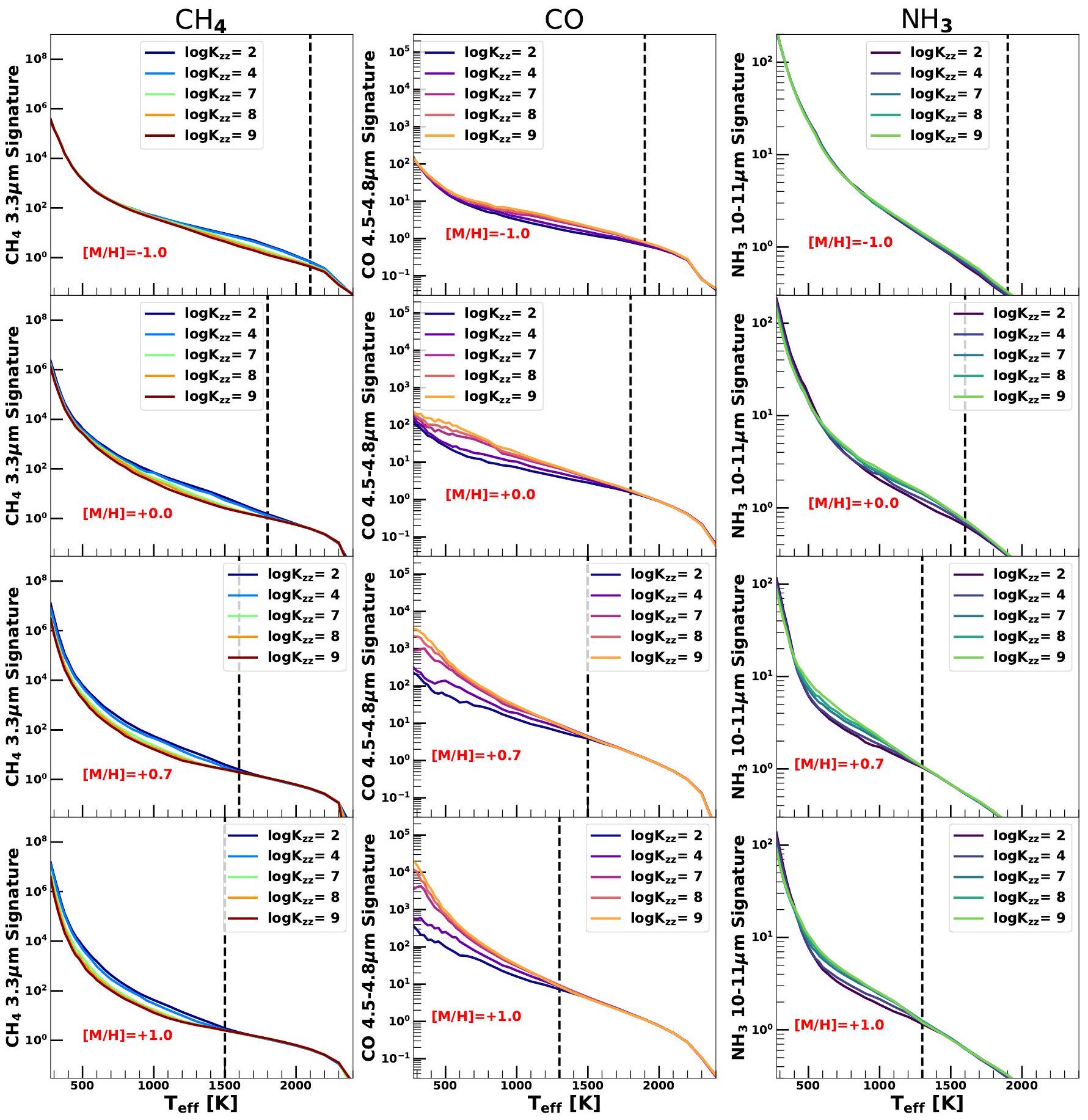
كيف تكون توقيعات الامتصاص للمواد الغازية الرئيسية مثل، و تختلف مع، المعدنية، ونسبة الكربون إلى الأكسجين؟
كيف يتم قياسمن طيف الأشعة تحت الحمراء المتاح للأجسام دون النجمية يختلف مع؟
نصف نموذجنا في §2. نقدم النتائج الرئيسية من شبكة نموذجنا في §4 تليها تطبيق هذه الشبكة في §5. تُعرض استنتاجاتنا ومناقشاتنا في §6 و §7، على التوالي.
2. النمذجة الجوية باستخدام بيكاسو 3.0
نستخدم نموذج الغلاف الجوي PICASO 3.0 المستند إلى بايثون والمفتوح المصدر (موكيرجي وآخرون 2023) لحساب شبكة نموذج بومة سونورا. لقد تم استخدام PICASO 3.0 على نطاق واسع لنمذجة الغلاف الجوي للكواكب الخارجية والأقزام البنية (على سبيل المثال، راستامكولوف وآخرون 2022؛ ألديرسون وآخرون 2022؛ فاينشتاين وآخرون 2022؛ أهرر وآخرون 2022؛ مايلز وآخرون 2022؛ غرينباوم وآخرون 2023؛ موكيرجي وآخرون 2022؛ بييلر وآخرون 2023). هذا النموذج له إرث من نموذج EGP المعروف (مارلي وآخرون 1996؛ مارلي وماكاي 1999؛ مارلي وآخرون 2002؛ ساومون ومارلي 2008؛ فورتني وآخرون 2005، 2008، 2007؛ مورلي وآخرون 2014أ؛ كاراليدي وآخرون 2021). نحن نصف فقط التحديثات الأخيرة للنموذج التي تتعلق بهذا العمل هنا ونشير إلى القارئ إلى موكيرجي وآخرون (2023) للحصول على وصف مفصل للنموذج الجوي الذاتي المتسق الكامل.
شبكة بومة سونورا الجنية هي خمسة أبعاد مع متغيرات، و نسب. يتم تقسيم كل نموذج جوي إلى 90 طبقة ضغط متوازية (أي 91 مستوى أو نقطة شبكة) لحساب الهيكل الجوي في نماذجنا. يتم توزيع الضغط المقابل لهذه الطبقات بشكل لوغاريتمي من الحد الأدنى إلى الحد الأقصى للضغط في النموذج. يتم اختيار الحد الأقصى للضغط في كل نموذج بعناية بحيث يكون الغلاف الجوي غير شفاف. ) عند جميع الأطوال الموجية عند ضغوط أقل من الضغط الأقصى للنموذج. نظرًا لأن أعماق الغاز الجوي البصري تتناسب عكسيًا مع الجاذبية، فإن النماذج ذات الجاذبية الأعلى لديها قيم ضغط أقصى أعلى من النماذج ذات الجاذبية الأقل. لذلك، فإن الحدود العليا الدقيقة و تختلف الحدود الدنيا للضغط الجوي عبر شبكتنا.
نستخدم تقريب زمن الإخماد لنمذجة تأثيرفي الكيمياء الجوية (برين وبارشاي 1977). يتم تحديد زمن الخلط في كل طبقة جوية بواسطة،
أينهو ارتفاع مقياس الضغط الجوي لتلك الطبقة الجوية التي يتم حسابها باستخدام درجة حرارة الطبقة، وضغط الطبقة، والوزن الجزيئي المتوسط، وجاذبية الجسم. نحن نعتبر إخماد، ، و في نماذجنا. التفاعلات الكيميائية الصافية لهذه الغازات هي (Zahnle & Marley 2014؛ Mukherjee et al. 2022)،
لكل من هذه التفاعلات الكيميائية الصافية، نستخدم نهج المقياس الزمني الكيميائي ( ) المقدمة في زاهنل ومارلي (2014). من أجل نستخدم تقريب المقياس الزمني الكيميائي من فيشر وفغلي (2005) وفيشر وآخرون (2006). ومع ذلك، نلاحظ أن هناك عدم يقين كبير في فهمنا لكيمياء الفوسفور لا يزال قائمًا اليوم، مما سيؤدي في النهاية إلى عدم اليقين بشأن أوقات تفاعلاته (على سبيل المثال، وانغ وآخرون 2016؛ فيشر 2020؛ باينز وآخرون 2023). نفترض أن هذه الأوقات التفاعلية مستقلة عن المعدنية ونسبة من أجل البساطة. نعتقد أن هذا افتراض صحيح لأن عدم اليقين في ضغوط التبريد للغازات المختلفة مدفوع بشكل رئيسي بعدم اليقين الكبير جداً فيمن المتوقع أن تكون تباينات الأوقات الكيميائية لهذه الغازات مع المعدنية ونسبة الكربون إلى الأكسجين التي تتراوح من قيم أقل قليلاً من الشمس إلى قيم أعلى من الشمس أصغر بكثير من هذه الشكوك الحالية.
المن التفاعلات المذكورة أعلاه يتم مقارنتها بالطبقةلكل طبقة جوية. يُسمح لكميات جميع الغازات باتباع قيم التوازن الكيميائي لجميع طبقات الضغط العميق حيث. ومع ذلك، فإن وفرة الغازات المكونة “تُخفف” عند الضغوط الأقل من ضغط التخفيف (” ). الـلكل تفاعل كيميائي صافي يُعرَّف بأنه الضغط الذي عندهرد الفعل المعني يساويتظل وفرة الغازات المشاركة ثابتة عند القيمة المطفأة عند ضغوط أقل منغازات غير، و يسمح بمتابعة التوازن الكيميائي في الغلاف الجوي في جميع النماذج.
نستخدم حسابات الكيمياء التوازنية المقدمة في لوبي وآخرون (2021) لحساب وفرة الغازات في التوازن الحراري الكيميائي. حسابات الكيمياء التوازنية عندقيم، ، و +1.0 تم استخدامها لشبكتنا، حيث
الخلط الجوي والكيمياء في الأقزام البنية
معامل
نطاق
زيادة/قيم
275 كلفن إلى 2400 كلفن
زيادة – 25 ك بينزيادة – 50 ألف بينزيادة – 100 ك بين
3.25 إلى 5.5
زيادة – 0.25 دكس
2 إلى
القيم – 2، 4، 7، 8، و 9
-1.0 إلى
القيم – -1.0، -0.5، +0.0 القيم –
عناية
0.22 إلى 1.14
0.22، 0.458، 0.687، و 1.12
الجدول 1
معلمات نموذج شبكة الغلاف الجوي لخفاش سونورا وأبعادها التي تم تغطيتها في هذا العمل. يتوافق مع المعدنية الشمسية. في كل توازن كيميائي للمعادن، جداول الكيمياء المقابلة لأربعةنسب، و 1.14 – تم استخدامها كمدخلات في نماذجنا (يُفترض أن نسبة الكربون إلى الأكسجين في الشمس هي 0.458 (لودرز وآخرون 2009)). تم استخدام وفرة العناصر الشمسية من لودرز وآخرون (2009) كوفرة عناصر لجو التركيب الشمسي. نلاحظ أن وفرة العناصر الشمسية قد تم تحديثها منذ ذلك الحين بواسطة لودرز (2019). من أجل التناسق مع أعمالنا السابقة، نستمر في استخدام قيم لودرز وآخرون (2009) في الوقت الحالي. لتغيير نسبة الكربون إلى الأكسجين، نحتفظ بـ ثابت بينما تتغير نسبة الكربون والأكسجين بالنسبة لقيمهما الشمسية. ثم، لأخذ التغير في المعدنية بعين الاعتبار، يتم ضرب جميع وفورات العناصر بعامل المعدنية. هذا يضمن أن التغير فيلا يغير أيضًا من المعدنية الجوية. كيمياء جميع الغازات عند الضغوط الأكبر من يتم استيفاؤها من جداول الكيمياء التوازنية المحسوبة مسبقًا.
نفترض خمسة مختلفينقيم تتراوح منإلىلنماذجنا. على عكس موكيرجي وآخرون (2022)، ولكن مشابه لكراليدي وآخرون (2021)،الملفات هنا لا تتغير مع الضغط الجوي. الشكل 1 يوضح أن هذه تبسيط للحالة الأكثر واقعية حيثيختلف بشكل كبير مع الضغط الجوي اعتمادًا على ما إذا كانت الغلاف الجوي إشعاعيًا محليًا أو حملًا. ولكن كما أن كل من الحمل والإشعاعغير مؤكدة للغاية، نحن نتبنى هذا التبسيط هنا لاستكشاف الاتجاهات في الاستجابة الجوية لـنناقش أيضًا تأثير هذا الافتراض في §6.
للتقاط تأثير وفرة الغازات المطفأة علىنقوم بملف تعريف ذاتي التناسق، حيث نخلط الشفافية المرتبطة الفردية لجميع غازات الغلاف الجوي “في الوقت الحقيقي” باستخدام تقنية إعادة التوزيع المفصلة في أموندسن وآخرون (2017). يتم وزن الشفافية المرتبطة للغازات التالية وفقًا لوفرتها في حالة التوازن/المخففة خلال تكرارات النموذج وتخلط “في الوقت الحقيقي”-، ، وFeH. يتم تكرار كل نموذج جوي حتى يتم تحقيق معيار تقارب محدد مسبقًا كما هو موضح في موكرجي وآخرون (2023). مصادر الشفافية الغازية المختلفة المستخدمة في حساب الشبكة مدرجة في الجدول 2. تم حساب بيانات الشفافية المدمجة في هذه النماذج باستخدام أحدث التحديثات من الدراسات المخبرية والدراسات الأولية. تعتبر معاملات الحرارة والتوسيع ذات صلة بالأجسام قيد الدراسة. لمناقشة متعمقة حول دقة قوائم الخطوط هذه ومقارنتها بإصدارات أخرى، نوجه القارئ إلى غريب-نژاد وآخرون (2021a). الانبعاث الحراري طيف بين 0.5 ويتم حسابها من النموذج الجوي المتقارب مع روتينات النقل الإشعاعي في PICASO (باتالها وآخرون 2019). يتم حساب هذه الأطياف بدقة طيفية (R) تبلغ 5000.
تشمل شبكة نموذجنا الجوي ذو الأبعاد الخمسة 43,200 نموذجًا متميزًا. جميع هذه النماذج متاحة للجمهور للتنزيل علىمصحوبة بنماذج ونصوص تحليلية. تلخص الجدول 1 خمسة معلمات تم تغييرها في شبكة النموذج لدينا مع النطاقات والزيادات المستخدمة لكل معلمة. تم الحفاظ على النطاقات والزيادات المختارة في معظم المعلمات مشابهة لمجموعة شبكات سونورا السابقة (على سبيل المثال، مارلي وآخرون 2021؛ كاراليدي وآخرون 2021).
3. سلسلة موديلات سونورا ولماذا يعتبر بومة إلف مهمة؟
تم نشر عدة إصدارات من نماذج سونورا مثل سونورا بوبكات وسونورا تشولا سابقًا (مارلي وآخرون 2021؛ كاراليدي وآخرون 2021). افترضت نماذج سونورا بوبكات توازن هطول الأمطار الحرارية الكيميائية عبر الكلفضاء المعلمات من 200 كلفن إلى 2400 كلفن. كما شمل تحت الشمسي (إلى معدنيات فوق شمسية و النسب. استنادًا إلى هذه النماذج، طور كاراليدي وآخرون (2021) نماذج سونورا تشولا التي تتضمن معالجة متسقة ذاتيًا لكيمياء عدم التوازن ولكن فقط لجو ذو تركيب شمسي. تضمنت هذه النماذج تباين فيعبر عدة أوامر من الحجم وأيضًا غطتمنتقدم نماذج بومة الجان تطورات إضافية في ثلاثة مجالات رئيسية –
تشمل نماذج بومة الجان آثار الكيمياء غير المتوازنة الناتجة عن الاختلاط، بالإضافة إلى الأجواء ذات التركيب الشمسي، من خلال تضمين معدلات تتراوح منإلى. هذا يعزز قابليته للتطبيق على مجموعة أوسع من الأجسام بما في ذلك الأقزام البنية الفقيرة بالمعادن والكواكب العملاقة الغنية بالمعادن.
كما يتضمن departures من الشمسنسبة تتراوح من 0.22 إلى 1.14.
الجدول 2 مراجع الشفافية الغازية المستخدمة في حساب النماذج الجوية والطيف الناتج في هذا العمل. ما لم يُذكر خلاف ذلك، فإن حسابات الشفافية مفصلة في Freedman وآخرون.
حسناً، على عكس سونورا تشولا التي تتوقف عند.
فرق منهجي آخر بين نماذج تشولا ونماذج بومة الجان هو أن نماذج تشولا تم حسابها عن طريق خلط فقط الشفافية الغازية لـ، و “في الوقت الحقيقي” على الرغم من أنه تضمن حسابات لعدم التوازن الكيميائي لـ، و HCN. كما تم وصفه بالفعل في §2، تم حساب نماذج بومة إلف من خلال خلط الشفافية لجميع الغازات الجوية “في الوقت الحقيقي” مما يعزز بشكل أكبر التناسق الذاتي لهذه النماذج حيث لا يوجد شبكة شفافية مختلطة مفترضة مسبقًا. هذه التحسينات ضرورية حيث أنه من المهم جدًا خلط غاز مثل “في الوقت الحقيقي” عند معدلات معدنية تفوق الشمس أو غاز مثل HCN عند مستويات عاليةالنسب. بالإضافة إلى ذلك، تم حساب نماذج بومة الجان مع أحدث التعتيمات المحدثة التي تم تحسينها منذ الأجيال السابقة من نماذج سونورا.
4. النتائج
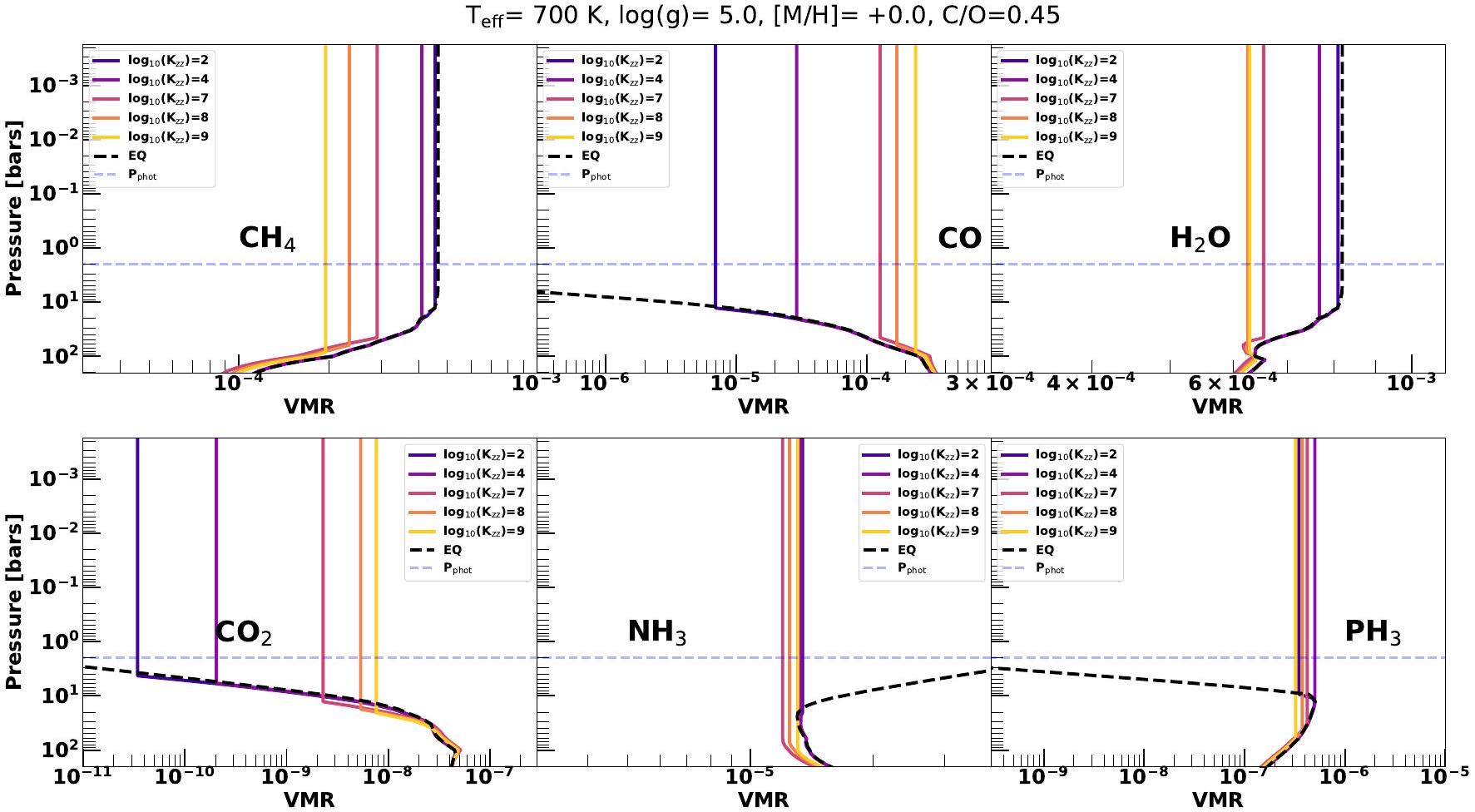
تخفيض الغازات بسببيمكن أن تؤدي إلى تغييرات بمقدار عدة مرات في وفرة العناصر في الغلاف الضوئي. توضح الشكل 2 تأثير التبريد على ملفات وفرة بعض الغازات الجوية الرئيسية مثل، ، و لجسم بتكوين شمسي 700 ك. تتبع الخطوط الملونة الصلبة المختلفة وفرة مختلفة مرتبطة بـ قيم منإلىبينما كانت ملفات الوفرة المتوقعة من التوازن تظهر الكيمياء مع الخطوط المتقطعة السوداء. النطاق فيالمختار هنا يعكس النموذج المعتادعدم اليقين في أجواء الأقزام البنية والكواكب الخارجية. الضغط الفوتوسفيرى المتوسط هوالأشرطة ويظهر بخط أزرق متصل في الشكل 2. يوضح الشكل 2 أن التغير فييمكن أن تسبب تباينات في الطبقة الضوئية و CO بعامل . هذه التباينات مشابهة للنتائج في فيشر وموسى (2011). و يمكن أن تتفاوت الوفرة بمقدار عدة أوامر من حيث الحجم بسبب التغير فيبينما تعتمد علىوفرة علىهو الحد الأدنى لهذه التركيبة المحددة من و . هذه التغيرات الكبيرة في كيمياء الفوتوسفير بسبب يمكن أن يكون له تأثير كبير ومعقد على الغلاف الجويالبنية والطيف المرئي. توضح الشكل 2 أيضًا أن الغازات المختلفة تتلاشى عند ضغوط مختلفة. على سبيل المثال،، أول أكسيد الكربون ، و تروي عند ضغط أعلى من (انظر فيشر وآخرون 2010). هذا الاختلاف في ضغوط التبريد يرجع إلى اختلاف الأوقات الكيميائية المرتبطة بـ و ديناميكا التفاعل.
4.1. تأثيرعلىالملفات عبر المعدنيات ونسب
نظرًا لأن وفرة الغازات المروية تؤثر على عمق الطبقة بالطبقة في الغلاف الجوي، فإنها تؤثر على التدفقات الإشعاعية في كل طبقة جوية. كما أن التدفقات الإشعاعية المتأثرة تؤدي أيضًا إلى تغيير في الغلاف الجوي.الملف الشخصي بالنسبة لـالملف المحسوب من خلال افتراض التوازن الحراري الكيميائي. لقد تم دراسة هذا التأثير سابقًا في الأجواء ذات التركيب الشمسي بواسطة
الشكل 2. ملفات نسبة خلط الحجم لـ، و مُعروضة في الألواح الستة لكائن بدرجة حرارة 700 كلفن معمع جو يتكون من مكونات شمسية. تمثل الخطوط الملونة المختلفة نماذج مع اختلافمنإلىتظهر ملفات نسب الخلط من نموذج التوازن الكيميائي لنفس الجسم مع الخطوط المنقطة السوداء. الضغط المتوسط في الطبقة الضوئية للنماذج هوالأشرطة، التي تظهر مع الخط المنقط الأزرق في جميع اللوحات.
الشكل 3. الفروقات فيتظهر اللوحات الثلاث (محور x العلوي) الفروق بين الغلاف الجوي في حالة توازن حراري كيميائي وغلاف جوي مع خلط نشط عند معدلات معدنية مختلفة. جميع نماذج الغلاف الجوي المعروضة هنا لديهاوالطاقة الشمسيةنسبة. الالملف المحسوب باستخدام التوازن الحراري الكيميائي موضح كخطوط متقطعة سوداء، بينما الملف المحسوب بافتراضتظهر كخطوط صلبة خضراء. تُظهر اللوحة اليسرى واللوحتان الوسطى واليمنى المقارنة في، ، و المعدلات الشمسية. الخلفية الملونة (محور x السفلي) في كل لوحة تُظهر الفرق في الضغط والأعماق البصرية المعتمدة على الطول الموجي بين نماذج التوازن الكيميائي وعدم التوازن مع الكميةقيمةيظهر أن نموذج التوازن الكيميائي أكثر غموضًا من نموذج الكيمياء غير المتوازنة عند تلك الطول الموجي والضغط المحددين، في حين أن القيمة السلبية تعكس السيناريو المعاكس. الخط الأحمر الأفقي في كل لوحة يظهر مستوى الضغط الذي عنده، و إخماد في كل نموذج جوي. النقاط الحمراء على كلالملف يدل على مستويات الضغط الفوتوسفيرية المتوسطة لكل حالة. لاحظ أن ضغط الإخماد لـ أو تختلف عن ما هو موضح بواسطة الخط الأحمر الأفقي.
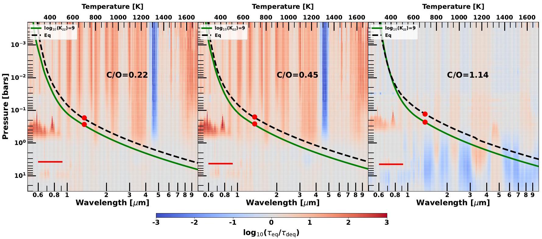
الشكل 4. الفروقات فيالملفات بين جو في توازن حراري كيميائي وجو مع خلط نشط عند مستويات مختلفةتظهر النسب من خلال الألواح الثلاثة (محور x العلوي). النماذج الجوية المعروضة هنا لديها و مع المعدنية الشمسية. الـالملف المحسوب باستخدام التوازن الحراري الكيميائي موضح كخطوط منقطة سوداء، بينما الملف المحسوب بافتراضتظهر كخطوط صلبة خضراء. تُظهر اللوحة اليسرى واللوحتان الوسطى واليمنى المقارنة في، و 1.14 ، على التوالي. الخلفية الملونة في كل لوحة تمثل نفس الكمية كما في الشكل 3. الخط الأحمر الأفقي في كل لوحة يوضح مستوى الضغط الذي عنده ، و إخماد في كل نموذج جوي. النقاط الحمراء على كلالملف يدل على مستويات الضغط الفوتوسفيرية المتوسطة لكل حالة. لاحظ أن ضغط الإخماد لـ أو تختلف عن ما هو موضح بواسطة الخط الأحمر الأفقي.
موكيرجي وآخرون (2022)؛ كاراليدي وآخرون (2021)؛ فيليبس وآخرون (2020)؛ هوبيني وبوروز (2007)؛ لايسي وبوروز (2023). لقد أثبتت هذه الدراسات أن هذه التأثيرات يمكن أن تحدث تغييرات في ملف تعريف الطلب لـعند المعدل الشمسينسبة (على سبيل المثال، موكيرجي وآخرون 2023؛ كاراليدي وآخرون 2021؛ موكيرجي وآخرون 2022). ومع ذلك، ستحتوي الأجواء الغنية بالمعادن (بالنسبة للشمس) على نسب خلط أعلى من، ، إلخ. جميعها حساسة للغاية لـ. لذلك، اعتمادًا على و يمكن أن يكون لتبريد هذه الغازات في الأجواء ذات المعدنية الفائقة للشمس تأثير أكثر أهمية على الغلاف الجويالملف الشخصي مقارنة بالتأثير الموجود في الأجواء ذات التركيب الشمسي. من ناحية أخرى، ستحتوي الأجواء ذات المعدنية دون الشمسية على كمية أقل من هذه الغازات، واعتماد الملف الشخصي علىمن المتوقع أن تكون أقل أهمية نسبيًا من الأجواء ذات التركيب الشمسي.
4.1.1.عمق الغلاف الجوي البصري، والملفات الشخصية
تظهر الشكل 3 تأثيرعلى الجوي الملف من خلال المقارنة الملفات التي تم الحصول عليها من التوازن الكيميائي معالملفات الشخصية المحسوبة باستخدام عند ثلاث معدنيات مختلفة لجسم مع و . هذا الاختيار للجاذبية يمثل نسخة شابة من كوكب مشابه للمشتري. تُظهر اللوحة اليسرى في الشكل 3 المقارنة لكائن فقير بالمعادن مع يظهر الخط المنقط الأسود الملف المحسوب باستخدام التوازن الحراري الكيميائي في حين أن الخط الأخضر الصلب يظهر الملف الشخصي المحسوب بـ تظهر الخريطة الملونة في الخلفية الكمية، الذي يقارن بين الطول الموجي والعمق البصري المعتمد على الضغط في التوازن الكيميائي الحراري و قيمة أكبر من 0 تشير إلى أن نموذج التوازن الحراري الكيميائي أكثر غموضًا من نموذج عند تلك الطول الموجي والضغط المحددين. على النقيض من ذلك، تعكس القيمة السلبية السيناريو المعاكس.
لـالحالة الموضحة في اللوحة اليسرى من الشكل 3، فإن معظم أعماق الضوء متشابهة بين التوازن الحراري الكيميائي و الحالات ونتيجة لذلك، هو ضمن ترتيب من حيث الحجم يساوي 0 في معظم الأطوال الموجية عبر جميع الضغوط. هذا يتسبب في التوازن الحراري الكيميائي وعدم التوازن.الملفات لتكون قريبة جدًا من بعضها البعض فيالشريط الأزرق بينفي جميع الألواح الثلاثة من الشكل 3 يعود ذلك إلى زيادة وفرة CO بسبب التبريد، في حين أن الاختلافات بين 0.6-1تعود المنطقة إلى امتصاص الصوديوم والبوتاسيوم الموسع بسبب الضغط. يتسبب زيادة ثاني أكسيد الكربون في جعل الأجواء ذات عدم التوازن الكيميائي أكثر تعتيمًا من الأجواء في حالة التوازن الكيميائي في هذه الأطوال الموجية.
ومع ذلك، عند المعدل الشمسي للمعادن (اللوحة الوسطى)، يكون نموذج التوازن الحراري الكيميائي أكثر تعتيمًا مقارنةً بـنموذج، خاصة فوق 1 بار. وذلك بسبب القيمة العالية لـفي نموذج كيمياء عدم التوازن يسببلتُروى في الغلاف الجوي الأعمق والأكثر حرارة مما يؤدي إلى انخفاضوفرة في الغلاف الجوي العلوي مما يجعل الغلاف الجوي أكثر شفافية منتوازن كيميائي غني الغلاف الجوي. منذيمتص عبر الأشعة تحت الحمراء القريبة، فإن الوفرة المنخفضة للغاز تسمح بتبريد إشعاعي أكثر كفاءة من أعماق الغلاف الجوي.ملف تعريف الـالنموذج بالتالي أبرد بمقدارمن نموذج التوازن الكيميائي عند المعدنية الشمسية. يتم تضخيم نفس التأثير إلى درجة أكبر عندالموضح في اللوحة اليمنى في الشكل 3. هذا يتسبب فيالنموذج ليكون أبرد بحواليمن نموذج التوازن الكيميائي فيالتركيز المعدني الشمسي. ضغوط التوقف لـ، و في الأجواء التي تحتوي على خلط عمودي يتم الإشارة إليها بخطوط أفقية حمراء في جميع الألواح الثلاثة من الشكل 3.
يمكن أن يؤثر نسبة الكربون إلى الأكسجين في الغلاف الجوي أيضًا على كيفيةيؤثر على الغلاف الجويالملف الشخصي. لنفس المعدل الجوي للمعادن،النسبة تتحكم في الوفرة النسبية للغازات المحتوية على الكربون والغازات المحتوية على الأكسجين مثل، أول أكسيد الكربون، إلخ. تحت التوازن الكيميائي، الغازات مثل، و وفيرة في الأجواء الغنية بالأكسجين (منخفضة ). ومع ذلك، إذا أصبحت الغلاف الجوي غنيًا بالكربون، فإن الغازات الحاملة للكربون مثل و تصبح HCN وفيرة، وغازات تحمل الأكسجين مثل و تقل وفرتها.
تظهر الشكل 4 تأثير الغلاف الجوينسبة علىملف تعريف لـكائن مع عند المعدل الشمسي للمعادن. تُظهر اللوحة اليسرى الفرق في الملفات بين النموذج الحراري الكيميائي ونموذج في جو غني بالأكسجين معمثل الشكل 3، ضغوط التبريد لـ، و في الأجواء التي تحتوي على خلط عمودي، يتم الإشارة إليها بخطوط أفقية حمراء في الشكل 4 أيضًا. عند ضغوط أقل منالشريط، يوضح الشكل 4 في اللوحة اليسرى أن كل من أعماق الطيف القصير والطويل في الأجواء الكيميائية المتوازنة أكبر منالغلاف الجوي. هذا يسبب التوازن الكيميائيالملف الشخصي ليكون أكثر جاذبية منالغلاف الجوي عند جميع الضغوط.
تظهر اللوحة الوسطى الفرق عندالغلاف الجوي في حالة التوازن الكيميائي أكثر تعتيمًا مننموذج عند الأطوال الموجية القصيرة ( )، ومع ذلك فإن الفرق في شفافية النموذجين عند الأطوال الموجية الأطول ( ) أصغر مما يُرى في نموذج C/O المنخفض في اللوحة اليسرى. الغلاف الجوي الأعمق والأكثر سخونة يشع عند أطوال موجية أقصر بينما الغلاف الجوي العلوي الأكثر برودة يشع عند أطوال موجية أطول. مع نموذج التوازن الكيميائي أكثر غموضًا من نموذج عدم التوازن الكيميائي عند الأطوال الموجية القصيرة، مما يتسبب في اختلافات أكبر بينملف النماذج في الغلاف الجوي العميق. ولكن نظرًا لأن الفرق في أعماق الطول الموجي الطويلة أصغر نسبيًا بين النموذجين، فإنالملف في غلافهم الجوي العلوي مشابه أيضًا لبعضه البعض. عند (الشكل 4 اللوحة اليمنى)، تصبح الغلاف الجوي هيمنت بسبب انخفاض وفرة الغازات الحاملة للأكسجين مثل و . هذا يسبب الفرق في الأعماق البصرية بين التوازن الكيميائي والنماذج التي يُعزى سببها بشكل رئيسي إلى التبريد لـفقط. تُظهر اللوحة اليمنى من الشكل 4 أن الفروق بين أعماق الضوء للنموذجين عند الأطوال الموجية الأطول أصغر مقارنة باللوحات الوسطى واليسرى. هذا يتسبب فيملفات النماذج الاثنين لتكون متطابقة تقريبًا عند ضغوط أقل منالبارات. ومع ذلك، بسبب إلى الفروق المتبقية بين شفافية الأجواء عند الأطوال الموجية الأقصر،تظهر الملفات عند الضغوط الأعمق اختلافات ملحوظة. الشكل 3 و 4 يوضحان تأثيربسعر ثابت و . لكن كيمياء الغلاف الجوي تتغير بشكل كبير مع و أيضًا.
4.1.2. آثارعلىملفات تعريف عبر و
و تؤدي إلى تغييرات كبيرة في كيمياء الغلاف الجوي. على سبيل المثال، الأجسام من النوع L معأكبر منمن المتوقع أن تكونفقير بالغازات مثل CO التي تحمل معظم ذرات الكربون تحت التوازن الكيميائي. ولكن هناك انتقال سريع من هيمنة CO إلىتحدث الأجواء المهيمنة كـيهدأ تحت. انتقال مشابه من الجو المسيطر (أعلى ) إلى الجو المسيطر (أدنى ) من المتوقع أيضًا أن يحدث تحت التوازن الكيميائي. من ناحية أخرى، يؤدي جاذبية الجسم إلى تغييرات كبيرة في ملف الأجواء أيضًا لأن الأعماق البصرية الجوية تتناسب عكسيًا مع الجاذبية. لذلك، كما أن كلا و يؤثر بشكل كبير على كيمياء الغلاف الجوي، من خلال دراسة كيفيةيؤثر علىملف تعريف في مختلف و هو أمر حاسم.
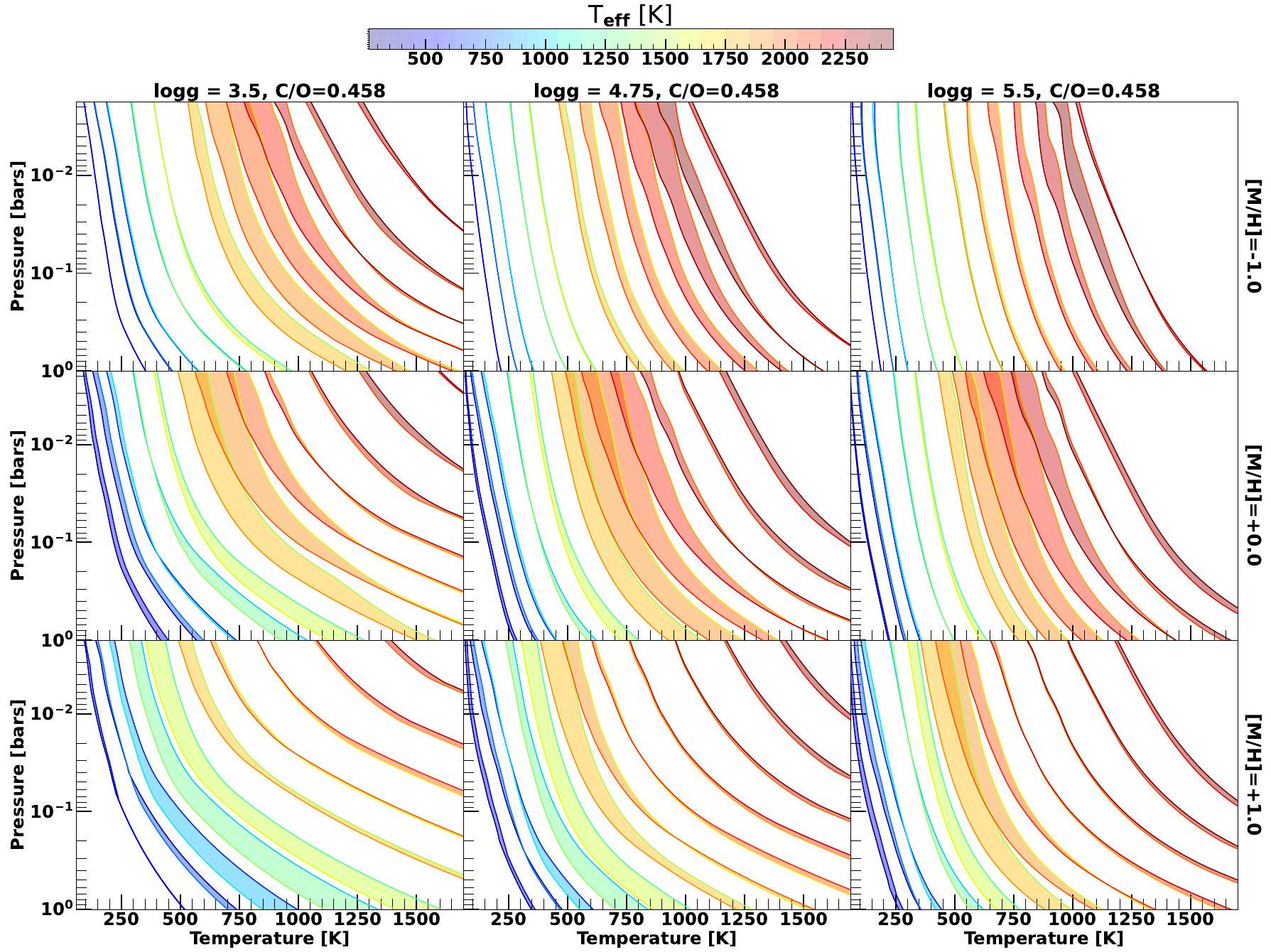
تظهر الشكل 5 كيفيؤثر علىالملف الشخصي فيقيم تتراوح من 300 ك إلى 2400 ك. كل عمود يتوافق مع القيمة مع العمود الأيسر الذي يظهر النماذج في العمود الأوسط يعرض النماذج في، والعمود الأيمن يعرض النماذج في الصف العلوي في الشكل 5 يظهر هذا التأثير فيبينما الصف الأوسط والسفلي يظهران التأثير في و ، على التوالي. المنطقة المظللة حول ملف شخصي لكل القيمة تمثل التغير في الملف الشخصي بسببيتراوح منإلىأعلىيؤدي إلىالملفات لتكون أبرد من الأدنىحالات.
عند المعدن دون الشمسي (الشكل 5 الصف العلوي)، يتغير في الـيحدث الملف بشكل كبير لـالقيم التي هي أكبر منيؤثر هذا النطاق الحراري بشكل أكبر لأن انخفاض المعدنية يؤدي إلى برودةالملفات مقارنةً بالجو الشمسي أو فوق الشمسي. ونتيجة لذلك،يصبح ماصًا غازيًا سائدًا تحت ظروف مرتفعة نسبيًاقيم قريبة منلنماذج الجاذبية المنخفضة الموضحة في الصف العلوي الأيسر في الشكل 5. بالنسبة للغلاف الجوي ذي الجاذبية الأعلى،يصبح ماصًا سائدًا تحت مستوى أعلى قليلاًقيم أكثر من 1800 ك.الوفرة حساسة جداً لـ، يؤثر المزج على الهيكل بشكل كبير في هذه القيم في الأجواء الفقيرة جداً بالمعادن. ولكن كمايذهب أدناهلـو 4.75 نماذج، تزداد الوفرة في الغلاف الجوي، ويفقد حساسيته العالية لـ. نتيجة لذلك، الـ يصبح الملف الشخصي أيضًا أقل حساسية لـ أدناه لـو 4.75 أجواء. بالنسبة للأجسام المعدنية الفقيرة ذات الجاذبية العالية (اللوحة العلوية اليمنى)، فإن فقدان الحساسية هذا لـيظهر عند مستوى أعلى حتى قيمة أكبر من 1200 ك. وذلك لأن الأجسام ذات الجاذبية الأعلى تكون أكثر برودة.ملفات تعريف أكثر من الأجسام ذات الجاذبية المنخفضة. ونتيجة لذلك، تصبح الغلافات الجويةهيمنت بشكل أعلىأكثر من 1800 كلفن وأيضًا تفقد حساسيتها لـفي أعلىأكثر من 1200 ك.
الصف الأوسط والسفلي في الشكل 5 يظهران نفس التأثير لجوذ الشمس وما فوق الشمس من حيث المعدنية. بسبب المعدنية الأعلى،الملفات عند هذه المعدلات المعدنية تكون أكثر حرارة نسبيًا من الملفات عند المعدلات المعدنية دون الشمس. تبدأ هذه الأجواء الأكثر حرارة في أن تصبحهيمنت في مستوى أدنىمنلأجواء المعدنية الشمسية والقريبة ك لـ الجو ذو المعدنية الشمسية. علاوة على ذلك، مع زيادة المعدنية، يتم تفضيل CO بشكل متزايد كغاز حامل للكربون مقارنةً بـوفقًا للتوازن الحراري الكيميائي (لودرز وفغلي 2002). يؤدي هذا التأثير أيضًا إلى انخفاضوفرة في الارتفاعالجو في المعادن العالية مقارنةً بالجو في المعادن المنخفضة مع تشابه. نتيجة لذلك، تُظهر الشكل 5 أن الانتقال ونوع T المبكر ( ) من المتوقع أن تحتوي الكائنات على الأكثر حساسالملفات عند المعدل الشمسي.المعدنية الشمسية، الأكثر حساسيةتظهر الملفات للأجسام من النوع T من المبكر إلى المتأخر معبين. نفس الاتجاه للأجسام ذات الجاذبية الأعلى يظهر حساسية أقل لـالملف الشخصي إلىتبقى للمعادن الشمسية وما فوق الشمسية أيضًا.
تظهر الشكل 4 أنالنسبة لها تأثير كبير أيضًا على الغلاف الجويالملف الشخصي عندما تكون الأجواء لديها خلط عمودي قوي. الشكل 6 يستكشف هذا التأثير مع أجواء ذات معدنية شمسية لنطاق مشابه من و القيم كما في الشكل 5. الصف العلوي في الشكل 6 يوضح كيفيؤثر علىالملف في الأجواء الغنية بـ O-تظهر الصفوف الوسطى والسفلى في الشكل 6 التأثير على و 1.14 ، على التوالي.
تظهر الشكل 6 أنه لا يوجد الكثير من التباين في تأثيرعلى الملف بين (الصف العلوي) و (الصف الأوسط). في كلا هذين النسبتين C /O، التأثير مشابه نوعياً لسلوك المعدن الشمسي الذي يظهر في الصف الأوسط من الشكل 5. ومع ذلك، عند مستويات أعلىنسبة 1.14 (الصف السفلي)، تأثيرعلىتغييرات الملف الشخصي. الـتبدو الملفات الشخصية أقل حساسية نسبيًا لـفي هذه الأجواء الغنية بالكربون. ولكن بالنسبة لحالات الجاذبية المنخفضة (الصف الأيسر)، فإن مستوى الحساسية أقلتستمر بين. بالنسبة للحالات ذات الجاذبية المتوسطة والعالية الموضحة في الصفين الأوسط والأيمن، فإن حساسية الـالملف الشخصي إلى أصغر حتى. من أجل من 4.75، تستمر الحساسية بينيؤثر علىالملف الشخصي بينلحالة الجاذبية العالية (5.5، الصف الأيمن) في هذه الأجواء الغنية بالكربون.هو ناقل رئيسي لذرات الكربون في هذه الأجواء الغنية بالكربون وبالتالي الوفرة تظهر حساسية أقل للتغيرات في . هذه هي السبب الرئيسي وراء انخفاض الحساسية لـالملفات الشخصية إلىفي أجواء كريتش معأكبر من الواحد.
لقد أظهرت هذه القسم كيفالمعدنية، ونسبة تؤثر على الغلاف الجويالملفات الشخصية. هذا يمنحنا فكرة عن مناقشتنا التالية التي تركز على طيف الانبعاث الاصطناعي من هذه النماذج.
4.2. الأطياف عبر تباينالمعدنية ونسب الكربون إلى الأكسجين
في هذا القسم نقدم اتجاهاتنا في الطيف بطريقتين. أولاً، نفحص الاتجاهات الطيفية الناتجة عنالمعدنية، وبسعر ثابت و القيمة المقابلة لكائن من النوع T. هذا يساعدنا في تحديد-
الشكل 5. حساسية الـالملف الشخصي إلىعبر نطاق واسع منتُظهر القيم عند معدلات معدنية جوية مختلفة وجاذبيات مختلفة. كل لوحة تُظهرملفات تعريف لـقيم من500 ك، و300 ك. المنطقة المظللة لـالملفات الشخصية في كليظهر حساسية الـملفات تعريف للاختلاف فيمنإلىأعلىيؤدي إلىالملفات لتكون أبرد من الأدنىالنماذج. الصف العلوي يظهر النماذج معالمعدنية الشمسية للغلاف الجوي بينما تظهر الصفوف الوسطى والسفلية نماذج مع شمسية والمعدنية الجوية الشمسية. الصف الأيسر يعرض النماذج عندبينما تُظهر الصفوف الوسطى واليمنى النماذج في و ، على التوالي. جميع النماذج المعروضة هنا تحتوي على .
تحديد الانحلالات وتأثيرات كل من هذه المعلمات على طيف الانبعاث للأجسام دون النجمية. نتبع ذلك بعرض اتجاهات ميزات طيفية معينة كدالة لـ، مما يساعدنا في التركيز على اتجاهات النماذج عبر تسلسلات الطيف L- و T- و Y-.
4.2.1. كيفالمعدنية، وطيف التأثيرات لـ-نوع الكائن: دراسة حالة
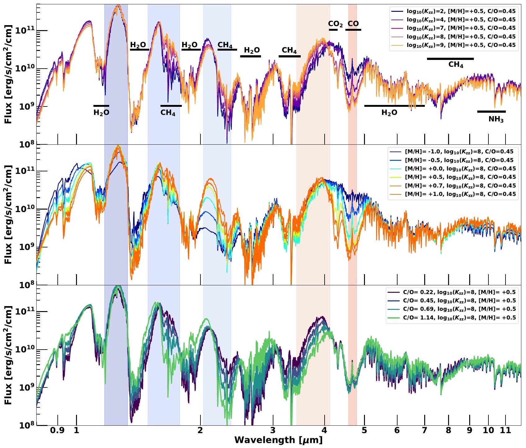
تظهر الشكل 7 تأثير، المعدنية، ونسبة الكربون إلى الأكسجين على طيف الانبعاث لـ و كائن. تُظهر اللوحة العلوية تباين طيف الانبعاث معيتراوح منإلىبينما يتم الحفاظ على الثقل المعدني ونسبة الكربون إلى الأكسجين ثابتين عندالشمسية و0.45، على التوالي. تباين طيفي كبير بسبب يحدث في أشرطة الامتصاص بين 1.6-1.82.1-2.5، و 3-4 . نطاق امتصاص CO بين أيضًا حساس لـ. الـنطاقات بين 1.10-1.20، و و الـ ميزات بين
10-11تظهر اختلافًا ضئيلًا جدًا مع. العاليالنماذج تظهر قمم Y-band أصغر من المنخفضةالنماذج. الانخفاضوفرة في الارتفاعالنماذج تسمح بإصدار مزيد من التدفق في نطاق H ونطاق L مقارنةً بالنطاق المنخفضنماذج. الـ و أشرطة الامتصاص بينتتأثر أيضًا بشدة بـفيالمعدنية الشمسية.
تظهر اللوحة الوسطى في الشكل 7 تأثير تغير المعدنية على طيف الانبعاث لنفس الجسم بينما و تظل ثابتة. تظهر النماذج ذات المعدن العالي تدفقًا أضعف في نطاق Y ولكن تدفقًا أعلى في نطاق J مقارنة بالنماذج ذات المعدن المنخفض. ومع ذلك، فإن النماذج ذات المعدن العالي تكون أكثر سطوعًا في نطاقي H و K مقارنة بالنموذج ذو المعدن المنخفض.أشرطة الامتصاص بين، ، و أعمق في النماذج ذات المعدنية المنخفضة مقارنة بالنماذج ذات المعدنية العالية. من ناحية أخرى، فإن نطاق CO بين و الـ نطاق بين 4-4.5أقوى للأجسام الغنية بالمعادن مقارنة بتلك الفقيرة بالمعادن. مقارنة
الشكل 6. حساسية الـالملف الشخصي إلىعبر نطاق واسع منقيم في أجواء مختلفةوتظهر الجاذبيات. كل لوحة تعرضملفات تعريف لـقيم من، و 300 كلفن. المنطقة المظللة لـ الملفات الشخصية في كليظهر حساسية الـملفات تعريف للتنوع فيمنإلى. الصف العلوي يعرض النماذج مع بينما الصفوف الوسطى والسفلية تعرض نماذج مع و 1.14. الصف الأيسر يعرض النماذج فيبينما تظهر الصفوف الوسطى واليمنى النماذج في و على التوالي. جميع النماذج المعروضة هنا لديها معدنية شمسية.
الشكل 7 الألواح الوسطى والعلوية بالقرب من حزام M (4.55.0)يظهر تدهورًا محتملاً بينوالمعادن حيث أن كلا هذين المعلمين لهما تأثيرات مشابهة على خاصية CO.تظهر الميزة اعتمادًا قويًا على المعدنية وضعيفًااعتماد بسبب اعتمادوفرة على المعدنية. لذلك، الـيمكن أن تساعد هذه الميزة في كسر هذه الانحطاط.الميزة غير قابلة للوصول من الملاحظات الأرضية بسبب التركيز العالي لـفي غلاف الأرض الجوي، لذا فإن الملاحظات المستندة إلى الفضاء منيمكن أن يساعد في تقييد كلاهماوالمعادن. مقارنة اللوحة الوسطى في الشكل 7 مع اللوحة العلوية تظهر أيضًا أنأشرطة الامتصاص بين، ، و أكثر حساسية للمعادن الجوية منمع تزايدقوة النطاقات مع زيادة المعدنية.
اعتماد طيف الانبعاث على الغلاف الجويمع الثابتوتم عرض المعدنية في الشكل 7 في اللوحة السفلية. بالنسبة لـالغلاف الجوي، و طيف تبدو مشابهة نوعيًا في معظم نطاق الطول الموجي الموضح في الشكل 7.ميزة فيالنموذج أقل عمقًا منميزات فينموذج، والذي من المتوقع أن يكون أصغريؤدي إلى جو أقل غنى بـ الذرات. ومع ذلك، فإن الطيف مختلف تمامًا عن النماذج الثلاثة الأخرى الموضحة في اللوحة السفلية من الشكل 7. تحتوي الأطياف الغنية بالكربون على انحدار أقل.ميزات وذروات أقوى في نطاق Y و J مقارنة بالنموذجين الآخرين الغنيين بالأكسجين. ومع ذلك، فإنالفرق في نطاقات H- و K- و L أعمق من الطيف الغني بالأكسجين كما هو1.14 أجواء هي جداًغني. التغير السريع في كيمياء الغلاف الجوي والطيف بالقرب منجزء من فضاء المعلمات يشير إلى أن المستخدمين يجب أن يكونوا حذرين عند استيفاء الطيف حول هذه المنطقة. أول أكسيد الكربون والميزات غير حساسة عمليًا للغلاف الجوي، مما يجعل منطقة مفيدة جدًا لكسر المعدنية والانحطاط.
تظهر الشكل 7 أنطيف الكواكب المصورة أو الأقزام البنية يتأثر بجميع العوامل الثلاثة-
الشكل 7. تأثيرعلى طيف الانبعاث بين لجسم وزنه 700 كيلوجرام مع يظهر في اللوحة العلوية. يتم الحفاظ على المعدنية ونسبة الكربون إلى الأكسجين ثابتة عبر جميع النماذج في اللوحة العلوية. تأثير المعدنية على طيف الانبعاث بين لجسم وزنه 700 كيلوجرام مع يظهر في اللوحة الوسطى. الـوتم الحفاظ على C/O ثابتة عبر جميع النماذج في اللوحة العلوية. تأثيرعلى طيف الانبعاث بين لجسم وزنه 700 كيلوجرام مع يظهر في اللوحة السفلية. الـوتم الحفاظ على المعدنية ثابتة عبر جميع النماذج في اللوحة العلوية. نطاقات التصوير الفوتوغرافي بالأشعة تحت الحمراء القياسية مثل J،و M موضحة أيضًا مع المنطقة المظللة.
معلمات – المعدنية، وإلى درجات مشابهة. على سبيل المثال، طيف نطاق M بينالذي تم استخدامه لوضع قيود علىتتأثر نماذج التركيب الشمسي، بشكل مشابه، بكل منوالكثافة المعدنية لثابت و . من ناحية أخرى، الـتتأثر الأشرطة في الطيف بجميع المعلمات الثلاث – المعدنية،، و C/O. أجزاء أخرى من الطيف مثل الفرق و الفرق أكثر حساسية للمعادن الجوية من أو . الـميزة بين يظهر حساسية قليلة جدًا تجاه هذه المعلمات الثلاثة. توضح الشكل 7 أنه أثناء ملاءمة بيانات الطيف المراقبة الدقيقة للكواكب الخارجية والأقزام البنية (على سبيل المثال، منمن الضروري أن يتناسب مع هذه المعلمات الثلاثة في الوقت نفسه وبشكل متسق.
توضح الأشكال 5 و 6 أن الكيمياء الجوية والملفات الشخصية حساسة لـبالإضافة إلى معايير مثل المعدنية الجوية،، و . هنا، نقدم الاتجاهات الطيفية كدالة لـللمعدنية المختلفة،، و القيم.
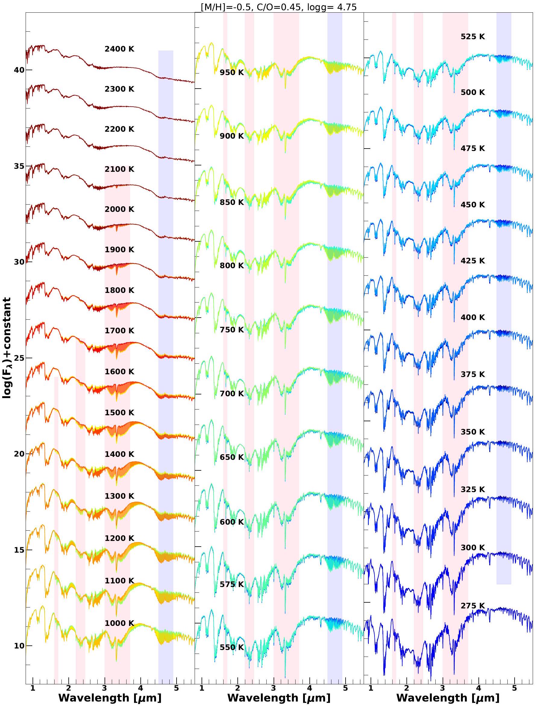
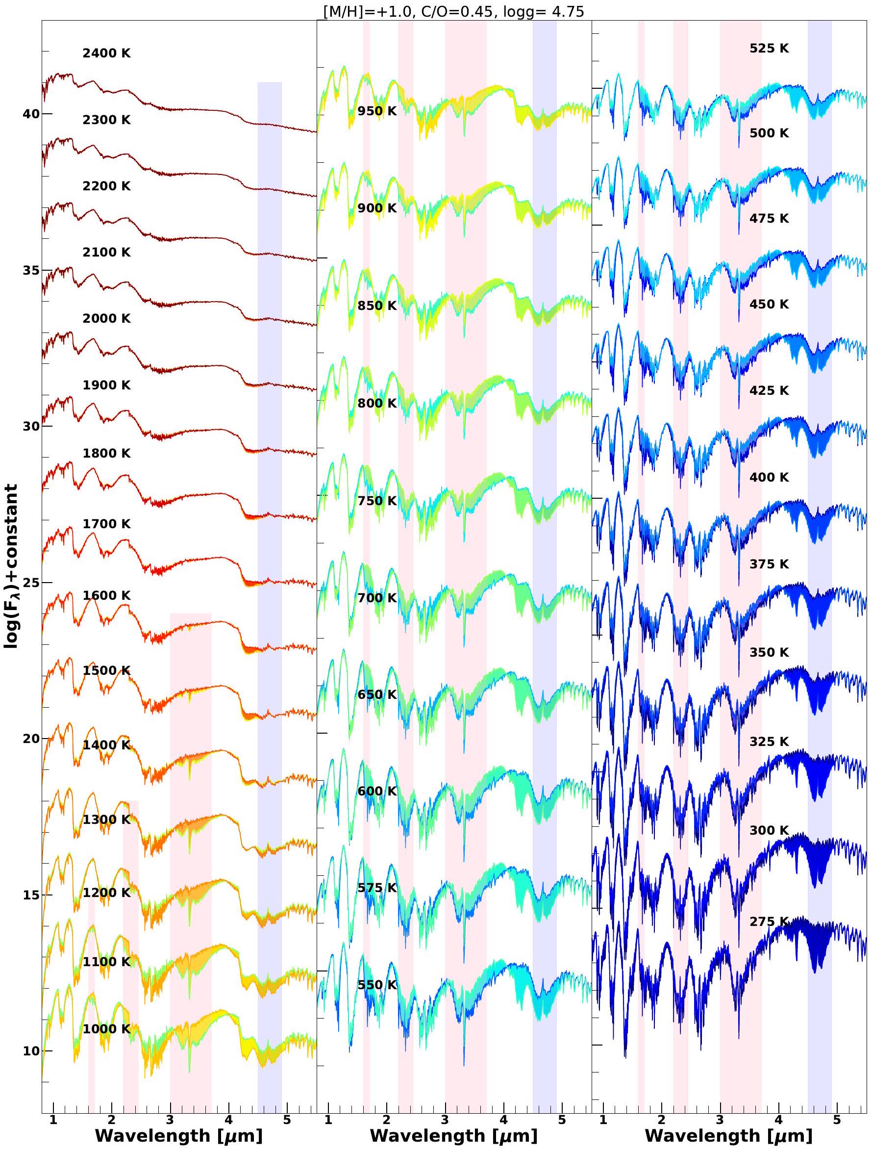
تظهر الشكل 8سلسلة الطيف الانبعاثي منإلىعند معدنية جوية تحت شمسية لـشمسي. جميع النماذج المعروضة هنا هي لـ ( ). لكل طيف موضح في الشكل 8، المساحة بين النموذج الطيفي مع أقل خلط عمودي ( ) وأعلى خلط عمودي ( ) مظلل لتصوير التغير في الميزات الطيفية بسبب التغيرات في في كلتظهر الشكل 9 نفس التسلسلات الطيفية ولكن لجو ذو معدنية تفوق الشمس.الشمسية).
تطور بعض الميزات الطيفية الملحوظة عبريمكن رؤيته بسهولة في الشكل 8 و 9. على سبيل المثال،
موكيرجي وآخرون
الشكل 8. طيف الانبعاث الحراري بينبمستويات متفاوتةمن 2400 كلفن إلى 275 كلفن لجو منخفض المعادن مع و مُعروضة هنا. جميع النماذج المعروضة هنا تحتوي على. في كل التغير في الطيف بسببيتم إظهاره بتظليل المنطقة بين الطيفين من النماذج مع و . نطاقات الامتصاص الرئيسية لـ وCO يظهران بأشرطة وردية وزرقاء، على التوالي.
الشكل 9. طيف الانبعاث الحراري بينبمستويات متفاوتةمن 2400 كلفن إلى 275 كلفن للغلاف الجوي الغني بالمعادن مع و مُعروضة هنا. جميع النماذج المعروضة هنا تحتوي على. في كل التغير في الطيف بسببيتم إظهاره بتظليل المنطقة بين الطيفين من النماذج مع و . نطاقات الامتصاص الرئيسية لـ وCO يظهران مع أشرطة وردية وزرقاء، على التوالي.
الشكل 10. مقياس القوة الطيفيةلـميزة فيكنتيجة لـيظهر في الألواح في العمود الأيسر. كل لوحة من الأعلى إلى الأسفل تتوافق مع معدنية مختلفة، وكل خط يمثل قوة الطيف من مختلفالقيم. العمود الأوسط يعرض نفس المقياس لميزة CO بينبينما العمود الأيمن يظهر المقياس لـالميزة. الخط المنقط الأسود يوضح القيمة التي تظهر تحتها هذه الميزات تقريبًا في الطيف.
الميزة فييبدأ بالظهور في الطيف عندلأجواء الفقيرة بالمعادن الممثلة في الشكل 8. السبب الرئيسي وراء ظهورفي مثل هذه الارتفاعات العاليةالقيم هي انخفاض المعدنية الجوية الذي يسبب الغلاف الجويأن تكون أبرد مما هو متوقع من الأجواء ذات المعدنية الشمسية أو فوق الشمسية. يمكن رؤية ذلك في الشكل 5 أيضًا. التأثير المعاكس يعمل في الشكل 9 الذي يصور طيف الأجواء فوق الشمسية. في هذه الحالة، تظهر التوقيع فقط في النماذج التي تكون أبرد منتتميز هذه الأجواء ذات المعدن العالي بدرجات حرارة أعلىالملفات الشخصية التي تعني أنيجب أن يكون أقل في هذه الأجواء لكي يتجمع بما فيه الكفايةحتىتظهر التوقيعات في الطيف. علاوة على ذلك، في مثل هذه الأجواء الغنية بالمعادن،النسبة أعلى من تلك الموجودة في الأجواء الفقيرة بالمعادن.الميزة تظهر أكبر حساسية لـلـبين 1900 كلفن و 450 كلفن لـ الأجسام الفقيرة بالمعادن في الشكل 8. أدناه، إن أجواء هذه الأجسام باردة جداً لدرجة أنها غنية جداً بـ، لدرجة أن الـالتوقيع يصبح غير حساس لـبالنسبة للأجسام الغنية بالمعادن الموضحة في الشكل 9، فإن حساسية الـيبقى الشريط في مكانه لـبارد مثل 275 ك.
تطور الـفرقة CO عبريمكن أيضًا رؤية النطاق في الشكل 8 و 9. بالنسبة لنماذج المعدنية تحت الشمس الموضحة في الشكل 8، فإن نطاق CO بينيبدأ في إظهار الاعتماد علىفيأقل من 1600 كلفن. مع انخفاضأقل من 1600 ك، حساسية نطاق CO لـتزداد هذه الحساسية وتصل إلى ذروتها حواليأشياء تكون أكثر برودة من، تفقد تدريجياً حساسية نطاق CO إلىمع تراجعفي الأجواء ذات المعدنية تحت الشمس. يمكن تفسير هذا السلوك بـالملفات عند معدنية تحت الشمس، والتي تكون أبرد منالملفات الشخصية المحسوبة من الأجواء ذات المعدنية الشمسية أو فوق الشمسية. أدناهمن المتوقع أن تكون الغلاف الجوي الأعمق لهذه الأجسام الفقيرة بالمعادن باردًا جدًا لدرجة أنها لا تحتوي على كمية كافية من ثاني أكسيد الكربون في الغلاف الجوي العميق ليتم نقله إلى الفوتوسفير عبر الخلط. المقارنة الأقلالنسبة في الأجسام الفقيرة بالمعادن مقارنةً بالجو الغني بالمعادن هي أيضًا سبب مهم وراء هذا الاتجاه. من ناحية أخرى، تظل نطاقات CO حساسة للغاية لـحتىلأطياف المعادن الفائقة الشمسية الموضحة في الشكل 9. الأعلىنسبة في الأجسام الغنية بالمعادن مقارنةً بالجو الفقير بالمعادن تجعل غاز CO غازًا بارزًا يحمل الكربون حتى في الأجسام الغنية بالمعادن الباردة جدًا. علاوة على ذلك،الملفات عند هذه المعدلات المعدنية المرتفعة أكثر حرارة منالملفات المحسوبة لجوّيات ذات معدنية شمسية أو دون شمسية، مما يجعل الأجواء الأعمق لهذه الأجسام لا تزال غنية جدًا بـ CO حتى في درجات الحرارة المنخفضة.قيم مثل 275 ك. يتم خلط وفرة CO هذه إلى الفوتوسفير بسبب الخلط وتسبب في أن يكون نطاق CO حساسًا للغاية لـحتى في هذه الأجسام من النوع Y الغنية بالمعادن.
الميزة فييظهر في الأطياف في الأجسام الأكثر برودة منفي طيف الغلاف الجوي الفقير بالمعادن الموضح في الشكل 8. ومع ذلك، فإن حساسيته لـيبقى منخفضًا جدًا في هذه النماذج ذات المعدنية تحت الشمس. من ناحية أخرى،يصبح الممتص السائد بينفيفي نماذج المعدن الفائق الشمسي الموضحة في الشكل 9.الوفرة حساسة جداً للمعادن مما يؤدي إلى مستويات عالية جداً الوفرة عند المعادن الفائقة الشمسية. الميزة في الشكل 9 تظهر أيضًا حساسية لـوكذلك عبر جميعقيم أقل من 1500 كلفن في هذه النماذج الغنية بالمعادن.
لتحسين تصور هذه الاتجاهات في الميزات الطيفية، نصمم مقياسًا يستكشف قوة الـميزة، ميزة، و الميزات. نحن نحدد هذه المقياس بالنسبة لطيف مرجعي. نحن نحدد المقياس على النحو التالي:
أينيمثل قيم التدفق ضمن نطاق الطول الموجي لخاصية الامتصاص المعنية. على سبيل المثال، بالنسبة لـميزة فيسيمثل الطيف بينيمثل الحد البسط في المعادلة 2 عمق الـ خاصية الامتصاص بالنسبة للطيف المرجعي، بينما المقام هو مصطلح تطبيقي لحساب الفرق في المستويات المطلقة للتدفقات المنبعثة بين الأطياف المعنية والطيف المرجعي. لاستخدام هذه المقياس لتقييم قوة خاصية معينة، يجب أن تحتوي الأطياف المرجعية على أضعف خاصية ذات اهتمام. لذلك، لتقييم قوة الميزات المختلفة، اخترناطيف معالمعدنية الشمسية، و كطيف مرجعي.
تظهر الشكل 10 تباين ثلاث ميزات طيفية عبرقيم مختلفةوقيم المعدنية من خلال رسم المقياس. العمود الأيسر يظهر التغير في الـميزة فيبالنسبة للطيف المرجعي المحدد أعلاه، حيث يتوافق كل صف مع معدنية جوية مختلفة. تُظهر الخطوط الملونة المختلفة في كل لوحة التغير فيقوة من أجل الاختلافالقيم. العمود الثاني من الشكل 10 يظهر التغير في ميزة CO بينبالنسبة للطيف المرجعي، بينما تظهر العمود الثالث التغير فيميزة الزوجية بين.
الشكل 8 و 9 أظهر بالفعل أن بدايةقيمة للمظهر لـالميزات في الأطياف هي دالة على المعدنية الجوية. يتم تسليط الضوء على هذه الظاهرة بشكل أكبر في الشكل 10 العمود الأيسر. الخط العمودي المتقطع الأسود في كل لوحة يسارية يحدد القيمة التي عندهاتظهر الميزة لأول مرة في طيف معين من المعدنية. يمكن ملاحظتها أن هذهبدايةتتفاوت القيمة بشكل كبير من 2100 كلفن في الأجواء ذات المعدنية تحت الشمسية إلى 1500 كلفن في الأجواء ذات المعدنية فوق الشمسية. حساسية الـميزة لـأيضًا هو دالة قوية لـأيضًا.
قوة الـميزة كدالة لـيظهر في العمود الأوسط من الشكل 10 لمعدلات معدنية جوية مختلفة. قيمة أعلى منيزيد من قوة ميزة CO عند جميع المعدنيات. مشابهة للاتجاهات التي لوحظت فيالميزة، بدايةالذي تصبح فيه ميزة CO حساسة لـيختلف أيضًا مع المعدنية. قوة الـميزة بينموضح في العمود الأيمن من الشكل 10. حساسية الـقوة الميزة علىمنخفض جدًا. هذه الافتقار إلى الحساسية لـهو بسبب منحنيات الوفرة الثابتة لـمن كيمياء التوازن لها انحدارات مشابهة متوقعة من-إنه الأديابات (سومون وآخرون 2006؛ فورتني وآخرون 2020؛ زاهنل ومارلي 2014؛ أونو وفورتني 2023). نتيجة لذلك، الـالتنبؤ بالوفرة من التوازن الحراري الكيميائي لا يظهر الكثير من التغير مع الضغط أو درجة الحرارة في الأجزاء الحملية من الغلاف الجوي الأعمق. لذلك، فإن التبريدتصبح الوفرة تقريبًا مستقلة عن ضغط التبريد عندما يكون ضغط التبريد في أو بالقرب من مناطق الحمل الحراري في الغلاف الجوي. على الرغم من أنه صغير، فإن الشكل 10 في العمود الأيمن يظهر أن هناك لا يزال بعض الاعتماد علىميزة في. هذه الاعتمادية الصغيرة تأتي من الطبيعة المتسقة ذاتياً لنماذجنا. كمايؤثر على الإشعاعالملف، يمكن أن يتسبب في أن يكون للطبقة العميقة من الغلاف الجوي اعتماد صغير ولكنه غير قابل للتجاهل علىأيضًا. كـالوفرة في الأجواء الأعمق تعتمد على الأديبات الجوي العميق،الميزة تظهر أيضًا اعتمادًا طفيفًا على.
5. التطبيق
نستخدم شبكة بومة سونورا إلف لتناسب الأطياف تحت الحمراء لسلسلة من الأقزام T من المبكر إلى المتأخر لتقييدها، و . نستخدم دالة RegularGridInterpolator المستندة إلى SciPy في بايثون لأداء تداخل خطي متعدد الأبعاد للطيف عند كل نقطة طول موجي. نستخدم هذه الدالة المتداخلة في إطار بايزي لتناسب الأطياف المرصودة لعدة أقزام بنية. تم استخدام كود أخذ العينات المتداخلة الديناميكية DYNESTY (Speagle 2020) كأداة أخذ عينات بايزية لهذا الغرض. تم استخدام أولويات موحدة على ، و تم استخدام النسبة لتناسب البيانات.
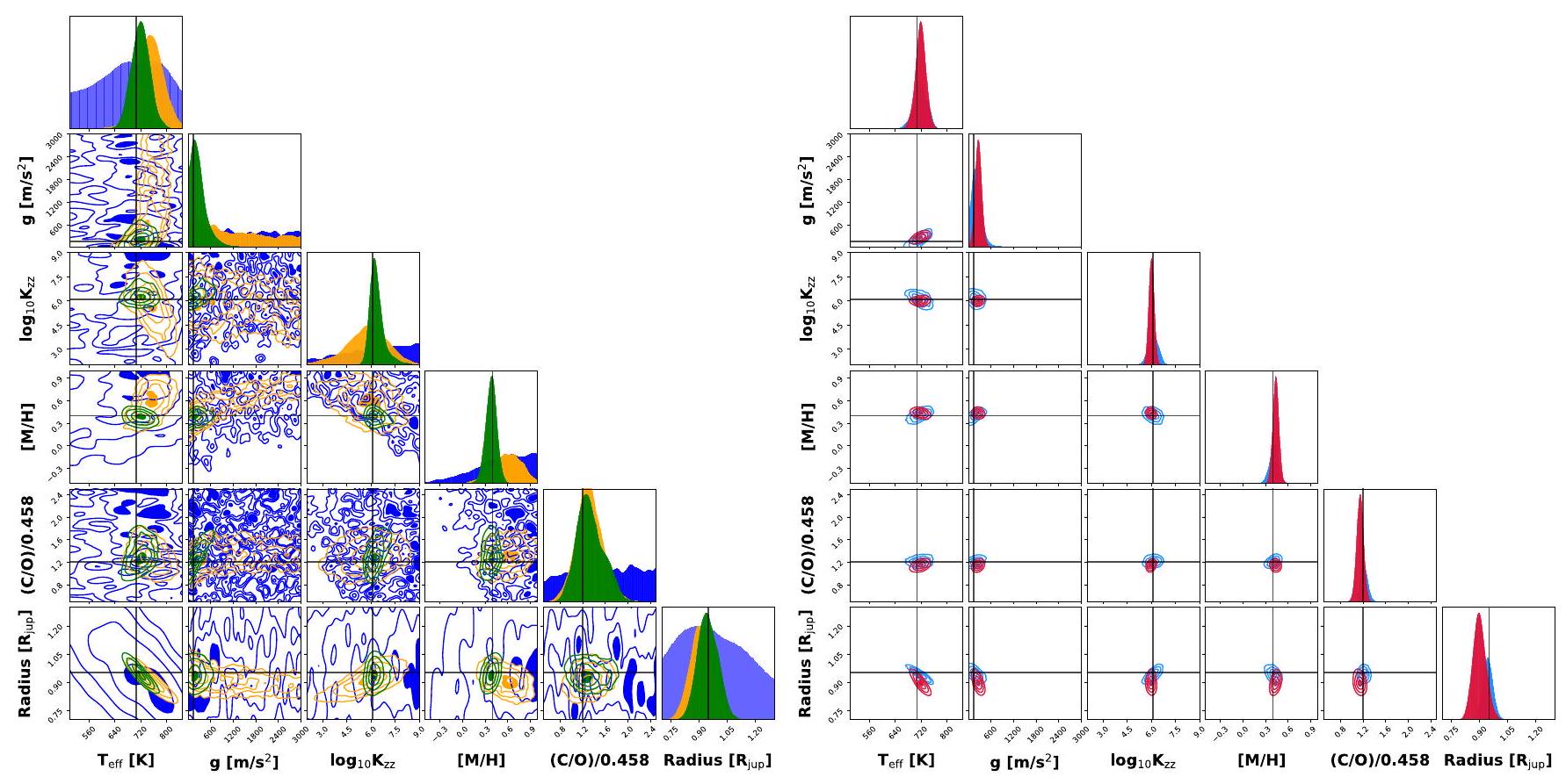
أولاً، نوضح كيف أن اختيار نطاقات الطول الموجي المختلفة والأدوات يؤدي إلى درجات متفاوتة من القيود على المعلمات الجوية مثل أو . عادةً، الـتم استخدام منطقة الطول الموجي (حزام M) لتقييد الأمور غير المؤكدة للغايةفي أجواء الأقزام البنية (على سبيل المثال، مايلز وآخرون 2020؛ موكيرجي وآخرون 2022). ومع ذلك، غالبًا ما تجاهلت هذه الجهود تأثير تغير المعدنية أوبالإضافة إلى التفاوتفي الطيف في نافذة الطول الموجي هذه. تُظهر الألواح العليا والوسطى في الشكل 7 كيف يُظهر طيف M-band تداخلًا بين تباين المعدنية و. لذلك، باستخدام شبكتنا، نقوم بفحص مدى قدرة طيف M-band فقط لنجم قزم بني على تقييد.
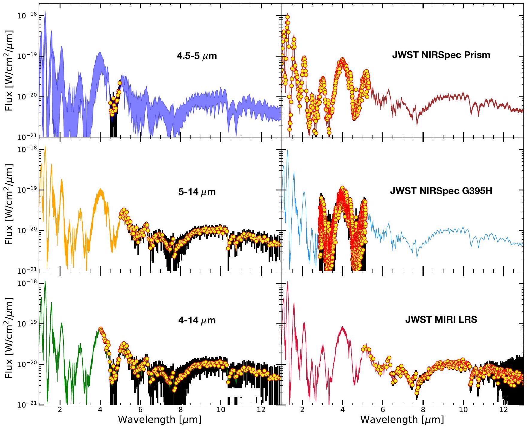
كمثال، نقوم بإنشاء طيف اصطناعي لجسم معشمسي )، ونصف القطر من شبكتنا المستخرجة. يمثل هذا الكائن المثال كائنًا غنيًا بالمعادن قليلاً من نوع القزم T المتأخر مع خلط جوي معتدل. نحن نختبر ستة سيناريوهات رصد مختلفة مع هذا الطيف الاصطناعي. لتمثيل بعض الملاحظات الأرضية أو الفضائية للأقزام البنية باستخدام أدوات مثلوبواسطة سبitzer، نقوم بمحاكاة طيف مشاهد اصطناعي عن طريق تقليل الدقة الطيفية لطيفنا الم interpolated إلىوإضافة ضوضاء بشكل مصطنع إلى البيانات من خلال الحفاظ على نسبة الإشارة إلى الضوضاء (SNR) تبلغ 5 عندمن الطيف الاصطناعي. نستخدم هذا الطيف الاصطناعي لفحص كيفية اعتماد القيود على هذه المعلمات على نطاقات الطول الموجي من خلال ملاءمة هذا الطيف الاصطناعي في نوافذ طول موجي مختلفة.، و . على الرغم من أن و لا تختلف الخيارات كثيرًا من حيث نطاق الطول الموجي، الإضافيتتميز الأطوال الموجية بخصائص امتصاص من CO وكلاهما حساس لـ والمعدنية. لتمثيل ملاحظات تلسكوب جيمس ويب (JWST) للأقزام البنية، نفترض أن القزم البني يقع على بعد 5 فرسخ فلكي ونستخدم حاسبة زمن التعرض الخاصة بـ JWST لمحاكاة نسبة الإشارة إلى الضوضاء في الطيف إذا تم رصده لمدة إجمالية تبلغ 30 دقيقة باستخدام وضع Prism في NIRSpec، ووضع G395H في NIRSpec، ووضع LRS في MIRI. تُظهر الشكل 11 نتائج ملاءمة الأطياف الاصطناعية في هذه السيناريوهات الستة المختلفة. يُظهر الشكل 12 الطيف الاصطناعي المرصود جنبًا إلى جنب مع أفضل نماذج الملاءمة لكل سيناريو. البيانات الاصطناعية الملائمة في كل حالة موضحة بالنقاط الصفراء مع الضوضاء الاصطناعية.تم أيضًا رسم أغلفة طيف النموذج المستمدة من التوزيعات البايزية التي تم الحصول عليها من خلال ملاءمة كل منطقة طول موجي في هذه اللوحات- خطوط الشكل 11 بألوان خطوط مختلفة. تظهر الشكل 11 تجميعًا لجميع الرسوم البيانية الزاوية التي تم الحصول عليها من خلال ملاءمة كل من هذه المناطق الطولية لمت spectra الاصطناعية. تظهر الرسوم البيانية الزاوية الموجودة في الجانب الأيسر توزيعات لاحقة من ملاءمة البيانات الاصطناعية والتي تمثل السيناريو النموذجي القائم على الأرض/AKARI/Spitzer. تظهر الرسم البياني الزاوي الأيمن التوزيعات اللاحقة التي تم الحصول عليها من خلال ملاءمة أنواع مختلفة من الملاحظات الممكنة معتم تمييز المعلمات الحقيقية التي تم إنشاء الأطياف الاصطناعية منها بخطوط سوداء صلبة في رسومات الزاوية.
تظهر المؤشرات الزرقاء في الزاوية اليسرى من الرسم النتائج الناتجة عن التوافق فقطجزء من الطيف الاصطناعي (M-band). التوزيعات الخلفية على، ، و المستمدة من نطاق M تظهر عدم يقين كبير. والأهم من ذلك،يبقى غير مقيد مع، و مع بيانات M-band. النتائج الموضحة باللون البرتقالي في الرسم البياني في الزاوية اليسرى هي نتائج التوفيق لـنافذة الطيف الاصطناعي. القيود على جميع المعلمات أفضل بكثير مع هذه النطاقات الطولية مقارنةً بتناسب بيانات نطاق M فقط. على عكس بيانات نطاق M، يمكن أن يقيد هذا النطاق الطولي، و . ومع ذلك، مثل نطاق M-، لا يمكن لهذا النطاق الطيفي بعد أن يقيّدتم تحقيق تحسين كبير في القيود على جميع المعلمات من خلال ملاءمة البيانات من. يتم عرض هذه الخلفيات باللون الأخضر. يسمح هذا النطاق الطيفي بتقييد جميع المعلمات، بما في ذلك تكون التوزيعات الخلفية لجميع المعلمات أكثر دقة وموثوقية مقارنةً بـ Mband (الأزرق) و (الخلفيات) الخضراء.
تم الحصول على المؤخرات الملونة باللون الأزرق السماوي في الزاوية اليمنى من الرسم البياني في الشكل 11 من خلال ملاءمة الاصطناعيطيف NIRSpec G395H لنفس الجسم. نظرًا للدقة الطيفية الأعلى ونسبة الإشارة إلى الضوضاء الأعلى لمثل هذه الملاحظات، فإن القيود المستخلصة منها أكثر دقة من السيناريوهات التي تم مناقشتها أعلاه. القيود على المعلمات من ملاءمة طيف MIRI LRS الاصطناعي موضحة بألوان قرمزية وهي مشابهة في الدقة لتلك المستخلصة من بيانات NIRSpec G395H. التقديرات اللاحقة المستخلصة من ملاءمة بيانات NIRSpec Prism موضحة أيضًا في الرسوم البيانية في الزاوية اليمنى ولكنها ضيقة جدًا ودقيقة بالنسبة لنطاق قيم المعلمات الموضحة في الشكل 11. الدقة العالية للقيود القابلة للتحقيق معتعود ملاحظات NIRSpec Prism إلى نسبة الإشارة إلى الضوضاء الأعلى التي يتم تحقيقها ضمن نفس زمن التعرض مع وضع هذه الأداة مقارنةً بالوضعين الآخرين.أنماط الأدوات المستكشفة هنا. النطاق الواسع من الأطوال الموجية لـتعتبر عدسة NIRSpec أيضًا عاملًا رئيسيًا وراء القيود الدقيقة القابلة للتحقيق مع هذا الوضع. تظهر الشكل 11 أن ملاءمة بيانات النطاق M عند Rلا يؤدي وحده إلى الحصول على معايير جوية مقيدة. على الرغم من أن هذه النتيجة صحيحة فقط إذا لم تكن هناك معلومات إضافية متاحة حول المعايير المختلفة من ملاحظات أخرى مثل الفوتومترية. ملاءمة الأطياف بينيوفر قيودًا ذات مغزى على، و لكنلا يزال غير مقيد. تناسب الأطياف بينيمكن أن يقيد جميع المعلمات الجوية المدروسة هنا، بما في ذلك، مع تقييدات أكثر صرامة على المعلمات الأخرى. يمكن الحصول على مثل هذه القيود من خلال ملاءمة بيانات AKARI و Spitzer معًا. كما تظهر الشكل 11
الشكل 11. يوضح الرسم في الزاوية اليسرى التوزيعات البعدية لـالجاذبية، ( الشمسية)، ونصف القطر عندما يتم ملاءمة مناطق الطول الموجي المختلفة لمجموعة بيانات اصطناعية باستخدام نهج ملاءمة الشبكة بايزي مع شبكة بومة سونورا إلف. يوضح الرسم البياني في الزاوية اليمنى التوزيعات اللاحقة عندما يتم ملاحظة نفس الطيف الاصطناعي مع أوضاع أدوات مختلفة من. تُظهر الألواح الستة في الشكل 12 مجموعة البيانات الاصطناعية المستخدمة في هذا التحليل للحصول على التوزيعات اللاحقة الموضحة في الرسوم البيانية الزاوية. الرسم البياني الزاوي الأيسر: تُظهر التوزيعات اللاحقة الزرقاء متى كانت الأطياف الاصطناعية بينمناسب بينما تمثل الأجزاء الخلفية البرتقالية ملاءمة البيانات الاصطناعية بين. تظهر النتائج الخضراء من التوافق مع المناطق، على التوالي. الرسم البياني في الزاوية اليمنى: تظهر الألوان الزرقاء السماوية والقرمزية النتائج عند استخدام بيانات اصطناعية منتم تركيب NIRSpec G395H و MIRI LRS، على التوالي. تظهر الخلفيات البنية القيود المستمدة من بيانات Prism الاصطناعية. الخلفيات المستمدة من بيانات Prism ضيقة جداً بالنسبة لنطاق المعلمات المعروضة في مخططات الزاوية. تظهر الخطوط السوداء في مخطط الزاوية القيم الحقيقية للمعلمات المستخدمة لإنتاج بيانات الطيف الاصطناعية.
القيود الممكن تحقيقها معالبيانات أكثر دقة من تلك المستمدة من هذه الأدوات الأخرى. نستخدم هذه النتائج من تمرين ملاءمة طيفنا الاصطناعي لتطبيق نماذجنا على عينة صغيرة من الأقزام البنية التي تحتوي على بيانات طيفية تحت الحمراء محفوظة.
5.1. ملاءمة الطيف المرصود مع نموذج شبكة بومة سونورا إلف
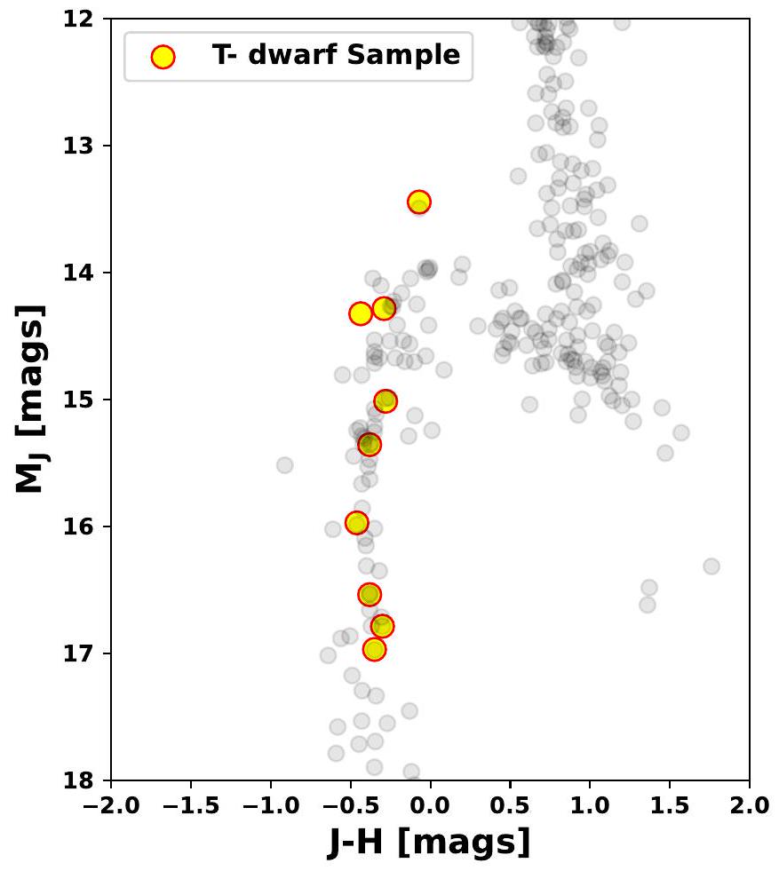
قمنا بتناسب أطياف 9 قزم T من المبكر إلى المتأخر مع شبكة نموذج Elf Owl لتقييم معاييرها الجوية. العينة موضحة في مقابل -H مخطط اللون-القدر الموضح في الشكل 13 وتم اختياره ليغطي جميع أنواع الطيف من الأقزام T بدءًا من الأقزام T المبكرة إلى المتأخرة. تغطي شبكتنا المعلمات لجميع الفئات الطيفية من L إلى الأجسام من نوع Y، لكننا اخترنا هذا النوع الطيفي لتناسب شبكتنا حيث من المتوقع أن تكون السحب في أجواء الأقزام T تحت مستوى الفوتوسفير القابل للرصد. نستبعدنستبعد الأجسام الانتقالية من عينتنا لأنها قد تحتوي أيضًا على سحب كثيفة بصريًا في صورها الشمسية، بينما شبكة بومة الجان هي خالية من السحب.
نستخدم فقط قياسات الطيفية المستندة إلى الفضاء المتاحة لهذه الأجسام باستثناء GL570D، حيث يمكن أن تتلوث الطيفية المستندة إلى الأرض لجو الكواكب تحت النجمية غالبًا بامتصاص من الغلاف الجوي للأرض نفسها، خاصة في نطاقات الامتصاص الجزيئية. بالنسبة لـ GL570D، فإن الطيفية المستندة إلى الأرض المتاحةالطيف من جيبال وآخرون (2009) لديه نسبة إشارة إلى ضوضاء أعلى بشكل ملحوظ منطيف في تلك الموجة- نافذة الطول. لذلك، نحن نستبدل الـ البيانات مع البيانات المستندة إلى الأرض لـ GL570D فقط بين استنادًا إلى النتائج الموضحة في الشكل 11، قمنا بتناسبطيف الكائنات التي تتوفر لها كل من ملاحظات أكاري وسبitzer. نحن فقط نقوم بتناسب الـطيف سبitzer لأجسام أخرى لا تتوفر لها ملاحظات في نطاق M بشكل علني. نستخدم أولويات موحدة على جميع المعلمات الجوية مشابهة لما هو مذكور في §5. العينة لـ، و سمح لنا بالذهاب قليلاً إلى ما وراء حدود شبكتنا الجوية، على سبيل المثال،كان مسموحًا بالتغير بين 0.5 إلى 9.5 (في نظام السنتيمتر-غرام-ثانية) على الرغم من أن حدود الشبكة هيلـفي تحليلنا، لا نأخذ في الاعتبار أيضًا أي انحرافات منهجية قد تكون ناتجة عن اختلافات في معايرة التدفق عبر أدوات مختلفة مثلو سبitzer.
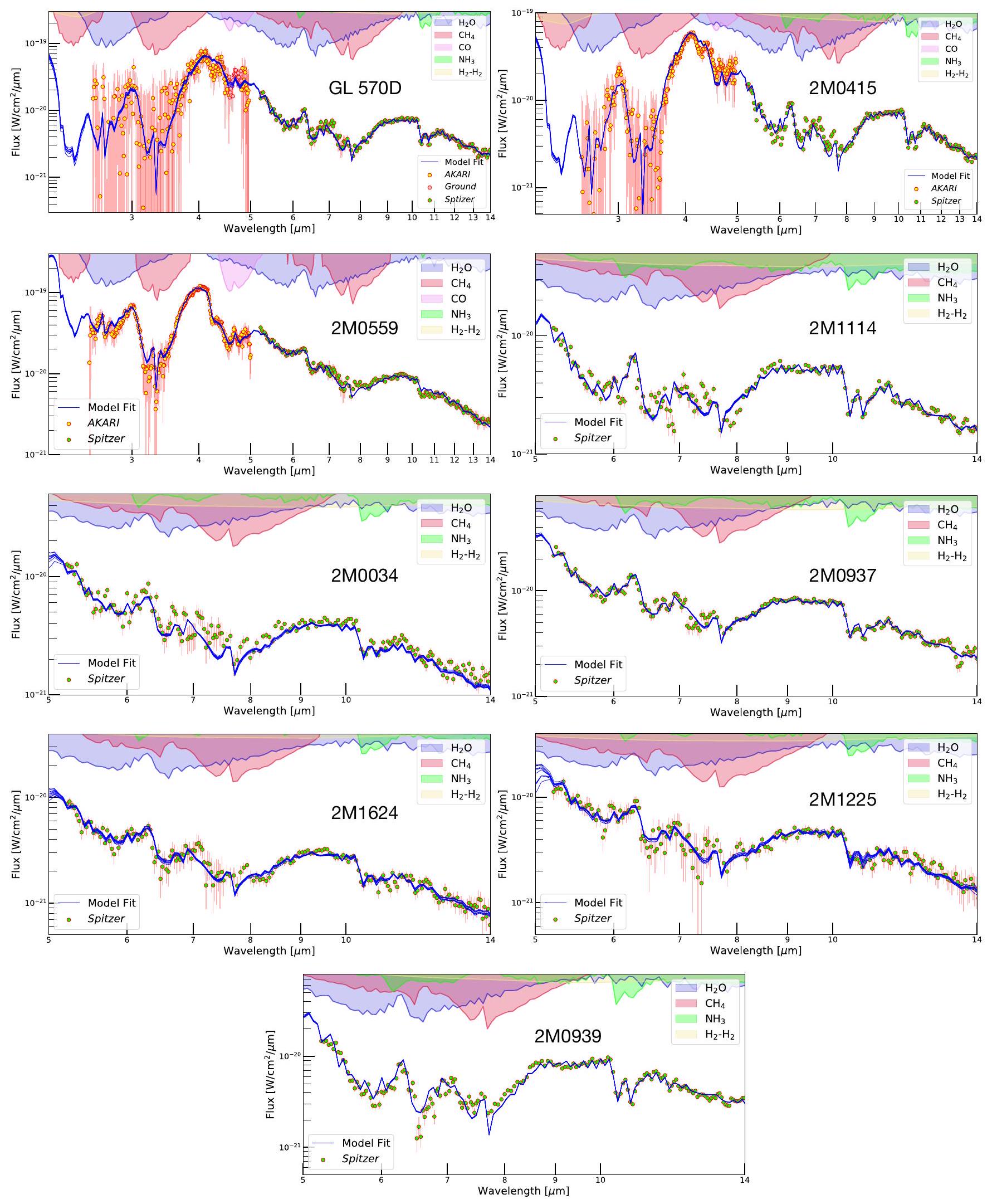
تظهر الأشكال 14 الطيف المرصود جنبًا إلى جنب مع أفضل نماذج الطيف الملائمة لكل كائن في كل لوحة. تُظهر البيانات من أدوات مختلفة علامات ملونة مختلفة في كل لوحة. يتم عرض 100 نموذج تم سحبه عشوائيًا من الخلفيات المتقاربة لكل كائن بخطوط زرقاء في جميع لوحات الشكل 14. لتحديد الممتصات الغازية الجوية السائدة في كل منطقة طول موجي، نعرض أيضًا مستوى الضغط كدالة لطول الموجة للمكونات الغازية السائدة في أفضل نموذج جوي لكل كائن.مستويات الضغط هي لأغراض توضيحية وتظهر مع محور ضغط مقلوب في الجزء العلوي من كل لوحة. على سبيل المثال، بالنسبة لـ GL570D في
الشكل 12. تُظهر الألواح الستة مجموعة البيانات الاصطناعية المستخدمة في هذا التحليل للحصول على التوزيعات البعدية الموضحة في الرسوم البيانية في الشكل 11. يُظهر اللوح العلوي الأيسر الأطياف الاصطناعية بينبينما يُظهر اللوح الأوسط الأيسر البيانات الاصطناعية بينتظهر اللوحة السفلية اليسرىمنطقة الطيف الاصطناعي. تُظهر اللوحات العلوية والوسطى اليمنى البيانات الاصطناعية منمشتت NIRSpec و NIRSpec G395H، على التوالي. تُظهر اللوحة السفلية اليمنى الطيف الاصطناعي من ميري LRS. كل لوحة تظهر أيضًا غلاف على الطيف من التوزيعات الخلفية الملائمة.
في الشكل 14، نجد أن الممتص السائد بين 7 هو (أحمر قرمزي مظلل)، بين هو CO (مظلل باللون الوردي)، بين هو (مظلل باللون الأزرق)، وبين هو (المظللة باللون الأخضر). نحصل على مخطط زاوية لجميع هذه الكائنات مشابه للمخطط الزاوي الموضح في الشكل 11.
توضح الجدول 3 الأجسام التي تم تحليلها في هذا العمل وأفضل المعلمات الجوية التي تم الحصول عليها من خلال ملاءمة طيفها بين أو البيانات. الأخطاء المذكورة في كل من هذه المعلمات المقدرة هيحدود على التوزيعات الخلفية للمعلمات التي تم الحصول عليها من عملية التناسب لدينا. نلاحظ أن أشرطة الخطأ على المعلمات التي تم الحصول عليها من إجراء التناسب لدينا تتجاهل عدم اليقين الناتج عن التداخل الطيفي في شبكتنا. من المعروف أن مثل هذه الأخطاء تكون كبيرة، خاصة بالنسبة للبيانات الطيفية ذات الدقة العالية أو نسبة الإشارة إلى الضوضاء العالية (على سبيل المثال، زانغ وآخرون 2021). ومع ذلك، فإن مجموعات البيانات التي قمنا بتناسبها لها دقة طيفية نموذجية من ونوع- إشارة إلى نسبة الضوضاء القصوى حوالي 100. لذلك، من أجل البساطة، نتجاهل هذه الأخطاء في الاستيفاء في هذا العمل بينما يتم إعداد عمل لاحق ينفذ هذه الأخطاء باستخدام شبكة بومة الجانح باستخدام أداة STARFISH (Zhang et al. ، قيد الإعداد). الآن نفحص الاتجاهات التي نجدها بين المعلمات الملائمة.
5.2. الاتجاهات في
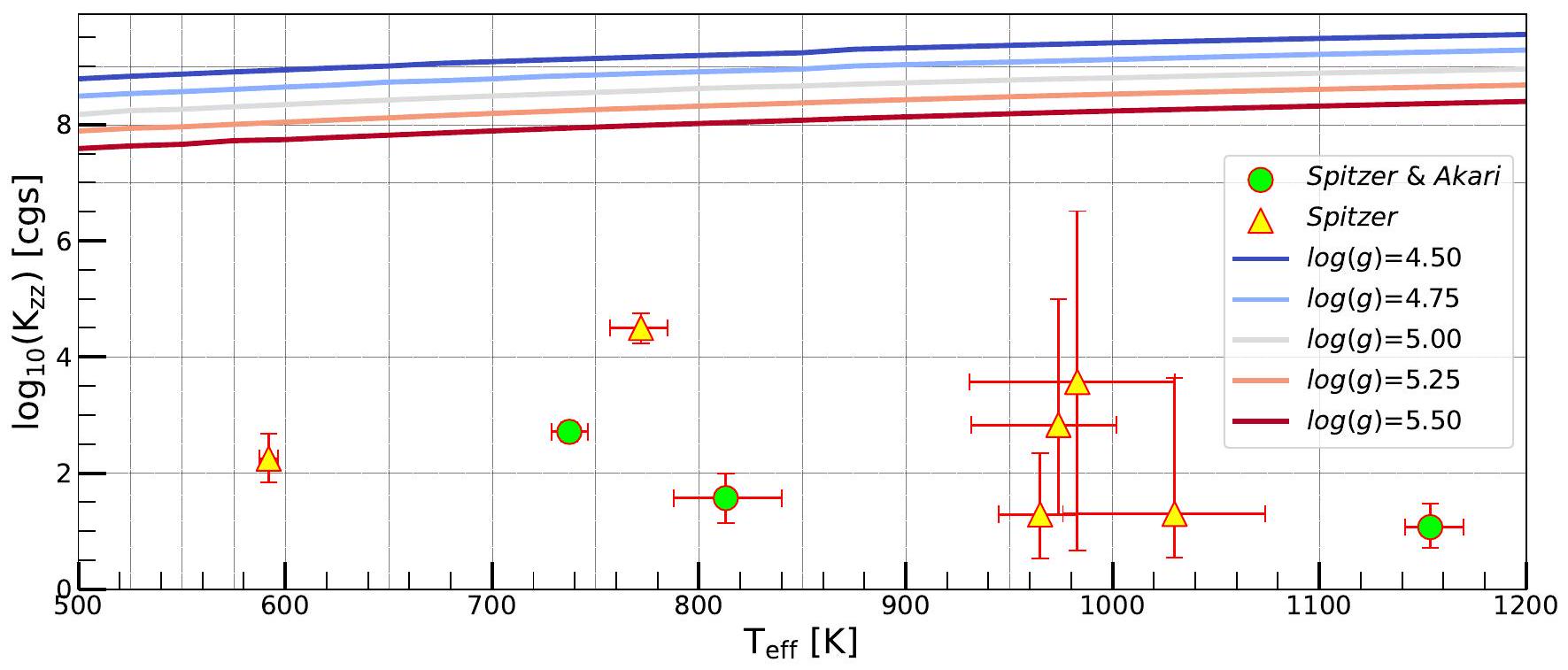
تظهر الشكل 15 الاستنتاجفي تحليلنا كدالة للمعطى المحددتم عرض الأجسام التي تم تقدير هذه المعلمات لها باستخدام بيانات AKARI و Spitzer بعلامات خضراء، بينما تم عرض الأجسام التي تم استخدام بيانات Spitzer فقط لها بعلامات صفراء. توضح الشكل 15 أن الاستنتاجاتبينفينطاق من.
هذا السلوك المنخفضبينتم رؤيته سابقًا في الأقزام البنية (على سبيل المثال، مايلز وآخرون 2020؛
معرّف الكائن
معرف مستخدم
آلة
[cgs]
[م/هـ]
عناية
نصف القطر
GL570D
GL570D
سبتزر 8 أكاري
2M0415
2M0415
سبتزر 8 أكاري
2M0559
2M0559
سبتزر 8 أكاري
2M1114
2M1114
سبايتزر
2M0034
2M0034
سبايتزر
2M0937
2M0937
سبايتزر
2M1624
2M1624
سبايتزر
2M1225
2M1225
سبايتزر
2M0939
2M0939
سبايتزر
الجدول 3 ملخص للمعلمات الأكثر ملاءمة التي تم الحصول عليها في هذا التحليل لمجموعة متنوعة من الأقزام البنية. البيانات المستخدمة هنا من AKARI هي من سوراهانا ويامامورا (2012) وبيانات سبitzer هي من سواريز ومتشيف (2022). بيانات نطاق M لـ GL570D هي من جيبال وآخرون (2009).
الشكل 13. مقابل يظهر مخطط اللون-القدر لسكان الأجسام تحت النجمية مع دوائر رمادية. عينة الأقزام T الخاصة بنا المكونة من 9 أجسام تظهر مع دوائر صفراء وتغطي بشكل موحد تقريبًا كامل تسلسل الأقزام T باستثناءأجسام الانتقال. جميع القيم المعروضة في هذا الرسم البياني هي قيم MKO. البيانات من Best وآخرون (2020).
موكيرجي وآخرون 2022) ومنخفضفي الكائنات بينتم التنبؤ به من قبل النماذج النظرية أيضًا (موكيرجي وآخرون 2022). استخدم مايلز وآخرون (2020) طيف M-band المستند إلى الأرض والفضاء لسلسلة من الأقزام T المتأخرة ووجدوا أن التقديرات منخفض بين معيظهر زيادة كبيرة مع انخفاضأقل من 500 ألف ميل. افترض ميلز وآخرون (2020) أن الانخفاض فيبين 500800 ك كان نتيجة لتبريد الغازات في منطقة إشعاعية عميقة محصورة حول هذهالقيم بينما تتوقف الغازات في المناطق الحملية للأجسام الأكثر برودة. استخدم موكيرجي وآخرون (2022) نماذج متسقة ذاتيًا لإظهار أن المناطق الإشعاعية المحصورة تظهر بالفعل بينعندما تكون الكيمياء غير متوازنة يتم معالجته بشكل ذاتي متسق. كما أظهر موكيرجي وآخرون (2022) أن الغازات يمكن أن تتوقف في هذه المناطق الإشعاعية المدمجة في هذانطاق يؤدي إلى انخفاضتقديرات. كما وجدوا أنه بالنسبة لـأعلى من 900 كلفن وأقل من 500 كلفن، يحدث التبريد بالغاز في المناطق الحملية ذات الحرارة العالية. ومع ذلك، الحد الأعلى فيالحد الأدنى الذي يمكن أن يحدث فيه إخماد المنطقة الإشعاعية يعتمد أيضًا على قوة الخلط في الغلاف الجوي العميق المتقلب (موكيرجي وآخرون 2022).
استخدمت كل من تحليل مايلز وآخرون (2020) وموكيرجي وآخرون (2022) نماذج تركيبية شمسية فقط. باستخدام المعدنية،، و شبكة بومة إلف سونورا التابعة، الشكل 15 يظهر أن الأجسام التيبينلا تزال تظهر منخفضة. هذا يشير بقوة إلى إخماد الغازات مثل أول أكسيد الكربون ويحدث في منطقة إشعاعية عميقة في هذا كلهنطاق. تظهر النماذج العددية المقدمة في موكيرجي وآخرون (2022) أنه إذا كانت فترة خلط الزمن في المناطق الحملية تتبع التوقعات من نظرية طول الخلط، فإن الأقزام T تميل إلى إظهار تقليل في منطقة الحمل.فوقمن. ولكن إذا كان الخلط في المنطقة الحملية أبطأ، فإنيمكن أن تستمر في الإخماد في المنطقة الإشعاعية على الأقل حتى1000 كلفن، والتي كانت حدود شبكة نمذجةهم. لاختبار حدود إخماد المنطقة الإشعاعية خارج حدود شبكة موكيرجي وآخرون (2022)، نقوم بتمديد شبكة نموذجهم المتسقة ذاتيًا إلى مستوى أعلى من 1500 ك. كلا اللوحين في الشكل 16 يوضحان وفرة ثاني أكسيد الكربون المتجمد كدالة لـ و كخريطة لونية. تُظهر اللوحة اليسرى نماذج حيث يتبع الخلط في المناطق الحملية نظرية طول الخلط، بينما تُظهر اللوحة اليمنى نماذج حيث يكون الخلط في المناطق الحملية أبطأ من التوقعات المستندة إلى نظرية طول الخلط. في هذه الحالة، تم تحقيق ذلك عن طريق تقليل طول الخلط في المنطقة الحملية بمقدار 10 مرات أقل من نظرية طول الخلط.
تظهر المناطق المخططة في كلا اللوحين الجزء من فضاء المعلمات حيث يتم إخماد CO في منطقة إشعاعية بدلاً من منطقة الحمل. كما تم العثور عليه سابقًا في موكيرجي وآخرون (2022)، يُظهر اللوح الأيسر من الشكل 16 أن إخماد CO في المنطقة الإشعاعية يحدث بين1000 كيلوجرام للأجسام ذات الجاذبية العالية، إذافي المنطقة الحملية يتبع نظرية طول الخلط. ولكن إذا كانت الحمليةأصغر من توقعات نظرية طول الخلط، توضح الشكل 16 أن إخماد CO في المنطقة الإشعاعية يحدث بينو1200 كيلوجرام أو أكثر اعتمادًا على جاذبية الجسم. هذا السيناريو الثاني بسهولة
الشكل 14. تُظهر الأطياف المرصودة لـ 9 أقزام T من عيّنتنا في اللوحات المختلفة. الملاحظات منمُظهَرة بدوائر صفراء، بينما تُظهِر بيانات سبitzer بدوائر خضراء. بالنسبة لـ GL570D، تم استخدام بيانات مأخوذة من الأرض أيضًا، والتي تُظهَر بدوائر وردية. في كل لوحة، تُظهَر الأطياف المحسوبة من 100 سحب عشوائي للمعلمات من توزيعاتها الخلفية المتقاربة أيضًا مع الخطوط الزرقاء. في أعلى كل لوحة، مستوى الضغط لكل غاز من النموذج الأفضل ملاءمة يظهر كدالة لطول الموجة. يتم عرض هذه المستويات الضغط فقط حتى يمكن ربط الميزات الطيفية في البيانات بالامتصاص الغازي الجوي السائد في النموذج الأفضل ملاءمة.تم الحصول على البيانات من سوراهانا ويامامورا (2012) وبيانات سبitzer من سواريز ومتشيف (2022). تم الحصول على البيانات الأرضية لـ GL570D من جيبال وآخرون (2009).
الشكل 15. أفضل ملاءمة مقابل يظهر لعينتنا من 9 أقزام T. تمثل الدوائر الخضراء الأجسام التي قمنا بتناسب الأطياف بينهابينما تمثل المثلثات الصفراء الأجسام التي من أجلهاتم ملاءمة البيانات مع نماذجنا. الخطوط الملونة تظهر النموذج المتوقع.كنتيجة لـمن نظرية طول الخلط بافتراض الحمل الحر في الغلاف الجوي العميق المتقلب. كل سطر يتوافق مع تظهر الخطوط الرمادية في الخلفية نقاط الشبكة الفعلية لشبكة بومة سونورا إلف. و بينما تم استيفاء الشبكة للحصول على النتائج.
الشكل 16. الاتجاهات فيالتبريد في المنطقة الإشعاعية أو الحملية كدالة لـ و يظهر هنا من نسخة موسعة من شبكة النموذج الذاتي المتسق المقدمة في موكيرجي وآخرون (2022). هذه النماذج لديهاتتفاوت عبر عمق الغلاف الجوي بدلاً من الثابتالنهج المستخدم في شبكة بومة سونورا القزمية ويكون نسبة الكربون إلى الأكسجين 0.45. تُظهر خريطة الألوان وفرة CO المطفأة كدالة لـ و في كلا اللوحين. اللوح الأيسر يصور نماذج حيثفي المنطقة الحملية، تتبع نظرية طول الخلط، بينما تُظهر اللوحة اليمنى نماذج حيث يكون طول الخلط في المنطقة الحملية أصغر من التوقعات من نظرية طول الخلط بعامل 10. المناطق المخططة تُظهر أجزاء من فضاء المعلمات حيث يتم إخماد CO في منطقة إشعاعية بدلاً من منطقة حملية.
يشرح الانخفاض الشديدوجدت في هذا العمل عبر مجموعة منكما هو موضح في الشكل 15 هو نتيجة لـالتبريد في المنطقة الإشعاعية عند هذهتظهر اللوحة اليمنى من الشكل 16 أيضًا أن الخلط في المنطقة الحملية يحتاج إلى أن يكون أقل حيوية من التوقعات المستندة إلى نظرية طول الخلط لـتمت دراستها باستخدام الأطياف لتكون منخفضة جداً بعد. ومع ذلك، فإن نماذج موكيرجي وآخرون (2022) والتوسعات التي أجريناها على تلك الشبكة تنطبق فقط على الأجواء ذات المعدن الشمسي. تُظهر هذه الدراسة أن المعدنية يمكن أن تصبح عاملاً مهماً جداً في تحديد هذه النطاقات فيالبيانات ذات نسبة الإشارة إلى الضوضاء الأعلى التي تم الحصول عليها بواسطةستساعد عينة أكبر من الأقزام T المدمجة مع هذه النماذج المتسقة ذاتيًا في إعادة تقييم هذا الاتجاه بدقة أعلى على كلا الجانبين. و .
المنطقة الإشعاعية المنخفضة جداًيمكن أن يكون للقيود على هذه الكائنات آثار كبيرة على فيزياء السحب في الكائنات التي تحتوي على بالقرب من حدود الانتقال. إذا كانت القيمة المنخفضة جداًقيموجدت لهذه الأجسام الأكثر برودة (إذا كانت ( ) ناتجة بالفعل عن إخماد المنطقة الإشعاعية، فإن هذا يعني أن الخلط في المناطق الإشعاعية لهذه الأجسام بطيء جداً. في مثل هذا السيناريو، قد يكون من الصعب جداً إبقاء جزيئات السحب من المكثفات مثل السيليكات عالياً بالقرب من الصور الفوتوغرافية لهذه الأجسام. هذه الآلية، بالإضافة إلى نقاط تكثف السحب التي تتحرك أعمق مع انخفاضيمكن أن يسرع من إزالة الغلاف الجوي للأقزام البنية مع برودتها تحت حدود انتقال L/T. كما يتنبأ الجانب الأيمن من الشكل 16 بزيادة حادة في القياسات.عندماأعلى من 1200 ك أو أكثر (اعتمادًا علىبسبب التحول من التبريدفي الغلاف الجوي الإشعاعي للأجسام الباردة إلى الغلاف الجوي الحملاني في الأجسام الأكثر حرارة. لكن الوجود المحتمل للسحب الفوتوسفيرية يعقد تفسيرمن الكيمياء فقط لهذه الأجسام الأكثر حرارة. نناقش هذا بمزيد من التفصيل في §6.1.
تتنبأ الشكل 16 أيضًا باعتماد قوي لسلوك إخماد المنطقة الإشعاعية مقابل المنطقة الحملية للغازات مثل CO وعلى جاذبية الجسم. وهذا يعني أنه بالنسبة للكواكب الخارجية التي تم تصويرها مباشرة والتي تتمتع بجاذبية أقل، على عكس الأقزام البنية، يجب أن نكون نستكشف الحمل الحراريخلال تسلسل Tنطاق ونتوقع رؤية قيم أعلى منفي أجوائهم. يجب ألا نتوقع على الإطلاق رؤية أي زيادة أو نقصان حاد في الإخماد.عبرأو يجب أن نرى التغيير الحاد ولكن لشيء أكثر برودة وضيقاًنطاق مثل هذه الأجسام. ستكون الملاحظات الخاصة بالكواكب الشابة التي تم تصويرها مباشرةً جنبًا إلى جنب مع الأقزام البنية ذات أهمية كبيرة في اختبار توقعات هذه النماذج.
6. المناقشة
6.1. السحب
لم نقم بتضمين أي تأثيرات للسحب في شبكة نموذجنا أو أثناء ملاءمة البيانات الرصدية في هذا العمل. من المعروف أن السحب موجودة في أجواء الأقزام البنية، والضغوط التي تتشكل عندها وعمقها البصري هي معلمات حاسمة تحدد ما إذا كانت ستؤثر على طيف القزم البني (على سبيل المثال، مورلي وآخرون 2012، 2014أ؛ أكرمان ومارلي 2001؛ مارلي وآخرون 2002؛ ساومون ومارلي 2008؛ بارمان وآخرون 2011؛ بورو وآخرون 2006؛ قاو وآخرون 2020؛ لايسي وبورو 2023؛ تشارني وآخرون 2018؛ كوبر وآخرون 2003). لقد أظهرت الألوان تحت الحمراء والبصرية بالفعل أن الأجسام القزمة من النوع L معقيم أعلى منلديها سحب سيليكات في الطبقة الضوئية وسحب حديدية (مثل، ساومون ومارلي 2008؛ مارلي وآخرون 2010؛ مايلز وآخرون 2022؛ مورلي وآخرون 2012؛ قاو وآخرون 2020). الأجسام التي تكون أبرد منمن المتوقع أيضًا أن يكون هناك 400 ألفالسحب (على سبيل المثال، مورلي وآخرون 2014a؛ لايسي وبوروز 2023). لذلك، قد لا تكون الجزء من شبكتنا فوق 1400 كلفن وتحت 400 كلفن كافية لتناسب طيف مثل هذه الأجسام ما لم تكن خالية من السحب بشكل غير عادي أو تحتوي على سحب رقيقة جداً من الناحية البصرية في غلافها الجوي أو حيث تؤثر كثافة السحب فقط على الجزء البصري/الأشعة تحت الحمراء القريبة من طيف الجسم.
الاتساق الذاتي هو جانب آخر مهم جداً من النماذج السحابية. تميل السحب إلى حبس الإشعاع الخارج في الغلاف الجوي في أطوال موجية أقصر، مما يتسبب في “احمرار” عام للطيف القابل للرصد (على سبيل المثال، مارلي وآخرون 2002؛ ساومون ومارلي 2008؛ مورلي وآخرون 2012، 2014ب). كما أن هذا يتسبب في تسخين الغلاف الجوي الأعمق. هذا السلوك هو عكس تأثيرعلىملف الغلاف الجوي، الذي يسبب الغلاف الجويملفات التعريف لتبريد (على سبيل المثال، الشكل 3 و 4) (كاراليدي وآخرون 2021؛ موكيرجي وآخرون 2022؛ فيليبس وآخرون 2020). لذلك، حتى في الأجسام التي تتشكل فيها السحب تحت صورها الضوئية، فإن الأجزاء الأعمق منيمكن تسخين الملف الشخصي. يمكن أن يؤدي ذلك إلى تغييرات في وفرة الغازات مثلفي الغلاف الجوي العميق. كمايستخرج الغازات من الغلاف الجوي الأعمق، ويمكن أن يؤدي تغيير في كيمياء الغلاف الجوي العميق بسبب السحب إلى تغييرات في وفرة الغازات في الطبقة الضوئية المطفأة. في هذه السيناريوهات، على الرغم من أن السحب لا تؤثر بشكل مباشر على قوة الميزات الطيفية، إلا أنها قد تؤثر عليها بشكل غير مباشر من خلال تسخين الغلاف الجوي الأعمق. لقد تجاهلت النماذج في شبكتنا هذه التأثيرات أيضًا من أجل البساطة في هذا العمل. تتنبأ الشكل 16 بزيادة حادة في القابلية للرصد.عبرمنلكن التحقق من ذلك بشكل ملاحظ من كائنات الانتقال L/T باستخدام شبكة خالية من السحب من النماذج قد يكون غير مناسب بسبب هذه التأثيرات غير المباشرة ولكن الكبيرة للسحب. لمعالجة هذه الفجوات في أدبيات النمذجة، نحن بالفعل نطور مجموعة من النماذج للأقزام البنية والكواكب الخارجية التي تعالج كل من السحب وكيمياء عدم التوازن بشكل متسق.
6.2. ثابتمع الضغط والانتشار الجزيئي
يفترض شبكة بومة سونورا القزمة قيمة ثابتة منفي جميع أنحاء الغلاف الجوي لكل نموذج. يتم تغيير هذه القيمة الثابتة عبر نطاق واسع. ومع ذلك، فإن السيناريو الأكثر واقعية سيكون لديهمتغير مع الضغط الجوي، مشابه للشكل 1 وما يُرى في أجواء كواكب النظام الشمسي (على سبيل المثال، زانغ وشومان 2018ب؛ موسى وآخرون 2005؛ فيشر وفغلي 2005). في هذا السيناريو الأكثر عملية،من المتوقع أن تكون مرتفعة في الأجزاء الحملية من الغلاف الجوي ومنخفضة في الأجزاء الإشعاعية من الغلاف الجوي. لقد تم استكشاف مثل هذا السيناريو وآثاره بالفعل من قبل موكيرجي وآخرين (2022) لجو ذو تركيب شمسي. واحدة من العواقب المهمة والمفيدة لمثل هذا السيناريو هي وفرة الغازات المختلفة التي تتبع عند ضغوط مختلفة. على سبيل المثال، إذا يطفئ عند ضغط مختلف عن CO، ثميجب أن يقيّد الوفرةعند ضغط مختلف عن أول أكسيد الكربون أو الوفرة. على الرغم من أن احتمال قياس تباين مع الارتفاع مثير للغاية للقادمالملاحظات، كيفيختلف معلا يزال الملف الشخصي في المنطقة الإشعاعية غير مؤكد (موكيرجي وآخرون 2022؛ بارمنتير وآخرون 2013؛ موسيس وآخرون 2021؛ كوماتشيك وآخرون 2019). لذلك، لجعل شبكة بومة سونورا المرنة أكثر ملاءمة لتناسب الملاحظات، نتجاهل التغير فيمعالملف الشخصي في هذا العمل.
آخر تبسيط لثابتالنهج هو التأثير على الانتشار. اعتمادًا على قيمةعند الضغوط الأقل من ضغط الهوموبوز، تصبح الانتشار الجزيئي العملية السائدة التي توجه كيمياء الغلاف الجوي بدلاً من الخلط (تساي وآخرون 2017، 2021؛ زاهنل ومارلي 2014). يبدأ ارتفاع المقياس لكل غاز في الغلاف الجوي بالاعتماد على كتلته الجزيئية بدلاً من الكتلة الجزيئية المتوسطة للغلاف الجوي عند الضغوط الأقل من ضغط الهوموبوز. إذا كان منخفض (على سبيل المثال، ) ثم قد يحدث الهوموبوز عند ضغوط أعلى بالقرب من الفوتوسفير في الغلاف الجوي (زانلي ومارلي 2014؛ تسائي وآخرون 2017). ومع ذلك، في سيناريو أكثر واقعية، في الغلاف الجوي العلوي من المتوقع أن تزداد بسبب العمليات الديناميكية مثل كسر موجات الجاذبية التي تدفع الهوموبوز عند ضغوط أقل (بارمنتير وآخرون 2013؛ زانغ وشومان 2018ب؛ موكيرجي وآخرون 2022؛ فريتاغ وآخرون 2010؛ تان 2022). لذلك، في شبكة بومة سونورا إلف نتجاهل هذا التأثير الناتج عن الانتشار الجزيئي حتى في المنخفضنماذج.
7. الملخص والاستنتاجات
نقدم في هذا العمل شبكة بومة سونورا القزمية، والتي تتضمن نماذج جوية كيميائية غير متوازنة خالية من السحب ومتسقة ذاتيًا تغطي مساحة كبيرة من المعلمات.، و نسبة. تم حساب هذه النماذج باستخدام كود النمذجة الجوية مفتوح المصدر PICASO وتطبق على الغلاف الجوي للكواكب الخارجية التي يتم تصويرها مباشرة والتي تهيمن عليها الهيدروجين والغلاف الجوي للأقزام البنية. تلتقط الشبكة التغيرات فيمن و من. تتضمن الشبكة أيضًا تباينات في منفي الأجواء ذات المعدنية من تحت الشمس إلى فوق الشمس مع تغير المعدنية منالطاقة الشمسية إلىقيم الطاقة الشمسية. بالإضافة إلى ذلك، نقوم بتغييرالنسبة من 0.229 إلى 1.14. وقد حللت الأعمال السابقة كيفتؤثر على هيكل الغلاف الجوي وطيف الأجسام دون النجمية باستخدام نماذج جوية متسقة ذاتيًا (مثل، هوبيني وبوروز 2007؛ كاراليدي وآخرون 2021؛ موكيرجي وآخرون 2022؛ فيليبس وآخرون 2020؛ لايسي وبوروز 2023). ومع ذلك، تم دراسة هذه التأثيرات في الغالب في الأجواء ذات التركيب الشمسي. ولكن بعيدًا عنتلعب التركيبة المعدنية الجوية ونسبة الكربون إلى الأكسجين أيضًا أدوارًا مهمة في تشكيل التركيب الكيميائي لكوكب أو قزم بني. تم إنشاء هذه الشبكة لفحص كيفيةالمعدنية، وتفاعل النسبة لتشكيلالملف، التركيب الكيميائي، وطيف الأجسام دون النجمية عبر مختلف و نسبة. نستنتج بالنقاط التالية من خلال استخدام وتحليل هذه الشبكة الواسعة من النماذج الجوية.
نحلل تأثير كيمياء عدم التوازن على الغلاف الجويملفات لعدة معدنيات تحت الشمسية إلى فوق الشمسية. كما هو موضح في الأعمال السابقة،أسبابالملفات الشخصية لتبريدها بالنسبة للنماذج التي تفترض التوازن الحراري الكيميائي. مع نمذجة متسقة ذاتيًا، نحن أظهر أن تبريد الـالملف هو دالة قوية من المعدنية الجوية في الشكل 3.
نجد أن تبريد الـالملف الشخصي بسببيعتمد أيضًا على نسبة الكربون إلى الأكسجين في الغلاف الجوي ولكن بدرجة أقل من اعتماده على المعدنية في الغلاف الجوي (الشكل 4). لقد ربطنا هذا التبريد بـملفات مع الفروق في أعماق الغلاف الجوي البصرية بين الغلاف الجوي في التوازن الكيميائي وعدم التوازن بسبب تبريد الغازات مثل، و شركة CO.
نجد أنالقيمة التي تدور حولهاالملف الشخصي يظهر أقصى حساسية للتغيرات فييعتمد بشكل كبير على المعدنية الجوية. بالنسبة للأجواء الفقيرة بالمعادن، ملفات بين يظهر أقصى حساسية للتغيرات في. ومع ذلك، بالنسبة للغلاف الجوي الغني بالمعادن، فإنالملفات بين 500-1200 ك تظهر أقصى حساسية لـ (الشكل . نستنتج أن هذا الاتجاه مرتبط بظهور في الغلاف الجوي.
نحن نفحص كيف أن طيف الأجسام دون النجمية حساس لـ، المعدنية، ونسبة C/O في الشكل 7. نجد أنتظهر الأطياف أعلى حساسية للتغيراتوتغيير المعدنية. يمكن أن يؤدي ذلك إلى تداخلات بينوالكثافة المعدنية عندما يتم تحليل منطقة طول موجي صغيرة جدًا وأيضًا عندما لا تأخذ النماذج في الاعتبار تغير الكثافة المعدنية وبالإضافة إلىبينما يتم ملاءمة البيانات الرصدية المتاحة والبيانات من أدوات حساسة جدًا مثل.
تتحكم المعدنية الجوية أيضًا في حساسية الطيف تجاهفي أماكن مختلفةالقيم، كما هو موضح في الأشكال 8 و 9. على سبيل المثال، بالنسبة لـالأجسام ذات المعدنية الشمسية،تظهر ميزة الامتصاص في نطاق L حساسية عالية لـبينقيم من 1900 ك إلى 450 ك. لكن بالنسبة لـالأجسام ذات المعدنية الشمسية،تظهر نطاق الامتصاص حساسية لـبين 1400 ك إلى 275 ك. سلوك مشابه يُلاحظ أيضًا في اعتماد الـفرقة CO إلى.
نستخدم شبكة بومة سونورا إلف لاختبار كيف تؤدي نطاقات الطول الموجي الطيفي المختلفة إلى قيود على معلمات جوية مختلفة. نجد أن فرض القيودالمعدنية، ومن الصعب التوافق فقط مع طيف M-band منخفض الدقة. ومع ذلك، تظهر الشكل 11 أن توافق نطاقات الطول الموجي الأخرى مثل و ، أو يمكن أن تؤدي الملاحظات إلى قيود صارمة جدًا على هذه المعلمات.
نستخدم هذه النماذج لتناسب أو راقبنا طيفي AKARI و Spitzer لـ 9 أقزام قزمة من نوع T، عينة من تسلسل الطيف من نوع T. نحن نقيد الـ، و من هذه الأشياء. بالنسبة للأشياء التي تحتوي على بين 5501150 كالقيم المحددة منخفضة جداً، تقع فيإلىالنطاق، كما هو موضح في الشكل 15.
قيودنا علىفيالنطاق مشابه لنتائج مايلز وآخرون (2020)، ولكن الآن مع نطاق أوسعنطاق. نسب موكيرجي وآخرون (2022) هذا الانخفاضإلى الغازات التي تتبخر في منطقة إشعاعية في هذهقيم مع نمذجة متسقة ذاتيًا. نحن نوسع شبكة النمذجة من موكيرجي وآخرون (2022) مع اعتماد العمق.إلىووجد أن منطقة الحمل الأكثر بطئًامن نظرية خلط الطول يمكن أن تفسر هذا التوقف الإشعاعي فيبقدر ما (الشكل 16).
هذا العمل يوضح أن التفاعل بينالمعدنية، وللتحكم في كيمياء الغلاف الجوي للكواكب الخارجية التي تم تصويرها مباشرة والأقزام البنية هو أمر معقد للغاية. نحن نحاول استكشاف هذه التعقيدات وفحص كيفية تأثير كل من هذه المعلمات على الملاحظات. ستساعد الشبكة الجوية المقدمة في هذا العمل بشكل كبير في تقييد جميع هذه الخصائص الجوية من بيانات عالية الإشارة إلى الضوضاء وعالية الدقة من تلسكوبات مثل. ومع ذلك، فإن جميع النماذج المقدمة هنا خالية من السحب، مما يحد من قابلية تطبيق هذه النماذج فقط على الأجسام الخالية نسبيًا من السحب. كعمل مستقبلي، نهدف إلى ترقية كود PICASO لمحاكاة السحب وكيمياء عدم التوازن في الوقت نفسه عبر مختلف المعدنيات وبالإضافة إلى ذلك، التأثير القوي للمعادن،، و علىالملف الشخصي ودرجة الحرارة الأعمق تشير إلى أن هذه النتائج سيكون لها أيضًا تأثيرات قوية على الحسابات التطورية للأقزام البنية والكواكب الخارجية التي تم تصويرها مباشرة. ومن المتوقع ذلك لأن درجة الحرارة الأعمق في الغلاف الجوي تتحكم في تبريد داخل هذه الأجسام، حيث من المتوقع أن تكون داخلها كاملة الحمل حراريًا بطبيعتها. كمامن المتوقع أن تقيس أكثر اللمعان دقة للأقزام البنية والكواكب الخارجية المصورة حتى الآن (على سبيل المثال، مايلز وآخرون 2022؛ بايلر وآخرون 2023؛ غرينباوم وآخرون 2023)، سنقوم بمتابعة هذا العمل مع جيل جديد من نماذج تطور بومة سونورا إلف، والتي تتماشى مع الأجواء في عدم التوازن الكيميائي عبر مختلف المعدلات المعدنية ونسب الكربون إلى الأكسجين.
8. الشكر والتقدير
تُقر SM بالدعم منبرنامج نظرية AR للدورة 2 GO PID-3245. كما يعترف SM بجائزة زمالة UC Regents لدعمه في هذا العمل. يعترف JJF بدعم من منحة NASA XRP رقم 80NSSC19K0446. يعترف JJF وCV وSM وRL بالدعم من برنامج نظرية AR للدورة 1 GO JWST PID-2232. يعترف MM وRL بالدعم من برنامج نظرية AR للدورة 1 GO JWST PID-1977. نعترف باستخدام حاسوب لوكس الفائق في جامعة كاليفورنيا سانتا كروز، الممول من منحة NSF MRI رقم AST 1828315. لقد استفاد هذا العمل من The UltracoolSheet فيhttp://bit.ly/UltracoolSheet، التي تم الحفاظ عليها بواسطة ويل بيست، ترينت دوبوي، مايكل ليو، روب سيفرد، وزوجيان زانغ، وتم تطويرها من تجميعات دوبوي وليو (2012)، دوبوي وكراوس (2013)، ليو وآخرون (2016)، بيست وآخرون (2018)، وبيست وآخرون (2021). نشكر المحكم المجهول على التعليقات المفيدة جداً التي ساعدت في تحسين جودة هذه المسودة.
Ackerman, A. S., & Marley, M. S. 2001, ApJ, 556, 872
Ahrer, E.-M., Stevenson, K. B., Mansfield, M., et al. 2022, arXiv e-prints, arXiv:2211.10489
Alderson, L., Wakeford, H. R., Alam, M. K., et al. 2022, arXiv e-prints, arXiv:2211.10488
Allard, F., Allard, N. F., Homeier, D., et al. 2007a, A&A, 474, L21
Allard, F., Homeier, D., & Freytag, B. 2012, Philosophical Transactions of the Royal Society of London Series A, 370, 2765
Allard, N. F., Kielkopf, J. F., & Allard, F. 2007b, European Physical Journal D, 44, 507
Allard, N. F., Spiegelman, F., & Kielkopf, J. F. 2016, A&A, 589, A21
Allard, N. F., Spiegelman, F., Leininger, T., & Molliere, P. 2019, A&A, 628, A120
Allen, M., Yung, Y. L., & Waters, J. W. 1981, Journal of Geophysical Research: Space Physics, 86, 3617
Amundsen, D. S., Tremblin, P., Manners, J., Baraffe, I., & Mayne, N. J. 2017, A&A, 598, A97
Azzam, A. A. A., Tennyson, J., Yurchenko, S. N., & Naumenko, O. V. 2016, Monthly Notices of the Royal Astronomical Society, 460, 4063
Bains, W., Pasek, M. A., Ranjan, S., et al. 2023, ACS Earth and Space Chemistry, 7, 1219
Barber, R. J., Strange, J. K., Hill, C., et al. 2014, MNRAS, 437, 1828
Bard, A., Kock, A., & Kock, M. 1991, A&A, 248, 315
Bard, A., & Kock, M. 1994, A&A, 282, 1014
Barman, T. S., Hauschildt, P. H., & Allard, F. 2001, ApJ, 556, 885
Barman, T. S., Konopacky, Q. M., Macintosh, B., & Marois, C. 2015, ApJ, 804, 61
Barman, T. S., Macintosh, B., Konopacky, Q. M., & Marois, C. 2011, ApJL, 735, L39
Barton, E. J., Yurchenko, S. N., & Tennyson, J. 2013, MNRAS, 434, 1469
Batalha, N. E., Marley, M. S., Lewis, N. K., & Fortney, J. J. 2019, ApJ, 878, 70
Beiler, S., Cushing, M., Kirkpatrick, D., et al. 2023, arXiv e-prints, arXiv:2306.11807
Bell, K. 1980, Journal of Physics B: Atomic and Molecular Physics (1968-1987), 13, 1859
Bell, K. L., & Berrington, K. A. 1987, Journal of Physics B: Atomic and Molecular Physics, 20, 801
Best, W. M. J., Dupuy, T. J., Liu, M. C., Siverd, R. J., & Zhang, Z. 2020, The UltracoolSheet: Photometry, Astrometry, Spectroscopy, and Multiplicity for 3000+ Ultracool Dwarfs and Imaged Exoplanets, doi:10.5281/zenodo. 4169085
Best, W. M. J., Liu, M. C., Magnier, E. A., & Dupuy, T. J. 2021, AJ, 161, 42
Best, W. M. J., Magnier, E. A., Liu, M. C., et al. 2018, ApJS, 234, 1
Bittner, D. M., & Bernath, P. F. 2018, VizieR Online Data Catalog, J/ApJS/235/8
Bjoraker, G. L., Larson, H. P., & Kunde, V. G. 1986, Icarus, 66, 579
Burgasser, A. J., Gerasimov, R., Bezanson, R., et al. 2023, arXiv e-prints, arXiv:2308.12107
Burrows, A., Ram, R. S., Bernath, P., Sharp, C. M., & Milsom, J. A. 2002, The Astrophysical Journal, 577, doi:10.1086/342242
Burrows, A., Sudarsky, D., & Hubeny, I. 2006, ApJ, 640, 1063
Calamari, E., Faherty, J. K., Burningham, B., et al. 2022, The Astrophysical Journal, 940, 164
Chamberlain, J. W., & Hunten, D. M. 1987, Theory of planetary atmospheres. An introduction to their physics andchemistry., Vol. 36
Charnay, B., Bézard, B., Baudino, J. L., et al. 2018, ApJ, 854, 172
Cooper, C. S., Sudarsky, D., Milsom, J. A., Lunine, J. I., & Burrows, A. 2003, ApJ, 586, 1320
Coppola, C. M., Lodi, L., & Tennyson, J. 2011, MNRAS, 415, 487
Drummond, B., Tremblin, P., Baraffe, I., et al. 2016, A&A, 594, A69
Dulick, M., Bauschlicher, C. W., J., Burrows, A., et al. 2003, ApJ, 594, 651
Dupuy, T. J., & Kraus, A. L. 2013, Science, 341, 1492
Dupuy, T. J., & Liu, M. C. 2012, ApJS, 201, 19
Fegley, Bruce, J., & Lodders, K. 1996, ApJL, 472, L37
Feinstein, A. D., Radica, M., Welbanks, L., et al. 2022, arXiv e-prints, arXiv:2211.10493
Fortney, J. J., Lodders, K., Marley, M. S., & Freedman, R. S. 2008, ApJ, 678, 1419
Fortney, J. J., Marley, M. S., & Barnes, J. W. 2007, ApJ, 659, 1661
Fortney, J. J., Marley, M. S., Lodders, K., Saumon, D., & Freedman, R. 2005, ApJL, 627, L69
Fortney, J. J., Visscher, C., Marley, M. S., et al. 2020, AJ, 160, 288
Freedman, R. S., Lustig-Yaeger, J., Fortney, J. J., et al. 2014, ApJS, 214, 25
Freedman, R. S., Marley, M. S., & Lodders, K. 2008, ApJS, 174, 504
Freytag, B., Allard, F., Ludwig, H. G., Homeier, D., & Steffen, M. 2010, A&A, 513, A19
Fuhr, J. R., Martin, G. A., & Wiese, W. L. 1988, Journal of Physical and Chemical Reference Data, 17
Gao, P., & Benneke, B. 2018, ApJ, 863, 165
Gao, P., Thorngren, D. P., Lee, G. K. H., et al. 2020, Nature Astronomy, doi:10.1038/s41550-020-1114-3
Geballe, T. R., Saumon, D., Golimowski, D. A., et al. 2009, ApJ, 695, 844
Gharib-Nezhad, E., Iyer, A. R., Line, M. R., et al. 2021a, ApJS, 254, 34
Gharib-Nezhad, E., Marley, M. S., Batalha, N. E., et al. 2021b, ApJ, 919, 21
GharibNezhad, E., Shayesteh, A., & Bernath, P. F. 2013, MNRAS, 432, 2043
Gierasch, P. J., & Conrath, B. J. 1985, in Recent Advances in Planetary Meteorology, ed. G. E. Hunt, 121-146
Gordon, I. E., Rothman, L. S., Tan, Y., Kochanov, R. V., & Hill, C. 2017, in 72nd International Symposium on Molecular Spectroscopy, TJ08
Gordon, I. E., Rothman, L. S., Hargreaves, R. J., et al. 2022, J. Quant. Spec. Radiat. Transf., 277, 107949
Greenbaum, A. Z., Llop-Sayson, J., Lew, B., et al. 2023, arXiv e-prints, arXiv:2301.11455
Hargreaves, R., Gordon, I., Huang, X., Conway, E., & Rothman, L. 2022, in American Astronomical Society Meeting Abstracts, Vol. 54, American Astronomical Society Meeting Abstracts, 217.01
Hargreaves, R. J., Hinkle, K. H., Bauschlicher, Charles W., J., et al. 2010, AJ, 140, 919
Harris, G. J., Tennyson, J., Kaminsky, B. M., Pavlenko, Y. V., & Jones, H. R. A. 2006, MNRAS, 367, 400
Helling, C., Oevermann, M., Lüttke, M. J. H., Klein, R., & Sedlmayr, E. 2001, A&A, 376, 194
Helling, C., Tootill, D., Woitke, P., & Lee, G. 2017, A&A, 603, A123
Hoch, K. K. W., Konopacky, Q. M., Theissen, C. A., et al. 2023, AJ, 166, 85
Huang, X., Gamache, R. R., Freedman, R. S., Schwenke, D. W., & Lee, T. J. 2014, Journal of Quantitative Spectroscopy and Radiative Transfer, 147, 134
Hubeny, I., & Burrows, A. 2007, ApJ, 659, 1458
Hunter, J. D. 2007, Computing in Science & Engineering, 9, 90
John, T. L. 1988, A&A, 193, 189
Karalidi, T., Marley, M., Fortney, J. J., et al. 2021, ApJ, 923, 269
Kluyver, T., Ragan-Kelley, B., Pérez, F., et al. 2016, in ELPUB, 87-90
Komacek, T. D., Showman, A. P., & Parmentier, V. 2019, The Astrophysical Journal, 881, 152
Lacy, B., & Burrows, A. 2023, ApJ, 950, 8
Lee, E., Dobbs-Dixon, I., Helling, C., Bognar, K., & Woitke, P. 2016, A&A, 594, A48
Lee, E. K. H., Tan, X., & Tsai, S.-M. 2023, MNRAS, 523, 4477
Lenzuni, P., Chernoff, D. F., & Salpeter, E. E. 1991, ApJS, 76, 759
Li, C., Zhang, X., Kammer, J. A., et al. 2014, Planet. Space Sci., 104, 48
Li, G., Gordon, I. E., Rothman, L. S., et al. 2015, ApJS, 216, 15
Line, M. R., Marley, M. S., Liu, M. C., et al. 2017, ApJ, 848, 83
Liu, M. C., Dupuy, T. J., & Allers, K. N. 2016, ApJ, 833, 96
Lodders, K. 2019, arXiv e-prints, arXiv:1912.00844
Lodders, K., & Fegley, B. 2002, Icarus, 155, 393
Lodders, K., Palme, H., & Gail, H. P. 2009, Landolt Börnstein, 4B, 712
Luna, J. L., & Morley, C. V. 2021, ApJ, 920, 146
Lupu, R., Freedman, R., Gharib-Nezhad, E., Visscher, C., & Molliere, P. 2021, Correlated k coefficients for H2-He atmospheres; 196 spectral windows and 1460 pressure-temperature points, doi:10.5281/zenodo. 7542068
Madhusudhan, N. 2012, ApJ, 758, 36
Madurowicz, A., Mukherjee, S., Batalha, N., et al. 2023, AJ, 165, 238
Mang, J., Gao, P., Hood, C. E., et al. 2022, arXiv e-prints, arXiv:2202.01355
Marley, M. S., & McKay, C. P. 1999, Icarus, 138, 268
Marley, M. S., Saumon, D., & Goldblatt, C. 2010, ApJL, 723, L117
Marley, M. S., Saumon, D., Guillot, T., et al. 1996, Science, 272, 1919
Marley, M. S., Seager, S., Saumon, D., et al. 2002, ApJ, 568, 335
Marley, M. S., Saumon, D., Visscher, C., et al. 2021, ApJ, 920, 85
McKemmish, L. K., Masseron, T., Hoeijmakers, H. J., et al. 2019, MNRAS, 488, 2836
McKemmish, L. K., Yurchenko, S. N., & Tennyson, J. 2016, MNRAS, 463, 771
McKinney, W. 2010, in Proceedings of the 9th Python in Science Conference, ed. S. van der Walt & J. Millman, 51-56
Meisner, A. M., Leggett, S. K., Logsdon, S. E., et al. 2023, Exploring the Extremes: Characterizing a New Population of Old and Cold Brown Dwarfs, doi:10.48550/ARXIV.2301.09817
Miles, B. E., Skemer, A. J. I., Morley, C. V., et al. 2020, AJ, 160, 63
Miles, B. E., Biller, B. A., Patapis, P., et al. 2022, arXiv e-prints, arXiv:2209.00620
Mizus, I. I., Alijah, A., Zobov, N. F., et al. 2017, MNRAS, 468, 1717
Morley, C. V., Fortney, J. J., Marley, M. S., et al. 2012, ApJ, 756, 172
Morley, C. V., Marley, M. S., Fortney, J. J., et al. 2014a, ApJ, 787, 78
. 2014b, ApJ, 787, 78
Moses, J. I., Fouchet, T., Bézard, B., et al. 2005, Journal of Geophysical Research (Planets), 110, E08001
Moses, J. I., Madhusudhan, N., Visscher, C., & Freedman, R. S. 2013, ApJ, 763, 25
Moses, J. I., Tremblin, P., Venot, O., & Miguel, Y. 2021, Experimental Astronomy, arXiv:2103.07023
Moses, J. I., Visscher, C., Fortney, J. J., et al. 2011, ApJ, 737, 15
Mukherjee, S., Batalha, N. E., Fortney, J. J., & Marley, M. S. 2023, ApJ, 942, 71
Mukherjee, S., Fortney, J. J., Batalha, N. E., et al. 2022, ApJ, 938, 107
Nair, H., Allen, M., Anbar, A. D., Yung, Y. L., & Clancy, R. T. 1994, Icarus, 111, 124
Noll, K. S., Geballe, T. R., & Marley, M. S. 1997, ApJL, 489, L87
O’Brian, T. R., Wickliffe, M. E., Lawler, J. E., Whaling, W., & Brault, J. W. 1991, Journal of the Optical Society of America B Optical Physics, 8, 1185
Ohno, K., & Fortney, J. J. 2023, ApJ, 946, 18
Oppenheimer, B. R., Kulkarni, S. R., Matthews, K., & van Kerkwijk, M. H. 1998, ApJ, 502, 932
Parmentier, V., Showman, A. P., & Lian, Y. 2013, A&A, 558, A91
Pérez, F., & Granger, B. E. 2007, Computing in Science & Engineering, 9
Phillips, M. W., Tremblin, P., Baraffe, I., et al. 2020, A&A, 637, A38
Polyansky, O. L., Kyuberis, A. A., Zobov, N. F., et al. 2018, MNRAS, 480, 2597
Prinn, R. G., & Barshay, S. S. 1977, Science, 198, 1031
Rothman, L. S., Gordon, I. E., Barber, R. J., et al. 2010, Journal of Quantitative Spectroscopy and Radiative Transfer, 111, doi:10.1016/j.jqsrt.2010.05.001
Rothman, L. S., Gordon, I. E., Babikov, Y., et al. 2013, Journal of Quantitative Spectroscopy and Radiative Transfer, 130, doi:10.1016/j.jqsrt.2013.07.002
Rustamkulov, Z., Sing, D. K., Mukherjee, S., et al. 2022, arXiv e-prints, arXiv:2211.10487
Ryabchikova, T., Piskunov, N., Kurucz, R. L., et al. 2015, Physica Scripta, 90, 054005
Saumon, D., & Marley, M. S. 2008, ApJ, 689, 1327
Saumon, D., Marley, M. S., Abel, M., Frommhold, L., & Freedman, R. S. 2012, ApJ, 750, 74
Saumon, D., Marley, M. S., Cushing, M. C., et al. 2006, ApJ, 647, 552
Sorahana, S., & Yamamura, I. 2012, ApJ, 760, 151
Sousa-Silva, C., Al-Refaie, A. F., Tennyson, J., & Yurchenko, S. N. 2014, Monthly Notices of the Royal Astronomical Society, 446, 2337
Speagle, J. S. 2020, MNRAS, 493, 3132
Suárez, G., & Metchev, S. 2022, arXiv e-prints, arXiv:2205.00168
Tan, X. 2022, Monthly Notices of the Royal Astronomical Society, 511, 4861
Tremblin, P., Amundsen, D. S., Mourier, P., et al. 2015, ApJL, 804, L17
Tsai, S.-M., Lyons, J. R., Grosheintz, L., et al. 2017, ApJS, 228, 20
Tsai, S.-M., Malik, M., Kitzmann, D., et al. 2021, ApJ, 923, 264
Varghese, A., Ratnasingam, R. P., Vanon, R., Edelmann, P. V. F., & Rogers, T. M. 2023, ApJ, 942, 53
Visscher, C. 2020, Journal of Geophysical Research (Planets), 125, e06526
Visscher, C., & Fegley, Bruce, J. 2005, ApJ, 623, 1221
Visscher, C., Lodders, K., & Fegley, Bruce, J. 2006, ApJ, 648, 1181
Visscher, C., & Moses, J. I. 2011, ApJ, 738, 72
Visscher, C., Moses, J. I., & Saslow, S. A. 2010, Icarus, 209, 602
Walt, S. v. d., Colbert, S. C., & Varoquaux, G. 2011, Computing in Science & Engineering, 13, 22
Wang, D., Lunine, J. I., & Mousis, O. 2016, Icarus, 276, 21
Wilzewski, J. S., Gordon, I. E., Kochanov, R. V., Hill, C., & Rothman, L. S. 2016, Journal of Quantitative Spectroscopy and Radiative Transfer, 168, 193
Woitke, P., Helling, C., & Gunn, O. 2020, A&A, 634, A23
Wong, M. L., Fan, S., Gao, P., et al. 2017, Icarus, 287, 110
Yadin, B., Veness, T., Conti, P., et al. 2012, MNRAS, 425, 34
Yung, Y. L., Drew, W. A., Pinto, J. P., & Friedl, R. R. 1988, Icarus, 73, 516
Yurchenko, S. N., Barber, R. J., & Tennyson, J. 2011, Monthly Notices of the Royal Astronomical Society, 413, 1828
Yurchenko, S. N., & Tennyson, J. 2014, Monthly Notices of the Royal Astronomical Society, 440, 1649
Yurchenko, S. N., Tennyson, J., Barber, R. J., & Thiel, W. 2013, Journal of Molecular Spectroscopy, 291, 69
Zahnle, K. J., & Marley, M. S. 2014, ApJ, 797, 41
Zalesky, J. A., Line, M. R., Schneider, A. C., & Patience, J. 2019, The Astrophysical Journal, 877, 24
Zalesky, J. A., Saboi, K., Line, M. R., et al. 2022, The Astrophysical Journal, 936, 44
Zhang, X., Liang, M. C., Mills, F. P., Belyaev, D. A., & Yung, Y. L. 2012, Icarus, 217, 714
Zhang, X., & Showman, A. P. 2018a, ApJ, 866, 1
-. 2018b, ApJ, 866, 1
Zhang, Z., Liu, M. C., Marley, M. S., Line, M. R., & Best, W. M. J. 2021, ApJ, 921, 95
Zhang, Z., Mollière, P., Hawkins, K., et al. 2023, arXiv e-prints, arXiv:2309.02488
THE SONORA SUBSTELLAR ATMOSPHERE MODELS. IV. ELF OWL: ATMOSPHERIC MIXING AND CHEMICAL DISEQUILIBRIUM WITH VARYING METALLICITY AND C/O RATIOS
Sagnick Mukherjee (D), Jonathan J. Fortney (D), Caroline V. Morley (D), Natasha E. Batalha (D), Mark S. Marley (D), Theodora Karalidi (D), Channon Visscher (D), Roxana Lupu , Richard Freedman , Ehsan Gharib-Nezhad (D) Department of Astronomy and Astrophysics, University of California, Santa Cruz, CA 95064, USA Department of Astronomy, University of Texas at Austin, Austin, TX 78712, USA NASA Ames Research Center, MS 245-3, Moffett Field, CA 94035, USA Lunar and Planetary Laboratory, The University of Arizona, Tucson, AZ 85721, USA Department of Physics, University of Central Florida, 4111 Libra Dr, Orlando, FL 32816, USA Chemistry & Planetary Sciences, Dordt University, Sioux Center, IA 51250, USA Center for Extrasolar Planetary Systems, Space Science Institute, Boulder, CO 80301, USA Eureka Scientific, Inc, Oakland, CA 94602 SETI Institute, NASA Ames Research Center, Moffett Field, CA 94035Draft version February 2, 2024
Abstract
Disequilibrium chemistry due to vertical mixing in the atmospheres of many brown dwarfs and giant exoplanets is well-established. Atmosphere models for these objects typically parameterize mixing with the highly uncertain diffusion parameter. The role of mixing in altering the abundances of C-N-Obearing molecules has mostly been explored for solar composition atmospheres. However, atmospheric metallicity and the ratio also impact atmospheric chemistry. Therefore, we present the Sonora Elf Owl grid of self-consistent cloud-free 1D radiative-convective equilibrium model atmospheres for JWST observations, which includes a variation of across several orders of magnitude and also encompasses sub-solar to super-solar metallicities and ratios. We find that the impact of on the profile and spectra is a strong function of both and metallicity. For metal-poor objects has large impacts on the atmosphere at significantly higher compared to metal-rich atmospheres where the impact of is seen to occur at lower . We identify significant spectral degeneracies between varying and metallicity in multiple wavelength windows, in particular at 3-5 . We use the Sonora Elf Owl atmospheric grid to fit the observed spectra of a sample of 9 early to late T – type objects from . We find evidence for very inefficient vertical mixing in these objects with inferred values lying in the range between . Using self-consistent models, we find that this slow vertical mixing is due to the observations probing mixing in the deep detached radiative zone in these atmospheres.
Keywords: Brown Dwarfs, T dwarfs, Y dwarfs, Atmospheric Composition, Extrasolar gaseous giant planets
1. INTRODUCTION
Exoplanet and brown dwarf atmospheres are primarily molecular due to their low temperatures and high pressures. The chemical composition of these atmospheres is dictated by the interplay between temperature- and pressure-dependant chemical reactions and atmospheric dynamical mixing processes.. The rates of molecular reactions are influenced by the atmospheric pressuretemperature structure and the inventory of chemical elements in the atmosphere. The atmosphere is said to be in chemical equilibrium if its chemistry is determined by thermochemical reactions based on the local pressure and temperature conditions. But processes like dynamical mixing can cause substellar atmospheres to deviate from chemical equilibrium (Fegley & Lodders 1996; Noll et al. 1997; Moses et al. 2011; Zahnle & Marley 2014; Tsai
et al. 2021; Lee et al. 2023) if mixing timescales are faster than the timescales of chemical reactions. However, dynamical mixing remains one of the most uncertain and poorly understood aspect of substellar atmospheres.
Dynamical mixing and its effects on atmospheric chemistry is a well-studied process in Solar System planetary atmospheres (e.g., Prinn & Barshay 1977; Yung et al. 1988; Bjoraker et al. 1986; Zhang & Showman 2018a; Zhang et al. 2012; Allen et al. 1981; Nair et al. 1994; Moses et al. 2005; Li et al. 2014; Visscher et al. 2010; Visscher & Moses 2011; Wong et al. 2017). However, as most brown dwarfs and strongly irradiated exoplanets belong to a very different temperature-pressure regime, dynamical processes in their atmospheres are still poorly understood.
1.1. Why is constraining important?
Atmospheric dynamics can transport gases and clouds/dust particles across several pressure scaleheights in the radial direction of substellar atmospheres (e.g., Parmentier et al. 2013; Tan 2022; Freytag et al. 2010). This process is often called vertical mixing. Under this assumption that this mixing can be modeled as a diffusion process, it is typically parameterized by the vertical eddy diffusion parameter is influenced by the rate of atmospheric turnover and heuristically can be understood as the product of the lengthscale over which mixing is occurring and the mixing velocity (Chamberlain & Hunten 1987). A high value of represents a very dynamically active atmosphere, whereas a low value represents a scenario with slow, inefficient mixing. In the convective parts of the atmosphere, the rate of mixing is expected to be linked with the convective energy flux, and indeed mixing length theory (MLT) provides estimates for (e.g., Gierasch & Conrath 1985; Ackerman & Marley 2001). In the radiative atmospheres, other dynamical processes, such as the breaking of atmospheric waves, can control the mixing and as a result, influence the value of .
A complete understanding of atmospheric dynamical mixing thus requires constraints on both in the convective and radiative parts of the atmosphere. Currently, in brown dwarf and exoplanet atmospheres remains uncertain by more than a factor of a million (Lacy & Burrows 2023; Mukherjee et al. 2022; Karalidi et al. 2021; Phillips et al. 2020; Fortney et al. 2020; Zahnle & Marley 2014; Hubeny & Burrows 2007; Barman et al. 2015). Theoretical estimates of profiles for a series of brown dwarf atmospheres with changing from Mukherjee et al. (2022) are shown in Figure 1, left panel. The right panel of Figure 1 shows the dependence of theoretical profiles on . These theoretical estimates show that can vary by orders of magnitude due to changes in both of these parameters. Moreover, in the same atmosphere, can vary by several orders of magnitude depending on whether a particular part of the atmosphere is radiative or convective in nature. Such variation of across radiative or convective regions is also seen in stellar models (e.g., Varghese et al. 2023). Figure 1 also shows that the position of convective and radiative zones can also be a strong function of both and .
Constraining is crucial to understand the physical nature of atmospheric dynamics operating in the deep atmospheres of brown dwarfs and exoplanets, as well as the implications for atmospheric chemistry and clouds, both of which have large imprints on the observed spectra of these objects. Atmospheric mixing dredges up gases from the deep atmosphere to the upper, visible atmosphere. If these gases are chemically destroyed faster than the typical timescale of mixing, then the atmosphere remains in thermochemical equilibrium. However, if the mixing process is faster than the chemical reaction timescales, then the upper atmosphere no longer remains in thermochemical equilibrium (Moses et al. 2011; Tsai et al. 2017, 2021; Zahnle & Marley 2014; Visscher & Fegley 2005; Visscher et al. 2006; Visscher & Moses 2011). This causes large changes in the chemical composition and optical depths of the observable photosphere thus changing the observable spectrum of the object (e.g., Phillips et al. 2020; Tremblin et al. 2015; Lacy & Burrows 2023; Karalidi et al. 2021; Mukherjee et al. 2022; Hubeny & Burrows
2007; Lee et al. 2023).
Vertical mixing can also transport gaseous vapor from the deeper atmosphere to the colder atmosphere where they can condense and form clouds (e.g., water clouds in Y-dwarfs, Fe clouds in L-dwarfs) (e.g., Ackerman & Marley 2001; Morley et al. 2014a, 2012; Saumon & Marley 2008; Woitke et al. 2020; Lacy & Burrows 2023; Freytag et al. 2010; Allard et al. 2012; Helling et al. 2017; Lee et al. 2016; Gao & Benneke 2018; Charnay et al. 2018; Cooper et al. 2003; Helling et al. 2001). Moreover, mixing can keep these cloud particles lofted in the photosphere by counteracting their gravitational settling. These lofted cloud particles “redden” the spectrum of substellar objects with their absorption and scattering opacities and also tend to heat up the deeper atmosphere by absorbing additional thermal radiation (e.g., Saumon & Marley 2008; Morley et al. 2012, 2014a; Luna & Morley 2021; Gao et al. 2020; Mang et al. 2022; Lee et al. 2016; Tan 2022). Even though it is highly uncertain, plays a major role in influencing the key atmospheric components of substellar objects like atmospheric chemistry, clouds, and the temperature-pressure ( ) structure (e.g., Drummond et al. 2016). With highly sensitive and stable instruments like , previous studies have shown that the dependence of atmospheric chemistry and clouds on can be leveraged to constrain itself (e.g., Miles et al. 2020; Karalidi et al. 2021; Mukherjee et al. 2022; Phillips et al. 2020).
Theoretical models have studied the effects of on the atmospheric chemistry and spectra previously for brown dwarfs and directly imaged planets with solar atmospheric composition. Karalidi et al. (2021) and Hubeny & Burrows (2007) have probed these effects with pressure-independent constant profiles for solar composition substellar atmospheres, whereas Phillips et al. (2020) have studied these effects at solar metallicity with pressure-independent but gravity dependant profiles. in the radiative regions can vastly differ from in the convective regions due to the completely separate turnover mechanisms operating in each regime. Mukherjee et al. (2022) explored the parameter space of solar-composition brown dwarf atmospheres and identified ways to measure in the radiative as well as convective atmosphere of these objects with . Lacy & Burrows (2023) explored a selfconsistent treatment of both water clouds and disequilibrium chemistry due to mixing for Y-dwarfs with solar and slightly sub- or supersolar metallicities. Using groundbased spectroscopic observations and solar composition atmospheric models, Miles et al. (2020) measured in a series of late T – and early Y – dwarfs and observed a sharp increase in at . It was hypothesized in Miles et al. (2020) that this low to high transition is due to the presence of “sandwiched” radiative zones in the deep atmospheres of objects with between , which was later theoretically confirmed in Mukherjee et al. (2022). This was a great demonstration of how constraining the uncertain can help us in gaining fundamental insights into the atmospheres of brown dwarfs and planets. However, not all brown dwarf atmospheres are expected to be of solar composition (e,g, Line et al. 2017; Zalesky et al. 2019; Zalesky et al. 2022; Meisner et al. 2023; Beiler et al. 2023; Hoch et al. 2023), and mixing-induced disequilibrium chem-
Figure 1. The left panel shows self-consistently calculated profiles as a function of pressure for a series of solar composition model atmospheres with from 1500 K to 400 K and . The in the convective zone has been calculated with mixing length theory whereas the in the radiative atmosphere follows the parameterization in Moses et al. (2021). The right panel shows the profiles for a 700 K model with varying between 4.5 and 5.5. The black dashed lines depict the constant profiles used in this work for sampling the several orders of magnitude range in values covered by these model calculations. Some colder models in the left panel with between show a sharp drop and rise in in the deep atmosphere which is indicative of the presence of a detached radiative zone in their atmospheres. Similar behaviour is also present in low gravity models shown in the right panel.
istry in non-solar composition atmospheres hasn’t been sufficiently explored.
1.2. Metallicity, Ratio, and
Bayesian retrieval studies of a growing population of brown dwarfs have revealed non-solar composition atmospheres. These range from very metal-poor atmospheres (e.g., Meisner et al. 2023; Zhang et al. 2021; Line et al. 2017; Zalesky et al. 2019; Zalesky et al. 2022; Burgasser et al. 2023) to objects with enhanced atmospheric metallicities (e.g., Zhang et al. 2021; Line et al. 2017; Zalesky et al. 2022; Zalesky et al. 2019; Zhang et al. 2023). Significant scatter in the atmospheric carbon-tooxygen (C/O) from sub-solar to super-solar values has also been established in the literature (e.g., Calamari et al. 2022; Zalesky et al. 2022; Zalesky et al. 2019; Line et al. 2017; Hoch et al. 2023). Published JWST observations of objects like VHS 1256b and HD 19467b already reveal strong signatures of chemical disequilibrium (Miles et al. 2022; Greenbaum et al. 2023; Beiler et al. 2023) in addition to ground-based and space-based observations of brown dwarfs obtained in the past two decades (e.g., Noll et al. 1997; Oppenheimer et al. 1998; Sorahana & Yamamura 2012; Miles et al. 2020; Madurowicz et al. 2023). Available and upcoming data from brown dwarfs and directly imaged planets are expected to show the presence of both vertical mixing induced disequilibrium chemistry and deviations from solar composition atmospheres.
Vertical mixing induces large changes in the photospheric abundances of gases like , , and by quenching their abundances in the deeper atmospheres. These gases are particularly affected due to vertical mixing as they have very long chemical reaction timescales. For example, the conversion of to or CO to requires the breaking
of strong molecular bonds. However, the abundances of all these gases are also sensitive to atmospheric metallicity and the C/O ratio. Elevated atmospheric metallicity leads to an increase in all these gases in the atmosphere to varying degrees, in particular for “metal-dominated” molecules like CO and . The ratio changes the relative abundance of various C – and O – bearing gases (e.g., Madhusudhan 2012; Moses et al. 2013). For example, a high ratio increases the abundance and decreases the abundance of O- bearing gases like in the atmosphere. Apart from changing the atmospheric chemistry, the metallicity, ratio, and also have impacts on the atmospheric profile due to enhanced or diminished atmospheric optical depths. Therefore, in order to constrain the metallicity, C/O ratio, and simultaneously from observations of brown dwarfs and directly imaged exoplanets, theoretical “self-consistent” radiative-convective models that include variations in , metallicity, and ratios are needed. Such atmospheric models are crucial for this purpose as all these three parameters impact the atmospheric profile. This can only be captured by self-consistent radiative-convective atmospheric models that calculate the chemistry, radiative transfer, and profile of atmospheres simultaneously by taking all the physical connections between these processes into account (e.g., Mukherjee et al. 2023; Phillips et al. 2020; Barman et al. 2001, 2011; Hubeny & Burrows 2007; Lacy & Burrows 2023).
In this work, we have used the open-sourced PICASO atmospheric model (Mukherjee et al. 2022; Batalha et al. 2019) to simulate the Sonora Elf Owl grid of selfconsistent cloud-free model atmospheres with vertical mixing induced chemical disequilibrium for directly im-
aged planets and brown dwarfs. Apart from the range in and values captured within the grid, it includes variation in across 7 orders of magnitude, variation in atmospheric metallicity from solar to solar values, and a variation of ratio from 0.22 to 1.14 . The range of variation in values is motivated by the large change in estimates from theoretical models between the radiative and convective zones in an atmosphere and also the large variation in theoretical estimates with both and (Figure 1).
Using this grid of models and by comparing it with existing space-based observational data from 9 sources, we address the following questions in this work:
What is the impact of on the profile of directly imaged planets and brown dwarfs at different metallicities and ratios?
How does impact the spectra of L-type, Ttype, and Y-type objects at sub-solar, solar, and super-solar metallicities and C/O ratios?
How do the absorption signatures of key gaseous absorbers like , and vary with , metallicity, and C/O ratio?
How do the measured from the available infrared spectroscopy of substellar objects vary with ?
We describe our model in §2. We present the key results from our model grid in §4 followed by application of this grid in §5. Our conclusions and discussions are presented in §6 and §7, respectively.
2. ATMOSPHERIC MODELING WITH PICASO 3.0
We use the open-sourced Python-based PICASO 3.0 atmospheric model (Mukherjee et al. 2023) to calculate the Sonora Elf Owl model grid. PICASO 3.0 has been widely used to model exoplanet and brown dwarf atmospheres (e.g., Rustamkulov et al. 2022; Alderson et al. 2022; Feinstein et al. 2022; Ahrer et al. 2022; Miles et al. 2022; Greenbaum et al. 2023; Mukherjee et al. 2022; Beiler et al. 2023). This model has legacy from the well known EGP model (Marley et al. 1996; Marley & McKay 1999; Marley et al. 2002; Saumon & Marley 2008; Fortney et al. 2005, 2008, 2007; Morley et al. 2014a; Karalidi et al. 2021). We only describe the latest upgrades of the model which are relevant to this work here and refer the reader to Mukherjee et al. (2023) for a detailed description of the full self-consistent atmospheric model.
The Sonora Elf Owl grid is five dimensional with varying , and ratios. Each model atmosphere is divided into 90 plane-parallel pressure layers (i.e., 91 levels or grid points) for computing the atmospheric structure in our models. The pressure corresponding to these layers are logarithmically spaced from the minimum to the maximum pressure of the model. The maximum pressure of each model is chosen carefully such that the atmosphere is opaque ( ) at all wavelengths at pressures less than the maximum pressure of the model. As atmospheric gaseous optical depths are inversely proportional to gravity, higher gravity models have higher maximum pressure values than lower gravity models. Therefore, the exact upper and
lower bounds of atmospheric pressure varies across our grid.
We use the quench time approximation to model the effect of on atmospheric chemistry (Prinn & Barshay 1977). The mixing timescale in each atmospheric layer is determined by,
where is the atmospheric pressure scale height of that atmospheric layer which is calculated using the layer temperature, layer pressure, mean molecular weight, and object gravity. We consider the quenching of , , and in our models. The net chemical reactions of these gases are (Zahnle & Marley 2014; Mukherjee et al. 2022),
For each of these net chemical reactions, we use the chemical timescale approach ( ) presented in Zahnle & Marley (2014). For , we use the chemical timescale approximation from Visscher & Fegley (2005) and Visscher et al. (2006). However, we note that large uncertainties in our understanding of phosphorus chemistry still remain today which will ultimately lead to uncertainties on its reaction timescales (e.g., Wang et al. 2016; Visscher 2020; Bains et al. 2023). We assume that these reaction timescales are independent of metallicity and ratio for simplicity. We think that this is a valid assumption because the uncertainty in quench pressures of various gases is mainly driven by the very large uncertainty in currently. The variations of chemical timescales of these gases with metallicity and C/O varying from slightly sub-solar to super-solar values are expected to be much smaller than this current uncertainty.
The of the above-listed reactions are compared to the layer for each atmospheric layer. The abundances of all the gases are allowed to follow chemical equilibrium values for all the deep pressure layers where . However, the abundances of the constituent gases are “quenched” at pressures smaller than the quench pressure ( ). The of each net chemical reaction is defined as the pressure at which of the relevant reaction is equal to . The abundances of the participating gases remain constant at the quenched value at pressures smaller than . Gases other than , and are allowed to follow chemical equilibrium throughout the atmosphere in all the models.
We use the equilibrium chemistry calculations presented in Lupu et al. (2021) for calculating the abundance of gases in thermochemical equilibrium. Equilibrium chemistry calculations at values , , and +1.0 were used for our grid, where
Atmospheric Mixing and Chemistry in Brown Dwarfs
Parameter
Range
Increment/Values
275 K to 2400 K
Increment- 25 K between Increment- 50 K between Increment- 100 K between
3.25 to 5.5
Increment- 0.25 dex
2 to
Values- 2,4,7,8, and 9
-1.0 to
Values- -1.0,-0.5,+0.0 Values-
C/O
0.22 to 1.14
0.22,0.458, 0.687, and 1.12
Table 1
Parameters of the Sonora Elf Owl Atmospheric Model Grid and their ranges covered in this work. corresponds to solar metallicity.
At each metallicity equilibrium chemistry tables corresponding to four ratios , and 1.14 – were used as inputs in our models (Solar C/O is assumed to be 0.458 (Lodders et al. 2009)). The solar elemental abundances from Lodders et al. (2009) are used as elemental abundances for the solar composition atmosphere. We note that the solar elemental abundances have been since updated by Lodders (2019). For consistency with our prior work for now we continue to use the Lodders et al. (2009) values. To change the C/O ratio, we keep fixed while the ratio of C and O are changed relative to their solar values. Then, to account for change in metallicity, all elemental abundances are multiplied with the metallicity factor. This makes sure that a changing doesn’t also change the atmospheric metallicity. The chemistry of all the gases at pressures larger than their are interpolated from these precalculated equilibrium chemistry tables.
We assume five different values ranging from to for our models. Unlike Mukherjee et al. (2022), but similar to Karalidi et al. (2021), the profiles here do not vary with atmospheric pressure. Figure 1 shows that this is a simplification of the more realistic case where varies substantially with atmospheric pressure depending on whether the atmosphere is locally radiative or convective. But as both the convective and radiative are very uncertain, we adapt this simplification here to explore trends in the atmospheric response to . We further discuss the effect of this assumption in §6.
To capture the effect of quenched gaseous abundances on the profile self-consistently, we mix the individual correlated-k opacities of all the atmospheric gases “on-the-fly” using the resort-rebin technique detailed in Amundsen et al. (2017). The correlated-k opacities of the following gases are weighted according to their equilibrium/quenched abundances during the model iterations and mixed “on-the-fly”- , , and FeH. Each model atmosphere is iterated until a predetermined convergence criterion described in Mukherjee et al. (2023) is met. The sources of various gaseous opacities used for calculating the grid are listed in Table 2. The opacity data incorporated into these models are computed using the most recent updates from both laboratory and ab initio studies. The temperature and broadening coefficients are relevant to the objects under study. For an in-depth discussion regarding the accuracy of these line lists and their comparison to other versions, we refer the reader to Gharib-Nezhad et al. (2021a). The thermal emission
spectra between 0.5 and is computed from the converged atmospheric model with the radiative transfer routines in PICASO (Batalha et al. 2019). These spectra are computed at a spectral resolution (R) of 5000.
Our five dimensional atmospheric model grid includes 43,200 distinct models. All these models are publicly available for download at accompanied by modeling and analysis tutorial scripts. Table 1 summarizes the five parameters which have been varied in our model grid along with the ranges and increments used for each parameter. The chosen ranges and increments in most of the parameters are kept similar to the previous set of Sonora grids (e.g., Marley et al. 2021; Karalidi et al. 2021).
3. THE SONORA MODEL SERIES AND WHY IS ELF OWL IMPORTANT?
Multiple editions of the Sonora models such as Sonora Bobcat and Sonora Cholla have been published previously (Marley et al. 2021; Karalidi et al. 2021). The Sonora Bobcat models assumed thermochemical rainout equilibrium across the whole parameter space from 200 K to 2400 K . It also included sub-solar ( to super-solar metallicities and ratios. Building on these models, Karalidi et al. (2021) developed the Sonora Cholla models which includes a self-consistent treatment of disequilibrium chemistry but only for solar composition atmospheres. These models included variation in across several orders of magnitude and also covered from . The Elf Owl models present further developments in three main areas –
The Elf Owl models include effects of mixinginduced disequilibrium chemistry beyond just solar-composition atmospheres by including metallicities ranging from to . This enhances its applicability to a wider range of objects including metal-poor brown dwarfs to metal-enriched giant planets.
It also includes departures from the solar ratio varying it from 0.22 to 1.14 .
Yurchenko et al. (2013); Yurchenko & Tennyson (2014) (CK) Hargreaves et al. (2022) (Hi-Res)
Huang et al. (2014)
CrH
Burrows et al. (2002)
FeH
Ryabchikova et al. (2015); O’Brian et al. (1991); Fuhr et al. (1988); Bard et al. (1991); Bard & Kock (1994)
Gordon et al. (2017)
Mizus et al. (2017)
Saumon et al. (2012) with added overtone from Lenzuni et al. (1991) Table 8
Saumon et al. (2012)
Saumon et al. (2012)
Saumon et al. (2012)
Bell (1980)
bf
John (1988)
ff
Bell & Berrington (1987)
Polyansky et al. (2018)
Azzam et al. (2016)
HCN
Harris et al. (2006); Barber et al. (2014); Gordon et al. (2022)
LiCl
Bittner & Bernath (2018) computed by Gharib-Nezhad et al. (2021b)
LiF
Bittner & Bernath (2018) computed by Gharib-Nezhad et al. (2021b)
LiH
Coppola et al. (2011) computed by Gharib-Nezhad et al. (2021b)
MgH
Yadin et al. (2012); GharibNezhad et al. (2013) computed by Gharib-Nezhad et al. (2021a)
Yurchenko et al. (2011); Wilzewski et al. (2016)
OCS
Gordon et al. (2017)
Sousa-Silva et al. (2014)
SiO
Barton et al. (2013)
TiO
McKemmish et al. (2019) computed by Gharib-Nezhad et al. (2021a)
VO
McKemmish et al. (2016) computed by Gharib-Nezhad et al. (2021a)
Ryabchikova et al. (2015); Allard et al. (2007a,b, 2016, 2019)
Table 2
References of gaseous opacities used for calculating the atmospheric models and resulting spectra in this work. Unless otherwise stated opacity calculations are detailed in Freedman et al.
well in contrast to Sonora Cholla which stops at .
Another methodological difference between the Cholla models and the Elf Owl models is that the Cholla models were computed by mixing only the gaseous opacities of , and “on-the-fly” even though it included calculations for chemical disequilibrium for , and HCN . As already described in §2, Elf Owl models were computed by mixing the opacities of all atmospheric gases “on-the-fly” which further enhances the self-consistency of these models as there is no pre-assumed mixed opacity grid. This improvement is necessary as it is very important to mix a gas like “on-the-fly” at super-solar metallicities or a gas like HCN at high ratios. Additionally, the Elf Owl models have been computed with the latest updated opacities which have been improved since the previous generations of Sonora models.
4. RESULTS
Quenching of gases due to can lead to orders of magnitude changes in their photospheric abundances. Figure 2 shows the effect of quenching on the abundance profiles of some key atmospheric gases like , , and for a 700 K solar composition object with . The different solid colored lines trace different abundances associated with different values from to while the abundance profiles predicted from equilibrium
chemistry are shown with the black dashed lines. The range in chosen here reflects the typical uncertainty in brown dwarf and exoplanet atmospheres. The mean photospheric pressure is bars and is depicted with the blue solid line in Figure 2. Figure 2 shows that variation in can cause variations in the photospheric and CO by a factor of . This variation is similar to the findings in Visscher & Moses (2011). and abundances can vary by several orders of magnitude due to variation in whereas the dependence of abundance on is minimal for this particular combination of and . These large changes in the photospheric chemistry due to can have a large and complex impact on the atmospheric structure and observable spectra. Figure 2 also shows that different gases quench at different pressures. For example, , CO , and quench at a higher pressure than (cf. Visscher et al. 2010). This difference in quench pressures is due to different chemical timescales associated with the and reaction kinetics.
4.1. Effect of on Profiles Across Metallicities and Ratios
As quenched gaseous abundances affect the layer-bylayer optical depth of the atmosphere, they impact the radiative fluxes in each atmospheric layer. The affected radiative fluxes also lead to a change in the atmospheric profile relative to the profile computed by assuming thermochemical equilibrium. This effect has been previously studied in solar-composition atmospheres by
Figure 2. The volume mixing ratio profiles of , and are shown in the six panels for a 700 K object with with solar composition atmosphere. Different colored lines represent models with different from to . The mixing ratio profiles from a chemical equilibrium model of the same object is shown with the black dashed lines. The mean photospheric pressure of the models is bars, which is shown with the blue dashed line in all the panels.
Figure 3. The differences in profiles between an atmosphere in thermochemical equilibrium and an atmosphere with vigorous mixing at different metallicities is shown by the three panels (top x-axis). All the atmospheric models shown here have , and solar ratio. The profile calculated with thermochemical equilibrium are shown as black dashed lines whereas the profile calculated by assuming are shown as green solid lines. The left panel, middle and right panels show the comparison at , , and solar metallicities. The colored background (bottom x-axis) in each panel maps the difference in the pressure and wavelength-dependant optical depths between the chemical equilibrium and disequilibrium models with the quantity . A value shows that the chemical equilibrium model is more opaque than the disequilibrium chemistry model at that particular wavelength and pressure whereas a negative value reflects the opposite scenario. The red horizontal line in each panel shows the pressure level at which , and quench in each model atmosphere. The red dots on each profile denotes the mean photospheric pressure levels of each case. Note that the quench pressure for or are different than depicted by the red horizontal line.
Figure 4. The differences in profiles between an atmosphere in thermochemical equilibrium and an atmosphere with vigorous mixing at different ratios is shown by the three panels (top x -axis). The atmospheric models shown here have and with solar metallicity. The profile calculated with thermochemical equilibrium are shown as black dashed lines whereas the profile calculated by assuming are shown as green solid lines. The left panel, middle and right panels show the comparison at , and 1.14 , respectively. The colored background in each panel maps the same quantity as in Figure 3. The red horizontal line in each panel shows the pressure level at which , and quench in each model atmosphere. The red dots on each profile denotes the mean photospheric pressure levels of each case. Note that the quench pressure for or are different than depicted by the red horizontal line.
Mukherjee et al. (2022); Karalidi et al. (2021); Phillips et al. (2020); Hubeny & Burrows (2007); Lacy & Burrows (2023). These studies have established that these effects can bring changes to the profile of the order of at solar metallicity and ratio (e.g., Mukherjee et al. 2023; Karalidi et al. 2021; Mukherjee et al. 2022). However, metal-enriched atmospheres (relative to the sun) will contain higher mixing ratios of , , etc. all of which are quite sensitive to . Therefore, depending on the and , quenching of these gases in super-solar metallicity atmospheres can have a more significant effect on the atmospheric profile compared to the effect found in solar composition atmospheres. On the other hand, atmospheres with sub-solar metallicity will contain a smaller amount of these gases, and the dependence of the profile on is expected to be relatively more minor than the solar composition atmospheres.
4.1.1. , Atmospheric Optical Depths, and Profiles
Figure 3 shows the effect of on the atmospheric profile by comparing profiles obtained with chemical equilibrium with profiles calculated using at three different metallicities for an object with and . This choice of gravity is representative of a young version of a Jupiter like planet. The left panel in Figure 3 shows the comparison for a metal-poor object with . The black-dashed line shows the profile computed with thermochemical equilibrium whereas the green solid line shows the profile computed with . The colored map in the background shows the quantity , which compares the wavelength and pressure-dependent optical depths in the thermochemical equilibrium and els. A value greater than 0 indicates that the thermochemical equilibrium model is more opaque than the model at that particular wavelength and pressure. In contrast, a negative value reflects the opposite scenario.
For the case shown in the left panel of Figure 3, most of the optical depths are similar between the thermochemical equilibrium and cases and as a result, is within an order of magnitude of 0 at most wavelengths across all the pressures. This causes the thermochemical equilibrium and disequilibrium profiles to be very close to each other at . The blue strip between in all three panels of Figure 3 is due to enhanced CO abundance due to quenching whereas the differences between the 0.6-1 region originate from the pressure-broadened Na and K absorption. The enhanced CO causes the atmospheres with chemical disequilibrium to be more opaque than atmospheres in chemical equilibrium in these wavelengths.
However, at solar metallicity (middle panel), the thermochemical equilibrium model is more opaque compared to the model, especially above 1 bar. This is because the high value of in the disequilibrium chemistry model causes to be quenched in the deeper hotter atmosphere leading to a lower abundance in the upper atmosphere making the atmosphere more transparent than the rich chemical equilibrium
atmosphere. Since absorbs across the near-infrared, the lower abundance of the gas allows more efficient radiative cooling from deeper in the atmosphere and the profile of the model is consequently colder by than the chemical equilibrium model at solar metallicity. The same effect gets amplified to a greater extent at shown in the right panel in Figure 3. This causes the model to be colder by about than the chemical equilibrium model at solar metallicity. The quench pressures for , and in the atmospheres with vertical mixing is denoted with red horizontal lines in all three panels of Figure 3.
The atmospheric C/O ratio can also influence how impacts the atmospheric profile. For the same atmospheric metallicity, the ratio controls the relative abundances of C – bearing and O – bearing gases like , CO , etc. Under chemical equilibrium, gases like , and are abundant in O- rich atmospheres (low ). However, if the atmosphere becomes C- rich, C- bearing gases like and HCN become abundant, and O- bearing gases like and become less abundant.
Figure 4 shows the impact of atmospheric ratio on the profile of a object with at solar metallicity. The left panel shows the difference in the profiles between the thermochemical model and the model in an O- rich atmosphere with . Like Figure 3, the quench pressures for , and in the atmospheres with vertical mixing are denoted with red horizontal lines in Figure 4 as well. At pressures less than bar, Figure 4 left panel shows that both the short and long wavelength optical depths in the chemical equilibrium atmospheres are larger than the atmosphere. This causes the chemical equilibrium profile to be hotter than the atmosphere at all pressures.
The middle panel shows the difference at . The chemical equilibrium atmosphere is more opaque than the model at short wavelengths ( ), however the difference in the transparency of the two models at longer wavelengths ( ) is smaller than what is seen in the low C/O model in the left panel. The deeper hotter atmosphere emits at shorter wavelengths whereas the upper colder atmosphere emits at longer wavelengths. As the chemical equilibrium model is more opaque than the chemical disequilibrium model at shorter wavelengths, this causes larger differences between the profile of the models in the deep atmosphere. But as the difference in the long wavelength optical depths are relatively smaller between the two models, the profile in their upper atmospheres are also similar to each other. At (Figure 4 right panel), the atmosphere becomes dominated due to lower abundances of O – bearing gases like and . This causes the difference in the optical depths between the chemical equilibrium and the models to be mainly caused by quenching of only. Figure 4 right panel shows the differences between optical depths of the two models at longer wavelengths is smaller compared to the middle and left panels. This causes the profiles of the two models to be almost identical at pressures less than bars. However, due
to the remaining differences between the transparency of the atmospheres at shorter wavelengths, the profiles at the deeper pressures show significant differences. Figure 3 and 4 shows the impact of at a fixed and . But atmospheric chemistry changes strongly with and as well.
4.1.2. Impacts of on profiles across and
and lead to large changes in atmospheric chemistry. For example, L-type objects with larger than are expected to be poor with gases like CO carrying most of the C – atoms under chemical equilibrium. But a rapid transition from CO dominated to dominated atmospheres occurs as the cools down below . A similar transition from dominated atmospheres (higher ) to dominated atmospheres (lower ) is also expected to occur under chemical equilibrium. The object’s gravity, on the other hand, leads to large changes in the profile of atmospheres as well because the atmospheric optical depths are inversely proportional to gravity. Therefore, as both and strongly affects atmospheric chemistry, investigating how affects the profile at different and is crucial.
Figure 5 shows how impacts the profile at values ranging from 300 K to 2400 K . Each column corresponds to a different value with the left column showing models at , middle column showing models at , and the right column showing models at . The top row in Figure 5 shows this effect at while the middle and bottom row shows the effect at and , respectively. The shaded area around the profile for each value represents the variation in the profile due to varying from to . Higher causes the profiles to be colder than the lower cases.
At sub-solar metallicity (Figure 5 top row), the variation in the profile largely occurs for values which are greater than affects this temperature range the most because low metallicity leads to colder profiles compared to solar or super-solar atmospheres. As a result, becomes a dominant gaseous absorber below relatively high values close to for low gravity models shown in the top left row in Figure 5. For higher gravity atmospheres, becomes a dominant absorber below a slightly higher values than 1800 K . As the abundance is very sensitive to , mixing impacts the structure heavily at these values in very metal-poor atmospheres. But as the goes below for and 4.75 models, the abundance in the atmosphere becomes high, and it loses its high sensitivity to . As a result, the profile also becomes less sensitive to below for and 4.75 atmospheres. For higher gravity metal-poor objects (top right panel), this loss of sensitivity to appears at an even higher value than 1200 K . This is because higher gravity objects have even colder profiles than lower gravity objects. As a result, the atmospheres become dominated at even higher than 1800 K and also loose their sensitivity to at higher than 1200 K .
The middle and bottom row in Figure 5 shows the
same effect for solar and super-solar metallicity atmospheres. Due to higher metallicity, the profiles at these metallicities are relatively hotter than the profiles at sub-solar metallicity. These hotter atmospheres start to become dominated at a lower of for the solar metallicity atmospheres and near K for the solar metallicity atmospheres. Moreover, with increasing metallicity CO is increasingly favored as a C- carrying gas compared to according to thermochemical equilibrium (Lodders & Fegley 2002). This effect also leads to lower abundance in high atmospheres at higher metallicities compared to the low metallicity atmospheres with similar . As a result, Figure 5 shows that the transition and early T type ( ) objects are expected to have the most sensitive profiles at solar metallicity. At solar metallicity, the most sensitive profiles appear for the early to late T – type objects with between . The same trend of higher gravity objects showing smaller sensitivity of the profile to remains for solar and super-solar metallicities as well.
Figure 4 shows that ratio also has a large impact on the atmospheric profile when atmospheres have strong vertical mixing. Figure 6 explores this effect with solar metallicity atmospheres for a similar range of and values as in Figure 5. The top row in Figure 6 shows how impact the profile in O- rich atmospheres with . The middle and bottom rows in Figure 6 shows the effect at and 1.14 , respectively.
Figure 6 shows that there is not much variation in the effect of on the profile between (top row) and (middle row). At both of these C /O ratios, the effect is qualitatively similar to the solar metallicity behaviour seen in the middle row of Figure 5 . However, at higher ratio of 1.14 (bottom row), the impact of on the profile changes. The profiles appear to be relatively less sensitive to in these C – rich atmospheres. But for the low gravity cases (left row), a lower level of sensitivity to persists between . For the moderate and high gravity cases shown in the middle and the right rows, the sensitivity of the profile to is even smaller. For a of 4.75 , the sensitivity persists between impacts the profile between for the high gravity case ( 5.5, right row) in these C- rich atmospheres. is a major carrier of C- atoms in these C- rich atmospheres and therefore the abundance shows less sensitivity to variations in . This is the main reason behind the diminished sensitivity of the profiles to in Crich atmospheres with greater than unity.
This section has shown how , metallicity, and ratio affect the atmospheric profiles. This gives us intuition for our next discussion which focuses on synthetic emission spectra from these models.
4.2. Spectra Across Varying , Metallicity, and C/O Ratios
In this section we present our trends in spectra in two ways. First, we inspect the spectral trends caused by , metallicity, and at a fixed and value corresponding to a T-type object. This helps us in iden-
Figure 5. Sensitivity of the profile to across a large range of values at different atmospheric metallicities and gravities are shown. Each panel shows profiles for values of , 500 K , and 300 K . The area shaded for the profiles at each shows the sensitivity of the profiles to variation in from to . Higher causes the profiles to be colder than lower models. The top row shows models with solar atmospheric metallicity while the middle and the bottom rows show models with solar and solar atmospheric metallicity. The left row shows models at while the middle and right rows show models at and , respectively. All models shown here have a .
tifying the degeneracies and distinguishing effects of each of these parameters on the emission spectra of substellar objects. We follow this by presenting the trends of particular spectral features as a function of , which helps us in focusing on model trends across the L-, T-, and Yspectral sequences.
4.2.1. How does , metallicity, and Impacts Spectra of a -type Object: A Case Study
Figure 7 shows the impact of , metallicity, and C/O on the emission spectra of a and object. The top panel shows the variation of the emission spectra with varying from to while the metallicity and the C/O ratio are kept constant at solar and 0.45 , respectively. Large spectral variation due to occurs in the absorption bands between 1.6-1.8 , 2.1-2.5 , and 3-4 . The CO absorption band between also is sensitive to . The bands between 1.10-1.20 , and and the features between
10-11 show very little variation with . The high models show smaller Y- band peaks than the low models. The decreased abundance in high models allows more flux to be emitted in the H- band and the L- band than the low models. The and absorption bands between also are strongly influenced by at solar metallicity.
The middle panel in Figure 7 shows the impact of varying metallicity on the emission spectra of the same object while the and are kept constant. Higher metallicity models show fainter flux in the Y – band but higher flux in the J- band compared to lower metallicity models. However, the higher metallicity models are brighter in the H- and K- bands compared to the lower metallicity model. The absorption bands between , , and are deeper in the lower metallicity models than the higher metallicity models. On the other hand, the CO band between and the band between 4-4.5 are stronger for the metalenriched objects than the metal-poor ones. Comparing
Figure 6. Sensitivity of the profile to across a large range of values at different atmospheric and gravities are shown. Each panel shows profiles for values of , and 300 K. The area shaded for the profiles at each shows the sensitivity of the profiles to variation in from to . The top row shows models with while the middle and the bottom rows show models with and 1.14. The left row shows models at while the middle and right rows show models at and , respectively. All models shown here have solar metallicity.
Figure 7 middle and top panels near the M- band (4.55.0) shows a potential degeneracy between and metallicity as both of these parameters have similar effects on the CO feature. The feature shows a strong metallicity dependence and weak dependence due to the dependence of abundance on metallicity. Therefore, the feature can help break this degeneracy. The feature is inaccessible from ground-based observations due to the high concentration of in Earth’s atmosphere, so space-based observations from can help in constraining both and metallicity. Comparing Figure 7 middle panel with the top panel also shows that the absorption bands between , , and are more sensitive to atmospheric metallicity than with increasing band strengths with increasing metallicity.
The dependence of the emission spectra on atmospheric with constant and metallicity is shown in Figure 7 bottom panel. For atmosphere, the , and spectra
look qualitatively similar throughout most of the wavelength range shown in Figure 7. The feature in the model is shallower than the features in the model, which is expected as the smaller leads to an atmosphere poorer in atoms. However, the spectra is very different than the three other models shown in Figure 7 bottom panel. The C- rich spectra have shallower features and stronger Y- and J- band peaks compared to the other two O- rich models. However, the bands in the H-, K- and Lbands are deeper than the O- rich spectra as the 1.14 atmospheres are very rich. The rapid change in atmospheric chemistry and spectra near the part of the parameter space suggests that users should be cautious about interpolating spectra around this region. The CO and the features are practically insensitive to atmospheric , which makes the region very useful for breaking the metallicity and degeneracy.
Figure 7 shows that the spectra of imaged planets or brown dwarfs are influenced by all the three pa-
Figure 7. Effect of on the emission spectra between of a 700 K object with is shown in the top panel. The metallicity and the C/O are kept constant across all the models in the top panel. Effect of metallicity on the emission spectra between of a 700 K object with is shown in the middle panel. The and the C/O are kept constant across all the models in the top panel. Effect of on the emission spectra between of a 700 K object with is shown in the bottom panel. The and the metallicity are kept constant across all the models in the top panel. Standard infrared photometric bands like J, , and M are also depicted with the shaded region.
rameters – , metallicity, and to similar extents. For example, the M- band spectra between , which has been used to place constraints on with solar composition models, is similarly influenced by both and metallicity for a fixed and . On the other hand, the bands in the spectra are influenced by all the three parameters – metallicity, , and C/O. Other parts of the spectra like the bands and the band are more sensitive to atmospheric metallicity than or . The feature between shows very little sensitivity to all these three parameters. Figure 7 makes it clear that while fitting precise observational spectral data of imaged exoplanets and brown dwarfs (e.g., from ), fitting for all these three parameters simultaneously and self-consistently is crucial.
Figure 5 and 6 establishes that atmospheric chemistry and profiles are sensitive to as well, in addition to parameters like atmospheric metallicity, , and . Here, we present the spectral trends as a function of for various metallicity, , and values.
Figure 8 shows the emission spectral sequence from to at a sub-solar atmospheric metallicity of solar and . All the models shown here are for a ( ). For each spectrum shown in Figure 8, the area between the spectral model with the lowest vertical mixing ( ) and the highest vertical mixing ( ) is shaded to depict the variation in spectral features due to changes in at each . Figure 9 shows the same spectral sequences but for super-solar metallicity atmospheres ( solar).
The evolution of some notable spectral features across can be readily seen in Figure 8 and 9. For example,
Mukherjee et al.
Figure 8. The thermal emission spectra between at varying from 2400 K to 275 K for metal-poor atmospheres with and is shown here. All models shown here have the . At each , the variation in the spectra due to is shown by shading the area between the spectra from models with and . The major absorption bands of and CO are shown with pink and blue bands, respectively.
Figure 9. The thermal emission spectra between at varying from 2400 K to 275 K for metal-rich atmospheres with and is shown here. All models shown here have the . At each , the variation in the spectra due to is shown by shading the area between the spectra from models with and . The major absorption bands of and CO are shown with pink and blue bands, respectively.
Figure 10. The spectral strength metric for the feature at as a function of is shown in the panels in the left column. Each panel from top to bottom corresponds to a different metallicity, and each line represents the spectral strength from different values. The middle column shows the same metric for the CO feature between , whereas the right column shows the metric for the feature. The black dashed line shows the value below which these features roughly appear in the spectra.
the feature at starts to appear in the spectrum at for the metal-poor atmospheres represented in Figure 8. The main reason behind the appearance of at such high values is the low atmospheric metallicity which causes the atmospheric to be colder than what is expected from solar or super-solar metallicity atmospheres. This can be seen in Figure 5 as well. The opposite effect is operating in Figure 9 which depicts super-solar atmospheric spectra. In this case, the signature only starts to appear in models which are colder than . These high metallicity atmospheres have hotter profiles which means that the needs to be lower in these atmospheres for it to build up enough so that the signatures appear in the spectra. Moreover, in such metal-rich atmospheres, ratio is higher than in metal-poor atmospheres. The feature shows the most sensitivity to for between 1900 K and 450 K for
the metal-poor objects in Figure 8. Below , the atmospheres of these objects are so cold that they are very rich in , so much so that the signature becomes insensitive to . For the metal-rich objects shown in Figure 9, the sensitivity of the band remains in place for as cold as 275 K .
The evolution of the CO band across the range can also be seen in Figure 8 and 9. For the subsolar metallicity models shown in Figure 8, the CO band between starts to show dependence on at lower than 1600 K . With decreasing below 1600 K , the sensitivity of the CO band to increases and this sensitivity peaks around . Objects that are cooler than , progressively lose the sensitivity of the CO band to with declining at sub-solar metallicity atmospheres. This behavior can be explained with the profiles at sub-solar metallicity, which are colder than the profiles calculated from solar or super-solar metallicity atmospheres. Below , the deeper atmosphere of these metal-poor objects is expected to be so cold that they do not have enough CO in the deep atmosphere to be transported to the photosphere via mixing. The comparatively lower ratio in metal-poor objects than in metal-rich atmospheres also is a significant reason behind this trend. On the other hand, the CO band remains extremely sensitive to until for super-solar metallicity spectra shown in Figure 9. The higher ratio in metal-rich objects than in metal-poor atmospheres causes CO to be a prominant C – carrying gas even in very cold metal-rich objects. Moreover, the profiles at these elevated metallicities are hotter than the profiles calculated for solar or sub-solar metallicity atmospheres, which causes the deeper atmospheres of these objects to be still very rich in CO even at cold values like 275 K . This CO abundance is mixed to the photosphere due to mixing and causes the CO band to very extremely sensitive to even in these metal-rich Y- type objects.
The feature at appears in the spectra in objects colder than in the metal-poor atmospheric spectra shown in Figure 8. However, its sensitivity to remains very low in these sub-solar metallicity models. On the other hand, becomes the dominant absorber between at in super-solar metallicity models shown in Figure 9. abundance is very sensitive to metallicity leading to very high abundance at super-solar metallicities. The feature in Figure 9 also shows sensitivity to as well across all values colder than 1500 K in these metal-rich models.
To better visualize these spectral feature trends, we design a metric that probes the strength of the feature, feature, and the features. We define this metric relative to a reference spectrum. We define the metric as,
where represents the flux values within the wavelength range of the absorption feature of interest. For example, for the feature at would represent the spectra between . The numerator term in Equation 2 represents the depth of the ab-
sorption feature relative to the reference spectra, whereas the denominator is a normalizing term to account for the difference in the absolute levels of emitted fluxes between the spectra of interest and the reference spectra. To use this metric to assess the strength of a particular feature, the reference spectra must have the weakest feature of interest. Therefore, to assess the strength of various features, we chose the spectra with solar metallicity, , and as the reference spectra.
Figure 10 shows the variation of three spectral features across values for different and metallicity values by plotting the metric . The left column shows the variation in the feature at relative to the reference spectra defined above, where each row corresponds to a different atmospheric metallicity. The different colored lines in each panel show the variation in strength for different values. The second column of Figure 10 shows the variation in the CO feature between relative to the reference spectra, while the third column shows the variation in the doublet feature between .
Figure 8 and 9 already showed that the onset value for the appearance of features on spectra is a function of atmospheric metallicity. This phenomenon is further highlighted in Figure 10 left column. The black dashed vertical line in each left panel marks the value at which the feature first appears in the spectra of a certain metallicity. It can be seen that this onset value varies strongly from 2100 K at sub-solar metallicity atmospheres to 1500 K at super-solar metallicity atmospheres. The sensitivity of the feature to also is a strong function of as well.
The strength of the feature as a function of is shown in the middle column of Figure 10 for various atmospheric metallicities. A higher value of increases the strength of the CO feature at all metallicities. Similar to the trends seen in the feature, the onset at which the CO feature becomes sensitive to also varies with metallicity. The strength of the feature between is shown in the right column of Figure 10. The sensitivity of the feature strength on is very low. This lack of sensitivity to is because the constant abundance curves of from equilibrium chemistry have similar slopes expected from -He adiabats (Saumon et al. 2006; Fortney et al. 2020; Zahnle & Marley 2014; Ohno & Fortney 2023). As a result, the abundance predicted from thermochemical equilibrium doesn’t show much variation with pressure or temperature in the convective parts of the deeper atmosphere. Therefore, the quenched abundance becomes almost independent of the quench pressure when the quench pressure lies in or near convective regions of the atmosphere. Even though small, Figure 10 right column shows that there is still some dependence of the feature on . This small dependence comes from the self-consistent nature of our models. As influences the radiative profile, it can cause the deeper adiabat of the atmosphere to have a small but non-negligible dependence on as well. As the abundance in the deeper atmospheres is dependent on the deep atmospheric adiabat, the feature also shows small dependence on .
5. APPLICATION
We use the Sonora Elf Owl grid to fit the infrared spectra of a series of early to late T -dwarfs to constrain their , and . We use the Python SciPy based RegularGridInterpolator function to perform a multi-dimensional linear interpolation of the spectra at each wavelength point. We use this interpolated function in a Bayesian framework to fit the observed spectra of several brown dwarfs. The dynamic nested sampling code DYNESTY (Speagle 2020) was used as a Bayesian sampler for this purpose. Uniform priors on , and ratio were used for fitting the data.
First, we demonstrate how the choice of different wavelength ranges and instruments leads to varying degrees of constraints on atmospheric parameters like or . Typically, the wavelength region (M- band) has been used to constrain the very uncertain in brown dwarf atmospheres (e.g., Miles et al. 2020; Mukherjee et al. 2022). However, such efforts have often ignored the effect of varying metallicity or in addition to varying on the spectrum in this wavelength window. Figure 7 top and middle panels show how the M- band spectrum shows degeneracy between varying metallicity and . Therefore, using our grid, we examine the extent to which only M- band spectrum of a brown dwarf can constrain .
As an example object, we generate a synthetic spectrum of an object with solar ( ), and Radius from our interpolated grid. This example object represents a slightly metal-rich late T – dwarf with moderate atmospheric mixing. We test six different observational scenarios with this synthetic spectrum. To represent some of the ground-based or space-based observations of brown dwarfs with instruments like and Spitzer, we simulate a synthetic observed spectrum by decreasing the spectral resolution of our interpolated spectra to and artificially adding noise to the data by maintaining a signal-to-noise ratio (SNR) of 5 at of the synthetic spectrum. We use this synthetic spectrum to examine how constraints on these parameters depend on the wavelength ranges by fitting this synthetic spectra in different wavelength windows , and . Even though the and choices do not differ much in terms of wavelength coverage, the additional wavelengths have absorption features from CO and both of which are sensitive to and metallicity. To represent JWST observations of brown dwarfs, we assume the brown dwarf is at a distance of 5 pc and use the JWST Exposure Time Calculator to simulate the signal-to-noise on the spectrum if observed for a total exposure time of 30 minutes with the NIRSpec Prism mode, NIRSpec G395H mode, and the MIRI LRS mode. Figure 11 shows the results of fitting the synthetic spectra in these six different scenarios. The synthetic observed spectrum along with the best fit models for each scenario is shown in Figure 12. The synthetic data fitted in each case is shown with yellow points along with the synthetic noise. The envelopes of the model spectra drawn from the Bayesian posteriors obtained by fitting each wavelength region are also overplotted in these pan-
els of Figure 11 with different line colors.
Figure 11 shows a compilation of all the corner plots obtained by fitting each of these wavelength regions of the synthetic spectra. The corner plots shown in the left side show posterior distributions from fitting the synthetic data which are representative of the typical ground-based/AKARI/Spitzer scenario. The right corner plot shows posteriors obtained by fitting various types of observations possible with . The true parameters from which the synthetic spectra were created are marked with solid black lines in the corner plots.
The blue posteriors in the left corner plot show the results of fitting only the (M- band) part of the synthetic spectra. The posteriors on , , and obtained from the M – band show large uncertainties. Most importantly, remains unconstrained along with , and with the M-band data. The orange posteriors overplotted in the left corner plot are the results of fitting the window of the synthetic spectra. The constraints on all the parameters are significantly better with this wavelength range compared to fits of the M- band data only. Unlike the M- band data, this wavelength region can constrain , and . However, like the M- band, this wavelength window can still not constrain . A significant improvement in the constraints on all the parameters is achieved by fitting the data from . These posteriors are shown with green color. This wavelength range allows all the parameters to be constrained, including . The posteriors on all the parameters are both more precise and accurate compared to the Mband (blue) and (green) posteriors.
The sky blue colored posteriors in the right corner plot in Figure 11 were obtained by fitting the synthetic NIRSpec G395H spectra of the same object. Due to the higher spectral resolution and higher signal-to-noise of such observations, the constraints obtained from it are more precise than the scenarios discussed above. Constraints on the parameters from fitting the MIRI LRS synthetic spectra are shown with crimson colors and are similar in precision as those obtained from NIRSpec G395H data. The posteriors estimated from fitting the NIRSpec Prism data are also shown in the right corner plots but are too narrow and precise for the range in parameter values plotted in Figure 11. The high precision of the constraints achievable with NIRSpec Prism observations is because of the higher signal-to-noise that is achieved within the same exposure time with this instrument mode compared to the other two instrument modes explored here. The broad wavelength coverage of NIRSpec Prism also is a major factor behind the precise constraints achievable with this mode.
Figure 11 shows that fitting the M- band data at R alone does not yield constrained atmospheric parameters. Although, this result is only valid if no additional priors are available on the different parameters from other observations like photometry. Fitting the spectra between provides meaningful constraints on , and but still remains unconstrained. Fitting the spectra between can constrain all the atmospheric parameters studied here, including , with tighter posteriors on the other parameters. Such constraints can be obtained by fitting AKARI and Spitzer data together. Figure 11 also shows
Figure 11. The left corner plot shows the posterior distributions for , gravity, ( Solar), and radius when various wavelength regions of a synthetic data set are fitted with the Bayesian grid fitting approach with the Sonora Elf Owl grid. The right corner plot shows posteriors when the same synthetic spectra is observed with various instrument modes of . The six panels in Figure 12 show the synthetic dataset used for this analysis to obtain the posterior distributions shown in the corner plots. Left corner plot: The blue posteriors show when the synthetic spectra between is fitted whereas the orange posteriors represent fitting the synthetic data between . The green show results from fitting the regions, respectively. Right corner plot: The sky blue and crimson posteriors show results when synthetic data from NIRSpec G395H and MIRI LRS is fitted, respectively. The brown posteriors show constraints obtained from synthetic Prism data. The posteriors obtained from the Prism data are too narrow for the range of the parameters shown in the corner plots. The black lines in the corner plot show the true parameter values used to produce the synthetic spectral data.
that constraints achievable with data are tighter than those from these other instruments. We use these findings from our synthetic spectra fitting exercise to apply our models to a small sample of brown dwarfs with archival infrared spectroscopic data.
5.1. Fitting Observed Spectrum with the Sonora Elf Owl Model grid
We fit the spectra of 9 early to late T -dwarfs with the Elf Owl model grid to asses their atmospheric parameters. The sample is shown in the vs. -H colormagnitude diagram shown in Figure 13 and was chosen such that it spans the entire T- dwarf spectral type starting from early to late T- dwarfs. Our grid covers the parameters for all the spectral classes from L to Y- type objects, but we choose this spectral type to fit our grid as clouds in T- dwarf atmospheres are expected to be well below the observable photosphere. We exclude transition objects from our sample because they too might have optically thick clouds in their photospheres and the Elf Owl grid is cloudless.
We only use available space-based spectroscopy measurements of these objects except GL570D, as groundbased spectroscopy of substellar atmospheres can often be contaminated by absorption from Earth’s own atmosphere, especially in the molecular absorption bands. For GL570D, the available ground-based spectra from Geballe et al. (2009) has a significantly higher signal-to-noise than the spectrum in that wave-
length window. Therefore, we replace the data with the ground-based data for GL570D only between . Based on the results shown in Figure 11, we fit the spectra of objects for which both the AKARI and Spitzer observations are available. We only fit the Spitzer spectra of other objects for which M- band observations are not publicly available. We use uniform priors on all the atmospheric parameters similar to §5. The sampling for , and were allowed to go slightly beyond the boundaries of our atmospheric grid e.g., was allowed to vary between 0.5 to 9.5 (in cgs) even though the grid boundaries are for . In our analysis, we also do not consider any systematic offsets which might be caused by differences in flux calibration across different instruments like and Spitzer.
Figures 14 show the observed spectra along with the best-fitting spectral models for each object in each panel. Data from different instruments are shown with different colored markers in each panel. 100 randomly drawn models from the converged posteriors of each object is shown with blue lines in all the panels of Figure 14. To identify the dominant atmospheric gaseous absorbers at each wavelength region, we also show the pressure level as a function of wavelength for the dominant gaseous components in the best-fit atmospheric model of each object. These pressure levels are for illustrative purposes and are shown with an inverted pressure y-axis on the top of each panel. For example, for GL570D in
Figure 12. The six panels show the synthetic dataset used for this analysis to obtain the posterior distributions shown in the corner plots in Figure 11. The top left panel shows the synthetic spectra between whereas the middle left panel shows the synthetic data between . The bottom left panel show the region of the synthetic spectra. The top and middle right panels show the synthetic data from NIRSpec Prism and NIRSpec G395H, respectively. The bottom right panel shows the synthetic spectrum from MIRI LRS. Each panel also shows the envelope on the spectra from the fitted posteriors.
Figure 14, we find that the dominant absorber between 7 is (shaded crimson red), between is CO (shaded pink), between is (shaded blue), and between is (shaded green). We obtain a corner plot for all these objects similar to the corner plot shown in Figure 11.
Table 3 lists the objects analyzed in this work and the best-fit atmospheric parameters obtained by fitting their spectra between or data. The errors quoted in each of these estimated parameters are the bounds on the posteriors of the parameters obtained from our fitting process. We note that the error bars on the parameters obtained by our fitting procedure ignores the uncertainty due to spectral interpolations in our grid. Such errors are known to be significant, especially for higher resolution or higher signal-to-noise spectral data (e.g., Zhang et al. 2021). However, the datasets we fit have a typical spectral resolution of and a typ-
ical maximum signal-to-noise of about 100. Therefore, for simplicity, we ignore these interpolation errors in this work while a follow-up work which implements these errors with the Elf Owl grid using the STARFISH tool is under preparation (Zhang et al., in prep). We now examine the trends we find among fitted parameters.
5.2. Trends in
Figure 15 shows the inferred in our analysis as a function of the determined . The objects for which these parameters were estimated using both AKARI and Spitzer data are shown with green markers, whereas objects for which only Spitzer data were used are shown with yellow markers. Figure 15 shows that the inferred are between in the range of .
This behavior of low between has been previously seen in brown dwarfs (e.g., Miles et al. 2020;
Object ID
Used ID
Instrument
[cgs]
[M/H]
C/O
Radius
GL570D
GL570D
Spitzer 8 Akari
2M0415
2M0415
Spitzer 8 Akari
2M0559
2M0559
Spitzer 8 Akari
2M1114
2M1114
Spitzer
2M0034
2M0034
Spitzer
2M0937
2M0937
Spitzer
2M1624
2M1624
Spitzer
2M1225
2M1225
Spitzer
2M0939
2M0939
Spitzer
Table 3
Summary of the best-fit parameters obtained in this analysis for various brown dwarfs. AKARI data used here is from Sorahana & Yamamura (2012) and Spitzer data is from Suárez & Metchev (2022). The M- band data for GL570D is from Geballe et al. (2009).
Figure 13. vs. color magnitude diagram of the substellar object population is shown with gray circles. Our T-dwarf sample of 9 objects is shown with yellow circles and it uniformly spans almost the whole of the T – dwarf sequence except the transition objects. All magnitudes shown in this diagram are MKO magnitudes. Data from Best et al. (2020).
Mukherjee et al. 2022) and low in objects between had been predicted by theoretical models as well (Mukherjee et al. 2022). Miles et al. (2020) used ground-based and space-based M- band spectra of a series of late T- dwarfs and found that the estimated is low between with the showing a large increase with decreasing below 500 K . Miles et al. (2020) hypothesized that the drop in between 500800 K was a result of the gases quenching in a deep sandwiched radiative zone around these values while gases quench in the convective zones of the colder objects. Mukherjee et al. (2022) used self-consistent models to show that the sandwiched radiative zones indeed appear between when disequilibrium chemistry
is treated self-consistently. Mukherjee et al. (2022) also showed that gases could quench in these sandwiched radiative zones in this range leading to low estimates. They also found that for higher than 900 K and lower than 500 K , gas quenching occurs in convective zones with high . However, the upper bound in below which radiative region quenching can occur depends also on the vigor of mixing in the deep convective atmosphere (Mukherjee et al. 2022).
The analysis of both Miles et al. (2020) and Mukherjee et al. (2022) used only solar composition models. Using the metallicity, , and dependant Sonora Elf Owl grid, Figure 15 shows that objects with between still show low . This strongly suggests that the quenching of gases like CO and occurs in a deep radiative zone in this entire range.
Numerical models presented in Mukherjee et al. (2022) show that if the mixing timescale in the convective zones follows predictions from mixing length theory, T- dwarfs tend to show convective zone quenching of above of . But if the mixing in the convective zone is slower, then can continue quenching in the radiative zone at least up to of 1000 K , which was the boundary of their modeling grid. To test the limits of radiative zone quenching beyond the grid boundaries of Mukherjee et al. (2022), we extend their self-consistent model grid to a higher of 1500 K . Both panels of Figure 16 show the quenched CO abundance as a function of and as a color map. The left panel shows models where mixing in the convective zones follows mixing length theory, whereas the right panel shows models where mixing in the convective zones is slower than the predictions from the mixing length theory. In this case, this has been achieved by reducing the mixing length in the convective zone by a factor of 10 less than mixing length theory.
The hatched regions in both panels show the part of the parameter space where CO quenches in a radiative zone instead of a convective zone. As previously found in Mukherjee et al. (2022), Figure 16 left panel shows that radiative zone quenching of CO occurs between 1000 K for high gravity objects, if in the convective zone follows mixing length theory. But if the convective is smaller than mixing length theory predictions, Figure 16 shows that radiative zone quenching of CO occurs between and 1200 K or more depending on the gravity of the object. This second scenario readily
Figure 14. The observed spectra of 9 T-dwarfs from our sample are shown in the different panels. Observations from are shown with yellow circles, whereas Spitzer data are shown with green circles. For GL570D, ground-based data was also used, which is shown with pink circles. In each panel, spectra calculated from 100 random draws of parameters from their converged posterior distributions are also shown with the blue lines. At the top of each panel, the pressure level for each gas from the best-fit model is shown as a function of wavelength. These pressure levels are only shown so that the spectral features in the data can be associated with the dominant atmospheric gaseous absorber in the best-fit model. The data was obtained from Sorahana & Yamamura (2012) and the Spitzer data from Suárez & Metchev (2022). The ground-based data for GL570D was obtained from Geballe et al. (2009).
Figure 15. The best-fit vs. is shown for our sample of 9 T- dwarfs. The green circles represent objects for which we have fit the spectra between whereas the yellow triangles represent the objects for which data was fit with our models. The colored lines show the expected model as a function of from mixing length theory assuming free convection in the deep convective atmosphere. Each line corresponds to a different . The gray lines in the background show the actual grid points of the Sonora Elf Owl grid for and between which the grid was interpolated to obtain the results.
Figure 16. The trends in the quenching in radiative or convective zone as a function of and is shown here from an extended version of the self-consistent model grid presented in Mukherjee et al. (2022). These models have varying across atmospheric depth instead of the constant approach used in the Sonora Elf Owl grid and have C/O ratio of 0.45 . The colormap shows the quenched CO abundance as a function of and in both the panels. The left panel depicts models where the in the convective zone follows mixing length theory whereas the right panel shows models where the convective zone mixing length is smaller than the predictions from mixing length theory by a factor of a 10 . The hatched regions depict parts of the parameter space where CO is quenched in a radiative zone instead of a convective zone.
explains the very low found in this work across a range of seen in Figure 15 is a result of quenching in the radiative zone at these . Figure 16 right panel also shows that the mixing in the convective zone needs to be less vigorous than predictions from mixing length theory for the probed with spectra to be very low beyond . However, the Mukherjee et al. (2022) models and our extensions to that grid are applicable only to solar metallicity atmospheres. This work shows that metallicity can become a very important factor in setting these ranges in . The higher SNR data obtained by for a larger sample of T- dwarfs combined with these self-consistent models will help reassess this trend with higher precision on both and .
The very low radiative zone constraints for these objects can have significant implications for cloud physics in objects with near the transition boundary. If the very low values found for these colder objects ( ) are indeed due to radiative zone quenching, then this implies that mixing in radiative regions of these objects is very slow. In such a scenario, it might be very difficult to keep cloud particles of condensates such as silicates aloft near the photospheres of these objects. This mechanism, in addition to the cloud condensation points moving deeper with lower , can accelerate the clearing of the atmospheres of brown dwarfs as they cool below the L/T transition boundary. The right panel of Figure 16 also predicts a sharp jump in probed when the is higher than 1200 K or more (depending on ) due to a switch from quenching of in the radiative atmosphere for colder objects to the convective atmosphere in hotter objects. But the possible presence of photospheric clouds complicates the interpretation of from chemistry alone for these hotter objects. We discuss this further in §6.1.
Figure 16 also predicts a strong dependence of the radiative zone vs. convective zone quenching behaviour of gases like CO and on the gravity of the object. This implies that for directly imaged exoplanets with lower gravity, unlike brown dwarfs, we should be probing the convective throughout the T- sequence range and expect to see higher values of in their atmospheres. We should either not at all expect to see any sharp increase and decrease of quench across or we should see the sharp change but for a colder and narrower range for such objects. Observations of young directly imaged planets along with brown dwarfs will be instrumental in testing these model predictions.
6. DISCUSSION
6.1. Clouds
We have not included any effects of clouds in our model grid or while fitting the observational data in this work. Clouds are known to be present in brown dwarf atmospheres, and the pressures at which they form and their optical depths are critical parameters that decide whether they would affect the spectrum of a brown dwarf (e.g., Morley et al. 2012, 2014a; Ackerman & Marley 2001; Marley et al. 2002; Saumon & Marley 2008; Barman et al. 2011; Burrows et al. 2006; Gao et al. 2020; Lacy & Burrows 2023; Charnay et al. 2018; Cooper et al. 2003). Infrared and optical colors have already shown
that L- dwarf objects with values higher than K have photospheric silicate clouds and iron clouds (e.g., Saumon & Marley 2008; Marley et al. 2010; Miles et al. 2022; Morley et al. 2012; Gao et al. 2020). Objects which are colder than of 400 K are also expected to have clouds (e.g., Morley et al. 2014a; Lacy & Burrows 2023). Therefore, the part of our grid above 1400 K and below 400 K might not be sufficient to fit the spectra of such objects unless they are unusually cloud-free or have very optically thin clouds in their photospheres or where the cloud opacity only affects the optical/near-infrared part of the object’s spectrum.
Self-consistency is another very important aspect of cloudy models. Clouds tend to trap the outgoing radiation in the atmosphere in shorter wavelengths, causing an overall “reddening” of observable spectra (e.g., Marley et al. 2002; Saumon & Marley 2008; Morley et al. 2012, 2014b). This also causes the deeper atmosphere to be heated up. This behavior is opposite from the effect of on the profile of the atmosphere, which causes atmospheric profiles to cool down (e.g., Figure 3 & 4) (Karalidi et al. 2021; Mukherjee et al. 2022; Phillips et al. 2020). Therefore, even in objects with clouds forming below their photospheres, the deeper parts of the profile can be heated up. This can lead to changes in the abundance of gases like in the deep atmosphere. As dredges up the gases from the deeper atmosphere, a change in the deep atmosphere chemistry due to clouds can lead to changes in the quenched photospheric abundances of various gases. In these scenarios, even though clouds do not directly affect the strength of spectral features, they could indirectly affect them by heating up the deeper atmosphere. The models in our grid have ignored these effects as well for simplicity in this work. Figure 16 predicts a sharp rise in observable across of . But verifying this observationally from L/T transition objects with a cloudless grid of models is perhaps inappropriate due to these indirect but large effects of clouds. To address these gaps in the modeling literature, we are already developing a set of models for brown dwarfs and exoplanets which treat both clouds and disequilibrium chemistry self-consistently.
6.2. Constant with Pressure and Molecular Diffusion
The Sonora Elf Owl grid assumes a constant value of throughout the atmosphere for each model. This constant value is varied across a large range. However, a more realistic scenario would have a variable with atmospheric pressure, similar to Figure 1 and like what is seen in solar System planet atmospheres (e.g., Zhang & Showman 2018b; Moses et al. 2005; Visscher & Fegley 2005). In this more practical scenario, the is expected to be high in the convective parts of the atmosphere and low in the radiative parts of the atmosphere. Such a scenario and its implications have already been explored by Mukherjee et al. (2022) for solar composition atmospheres. One important and useful consequence of such a scenario is different gas abundances tracing at different pressures. For example, if quenches at a different pressure than CO , then the abundance should constrain the at a different pressure than the CO or abundance. Although the prospect of measuring the variation of with altitude is very exciting
for upcoming observations, how varies with the profile in the radiative zone is still uncertain (Mukherjee et al. 2022; Parmentier et al. 2013; Moses et al. 2021; Komacek et al. 2019). Therefore, to make the Sonora Elf Owl grid more flexible for fitting observations, we ignore the variation of with profile in this work.
The last simplification of a constant approach is the effect on diffusion. Depending on the value of , at pressures less than the homopause pressure, molecular diffusion becomes the dominant process guiding atmospheric chemistry instead of mixing (Tsai et al. 2017, 2021; Zahnle & Marley 2014). The scale height for each gas in the atmosphere starts to depend on its molecular mass instead of the atmospheric mean molecular mass at pressures less than the homopause pressure. If the is low (e.g., ) then the homopause might occur at higher pressures near the photosphere of the atmosphere (Zahnle & Marley 2014; Tsai et al. 2017). However, in a more realistic scenario the in the upper atmosphere is expected to increase due to dynamical processes like gravity wave-breaking pushing the homopause at lower pressures (Parmentier et al. 2013; Zhang & Showman 2018b; Mukherjee et al. 2022; Freytag et al. 2010; Tan 2022). Therefore, in the Sonora Elf Owl grid we ignore this molecular diffusion effect even in the low models.
7. SUMMARY AND CONCLUSIONS
We present the Sonora Elf Owl grid in this work, which includes self-consistent cloud-free disequilibrium chemistry cloud-free atmospheric models which cover a large parameter space of , and ratio. These models were calculated using the opensource atmospheric modeling code PICASO and apply to H-dominated directly imaged exoplanet and brown dwarf atmospheres. The grid captures variations in from and from . The grid also includes variations in from in subsolar to supersolar metallicity atmospheres with metallicity varying from solar to solar values. Additionally, we vary the ratio from 0.229 to 1.14 . Previous work has analyzed how impacts atmospheric structure and spectra of substellar objects with self-consistent atmospheric models (e.g., Hubeny & Burrows 2007; Karalidi et al. 2021; Mukherjee et al. 2022; Phillips et al. 2020; Lacy & Burrows 2023). However, these effects were studied mostly in solar composition atmospheres. But apart from , atmospheric metallicity and C/O ratio also play important roles in shaping the chemical composition of a planet or a brown dwarf. This grid was created to examine how , metallicity, and ratio interplay to shape the profile, chemical composition, and spectrum of substellar objects across different and ratio. We conclude with the following points by using and analyzing this vast grid of atmospheric models.
We analyze the effect of disequilibrium chemistry on atmospheric profiles for various subsolar to supersolar metallicities. As seen in previous work, causes profiles to cool down relative to models which assume thermochemical equilibrium. With our self-consistent modeling, we
show that the cooling of the profile is a strong function of atmospheric metallicity in Figure 3.
We find that the cooling of the profile due to also depends on the atmospheric C/O ratio but to a lesser extent than its dependence on atmospheric metallicity (Figure 4). We have linked this cooling of profiles with the differences in atmospheric optical depths between atmospheres in chemical equilibrium and disequilibrium due to quenching of gases like , and CO .
We find that the value around which the profile shows the maximum sensitivity to changes in depends strongly on the atmospheric metallicity. For metal-poor atmospheres, profiles between shows the maximum sensitivity to changes in . However, for metal-rich atmospheres, the profiles between 500-1200 K show the maximum sensitivity to (Figure . We conclude that this trend is related to the appearance of in the atmosphere.
We examine how the spectra of substellar objects are sensitive to , metallicity, and C/O ratio in Figure 7. We find that the spectra show the highest sensitivity to both changing and changing metallicity. This can lead to degeneracies between and metallicity when a very small wavelength region is analyzed and also when models do not consider varying metallicity and in addition to while fitting available observational data and data from very sensitive instruments like .
Atmospheric metallicity also controls the sensitivity of the spectra to at various values, as shown in Figures 8 & 9. For example, for solar metallicity objects, the absorption feature in the L- band shows high sensitivity to between values of 1900 K to 450 K . But for solar metallicity objects, the absorption band shows sensitivity to between 1400 K to 275 K . A similar behavior is also seen in the dependence of the CO band to .
We use the Sonora Elf Owl grid to test how different spectral wavelength ranges lead to constraints on different atmospheric parameters. We find that constraining , metallicity, and is difficult by fitting low-resolution M- band spectra only. However, Figure 11 shows that fitting other wavelength ranges like and , or observations can lead to very tight constraints on these parameters.
We use these models to fit the or observed AKARI and Spitzer spectra of 9 Tdwarfs sampling the T- type spectral sequence. We constrain the , and of these objects. For objects with between 5501150 K , the values determined are very low, lying in the to range, shown in Figure 15.
Our constraints on in the range are similar to the findings of Miles et al. (2020), but now with a wider range. Mukherjee et al. (2022) attributed this low to gases quenching in a radiative zone in these values with selfconsistent modeling. We extend the modeling grid from Mukherjee et al. (2022) with depth-dependant to and find that more sluggish convective zone than from mixing length theory can explain this radiative zone quenching at as high as (Figure 16).
This work demonstrates that the interplay between , metallicity, and to control the atmospheric chemistry of directly imaged exoplanets and brown dwarfs is very complex. We try to explore these complexities and examine how each of these parameters influence the observables. The atmospheric grid presented in this work will be very useful to constrain all these atmospheric properties from high signal-to-noise and highresolution data from telescopes like . However, all the models presented here are cloud-free, which limits the applicability of these models only to relatively cloud-free objects. As a future work, we aim to upgrade the PICASO code to simulate clouds and disequilibrium chemistry simultaneously across different metallicities and . Additionally, the strong influence of metallicity, , and on the profile and its deeper adiabat suggests that these results will also have strong implications for evolutionary calculations of brown dwarfs and directly imaged exoplanets. This is expected since the deeper atmospheric adiabat controls the cooling of the interior of such objects, as their interiors are expected to be fully convective in nature. As is expected to measure the most precise luminosities of brown dwarfs and imaged exoplanets till date (e.g., Miles et al. 2022; Beiler et al. 2023; Greenbaum et al. 2023), we will follow up this work with a new generation of Sonora Elf Owl evolutionary models, which are consistent with atmospheres in chemical disequilibrium across various metallicities and C/O ratios.
8. ACKNOWLEDGMENTS
SM acknowledges the support from the cycle 2 GO AR theory program PID-3245. SM also acknowledges the UC Regents Fellowship award for supporting him in this work. JJF acknowledges the support of NASA XRP grant 80NSSC19K0446. JJF, CV, SM, and RL acknowledges support from the JWST cycle 1 GO AR theory program PID-2232. MM and RL acknowledges support from the JWST cycle 1 GO AR theory program PID-1977. We acknowledge the use of the lux supercomputer at UC Santa Cruz, funded by NSF MRI grant AST 1828315. This work has benefited from The UltracoolSheet at http://bit.ly/UltracoolSheet, maintained by Will Best, Trent Dupuy, Michael Liu, Rob Siverd, and Zhoujian Zhang, and developed from compilations by Dupuy & Liu (2012), Dupuy & Kraus (2013), Liu et al. (2016), Best et al. (2018), and Best et al. (2021). We thank the anonymous referee for very helpful comments which helped in improving the quality of this draft.
Software: PICASO 3.0 (Mukherjee et al. 2023), PICASO (Batalha et al. 2019), pandas (McKinney 2010), NumPy (Walt et al. 2011), IPython (Pérez & Granger 2007),
Jupyter (Kluyver et al. 2016), matplotlib (Hunter 2007), the model grid will be formally released via Zenodo.
REFERENCES
Ackerman, A. S., & Marley, M. S. 2001, ApJ, 556, 872
Ahrer, E.-M., Stevenson, K. B., Mansfield, M., et al. 2022, arXiv e-prints, arXiv:2211.10489
Alderson, L., Wakeford, H. R., Alam, M. K., et al. 2022, arXiv e-prints, arXiv:2211.10488
Allard, F., Allard, N. F., Homeier, D., et al. 2007a, A&A, 474, L21
Allard, F., Homeier, D., & Freytag, B. 2012, Philosophical Transactions of the Royal Society of London Series A, 370, 2765
Allard, N. F., Kielkopf, J. F., & Allard, F. 2007b, European Physical Journal D, 44, 507
Allard, N. F., Spiegelman, F., & Kielkopf, J. F. 2016, A&A, 589, A21
Allard, N. F., Spiegelman, F., Leininger, T., & Molliere, P. 2019, A&A, 628, A120
Allen, M., Yung, Y. L., & Waters, J. W. 1981, Journal of Geophysical Research: Space Physics, 86, 3617
Amundsen, D. S., Tremblin, P., Manners, J., Baraffe, I., & Mayne, N. J. 2017, A&A, 598, A97
Azzam, A. A. A., Tennyson, J., Yurchenko, S. N., & Naumenko, O. V. 2016, Monthly Notices of the Royal Astronomical Society, 460, 4063
Bains, W., Pasek, M. A., Ranjan, S., et al. 2023, ACS Earth and Space Chemistry, 7, 1219
Barber, R. J., Strange, J. K., Hill, C., et al. 2014, MNRAS, 437, 1828
Bard, A., Kock, A., & Kock, M. 1991, A&A, 248, 315
Bard, A., & Kock, M. 1994, A&A, 282, 1014
Barman, T. S., Hauschildt, P. H., & Allard, F. 2001, ApJ, 556, 885
Barman, T. S., Konopacky, Q. M., Macintosh, B., & Marois, C. 2015, ApJ, 804, 61
Barman, T. S., Macintosh, B., Konopacky, Q. M., & Marois, C. 2011, ApJL, 735, L39
Barton, E. J., Yurchenko, S. N., & Tennyson, J. 2013, MNRAS, 434, 1469
Batalha, N. E., Marley, M. S., Lewis, N. K., & Fortney, J. J. 2019, ApJ, 878, 70
Beiler, S., Cushing, M., Kirkpatrick, D., et al. 2023, arXiv e-prints, arXiv:2306.11807
Bell, K. 1980, Journal of Physics B: Atomic and Molecular Physics (1968-1987), 13, 1859
Bell, K. L., & Berrington, K. A. 1987, Journal of Physics B: Atomic and Molecular Physics, 20, 801
Best, W. M. J., Dupuy, T. J., Liu, M. C., Siverd, R. J., & Zhang, Z. 2020, The UltracoolSheet: Photometry, Astrometry, Spectroscopy, and Multiplicity for 3000+ Ultracool Dwarfs and Imaged Exoplanets, doi:10.5281/zenodo. 4169085
Best, W. M. J., Liu, M. C., Magnier, E. A., & Dupuy, T. J. 2021, AJ, 161, 42
Best, W. M. J., Magnier, E. A., Liu, M. C., et al. 2018, ApJS, 234, 1
Bittner, D. M., & Bernath, P. F. 2018, VizieR Online Data Catalog, J/ApJS/235/8
Bjoraker, G. L., Larson, H. P., & Kunde, V. G. 1986, Icarus, 66, 579
Burgasser, A. J., Gerasimov, R., Bezanson, R., et al. 2023, arXiv e-prints, arXiv:2308.12107
Burrows, A., Ram, R. S., Bernath, P., Sharp, C. M., & Milsom, J. A. 2002, The Astrophysical Journal, 577, doi:10.1086/342242
Burrows, A., Sudarsky, D., & Hubeny, I. 2006, ApJ, 640, 1063
Calamari, E., Faherty, J. K., Burningham, B., et al. 2022, The Astrophysical Journal, 940, 164
Chamberlain, J. W., & Hunten, D. M. 1987, Theory of planetary atmospheres. An introduction to their physics andchemistry., Vol. 36
Charnay, B., Bézard, B., Baudino, J. L., et al. 2018, ApJ, 854, 172
Cooper, C. S., Sudarsky, D., Milsom, J. A., Lunine, J. I., & Burrows, A. 2003, ApJ, 586, 1320
Coppola, C. M., Lodi, L., & Tennyson, J. 2011, MNRAS, 415, 487
Drummond, B., Tremblin, P., Baraffe, I., et al. 2016, A&A, 594, A69
Dulick, M., Bauschlicher, C. W., J., Burrows, A., et al. 2003, ApJ, 594, 651
Dupuy, T. J., & Kraus, A. L. 2013, Science, 341, 1492
Dupuy, T. J., & Liu, M. C. 2012, ApJS, 201, 19
Fegley, Bruce, J., & Lodders, K. 1996, ApJL, 472, L37
Feinstein, A. D., Radica, M., Welbanks, L., et al. 2022, arXiv e-prints, arXiv:2211.10493
Fortney, J. J., Lodders, K., Marley, M. S., & Freedman, R. S. 2008, ApJ, 678, 1419
Fortney, J. J., Marley, M. S., & Barnes, J. W. 2007, ApJ, 659, 1661
Fortney, J. J., Marley, M. S., Lodders, K., Saumon, D., & Freedman, R. 2005, ApJL, 627, L69
Fortney, J. J., Visscher, C., Marley, M. S., et al. 2020, AJ, 160, 288
Freedman, R. S., Lustig-Yaeger, J., Fortney, J. J., et al. 2014, ApJS, 214, 25
Freedman, R. S., Marley, M. S., & Lodders, K. 2008, ApJS, 174, 504
Freytag, B., Allard, F., Ludwig, H. G., Homeier, D., & Steffen, M. 2010, A&A, 513, A19
Fuhr, J. R., Martin, G. A., & Wiese, W. L. 1988, Journal of Physical and Chemical Reference Data, 17
Gao, P., & Benneke, B. 2018, ApJ, 863, 165
Gao, P., Thorngren, D. P., Lee, G. K. H., et al. 2020, Nature Astronomy, doi:10.1038/s41550-020-1114-3
Geballe, T. R., Saumon, D., Golimowski, D. A., et al. 2009, ApJ, 695, 844
Gharib-Nezhad, E., Iyer, A. R., Line, M. R., et al. 2021a, ApJS, 254, 34
Gharib-Nezhad, E., Marley, M. S., Batalha, N. E., et al. 2021b, ApJ, 919, 21
GharibNezhad, E., Shayesteh, A., & Bernath, P. F. 2013, MNRAS, 432, 2043
Gierasch, P. J., & Conrath, B. J. 1985, in Recent Advances in Planetary Meteorology, ed. G. E. Hunt, 121-146
Gordon, I. E., Rothman, L. S., Tan, Y., Kochanov, R. V., & Hill, C. 2017, in 72nd International Symposium on Molecular Spectroscopy, TJ08
Gordon, I. E., Rothman, L. S., Hargreaves, R. J., et al. 2022, J. Quant. Spec. Radiat. Transf., 277, 107949
Greenbaum, A. Z., Llop-Sayson, J., Lew, B., et al. 2023, arXiv e-prints, arXiv:2301.11455
Hargreaves, R., Gordon, I., Huang, X., Conway, E., & Rothman, L. 2022, in American Astronomical Society Meeting Abstracts, Vol. 54, American Astronomical Society Meeting Abstracts, 217.01
Hargreaves, R. J., Hinkle, K. H., Bauschlicher, Charles W., J., et al. 2010, AJ, 140, 919
Harris, G. J., Tennyson, J., Kaminsky, B. M., Pavlenko, Y. V., & Jones, H. R. A. 2006, MNRAS, 367, 400
Helling, C., Oevermann, M., Lüttke, M. J. H., Klein, R., & Sedlmayr, E. 2001, A&A, 376, 194
Helling, C., Tootill, D., Woitke, P., & Lee, G. 2017, A&A, 603, A123
Hoch, K. K. W., Konopacky, Q. M., Theissen, C. A., et al. 2023, AJ, 166, 85
Huang, X., Gamache, R. R., Freedman, R. S., Schwenke, D. W., & Lee, T. J. 2014, Journal of Quantitative Spectroscopy and Radiative Transfer, 147, 134
Hubeny, I., & Burrows, A. 2007, ApJ, 659, 1458
Hunter, J. D. 2007, Computing in Science & Engineering, 9, 90
John, T. L. 1988, A&A, 193, 189
Karalidi, T., Marley, M., Fortney, J. J., et al. 2021, ApJ, 923, 269
Kluyver, T., Ragan-Kelley, B., Pérez, F., et al. 2016, in ELPUB, 87-90
Komacek, T. D., Showman, A. P., & Parmentier, V. 2019, The Astrophysical Journal, 881, 152
Lacy, B., & Burrows, A. 2023, ApJ, 950, 8
Lee, E., Dobbs-Dixon, I., Helling, C., Bognar, K., & Woitke, P. 2016, A&A, 594, A48
Lee, E. K. H., Tan, X., & Tsai, S.-M. 2023, MNRAS, 523, 4477
Lenzuni, P., Chernoff, D. F., & Salpeter, E. E. 1991, ApJS, 76, 759
Li, C., Zhang, X., Kammer, J. A., et al. 2014, Planet. Space Sci., 104, 48
Li, G., Gordon, I. E., Rothman, L. S., et al. 2015, ApJS, 216, 15
Line, M. R., Marley, M. S., Liu, M. C., et al. 2017, ApJ, 848, 83
Liu, M. C., Dupuy, T. J., & Allers, K. N. 2016, ApJ, 833, 96
Lodders, K. 2019, arXiv e-prints, arXiv:1912.00844
Lodders, K., & Fegley, B. 2002, Icarus, 155, 393
Lodders, K., Palme, H., & Gail, H. P. 2009, Landolt Börnstein, 4B, 712
Luna, J. L., & Morley, C. V. 2021, ApJ, 920, 146
Lupu, R., Freedman, R., Gharib-Nezhad, E., Visscher, C., & Molliere, P. 2021, Correlated k coefficients for H2-He atmospheres; 196 spectral windows and 1460 pressure-temperature points, doi:10.5281/zenodo. 7542068
Madhusudhan, N. 2012, ApJ, 758, 36
Madurowicz, A., Mukherjee, S., Batalha, N., et al. 2023, AJ, 165, 238
Mang, J., Gao, P., Hood, C. E., et al. 2022, arXiv e-prints, arXiv:2202.01355
Marley, M. S., & McKay, C. P. 1999, Icarus, 138, 268
Marley, M. S., Saumon, D., & Goldblatt, C. 2010, ApJL, 723, L117
Marley, M. S., Saumon, D., Guillot, T., et al. 1996, Science, 272, 1919
Marley, M. S., Seager, S., Saumon, D., et al. 2002, ApJ, 568, 335
Marley, M. S., Saumon, D., Visscher, C., et al. 2021, ApJ, 920, 85
McKemmish, L. K., Masseron, T., Hoeijmakers, H. J., et al. 2019, MNRAS, 488, 2836
McKemmish, L. K., Yurchenko, S. N., & Tennyson, J. 2016, MNRAS, 463, 771
McKinney, W. 2010, in Proceedings of the 9th Python in Science Conference, ed. S. van der Walt & J. Millman, 51-56
Meisner, A. M., Leggett, S. K., Logsdon, S. E., et al. 2023, Exploring the Extremes: Characterizing a New Population of Old and Cold Brown Dwarfs, doi:10.48550/ARXIV.2301.09817
Miles, B. E., Skemer, A. J. I., Morley, C. V., et al. 2020, AJ, 160, 63
Miles, B. E., Biller, B. A., Patapis, P., et al. 2022, arXiv e-prints, arXiv:2209.00620
Mizus, I. I., Alijah, A., Zobov, N. F., et al. 2017, MNRAS, 468, 1717
Morley, C. V., Fortney, J. J., Marley, M. S., et al. 2012, ApJ, 756, 172
Morley, C. V., Marley, M. S., Fortney, J. J., et al. 2014a, ApJ, 787, 78
. 2014b, ApJ, 787, 78
Moses, J. I., Fouchet, T., Bézard, B., et al. 2005, Journal of Geophysical Research (Planets), 110, E08001
Moses, J. I., Madhusudhan, N., Visscher, C., & Freedman, R. S. 2013, ApJ, 763, 25
Moses, J. I., Tremblin, P., Venot, O., & Miguel, Y. 2021, Experimental Astronomy, arXiv:2103.07023
Moses, J. I., Visscher, C., Fortney, J. J., et al. 2011, ApJ, 737, 15
Mukherjee, S., Batalha, N. E., Fortney, J. J., & Marley, M. S. 2023, ApJ, 942, 71
Mukherjee, S., Fortney, J. J., Batalha, N. E., et al. 2022, ApJ, 938, 107
Nair, H., Allen, M., Anbar, A. D., Yung, Y. L., & Clancy, R. T. 1994, Icarus, 111, 124
Noll, K. S., Geballe, T. R., & Marley, M. S. 1997, ApJL, 489, L87
O’Brian, T. R., Wickliffe, M. E., Lawler, J. E., Whaling, W., & Brault, J. W. 1991, Journal of the Optical Society of America B Optical Physics, 8, 1185
Ohno, K., & Fortney, J. J. 2023, ApJ, 946, 18
Oppenheimer, B. R., Kulkarni, S. R., Matthews, K., & van Kerkwijk, M. H. 1998, ApJ, 502, 932
Parmentier, V., Showman, A. P., & Lian, Y. 2013, A&A, 558, A91
Pérez, F., & Granger, B. E. 2007, Computing in Science & Engineering, 9
Phillips, M. W., Tremblin, P., Baraffe, I., et al. 2020, A&A, 637, A38
Polyansky, O. L., Kyuberis, A. A., Zobov, N. F., et al. 2018, MNRAS, 480, 2597
Prinn, R. G., & Barshay, S. S. 1977, Science, 198, 1031
Rothman, L. S., Gordon, I. E., Barber, R. J., et al. 2010, Journal of Quantitative Spectroscopy and Radiative Transfer, 111, doi:10.1016/j.jqsrt.2010.05.001
Rothman, L. S., Gordon, I. E., Babikov, Y., et al. 2013, Journal of Quantitative Spectroscopy and Radiative Transfer, 130, doi:10.1016/j.jqsrt.2013.07.002
Rustamkulov, Z., Sing, D. K., Mukherjee, S., et al. 2022, arXiv e-prints, arXiv:2211.10487
Ryabchikova, T., Piskunov, N., Kurucz, R. L., et al. 2015, Physica Scripta, 90, 054005
Saumon, D., & Marley, M. S. 2008, ApJ, 689, 1327
Saumon, D., Marley, M. S., Abel, M., Frommhold, L., & Freedman, R. S. 2012, ApJ, 750, 74
Saumon, D., Marley, M. S., Cushing, M. C., et al. 2006, ApJ, 647, 552
Sorahana, S., & Yamamura, I. 2012, ApJ, 760, 151
Sousa-Silva, C., Al-Refaie, A. F., Tennyson, J., & Yurchenko, S. N. 2014, Monthly Notices of the Royal Astronomical Society, 446, 2337
Speagle, J. S. 2020, MNRAS, 493, 3132
Suárez, G., & Metchev, S. 2022, arXiv e-prints, arXiv:2205.00168
Tan, X. 2022, Monthly Notices of the Royal Astronomical Society, 511, 4861
Tremblin, P., Amundsen, D. S., Mourier, P., et al. 2015, ApJL, 804, L17
Tsai, S.-M., Lyons, J. R., Grosheintz, L., et al. 2017, ApJS, 228, 20
Tsai, S.-M., Malik, M., Kitzmann, D., et al. 2021, ApJ, 923, 264
Varghese, A., Ratnasingam, R. P., Vanon, R., Edelmann, P. V. F., & Rogers, T. M. 2023, ApJ, 942, 53
Visscher, C. 2020, Journal of Geophysical Research (Planets), 125, e06526
Visscher, C., & Fegley, Bruce, J. 2005, ApJ, 623, 1221
Visscher, C., Lodders, K., & Fegley, Bruce, J. 2006, ApJ, 648, 1181
Visscher, C., & Moses, J. I. 2011, ApJ, 738, 72
Visscher, C., Moses, J. I., & Saslow, S. A. 2010, Icarus, 209, 602
Walt, S. v. d., Colbert, S. C., & Varoquaux, G. 2011, Computing in Science & Engineering, 13, 22
Wang, D., Lunine, J. I., & Mousis, O. 2016, Icarus, 276, 21
Wilzewski, J. S., Gordon, I. E., Kochanov, R. V., Hill, C., & Rothman, L. S. 2016, Journal of Quantitative Spectroscopy and Radiative Transfer, 168, 193
Woitke, P., Helling, C., & Gunn, O. 2020, A&A, 634, A23
Wong, M. L., Fan, S., Gao, P., et al. 2017, Icarus, 287, 110
Yadin, B., Veness, T., Conti, P., et al. 2012, MNRAS, 425, 34
Yung, Y. L., Drew, W. A., Pinto, J. P., & Friedl, R. R. 1988, Icarus, 73, 516
Yurchenko, S. N., Barber, R. J., & Tennyson, J. 2011, Monthly Notices of the Royal Astronomical Society, 413, 1828
Yurchenko, S. N., & Tennyson, J. 2014, Monthly Notices of the Royal Astronomical Society, 440, 1649
Yurchenko, S. N., Tennyson, J., Barber, R. J., & Thiel, W. 2013, Journal of Molecular Spectroscopy, 291, 69
Zahnle, K. J., & Marley, M. S. 2014, ApJ, 797, 41
Zalesky, J. A., Line, M. R., Schneider, A. C., & Patience, J. 2019, The Astrophysical Journal, 877, 24
Zalesky, J. A., Saboi, K., Line, M. R., et al. 2022, The Astrophysical Journal, 936, 44
Zhang, X., Liang, M. C., Mills, F. P., Belyaev, D. A., & Yung, Y. L. 2012, Icarus, 217, 714
Zhang, X., & Showman, A. P. 2018a, ApJ, 866, 1
-. 2018b, ApJ, 866, 1
Zhang, Z., Liu, M. C., Marley, M. S., Line, M. R., & Best, W. M. J. 2021, ApJ, 921, 95
Zhang, Z., Mollière, P., Hawkins, K., et al. 2023, arXiv e-prints, arXiv:2309.02488