DOI: https://doi.org/10.1186/s13660-025-03261-2
تاريخ النشر: 2025-03-18
نموذج فرق محدود مضغوط لحل نموذج تسعير خيارات بلاك-شولز الكسرية
liaoyuan1126@163.com
القائمة الكاملة لمعلومات المؤلفين متاحة في نهاية المقالة
الملخص
في هذا العمل، نقدم طريقة فرق نهائية مضغوطة (CFD) فعالة لحل نموذج تسعير خيارات بلاك-شولز الكسرية (TFBS). يتم وصف المشتق الكسرية الزمنية باستخدام المشتق الكسرية كابوتو-فابريزيو (C-F)، وتستخدم طريقة فرق نهائية مضغوطة لتفكيك المشتق المكاني. المساهمة الرئيسية في هذا العمل هي تطوير مخطط تفاضلي عالي الرتبة لنموذج TFBS. في المخطط العددي، قمنا بتطوير معدل تقارب قدره
الكلمات الرئيسية: نموذج بلاك-شولز؛ المشتق الكسرية كابوتو-فابريزيو؛ طريقة فرق نهائية مضغوطة؛ الاستقرار؛ تقدير الخطأ
1 المقدمة
نموذج بلاك-شولز (BS)، الذي قدمه بلاك وشولز وميرتون [16، 17]، يقدم صيغة تسعير للخيارات الأوروبية واستراتيجية محفظة تحوط. يعمل هذا النموذج تحت افتراضات صارمة: أسواق خالية من الاحتكاك، حركات أسعار مستمرة وسلسة، وممارسة الخيارات فقط عند الاستحقاق. قام جوماري [18، 19] بصياغة نسخ كسرية زمنية ومكانية من معادلات BS ثم استخرج محفظة مورتون كسرية مثلى. في مجال الأسواق المالية أو تسعير الخيارات، تحمل معادلة BS الكسرية إمكانيات هائلة للتطبيق. يمكن أن توفر للمستثمرين معلومات أكثر دقة،
© المؤلفون 2025. الوصول المفتوح. هذه المقالة مرخصة بموجب رخصة المشاع الإبداعي للاستخدام غير التجاري، والتي تسمح بأي استخدام غير تجاري، ومشاركة، وتوزيع وإعادة إنتاج في أي وسيلة أو صيغة، طالما أنك تعطي الائتمان المناسب للمؤلفين الأصليين والمصدر، وتوفر رابطًا لرخصة المشاع الإبداعي، وتوضح إذا قمت بتعديل المادة المرخصة. ليس لديك إذن بموجب هذه الرخصة لمشاركة المواد المعدلة المشتقة من هذه المقالة أو أجزاء منها. الصور أو المواد الأخرى من طرف ثالث في هذه المقالة مشمولة في رخصة المشاع الإبداعي للمقالة، ما لم يُشار إلى خلاف ذلك في سطر ائتمان للمادة. إذا لم تكن المادة مشمولة في رخصة المشاع الإبداعي للمقالة واستخدامك المقصود غير مسموح به بموجب اللوائح القانونية أو يتجاوز الاستخدام المسموح به، ستحتاج إلى الحصول على إذن مباشرة من صاحب حقوق الطبع والنشر. لعرض نسخة من هذه الرخصة، قم بزيارة http://creativecommons.org/licenses/by-nc-nd/ 4.0/.
تتيح منهجيات تسعير الخيارات المنسقة، مما يمكنهم من اتخاذ قرارات استثمارية أكثر اطلاعًا. بالإضافة إلى ذلك، يمكن استغلال هذا النموذج في إدارة المخاطر وتحسين المحفظة، مما يساعد المستثمرين في تحقيق أقصى عوائد استثمارية مع الحفاظ على مستوى مقبول من المخاطر. مع استمرار تطور الأسواق المالية وتعقيدها بشكل متزايد، فإن آفاق تطبيق معادلة BS الكسرية تتجه نحو التوسع أكثر. في هذه الورقة، نعتبر نموذج TFBS التالي من الشكل [20، 21]
لحل معادلة TFBS. على سبيل المثال، استخدم حق وحسين [38] طريقة سلسلة القوة المتبقية وطريقة خالية من الشبكة تعتمد على التجميع لحل فئة من نماذج TFBS ذات معاملات ثابتة ومتغيرة. قدم غولباباي وآخرون [39] حلاً عدديًا لنموذج TFBS باستخدام طريقة الدوال الأساسية الشعاعية، والتي تتميز بأنها مخطط خالي من الشبكة. اقترح فادوجبا [40] تطبيق طريقة تحليل الهوموتوب في تقييم خيار شراء أوروبي مع معادلة TFBS. استخدم غولباباي ونيكان [41] طريقة المربعات الأقل المتحركة للحصول على حل تقريبي لنموذج TFBS. استخدم آن وآخرون [42] طريقة طيفية زمنية لتطوير مخطط عددي لحل نموذج TFBS مع دالة دفع سلسة. قدم طاغيبور وأمينكه [43] طريقة تجميع طيفية فعالة تعتمد على دوال بيل الكسرية لحل معادلة TFBS. طور كازمي [44] مخططًا عدديًا لحل معادلة TFBS التي تحكم الخيارات الأوروبية بمعدل تقارب قدره
2 بناء نظام عددي من الرتبة الرابعة
في هذا القسم، نعتبر بشكل أساسي بناء المخطط المنفصل للمعادلة (2.1). بالنسبة للأعداد الصحيحة الموجبة المعطاة
اللمّا 2.1 ([46]) دع
الخطوة 2. احسب القيمة الدقيقة
الخطوة 3. الحصول على مصفوفات المعاملات
الخطوة 4. استخدم تنسيقات تقريبية للتعامل مع العقد خارج الحدود، وقدم مصفوفات
الخطوة 5. احسب القيمة العددية لـ
الخطوة 6. احسب الخطأ المقابل
الخطوة 7. إنهاء العملية بكتابة البيانات.
3 تحليل الاستقرار وتقدير الخطأ
الحل التقريبي للمعادلة (2.7)، وتعريف
باستخدام معادلة بارسفال
النظرية التالية تتعلق باستقرار المخطط المتقطع المعادلة (2.7).
النظرية 3.2 المخطط العددي المعادلة (2.7) مستقر بلا شروط.
إثبات باستخدام المعادلة (3.3) ونتيجة النظرية 3.1، نحصل على
لـ
4 النتائج العددية
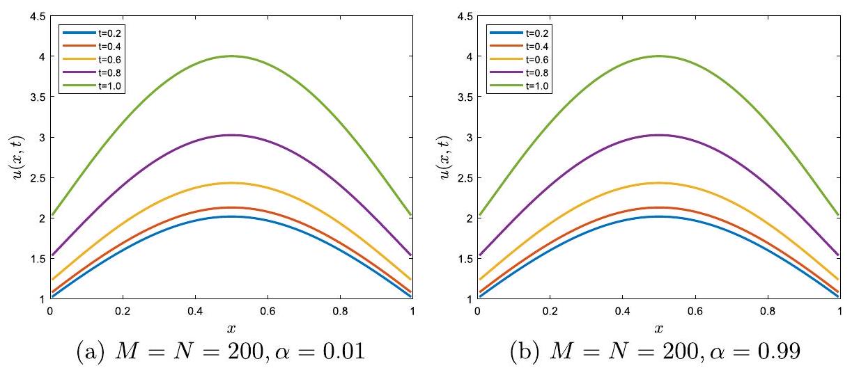
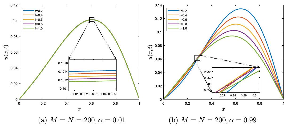
مثال 1 نعتبر المعادلة (2.1) مع
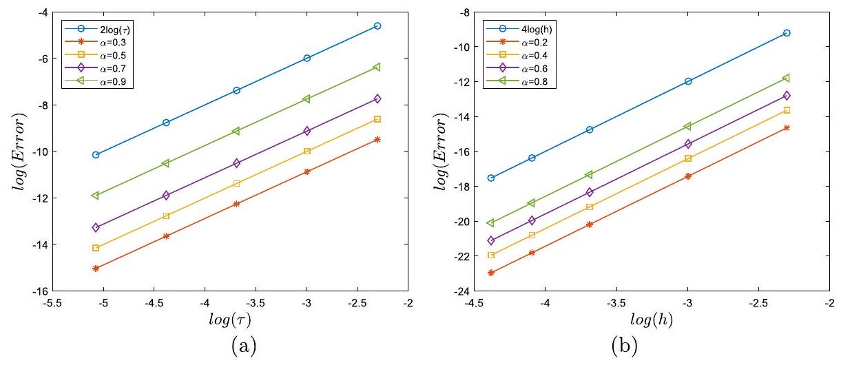
في الشكل 1(أ)، نرسم
|
|
M | ن |
|
معدل
|
زمن وحدة المعالجة المركزية |
| 0.2 | 100 | 10 |
|
– | 0.0113 |
| 100 | 15 |
|
2.00 | 0.0123 | |
| 100 | 20 |
|
2.00 | 0.0132 | |
| 100 | ٢٥ |
|
2.00 | 0.0138 | |
| 100 | 30 |
|
2.00 | 0.0158 | |
| 0.5 | 100 | 10 |
|
– | 0.0112 |
| 100 | 15 |
|
2.00 | 0.0121 | |
| 100 | 20 |
|
2.00 | 0.0130 | |
| 100 | 25 |
|
2.00 | 0.0153 | |
| 100 | 30 |
|
2.00 | 0.0157 | |
| 0.8 | 100 | 10 |
|
– | 0.0116 |
| 100 | 15 |
|
2.00 | 0.0126 | |
| 100 | 20 |
|
2.00 | 0.0134 | |
| 100 | ٢٥ |
|
2.00 | 0.0148 | |
| 100 | 30 |
|
2.00 | 0.0172 |
|
|
M |
|
|
معدل
|
زمن وحدة المعالجة المركزية |
| 0.3 | 10 | 100 |
|
– | 0.0184 |
| 15 | 225 |
|
٤.٠٠ | 0.0450 | |
| 20 | ٤٠٠ |
|
٤.٠٠ | 0.1191 | |
| 25 | 625 |
|
٤.٠٠ | 0.2795 | |
| 30 | ٩٠٠ |
|
٤.٠٠ | 0.5791 | |
| 0.6 | 10 | 100 |
|
– | 0.0166 |
| 15 | 225 |
|
٤.٠٠ | 0.0431 | |
| 20 | ٤٠٠ |
|
٤.٠٠ | 0.1230 | |
| ٢٥ | 625 |
|
٤.٠٠ | 0.2811 | |
| 30 | ٩٠٠ |
|
٤.٠٠ | 0.5797 | |
| 0.9 | 10 | 100 |
|
– | 0.0166 |
| 15 | 225 |
|
٤.٠٠ | 0.0451 | |
| 20 | ٤٠٠ |
|
٤.٠٠ | 0.1243 | |
| 25 | 625 |
|
٤.٠٠ | 0.2828 | |
| 30 | ٩٠٠ |
|
٤.٠٠ | 0.5787 |
-
، ومصطلح المصدر هو قيم المعلمات ذات الصلة ، و المرتبطة بالمثال تعتبر كـ و .
|
|
M | ن |
|
معدل
|
زمن وحدة المعالجة المركزية |
| 0.2 | ٢٠٠ | ٥ |
|
– | 0.0258 |
| ٢٠٠ | 10 |
|
2.00 | 0.0342 | |
| ٢٠٠ | 15 |
|
2.00 | 0.0413 | |
| ٢٠٠ | 20 |
|
2.00 | 0.0462 | |
| ٢٠٠ | ٢٥ |
|
2.00 | 0.0512 | |
| 0.5 | ٢٠٠ | ٥ |
|
– | 0.0256 |
| ٢٠٠ | 10 |
|
2.00 | 0.0352 | |
| ٢٠٠ | 15 |
|
2.00 | 0.0400 | |
| ٢٠٠ | 20 |
|
2.00 | 0.0465 | |
| ٢٠٠ | ٢٥ |
|
2.00 | 0.0520 | |
| 0.8 | ٢٠٠ | ٥ |
|
– | 0.0248 |
| ٢٠٠ | 10 |
|
1.99 | 0.0354 | |
| ٢٠٠ | 15 |
|
2.00 | 0.0408 | |
| ٢٠٠ | 20 |
|
2.00 | 0.0450 | |
| ٢٠٠ | 25 |
|
2.00 | 0.0519 |
|
|
M | ن |
|
معدل
|
زمن وحدة المعالجة المركزية |
| 0.3 | 10 | 100 |
|
– | 0.0389 |
| 15 | 225 |
|
٤.٠٠ | 0.1040 | |
| 20 | ٤٠٠ |
|
٤.٠٠ | 0.2452 | |
| 25 | 625 |
|
٤.٠٠ | 0.5672 | |
| 30 | ٩٠٠ |
|
٤.٠٠ | 1.0806 | |
| 0.6 | 10 | 100 |
|
– | 0.0405 |
| 15 | 225 |
|
٤.٠٠ | 0.0842 | |
| 20 | ٤٠٠ |
|
٤.٠٠ | 0.2597 | |
| 25 | 625 |
|
٤.٠٠ | 0.5239 | |
| 30 | ٩٠٠ |
|
٤.٠٠ | 1.0479 | |
| 0.9 | 10 | 100 |
|
– | 0.0375 |
| 15 | 225 |
|
٤.٠٠ | 0.0853 | |
| 20 | ٤٠٠ |
|
٤.٠٠ | 0.2361 | |
| 25 | 625 |
|
٤.٠٠ | 0.5405 | |
| 30 | ٩٠٠ |
|
٤.٠٠ | 1.0709 |
| ن | طريقة [48]
|
طريقة [49]
|
طريقة [50]
|
طريقتنا
|
| 10 |
|
|
|
|
| 20 |
|
|
|
|
| 40 |
|
|
|
|
| ٨٠ |
|
|
|
|
| ١٦٠ |
|
|
|
|
|
|
M | ن |
|
معدل
|
زمن وحدة المعالجة المركزية |
| 0.2 | ٢٠٠ | ٥ |
|
– | 0.0287 |
| ٢٠٠ | 10 |
|
2.00 | 0.0411 | |
| ٢٠٠ | 15 |
|
2.00 | 0.0454 | |
| ٢٠٠ | 20 |
|
2.00 | 0.0514 | |
| ٢٠٠ | ٢٥ |
|
2.00 | 0.0552 | |
| 0.5 | ٢٠٠ | ٥ |
|
– | 0.0292 |
| ٢٠٠ | 10 |
|
1.99 | 0.0396 | |
| ٢٠٠ | 15 |
|
2.00 | 0.0439 | |
| ٢٠٠ | 20 |
|
2.00 | 0.0483 | |
| ٢٠٠ | ٢٥ |
|
2.00 | 0.0542 | |
| 0.8 | ٢٠٠ | ٥ |
|
– | 0.0269 |
| ٢٠٠ | 10 |
|
1.97 | 0.0369 | |
| ٢٠٠ | 15 |
|
1.99 | 0.0384 | |
| ٢٠٠ | 20 |
|
1.99 | 0.0432 | |
| ٢٠٠ | ٢٥ |
|
2.00 | 0.0518 |
|
|
M | ن |
|
معدل
|
زمن وحدة المعالجة المركزية |
| 0.3 | 40 | ١٦٠٠ |
|
– | ٣.١٣٩٦ |
| ٤٥ | ٢٠٢٥ |
|
٤.٠٣ | ٥.٢٢٤٦ | |
| 50 | ٢٥٠٠ |
|
٤.٠٢ | 10.0944 | |
| ٥٥ | 3025 |
|
٤.٠٢ | 15.3994 | |
| 60 | ٣٦٠٠ |
|
٤.٠١ | ٢٢٫٩٩٠٥ | |
| 0.6 | 40 | ١٦٠٠ |
|
– | 3.1529 |
| ٤٥ | ٢٠٢٥ |
|
٤.٠٢ | 5.1031 | |
| 50 | ٢٥٠٠ |
|
٤.٠٢ | 10.1676 | |
| ٥٥ | 3025 |
|
٤.٠١ | 15.1544 | |
| 60 | ٣٦٠٠ |
|
٤.٠١ | ٢٢.٦٢٩٦ | |
| 0.9 | 40 | ١٦٠٠ |
|
– | 3.1531 |
| ٤٥ | ٢٠٢٥ |
|
٤.٠٠ | 5.1108 | |
| 50 | ٢٥٠٠ |
|
٤.٠٠ | 10.5489 | |
| ٥٥ | 3025 |
|
٤.٠٠ | 14.9813 | |
| 60 | ٣٦٠٠ |
|
٤.٠٠ | ٢٢.٧١١٣ |
|
|
M | ن |
|
معدل
|
زمن وحدة المعالجة المركزية |
| 0.3 | ٢٥ | ٤٨٠ |
|
– | 0.3451 |
| ٢٥ | ٤٩٠ |
|
2.05 | 0.3502 | |
| ٢٥ | ٥٠٠ |
|
2.10 | 0.3624 | |
| ٢٥ | 510 |
|
2.15 | 0.3896 | |
| 25 | 520 |
|
2.19 | 0.4063 | |
| 0.6 | ٢٥ | ٤٨٠ |
|
– | 0.3251 |
| ٢٥ | ٤٩٠ |
|
2.00 | 0.3428 | |
| 25 | ٥٠٠ |
|
2.02 | 0.3690 | |
| ٢٥ | 510 |
|
2.06 | 0.3730 | |
| ٢٥ | 520 |
|
2.10 | 0.3899 | |
| 0.9 | 25 | ٤٨٠ |
|
– | 0.3269 |
| ٢٥ | ٤٩٠ |
|
1.94 | 0.3455 | |
| ٢٥ | ٥٠٠ |
|
1.98 | 0.3605 | |
| ٢٥ | 510 |
|
2.02 | 0.3886 | |
| ٢٥ | 520 |
|
2.07 | 0.4008 |
|
|
M | ن |
|
معدل
|
زمن وحدة المعالجة المركزية |
| 0.2 | ٥ | ٦٠٠ |
|
– | 0.3559 |
| 10 | ٦٠٠ |
|
3.66 | 0.3813 | |
| 15 | ٦٠٠ |
|
٤.٤٣ | 0.4279 | |
| 20 | ٦٠٠ |
|
٤.٥٥ | 0.4674 | |
| 30 | ٦٠٠ |
|
٤.٥٦ | 0.5084 | |
| 0.5 | ٥ | ٦٠٠ |
|
– | 0.3635 |
| 10 | ٦٠٠ |
|
3.92 | 0.3873 | |
| 15 | ٦٠٠ |
|
٤.٦٥ | 0.4169 | |
| 20 | ٦٠٠ |
|
٤.٦٣ | 0.4559 | |
| 30 | ٦٠٠ |
|
٤.٤٩ | 0.4947 | |
| 0.8 | ٥ | ٦٠٠ |
|
– | 0.3603 |
| 10 | ٦٠٠ |
|
3.69 | 0.3824 | |
| 15 | ٦٠٠ |
|
3.66 | 0.4160 | |
| 20 | ٦٠٠ |
|
٤.٢١ | 0.4518 | |
| 30 | ٦٠٠ |
|
٤.٥٦ | 0.5056 |
5 الاستنتاج
معادلات تفاضلية جزئية كسرية زمنية أخرى من نوع مشابه مع المشتق الكسرى كابوتو-فابريزيو.
الشكر والتقدير
مساهمات المؤلفين
التمويل
توفر البيانات
الإعلانات
موافقة الأخلاقيات والموافقة على المشاركة
المصالح المتنافسة
تفاصيل المؤلف
References
- Faridi, W.A., Bakar, M.A., Akgül, A., El-Rahman, M.A., El Din, S.M.: Exact fractional soliton solutions of thin-film ferroelectric material equation by analytical approaches. Alex. Eng. J. 78, 483-497 (2023)
- Hosseini, V.R., Mehrizi, A.A., Karimi-Maleh, H., Naddafi, M.: A numerical solution of fractional reaction-convection-diffusion for modeling PEM fuel cells based on a meshless approach. Eng. Anal. Bound. Elem. 155, 707-716 (2023)
- Kavitha, K., Vijayakumar, V., Udhayakumar, R., Ravichandran, C.: Results on controllability of Hilfer fractional differential equations with infinite delay via measures of noncompactness. Asian J. Control 24, 1406-1415 (2022)
- Selvam, A.P., Vellappandi, M., Govindaraj, V.: Controllability of fractional dynamical systems with
-Caputo fractional derivative. Phys. Scr. 98, 025206 (2023) - Alchikh, R., Khuri, S.A.: Numerical solution of a fractional differential equation arising in optics. Optik 208, 163911 (2020)
- Murad, M.A.S.: New optical soliton solutions for time-fractional Kudryashov’s equation in optical fiber. Optik 283, 170897 (2023)
- Shen, L.J.: Fractional derivative models for viscoelastic materials at finite deformations. Int. J. Solids Struct. 190, 226-237 (2020)
- Bhangale, N., Kachhia, K.B., Gómez-Aguilar, J.F.: Fractional viscoelastic models with Caputo generalized fractional derivative. Math. Methods Appl. Sci. 46, 7835-7846 (2023)
- Arqub, O.A.: Numerical simulation of time-fractional partial differential equations arising in fluid flows via reproducing Kernel method. Int. J. Numer. Methods Heat Fluid Flow 30, 4711-4733 (2020)
- Kumar, D., Seadawy, A.R., Joardar, A.K.: Modified Kudryashov method via new exact solutions for some conformable fractional differential equations arising in mathematical biology. Chin. J. Phys. 56, 75-85 (2018)
- Khan, H., Ahmed, S., Alzabut, J., Azar, A.T.: A generalized coupled system of fractional differential equations with application to finite time sliding mode control for leukemia therapy. Chaos Solitons Fractals 174, 113901 (2023)
- Fall, A.N., Ndiaye, S.N., Sene, N.: Black-Scholes option pricing equations described by the Caputo generalized fractional derivative. Chaos Solitons Fractals 125, 108-118 (2019)
- Roul, P.: A high accuracy numerical method and its convergence for time-fractional Black-Scholes equation governing European options. Appl. Numer. Math. 151, 472-493 (2020)
- Nuugulu, S.M., Gideon, F., Patidar, K.C.: A robust numerical scheme for a time-fractional Black-Scholes partial differential equation describing stock exchange dynamics. Chaos Solitons Fractals 145, 110753 (2021)
- Zhang, H.M., Zhang, M.C., Liu, F.W., Shen, M.: Review of the fractional Black-Scholes equations and their solution techniques. Fractal Fract. 8, 101 (2024)
- Black, F., Scholes, M.: The pricing of options and corporate liabilities. J. Polit. Econ. 81, 637-654 (1973)
- Merton, R.C.: Theory of rational option pricing. Bell J. Econ. Manag. Sci. 4, 141-183 (1973)
- Jumarie, G.: Stock exchange fractional dynamics defined as fractional exponential growth driven by (usual) Gaussian white noise. Application to fractional Black-Scholes equations. Insur. Math. Econ. 42, 271-287 (2008)
- Jumarie, G.: Derivation and solutions of some fractional Black Scholes equations in coarse-grained space and time. Application to Merton’s optimal portfolio. Comput. Math. Appl. 59, 1142-1164 (2010)
- Chen, W.T., Xu, X., Zhu, S.P.: Analytically pricing double barrier options based on a time-fractional Black-Scholes equation. Comput. Math. Appl. 69, 1407-1419 (2015)
- Roul, P., Goura, V.M.K.P.: A compact finite difference scheme for fractional Black-Scholes option pricing model. Appl. Numer. Math. 166, 40-60 (2021)
- Caputo, M., Fabrizio, M.: A new definition of fractional derivative without singular kernel. Prog. Fract. Differ. Appl. 1, 73-85 (2015)
- Atangana, A., Alqahtani, R.T.: Numerical approximation of the space-time Caputo-Fabrizio fractional derivative and application to groundwater pollution equation. Adv. Differ. Equ. 2016, 156 (2016)
- Djida, J.D., Atangana, A.: More generalized groundwater model with space-time Caputo-Fabrizio fractional differentiation. Numer. Methods Partial Differ. Equ. 33, 1616-1627 (2017)
- Firoozjaee, M.A., Jafari, H., Lia, A., Baleanu, D.: Numerical approach of Fokker-Planck equation with Caputo-Fabrizio fractional derivative using Ritz approximation. J. Comput. Appl. Math. 339, 367-373 (2018)
- Rubbab, Q., Nazeer, M., Ahmad, F., Chu, Y.M., Khan, M.I., Kadry, S.: Numerical simulation of advection-diffusion equation with Caputo-Fabrizio time fractional derivative in cylindrical domains: applications of pseudo-spectral collocation method. Alex. Eng. J. 60, 1731-1738 (2021)
- Nieto, J.J.: Solution of a fractional logistic ordinary differential equation. Appl. Math. Lett. 123, 107568 (2022)
- Kebede, S.G., Lakoud, A.G.: Analysis of mathematical model involving nonlinear systems of Caputo-Fabrizio fractional differential equation. Bound. Value Probl. 2023, 44 (2023)
- Souigat, A., Korichi, Z., Meftah, M.T.: Solution of the fractional diffusion equation by using Caputo-Fabrizio derivative: application to intrinsic arsenic diffusion in germanium. Rev. Mex. Fis. 70, 010501 (2024)
- Hussein, M.A.: Using the Elzaki decomposition method to solve nonlinear fractional differential equations with the Caputo-Fabrizio fractional operator. Baghdad Sci. J. 21, 1044-1054 (2024)
- Amin, M., Abbas, M., Iqbal, M.K., Baleanu, D.: Non-polynomial quintic spline for numerical solution of fourth-order time fractional partial differential equations. Adv. Differ. Equ. 2019, 183 (2019)
- Amin, M., Abbas, M., Iqbal, M.K., Ismail, A.I.M., Baleanu, D.: A fourth order non-polynomial quintic spline collocation technique for solving time fractional superdiffusion equations. Adv. Differ. Equ. 2019, 514 (2019)
- Amin, M., Abbas, M., Iqbal, M.K., Baleanu, D.: Numerical treatment of time-fractional Klein-Gordon equation using redefined extended cubic B-spline functions. Front. Phys. 8, 288 (2020)
- Amin, M., Abbas, M., Baleanu, D., Iqbal, M.K., Riaz, M.B.: Redefined extended cubic B-spline functions for numerical solution of time-fractional telegraph equation. Comput. Model. Eng. Sci. 127, 361-384 (2021)
- Mesgarani, H., Aghdam, Y.E., Khoshkhahtinat, M., Farnam, B.: Analysis of the numerical scheme of the one-dimensional fractional Rayleigh-Stokes model arising in a heated generalized problem. AIP Adv. 13, 085024 (2023)
- Aghdam, Y.E., Mesgarani, H., Asadi, Z., Nguyen, V.T.: Investigation and analysis of the numerical approach to solve the multi-term time-fractional advection-diffusion model. AIMS Math. 8, 29474-29489 (2023)
- Aghdam, Y.E., Mesgarani, H., Asadi, Z.: Estimate of the fractional advection-diffusion equation with a time-fractional term based on the shifted Legendre polynomials. J. Math. Model. 11, 731-744 (2023)
- Haq, S., Hussain, M.: Selection of shape parameter in radial basis functions for solution of time-fractional Black-Scholes models. Appl. Math. Comput. 335, 248-263 (2018)
- Golbabai, A., Nikan, O., Nikazad, T.: Numerical analysis of time fractional Black-Scholes European option pricing model arising in financial market. Comput. Appl. Math. 38, 1-24 (2019)
- Fadugba, S.E.: Homotopy analysis method and its applications in the valuation of European call options with time-fractional Black-Scholes equation. Chaos Solitons Fractals 141, 110351 (2020)
- Golbabai, A., Nikan, O.: A computational method based on the moving least-squares approach for pricing double barrier options in a time-fractional Black-Scholes model. Comput. Econ. 55, 119-141 (2020)
- An, X.Y., Liu, F.W., Zheng, M.L., Anh, V.V., Turner, I.W.: A space-time spectral method for time-fractional Black-Scholes equation. Appl. Numer. Math. 165, 152-166 (2021)
- Taghipour, M., Aminikhah, H.: A spectral collocation method based on fractional Pell functions for solving time-fractional Black-Scholes option pricing model. Chaos Solitons Fractals 163, 112571 (2022)
- Kazmi, K.: A second order numerical method for the time-fractional Black-Scholes European option pricing model. J. Comput. Appl. Math. 418, 114647 (2023)
- Aghdam, Y.E., Mesgarani, H., Amin, A., Gómez-Aguilar, J.F.: An efficient numerical scheme to approach the time fractional Black-Scholes model using orthogonal Gegenbauer polynomials. Comput. Econ. 64, 211-224 (2024)
- Sun, Z.Z.: Compact difference scheme for heat equation with Neumann boundary conditions. Numer. Methods Partial Differ. Equ. 25, 1320-1341 (2009)
- Shi, J.K., Chen, M.H.: A second-order accurate scheme for two-dimensional space fractional diffusion equations with time Caputo-Fabrizio fractional derivative. Appl. Numer. Math. 151, 246-262 (2020)
- Akram, T., Abbas, M., Abualnaja, K.M., Iqbal, A., Majeed, A.: An efficient numerical technique based on the extended cubic B-spline functions for solving time fractional Black-Scholes model. Eng. Comput. 38, 1705-1716 (2022)
- Mesgarani, H., Ahanj, S., Aghdam, Y.E.: Numerical investigation of the time-fractional Black-Scholes equation with barrier choice of regulating European option. J. Math. Model. 10, 1-10 (2022)
- Abdi, N., Aminikhah, H., Sheikhani, A.H.R.: High-order compact finite difference schemes for the time-fractional Black-Scholes model governing European options. Chaos Solitons Fractals 162, 112423 (2022)
ملاحظة الناشر
DOI: https://doi.org/10.1186/s13660-025-03261-2
Publication Date: 2025-03-18
A compact finite difference scheme for solving fractional Black-Scholes option pricing model
liaoyuan1126@163.com
Full list of author information is available at the end of the article
Abstract
In this work, we introduce an efficient compact finite difference (CFD) method for solving the time-fractional Black-Scholes (TFBS) option pricing model. The time-fractional derivative is described using Caputo-Fabrizio (C-F) fractional derivative, and a compact finite difference method is employed to discretize the spatial derivative. The main contribution of this work is to develop a high-order discrete scheme for the TFBS model. In the numerical scheme, we have developed a convergence rate of
Keywords: Black-Scholes model; Caputo-Fabrizio fractional derivative; Compact finite difference method; Stability; Error estimate
1 Introduction
The Black-Scholes (BS) model, introduced by Black, Scholes and Merton [16, 17], offers both a pricing formula for European options and a hedging portfolio strategy. This model operates under strict assumptions: frictionless markets, continuous and smooth price movements, and option exercise only at maturity. Jumarie [18, 19] formulated both time- and space-fractional versions of BS equations and then derived an optimal fractional Merton portfolio. In the realm of financial markets or option pricing, the fractional BS equation holds immense potential for application. It can provide investors with more ac-
© The Author(s) 2025. Open Access This article is licensed under a Creative Commons Attribution-NonCommercial-NoDerivatives 4.0 International License, which permits any non-commercial use, sharing, distribution and reproduction in any medium or format, as long as you give appropriate credit to the original author(s) and the source, provide a link to the Creative Commons licence, and indicate if you modified the licensed material. You do not have permission under this licence to share adapted material derived from this article or parts of it. The images or other third party material in this article are included in the article’s Creative Commons licence, unless indicated otherwise in a credit line to the material. If material is not included in the article’s Creative Commons licence and your intended use is not permitted by statutory regulation or exceeds the permitted use, you will need to obtain permission directly from the copyright holder. To view a copy of this licence, visit http://creativecommons.org/licenses/by-nc-nd/ 4.0/.
curate option pricing methodologies, enabling them to make more informed investment decisions. Additionally, this model can be harnessed in risk management and portfolio optimization, aiding investors in achieving maximum investment returns while maintaining an acceptable level of risk. As financial markets continue to evolve and become increasingly complex, the application prospects of the fractional BS equation are poised to broaden even further. In this paper, we consider the following TFBS model of the form [20, 21],
for solving the TFBS equation. For instance, Haq and Hussain [38] applied the Residual Power Series method and a collocation-based mesh-free method to solve a class of TFBS models with constant and variable coefficients. Golbabai et al. [39] presented a numerical solution for the TFBS model using the radial basis functions method, which is characterized as a mesh-free scheme. Fadugba [40] proposed the application of the homotopy analysis method in the valuation of a European call option with a TFBS equation. Golbabai and Nikan [41] used the moving least-squares method to obtain an approximation solution of the TFBS model. An et al. [42] employed a space-time spectral method to develop a numerical scheme for solving the TFBS model with a smooth payoff function. Taghipour and Aminikhah [43] presented an efficient spectral collocation method based on fractional Pell functions for solving the TFBS equation. Kazmi [44] developed a numerical scheme to solve the TFBS equation governing European options with a convergence order of
2 Construction of fourth-order numerical scheme
In this section, we mainly consider the construction of discrete scheme for Eq. (2.1). For given positive integers
Lemma 2.1 ([46]) Let
Step 2. Calculate the exact value
Step 3. Obtain the coefficient matrices
Step 4. Use approximate formats to handle nodes beyond the boundary, and supplement matrices
Step 5. Calculate the numerical value of
Step 6. Calculate the corresponding error
Step 7. Finish the process by writing the data.
3 Stability analysis and error estimation
approximate solution of Eq. (2.7), and define
Using the Parseval equality
The following theorem is about stability of discrete scheme Eq. (2.7).
Theorem 3.2 The numerical scheme Eq. (2.7) is unconditionally stable.
Proof Using Eq. (3.3) and the result of Theorem 3.1, we get
For
4 Numerical results
Example 1 We consider Eq. (2.1) with
In Fig. 1(a), we plot
|
|
M | N |
|
Rate
|
CPU time(s) |
| 0.2 | 100 | 10 |
|
– | 0.0113 |
| 100 | 15 |
|
2.00 | 0.0123 | |
| 100 | 20 |
|
2.00 | 0.0132 | |
| 100 | 25 |
|
2.00 | 0.0138 | |
| 100 | 30 |
|
2.00 | 0.0158 | |
| 0.5 | 100 | 10 |
|
– | 0.0112 |
| 100 | 15 |
|
2.00 | 0.0121 | |
| 100 | 20 |
|
2.00 | 0.0130 | |
| 100 | 25 |
|
2.00 | 0.0153 | |
| 100 | 30 |
|
2.00 | 0.0157 | |
| 0.8 | 100 | 10 |
|
– | 0.0116 |
| 100 | 15 |
|
2.00 | 0.0126 | |
| 100 | 20 |
|
2.00 | 0.0134 | |
| 100 | 25 |
|
2.00 | 0.0148 | |
| 100 | 30 |
|
2.00 | 0.0172 |
|
|
M |
|
|
Rate
|
CPU time(s) |
| 0.3 | 10 | 100 |
|
– | 0.0184 |
| 15 | 225 |
|
4.00 | 0.0450 | |
| 20 | 400 |
|
4.00 | 0.1191 | |
| 25 | 625 |
|
4.00 | 0.2795 | |
| 30 | 900 |
|
4.00 | 0.5791 | |
| 0.6 | 10 | 100 |
|
– | 0.0166 |
| 15 | 225 |
|
4.00 | 0.0431 | |
| 20 | 400 |
|
4.00 | 0.1230 | |
| 25 | 625 |
|
4.00 | 0.2811 | |
| 30 | 900 |
|
4.00 | 0.5797 | |
| 0.9 | 10 | 100 |
|
– | 0.0166 |
| 15 | 225 |
|
4.00 | 0.0451 | |
| 20 | 400 |
|
4.00 | 0.1243 | |
| 25 | 625 |
|
4.00 | 0.2828 | |
| 30 | 900 |
|
4.00 | 0.5787 |
-
, and the source term is . The values of relevant parameters , and associated with the example are considered as and .
|
|
M | N |
|
Rate
|
CPU time(s) |
| 0.2 | 200 | 5 |
|
– | 0.0258 |
| 200 | 10 |
|
2.00 | 0.0342 | |
| 200 | 15 |
|
2.00 | 0.0413 | |
| 200 | 20 |
|
2.00 | 0.0462 | |
| 200 | 25 |
|
2.00 | 0.0512 | |
| 0.5 | 200 | 5 |
|
– | 0.0256 |
| 200 | 10 |
|
2.00 | 0.0352 | |
| 200 | 15 |
|
2.00 | 0.0400 | |
| 200 | 20 |
|
2.00 | 0.0465 | |
| 200 | 25 |
|
2.00 | 0.0520 | |
| 0.8 | 200 | 5 |
|
– | 0.0248 |
| 200 | 10 |
|
1.99 | 0.0354 | |
| 200 | 15 |
|
2.00 | 0.0408 | |
| 200 | 20 |
|
2.00 | 0.0450 | |
| 200 | 25 |
|
2.00 | 0.0519 |
|
|
M | N |
|
Rate
|
CPU time(s) |
| 0.3 | 10 | 100 |
|
– | 0.0389 |
| 15 | 225 |
|
4.00 | 0.1040 | |
| 20 | 400 |
|
4.00 | 0.2452 | |
| 25 | 625 |
|
4.00 | 0.5672 | |
| 30 | 900 |
|
4.00 | 1.0806 | |
| 0.6 | 10 | 100 |
|
– | 0.0405 |
| 15 | 225 |
|
4.00 | 0.0842 | |
| 20 | 400 |
|
4.00 | 0.2597 | |
| 25 | 625 |
|
4.00 | 0.5239 | |
| 30 | 900 |
|
4.00 | 1.0479 | |
| 0.9 | 10 | 100 |
|
– | 0.0375 |
| 15 | 225 |
|
4.00 | 0.0853 | |
| 20 | 400 |
|
4.00 | 0.2361 | |
| 25 | 625 |
|
4.00 | 0.5405 | |
| 30 | 900 |
|
4.00 | 1.0709 |
| N | Method of [48]
|
Method of [49]
|
Method of [50]
|
Our method
|
| 10 |
|
|
|
|
| 20 |
|
|
|
|
| 40 |
|
|
|
|
| 80 |
|
|
|
|
| 160 |
|
|
|
|
|
|
M | N |
|
Rate
|
CPU time(s) |
| 0.2 | 200 | 5 |
|
– | 0.0287 |
| 200 | 10 |
|
2.00 | 0.0411 | |
| 200 | 15 |
|
2.00 | 0.0454 | |
| 200 | 20 |
|
2.00 | 0.0514 | |
| 200 | 25 |
|
2.00 | 0.0552 | |
| 0.5 | 200 | 5 |
|
– | 0.0292 |
| 200 | 10 |
|
1.99 | 0.0396 | |
| 200 | 15 |
|
2.00 | 0.0439 | |
| 200 | 20 |
|
2.00 | 0.0483 | |
| 200 | 25 |
|
2.00 | 0.0542 | |
| 0.8 | 200 | 5 |
|
– | 0.0269 |
| 200 | 10 |
|
1.97 | 0.0369 | |
| 200 | 15 |
|
1.99 | 0.0384 | |
| 200 | 20 |
|
1.99 | 0.0432 | |
| 200 | 25 |
|
2.00 | 0.0518 |
|
|
M | N |
|
Rate
|
CPU time(s) |
| 0.3 | 40 | 1600 |
|
– | 3.1396 |
| 45 | 2025 |
|
4.03 | 5.2246 | |
| 50 | 2500 |
|
4.02 | 10.0944 | |
| 55 | 3025 |
|
4.02 | 15.3994 | |
| 60 | 3600 |
|
4.01 | 22.9905 | |
| 0.6 | 40 | 1600 |
|
– | 3.1529 |
| 45 | 2025 |
|
4.02 | 5.1031 | |
| 50 | 2500 |
|
4.02 | 10.1676 | |
| 55 | 3025 |
|
4.01 | 15.1544 | |
| 60 | 3600 |
|
4.01 | 22.6296 | |
| 0.9 | 40 | 1600 |
|
– | 3.1531 |
| 45 | 2025 |
|
4.00 | 5.1108 | |
| 50 | 2500 |
|
4.00 | 10.5489 | |
| 55 | 3025 |
|
4.00 | 14.9813 | |
| 60 | 3600 |
|
4.00 | 22.7113 |
|
|
M | N |
|
Rate
|
CPU time(s) |
| 0.3 | 25 | 480 |
|
– | 0.3451 |
| 25 | 490 |
|
2.05 | 0.3502 | |
| 25 | 500 |
|
2.10 | 0.3624 | |
| 25 | 510 |
|
2.15 | 0.3896 | |
| 25 | 520 |
|
2.19 | 0.4063 | |
| 0.6 | 25 | 480 |
|
– | 0.3251 |
| 25 | 490 |
|
2.00 | 0.3428 | |
| 25 | 500 |
|
2.02 | 0.3690 | |
| 25 | 510 |
|
2.06 | 0.3730 | |
| 25 | 520 |
|
2.10 | 0.3899 | |
| 0.9 | 25 | 480 |
|
– | 0.3269 |
| 25 | 490 |
|
1.94 | 0.3455 | |
| 25 | 500 |
|
1.98 | 0.3605 | |
| 25 | 510 |
|
2.02 | 0.3886 | |
| 25 | 520 |
|
2.07 | 0.4008 |
|
|
M | N |
|
Rate
|
CPU time(s) |
| 0.2 | 5 | 600 |
|
– | 0.3559 |
| 10 | 600 |
|
3.66 | 0.3813 | |
| 15 | 600 |
|
4.43 | 0.4279 | |
| 20 | 600 |
|
4.55 | 0.4674 | |
| 30 | 600 |
|
4.56 | 0.5084 | |
| 0.5 | 5 | 600 |
|
– | 0.3635 |
| 10 | 600 |
|
3.92 | 0.3873 | |
| 15 | 600 |
|
4.65 | 0.4169 | |
| 20 | 600 |
|
4.63 | 0.4559 | |
| 30 | 600 |
|
4.49 | 0.4947 | |
| 0.8 | 5 | 600 |
|
– | 0.3603 |
| 10 | 600 |
|
3.69 | 0.3824 | |
| 15 | 600 |
|
3.66 | 0.4160 | |
| 20 | 600 |
|
4.21 | 0.4518 | |
| 30 | 600 |
|
4.56 | 0.5056 |
5 Conclusion
other time-fractional partial differential equations of a similar type with Caputo-Fabrizio fractional derivative.
Acknowledgements
Author contributions
Funding
Data Availability
Declarations
Ethics approval and consent to participate
Competing interests
Author details
References
- Faridi, W.A., Bakar, M.A., Akgül, A., El-Rahman, M.A., El Din, S.M.: Exact fractional soliton solutions of thin-film ferroelectric material equation by analytical approaches. Alex. Eng. J. 78, 483-497 (2023)
- Hosseini, V.R., Mehrizi, A.A., Karimi-Maleh, H., Naddafi, M.: A numerical solution of fractional reaction-convection-diffusion for modeling PEM fuel cells based on a meshless approach. Eng. Anal. Bound. Elem. 155, 707-716 (2023)
- Kavitha, K., Vijayakumar, V., Udhayakumar, R., Ravichandran, C.: Results on controllability of Hilfer fractional differential equations with infinite delay via measures of noncompactness. Asian J. Control 24, 1406-1415 (2022)
- Selvam, A.P., Vellappandi, M., Govindaraj, V.: Controllability of fractional dynamical systems with
-Caputo fractional derivative. Phys. Scr. 98, 025206 (2023) - Alchikh, R., Khuri, S.A.: Numerical solution of a fractional differential equation arising in optics. Optik 208, 163911 (2020)
- Murad, M.A.S.: New optical soliton solutions for time-fractional Kudryashov’s equation in optical fiber. Optik 283, 170897 (2023)
- Shen, L.J.: Fractional derivative models for viscoelastic materials at finite deformations. Int. J. Solids Struct. 190, 226-237 (2020)
- Bhangale, N., Kachhia, K.B., Gómez-Aguilar, J.F.: Fractional viscoelastic models with Caputo generalized fractional derivative. Math. Methods Appl. Sci. 46, 7835-7846 (2023)
- Arqub, O.A.: Numerical simulation of time-fractional partial differential equations arising in fluid flows via reproducing Kernel method. Int. J. Numer. Methods Heat Fluid Flow 30, 4711-4733 (2020)
- Kumar, D., Seadawy, A.R., Joardar, A.K.: Modified Kudryashov method via new exact solutions for some conformable fractional differential equations arising in mathematical biology. Chin. J. Phys. 56, 75-85 (2018)
- Khan, H., Ahmed, S., Alzabut, J., Azar, A.T.: A generalized coupled system of fractional differential equations with application to finite time sliding mode control for leukemia therapy. Chaos Solitons Fractals 174, 113901 (2023)
- Fall, A.N., Ndiaye, S.N., Sene, N.: Black-Scholes option pricing equations described by the Caputo generalized fractional derivative. Chaos Solitons Fractals 125, 108-118 (2019)
- Roul, P.: A high accuracy numerical method and its convergence for time-fractional Black-Scholes equation governing European options. Appl. Numer. Math. 151, 472-493 (2020)
- Nuugulu, S.M., Gideon, F., Patidar, K.C.: A robust numerical scheme for a time-fractional Black-Scholes partial differential equation describing stock exchange dynamics. Chaos Solitons Fractals 145, 110753 (2021)
- Zhang, H.M., Zhang, M.C., Liu, F.W., Shen, M.: Review of the fractional Black-Scholes equations and their solution techniques. Fractal Fract. 8, 101 (2024)
- Black, F., Scholes, M.: The pricing of options and corporate liabilities. J. Polit. Econ. 81, 637-654 (1973)
- Merton, R.C.: Theory of rational option pricing. Bell J. Econ. Manag. Sci. 4, 141-183 (1973)
- Jumarie, G.: Stock exchange fractional dynamics defined as fractional exponential growth driven by (usual) Gaussian white noise. Application to fractional Black-Scholes equations. Insur. Math. Econ. 42, 271-287 (2008)
- Jumarie, G.: Derivation and solutions of some fractional Black Scholes equations in coarse-grained space and time. Application to Merton’s optimal portfolio. Comput. Math. Appl. 59, 1142-1164 (2010)
- Chen, W.T., Xu, X., Zhu, S.P.: Analytically pricing double barrier options based on a time-fractional Black-Scholes equation. Comput. Math. Appl. 69, 1407-1419 (2015)
- Roul, P., Goura, V.M.K.P.: A compact finite difference scheme for fractional Black-Scholes option pricing model. Appl. Numer. Math. 166, 40-60 (2021)
- Caputo, M., Fabrizio, M.: A new definition of fractional derivative without singular kernel. Prog. Fract. Differ. Appl. 1, 73-85 (2015)
- Atangana, A., Alqahtani, R.T.: Numerical approximation of the space-time Caputo-Fabrizio fractional derivative and application to groundwater pollution equation. Adv. Differ. Equ. 2016, 156 (2016)
- Djida, J.D., Atangana, A.: More generalized groundwater model with space-time Caputo-Fabrizio fractional differentiation. Numer. Methods Partial Differ. Equ. 33, 1616-1627 (2017)
- Firoozjaee, M.A., Jafari, H., Lia, A., Baleanu, D.: Numerical approach of Fokker-Planck equation with Caputo-Fabrizio fractional derivative using Ritz approximation. J. Comput. Appl. Math. 339, 367-373 (2018)
- Rubbab, Q., Nazeer, M., Ahmad, F., Chu, Y.M., Khan, M.I., Kadry, S.: Numerical simulation of advection-diffusion equation with Caputo-Fabrizio time fractional derivative in cylindrical domains: applications of pseudo-spectral collocation method. Alex. Eng. J. 60, 1731-1738 (2021)
- Nieto, J.J.: Solution of a fractional logistic ordinary differential equation. Appl. Math. Lett. 123, 107568 (2022)
- Kebede, S.G., Lakoud, A.G.: Analysis of mathematical model involving nonlinear systems of Caputo-Fabrizio fractional differential equation. Bound. Value Probl. 2023, 44 (2023)
- Souigat, A., Korichi, Z., Meftah, M.T.: Solution of the fractional diffusion equation by using Caputo-Fabrizio derivative: application to intrinsic arsenic diffusion in germanium. Rev. Mex. Fis. 70, 010501 (2024)
- Hussein, M.A.: Using the Elzaki decomposition method to solve nonlinear fractional differential equations with the Caputo-Fabrizio fractional operator. Baghdad Sci. J. 21, 1044-1054 (2024)
- Amin, M., Abbas, M., Iqbal, M.K., Baleanu, D.: Non-polynomial quintic spline for numerical solution of fourth-order time fractional partial differential equations. Adv. Differ. Equ. 2019, 183 (2019)
- Amin, M., Abbas, M., Iqbal, M.K., Ismail, A.I.M., Baleanu, D.: A fourth order non-polynomial quintic spline collocation technique for solving time fractional superdiffusion equations. Adv. Differ. Equ. 2019, 514 (2019)
- Amin, M., Abbas, M., Iqbal, M.K., Baleanu, D.: Numerical treatment of time-fractional Klein-Gordon equation using redefined extended cubic B-spline functions. Front. Phys. 8, 288 (2020)
- Amin, M., Abbas, M., Baleanu, D., Iqbal, M.K., Riaz, M.B.: Redefined extended cubic B-spline functions for numerical solution of time-fractional telegraph equation. Comput. Model. Eng. Sci. 127, 361-384 (2021)
- Mesgarani, H., Aghdam, Y.E., Khoshkhahtinat, M., Farnam, B.: Analysis of the numerical scheme of the one-dimensional fractional Rayleigh-Stokes model arising in a heated generalized problem. AIP Adv. 13, 085024 (2023)
- Aghdam, Y.E., Mesgarani, H., Asadi, Z., Nguyen, V.T.: Investigation and analysis of the numerical approach to solve the multi-term time-fractional advection-diffusion model. AIMS Math. 8, 29474-29489 (2023)
- Aghdam, Y.E., Mesgarani, H., Asadi, Z.: Estimate of the fractional advection-diffusion equation with a time-fractional term based on the shifted Legendre polynomials. J. Math. Model. 11, 731-744 (2023)
- Haq, S., Hussain, M.: Selection of shape parameter in radial basis functions for solution of time-fractional Black-Scholes models. Appl. Math. Comput. 335, 248-263 (2018)
- Golbabai, A., Nikan, O., Nikazad, T.: Numerical analysis of time fractional Black-Scholes European option pricing model arising in financial market. Comput. Appl. Math. 38, 1-24 (2019)
- Fadugba, S.E.: Homotopy analysis method and its applications in the valuation of European call options with time-fractional Black-Scholes equation. Chaos Solitons Fractals 141, 110351 (2020)
- Golbabai, A., Nikan, O.: A computational method based on the moving least-squares approach for pricing double barrier options in a time-fractional Black-Scholes model. Comput. Econ. 55, 119-141 (2020)
- An, X.Y., Liu, F.W., Zheng, M.L., Anh, V.V., Turner, I.W.: A space-time spectral method for time-fractional Black-Scholes equation. Appl. Numer. Math. 165, 152-166 (2021)
- Taghipour, M., Aminikhah, H.: A spectral collocation method based on fractional Pell functions for solving time-fractional Black-Scholes option pricing model. Chaos Solitons Fractals 163, 112571 (2022)
- Kazmi, K.: A second order numerical method for the time-fractional Black-Scholes European option pricing model. J. Comput. Appl. Math. 418, 114647 (2023)
- Aghdam, Y.E., Mesgarani, H., Amin, A., Gómez-Aguilar, J.F.: An efficient numerical scheme to approach the time fractional Black-Scholes model using orthogonal Gegenbauer polynomials. Comput. Econ. 64, 211-224 (2024)
- Sun, Z.Z.: Compact difference scheme for heat equation with Neumann boundary conditions. Numer. Methods Partial Differ. Equ. 25, 1320-1341 (2009)
- Shi, J.K., Chen, M.H.: A second-order accurate scheme for two-dimensional space fractional diffusion equations with time Caputo-Fabrizio fractional derivative. Appl. Numer. Math. 151, 246-262 (2020)
- Akram, T., Abbas, M., Abualnaja, K.M., Iqbal, A., Majeed, A.: An efficient numerical technique based on the extended cubic B-spline functions for solving time fractional Black-Scholes model. Eng. Comput. 38, 1705-1716 (2022)
- Mesgarani, H., Ahanj, S., Aghdam, Y.E.: Numerical investigation of the time-fractional Black-Scholes equation with barrier choice of regulating European option. J. Math. Model. 10, 1-10 (2022)
- Abdi, N., Aminikhah, H., Sheikhani, A.H.R.: High-order compact finite difference schemes for the time-fractional Black-Scholes model governing European options. Chaos Solitons Fractals 162, 112423 (2022)