يمكن أن يحسن التعلم الآلي الموجه بالمعرفة من تقدير دورة الكربون في النظم الزراعية Knowledge-guided machine learning can improve carbon cycle quantification in agroecosystems

المجلة: Nature Communications، المجلد: 15، العدد: 1
DOI: https://doi.org/10.1038/s41467-023-43860-5
PMID: https://pubmed.ncbi.nlm.nih.gov/38191521
تاريخ النشر: 2024-01-08

يمكن أن يحسن التعلم الآلي الموجه بالمعرفة من تقدير دورة الكربون في النظم الزراعية

تاريخ الاستلام: 1 يناير 2023
تاريخ القبول: 22 نوفمبر 2023
تاريخ النشر على الإنترنت: 08 يناير 2024
(A) تحقق من التحديثات

الملخص

ليتشينغ ليو (1) , وانغ زو , كاييو جوان , بين بينغ (1) , شاو مينغ شو , جينيون تانغ , تشينغ زو , جيسيكا تيل , شياوي جيا , تشونغيا جيانغ , شينغ وانغ (1) , زيكي تشين , هوي كونغ , روبرت غرانت (1) , سيمون ميزباه الدين © , فيبين كومار & زينونغ جين (B)

الملخص

يعد التقدير الدقيق والفعال من حيث التكلفة لدورة الكربون في النظم الزراعية على مقاييس ذات صلة بالقرار أمرًا حاسمًا للتخفيف من تغير المناخ وضمان إنتاج غذائي مستدام. ومع ذلك، فإن الأساليب التقليدية القائمة على العمليات أو المدفوعة بالبيانات وحدها تحمل عدم يقين كبير في التنبؤ بسبب العمليات البيوجيوكيميائية المعقدة التي يجب نمذجتها ونقص الملاحظات لتقييد العديد من المتغيرات الرئيسية للحالة والتدفق. هنا نقترح إطار عمل للتعلم الآلي الموجه بالمعرفة (KGML) الذي يعالج التحديات المذكورة أعلاه من خلال دمج المعرفة المضمنة في نموذج قائم على العمليات، وملاحظات الاستشعار عن بعد عالية الدقة، وتقنيات التعلم الآلي (ML). باستخدام حزام الذرة الأمريكي كحقل اختبار، نوضح أن KGML يمكن أن يتفوق على النماذج التقليدية القائمة على العمليات ونماذج ML السوداء في تقدير ديناميات دورة الكربون. يكشف نهجنا عالي الدقة بشكل كمي عن مزيد من التفاصيل المكانية حول تغييرات الكربون العضوي في التربة مقارنة بالأساليب التقليدية ذات الدقة الخشنة. علاوة على ذلك، نحدد بروتوكولًا لتحسين KGML عبر مسارات مختلفة، يمكن تعميمه لتطوير نماذج هجينة للتنبؤ بشكل أفضل بديناميات النظام الأرضي المعقدة.

تغطي أنظمة إنتاج المحاصيل وتفاعلاتها مع البيئة، المعروفة بالنظم الزراعية، حوالي ثلث سطح الأرض. حيث أن التربة تشكل أكبر خزان للكربون على اليابسة، تلعب النظم الزراعية دورًا رئيسيًا في دورة الكربون الأرضية العالمية من خلال تفاعلات المحاصيل مع التربة والغلاف الجوي . على مستوى العالم، تعتبر الزراعة مصدرًا كبيرًا لغازات الدفيئة (GHGs)؛ ومع ذلك، فإن امتصاص الكربون
من قبل المحاصيل يزيل أيضًا كميات كبيرة من ثاني أكسيد الكربون ( ) من الغلاف الجوي، وبعضها يمكن أن يتم استقراره في التربة . نظرًا لأن معظم التربة المزروعة بشكل مكثف غير مشبعة بالكربون، فإن الممارسات التي تزيد من الكربون العضوي في التربة (SOC) تمثل استراتيجية منخفضة التكلفة وعالية النطاق لتقليل تركيزات غازات الدفيئة في الغلاف الجوي . لذلك، من الضروري تقدير تدفقات الكربون والتغيرات في SOC بدقة في
النظم الزراعية حتى يمكن تحديد الممارسات الحفظ المناسبة والفعالة لأي موقع معين.
يعد زيادة احتجاز الكربون الزراعي استراتيجية رئيسية للتخفيف من تغير المناخ. تم بذل جهود واستثمارات كبيرة في الولايات المتحدة وحول العالم لتنفيذ برامج تحفز إثراء SOC . في ضوء هذه المبادرات، من المهم تطوير طرق قوية وقابلة للتوسع لتقدير احتجاز الكربون على مستوى الحقل بشكل موثوق، سواء لتقييم تأثير التخفيف المناخي أو لضمان تعويض المزارعين عن إجراءات التخفيف بشكل عادل ودقيق. تتضمن طرق تقدير الكربون التقليدية التي تعتمد على أخذ عينات من التربة، وعوامل الانبعاث، والنمذجة القائمة على العمليات (PB) حواجز متأصلة لتحقيق المستويات المطلوبة من الدقة، وقابلية التوسع، والفعالية من حيث التكلفة . على وجه الخصوص، فإن التباين المكاني الكبير والموسمية بسبب التغيرات في الظروف البيئية، وأنواع المحاصيل، وممارسات الإدارة تمثل تحديات لتقدير ميزانيات الكربون بدقة . بينما تتضمن أساليب النمذجة القائمة على العمليات المعرفة العلمية، تنشأ عدم اليقين الكبير في نماذج PB إذا لم يتم معايرة المعلمات المحلية والخاصة بالمحاصيل بشكل صحيح أو إذا كانت الآليات الأساسية مبسطة بشكل مفرط أو ممثلة بشكل غير كامل . بالإضافة إلى ذلك، يمكن أن تكون نماذج PB التي تحتوي على تمثيلات مفصلة للمبادئ العلمية الحالية مكلفة حسابيًا عند تطبيقها على مناطق كبيرة بدقة مكانية وزمنية عالية (مثل 250 م يوميًا). من ناحية أخرى، فإن أساليب التعلم الآلي المدفوعة بالبيانات (ML) لديها القدرة على الكفاءة الحسابية العالية والدقة لكنها تعاني من فشل التنبؤ خارج العينة في غياب مجموعات بيانات تدريب كبيرة، والتي لا تتوفر لمعظم التطبيقات الزراعية. علاوة على ذلك، غالبًا ما تكون نتائج نماذج ML غير قابلة للتفسير بسبب طبيعتها السوداء . لذلك، هناك حاجة إلى طرق جديدة للتغلب على قيود نماذج PB وML، مما يمكّن من قياس وتقدير نتائج الكربون بشكل فعال من حيث التكلفة، ودقيق، وقابل للتفسير على مستوى الحقل الفردي. سيساعد ذلك في تقليل الأخطاء في التقديرات المجمعة وتعزيز ممارسات إدارة الأراضي الأكثر استدامة .
يقدم مجال التعلم الآلي الموجه بالمعرفة (KGML) المتزايد منهجية واعدة تجمع بين مزايا نماذج PB، ونماذج ML، ومجموعات البيانات متعددة المصادر (مثل بيانات الاستشعار عن بعد والبيانات الميدانية). يمكن أن تنجح KGML الحالية في نمذجة بعض أنظمة الأرض التي تمثل فيها العمليات الديناميكية بشكل جيد بواسطة المعادلات الحاكمة المعروفة، مثل الهيدرولوجيا وعلوم الغلاف الجوي . ومع ذلك، فإن العمليات البيئية المعقدة والحاسمة مثل الدورة البيوجيوكيميائية غير خطية رياضيًا وأكثر تعقيدًا بشكل كبير. علاوة على ذلك، على عكس الأنظمة السطحية، لا يمكن ملاحظة تفاعلات التربة في النظم الزراعية بشكل مباشر من خلال الاستشعار عن بعد، بينما غالبًا ما تكون القياسات المباشرة في الموقع مكلفة ومحدودة. لذلك، يجب تطوير أساليب KGML جديدة لدمج المعرفة البيوجيوكيميائية الكافية ودمج القياسات غير المباشرة (مثل بيانات الاستشعار عن بعد وبيانات الاستطلاع) لالتقاط العمليات الأرضية التي يصعب ملاحظتها بشكل مباشر .
لمعالجة الفجوات الحالية في قدرات نمذجة ميزانية الكربون، طورنا إطار عمل KGML جديد يجمع بين المعرفة البيوجيوكيميائية السابقة لديناميات الكربون مع نموذج تعلم عميق لتوليد توقعات موثوقة لتدفقات الكربون الزراعي، وعوائد المحاصيل، والتغيرات في مخزونات الكربون في التربة (KGML-ag-Carbon، الشكل 1). تم دمج بيانات برج تدفق التباين الإيدي (EC) في الموقع، وبيانات عوائد المسح الإقليمي، وبيانات الإنتاج الأولي الإجمالي (GPP) المستشعرة عن بعد، وبيانات اصطناعية تم إنشاؤها بواسطة نموذج PB في KGML-ag-Carbon. يتم إثبات فعالية النموذج هنا لإنتاج الذرة وفول الصويا في الغرب الأوسط الأمريكي (الشكل S1)، مع نتائج دقيقة للغاية لتدفقات الكربون، وعوائد المحاصيل، والتغيرات في الكربون في التربة بدقة مكانية (250 م) وزمنية (يومية) عالية، مما يوفر بيانات قابلة للاستخدام لمديري الأراضي. كما قمنا بتحليل التحسين الناتج عن كل مكون من مكونات KGML واستجابات بيوجيوكيميائية معينة. يمثل تصميم النموذج المقدم هنا حلاً للتحديات في محاكاة الأنظمة الديناميكية غير المتجانسة، مما سيساعد في تعزيز التطبيقات الأوسع لـ KGML لفهم العمليات الأرضية.
الشكل 1 | نظرة عامة على الطريقة والإطار المستخدم لتطوير KGML-ag-Carbon. يتكون تطوير KGML-ag-Carbon من ثلاث خطوات رئيسية: (1) تطوير هيكل نموذج التعلم الآلي بناءً على العلاقات السببية المستمدة من نموذج قائم على العمليات الزراعية؛ (2) التدريب المسبق لـ KGML-ag-Carbon باستخدام بيانات اصطناعية تم إنشاؤها بواسطة نموذج قائم على العمليات؛ و (3)
تعديل KGML-ag-Carbon باستخدام بيانات عوائد المحاصيل منخفضة الدقة وبيانات تدفقات الكربون من مواقع تباين موزعة بشكل نادر. تم تصميم الخسائر الموجهة بالمعرفة بناءً على النموذج القائم على العمليات لتقييد استجابة المتغيرات المستهدفة للمتغيرات المدخلة خلال كل من عمليات التدريب المسبق للنموذج وعملية التعديل.

النتائج

نظرة عامة على إطار KGML-ag-Carbon

KGML-ag-Carbon هو إطار عمل جديد يجمع بين الفهم القائم على العمليات والأساليب المتقدمة للذكاء الاصطناعي لمحاكاة دورات البيوجيوكيمياء المعقدة تحت ممارسات الإدارة المكثفة للنظم الزراعية. يميز KGML-ag-Carbon نفسه عن التطبيقات السابقة لـ KGML في مجالات أخرى من خلال استخدام نموذج PB موثوق به جيدًا، ecosys وقدرتها على استيعاب بيانات الاستشعار عن بُعد بشكل مباشر. نموذج التعلم العميق القائم على آلية الوحدة المتكررة المغلقة (GRU) تم استخدامه لتطوير بنية KGML-ag-Carbon (الشكل 1). تعتبر نظرية النظام البيئي لتخصيص الكربون أساس نموذج ecosys، الذي تم استخدامه لتصميم الهيكل الهرمي لـ KGML-ag-Carbon، بما في ذلك الوحدات الفرعية المتعلقة بالنباتات والتربة وتبادل الكربون الجوي والتغذية الراجعة للكربون من النباتات إلى التربة (الشكل S2). من المهم أن البيانات الناتجة عن نموذج ecosys قدمت بيانات تركيبية حول تخصيص الكربون في النظام البيئي، والتدفقات المرتبطة، والاستجابات البيئية التي تم استخدامها لتدريب نموذج KGML-ag-Carbon مسبقًا. هذه الخطوة في التدريب المسبق تمنح النموذج ميزة كبيرة من خلال تحسين القدرة التنبؤية مع الحد الأدنى من العينات المعلّمة وتسريع التقارب في ضبط النموذج باستخدام العينات المعلّمة. تم استرجاع بيانات GPP، التي تمثل المدخلات الرئيسية للكربون في الأنظمة الزراعية، من ملاحظات الاستشعار عن بُعد وتم دمجها في KGML-ag-Carbon كقيود مكانية.
KGML-ag-Carbon يحل المكونات الرئيسية لميزانية الكربون، بما في ذلك التنفس الذاتي (Ra)، والتنفس غير الذاتي (Rh)، وإجمالي تنفس النظام البيئي (Reco، )، وتبادل الكربون في النظام البيئي الصافي (NEE) على مقياس يومي، والعائد على مقياس سنوي. كما هو الحال في النظم البيئية الطبيعية، يتم تحديد التغيرات في تخزين الكربون في التربة في النظم الزراعية من خلال ميزان الكتلة لتدفقات الكربون الداخلة والخارجة. ت originate من عملية التمثيل الضوئي للنباتات، أي الإنتاج الأولي الإجمالي (GPP)، بينما تشمل مدخلات الكربون في التربة كل من الحطام فوق الأرض وتحت الأرض وإفرازات الجذور. تحدث مخرجات الكربون من خلال التنفس، بما في ذلك Ra من سيقان الج plants والجذور وRh من تحلل الكربون العضوي في التربة بواسطة الميكروبات والفطريات. كما أن الاضطرابات مثل الحصاد تزيل الكربون من النظام البيئي بشكل دوري. استنادًا إلى تدفقات الكربون والعائد المقدر من KGML-ag-Carbon، يمكن تحديد التغيرات السنوية في الكربون العضوي في التربة باستخدام معادلة ميزان الكتلة. ني – العائد .
قمنا باستكشاف منهجيات متعددة لتحسين أداء التنبؤ لـ KGML-ag-Carbon بشكل منهجي، بما في ذلك تدريب النموذج مسبقًا باستخدام بيانات اصطناعية ودمج دوال خسارة موجهة بالمعرفة (KG)، مما يعالج قضايا أوسع تتعلق بتقليل عدم اليقين في النمذجة الهجينة. تم استخدام أكثر من 14 مليون بيانات اصطناعية ومجموعة متنوعة من دوال خسارة KG لتدريب KGML-ag-Carbon مسبقًا لتعلم المعرفة السابقة من نموذج PB (الشكل 1). استخدام بيانات اصطناعية تم إنشاؤها بواسطة نموذج PB هو أقل تكلفة بعدة مرات من تكلفة جمع الملاحظات من العالم الحقيقي. تشمل دوال خسارة KG قيودًا بيولوجية كيميائية/فيزيائية مثل توازن الكتلة ( )، عتبات التنبؤ (على سبيل المثال، عائد و استجابة المخرجات للمدخلات (على سبيل المثال، يجب أن تزداد Rh بشكل أحادي مع محتوى SOC تحت ظروف ثابتة أخرى).
مجموعة فرعية من بيانات العائد الملاحظة من وزارة الزراعة الأمريكية (320 من أصل 630 مقاطعة) جنبًا إلى جنب مع Reco ( ) وبيانات NEE من 11 موقعًا لبرج تدفق EC في الأراضي الزراعية تم استخدامها بعد ذلك لضبط نموذج KGML-ag-Carbon المدرب مسبقًا لتحسين قدرته على التنبؤ بميزانيات الكربون في العالم الحقيقي (الشكل 1). تم تضمين دوال خسارة KG مع قيود بيوجيوكيميائية/فيزيائية مشابهة لتلك المستخدمة في التدريب المسبق في عملية الضبط. ومع ذلك، للحفاظ على معرفة كافية من التدريب المسبق، تم دمج البيانات الاصطناعية مع البيانات الملاحظة أثناء الضبط، بينما أضيفت قيود إضافية إلى دوال خسارة KG للحفاظ على استجابة المخرجات للمدخلات (على سبيل المثال، تظل التغيرات في استجابات Ra للبيئة ضمن ). تفاصيل حول التطوير الهيكلي، ومجموعات البيانات المستخدمة، و
استراتيجيات التدريب لنموذج KGML-ag-Carbon موضحة في قسم الطرق.

أداء النموذج في توقعات إنتاج المحاصيل وتدفقات الكربون

قمنا بتقييم أداء KGML-ag-Carbon قبل وبعد التعديل الدقيق، بالإضافة إلى حساسية أداء النموذج لحجم عينة التدريب في العالم الحقيقي (الأشكال 2، S4، S6، S8). كتحقق أولي من فعالية ما قبل التدريب، تم مقارنة نتائج نموذج KGML-ag-Carbon المدرب مسبقًا لمجموعة اختبار البيانات الاصطناعية (سنتان من فترة 18 عامًا) مع محاكيات ecosys ووجدت أنها متسقة للغاية، مع قيم من 0.97 للإنتاج، Ra، Rh، و NEE، على التوالي (الشكل S4). كانت قيم نموذج الإيكوسيس لمحاصيل الذرة وفول الصويا لتوقعات الغلة 0.49 و0.42 على التوالي، كما تم قياسها مع الغلات المحصولية الملاحظة على مستوى المقاطعة، بينما كانت القيم لتوقعات Reco وNEE اليومية هي و 0.59-0.88، على التوالي، مقارنة بالقياسات من مواقع EC (النجوم/الصناديق الخضراء في الشكل 2، المستمدة من زو وآخرون. ). بعد التعديل الدقيق، ال كانت قيم KGML-ag-Carbon لتوقعات محصول الذرة وفول الصويا على مجموعة اختبار مكونة من 210 مقاطعات 0.91 و0.88، بينما كانت القيم لتوقعات Reco وNEE اليومية التي تم اختبارها على مدى عامين من بيانات خارج العينة من 11 موقعًا لبرج تدفق EC 0.94 و0.96، على التوالي (الشكل S8).
تكشف اختبار القوة (الشكل 2) أنه بالمقارنة مع نموذج التعلم الآلي النقي القائم على GRU باستخدام نفس المدخلات، يتفوق KGML-ag-Carbon باستمرار على نموذج التعلم الآلي النقي ويتميز بحساسية أقل بكثير لعدد عينات التدريب من العالم الحقيقي. باختصار، تكمن الاختلافات الرئيسية بين KGML-ag-Carbon والتعلم الآلي النقي في عملية ما قبل التدريب الإضافية وبنية النموذج المخصصة ودوال الخسارة الموجهة بواسطة المعرفة العلمية المعروفة. تعزز هذه التطورات عملية تحسين نموذج التعلم الآلي وتسمح بإجراء توقعات موثوقة مع عدد أقل من العينات المعلّمة. اقترب أداء نموذج التعلم الآلي النقي من أداء KGML-ag-Carbon عند أحجام عينات كبيرة لكنه كان ضعيف الأداء مع مجموعات تدريب صغيرة، خاصة بالنسبة لعائد المحاصيل (الشكل 2أ، ب). الحاجة المنخفضة لعينات التدريب هي ميزة مركزية لـ KGML-ag-Carbon لتقديرات عائد المحاصيل وتدفقات الكربون في العالم الحقيقي لأن البيانات التدريبية المتاحة عادة ما تكون محدودة وجمع البيانات من العينات الفيزيائية مكلف. تأتي التحسينات في توقعات تدفقات الكربون مع زيادة حجم العينة في الغالب من التقاط الديناميات الكربونية بين السنوات، والتي يمكن تعلمها بسهولة أكبر من الأنماط الموسمية لـ GPP والمناخ (الشكل 2ج، د). حتى بدون ضبط دقيق (حجم عينة تدريب 0)، يمكن لـ KGML-ag-Carbon من خلال استيعاب بيانات GPP كمدخلات، أن يتفوق على كل من نموذج ecosys ونموذج التعلم الآلي النقي المدرب بعينات تدريب صغيرة (الشكل 2).
قمنا بإجراء عدة تجارب إضافية لتقييم أداء KGML-ag-Carbon تحت تقسيمات مختلفة لمجموعات بيانات التدريب والتحقق والاختبار، بما في ذلك الأداء خارج العينة لتوقعات العائد في المجالات المكانية والزمنية (الشكل S9a-f). على سبيل المثال، استخدمنا بيانات من إلينوي للاختبار وبيانات من ولايات أخرى للتدريب والتحقق، واستخدمنا عدة سنوات متتالية من البيانات للتدريب والتحقق مع سنوات أخرى للاختبار. كما قمنا بفحص تأثير استخدام سنوات متطرفة ذات عوائد مرتفعة أو منخفضة بشكل استثنائي للاختبار وسنوات أخرى للتدريب والتحقق. نلاحظ أن نموذج KGML-ag-Carbon يتفوق على نماذج التعلم الآلي البحتة والنماذج المعتمدة على العمليات في توقع العائد في السنوات المتطرفة (الشكل S9e، f) بشكل أساسي لأنه مقيد بكل من الملاحظات والبيانات الاصطناعية الناتجة عن نموذج PB. وبالمثل، تم التحقيق في الأداء خارج العينة لتوقعات Reco وNEE على كل من المقاييس الزمنية السنوية واليومية، وتم فحصها بشكل خاص لمواقع (أبراج تدفق EC US-NE 1-3) التي تحتوي على ملاحظات طويلة الأجل تغطي الفترة من 2001 إلى 2019 (الشكل S9g-l). تظهر النتائج أداءً أفضل باستمرار لنموذج KGML-ag-Carbon مقارنة بالتعلم الآلي البحت في جميع الحالات المختبرة. يمكن العثور على تفاصيل اختبارات المتانة على أداء KGML-ag-Carbon في قسم الطرق.
الشكل 2 | الأداء المقارن لنموذج التعلم الآلي النقي (الصناديق الزرقاء) وKGML-ag-Carbon (الصناديق الحمراء) عند استخدام أحجام مختلفة من الملاحظات
عينات البيانات لتدريب النموذج. أ، ب أداء توقع العائد عبر 210 مقاطعة. ، و 1 تجربة مستقلة لفرق النماذج بحجم عينة تدريب , و320، على التوالي. تحتوي كل عينة تدريب على فترة 21 عامًا من ملاحظات العائد السنوي في مقاطعة واحدة. أداء توقعات Reco و NEE عبر 11 برج تدفق EC. تجارب مستقلة لحجم عينة التدريب من 1 إلى 7. و6 تجارب مستقلة لنموذج ecosys وKGML-ag-Carbon مع حجم عينة تدريب قدره 0، على التوالي. تحتوي كل عينة تدريب على ملاحظات يومية خلال فترة الملاحظة في موقع واحد (تتفاوت
حسب الموقع، تتراوح من 5 إلى 19 عامًا). توضح كل مخطط صندوقي الربع الأول والثالث (حواف الصندوق السفلية والعلوية)، الوسيط (الخط المركزي)، والحد الأدنى والحد الأقصى (الشعيرات السفلية والعلوية)، مع القيم الشاذة كدوائر مستديرة. تمثل النجوم الخضراء أداء ecosys في محاكاة عائد المحاصيل عبر الولايات الأمريكية إلينوي وآيوا وإنديانا المقيدة بـ GPP المستشعر عن بُعد والعائد المرصود، وتمثل الصناديق الخضراء أداء ecosys في محاكاة تدفقات الكربون في 7 مواقع برج تدفق EC عبر الغرب الأوسط الأمريكي من Zhou et al. , وهو مجموعة فرعية من مجموعة البيانات المستخدمة في هذه الدراسة. يتم تصوير نتائج الاختبار خارج العينة فقط من مجموعات التحقق المتقاطع هنا. يمكن العثور على تفاصيل التجارب في قسم “الطرق”. يتم توفير بيانات المصدر كملف بيانات مصدر.

طرق لتقليل عدم اليقين في KGML-ag-Carbon

لفهم مساهمة استراتيجيات مختلفة في تحسين أداء KGML-ag-Carbon، أجرينا اختبارات كاملة العوامل لتضمين أو استبعاد مكونات نموذج مختلفة واخترنا خمسة نماذج تمثيلية لاستخدامها في تفسير النتائج (الشكل 3). تكشف النتائج أن استخدام بيانات GPP كمدخلات وتدريب KGML-ag-Carbon مسبقًا ببيانات اصطناعية يساهمان بشكل أكبر في تحسين أداء KGML-ag-Carbon مقارنةً بالاستراتيجيات الأخرى. عند استخدام ملاحظات العالم الحقيقي الأكبر لتعديل النموذج، فإن بيانات GPP لها أكبر مساهمة في تحسين أداء KGML-ag-Carbon؛ بينما يكون التدريب المسبق باستخدام بيانات اصطناعية أكثر أهمية عند استخدام مجموعات ملاحظات العالم الحقيقي الأصغر لتعديل النموذج (الشكل 3a، b). يشير هذا إلى أنه في ظل ظروف نقص البيانات، يمكن أن يوفر التدريب المسبق بناءً على مجموعات بيانات تم إنشاؤها بواسطة نماذج العمليات ذات الآليات الممثلة بشكل جيد معرفة مسبقة تساعد بشكل كبير في تحسين أداء ML. على النقيض من ذلك، عندما تتوفر مجموعات بيانات ملاحظات عالية الجودة، يمكن لنموذج ML تعلم العلاقات المعقدة مباشرة من البيانات، لذا فإن التدريب المسبق يكون أقل أهمية.
التحسينات التي قدمتها الهيكلية الهرمية ودوال خسارة KG لـ KGML-ag-Carbon صغيرة نسبيًا مقارنة بتلك الناتجة عن مدخلات GPP وعمليات التدريب المسبق. أحد الأسباب المحتملة هو أن مقاييس أداء النموذج ( هنا) كانت بالفعل مرتفعة جدًا بعد إضافة مدخلات GPP والتدريب المسبق (الشكل 3a، b). ومع ذلك، فإن تضمين الهيكلية الهرمية ودوال خسارة KG يزيد بشكل كبير من قدرة KGML-ag-Carbon على التقاط ديناميات تدفق الكربون المعقدة وقابلية تفسير التوقعات.
تقلل عملية التدريب المسبق بشكل كبير من توازن الكتلة المتبقية لتدفقات الكربون (أي، GPP-Reco-NEE)، بينما تقلل الهيكلية الهرمية ودوال خسارة KG من بقايا توازن الكتلة إلى ما يقرب من الصفر (الشكل 3c)، مما يشير إلى أن تضمين الهيكلية الهرمية ودوال خسارة KG يقيد النموذج ليتبع القواعد الفيزيائية. على الرغم من أن KGML-ag-Carbon لديه أداء عام مشابه لنماذج ML+GPP وML+GPP+pretrain، إلا أن تحسينات كبيرة في توقعات NEE تتحقق في الشتاء والصيف، خاصة خلال الفترات ذات الديناميات المعقدة (الشكل 3d). تعزى ميزة KGML-ag-Carbon على النماذج الأخرى لفترات زمنية مختلفة بشكل رئيسي إلى المعرفة المدمجة بأنماط زمنية متميزة في Ra وRh، مثل Rh يساوي Reco في الشتاء عندما يكون نمو النبات غائبًا، والتي يمكن استخدامها لتحسين أداء نماذج Ra وRh الفرعية في KGML-ag-Carbon بشكل منفصل. يمكن العثور على نتائج أخرى من اختبارات كاملة العوامل واختبارات توازن الكتلة في الشكل S11 والشكل S12، على التوالي. يمكن العثور على التفاصيل التي توضح كيفية تحديد مساهمات مكونات KGML-ag-Carbon في قسم “الطرق”.

تقديرات تدفق الكربون عالية الدقة عبر الغرب الأوسط الأمريكي

باستخدام KGML-ag-Carbon المعدل بدقة، توقعنا تدفقات الكربون اليومية الإقليمية وعوائد المحاصيل السنوية عبر الغرب الأوسط الأمريكي بدقة مكانية (أصغر من حقل غرب الأوسط الأمريكي النموذجي، الشكل 4a-c). تشمل المدخلات التي تدفع KGML-ag-Carbon بيانات المناخ اليومية من NLDAS-2، وخصائص التربة السطحية من gSSURGO، وGPP اليومي المستشعر عن بُعد من منتج SLOPE , ومعلومات دوران المحاصيل. تسهل الدقة المكانية العالية من خلال بيانات التربة عالية الدقة
الشكل 3 | مساهمات هيكل النموذج واستراتيجيات التدريب في تحسين أداء KGML-ag-Carbon. أ مساهمات من مكونات مختلفة لـ KGML-ag-Carbon في تحسين دقة توقع عائد الذرة السنوي من خلال إضافة مكون واحد إلى نموذج ML النقي بشكل متسلسل. و5 تجارب مستقلة لمجموعات النماذج مع بيانات تدريب صغيرة وكبيرة، على التوالي. المساهمات في تحسين دقة توقع تدفق NEE التراكمي السنوي. تجارب مستقلة لمجموعات النماذج مع بيانات تدريب صغيرة وكبيرة. البيانات في و مقدمة كقيم متوسطة الانحراف المعياري. القيم الموجودة أسفل كل شريط تمثل متوسط زيادة الأداء من الخطوة السابقة. ML بدون GPP تشير إلى نموذج ML النقي بدون مدخلات GPP؛ بيانات GPP تشير إلى نموذج ML مع مدخلات GPP؛ Pretrain تشير إلى نموذج بيانات GPP المدرب مسبقًا باستخدام البيانات الاصطناعية التي تم إنشاؤها بواسطة النموذج القائم على العمليات؛ الهيكل يشير إلى النموذج الذي يحتوي على هيكل هرمي، تم تدريبه مسبقًا باستخدام بيانات اصطناعية، ويشمل مدخلات GPP؛ خسارة KG تشير إلى نموذج الهيكل الذي يأخذ في الاعتبار مصطلحات خسارة موجهة بالمعرفة؛ KGML-
ag-Carbon تشير إلى النموذج النهائي الذي يأخذ في الاعتبار كل من الهيكل الموجه بالمعرفة ومصطلحات الخسارة، ويحتوي على مدخلات GPP وتم تدريبه مسبقًا باستخدام بيانات اصطناعية. ج فوائد المكونات الموجهة بالمعرفة (التدريب المسبق، الهيكل، وخسارة KG) في تقليل بقايا توازن الكتلة (GPP-Reco-NEE). تجارب مستقلة. توضح كل مخطط صندوقي الربع الأول والثالث (حواف الصندوق السفلية والعلوية)، الوسيط (الخط المركزي)، المتوسط (نقطة حمراء صلبة)، والحد الأدنى والحد الأقصى (الشعيرات السفلية والعلوية). د مثال (2016 من US-NE1) لتوقعات تدفقات NEE من نماذج مع مكونات موجهة بالمعرفة مختلفة. تجارب مستقلة لمجموعات النماذج في هذا الموقع. تمثل المناطق المظللة المنطقة ضمن الحد الأقصى والحد الأدنى من مجموعات المحاكاة، بينما تمثل الخطوط الصلبة القيم المتوسطة. البيانات في المخططات الفرعية مقدمة كقيم متوسطة (نقاط صلبة) وحدود دنيا وعليا (شعيرات) من RMSE. ML + GPP تشير إلى نموذج ML النقي مع مدخلات GPP؛ ML + GPP + pretrain تشير إلى نموذج ML النقي المدرب مسبقًا باستخدام بيانات اصطناعية ومع مدخلات GPP؛ KGML-ag-Carbon تشير إلى النموذج النهائي. يتم توفير بيانات المصدر كملف بيانات مصدر.
معلومات، خرائط دوران المحاصيل، ومنتج GPP. تأتي الدقة الزمنية العالية من بيانات المناخ وبيانات منتج GPP، التي توفر معلومات يومية عن الظروف البيئية ومدخلات كربون النظام البيئي. يتم تقديم الإجراءات اللازمة لتوليد توقعات عالية الدقة عبر الغرب الأوسط الأمريكي في قسم “الطرق”.
تكون بيانات GPP المتوسطة على مدى سنوات متعددة وتدفقات الكربون الناتجة عن KGML-ag-Carbon أقرب إلى ملاحظات برج تدفق EC (نفس مجموعة البيانات المستخدمة في الشكل 2) من التقديرات من Trendy , وهو منتج مجموعة تدفق كربون مستخدم على نطاق واسع تم إنشاؤه بواسطة مجموعة من نماذج الغطاء النباتي الديناميكية العالمية (الشكل 4). على الرغم من أن الطرق لتقييم KGML-ag-Carbon محدودة إلى حد ما على النطاق الإقليمي، فإن بيانات برج تدفق EC وTrendy هي مجموعات بيانات مناسبة للمقارنة في غياب معايير مثالية لهذه المنطقة الكبيرة.
توزيعات قيم GPP متشابهة عبر ملاحظات برج تدفق SLOPE و EC ومجموعة Trendy (الشكل 4d). توزيعات Reco و NEE المقدرة بواسطة KGML-ag-Carbon مشابهة لتلك الخاصة بملاحظات برج التدفق EC، لكن مجموعة نماذج Trendy قدّرت كل من Reco و NEE بشكل مفرط في منطقة الغرب الأوسط الأمريكي مقارنة بملاحظات برج التدفق (الشكل 4e، f). بالإضافة إلى ذلك، تختلف توزيعات GPP و Reco و NEE المقدرة بشكل كبير بين نماذج Trendy الفردية، مما قد ينشأ عن اختلافات في الهيكل والمعلمات بين النماذج. وهذا يعكس عدم اليقين الكبير المتبقي في النماذج الحالية المتطورة لحسابات الكربون، خاصةً للتقديرات على النطاق الإقليمي. لتلخيص هذه المقارنات، تُظهر تدفقات الكربون المقدرة بواسطة KGML-ag-Carbon دقة عالية في الزمان والمكان، مما يوفر منتجًا جديدًا لتحديد ميزانية الكربون بدقة على نطاق إقليمي يصل إلى حقل واحد.
الشكل 4 | النمط المكاني لمتوسط التدفقات الكربونية السنوية المتراكمة (2000-2019) من KGML-ag-Carbon وتوزيعاتها مقارنة بمنتج Trendy-v9. أ المنتج المتوسط لعدة سنوات من GPP المستشعر عن بُعد بناءً على الانعكاس القريب من الأشعة تحت الحمراء MODIS (SLOPE GPP)، والذي يعد أحد مدخلات KGML-ag-Carbon. تنبؤات التدفقات السنوية المتراكمة لرا وRh المتوسطة على مدى عدة سنوات بواسطة KGML-ag-Carbon. ج التنبؤات السنوية المتراكمة لNEE المتوسطة على مدى عدة سنوات بواسطة KGML-ag-Carbon. د-و توزيعات GPP السنوية المتراكمة.

الملخص

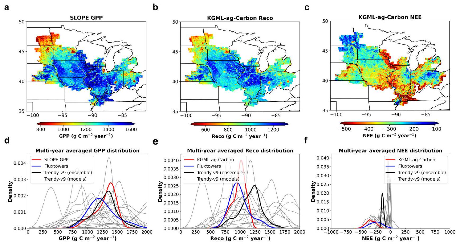
Reco و NEE، على التوالي، من توقعات KGML-ag-Carbon وTrendy-v9 خلال الفترة من 2000 إلى 2019 ومواقع قياس تدفق الإيدى في الأراضي الزراعية المختارة في وسط غرب الولايات المتحدة. المنتج Trendy المستخدم في هذه المقارنة هو منتج جماعي من نماذج متعددة قائمة على العمليات تحاكي ميزانية الكربون (خط رمادي واحد في يمثل نموذجًا واحدًا في Trendy، والخطوط السوداء هي متوسط المخرجات لجميع النماذج). تم حساب متوسط تدفقات SLOPE GPP و KGML-ag-Carbon من 250 م إلى في للعرض. يتم توفير بيانات المصدر كملف بيانات المصدر.

نقاش
فوائد ميزانيات الكربون عالية الدقة

القياس على مستوى الحقل لميزانيات الكربون، وعوائد المحاصيل، و تم إنتاجه باستخدام KGML-ag-Carbon (كما تم توضيحه في منطقة الغرب الأوسط الأمريكي) ويوفر منتجًا دقيقًا وفعالًا من حيث التكلفة وعالي الدقة لتحسين تقييمات احتجاز الكربون المحتملة. لتأكيد ضرورة وجود ميزانية كربونية عالية الدقة وقياس غلة المحاصيل، قمنا بإنشاء دقة 0.0025 درجة و0.5 درجة. تقديرات من 2000 إلى 2020 باستخدام نهج ميزان الكتلة مع KGML-ag-Carbon. قمنا بإنشاء منتج عالي الدقة باستخدام بيانات NEE بدقة 250 متر وعائد المحاصيل المتوقعة بواسطة KGML-ag-Carbon (الشكل 5a-c). تم مقارنة هذه النتائج مع تقديرات باستخدام نهج مشابه من خلال تنفيذ KGML-ag-Carbon بدقة 0.5 درجة (الشكل 5d-f). الدقة العالية تظهر التقديرات أن الغالبية العظمى من التغييرات تقع ضمن نطاق إلى سنة/م (86%)، وهو ما يتماشى جيدًا مع النطاقات التي لوحظت في الدراسات التجريبية (الشكل 5ج). تشمل الأنماط الملحوظة انخفاضًا في الكربون العضوي في التربة عبر جنوب مينيسوتا، شمال آيوا، وشمال شرق إلينوي، بالإضافة إلى زيادة في جنوب غرب الولايات المتحدة. تتأثر هذه الأنماط بشكل أساسي بعوامل التربة (تفسير التباين) وعوامل المناخ (تفسير 11% من التباين). تساهم الظروف الأكثر برودة وجفافًا، وقلة المدخلات الكربونية في التربة، ومستويات مخزون الكربون العضوي المرتفعة (Rh أكبر) في زيادة فقدان الكربون في المناطق الشمالية (الشكل S14). تقييم أكثر تفصيلًا لـ تم تقديم الأنماط في المناقشة التكميلية. مقارنة بين الدقة الخشنة والدقة العالية تظهر التقديرات اختلافات ملحوظة (NRMSE العام = 86%) بسبب فقدان التفاصيل (مثل النقاط الساخنة/الباردة) وتأثيرات البكسل المختلط الأقوى نسبيًا في بكسلات 0.5 درجة (الشكل 5d، e). تشير توزيع المدرج التكراري (الشكل 5f) إلى اختلاف يتراوح من – 0.1 ( النسب المئوية) إلى 0.9 ( نسبة (كوانتيل) %/سنة بين التقديرات ذات الدقة المنخفضة والعالية. لا يمكن تجاهل هذا الاختلاف عند مقارنته بالتقديرات عالية الدقة. توزيعات المدرجات التكرارية (الشكل 5c).
تُقدم نتائج أكثر تفصيلاً بشأن الفروق بين مدخلات GPP عالية الدقة ومدخلات GPP منخفضة الدقة، بالإضافة إلى مؤهلات Ra وRh وNEE وعائد المحاصيل في الشكل S15.
تستخدم KGML-ag-Carbon نهج توازن الكتلة لتقدير من NEE والعائد، والتي يتم تقديرها من خلال دمج جميع البيانات المتاحة، بما في ذلك تأثيرات الطقس، وخصائص التربة (التي تشمل SOC الثابت)، ونوع المحاصيل، وGPP المستشعر عن بُعد. هذه المدخلات وNEE والعائد المتوقعين تم التحقق منها جيدًا من خلال الملاحظات. تتيح لنا هذه الطريقة الاستفادة القصوى من البيانات الموجودة لتقدير الإقليمي بتكلفة منخفضة ودقة عالية، حتى في غياب قياسات مستوى الحقل. لقد قمنا بجهود التحقق، مع التركيز على المواقع داخل منطقة الغرب الأوسط الأمريكي مع قياسات SOC في عدة سنوات بعد عام 2000 (الشكل S16، الجدول S1). تُظهر هذه التحققات أن نموذجنا تقديرات SOC تقع ضمن النطاقات الملحوظة في معظم الحالات. ومع ذلك، فإن الأداء مقيد بأربعة عوامل رئيسية: (1) بينما جميع تم جمع بيانات SOC على مستوى القطعة المقياس)، غياب بيانات القوة المحلية المطلوبة جعلنا نستخدم مدخلات على مستوى الحقل، وهي بيانات GPP والطقس، لتشغيل النموذج؛ (2) تقديراتنا يمثل مزيجًا من بقايا المحاصيل والهيوموس، بينما تركز الغالبية العظمى من القياسات عادةً على محتوى الهيوموس؛ (3) الاختلافات في ممارسات الإدارة بين كل قطعة أرض، مثل الحراثة، وتطبيق الأسمدة، وتناوب المحاصيل، تعقد أيضًا تقدير مستوى الحقل، و(4) تنشأ عدم اليقين في الكربون العضوي في التربة على مستوى الحقل من أخطاء قياس المختبر (حتى 12%)، وأخطاء أخذ العينات المكانية (حتى ) وأخطاء إعادة العينة (حتى ، ويمكن أن تتفاقم على مدى فترات زمنية طويلة. على الرغم من هذه التحديات، فإن نهجنا ذو قيمة في التخفيف من أخطاء تقدير ميزانية الكربون، مدفوعًا بدقته العالية (250 م) وموثوقيته (الأشكال 2-4)، مع الحفاظ على تكلفة حسابية منخفضة. ومن الجدير بالذكر أنه بينما يتم تحديد قيم NEE وReco وعائد المحاصيل في KGML-ag-Carbon بشكل جيد، فإن المتغيرات الوسيطة مثل ، ولا تزال بقايا المحاصيل تحتوي على مستويات عالية من عدم اليقين بسبب نقص
الشكل 5 | توزيع التقديرات خلال الفترة من 2000 إلى 2020 وإظهار تأثير الدقة الخشنة على . أ الـ تقدير مستمد من نهج ميزان الكتلة باستخدام KGML-ag-Carbon مع ميزانيات كربونية بدقة 0.0025 درجة. نسبة الكسر المقدرة في (أ) مقارنةً بمخزون SOC من SoilGrids، مقتصرًا على المناطق التي تزيد فيها زراعة الذرة أو فول الصويا عن 50٪؛ ج توزيع المدرج التكراري للنسبة المئوية
الكسور في (ب). د تقدير SOC المستمد من نهج ميزان الكتلة باستخدام KGML-ag-Carbon مع ميزانيات كربونية بدقة 0.5 درجة. التوزيع المكاني للاختلافات بين الدقة الخشنة ) ودقة عالية ( 0.0025 درجة) تقديرات SOC، بالنسبة لمخزون SOC في SoilGrids ومقتصرة على المناطق التي تزيد عن زراعة الذرة أو فول الصويا؛ يظهر توزيع المدرج التكراري للاختلافات في e. تم توفير بيانات المصدر كملف بيانات المصدر.
قيود البيانات الملاحظة المباشرة. ومع ذلك، فإن هذه المتغيرات أساسية لفهم الآليات الأساسية. لذلك، تبرز هذه الدراسة أيضًا الحاجة إلى دقة البيانات على مستوى الميدان. قياسات SOC لتحسين الموثوقية لـ تحديد الكميات والحاجة إلى قياسات دقيقة لـ Ra و Rh وبقايا المحاصيل لتقييد العمليات الأساسية.

الرؤى المستفادة من تطوير KGML-ag-Carbon

اختيار نموذج PB مناسب كأساس علمي لتطوير KGML أمر حاسم. على الرغم من وجود عدد كبير من نماذج PB لنمذجة دورة الكربون في النظام البيئي، فإن النماذج التي تتضمن تمثيلات واضحة بما فيه الكفاية للعمليات وتم التحقق منها بشكل جيد لديها إمكانيات أكبر للاستفادة من نماذج الذكاء الاصطناعي، خاصة في الحالات التي لا تتوفر فيها عينات من العالم الحقيقي أو تكون قليلة لتدريب النماذج. النموذج PB المستخدم في هذه الدراسة، ecosys، يحتوي على أوصاف شاملة للمبادئ الأساسية لعمليات تحويل ونقل الكربون في النباتات والتربة، وقد تم التحقق منه بشكل جيد لأنواع المحاصيل المختلفة والمناطق. . يوفر معرفة أساسية قيمة لتوجيه التصميم الهيكلي وتدريب نموذج KGML. تم عكس فوائد ecosys في تحسين غلة المحاصيل وتوقعات تدفق الكربون لنموذج KGML-ag-Carbon في اختبارات المساهمة على شكل زيادة دقة التوقعات (الشكل 3a، b)، وتقليل بقايا ميزان الكتلة (الشكل 3c). قد تتضمن الأعمال المستقبلية اختبار نماذج نظم بيئية PB مختلفة (مثل النماذج التي تم التحقق منها جيدًا في Asseng et al. و سيتش وآخرون لاستكشاف الشكوك الناشئة عن اختيار النموذج للتدريب المسبق. ومع ذلك، سيتطلب ذلك جهدًا تعاونيًا كبيرًا.
يوفر KGML طريقة واعدة لاستخدام الملاحظات المحدودة بشكل صحيح وفعال من خلال دمجها مع مصادر بيانات أخرى. في هذه الدراسة، استخدمنا ثلاثة أنواع من البيانات من مصادر ومقاييس مختلفة لتدريب KGML-ag-Carbon. (1) البيانات الاصطناعية التي تم إنشاؤها بواسطة ecosys أرخص بكثير من الملاحظات الواقعية ويمكن استخدامها.
لإعادة تدريب نموذج KGML وتصميم دوال خسارة KGML. تشير نتائجنا إلى أن المعرفة السابقة المستفادة من البيانات الاصطناعية تساهم بشكل كبير في تحسين أداء KGML-agCarbon، خاصة في الحالات التي تفتقر إلى البيانات (الأشكال 2 و 4). (2) قد تتضمن الملاحظات في الموقع (مثل أبراج تدفق EC، والغرف) بعض المتغيرات الوسيطة المهمة ويمكن أن تكون كثيفة زمنياً (ملاحظات طويلة الأمد، متكررة)، لكنها غالباً ما تكون متفرقة مكانياً بسبب تكاليف التركيب والعمالة. يمكن استخدامها لضبط نموذج KGML لالتقاط الديناميات الزمنية والعمليات الوسيطة، ولكن من الضروري التحكم في الاستجابات لعوامل معينة ثابتة زمنياً ولكنها متنوعة مكانياً (مثل خصائص التربة) التي تم تعلمها من نموذج PB (الشكل S7). (3) قد تحتوي الملاحظات على نطاق إقليمي بدقة خشن (مثل بيانات مسح إنتاج المحاصيل على مستوى المقاطعة) على عدم تطابق في المقياس مع متغيرات الإدخال/الإخراج لنموذج KGML. إن استخدام تلك البيانات ببساطة لتدريب KGML عن طريق تكبير (أو متوسط) مخرجات النموذج إلى مقياس خشن لحساب الخسارة قد يجبر توقعات النموذج الدقيق على الوضع المتوسط للملاحظات ذات المقياس الخشن. للتغلب على هذه العيوب، يجب أن تكون استجابات المتغيرات المستهدفة لعوامل مكانية وزمنية متنوعة موجهة بواسطة المعرفة الميدانية أثناء استخدام الملاحظات بدقة خشن لتقييد النموذج (الشكل S5).

طرق محتملة لتحسين تقديرات غازات الدفيئة الزراعية بواسطة KGML

تطوير نموذج KGML بأداء مقبول لتقدير انبعاثات غازات الدفيئة يعد تحديًا كبيرًا لأن الانبعاثات تتفاوت بشكل كبير عبر الفضاء (نقاط ساخنة) والزمن (لحظات ساخنة)، خاصةً في النظم الزراعية المدارة بشكل مكثف. لتحديد الكمية بدقة أكبر للتغيرات المكانية والزمانية العالية لغازات الدفيئة، يمكن تعديل KGML-ag-Carbon لاستكشاف استخدام الهياكل الشبكية الداخلية في الشبكات العصبية التكرارية (RNN)، التي تأخذ في الاعتبار
الارتباطات الزمنية للحالات، والشبكات العصبية التلافيفية (CNN)، التي تتضمن الارتباطات المكانية للحالات. يمكن تعزيز إطار التعلم المتعدد المهام لـ KGML-ag-Carbon، جنبًا إلى جنب مع الهيكل الهرمي، من خلال دمج عمليات أكثر تمثيلاً ومحاكاة المتغيرات الوسيطة الرئيسية. . نظرًا لأن غازات الدفيئة المختلفة مرتبطة ببعض الحالات البيئية المشتركة (مثل رطوبة التربة ودرجة حرارة التربة)، فإن إحدى الحلول الفعالة المحتملة يمكن أن تكون تطوير وحدات محمولة للتنبؤ بالحالات القابلة للمشاركة، والتي يمكن استخدامها كمدخلات لمختلف الوحدات الفرعية. في إطار KGML-ag-Carbon الحالي، لم يتم اعتبار بعض الممارسات الإدارية المهمة مثل التسميد والري والحراثة بشكل صريح في النموذج بسبب نقص المعلومات الإدارية المحددة بالموقع. يُفترض حاليًا أن دمج بيانات GPP المستشعرة عن بُعد في نموذج KGML-ag-Carbon يمكن أن يلتقط إلى حد كبير التباينات المحلية في تدفقات الكربون بسبب الممارسات الإدارية. لقد أظهرت بيانات الاستشعار عن بُعد إمكانات لتقييم الممارسات الإدارية المحلية مثل زراعة المحاصيل الغطائية. الحراثة والري التطورات الأخيرة في النمذجة العكسية المعتمدة على الذكاء الاصطناعي، مثل التعلم الذاتي الموجه بالمعرفة قد تحسن التقديرات بشكل أكبر حيث تكون المعلومات الإدارية غير معروفة. ومع ذلك، يجب ملاحظة أن هذه الأساليب لا تزال في مراحلها الأولى من التطوير. بالإضافة إلى ذلك، من المهم أن نأخذ في الاعتبار أن الممارسات الإدارية التي تهدف إلى تعزيز تخزين الكربون في النظم الزراعية المرتفعة قد تؤدي بشكل غير مقصود إلى زيادة في انبعاثات غازات الدفيئة الأخرى. على سبيل المثال، بينما يمكن أن يؤدي زيادة استخدام الأسمدة النيتروجينية إلى تحسين احتجاز الكربون، فإنه يمكن أن يسهم أيضًا في زيادة الانبعاثات، مما يعوض جزئيًا تأثير التخفيف من المناخ. لذلك، لإجراء تقييم شامل لتأثيرات الإدارة على انبعاثات غازات الدفيئة (معظمها و ) من النظم البيئية الزراعية المرتفعة، يجب دمج دورة النيتروجين في الإطار بسبب التأثيرات غير التافهة لـ على المناخ والتفاعلات بين الكربون و . ومع ذلك، دمج تعتبر التفاعلات تحديًا لأن القياسات الشاملة لكل من تدفقات الكربون والنيتروجين وحالات التربة، التي تحتاجها لتأكيد أي نموذج جديد، غير متوفرة، كما أن المدخلات الحيوية مثل تطبيقات الأسمدة ونوافذ المحاصيل اللازمة للتوسع الإقليمي للنموذج غير متاحة. علاوة على ذلك، على الرغم من أن KGML-ag-Carbon يمكنه التنبؤ بدقة بالعائد في السنوات القاسية، إلا أن تأثير الظروف الجوية القاسية مثل موجات الحرارة أو الجفاف المفاجئ على النظم الزراعية لا يزال غير واضح. قد يساعد إثراء KGML-ag-Carbon بمحاكاة المتغيرات البيئية المتوسطة، مثل درجة حرارة السطح و رطوبة التربة، إلى جانب تقدير ميزانية الكربون في تحليل وتوضيح آثار الطقس القاسي. إذا كان هناك أداة KGML موثوقة متاحة لت quantifying تأثيرات ممارسات الإدارة المختلفة والطقس القاسي على انبعاثات غازات الدفيئة والإنتاجية، سيكون من الممكن تطوير أساليب التعلم المعزز. لتحسين ممارسات الإدارة لتعظيم المكافآت البيئية والاقتصادية.

قابلية نقل KGML-ag-Carbon إلى تطبيقات أخرى

يمكن استخدام إطار KGML-ag-Carbon للعديد من المهام الأخرى، بما في ذلك التنبؤ بمتغيرات مستهدفة أخرى (مثل دورات النيتروجين والفوسفور)، وتقدير نتائج الكربون على مناطق أكبر (مثل الولايات المتحدة بأكملها)، ومحاكاة ديناميات الكربون في نظم بيئية مختلفة (مثل الغابات الطبيعية)، وتقييم تأثيرات ممارسات الإدارة (مثل زراعة المحاصيل الغطائية، والحراثة) والطقس القاسي (مثل الحرارة الشديدة أو الجفاف المفاجئ). هناك ثلاثة جوانب رئيسية تساهم في قابلية نقل إطار عملنا على نطاق واسع. أولاً، نموذج ecosys، الذي يوفر الأساس العلمي لـ KGML-ag-Carbon، هو نموذج متقدم للأنظمة الزراعية تم التحقق منه بشكل جيد، مع تمثيل تفصيلي للعمليات لمحاكاة التفاعلات المعقدة بين دورات الكربون والمواد المغذية والمياه والطاقة. لقد أظهرت دراسات متنوعة قدرته العالمية على محاكاة نظم زراعة المحاصيل. النظم البيئية الطبيعية ، وتأثير ممارسات الإدارة . وبالتالي، يمكن لنظام الإيكولوجيا أن يستمر في توليد بيانات اصطناعية وفيرة لتدريب النموذج مسبقًا ليتكيف مع محددات معينة
مسارات من المتغيرات المدخلة إلى المتغيرات المستهدفة. ثانياً، يمكن أن يؤدي دمج البيانات من مصادر متعددة إلى توسيع الإطار ليشمل مناطق أكبر وأنواع أكثر من النظم البيئية. . على سبيل المثال، فإن بيانات GPP المستشعرة عن بُعد المستخدمة في دراستنا متاحة لمنطقة الولايات المتحدة، بينما قد تتوفر بيانات أخرى مستشعرة عن بُعد (مثل بيانات MODIS وLandsat وWorldView وLegion وSentinel-1 وSentinel-2 وOCO-2 وPlanet Dove وSMAP) على مناطق أكبر ويمكن استخدامها لتقدير مؤشر مساحة الأوراق، ودرجة حرارة سطح الأرض، والتبخر والنتح، ورطوبة التربة، والزراعة، ونقص الخصوبة، وظهور المحاصيل الغطائية، وتخزين الكربون في التربة، وانبعاثات غازات الدفيئة، وممارسات إدارة المخلفات. بالإضافة إلى ذلك، FLUXNET لديها إجمالي 212 موقعًا لبرج تدفق الكربون في جميع أنحاء العالم تقع في أنظمة بيئية مختلفة، مما يوفر بيانات تدفق الكربون والمتغيرات المقابلة المتاحة لضبط/تحقق نموذج KGML. ثالثًا، تم اختبار KGML-agCarbon ليكون أكثر من أسرع من ecosys، حيث أكمل تقدير ميزانية الكربون اليومية على نطاق الحقل لمدة 21 عامًا في وسط غرب الولايات المتحدة في غضون 1.6 يوم باستخدام وحدة معالجة الرسوميات واحدة، بينما كان نموذج ecosys سيتطلب 5.9 سنوات باستخدام 1000 وحدة معالجة مركزية. بينما يمكن الآن تسريع النماذج المعتمدة على العمليات باستخدام وحدات معالجة الرسوميات، فإن ذلك يتطلب عادةً إعادة تصميم وإعادة كتابة كبيرة للكود. لسوء الحظ، لا يمكن لنظام ecosys حاليًا العمل على وحدات معالجة الرسوميات (GPUs). قد تسهل هذه الكفاءة العالية، جنبًا إلى جنب مع الدقة العالية لـ KGML-ag-Carbon بالنسبة للبيانات الملاحظة، التقييم واسع النطاق عالي الدقة لأساليب الإدارة وتخصيص المعلمات بشكل مكاني، مع بعض التعديلات لتضمين الاستجابات من دورات الكربون لبعض ممارسات الإدارة أو معلمات ecosys.

طرق

بيانات التدريب الاصطناعي المسبق لنموذج KGML

استخدمنا نموذج النظام البيئي الزراعي ecosys لتوليد بيانات اصطناعية لعائد المحاصيل، والتنفس الذاتي للنظام البيئي (Ra)، والتنفس غير الذاتي للنظام البيئي (Rh)، وتبادل النظام البيئي الصافي (NEE)، والإنتاج الأولي الإجمالي (GPP). تم استخدام هذه البيانات الاصطناعية لتدريب نموذج التعلم الآلي الموجه بالمعرفة لميزانية الكربون الزراعي (KGML-ag-Carbon). يقوم ecosys بمحاكاة دورات الكربون والمياه والمغذيات داخل نظام التربة والنبات في آن واحد استنادًا إلى المبادئ الفيزيائية الحيوية والبيوكيميائية. لقد تم التحقق بشكل واسع من قدرتها على محاكاة تدفقات الكربون وعوائد المحاصيل عبر أنظمة الزراعة في وسط غرب الولايات المتحدة. قمنا بإجراء محاكاة على مستوى المقاطعات باستخدام ecosys لـ 293 مقاطعة في ولايات إلينوي وآيوا وإنديانا باستخدام بيانات المناخ من نظام دمج بيانات الأراضي في أمريكا الشمالية (NLDAS-2) وبيانات التربة من قاعدة بيانات المسح الجغرافي للتربة المصفاة (gSSURGO). تحتوي قاعدة البيانات الاصطناعية على 10,335 محاكاة، تشمل مدخلاتها معلومات التربة، وتواريخ الزراعة والحصاد، ومعلمات المحاصيل، ومعلومات دوران المحاصيل التي تم اختيارها عشوائيًا من بين نطاقات محددة مسبقًا لضمان قاعدة بيانات اصطناعية تمثيلية. داخل كل مقاطعة، تم اختيار معلومات التربة عشوائيًا من بين أعلى 10 أنواع تربة زراعية سائدة في كل دولة. النطاق المحدد مسبقًا لتواريخ الزراعة هو من 15 أبريل إلى 10 يونيو، وتاريخ الحصاد هو من 31 أكتوبر إلى 20 نوفمبر، وهو ما يمثل التقويم الزراعي العام في هذه المنطقة. في قاعدة البيانات، ثلث إجمالي المحاكاة يحتوي على دورات زراعة الذرة وفول الصويا، وثلث آخر يحتوي على دورات زراعة فول الصويا والذرة، بينما تم زراعة الذرة وفول الصويا بشكل عشوائي من 2001 إلى 2018 لتمثيل استراتيجيات الدوران الشائعة في هذه المنطقة.

مجموعة البيانات للتخصيص، والتحقق، والاستنتاجات

قمنا بضبط وتحقيق صحة KGML-ag-Carbon لتقدير غلة المحاصيل في 637 مقاطعة وتقدير تدفقات الكربون (أي، Ra، Rh، NEE) في 11 موقعًا لبرج تدفق EC في الأراضي الزراعية الواقعة ضمن المناطق الرئيسية لإنتاج الذرة وفول الصويا في الولايات المتحدة (الشكل S1). من أجل ضبط وتحقيق صحة الوحدة الفرعية الإقليمية لتقدير غلة المحاصيل، منتج GPP اليومي المستمد من نماذج التعلم الآلي المعتمدة على الانعكاسية القريبة من الأشعة تحت الحمراء المعدلة حسب التربة للنباتات (SANIRv) خصائص التربة gSSURGO، بيانات المناخ NLDAS-2، ومعلومات نوع المحاصيل (CDL و CSDL) تم استخدامها بعد وقبل عام 2008، على التوالي) تم استخدامها كـ
مدخلات KGML-ag-Carbon. غلات الذرة وفول الصويا على مستوى المقاطعة من NASS و USDAhttps://quickstats.nass.usda.gov/) تم استخدامها كمعيار. من أجل ضبط وتحقيق صحة نماذج تدفق الكربون الفرعية، شملت مدخلات KGML-ag-Carbon بيانات GPP التي تم تحليلها من NEE المرصودة في مواقع أبراج تدفق EC باستخدام أداة ONEFlux. تمت ملاحظة بيانات المناخ من أبراج تدفق EC، ومعلومات التربة gSSURGO، ونوع المحاصيل CDL، بينما تم استخدام NEE وReco الملاحظتين من بيانات أبراج تدفق EC كمعايير مرجعية. نظرًا لأن بيانات GPP اليومية التي استخدمناها هي متوسط GPP المستخرج من NEE باستخدام طرق تقسيم مختلفة بين النهار والليل، فقد لا تحافظ على توازن الكتلة بين NEE وReco وGPP؛ وبالتالي، قمنا بتصحيح GPP اليومي لأبراج تدفق EC عن طريق استبداله بـ Reco الملاحظ بالإضافة إلى NEE في التحليل التالي. لتقدير تدفقات الكربون على النطاق الإقليمي، استخدمنا GPP المعتمد على SANIRv، وبيانات المناخ NLDAS-2، ومعلومات التربة gSSURGO كمدخلات للنموذج.

هيكل KGML-ag-Carbon

يستخدم KGML-ag-Carbon هيكلًا هرميًا لدمج العلاقات السببية بين المتغيرات والعمليات المختلفة مع معرفة النظام البيئي للإرشاد، كما هو موضح في الشكل S2. يحتوي على خمسة وحدات فرعية، بما في ذلك (1) وحدة GRU_Ra لتقدير Ra اليومي، (2) وحدة GRU_Rh لتقدير Rh اليومي، (3) وحدة GRU_NEE لتقدير NEE اليومي، (4) وحدة الانتباه لتقدير محصول المحاصيل، و(5) وحدة GRU_Basis لربط ودعم الوحدات الأربع الأخرى. استخدمنا نوعًا من الشبكات العصبية المتكررة يسمى وحدة التكرار المغلقة (GRU) كالوحدة الأساسية لتعلم الآلة لتطوير هيكل نموذجنا. لقد ثبت أن GRU يؤدي بشكل مشابه لذاكرة المدى الطويل والقصير (LSTM). ) في استخدام حالات الخلايا كذاكرات داخلية للحفاظ على المعلومات التاريخية؛ ومع ذلك، يستخدم GRU هيكلًا أبسط مع عدد أقل من الحالات المخفية مقارنةً بـ LSTM وبالتالي غالبًا ما يبقى أكثر استقرارًا مع عدد صغير من عينات التدريب. .
يمكن تقديم التمثيلات التكرارية لـ GRU على النحو التالي:
أين هو الحالة المخفية في الزمن هو المدخل في الوقت ، و هو الحالة المخفية في الوقت أو الحالة المخفية الأولية في الزمن ، و هي التحديث، وإعادة الضبط، والأبواب الجديدة، على التوالي. هي دالة سيغمويد و هو حاصل ضرب هادامارد. ، ، و هي مصفوفات تحويل خطي قابلة للتعلم. ، ، و هي متجهات انحياز قابلة للتعلم.
تمثل كل خلية GRU في KGML-ag-Carbon GRU مع 64 وحدة مخفية بعدد الأبعاد وكل خلية كثيفة هي طبقة تحويل خطي، والتي يمكن تمثيلها على النحو التالي:
أين هو المتغيرات المستهدفة للتدفق المتوقع في الوقت بما في ذلك را، ره، وني. و هي الأوزان القابلة للتعلم والانحياز، على التوالي. تحتوي الوحدات الفرعية GRU_basic و GRU_Ra و GRU_NEE على طبقة واحدة من خلايا GRU بينما تحتوي GRU_Rh على طبقتين من خلايا GRU. يتم إسقاط 20% من حالات الإخراج المخفية من خلايا GRU بشكل عشوائي عن طريق استبدالها بقيم صفرية (ما يسمى بـ التخلي عن بعض الوحدات) لتجنب الإفراط في التكيف.
وحدة الانتباه في KGML-ag-Carbon هي نسخة معدلة من نموذج الانتباه التقليدي LSTM. ، يحتوي على طبقتين:
ATTN_الوزن و ATTN_الكثافة. يمكن تمثيل ATTN_الوزن كالتالي:
أين هو احتمال درجة الانتباه المحسوبة من دالة سوفتماكس، والتي تمثل أهمية الوقت على مدار السنة بأكملها. هو وزن النقطة لـ في الوقت تم حسابه من شبكة عصبية أمامية مكونة من 4 طبقات (FNN) مع وحدة خطية مصححة (ReLU) كدالة تنشيط للطبقات الثلاث الأولى ودالة تانجنت هايبر بولي (tanh) للطبقة الأخيرة. و هي الأوزان والانحياز القابلة للتعلم لـ طبقة في الشبكة العصبية الاصطناعية، على التوالي ( ، و 4 ). و ثم يتم ضربها في طبقة ATTN_Densor لحساب العائد السنوي:
أين هو العائد المتوقع للسنة المدخلة، المحسوب من شبكة عصبية اصطناعية ذات 4 طبقات مع دالة تفعيل ReLU للطبقات الثلاث الأولى. هو متجه السياق ذو الوزن الذاتي، الذي له نفس أبعاد الحالة المخفية. و هي الأوزان والانحياز القابلة للتعلم لـ طبقة في الشبكة العصبية الاصطناعية، على التوالي ( ، و 4). تجمع وحدة الانتباه للإنتاج معلومات محاكاة لكل يوم من الوحدة الفرعية GRU_basis كمدخل وتزن مساهمة معلومات كل يوم في التنبؤ النهائي بالإنتاج.
بقايا المحاصيل السنوية يمكن التعبير عنها كـ:
أين و هي مدخلات GPP و Ra المتوقعة في خطوة الزمن ; هو العائد المتوقع السنوي؛ و Tx هو عدد الأيام في سلسلة الوقت المدخلة (في هذه الدراسة ). تُستخدم دالة ReLU لمنع حدوث حالة يكون فيها مجموع العائد السنوي المتوقع و Ra أكبر من الناتج الإجمالي الأولي السنوي (GPP).
مدخلات KGML-ag-Carbon ( ) تشمل سبعة متغيرات مناخية يومية: الإشعاع الشمسي السطحي الهابط (RADN، يوم الحد الأقصى لدرجة حرارة الهواء (TMAX_AIR، الفارق بين أقصى وأدنى درجة حرارة للهواء (TDIF_AIR، الرطوبة القصوى (HMAX_AIR، كيلو باسكال)، الفرق بين الرطوبة القصوى والدنيا (HDIF_AIR، كيلو باسكال)، سرعة الرياح (WIND، كيلومتر في اليوم )، وهطول الأمطار (PRECN، ). المدخلات الإضافية هي الناتج اليومي الإجمالي ( GPP يوم )، السنة، نوع المحصول (ذرة/فول الصويا)، وتسع خصائص للتربة متوسطة من عمق 0 إلى 30 سم: الكثافة الظاهرية (TBKDS، )، محتوى الرمل (TCSAND، ) ، محتوى الطين (TCSILT، )، محتوى الماء عند سعة الحقل ( نقطة الذبول (TWP، محتوى الماء عند التوصيل الهيدروليكي المشبع (TKSat، الكربون العضوي في التربة (TSOC، )، الرقم الهيدروجيني (TPH)، وسعة تبادل الكاتيونات (TCEC، لزيادة كفاءة عملية التدريب، استخدمنا طريقة التطبيع Z لتطبيع كل متغير بشكل منفصل على بيانات اصطناعية. يمكن التعبير عن طريقة التطبيع Z كما يلي:
أين هو المتغير المُعَدل؛ هو متجه لمتغير معين عبر جميع عينات البيانات في مجموعة البيانات؛ هو القيمة المتوسطة لـ
; و هو الانحراف المعياري (STD) لـ تم استخدام عوامل التحجيم المستمدة من بيانات ecosys الاصطناعية لكل متغير لتطبيع البيانات المرصودة إلى نفس النطاقات مثل البيانات الاصطناعية. تم استخدام TDIF_AIR و HDIF_AIR بدلاً من الحد الأدنى المطلق لدرجة الحرارة (TMIN_AIR) والرطوبة (HMIN_AIR) لأن TMIN_AIR و HMIN_AIR تتبعان اتجاهات مشابهة لـ TMAX_AIR و HMAX_AIR، مما يتسبب في أن يكون Z-normalization غير محدد بشكل جيد عددياً. يوفر استخدام الفرق بين القيم القصوى والدنيا معلومات أوضح حول تقلبات درجة حرارة الهواء ورطوبته اليومية.
هي المدخلات إلى الوحدات الفرعية لـ GRU_Basis و GRU_Ra و GRU_Rh و GRU_NEE. بالإضافة إلى ذلك، فإن حالات الإخفاء الناتجة من GRU_Basis هي مدخلات لـ GRU_Ra و GRU_Rh ووحدة الانتباه. ثم يتم استخدام العائد السنوي المتوقع، و GPP اليومي، و Ra اليومي لحساب الكربون في بقايا المحاصيل السنوية بعد الحصاد في Residuelayer. يتم إرجاع البقايا السنوية إلى التربة لحساب Rh من خلال إدخالها على يوم السنة لتقييم العلاقة بين خزانات الكربون في التربة والنبات. أخيرًا، يأخذ GRU_NEE Ra وRh اليوميين المتوقعين معًا كمدخل للتنبؤ بـ NEE اليومي لتقييم مساهمة تدفقات الكربون المختلفة في NEE.

استراتيجيات التدريب لـ KGML-ag-carbon

استخدمنا طريقة تدريب من خمس خطوات لتدريب KGML-ag-Carbon باستخدام بيانات اصطناعية تم إنشاؤها بواسطة ecosys وبيانات ملاحظة، بما في ذلك (1) تدريب أولي لوحدات العائد وRa باستخدام بيانات اصطناعية، (2) تدريب أولي لوحدات Ra وRh وNEE باستخدام بيانات اصطناعية، (3) ضبط دقيق لوحدة العائد باستخدام بيانات ملاحظة، (4) إعادة تدريب وحدات Ra وRh وNEE باستخدام بيانات اصطناعية، و(5) ضبط دقيق لوحدات Ra وRh وNEE باستخدام بيانات ملاحظة (الجدول 1). استخدمنا استراتيجية تعلم معززة باستخدام دفعات صغيرة. للاحتفاظ بفعالية بالاعتمادات الزمنية الطويلة الأمد في النموذج. يتم حفظ أفضل الوحدات الفرعية أداءً في مجموعة التحقق في كل خطوة للتدريب في الخطوة التالية.
على وجه التحديد، تم تدريب نموذج KGML-ag-Carbon مسبقًا باستخدام بيانات اصطناعية لاكتساب المعرفة السابقة في الخطوات 1-2، حيث تم اختيار بيانات لمدة عامين عشوائيًا من فترة 18 عامًا من البيانات الاصطناعية للتحقق من صحة النموذج، بينما تم استخدام الـ 16 عامًا المتبقية من البيانات لتدريب النموذج. في الخطوة 1، قمنا بتدريب وحدات الإنتاج ووحدات Ra معًا نظرًا لأنها متغيرات مرتبطة بالمحاصيل وتستخدم معًا لحساب بقايا المحاصيل (المعادلة (10))، مع “تجميد” وحدات GRU_Rh و GRU_NEE عن طريق ضبط تدرج التعلم على الصفر. استخدمنا طريقة التعلم الذاتي القائم على متوسط الخطأ التربيعي (MSE) لبناء خسائر التدريب لدينا لتدريب النموذج من عينات “أسهل” إلى عينات “أصعب” (انظر الملاحظة S1).
في الخطوة 2، قمنا بإعادة تدريب الوحدات الفرعية لتوقع Ra و Rh و NEE معًا باستخدام الخسائر المعتمدة على المعرفة والاستجابات من خلال تجميد وحدة الانتباه ووحدة GRU_Basis، مع الأخذ في الاعتبار العلاقة بين تدفقات الكربون. بالإضافة إلى خسارة MSE، تتضمن دالة الخسارة في الخطوة 2 أيضًا (1) معرفة ميزان الكتلة (GPP – Ra – Rh = -NEE، مع اعتبار اتجاه NEE الإيجابي من التربة إلى الغلاف الجوي) للتحكم في العلاقة بين GPP المدخل و المتوقع. و NEE، (2) رسم الاعتماد الجزئي (PDP، الشكل S3) للتحكم في استجابة Rh لـ TSOC (الملاحظة S2). بعد خطوتين من التدريب المسبق، يمكن لـ KGML-ag-Carbon تقليد ecosys بنجاح لمحاكاة العائد و Ra و Rh و NEE (الشكل S4).
في الخطوة 3، قمنا بضبط وحدة العائد الفرعية باستخدام بيانات محصول العائد على مستوى الدولة. كانت وحدات GRU_Ra و GRU_Rh و GRU_NEE مجمدة بالكامل، بينما كانت وحدة GRU_Basis مجمدة جزئيًا عن طريق ضبط معدل التعلم على من النسخة الأصلية. قمنا بتضمين القيود المستندة إلى المعرفة في دالة الخسارة للتحكم في نطاق العائد (أكبر من 0 وأقل من 0.5 مرة من الناتج المحلي الإجمالي السنوي) والحفاظ على ثلاثة استجابات رئيسية (أي، استجابات العائد لـ TSOC و GPP والسنة) التي تم تعلمها من نموذج PB (ملاحظة S3، الشكل S5). يتم وصف معلومات مفصلة حول استخدام بيانات العائد بدقة منخفضة (على مستوى المقاطعة) لضبط نموذجنا عالي الدقة (250 م) في الملاحظة التكميلية S3.
الجدول 1 | استراتيجيات التدريب المعتمدة لنموذج KGML-ag-Carbon
خطوات التدريب الأغراض ومجموعات البيانات الوحدات الفرعية دوال الخسارة التكوينات
الخطوة 1 العائد المسبق ورا مع بيانات اصطناعية GRU_الأساس؛ وحدة الانتباه؛ GRU_را برنامج MSE الذاتي (التفاصيل في الملاحظة التكميلية S1) محسن آدم؛ معدل التعلم = 0.001؛ تراجع بمقدار 0.5 مرة كل 100 دورة؛ الحد الأقصى 1000 دورة؛ حجم الدفعة = 500 عينة؛ خلط عشوائي؛ إيقاف مبكر بعد 100 دورة
الخطوة 2 تدريب Ra و Rh و NEE مسبقًا باستخدام بيانات اصطناعية GRU_Ra; GRU_Rh; GRU_NEE تحكم في MSE + توازن الكتلة + تحكم في الاستجابة (التفاصيل في الملاحظة التكميلية S2) محسن آدم؛ معدل التعلم = 0.001؛ تراجع بمقدار 0.5 مرة كل 20 دورة؛ الحد الأقصى 80 دورة؛ حجم الدفعة = 500 عينة؛ خلط عشوائي؛ إيقاف مبكر لمدة 10 دورات
الخطوة 3 تحسين العائد باستخدام بيانات العائد من وزارة الزراعة الأمريكية (USDA NASS) والبيانات الاصطناعية GRU_الأساس؛ وحدة الانتباه تحكم في MSE + التحكم في العتبة + التحكم في الاستجابة (التفاصيل في الملاحظة التكميلية S3) محسن آدم؛ معدل التعلم للوحدة الانتباه 0.0002 لـ GRU_Basis؛ تناقص بمعدل 0.5 مرة كل 10 عصور؛ الحد الأقصى 40 عصرًا؛ حجم الدفعة = 21 مقاطعة؛ خلط عشوائي؛ إيقاف مبكر لمدة 10 عصور
الخطوة 4 الحفاظ على النموذج المدرب مسبقًا ، و NEE بعد تحسين العائد باستخدام بيانات صناعية GRU_Ra; GRU_Rh; GRU_NEE تحكم في MSE + توازن الكتلة + تحكم في الاستجابة (مشابه للخطوة 2) محسن آدم؛ معدل التعلم = 0.001؛ تراجع بمقدار 0.5 مرة كل 10 عصور؛ الحد الأقصى 40 عصرًا؛ حجم الدفعة = 500 عينة؛ خلط عشوائي؛ إيقاف مبكر لمدة 5 عصور
الخطوة 5 تحسين Ra و Rh و NEE باستخدام بيانات برج تدفق EC وبيانات تركيبية GRU_Ra; GRU_Rh; GRU_NEE تحكم في MSE + توازن الكتلة + تحكم في الاستجابة (التفاصيل في الملاحظة التكميلية S4) محسن آدم؛ معدل التعلم ، و 0.0005 لـ GRU_Ra و GRU_Rh و GRU_NEE، على التوالي؛ تراجع بمعدل 0.6 لكل 30 دورة؛ الحد الأقصى 120 دورة؛ حجم الدفعة = 1 موقع؛ خلط عشوائي؛ إيقاف مبكر لمدة 5 دورات
الخطوة 4 مشابهة للخطوة 2 من حيث استخدام البيانات الاصطناعية لتدريب الوحدات الفرعية Ra و Rh و NEE لتجنب فقدان المعرفة السابقة بشكل كبير بعد ضبط وحدة العائد. أظهر تجربة مقارنة أداء توقع Ra و Rh و NEE بعد الخطوة 4 والنماذج مع وبدون الخطوة 2 فعالية الخطوة 2 (الشكل S6). حاولنا إزالة الخطوة 2 وتدريب النموذج فقط في الخطوة 4 لتدفقات الكربون مع 80 دورة كحد أقصى. أظهرت النتائج انخفاضًا في الأداء لتوقع Ra و Rh و NEE قبل التدريب، خاصة على المقياس السنوي (الشكل S6؛ مع الخطوة 2: RMSE السنوي = 13.9 و 24.4 و يوم لـ Ra و Rh و NEE، على التوالي؛ بدون الخطوة 2: RMSE السنوي , و يوم ).
أخيرًا، قمنا بضبط KGML-ag-Carbon باستخدام بيانات Reco اليومية الملاحظة ( ), و NEE، و GPP من 11 موقعًا لبرج تدفق EC في جميع أنحاء الغرب الأوسط الأمريكي، مع تجميد وحدات GRU_Basis و Attention (الشكل S2). تم تعيين معدلات التعلم لوحدات GRU_Ra و GRU_Rh و GRU_NEE الفرعية إلى , و من الأصلية في مرحلة الضبط، على التوالي، لتجنب الإفراط في التكيف وفقدان الكثير من المعرفة السابقة. تتضمن دالة الخسارة للخطوة 5 قيد توازن كتلة مشابهًا للخطوة 2 ولكن تحتوي على قيد استجابة مختلف للحفاظ على استجابات Ra و Rh للمتغيرات البيئية التي تم تعلمها من النموذج القائم على العمليات في المناطق ذات البيانات القليلة (الملاحظة S4، الشكل S7). بالإضافة إلى ذلك، قدمنا طريقة لفصل Ra و Rh خلال الشتاء من خلال افتراض أن معظم Reco خلال الشتاء يأتي من Rh حيث كانت مواقع برج تدفق EC المختارة غير مزروعة خلال الشتاء (الملاحظة S4). في كل موقع، تم اختيار سنتين من البيانات عشوائيًا من الفترة الملاحظة الكاملة كبيانات تحقق، وتم استخدام البيانات المتبقية كبيانات تدريب. يتم تقديم نتائج الاختبار النهائية المعدلة خارج العينة في الشكل S8.

اختبار القوة لأداء KGML-ag-Carbon

للتحقيق في قوة KGML-ag-Carbon لتوقعات العائد و Reco و NEE، أجرينا عدة تجارب بأحجام عينات تدريب مختلفة لمقارنة أداء KGML-ag-Carbon مع نموذج ML نقي تحت ظروف مختلفة (الشكل 2، الشكل S9).
لتوقعات العائد، قمنا أولاً باختيار 210 مقاطعة عشوائيًا من جميع 637 مقاطعة في الغرب الأوسط الأمريكي من بيانات NASS للاختبار واحتفظنا بـ 100 مقاطعة من المتبقي للتحقق (الشكل 2a، b). على وجه التحديد، لإجراء اختبار قوة العائد، تم اختيار أحجام عينات مختلفة من , و 320 مقاطعة عشوائيًا من البيانات المتبقية، مع أوقات تجميع قدرها ، 1، و 1، على التوالي. تم تدريب نموذج KGML-ag-Carbon وفقًا لاستراتيجية التدريب المكونة من 5 خطوات الموضحة أعلاه، مع حجم عينة تدريب متغير لضبط في الخطوة 3. تم أيضًا اعتبار حجم عينة صفر لضبط عن طريق تخطي الخطوة 3 لتدريب KGML-agCarbon. نموذج ML النقي لتوقع العائد هو نموذج GRU ذو طبقتين مع انتباه، وهو مشابه لـ GRU_Basis المدمج مع وحدة الانتباه المقدمة في الشكل S2، مع نفس ميزات الإدخال مثل KGML-ag-Carbon (بما في ذلك GPP). تم تدريب نماذج ML النقية بطريقة مشابهة لـ KGML-ag-Carbon في الخطوة 3 مع ضعف الحد الأقصى لدورات التدريب ولكن بدون خسارة موجهة بالمعرفة (فقط خسارة MSE) وبدون تدريب مسبق (جميع الخطوات الأخرى). بالإضافة إلى ذلك، أجرينا تجارب إضافية مع طرق تقسيم تدريب/اختبار مختلفة مثل (1) استخدام المقاطعات باستثناء إلينوي للتدريب وإلينوي للاختبار لاكتشاف قابلية النقل المكاني، (2) التدريب على بيانات السنوات القليلة السابقة والاختبار على السنوات اللاحقة لاكتشاف قابلية النقل الزمني، و (3) التدريب على السنوات العادية والاختبار على السنوات المتطرفة (الشكل S9a-f). استخدمنا مقاطعات من إلينوي (100) للاختبار وعشوائيًا عينة من 100 مقاطعة من الولايات المتبقية للتحقق لاختبار نموذج KGML-ag-Carbon في مجموعة بيانات اختبار مستقلة خارج العينة (الشكل S9a، b). كانت طريقة اختيار عينة التدريب هي نفسها طريقة العينة العشوائية. لاكتشاف قابلية النقل الزمني، قمنا بتدريب النموذج مع جميع المقاطعات ولكن قسمنا بيانات الـ 21 عامًا إلى فترات تدريب/تحقق/اختبار (الشكل S9c، d). اخترنا السنوات الأمامية , و 20 عامًا للتدريب والتحقق، مع السنوات الأخيرة ، و
، و 3، و 3 سنوات من الفترات المختارة كمجموعات تحقق، على التوالي. تم استخدام السنوات المتبقية من فترة الـ 21 عامًا لاختبار النموذج. تم حساب أداء التوقع لكل سنة اختبار بشكل منفصل وعرضه في الشكل S9c، d. لاختبار الأداء في السنوات المتطرفة، قمنا بتدريب نموذج KGML-ag-Carbon ونموذج ML النقي باستخدام بيانات من جميع المقاطعات ولكن استبعدنا السنوات المتطرفة المختارة لعامي 2002 و 2003 و 2012 (الشكل S9e، f). تم اختيار السنوات المتطرفة من خلال اكتشاف القيم الشاذة (خارج نطاق المتوسط مرتين من الانحراف المعياري) لكل سنة بناءً على توزيع العائد المحسوب من العائد غير المتجه لجميع المقاطعات وجميع السنوات (الشكل S10). كانت سنوات 2002 و 2003 و 2012 هي الأعلى في عدد القيم الشاذة، مع 98 و 89 و 349 مقاطعة.
لتوقعات Reco و NEE، قسمنا 11 موقعًا لبرج تدفق EC إلى 6 مجموعات اختبار بناءً على التوزيع المكاني لاكتشاف قابلية النقل المكاني لـ KGML-ag-Carbon على مقاييس زمنية مختلفة (الشكل 2c، d، الشكل S9g-I). أجرينا تجارب التجميع، وفي كل مرة، اخترنا مجموعة واحدة لاختبار KGML-agCarbon ونموذج ML النقي، والتي تم تدريبها والتحقق منها من خلال مواقع مختارة عشوائيًا من المجموعات المتبقية. على وجه التحديد، قسمنا أولاً 11 موقعًا لتدفق الإدي إلى 6 مجموعات اختبار بناءً على التوزيع المكاني، مع US-Bo1 و 2 كمجموعة 1، و US-Br1 و 3 كمجموعة 2، و US-IB1 كمجموعة 3، و US-KL1 كمجموعة 4، و US-NE 1 و 2 و 3 كمجموعة 5، و US-Ro1 و 5 كمجموعة 6 (الشكل S1). اخترنا موقعًا واحدًا كبيانات تحقق لكل مجموعة واخترنا أحجام عينات مختلفة من 1 و و 7 مواقع كبيانات تدريب من المواقع المتبقية. كانت بيانات التحقق تمر عبر كل من المواقع المتبقية وبيانات التدريب بنفس الحجم ستجبر على أن تكون مختلفة عن بعضها البعض. على سبيل المثال، تحتوي المجموعة 1 على موقعين للاختبار. إذا أردنا اختيار عينة تدريب/تحقق لحجم عينة 5، سنختار أولاً موقعًا واحدًا من 9 مواقع المتبقية (باستثناء موقعين للاختبار) ونعمل عشوائيًا على 5 مواقع من 8 مواقع المتبقية (باستثناء موقعين للاختبار وموقع تحقق واحد). ستتم مقارنة المواقع الخمسة المختارة مع بيانات التدريب المكونة من 5 مواقع المختارة مسبقًا وإذا كانت هي نفسها، سيتم تطبيق العينة مرة أخرى. تم إجراء هذه العملية 9 مرات لتغطية جميع المواقع المتبقية بحيث كان عدد التجميع لكل حجم عينة في المجموعة 1 هو 9. وبالمثل، كانت أوقات التجميع لكل حجم عينة في المجموعات و 6 هي و 9، على التوالي. تم تدريب نموذج KGML-ag-Carbon وفقًا لاستراتيجية التدريب المكونة من 5 خطوات الموضحة أعلاه مع حجم عينة التدريب المتغير لضبط في الخطوة 5. تم أيضًا فحص حجم عينة صفر لضبط عن طريق تخطي الخطوة 5 في تدريب KGML-ag-Carbon. نموذج ML النقي هو نموذج GRU متعدد المهام ذو طبقتين و 64 وحدة لمحاكاة Ra و Rh و NEE بنفس الإدخال مثل نموذج KGML-ag-Carbon. تم تدريب نماذج ML النقية بطريقة مشابهة لـ KGML-ag-Carbon في الخطوة 5 مع ضعف الحد الأقصى لدورات التدريب ولكن بدون خسارة موجهة بالمعرفة (فقط خسارة MSE) وبدون تدريب مسبق (جميع الخطوات الأخرى). أخيرًا، قمنا بالتحقيق في الأداء العام لتوقع Reco و NEE من خلال دمج النتائج من جميع تجارب التجميع على مقاييس يومية وسنوية (الشكل 2c، d، الشكل S9g، h)، وحققنا في الأداء في موقع تمثيلي واحد (المنطقة التي تحتوي على US-NE1 و 2 و 3 مع بيانات 19 عامًا في كل موقع) على مقاييس يومية وسنوية (الشكل S9i-I).

كشف مساهمات مكونات KGML-ag-Carbon

للتحقيق في مساهمات مكونات مختلفة من KGML-ag-Carbon في الأداء النهائي لـ KGML-ag-Carbon الجاهز للاستخدام، قمنا بإجراء اختبارات كاملة العوامل لكل مكون في النموذج واختبرنا أداء النموذج على مجموعة بيانات خارج العينة (الشكل S11). على وجه التحديد، قمنا بتضمين أو استبعاد أربعة مكونات: (1) استخدام بيانات GPP كمدخل (GPP اختصارًا)، (2) تدريب النموذج مسبقًا باستخدام بيانات اصطناعية، (3) دمج هيكل KGML-ag-Carbon، و(4) تنفيذ دوال خسارة KG واستراتيجية التدريب ذات الخمس خطوات (إذا كان الهيكل قابلاً للتطبيق). في المجموع، تم تدريب 16 نموذجًا فرديًا. بيانات التدريب والاختبار مشابهة لتجربة المتانة الموصوفة أعلاه. على وجه التحديد، لتحديد المساهمات في توقعات العائد (التدفق)، استخدمنا مجموعات تدريب من 5 و 40 مقاطعة.
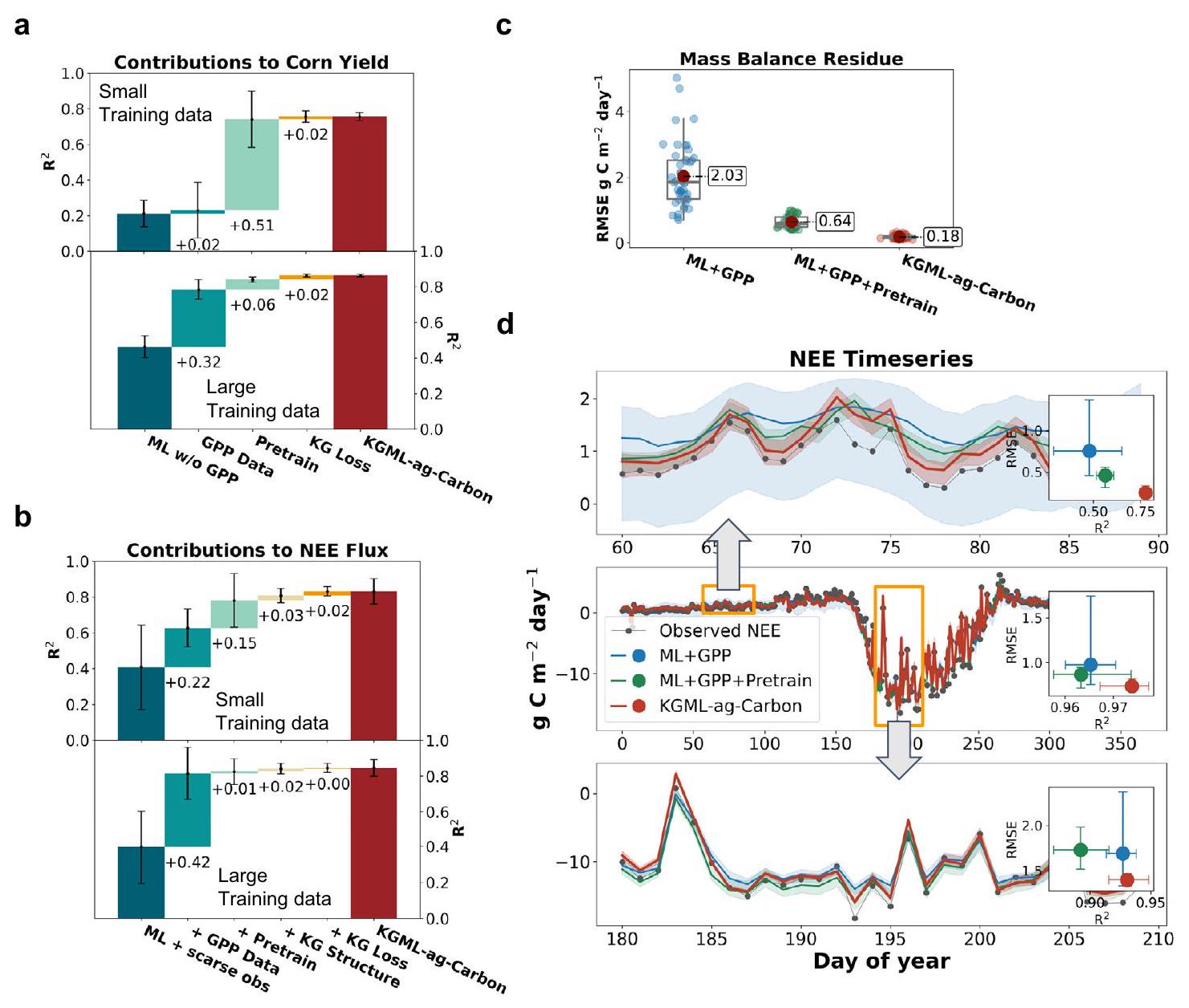
(1 و 7 مواقع) لتدريب النماذج، المشار إليها على أنها مجموعات عينات تدريب صغيرة وكبيرة، على التوالي. تم اختبار النماذج المحسّنة على مجموعات بيانات خارج العينة، والتي تشمل غلات NASS من 210 مقاطعات مختارة عشوائيًا وReco وNEE من 6 مجموعات من مواقع أبراج تدفق EC (تم تدريب النماذج التي تم اختبارها على مجموعة واحدة والتحقق من صحتها باستخدام بيانات من مواقع مختارة من مجموعات أخرى). قمنا بحساب المتوسط والانحراف المعياري لدقة التنبؤ لجميع النماذج من تجارب التجميع واكتشفنا تغييرات الأداء من خلال مقارنة النماذج مع وبدون كل مكون من مكونات KGML-ag-Carbon (الشكل S11). لتوضيح العوامل التي تساهم في أداء نموذج KGML-ag-Carbon، اخترنا خمسة نماذج تمثيلية من بين 16 نموذجًا تم تدريبها لعرض اتجاه تحسين الأداء. تشمل هذه النماذج (1) ML، (2) ML + GPP، (3) ML + GPP + التدريب المسبق، (4) التدريب المسبق + هيكل KG، و (5) ML + GPP + التدريب المسبق + هيكل KG + خسارة KG (الشكل 3a، b). للكشف بشكل أكبر عن تأثيرات مكونات المعرفة الموجهة (أي، التدريب المسبق، الهيكل الهرمي، ودوال خسارة KG) على تحسين أداء التنبؤ، قمنا بمقارنة ثلاثة أنواع من النماذج، بما في ذلك نموذج ML مع بيانات GPP، ونموذج ML مع GPP والتدريب المسبق، وKGML-ag-Carbon، فيما يتعلق بمخلفات توازن الكتلة للتنبؤات والأداء في التقاط التدفقات اليومية المعقدة لموقع-سنة تمثيلي (US-NE1-سنة 2016؛ الشكل 3c، d؛ الشكل S12).

تنبؤات عالية الدقة عبر منطقة الغرب الأوسط الأمريكي

بعد ضبط KGML-ag-Carbon باستخدام بيانات إنتاج الذرة وفول الصويا على مستوى المقاطعات بالإضافة إلى ملاحظات برج تدفق الكربون من مواقع النظم الزراعية (الجدول 1، الخطوة 5)، تم استخدام النموذج لمحاكاة إنتاج المحاصيل السنوي الإقليمي وتدفقات الكربون اليومية (أي، NEE، Ra، Rh، Reco) بدقة مكانية تبلغ 250 مترًا على مدى المنطقة الرئيسية لإنتاج الذرة وفول الصويا في الغرب الأوسط الأمريكي (الشكل S1) من عام 2000 إلى 2020. لتقييم أداء تقديرات تدفق الكربون على المستوى الإقليمي، قمنا بمقارنة نتائج النموذج مع Trendy. ، الذي تم إنشاؤه بواسطة مجموعة من نماذج الغطاء النباتي العالمية الديناميكية على مقياس شهري بدقة مكانية تبلغ أو أكثر خشونة. تم إعادة تنظيم قيم تدفق الكربون من هذه الدراسة إلى عن طريق حساب متوسط قيمة البكسلات داخل شبكة للمقارنة. تم استخدام توزيع الناتج الأولي السنوي المتراكم (GPP) وتدفق الكربون الصافي (NEE) واسترداد الكربون (Reco) من هذين المجموعتين من البيانات والملاحظات من مواقع أبراج تدفق EC المختارة للمقارنة (الشكل 4). يمكن أن يُعزى النطاق الواسع من التباين الذي لوحظ في مجموعة نماذج Trendy إلى تضمين عمليات متنوعة ومعلمات بديلة اعتمدتها نماذج من مجتمعات بحثية مختلفة، كما وصفه Sitch وآخرون. .

التحقيق في فوائد القياس عالي الدقة

لإنتاج دقة تبلغ 0.0025 درجة التقديرات لمنطقة الغرب الأوسط الأمريكي (الشكل 5أ-ج)، استخدمنا معادلة توازن الكتلة NEE – محصول المحاصيل على مدى الفترة من 2000 إلى 2020. على وجه التحديد، قمنا بإعادة تشكيل تقديرات NEE وإنتاج المحاصيل بدقة 250 متر من KGML-ag-Carbon إلى تقديرات للاستخدام في معادلة الميزان الكتلي. لتقليل تأثير بقايا المحاصيل السطحية غير المتحللة، التي لا تساهم في لكن يتم احتسابها كجزء من التقديرات من خلال نهج ميزان الكتلة، اخترنا القيمة المتوسطة على مدى 21 عامًا . ثم ركزنا على المناطق التي يزيد فيها تم زراعة المنطقة بالذرة أو محاصيل فول الصويا (الشكل S13a). تم تحويل القيم إلى كسور مئوية (الشكل 5ب) باستخدام مخزونات SOC المستندة إلى التعلم الآلي المستمدة من SoilGrids (الشكل S13b). على وجه التحديد، استخدمنا أجزاء من الذرة وفول الصويا من بيانات CDL وCSDL (الشكل S13a) لتحديد نظم الزراعة الخاصة بالذرة وفول الصويا بشكل حصري (إجمالي الجزء > 0.5). ساعد هذا التوافق مع نطاق تدريب نموذجنا الحالي في تقليل تأثير البكسل المختلط الناتج عن إدخال بيانات GPP المستشعرة عن بُعد من نظم بيئية أخرى. تم اشتقاق مخزون SOC من SoilGrids (الشكل S13b) من كثافة الكربون العضوي (OCD) في كل طبقة من عمق التربة عند قرار .
لنسب الأنماط المكانية المقدرة قمنا بإجراء تحليلات ارتباط بيرسون بين المتغيرات المدخلة (بما في ذلك سبعة متغيرات مناخية وتسعة متغيرات تربة) والمتغيرات المستهدفة (بما في ذلك GPP و NEE و Ra و Rh و Yield و Reco و Residue و ) (الشكل S14). في نهجنا، تم تجميع كل متغير زمنياً إلى مقياس 21 عاماً وتم تطبيعه باستخدام المعادلة (11). تم حساب متغير البقايا كـ GPP – Ra – العائد، مما يمثل صافي عائد الكربون من النباتات إلى التربة. بينما كانت GPP بمثابة مدخل إلى نموذج KGML-ag-Carbon، قمنا بتضمينها كمتغير مستهدف في تقييم الارتباط بسبب دورها المحوري في دورة الكربون. بالإضافة إلى ذلك، أجرينا تحليل الانحدار الخطي المتعدد لتقييم التأثير الكلي لعوامل المناخ وعوامل التربة على للحصول على تفسيرات أكثر شمولاً، يرجى الرجوع إلى المناقشة التكميلية.
لإظهار مزايا تقدير ميزانية الكربون عالية الدقة، قمنا بإنتاج دقة 0.5 درجة التقدير (الشكل 5d) وأجرينا تحليلًا مقارنًا مع تقدير دقة 0.0025 درجة (الشكل 5e، f). على وجه التحديد، استخدمنا KGML-ag-Carbon بدقة 0.5 درجة وطبقنا نهج توازن الكتلة لاشتقاق باستخدام تقديرات NEE وعائد المحاصيل بدقة 0.5 درجة (الشكل S15؛ الشكل 5d). لتحقيق ذلك، استخدمنا نهج التجميع المتوسط لكل متغير مدخل، محولين من دقة 250 متر إلى دقة 0.5 درجة. ومع ذلك، لم يكن تجميع أنواع المحاصيل من دقة عالية إلى دقة منخفضة أمرًا بسيطًا. لتقليد دورات المحاصيل الواقعية بشكل أفضل في المحاكاة ذات الدقة المنخفضة، أجرينا محاكاتين تتضمنان دورات الذرة وفول الصويا (الذرة في السنوات الزوجية وفول الصويا في السنوات الفردية) ودورات فول الصويا والذرة (فول الصويا في السنوات الزوجية والذرة في السنوات الفردية). بعد ذلك، استخدمنا نسب الذرة وفول الصويا من بيانات CDL وCSDL لحساب المتوسطات الموزونة لتقديرات الذرة وفول الصويا لكل عام باستخدام هاتين المحاكاتين. الفروقات بين دقة 0.5 درجة ودقة 0.0025 درجة تم حساب التقديرات بعد ذلك (الشكل 5e، f) عن طريق طرح تقدير دقة 0.0025 درجة من تقدير دقة 0.5 درجة. لتعزيز الوضوح، تم استبعاد المناطق خارج نظام الزراعة المعتمدة على الذرة وفول الصويا، وتم تحويل الفروقات المقدرة إلى كسور نسبية باستخدام طرق مشابهة لتلك المستخدمة في إنشاء الشكل 5b-c. لقد اعتمدنا على خطأ الجذر التربيعي المتوسط الطبيعي (NRMSE) لوصف الفروقات العامة:
حيث RMSE هو الجذر التربيعي لمتوسط الخطأ بين تقديرات دقة 0.5 درجة و 0.0025 درجة، و Q1 و Q3 تمثلان الثلاثة كوانتيلات وكوانتيل واحد لتقدير دقة 0.0025 درجة، على التوالي. تم اختيار هذه الطريقة لتجنب أن يصبح المقام صغيرًا جدًا. كما طبقنا نهجًا مشابهًا لحساب الفروقات في متغيرات أخرى، بما في ذلك GPP و Ra و Rh و NEE و Yield (الشكل S15). نلاحظ أن الفروقات النسبية في الشكل S15 تم حسابها كالتالي: (تقدير دقة 0.5 درجة – تقدير دقة 0.0025 درجة) / تقدير دقة 0.0025 درجة، مما يمثل الفروقات النسبية بالنسبة لكل بكسل بدقة 0.0025 درجة.
قمنا بإجراء مراجعة شاملة للأدبيات لجمع قياسات الكربون العضوي في التربة (SOC) المتاحة في وسط غرب الولايات المتحدة. شمل هذا الجهد بيانات من 18 موقعًا، كل منها يحتوي على قياسات متعددة للكربون العضوي في التربة على مستوى القطعة. ) بعد عام 2000، مما يسهل تحقق SOC لنموذج KGML-ag-Carbon (الشكل S16، الجدول S1). تم دمج البيانات الملاحظة مثل الكثافة الكلية، واحتياطي SOC الأولي في العمق 30 سم، وإدارة الدوران في ميزات الإدخال عند الاقتضاء. تم اشتقاق مدخلات أخرى مباشرة من قاعدة بياناتنا الإقليمية بدقة 250 مترًا، مثل قوى الطقس وGPP بناءً على المواقع الجغرافية الفيزيائية. لقد استخدمنا معادلة تجريبية لتمثيل
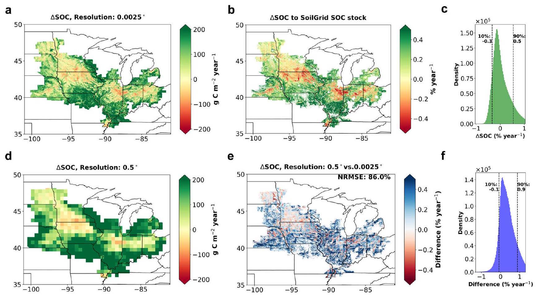
نسبة الكتلة من الكربون العضوي في التربة عند أعماق مختلفة إلى إجمالي المخزون (يفترض أن يكون الكربون العضوي في التربة في )، معبرًا عنه بـ:
أين هو النسبة المقدرة لحالة الشحن بين 0 إلى العمق. ساعدت هذه المعاملات في تحويل قيم SOC الملاحظة إلى الملف الكامل أو إلى العمق 30 سم العلوي في الحالات التي كانت فيها البيانات الخاصة بالعمق غير متاحة. ومن الجدير بالذكر أن جميع البيانات المجمعة البيانات تتعلق بمستوى القطعة ( القياسات التجريبية التي تركز بشكل أساسي على اكتشاف تأثيرات ممارسات الإدارة. غالبًا ما تفتقر البيانات من تلك المواقع إلى بيانات القوة المحلية المطلوبة من قبل نموذجنا. وبالتالي، نلجأ إلى استخدام قوى على مستوى الحقل (250 م) مثل الناتج الأولي الأولي المستشعر عن بُعد وإعادة تحليل بيانات الطقس من NLDAS، مما يسبب عدم تطابق في المقياس عند مقارنته بالملاحظات على مستوى الموقع. لتوضيح هذا عدم التطابق في المقياس، اخترنا موقعين من دراسات مختلفة. لمقارنة أحجام القطع التجريبية مع أحجام توقعاتنا والحقول الحقيقية المجاورة، كما هو موضح في الشكل S16a وb.

وصف بيئة التطوير

استخدمنا Pytorch 1.6.0 (https://pytorch.org/get-started/previousversions/، آخر وصول: 21 أكتوبر 2023) و بايثون 3.7.11 (https://www. python.org/downloads/release/python-3711/، آخر وصول: 21 أكتوبر 2023) كبيئة برمجية لتطوير النموذج. تم إجراء التحليل الإحصائي، مثل الانحدار الخطي، باستخدام Statsmodels 0.14.0 (https://github.com/statsmodels/statsmodels/، آخر وصول: 21 أكتوبر 2023) من أجل استخدام وحدة معالجة الرسومات (GPU) لتسريع عملية التدريب، قمنا بتثبيت مجموعة أدوات CUDA 10.1.243 (https://developer.nvidia.com/أداة كودا، آخر وصول: 21 أكتوبر 2023). تم استخدام جهاز كمبيوتر مكتبي مزود ببطاقة رسومات NVIDIA 2080 سوبر لتطوير واختبار الكود. تم إجراء عمليات التدريب، التي تتطلب وقتًا ومساحة ذاكرة واسعة، على مجموعات مانجي وأغيت.https://www.msi. umn.edu/mangi“، آخر وصول: 21 أكتوبر 2023) من مرفق الحوسبة عالية الأداء لمعهد مينيسوتا للحوسبة الفائقة (HPCMSI،https://www.msi.umn.edu/content/hpc، آخر وصول: 21 أكتوبر 2023) مع وحدات معالجة الرسوميات NVIDIA Tesla V100 ثنائية الاتجاه.

ملخص التقرير

معلومات إضافية حول تصميم البحث متاحة في ملخص تقارير مجموعة نيتشر المرتبط بهذه المقالة.

توفر البيانات

جميع البيانات المستخدمة في هذه الدراسة متاحة للجمهور كما هو موضح في الطرق. باختصار، بيانات NLDAS-2 المستخدمة في الدراسة متاحة على https:// ldas.gsfc.nasa.gov/nldas/nldas-2-forcing-data;gSSURGO متاح فيhttps://www.nrcs.usda.gov/resources/data-and-reports/description-of-gridded-soil-survey-geographic-gssurgo-database;بيانات محصول الذرة وفول الصويا متاحة علىhttps://quickstats.nass.usda.gov/؛بيانات CDL متاحة علىhttps://croplandcros.scinet.usda.gov/;بيانات CSDL متاحة في زينودو تحت رمز الوصولhttps://doi.org/10.5281/zenodo.4571628؛ بيانات GPP الخاصة بـ SLOPE متاحة علىhttps://daac.ornl.gov/cgi-bin/dsviewer.pl?ds_id=1786;بيانات معيار TRENDY-v9 متاحة علىhttps://www.wdc-climate.de/ui/entry؟ الاختصار=DKRZ_LTA_891_ds00012؛ وبيانات كثافة الكربون العضوي المستخدمة في هذه الدراسة متاحة في SoilGrids تحت رمز الوصولhttps://files.isric.org/soilgrids/latest/data/ocd/تنبؤات KGML-ag-Carbon المجمعة عند تم توفير البيانات الناتجة في هذه الدراسة في ملف البيانات المصدر، الذي تم إيداعه في قاعدة بيانات زينودو تحت رمز الوصولhttps://doi.org/10.5281/zenodo.10155516.

توفر الشيفرة

نموذج ecosys القائم على العمليات متاح علىhttps://github.com/jinyun1tang/ECOSYS، وOneFLUX لمعالجة بيانات برج تدفق الكربون متاحة عندhttps://github.com/fluxnet/ONEFluxشفرة المصدر
لإجراء معالجة البيانات ومكتبة بايثون قابلة للتنفيذ لنماذج KGML-agCarbon لتشغيل بيانات العرض متاحة من خلال Zenodo تحت رمز الوصولhttps://doi.org/10.5281/zenodo.10155516.

References

  1. Forster, P. et al. Chapter 7: The Earth’s Energy Budget, Climate Feedbacks, and Climate Sensitivity. https://doi.org/10.25455/ WGTN.16869671.V1 (2021).
  2. Skea, J. et al. Climate Change 2022: Mitigation of Climate Change. https://www.ipcc.ch/report/ar6/wg3/ (2022).
  3. Clark, M. A. et al. Global food system emissions could preclude achieving the and climate change targets. Science 370, 705-708 (2020).
  4. Bossio, D. A. et al. The role of soil carbon in natural climate solutions. Nat. Sustain. https://doi.org/10.1038/s41893-020-0491-z (2020).
  5. Fargione, J. E. et al. Natural climate solutions for the United States. Sci. Adv. 4, eaat1869 (2018).
  6. Wollenberg, E. et al. Reducing emissions from agriculture to meet the target. Glob. Chang. Biol. 22, 3859-3864 (2016).
  7. Oldfield, E. E. et al. Crediting agricultural soil carbon sequestration. Science 375, 1222-1225 (2022).
  8. Novick, K. A. et al. Informing nature-based climate solutions for the United States with the best-available science. Glob. Chang. Biol. 28, 3778-3794 (2022).
  9. Bradford, M. A. et al. Soil carbon science for policy and practice. Nat. Sustain. 2, 1070-1072 (2019).
  10. Ranganathan, J., Waite, R., Searchinger, T. & Zionts, J. Regenerative Agriculture: Good for Soil Health, but Limited Potential to Mitigate Climate Change. https://www.wri.org/insights/regenerative-agriculture-good-soil-health-limited-potential-mitigate-climatechange (2020).
  11. Smith, P. et al. How to measure, report and verify soil carbon change to realize the potential of soil carbon sequestration for atmospheric greenhouse gas removal. Glob. Chang. Biol. 26, 219-241 (2020).
  12. Guan, K. et al. A scalable framework for quantifying field-level agricultural carbon outcomes. Earth-Science Reviews 243, 104462 (2023).
  13. Zhou, W. et al. Quantifying carbon budget, crop yields and their responses to environmental variability using the ecosys model for U.S. Midwestern agroecosystems. Agric. Meteorol. 307, 108521 (2021).
  14. Irrgang, C. et al. Towards neural Earth system modelling by integrating artificial intelligence in Earth system science. Nat. Mach. Intell. https://doi.org/10.1038/s42256-021-00374-3 (2021).
  15. Jung, M. et al. Scaling carbon fluxes from eddy covariance sites to globe: synthesis and evaluation of the FLUXCOM approach. Biogeosciences 17, 1343-1365 (2020).
  16. Rasp, S., Pritchard, M. S. & Gentine, P. Deep learning to represent subgrid processes in climate models. Proc. Natl Acad. Sci. USA 115, 9684-9689 (2018).
  17. Zhan, W. et al. Two for one: partitioning CO2 fluxes and understanding the relationship between solar-induced chlorophyll fluorescence and gross primary productivity using machine learning. Agric. Meteorol. 321, 108980 (2022).
  18. Hutson, M. TAUGHT TO THE TEST: AI software clears high hurdles on IQ tests but still makes dumb mistakes. Can better benchmarks help?. Science 376, 570-573 (2022).
  19. Karpatne, A. et al. Theory-guided data science: a new paradigm for scientific discovery from data. IEEE Trans. Knowl. Data Eng. 29, 2318-2331 (2017).
  20. Grosz, B. et al. The implication of input data aggregation on upscaling soil organic carbon changes. Environ. Model. Softw. 96, 361-377 (2017).
  21. Karpatne, A., Kannan, R. & Kumar, V. Knowledge Guided Machine Learning: Accelerating Discovery using Scientific Knowledge and Data. (CRC Press, 2022).
  22. Willard, J., Jia, X., Xu, S., Steinbach, M. & Kumar, V. Integrating scientific knowledge with machine learning for engineering and environmental systems. ACM Comput. Surv. https://doi.org/10. 1145/3514228 (2022).
  23. Kraft, B., Jung, M., Körner, M., Koirala, S. & Reichstein, M. Towards hybrid modeling of the global hydrological cycle. Hydrol. Earth Syst. Sci. https://doi.org/10.5194/hess-26-1579-2022 (2022).
  24. ElGhawi, R. et al. Hybrid Modeling of evapotranspiration: inferring stomatal and aerodynamic resistances using combined physicsbased and machine learning. ESSOAr https://doi.org/10.1002/ essoar. 10512258.1 (2022).
  25. He, X. et al. Improving predictions of evapotranspiration by integrating multi-source observations and land surface model. Agric. Water Manag. 272, 107827 (2022).
  26. Beucler, T. et al. Enforcing analytic constraints in neural networks emulating physical systems. Phys. Rev. Lett. 126, 098302 (2021).
  27. Reichstein, M. et al. Deep learning and process understanding for data-driven Earth system science. Nature 566, 195-204 (2019).
  28. Liu, L. et al. KGML-ag: a modeling framework of knowledge-guided machine learning to simulate agroecosystems: a case study of estimating N2O emission using data from mesocosm experiments. Geosci. Model Dev. 15, 2839-2858 (2022).
  29. Grant, R. A Review of the Canadian Ecosystem Model-ecosys. in Modeling Carbon and Nitrogen Dynamics for Soil Management (CRC Press, 2001).
  30. Cho, K., van Merrienboer, B., Bahdanau, D. & Bengio, Y. On the Properties of Neural Machine Translation: Encoder-Decoder Approaches. https://doi.org/10.48550/arXiv.1409.1259 (2014).
  31. Stuart Chapin, F., III, Matson, P. A. & Mooney, H. A. Principles of Terrestrial Ecosystem Ecology. (Springer Science & Business Media, 2011).
  32. Reichle, D. E. The Global Carbon Cycle and Climate Change. (Elsevier Science Publishing, 2019).
  33. Baker, J. M. & Griffis, T. J. Examining strategies to improve the carbon balance of corn/soybean agriculture using eddy covariance and mass balance techniques. Agric. Meteorol. 128, 163-177 (2005).
  34. Jiang, C., Guan, K., Wu, G., Peng, B. & Wang, S. A daily, 250 m and real-time gross primary productivity product (2000-present) covering the contiguous United States. Earth Syst. Sci. Data 13, 281-298 (2021).
  35. Sitch, S. et al. Recent trends and drivers of regional sources and sinks of carbon dioxide. Biogeosciences 12, 653-679 (2015).
  36. Al-Kaisi, M. M. & Kwaw-Mensah, D. Quantifying soil carbon change in a long-term tillage and crop rotation study across lowa landscapes. Soil Sci. Soc. Am. J. 84, 182-202 (2020).
  37. Ibrahim, M. A., Chua-Ona, T., Liebman, M. & Thompson, M. L. Soil organic carbon storage under biofuel cropping systems in a humid, continental climate. Agron. J. 110, 1748-1753 (2018).
  38. Poffenbarger, H. J. et al. Maximum soil organic carbon storage in Midwest U.S. cropping systems when crops are optimally nitrogenfertilized. PLoS ONE 12, e0172293 (2017).
  39. Olson, K., Ebelhar, S. A. & Lang, J. M. Long-term effects of cover crops on crop yields, soil organic carbon stocks and sequestration. Open J. Soil Sci. 04, 284-292 (2014).
  40. Jin, V. L. et al. Twelve years of Stover removal increases soil erosion potential without impacting yield. Soil Sci. Soc. Am. J. 79, 1169-1178 (2015).
  41. Schmer, M. R., Jin, V. L., Wienhold, B. J., Varvel, G. E. & Follett, R. F. Tillage and residue management effects on soil carbon and nitrogen under irrigated continuous corn. Soil Sci. Soc. Am. J. 78, 1987-1996 (2014).
  42. Stanley, P., Spertus, J., Chiartas, J., Stark, P. B. & Bowles, T. Valid inferences about soil carbon in heterogeneous landscapes. Geoderma 430, 116323 (2023).
  43. Goidts, E., Van Wesemael, B. & Crucifix, M. Magnitude and sources of uncertainties in soil organic carbon (SOC) stock assessments at various scales. Eur. J. Soil Sci. 60, 723-739 (2009).
  44. Asseng, S., Ewert, F. & Rosenzweig, C. Uncertainty in simulating wheat yields under climate change. Nature Clim Change. Nat. Clim. Change 3, 827-832 (2013).
  45. Mezbahuddin, S. et al. Assessing effects of agronomic nitrogen management on crop nitrogen use and nitrogen losses in the western Canadian prairies. Front. Sustain. Food Syst. 4, 512292 (2020).
  46. Grant, R. F. et al. Net biome productivity of irrigated and rainfed maize-soybean rotations: Modeling vs. Measurements. Agron. J. 99, 1404-1423 (2007).
  47. Grant, R. F. et al. Controlled Warming Effects on Wheat Growth and Yield: Field Measurements and Modeling. Crop Ecol. Physiol. https://doi.org/10.2134/agronj2011.0158 (2011).
  48. Zhou, Q. et al. Recent rapid increase of cover crop adoption across the U.S. midwest detected by fusing multi-source satellite data. Geophys. Res. Lett. 49, e2022GL100249 (2022).
  49. Wang, S. et al. Cross-scale sensing of field-level crop residue cover: Integrating field photos, airborne hyperspectral imaging, and satellite data. Remote Sens. Environ. 285, 113366 (2023).
  50. Zhang, J. et al. Combining remotely sensed evapotranspiration and an agroecosystem model to estimate center-pivot irrigation water use at high spatio-temporal resolution. Water Resour. Res. 59, e2022WR032967 (2023).
  51. Ghosh, R. et al. Robust Inverse Framework using knowledge-guided self-supervised learning. in Proc 28th ACM SIGKDD Conference on Knowledge Discovery and Data Mining. https://doi.org/10.1145/ 3534678.3539448 (ACM, 2022).
  52. Ding, F. & Xue, Y. X-MEN: guaranteed XOR-maximum entropy constrained inverse reinforcement learning. in Uncertainty in Artificial Intelligence 589-598 (PMLR, 2022).
  53. Jia, X. et al. Graph-based reinforcement learning for active learning in real time: an application in modeling river networks. Proc 2021 SIAM International Conference on Data Mining (SDM). 621-629 https://doi.org/10.1137/1.9781611976700.70 (2021).
  54. Mekonnen, Z. A., Riley, W. J., Randerson, J. T., Grant, R. F. & Rogers, B. M. Expansion of high-latitude deciduous forests driven by interactions between climate warming and fire. Nat. Plants 5, 952-958 (2019).
  55. Grant, R. F., Lin, S. & Hernandez-Ramirez, G. Modelling nitrification inhibitor effects on N 2 O emissions after fall- and spring-applied slurry by reducing nitrifier NH4 oxidation rate. Biogeosciences https://doi.org/10.5194/bg-17-2021-2020 (2020).
  56. Qin, Z. et al. Assessing the impacts of cover crops on maize and soybean yield in the U.S. Midwestern agroecosystems. Field Crops Res. https://doi.org/10.1016/j.fcr.2021.108264 (2021).
  57. Li, Z. et al. Assessing the impacts of pre-growing-season weather conditions on soil nitrogen dynamics and corn productivity in the U.S. Midwest. Field Crops Res. https://doi.org/10.1016/j.fcr.2022. 108563 (2022).
  58. Ma, Z. et al. Interaction of hydrological and anthropogenic processes controls the relationship between streamflow discharge and nitrogen concentration in the U.S. Midwestern watersheds. B45L-1769 (2021).
  59. Yang, Y. et al. Distinct driving mechanisms of non-growing season N2O emissions call for spatial-specific mitigation strategies in the US Midwest. Agricult. Forest Meteorol. https://doi.org/10.1016/j. agrformet.2022.109108 (2022).
  60. Walther, S. et al. Technical note: a view from space on global flux towers by MODIS and Landsat: the FluxnetEO data set. Biogeosciences https://doi.org/10.5194/bg-19-2805-2022 (2022).
  61. Pastorello, G. et al. The FLUXNET2O15 dataset and the ONEFlux processing pipeline for eddy covariance data. Sci. Data 7, 225 (2020).
  62. Bauer, P. et al. The digital revolution of Earth-system science. Nat. Comput. Sci. 1, 104-113 (2021).
  63. Wang, S., Di Tommaso, S., Deines, J. M. & Lobell, D. B. Mapping twenty years of corn and soybean across the US Midwest using the Landsat archive. Sci. Data 7, 307 (2020).
  64. Khandelwal, A. et al. Physics Guided Machine Learning Methods for Hydrology. https://doi.org/10.48550/ARXIV.2012.02854 (2020).
  65. Hochreiter, S. & Schmidhuber, J. Long short-term memory. Neural Comput. 9, 1735-1780 (1997).
  66. Chung, J., Gulcehre, C., Cho, K. & Bengio, Y. Empirical Evaluation of Gated Recurrent Neural Networks on Sequence Modeling. https:// doi.org/10.48550/arXiv.1412.3555 (2014).
  67. Bahdanau, D., Cho, K. & Bengio, Y. Neural Machine Translation by Jointly Learning to Align and Translate. https://doi.org/10.48550/ arXiv.1409.0473 (2014).
  68. Xu, S. et al. Mini-Batch Learning Strategies for modeling long term temporal dependencies: a study in environmental applications. in Proc 2023 SIAM International Conference on Data Mining (SDM) 649-657 (Society for Industrial and Applied Mathematics, 2023).
  69. Kumar, M. P., Packer, B. & Koller, D. Self-paced learning for latent variable models. in Proc 24th Annual Conference on Neural Information Processing Systems 1189-1197 (Curran Associates, Inc., 2010).
  70. Bengio, Y., Louradour, J., Collobert, R. & Weston, J. Curriculum learning. in Proc 26th Annual International Conference on Machine Learning. https://doi.org/10.1145/1553374.1553380 (ACM, 2009).
  71. Poggio, L. et al. SoilGrids 2.0: producing soil information for the globe with quantified spatial uncertainty. SOIL 7, 217-240 (2021).
  72. Cao, Q. et al. On the spatial variability and influencing factors of soil organic carbon and total nitrogen stocks in a desert oasis ecotone of northwestern China. Catena 206, 105533 (2021).

شكر وتقدير

يقر المؤلفون بالدعم من وكالة مشاريع الأبحاث المتقدمة للطاقة التابعة لوزارة الطاقة (ARPA-E) برامج SMARTFARM (رقم الجائزة DE-AR0001382)، برنامج نظام مراقبة الكربون التابع لناسا (رقم الجائزة 80NSSC18K0170)، برنامج الإشارة في التربة التابع لمؤسسة العلوم الوطنية (رقم الجائزة 2034385) وبرنامج جائزة CAREER للهيئة التدريسية (رقم الجائزة 1847334)، برنامج المعهد الوطني للغذاء والزراعة التابع لوزارة الزراعة الأمريكية (NIFA) (رقم الجائزة 2017-67013-26253)، ومؤسسة أبحاث الغذاء والزراعة (رقم الجائزة 602757). كما نقر بالمواقع التالية من AmeriFlux لسجلات بياناتها:
US-Ne1، US-Ne2، US-Ne3، US-Bo1، US-Bo2، US-Br1، US-Br3، US-Ib1، USRo1، US-Ro5، و US-KL1.

مساهمات المؤلفين

قام L.L. و Z.J. و W.Z. و K.G. بتصميم الدراسة. قاد L.L. و W.Z. التحليل بشكل مشترك، وقاما بإنتاج الأشكال والجداول، وكتابة الورقة الأولية. أشرف Z.J. و K.G. على العملية بأكملها. ساهم B.P. و S.X. و J. Tang و Q.Z. و X.J. و C.J. و Z.Q. و V.K. بالبيانات الخام، وكود ecosys، والوثائق، و/أو منهجية التعلم الآلي. ساهم جميع المؤلفين في تفسير النتائج وقاموا بتحرير الورقة. المؤلف الرئيسي المراسل هو Z.J.، الذي يحتفظ مختبره بجميع البيانات والكود المشتركة المتعلقة بهذه الورقة.

المصالح المتنافسة

يعلن المؤلفون عدم وجود مصالح متنافسة.

معلومات إضافية

معلومات إضافية النسخة الإلكترونية تحتوي على
المواد التكميلية متاحة على
https://doi.org/10.1038/s41467-023-43860-5.
يجب توجيه المراسلات والطلبات للحصول على المواد إلى كايو غوان أو زينونغ جين.
معلومات مراجعة الأقران تشكر مجلة Nature Communications المراجعين المجهولين على مساهمتهم في مراجعة هذا العمل. يتوفر ملف مراجعة الأقران.
معلومات إعادة الطباعة والتصاريح متاحة على
http://www.nature.com/reprints
ملاحظة الناشر: تظل شركة سبرينغر ناتشر محايدة فيما يتعلق بالمطالبات القضائية في الخرائط المنشورة والانتماءات المؤسسية.
الوصول المفتوح هذه المقالة مرخصة بموجب رخصة المشاع الإبداعي النسب 4.0 الدولية، التي تسمح بالاستخدام والمشاركة والتكيف والتوزيع وإعادة الإنتاج بأي وسيلة أو صيغة، طالما أنك تعطي الائتمان المناسب للمؤلفين الأصليين والمصدر، وتوفر رابطًا لرخصة المشاع الإبداعي، وتوضح إذا ما تم إجراء تغييرات. الصور أو المواد الأخرى من طرف ثالث في هذه المقالة مشمولة في رخصة المشاع الإبداعي الخاصة بالمقالة، ما لم يُشار إلى خلاف ذلك في سطر الائتمان للمواد. إذا لم تكن المادة مشمولة في رخصة المشاع الإبداعي الخاصة بالمقالة وكان استخدامك المقصود غير مسموح به بموجب اللوائح القانونية أو يتجاوز الاستخدام المسموح به، فسيتعين عليك الحصول على إذن مباشرة من صاحب حقوق الطبع والنشر. لعرض نسخة من هذه الرخصة، قم بزيارةhttp://creativecommons.org/رخصة/بواسطة/4.0/.
© المؤلف(ون) 2024

  1. قسم المنتجات الحيوية وهندسة الأنظمة الحيوية، جامعة مينيسوتا، سانت بول، MN 55108، الولايات المتحدة الأمريكية. مركز استدامة النظم الزراعية، معهد الاستدامة والطاقة والبيئة، جامعة إلينوي في أوربانا-شامبين، أوربانا، إلينوي 61801، الولايات المتحدة الأمريكية. قسم الموارد الطبيعية وعلوم البيئة، كلية الزراعة والمستهلك والعلوم البيئية، جامعة إلينوي في أوربانا-شامبين، أوربانا، إلينوي 61801، الولايات المتحدة الأمريكية. قسم علوم الحاسوب، جامعة إلينوي في أوربانا-شامبين، أوربانا، إلينوي 61801، الولايات المتحدة الأمريكية. المركز الوطني لتطبيقات الحوسبة الفائقة، جامعة إلينوي في أوربانا-شامبين، أوربانا، إلينوي 61801، الولايات المتحدة الأمريكية. قسم علوم الحاسوب والهندسة، جامعة مينيسوتا، مينيابوليس، MN 55455، الولايات المتحدة الأمريكية. علوم الأرض والبيئة، مختبر لورانس بيركلي الوطني، بيركلي، كاليفورنيا 94720، الولايات المتحدة الأمريكية. قسم علوم الحاسوب، جامعة بيتسبرغ، بيتسبرغ، بنسلفانيا 15260، الولايات المتحدة الأمريكية. قسم الزراعة البيئية، جامعة آرهوس، 4200 سلاجلز، الدنمارك. مدرسة همفري للشؤون العامة، جامعة مينيسوتا، مدن التوأم، مينيسوتا 55455، الولايات المتحدة الأمريكية. قسم الموارد المتجددة، جامعة ألبرتا، إدمونتون، ألبرتا T6G2E3، كندا. فرع المعرفة البيئية والتنبؤ، وزارة البيئة والمناطق المحمية في ألبرتا، إدمونتون، ألبرتا T5K 2J6، كندا. هؤلاء المؤلفون ساهموا بالتساوي: ليشينغ ليو، وانغ زو. البريد الإلكتروني:kaiyug@illinois.edu; jinzn@umn.edu

Journal: Nature Communications, Volume: 15, Issue: 1
DOI: https://doi.org/10.1038/s41467-023-43860-5
PMID: https://pubmed.ncbi.nlm.nih.gov/38191521
Publication Date: 2024-01-08

Knowledge-guided machine learning can improve carbon cycle quantification in agroecosystems

Received: 1 January 2023
Accepted: 22 November 2023
Published online: 08 January 2024
(A) Check for updates

Abstract

Licheng Liu (1) , Wang Zhou , Kaiyu Guan , Bin Peng (1) , Shaoming Xu , Jinyun Tang , Qing Zhu , Jessica Till , Xiaowei Jia , Chongya Jiang , Sheng Wang (1) , Ziqi Qin , Hui Kong , Robert Grant (1) , Symon Mezbahuddin © , Vipin Kumar & Zhenong Jin (B)

Abstract

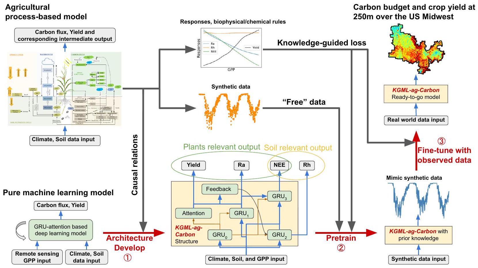
Accurate and cost-effective quantification of the carbon cycle for agroecosystems at decision-relevant scales is critical to mitigating climate change and ensuring sustainable food production. However, conventional process-based or data-driven modeling approaches alone have large prediction uncertainties due to the complex biogeochemical processes to model and the lack of observations to constrain many key state and flux variables. Here we propose a Knowledge-Guided Machine Learning (KGML) framework that addresses the above challenges by integrating knowledge embedded in a process-based model, high-resolution remote sensing observations, and machine learning (ML) techniques. Using the U.S. Corn Belt as a testbed, we demonstrate that KGML can outperform conventional process-based and black-box ML models in quantifying carbon cycle dynamics. Our high-resolution approach quantitatively reveals more spatial detail of soil organic carbon changes than conventional coarse-resolution approaches. Moreover, we outline a protocol for improving KGML via various paths, which can be generalized to develop hybrid models to better predict complex earth system dynamics.

Crop production systems and their interactions with the environment, known as agroecosystems, cover about one-third of the Earth’s land surface. As soil constitutes the largest single carbon reservoir on land, agroecosystems play a key role in the global terrestrial carbon cycle through crop interactions with soils and atmosphere . Globally, agriculture is a significant source of greenhouse gasses (GHGs); yet, carbon
uptake by crops also removes large amounts of carbon dioxide ( ) from the atmosphere, some of which can be stabilized in soil . Because most intensively cultivated soils are carbon-unsaturated, practices that increase soil organic carbon (SOC) represent a low-cost, large-scale strategy for reducing atmospheric GHG concentrations . Thus, it is essential to accurately quantify carbon fluxes and changes in SOC in
agroecosystems so that appropriate and effective conservation practices can be identified for any given location.
Increasing agricultural carbon sequestration is a key strategy for mitigating climate change. Significant efforts and investments have been made in the U.S. and across the globe to implement programs that incentivize SOC enrichment . In light of these initiatives, it is important to develop robust and scalable methods for reliably quantifying fieldlevel carbon sequestration, both to assess the climate mitigation effect and to ensure that mitigation actions by individual farmers are compensated fairly and accurately. Traditional carbon quantification methods that rely on soil sampling, emission factors, and process-based (PB) modeling entail inherent barriers to achieving the required levels of accuracy, scalability, and cost-effectiveness . In particular, high spatial heterogeneity and seasonality due to variations in environmental conditions, crop types, and management practices present challenges for accurately quantifying carbon budgets . While PB modeling approaches incorporate scientific knowledge, large uncertainties arise in PB models if local- and crop-specific parameters are not calibrated properly or if the underlying mechanisms are oversimplified or incompletely represented . Additionally, PB models with detailed representations of existing scientific principles can be computationally prohibitive when applied to large regions at high spatial-temporal resolution (e.g., 250 m daily). On the other hand, data-driven machine learning (ML) approaches have the potential for high computational efficiency and accuracy but suffer from out-of-sample prediction failure in the absence of large training datasets, which are unavailable for most agricultural applications. Moreover, the results of ML models are often uninterpretable due to their black-box nature . Therefore, new methods are needed to overcome the limitations of PB and ML models, enabling cost-effective, accurate, and interpretable measurement and monetization of carbon outcomes at the individual field level. This will reduce errors in aggregated quantifications and promote more sustainable land management practices .
The growing field of knowledge-guided machine learning (KGML) provides a promising methodology that combines the advantages of PB models, ML models, and multi-source datasets (e.g., in-situ and remote sensing data). Existing KGMLs can successfully model certain Earth systems for which dynamic processes are wellrepresented by established governing equations, such as hydrology and atmospheric sciences . However, complex and crucial ecosystem processes such as biogeochemical cycling are mathematically non-linear and substantially more complicated. Furthermore, unlike surficial systems, soil interactions in agroecosystems largely cannot be directly observed by remote sensing, whereas in-situ direct measurements are often expensive and limited. Therefore new KGML approaches must be developed to incorporate sufficient biogeochemical knowledge and effectively assimilate indirect measurements (e.g., remote sensing and survey data) to capture terrestrial processes that are less directly observable .
To address the existing gaps in carbon budget modeling capabilities, we developed a novel KGML framework that combines prior biogeochemical knowledge of carbon dynamics with a deep learning model to generate reliable predictions of agricultural carbon fluxes, crop yields, and changes in soil carbon stocks (KGML-ag-Carbon, Fig. 1). In-situ eddy covariance (EC) flux tower data, regional survey yield data, remotely-sensed gross primary production (GPP) data, and synthetic data generated by a PB model were assimilated into KGML-ag-Carbon. The model effectiveness is demonstrated here for corn and soybean production in the U.S. Midwest (Fig. S1), with highly accurate outputs for carbon fluxes, crop yields, and changes in soil carbon at high spatial ( 250 m ) and temporal (daily) resolution, providing usable data for land managers. We also analyzed the improvement resulting from each KGML component and certain biogeochemical responses. The model design presented here exemplifies a solution to challenges in simulating dynamic heterogeneous systems, which will help advance broader applications of KGML for understanding Earth processes.
Fig. 1 | Overview of the method and framework used for KGML-ag-Carbon development. The development of KGML-ag-Carbon has three main steps: (1) Developing the architecture of the machine learning model based on the causal relations derived from an agricultural process-based model; (2) pre-training the KGML-ag-Carbon using synthetic data generated by a process-based model; and (3)
fine-tuning KGML-ag-Carbon using observed low-resolution crop yield data and carbon fluxes from sparsely distributed eddy-covariance sites. The knowledgeguided losses were designed based on the process-based model to further constrain the response of target variables to input variables during both model pretraining and fine-tuning processes.

Results

Overview of the KGML-ag-Carbon framework

KGML-ag-Carbon is a novel framework combining process-based understanding and advanced AI approaches for simulating complex biogeochemical cycles under intensive management practices for agroecosystems. KGML-ag-Carbon distinguishes itself from previous KGML applications in other disciplines by its use of a well-validated PB model, ecosys , and its ability to directly assimilate remote sensing data. The deep learning model based on the gated recurrent unit (GRU) mechanism was used to develop KGML-ag-Carbon’s architechture (Fig. 1). The ecosystem theory of carbon allocation is the basis for the ecosys model, which was used to design the hierarchical structure of KGML-ag-Carbon, including submodules related to plants, soil, atmospheric carbon exchange, and feedback of carbon from plants to soil (Fig. S2). Importantly, outputs from the ecosys model provided synthetic data on ecosystem carbon allocation, associated fluxes, and environmental responses that were used to pre-train the KGML-ag-Carbon model. This pre-training step confers a major advantage to the model by improving the predictive ability with a minimal amount of labeled samples and accelerating the convergence in model tuning using labeled samples. GPP data, which represents the dominant carbon input to agroecosystems, was retrieved from remote sensing observations and assimilated into KGML-ag-Carbon as spatial constraints.
KGML-ag-Carbon resolves the major carbon budget components, including autotrophic respiration (Ra), heterotrophic respiration (Rh), total ecosystem respiration (Reco, ), and net ecosystem carbon exchange (NEE) on a daily scale, and yield on an annual scale. As in natural ecosystems, changes in agroecosystem soil carbon storage are determined by the mass balance of input and output carbon fluxes . Ecosystem carbon inputs originate from plant photosynthesis, i.e., gross primary production (GPP), while soil carbon inputs include both aboveground and belowground litter and root exudates. Carbon outputs occur through respiration, including Ra from plant shoots and roots and Rh from SOC decomposition by microbes and fungi. Disturbances such as harvesting also remove carbon from the ecosystem periodically. Based on the carbon fluxes and yield estimated from KGML-ag-Carbon, annual changes in SOC can be determined using the mass balance equation NEE – Yield .
We systematically explored multiple paths for improving the prediction performance of KGML-ag-Carbon, including pre-training the model with synthetic data and incorporating knowledge-guided (KG) loss functions, which addresses broader issues about reducing uncertainty for hybrid modeling. Over 14 million synthetic data and various KG loss functions were used to pre-train KGML-ag-Carbon to learn the prior knowledge from the PB model (Fig. 1). Using synthetic data generated by a PB model is several orders of magnitude cheaper than the cost of collecting real-world observations. The KG loss functions include biogeochemical/physical constraints such as mass balance ( ), prediction thresholds (e.g., yield ), and responses of outputs to inputs (e.g., Rh should monotonically increase with SOC content under other fixed conditions).
A subset of the observed yield data from USDA ( 320 out of 630 counties) along with Reco ( ) and NEE data from 11 cropland EC flux tower sites were then used to fine-tune the pre-trained KGML-ag-Carbon model to improve its prediction ability for realworld carbon budgets (Fig. 1). KG loss functions with biogeochemical/physical constraints similar to those used in pre-training were included in the fine-tuning. However, to preserve sufficient pretraining knowledge, the synthetic data were merged with observational data during fine-tuning, while extra constraints were added to the KG loss functions to maintain the responses of outputs to inputs (e.g., changes in Ra responses to the environment remain within ). Details on the structural development, datasets utilized, and
training strategies for the KGML-ag-Carbon model are provided in the Methods section.

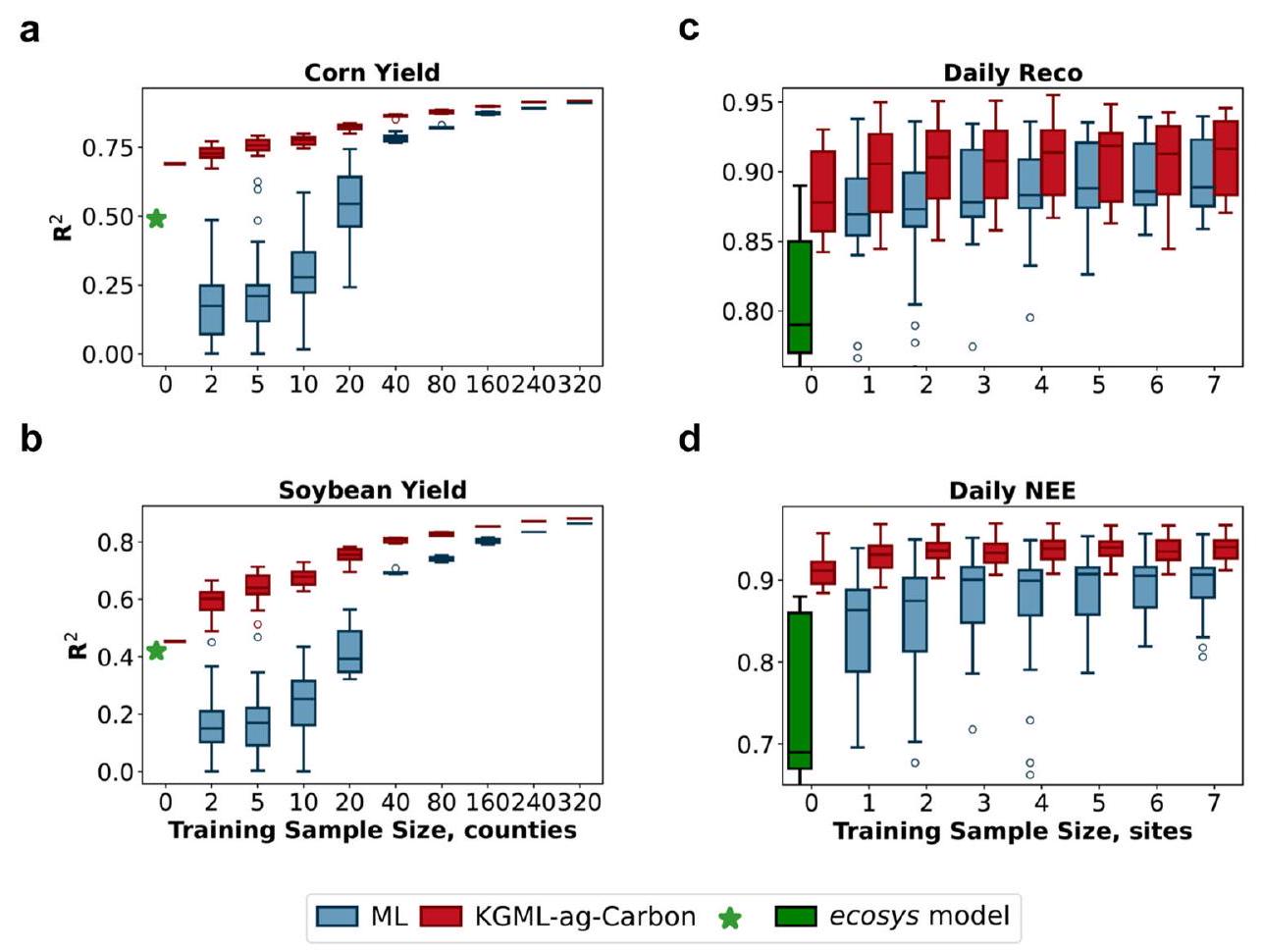
Model performance in crop yield and carbon flux predictions

We evaluated the performance of KGML-ag-Carbon both before and after fine-tuning along with the sensitivity of model performance to the real-world training sample size (Figs. 2, S4, S6, S8). As an initial check on pre-training effectiveness, the pre-trained KGML-ag-Carbon model results for the test set of synthetic data (two years out of the 18-year period) were compared with ecosys simulations and found to be highly consistent, with values of , and 0.97 for yield, Ra, Rh, and NEE, respectively (Fig. S4). values of the ecosys model for corn and soybean yield predictions were 0.49 and 0.42, respectively, as benchmarked with observed county-scale crop yields, while values for daily Reco and NEE predictions were and 0.59-0.88, respectively, compared with measurements from EC sites (green stars/boxes in Fig. 2, derived from Zhou et al. ). After fine-tuning, the of KGML-ag-Carbon for corn and soybean yield predictions on a test set of 210 counties were 0.91 and 0.88, while values for daily Reco and NEE predictions tested on 2 years of out-of-sample data from 11 EC flux tower sites were 0.94 and 0.96 , respectively (Fig. S8).
The robustness test (Fig. 2) reveals that compared with a GRUbased pure ML model using the same inputs, KGML-ag-Carbon both consistently outperforms the pure ML model and has much lower sensitivity to the number of real-world training samples. In summary, the major differences between KGML-ag-Carbon and pure ML lie in the additional pre-training process and the customized model structure and loss functions guided by known scientific knowledge. These advancements enhance the optimization process of the ML model and allow reliable predictions to be made with fewer labeled samples. The pure ML model performance approached that of KGML-ag-Carbon at large sample sizes but performed poorly with small training sets, particularly for crop yield (Fig. 2a, b). The reduced need for training samples is a central advantage of KGML-ag-Carbon for real-world crop yield and carbon flux estimates because available training data are usually limited and collecting data from physical sampling is costly. The improvements in carbon flux predictions with increasing sample size mostly arise from capturing the interannual carbon dynamics, which can be more easily learned from seasonal patterns of GPP and climate (Fig. 2c, d). Even without fine-tuning (a training sample size of 0 ), the KGML-ag-Carbon by assimilating the GPP data as input, can outperform both ecosys model and pure ML model trained with small training samples (Fig. 2).
We conducted several additional experiments to evaluate the performance of KGML-ag-Carbon under different training, validation, and testing dataset splits, including out-of-sample performance of yield predictions in the spatial and temporal domains (Fig. S9a-f). For example, we used data from Illinois for testing and data from other states for training and validation and used several continuous years of data for training and validation with other years for testing. We also examined the effect of using extreme years with exceptionally high or low yields for testing and other years for training and validation. We note that the KGML-ag-Carbon model outperforms pure ML and process-based models in predicting yield in extreme years (Fig. S9e, f) primarily because it is constrained by both observations and synthetic data generated from the PB model. Similarly, out-of-sample performance for Reco and NEE predictions was investigated on both annual and daily temporal scales and specifically examined for sites (EC flux towers US-NE 1-3) with longer-term observations covering 2001-2019 (Fig. S9g-l). The results demonstrate consistently better performance of KGML-ag-Carbon compared to pure ML in all tested situations. The details of robustness tests on the KGML-ag-Carbon performance can be found in the Methods section.
Fig. 2 | The comparative performance of the pure ML model (blue boxes) and KGML-ag-Carbon (red boxes) when using different sizes of observed
data samples for model training. a, b The yield prediction performance over 210 counties. , and 1 independent experiments for model ensembles with a training sample size of , and 320 , respectively. Each training sample has a 21-year period of annual yield observations in one county. The Reco and NEE prediction performance across 11 EC flux towers. independent experiments for training sample size from 1 to 7 . and 6 independent experiments for the ecosys model and KGML-ag-Carbon model ensembles with a training sample size of 0 , respectively. Each training sample has daily observations during the observation period in one site (varying
by site, ranging from 5 to 19 years). Each box plot illustrates the first and third quartiles (lower and upper box edges), median (central line), and minimum and maximum (lower and upper whiskers), with outliers as round circles. The green stars represent the performance of ecosys in crop yield simulations across the U.S. states of Illinois, Iowa, and Indiana constrained with remotely sensed GPP and observed yield, and the green boxes represent the performance of ecosys in carbon flux simulations at 7 EC flux tower sites across the U.S. Midwest from Zhou et al. , which is a subset of the dataset used in this study. Only out-of-sample test results from cross-validation ensembles are depicted here. Details of the experiments can be found in the “Methods” section. Source data are provided as a Source Data file.

Pathways to reduce KGML-ag-Carbon uncertainty

To understand the contribution of different strategies to improvements in the performance of KGML-ag-Carbon, we conducted fullfactorial tests to include or exclude different model components and selected five representative models to use in interpreting the results (Fig. 3). The results reveal that using GPP data as an input and pretraining KGML-ag-Carbon with synthetic data contribute most to improving the performance of KGML-ag-Carbon relative to other strategies. When using larger real-world observations for model finetuning, the GPP data has the largest contribution to improving KGML-ag-Carbon performance; while pre-training with synthetic data is more important when using smaller real-world observation sets for model fine-tuning (Fig. 3a, b). This indicates that under data-limited situations, pre-training based on datasets generated by process models with sufficiently well-represented mechanisms can provide prior knowledge to significantly help improve the performance of ML. In contrast, when good-quality observational datasets are available, the ML model can learn complex relationships directly from the data so pre-training is less important.
The improvements to KGML-ag-Carbon provided by the hierarchical structure and KG loss functions are relatively small compared to those from GPP inputs and pre-training processes. One potential reason is that the model performance metrics ( here) were already very high after adding GPP inputs and pre-training (Fig. 3a, b). However, including the hierarchical structure and KG loss functions significantly increases the ability of KGML-ag-Carbon to capture complex carbon flux dynamics and the interpretability of the predictions.
The pre-training process significantly reduces the residual mass balance of carbon fluxes (i.e., GPP-Reco-NEE), while the hierarchical structure and KG loss functions further reduce the mass balance residual to near-zero (Fig. 3c), indicating that the inclusion of hierarchical structure and KG loss functions constrain the model to follow physical rules. Although KGML-ag-Carbon has an overall performance similar to the ML+GPP and ML+GPP+pretrain models, significant improvements in NEE predictions are achieved in winter and summer, especially over periods with complex dynamics (Fig. 3d). The advantage of KGML-ag-Carbon over other models for various time periods is mainly attributed to the incorporated knowledge of distinct temporal patterns in Ra and Rh, such as Rh equals Reco in winter when plant growth is absent, which can be utilized to separately improve the performance of the Ra and Rh submodels in KGML-ag-Carbon. Other results from full-factorial tests and mass balance tests can be found in Fig. S11 and Fig. S12, respectively. The details outlining how the contributions of KGML-ag-Carbon components were identified can be found in the “Methods” section.

High-resolution carbon flux estimates across the U.S. Midwest

Using the fine-tuned KGML-ag-Carbon, we predicted regional daily carbon fluxes and annual crop yields across the U.S. Midwest at a spatial resolution (smaller than a typical U.S. Midwest field, Fig. 4a-c). Inputs that drive KGML-ag-Carbon include daily climate data from NLDAS-2, topsoil properties from gSSURGO, remotely sensed daily GPP from the SLOPE product , and crop rotation information. The high spatial resolution is facilitated by high-resolution soil
Fig. 3 | The contributions of model structure and training strategies to improving KGML-ag-Carbon performance. a The contributions from different components of KGML-ag-Carbon in improving the annual corn yield prediction accuracy by sequentially adding one component to the pure ML model. and 5 independent experiments for model ensembles with small and large training data, respectively. The contributions to improving the annual cumulative NEE flux prediction accuracy. independent experiments for model ensembles with both small and large training data. Data in and are presented as mean values standard deviation. Values below each bar represent the mean performance increase from the previous step. ML w/o GPP indicates the pure ML model without GPP input; GPP Data indicates the ML model with GPP inputs; Pretrain indicates the GPP Data model pre-trained using the synthetic data generated by the process-based model; Structure indicates the model that contains hierarchical architecture, is pre-trained with synthetic data, and includes GPP inputs; KG Loss indicates the Structure model that considers knowledge-guided loss terms; KGML-
ag-Carbon indicates the final model that considers both knowledge-guided architecture and loss terms, contains GPP inputs and is pre-trained using synthetic data. c The benefits of knowledge-guided components (pretrain, structure, and KG Loss) on reducing the residual mass balance (GPP-Reco-NEE). independent experiments. Each box plot illustrates the first and third quartiles (lower and upper box edges), median (central line), mean (solid red dot), and minimum and maximum (lower and upper whiskers). d An example (2016 of US-NE1) of predicted NEE fluxes from models with different knowledge-guided components. independent experiments for model ensembles at this site. Shaded areas represent the region within the max and min of the simulation ensembles, while the solid lines represent the mean values. Data in inset plots are presented as mean values (solid dots) and minimums and maximums (whiskers) of RMSE. ML + GPP indicates the pure ML model with GPP inputs; ML + GPP + pretrain indicates the pure ML model pre-trained with synthetic data and with GPP inputs; KGML-ag-Carbon indicates the final model. Source data are provided as a Source Data file.
information, crop rotation maps, and the GPP product. The high temporal resolution comes from the climate and GPP product data, which provide daily information on environmental conditions and ecosystem carbon inputs. The procedures for generating highresolution predictions across the U.S. Midwest are given in the “Methods” section.
The multi-year-averaged SLOPE GPP data and the carbon fluxes generated by KGML-ag-Carbon are closer to the EC flux tower observations (same dataset used in Fig. 2) than estimates from Trendy , a widely used carbon flux ensemble product generated by a suite of dynamic global vegetation models (Fig. 4). Although methods for evaluating KGML-ag-Carbon are somewhat limited at the regional scale, EC flux tower data and Trendy are suitable datasets for comparison in the absence of ideal benchmarks for this large region.
The distributions of GPP values are similar across SLOPE, EC flux tower observations, and the Trendy ensemble (Fig. 4d). The distributions of Reco and NEE estimated by KGML-ag-Carbon are similar to those of EC flux tower observations, but the ensemble of Trendy models overestimated both Reco and NEE in the U.S. Midwest compared with flux tower observations (Fig. 4e, f). In addition, the estimated distributions of GPP, Reco, and NEE vary widely among individual Trendy models, which may arise from differences in structure and parameters among models. This reflects the large uncertainties remaining in current state-of-the-art PB models for carbon budgets, especially for regional-scale estimates. To summarize these comparisons, the carbon fluxes estimated by KGML-ag-Carbon demonstrate high spatial-temporal resolution and accuracy, providing a novel product for precise regionalscale carbon budget quantification down to a single field.
Fig. 4 | The spatial pattern of averaged (2000-2019) annual accumulated carbon fluxes from KGML-ag-Carbon and their distributions compared with the Trendy-v9 product. a The multi-year averaged remotely sensed GPP product based on MODIS near-infrared reflectance (SLOPE GPP), which is one of the KGML-ag-Carbon inputs. The multi-year averaged annual accumulated Ra and Rh fluxes predicted by KGML-ag-Carbon. c The multi-year averaged annual accumulated NEE predicted by KGML-ag-Carbon. d-f The distributions of annual accumulated GPP,

Abstract

Reco, and NEE, respectively, from KGML-ag-Carbon predictions and Trendy-v9 during 2000-2019 and selected cropland eddy-covariance sites in the U.S. Midwest. The Trendy product used in this comparison is an ensemble product from multiple process-based models simulated carbon budget (a single gray line in represents one model in Trendy, and black lines are the average outputs of all the models). The SLOPE GPP and KGML-ag-Carbon fluxes were averaged from 250 m to in for display. Source data are provided as a Source Data file.

Discussion
The benefits of high-resolution carbon budgets

The field-level quantification of carbon budgets, crop yields, and produced using KGML-ag-Carbon (as demonstrated for the U.S. Midwest) provides an accurate, cost-effective, and high-resolution product for potentially improving carbon sequestration assessments. To underscore the necessity of a high-resolution carbon budget and crop yield quantification, we generated 0.0025 -degree and 0.5 -degree resolution estimates from 2000 to 2020 using the mass balance approach with KGML-ag-Carbon. We created a high-resolution product using 250 -m-resolution NEE and crop yield data predicted by KGML-ag-Carbon (Fig. 5a-c). These results were compared with estimates using a similar approach by implementing KGML-ag-Carbon at a 0.5 -degree resolution (Fig. 5d-f). The high-resolution estimates reveal that the majority of changes fall within the range of to C/year (86%), which aligns well with the ranges observed in experimental studies (Fig. 5c). Notable patterns include a decline in SOC across southern Minnesota, northern Iowa, and northeastern Illinois, as well as an increase in the southern U.S. Midwest. These patterns are primarily influenced by soil factors (explaining variance) and climate factors (explaining 11% variance). Relatively colder, drier conditions, fewer carbon inputs into the soil, and higher SOC stock levels (larger Rh) contribute to greater carbon losses in northern regions (Fig. S14). A more detailed assessment of the patterns is given in the supplementary discussion. A comparison of the coarse and highresolution estimations reveals notable differences (overall NRMSE = 86%) due to loss of detail (e.g., hot/cold spots) and relatively stronger mixed pixel effects in the 0.5 -degree pixels (Fig. 5d, e). The histogram distribution (Fig. 5f) indicates a difference ranging from – 0.1 ( quantiles) to 0.9 ( quantile) %/year between coarse- and highresolution estimates. This difference cannot be neglected when compared with the high-resolution histogram distributions (Fig. 5c).
More detailed results regarding the differences between highresolution and coarse-resolution GPP inputs, as well as Ra, Rh, NEE, and crop yield qualifications are provided in Fig. S15.
KGML-ag-Carbon employs a mass balance approach to estimate from NEE and yield, which are estimated by integrating all available data, including weather forcing, soil properties (which include static SOC), crop type, and remotely sensed GPP. These inputs and predicted NEE and yield are well-validated by observations. This approach allows us to make the best use of existing data to estimate the regional at low cost and high resolution, even in the absence of field-level measurements. We have undertaken validation efforts, focusing on sites within the U.S. Midwest with SOC measurements in multiple years post-2000 (Fig. S16, Table S1). These validations demonstrate that our model’s SOC estimates fall within observed ranges in most cases. However, performance is constrained by four key factors: (1) while all SOC data was collected at the plot level ( scale), the absence of localized forcing data required us to employ field-level inputs, namely GPP and weather data, to drive the model; (2) our estimated represents a combination of crop residue and humus, while the majority of measurements typically focus on humus content; (3) variations in management practices between each plot, such as tillage, fertilizer application, and crop rotation, further complicate field-level estimation, and (4) uncertainty in field-level SOC arises from lab measurement errors (up to 12%), spatial sampling errors (up to ), and resampling errors (up to , and can be exacerbated over extended time periods. Despite these challenges, our approach is valuable for mitigating carbon budget quantification errors, driven by its high resolution ( 250 m ) and accuracy (Figs. 2-4), all while maintaining a low computational cost. It is also worth noting that while the NEE, Reco, and crop yield values in KGML-ag-Carbon are well-constrained, intermediate variables such as , and crop residue still contain high uncertainties due to a lack of
Fig. 5 | The distribution of estimated during 2000-2020 and the demonstration of the impact of coarse resolution on . a The estimation derived from the mass balance approach using KGML-ag-Carbon with 0.0025 -degree-resolution carbon budgets. The percentage fraction of the estimated in (a) compared to the SoilGrids SOC stock, limited to regions with over 50% corn or soybean planting; c The histogram distribution of percentage
fractions in (b). d The SOC estimation derived from the mass balance approach using KGML-ag-Carbon with 0.5 -degree-resolution carbon budgets. e The spatial distribution of differences between coarse-resolution ( ) and fine-resolution ( 0.0025 degrees) SOC estimations, relative to the SoilGrids SOC stock and limited to regions with over corn or soybean planting; shows the histogram distribution of the differences in e. Source data are provided as a Source Data file.
direct observational data constraints. These variables, however, are fundamental to understanding the underlying mechanisms. Therefore, this study also highlights the need for accurate field-level SOC measurements to improve the reliability of quantification and the need for accurate measurements of Ra, Rh, and crop residues to constrain the underlying processes.

Insights gained from the development of KGML-ag-Carbon

Choosing a proper PB model as the scientific foundation for KGML development is critical. Although a large number of PB models exist for ecosystem carbon cycle modeling, models that incorporate sufficiently explicit representations of processes and are well-validated have more potential to benefit AI models, especially where no or few real-world samples are available to train the models. The PB model used in this study, ecosys, contains comprehensive first-principles descriptions of carbon transformation and translocation processes in plants and soil, and has been well-validated for different crop types and regions . It provides valuable basic knowledge to guide the structural design and training of the KGML model. The benefits of ecosys in improving KGML-ag-Carbon’s crop yield and carbon flux predictions were reflected in contribution tests as increased prediction accuracy (Fig. 3a, b), and reduced mass balance residuals (Fig. 3c). Future work may involve testing different PB ecosystem models (e.g., well-validated models in Asseng et al. and Sitch et al. ) to explore the uncertainties arising from model selection for pre-training. However, this would require a significant collaborative effort.
KGML provides a promising way to use limited observations properly and efficiently by integrating them with other sources of data. In this study, we used three types of data from different sources and scales to train KGML-ag-Carbon. (1) The synthetic data generated by ecosys are much cheaper than real-world observations and can be used
for KGML model pre-training and designing KGML loss functions. Our results indicate that the prior knowledge learned from the synthetic data strongly contributes to improving the performance of KGML-agCarbon, especially in data-sparse situations (Figs. 2 and 4). (2) In-situ observations (e.g., EC flux towers, chambers) may include some important intermediate variables and can be temporally dense (longterm, frequent observations), but are often spatially sparse due to installation and labor expenses. They can be used to fine-tune the KGML model to capture temporal dynamics and intermediate processes, but it is necessary to control the responses to certain temporally static but spatially diverse factors (such as soil properties) learned from the PB model (Fig. S7). (3) Regional-scale observations at coarse resolution (e.g., county-level crop yield survey data) may have scale mismatches with the KGML input/output variables. Simply using those data to train the KGML by upscaling (or averaging) the model outputs to a coarse scale to calculate loss may force predictions of the finescale model to the average status of the coarse-scale observations. To overcome these shortcomings, the responses of target variables to diverse spatial and temporal factors must be guided by domain knowledge while using observations at coarse resolution to constrain the model (Fig. S5).

Potential paths to improve agricultural GHG estimations by KGML

Developing a KGML model with acceptable performance for GHG estimation is extremely challenging because emissions have large variations over space (hot spots) and time (hot moments), especially for intensively managed agroecosystems . To further accurately quantify the high spatiotemporal variability of GHGs, KGML-ag-Carbon can be adapted to explore the use of internal network structures in recurrent neural networks (RNN), which take into account the
temporal correlations of states, and convolutional neural networks (CNN), which incorporate the spatial correlations of states. The multitask learning framework of KGML-ag-Carbon, along with the hierarchical structure, can be further enhanced by incorporating more representative processes and simulating key intermediate variables . Since different GHGs are related to some common environmental states (e.g., soil moisture and soil temperature), one potential effective solution can be developing portable modules to predict shareable states, which can be used as inputs for different submodules. In the current KGML-ag-Carbon framework, some important management practices such as fertilization, irrigation, and tillage have not been explicitly considered in the model due to a lack of location-specific management information. It is currently assumed that the incorporation of remotely sensed GPP data in the KGML-ag-Carbon model can largely capture local variations in carbon fluxes due to management practices. Remote sensing data has shown potential for assessing local management practices such as cover cropping , tillage , and irrigation . Recent advances in Al-based inverse modeling, such as Knowledge-Guided Self-Supervised Learning , may further improve estimates where management information is unknown. However, it should be noted that such methods are still in the early stages of development. Additionally, it is important to consider that management practices aimed at enhancing carbon storage in upland agroecosystems may inadvertently lead to an increase in other GHG emissions. For instance, while increasing the use of N fertilizers can improve carbon sequestration, it can also contribute to higher emissions, partially offsetting the climate mitigation effect. Therefore, to conduct a comprehensive assessment of management impacts on GHG emissions (mostly and ) from upland agroecosystems, the N cycle needs to be incorporated into the framework due to the non-trivial impacts of on the climate and the interactions between C and . However, incorporating interactions is challenging because comprehensive measurements of both C – and N -related fluxes and soil states, which are needed to validate any new model, are lacking, and vital inputs such as fertilizer applications and crop windows needed for regional-scale extrapolation of the model are unavailable. Moreover, although KGML-ag-Carbon can accurately predict yield in extreme years (Fig. S9e, f), the impact of extreme weather conditions such as heat waves or flash droughts on agroecosystems remains unclear. Enriching KGML-ag-Carbon with simulations of intermediate environmental variables, such as canopy temperature and soil moisture, alongside the carbon budget quantification could potentially help dissect and elucidate the effects of extreme weather. If a reliable KGML tool was available to quantify the influences of different management practices and extreme weather on GHG emissions and productivity, it would be possible to develop reinforcement learning approaches for optimizing management practices to maximize environmental and economic rewards.

Transferability of the KGML-ag-Carbon to other applications

The KGML-ag-Carbon framework can be used for numerous other tasks, including predicting other target variables (e.g., N and P cycles), estimating C outcomes over larger regions (e.g., the entire U.S.), simulating carbon dynamics in different ecosystems (e.g., natural forests), and assessing impacts of management practices (e.g., cover cropping, tillage) and extreme weather (e.g., extreme heat or flash droughts). Three main aspects factor into the wide transferability of our framework. First, the ecosys model, which provides the scientific foundation for KGML-ag-Carbon, is a well-validated advanced agroecosystem model with detailed process representation for simulating complex interactions among carbon, nutrients, water, and energy cycles . Various studies have demonstrated its global capability for simulating crop ecosystems , natural ecosystems , and management practice impacts . Thus, ecosys can continue to generate abundant synthetic data for pre-training the model to adapt specific
pathways from input variables to target variables. Second, assimilating multi-source data can extend the framework to larger regions and more ecosystem types . For example, the remotely sensed GPP data used in our study is available for the U.S. region, while other remotely sensed data (e.g., from MODIS, Landsat, WorldView, Legion, Sentinel-1, Sentinel-2, OCO-2, Planet Dove, SMAP satellites) may be available over larger areas and be used to estimate leaf area index, land surface temperature, evapotranspiration, soil moisture, tillage, fertility deficiencies, cover crop emergence, soil carbon sequestration, GHG emissions, and residue management practices. In addition, FLUXNET has a total of 212 EC flux tower sites worldwide located in different ecosystems, providing carbon flux data and corresponding variables available for KGML model fine-tuning/validating. Third, KGML-agCarbon was tested to be over faster than ecosys, completing the 21-year daily field-scale carbon budget quantification for the U.S. Midwest within 1.6 days using one GPU, while the ecosys model would require 5.9 years using 1000 CPUs. While process-based models can now be accelerated using GPUs, this typically requires significant code redesign and rewriting . Unfortunately, ecosys is currently unable to run on GPUs. This high efficiency, together with the high fidelity of KGML-ag-Carbon to observational data, may facilitate the large-scale high-resolution multi-scenario assessment of management practices and spatially explicit parameter optimization, with some modifications to including the responses from carbon cycles to certain management practices or ecosys parameters.

Methods

Synthetic pre-training data for the KGML model

We used the agroecosystem model ecosys to generate synthetic data for crop yield, ecosystem autotrophic respiration (Ra), ecosystem heterotrophic respiration (Rh), net ecosystem exchange (NEE), and gross primary production (GPP). This synthetic data was used to pretrain the Knowledge-Guided Machine Learning for the Agricultural Carbon budget model (KGML-ag-Carbon). Ecosys simultaneously simulates carbon, water, and nutrient cycles within the soil and plant system based on biophysical and biochemical principles . Its ability to simulate carbon fluxes and crop yields has been extensively validated across midwestern U.S. cropping systems . We conducted countylevel simulations using ecosys for 293 counties in the states of Illinois, Iowa, and Indiana using climate data from the North American Land Data Assimilation System (NLDAS-2 and soil data from the Gridded Soil Survey Geographic Database (gSSURGO). The synthetic database contains 10,335 simulations whose inputs include soil information, planting and harvest dates, crop parameters, and crop rotation information randomly selected from among predefined ranges to ensure a representative synthetic database. Within each county, the soil information was randomly selected from among the top 10 dominant cropland soil types in each country. The predefined range of planting dates is from April 15 to June 10, and the harvest date is from October 31 to November 20, which represents the general crop calendar in this region. In the database, one-third of the total simulations have cornsoybean rotations, one-third are soybean-corn rotations, and the remaining had corn and soybean planted randomly from 2001 to 2018 to represent common rotation strategies within this region.

Datasets for fine-tuning, validation, and extrapolations

We fine-tuned and validated KGML-ag-Carbon for crop yield estimation over 637 counties and carbon fluxes estimation (i.e., Ra, Rh, NEE) at 11 cropland EC flux tower sites located within major U.S. corn and soybean production regions (Fig. S1). For fine-tuning and validation of the regional crop yield submodule, the daily GPP product derived from machine learning models based on Soil-Adjusted NearInfrared Reflectance of vegetation (SANIRv) gSSURGO soil properties, NLDAS-2 climate data, and crop type information (CDL and CSDL were used after and prior to 2008, respectively) were used as
KGML-ag-Carbon inputs. County-scale corn and soybean yields from NASS, and USDA (https://quickstats.nass.usda.gov/) were used as a benchmark. For fine-tuning and validation of the carbon flux submodules, the KGML-ag-Carbon inputs included the GPP data decomposed from observed NEE at EC flux tower sites using the ONEFlux tool , observed climate data from EC flux towers, gSSURGO soil information, and CDL crop type, while observed NEE and Reco from EC flux tower data were used as benchmarks. Because the daily GPP data we used is an average of GPP decomposed from NEE using different daytime and nighttime partition methods, it may not preserve the mass balance among NEE, Reco, and GPP; thus, we corrected the EC flux tower daily GPP by replacing it with observed Reco plus NEE in the following analysis. For estimating carbon fluxes at the regional scale, we used SANIRv-based GPP, NLDAS-2 climate data, and gSSURGO soil information as the model inputs.

The structure of KGML-ag-Carbon

KGML-ag-Carbon uses a hierarchical structure to incorporate the causal relations between different variables and processes with ecosystem knowledge for guidance, as presented in Fig. S2. It contains five submodules, including (1) a GRU_Ra module for daily Ra estimation, (2) a GRU_Rh module for daily Rh estimation, (3) a GRU_NEE module for daily NEE estimation, (4) an attention module for crop yield estimation, and (5) a GRU_Basis module to connect and support the other four modules. We used a type of recurrent neural network called a Gated Recurrent Unit (GRU) as the basic machine learning module to develop our model structure. GRU has been proven to perform similarly to Long short-term memory (LSTM ) in using cell states as internal memories to preserve historical information; however, GRU uses a simpler structure with fewer hidden states compared to LSTM and thus often remains more stable with a small number of training samples .
The recursive representations of GRU can be presented as:
where is the hidden state at time is the input at time , and is the hidden state at time or the initial hidden state at time , and are the update, reset, and new gates, respectively. is the sigmoid function and is the Hadamard product. , , and are learnable linear transformation matrices. , , and are corresponding learnable bias vectors.
Each GRU cell in KGML-ag-Carbon represents a GRU with 64 hidden units ( vector dimension ), and each dense cell is a linear transformation layer, which can be presented as:
where is the predicted flux target variables at time , including Ra, Rh, and NEE. and are the learnable weight and bias, respectively. The GRU_basic, GRU_Ra, and GRU_NEE submodules have one layer of GRU cells while GRU_Rh has two layers of GRU cells. 20% of the output hidden states from GRU cells are randomly dropped by replacing them with zero values (the so-called dropout) to avoid overfitting.
The attention module in KGML-ag-Carbon is a modified version of the traditional LSTM attention model , containing two layers:
ATTN_Weight and ATTN_Densor. ATTN_weight can be represented as:
where is the probability attention score calculated from a softmax function, representing the importance of time over the whole year. is the weight score of at time calculated from a 4-layer feedforward neural network (FNN) with a Rectified Linear Unit (ReLU) as the activation function for the first three layers and a hyperbolic tangent function (tanh) for the last layer. and are the learnable weight and bias for the layer in the FNN, respectively ( , and 4 ). and are then multiplied in the ATTN_Densor layer to calculate the annual yield:
where is the predicted yield for the input year, calculated from a 4-layer FNN with ReLU as the activation function for the first three layers. is the self-weighted context vector, which has the same dimensions as the hidden state. and are the learnable weight and bias for the layer in the FNN, respectively ( , and 4 ). The attention module for yield collects simulated information of each day from the GRU_basis submodule as input and weighs the contribution of each day’s information to the final yield prediction.
Crop annual residue can be expressed as:
where and are the GPP input and predicted Ra at time step ; is the annual predicted yield; and Tx is the number of days in the input time series (in this study ). The ReLU function is used to prevent a situation in which the sum of predicted annual yield and Ra is bigger than the annual GPP.
The KGML-ag-Carbon inputs ( ) include seven daily climate variables: surface downward shortwave radiation (RADN, day ), maximum air temperature (TMAX_AIR, ), the difference between the maximum and minimum air temperature (TDIF_AIR, ), maximum humidity (HMAX_AIR, kPa), the difference between the maximum and minimum humidity (HDIF_AIR, kPa), wind speed (WIND, km day ), and precipitation (PRECN, ). Additional inputs are daily GPP ( day ), year, crop type (corn/soybean), and nine soil properties averaged from 0 to 30 cm soil depth: bulk density (TBKDS, ), sand content (TCSAND, ), silt content (TCSILT, ), water content at field capacity ( ), water content at wilting point (TWP, ), saturated hydraulic conductivity (TKSat, ), soil organic carbon (TSOC, ), pH (TPH), and cation exchange capacity (TCEC, ). To increase the efficiency of the training process, we used the Z-normalization method to normalize each variable separately on synthetic data. The Z-normalization method can be expressed as:
where is the normalized variable; is the vector of a particular variable over all the data samples in the data set; is the mean value of
; and is the standard deviation (STD) of . The scaling factors derived from the ecosys synthetic data for each variable were used to normalize observed data into the same ranges as synthetic data. TDIF_AIR and HDIF_AIR were used instead of absolute minimums of temperature (TMIN_AIR) and humidity (HMIN_AIR) because TMIN_AIR and HMIN_AIR follow similar trends as TMAX_AIR and HMAX_AIR, causing Z-normalization to be poorly defined numerically. Using the difference between maximum and minimum values provides clearer information about daily air temperature and humidity variations.
are the inputs to the submodules of GRU_Basis, GRU_Ra, GRU_Rh, and GRU_NEE. Additionally, the output hidden states from GRU_Basis are inputs to GRU_Ra, GRU_Rh, and the attention module. The predicted annual yield, daily GPP, and daily Ra are then used to calculate the carbon in crop annual residue after harvest in Residuelayer. The annual residue is fed back to the soil for Rh calculation by inputting it on the day of the year to GRU_Rh to assess the relationship between soil and plant carbon pools. Finally, the GRU_NEE takes predicted daily Ra and Rh together with as input to predict daily NEE to assess the contribution of different carbon fluxes to NEE.

Training strategies for KGML-ag-carbon

We used a five-step training method to train KGML-ag-Carbon with ecosys-generated synthetic data and observed data, including (1) pretraining yield and Ra submodules using synthetic data, (2) pre-training Ra, Rh, and NEE submodules using synthetic data, (3) fine-tuning the yield submodule using observed data, (4) retraining Ra, Rh, and NEE submodules using synthetic data, and (5) fine-tuning Ra, Rh, and NEE submodules using observed data (Table 1). We utilized an enhanced mini-batch learning strategy to effectively capture and maintain longterm temporal dependencies in the model. The best-performing submodules in the validation set at each step are saved for training in the next step.
Specifically, the KGML-ag-Carbon model was pre-trained using synthetic data to gain prior knowledge in steps 1-2, with two years of data randomly selected from the 18-year period of synthetic data for model validation, while the remaining 16 years of data were used for model training. In step 1, we trained the yield and Ra submodules together since they are crop-related variables and are used together for crop residue calculations (Eq. (10)), with the GRU_Rh and GRU_NEE submodules “frozen” by setting the learning gradient to zero. We used a mean-square-error (MSE)-based self-paced learning (SPL) method to build our training losses to train the model from “easier” samples to “harder” samples (Note S1).
In step 2, we further pretrained the submodules for Ra, Rh, and NEE prediction together with the knowledge-based losses and responses by freezing the attention module and GRU_Basis module, considering the relationship of carbon fluxes. Besides the MSE loss, the loss function for step 2 also involves (1) the knowledge of mass balance (GPP – Ra -Rh = -NEE, considering the positive NEE direction to be from soil to atmosphere) to control the relationship between the input GPP and predicted , and NEE, (2) the partial dependence plot (PDP, Fig. S3) to control the response of Rh to TSOC (Note S2). After two steps of pre-training, the KGML-ag-Carbon can successfully imitate ecosys for simulating yield, Ra, Rh, and NEE (Fig. S4).
In step 3, we fine-tuned the yield submodule with country-level crop yield data. The GRU_Ra, GRU_Rh, and GRU_NEE submodules were fully frozen and the GRU_Basis submodule was partially frozen by setting the learning rate to of the original one. We included the knowledge-guided constraints in the loss function to control the range of yield (bigger than 0 and less than 0.5 times annual GPP) and maintain three key responses (i.e., yield responses to TSOC, GPP, and year) learned from the PB model (Note S3, Fig. S5). Detailed information on using coarse resolution (county-level) yield data to fine-tune our highresolution model ( 250 m) is described in supplementary Note S3.
Table 1 | Training strategies adopted for the KGML-ag-Carbon model
Training steps Purposes and datasets Submodules Loss functions Configurations
Step 1 Pretrain yield and Ra with synthetic data GRU_Basis; Attention module; GRU_Ra Self-paced MSE (details in supplementary Note S1) Adam optimizer; Learning rate = 0.001; Decay by 0.5 times per 100 epochs; Maximum 1000 epochs; Batch size = 500 samples; Random shuffle; 100-epoch early stop
Step 2 Pretrain Ra, Rh, and NEE with synthetic data GRU_Ra; GRU_Rh; GRU_NEE MSE + Mass balance control + Response control (details in supplementary Note S2) Adam optimizer; Learning rate = 0.001; Decay by 0.5 times per 20 epochs; Maximum 80 epochs; Batch size = 500 samples; Random shuffle; 10-epoch early stop lasting
Step 3 Fine-tune yield with USDA NASS yield and synthetic data GRU_Basis; Attention module MSE + threshold control + response control (details in supplementary Note S3) Adam optimizer; Learning rate for Attention module and 0.0002 for GRU_Basis; Decay by 0.5 times per 10 epochs; Maximum 40 epochs; Batch size = 21 counties; Random shuffle; 10-epoch early stop lasting
Step 4 Maintain pretrained , and NEE after yield finetuned with Synthetic data GRU_Ra; GRU_Rh; GRU_NEE MSE + Mass balance control + Response control (similar as Step 2) Adam optimizer; Learning rate = 0.001; Decay by 0.5 times per 10 epochs; Maximum 40 epochs; Batch size = 500 samples; Random shuffle; 5-epoch early stop lasting
Step 5 Finetune Ra, Rh, and NEE with EC flux tower data and synthetic data GRU_Ra; GRU_Rh; GRU_NEE MSE + Mass balance control + Response control (details in supplementary Note S4) Adam optimizer; Learning rate , and 0.0005 for GRU_Ra, GRU_Rh, and GRU_NEE, respectively; Decay by 0.6 times per 30 epochs; Maximum 120 epochs; Batch size = 1 site; Random shuffle; 5-epoch early stop lasting
Step 4 is similar to step 2 in terms of using synthetic data to train the Ra, Rh, and NEE submodules to avoid too much prior knowledge loss after fine-tuning the yield submodule. An experiment comparing Ra, Rh, and NEE prediction performance after step 4 and models with and without step 2 demonstrated the effectiveness of step 2 (Fig. S6). We attempted to remove step 2 and trained the model only in step 4 for carbon fluxes with 80 maximum epochs. The results showed a performance drop for Ra, Rh, and NEE pre-training, especially at the annual scale (Fig. S6; with step 2: annual RMSE = 13.9, 24.4, and day for Ra, Rh, and NEE, respectively; without step 2: annual RMSE , and day ).
Finally, we fine-tuned KGML-ag-Carbon using the daily observed Reco ( ), NEE, and GPP data from 11 EC flux tower sites throughout the U.S. Midwest, with the GRU_Basis and Attention modules frozen (Fig. S2). The learning rates of the GRU_Ra, GRU_Rh, and GRU_NEE submodules were set to , and of the original one at the fine-tuning stage, respectively, to avoid overfitting and losing too much prior knowledge. The loss function for step 5 involves a similar mass balance constraint as step 2 but contains a different response constraint to preserve Ra and Rh responses to environmental variables learned from the processes-based model in data-sparse regions (Note S4, Fig. S7). Additionally, we introduced a method to separate the Ra and Rh during winter by assuming that most Reco during winter is from Rh since the selected EC flux tower sites were fallow during winter (Note S4). At each site, two years of data were randomly selected from the whole observed period as validation data, and the remaining data were used as training data. The final fine-tuned out-of-sample testing results are presented in Fig. S8.

Robustness test for the performance of KGML-ag-Carbon

To investigate the robustness of KGML-ag-Carbon for yield, Reco, and NEE predictions, we conducted several experiments with different training sample sizes to compare the performance of KGML-ag-Carbon with a pure ML model under different conditions (Fig. 2, Fig. S9).
For yield predictions, we first randomly sampled 210 counties out of all 637 counties in the U.S. Midwest from NASS data for testing and kept 100 counties from the remainder for validation (Fig. 2a, b). Specifically, to conduct the yield robustness test, different sample sizes of , and 320 counties were randomly selected from the remaining data, with ensemble times of , 1 , and 1 , respectively. The KGML-ag-Carbon model was trained following the 5 -step training strategy described above, with a varying training sample size for fine-tuning in step 3. A sample size of zero for fine-tuning was also considered by skipping step 3 for the KGML-agCarbon training. The pure ML model for yield prediction is a 2-layer GRU model with attention, which is similar to GRU_Basis combined with the attention module presented in Fig. S2, with the same input features as KGML-ag-Carbon (including GPP). The pure ML models were trained with a similar method as KGML-ag-Carbon in step 3 with doubled maximum training epochs but without a knowledge-guided loss (only MSE loss) and pre-training (all other steps). In addition, we conducted further experiments with different training/testing split methods such as (1) using counties except for Illinois for training and Illinois for testing to detect spatial transferability, (2) training on the prior few years of data and testing on latter years to detect temporal transferability, and (3) training on the normal years and testing on extreme years (Fig. S9a-f). We used counties from Illinois (100) for testing and randomly sampled 100 counties from the remaining states for validation to test the KGML-ag-Carbon model in an independent out-of-sample testing data set (Fig. S9a, b). The training sample selection method was the same as the random sampling method. For detecting temporal transferability, we trained the model with all counties but split the 21-year data into training/validation/testing periods (Fig. S9c, d). We selected the front , and 20 years for training and validation, with the last ,
3, and 3 years of the selected periods as the validation sets, respectively. The remaining years of the 21-year period were used for testing the model. The prediction performance of each testing year was calculated separately and presented in Fig. S9c, d. To test the performance in extreme years, we trained the KGML-ag-Carbon model and pure ML model with data from all counties but excluded the selected extreme years of 2002, 2003, and 2012 (Fig. S9e, f). The extreme years were selected by detecting the outliers (outside the range of mean two times the STD) for each year based on a yield distribution calculated from the detrended yield for all counties and all years (Fig. S10). 2002, 2003, and 2012 have the top three numbers of outliers, with 98, 89 , and 349 counties.
For Reco and NEE predictions, we divided the 11 EC flux tower sites into 6 testing groups based on the spatial distribution to detect the spatial transferability of the KGML-ag-Carbon at different temporal scales (Fig. 2c, d, Fig. S9g-I). We conducted the ensemble experiments, and each time, we selected one group on which to test KGML-agCarbon and the pure ML model, which were trained and validated by randomly selected sites from the remaining groups. Specifically, we first divided the 11 eddy-covariance sites into 6 testing groups based on the spatial distribution, with US-Bo1 and 2 as group 1, US-Br1 and 3 as group 2, US-IB1 as group 3, US-KL1 as group 4, US-NE 1, 2 and 3 as group 5, and US-Ro1 and 5 as group 6 (Fig. S1). We selected one site as the validation data for each group and selected different sample sizes of 1 , , and 7 sites as the training data from the remaining sites. The validation data traversed each of the remaining sites and training data of the same size would be forced to be different from each other. For example, group 1 has 2 sites for testing. If we would like to choose a training/validation sample for sample size 5 , we would first select one site from the remaining 9 sites (excluding 2 test sites) and randomly sample 5 sites from the remaining 8 sites (excluding 2 test sites and 1 validation site). The 5 sampled sites would be compared with the previously selected 5 -site training data and if they are the same, the sampling would be applied again. This process was conducted 9 times to cover all of the remaining sites so that the ensemble count for each sample size in group 1 was 9 . Similarly, the ensemble times for each sample size in groups , and 6 are , and 9 , respectively. The KGML-ag-Carbon model was trained following the 5 -step training strategy described above with the training sample size varying for finetuning in step 5. A sample size of zero for fine-tuning was also examined by skipping step 5 in the KGML-ag-Carbon training. The pure ML model is a multitask 2-layer 64-unit GRU for Ra, Rh, and NEE simulation with the same input as the KGML-ag-Carbon model. The pure ML models were trained by a similar method as KGML-ag-Carbon in step 5 with doubled maximum training epochs but without a knowledgeguided loss (only MSE loss) and pre-training (all other steps). Finally, we investigated the overall performance of Reco and NEE prediction by combining results from all ensemble experiments at daily and annual scales (Fig. 2c, d, Fig. S9g, h), and investigated the performance at one representative location (the area containing US-NE1, 2, and 3 with 19-year data at each site) at daily and annual scales (Fig. S9i-I).

Detecting the contributions of KGML-ag-Carbon components

To investigate the contributions of different KGML-ag-Carbon components to the final ready-to-go KGML-ag-Carbon performance, we conducted full-factorial tests for each component in the model and tested the model performance on an out-of-sample dataset (Fig. S11). Specifically, we included or excluded four components: (1) using GPP data as an input (GPP for short), (2) pre-training the model with synthetic data, (3) incorporating the KGML-ag-Carbon structure, and (4) implementing KG loss functions and the 5 -step training strategy (if structure is applicable). In total, 16 individual models were trained. The training and testing data are similar to the robustness experiment described above. Specifically, to determine the contributions to the yield (flux) predictions, we used training sets of 5 and 40 counties
(1 and 7 sites) to train the models, referred to as small and large training sample sets, respectively. The optimized models were tested on out-ofsample data sets, which are NASS yields from 210 randomly selected counties and Reco and NEE from 6 groups of EC flux tower sites (the models tested on one group were trained and validated with data from sites chosen from other groups). We calculated the mean and STD of the prediction accuracy for all the models from ensemble experiments and detected the performance changes by comparing the models with and without each KGML-ag-Carbon component (Fig. S11). To illustrate the factors that contribute to the KGML-ag-Carbon model performance, we selected five representative models from the 16 trained models to showcase the direction of performance improvement. These models include (1) ML, (2) ML + GPP, (3) ML + GPP + pre-training, (4) pre-training + KG structure, and (5) ML+GPP+pretraining + KG structure + KG loss (Fig. 3a, b). To further detect the influences of knowledge-guided components (i.e., pre-training, hierarchical structure, and KG loss functions) on improving the prediction performances, we compared three kinds of models, including an ML model with GPP data, an ML model with GPP and pre-training, and KGML-ag-Carbon, regarding the mass balance residues of predictions and the performance in capturing complex daily fluxes for a representative site-year (US-NE1-year 2016; Fig. 3c, d; Fig. S12).

High-resolution predictions across the U.S. Midwest

After fine-tuning KGML-ag-Carbon with county-scale corn and soybean yield as well as EC flux tower observations from agroecosystem sites (Table 1, Step 5), the model was used to simulate regional annual crop yields and daily carbon fluxes (i.e., NEE, Ra, Rh, Reco) with a spatial resolution of 250 m over the main corn- and soybeanproducing region of the U.S. Midwest (Fig. S1) from 2000 to 2020. To evaluate the performance of regional-scale carbon flux estimates, we compared the model results with Trendy , which was generated by a suite of dynamic global vegetation models at a monthly scale with spatial resolutions of or coarser. The carbon flux values from this study were regridded to by averaging the value of pixels within a grid for comparison. The distribution of annual accumulated GPP, NEE, and Reco from these two datasets and the observations from the selected EC flux tower sites were used for the comparison (Fig. 4). The wide range of variation observed in the Trendy models ensemble can be attributed to the inclusion of diverse processes and alternative parameterizations adopted by models from different research communities, as described by Sitch et al. .

Investigating the benefits of high-resolution quantification

To generate 0.0025 -degree-resolution estimates for the U.S. Midwest (Fig. 5a-c), we employed the mass balance equation NEE – crop yield over the period 2000-2020. Specifically, we regridded the 250 -m-resolution NEE and crop yield estimations from KGML-ag-Carbon into estimations for use in the mass balance equation. To minimize the influence of undecomposed surface crop residues, which do not contribute to but are counted as part of our estimations through the mass balance approach, we selected the 21 -year averaged value of . We then focused on regions where more than of the area was planted with corn or soybean crops (Fig. S13a). The values were converted to percentage fractions (Fig. 5b) using ML-based SOC stocks derived from SoilGrids (Fig. S13b). Specifically, we used corn and soybean fractions from CDL and CSDL data (Fig. S13a) to exclusively identify corn and soybean agroecosystems (total fraction > 0.5). This alignment with our model’s current training scope helped reduce the mixed pixel effect resulting from inputing remotely sensed GPP data from other ecosystems. The SoilGrids SOC stock (Fig. S13b) was derived from organic carbon density (OCD) in each layer of the soil depth at a resolution .
To attribute the spatial patterns of estimated , we conducted Pearson correlation analyses between the input variables (including seven climate variables and nine soil variables) and the target variables (including GPP, NEE, Ra, Rh, Yield, Reco, Residue, and ) (Fig. S14). In our approach, each variable was temporally aggregated to a 21 -year scale and Z-normalized using Eq. (11). The Residue variable was computed as GPP – Ra – Yield, representing the net carbon return from plants to the soil. While GPP served as an input to the KGML-ag-Carbon model, we included it as a target variable in the correlation assessment due to its pivotal role in the carbon cycle. In addition, we conducted a multiple linear regression to assess the total influence of climate factors and soil factors on . For more comprehensive explanations, please refer to the Supplementary discussion.
To demonstrate the advantages of high-resolution carbon budget quantification, we produced a 0.5 -degree-resolution estimation (Fig. 5d) and conducted a comparative analysis with the 0.0025 -degree-resolution estimation (Fig. 5e, f). Specifically, we employed KGML-ag-Carbon at a 0.5 -degree-resolution and applied the mass balance approach to derive using 0.5 -degree estimates of NEE and crop yield (Fig. S15; Fig. 5d). To achieve this, we employed a mean aggregation approach for each input variable, converting from 250 -meter resolution to 0.5 -degree resolution. However, the aggregation of crop types from high resolution to coarse resolution was not straightforward. To better emulate realistic crop rotations in the coarse-resolution simulation, we conducted two simulations involving corn-soybean rotations (corn in even years and soybean in odd years) and soybean-corn rotations (soybean in even years and corn in odd years). Subsequently, we used the corn/soybean fractions from CDL and CSDL data to compute weighted averages of corn and soybean estimations for each year using those two simulations. The differences between the 0.5 -degree-resolution and 0.0025 -degree-resolution estimations were then calculated (Fig. 5e, f) by subtracting the 0.0025 -degreeresolution estimation from the 0.5 -degree-resolution estimation. To enhance clarity, regions outside the corn/soybean agroecosystem were excluded, and the estimated differences were converted to percentage fractions using methods similar to those employed in generating Fig. 5b-c. We have adopted the normalized root mean square error (NRMSE) to describe the overall differences:
Where RMSE is the root mean square error between 0.5 -degreeand 0.0025 -degree-resolution estimations, and Q1 and Q3 represent the three quantiles and one quantile of 0.0025 -degree-resolution estimation, respectively. This method was chosen to avoid the denominator becoming too small. We also applied a similar approach to calculate the differences in other variables, including GPP, Ra, Rh, NEE, and Yield (Fig. S15). We note that the relative differences in Fig. S15 were calculated as (0.5-degree-resolution estimation – 0.0025-degree-resolution estimation)/0.0025-degree-resolution estimation, representing the relative differences relative to each 0.0025 degree pixel.
We conducted an extensive literature review to gather available soil organic carbon (SOC) measurements in the U.S. Midwest. This effort involved data from 18 sites, each with multiple SOC measurements at the plot level ( ) after 2000, facilitating SOC validation for the KGML-ag-Carbon model (Fig. S16, Table S1). Observed data such as bulk density, initial SOC stock in the top 30 cm , and rotation management were integrated into the input feature when applicable. Other inputs were directly derived from our 250-m-resolution regional database, such as weather forcings and GPP based on the sites’ geophysical locations. We have used an empirical equation to simulate
the percentage fraction of SOC at different depths to total stock (assumed to be SOC in ), expressed as:
Where is the estimated SOC percentage between 0 to depth. This conversion factor aided in translating observed SOC values to the entire profile or to the top 30 cm in cases where depth-specific data was unavailable. It is worth noting that all of the collected data pertain to plot-level ( ) experimental measurements that primarily focus on detecting the influences of management practices. Data from those plots often lack the requisite localized forcing data needed by our model. Consequently, we resort to utilizing field-level ( 250 m ) forcings such as remotely sensed GPP and reanalysis of NLDAS weather forcing, which poses a scale mismatch when compared to the plot-level observations. To illustrate this scale mismatch, we selected two sites from different studies to compare the sizes of the experimental plots with the sizes of our predictions and neighboring real fields, as depicted in Fig. S16a, b.

Development environment description

We used Pytorch 1.6.0 (https://pytorch.org/get-started/previousversions/, last access: 21 Oct 2023) and Python 3.7.11 (https://www. python.org/downloads/release/python-3711/, last access: 21 Oct 2023) as the programming environment for model development. Statistical analysis, such as linear regression, was conducted using Statsmodels 0.14.0 (https://github.com/statsmodels/statsmodels/, last access: 21 Oct 2023) In order to use a GPU to speed-up the training process, we installed the CUDA Toolkit 10.1.243 (https://developer.nvidia.com/ cuda-toolkit, last access: 21 Oct 2023). A desktop with an NVIDIA 2080 super GPU was used for code development and testing. The training processes, which required extensive time and memory space, were conducted on the Mangi and Agate clusters (https://www.msi. umn.edu/mangi, last access: 21 Oct 2023) from the High-Performance Computing facility of the Minnesota Supercomputing Institute (HPCMSI, https://www.msi.umn.edu/content/hpc, last access: 21 Oct 2023) with two-way NVIDIA Tesla V100 GPUs.

Reporting summary

Further information on research design is available in the Nature Portfolio Reporting Summary linked to this article.

Data availability

All data used in this study are publicly available as detailed in the Methods. Briefly, the NLDAS-2 data used in study is available at https:// ldas.gsfc.nasa.gov/nldas/nldas-2-forcing-data; gSSURGO is available at https://www.nrcs.usda.gov/resources/data-and-reports/description-of-gridded-soil-survey-geographic-gssurgo-database; the corn and soybean yield data is available at https://quickstats.nass.usda.gov/; the CDL data is available at https://croplandcros.scinet.usda.gov/; the CSDL data is available in Zenodo under accession code https://doi.org/ 10.5281/zenodo.4571628; the SLOPE GPP data is available at https://daac.ornl.gov/cgi-bin/dsviewer.pl?ds_id=1786; the benchmark TRENDY-v9 data is available at https://www.wdc-climate.de/ui/entry? acronym=DKRZ_LTA_891_ds00012; and the organic carbon density data used in this study is available in SoilGrids under accession code https://files.isric.org/soilgrids/latest/data/ocd/. The aggregated KGML-ag-Carbon predictions at generated in this study are provided in the Source Data file, which has been deposited in the Zenodo database under accession code https://doi.org/10.5281/zenodo.10155516.

Code availability

The ecosys process-based model is available at https://github.com/ jinyun1tang/ECOSYS, and OneFLUX for EC flux tower data processing is available at https://github.com/fluxnet/ONEFlux. The source codes
for data processing and an executable Python library of KGML-agCarbon models for running demo data are accessible through Zenodo under accession code https://doi.org/10.5281/zenodo.10155516.

References

  1. Forster, P. et al. Chapter 7: The Earth’s Energy Budget, Climate Feedbacks, and Climate Sensitivity. https://doi.org/10.25455/ WGTN.16869671.V1 (2021).
  2. Skea, J. et al. Climate Change 2022: Mitigation of Climate Change. https://www.ipcc.ch/report/ar6/wg3/ (2022).
  3. Clark, M. A. et al. Global food system emissions could preclude achieving the and climate change targets. Science 370, 705-708 (2020).
  4. Bossio, D. A. et al. The role of soil carbon in natural climate solutions. Nat. Sustain. https://doi.org/10.1038/s41893-020-0491-z (2020).
  5. Fargione, J. E. et al. Natural climate solutions for the United States. Sci. Adv. 4, eaat1869 (2018).
  6. Wollenberg, E. et al. Reducing emissions from agriculture to meet the target. Glob. Chang. Biol. 22, 3859-3864 (2016).
  7. Oldfield, E. E. et al. Crediting agricultural soil carbon sequestration. Science 375, 1222-1225 (2022).
  8. Novick, K. A. et al. Informing nature-based climate solutions for the United States with the best-available science. Glob. Chang. Biol. 28, 3778-3794 (2022).
  9. Bradford, M. A. et al. Soil carbon science for policy and practice. Nat. Sustain. 2, 1070-1072 (2019).
  10. Ranganathan, J., Waite, R., Searchinger, T. & Zionts, J. Regenerative Agriculture: Good for Soil Health, but Limited Potential to Mitigate Climate Change. https://www.wri.org/insights/regenerative-agriculture-good-soil-health-limited-potential-mitigate-climatechange (2020).
  11. Smith, P. et al. How to measure, report and verify soil carbon change to realize the potential of soil carbon sequestration for atmospheric greenhouse gas removal. Glob. Chang. Biol. 26, 219-241 (2020).
  12. Guan, K. et al. A scalable framework for quantifying field-level agricultural carbon outcomes. Earth-Science Reviews 243, 104462 (2023).
  13. Zhou, W. et al. Quantifying carbon budget, crop yields and their responses to environmental variability using the ecosys model for U.S. Midwestern agroecosystems. Agric. Meteorol. 307, 108521 (2021).
  14. Irrgang, C. et al. Towards neural Earth system modelling by integrating artificial intelligence in Earth system science. Nat. Mach. Intell. https://doi.org/10.1038/s42256-021-00374-3 (2021).
  15. Jung, M. et al. Scaling carbon fluxes from eddy covariance sites to globe: synthesis and evaluation of the FLUXCOM approach. Biogeosciences 17, 1343-1365 (2020).
  16. Rasp, S., Pritchard, M. S. & Gentine, P. Deep learning to represent subgrid processes in climate models. Proc. Natl Acad. Sci. USA 115, 9684-9689 (2018).
  17. Zhan, W. et al. Two for one: partitioning CO2 fluxes and understanding the relationship between solar-induced chlorophyll fluorescence and gross primary productivity using machine learning. Agric. Meteorol. 321, 108980 (2022).
  18. Hutson, M. TAUGHT TO THE TEST: AI software clears high hurdles on IQ tests but still makes dumb mistakes. Can better benchmarks help?. Science 376, 570-573 (2022).
  19. Karpatne, A. et al. Theory-guided data science: a new paradigm for scientific discovery from data. IEEE Trans. Knowl. Data Eng. 29, 2318-2331 (2017).
  20. Grosz, B. et al. The implication of input data aggregation on upscaling soil organic carbon changes. Environ. Model. Softw. 96, 361-377 (2017).
  21. Karpatne, A., Kannan, R. & Kumar, V. Knowledge Guided Machine Learning: Accelerating Discovery using Scientific Knowledge and Data. (CRC Press, 2022).
  22. Willard, J., Jia, X., Xu, S., Steinbach, M. & Kumar, V. Integrating scientific knowledge with machine learning for engineering and environmental systems. ACM Comput. Surv. https://doi.org/10. 1145/3514228 (2022).
  23. Kraft, B., Jung, M., Körner, M., Koirala, S. & Reichstein, M. Towards hybrid modeling of the global hydrological cycle. Hydrol. Earth Syst. Sci. https://doi.org/10.5194/hess-26-1579-2022 (2022).
  24. ElGhawi, R. et al. Hybrid Modeling of evapotranspiration: inferring stomatal and aerodynamic resistances using combined physicsbased and machine learning. ESSOAr https://doi.org/10.1002/ essoar. 10512258.1 (2022).
  25. He, X. et al. Improving predictions of evapotranspiration by integrating multi-source observations and land surface model. Agric. Water Manag. 272, 107827 (2022).
  26. Beucler, T. et al. Enforcing analytic constraints in neural networks emulating physical systems. Phys. Rev. Lett. 126, 098302 (2021).
  27. Reichstein, M. et al. Deep learning and process understanding for data-driven Earth system science. Nature 566, 195-204 (2019).
  28. Liu, L. et al. KGML-ag: a modeling framework of knowledge-guided machine learning to simulate agroecosystems: a case study of estimating N2O emission using data from mesocosm experiments. Geosci. Model Dev. 15, 2839-2858 (2022).
  29. Grant, R. A Review of the Canadian Ecosystem Model-ecosys. in Modeling Carbon and Nitrogen Dynamics for Soil Management (CRC Press, 2001).
  30. Cho, K., van Merrienboer, B., Bahdanau, D. & Bengio, Y. On the Properties of Neural Machine Translation: Encoder-Decoder Approaches. https://doi.org/10.48550/arXiv.1409.1259 (2014).
  31. Stuart Chapin, F., III, Matson, P. A. & Mooney, H. A. Principles of Terrestrial Ecosystem Ecology. (Springer Science & Business Media, 2011).
  32. Reichle, D. E. The Global Carbon Cycle and Climate Change. (Elsevier Science Publishing, 2019).
  33. Baker, J. M. & Griffis, T. J. Examining strategies to improve the carbon balance of corn/soybean agriculture using eddy covariance and mass balance techniques. Agric. Meteorol. 128, 163-177 (2005).
  34. Jiang, C., Guan, K., Wu, G., Peng, B. & Wang, S. A daily, 250 m and real-time gross primary productivity product (2000-present) covering the contiguous United States. Earth Syst. Sci. Data 13, 281-298 (2021).
  35. Sitch, S. et al. Recent trends and drivers of regional sources and sinks of carbon dioxide. Biogeosciences 12, 653-679 (2015).
  36. Al-Kaisi, M. M. & Kwaw-Mensah, D. Quantifying soil carbon change in a long-term tillage and crop rotation study across lowa landscapes. Soil Sci. Soc. Am. J. 84, 182-202 (2020).
  37. Ibrahim, M. A., Chua-Ona, T., Liebman, M. & Thompson, M. L. Soil organic carbon storage under biofuel cropping systems in a humid, continental climate. Agron. J. 110, 1748-1753 (2018).
  38. Poffenbarger, H. J. et al. Maximum soil organic carbon storage in Midwest U.S. cropping systems when crops are optimally nitrogenfertilized. PLoS ONE 12, e0172293 (2017).
  39. Olson, K., Ebelhar, S. A. & Lang, J. M. Long-term effects of cover crops on crop yields, soil organic carbon stocks and sequestration. Open J. Soil Sci. 04, 284-292 (2014).
  40. Jin, V. L. et al. Twelve years of Stover removal increases soil erosion potential without impacting yield. Soil Sci. Soc. Am. J. 79, 1169-1178 (2015).
  41. Schmer, M. R., Jin, V. L., Wienhold, B. J., Varvel, G. E. & Follett, R. F. Tillage and residue management effects on soil carbon and nitrogen under irrigated continuous corn. Soil Sci. Soc. Am. J. 78, 1987-1996 (2014).
  42. Stanley, P., Spertus, J., Chiartas, J., Stark, P. B. & Bowles, T. Valid inferences about soil carbon in heterogeneous landscapes. Geoderma 430, 116323 (2023).
  43. Goidts, E., Van Wesemael, B. & Crucifix, M. Magnitude and sources of uncertainties in soil organic carbon (SOC) stock assessments at various scales. Eur. J. Soil Sci. 60, 723-739 (2009).
  44. Asseng, S., Ewert, F. & Rosenzweig, C. Uncertainty in simulating wheat yields under climate change. Nature Clim Change. Nat. Clim. Change 3, 827-832 (2013).
  45. Mezbahuddin, S. et al. Assessing effects of agronomic nitrogen management on crop nitrogen use and nitrogen losses in the western Canadian prairies. Front. Sustain. Food Syst. 4, 512292 (2020).
  46. Grant, R. F. et al. Net biome productivity of irrigated and rainfed maize-soybean rotations: Modeling vs. Measurements. Agron. J. 99, 1404-1423 (2007).
  47. Grant, R. F. et al. Controlled Warming Effects on Wheat Growth and Yield: Field Measurements and Modeling. Crop Ecol. Physiol. https://doi.org/10.2134/agronj2011.0158 (2011).
  48. Zhou, Q. et al. Recent rapid increase of cover crop adoption across the U.S. midwest detected by fusing multi-source satellite data. Geophys. Res. Lett. 49, e2022GL100249 (2022).
  49. Wang, S. et al. Cross-scale sensing of field-level crop residue cover: Integrating field photos, airborne hyperspectral imaging, and satellite data. Remote Sens. Environ. 285, 113366 (2023).
  50. Zhang, J. et al. Combining remotely sensed evapotranspiration and an agroecosystem model to estimate center-pivot irrigation water use at high spatio-temporal resolution. Water Resour. Res. 59, e2022WR032967 (2023).
  51. Ghosh, R. et al. Robust Inverse Framework using knowledge-guided self-supervised learning. in Proc 28th ACM SIGKDD Conference on Knowledge Discovery and Data Mining. https://doi.org/10.1145/ 3534678.3539448 (ACM, 2022).
  52. Ding, F. & Xue, Y. X-MEN: guaranteed XOR-maximum entropy constrained inverse reinforcement learning. in Uncertainty in Artificial Intelligence 589-598 (PMLR, 2022).
  53. Jia, X. et al. Graph-based reinforcement learning for active learning in real time: an application in modeling river networks. Proc 2021 SIAM International Conference on Data Mining (SDM). 621-629 https://doi.org/10.1137/1.9781611976700.70 (2021).
  54. Mekonnen, Z. A., Riley, W. J., Randerson, J. T., Grant, R. F. & Rogers, B. M. Expansion of high-latitude deciduous forests driven by interactions between climate warming and fire. Nat. Plants 5, 952-958 (2019).
  55. Grant, R. F., Lin, S. & Hernandez-Ramirez, G. Modelling nitrification inhibitor effects on N 2 O emissions after fall- and spring-applied slurry by reducing nitrifier NH4 oxidation rate. Biogeosciences https://doi.org/10.5194/bg-17-2021-2020 (2020).
  56. Qin, Z. et al. Assessing the impacts of cover crops on maize and soybean yield in the U.S. Midwestern agroecosystems. Field Crops Res. https://doi.org/10.1016/j.fcr.2021.108264 (2021).
  57. Li, Z. et al. Assessing the impacts of pre-growing-season weather conditions on soil nitrogen dynamics and corn productivity in the U.S. Midwest. Field Crops Res. https://doi.org/10.1016/j.fcr.2022. 108563 (2022).
  58. Ma, Z. et al. Interaction of hydrological and anthropogenic processes controls the relationship between streamflow discharge and nitrogen concentration in the U.S. Midwestern watersheds. B45L-1769 (2021).
  59. Yang, Y. et al. Distinct driving mechanisms of non-growing season N2O emissions call for spatial-specific mitigation strategies in the US Midwest. Agricult. Forest Meteorol. https://doi.org/10.1016/j. agrformet.2022.109108 (2022).
  60. Walther, S. et al. Technical note: a view from space on global flux towers by MODIS and Landsat: the FluxnetEO data set. Biogeosciences https://doi.org/10.5194/bg-19-2805-2022 (2022).
  61. Pastorello, G. et al. The FLUXNET2O15 dataset and the ONEFlux processing pipeline for eddy covariance data. Sci. Data 7, 225 (2020).
  62. Bauer, P. et al. The digital revolution of Earth-system science. Nat. Comput. Sci. 1, 104-113 (2021).
  63. Wang, S., Di Tommaso, S., Deines, J. M. & Lobell, D. B. Mapping twenty years of corn and soybean across the US Midwest using the Landsat archive. Sci. Data 7, 307 (2020).
  64. Khandelwal, A. et al. Physics Guided Machine Learning Methods for Hydrology. https://doi.org/10.48550/ARXIV.2012.02854 (2020).
  65. Hochreiter, S. & Schmidhuber, J. Long short-term memory. Neural Comput. 9, 1735-1780 (1997).
  66. Chung, J., Gulcehre, C., Cho, K. & Bengio, Y. Empirical Evaluation of Gated Recurrent Neural Networks on Sequence Modeling. https:// doi.org/10.48550/arXiv.1412.3555 (2014).
  67. Bahdanau, D., Cho, K. & Bengio, Y. Neural Machine Translation by Jointly Learning to Align and Translate. https://doi.org/10.48550/ arXiv.1409.0473 (2014).
  68. Xu, S. et al. Mini-Batch Learning Strategies for modeling long term temporal dependencies: a study in environmental applications. in Proc 2023 SIAM International Conference on Data Mining (SDM) 649-657 (Society for Industrial and Applied Mathematics, 2023).
  69. Kumar, M. P., Packer, B. & Koller, D. Self-paced learning for latent variable models. in Proc 24th Annual Conference on Neural Information Processing Systems 1189-1197 (Curran Associates, Inc., 2010).
  70. Bengio, Y., Louradour, J., Collobert, R. & Weston, J. Curriculum learning. in Proc 26th Annual International Conference on Machine Learning. https://doi.org/10.1145/1553374.1553380 (ACM, 2009).
  71. Poggio, L. et al. SoilGrids 2.0: producing soil information for the globe with quantified spatial uncertainty. SOIL 7, 217-240 (2021).
  72. Cao, Q. et al. On the spatial variability and influencing factors of soil organic carbon and total nitrogen stocks in a desert oasis ecotone of northwestern China. Catena 206, 105533 (2021).

Acknowledgements

The authors acknowledge the support from DOE Advanced Research Projects Agency-Energy (ARPA-E) SMARTFARM programs (award No. DE-AR0001382), NASA Carbon Monitoring System Program (award No. 80NSSC18K0170), National Science Foundation Signal in the Soil program (award No. 2034385) and the Faculty CAREER Award program (award No. 1847334), USDA National Institute of Food and Agriculture (NIFA) Program (award No. 2017-67013-26253), and the Foundation for Food and Agriculture Research (award No. 602757). We also acknowledge the following AmeriFlux sites for their data records:
US-Ne1, US-Ne2, US-Ne3, US- Bo1, US- Bo2, US-Br1, US-Br3, US-Ib1, USRo1, US-Ro5, and US-KL1.

Author contributions

L.L., Z.J., W.Z., and K.G. conceived the study. L.L. and W.Z. jointly led the analysis, generated figures and tables, and wrote the initial paper. Z.J. and K.G. supervised the whole process. B.P., S.X., J. Tang, Q.Z., X.J., C.J., Z.Q., and V.K. contributed raw data, ecosys code and documentation, and/or machine learning methodology. All authors contributed to the interpretation of the results and edited the paper. The primary corresponding author is Z.J., whose lab maintains all shared data and code related to this paper.

Competing interests

The authors declare no competing interests.

Additional information

Supplementary information The online version contains
supplementary material available at
https://doi.org/10.1038/s41467-023-43860-5.
Correspondence and requests for materials should be addressed to Kaiyu Guan or Zhenong Jin.
Peer review information Nature Communications thanks the anonymous reviewers for their contribution to the peer review of this work. A peer review file is available.
Reprints and permissions information is available at
http://www.nature.com/reprints
Publisher’s note Springer Nature remains neutral with regard to jurisdictional claims in published maps and institutional affiliations.
Open Access This article is licensed under a Creative Commons Attribution 4.0 International License, which permits use, sharing, adaptation, distribution and reproduction in any medium or format, as long as you give appropriate credit to the original author(s) and the source, provide a link to the Creative Commons license, and indicate if changes were made. The images or other third party material in this article are included in the article’s Creative Commons license, unless indicated otherwise in a credit line to the material. If material is not included in the article’s Creative Commons license and your intended use is not permitted by statutory regulation or exceeds the permitted use, you will need to obtain permission directly from the copyright holder. To view a copy of this license, visit http://creativecommons.org/ licenses/by/4.0/.
© The Author(s) 2024

  1. Department of Bioproducts and Biosystems Engineering, University of Minnesota, St. Paul, MN 55108, USA. Agroecosystem Sustainability Center, Institute for Sustainability, Energy, and Environment, University of Illinois at Urbana-Champaign, Urbana, IL 61801, USA. Department of Natural Resources and Environmental Sciences, College of Agricultural, Consumer and Environmental Sciences, University of Illinois at Urbana-Champaign, Urbana, IL 61801, USA. Department of Computer Science, University of Illinois at Urbana-Champaign, Urbana, IL 61801, USA. National Center for Supercomputing Applications, University of Illinois at Urbana-Champaign, Urbana, IL 61801, USA. Department of Computer Science and Engineering, University of Minnesota, Minneapolis, MN 55455, USA. Earth and Environmental Sciences Area, Lawrence Berkeley National Laboratory, Berkeley, CA 94720, USA. Department of Computer Science, University of Pittsburgh, Pittsburgh, PA 15260, USA. Department of Agroecology, Aarhus University, 4200 Slagelse, Denmark. Humphrey School of Public Affairs, University of Minnesota, Twin Cities, MN 55455, USA. Department of Renewable Resources, University of Alberta, Edmonton, AB T6G2E3, Canada. Environmental Knowledge and Prediction Branch, Alberta Environment and Protected Areas, Edmonton, AB T5K 2J6, Canada. These authors contributed equally: Licheng Liu, Wang Zhou. e-mail: kaiyug@illinois.edu; jinzn@umn.edu