300 سنة من قياسات حرارة الإسفنجات الصلبة تظهر أن الاحترار العالمي قد تجاوز 1.5 درجة مئوية 300 years of sclerosponge thermometry shows global warming has exceeded 1.5 °C
تدفع الانبعاثات الناتجة عن الأنشطة البشرية الاحترار على نطاق عالمي، ومع ذلك فإن زيادة درجة الحرارة مقارنة بمستويات ما قبل الصناعة غير مؤكدة. باستخدام سجلات درجة حرارة طبقة المحيط المختلطة على مدى 300 عام محفوظة في هياكل كربونات السكليروسبونج، نثبت أن الاحترار في عصر الصناعة بدأ في منتصف ستينيات القرن التاسع عشر، أي أكثر من 80 عامًا قبل سجلات درجة حرارة سطح البحر instrumentية.تم معايرة مقياس الحرارة القديم ضد البيانات ‘الحديثة’ (ما بعد 1963) ذات الارتباط العاليسجلات الآلات لدرجات حرارة سطح البحر العالمية، مع تعريف ما قبل الصناعة بأنه ثابت تقريبًادرجات الحرارة من 1700 إلى أوائل الستينيات. تتداخل درجات حرارة المحيطات والهواء فوق اليابسة المتزايدة حتى أواخر القرن العشرين، عندما بدأت اليابسة في الاحترار بمعدل يقارب ضعف معدل المحيطات السطحية. تشير درجات حرارة اليابسة الأكثر سخونة، جنبًا إلى جنب مع بدء الاحترار في عصر الصناعة في وقت مبكر، إلى أن الاحترار العالمي كان قد بدأ بالفعل فوق المستويات ما قبل الصناعية بحلول عام 2020. نتيجتنا هي أعلى من تقديرات الهيئة الحكومية الدولية المعنية بتغير المناخ، معمن المتوقع أن يحدث الاحتباس الحراري بحلول أواخر العقد 2020، أي قبل عقدين من الزمن مما كان متوقعًا.
يؤدي الاحتباس الحراري إلى تغييرات كبيرة في مناخ الأرضمع حدوث موجات حر غير مسبوقة في جميع أنحاء جنوب أوروبا والصين وأجزاء كبيرة من أمريكا الشمالية. علاوة على ذلك، خلال صيف نصف الكرة الشمالي لعام 2023، حدثت موجات حر في نهاية مرحلة لا نينا الباردة الممتدة، عندما كانت درجات الحرارة العالمية المتوسطة أقل من الاتجاه طويل الأمد للاحتباس الحراري. هذا والتحول في ظاهرة النينيو/ oscillation الجنوبية (ENSO) إلى مرحلة نينيو أكثر دفئًا من المتوسط في 2023-24، يعني أن موجات الحر الشديدة والأحداث المتطرفة المرتبطة بها قد تصبح الآن الوضع الطبيعي الجديد. وهذا يثير تساؤلات حول ما إذا كانت درجات حرارة السطح العالمية المتوسطة (GMSTs) قد تجاوزت، أو ستتجاوز قريبًا، اتفاق باريس لعام 2015 الذي ينص على الحفاظ على GMSTs “أقل بكثير من فوق المستويات ما قبل الصناعية والسعي للحد من ارتفاع درجة الحرارة إلى ما لا يزيد عن فوق المستويات ما قبل الصناعية.
للإجابة على هذا السؤال وما إذا كانت الأحداث الأكثر تطرفًا محتملة في المستقبل القريبيتطلب معرفة الحجم الكلي للاحتباس الحراري العالمي الذي حدث منذ الفترة ما قبل الصناعية. تُعرف الفترة ما قبل الصناعية بأنها “حالة المناخ المتوسطة المستقرة فقط قبل أن تبدأ الأنشطة البشرية في تغيير المناخ بشكل واضح من خلال احتراق الوقود الأحفورينظرًا لتركيزات الغازات الناتجة عن الأنشطة البشرية في الغلاف الجويبدأت في الزيادة في أوائليجب أن يتم تعريف فترة المرجع ما قبل الصناعية بشكل مثالي قبل ذلك بكثير، في منتصف القرن الثامن عشر أو قبل ذلك. ما يعقد هذا المتطلب هو سلسلة من الانفجارات البركانية الكبيرة بشكل استثنائي في أوائل القرن التاسع عشر التي تسببت في تبريد على مستوى عالمي بمستويات غير مسبوقة في التاريخ الحديث.ومع ذلك، فإن الأكثر تقييدًا هو أن السجلات instrumentية لدرجة حرارة سطح البحر العالمية (SST) لم تبدأ إلا في خمسينيات القرن التاسع عشر، ثم كانت بتغطية محدودة (الشكل البياني الإضافي 1).. وبالتالي، لأسباب عمليةتم استخدام السجلات الآلية المتاحة من 1850 إلى 1900 لتعريف فترة ‘ما قبل الصناعة’ وفقًا للهيئة الحكومية الدولية المعنية بتغير المناخ (IPCC). وبالتالي، تم بناء السجل الآلي لدرجة حرارة سطح الأرض العالمية من المتوسط المرجح لمساحة درجات حرارة سطح البحر، ممزوجًا مع درجات حرارة الهواء على اليابسة.، والأخيرة تمتد إلى لكن مع عدم اليقين الأكبر. بالنسبة لدرجات حرارة سطح البحر العالمية، تعتمد المنتجات الأكثر استخدامًا (على سبيل المثال، HadSST4 (المرجع 13) و ERSST5 (المرجع 14)) على الشمولية الدولية.
الشكل 1|انحرافات درجة حرارة سطح البحر والهواء فوق اليابسة العالمية منذ عام 1850. الانحرافات المشار إليها بالنسبة لمتوسط 1961-1990 مع HadSST4 (المرجع 13) كانت دائمًا أكثر دفئًا من درجات حرارة الهواء على اليابسة.من 1850 إلى 1900. ب، الشذوذ المشار إليه لفترة ما قبل الصناعة من 1850 إلى 1900 وفقًا للهيئة الحكومية الدولية المعنية بتغير المناخ (IPCC)مع التبريد الشاذ لدرجات حرارة سطح البحر بالنسبة للأرض منذ أوائل القرن العشرين. الاحترار العالمي (متوسط درجة حرارة سطح الأرض) هو المتوسط المرجح لدرجات حرارة الهواء فوق اليابسة ( ) وسطح البحر ( درجات الحرارة. تمثل الشكوك فترة الثقة.
مجموعة بيانات الغلاف الجوي للمحيط (ICOADS)مع بدء الشبكة الأكثر كثافة من الملاحظات ‘الحديثة’ الموثوقة في النصف الثاني من القرن العشرين.
تظهر قيود هذه المنتجات بوضوح عندما تكون أولى بيانات درجة حرارة سطح البحر العالمية المتاحةيتم مقارنتها (الشكل 1) مع درجات حرارة الأرض والهواءعند تطبيعها إلى فترة مرجعية للانحراف ‘الحديث’ من 1961 إلى 1990، تتداخل السجلات بشكل وثيق من حوالي عام 1900 إلى الثمانينيات (الشكل 1أ)، مع درجات حرارة أرضية أكثر دفئًا عمومًا خلال ظاهرة النينيو ودرجات حرارة أكثر برودة خلال مراحل اللانينا. ومع ذلك، تتباعد السجلات بشكل ملحوظ بين عامي 1850 و1900، عندما تكون درجات حرارة سطح البحر أكثر دفئًا. ) من اليابسة، باستثناء خلال ظاهرة النينيو القوية جداً في 1877-78 (الشكل 1أ). هذه معضلة لأنه في حالة مستقرة، يجب أن تتبع التغيرات في درجات حرارة اليابسة عن كثب تلك الموجودة في المحيطات العليا ذات السعة الحرارية الأعلى بكثير، كما حدث لمعظم القرن العشرين (الشكل 1أ). وبالتالي، عندما يتم الإشارة إلى الشذوذات في المحيط واليابسة بدلاً من ذلك إلى فترة ما قبل الصناعة من 1850-1900 التي حددها الفريق الحكومي الدولي المعني بتغير المناخ، يبدو أن درجات حرارة سطح البحر أبرد من اليابسة في أوائل القرن العشرين، وهو انحراف يستمر حتى الثمانينيات، ثم يزداد أكثر كجزء من الاحترار المعزز لليابسة في أواخر القرن العشرين (الشكل 1ب). بالإضافة إلى عدم وجود تفسير معقول لمثل هذا التبريد المفاجئ للمحيطات في أوائل القرن العشرين بينما استمر اليابس في الاحترار، فإن هذه التناقضات لها تداعيات مهمة على العمليات المسؤولة عن معدلات الاحترار السريع لليابس في أواخر القرن العشرين. على سبيل المثال، هل الاحترار المتسارع لليابس منذ بسبب تحول كبير في النظام المناخي (الشكل 1أ) أم أنه جزء من نفس الاتجاه الطويل الأمد للاحتباس الحراري الذي يظهر عند الإشارة إلى سجلات الفترة ما قبل الصناعية من 1850-1900 وفقًا للهيئة الحكومية الدولية المعنية بتغير المناخ (IPCC)؟ (الشكل 1ب)؟
لحل هذا السؤال، هنا نبلغ عن تمديدسجل درجات الحرارة القديمة المحفوظ في كربونات الكالسيوم
الشكل 2 |سجلات درجة الحرارة من الإسفنجات الصلبة في الكاريبي. أ،نسب ( ) من هياكل الأراجونيت المأخوذة من عينات مستمرة فترات (0.5 مم) من السنوات 2012 إلى 1700. تم جمع العينات من أعماق OML من 33-91 م قبالة سواحل بورتو ريكو وسانت كروix. تم نشرهااسكلروسponge منخفض الدقةالتحليلات (الرموز الرمادية Ce-96) المجمعةمن داخل OML.b، مكدسالانحرافات المشار إليها من 1961-1990 تعني (طرق). المحور الأيمن يظهر الغلاف الجويسجلات من ماونا لوا (الرموز المفتوحة) وقبة القانون نواة الجليد (رموز مملوءة).
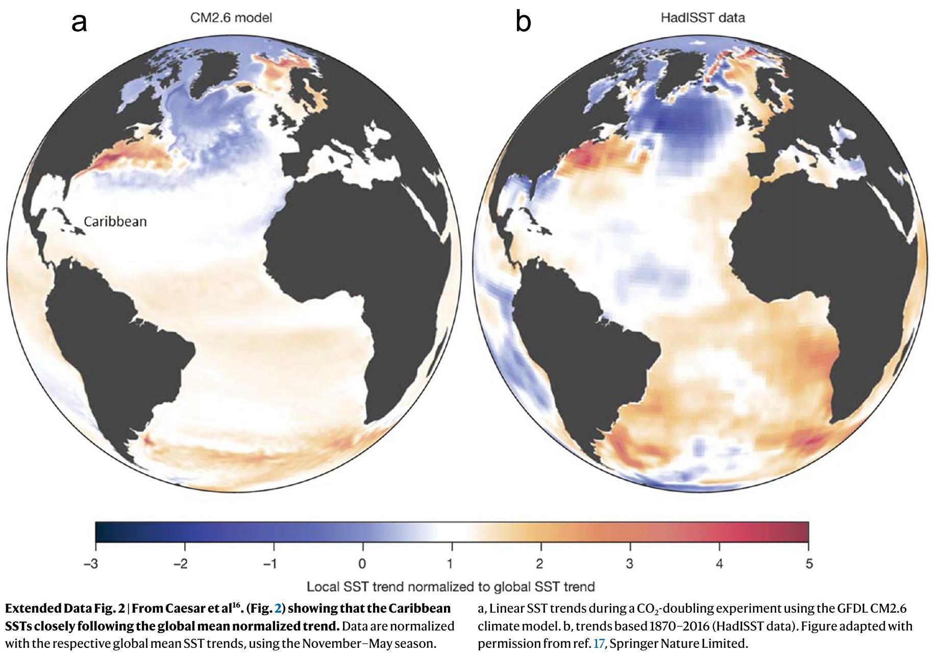
هياكل الإسفنجيات الصلبة طويلة العمر. تم جمع عينات حية من منطقة الكاريبي على أعماق تتراوح بين 33 و 91 مترًا، ضمن طبقة الخلط المحيطية (OML)، وهي المنطقة التي يتم فيها تبادل الحرارة بين الغلاف الجوي وداخل المحيط.. هنا، يتم توحيد التدرج الحراري من خلال الخلط المضطرب من سطح البحر إلى قاعدة طبقة الخلط السطحي، حيث توفر الكتلة الحرارية الأكبر لها سجلاً أكثر استقرارًا وتمثيلاً لدرجات حرارة سطح المحيط العلوي مقارنةً بالطبقة العليا المتغيرة بشكل كبير (طبقة سطح البحرعلاوة على ذلك، في الجزء الكاريبي من المحيط الأطلسي الغربي، فإن المصدر السائد لتقلبات درجة حرارة سطح المحيط العلوي على مدى عدة سنوات هو من التأثيرات الجوية العالمية، مع تأثير مباشر ضئيل (الشكل البياني الممتد 2) من ‘أنماط طبيعية’ أخرى من التقلبات الداخلية، مثل الدورة الدموية الأطلسية العمودية (AMOC).لذا، يبدو أن التغيرات في درجة الحرارة في الطبقة المختلطة السطحية في منطقة الكاريبي مدفوعة بشكل رئيسي بالقوى الإشعاعية الخارجية، مما يجعل هذه المنطقة مثالية لمراقبة الاتجاهات العالمية في درجات حرارة سطح البحر..
النتائج
الاسفنجات الكلسية الكورالية هي سلالة قديمة من الاسفنجات التي تتكلس.، التي توجد عادة في البيئات البحرية المظلمة المحدودة الضوء والتي تمتد من نظام درجة الحرارة النسبي الموحد لطبقة المياه السطحية إلى ما دون طبقة الثرموكلين. في هذه الدراسة، تم جمع عينات من Ceratoporella nicholsoniتم استهدافها بشكل محدد من داخل OML في الكاريبي الشرقي، على المنحدر الجزيئي الحاد، قبالة بورتو ريكو وجزيرة سانت كروix القريبة (الشكل البياني الممتد 3). تم تحديد أعمار ومعدلات نمو العينات التي تم جمعها من 2007 إلى 2017 باستخدام حساسية-تحليلات السلاسلالعودة إلى خمسينيات القرن التاسع عشر، مع عدة قياسات تعود إلى بداية القرن الثامن عشر (الطرق). تم اشتقاق درجات حرارة مياه البحر المحيطة من قياسات
الشكل 3 | المعايرة لـضد شذوذات SST الحديثة. أ، المحور الأيسر، شذوذات متوسط حرارة سطح البحر العالمي HadSST4 (المرجع 13) المشار إليها من 1961-1990 مع خط صلب يظهر الانحدار الخطي مقابل الزمن (الشكل البياني الممتد 4أ). المحور الأيمن، الإسفنج القاسي (الأزرق الداكن) والانحرافات المتوسطة سنويًا (دوائر زرقاء فاتحة) من أخذ عينات عالية الدقة (كل شهرين). ب، ارتباط الشذوذات مع مصفوفة HadSST4 العالمية الخطية حيث: (HadSST4) معLINESTوخطوط منقطة تظهر 1 انحراف معياري من المتوسط المتبقي ( ). الخطوط الأفقية والعمودية المنقطة تمثل انحرافات الفترة من 1961 إلى 1990 والتي تدور حولها الانحدارات. ج، علاقات HadSST4 وOML مع الغلاف الجويتركيزات مع حساسية درجة الحرارة لـالتقليل إلى النصف منذ عام 1984. ما لم يُذكر، فإن الشكوك بالنسبة لنقاط البيانات أصغر من حجم الرمز (البيانات التكميلية). نسبمنزيادات مستمرة (الشكل 2أ)، من الطبقة الخارجية إلى أسفل على محور النمو للهياكل الكربونية الكالسيومية (الأراجونيت) الأقدم تدريجياً (الطرق). تم تأكيد غياب التداخل الموسمي بواسطة دقة عالية تبلغ 0.05 مم (عينة من عينة بين عامي 1960 و 2017، والتي أظهرت القليل من التغيرات الموسمية (الشكل البياني الممتد 4ب) وبالتالي تم حسابها بمتوسط دقة سنة واحدة.
على مدارتظهر جميع العينات صفوفًا شبه متوازية مننسب (الشكل 2أ)، تشير إلى نفس الاستجابة النسبية للتغيرات في درجة حرارة مياه البحر المحيطة. ومع ذلك، تشير الفجوات بين المصفوفات إلى اختلافات محدودة في درجة الحرارة تعتمد على العمق، جنبًا إلى جنب مع بعض التأثيرات الحيوية الناتجة عن الكائنات الحية. التأثيرات الحيوية هي سمة شائعة للأنظمة البيولوجية.وهنا تم تصحيح الانحرافات الثابتة عن طريق تطبيع نسب Sr/Ca إلى متوسط فترة المرجع 1961-1990 لكل عينة. الناتج هو مجموعة متماسكة للغاية من المكدساتتشير الشذوذات (الشكل 2ب) بذلك إلى حساسية ثابتة للنماذج تجاه التغيرات التفاضلية في درجة الحرارة (أي الشذوذات).
معايرة درجات حرارة سكليروسبونج Sr/Ca OML
لتحديد حساسية درجة الحرارة للسكيروسبونجتمت مقارنة المصفوفات المتوسطة لمدة عامين وسنة واحدة مع متوسط درجات حرارة سطح البحر العالمية (HadSST4)من 1964 إلى 2012 شاملة. وفقًا لما هو مت established إجراءاتتم إزالة الاتجاه من متوسط الانحرافات العالمية لـ HadSST4 باستخدام طريقة محددة جيدًا (علاقة خطية، حيث أن البقايا تعود بشكل رئيسي إلى فترات من تباين ENSO العالي (الشكل البياني الإضافي 4a). العصر الحديث (1964-2012)تم إجراء تحليل الانحدار للانحرافات OML مقابل بيانات هادSST4 العالمية الخطية (الشكل 3أ، ب)، والتي تفترض أنأوه، يا إلهيتتضمن سجلات Ca جزءًا كبيرًا من الزيادة المحددة جيدًا في درجات حرارة سطح البحر العالمية الحديثة. وهذا يؤدي إلى ميل قدره، حيث تمثل فترة المعايرة ما يقرب من نصف إجمالي كمية الاحترار العالمي التي حدثت حتى الآن.
على الرغم من أنتشير الشذوذات إلى ما هو متوقع بناءً على الديناميكا الحراريةارتباط سلبي مع درجات حرارة سطح البحر العالمية، حساسية الحرارة أكبر من الدراسات السابقةبما في ذلك تلك الخاصة بالشعاب المرجانية السكلرية. ومع ذلك، كانت المحاولات السابقة لمعايرة حساسية الحرارة لـنسب الكالسيوم في الإسفنجيات الصلبةلقد كانت مستندة إما إلى اختلافات في درجة الحرارة تعتمد على العمق وتدمج التأثيرات الحيويةأو، بدلاً من ذلك، دراسة موسمية باستخدام ليزر ICP بدقة أقلداخل منطقة الأنسجة التي تتكلس بنشاط. الحساسية العالية المستمرة لـشذوذ درجات الحرارةفي. نيكولسوني، الموجود هنا للعديد من العينات، يُنسب إلى التكلس التجديدي متعدد المراحل حيث يتم ضخ وتبادل مياه البحر داخل النشط (منطقة التكلس، التي تمتد من السطح العلوي إلى المنطقة القاعدية السفلية. هذا يفسر أيضًا غياب
الشكل 4 | الشذوذات العالمية المتوسطة لـ OML و HadSST4. أ، مقارنة سجلات OML و HadSST4 (المرجع 13) مع انزلاقات لـلأخذ في الاعتبار الاحترار من الفترة ما قبل الصناعية (التظليل الأزرق من 1700 إلى أوائل 1790s ومن 1840 إلى أوائل 1860s) إلى متوسط انحراف 1961-1990 (الخط العمودي المنقط). ب، توقيت الثورات البركانية الكبرى المشار إليها بالأسهم الرمادية مع تأثير إشعاعي سلبي.بدء الاحترار الصناعي في منتصف الستينيات من القرن التاسع عشر
(سهم أزرق فاتح) يتبعه ظهور في أوائل عام 1870 (سهم أزرق). أشرطة الخطأ هي 2 انحراف معياري. (الشكل التكميلية 1) مع خط أزرق فاتح يظهر المتوسط المتحرك لمدة 5 سنوات. ج، مقارنة بين قيم OML و IPCC ما قبل الصناعة مع متوسط انحراف من . الأسهم الأفقية توضح مراحل الاحترار في عصر الصناعة. د، الفرق بين شذوذ السكليروسبونج OML وشذوذ HadSST4 مع سنوات النينيو الموضحة بخط مائل. الرموز المفتوحة تظهر تصحيحات الأسطول الوطني. إشارة موسمية في أي منأخذ عينات لمدة شهر (الشكل 4b من البيانات الموسعة) أو المصفوفات المكدسة لمدة عامين (الشكل 2b). هذا، جنبًا إلى جنب مع الحساسية المنخفضة لـ OML الكاريبي للاتصالات البعيدة الناتجة عن ENSO في المحيط الهادئ المركزييُفسر محدودية تباين ظاهرة النينيو الجنوبية (ENSO) في سجل الإسفنج القاسي OML، على سبيل المثال، بغياب النينيو الكبير في 1997-1998.
تعيير مقياس الحرارة القديم Sr/Ca باستخدام الإسفنج القاسي مقابل التغيرات في درجات الحرارة العالمية يوفر بالتالي دليلًا تجريبيًا قويًا على أن منطقة البحر الكاريبي OML قد ارتفعت حرارتها بشكل متناسب مع الزيادة المتوسطة العالمية في درجة حرارة سطح البحر، على مدى السنوات الأخيرة.. تدعم هذه النتيجة النمذجة مما يظهر أنه، عبر هذه المنطقة الواسعة من المحيط الأطلسي الغربي المركزي، قد زادت درجات حرارة سطح البحر بمعدل يقارب المعدل العالمي (الشكل البياني الإضافي 2) يمكن فهم ذلك على أنه تسخين إشعاعي مفروض من الأنشطة البشرية يعتبر مؤشراً سلبياً أساسياً في الطبقة المختلطة في البحر الكاريبي.بينما في شمال الأطلسي، يلعب الاحتباس الحراري دورًا نشطًا في تعديلومن ثم امتصاص الحرارة في تلك المنطقة. وبالتالي، فإن نتائجنا التجريبية تتماشى مع كون منطقة الكاريبي في وضع مثالي لمراقبة ظاهرة الاحتباس الحراري العالمية على نطاق واسع مع تغييرات متراكبة minimal.بينما لا يزال يسجل التأثيرات الأوسع لروابط ENSOمن المهم، النمذجةكما يوفر أساسًا ماديًا قويًا لتمديد المعايرة الحديثة (1964-2012) لمقياس حرارة السكليروسبونج Sr/Ca إلى القرنين الثامن عشر والتاسع عشر، عندما كانت القياسات الآلية البدائية لدرجات حرارة سطح البحر إما غائبة أو، في أفضل الأحوال، محدودة في التغطية الجغرافية (الشكل البياني الممتد 1)..
فترة ما قبل الصناعة وبداية الاحترار في عصر الصناعة
تظهر التغيرات في درجة حرارة OML على مدى ثلاثة قرون المحفوظة في هياكل الإسفنجيات الصلبة طويلة العمر في الكاريبي (الشكل 4) أن يتم تعريف فترة الأساس ما قبل الصناعية بنفس الثابت الأساسي تقريبًا (عقددرجات الحرارة من 1700 إلى 1790 ثم من 1840 إلى أوائل الستينيات. الفترة الفاصلة تتميز بتبريد عالمي مستمر (الشكل 4 أ، ب)، متسق مع التركيزات العالية من الهباء الجوي الكبريتي الناتج عن البراكين الموجودة في الجليد.. يشمل ذلك الثورات البركانية الكبرى (الشكل 4ب) في عام 1783 (لاكي)، 1809 (غير معروف)، 1815 (تامبورا) و1832 (كوسيجينا). الأهم هو ثوران تامبورا في إندونيسيا خلالأكبر حدث انفجاري تم تسجيله حتى الآن في ‘التاريخ الحي’. هذا تسبب في “عام بلا صيف” في 1816، مع التبريد على نطاق عالمي ( ) يتضح ذلك في سجل OML الكاريبي من 1808 إلى 1828، مع عودة تدريجية إلى مستويات ما قبل الصناعة الأكثر دفئًا خلال ثلاثينيات القرن التاسع عشر (الشكل 4ب). وبالتالي، يتم تعريف المرحلة النهائية من فترة ما قبل الصناعة من خلال الهضبة في درجات الحرارة بين 1840 وأوائل ستينيات القرن التاسع عشر، عند درجات حرارة أكثر دفئًا بشكل طفيف ( درجات الحرارة ما قبل الصناعية مقارنةً بالقرن الثامن عشر. سجل الإسكلورسبونج (الشكل 4ب) لهذه الأحداث التاريخية المعروفةوبذلك يؤكد صحة الكاريبيترمومتر OML كمسجل للتغيرات في درجة الحرارة الإشعاعية الناتجة عن التأثيرات العالمية. كما هو متوقعتغيرات درجة الحرارة في OML مخففة بالنسبة للغلاف الجوي بسبب السعة الحرارية الأكبر بكثير لـ OML (الشكل 5a).
بالنسبة لهذا الخط الأساسي الممتد والذي تم تحديده الآن بشكل جيد قبل الصناعة، يتم تطبيق تعويض قدره (الشكل 4) لحساب الزيادة في درجة الحرارة من فترة الخط الأساسي قبل الصناعة (أي، متوسط درجات الحرارة من 1700 إلى 1790 ومن 1840 إلى 1860) إلى فترة مرجع الشذوذ من 1961-1990. بناءً على ذلك، فإن بداية الاحترار في عصر الصناعة واضحة بحلول منتصف الستينيات من القرن التاسع عشر. على الرغم من أنها كانت قبل تقدير IPCC (الشكل 4b,c)، إلا أنها تتفق جيدًا مع إعادة بناء المناخ القديم السابقة التي تشير إلى ‘بداية مبكرة’
الشكل 5 | OML و GMSTs. الشذوذ بالنسبة لخط الأساس من 1961-1990 مع تعويض (ما لم يُذكر خلاف ذلك). أ، OML وشذوذ درجات حرارة الأرض في بيركلي مع بداية درجات حرارة الأرض والهواء القصوى من حوالي 1990 (تظليل وردي). ب، GMSTs من OML المدمج ودرجات حرارة الأرض (هذه الدراسة دوائر حمراء داكنة) ومن درجات حرارة HadSST4 المدمجة ودرجات حرارة الأرض (دوائر برتقالية)، الأخيرة بالنسبة لفترة IPCC 1850-1900 قبل الصناعة، والتي تقلل من تقدير الاحترار العالمي بمقدار . انظر المراجع. وبيانات إضافية للشكوك.
ج، OML و HadSST4 من وزيادات درجات حرارة الأرض بحلول عام 2020. د، سجلات GMST لـ OML + الأرض المدمجة و HadSST4 + الأرض المدمجة مع التي مرت خلال 2012-2015. عند معدلات الانبعاثات الحالية سيتم الوصول إلى الاحترار العالمي بحلول أواخر عشرينيات القرن الواحد والعشرين. التطور التاريخي للغلاف الجوي (خط صلب)، الزيادات المستقبلية بمعدلات الانبعاثات الحالية (خط متقطع) و التخفيضات السنوية من 2025 لتقليل الانبعاثات إلى النصف بحلول أوائل 2030 (خط منقط).
بداية الاحترار في عصر الصناعة في منتصف القرن التاسع عشر. هذا هو الحال بشكل خاص إذا تم أخذ في الاعتبار التحسين الكبير الآن في دقة سجل OML لدينا، الذي يميز بوضوح بداية الاحترار الصناعي المبكر في منتصف الستينيات من القرن التاسع عشر عن الانتعاش المطول الذي تلا التبريد البركاني على نطاق عالمي في أوائل القرن التاسع عشر. وبالتالي، فإن ظهور احترار OML واضح بحلول منتصف السبعينيات من القرن التاسع عشر (الشكل 4b)، مع تعريف الظهور بمعايير أكثر صرامة للاحتباس الحراري التي تتجاوز أولاً وتبقى فوق الفترة قبل الصناعية . هذا أكثر من 80 عامًا قبل سجلات SST الآلية (الشكل 4c) أو سجلات الشعاب المرجانية القديمة في المياه الضحلة التي تخفي التغيرات الطبيعية العالية ظهور الاحترار في عصر الصناعة حتى منتصف القرن العشرين (الشكل 5b).
درجات حرارة OML خلال عصر الصناعة
استنادًا إلى سجل OML من الإسفنج القاسي، يمكن تصنيف الاحترار في عصر الصناعة إلى ثلاث مراحل واسعة (الشكل 4c). الأولى هي الفترة الصناعية المبكرة من منتصف الستينيات من القرن التاسع عشر إلى أوائل القرن العشرين، عندما زادت درجات الحرارة بمعدل متوسط قدره بمعدل متوسط قدره عقد . تلا ذلك مقدار مشابه من الاحترار () من أوائل القرن العشرين إلى أوائل الستينيات (الفترة الصناعية المتوسطة) ولكن بمعدل يقارب نصف المعدل المتوسط عقد . أخيرًا، بدءًا من منتصف الستينيات (الفترة ‘الحديثة’) زادت درجات الحرارة بمعدل أسرع بكثير قدره عقد (الشكل 4c) استجابةً لزيادة سريعة في الغلاف الجوي . منذ منتصف الثمانينيات، حساسية درجة الحرارة لزيادة قد انخفضت إلى النصف، من لكل 10 جزء في المليون CO خلال 1964-1984 إلى الوقت الحاضر (1985-2020) لكل 10 جزء في المليون CO 2 (الأشكال 3c و 4c). بينما تتطلب أسباب
هذا الانخفاض في حساسية احترار OML لـ مزيدًا من التحقيق، نلاحظ أنه من الصعب التوفيق بينه وبين آثار التبريد الناتجة عن الهباء الجوي الصناعي لكنه يتزامن مع الزيادة العالمية في أعماق الطبقة المختلطة في فصل الصيف ومن ثم سعة حرارية أكبر لـ OML.
على عكس هذا النمط المتماسك من احترار OML، تظهر سجلات SST المستندة إلى السفن (على سبيل المثال، HadSST4) تقلبات أكبر بكثير تشبه ‘الأفعوانية’، مع فترات من الاحترار السريع تليها انخفاضات في درجات الحرارة (الشكل 4). الأكثر بروزًا هو الفترة من 1850 إلى 1880، الجزء الأول من فترة مرجع IPCC قبل الصناعة، التي تتميز بدرجات حرارة دافئة بشكل غير عادي، خاصة خلال النينيو . ثم، من حوالي 1880 حتى أوائل القرن العشرين، انخفضت SSTs في سلسلة من الخطوات مع كون الخطوة الأولى فقط تعود إلى التبريد الناتج عن ثوران كراكاتوا في 1883 (الشكل 4c,d). بحلول أوائل القرن العشرين وخاصة خلال ما يسمى بـ ‘الانحراف البارد’ من 1908 إلى 1910، هناك توافق جيد بين سجلات OML و HadSST4. بشكل متناقض، خلال فترة IPCC 1850-1900 قبل الصناعة (الشكل 4c)، كانت درجات الحرارة أكثر دفئًا بشكل غير عادي من بداية ‘عصر الصناعة’ في القرن العشرين على الرغم من زيادة الغلاف الجوي .
بينما هناك توافق جيد بين سجلات OML و HadSST4 خلال أوائل القرن العشرين (الشكل 4)، كانت HadSST4 مرة أخرى أكثر دفئًا خلال منتصف عشرينيات القرن العشرين وخاصة خلال فترة الحرب العالمية الثانية في منتصف الأربعينيات (الشكل 4c,d). يُعزى هذا التباين الأخير إلى التغييرات من قياسات سحب المياه إلى قياسات سحب المياه من غرفة المحرك ، فضلاً عن التحيزات التي تم تحديدها مؤخرًا بين أساطيل وطنية مختلفة . ومع ذلك، من غير المؤكد ما إذا كانت هذه والتعويضات الأكثر أهمية خلال فترة IPCC قبل الصناعة تعود، على سبيل المثال، إلى تمثيل مفرط
لأحداث النينيو الدافئة في سجلات ICOADS في القرن التاسع عشر التي لم يتم ضبطها بشكل جيد أو إلى تقلبات طبيعية أكبر في ENSO قبل عام 1960، على الرغم من أن سجل OML لدينا يشير إلى الأول.
نقاش
فهم كيف أثر الاحترار الناتج عن غازات الدفيئة على درجات حرارة الأرض والهواء بالنسبة لخزان الحرارة الأكبر بكثير في المحيط العلوي لا يزال يمثل تحديًا. هنا، نفترض أنه، بالنسبة لفترة مرجع 1961-1990، يمكن تطبيق نفس التعويض الثابت قدره على درجات حرارة الأرض والهواء وكذلك على شذوذ OML (الأشكال 4 و 5)، على الرغم من وجود شكوك أكبر في السجلات الأرضية من 1750 إلى 1860 (الشكل 5a). على الرغم من هذا القيد، هناك مع ذلك توافق جيد بين سجلات الأرض والهواء وOML، خاصة خلال ثوران تامبورا التاريخي الموثق جيدًا عندما تسبب الهباء البركاني في تبريد عالمي. بشكل ملحوظ، من منتصف الستينيات إلى 1900، زادت درجات حرارة الأرض وOML بشكل متزامن بمقدار . على العكس من ذلك، خلال نفس فترة IPCC 1850-1900 قبل الصناعة، كانت HadSST4 في البداية أكثر دفئًا بمقدار يصل إلى (الشكل 4c) تليها اتجاه تبريد غير عادي مقارنة بسجلات OML والأرض المحددة جيدًا من الاحترار المستمر منذ الستينيات. الآن، تحل نتائجنا ‘مفارقة الأرض الدافئة والمحيط البارد’ التي طرحت باستخدام فترة مرجع IPCC قبل الصناعة (الشكل 1b). وبالتالي، يجب أن تستمر الملاحظات الحديثة في الإشارة إلى المتوسط من 1961-1990 (الشكل 1a) ولكن مع تعديل قدره لحساب الزيادة في درجة الحرارة منذ بداية الاحترار في عصر الصناعة في منتصف الستينيات إلى المتوسط من 1961-1990 (الشكل 4a). بناءً على ذلك، أظهرت سجلات الأرض وSST استجابة متماسكة عمومًا لـ ENSO حتى التسعينيات، تتميز بدرجات حرارة أرضية أكثر دفئًا نسبيًا خلال أحداث النينيو القوية ودرجات حرارة أكثر برودة خلال أحداث النينيا (الشكل 5a).
من المهم، مع ذلك، أن التشابه على المدى الطويل في معدلات الاحترار في الأرض وسطح المحيط العلوي يبدأ في الانهيار في أواخر القرن العشرين، مع زيادة درجات حرارة الأرض والهواء الآن بمعدل يقارب ضعف معدل المحيطات السطحية بغض النظر عن مرحلة ENSO (الشكل 5a,c). بدلاً من أن تكون سجلات الأرض والهواء جزءًا من اتجاه الاحترار المستمر بعد عام 1900 بالنسبة لفترة IPCC 1850-1900 قبل الصناعة، كما يُفترض حاليًا (الشكل 1b)، تظهر نتائجنا انحرافًا واضحًا عن المحيط السطحي من حوالي 1980-1990 (الشكل 5a,c). يتماشى هذا مع الاحترار المعزز الموثق جيدًا لكتل اليابسة في نصف الكرة الشمالي عالية العرض وانخفاض الجليد الدائم في القطب الشمالي . يتزامن هذا التغيير أيضًا مع زيادة تكرار كل من موجات الحرارة في نصف الكرة الجنوبي والشمالي والأحداث المتطرفة المرتبطة بها، مثل الجفاف وحرائق الغابات . تعتبر حرائق الغابات وحرائق الأدغال الأكثر تكرارًا أيضًا مصدرًا إضافيًا للغلاف الجوي ، مما يوفر آلية تغذية راجعة معززة. على الرغم من أن الأهمية النسبية للعمليات الإقليمية والعالمية التي تدفع زيادة تكرار وشدة موجات الحرارة الأرضية لا تزال غير مؤكدة سجلنا المعدل المنقح للاحترار في عصر الصناعة يظهر الآن بوضوح أن البيئات الأرضية قد تعرضت لمعدل أسرع بكثير من الاحترار منذ التسعينيات، مقارنة بتلك الموجودة في الطبقات السطحية الأكثر استقرارًا من المحيطات.
تتمتع هذه النتائج أيضًا بتداعيات مهمة على التوقعات القريبة المدى للاحتباس الحراري العالمي. كما تم وصفه بالفعل، بالنسبة للمرجع من 1961 إلى 1990، زادت درجات حرارة OML والأرض (الشكل 5أ) وبالتالي درجات حرارة السطح العالمية (الشكل 5ب) بـمنذ الفترة ما قبل الصناعية 1700-1860. وهذا يقارن فقط بـعندما يتم تقدير درجات حرارة HadSST4 ودرجات حرارة اليابسة بالنسبة لفترة ما قبل الصناعة من 1850 إلى 1900 وفقًا للهيئة الحكومية الدولية المعنية بتغير المناخ (IPCC)، فرق قدره (الشكل 5ب). الإضافي في ارتفاع درجة الحرارة العالمية فوق تقديرات الهيئة الحكومية الدولية المعنية بتغير المناخكما يعني أن درجات حرارة السطح العالمية كانتفوقالمستويات ما قبل الصناعية بحلول 2018-2022، مقارنة بتقدير الهيئة الحكومية الدولية المعنية بتغير المناخمن (الشكل 5ب). وبالتالي، فإن الفرصة لتقليل الاحترار العالمي إلى ما لا يزيد عن لقد انقضى الوقت الذي يمكن فيه تحقيق ذلك من خلال تقليل الانبعاثات فقط، ومع معدلات الانبعاث الحالية،سيتم الوصول إلى العتبة لدرجات حرارة سطح الأرض العالمية بحلول أواخر العقد 2020 (الشكل 5d).
لقد أظهرنا أن درجات حرارة اليابسة والهواء في أواخر القرن العشرين كانت ترتفع بمعدل يقارب ضعف معدل ارتفاع درجات حرارة المحيطات السطحية. وهم الآنمستويات ما قبل الصناعة. إذا استمرت معدلات الاحترار الحالية، ستتجاوز متوسط درجة حرارة اليابسة بحلول عام 2035 تقريبًا، مع توقع ارتفاع درجات الحرارة العالمية السطحية في أوائل عام 2040 (الشكل 5c، d). وبالتالي، فإن الهدف الرئيسي من اتفاقية باريس التابعة للأمم المتحدة هو الحفاظ على زيادة درجة حرارة السطح العالمية المجمعة للأرض والمحيطات دون أصبح الآن تحديًا أكبر بكثير، مما يبرز الحاجة الملحة أكثر لتقليص الانبعاثات إلى النصف بحلول عام 2030.
المحتوى عبر الإنترنت
أي طرق، مراجع إضافية، ملخصات تقارير Nature Portfolio، بيانات المصدر، بيانات موسعة، معلومات تكميلية، شكر وتقدير، معلومات مراجعة الأقران؛ تفاصيل مساهمات المؤلفين والمصالح المتنافسة؛ وبيانات توفر البيانات والرموز متاحة علىhttps://doi.org/10.1038/s41558-023-01919-7.
References
IPCC Climate Change 2023: Synthesis Report (eds Core Writing Team, Lee, H. et al.) (IPCC, 2023).
Russo, E. & Domeisen, D. I. Increasing intensity of extreme heatwaves: the crucial role of metrics. Geophys. Res. Lett. 50, e2023GL103540 (2023).
Domeisen, D. I. V. et al. Prediction and projection of heatwaves. Nat. Rev. Earth Environ. 4, 36-50 (2023).
Hawkins, E. et al. Estimating changes in global temperature since the preindustrial period. Bull. Am. Meteorol. Soc. 98, 1841-1856 (2017).
Etheridge, D. et al. Natural and anthropogenic changes in atmospheric over the last 1000 years from air in Antarctic ice and firn. J. Geophys. Res. 101, 4115-4128 (1996).
Gao, C., Robock, A. & Ammann, C. Volcanic forcing of climate over the past 1500 years: an improved ice core-based index for climate models. J. Geophys. Res. 113, D23111 (2008).
Kent, E. C. & Kennedy, J. J. Historical estimates of surface marine temperatures. Annu. Rev. Mar. Sci. 13, 283-311 (2021).
Deser, C., Alexander, M. A., Xie, S.-P. & Phillips, A. S. Sea surface temperature variability: patterns and mechanisms. Annu. Rev. Mar. Sci. 2, 115-143 (2010).
IPCC Special Report on Global Warming of (eds Masson-Delmotte, V. et al.) (WMO, 2018).
Morice, C. P. et al. An updated assessment of near-surface temperature change from 1850: the HadCRUT5 data set. J. Geophys. Res. 126, e2019JD032361 (2021).
Rohde, R. A. & Hausfather, Z. The Berkeley Earth Land/Ocean temperature record. Earth Syst. Sci. Data 12, 3469-3479 (2020).
Kennedy, J. J., Rayner, N. A., Atkinson, C. P. & Killick, R. E. An ensemble data set of sea surface temperature change from 1850: the Met Office Hadley Centre HadSST. 4.0. 0.0 data set. J. Geophys. Res. 124, 7719-7763 (2019).
Huang, B. et al. Extended reconstructed sea surface temperature, version 5 (ERSSTv5): upgrades, validations and intercomparisons. J. Clim. 30, 8179-8205 (2017).
Freeman, E. et al. ICOADS Release 3.0: a major update to the historical marine climate record. Int. J. Climatol. 37, 2211-2232 (2017).
Gulev, S. K. et al. In Climate Change 2021: The Physical Science Basis (eds Masson-Delmotte, V. et al.) Ch. 2 (IPCC, Cambridge Univ. Press, 2021).
Caesar, L., Rahmstorf, S., Robinson, A., Feulner, G. & Saba, V. Observed fingerprint of a weakening Atlantic Ocean overturning circulation. Nature 556, 191-196 (2018).
Willenz, P. & Willenz, P. Micromorphology and ultrastructure of Caribbean sclerosponges. I. Ceratoporella nicholsoni and Stromatospongia norae (Ceratoporellidae: Porifera). Mar. Biol. 103, 387-401 (1989).
McCulloch, M. T. & Mortimer, G. E. Applications of the decay series to dating of fossil and modern corals using MC-ICPMS. Aust. J. Earth Sci. 55, 955-965 (2008).
McCulloch, M. T., Gagan, M. K., Mortimer, G. E., Chivas, A. R. & Isdale, P. J. A high-resolution and coral record from the Great-Barrier-Reef, Australia and the 1982-1983 El-Nino. Geochim. Cosmochim. Acta 58, 2747-2754 (1994).
D’Olivo, J. P., Sinclair, D. J., Rankenburg, K. & McCulloch, M. T. A universal multi-trace element calibration for reconstructing sea surface temperatures from long-lived Porites corals: removing ‘vital-effects’. Geochim. Cosmochim. Acta 239, 109-135 (2018).
Weiner, S. & Dove, P. M. An overview of biomineralization processes and the problem of the vital effect. Rev. Mineral. Geochem. 54, 1-29 (2003).
Hawkins, E. et al. Observed emergence of the climate change signal: from the familiar to the unknown. Geophys. Res. Lett. 47, e2019GL086259 (2020).
Gaetani, G. A. & Cohen, A. L. Element partitioning during precipitation of aragonite from seawater: a framework for understanding paleoproxies. Geochim. Cosmochim. Acta 70, 4617-4634 (2006).
Haase-Schramm, A. et al. Sr/Ca ratios and oxygen isotopes from sclerosponges: temperature history of the Caribbean mixed layer and thermocline during the Little Ice Age. Paleoceanography 18,1073 (2003).
Waite, A. J., Swart, P. K., Rosenheim, B. E. & Rosenberg, A. D. Improved calibration of the Sr/Ca-temperature relationship in the sclerosponge Ceratoporella nicholsoni: re-evaluating Sr/Ca derived records of post-industrial era warming. Chem. Geol. 488, 56-61 (2018).
Rosenheim, B. E. et al. High-resolution Ca records in sclerosponges calibrated to temperature in situ. Geology 32, 145-148 (2004).
Cai, W. et al. Pantropical climate interactions. Science 363, eaav4236 (2019).
Marshall, J. et al. The ocean’s role in the transient response of climate to abrupt greenhouse gas forcing. Clim. Dynam. 44, 2287-2299 (2015).
Brohan, P. et al. Constraining the temperature history of the past millennium using early instrumental observations. Climate 8, 1551-1563 (2012).
Newhall, C. G. & Self, S. The Volcanic Explosivity Index (VEI): an estimate of explosive magnitude for historical volcanism. J. Geophys. Res. 87, 1231-1238 (1982).
Abram, N. J. et al. Early onset of industrial-era warming across the oceans and continents. Nature 536, 411-418 (2016).
Tierney, J. E. et al. Tropical sea surface temperatures for the past four centuries reconstructed from coral archives. Paleoceanography 30, 226-252 (2015).
Hawkins, E. & Sutton, R. Time of emergence of climate signals. Geophys. Res. Lett. 39, L01702 (2012).
Sallée, J.-B. et al. Summertime increases in upper-ocean stratification and mixed-layer depth. Nature 591, 592-598 (2021).
Gergis, J. L. & Fowler, A. M. A history of ENSO events since AD 1525: implications for future climate change. Clim. Change 92, 343-387 (2009).
Chan, D. & Huybers, P. Correcting observational biases in sea surface temperature observations removes anomalous warmth during World War II. J. Clim. 34, 4585-4602 (2021).
Natali, S. M. et al. Large loss of in winter observed across the northern permafrost region. Nat. Clim. Change 9, 852-857 (2019).
IPCC Climate Change 2022: Impacts, Adaptation, and Vulnerability (eds Pörtner, H.-O. et al.) (IPCC, 2022).
Bousfield, C. G., Lindenmayer, D. B. & Edwards, D. P. Substantial and increasing global losses of timber-producing forest due to wildfires. Nat. Geosci. 16, 1145-1150 (2023).
Keeling, C. D. et al. Exchanges of Atmospheric and with the Terrestrial Biosphere and Oceans from 1978 to 2000. I. Global Aspects (Scripps Institution of Oceanography, 2001); https:// escholarship.org/uc/item/09v319r9
Publisher’s note Springer Nature remains neutral with regard to jurisdictional claims in published maps and institutional affiliations.
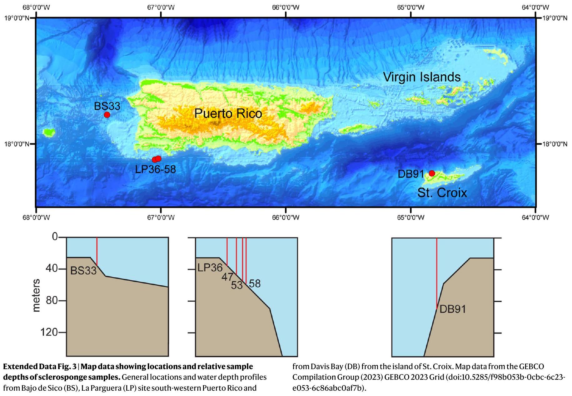
تم جمع عينات حية من الإسفنج الصلب الكاريبي C. nicholsoni باستخدام أجهزة التنفس المغلقة ذات الغاز المختلط من قبل فريق الغوص الفني التابع لجامعة بورتو ريكو – ماياجويز، قسم العلوم البحرية، والذي يتضمن C. Sherman وM. Carlo وH. Ruíz وM. Nemeth وE. Tuohy وI. Bejarano وD. Kesling. تم إجراء الجمع من عام 2007 إلى عام 2017 ويغطي نطاق عمقإلى 91 م. تشمل مواقع أخذ العينات (الشكل البياني الإضافي 3 والجدول التكميلي 1) لهذه الدراسة باخو دي سيكو (BS33)، قناة مونا، بورتو ريكو، الهامش الجنوبي للجزيرة في جنوب غرب بورتو ريكو قبالة لا بارغويرا (LP36، LP47، LP53، LP58) وعلى بعد سواحل شمال غرب جزيرة سانت كروا، جزر العذراء الأمريكية (DB91). بعد الجمع، تم تقطيع العينات إلىشرائح سميكة، تم تنظيفها في ماء منزوع الأيونات باستخدام مسبار فوق صوتي استعدادًا لأخذ عينات فرعية (طحن) وتحليلات جيولوجية كيميائية أجريت في مختبرات النظائر بجامعة أستراليا الغربية.
في البداية، تم إخضاع العينات لتأريخ سلسلة اليورانيوم بدقة عالية (انظر أدناه) لإنشاء تواريخ دقيقة لنمو الهيكل العظمي. لهذا الغرض، تم إجراء تأريخ باستخدام سلسلة اليورانيوم على ( عينات مستخرجة من ضيقةفتحات بعرض مم) تم تفريزها بجوار العينة لـتحليلات.تم قطع الفتحات فيالفترات على طول محور نمو ألواح الإسفنج القاسي المنظف مسبقًا مع أخذ العينة العليا (الأحدث) مباشرة أسفلمنطقة الأنسجة السميكة. حيث توجد أدلة على التآكل البيولوجي وبالتالي احتمال وجود فترة توقف في النمو (على سبيل المثال، BS33) تم أخذ عينات إضافية فوق وتحت لتحديد أي انقطاع زمني (الشكل التوضيحي 2a).
لتحليل Sr/Ca، ولتقليل التنعيم الزمني بسبب الأشرطة النامية المائلة، فإنتمت معالجة حافة بسمك مم على طول محور نمو العينة، بجوار أخذ العينات لتأريخ اليورانيوم-الثوريوم. عينات لـتم استخراج التحليلات بعد ذلك بشكل مستمرزيادات تؤدي إلىعينات عشوائية، باستخدام مطحنة زينبوت التي يتم التحكم فيها بواسطة الكمبيوتر. بالنسبة للعينة التي تم جمعها مؤخرًا (LP53)، تم جمع عينات إضافية على طول القمة. (1960-2017) بدقة فائقة ) في زيادات مستمرة على طول حافة سميكة، كل عينة تعادلشهور من النمو المتوسط والوزنبالنسبة لعينات 0.5 و 0.05 مم، تم استخراج العينات بشكل مستمر على طول الحافة الميكانيكية، مع الحفاظ على الموقع الدقيق لحافة الثقب بالنسبة للسطح العلوي. عند الضرورة، ولتقليل التنعيم الزمني، تم إجراء تعديلات طفيفة على اتجاه الحافة الأفقية لأخذ العينات بحيث تظل حزم النمو موازية لمحور المطحنة.
تحليلات العناصر Sr/Ca
تم إذابة عينات المساحيق فيعلى مدار عدة ساعات ثم تم تحريكها وطردها مركزيًا لمدة دقيقة واحدة بسرعة 3500 دورة في الدقيقة لضمان الذوبان الكامل. تم تخفيف عينات من العينة المذابة لتوفير تمثيل.حل في وقت محدد بدقةتركيز الكالسيوم بالجزء في المليون لتحليل السيريوم والكالسيوم باستخدام جهاز ICPMS رباعي القطب من سلسلة Xلضمان جودة البيانات، تم أيضًا تحليل المعايير الداخلية للمختبر والمعيار الدولي للشعاب المرجانية JCp-1 خلال نفس الجلسة التحليلية لعينات الإسكليروسبونج. تم إجراء قياسات متعددة للمعيار الشعابي JCp-1 بنفس تركيز 10 جزء في المليون من الكالسيوم على مدارأعطت فترة السنة المتوسطة انحراف معياري نسبي (RSD) قدره 0.15% (RSD) الذي يتوافق مع قيمة متوسطة لـ Sr/Caعادةً ما تعطي إعادة تحليل عينات الإسكلوروسبونج ضمن نفس الجلسة التحليلية تحسينًا في القابلية للتكرار لـ ( RSD) متسقة مع عدم اليقين في درجة الحرارة الموضح في الشكل التوضيحي 1. تم معالجة الفراغات الإجرائية مع دفعات العينات للتحقق من التلوث الإجرائي وكانت تحت حدود الكشف.
معايرة شذوذات درجة حرارة Sr/Ca
كما هو موصوف في النص،تم حساب الشذوذات بالنسبة لمتوسط 1961-1990. وبالتالي، لكل عينةشذوذ نسبة Ca عند زيادة الوقتيتم إعطاؤه بواسطة: أين هو النسبة المقاسة ( ) و (1961-1990) هو النسبة المتوسطة لفترة المرجع المشتركة من 1961 إلى 1990 (شاملة). لتسهيل التكديس (المتوسط) للعديد من العينات، فإن Sr/ ثم تم إعادة قياسها إلى فترات مدتها سنتان مع الحد الأدنى من الاستقراء حيث تمثل عينة 0.5 ممالفترات، اعتمادًا على معدل نمو العينة.شذوذاتثم تم تجميعها (أي، تم حساب متوسطها) مع عدم اليقين المعطى بواسطةس.م. س.د. / جذر( ) حيث هو عدد (3-6) من العينات التي تم تحليلها. بالنسبة لفترة المعايرة الحديثة (1964-2012)، تم أيضًا تحديد المتوسطات السنوية من أخذ عينات متزايدة لمدة شهرين تقريبًا (0.05 مم) من LP53 (الشكل 4b من البيانات الموسعة). تم إجراء تحليل الانحدار لكل من الشذوذات المجمعة لمدة عامين وسنة واحدة مقابل الشذوذات العالمية لدرجة حرارة سطح البحر (SST) الملساء (الخطية) من HadSST4 (الشكل 4a من البيانات الموسعة) للفترة من 1964 إلى 2022. وقد أسفر ذلك عن ميل قدرهس.م.، مع تضمين المعايرة لما يقرب من نصف إشارة الاحترار العالمي الإجمالية. استنادًا إلى هذا الانحدار، فإن متوسط الانحراف المعياري للمتوسطات لمدة عامين هومتسق مع ما هو متوقع من عدم اليقين المدمج في التحليلات بالإضافة إلى التباين بين العينات.
تأريخ اليورانيوم-الثوريوم للسبونجيات الصلبة
جانب حاسم في هذه الدراسة هو الحاجة إلى تواريخ دقيقة للسكليروسبونج. لهذا الغرض، دقة عاليةتاريخ السلاسلتم القيام به في (عينات مستخرجة من الضيقفتحات (انظر السابق). تم إذابة عينات مسحوق اليورانيوم والثوريوم ثم تم إضافة محلول معاير. و نظائر الثوريومتمت بعد ذلك تنقية المحلول المضاف كيميائيًا باستخدام إجراءات تبادل الأيونات مع المفصولوتم تحليل نظائر الثوريوم باستخدام جهاز NEPTUNE MC-ICPMS وفقًا لإجراءات مشابهة لتلك الموصوفة في المرجع 19.
للدقة التحليلية العالية المطلوبة في هذه الدراسة،تم تصحيح النسبة المقاسة لنمو الداخلبين وقت الجمع والتحليلات الجيوكيميائية، وهي فترة تراوحت من عدة أشهر فقط إلى ما يقرب من عقد من الزمن. التصحيحات التي تفترض وجود ثم تم تطبيقه على جميع عينات سلسلة U لنفس العينة، مع إجراء تعديلات إضافية لتحسين انحدار العمر. ) مقابل المسافة من سطح النمو الخارجي. وبالتالي، لكل عينة، كانت علاقة العمر بالمسافة معطاة بواسطة: .
هنا، السطح الخارجييتم تعريفه من خلال عمر الجمع (الجدول التكميلي 2). تصحيح للبدء هو عدم اليقين الرئيسي ( ) في تحديد وقت التكلس وبالتالي معدل نمو الأجزاء الهيكلية، مقارنة بالدقة النظرية لـ بدون تصحيحات للبداية. البداية تراوحت نسب النشاط بين 1.45 و 2.74، مع أكبر انحراف (مطلوب لأعمق عينة (91 م) (DB91)، متسق مع الاتجاه الملحوظ عادةً لزيادة المواد المذابة/الجسيمات.مع زيادة العمق وبالتالي أكبر i. من أجل الأكبر ( قطر) العينات الأقدم، علاقة خطية بسيطة ( ) كان يُعتبر عمومًا الأفضل من حيث التوافق مع الحد الأدنى من درجات الحرية. بالنسبة لعينات أخرى، تم استخدام ملاءمة متعددة الحدود ( كان من الضروري حساب تأثير النمو الجنيني لمعدل التمدد المنخفض في مرحلة النمو المبكرة (الجدول التكميلي 2). يتم عرض أفضل ملاءمة لخطوط الزمن حسب العمر والمسافة في الشكل التكميلي 2 لكل عينة مع إدراج يظهر الفروق في أعمار سلسلة U الفردية عن الخط الزمني. نلاحظ أن معدل النمو الثابت تقريبًا للسكيروسبونجات التي تم تحليلها في هذه الدراسة يتناقض بشكل ملحوظ مع غيرها من المؤشرات المناخية المستخدمة بشكل شائع، مثل الشعاب المرجانية السكليركتينية في المياه الضحلة حيث يمكن أن يكون هناك اعتماد قوي ولكنه متغير عمومًا لمعدل النمو على درجة الحرارة..
تم دعم هذا العمل من خلال جوائز زمالة لوريت من ARC (LF120100049) لم.م. وزمالة مستقبلية من ARC (FT160100259) لج.ت. ومركز التميز لدراسات الشعاب المرجانية من ARC (CE140100020). تم دعم جمع الإسفنجات الصلبة من خلال منح NOAA-NCCOS، NA06NOS4780190، NA09NOS4260243، NA10NOS4260223 وNA11NOS4260184 لمعهد الشعاب المرجانية الكاريبي في UPRM ومنحة NSF 0738825 لـ أ.و. نشكر ج. ب. د. أوليفو، أ. كورت، ك. رانكنبرغ وأ. م. نيسوما-كومو على تقديم الدعم الفني في مختبرات الجيوكيمياء في UWA. نحن نقدر بشدة التعليقات المفيدة والمشجعة التي قدمها الزملاء.
مساهمات المؤلفين
صمم م.م. و أ.و. المشروع. كتب م.م. المسودة الأولية للبحث. جمع فريق الغوص باستخدام جهاز التنفس تحت الماء من جامعة بورتو ريكو العينات. قام م.م. و أ.و. بإجراء التحضير الأولي للعينات. أشرف ج.ت. على تحضير عينات Sr/Ca والمواد الكيميائية في غرفة نظيفة. الاستخراجات. ساهم جميع المؤلفين في كتابة المخطوطة والتعديلات.
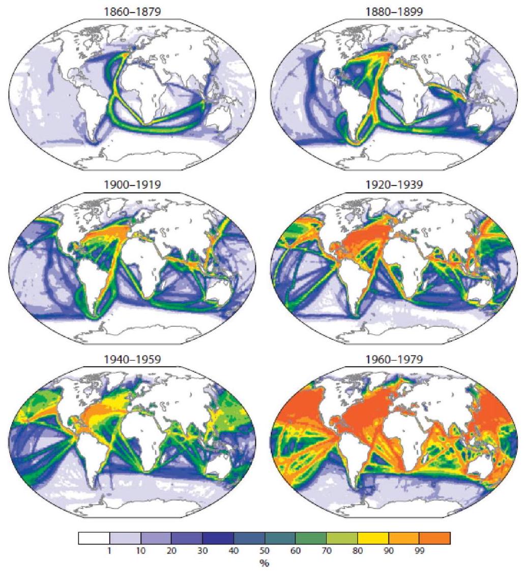
الشكل البياني الموسع 1| من ديزر وآخرون، (الشكل 3) يوضح توزيع ملاحظات درجة حرارة سطح البحر منذ عام 1860. البيانات من مجموعة بيانات المحيطات والغلاف الجوي الدولية الشاملة.لكل فترة مدتها 20 عامًا منذ عام 1860. تشير تدرجات الألوان إلى نسبة الأشهر التي تحتوي على
قياس واحد على الأقل فيخط العرض بواسطةصندوق شبكة الطول. لاحظ الملاحظات القليلة جدًا، خاصة في المناطق الحرجة لظاهرة النينيو والتذبذب الجنوبي في المحيط الهادئ المركزي من 1860-1899 مع وجود عدد قليل من الملاحظات للمحيطات الجنوبية حتى عام 1980. الشكل مُعدل بإذن من المرجع 9، المراجعات السنوية.
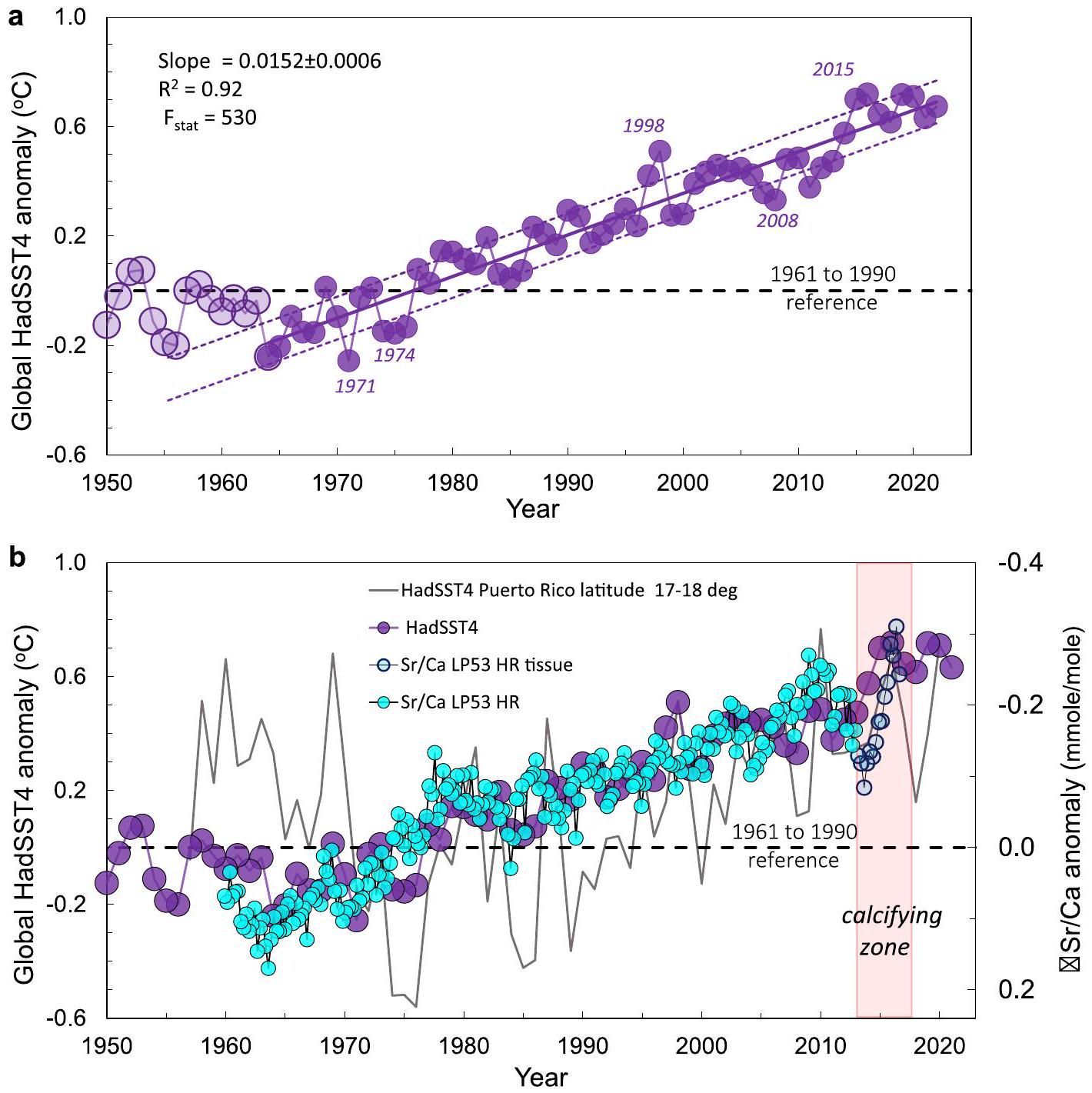
الشكل 4 من البيانات الموسعة | الانحدار الخطي لبيانات HadSST4 العالمية الحديثة مقابل الزمن وضد OML والغلاف الجوي. تحليل الانحدار الخطي (Linest) لبيانات درجة حرارة سطح البحر العالمية HadSST4 مقابل الزمن من 1964 إلى 2022 (شاملة) والذي يتم مقارنته بـتم معايرة الشذوذات (انظر نص الشكل 3). الخط المنقط يظهر 1SDs من المتوسط المتبقيات ( ) من الانحدار الخطي. ب، مقارنة عالمية متوسط HadSST4 مع الإسفنج القاسينسب أخذ عينات عالية الدقة لمدة شهرين من LP53 تظهر دليلاً محدوداً فقط على الموسمية. منطقة التكلس النشطة مظللة. الخط الرمادي يظهر درجات حرارة سطح البحر المحلية المصفاة قبالة خط عرض لا بارغويرا.خط الطول.
مدرسة المحيطات العليا ومعهد المحيطات بجامعة أستراليا الغربية، كراولي، أستراليا الغربية، أستراليا.مركز التميز في دراسات الشعاب المرجانية، جامعة أستراليا الغربية، كراولي، أستراليا الغربية، أستراليا.قسم نظم الأرض والبيئة، جامعة ولاية إنديانا، تير هوت، إنديانا، الولايات المتحدة الأمريكية.قسم علوم البحار، جامعة بورتو ريكو – ماياجويز، ماياجويز، بورتو ريكو، الولايات المتحدة الأمريكية. البريد الإلكتروني: مالكوم.ماكولوك@uwa.edu.au
Anthropogenic emissions drive global-scale warming yet the temperature increase relative to pre-industrial levels is uncertain. Using 300 years of ocean mixed-layer temperature records preserved in sclerosponge carbonate skeletons, we demonstrate that industrial-era warming began in the mid-1860s, more than 80 years earlier than instrumental sea surface temperature records. The Ca palaeothermometer was calibrated against ‘modern’ (post-1963) highly correlated ( ) instrumental records of global sea surface temperatures, with the pre-industrial defined by nearly constant ( ) temperatures from 1700 to the early 1860s. Increasing ocean and land-air temperatures overlap until the late twentieth century, when the land began warming at nearly twice the rate of the surface oceans. Hotter land temperatures, together with the earlier onset of industrial-era warming, indicate that global warming was already above pre-industrial levels by 2020 . Our result is higher than IPCC estimates, with global warming projected by the late 2020s, nearly two decades earlier than expected.
Global warming is causing major changes to the Earth’s climate , with heatwaves of unprecedented scale occurring across southern Europe, China and large parts of North America . Furthermore, during the 2023 Northern Hemisphere summer, heatwaves occurred towards the end of a prolonged La Niña cool phase, when global mean temperatures were below the long-term warming trend. This and the switch of ENSO (El Niño/Southern Oscillation) to a warmer-than-average El Niño phase in 2023-24, means that intense heatwaves and associated extreme events may now be the new normal. This questions whether global mean surface temperatures (GMSTs) have, or will soon exceed, the Paris Agreement of 2015 of holding GMSTs to “well below above pre-industrial levels and pursuing efforts to limit the temperature rise to no more than above pre-industrial levels” .
To address this question and whether even more extreme events are likely in the near future requires knowledge of the total magnitude of global warming that has occurred since the pre-industrial period. The pre-industrial-period is defined as the stable “mean climate state just
before human activities started to demonstrably change the climate through combustion of fossil fuels” . Given that anthropogenic concentrations of atmospheric started to increase in the early , the pre-industrial reference period should ideally be defined well before this, in the mid-1700s or earlier. Complicating this requirement is the series of exceptionally large volcanic eruptions in the early 1800s that caused global-scale cooling of unprecedented levels in recent living history . Most limiting, however, is that instrumental ship-based records of global sea surface temperature (SST) only began in the 1850s and then with limited coverage (Extended Data Fig. 1) . Thus, for pragmatic reasons , the earliest available instrumental records from 1850 to 1900 have been used to define the IPCC ‘pre-industrial’ period. The instrumental record of GMST is therefore constructed from the areal weighted average of SST, blended with land-air temperatures , the latter extending back to the but with larger uncertainties. For global SSTs, the most widely used products (for example, HadSST4 (ref.13) and ERSST5 (ref.14)) rely on the International Comprehensive
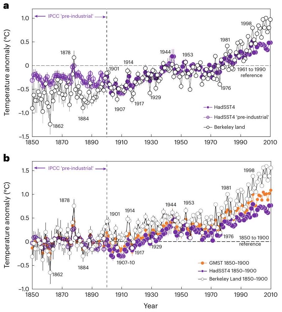
Fig. 1|Global sea surface and land-air temperature anomalies since 1850.
a, Anomalies referenced to the 1961-1990 average with HadSST4 (ref.13) being consistently warmer than land-air temperatures from 1850 to 1900. b, Anomalies referenced to the IPCC 1850-1900 pre-industrial period with anomalous cooling of SSTs relative to the land from the early 1900s. Global warming (GMST) is the weighted mean of land-air ( ) and sea surface ( ) temperatures. Uncertainties represent the confidence interval .
Ocean Atmosphere Data Set (ICOADS) , with the denser network of ‘modern’ reliable observations beginning in the second-half of the twentieth century .
The limitations of these products are evident when the earliest available global SSTs are compared (Fig. 1) with the land-air temperatures . When normalized to the ‘modern’ 1961-1990 anomaly reference period, the records overlap closely from about 1900 to the 1980s (Fig. 1a), with generally warmer land temperatures during El Niño and cooler temperatures during La Niña phases. However, the records diverge markedly between 1850 and 1900, when SSTs are warmer ( ) than the land, except during the very strong El Niño of 1877-78 (Fig. 1a). This is a conundrum because in a stable state, changes in land temperatures should closely track those in the much higher heat capacity upper oceans, as has occurred for most of the twentieth century (Fig. 1a). Consequently, when ocean and land anomalies are instead referenced to the IPCC 1850-1900 pre-industrial period , SSTs are apparently cooler than the land from the early 1900s, an offset that continues to the 1980s, then increases further as part of the late-twentieth-century enhanced warming of the land (Fig.1b) . In addition to there being no plausible explanation for such an abrupt cooling of the oceans in the early 1900s while the land continued to warm, this inconsistency has important implications for the processes responsible for the now even faster rates of late-twentieth-century land warming. For example, is the accelerated warming of the land since the due to a major regime shift in climate (Fig. 1a) or is it part of the same long-term warming trend shown when records are referenced to the IPCC 1850-1900 pre-industrial period (Fig. 1b)?
To resolve this question, here we report an extended Ca palaeotemperature record preserved in the calcium carbonate
Fig. 2 | /Ca temperature records from Caribbean sclerosponges. a, ratios ( ) from the aragonite skeletons sampled at continuous ( 0.5 mm ) intervals from the years 2012 back to 1700. Specimens were collected from OML depths of 33-91 m offshore Puerto Rico and St Croix. Published lower-resolution sclerosponge analyses (Ce-96 grey symbols) collected from within the OML.b, Stacked anomalies referenced to 1961-1990 means (Methods). Right axis shows atmospheric records from Mauna Loa (open symbols) and the Law Dome ice core (filled symbols).
skeletons of long-lived sclerosponges. Live specimens were collected from the Caribbean at depths between 33 and 91 m , within the ocean mixed-layer (OML), the region where heat is exchanged between the atmosphere and the ocean interior . Here, the thermal gradient is homogenized by turbulent mixing from the sea surface to the base of the OML, with its much greater thermal inertia providing a more stable, representative record of upper surface ocean temperatures compared to the highly variable uppermost ( ) sea surface layer . Furthermore, in the Caribbean part of the western Atlantic, the dominant source of multi-annual upper ocean surface temperature variability is from global atmospheric forcing, with little direct influence (Extended Data Fig. 2) from other ‘natural modes’ of internal variability, such as the Atlantic Meridional Overturning Circulation (AMOC) . Thus, temperature changes in the Caribbean OML appear to be mainly driven by external radiative forcing, which makes this an ideal region to monitor global trends in SSTs .
Results
Coralline sclerosponges are an ancient lineage of calcifying sponges , typically found in light-limited cryptic marine environments that extend from the relatively uniform temperature regime of the OML to below the thermocline. In this study, specimens of Ceratoporella nicholsoni were specifically targeted from within the OML of the eastern Caribbean, along the steeply dipping insular slope, offshore Puerto Rico and the nearby island of St Croix (Extended Data Fig.3). The ages and growth rates of specimens collected from 2007 to 2017 were determined using sensitive -series analyses back to the 1850s, with several to the beginning of the 1700s (Methods). Ambient seawater temperatures were derived from measurements of
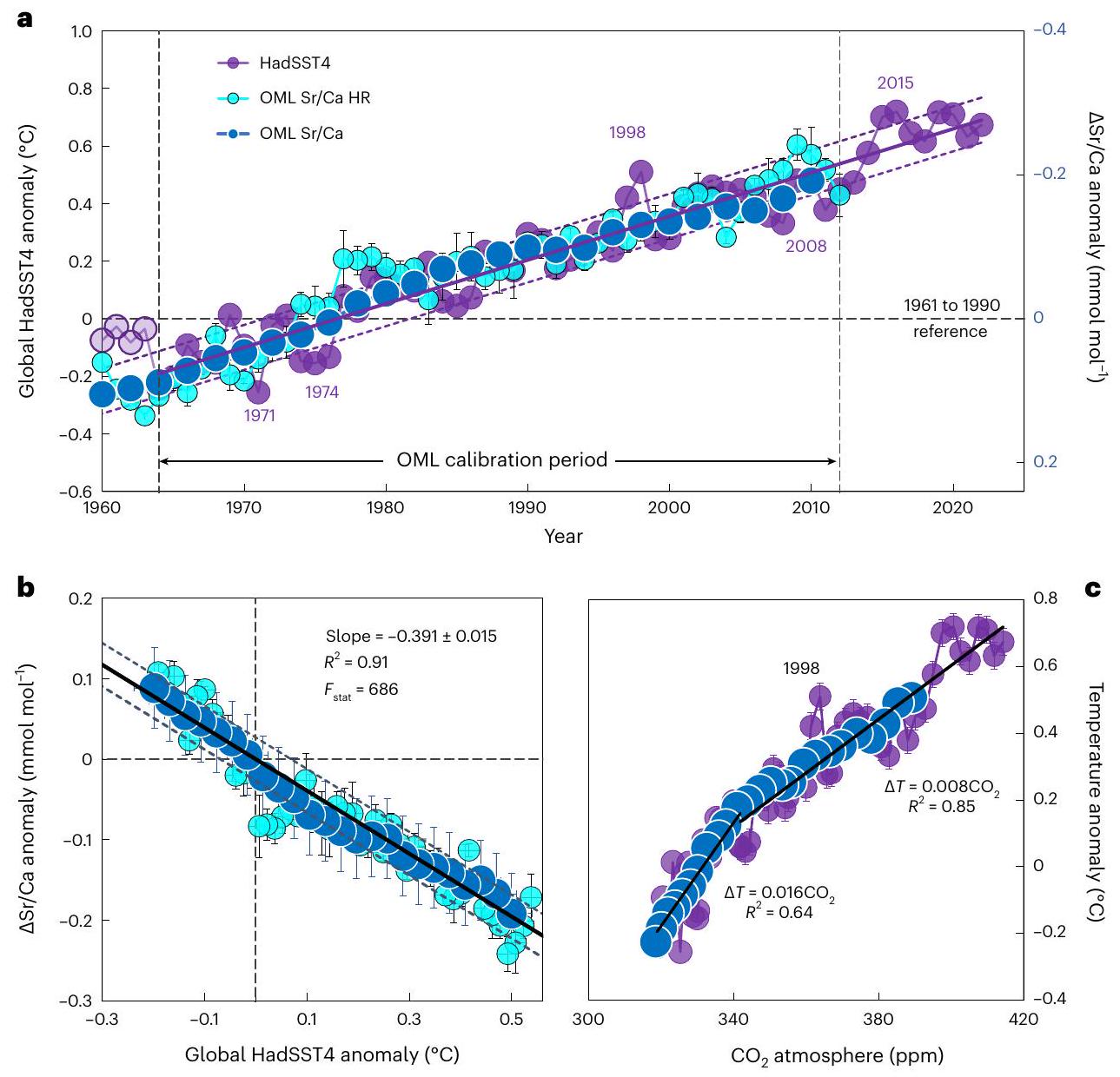
Fig. 3 | Calibration of against modern SST anomalies. a, Left axis, global mean HadSST4 (ref. 13) anomalies referenced to 1961-1990 with solid line showing linear regression versus time (Extended Data Fig. 4a). Right axis sclerosponge (dark blue) and annually averaged (light blue circles) anomalies from high-resolution (2 month) sampling. b, Correlation of anomalies with linear global HadSST4 array where:
(HadSST4) with , LINEST and dashed lines showing 1 s.d. of average residuals ( ). Dotted horizontal and vertical lines are 1961-1990 anomaly means about which the regressions pivot. c, Correlations of HadSST4 and OML with atmospheric concentrations with the temperature sensitivity to halving since 1984. Unless shown, uncertainties for data points are smaller than symbol size (Supplementary Data).
ratios of continuous increments (Fig. 2a), from the outermost layer down along the growth axis of the progressively older calcium carbonate (aragonite) skeletons (Methods). The absence of seasonal aliasing was confirmed by high-resolution 0.05 mm ( month) sampling of a specimen between 1960 and 2017, which showed little seasonal variation (Extended Data Fig. 4b) and was therefore averaged to 1 yr resolution.
Over the last , all specimens show subparallel arrays of ratios (Fig. 2a), indicative of the same proportionate response to changes in ambient seawater temperature. However, the offsets between the arrays indicate limited depth-dependent temperature differences, together with some biological induced vital effects. Vital effects are a common feature of biological systems and here the constant offsets were corrected by normalizing the Sr/Ca ratios to the mean of the 1961-1990 reference period for each specimen. The resultant, highly coherent array of stacked anomalies (Fig. 2b) thus indicates a constant sensitivity of the specimens to differential changes in temperature (that is, anomalies).
Calibration of sclerosponge Sr/Ca OML temperatures
To determine the temperature sensitivity of sclerosponge anomalies, the 2 and 1 yr averaged arrays were compared with global mean SSTs (HadSST4) from 1964 to 2012 inclusive. Following established
procedures , the global average HadSST4 anomalies were detrended using a well-defined ( ) linear relationship, with the residuals being mainly due to periods of high ENSO variability (Extended Data Fig. 4a). The modern (1964-2012) OML anomalies were then regressed against the linear global HadSST4 (Fig.3a,b), which assumes that the OML Ca record incorporates a large fraction of the well-defined increase in modern global SSTs. This yields a slope of , with the calibration period representing nearly one-half of the total amount global warming that has occurred to date.
Although the anomalies show the expected thermodynamic-based negative correlation with global SSTs, the temperature sensitivity is greater than previous studies , including those of scleractinian corals . However, previous attempts to calibrate the temperature sensitivity of Ca ratios in sclerosponges have been based on either depth-dependent differences in temperature that incorporate vital effects or, alternatively, a lower precision laser-ICP seasonal study within the actively calcifying tissue zone. The constant, high sensitivity of Ca temperature anomalies in . nicholsoni, found here for many specimens, is attributed to multistage regenerative calcification as seawater is pumped and exchanged within the active ( ) calcification zone, which extends from the uppermost surface to lower basal zone . This also accounts for the absence of a
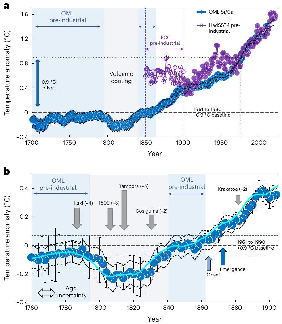
Fig. 4 | OML and HadSST4 global mean anomalies. a, Comparison of OML and HadSST4 (ref.13) records with offsets of to account for warming from the pre-industrial period (blue shading from the 1700 to early 1790 s and 1840 to early 1860s) to the 1961-1990 anomaly reference mean (vertical dotted line). b, Timing of major volcanic eruptions denoted by grey arrows with negative radiative forcing ( ) (ref. 16). Onset of industrial warming in mid-1860s
(light blue arrow) followed by emergence in early 1870 (blue arrow). Error bars are 2 s.e.m. (Supplementary Fig.1) with light blue line showing 5-year moving average. c, Comparison of OML and IPCC pre-industrial values with mean offset of . Horizontal arrows show stages of industrial-era warming. d, Difference between sclerosponge OML and HadSST4 anomalies with El Niño years shown in italics. Open symbols show national fleet corrections .
seasonal signal in either the month sampling (Extended Data Fig. 4b) or the 2 yr stacked arrays (Fig.2b). This, together with the low sensitivity of Caribbean OML to central Pacific generated ENSO teleconnections , accounts for the limited ENSO variability in the sclerosponge OML record with, for example, the main 1997-98 El Niño being absent.
Calibration of the sclerosponge Sr/Ca palaeothermometer against global temperature changes thus provides strong empirical evidence that the Caribbean OML has warmed proportionately to the average global increase in SST, over the last . This finding is supported by modelling which shows that, across this broad central western Atlantic region, SSTs have also increased at approximately the same rate as the global average (Extended Data Fig. 2) . This can be understood as anthropogenic imposed radiative heating being an essentially passive tracer in the Caribbean OML , whereas in the northern Atlantic, global warming plays an active role in modifying and hence heat uptake in that region. Thus, our empirical findings are consistent with the Caribbean being ideally positioned to monitor at-scale global greenhouse warming with minimal superimposed changes from , whilst still registering the broader effects of ENSO teleconnections . Importantly, modelling also provides a strong physical basis for extending the modern (1964-2012) calibration of the sclerosponge Sr/Ca palaeothermometer back to the eighteenth to nineteenth centuries, when still rudimentary instrumental measurements of SSTs were either absent or, at best, limited in geographic coverage (Extended Data Fig. 1) .
Pre-industrial period and onset of industrial-era warming
The three centuries of OML temperature changes preserved in the skeletons of long-lived Caribbean sclerosponges (Fig. 4) show that the
pre-industrial baseline period is defined by the same essentially constant ( decade ) temperatures from 1700 to 1790 and then from 1840 to the early 1860s. The intervening period is marked by prolonged global-scale cooling (Fig. 4a,b), consistent with high concentrations of volcanic-generated sulfate aerosols found in ice . This includes major volcanic eruptions (Fig. 4b) in 1783 (Laki), 1809 (unknown), 1815 (Tambora) and 1832 (Cosiguina). The most important is the Tambora eruption in Indonesia during , the largest explosive event yet recorded in ‘living’ history . This caused “The Year without a Summer” in 1816 , with the global-scale cooling ( ) being evident in the Caribbean OML record from 1808 to 1828, with a gradual return to warmer pre-industrial levels during the 1830s (Fig. 4b). The final stage of the pre-industrial period is thus defined by the plateau in temperatures between 1840 and the early 1860 s, at marginally warmer ( ) pre-industrial temperatures compared to the 1700s. The sclerosponge record (Fig. 4b) of these well-known historic events thus confirms the veracity of the Caribbean OML thermometer as a recorder of globally forced radiative temperature changes. As expected , temperature changes in the OML are dampened relative to the atmosphere due to the much greater heat capacity of the OML (Fig. 5a).
Relative to this extended and now well-defined pre-industrial baseline, an offset of is applied (Fig. 4) to account for the temperature increase from the pre-industrial baseline period (that is, mean temperatures from 1700 to 1790 and from 1840 to 1860) to the 1961-1990 anomaly reference period. On this basis, the onset of industrial-era warming is evident by the mid-1860s. Although earlier than the IPCC estimate (Fig. 4b,c), it is in good agreement with previous palaeoclimate reconstructions that indicate an ‘early’
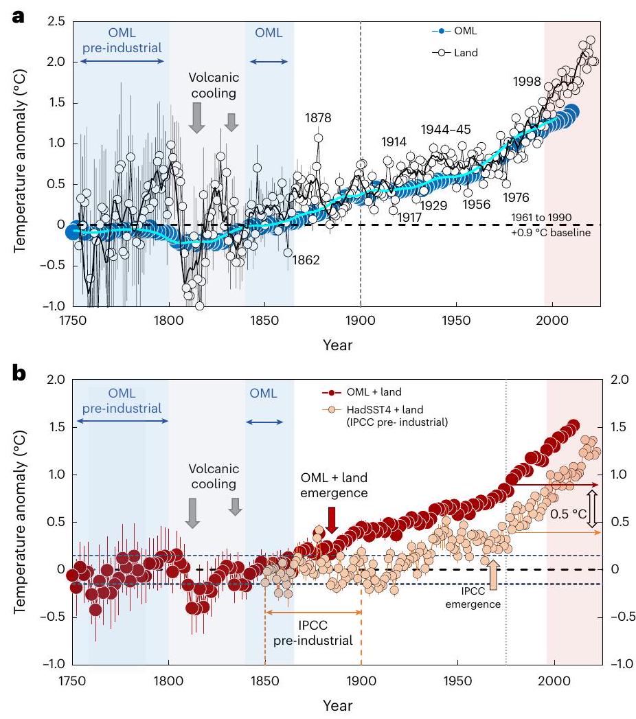
Fig. 5 | OML and GMSTs. Anomalies relative to 1961-1990 baseline with offset (unless indicated). a, OML and Berkeley land temperature anomalies with onset of extreme land-air temperature from about 1990 (pink shading). b, GMSTs from blended OML and land anomalies (this study dark red circles) and from blended HadSST4 and land temperatures (orange circles), the latter relative to IPCC 1850-1900 pre-industrial period, which underestimates global warming by . See refs. and Supplementary Data for uncertainties.
c, OML and HadSST4 of and land temperature increases by 2020. d, GMST records for blended OML + land and blended HadSST4 + land with passed during 2012-2015. At current rates of emissions global warming will be reached by late 2020s. Historic evolution of atmospheric (solid line), future increases with present-day rates of emissions (dashed line) and annual reductions from 2025 to halve emissions by early 2030 (dotted line).
mid-nineteenth-century onset of industrial-era warming. This is especially the case if account is taken of the now much improved resolution of our OML record, which clearly distinguishes the initiation of early industrial warming in the mid-1860s from the prolonged recovery that followed the early 1800s global-scale volcanic cooling. Thus, the emergence of OML warming is apparent by the mid-1870s (Fig. 4b), with emergence being defined by the more stringent criteria of warming that first exceeds and remains above the pre-industrial period . This is more than 80 years earlier than instrumental SST records (Fig. 4c) or shallow-water palaeoclimate coral records in which high natural variability masks the emergence of industrial-era warming until the mid twentieth century (Fig. 5b).
OML temperatures over the industrial era
On the basis of the sclerosponge OML record, industrial-era warming can be categorized into three broad stages (Fig. 4c). The first is the early industrial period from the mid-1860s to early 1900s, when temperatures increased by at an average rate of decade . This was followed by a similar amount of warming ( ) from the early 1900s to the early 1960s (the mid-industrial period) but at nearly half the average rate decade . Finally, starting from the mid-1960s (the ‘modern’ period) temperatures increased at a much faster rate of decade (Fig. 4c) in response to rapidly increasing atmospheric . Since the mid-1980s, the temperature sensitivity to increasing has halved, from per 10 ppm CO during 1964-1984 to the present-day (1985-2020) per 10 ppm CO 2 (Figs. 3c and 4c). While the causes of
this decrease in the sensitivity of OML warming to require further investigation, we note that it is difficult to reconcile with the cooling effects of industrial aerosols but it does coincide with the global increase in summertime mixed-layer depths and hence greater heat capacity of the OML.
In contrast to this coherent pattern of OML warming, ship-based records of SSTs (for example, HadSST4) show much greater ‘roller-coaster’ like variability, with periods of rapid warming followed by falling temperatures (Fig. 4). Most notable is the period from 1850 to 1880, the first part of the IPCC pre-industrial reference period, that is characterized by unusually warm temperatures, especially during the El Niño . Then, from around 1880 until the early 1900s, SSTs cooled in a series of steps with only the first being attributable to cooling from the Krakatau eruption in 1883 (Fig. 4c,d). By the early 1900s and especially during the so-called 1908 to 1910 ‘cool excursion’, there is good agreement between the OML and HadSST4 records. Paradoxically, during the IPCC 1850-1900 pre-industrial period (Fig. 4c), temperatures were anomalously warmer than the beginning of the twentieth-century ‘industrial era’ despite increasing atmospheric .
While there is good agreement between the OML and HadSST4 records during the early 1900s (Fig. 4), HadSST4 is again warmer during the mid-1920s and especially during the mid-1940s World War II period (Fig. 4c,d). The latter discrepancy is attributed to changes from bucket to engine-room water intake measurements , as well as recently identified biases between different national fleets . It is uncertain, however, whether these and the much more significant offsets during the IPCC pre-industrial period are due, for example, to an over-representation
of warm El Niño events in the poorly constrained nineteenth-century ICOADS records or to greater natural variability in ENSO before 1960, although our OML record suggests the former.
Discussion
Understanding how greenhouse forced warming has affected land-air temperatures relative to the much larger heat sink of the upper ocean remains a challenge. Here, we assume that, relative to the 1961-1990 reference period, the same fixed offset of can be applied to land-air as well as the OML anomalies (Figs. 4 and 5), although there are larger uncertainties in land-based records from 1750 to 1860 (Fig. 5a). Despite this limitation, there is nevertheless good agreement between the land-air and OML records, especially during the historically well-documented Tambora eruption when volcanic aerosols induced global cooling. Significantly, from mid-1860 to 1900, both land and OML temperatures increased synchronously by . Conversely, over the same IPCC 1850-1900 pre-industrial period, HadSST4 is initially up to warmer (Fig. 4c) followed by an anomalous cooling trend compared to the well-defined OML and land records of consistent warming from the 1860s. Our findings now resolve the ‘warm-land cool-ocean’ conundrum posed by using the IPCC pre-industrial reference period (Fig.1b). Hence modern observations should continue to be referenced to the 1961-1990 mean (Fig. 1a) but with an adjustment of to account for the temperature increase since the onset of industrial-era warming in the mid-1860s to the 1961-1990 mean (Fig. 4a). On this basis, the land and SST records have shown a generally coherent response to ENSO up until the 1990s, characterized by relatively warmer land temperatures during strong El Niño and cooler temperatures during La Niña events (Fig. 5a).
Importantly, however, the long-term similarity in rates of land and upper ocean surface warming starts to breakdown in the late twentieth century, with land-air temperatures now increasing at nearly twice the rate of the surface oceans regardless of the ENSO phase (Fig. 5a,c). Rather than the land-air record being part of an ongoing post-1900s warming trend relative to the IPCC 1850-1900 pre-industrial period, as currently assumed (Fig. 1b), our findings show a distinct divergence from the surface ocean from around 1980-1990 (Fig. 5a,c). This is consistent with the already well-documented amplified warming of the high-latitude Northern Hemisphere land masses and the decline of Artic permafrost . This change also coincides with the increased frequency of both Southern Hemisphere and Northern Hemisphere heatwaves and associated extreme events, such as droughts and wildfires . Wildfires and more frequent bushfires are also an additional source of atmospheric , providing an enhanced feedback mechanism. Although the relative importance of the regional and global processes driving the increased frequency and intensity of land-based heatwaves is still uncertain , our revised record of industrial-era warming now clearly shows that terrestrial environments have been subject to a much faster rate of warming since the 1990s, compared to those in the more stable OML of the upper surface oceans.
These findings also have important implications for near-term projections of global warming. As already described, relative to the 1961-1990 reference, OML and land temperatures (Fig. 5a) and hence GMSTs (Fig. 5b) increased by since the 1700-1860 pre-industrial period. This compares with only when HadSST4 and land temperatures are estimated relative to the IPCC 1850-1900 pre-industrial period , a difference of (Fig. 5b). The additional in global warming above IPCC estimates also implies that GMSTs were above pre-industrial levels by 2018-2022, compared to the IPCC estimate of (Fig. 5b). Thus, the opportunity to limit global warming to no more than by emission reductions alone has now passed and at current emission rates, the threshold for GMSTs will be reached by the late2020s (Fig. 5d).
We have shown that the late-twentieth-century land-air temperatures have been increasing at almost twice the rate of the surface oceans
and are now above pre-industrial levels. If these current rates of warming continue, mean land temperature will exceed by about 2035, with GMSTs expected to follow in early 2040 (Fig. 5c,d). Consequently, the overriding aim of the UN Paris agreement to keep the combined land and ocean global surface temperature increase to below is now a much greater challenge, emphasizing the even more urgent need to halve emissions by 2030.
Online content
Any methods, additional references, Nature Portfolio reporting summaries, source data, extended data, supplementary information, acknowledgements, peer review information; details of author contributions and competing interests; and statements of data and code availability are available at https://doi.org/10.1038/s41558-023-01919-7.
References
IPCC Climate Change 2023: Synthesis Report (eds Core Writing Team, Lee, H. et al.) (IPCC, 2023).
Russo, E. & Domeisen, D. I. Increasing intensity of extreme heatwaves: the crucial role of metrics. Geophys. Res. Lett. 50, e2023GL103540 (2023).
Domeisen, D. I. V. et al. Prediction and projection of heatwaves. Nat. Rev. Earth Environ. 4, 36-50 (2023).
Hawkins, E. et al. Estimating changes in global temperature since the preindustrial period. Bull. Am. Meteorol. Soc. 98, 1841-1856 (2017).
Etheridge, D. et al. Natural and anthropogenic changes in atmospheric over the last 1000 years from air in Antarctic ice and firn. J. Geophys. Res. 101, 4115-4128 (1996).
Gao, C., Robock, A. & Ammann, C. Volcanic forcing of climate over the past 1500 years: an improved ice core-based index for climate models. J. Geophys. Res. 113, D23111 (2008).
Kent, E. C. & Kennedy, J. J. Historical estimates of surface marine temperatures. Annu. Rev. Mar. Sci. 13, 283-311 (2021).
Deser, C., Alexander, M. A., Xie, S.-P. & Phillips, A. S. Sea surface temperature variability: patterns and mechanisms. Annu. Rev. Mar. Sci. 2, 115-143 (2010).
IPCC Special Report on Global Warming of (eds Masson-Delmotte, V. et al.) (WMO, 2018).
Morice, C. P. et al. An updated assessment of near-surface temperature change from 1850: the HadCRUT5 data set. J. Geophys. Res. 126, e2019JD032361 (2021).
Rohde, R. A. & Hausfather, Z. The Berkeley Earth Land/Ocean temperature record. Earth Syst. Sci. Data 12, 3469-3479 (2020).
Kennedy, J. J., Rayner, N. A., Atkinson, C. P. & Killick, R. E. An ensemble data set of sea surface temperature change from 1850: the Met Office Hadley Centre HadSST. 4.0. 0.0 data set. J. Geophys. Res. 124, 7719-7763 (2019).
Huang, B. et al. Extended reconstructed sea surface temperature, version 5 (ERSSTv5): upgrades, validations and intercomparisons. J. Clim. 30, 8179-8205 (2017).
Freeman, E. et al. ICOADS Release 3.0: a major update to the historical marine climate record. Int. J. Climatol. 37, 2211-2232 (2017).
Gulev, S. K. et al. In Climate Change 2021: The Physical Science Basis (eds Masson-Delmotte, V. et al.) Ch. 2 (IPCC, Cambridge Univ. Press, 2021).
Caesar, L., Rahmstorf, S., Robinson, A., Feulner, G. & Saba, V. Observed fingerprint of a weakening Atlantic Ocean overturning circulation. Nature 556, 191-196 (2018).
Willenz, P. & Willenz, P. Micromorphology and ultrastructure of Caribbean sclerosponges. I. Ceratoporella nicholsoni and Stromatospongia norae (Ceratoporellidae: Porifera). Mar. Biol. 103, 387-401 (1989).
McCulloch, M. T. & Mortimer, G. E. Applications of the decay series to dating of fossil and modern corals using MC-ICPMS. Aust. J. Earth Sci. 55, 955-965 (2008).
McCulloch, M. T., Gagan, M. K., Mortimer, G. E., Chivas, A. R. & Isdale, P. J. A high-resolution and coral record from the Great-Barrier-Reef, Australia and the 1982-1983 El-Nino. Geochim. Cosmochim. Acta 58, 2747-2754 (1994).
D’Olivo, J. P., Sinclair, D. J., Rankenburg, K. & McCulloch, M. T. A universal multi-trace element calibration for reconstructing sea surface temperatures from long-lived Porites corals: removing ‘vital-effects’. Geochim. Cosmochim. Acta 239, 109-135 (2018).
Weiner, S. & Dove, P. M. An overview of biomineralization processes and the problem of the vital effect. Rev. Mineral. Geochem. 54, 1-29 (2003).
Hawkins, E. et al. Observed emergence of the climate change signal: from the familiar to the unknown. Geophys. Res. Lett. 47, e2019GL086259 (2020).
Gaetani, G. A. & Cohen, A. L. Element partitioning during precipitation of aragonite from seawater: a framework for understanding paleoproxies. Geochim. Cosmochim. Acta 70, 4617-4634 (2006).
Haase-Schramm, A. et al. Sr/Ca ratios and oxygen isotopes from sclerosponges: temperature history of the Caribbean mixed layer and thermocline during the Little Ice Age. Paleoceanography 18,1073 (2003).
Waite, A. J., Swart, P. K., Rosenheim, B. E. & Rosenberg, A. D. Improved calibration of the Sr/Ca-temperature relationship in the sclerosponge Ceratoporella nicholsoni: re-evaluating Sr/Ca derived records of post-industrial era warming. Chem. Geol. 488, 56-61 (2018).
Rosenheim, B. E. et al. High-resolution Ca records in sclerosponges calibrated to temperature in situ. Geology 32, 145-148 (2004).
Cai, W. et al. Pantropical climate interactions. Science 363, eaav4236 (2019).
Marshall, J. et al. The ocean’s role in the transient response of climate to abrupt greenhouse gas forcing. Clim. Dynam. 44, 2287-2299 (2015).
Brohan, P. et al. Constraining the temperature history of the past millennium using early instrumental observations. Climate 8, 1551-1563 (2012).
Newhall, C. G. & Self, S. The Volcanic Explosivity Index (VEI): an estimate of explosive magnitude for historical volcanism. J. Geophys. Res. 87, 1231-1238 (1982).
Abram, N. J. et al. Early onset of industrial-era warming across the oceans and continents. Nature 536, 411-418 (2016).
Tierney, J. E. et al. Tropical sea surface temperatures for the past four centuries reconstructed from coral archives. Paleoceanography 30, 226-252 (2015).
Hawkins, E. & Sutton, R. Time of emergence of climate signals. Geophys. Res. Lett. 39, L01702 (2012).
Sallée, J.-B. et al. Summertime increases in upper-ocean stratification and mixed-layer depth. Nature 591, 592-598 (2021).
Gergis, J. L. & Fowler, A. M. A history of ENSO events since AD 1525: implications for future climate change. Clim. Change 92, 343-387 (2009).
Chan, D. & Huybers, P. Correcting observational biases in sea surface temperature observations removes anomalous warmth during World War II. J. Clim. 34, 4585-4602 (2021).
Natali, S. M. et al. Large loss of in winter observed across the northern permafrost region. Nat. Clim. Change 9, 852-857 (2019).
IPCC Climate Change 2022: Impacts, Adaptation, and Vulnerability (eds Pörtner, H.-O. et al.) (IPCC, 2022).
Bousfield, C. G., Lindenmayer, D. B. & Edwards, D. P. Substantial and increasing global losses of timber-producing forest due to wildfires. Nat. Geosci. 16, 1145-1150 (2023).
Keeling, C. D. et al. Exchanges of Atmospheric and with the Terrestrial Biosphere and Oceans from 1978 to 2000. I. Global Aspects (Scripps Institution of Oceanography, 2001); https:// escholarship.org/uc/item/09v319r9
Publisher’s note Springer Nature remains neutral with regard to jurisdictional claims in published maps and institutional affiliations.
Living specimens of the Caribbean sclerosponge C. nicholsoni were collected using mixed-gas closed-circuit rebreathers by the University of Puerto Rico-Mayagüez, Department of Marine Sciences technical diving team that includes C. Sherman, M. Carlo, H. Ruíz, M. Nemeth, E. Tuohy, I. Bejarano and D. Kesling. Collections were made from 2007 to 2017 and cover a depth range of to 91 m . Sampling locations (Extended Data Fig. 3 and Supplementary Table 1) for this study include Bajo de Sico (BS33), Mona Channel, Puerto Rico, the southern insular margin of southwest Puerto Rico off La Parguera (LP36, LP47, LP53, LP58) and offshore the northwest coast of the island of St. Croix, US Virgin Islands (DB91). After collection, the specimens were slabbed into thick slices, cleaned in deionized water using an ultrasonic probe in preparation for precisely controlled subsampling (milling) and geochemical analyses conducted at the UWA isotope laboratories.
Initially, samples were subject to high-precision U-series dating (see below) to establish accurate chronologies of skeletal growth. For this purpose, U-series dating was undertaken on ( ) samples extracted from narrow ( mm wide) slots milled adjacent to the sampling for Caanalyses. The slots were cut at intervals along the growth axis of the precleaned sclerosponge slabs with the top (youngest) sample being extracted immediately below the thick tissue zone. Where there is evidence of bio-erosion and hence a possible growth hiatus (for example, BS33) additional samples were taken above and below to determine any temporal discontinuity (Supplementary Fig.2a).
ForSr/Ca analyses, to minimize temporal smoothing due to sloping growth bands, an mm thick ledge was milled along the sample growth axis, adjacent to sampling for U-Th dating. Samples for analysis were then extracted at continuous increments resulting in sample aliquots, using a computer-controlled Zenbot mill. For the most recently collected specimen (LP53), additional samples were collected down along the top (1960-2017) at ultra-high-resolution ( ) in continuous increments along an adjacent thick ledge, each sample equivalent to months of average growth and weighing . For both 0.5 and 0.05 mm sampling, the aliquots were extracted continuously down along the machined ledge, maintaining precise location of the drill edge relative to the uppermost surface. When necessary, to minimize temporal smoothing, minor adjustments were made to the orientation of the horizontal sampling ledge so that growth bands remained parallel to the mill axis.
Sr/Ca elemental analyses
Sample powders were dissolved in over several hours and then agitated and centrifuged for 1 min at 3,500 r.p.m. to ensure complete dissolution. Aliquots from the dissolved sample were diluted to provide a representative solution at a precisely determined ppm Ca concentration for analyses of Sr and Ca using an X-series quadrupole ICPMS . To ensure data quality, internal laboratory standards and the international coral standard JCp-1 were also analysed during the same analytical session as the sclerosponge samples. Multiple measurements of the coral standardJCp-1 at the same 10 ppm Ca concentration over an yr period gave an average relative standard deviation (RSD) of 0.15% ( RSD) corresponding to a mean Sr/Ca value of . Repeat analysis of sclerosponge samples within the same analytical session typically gave an improved reproducibility of ( RSD) consistent with the temperature uncertainties shown in Supplementary Fig. 1. Procedural blanks were processed with sample batches to check for procedural contamination and were below detection limits.
Calibration of Sr/Ca temperature anomalies
As described in the text, anomalies were calculated relative to the 1961-1990 mean. Thus, for each specimen the Ca ratio anomalies at time increment is given by:
where is the measured ratio ( ) and (1961-1990) is the mean ratio for the common reference period from 1961 to 1990 (inclusive). To facilitate stacking (averaging) of many specimens, the Sr/ were then rescaled to 2 yr intervals with minimal extrapolation as the 0.5 mm sampling represented intervals, depending on the specimen growth rate. The anomalies were then stacked (that is, averaged) with uncertainties given by s.e.m. s.d./ Sqrt( ) where is the number (3-6) of specimens analysed. For the modern calibration period (1964-2012), annual means were also determined from the ultra-high ( 0.05 mm ) ~2 month incremental sampling of LP53 (Extended Data Fig. 4b). Both the stacked 2 and 1 yr anomalies were regressed against the smoothed (linear) HadSST4 global mean SST anomalies (Extended Data Fig. 4a) for the period 1964-2022. This yielded a slope of s.e.m. , with the calibration incorporating nearly one-half of the total global warming signal. On the basis of this regression, the average standard deviation of the 2 yr means is , consistent with that expected from combined uncertainties in analyses as well as variability between samples.
U-Th dating of sclerosponges
A critical aspect of this study is the requirement for accurate sclerosponge chronologies. For this purpose high-precision series dating was undertaken on ( ) samples extracted from the narrow ( wide) slots (see previous). The U-Th sample powders were dissolved and then spiked with a calibrated solution of and Th isotopes . The spiked solution was then chemically purified using ion-exchange procedures with the separated and Th fractions analysed using a NEPTUNE MC-ICPMS following procedures similar to those described by ref.19.
For the high analytical precision required in this study, the measured ratio was corrected for ingrowth of between the time of collection and geochemical analyses, a period which ranged from only several months to nearly a decade. Corrections assuming a constant initial i were then applied to all U-series samples of the same specimen, with further adjustments to optimize the regression of age ( ) versus distance from the outer growth surface. Thus, for each specimen, the age-distance relationship was given by: .
Here, the outermost surface is defined by the collection age (Supplementary Table 2). Correction for initial is the major uncertainty ( ) in determining the time of calcification and hence growth rate of the skeletal segments, compared to the theoretical precision of without corrections for initial . The initial i activity ratios ranged from 1.45 to 2.74 , with the largest offset ( ) required for the deepest ( 91 m ) sample (DB91), consistent with the commonly observed trend of increased dissolved/ particulate with increasing depth and hence greater i. For the larger ( diameter) older specimens, a simple linear relationship ( ) was generally found to provide the best fit with minimal degrees of freedom. For other specimens, a polynomial fit ( ) was required to account for the ontogenetic effect of initially lower extension rate in the early growth phase (Supplementary Table 2). The best fit age-distance isochrons are shown in Supplementary Fig. 2 for each specimen together with an insert showing differences of the individual U-series ages from the isochron. We note that the almost constant growth rate of sclerosponges analysed in this study is in marked contrast with other commonly used climate proxies, such as shallow-water scleractinian corals where there can be a strong but generally variable dependence of growth rate on temperature .
This work was supported by the awards of an ARC Laureate Fellowship (LF120100049) to M.M. and an ARC Future Fellowship (FT160100259) to J.T. and the ARC Coral Reef Studies Centre of Excellence (CE140100020). Collection of sclerosponges was supported by NOAA-NCCOS grants, NA06NOS4780190, NA09NOS4260243, NA10NOS4260223 and NA11NOS4260184 to the UPRM Caribbean Coral Reef Institute and NSF Award 0738825 to A.W. We thank J. P. D’Olivo, A. Kuret, K. Rankenburg and A.-M. Nisumaa-Comeau for providing technical support at the UWA geochemical laboratories. We greatly appreciated the helpful and encouraging comments provided by colleagues.
Author contributions
M.M. and A.W. designed the project. M.M. wrote the initial draft manuscript. C.S. and the UPRM rebreather dive team collected the samples. M.M. and A.W. undertook initial sample preparation. J.T. oversaw Sr/Ca sample preparation and clean-room chemical
extractions. All authors contributed to manuscript writing and revisions.
Extended Data Fig. 1| From Deser et al., (Fig. 3) showing the distribution of sea surface temperature observations since 1860. Data from the International Comprehensive Ocean Atmosphere Data Set for each 20-year period since 1860. Colour shading indicates the percentage of months with at
least one measurement in a latitude by longitude grid box. Note very sparse observations of especially the critical ENSO regions in the central Pacific Ocean from 1860-1899 with still few observations for the Southern Oceans up to 1980. Figure adapted with permission from ref. 9, Annual Reviews.
Extended Data Fig. 4 | Linear regression of modern global HadSST4 versus time and against OML and atmospheric . a, Linear (Linest) regression of global HadSST4 versus time from 1964 to 2022 (inclusive) against which the anomalies are calibrated (see Fig. 3 text). Dashed line show 1SDs of average residuals ( ) from linear regression.b, Comparison of global
average HadSST4 with sclerosponge ratios for 2-month high-resolution sampling of LP53 showing only limited evidence for seasonality. Active calcification zone is shaded. Grey line shows local gridded SST’s offshore La Parguera latitude , longitude .
Oceans Graduate School and UWA Oceans Institute, The University of Western Australia, Crawley, Western Australia, Australia. ARC Centre of Excellence in Coral Reef Studies, The University of Western Australia, Crawley, Western Australia, Australia. Earth and Environmental Systems Department, Indiana State University, Terre Haute, IN, USA. Department of Marine Sciences, University of Puerto Rico-Mayaguez, Mayaguez, PR, USA.
-e-mail: Malcolm.McCulloch@uwa.edu.au