GLC_FCS30D: أول منتج عالمي لمراقبة ديناميات تغطية الأرض بدقة 30 مترًا مع نظام تصنيف دقيق للفترة من 1985 إلى 2022 تم إنشاؤه باستخدام صور لاندسات ذات سلسلة زمنية كثيفة وطريقة الكشف المستمر عن التغيرات GLC_FCS30D: the first global 30 m land-cover dynamics monitoring product with a fine classification system for the period from 1985 to 2022 generated using dense-time-series Landsat imagery and the continuous change-detection method

المجلة: Earth system science data، المجلد: 16، العدد: 3
DOI: https://doi.org/10.5194/essd-16-1353-2024
تاريخ النشر: 2024-03-15

GLC_FCS30D: أول منتج عالمي لمراقبة ديناميات تغطية الأرض بدقة 30 مترًا مع نظام تصنيف دقيق للفترة من 1985 إلى 2022 تم إنشاؤه باستخدام صور لاندسات ذات سلسلة زمنية كثيفة وطريقة الكشف المستمر عن التغيرات

شياو تشانغ تينغتينغ تشاو هونغ شيو ويندي ليو جينكينغ وانغ زيدونغ تشين وليانغيون ليو المركز الدولي للبحوث حول البيانات الضخمة من أجل أهداف التنمية المستدامة، بكين 100094، الصين المختبر الرئيسي لعلوم الأرض الرقمية، معهد أبحاث المعلومات الفضائية، الأكاديمية الصينية للعلوم، بكين 100094، الصين مدرسة الهندسة الإلكترونية والكهربائية والاتصالات، أكاديمية العلوم الصينية، بكين 100049، الصين كلية الجيوماتكس، جامعة شيان للعلوم والتكنولوجيا، شيان 710054، الصين مركز البحث والتطوير عالي التقنية (HTRDC) التابع لمؤسسة العلوم الطبيعية الوطنية في الصين، بكين 100044، الصين مختبر الحضرية المستقبلية والبيئة المستدامة (FUSE)، جامعة هونغ كونغ، منطقة هونغ كونغ الإدارية الخاصة، 999007، الصينالمراسلة: ليانغيون ليو (liuly@radi.ac.cn)

تاريخ الاستلام: 7 أغسطس 2023 – بدأت المناقشة: 31 أغسطس 2023
تمت المراجعة: 15 يناير 2024 – تم القبول: 31 يناير 2024 – تم النشر: 15 مارس 2024

الملخص

تم تحديد تغيير استخدام الأراضي كسبب مهم أو قوة دافعة لتغير المناخ العالمي وهو موضوع بحثي كبير. على مدى العقود القليلة الماضية، تقدم رسم خرائط استخدام الأراضي العالمي؛ ومع ذلك، لا تزال بيانات مراقبة تغيير استخدام الأراضي العالمية على مدى فترات زمنية طويلة نادرة، خاصة تلك التي بدقة 30 مترًا. في هذه الدراسة، نصف مجموعة بيانات جديدة لمراقبة ديناميات استخدام الأراضي العالمية بدقة 30 مترًا، والتي تحتوي على 35 فئة فرعية من استخدام الأراضي وتغطي الفترة من 1985 إلى 2022 في 26 نقطة زمنية (تم تحديث الخرائط كل 5 سنوات قبل عام 2000 وسنويًا بعد عام 2000). تم تطوير GLC_FCS30D باستخدام نموذج الكشف عن التغيير المستمر وجميع صور لاندسات المتاحة استنادًا إلى منصة Google Earth Engine. على وجه التحديد، نستفيد أولاً من نموذج الكشف عن التغيير المستمر والسلسلة الزمنية الكاملة لملاحظات لاندسات لالتقاط نقاط الزمن للبكسلات المتغيرة وتحديد المناطق المستقرة زمنياً. ثم، نطبق طريقة تحسين مكاني زمني لاشتقاق عينات تدريب موزعة عالميًا وعالية الثقة من هذه المناطق المستقرة زمنياً. بعد ذلك، تُستخدم نماذج التصنيف التكيفية المحلية لتحديث معلومات استخدام الأراضي للبكسلات المتغيرة، ويتم اعتماد خوارزمية تحسين التناسق الزمني لتحسين استقرارها الزمني وكبح بعض التغيرات الزائفة. علاوة على ذلك، يتم التحقق من صحة منتج GLC_FCS30D باستخدام 84526 عينة تحقق موزعة عالميًا من عام 2020. ويحقق دقة عامة من لنظام التصنيف الأساسي (10 أنواع رئيسية من تغطية الأرض) و لنظام التحقق من المستوى الأول لنظام تصنيف الغطاء الأرضي (LCCS) (17 نوعًا من أنواع الغطاء الأرضي LCCS). في الوقت نفسه، تم جمع مجموعتين من البيانات الزمنية من طرف ثالث من الولايات المتحدة والاتحاد الأوروبي لاستخدامها في التحقق من دقة النتائج، وتظهر النتائج أن GLC_FCS30D يقدم استقرارًا كبيرًا من حيث التغير عبر سلسلة دقة الوقت ويحقق دقة متوسطة من و على المنطقتين. أخيرًا، نستنتج استنتاجات حول معلومات تغيير الغطاء الأرضي العالمي من مجموعة بيانات GLC_FCS30D؛ وهي:

أن تغييرات الغابات والأراضي الزراعية قد هيمنت على تغيرات تغطية الأرض العالمية على مدى السنوات السبع والثلاثين الماضية، حيث بلغ صافي فقدان الغابات حوالي 2.5 مليون. ، وصافي الزيادة في مساحة الأراضي الزراعية حوالي 1.3 مليون . لذلك، فإن مجموعة البيانات الجديدة GLC_FCS30D هي منتج دقيق لمراقبة ديناميات تغطية الأرض على مدى الزمن، تستفيد من نظام تصنيفها المتنوع، ودقتها المكانية العالية، ومدة زمنية طويلة (1985-2022)؛ وبالتالي، ستدعم بشكل فعال أبحاث تغير المناخ العالمية وتعزز تحليل التنمية المستدامة. مجموعة بيانات GLC_FCS30D متاحة عبرhttps://doi.org/10.5281/zenodo. 8239305 (ليو وآخرون، 2023).

1 المقدمة

تعتبر بيانات تغطية الأرض مهمة وضرورية لدعم أهداف التنمية المستدامة، والحفاظ على التنوع البيولوجي، ورصد الموارد الطبيعية (L. Liu et al., 2021; Potapov et al., 2022). تؤثر تغييرات تغطية الأرض بشكل مباشر أو غير مباشر على أنماط المناخ العالمية وسرعة وحجم تغير المناخ (Song et al., 2018)، كما أنها تؤثر بشكل متزايد على الدورات البيوجيوكيميائية، ودورة الكربون، وتوازن الطاقة على الأرض (Foley et al., 2005; Hong et al., 2021; Winkler et al., 2021). منذ الثورة الصناعية، وتحت الضغط المزدوج من تغير المناخ العالمي والأنشطة البشرية، شهدت تغطية الأرض العالمية تغييرات جذرية. وفقًا لتقرير مشروع الكربون العالمي في عام 2020، منذ فترة التصنيع، ساهمت تغييرات تغطية الأرض واستخدام الأراضي في حوالي من إجمالي انبعاثات غازات الدفيئة العالمية (Friedlingstein et al., 2020)، وتزداد حدة هذا الاتجاه بسبب الزيادة المستمرة في عدد السكان واستهلاك الطاقة للفرد (Xian et al., 2022). لذلك، فإن فهم ودراسة تغييرات استخدام الأراضي له أهمية حيوية في معالجة التغيرات البيئية العالمية، وتعزيز التنمية المستدامة، وحماية البيئة الإيكولوجية للأرض.
تقدم تقنيات الاستشعار عن بُعد، بفضل قدرتها على مراقبة الأرض بشكل دوري ووجود بيانات مراقبة طويلة الأمد محفوظة منذ عام 1972، الحلول الأكثر فعالية من حيث التكلفة والعملية لمراقبة تغييرات تغطية الأرض على مدى فترات زمنية طويلة وفي مناطق واسعة. في العقود القليلة الماضية، ومع التحسين المستمر لتقنية الاستشعار عن بُعد وقدرات التخزين والحوسبة، انتقلت مراقبة تغييرات تغطية الأرض العالمية (GLCCM) من دقة مكانية تبلغ 1 كم إلى دقة عالية تبلغ 30 أو 10 م ومن رسم الخرائط أحادية المرحلة إلى المراقبة طويلة الأمد (بان وآخرون، 2015؛ فريدل وآخرون، 2010، 2022؛ جيري وآخرون، 2013). في مراحلها الأولى، اعتمدت GLCCM بشكل أساسي على سلاسل زمنية من صور MODIS وAVHRR ومشروع الاستقلالية على متن الطائرة (PROBA)-V (بوشهورن وآخرون، 2020؛ فريدل وآخرون، 2010)؛ على سبيل المثال، قام سولا-ميناشه وآخرون (2019) بإنتاج منتج تغطية أرضية عالمي بدقة 500 م سنويًا (MCD12Q1) يغطي الفترة من 2001 حتى الآن باستخدام صور MODIS الزمنية بدقة عامة تبلغ دمج ديفورني وآخرون (2018) ملاحظات سلسلة زمنية من PROBA-V ومقياس التصوير متوسط الدقة (MERIS) لتطوير مجموعة بيانات عالمية لديناميات تغطية الأرض بدقة 300 متر سنويًا (CCI_LC: مبادرة تغير المناخ لتغطية الأرض العالمية) لـ
الفترة من 1992 إلى 2020 بدقة عامة تبلغ لقد التقطت هذه المنتجات الخشنة لتغيرات تغطية الأرض أنماط الفضاء لأنواع تغطية الأرض المختلفة وكمّنت التغيرات العالمية في تغطية الأرض الناتجة عن الأنشطة البشرية والطبيعية بشكل شامل. ومع ذلك، لا تزال لديها قيود كبيرة، خاصة في المناطق ذات النشاط البشري المكثف والتباين المكاني العالي، لأن هذه التغيرات المكسورة وغير المتجانسة في تغطية الأرض لا يمكن التقاطها بواسطة ملاحظات الأقمار الصناعية ذات الدقة الخشنة (هانسن وآخرون، 2013؛ هيرولد وآخرون، 2008؛ ل. ليو وآخرون، 2021؛ ي. زانغ وآخرون، 2021).
مؤخراً، وبفضل الوصول المجاني إلى صور الأقمار الصناعية عالية الدقة وقدرات الحوسبة والتخزين القوية وارتفاع الحوسبة السحابية (مثل Google Earth Engine (Gorelick et al., 2017) وMicrosoft Planetary Computer) بشكل خاص، شهدت مراقبة ديناميات تغطية الأراضي عالية الدقة تطوراً سريعاً. وبالمثل، تم تطوير العديد من منتجات ديناميات تغطية الأراضي الوطنية والعالمية بدقة 30 متر (Chen et al., 2015; Homer et al., 2020; H. Liu et al., 2021; Potapov et al., 2022; Yang and Huang, 2021; Zhang et al., 2022). على سبيل المثال، استخدم Yang وHuang (2021) مجموعات بيانات استخدام/تغطية الأراضي في الصين (CLUDs) كبيانات سابقة ثم دمجوا طرق التصنيف المتعددة الأوقات وطرق المعالجة اللاحقة للتناسق الزماني والمكاني لتطوير مجموعة بيانات تغطية الأراضي السنوية بدقة 30 متر (CLCD) للصين من 1990 إلى 2019. وبالمثل، دمج H. Liu et al. (2021) التصنيف القائم على البكسل وطرق المعالجة اللاحقة للتناسق الزماني والمكاني لتوليد أول منتجات تغيير تغطية الأراضي العالمية بدقة 30 متر. ومع ذلك، أظهرت العديد من الدراسات أن التصنيفات المستقلة متعددة الفترات تؤدي إلى تراكم كبير في أخطاء التصنيف في مراقبة سلسلة زمنية لتغيير تغطية الأراضي (Sulla-Menashe et al., 2019; Zhu, 2017). على سبيل المثال، ذكر Xian et al. (2022) أن استراتيجية التصنيف المستقل تعاني من قيود متطلبات المعالجة اللاحقة التي تضمن التناسق الزمني لخرائط تغيير تغطية الأراضي. لذلك، على الرغم من أن GLCCM قد تقدم بشكل كبير على مدى العقود القليلة الماضية، إلا أن منتج الكشف عن تغيير تغطية الأراضي العالمية بدقة 30 متر الذي يتم إنتاجه بواسطة طريقة فعالة لتغيير تغطية الأراضي لا يزال مطلوباً بشكل عاجل.
أحد أكبر التحديات في الكشف عن تغيير تغطية الأراضي في المناطق الواسعة هو اختيار الخوارزمية المثلى لالتقاط تغييرات تغطية الأراضي من الملاحظات الزمنية (Healey et al., 2018; Zhu, 2017). على مدى العقود القليلة الماضية، تم اقتراح سلسلة من خوارزميات الكشف عن التغيير
لمراقبة اضطراب الغابات (Huang et al., 2009; Jin et al., 2023; Kennedy et al., 2007, 2010; Qin et al., 2021)، التوسع الحضري (Liu et al., 2019; X. Zhang et al., 2021a)، ديناميات الأراضي الزراعية (Dong et al., 2015; Potapov et al., 2021)، وتغييرات تغطية الأراضي (Bullock et al., 2019; Jin et al., 2017; Verbesselt et al., 2010; Zhu et al., 2019). ومع ذلك، فإن معظمها مناسب فقط لمراقبة تغيير تغطية الأراضي على المستوى الإقليمي، وبعض الخوارزميات تحتاج إلى معرفة مسبقة (مثل تلك الخاصة بالتوسع الحضري). استعرض Zhu (2017) بشكل منهجي أداء وقيود طرق الكشف عن التغيير المختلفة بناءً على بيانات الأقمار الصناعية متعددة الأوقات وشرح بشكل أكبر أن خوارزميات الكشف عن التغيير ذات التردد الزمني العالي والمتعددة المتغيرات أكثر ملاءمة لسلسلة زمنية طويلة من تغييرات تغطية الأراضي في منطقة واسعة، بشرط أن يتم حل مشكلة الكمية الهائلة من الحسابات المعنية. وبالمثل، استنتج Xian et al. (2022) وLiu et al. (2019) أن طرق الكشف عن التغيير الكثيفة والمستمرة توفر دقة أعلى وموثوقية أكبر من طرق الكشف عن التغيير التقليدية لالتقاط تغييرات متعددة ومعقدة.
خوارزمية الكشف عن التغيير والتصنيف المستمر (CCDC)، وهي طريقة كلاسيكية للكشف عن التغيير تعتمد على ملاحظات زمنية كثيفة اقترحها Zhu وWoodcock (2014b)، تُستخدم على نطاق واسع لمراقبة تغطية الأراضي الإقليمية والوطنية (Xian et al., 2022; Xie et al., 2022). تستخدم جميع ملاحظات Landsat المتاحة لبناء نماذج انحدار زمنية ثم تلتقط القيم الشاذة من خلال تحليل الفروق بين الملاحظات الفعلية وتقديرات النموذج. أظهر Zhu وWoodcock (2014b) أن خوارزمية CCDC حققت دقة عامة من ودقة زمنية من لالتقاط تغييرات تغطية الأراضي. وبالتالي، تم اعتمادها من قبل المسح الجيولوجي الأمريكي (USGS) كخوارزمية رسمية لمراقبة تغييرات تغطية الأراضي في الولايات المتحدة (Pengra et al., 2016). على سبيل المثال، نفذ Xian et al. (2022) خوارزمية CCDC وجميع بيانات Landsat المتاحة لتطوير منتجات تغيير تغطية الأراضي السنوية التي تغطي الولايات المتحدة المتجاورة (CONUS) من 1985 إلى 2017 بدقة عامة تبلغ .
باختصار، في العقود الأخيرة، حقق رسم خرائط ومراقبة تغطية الأراضي تقدمًا كبيرًا؛ ومع ذلك، لا تزال منتجات ديناميات تغطية الأراضي العالمية بدقة 30 متر المستمدة من خوارزميات الكشف عن التغيير مفقودة. في هذه الدراسة، كان لدينا ثلاثة أهداف: (1) استخدام خوارزمية الكشف عن التغيير المستمر وسلسلة زمنية كاملة من ملاحظات Landsat لتوليد أول منتج ديناميات تغطية الأراضي العالمية بدقة 30 متر يغطي الفترة من 1985 إلى 2022 ويستخدم نظام تصنيف دقيق يحتوي على 35 فئة فرعية دقيقة من تغطية الأراضي مع 26 خطوة زمنية (تُحدث الخرائط كل 5 سنوات قبل عام 2000 وسنويًا بعد عام 2000)، المعروف باسم GLC_FCS30D (يجب ملاحظة أن GLC_FCS30D يتم تحديثه كل 5 سنوات قبل عام 2000 بسبب توافر صور Landsat 5 بشكل نادر؛ وبالتالي، نقوم بدمج ملاحظات الأقمار الصناعية من عامين قبل وبعد السنة المركزية الاسمية من 1985 إلى 1995 لضمان دقة رسم الخرائط لـ
GLC_FCS30D قبل عام 2000)؛ (2) قياس تغييرات تغطية الأراضي وتحليل أنماط التغيير الزماني والمكاني لمختلف أنواع تغطية الأراضي بناءً على مجموعة بيانات GLC_FCS30D المطورة؛ و(3) تحليل أداء منتج GLC_FCS30D بشكل كمي باستخدام مجموعات بيانات تحقق متعددة المصادر.

2 مجموعات البيانات

2.1 صور Landsat المستمرة من 1984 إلى 2022

تم جمع جميع صور Landsat المتاحة من 1984 إلى 2022 – التي تغطي Landsat 5 Thematic Mapper (TM) وLandsat 7 Enhanced Thematic Mapper Plus (ETM+) وLandsat 8 Operational Land Imager (OLI) وLandsat 9 OLI – عبر منصة الحوسبة السحابية Google Earth Engine (GEE). تم اتخاذ تدابير محددة لبناء مجموعة زمنية مستمرة عالية الجودة من Landsat. أولاً، خضعت جميع صور Landsat لتصحيح جوي لتحويلها إلى انعكاس سطحي باستخدام نظام معالجة اضطراب النظام البيئي Landsat (LEDAPS) وطرق كود انعكاس سطح الأرض (LaSRC) (Vermote, 2007; Vermote and Kotchenova, 2008). ثم، على الرغم من أن مهام Landsat 5 و7 و8 و9 تشترك في نطاقات طيفية مماثلة، لا يمكن تجاهل الفروق في الطول الموجي بين TM وETM+ وOLI. تم تطبيق تطبيع إشعاعي نسبي على صور TM وETM+ باستخدام معاملات التحويل المقترحة من قبل Roy et al. (2016).

2.2 مجموعة بيانات تغطية الأراضي العالمية بدقة 30 متر لعام 2020

منتج تغطية الأراضي العالمية بدقة 30 متر مع نظام تصنيف دقيق لعام 2020 (GLC_FCS30-2020) هو الأساس لتوليد عينات التدريب وتحديد معلومات تغطية الأراضي في المناطق المستقرة زمنياً في القسم 3. تم تطوير مجموعة بيانات GLC_FCS30 باستخدام تصنيفات محلية تكيفية وعينات تدريب موثوقة وموزعة عالمياً، ثم تم التحقق منها للوصول إلى دقة عامة تبلغ مع نظام التحقق الأساسي (X. Zhang et al., 2021b). أظهرت المقارنات المتقاطعة مع منتجات تغطية الأراضي الأخرى مزايا واضحة لـ GLC_FCS30 من حيث دقة الرسم وتنوع أنواع تغطية الأراضي. مجموعة بيانات GLC_FCS30-2020 متاحة مجانًا على https://doi.org/10.5281/zenodo. 4280923 (Liu et al., 2020).

2.3 مجموعة بيانات ديناميات السطح غير المنفذ بدقة 30 متر من 1985 إلى 2022

وجدت العديد من الدراسات أن التباين المكاني والزماني العالي للأسطح غير المنفذة والبناءات غير المنفذة المكسورة تسبب عدم اليقين العالي والصعوبة عند مراقبة ديناميات هذه الأسطح (Gong et al., 2019a; Zhang et al., 2022)، وتواجه مشكلات تتعلق بكل من الكشف المفقود والإنذارات الكاذبة عند تطبيق طرق الكشف عن التغيير على المراقبة الديناميكية لـ
أسطح غير متجانسة غير نفاذة. وبالتالي، قمنا بشكل مستقل بإنتاج مجموعة بيانات زمنية عالمية لديناميات الأسطح غير النفاذة بدقة 30 متر (GISD30) للفترة من 1985 إلى 2022، ثم قمنا بتراكب هذه المجموعة الموضوعية على مجموعة بيانات GLC_FCS30D لضمان ثقة عالية في ديناميات الأسطح غير النفاذة. تم تطوير مجموعة بيانات GISD30 من خلال دمج طرق هجرة العينات، والتعميم الطيفي، ونمذجة التكيف المحلي، ثم تم تحسينها بواسطة طريقة تصحيح التناسق الزماني والمكاني (Zhang et al.، 2022). تم التحقق منها ووجد أنها تحقق دقة عامة متوسطة تبلغ حول العالم وأداء أفضل من المنتجات المماثلة الأخرى في التقاط التغيرات في الأسطح غير النفاذة بمرور الوقت وعبر أنواع مختلفة من المناظر الطبيعية. في الوقت نفسه، أظهرت التحقق من الطرف الثالث أيضًا أن GISD30 أظهر أداءً متفوقًا على المنتجات العالمية المماثلة للأسطح غير النفاذة بارتفاع 30 مترًا (وانغ وآخرون، 2022).

2.4 مجموعات بيانات الأراضي الرطبة العالمية بارتفاع 30 متر من 1985 إلى 2022

مثل مجموعة بيانات السطح غير النفاذ، تم إنتاج مجموعة بيانات ديناميات الأراضي الرطبة العالمية بشكل مستقل لأن طيف الانعكاس للأراضي الرطبة والتغيرات الفينولوجية كانت تتغير يوميًا مع مستويات المياه. ستعاني طريقة الكشف عن التغير المستمر من أخطاء كبيرة في الإيجابيات الكاذبة والسلبيات الكاذبة إذا تم استخدامها لمراقبة ديناميات الأراضي الرطبة (غالانت، 2015). في هذه الدراسة، تم دمج مجموعة بيانات الأراضي الرطبة GWL_FCS30 (خريطة الأراضي الرطبة العالمية بدقة 30 مترًا مع نظام تصنيف دقيق) من 1985 إلى 2022 – التي تم تطويرها من خلال دمج طريقة استخراج العينات التلقائية، واستراتيجية التصنيف الطبقي، وسلاسل زمنية من ملاحظات لاندسات (تشانغ وآخرون، 2023) – مع مجموعة بيانات ديناميات تغطية الأرض GLC_FCS30D. تم تقييم GWL_FCS30 كميًا على أنه يمتلك دقة عامة متوسطة قدرها باستخدام 25708 نقطة تحقق، أظهر مستوى أعلى من الأداء مقارنةً بمنتجات الأراضي الرطبة الأخرى عندما يتعلق الأمر بالتقاط الأنماط المكانية للأراضي الرطبة خلال المقارنات المتقاطعة (Zhang et al., 2023). يقوم GWL_FCS30 بتقسيم الأراضي الرطبة إلى سبع فئات فرعية (أربع فئات داخلية وثلاث فئات ساحلية) ويتم تراكبها مباشرة على مجموعة بيانات GLC_FCS30D لتحسين دقة المراقبة للأراضي الرطبة وأيضًا لإثراء عدد أنواع تغطية الأرض (انظر الجدول 1).

2.5 مجموعات بيانات التحقق

لتحليل شامل لمقاييس الدقة لمجموعة بيانات GLC_FCS30D، تم جمع نوعين من مجموعات بيانات التحقق: مجموعة بيانات تحقق عالمية مستقلة من عام 2020 واثنتين من مجموعات بيانات السلاسل الزمنية من طرف ثالث المستخدمة للتحقق للولايات المتحدة والاتحاد الأوروبي.

2.5.1 مجموعة بيانات التحقق العالمية

تم جمع ما مجموعه 84526 عينة تحقق موزعة عالميًا لتحليل مقاييس الدقة لـ
مجموعة بيانات GLC_FCS30D لعام 2020، وتوزيعها المكاني موضح في الشكل 1. بشكل بديهي، تتوافق الأنماط المكانية لمجموعة بيانات التحقق العالمية مع الوضع الفعلي لتغطية الأرض العالمية. على وجه التحديد، لضمان الثقة في وموضوعية مجموعات بيانات التحقق، تم اتخاذ عدة تدابير، والتي تم شرحها بالتفصيل في عملنا السابق (تشاو وآخرون، 2023). أولاً، تم تطبيق طريقة أخذ عينات عشوائية طبقية من خلال دمج تباين المناظر الطبيعية، وبيانات كثافة السكان، ومجموعات مناخ كوبن، مما يزيد بشكل فعال من حجم العينة في المناظر الطبيعية غير المتجانسة ولبعض أنواع تغطية الأرض النادرة (مثل الأسطح غير المنفذة، والثلج الدائم، والثلوج). ثانياً، لكل عينة تحقق، يتم تحديد نوع تغطية الأرض من خلال تفسير مستقل من قبل مفسرين مدربين بعد دمج التصوير الجوي عالي الدقة، وصور لاندسات متعددة الأوقات، ومجموعات بيانات مساعدة ذات صلة أخرى (مثل تغطية النبات، وارتفاع الأشجار، ومنحنيات الظواهر، وخصائص التضاريس). برنامج التفسير المستقل يعتمد على منصة GEE (https://eliza-ting.users.earthengine.app/view/crd-vitتم تطوير نظام فعال للتعرف على أنواع تغطية الأرض لكل عينة (آخر وصول: 12 مارس 2024). ثالثًا، يتم استخدام عملية مراقبة الجودة بناءً على تفسيرات مكررة لضمان مستوى الثقة لكل عينة تحقق. يتم تصنيف كل عينة بشكل مستقل بواسطة ثلاثة مفسرين مبتدئين ثم يتم التحقق منها مرة أخرى بواسطة الخبراء الكبار، ويتمdiscard العينات التي تحتوي على تباينات كبيرة. بالإضافة إلى ذلك، نظرًا لأن مجموعات بيانات الأسطح غير النفاذة والأراضي الرطبة تم إنتاجها بشكل مستقل وتم التحقق منها في أعمالنا السابقة (Zhang et al.، 2023، 2022)، يتم أيضًا استيراد عينات التحقق عالية الجودة المقابلة لهذه النوعين الموضوعيين إلى مجموعات بيانات التحقق العالمية.

2.5.2 مجموعات بيانات السلاسل الزمنية الإقليمية من طرف ثالث المستخدمة للتحقق

نظرًا للصعوبة الكبيرة في جمع مجموعات بيانات زمنية طويلة عالمية تستخدم للتحقق، استخدمنا مجموعتين من البيانات الإقليمية من طرف ثالث لمنطقة الولايات المتحدة المتجاورة (CONUS) والاتحاد الأوروبي. مجموعة البيانات الزمنية الأولى للتحقق من الأداء قيمت أداء منتجات تغطية الأرض السنوية لمراقبة وتقييم وتوقع تغطية الأرض (LCMAP) الإصدار 1.0 (Stehman et al., 2021) (المعروفة باسم LCMAP_Val، https://www.usgs.gov/special-topics/lcmap/validation-dataتكونت LCMAP_Val من 24971 عينة تحقق بدقة مكانية تبلغ 30 مترًا وغطت الفترة الزمنية من 1985 إلى 2017. تم تطويرها من خلال دمج طريقة أخذ عينات عشوائية بسيطة والتفسير البصري من التصوير الجوي عالي الدقة، وصور لاندسات متعددة الأوقات، ومجموعات بيانات مساعدة أخرى. في الوقت نفسه، لضمان موثوقية كل عينة تحقق، تم أيضًا اعتماد أداة TimeSync المساعدة لالتقاط تغييرات استخدام الأراضي (Stehman et al., 2021). تم تنفيذ مراقبة الجودة من خلال تفسيرات مكررة (Xian et al., 2022).
الشكل 1. التوزيع المكاني لـ 84526 نقطة تحقق عالمية تتعلق بـ 17 نوعًا دقيقًا من تغطية الأرض في السنة العادية 2020.
كانت مجموعة بيانات التحقق الإقليمية الثانية هي مسح إطار منطقة استخدام/غطاء الأرض (LUCAS)، وهو أكثر مجموعات بيانات التحقق من غطاء الأرض شمولاً وأكبرها في الاتحاد الأوروبي ومتاحة مجانًا علىhttps://esdac.jrc. ec.europa.eu/projects/lucas (آخر وصول: 12 مارس 2024). يحتوي على 1090863 نقطة تحقق بناءً على نظام منهجي الشبكة تغطي الفترة من 2006 إلى 2018 بفواصل زمنية قدرها 3 سنوات (d’Andrimont et al., 2020). تم تقييم دقة السلاسل الزمنية لـ GLC_FCS30D من خلال خمس مسوحات LUCAS في 2006 و2009 و2012 و2015 و2018. تم تطوير LUCAS من مزيج من الملاحظات الميدانية وتفسير الصور (Ballin et al., 2018)؛ وبالتالي، يمكن استخدامه بثقة عالية ويجذب أيضًا اهتمامًا واسع النطاق للتحقق من تغطية الأراضي (Gao et al., 2020؛ Venter et al., 2022).

3 طرق

تقدم الشكل 2 مخطط تدفق مفصل لمراقبة تغييرات تغطية الأرض من خلال دمج خوارزمية الكشف عن التغيرات المستمرة (CCD) التي اقترحها زو وودكوك (2014b) مع طريقة التحديث التكيفية المحلية. بشكل محدد، يحتوي مخطط التدفق على أربع إجراءات رئيسية: (1) الكشف عن البكسلات المستقرة زمنياً ونقاط الوقت لـ
تغييرات مفاجئة في بكسلات تغطية الأرض الأخرى باستخدام نموذج الكشف عن التغير المستمر؛ (2) اشتقاق عينات تدريب مستقرة زمانيًا ومكانيًا باستخدام طريقة تحسين الزمان والمكان من منتج تغطية الأرض GLC_FCS30 والأقنعة المستقرة زمانيًا؛ (3) بناء نماذج تصنيف محلية قابلة للتكيف لكل منطقة محلية ثم تحديث معلومات تغطية الأرض في البكسلات المتغيرة؛ و(4) استخدام طريقة تحسين التناسق الزماني والمكاني لتحسين جودة خرائط تغير تغطية الأرض وكبح التغيرات الزائفة.
قبل الكشف عن بكسلات تغطية الأرض المتغيرة، تم أولاً إخفاء جميع البكسلات ذات الجودة المنخفضة (السحب، الظلال، والبكسلات المشبعة بالإضافة إلى بكسلات “مصحح خط المسح غير مفعل” في لاندسات 7) في صور لاندسات ذات السلاسل الزمنية المستمرة باستخدام خوارزمية CFmask، التي تم إثبات أنها تحقق دقة عامة من وتم اعتمادها من قبل USGS كخوارزمية رسمية للكشف عن السحب والظلال (Zhu et al., 2015; Zhu and Woodcock, 2012). ثم، فيما يتعلق بهذه البكسلات السحابية المتبقية (أي، تلك الملوثة بالسحب الخفيفة والضباب)، تم استخدام خوارزمية Tmask (قناع متعدد الأزمان)، التي تستخدم المعلومات الزمنية من بكسلات السماء الصافية لتحسين قدرة الكشف عن السحب (Zhu and Woodcock, 2014a)، لتغطية بكسلات السحب المتبقية (لاحظ أن Tmask
تم دمجه في خوارزمية CCD على منصة GEE كـ ee.Algorithms.TemporalSegmentation.Ccdc()). بعبارة أخرى، تم تقليل تأثير البكسلات ذات الجودة المنخفضة.

3.1 نظام تصنيف الغرامات المستخدم في GLC_FCS30D

تحديد نظام التصنيف عادة ما يكون شرطًا مسبقًا لرسم خرائط تغطية الأرض ومراقبتها. في هذه الدراسة، حيث استخدمنا GLC_FCS30-2020 كمنتج أساسي لتغطية الأرض وقمنا بتراكب مجموعة بيانات GWL_FCS30 على GLC_FCS30D لضمان دقة عالية في المناطق الرطبة، فإن نظام التصنيف الدقيق المستخدم في هذه الدراسة مستمد من تلك الخاصة بـ GLC_FCS30-2020 و GWL_FCS30. الجدول 1 يوضح تفاصيل نظام التصنيف الدقيق. يحتوي على 35 نوعًا دقيقًا من تغطية الأرض وله مزايا واضحة عند تحديد الفئات الفرعية للغابات والمناطق الرطبة.

3.2 اكتشاف التغيرات باستخدام خوارزمية CCD وصور لاندسات المستمرة

بشكل عام، يمكن تصنيف تغييرات تغطية الأرض إلى ثلاث فئات: تغييرات دورية ناتجة عن التغيرات الفينولوجية، تغييرات اتجاهية مدفوعة بالسلوك الطبيعي (مثل نمو النباتات)، وتغييرات مفاجئة ناتجة عن الاضطرابات الطبيعية أو البشرية (مثل إزالة الغابات أو التوسع الحضري). وبالتالي، فإن التقاط هذه التغييرات المفاجئة وكبت التغييرات الدورية والاتجاهية في الوقت نفسه هو المفتاح لمراقبة تغطية الأرض. في هذه الدراسة، تم استخدام خوارزمية CCD (زو وودكوك، 2014ب) لالتقاط هذه التغييرات المفاجئة. تستخدم هذه الخوارزمية تحويل فورييه لتناسب الملاحظات الزمنية مع مصطلح الاتجاه (تقدير التغييرات الاتجاهية) والمصطلحات التوافقية (وصف التغييرات الدورية) في المعادلة (1):
أين يمثل القيمة المتوقعة لـ الفرقة على اليوم الجولياني؛ و هي ميل الانحدار والاعتراض لـ الفرقة، على التوالي؛ و تمثل معاملات الـ حد التوافقي من الرتبة th لـ الفرقة؛ يدل على عدد الحدود التوافقية؛ و هو رقم اليوم في السنة (عادة ما يُعرّف بأنه 365). فيما يتعلق بتحديد قيمة شرح زو وودكوك (2014ب) أن الحدود التوافقية من الدرجة العليا قدمت أداءً أفضل عند التقاط التغيرات الدورية لكنها تسببت في الإفراط في التكيف في نموذج السلاسل الزمنية واحتاجت إلى المزيد من الملاحظات في السماء الصافية لتهيئة المعاملات. و بعد موازنة مزايا وعيوب مصطلحات التوافقيات من الرتبة الأعلى، قررنا أخيرًا لتكون 3، كما اقترحت دراسات أخرى (شيان وآخرون، 2022؛ شيا وآخرون، 2022).
ثم، بما أن CCD هو خوارزمية متعددة المتغيرات لاكتشاف التغيرات في أنواع تغطية الأرض المختلفة (Zhu 2017)، تم دمج خمسة نطاقات طيفية من لاندسات (باستثناء النطاق الأزرق لتقليل تأثيرات الغلاف الجوي والسحب) وثلاثة مؤشرات طيفية (NDVI (مؤشر الفرق النباتي المعدل)، NDWI (مؤشر الفرق المائي المعدل)، وNBR (نسبة الاحتراق المعدلة)، كما هو موضح في المعادلة 2) لاكتشاف العديد من أنواع التغيرات في سلسلة زمنية لاندسات.
،
NBR ،
أين ، و هي الانعكاسية السطحية للأخضر والأحمر والأشعة تحت الحمراء القريبة (NIR) والأشعة تحت الحمراء القصيرة 1 (SWIR1) في صور لاندسات، على التوالي. بعد ذلك، لتحديد المعاملات الملائمة لـ تم تطبيق خوارزمية الانحدار باستخدام مشغل الانكماش والاختيار المطلق الأدنى (LASSO) على الحد الثالث في المعادلة (1)، والتي أظهرت أداءً أفضل من طريقة المربعات الصغرى العادية التقليدية في تقليل مشكلة الإفراط في التكيف والتعامل مع ملاحظات لاندسات الموزعة بشكل غير متساوٍ والنادرة (زو وودكوك (2014ب).
بعد ذلك، نموذج CCD هو نموذج للكشف عن التغيرات متعدد المعلمات وقد تم إثبات حساسيته لإعدادات المعلمات (شياو وآخرون، 2023؛ زو وودكوك، 2014ب). تحتوي خوارزمية CCDC على منصة Google Earth Engine (ee.Algorithms.TemporalSegmentation.Ccdc) على ثلاثة معلمات رئيسية قابلة للتعديل: minObservations و chiSquareProbability و minNumOfYearScaler. قام زو وآخرون (2019) بتحليل علاقات خطأ الإغفال وخطأ الإسناد لتغيرات تغطية الأرض مع تقلبات المعلمات الثلاث في الولايات المتحدة، ووجدوا أن قيم المعلمات الثلاث أثرت على دقة الكشف عن التغيرات. في هذه الدراسة، قمنا أيضًا بالتحقيق في حساسية دقة الكشف عن التغيرات لإعدادات المعلمات في الشكل S1 (في الملحق) باستخدام نقاط السلاسل الزمنية من مجموعتي بيانات LCMAP_Val و LUCAS بعد أخذ عينات جزئية. ومن الجدير بالذكر أن تحليل الحساسية تم تنفيذه في منطقتين كبيرتين لضمان جدوى استخدام المعلمات المحسّنة لمناطق أخرى في الكشف عن تغيرات تغطية الأرض. كما أظهرت النتائج أن CCD هو خوارزمية حساسة للمعلمات وأن القيم المثلى للمعلمات كانت وسنتين لـ minObservations و chiSquareProbability و minNumOfYearScaler، على التوالي.
بعد نمذجة ملاحظات السلاسل الزمنية باستخدام خوارزمية CCD، قمنا بتحليل تغييرات استخدام الأراضي بناءً على الفروق بين الملاحظات الفعلية والقيم المتوقعة من نماذج ملاءمة السلاسل الزمنية. توضح الشكل 3 ثلاثة سيناريوهات نموذجية حيث تم نمذجة ديناميات استخدام الأراضي بواسطة خوارزمية CCD. على وجه التحديد، يوضح الشكل 3a أنه لم يكن هناك انقطاع مفاجئ خلال الفترة بأكملها-
الشكل 2. مخطط تدفق الطريقة المقترحة التي تجمع بين خوارزمية الكشف عن التغير المستمر (CCD) وخوارزمية التحديث التكيفية المحلية.
تم بناء نموذج واحد فقط لسلسلة زمنية، وبالتالي تم تصنيف البكسل عادةً على أنه مستقر زمنياً. تشير الشكل 3ب إلى أن البكسل شهد تغييراً مفاجئاً وتم تقسيم ملاحظات السلسلة الزمنية إلى شقين. حدثت نقطة التغيير المفاجئ حوالي عام 1996. تقدم الشكل 3ج مثالاً معقداً على اضطراب السلسلة الزمنية حيث تم اكتشاف تغييرات مفاجئة متعددة وتم تقسيم ملاحظات السلسلة الزمنية إلى أربعة شقوق. أظهرت نماذج السلسلة الزمنية للشقوق 1 و2 و4 تغييرات واضحة في الاتجاه.

3.3 تحديث المناطق المتغيرة باستخدام التصنيفات التكيفية المحلية

باستخدام خوارزمية CCD وصور لاندسات المستمرة، حددنا البكسلات المستقرة زمنياً ونقاط الوقت للتغيرات المفاجئة لبكسلات تغيير الغطاء الأرضي. إن تحديد تسميات الغطاء الأرضي بدقة للبكسلات المتغيرة (أو فهم عملية التغيير “من-إلى”) هو إجراء رئيسي آخر لمراقبة سلسلة زمنية للغطاء الأرضي. لتحقيق هذا الهدف، استخرجنا عينات تدريب مستقرة زمانياً ومكانياً (انظر القسم 3.3.1)، وقمنا بتحديث البكسلات المتغيرة باستخدام تصنيفات متعددة الزمن، وأخيراً قللنا من الخطأ التراكمي الناتج عن التصنيفات المستقلة.

3.3.1 اشتقاق عينات تدريب مستقرة زمانياً ومكانياً

لقد أظهرت العديد من الدراسات أن دقة عينات التدريب تلعب دورًا حاسمًا في الخرائط الدقيقة (فودي وأرورا، 2010؛ زانغ وآخرون، 2020). يمكن أن تضمن التفسير البصري عينات عالية الثقة، لكنه يتطلب
الكثير من المشاركة اليدوية، لذا فهي غير مناسبة لجمع عينات تدريبية لمساحات كبيرة. تتضمن خيارًا بديلاً يتمثل في توليد عينات تدريبية من خلال تحسين منتجات تغطية الأرض الحالية من خلال سلسلة من تدابير التحسين (X. Zhang et al., 2021b; Zhang et al., 2023). مستلهمين من الخيار الأخير، قمنا بدمج مجموعة البيانات السابقة GLC_FCS30-2020 وقناع الكشف عن التغيير (المستمد باستخدام خوارزمية CCD الموضحة في القسم 3.2) للحصول على عينات تدريبية مستقرة زمانيًا ومكانيًا. على وجه التحديد، من المعروف أن المناطق المستقرة زمانيًا تتمتع بدقة رسم خرائط أعلى (Yang and Huang, 2021; Zhang and Roy, 2017; Zhang et al., 2023)؛ لذلك، استخدمنا أولاً قناع CCD المذكور للاحتفاظ بالمناطق التي كانت مستقرة زمانيًا خلال الفترة من 1985 إلى 2022، ثم قمنا بتداخلها مع خرائط GLC_FCS30-2020 لتحديد تسميات تغطية الأرض الخاصة بها. بعد ذلك، نظرًا لأن Radoux et al. (2014) أكدوا أن مناطق انتقال تغطية الأرض عادة ما تكون عرضة لمشاكل تصنيف أكثر خطورة وأن البكسلات ذات تغطية أرض متجانسة لديها احتمال أعلى لتحقيق دقة مقبولة، استخدمنا مرشح تآكل مورفولوجي بسمك 3 بكسلات. بكسلات لتحسين هذه المناطق المستقرة زمنياً إلى مناطق متجانسة زمانياً ومكانياً.
تم تحديد المناطق المستقرة زمانياً ومكانياً باستخدام فحص الاستقرار الزمني خلال الفترة من 1985 إلى 2022، وتحليل التجانس المكاني، ومنتج GLC_FCS30-2020 (الذي يتمتع بدقة عامة من تم الاحتفاظ بـ ( ) لتوليد عينات التدريب. يجب ملاحظة أن هذه المناطق المستقرة زمانياً ومكانياً ليست مضمونة أن تكون دقيقة تماماً؛ أي أن عددًا قليلاً من عينات التدريب المستمدة قد تكون قد تم تصنيفها بشكل خاطئ. لحسن الحظ، أظهرت الدراسات السابقة حول رسم خرائط تغطية الأراضي على نطاق واسع
الجدول 1. تفاصيل نظام تصنيف الغرامات المستخدم في مجموعة بيانات ديناميات تغطية الأرض GLC_FCS30D.
نظام التصنيف الأساسي نظام التحقق من المستوى الأول نظام التصنيف الدقيق هوية
الأراضي الزراعية CRP الأراضي الزراعية المعتمدة على الأمطار RCP الأراضي الزراعية المعتمدة على الأمطار 10
أراضي زراعية مغطاة بالنباتات العشبية 11
غطاء الأشجار أو الشجيرات للأراضي الزراعية 12
الأراضي الزراعية المروية ICP الأراضي الزراعية المروية 20
غابة FST غابة دائمة الخضرة ذات الأوراق العريضة EBF غابة دائمة الخضرة ذات الأوراق العريضة المغلقة 51
غابة دائمة الخضرة ذات الأوراق العريضة المفتوحة 52
غابة نفضية عريضة الأوراق BDF غابة نفضية عريضة الأوراق مغلقة 61
غابة عريضة الأوراق المتساقطة المفتوحة 62
غابة دائمة الخضرة ذات الإبر إنف غابة مغلقة من الأشجار دائمة الخضرة ذات الإبر 71
غابة دائمة الخضرة ذات إبر 72
غابة صنوبرية متساقطة الأوراق لم يُنهَ غابة مغلقة من الأشجار الصنوبرية المتساقطة 81
غابة مفتوحة من الأشجار الصنوبرية المتساقطة 82
غابة مختلطة الأوراق MFT غابة مختلطة الأوراق مغلقة 91
غابة مختلطة الأوراق المفتوحة 92
أراضي الشجيرات SHR أراضي الشجيرات SHR أراضي الشجيرات ١٢٠
أراضي الشجيرات دائمة الخضرة 121
أراضي الشجيرات المتساقطة الأوراق ١٢٢
المراعي جي آر إس المراعي جي آر إس المراعي ١٣٠
التندرا TUD الطحالب واللخاخ نظام إدارة التعلم الطحالب واللخاخ ١٤٠
الأراضي الرطبة رطب الأراضي الرطبة الداخلية إي دبليو إل مستنقع 181
مستنقع 182
شقة غارقة 183
ملحي 184
الأراضي الرطبة الساحلية CWL مانغروف 185
مستنقع ملحي 186
السهول المدية 187
سطح غير نفاذ IMP سطح غير نفاذ IMP سطح غير نفاذ 190
المناطق العارية بال نباتات متناثرة SVG نباتات متناثرة 150
أراضي الشجيرات المتناثرة 152
غطاء عشبي متفرق 153
المناطق العارية بال المناطق العارية ٢٠٠
المناطق العارية المجمعة ٢٠١
المناطق العارية غير المجمعة ٢٠٢
جسم مائي WTR مسطح مائي WTR جسم مائي ٢١٠
ثلج وجليد دائم PSI ثلج وجليد دائم PSI ثلج وجليد دائم 220
أن نموذج تصنيف الغابة العشوائية (المعتمد في هذه الدراسة؛ انظر القسم 3.3.2) يتمتع بمرونة عالية تجاه عينات التدريب الخاطئة (جونغ وآخرون، 2019ب؛ ميلور وآخرون، 2015؛ إكس. زانغ وآخرون، 2021ب). على سبيل المثال، وجد جونغ وآخرون (2019ب) أن الدقة العامة ظلت مستقرة نسبيًا بشرط أن تكون نسبة عينات التدريب الخاطئة ضمن . هذا يوفر دعماً لاستخدام المناطق المستقرة زمانياً ومكانياً لاشتقاق عينات تدريب موثوقة ويضمن بشكل أكبر جودة مراقبة ديناميات تغطية الأرض.
لقد أبرزت العديد من الدراسات أهمية توازن وتوزيع عينة التدريب، حيث تؤثر بشكل كبير على أداء الخرائط (فودي، 2009؛ جين وآخرون، 2014؛ ميلارد وريتشاردسون، 2015). أولاً، هناك خياران لتوزيع عينة التدريب: التوزيع النسبي المساحي أو التوزيع المتساوي. وقد أظهر الخيار الأول دقة أعلى من الخيار الثاني في رسم خرائط استخدام الأراضي، خاصة في ظروف استخدام الأراضي المعقدة (جين وآخرون، 2014). ومع ذلك، عند استخدام عينة التوزيع النسبي المساحي-
الشكل 3. ثلاثة تغييرات نموذجية في تغطية الأرض تم تحديدها باستخدام خوارزمية الكشف عن التغير المستمر (CCD) وملاحظات لاندسات المستمرة. تظهر السلاسل الزمنية (أ) حالة مستقرة لتغطية الأرض، (ب) تغيير مفاجئ واحد، و(ج) تغييرات مفاجئة متعددة.
كانت أنواع تغطية الأرض النادرة عادةً تحتوي على أحجام عينات صغيرة وتم التضحية بها لأن الهدف من رسم خرائط تغطية الأرض كان تحقيق الأمثل العالمي بدلاً من الأمثل المحلي. وبالتالي، اقترحت دراسة زو وآخرون (2016) أحجام عينات قصوى ودنيا لأنواع تغطية الأرض الوفيرة والنادرة تبلغ 8000 و600 على التوالي، لتجنب استخدام أحجام عينات كبيرة جداً أو صغيرة جداً. وبالتالي، تم تقسيم منتج GLC_FCS302020 إلى بلاطات جغرافية، واستخدمنا استراتيجية أخذ العينات النسبية المساحية وعتبتين لموازنة العينات لتخصيص عينات التدريب من المناطق المستقرة زمانياً ومكانياً في كل البلاطة الجغرافية. أخيرًا، تم استبعاد عينات السطح غير النفاذ والأراضي الرطبة لأن كلاهما تم تطويره بشكل مستقل كبيانات موضوعية في الأقسام 2.3 و 2.4.

3.3.2 تحديث المناطق المتغيرة باستخدام التصنيفات التكيفية المحلية

قبل بناء نماذج التصنيف التكيفية المحلية، كان علينا استخراج ميزات طيفية مفيدة من ملاحظات سلسلة زمنية لاندسات. في هذه الدراسة، استخدمنا ميزات فينولوجية متعددة الأوقات، وميزات نسيجية، وميزات طبوغرافية. على وجه التحديد، تم استخراج الميزات الفينولوجية متعددة الأوقات باستخدام طريقة تجميع النسب المئوية، التي لديها قيود أقل من خوارزميات التجميع الأخرى (مثل طريقة التجميع المعتمدة على الموسم) ولكنها تحقق دقة رسم خرائط مماثلة (أزارى ولوبيل، 2017). تم تجميع الأطياف الطيفية لسلسلة لاندسات (خمسة أطياف بصرية بعد استبعاد الطيف الأزرق الحساس جويًا) ومؤشرات الطيف المقابلة (NDVI، NDWI، وNBR في المعادلة 2) إلى خمسة نسب مئوية (10، 25، 50، 75، و90). بعد ذلك، أوضحت دراستنا السابقة أن ميزات النسيج قدمت مساهمة إيجابية في رسم خرائط استخدام الأراضي (X. Zhang et al.، 2021b)، لذا فإن الرمادي-
تم استخدام طريقة مصفوفة التكرار المشترك على مستوى 50 بالمائة لاستخراج التجانس، والانتروبيا، والاختلاف، والتباين، والتباين، والارتباط من نطاق NIR. أخيرًا، نظرًا لأن توزيع الغطاء الأرضي عادة ما يكون مرتبطًا بالبيئة الطبوغرافية (على سبيل المثال، تُوزع الأراضي الزراعية والمسطحات المائية بشكل رئيسي في المناطق المسطحة)، تم استيراد ثلاثة متغيرات طبوغرافية (الارتفاع، والانحدار، والاتجاه) تم حسابها من مجموعة بيانات DEM العالمية بارتفاع 30 مترًا المسماة ASTER_GDEM (Tachikawa et al.، 2011). بالإضافة إلى ذلك، نظرًا لسعة التخزين المحدودة وسعة نقل البيانات بين الأقمار الصناعية والأرض في الأقمار الصناعية المبكرة، كانت كثافة صور لاندسات نادرة قبل عام 2000 (حيث حصل قمر صناعي واحد فقط، لاندسات 5، على البيانات) (Roy et al.، 2014b). لذلك، اخترنا دورة زمنية خشنة مدتها 5 سنوات لضمان دقة الخرائط قبل عام 2000؛ أي أنه تم استخدام الملاحظات الساتلية من عامين قبل وبعد لتحديد السنة المركزية الاسمية. على سبيل المثال، قمنا بتحديث خرائط الغطاء الأرضي في عام 1995 باستخدام جميع الصور المتاحة من عام 1993 إلى عام 1997. في المجموع، كان هناك 49 ميزة متعددة المصادر، بما في ذلك 40 ميزة طيفية فينولوجية، و6 ميزات نسيجية، و3 متغيرات طبوغرافية.
هناك خياران لرسم خرائط تغطية الأرض العالمية وتحديثها: النمذجة العالمية والنمذجة التكيفية المحلية، وقد وجدت دراساتنا السابقة أن النمذجة التكيفية المحلية تحقق نتائج أفضل مقارنة بالنمذجة العالمية. ويرجع ذلك أساسًا إلى قدرة الأولى على أخذ الخصائص الإقليمية في الاعتبار بشكل أكثر فعالية، مما يؤدي إلى زيادة الحساسية في عينات التدريب ودقة أعلى في تصنيف تغطية الأرض (X. Zhang et al., 2021b, 2023, 2022). لذلك، ورثنا أولاً نمط تقسيم المناطق المستخدم في GLC_FCS30 (X. Zhang et al., 2021b)؛ أي، تم تقسيم الأرض العالمية إلى البلاطات الجغرافية. بعد ذلك، تم بناء نماذج التصنيف المحلية بشكل مستقل لتحديث تغطية الأرض في كل بلاطة باستخدام عينات التدريب المقابلة في البلاطات الثمانية المحيطة. نافذة. تم استيراد عينات التدريب المجاورة لزيادة استمرارية خرائط تغطية الأرض المجاورة.
أخيرًا، فيما يتعلق باختيار خوارزمية التصنيف الأكثر ملاءمة، فإن مصنف الغابة العشوائية (RF) له مزايا كبيرة، بما في ذلك قدرته على استيعاب ميزات التدريب عالية الأبعاد وقدرته الأفضل على التعامل مع مشكلة الإفراط في التخصيص ودقة التصنيف الأعلى مقارنةً بمصنفات أخرى مستخدمة على نطاق واسع (Belgiu و Drãgup، 2016؛ Gislason وآخرون، 2006). كما تم دمج خوارزمية RF في مكتبة الوظائف الداخلية لمنصة GEE السحابية كـ ee.Classifier.smileRandomForest(). وبالتالي، تم استخدام خوارزمية RF لدمج عينات التدريب والميزات متعددة المصادر لتحديث البكسلات المتغيرة. تسمح خوارزمية RF بضبط معلمين رئيسيين (عدد أشجار القرار (Ntree) وعدد المتغيرات المتوقعة (Mtry)، وقد قامت الدراسات السابقة بتحليل كمي للعلاقات بين دقة التصنيف وقيم هذين المعلمين. كل من النظرية-
أشارت النتائج النظرية والتجريبية إلى أن اختيار Mtry و Ntree كان له تأثير ضئيل على دقة التصنيف (Belgiu و Drãgup، 2016؛ Du وآخرون، 2015). وبالتالي، استنادًا إلى الدراسات السابقة (Belgiu و Drãgup، 2016؛ Zhang وآخرون، 2019)، تم استخدام القيم الافتراضية الموصى بها وهي 500 لـ Ntree ومربع العدد الإجمالي لميزات الإدخال لـ Mtry.

3.3.3 تحسين التناسق الزمني

لضمان عقلانية وتناسق تغييرات استخدام الأراضي على مدى فترات زمنية طويلة، تم تطبيق خوارزمية CCD لالتقاط نقاط الزمن لتغييرات استخدام الأراضي، ثم تم تحديث البكسلات المتغيرة باستخدام التصنيفات التكيفية المحلية. في هذه الدراسة، على الرغم من جهودنا الكبيرة، كان من الصعب القضاء تمامًا على أخطاء التصنيف، خاصة عند التعامل مع التغييرات على مر الزمن. لمعالجة هذه المشكلة وتعزيز الدقة في المناطق ذات التغيرات الزمنية، استخدمنا طريقة تحسين التناسق الزمني الموضحة في المعادلة (3). تتضمن هذه الطريقة معلومات جيرانية زمنية ومكانية لتقييم التجانس، مما يقلل من احتمالية التصنيفات الخاطئة للمناطق المتغيرة في السلسلة الزمنية.
هنا، هو احتمال التجانس للبكسل في الموقع المكاني ( ) ونقطة زمنية ; عادةً، كلما زادت قيمة ، كلما كان تأثير خطأ التصنيف أضعف. و هي، على التوالي، تسميات تغطية الأرض للبكسل المركزي والبكسلات المجاورة له زمانياً ومكانياً في نافذة محلية من ، و () يدل على دالة المؤشر لمعادلة الحالة بين بكسلين. أي، إذا يساوي ، فإن قيمة دالة المؤشر تساوي 1؛ وإلا، فإنها تساوي 0 (كيني، 2003). في هذه الدراسة، تم حساب احتمال التجانس لكل بكسل متغير، وتم استخدام عتبة قدرها 0.5 (كما اقترح واستخدم في دراسات لي وآخرون، 2015 وزانغ وآخرون، 2022) للحكم على منطقية تغييرات استخدام الأراضي؛ أي، عندما كان أقل من العتبة، تم تعديلها وفقًا للبكسلات الزمكانية.

3.4 تقييم الدقة

عملية التحقق من صحة مجموعة بيانات GLC_FCS30D اتبعت الإرشادات الموصى بها التي اقترحها بونتوس أولوفسون (2014). تشمل هذه الإرشادات عنصرين رئيسيين: تقدير المساحة (دقة غير محددة الموقع) وتقييم الدقة (دقة محددة الموقع). يركز تقييم الدقة المحددة الموقع بشكل أساسي على تقدير مصفوفة الالتباس وحساب بعض مقاييس الدقة، بما في ذلك الدقة العامة (O.A.)، ودقة المنتج (P.A.)، ودقة المستخدم (U.A.); ويتم استخدام مُقدّر ما بعد التصنيف.
لحساب الأخطاء المعيارية المقابلة (بونتوس أولوفسون، 2014).
مساعد شخصي

أ.ع.
هنا، هو نسبة المساحة المرسومة كفئة التي كان لها فئة مرجعية من و هي نسبة المساحة المرسومة كفئة ونسبة المنطقة المرجعية المرسومة كفئة ، على التوالي؛ و يشير إلى عدد أنواع تغطية الأرض. بعد ذلك، نظرًا لعدم وجود مجموعة بيانات تحقق عالمية طويلة الأمد حاليًا، استخدمنا 84526 نقطة تحقق عالمية لتقييم مقاييس الدقة لمجموعة بيانات GLC_FCS30D في عام 2020 واستخدمنا مجموعتين من البيانات من طرف ثالث لتحليل التغير عبر سلسلة زمنية للدقة. تعتمد GLC_FCS30D نظام تصنيف دقيق يحتوي على 35 فئة فرعية، حيث طبقنا بروتوكول تحليل على نظام التصنيف الأساسي ونظام تحقق LCCS المستوى 1، والتي تم شرح تفاصيلها في الجدول 1 وتحتوي على 10 أنواع رئيسية من تغطية الأرض و17 نوعًا دقيقًا من تغطية الأرض. أخيرًا، لت quantifying أداء بكسلات تغطية الأرض المتغيرة، اتبعنا اقتراح Stehman وآخرون (2021) لتقييم منتجات تغطية الأرض السنوية LCMAP للفترة من 1985 إلى 2017؛ أي، تم تجميع بكسلات التحقق إلى فئات “متغيرة” و”غير متغيرة” وتم حساب مصفوفة الارتباك المقابلة. في الوقت نفسه، لتقليل عدم التوازن في حجم العينة بين عينات “التغيير” و”عدم التغيير”، تم حساب درجة مقياس F1 كـ
.

4 النتائج والمناقشة

4.1 نظرة عامة على خرائط GLC_FCS30D والتغييرات التي طرأت عليها

يوفر الشكل 4 نظرة عامة على مجموعة بيانات GLC_FCS30D لعام 2022 (تُعطى نظرة عامة على GLC_FCS30D لعام 1985 في الشكل S3)؛ بشكل عام، يتماشى مع أنماط تغطية الأرض في العالم الحقيقي على نطاق عالمي. الغابات، الأراضي الزراعية، الأراضي القاحلة، والأراضي العشبية هي الأنواع السائدة من تغطية الأرض، وكل منها موزع في المناطق البيئية الفرعية المقابلة. على سبيل المثال، تتركز الغابات ذات الأوراق الإبرية بشكل رئيسي في المناطق الباردة ذات العرض الجغرافي العالي، بينما تتوزع الغابات ذات الأوراق العريضة بشكل رئيسي في المناطق الاستوائية؛ الجليد الدائم والثلوج تقع بشكل رئيسي في غرينلاند والجبال العالية. تتمتع GLC_FCS30D بمزايا كبيرة على مجموعات بيانات تغطية الأرض العالمية الأخرى من حيث تنوع أنواع تغطية الأرض: تحتوي على 35 نوعًا منفصلًا من تغطية الأرض، من بينها تُقسم الغابات والأراضي الرطبة إلى 10 و7 فئات فرعية من تغطية الأرض، على التوالي.
الشكل 5أ يوضح التوزيع المكاني لشدة تغيير استخدام الأراضي (يقيس نسب البكسلات المتغيرة في الـ الشبكة) في GLC_FCS30D من 1985 إلى 2022 بعد الترقية إلى دقة من الواضح أن تغطية الأراضي العالمية قد شهدت تغييرات كبيرة على مدى السنوات السبع والثلاثين الماضية، principalmente في ثلاثة مجالات: (1) المناطق على أطراف الغابات الاستوائية في أمريكا الجنوبية وجنوب شرق آسيا، حيث كانت إزالة الغابات هي السبب الرئيسي؛ (2) المناطق التي تتداخل فيها الأراضي الرطبة والمسطحات المائية (أي، تتحول المسطحات المائية والأراضي الرطبة إلى بعضها البعض بسبب مستويات المياه السنوية المختلفة؛ لاحظ أن نوع تغطية الأراضي للمسطحات المائية في GLC_FCS30D يمثل المياه الدائمة خلال سنة الاهتمام، على الرغم من أن نفس المنطقة قد تكون أرضًا رطبة في سنوات أخرى)، مثل تلك الموجودة في أمريكا الشمالية وآسيا الشمالية؛ و(3) المناطق شبه الجافة في أستراليا وآسيا الوسطى وغرب إفريقيا، حيث تتأثر تغطية الأراضي (مثل الغطاء النباتي المتناثر أو الأراضي العارية) مباشرةً بالهطول ودرجة الحرارة (على سبيل المثال، إذا كان هناك هطول كافٍ في السنة، فإن الأراضي ذات الغطاء النباتي المتناثر وبعض الأراضي العارية ستغطيها الأعشاب في المناطق شبه الجافة؛ وبالمثل، أظهر عمل وينكلر وآخرون، 2021 أن هذه المناطق شبه الجافة شهدت تغييرات خطيرة ومتكررة في تغطية الأراضي). يحدد الشكل 5ب المساحة المتغيرة لـ 10 أنواع رئيسية من تغطية الأراضي من 1985 إلى 2022. كانت التغيرات في الغابات والأراضي الزراعية هي السائدة في تغيير تغطية الأراضي العالمية. وصل صافي فقدان الغابات على مدى السنوات السبع والثلاثين الماضية إلى حوالي 2.5 مليون. ، وقد كان الانخفاض مستمرًا على مر الزمن. على العكس من ذلك، أظهرت الأراضي الزراعية زيادة مستقرة، ويبلغ صافي الزيادة في مساحة الأراضي الزراعية حوالي 1.3 مليون زادت مساحة الأراضي الشجرية، والأراضي الرطبة، والأسطح غير النفاذة بمقدار 0.45 مليون، 0.40 مليون، و0.37 مليون ، على التوالي. وقد نتج عن زيادة الأراضي الشجرية تعافي الأراضي التي تم إزالة الغابات منها، وتعود مكاسب الأراضي الرطبة إلى الزيادات في المسطحات المائية الموسمية. وأكد عمل بيكل وآخرون (2016) أن المسطحات المائية الموسمية العالمية (المعروفة باسم “الأراضي الرطبة الداخلية” في GLC_FCS30D) أظهرت زيادة عامة.
الشكل 6 يحلل المزيد من التغيرات في المساحة الصافية لـ 10 أنواع رئيسية من تغطية الأرض في ست قارات. تظهر القارات الست خصائص متنوعة لتغير تغطية الأرض؛ على سبيل المثال، تهيمن خسارة الغابات المستمرة وزيادة الأراضي الزراعية على تغير تغطية الأرض في أمريكا الجنوبية، بينما تتقلب التغيرات في المساحة الصافية لمعظم أنواع تغطية الأرض في أستراليا. شهدت أمريكا الشمالية إزالة واضحة للغابات، وتصل مساحة فقدان الغابات إلى حوالي . بالمقابل، تُظهر أنواع تغطية الأراضي من الشجيرات، والمراعي، والأسطح غير النفاذة اتجاهات متزايدة بشكل عام، مع زيادات في ، و ، على التوالي. وبالمثل، أفاد شيان وآخرون (2022) أن خسائر الغابات وزيادة الأراضي الشجرية والأراضي العشبية والأسطح غير المنفذة كانت الخصائص السائدة في الولايات المتحدة القارية من 1985 إلى 2017. في أوروبا، استمر انخفاض مساحة الغابات، وانخفضت مساحة الأراضي الزراعية أولاً ثم زادت بسبب انهيار الاتحاد السوفيتي في التسعينيات. تم تحويل الأراضي الزراعية المهجورة إلى مراعٍ (التي تنتمي أيضًا إلى نوع تغطية الأراضي الزراعية في GLC_FCS30D). من بين
الشكل 4. نظرة عامة على GLC_FCS30D لعام 2022؛ الأسطورة الملونة مستمدة من مجموعة بيانات تغطية الأرض لمبادرة تغير المناخ التابعة لوكالة الفضاء الأوروبية (ESA) (Defourny et al., 2018).
القارات الست، الزيادة في السطح غير النفاذ هي الأكثر أهمية في آسيا، مع زيادة صافية قدرها ؛ كما يظهر المستنقع زيادة كبيرة في . إن زيادة تغطية الأراضي الرطبة تأتي من الزيادة في المسطحات المائية الموسمية. شهدت أمريكا الجنوبية وأفريقيا خصائص مشابهة في تغيير تغطية الأراضي: حيث تظهر أعلى معدلات إزالة الغابات وأكبر الزيادات في الأراضي الزراعية. وفقًا لإحصائياتنا، فإن فقدان الغابات في هذين القارتين يصل إلى ، وزيادة الأراضي الزراعية المقابلة تقدر بحوالي أخيرًا، تعتبر أوقيانوسيا أكثر حساسية لتغير المناخ، خاصة من حيث هطول الأمطار، لذا فإن التقلبات في الأراضي الشجرية، والأراضي العشبية، والأراضي العارية واضحة هناك لأن العلاقة التحويلية بين الأنواع الثلاثة من تغطية الأرض مرتبطة بهطول الأمطار السنوي.
تظهر الشكل 7 علاقات تحويل تغطية الأرض من 1985 إلى 2022 في مجموعة بيانات GLC_FCS30D باستخدام مخططات سانكي. تظهر الأراضي الزراعية والغابات العالمية تغييرات واضحة في المساحة، مع تغير نسب المساحة من و على التوالي، في عام 1985 إلى و ، على التوالي، في عام 2022. تغيرت الأراضي الشجرية من في عام 1985 إلى في عام 2022. نحن نركز بشكل أساسي على الغابات والأراضي الزراعية،
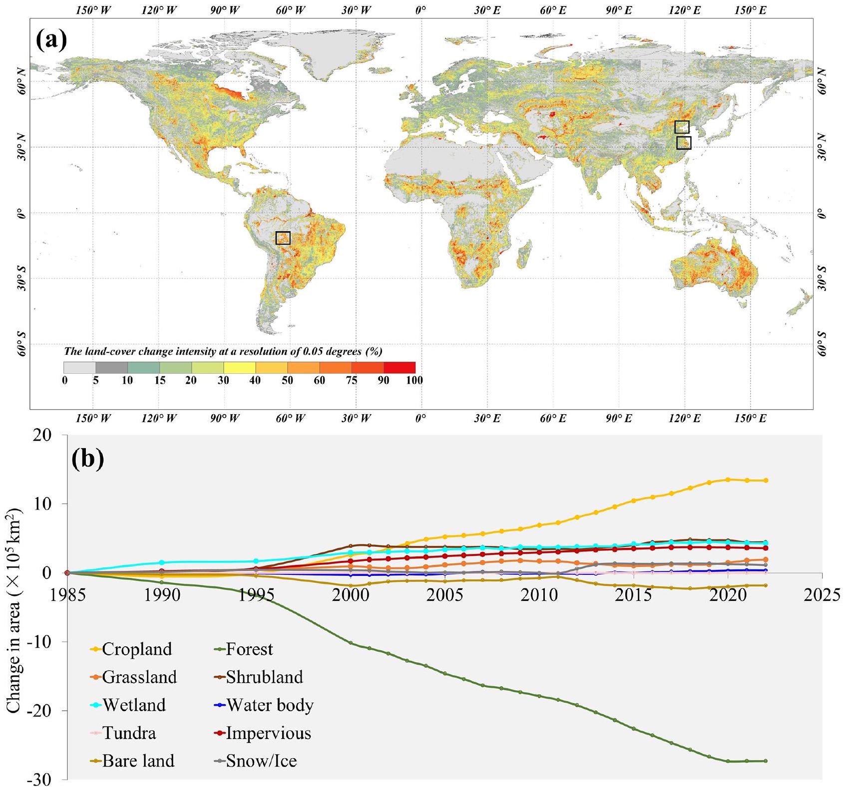
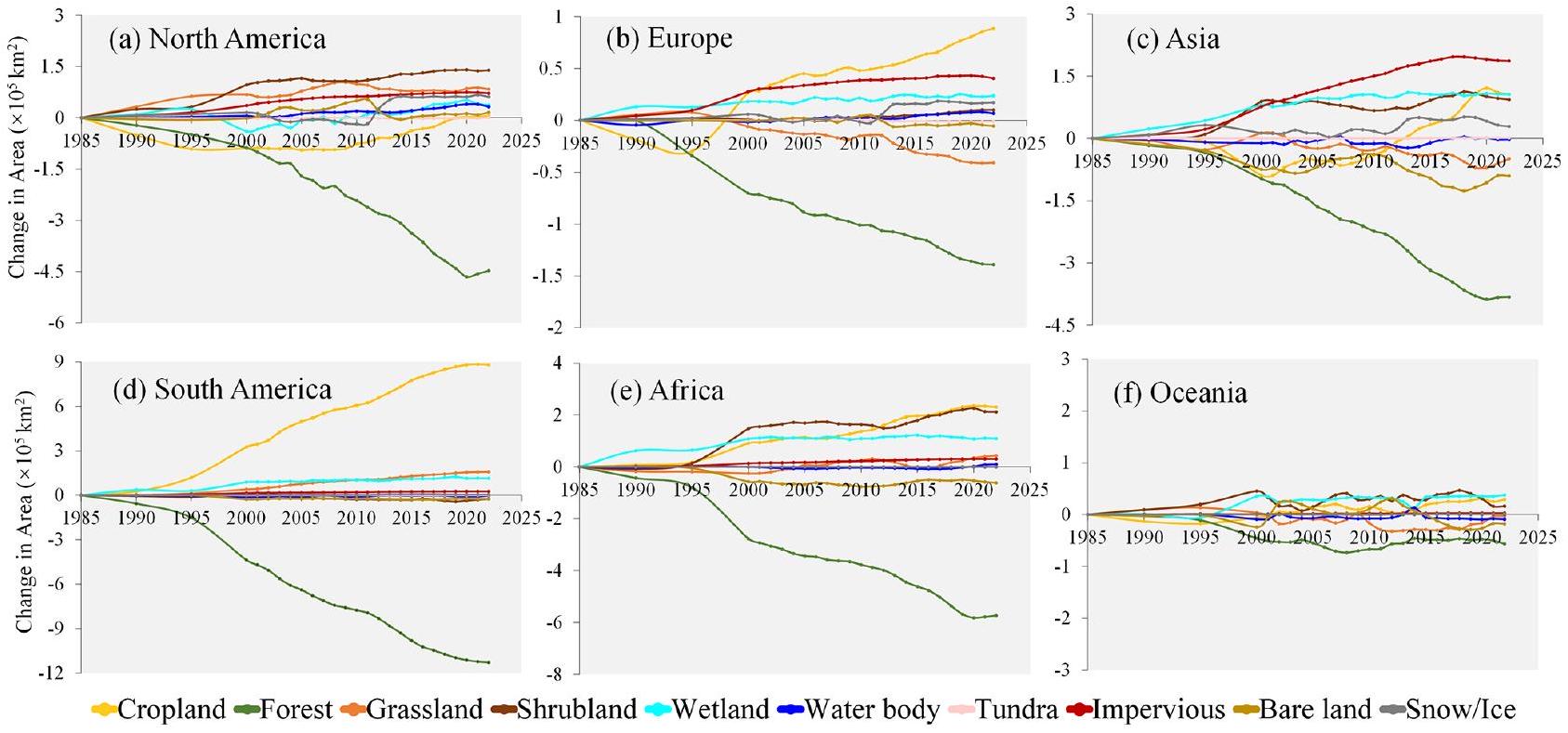
الأراضي الشجرية، وتغيرات السطح غير النفاذ، التي تهيمن على تغييرات تغطية الأرض في الشكل 5. هناك ثلاثة أسباب رئيسية لفقدان الغابات على مدى السنوات السبع والثلاثين الماضية: (1) تم تحويل جزء من الأراضي التي تم إزالة الغابات منها إلى أراضي زراعية (كان هذا التحول أكثر وضوحًا في مناطق الغابات الاستوائية؛ الشكل 8أ)؛ (2) تمت إعادة زراعة الغابة المفقودة كأرض شجيرات، وهو ما هو أكثر شيوعًا في المناطق الجبلية المتأثرة بالحرائق البرية؛ و (3) تم تحويل جزء من الأراضي التي تم إزالة الغابات منها إلى أراضٍ عشبية. يتم تحويل الأراضي الزراعية إلى غابات وأراضٍ عشبية وسطح غير نفاذ. المجموع هو تم تحويل جزء من الأراضي الزراعية المفقودة إلى أراضٍ عشبية بسبب التخلي عنها، من الأراضي الزراعية المفقودة مغطاة بالغابات، و فقدان الأراضي الزراعية الناتج عن التحضر. أخيرًا، فيما يتعلق بالأسطح غير النفاذة، كان تركيزنا الأساسي على تحديد المصادر التي تسهم في توسعها. تشير نتائجنا إلى أن حوالي يمكن أن يُعزى زيادة السطح غير النفاذ إلى تحويل الأراضي الزراعية، بينما الزيادة ناتجة عن إزالة الغابات.
لفهم عملية تغيير تغطية الأرض بصريًا كما تم التقاطها بواسطة مجموعة بيانات GLC_FCS30D على مدى السنوات السبع والثلاثين الماضية، تعرض الشكل 8 ثلاثة تكبيرات نموذجية (الموقع المكاني-
الشكل 5. (أ) التوزيع المكاني لشدة تغيير غطاء الأرض العالمي من 1985 إلى 2022 بعد التجميع إلى دقة . (ب) المساحة الصافية المتغيرة لـ 10 أنواع رئيسية من تغطية الأرض في GLC_FCS30D من 1985 إلى 2022.
تم توضيح المناطق المتضخمة كأربعة مستطيلات سوداء في الشكل 5 أ) من غابة الأمازون المطيرة (التي شهدت إزالة كبيرة للغابات) ودلتا نهر اليانغتسي في الصين (التي شهدت تحضرًا سريعًا) ودلتا نهر الأصفر (التي أظهرت تغييرات واضحة في تغطية الأراضي على المناطق الساحلية). شهدت هذه المناطق الثلاثة النموذجية تغييرات جذرية في تغطية الأراضي، وGLC_FCS30D يلتقط بدقة تلك التغييرات المكانية والزمانية. على وجه التحديد، فإن إزالة الغابات في أمريكا الجنوبية معروفة على نطاق واسع، وGLC_FCS30D يعكس بوضوح هذا الاتجاه. بمعنى آخر، أظهرت إزالة الغابات المبكرة توزيعًا شبكيًا، ثم امتد كل شبكة تدريجيًا إلى الخارج وأخيرًا اتصلت ببعضها لتشكل بقعًا.
تظهر بيانات GLC_FCS30D أيضًا أن إزالة الغابات لم تتوقف في المنطقة من حيث معدل فقدان الغابات، وهذه النتائج تتماشى مع نتائج الأبحاث السابقة (هاريس وآخرون، 2021؛ بوتابوف وآخرون، 2022). في دلتا نهر اليانغتسي، توضح بيانات GLC_FCS30D أن التغيير السائد في استخدام الأراضي خلال التوسع هو التحضر، وقد تم تحويل كمية كبيرة من الأراضي الزراعية المروية إلى أسطح غير نفاذة. في الوقت نفسه، كان التوسع الحضري أسرع بكثير قبل عام 2010 مقارنةً بعد عام 2010 وفقًا لبيانات GLC_FCS30D. أخيرًا، تم اختيار دلتا نهر الأصفر، وهي منطقة ساحلية نموذجية، لتقييم قدرة GLC_FCS30D على التقاط هذه التغيرات في استخدام الأراضي الساحلية. من الواضح أن التغيرات في استخدام الأراضي في
الشكل 6. التغيرات في المساحة الصافية لـ 10 أنواع رئيسية من تغطية الأرض في ست قارات من 1985 إلى 2022.
الشكل 7. مخططات سانكي للتغيرات في تغطية الأرض العالمية خلال الفترة من 1985 إلى 2022 في مجموعة بيانات GLC_FCS30D.
يمكن تلخيص GLC_FCS30D في ثلاثة جوانب: (1) تم استصلاح عدد كبير من الأراضي المنخفضة والمسطحات المدية كبرك لتربية الأحياء المائية، خاصة بعد عام 2000؛ (2) تغير مصب نهر هوانغ من اتجاه جنوبي إلى اتجاه شمالي (مستطيل أسود)، أي أنه كانت هناك تغييرات كبيرة في تغطية الأرض بين المسطحات المدية/المغمورة، والمسطحات المائية، والأراضي المالحة؛ و(3) اقتحمت العديد من الأسطح غير النفاذة المسطحات المائية والسواحل. باختصار، من خلال دمج بيانات سلسلة زمنية حقيقية للمراقبة عن بُعد، يلتقط GLC_FCS30D بفعالية التغيرات المكانية والزمانية لسطح الأرض.

4.2 تقييم دقة GLC_FCS30D لعام 2020

يوفر الجدول 2 مصفوفة الأخطاء ومقاييس الدقة لمجموعة بيانات GLC_FCS30D في نظام التصنيف الأساسي.
تحتوي على 10 أنواع رئيسية من تغطية الأرض. حقق مجموعة بيانات GLC_FCS30D الجديدة دقة عامة تبلغ تؤدي الأراضي الزراعية والغابات والأسطح غير المنفذة ومسطحات المياه والثلوج والجليد الدائم بشكل أفضل من حيث الدقة النسبية والدقة العامة مقارنة بأنواع تغطية الأرض الأخرى، حيث تتجاوز الدقة المقابلة تم إنشاء مجموعات بيانات الأسطح غير المنفذة والأراضي الرطبة بشكل مستقل ثم تم تراكبها على GLC_FCS30D، مما يساعد هذه الأنواع المعقدة من تغطية الأرض على تحقيق مقاييس دقة عالية. على العكس من ذلك، فإن الأراضي العشبية، والأراضي الشجرية، والتندرا لديها دقة أقل؛ على سبيل المثال، كانت الأراضي العشبية لديها أدنى نسبة دقة. وكانت الأراضي الشجرية لديها أقل نسبة من U.A. السببين اللذين أديا إلى أدائهم الضعيف كانا كما يلي: (1) عادةً ما تعكس هذه الأنواع من تغطية الأرض خصائص طيفية ومكانية غير متجانسة ومتنوعة، على سبيل المثال، أظهرت الأراضي العشبية طيفًا مشابهًا للأراضي الزراعية والأراضي الشجرية المتناثرة في موسم النمو ولكن
الشكل 8. ثلاث تكبيرات نموذجية تظهر تغييرات تغطية الأرض وفقًا لـ GLC_FCS30D من 1985 إلى 2022 في (أ) غابة الأمازون المطيرة، (ب) دلتا نهر اليانغتسي في الصين، و(ج) دلتا نهر الأصفر في الصين. ترميز الألوان هو نفسه المستخدم في الخريطة العالمية في الشكل 4. في كل حالة، تم أخذ الصور الطبيعية من 1985 إلى 2022 من صور لاندسات.
قلدت ميزات الأراضي العارية في موسم الحصاد، و(2) تم توزيعها جميعًا في مناطق انتقال المناخ ذات التغيرات المناخية المعقدة والمناظر الطبيعية.
يوفر الجدول 3 مصفوفة الخطأ لـ GLC_FCS30D لعام 2020 في نظام التحقق من المستوى الأول LCCS مع 17 نوعًا من تغطية الأرض. يحقق مجموعة بيانات GLC_FCS30D-2020 O.A. من ، وهو أقل من ذلك الذي تم تحقيقه باستخدام نظام التصنيف الأساسي لأن هذه الفئات الفرعية المتشابهة من تغطية الأرض تعاني أكثر من غيرها من سوء التصنيف. على سبيل المثال، الغابة لديها نسبة دقة تبلغ 92.83 % ، لكن الضغط الجوي ينخفض بسرعة إلى نطاق
إلى عندما يتم تقسيم الغابة إلى خمس فئات فرعية دقيقة. تُظهر الأراضي الزراعية والغابات والأراضي العارية، التي تُقسم بدورها إلى عدة فئات فرعية، انخفاضًا واضحًا في الدقة لفئاتها الفرعية من حيث P.A. و U.A. مع أخذ الأراضي الزراعية والغابات كمثال، تقريبًا من الأراضي الزراعية المروية (ICP) تم تصنيفها بشكل خاطئ كأراضي زراعية معتمدة على الأمطار (RCP)، وبالتالي فإن المساحة المستخدمة من ICP هي فقط أكثر من تُصنَّف الغابات ذات الأوراق المختلطة (MFT) بشكل خاطئ كأحد الفئات الفرعية الأربعة الأخرى، وبالتالي فإن ‘الغابات ذات الأوراق المختلطة’ لديها أقل U.A. في هذه الأثناء، الغطاء النباتي المتناثر
) 6 و 6 (9 I) (で I) 969 L (II.I) 89 I9 )S0.99 ) )
t6 II س ISZ إي LL8* [W]OL
أنا ) أنا ISE أنا 0 100.0 EZ0.0 0 س00.0 t00\% 0 ISd
(8.0)S* 6 L 829*II IEI*0 6EZ6 8 إلى 0 LLS* 0 ست0.0 Et0.0 S8S* 0 E8L0 6500 تي في جي
(19*0)القديس S6 E8Z’S 0 tZ0* ٢٠٠٠ 9000 100.0 ت0.0 tZ0.0 8S0.0 سبعة وثمانون دوي
) تست إي ز00\٪ vtt؟ ٨١٠.٠ L91.0 8910 EZI•0 10.0 ج
زي أنا إنترنت إكسبلورر 8 ٢٠٠٠ 6E0*0 ZI0\% ٨٠٠.٠ S0E إي て0E 0 6100 9800 ت0.0 yLM
أنا ) 9IS’S تيتي دي 0 IZ0.0 ل E0.0 LSI•0 9 SI*0 اس9+ 0 لام
9 SE 6 ٢٠٠٠ ز0س*0 ص0.0 6100 I9I*0 Z6E E98* SSS.0 YHS
هو SS8.0I L8I'I LS0.0 t80.0 ١١٠٠ IEZ 0 I8I*I 906 س 99I'I SE0.I SHD
(IE*0)E8*Z6 ز00\٪ EII*0 ٨٠٠.٠ IZ0.0 ILE 0 II8.0 SIE゙0 زيل•8 EIS゙0 LSA
) t0ピLI 0 LII*0 tLI•0 0 ل20\٪ Z6L*0 ز نعم дY( 3
(AS) V د [ண口 ISd تلفازЯ دوي ج YLM لام أون إس سيد LSA دو әวแวเอมิy
(\٪LZ ) دو
I’m sorry, but the text you provided does not appear to be in a recognizable language or format for translation. Please provide a clear text for translation.
الشكل 9. سلسلة زمنية للدقة العامة لمجموعة بيانات GLC_FCS30D باستخدام مجموعة بيانات المرجع السنوي LCMAP_Val عبر الولايات المتحدة المتجاورة (CONUS) من 1985 إلى 2018. تظهر أشرطة الخطأ على الرسم البياني عدم اليقين في نقاط البيانات.
لديه ثاني أدنى معدل U.A. بسبب الارتباك بين الغطاء النباتي المتناثر، والمراعي، والأراضي العارية. في نظام التصنيف الأساسي (الجدول 1)، يتم تصنيف الغطاء النباتي المتناثر مع الأراضي العارية. اقترحت دراسة سابقة في الاتحاد الأوروبي تصنيفه مع المراعي (جاو وآخرون، 2020). يتم تقسيم الأراضي الرطبة بشكل أكبر إلى أراضي رطبة ساحلية (CWL) وأراضي رطبة داخلية (IWL) في الجدول 3، ولدى CWL U.A. أعلى من تلك الخاصة بالأراضي الرطبة في الجدول 2، وهو ما يُعزى بشكل أساسي إلى التصنيف الأكثر دقة بشكل ملحوظ للأراضي الرطبة في فئة CWL الفرعية (تشانغ وآخرون، 2023).

4.3 تقييم الدقة استنادًا إلى مجموعتي بيانات التحقق الإقليمي من طرف ثالث

4.3.1 سلسلة زمنية لمقاييس الدقة لـ GLC_FCS30D من مجموعة بيانات LCMAP_Val

تظهر الشكل 9 سلسلة زمنية للدقة العامة لمجموعة بيانات GLC_FCS30D باستخدام مجموعة بيانات التحقق السنوي LCMAP_Val من 1985 إلى 2018 على منطقة الولايات المتحدة المتجاورة. تحقق GLC_FCS30D متوسط دقة عامة قدره وتتفاوت القيمة O.A من قيمة عالية في عام 2015 إلى قيمة منخفضة من في عام 2000. كانت الدقة العامة لجهاز GLC_FCS30D أقل قليلاً في المرحلة المبكرة، وهو ما قد يكون مرتبطًا بكثافة ملاحظات لاندسات. كانت المهام المبكرة لاندسات تتمتع بقدرات أضعف في نقل البيانات من الأقمار الصناعية إلى الأرض والتسجيل على متنها (روي وآخرون، 2014أ)، لذا كانت التغيرات الفينولوجية وتغيرات تغطية الأرض أكثر صعوبة في الالتقاط في المرحلة المبكرة.
تظهر الشكل 10 السلاسل الزمنية لـ P.A. و U.A. لمجموعة بيانات GLC_FCS30D في CONUS. بصريًا، تتراوح قيم P.A. و U.A. لأنواع الغطاء الأرضي العشرة الرئيسية من إلى ومن إلى على التوالي، و
الجدول 3. مصفوفة الخطأ لمجموعة بيانات GLC_FCS30D لعام 2020 بناءً على نظام التحقق من صحة LCCS المستوى 1. تأتي دقة المنتج المبلغ عنها (P.A.) ودقة المستخدم (U.A.) مع الأخطاء المعيارية المقابلة (SE) الموضحة بين قوسين.
مرجع RCP ICP EBF DBF إنف لم يُنهَ MFT SHR جي آر إس نظام إدارة التعلم SVG إي دبليو إل CWL IMP بال WTR PSI إجمالي مساعد شخصي (SE)
RCP ١٢.٢٢٥ 1.023 0.239 0.358 0.102 0.016 0.009 0.382 0.66 0 0.078 0.056 0.005 0.124 0.028 0.001 0 15.332 79.7 (0.7)
ICP 0.397 1.932 0.026 0.016 0.005 0 0 0.01 0.025 0 0.012 0.029 0.005 0.052 0 0.018 0 ٢.٥٢٧ ٧٦.٤٥ (١.٨١)
EBF 0.2 0.048 9.091 1.098 0.262 0.103 0.151 0.371 0.084 0 0.012 0.136 0.028 0.029 0.001 0.004 0 ١١.٥١٤ 78.96 (0.82)
DBF 0.187 0.016 0.632 6.838 0.537 0.294 0.396 0.235 0.144 0.002 0.019 0.077 0.002 0.025 0.005 0.004 0.002 9.054 75.53 (0.97)
ENF 0.046 0.004 0.174 0.316 5.681 0.328 0.٤٣٩ 0.128 0.034 0.006 0.043 0.094 0 0.008 0.01 0.01 0 6.895 82.39 (0.98)
لم يُنهَ 0.008 0 0.002 0.13 0.245 1.854 0.073 0.071 0.053 0 0.011 0.025 0 0.001 0.007 0.002 0 2.414 76.79 (1.85)
MFT 0.004 0 0.019 0.176 0.234 0.013 0.828 0.014 0.004 0 0 0.010 0.05 0 0.001 0 0 1.308 ٥٨٫٢٩ (١٫٥٣)
SHR 0.518 0.042 0.299 0.9 0.328 0.131 0.034 ٥.٤٤ 0.871 0.019 0.441 0.157 0.005 0.05 0.065 0.013 0.002 9.438 57.63 (1.09)
جي آر إس 0.947 0.097 0.167 0.582 0.209 0.154 0.024 1.191 ٥.٩٥٨ 0.085 0.974 0.229 0.006 0.052 0.217 0.008 0.01 10.95 54.41 (1.02)
نظام إدارة التعلم 0.006 0.004 0.001 0.022 0.044 0.053 0.001 0.168 0.169 ٢.٤٦٥ 0.379 0.02 0.001 0.002 0.098 0.026 0.02 ٣.٤٨٤ 70.76 (1.65)
SVG 0.064 0.01 0.008 0.006 0.007 0.01 0.001 0.397 0.462 0.025 2.71 0.012 0 0.013 0.643 0.002 0.024 ٤.٣٩٩ 61.6 (1.57)
إي دبليو إل 0.01 0.002 0.044 0.029 0.١٠٣ 0.022 0.002 0.048 0.017 0.008 0.042 2.673 0.024 0.001 0.012 0.224 0 ٣.٢٦٣ 81.91 (1.45)
CWL 0.004 0.002 0.008 0.002 0.004 0.002 0.004 0.008 0.006 0 0.008 0.188 1.476 0.007 0.007 0.059 0 1.783 82.77 (1.92)
IMP 0.074 0.011 0.008 0.008 0.037 0.002 0 0.041 0.024 0.002 0.014 0.004 0 ٥.٠٨٧ 0.01 0.004 0 5.329 95.45 (0.61)
بال 0.048 0.01 0.002 0.004 0.002 0.001 0 0.193 0.328 0.557 0.582 0.043 0.002 0.035 ٥.٣٨٤ 0.029 0.108 7.33 73.45 (1.11)
WTR 0.014 0.024 0.014 0.014 0.019 0.008 0.006 0.011 0.016 0.007 0.011 0.168 0.114 0.011 0.019 ٣.٠٥٤ 0.002 ٣.٥٠٩ ٨٧.٠٤ (١.٢٢)
PSI 0 0 0 0.001 0.002 0 0 0.005 0.03 0.001 0.011 0 0 0 0.019 0.023 1.363 1.455 93.65 (1.37)
إجمالي 14.757 ٣.٢٢٤ 10.753 10.56 ٧.٨٣٣ ٣.٧٢٤ 1.97 8.711 8.883 3.179 ٥.٣٥٣ ٣.٩٢٧ 1.668 ٥.٤٩٧ ٦.٥٢٦ ٣.٤٨٢ 1.532
الإمارات العربية المتحدة (جنوب شرق) 82.85 (0.67) ٥٩.٩٢ (١.٨٥) ٨٤.٥٥ (١.٧٥) 64.76 (1) 72.52 (1.08) ٤٩.٧٧ (١.٧٦) ٣٩٫٣٤ (١٫٣٨) 62.44 (1.11) 67.07 (1.07) 77.55 (1.59) 50.63 (1.47) 68.07 (1.6) ٨٨.٤٩ (١.٦٨) ٩٢.٥٤ (٠.٧٦) 82.5 (1.01) 87.73 (1.19) ٨٨.٩٦ (١.٧٢)
أ.ع. 73.04 % %)
ملاحظة: الاختصارات تتوافق مع الفئات السبع عشرة لنظام التحقق من LCCS في الجدول 1.
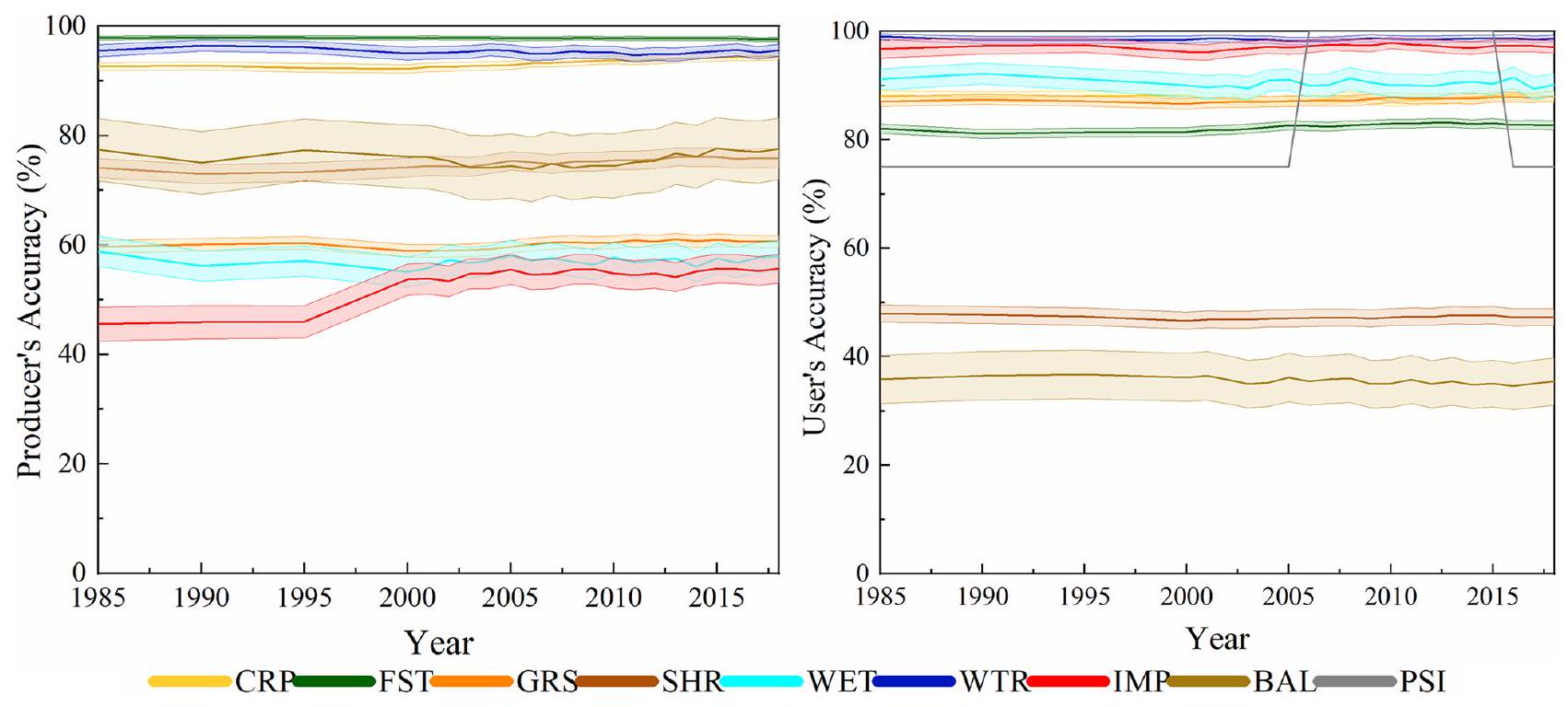
تكون التغيرات الزمنية مستقرة. من بينها، نوع تغطية الأرض للمسطحات المائية لديه أعلى مقاييس دقة، حيث حقق قيم P.A. و U.A. المتوسطة من و على التوالي، والتي تستفيد من الخصائص الطيفية الفريدة لهذا النوع من تغطية الأرض. يليها الأراضي الزراعية، مع قيم P.A. و U.A. المتوسطة بنسبة 93.37 % و على التوالي. تحتل الغابة المرتبة الثالثة، مع درجة P.A. عالية من لكن نسبة U.A. منخفضة نسبيًا ؛ تحدث المقاييس غير المتوازنة لأن GLC_FCS30D و LCMAP_Val لديهما تعريفات مختلفة للغابة. يعرف GLC_FCS30D الغابة بأنها تحتوي على تغطية شجرية أكبر من بينما إعداد عتبة LCMAP_Val هو لذلك، تم تصنيف العديد من الأراضي الشجرية في GLC_FCS30D كغابات في LCMAP_Val. تحتوي الأراضي الرطبة على قيمة U.A. تبلغ 90.47 % ) ولكن قيمة P.A. ، والذي يحدث أيضًا بسبب اختلاف في تعريف الأراضي الرطبة. يحدد GLC_FCS30D المسطحات المائية الموسمية كأراض رطبة بينما يصنف LCMAP_Val هذه المسطحات كمسطحات مائية. السطح غير النفاذ له قيمة P.A. أقل من ، ويرجع ذلك أساسًا إلى أن مجموعتي بيانات GLC_FCS30D و LCMAP_Val لديهما تعريفات مختلفة للسطح غير النفاذ. تعرف LCMAP_Val المباني والمناطق الخضراء المحيطة بها على أنها مطورة، بينما تشمل GLC_FCS30D فقط المباني الاصطناعية (المنازل، الطرق، الساحات، وما إلى ذلك). تمتلك الأراضي العارية والأراضي الشجرية أدنى قيم U.A. و ، على التوالي، principalmente porque كلاهما يمكن أن يُخلط بسهولة مع المراعي بسبب خصائصهما الطيفية المعقدة ولأنهما يتواجدان معًا في مناطق شبه جافة حساسة للمناخ (مثل الغرب الأوسط للولايات المتحدة). وأكد شيان وآخرون (2022) أن المراقبة طويلة الأمد للشجيرات والمراعي تمثل تحديات كبيرة في الولايات المتحدة المتجاورة. الثلوج والجليد الدائم، الذي يتوزع بشكل نادر في المناطق الجبلية ذات الارتفاع العالي في الولايات المتحدة، له خصائص طيفية فريدة ومحددة، لذا فإنه يحقق نسبة في GLC_FCS30D. تُعزى التقلبات الكبيرة في U.A. للثلج والجليد إلى (1) حجم العينة الصغيرة للثلج والجليد في مجموعة بيانات LCMAP_Val و(2) بعض بكسلات العشب/الأرض العارية التي تم تصنيفها بشكل خاطئ والتي تم التعرف عليها بشكل صحيح على أنها ثلج وجليد خلال الفترة من 2005 إلى 2014.
تظهر الشكل 11 نسب الانحياز حسب المساحة لثمانية أنواع من تغطية الأرض المقدرة بواسطة GLC_FCS30D و LCMAP_Val عبر الولايات المتحدة القارية. بشكل بديهي، تشترك GLC_FCS30D و LCMAP_Val في مساحات إجمالية مماثلة لتقديرات الأراضي الزراعية، والأراضي العارية، والمسطحات المائية، ولكن هناك انحرافات واضحة في تقديرات الغابات، والأراضي الشجرية، والمراعي. تحدث الانحرافات في الأراضي الشجرية والمراعي بشكل رئيسي لأن هذه الأنواع من تغطية الأرض تتواجد معًا في المناطق شبه الجافة في وسط الولايات المتحدة وتشارك في خصائص طيفية ومرونة زمنية مماثلة؛ وبالتالي، تعتبر بعض المراعي في LCMAP_Val أراضي شجرية في GLC_FCS30D. كما فشل شيان وآخرون (2022) في تمييز المراعي عن الأراضي الشجرية ودمجوها في مجموعة واحدة عند إنشاء خرائط LCMAP السنوية. لدى LCMAP_Val تعريف أوسع للسطح غير النفاذ، مما يؤدي إلى انحياز سلبي، لذا
تقدير مساحة السطح غير النفاذ في LCMAP_Val أكبر من التقييم في مجموعة بيانات GLC_FCS30D.
الجدول 4 يحلل مصفوفة الالتباس لبيكسلات الغطاء الأرضي المتغير وغير المتغير في GLC_FCS30D باستخدام مجموعة بيانات LCMAP_Val. يجب ملاحظة أن عينات الغطاء الأرضي المتغيرة في LCMAP_Val كانت لا تزال نادرة؛ أي أن حجم العينات المتغيرة لا يمكن أن يدعم تحليل تغييرات الغطاء الأرضي المحددة. وبالمثل، قام ستيمان وآخرون (2021) بتجميع أنواع الغطاء الأرضي إلى نوعين “لا تغيير” و”تغيير” لتحليل تغييرات الغطاء الأرضي. في هذه الدراسة، عند استخدام نقاط التحقق “المتغيرة” و”غير المتغيرة” في LCMAP_Val، وصلت O.A. لـ GLC_FCS30D إلى . على وجه الخصوص، لعبت بكسلات تغطية الأرض غير المتغيرة دورًا رئيسيًا وحققت نسبة عالية من ومعدل U.A. مرتفع . بالمقابل، كانت P.A. و U.A. لبيكسلات تغطية الأرض المتغيرة و وكانت درجة F1 63.49%.

4.3.2 سلسلة زمنية لمقاييس الدقة لـ GLC_FCS30D من مجموعة بيانات LUCAS

توضح الجدول 5 سلسلة زمنية لمقاييس الدقة لمجموعة بيانات GLC_FCS30D عبر الاتحاد الأوروبي (EU) من 2006 إلى 2018 باستخدام مجموعة بيانات LUCAS. تحتوي مجموعة بيانات GLC_FCS30D على متوسط دقة O.A. ونطاق O.A. من إلى في الاتحاد الأوروبي. نوعا الغطاء الأرضي السائدين (الأراضي الزراعية والغابات)، اللذان يغطيان تقريبًا منطقة الاتحاد الأوروبي بأكملها (جاو وآخرون، 2020)، لديها قيم أعلى من P.A. و U.A. مقارنة بأنواع تغطية الأرض الأخرى. تتجاوز قيم P.A. و U.A. للأراضي الزراعية و ، على التوالي. الغابة لديها نسبة غير متوازنة. ) و U.A. ( تقريباً القيم) لأن مجموعة بيانات LUCAS تعرف الغابة بشكل أوسع من مجموعة بيانات GLC_FCS30D. على وجه الخصوص، يتم تجميع الغطاء النباتي النادر المرتبط بالغابة مع الغابة في LUCAS ولكن مع الأراضي العارية في GLC_FCS30D. أوضح غاو وآخرون (2020) التباين في تعريف الغابة بين LUCAS وGLC_FCS30. أظهرت الأراضي الشجرية، والأراضي العشبية، والأراضي العارية أداءً أقل من حيث كل من P.A. وU.A. بسبب تعقيد تباينها الطيفي وتنوعها المكاني. كما وجد غاو وآخرون (2020) أن ثلاثة منتجات عالمية لتغطية الأراضي بمقياس 30 مترًا (GlobeLand30، FROM_GLC، وGLC_FCS30) أظهرت أداءً ضعيفًا لهذه الأنواع الثلاثة من تغطية الأراضي. المساحات الخضراء الحضرية والنسيج الحضري المتقطع، التي تم استبعادها من GLC_FCS30D، يتم تجميعها مع السطح غير النفاذ في LUCAS. وبالتالي، فإن السطح غير النفاذ أيضًا لديه P.A. منخفض يبلغ حوالي أخيرًا، عند التحقيق في التغير الزمني لـ P.A. و U.A. نجد أن الجليد الدائم والثلوج والأراضي الرطبة تظهر تباينًا أكبر وأن كلاهما مرتبط ارتباطًا وثيقًا بدرجات الحرارة السنوية وهطول الأمطار؛ أي أن توزيعاتها المكانية تتأثر بالبيئة الطبيعية.
الشكل 10. سلسلة زمنية لدقة المنتج ودقة المستخدم لـ GLC_FCS30D استنادًا إلى مجموعة بيانات LCMAP_Val من 1985 إلى 2018 في الولايات المتحدة المتجاورة (CONUS). تمثل نطاقات الخطأ خطأ قياسي.
الشكل 11. نسب التحيز حسب المساحة لثمانية أنواع من تغطية الأرض في مجموعتي بيانات GLC_FCS30D و LCMAP_Val من عام 1985 إلى 2017 في الولايات المتحدة المتجاورة (CONUS).
يوضح الجدول 6 نسب المساحات لأنواع الغطاء الأرضي العشرة الرئيسية من كل من مجموعة بيانات GLC_FCS30D (“الخريطة”) ومجموعة بيانات التحقق LUCAS (“المرجع”). يقيس انحياز المساحة (“AB”) انحرافات المساحة بين مجموعتي البيانات المختلفتين لنفس نوع الغطاء الأرضي. بشكل عام، يبالغ GLC_FCS30D في تقدير التقييمات الإجمالية لمساحات الغابات والأراضي القاحلة والجليد والثلج ويقلل من تقدير…
أنواع الغطاء الأرضي الرئيسية مقارنة بتقديرات LUCAS. على وجه الخصوص، وفقًا لـ AB الخاصة به تظهر الغابات أكبر تقدير مفرط، بينما تظهر الأراضي الزراعية أكبر تقدير ناقص (AB من تغطي الأراضي الزراعية والغابات معًا حوالي من إجمالي مساحة الاتحاد الأوروبي (جاو وآخرون، 2020)؛ ونتيجة لذلك، فإن قيم انحياز المساحة (AB) لهذه النوعين من تغطية الأرض هي
الجدول 4. مصفوفة الالتباس للبكسلات المتغيرة وغير المتغيرة في GLC_FCS30D عند استخدام مجموعات بيانات LCMAP_Val.
غير متغير تغير إجمالي مساعد شخصي (SE) فورمولا 1
غير متغير 82.21 6.34 ٨٨.٥٥ 94.53
تغير 3.18 8.27 11.45 63.49
إجمالي ٨٥.٣٩ 14.61
الإمارات العربية المتحدة (جنوب شرق)
أ.ع. (س.إ)
الجدول 5. سلسلة زمنية لمقاييس الدقة لمجموعة بيانات GLC_FCS30D باستخدام مجموعة بيانات التحقق LUCAS عبر الاتحاد الأوروبي.
2006 2009 2012 2015 2018
مساعد شخصي (جنوب شرق) الإمارات العربية المتحدة (جنوب شرق) مساعد شخصي (جنوب شرق) الإمارات العربية المتحدة (الجنوبية الشرقية) مساعد شخصي (SE) الإمارات العربية المتحدة (الجنوبية الشرقية) مساعد شخصي (جنوب شرق) الإمارات العربية المتحدة (جنوب شرق) مساعد شخصي (SE) الإمارات العربية المتحدة (جنوب شرق)
CRP 85.49 (0.11) 93.37 (0.08) 85.40 (0.11) 93.31 (0.08) 85.50 (0.11) 93.17 (0.08) 85.47 (0.11) 93.05 (0.08) 85.52 (0.11) 92.82 (0.08)
FST 95.22 (0.08) 76.71 (0.15) 94.97 (0.08) 76.71 (0.15) 94.79 (0.09) 76.82 (0.15) 94.36 (0.09) 76.82 (0.15) 93.71 (0.09) 76.85 (0.15)
جي آر إس 6.13 (0.26) ٢١.٣١ (٠.٨٣) 6.10 (0.26) ٢١.١٣ (٠.٨٣) 6.05 (0.26) 20.98 (0.83) 6.08 (0.26) 20.71 (0.82) 5.99 (0.26) 20.74 (0.82)
SHR 8.13 (0.42) 8.93 (0.46) 8.25 (0.43) 8.92 (0.46) 8.02 (0.42) 8.77 (0.46) 7.84 (0.42) 8.60 (0.45) 8.35 (0.43) 8.96 (0.46)
رطب 63.10 (0.81) 66.55 (0.81) 61.40 (0.81) 65.55 (0.82) 61.86 (0.81) 66.21 (0.82) 62.64 (0.81) 66.60 (0.81) 62.94 (0.81) 65.34 (0.81)
WTR 89.73 (0.40) ٩٢.٤٤ (٠.٣٦) 90.09 (0.40) 92.53 (0.35) 90.28 (0.39) 92.36 (0.36) 90.83 (0.38) 91.63 (0.37) 90.10 (0.40) 91.56 (0.37)
IMP ٥٨.٥٥ (٠.٥٦) 72.69 (0.56) ٥٩.٢١ (٠.٥٥) 72.06 (0.56) ٥٩.٠٦ (٠.٥٥) 71.72 (0.56) 58.65 (0.55) 70.85 (0.56) ٥٩.٠١ (٠.٥٥) 70.29 (0.56)
بال 52.77 (1.12) ٣٩.٦٢ (٠.٩٥) 52.90 (1.12) ٣٨.٤٤ (٠.٩٣) ٥٢.١٩ (١.١٣) ٣٧.٧٠ (٠.٩٣) ٥٢.٠٧ (١.١٣) ٣٦.١٦ (٠.٩٠) ٥٢.٣٣ (١.١٣) ٣٤.٦٩ (٠.٨٧)
PSI ٨٦٫٠٢ (٥٫٠٠) ٣٥.٠١ (٤.٣٨) 91.40 (4.04) ٣٦.٥٦ (٤.٣٨) ٨٩.٢٥ (٤.٤٦) 31.86 (4.00) ٩٦.٢٤ (٢.٧٤) ٣١.٤٠ (٣.٨١) ٩٦.٢٤ (٢.٧٤) ٣١.٣٥ (٣.٨١)
أ.ع. (س.إ) 82.11 (0.09) 81.99 (0.09) 81.97 (0.09) 81.82 (0.09) 81.64 (0.09)
أكثر وضوحًا أو بروزًا مقارنة بقيم AB لأنواع تغطية الأرض الأخرى.
تقدم الجدول 7 مصفوفة الالتباس للبكسلات المتغيرة وغير المتغيرة التي تم الحصول عليها باستخدام مجموعات بيانات التحقق LUCAS. وصلت النسبة العامة للدقة (O.A.) لـ GLC_FCS30D إلى ; كانت P.A. و U.A. للبكسلات المتغيرة و على التوالي؛ وكانت درجة F1 المقابلة هي . على النقيض من ذلك، وصلت بكسلات تغطية الأرض غير المتغيرة إلى قيم عالية من P.A. و U.A.، حيث تجاوزت كلا المقياسين . وبالتالي، كانت بكسلات تغطية الأرض المتغيرة أكثر صعوبة في الالتقاط مقارنةً بهذه البكسلات غير المتغيرة. وبالمثل، وجد ستيمان وآخرون (2021) أيضًا أن مقاييس الدقة للبكسلات المتغيرة كانت أقل بكثير من تلك الخاصة بالبكسلات غير المتغيرة: كانت دقة المنتج للبكسلات المتغيرة وغير المتغيرة و ، على التوالي.

4.4 مقارنات مع منتجات ديناميات تغطية الأرض العالمية الأخرى

تقدم الشكل 12 مقارنات نوعية بين بيانات GLC_FCS30D واثنين من مجموعات بيانات ديناميات تغطية الأرض المستخدمة على نطاق واسع (CCI_LC وMCD12Q1) للفترة من 2001 إلى 2020 في شبه جزيرة الهند الصينية، التي شهدت تغييرات واضحة في تغطية الأرض من حيث إزالة الغابات والتوسع الحضري خلال تلك الفترة. فيما يتعلق بالتوسع الحضري، كشفت المجموعات الثلاث عن تحضر سريع في مدينة بانكوك الكبرى، بينما كانت بيانات CCI_LC تقلل من تقدير مساحة السطح غير النفاذ في عام 2001 مقارنة بالمجموعتين الأخريين. في الوقت نفسه، التقطت بيانات GLC_FCS30D أيضًا مزيدًا من التفاصيل المكانية.
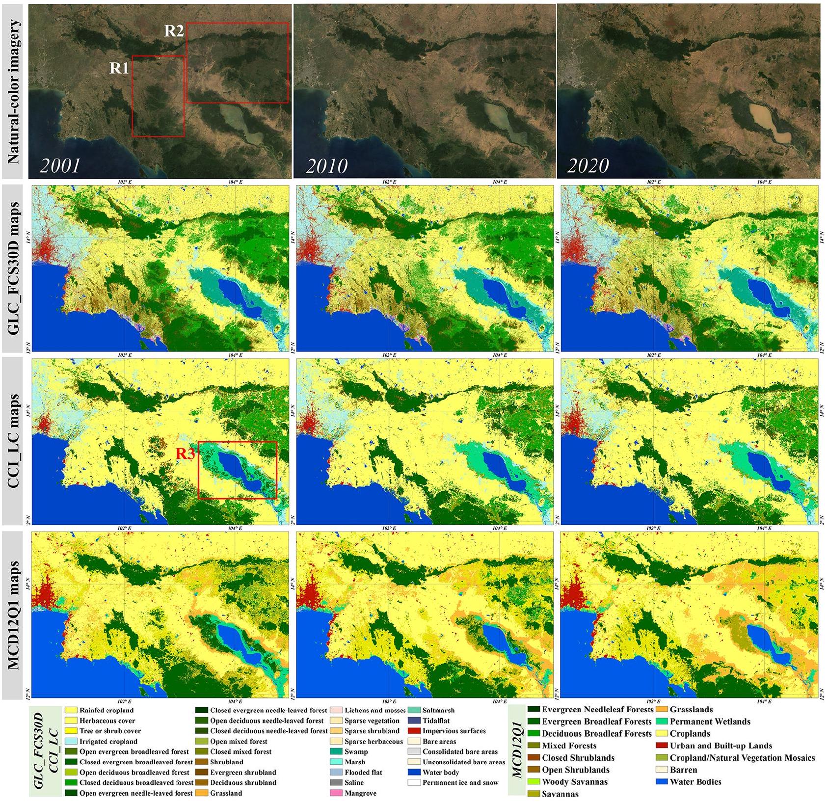
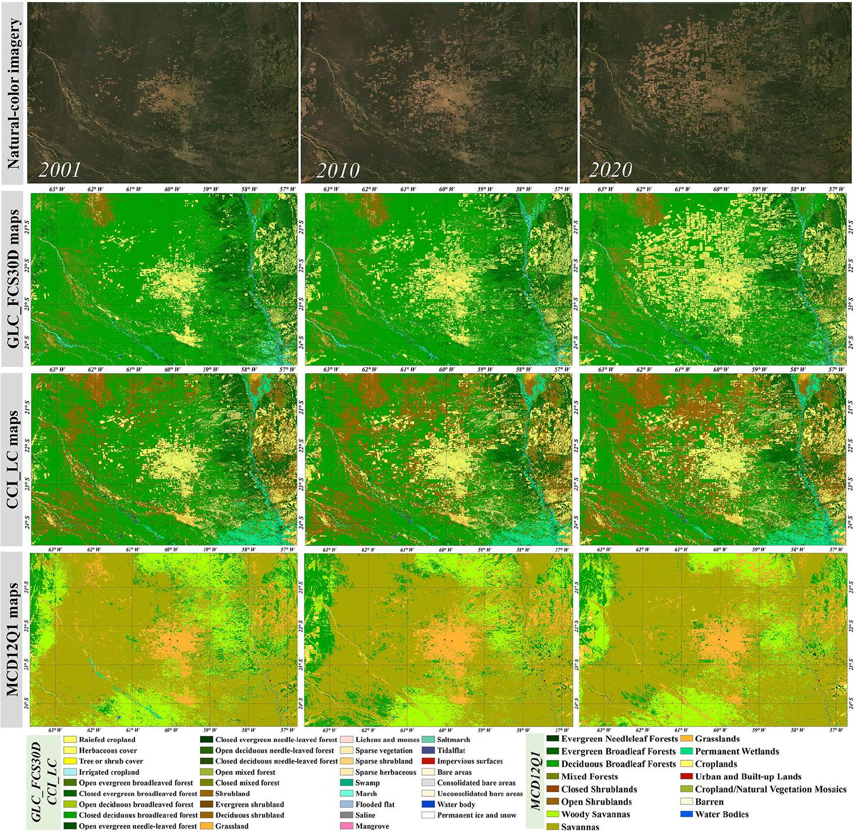
(مثل المباني الريفية وشبكات الطرق) أكثر من CCI_LC و MCD12Q1 بسبب دقتها المكانية العالية التي تبلغ 30 متر.
فيما يتعلق بأكثر حالات إزالة الغابات أهمية، أظهر CCI_LC أسوأ أداء لأنه (1) قلل من تقدير غطاء الغابات في عام 2001 (المنطقة المستطيلة 1: R1)، أي أن بعض الغابات تم تصنيفها بشكل خاطئ كأراض زراعية؛ (2) لم يتم التقاط بعض المناطق التي تم إزالة الغابات منها خلال الفترة من 2001 إلى 2020 في المنطقة المستطيلة 2 (R2)، لذا كانت مساحة الغابات المزالة أقل من GLC_FCS30D وMCD12Q1؛ و(3) كان هناك مشكلة واضحة في تصنيف الغابات كأراض رطبة في عام 2001 (المنطقة المستطيلة 3: R3). كما عانى MCD12Q1 من خطأ في إغفال الغابات في R1؛ حيث كانت مساحة الغابات الملتقطة في عام 2001 أقل من المساحة الفعلية للغابات بناءً على الصور الطبيعية. أما بالنسبة لإزالة الغابات الواضحة في R2، نجد أن جميع بكسلات الغابات تقريبًا تحولت إلى أنواع أخرى من تغطية الأرض (السافانا والأراضي العشبية) في MCD12Q1، مما انحرف بوضوح عن الوضع الفعلي؛ وبالتالي، فإن MCD12Q1 قد بالغ في تقدير إزالة الغابات. في الوقت نفسه، أظهرت سلسلة زمنية MCD12Q1 توزيعات مختلفة لتغطية الأرض في R3، مما يشير إلى أن MCD12Q1 لديه دقة رسم خرائط أقل وثبات زمني أقل لهذه المناطق الرطبة. بالمقارنة، حقق GLC_FCS30D أفضل أداء في التقاط التوزيع المكاني للغابات في عام 2001، وإزالة الغابات خلال 2001-2020، واستقرار الأراضي الرطبة.
تظهر الشكل 13 مثالاً آخر للمقارنة بين هذه المجموعات الثلاثة من البيانات، مع التركيز بدلاً من ذلك على باراغواي، أمريكا الجنوبية. كانت التغيرات الأكثر وضوحًا في تغطية الأرض هي إزالة الغابات وزيادة الأراضي الزراعية وفقًا لسلاسل الزمن لصور لاندسات بالألوان الطبيعية. من حيث الفضاء-
الجدول 6. نسب المساحات وقيم انحياز المساحة (AB) لـ 10 أنواع رئيسية من تغطية الأرض من مجموعة بيانات GLC_FCS30D (الخريطة) ومجموعة بيانات التحقق LUCAS (المرجع).
2006 2009 2012 2015 2018
خريطة مرجع أب خريطة مرجع أب خريطة مرجع أب خريطة مرجع أب خريطة مرجع أب
CRP ٤٦.٤٨ 50.62 -4.14 ٤٦.٤٦ 50.64 -4.18 ٤٦.٥٩ 50.67 -4.08 ٤٦.٦٣ 50.69 -4.06 ٤٦.٧٧ 50.74 -3.97
FST ٤١.٣٩ ٣٣.٧٦ 7.63 ٤١.٢٨ ٣٣.٧٥ 7.53 41.14 ٣٣.٧٣ 7.41 ٤٠.٩٦ ٣٣.٧٣ 7.23 ٤٠.٦٦ ٣٣.٦٨ 6.98
جي آر إس 1.21 ٤.١٥ -2.94 1.21 ٤.١٥ -2.94 1.21 ٤.١٥ -2.94 1.23 ٤.١٥ -2.92 1.21 ٤.١٥ -2.94
SHR 1.91 2.08 -0.17 1.94 2.08 -0.14 1.92 2.08 -0.16 1.91 2.07 -0.16 1.95 2.06 -0.11
رطب 1.70 1.75 -0.05 1.68 1.74 -0.06 1.68 1.73 -0.05 1.69 1.71 -0.02 1.73 1.72 0.01
WTR ٢.٧٥ 2.85 -0.1 2.76 2.85 -0.09 2.77 2.85 -0.08 2.81 2.85 -0.04 2.79 2.86 -0.07
IMP 3.18 3.82 -0.64 ٣.٢٥ 3.83 -0.58 ٣.٢٥ 3.82 -0.57 ٣.٢٧ 3.82 -0.55 3.32 3.82 -0.5
بال 1.32 0.95 0.37 1.36 0.95 0.41 1.37 0.95 0.42 1.42 0.95 0.47 1.49 0.95 0.54
PSI 0.06 0.02 0.04 0.06 0.02 0.04 0.07 0.02 0.05 0.07 0.02 0.05 0.07 0.02 0.05
الجدول 7. مصفوفة الالتباس للبكسلات المتغيرة وغير المتغيرة في GLC_FCS30D عند استخدام مجموعات بيانات LUCAS الزمنية عبر الاتحاد الأوروبي.
غير متغير تغير إجمالي مساعد شخصي (SE) فورمولا 1
غير متغير 82.69 ٢.٧٩ 85.48 ٩٦.٧٣ ٩٤.٤٩
تغير 6.84 7.68 14.52 ٥٢.٨٦ ٦١.٤٣
إجمالي 89.53 10.47
الإمارات العربية المتحدة (الجنوبية الشرقية)
أ.ع. (س.إ)
كان التوافق بين GLC_FCS30D و CCI_LC أعلى، بينما كان MCD12Q1 مختلفًا بشكل واضح عن المجموعتين الأخريين. تم تصنيف عدد كبير من الغابات النفضية العريضة الأوراق على أنها سافانا وسافانا شجرية، وتم التعرف على معظم الأراضي الزراعية على أنها أراضٍ عشبية في MCD12Q1، ويرجع ذلك أساسًا إلى الاختلاف في نظام التصنيف. من حيث مناطق تغطية الأرض المتغيرة، أظهر GLC_FCS30D أعلى دقة واحتوى على تفاصيل مكانية أغنى. على سبيل المثال، كانت شدة إزالة الغابات خلال الفترة من 2010 إلى 2020 أكبر بكثير من تلك التي كانت خلال الفترة من 2001 إلى 2010، كما كشف GLC_FCS30D عن إزالة الغابات المنتظمة الناتجة عن العوامل البشرية. بالمقابل، لم يتمكن CCI_LC و MCD12Q1 من التقاط إزالة الغابات خلال الفترة من 2010 إلى 2020 ولا التغيرات الصغيرة والمجزأة (الناجمة عن الأنشطة البشرية).

4.5 قيود وآفاق مجموعة بيانات GLC_FCS30D

لتحقيق هدف المراقبة الدقيقة والموثوقة لتغير تغطية الأرض العالمية، تم اعتماد أربع خطوات: (1) يتم دمج مزايا نموذج CCD والسلسلة الزمنية الكاملة لملاحظات لاندسات لالتقاط نقاط زمنية لتغير تغطية الأرض لأي بكسل متغير؛ (2) تُستخدم المناطق المستقرة زمنياً كمعرفة سابقة لضمان جودة عينات التدريب ويتم اعتماد النمذجة التكيفية المحلية لتحديث انتقالات تغطية الأرض لهذه البكسلات المتغيرة؛ (3) منتجات موضوعية عالمية لاثنين من تغطيات الأرض المعقدة.
تم تطوير الأنواع (السطح غير القابل للاختراق والأراضي الرطبة) بشكل مستقل لتحسين موثوقية GLC_FCS30D؛ و(4) تم تطبيق تحسين “التحقق من الاتساق الزماني والمكاني” في القسم 3.3.3 لضمان استقرار ودقة GLC_FCS30D بشكل أكبر. تظهر تقييمات الدقة التي تم إجراؤها باستخدام مجموعة البيانات العالمية التي تم تطويرها واثنين من مجموعات البيانات التابعة لجهات خارجية أن GLC_FCS30D يلبي متطلبات الدقة لسنة الأساس ولتغيرات السلاسل الزمنية على نطاق عالمي أو وطني. كما تبرز المقارنات مع منتجات تغطية الأراضي الأخرى تفوق GLC_FCS30D من حيث تنوع نظام التصنيف ودقة مراقبة هذه المناطق المتغيرة. ومع ذلك، فإن مراقبة تغير تغطية الأراضي العالمية على مدى سلسلة زمنية طويلة هي مهمة معقدة وصعبة للغاية (هانسن ولوفيلاند، 2012؛ سونغ وآخرون، 2018؛ وينكلر وآخرون، 2021؛ شيان وآخرون، 2022). على الرغم من أن هذه الدراسة تستخدم سلسلة من القياسات والأساليب لتحقيق مراقبة تغير تغطية الأراضي العالمية بدقة 30 مترًا على مدى السنوات الـ 37 الماضية، لا تزال هناك بعض عدم اليقين والقيود التي تحتاج إلى حل في العمل المستقبلي.
يستفيد خوارزم CCD بشكل كامل من الملاحظات الكثيفة للأقمار الصناعية لالتقاط تغييرات الغطاء الأرضي بشكل موثوق ودقيق (Zhu وWoodcock، 2014b؛ Zhu وآخرون، 2012). ومع ذلك، أظهرت الدراسات السابقة أن موثوقيتها مرتبطة ارتباطًا وثيقًا بكثافة الملاحظات الساتلية الصالحة (Bullock وآخرون، 2022؛ Ye وآخرون، 2021؛ Zhu وآخرون، 2019). تؤدي المناطق الملبدة بالغيوم والثلوج إلى زيادة عدم اليقين عندما
الشكل 12. مقارنات بين GLC_FCS30D ومنتجات ديناميات تغطية الأرض CCI_LC وMCD12Q1 لشبه جزيرة الهند الصينية خلال الفترة من 2001 إلى 2020. تم تجميع الصور الطبيعية من سلسلة زمنية من صور لاندسات.
تسجيل نقاط الزمن لتغير استخدام الأراضي (DeVries et al., 2015; Xian et al., 2022). بالإضافة إلى ذلك، بسبب سعة التخزين المحدودة وسعة نقل البيانات بين الأقمار الصناعية والأرض في الأقمار الصناعية المبكرة، كانت كثافة صور لاندسات قليلة قبل عام 2000 (حيث حصل قمر صناعي واحد فقط، لاندسات 5، على بيانات) (Roy et al., 2014b). في هذه الدراسة، نجمع الملاحظات من الأقمار الصناعية من عامين قبل وبعد السنة المركزية الاسمية من 1985 إلى 1995؛ على سبيل المثال، نقوم بتحديث خرائط استخدام الأراضي في عام 1995 باستخدام جميع الصور المتاحة من 1993 إلى 1997. ومع ذلك، وجدت دراسة سابقة أن شمال شرق آسيا لم يكن لديها أي ملاحظات صالحة من لاندسات.
قبل عام 2000 (Zhang et al., 2022)، مما يعني أن بعض تغييرات استخدام الأراضي لم يكن بالإمكان التقاطها في هذه المناطق قبل عام 2000 في GLC_FCS30D. لحل مشكلة الملاحظات المفقودة والنادرة، فإن حلاً مفيداً هو دمج صور الاستشعار عن بعد متعددة المصادر. على سبيل المثال، قام Y. Zhang et al. (2021) بدمج صور Landsat وSentinel-2 لتتبع الاضطرابات في الغابات الاستوائية بدقة إجمالية تزيد عن . لذلك، ستقوم الأعمال الإضافية بالتحقيق في جدوى دمج صور Sentinel-1/2 و SPOT و MODIS و AVHRR كبيانات مساعدة لتحقيق تغطية الأرض السنوية
الشكل 13. مقارنات بين GLC_FCS30D ومجموعتين من بيانات السلاسل الزمنية لديناميات تغطية الأرض في باراغواي، أمريكا الجنوبية، خلال الفترة من 2001 إلى 2020. تم تجميع الصور بالألوان الطبيعية من صور السلاسل الزمنية للاقمار الصناعية لاندسات.
المراقبة قبل عام 2000 وضمان جودة مراقبة تغطية الأرض.
لضمان استقرار GLC_FCS30D، تم تطبيق خوارزمية تحسين التناسق الزمكاني التي تم استخدامها على نطاق واسع في تحسينات تغيير الأسطح غير النفاذة (Li et al., 2015; Zhang et al., 2022). يستفيد هذا بشكل كامل من البيكسلات المجاورة زمنياً ومكانياً لحساب تجانس تغطية الأرض ثم إزالة ضوضاء “الملح والفلفل” الناتجة عن التصنيفات المعتمدة على البيكسلات. تم إجراء مقارنات نوعية لمناطق إزالة الغابات في الأمازون ومناطق في الصين التي شهدت توسعاً حضرياً (الشكل S2).
في الملحق) أظهر أيضًا أن تحسين التناسق الزماني المكاني يمكن أن يحسن جودة بيانات GLC_FCS30D من خلال تقليل ضوضاء الملح والفلفل وتحسين التناسق الزمني. وبالمثل، استخدم يانغ وهوانغ (2021) هذه الخوارزمية لتحسين منتجات تغطية الأراضي السنوية في الصين خلال الفترة من 1990 إلى 2019، ووجدوا أنها حسنت دقة رسم خريطة مجموعة بيانات تغطية الأراضي الزمنية.
يكشف GLC_FCS30D عن عدد كبير من تغييرات استخدام الأراضي في المناطق شبه الجافة كما هو موضح في الشكل 5a؛ هذه التغييرات في استخدام الأراضي تتأثر أكثر بالعوامل المناخية.
على سبيل المثال، تعتبر المنطقة الوسطى من أستراليا منطقة شبه جافة نموذجية، وأنواع الغطاء الأرضي السائدة هي المراعي، والنباتات المتناثرة، والأراضي الشجرية، والأراضي العارية. بشكل عام، إذا كان هناك هطول كافٍ من الأمطار سنويًا، ستكون توزيعات الأراضي الشجرية والمراعي في المنطقة أكثر اتساعًا؛ وإلا، ستسيطر الأراضي العارية والنباتات المتناثرة على المنطقة (دونغ وآخرون، 2020؛ جي وآخرون، 2022). مؤخرًا، اقترحت بعض الدراسات قمع هذه التغيرات؛ على سبيل المثال، اختار باستوس وآخرون (2022) قمع هذه التغيرات في الغطاء الأرضي من خلال دمج هذه الأنواع الأربعة من الغطاء الأرضي في نوع واحد من غطاء المراعي لأستراليا، ودمج شيان وآخرون (2022) المراعي والأراضي الشجرية في الولايات المتحدة المتجاورة. سيتم النظر فيما إذا كان ينبغي قمع هذه التغيرات المتكررة والحساسة للمناخ في أعمالنا المستقبلية.
على الرغم من أننا استخدمنا مجموعة بيانات تحقق عالمية لتقييم قدرة GLC_FCS30D في سنة الأساس 2020 ومجموعتين من البيانات الإقليمية من طرف ثالث لتقييم تباين الدقة عبر السلاسل الزمنية في الاتحاد الأوروبي وCONUS، يجب تعزيز عمل تقييم الدقة. على وجه الخصوص، لا يمكن تجاهل الفروق في نظام التصنيف بين GLC_FCS30D وLUCAS وLCMAP_Val. على سبيل المثال، نوع تغطية الأرض السطحية غير النفاذة في LUCAS وLCMAP_Val يحتوي على الأسطح الاصطناعية وما يحيط بها (مثل المساحات الخضراء في المدينة) (Stehman et al., 2021; Xian et al., 2022)، بينما GLC_FCS30D يتضمن فقط الهياكل الاصطناعية (Zhang et al., 2022)، لذا كانت السطح غير النفاذ في GLC_FCS30D ذات دقة منخفضة عند التحقق منها مع مجموعات بيانات LUCAS وLCMAP_Val في القسم 4.3. تم تحليل تباين دقة السلاسل الزمنية فقط في منطقتين، لذا يحتاج أداؤها في المناطق الأكثر تعقيدًا (مثل أفريقيا وآسيا) إلى مزيد من التحقيق. وبالتالي، ستركز أعمالنا المستقبلية على إنشاء مجموعات بيانات زمنية طويلة الأجل تستخدم للتحقق لمزيد من المناطق وعلى بناء مجموعة بيانات تحقق عالمية طويلة الأجل استنادًا إلى الأعمال الحالية في القسم 2.5.1، وبعد ذلك سيتم تحليل مقاييس دقة البكسلات التي تغيرت تغطيتها الأرضية وتباينها داخل السنة لجميع أنواع تغطية الأرض.

5 توفر البيانات

يمكن الوصول إلى مجموعة بيانات GLC_FCS30D المطورة مجانًا عبرhttps://doi.org/10.5281/zenodo.8239305 (Liu وآخرون، 2023). لمساعدة المستخدمين في التنقل في هذه المجموعة من البيانات، تم حفظها كـ بلاط مستقل. كل بلاطة تُسمى “GLC_FCS30D_yyyyYYYY_E/WN/S.tif”، حيث “E/Wن/س” يمثل إحداثيات الطول والعرض للزاوية العلوية اليسرى و yyyy و YYYY هما سنوات البداية والنهاية لمراقبة تغيرات استخدام الأراضي. يحتوي GLC_FCS30D على 26 خريطة لفترات زمنية من 1985 إلى 2022، يتم تحديثها كل 5 سنوات قبل عام 2000 وسنويًا من عام 2000 إلى 2022. يجب ملاحظة أن GLC_FCS30D اعتمد دورة مدتها 5 سنوات قبل عام 2000 بسبب الندرة.
توفر صور لاندسات 5 في هذه المرحلة المبكرة؛ وبالتالي، قمنا بزيادة طول الدورة الزمنية لضمان دقة رسم خرائط استخدام الأراضي. يتم حفظ الخطوات الزمنية الثلاث الأولى معًا ويتم حفظ الخطوات الزمنية الـ 23 التالية بشكل منفصل. على سبيل المثال، GLC_FCS30D_19851995_E115N15.tif و GLC_FCS30D_20002022_E115N15.tif هما، على التوالي، البيانات للخطوات الزمنية الثلاث الأولى والبيانات للـ 23 خطوة زمنية السنوية التالية من 1985 إلى 2022 للمنطقة المقابلة لـ .

6 الخاتمة

تغيير استخدام الأراضي هو السبب الرئيسي أو القوة الدافعة وراء تغير المناخ العالمي وقد جذب اهتمامًا متزايدًا في العقود الأخيرة. لا يزال رصد ديناميات استخدام الأراضي العالمية على مدى فترات زمنية طويلة مهمة صعبة. في هذه الدراسة، تم إنشاء أول مجموعة بيانات عالمية لديناميات استخدام الأراضي بدقة 30 مترًا (GLC_FCS30D) تحتوي على 35 فئة فرعية دقيقة من استخدام الأراضي وتغطي الفترة من 1985 إلى 2022 في 26 نقطة زمنية على منصة GEE. على وجه التحديد، استفدنا من السلسلة الزمنية الكاملة لملاحظات لاندسات وخوارزمية CCD لالتقاط النقاط الزمنية للمناطق المتغيرة، ثم قمنا بتحديث وتحسين مناطق استخدام الأراضي المتغيرة بناءً على استراتيجية النمذجة التكيفية المحلية وخوارزمية التناسق الزمني. تشير تقييمات الدقة إلى أن الطريقة المقترحة يمكن أن تحقق رصدًا دقيقًا ومتسقًا زمنيًا ومكانيًا لتغير استخدام الأراضي وأن GLC_FCS30D حققت دقة عامة لعام 2020 قدرها لأنواع الغطاء الأرضي العشرة الرئيسية في نظام التصنيف الأساسي و لنظام التحقق من المستوى الأول LCCS 17 نوعًا من أنواع تغطية الأرض. لذلك، يُعتبر GLC_FCS30D أول منتج عالمي لمراقبة ديناميات تغطية الأرض بفترة زمنية تمتد لـ 37 عامًا، ويتميز بأكثر أنظمة التصنيف تنوعًا. سيكون هذا ضروريًا للتنمية المستدامة، وحماية البيئة، واتخاذ قرارات مستنيرة لمواجهة تحديات عالم سريع التغير.
ملحق. الملحق المتعلق بهذه المقالة متاح على الإنترنت على:https://doi.org/10.5194/essd-16-1353-2024-supplement.
مساهمات المؤلفين. قام LL و XZ بتصميم المشروع والتحقيق فيه. صمم XZ و TZ و XC المنهجية؛ قام TZ و WL و HX و JW بإجراء التحقق. أعد XZ المسودة الأصلية للورقة؛ قام LL و HX بمراجعة وتحرير الورقة.
المصالح المتنافسة. لقد أعلن المؤلف المسؤول أنه لا يوجد لدى أي من المؤلفين أي مصالح متنافسة.
تنبيه. ملاحظة الناشر: تظل منشورات كوبرنيكوس محايدة فيما يتعلق بالمطالبات القضائية الواردة في النص، نشر-
لا تحتوي هذه الورقة على خرائط منشورة أو انتماءات مؤسسية أو أي تمثيل جغرافي آخر. بينما تبذل منشورات كوبرنيكوس كل جهد ممكن لتضمين أسماء الأماكن المناسبة، فإن المسؤولية النهائية تقع على عاتق المؤلفين.
الشكر والتقدير. نعرب عن امتناننا لجميع مزودي البيانات الذين تم استخدام بياناتهم في هذه الدراسة، ونتقدم بالشكر الجزيل للمحرر الموضوعي والمراجعين الثلاثة المجهولين على تعليقاتهم المفيدة والبناءة.
الدعم المالي. لقد تم دعم هذا البحث من قبل المؤسسة الوطنية للعلوم الطبيعية في الصين (أرقام المنح 41825002 و 42201499) وبرنامج البحث المفتوح لمركز الأبحاث الدولي للبيانات الكبيرة من أجل أهداف التنمية المستدامة (رقم المنحة CBAS2022ORP03).
بيان المراجعة. تم تحرير هذه الورقة بواسطة يوانتشي ياو وتمت مراجعتها من قبل ثلاثة محكمين مجهولين.

References

Azzari, G. and Lobell, D. B.: Landsat-based classification in the cloud: An opportunity for a paradigm shift in land cover monitoring, Remote Sens. Environ., 202, 64-74, https://doi.org/10.1016/j.rse.2017.05.025, 2017.
Ballin, M., Barcaroli, G., Masselli, M., and Scarnò, M.: Redesign sample for land use/cover area frame survey (LUCAS) 2018, Eurostat: statistical working papers, 10, 132365, 2018.
Ban, Y., Gong, P., and Giri, C.: Global land cover mapping using Earth observation satellite data: Recent progresses and challenges, ISPRS J. Photogramm. Remote, 103, 1-6, https://doi.org/10.1016/j.isprsjprs.2015.01.001, 2015.
Bastos, A., Ciais, P., Sitch, S., Aragao, L., Chevallier, F., Fawcett, D., Rosan, T. M., Saunois, M., Gunther, D., Perugini, L., Robert, C., Deng, Z., Pongratz, J., Ganzenmuller, R., Fuchs, R., Winkler, K., Zaehle, S., and Albergel, C.: On the use of Earth Observation to support estimates of national greenhouse gas emissions and sinks for the Global stocktake process: lessons learned from ESA-CCI RECCAP2, Carbon Balance Manag., 17, 15, https://doi.org/10.1186/s13021-022-00214-w, 2022.
Belgiu, M. and Drãgup, L.: Random forest in remote sensing: A review of applications and future directions, ISPRS J. Photogramm. Remote, 114, 24-31, https://doi.org/10.1016/j.isprsjprs.2016.01.011, 2016.
Buchhorn, M., Lesiv, M., Tsendbazar, N.-E., Herold, M., Bertels, L., and Smets, B.: Copernicus Global Land Cover Layers – Collection 2, Remote Sens., 12, 1044, https://doi.org/10.3390/rs12061044, 2020.
Bullock, E. L., Woodcock, C. E., and Holden, C. E.: Improved change monitoring using an ensemble of time series algorithms, Remote Sens. Environ., 111165, https://doi.org/10.1016/j.rse.2019.04.018, 2019.
Bullock, E. L., Healey, S. P., Yang, Z., Houborg, R., Gorelick, N., Tang, X., and Andrianirina, C.: Timeliness in forest change monitoring: A new assessment framework
demonstrated using Sentinel-1 and a continuous change detection algorithm, Remote Sens. Environ., 276, 113043, https://doi.org/10.1016/j.rse.2022.113043, 2022.
Chen, J., Chen, J., Liao, A., Cao, X., Chen, L., Chen, X., He, C., Han, G., Peng, S., Lu, M., Zhang, W., Tong, X., and Mills, J.: Global land cover mapping at 30 m resolution: A POK-based operational approach, ISPRS J. Photogramm. Remote, 103, 7-27, https://doi.org/10.1016/j.isprsjprs.2014.09.002, 2015.
d’Andrimont, R., Yordanov, M., Martinez-Sanchez, L., Eiselt, B., Palmieri, A., Dominici, P., Gallego, J., Reuter, H. I., Joebges, C., and Lemoine, G.: Harmonised LUCAS in-situ land cover and use database for field surveys from 2006 to 2018 in the European Union, Sci. Data, 7, 352, https://doi.org/10.1038/s41597-020-00675-z, 2020.
Defourny, P., Kirches, G., Brockmann, C., Boettcher, M., Peters, M., Bontemps, S., Lamarche, C., Schlerf, M., and M., S.: Land Cover CCI: Product User Guide Version 2, 2018, 2018.
DeVries, B., Verbesselt, J., Kooistra, L., and Herold, M.: Robust monitoring of small-scale forest disturbances in a tropical montane forest using Landsat time series, Remote Sens. Environ., 161, 107-121, https://doi.org/10.1016/j.rse.2015.02.012, 2015.
Dong, J., Xiao, X., Kou, W., Qin, Y., Zhang, G., Li, L., Jin, C., Zhou, Y., Wang, J., Biradar, C., Liu, J., and Moore, B.: Tracking the dynamics of paddy rice planting area in 1986-2010 through time series Landsat images and phenology-based algorithms, Remote Sens. Environ., 160, 99113, https://doi.org/10.1016/j.rse.2015.01.004, 2015.
Dong, S., Shang, Z., Gao, J., and Boone, R. B.: Enhancing sustainability of grassland ecosystems through ecological restoration and grazing management in an era of climate change on Qinghai-Tibetan Plateau, Agric. Ecosyst. Environ., 287, 106684, https://doi.org/10.1016/j.agee.2019.106684, 2020.
Du, P., Samat, A., Waske, B., Liu, S., and Li, Z.: Random Forest and Rotation Forest for fully polarized SAR image classification using polarimetric and spatial features, ISPRS J. Photogramm. Remote, 105, 38-53, https://doi.org/10.1016/j.isprsjprs.2015.03.002, 2015.
Foley, J. A., Defries, R., Asner, G. P., Barford, C., Bonan, G., Carpenter, S. R., Chapin, F. S., Coe, M. T., Daily, G. C., Gibbs, H. K., Helkowski, J. H., Holloway, T., Howard, E. A., Kucharik, C. J., Monfreda, C., Patz, J. A., Prentice, I. C., Ramankutty, N., and Snyder, P. K.: Global consequences of land use, Science, 309, 570-574, https://doi.org/10.1126/science.1111772, 2005.
Foody, G. M.: Sample size determination for image classification accuracy assessment and comparison, Int. J. Remote, 30, 52735291, https://doi.org/10.1080/01431160903130937, 2009.
Foody, G. M. and Arora, M. K.: An evaluation of some factors affecting the accuracy of classification by an artificial neural network, Int. J. Remote, 18, 799-810, https://doi.org/10.1080/014311697218764, 2010.
Friedl, M. A., Sulla-Menashe, D., Tan, B., Schneider, A., Ramankutty, N., Sibley, A., and Huang, X.: MODIS Collection 5 global land cover: Algorithm refinements and characterization of new datasets, Remote Sens. Environ., 114, 168-182, https://doi.org/10.1016/j.rse.2009.08.016, 2010.
Friedl, M. A., Woodcock, C. E., Olofsson, P., Zhu, Z., Loveland, T., Stanimirova, R., Arevalo, P., Bullock, E., Hu, K.-T., Zhang, Y., Turlej, K., Tarrio, K., McAvoy, K., Gorelick, N., Wang, J. A., Barber, C. P., and Souza, C.: Medium Spatial Resolution Map-
ping of Global Land Cover and Land Cover Change Across Multiple Decades From Landsat, Front. Remote Sens., 3, 894571, https://doi.org/10.3389/frsen.2022.894571, 2022.
Friedlingstein, P., O’Sullivan, M., Jones, M. W., Andrew, R. M., Hauck, J., Olsen, A., Peters, G. P., Peters, W., Pongratz, J., Sitch, S., Le Quéré, C., Canadell, J. G., Ciais, P., Jackson, R. B., Alin, S., Aragão, L. E. O. C., Arneth, A., Arora, V., Bates, N. R., Becker, M., Benoit-Cattin, A., Bittig, H. C., Bopp, L., Bultan, S., Chandra, N., Chevallier, F., Chini, L. P., Evans, W., Florentie, L., Forster, P. M., Gasser, T., Gehlen, M., Gilfillan, D., Gkritzalis, T., Gregor, L., Gruber, N., Harris, I., Hartung, K., Haverd, V., Houghton, R. A., Ilyina, T., Jain, A. K., Joetzjer, E., Kadono, K., Kato, E., Kitidis, V., Korsbakken, J. I., Landschützer, P., Lefèvre, N., Lenton, A., Lienert, S., Liu, Z., Lombardozzi, D., Marland, G., Metzl, N., Munro, D. R., Nabel, J. E. M. S., Nakaoka, S.-I., Niwa, Y., O’Brien, K., Ono, T., Palmer, P. I., Pierrot, D., Poulter, B., Resplandy, L., Robertson, E., Rödenbeck, C., Schwinger, J., Séférian, R., Skjelvan, I., Smith, A. J. P., Sutton, A. J., Tanhua, T., Tans, P. P., Tian, H., Tilbrook, B., van der Werf, G., Vuichard, N., Walker, A. P., Wanninkhof, R., Watson, A. J., Willis, D., Wiltshire, A. J., Yuan, W., Yue, X., and Zaehle, S.: Global Carbon Budget 2020, Earth Syst. Sci. Data, 12, 32693340, https://doi.org/10.5194/essd-12-3269-2020, 2020.
Gallant, A.: The Challenges of Remote Monitoring of Wetlands, Remote Sens., 7, 10938-10950, https://doi.org/10.3390/rs70810938, 2015.
Gao, Y., Liu, L., Zhang, X., Chen, X., Mi, J., and Xie, S.: Consistency Analysis and Accuracy Assessment of Three Global Land-Cover Products over the European Union using the LUCAS Dataset, Remote Sens., 12, 3479, https://doi.org/10.3390/rs12213479, 2020.
Ge, F., Xu, M., Gong, C., Zhang, Z., Tan, Q., and Pan, X.: Land cover changes the soil moisture response to rainfall on the Loess Plateau, Hydrol. Process., 36, e14714, https://doi.org/10.1002/hyp.14714, 2022.
Giri, C., Pengra, B., Long, J., and Loveland, T. R.: Next generation of global land cover characterization, mapping, and monitoring, Int. J. Appl. Earth Obs., 25, 30-37, https://doi.org/10.1016/j.jag.2013.03.005, 2013.
Gislason, P. O., Benediktsson, J. A., and Sveinsson, J. R.: Random Forests for land cover classification, Pattern Recogn. Lett., 27, 294-300, https://doi.org/10.1016/j.patrec.2005.08.011, 2006.
Gong, P., Li, X., and Zhang, W.: 40-Year (1978-2017) human settlement changes in China reflected by impervious surfaces from satellite remote sensing, Sci. Bull., 64, 756-763, https://doi.org/10.1016/j.scib.2019.04.024, 2019a.
Gong, P., Liu, H., Zhang, M., Li, C., Wang, J., Huang, H., Clinton, N., Ji, L., Li, W., Bai, Y., Chen, B., Xu, B., Zhu, Z., Yuan, C., Ping Suen, H., Guo, J., Xu, N., Li, W., Zhao, Y., Yang, J., Yu, C., Wang, X., Fu, H., Yu, L., Dronova, I., Hui, F., Cheng, X., Shi, X., Xiao, F., Liu, Q., and Song, L.: Stable classification with limited sample: transferring a resolution sample set collected in 2015 to mapping 10-m resolution global land cover in 2017, Sci. Bull., 64, 370-373, https://doi.org/10.1016/j.scib.2019.03.002, 2019b.
Gorelick, N., Hancher, M., Dixon, M., Ilyushchenko, S., Thau, D., and Moore, R.: Google Earth Engine: Planetary-scale geospatial analysis for everyone, Remote Sens. Environ., 202, 18-27, https://doi.org/10.1016/j.rse.2017.06.031, 2017.
Hansen, M. C. and Loveland, T. R.: A review of large area monitoring of land cover change using Landsat data, Remote Sens. Environ., 122, 66-74, https://doi.org/10.1016/j.rse.2011.08.024, 2012.
Hansen, M. C., Potapov, P. V., Moore, R., Hancher, M., Turubanova, S. A., Tyukavina, A., Thau, D., Stehman, S. V., Goetz, S. J., Loveland, T. R., Kommareddy, A., Egorov, A., Chini, L., Justice, C. O., and Townshend, J. R.: High-resolution global maps of 21st-century forest cover change, Science, 342, 850-853, https://doi.org/10.1126/science.1244693, 2013.
Harris, N. L., Gibbs, D. A., Baccini, A., Birdsey, R. A., de Bruin, S., Farina, M., Fatoyinbo, L., Hansen, M. C., Herold, M., Houghton, R. A., Potapov, P. V., Suarez, D. R., Roman-Cuesta, R. M., Saatchi, S. S., Slay, C. M., Turubanova, S. A., and Tyukavina, A.: Global maps of twenty-first century forest carbon fluxes, Nat. Clim. Change, 11, 234-240, https://doi.org/10.1038/s41558-020-00976-6, 2021.
Healey, S. P., Cohen, W. B., Yang, Z., Kenneth Brewer, C., Brooks, E. B., Gorelick, N., Hernandez, A. J., Huang, C., Joseph Hughes, M., Kennedy, R. E., Loveland, T. R., Moisen, G. G., Schroeder, T. A., Stehman, S. V., Vogelmann, J. E., Woodcock, C. E., Yang, L., and Zhu, Z.: Mapping forest change using stacked generalization: An ensemble approach, Remote Sens. Environ., 204, 717728, https://doi.org/10.1016/j.rse.2017.09.029, 2018.
Herold, M., Mayaux, P., Woodcock, C. E., Baccini, A., and Schmullius, Some challenges in global land cover mapping: An assessment of agreement and accuracy in existing 1 km datasets, Remote Sens. Environ., 112, 2538-2556, https://doi.org/10.1016/j.rse.2007.11.013, 2008.
Homer, C., Dewitz, J., Jin, S., Xian, G., Costello, C., Danielson, P., Gass, L., Funk, M., Wickham, J., Stehman, S., Auch, R., and Riitters, K.: Conterminous United States land cover change patterns 2001-2016 from the 2016 National Land Cover Database, ISPRS J. Photogramm. Remote, 162, 184-199, https://doi.org/10.1016/j.isprsjprs.2020.02.019, 2020.
Hong, C., Burney, J. A., Pongratz, J., Nabel, J., Mueller, N. D., Jackson, R. B., and Davis, S. J.: Global and regional drivers of land-use emissions in 1961-2017, Nature, 589, 554-561, https://doi.org/10.1038/s41586-020-03138-y, 2021.
Huang, C., Goward, S. N., Schleeweis, K., Thomas, N., Masek, J. G., and Zhu, Z.: Dynamics of national forests assessed using the Landsat record: Case studies in eastern United States, Remote Sens. Environ., 113, 1430-1442, https://doi.org/10.1016/j.rse.2008.06.016, 2009.
Jin, H., Stehman, S. V., and Mountrakis, G.: Assessing the impact of training sample selection on accuracy of an urban classification: a case study in Denver, Colorado, Int. J. Remote Sens., 35, 20672081, https://doi.org/10.1080/01431161.2014.885152, 2014.
Jin, S., Yang, L., Zhu, Z., and Homer, C.: A land cover change detection and classification protocol for updating Alaska NLCD 2001 to 2011, Remote Sens. Environ., 195, 44-55, https://doi.org/10.1016/j.rse.2017.04.021, 2017.
Jin, S., Dewitz, J., Li, C., Sorenson, D., Zhu, Z., Shogib, M. R. I., Danielson, P., Granneman, B., Costello, C., Case, A., and Gass, L.: National Land Cover Database 2019: A Comprehensive Strategy for Creating the 19862019 Forest Disturbance Product, J. Remote Sens., 3, 0021, https://doi.org/10.34133/remotesensing.0021, 2023.
Kennedy, R. E., Cohen, W. B., and Schroeder, T. A.: Trajectorybased change detection for automated characterization of forest disturbance dynamics, Remote Sens. Environ., 110, 370-386, https://doi.org/10.1016/j.rse.2007.03.010, 2007.
Kennedy, R. E., Yang, Z., and Cohen, W. B.: Detecting trends in forest disturbance and recovery using yearly Landsat time series: 1. LandTrendr – Temporal segmentation algorithms, Remote Sens. Environ., 114, 2897-2910, https://doi.org/10.1016/j.rse.2010.07.008, 2010.
Kenny, Q. Y.: Indicator function and its application in two-level factorial designs, Ann. Stat., 31, 984-994, https://doi.org/10.1214/aos/1056562470, 2003.
Li, X., Gong, P., and Liang, L.: A 30-year (1984-2013) record of annual urban dynamics of Beijing City derived from Landsat data, Remote Sens. Environ., 166, 78-90, https://doi.org/10.1016/j.rse.2015.06.007, 2015.
Liu, C., Zhang, Q., Luo, H., Qi, S., Tao, S., Xu, H., and Yao, Y.: An efficient approach to capture continuous impervious surface dynamics using spatial-temporal rules and dense Landsat time series stacks, Remote Sens. Environ., 229, 114-132, https://doi.org/10.1016/j.rse.2019.04.025, 2019.
Liu, H., Gong, P., Wang, J., Wang, X., Ning, G., and Xu, B.: Production of global daily seamless data cubes and quantification of global land cover change from 1985 to 2020 – iMap World 1.0, Remote Sens. Environ., 258, 112364, https://doi.org/10.1016/j.rse.2021.112364, 2021.
Liu, L., Zhang, X., Chen, X., Gao, Y., and Mi, J.: GLC_FCS30-2020:Global Land Cover with Fine Classification System at 30 m in 2020 (v1.2), Zenodo [data set], https://doi.org/10.5281/zenodo.4280923, 2020.
Liu, L., Zhang, X., Gao, Y., Chen, X., Shuai, X., and Mi, J.: FinerResolution Mapping of Global Land Cover: Recent Developments, Consistency Analysis, and Prospects, J. Remote Sens., 2021, 5289697, https://doi.org/10.34133/2021/5289697, 2021.
Liu, L., Zhang, X., and Zhao, T.: GLC_FCS30D: the first global land-cover dynamic monitoring product with fine classification system from 1985 to 2022, Zenodo [data set], https://doi.org/10.5281/zenodo.8239305, 2023.
Mellor, A., Boukir, S., Haywood, A., and Jones, S.: Exploring issues of training data imbalance and mislabelling on random forest performance for large area land cover classification using the ensemble margin, ISPRS J. Photogramm. Remote, 105, 155-168, https://doi.org/10.1016/j.isprsjprs.2015.03.014, 2015.
Millard, K. and Richardson, M.: On the Importance of Training Data Sample Selection in Random Forest Image Classification: A Case Study in Peatland Ecosystem Mapping, Remote Sens., 7, 8489-8515, https://doi.org/10.3390/rs70708489, 2015.
Pekel, J. F., Cottam, A., Gorelick, N., and Belward, A. S.: High-resolution mapping of global surface water and its long-term changes, Nature, 540, 418-422, https://doi.org/10.1038/nature20584, 2016.
Pengra, B., Gallant, A., Zhu, Z., and Dahal, D.: Evaluation of the Initial Thematic Output from a Continuous Change-Detection Algorithm for Use in Automated Operational Land-Change Mapping by the U.S. Geological Survey, Remote Sens., 8, 811, https://doi.org/10.3390/rs8100811, 2016.
Pontus Olofsson, G. M. F.: Good practices for estimating area and assessing accuracy of land change, Remote Sens. Environ., 148, 42-57, https://doi.org/10.1016/j.rse.2014.02.015, 2014.
Potapov, P., Turubanova, S., Hansen, M. C., Tyukavina, A., Zalles, V., Khan, A., Song, X.-P., Pickens, A., Shen, Q., and Cortez, J.: Global maps of cropland extent and change show accelerated cropland expansion in the twenty-first century, Nature Food, 3, 19-28, https://doi.org/10.1038/s43016-021-00429-z, 2021.
Potapov, P., Hansen, M. C., Pickens, A., Hernandez-Serna, A., Tyukavina, A., Turubanova, S., Zalles, V., Li, X., Khan, A., Stolle, F., Harris, N., Song, X.-P., Baggett, A., Kommareddy, I., and Kommareddy, A.: The Global 2000-2020 Land Cover and Land Use Change Dataset Derived From the Landsat Archive: First Results, Front. Remote Sens., 3, 856903, https://doi.org/10.3389/frsen.2022.856903, 2022.
Qin, Y., Xiao, X., Wigneron, J.-P., Ciais, P., Canadell, J. G., Brandt, M., Li, X., Fan, L., Wu, X., Tang, H., Dubayah, R., Doughty, R., Chang, Q., Crowell, S., Zheng, B., Neal, K., Celis, J. A., and Moore, B.: Annual Maps of Forests in Australia from Analyses of Microwave and Optical Images with FAO Forest Definition, J. Remote Sens., 2021, 9784657, https://doi.org/10.34133/2021/9784657, 2021.
Radoux, J., Lamarche, C., Van Bogaert, E., Bontemps, S., Brockmann, C., and Defourny, P.: Automated Training Sample Extraction for Global Land Cover Mapping, Remote Sens., 6, 39653987, https://doi.org/10.3390/rs6053965, 2014.
Roy, D. P., Qin, Y., Kovalskyy, V., Vermote, E. F., Ju, J., Egorov, A., Hansen, M. C., Kommareddy, I., and Yan, L.: Conterminous United States demonstration and characterization of MODISbased Landsat ETM+ atmospheric correction, Remote Sens. Environ., 140, 433-449, https://doi.org/10.1016/j.rse.2013.09.012, 2014a.
Roy, D. P., Wulder, M. A., Loveland, T. R., C.E, W., Allen, R. G., Anderson, M. C., Helder, D., Irons, J. R., Johnson, D. M., Kennedy, R., Scambos, T. A., Schaaf, C. B., Schott, J. R., Sheng, Y., Vermote, E. F., Belward, A. S., Bindschadler, R., Cohen, W. B., Gao, F., Hipple, J. D., Hostert, P., Huntington, J., Justice, C. O., Kilic, A., Kovalskyy, V., Lee, Z. P., Lymburner, L., Masek, J. G., McCorkel, J., Shuai, Y., Trezza, R., Vogelmann, J., Wynne, R. H., and Zhu, Z.: Landsat-8: Science and product vision for terrestrial global change research, Remote Sens. Environ., 145, 154-172, https://doi.org/10.1016/j.rse.2014.02.001, 2014b.
Roy, D. P., Kovalskyy, V., Zhang, H. K., Vermote, E. F., Yan, L., Kumar, S. S., and Egorov, A.: Characterization of Landsat-7 to Landsat-8 reflective wavelength and normalized difference vegetation index continuity, Remote Sens. Environ., 185, 57-70, https://doi.org/10.1016/j.rse.2015.12.024, 2016.
Song, X. P., Hansen, M. C., Stehman, S. V., Potapov, P. V., Tyukavina, A., Vermote, E. F., and Townshend, J. R.: Global land change from 1982 to 2016, Nature, 560, 639-643, https://doi.org/10.1038/s41586-018-0411-9, 2018.
Stehman, S. V., Pengra, B. W., Horton, J. A., and Wellington, D. F.: Validation of the U.S. Geological Survey’s Land Change Monitoring, Assessment and Projection (LCMAP) Collection 1.0 annual land cover products 1985-2017, Remote Sens. Environ., 265, 112646, https://doi.org/10.1016/j.rse.2021.112646, 2021.
Sulla-Menashe, D., Gray, J. M., Abercrombie, S. P., and Friedl, M. A.: Hierarchical mapping of annual global land cover 2001 to present: The MODIS Collection 6 Land Cover product, Remote Sens. Environ., 222, 183-194, https://doi.org/10.1016/j.rse.2018.12.013, 2019.
Tachikawa, T., Hato, M., Kaku, M., and Iwasaki, A.: Characteristics of ASTER GDEM Version 2, Geoscience and Remote Sensing Symposium (IGARSS), 3657-3660, https://doi.org/10.1109/IGARSS.2011.6050017, 2011.
Venter, Z. S., Barton, D. N., Chakraborty, T., Simensen, T., and Singh, G.: Global 10 m Land Use Land Cover Datasets: A Comparison of Dynamic World, World Cover and Esri Land Cover, Remote Sens., 14, 4101, https://doi.org/10.3390/rs14164101, 2022.
Verbesselt, J., Hyndman, R., Newnham, G., and Culvenor, D.: Detecting trend and seasonal changes in satellite image time series, Remote Sens. Environ., 114, 106-115, 2010.
Vermote, E.: LEDAPS surface reflectance product description, https://www.usgs.gov/media/files/ landsat-4-7-collection-1-surface-reflectance-code-ledaps-product(last access: 12 March 2024), 2007.
Vermote, E. F. and Kotchenova, S.: Atmospheric correction for the monitoring of land surfaces, J. Geophys. Res., 113, D23S90, https://doi.org/10.1029/2007jd009662, 2008.
Wang, N., Zhang, X., Yao, S., Wu, J., and Xia, H.: How Good Are Global Layers for Mapping Rural Settlements? Evidence from China, Land, 11, 1308, https://doi.org/10.3390/land11081308, 2022.
Winkler, K., Fuchs, R., Rounsevell, M., and Herold, M.: Global land use changes are four times greater than previously estimated, Nat. Commun., 12, 2501, https://doi.org/10.1038/s41467-021-22702-2, 2021.
Xian, G. Z., Smith, K., Wellington, D., Horton, J., Zhou, Q., Li, C., Auch, R., Brown, J. F., Zhu, Z., and Reker, R. R.: Implementation of the CCDC algorithm to produce the LCMAP Collection 1.0 annual land surface change product, Earth Syst. Sci. Data, 14, 143-162, https://doi.org/10.5194/essd-14-143-2022, 2022.
Xiao, Y., Wang, Q., Tong, X., and Atkinson, P. M.: Thirty-meter map of young forest age in China, Earth Syst. Sci. Data, 15, 3365-3386, https://doi.org/10.5194/essd-15-3365-2023, 2023.
Xie, S., Liu, L., Zhang, X., and Yang, J.: Mapping the annual dynamics of land cover in Beijing from 2001 to 2020 using Landsat dense time series stack, ISPRS J. Photogramm. Remote, 185, 201-218, https://doi.org/10.1016/j.isprsjprs.2022.01.014, 2022.
Yang, J. and Huang, X.: The 30 m annual land cover dataset and its dynamics in China from 1990 to 2019, Earth Syst. Sci. Data, 13, 3907-3925, https://doi.org/10.5194/essd-13-3907-2021, 2021.
Ye, S., Rogan, J., Zhu, Z., and Eastman, J. R.: A near-real-time approach for monitoring forest disturbance using Landsat time series: stochastic continuous change detection, Remote Sens. Environ., 252, 112167, https://doi.org/10.1016/j.rse.2020.112167, 2021.
Zhang, H. K. and Roy, D. P.: Using the 500 m MODIS land cover product to derive a consistent continental scale 30 m Landsat land cover classification, Remote Sens. Environ., 197, 15-34, https://doi.org/10.1016/j.rse.2017.05.024, 2017.
Zhang, X., Liu, L., Chen, X., Xie, S., and Gao, Y.: Fine LandCover Mapping in China Using Landsat Datacube and an Operational SPECLib-Based Approach, Remote Sens., 11, 1056, https://doi.org/10.3390/rs11091056, 2019.
Zhang, X., Liu, L., Wu, C., Chen, X., Gao, Y., Xie, S., and Zhang, B.: Development of a global 30 m impervious surface map using multisource and multitemporal remote sensing datasets with the
Google Earth Engine platform, Earth Syst. Sci. Data, 12, 16251648, https://doi.org/10.5194/essd-12-1625-2020, 2020.
Zhang, X., Liu, L., Chen, X., Gao, Y., and Jiang, M.: Automatically Monitoring Impervious Surfaces Using Spectral Generalization and Time Series Landsat Imagery from 1985 to 2020 in the Yangtze River Delta, J. Remote Sens., 2021, 1-16, https://doi.org/10.34133/2021/9873816, 2021a.
Zhang, X., Liu, L., Chen, X., Gao, Y., Xie, S., and Mi, J.: GLC_FCS30: global land-cover product with fine classification system at 30 m using time-series Landsat imagery, Earth Syst. Sci. Data, 13, 2753-2776, https://doi.org/10.5194/essd-13-27532021, 2021b.
Zhang, X., Liu, L., Zhao, T., Gao, Y., Chen, X., and Mi, J.: GISD30: global 30 m impervious-surface dynamic dataset from
uide1985 to 2020 using time-series Landsat imagery on the Google Earth Engine platform, Earth Syst. Sci. Data, 14, 1831-1856, https://doi.org/10.5194/essd-14-1831-2022, 2022.
Zhang, X., Liu, L., Zhao, T., Chen, X., Lin, S., Wang, J., Mi, J., and Liu, W.: GWL_FCS30: a global 30 m wetland map with a fine classification system using multi-sourced and time-series remote sensing imagery in 2020, Earth Syst. Sci. Data, 15, 265293, https://doi.org/10.5194/essd-15-265-2023, 2023.
Zhang, Y., Ling, F., Wang, X., Foody, G. M., Boyd, D. S., Li, X., Du, Y., and Atkinson, P. M.: Tracking smallscale tropical forest disturbances: Fusing the Landsat and Sentinel-2 data record, Remote Sens. Environ., 261, 112470, https://doi.org/10.1016/j.rse.2021.112470, 2021c.
Zhao, T., Zhang, X., Gao, Y., Mi, J., Liu, W., Wang, J., Jiang, M., and Liu, L.: Assessing the Accuracy and Consistency of Six FineResolution Global Land Cover Products Using a Novel Stratified Random Sampling Validation Dataset, Remote Sens., 15, 2285, https://doi.org/10.3390/rs15092285, 2023.
Zhu, Z., Wang, S. X., and Woodcock, C. E.: Improvement and expansion of the Fmask algorithm: cloud, cloud shadow, and snow detection for Landsats 4-7, 8, and Sentinel 2 images, Remote Sens. Environ., 159, 269-277, https://doi.org/10.1016/j.rse.2014.12.014, 2015.
Zhu, Z., Gallant, A. L., Woodcock, C. E., Pengra, B., Olofsson, P., Loveland, T. R., Jin, S., Dahal, D., Yang, L., and Auch, R. F.: Optimizing selection of training and auxiliary data for operational land cover classification for the LCMAP initiative, ISPRS J. Photogramm. Remote, 122, 206221, https://doi.org/10.1016/j.isprsjprs.2016.11.004, 2016.
Zhu, Z.: Change detection using landsat time series: A review of frequencies, preprocessing, algorithms, and applications, ISPRS J. Photogramm. Remote, 130, 370-384, https://doi.org/10.1016/j.isprsjprs.2017.06.013, 2017.
Zhu, Z. and Woodcock, C. E.: Object-based cloud and cloud shadow detection in Landsat imagery, Remote Sens. Environ., 118, 8394, https://doi.org/10.1016/j.rse.2011.10.028, 2012.
Zhu, Z. and Woodcock, C. E.: Automated cloud, cloud shadow, and snow detection in multitemporal Landsat data: An algorithm designed specifically for monitoring land cover change, Remote Sens. Environ., 152, 217-234, https://doi.org/10.1016/j.rse.2014.06.012, 2014a.
Zhu, Z. and Woodcock, C. E.: Continuous change detection and classification of land cover using all available Landsat data, Remote Sens. Environ., 144, 152-171, https://doi.org/10.1016/j.rse.2014.01.011, 2014b.
Zhu, Z., Woodcock, C. E., and Olofsson, P.: Continuous monitoring of forest disturbance using all available Landsat imagery, Remote Sens. Environ., 122, 75-91, https://doi.org/10.1016/j.rse.2011.10.030, 2012.
Zhu, Z., Zhang, J., Yang, Z., Aljaddani, A. H., Cohen, W. B., Qiu, S., and Zhou, C.: Continuous monitoring of land disturbance based on Landsat time series, Remote Sens. Environ., 238, 111116, https://doi.org/10.1016/j.rse.2019.03.009, 2019.

Journal: Earth system science data, Volume: 16, Issue: 3
DOI: https://doi.org/10.5194/essd-16-1353-2024
Publication Date: 2024-03-15

GLC_FCS30D: the first global 30 m land-cover dynamics monitoring product with a fine classification system for the period from 1985 to 2022 generated using dense-time-series Landsat imagery and the continuous change-detection method

Xiao Zhang , Tingting Zhao , Hong Xu , Wendi Liu , Jinqing Wang , Xidong Chen , and Liangyun Liu International Research Center of Big Data for Sustainable Development Goals, Beijing 100094, China Key Laboratory of Digital Earth Science, Aerospace Information Research Institute, Chinese Academy of Sciences, Beijing 100094, China School of Electronic, Electrical and Communication Engineering, University of Chinese Academy of Sciences, Beijing 100049, China College of Geomatics, Xi’an University of Science and Technology, Xi’an 710054, China The High-Tech Research & Development Center (HTRDC) of the National Natural Science Foundation of China, Beijing 100044, China Future Urbanity & Sustainable Environment (FUSE) Lab, The University of Hong Kong, Hong Kong SAR, 999007, ChinaCorrespondence: Liangyun Liu (liuly@radi.ac.cn)

Received: 7 August 2023 – Discussion started: 31 August 2023
Revised: 15 January 2024 – Accepted: 31 January 2024 – Published: 15 March 2024

Abstract

Land-cover change has been identified as an important cause or driving force of global climate change and is a significant research topic. Over the past few decades, global land-cover mapping has progressed; however, long-time-series global land-cover-change monitoring data are still sparse, especially those at 30 m resolution. In this study, we describe GLC_FCS30D, a novel global 30 m land-cover dynamics monitoring dataset containing 35 land-cover subcategories and covering the period 1985-2022 in 26 time steps (maps were updated every 5 years before 2000 and annually after 2000). GLC_FCS30D has been developed using continuous change detection and all available Landsat imagery based on the Google Earth Engine platform. Specifically, we first take advantage of the continuous change-detection model and the full time series of Landsat observations to capture the time points of changed pixels and identify the temporally stable areas. Then, we apply a spatiotemporal refinement method to derive the globally distributed and high-confidence training samples from these temporally stable areas. Next, local adaptive classification models are used to update the land-cover information for the changed pixels, and a temporal-consistency optimization algorithm is adopted to improve their temporal stability and suppress some false changes. Further, the GLC_FCS30D product is validated using 84526 globally distributed validation samples from 2020. It achieves an overall accuracy of for the basic classification system ( 10 major land-cover types) and for the LCCS (Land Cover Classification System) level-1 validation system ( 17 LCCS land-cover types). Meanwhile, two third-party time-series datasets used for validation from the United States and Europe Union are also collected for analyzing accuracy variations, and the results show that GLC_FCS30D offers significant stability in terms of variation across the accuracy time series and achieves mean accuracies of and over the two regions. Lastly, we draw conclusions about the global land-cover-change information from the GLC_FCS30D dataset; namely,

that forest and cropland variations have dominated global land-cover change over past 37 years, the net loss of forests reached about 2.5 million , and the net gain in cropland area is approximately 1.3 million . Therefore, the novel dataset GLC_FCS30D is an accurate land-cover-dynamics time-series monitoring product that benefits from its diverse classification system, high spatial resolution, and long time span (1985-2022); thus, it will effectively support global climate change research and promote sustainable development analysis. The GLC_FCS30D dataset is available via https://doi.org/10.5281/zenodo. 8239305 (Liu et al., 2023).

1 Introduction

Land-cover data are important and necessary for supporting sustainable development goals, maintaining biodiversity, and monitoring natural resources (L. Liu et al., 2021; Potapov et al., 2022). Land-cover changes directly or indirectly influence global climate patterns and the speed and magnitude of climate change (Song et al., 2018), and they increasingly affect biogeochemical cycles, the carbon cycle, and the Earth’s energy balance (Foley et al., 2005; Hong et al., 2021; Winkler et al., 2021). Since the Industrial Revolution, under the dual pressure from global climate change and human activities, global land cover has undergone drastic changes. According to a Global Carbon Project report in 2020, since the industrialization period, land-cover and land-use changes have contributed to approximately of all global greenhouse gas emissions (Friedlingstein et al., 2020), and this trend is exacerbated by the ongoing increase in population and per capita energy consumption (Xian et al., 2022). Therefore, understanding and studying land-cover changes is of vital significance for addressing global environmental changes, promoting sustainable development, and safeguarding the Earth’s ecological environment.
Remote-sensing techniques, with their periodic Earth observation capability and archived massive long-term observation data since 1972, provide the most cost-effective and practical solutions for long-time-series, large-area land-cover-change monitoring. In the past few decades, with the continuous improvement of remote sensing technology and storage and computing capabilities, global land-coverchange monitoring (GLCCM) has transitioned from 1 km spatial resolution to fine resolutions of 30 or 10 m and from single-phase mapping to long-term monitoring (Ban et al., 2015; Friedl et al., 2010, 2022; Giri et al., 2013). In its early stages, GLCCM mainly relied on time series of MODIS, AVHRR, and Project for Onboard Autonomy (PROBA)-V imagery (Buchhorn et al., 2020; Friedl et al., 2010); for example, Sulla-Menashe et al. (2019) generated a global 500 m annual land-cover product (MCD12Q1) covering the period from 2001 to the present using MODIS time-series imagery with an overall accuracy of . Defourny et al. (2018) integrated PROBA-V and Medium Resolution Imaging Spectrometer (MERIS) time-series observations to develop a global 300 m annual land-cover dynamics dataset (CCI_LC: Climate Change Initiative Global Land Cover) for
the period from 1992 to 2020 with an overall accuracy of . These coarse land-cover-change products comprehensively captured the spatial patterns of various land-cover types and quantified the global land-cover changes caused by human and natural activities. However, they still had major limitations, especially in regions with intense human activity and high spatial heterogeneity, because these broken and heterogeneous land-cover changes cannot be captured by coarse-resolution satellite observations (Hansen et al., 2013; Herold et al., 2008; L. Liu et al., 2021; Y. Zhang et al., 2021).
Recently, benefiting from the free access to fine-resolution satellite imagery and powerful computing and storage capabilities and the rise of cloud computing (such as the Google Earth Engine (Gorelick et al., 2017) and Microsoft Planetary Computer) in particular, fine-resolution land-cover dynamics monitoring has been experiencing rapid development. Correspondingly, numerous national and global 30 m landcover dynamics products have been developed (Chen et al., 2015; Homer et al., 2020; H. Liu et al., 2021; Potapov et al., 2022; Yang and Huang, 2021; Zhang et al., 2022). For example, Yang and Huang (2021) used China’s land-use/cover datasets (CLUDs) as the prior dataset and then combined multitemporal classification and spatiotemporal consistency post-processing methods to develop an annual 30 m landcover dataset (CLCD) for China from 1990 to 2019. Similarly, H. Liu et al. (2021) combined pixel-based classification and spatiotemporal consistency post-processing methods to generate the first global 30 m land-cover change products. However, many studies have demonstrated that multiperiod independent classifications lead to significant classification error accumulation in land-cover-change time-series monitoring (Sulla-Menashe et al., 2019; Zhu, 2017). For example, Xian et al. (2022) stated that the independent classification strategy suffered from the constraints of the post-processing requirements that ensure the temporal consistency of landcover change maps. Therefore, although GLCCM has progressed significantly over the past few decades, an accurate global 30 m land-cover change-detection product generated by an efficient land-cover change method is still urgently required.
One of the greatest challenges in large-area land-cover change detection is to select the optimal algorithm to capture the land-cover changes from time-series observations (Healey et al., 2018; Zhu, 2017). Over the past few decades, a series of change-detection algorithms have been proposed
for monitoring forest disturbance (Huang et al., 2009; Jin et al., 2023; Kennedy et al., 2007, 2010; Qin et al., 2021), urban expansion (Liu et al., 2019; X. Zhang et al., 2021a), cropland dynamics (Dong et al., 2015; Potapov et al., 2021), and land-cover changes (Bullock et al., 2019; Jin et al., 2017; Verbesselt et al., 2010; Zhu et al., 2019). However, most of them are only suitable for regional land-cover change monitoring, and some of the algorithms need prior knowledge (such as that for urban expansion). Zhu (2017) systematically reviewed the performance and limitations of various changedetection methods based on multitemporal satellite data and further explained that the high-temporal-frequency and multivariate change-detection algorithms are more suitable for a long time series of land-cover changes in a large area, provided that the problem of the huge amount of computation involved can be solved. Similarly, Xian et al. (2022) and Liu et al. (2019) concluded that dense and continuous changedetection methods provided higher accuracy and more robustness than traditional change-detection methods for capturing multiple, complicated changes.
The continuous change-detection and classification (CCDC) algorithm, a classical change-detection method based on dense time-series observations proposed by Zhu and Woodcock (2014b), is widely used for regional and national land-cover monitoring (Xian et al., 2022; Xie et al., 2022). It uses all available Landsat observations to build time-series regression models and then captures the outliers by analyzing the differences between the actual observations and model estimations. Zhu and Woodcock (2014b) demonstrated that the CCDC algorithm attained a general accuracy of and temporal accuracy of for capturing land-cover changes. Thus, it has been adopted by the United States Geological Survey (USGS) as the official algorithm for monitoring land-cover changes over the United States (Pengra et al., 2016). For example, Xian et al. (2022) implemented the CCDC algorithm and all available Landsat data to develop annual land-cover-change products that cover the contiguous United States (CONUS) for 1985-2017 with an overall accuracy of .
In summary, in recent decades, land-cover mapping and monitoring has made significant progress; however, global 30 m land-cover-dynamics time-series products derived from change-detection algorithms are still lacking. In this study, we had three aims: (1) to use the continuous changedetection algorithm and the full time series of Landsat observations to generate the first global 30 m land-cover dynamics product that covers the period from 1985 to 2022 and uses a fine classification system that contains 35 fine landcover subcategories with 26 time steps (the maps are updated every 5 years before 2000 and annually after 2000), known as GLC_FCS30D (it should be noted that GLC_FCS30D is updated every 5 years before 2000 due to the sparse availability of Landsat 5 imagery; thus, we combine the satellite observations from 2 years before and after the nominal center year from 1985 to 1995 to ensure the mapping ac-
curacy of GLC_FCS30D before 2000); (2) to quantify the land-cover changes and analyze the spatiotemporal change patterns of various land-cover types based on the developed GLC_FCS30D dataset; and (3) to quantitatively analyze the performance of the GLC_FCS30D product using multisourced validation datasets.

2 Datasets

2.1 Continuous Landsat imagery from 1984 to 2022

All available Landsat imagery from 1984 to 2022 – covering the Landsat 5 Thematic Mapper (TM), Landsat 7 Enhanced Thematic Mapper Plus (ETM+), Landsat 8 Operational Land Imager (OLI), and Landsat 9 OLI missions – were collected via the Google Earth Engine (GEE) cloud-computing platform. Specific measures were taken to build a high-quality, continuous Landsat time-series collection. First, all Landsat images underwent atmospheric correction to convert them to surface reflectance using the Landsat Ecosystem Disturbance Adaptive Processing System (LEDAPS) and Land Surface Reflectance Code (LaSRC) methods (Vermote, 2007; Vermote and Kotchenova, 2008). Then, although the Landsat 5, 7,8 , and 9 missions share similar spectral bands, the wavelength differences between the TM, ETM+, and OLI cannot be ignored. Relative radiometric normalization was applied to the TM and ETM+ imagery using the transformation coefficients suggested by Roy et al. (2016).

2.2 Global land-cover dataset at 30 m for the year 2020

The global 30 m land-cover product with a fine classification system for the year 2020 (GLC_FCS30-2020) is the baseline for generating training samples and identifying land-cover information in the temporally stable regions in Sect. 3. The GLC_FCS30 dataset was developed using local adaptive classifications and confident and globally distributed training samples, and then validated to reach an overall accuracy of with the basic validation system (X. Zhang et al., 2021b). Cross-comparisons with other landcover products showed obvious advantages for GLC_FCS30 in terms of mapping accuracy and diversity of land-cover types. The GLC_FCS30-2020 dataset is freely available at https://doi.org/10.5281/zenodo. 4280923 (Liu et al., 2020).

2.3 Global impervious surface dynamics dataset at 30 m from 1985 to 2022

Many studies found that high spatiotemporal heterogeneity of impervious surfaces and broken impervious surface constructions caused high uncertainty and difficulty when monitoring the dynamics of such surfaces (Gong et al., 2019a; Zhang et al., 2022), and issues with both missed detections and false alarms are encountered when change detection methods are applied to the dynamic monitoring of
heterogeneous impervious surfaces. Thus, we independently produced a global impervious-surface-dynamics time-series dataset at 30 m (GISD30) for 1985-2022 and then overlaid this thematic dataset on the GLC_FCS30D dataset to ensure high confidence in the impervious surface dynamics. The GISD30 dataset was developed by combining the sample migration, spectral generalization, and local adaptive modeling methods and then optimized by the spatiotemporalconsistency correction method (Zhang et al., 2022). It was validated and found to attain a mean overall accuracy of around the globe and to perform better than other similar products in capturing the changes in impervious surfaces over time and across different types of landscapes. At the same time, third-party validation also indicated that GISD30 exhibited superior performance to similar global 30 m impervious surface products (Wang et al., 2022).

2.4 Global 30 m wetland datasets from 1985 to 2022

Like the impervious surface dataset, the global wetland dynamics dataset is independently produced because the reflectance spectra of the wetlands and phenological variations changed daily with the water levels. The continuous changedetection method would suffer from serious commission and omission errors if used for wetland dynamics monitoring (Gallant, 2015). In this study, the GWL_FCS30 (global 30 m wetland map with a fine classification system) wetland dataset from 1985 to 2022 – developed by integrating the automatic sample extraction method, a stratified classification strategy, and the time series of Landsat observations (Zhang et al., 2023) – is superimposed on the GLC_FCS30D landcover dynamics dataset. GWL_FCS30 was quantitatively assessed as having a mean overall accuracy of using 25708 validation points, and it demonstrated a higher level of performance than other wetland products when it came to capturing the spatial patterns of wetlands during cross-comparisons (Zhang et al., 2023). GWL_FCS30 further splits wetlands into seven wetland subcategories (four inland and three coastal subcategories) and is overlaid directly onto the GLC_FCS30D dataset to not only improve the monitoring accuracy for wetlands but also enrich the number of land-cover types (see Table 1).

2.5 Validation datasets

To comprehensively analyze the accuracy metrics for the GLC_FCS30D dataset, two types of validation datasets were collected: an independent global validation dataset from 2020 and two third-party time-series datasets used for validation for the United States and the European Union.

2.5.1 Global validation dataset

A total of 84526 globally distributed validation samples are collected to analyze the accuracy metrics for the
GLC_FCS30D dataset for 2020, and their spatial distribution is illustrated in Fig. 1. Intuitively, the spatial patterns of the global validation dataset are consistent with the actual global land-cover situation. Specifically, to ensure confidence in and the rationality of the validation datasets, several measures are taken, which were explained in detail in our previous work (Zhao et al., 2023). First, a stratified random sampling method is applied by combining the landscape heterogeneity, population density data, and Köppen climate groups, which effectively increases the sample size in the heterogeneous landscapes and for some rare land-cover types (such as impervious surfaces, permanent ice, and snow). Second, for each validation sample, the land-cover type is determined through independent interpretation by trained interpreters after combining high-resolution aerial photography, multitemporal Landsat images, and other relevant ancillary datasets (such as vegetation coverage, tree height, phenological curves, and terrain characteristics). Independent interpretation software based on the GEE platform (https: //eliza-ting.users.earthengine.app/view/crd-vit, last access: 12 March 2024) for efficiently recognizing the land-cover types of each sample was also developed. Third, a qualitycontrol operation based on duplicate interpretations is used to ensure the confidence level of each validation sample. Each sample is independently labeled by three junior interpreters and then double-checked by the senior experts, and validation samples with huge disparities are discarded. In addition, because the impervious-surface and wetland datasets were produced independently and were validated in our previous works (Zhang et al., 2023, 2022), the corresponding highquality validation samples of these two thematic types are also imported into the global validation datasets.

2.5.2 Third-party regional time-series datasets used for validation

Due to the great difficulty in collecting global long timeseries datasets used for validation, we used two third-party regional datasets for the CONUS and the European Union. The first time-series validation dataset assessed the performance of the Land Cover Monitoring, Assessment, and Projection (LCMAP) Collection 1.0 annual land-cover products (Stehman et al., 2021) (called LCMAP_Val, https:// www.usgs.gov/special-topics/lcmap/validation-data, last access: 12 March 2024). LCMAP_Val consisted of 24971 validation samples with 30 m spatial resolution and covered the time period of 1985 to 2017. It was developed by combining a simple random sampling method and visual interpretation from high-resolution aerial photography, multitemporal Landsat images, and other auxiliary datasets. Meanwhile, to guarantee the reliability of each validation sample, the TimeSync auxiliary tool was also adopted to capture the land-cover changes (Stehman et al., 2021). Quality control was implemented through duplicate interpretations (Xian et al., 2022).
Figure 1. Spatial distribution of 84526 global validation points relating to 17 fine land-cover types in the normal year of 2020.
The second regional validation dataset was the Land Use/Cover Area frame Survey (LUCAS), which is the most comprehensive and largest land-cover validation dataset for the European Union and is freely available at https://esdac.jrc. ec.europa.eu/projects/lucas (last access: 12 March 2024). It contains 1090863 validation points based on a systematic grid and covers the period from 2006 to 2018 in intervals of 3 years (d’Andrimont et al., 2020). Five LUCAS surveys in 2006, 2009, 2012, 2015, and 2018 assessed the accuracies of the time series of GLC_FCS30D. LUCAS was developed from a combination of field observations and photo interpretation (Ballin et al., 2018); thus, it can be used with high confidence and also attracts widespread attention for land-cover validations (Gao et al., 2020; Venter et al., 2022).

3 Methods

Figure 2 presents a detailed flowchart for monitoring land-cover changes by combining the continuous changedetection (CCD) algorithm proposed by Zhu and Woodcock (2014b) with the local adaptive updating method. Specifically, the flowchart contains four main procedures: (1) detecting the temporally stable pixels and the time points of
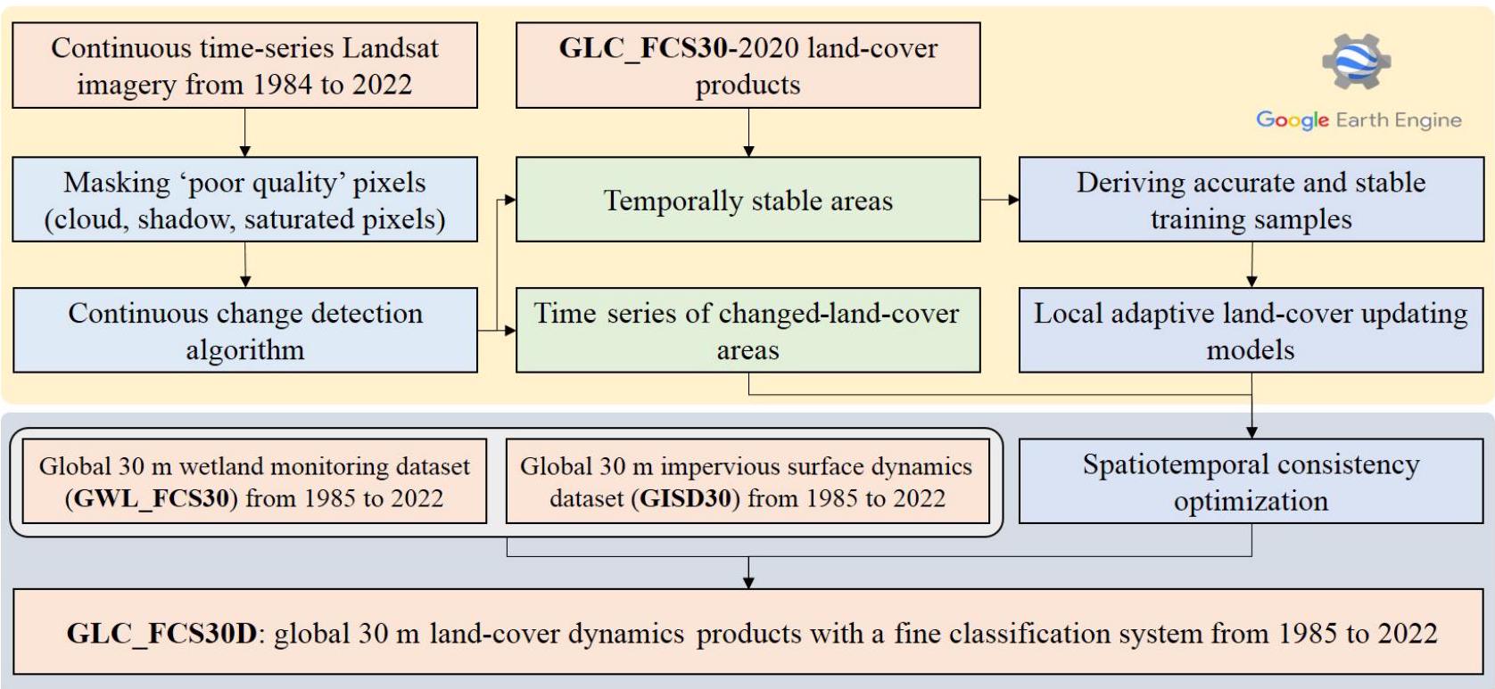
abrupt changes in the other land-cover pixels using the continuous change-detection model; (2) deriving the spatiotemporally stable training samples by using the spatiotemporal refinement method from the GLC_FCS30 land-cover product and temporally stable masks; (3) building the local adaptive classification models for each local region and then updating the land-cover information in the changed pixels; and (4) using the spatiotemporal consistency optimization method to improve the quality of land-cover change maps and suppress false changes.
Before detecting the changed land-cover pixels, all poor-quality pixels (cloud, shadow, and saturated pixels as well as the “scan line corrector off” pixels in Landsat 7) in the continuous-time-series Landsat imagery were first masked using the CFmask algorithm, which has been demonstrated to achieve an overall accuracy of and was adopted by the USGS as its official cloud and shadow detection algorithm (Zhu et al., 2015; Zhu and Woodcock, 2012). Then, in terms of these residual cloud pixels (i.e., those contaminated with light cloud and haze), the Tmask (multiTemporal mask) algorithm, which uses the temporal information from the clear-sky pixels to improve the cloud-detection capability (Zhu and Woodcock, 2014a), was used to mask the residual cloud pixels (note that Tmask
is integrated into the CCD algorithm on the GEE platform as ee.Algorithms.TemporalSegmentation.Ccdc()). In other words, the effect of poor-quality pixels was minimized.

3.1 The fine classification system used in GLC_FCS30D

Determining the classification system is usually a prerequisite for land-cover mapping and monitoring. In this study, as we used GLC_FCS30-2020 as the baseline land-cover product and overlaid the GWL_FCS30 dataset on GLC_FCS30D to ensure high accuracy in the wetland areas, the fine classification system used in this study is inherited from those of GLC_FCS30-2020 and GWL_FCS30. Table 1 lists the details of the fine classification system. It contains 35 fine land-cover types and has obvious advantages when identifying forest and wetland subcategories.

3.2 Detecting changes using the CCD algorithm and continuous Landsat imagery

In general, land-cover changes can be grouped into three categories: periodic changes caused by phenological variability, trend changes driven by natural behavior (such as vegetation growth), and abrupt changes caused by natural or human disturbances (such as deforestation or urban expansion). Thus, capturing these abrupt changes and simultaneously suppressing the periodic and trend changes is the key to land-cover monitoring. In this study, the CCD algorithm (Zhu and Woodcock, 2014b) was used to capture these abrupt changes. This algorithm uses Fourier transformation to fit the time-series observations with the trend term (estimating the trend changes) and harmonic terms (describing the periodic changes) in Eq. (1):
where represents the predicted value of the th band on the th Julian day; and are the regression slope and intercept of the th band, respectively; and represent the coefficients of the th-order harmonic term for the th band; denotes the number of harmonic terms; and is the day number of the year (usually defined as 365 ). In relation to determining the value of , Zhu and Woodcock (2014b) explained that higher-order harmonic terms provided better performance when capturing the periodic variability but caused overfitting in the time-series model and needed more clear-sky observations to initialize the coefficients and . After balancing the advantages and disadvantages of the higher-order harmonic terms, we finally set to be 3 , as suggested by other studies (Xian et al., 2022; Xie et al., 2022).
Then, as the CCD is a multivariate change-detection algorithm for capturing the changes in various land-cover types Zhu (2017), five Landsat spectral bands (excluding the blue band for minimizing the effects of the atmosphere and clouds) and three spectral indexes (NDVI (normalized difference vegetation index), NDWI (normalized difference water index), and NBR (normalized burn ratio), as given in Eq. 2) were combined to detect many kinds of changes in the Landsat time series.
,
NBR ,
where , and are the surface reflectance of green, red, NIR (near infrared) and SWIR1 (short-wave infrared 1) spectral bands in the Landsat imagery, respectively. Next, to determine the fitted coefficients of the thorder harmonic term in Eq. (1), the least absolute shrinkage and selection operator (LASSO) regression algorithm was applied, which demonstrated better performance than the traditional ordinary least squares method in reducing the overfitting problem and dealing with unevenly distributed and sparse Landsat observations (Zhu and Woodcock (2014b).
Next, the CCD model is a multiparameter change detection model and has been demonstrated to be sensitive to the parameter settings (Xiao et al., 2023; Zhu and Woodcock, 2014b). The CCDC algorithm on the Google Earth Engine platform (ee.Algorithms.TemporalSegmentation.Ccdc) contains three key adjustable parameters: minObservations, chiSquareProbability, and minNumOfYearScaler. Zhu et al. (2019) analyzed the relationships of the omission error and commission error of land-cover changes with the variabilities of three parameters in the United States, and they found that the values of the three parameters affected the change detection accuracy. In this study, we also investigated the sensitivity of the change detection accuracy to the parameter settings in Fig. S1 (in the Supplement) using the time-series points from the LCMAP_Val and LUCAS datasets after partly sampling. Notably, the sensitivity analysis was implemented in two large areas to ensure the feasibility of using the optimized parameters for other areas in land-cover change detection. The results also showed that CCD is a parameter-sensitive algorithm and that the optimal parameter values were , and 2 years for minObservations, chiSquareProbability, and minNumOfYearScaler, respectively.
After modeling the time-series observations using the CCD algorithm, we analyzed the land-cover changes based on the differences between the actual observations and the predicted values from the time-series fitting models. Figure 3 shows three typical scenarios in which the land-cover dynamics were modeled by the CCD algorithm. Specifically, Fig. 3a illustrates that there was no abrupt break during the whole pe-
Figure 2. The flowchart of the proposed method combining the continuous change-detection (CCD) algorithm and a local adaptive updating algorithm.
riod, and thus only a single time-series model was built and the pixel was usually labeled as temporally stable. Figure 3b indicates that the pixel underwent an abrupt change and the time-series observations were split into two segments. The time point of the abrupt change occurred around 1996. Figure 3c gives a complicated time-series disturbance example in which multiple abrupt changes were detected and the timeseries observations were split into four segments. The timeseries models for segments 1,2 , and 4 showed obvious trend changes.

3.3 Updating changed areas using local adaptive classifications

Using the CCD algorithm and continuous Landsat imagery, we identified the temporally stable pixels and the time points of abrupt changes for the land-cover change pixels. Accurately determining the land-cover labels of the changed pixels (or understanding the “from-to” change process) is another key procedure for land-cover time-series monitoring. To achieve this goal, we derived spatiotemporally stable training samples (see Sect. 3.3.1), updated the changed pixels using multitemporal classifications, and finally minimized the cumulative error caused by independent classifications.

3.3.1 Deriving spatiotemporally stable training samples

Numerous studies have demonstrated that the accuracy of the training samples plays a critical role in accurate mapping (Foody and Arora, 2010; Zhang et al., 2020). Visual interpretation can ensure high-confidence samples, but it requires
a lot of manual participation, so it is not suitable for collecting large-area training samples. An alternative option involves generating training samples by refining existing landcover products through a series of improvement measures (X. Zhang et al., 2021b; Zhang et al., 2023). Inspired by the latter option, we combined the GLC_FCS30-2020 prior dataset and the change-detection mask (derived using the CCD algorithm described in Sect. 3.2) to obtain the spatiotemporally stable training samples. Specifically, temporally stable areas are known to have higher mapping accuracy (Yang and Huang, 2021; Zhang and Roy, 2017; Zhang et al., 2023); thus, we first used the aforementioned CCD mask to retain the areas that were temporally stable during 19852022, and then we overlapped them with the GLC_FCS302020 maps to determine their land-cover labels. Next, because Radoux et al. (2014) emphasized that land-cover transition areas are usually subject to more serious misclassification problems and that pixels with homogeneous land cover have a higher probability of achieving acceptable accuracy, we used a morphological erosion filter of 3 pixels
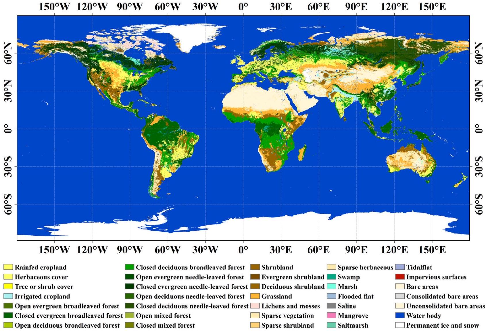
 pixels to refine these temporally stable areas into spatiotemporally homogeneous areas.
The spatiotemporally stable areas identified using the check for temporal stability during 1985-2022, spatial homogeneity analysis, and the GLC_FCS30-2020 product (which have an overall accuracy of ) were retained to generate the training samples. It should be noted that these spatiotemporally stable areas are not guaranteed to be completely accurate; that is, a small number of the derived training samples may have been mislabeled. Fortunately, previous studies of large-area land-cover mapping demonstrated
Table 1. The details of the fine classification system used in the GLC_FCS30D land-cover dynamics dataset.
Basic classification system Level-1 validation system Fine classification system ID
Cropland CRP Rainfed cropland RCP Rainfed cropland 10
Herbaceous cover cropland 11
Tree or shrub cover cropland 12
Irrigated cropland ICP Irrigated cropland 20
Forest FST Evergreen broadleaved forest EBF Closed evergreen broadleaved forest 51
Open evergreen broadleaved forest 52
Deciduous broadleaved forest BDF Closed deciduous broadleaved forest 61
Open deciduous broadleaved forest 62
Evergreen needleleaved forest ENF Closed evergreen needleleaved forest 71
Open evergreen needleleaved forest 72
Deciduous needleleaved forest DNF Closed deciduous needleleaved forest 81
Open deciduous needleleaved forest 82
Mixed-leaf forest MFT Closed mixed-leaf forest 91
Open mixed-leaf forest 92
Shrubland SHR Shrubland SHR Shrubland 120
Evergreen shrubland 121
Deciduous shrubland 122
Grassland GRS Grassland GRS Grassland 130
Tundra TUD Lichens and mosses LMS Lichens and mosses 140
Wetland WET Inland wetland IWL Swamp 181
Marsh 182
Flooded flat 183
Saline 184
Coastal wetland CWL Mangrove 185
Salt marsh 186
Tidal flat 187
Impervious surface IMP Impervious surface IMP Impervious surface 190
Bare areas BAL Sparse vegetation SVG Sparse vegetation 150
Sparse shrubland 152
Sparse herbaceous cover 153
Bare areas BAL Bare areas 200
Consolidated bare areas 201
Unconsolidated bare areas 202
Water body WTR Water body WTR Water body 210
Permanent snow and ice PSI Permanent snow and ice PSI Permanent snow and ice 220
that the random forest classification model (adopted in this study; see Sect. 3.3.2) is highly robust to erroneous training samples (Gong et al., 2019b; Mellor et al., 2015; X. Zhang et al., 2021b). For example, Gong et al. (2019b) found that the overall accuracy remained relatively stable provided the proportion of erroneous training samples was within . This provides support for the use of the spatiotemporally stable areas to derive confident training samples and further ensures the quality of land-cover dynamics monitoring.
Numerous studies have highlighted the importance of the training sample balance and distribution, as they significantly influence the mapping performance (Foody, 2009; Jin et al., 2014; Millard and Richardson, 2015). First, there are two options for the training sample distribution: areal-proportional or equal allocation. The former was shown to achieve higher accuracy than the latter option in land-cover mapping, especially in complicated land-cover conditions (Jin et al., 2014). However, when using the areal-proportional sampling strat-
Figure 3. Three typical land-cover changes identified using the continuous change-detection (CCD) algorithm and continuous Landsat observations. The times series show (a) a stable land-cover condition, (b) a single abrupt change, and (c) multiple abrupt changes.
egy, the rare land-cover types usually had small sample sizes and were sacrificed because the aim of land-cover mapping was to achieve a global optimum rather than a local optimum. Thus, the study of Zhu et al. (2016) suggested maximum and minimum sample sizes for abundant and rare land-cover types of 8000 and 600, respectively, to avoid the use of extremely large or small sample sizes. Thus, the GLC_FCS302020 product was then split into geographical tiles, and we used the areal-proportional sampling strategy and two sample balancing thresholds to allocate the training samples from the spatiotemporally stable areas in each geographical tile. Lastly, the impervious surface and wetland samples were excluded because both were independently developed as thematic datasets in Sects. 2.3 and 2.4.

3.3.2 Updating changed areas using local adaptive classifications

Before building the local adaptive classification models, we had to extract useful spectral features from the Landsat time-series observations. In this study, we used multitemporal phenological, texture, and topographical features. Specifically, the multitemporal phenological features were extracted by using the percentile-compositing method, which has fewer constraints than other compositing algorithms (such as the season-based compositing method) but achieves similar mapping accuracy (Azzari and Lobell, 2017). The spectral bands for the Landsat time series (five optical bands after excluding the atmospherically sensitive blue band) and the corresponding spectral indexes (NDVI, NDWI, and NBR in Eq. 2) were composited into five percentiles (10th, 25th, 50th, 75th, and 90th). Next, our previous study explained that the texture features made a positive contribution to land-cover mapping (X. Zhang et al., 2021b), so the gray-
level co-occurrence matrix method was used for the 50th-percentile-composited NIR band to extract the homogeneity, entropy, dissimilarity, variance, contrast, and correlation. Lastly, since the land-cover distribution is usually related to the topographical environment (for example, croplands and water bodies are mainly distributed in flat areas), three topographical variables (elevation, slope, and aspect) calculated from a global 30 m DEM dataset named ASTER_GDEM (Tachikawa et al., 2011) were also imported. In addition, due to the limited storage capacity and satellite-ground datatransmission capacity of early satellites, the density of Landsat imagery is sparse before 2000 (only a single satellite, Landsat 5, acquired data) (Roy et al., 2014b). Thus, we chose a coarse temporal cycle of 5 years to ensure the mapping accuracy before 2000; that is, the satellite observations from 2 years before and after were used for the nominal center year. For example, we updated the land-cover maps in 1995 using all available imagery from 1993 to 1997. In total, there were 49 multisource features, including 40 phenological spectra features, 6 texture features, and 3 topographical variables.
There are two options for global land-cover mapping and updating: global modeling and local adaptive modeling, and our previous studies have found that local adaptive modeling yields superior results compared to global modeling. This is primarily due to the former’s capability to take regional characteristics into account more effectively, leading to increased sensitivity in training samples and higher accuracy in land-cover classification (X. Zhang et al., 2021b, 2023, 2022). Thus, we first inherited the regional gridding style used in the GLC_FCS30 (X. Zhang et al., 2021b); namely, the global land was divided into geographical tiles. Afterward, the local classification models were independently built to update the land cover in each tile using the corresponding training samples in the neighboring eight surrounding tiles in a window. The adjacent training samples were imported to increase the continuity of the adjacent land-cover maps.
Lastly, in relation to the selection of the most suitable classification algorithm, the random forest (RF) classifier has significant advantages, including its capacity to accommodate high-dimensional training features and its better ability to deal with the overfitting problem and higher classification accuracy than other widely used classifiers (Belgiu and Drãgup, 2016; Gislason et al., 2006). The RF algorithm was also integrated into the internal function library of the GEE cloud platform as ee.Classifier.smileRandomForest(). Thus, the RF algorithm was used to combine the training samples and multisourced features to update the changed pixels. The RF algorithm allows for the adjustment of two key parameters (the number of decision trees (Ntree) and the number of predicted variables (Mtry), and previous studies have quantitatively analyzed the relationships between classification accuracy and the values of these two parameters. Both theoret-
ical and experimental results indicated that the selection of Mtry and Ntree had little influence on the classification accuracy (Belgiu and Drãgup, 2016; Du et al., 2015). Thus, based on previous studies (Belgiu and Drãgup, 2016; Zhang et al., 2019), the default recommended values of 500 for Ntree and the square of the total number of input features for Mtry were used.

3.3.3 Temporal-consistency optimization

To ensure the rationality and consistency of land-cover changes for long time series, the CCD algorithm was applied to capture the time points of land-cover changes, and then the changed pixels were updated using the local adaptive classifications. In this study, despite our best efforts, it was difficult to completely eliminate classification errors, particularly when dealing with changes over time. To address this issue and enhance accuracy in areas with temporal variations, we employed the temporal consistency optimization method described in Eq. (3). This approach incorporates both temporal and spatial neighboring information to assess homogeneity, thereby reducing potential misclassifications of changed areas in the time series.
Here, is the homogeneity probability of the pixel at spatial location ( ) and time point ; usually, the higher the value of , the weaker the classification error effect. and are, respectively, the land-cover labels of the central pixel and the corresponding spatiotemporally neighboring pixels in a local window of , and () denotes the indicator function for the equation of the status between two pixels. Namely, if is equal to , then the value of the indicator function is 1 ; otherwise, it is equal to 0 (Kenny, 2003). In this study, the homogeneity probability was calculated for each changed pixel, and a threshold of 0.5 (as suggested by and used in the studies of Li et al., 2015 and Zhang et al., 2022) was used to judge the rationality of land-cover changes; namely, when was less than the threshold, was modified according to the spatiotemporal pixels.

3.4 Accuracy assessment

The validation process for the GLC_FCS30D dataset followed the recommended guidelines proposed by Pontus Olofsson (2014). These guidelines encompass two key components: area estimation (non-site-specific accuracy) and accuracy assessment (site-specific accuracy). The site-specific accuracy assessment mainly focuses on estimating the confusion matrix and calculating some accuracy metrics, including overall accuracy (O.A.), producer’s accuracy (P.A.), and user’s accuracy (U.A.); and a poststratified estimator is used
to calculate the corresponding standard errors (Pontus Olofsson, 2014).
P.A.

O.A.
Here, is the proportion of the area mapped as class that had a reference class of and are the proportion of the area mapped as class and the proportion of the reference area mapped as class , respectively; and denotes the number of land-cover types. Afterwards, because there is currently no global long-time-series validation dataset, we used 84526 global validation points to assess the accuracy metrics of the GLC_FCS30D dataset in 2020 and used two third-party datasets to analyze the variation across the accuracy time series. GLC_FCS30D adopts a fine classification system containing 35 subcategories, for which we applied an analysis protocol to the basic classification system and the LCCS level-1 validation system, whose details are explained in the Table 1 and contained 10 major land-cover types and 17 fine land-cover types. Lastly, to quantify the performance of land-cover changed pixels, we followed the proposal of Stehman et al. (2021) for assessing the LCMAP annual land-cover products for 1985-2017; that is, the validation pixels were grouped into “changed” and “unchanged” categories and the corresponding confusion matrix was calculated. Meanwhile, to minimize the imbalance in sample size between the “change” and “no-change” samples, the F1 metric score was calculated as
.

4 Results and discussion

4.1 Overview of the GLC_FCS30D maps and their changes

Figure 4 provides an overview of the GLC_FCS30D dataset for 2022 (an overview of GLC_FCS30D for 1985 is given in Fig. S3); overall, it aligns with the real-world land-cover patterns on a global scale. Forest, cropland, barren land, and grassland are the dominant land-cover types, and each of them is distributed in the corresponding ecology subregions. For example, needle-leaved forest is mainly concentrated in the high-latitude cold regions, while broad-leaved forests are mainly distributed in tropical regions; permanent ice and snow are mainly located in Greenland and high-altitude mountains. GLC_FCS30D has significant advantages over other global land-cover datasets in terms of land-cover type diversity: it contains 35 discrete land-cover types, among which forests and wetlands are subdivided into 10 and 7 land-cover subcategories, respectively.
Figure 5a illustrates the spatial distribution of land-cover change intensity (measuring the proportions of changed pixels in the grid) in GLC_FCS30D from 1985 to 2022 after upscaling to a resolution of . Obviously, global land cover has experienced significant changes over the past 37 years, mainly in three areas: (1) areas on the periphery of tropical rainforests in South America and Southeast Asia, with deforestation the dominant cause; (2) areas where wetlands and water bodies intermingle (i.e., water bodies and wetlands transform into one another due to different annual water levels; note that the water body land-cover type in GLC_FCS30D represents permanent water during the year of interest, although the same area may be a wetland in other years), such as those in North America and northern Asia; and (3) semi-arid areas in Australia, Central Asia, and western Africa, where land cover (such as sparse vegetation or bare land) is directly affected by precipitation and temperature (for example, if there is sufficient precipitation in the year, the sparsely vegetated land and some of the bare land would be covered by grass in semi-arid areas; similarly, the work of Winkler et al., 2021 revealed that these semi-arid areas experienced serious and frequent land-cover changes). Figure 5b quantifies the changed area for 10 major land-cover types from 1985 to 2022. Forest and cropland variations dominated the global land-cover change. The net loss of forests over the past 37 years reached approximately 2.5 million , and the decline has been steady over time. Conversely, cropland showed a stable increase, and the net gain in cropland area is approximately 1.3 million . Shrubland, wetland, and impervious surface increased in area by 0.45 million, 0.40 million, and 0.37 million , respectively. The increased shrubland resulted from the recovery of deforested land, and the wetland gains are due to increases in seasonal water bodies. The work of Pekel et al. (2016) emphasized that global seasonal water bodies (labeled “inland wetlands” in GLC_FCS30D) showed an overall increase.
Figure 6 further analyzes the net area variations of 10 major land-cover types on six continents. The six continents exhibit various land-cover change characteristics; for example, steady forest loss and cropland gain dominate landcover change in South America, while the net area variations of most land-cover types fluctuate in Australia. North America has experienced obvious deforestation, and the area of forest loss reaches approximately . In contrast, the shrubland, grassland, and impervious surface landcover types show increasing trends overall, with increases of , and , respectively. Similarly, Xian et al. (2022) reported that forest losses and shrubland, grassland, and impervious surface gains were the dominant characteristics of the CONUS from 1985 to 2017. In Europe, the forest area continuously decreased, and the cropland area first decreased and then increased because of the collapse of the Soviet Union in 1990s. Abandoned croplands were transformed into pasture (which also belongs to the cropland land-cover type in GLC_FCS30D). Among
Figure 4. Overview of GLC_FCS30D for 2022; the color-coded legend is derived from the European Space Agency (ESA) Climate Change Initiative land-cover dataset (Defourny et al., 2018).
the six continents, the increase in impervious surface is the most significant in Asia, with a net increase of ; wetland also shows a large increase of . The increased wetland coverage comes from the increase in seasonal water bodies. South America and Africa have experienced similar land-cover change characteristics: they show the most intense deforestation rates and the most significant increases in cropland. According to our statistics, the forest loss on these two continents amounts to , and the corresponding increase in cropland is approximately . Lastly, Oceania is more sensitive to climate change, especially in terms of precipitation, so fluctuations in shrubland, grassland, and bare land are evident there because the conversion relationship between the three landcover types is related to annual precipitation.
Figure 7 displays the land-cover transformation relationships from 1985 to 2022 in the GLC_FCS30D dataset using Sankey diagrams. Global cropland and forest show obvious area changes, with area proportions changing from and , respectively, in 1985 to and , respectively, in 2022. Shrubland changed from in 1985 to in 2022. We mainly focus on forest, cropland,
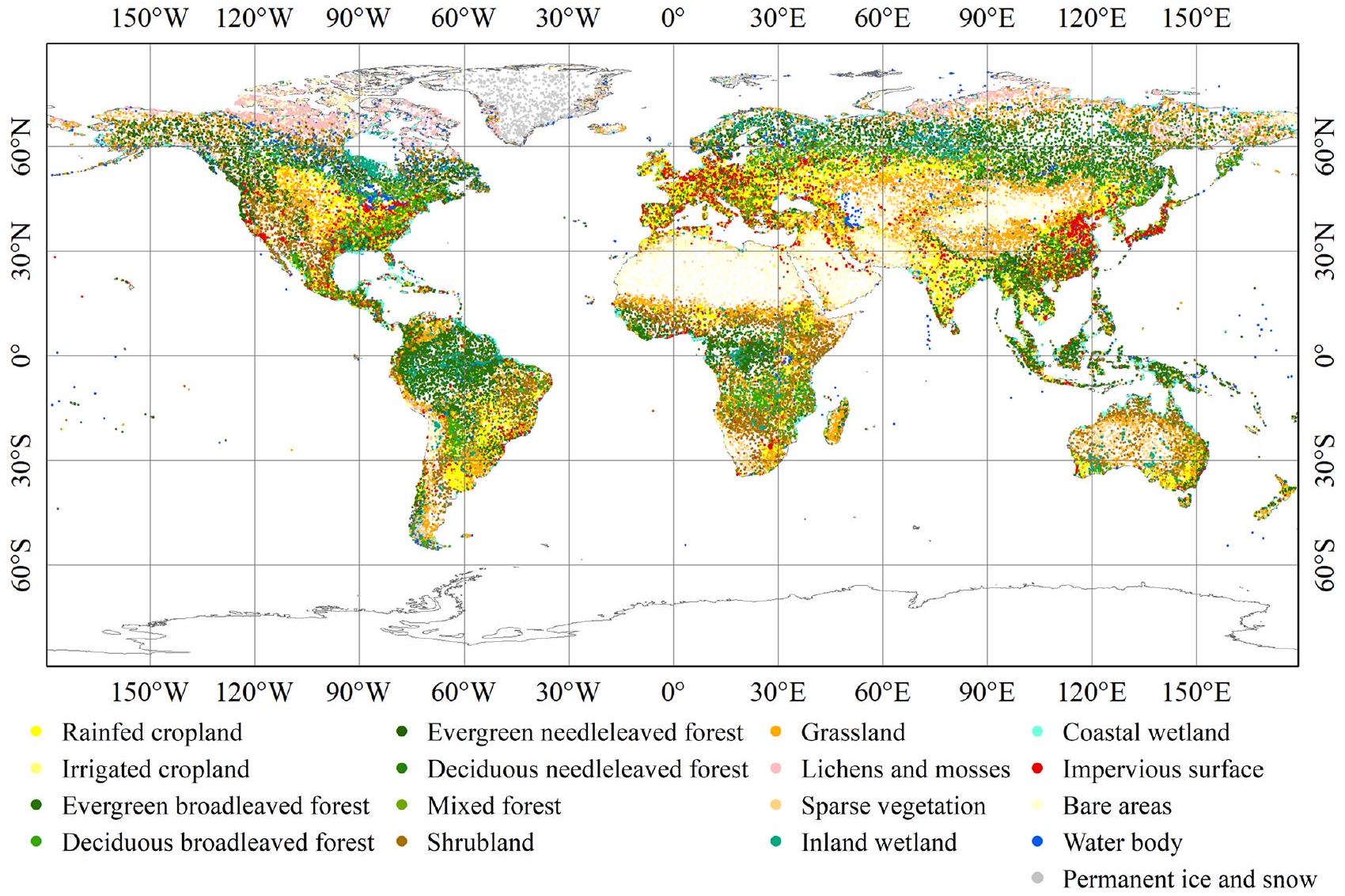
shrubland, and impervious surface changes, which dominate the land-cover changes in Fig. 5. There are three main causes of forest loss over the past 37 years: (1) of the deforested land was converted to cropland (this transformation was more significant in tropical rainforest areas; Fig. 8a); (2) of the lost forest was regrown as shrubland, which is more common in mountainous areas affected by wildfires; and (3) of the deforested land was converted to grassland. Cropland is converted to forest, grassland, and impervious surfaces. A total of of the lost cropland is converted to grassland due to abandonment, of the lost cropland is covered by forests, and of the lost cropland resulted from urbanization. Lastly, regarding impervious surfaces, our primary focus was on identifying the sources contributing to their expansion. Our findings indicate that approximately of the impervious surface increase can be attributed to the conversion of cropland, while of the increase is a result of deforestation.
To visually understand the land-cover change process captured by the GLC_FCS30D dataset over the past 37 years, Fig. 8 displays three typical enlargements (the spatial loca-
Figure 5. (a) The spatial distribution of global land-cover-change intensity from 1985 to 2022 after aggregation to a resolution of . (b) The net changed area of 10 major land-cover types in GLC_FCS30D from 1985 to 2022.
tions of the enlarged areas are illustrated as two black rectangles in Fig. 5a) of the Amazon rainforest (which experienced significant deforestation) and China’s Yangtze River Delta (which underwent rapid urbanization) and Yellow River delta (which showed evident land-cover changes over coastal regions). These three typical areas experienced drastic landcover changes, and GLC_FCS30D accurately captures those spatiotemporal changes. Specifically, the deforestation in South America is widely recognized, and GLC_FCS30D clearly reflects this trend. Namely, the early deforestation showed a grid distribution, and then each grid gradually extended outward and finally connected into patches.
GLC_FCS30D also shows that deforestation has not stopped in the region in terms of the rate of forest loss, and these findings are in line with the results of earlier research (Harris et al., 2021; Potapov et al., 2022). In the Yangtze River Delta, GLC_FCS30D depicts that the dominant land-cover change over the enlargement is urbanization, and a large quantity of irrigated cropland has been converted to impervious surfaces. Meanwhile, urban expansion was significantly faster before 2010 than after 2010 according to GLC_FCS30D. Lastly, the Yellow River delta, a typical coastal region, was selected to assess the ability of GLC_FCS30D to capture these coastal land-cover changes. Obviously, the land-cover changes in
Figure 6. The net area variations of 10 major land-cover types on six continents from 1985 to 2022.
Figure 7. Sankey diagrams of the global land-cover changes during 1985-2022 in the GLC_FCS30D dataset.
GLC_FCS30D can be summarized as three aspects: (1) a large number of flooded flats and tidal flats were reclaimed as aquaculture ponds, especially after 2000; (2) the mouth of the Yellow River changed from a southerly orientation to a northerly one (black rectangle), i.e., there were large land-cover changes between tidal/flooded flats, water bodies, and salt marshes; and (3) a lot of impervious surfaces encroached on the coastal water bodies and flats. In short, by combining real remote-sensing observation time series data, GLC_FCS30D effectively captures the spatiotemporal changes of the land surface.

4.2 Accuracy assessment of GLC_FCS30D for 2020

Table 2 provides the error matrix and accuracy metrics for the GLC_FCS30D dataset in the basic classification system con-
taining 10 major land-cover types. The novel GLC_FCS30D dataset attained an O.A. of . Cropland, forest, impervious surface, water body, and permanent snow and ice perform better in terms of the P.A. and U.A. than the remaining land-cover types, with the corresponding accuracies exceeding . The impervious surface and wetland datasets are independently generated and then overlaid on GLC_FCS30D, helping these complicated land-cover types to achieve high accuracy metrics. Conversely, grassland, shrubland, and tundra have lower accuracies; for example, grassland had the lowest P.A. of and shrubland had the lowest U.A. of . The two reasons that they performed poorly were as follows: (1) these land-cover types usually reflected heterogeneous and varied spectral and spatial characteristics, e.g., the grassland showed similar spectra to cropland and sparse shrubland in the growing season but
Figure 8. Three typical enlargements showing the land-cover changes according to GLC_FCS30D from 1985 to 2022 in (a) the Amazon rainforest, (b) the Yangtze River Delta in China, and (c) the Yellow River delta in China. The color coding is the same as that used for the global map in Fig. 4. In each case, the natural-color imagery from 1985 to 2022 are composites taken from Landsat imagery.
mimicked bare-land features in harvest season, and (2) all of them were distributed in climate-transition areas with complicated climate variations and landscapes.
Table 3 provides the error matrix of GLC_FCS30D for 2020 in the LCCS level-1 validation system with 17 landcover types. The GLC_FCS30D-2020 dataset achieves an O.A. of , which is lower than that achieved with the basic classification system because these similar land-cover subcategories suffer more easily from misclassification. For example, forest has a P.A. of 92.83 % , but the P.A. rapidly decreases to the range of
to when forest is split into five fine subcategories. Cropland, forest, and bare land, which are further divided into multiple subcategories, show obvious decreases in accuracy for their subcategories in terms of P.A. and U.A. Taking cropland and forest as examples, approximately of the irrigated cropland (ICP) is misclassified as rainfed cropland (RCP), and so the U.A. of ICP is only . More than of the mixed-leaf forests (MFT) are wrongly labeled as the other four forest subcategories, and so the ‘mixed-leaf forests have the lowest U.A. of . Meanwhile, sparse vegetation
)6でて6 (9 I) (で I) 969 L (II.I) 89 I9 )S0.99
t6 II S ISZ E LL8* [W]OL
I) I ISE I 0 100.0 EZ0.0 0 S00.0 t00% 0 ISd
(8.0)S* 6 L 829*II IEI*0 6EZ6 8 to. 0 LLS* 0 St0.0 Et0.0 S8S* 0 E8L0 6500 TVG
(19*0)St S6 E8Z'S 0 tZ0* 2000 9000 100.0 t0.0 tZ0.0 8S0.0 七80.0 dWI
tSt E Z00% vtt? 810.0 L91.0 8910 EZI•0 10.0 G
ZI I IE8 2000 6E0*0 ZI0% 800.0 S0E E て0E 0 6100 9800 t0.0 yLM
I) 9IS'S ててで0 IZ0.0 L E0.0 LSI•0 9 SI*0 S9+ 0 LAM
9 SE 6 2000 Z0S*0 S0.0 6100 I9I*0 Z6E E98* SSS.0 YHS
It SS8.0I L8I'I LS0.0 t80.0 1100 IEZ 0 I8I*I 906 S 99I'I SE0.I SHD
(IE*0)E8*Z6 Z00% EII*0 800.0 IZ0.0 ILE 0 II8.0 SIE゙0 ZIL•8 EIS゙0 LSA
t0ピLI 0 LII*0 tLI•0 0 L20% Z6L*0 Z SI дY( 3
(AS) V d [ண口 ISd TVЯ dWI G YLM LAM УНS SYD LSA дУО әวแวเอมิy
(%LZ dw
*sәзәциәнех иі имоцу( AS )яюнә рлериемs виџриоdsәнюл
Figure 9.Time series of the overall accuracy of the GLC_FCS30D dataset using the LCMAP_Val annual reference dataset across the contiguous United States(CONUS)from 1985 to 2018.The error bars on the graph show the uncertainty of the data points.
has the second lowest U.A.of because of the confusion between sparse vegetation,grassland,and bare land.In the basic classification system(Table 1),sparse vegetation is grouped with bare land.A previous study in the European Union proposed grouping it with grassland(Gao et al.,2020).Wetland is further divided into coastal wetland (CWL)and inland wetland(IWL)in Table 3,and CWL has a higher U.A.than that of wetland in Table 2,which is pri- marily attributable to the significantly more accurate classi- fication of wetland in the CWL subcategory(Zhang et al., 2023).

4.3 Accuracy assessment based on two third-party regional validation datasets

4.3.1 Time series of accuracy metrics of GLC_FCS30D from the LCMAP_Val dataset

Figure 9 displays a time series of the overall accuracy of the GLC_FCS30D dataset using the LCMAP_Val annual validation dataset from 1985 to 2018 over the CONUS. GLC_FCS30D achieves a mean O.A.of and the O.A.varies from a high value of in 2015 to a low value of in 2000.The overall accuracy of GLC_FCS30D is slightly lower at the early stage,which might be related to the density of Land- sat observations.The early Landsat missions had weaker satellite-to-ground transmission and onboard recording ca- pabilities(Roy et al.,2014a),so the phenological variability and land-cover changes were more difficult to capture at the early stage.
Figure 10 shows time series of the P.A.and U.A.for the GLC_FCS30D dataset in the CONUS.Visually,the P.A.and U.A.values of the 10 major land-cover types range from to and from to ,respectively,and
Table 3. Error matrix of the GLC_FCS30D dataset for 2020 based on the LCCS level-1 validation system. The reported producer’s accuracy (P.A.) and user’s accuracy (U.A.) come with corresponding standard errors (SE) shown in parentheses.
Reference RCP ICP EBF DBF ENF DNF MFT SHR GRS LMS SVG IWL CWL IMP BAL WTR PSI Total P.A. (SE)
RCP 12.225 1.023 0.239 0.358 0.102 0.016 0.009 0.382 0.66 0 0.078 0.056 0.005 0.124 0.028 0.001 0 15.332 79.7 (0.7)
ICP 0.397 1.932 0.026 0.016 0.005 0 0 0.01 0.025 0 0.012 0.029 0.005 0.052 0 0.018 0 2.527 76.45 (1.81)
EBF 0.2 0.048 9.091 1.098 0.262 0.103 0.151 0.371 0.084 0 0.012 0.136 0.028 0.029 0.001 0.004 0 11.514 78.96 (0.82)
DBF 0.187 0.016 0.632 6.838 0.537 0.294 0.396 0.235 0.144 0.002 0.019 0.077 0.002 0.025 0.005 0.004 0.002 9.054 75.53 (0.97)
ENF 0.046 0.004 0.174 0.316 5.681 0.328 0.439 0.128 0.034 0.006 0.043 0.094 0 0.008 0.01 0.01 0 6.895 82.39 (0.98)
DNF 0.008 0 0.002 0.13 0.245 1.854 0.073 0.071 0.053 0 0.011 0.025 0 0.001 0.007 0.002 0 2.414 76.79 (1.85)
MFT 0.004 0 0.019 0.176 0.234 0.013 0.828 0.014 0.004 0 0 0.010 0.05 0 0.001 0 0 1.308 58.29 (1.53)
SHR 0.518 0.042 0.299 0.9 0.328 0.131 0.034 5.44 0.871 0.019 0.441 0.157 0.005 0.05 0.065 0.013 0.002 9.438 57.63 (1.09)
GRS 0.947 0.097 0.167 0.582 0.209 0.154 0.024 1.191 5.958 0.085 0.974 0.229 0.006 0.052 0.217 0.008 0.01 10.95 54.41 (1.02)
LMS 0.006 0.004 0.001 0.022 0.044 0.053 0.001 0.168 0.169 2.465 0.379 0.02 0.001 0.002 0.098 0.026 0.02 3.484 70.76 (1.65)
SVG 0.064 0.01 0.008 0.006 0.007 0.01 0.001 0.397 0.462 0.025 2.71 0.012 0 0.013 0.643 0.002 0.024 4.399 61.6 (1.57)
IWL 0.01 0.002 0.044 0.029 0.103 0.022 0.002 0.048 0.017 0.008 0.042 2.673 0.024 0.001 0.012 0.224 0 3.263 81.91 (1.45)
CWL 0.004 0.002 0.008 0.002 0.004 0.002 0.004 0.008 0.006 0 0.008 0.188 1.476 0.007 0.007 0.059 0 1.783 82.77 (1.92)
IMP 0.074 0.011 0.008 0.008 0.037 0.002 0 0.041 0.024 0.002 0.014 0.004 0 5.087 0.01 0.004 0 5.329 95.45 (0.61)
BAL 0.048 0.01 0.002 0.004 0.002 0.001 0 0.193 0.328 0.557 0.582 0.043 0.002 0.035 5.384 0.029 0.108 7.33 73.45 (1.11)
WTR 0.014 0.024 0.014 0.014 0.019 0.008 0.006 0.011 0.016 0.007 0.011 0.168 0.114 0.011 0.019 3.054 0.002 3.509 87.04 (1.22)
PSI 0 0 0 0.001 0.002 0 0 0.005 0.03 0.001 0.011 0 0 0 0.019 0.023 1.363 1.455 93.65 (1.37)
Total 14.757 3.224 10.753 10.56 7.833 3.724 1.97 8.711 8.883 3.179 5.353 3.927 1.668 5.497 6.526 3.482 1.532
U.A. (SE) 82.85 (0.67) 59.92 (1.85) 84.55 (1.75) 64.76 (1) 72.52 (1.08) 49.77 (1.76) 39.34 (1.38) 62.44 (1.11) 67.07 (1.07) 77.55 (1.59) 50.63 (1.47) 68.07 (1.6) 88.49 (1.68) 92.54 (0.76) 82.5 (1.01) 87.73 (1.19) 88.96 (1.72)
O.A. 73.04 % ( %)
Note: the abbreviations correspond to the 17 categories of the LCCS validation system in Table 1.
the time-series variations are stable. Among them, the water body land-cover type has the highest accuracy metrics, achieving mean P.A. and U.A. values of and , respectively, which benefit from the unique spectral characteristics of this land-cover type. Cropland follows, with mean P.A. and U.A. values of 93.37 % and , respectively. Forest ranks third, with a high P.A. of but a relatively low U.A. of ; the unbalanced metrics occur because GLC_FCS30D and LCMAP_Val have different definitions for forest. GLC_FCS30D defines a forest as having a tree cover greater than , while the threshold setting of LCMAP_Val is , so many of the shrublands in GLC_FCS30D are labeled as forests in LCMAP_Val. Wetland has a U.A. value of 90.47 % ( ) but a P.A. value of , which is also caused by a discrepancy in the definition of wetland. GLC_FCS30D identifies seasonal water bodies as wetlands while LCMAP_Val classifies them as water bodies. Impervious surface has a P.A. lower than , mainly because the GLC_FCS30D and LCMAP_Val datasets have different definitions of impervious surface. LCMAP_Val defines buildings and the surrounding green areas as developed, while GLC_FCS30D only includes the artificial buildings (houses, roads, squares, and so on). Bare land and shrubland have the lowest U.A. values of and , respectively, mainly because both of them are easily confused with grassland due to their complicated spectral characteristics and because they coexist in climate-sensitive semi-arid regions (e.g., the Midwestern United States). Xian et al. (2022) emphasized that long-term monitoring of shrubs and grasslands presents significant challenges in the CONUS. Permanent snow and ice, which is sparsely distributed in highelevation mountainous areas of the United States, has unique and specific spectral characteristics, so it achieves a P.A. of in GLC_FCS30D. The large fluctuations in U.A. for ice and snow are attributed to (1) the small sample size for ice and snow in the LCMAP_Val dataset and (2) a few misclassified grass/bare land pixels that are correctly identified as snow and ice during 2005-2014.
Figure 11 shows the area-bias percentages of eight landcover types estimated by GLC_FCS30D and LCMAP_Val across the CONUS. Intuitively, GLC_FCS30D and LCMAP_Val share similar total areas for estimations of cropland, bare land, and water bodies but evident area deviations for estimations of forest, shrubland, and grassland. The deviations in shrubland and grassland occur mainly because these land-cover types coexist in the semi-arid regions of the central United States and share similar spectral characteristics and temporal variability; thus, some grasslands in LCMAP_Val are considered shrublands in GLC_FCS30D. Xian et al. (2022) also failed to distinguish grassland from shrubland and combined them into a group when generating LCMAP annual maps. LCMAP_Val has a broader definition of impervious surface, which results in negative bias, so the
impervious surface area estimated in LCMAP_Val is larger than the assessment in the GLC_FCS30D dataset.
Table 4 analyzes the confusion matrix of changed and unchanged land-cover pixels in GLC_FCS30D using the LCMAP_Val dataset. It should be noted that the changed land-cover samples in LCMAP_Val were still sparse; that is, the size of the changed samples cannot support the analysis of specific land-cover changes. Similarly, Stehman et al. (2021) grouped the land-cover types into “no change” and “change” types for analyzing the land-cover changes. In this study, when using the “changed” and “unchanged” validation points in LCMAP_Val, the O.A. of GLC_FCS30D reached . In particular, the unchanged landcover pixels played a dominant role and reached a high P.A. of and a high U.A. of . In contrast, the P.A. and U.A. of the changed land-cover pixels were and , and the F1 score was 63.49 %.

4.3.2 Time series of accuracy metrics of GLC_FCS30D from the LUCAS dataset

Table 5 lists the time series of accuracy metrics of the GLC_FCS30D dataset across the European Union (EU) from 2006 to 2018 using the LUCAS dataset. The GLC_FCS30D dataset has a mean O.A. of and an O.A. range of to in the EU . The two dominant land-cover types (cropland and forest), which cover almost of the entire EU area (Gao et al., 2020), have higher P.A. and U.A. values than the other land-cover types. The P.A. and U.A. of cropland exceed and , respectively. Forest has unbalanced P.A. (approximately ) and U.A. (approximately ) values because the LUCAS dataset defines forest more broadly than the GLC_FCS30D dataset does. In particular, sparse vegetation associated with forest is grouped with forest in LUCAS but with bare land in GLC_FCS30D. Gao et al. (2020) explained the discrepancy in the definition of forest between LUCAS and GLC_FCS30. Shrubland, grassland, and bare land showed inferior performance in terms of both P.A. and U.A. because of their complicated spectral variability and spatial heterogeneity. Gao et al. (2020) also found that three global 30 m land-cover products (GlobeLand30, FROM_GLC, and GLC_FCS30) exhibited poor performance for these three land-cover types. Urban green space and discontinuous urban fabric, which are excluded from GLC_FCS30D, are grouped with impervious surface in LUCAS. Thus, impervious surface also has a low P.A. of approximately . Lastly, upon investigating the temporal variability of P.A. and U.A. we find that permanent ice and snow and wetland show greater variability and that both are closely related to annual temperature and precipitation; i.e., their spatial distributions are affected by the natural environment.
Figure 10. Time series of the producer’s accuracy and user’s accuracy of GLC_FCS30D based on the LCMAP_Val dataset from 1985 to 2018 in the contiguous United States (CONUS). The error bands represent standard error.
Figure 11. The area-bias percentages of eight land-cover types in the GLC_FCS30D and LCMAP_Val datasets from 1985 to 2017 in the contiguous United States (CONUS).
Table 6 shows the area proportions of 10 major landcover types from both the GLC_FCS30D dataset (“Map”) and the LUCAS validation dataset (“Ref”). The area bias (“AB”) measures the area deviations between the two different datasets for the same land-cover type. Overall, GLC_FCS30D overestimates the total area assessments of forest, bare land, and ice and snow and underestimates the re-
maining land-cover types in comparison to the LUCAS estimations. In particular, according to its AB of , forest shows the most significant overestimation, while cropland shows the most underestimation ( AB of ). Cropland and forest cover together account for approximately of the total EU area (Gao et al., 2020)); as a result, the area bias (AB) values for these two land-cover types are
Table 4. The confusion matrix of changed and unchanged pixels in GLC_FCS30D when using the LCMAP_Val datasets.
Unchanged Changed Total P.A. (SE) F1
Unchanged 82.21 6.34 88.55 94.53
Changed 3.18 8.27 11.45 63.49
Total 85.39 14.61
U.A. (SE)
O.A. (SE)
Table 5. Time series of accuracy metrics of the GLC_FCS30D dataset using the LUCAS validation dataset across the European Union.
2006 2009 2012 2015 2018
P.A. (SE) U.A. (SE) P.A. (SE) U.A. (SE) P.A. (SE) U.A. (SE) P.A. (SE) U.A. (SE) P.A. (SE) U.A. (SE)
CRP 85.49 (0.11) 93.37 (0.08) 85.40 (0.11) 93.31 (0.08) 85.50 (0.11) 93.17 (0.08) 85.47 (0.11) 93.05 (0.08) 85.52 (0.11) 92.82 (0.08)
FST 95.22 (0.08) 76.71 (0.15) 94.97 (0.08) 76.71 (0.15) 94.79 (0.09) 76.82 (0.15) 94.36 (0.09) 76.82 (0.15) 93.71 (0.09) 76.85 (0.15)
GRS 6.13 (0.26) 21.31 (0.83) 6.10 (0.26) 21.13 (0.83) 6.05 (0.26) 20.98 (0.83) 6.08 (0.26) 20.71 (0.82) 5.99 (0.26) 20.74 (0.82)
SHR 8.13 (0.42) 8.93 (0.46) 8.25 (0.43) 8.92 (0.46) 8.02 (0.42) 8.77 (0.46) 7.84 (0.42) 8.60 (0.45) 8.35 (0.43) 8.96 (0.46)
WET 63.10 (0.81) 66.55 (0.81) 61.40 (0.81) 65.55 (0.82) 61.86 (0.81) 66.21 (0.82) 62.64 (0.81) 66.60 (0.81) 62.94 (0.81) 65.34 (0.81)
WTR 89.73 (0.40) 92.44 (0.36) 90.09 (0.40) 92.53 (0.35) 90.28 (0.39) 92.36 (0.36) 90.83 (0.38) 91.63 (0.37) 90.10 (0.40) 91.56 (0.37)
IMP 58.55 (0.56) 72.69 (0.56) 59.21 (0.55) 72.06 (0.56) 59.06 (0.55) 71.72 (0.56) 58.65 (0.55) 70.85 (0.56) 59.01 (0.55) 70.29 (0.56)
BAL 52.77 (1.12) 39.62 (0.95) 52.90 (1.12) 38.44 (0.93) 52.19 (1.13) 37.70 (0.93) 52.07 (1.13) 36.16 (0.90) 52.33 (1.13) 34.69 (0.87)
PSI 86.02 (5.00) 35.01 (4.38) 91.40 (4.04) 36.56 (4.38) 89.25 (4.46) 31.86 (4.00) 96.24 (2.74) 31.40 (3.81) 96.24 (2.74) 31.35 (3.81)
O.A. (SE) 82.11 (0.09) 81.99 (0.09) 81.97 (0.09) 81.82 (0.09) 81.64 (0.09)
more noticeable or pronounced compared to the AB values of the other land-cover types.
Table 7 presents the confusion matrix of changed and unchanged pixels obtained using the LUCAS validation datasets. The O.A. of GLC_FCS30D reached ; the P.A. and U.A. of the changed pixels were and , respectively; and the corresponding F1 score was . In contrast, the unchanged land-cover pixels reached high P.A. and U.A. values, with both metrics exceeding . Thus, the changed land-cover pixels were more difficult to capture compared with these unchanged pixels. Similarly, Stehman et al. (2021) also found that the accuracy metrics of the changed pixels were far lower than those of the unchanged pixels: the producer’s accuracy of the changed pixels and unchanged pixels was and , respectively.

4.4 Comparisons with other global land-cover dynamics products

Figure 12 gives qualitative comparisons between our GLC_FCS30D and two widely used land-cover dynamics datasets (CCI_LC and MCD12Q1) for 2001-2020 in the Indo-China Peninsula, which experienced evident land-cover changes in terms of forest deforestation and urban expansion during that period. In terms of urban expansion, the three datasets revealed rapid urbanization in the megacity of Bangkok, while CCI_LC underestimated the impervious surface area in 2001 compared with the other two datasets. Meanwhile, GLC_FCS30D also captured more spatial detail
(such as rural buildings and road networks) than CCI_LC and MCD12Q1 because of its high spatial resolution of 30 m .
In terms of the most significant deforestation, CCI_LC showed the worst performance because (1) it underestimated the forest cover in 2001 (rectangular region 1: R1), i.e., some forests were wrongly labeled croplands; (2) some deforested areas were not captured during the period 2001-2020 in rectangular region 2 (R2), so its deforested forest area was less than in GLC_FCS30D and MCD12Q1; and (3) there was an obvious problem with the misclassification of forest as wetland in 2001 (rectangular region 3: R3). MCD12Q1 also suffered from a forest omission error in R1; namely, the captured forest area in 2001 was lower than the actual forest area based on natural-color imagery. As for the evident deforestation in R2, we find that almost all forest pixels changed to the other land-cover types (savanna and grassland) in MCD12Q1, which obviously deviated from the actual situation; thus, MCD12Q1 overestimated the forest deforestation. Meanwhile, the MCD12Q1 time series showed various land-cover distributions in R3, which indicated that MCD12Q1 has lower mapping accuracy and temporal stability for these wetland areas. In comparison, GLC_FCS30D achieved the best performance in capturing the spatial distribution of forest in 2001, deforestation during 2001-2020, and wetland stability.
Figure 13 shows another comparison example for these three datasets, focusing instead on Paraguay, South America. The most evident land-cover changes were deforestation and increased cropland according to the time seriies of Landsat natural-color imagery. In terms of the spa-
Table 6. The area proportions and area bias (AB) values of 10 major land-cover types from the GLC_FCS30D dataset (Map) and the LUCAS validation dataset (Ref).
2006 2009 2012 2015 2018
Map Ref AB Map Ref AB Map Ref AB Map Ref AB Map Ref AB
CRP 46.48 50.62 -4.14 46.46 50.64 -4.18 46.59 50.67 -4.08 46.63 50.69 -4.06 46.77 50.74 -3.97
FST 41.39 33.76 7.63 41.28 33.75 7.53 41.14 33.73 7.41 40.96 33.73 7.23 40.66 33.68 6.98
GRS 1.21 4.15 -2.94 1.21 4.15 -2.94 1.21 4.15 -2.94 1.23 4.15 -2.92 1.21 4.15 -2.94
SHR 1.91 2.08 -0.17 1.94 2.08 -0.14 1.92 2.08 -0.16 1.91 2.07 -0.16 1.95 2.06 -0.11
WET 1.70 1.75 -0.05 1.68 1.74 -0.06 1.68 1.73 -0.05 1.69 1.71 -0.02 1.73 1.72 0.01
WTR 2.75 2.85 -0.1 2.76 2.85 -0.09 2.77 2.85 -0.08 2.81 2.85 -0.04 2.79 2.86 -0.07
IMP 3.18 3.82 -0.64 3.25 3.83 -0.58 3.25 3.82 -0.57 3.27 3.82 -0.55 3.32 3.82 -0.5
BAL 1.32 0.95 0.37 1.36 0.95 0.41 1.37 0.95 0.42 1.42 0.95 0.47 1.49 0.95 0.54
PSI 0.06 0.02 0.04 0.06 0.02 0.04 0.07 0.02 0.05 0.07 0.02 0.05 0.07 0.02 0.05
Table 7. The confusion matrix of changed and unchanged pixels in GLC_FCS30D when using LUCAS time-series datasets across the Europe Union.
Unchanged Changed Total P.A. (SE) F1
Unchanged 82.69 2.79 85.48 96.73 94.49
Changed 6.84 7.68 14.52 52.86 61.43
Total 89.53 10.47
U.A. (SE)
O.A. (SE)
tial distribution, the consistency between GLC_FCS30D and CCI_LC was higher, while MCD12Q1 was obviously different from the other two datasets. A large number of deciduous broadleaved forests were labeled as savanna and woody savanna, and most croplands were identified as grasslands in MCD12Q1, mainly because of the difference in classification system. In terms of the changed-land-cover areas, the GLC_FCS30D showed the highest accuracy and captured richer spatial detail. For example, the deforestation intensity during 2010-2020 was significantly greater than that during 2001-2010, and GLC_FCS30D also revealed the regular deforestation caused by human factors. In contrast, CCI_LC and MCD12Q1 captured neither the deforestation during 2010-2020 nor the small and fragmented changes (caused by human activities).

4.5 Limitations of and perspectives on the GLC_FCS30D dataset

To achieve the goal of accurate and robust monitoring of global land-cover change, four steps are adopted: (1) the advantages of the CCD model and the full time series of Landsat observations are combined to capture the land-cover change time points for any changed pixels; (2) the temporally stable areas are used as prior knowledge to ensure the quality of training samples and local adaptive modeling is adopted to update the land-cover transitions of these changed pixels; (3) global thematic products for two complicated land-cover
types (impervious surface and wetland) are independently developed to improve the reliability of GLC_FCS30D; and (4) the “spatiotemporal consistency checking” optimization in Sect. 3.3.3 is applied to further guarantee the stability and accuracy of GLC_FCS30D. The accuracy assessments performed using the developed global validation dataset and two third-party datasets demonstrate that GLC_FCS30D fulfills the accuracy requirements for a baseline year and for timeseries variability at a global or national scale. Comparisons with other land-cover products also highlight the superiority of GLC_FCS30D in terms of classification system diversity and the monitoring accuracy of these changed areas. However, monitoring global land-cover change across a long time series is an extremely complex and difficult task (Hansen and Loveland, 2012; Song et al., 2018; Winkler et al., 2021; Xian et al., 2022). Although this study uses a series of measurements and methods to achieve global 30 m land-cover change monitoring for the past 37 years, there are still some uncertainties and limitations that need to be resolved in further work.
The CCD algorithm makes full use of dense satellite observations to capture land-cover changes robustly and accurately (Zhu and Woodcock, 2014b; Zhu et al., 2012). However, previous studies have demonstrated that their reliability is highly correlated to the density of valid satellite observations (Bullock et al., 2022; Ye et al., 2021; Zhu et al., 2019). Cloudy and snowy areas lead to greater uncertainty when
Figure 12. Comparisons of GLC_FCS30D with the CCI_LC and MCD12Q1 land-cover dynamics products for the Indo-China Peninsula during 2001-2020. The natural-color imagery were composited from the time-series Landsat imagery.
capturing the time points of land-cover change (DeVries et al., 2015; Xian et al., 2022). Additionally, due to the limited storage capacity and satellite-ground data-transmission capacity of early satellites, the density of Landsat imagery is sparse before 2000 (only a single satellite, Landsat 5, acquired data) (Roy et al., 2014b). In this study, we combine the satellite observations from 2 years before and after the nominal center year from 1985 to 1995; for example, we update the land-cover maps in 1995 using all available imagery from 1993 to 1997. However, a previous study found that northeastern Asia did not have any valid Landsat observations be-
fore 2000 (Zhang et al., 2022), which means that some landcover changes could not be captured in these areas before 2000 in GLC_FCS30D. To solve the problem of missing and sparse observations, a useful solution is to fuse multisourced remote-sensing imagery. For example, Y. Zhang et al. (2021) combined Landsat and Sentinel-2 imagery to track tropical forest disturbances with an overall accuracy of more than . Therefore, further work will investigate the feasibility of integrating Sentinel-1/2, SPOT, MODIS, and AVHRR imagery as auxiliary datasets to achieve annual land-cover
Figure 13. Comparisons of GLC_FCS30D with two land-cover-dynamics time-series datasets for Paraguay, South America, during 20012020. The natural-color imagery were composited from the time-series Landsat imagery.
monitoring before 2000 and further ensure land-cover monitoring quality.
To ensure the stability of GLC_FCS30D, a spatiotemporal consistency optimization algorithm that has been widely used in impervious surface change optimizations (Li et al., 2015; Zhang et al., 2022) was applied. This makes full use of spatiotemporally neighboring pixels to calculate the landcover homogeneity and then remove the “salt and pepper” noise caused by the pixel-based classifications. Qualitative comparisons for deforested areas of the Amazon and areas of China that have undergone urban expansion (Fig. S2
in the Supplement) also showed that the spatiotemporal consistency optimization can improve the data quality of GLC_FCS30D by suppressing salt and pepper noise and optimizing the temporal consistency. Similarly, Yang and Huang (2021) used this algorithm to optimize China’s annual land-cover products during 1990-2019, and found that it improved the mapping accuracy of the land-cover time-series dataset.
GLC_FCS30D reveals a large number of land-cover changes in the semi-arid regions illustrated in Fig. 5a; these land-cover changes are more influenced by climate factors.
For example, the central region of Australia is a typical semiarid region, and the dominant land-cover types are grassland, sparse vegetation, shrubland, and bare land. In general, if there is sufficient annual precipitation, the distributions of shrubland and grassland in the area will be more extensive; otherwise, the area will be dominated by bare land and sparse vegetation (Dong et al., 2020; Ge et al., 2022). Recently, some studies suggested suppressing these changes; for example, Bastos et al. (2022) chose to suppress these land-cover changes by fusing these four land-cover types into a single grassland land-cover type for Australia, and Xian et al. (2022) combined grassland and shrubland in the CONUS. Whether these frequent and climate-sensitive landcover changes should be suppressed will be considered in our further work.
Although we used a global validation dataset to assess the capability of GLC_FCS30D in the baseline year of 2020 and two third-party regional datasets to assess its variability of the accuracy across the time series in the European Union and the CONUS, the accuracy assessment work should be strengthened. In particular, the classification system differences between GLC_FCS30D, LUCAS, and LCMAP_Val cannot be ignored. For example, the impervious surface land-cover type in LUCAS and LCMAP_Val contains artificial surfaces and their surroundings (such as city greenery) (Stehman et al., 2021; Xian et al., 2022), while GLC_FCS30D only includes artificial structures (Zhang et al., 2022), so the impervious surface in GLC_FCS30D had low P.A. when validated with the LUCAS and LCMAP_Val datasets in Sect. 4.3. The time-series accuracy variability was only analyzed in two regions, so its performance in more complex areas (such as Africa and Asia) needs to be further investigated. Thus, our future work will focus on creating long-term time-series datasets used for validation for more regions and on building a long-time-series global validation dataset based on the existing works in Sect. 2.5.1, after which the accuracy metrics of the pixels with changed land cover and their intra-annual variability will be analyzed for all land-cover types.

5 Data availability

The developed GLC_FCS30D dataset can be freely accessed via https://doi.org/10.5281/zenodo.8239305 (Liu et al., 2023). To help users to navigate this dataset, it is saved as independent tiles. Each tile is named “GLC_FCS30D_yyyyYYYY_E/WN/S.tif”, where “E/WN/S” represents the longitude and latitude coordinates of the top-left corner and yyyy and YYYY are the start and end years of the land-cover change monitoring. GLC_FCS30D contains 26 maps for time steps from 1985 to 2022, updated every 5 years before 2000 and annually from 2000 to 2022. It should be noted that GLC_FCS30D adopted a 5-year cycle before 2000 because of the sparse
availability of Landsat 5 imagery at this early stage; thus, we increased the temporal cycle length to guarantee land-cover mapping accuracy. The first three time steps are saved together and the following 23 time steps are saved separately. For example, GLC_FCS30D_ 19851995_E115N15.tif and GLC_FCS30D_20002022_E115N15.tif are, respectively, the data for the first three time steps and the data for the following 23 annual time steps from 1985 to 2022 for the region corresponding to .

6 Conclusion

Land-cover change is the main cause or driving force of global climate change and has attracted increasing attention in recent decades. Long-time-series global land-cover dynamics monitoring is still a challenging task. In this study, the first global 30 m land-cover dynamics dataset that has a fine classification system (GLC_FCS30D) containing 35 fine land-cover subcategories and which covers the period from 1985 to 2022 in 26 time steps was generated on the GEE platform. Specifically, we took advantage of the full time series of Landsat observations and the CCD algorithm to capture the time points of changed areas, and then we updated and optimized the changed-land-cover areas based on the local adaptive modeling strategy and a temporal-consistency algorithm. The accuracy assessments indicate that the proposed method can achieve accurate and spatiotemporally consistent land-cover change monitoring and that GLC_FCS30D achieved an overall accuracy for 2020 of for the basic classification system’s 10 major land-cover types and for the LCCS level-1 validation system’s 17 land-cover types. Therefore, GLC_FCS30D is the first global land-cover dynamics monitoring product with a 37-year time span, and it has the most diverse classification system. It will be essential for sustainable development, environmental protection, and informed decision-making to address the challenges of a rapidly changing world.
Supplement. The supplement related to this article is available online at: https://doi.org/10.5194/essd-16-1353-2024-supplement.
Author contributions. LL and XZ conceptualized and investigated the project. XZ, TZ, and XC designed the methodology; TZ, WL, HX, and JW performed the validation. XZ prepared the original draft of the paper; LL and HX reviewed and edited the paper.
Competing interests. The contact author has declared that none of the authors has any competing interests.
Disclaimer. Publisher’s note: Copernicus Publications remains neutral with regard to jurisdictional claims made in the text, pub-
lished maps, institutional affiliations, or any other geographical representation in this paper. While Copernicus Publications makes every effort to include appropriate place names, the final responsibility lies with the authors.
Acknowledgements. We gratefully acknowledge all data providers whose data have been used in this study and greatly thank the topical editor and the three anonymous referees for their useful and constructive comments.
Financial support. This research has been supported by the National Natural Science Foundation of China (grant nos. 41825002 and 42201499) and the Open Research Program of the International Research Center of Big Data for Sustainable Development Goals (grant no. CBAS2022ORP03).
Review statement. This paper was edited by Yuanzhi Yao and reviewed by three anonymous referees.

References

Azzari, G. and Lobell, D. B.: Landsat-based classification in the cloud: An opportunity for a paradigm shift in land cover monitoring, Remote Sens. Environ., 202, 64-74, https://doi.org/10.1016/j.rse.2017.05.025, 2017.
Ballin, M., Barcaroli, G., Masselli, M., and Scarnò, M.: Redesign sample for land use/cover area frame survey (LUCAS) 2018, Eurostat: statistical working papers, 10, 132365, 2018.
Ban, Y., Gong, P., and Giri, C.: Global land cover mapping using Earth observation satellite data: Recent progresses and challenges, ISPRS J. Photogramm. Remote, 103, 1-6, https://doi.org/10.1016/j.isprsjprs.2015.01.001, 2015.
Bastos, A., Ciais, P., Sitch, S., Aragao, L., Chevallier, F., Fawcett, D., Rosan, T. M., Saunois, M., Gunther, D., Perugini, L., Robert, C., Deng, Z., Pongratz, J., Ganzenmuller, R., Fuchs, R., Winkler, K., Zaehle, S., and Albergel, C.: On the use of Earth Observation to support estimates of national greenhouse gas emissions and sinks for the Global stocktake process: lessons learned from ESA-CCI RECCAP2, Carbon Balance Manag., 17, 15, https://doi.org/10.1186/s13021-022-00214-w, 2022.
Belgiu, M. and Drãgup, L.: Random forest in remote sensing: A review of applications and future directions, ISPRS J. Photogramm. Remote, 114, 24-31, https://doi.org/10.1016/j.isprsjprs.2016.01.011, 2016.
Buchhorn, M., Lesiv, M., Tsendbazar, N.-E., Herold, M., Bertels, L., and Smets, B.: Copernicus Global Land Cover Layers – Collection 2, Remote Sens., 12, 1044, https://doi.org/10.3390/rs12061044, 2020.
Bullock, E. L., Woodcock, C. E., and Holden, C. E.: Improved change monitoring using an ensemble of time series algorithms, Remote Sens. Environ., 111165, https://doi.org/10.1016/j.rse.2019.04.018, 2019.
Bullock, E. L., Healey, S. P., Yang, Z., Houborg, R., Gorelick, N., Tang, X., and Andrianirina, C.: Timeliness in forest change monitoring: A new assessment framework
demonstrated using Sentinel-1 and a continuous change detection algorithm, Remote Sens. Environ., 276, 113043, https://doi.org/10.1016/j.rse.2022.113043, 2022.
Chen, J., Chen, J., Liao, A., Cao, X., Chen, L., Chen, X., He, C., Han, G., Peng, S., Lu, M., Zhang, W., Tong, X., and Mills, J.: Global land cover mapping at 30 m resolution: A POK-based operational approach, ISPRS J. Photogramm. Remote, 103, 7-27, https://doi.org/10.1016/j.isprsjprs.2014.09.002, 2015.
d’Andrimont, R., Yordanov, M., Martinez-Sanchez, L., Eiselt, B., Palmieri, A., Dominici, P., Gallego, J., Reuter, H. I., Joebges, C., and Lemoine, G.: Harmonised LUCAS in-situ land cover and use database for field surveys from 2006 to 2018 in the European Union, Sci. Data, 7, 352, https://doi.org/10.1038/s41597-020-00675-z, 2020.
Defourny, P., Kirches, G., Brockmann, C., Boettcher, M., Peters, M., Bontemps, S., Lamarche, C., Schlerf, M., and M., S.: Land Cover CCI: Product User Guide Version 2, 2018, 2018.
DeVries, B., Verbesselt, J., Kooistra, L., and Herold, M.: Robust monitoring of small-scale forest disturbances in a tropical montane forest using Landsat time series, Remote Sens. Environ., 161, 107-121, https://doi.org/10.1016/j.rse.2015.02.012, 2015.
Dong, J., Xiao, X., Kou, W., Qin, Y., Zhang, G., Li, L., Jin, C., Zhou, Y., Wang, J., Biradar, C., Liu, J., and Moore, B.: Tracking the dynamics of paddy rice planting area in 1986-2010 through time series Landsat images and phenology-based algorithms, Remote Sens. Environ., 160, 99113, https://doi.org/10.1016/j.rse.2015.01.004, 2015.
Dong, S., Shang, Z., Gao, J., and Boone, R. B.: Enhancing sustainability of grassland ecosystems through ecological restoration and grazing management in an era of climate change on Qinghai-Tibetan Plateau, Agric. Ecosyst. Environ., 287, 106684, https://doi.org/10.1016/j.agee.2019.106684, 2020.
Du, P., Samat, A., Waske, B., Liu, S., and Li, Z.: Random Forest and Rotation Forest for fully polarized SAR image classification using polarimetric and spatial features, ISPRS J. Photogramm. Remote, 105, 38-53, https://doi.org/10.1016/j.isprsjprs.2015.03.002, 2015.
Foley, J. A., Defries, R., Asner, G. P., Barford, C., Bonan, G., Carpenter, S. R., Chapin, F. S., Coe, M. T., Daily, G. C., Gibbs, H. K., Helkowski, J. H., Holloway, T., Howard, E. A., Kucharik, C. J., Monfreda, C., Patz, J. A., Prentice, I. C., Ramankutty, N., and Snyder, P. K.: Global consequences of land use, Science, 309, 570-574, https://doi.org/10.1126/science.1111772, 2005.
Foody, G. M.: Sample size determination for image classification accuracy assessment and comparison, Int. J. Remote, 30, 52735291, https://doi.org/10.1080/01431160903130937, 2009.
Foody, G. M. and Arora, M. K.: An evaluation of some factors affecting the accuracy of classification by an artificial neural network, Int. J. Remote, 18, 799-810, https://doi.org/10.1080/014311697218764, 2010.
Friedl, M. A., Sulla-Menashe, D., Tan, B., Schneider, A., Ramankutty, N., Sibley, A., and Huang, X.: MODIS Collection 5 global land cover: Algorithm refinements and characterization of new datasets, Remote Sens. Environ., 114, 168-182, https://doi.org/10.1016/j.rse.2009.08.016, 2010.
Friedl, M. A., Woodcock, C. E., Olofsson, P., Zhu, Z., Loveland, T., Stanimirova, R., Arevalo, P., Bullock, E., Hu, K.-T., Zhang, Y., Turlej, K., Tarrio, K., McAvoy, K., Gorelick, N., Wang, J. A., Barber, C. P., and Souza, C.: Medium Spatial Resolution Map-
ping of Global Land Cover and Land Cover Change Across Multiple Decades From Landsat, Front. Remote Sens., 3, 894571, https://doi.org/10.3389/frsen.2022.894571, 2022.
Friedlingstein, P., O’Sullivan, M., Jones, M. W., Andrew, R. M., Hauck, J., Olsen, A., Peters, G. P., Peters, W., Pongratz, J., Sitch, S., Le Quéré, C., Canadell, J. G., Ciais, P., Jackson, R. B., Alin, S., Aragão, L. E. O. C., Arneth, A., Arora, V., Bates, N. R., Becker, M., Benoit-Cattin, A., Bittig, H. C., Bopp, L., Bultan, S., Chandra, N., Chevallier, F., Chini, L. P., Evans, W., Florentie, L., Forster, P. M., Gasser, T., Gehlen, M., Gilfillan, D., Gkritzalis, T., Gregor, L., Gruber, N., Harris, I., Hartung, K., Haverd, V., Houghton, R. A., Ilyina, T., Jain, A. K., Joetzjer, E., Kadono, K., Kato, E., Kitidis, V., Korsbakken, J. I., Landschützer, P., Lefèvre, N., Lenton, A., Lienert, S., Liu, Z., Lombardozzi, D., Marland, G., Metzl, N., Munro, D. R., Nabel, J. E. M. S., Nakaoka, S.-I., Niwa, Y., O’Brien, K., Ono, T., Palmer, P. I., Pierrot, D., Poulter, B., Resplandy, L., Robertson, E., Rödenbeck, C., Schwinger, J., Séférian, R., Skjelvan, I., Smith, A. J. P., Sutton, A. J., Tanhua, T., Tans, P. P., Tian, H., Tilbrook, B., van der Werf, G., Vuichard, N., Walker, A. P., Wanninkhof, R., Watson, A. J., Willis, D., Wiltshire, A. J., Yuan, W., Yue, X., and Zaehle, S.: Global Carbon Budget 2020, Earth Syst. Sci. Data, 12, 32693340, https://doi.org/10.5194/essd-12-3269-2020, 2020.
Gallant, A.: The Challenges of Remote Monitoring of Wetlands, Remote Sens., 7, 10938-10950, https://doi.org/10.3390/rs70810938, 2015.
Gao, Y., Liu, L., Zhang, X., Chen, X., Mi, J., and Xie, S.: Consistency Analysis and Accuracy Assessment of Three Global Land-Cover Products over the European Union using the LUCAS Dataset, Remote Sens., 12, 3479, https://doi.org/10.3390/rs12213479, 2020.
Ge, F., Xu, M., Gong, C., Zhang, Z., Tan, Q., and Pan, X.: Land cover changes the soil moisture response to rainfall on the Loess Plateau, Hydrol. Process., 36, e14714, https://doi.org/10.1002/hyp.14714, 2022.
Giri, C., Pengra, B., Long, J., and Loveland, T. R.: Next generation of global land cover characterization, mapping, and monitoring, Int. J. Appl. Earth Obs., 25, 30-37, https://doi.org/10.1016/j.jag.2013.03.005, 2013.
Gislason, P. O., Benediktsson, J. A., and Sveinsson, J. R.: Random Forests for land cover classification, Pattern Recogn. Lett., 27, 294-300, https://doi.org/10.1016/j.patrec.2005.08.011, 2006.
Gong, P., Li, X., and Zhang, W.: 40-Year (1978-2017) human settlement changes in China reflected by impervious surfaces from satellite remote sensing, Sci. Bull., 64, 756-763, https://doi.org/10.1016/j.scib.2019.04.024, 2019a.
Gong, P., Liu, H., Zhang, M., Li, C., Wang, J., Huang, H., Clinton, N., Ji, L., Li, W., Bai, Y., Chen, B., Xu, B., Zhu, Z., Yuan, C., Ping Suen, H., Guo, J., Xu, N., Li, W., Zhao, Y., Yang, J., Yu, C., Wang, X., Fu, H., Yu, L., Dronova, I., Hui, F., Cheng, X., Shi, X., Xiao, F., Liu, Q., and Song, L.: Stable classification with limited sample: transferring a resolution sample set collected in 2015 to mapping 10-m resolution global land cover in 2017, Sci. Bull., 64, 370-373, https://doi.org/10.1016/j.scib.2019.03.002, 2019b.
Gorelick, N., Hancher, M., Dixon, M., Ilyushchenko, S., Thau, D., and Moore, R.: Google Earth Engine: Planetary-scale geospatial analysis for everyone, Remote Sens. Environ., 202, 18-27, https://doi.org/10.1016/j.rse.2017.06.031, 2017.
Hansen, M. C. and Loveland, T. R.: A review of large area monitoring of land cover change using Landsat data, Remote Sens. Environ., 122, 66-74, https://doi.org/10.1016/j.rse.2011.08.024, 2012.
Hansen, M. C., Potapov, P. V., Moore, R., Hancher, M., Turubanova, S. A., Tyukavina, A., Thau, D., Stehman, S. V., Goetz, S. J., Loveland, T. R., Kommareddy, A., Egorov, A., Chini, L., Justice, C. O., and Townshend, J. R.: High-resolution global maps of 21st-century forest cover change, Science, 342, 850-853, https://doi.org/10.1126/science.1244693, 2013.
Harris, N. L., Gibbs, D. A., Baccini, A., Birdsey, R. A., de Bruin, S., Farina, M., Fatoyinbo, L., Hansen, M. C., Herold, M., Houghton, R. A., Potapov, P. V., Suarez, D. R., Roman-Cuesta, R. M., Saatchi, S. S., Slay, C. M., Turubanova, S. A., and Tyukavina, A.: Global maps of twenty-first century forest carbon fluxes, Nat. Clim. Change, 11, 234-240, https://doi.org/10.1038/s41558-020-00976-6, 2021.
Healey, S. P., Cohen, W. B., Yang, Z., Kenneth Brewer, C., Brooks, E. B., Gorelick, N., Hernandez, A. J., Huang, C., Joseph Hughes, M., Kennedy, R. E., Loveland, T. R., Moisen, G. G., Schroeder, T. A., Stehman, S. V., Vogelmann, J. E., Woodcock, C. E., Yang, L., and Zhu, Z.: Mapping forest change using stacked generalization: An ensemble approach, Remote Sens. Environ., 204, 717728, https://doi.org/10.1016/j.rse.2017.09.029, 2018.
Herold, M., Mayaux, P., Woodcock, C. E., Baccini, A., and Schmullius, Some challenges in global land cover mapping: An assessment of agreement and accuracy in existing 1 km datasets, Remote Sens. Environ., 112, 2538-2556, https://doi.org/10.1016/j.rse.2007.11.013, 2008.
Homer, C., Dewitz, J., Jin, S., Xian, G., Costello, C., Danielson, P., Gass, L., Funk, M., Wickham, J., Stehman, S., Auch, R., and Riitters, K.: Conterminous United States land cover change patterns 2001-2016 from the 2016 National Land Cover Database, ISPRS J. Photogramm. Remote, 162, 184-199, https://doi.org/10.1016/j.isprsjprs.2020.02.019, 2020.
Hong, C., Burney, J. A., Pongratz, J., Nabel, J., Mueller, N. D., Jackson, R. B., and Davis, S. J.: Global and regional drivers of land-use emissions in 1961-2017, Nature, 589, 554-561, https://doi.org/10.1038/s41586-020-03138-y, 2021.
Huang, C., Goward, S. N., Schleeweis, K., Thomas, N., Masek, J. G., and Zhu, Z.: Dynamics of national forests assessed using the Landsat record: Case studies in eastern United States, Remote Sens. Environ., 113, 1430-1442, https://doi.org/10.1016/j.rse.2008.06.016, 2009.
Jin, H., Stehman, S. V., and Mountrakis, G.: Assessing the impact of training sample selection on accuracy of an urban classification: a case study in Denver, Colorado, Int. J. Remote Sens., 35, 20672081, https://doi.org/10.1080/01431161.2014.885152, 2014.
Jin, S., Yang, L., Zhu, Z., and Homer, C.: A land cover change detection and classification protocol for updating Alaska NLCD 2001 to 2011, Remote Sens. Environ., 195, 44-55, https://doi.org/10.1016/j.rse.2017.04.021, 2017.
Jin, S., Dewitz, J., Li, C., Sorenson, D., Zhu, Z., Shogib, M. R. I., Danielson, P., Granneman, B., Costello, C., Case, A., and Gass, L.: National Land Cover Database 2019: A Comprehensive Strategy for Creating the 19862019 Forest Disturbance Product, J. Remote Sens., 3, 0021, https://doi.org/10.34133/remotesensing.0021, 2023.
Kennedy, R. E., Cohen, W. B., and Schroeder, T. A.: Trajectorybased change detection for automated characterization of forest disturbance dynamics, Remote Sens. Environ., 110, 370-386, https://doi.org/10.1016/j.rse.2007.03.010, 2007.
Kennedy, R. E., Yang, Z., and Cohen, W. B.: Detecting trends in forest disturbance and recovery using yearly Landsat time series: 1. LandTrendr – Temporal segmentation algorithms, Remote Sens. Environ., 114, 2897-2910, https://doi.org/10.1016/j.rse.2010.07.008, 2010.
Kenny, Q. Y.: Indicator function and its application in two-level factorial designs, Ann. Stat., 31, 984-994, https://doi.org/10.1214/aos/1056562470, 2003.
Li, X., Gong, P., and Liang, L.: A 30-year (1984-2013) record of annual urban dynamics of Beijing City derived from Landsat data, Remote Sens. Environ., 166, 78-90, https://doi.org/10.1016/j.rse.2015.06.007, 2015.
Liu, C., Zhang, Q., Luo, H., Qi, S., Tao, S., Xu, H., and Yao, Y.: An efficient approach to capture continuous impervious surface dynamics using spatial-temporal rules and dense Landsat time series stacks, Remote Sens. Environ., 229, 114-132, https://doi.org/10.1016/j.rse.2019.04.025, 2019.
Liu, H., Gong, P., Wang, J., Wang, X., Ning, G., and Xu, B.: Production of global daily seamless data cubes and quantification of global land cover change from 1985 to 2020 – iMap World 1.0, Remote Sens. Environ., 258, 112364, https://doi.org/10.1016/j.rse.2021.112364, 2021.
Liu, L., Zhang, X., Chen, X., Gao, Y., and Mi, J.: GLC_FCS30-2020:Global Land Cover with Fine Classification System at 30 m in 2020 (v1.2), Zenodo [data set], https://doi.org/10.5281/zenodo.4280923, 2020.
Liu, L., Zhang, X., Gao, Y., Chen, X., Shuai, X., and Mi, J.: FinerResolution Mapping of Global Land Cover: Recent Developments, Consistency Analysis, and Prospects, J. Remote Sens., 2021, 5289697, https://doi.org/10.34133/2021/5289697, 2021.
Liu, L., Zhang, X., and Zhao, T.: GLC_FCS30D: the first global land-cover dynamic monitoring product with fine classification system from 1985 to 2022, Zenodo [data set], https://doi.org/10.5281/zenodo.8239305, 2023.
Mellor, A., Boukir, S., Haywood, A., and Jones, S.: Exploring issues of training data imbalance and mislabelling on random forest performance for large area land cover classification using the ensemble margin, ISPRS J. Photogramm. Remote, 105, 155-168, https://doi.org/10.1016/j.isprsjprs.2015.03.014, 2015.
Millard, K. and Richardson, M.: On the Importance of Training Data Sample Selection in Random Forest Image Classification: A Case Study in Peatland Ecosystem Mapping, Remote Sens., 7, 8489-8515, https://doi.org/10.3390/rs70708489, 2015.
Pekel, J. F., Cottam, A., Gorelick, N., and Belward, A. S.: High-resolution mapping of global surface water and its long-term changes, Nature, 540, 418-422, https://doi.org/10.1038/nature20584, 2016.
Pengra, B., Gallant, A., Zhu, Z., and Dahal, D.: Evaluation of the Initial Thematic Output from a Continuous Change-Detection Algorithm for Use in Automated Operational Land-Change Mapping by the U.S. Geological Survey, Remote Sens., 8, 811, https://doi.org/10.3390/rs8100811, 2016.
Pontus Olofsson, G. M. F.: Good practices for estimating area and assessing accuracy of land change, Remote Sens. Environ., 148, 42-57, https://doi.org/10.1016/j.rse.2014.02.015, 2014.
Potapov, P., Turubanova, S., Hansen, M. C., Tyukavina, A., Zalles, V., Khan, A., Song, X.-P., Pickens, A., Shen, Q., and Cortez, J.: Global maps of cropland extent and change show accelerated cropland expansion in the twenty-first century, Nature Food, 3, 19-28, https://doi.org/10.1038/s43016-021-00429-z, 2021.
Potapov, P., Hansen, M. C., Pickens, A., Hernandez-Serna, A., Tyukavina, A., Turubanova, S., Zalles, V., Li, X., Khan, A., Stolle, F., Harris, N., Song, X.-P., Baggett, A., Kommareddy, I., and Kommareddy, A.: The Global 2000-2020 Land Cover and Land Use Change Dataset Derived From the Landsat Archive: First Results, Front. Remote Sens., 3, 856903, https://doi.org/10.3389/frsen.2022.856903, 2022.
Qin, Y., Xiao, X., Wigneron, J.-P., Ciais, P., Canadell, J. G., Brandt, M., Li, X., Fan, L., Wu, X., Tang, H., Dubayah, R., Doughty, R., Chang, Q., Crowell, S., Zheng, B., Neal, K., Celis, J. A., and Moore, B.: Annual Maps of Forests in Australia from Analyses of Microwave and Optical Images with FAO Forest Definition, J. Remote Sens., 2021, 9784657, https://doi.org/10.34133/2021/9784657, 2021.
Radoux, J., Lamarche, C., Van Bogaert, E., Bontemps, S., Brockmann, C., and Defourny, P.: Automated Training Sample Extraction for Global Land Cover Mapping, Remote Sens., 6, 39653987, https://doi.org/10.3390/rs6053965, 2014.
Roy, D. P., Qin, Y., Kovalskyy, V., Vermote, E. F., Ju, J., Egorov, A., Hansen, M. C., Kommareddy, I., and Yan, L.: Conterminous United States demonstration and characterization of MODISbased Landsat ETM+ atmospheric correction, Remote Sens. Environ., 140, 433-449, https://doi.org/10.1016/j.rse.2013.09.012, 2014a.
Roy, D. P., Wulder, M. A., Loveland, T. R., C.E, W., Allen, R. G., Anderson, M. C., Helder, D., Irons, J. R., Johnson, D. M., Kennedy, R., Scambos, T. A., Schaaf, C. B., Schott, J. R., Sheng, Y., Vermote, E. F., Belward, A. S., Bindschadler, R., Cohen, W. B., Gao, F., Hipple, J. D., Hostert, P., Huntington, J., Justice, C. O., Kilic, A., Kovalskyy, V., Lee, Z. P., Lymburner, L., Masek, J. G., McCorkel, J., Shuai, Y., Trezza, R., Vogelmann, J., Wynne, R. H., and Zhu, Z.: Landsat-8: Science and product vision for terrestrial global change research, Remote Sens. Environ., 145, 154-172, https://doi.org/10.1016/j.rse.2014.02.001, 2014b.
Roy, D. P., Kovalskyy, V., Zhang, H. K., Vermote, E. F., Yan, L., Kumar, S. S., and Egorov, A.: Characterization of Landsat-7 to Landsat-8 reflective wavelength and normalized difference vegetation index continuity, Remote Sens. Environ., 185, 57-70, https://doi.org/10.1016/j.rse.2015.12.024, 2016.
Song, X. P., Hansen, M. C., Stehman, S. V., Potapov, P. V., Tyukavina, A., Vermote, E. F., and Townshend, J. R.: Global land change from 1982 to 2016, Nature, 560, 639-643, https://doi.org/10.1038/s41586-018-0411-9, 2018.
Stehman, S. V., Pengra, B. W., Horton, J. A., and Wellington, D. F.: Validation of the U.S. Geological Survey’s Land Change Monitoring, Assessment and Projection (LCMAP) Collection 1.0 annual land cover products 1985-2017, Remote Sens. Environ., 265, 112646, https://doi.org/10.1016/j.rse.2021.112646, 2021.
Sulla-Menashe, D., Gray, J. M., Abercrombie, S. P., and Friedl, M. A.: Hierarchical mapping of annual global land cover 2001 to present: The MODIS Collection 6 Land Cover product, Remote Sens. Environ., 222, 183-194, https://doi.org/10.1016/j.rse.2018.12.013, 2019.
Tachikawa, T., Hato, M., Kaku, M., and Iwasaki, A.: Characteristics of ASTER GDEM Version 2, Geoscience and Remote Sensing Symposium (IGARSS), 3657-3660, https://doi.org/10.1109/IGARSS.2011.6050017, 2011.
Venter, Z. S., Barton, D. N., Chakraborty, T., Simensen, T., and Singh, G.: Global 10 m Land Use Land Cover Datasets: A Comparison of Dynamic World, World Cover and Esri Land Cover, Remote Sens., 14, 4101, https://doi.org/10.3390/rs14164101, 2022.
Verbesselt, J., Hyndman, R., Newnham, G., and Culvenor, D.: Detecting trend and seasonal changes in satellite image time series, Remote Sens. Environ., 114, 106-115, 2010.
Vermote, E.: LEDAPS surface reflectance product description, https://www.usgs.gov/media/files/ landsat-4-7-collection-1-surface-reflectance-code-ledaps-product(last access: 12 March 2024), 2007.
Vermote, E. F. and Kotchenova, S.: Atmospheric correction for the monitoring of land surfaces, J. Geophys. Res., 113, D23S90, https://doi.org/10.1029/2007jd009662, 2008.
Wang, N., Zhang, X., Yao, S., Wu, J., and Xia, H.: How Good Are Global Layers for Mapping Rural Settlements? Evidence from China, Land, 11, 1308, https://doi.org/10.3390/land11081308, 2022.
Winkler, K., Fuchs, R., Rounsevell, M., and Herold, M.: Global land use changes are four times greater than previously estimated, Nat. Commun., 12, 2501, https://doi.org/10.1038/s41467-021-22702-2, 2021.
Xian, G. Z., Smith, K., Wellington, D., Horton, J., Zhou, Q., Li, C., Auch, R., Brown, J. F., Zhu, Z., and Reker, R. R.: Implementation of the CCDC algorithm to produce the LCMAP Collection 1.0 annual land surface change product, Earth Syst. Sci. Data, 14, 143-162, https://doi.org/10.5194/essd-14-143-2022, 2022.
Xiao, Y., Wang, Q., Tong, X., and Atkinson, P. M.: Thirty-meter map of young forest age in China, Earth Syst. Sci. Data, 15, 3365-3386, https://doi.org/10.5194/essd-15-3365-2023, 2023.
Xie, S., Liu, L., Zhang, X., and Yang, J.: Mapping the annual dynamics of land cover in Beijing from 2001 to 2020 using Landsat dense time series stack, ISPRS J. Photogramm. Remote, 185, 201-218, https://doi.org/10.1016/j.isprsjprs.2022.01.014, 2022.
Yang, J. and Huang, X.: The 30 m annual land cover dataset and its dynamics in China from 1990 to 2019, Earth Syst. Sci. Data, 13, 3907-3925, https://doi.org/10.5194/essd-13-3907-2021, 2021.
Ye, S., Rogan, J., Zhu, Z., and Eastman, J. R.: A near-real-time approach for monitoring forest disturbance using Landsat time series: stochastic continuous change detection, Remote Sens. Environ., 252, 112167, https://doi.org/10.1016/j.rse.2020.112167, 2021.
Zhang, H. K. and Roy, D. P.: Using the 500 m MODIS land cover product to derive a consistent continental scale 30 m Landsat land cover classification, Remote Sens. Environ., 197, 15-34, https://doi.org/10.1016/j.rse.2017.05.024, 2017.
Zhang, X., Liu, L., Chen, X., Xie, S., and Gao, Y.: Fine LandCover Mapping in China Using Landsat Datacube and an Operational SPECLib-Based Approach, Remote Sens., 11, 1056, https://doi.org/10.3390/rs11091056, 2019.
Zhang, X., Liu, L., Wu, C., Chen, X., Gao, Y., Xie, S., and Zhang, B.: Development of a global 30 m impervious surface map using multisource and multitemporal remote sensing datasets with the
Google Earth Engine platform, Earth Syst. Sci. Data, 12, 16251648, https://doi.org/10.5194/essd-12-1625-2020, 2020.
Zhang, X., Liu, L., Chen, X., Gao, Y., and Jiang, M.: Automatically Monitoring Impervious Surfaces Using Spectral Generalization and Time Series Landsat Imagery from 1985 to 2020 in the Yangtze River Delta, J. Remote Sens., 2021, 1-16, https://doi.org/10.34133/2021/9873816, 2021a.
Zhang, X., Liu, L., Chen, X., Gao, Y., Xie, S., and Mi, J.: GLC_FCS30: global land-cover product with fine classification system at 30 m using time-series Landsat imagery, Earth Syst. Sci. Data, 13, 2753-2776, https://doi.org/10.5194/essd-13-27532021, 2021b.
Zhang, X., Liu, L., Zhao, T., Gao, Y., Chen, X., and Mi, J.: GISD30: global 30 m impervious-surface dynamic dataset from
uide1985 to 2020 using time-series Landsat imagery on the Google Earth Engine platform, Earth Syst. Sci. Data, 14, 1831-1856, https://doi.org/10.5194/essd-14-1831-2022, 2022.
Zhang, X., Liu, L., Zhao, T., Chen, X., Lin, S., Wang, J., Mi, J., and Liu, W.: GWL_FCS30: a global 30 m wetland map with a fine classification system using multi-sourced and time-series remote sensing imagery in 2020, Earth Syst. Sci. Data, 15, 265293, https://doi.org/10.5194/essd-15-265-2023, 2023.
Zhang, Y., Ling, F., Wang, X., Foody, G. M., Boyd, D. S., Li, X., Du, Y., and Atkinson, P. M.: Tracking smallscale tropical forest disturbances: Fusing the Landsat and Sentinel-2 data record, Remote Sens. Environ., 261, 112470, https://doi.org/10.1016/j.rse.2021.112470, 2021c.
Zhao, T., Zhang, X., Gao, Y., Mi, J., Liu, W., Wang, J., Jiang, M., and Liu, L.: Assessing the Accuracy and Consistency of Six FineResolution Global Land Cover Products Using a Novel Stratified Random Sampling Validation Dataset, Remote Sens., 15, 2285, https://doi.org/10.3390/rs15092285, 2023.
Zhu, Z., Wang, S. X., and Woodcock, C. E.: Improvement and expansion of the Fmask algorithm: cloud, cloud shadow, and snow detection for Landsats 4-7, 8, and Sentinel 2 images, Remote Sens. Environ., 159, 269-277, https://doi.org/10.1016/j.rse.2014.12.014, 2015.
Zhu, Z., Gallant, A. L., Woodcock, C. E., Pengra, B., Olofsson, P., Loveland, T. R., Jin, S., Dahal, D., Yang, L., and Auch, R. F.: Optimizing selection of training and auxiliary data for operational land cover classification for the LCMAP initiative, ISPRS J. Photogramm. Remote, 122, 206221, https://doi.org/10.1016/j.isprsjprs.2016.11.004, 2016.
Zhu, Z.: Change detection using landsat time series: A review of frequencies, preprocessing, algorithms, and applications, ISPRS J. Photogramm. Remote, 130, 370-384, https://doi.org/10.1016/j.isprsjprs.2017.06.013, 2017.
Zhu, Z. and Woodcock, C. E.: Object-based cloud and cloud shadow detection in Landsat imagery, Remote Sens. Environ., 118, 8394, https://doi.org/10.1016/j.rse.2011.10.028, 2012.
Zhu, Z. and Woodcock, C. E.: Automated cloud, cloud shadow, and snow detection in multitemporal Landsat data: An algorithm designed specifically for monitoring land cover change, Remote Sens. Environ., 152, 217-234, https://doi.org/10.1016/j.rse.2014.06.012, 2014a.
Zhu, Z. and Woodcock, C. E.: Continuous change detection and classification of land cover using all available Landsat data, Remote Sens. Environ., 144, 152-171, https://doi.org/10.1016/j.rse.2014.01.011, 2014b.
Zhu, Z., Woodcock, C. E., and Olofsson, P.: Continuous monitoring of forest disturbance using all available Landsat imagery, Remote Sens. Environ., 122, 75-91, https://doi.org/10.1016/j.rse.2011.10.030, 2012.
Zhu, Z., Zhang, J., Yang, Z., Aljaddani, A. H., Cohen, W. B., Qiu, S., and Zhou, C.: Continuous monitoring of land disturbance based on Landsat time series, Remote Sens. Environ., 238, 111116, https://doi.org/10.1016/j.rse.2019.03.009, 2019.