المجلة: Scientific Data، المجلد: 12، العدد: 1
DOI: https://doi.org/10.1038/s41597-025-04610-y
PMID: https://pubmed.ncbi.nlm.nih.gov/40064907
تاريخ النشر: 2025-03-10
DOI: https://doi.org/10.1038/s41597-025-04610-y
PMID: https://pubmed.ncbi.nlm.nih.gov/40064907
تاريخ النشر: 2025-03-10
بيانات علمية
افتح
وصف البيانات
GLEAM4: مجموعة بيانات التبخر العالمي من اليابسة ورطوبة التربة بدقة 0.1° من 1980 حتى الوقت الحاضر تقريبًا
تلعب التبخر الأرضي دورًا حاسمًا في تعديل المناخ وموارد المياه. هنا، نقدم مجموعة بيانات يومية مستمرة تغطي
الخلفية والملخص
التبخر الأرضي (E) أو ‘التبخر النتحي’
اعتراض الأمطار
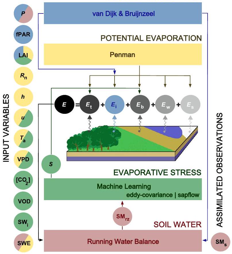
الشكل 1 مخطط GLEAM4. أسماء المتغيرات ومصادر البيانات مدرجة في الجدول 1، ولونها يدل على الوحدة التي تم استخدامها فيها.
| متغير | مصدر | نوع | قرار |
| الإشعاع الصافي
|
MSWX الإصدار 1.00
|
إعادة تحليل مصغرة |
|
| سيريس
|
قمر صناعي |
|
|
| درجة حرارة الهواء (
|
MSWX الإصدار 1.00
|
إعادة تحليل منخفضة الدقة |
|
| أيرز
|
قمر صناعي |
|
|
| هطول
|
MSWEP الإصدار 2.8
|
الاندماج الملاحظ |
|
| IMERG النهائي V07
|
قمر صناعي |
|
|
| سرعة الرياح (
|
ERA5
|
إعادة تحليل |
|
| عجز ضغط البخار (VPD) | MSWX الإصدار 1.00
|
إعادة تحليل مصغرة |
|
| أيرز
|
قمر صناعي |
|
|
| تركيز ثاني أكسيد الكربون
|
كامز
|
إعادة تحليل |
|
| مكافئ مياه الثلج (SWE) | جلوب سنو
|
قمر صناعي | 25 كم |
| رطوبة التربة السطحية
|
وكالة الفضاء الأوروبية – مركز بيانات تغير المناخ
|
قمر صناعي |
|
| عمق البصريات للنباتات (VOD) | فودكا v2
|
قمر صناعي |
|
| كسر امتصاص الإشعاع الضوئي الاصطناعي (fPAR) | MOD15A3H
|
قمر صناعي | 500 م |
| مؤشر مساحة الورقة (LAI) | MOD15A3H
|
قمر صناعي | 500 م |
| ارتفاع الغطاء النباتي (
|
GEDI / لاندسات
|
قمر صناعي | 30 م |
| نسب تغطية الأرض | MEaSURES
|
إعادة تحليل مصغرة |
|
| خصائص التربة | هاي هيدرو سول
|
مدفوع بالملاحظة | 250 م |
“الجدول 1. مصادر البيانات المستخدمة في GLEAM4. عندما تتوفر مجموعتان من البيانات لنفس المتغير، تشير البيانات الموجودة في الأعلى إلى أرشيف البيانات ‘
بطريقة تآزرية، لإنتاج ما يُشار إليه غالبًا بـ ‘النماذج الهجينة’ والتي حققت بالفعل بعض النجاح في
نموذج تبخر المياه من اليابسة العالمي في أمستردام (GLEAM)
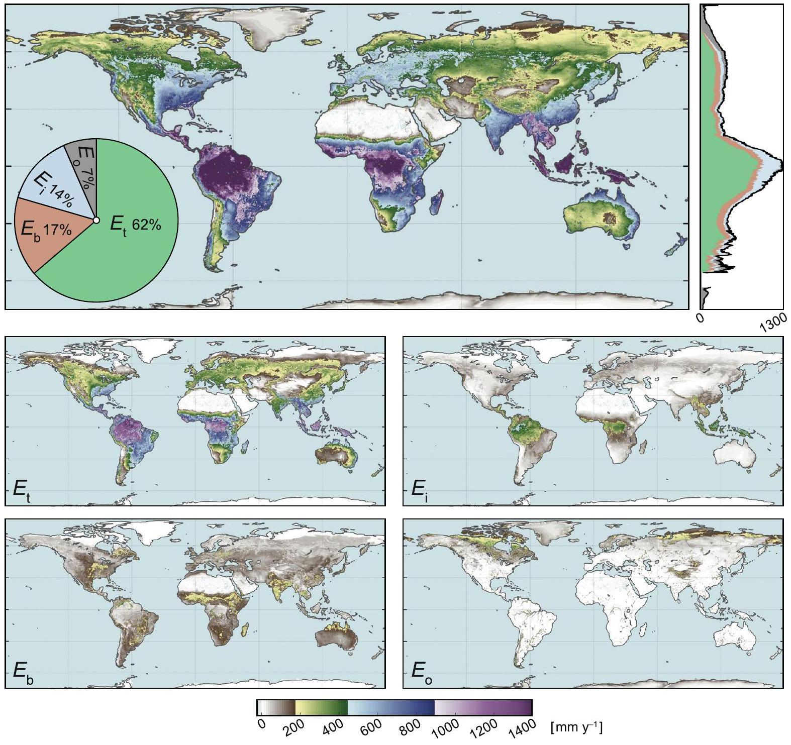
الشكل 2 متوسط التبخر ومكوناته. متوسط التبخر الأرضي على المدى الطويل (1980-2023)
تحديد كميات موارد المياه، ودفع نماذج الهيدرولوجيا على مستوى الأحواض، ودراسة الاتجاهات المناخية العالمية، ومعايرة نماذج المناخ
طرق
السبب وراء GLEAM هو التركيز بشكل حصري على العمليات التي تؤثر بشكل مباشر
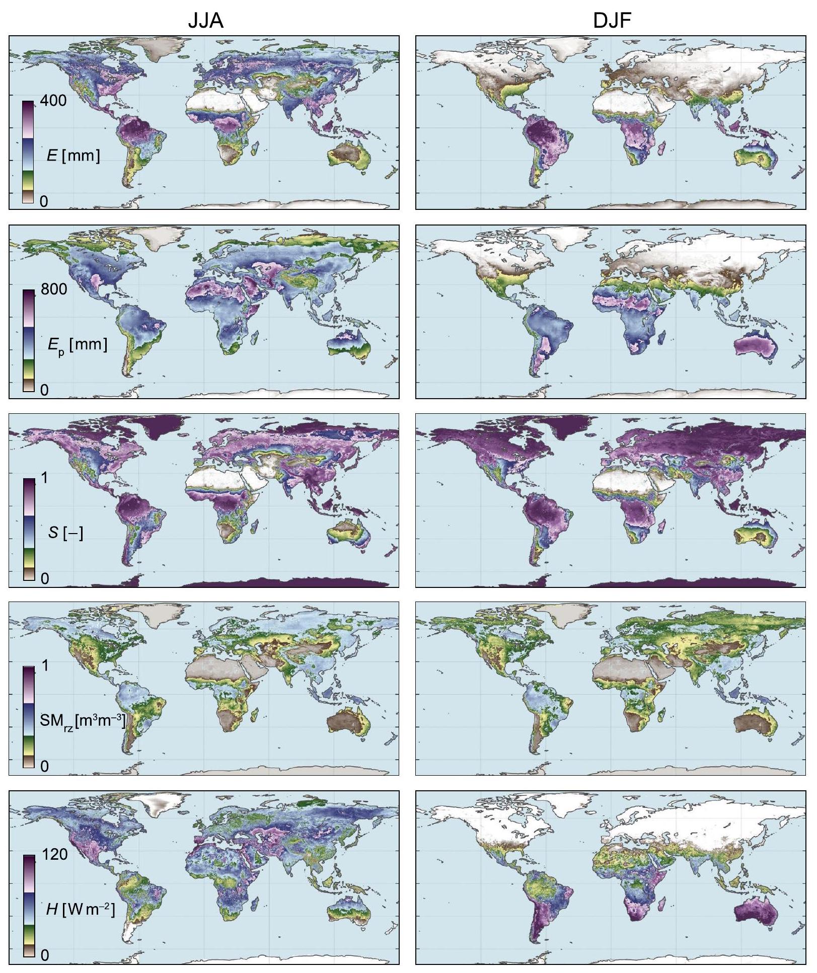
الشكل 3 الأنماط الموسمية. المتوسطات طويلة الأجل (1980-2023) لشهور يونيو ويوليو وأغسطس (JJA، يسار) وديسمبر ويناير وفبراير (DJF، يمين) لتبخر اليابسة
من كل وحدة. أولاً، فقدان تقاطُع الأمطار على الأسطح النباتية (
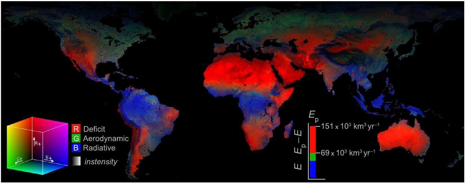
الشكل 4 عوامل التحكم في التبخر. الأهمية النسبية للطاقة الإشعاعية (الحد الأيسر في المعادلة 1)، الديناميكا الهوائية (الحد الأيمن في المعادلة 1)، والعجز التبخيري (
الشكل 5 المقارنة العالمية بين
استنادًا إلى مؤشر مساحة الورقة (LAI)
منذ نشر إصدار GLEAM
GLEAM4
GLEAM v3.8
ERA5-Land
فلوكسكوم
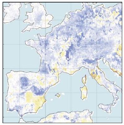
الشكل 6 المقارنة الإقليمية خلال فترات الجفاف الصيفية. الأرقام العلوية تشير إلى شذوذ E خلال جفاف الصيف الأوروبي عام 2003 (يونيو-يوليو-أغسطس). الأرقام السفلية تظهر شذوذ E خلال جفاف الصيف في أمريكا الشمالية عام 1988 (يونيو-يوليو-أغسطس). من اليسار إلى اليمين: GLEAM4، GLEAM v3.8a
وراء GLEAM4، مع التركيز على التحسينات التي تم إجراؤها على GLEAM v3 وكيف تؤثر هذه التحسينات على التقديرات لـ
وراء GLEAM4، مع التركيز على التحسينات التي تم إجراؤها على GLEAM v3 وكيف تؤثر هذه التحسينات على التقديرات لـ
اعتراض الأمطار.
التبخر المحتمل. على عكس الإصدارات السابقة من GLEAM، التي كانت تعتمد على معادلة بريستلي وتايلور
أين
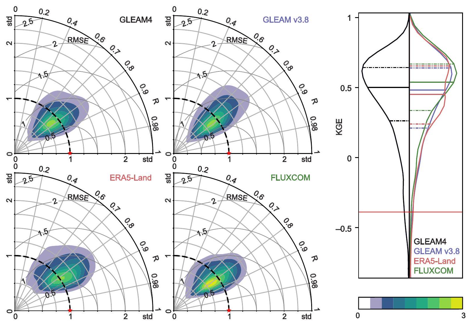
الشكل 7 التحقق باستخدام قياسات التباين المتزامن في الموقع. مخططات تايلور الكثافة للتحقق من GLEAM4 و GLEAM v3.8a
أين
مياه التربة. يتطلب محتوى مياه التربة عبر عمق الجذور للحسابات اللاحقة للضغط الناتج عن التبخر (انظر أدناه). يستخدم GLEAM توازن مياه متعدد الطبقات مدفوعًا ببيانات الهطول (و
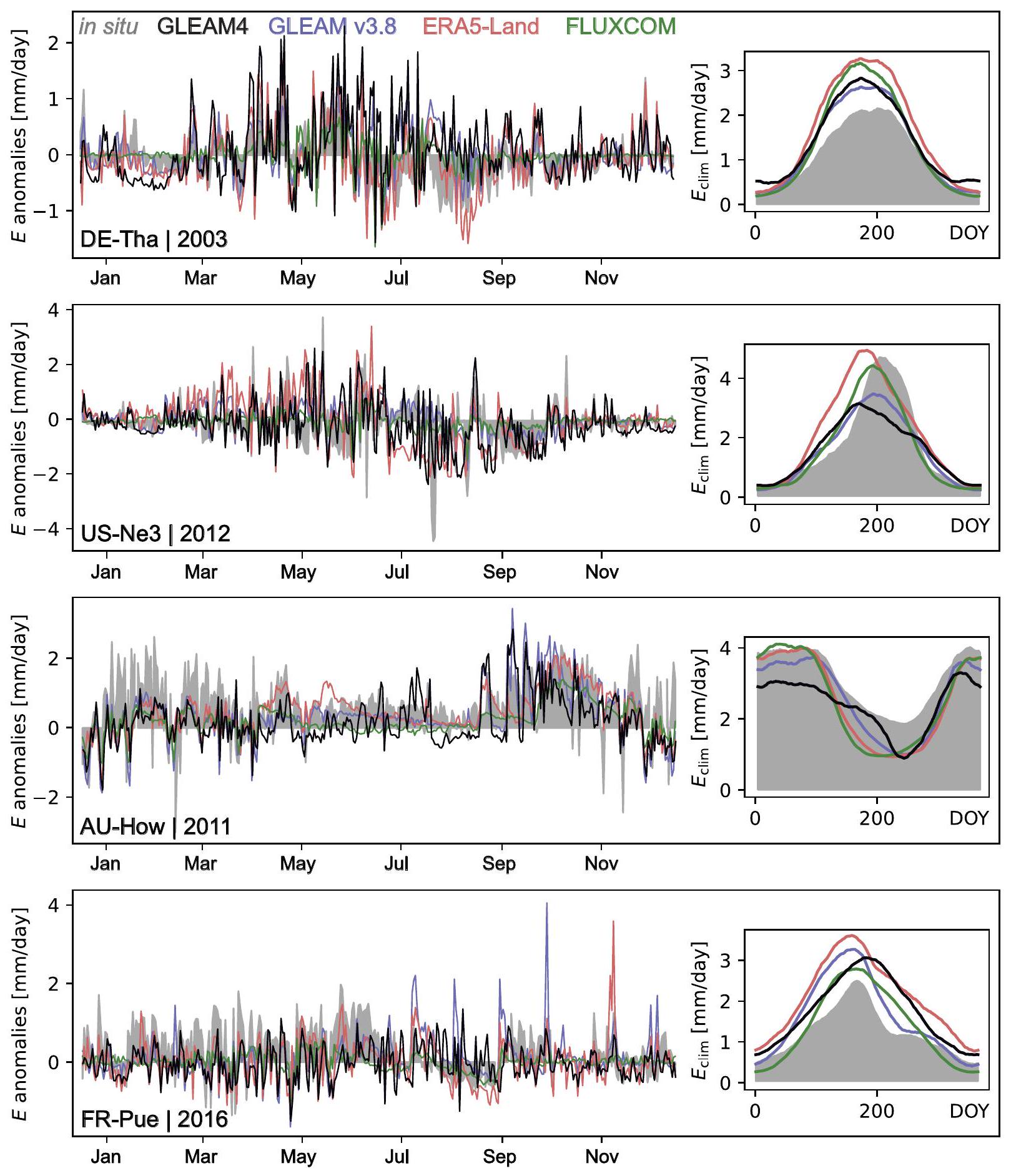
الشكل 8 مثال على السلاسل الزمنية. السلاسل الزمنية لـ GLEAM4، GLEAM v3.8a
إجهاد التبخر. كما ذُكر أعلاه، لتقييد
مضمنة ضمن GLEAM4، مما يتيح الربط الثنائي الاتجاه مع النموذج القائم على العمليات ويؤثر على كلاهما
مضمنة ضمن GLEAM4، مما يتيح الربط الثنائي الاتجاه مع النموذج القائم على العمليات ويؤثر على كلاهما
بيانات الإدخال. الجدول 1 يسرد جميع المتغيرات المدخلة ومجموعات البيانات المستخدمة في توليد مجموعات بيانات GLEAM4. تم إعادة أخذ عينات بيانات الإدخال إلى مستوى مشترك
سجلات البيانات
أرشيف البيانات. يبلغ حجم مجموعة بيانات GLEAM4 حاليًا حوالي 1.1 تيرابايت. البيانات متاحة مجانًا على خادم SFTP عام بموجب ترخيص CC BY، ويمكن الوصول إليها من خلالhttps://www.gleam.eu/#downloadsللحصول على وصف مفصل لمجموعة البيانات، نوجه القراء إلى الملاحظات الفنية فيhttps://doi.org/10.5281/زينودو.14056079. الـ
مثل الإصدارات السابقة من GLEAM
المتغيرات الاثنا عشر التالية متاحة لكل من أرشيفي البيانات (‘أ’ و ‘ب’):
التبخر الفعلي
النتح (
تبخر التربة العارية (
خسارة الاعتراض (
تبخر المياه المفتوحة (
تكثف (
تبخر فوق الثلج والجليد
التبخر المحتمل (
إجهاد التبخر (
رطوبة التربة السطحية (
رطوبة التربة في منطقة الجذور (
تدفق الحرارة السطحية الحسية (
هيكل البيانات. يتم تنظيم البيانات في ملفات netCDF، مع ملف واحد لكل متغير لكل سنة. يحتوي كل ملف يومي على مصفوفة ثلاثية الأبعاد بأبعاد
تُخزن هذه المجموعات البيانية على الخادم العام في هيكل الدليل التالي: <ARCHIVE>/ <TEMPORAL_RESOLUTION>/، حيث يشير <ARCHIVE> إما إلى GLEAM4.2a (v4.2a) أو GLEAM4.2b (v4.2b)، و <TEMPORAL_RESOLUTION> يشير إلى مستوى التجميع الزمني (‘يومي’، ‘شهري’، أو ‘سنوي’)، و ‘v4.2’ تشير إلى النسخة الفرعية من مجموعة بيانات GLEAM4. تُنظم المجموعات البيانية اليومية حسب السنة، بينما تُنظم المجموعات البيانية الشهرية والسنوية حسب المتغير.
تتبع الملفات اليومية هذا النمط في التسمية: <VARIABLE><سنة>بريق<ARCHIVE>.nc، حيث <VARIABLE> يتوافق مع أسماء المتغيرات المدرجة في القسم السابق: ‘E’، ‘Et’، ‘Eb’، ‘Ei’، ‘Ew’، ‘Ec’، ‘Es’، ‘Ep’، ‘S’، ‘SMrz’، ‘SMs’، ‘H’، و <YEAR> هو السنة المكونة من أربعة أرقام. على سبيل المثال، سيكون اسم الملف الذي يحتوي على بيانات التبخر اليومية لعام 2023 في مجموعة البيانات ‘a’ كالتالي:
v4.2a/يومي/2023/E_2023_GLEAM_v4.2a.nc.
تتبع الملفات الشهرية والسنوية هذا النمط في التسمية: <VARIABLE><سنة>بريق<ARCHIVE>_<TEMPORAL_RESOLUTION>.nc، حيث يتم اختصار <TEMPORAL_RESOLUTION> إلى ‘MO’ للشهري أو ‘YR’ للسنو. بالنسبة للملفات الشهرية والسنوية، وحدات التدفق هي مم في الشهر
v4.2b/شهري/SMrz/SMrz_2010_GLEAM_v4.2b_MO.nc.
التحقق الفني
أنماط عالمية. الشكل 2 يستكشف المتوسط العالمي
النسبة العالمية لـ
النسبة العالمية لـ
تُظهر الديناميات الموسمية لبعض المتغيرات الرئيسية من GLEAM4 في الشكل 3. تعرض الألواح الفرعية المتوسط العالمي لعدة سنوات (1980-2023).
فهم الاعتماد على
التحقق والمقارنة. الشكل 5 يوضح مقارنة بين GLEAM4
التقديرات العالمية المتوسطة لـ
على المقاييس الإقليمية، تبدو أنماط GLEAM4 واقعية وتبرز قيمة الانتقال إلى دقة مكانية أعلى لالتقاط تأثير التضاريس المعقدة وتغيرات استخدام الأراضي بشكل أفضل. الشكل 6 يقارن التقديرات من GLEAM4 بتلك من مجموعات البيانات الثلاث الأخرى خلال اثنين من أكثر فترات الجفاف الصيفية أهمية في السجل التاريخي: جفاف أمريكا الشمالية عام 1988.
لتقييم مهارة GLEAM4 في التقاط الديناميات الزمنية على مستوى النظام البيئي،
عينة نهائية من 473 موقعًا و2511 سنة من البيانات. الشكل 7 يقارن الأداء العام لمجموعات البيانات الأربعة GLEAM4 والمجموعات الثلاث الأخرى (أي GLEAM v3.8a وERA5-Land وFLUXCOM) في المحاكاة
عينة نهائية من 473 موقعًا و2511 سنة من البيانات. الشكل 7 يقارن الأداء العام لمجموعات البيانات الأربعة GLEAM4 والمجموعات الثلاث الأخرى (أي GLEAM v3.8a وERA5-Land وFLUXCOM) في المحاكاة
الشكل 8 يzoom إلى سلسلة زمنية مثال في أربعة مواقع محددة. المواقع تتوافق مع غابة التنوب في ثارانديت في شرق ألمانيا (DE-Tha)، وموقع زراعة الذرة وفول الصويا المعتمد على الأمطار في نبراسكا (US-Ne3)، وموقع السافانا في الغابات المفتوحة الأسترالية في هاوارد سبرينغز (AU-How)، والغابة المتوسطية دائمة الخضرة في فرنسا في بويشابون (FR-Pue). تم اختيار هذه المواقع بناءً على سجلاتها الطويلة (
توفر الشيفرة
يمكن الحصول على شيفات MATLAB و Python لتوليد النتائج وإنشاء جميع الأشكال في المقالة من المستودع العام على https://doi.org/10.5281/zenodo.14056593
تاريخ الاستلام: 19 نوفمبر 2024؛ تاريخ القبول: 11 فبراير 2025؛
تاريخ النشر: 10 مارس 2025
تاريخ النشر: 10 مارس 2025
References
- Miralles, D. G., Brutsaert, W., Dolman, A. J. & Gash, J. H. On the use of the term “Evapotranspiration”. Water Resour. Res. 56, e2020WR028055, https://doi.org/10.1029/2020wr028055 (2020).
- Miralles, D. G., Gentine, P., Seneviratne, S. I. & Teuling, A. J. Land-atmospheric feedbacks during droughts and heatwaves: State of the science and current challenges. Annals New York Acad. Sci. 1436, 19-35, https://doi.org/10.1111/nyas. 13912 (2019).
- Teuling, A. J. et al. Evapotranspiration amplifies European summer drought. Geophys. Res. Lett. 40, 2071-2075, https://doi. org/10.1002/grl. 50495 (2013).
- Brocca, L. et al. A Digital Twin of the terrestrial water cycle: a glimpse into the future through high-resolution Earth observations. Front. Sci. 1, 1190191, https://doi.org/10.3389/fsci.2023.1190191 (2024).
- Miralles, D. G. et al. El Niño-La Niña cycle and recent trends in continental evaporation. Nat. Clim. Chang. 4, 122-126, https://doi. org/10.1038/nclimate2068 (2014).
- Vicente-Serrano, S. M. et al. The uncertain role of rising atmospheric CO2 on global plant transpiration. Earth-Science Rev. 230, 104055, https://doi.org/10.1016/j.earscirev.2022.104055 (2022).
- Zhao, M., A, G., Liu, Y. & Konings, A. G. Evapotranspiration frequently increases during droughts. Nat. Clim. Chang.1-7, https:// doi.org/10.1038/s41558-022-01505-3 (2022).
- Dorigo, W. et al. Closing the water cycle from observations across scales: Where do we stand? Bull. Am. Meteorol. Soc. 1-95, https:// doi.org/10.1175/bams-d-19-0316.1 (2021).
- Ezenne, G. I., Eyibio, N. U., Tanner, J. L., Asoiro, F. U. & Obalum, S. E. An overview of uncertainties in evapotranspiration estimation techniques. J. Agrometeorology 25, https://doi.org/10.54386/jam.v25i1. 2014 (2023).
- Miralles, D. G. et al. Global land-surface evaporation estimated from satellite-based observations. Hydrol. Earth Syst. Sci. 15, 453-469, https://doi.org/10.5194/hess-15-453-2011 (2011).
- Fisher, J. B., Tu, K. P. & Baldocchi, D. D. Global estimates of the land-atmosphere water flux based on monthly AVHRR and ISLSCPII data, validated at 16 FLUXNET sites. Remote. Sens. Environ. 112, 901-919 (2008).
- Mu, Q., Zhao, M. & Running, S. W. Improvements to a MODIS global terrestrial evapotranspiration algorithm. Remote. Sens. Environ. 115, 1781-1800, https://doi.org/10.1016/j.rse.2011.02.019 (2011).
- Penman, H. L. Natural evaporation from open water, bare soil and grass. Proc. Royal Society of London Series A- Mathematical and Physical Sciences 193, 120-145 (1948).
- Priestley, C. H. B. & Taylor, R. J. On the assessment of surface heat flux and evaporation using large-scale parameters. Mon. Weather. Rev. 100, 81-92 (1972).
- Monteith, J. L. Evaporation and environment. Symp. Soc. for Exp. Biol. 19, 4 (1965).
- Jung, M., Reichstein, M. & Bondeau, A. Towards global empirical upscaling of FLUXNET eddy covariance observations: Validation of a model tree ensemble approach using a biosphere model. Biogeosciences 6, 2001-2013 (2009).
- Nelson, J. A. et al. X-BASE: The first terrestrial carbon and water flux products from an extended data-driven scaling framework, FLUXCOM-X. EGUsphere 2024, 1-51, https://doi.org/10.5194/egusphere-2024-165 (2024).
- Reichstein, M. et al. Deep learning and process understanding for data-driven earth system science. Nature 566, 195-204, https:// doi.org/10.1038/s41586-019-0912-1 (2019).
- Zhao, W. L. et al. Physics-constrained machine learning of evapotranspiration. Geophys. Res. Lett. 46, 14496-14507, https://doi. org/10.1029/2019gl085291 (2019).
- Kraft, B., Jung, M., Körner, M., Koirala, S. & Reichstein, M. Towards hybrid modeling of the global hydrological cycle. Hydrol. Earth Syst. Sci. Discuss. 2021, 1-40, https://doi.org/10.5194/hess-2021-211 (2021).
- Koppa, A., Rains, D., Hulsman, P., Poyatos, R. & Miralles, D. G. A deep learning-based hybrid model of global terrestrial evaporation. Nat. Commun. 13, 1912, https://doi.org/10.1038/s41467-022-29543-7 (2022).
- ElGhawi, R. et al. Hybrid modeling of evapotranspiration: Inferring stomatal and aerodynamic resistances using combined physicsbased and machine learning. Environ. Res. Lett. 18, 034039, https://doi.org/10.1088/1748-9326/acbbe0 (2023).
- Jahromi, M. N. et al. Ten years of GLEAM: A review of scientific advances and applications. In Bozorg-Haddad, O. & Zolghadr-Asli, B. (eds.) Computational Intelligence for Water and Environmental Sciences, 525-540, https://doi.org/10.1007/978-981-19-2519-1_25 (Springer Nature Singapore, Singapore, 2022).
- Michel, D. et al. The WACMOS-ET project – Part 1: Tower-scale evaluation of four remote-sensing-based evapotranspira- tion algorithms. Hydrol. Earth Syst. Sci. 20, 803-822, https://doi.org/10.5194/hess-20-803-2016 (2016).
- Talsma, C. J. et al. Partitioning of evapotranspiration in remote sensing-based models. Agric. For. Meteorol. 260, 131-143, https:// doi.org/10.1016/j.agrformet.2018.05.010 (2018).
- Miralles, D. G. et al. The WACMOS-ET project – part 2: Evaluation of global terrestrial evaporation data sets. Hydrol. Earth Syst. Sci. 20, 823-842, https://doi.org/10.5194/hess-20-823-2016 (2016).
- Mccabe, M. F. et al. The GEWEX LandFlux project: evaluation of model evaporation using tower-based and globally gridded forcing data. Geosci. Model. Dev. 9, 283-305, https://doi.org/10.5194/gmd-9-283-2016 (2016).
- Hulsman, P., Keune, J., Koppa, A., Schellekens, J. & Miralles, D. G. Incorporating plant access to groundwater in existing global, satellite-based evaporation estimates. Water Resour. Res. 59, https://doi.org/10.1029/2022WR033731 (2023).
- Zhong, F. et al. Revisiting large-scale interception patterns constrained by a synthesis of global experimental data. Hydrol. Earth Syst. Sci. 26, 5647-5667, https://doi.org/10.5194/hess-26-5647-2022 (2022).
- van Dijk, A. I. J. M. & Bruijnzeel, L. A. Modelling rainfall interception by vegetation of variable density using an adapted analytical model. part 1. model description. J. Hydrol. 247, 230-238, https://doi.org/10.1016/s0022-1694(01)00392-4 (2001).
- Martens, B. et al. GLEAM v3: Satellite-based land evaporation and root-zone soil moisture. Geosci. Model. Dev. 10, 1903-1925, https://doi.org/10.5194/gmd-10-1903-2017 (2017).
- Miralles, D. G., Gash, J. H., Holmes, T. R. H., de Jeu, R. A. M. & Dolman, A. J. Global canopy interception from satellite observations. J. Geophys. Res. Atmospheres 115, D16122, https://doi.org/10.1029/2009jd013530 (2010).
- Gash, J. H. C. & Morton, A. J. An application of the Rutter model to the estimation of the interception loss from Thetford Forest. J. Hydrol. 38, 49-58, https://doi.org/10.1016/0022-1694(78)90131-2 (1978).
- van Dijk, A. I. J. M. & Bruijnzeel, L. A. Modelling rainfall interception by vegetation of variable density using an adapted analytical model. part 2. model validation for a tropical upland mixed cropping system. J. Hydrol. 247, 239-262, https://doi.org/10.1016/s0022-1694(01)00393-6 (2001).
- Zhong, F. et al. Multi-Decadal Dynamics of Global Rainfall Interception and Their Drivers. Geophys. Res. Lett. 51, https://doi. org/10.1029/2024gl109295 (2024).
- Potapov, P. et al. Mapping global forest canopy height through integration of GEDI and Landsat data. Remote. Sens. Environ. 253, 112165, https://doi.org/10.1016/j.rse.2020.112165 (2021).
- Beck, H. E. et al. MSWX: Global 3-hourly
bias-corrected meteorological data including near-real-time updates and forecast ensembles. Bull. Am. Meteorol. Soc. 103, E710-E732, https://doi.org/10.1175/bams-d-21-0145.1 (2022). - Aumann, H. H. et al. AIRS/AMSU/HSB on the Aqua mission: Design, science objectives, data products, and processing systems. IEEE Transactions on Geosci. Remote. Sens. 41, 253-264, https://doi.org/10.1109/TGRS. 2002.808356 (2003).
- Allen, R. G., Tasumi, M. & Trezza, R. Satellite-based energy balance for mapping evapotranspiration with internalized calibration (METRIC)-model. J. Irrigation Drainage Eng. 133, 380-394, 10.1061/(asce)0733-9437(2007)133:4(380) (2007).
- Thom, A. S. Momentum, mass and heat exchange of plant communities. Q. J. Royal Meteorol. Soc. 18 (1975).
- Shuttleworth, W. J. Whole-Canopy Interactions, chap. 22, 316-333 https://doi.org/10.1002/9781119951933.ch22 (John Wiley & Sons, Ltd, 2012).
- Garrat, J. R. Surface roughness and local advection, chap. 4, 85-114 (Cambridge University Press, 1994).
- Rigden, A. J. & Salvucci, G. D. Evapotranspiration based on equilibrated relative humidity (ETRHEQ): Evaluation over the continental U.S. Water Resour. Res. 51, 2951-2973, https://doi.org/10.1002/2014WR016072 (2015).
- Rains, D. et al. Sentinel-1 backscatter assimilation using support vector regression or the water cloud model at european soil moisture sites. IEEE Geosci. Remote. Sens. Lett. PP, 1-5, https://doi.org/10.1109/lgrs.2021.3073484 (2021).
- Lievens, H. et al. Assimilation of global radar backscatter and radiometer brightness temperature observations to improve soil moisture and land evaporation estimates. Remote. Sens. Environ. 189, 194-210, https://doi.org/10.1016/j.rse.2016.11.022 (2017).
- Maxwell, R. M. & Condon, L. E. Connections between groundwater flow and transpiration partitioning. Science 353, 377-380, https://doi.org/10.1126/science.aaf7891 (2016).
- Haghdoost, S., Koppa, A., Lievens, H. & Miralles, D. G. Improving global evaporation estimation using GRACE and GRACE-FO satellite data assimilation. In EGU General Assembly 2024, Vienna, Austria, EGU24-17588, https://doi.org/10.5194/egusphere-egu24-17588 (2024).
- Dorigo, W. et al. ESA CCI Soil Moisture for improved earth system understanding: State-of-the art and future directions. Remote. Sens. Environ. 203, 185-215, https://doi.org/10.1016/j.rse.2017.07.001 (2017).
- Miralles, D. G. et al. GLEAM4 https://doi.org/10.5281/zenodo. 14056079 (2024).
- Beck, H. E. et al. MSWEP V2 global 3-hourly
precipitation: Methodology and quantitative assessment. Bull. Am. Meteorol. Soc. 100, 473-500, https://doi.org/10.1175/bams-d-17-0138.1 (2018). - Wielicki, B. A. et al. Clouds and the Earth’s Radiant Energy System (CERES): An Earth Observing System Experiment. Bull. Am. Meteorol. Soc. 77, 853-868, 10.1175/1520-0477(1996)077<0853:CATERE>2.0.CO;2 (1996).
- Hou, A. Y. et al. The Global Precipitation Measurement Mission. Bull. Am. Meteorol. Soc. 95, 701-722, https://doi.org/10.1175/ bams-d-13-00164.1 (2014).
- Wei, Z. et al. Revisiting the contribution of transpiration to global terrestrial evapotranspiration. Geophys. Res. Lett. 44, 2792-2801, https://doi.org/10.1002/2016gl072235 (2017).
- Miralles, D. G., de Jeu, R. A. M., Gash, J. H., Holmes, T. R. H. & Dolman, A. J. Magnitude and variability of land evaporation and its components at the global scale. Hydrol. Earth Syst. Sci. 15, 967-981, https://doi.org/10.5194/hess-15-967-2011 (2011).
- Singer, M. B. et al. Hourly potential evapotranspiration at
resolution for the global land surface from 1981-present. Sci. Data 8, 224, https://doi.org/10.1038/s41597-021-01003-9 (2021). - Jung, M. et al. The FLUXCOM ensemble of global land-atmosphere energy fluxes. Sci. Data 6, 74, https://doi.org/10.1038/s41597-019-0076-8 (2019).
- Zhang, K. A global dataset of terrestrial evapotranspiration and soil moisture dynamics from 1982 to 2020. Scientific Data 11, 445 (2024).
- Teuling, A. J. et al. A regional perspective on trends in continental evaporation. Geophys. Res. Lett. 36, https://doi. org/10.1029/2008gl036584 (2009).
- Muñoz-Sabater, J. et al. ERA5-Land: A state-of-the-art global reanalysis dataset for land applications. Earth Syst. Sci. Data 13, 4349-4383, https://doi.org/10.5194/essd-13-4349-2021 (2021).
- Trenberth, K. E., Branstator, G. W. & Arkin, P. A. Origins of the 1988 North American Drought. Science 242, 1640-1645, https://doi. org/10.1126/science.242.4886.1640 (1988).
- García-Herrera, R., Díaz, J., Trigo, R. M., Luterbacher, J. & Fischer, E. M. A Review of the European Summer Heat Wave of 2003. Critical Rev. Environ. Sci. Technol. 40, 267-306, https://doi.org/10.1080/10643380802238137 (2010).
- García-Herrera, R. et al. The European 2016/17 drought. J. Clim. 32, 3169-3187, https://doi.org/10.1175/JCLI-D-18-0331.1 (2019).
- Kerr, E. Brutal drought depresses agriculture, thwarting US and Texas economies. Southwest Econ. 10-13 (2012).
- Ciais, P. et al. Europe-wide reduction in primary productivity caused by the heat and drought in 2003. Nature 437, 529-533, https:// doi.org/10.1038/nature03972 (2005).
- Australian Government Bureau of Meteorology. Annual climate summary 2010. Tech. Rep., Australian Government Bureau of Meteorology (2011).
- Miralles, D. G., Crow, W. T. & Cosh, M. H. Estimating spatial sampling errors in coarse-scale soil moisture estimates derived from point-scale observations. J. Hydrometeorol. 11, 1423-1429, https://doi.org/10.1175/2010JHM1285.1 (2010).
- Miralles, D. G. et al. h-cel/GLEAM4: First submission. Zenodo [Code] https://doi.org/10.5281/zenodo.14056593 (2024).
- NASA/LARC/SD/ASDC. CERES and GEO-Enhanced TOA, Within-Atmosphere and Surface Fluxes, Clouds and Aerosols 1-Hourly Terra-Aqua Edition4A, https://doi.org/10.5067/TERRA+AQUA/CERES/SYN1DEG-1HOUR_L3.004A (2017).
- Goddard Earth Sciences Data and Information Services Center. Aqua/AIRS L3 Daily Standard Physical Retrieval (AIRS-only) 1 degree × 1 degree V7.0, https://doi.org/10.5067/UO3Q64CTTS1U (2019).
- Huffman, G., Stocker, E., Bolvin, D., Nelkin, E. & Tan, J. GPM IMERG Final Precipitation L3 1 day 0.1 degree
degree V07, https://doi.org/10.5067/GPM/IMERGDF/DAY/07 (2023). - Hersbach, H. et al. The ERA5 global reanalysis. Q. J. Royal Meteorol. Soc. 146, 1999-2049, https://doi.org/10.1002/qj.3803 (2020).
- Hersbach, H. et al. ERA5 hourly data on single levels from 1940 to present, https://doi.org/10.24381/cds.adbb2d47 (2023).
- Inness, A. et al. The CAMS reanalysis of atmospheric composition. Atmospheric Chem. Phys. 19, 3515-3556, https://doi.org/10.5194/ acp-19-3515-2019 (2019).
- Copernicus Atmosphere Monitoring Service Atmosphere Data Store. CAMS global greenhouse gas reanalysis (EGG4), https://doi. org/10.24380/8fck-9w87 (2021).
- Luojus, K., Pulliainen, J., Takala, M., Lemmetyinen, J. & Moisander, M. GlobSnow v3.0 snow water equivalent (SWE) https://doi. org/10.1594/PANGAEA. 911944 (2020).
- Armstrong, R., Brodzik, M. J., Knowles, K. & Savoie, M. Global monthly EASE-Grid snow water equivalent climatology, version 1 https://doi.org/10.5067/KJVERY3MIBPS (2005).
- Dorigo, W. et al. Soil moisture gridded data from 1978 to present, v201706.0.0., https://doi.org/10.24381/cds.d7782f18 (2017).
- Zotta, R.-M. et al. VODCA v2: Multi-sensor, multi-frequency vegetation optical depth data for long-term canopy dynamics and biomass monitoring. Earth Syst. Sci. Data 16, 4573-4617, https://doi.org/10.5194/essd-16-4573-2024 (2024).
- Moesinger, L. et al. The Global Long-term Microwave Vegetation Optical Depth Climate Archive VODCA, https://doi.org/10.5281/ zenodo. 2575599 (2019).
- Myneni, R., Knyazikhin, Y. & Park, T. Mcd15a3h modis/terra+aqua leaf area index/fpar 4 -day 14 global 500 m sin grid v006 [data set]. nasa eosdis land processes distributed active archive center. accessed 2024-11-19. https://doi.org/10.5067/MODIS/ MCD15A3H.006.
- Hansen, M. & Song, X. Vegetation continuous fields (VCF) yearly global 0.05 deg. 2018, distributed by NASA EOSDIS Land Processes Distributed Active Archive Center, https://doi.org/10.5067/MEaSUREs/VCF/VCF5KYR. 001 (2017).
- DiMiceli, C. et al. MOD44B MODIS/Terra Vegetation Continuous Fields Yearly L3 Global 250m SIN Grid V006, distributed by NASA EOSDIS Land Processes Distributed Active Archive Center https://doi.org/10.5067/MODIS/MOD44B. 006 (2015).
- Simons, G., Koster, R. & Droogers, P. Hihydrosoil v2.0-high resolution soil maps of global hydraulic properties. Futur. Work. Available from https://www.futurewater.eu/projects/hihydrosoil (2020).
الشكر والتقدير
تم تطوير GLEAM4 في السنوات الأخيرة بفضل التمويل المتكرر من مكتب السياسة العلمية البلجيكية (BELSPO) برنامج STEREO (SR/02/402، SR/02/377، SR/00/373) ووكالة الفضاء الأوروبية (ESA) (
مساهمات المؤلفين
قاد D.G.M. تطوير GLEAM كمدير رئيسي منذ عام 2009. قام F.Z. و D.G.M. و P.H. و A.K. بتنسيق تطوير النسخ الجديدة من وحدات التقاط المياه، والتبخر المحتمل، ومياه التربة، وإجهاد التبخر، على التوالي. ساهم D.G.M. و A.K. و O.B. و O.B.-V. و E.T. و P.H. و F.Z. و S.H. في تطوير الشيفرة والقرارات المتعلقة بالخوارزمية وبنية مجموعة البيانات. قام O.B. بتبسيط شيفرة النموذج. جمع O.B.-V. و A.K. البيانات الضاغطة وقاموا بمعالجتها مسبقًا. طور H.E.B. وقدم البيانات الضاغطة الجوية. طور W.D. وقدم بيانات إدخال VOD ورطوبة التربة السطحية. نفذ A.K. و O.B.-V. النموذج. قاد E.T. التحقق من صحة البيانات مقابل البيانات الميدانية. قام D.G.M. بتحليل المخرجات، وإعداد الأشكال، وكتابة المسودة الأولى. ساهم جميع المؤلفين في المناقشة وتفسير النتائج، بالإضافة إلى تحرير المخطوطة.
المصالح المتنافسة
يعلن المؤلفون عدم وجود مصالح متنافسة.
معلومات إضافية
يجب توجيه المراسلات والطلبات للحصول على المواد إلى D.G.M.
معلومات إعادة الطبع والتصاريح متاحة على www.nature.com/reprints.
معلومات إعادة الطبع والتصاريح متاحة على www.nature.com/reprints.
ملاحظة الناشر تظل Springer Nature محايدة فيما يتعلق بالمطالبات القضائية في الخرائط المنشورة والانتماءات المؤسسية.
الوصول المفتوح هذه المقالة مرخصة بموجب رخصة المشاع الإبداعي للاستخدام غير التجاري، والتي تسمح بأي استخدام غير تجاري، ومشاركة، وتوزيع، وإعادة إنتاج في أي وسيلة أو صيغة، طالما أنك تعطي الائتمان المناسب للمؤلفين الأصليين والمصدر، وتوفر رابطًا لرخصة المشاع الإبداعي، وتوضح إذا قمت بتعديل المادة المرخصة. ليس لديك إذن بموجب هذه الرخصة لمشاركة المواد المعدلة المشتقة من هذه المقالة أو أجزاء منها. الصور أو المواد الأخرى من طرف ثالث في هذه المقالة مشمولة في رخصة المشاع الإبداعي للمقالة، ما لم يُذكر خلاف ذلك في سطر ائتمان للمادة. إذا لم تكن المادة مشمولة في رخصة المشاع الإبداعي للمقالة واستخدامك المقصود غير مسموح به بموجب اللوائح القانونية أو يتجاوز الاستخدام المسموح به، ستحتاج إلى الحصول على إذن مباشرة من صاحب حقوق الطبع والنشر. لعرض نسخة من هذه الرخصة، قم بزيارة http://creativecommons.org/licenses/by-nc-nd/4.0/.
© المؤلفون 2025
© المؤلفون 2025
مختبر extremes المناخية المائية (H-CEL)، جامعة غنت، غنت، بلجيكا. مختبر هيدرولوجيا الحوض والجيومورفولوجيا، المدرسة الفيدرالية المتعددة التقنيات في لوزان (EPFL)، سيون، سويسرا. العلوم الفيزيائية والهندسة، جامعة الملك عبدالله للعلوم والتقنية (KAUST)، ثول، المملكة العربية السعودية. قسم الجيوديسيا والمعلومات الجغرافية، TU Wien، فيينا، النمسا. البريد الإلكتروني: diego.miralles@ugent.be
Journal: Scientific Data, Volume: 12, Issue: 1
DOI: https://doi.org/10.1038/s41597-025-04610-y
PMID: https://pubmed.ncbi.nlm.nih.gov/40064907
Publication Date: 2025-03-10
DOI: https://doi.org/10.1038/s41597-025-04610-y
PMID: https://pubmed.ncbi.nlm.nih.gov/40064907
Publication Date: 2025-03-10
scientific data
OPEN
DATA DESCRIPTOR
GLEAM4: global land evaporation and soil moisture dataset at
Terrestrial evaporation plays a crucial role in modulating climate and water resources. Here, we present a continuous, daily dataset covering
Background & Summary
Terrestrial evaporation (E) or ‘evapotranspiration’
RAINFALL INTERCEPTION
Fig. 1 Schematic of GLEAM4. Variable names and data sources are listed in Table 1, and their colour denotes the module in which they are employed.
| Variable | Source | Type | Resolution |
| Net radiation (
|
MSWX v1.00
|
Downscaled reanalysis |
|
| CERES
|
Satellite |
|
|
| Air temperature (
|
MSWX v1.00
|
Downscaled reanalysis |
|
| AIRS
|
Satellite |
|
|
| Precipitation (
|
MSWEP v2.8
|
Observational merger |
|
| IMERG Final V07
|
Satellite |
|
|
| Wind speed (
|
ERA5
|
Reanalysis |
|
| Vapour pressure deficit (VPD) | MSWX v1.00
|
Downscaled reanalysis |
|
| AIRS
|
Satellite |
|
|
| Carbon dioxide concentration (
|
CAMS
|
Reanalysis |
|
| Snow water equivalent (SWE) | GlobSnow
|
Satellite | 25 km |
| Surface soil moisture (
|
ESA CCI
|
Satellite |
|
| Vegetation optical depth (VOD) | VODCA v2
|
Satellite |
|
| Fraction absorbed photos ynthetic radiation (fPAR) | MOD15A3H
|
Satellite | 500 m |
| Leaf area index (LAI) | MOD15A3H
|
Satellite | 500 m |
| Vegetation height (
|
GEDI/Landsat
|
Satellite | 30 m |
| Land cover fractions | MEaSURES
|
Downscaled reanalysis |
|
| Soil properties | HiHydroSoil
|
Observation driven | 250 m |
Table 1. Sources of data used in GLEAM4. When two datasets are available for the same variable, the top one refers to data archive ‘
a synergistic manner, to yield what is frequently referred to as ‘hybrid models’ and which has already met some success in
The Global Land Evaporation Amsterdam Model (GLEAM
Fig. 2 Mean evaporation and its components. Long-term (1980-2023) mean terrestrial evaporation (
the quantification of water resources, driving basin-scale hydrological models, studying global climate trends, and benchmarking climate models
Methods
The rationale behind GLEAM is to focus exclusively on processes that directly impact
Fig. 3 Seasonal patterns. Long-term (1980-2023) means for June, July, and August (JJA, left) and December, January, and February (DJF, right) for terrestrial evaporation (
of each module. First, rainfall interception loss over vegetated surfaces (
Fig. 4 Evaporation control factors. Relative importance of radiative energy (left-hand term in Eq. 1), aerodynamics (right-hand term in Eq. 1), and evaporative deficit (
Fig. 5 Global inter-comparison of
based on leaf area index (LAI)
Since the publication of GLEAM version
GLEAM4
GLEAM v3.8
ERA5-Land
FLUXCOM
Fig. 6 Regional inter-comparison during summer droughts. Top figures refer to the E anomalies during the 2003 summer (JJA) European drought. Bottom figures show E anomalies during the 1988 summer (JJA) North American drought. From the left to right: GLEAM4, GLEAM v3.8a
behind GLEAM4, concentrating on the improvements upon GLEAM v3 and how these affect the estimates of
behind GLEAM4, concentrating on the improvements upon GLEAM v3 and how these affect the estimates of
Rainfall interception.
Potential evaporation. Unlike previous GLEAM versions, which were based on Priestley and Taylor’s equation
where
Fig. 7 Validation using in situ eddy-covariance measurements. Density Taylor diagrams for the validation of GLEAM4, GLEAM v3.8a
where
Soil water. Soil water content across the root depth is required for later computation of evaporative stress (see below). GLEAM uses a multi-layer running water balance driven by precipitation data (and
Fig. 8 Example time series. Time series for GLEAM4, GLEAM v3.8a
Evaporative stress. As mentioned above, to constrain
are embedded within GLEAM4, enabling bidirectional coupling with the process-based model and influencing both
are embedded within GLEAM4, enabling bidirectional coupling with the process-based model and influencing both
Input data. Table 1 lists all the input variables and datasets used in the generation of GLEAM4 datasets. Input data have been resampled to a common
Data Records
Data archive. The GLEAM4 dataset currently amounts to approximately 1.1TB. Data are freely available in a public SFTP server under a CC BY licence, and can be accessed through https://www.gleam.eu/#downloads. For a detailed description of the dataset, we refer readers to the technical notes at https://doi.org/10.5281/ zenodo.14056079. The
Like in previous versions of GLEAM
The following 12 variables are available for each of the two data archives (‘ a ‘ and ‘ b ‘):
Actual evaporation
Transpiration (
Bare soil evaporation (
Interception loss (
Open-water evaporation (
Condensation (
Evaporation over snow and ice (
Potential evaporation (
Evaporative stress (
Surface soil moisture (
Root-zone soil moisture (
Surface sensible heat flux (
Data structure. Data are organized into netCDF files, with one file per variable per year. Each daily file contains a 3D array with dimensions
These datasets are stored on the public server in the following directory structure: <ARCHIVE>/ <TEMPORAL_RESOLUTION>/, where <ARCHIVE> refers to either GLEAM4.2a (v4.2a) or GLEAM4.2b (v4.2b), <TEMPORAL_RESOLUTION> indicates the temporal aggregation level (‘daily’, ‘monthly’, or ‘yearly’), and ‘v4.2’ indicates the subversion of the GLEAM4 dataset. Daily datasets are organized by year, while monthly and yearly datasets are organized by variable.
Daily files follow this naming convention: <VARIABLE><YEAR>GLEAM<ARCHIVE>.nc, where <VARIABLE> corresponds to the variable names listed in the previous section: ‘E’, ‘Et, ‘Eb’, ‘Ei,’ ‘Ew’, ‘Ec’, ‘Es, ‘Ep’, ‘S’, ‘SMrz, ‘SMs,’ ‘H’, and < YEAR > is the four-digit year. For example, a file containing daily evaporation data for 2023 in the ‘a’ dataset would be named:
v4.2a/daily/2023/E_2023_GLEAM_v4.2a.nc.
Monthly and yearly files follow this naming convention: <VARIABLE><YEAR>GLEAM <ARCHIVE>_<TEMPORAL_RESOLUTION>.nc, where <TEMPORAL_RESOLUTION> is abbreviated as ‘MO’ for monthly or ‘YR’ for yearly. For monthly and yearly files, flux units are mm month
v4.2b/monthly/SMrz/SMrz_2010_GLEAM_v4.2b_MO.nc.
Technical Validation
Global patterns. Figure 2 explores mean global
global proportion of
global proportion of
The seasonal dynamics of some of the key variables from GLEAM4 are portrayed in Fig. 3. The sub-panels showcase global multi-year (1980-2023) mean
Understanding the dependency of
Validation and inter-comparison. Figure 5 shows a comparison of GLEAM4
The global mean estimates of
At regional scales, the patterns of GLEAM4 appear realistic and highlight the value of transitioning to higher spatial resolutions to better capture the influence of complex topography and land use changes. Figure 6 compares the estimates from GLEAM4 to those from the other three datasets during two of the most significant summer droughts in the historical record: the 1988 North American drought
To evaluate the skill of GLEAM4 in capturing temporal dynamics at the ecosystem scale,
final sample of 473 sites and 2511 years of data. Figure 7 compares the overall performance of the four datasets GLEAM4 and the other three datasets (i.e., GLEAM v3.8a, ERA5-Land, and FLUXCOM) in simulating
final sample of 473 sites and 2511 years of data. Figure 7 compares the overall performance of the four datasets GLEAM4 and the other three datasets (i.e., GLEAM v3.8a, ERA5-Land, and FLUXCOM) in simulating
Figure 8 zooms into example time series at four specific sites. The sites correspond to the Tharandt spruce forest in Eastern Germany (DE-Tha), a rainfed maize-soybean rotation site in Nebraska (US-Ne3), the Australian open woodland savanna site in Howard Springs (AU-How), and the French evergreen Mediterranean forest in Puechabon (FR-Pue). These sites were selected based on their long records (
Code availability
MATLAB and Python code for synthesizing the results and generating all figures of the article can be obtained from the public repository at https://doi.org/10.5281/zenodo.14056593
Received: 19 November 2024; Accepted: 11 February 2025;
Published: 10 March 2025
Published: 10 March 2025
References
- Miralles, D. G., Brutsaert, W., Dolman, A. J. & Gash, J. H. On the use of the term “Evapotranspiration”. Water Resour. Res. 56, e2020WR028055, https://doi.org/10.1029/2020wr028055 (2020).
- Miralles, D. G., Gentine, P., Seneviratne, S. I. & Teuling, A. J. Land-atmospheric feedbacks during droughts and heatwaves: State of the science and current challenges. Annals New York Acad. Sci. 1436, 19-35, https://doi.org/10.1111/nyas. 13912 (2019).
- Teuling, A. J. et al. Evapotranspiration amplifies European summer drought. Geophys. Res. Lett. 40, 2071-2075, https://doi. org/10.1002/grl. 50495 (2013).
- Brocca, L. et al. A Digital Twin of the terrestrial water cycle: a glimpse into the future through high-resolution Earth observations. Front. Sci. 1, 1190191, https://doi.org/10.3389/fsci.2023.1190191 (2024).
- Miralles, D. G. et al. El Niño-La Niña cycle and recent trends in continental evaporation. Nat. Clim. Chang. 4, 122-126, https://doi. org/10.1038/nclimate2068 (2014).
- Vicente-Serrano, S. M. et al. The uncertain role of rising atmospheric CO2 on global plant transpiration. Earth-Science Rev. 230, 104055, https://doi.org/10.1016/j.earscirev.2022.104055 (2022).
- Zhao, M., A, G., Liu, Y. & Konings, A. G. Evapotranspiration frequently increases during droughts. Nat. Clim. Chang.1-7, https:// doi.org/10.1038/s41558-022-01505-3 (2022).
- Dorigo, W. et al. Closing the water cycle from observations across scales: Where do we stand? Bull. Am. Meteorol. Soc. 1-95, https:// doi.org/10.1175/bams-d-19-0316.1 (2021).
- Ezenne, G. I., Eyibio, N. U., Tanner, J. L., Asoiro, F. U. & Obalum, S. E. An overview of uncertainties in evapotranspiration estimation techniques. J. Agrometeorology 25, https://doi.org/10.54386/jam.v25i1. 2014 (2023).
- Miralles, D. G. et al. Global land-surface evaporation estimated from satellite-based observations. Hydrol. Earth Syst. Sci. 15, 453-469, https://doi.org/10.5194/hess-15-453-2011 (2011).
- Fisher, J. B., Tu, K. P. & Baldocchi, D. D. Global estimates of the land-atmosphere water flux based on monthly AVHRR and ISLSCPII data, validated at 16 FLUXNET sites. Remote. Sens. Environ. 112, 901-919 (2008).
- Mu, Q., Zhao, M. & Running, S. W. Improvements to a MODIS global terrestrial evapotranspiration algorithm. Remote. Sens. Environ. 115, 1781-1800, https://doi.org/10.1016/j.rse.2011.02.019 (2011).
- Penman, H. L. Natural evaporation from open water, bare soil and grass. Proc. Royal Society of London Series A- Mathematical and Physical Sciences 193, 120-145 (1948).
- Priestley, C. H. B. & Taylor, R. J. On the assessment of surface heat flux and evaporation using large-scale parameters. Mon. Weather. Rev. 100, 81-92 (1972).
- Monteith, J. L. Evaporation and environment. Symp. Soc. for Exp. Biol. 19, 4 (1965).
- Jung, M., Reichstein, M. & Bondeau, A. Towards global empirical upscaling of FLUXNET eddy covariance observations: Validation of a model tree ensemble approach using a biosphere model. Biogeosciences 6, 2001-2013 (2009).
- Nelson, J. A. et al. X-BASE: The first terrestrial carbon and water flux products from an extended data-driven scaling framework, FLUXCOM-X. EGUsphere 2024, 1-51, https://doi.org/10.5194/egusphere-2024-165 (2024).
- Reichstein, M. et al. Deep learning and process understanding for data-driven earth system science. Nature 566, 195-204, https:// doi.org/10.1038/s41586-019-0912-1 (2019).
- Zhao, W. L. et al. Physics-constrained machine learning of evapotranspiration. Geophys. Res. Lett. 46, 14496-14507, https://doi. org/10.1029/2019gl085291 (2019).
- Kraft, B., Jung, M., Körner, M., Koirala, S. & Reichstein, M. Towards hybrid modeling of the global hydrological cycle. Hydrol. Earth Syst. Sci. Discuss. 2021, 1-40, https://doi.org/10.5194/hess-2021-211 (2021).
- Koppa, A., Rains, D., Hulsman, P., Poyatos, R. & Miralles, D. G. A deep learning-based hybrid model of global terrestrial evaporation. Nat. Commun. 13, 1912, https://doi.org/10.1038/s41467-022-29543-7 (2022).
- ElGhawi, R. et al. Hybrid modeling of evapotranspiration: Inferring stomatal and aerodynamic resistances using combined physicsbased and machine learning. Environ. Res. Lett. 18, 034039, https://doi.org/10.1088/1748-9326/acbbe0 (2023).
- Jahromi, M. N. et al. Ten years of GLEAM: A review of scientific advances and applications. In Bozorg-Haddad, O. & Zolghadr-Asli, B. (eds.) Computational Intelligence for Water and Environmental Sciences, 525-540, https://doi.org/10.1007/978-981-19-2519-1_25 (Springer Nature Singapore, Singapore, 2022).
- Michel, D. et al. The WACMOS-ET project – Part 1: Tower-scale evaluation of four remote-sensing-based evapotranspira- tion algorithms. Hydrol. Earth Syst. Sci. 20, 803-822, https://doi.org/10.5194/hess-20-803-2016 (2016).
- Talsma, C. J. et al. Partitioning of evapotranspiration in remote sensing-based models. Agric. For. Meteorol. 260, 131-143, https:// doi.org/10.1016/j.agrformet.2018.05.010 (2018).
- Miralles, D. G. et al. The WACMOS-ET project – part 2: Evaluation of global terrestrial evaporation data sets. Hydrol. Earth Syst. Sci. 20, 823-842, https://doi.org/10.5194/hess-20-823-2016 (2016).
- Mccabe, M. F. et al. The GEWEX LandFlux project: evaluation of model evaporation using tower-based and globally gridded forcing data. Geosci. Model. Dev. 9, 283-305, https://doi.org/10.5194/gmd-9-283-2016 (2016).
- Hulsman, P., Keune, J., Koppa, A., Schellekens, J. & Miralles, D. G. Incorporating plant access to groundwater in existing global, satellite-based evaporation estimates. Water Resour. Res. 59, https://doi.org/10.1029/2022WR033731 (2023).
- Zhong, F. et al. Revisiting large-scale interception patterns constrained by a synthesis of global experimental data. Hydrol. Earth Syst. Sci. 26, 5647-5667, https://doi.org/10.5194/hess-26-5647-2022 (2022).
- van Dijk, A. I. J. M. & Bruijnzeel, L. A. Modelling rainfall interception by vegetation of variable density using an adapted analytical model. part 1. model description. J. Hydrol. 247, 230-238, https://doi.org/10.1016/s0022-1694(01)00392-4 (2001).
- Martens, B. et al. GLEAM v3: Satellite-based land evaporation and root-zone soil moisture. Geosci. Model. Dev. 10, 1903-1925, https://doi.org/10.5194/gmd-10-1903-2017 (2017).
- Miralles, D. G., Gash, J. H., Holmes, T. R. H., de Jeu, R. A. M. & Dolman, A. J. Global canopy interception from satellite observations. J. Geophys. Res. Atmospheres 115, D16122, https://doi.org/10.1029/2009jd013530 (2010).
- Gash, J. H. C. & Morton, A. J. An application of the Rutter model to the estimation of the interception loss from Thetford Forest. J. Hydrol. 38, 49-58, https://doi.org/10.1016/0022-1694(78)90131-2 (1978).
- van Dijk, A. I. J. M. & Bruijnzeel, L. A. Modelling rainfall interception by vegetation of variable density using an adapted analytical model. part 2. model validation for a tropical upland mixed cropping system. J. Hydrol. 247, 239-262, https://doi.org/10.1016/s0022-1694(01)00393-6 (2001).
- Zhong, F. et al. Multi-Decadal Dynamics of Global Rainfall Interception and Their Drivers. Geophys. Res. Lett. 51, https://doi. org/10.1029/2024gl109295 (2024).
- Potapov, P. et al. Mapping global forest canopy height through integration of GEDI and Landsat data. Remote. Sens. Environ. 253, 112165, https://doi.org/10.1016/j.rse.2020.112165 (2021).
- Beck, H. E. et al. MSWX: Global 3-hourly
bias-corrected meteorological data including near-real-time updates and forecast ensembles. Bull. Am. Meteorol. Soc. 103, E710-E732, https://doi.org/10.1175/bams-d-21-0145.1 (2022). - Aumann, H. H. et al. AIRS/AMSU/HSB on the Aqua mission: Design, science objectives, data products, and processing systems. IEEE Transactions on Geosci. Remote. Sens. 41, 253-264, https://doi.org/10.1109/TGRS. 2002.808356 (2003).
- Allen, R. G., Tasumi, M. & Trezza, R. Satellite-based energy balance for mapping evapotranspiration with internalized calibration (METRIC)-model. J. Irrigation Drainage Eng. 133, 380-394, 10.1061/(asce)0733-9437(2007)133:4(380) (2007).
- Thom, A. S. Momentum, mass and heat exchange of plant communities. Q. J. Royal Meteorol. Soc. 18 (1975).
- Shuttleworth, W. J. Whole-Canopy Interactions, chap. 22, 316-333 https://doi.org/10.1002/9781119951933.ch22 (John Wiley & Sons, Ltd, 2012).
- Garrat, J. R. Surface roughness and local advection, chap. 4, 85-114 (Cambridge University Press, 1994).
- Rigden, A. J. & Salvucci, G. D. Evapotranspiration based on equilibrated relative humidity (ETRHEQ): Evaluation over the continental U.S. Water Resour. Res. 51, 2951-2973, https://doi.org/10.1002/2014WR016072 (2015).
- Rains, D. et al. Sentinel-1 backscatter assimilation using support vector regression or the water cloud model at european soil moisture sites. IEEE Geosci. Remote. Sens. Lett. PP, 1-5, https://doi.org/10.1109/lgrs.2021.3073484 (2021).
- Lievens, H. et al. Assimilation of global radar backscatter and radiometer brightness temperature observations to improve soil moisture and land evaporation estimates. Remote. Sens. Environ. 189, 194-210, https://doi.org/10.1016/j.rse.2016.11.022 (2017).
- Maxwell, R. M. & Condon, L. E. Connections between groundwater flow and transpiration partitioning. Science 353, 377-380, https://doi.org/10.1126/science.aaf7891 (2016).
- Haghdoost, S., Koppa, A., Lievens, H. & Miralles, D. G. Improving global evaporation estimation using GRACE and GRACE-FO satellite data assimilation. In EGU General Assembly 2024, Vienna, Austria, EGU24-17588, https://doi.org/10.5194/egusphere-egu24-17588 (2024).
- Dorigo, W. et al. ESA CCI Soil Moisture for improved earth system understanding: State-of-the art and future directions. Remote. Sens. Environ. 203, 185-215, https://doi.org/10.1016/j.rse.2017.07.001 (2017).
- Miralles, D. G. et al. GLEAM4 https://doi.org/10.5281/zenodo. 14056079 (2024).
- Beck, H. E. et al. MSWEP V2 global 3-hourly
precipitation: Methodology and quantitative assessment. Bull. Am. Meteorol. Soc. 100, 473-500, https://doi.org/10.1175/bams-d-17-0138.1 (2018). - Wielicki, B. A. et al. Clouds and the Earth’s Radiant Energy System (CERES): An Earth Observing System Experiment. Bull. Am. Meteorol. Soc. 77, 853-868, 10.1175/1520-0477(1996)077<0853:CATERE>2.0.CO;2 (1996).
- Hou, A. Y. et al. The Global Precipitation Measurement Mission. Bull. Am. Meteorol. Soc. 95, 701-722, https://doi.org/10.1175/ bams-d-13-00164.1 (2014).
- Wei, Z. et al. Revisiting the contribution of transpiration to global terrestrial evapotranspiration. Geophys. Res. Lett. 44, 2792-2801, https://doi.org/10.1002/2016gl072235 (2017).
- Miralles, D. G., de Jeu, R. A. M., Gash, J. H., Holmes, T. R. H. & Dolman, A. J. Magnitude and variability of land evaporation and its components at the global scale. Hydrol. Earth Syst. Sci. 15, 967-981, https://doi.org/10.5194/hess-15-967-2011 (2011).
- Singer, M. B. et al. Hourly potential evapotranspiration at
resolution for the global land surface from 1981-present. Sci. Data 8, 224, https://doi.org/10.1038/s41597-021-01003-9 (2021). - Jung, M. et al. The FLUXCOM ensemble of global land-atmosphere energy fluxes. Sci. Data 6, 74, https://doi.org/10.1038/s41597-019-0076-8 (2019).
- Zhang, K. A global dataset of terrestrial evapotranspiration and soil moisture dynamics from 1982 to 2020. Scientific Data 11, 445 (2024).
- Teuling, A. J. et al. A regional perspective on trends in continental evaporation. Geophys. Res. Lett. 36, https://doi. org/10.1029/2008gl036584 (2009).
- Muñoz-Sabater, J. et al. ERA5-Land: A state-of-the-art global reanalysis dataset for land applications. Earth Syst. Sci. Data 13, 4349-4383, https://doi.org/10.5194/essd-13-4349-2021 (2021).
- Trenberth, K. E., Branstator, G. W. & Arkin, P. A. Origins of the 1988 North American Drought. Science 242, 1640-1645, https://doi. org/10.1126/science.242.4886.1640 (1988).
- García-Herrera, R., Díaz, J., Trigo, R. M., Luterbacher, J. & Fischer, E. M. A Review of the European Summer Heat Wave of 2003. Critical Rev. Environ. Sci. Technol. 40, 267-306, https://doi.org/10.1080/10643380802238137 (2010).
- García-Herrera, R. et al. The European 2016/17 drought. J. Clim. 32, 3169-3187, https://doi.org/10.1175/JCLI-D-18-0331.1 (2019).
- Kerr, E. Brutal drought depresses agriculture, thwarting US and Texas economies. Southwest Econ. 10-13 (2012).
- Ciais, P. et al. Europe-wide reduction in primary productivity caused by the heat and drought in 2003. Nature 437, 529-533, https:// doi.org/10.1038/nature03972 (2005).
- Australian Government Bureau of Meteorology. Annual climate summary 2010. Tech. Rep., Australian Government Bureau of Meteorology (2011).
- Miralles, D. G., Crow, W. T. & Cosh, M. H. Estimating spatial sampling errors in coarse-scale soil moisture estimates derived from point-scale observations. J. Hydrometeorol. 11, 1423-1429, https://doi.org/10.1175/2010JHM1285.1 (2010).
- Miralles, D. G. et al. h-cel/GLEAM4: First submission. Zenodo [Code] https://doi.org/10.5281/zenodo.14056593 (2024).
- NASA/LARC/SD/ASDC. CERES and GEO-Enhanced TOA, Within-Atmosphere and Surface Fluxes, Clouds and Aerosols 1-Hourly Terra-Aqua Edition4A, https://doi.org/10.5067/TERRA+AQUA/CERES/SYN1DEG-1HOUR_L3.004A (2017).
- Goddard Earth Sciences Data and Information Services Center. Aqua/AIRS L3 Daily Standard Physical Retrieval (AIRS-only) 1 degree × 1 degree V7.0, https://doi.org/10.5067/UO3Q64CTTS1U (2019).
- Huffman, G., Stocker, E., Bolvin, D., Nelkin, E. & Tan, J. GPM IMERG Final Precipitation L3 1 day 0.1 degree
degree V07, https://doi.org/10.5067/GPM/IMERGDF/DAY/07 (2023). - Hersbach, H. et al. The ERA5 global reanalysis. Q. J. Royal Meteorol. Soc. 146, 1999-2049, https://doi.org/10.1002/qj.3803 (2020).
- Hersbach, H. et al. ERA5 hourly data on single levels from 1940 to present, https://doi.org/10.24381/cds.adbb2d47 (2023).
- Inness, A. et al. The CAMS reanalysis of atmospheric composition. Atmospheric Chem. Phys. 19, 3515-3556, https://doi.org/10.5194/ acp-19-3515-2019 (2019).
- Copernicus Atmosphere Monitoring Service Atmosphere Data Store. CAMS global greenhouse gas reanalysis (EGG4), https://doi. org/10.24380/8fck-9w87 (2021).
- Luojus, K., Pulliainen, J., Takala, M., Lemmetyinen, J. & Moisander, M. GlobSnow v3.0 snow water equivalent (SWE) https://doi. org/10.1594/PANGAEA. 911944 (2020).
- Armstrong, R., Brodzik, M. J., Knowles, K. & Savoie, M. Global monthly EASE-Grid snow water equivalent climatology, version 1 https://doi.org/10.5067/KJVERY3MIBPS (2005).
- Dorigo, W. et al. Soil moisture gridded data from 1978 to present, v201706.0.0., https://doi.org/10.24381/cds.d7782f18 (2017).
- Zotta, R.-M. et al. VODCA v2: Multi-sensor, multi-frequency vegetation optical depth data for long-term canopy dynamics and biomass monitoring. Earth Syst. Sci. Data 16, 4573-4617, https://doi.org/10.5194/essd-16-4573-2024 (2024).
- Moesinger, L. et al. The Global Long-term Microwave Vegetation Optical Depth Climate Archive VODCA, https://doi.org/10.5281/ zenodo. 2575599 (2019).
- Myneni, R., Knyazikhin, Y. & Park, T. Mcd15a3h modis/terra+aqua leaf area index/fpar 4 -day 14 global 500 m sin grid v006 [data set]. nasa eosdis land processes distributed active archive center. accessed 2024-11-19. https://doi.org/10.5067/MODIS/ MCD15A3H.006.
- Hansen, M. & Song, X. Vegetation continuous fields (VCF) yearly global 0.05 deg. 2018, distributed by NASA EOSDIS Land Processes Distributed Active Archive Center, https://doi.org/10.5067/MEaSUREs/VCF/VCF5KYR. 001 (2017).
- DiMiceli, C. et al. MOD44B MODIS/Terra Vegetation Continuous Fields Yearly L3 Global 250m SIN Grid V006, distributed by NASA EOSDIS Land Processes Distributed Active Archive Center https://doi.org/10.5067/MODIS/MOD44B. 006 (2015).
- Simons, G., Koster, R. & Droogers, P. Hihydrosoil v2.0-high resolution soil maps of global hydraulic properties. Futur. Work. Available from https://www.futurewater.eu/projects/hihydrosoil (2020).
Acknowledgements
GLEAM4 has been developed in recent years thanks to recurrent funding from the Belgian Science Policy Office (BELSPO) STEREO program (SR/02/402, SR/02/377, SR/00/373) and the European Space Agency (ESA) (
Author contributions
D.G.M. has led the development of GLEAM as P.I. since 2009. F.Z., D.G.M., P.H. and A.K. coordinated the development of the new versions of the interception, potential evaporation, soil water, and evaporative stress modules, respectively. D.G.M., A.K., O.B., O.B.-V., E.T., P.H., F.Z. and S.H. contributed to the development of the code and decisions regarding the algorithm and dataset structure. O.B. streamlined the model code. O.B.-V., A.K. and F.Z. collected and pre-processed the forcing data. H.E.B. developed and provided the meteorological forcing. W.D. developed and provided the VOD and surface soil moisture input data. A.K. and O.B.-V. executed the model. E.T. led the validation against in situ data. D.G.M. analysed the output, prepared the figures, and wrote the first draft. All authors contributed to the discussion and interpretation of the results, as well as the editing of the manuscript.
Competing interests
The authors declare no competing interests.
Additional information
Correspondence and requests for materials should be addressed to D.G.M.
Reprints and permissions information is available at www.nature.com/reprints.
Reprints and permissions information is available at www.nature.com/reprints.
Publisher’s note Springer Nature remains neutral with regard to jurisdictional claims in published maps and institutional affiliations.
Open Access This article is licensed under a Creative Commons Attribution-NonCommercialNoDerivatives 4.0 International License, which permits any non-commercial use, sharing, distribution and reproduction in any medium or format, as long as you give appropriate credit to the original author(s) and the source, provide a link to the Creative Commons licence, and indicate if you modified the licensed material. You do not have permission under this licence to share adapted material derived from this article or parts of it. The images or other third party material in this article are included in the article’s Creative Commons licence, unless indicated otherwise in a credit line to the material. If material is not included in the article’s Creative Commons licence and your intended use is not permitted by statutory regulation or exceeds the permitted use, you will need to obtain permission directly from the copyright holder. To view a copy of this licence, visit http://creativecommons.org/licenses/by-nc-nd/4.0/.
© The Author(s) 2025
© The Author(s) 2025
Hydro-Climate Extremes Lab (H-CEL), Ghent University, Ghent, Belgium. Laboratory of Catchment Hydrology and Geomorphology, École Polytechnique Fédérale de Lausanne (EPFL), Sion, Switzerland. Physical Sciences and Engineering, King Abdullah University of Science and Technology (KAUST), Thuwal, Saudi Arabia. Department of Geodesy and Geoinformation, TU Wien, Vienna, Austria. e-mail: diego.miralles@ugent.be