مقالة

تاريخ الاستلام: 15 نوفمبر 2024

نُشر على الإنترنت: 25 مارس 2025
تحقق من التحديثات

يمكن تحليل الدماغ إلى شبكات وظيفية على نطاق واسع، لكن الطوبوغرافيات المكانية المحددة لهذه الشبكات والأسماء المستخدمة لوصفها تختلف عبر الدراسات. لقد أعاقت هذه التباينات تفسير وتوافق نتائج الأبحاث عبر هذا المجال. لقد طورنا أداة توافق الشبكات (NCT) للسماح للباحثين بفحص والإبلاغ عن التوافق المكاني بين نتائجهم الجديدة في التصوير العصبي والعديد من الأطالس الوظيفية المعروفة. نقدم عدة عروض توضيحية نموذجية لتوضيح كيفية استخدام الباحثين لأداة NCT للإبلاغ عن نتائجهم الخاصة. توفر أداة NCT وسيلة مريحة لحساب معاملات دايس مع اختبارات الدوران لتحديد حجم وأهمية التوافق الإحصائي بين الخرائط المعرفة من قبل المستخدم وتسميات الأطلس الموجودة. ستجعل اعتماد أداة NCT من الأسهل على الباحثين في علم الأعصاب الشبكي الإبلاغ عن نتائجهم بطريقة موحدة، مما يساعد على إعادة الإنتاج ويسهل المقارنات بين الدراسات لإنتاج رؤى متعددة التخصصات.

يمكن أن تسهل التسمية العلمية الموحدة التواصل الفعال للمفاهيم المتعلقة بالأنظمة البيولوجية المعقدة. تمتلك علوم الأعصاب تاريخًا طويلًا في تصنيف المناطق التشريحية المتميزة في الدماغ عبر مقاييس مكانية متعددة، بدءًا من الفصوص القشرية، والتجاعيد والفجوات المتميزة في القشرة الدماغية، والنوى تحت القشرية، وصولاً إلى مناطق بروتمان المعمارية الخلوية. تمت أيضًا محاولات لتصنيف الدوائر العصبية والأنظمة المحددة جيدًا بناءً على معايير تشريحية ووظيفية متنوعة، مثل المسار القشري الشوكي، والدوائر القشرية-striato-thalamic، وتيارات المعالجة البصرية الظهرية والبطنية. تساعد مثل هذه المحاولات للتوحيد القياسي في تسهيل التواصل حول تنظيم الدماغ بين الباحثين وتساعد في تعليم الطلاب.

لقد أحدثت طرق التصوير العصبي الحديثة، وخاصة تلك التي تعتمد على التصوير بالرنين المغناطيسي، ثورة في قدرتنا على رسم خرائط غير جراحية لمختلف جوانب بنية الدماغ ووظيفته في البشر الأحياء. كان من التطورات الرئيسية القدرة على رسم خرائط الشبكات الدماغية الوظيفية، أو مجموعات من مناطق الدماغ التي تظهر تزامنًا وظيفيًا. نتيجة لشعبية هذا النهج المتزايدة، يتم وصف العديد من النتائج من دراسات التصوير العصبي من حيث الشبكات الدماغية، بدلاً من مناطق الدماغ التي يتم تحديدها. ومع ذلك، يتم ذلك غالبًا بطريقة عشوائية بسبب نقص التوحيد في تسمية هذه الشبكات. هذه التناقضات في التقارير العلمية تعقد المقارنات بين النتائج عبر الدراسات وتحد من دمج الاكتشافات الجديدة. .

ظهور أطلس الشبكات الدماغية الوظيفية، التي تُستخدم الآن بشكل روتيني في علم الأعصاب المعرفي والشبكي يجب، من حيث المبدأ، أن تسهم في توحيد تسمية الشبكات الوظيفية. عادةً ما تعين هذه الأطالس المناطق القشرية و/أو تحت القشرية المقسمة إلى واحدة من مجموعة من الشبكات الدماغية الكبيرة ذات الطوبوغرافيات المتنوعة، التي تتراوح من المناطق الأحادية النمط المتجاورة إلى الأنظمة الترابطية التي تمتد عبر مناطق متعددة مفصولة وموزعة في الدماغ. كما تختلف الأطالس في كيفية تسمية الشبكات الدماغية الكبيرة وفي عدد الشبكات الدماغية، فضلاً عن نهجها في تعريف الشبكات، وتوصيف طوبوغرافيتها المكانية، وتحديد كيفية تسميتها (على سبيل المثال، بناءً على موقعها التشريحي أو ما يُفترض أنها ترتبط به من جوانب معرفية). تؤدي هذه الاختلافات بين الأطالس إلى مزيد من التباين وعدم اليقين في التقارير العلمية.

اعترافًا بهذه التحديات، أنشأت منظمة رسم خرائط الدماغ البشري (OHBM) لجنة لأفضل الممارسات بشأن تسميات الشبكات الدماغية واسعة النطاق، بعد نجاح مبادرات سابقة مماثلة لبناء توافق الآراء تهدف إلى تعزيز التوحيد القياسي من خلال تقديم إرشادات للتقارير في هذا المجال. . هذه اللجنة، التي تم تشكيلها في عام 2020، تعرف باسم مجموعة العمل لتصنيف الشبكات المتناغمة (WHATNET). أدت المحاولات الأولية من قبل مجموعة العمل لتحديد التقارب بشكل مفهومي عبر الشبكات الدماغية الوظيفية واسعة النطاق إلى مناقشة وإحصاء التحديات المتعددة الكامنة في هذا المشروع. قامت مجموعة العمل باستطلاع آراء مئات من العلماء وطلبت أسماء محتملة للشبكات استنادًا إلى تصورات لمختلف الطوبوغرافيات المكانية للشبكات. تم وصف نتائج الاستطلاع بالتفصيل في التقرير الأول من WHATNET. ومتاحة للجمهورhttps://osf.io/3fzta/)، أشار إلى أن الشبكات المستندة إلى مناطق الدماغ غير الموزعة أحادية النمط (أنظمة الحركة الجسدية والبصرية) يمكن تحديدها بسهولة وموثوقية. أظهرت شبكة الحركة الجسدية الاتفاق بين المقيمين، بينما أظهر الشبكة البصرية 92% من الاتفاق بين المقيمين. فقط شبكة واحدة موزعة مكانيًا، وهي الشبكة الافتراضية، أظهرت توافقًا في الاسم والتضاريس، مع الاتفاق بين المقيمين. أظهرت شبكات أخرى، مثل تلك التي يُشار إليها أحيانًا بالبارزة أو الجبهية الجدارية، تناسقًا أقل. تشير هذه النتائج إلى أن اتفاق الإجماع في التسمية محدود بالأقطاب القصوى من التسلسل الهرمي القشري الكنسي. مرتبطًا من طرف واحد بأنظمة البصر والحركة الجسدية ومن الطرف الآخر بالشبكة الافتراضية. في ما بين هذه الأنظمة يوجد مساحة من القشرة مع هيكل شبكي قابل للملاحظة، ولكن مع قلة الاتفاق بين الباحثين بشأن طوبوغرافيتها المكانية أو تسميتها. هذه التباينات تشكل مشكلة كبيرة لأي محاولات لمقارنة أو دمج النتائج عبر الدراسات.

استجابةً لنتائج مسح WHATNET، نقدم هنا صندوق أدوات مراسلة الشبكة (NCT). يوفر هذا الصندوق للباحثين حلاً عمليًا لتسمية تنشيط fMRI الجديد الملاحظ، وأنماط الاتصال الوظيفي، أو خرائط التصوير العصبي الأخرى التي تم تحديد عتبتها بناءً على تقييم كمي مقابل عدة أطلسات منشورة حاليًا في وقت واحد. كما يتيح NCT للمستخدمين تقييم التوافق المكاني بين الشبكات في الأطلسات الجديدة والقديمة. نوضح فائدة NCT في توفير تسميات الشبكة لخرائط التصوير العصبي النموذجية بناءً على تقييم كمي للتوافق المكاني مع عدة أطلسات شبكية منشورة. يتم تحديد الأدلة الكمية للتوافق من خلال حجم معامل دايس، بالإضافة إلى اختبارات التدوير لتقييم إحصائي قوي للأهمية. نختتم بتوصية بأن تتضمن التقارير المستقبلية حول الشبكات وعلم الأعصاب المعرفي تقييمًا للتوافق بين مخططات تسمية الشبكات الخاصة بهم وعدة أطلسات شبكية منشورة أنتجتها مختبرات بحثية مستقلة، كما يسهل NCT. تعترف هذه المقاربة بشفافية وتعالج كميًا الغموض المتأصل في تعيين التسميات إلى
خرائط الدماغ الطبوغرافية وتشجع على تحقيق توافق أكبر عبر دراسات علوم الأعصاب الشبكية من خلال تقييم موضوعي للتقارب أو التباين بين النتائج الجديدة والتسميات والشبكات المنشورة. من المهم أن نلاحظ أن NCT ليست وصفية فيما يتعلق بالمشكلة الكبيرة التي يصعب حلها والمتعلقة بتسميات الشبكات غير المتسقة. بل هي أداة لتسهيل المقارنة والتفسير الذي يمكن استخلاصه عبر الأطالس، مما يؤدي في النهاية إلى تحقيق مزيد من التوحيد في الإبلاغ عن النتائج.

نبدأ بتوضيح مشكلة تطابق الشبكات من خلال حساب تداخل الشبكات عبر ستة عشر أطلس دماغي وظيفي مستخدم على نطاق واسع. بعد ذلك، كمثال كمي آخر، نوضح التطابق بين أطلسين مستخدمين على نطاق واسع يحددان القشرة إلى 17 شبكة منفصلة: Yeo2011-17 وGordon2017-17. هذه الأمثلة تهدف إلى توضيح مشكلة التسمية الشبكية وتحفيز استخدام NCT. ثم نقدم إرشادات خطوة بخطوة لاستخدام NCT. أخيرًا، نعرض عدة أمثلة على كيفية استخدام NCT من خلال معالجة نتائج fMRI لمشروع الاتصال البشري (HCP) المتاحة للجمهور وخرائط تحليل المكونات المستقلة (ICA) لمشروع UK Biobank كـ “نتائج جديدة” لأغراض العرض. تم اختيار هذه الخرائط المحددة لتوضيح كيفية أداء NCT في الحالات التي تتوافق فيها بيانات الإدخال مع الشبكات الموجودة بدرجة قوية، وكذلك في السيناريوهات الأكثر تحديًا حيث يكون التطابق أقل.

تحديد المواقع التشريحية لأنماط نشاط الدماغ أمر ممل لكن العديد من الأطالس الرقمية والورقية متاحة لتسهيل العملية تحديد المواقع لشبكات الدماغ الوظيفية على نطاق واسع هو تطور أكثر حداثة، مع الطلب على أدوات موحدة (انظر لإدخال حديث لتحديد المواقع الشبكية الاحتمالية). يسمح NCT بشكل مرن بتقييم التوافق المكاني بين عدة أطلس مرجعي مستهدف وخرائط دماغ جديدة بما في ذلك، ولكن لا تقتصر على، نتائج الاتصال الوظيفي وتنشيط المهام، بالإضافة إلى خرائط أخرى في الفضاء القياسي. لاحظ أن بعض الأطالس المدرجة في NCT تحتوي على نسخ متعددة: Yeo2011، Schaefer2018، Kong2021، Power2011، Shen2013، Gordon2017، Cole-Anticevic2019، ICA-UK Biobank، ICA-HCP، ICA-BrainMap، وShirer2012. (الشكل 1 والجدول التكميلي 1). تتضمن النسخة الأحدث من NCT (الإصدار 0.3.1) 23 أطلس دماغي. يمكن العثور على قائمة كاملة بالأطالس المتاحة حاليًا في NCT في https://pypi.org/project/cbig_network_المراسلة.

قمنا بدراسة 16 أطلس دماغي وظيفي مستخدم على نطاق واسع بما في ذلك Yeo2011 وSchaefer2018 وKong2021 وPower2011 وShen2013 وGordon2017 وCole-Anticevic2019 وICA-UK Biobank وICA-HCP وICA-BrainMap وShirer2012. (الشكل 1 والجدول التكميلي 1). لحساب تداخل الشبكات عبر الأطالس، اعتبرنا كل أطلس كأطلس مرجعي وقمنا بإسقاط الأطالس الأخرى في ذلك الأطلس المرجعي. بين كل شبكة مرجعية وكل شبكة من جميع الأطالس الأخرى، قمنا بحساب معامل دايس. سمح لنا ذلك بمقارنة الاتفاق على مستوى الفوكسل بين الشبكة المرجعية وجميع الشبكات الأخرى، حيث 0 يعني عدم وجود تطابق و1 يعني تطابق كامل. بافتراض وجود K شبكة في الأطلس المرجعي وM شبكة في أطلس آخر، قمنا بإنشاء مصفوفة تداخل الشبكات بحجم KxM، حيث -صف و يمثل العمود -th معامل تداخل دايس بين الشبكة من الأطلس المرجعي والشبكة من الأطلس الآخر. يشير معامل ديس العالي إلى تداخل مكاني كبير بين الشبكتين من أطلسين مختلفين.

تم حساب وفحص معاملات ديس بين جميع الأطالس الستة عشر. تُظهر المصفوفة غير المتماثلة اختلافات نسبية بسبب الإشارة إلى الأطالس في المثلثين العلوي والسفلي (الشكل 2). يكشف كل جزء فرعي من المصفوفة عن أنماط من المطابقة (مع المجموع

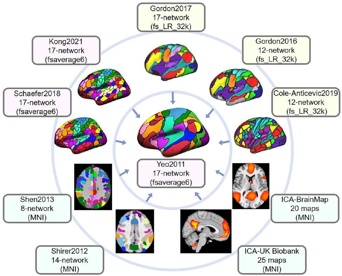
الشكل 1 | الأطالس المثال المدرجة في تطابق الشبكة
صندوق الأدوات (NCT). الـ NCT هو صندوق أدوات يسهل استكشاف التوافقات الشبكية عبر عدة أطلسات شبكية وظيفية بالإضافة إلى المقارنة الكمية للنتائج الجديدة في تصوير الأعصاب مع عدة أطلسات. يتم عرض عشرة أطلسات هنا لأغراض التوضيح. في هذا المثال، أطلس الشبكة المكون من 17 شبكة وفقًا لـ Yeo في
تستخدم مساحة fsaverage6 (المركز) كأطلس مرجعي. يتم إسقاط جميع الأطالس المحيطة في مساحات مختلفة إلى مساحة fsaverage6 لحساب معاملات تداخل دايس مع الشبكات المرجعية. يمكن العثور على قائمة كاملة بالأطالس المتاحة حاليًا في NCT فيhttps://pypi.org/project/cbig_network_المراسلة.
التراسل داخل الأطلس على القطر). الكتل الفرعية غير المربعة من المصفوفة تعود إلى الاختلافات في عدد الشبكات المحددة بين الأطالس، والتي تراوحت من 7 (Yeo2011) إلى 25 (Smith2013; Miller2016). تظهر الطوبوغرافيات المكانية الموزعة للشبكات الوظيفية عبر الأطالس بعض التوافق الموثوق، استنادًا إلى الهيكل الفرعي القابل للملاحظة على القطر.

من بين 16 أطلسًا تم تضمينها، كانت هناك اختلافات في أعداد الشبكات التي تضمنت بعض الحالات من الحلول غير المستقلة التي تم اشتقاقها من نفس مجموعة البيانات أو من نفس المختبر. لهذا السبب، لا يمكن للتحقيق الحالي تحديد الحل الأمثل لعدد الشبكات واسعة النطاق في الدماغ البشري، كما تم تقييمه باستخدام التصوير بالرنين المغناطيسي الوظيفي. استنادًا إلى تداخل دايس، تم فحص الهياكل الهرمية لمصفوفة تشابه الشبكات باستخدام نموذج كتلة عشوائية متداخلة. مع تطبيق 15 مجموعة (العدد المتوسط من الشبكات عبر الأطلس). من المهم ملاحظة أن هذا التجميع لا يهدف إلى توليد شبكات توافقية عبر الأطلس. بدلاً من ذلك، يسمح خوارزم التجميع بفحص التوافق المكاني عبر الأطلس، مع الإشارة إلى مصدر الأطلس وأسماء الشبكات المحددة. تُعرض خرائط احتمالية الشبكة لكل مجموعة في الشكل 3.

قمنا بفحص بصري لكل مجموعة وأسماء الشبكات المرتبطة بالتقسيمات التي قدمت تسميات الشبكة. كانت المساحة المكانية لخرائط احتمالية الشبكة وتسمياتها المقابلة (متجاهلين تسميات الشبكات الفرعية) متشابهة عبر الأطالس للعديد من المجموعات. كانت جميع المجموعات ثنائية الجانب. كانت المجموعة 5، التي تتكون من القشرة الجبهية الحوضية والقشرة الجدارية الحوضية، الفص الجبهي السفلي، الفص الزمني الجانبي والفص الزمني الحوضي، التلافيف الجبهية السفلية، والتلافيف الجبهية الوسطى العليا، شبه موحدة في تسميتها “شبكة الوضع الافتراضي” عبر الأطالس. ومع ذلك، تم تسمية بعض المجموعات الوظيفية بشكل متنوع، وتم ملاحظة تناقضات واضحة.

أظهر الشبكة الموزعة من الكتلة 12، بما في ذلك القشرة الجبهية الجانبية، الفص الجداري السفلي الأمامي، التلم الزمني السفلي الخلفي، والقشرة الحزامية الأمامية الظهرية، أيضًا قوة كبيرة
التواصل عبر عدة أطلس، لكن الأطلس المستخدم استخدم تسميات متنوعة، مثل “الجبهية الجدارية”، “التحكم”، و”التنفيذ المركزي”. هذه الشبكة معروفة جيدًا ومعروفة بدورها في التحكم التنفيذي في معالجة المعلومات في الدماغ البشري. تشير الأسماء المتباينة إلى نفس البناء المعرفي إلى حد كبير حتى في غياب التسمية المتسقة والمتفق عليها عبر الأطلسيات. .

تمت ملاحظة التقارب لشبكات الإدراك والحركة. تلاقت خرائط الاحتمالات للعناقيد 2 و3 في الفص القذالي، مع تسميات متسقة تتعلق بالرؤية (“بصري”). أمام الشبكات القذالية كان هناك العنقود 4، الذي امتد إلى الأعلى في القشرة الجدارية العلوية وإلى الأسفل في القشرة الصدغية السفلية. تم تصنيف هذه الشبكة بشكل متنوع على أنها “انتباه ظهري”، “جمع بصري”، و”بصري”. شمل العنقود 1 منطقتين أماميتين لتلك المحددة في العنقود 4، وهما الفص الجبهي العلوي ومجمع الحركة الصدغي الأوسط، بالإضافة إلى الحقول البصرية الجبهية المفترضة والشق الجبهي السفلي. كانت هذه المناطق الموزعة تحمل بشكل أساسي تسمية “انتباه ظهري” بالإضافة إلى “بصري مكاني” و”قبل حركي”.

تشمل القشرة الحركية والقشرة الحسية الجسدية، الأمامية والخلفية للثلم المركزي، التلافيف ما قبل المركزية وما بعد المركزية، وتمتد وسطيًا إلى الفص الجانبي (منطقة الحركية التكميلية). شمل العنقود 10 هذه المناطق مع تسميات موثوقة لـ “الحركية الجسدية” أو “الحركية”. تم إعادة تأكيد الامتداد الظهري والوسطي بشكل خاص في العنقود 8، مع تسميات “الحركية الجسدية”، و”اليد”، و”القدم”، و”الحركية الجسدية الظهرية”. شمل العنقود 11 الامتداد البطني للقشرة الحركية والقشرة الحسية الجسدية، نازلاً عبر الجزيرة الوسطى، وينتهي في التلافيف الزمنية العلوية. تم تقسيم هذا العنقود في الأسماء بين تسميات “الحركية الجسدية” و”السمعية” عبر أطلسات مختلفة.

أخيرًا، كان من الواضح تداخل شبكات “الانتباه البطني” و”الأهمية” و”الشبكة الحزامية-العمودية” في الكتلة 9، مع مناطق تشمل القشرة المعزولة الأمامية، والقشرة الحزامية الأمامية الوسطى والظهرية، والقشرة الجدارية الجانبية. على سبيل المثال، كانت الأهمية/البطنية

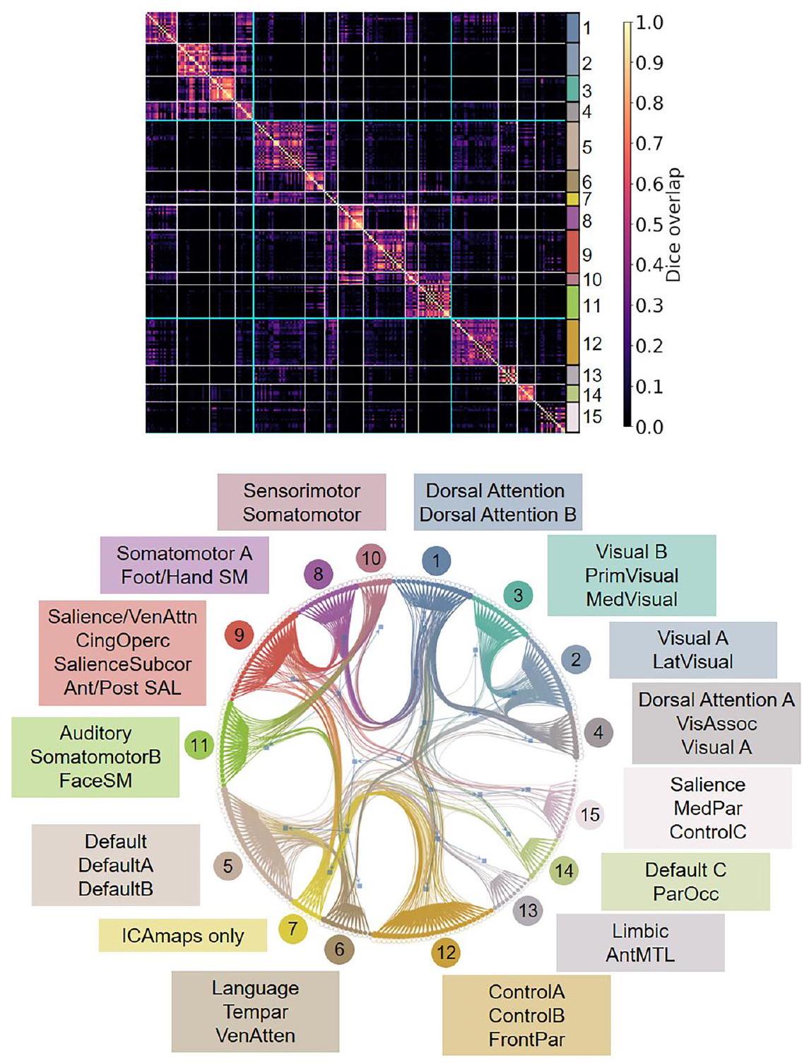
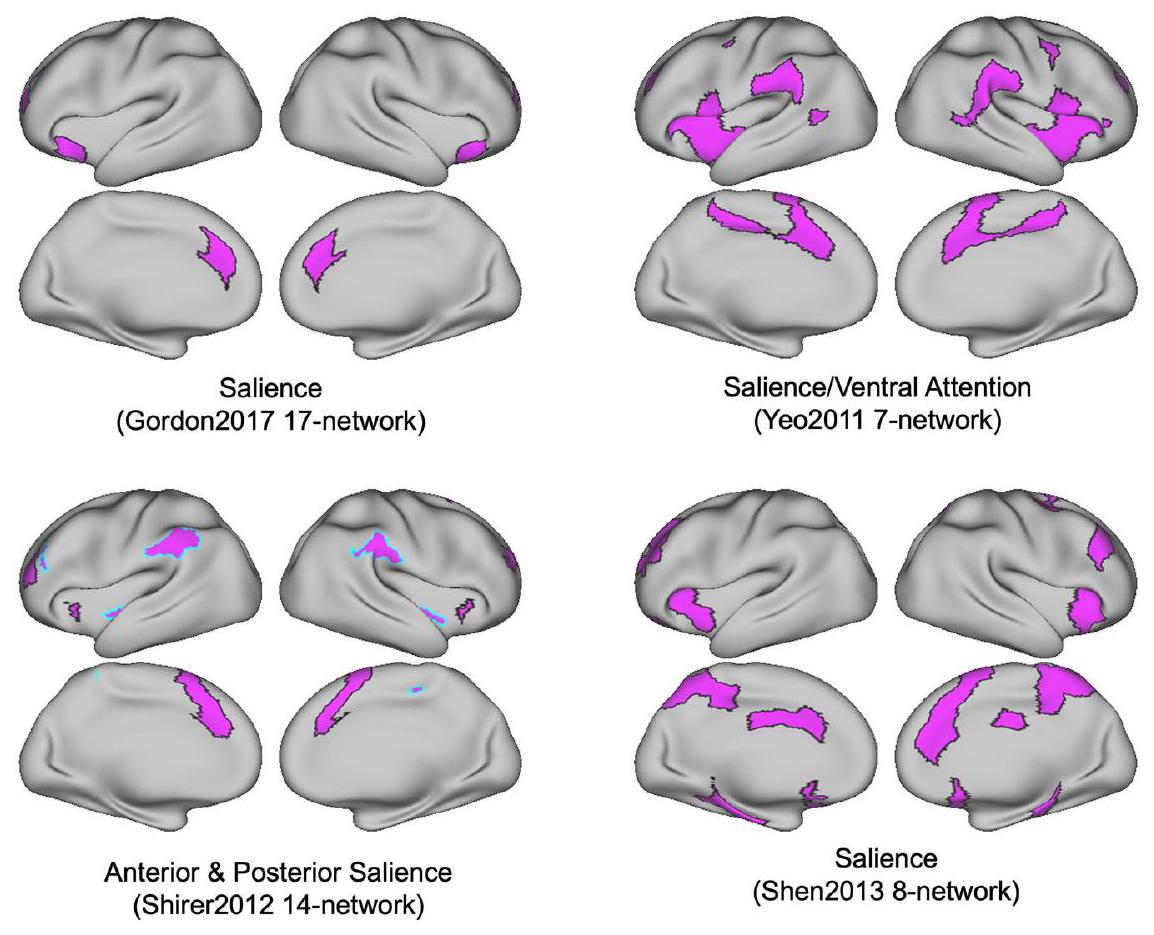
الشكل 2 | الهياكل الهرمية لمصفوفة تشابه الشبكة (تداخل دايس). تم تطبيق نموذج الكتلة العشوائية المتداخلة مع 15 مجموعة على مصفوفة تشابه الشبكة حيث تم حساب معاملات دايس بين كل زوج من الشبكات من أطلسات مختلفة. مصفوفة تشابه الشبكة هي المصفوفة حيث يوجد 16 أطلس مع 230 شبكة. كل كتلة تتوافق مع مجموعة شبكات. تم تسليط الضوء على أسماء الشبكات التمثيلية داخل كل مجموعة هنا. انظر الشكل التكميلية 1 لنتائج التجميع مع ارتباطات الأطلس. نحن نؤكد
إن التجميع الهرمي ليس مقصودًا منه إنشاء أطلس توافق جديد؛ بل هو وسيلة لنا لفحص التقارب والتباعد عبر الأطالس. Prim أساسي، med وسطي، lat جانبي، vis بصري، assoc ارتباط، par جداري، occ قذالي، ant أمامي، MTL الفص الزمني الوسيط، front جبهي، ven بطني، attn انتباه، tem زمني، SM حركي جسدي، post خلفي، SAL بروز، subcor تحت القشرة، cing حزامي، operc مغلق.
شبكة الانتباه-A من أطلس Yeo2011-17 تتداخل بشكل كبير مع شبكة القشرة الحزامية من أطلس Gordon2017. ومع ذلك، تم تطبيق تسمية شبكة الأهمية أيضًا على مناطق تشريحية مختلفة، مع تباين ضعيف بين بعض الأطالس. تظهر شبكة الأهمية كما هو موضح في شبكة Gordon2017 المكونة من 17 شبكة، وشبكة Yeo2011 المكونة من 7 شبكات، وشبكة Shirer2012 المكونة من 14 شبكة، وشبكة Shen2013 المكونة من 8 شبكات، طوبوغرافيات مكانية موزعة مميزة (الشكل 4).

كانت خرائط احتمالية الشبكة الخمس أكثر غموضًا في تضاريسها وتسميتها. المجموعات ، و6 شملت منطقتين إلى ثلاث مناطق منفصلة في كل نصف كرة. قد تكون هذه المناطق جزءًا من أنظمة أكبر مسماة ولكن يمكن أن تظهر كتركيبات فريدة، اعتمادًا على الأطلس المستخدم. تم تصنيف العنقود 13، الذي يشمل المناطق الجبهية المدارية والأمامية الزمنية، على أنه “ليمبيك” و”أمامي وسطي زمني” (لاحظ أن هذه المناطق غالبًا ما تُترك بدون تسمية في بعض الأطالس بسبب التداخل الكبير مع فنون الحساسية في التصوير بالرنين المغناطيسي الوظيفي). شمل العنقود 14
القشرة الخلفية البطنية، المناطق الزمنية السفلية والجانبية، وتم تسميتها بشكل متنوع بـ “السياق”، “الجدارية-occipital”، و”الافتراضي”. شمل العنقود 15 القشرة الخلفية الظهرية والجزء الخلفي العلوي من القشرة الجدارية، وتم تسميته بـ “التحكم”، “الأهمية”، و”الذاكرة الجدارية الوسطى”. شمل العنقود 6 التلافيف الجبهية السفلية والمناطق الزمنية الجانبية العليا، وتم تسميته بـ “TempPar”، “اللغة”، و”الانتباه البطني”. تشبه طبوغرافيا العنقود 6 وظيفة اللغة المدفوعة بالمهمة. بشكل إشكالي، فإن المصطلحات الشبكية المعرفية المرتبطة بالعناقيد 14 و15 و6 غير متوافقة.

كان العنقود 7 فريدًا من نوعه لأنه شمل فقط الشبكات التي تم تحديدها من الأطالس المستمدة باستخدام تحليل المكونات المستقلة (ICA). تم إعطاء هذه الشبكات معرفًا رقميًا بدلاً من تسميات مستمدة من الميزات التشريحية أو المعرفية، وكانت مستمدة من مشروع HCP وUKBiobank. تشمل مناطق الدماغ القشرة الجبهية الظهرية الوسطى، والجزء الأمامي من اللوزة، والفص الجداري السفلي، والقشرة الصدغية الجانبية، والجزء العلوي من القشرة القذالية الأمامية، والتجاعيد الجبهية العليا الخلفية.

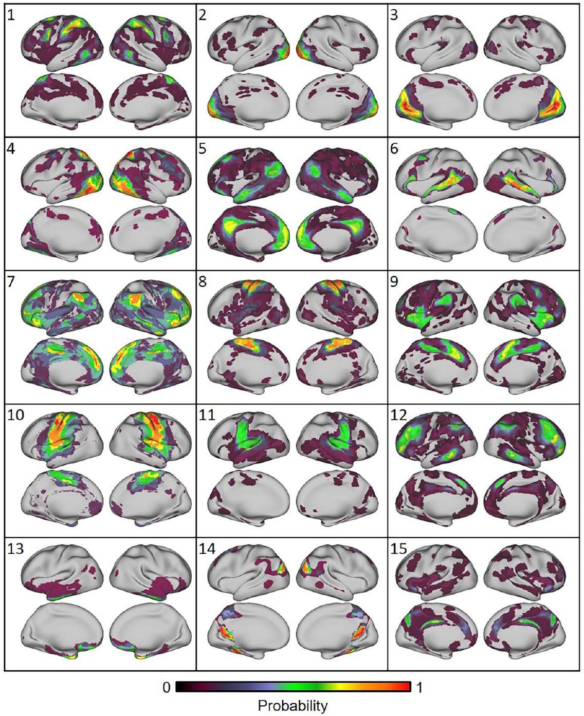
الشكل 3 | الطبوغرافيا المكانية لـ 15 مجموعة شبكية. انظر الشكل التكميلية 1 لمساهمات الأطلس والعلاقات الهرمية. الألوان الأكثر دفئًا تشير إلى توافق أكبر عبر الأطالس. نؤكد أن هذه الخرائط ليست مقصودة لتكون
شبكات التوافق، أي أننا لا نقترح أطلسًا جديدًا. بدلاً من ذلك، تهدف هذه الخرائط إلى توضيح التوافقات والاختلافات بين الأطالس الموجودة.

كإثبات كمي آخر لمشكلة تطابق الشبكات التي دفعت لتطوير NCT، قمنا بتقييم التطابق المكاني بين الشبكتين لشبكتين مستخدمتين على نطاق واسع. لهذه التوضيح، تم فحص جميع أزواج الشبكات الـ 136 من أطلسي Yeo2011-17 وGordon2017-17 (الشكل 5؛ انظر الجدول التكميلي 2 للحصول على معاملات دايس والتوافقات المقابلة). القيم). بشكل عام، لاحظنا تطابقًا جيدًا بين عدة شبكات عبر هذين الأطلسين. على سبيل المثال، كانت الشبكات البصرية الجانبية والوسطى في Gordon2017-17 تتوافق بشكل كبير مع الشبكات البصرية A وB في Yeo2011-17، على التوالي. كما أظهرت الشبكات الحركية الخاصة باليد والوجه والقدم في Gordon2017-17 تطابقًا كبيرًا مع الشبكات الحركية A وB في Yeo2011-17. ومع ذلك، ظهرت أيضًا تناقضات ملحوظة، خاصة فيما يتعلق باسم الشبكة والوظيفة المزعومة. على سبيل المثال، كانت الشبكة السمعية في Gordon2017-17 تتوافق أيضًا مكانيًا مع الشبكة الحركية B في Yeo2011-17. بينما أظهرت الشبكة الانتباهية الظهرية في Gordon2017-17 تطابقًا كبيرًا مع الشبكات الانتباهية الظهرية A وB في Yeo2011-17، كانت الشبكة الحركية السابقة في Gordon2017-17 تتوافق أيضًا بشكل كبير مع الشبكة الانتباهية الظهرية في Yeo2011-17.
الشبكة B. كانت الشبكة Cingulo-opercular من Gordon2017-17 تتوافق بشكل كبير مع الشبكتين Salience / Ventral Attention A و B من Yeo2011-17. ومع ذلك، كانت هناك شبكة Salience متميزة من Gordon2017-17 تتوافق أيضًا مع الشبكة Salience / Ventral Attention B من Yeo2011-17. كانت الشبكة Anterior Medial Temporal Lobe من Gordon2017-17 تتوافق بشكل كبير مع الشبكة Limbic A من Yeo2011-17 (التي تشمل الفصوص الزمنية الأمامية). وباتفاق قوي، كانت الشبكة Frontoparietal من Gordon2017-17 تتوافق بشكل كبير مع الشبكتين Frontoparietal Control A و B من Yeo2011-17. ومع ذلك، كانت الشبكة Parietal Memory من Gordon2017-17 تتوافق بشكل كبير مع الشبكة Frontoparietal Control C من Yeo2011-17. في مثال آخر على التوافق المكاني الجيد، كانت الشبكة Default من Gordon2017-17 تتوافق بشكل كبير مع الشبكتين Default A و B من Yeo2011-17. ومع ذلك، أظهرت الشبكة Default من Gordon2017-17 أيضًا توافقًا كبيرًا مع الشبكة Frontoparietal Control B من Yeo2011-17، مما يبرز أهمية النظر في الحجم النسبي لمعامل Dice. كانت الشبكة Language من Gordon2017-17 تتوافق بشكل كبير مع الشبكة Temporal Parietal من Yeo2011-17، بالإضافة إلى الشبكة Default B. كانت الشبكة Context من Gordon2017-17 والشبكة Posterior Medial Temporal Lobe تتوافقان بشكل كبير مع الشبكة Default C من Yeo2011-17. ومن الجدير بالذكر، أن Yeo2011-

شبكة 17 Limbic B (التي تتضمن القشرة الجبهية المدارية) لم تظهر أي تطابق مع أي من شبكات Gordon2017-17.

هذا المثال من Yeo2011-17 و Gordon2017-17 يوضح بشكل أكبر مشاكل (1) عدم التوافق في تسميات الشبكات، و (2) مستويات مختلفة من التوافق الشبكي عبر الأطالس. تحليل التوافق المكاني الثنائي لجميع الشبكات المدرجة ضمن جميع الأطالس الستة عشر خارج نطاق التقرير الحالي. ومع ذلك، يحتفظ NCT بهذه الوظيفة للقراء المهتمين. التقييم الثنائي المتعمق بين أطالس الشبكات الدماغية، بالإضافة إلى تقييم نتائج التصوير العصبي الجديدة مقابل الشبكات المحددة عبر عدة أطالس، هو وظيفة أساسية لـ NCT. بسبب التباين المكاني والتسمياتي عبر الأطالس، توصي لجنة أفضل الممارسات في OHBM الآن بأن يستخدم المستخدمون عدة أطالس تنشأ من مختبرات بحثية مختلفة للإبلاغ عن التوافق بين النتائج الجديدة وتسميات الشبكات الموجودة. تأتي التوصية بالإبلاغ عن النتائج بالإشارة إلى عدة أطالس من الملاحظة أن حتى الشبكات ذات التسميات المتشابهة عبر الأطالس (مثل “البارز”) قد لا تشترك في نفس الطبوغرافيا المكانية (الشكل 4).

بالنسبة لكل شبكة من أطلس مرجعي، يمكن تحديد حجم التوافق المكاني مع خريطة دماغية تجريبية، والأهمية الإحصائية لهذا التوافق، باستخدام NCT. يتم إسقاط جميع الأطالس ونتائج fMRI من مساحة قياسية إلى مساحة fsaverage6. يتم تقييم التوافق كمعامل Dice، حيث 0 يعني عدم وجود توافق مكاني و 1 يعني توافق مكاني كامل. من أجل تقييم الأهمية الإحصائية، يتم تنفيذ اختبار دوران المنفذ بلغة بايثون مع 1000 تبديل لكل شبكة من أطلس مرجعي.

يمكن تثبيت NCT باستخدام الأمر pip install cbig_network_correspondence. يوضح الشكل 6 استخدام NCT لاستكشاف التوافق الشبكي بين بيانات الإدخال المحددة من قبل المستخدم ومجموعة من الأطالس. على وجه التحديد، يحدد المستخدمون المسار إلى بيانات الإدخال ويقدمون ملف تكوين يحتوي على تفاصيل بيانات الإدخال مثل اسم البيانات، مساحة البيانات، ونوع البيانات. بالإضافة إلى ذلك، يقدم المستخدمون
قائمة بالأطالس المدرجة في NCT، المتاحة على https://github. com/rubykong/cbig_network_correspondence#atlases-we-included.

يبدأ NCT بقراءة بيانات الإدخال، وإسقاط الأطالس المحددة في القائمة إلى مساحة بيانات الإدخال، وحساب التشابه المكاني بين البيانات والأطالس، وإجراء التحليلات الإحصائية. ثم يتم تقديم نتائج التوافق الشبكي بصريًا.

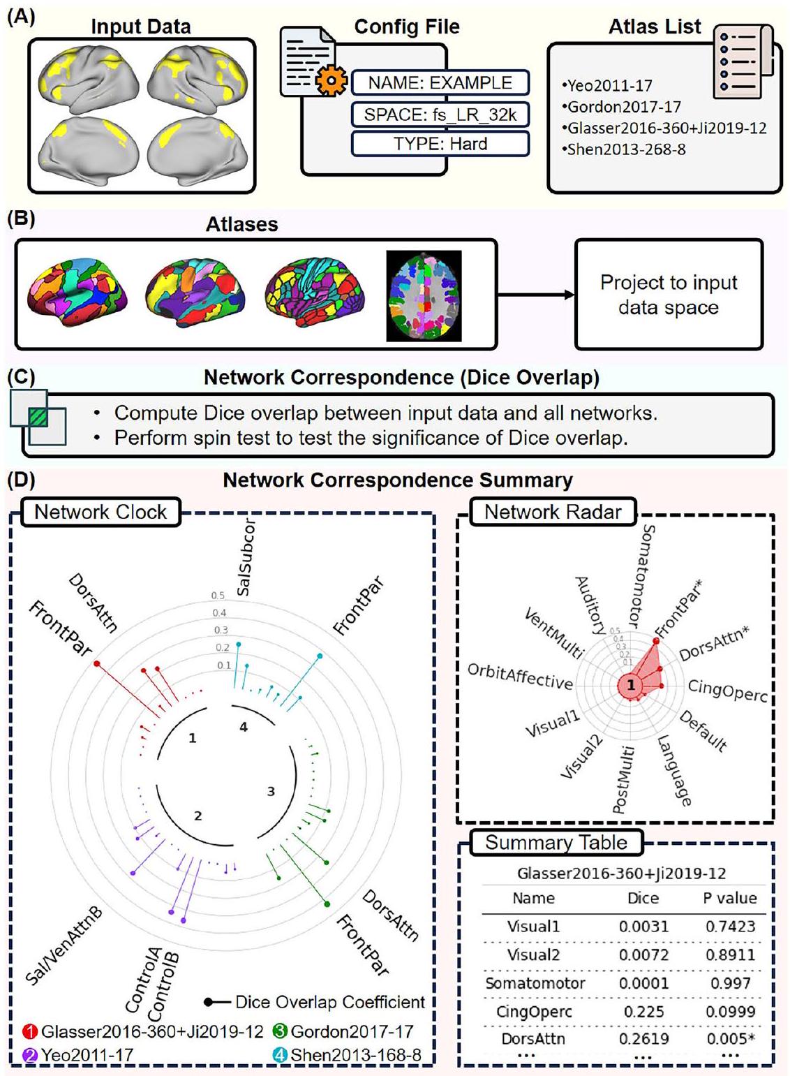
يمكن أن تكون بيانات الإدخال أحادية البعد أو متعددة الأبعاد. تشمل أمثلة البيانات أحادية البعد خريطة مكانية لمكون ICA واحد، خريطة تباين مهمة، أو شبكة واحدة من تقسيم صارم. يتم توضيح نتائج التوافق الشبكي للبيانات أحادية البعد كرسوم بيانية “ساعة الشبكة”، ورسم بياني “رادار الشبكة”، وجدول ملخص (الشكل 6D). توفر “ساعة الشبكة” مقارنة بصرية لتداخل Dice بين بيانات الإدخال والشبكات من أطالس مختلفة. تمثل الألوان المختلفة أطالس مختلفة. تمثل قضبان الحلوى معاملات تداخل Dice. يتم الإشارة إلى الشبكات التي تتداخل بشكل كبير مع بيانات الإدخال ( ) بأسماء الشبكات. في هذا الرسم، يتم عرض الشبكات التي لديها معاملات Dice أكبر بحجم خط أكبر. يظهر “رادار الشبكة” تداخل Dice عبر الشبكات داخل كل أطلس. يتم الإشارة إلى الشبكات التي تتداخل بشكل كبير مع بيانات الإدخال ( ) بـ “*”. يوفر NCT “جدول ملخص” يظهر معاملات Dice الدقيقة و القيم لأطالس مختلفة.

في حالة تعدد الأبعاد، يمكن أن تشمل الأمثلة مجموعة من خرائط ICA المكانية، أو عدة خرائط تباين مهمة، أو أي أطلس مدرج في NCT. يقدم NCT نتائج التوافق الشبكي للبيانات متعددة الأبعاد كرسوم بيانية “خريطة حرارة التداخل”، حيث تتوافق الصفوف مع بيانات الإدخال، والأعمدة تتوافق مع الشبكات من أطلس المقارنة. يمثل الصف – والعمود – معامل تداخل Dice بين البعد – من بيانات الإدخال والشبكة من الأطلس. في هذا الرسم، يشير اللون الأكثر سطوعًا إلى تداخل أعلى، بينما يشير اللون الأكثر قتامة إلى تداخل أقل. يتم الإشارة إلى الشبكات التي تتداخل بشكل كبير مع بيانات الإدخال ( ) بـ “*”. يوفر NCT أيضًا جدول ملخص يظهر معاملات Dice الدقيقة و -القيم.

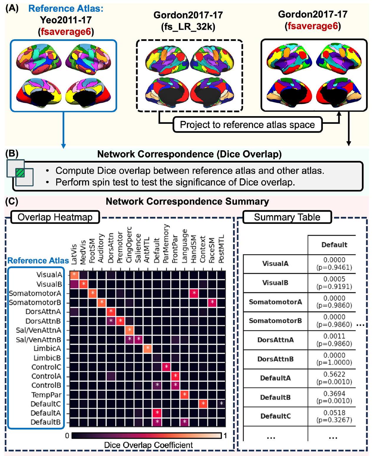
الشكل 5 | توضيح استخدام NCT لاستكشاف التوافق الشبكي بين أطلسين. في هذا المثال، نستكشف التداخل بين أطلس الشبكة Yeo2011 17-network (الأطلس المرجعي) وأطلس الشبكة Gordon2017 17-network. أ يحدد المستخدم اسم الأطلس المرجعي (هنا، Yeo2011-17) واسم أطلس المقارنة (هنا، Gordon2017-17). يقع أطلس الشبكة Yeo 17-network في مساحة fsaverage6، بينما يقع أطلس الشبكة Gordon2017 17-network في fs_LR_32k. في هذه الحالة، تكون مساحة الأطلس المرجعي هي fsaverage6. لذلك، يقوم NCT بإسقاط الشبكة Gordon2017 17-network إلى مساحة fsaverage6. ب يقوم NCT بحساب تداخل Dice بين الشبكات من أطلس الشبكة Yeo 17-network وأطلس الشبكة Gordon2017 17-network. يقوم NCT أيضًا بإجراء اختبار دوران لاختبار ما إذا كانت الشبكات تتداخل بشكل كبير. ج يقوم NCT بالإبلاغ عن التوافق الشبكي بين هذين الأطلسين باستخدام رسم بياني لخريطة حرارة التداخل،
حيث يمثل الصف – والعمود – معامل تداخل Dice بين الشبكة من أطلس الشبكة Yeo 17-network والشبكة من أطلس الشبكة Gordon2017 17-network. يشير معامل Dice العالي إلى تداخل عالٍ بين الشبكتين. تشير الألوان الأكثر سطوعًا إلى تداخل أعلى، بينما تشير الألوان الأكثر قتامة إلى تداخل أقل. يشير “*” إلى أن شبكتين تتداخلان بشكل كبير ( ). تتداخل معظم شبكات Yeo2011 مع شبكة واحدة على الأقل في أطلس Gordon2017. يوفر NCT أيضًا جدول ملخص يظهر معاملات Dice الدقيقة و القيم (انظر الجدول التكميلي 2). يستخدم NCT أسماء الشبكات من الورقة الأصلية لكل أطلس. Dors dorsal، attn attention، sal salience، ven ventral، temp temporal، par parietal، lat lateral، vis visual، med medial، SM somatomotor، cing cingulo، operc opercular، ant anterior، MTL medial temporal lobe.

تم بناء NCT بلغة بايثون وهو متاح في مستودع GitHub: https://github.com/rubykong/cbig_network_correspondence. تم إصدار صندوق الأدوات في فهرس حزم بايثون (PyPI): https://pypi.org/project/cbig-network-correspondence. الوثائق التفصيلية ودليل الاستخدام متاحة على: https://rubykong.github.io/ cbig_network_correspondence.

لإظهار تطبيقات مختلفة لـ NCT في كل من الحالات البسيطة والتحديات، نعرض بعد ذلك نتائج توافق الشبكات المتعددة. بالنسبة للأمثلة التالية، تم تحميل الصورة من
تحليل (مثل خريطة تنشيط المهمة)، وتم تعيين مساحة مجموعة الصور إلى مساحة قياسية محددة (مثل MNI152)، وتم تعيين عتبة للفاكسلات المهمة. ثم تم تحديد معاملات Dice لجميع الأطالس المرجعية، وتم إخراجها كمصفوفة معاملات Dice. لكل شبكة داخل كل أطلس، حددنا معامل Dice لتداخل الشبكة واستخدمنا اختبارات دوران لتحديد مستويات الأهمية.

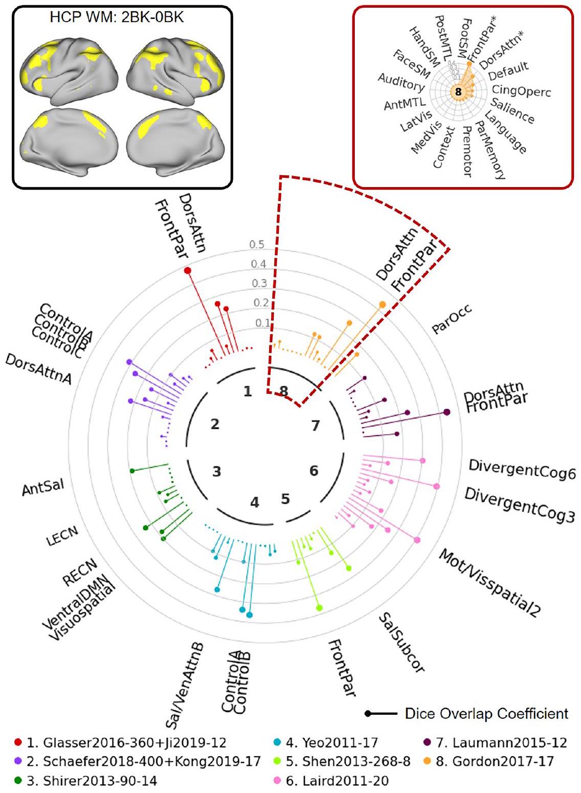
في المثال الأول، استخدمنا تباين مهمة الذاكرة العاملة HCP fMRI (2BK-OBK) الذي يتضمن بيانات من 997 موضوعًا من HCP S1200 . كما هو موضح في “ساعة الشبكة” الموضحة في الشكل 7، يظهر هذا التباين في مهمة fMRI (أعلى اليسار) تداخلًا مكانيًا كبيرًا مع

الشكل 6 | توضيح لاستخدام NCT لاستكشاف تطابق الشبكة بين بيانات الإدخال المحددة من قبل المستخدم ومجموعة من الأطالس. في هذا المثال، نستكشف التداخل بين مجموعة بيانات إدخال أحادية البعد و4 أطالس: أطلس الشبكة Yeo2011 17 (“Yeo2011-17”)، أطلس الشبكة Gordon2017 17 (“Gordon2011-17”)، أطلس Glasser2016 360-ROI مع شبكات Ji2019 12 Cole-Anticevic (“Glasser2016-360 + Ji2019-12”)، وأطلس Shen2013 268-ROI مع 8 شبكات (“Shen2013-268-8”). A يقوم المستخدم بتوفير بيانات الإدخال مع ملف تكوين يحدد الاسم، مساحة البيانات (مثل fs_LR_32k، fsaverage6، FSLMNI2mm)، ونوع البيانات (“Metric” إذا كانت بيانات الإدخال تحتوي على قيم عائمة؛ “Hard” إذا كانت بيانات الإدخال تحتوي على قيم ثنائية). في هذا المثال، بيانات الإدخال في مساحة fs_LR_32k وتحتوي على قيم ثنائية. نوع البيانات هو “Hard”. كما يقدم المستخدم قائمة الأطالس التي تحدد الأطالس التي يجب تضمينها. B يقوم NCT بقراءة بيانات الإدخال ويقوم بإسقاط الأطالس في قائمة الأطالس إلى مساحة بيانات الإدخال. C يقوم NCT بحساب تداخل Dice بين بيانات الإدخال والشبكات من الأطالس في القائمة. كما يقوم NCT بإجراء اختبارات دوران لاختبار ما إذا كانت بيانات الإدخال والشبكات ذات دلالة إحصائية.
التداخل. D تقارير NCT ملخص تطابق الشبكة باستخدام رسم “ساعة الشبكة”، ورسم “رادار الشبكة”، وجدول ملخص للبيانات أحادية الأبعاد. توفر “ساعة الشبكة” مقارنة بصرية لتداخل Dice عبر الشبكات من أطالس مختلفة. تمثل الألوان المختلفة أطالس مختلفة. تمثل أعمدة المصاصة معاملات تداخل Dice. الشبكات التي تتداخل بشكل كبير مع بيانات الإدخال تشير إليها أسماء الشبكات. تمثل حجم الخط الأكبر معامل ديس أكبر. تُظهر “رادار الشبكة” تداخل ديس عبر الشبكات داخل كل أطلس. الشبكات التي تتداخل بشكل كبير مع بيانات الإدخال “مشار إليها بـ “*”. كما يوفر NCT جدول ملخص يوضح معاملات ديس. -قيم عبر أطلس مختلفة (انظر الجدول التكميلي 3). يستخدم NCT أسماء الشبكات من الورقة الأصلية لكل أطلس. دورس ظهري، انتباه، بارتيال، بطني، أهمية، تحت القشري، سينيغولو، أوبيركولار، بطني، متعدد الوسائط، مداري، أمامي.
عدة شبكات عبر عدة أطلس (مثل شبكة “FrontPar” من أطلس غلاسر وغوردون، وشبكة “DorsAttn” من أطلس لاومان). كما هو موضح في مخطط “رادار الشبكة” (في أعلى اليمين)، يمكن استخدام NCT بشكل أكبر لقياس التداخل بين الخرائط المحددة من قبل المستخدم والشبكات المحددة داخل الأطلس. في المثال المميز في هذه الصورة، يظهر التباين المدخل تداخلاً كبيراً مع الشبكة.
تسميات “FrontPar” و”DorsAttn” في أطلس غوردون. يوضح هذا المثال حالة تتوافق فيها خريطة تنشيط المهمة بشكل جيد مع الشبكات المحددة في عدة أطالس.

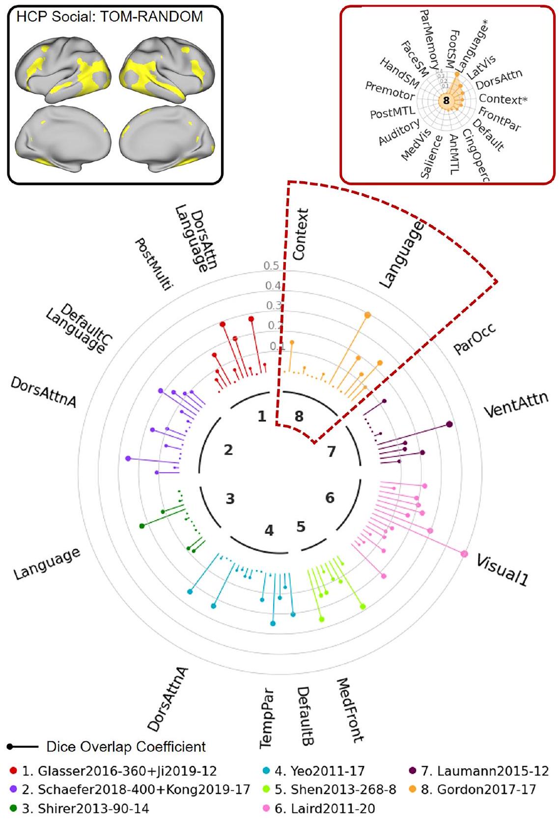
في المثال الثاني، استخدمنا تباين مهمة التصوير بالرنين المغناطيسي الاجتماعي HCP (TOM-random) الذي يتضمن بيانات من 997 موضوعًا. كما هو موضح في “ساعة الشبكة” الموضحة في الشكل 8، تتعلق هذه المهمة بتصوير الرنين المغناطيسي.

الشكل 7 | توضيح استخدام NCT لاستكشاف تطابق الشبكات بين بيانات الإدخال المحددة من قبل المستخدم والخرائط المتعددة: مثال HCP 1. في هذا المثال، نستكشف التداخل بين تباين مهمة الذاكرة العاملة HCP (2BK مقابل OBK) والشبكات من 8 خرائط. يقدم المستخدم بيانات الإدخال مع ملف تكوين يحدد الاسم، مساحة البيانات، نوع البيانات، والعتبة المستخدمة لتحديد بيانات الإدخال. كما يقدم المستخدم قائمة الخرائط التي تشير إلى الخرائط التي يجب تضمينها. يقوم NCT بتحديد البيانات بناءً على ملف التكوين ويعرض الخرائط في قائمة الخرائط إلى مساحة بيانات الإدخال. يحسب NCT تداخل Dice بين البيانات المحددة وجميع الشبكات من الخرائط في القائمة. كما يقوم NCT بإجراء اختبارات دوران لاختبار ما إذا كانت بيانات الإدخال المحددة والشبكات تتداخل بشكل كبير. يقدم NCT ملخص تطابق الشبكة باستخدام رسم بياني “ساعة الشبكة” (في المنتصف)، ورسم بياني “رادار الشبكة” (في أعلى اليمين)، وجدول ملخص يظهر معاملات Dice الدقيقة و
-قيم لجميع الأطلسيات (انظر الجدول التكميلي 3). يوفر “ساعة الشبكة” مقارنة بصرية لتداخل ديس عبر الشبكات من أطلسيات مختلفة. تمثل الألوان المختلفة أطلسيات مختلفة. تمثل القضبان على شكل مصاصة معاملات تداخل ديس. الشبكات التي تتداخل بشكل كبير مع بيانات الإدخال المحددة ( ) يتم الإشارة إليها بأسماء الشبكات. تمثل أحجام الخطوط الأكبر معاملات ديس. يُظهر “رادار الشبكة” تداخل ديس عبر الشبكات داخل كل أطلس. الشبكات التي تتداخل بشكل كبير مع بيانات الإدخال المحددة تشير إلى “*” في “رادار الشبكة”. WM الذاكرة العاملة، BK الظهر، dors الظهرية، attn الانتباه، par الجدارية، ant الأمامية، sal البروز، LECN شبكة التحكم التنفيذية اليسرى، RECN شبكة التحكم التنفيذية اليمنى، DMN شبكة الوضع الافتراضي، ven البطنية، subcor تحت القشرية، mot الحركية، vis البصرية، cog الإدراك، occ القذالية، front الجبهية، cing الحزامية، operc القشرية، med الوسطى، lat الجانبية، ant الأمامية، MTL الفص الصدغي الأوسط، SM الحركية الجسدية، post الخلفية.
التباين (في الزاوية العليا اليسرى) يظهر تداخلًا مكانيًا كبيرًا مع عدة شبكات عبر عدة أطلسات (مثل شبكة “VentAttn” من أطلس لاومان، وشبكة “Language” من أطلس غوردون). كما هو موضح في مخطط “رادار الشبكة” (في الزاوية العليا اليمنى)، يمكن استخدام NCT أيضًا لقياس التداخل بين الخرائط المحددة من قبل المستخدم والشبكات المحددة داخل الأطلس. في المثال المميز في هذه الصورة، يظهر التباين المدخل تداخلًا كبيرًا مع تسميات الشبكة “Language” و”Context” في أطلس غوردون. هذا المثال يوضح حالة حيث لا تتوافق خريطة تنشيط المهمة بشكل جيد مع الشبكات.
محدد في عدة أطالس. وبالتالي، فإنه يشير إلى أنه يجب تطبيق أي تسميات للشبكة على هذه الخريطة بحذر شديد.

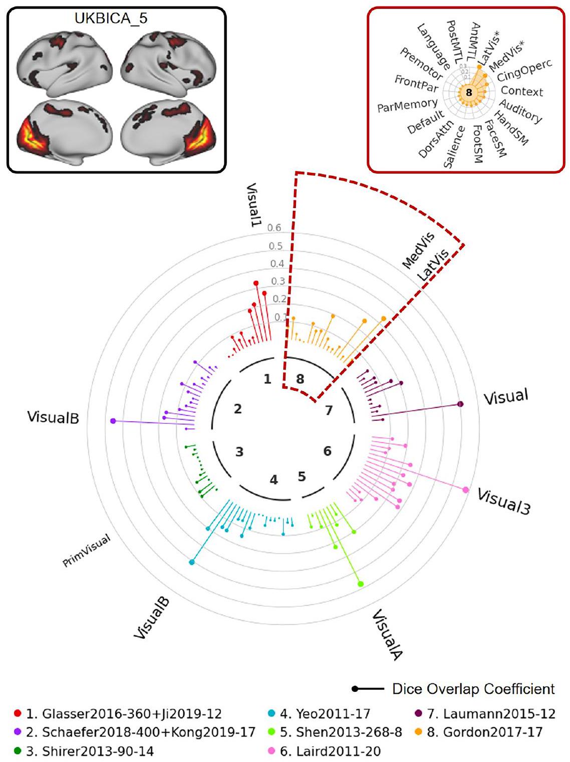
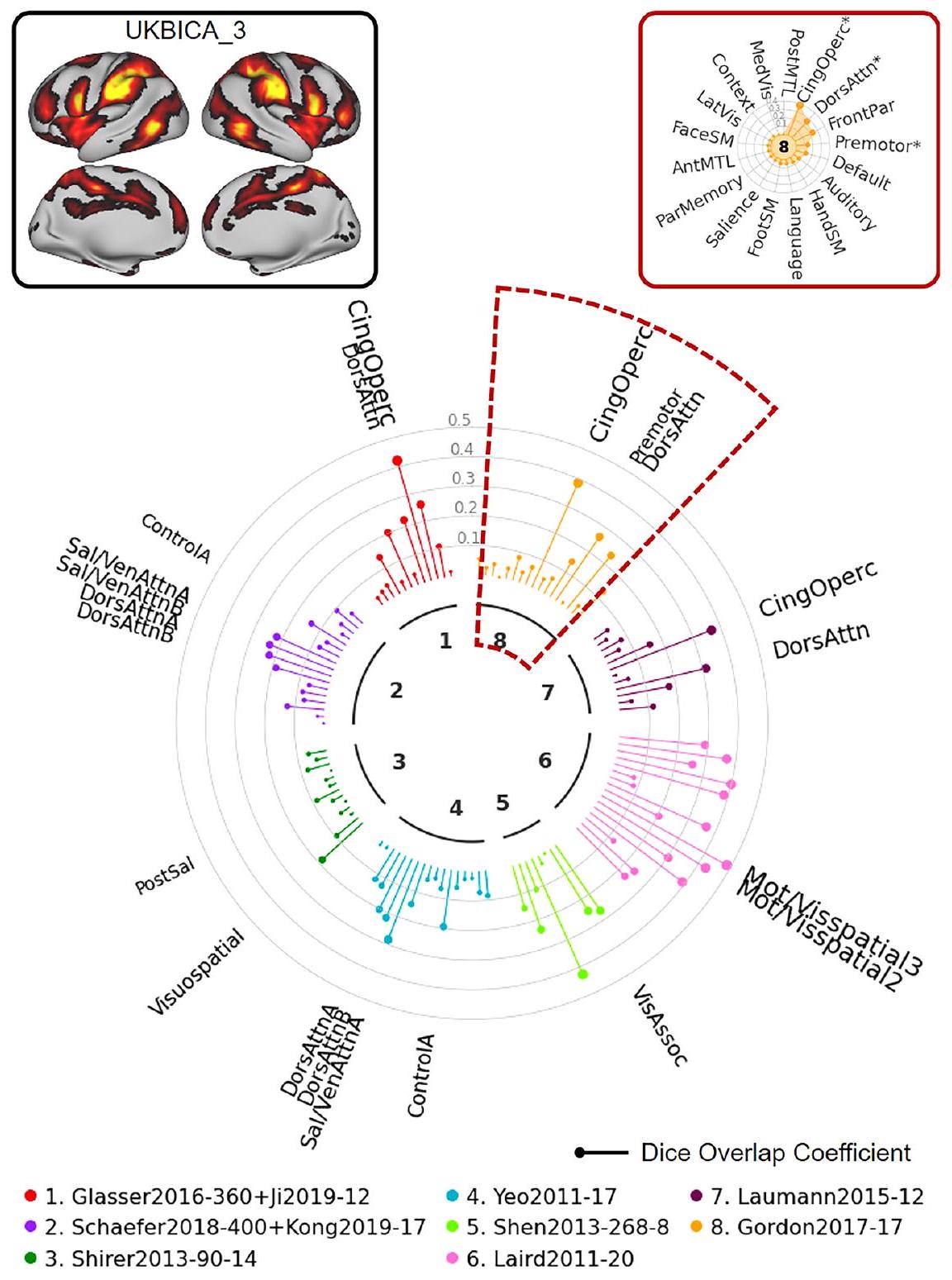
في المثال التالي، استخدمنا مكون ICA 5 من بنك المملكة المتحدة الحيوي لتوضيح كيف يمكن أن يسهل NCT الإبلاغ عن نتائج هذا النوع من التحليل. كما هو موضح في “ساعة الشبكة” الموضحة في الشكل 9، تُظهر هذه الخريطة ICA (في الزاوية العليا اليسرى) تداخلًا مكانيًا كبيرًا مع الشبكات الم labeled “بصري” عبر عدة أطلس. المثال النهائي (الشكل 10) يستخدم مكون ICA 3 من بنك المملكة المتحدة الحيوي كخريطة إدخال. حتى مع هذا الإدخال المعقد الذي يمتد عبر مناطق متعددة من الدماغ، يمكن استخدام NCT لت quantifying

الشكل 8 | توضيح لاستخدام NCT لاستكشاف تطابق الشبكة بين بيانات الإدخال المحددة من قبل المستخدم والعديد من الأطالس: مثال HCP 2. في هذا المثال، نستكشف التداخل بين تباين المهمة الاجتماعية لـ HCP (نظرية العقل مقابل العشوائي) و8 أطالس. يقدم المستخدم بيانات الإدخال مع ملف تكوين يحدد الاسم، مساحة البيانات، نوع البيانات، والعتبة التي تُستخدم لتحديد بيانات الإدخال. كما يقدم المستخدم قائمة الأطالس التي تشير إلى الأطالس التي يجب تضمينها. يقوم NCT بتحديد البيانات بناءً على ملف التكوين ويعرض الأطالس في قائمة الأطالس إلى مساحة بيانات الإدخال. يحسب NCT تداخل Dice بين البيانات المحددة وجميع الشبكات من الأطالس في القائمة. كما يقوم NCT بإجراء اختبارات دوران لاختبار ما إذا كانت بيانات الإدخال المحددة والشبكات تتداخل بشكل كبير. يقدم NCT ملخص تطابق الشبكة باستخدام رسم “ساعة الشبكة” (في المنتصف)، ورسم “رادار الشبكة” (في أعلى اليمين)، وملخص.
جدول يوضح معاملات ديس بدقة و -قيم لجميع الأطالس (انظر الجدول التكميلي 4). يوفر “ساعة الشبكة” مقارنة بصرية لتداخل ديس عبر الشبكات من أطالس مختلفة. تمثل الألوان المختلفة أطالس مختلفة. تمثل القضبان على شكل مصاصة معاملات تداخل ديس. الشبكات التي تتداخل بشكل كبير مع بيانات الإدخال المحددة ( ) يتم الإشارة إليها بأسماء الشبكات. تمثل أحجام الخطوط الأكبر معاملات ديس. تُظهر “رادار الشبكة” تداخل ديس عبر الشبكات داخل كل أطلس. الشبكات التي تتداخل بشكل كبير مع بيانات الإدخال المحددة ( ) يتم الإشارة إليها بـ “*” في “رادار الشبكة”. دورس ظهري، انتباه، بوست خلفي، متعدد الوسائط، مؤقت زمني، بارتيال، وسطي، أمامي، بطني، occ خلفي، جانبي، بصري، cing cingulo، operc opercular، أمامي، MTL الفص الصدغي الوسيط، SM حركي جسمي.
التداخل مع تسميات الشبكة الموجودة لتسهيل التواصل والمقارنة. مرة أخرى، توضح هذان المثالان حالات تتوافق فيها الخرائط المدخلة بشكل جيد (الشكل 9) ولا تتوافق بشكل جيد (الشكل 10) مع الشبكات المحددة في أطالس متعددة.

مجتمعة، توضح هذه الأمثلة كيف يمكن للباحثين استخدام NCT لتقديم نتائج جديدة في علم الأعصاب المعرفي والشبكي بشكل كمي ودقيق بالإشارة إلى الأطالس المستخدمة على نطاق واسع.
تعزيز قابلية التفسير والمقارنة مع النتائج الموجودة في الأدبيات.

على الرغم من عقود من أبحاث التصوير العصبي الوظيفي التي أسفرت عن ملاحظات متكررة وقوية لعدة شبكات دماغية وظيفية كبيرة، فإن التسمية التي تصف هذه الشبكات في

الشكل 9 | توضيح استخدام NCT لاستكشاف تطابق الشبكة بين بيانات الإدخال المحددة من قبل المستخدم والأطالس المتعددة: مثال UKB 1. في هذا المثال، نستكشف التداخل بين مكون UKB ICA 5 و 8 من الأطالس التمثيلية. تم تحديد خرائط z-stat الخاصة بـ UKB ICA مع 21 مكون جيد (https://www.fmrib.ox.ac.uk/ ukbiobank/group_means/rfMRI_GoodComponents_d25_v1.txt) وتم تحديدها بواسطة نموذج خلط FSL بمستوى عتبة 0.6. يتوافق المكون 16 مع المخيخ وتم استبعاده، مما أسفر عن 20 خريطة UKB ICA محددة.
يمكن العثور على خرائط UKB ICA المحددة الـ 20 في الشكل التكميلي 1. يوفر NCT أيضًا جدول ملخص يظهر معاملات Dice الدقيقة و القيم لجميع الأطالس (الجدول التكميلي 5). وسطي، بصري، جانبي، أولي، cing cingulo، operc opercular، SM حركي جسمي، دورس ظهري، انتباه، بارتيال، أمامي، خلفي، أمامي، MTL الفص الصدغي الوسيط.
البشر ليس موحدًا . بدلاً من ذلك، كان هناك انتشار لمتوسطات الشبكة السكانية المختلفة التي تعتمد على تسميات متميزة مستمدة من مجموعات بحث مستقلة تستخدم أساليب متباينة . في الواقع، لقد رأينا أن الشبكات حتى مع تسميات مشابهة (مثل “البارز”) عبر الأطالس قد لا تشترك في نفس الطبوغرافيا المكانية.

على الرغم من أن الأطالس تختلف في عدد الشبكات والأساليب المستخدمة لتحديد الشبكات، إلا أنها جميعًا تسعى لتصنيف الانتماءات الشبكية للقشرة والجزء تحت القشري. الهدف من كل لجنة أفضل الممارسات في OHBM هو توحيد وتأييد أفضل الممارسات عبر مجالات أبحاث التصوير العصبي البشري لتعزيز معرفة العلوم، والشفافية، وإمكانية التكرار. بناءً على الاستنتاجات التوافقية من لجنة أفضل الممارسات في OHBM حول تسميات الشبكة (WHATNET)، نقدم هنا NCT.

في بناء NCT، قمنا أولاً بالتحقيق في التطابق المكاني للشبكات الدماغية الوظيفية الكبيرة المحددة في ستة عشر أطلسًا مستخدمًا على نطاق واسع من مجموعة متنوعة من المساحات القياسية المعيارية (صور الحجم وخرائط السطح)، وطرق تعريف الشبكة، ومجموعات البيانات. بشكل عام، لوحظ درجة عالية من التطابق المكاني عبر الأطالس للعديد من الشبكات الوظيفية. ومع ذلك، تم ملاحظة مناطق من التباين الملحوظ أيضًا، خاصة بالنسبة للشبكات التي تمتد عبر القشرة المرتبطة. قمنا أيضًا بالتحقيق كميًا في التقارب مباشرة عبر أطلسين مستخدمين على نطاق واسع (Yeo201117 وGordon2017-17). كشفت هذه التحليلات أن شبكة تظهر كواحدة في أطلس واحد تم تقسيمها في بعض الحالات إلى شبكتين في الأطلس الآخر. كانت تسميات الشبكة عبر الأطلسين أيضًا غير متسقة في العديد من الحالات. تدعم مثل هذه التباينات التوصيات المنشورة في 2023 من WHATNET التي تنصح بأن التفسيرات المعتمدة على الشبكة للتفعيل الجديد أو الوظيفي

الشكل 10 | توضيح استخدام NCT لاستكشاف تطابق الشبكة بين بيانات الإدخال المحددة من قبل المستخدم والأطالس المتعددة: مثال UKB 2. في هذا المثال، نستكشف التداخل بين مكون UKB ICA 3 و 8 من الأطالس التمثيلية. تم تحديد خرائط z-stat الخاصة بـ UKB ICA مع 21 مكون جيد (https://www.fmrib.ox.ac.uk/ ukbiobank/group_means/rfMRI_GoodComponents_d25_v1.txt) وتم تحديدها بواسطة نموذج خلط FSL بمستوى عتبة 0.6. يتوافق المكون 16 مع المخيخ وتم استبعاده، مما أسفر عن 20 خريطة UKB ICA محددة.
يمكن العثور على خرائط UKB ICA المحددة الـ 20 في الشكل التكميلي 1. يوفر NCT أيضًا جدول ملخص يظهر معاملات Dice الدقيقة و القيم لجميع الأطالس (الجدول التكميلي 6). cing cingulo، operc opercular، دورس ظهري، انتباه، mot حركي، بصري، assoc ارتباط، sal بارز، vent بطني، بوست خلفي، أمامي، بارتيال؛ SM حركي جسمي، أمامي، MTL الفص الصدغي الوسيط، جانبي، وسطي.
تستخدم نتائج الاتصال المتعددة الأطالس المرجعية التي تم إنتاجها بواسطة مختبرات بحث مستقلة لتأكيد تحديد الشبكة . تم تصميم NCT لتعزيز وتسهيل اعتماد هذه التوصية من خلال تزويد الباحثين بأداة سهلة الاستخدام لإجراء التقارير حول تطابق الشبكات، كما هو موضح مع عدة أمثلة. نقترح أن تشير الدراسات المستقبلية إلى عدة أطالس مستقلة لتقييم تحديد الشبكة للنشاط أو الاتصال الوظيفي بشكل كمي، باستخدام NCT . سيساعد ذلك في المقارنات عبر الدراسات للتكرار، ويساعد في تفسير النتائج الجديدة، ويشجع على مزيد من الحوار بين مجموعات البحث ومجال علم الأعصاب الشبكي بشكل أوسع.

تتم سياقة العديد من الاكتشافات الجديدة في علم الأعصاب المعرفي والشبكي ضمن حدود الطبوغرافيات الشبكية المحددة مسبقًا. تختلف طرق تقييم تداخل الشبكة مع
الاتصال الوظيفي أو خرائط تفعيل مهام fMRI من الفحص البصري، والمسافة الإقليدية بين مركز كتلة مناطق الشبكة وذروات التفعيل، إلى الكمية المباشرة بين الأطلس والصورة العصبية. يمكن أن تكون التباينات في تنسيقات الصور بين الأطالس وصور النتائج عقبة كبيرة أمام تقييم التطابق بشكل مباشر و/أو تجريبي. يتم إجراء العديد من دراسات مهام fMRI في مساحة الحجم، ومع ذلك، يتم مشاركة بعض الأطالس فقط من قبل المبدعين في مساحة السطح ، مما يجادل بأن عرض الحجم أقل دقة . للتغلب على هذه المشكلة، تم تحويل جميع الأطالس المدرجة في NCT من مساحتها القياسية الأصلية لتكون متوافقة وقابلة للتشغيل مع جميع المساحات القياسية الأخرى، سواء في الحجم أو السطح. كانت هذه الطريقة أساسية لتقييم التطابق بين جميع الأطالس. علاوة على ذلك، تتيح هذه الطريقة الآن فحصًا مباشرًا وتجريبيًا للاكتشافات الجديدة في علم الأعصاب مقابل عدة أطالس مستخدمة على نطاق واسع في وقت واحد.

حاولت الأعمال السابقة قياس التباين المكاني بين الشبكات الدماغية الكبيرة المحددة في الأطالس الوظيفية المستخدمة على نطاق واسع، مشيرة أيضًا إلى تشابه معتدل فقط بين الأطالس. قام البعض بإنشاء أدوات تسمية قائمة على الأطلس ، لكن لم يقدم أي منها وسيلة لمقارنة النتائج الجديدة مع عدة أطالس في وقت واحد. أنشأ مشروع واحد أطلسًا توافقياً لشبكة الحالة الراحة بناءً على أطالس Yeo وGordon وDoucet . أدت الجهود الأولية لتوحيد تقسيمات الدماغ البشري إلى أدوات مثل Neuroparc، التي توفر وسيلة للمقارنة بين الأطالس المستخدمة على نطاق واسع . قارن آخرون بين التقسيمات التشريحية، والاتصال الوظيفي، والتقسيمات العشوائية وخلصوا إلى أنه لا يوجد نهج مثالي لاختيار تقنية التقسيم . اقترحت دراسات تقييم التقسيم الأخيرة أن التقسيمات متعددة الوسائط التي تجمع بين المقاييس الوظيفية والتشريحية قد تؤدي أداءً أسوأ من تلك المعتمدة فقط على البيانات الوظيفية لأن المناطق الدماغية المتجانسة وظيفيًا يمكن أن تمتد عبر المعالم التشريحية الرئيسية. بشكل حاسم، قامت هذه الدراسات إما بتقييم العلاقة بين الأطالس المختلفة ببساطة أو حاولت اشتقاق أطلس ‘توافقي’ واحد. إن NCT يلغي الحاجة للاعتماد على أي أطلس واحد. بدلاً من ذلك، يتناول بوضوح الغموض الكامن في تعيين تسميات الشبكات لخرائط الدماغ التجريبية من خلال قياس العلاقة المكانية بين خريطة تجريبية معينة وعدة تسميات أطلس موجودة ومستخدمة على نطاق واسع في الوقت نفسه.

يجدر بالذكر أن جميع الخرائط المكانية المستمدة من التصوير العصبي حساسة لاختيارات العتبة. إن مسألة تحديد العتبة المناسبة لنتائج التصوير بالرنين المغناطيسي الوظيفي خارج نطاق العمل الحالي، ولكن هناك العديد من المناقشات السابقة حول هذا الموضوع متاحة، وتُقدم إرشادات بشأن تحديد العتبة في تقارير أفضل الممارسات المبكرة لجمعية OHBM. “. نوصي بإيداع الصور غير المصفاة في مستودع مفتوح الوصول (مثل Neurovault)https://neurovault.org/) حتى يتمكن الباحثون من الوصول إلى استنتاجاتهم الخاصة بشأن التداخل بين النتائج الجديدة ومخططات التقسيم الموجودة.

من المهم الاعتراف بأن NCT لا تحدد للمستخدم ما هو مستوى المطابقة الذي يجب اعتباره كافياً لتبرير تسمية شبكة معينة لنتيجة معينة. الهدف من تقديم NCT للمجتمع هو المساعدة في ربط النتائج الجديدة بالتسميات الشبكية المعتمدة من قبل العديد من الأطالس المستخدمة على نطاق واسع. لا نرغب في أن نكون توجيهين بشأن عدد المطابقات التي يجب على المستخدم اختيارها لأي مجموعة معينة من النتائج، حيث أن ذلك يعتمد تمامًا على سؤال البحث قيد التحقيق. ومع ذلك، نظرًا لأن معامل دايس هو مقياس لحجم التأثير، والذي يتم الإبلاغ عنه في نفس الوقت مع -القيمة، كلاهما ضروري للتفسير. نتفق على أن القيم وحدها لا تكفي أبداً لتحديد تفسير النتائج. لهذا السبب، توفر معايير الإبلاغ النموذجية في التقديم المعدل مقاييس لكل من حجم التأثير والأهمية.

توصي WHATNET الآن بأن يتم فهرسة التقارير العلمية الجديدة حول أنماط تنشيط المهام أو الاتصال الوظيفي، إذا كانت تدعي الانخراط في شبكة دماغية وظيفية كبيرة محددة، إلى عدة أطلسات مستقلة للتحقق. يوفر NCT أداة سهلة الاستخدام ومتاحة لمتابعة هذه التوصية بالكامل. من المهم أن نرى NCT كمورد متطور، حيث ستكون قواعد بيانات الأطلسات مفتوحة أمام المجتمع البحثي. سيمكن ذلك NCT، كأداة لقياس توافق الشبكات، من التوسع مع تقديم مخططات تقسيم جديدة وأطلسات. ستكون أدوات مثل NCT حاسمة بشكل خاص لدمج النتائج عبر الطب النفسي وعلم الأعصاب، حيث يمكن أن يكون نقص التوجيه بشأن توافق الأطلسات وتسميات الشبكات عائقًا أمام التقدم السريري. .

قمنا بالتحقيق في تطابقات الشبكات القشرية بين بيانات الإدخال المحددة من قبل المستخدم ومجموعة من الأطالس الشبكية الوظيفية. بينما
يوجد 23 أطلسًا متاحًا في الإصدار الأحدث من NCT (الإصدار 0.3.1)، وقد اعتبرنا 16 أطلسًا لشبكات وظيفية مستخدمة على نطاق واسع ومتاحة للجمهور في فضاء سطح fsaverage6، وفضاء سطح fs_LR_32k، وفضاء MNI بما في ذلك Laird2011، Yeo2011، Shirer2012، Smith2013، Shen2013، Laumann2015، Miller2016، Gordon2016، Gordon2017، Schaefer2018، وJi2019. لتحليلات الموضحة في الأشكال 2 و 3. تستند الغالبية العظمى من هذه الأطالس إلى بيانات التصوير بالرنين المغناطيسي الوظيفي في حالة الراحة، على الرغم من أن القليل منها يعتمد على التصوير بالرنين المغناطيسي الوظيفي أثناء المهام. تحتوي بعض هذه الأطالس على دقة متعددة، مما يؤدي إلى 16 أطلس مختلف (الجدول التكميلي 1). ركزنا في هذه الدراسة على الشبكات القشرية؛ وتم إخفاء المناطق غير القشرية لجميع الأطالس. كما تم استبعاد الشبكات التي تتوافق فقط مع المناطق تحت القشرية والمخيخ من جميع التقسيمات المدروسة. يمكن العثور على قائمة كاملة بالأطالس المتاحة حاليًا في NCT فيhttps://pypi.org/project/cbig_network_المراسلة.

لحساب تشابه الشبكة بين بيانات الإدخال والأطالس المضمنة في NCT، نتعامل مع مساحة بيانات الإدخال كمساحة بيانات مرجعية ونقوم بإسقاط الأطالس إلى مساحة الأطلس المرجعي (انظر قسم الإسقاط بين الأطالس في مساحات مختلفة للحصول على تفاصيل الإسقاط). في حالة كون بيانات الإدخال أطلسًا، سيتم الإشارة إلى بيانات الإدخال باسم “الأطلس المرجعي”. توضح الشكل 1 مثالًا حيث كان أطلس شبكة Yeo 17 في مساحة fsaverage6 (في المنتصف) هو الأطلس المرجعي. تم إسقاط جميع الأطالس المحيطة الأخرى في مساحات مختلفة إلى مساحة fsaverage6. يتم تعريف تشابه الشبكة على أنه معاملات Dice بين بيانات الإدخال والأطالس المختلفة في مساحة البيانات المرجعية.

لكل شبكة مرجعية، قمنا بحساب معامل دايس بين هذه الشبكة المرجعية وكل شبكة من جميع الأطالس الأخرى في فضاء الأطلس المرجعي. بافتراض وجود K شبكة في الأطلس المرجعي وM شبكة في أطلس آخر، قمنا بإنشاء مصفوفة تشابه الشبكات بحجم KxM، حيث تمثل الصف k والعمود m معامل تداخل دايس بين الشبكة k من الأطلس المرجعي والشبكة. من الأطلس الآخر. يشير معامل ديس العالي إلى تداخل مكاني كبير بين الشبكتين. تم ترتيب مصفوفة تشابه الشبكات بحيث يتم إقران كل شبكة مرجعية مع الشبكة من الأطلس الآخر التي لديها أفضل تداخل (أي، أعلى معامل ديس) على طول القطر الرئيسي للمصفوفة. تشمل ستة عشر أطلسًا وظيفيًا تم تضمينها في هذه الدراسة 240 مصفوفة تشابه شبكة مختلفة.

لاستكشاف الاتفاق والاختلاف في تسميات الشبكات عبر ستة عشر أطلسًا مستخدمًا على نطاق واسع، قمنا بتجميع الشبكات ذات التداخل المكاني العالي معًا. خوارزمية التجميع الهرمي تم تطبيقه على مصفوفة تشابه الشبكات لتجميع جميع الشبكات في 15 مجموعة، وهو العدد المتوسط للشبكات عبر الأطالس. قمنا بإعادة ترتيب مصفوفة تشابه الشبكات بناءً على نتائج التجميع الهرمي. كما تم تصور نتائج التجميع الهرمي كخريطة وترية. ثم قمنا بفحص أسماء الشبكات يدويًا داخل كل مجموعة لتحديد الطوبوغرافيا المكانية للشبكات وتسمياتها.

نستخدم اختبار الدوران تم تنفيذه بلغة بايثون لتقييم ما إذا كانت بيانات المدخلات المرجعية تتداخل بشكل كبير مع الشبكات من أطلسات مختلفة. على وجه التحديد، يتم تدوير بيانات المدخلات المرجعية عشوائيًا 1000 مرة. لكل شبكة، نحسب معامل دايس بين بيانات المدخلات المدورة وهذه الشبكة. بالنسبة لشبكة تتداخل بشكل كبير مع بيانات المدخلات، نتوقع أن يكون معامل دايس بين هذه الشبكة وبيانات المدخلات المدورة أصغر من معامل دايس بين هذه الشبكة وبيانات المدخلات الأصلية. -القيمة تُعرف على أنها عدد بيانات الإدخال المدورة التي تحتوي على Dice
المعاملات أكبر من بيانات الإدخال الأصلية مقسومة على العدد الإجمالي للدورات. ومع ذلك، فإن اختبار الدوران يعمل فقط على البيانات في الفضاء السطحي. بالنسبة للبيانات الحجمية، نقوم بإسقاط البيانات إلى fsaverage6 باستخدام نهج متقدم للتخطيط غير الخطي. وأجرِ اختبار الدوران في مساحة سطح fsaverage6.

بالنسبة للأطالس المدرجة في NCT، اعتبرنا كل أطلس كأطلس مرجعي وقمنا بإسقاط الأطالس الأخرى إلى فضاء الأطلس المرجعي.

تم تحديد خرائط ICA المكانية لمجموعتي HCP و UKB من خلال ملاءمة نموذج خليط مكاني إلى هيستوغرام قيم الكثافة في كل خريطة مكون مستقل. يقوم نموذج الخليط بنمذجة الأجزاء الفارغة (ضوضاء الخلفية) والإشارة (“مفعلة” أو “موقفة”) من الخريطة المكانية بشكل صريح. تم تعيين قيمة عتبة قدرها 0.6 لإعطاء أهمية أكبر قليلاً لتحديد الإشارة على الضوضاء. في الممارسة العملية، تكون خرائط الفضاء المكانية الناتجة قوية أمام الانحرافات الصغيرة (على سبيل المثال، قيمة العتبة الذي يضع أهمية متساوية على تصنيف الفوكسل كإشارة مقابل ضوضاء، ويؤدي إلى نتائج أعلى في الخرائط المكانية التي تكون متشابهة جداً).

معلومات إضافية حول تصميم البحث متاحة في ملخص تقارير مجموعة نيتشر المرتبط بهذه المقالة.

جميع بيانات التصوير العصبي المضمنة في هذه الدراسة متاحة من الاتصال البشري:https://www.humanconnectome.org/study/hcp-
الشباب والبيانات الحيوية في المملكة المتحدة:https://www.ukbiobank.ac.uk/تم توفير بيانات مصدر المشروع في الجداول التكميلية.

صندوق أدوات مراسلة الشبكة هو صندوق أدوات بايثون متاح في مستودع جيت هاب:https://github.com/rubykong/cbig_network_correspondence. تم إصدار صندوق الأدوات إلى فهرس حزم بايثون (PyPI):https://pypi.org/project/cbig-network-correspondence. تتوفر وثائق مفصلة ودليل تعليمي علىhttps://rubykong.github.io/cbig_network_المراسلة.

يود المؤلفون أن يشكروا تايلور بولت، فيرونيكا ديفيتش، سارة م. أولشان، وسمر السيد لاختبارهم NCT وتقديم الملاحظات. كما يودون أن يشكروا أعضاء لجنة الممارسات المثلى في OHBM على دعمهم لهذا المشروع. R.K. و B.T.T.Y. مدعومان من كلية الطب في جامعة نانيانغ التكنولوجية (NUHSRO/2020/124/TMR/LOA)، ومجلس البحوث الطبية الوطني في سنغافورة (NMRC) LCG (OFLCG19May-0035)، وNMRC OF-IRG (OFIRG24jan-0006)، وNMRC CTG-IIT (CTGIIT23jan-0001)، وNMRC STaR (STaR20nov-0003)، ومنحة المركز من وزارة الصحة في سنغافورة (MOH) (CG21APR1009)، ومؤسسة تيمسيك (TF2223-IMH-O1)، والمعاهد الوطنية للصحة في الولايات المتحدة (NIH RO1MH12OO80 & RO1MH133334). L.Q.U. مدعوم من NIH (R21HD111805 و U01DA050987). R.N.S. مدعوم من منح من معاهد كندا للبحوث الصحية (CIHR) ومجلس البحوث الطبيعية والهندسية في كندا (NSERC) وNIH (NIA RO1AGO68563) وهو باحث في Fonds de recherche du Québec-Santé (FRQS). L.D.N. مدعوم من NIH (RF1AG078304). S.S. مدعوم من NIH (RO1MH116226) ومؤسسة العلوم الوطنية (CAREER 2237385). A.L.P. هو الحاصل على زمالة ما بعد الدكتوراه BrainsCAN في جامعة ويسترن من صندوق كندا للتميز في البحث. أي آراء أو نتائج أو استنتاجات أو توصيات معبر عنها في هذا المادة هي آراء المؤلفين ولا تعكس وجهات نظر الممولين.

ساهم R.K. في تحليل البيانات وتفسيرها وإنشاء البرمجيات. ساهم A.X. في إنشاء البرمجيات. ساهم R.N.S. وB.T.T.Y. وL.Q.U. في تصور وتصميم الدراسة، وتفسير البيانات، وصياغة العمل. ساهم R.F.B. وJ.R.C. وJ.S.D. وF.D.B. وS.B.E. وA.F. وC.G. وE.M.G. وA.J.H. وA.R.L. وL.L.P. وL.D.N. وA.L.P. وA.R. وS.S. وJ.M.S. وA.Y. في تفسير البيانات وإجراء مراجعة جوهرية للعمل.

يعلن المؤلفون عدم وجود مصالح متنافسة.

معلومات إضافية النسخة الإلكترونية تحتوي على مواد إضافية متاحة علىhttps://doi.org/10.1038/s41467-025-58176-9.

يجب توجيه المراسلات والطلبات للحصول على المواد إلى R. Nathan Spreng أو B. T. Thomas Yeo أو Lucina Q. Uddin.

معلومات مراجعة الأقران تشكر مجلة Nature Communications المراجع(ين) المجهول(ين) على مساهمتهم في مراجعة هذا العمل. يتوفر ملف مراجعة الأقران.

معلومات إعادة الطباعة والتصاريح متاحة علىhttp://www.nature.com/reprints

ملاحظة الناشر: تظل شركة سبرينجر ناتشر محايدة فيما يتعلق بالمطالبات القضائية في الخرائط المنشورة والانتماءات المؤسسية.

الوصول المفتوح هذه المقالة مرخصة بموجب رخصة المشاع الإبداعي النسب 4.0 الدولية، التي تسمح بالاستخدام والمشاركة والتكيف والتوزيع وإعادة الإنتاج بأي وسيلة أو صيغة، طالما أنك تعطي الائتمان المناسب للمؤلفين الأصليين والمصدر، وتوفر رابطًا لرخصة المشاع الإبداعي، وتوضح إذا ما تم إجراء تغييرات. الصور أو المواد الأخرى من طرف ثالث في هذه المقالة مشمولة في رخصة المشاع الإبداعي الخاصة بالمقالة، ما لم يُشار إلى خلاف ذلك في سطر الائتمان للمواد. إذا لم تكن المادة مشمولة في رخصة المشاع الإبداعي الخاصة بالمقالة وكان استخدامك المقصود غير مسموح به بموجب اللوائح القانونية أو يتجاوز الاستخدام المسموح به، فستحتاج إلى الحصول على إذن مباشرة من صاحب حقوق الطبع والنشر. لعرض نسخة من هذه الرخصة، قم بزيارةhttp://creativecommons.org/رخصة/بواسطة/4.0/.
(ج) المؤلف(ون) 2025

¹مركز أبحاث التصوير بالرنين المغناطيسي الانتقالي ومركز النوم والإدراك، الجامعة الوطنية في سنغافورة، سنغافورة، سنغافورة. ²قسم الأعصاب وجراحة الأعصاب، جامعة مكغيل، مونتريال، كيو بي، كندا. قسم العلوم النفسية وعلوم الدماغ، جامعة إنديانا، بلومنجتون، إنديانا، الولايات المتحدة الأمريكية. قسم علم النفس وعلم الأعصاب، جامعة نورث كارولينا، تشابل هيل، نورث كارولينا، الولايات المتحدة الأمريكية. قسم علم النفس، جامعة وين ستيت، ديترويت، ميشيغان، الولايات المتحدة الأمريكية. معهد علم الشيخوخة، جامعة وين ستيت، ديترويت، ميشيغان، الولايات المتحدة الأمريكية. قسم الفلسفة، جامعة ديوك، دورهام، نورث كارولينا، الولايات المتحدة الأمريكية. معهد علوم الأعصاب النظامية، كلية الطب، جامعة هاينريش هاينه دوسلدورف، دوسلدورف، ألمانيا. معهد علوم الأعصاب والطب، الدماغ والسلوك (INM-7)، مركز أبحاث يوليش، يوليش، ألمانيا. مدرسة العلوم النفسية، جامعة موناش، ملبورن، فيكتوريا، أستراليا. معهد تيرنر للدماغ والصحة النفسية، جامعة موناش، ملبورن، فيكتوريا، أستراليا. تصوير الطب الحيوي في موناش، جامعة موناش، ملبورن، فيكتوريا، أستراليا. قسم علم النفس، جامعة إلينوي، أوربانا شامبين، إلينوي، الولايات المتحدة الأمريكية. معهد بيكمان للعلوم والتكنولوجيا المتقدمة، جامعة إلينوي، أوربانا شامبين، إلينوي، الولايات المتحدة الأمريكية. معهد مالينكروت للأشعة، جامعة واشنطن، سانت لويس، ميزوري، الولايات المتحدة الأمريكية. قسم الطب النفسي، جامعة روتجرز، نيو برunswick، نيو جيرسي، الولايات المتحدة الأمريكية. مركز صحة الدماغ، جامعة روتجرز، نيو برunswick، نيو جيرسي، الولايات المتحدة الأمريكية. قسم الفيزياء، جامعة فلوريدا الدولية، ميامي، فلوريدا، الولايات المتحدة الأمريكية. قسم الطب النفسي، جامعة أركنساس للعلوم الطبية، ليتل روك، أركنساس، الولايات المتحدة الأمريكية. قسم علوم الأعصاب، جامعة أركنساس للعلوم الطبية، ليتل روك، أركنساس، الولايات المتحدة الأمريكية. قسم الطب النفسي، كلية هارفارد الطبية، مستشفى مكليان، بوسطن، ماساتشوستس، الولايات المتحدة الأمريكية. المركز الغربي للدماغ والعقل، جامعة ويسترن، لندن، أونتاريو، كندا. قسم علوم الحاسوب وقسم علم النفس، جامعة ويسترن، لندن، أونتاريو، كندا. مركز الدماغ والعقل، جامعة سيدني، سيدني، نيو ساوث ويلز، أستراليا. قسم الأشعة، مستشفى ماساتشوستس العام، بوسطن، ماساتشوستس، الولايات المتحدة الأمريكية. قسم الطب النفسي وعلوم السلوك الحيوي، جامعة كاليفورنيا في لوس أنجلوس، لوس أنجلوس، كاليفورنيا، الولايات المتحدة الأمريكية. قسم علم النفس، جامعة كاليفورنيا في لوس أنجلوس، لوس أنجلوس، كاليفورنيا، الولايات المتحدة الأمريكية. البريد الإلكتروني:nathan.spreng@mcgill.ca;thomas.yeo@nus.edu.sg;lucina@ucla.edu

Article

Received: 15 November 2024

Published online: 25 March 2025
Check for updates

The brain can be decomposed into large-scale functional networks, but the specific spatial topographies of these networks and the names used to describe them vary across studies. Such discordance has hampered interpretation and convergence of research findings across the field. We have developed the Network Correspondence Toolbox (NCT) to permit researchers to examine and report spatial correspondence between their novel neuroimaging results and multiple widely used functional brain atlases. We provide several exemplar demonstrations to illustrate how researchers can use the NCT to report their own findings. The NCT provides a convenient means for computing Dice coefficients with spin test permutations to determine the magnitude and statistical significance of correspondence among user-defined maps and existing atlas labels. The adoption of the NCT will make it easier for network neuroscience researchers to report their findings in a standardized manner, thus aiding reproducibility and facilitating comparisons between studies to produce interdisciplinary insights.

Standardized scientific nomenclature can facilitate the effective communication of concepts related to complex biological systems. Neuroscience has a long history of classifying distinct anatomical regions of the brain across multiple spatial scales, from the cortical lobes, discrete gyri and sulci of the cerebral cortex and subcortical nuclei, to Brodmann’s cytoarchitectonic areas . Attempts have also been made to categorize well-defined neural circuits and systems based on various anatomical and functional criteria, such as the cortico-spinal tract, cortico-striato-thalamic circuits, and the dorsal and ventral visual processing streams . Such attempts at standardization facilitate communication about brain organization between researchers and assist in educating students.

Modern neuroimaging methods, particularly those relying on magnetic resonance imaging, have revolutionized our capacity to noninvasively map different aspects of brain structure and function in living humans. A key development has been the ability to map functional brain networks, or groups of brain areas that exhibit functional synchrony. As a result of the growing popularity of this approach, many findings from neuroimaging studies are described in terms of the brain networks, rather than the brain areas, where they are localized. However, this is often done in an ad hoc way due to the lack of standardization in the naming of these networks. This inconsistency in scientific reporting complicates comparisons of findings across studies and limits the integration of novel discoveries .

The emergence of functional brain network atlases, which are now routinely used in cognitive and network neuroscience , should, in principle, contribute to standardization in the naming of functional networks. These atlases typically assign parcellated cortical and/or subcortical regions to one of a set of large-scale brain networks with varying topographies, ranging from largely contiguous unimodal territories (e.g., visual network in occipital cortex) to associative systems that span multiple spatially segregated and distributed regions across the brain (e.g., default network encompassing frontal, temporal and parietal regions). The atlases also vary in how they name large-scale brain networks and in terms of the number of brain networks, as well as their approach to defining the networks, characterizing their spatial topography, and deciding how they should be labeled (e.g., based on their anatomical location or purported cognitive correlates) . These differences between atlases lead to further variability and uncertainty in scientific reporting.

Recognizing these challenges, the Organization for Human Brain Mapping (OHBM) established a Best Practices committee on large-scale brain network nomenclature, following the success of earlier similar consensus-building initiatives aiming to enhance standardization by providing reporting guidelines for the field . This committee, formed in 2020, is known as the Workgroup for HArmonized Taxonomy of NETworks (WHATNET). Initial attempts by the workgroup to conceptually identify convergence across large-scale functional brain networks led to discussion and enumeration of the multiple challenges inherent to this enterprise . The workgroup surveyed hundreds of scientists and solicited putative network names based upon renderings of various network spatial topographies. Results from the survey, described in detail in the initial report from WHATNET and publicly available (https://osf.io/3fzta/), indicated that networks based in nondistributed unimodal brain regions (somatomotor and visual systems) could be readily and reliably identified. The somatomotor network showed agreement amongst raters, while the visual network showed 92% agreement amongst raters. Only one spatially distributed network, the default network, demonstrated consensus agreement in name and topography, with agreement amongst raters. Other networks, such as those sometimes referred to as salience or frontoparietal, showed less consistency. These findings indicate that consensus agreement in nomenclature is limited to the extreme poles of the canonical cortical hierarchy , anchored at one end by the visual and somatomotor systems and on the other by the default network. In between these systems is an expanse of cortex with observable network structure, but with little agreement between researchers regarding their spatial topography or nomenclature. Such variability poses a major problem for any attempts to compare or integrate findings across studies.

In response to the WHATNET survey findings, here we present the Network Correspondence Toolbox (NCT). This toolbox provides researchers with a practical solution for labeling novel observed fMRI activation, functional connectivity patterns, or other thresholded neuroimaging maps based on a quantitative evaluation against multiple currently published atlases simultaneously. The NCT also allows users to assess the spatial correspondence between networks in new and existing atlases. We demonstrate the utility of the NCT in providing network labels to exemplar neuroimaging maps based on a quantitative evaluation of spatial correspondence with multiple published network atlases. Quantitative evidence of correspondence is determined by the magnitude of the Dice coefficient, in addition to spin test permutations for robust statistical assessment of significance. We conclude with a recommendation that future network and cognitive neuroscience reports include an evaluation of the correspondence between their network labeling schemes and multiple published network atlases produced by independent research laboratories, as facilitated by the NCT. This approach transparently acknowledges and quantitatively addresses the ambiguity inherent in assigning labels to
topographic brain maps and encourages greater alignment across network neuroscience studies by objectively assessing the convergence or divergence between new findings and published network labels and schema. Importantly, the NCT is not prescriptive regarding the largely intractable problem of inconsistent network nomenclature. Rather, it is a tool to facilitate comparison and interpretation to be drawn across atlases, ultimately resulting in greater standardization in reporting of results.

We begin by illustrating the network correspondence problem by computing network overlap across sixteen widely used functional brain atlases. Next, as another quantitative example, we demonstrate the correspondence between two widely-used atlases that delineate the cortex into 17 discrete networks: Yeo2011-17 and Gordon2017-17. These examples serve to illustrate the network nomenclature problem and to motivate NCT usage. Then, we provide step-by-step guidelines for NCT usage. Finally, we report several examples of how the NCT can be used by treating publicly available Human Connectome Project (HCP) task fMRI results and UK Biobank independent component analysis (ICA) maps as “novel” findings for demonstration purposes. These specific maps were chosen to illustrate how the NCT performs in cases where the input data correspond with existing networks to a strong degree, as well as in more challenging scenarios where correspondence is lower.

Anatomical localization of patterns of brain activity is tedious , but many digital and paper atlases are available to facilitate the process . Localization to large-scale functional brain networks is a more recent development, with standardized tools in demand (see for a recent introduction of probabilistic network localization). The NCT flexibly permits the assessment of spatial correspondence between several target reference atlases and novel brain maps including, but not limited to, functional connectivity and task activation results, as well as other maps in standard space . Note that some of the included atlases included in the NCT contain multiple versions: Yeo2011, Schaefer2018, Kong2021, Power2011, Shen2013, Gordon2017, Cole-Anticevic2019, ICA-UK Biobank, ICA-HCP, ICA-BrainMap, and Shirer2012 (Fig. 1 and Supplementary Table 1). The most recent release of the NCT (v 0.3 .1) includes 23 brain atlases. A full list of currently available atlases in the NCT can be found in https://pypi.org/project/cbig_network_ correspondence.

We considered 16 widely used functional brain atlases including the Yeo2011, Schaefer2018, Kong2021, Power2011, Shen2013, Gordon2017, Cole-Anticevic2019, ICA-UK Biobank, ICA-HCP, ICA-BrainMap, and Shirer2012 (Fig. 1 and Supplementary Table 1). To compute the network overlap across atlases, we treated each atlas as the reference atlas and projected other atlases into that reference atlas. Between each reference network and each network from all other atlases, we computed the Dice coefficient. This allowed us to compare the voxel-wise agreement between the reference network and all other networks, where 0 is no correspondence and 1 is total correspondence. Assuming there are K networks in the reference atlas and M networks in another atlas, we generated a KxM network overlap matrix, where the -th row and -th column represents the Dice overlap coefficient between network of the reference atlas and network from the other atlas. A high Dice coefficient indicates high spatial overlap between the two networks from different atlases.

Dice coefficients between all 16 atlases were computed and examined. The non-symmetrical matrix shows relative differences due to atlases referencing in the upper and lower triangles (Fig. 2). Each matrix sub-block reveals patterns of correspondence (with total

Fig. 1 | Example atlases included in the Network Correspondence
Toolbox (NCT). The NCT is a toolbox that facilitates exploration of network correspondences across multiple functional network atlases as well as quantitative comparison of novel neuroimaging results with multiple atlases. Ten atlases are shown here for illustration purposes. In this example, the Yeo 17-network atlas in
fsaverage6 space (center) serves as the reference atlas. All other surrounding atlases in different spaces are projected to the fsaverage6 space to compute Dice overlap coefficients with the reference networks. A full list of currently available atlases in the NCT can be found in https://pypi.org/project/cbig_network_ correspondence.
correspondence within-atlas on the diagonal). Non-square sub-blocks of the matrix are due to differences in the number of networks identified between atlases, which ranged from 7 (Yeo2011) to 25 (Smith2013; Miller2016). Distributed spatial topographies of functional networks across atlases show some reliable correspondence, based on the observable sub-block diagonal structure.

Among the 16 atlases included, differences in numbers of networks included some cases of non-independent solutions that were derived from the same dataset or from the same laboratory. For this reason, the present investigation cannot determine the optimal solution for the number of large-scale networks in the human brain, as assessed using fMRI. Based on the Dice overlap, hierarchical structures of the network similarity matrix were examined using a nested stochastic block model , with 15 clusters applied (the average number of networks across atlases). It is important to note that this clustering is not meant to generate consensus networks across atlases. Rather, the clustering algorithm permits an examination of the spatial correspondence across atlases, indexed by atlas source, and specific network names. The network probability maps of each cluster are displayed in Fig. 3.

We visually inspected each cluster and associated network names for parcellations that provided network labels. The spatial extent of the network probability maps and their corresponding labels (ignoring subnetwork designations) were similar across atlases for many clusters. All clusters were bilateral. Cluster 5, comprising medial prefrontal and medial parietal cortex, inferior parietal lobule, lateral temporal and medial temporal lobe, inferior frontal gyrus, and superior middle frontal gyrus, was nearly uniform in being labeled the “default network” across atlases. However, some functional ensembles were diversely named, and distinct inconsistencies were noted.

The distributed network of Cluster 12, including lateral prefrontal cortex, anterior inferior parietal lobule, posterior inferior temporal gyrus, and dorsal anterior cingulate cortex, also showed strong
correspondence across multiple atlases, but the atlases used diverse labels, such as “frontoparietal”, “control”, and “central executive”. This network is well known and identified for its role in the executive control of information processing in the human brain . The divergent names largely point to the same cognitive construct even in the absence of consistent and consensus nomenclature across atlases .

Convergence was observed for perceptual and motor networks. Probability maps of Clusters 2 and 3 converged in the occipital lobe, with consistent labels related to vision (“visual”). Rostral to the occipital networks was Cluster 4, which extended dorsally into superior parietal cortex and ventrally into inferior temporal cortex This network was variously labeled “dorsal attention”, “visual association”, and “visual”. Cluster 1 included two regions rostral to those identified in Cluster 4, the superior parietal lobule and middle temporal motion complex, as well as the putative frontal eye fields and inferior precentral sulcus. These distributed regions were predominantly labeled “dorsal attention” in addition to “visuospatial” and “premotor”.

Motor and somatosensory cortex, anterior and posterior to the central sulcus, include the precentral and postcentral gyri, and extend medially into the juxtapositional lobule (supplementary motor area). Cluster 10 included these areas with reliable labels of “somatomotor” or “motor”. The dorsal and medial extent were specifically recapitulated in Cluster 8, with labels of “somatomotor”, and specifically “hand”, “foot”, and “dorsal somatomotor”. Cluster 11 included the ventral extent of motor and somatosensory cortex, descending through the middle insula, and terminating in the superior temporal gyrus. This cluster was split in names between “somatomotor” and “auditory” labels across different atlases.

Finally, convergence of the “ventral attention”, “salience”, and “cingulo-opercular” networks was apparent in Cluster 9, with regions including anterior insula, middle and dorsal anterior cingulate cortex, and lateral parietal cortex. For example, the salience/ventral

Fig. 2 | Hierarchical structures of the network similarity matrix (Dice overlap). The nested stochastic block model with 15 clusters was applied onto the network similarity matrix where Dice coefficients were calculated between each pair of networks from different atlases. The network similarity matrix is a matrix since there are 16 atlases with 230 networks. Each block corresponds to a network cluster. Representative network names within each cluster are highlighted here. See Supplementary Fig. 1 for clustering results with atlas associations. We emphasize
that the hierarchical clustering is not meant to generate a new consensus atlas; rather it is a way for us to examine convergence and divergence across atlases. Prim primary, med medial, lat lateral, vis visual, assoc association, par parietal, occ occipital, ant anterior, MTL medial temporal lobe, front frontal, ven ventral, attn attention, tem temporal, SM somatomotor, post posterior, SAL salience, subcor subcortical, cing cingulo, operc opercular.
attention network-A from the Yeo2011-17 atlas largely overlapped with the cingulo-opercular network from the Gordon2017 atlas. However, the salience network label has also been applied to anatomically different regions as well, with poor convergence between some atlases. The salience network as labeled in the Gordon2017 17-network, Yeo2011 7-network, Shirer2012 14-network, and Shen2013 8-network show distinct distributed spatial topographies (Fig. 4).

Five network probability maps were more ambiguous in their topography and naming. Clusters , and 6 included two to three discrete regions in each hemisphere. These regions may be part of larger named systems but can present as unique ensembles, depending on the atlas used. Cluster 13, including orbitofrontal and anterior temporal regions, was labeled “limbic” and “anterior medial temporal” (note these regions are often left unlabeled in some atlases due to heavy overlap with susceptibility artifact in fMRI). Cluster 14 included
ventral retrosplenial cortex, inferior temporal and lateral occipital regions and was diversely labeled “context”, “parietal-occipital”, and “default”. Cluster 15 included dorsal retrosplenial cortex and dorsal posterior precuneus, and was labeled “control”, “salience”, and “medial parietal memory”. Cluster 6 included the inferior frontal gyrus and superior lateral temporal regions, and was labeled “TempPar”, “language”, and “ventral attention”. The topography of Cluster 6 resembles task-driven language function . Problematically, the cognitive network terms associated with Clusters 14, 15, and 6 are incongruent.

Cluster 7 was unique in that it only included networks identified from atlases derived using ICA. These networks were given a numerical ID rather than labels derived from anatomical or cognitive features and originated from HCP and UKBiobank. Brain regions included dorsomedial prefrontal cortex, anterior insula, inferior parietal lobule, lateral temporal cortex, dorsal anterior precuneus, and posterior superior frontal gyrus.”

Fig. 3 | Spatial topography of the 15 network clusters. See Supplementary Fig. 1 for atlas contributions and hierarchical relations. Warmer colors indicate greater concordance across atlases. We emphasize that these maps are not meant to be
consensus networks, i.e., we are not proposing a new atlas. Instead, these maps are meant to illustrate the convergences and divergences between existing atlases.

As another quantitative demonstration of the network correspondence problem that motivated the development of the NCT, we evaluated network-to-network spatial correspondence between two widely used atlases. For this illustration, all 136 network pairs from the Yeo2011-17 and Gordon2017-17 atlases were examined (Fig. 5; See Supplementary Table 2 for Dice coefficients and corresponding values). Overall, we observed good correspondence between several of the networks across these two atlases. For example, Gordon201717 Lateral Visual and Medial Visual networks significantly corresponded to the Yeo2011-17 Visual A and B networks, respectively. Specific Hand, Face, and Foot Somatomotor networks in the Gordon2017-17 showed significant correspondence with Somatomotor networks A and B in Yeo2011-17. However, notable discrepancies also emerged, particularly with regard to network name and purported function. For example, the Gordon2017-17 Auditory network also spatially corresponded to the Yeo2011-17 Somatomotor network B. While the Gordon2017-17 Dorsal Attention network showed significant correspondence with the Yeo2011-17 Dorsal Attention networks A and B, the Gordon2017-17 Premotor network also significantly corresponded with the Yeo2011-17 Dorsal Attention
network B. The Gordon2017-17 Cingulo-opercular network significantly corresponded with the Yeo2011-17 Salience / Ventral Attention networks A and B. Yet a distinct Gordon2017-17 Salience network also corresponded with Yeo2011-17 Salience / Ventral Attention network B. The Gordon2017-17 Anterior Medial Temporal Lobe network significantly corresponded to Yeo2011-17 Limbic A network (which comprises the anterior temporal lobes). In robust agreement, the Gordon2017-17 Frontoparietal network significantly corresponded to the Yeo2011-17 Frontoparietal Control networks A and B. However, the Gordon2017-17 Parietal Memory network significantly corresponded to the Yeo2011-17 Frontoparietal Control network C. In another example of seemingly good spatial alignment, the Gordon2017-17 Default network significantly corresponded to the Yeo2011-17 Default networks A and B. However, the Gordon201717 Default network also showed significant correspondence with Yeo2011-17 Frontoparietal Control network B, highlighting the importance of considering the relative magnitude of the Dice coefficient. The Gordon2017-17 Language network significantly corresponded with the Yeo2011-17 Temporal Parietal network, as well as Default network B. The Gordon2017-17 Context network and Posterior Medial Temporal Lobe network both significantly corresponded to the Yeo2011-17 Default network C. Notably, the Yeo2011-

17 Limbic B network (which comprises orbitofrontal cortex) showed no correspondence with any Gordon2017-17 networks.

This Yeo2011-17 and Gordon2017-17 example further illustrates the problems of (1) incongruence in network nomenclature, and (2) varying levels of network correspondence across atlases. A pair-wise spatial correspondence analysis of all networks included within all sixteen atlases is outside the scope of the present report. However, the NCT retains this functionality for interested readers. In-depth pairwise assessment between brain network atlases, in addition to benchmarking of novel neuroimaging results against networks defined across multiple atlases, is a core function of the NCT. Due to spatial and nomenclature variability across atlases, the OHBM Best Practices committee now recommends that users use multiple atlases originating from different research laboratories for reporting correspondence between novel results and existing network labels. The recommendation to report results in reference to multiple atlases comes from the observation that even networks with similar nomenclature across atlases (e.g., “salience”) may not share the same spatial topography (Fig. 4).

For each network of a reference atlas, the magnitude of spatial correspondence with an empirical brain map, and the statistical significance of this correspondence, can be determined using the NCT. All atlases and fMRI results are projected from a standard space into fsaverage6 space. Correspondence is assessed as the Dice coefficient, where 0 is no spatial correspondence and 1 is total spatial correspondence. In order to assess statistical significance, a spin test implemented in Python is performed with 1000 permutations for each reference atlas network.

The NCT can be installed using the command pip install cbig_network_correspondence. Figure 6 illustrates the usage of the NCT to explore network correspondence between user-defined input data and a set of atlases. Specifically, users specify the pathway to the input data and provide a configuration file containing input data details such as the data name, data space, and data type. Additionally, users
provide a list of atlases included in the NCT, available at https://github. com/rubykong/cbig_network_correspondence#atlases-we-included.

The NCT proceeds by first reading the input data, projecting the atlases specified in the list to the input data space, computing the spatial similarity between the data and atlases, and conducting statistical analyses. The network correspondence results are then visually presented.

The input data can be either uni-dimensional or multidimensional. Examples of unidimensional data include a spatial map of a single ICA component, a task contrast map, or a single network from a hard parcellation. The network correspondence results of unidimensional data are illustrated as a “Network Clock” plot, a “Network Radar” plot, and a summary table (Fig. 6D). The “Network Clock” provides a visual comparison of the Dice overlap between the input data and networks from different atlases. Different colors represent different atlases. The lollipop bars represent the Dice overlap coefficients. Networks significantly overlapping with the input data ( ) are indicated by the network names. In this plot, networks that have larger Dice coefficients are shown by larger font sizes. The “Network Radar” shows the Dice overlap across networks within each atlas. Networks significantly overlapping with the input data ( ) are indicated by “*”. The NCT provides a “Summary Table” showing the exact Dice coefficients and values for different atlases.

In the case of multidimensionality, examples could include a set of ICA spatial maps, multiple task contrast maps, or any atlas included in the NCT. The NCT reports the network correspondence results of multidimensional data as “Overlap Heatmap” plots, where the rows correspond to the input data, and columns correspond to the networks of a comparison atlas. The -th row and -th column represents the Dice overlap coefficient between the -th dimension of the input data and the network from the atlas. In this plot, a brighter color indicates higher overlap, while a darker color indicates lower overlap. Networks significantly overlapping with the input data ( ) are indicated by “*”. The NCT also provides a summary table showing the exact Dice coefficients and -values.

Fig. 5 | Illustration of NCT usage to explore network correspondence between two atlases. In this example, we explore overlap between the Yeo2011 17-network atlas (reference atlas) and the Gordon2017 17-network atlas. A The user specifies the name of the reference atlas (here, Yeo2011-17) and the name of comparison atlas (here, Gordon2017-17). The Yeo 17-network atlas is in fsaverage6 space, while the Gordon2017 17-network atlas is in fs_LR_32k. In this case, the reference atlas space is fsaverage6. Therefore, the NCT projects the Gordon2017 17-network to fsaverage6 space. B The NCT computes the Dice overlap between networks from Yeo 17-network atlas and Gordon2017 17-network atlas. The NCT also performs a spin test to test whether networks significantly overlap. C The NCT reports the network correspondence between these two atlases using an overlap heatmap plot,
where the -th row and -th column represents the Dice overlap coefficient between network of the Yeo 17-network atlas and network from the Gordon2017 17-network atlas. A high Dice coefficient indicates high overlap between the two networks. Brighter colors indicate higher overlap, darker colors indicate lower overlap. The “*” indicates two networks significantly overlap ( ). Most Yeo2011 networks overlap with at least one network in the Gordon2017 atlas. The NCT also provides a summary table showing the exact Dice coefficients and values (see Supplementary Table 2). The NCT uses network names from the original paper for each atlas. Dors dorsal, attn attention, sal salience, ven ventral, temp temporal, par parietal, lat lateral, vis visual, med medial, SM somatomotor, cing cingulo, operc opercular, ant anterior, MTL medial temporal lobe.

The NCT was built in Python and is available at the GitHub repository: https://github.com/rubykong/cbig_network_correspondence. The toolbox has been released to the Python Package Index (PyPI): https://pypi.org/project/cbig-network-correspondence. Detailed documentation and a tutorial are available at: https://rubykong.github.io/ cbig_network_correspondence.

To demonstrate various applications of the NCT in both straightforward and challenging cases, we next show multiple network correspondence results. For the following examples, the image from
an analysis (e.g., task activation map) was loaded, the space of the image set to a specific standard space (e.g., MNI152), and a threshold set for significant voxels. Dice coefficients were then determined for all reference atlases, and output as a Dice coefficient array. For each network within each atlas, we determined the Dice coefficient of network overlap and used spin tests to quantify levels of significance.

For the first example, we used the HCP working memory task fMRI contrast (2BK-OBK) which includes data from 997 HCP S1200 subjects . As illustrated in the “Network Clock” depicted in Fig. 7, this task fMRI contrast (top left) shows significant spatial overlap with

Fig. 6 | Illustration of NCT usage to explore network correspondence between user-defined input data and a set of atlases. In this example, we explore the overlap between a single-dimension input dataset and 4 atlases: the Yeo2011 17network atlas (“Yeo2011-17”, the Gordon2017 17-network atlas (“Gordon2011-17”), the Glasser2016 360-ROI atlas with Ji2019 12 Cole-Anticevic networks (“Glas-ser2016-360 + Ji2019-12”), and the Shen2013 268-ROI atlas with 8 networks (“Shen2013-268-8”). A The user provides the input data together with a config file specifying the name, data space (e.g., fs_LR_32k, fsaverage6, FSLMNI2mm), and data type (“Metric” if the input data contains floating values; “Hard” if the input data contains binary values). In this example, the input data is in fs_LR_32k space and contains binary values. The data type is “Hard”. The user also provides an atlas list indicating which atlases to include. B The NCT reads the input data and projects the atlases in the atlas list to the input data space. C The NCT computes the Dice overlap between the input data and networks from the atlases in the list. The NCT also performs spin tests to test whether the input data and networks significantly
overlap. D The NCT reports the network correspondence summary using a “Network Clock” plot, a “Network Radar” plot, and a summary table for singledimensional data. The “Network Clock” provides a visual comparison of the Dice overlap across networks from different atlases. Different colors represent different atlases. The lollipop bars represent the Dice overlap coefficients. Networks significantly overlapping with the input data are indicated by the network names. A larger font size represents a larger Dice coefficient. The “Network Radar” shows the Dice overlap across networks within each atlas. Networks significantly overlapping with the input data are indicated by “*”. The NCT also provides a summary table showing the exact Dice coefficients and -values across different atlases (see Supplementary Table 3). The NCT uses network names from the original paper for each atlas. Dors dorsal, attn attention, par parietal, ven ventral, sal salience, subcor subcortical, cing cingulo, operc opercular, vent ventral, multi multimodal, orbit orbital, front frontal.
several networks across multiple atlases (e.g., “FrontPar” network from the Glasser and Gordon atlases, “DorsAttn” network from the Laumann atlas). As shown in the “Network Radar” plot (top right), the NCT can be further used to quantify the overlap between user-defined maps and specific networks within an atlas. In the example highlighted in this figure, the input contrast shows significant overlap with the network
labels “FrontPar” and “DorsAttn” in the Gordon atlas. This example illustrates a case where the task activation map corresponds well with networks specified in multiple atlases.

For the second example, we used the HCP social task fMRI contrast (TOM-random) which includes data from 997 subjects. As illustrated in the “Network Clock” depicted in Fig. 8, this task fMRI

Fig. 7 | Illustration of usage of the NCT to explore network correspondence between user-defined input data and multiple atlases: HCP Example 1. In this example, we explore overlap between the HCP working memory task contrast (2BK vs. OBK) and networks from 8 atlases. The user provides the input data together with a config file specifying the name, data space, data type, and the threshold which is used to threshold the input data. The user also provides an atlas list indicating which atlases to include. The NCT thresholds the data based on the config file and projects the atlases in the atlas list to the input data space. The NCT computes the Dice overlap between the thresholded data and all networks from atlases in the list. The NCT also performs spin tests to test whether the thresholded input data and networks significantly overlap. The NCT reports the network correspondence summary using a “Network Clock” plot (middle), a “Network Radar” plot (top right), and a summary table showing the exact Dice coefficients and
-values for all atlases (see Supplementary Table 3). The “Network Clock” provides a visual comparison of Dice overlap across networks from different atlases. Different colors represent different atlases. The lollipop bars represent the Dice overlap coefficients. Networks significantly overlapping with the thresholded input data ( ) are indicated by the network names. Larger font sizes represent larger Dice coefficients. The “Network Radar” shows the Dice overlap across networks within each atlas. Networks significantly overlapping with the thresholded input data are indicated by “*” in the “Network Radar”. WM working memory, BK back, dors dorsal, attn attention, par parietal, ant anterior, sal salience, LECN left executive control network, RECN right executive control network, DMN default mode network, ven ventral, subcor subcortical, mot motor, vis visual, cog cognition, occ occipital, front frontal, cing cingulo, operc opercular, med medial, lat lateral, ant anterior, MTL medial temporal lobe, SM somatomotor, post posterior.
contrast (top left) shows significant spatial overlap with several networks across multiple atlases (e.g., “VentAttn” network from the Laumann atlas, “Language” network from the Gordon atlas). As shown in the “Network Radar” plot (top right), the NCT further can be used to quantify the overlap between user-defined maps and specific networks within an atlas. In the example highlighted in this figure, the input contrast shows significant overlap with the network labels “Language” and “Context” in the Gordon atlas. This example illustrates a case where the task activation map does not correspond well with networks
specified in multiple atlases. It thus signals that any network labels should be applied to this map with great caution.

For the next example, we used the UK Biobank ICA component 5 to illustrate how the NCT can facilitate reporting of results from this type of analysis. As illustrated in the “Network Clock” depicted in Fig. 9, this ICA map (top left) shows significant spatial overlap with networks labeled “Visual” across multiple atlases. The final example (Fig. 10) uses UK Biobank ICA component 3 as the input map. Even with this complex input spanning multiple brain areas, the NCT can be used to quantify

Fig. 8 | Illustration of NCT usage to explore network correspondence between user-defined input data and multiple atlases: HCP Example 2. In this example, we explore the overlap between the HCP social task contrast (theory of mind vs. random) and 8 atlases. The user provides the input data together with a config file specifying the name, data space, data type, and the threshold which is used to threshold the input data. The user also provides an atlas list indicating which atlases to include. The NCT thresholds the data based on the config file and projects the atlases in the atlas list to the input data space. The NCT computes the Dice overlap between the thresholded data and all networks from atlases in the list. The NCT also performs spin tests to test whether the thresholded input data and networks significantly overlap. The NCT reports the network correspondence summary using a “Network Clock” plot (middle), a “Network Radar” plot (top right), and a summary
table showing the exact Dice coefficients and -values for all atlases (see Supplementary Table 4). The “Network Clock” provides a visual comparison of Dice overlap across networks from different atlases. Different colors represent different atlases. The lollipop bars represent the Dice overlap coefficients. Networks significantly overlapping with the thresholded input data ( ) are indicated by the network names. Larger font sizes represent larger Dice coefficients. The “Network Radar” shows the Dice overlap across networks within each atlas. Networks significantly overlapping with the thresholded input data ( ) are indicated by “*” in the “Network Radar”. Dors dorsal, attn attention, post posterior, multi multimodal, temp temporal, par parietal, med medial, front frontal, ven ventral occ occipital, lat lateral, vis visual, cing cingulo, operc opercular, ant anterior, MTL medial temporal lobe, SM somatomotor.
overlap with existing network labels to facilitate communication and comparison. Again, these two examples illustrate cases in which the input maps correspond well (Fig. 9) and do not correspond well (Fig. 10) with networks specified in multiple atlases.

Taken together, these examples illustrate how researchers can use the NCT to quantitatively and accurately present novel cognitive and network neuroscience results in reference to widely used atlases to
enhance interpretability and comparison with existing findings in the literature.

Despite decades of functional neuroimaging research resulting in repeated and robust observation of multiple large-scale functional brain networks, the nomenclature describing these networks in

Fig. 9 | Illustration of NCT usage to explore network correspondence between user-defined input data and multiple atlases: UKB Example 1. In this example, we explore overlap between UKB ICA component 5 and 8 representative atlases. The UKB ICA z-stat maps with 21 good components (https://www.fmrib.ox.ac.uk/ ukbiobank/group_means/rfMRI_GoodComponents_d25_v1.txt) were thresholded by FSL melodic mixture-modeling threshold 0.6. The component 16 corresponds to the cerebellum and was further excluded, resulting in 20 thresholded UKB ICA
maps. The 20 thresholded UKB ICA maps can be found in Supplementary Fig. 1. The NCT also provides a summary table showing the exact Dice coefficients and values for all atlases (Supplementary Table 5). Med medial, vis visual, lat lateral, prim,primary, cing cingulo, operc opercular, SM somatomotor, dors dorsal, attn attention, par parietal, front,frontal, post posterior, ant anterior, MTL medial temporal lobe.
humans is not standardized . Instead, there has been a proliferation of different population-average network atlases that rely on distinct nomenclatures derived by independent research groups using disparate approaches . Indeed, we have seen that even networks with similar nomenclature (e.g., “salience”) across atlases may not share the same spatial topography.

Although atlases vary both in their number of networks and the methods used to identify networks, they all seek to categorize network affiliations for the cortical mantle and subcortex. The goal of each OHBM Best Practices committee is to formalize and endorse best practices across domains of human neuroimaging research to promote science literacy, transparency, and reproducibility. Building on the consensus conclusions from the OHBM Best Practices committee on network nomenclature (WHATNET), here we introduce the NCT.

In building the NCT we first investigated the spatial correspondence of discrete large-scale functional brain networks defined in sixteen widely used atlases from a variety of standardized stereotaxic spaces (volume images and surface maps), network definition methods, and datasets. Overall, a high degree of spatial correspondence across atlases was observed for many functional networks. However, areas of notable divergence were also observed, especially for networks spanning association cortices. We further quantitatively interrogated convergence directly across two widely used atlases (Yeo201117 and Gordon2017-17). These analyses revealed that a network presenting as unitary in one atlas was in some cases broken down into two networks in the other atlas. Network nomenclature across the two atlases was also inconsistent in many cases. Such discrepancies support the published 2023 recommendations of WHATNET advising that network-based interpretations of novel activation or functional

Fig. 10 | Illustration of NCT usage to explore network correspondence between user-defined input data and multiple atlases: UKB Example 2. In this example, we explore overlap between UKB ICA component 3 and 8 representative atlases. The UKB ICA z-stat maps with 21 good components (https://www.fmrib.ox.ac.uk/ ukbiobank/group_means/rfMRI_GoodComponents_d25_v1.txt) were thresholded by FSL melodic mixture-modeling threshold 0.6 . The component 16 corresponds to the cerebellum and was further excluded, resulting in 20 thresholded UKB ICA
maps. The 20 thresholded UKB ICA maps can be found in Supplementary Fig. 1. The NCT also provides a summary table showing the exact Dice coefficients and values for all atlases (Supplementary Table 6). Cing cingulo, operc opercular, dors dorsal, attn attention, mot motor, vis visual, assoc association, sal salience, ven ventral, post posterior, front frontal, par parietal; SM somatomotor, ant anterior, MTL medial temporal lobe, lat lateral, med medial.
connectivity findings use multiple reference atlases produced by independent research laboratories to corroborate network localization . The NCT is designed to further promote and facilitate the adoption of this recommendation by providing researchers with a user-friendly tool to readily conduct and report on network correspondences, as demonstrated with multiple examples. We suggest that future studies reference multiple independent atlases to quantitatively evaluate network localization of activity or functional connectivity, using the NCT . This would support cross-study comparisons for replicability, aid in the interpretation of novel findings, and encourage greater dialogue across research groups and the field of network neuroscience more broadly.

Many novel discoveries in cognitive and network neuroscience are contextualized within the bounds of previously identified network topographies. Methods for assessing network overlap with novel
functional connectivity or fMRI task activation maps vary from visual inspection, Euclidean distance between network regions’ center of mass and activation peaks, to direct quantification between an atlas and neuroimage. Variability in image formats between atlases and result images can be a significant obstacle to assessing correspondence directly and/or empirically. Many fMRI task studies are conducted in volume space, yet some atlases are only shared by the creators in surface space , arguing that volume rendering is less precise . In order to surmount this problem, all atlases included in the NCT were transformed from their original standard space to be interoperable and compatible with all other standard spaces, in the volume or surface. This approach was integral to assessing the correspondence between all atlases. Further, this approach now allows for a direct and empirical examination of novel neuroscience findings against multiple existing widely used atlases simultaneously.

Previous work has attempted to quantify spatial variability among major large-scale brain networks as defined in widely used functional atlases, also noting only modest similarity between atlases. Some have created atlas-based labeling tools , but none have provided a means for comparing novel results with multiple atlases simultaneously. One project created a Consensual Atlas of REsting-state Network based on Yeo, Gordon, and Doucet atlases . Initial efforts to standardize human brain parcellations have resulted in tools such as Neuroparc, which provides a means for comparison among widely used atlases . Others have compared anatomical, functional connectivity, and random parcellations and concluded that there is no optimal approach for choice of parcellation technique . Recent parcellation evaluation studies have suggested that multi-modal parcellations combining functional and anatomical metrics may perform worse than those based only on functional data because functionally homogeneous brain regions can span major anatomical landmarks . Critically, these studies have either simply evaluated the correspondence between different atlases or attempted to derive a single ‘consensus’ atlas. The NCT obviates the need to rely on any single atlas. Instead, it transparently addresses the inherent ambiguity in assigning network labels to empirical brain maps by objectively quantifying the spatial correspondence between a given empirical map and multiple existing, widely used atlas nomenclatures simultaneously.

It should be noted that all neuroimaging-derived spatial maps are sensitive to thresholding choices. The issue of appropriate thresholding of fMRI results is outside the scope of the current work, but several previous discussions of this topic are available, and guidelines regarding thresholding are put forth in early OHBM Best Practices reports . We recommend unthresholded image deposition in an open access repository (e.g., Neurovault https://neurovault. org/) so that researchers can come to their own conclusions regarding overlap between novel results and existing parcellation schemes.

It is important to acknowledge that the NCT does not determine for the user what level of correspondence should be considered sufficient to warrant a particular network label for a given result. The goal of providing the NCT to the community is to assist in mapping novel results to network nomenclatures adopted by multiple widely-used atlases. We do not wish to be prescriptive regarding how many matches a user should pick for any given set of results, as that depends entirely on the research question under investigation. However, as the Dice coefficient is a measure of effect size, which is reported at the same time as the -value, both are integral for interpretation. We agree that -values alone are never sufficient to determine the interpretation of findings. For this reason, exemplar reporting standards in the revised submission provide measures of both effect size and significance.

The WHATNET now recommends that new scientific reports on patterns of task activation or functional connectivity, if purported to engage a specific large-scale functional brain network, be indexed to multiple independent atlases for verification. The NCT provides an accessible, easy-to-use tool to follow this recommendation in full. Critically, we see the NCT as an evolving resource, wherein the databases of atlases will be open to the research community. This will enable the NCT, as a tool to quantify network correspondences, to expand as novel parcellation schemes and atlases are introduced. Tools like the NCT will be especially critical for integrating findings across psychiatry and neurology, where the lack of guidance regarding atlas correspondence and network nomenclature can be an impediment to clinical progress .

We investigated cortical network correspondences between userdefined input data and a set of functional network atlases. While
there are 23 atlases available in the most recent release of the NCT (v 0.3.1), we considered 16 widely used functional network atlases that are publicly available in fsaverage6 surface space, fs_LR_32k surface space, and MNI space including the Laird2011, Yeo2011, Shirer2012, Smith2013, Shen2013, Laumann2015, Miller2016, Gordon2016, Gordon2017, Schaefer2018, and Ji2019 for the analyses depicted in Figs. 2 and 3. The majority of these atlases are derived from resting state fMRI data, though a few are based on task fMRI. Some of these atlases have multiple resolutions, resulting in 16 different atlases (Supplementary Table 1). We focused on cortical networks in this study; the non-cortical regions were masked for all atlases. Networks only corresponding to subcortical regions and the cerebellum were also excluded from all parcellations examined. A full list of currently available atlases in the NCT can be found in https://pypi.org/project/cbig_network_ correspondence.

To compute the network similarity between the input data and the atlases included in NCT, we treat the input data space as the reference data space and project the atlases to the reference atlas space (see section Projection between atlases in different spaces for projection details). In the case of input data being an atlas, the input data will be referred to as the “reference atlas”. Figure 1 shows an example where the Yeo 17-network atlas in fsaverage6 space (the center) served as the reference atlas. All other surrounding atlases in different spaces were projected to the fsaverage6 space. The network similarity is defined as the Dice coefficients between the input data and different atlases in the reference data space.

For each reference network, we computed the Dice coefficient between this reference network and each network from all other atlases in the reference atlas space. Assuming there are K networks in the reference atlas and M networks in another atlas, we generated a KxM network similarity matrix, where the k-th row and m-th column represents the Dice overlap coefficient between network k of the reference atlas and network from the other atlas. A high Dice coefficient indicates high spatial overlap between the two networks. The network similarity matrix was ordered so that each reference network was paired up with the network from the other atlas with the best overlap (i.e., highest Dice coefficient) along the diagonal of the matrix. Sixteen functional atlases included in this study yields 240 different network similarity matrices.

To explore the agreement and disagreement of network labels across sixteen widely used atlases, we clustered the networks with high spatial overlap together. A hierarchical clustering algorithm was applied onto the network similarity matrix to group all networks into 15 clusters, the average number of networks across atlases. We reordered the network similarity matrix based on the hierarchical clustering results. The hierarchical clustering results were also visualized as a chord map. We then manually examined network names within each cluster to identify network spatial topography and their labels.

We use the spin test implemented in Python to assess if the reference input data significantly overlaps with networks from different atlases. Specifically, the reference input data is randomly rotated 1000 times. For each network, we compute the Dice coefficient between the rotated input data and this network. For a network highly overlapping with the input data, we expect the Dice coefficient between this network and the rotated input data to be smaller than the Dice coefficient between this network and the original input data. The -value is defined as the number of rotated input data whose Dice
coefficients are larger than the original input data divided by the total number of rotations. However, the spin test only works for data in surface space. For volumetric data, we project the data to fsaverage6 using an advanced nonlinear mapping approach and perform the spin test in fsaverage6 surface space.

For atlases included in NCT, we treated each atlas as the reference atlas and projected other atlases to the reference atlas space.

HCP and UKB group ICA spatial maps were thresholded by fitting a spatial mixture model to the histogram of intensity values in each independent component spatial map. Mixture modeling explicitly models the null (background noise) and signal (“activated” or “deactivated”) parts of the spatial map. A threshold value of 0.6 was set to give slightly more importance to identifying signal over noise. In practice, the resulting thresholded spatial maps are robust to small deviations (e.g., threshold value , which places equal importance on labeling a voxel as signal vs noise, and higher result in spatial maps that are very similar).

Further information on research design is available in the Nature Portfolio Reporting Summary linked to this article.

All neuroimaging data included in this study are available from the Human Connectome: https://www.humanconnectome.org/study/hcp-
young-adult and the UK Biobank: https://www.ukbiobank.ac.uk/. Project source data are provided in Supplementary Tables.

The Network Correspondence Toolbox is a Python toolbox that is available at the GitHub repository: https://github.com/rubykong/ cbig_network_correspondence. The toolbox has been released to the Python Package Index (PyPI): https://pypi.org/project/ cbig-network-correspondence. Detailed documentation and a tutorial are available at https://rubykong.github.io/cbig_network_ correspondence.

The authors would like to thank Taylor Bolt, Veronica Diveicã, Sarah M. Olshan, and Samar ElSayed for testing the NCT and providing feedback. They would also like to thank members of the OHBM Best Practices Committee for their support of this project. R.K. and B.T.T.Y. are supported by the NUS Yong Loo Lin School of Medicine (NUHSRO/2020/ 124/TMR/LOA), the Singapore National Medical Research Council (NMRC) LCG (OFLCG19May-0035), NMRC OF-IRG (OFIRG24jan-0006), NMRC CTG-IIT (CTGIIT23jan-0001), NMRC STaR (STaR20nov-0003), Singapore Ministry of Health (MOH) Centre Grant (CG21APR1009), the Temasek Foundation (TF2223-IMH-O1), and the United States National Institutes of Health (NIH RO1MH12OO80 & RO1MH133334). L.Q.U. is supported NIH (R21HD111805 and U01DA050987). R.N.S. is supported by grants from the Canadian Institutes of Health Research (CIHR) the Natural Sciences and Engineering Research Council of Canada (NSERC) and NIH (NIA RO1AGO68563) and is a Fonds de recherche du Québec-Santé (FRQS) research scholar. L.D.N. is supported by NIH (RF1AG078304). S.S. is supported by NIH (RO1MH116226) and the National Science Foundation (CAREER 2237385). A.L.P. is the recipient of a BrainsCAN Postdoctoral Fellowship at Western University from the Canada First Research Excellence Fund. Any opinions, findings and conclusions or recommendations expressed in this material are those of the authors and do not reflect the views of the funders.

R.K. contributed to data analysis and interpretation and creation of software. A.X. contributed to creation of software. R.N.S., B.T.T.Y., and L.Q.U. contributed to conception and design of the study, interpretation of data, and drafting the work. R.F.B., J.R.C., J.S.D., F.D.B., S.B.E., A.F., C.G., E.M.G., A.J.H., A.R.L., L.L.P., L.D.N., A.L.P., A.R., S.S., J.M.S., and A.Y. contributed to interpretation of data and substantively revising the work.

The authors declare no competing interests.

Supplementary information The online version contains supplementary material available at https://doi.org/10.1038/s41467-025-58176-9.

Correspondence and requests for materials should be addressed to R. Nathan Spreng, B. T. Thomas Yeo or Lucina Q. Uddin.

Peer review information Nature Communications thanks the anonymous reviewer(s) for their contribution to the peer review of this work. A peer review file is available.

Reprints and permissions information is available at http://www.nature.com/reprints

Publisher’s note Springer Nature remains neutral with regard to jurisdictional claims in published maps and institutional affiliations.

Open Access This article is licensed under a Creative Commons Attribution 4.0 International License, which permits use, sharing, adaptation, distribution and reproduction in any medium or format, as long as you give appropriate credit to the original author(s) and the source, provide a link to the Creative Commons licence, and indicate if changes were made. The images or other third party material in this article are included in the article’s Creative Commons licence, unless indicated otherwise in a credit line to the material. If material is not included in the article’s Creative Commons licence and your intended use is not permitted by statutory regulation or exceeds the permitted use, you will need to obtain permission directly from the copyright holder. To view a copy of this licence, visit http://creativecommons.org/ licenses/by/4.0/.
(c) The Author(s) 2025

¹Centre for Translational MR Research and Centre for Sleep & Cognition, National University of Singapore, Singapore, Singapore. ²Department of Neurology and Neurosurgery, McGill University, Montreal, QC, Canada. Department of Psychological and Brain Sciences, Indiana University, Bloomington, IN, USA. Department of Psychology and Neuroscience, University of North Carolina, Chapel Hill, NC, USA. Department of Psychology, Wayne State University, Detroit, MI, USA. Institute of Gerontology, Wayne State University, Detroit, MI, USA. Department of Philosophy, Duke University, Durham, NC, USA. Institute of Systems Neuroscience, Medical Faculty, Heinrich Heine University Düsseldorf, Düsseldorf, Germany. Institute of Neuroscience and Medicine, Brain & Behaviour (INM-7), Research Centre Jülich, Jülich, Germany. School of Psychological Sciences, Monash University, Melbourne, VIC, Australia. Turner Institute for Brain and Mental Health, Monash University, Melbourne, VIC, Australia. Monash Biomedical Imaging, Monash University, Melbourne, VIC, Australia. Department of Psychology, University of Illinois, Urbana Champaign, IL, USA. Beckman Institute for Advanced Science and Technology, University of Illinois, Urbana Champaign, IL, USA. Mallinckrodt Institute of Radiology, Washington University, St. Louis, MO, USA. Department of Psychiatry, Rutgers University, New Brunswick, NJ, USA. Center for Brain Health, Rutgers University, New Brunswick, NJ, USA. Department of Physics, Florida International University, Miami, FL, USA. Department of Psychiatry, University of Arkansas for Medical Sciences, Little Rock, AR, USA. Department of Neurosciences, University of Arkansas for Medical Sciences, Little Rock, AR, USA. Department of Psychiatry, Harvard Medical School, McLean Hospital, Boston, MA, USA. Western Centre for Brain and Mind, Western University, London, ON, Canada. Department of Computer Science and Department of Psychology, Western University, London, ON, Canada. Brain and Mind Center, University of Sydney, Sydney, NSW, Australia. Department of Radiology, Massachusetts General Hospital, Boston, MA, USA. Department of Psychiatry and Biobehavioral Sciences, University of California Los Angeles, Los Angeles, CA, USA. Department of Psychology, University of California Los Angeles, Los Angeles, CA, USA. e-mail: nathan.spreng@mcgill.ca; thomas.yeo@nus.edu.sg; lucina@ucla.edu

References

Brodmann, K. Vergleichende Lokalisationslehre der Grosshirnrinde in Ihren Prinzipien dargestellt auf Grund des Zellenbaues. (Barth, 1909).
Goodale, M. A. & Milner, A. D. Separate visual pathways for perception and action. Trends Neurosci. 15, 20-25 (1992).
Fürtjes, A. E., Cole, J. H., Couvy-Duchesne, B. & Ritchie, S. J. A quantified comparison of cortical atlases on the basis of trait morphometricity. Cortex 158, 110-126 (2023).
Eickhoff, S. B., Yeo, B. T. T. & Genon, S. Imaging-based parcellations of the human brain. Nat. Rev. Neurosci. 19, 672-686 (2018).
Uddin, L. Q., Yeo, B. T. T. & Spreng, R. N. Towards a universal taxonomy of macro-scale functional human brain networks. Brain Topogr. 32, 926-942 (2019).
Nichols, T. E. et al. Best practices in data analysis and sharing in neuroimaging using MRI. Nat. Neurosci. 20, 299-303 (2017).
Pernet, C. et al. Issues and recommendations from the OHBM COBIDAS MEEG committee for reproducible EEG and MEG research. Nat. Neurosci. 23, 1473-1483 (2020).
Uddin, L. Q. et al. Controversies and current progress on largescale brain network nomenclature from OHBM WHATNET: Workgroup for Harmonized Taxonomy of NETworks. Netw. Neurosci. 7, 864-905 (2023).
Margulies, D. S. et al. Situating the default-mode network along a principal gradient of macroscale cortical organization. Proc. Natl Acad. Sci. USA 113, 12574-12579 (2016).
Devlin, J. T. & Poldrack, R. A. In praise of tedious anatomy. Neuroimage 37, 1033-1041 (2007).
Talairach, J. Atlas of Stereotaxic Anatomy of the Telencephalon. (Masson, 1967).
Dworetsky, A. et al. Probabilistic mapping of human functional brain networks identifies regions of high group consensus. Neuroimage 237, 118164 (2021).
Markello, R. D. et al. neuromaps: structural and functional interpretation of brain maps. Nat. Methods 19, 1472-1479 (2022).
Laird, A. R. et al. Behavioral interpretations of intrinsic connectivity networks. J. Cogn. Neurosci. 23, 4022-4037 (2011).
Power, J. D. et al. Functional network organization of the human brain. Neuron 72, 665-678 (2011).
Yeo, B. T. et al. The organization of the human cerebral cortex estimated by intrinsic functional connectivity. J. Neurophysiol. 106, 1125-1165 (2011).
Shirer, W. R., Ryali, S., Rykhlevskaia, E., Menon, V. & Greicius, M. D. Decoding subject-driven cognitive states with whole-brain connectivity patterns. Cereb. Cortex 22, 158-165 (2012).
Shen, X., Tokoglu, F., Papademetris, X. & Constable, R. T. Groupwise whole-brain parcellation from resting-state fMRI data for network node identification. Neuroimage 82, 403-415 (2013).
Smith, S. M., Hyvärinen, A., Varoquaux, G., Miller, K. L. & Beckmann, C. F. Group-PCA for very large fMRI datasets. Neuroimage 101, 738-749 (2014).
Gordon, E. M. et al. Generation and evaluation of a cortical area parcellation from resting-state correlations. Cereb. Cortex 26, 288-303 (2016).
Gordon, E. M. et al. Precision functional mapping of individual human brains. Neuron 95, 791-807.e7 (2017).
Miller, K. L. et al. Multimodal population brain imaging in the UK Biobank prospective epidemiological study. Nat. Neurosci. 19, 1523-1536 (2016).
Schaefer, A. et al. Local-global parcellation of the human cerebral cortex from intrinsic functional connectivity MRI. Cereb. Cortex 28, 3095-3114 (2018).
Ji, J. L. et al. Mapping the human brain’s cortical-subcortical functional network organization. Neuroimage 185, 35-57 (2019).
Kong, R. et al. Individual-specific areal-level parcellations improve functional connectivity prediction of behavior. Cereb. Cortex 31, 4477-4500 (2021).
Peixoto, T. P. Hierarchical block structures and high-resolution model selection in large networks. Phys. Rev. X 4, 011047 (2014).
Niendam, T. A. et al. Meta-analytic evidence for a superordinate cognitive control network subserving diverse executive functions. Cogn. Affect. Behav. Neurosci. 12, 241-268 (2012).
Witt, S. T., van Ettinger-Veenstra, H., Salo, T., Riedel, M. C. & Laird, A. R. What executive function network is that? An image-based metaanalysis of network labels. Brain Topogr. 34, 598-607 (2021).
Malik-Moraleda, S. et al. An investigation across 45 languages and 12 language families reveals a universal language network. Nat. Neurosci. 25, 1014-1019 (2022).
Lipkin, B. et al. Probabilistic atlas for the language network based on precision fMRI data from >800 individuals. Sci. Data 9, 529 (2022).
Markello, R. D. & Misic, B. Comparing spatial null models for brain maps. Neuroimage 236, 118052 (2021).
Alexander-Bloch, A. F. et al. On testing for spatial correspondence between maps of human brain structure and function. Neuroimage 178, 540-551 (2018).
Vos de Wael, R. et al. BrainSpace: a toolbox for the analysis of macroscale gradients in neuroimaging and connectomics datasets. Commun. Biol. 3, 103 (2020).
Barch, D. M. et al. Function in the human connectome: task-fMRI and individual differences in behavior. Neuroimage 80, 169-189 (2013).
Kozák, L. R., van Graan, L. A., Chaudhary, U. J., Szabó, Á. G. & Lemieux, L. ICN_Atlas: automated description and quantification of functional MRI activation patterns in the framework of intrinsic connectivity networks. Neuroimage 163, 319-341 (2017).
Glasser, M. F. et al. A multi-modal parcellation of human cerebral cortex. Nature 536, 171-178 (2016).
Coalson, T. S., Van Essen, D. C. & Glasser, M. F. The impact of traditional neuroimaging methods on the spatial localization of cortical areas. Proc. Natl. Acad. Sci. USA 115, E6356-E6365 (2018).
Doucet, G. E., Lee, W. H. & Frangou, S. Evaluation of the spatial variability in the major resting-state networks across human brain functional atlases. Hum. Brain Mapp. 40, 4577-4587 (2019).
Lawrence, R. M. et al. Standardizing human brain parcellations. Sci. Data 8, 78 (2021).
Arslan, S. et al. Human brain mapping: a systematic comparison of parcellation methods for the human cerebral cortex. Neuroimage 170, 5-30 (2018).
Zhi, D., King, M., Hernandez-Castillo, C. R. & Diedrichsen, J. Evaluating brain parcellations using the distance-controlled boundary coefficient. Hum. Brain Mapp. 43, 3706-3720 (2022).
Revell, A. Y. et al. A framework for brain atlases: lessons from seizure dynamics. Neuroimage 254, 118986 (2022).
Wu, J. et al. Accurate nonlinear mapping between MNI volumetric and FreeSurfer surface coordinate systems. Hum. Brain Mapp. 39, 3793-3808 (2018).
Van Essen, D. C. et al. The human connectome project: a data acquisition perspective. Neuroimage 62, 2222-2231 (2012).
Acknowledgements