الإصدار الثاني من البيانات من مجموعة توقيت النبضات الأوروبية The second data release from the European Pulsar Timing Array

المجلة: Astronomy and Astrophysics، المجلد: 685
DOI: https://doi.org/10.1051/0004-6361/202347433
تاريخ النشر: 2024-01-25

الإصدار الثاني من البيانات من مجموعة توقيت النبضات الأوروبية

IV. الآثار المترتبة على الثقوب السوداء الضخمة، المادة المظلمة، والكون المبكر

تعاون EPTA وتعاون InPTA: ج. أنطونيدس (I ó ³©س. أروماجام (ㅇ) ، س. بابك (ㅏ) ، م. باغتشي () ، أ.-س. باك نيلسن (ㅇ) سي. جي. بسا (ㄹ) ، أ. باثولا (ㅇ)، أ. بيرترو م. بونتي (ㅇ) إي. بورتولاس بي. آر. بروك (ㅁ) م. بورغاي (ㅇ) ر. ن. كاباليرو (ㅇ)

س. ديساي (D) ج. ديفين (D) ن. داندا-باترا سي. دويفيدي (دي، م. فالكسا ر. د. فردمان أ. فرانشيني ج. ر. جير (D)، ب. غونشاروف (D) أ. جوباكومار (D) إي. غرايكو ج.م. غريسمير (D)، أ. غوالاندريس ” (دي. إل. غيليمو) (D)، ي. ج. قوه ي. غوبتا (D) س. هيسانو (د) هـ. هو (D) ف. إيراسي دي. إيزكويردو-فيلا Alba (D) ج. جانغ (ب) ج. جاور (دي، جي. إتش. يانسن (دي، أ. جيسنر (دي، بي. سي. جوشي (دي، ف. كريم (ㅇ)، ر. كاروبوسامي (ㄹ)، إي. إف. كين (ㅇ) م. ج. كيث (ㅇ) دي. خارباندا (ㅇ) تي. كيكو ناجا (ㅇ)، ن. كولهي (©) م. كرامر م. أ. كريشناكومار (ㅜ) ك. لاكيوس (D) ك. ج. لي كي. ليو ي. ليو (D)، أ. ج. لاين جي. دبليو. مككي (D) ي. معان ر. أ. مين م. ب. ميكالجر (©) I. C. نيتو (دي، ك. نوبلسون (D)، أ. ك. بالادي (D)، أ. بارثاساراثي (i)، ب. ب. ب. بيريرا (D)، د. بيرودين © ، أ. بيتيتو (i) ن. ك. بورايكو أ. بوسينتي ت. برابو ه. كيلكومجي ليكلير ب. رنا (D) أ. سماجدير (D) س. أ. سانيداس أ. سيسانا جي. شيف الله (ㄹ) ج. سينغا ل. سبيري (D) ر. سبياك أ. شريفاستافا (D)، ب. و. ستابرز م. سورنيس (•)، س. ج. سوسارلا (D)، أ. سوسوبهانان (دي، ك. تاكاهashi (D)، ب. تارافدار جي. ثيرو (D) سي. تيبورزي إ. فان دير واتيرن (D) أ. فيكيو (د) في. فينكاترامان كريشنان (D)، ج. ب. و. فيربيست (D) ج. وانغ وبي. أوكلير (ㄹ) إي. باراوسي (ㄹ) سي. كابريني (ㅇ) م. كريسوستومى (ㄹ) F. إزعاج ت. خزر ييف هـ. ميدلتون (ㄹ)، أ. نيرونوف ك. بوستنوف (دي، أ. روبر بول (D, د. سيمي كوز ، سي. سمارة دي. إيه. ستير (دي، آر. جي. ترونت “، و س. فالتولينا (يمكن العثور على الانتماءات بعد المراجع)

استلم في 11 يوليو 2023 / قبل في 20 نوفمبر 2023

الملخص

لقد قامت تعاونيات مجموعة توقيت النبضات الأوروبية (EPTA) ومجموعة توقيت النبضات الهندية (InPTA) بقياس إشارة مشتركة ذات تردد منخفض في مجموعة بياناتها الثانية والأولى، على التوالي، مع خصائص الارتباط لخلفية موجات الجاذبية (GWB). قد تكون هذه الإشارة ناتجة عن عدد من العمليات الفيزيائية بما في ذلك مجموعة كونية من أزواج الثقوب السوداء الفائقة الكتلة المتصاعدة (SMBHBs)؛ التضخم، الانتقالات الطورية، الخيوط الكونية، وتوليد أوضاع الموتر من خلال التطور غير الخطي للاختلالات القياسية في الكون المبكر؛ وتذبذبات الجاذبية في وجود مادة مظلمة خفيفة للغاية (ULDM). في المرحلة الحالية من الأدلة الناشئة، من المستحيل التمييز بين المصادر المختلفة. لذلك، في هذه الورقة، نعتبر كل عملية على حدة، ونحقق في تداعيات الإشارة تحت فرضية أنها ناتجة عن تلك العملية المحددة. نجد أن الإشارة تتماشى مع مجموعة كونية من أزواج الثقوب السوداء الفائقة الكتلة المتصاعدة، ويمكن استخدام سعتها العالية نسبياً لوضع قيود على أوقات اندماج الأزواج وعلاقات قياس الثقوب السوداء الفائقة الكتلة مع المجرات المضيفة. إذا تم تأكيد هذا الأصل، فستكون هذه هي أول دليل مباشر على أن الثقوب السوداء الفائقة الكتلة تندمج في الطبيعة، مما يضيف قطعة مهمة من الملاحظات إلى لغز تشكيل الهيكل وتطور المجرات. أما بالنسبة لعمليات الكون المبكر، فإن القياس سيضع قيوداً صارمة على توتر الخيوط الكونية وعلى مستوى الاضطراب الذي يتطور من خلال الانتقالات الطورية من الدرجة الأولى. ستتطلب العمليات الأخرى سيناريوهات غير قياسية، مثل طيف تضخمي مائل للأزرق أو فائض في الطيف الأولي للاختلالات القياسية عند أعداد موجية كبيرة. أخيراً، يتم استبعاد أصل ULDM للإشارة المكتشفة، مما يؤدي إلى قيود مباشرة على وفرة ULDM في مجرتنا.

الكلمات الرئيسية. فيزياء الثقوب السوداء – الجاذبية – موجات الجاذبية – الطرق: تحليل البيانات – النباضات: عام – المادة المظلمة – الكون المبكر

1. المقدمة

الملاحظة الأخيرة لإشارة شائعة ذات طاقة زائدة في نطاقات تردد النانوهيرتز (أي إشارة حمراء شائعة، كما تم تعريفها في أرتزومانيان وآخرون 2020؛ غونشاروف وآخرون 2021؛ تشين وآخرون 2021) في مجموعات بيانات مصفوفة توقيت النباضات (PTA)، مع أدلة ناشئة على الارتباطات رباعية القطب. يفتح عصرًا جديدًا في استكشاف الكون. تم تحقيق هذه المعلمة المهمة بفضل جهود مجموعة توقيت النبضات الأوروبية (EPTA، ديسفينس وآخرون 2016)، مجموعة توقيت النبضات الهندية (InPTA، جوشي وآخرون 2022)، المرصد الشمالي الأمريكي للأمواج الجاذبية بتردد نانو هيرتز (NANOGrav، مكلاكلين 2013)، مجموعة توقيت النبضات في باركس (PPTA، مانشستر وآخرون 2013)، ومجموعة توقيت النبضات الصينية (CPTA، لي 2016). على الرغم من أن دلالة الإشارة لا تزال لا تصل إلى علامة، والتي تُعتبر عمومًا ‘القاعدة الذهبية’ لادعاء الكشف المؤكد، تتراوح الأدلة المبلغ عنها من قبل التعاونيات المختلفة بين و (EPTA Collaboration & InPTA Collaboration 2023b؛ Agazie 2023؛ Reardon et al. 2023؛ Xu et al. 2023)، مما يشير بقوة إلى أصل حقيقي لموجات الجاذبية (GW). في انتظار تأكيد حاسم ضمن إطار التعاون الدولي لموجات الجاذبية (IPTA، Verbiest et al. 2016؛ Perera et al. 2019)، مع المساهمة الإضافية من MeerKAT PTA (Miles et al. 2023)، نسمع، للمرة الأولى، همسات خافتة من كون موجات الجاذبية عند ترددات تتراوح بين 1 إلى 30 نانو هرتز، وهو أقل بعشرة أوامر من حيث الحجم من الترددات التي يتم استكشافها حاليًا بواسطة أجهزة القياس الأرضية (Abbott et al. 2016). هذا يفتح نافذة جديدة تمامًا على الكون، مما يسمح لنا بالنظر إلى ظواهر مختلفة، واستكشاف مصادر جديدة في علم الفلك وعلم الكونيات، وربما، فيزياء جديدة أيضًا.
من خلال مراقبة مجموعة من النباضات الملي ثانية (MSPs) على مدى عقود بتكرار أسبوعي، تكون PTAs حساسة لموجات الجاذبية في النطاق (Foster & Backer 1990). عند تلك الترددات، فإن الإشارة الأكثر توقعًا للكشف عنها هي خلفية موجات الجاذبية العشوائية (GWB) الناتجة عن التراكب غير المتماسك للموجات المنبعثة من ثنائيات الثقوب السوداء الضخمة التي تتجه نحو بعضها البعض (SMBHBs، Rajagopal & Romani 1995؛ Jaffe & Backer 2003). تظهر الإشارة كعملية غاوسية عشوائية تتميز بطيف فورييه ذو قانون القوة للتأخيرات-التقدمات في أوقات وصول النبضات، مع ارتباطات بين النبضات مميزة لنظرية النسبية العامة التي حددها Hellings & Downs (1983). من المتوقع أن تنحرف الخصائص الإحصائية للإشارة بشكل كبير عن الاستواء النموذجي، والغاوسية، وربما حتى الثبات الذي يتميز به العديد من الإشارات العشوائية من الكون المبكر (على سبيل المثال، Sesana et al. 2008؛ Ravi et al. 2012). في الواقع، بسبب شكل دالة كتلة SMBHB وتوزيعها الزمني، غالبًا ما تهيمن الإشارة العامة على عدد قليل من المصادر، وقد تؤدي SMBHBs القريبة والثقيلة بشكل خاص إلى إشارات عالية بما يكفي ليتم حلها بشكل فردي كأمواج جاذبية مستمرة (CGWs، Sesana et al. 2009؛ Babak & Sesana 2012؛ Kelley et al. 2018) تنبثق من GWB. يرتبط السعة الدقيقة والشكل الطيفي للطيف ارتباطًا وثيقًا بمعدل اندماج المجرات الكونية وبالخصائص الديناميكية للثنائيات المنبعثة التي تتشكل في أعقاب عملية الاندماج (Enoki & Nagashima 2007؛ Kocsis & Sesana 2011؛ Sesana 2013a,b؛ Ravi et al. 2014). لذلك، فإن إثبات أصل SMBHB للإشارة التي رصدتها PTAs يوفر رؤى لا تقدر بثمن حول تشكيل وتطور وديناميات هذه الأجسام. علاوة على ذلك، فإنه يقدم دليلًا حاسمًا على أن SMBHBs تندمج في الطبيعة، وبالتالي تتغلب على ‘مشكلة البارسيك النهائي’.
(ميلوسافليفيتش وميريت 2003)، وهو سؤال لا يزال مفتوحًا في فهمنا لتكوين المجرات والهياكل.
بعيدًا عن SMBHBs، يمكن أن تؤدي عدد من العمليات (المحتملة) التي تحدث في الكون المبكر أيضًا إلى إنتاج GWB عشوائي عند ترددات النانو هيرتز. يمكن إنتاج أوضاع التنسور في وقت مبكر يصل إلى الجزء الأول الصغير من الثانية بعد الانفجار العظيم من خلال تقلبات الكم في المجال الجاذبي الذي تمدد بفعل التوسع المعجل للتضخم (Grishchuk 1975؛ Rubakov et al. 1982؛ Starobinskii 1985؛ Fabbri & Pollock 1983؛ Abbott & Wise 1984). في الأدبيات، تُعرف هذه الموجات الجاذبية بـ “البدائية”. في هذه الحالة، يتم تحديد شكل طيف الطاقة بواسطة نموذج التضخم المحدد. يمكن أيضًا أن يحدث إنتاج أوضاع التنسور الكلاسيكية التي تستدعي وجود مصطلح مصدر في معادلة حركة الموجات الجاذبية في الكون المبكر. هناك العديد من العمليات الفيزيائية التي يمكن أن تؤدي إلى مثل هذا المصطلح المصدر، وتثير إنتاج الموجات الجاذبية. العيوب الطوبولوجية، على سبيل المثال، حلقات خيوط كونية متحللة (Vilenkin & Shellard 2000؛ Damour & Vilenkin 2001، 2005؛ Jones et al. 2003؛ Dvali & Vilenkin 2004)، إنتاج الجسيمات أثناء التضخم (Sorbo 2011a؛ Barnaby et al. 2012؛ Cook & Sorbo 2013a؛ Anber & Sorbo 2012)، الاضطراب الهيدروديناميكي (المغناطيسي) ((M)HD، Kamionkowski et al. 1994؛ Kosowsky et al. 2002؛ Dolgov et al. 2002؛ Caprini & Durrer 2006؛ Gogoberidze et al. 2007؛ Caprini et al. 2009)، تصادم جدران الفقاعات أثناء انتقال الطور البدائي من الدرجة الأولى (Kosowsky et al. 1992؛ Kosowsky & Turner 1993؛ Caprini et al. 2008؛ Huber & Konstandin 2008؛ Jinno & Takimoto 2017؛ Cutting et al. 2018)، موجات الصوت في أعقاب انتقال الطور من الدرجة الأولى (Hindmarsh et al. 2014، 2015، 2017)، بالإضافة إلى الاضطرابات القياسية من الدرجة الثانية في نظرية الاضطرابات الكونية (Baumann et al. 2007؛ Ananda et al. 2007)، هي من بين السيناريوهات الأكثر شيوعًا. تنفصل الموجات الجاذبية عن بقية المادة والإشعاع مباشرة بعد توليدها عند أي درجة حرارة تقريبًا في الكون، بحيث في حالة وجود دليل رصدي واضح على هذه الأنواع من الإشارات، يمكننا استنتاج معلومات شبه غير متغيرة عن العمليات الفيزيائية التي تحدث أثناء أو بعد ولادة الكون مباشرة (Caprini & Figueroa 2018).
على عكس التراكب غير المتماسك لموجات الجاذبية من الثقوب السوداء الثنائية الضخمة، يُفترض عادةً أن موجات الجاذبية العشوائية من المصادر في الكون المبكر متجانسة إحصائيًا ومتساوية في جميع الاتجاهات، وغير قطبية، وغاوسية (ألين 1996؛ ماجوري 2000؛ كابريني وفيغيروا 2018). يتم وراثة التجانس الإحصائي والتساوي في جميع الاتجاهات من نفس خاصية كون فريدمان-لمايتر-روبرتسون-ووك. غياب القطبية يبقى ساريًا بشرط عدم وجود مصدر ماكروسكوبي لانتهاك التماثل في الكون. تتبع الغاوسية من نظرية الحد المركزي في معظم حالات موجات الجاذبية الناتجة عن عمليات تعمل بشكل مستقل في العديد من المناطق غير المرتبطة، تحت الأفق. ينطبق هذا أيضًا على موجات الجاذبية غير القابلة للاختزال الناتجة خلال التضخم في أبسط السيناريوهات، عندما يمكن كوانتة اضطراب المترية التنسورية كحقل حر، وبالتالي مع توزيع احتمالي غاوسي للاتساع. ومع ذلك، هناك استثناءات ملحوظة، من بينها على سبيل المثال انفجارات موجات جاذبية نادرة من قمم وخطوط كونية (دامور وفيليكين 2000، 2001)، أو موجات الجاذبية الناتجة عن إنتاج الجسيمات خلال التضخم (كوك وسوربو 2013ب؛ سوربو 2011ب؛ أنبر وسوربو 2012). لذلك، على الرغم من أن الخصائص الإحصائية قد تكون مفيدة في التمييز بين الثقوب السوداء الثنائية الضخمة والعديد من العمليات في الكون المبكر، فإن التقييم الكامل لطبيعة إشارة موجات الجاذبية لن يكون سهلاً.
تأخيرات زمن الوصول (TOAs) المرتبطة مكانيًا في مجموعة من MSPs ليست بصمة فريدة من نوعها لموجات الجاذبية. على سبيل المثال، من المعروف جيدًا (مثلما ذكر تيبورزي وآخرون 2016) أن مثل هذه التأخيرات يمكن أن تظهر بسبب التوافق غير المثالي للطاقة الشمسية.
نظام الإيفيميريد (ضوضاء مرتبطة ثنائية القطب)، أو بسبب سوء معايرة المعيار الزمني الذي يُشار إليه TOAs المقاسة (ضوضاء مرتبطة أحادية القطب). علاوة على ذلك، قد تتضمن التوافقيات الفردية لفورييه لإشارة مشتركة في بيانات PTA مساهمات من تذبذبات الجاذبية المرتبطة بوجود مادة مظلمة خفيفة للغاية (ULDM، سمارة وآخرون 2023). المعروف أيضًا باسم المادة المظلمة الضبابية (FDM)، في هالة المجرة (خملنيتسكي وروباكوف 2014). إن وجود المتجهات الفائقة الخفة، التي تحفزها عمومًا الأطر النظرية للأوتار (غرين وآخرون 1988؛ سيفريك وويتن 2006؛ أرفانيتيكي وآخرون 2010)، جذاب بشكل خاص من وجهة نظر فلكية وكوزمولوجية. في الواقع، يمكن التخلص من عدة قضايا محتملة في الهيكل الصغير النطاق للكون، مثل مشكلة القمة مقابل النواة (فلوريس وبريماك 1994؛ مور 1994؛ كاروكيس وآخرون 2015) أو مشكلة الأقمار الصناعية المفقودة (كليبين وآخرون 1999؛ مور وآخرون 1999)، أو على الأقل تخفيفها، بافتراض أن المادة المظلمة تتكون من جزيئات فائقة الخفة. كما تنبأ خملنيتسكي وروباكوف (2014)، فإن وجود ULDM يؤدي إلى تأخيرات توافقيه في أوقات الوصول، مع تردد يتناسب مع كتلة البوزون الفائق الخفة.
في هذه الورقة، نقدم نظرة عامة واسعة على تداعيات الإشارة التي تم ملاحظتها في الإصدار الثاني من بيانات EPTA+InPTA (تعاون EPTA 2023) للعمليات الفيزيائية المختلفة المذكورة أعلاه. سيكون التحليل الأكثر عمقًا لعدة من هذه السيناريوهات موضوع منشورات مستقبلية منفصلة. ما لم يُذكر خلاف ذلك، نعتبر كل عملية بشكل منفصل، ونناقش تداعيات الإشارة المكتشفة تحت فرضية أنها ناتجة عن تلك العملية المحددة. نحن لا نحاول أي اختيار نموذج بايزي حول أصل الإشارة، على الرغم من أنه يتم تطوير إطار عام لذلك (مور & فيكيو 2021). السبب الرئيسي لهذا الاختيار هو أنه، في هذه المرحلة من جمع البيانات والتحليل، المعلومات التي تحملها الإشارة ليست مقيدة بشكل خاص؛ فدليل القياس لا يزال عند ، وشدة وشكل الطيف للإشارة ليست مقاسة بشكل جيد. مع هذه الافتراضات، فإن نتيجة أي اختيار نموذج ستكون معرضة بشدة للتأثير من الافتراضات المستخدمة لكل من النماذج قيد الفحص. تصبح هذه العملية أكثر معنى كلما كانت البيانات أكثر إخبارية، وهو ما نسعى لتحقيقه من خلال تحليل الإصدار الثالث من بيانات IPTA المجمعة، والتي يتم تجميعها الآن.
تنظم الورقة على النحو التالي. في القسم 2، نصف الإشارة التي تم رصدها بواسطة EPTA+InPTA وميزاتها الرئيسية، بما في ذلك طيفها الحر ومعلماتها الأفضل ملاءمة. ثم نتابع بتفصيل الآثار الرئيسية للإشارات المكتشفة تحت فرضية أنها ناتجة عن مجموعة كونية من الثقوب السوداء الثنائية الضخمة (القسم 3) أو من عدد من العمليات التي تحدث في الكون المبكر (القسم 4). في القسم 5، نحقق في توافق الإشارة المرصودة مع أصل المادة المظلمة ونضع قيودًا على مرشحي ULDM. أخيرًا، في القسم 6، نلخص نتائجنا الرئيسية ونناقش الآفاق المستقبلية.

2. الإشارة الملحوظة في مجموعة بيانات EPTA DR2

تحقيقنا يعتمد على النتائج المبلغ عنها في تعاون EPTA وتعاون InPTA (2023b، المشار إليه فيما بعد بالورقة III)، التي تحلل بيانات 25 MSP تم جمعها بواسطة EPTA باستخدام خمسة من أكبر التلسكوبات الراديوية في أوروبا: تلسكوب لوفيل في مرصد جودريل بانك، وتلسكوب نانسي الراديوي الديسيمتري، وتلسكوب ويستربورك السنتيسي.
يشمل النطاق تلسكوب إيفيلسبرغ الراديوي بقطر 100 متر، وتلسكوب سردينيا الراديوي. تتضمن مجموعة البيانات أيضًا بيانات مجموعة التلسكوبات الأوروبية الكبيرة للنباضات (LEAP)، حيث يتم تنسيق ملاحظات التلسكوب الفردية بشكل متماسك لتشكيل طبق مكافئ بقطر يصل إلى 194 مترًا (باسا وآخرون 2016). تكمل هذه البيانات ملاحظات التردد المنخفض لمجموعة فرعية من 10 نباضات سريعة تم تنفيذها بواسطة InPTA باستخدام تلسكوب الموجات الراديوية العملاق المحدث (uGMRT) وتغطي حوالي 3.5 سنوات.
تم دمج بيانات كل نباض كما هو موضح في تعاون EPTA (2023) ثم تم استخراج خصائص الضوضاء لكل نباض وفقًا لنماذج الضوضاء المخصصة المحسّنة المقدمة في تعاون EPTA وتعاون InPTA (2023a). النتيجة النهائية هي مجموعة بيانات ذات حساسية غير مسبوقة تمتد حتى 24.7 عامًا. تم تحليل أربع نسخ من مجموعة البيانات:
  1. DR2full. 24.7 سنة من البيانات التي تم جمعها بواسطة EPTA؛
  2. DR2new. 10.3 سنوات من البيانات التي تم جمعها بواسطة EPTA باستخدام أنظمة خلفية عريضة النطاق من الجيل الجديد؛
  3. DR2full+. نفس DR2full، ولكن مع إضافة بيانات InPTA؛
  4. DR2new+. نفس DR2new، ولكن مع إضافة بيانات InPTA.
    التحليل المقدم في هذه الورقة يشير فقط إلى مجموعة بيانات DR2new. نحن لا نأخذ في الاعتبار DR2full و DR2full+ لأن الأدلة على الارتباط الرباعي (الذي يُشار إليه عادةً بارتباط HD، من Hellings & Downs 1983) للعملية المشتركة أضعف في تلك المجموعات، ربما بسبب الجودة المنخفضة للبيانات المبكرة التي تم جمعها باستخدام أنظمة خلفية ضيقة النطاق (انظر المناقشة في الورقة الثالثة). من ناحية أخرى، على الرغم من أن تحليل DR2new+ أنتج نتائج تتفق بشكل عام مع DR2new، إلا أن تلك المجموعة تم تجميعها مؤخرًا نسبيًا ولم يتم تحليلها بدقة. على سبيل المثال، الطيف الحر المجمّع الذي سنستخدمه في بعض التحليلات التالية تم إنتاجه فقط بعد الانتهاء من هذا العمل.
قبل المضي قدمًا في وصف الإشارة المكتشفة في DR2new، هنا نلخص بعض الرموز المستخدمة في تحليل PTA لفائدة القارئ. يتم وصف الاضطراب الذي يؤثر على أوقات الوصول، سواء كان ناتجًا عن موجات الجاذبية أو المادة المظلمة، من حيث إجهادها غير البعدي. يتم تعريف الاضطراب العشوائي واسع النطاق من خلال إجهادها غير البُعدي المميز غالبًا ما يتم نمذجته كقانون قوة
.
على سبيل المثال، تنتج مجموعة من ثنائيات الثقوب السوداء الدائرية المدفوعة بواسطة موجات الجاذبية طيفًا مع وسعة ، على افتراض مرتبط بمحتوى الطاقة التفاضلية للإشارة لكل تردد لوغاريتمي من خلال المعادلة:
،
أين هو معامل توسع هابل اليوم. نلاحظ أن و تقدم تمثيلات معادلة للطيف. الأول أكثر شيوعًا في مجال الفيزياء الفلكية، بينما الثاني هو الخيار المفضل لعلم الكونيات والكون المبكر.
معطى كثافة الطيف الترددي أحادية الجانب الناتجة عن إشارة موجات الجاذبية في بقايا التوقيت تُعطى بواسطة (Lentati et al. 2015):
،
الشكل 1. خصائص الإشارة المشتركة المرتبطة المكتشفة في DR2new. اللوحة اليسرى: الطيف الحر لجذر متوسط المربعات الناتج عن الإشارة المرتبطة الزائدة في كل حاوية دقة تردد (مع عرض محدد بواسطة معكوس مدى البيانات، ). الخط المستقيم هو أفضل ملاءمة لقانون القوة للبيانات. اللوحة اليمنى: التوزيع البعدي المشترك في طائرة. لاحظ أننا نقوم بتطبيع إلى تردد محوري .
أين . تبحث PTAs عن تأخيرات زمنية مرتبطة بـ HD مع مثل هذا الطيف الترددي في البيانات، وتقيس المعلمات و لفترة زمنية للملاحظة يتم تقسيم القياسات إلى صناديق ترددية ، حيث . من المعتاد بعد ذلك تحويل في الجذر التربيعي للمتوسط التربيعي المتبقي الناتج في أوقات الوصول في كل حزمة ترددية:
الخصائص الرئيسية لإشارة GWB التي تم ملاحظتها في DR2new وتم فحصها في هذه الورقة موضحة في الشكل 1. طول مجموعة البيانات هو سنوات، وتم الكشف عن قوة مشتركة زائدة مرتبطة في عدة حاويات ترددية تصل إلى (الشكل 1 اللوحة اليسرى). على العكس، بعض الحاويات غير مقيدة، مما يؤدي إلى تحديد فضفاض نسبيًا لخصائص الطيف للإشارة الملاحظة. في الأدبيات، و في المعادلات (1) و (3) عادة ما تكون مرتبطة بالتردد المحوري . ومع ذلك، فإن البيانات تكون الأكثر إفادة عند أدنى الترددات، بينما القوة الشائعة عند غير مقيد أساسًا. وهذا يقود بطبيعة الحال إلى تدهور قوي لـ الخلفي، كما هو موضح على سبيل المثال في الشكل 1 من الورقة الثالثة. لذلك، ما لم يُذكر خلاف ذلك، نقوم بتغيير تردد المرجع إلى ، حيث تكون البيانات في الواقع مقيدة، مما يؤدي إلى اعتماد أضعف على على كما هو موضح في اللوحة اليمنى من الشكل 1.
في الأقسام الثلاثة التالية، نناقش ثلاثة مساهمات محتملة للإشارة، تستكشف عصورًا ومقاييس مختلفة تمامًا من كوننا، والآثار المترتبة على العمليات الفيزيائية المرتبطة بها. وهي، السكان الكونيون من الثقوب السوداء الثنائية الضخمة (عند الانزياحات الحمراء )، الكون المبكر ( )، و DM (داخل مجرتنا).

3. الآثار I: ثنائيات الثقوب السوداء فائقة الكتلة

تعتبر مجموعة كونية من الثقوب السوداء الثنائية ذات الكتلة السوبر (SMBHBs) المرشح الرئيسي في علم الفلك لإنتاج إشارة في نطاق النانوهيرتز القابلة للكشف بواسطة جمعيات توقيع النانوهيرتز (PTAs). إذا قمنا بتعريف معدل الاندماج الكوني لثنائيات الثقوب السوداء ذات الكتلة المتوسطة كدالة للانزياح الأحمر، الثقب الأسود الرئيسي
الكتلة، نسبة الكتلة، والانحراف، الشكل العام للـ GWB الناتج كدالة للتردد المرصود يمكن كتابته على النحو التالي (Sesana 2013a)
هنا، هو الوقت الذي يقضيه الثنائي المتقلص ضمن حاوية تردد مداري لوغاريتمي معين، والذي يحول معدل الاندماج إلى توزيع ترددات المدارات في إطار السكون للسكان المنبعثة. تعتمد هذه الكمية على العمليات الفيزيائية التي تقود تطور الثنائيات الضخمة ذات الكتل السوداء، بما في ذلك، بالإضافة إلى انبعاث موجات الجاذبية، التفاعل مع البيئة النجمية والغازية المحيطة بها. وبالتالي، فهي عادة ما تكون دالة على معلمات الثنائي. ، والمعلمات الإضافية التي تصف البيئة، مثل كثافة النجوم في نواة المجرة المضيفة (لمزيد من التفاصيل، انظر سيسانا 2013أ). السطر الثاني من المعادلة (5) هو سعة التوتر الناتجة عن كل ثنائي SMBHB غريب الأطوار، مصاغة كمجموع التوافقيات التي تحقق الشرط . في تلك العبارة، هو إجهاد الدائرة الثنائية المعادلة المنبعثة عند ضعف التردد المداري للنظام، كما هو موضح في المعادلات (4)(7) من روسادو وآخرون (2015)، و هو مزيج من دوال بيسل (انظر، على سبيل المثال، بونتي وسيسانا 2020، لمزيد من التفاصيل). بالنسبة لتوزيع الثنائيات الدائرية المدفوعة بواسطة موجات الجاذبية، فإن المعامل الكتلي الوحيد ذي الصلة هو الكتلة المتذبذبة. والمعادلة (5) تأخذ الشكل المألوف (سيسانا وآخرون 2008)
يمكن إعادة صياغة هذا من حيث كثافة العدد المتحركة للثنائيات المتداخلة. (فينى 2001)
الذي يبرز أنه، في هذه الحالة، الطيف المتوقع يتبع قانون القوة والمعامل الحر الوحيد هو إجماليه
الشكل 2. توزيعات سعة GWB المتوقعة بواسطة نماذج RSG15. الخط الأصفر المنقط الرقيق يمثل مجموعة النماذج الكاملة في RSG15، بينما الخط البرتقالي المنقط السميك يمثل المجموعة الفرعية المعنية هنا. الخط الأزرق المتصل هو التوزيع المتوقع من العينة المختارة المكونة من 108 المستخدمة في التحليل. الخط العمودي يحدد القيمة الوسيطة لـ في تم الإبلاغ عنه في الورقة الثالثة عند الإصلاح في البحث. لاحظ أن الأدنى -محور القياس هو لـ A عند بينما الجزء العلوي -المحور مخصص لـ A عند (التطبيع المستخدم في هذه الورقة). منذ بالنسبة للثنائيات المدفوعة بواسطة موجات الجاذبية الدائرية، هناك انزياح قدره 0.666 دكس بين الاثنين.
السعة. يتم تحديد الأخيرة بواسطة الدالة ، الذي يحتوي على كل المعرفة الفلكية للسكان الكونيين من الثقوب السوداء الهائلة المتقاربة، ويتحدد من خلال التجميع الهرمي الكوني للمجرات وثقوبها السوداء المركزية. وعلى العكس، في الحالة العامة الأكثر وصفًا بواسطة المعادلة (5) هناك أيضًا معلومات في الشكل الطيفي للإشارة، حيث أن التفاعل مع البيئة وكذلك الإهليلجية يؤثران على الوظيفة ، مما يؤدي إلى كبح الإشارة عند أدنى الترددات. علاوة على ذلك، توزع اللامركزية طاقة موجات الجاذبية عند عدة توافقيات أعلى من التردد المداري، مما يعدل قليلاً سلوك القوة عند الترددات العالية. بشكل عام، لا يمكن التعبير عن موجات الجاذبية الخلفية بشكل بسيط في صيغة تحليلية، على الرغم من أن قانون القوة المكسور هو تقريبا كافٍ لمعظم الحالات (انظر، على سبيل المثال، رافي وآخرون 2014؛ سيسانا 2015؛ كيلي وآخرون 2017؛ تشين وآخرون 2017ب).
الأدبيات التي تبحث في GWB الناتج عن مجموعة من SMBHBs واسعة، تعود إلى منتصف التسعينيات وأوائل العقد الأول من القرن الحادي والعشرين (راجاجوبال وروماني 1995؛ جافي وباكر 2003؛ وايث ولوبي 2003؛ سيسانا وآخرون 2004)، وقد تم إجراء توقعات من خلال استخدام نماذج وتقنيات مختلفة. يمكن تصنيف النماذج بشكل عام إلى فئتين: نماذج نظرية متسقة ذاتيًا لتطور SMBH داخل مجراتها (سيسانا وآخرون 2008، 2009؛ رافي وآخرون 2012؛ كولير وآخرون 2015؛ كيلي وآخرون 2017؛ بونتيتي وآخرون 2018؛ سيويك وآخرون 2020؛ إزكييردو-فياللبا وآخرون 2022)، ونماذج تجريبية تعتمد على الخصائص المرصودة لأزواج المجرات المرتبطة بعلاقات SMBH-المجرة المضيفة (سيسانا 2013ب؛ روسادو وآخرون 2015؛ رافي وآخرون 2015؛ سيمون 2023)، أو على تطور دالة كتلة SMBH المستنتجة من الملاحظات (ماكويليامز وآخرون 2014). لاحظ أننا نجمع بين كل من النماذج شبه التحليلية (SAMs) والمحاكاة الكونية الكبيرة في الفئة الأولى. الفرق الرئيسي بين هاتين الفئتين هو أن النماذج المتسقة ذاتيًا تم بناؤها لإعادة إنتاج مجموعة كبيرة من الملاحظات المتعلقة بالمجرات وSMBH التي تستضيفها، مثل دالة كتلة المجرة المعتمدة على الانزياح الأحمر، ودالة سطوع الكوازارات، وما إلى ذلك.
على العكس من ذلك، فإن النماذج التجريبية، من حيث البناء، متسقة مع الملاحظات التي تستند إليها، ولكن عادةً ما لا يتم اختبارها ضد قيود مستقلة. ونتيجة لذلك، يمكنها عمومًا إنتاج توزيع أوسع من سعات GWB، ولكن التوافق مع ملاحظات أخرى ليس مضمونًا بالضرورة.
في هذا القسم، نحقق في تداعيات الإشارة المرصودة في مجموعة بيانات DR2new لنماذج تمثيلية من الفئتين. في القسم 3.1، نقوم بإجراء مقارنة شبه كمية بين الإشارة المقاسة وتوقعات نسخة موسعة من نماذج روسادو وآخرون (2015) (المشار إليها فيما بعد بـ RSG15) بما في ذلك الانحراف الثنائي والارتباط البيئي. في القسم 3.2، نستفيد من الإطار الذي تم تطويره في ميدلتون وآخرون (2016)، تشين وآخرون (2017أ، 2019) لاستنتاج فيزياء SMBHB من البيانات، إما من خلال افتراض أولويات فيزيائية فلكية من ملاحظات مستقلة، أو باستخدام نموذج عام تمامًا لدالة كتلة SMBHB مع افتراضات قليلة. في القسم 3.3، نوضح كيف يمكن أن تُعلم الإشارة المقاسة نماذج تشكيل المجرات وSMBH من خلال فحص قوتها التقييدية على نموذجين من أحدث النماذج شبه التحليلية، وهما L-galaxies (هنريكس وآخرون 2015) والنموذج الذي طوره باراوس وزملاؤه (باراوس 2012؛ بونتيتي وآخرون 2018؛ باراوس وآخرون 2020). نناقش التحذيرات والاتجاهات المستقبلية للتحسين في القسم 3.4.

3.1. تحليل نوعي لنماذج سكان SMBHB التجريبية

لإجراء مقارنة شبه كمية بين الملاحظات والنماذج التجريبية، نستخدم مجموعة موسعة من سكان SMBHB بناءً على عمل سيسانا (2013ب؛ S13 فيما بعد) وRSG15.

3.1.1. وصف النماذج

كما هو موضح في S 13، تم بناء النماذج حول كثافة عدد الثقوب السوداء المتصادمة لكل وحدة كتلة أولية، ونسبة الكتلة، والانزياح الأحمر، التي تم الحصول عليها من خلال دمج ملاحظات مختلفة لدالة كتلة المجرة ونسبة الأزواج، وتقديرات أوقات اندماج أزواج المجرات، وعلاقات SMBH-المجرة المضيفة، ووصفة لامتصاص SMBH أثناء الاندماجات (انظر القسم 2 من S13 للحصول على التفاصيل الكاملة). نظرًا للاختلافات الكبيرة في جميع المكونات، تتنبأ النماذج بتوزيع واسع من سعات GW المتوقعة، كما هو موضح في الشكل 2.
مستندين إلى السعة الكبيرة نسبيًا للإشارة المكتشفة والتقدم النظري والمرصود في العقد الماضي، نختار عينة فرعية من تلك النماذج، كما نبرر الآن. أولاً، تدعم المحاكاة الهيدروديناميكية للمجرات المتصادمة على مقاييس مختلفة بالإضافة إلى الملاحظات العميقة للأشعة السينية للمجرات المتصادمة تفعيل الامتصاص على الثقوب السوداء الفردية قبل الاندماج (على سبيل المثال، كابيليو وآخرون 2017؛ كوس وآخرون 2018). علاوة على ذلك، وجدت المحاكاة الهيدروديناميكية للثنائيات على مقياس فرعي-بكسل أن معظم الامتصاص يحدث على الثقب الأسود الثانوي (أي الأقل كتلة) (فاريس وآخرون 2014). لذلك، نقيد التحليل على النماذج التي تمتص فيها SMBHs قبل الاندماج، إما مع نسبة إيدينغتون متساوية أو مع امتصاص تفضيلي على الثانوي . ثانيًا، أدت الملاحظات حول الثقوب السوداء الضخمة في مركز المجرات الإهليلجية الكبيرة (ماكونيل وآخرون 2011) إلى مراجعة تصاعدية
لعلاقات SMBH-المجرة. على عكس S13 وRSG15، هنا نعتبر فقط تلك العلاقات المعدلة، وهي تلك التي أبلغ عنها كرمندي وهو (2013)، ماكونيل وما (2013)، غراهام وسكوت (2013). أخيرًا، نظرًا للعدد الكبير من النماذج، لتوفير الطاقة الحاسوبية، نقوم بإجراء اختيار خاص لـ 108 نماذج تحافظ على التوزيع العام لسعات GWB المتوقعة، كما هو موضح في الشكل 2.
على عكس RSG15، نتجاوز تقريب الثنائي المدفوع بـ GW الدائري ونعتبر التطور المتسق ذاتيًا لـ SMBHBs داخل بيئتها النجمية . يتم ذلك من خلال استخدام نماذج التصلب الخاصة بسيسانا (2010) التي تطور بشكل متسق المحور شبه الرئيسي والانحراف الثنائي لـ SMBHB تحت تأثير التصلب النجمي وإصدار GW، بمجرد إعطاء انحراف أولي معين عند تشكيل الثنائي. تسمح لنا تلك المسارات التطورية بتقييم المصطلح في المعادلة (5)، وبالتالي إعادة بناء من توزيع الكثافة للثنائيات المتصادمة، التوزيع العددي للأنظمة التي تصدر في أي وقت في السماء بأكملها كدالة للكتلة، ونسبة الكتلة، والانزياح الأحمر، وتردد المدار والانحراف، . لكل نموذج، نعتبر 10 قيم من وثلاثة تطبيع مختلفة لملف كثافة النجوم، موصوفة كـ ، مع (تفاصيل في سيسانا 2010).
بشكل إجمالي، نستكشف نماذج، تغطي انحرافات وكثافات مختلفة من البيئة النجمية. لكل نموذج، نقوم برسم 100 عينة مونت كارلو من توزيع الثنائيات المصدرة، نقوم بتفكيك مجال التردد إلى صناديق من ، ونضيف إشارات الثنائيات التي تقع في نفس الصندوق في مربع. يؤدي ذلك إلى طيف الإجهاد المميز الموزع الذي نقوم بتحويله بعد ذلك إلى و RMS المتبقية باستخدام المعادلات (3) و(4). يتم وصف الإجراء الكامل في أمارو-سيواني وآخرون (2010)، بونتيتي وسيسانا (2020). بهذه الطريقة، نولد إجمالي 324 ألف تحقيقات مونت كارلو للطيف المتوقع لـ GW في نطاق PTA.

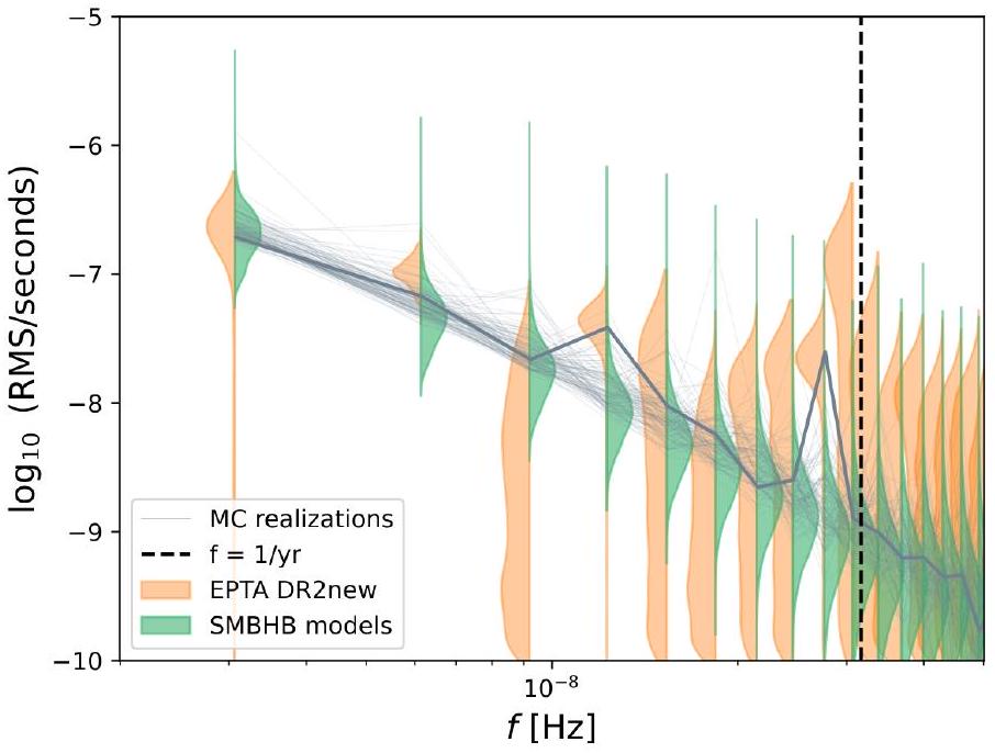
3.1.2. مقارنة مع الإشارة المرصودة

يتناقض الطيف الموزع الموضح في الشكل 3 توقعات من 324 ألف نموذج (أخضر) مع الإشارة المرتبطة المقاسة في DR2new (برتقالي). المجموعتان من الرسوم البيانية للفيولن متوافقتان جيدًا في أقل صناديق التردد، حيث تكون القياسات الأكثر تقييدًا. لاحظ أن توزيعات توقعات النموذج غير غاوسية للغاية وغير متناسقة، مع ذيول طويلة تمتد لأعلى. ويرجع ذلك إلى أن الثنائيات الضخمة/القريبة النادرة يمكن أن تنتج أحيانًا إشارات عالية بشكل استثنائي، كما هو موضح من خلال 100 GWB فردية المرسومة فوق الفيولن. في الواقع، قد يفسر هذا القوة الإضافية المقاسة في الصندوق الرابع، والأكثر لفتًا للنظر، في الصندوق التاسع الأدنى مقارنة بمعظم توقعات النموذج. نتحفظ على أن الصندوق التاسع قريب من علامة، حيث تكون PTAs عمياء بسبب التكيف لحركة مدار الأرض، وقد يؤثر التسرب من التكيف غير المثالي على تلك القياس. في أي حال، إذا كانت هذه القوة الإضافية ناتجة بالفعل عن GWs، فيمكن بسهولة استيعابها من قبل النماذج النظرية، كما يتضح من التحقيق المميز الذي يبرزه الخط الرمادي المتقطع.
تسمح لنا مقاربتنا مونت كارلو لتوليد سكان SMBHB وإشارة GW المرتبطة بها أيضًا بالتحقيق في حدوث CGWs في البيانات، حيث وُجد أن الأدلة في DR2new غير حاسمة (EPTA Collaboration & InPTA Collaboration 2023ج). نظرًا لأن البحث الذي تم إجراؤه في تلك الورقة كان محدودًا بالثنائي الدائري-
الشكل 3. رسم بياني لمدى الطيف الحر يقارن بين الإشارات المقاسة (باللون البرتقالي) والمتوقعة (باللون الأخضر). تم تراكب 100 تحقيق مونت كارلو لنموذج محدد على الرسوم البيانية؛ من بين تلك، يمثل الخط السميك مثالاً على إشارة SMBHB تتوافق مع القوة الزائدة المقاسة في البيانات عند جميع الترددات.
نعم، نحن نقوم بإجراء هذا التحليل فقط لنماذج 32.4 ك مع يتطلب التقييم الكامل لقدرة الكشف عن موجات الجاذبية الكونية (CGWs) تقييم احتمال الكشف عن كل ثنائي فردي لمعدل إنذار كاذب معين، كما هو موضح في RSG15. من أجل البساطة، ونظرًا للطبيعة النوعية لهذا التحليل، نقوم فقط بحساب نسبة الإشارة إلى الضوضاء (S/N) لكل ثنائي فردي وفقًا للمعادلة (46) من RSG15 (مما يقتصر أيضًا على مصطلح الأرض فقط). عند حساب S/N لمصدر، نقوم بنمذجة ضوضاء كل نباض باستخدام قيم الاحتمالية القصوى لتحليل ضوضاء النباض الفردي المقدم في تعاون EPTA وتعاون InPTA (2023a)، ونضيف موجات الجاذبية الناتجة عن جميع الثنائيات الأخرى إلى كثافة الطيف الضوضائي. نحن نحدد عتبة القابلية للكشف بشكل تعسفي عند في ما يلي.
تظهر النتائج في الشكل 4، الذي يقارن توزيع الطاقة للأمواج الجاذبية القابلة للحل مع الأطياف المجمعة للإشارة المتوقعة العامة وقياسات DR2new. وفقًا لـ RSG15، فإن احتمال اكتشاف موجة جاذبية قابلة للحل يكون في أقصى حد عند أدنى تردد، ويتناقص بسرعة ليصبح أقل من 0.01 بعد السلة السادسة. على الرغم من أن هذا يبدو أنه يشير إلى أن الميزة الملحوظة عند السلة الترددية التاسعة من غير المحتمل أن تكون ناتجة عن موجة جاذبية قابلة للحل، يجب ملاحظة أننا اعتبرنا هنا عتبة من الإشارة العامة لموجات الجاذبية في بياناتنا لديها إجمالي 3.5-4 (تعاون EPTA وتعاون InPTA 2023b)، تم تجميعها في الغالب في أدنى ترددات. قد لا يزال من الممكن أن تكون الميزة في السلة التاسعة ناتجة عن CGW غير محلولة مع ، والتي ستكون حدثًا أكثر شيوعًا في البيانات. لاحظ أن المتوسط تزداد نسبة CGWs قليلاً عند الترددات الأعلى، وهو ما يرجع أساسًا إلى اعتماد إجهاد CGW المميز على التردد، . إذا هو احتمال وجود CGW من في من خلال الحاوية، يمكننا حساب احتمال اكتشاف على الأقل واحدة من CGW مع في DR2new وفقًا لهذه النماذج كـ الذي يعطي . لذلك من الممكن تمامًا أن
الشكل 4. الخصائص المتوقعة لموجات الجاذبية الكونية كدالة للتردد. اللوحة العلوية: مخطط عازف الكمان الحر يقارن الإشارة المقاسة (باللون البرتقالي) بتوزيع الطاقة لموجات الجاذبية الكونية (باللون الأخضر). تظهر الكمانات الفارغة كامل موجات الجاذبية الكونية الناتجة عن النماذج للمقارنة. اللوحة السفلية: احتمال اكتشاف موجة جاذبية كونية مع كنتيجة للتردد (دوائر خضراء، اليسار -محور المقياس). يتم أيضًا عرض متوسط نسبة الإشارة إلى الضوضاء (S/N) للـ CGWs كصليب أحمر (يمين -مقياس المحور).
الإشارة الملاحظة تهيمن عليها بعض المصادر الساطعة، والتي قد تكون قابلة للحل في المستقبل مع مجموعات بيانات أكثر حساسية. حتى الآن، أسفرت عمليات البحث عن CGWs في مجموعة البيانات الحالية عن أدلة غير حاسمة (تعاون EPTA وتعاون InPTA 2023c). هذه الاحتمالية واضحة. يعتمد على العتبة. على سبيل المثال، من خلال زيادة هذه العتبة إلى نحن نحصل على 0.13. هذا قابل للمقارنة بـ الفرصة التي وجدها بيكسي وآخرون (2022). ومن المحتمل أن تكون الاحتمالية الأكبر قليلاً في نماذجنا ناتجة عن السعات العامة الأعلى للإشارات المدروسة هنا. ومع ذلك، نؤكد أن هذه النتائج تنطبق على النماذج التي تظل فيها الثنائيات دائرية بشكل أساسي. في الواقع، يميل عدد موجات الجاذبية القابلة للحل إلى الانخفاض قليلاً عندما تزداد الإهليلجية (ترونت وآخرون قيد الإعداد).
أخيرًا، نقترح مرة أخرى المقارنة التي عرضها ميدلتون وآخرون (2021)، الذين قارنوا القياسات ثنائية الأبعاد. بعد توقعات النموذج. بالنسبة للأخير، نقوم فقط بتناسب 9 من أدنى ترددات طيف GWB لكل تحقيق مونت كارلو للكون مع خط مستقيم في الطائرة. كما هو موضح في القسم 2، نقوم بتطبيع القياس إلى ، حيث تكون بياناتنا مفيدة، مما يخفف من الانحلال في الجزء الخلفي. تظهر النتائج في الشكل 5. على الرغم من أن الطيف المقاس يميل إلى أن يكون أقل عمقًا من الطيف النظري (انظر أيضًا القسم 3.4)، إلا أن الخطوط المتساوية تتداخل عند والأطياف المهمشة متسقة بشكل عام.

3.2. الاستدلال على مجموعة SMBHB.

بعد التحقق من التوافق العام للإشارة الملاحظة مع التوقعات من نماذج السكان التجريبية لـ SMBHB، نتبنى نهجًا أكثر كمية ونستغل الاستدلال بايزي لتقييد خصائص SMBHBs من البيانات. نكرر التحليل الذي أجراه ميدلتون وآخرون (2021) على الإشارة المشتركة المكتشفة في مجموعة بيانات NANOGrav لمدة 12.5 سنة (أرزوماينيان وآخرون 2020)، مستفيدين من الإطار الموضح في
قانون القوة ملائم لـ 9 صناديق
الشكل 5. توزيع الإشارة المقاسة (باللون البرتقالي) مقارنة بتوقعات النموذج (باللون الأخضر). و تظهر الخطوط الخارجية. كما تظهر الفئات المهمشة (يسار) و (اليمين) التوزيعات، مع فترات المصداقية المميزة كمناطق مظللة.
مجموعة SMBHB لنموذج معين يتم وصفه بمجموعة من المعلمات ثم نستخدم الاستدلال البايزي للعثور على التوزيع البعدي للمعلمات نموذج بالنظر إلى بيانات الملاحظة :
هنا، هو التوزيع السابق على معلمات النموذج، هو احتمال النموذج مع المعلمات إنتاج البيانات، و هو الدليل. لكل مجموعة من يتم حساب الاحتمالية من خلال مقارنة سعة الإشارة الناتجة عن عند الترددات ، إلى التوزيع الخلفي للإشارة المرتبطة المقاسة في DR2new عند نفس الترددات. نحن نتعامل مع كل حاوية على أنها مستقلة، لذلك يأخذ الاحتمال الشكل
أين هو كثافة الاحتمال للسعة الإشارة المرتبطة المقاسة في الصندوق الث، ويتم تقييمه عند القيمة تم التنبؤ به بواسطة النموذج. نحن نقدر الاحتمالية في كل حاوية باستخدام تقدير KDE للاحتمالات الخلفية لـ DR2new، مشابه للطريقة المستخدمة في مور و فيكيو (2021).
لاحظ أن النماذج التي نستخدمها حتمية بمعنى أنها تمتلك المراسلة بين والتنبؤ بـ . في الواقع، نظرًا لـ ، يتم سحب مجموعة SMBHBs التي تولد الإشارة إحصائيًا من دالة التوزيع الحتمية، مما يؤدي إلى تشتت كبير لـ كما يتضح من الأطياف الفردية المعروضة في الشكل 3. نود أن نلفت الانتباه إلى أن هذا التباين غير موضح في هذه النماذج، وأن تضمينه في عملية الاستدلال بايزي هو موضوع عمل جارٍ.
كما في ميدلتون وآخرون (2021)، نستخدم نموذجين لوصف مجموعة SMBHB، والتي سيتم وصفها بدورها أدناه.

3.2.1. نموذج سكان SMBHB غير المتحيز

النموذج غير المؤكد، الذي تم تطويره في ميدلتون وآخرون (2016)، يقوم بفرض افتراضات قليلة جداً حول السكان الأساسيين من ثنائيات الثقوب السوداء المتوسطة. يُفترض أن الثنائيات دائرية، مدفوعة بواسطة موجات الجاذبية، ويتم حساب الإجهاد المميز وفقًا للمعادلة (7) حيث يتم وصف توزيع المصدر بواسطة دالة شكتير (شكتير 1976) في و ،
أين هو الوقت في إطار المصدر ونفترض معلمات كونية من Planck18 (تعاون Planck VI 2020). المعلمات الخمسة للنموذج هي ، حيث هو معدل الاندماج لكل وحدة زمنية في إطار الراحة، والحجم المتحرك، واللوغاريتمي الفترة، وأزواج المعلمات و تحكم في شكل الـ و التوزيعات، على التوالي. حدود التكامل في و هم و على التوالي. كانت النطاقات السابقة للمعلمات الخمسة للنموذج متطابقة مع تلك المستخدمة في ميدلتون وآخرون (2021).

3.2.2. نموذج سكان SMBHB المستند إلى علم الفلك

تم تطوير النموذج المستند إلى علم الفلك في تشين وآخرون (2019). يلتقط هذا النموذج التفاعل بين الثقوب السوداء الثنائية ذات الكتلة الكبيرة وبيئتها ويسمح بمدارات غير دائرية، وكلاهما يؤدي إلى سعة مميزة لا تتبع قانون قوة بسيط واحد، كما هو موضح في المعادلة (5). يحتوي النموذج على 18 معلمة، 16 منها تصف الملاحظات الفلكية التي تربط عدد اندماجات الثقوب السوداء الثنائية ذات الكتلة الكبيرة بعدد اندماجات المجرات. يتم نمذجة دالة كتلة النجوم في المجرات كدالة شكتير تعتمد على الانزياح الأحمر محددة بخمسة معلمات: كل من نسبة أزواج المجرات وأوقات الاندماج تعتمد على قانون القوة لكتلة النجوم في المجرة الرئيسية. نسبة الكتلة وظيفة الانزياح الأحمر ( ) وكل واحد منهم يتم تعريفه بمجموعة من أربعة معايير: لنسبة الزوج، و لجدول زمني للاندماج:
ثم يتم ملء أزواج المجرات بثقوب سوداء فائقة الكتلة بكتلة وفقًا لعلاقة الكتلة بين الثقب الأسود والنتوء النجمي بالشكل
أين هو توزيع لوغاريتمي طبيعي بمتوسط قيمة والانحراف المعياري ، والتي تضيف ثلاثة معايير إضافية، ، إلى النموذج. تصف المعلمتان الأخيرتان الانحراف عند اقتران SMBHB وكثافة البيئة النجمية بالنسبة للمعايير الثمانية عشر المذكورة أعلاه، في التحليل المقدم هنا، نستخدم الفترات السابقة الموسعة المدرجة في الجدول الأول من تشين وآخرون (2019).
الشكل 6. التوزيعات الخلفية المهمشة لـ باستخدام نموذجين لسكان ثنائيات الثقوب السوداء المتوسطة. تُظهر المدرجات المفتوحة باللون البرتقالي والأخضر التوزيعات الهامشية للنماذج غير المعرفية والنماذج المستندة إلى علم الفلك، على التوالي. تُظهر المدرجة المملوءة باللون الأخضر التوزيع السابق للنموذج المستند إلى علم الفلك (التوزيع السابق للنموذج غير المعرفي هو موحد في النطاق [-20,3]). تُظهر الخطوط العمودية المنقطة النسب المئوية الخامسة والتسعين للتوزيعات.
الشكل 7. التوزيع الخلفي لدالة كتلة الاهتزاز للأزواج الثقالية المتقاربة SMBHBs لكل من النموذجين غير المتحيزين (باللون البرتقالي) والمستندين إلى المعلومات الفلكية (باللون الأخضر). بالنسبة لكلا النموذجين، فإن المناطق المظللة تمثل النسبة المركزية 50% و المناطق الموثوقة والخطوط المتقطعة تظهر الوسائط. الخطوط المنقطة السوداء تظهر المركز. المنطقة للفرضيات الفلكية.

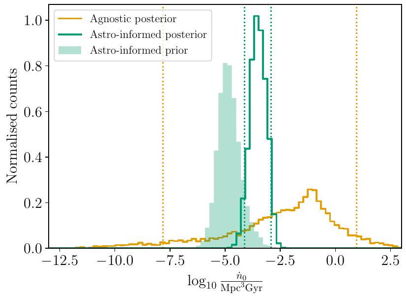
3.2.3. نتائج الاستدلال

تظهر النتائج الرئيسية للاستدلال في الأشكال 6-8. الشكل 6 يظهر التوزيع البعدي المارجي لتطبيع كثافة معدل الاندماج. من النموذج الملحد مقارنةً بمعامل مكافئ مستمد من النموذج المستند إلى علم الفلك. يفرض القيد على سعة الإشارة قيدًا معلوماتيًا على تطبيع كثافة اندماج الثقوب السوداء الثنائية الضخمة. باستخدام تسع حاويات ترددية، الوسيط والمركزي المناطق الموثوقة لـ هم و للنماذج الملحدة والمطلعة على الفيزياء الفلكية، على التوالي. القياس يقيّد بشكل أساسي سعة الإشارة، مما يفرض قيدًا معلوماتيًا على يظهر النموذج المستند إلى علم الفلك بوضوح أن الإشارة تفضل في الحافة العليا للسابقة الفلكية. كل
الشكل 8. التوزيع الخلفي للمعلمات المختارة للنموذج المستند إلى علم الفلك باستخدام تسع حاويات ترددية للطيف الحر من أجل الاستدلال. تم وصف المعلمات في القسم 3.2.2.
المعلمات الأخرى للنموذج غير المتحيز غير مقيدة والتوزيع اللاحق مشابه جدًا للتوزيع السابق (انظر الملحق أ للحصول على التوزيعات اللاحقة الكاملة لكلا النموذجين).
تظهر الشكل 7 التوزيع الخلفي لدالة كتلة الصدى الثنائي للثقب الأسود الضخم (SMBHB) للنموذجين المدمجين على مدى انزياح الطيف الأحمر. على الرغم من أن النموذج الإلحادي يؤدي إلى دالة كتلة غير مقيدة بشكل صارم، إلا أن إشارة PTA المقاسة وحدها تضع حدودًا دنيا مثيرة للاهتمام على معدل اندماج الثنائيات SMBHB في الكون. على سبيل المثال، يمكننا أن نقول عند الثقة أنه لكل ، كان هناك على الأقل اندماج SMBHB مع منذ الظهر الكوني. عندما تدخل الأوزان السابقة الفيزيائية الفلكية، فإن دالة الكتلة للثنائيات السوداء الضخمة المت merging تكون محددة جيدًا بواسطة إشارة PTA، وكما هو متوقع من
الشكل 6، يقع في النطاق العلوي من الأوليات المستندة إلى علم الفلك. ضمن هذا النموذج، تشير الإشارة المقاسة DR2new إلى أنه كان هناك حوالي اندماجات SMBHB لكل متحرك مع منذ . هذا يشير إلى تاريخ نشط للغاية من اندماج المجرات الضخمة وتطور ديناميكي فعال جداً للأزواج الثنائية من الثقوب السوداء الهائلة التي تتشكل في عملية الاندماج.
بالنسبة للنموذج المستند إلى المعلومات الفلكية، يوفر DR2new أيضًا معلومات مثيرة للاهتمام حول عدة معلمات نموذجية. وذلك لأن الأولويات الفلكية تضيق بشكل كبير نطاق سعات الإشارة المسموح بها من قبل النموذج، وتدفع الإشارة المقاسة نحو الحد الأعلى من هذا النطاق. وهذا يؤدي إلى قيود مفيدة على عدة معلمات رئيسية.
مرتبط بشكل خاص بإطار زمن اندماج الثقوب السوداء الفائقة الكتلة وعلاقة كتلة الثقب الأسود مع البروز. كما هو موضح في الشكل 8، فإن إطار زمن اندماج الثقوب السوداء الفائقة الكتلة يجب أن يكون اقتران المجرة التالي أقصر من ( الثقة)، مع البيانات التي تميل قليلاً لصالح أوقات الاندماج الأقصر للمجرات الضخمة عند الانزياحات الحمراء المنخفضة (أي علاوة على ذلك، فإن البيانات تدعم تطبيعًا عاليًا لعلاقة كتلة الثقب الأسود الهائل مع الكتلة المركزية. ، مقارنةً مع نطاق أوسع بكثير يمتد حتى . يتماشى هذا مع التحليل النوعي في القسم 3.1، الذي أظهر أن الإشارة تتوافق مع العلاقات المعدلة حديثًا بين الثقوب السوداء الضخمة والمجرات. هناك أيضًا تفضيل طفيف لنسبة عالية من زوج الثقوب السوداء. بشكل إيجابي اعتماد على الرغم من الانخفاض القيمة المفضلة من قبل البيانات، تشير إلى طيف أكثر تسطحًا مقارنة بالقيمة الكنسية المتوقعة من الثنائيات المدفوعة بواسطة موجات الجاذبية الدائرية، ديناميات الثنائيات الضخمة ذات الكتلة العالية غير محددة إلى حد كبير، ربما مع تفضيل هامشي للثنائيات ذات الشكل البيضاوي التي تتطور في بيئات كثيفة. و الاحتمالات الخلفية ترتفع قليلاً نحو الحد الأيمن من السابق.
بشكل عام، تشير هذه النتائج إلى تآكل مداري فعال للثنائيات السوداء الضخمة في أعقاب اندماجات المجرات، مما يوفر دليلاً مباشراً على أن ‘مشكلة البارسيك النهائي’ قد تم حلها في الطبيعة وأن الثنائيات السوداء الضخمة المدمجة دون البارسيك يجب أن تكون شائعة في مركز المجرات الضخمة.

3.3. الآثار المترتبة على SAMs

نستكشف الآن دلالة هذه الإشارة على النمذجة المشتركة لتكوين وتطور المجرة والثقوب السوداء الهائلة من خلال إلقاء نظرة فاحصة على نموذجين متقدمين: النموذج الذي أنشأه باراوسي وزملاؤه (باراوسي 2012؛ سيسانا وآخرون 2014؛ أنطونيني وآخرون 2015؛ كلاين وآخرون 2016؛ بونتيتي وآخرون 2018؛ باراوسي وآخرون 2020) وL-Galaxies (هينريكيس وآخرون 2015؛ إزكييردو-فيلا alba وآخرون 2022). في هذه الدراسة الأولية، لا نقوم بنمذجة التطور الديناميكي للثنائيات ونفترض أنها دائرية ومدفوعة بواسطة موجات الجاذبية، مما يؤدي إلى طيف إجهاد مميز مع .

3.3.1. تأخيرات SAMs و SMBHB

في الشكل 9، نعرض هذه المقارنة لنموذج باراوسي (2012) في نسخته الأصلية (B12) وتطوراته اللاحقة، التي استخدمت لإنتاج نتائج كلاين وآخرون (2016، K+16)، بونتي وآخرون (2018، B+18) وباراوسي وآخرون (2020، B+20). بالإضافة إلى تنفيذ SAM المحدد و(الفيزياء) الفلكية، تختلف هذه النماذج بشكل رئيسي في الوصفات الفيزيائية التي تصف التأخيرات بين اندماجات المجرات واندماجات الثقوب السوداء الضخمة، حيث تفترض النماذج “LS-nod (B12)”، “HS-nod (B12)”، “Q3nod (K+16)”، “LS-nod-noSN (B+20)”، “HS-nod-noSN (B+20)” و”HS-nod-SN-high-accr (B+20)” عدم وجود مثل هذه التأخيرات (باستثناء التأخيرات بين اندماجات الهالات وتلك الخاصة بالمكونات الباريونية المقابلة). ; (ii) نماذج “popIII-d ( )”, “Q3-d (K+16)”, “LS-d (B+18)”, “HS-d (B+18)” بالإضافة إلى تقديم تأثير تصلب النجوم، وتفاعلات MBH الثلاثية، والهجرة المدفوعة بالغاز؛ و(iii) النماذج “LS-noSN-d (B+20)”, “LS-SN-d (B+20)”, “HS-noSN-d (B+20)” و”HS-SN-d (B+20)” التي تأخذ في الاعتبار تأخيرات أطول (بما في ذلك مساهمات كبيرة من SMBHB
الشكل 9. التنبؤات لسعة إجهاد GWB المميزة عند من مجموعة من نماذج الأنظمة الديناميكية المنشورة في الأدبيات، مع افتراض مدارات شبه دائرية وعدم وجود تفاعلات بيئية (أي )، ولكن وصفات مادية مختلفة للتأخيرات (تزداد من اليسار إلى اليمين) بين اندماجات المجرات واندماجات الثقوب السوداء. نماذج “بدون تأخيرات” و”تأخيرات متوسطة” و”تأخيرات طويلة” تتوافق على التوالي مع فئات النماذج (i) و(ii) و(iii) المحددة في النص. النطاقات تأخذ في الاعتبار الدقة المحدودة للنماذج. المنطقة المظللة هي حد الثقة 95% لـ DR2new. مزيد من التفاصيل حول النماذج موضحة في النص.
فصلات مئات من وحدات الكمبيوتر). لاحظ أن التسميات “SN” (و”noSN”) تشير على التوالي إلى تأثير مفترض لتغذية SN على تراكم الثقب الأسود (وانعدام ذلك)، بينما تشير “LS”/”popIII” و”HS”/”Q3″ على التوالي إلى بذور خفيفة وثقيلة عالية الانزياح الأحمر لسكان الثقوب السوداء.
يتم حساب التنبؤات من خلال جمع طيف الطاقة الجاذبية لجميع أزواج الثقوب السوداء الضخمة في كل نموذج من السكان النظريين، مع افتراض مدارات شبه دائرية. ونتيجة لذلك، فإن الطيف له ميل من وليس له تباين كوني (أي أننا لا نأخذ في الاعتبار في هذه المرحلة التشتت من تحقيق إلى آخر من سكان أزواج الثقوب السوداء الضخمة). النطاق المعروض لكل نموذج يمثل عدم اليقين بسبب التصحيح لدقة شجرة الاندماج في نموذج SAM. بمزيد من التفصيل، يمثل الطرف السفلي من النطاق تنبؤ نموذج عند الدقة المحدودة، بينما الطرف العلوي هو الاستقراء الذي تم إجراؤه كما هو موضح في الشكل 4 من Klein et al. (2016) – إلى دقة غير محدودة. يجب تفسير السهم السفلي (المؤشر لأعلى) على أنه حد أدنى، بينما يجب فهم السهم العلوي (المؤشر لأسفل) على أنه حد أعلى (بسبب عدم اليقين في إجراء الاستقراء). لم يتم إجراء الاستقراء لنموذج HS-nod-SN-high-accr (B+20)، الذي نبلغ فيه فقط عن التنبؤ (الأكثر موثوقية) عند الدقة المحدودة. الأخير يتفق بالفعل مع السعة المقاسة، نتيجة لمعدل اكتساب أعلى (بعامل ) لأزواج الثقوب السوداء الضخمة.
بالنسبة لنموذجين من النماذج التي تتفق بشكل أفضل نوعيًا مع البيانات (أي “HS-nod-SN-high-accr (B+20)” و”HS-nod-noSN (B+20)”)، نقارن الإشارة المتوقعة مع الطيف الحر المقاس DR2new في الشكل 10. على عكس حالة
الشكل 10. طيف مقسم لسعة GWB المتوقعة لنماذج “HS-nod-SN-high-accr (B+20)” و”HS-nod-noSN (B+20)”. تمثل توزيع التنبؤات التشتت بين تحقيقات مختلفة من سكان أزواج الثقوب السوداء الضخمة (“التباين الكوني”). كما تم عرض ملاءمات القوة للتنبؤات.
الشكل 9، تم الحصول على هذه التنبؤات لعدة تحقيقات محددة من سكان أزواج الثقوب السوداء الضخمة، وفقًا لـ Sesana et al. . تمثل دالة توزيع الاحتمالات المرسومة في كل حاوية التشتت لهذه التحقيقات المتعددة، وبالتالي يجب تفسيرها على أنها “تباين كوني”. بالمثل، في الشكل 11 نعرض التوقعات النظرية لـ من مجموعة فرعية من النماذج المقدمة أعلاه (أي تلك المتوافقة نوعيًا مع البيانات في الشكل 9). يتم الحصول على هذه التوقعات من خلال ملاءمة التنبؤات النموذجية (من تحقيقات متعددة من سكان أزواج الثقوب السوداء الضخمة) في أول 9 حاويات تردد مع قانون القوة مع . تمثل أشرطة الخطأ مناطق الثقة (مع الأخذ في الاعتبار التشتت بسبب التباين الكوني)، بينما تشير المنطقة المظللة إلى منطقة الثقة لل posterior لـ (مع افتراض مرة أخرى ).
بشكل عام، تشير هذه المقارنة النوعية، على الرغم من اعتمادها إلى حد ما على تفاصيل تنفيذ SAM، إلى أن (1) التأخيرات الكبيرة الناجمة عن ديناميات أزواج الثقوب السوداء عند المسافات الكبيرة غير مفضلة، (2) تتم عمليات اندماج أزواج الثقوب السوداء الضخمة بكفاءة بعد أن تتجمع مجراتها المضيفة. علاوة على ذلك، يبدو أن هذه النتائج تشير إلى أن (3) الاكتساب على أزواج الثقوب السوداء الضخمة يتم بكفاءة، مما قد يؤدي إلى وظيفة كتلة محلية أكبر لأزواج الثقوب السوداء الضخمة عند الكتل العالية.

3.3.2. L-Galaxies

بعد ذلك، نستكشف الآثار التي تترتب على نتائج EPTA بالنسبة لـ L-Galaxies (Henriques et al. 2015؛ Izquierdo-Villalba et al. 2022)، وهو نموذج SAM متطور تم بناؤه على أشجار اندماج المادة المظلمة المستخرجة من مجموعة محاكاة الألفية (Springel et al. 2005؛ Boylan-Kolchin et al. 2009). بالإضافة إلى فيزياء المجرات، يتميز L-Galaxies بنموذج شامل لتجميع أزواج الثقوب السوداء الضخمة، بما في ذلك الاكتساب الغازي الناتج عن اندماجات المجرات وعدم استقرار القرص والتطور الديناميكي لأزواج الثقوب السوداء الضخمة ضمن عملية اندماج المجرات. الأخير يأخذ في الاعتبار الاحتكاك الديناميكي (DF)، وتصلب النجوم والغاز الصلب-
الشكل 11. التنبؤات لـ في نماذج SAM المختلفة، تم الحصول عليها من خلال ملاءمة الطيف في أول 9 حاويات تردد مع لتحقيقات متعددة من سكان أزواج الثقوب السوداء الضخمة. تمثل أشرطة الخطأ فترة الثقة 95% للتنبؤات، وتأخذ في الاعتبار التشتت بسبب التباين الكوني. لكل نموذج (باستثناء نموذج الاكتساب المعزز HS-nod-SN-high-accr (B+20))، فإن التنبؤ الأعلى هو الاستقراء إلى دقة SAM غير المحدودة، بينما التنبؤ الأدنى هو التنبؤ عند الدقة المحدودة. المنطقة المظللة هي فترة الثقة لقياس ، مع تثبيت . بالنسبة لـ HS-nod-SN-high-accr (B+20) نعرض فقط النتيجة غير المصححة للدقة.
والتصلب، وفي النهاية، انبعاث GW. جميع هذه العمليات تخضع لمجموعة من المعلمات التي تم ضبطها لإعادة إنتاج مجموعة واسعة من الملاحظات بما في ذلك، من بين أمور أخرى، وظيفة كتلة المجرات والتوزيع الشكلي، وظيفة سطوع الكوازارات وعلاقات الثقوب السوداء الضخمة مع المجرات المضيفة.
وجد Izquierdo-Villalba et al. (2022) أن ضبط L-Galaxies القياسي يؤدي إلى GWB مع عند ، أقل من ذلك المقاس في DR2new. هنا نقوم بإجراء تحقيق منهجي حول كيفية اعتماد GWB العشوائي عند ترددات النانو هيرتز على المعلمات التي تحكم فيزياء الثقوب السوداء الضخمة وأزواج الثقوب السوداء الضخمة في SAM. لهذا الغرض، نقوم بتشغيل L-Galaxies في التكوينات التالية:
  • std: التكوين القياسي (Izquierdo-Villalba et al. 2022);
  • t_DF_x0.1: تم تقليل وقت الاحتكاك الديناميكي (DF) للثقب الأسود الضخم بعامل عشرة؛
  • NO_GAS_HARD: فقط تصلب النجوم؛
  • growthDF_x10: تم تعزيز الاكتساب بعشرة في مرحلة DF؛
  • boostBH1: تم مضاعفة الاكتساب الغازي بعد اندماجات المجرات وعدم استقرار القرص؛
  • boostBH2: تم مضاعفة الاكتساب الغازي بعد اندماجات المجرات وتمت مضاعفته ثلاث مرات بعد عدم استقرار القرص؛
  • boostBH1_growthDF_x10: إضافة تعزيز الاكتساب في مرحلة DF لنموذج boostBH1؛
  • boostBH2_growthDF_x10: إضافة تعزيز الاكتساب في مرحلة DF لنموذج boostBH2.
    تظهر النتائج في الشكل 12. يبدو أن التغييرات في ديناميات الثقوب السوداء الضخمة لها تأثير طفيف على سعة GWB. بينما يسمح تقصير وقت DF (t_DF_x0.1) بمزيد من أزواج الثقوب السوداء الضخمة للاندماج ضمن زمن هابل، فإن الأكثر
الشكل 12. التنبؤات لسعة الشد المميزة لـ GWB عند من مجموعة من إصدارات نموذج L-Galaxies شبه التحليلية، مع افتراض أن . تم حساب أشرطة الخطأ مع الأخذ في الاعتبار التباين الكوني. لهذا الغرض، قسمنا صندوق الألفية إلى 125 صندوقًا فرعيًا وحسبنا GWB في كل واحد. الانحراف المعياري الذي توفره 125 GWB يتوافق مع امتداد أشرطة الخطأ لدينا.
الأكثر ضخامة، والتي تتحمل الجزء الأكبر من إشارة GW، لديها بالفعل أوقات DF قصيرة، والإشارة العامة لـ GW تزداد بشكل طفيف فقط. يؤدي إيقاف تصلب الغاز إلى أزواج ثقوب سوداء ضخمة تعيش لفترة أطول تميل إلى الاندماج عند انزياحات حمراء أقل، مما يؤدي إلى إشارات GW أعلى. ومع ذلك، فإن التأثير ضئيل. على العكس، يمكن أن يغير ضبط الاكتساب الغازي بشكل كبير كتل أزواج الثقوب السوداء الضخمة، مما يؤدي إلى تأثير أكبر على GWB. يترك نموذج growthDF_x10 السكان العام من الثقوب السوداء الضخمة دون تغيير، مما يعزز فقط نمو أولئك في مرحلة الاحتكاك الديناميكي. هذا وحده يزيد من مستوى GWB بعامل مقارنة بالنموذج القياسي. أخيرًا، تزيد النماذج boostBH1 و boostBH2 من الاكتساب الغازي على كامل سكان الثقوب السوداء الضخمة، مما يجعل GWB أعلى بمقدار 2.5 مقارنة بالنموذج الأساسي. يؤدي تعزيز الاكتساب على كامل السكان وفي مرحلة التصلب إلى تضخيم GWB المتوقع، ليصل إلى الحد الأعلى للقيمة المقاسة (النماذج boostBH1_growthDF_x10 و boostBH2_growthDF_x10 في الشكل). على الرغم من أن هذه النماذج يمكن أن تستوعب إشارة GWB المقاسة في PTAs، فإن الاكتساب المعزز والكتل الأكبر للثقوب السوداء الضخمة يمكن أن يجعل من الصعب إعادة إنتاج وظائف الكتلة للثقوب السوداء الضخمة ووظائف سطوع الكوازارات الملاحظة (Izquierdo-Villalba et al. 2022). بالإضافة إلى ذلك، هناك حاجة إلى مزيد من العمل للعثور على نموذج يمكنه إعادة إنتاج جميع القيود الملاحظة في ضوء إشارة GW من PTA (Izquierdo-Villalba et al. 2024).

3.4. اعتبارات إضافية حول الطيف المقاس: الانحرافات الإحصائية والانحرافات.

تشير التحليلات المقدمة حتى الآن إلى أن الإشارة متوافقة مع مجموعة كونية من أزواج الثقوب السوداء الضخمة التي تتجمع بسرعة في أعقاب اندماجات المجرات. قد يكون الميل النسبي المسطح للطيف المقاس مؤشرًا على قوة
الشكل 13. المعلمات المدارية (المسافة بين الثقوب السوداء الهائلة، المحور شبه الرئيسي والانحراف) لثقبين أسودين هائلين تشكلا في نموذج تمثيلي -محاكاة جسيمات لاندماج مجري مع معلمات مستمدة من أسلاف مصادر PTA المحتملة في محاكاة إيلستريسTNG100-1 الكونية. يتم اختيار الاندماجات من أشجار الاندماج لأكثر 100 مجرة ضخمة. استنادًا إلى نسبة كتلة المجرة (الاندماجات الكبرى مع نسبة الكتلة أو أعلى) والانزياح الأحمر ( ). تشير الخطوط المتقطعة إلى الفصل الحرج والانحراف المقابل في الوقت الذي يمثل فيه التطور تقريبًا نهاية انغماس الثقب الأسود الهائل بسبب DF وبداية مرحلة التصلب. النقاط تمثل و تم حسابه من فصل الأبوستران-بيريسترون بين الثقبين الأسودين الهائلين قبل الاقتران في ثنائي مقيد.
الارتباط البيئي والانحرافات العالية، على الرغم من أن الاستنتاج من البيانات غير حاسم في هذا الصدد (انظر الشكل 8).
الغرابة في SMBHBs لها أهمية خاصة لأنها قد تحمل معلومات مهمة عن العمليات الديناميكية التي تقود تطور الثنائيات على مقاييس دون السنتيمتر (انظر على سبيل المثال Roedig & Sesana 2012). بينما من المتوقع أن تؤدي الديناميات المدفوعة بالغاز إلى تشبع الغرابة الثنائية عند قيمة (Roedig وآخرون 2011؛ D’Orazio & Duffell 2021)، من المعروف أن تصلب النجوم يزيد إحصائيًا من الانحراف دون أي نقطة تشبع (Quinlan 1996)، مما قد يؤدي إلى أنظمة ذات انحراف شديد (Sesana 2010). للانحراف الثنائي الكبير دلالتان مهمتان لتفسير البيانات الحالية: إنه يسطح الطيف منخفض التردد ويزيد من سرعة عملية اندماج SMBHB، كما يُستنتج من الصغير مشتق في القسم 3.2.
تعتبر المجرات الضخمة ذات الانزياح الأحمر المنخفض عمومًا فقيرة بالغاز، ويمثل التصلب المدفوع بالنجوم الآلية الرئيسية التي تدفع تطور الثنائيات التي تشكل الجزء الأكبر من إشارة موجات الجاذبية في شبكة المراقبة. إن نمذجة التطور الديناميكي الكامل، من أول لقاء بين المجرات إلى اقتران الثقوب السوداء والاندماج النهائي، تمثل تحديًا نظريًا وعدديًا وقد كانت موضوعًا للعديد من الدراسات (مثل: بريتو وآخرون 2011؛ خان وآخرون 2012، 2016؛ نسيم وآخرون 2021؛ غوالاندريس وآخرون 2022). على وجه الخصوص، فإن الإهليلجية الثنائية حساسة جدًا لمدارات المجرات المندمجة الأولية (غوالاندريس وآخرون 2022). في العمل الجاري (فاستيديو وآخرون قيد الإعداد)، نقوم بربط الديناميات دون السنتيمتر من الثقوب السوداء الثنائية الضخمة بالمعلمات واسعة النطاق للاقتباسات المجرية المستخرجة من محاكاة إيلستريسTNG100 (بيليبش وآخرون 2018). تظهر النتائج الأولية أن اندماجات المجرات الضخمة تحدث بشكل تفضيلي على مدارات شبه شعاعية، مما قد يؤدي إلى ثنائيات ذات إهليلجية عالية. توضح الشكل 13 المعلمات المدارية لثقبين أسودين ثنائيين تشكلا بدقة عالية. -محاكاة متعددة الأجسام لاندماج مجري تمثيلي مع خصائص مأخوذة من شجرة اندماج في IllustrisTNG100. تم اختيار أشجار الاندماج لتمثيل مصادر PTA المحتملة عند الانزياحات الحمراء المنخفضة. يتم متابعة الاندماج المجري من أوقات مبكرة.
الشكل 14. التوزيعات الخلفية لـ GWB المستعاد من الحقن على بيانات اصطناعية تحاكي DR2new. اللوحة العلوية: الانحراف الإحصائي في مجموعة بيانات مثالية. المربع يحدد القيمة المحقونة والكونتور الأزرق هو و من الاستعادة المستعادة. اللوحة السفلية: تأثير عدم نمذجة الضوضاء عالية التردد على الاستعادة. يتم الحصول على الخطوط المحيطية البرتقالية والزرقاء والخضراء على التوالي عندما تُستخدم للاسترداد (تم حقنها ).
من خلال الانغماس، والتزاوج، وتصلب الثقوب السوداء الهائلة عبر نظام عددي هجين قادر على نمذجة التطور بشكل ذاتي متسق من مقاييس الكيلوبارسيك إلى مقاييس الميليبارسيك (ديهن 2014). على الرغم من العشوائية الجوهرية للعمليات التي تقود تشكيل الثنائيات وتصلبها (نسيم وآخرون 2020)، تميل الثنائيات إلى التكون بزاوية ميل كبيرة، والتي تنمو بعد ذلك بسبب التفاعلات مع النجوم الخلفية، كما وجدت تجارب التشتت (سيسانا 2010). على الرغم من الحاجة إلى مزيد من العمل لتحديد توزيع الزوايا المتوقعة للثنائيات وبيانات EPTA الحالية ليست بعد مفيدة بشكل كبير، إلا أن هذه الدراسة التجريبية تظهر إمكانيات استخدام هذه القياسات في المستقبل القريب لتقييد فيزياء اندماجات المجرات والثقوب السوداء الهائلة.
عند استنتاج الخصائص الفيزيائية لمصادر إشارة موجات الجاذبية، من المفيد أن نأخذ في الاعتبار ليس فقط أن القيود على الطيف نسبياً فضفاضة (انظر الشكل 1)، ولكن أيضاً أن المعلمات المقاسة يمكن أن تخضع لـ
التحيزات الإحصائية والمنهجية. لمعالجة ذلك، قمنا بإجراء حملة واسعة من المحاكاة عن طريق حقن واستعادة أنواع مختلفة من الإشارات في PTAs الاصطناعية التي تحاكي خصائص مجموعة بيانات EPTA DR2new (فالطولينا وآخرون 2024). قمنا بتوليد ضوضاء فردية لـ 25 نباضًا باستخدام قيم الاحتمالية القصوى للضوضاء البيضاء المقاسة وسحبنا معلمات الضوضاء الحمراء وقياس التشتت من التوزيع الخلفي لنماذج الضوضاء المخصصة (تعاون EPTA وتعاون InPTA 2023a). قمنا بمحاكاة TOAs من الملاحظات متعددة الترددات وأضفنا طيف GWB من مجموعة فلكية من SMBHBs الدائرية التي تنتج GWB اسمي مع متسق مع قياس DR2new عند قمنا بإجراء 100 تجربة من خلال تغيير تحقيق الضوضاء المحددة وعينة السكان المدخلة من SMBHB. تم إجراء التحليل باستخدام حزمة برامج ENTERPRISE (إيليس وآخرون 2020).
يتم عرض مثالين توضيحيين لعدم تطابق الحقن والاسترداد في الشكل 14. تُظهر اللوحة العلوية واحدة من استردادات GWB. على الرغم من أن الحقن لم يظهر ميزات معينة (مثل CGWs العالية الصوت)، إلا أن الإشارة المستردة لهذه الواقعة الضوضائية المحددة لها ميل ضحل بقيمة متوسطة من تمت ملاحظة حالات مماثلة عند حقن مادة نقية قانون القوة مع دالة createGWB من مكتبة libstempo (فالسينييري 2020). هذا يُظهر أنه حتى مع إعداد مثالي عند ملاءمة عدة معلمات في وقت واحد (102 في هذه الحالة) في مشكلة معقدة، يمكن أن تؤثر الخصائص العشوائية للضوضاء بسهولة على الإشارة المستعادة، خاصة إذا كانت نسبة الإشارة إلى الضوضاء منخفضة. لـ DR2new). تظهر الحقن المتعددة باستخدام نموذج GWB الواقعي وcreateGWB انحيازات منهجية في استعادة إشارة GWB الواقعية، عندما يتم نمذجتها بقانون القوة المثالي. يتم استكشاف ذلك بالتفصيل في عمل لاحق. في اللوحة السفلية من الشكل 14، نوضح كيف أن وجود بعض الضوضاء عالية التردد الإضافية التي لم تؤخذ في الاعتبار في نموذج ضوضاء MSP يمكن أن يؤثر أيضًا على استعادة المعلمات. الإعداد هو نفسه كما في اللوحة اليسرى، ولكننا نحاكي عدم تطابق الضوضاء عالية التردد عن طريق تعيين قيم مختلفة من في الاسترداد. على الرغم من أن الجزء الخلفي من سعة الإشارة يتأثر بالكاد، يمكن أن تتغير بشكل كبير اعتمادًا على ما إذا كان الضجيج عالي التردد قد تم تقديره بشكل زائد أو ناقص قليلاً. بينما هذه مجرد مثالين، فإنها تبرز تعقيد قياسات PTA وتدعونا إلى توخي الحذر عند استخلاص الاستنتاجات التي قد تتأثر بشدة بالتحيزات المحتملة في الإشارة المستعادة.

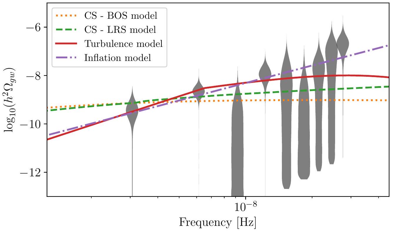
4. الآثار II: فيزياء الكون المبكر

على الرغم من أن موجات الجاذبية الناتجة عن مجموعة من الثنائيات السوداء الضخمة المفترضة هي المصدر الأكثر احتمالاً لعملية الضوضاء الحمراء المشتركة الملاحظة في بيانات النباضات، إلا أن تفسيرات أكثر غرابة ممكنة، مثل الإشارات التي نشأت في الكون المبكر. يتم مراجعة الأنواع المختلفة الممكنة من الخلفيات الكونية لموجات الجاذبية المرتبطة بفيزياء الكون المبكر في كابرييني وفيغيروا (2018) وتظهر أنها عشوائية. على غرار الحالة التقليدية التي تستدعي الثنائيات السوداء الضخمة، تتبع العلاقة الزاوية المكانية لتلك السيناريوهات منحنى HD. ومع ذلك، فإن الأشكال الطيفية للطيف المتوقع لموجات الجاذبية تختلف عمومًا، مما يمكن أن يساعد في التفريق بين أنواع الخلفيات المختلفة. في هذا العمل، نركز على أربعة سيناريوهات ممكنة:
  1. زيادة تضخمية في جاذبية الجاذبية نتيجة لتضخيم التقلبات الكمومية في المجال الجاذبي
  2. جاذبية جاذبية من شبكة من حلقات الخيوط الكونية،
  3. جبهة موجية من الاضطراب الدوراني (M)HD عند مقياس طاقة QCD
  4. جاذبية جاذبية ناتجة عن الاضطرابات الاسكالية الناتجة عن التضخم في المرتبة الثانية في نظرية الاضطراب.
    نظرًا للأهمية المنخفضة للإشارة المكتشفة وعدد حاويات الترددات المحدود بسبب قصر فترة البيانات، لا يمكن حاليًا إجراء اختيار موثوق للنموذج. لذلك، نعتبر هذه السيناريوهات بشكل منفصل ونفترض أن كل منها يمكن أن يفسر الإشارة المكتشفة بشكل كامل بشكل مستقل. سيتم النظر في التحليل الذي يستدعي نماذج أكثر تعقيدًا مع ملاءمات متزامنة لعدة سيناريوهات، بالإضافة إلى الفرص لفك الارتباط بين تلك السيناريوهات (مثل غونشاروف وآخرون 2022؛ كايسر وآخرون 2022) في عدد من الأعمال المستقبلية.

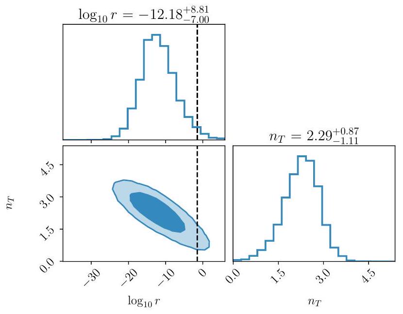
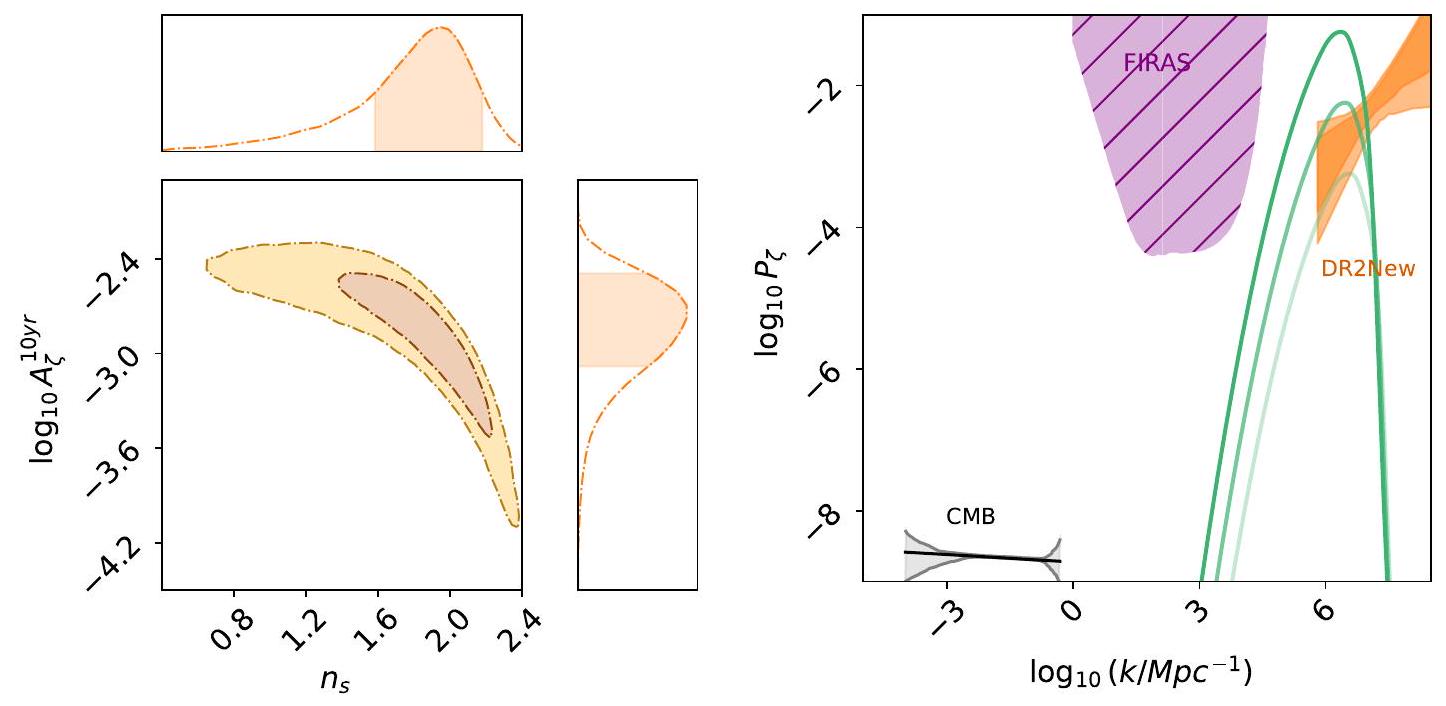
4.1. الآثار على خلفية عشوائية من موجات الجاذبية الأولية (التضخمية)

هنا نتناول الخلفية الجاذبية الموجية التي قد تتولد أثناء التضخم (غريشوك 1975؛ روباكوف وآخرون 1982؛ ستاروبينسكي 1985؛ فابري وبولوك 1983؛ أبوت ووايز 1984). في السيناريو التضخمي القياسي، يتم تضخيم تقلبات الفراغ الكمومي التنسوري للمتري بواسطة التوسع المتسارع، مما يؤدي إلى خلفية جاذبية موجية حيث تعود للدخول إلى الأفق خلال عصر الإشعاع (أو المادة). يوفر إشعاع الخلفية الكونية الميكرووي (CMB) وتخليق العناصر الثقيلة في الانفجار العظيم (BBN) قياسات دقيقة لكثافة الطاقة الإشعاعية، والتي يمكن من خلالها اشتقاق حدود عليا ضعيفة على سعة مثل هذه الخلفية الجاذبية الموجية (انظر على سبيل المثال كابرييني وفيغيروا 2018، والمراجع هناك). علاوة على ذلك، تؤدي الاضطرابات التنسورية في المتري إلى تباينات في درجة حرارة CMB واستقطاب على مقاييس زاوية كبيرة (ساكس وولف 1967؛ ستاروبينسكي 1985؛ كوسوفسكي 1996؛ ألين وكوراندا 1994). نظرًا لأن التباينات والاستقطاب المكتشفة حتى الآن تعود إلى الاضطرابات القياسية، فمن الممكن تقييد كثافة الطاقة لخلفية موجات الجاذبية من خلال وضع حد أعلى على نسبة التنسور إلى القياسي. على مقاييس CMB: تم تقديم حدود عليا حديثة، على سبيل المثال في Tristram وآخرون (2022)، Galloni وآخرون (2023). معلمة أخرى يجب أخذها في الاعتبار هي مؤشر الطيف التنسوري. لاضطرابات الموتر. في سياق التضخم أحادي الحقل ببطء، ترتبط هذان المعاملان عبر علاقة التناسق من خلال تثبيت علاقة الاتساق، وجد تريسترام وآخرون (2022) عند مستوى ثقة 95%، بينما من خلال تخفيفه، تجد مجموعة بلانك X (2020) و في سي إل.
ضمن علاقة الاتساق البطيء، فإن ميل طيف GWB مائل قليلاً نحو الأحمر، مما يجعل هذه الإشارة خارج نطاق معظم كواشف GW الحالية والمخطط لها مثل PTAs وLISA وaLIGO وaVirgo أو تلسكوب أينشتاين. من ناحية أخرى، من العادل أن نعتبر أن ميل الطيف قد يتغير عبر النطاق الترددي الواسع الذي يمتد من مقاييس CMB إلى تلك التي تستكشفها كواشف GW (Lasky et al. 2016). قد تؤدي السيناريوهات التضخمية التي تكسر علاقة الاتساق عند المقاييس الصغيرة إلى إنتاج GWB قابل للاكتشاف، إذا أدت إلى طيف مائل نحو الأزرق. في هذه الحالة، يمكن أن تضع PTAs وLISA والأجهزة الأرضية حدودًا عليا على (انظر على سبيل المثال أبوت وآخرون 2017). من المثير للاهتمام التحقيق في أنواع العمليات التي يمكن أن تؤدي إلى خلفية موجات جاذبية مائلة نحو الأزرق مع الالتزام بقيود إشعاع الخلفية الكونية الميكروي على المقاييس الكبيرة. إحدى الاحتمالات هي وجود، بعد التضخم، مكون صارم في الكون، مع معادلة حالة (بويل وبوانانو 2008؛ جيوفانيني 1998؛ بويل وستينهاردت 2008). يمكن أيضًا إنتاج تعزيز طيف التنسور خلال التضخم بفضل عمليات مثل، على سبيل المثال، (ط) إنتاج الجسيمات خلال التضخم (انظر على سبيل المثال سوربو 2011أ؛ بارنابي وآخرون 2012؛ كوك وسوربو 2013أ؛ أنبر وسوربو 2012؛ بارتولو وآخرون 2016) (2) تعزيز الاضطرابات التنسورية على سبيل المثال بواسطة…
حقول التاتور، أو التضخم المعتمد على الفضاء (انظر على سبيل المثال بارطولو وآخرون 2007؛ بياجيتي وآخرون 2013، 2015؛ فوجيتا وآخرون 2015) (iii) نظريات الجاذبية المعدلة مثل أو جاذبية هورنيدسكي (هورندسكي 1974؛ سوتيريو وفاروني 2010) و iv) الاضطرابات القياسية المعززة عند المقاييس الصغيرة و/أو الثقوب السوداء الأولية، التي يتم تناولها في القسم 4.4.

4.1.1. التحليل

على غرار ما تم في دراسة لاسكي وآخرون (2016)، نقيد المعلمات الرئيسية التي تحدد GWB، و بينما نكون غير متحيزين بشأن العملية الأساسية التي تولد الطيف المائل نحو الأزرق. إذا افترضنا أن إشارة الضوضاء الحمراء الرباعية الشائعة الموجودة في بيانات EPTA هي من أصل تضخمي، يمكن تقدير هذين المعلمين باستخدام مجموعة بيانات DR2new. لاحظ أن مؤشر الطيف من المتوقع أن يختلف مع مقياس التردد المعتمد (انظر على سبيل المثال Giarè & Melchiorri 2021؛ Giarè et al. 2023؛ Auclair & Ringeval 2022). ومع ذلك، من أجل البساطة، هنا نعتبره ثابتًا. من جميع المقاييس من خلفية الموجات الكونية إلى تلك التي تتوافق مع نطاق تردد EPTA (الضيق). ومن ثم، من الممكن تقريبيًا حساب الكثافة الطاقية المميزة للموجات الجاذبية باستخدام (لاسكي وآخرون 2016؛ كابريني وفيغيروا 2018)
حيث تكون السطر الثاني صالحًا في نطاق تردد PTA، وقد تم الحصول عليه عن طريق ضبط مع سعة الطيف القياسي ، و متعلق بمقياس المحور لدرجة الحرارة الكونية (تعاون بلانك السادس عشر 2014). تشير إلى التردد الذي يدخل الأفق عند تساوي المادة والإشعاع.
ثم نستخدم التسعة ترددات الأقل في الخلفيات الاحتمالية لطيف RMS الحر الموضح في الشكل 1 (انظر مور وفيكيو 2021؛ لامب وآخرون 2023؛ ليكلير وآخرون 2023، للحصول على تفاصيل حول الطريقة) لملاءمة الطيف التضخمي في المعادلة (14) والحصول على خلفيات احتمالية على و تُعرض النتائج في الشكل 15. لاحظ أنه، نظرًا لـ الارتباط بين السعة ومؤشر الطيف للإشارة يتوافق مع الشكل 5. الفترات الموثوقة (المتناظرة) هي و القيمة التي تم الحصول عليها يتوافق مع مؤشر طيف PSD من كما هو موضح في الشكل 1. القيمة الصغيرة بشكل مفرط لـ هو نتيجة لتبسيط المعاملات في المعادلة (14)، التي تفترض ثبات على جميع المقاييس. تم رسم طيف كثافة الطاقة الكسرية المستمدة من قيم المعلمات القصوى اللاحقة في الشكل 16.
لقد اعتبرنا حتى الآن أن الخلفية الأولية هي المصدر الوحيد لموجات الجاذبية في بياناتنا. نتذكر الآن أن المصدر الأكثر احتمالاً وصوتاً لخلفية موجات الجاذبية عند هذه الترددات لا يزال هو خلفية الثقب الأسود الثنائي الضخم. لذلك من المحتمل أن أي توقيع لخلفية كونية يحتاج إلى أن يُعتبر بالتوازي مع خلفية الثقب الأسود الثنائي الضخم، أو في هذه الحالة يُطلق عليه بشكل أكثر دقة ‘الخلفية الأمامية’. استكشف كايسر وآخرون (2022) احتمال اكتشاف خلفية كونية في وجود خلفية ثقب أسود ثنائي ضخم باستخدام المحاكاة، ووجدوا أن كلما كان انحدار الخلفية الكونية أقل حدة (على سبيل المثال على عكس )، كلما كان من الأصعب اكتشافه (وكلما استغرق الأمر وقتًا أطول، ربما أكثر من 20 عامًا). وفقًا لهذه المحاكاة، فإن هذا لا يبشر بالخير لمنحدر أكثر انحدارًا، مشابه لذلك الذي تم اكتشافه في DR2new مع احتمال .
هنا نستكشف تراكب هذين الخلفيتين في مجموعة بيانات DR2new. بالنظر إلى نموذج الضوضاء الحمراء المشتركة ذو المكونين، نضع قيودًا على لقيم معينة من يمتد عبر النطاق في هذه الحالة، فرضيتنا الصفرية هي GWB من مجموعة من SMBHBs الدائرية المدفوعة بواسطة GW، مُعَلمة فقط بواسطة سعة PSD. من المعادلة (3) (نحن نثبت ). نقوم بإجراء عدة تحليلات مع ثابت لخلفية التضخم، أخذ عينات على . لكل من القيم، نحصل على توزيع لـ وخذ الـ الكمية كحد أعلى. كما وجد في لاسكي وآخرون (2016)، و الـ تتعلق الحدود العليا بدقة جيدة من خلال علاقة خطية:
تحليلنا يعطي و ، وهو ما يمكن مقارنته بالقيم المتوقعة المقدمة في لاسيكي وآخرون (2016) (لاحظ أنهم يقومون بتطبيع إلى 0.11).

4.1.2. المناقشة

من تحليل مجموعة بيانات DR2new أعلاه، حصلنا على فترات موثوقة لنسبة الموتر إلى السكالار ومؤشر الطيف . تم تنفيذ ذلك على افتراض أن إعادة التسخين فورية، وأن التضخم يتبعه مباشرة عصر هيمنة الإشعاع، الذي يكون فيه معامل حالة الكون هو تحت هذا الافتراض، يجد المرء أن أفضل قيمة ملائمة لمؤشر الطيف التنسوري هي الذي يرتبط ارتباطًا مباشرًا بمؤشر الطيف PSD الأنسب 2.7. هذه القيمة العالية لـ لا يتماشى مع تضخم التباطؤ البطيء. ومع ذلك، إذا تبع التضخم مرحلة يتم فيها ، فإن العلاقة بين مؤشر الطيف PSD ومؤشر الطيف التنسوري البدائي تتغير إلى (أرزومانيان وآخرون 2016؛ كابريني وفيغيروا 2018)
مرة أخرى مع . إذا كانت مكونة سائلة صارمة ( ) ستسيطر على الكون لفترة محدودة بعد التضخم، فإن الحد الأخير في المعادلة (16) سيكون محصورًا بين 0 و -2. ومن ثم، ، مما يعني أنه حتى مع السماح بوجود مكون صارم بعد التضخم، لا يبدو أنه من الممكن تفسير الضوضاء الحمراء الشائعة في سياق تضخم التباطؤ البطيء ( ) لأفضل قيمة ملائمة . ومع ذلك، من خلال توسيع نطاق القيم الممكنة إلى ، تصبح متوافقة مع الضوضاء الحمراء الشائعة.

4.2. الآثار على خلفية الخيوط الكونية

الخيوط الكونية هي عيوب طوبولوجية على شكل خطوط قد تتشكل بعد انتقال مرحلة كسر التناظر في الكون المبكر (كيبل 1976؛ هيندمارش وكيبل 1995)؛ وهي تنبؤات عامة لمعظم سيناريوهات نظريات التوحيد الكبرى (جيانيروت وآخرون 2003). هذه الأجسام ذات الأبعاد الواحدة تتميز بتوتر الخيط (أو ما يعادلها من الطاقة لكل وحدة طول) والتي ترتبط بمقياس الطاقة لمرحلة الانتقال.
بشكل عام، تجمع الخيوط الكونية بين السرعات النسبية وكثافات الطاقة الكبيرة، مما يجعلها مصادر طبيعية لموجات الجاذبية. قد تأخذ هذه الموجات شكل انفجارات من القمم، والانحناءات، وتصادمات الانحناءات على الحلقات (دامور وفيليكين 2001)، وقد تم البحث عنها في كواشف LIGO/Virgo/KAGRA (LVK) (أبوت وآخرون 2018، 2021). القمم هي نقاط على الخيط التي، في تقريب نامبو-غوتو، تنتشر بسرعة
الشكل 15. التوزيعات الخلفية ثنائية الأبعاد لنسبة التنسور إلى السكالار (بالـ ) ومؤشر كثافة الطاقة الطيفية في نطاق تردد PTA. يتم عرض مناطق الثقة بنسبة 68% و 95%. تمثل الخطوط المنقطة السوداء الحد الأعلى لنسبة التنسور إلى السكالار الموجودة في تريسترام وآخرون (2022) بافتراض تضخم بطيء وحيد الحقل.
بسرعة الضوء، ويعود الخيط على نفسه. من ناحية أخرى، فإن الانحناءات هي انقطاع في المتجه المماس لخيط وتتكون عند كل تبادل للخيوط. من المتوقع أن يكون الكاشف المستقبلي LISA حساسًا لانفجارات الخيوط الكونية لتوترات منخفضة تصل إلى (أوكلاير وآخرون 2023أ). من الجدير بالذكر، في حال اكتشاف LISA لانفجارات موجات الجاذبية من الخيوط الكونية، فمن المحتمل أن تتكرر عدة مرات في السنة بسبب الطبيعة الدورية لحلقات الخيوط الكونية (أوكلاير وآخرون 2023ب).
المجموع غير المتماسك لهذه الانفجارات من موجات الجاذبية ينتج أيضًا موجة جاذبية عشوائية (SGWB)، والتي تم البحث عنها من قبل LVK (أبوت وآخرون 2018، 2021). من المتوقع أن يكون LISA قادرًا على اكتشاف SGWB من الخيوط الكونية بتوترات منخفضة تصل إلى (أوكلاير وآخرون 2020). لقد تم البحث بالفعل عن خلفية الخيوط في EPTA (سانيداس وآخرون 2012؛ ليكلير وآخرون 2023)، في NANOGrav (بلاسي وآخرون 2021؛ إليس ولوويكي 2021) و PPTA (بيان وآخرون 2022؛ تشين وآخرون 2022). وجدت هذه التحليلات السابقة توافقًا جيدًا بين الإشارة الحمراء الشائعة غير المرتبطة (CURN) الموجودة في البيانات و SGWB من الخيوط الكونية بتوترات .

4.2.1. وصف النماذج

نظرًا لأن SGWB مصدره حلقات الخيوط الكونية تحت الأفق، فإن الكمية المركزية في تحليلنا هي توزيع كثافة الحلقات، ، حيث هو الطول الثابت للحلقة (المعرف من خلال طاقتها الكلية مقسومة على ) و هو الزمن الكوني. نركز على أحدث توزيعات الحلقات، المعايرة على مقاييس كبيرة باستخدام محاكيات نامبو-غوتو (لورينز وآخرون 2010؛ بلانكو-بيلادو وآخرون 2014). تتشكل الحلقات من تبادل خيوط غير محدودة فوق الأفق، بحجم أقصى في الوقت . (لاحظ أن المحاكيات تفترض احتمال تبادل قدره 1، كما هو الحال بالنسبة لخيوط نظرية الحقل.) تختلف النماذج الاثنان – التي نشير إليها باسم BOS (بلانكو-بيلادو وآخرون 2015) و LRS (لورينز وآخرون 2010)، بعد أسماء مؤلفيها – في معالجتها للحلقات الصغيرة، خاصة على المقاييس التي يمكن أن يكون للإشعاع الجاذبي (غير المدرج في المحاكيات العددية) تأثيرات مهمة. في الواقع، مقارنةً بنموذج BOS، فإن نموذج LRS لديه
الشكل 16. طيف SGWB (من حيث ) لأربعة نماذج مختلفة من SGWB في الكون المبكر التي تم النظر فيها في هذه الورقة. تتوافق BOS/LRS مع خلفية خيط كوني مع و ، و . تم رسم GWB من الاضطراب بخط صلب لـ ، و . يتم عرض طيف التضخم لـ و (أقصى قيمة بعدية). يتم عرض طيف الطاقة من GWB من اضطرابات انحناء السكالار الموصوفة بواسطة نموذج القوة مع و بخط منقط بني. تمثل تسعة أولى مناطق التوزيع الخلفية للإشارة الشائعة بواسطة مناطق كمان رمادية.
مجموعة إضافية من الحلقات الصغيرة، التي تترك بصمة في طيف SGWB (أوكلاير 2020). يتم إعطاء التعبيرات الصريحة لتوزيعات الحلقات الاثنين في أبوت وآخرون (2018)، وقد تم النظر في كلاهما من قبل LVK (أبوت وآخرون 2021) و LISA (أوكلاير وآخرون 2020). وضعت الجولة الثالثة من المراقبة لـ LVK قيودًا على ، بناءً على عدم اكتشاف SGWB. هذه هي لـ BOS و لـ LRS. عند تردد كواشف الأرض، يتم إنتاج إشارة SGWB بواسطة حلقات تشكلت خلال عصر الإشعاع. عند ترددات PTA المنخفضة، تهيمن إشارة SGWB على الحلقات الأكبر، أي تلك التي تشكلت في الأوقات الأخيرة، في الانتقال من عصر الإشعاع إلى عصر المادة وأيضًا في عصر المادة (رينجيفال وسوياما 2017؛ أوكلاير 2020؛ ليكلير وآخرون 2023).
بخلاف ، يظهر معلم آخر في ، وهو ، الذي يصف المعدل الذي تفقد فيه الحلقات الطاقة من خلال الإشعاع الجاذبي: . إذا كان كبيرًا، فإن عدد الحلقات الموجودة في التوزيع يكون أقل حيث تتلاشى الحلقات بشكل أسرع. من ناحية أخرى، يتم إصدار موجات الجاذبية بشكل أكثر كثافة: التأثير النهائي هو مزيج من هذين الأمرين، مما يؤثر على SGWB لنماذج BOS و LRS بطرق مختلفة بشكل دقيق (أوكلاير 2020). تعتمد قيمة على خصائص الحلقات، وخاصة على عدد القمم والانحناءات والانحناءات المتداخلة التي تحتوي عليها (دامور وفيليكين 2001؛ سيمنز وآخرون 2007؛ رينجيفال وسوياما 2017)
حيث هو عدد أحداث القمم/الانحناءات لكل فترة تذبذب للحلقة، عدد تصادمات الانحناءات المتداخلة، و
حيث .
في هذه الورقة، نعتبر حالتين. بالنسبة للنموذج الأول (i) و ، الذي له (ليكلير وآخرون 2023)، قيمة قريبة من تلك الملاحظة في المحاكيات العددية للحلقات الفردية (فاشاسباتي وفيليكين 1985؛ بلانكو-بيلادو وأولوم 2017). لذلك، فإن المعلم الحر الوحيد لهذا النموذج هو . أما بالنسبة للنموذج الثاني (ii)، فإننا نثبت ونسمح لـ بالتغير بين 1 و 200 (مع أولوية موحدة) من أجل حساب عدم اليقين النظري حول العدد الأولي من الانحناءات عند إنشاء الحلقة، وعلى كفاءة رد الفعل الجاذبي الذي يجب أن ينعش الحلقات (انظر تحليل LVK، أبوت وآخرون 2021، لنهج مشابه). لذلك، هذا نموذج ذو معلمين .
كثافة الطاقة الكسرية لـ SGWB لكل فترة لوغاريتمية من التردد معطاة بـ
حيث هو ثابت هابل، هو معامل هابل الذي نفترض أنه يتبع نموذج كوني قياسي مع المعلمات المرجعية لـ Planck-2018 (تعاون Planck VI 2020)، و هو الزمن الكوني اليوم. المجموع هو على مساهمات القمم والانحناءات والانحناءات المتداخلة (المعلمة بالمؤشر ) حيث و 2 على التوالي.

4.2.2. نتائج التحليل

يتبع تحليلنا ذلك المقدم في ليكلير وآخرون (2023)، الذي كان قائمًا على ستة نبضات ذات أفضل دقة توقيت من الإصدار المبكر 2 من EPTA (تشين وآخرون 2021). نحن الآن نحلل مجموعة بيانات DR2new مع 25 نبضة، باستخدام طريقة تحليل البيانات الاحتمالية الهرمية (المكثفة حسابيًا)
الشكل 17. مقارنة توزيعات توتر الخيط للنموذجين الخيطيين (BOS و LRS) في الحالة (i)، و ( ). تفترض الخطوط الصلبة وجود خلفية خيط كوني فقط، بينما تفترض الخطوط المنقطة وجود كل من مجموعة من SMBHBs الدائرية المدفوعة بموجات الجاذبية والخيوط الكونية.
الموصوفة في الورقة الثالثة. نحن نأخذ عينات من معلمات SGWB ( ) أو ( ) بالإضافة إلى معلمات ضوضاء النبضات الفردية.
تظهر الخطوط الصلبة في الشكل 17 التوزيع الخلفي على في حالة (i) ، والتي و . توتر السلسلة الفترة الموثوقة (المتناظرة) هي (على التوالي ) لنموذج BOS (على التوالي LRS). يتم عرض طيف SGWB المقابل في الشكل 16 حيث، لكل نموذج، نحدد إلى قيمها المتوسطة. نحن أيضًا نعتبر نموذج SGWB ذو المكونين المكون من مجموع خلفية من الخيوط الكونية وواحد من مجموعة من SMBHBs الدائرية المدفوعة بواسطة GW والتي تتميز بـ PSD من المعادلة (3). الخلفيات البعدية للمعاملين الخلفيين مرتبطة بشدة، حيث أن كلاهما يوفر تفسيرًا ممكنًا للإشارة المكتشفة. نتيجة لذلك، لم يعد البعد الخلفي على يمتلك دعمًا مضغوطًا، ولكن له ذيل إلى قيم أقل (انظر الخطوط المتقطعة في الشكل 16). لذلك نستخرج الكمية 95 من البعد الخلفي لتوتر السلسلة للحصول على حد أعلى من (على التوالي -10.44) لنماذج BOS (على التوالي LRS).
تظهر مجموعة بيانات DR2new انحدارًا أقل حدة لطيف PSD للإشارة الحمراء المشتركة مقارنة بـ DR2full. بينما كانت الخيوط الكونية ملائمة جيدة للإشارة الحمراء المشتركة لـ 6 نبضات من DR2 full (Leclere et al. 2023)، لم يعد هذا صحيحًا بالنسبة لـ DR2new. وذلك لأن PSD SGWB المتوقع عمومًا أكثر حدة من الإشارة الحمراء المرتبطة المقاسة في البيانات، كما يمكن رؤيته في الشكل 16.
بالنسبة للحالة (ii)، نحصل على نتائج مشابهة جدًا لتلك التي تم مناقشتها في Leclere et al. (2023). أي، نحصل على خلفيات شبه غير معلوماتية لـ ، مما يظهر أن البيانات يمكن أن تفسر بالتساوي من خلال مجموعة من الحلقات الملتوية مع . بعبارة أخرى، لا يمكننا استخراج أي حد أعلى لعدد الكتل، حيث أن هذه الكمية متدهورة مع .

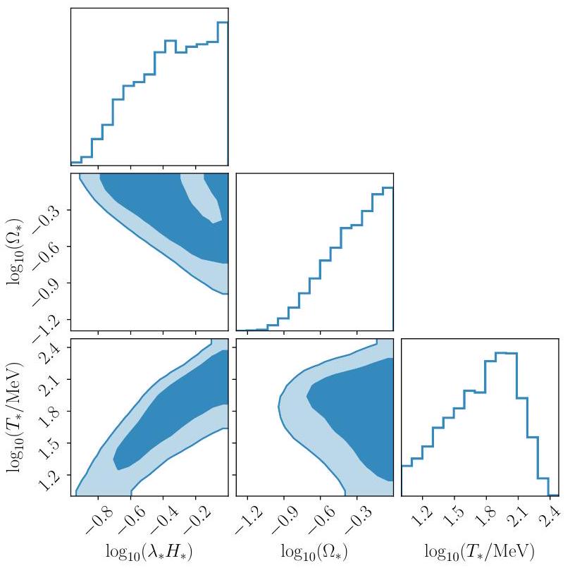
4.3. الآثار على الخلفية من الاضطراب حول مقياس طاقة QCD

يمكن أن ينشأ الاضطراب في الكون المبكر في أعقاب انتقال الطور من الدرجة الأولى (Witten 1984؛ Kamionkowski et al. 1994)، أو يمكن أن يكون مدفوعًا بواسطة مجالات مغناطيسية بدائية موجودة مسبقًا (Quashnock et al. 1989؛ Brandenburg et al. 1996). إذا كان الاضطراب (المغناطيسي-) الهيدروديناميكي موجودًا حول حقبة QCD، عندما كان للكون درجة حرارة
100 MeV، فإنه سيولد GWB في نطاق PTA. المقياس المميز للاضطراب، الذي يحدد تردد GW المميز، مرتبط في الواقع بنصف قطر هابل (المتحرك) في تلك الحقبة حيث
و تشير إلى عدد درجات الحرية النسبية. إذا كانت هناك عدم تماثل كبير في اللبتون و/أو مجالات مغناطيسية بدائية موجودة في الكون المبكر، فقد يكون انتقال الطور QCD من الدرجة الأولى (Schwarz & Stuke 2009؛ Wygas et al. 2018؛ Middeldorf-Wygas et al. 2022؛ Vovchenko et al. 2021؛ Cao 2023). في هذه الحالة، من المتوقع أن تكون هناك مصادر إضافية لـ GWs، من تصادم فقاعات الطور المكسورة والتطور اللاحق لموجات الصوت في السائل البدائي (Kosowsky et al. 1992؛ Kosowsky & Turner 1993؛ Caprini et al. 2008؛ Huber & Konstandin 2008؛ Jinno & Takimoto 2017؛ Cutting et al. 2018؛ Hindmarsh et al. 2014، 2015، 2017). تم تحليل ذلك بالنسبة لـ PTAs، على سبيل المثال في Moore & Vecchio (2021)، Arzoumanian et al. (2021)، Xue (2021). فيما يلي، نركز على GWB الناتج عن الاضطراب (M)HD المتحلل.

4.3.1. وصف النموذج

وجود سرعة الكتلة والمجالات المغناطيسية ينتج ضغوط غير متساوية، والتي بدورها تعمل كمصدر لـ GWs (Kamionkowski et al. 1994؛ Kosowsky et al. 2002؛ Dolgov et al. 2002؛ Caprini & Durrer 2006؛ Gogoberidze et al. 2007؛ Caprini et al. 2009). تم دراسة ذلك مؤخرًا من خلال محاكاة عددية في Roper Pol et al. (2020a، b، 2022a)، Brandenburg et al. (2021). على وجه الخصوص، يظهر Roper Pol et al. (2022a) أن غلاف GWB الناتج عن الاضطراب MHD المتحلل يمكن تقديره تحليليًا، بافتراض أن الضغوط غير المتساوية الناتجة عن السرعة والمجالات المغناطيسية تتغير ببطء أكثر من الإنتاج الديناميكي لـ GWs. تم التحقق من ذلك أيضًا من خلال محاكاة عددية للاضطراب الحركي البحت في Auclair et al. (2022). تؤدي هذه الفرضية إلى إشارة GWB التالية:
حيث هو نسبة كثافة الطاقة الاضطرابية (M)HD إلى كثافة الإشعاع، و هو نسبة طول المقياس المميز للاضطراب، إلى أفق هابل المتحرك في حقبة QCD. المعامل هو كفاءة إنتاج GW ، المقدرة في Roper Pol et al. (2022a). الدالة هي كثافة الطاقة الإشعاعية الجزئية في حقبة توليد GW إلى قيمتها في الوقت الحاضر. تعتمد على مقياس درجة الحرارة عبر عدد درجات الحرية ,
شكل الطيف لإشارة GWB، هو
حيث هو عامل تطبيع، و تشير إلى المدة الفعالة للاضطراب. يمكن تقدير الأخيرة، من المحاكاة العددية التي أجريت في Roper Pol et al. (2022a)، لتكون . الدالة في المعادلة (23) تشير إلى طيف الضغوط غير المتساوية. بالنسبة للمجالات الحلزونية (مثل المجال المغناطيسي البدائي أو حركة السائل الكتلي الدوامية) المميزة بمقياس ارتباط نموذجي من ترتيب مقياس الاضطراب ، فهي ثابتة لـ . علاوة على ذلك، تتلاشى كما لـ ، إذا كان الاضطراب من نوع كولموغوروف، كما نفترض هنا. وبالتالي، فإن الشكل الطيفي الناتج لـ GWB في المعادلة (21) يقدم ثلاثة قوانين قوة: عند الترددات أقل من العكس الفعال لمدة الاضطراب ، عند الترددات المتوسطة ، و عند الترددات الكبيرة .
لذا فإن GWB الناتج عن الاضطراب (M)HD يتحدد بثلاثة معلمات: مقياس درجة الحرارة ، قوة الاضطراب ، وطول مقياس الاضطراب المميز . بحكم السببية، يجب أن يكون أصغر من واحد. بشكل عام، أيضًا ، وإلا سيتغير الاضطراب ديناميات الكون. ومع ذلك، لاحظ أن القالب الموصوف أعلاه تم التحقق منه من حيث المبدأ فقط لحركات البلازما غير النسبية، والتي من أجلها .

4.3.2. نتائج التحليل

كما في القسم 4.1، هنا نستخدم طريقة تحليل الطيف الحر السريع على بيانات DR2new لتقييد النموذج، مع الأخذ في الاعتبار تسعة أول صناديق فورييه من طيف RMS في الشكل 1. نستخدم -أولويات موحدة لمعلمات النموذج، مختارين ، و . يتم عرض الخلفيات البعدية ثنائية الأبعاد التي تم الحصول عليها في الشكل 18.
بالنسبة للقيم من أقل من 0.1، يمكن للنموذج أن يفسر فقط مستوى الضوضاء المرتبطة عند أدنى صندوق تردد إذا كانت سعة الطيف مرتفعة بما فيه الكفاية. يمكن تحقيق ذلك فقط إذا كان قريبًا من 1 وكان تردد الذروة يقع ضمن نطاق تردد PTA، مما يعني . ومع ذلك، عند الترددات حول الذروة، تتوافق الإشارة مع كثافة طيفية قوية للبقايا أكثر حدة من ، مما لا يمكن أن يناسب البيانات بشكل جيد. لهذا السبب، يتم استبعاد قيم .
بالنسبة للقيم الأكبر من ، يمكن أن يدخل الجزء من الطيف عند الترددات أقل من نطاق PTA بسعة مرتفعة بما فيه الكفاية. علاوة على ذلك، يصبح البعد بين الكسر عند وقمة الطيف عند أقل ما يمكن في حد . تؤدي كلتا هاتين الميزتين إلى ملاءمة أفضل للبيانات. يتم استرداد ذلك في الخلفيات البعدية في الشكل 18، مع التدهور بين و من سعة الإشارة (انظر المعادلة (21))، والتدهور بين و من الكسر عند (لاحظ أن اعتماد الأخير على ثانوي).
لذا فإن النموذج يوفر ملاءمة جيدة للبيانات في حد كبير ، قريب من الحد الأعلى للأولوية. سيكون توسيع مجموعة البيانات إلى وقت المراقبة الأطول أمرًا حاسمًا لتقييد هذا النموذج بشكل أكبر عند الترددات المنخفضة.

4.4. الآثار على GWB من الدرجة الثانية الناتج عن اضطرابات الانحناء البدائية

من المعروف جيدًا أن أوضاع المقياس السلمي، المتجه والتنسوري من المقياس المضطرب لا تختلط عند الترتيب الخطي من معادلات أينشتاين (Lifshitz 1946؛ Baumann 2022). ومع ذلك، ستقوم اضطرابات الانحناء السلمي بتغذية أوضاع تنسورية متحركة (GWs) عند الدرجة الثانية في نظرية الاضطراب (Tomita 1967؛ Matarrese et al.
الشكل 18. الخلفيات البعدية ثنائية الأبعاد لمعلمات الخلفية من الاضطراب حول مقياس طاقة QCD التي تم الحصول عليها باستخدام ملاءمة طيف حر على بيانات DR2new. يتم عرض مناطق و الموثوقة.
1993، 1998؛ نوه وهوانغ 2004؛ كاربوني وماتاريسي 2005؛ أناندا وآخرون 2007؛ باومان وآخرون 2007). مثل هذه الاضطرابات في انحناء المقياس والتقلبات الأولية المرتبطة بها موجودة حتمًا في الكون ويمكن تقييدها مباشرة من خلال ملاحظات إشعاع الخلفية الكونية الميكروي. تشير أحدث بيانات بلانك (تعاون بلانك X 2020) إلى أن طيف القدرة لاضطرابات الانحناء قريب من كونه غير متغير مع المقياس مع السعة ، مما يعني كثافة طاقة هامشية للـ GWB الناتج. بشكل محدد، عند إسقاطها على نطاق حساسية PTA، تصبح المساهمة النسبية لكثافة الطاقة في الـ GWs المرتبطة ، والتي تكاد تكون غير قابلة للاكتشاف من قبل التجارب الحالية. من ناحية أخرى، تجعل بعض نماذج التضخم (انظر، على سبيل المثال، دي وغونغ 2018؛ بيرنز وآخرون 2019؛ براغليا وآخرون 2020؛ يي وفاي 2023) من الممكن إنتاج زيادة حادة في طيف الطاقة للاختلالات المنحنية الأولية عبر العديد من أوامر الحجم على المقاييس الصغيرة.
بينما يمكن لـ CMB فقط أخذ عينات مباشرة من المقاييس الكونية الكبيرة بـ تظل المقاييس الصغيرة غير مغطاة إلى حد كبير. توفر PTAs فرصة فريدة لتكملة قياسات CMB من خلال استكشاف اضطرابات انحناء السكالار بشكل غير مباشر في نطاق مقاييس. من خلال GWB الناتج من الدرجة الثانية، ووضع حدود على أقصى نمو ممكن لطيف الطاقة بالإضافة إلى النماذج المقابلة للتضخم (سايتو ويوكوياما 2009؛ بوغايف وكليمائي 2011؛ تشين وآخرون 2020؛ داندوي وآخرون 2023؛ تشاو ووانغ 2023).
في هذا العمل، نعتبر نموذجين من طيف انحناء البدائي: i) أحادي اللون و ii) قانون القوة. بالنسبة للأول، يتم نمذجة الطيف البدائي كالتالي:
أين هو سعة بلا أبعاد و هو عدد موجي يكون عنده طيف القدرة الأحادي اللون له قمة دلتا ديراك. بالنسبة للحالة الثانية:
الشكل 19. نتائج الاضطرابات المنحنية أحادية اللون الموضحة بالمعادلة (24). اللوحة اليسرى: المنحدرات المستعادة لنموذج بسيط من قانون القوة كدالة لمقياس مميز لـ GWB المُحقن الناتج عن اضطرابات الانحناء أحادية اللون. تُظهر الخطوط الأفقية القيمة النظرية لـ من مجموعة من ثنائيات الثقوب السوداء المتوسطة الحجم المدفوعة بواسطة موجات الجاذبية (رمادي) وتلك التي تم الحصول عليها في الورقة الثالثة (برتقالي). اللوحة اليمنى: و خطوط توزيع الخلفية على السعة ومقياس الخصائص للتقلبات لـ DR2new (اللون البرتقالي). يتم تراكب التوزيع الخلفي مع القيود الحالية على طيف القوة البدائي باستخدام بيانات بلانك (CMB). اللون الرمادي يمثل -فترات الثقة. تمثل المنطقة المظللة باللون الأرجواني الحدود الناتجة عن التشوهات الطيفية (Chluba et al. 2012). للمقارنة، نضع باللون الأخضر توقع الطيف البدائي للاختلالات القياسية في نموذج الحقلين للتضخم الموصوف في Braglia et al. (2020) لمجموعة من معلمات النموذج. جميع النماذج الثلاثة تؤدي إلى دوال كتلة PBH تتركز عند مع الخط الأكثر سطوعًا الذي يتوافق مع نسبة المادة المظلمة من الثقوب السوداء الأولية .
أين يتميز المنحدر و هو مقياس تطبيعي ، حتى يتوافق مع سعة بلا أبعاد عند عشر سنوات.
في السيناريو الأول، يوجد حل شبه تحليلي لطيف الطيف الناتج عن GWB ويعطى بواسطة (كوهري وتيرادا 2018؛ إسبينوزا وآخرون 2018):
أين و هو دالة هيفسايد ثيتا. على الرغم من كونها غير فيزيائية، فإن -تصف دالة الذروة تقريبًا الحد الأقصى لـ GWB المنتج في النموذج التضخمي بأقصى انحدار ممكن نمو قمة طيفية في التضخم أحادي الحقل عند المقاييس الصغيرة (انظر الشكل 7 في بيرنز وآخرون 2019).
في الحالة الثانية من طيف القوة الأكثر عمومية (والأكثر واقعية)، يمكن الحصول على النتيجة فقط عدديًا (كوهي وتيرادا 2018):
أين هو عامل التحجيم الذي يمكن تقييمه في نطاق من باستخدام نقاط الاستيفاء من الجدول 1 في كوهري وتيرادا (2018).
بعد إنتاجه، يتم تخميد GWB بسبب التفاعلات الكمية مع جزيئات البلازما الأولية في عصر الهيمنة الإشعاعية، ويتعرض لانزياح أحمر يتناسب عكسيًا مع عامل المقياس (كما يحدث أيضًا مع الإشعاع) بدءًا من عصر تساوي المادة والإشعاع (سايكوا وشيراي).
2018). القيمة الحالية لكثافة الطاقة الكسرية هي إذن:
أين هي درجة حرارة الكون في اللحظة التي تكون فيها الهياكل بحجم نموذجي إعادة دخول الأفق هي درجة حرارة الكون في عصر تساوي المادة والإشعاع، و هي درجات الحرية النسبية ودرجات الحرية في الإنتروبيا، على التوالي. التعبير النهائي لكثافة الطيف التلقائي لبقايا التوقيت هو:
أين هو ثابت هابل في العصر الحالي.
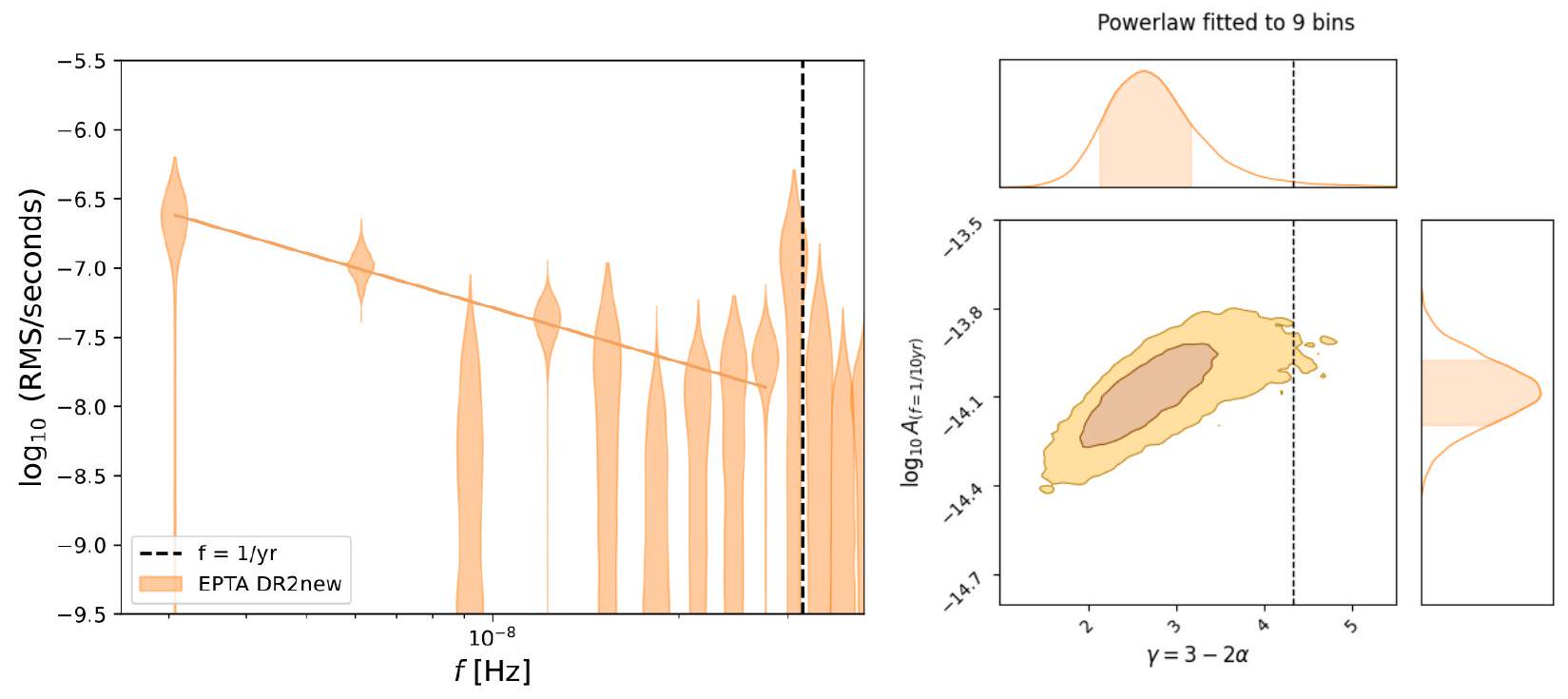
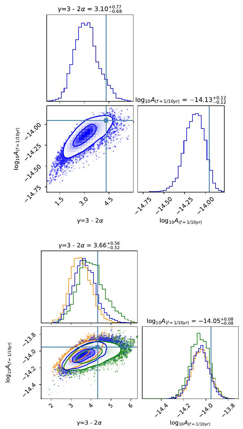
تم تطبيق الشكل الرسمي الموضح على النسخة DR2new من أحدث مجموعة بيانات EPTA. تم تثبيت عدد مكونات التردد التي تم استخدامها لتمثيل فورييه للإشارة عند 9. لقد اخترنا أولويات واسعة غير معلوماتية للمعلمات: موحدة في لـ و متساوي في [4، 12] لـ ويوزع بشكل متساوٍ في [0.4، 2.6] لـ تُقيد الحدود بالنسبة للأخير بالقيود المفروضة على التقريب العددي لنموذج قانون القوة. في هذا التحليل، افترضنا أن عملية الضوضاء الحمراء الشائعة التي تم اكتشافها في أحدث مجموعة بيانات EPTA يمكن تفسيرها بالكامل بواسطة موجات الجاذبية الناتجة عن التأثيرات السلمية من الدرجة الثانية.
تظهر نتائج النماذج أحادية اللون ونماذج قانون القوة في الشكلين 19 و20، على التوالي. يتم تصوير توزيع الخلفية ثنائي الأبعاد لبارامترات النموذج للنموذج أحادي اللون مع خطوط برتقالية على اللوحة اليمنى من الشكل 19. قد يلاحظ المرء أن مناطق أعلى احتمال هي بشكل قوي
الشكل 20. نتائج نموذج القوة للقوى المنحنية الموضحة بالمعادلة (25). اللوحة اليسرى: و خطوط توزيع الخلفية على السعة وميل طيف الطاقة تم الحصول عليه من تحليل DR2New. اللوحة اليمنى: و ملامح طيف القوة المستنتج من تحليل DR2New من خلال اختيار 1000 عينة عشوائية من التوزيعات الخلفية مغطاة بالقيود الحالية على طيف القوة البدائي باستخدام أحدث بيانات بلانك. اللون الرمادي يمثل -فترات الثقة. الخطوط الخضراء والمناطق المظللة باللون الأرجواني هي نفسها كما في الشكل 19.
ممتد بسبب وجود علاقة إيجابية قوية بين و ؛ هذه المعلمات في الأساس متدهورة. لذلك، يمكن أن يوفر DR2new حدودًا دنيا فقط على المقياس المميز وسعة النموذج أحادي الطيف: 7.6 و مما يعني أن مجموعة كاملة من النماذج التي تتنبأ بطيف الطاقة لديراك دلتا يمكن أن تصف بشكل جيد إشارة DR2new. يتم تفسير هذا السلوك في اللوحة اليسرى من الشكل 19، حيث قمنا بمحاكاة إشارة GWB الناتجة عن الاضطرابات السكلارية الأولية الأحادية الطيف، المعادلة (26)، وحاولنا استعادة نموذج أكثر عمومية لقانون القوة على الشكل استخدم في الورقة الثالثة لنمذجة عملية ضوضاء حمراء شائعة عشوائية. بعد انخفاض سريع، يستقر الميل المستعاد عند في حد كبير ، ويصبح متسقًا مع كل من القيم التي تم الحصول عليها باستخدام DR2new والقيمة المتوقعة نظريًا 13/3 للخلفية الناتجة عن الثقوب السوداء الثنائية المدفوعة بواسطة موجات الجاذبية. يمكن أن تثير هذه التداخلات قضايا مهمة عندما يحاول المرء فصل إشارة عن أخرى. بالنسبة لحالة القوة النسبية، يتم عرض التوزيعات الخلفية ثنائية الأبعاد في اللوحة اليسرى من الشكل 20 مع المتوسطات التالية و 1- الشكوك: و .
في الألواح اليمنى من الأشكال 19 و 20، نقوم أيضًا برسم طيف القوة البدائي المستنتج مع ذلك الذي تم الحصول عليه من بيانات بلانك. المناطق البرتقالية في اللوحة اليمنى من الشكل 20 هي و تخطيط نموذج القوة الذي تم وصفه بالمعادلة (25) والذي تم إعادة بنائه باستخدام 1000 سحب عشوائي من التوزيعات الخلفية. لشرح التوقيعات الملحوظة لـ DR2new من حيث GWB من الدرجة الثانية الناتج عن الاضطرابات السكلارية الأولية، يجب استدعاء فائض في الطيف الأولي عند المقاييس المنخفضة دون انتهاك معلمات التضخم في CMB. وقد تم اقتراح مثل هذا الفائض في العديد من الأوراق، على سبيل المثال في الأعمال المذكورة أعلاه من قبل إيفانوف وآخرين (1994)، جيرماني وبروكوبك (2017)، دي وغونغ (2018)، كاي وآخرين (2018)، بياجيتي وآخرين (2018)، بيرنز وآخرين (2019)، موتوهashi وآخرين (2020)، براغليا وآخرين (2020)، يي وفاي (2023). ومن الجدير بالذكر أن هذا الفائض في القوة سيؤدي إلى إنتاج وفير من الثقوب السوداء الأولية (PBHs) في المرحلة التي تهيمن عليها الإشعاع، والتي تُعتبر أحيانًا من قبل المؤلفين كدافع لتقديمها كمرشحة للمادة المظلمة الباردة.
تاريخ (Carr وآخرون 2016، والمراجع هناك). تم استكشاف تشكيل الثقوب السوداء الأولية من الاضطرابات الكونية بشكل موسع من قبل ساساكي وآخرون (2018). في مرحلة الهيمنة الإشعاعية، يرتبط كتلة الثقب الأسود الأولي بالكتلة داخل الأفق في وقت دخول الاضطراب. ، حيث هي الكتلة البلانكية، هو درجة الحرارة. من حيث عدد الموجات المتحركة في الوضع عند لحظة عبور الأفق، ، الجزء من أفق الكتلة الذي ينهار إلى ثقب أسود بدائي يقرأ
على سبيل المثال، في نموذج التضخم ذو الحقلين الذي قدمه براغليا وآخرون (2020)، يوجد ذروة حول يمكن أن يفسر القوة وفي الوقت نفسه تؤدي إلى إنتاج الثقوب السوداء الأولية ذات الكتل التي تتركز عند (انظر أيضًا تحليل نتائج NANOGrav في Vaskonen & Veermäe 2021). من المثير للاهتمام أن مثل هذه القمة يبدو أنها لوحظت في توزيع الكتلة المتزايدة للثقوب السوداء الثنائية المتصادمة LVK (Abbott et al. 2023). سيتم النظر في قائمة أكثر عمومية من طيف القوة البدائية، بالإضافة إلى إعادة ترجمة دقيقة لها إلى وفرة الثقوب السوداء الأولية ودالة كتلتها، في ورقة متابعة (Porayko et al.، قيد الإعداد).

5. الآثار III: المادة المظلمة

على عكس العمليات العشوائية المرتبطة مكانيًا وزمنيًا التي تم مناقشتها في الأقسام 3 و 4، نستكشف في هذا القسم مساهمة محتملة حتمية في إشارة EPTA من مادة مظلمة ذات حقل عددي خفيف للغاية (ULDM). للمقارنة، فإن شكل إشارة ULDM المفترضة، التي تنبأ بها خملنيتسكي وروباكوف (2014)، مشابه لإشارة موجات الجاذبية الكونية من ثقب أسود ثنائي ضخم، أي أنها بارزة فقط في حزمة تردد واحدة. نظرًا لأن الإشارة الملاحظة مع DR2new تظهر بشكل رئيسي في أول حزمتي تردد أساسية. صناديق التردد، من المهم النظر في المساهمات المحتملة من العمليات الفيزيائية ذات الطيف الضيق. لذلك، فإن التحليل
الجدول 1. المعلمات المستخدمة في البحث وأولوياتها المقابلة.
معامل وصف سابق حدوث
ضوضاء بيضاء )
EFAC لكل نظام خلفي/مستقبل موحد [0، 10] 1 لكل نبضة
نظام EQUAD للباك إند/المستقبل -موحد [-10، -5] 1 لكل نبضة
ضوضاء حمراء
سعة قانون القوة للضوضاء الحمراء -موحد [-20، -6] 1 لكل نبضة
مؤشر الطيف لقوة الضوضاء الحمراء موحد [0، 10] 1 لكل نبضة
ULDM
سعة ULDM -موحد [-20، -12] 1 للـ PTA
كتلة ULDM -موحد [-24، -22] 1 للـ PTA
عامل الأرض 1 للـ PTA
عامل النبض 1 لكل نبضة
طور إشارة الأرض زي موحد ] 1 لكل جمعية أولياء الأمور
طور إشارة النبض زي موحد ] 1 لكل نبضة
ضوضاء حمراء غير مرتبطة مكانياً شائعة (CURN)
سعة إجهاد العملية الشائعة -موحد [-20، -6] 1 للـ PTA
ملاحظات. في الحد المرتبط، ويمكن إعادة امتصاصه في إعادة تعريف .
المقدم هنا يكمل تفسير CGW للإشارة من قبل تعاون EPTA وتعاون InPTA (2023c). بالإضافة إلى ذلك، تم إجراء بحث ULDM باستخدام DR2full في سمارة وآخرون (2023).
تشكل المادة المظلمة حاليًا حوالي كثافة الطاقة في الكون، كما تم تأكيده من خلال، على سبيل المثال، منحنيات دوران المجرات (روبن وآخرون 1970، 1980؛ دي سالاس وآخرون 2019)، والتذبذبات الصوتية الباريونية وقياسات الخلفية الكونية الميكروية (بينيت وآخرون 2013؛ تعاون بلانك VI 2020) بالإضافة إلى مسوحات المجرات (إسكوديرو وآخرون 2015). الصورة القياسية للمادة المظلمة الباردة (CDM)، التي تشمل المرشحين الرئيسيين مثل الجسيمات الضخمة ذات التفاعل الضعيف (WIMPs؛ أركادي وآخرون 2018) والأكسيون QCD (لوزيو وآخرون 2020)، تفهم بنجاح الهيكل الكبير للكون. ومع ذلك، فإنها تواجه بعض القضايا المعروفة جيدًا عندما يتعلق الأمر بشرح الملاحظات على مقاييس أصغر من من بين هذه المشكلات، تتعلق مشكلة القمة-النواة (فلوريس وبريماك 1994؛ مور 1994؛ كاروكيس وآخرون 2015) بعدم التوافق بين ملاحظة ملف كثافة مسطح في مركز المجرات والسلوك الشبيه بالقوة الذي تتنبأ به نظرية المادة المظلمة الباردة، بينما يُشار غالبًا إلى الفجوة بين عدد المجرات القزمة المحاكاة والملاحظة في قرب مجرتنا درب التبانة بمشكلة الأقمار الصناعية المفقودة (كليبين وآخرون 1999؛ مور 1994).
بينما قد يساعد الفهم الشامل لآليات التغذية الراجعة في الفيزياء الباريونية (نافارو وآخرون 1996؛ غوفناتو وآخرون 2012؛ بروكس وآخرون 2013؛ تشان وآخرون 2015؛ أونوربي وآخرون 2015؛ ريد وآخرون 2016؛ مورغانتي 2017) في تخفيف بعض هذه القضايا، يمكن التخلص منها بشكل أسهل بافتراض أن المادة المظلمة هي خفيفة للغاية ( ) حقل قياسي/زائف قياسي أو حقل مشابه للأكسيون، الذي يكون كبيرًا من الناحية الفلكية ( طول موج دي بروغلي يخفف القوة على المقاييس الصغيرة. علاوة على ذلك، فإن المتجهات الخفيفة للغاية موجودة أيضًا بشكل عام في تقليصات نظرية الأوتار (غرين وآخرون 1988؛ سيفريك وويتن 2006؛ أرفانيتيكي وآخرون 2010)، مما يجعلها مرشحة مثيرة للاهتمام للفيزياء الجديدة أيضًا. تُستخدم الحجج المستندة إلى إشعاع الخلفية الكونية لتقييد (هلازيك وآخرون 2015)، بينما لايمان- الحدود تدفع الحد إلى شرط أن تمثل الجسيمات الخفيفة للغاية أكثر من من الميزانية الكاملة للمادة المظلمة (إيرشيك وآخرون 2017؛ أرمينغود وآخرون.
2017؛ كوباياشي وآخرون 2017؛ نوري وآخرون 2018؛ روجرز وبييريس 2021). حد أدنى من تدعي دراسات المجرات القزمة فائقة الضعف (UFD) (هاياشي وآخرون 2021؛ دلال وكرافستوف 2022)، لكن لم يتم التوصل بعد إلى توافق واسع. في عمل رائد، أظهر خملنيتسكي وروباكوف (2014) أن زمن سفر أشعة راديو النباضات يتأثر بالجهد الجاذبي الناتج عن جزيئات ULDM، مما يجعل PTAs مرافق ممتازة للتحقيق في وجود جزيئات ULDM. علاوة على ذلك، تمثل أدوات تكاملية لا تعاني من عدم اليقين في نمذجة البنية على المقياس الصغير التي تؤثر على القيود غير المتعلقة بـ CMB (شيف وآخرون 2014؛ زانغ وآخرون 2019)، كما هو مذكور في ليمان- أو حدود UFD. في ما يلي، نفترض بقوة أن ULDM يتفاعل فقط جاذبيًا، مما يؤدي إلى ظهور تذبذبات دورية في أوقات الوصول (TOAs) للنبضات الراديوية كما هو موصوف في خملنيتسكي وروباكوف (2014).
كونه غير نسبي ومع عدد شغل مميز كبير جداً، يمكن وصف حقل ULDM السكالاري كموجة كلاسيكية يكون تردد تذبذبها ضعف كتلتها. (خملنيتسكي وروباكوف 2014). الإزاحة الدورية التي تسببها ULDM على أوقات الوصول (TOAs) للإشارة من نجم نابض يمكن كتابته على النحو التالي (Porayko وآخرون 2018):
أين
أين هي مرحلة تعتمد على النباض (الأرض) و يأخذ في الاعتبار الطبيعة العشوائية للحقل الشبيه بالأكسيون بالقرب من النجم النابض (الأرض). يتم تلخيص المعلمات وأولوياتها في الجدول 1. بالنظر إلى قيمة نموذجية لـ بالنسبة لسرعة ULDM، المنطقة التي يتذبذب فيها الحقل السكالاري بشكل متماسك، أي بنفس القيمة لـ يمتد بواسطة طول التماسك:
الشكل 21. الاحتمالات الخلفية لسعة ULDM والكتلة من التحليل المرتبط (الصف العلوي) وغير المرتبط (الصف السفلي) لمجموعة بيانات DR2new. لم يتم عرض تحليل النباضات المرتبط، ولكنه يظهر نفس الميزات.
على وجه الخصوص، لاحظ أن و يجب أن يؤخذ على أنه:
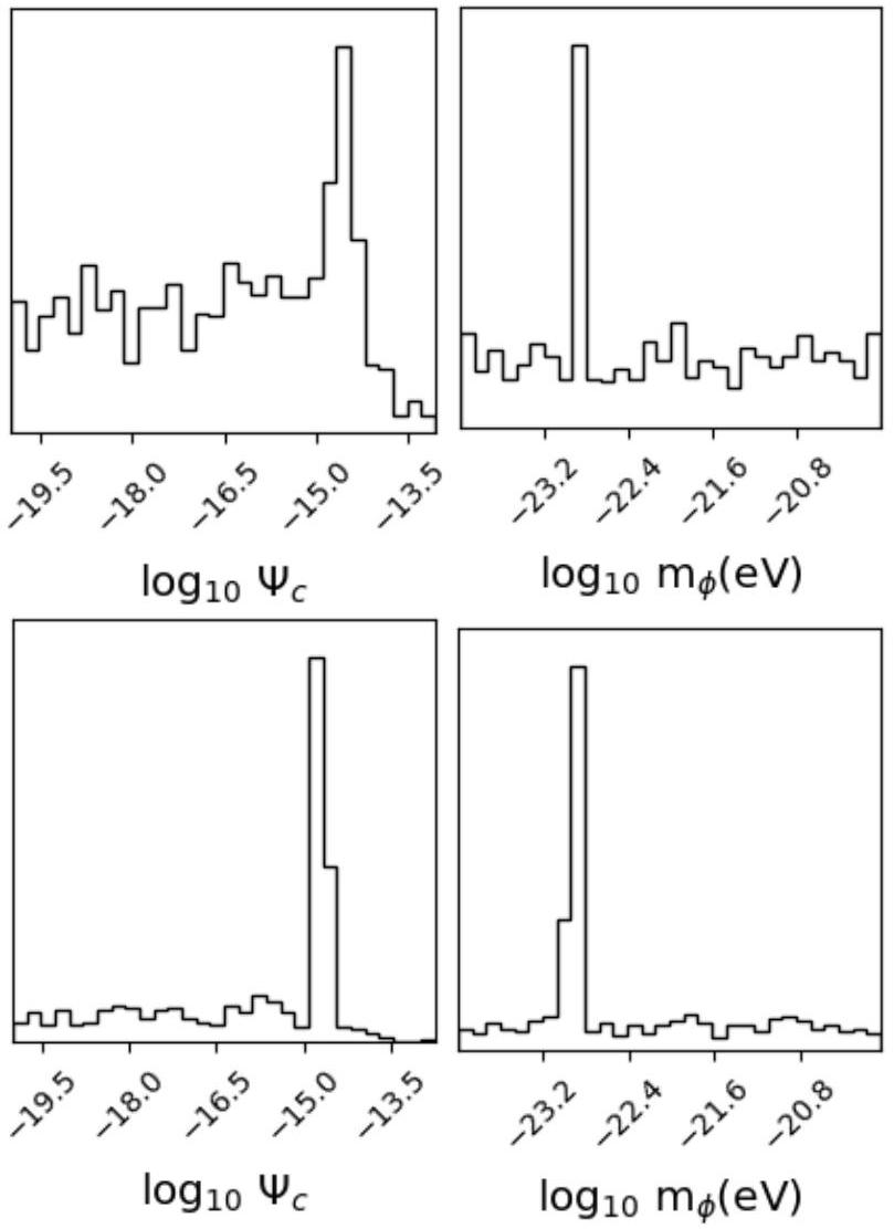
  • معلمات مختلفة عندما يكون متوسط المسافة بين النجم النابض والأرض والمسافة بين النجوم النابضة أكبر من طول التماسك؛
  • نفس المعامل عندما يكون متوسط المسافة بين النجم النابض والأرض والمسافة بين النجوم النابضة أصغر من طول التماسك. وفقًا للإجراء في سمارة وآخرون (2023)، نقوم بتحليل ثلاث حالات منفصلة، والتي نشير إليها على أنها غير مترابطة، مترابطة بين النجوم النابضة، وحدود مترابطة. حيث أن متوسط الفصل بين النجوم النابضة وفصل الأرض عن النجوم النابضة هو تظهر السيناريوهات المرتبطة وغير المرتبطة كحدود دقيقة في نهاية الكتلة المنخفضة ونهاية الكتلة العالية من نطاق PTAs، على التوالي. بدلاً من ذلك، يظل حد النبضات المرتبطة ساريًا عندما يكون طول التماسك لـ ULDM أصغر من نصف القطر المجري الذي يتم استكشافه بواسطة منحنيات الدوران (الداخلية )، ولكن أكبر من متوسط المسافة بين النبضات والمسافة بين النبضات والأرض. بشكل أكثر تحديدًا، فإن النظام المرتبط ينطبق على الكتل الأقل من ; نظام التوافق النابض لـ والحد غير المرتبط لـ نؤجل دراسة أكثر تفصيلاً إلى تحليل مستقبلي.
استنادًا إلى ما سبق، نقوم بتطبيق النموذج من المعادلة (31) على DR2new كما في سمارة وآخرون (2023). كمثال، التوزيعات الخلفية الهامشية لـ و مُرسومة في الشكل 21. جميع الحدود الثلاثة تصل إلى ذروتها عند كتلة ULDM مع السعة ، والذي يُترجم إلى كثافة لحقل السكالار. بينما هذه القيمة أعلى من كثافة المادة المظلمة المحلية المرجعية ، إنه ضمن حدود قياس الشكوك (بوفي وتريمين 2012؛ ريد 2014؛ سيفرتسون وآخرون 2018؛ دي سالاس 2020).
الشكل 22. القيود على كنتيجة لـ استخدام مجموعة بيانات EPTA DR2new من الورقة الثالثة. التحليلات السابقة موضحة للمقارنة، انظر إلى Porayko & Postnov (2014)، Porayko et al. (2018) لمزيد من التفاصيل. تمثل الخطوط الزرقاء والبرتقالية والبنية الحد الأعلى بايزي تم الحصول عليها من مجموعة بيانات EPTA DR2new مع التحليل المرتبط، غير المرتبط وتحليل الارتباط مع النباض، على التوالي. الخط الأرجواني يظهر وفرة ULDM المتوقعة المحسوبة من المعادلة (32).
الشكل 23. القيود على كثافة ULDM مُعَيار إلى قيمة خلفية DM تمثل الخطوط الزرقاء والبرتقالية والبنية الحد الأعلى بايزي تم الحصول عليها من مجموعة بيانات EPTA DR2new مع التحليل المرتبط، غير المرتبط وتحليل النبضات المرتبطة، على التوالي. الخط الأرجواني المنقط يظهر قيمة كثافة DM المحلية المرجعية.
بالإضافة إلى ذلك، نبحث عن توقيع محتمل لـ ULDM جنبًا إلى جنب مع خلفية موجات الجاذبية SMBHB. وبالتالي، نقدم نموذجًا جديدًا يحتوي على مساهمات ULDM جنبًا إلى جنب مع إشارة حمراء شائعة لحساب مساهمات موجات الجاذبية. لم نجد أي إشارة لـ ULDM تحت هذه الفرضية، بما يتماشى مع حقيقة أن البيانات تدعم الارتباط HD، الذي يفضل بشكل طبيعي GWs على ULDM في بحث مشترك. وبالتالي، نحن نضع الحد الأقصى للسعة وكثافة لحقل السكالار.
تظهر الأشكال 22 و 23 أن EPTA عند الحساسية الحالية قادر على تقييد وجود ULDM على المستوى
من وفرة المادة المظلمة المتوقعة في نطاق الكتلة تحليل DR2Full الذي تم إجراؤه في سمارة وآخرون (2023) يدفع هذه الحدود إلى الأسفل، مما يعني أن مثل هذه المرشحات ULDM لا يمكن أن تشكل كامل المادة المظلمة. نبرز أن حدودنا تمتد إلى ما دون تردد العينة DR2new. مع في الواقع، بينما قد يُعتقد بسذاجة أن مجال ULDM يحتاج إلى إكمال تذبذب في الإطار الزمني لتجربة PTA لإنتاج تأثير قابل للكشف، نشير إلى أن موجة ULDM بتردد لا يزال بالإمكان تقريبه بواسطة توسيع في قوى (كابلان وآخرون 2022)، على الرغم من أن حساسية PTAs ستنخفض بسبب التداخلات مع نموذج التوقيت (راماني وآخرون 2020). بالاعتماد على الحدود القوية لـ CMB المذكورة سابقًا، نثبت الحد الأدنى من بحثنا عند من المهم أننا نزيل الـ معامل من البحث في الحد المرتبط، حيث إنه متطابق تمامًا مع بعبارة أخرى، بناءً على الملاحظة بأن قياسات منحنى دوران مجرتنا تتم ضمن طول تماسك ULDM في الحد المرتبط، نعيد تعريف متغير جديد، ، الذي يمثل حالة المادة المظلمة في درب التبانة. أخيرًا، كما هو موضح في الشكل 22، نبلغ عن زيادة في الحدود العليا عند ، والذي يقع حول الحد الأقصى لكتلة البوزون في الشكل 21. هذه الكتلة تتوافق أيضًا مع تردد CGW الذي تم تحليله في تعاون EPTA وتعاون InPTA (2023c). عند النظر إلى التوزيعات الخلفية في هذا النطاق الكتلي، نجد أيضًا مساهمة إضافية، بالإضافة إلى عملية CURN. كما أن هناك ارتفاعًا مشابهًا في الحدود العليا موجود في مجموعة بيانات DR2Full، كما تم مناقشته في Smarra et al. (2023). ومع ذلك، فإن عامل بايز من نجد أن وجود إشارة ULDM لا يزال غير حاسم. نوصي بمتابعة هذه الزيادة في الأعمال المستقبلية.

6. المناقشة والتطلعات

في هذه الورقة، استكشفنا تداعيات الإشارة المشتركة والمتعلقة ذات التردد المنخفض التي تم ملاحظتها في أحدث إصدار من بيانات تعاون EPTA+InPTA. تم تجميع أربعة مجموعات بيانات مختلفة، وكانت الإشارة أكثر وضوحًا في تلك التي تشمل فقط بيانات عريضة النطاق وعالية الجودة المأخوذة باستخدام أنظمة التلسكوب من الجيل الجديد. لذلك، اعتبرنا، كمعيار لتحليلنا، الإشارة المقاسة في مجموعة بيانات DR2new، التي تم الكشف فيها عن الارتباط عالي الدقة مع عامل بايز. أو، بشكل مكافئ، عند -قيمة ، دلالة على الثقة. يمكن نمذجة الإشارة بواسطة طيف قانون القوة الواحد كما في المعادلة (3)، مع معلمات أفضل ملاءمة و (الورقة الثالثة).
قمنا بدراسة عدة عمليات فيزيائية بشكل منفصل، مستكشفين تداعيات الإشارة المكتشفة تحت فرضية أنها ناتجة عن تلك العملية المحددة. يمكن تلخيص نتائجنا الرئيسية كما يلي.
SMBHBs. الإشارة متسقة مع مجموعة كونية من SMBHBs المتداخلة. يمكن أن تحسب النماذج الظواهرية المستندة إلى ملاحظات أزواج المجرات توزيع الطيف القوي للإشارة المرتبطة. يمكن أيضًا استخدام تلك النماذج للتنبؤ بفرصة اكتشاف CGWs في البيانات الحالية، التي أعطت حتى الآن نتائج غير حاسمة (EPTA Collaboration & InPTA Collaboration 2023c). وفقًا لتلك النماذج، هناك تقريبًا فرصة لاكتشاف CGW في DR2new عند يمكن استخدام السعة العالية نسبيًا للإشارة لوضع قيود على الخصائص الرئيسية لعدد السكان من الثقوب السوداء الهائلة الثنائية في الكون. من خلال استغلال إطار الاستدلال الذي تم تطويره في ميدلتون وآخرون (2016)،
يمكننا أن نستنتج من تشين وآخرون (2019) أن الثقوب السوداء الهائلة تتزاوج في أقل من 1 مليار سنة بعد اندماج المجرات، وأن علاقة الثقوب السوداء الهائلة مع البروز النجمي لها تطبيع. عند كتلة نجمية مرجعية للنتوء وفقًا للنتائج المجمعة الأخيرة (مثل كرمندي وهو 2013). أخيرًا، بحثنا في كيفية مقارنة الإشارة المكتشفة مع التوقعات من نماذج تشكيل المجرات المتطورة (باراوس 2012؛ إزكييردو-فيلا Alba وآخرون 2022). وجدنا أن ارتفاع سعة الإشارة يفرض قيودًا غير تافهة على نماذج تطور المجرات والثقوب السوداء الهائلة. على وجه الخصوص، هناك حاجة إلى زيادة في اكتساب الثقوب السوداء الهائلة وأوقات تطور قصيرة لثنائيات الثقوب السوداء الهائلة لمطابقة الإشارة المرصودة، مما قد يؤدي إلى صعوبات عند محاولة إعادة إنتاج الملاحظات المستقلة مثل دالة سطوع الكوازارات. إذا تم تأكيد أصل ثنائيات الثقوب السوداء الهائلة للإشارة المرصودة، فسيكون ذلك إنجازًا كبيرًا لعلم الفلك الرصدي ولفهمنا لتشكيل المجرات. ستكون هذه أول دليل مباشر على أن ثنائيات الثقوب السوداء الهائلة تندمج في الطبيعة، مما يضيف قطعة مهمة من الملاحظات إلى لغز تشكيل البنية وتطور المجرات.
الكون المبكر. سيكون للإشارة المقاسة دلالات مختلفة لكل من العمليات الفيزيائية التي تم النظر فيها في هذه الدراسة. يتطلب الأصل التضخمي سيناريوهات تضخمية غير قياسية تكسر علاقة التباطؤ الثابت، مما يؤدي إلى طيف مائل نحو الأزرق. على وجه الخصوص، فإن القياس الذي تم يعني لكون يهيمن عليه الإشعاع مع سيتيح أصل الخيط الكوني تضييق نطاق توتر الخيط إلى قيم من , اعتمادًا على التوزيع المحدد للحلقات في شبكة الخيوط. وعلى العكس من ذلك، لا يمكن تقييد عدد الانحناءات. يمكن أن يفسر GWB الناتج عن اضطراب (M)HD عند مقياس طاقة QCD أيضًا الضوضاء الحمراء الشائعة، ولكنه يتطلب إما كثافات طاقة مضطربة عالية، من نفس ترتيب كثافة الطاقة الإشعاعية، أو مقياس مضطرب مميز قريب من الأفق في حقبة QCD. أخيرًا، يمكن أن ينتج الإشارة المقاسة من تطور الاضطرابات السلمية من الدرجة الثانية فقط إذا كان هناك فائض من طيفها البدائي موجود عند أعداد موجية كبيرة، مقارنة بالمستوى المستمد من ملاحظات CMB عند أعداد موجية صغيرة. ومن الجدير بالذكر أن مثل هذا الفائض قد يؤدي إلى إنتاج PBHs التي يمكن أن تساهم بشكل غير ضئيل في كثافة CDM.
ULDM. أخيرًا، بحثنا عن توقيعات ULDM في DR2new. أعاد البحث قمة بارزة في التوزيع الخلفي لكتلة جزيء ULDM حول -23. وهذا يتوافق مع تردد اهتزاز الحقل قدره , وهو متسق مع مرشح CGW الذي تم فحصه في تعاون EPTA وتعاون InPTA (2023c). ومع ذلك، عندما يتم إجراء بحث مشترك عن ULDM+GWB، تختفي القمة في توزيع الكتلة الخلفية لـ ULDM، حيث تفضل البيانات بشدة وجود ارتباط HD في الطاقة المشتركة. لذلك نستنتج أن أصل ULDM للإشارة المكتشفة غير مفضل، مما يضع قيدًا مباشرًا على وفرة ULDM في مجرتنا. إن عدم الكشف في DR2new يعني أن حوالي من كثافة DM في الجوار الشمسي يمكن أن يُعزى إلى ULDM مع . يتم الحصول على قيود أكثر صرامة من DR2full وتُعرض في ورقة منفصلة (Smarra et al. 2023).
من المثير للاهتمام أن نلاحظ أن أفضل ملاءمة لمنحدر القوة المقاسة هو , وهو أقل بكثير من المتوقع من مجموعة كونية من SMBHBs، وغالبًا ما يُشار إليه كمرشح رئيسي لتوليد GWs بتردد نانو هيرتز. قبل أن نترك المجال للتكهنات، نحذر من أن هذه ‘عدم التناسق’ قد يكون لها جذور متعددة، كما ذُكر في القسم 3.4. أولاً،
يفترض وجود مجموعة من الثنائيات المدفوعة بـ GW الدائرية. يمكن أن يؤدي الانحراف والارتباط البيئي بسهولة إلى تسطيح الطيف منخفض التردد. حتى بالنسبة للثنائيات الدائرية، فإن قانون القوة البسيط لـ هو حد مثالي؛ تؤدي إحصائيات الأعداد الصغيرة بسبب ندرة الأنظمة الضخمة والقريبة إلى طيف ضوضائي مع تباين كبير، مما يمكن أن ينتج عنه مؤشرات طيفية مختلفة عند ملاءمتها بقانون القوة. ثانيًا، يمكن أن تكون القيمة المقاسة عرضة للتحيزات الإحصائية والنظامية. لقد أظهرنا في الواقع أنه حتى عند حقن قانون القوة بـ في البيانات، يمكن أن تكون القيم المقاسة متحيزة بسبب التجسيد الإحصائي للضوضاء. علاوة على ذلك، يمكن أن يؤدي سوء نمذجة الضوضاء عالية التردد إلى تحيز منهجي في القيم المستعادة لـ ، مما يؤدي إلى طيف أكثر تسطيحًا إذا كانت الضوضاء عالية التردد غير المحسوبة موجودة في البيانات. لذلك، يجب توخي الحذر عند استخلاص الاستنتاجات من هذه القياسات.
وعلى العكس من ذلك، قد يشير منحدر الطيف الضحل إلى أن إشارة GW لها أصل مختلف، ربما من بعض العمليات الفيزيائية الرئيسية التي تحدث في الكون المبكر، كما تم التحقيق فيه في القسم 4. احتمال آخر، اقترحه ليو وآخرون (2022) هو أن GWs يمكن أن تفقد الطاقة أثناء انتشارها عبر الوسط بين المجرات عبر تسريع الجسيمات المشحونة. نظرًا لسرعة الحرارة الأعلى بكثير للإلكترونات مقارنة بالبروتونات ووجود حقل مغناطيسي في الوسط بين المجرات، يمكن تحويل جزء كبير من GWs إلى إشعاع كهرومغناطيسي. إن شدة الكهرومغناطيسية الناتجة تتناسب عكسيًا مع التردد. قد يفسر فقدان جزئي لـ GW عبر هذه الآلية طيف GWB أكثر تسطيحًا مما هو متوقع. تعتمد كفاءة مثل هذه الآلية على قوة الحقل المغناطيسي في الوسط بين المجرات.
من الممكن أيضًا أن الإشارة المرصودة تأتي من عدة GWB متداخلة. في تحليلاتنا، افترضنا أصلًا واحدًا لجميع طاقة الإشارة المرصودة في بيانات EPTA+InPTA، ومع ذلك، يمكن أن يتسبب تداخل GWB من أصول مختلفة في انحراف شكل الطيف للإشارة المستعادة عن القيمة المتوقعة لأي GWB واحد. سيكون البحث عن العمليات الفيزيائية الأساسية وفصلها وتحديدها جزءًا من توصيف الطيف في المستقبل (مور & فيكيو 2021؛ كايسر وآخرون 2022).
مع مرور الوقت وتحسن تجربة PTA، سيترك GWB منخفض التردد توقيعًا مميزًا بشكل متزايد في البيانات. سيكون من الضروري تفسير جميع تفاصيل هذا التوقيع لفهم طبيعة الإشارة واستغلال الإمكانات الكاملة لهذه النافذة الجديدة إلى الكون. كما ذُكر في المقدمة، من المتوقع أن تولد مجموعة من SMBHBs إشارة غير غاوسية للغاية، جزئيًا غير متساوية وربما غير ثابتة. مع زيادة فترة بياناتنا، وتحسين أدواتنا، ودمج المزيد من النبضات، ستظهر الخصائص التفصيلية للإشارة في النهاية في البيانات (على سبيل المثال، كورنيش وسيسانا 2013؛ تايلور وجاير 2013؛ تايلور وآخرون 2020؛ بول وآخرون 2022). بينما من المتوقع أن تكون العديد من إشارات الكون المبكر متساوية وغاوسية، توجد استثناءات ملحوظة، مثل GWB من انفجارات الخيوط الكونية. يمكن أن يوفر التداخل المتقاطع لتوزيع الطاقة في سماء GW بتردد نانو هيرتز إلى توزيع المجرات الضخمة والهياكل الكبيرة في الكون المنخفض المفتاح لتحديد الطبيعة الحقيقية – الفلكية مقابل الكون المبكر لهذه الإشارة (روسادو وسيسانا 2014؛ مينغاريلي وآخرون 2017). في هذا الصدد، فإن دمج جميع مجموعات البيانات عالية الجودة المتاحة ضمن إطار IPTA هو الخطوة التالية نحو تحقيق وعود علم GW بتردد نانو هيرتز.
الشكر. مجموعة توقيت النبضات الأوروبية (EPTA) هي تعاون بين المعاهد الأوروبية والشريكة، وهي ASTRON (NL)، INAF/مرصد كالياري (IT)، معهد ماكس بلانك لعلم الفلك الراديوي
(ألمانيا)، مرصد نانساي/باريس (فرنسا)، جامعة مانشستر (المملكة المتحدة)، جامعة برمنغهام (المملكة المتحدة)، جامعة شرق أنجليا (المملكة المتحدة)، جامعة بيليفيلد (ألمانيا)، جامعة باريس (فرنسا)، جامعة ميلانو-بيكوكا (إيطاليا)، مؤسسة البحث والتكنولوجيا، هيللاس (اليونان)، وجامعة بكين (الصين)، بهدف توفير توقيت نبضات عالي الدقة للعمل نحو الكشف المباشر عن موجات الجاذبية ذات التردد المنخفض. سمح منحة متقدمة من المجلس الأوروبي للبحث بتنفيذ الشبكة الأوروبية الكبيرة للنبضات (LEAP) بموجب رقم اتفاقية المنحة 227947 (PI M. Kramer). تعتبر EPTA جزءًا من مجموعة توقيت النبضات الدولية (IPTA)؛ نشكر زملاءنا في IPTA على دعمهم ومساعدتهم في هذه الورقة وأعضاء لجنة الكشف الخارجية على عملهم في قائمة التحقق من الكشف. يعتمد جزء من هذا العمل على الملاحظات باستخدام تلسكوب 100 متر من معهد ماكس بلانك لعلم الفلك الراديوي (MPIfR) في إيفيلسبرغ في ألمانيا. يتم دعم أبحاث النبضات في مركز جودريل بانك لعلم الفلك والدراسات باستخدام تلسكوب لوفيل من خلال منحة موحدة (ST/T000414/1) من مجلس العلوم والتكنولوجيا في المملكة المتحدة (STFC). كما يتم دعم ICN من خلال منحة تدريب الدكتوراه ST/T506291/1 من STFC. يتم تشغيل مرصد نانساي الراديو من قبل مرصد باريس، المرتبط بالمركز الوطني الفرنسي للبحث العلمي (CNRS)، ومدعوم جزئيًا من قبل منطقة مركز-فال دو لوار في فرنسا. نعترف بالدعم المالي من “البرنامج الوطني لعلم الكونيات والمجرات” (PNCG)، و”البرنامج الوطني للطاقة العالية” (PNHE) الممول من CNRS/INSU-IN2P3-INP، CEA وCNES، فرنسا. نعترف بالدعم المالي من الوكالة الوطنية للبحث (ANR-18-CE31-0015)، فرنسا. يتم تشغيل تلسكوب ويستربورك للراديو من قبل المعهد الهولندي لعلم الفلك الراديوي (ASTRON) بدعم من مؤسسة الأبحاث العلمية الهولندية (NWO). يتم تمويل تلسكوب سردينيا الراديوي (SRT) من قبل وزارة التعليم والجامعة والبحث (MIUR)، وكالة الفضاء الإيطالية (ASI)، والمنطقة المستقلة لسردينيا (RAS) ويتم تشغيله كمنشأة وطنية من قبل المعهد الوطني لعلم الفلك (INAF). يتم دعم العمل من قبل البرنامج الوطني SKA في الصين (2020SKA0120100)، مجموعة شراكة ماكس بلانك، NSFC 11690024، مشروع زراعة CAS لعلم FAST. يتم دعم هذا العمل أيضًا كجزء من تعاون “LEGACY” MPG-CAS في علم الفلك لموجات الجاذبية ذات التردد المنخفض. يعترف JA بالدعم من المفوضية الأوروبية (رقم اتفاقية المنحة: 101094354). تم دعم JA وSCha جزئيًا من قبل مؤسسة ستافروس نيارخوس (SNF) والمؤسسة الهيلينية للبحث والابتكار (H.F.R.I.) بموجب الدعوة الثانية لـ “عمل العلوم والمجتمع دائمًا السعي نحو التميز – ثيودوروس بابازوغلو” (رقم المشروع: 01431). يعترف AC بالدعم من منطقة باريس إيل دو فرانس. يعترف AC وAF وASe وASa وEB وDI وGMS وMBo بالدعم المالي المقدم بموجب منحة ERC الموحدة من الاتحاد الأوروبي “علم الفلك للثقوب السوداء الثنائية الضخمة” (B Massive، رقم اتفاقية المنحة: 818691). يعترف GD وKLi وRK وMK بالدعم من منحة التعاون من المجلس الأوروبي للبحث (ERC) “BlackHoleCam”، رقم اتفاقية المنحة 610058. يتم دعم هذا العمل من قبل منحة ERC المتقدمة “LEAP”، رقم اتفاقية المنحة 227947 (PI M. Kramer). يتم دعم AV وPRB من قبل مجلس العلوم والتكنولوجيا في المملكة المتحدة (STFC؛ المنحة ST/W000946/1). كما يعترف AV بدعم الجمعية الملكية ومؤسسة وولفسون. يعترف JPWV بالدعم من الجمعية الألمانية للبحث (DFG) من خلال برنامج هايزنبرغ (رقم المشروع 433075039) ومن NSF من خلال جائزة AccelNet #2114721. يتم تمويل NKP من قبل الجمعية الألمانية للبحث (DFG، مؤسسة البحث الألمانية) – رقم المشروع PO 2758/1-1، من خلال برنامج والتر بنجامين. يشكر ASa مؤسسة ألكسندر فون همبولت في ألمانيا على منحة همبولت للباحثين ما بعد الدكتوراه. يعترف APo وDP وMBu بالدعم من منحة البحث “iPeska” (P.I. أندريا بوسينتي) الممولة بموجب الدعوة الوطنية INAF Prin-SKA/CTA المعتمدة بموجب المرسوم الرئاسي 70/2016 (إيطاليا). يعترف RNC بالدعم المالي من الحساب الخاص لصناديق البحث في الجامعة المفتوحة الهيلينية (ELKEHOU) بموجب البرنامج البحثي “GRAVPUL” (رقم اتفاقية المنحة 319/10-10-2022). يعترف EvdW وCGB وGHJ بالدعم من أجندة العلوم الوطنية الهولندية، NWA Startimpuls – 400.17.608. يتم دعم BG من قبل وزارة التعليم والجامعة والبحث الإيطالية ضمن إطار برنامج البحث PRIN 2017، رقم 2017SYRTCN. يعترف LS باستخدام نظام HPC كوبا في مرفق ماكس بلانك للحوسبة والبيانات. مجموعة توقيت النبضات الهندية (InPTA) هي تعاون هندي-ياباني يستخدم بشكل روتيني تلسكوب TIFR المحدث لمراقبة مجموعة من نبضات IPTA. يعترف BCJ وYG وYM وSD وAG وPR بدعم من وزارة الطاقة الذرية، حكومة الهند، بموجب رقم تعريف المشروع # RTI 4002. يعترف BCJ وYG وYM بدعم من وزارة الطاقة الذرية، حكومة الهند، بموجب رقم المشروع 12-R&D-TFR-5.02-0700 بينما يعترف SD وAG وPR بدعم من وزارة الطاقة الذرية، حكومة الهند، بموجب رقم المشروع 12-R&D-TFR-5.02-0200. يتم دعم KT جزئيًا من قبل منح JSPS KAKENHI رقم 20H00180 و21H01130 و21H04467، مشاريع البحث المشتركة الثنائية من JSPS، وبرنامج البحث التعاوني ISM (2021-ISMCRP-2017). يتم دعم AS من قبل مركز NANOGrav NSF لفيزياء الحدود (الجوائز #1430284 و2020265). يتم دعم AKP من قبل منحة زمالة CSIR رقم 09/0079(15784)/2022-EMR-I. SH
مدعوم من منحة JSPS KAKENHI رقم 20J20509. يتم دعم KN من قبل زمالة معهد بيرلا للتكنولوجيا والعلوم. يتم دعم AmS من قبل منحة زمالة CSIR رقم 09/1001(12656)/2021-EMR-I وT641 (DST-ICPS). يتم دعم TK جزئيًا من قبل برنامج التحدي الخارجي JSPS للباحثين الشباب. نعترف بمهمة الحوسبة الوطنية (NSM) لتوفير موارد الحوسبة لـ ‘PARAM Ganga’ في المعهد الهندي للتكنولوجيا رووركي وكذلك ‘PARAM Seva’ في IIT حيدر أباد، والتي تم تنفيذها من قبل C-DAC ومدعومة من وزارة الإلكترونيات وتكنولوجيا المعلومات (MeitY) ووزارة العلوم والتكنولوجيا (DST)، حكومة الهند. يعترف DD بالدعم من وزارة الطاقة الذرية، حكومة الهند من خلال مشروع Apex للبحث المتقدم والتعليم في العلوم الرياضية في IMSc. العمل المقدم هنا هو نتيجة لسنوات عديدة من تحليل البيانات بالإضافة إلى تطوير البرمجيات والأدوات. بشكل خاص، نشكر الدكتور N. D’Amico، P. C. C. Freire، R. van Haasteren، C. Jordan، K. Lazaridis، P. Lazarus، L. Lentati، O. Löhmer وR. Smits على مساهماتهم السابقة. كما نشكر الدكتور N. Wex على دعم حسابات التسارع المجري بالإضافة إلى المناقشات ذات الصلة. نود أن نشكر البروفيسور الدكتور أليكسي ستاروبينسكي، سيرجي بليننيكوف وألكسندر دولغوف على المناقشات حول فيزياء الكون المبكر. يعترف HM بدعم وكالة الفضاء البريطانية، رقم المنحة ST/V002813/1 وST/X002071/1. تم إجراء بعض الحسابات الموصوفة في هذه الورقة باستخدام خدمة BlueBEAR HPC في جامعة برمنغهام، والتي توفر خدمة حوسبة عالية الأداء لمجتمع البحث في الجامعة. انظر http://www.birmingham.ac.uk/bearللمزيد من التفاصيل. كما أن EPTA ممتنة للموظفين في مراصدها وتلسكوباتها الذين جعلوا الملاحظات المستمرة ممكنة. مساهمات المؤلفين: EPTA هو جهد متعدد العقود وقد ساهم جميع المؤلفين من خلال التصور، والحصول على التمويل، وتنظيم البيانات، والمنهجية، وتطوير البرمجيات والأجهزة بالإضافة إلى (جوانب من) استمرار تشغيل الحملات الرصدية، والتي تشمل كتابة وتدقيق مقترحات المراقبة، وتقييم الملاحظات وأنظمة المراقبة، وتوجيه الطلاب، وتطوير حالات علمية. كما ساعد جميع المؤلفين في (جوانب من) التحقق من البيانات، والتحليل والنتائج بالإضافة إلى إنهاء مسودة الورقة. المساهمات المحددة من أعضاء EPTA الفرديين مدرجة في تنسيق CRediT (https://credit.niso.org/) أدناه. ساهم أعضاء InPTA في ملاحظات uGMRT وتقليل البيانات لإنشاء مجموعة بيانات InPTA التي يتم استخدامها أثناء تجميع مجموعات بيانات DR2full+ و DR2new+.

References

Abbott, L. F., & Wise, M. B. 1984, Nucl. Phys. B, 244, 541
Abbott, B. P., Abbott, R., Abbott, T. D., et al. 2016, Phys. Rev. Lett., 116, 061102
Abbott, B. P., Abbott, R., Abbott, T. D., et al. 2017, Phys. Rev. Lett., 118, 121101
Abbott, B. P., Abbott, R., Abbott, T. D., et al. 2018, Phys. Rev. D, 97, 102002
Abbott, R., Abbott, T. D., Abraham, S., et al. 2021, Phys. Rev. Lett., 126, 241102
Abbott, R., Abbott, T. D., Acernese, F., et al. 2023, Phys. Rev. X, 13, 011048
Allen, B. 1996, in Les Houches School of Physics: Astrophysical Sources of Gravitational Radiation, 373
Allen, B., & Koranda, S. 1994, Phys. Rev. D, 50, 3713
Amaro-Seoane, P., Sesana, A., Hoffman, L., et al. 2010, MNRAS, 402, 2308
Ananda, K. N., Clarkson, C., & Wands, D. 2007, Phys. Rev. D, 75, 123518
Anber, M. M., & Sorbo, L. 2012, Phys. Rev. D, 85, 123537
Antonini, F., Barausse, E., & Silk, J. 2015, ApJ, 806, L8
Arcadi, G., Dutra, M., Ghosh, P., et al. 2018, Eur. Phys. J. C, 78, 203
Armengaud, E., Palanque-Delabrouille, N., Yèche, C., Marsh, D. J. E., & Baur, J. 2017, MNRAS, 471, 4606
Arvanitaki, A., Dimopoulos, S., Dubovsky, S., Kaloper, N., & March-Russell, J. 2010, Phys. Rev. D, 81, 123530
Arzoumanian, Z., Brazier, A., Burke-Spolaor, S., et al. 2016, ApJ, 821, 13
Arzoumanian, Z., Baker, P. T., Blumer, H., et al. 2020, ApJ, 905, L34
Arzoumanian, Z., Baker, P. T., Blumer, H., et al. 2021, Phys. Rev. Lett., 127, 251302
Auclair, P. G. 2020, JCAP, 11, 050
Auclair, P., & Ringeval, C. 2022, Phys. Rev. D, 106, 063512
Auclair, P., Blanco-Pillado, J. J., Figueroa, D. G., et al. 2020, JCAP, 04, 034
Auclair, P., Caprini, C., Cutting, D., et al. 2022, JCAP, 09, 029
Auclair, P., Babak, S., Quelquejay Leclere, H., & Steer, D. A. 2023a, Phys. Rev. D, 108, 043519
Auclair, P., Steer, D. A., & Vachaspati, T. 2023b, Phys. Rev. D, 108, 123540
Babak, S., & Sesana, A. 2012, Phys. Rev. D, 85, 044034
Barausse, E. 2012, MNRAS, 423, 2533
Barausse, E., Dvorkin, I., Tremmel, M., Volonteri, M., & Bonetti, M. 2020, ApJ, 904, 16
Barnaby, N., Moxon, J., Namba, R., et al. 2012, Phys. Rev. D, 86, 103508
Bartolo, N., Matarrese, S., Riotto, A., & Väihkönen, A. 2007, Phys. Rev. D, 76, 061302
Bartolo, N., Caprini, C., Domcke, V., et al. 2016, JCAP, 2016, 026
Bassa, C. G., Janssen, G. H., Karuppusamy, R., et al. 2016, MNRAS, 456, 2196
Baumann, D. 2022, Cosmology (Cambridge University Press)
Baumann, D., Steinhardt, P., Takahashi, K., & Ichiki, K. 2007, Phys. Rev. D, 76, 084019
Bécsy, B., Cornish, N. J., & Kelley, L. Z. 2022, ApJ, 941, 119
Bennett, C. L., Larson, D., Weiland, J. L., et al. 2013, ApJS, 208, 20
Biagetti, M., Fasiello, M., & Riotto, A. 2013, Phys. Rev. D, 88, 103518
Biagetti, M., Dimastrogiovanni, E., Fasiello, M., & Peloso, M. 2015, JCAP, 2015, 011
Biagetti, M., Franciolini, G., Kehagias, A., & Riotto, A. 2018, JCAP, 2018, 032
Bian, L., Shu, J., Wang, B., Yuan, Q., & Zong, J. 2022, Phys. Rev. D, 106, L101301
Blanco-Pillado, J. J., & Olum, K. D. 2017, Phys. Rev. D, 96, 104046
Blanco-Pillado, J. J., Olum, K. D., & Shlaer, B. 2014, Phys. Rev. D, 89, 023512
Blanco-Pillado, J. J., Olum, K. D., & Shlaer, B. 2015, Phys. Rev. D, 92, 063528
Blasi, S., Brdar, V., & Schmitz, K. 2021, Phys. Rev. Lett., 126, 041305
Bonetti, M., & Sesana, A. 2020, Phys. Rev. D, 102, 103023
Bonetti, M., Sesana, A., Barausse, E., & Haardt, F. 2018, MNRAS, 477, 2599
Bovy, J., & Tremaine, S. 2012, ApJ, 756, 89
Boylan-Kolchin, M., Springel, V., White, S. D. M., Jenkins, A., & Lemson, G. 2009, MNRAS, 398, 1150
Boyle, L. A., & Buonanno, A. 2008, Phys. Rev. D, 78, 043531
Boyle, L. A., & Steinhardt, P. J. 2008, Phys. Rev. D, 77, 063504
Braglia, M., Hazra, D. K., Finelli, F., et al. 2020, JCAP, 2020, 001
Brandenburg, A., Enqvist, K., & Olesen, P. 1996, Phys. Rev. D, 54, 1291
Brandenburg, A., Clarke, E., He, Y., & Kahniashvili, T. 2021, Phys. Rev. D, 104, 043513
Brooks, A. M., Kuhlen, M., Zolotov, A., & Hooper, D. 2013, ApJ, 765, 22
Bugaev, E., & Klimai, P. 2011, Phys. Rev. D, 83, 083521
Byrnes, C. T., Cole, P. S., & Patil, S. P. 2019, JCAP, 2019, 028
Cai, Y.-F., Tong, X., Wang, D.-G., & Yan, S.-F. 2018, Phys. Rev. Lett., 121, 081306
Cao, G. 2023, Phys. Rev. D, 107, 014021
Capelo, P. R., Dotti, M., Volonteri, M., et al. 2017, MNRAS, 469, 4437
Caprini, C., & Durrer, R. 2006, Phys. Rev. D, 74, 063521
Caprini, C., & Figueroa, D. G. 2018, CQG, 35, 163001
Caprini, C., Durrer, R., & Servant, G. 2008, Phys. Rev. D, 77, 124015
Caprini, C., Durrer, R., & Servant, G. 2009, JCAP, 2009, 024
Carbone, C., & Matarrese, S. 2005, Phys. Rev. D, 71, 043508
Carr, B., Kühnel, F., & Sandstad, M. 2016, Phys. Rev. D, 94, 083504
Chan, T. K., Kereš, D., Oñorbe, J., et al. 2015, MNRAS, 454, 2981
Chen, S., Middleton, H., Sesana, A., Del Pozzo, W., & Vecchio, A. 2017a, MNRAS, 468, 404
Chen, S., Sesana, A., & Del Pozzo, W. 2017b, MNRAS, 470, 1738
Chen, S., Sesana, A., & Conselice, C. J. 2019, MNRAS, 488, 401
Chen, Z.-C., Yuan, C., & Huang, Q.-G. 2020, Phys. Rev. Lett., 124, 251101
Chen, S., Caballero, R. N., Guo, Y. J., et al. 2021, MNRAS, 508, 4970
Chen, Z.-C., Wu, Y.-M., & Huang, Q.-G. 2022, ApJ, 936, 20
Chluba, J., Erickcek, A. L., & Ben-Dayan, I. 2012, ApJ, 758, 76
Cook, J. L., & Sorbo, L. 2013a, JCAP, 2013, 047
Cook, J. L., & Sorbo, L. 2013b, JCAP, 11, 047
Cornish, N. J., & Sesana, A. 2013, CQG, 30, 224005
Cutting, D., Hindmarsh, M., & Weir, D. J. 2018, Phys. Rev. D, 97, 123513
Dalal, N., & Kravtsov, A. 2022, arXiv e-prints [arXiv:2203.05750]
Damour, T., & Vilenkin, A. 2000, Phys. Rev. Lett., 85, 3761
Damour, T., & Vilenkin, A. 2001, Phys. Rev. D, 64, 064008
Damour, T., & Vilenkin, A. 2005, Phys. Rev. D, 71, 063510
Dandoy, V., Domcke, V., & Rompineve, F. 2023, SciPost Phys. Core, 6, 060
de Salas, P. F. 2020, J. Phys. Conf. Ser., 1468, 012020
de Salas, P., Malhan, K., Freese, K., Hattori, K., & Valluri, M. 2019, JCAP, 2019, 037
Dehnen, W. 2014, Comput. Astrophys. Cosmol., 1, 1
Desvignes, G., Caballero, R. N., Lentati, L., et al. 2016, MNRAS, 458, 3341
Di, H., & Gong, Y. 2018, JCAP, 2018, 007
Dolgov, A. D., Grasso, D., & Nicolis, A. 2002, Phys. Rev. D, 66, 103505
D’Orazio, D. J., & Duffell, P. C. 2021, ApJ, 914, L21
Dvali, G., & Vilenkin, A. 2004, JCAP, 2004, 010
Ellis, J., & Lewicki, M. 2021, Phys. Rev. Lett., 126, 041304
Ellis, J. A., Vallisneri, M., Taylor, S. R., & Baker, P. T. 2020, https://doi . org/10.5281/zenodo. 4059815
Enoki, M., & Nagashima, M. 2007, Prog. Theor. Phys., 117, 241
EPTA Collaboration (Antoniadis, J., et al.) 2023, A&A, 678, A48 (Paper I)
EPTA Collaboration & InPTA Collaboration (Antoniadis, J., et al.) 2023a, A&A, 678, A49 (Paper II)
EPTA Collaboration & InPTA Collaboration (Antoniadis, J., et al.) 2023b, A&A, 678, A50 (Paper III)
EPTA Collaboration & InPTA Collaboration (Antoniadis, J., et al.) 2023c, A&A, submitted (Paper V)
Escudero, M., Mena, O., Vincent, A. C., Wilkinson, R. J., & Bœhm, C. 2015, JCAP, 2015, 034
Espinosa, J. R., Racco, D., & Riotto, A. 2018, JCAP, 2018, 012
Fabbri, R., & Pollock, M. D. 1983, Phys. Lett. B, 125, 445
Farris, B. D., Duffell, P., MacFadyen, A. I., & Haiman, Z. 2014, ApJ, 783, 134
Flores, R. A., & Primack, J. R. 1994, ApJ, 427, L1
Foster, R. S., & Backer, D. C. 1990, ApJ, 361, 300
Fujita, T., Yokoyama, J., & Yokoyama, S. 2015, Prog. Theor. Exp. Phys., 2015, 043E01
Galloni, G., Bartolo, N., Matarrese, S., et al. 2023, JCAP, 2023, 062
Germani, C., & Prokopec, T. 2017, Phys. Dark Universe, 18, 6
Giarè, W., & Melchiorri, A. 2021, Phys. Lett. B, 815, 136137
Giarè, W., Forconi, M., Di Valentino, E., & Melchiorri, A. 2023, MNRAS, 520, 1757
Giovannini, M. 1998, Phys. Rev. D, 58, 083504
Gogoberidze, G., Kahniashvili, T., & Kosowsky, A. 2007, Phys. Rev. D, 76, 083002
Goncharov, B., Shannon, R. M., Reardon, D. J., et al. 2021, ApJS, 917, 8
Goncharov, B., Thrane, E., Shannon, R. M., et al. 2022, ApJ, 932, L22
Governato, F., Zolotov, A., Pontzen, A., et al. 2012, MNRAS, 422, 1231
Graham, A. W., & Scott, N. 2013, ApJ, 764, 151
Green, M. B., Schwarz, J. H., & Witten, E. 1988, Superstring Theory. Vol. 1: Introduction, (Cambridge University Press)
Grishchuk, L. P. 1975, Sov. J. Exp. Theor. Phys., 40, 409
Gualandris, A., Khan, F. M., Bortolas, E., et al. 2022, MNRAS, 511, 4753
Hayashi, K., Ferreira, E. G. M., & Chan, H. Y. J. 2021, ApJS, 912, L3
Hellings, R. W., & Downs, G. S. 1983, ApJ, 265, L39
Henriques, B. M. B., White, S. D. M., Thomas, P. A., et al. 2015, MNRAS, 451, 2663
Hindmarsh, M. B., & Kibble, T. W. B. 1995, Rept. Prog. Phys., 58, 477
Hindmarsh, M., Huber, S. J., Rummukainen, K., & Weir, D. J. 2014, Phys. Rev. Lett., 112, 041301
Hindmarsh, M., Huber, S. J., Rummukainen, K., & Weir, D. J. 2015, Phys. Rev. D, 92, 123009
Hindmarsh, M., Huber, S. J., Rummukainen, K., & Weir, D. J. 2017, Phys. Rev. D, 96, 103520
Hlozek, R., Grin, D., Marsh, D. J. E., & Ferreira, P. G. 2015, Phys. Rev. D, 91, 103512
Horndeski, G. W. 1974, Int. J. Theor. Phys., 10, 363
Huber, S. J., & Konstandin, T. 2008, JCAP, 2008, 022
Iršič, V., Viel, M., Haehnelt, M. G., Bolton, J. S., & Becker, G. D. 2017, Phys. Rev. Lett., 119, 031302
Ivanov, P., Naselsky, P., & Novikov, I. 1994, Phys. Rev. D, 50, 7173
Izquierdo-Villalba, D., Sesana, A., Bonoli, S., & Colpi, M. 2022, MNRAS, 509, 3488
Izquierdo-Villalba, D., Sesana, A., Colpi, M., et al. 2024, A&A, in press https: //doi.org/10.1051/0004-6361/202449293
Jaffe, A. H., & Backer, D. C. 2003, ApJ, 583, 616
Jeannerot, R., Rocher, J., & Sakellariadou, M. 2003, Phys. Rev. D, 68, 103514
Jinno, R., & Takimoto, M. 2017, Phys. Rev. D, 95, 024009
Jones, N. T., Stoica, H., & Tye, S. H. H. 2003, Phys. Lett. B, 563, 6
Joshi, B. C., Gopakumar, A., Pandian, A., et al. 2022, J. Astrophys. Astron., 43, 98
Kahniashvili, T., Brandenburg, A., Gogoberidze, G., Mandal, S., & Roper Pol, A. 2021, Phys. Rev. Res., 3, 013193
Kaiser, A. R., Pol, N. S., McLaughlin, M. A., et al. 2022, ApJ, 938, 115
Kamionkowski, M., Kosowsky, A., & Turner, M. S. 1994, Phys. Rev. D, 49, 2837
Kaplan, D. E., Mitridate, A., & Trickle, T. 2022, Phys. Rev. D, 106, 035032
Karukes, E. V., Salucci, P., & Gentile, G. 2015, A&A, 578, A13
Kelley, L. Z., Blecha, L., Hernquist, L., Sesana, A., & Taylor, S. R. 2017, MNRAS, 471, 4508
Kelley, L. Z., Blecha, L., Hernquist, L., Sesana, A., & Taylor, S. R. 2018, MNRAS, 477, 964
Khan, F. M., Preto, M., Berczik, P., et al. 2012, ApJ, 749, 147
Khan, F. M., Fiacconi, D., Mayer, L., Berczik, P., & Just, A. 2016, ApJ, 828, 73
Khmelnitsky, A., & Rubakov, V. 2014, JCAP, 2014, 019
Kibble, T. 1976, J. Phys. A, 9, 1387
Klein, A., Barausse, E., Sesana, A., et al. 2016, Phys. Rev. D, 93, 024003
Klypin, A., Kravtsov, A. V., Valenzuela, O., & Prada, F. 1999, ApJ, 522, 82
Kobayashi, T., Murgia, R., Simone, A. D., Iršič, V., & Viel, M. 2017. Phys. Rev. D, 96, 123514
Kocsis, B., & Sesana, A. 2011, MNRAS, 411, 1467
Kohri, K., & Terada, T. 2018, Phys. Rev. D, 97, 123532
Kormendy, J., & Ho, L. C. 2013, ARA&A, 51, 511
Kosowsky, A. 1996, Ann. Phys., 246, 49
Kosowsky, A., & Turner, M. S. 1993, Phys. Rev. D, 47, 4372
Kosowsky, A., Turner, M. S., & Watkins, R. 1992, Phys. Rev. D, 45, 4514
Kosowsky, A., Mack, A., & Kahniashvili, T. 2002, Phys. Rev. D, 66, 024030
Koss, M. J., Blecha, L., Bernhard, P., et al. 2018, Nature, 563, 214
Kulier, A., Ostriker, J. P., Natarajan, P., Lackner, C. N., & Cen, R. 2015, ApJ, 799, 178
Lamb, W. G., Taylor, S. R., & van Haasteren, R. 2023, Phys. Rev. D, 108, 103019
Lasky, P. D., Mingarelli, C. M. F., Smith, T. L., et al. 2016, Phys. Rev. X, 6, 011035
Leclere, H. Q., Auclair, P., Babak, S., et al. 2023, Phys. Rev. D, 108, 123527
Lee, K. J. 2016, ASP Conf. Ser., 502, 19
Lentati, L., Taylor, S. R., Mingarelli, C. M. F., et al. 2015, MNRAS, 453, 2576
Lieu, R., Lackeos, K., & Zhang, B. 2022, CQG, 39, 075014
Lifshitz, E. M. 1946, Zhurnal Eksperimentalnoi i Teoreticheskoi Fiziki, 16, 587
Lorenz, L., Ringeval, C., & Sakellariadou, M. 2010, JCAP, 10, 003
Luzio, L. D., Giannotti, M., Nardi, E., & Visinelli, L. 2020, Phys. Rep., 870, 1
Maggiore, M. 2000, Phys. Rept., 331, 283
Manchester, R. N., Hobbs, G., Bailes, M., et al. 2013, PASA, 30, e017
Matarrese, S., Pantano, O., & Saez, D. 1993, Phys. Rev. D, 47, 1311
Matarrese, S., Mollerach, S., & Bruni, M. 1998, Phys. Rev. D, 58, 043504
McConnell, N. J., & Ma, C.-P. 2013, ApJ, 764, 184
McConnell, N. J., Ma, C.-P., Gebhardt, K., et al. 2011, Nature, 480, 215
McLaughlin, M. A. 2013, CQG, 30, 224008
McWilliams, S. T., Ostriker, J. P., & Pretorius, F. 2014, ApJ, 789, 156
Middeldorf-Wygas, M. M., Oldengott, I. M., Bödeker, D., & Schwarz, D. J. 2022, Phys. Rev. D, 105, 123533
Middleton, H., Del Pozzo, W., Farr, W. M., Sesana, A., & Vecchio, A. 2016, MNRAS, 455, L72
Middleton, H., Sesana, A., Chen, S., et al. 2021, MNRAS, 502, L99
Miles, M. T., Shannon, R. M., Bailes, M., et al. 2023, MNRAS, 519, 3976
Milosavljević, M., & Merritt, D. 2003, ApJ, 596, 860
Mingarelli, C. M. F., Lazio, T. J. W., Sesana, A., et al. 2017, Nat. Astron., 1, 886
Moore, B. 1994, Nature, 370, 629
Moore, C. J., & Vecchio, A. 2021, Nat. Astron., 5, 1268
Moore, B., Ghigna, S., Governato, F., et al. 1999, ApJ, 524, L19
Morganti, R. 2017, Front. Astron. Space Sci., 4
Motohashi, H., Mukohyama, S., & Oliosi, M. 2020, JCAP, 2020, 002
Nasim, I., Gualandris, A., Read, J., et al. 2020, MNRAS, 497, 739
Nasim, I. T., Gualandris, A., Read, J. I., et al. 2021, MNRAS, 502, 4794
Navarro, J. F., Eke, V. R., & Frenk, C. S. 1996, MNRAS, 283, L72
Noh, H., & Hwang, J.-C. 2004, Phys. Rev. D, 69, 104011
Nori, M., Murgia, R., Iršič, V., Baldi, M., & Viel, M. 2018, MNRAS, 482, 3227
Oñorbe, J., Boylan-Kolchin, M., Bullock, J. S., et al. 2015, MNRAS, 454, 2092
Perera, B. B. P., DeCesar, M. E., Demorest, P. B., et al. 2019, MNRAS, 490, 4666
Phinney, E. S. 2001, arXiv e-prints [arXiv:astro-ph/0108028]
Pillepich, A., Springel, V., Nelson, D., et al. 2018, MNRAS, 473, 4077
Planck Collaboration XVI. 2014, A&A, 571, A16
Planck Collaboration VI. 2020, A&A, 641, A6
Planck Collaboration X. 2020, A&A, 641, A10
Pol, N., Taylor, S. R., & Romano, J. D. 2022, ApJ, 940, 173
Porayko, N. K., & Postnov, K. A. 2014, Phys. Rev. D, 90, 062008
Porayko, N. K., Zhu, X., Levin, Y., et al. 2018, Phys. Rev. D, 98, 102002
Preto, M., Berentzen, I., Berczik, P., & Spurzem, R. 2011, ApJ, 732, L26
Quashnock, J. M., Loeb, A., & Spergel, D. N. 1989, ApJ, 344, L49
Quinlan, G. D. 1996, New A, 1, 35
Rajagopal, M., & Romani, R. W. 1995, ApJ, 446, 543
Ramani, H., Trickle, T., & Zurek, K. M. 2020, JCAP, 2020, 033
Ravi, V., Wyithe, J. S. B., Hobbs, G., et al. 2012, ApJ, 761, 84
Ravi, V., Wyithe, J. S. B., Shannon, R. M., Hobbs, G., & Manchester, R. N. 2014, MNRAS, 442, 56
Ravi, V., Wyithe, J. S. B., Shannon, R. M., & Hobbs, G. 2015, MNRAS, 447, 2772
Read, J. I. 2014, J. Phys. G: Nucl. Part. Phys., 41, 063101
Read, J. I., Agertz, O., & Collins, M. L. M. 2016, MNRAS, 459, 2573
Reardon, D. J., Zic, A., Shannon, R. M., et al. 2023, ApJ, 951, L6
Ringeval, C., & Suyama, T. 2017, JCAP, 12, 027
Roedig, C., & Sesana, A. 2012, J. Phys. Conf. Ser., 363, 012035
Roedig, C., Dotti, M., Sesana, A., Cuadra, J., & Colpi, M. 2011, MNRAS, 415, 3033
Rogers, K. K., & Peiris, H. V. 2021, Phys. Rev. Lett., 126, 071302
Roper Pol, A., Brandenburg, A., Kahniashvili, T., Kosowsky, A., & Mandal, S. 2020a, Geophys. Astrophys. Fluid Dyn., 114, 130
Roper Pol, A., Mandal, S., Brandenburg, A., Kahniashvili, T., & Kosowsky, A. 2020b, Phys. Rev. D, 102, 083512
Roper Pol, A., Caprini, C., Neronov, A., & Semikoz, D. 2022a, Phys. Rev. D, 105, 123502
Roper Pol, A., Mandal, S., Brandenburg, A., & Kahniashvili, T. 2022b, JCAP, 04, 019
Rosado, P. A., & Sesana, A. 2014, MNRAS, 439, 3986
Rosado, P. A., Sesana, A., & Gair, J. 2015, MNRAS, 451, 2417
Rubakov, V. A., Sazhin, M. V., & Veryaskin, A. V. 1982, Phys. Lett. B, 115, 189
Rubin, V. C., Ford, W., & Kent, J. 1970, ApJ, 159, 379
Rubin, V. C., Ford, W. K.Jr, & Thonnard, N. 1980, ApJ, 238, 471
Sachs, R. K., & Wolfe, A. M. 1967, ApJ, 147, 73
Saikawa, K., & Shirai, S. 2018, JCAP, 2018, 035
Saito, R., & Yokoyama, J. 2009, Phys. Rev. Lett., 102, 161101
Sanidas, S. A., Battye, R. A., & Stappers, B. W. 2012, Phys. Rev. D, 85, 122003
Sasaki, M., Suyama, T., Tanaka, T., & Yokoyama, S. 2018, CQG, 35, 063001
Schechter, P. 1976, ApJ, 203, 297
Schive, H.-Y., Liao, M.-H., Woo, T.-P., et al. 2014, Phys. Rev. Lett., 113, 261302
Schwarz, D. J., & Stuke, M. 2009, JCAP, 2009, 025
Sesana, A. 2010, ApJ, 719, 851
Sesana, A. 2013a, CQG, 30, 224014
Sesana, A. 2013b, MNRAS, 433, L1
Sesana, A. 2015, Astrophys. Space Sci. Proc., 40, 147
Sesana, A., Haardt, F., Madau, P., & Volonteri, M. 2004, ApJ, 611, 623
Sesana, A., Vecchio, A., & Colacino, C. N. 2008, MNRAS, 390, 192
Sesana, A., Vecchio, A., & Volonteri, M. 2009, MNRAS, 394, 2255
Sesana, A., Barausse, E., Dotti, M., & Rossi, E. M. 2014, ApJ, 794, 104
Siemens, X., Mandic, V., & Creighton, J. 2007, Phys. Rev. Lett., 98, 111101
Simon, J. 2023, ApJ, 949, L24
Sivertsson, S., Silverwood, H., Read, J. I., Bertone, G., & Steger, P. 2018, MNRAS, 478, 1677
Siwek, M. S., Kelley, L. Z., & Hernquist, L. 2020, MNRAS, 498, 537
Smarra, C., Goncharov, B., Barausse, E., & EPTA and InPTA 2023, Phys. Rev. Lett., 131, 171001
Sorbo, L. 2011a, JCAP, 2011, 003
Sorbo, L. 2011b, JCAP, 06, 003
Sotiriou, T. P., & Faraoni, V. 2010, Rev. Mod. Phys., 82, 451
Springel, V., White, S. D. M., Jenkins, A., et al. 2005, Nature, 435, 629
Starobinskii, A. A. 1985, Soviet. Astron. Lett., 11, 133
Svrcek, P., & Witten, E. 2006, J. High Energy Phys., 2006, 051
Taylor, S. R., & Gair, J. R. 2013, Phys. Rev. D, 88, 084001
Taylor, S. R., van Haasteren, R., & Sesana, A. 2020, Phys. Rev. D, 102, 084039
The Nanograv Collaboration (Agazie, G., et al.) 2023, ApJ, 951, L8
Tiburzi, C., Hobbs, G., Kerr, M., et al. 2016, MNRAS, 455, 4339
Tomita, K. 1967, Prog. Theor. Phys., 37, 831
Tristram, M., Banday, A. J., Górski, K. M., et al. 2022, Phys. Rev. D, 105, 083524
Vachaspati, T., & Vilenkin, A. 1985, Phys. Rev. D, 31, 3052
Vallisneri, M. 2020, Astrophysics Source Code Library [record ascl:2002 .017]
Valtolina, S., Shaifullah, G., Samajdar, A., et al. 2024, A&A, 683, A201
Vaskonen, V., & Veermäe, H. 2021, Phys. Rev. Lett., 126, 051303
Verbiest, J. P. W., Lentati, L., Hobbs, G., et al. 2016, MNRAS, 458, 1267
Vilenkin, A., & Shellard, E. P. S. 2000, Cosmic Strings and Other Topological Defects (Cambridge, UK: Cambridge University Press)
Vovchenko, V., Brandt, B. B., Cuteri, F., et al. 2021, Phys. Rev. Lett., 126, 012701
Witten, E. 1984, Phys. Rev. D, 30, 272
Wygas, M. M., Oldengott, I. M., Bödeker, D., & Schwarz, D. J. 2018, Phys. Rev. Lett., 121, 201302
Wyithe, J. S. B., & Loeb, A. 2003, ApJ, 590, 691
Xu, H., Chen, S., Guo, Y., et al. 2023, Res. Astron. Astrophys., 23, 075024
Xue, X., Bian, L., Shu, J., et al. 2021, Phys. Rev. Lett., 127, 251303
Yi, Z., & Fei, Q. 2023, Eur. Phys. J. C, 83, 82
Zhang, J., Liu, H., & Chu, M.-C. 2019, Front. Astron. Space Sci., 5
Zhao, Z.-C., & Wang, S. 2023, Universe, 9, 157
Institute of Astrophysics, FORTH, N. Plastira 100, 70013 Heraklion, Greece
Max-Planck-Institut für Radioastronomie, Auf dem Hügel 69, 53121 Bonn, Germany
Department of Physics, Indian Institute of Technology Roorkee, Roorkee 247667, India
4 Department of Electrical Engineering, IIT Hyderabad, Kandi Telangana 502284, India
Cosmology, Universe and Relativity at Louvain (CURL), Institute of Mathematics and Physics, University of Louvain, 2 Chemin du Cyclotron, 1348 Louvain-la-Neuve, Belgium
Université Paris Cité, CNRS, Astroparticule et Cosmologie, 75013 Paris, France
The Institute of Mathematical Sciences, C. I. T. Campus, Taramani, Chennai 600113, India
Homi Bhabha National Institute, Training School Complex, Anushakti Nagar, Mumbai 400094, India
Fakultät für Physik, Universität Bielefeld, Postfach 100131, 33501 Bielefeld, Germany
Scuola Internazionale Superiore di Studi Avanzati, Via Bonomea 265, 34136 Trieste, Italy and INFN Sezione di Trieste
11 ASTRON, Netherlands Institute for Radio Astronomy, Oude Hoogeveensedijk 4, 7991 PD Dwingeloo, The Netherlands
Department of Physical Sciences, Indian Institute of Science Education and Research, Mohali, Punjab 140306, India
Laboratoire de Physique et Chimie de l’Environnement et de l’Espace, Université d’Orléans/CNRS, 45071 Orléans Cedex 02, France
14 Observatoire Radioastronomique de Nançay, Observatoire de Paris, Université PSL, Université d’Orléans, CNRS, 18330 Nançay, France
15 Dipartimento di Fisica “G. Occhialini”, Università degli Studi di Milano-Bicocca, Piazza della Scienza 3, 20126 Milano, Italy
16 INFN, Sezione di Milano-Bicocca, Piazza della Scienza 3, 20126 Milano, Italy
17 INAF – Osservatorio Astronomico di Brera, via Brera 20, 20121 Milano, Italy
Institute for Gravitational Wave Astronomy and School of Physics and Astronomy, University of Birmingham, Edgbaston, Birmingham B15 2TT, UK
19 INAF – Osservatorio Astronomico di Cagliari, via della Scienza 5, 09047 Selargius, (CA), Italy
Hellenic Open University, School of Science and Technology, 26335 Patras, Greece
Université de Genève, Département de Physique Théorique and Centre for Astroparticle Physics, 24 quai Ernest-Ansermet, 1211 Genève 4, Switzerland
22 CERN, Theoretical Physics Department, 1 Esplanade des Particules, 1211 Genéve 23, Switzerland
Kavli Institute for Astronomy and Astrophysics, Peking University, Beijing 100871, PR China
Department of Astronomy and Astrophysics, Tata Institute of Fundamental Research, Homi Bhabha Road, Navy Nagar, Colaba, Mumbai 400005, India
Department of Physics, IIT Hyderabad, Kandi, Telangana 502284, India
Department of Physics and Astrophysics, University of Delhi, Delhi 110007, India
27 Department of Earth and Space Sciences, Indian Institute of Space Science and Technology, Valiamala, Thiruvananthapuram, Kerala 695547, India
School of Mathematics and Physics, Faculty of Engineering and Physical Science, University of Surrey, Guildford GU2 7XH, UK
School of Physics, Faculty of Science, University of East Anglia, Norwich NR4 7TJ, UK
30 Sternberg Astronomical Institute, Moscow State University, Universitetsky pr., 13, Moscow 119234, Russia
Max Planck Institute for Gravitational Physics (Albert Einstein Institute), Am Muühlenberg 1, 14476 Potsdam, Germany
Gran Sasso Science Institute (GSSI), 67100 L’Aquila, Italy
33 INFN, Laboratori Nazionali del Gran Sasso, 67100 Assergi, Italy
34 National Centre for Radio Astrophysics, Pune University Campus, Pune 411007, India
35 Kumamoto University, Graduate School of Science and Technology, Kumamoto 860-8555, Japan
36 Università di Cagliari, Dipartimento di Fisica, S.P. MonserratoSestu Km 0,700, 09042 Monserrato, (CA), Italy
37 Department of Astrophysics/IMAPP, Radboud University Nijmegen, PO Box 9010, 6500 GL Nijmegen, The Netherlands
38 Department of Physical Sciences, Indian Institute of Science Education and Research Kolkata, Mohanpur 741246, India
Center of Excellence in Space Sciences India, Indian Institute of Science Education and Research Kolkata, Kolkata 741246, India
School of Physics, Trinity College Dublin, College Green, Dublin 2 D02 PN40, Ireland
Jodrell Bank Centre for Astrophysics, Department of Physics and Astronomy, University of Manchester, Manchester M13 9PL, UK
42 Department of Physics, St. Xavier’s College (Autonomous), Mumbai 400001, India
National Astronomical Observatories, Chinese Academy of Sciences, Beijing 100101, PR China
44 E.A. Milne Centre for Astrophysics, University of Hull, Cottingham Road, Kingston-upon-Hull HU6 7RX, UK
Centre of Excellence for Data Science, Artificial Intelligence and Modelling (DAIM), University of Hull, Cottingham Road, Kingston-upon-Hull HU6 7RX, UK
Laboratory of Astrophysics, École Polytechnique Fédérale de Lausanne, 1015 Lausanne, Switzerland
47 Department of Physics, BITS Pilani Hyderabad Campus, Hyderabad 500078, Telangana, India
48 Joint Astronomy Programme, Indian Institute of Science, Bengaluru, Karnataka 560012, India
49 Arecibo Observatory, HC3 Box 53995, Arecibo, PR 00612, USA
IRFU, CEA, Université Paris-Saclay, 91191 Gif-sur-Yvette, France
Raman Research Institute India, Bengaluru, Karnataka 560080, India
52 Institut für Physik und Astronomie, Universität Potsdam, Haus 28, Karl-Liebknecht-Str. 24/25, 14476 Potsdam, Germany
Kazan Federal University, 18 Kremlyovskaya, 420008 Kazan, Russia
54 Department of Physics, IISER Bhopal, Bhopal Bypass Road, Bhauri, Bhopal 462066, Madhya Pradesh, India
Ollscoil na Gaillimhe – University of Galway, University Road, Galway H91 TK33, Ireland
56 Center for Gravitation, Cosmology, and Astrophysics, University of Wisconsin-Milwaukee, Milwaukee, WI 53211, USA
57 Division of Natural Science, Faculty of Advanced Science and Technology, Kumamoto University, 2-39-1 Kurokami, Kumamoto 8608555, Japan
International Research Organization for Advanced Science and Technology, Kumamoto University, 2-39-1 Kurokami, Kumamoto 860-8555, Japan
Laboratoire Univers et Théories LUTh, Observatoire de Paris, Université PSL, CNRS, Université de Paris, 92190 Meudon, France
Max Planck Institute for Gravitational Physics (Albert Einstein Institute), Leibniz Universität Hannover, Callinstrasse 38, 30167 Hannover, Germany
Florida Space Institute, University of Central Florida, 12354 Research Parkway, Partnership 1 Building, Suite 214, Orlando 32826-0650, FL, USA
62 Ruhr University Bochum, Faculty of Physics and Astronomy, Astronomical Institute (AIRUB), 44780 Bochum, Germany
63 Advanced Institute of Natural Sciences, Beijing Normal University, Zhuhai 519087, PR China
64 Department of Astronomy, School of Physics, Peking University, Beijing 100871, PR China
EPTA Collaboration, et al.: A&A, 685, A94 (2024)

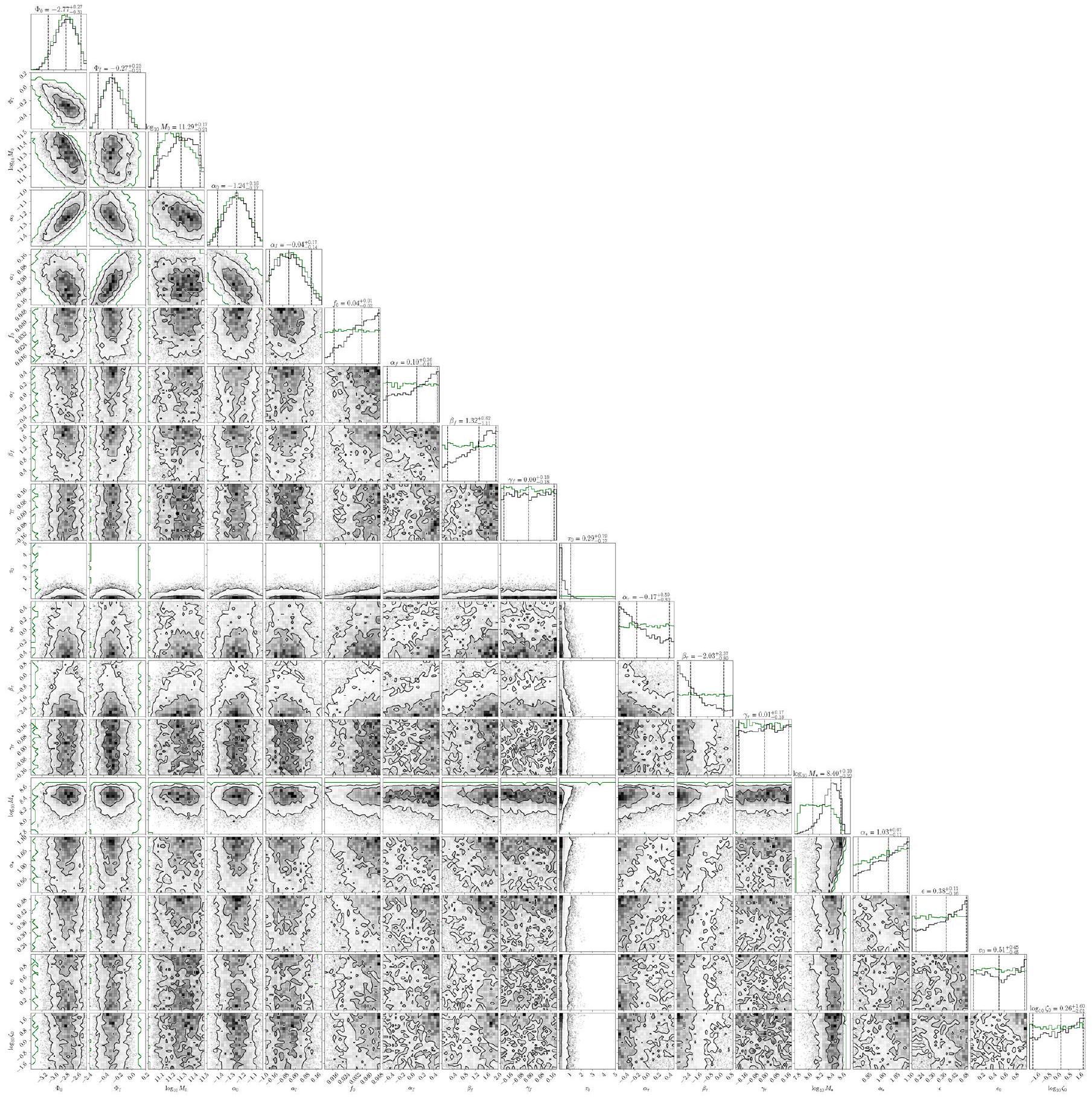
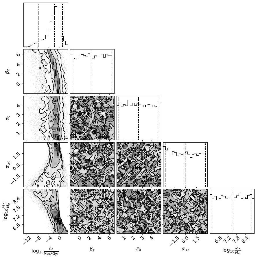
الملحق أ: ثنائيات الثقوب السوداء فائقة الكتلة – مخططات الزاوية الكاملة

تظهر الأشكال A.1 و A.2 النتائج الكاملة للنتائج الخلفية المستندة إلى علم الفلك ونموذج اللامبالاة، على التوالي. يتم إدراج المعلمات الفردية في النص الرئيسي.
الشكل A.1. التوزيعات الخلفية الهامشية لجميع 18 معلمة من نموذج علم الفلك المستند. يتم عرض الخلفية السابقة واللاحقة باللون الرمادي والأخضر، على التوالي.
الشكل A.2. الخلفيات الهامشية لجميع المعلمات الخمس لنموذج SMBHB اللامبالي.

  1. يمكن للقراء الرجوع إلى تعاون EPTA وتعاون InPTA (2023ب) لمزيد من التفاصيل حول الارتباطات بين النبضات.
  2. في مجتمع توقيت النبضات، من المعتاد الإشارة إلى قياس التشتت بالاختصار DM. يرجى ملاحظة أنه في هذه الورقة، ستقف DM حصريًا على المادة المظلمة.
  3. 3 يتم تنفيذ ذلك وفقًا لنظام بسيط حيث يتم إخماد التراكم على الثقب الأسود الأولي حتى تصبح الثنائي متساوي الكتلة. إذا/عندما يحدث ذلك، يتم توزيع المزيد من التراكم بالتساوي بين مكوني الثنائي (الآن متساوي الكتلة).
  4. 4 يأتي معظم الإشارة من SMBHBs المستضافة في مجرات ضخمة ذات انزياح أحمر منخفض (لكن انظر سيمون 2023)، والتي تكون فقيرة نسبيًا في الغاز.
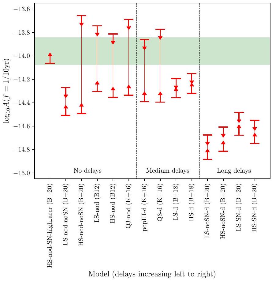
  5. 5 بالنسبة للثنائيات التي تبدأ بـ , تبقى الانحرافات أقل بكثير من 0.1 خلال تطور صلابة النجوم، ويمكن تقريب إشارات GW على أنها أحادية الطيف.
  6. النماذج “LS-nod-noSN (B+20)”، “HS-nod-noSN (B+20)” و”HS-nod-SN-high-accr ( )” لم يتم تقديمها في ، ولكن تم إنتاجها باستخدام نموذج تلك الورقة، مع تعيين التأخيرات بين اندماجات المجرات و MBH إلى الصفر (باستثناء زمن الاحتكاك الديناميكي – بما في ذلك التأثيرات المدية – بين هالات المادة المظلمة).
  7. ومع ذلك، لاحظ أنه وفقًا لسيسانا وآخرون (2008)، ومختلف عن RSG15، نقوم بمتوسط ​​الموقع السماوي وزاوية الثنائي.
  8. 8 هذه التقديرات محافظة لأنها تأخذ في الاعتبار فقط المرحلة المتدهورة من الاضطراب. تجد المحاكاة العددية قيمًا أكبر عند تضمين مرحلة إنتاج الاضطراب (روبر بول وآخرون 2020ب، 2022ب؛ كاهنيشفيلي وآخرون 2021).
  9. نقوم بتعيين درجة الحرارة بشكل محافظ في عصر الإنتاج إلى 17.35 كلفن.

Journal: Astronomy and Astrophysics, Volume: 685
DOI: https://doi.org/10.1051/0004-6361/202347433
Publication Date: 2024-01-25

The second data release from the European Pulsar Timing Array

IV. Implications for massive black holes, dark matter, and the early Universe

EPTA Collaboration and InPTA Collaboration: J. Antoniadis (I ó ³© S. Arumugam (ㅇ) , S. Babak (ㅏ) , M. Bagchi () , A.-S. Bak Nielsen (ㅇ) C. G. Bassa (ㄹ) , A. Bathula (ㅇ), A. Berthereau , M. Bonetti (ㅇ) E. Bortolas , P. R. Brook (ㅁ) M. Burgay (ㅇ) R. N. Caballero (ㅇ),

S. Desai (D) G. Desvignes (D) N. Dhanda-Batra , C. Dwivedi (D, M. Falxa , R. D. Ferdman , A. Franchini , J. R. Gair (D), B. Goncharov (D) A. Gopakumar (D) E. Graikou , J.-M. Grießmeier (D), A. Gualandris (D. L. Guillemot (D), Y. J. Guo , Y. Gupta (D) S. Hisano (D) H. Hu (D) F. Iraci , D. Izquierdo-Villalba (D) J. Jang (B) J. Jawor (D, G. H. Janssen (D, A. Jessner (D, B. C. Joshi (D, F. Kareem (ㅇ), R. Karuppusamy (ㄹ), E. F. Keane (ㅇ) M. J. Keith (ㅇ) D. Kharbanda (ㅇ) T. Kikunaga (ㅇ), N. Kolhe (©) M. Kramer , M. A. Krishnakumar (ㅜ) K. Lackeos (D) K. J. Lee , K. Liu , Y. Liu (D), A. G. Lyne , J. W. McKee (D) Y. Maan , R. A. Main , M. B. Mickaliger (©) I. C. Niţu (D, K. Nobleson (D), A. K. Paladi (D), A. Parthasarathy (i), B. B. P. Perera (D), D. Perrodin © , A. Petiteau (i) N. K. Porayko , A. Possenti , T. Prabu , H. Quelquejay Leclere , P. Rana (D) A. Samajdar (D) S. A. Sanidas , A. Sesana , G. Shaifullah (ㄹ) J. Singha L. Speri (D) R. Spiewak , A. Srivastava (D), B. W. Stappers , M. Surnis (•), S. C. Susarla (D), A. Susobhanan (D, K. Takahashi (D), P. Tarafdar , G. Theureau (D) C. Tiburzi , E. van der Wateren (D) A. Vecchio (D) V. Venkatraman Krishnan (D), J. P. W. Verbiest (D) J. Wang andP. Auclair (ㄹ) E. Barausse (ㄹ) C. Caprini (ㅇ) M. Crisostomi (ㄹ) F. Fastidio , T. Khizriev , H. Middleton (ㄹ), A. Neronov , K. Postnov (D, A. Roper Pol (D, D. Semikoz , C. Smarra , D. A. Steer (D, R. J. Truant , and S. Valtolina (Affiliations can be found after the references)

Received 11 July 2023 / Accepted 20 November 2023

Abstract

The European Pulsar Timing Array (EPTA) and Indian Pulsar Timing Array (InPTA) collaborations have measured a low-frequency common signal in the combination of their second and first data releases, respectively, with the correlation properties of a gravitational wave background (GWB). Such a signal may have its origin in a number of physical processes including a cosmic population of inspiralling supermassive black hole binaries (SMBHBs); inflation, phase transitions, cosmic strings, and tensor mode generation by the non-linear evolution of scalar perturbations in the early Universe; and oscillations of the Galactic potential in the presence of ultra-light dark matter (ULDM). At the current stage of emerging evidence, it is impossible to discriminate among the different origins. Therefore, for this paper, we consider each process separately, and investigated the implications of the signal under the hypothesis that it is generated by that specific process. We find that the signal is consistent with a cosmic population of inspiralling SMBHBs, and its relatively high amplitude can be used to place constraints on binary merger timescales and the SMBHhost galaxy scaling relations. If this origin is confirmed, this would be the first direct evidence that SMBHBs merge in nature, adding an important observational piece to the puzzle of structure formation and galaxy evolution. As for early Universe processes, the measurement would place tight constraints on the cosmic string tension and on the level of turbulence developed by first-order phase transitions. Other processes would require non-standard scenarios, such as a blue-tilted inflationary spectrum or an excess in the primordial spectrum of scalar perturbations at large wavenumbers. Finally, a ULDM origin of the detected signal is disfavoured, which leads to direct constraints on the abundance of ULDM in our Galaxy.

Key words. black hole physics – gravitation – gravitational waves – methods: data analysis – pulsars: general – dark matter – early Universe

1. Introduction

The recent observation of a common signal with excess power in the nanohertz frequency ranges (i.e. a common red signal, as defined in Arzoumanian et al. 2020; Goncharov et al. 2021; Chen et al. 2021) in pulsar timing array (PTA) datasets, with emerging evidence for quadrupolar correlations opens a new era in the exploration of the Universe. This important milestone has been achieved thanks to the efforts of the European Pulsar Timing Array (EPTA, Desvignes et al. 2016), the Indian PTA (InPTA, Joshi et al. 2022), the North American Nanohertz Observatory for Gravitational Waves (NANOGrav, McLaughlin 2013), the Parkes PTA (PPTA, Manchester et al. 2013), and the Chinese PTA (CPTA, Lee 2016). Although the significance of the signal does not yet reach the mark, which is generally accepted as the ‘golden rule’ for a firm detection claim, the evidence reported by the different collaborations ranges between and (EPTA Collaboration & InPTA Collaboration 2023b; Agazie 2023; Reardon et al. 2023; Xu et al. 2023), strongly suggesting a genuine gravitational wave (GW) origin. Awaiting decisive confirmation within the International PTA (IPTA, Verbiest et al. 2016; Perera et al. 2019) framework, with the additional contribution of the MeerKAT PTA (Miles et al. 2023), we are hearing, for the first time, the faint murmur of the GW Universe at frequencies of 1-to-30 nano-Hz, which is ten orders of magnitude lower than the frequencies currently probed by ground-based interferometers (Abbott et al. 2016). This opens a completely new window onto the Universe, allowing us to look at different phenomena, probe new astrophysical and cosmological sources, and, potentially, new physics as well.
By monitoring an array of millisecond pulsars (MSPs) for decades with a weekly cadence, PTAs are sensitive to GWs in the range (Foster & Backer 1990). At those frequencies, the most anticipated signal to be detected is a stochastic GW background (GWB) produced by the incoherent superposition of waves emitted by adiabatically inspiralling supermassive black hole binaries (SMBHBs, Rajagopal & Romani 1995; Jaffe & Backer 2003). The signal manifests as a stochastic Gaussian process characterised by a power-law Fourier spectrum of delays-advances to pulse arrival times, with characteristic inter-pulsar correlations of general relativity identified by Hellings & Downs (1983). The statistical properties of the signal are expected to significantly deviate from the typical isotropy, Gaussianity and perhaps even stationarity that is typical of many stochastic signals from the early Universe (e.g. Sesana et al. 2008; Ravi et al. 2012). In fact, due the shape of the SMBHB mass function and their redshift distribution, the overall signal is often dominated by a few sources, and particularly massive, nearby SMBHBs might result in loud enough signals to be individually resolved as continuous GWs (CGWs, Sesana et al. 2009; Babak & Sesana 2012; Kelley et al. 2018) emerging from the GWB. The exact amplitude and spectral shape of the spectrum are intimately related to the cosmological galaxy merger rate and to the dynamical properties of the emitting binaries forming in the aftermath of the merger process (Enoki & Nagashima 2007; Kocsis & Sesana 2011; Sesana 2013a,b; Ravi et al. 2014). Therefore, the demonstration of an SMBHB origin of the signal observed by PTAs provides invaluable insights into the formation, evolution, and dynamics of these objects. Moreover, it brings decisive evidence that SMBHBs merge in nature, thus overcoming the ‘final parsec problem’
(Milosavljević & Merritt 2003), which is still an open question in our understanding of galaxy and structure formation.
Beyond SMBHBs, a number of processes (potentially) occurring in the early Universe can also produce a stochastic GWB at nanohertz frequencies. Tensor modes can be produced as early as during the first tiny fraction of a second after the Big Bang through quantum fluctuations of the gravitational field stretched by the accelerated expansion of inflation (Grishchuk 1975; Rubakov et al. 1982; Starobinskii 1985; Fabbri & Pollock 1983; Abbott & Wise 1984). In the literature, these GWs are referred to as ‘primordial’. In this case, the shape of the power spectrum is defined by the specific model of inflation. Classical tensor mode production invoking the presence of a source term in the GW equation of motion can also take place in the early Universe. There are a plethora of physical processes that can lead to such a source term, and trigger the production of GWs. Topological defects, for example decaying cosmic string loops (Vilenkin & Shellard 2000; Damour & Vilenkin 2001, 2005; Jones et al. 2003; Dvali & Vilenkin 2004), particle production during inflation (Sorbo 2011a; Barnaby et al. 2012; Cook & Sorbo 2013a; Anber & Sorbo 2012), (magneto-) hydrodynamic turbulence ((M)HD, Kamionkowski et al. 1994; Kosowsky et al. 2002; Dolgov et al. 2002; Caprini & Durrer 2006; Gogoberidze et al. 2007; Caprini et al. 2009), the collision of bubble walls during a first-order primordial phase transition (Kosowsky et al. 1992; Kosowsky & Turner 1993; Caprini et al. 2008; Huber & Konstandin 2008; Jinno & Takimoto 2017; Cutting et al. 2018), sound waves in the aftermath of a first-order phase transition (Hindmarsh et al. 2014, 2015, 2017), as well as scalar perturbations at second order in cosmological perturbation theory (Baumann et al. 2007; Ananda et al. 2007), are among the most commonly considered scenarios. GWs decouple from the rest of the matter and radiation immediately after their generation at essentially any temperature in the Universe, so that in the case of clear observational evidence for these types of signals, we can infer nearly unaltered information on the physical processes occurring during or just after the birth of the Universe (Caprini & Figueroa 2018).
Contrary to the incoherent superposition of GWs from SMBHBs, the stochastic GWB from sources in the early Universe is usually assumed to be statistically homogeneous and isotropic, unpolarised, and Gaussian (Allen 1996; Maggiore 2000; Caprini & Figueroa 2018). Statistical homogeneity and isotropy are inherited from the same property of the FLRW Universe. The absence of polarisation holds provided no macroscopic source of parity violation is present in the Universe. Gaussianity follows by the central limit theorem in most cases of GWBs generated by processes operating independently in many uncorrelated, sub-horizon regions. This also applies to the irreducible GWB generated during inflation in the simplest scenarios, when the tensor metric perturbation can be quantised as a free field, and hence with Gaussian probability distribution for the amplitude. There are, however, notable exceptions, among which for example rare GWB bursts from cosmic strings cusps and kinks (Damour & Vilenkin 2000, 2001), or the GWB from particle production during inflation (Cook & Sorbo 2013b; Sorbo 2011b; Anber & Sorbo 2012). Therefore, although statistical properties might be useful for discriminating between SMBHBs and several processes in the early Universe, a full assessment of the nature of the GW signal will not be trivial.
Spatially correlated delays of the time of arrivals (TOAs) in an array of MSPs are not a unique imprint of GWs. For example, it is well known (e.g. Tiburzi et al. 2016) that such delays can emerge due to the imperfect fitting of the solar
system ephemerides (dipolar correlated noise), or due to a miscalibration of the time standard to which the measured TOAs are referred (monopolar correlated noise). Furthermore, individual Fourier harmonics of a common signal in PTA data may include contributions from the oscillations of the gravitational potential associated with the presence of ultralight dark matter (ULDM, Smarra et al. 2023) , also known as fuzzy dark matter (FDM), in the Galactic halo (Khmelnitsky & Rubakov 2014). The existence of ultralight scalars, generally motivated by stringtheoretical frameworks (Green et al. 1988; Svrcek & Witten 2006; Arvanitaki et al. 2010), is also particularly appealing from the astrophysical and cosmological point of view. In fact, several potential issues in the small-scale structure of the Universe, such as the cusp vs core (Flores & Primack 1994; Moore 1994; Karukes et al. 2015) or the missing satellite (Klypin et al. 1999; Moore et al. 1999) problems, could be disposed of or, at least, mitigated assuming that dark matter is made of ultralight particles. As predicated by Khmelnitsky & Rubakov (2014), the presence of ULDM induces harmonic delays in the arrival times, with a frequency proportional to the ultralight boson mass.
In this paper, we provide a broad overview of the implications of the signal observed in the second data release of the EPTA+InPTA (EPTA Collaboration 2023) for the different physical processes mentioned above. More in-depth analysis of several of these scenarios will be the subject of separate future publications. Unless otherwise stated, we consider each process separately, and we discuss the implications of the detected signal under the hypothesis that it is generated by that specific process. We do not attempt any Bayesian model selection on the signal origin, although a general framework for that is being developed (Moore & Vecchio 2021). The main reason for this choice is that, at this stage of data taking and analysis, the information carried by the signal is not particularly constraining; the evidence of the measurement is still at , and the amplitude and spectral shape of the signal are not very well measured. With these premises, the result of any model selection is bound to be severely influenced by the priors employed for each of the models under examination. This exercise becomes more meaningful as data get more informative, which we strive to achieve with the analysis of the third release of the combined IPTA data, which is now being assembled.
The paper is organised as follows. In Sect. 2, we describe the signal observed by EPTA+InPTA and its main features, including its free spectrum and best-fit parameters. We then proceed with detailing the main implications of the detected signals under the assumption that it is generated by a cosmic population of SMBHBs (Sect. 3) or by a number of processes occurring in the early Universe (Sect. 4). In Sect. 5, we investigate the compatibility of the observed signal with a DM origin and place constraints on ULDM candidates. Finally, in Sect. 6, we summarise our main results and discuss future prospects.

2. The observed signal in the EPTA DR2 dataset

Our investigation is based on the results reported in EPTA Collaboration & InPTA Collaboration (2023b, hereinafter Paper III), which analyses the data of 25 MSPs collected by the EPTA using five of the largest radio telescopes in Europe: the Lovell telescope at the Jodrell Bank Observatory, the Nançay decimetric radio telescope, the Westerbork synthesis radio tele-
scope, the Effelsberg 100 m radio telescope, and the Sardinia radio telescope. The dataset also includes the Large European Array for Pulsars (LEAP) data, in which individual telescope observations are coherently phased to form an equivalent dish with a diameter of up to 194 m (Bassa et al. 2016). These data are complemented by low-frequency observations of a subset of 10 MSPs performed by the InPTA using the upgraded Giant Metrewave Radio Telescope (uGMRT) and covering about 3.5 years.
The data of each individual pulsar are combined as described in EPTA Collaboration (2023) and the noise properties of each pulsar are then extracted according to the optimised custom noise models presented in EPTA Collaboration & InPTA Collaboration (2023a). The final result is a dataset of unprecedented sensitivity spanning up to 24.7 years. Four versions of the dataset were analyzed:
  1. DR2full. 24.7 years of data taken by the EPTA;
  2. DR2new. 10.3 years of data collected by the EPTA using newgeneration wide-band backends;
  3. DR2full+. The same as DR2full, but with the addition of InPTA data;
  4. DR2new+. The same as DR2new, but with the addition of InPTA data.
    The analysis presented in this paper refers to the DR2new dataset only. We do not consider DR2full and DR2full+ because evidence of quadrupolar correlation (usually referred to as HD correlation, from Hellings & Downs 1983) of the common process is weaker in those datasets, potentially due to the lower quality of early data that were collected with narrowband backends (see discussion in Paper III). On the other hand, although the analysis of DR2new+ produced results in broad agreement with DR2new, that dataset was assembled relatively recently and has not been analysed as thoroughly. For example, the binned freespectra that we will use in some of the following analyses have only been produced after this work was completed.
Before proceeding with the description of the signal detected in DR2new, here we summarise some notations used in PTA analysis for the benefit of the reader. The perturbation affecting the TOAs, whether produced by GWs or DM, is described in terms of its dimensionless strain . A broad-band stochastic perturbation is defined by its characteristic dimensionless strain , often modelled as a power law
.
For example, a population of GW-driven circular SMBHBs produces a spectrum with and amplitude , assuming is connected to the differential energy content of the signal per logarithmic frequency through the equation:
,
where is today’s Hubble expansion parameter. We note that and provide equivalent parametrizations of the spectrum. The former is more popular in the astrophysics domain, whereas the latter is the preferred choice for early Universe and cosmology.
Given , the one-sided power spectral density induced by the GW signal in the timing residuals is given by (Lentati et al. 2015):
,
Fig. 1. Properties of the common correlated signal detected in DR2new. Left panel: free spectrum of the RMS induced by the excess correlated signal in each frequency resolution bin (with width defined by the inverse of the data span, ). The straight line is the best power-law fit to the data. Right panel: joint posterior distribution in the plane. Note that we normalise to a pivotal frequency .
where . PTAs search for HD correlated time delays with such a power spectrum in the data, and measure the parameters and . For an observation timespan , measurements are discretised in frequency bins , where . It is then customary to convert in RMS residual induced in the TOAs in each frequency bin:
The main properties of the GWB signal observed in DR2new and examined in this paper are shown in Fig. 1. The length of the dataset is years, and excess common correlated power is detected in several frequency bins up to (Fig. 1 left panel). Conversely, some bins are unconstrained, which results in a relatively loose determination of the spectral properties of the observed signal. In the literature, and in Eqs. (1) and (3) are usually anchored to the pivotal frequency . The data are, however, most informative at the lowest frequencies, while the common power at is essentially unconstrained. This naturally leads to a strong degeneracy of the posterior, as shown for example in Fig. 1 of Paper III. Therefore, unless otherwise stated, we change the reference frequency to , where the data are actually constraining, which results in a weaker dependence of upon , as shown in the right panel of Fig. 1.
In the following three sections, we discuss three possible contributions to the signal, probing completely different epochs and scales of our Universe, and the implications for the associated physical processes. Namely, the cosmic population of SMBHBs (at redshifts ), the early Universe ( ), and DM (within our Galaxy).

3. Implications I: supermassive black hole binaries

A cosmic population of SMBHBs is the primary astrophysical candidate to produce a signal in the nanohertz band detectable by PTAs. If we define as the cosmic merger rate of SMBHBs as a function of redshift, primary black hole
mass, mass ratio, and eccentricity, the general form of the generated GWB as a function of observed frequency can be written as (Sesana 2013a)
Here, is the time spent by the shrinking binary within a given logarithmic orbital frequency bin, which converts the merger rate into the distribution of rest-frame orbital frequencies of the emitting population. This quantity depends on the physical processes driving the evolution of the SMBHBs including, besides GW emission, interaction with the stellar and gaseous environment surrounding them. As such, it is generally a function of the binary parameters , and extra parameters describing the environment, such as the stellar density in the nucleus of the galaxy host (for more details, see Sesana 2013a). The second line of Eq. (5) is the strain amplitude produced by each individual eccentric SMBHB binary, cast as the sum of harmonics fulfilling the condition . In that expression, is the strain of the equivalent circular binary emitted at twice the orbital frequency of the system, as given in Eqs. (4)(7) of Rosado et al. (2015), and is a combination of Bessel functions (see, e.g. Bonetti & Sesana 2020, for details). For a distribution of circular, GW-driven binaries, the only relevant mass parameter is the chirp mass , and Eq. (5) takes the familiar form (Sesana et al. 2008)
This can be recast in terms of the comoving number density of merging binaries (Phinney 2001)
which highlights that, in this case, the expected spectrum follows a power law , and the only free parameter is its overall
Fig. 2. GWB amplitude distributions predicted by the RSG15 models. The thin-dashed yellow line is for the full set of models in RSG15, whereas the thick-dashed orange line is for the subset considered here. The solid blue line is the distribution predicted by the 108 downselected sample used in the analysis. The vertical line marks the median value of at reported in Paper III when fixing in the search. Note that the lower -axis scale is for A at , whereas the upper -axis is for A at (the normalization used in this paper). Since for circular GW-driven binaries, there is a shift of 0.666 dex between the two.
amplitude. The latter is set by the function , which contains all the astrophysical knowledge of the cosmic population of merging SMBHBs, and is determined by the cosmological hierarchical assembly of galaxies and their central SMBHs. Conversely, in the most general case described by Eq. (5) there is also information in the spectral shape of the signal, since coupling with the environment as well as eccentricity affect the function , suppressing signal at the lowest frequencies. Moreover, eccentricity distributes the GW power at several higher harmonics of the orbital frequency, slightly modifying the power-law behaviour at high frequencies. In general, the GWB cannot be cast in term of a simple analytical form, although a broken power-law is a sufficient approximation for most situations (see, e.g. Ravi et al. 2014; Sesana 2015; Kelley et al. 2017; Chen et al. 2017b).
The literature investigating the GWB produced by a population of SMBHBs is vast, dating back to the mid-nineties and early 2000s (Rajagopal & Romani 1995; Jaffe & Backer 2003; Wyithe & Loeb 2003; Sesana et al. 2004), and predictions have been made by employing different models and techniques. Models can be broadly classified into two categories: selfconsistent theoretical models for SMBH evolution within their galaxies (Sesana et al. 2008, 2009; Ravi et al. 2012; Kulier et al. 2015; Kelley et al. 2017; Bonetti et al. 2018; Siwek et al. 2020; Izquierdo-Villalba et al. 2022), and empirical models based on observed properties of galaxy pairs coupled to SMBH-host galaxy relations (Sesana 2013b; Rosado et al. 2015; Ravi et al. 2015; Simon 2023), or on the evolution of the SMBH mass function inferred from observations (McWilliams et al. 2014). Note that we group both semianalytic models (SAMs) and large cosmological simulations in the first class. The main difference between these two classes is that self-consistent models are constructed to reproduce a large array of observations related to galaxies and the SMBH they host, such as the redshift-dependent galaxy mass function, quasar luminosity function, and so on.
Conversely, empirical models are, by construction, consistent with the observations upon which they are based, but are usually not tested against independent constraints. As a consequence, they can generally produce a wider distribution of GWB amplitudes, but consistency with other observations is not necessarily guaranteed.
In this section, we investigate the implications of the signal observed in the DR2new dataset for representative models of the two classes. In Sect. 3.1, we perform a semi-quantitative comparison between the measured signal and predictions of an extended version of the Rosado et al. (2015) models (hereinafter RSG15) including binary eccentricity and environmental coupling. In Sect. 3.2, we exploit the framework developed in Middleton et al. (2016), Chen et al. (2017a, 2019) to draw inference on SMBHB astrophysics from the data, either by assuming astrophysical priors from independent observations, or by using a completely generic model for the SMBHB mass function with minimal assumptions. In Sect. 3.3, we demonstrate how the measured signal can inform galaxy and SMBH formation models by examining its constraining power on two state-of-theart SAMs, namely L-galaxies (Henriques et al. 2015) and the model developed by Barausse and collaborators (Barausse 2012; Bonetti et al. 2018; Barausse et al. 2020). We discuss caveats and future directions of improvement in Sect. 3.4.

3.1. Qualitative analysis of empirical SMBHB population models

To carry out a semi-quantitative comparison between observations and empirical models, we use an extended set of SMBHB populations based on the work of Sesana (2013b; S13 hereinafter) and RSG15.

3.1.1. Description of the models

As described in S 13 , the models are constructed around the number density of merging SMBHs per unit primary mass, mass ratio, and redshift, obtained by combining different observations of the galaxy mass function and pair fraction, estimated galaxy pair merger timescales, SMBH-host galaxy relations, and prescription for SMBH accretion during mergers (see Sect. 2 of S13 for full details). Given the large uncertainties in all of the ingredients, the models predict a broad distribution of expected GW amplitudes, as shown in Fig. 2.
Guided by the relatively large amplitude of the detected signal and by theoretical and observational advancements in the last decade, we select a sub-sample of those models, as we now justify. First, hydrodynamical simulations of merging galaxies at different scales as well as deep X-ray observations of merging galaxies support accretion activation onto the individual SMBHs prior to merger (e.g. Capelo et al. 2017; Koss et al. 2018). Moreover, hydrodynamical simulations of sub-pc scale binaries, have found most of the accretion to occur on the secondary (i.e. less massive) SMBH (Farris et al. 2014). We therefore restrict the analysis to models where SMBHs accrete prior to the merger, either with an equal Eddington ratio or with preferential accretion onto the secondary . Second, observations of overmassive black holes in the centre of large ellipticals (McConnell et al. 2011) has led to an upward revision
of the SMBH-galaxy relations. Contrary to S13 and RSG15, here we consider only those revised realations, namely the ones reported by Kormendy & Ho (2013), McConnell & Ma (2013), Graham & Scott (2013). Finally, given the large number of models, to save computing power, we perform an ad hoc downselection of 108 models that preserves the overall distribution of the expected GWB amplitudes, as shown in Fig. 2.
As opposed to RSG15, we go beyond the circular-GW driven binary approximation and consider the self-consistent evolution of SMBHBs within their stellar environment . This is done by employing the hardening models of Sesana (2010) that selfconsistently evolve the SMBHB semimajor axis and eccentricity under the combined effect of stellar hardening and GW emission, once a given initial eccentricity at binary formation is given. Those evolutionary tracks allow us to evaluate the term in Eq. (5), and thus to reconstruct from the density distribution of merging binaries, , the numerical distribution of systems emitting at any time in the whole sky as a function of mass, mass ratio, redshift, orbital frequency and eccentricity, . For each model, we consider 10 values of and three different normalizations of the stellar density profile, described as , with (details in Sesana 2010).
In total, we explore models, spanning different eccentricities and densities of the stellar environment. For each model, we draw 100 Monte Carlo samplings of the distribution of the emitting binaries, we discretise the frequency domain in bins of , and add the signals of binaries falling in the same bin in quadrature. This leads to the binned characteristic strain spectrum that we then convert in and RMS residuals using Eqs. (3) and (4). The full procedure is described in Amaro-Seoane et al. (2010), Bonetti & Sesana (2020). In this way, we generate a grand total of 324 k Monte Carlo realizations of the predicted GW spectrum in the PTA band.

3.1.2. Comparison with the observed signal

The binned spectrum shown in Fig. 3 contrasts expectations from the 324 k models (green) to the measured correlated signal in DR2new (orange). The two sets of violin plots are in good agreement in the few lowest frequency bins, where measurements are the most constraining. Note that the model prediction distributions are highly non-Gaussian and asymmetric, with long tails extending upwards. This is due to the fact that sparse very massive/nearby binaries can sometimes produce exceptionally loud signals, as illustrated by the 100 individual GWBs overplotted to the violins. In fact, this might explain the extra power measured in the 4th and, most strikingly, in the 9th lowest bins compared to the bulk of the model predictions. We caution that the 9th bin is close to the mark, where PTAs are blind due to fitting for the Earth orbital motion, and leakage from imperfect fitting might affect that measurement. In any case, if this extra power is indeed due to GWs, it can be easily accommodated by theoretical models, as demonstrated by the realization highlighted by the tick grey line.
Our Monte Carlo approach to generate the SMBHB population and its associated GW signal also allows us to investigate the occurrence of CGWs in the data, for which evidence in DR2new is found to be inconclusive (EPTA Collaboration & InPTA Collaboration 2023c). Since the search performed in that paper was limited to circular bina-
Fig. 3. Free spectrum violin plot comparing measured (orange) and expected (green) signals. Overlaid to the violins are the 100 Monte Carlo realizations of one specific model; among those, the thick one represents an example of a SMBHB signal consistent with the excess power measured in the data at all frequencies.
ries, we only carry out this analysis for the 32.4 k models with . A full assessment of the detectability of CGWs requires the evaluation of the detection probability of each individual binary for a given false alarm rate, as detailed in RSG15. For the sake of simplicity, and given the qualitative nature of this analysis, we just compute the signal-to-noise ratio (S/N) of each individual binary according to Eq. (46) of RSG15 (thus also restricting to the Earth term only). When computing the S/N of a source, we model each pulsar noise by using the maximum likelihood values of the single pulsar noise analysis presented in EPTA Collaboration & InPTA Collaboration (2023a), and add the GWB produced by all of the other binaries to the noise spectral density. We arbitrarily set the detectability threshold at in the following.
Results are shown in Fig. 4, which compares the power distribution of resolvable CGWs to the binned spectra of the overall predicted GW signal and of the DR2new measurements. In line with RSG15, the probability of detecting a CGW is maximum at the lowest frequency, rapidly decaying to less than 0.01 past the 6th bin. Although this seems to suggests that the feature observed at the 9th frequency bin is unlikely to be due to a CGW, it should be noticed that we considered here a threshold of . The overall GW signal in our data has a total 3.5-4 (EPTA Collaboration & InPTA Collaboration 2023b), mostly accumulated at the lowest frequency bins. It might still be the case that the feature at the 9 th bin is due to an unresolved CGW with , which would be a more common occurrence in the data. Note that the average of CGWs slightly increases at higher frequencies, which is primarily due to the frequency dependence of the CGW characteristic strain, . If is the probability of having a CGW of in the th bin, we can compute the probability of detecting at least one CGW with in DR2new according to these models as , which gives . It is therefore quite possible that the
Fig. 4. Expected properties of CGWs as a function of frequency. Top panel: free spectrum violin plot comparing the measured signal (orange) to the power distribution of CGWs (green). Empty violins show the full GWB produced by the models for comparison. Bottom panel: the probability of detecting a CGW with as a function of frequency (green circles, left -axis scale). The average S/N of CGWs is also shown as red crosses (right -axis scale).
observed signal is dominated by few bright sources, which might be resolvable in the future with more sensitive datasets. Thus far, searches for CGWs on the current dataset yielded inconclusive evidence (EPTA Collaboration & InPTA Collaboration 2023c). This probability is obviously threshold dependent. For example, by increasing this threshold to , we get 0.13. This is comparable to the chance found by Bécsy et al. (2022). and the slightly larger probability in our models is likely due to the louder overall amplitudes of the signals considered here. We stress, however, that these findings apply to models where binaries remain essentially circular. The number of resolvable CGWs, tends, in fact, to slightly decrease when the eccentricity increases (Truant et al. in prep.).
Finally, we once again propose the comparison first shown by Middleton et al. (2021), who contrasted the measured 2D posterior to model expectations. For the latter, we just fit the 9 lowest frequency bins of the GWB spectrum of each Monte Carlo realization of the Universe with a straight line in the plane. As described in Sect. 2, we normalise the measurement to , where our data are informative, which alleviates the degeneracy in the posterior. Results are shown in Fig. 5. Although the measured spectrum tends to be shallower than the theoretical one (see also Sect. 3.4), the contours overlap at and the marginalised amplitudes are broadly consistent.

3.2. Inference on the SMBHB population.

After checking the general compatibility of the observed signal with expectations from empirical SMBHB population models, we take a more quantitative approach and exploit Bayesian inference to constrain the properties of SMBHBs from the data. We repeat the analysis carried out by Middleton et al. (2021) on the common signal detected in the NANOGrav 12.5 year dataset (Arzoumanian et al. 2020), exploiting the framework laid out in
Powerlaw fitted to 9 bins
Fig. 5. distribution of the measured signal (orange) compared to model predictions (green). and contours are displayed. Shown are also the marginalised (left) and (right) distributions, with their credible intervals highlighted as shaded areas.
Middleton et al. (2016), Chen et al. (2017a, 2019). The SMBHB population of a given model is described by a set of parameters , we then use Bayesian inference to find the posterior distribution for the parameters of model given the observation data :
Here, is the prior distribution on the model parameters, is the likelihood of model with parameters of producing the data, and is the evidence. For each set of , the likelihood is computed by comparing the signal amplitude produced by at frequencies , to the posterior distribution of the correlated signal measured in DR2new at the same frequencies. We treat each bin as independent, therefore the likelihood takes the form
where is the probability density of the amplitude of the correlated signal measured in the th bin, and it is evaluated at the value predicted by the model. We estimate the likelihood in each bin using a KDE estimate of the DR2new posteriors, similar to the method used in Moore & Vecchio (2021).
Note that the models we use are deterministic in the sense that they have a correspondence between and the predicted . In reality, given , the ensemble of SMBHBs generating the signal is statistically drawn from the deterministic distribution function, which results in a significant scatter of , as demonstrated by the individual spectra shown in Fig. 3. We caution that this variance is not captured by these models, and its inclusion in the Bayesian inference pipeline is the subject of ongoing work.
As in Middleton et al. (2021), we use two models to describe the SMBHB population, which are described in turn below.

3.2.1. Agnostic SMBHB population model

The agnostic model, developed in Middleton et al. (2016), makes minimal assumptions about the underlying population of SMBHBs. Binaries are assumed to be circular, GW-driven and the characteristic strain is computed according to Eq. (7) where the source distribution is described by a Schechter function (Schechter 1976) in and ,
where is the time in the source frame and we assume cosmological parameters from Planck18 (Planck Collaboration VI 2020). The five model parameters are , where is the merger rate per unit rest-frame time, co-moving volume, and logarithmic interval, and the parameter pairs and control the shape of the and distributions, respectively. The integration limits in and are and , respectively. The prior ranges of the five model parameters are identical to those used in Middleton et al. (2021).

3.2.2. Astrophysically-informed SMBHB population model

The astrophysically-informed model was developed in Chen et al. (2019). This model captures the interaction between the SMBHBs and their environment and allows for eccentric orbits, both of which lead to a characteristic amplitude that does not follow a simple single power law, as in Eq. (5). The model has 18 parameters, 16 of which describe astrophysical observables linking the number of SMBHB mergers to the number of galaxy mergers. The galaxy stellar mass function is modelled as a redshift-dependent Schechter function defined by five parameters: . Both the galaxy pair fraction and merger timescales have power law dependencies on the primary galaxy stellar mass , mass ratio and redshift function ( ) and each of them is defined by a set of four parameters: for the pair fraction, and for the merger timescale:
Galaxy pairs are then populated with SMBHs of mass following a standard black hole to stellar bulge mass relation of the form
where is a log normal distribution with mean value and standard deviation , which adds three further parameters, , to the model. The final two parameters describe the eccentricity at SMBHB pairing and the density of the stellar environment . For the 18 parameters listed above, in the analysis presented here, we use the extended prior intervals listed in Table I of Chen et al. (2019).
Fig. 6. Marginalised posterior distributions for using two SMBHB population models. The orange and green open histograms show marginalised posteriors for the agnostic and astrophysically-informed models, respectively. The filled-green histogram shows the prior for the astrophysically-informed model (the prior for the agnostic model is uniform in the range [-20,3]). The vertical dotted lines show the 5th and 95th percentiles of the posteriors.
Fig. 7. Posterior distribution of the chirp mass function of merging SMBHBs for both the agnostic (orange) and astrophysically informed (green) models. For both models, shaded areas are the central 50% and credible regions and the dashed lines show the medias. The blackdotted lines show the central region for the astrophysical prior.

3.2.3. Results of the inference

The main results of the inference are shown in Figs. 6-8. Figure 6 shows the marginalised posterior distribution for the normalization of the merger rate density from the agnostic model compared to an equivalent parameter derived from the astrophysically-informed model. The constraint on the amplitude of the signal imposes an informative constraint on the normalization of the SMBHB merger density. Using nine frequency bins, the median and central credible regions for are and for the agnostic and astrophysically-informed models, respectively. The measurement essentially constrains the amplitude of the signal, which imposes an informative constraint on . The astrophysically-informed model clearly shows that the signal favours an at the upper edge of the astrophysical prior. All
Fig. 8. Posterior distribution of selected parameters for the astrophysically-informed model using nine frequency bins of the free spectrum for the inference. Parameters are described in Sect. 3.2.2.
other parameters of the agnostic model are unconstrained and the posterior is very similar to the prior (see Appendix A for full posterior distributions for both models).
Figure 7 displays the posterior on the SMBHB chirp mass function for the two models integrated over the redshift range . Although the agnostic model results in a loosely constrained mass function, the measured PTA signal alone places interesting lower limits on the SMBHB binary merger rate in the Universe. For example, we can say at confidence that for each comoving , there have been at least SMBHB mergers with since cosmic noon. When astrophysical priors weights in, the mass function of merging SMBHBs is well constrained by the PTA signal and, as expected from
Fig. 6, it lies in the upper range of the astrophysically informed prior. Within this model, the DR2new measured signal implies there have been about SMBHB mergers for each comoving , with since . This points towards a very active merger history of massive galaxies and a very efficient dynamical evolution of the SMBHBs forming in the merger process.
For the astrophysically informed model, DR2new also provides interesting information on several model parameters. This is because the astrophysical prior considerably narrows down the range of signal amplitudes allowed by the model, and the measured signal pushes towards the upper bound of this range. This results in informative constraints on several key parameters,
related in particular to the SMBHB merger timescale and the SMBH-bulge mass relation. As shown in Fig. 8, the SMBH merger timescale following galaxy pairing must be shorter than ( confidence), with the data mildly favouring shorter merger times for massive galaxies at low redshifts (i.e. ). Moreover, the data favour a high normalization of the SMBH-bulge mass relation , compared to a much wider prior range extending all the way down to . This is in line with the qualitative analysis of Sect. 3.1, which showed that the signal is consistent with recent, upward-revised, SMBH-galaxy relations. There is also a slight preference for a high normalization of the pair fraction with a positive dependence, . Despite the low value favoured by the data, indicative of a flatter spectrum compared to the canonical value predicted by circular GW-driven binaries, SMBHB dynamics is largely unconstrained, perhaps with a marginal preference for eccentric binaries evolving in dense environments ( and posteriors slightly rising towards the right bound of the prior).
Altogether, these results point towards efficient orbital decay of SMBHBs in the aftermath of galaxy mergers, providing direct evidence that the ‘final parsec problem’ is solved in nature and that compact sub-parsec SMBHBs must be common in the centre of massive galaxies.

3.3. Implications for SAMs

We now explore the implication of this signal for the joint modelling of the galaxy and SMBH formation and evolution by taking a close look at two state-of-the-art SAMs: the model constructed by Barausse and collaborators (Barausse 2012; Sesana et al. 2014; Antonini et al. 2015; Klein et al. 2016; Bonetti et al. 2018; Barausse et al. 2020) and L-Galaxies (Henriques et al. 2015; Izquierdo-Villalba et al. 2022). In this preliminary study, we do not model the dynamical evolution of the binaries and we assume them to be circular and GW driven, thus resulting in a characteristic strain spectrum with .

3.3.1. SAMs and SMBHB delays

In Fig. 9, we show this comparison for the model of Barausse (2012) in its original version (B12) and its subsequent evolutions, which were used to produce the results of Klein et al. (2016, K+16), Bonetti et al. (2018, B+18) and Barausse et al. (2020, B+20). Besides the specific SAM implementation and (astro)physics, these models mainly differ for the physical prescriptions describing the delays between galaxy and MBH mergers, with (i) models “LS-nod (B12)”, “HS-nod (B12)”, “Q3nod (K+16)”, “LS-nod-noSN (B+20)”, “HS-nod-noSN (B+20)” and “HS-nod-SN-high-accr (B+20)” assuming no such delays (except for the delays between the mergers of the halos and those of the corresponding baryonic components) ; (ii) models “popIII-d ( )”, “Q3-d (K+16)”, “LS-d (B+18)”, “HS-d (B+18)” additionally introducing the effect of stellar hardening, triple MBH interactions and gas-driven migration; and (iii) models “LS-noSN-d (B+20)”, “LS-SN-d (B+20)”, “HS-noSN-d (B+20)” and “HS-SN-d (B+20)” accounting for even longer delays (including large contributions from SMBHB
Fig. 9. Predictions for the GWB characteristic strain amplitude at from a range of SAMs published in the literature, assuming quasicircular orbits and no environmental interactions (i.e. ), but different physical prescriptions for the delays (increasing from left to right) between galaxy mergers and black hole mergers. The “no delays”, “medium delays” and “long delays” models correspond respectively to the classes of models (i), (ii) and (iii) defined in the text. The ranges account for the finite resolution of the models. The shaded area is the DR2new 95% confidence bound. More details about the models are provided in the text.
separations of hundreds of pc). Note that the labels “SN” (and “noSN”) refer respectively to a putative effect of SN feedback on black hole accretion (and the absence thereof), while “LS”/”popIII” and “HS”/”Q3” denote respectively light and heavy high-redshift seeds for the black hole population.
The predictions are computed by summing the gravitational energy spectra of all the SMBHBs in each model’s theoretical population, assuming quasi-circular orbits. As a result, the spectrum has a slope of and has no cosmic variance (i.e. we do not account at this stage for the scatter from one realization of the SMBHB population to another). The range shown for each model represents the uncertainty due to the correction for the finite resolution of the SAM’s merger tree. In more detail, the lower end of the range represents a model’s prediction at the finite resolution, while the upper end is the extrapolation performed as described in Fig. 4 of Klein et al. (2016) – to infinite resolution. The lower arrow (pointing up) should therefore be interpreted as a lower limit, while the upper arrow (pointing down) should be understood as an upper bound (due to the uncertainty of the extrapolation procedure). The extrapolation has not been performed for the model HS-nod-SN-high-accr (B+20), for which we report only the (more robust) prediction at finite resolution. The latter already agrees with the measured amplitude, as a result of a higher accretion rate (by a factor ) for SMBHs.
For two of the models in better qualitative agreement with the data (i.e. “HS-nod-SN-high-accr (B+20)” and “HS-nodnoSN (B+20)”), we compare the predicted signal with the measured DR2new free spectrum in Fig. 10. Unlike in the case of
Fig. 10. Binned spectrum of the predicted GWB amplitude for models “HS-nod-SN-high-accr (B+20)” and “HS-nod-noSN (B+20)”. The distribution of the predictions represents the scatter among different realizations of the SMBHB population (“cosmic variance”). Also shown are power-law fits to the predictions.
Fig. 9, these predictions were obtained for multiple specific realizations of the SMBHB population, following Sesana et al. . The probability distribution function plotted in each bin represents the scatter of these multiple realizations, and should therefore be interpreted as a “cosmic variance”. Similarly, in Fig. 11 we show the theoretical forecasts for from a subset of the models presented above (namely those in qualitative agreement with the data in Fig. 9). These forecasts are obtained by fitting the model predictions (from multiple realizations of the SMBHB population) in the first 9 frequency bins with a power law with . The error bars represent the confidence regions (accounting for the scatter due to cosmic variance), while the shaded area indicates the confidence region of the posterior for (assuming again ).
Overall, this qualitative comparison, while somewhat dependent on the details of the SAM implementation, suggests that (i) large delays arising from the dynamics of black hole pairs at large separations are disfavoured, (ii) SMBHB mergers proceed efficiently after their host galaxies have coalesced. Moreover, these results seem to suggest that (iii) accretion onto SMBHs proceeds efficiently, possibly resulting in a larger local SMBH mass function at high masses.

3.3.2. L-Galaxies

Next, we explore the implications that the EPTA results have for L-Galaxies (Henriques et al. 2015; Izquierdo-Villalba et al. 2022), a sophisticated SAM constructed on the dark matter merger trees extracted from the Millennium simulation suite (Springel et al. 2005; Boylan-Kolchin et al. 2009). On top of the galaxy physics, L-Galaxies features a comprehensive modelling for the assembly of SMBHs, including gas accretion triggered by galactic mergers and disc instabilities and dynamical evolution of SMBHBs within the galaxy merger process. The latter accounts for dynamical friction (DF), stellar and gas hard-
Fig. 11. Predictions for in various SAMs, obtained by fitting the spectrum in the first 9 frequency bins with for multiple realizations of the SMBHB population. The error bars represent the 95% confidence interval for the predictions, and account for the scatter due to cosmic variance. For each model (except for the boosted accretion model HS-nod-SN-high-accr (B+20)), the higher prediction is the extrapolation to infinite SAM resolution, while the lower one is the finite-resolution prediction. The shaded area is the confidence interval for the measurement of , fixing . For HS-nod-SN-high-accr (B+20) we only show the result uncorrected for resolution.
ening and, eventually, GW emission. All of these processes are governed by a set of parameters that are tuned to reproduce a vast array of observations including, among others, the galaxy mass function and morphological distribution, the quasar luminosity function and the SMBH-host galaxy relations.
Izquierdo-Villalba et al. (2022) found that the standard L-Galaxies tuning results in a GWB with at , lower than that measured in DR2new. Here we perform a systematic investigation of how the stochastic GWB at nanohertz frequencies depends upon the parameters governing the physics of SMBHs and SMBHBs in the SAM. To this aim, we run L-Galaxies in the following configurations:
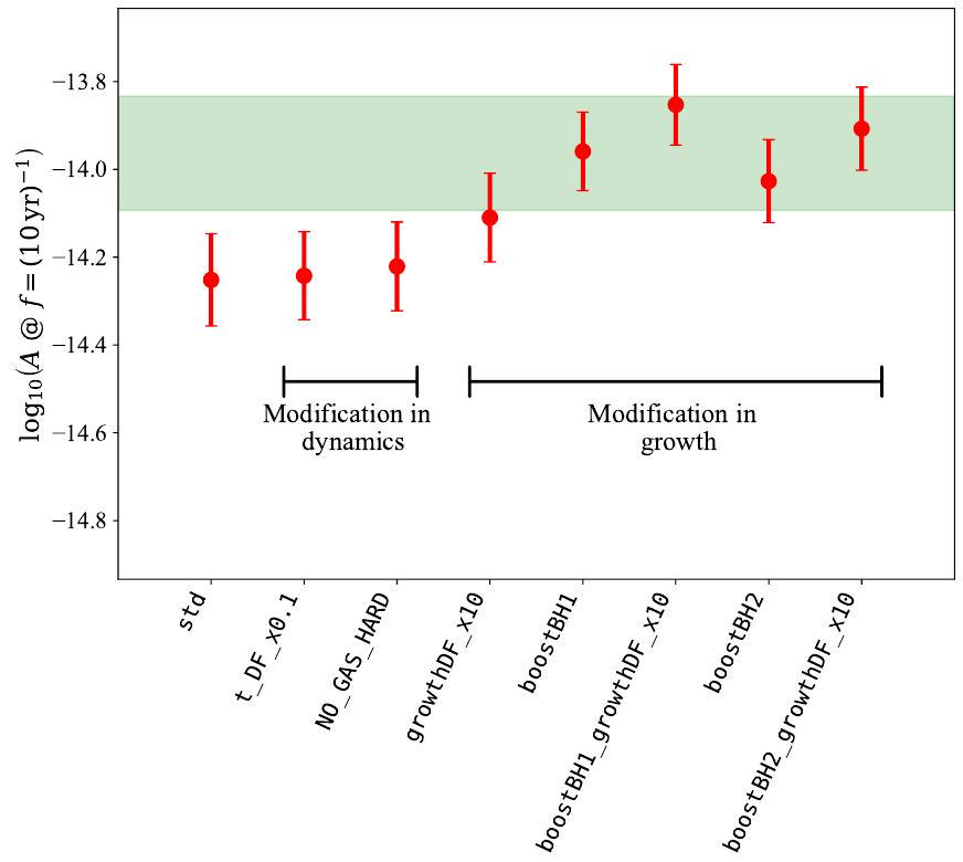
  • std: standard configuration (Izquierdo-Villalba et al. 2022);
  • t_DF_x0.1: SMBH dynamical friction (DF) time reduced by a factor of ten;
  • NO_GAS_HARD: only stellar hardening;
  • growthDF_x10: accretion boosted by ten in the DF phase;
  • boostBH1: gas accretion doubled after galaxy mergers and disc instabilities;
  • boostBH2 gas accretion doubled after galaxy mergers and tripled after disc instabilities;
  • boostBH1_growthDF_x10: adding accretion boost in the DF phase to model boostBH1;
  • boostBH2_growthDF_x10: adding accretion boost in the DF phase to model boostBH2.
    Results are shown in Fig. 12. Changes to the dynamics of SMBHs appear to have a minor effect on the amplitude of the GWB. While shortening the DF time (t_DF_x0.1) allows more SMBHBs to merge within the Hubble time, the most
Fig. 12. Predictions for the GWB characteristic strain amplitude at from a range of L-Galaxies semi-analytical model versions, assuming that . The error bars are computed taking into account the cosmic variance. To this end, we divided the Millennium box into 125 sub-boxes and we compute the GWB in each one. The standard deviation provided by the 125 GWBs corresponds to the extension of our error bars.
massive ones, which are responsible for the bulk of the GW signal, already have short DF timescales, and the overall GW signal is only mildly increased. Turning off gas hardening results in longer-lived SMBHBs that tend to merge at lower redshifts, resulting in louder GW signals. The effect is, however, negligible. Conversely, the tuning of gas accretion can significantly change the masses of the SMBHBs, resulting in a larger impact on the GWB. Model growthDF_x10 leaves the general population of SMBHs untouched, only boosting the growth of those in the dynamical friction phase. This alone increases the level of the GWB by a factor compared to model std. Finally, the models boostBH1 and boostBH2 increase the gas accretion onto the whole population of SMBHs, making the GWB a factor of 2.5 louder with respect to the baseline model. Boosting accretion onto the whole population and in the hardening phase further amplifies the expected GWB, reaching the upper bound of the measured value (models boostBH1_growthDF_x10 and boostBH2_growthDF_x10 in the figure). Although these models can accommodate the GWB signal measured in PTAs, the boosted accretion and subsequently larger SMBH masses can make it harder to reproduce the observed SMBH mass and quasar luminosity functions (Izquierdo-Villalba et al. 2022). Additionally, more work is required to find a model that can reproduce all observational constraints in the light of the PTA GW signal (Izquierdo-Villalba et al. 2024).

3.4. Further considerations on the measured spectrum: eccentricity and statistical biases.

The analyses presented so far give strong indications that the signal is compatible with a cosmic population of SMBHBs swiftly coalescing in the aftermath of galaxy mergers. The relatively flat slope of the measured spectrum might be indicative of strong
Fig. 13. Orbital parameters (distance between the SMBHs, semi-major axis and eccentricity) of a SMBHB formed in a representative -body simulation of a galactic merger with parameters drawn from progenitors of likely PTA sources in the IllustrisTNG100-1 cosmological simulation. Mergers are selected from the merger trees of the 100 most massive galaxies at , based on galaxy mass ratio (major mergers with mass ratio or higher) and redshift ( ). The dashed lines indicate the critical separation and the corresponding eccentricity at the time in the evolution marking approximately the end of the SMBH inspiral due to DF and the beginning of the hardening phase. Dots represent and computed from the apoastron-periastron separation of the two SMBHs before pairing in a bound binary.
environmental coupling and high eccentricities, although inference from the data is inconclusive in this respect (see Fig. 8).
The eccentricity of SMBHBs is of particular relevance as it might carry important information on the dynamical processes driving binary evolution at sub-pc scales (see e.g. Roedig & Sesana 2012). While gas-driven dynamics is expected to saturate the binary eccentricity at a value (Roedig et al. 2011; D’Orazio & Duffell 2021), stellar hardening is known to statistically increase eccentricity without any saturation point (Quinlan 1996), potentially leading to extremely eccentric systems (Sesana 2010). A large binary eccentricity has two important implications for the interpretation of the current data: it flattens the low-frequency spectrum and it speeds up the SMBHB merger process, as inferred by the small derived in Sect. 3.2.
Low-redshift massive galaxies are generally gas-poor, and stellar-driven hardening represents the main mechanism driving the evolution of the binaries comprising the bulk of the PTA GW signal. Modelling the whole dynamical evolution, from the first galaxy encounter to black hole pairing and final coalescence, is theoretically and numerically challenging and has been the subject of many studies (e.g. Preto et al. 2011; Khan et al. 2012, 2016; Nasim et al. 2021; Gualandris et al. 2022). In particular, the binary eccentricity is very sensitive to the initial orbits of the merging galaxies (Gualandris et al. 2022). In ongoing work (Fastidio et al. in prep), we are connecting the sub-pc dynamics of SMBHBs to the large-scale parameters of the galactic encounters extracted from the IllustrisTNG100 simulation (Pillepich et al. 2018). Preliminary results show that mergers of massive galaxies occur preferentially on nearly radial orbits, potentially resulting in highly eccentric binaries. Figure 13 shows the orbital parameters of a SMBHB formed in a highaccuracy -body simulation of a representative galactic merger with properties taken from a merger tree in IllustrisTNG100. Merger trees are selected to represent likely PTA sources at low redshifts. The galactic merger is followed from early times
Fig. 14. Posterior distributions of the recovered GWB from injections on synthetic data mimicking DR2new. Top panel: statistical offset in an ideal dataset. The square marks the injected value and the blue contours are and of the recovered posterior. Bottom panel: effect of highfrequency noise mismodeling on the recovery. The orange, blue and green contours are respectively obtained when are used for the recovery (injected ).
through the inspiral, pairing and hardening of the SMBHs via a hybrid numerical scheme able to model the evolution selfconsistently from kpc to mpc scales (Dehnen 2014). Despite the intrinsic stochasticity of the processes driving binary formation and hardening (Nasim et al. 2020), binaries tend to form with a large eccentricity, which then further grows due to encounters with background stars, as also found by scattering experiments (Sesana 2010). Although more work is needed to determine the distribution of expected binary eccentricities and current EPTA data are not yet strongly informative, this pilot study shows the potential of using these measurements in the near future to constrain the physics of galaxy and SMBH mergers.
When drawing conclusions on the physical properties of the sources of the GW signal, it is useful to bear in mind not only that the constraints on the spectrum are relatively loose (see Fig. 1), but also that the measured parameters can be subject to
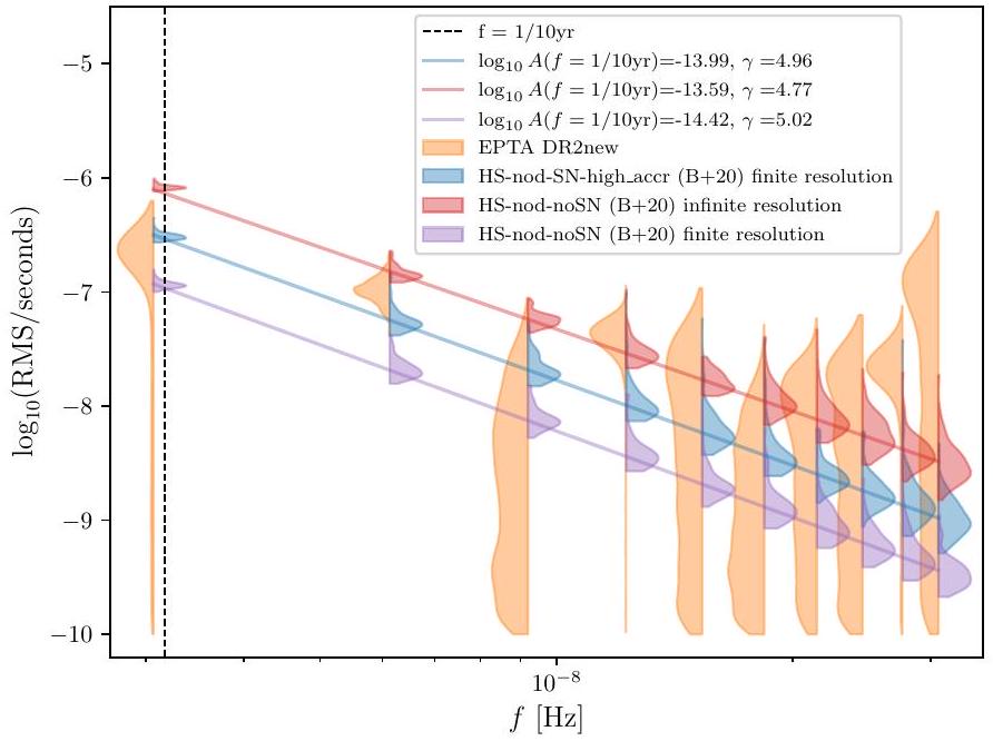
statistical and systematic biases. To address this, we have conducted an extensive campaign of simulations by injecting and recovering different types of signals in synthetic PTAs mimicking the properties of the EPTA DR2new dataset (Valtolina et al. 2024). We generated individual noises for 25 pulsars using the maximum likelihood values of the measured white noise and drew the red noise and dispersion measure parameters from the posterior distribution of the customised noise models (EPTA Collaboration & InPTA Collaboration 2023a). We simulated TOAs from multi-frequency observations and added a GWB spectrum from an astrophysical population of circular SMBHBs producing a nominal GWB with , consistent with the DR2new measurement at . We performed 100 experiments by changing the specific noise realization and the sampling of the injected SMBHB population. The analysis was carried using the ENTERPRISE software package (Ellis et al. 2020).
Two illustrative examples of injection-recovery mismatch are shown in Fig. 14. The top panel shows one of the GWB recoveries. Although the injection did not present particular features (e.g. loud CGWs), for this specific noise realization, the recovered signal has a shallow slope with a median value of . Similar cases have been observed when injecting a pure power law with the createGWB function of libstempo (Vallisneri 2020). This shows that even with an ideal setup when simultaneously fitting multiple parameters (102 in this case) in a complex problem, the stochastic properties of the noise can easily bias the recovered signal, especially if the S/N is low ( for DR2new). Multiple injections with the realistic GWB model and createGWB show systematic biases of recovery of the realistic GWB signal, when modelled with an ideal power law. This is explored in detail in a follow-up work. In the bottom panel of Fig. 14, we show how the presence of some extra high-frequency noise unaccounted for in the MSP noise model can also influence the recovery of the parameters. The setup is the same as in the left panel, but we simulate high-frequency noise mismatch by setting different values of in the recovery. Although the posterior of the signal amplitude is hardly affected, can shift significantly depending on whether the high-frequency noise is slightly overor under-estimated. While these are only two examples, they highlight the complexity of PTA measurements and invite us to be cautious when drawing conclusions that might strongly be influenced by potential biases in the recovered signal.

4. Implications II: physics of the early Universe

Although a GWB generated by an ensemble of the putative SMBHBs is the most plausible source of the observed commonred noise process in pulsar data, more exotic explanations are possible, such as signals originated in the early Universe. The various possible types of cosmological backgrounds of GWs associated with early Universe physics are reviewed in Caprini & Figueroa (2018) and are found to be stochastic. Similarly to the traditional case invoking SMBHBs, the angular spatial correlation for those scenarios follows the HD curve. However, the spectral shapes of the predicted GW spectra are generally different, which can help to disentangle between different types of backgrounds. In this work, we focus on four possible scenarios:
  1. An inflationary GWB from the amplification of quantum fluctuations of the gravitational field,
  2. A GWB from a network of cosmic string loops,
  3. A GWB from vortical (M)HD turbulence at the QCD energy scale,
  4. A scalar-induced GWB arising from inflationary scalar perturbations at the 2nd order in perturbation theory.
    Given the low significance of the detected signal and the limited number of probed frequency bins due to the short timespan of the data, one cannot currently perform a reliable model selection. Therefore, throughout the section, we consider these scenarios separately and assume that each of them can fully explain the detected signal independently. Analysis invoking more complex models with simultaneous fits for multiple scenarios as well as opportunities to disentangle between those (e.g. Goncharov et al. 2022; Kaiser et al. 2022) will be considered in a number of future works.

4.1. Implications on a stochastic background of primordial (inflationary) gravitational waves

Here we address the GWB possibly generated during inflation (Grishchuk 1975; Rubakov et al. 1982; Starobinskii 1985; Fabbri & Pollock 1983; Abbott & Wise 1984). In the standard inflationary scenario, tensor quantum vacuum fluctuations of the metric are amplified by the accelerated expansion, leading to a GWB as they subsequently re-enter the horizon during the radiation (or matter) era. The cosmic microwave background (CMB) and Big Bang Nucleosynthesis (BBN) provide precise measurements of the radiation energy density, from which one can derive weak upper bounds on the amplitude of such a GWB (see e.g. Caprini & Figueroa 2018, and references therein). Furthermore, tensor metric perturbations lead to CMB temperature anisotropies and polarisation at large angular scales (Sachs & Wolfe 1967; Starobinskii 1985; Kosowsky 1996; Allen & Koranda 1994). Since the anisotropies and polarisation detected so far are due to scalar perturbations, it is possible to constrain the energy density of a GW background by placing an upper limit on the tensor-to-scalar ratio at CMB scales: recent upper bounds are given e.g. in Tristram et al. (2022), Galloni et al. (2023). Another parameter to consider is the tensor spectral index of the tensor perturbations. In the context of slow-roll single-field inflation, these two parameters are linked via the consistency relation . By fixing the consistency relation, Tristram et al. (2022) finds at 95% CL, while by relaxing it, Planck Collaboration X (2020) finds and at CL.
Within the slow-roll consistency relation, the GWB spectral slope is therefore slightly red-tilted, causing this signal to be out of reach of most current and planned GW detectors such as PTAs, LISA, aLIGO, aVirgo or the Einstein Telescope. On the other hand, it is fair to consider that the spectral slope could vary over the large frequency span ranging from CMB scales to those probed by GW detectors (Lasky et al. 2016). Inflationary scenarios breaking the consistency relation at small scales might therefore produce a detectable GWB, if they lead to a blue-tilted spectrum. In this case, PTAs, LISA and ground-based devices can place upper limits on (see e.g. Abbott et al. 2017). It is interesting to investigate which kinds of processes could give rise to a blue-tilted GW background while still obeying CMB constraints at large scales. One possibility is the presence, after inflation, of a stiff component in the Universe, with an equation of state (Boyle & Buonanno 2008; Giovannini 1998; Boyle & Steinhardt 2008). The enhancement of the tensor spectra can also be produced during inflation thanks to processes such as, for example, (i) particle production during inflation (see e.g. Sorbo 2011a; Barnaby et al. 2012; Cook & Sorbo 2013a; Anber & Sorbo 2012; Bartolo et al. 2016) (ii) enhancement of tensor perturbations for example by spec-
tator fields, or space-dependent inflation (see e.g. Bartolo et al. 2007; Biagetti et al. 2013, 2015; Fujita et al. 2015) (iii) modified gravity theories such as or Horndeski gravity (Horndeski 1974; Sotiriou & Faraoni 2010) and iv) enhanced scalar perturbations at small scales and/or primordial black holes, which are treated in Sect. 4.4.

4.1.1. Analysis

Similarly to what was done in Lasky et al. (2016), we constrain the key parameters defining the GWB, and , while being agnostic on the underlying process generating the blue-tilted spectrum. If we assume that the common quadrupolar red noise signal present in EPTA data is of inflationary origin, these two parameters can be estimated using the DR2new dataset. Note that the spectral index is expected to vary with the frequency scale considered (see e.g. Giarè & Melchiorri 2021; Giarè et al. 2023; Auclair & Ringeval 2022). However, for simplicity, here we consider a constant all the way from CMB scales to those corresponding to the (narrow) EPTA frequency band. It is then possible to approximate the fractional characteristic GW energy density using (Lasky et al. 2016; Caprini & Figueroa 2018)
where the second line is valid in the PTA frequency band, and has been obtained by setting with , the amplitude of the scalar spectrum , and related to the CMB pivot scale (Planck Collaboration XVI 2014). denotes the frequency entering the horizon at matter-radiation equality.
We then use the nine lowest frequency posteriors of the RMS free spectrum shown in Fig. 1 (see Moore & Vecchio 2021; Lamb et al. 2023; Leclere et al. 2023, for details on the method) to fit the inflationary spectrum of Eq. (14) and obtain posteriors on and . Results are reported in Fig. 15. Note that, since , the correlation between the amplitude and spectral index of the signal is compatible with Fig. 5. The credible (symmetric) intervals are and . The obtained value of corresponds to a PSD spectral index of , as in Fig. 1. The excessively small value of is a consequence of the simplistic parameterisation of Eq. (14), which assumes a constant at all scales. The fractional energy density spectrum obtained from the maximum a posteriori parameter values is plotted in Fig. 16.
We have so far considered a primordial background to be the only source of GWs in our data. We now recall that the most plausible and loud source of a GW background at these frequencies remains that of a SMBHB background. It is therefore likely that any signature for a cosmological background needs to be considered in parallel with a SMBHB background, or in this case more accurately termed ‘foreground’. Kaiser et al. (2022) have explored the likelihood of detecting a cosmological background in the presence of a SMBHB foreground using simulations, and found that the shallower the slope of the cosmological background (for example as opposed to ), the harder it is to detect (and the longer it takes, possibly more than 20 years). According to these simulations, this does not bode well for an even shallower slope, similar to the one detected in DR2new with a possible .
Here we explore a superposition of these two backgrounds in the DR2new dataset. Considering a two-component GWB for the common red noise model, we place constraints on for given values of spanning the range . In this case, our null hypothesis is a GWB from a population of GW-driven circular SMBHBs parameterised only by the PSD amplitude of Eq. (3) (we fix ). We run several analyses with a fixed for the inflationary background, sampling over . For each of the values, we obtain a distribution for and take the quantile as an upper bound. As found in Lasky et al. (2016), and the upper bounds are related with good precision by a linear relation:
Our analysis gives and , which is comparable to the forecast values given in Lasky et al. (2016) (note that they normalise to 0.11).

4.1.2. Discussion

From the analysis of the DR2new dataset above, we have obtained credible intervals for the tensor-to-scalar ratio and the spectral index . This was performed assuming that reheating is instantaneous, and that inflation is followed directly by the radiationdominated era, for which the equation of state parameter of the Universe is . Under this assumption, one finds that the best-fit value for the tensor spectral index is , which is directly linked to the best-fit PSD spectral index 2.7. This high value of is not consistent with slow roll inflation. However, if inflation is followed by a stage in which , the relation between the PSD spectral index and the primordial tensor spectral index changes to (Arzoumanian et al. 2016; Caprini & Figueroa 2018)
again with . If a stiff fluid component ( ) were to dominate the Universe for a finite amount of time after inflation, the last term in Eq. (16) would be bounded between 0 and -2 . Hence, , meaning that even allowing for the presence of a stiff component after inflation, it does not seem possible to explain the common red noise in the context of slow roll inflation ( ) for the best fit value . However, by broadening the range of possible values to does become compatible with the common red noise.

4.2. Implications on a background of cosmic strings

Cosmic strings are line-like topological defects that may form after a symmetry-breaking phase transition in the early Universe (Kibble 1976; Hindmarsh & Kibble 1995); they are generic predictions of most Grand Unification Theories scenarios (Jeannerot et al. 2003). These 1D objects are characterised by the string tension (or equivalently their energy per unit length) which is related to the energy scale of the phase transition.
Overall, cosmic strings combine relativistic velocities and large energy densities, making them natural sources of GWs. These GWs may take the form of bursts from cusps, kinks and kink-kink collisions on the loops (Damour & Vilenkin 2001), and have been searched for in the LIGO/Virgo/KAGRA (LVK) detectors (Abbott et al. 2018, 2021). Cusps are points on the string which, in the Nambu-Goto approximation, propagate at
Fig. 15. 2D posteriors of the tensor-to-scalar ratio (in ) and the fractional energy density spectral index in the PTA frequency range. The 68% and 95% credible regions are displayed. The black dashed line represents the tensor-to-scalar ratio upper bound found in Tristram et al. (2022) assuming single-field slow-roll inflation.
the speed of light, and the string doubles back on itself. On the other hand, kinks are discontinuities in the tangent vector of a string and are formed at each intercommutation of strings. The future space-based detector LISA will be sensitive to cosmic string bursts for tensions as low as (Auclair et al. 2023a). Most notably, in the event that LISA detects GW bursts from cosmic strings, they will likely repeat multiple times a year due to the periodic nature of the cosmic string loops (Auclair et al. 2023b).
The incoherent sum of these GW bursts also produces a stochastic GWB (SGWB), which has been looked for by LVK (Abbott et al. 2018, 2021). LISA is expected to be able to detect a SGWB from cosmic strings with tensions as low as (Auclair et al. 2020). The strings background has already been looked for in EPTA (Sanidas et al. 2012; Leclere et al. 2023), in NANOGrav (Blasi et al. 2021; Ellis & Lewicki 2021) and PPTA (Bian et al. 2022; Chen et al. 2022). These earlier analyses consistently found a good agreement between the common uncorrelated red signal (CURN) present in the data and a SGWB from cosmic strings with tensions .

4.2.1. Description of the models

Since the SGWB is sourced by sub-horizon cosmic string loops, the central quantity in our analysis is the loop density distribution, , where is the invariant length of the loop (defined by its total energy divided by ) and is cosmic time. We focus on the most up-to-date loop distributions, calibrated on large scales with Nambu-Goto simulations (Lorenz et al. 2010; Blanco-Pillado et al. 2014). Loops are formed from the intercommutation of super-Horizon infinite strings, with a maximal size at time . (Note that the simulations assume an intercommutation probability of 1 , as is the case for field theory strings.) The two models – which we refer to as BOS (Blanco-Pillado et al. 2015) and LRS (Lorenz et al. 2010), after the names of their authors – differ in their treatment of small loops, particularly on scales at which gravitational radiation (not included in numerical simulations) can have important effects. Indeed, compared to the BOS model, the LRS model has an
Fig. 16. SGWB spectra (in terms of ) for four different early Universe SGWB models considered in this paper. BOS/LRS correspond to a cosmic string background with and , and . The GWB from turbulence is plotted in solid line for , and . The inflationary spectra is shown for and (maximum a posteriori value). Power spectrum of the 2 nd-order GWB from the scalar curvature perturbations described by the powerlaw model with and is shown with brown puncture-dot line. The nine first Fourier bins posteriors of the common signal are represented by the grey violin areas.
additional population of small loops, which leaves an imprint in the SGWB spectrum (Auclair 2020). The explicit expressions for the two loop distributions are given in Abbott et al. (2018), and both have been considered by the LVK (Abbott et al. 2021) and LISA (Auclair et al. 2020) collaborations. The third observing run of LVK placed constraints on , based on the non-detection of a SGWB. These are for BOS and for LRS. At the frequency of ground-based detectors, the SGWB signal is produced by loops formed during the radiation era. At low PTA frequencies, the SGWB signal is dominated by larger loops, namely those formed at recent times, in transition from the radiation to matter era and also in the matter era (Ringeval & Suyama 2017; Auclair 2020; Leclere et al. 2023).
Other than , a further parameter appears in , namely , which describes the rate at which loops lose energy through gravitational radiation: . If is large, fewer loops are present in the distribution since loops decay more rapidly. On the other hand, GWs are emitted more intensively: the final effect is a combination of these two, which impacts the SGWB of the BOS and LRS models in subtly different ways (Auclair 2020). The value of depends on the properties of loops, and in particular on how many cusps, kinks, and kinkkink they contain as (Damour & Vilenkin 2001; Siemens et al. 2007; Ringeval & Suyama 2017)
where is the number of cusps/kink events per oscillation period of the loop, the number of kink-kink collisions, and
where .
In this paper, we consider 2 cases. For the first model (i) and , for which (Leclere et al. 2023), a value close to that observed in numerical simulations of individual loops (Vachaspati & Vilenkin 1985; Blanco-Pillado & Olum 2017). Therefore, the only free parameter for this model is . As for the second model (ii), we fix and allow to vary between 1 and 200 (with a uniform prior) so as to account for theoretical uncertainties on the initial number of kinks at loop creation, and on the efficiency of the gravitational backreaction that should smooth out the loops (see the LVK analysis, Abbott et al. 2021, for a similar approach). Therefore, this is a two-parameter model .
The fractional energy density of the SGWB per logarithmic interval of frequency is given by
where is the Hubble constant, is the Hubble parameter for which we assume standard cosmology with the Planck-2018 fiducial parameters (Planck Collaboration VI 2020), and is the cosmic time today. The sum is over the cusp, kink and kink-kink contributions (labelled with the index ) for which and 2 respectively.

4.2.2. Analysis results

Our analysis follows the one presented in Leclere et al. (2023), which was based on six pulsars with the best timing precision from the EPTA early Data Release 2 (Chen et al. 2021). We now analyse the DR2new dataset with 25 pulsars, using the (computationally heavy) hierarchical likelihood data analysis method
Fig. 17. Comparison of the string tension posteriors for the two string models (BOS and LRS) in case (i), and ( ). Solid lines assume only a cosmic string background, dashed lines assume both a population of GW-driven circular SMBHBs and cosmic strings.
described in Paper III. We sample the SGWB parameters ( ) or ( ) as well as the individual pulsar noise parameters.
Solid lines in Fig. 17 show the posterior distribution on in case (i), for which and . The string tension credible (symmetric) interval is (resp. ) for the BOS (resp. LRS) model. The corresponding SGWB spectra are shown in Fig. 16 where, for each model, we set to their median values. We also consider the two-component SGWB model made of the sum of a background from cosmic strings and one from a population of GW-driven circular SMBHBs characterised by the PSD of Eq. (3). The posteriors of the two background parameters are highly correlated, since both provide a possible explanation for the detected signal. As a result, the posterior on no longer has compact support, but a tail to lower values (see the dashed lines in Fig. 16). We therefore extract the 95-quantile of the string tension posterior to obtain an upper bound of (resp. -10.44) for the BOS (resp. LRS) models.
The DR2new dataset exhibits a shallower slope for the PSD of the common red signal than DR2full. While cosmic strings were a good fit to the common red signal of 6 pulsars of DR2 full (Leclere et al. 2023), this is no longer true for DR2new. This is because the predicted SGWB PSD is generally steeper than the measured correlated red signal in the data, as can be seen in Fig. 16.
For case (ii), we obtain very similar results to those discussed in Leclere et al. (2023). Namely, we obtain quasi noninformative posteriors for , showing that the data can be equally explained by a population of kinky loops with . In other words, we cannot extract any upper bound on the number of kinks, since this quantity is degenerate with .

4.3. Implications on background from turbulence around the QCD energy scale

Turbulence can arise in the early Universe in the aftermath of a first-order phase transition (Witten 1984; Kamionkowski et al. 1994), or can be driven by pre-existing primordial magnetic fields (Quashnock et al. 1989; Brandenburg et al. 1996). If the (magneto-)hydrodynamic turbulence were present around the QCD epoch, when the Universe had a temperature of
100 MeV , it would generate a GWB in the PTA band. The characteristic scale of the turbulence, determining the characteristic GW frequency, is in fact related to the (comoving) Hubble radius at that epoch , where
and denotes the number of relativistic degrees of freedom. If a large lepton asymmetry and/or primordial magnetic fields were present in the early Universe, the QCD phase transition might have been of first order (Schwarz & Stuke 2009; Wygas et al. 2018; Middeldorf-Wygas et al. 2022; Vovchenko et al. 2021; Cao 2023). In this case, one would expect additional sources of GWs, from the collision of broken phase bubbles and the subsequent development of sound waves in the primordial fluid (Kosowsky et al. 1992; Kosowsky & Turner 1993; Caprini et al. 2008; Huber & Konstandin 2008; Jinno & Takimoto 2017; Cutting et al. 2018; Hindmarsh et al. 2014, 2015, 2017). This was analysed for PTAs, e.g. in Moore & Vecchio (2021), Arzoumanian et al. (2021), Xue (2021). In what follows, we focus on the GWB generated by decaying (M)HD turbulence.

4.3.1. Description of the model

The presence of bulk velocity and magnetic fields produce anisotropic stresses, which in turn act as a source of GWs (Kamionkowski et al. 1994; Kosowsky et al. 2002; Dolgov et al. 2002; Caprini & Durrer 2006; Gogoberidze et al. 2007; Caprini et al. 2009). This has been recently studied via numerical simulations in Roper Pol et al. (2020a,b, 2022a), Brandenburg et al. (2021). In particular, Roper Pol et al. (2022a) show that the envelope of the GWB produced by decaying MHD turbulence can be estimated analytically, assuming that the anisotropic stresses from the velocity and magnetic fields vary more slowly than the dynamical production of GWs. This was also validated by numerical simulations of purely kinetic turbulence in Auclair et al. (2022). This assumption leads to the following GWB signal:
where is the ratio of the (M)HD turbulent energy density to the radiation one, and is the ratio of the characteristic length scale of the turbulence, , to the comoving Hubble horizon at the QCD epoch. The parameter is the efficiency of GW production , estimated in Roper Pol et al. (2022a). The function is the fractional radiation energy density at the epoch of GW generation to its value at the present time. It depends on the temperature scale via the number of degrees of freedom ,
The spectral shape of the GWB signal, , is
where is a normalising factor, and denotes the effective duration of the turbulence. The latter can be estimated, from the numerical simulations performed in Roper Pol et al. (2022a), to be . The function in Eq. (23) denotes the spectrum of the anisotropic stresses. For solenoidal fields (e.g. a primordial magnetic field or vortical bulk fluid motion) characterised by a typical correlation scale of the order of the turbulence scale , it is constant for . Furthermore, it decays as for , if the turbulence is of the Kolmogorov type, as we assume here. Hence, the resulting spectral shape of the GWB in Eq. (21) presents three power laws: at frequencies below the inverse effective duration of the turbulence , at intermediate frequencies , and at large frequencies .
The GWB produced from vortical (M)HD turbulence is therefore determined by three parameters: the temperature scale , the turbulence strength , and the turbulence characteristic length scale . By causality, is bound to be smaller than one. In general, also , otherwise turbulence would change the dynamics of the Universe. However, note that the template described above has been validated in principle only for non-relativistic plasma motions, for which .

4.3.2. Analysis results

As in Sect. 4.1, here we use the fast free spectrum analysis method on DR2new data to constrain the model, considering the nine first Fourier bins of the RMS spectrum of Fig. 1. We use -uniform priors for the model parameters, choosing , and . The 2D posteriors obtained are shown in Fig. 18.
For values of below 0.1 , the model can only explain the level of correlated noise at the lowest frequency bin if the amplitude of the spectrum is sufficiently high. This can be achieved only if is close to 1 and the peak frequency lies within the PTA frequency range, implying . However, at frequencies around the peak, the signal corresponds to a power spectral density for the residuals steeper than , which cannot fit the data well. For this reason, values of are disfavoured.
For larger values of , the part of the spectrum at frequencies below can enter the PTA band with a sufficiently high amplitude. Furthermore, the distance between the break at and the spectral peak at becomes minimal in the limit . Both of these characteristics lead to a better fit to the data. This is recovered in the posteriors of Fig. 18, together with the degeneracy between and from the signal amplitude (see Eq. (21)), and the degeneracy between and from the break at (note that the dependence of the latter on is subdominant).
The model therefore provides a good fit to the data in the limit of large , close to the upper bound of the prior. The extension of the dataset to longer observation time will be crucial for further constraining this model at low frequencies.

4.4. Implications on the 2nd-order GWB produced by primordial curvature perturbations

It is well-known that scalar, vector and tensor modes of the perturbed metric do not mix at linear order of the Einstein equations (Lifshitz 1946; Baumann 2022). However, scalar curvature perturbations will source propagating tensorial modes (GWs) at the 2nd order in perturbation theory (Tomita 1967; Matarrese et al.
Fig. 18. 2D posteriors for the parameters of the background from turbulence around the QCD energy scale obtained using a free spectrum fit on DR2new data. The and credible regions are displayed.
1993, 1998; Noh & Hwang 2004; Carbone & Matarrese 2005; Ananda et al. 2007; Baumann et al. 2007). Such scalar curvature perturbations and associated primordial density fluctuations inevitably exist in the Universe and can be directly constrained by observations of the CMB. The latest Planck data (Planck Collaboration X 2020) suggests that the power spectrum of the curvature perturbations is nearly scale-invariant with the amplitude , which implies a marginal energydensity of the generated GWB. Specifically, when projected to the PTA sensitivity band, the fractional contribution of the energy density in the associated GWs becomes , which is practically non-detectable by current experiments. On the other hand, some models of inflation (see, for example, Di & Gong 2018; Byrnes et al. 2019; Braglia et al. 2020; Yi & Fei 2023) make it possible to produce a sharp increase in the power spectrum of primordial curvature perturbations over many orders of magnitude at small scales.
While the CMB is only capable of directly sampling large cosmological scales with , small scales stay largely uncovered. PTAs provide a unique opportunity to complement the CMB measurements by indirectly probing the scalar curvature perturbations in a scale range through the second-order generated GWB, and to place bounds on the steepest possible growth of the power spectrum as well as corresponding models of inflation (Saito & Yokoyama 2009; Bugaev & Klimai 2011; Chen et al. 2020; Dandoy et al. 2023; Zhao & Wang 2023).
In this work, we consider two models of the primordial curvature power spectrum: i) monochromatic and ii) powerlaw. For the former, the primordial spectrum is modelled as:
where is a dimensionless amplitude and is a wavenumber at which the monochromatic power spectrum has a Dirac-delta peak. For the second case:
Fig. 19. Results for the monochromatic curvature perturbations described by Eq. (24). Left panel: recovered slopes of a simple power-law model as a function of characteristic scale of the injected GWB generated by the monochromatic curvature perturbations. The horizontal lines show the theoretical value of from a population of circular, GW-driven SMBHBs (grey) and the one obtained in Paper III (orange). Right panel: and contours of the posterior distributions on the amplitude and characteristic scale of fluctuations for DR2new (orange colour). The posterior distribution is overlaid with the current constraints on the primordial power spectrum using Planck data (CMB). The grey colour depicts the -confidence intervals. The purple shaded area represents the bounds from spectral distortions (Chluba et al. 2012). For comparison in green we place the prediction of the primordial spectrum of scalar perturbations in the two-field model of inflation described in Braglia et al. (2020) for a range of the model parameters. All three models result in PBH mass functions peaked at with the brightest line corresponding to the dark matter fraction of PBHs of .
where characterises the slope and is a normalizing scale , so that corresponds to dimensionless amplitude at ten years.
In the first scenario, a semi-analytical solution for the induced spectrum of GWB exists and is given by (Kohri & Terada 2018; Espinosa et al. 2018):
where and is the Heaviside theta function. In spite of being nonphysical, the -function peak approximately describes the maximum of the produced GWB in the inflationary model with the steepest possible growth of a spectral peak in the single-field inflation at small scales (see Fig. 7 in Byrnes et al. 2019).
In the second case of a more general (and more realistic) power-law spectrum, the result can only be obtained numerically (Kohri & Terada 2018):
where is the scaling factor which can be evaluated in a range of using interpolation points from Table 1 of Kohri & Terada (2018).
After its production, the GWB is damped due to quantum interactions with the particles of the primordial plasma at the radiation-dominated epoch, and redshifted inversely proportionally to the scale factor (as it also occurs to radiation) starting from the epoch of matter-radiation equality (Saikawa & Shirai
2018). The present value of the fractional energy density is then:
where is the temperature of the Universe at the moment when structures of a typical size re-enter the horizon is the temperature of the Universe at the epoch of matter-radiation equality, and are relativistic degrees of freedom and degrees of freedom in entropy, respectively. The final expression for the auto-power spectral density of the timing residuals is:
where is the Hubble constant at the present epoch.
The outlined formalism was applied to the DR2new version of the latest EPTA dataset. The number of frequency components which was used for the Fourier representation of the signal was fixed to 9 . We have chosen broad uninformative priors for the parameters: uniform in for and , uniform in [4, 12] for , and uniform in [0.4, 2.6] for . Boundaries for the latter are constrained by the limitations of the numerical approximation of the power law model. For this analysis, we assumed that the common red noise process detected in the latest EPTA dataset can be fully explained by the 2nd-order scalar-induced GWs.
Results for monochromatic and power law models are shown in Figs. 19 and 20, respectively. The 2D posterior distribution of the model parameters of the monochromatic model is depicted with orange contours on the right panel of Fig. 19. One may notice that the regions of the highest probability are strongly
Fig. 20. Results for the power-law model of the curvature perturbations described by Eq. (25). Left panel: and contours of the posterior distributions on the amplitude and the slope of the power spectrum obtained by the analysis of DR2New. Right panel: and contours of the power spectra inferred from the DR2New analysis by picking 1000 random samples from the posteriors overlaid with the current constraints on the primordial power spectrum using the latest Planck data. The grey colour depicts the -confidence intervals. The green lines and purple shaded areas are the same as in Fig. 19.
elongated due to a strong positive correlation between and ; these parameters are essentially degenerate. Therefore, DR2new can only provide lower limits on the characteristic scale and amplitude of the monochromatic model: 7.6 and meaning that a whole range of models predicting Dirac-delta power spectrum can equally good describe the signal of DR2new. This behaviour is explained in the left panel of Fig. 19, for which we have simulated GWB signal generated by the monochromatic primordial scalar perturbations, Eq. (26), and attempted to recover a more general power law model of the form used in Paper III to model an arbitrary common red noise process. After a rapid decrease, the recovered slope stabilises at in the limit of large , and becomes consistent with both values obtained with DR2new and the theoretically predicted 13/3 for the background from circular, GW-driven SMBHBs. This degeneracy can raise important issues when one tries to disentangle one signal from another. For the power-law case, the 2D posteriors are shown in the left panel of Fig. 20 with the following means and 1- uncertainties: and .
On the right panels of Figs. 19 and 20, we also overplot the inferred primordial power spectrum with the one obtained from the Planck data. The orange areas on the right panel of Fig. 20 are and contours of the power-law model described by Eq. (25) reconstructed using 1000 random draws from the posteriors. To explain the observed signatures of the DR2new in terms of the second-order GWB from the primordial scalar perturbations, an excess in the primordial spectrum at low scales should be invoked without violating the CMB inflationary parameters. Such excess has been proposed in many papers, e.g. in the aforementioned works by Ivanov et al. (1994), Germani & Prokopec (2017), Di & Gong (2018), Cai et al. (2018), Biagetti et al. (2018), Byrnes et al. (2019), Motohashi et al. (2020), Braglia et al. (2020), Yi & Fei (2023). Notably, this power excess would lead to a copious production of primordial black holes (PBHs) at the radiationdominated stage, which is sometimes taken by the authors as the motivation to introduce them as cold dark matter candi-
dates (Carr et al. 2016, and reference therein). The PBH formation from cosmological perturbations has been extensively explored Sasaki et al. (2018). On the radiation-dominated stage, the PBH mass is related to the mass inside the horizon at the time of the perturbation entering, , where is the Planckian mass, is the temperature. In terms of the mode comoving wavenumber at the moment of the horizon crossing, , the part of the horizon mass collapsing into a PBH reads
For example, in the two-field inflationary model by Braglia et al. (2020), a peak around could explain the power and simultaneously lead to the production of PBHs with masses peaked at (see also the analysis of the NANOGrav results in Vaskonen & Veermäe 2021). Interestingly, such a peak seems to be observed in the chirp mass distribution of LVK merging binary black holes (Abbott et al. 2023). A more general list of primordial power spectra, as well as a careful retranslation of them to the PBH abundance and their mass function, will be considered in a follow-up paper (Porayko et al., in prep.).

5. Implications III: dark matter

Unlike spatially and temporally-correlated stochastic processes discussed in Sects. 3 and 4, in this section, we explore a possible deterministic contribution to the EPTA signal from ultralight scalar-field dark matter (ULDM). For comparison, the morphology of a putative ULDM signal, predicted by Khmelnitsky & Rubakov (2014), is similar to a CGW from a SMBHB, that is, it is prominent only in one frequency bin. Given that the signal observed with DR2new is mostly apparent in the first two fundamental frequency bins, it is of interest to consider possible contributions from physical processes with narrowband spectra. Therefore, the analysis
Table 1. Parameters used for the search and their respective priors.
Parameter Description Prior Occurrence
White noise ( )
EFAC per backend/receiver system Uniform [0, 10] 1 per pulsar
EQUAD per backend/receiver system -Uniform [-10, -5] 1 per pulsar
Red noise
Red noise power-law amplitude -Uniform [-20, -6] 1 per pulsar
Red noise power-law spectral index Uniform [0, 10] 1 per pulsar
ULDM
ULDM amplitude -Uniform [-20, -12] 1 for PTA
ULDM mass -Uniform [-24, -22] 1 for PTA
Earth factor 1 for PTA
Pulsar factor 1 per pulsar
Earth signal phase Uniform [ ] 1 per PTA
Pulsar signal phase Uniform [ ] 1 per pulsar
Common spatially Uncorrelated Red Noise (CURN)
Common process strain amplitude -Uniform [-20, -6] 1 for PTA
Notes. In the correlated limit, and can be reabsorbed in a redefinition of .
presented here complements the CGW interpretation of the signal by EPTA Collaboration & InPTA Collaboration (2023c). Additionally, the ULDM search with DR2full is performed in Smarra et al. (2023).
Dark matter currently constitutes approximately of the energy density of the Universe, as confirmed by, e.g., galactic rotation curves (Rubin et al. 1970, 1980; de Salas et al. 2019), baryonic acoustic oscillations and cosmic microwave background measurements (Bennett et al. 2013; Planck Collaboration VI 2020) as well as galaxy surveys (Escudero et al. 2015). The standard cold dark matter (CDM) picture, whose leading candidates are the weakly interacting massive particles (WIMPs; Arcadi et al. 2018) and the QCD axion (Luzio et al. 2020), successfully grasps the large-scale structure of the Universe. However, it presents some wellknown issues, when it comes to explaining observations at scales smaller than . Among these, the cusp-core problem (Flores & Primack 1994; Moore 1994; Karukes et al. 2015) concerns the inconsistency between the observation of a flat density profile in the centre of galaxies and the power-law-like behavior predicated by CDM, while the mismatch between the simulated and observed number of dwarf galaxies in the proximity of our Milky Way is often referred to as the missing satellite problem (Klypin et al. 1999; Moore 1994).
While a thorough understanding of baryonic physics feedback mechanisms (Navarro et al. 1996; Governato et al. 2012; Brooks et al. 2013; Chan et al. 2015; Oñorbe et al. 2015; Read et al. 2016; Morganti 2017) might help to alleviate some of these issues, they can be more easily disposed of assuming that DM is an ultralight ( ) scalar/pseudoscalar or axion-like field, whose astrophysically large ( ) de Broglie wavelength suppresses power on small scales. Moreover, ultralight scalars are also generally present in string theory compactifications (Green et al. 1988; Svrcek & Witten 2006; Arvanitaki et al. 2010), which makes them interesting candidates for new physics as well. CMB-based arguments are used to constrain (Hlozek et al. 2015), while Lyman- bounds push the limit up to , provided that the ultralight particles account for more than of the full dark matter budget (Iršič et al. 2017; Armengaud et al.
2017; Kobayashi et al. 2017; Nori et al. 2018; Rogers & Peiris 2021). A lower limit of is claimed by studies of ultra-faint dwarf (UFD) galaxies (Hayashi et al. 2021; Dalal & Kravtsov 2022), but a wide consensus is yet to be reached. In a seminal work, Khmelnitsky & Rubakov (2014) showed that the travel time of pulsar radio beams is affected by the gravitational potential induced by ULDM particles, making thus PTAs excellent facilities to investigate the existence of ULDM particles. Moreover, they represent complementary probes which do not suffer from the small-scale structure modelling uncertainties that affect non-CMB bounds (Schive et al. 2014; Zhang et al. 2019), as the aforementioned Lyman- or UFD limits. In the following, we robustly assume that ULDM interacts only gravitationally, therefore giving rise to periodic oscillations in the TOAs of radio pulses as described in Khmelnitsky & Rubakov (2014).
Being non-relativistic and with a very large characteristic occupation number, the ULDM scalar field can be described as a classical wave whose oscillation frequency is twice its mass (Khmelnitsky & Rubakov 2014). The periodic displacement that ULDM induces on the TOAs of signal from a pulsar can be written as follows (Porayko et al. 2018):
where
where is a pulsar (Earth) dependent phase and takes into account the stochastic nature of the axion-like field near the pulsar (Earth). The parameters and their priors are summarised in Table 1. Considering a typical value of for the ULDM velocity, the region in which the scalar field oscillates coherently, i.e. with the same value of , is spanned by the coherence length:
Fig. 21. Posterior probabilities for the ULDM amplitude and mass , from the correlated (top row) and uncorrelated (bottom row) analysis of the DR2new dataset. The pulsar correlated analysis is not shown, but displays the same features.
In particular, notice that and should be taken as:
  • different parameters when the average pulsar-Earth and pulsar-pulsar distance is larger than the coherence length;
  • the same parameter when the average pulsar-Earth and pulsar-pulsar distance is smaller than the coherence length. Following the procedure in Smarra et al. (2023), we analyze three separate cases, which we refer to as the uncorrelated, the pulsar correlated and the correlated limit. As the average inter-pulsar and Earth-pulsar separation is , the correlated and uncorrelated scenarios stand out as exact limits at the low mass and high mass end of the PTAs band, respectively. Instead, the pulsar correlated limit holds when the coherence length of ULDM is smaller than the Galacto-centric radius probed by rotation curves (inner ), but larger than the average interpulsar and pulsar-Earth distance. More specifically, the correlated regime holds for masses lower than ; the pulsar correlated regime for and the uncorrelated limit for . We defer a more detailed study to future analysis.
Based on the above, we fit the model from Eq. (31) to the DR2new as in Smarra et al. (2023). As an example, marginalised posterior distributions for and are plotted in Fig. 21. All the three limits peak at a ULDM mass with amplitude , which translates into a density of the scalar field. While this value is higher than the fiducial local DM density , it is well within the measurement uncertainties (Bovy & Tremaine 2012; Read 2014; Sivertsson et al. 2018; de Salas 2020).
Fig. 22. Constraints on as a function of using the EPTA DR2new dataset from Paper III. Previous analyses are shown for comparison, cf. Porayko & Postnov (2014), Porayko et al. (2018) for further details. The blue, orange and brown lines represent the Bayesian upper limit on obtained from the EPTA DR2new dataset with the correlated, uncorrelated and pulsar correlated analysis, respectively. The purple line shows the expected ULDM abundance computed from Eq. (32).
Fig. 23. Constraints on the ULDM density normalised to the DM background value . The blue, orange and brown lines represent the Bayesian upper limit on , obtained from the EPTA DR2new dataset with the correlated, uncorrelated and pulsar correlated analysis, respectively. The purple dotted line shows the fiducial local DM density value.
Additionally, we search for a potential ULDM signature alongside the SMBHB gravitational-wave background. Thus, we introduce a new model that contains ULDM contributions alongside a common red signal to account for gravitational wave contributions. We find no ULDM signal under this hypothesis, in agreement with the fact that the data support HD correlation, which naturally favours GWs over ULDM in a joint search. Thus we put upper limit on the amplitude and the density of the scalar field.
Figures 22 and 23 show that the EPTA at current sensitivity is able to constrain the presence of ULDM at the level
of the expected DM abundance in the mass range . The DR2Full analysis performed in Smarra et al. (2023) pushes these limits down, thus implying that such ULDM candidates cannot constitute the entire DM. We highlight that our bounds extend below the DR2new sampling frequency , with . In fact, while it might naively be thought that the ULDM field needs to complete an oscillation in the timescale of the PTA experiment to produce a detectable effect, we point out that an ULDM wave with frequency can still be approximated by an expansion in powers of (Kaplan et al. 2022), though the sensitivity of PTAs will be reduced due to degeneracies with the timing model (Ramani et al. 2020). Relying on the robust CMB bounds mentioned before, we fix the lower end of our search at . Importantly, we remove the parameter from the search in the correlated limit, as it is fully degenerate with . In other words, building upon the observation that our Galaxy rotation curve measurements are performed within an ULDM coherence length in the correlated limit, we redefine a new variable, , which represents the instance of DM in the Milky Way. Finally, as shown by Fig. 22, we report a bump in upper limits at , which is at around the maximum-a-posteriori boson mass in Fig. 21. This mass further corresponds to the frequency of the CGW analyzed in EPTA Collaboration & InPTA Collaboration (2023c). Looking at the posteriors in this mass range, we also find an additional contribution, on top of the CURN process. A similar bump in upper limits is also present in the DR2Full dataset, as discussed in Smarra et al. (2023). However, the Bayes factor of we find in favour of the presence of ULDM signal is still inconclusive. We recommend following up on this bump in future work.

6. Discussion and outlook

In this paper, we have explored the implications of the common, correlated low-frequency signal observed in the latest data release of the EPTA+InPTA collaboration. Four different datasets were assembled, and the signal was more significant in those including only broadband, high-quality data taken with telescope backends of the new generation. Therefore, we took, as benchmark for our analysis, the signal measured in the DR2new dataset, for which the HD correlation is detected at high significance with a Bayes factor of or, equivalently, at a -value of , indicative of a confidence. The signal can be modelled by a single power law spectrum as in Eq. (3), with best-fit parameters and (Paper III).
We considered several physical processes separately, investigating the implications of the detected signal under the hypothesis that it is generated by that specific process. Our main findings can be summarised as follows.
SMBHBs. The signal is consistent with a cosmic population of merging SMBHBs. Phenomenological models based on galaxy pairs observations can account for the power spectral distribution of the correlated signal. Those models can also be used to predict the chance to detect CGWs in the current data, for which the search has given inconclusive results so far (EPTA Collaboration & InPTA Collaboration 2023c). According to those models, there is roughly a chance to detect a CGW in DR2new at . The relatively high amplitude of the signal can be used to place constraints on key properties of the cosmic SMBHB population. By exploiting the inference framework developed in Middleton et al. (2016),
Chen et al. (2019), we can infer that SMBHBs merge in less than 1Gyr following galaxy mergers, and that the SMBHstellar bulge relation has a normalization at a reference stellar mass bulge of , in line with recent compiled results (e.g. Kormendy & Ho 2013). Finally, we investigated how the detected signal compares with predictions from state-of-the-art galaxy formation SAMs (Barausse 2012; Izquierdo-Villalba et al. 2022). We found that the high amplitude of the signal imposes non-trivial constraints on galaxy and SMBH evolution models. In particular, boosted SMBH accretion and short SMBHB evolution timescales are needed to match the observed signal, which might lead to difficulties when trying to reproduce independent observables such as the quasar luminosity function. If the SMBHB origin of the observed signal is confirmed, it would be a major breakthrough for observational astrophysics and for our understanding of galaxy formation. This would be the first direct evidence that SMBHBs merge in nature, adding an important observational piece to the puzzle of structure formation and galaxy evolution.
Early Universe. The measured signal would have different implications for each of the physical processes considered in this study. An inflationary origin requires non-standard inflationary scenarios breaking the slow-roll consistency relation, leading to a blue-tilted spectrum. In particular, the measured implies for a radiation-dominated universe with . A cosmic string origin would allow narrowing down the string tension to values of , depending on the specific distribution of loops in the string network. Conversely, the number of kinks cannot be constrained. A GWB induced by (M)HD turbulence at the QCD energy scale can also potentially explain the common red noise, but requires either high turbulent energy densities, of the same order of the radiation energy density, or a characteristic turbulent scale close to the horizon at the QCD epoch. Finally, the measured signal can be produced by the evolution of scalar perturbations at second order only if an excess of their primordial spectrum is present at large wavenumbers, compared to the level derived from CMB observations at small wave numbers. Notably, such an excess would lead to the production of PBHs which can non-negligibly contribute to the CDM density.
ULDM. Finally, we searched for ULDM signatures in DR2new. The search returned a prominent peak in the posterior distribution of the ULDM particle mass around -23. This corresponds to a field oscillation frequency of , which is consistent with the CGW candidate examined in EPTA Collaboration & InPTA Collaboration (2023c). When a joint ULDM+GWB search is performed, however, the peak in the ULDM mass posterior distribution vanishes, as the data strongly prefer the presence of an HD correlation in the common power. We therefore conclude that an ULDM origin of the detected signal is disfavoured, placing a direct constraint on the abundance of ULDM in our Galaxy. The non-detection in DR2new implies that only about of the DM density in the solar neighbourhood can be attributed to ULDM with . More stringent constraints are obtained from DR2full and are presented in a separate paper (Smarra et al. 2023).
It is interesting to remark that the best fit to the measured power-law slope is , well below the predicted expected from a cosmic population of SMBHBs, often indicated as the primary candidate for generating nanohertz GWs. Before leaving the floor to speculations, we caution that this ‘inconsistency’ might have multiple roots, as mentioned in Sect. 3.4. First,
assumes a population of circular GW-driven binaries. Eccentricity and environmental coupling can easily flatten the low-frequency spectrum. Even for circular binaries, a simple power-law of is an ideal limit; small number statistics due to the sparseness of massive, nearby systems results in noisy spectra with a large variance, which can produce different spectral indices when fitted by a power-law. Second, the measured value can be subject to statistical and systematic biases. We have in fact shown that even when a power law with is injected into the data, the measured values can be biased due to the statistical realization of the noise. Moreover, the mis-modeling of highfrequency noise can systematically bias the recovered , leading to flatter spectra if unaccounted high-frequency noise is present in the data. Therefore, caution should be taken when drawing conclusions from this measurement.
Conversely, a shallow spectral slope might indicate that the GW signal has a different origin, perhaps from some key physical process occurring in the early Universe, as investigated in Sect. 4. Another possibility, proposed by Lieu et al. (2022) is that GWs can lose energy while propagating through the intergalactic medium via the acceleration of charged particles. Owing to the much higher thermal velocity of electrons over protons and the presence of an intergalactic medium magnetic field, a significant fraction of the GWs can be converted to EM radiation. The ensuing electromagnetic intensity is inversely proportional to frequency. Partial GW loss via this mechanism could explain a flatter-than-expected GWB spectrum. The efficiency of such a mechanism depends on the strength of the intergalactic medium magnetic field.
It is also possible that the observed signal is coming from multiple overlapping GWBs. In our analyses, we have assumed a single origin for all the observed signal power in the EPTA+InPTA data, however, an overlap of GWBs of different origins can cause the spectral shape of the recovered signal to deviate from the expected value of any single GWB. Searching, disentangling and identifying the underlying physical processes will be part of the spectral characterisation moving forward (Moore & Vecchio 2021; Kaiser et al. 2022).
As time goes by and the PTA experiment improves, the lowfrequency GWB will leave an increasingly distinctive signature in the data. Interpreting all of the details of this signature will be necessary to understand the nature of the signal and exploit the full potential of this new window into the Universe. As mentioned in the introduction, a population of SMBHBs is expected to generate a highly non-Gaussian, partially anisotropic and perhaps non-stationary signal. As we increase the timespan of our data, improve our instrumentation and combine more pulsars, the detailed properties of the signal will eventually reveal themselves in the data (e.g. Cornish & Sesana 2013; Taylor & Gair 2013; Taylor et al. 2020; Pol et al. 2022). While many early Universe signals are expected to be isotropic and Gaussian, noticeable exceptions exist, such as GWBs from bursts of cosmic strings. Cross-correlating the power distribution of the nanohertz GW sky to the distribution of massive galaxies and large-scale structures in the low- universe can eventually provide the key to determining the true nature – astrophysical vs. early Universe of this signal (Rosado & Sesana 2014; Mingarelli et al. 2017). In this respect, combining all of the available high-quality datasets within the IPTA framework is the next step towards the fulfilment of the promises of nanohertz GW science.
Acknowledgements. The European Pulsar Timing Array (EPTA) is a collaboration between European and partner institutes, namely ASTRON (NL), INAF/Osservatorio di Cagliari (IT), Max-Planck-Institut für Radioastronomie
(GER), Nançay/Paris Observatory (FRA), the University of Manchester (UK), the University of Birmingham (UK), the University of East Anglia (UK), the University of Bielefeld (GER), the University of Paris (FRA), the University of Milan-Bicocca (IT), the Foundation for Research and Technology, Hellas (GR), and Peking University (CHN), with the aim to provide high-precision pulsar timing to work towards the direct detection of low-frequency gravitational waves. An Advanced Grant of the European Research Council allowed to implement the Large European Array for Pulsars (LEAP) under Grant Agreement Number 227947 (PI M. Kramer). The EPTA is part of the International Pulsar Timing Array (IPTA); we thank our IPTA colleagues for their support and help with this paper and the external Detection Committee members for their work on the Detection Checklist. Part of this work is based on observations with the 100m telescope of the Max-Planck-Institut für Radioastronomie (MPIfR) at Effelsberg in Germany. Pulsar research at the Jodrell Bank Centre for Astrophysics and the observations using the Lovell Telescope are supported by a Consolidated Grant (ST/T000414/1) from the UK’s Science and Technology Facilities Council (STFC). ICN is also supported by the STFC doctoral training grant ST/T506291/1. The Nançay radio Observatory is operated by the Paris Observatory, associated with the French Centre National de la Recherche Scientifique (CNRS), and partially supported by the Région Centre-Val de Loire in France. We acknowledge financial support from “Programme National de Cosmologie et Galaxies” (PNCG), and “Programme National Hautes Énergies” (PNHE) funded by CNRS/INSU-IN2P3-INP, CEA and CNES, France. We acknowledge financial support from Agence Nationale de la Recherche (ANR-18-CE31-0015), France. The Westerbork Synthesis Radio Telescope is operated by the Netherlands Institute for Radio Astronomy (ASTRON) with support from the Netherlands Foundation for Scientific Research (NWO). The Sardinia Radio Telescope (SRT) is funded by the Department of University and Research (MIUR), the Italian Space Agency (ASI), and the Autonomous Region of Sardinia (RAS) and is operated as a National Facility by the National Institute for Astrophysics (INAF). The work is supported by the National SKA programme of China (2020SKA0120100), Max-Planck Partner Group, NSFC 11690024, CAS Cultivation Project for FAST Scientific. This work is also supported as part of the “LEGACY” MPG-CAS collaboration on low-frequency gravitational wave astronomy. JA acknowledges support from the European Commission (Grant Agreement number: 101094354). JA and SCha were partially supported by the Stavros Niarchos Foundation (SNF) and the Hellenic Foundation for Research and Innovation (H.F.R.I.) under the 2nd Call of the “Science and Society Action Always strive for excellence – Theodoros Papazoglou” (Project Number: 01431). AC acknowledges support from the Paris Île-de-France Region. AC, AF, ASe, ASa, EB, DI, GMS, MBo acknowledge financial support provided under the European Union’s H2020 ERC Consolidator Grant “Binary Massive Black Hole Astrophysics” (B Massive, Grant Agreement: 818691). GD, KLi, RK and MK acknowledge support from European Research Council (ERC) Synergy Grant “BlackHoleCam”, Grant Agreement Number 610058. This work is supported by the ERC Advanced Grant “LEAP”, Grant Agreement Number 227947 (PI M. Kramer). AV and PRB are supported by the UK’s Science and Technology Facilities Council (STFC; grant ST/W000946/1). AV also acknowledges the support of the Royal Society and Wolfson Foundation. JPWV acknowledges support by the Deutsche Forschungsgemeinschaft (DFG) through thew Heisenberg programme (Project No. 433075039) and by the NSF through AccelNet award #2114721. NKP is funded by the Deutsche Forschungsgemeinschaft (DFG, German Research Foundation) – Projektnummer PO 2758/1-1, through the WalterBenjamin programme. ASa thanks the Alexander von Humboldt foundation in Germany for a Humboldt fellowship for postdoctoral researchers. APo, DP and MBu acknowledge support from the research grant “iPeska” (P.I. Andrea Possenti) funded under the INAF national call Prin-SKA/CTA approved with the Presidential Decree 70/2016 (Italy). RNC acknowledges financial support from the Special Account for Research Funds of the Hellenic Open University (ELKEHOU) under the research programme “GRAVPUL” (grant agreement 319/10-10-2022). EvdW, CGB and GHJ acknowledge support from the Dutch National Science Agenda, NWA Startimpuls – 400.17.608. BG is supported by the Italian Ministry of Education, University and Research within the PRIN 2017 Research Program Framework, n. 2017SYRTCN. LS acknowledges the use of the HPC system Cobra at the Max Planck Computing and Data Facility. The Indian Pulsar Timing Array (InPTA) is an Indo-Japanese collaboration that routinely employs TIFR’s upgraded Giant Metrewave Radio Telescope for monitoring a set of IPTA pulsars. BCJ, YG, YM, SD, AG and PR acknowledge the support of the Department of Atomic Energy, Government of India, under Project Identification # RTI 4002. BCJ, YG and YM acknowledge support of the Department of Atomic Energy, Government of India, under project No. 12-R&D-TFR-5.02-0700 while SD, AG and PR acknowledge support of the Department of Atomic Energy, Government of India, under project no. 12-R&D-TFR-5.02-0200. KT is partially supported by JSPS KAKENHI Grant Numbers 20H00180, 21H01130, and 21H04467, Bilateral Joint Research Projects of JSPS, and the ISM Cooperative Research Program (2021-ISMCRP-2017). AS is supported by the NANOGrav NSF Physics Frontiers Center (awards #1430284 and 2020265). AKP is supported by CSIR fellowship Grant number 09/0079(15784)/2022-EMR-I. SH
is supported by JSPS KAKENHI Grant Number 20J20509. KN is supported by the Birla Institute of Technology & Science Institute fellowship. AmS is supported by CSIR fellowship Grant number 09/1001(12656)/2021-EMR-I and T641 (DST-ICPS). TK is partially supported by the JSPS Overseas Challenge Program for Young Researchers. We acknowledge the National Supercomputing Mission (NSM) for providing computing resources of ‘PARAM Ganga’ at the Indian Institute of Technology Roorkee as well as ‘PARAM Seva’ at IIT Hyderabad, which is implemented by C-DAC and supported by the Ministry of Electronics and Information Technology (MeitY) and Department of Science and Technology (DST), Government of India. DD acknowledges the support from the Department of Atomic Energy, Government of India through Apex Project Advance Research and Education in Mathematical Sciences at IMSc. The work presented here is a culmination of many years of data analysis as well as software and instrument development. In particular, we thank Drs. N. D’Amico, P. C. C. Freire, R. van Haasteren, C. Jordan, K. Lazaridis, P. Lazarus, L. Lentati, O. Löhmer and R. Smits for their past contributions. We also thank Dr. N. Wex for supporting the calculations of the galactic acceleration as well as the related discussions. We would like to thank Prof. Drs. Alexey Starobinskiy, Sergei Blinnikov and Alexander Dolgov for discussions on the early Universe physics. HM acknowledges the support of the UK Space Agency, Grant No. ST/V002813/1 and ST/X002071/1. Some of the computations described in this paper were performed using the University of Birmingham’s BlueBEAR HPC service, which provides a High Performance Computing service to the University’s research community. See http://www.birmingham.ac.uk/bear for more details. The EPTA is also grateful to staff at its observatories and telescopes who have made the continued observations possible. Author contributions: The EPTA is a multi-decade effort and all authors have contributed through conceptualisation, funding acquisition, data-curation, methodology, software and hardware developments as well as (aspects of) the continued running of the observational campaigns, which includes writing and proofreading observing proposals, evaluating observations and observing systems, mentoring students, developing science cases. All authors also helped in (aspects of) verification of the data, analysis and results as well as in finalising the paper draft. Specific contributions from individual EPTA members are listed in the CRediT (https://credit.niso.org/) format below. InPTA members contributed in uGMRT observations and data reduction to create the InPTA data set which is employed while assembling the DR2full+ and DR2new+ data sets.

References

Abbott, L. F., & Wise, M. B. 1984, Nucl. Phys. B, 244, 541
Abbott, B. P., Abbott, R., Abbott, T. D., et al. 2016, Phys. Rev. Lett., 116, 061102
Abbott, B. P., Abbott, R., Abbott, T. D., et al. 2017, Phys. Rev. Lett., 118, 121101
Abbott, B. P., Abbott, R., Abbott, T. D., et al. 2018, Phys. Rev. D, 97, 102002
Abbott, R., Abbott, T. D., Abraham, S., et al. 2021, Phys. Rev. Lett., 126, 241102
Abbott, R., Abbott, T. D., Acernese, F., et al. 2023, Phys. Rev. X, 13, 011048
Allen, B. 1996, in Les Houches School of Physics: Astrophysical Sources of Gravitational Radiation, 373
Allen, B., & Koranda, S. 1994, Phys. Rev. D, 50, 3713
Amaro-Seoane, P., Sesana, A., Hoffman, L., et al. 2010, MNRAS, 402, 2308
Ananda, K. N., Clarkson, C., & Wands, D. 2007, Phys. Rev. D, 75, 123518
Anber, M. M., & Sorbo, L. 2012, Phys. Rev. D, 85, 123537
Antonini, F., Barausse, E., & Silk, J. 2015, ApJ, 806, L8
Arcadi, G., Dutra, M., Ghosh, P., et al. 2018, Eur. Phys. J. C, 78, 203
Armengaud, E., Palanque-Delabrouille, N., Yèche, C., Marsh, D. J. E., & Baur, J. 2017, MNRAS, 471, 4606
Arvanitaki, A., Dimopoulos, S., Dubovsky, S., Kaloper, N., & March-Russell, J. 2010, Phys. Rev. D, 81, 123530
Arzoumanian, Z., Brazier, A., Burke-Spolaor, S., et al. 2016, ApJ, 821, 13
Arzoumanian, Z., Baker, P. T., Blumer, H., et al. 2020, ApJ, 905, L34
Arzoumanian, Z., Baker, P. T., Blumer, H., et al. 2021, Phys. Rev. Lett., 127, 251302
Auclair, P. G. 2020, JCAP, 11, 050
Auclair, P., & Ringeval, C. 2022, Phys. Rev. D, 106, 063512
Auclair, P., Blanco-Pillado, J. J., Figueroa, D. G., et al. 2020, JCAP, 04, 034
Auclair, P., Caprini, C., Cutting, D., et al. 2022, JCAP, 09, 029
Auclair, P., Babak, S., Quelquejay Leclere, H., & Steer, D. A. 2023a, Phys. Rev. D, 108, 043519
Auclair, P., Steer, D. A., & Vachaspati, T. 2023b, Phys. Rev. D, 108, 123540
Babak, S., & Sesana, A. 2012, Phys. Rev. D, 85, 044034
Barausse, E. 2012, MNRAS, 423, 2533
Barausse, E., Dvorkin, I., Tremmel, M., Volonteri, M., & Bonetti, M. 2020, ApJ, 904, 16
Barnaby, N., Moxon, J., Namba, R., et al. 2012, Phys. Rev. D, 86, 103508
Bartolo, N., Matarrese, S., Riotto, A., & Väihkönen, A. 2007, Phys. Rev. D, 76, 061302
Bartolo, N., Caprini, C., Domcke, V., et al. 2016, JCAP, 2016, 026
Bassa, C. G., Janssen, G. H., Karuppusamy, R., et al. 2016, MNRAS, 456, 2196
Baumann, D. 2022, Cosmology (Cambridge University Press)
Baumann, D., Steinhardt, P., Takahashi, K., & Ichiki, K. 2007, Phys. Rev. D, 76, 084019
Bécsy, B., Cornish, N. J., & Kelley, L. Z. 2022, ApJ, 941, 119
Bennett, C. L., Larson, D., Weiland, J. L., et al. 2013, ApJS, 208, 20
Biagetti, M., Fasiello, M., & Riotto, A. 2013, Phys. Rev. D, 88, 103518
Biagetti, M., Dimastrogiovanni, E., Fasiello, M., & Peloso, M. 2015, JCAP, 2015, 011
Biagetti, M., Franciolini, G., Kehagias, A., & Riotto, A. 2018, JCAP, 2018, 032
Bian, L., Shu, J., Wang, B., Yuan, Q., & Zong, J. 2022, Phys. Rev. D, 106, L101301
Blanco-Pillado, J. J., & Olum, K. D. 2017, Phys. Rev. D, 96, 104046
Blanco-Pillado, J. J., Olum, K. D., & Shlaer, B. 2014, Phys. Rev. D, 89, 023512
Blanco-Pillado, J. J., Olum, K. D., & Shlaer, B. 2015, Phys. Rev. D, 92, 063528
Blasi, S., Brdar, V., & Schmitz, K. 2021, Phys. Rev. Lett., 126, 041305
Bonetti, M., & Sesana, A. 2020, Phys. Rev. D, 102, 103023
Bonetti, M., Sesana, A., Barausse, E., & Haardt, F. 2018, MNRAS, 477, 2599
Bovy, J., & Tremaine, S. 2012, ApJ, 756, 89
Boylan-Kolchin, M., Springel, V., White, S. D. M., Jenkins, A., & Lemson, G. 2009, MNRAS, 398, 1150
Boyle, L. A., & Buonanno, A. 2008, Phys. Rev. D, 78, 043531
Boyle, L. A., & Steinhardt, P. J. 2008, Phys. Rev. D, 77, 063504
Braglia, M., Hazra, D. K., Finelli, F., et al. 2020, JCAP, 2020, 001
Brandenburg, A., Enqvist, K., & Olesen, P. 1996, Phys. Rev. D, 54, 1291
Brandenburg, A., Clarke, E., He, Y., & Kahniashvili, T. 2021, Phys. Rev. D, 104, 043513
Brooks, A. M., Kuhlen, M., Zolotov, A., & Hooper, D. 2013, ApJ, 765, 22
Bugaev, E., & Klimai, P. 2011, Phys. Rev. D, 83, 083521
Byrnes, C. T., Cole, P. S., & Patil, S. P. 2019, JCAP, 2019, 028
Cai, Y.-F., Tong, X., Wang, D.-G., & Yan, S.-F. 2018, Phys. Rev. Lett., 121, 081306
Cao, G. 2023, Phys. Rev. D, 107, 014021
Capelo, P. R., Dotti, M., Volonteri, M., et al. 2017, MNRAS, 469, 4437
Caprini, C., & Durrer, R. 2006, Phys. Rev. D, 74, 063521
Caprini, C., & Figueroa, D. G. 2018, CQG, 35, 163001
Caprini, C., Durrer, R., & Servant, G. 2008, Phys. Rev. D, 77, 124015
Caprini, C., Durrer, R., & Servant, G. 2009, JCAP, 2009, 024
Carbone, C., & Matarrese, S. 2005, Phys. Rev. D, 71, 043508
Carr, B., Kühnel, F., & Sandstad, M. 2016, Phys. Rev. D, 94, 083504
Chan, T. K., Kereš, D., Oñorbe, J., et al. 2015, MNRAS, 454, 2981
Chen, S., Middleton, H., Sesana, A., Del Pozzo, W., & Vecchio, A. 2017a, MNRAS, 468, 404
Chen, S., Sesana, A., & Del Pozzo, W. 2017b, MNRAS, 470, 1738
Chen, S., Sesana, A., & Conselice, C. J. 2019, MNRAS, 488, 401
Chen, Z.-C., Yuan, C., & Huang, Q.-G. 2020, Phys. Rev. Lett., 124, 251101
Chen, S., Caballero, R. N., Guo, Y. J., et al. 2021, MNRAS, 508, 4970
Chen, Z.-C., Wu, Y.-M., & Huang, Q.-G. 2022, ApJ, 936, 20
Chluba, J., Erickcek, A. L., & Ben-Dayan, I. 2012, ApJ, 758, 76
Cook, J. L., & Sorbo, L. 2013a, JCAP, 2013, 047
Cook, J. L., & Sorbo, L. 2013b, JCAP, 11, 047
Cornish, N. J., & Sesana, A. 2013, CQG, 30, 224005
Cutting, D., Hindmarsh, M., & Weir, D. J. 2018, Phys. Rev. D, 97, 123513
Dalal, N., & Kravtsov, A. 2022, arXiv e-prints [arXiv:2203.05750]
Damour, T., & Vilenkin, A. 2000, Phys. Rev. Lett., 85, 3761
Damour, T., & Vilenkin, A. 2001, Phys. Rev. D, 64, 064008
Damour, T., & Vilenkin, A. 2005, Phys. Rev. D, 71, 063510
Dandoy, V., Domcke, V., & Rompineve, F. 2023, SciPost Phys. Core, 6, 060
de Salas, P. F. 2020, J. Phys. Conf. Ser., 1468, 012020
de Salas, P., Malhan, K., Freese, K., Hattori, K., & Valluri, M. 2019, JCAP, 2019, 037
Dehnen, W. 2014, Comput. Astrophys. Cosmol., 1, 1
Desvignes, G., Caballero, R. N., Lentati, L., et al. 2016, MNRAS, 458, 3341
Di, H., & Gong, Y. 2018, JCAP, 2018, 007
Dolgov, A. D., Grasso, D., & Nicolis, A. 2002, Phys. Rev. D, 66, 103505
D’Orazio, D. J., & Duffell, P. C. 2021, ApJ, 914, L21
Dvali, G., & Vilenkin, A. 2004, JCAP, 2004, 010
Ellis, J., & Lewicki, M. 2021, Phys. Rev. Lett., 126, 041304
Ellis, J. A., Vallisneri, M., Taylor, S. R., & Baker, P. T. 2020, https://doi . org/10.5281/zenodo. 4059815
Enoki, M., & Nagashima, M. 2007, Prog. Theor. Phys., 117, 241
EPTA Collaboration (Antoniadis, J., et al.) 2023, A&A, 678, A48 (Paper I)
EPTA Collaboration & InPTA Collaboration (Antoniadis, J., et al.) 2023a, A&A, 678, A49 (Paper II)
EPTA Collaboration & InPTA Collaboration (Antoniadis, J., et al.) 2023b, A&A, 678, A50 (Paper III)
EPTA Collaboration & InPTA Collaboration (Antoniadis, J., et al.) 2023c, A&A, submitted (Paper V)
Escudero, M., Mena, O., Vincent, A. C., Wilkinson, R. J., & Bœhm, C. 2015, JCAP, 2015, 034
Espinosa, J. R., Racco, D., & Riotto, A. 2018, JCAP, 2018, 012
Fabbri, R., & Pollock, M. D. 1983, Phys. Lett. B, 125, 445
Farris, B. D., Duffell, P., MacFadyen, A. I., & Haiman, Z. 2014, ApJ, 783, 134
Flores, R. A., & Primack, J. R. 1994, ApJ, 427, L1
Foster, R. S., & Backer, D. C. 1990, ApJ, 361, 300
Fujita, T., Yokoyama, J., & Yokoyama, S. 2015, Prog. Theor. Exp. Phys., 2015, 043E01
Galloni, G., Bartolo, N., Matarrese, S., et al. 2023, JCAP, 2023, 062
Germani, C., & Prokopec, T. 2017, Phys. Dark Universe, 18, 6
Giarè, W., & Melchiorri, A. 2021, Phys. Lett. B, 815, 136137
Giarè, W., Forconi, M., Di Valentino, E., & Melchiorri, A. 2023, MNRAS, 520, 1757
Giovannini, M. 1998, Phys. Rev. D, 58, 083504
Gogoberidze, G., Kahniashvili, T., & Kosowsky, A. 2007, Phys. Rev. D, 76, 083002
Goncharov, B., Shannon, R. M., Reardon, D. J., et al. 2021, ApJS, 917, 8
Goncharov, B., Thrane, E., Shannon, R. M., et al. 2022, ApJ, 932, L22
Governato, F., Zolotov, A., Pontzen, A., et al. 2012, MNRAS, 422, 1231
Graham, A. W., & Scott, N. 2013, ApJ, 764, 151
Green, M. B., Schwarz, J. H., & Witten, E. 1988, Superstring Theory. Vol. 1: Introduction, (Cambridge University Press)
Grishchuk, L. P. 1975, Sov. J. Exp. Theor. Phys., 40, 409
Gualandris, A., Khan, F. M., Bortolas, E., et al. 2022, MNRAS, 511, 4753
Hayashi, K., Ferreira, E. G. M., & Chan, H. Y. J. 2021, ApJS, 912, L3
Hellings, R. W., & Downs, G. S. 1983, ApJ, 265, L39
Henriques, B. M. B., White, S. D. M., Thomas, P. A., et al. 2015, MNRAS, 451, 2663
Hindmarsh, M. B., & Kibble, T. W. B. 1995, Rept. Prog. Phys., 58, 477
Hindmarsh, M., Huber, S. J., Rummukainen, K., & Weir, D. J. 2014, Phys. Rev. Lett., 112, 041301
Hindmarsh, M., Huber, S. J., Rummukainen, K., & Weir, D. J. 2015, Phys. Rev. D, 92, 123009
Hindmarsh, M., Huber, S. J., Rummukainen, K., & Weir, D. J. 2017, Phys. Rev. D, 96, 103520
Hlozek, R., Grin, D., Marsh, D. J. E., & Ferreira, P. G. 2015, Phys. Rev. D, 91, 103512
Horndeski, G. W. 1974, Int. J. Theor. Phys., 10, 363
Huber, S. J., & Konstandin, T. 2008, JCAP, 2008, 022
Iršič, V., Viel, M., Haehnelt, M. G., Bolton, J. S., & Becker, G. D. 2017, Phys. Rev. Lett., 119, 031302
Ivanov, P., Naselsky, P., & Novikov, I. 1994, Phys. Rev. D, 50, 7173
Izquierdo-Villalba, D., Sesana, A., Bonoli, S., & Colpi, M. 2022, MNRAS, 509, 3488
Izquierdo-Villalba, D., Sesana, A., Colpi, M., et al. 2024, A&A, in press https: //doi.org/10.1051/0004-6361/202449293
Jaffe, A. H., & Backer, D. C. 2003, ApJ, 583, 616
Jeannerot, R., Rocher, J., & Sakellariadou, M. 2003, Phys. Rev. D, 68, 103514
Jinno, R., & Takimoto, M. 2017, Phys. Rev. D, 95, 024009
Jones, N. T., Stoica, H., & Tye, S. H. H. 2003, Phys. Lett. B, 563, 6
Joshi, B. C., Gopakumar, A., Pandian, A., et al. 2022, J. Astrophys. Astron., 43, 98
Kahniashvili, T., Brandenburg, A., Gogoberidze, G., Mandal, S., & Roper Pol, A. 2021, Phys. Rev. Res., 3, 013193
Kaiser, A. R., Pol, N. S., McLaughlin, M. A., et al. 2022, ApJ, 938, 115
Kamionkowski, M., Kosowsky, A., & Turner, M. S. 1994, Phys. Rev. D, 49, 2837
Kaplan, D. E., Mitridate, A., & Trickle, T. 2022, Phys. Rev. D, 106, 035032
Karukes, E. V., Salucci, P., & Gentile, G. 2015, A&A, 578, A13
Kelley, L. Z., Blecha, L., Hernquist, L., Sesana, A., & Taylor, S. R. 2017, MNRAS, 471, 4508
Kelley, L. Z., Blecha, L., Hernquist, L., Sesana, A., & Taylor, S. R. 2018, MNRAS, 477, 964
Khan, F. M., Preto, M., Berczik, P., et al. 2012, ApJ, 749, 147
Khan, F. M., Fiacconi, D., Mayer, L., Berczik, P., & Just, A. 2016, ApJ, 828, 73
Khmelnitsky, A., & Rubakov, V. 2014, JCAP, 2014, 019
Kibble, T. 1976, J. Phys. A, 9, 1387
Klein, A., Barausse, E., Sesana, A., et al. 2016, Phys. Rev. D, 93, 024003
Klypin, A., Kravtsov, A. V., Valenzuela, O., & Prada, F. 1999, ApJ, 522, 82
Kobayashi, T., Murgia, R., Simone, A. D., Iršič, V., & Viel, M. 2017. Phys. Rev. D, 96, 123514
Kocsis, B., & Sesana, A. 2011, MNRAS, 411, 1467
Kohri, K., & Terada, T. 2018, Phys. Rev. D, 97, 123532
Kormendy, J., & Ho, L. C. 2013, ARA&A, 51, 511
Kosowsky, A. 1996, Ann. Phys., 246, 49
Kosowsky, A., & Turner, M. S. 1993, Phys. Rev. D, 47, 4372
Kosowsky, A., Turner, M. S., & Watkins, R. 1992, Phys. Rev. D, 45, 4514
Kosowsky, A., Mack, A., & Kahniashvili, T. 2002, Phys. Rev. D, 66, 024030
Koss, M. J., Blecha, L., Bernhard, P., et al. 2018, Nature, 563, 214
Kulier, A., Ostriker, J. P., Natarajan, P., Lackner, C. N., & Cen, R. 2015, ApJ, 799, 178
Lamb, W. G., Taylor, S. R., & van Haasteren, R. 2023, Phys. Rev. D, 108, 103019
Lasky, P. D., Mingarelli, C. M. F., Smith, T. L., et al. 2016, Phys. Rev. X, 6, 011035
Leclere, H. Q., Auclair, P., Babak, S., et al. 2023, Phys. Rev. D, 108, 123527
Lee, K. J. 2016, ASP Conf. Ser., 502, 19
Lentati, L., Taylor, S. R., Mingarelli, C. M. F., et al. 2015, MNRAS, 453, 2576
Lieu, R., Lackeos, K., & Zhang, B. 2022, CQG, 39, 075014
Lifshitz, E. M. 1946, Zhurnal Eksperimentalnoi i Teoreticheskoi Fiziki, 16, 587
Lorenz, L., Ringeval, C., & Sakellariadou, M. 2010, JCAP, 10, 003
Luzio, L. D., Giannotti, M., Nardi, E., & Visinelli, L. 2020, Phys. Rep., 870, 1
Maggiore, M. 2000, Phys. Rept., 331, 283
Manchester, R. N., Hobbs, G., Bailes, M., et al. 2013, PASA, 30, e017
Matarrese, S., Pantano, O., & Saez, D. 1993, Phys. Rev. D, 47, 1311
Matarrese, S., Mollerach, S., & Bruni, M. 1998, Phys. Rev. D, 58, 043504
McConnell, N. J., & Ma, C.-P. 2013, ApJ, 764, 184
McConnell, N. J., Ma, C.-P., Gebhardt, K., et al. 2011, Nature, 480, 215
McLaughlin, M. A. 2013, CQG, 30, 224008
McWilliams, S. T., Ostriker, J. P., & Pretorius, F. 2014, ApJ, 789, 156
Middeldorf-Wygas, M. M., Oldengott, I. M., Bödeker, D., & Schwarz, D. J. 2022, Phys. Rev. D, 105, 123533
Middleton, H., Del Pozzo, W., Farr, W. M., Sesana, A., & Vecchio, A. 2016, MNRAS, 455, L72
Middleton, H., Sesana, A., Chen, S., et al. 2021, MNRAS, 502, L99
Miles, M. T., Shannon, R. M., Bailes, M., et al. 2023, MNRAS, 519, 3976
Milosavljević, M., & Merritt, D. 2003, ApJ, 596, 860
Mingarelli, C. M. F., Lazio, T. J. W., Sesana, A., et al. 2017, Nat. Astron., 1, 886
Moore, B. 1994, Nature, 370, 629
Moore, C. J., & Vecchio, A. 2021, Nat. Astron., 5, 1268
Moore, B., Ghigna, S., Governato, F., et al. 1999, ApJ, 524, L19
Morganti, R. 2017, Front. Astron. Space Sci., 4
Motohashi, H., Mukohyama, S., & Oliosi, M. 2020, JCAP, 2020, 002
Nasim, I., Gualandris, A., Read, J., et al. 2020, MNRAS, 497, 739
Nasim, I. T., Gualandris, A., Read, J. I., et al. 2021, MNRAS, 502, 4794
Navarro, J. F., Eke, V. R., & Frenk, C. S. 1996, MNRAS, 283, L72
Noh, H., & Hwang, J.-C. 2004, Phys. Rev. D, 69, 104011
Nori, M., Murgia, R., Iršič, V., Baldi, M., & Viel, M. 2018, MNRAS, 482, 3227
Oñorbe, J., Boylan-Kolchin, M., Bullock, J. S., et al. 2015, MNRAS, 454, 2092
Perera, B. B. P., DeCesar, M. E., Demorest, P. B., et al. 2019, MNRAS, 490, 4666
Phinney, E. S. 2001, arXiv e-prints [arXiv:astro-ph/0108028]
Pillepich, A., Springel, V., Nelson, D., et al. 2018, MNRAS, 473, 4077
Planck Collaboration XVI. 2014, A&A, 571, A16
Planck Collaboration VI. 2020, A&A, 641, A6
Planck Collaboration X. 2020, A&A, 641, A10
Pol, N., Taylor, S. R., & Romano, J. D. 2022, ApJ, 940, 173
Porayko, N. K., & Postnov, K. A. 2014, Phys. Rev. D, 90, 062008
Porayko, N. K., Zhu, X., Levin, Y., et al. 2018, Phys. Rev. D, 98, 102002
Preto, M., Berentzen, I., Berczik, P., & Spurzem, R. 2011, ApJ, 732, L26
Quashnock, J. M., Loeb, A., & Spergel, D. N. 1989, ApJ, 344, L49
Quinlan, G. D. 1996, New A, 1, 35
Rajagopal, M., & Romani, R. W. 1995, ApJ, 446, 543
Ramani, H., Trickle, T., & Zurek, K. M. 2020, JCAP, 2020, 033
Ravi, V., Wyithe, J. S. B., Hobbs, G., et al. 2012, ApJ, 761, 84
Ravi, V., Wyithe, J. S. B., Shannon, R. M., Hobbs, G., & Manchester, R. N. 2014, MNRAS, 442, 56
Ravi, V., Wyithe, J. S. B., Shannon, R. M., & Hobbs, G. 2015, MNRAS, 447, 2772
Read, J. I. 2014, J. Phys. G: Nucl. Part. Phys., 41, 063101
Read, J. I., Agertz, O., & Collins, M. L. M. 2016, MNRAS, 459, 2573
Reardon, D. J., Zic, A., Shannon, R. M., et al. 2023, ApJ, 951, L6
Ringeval, C., & Suyama, T. 2017, JCAP, 12, 027
Roedig, C., & Sesana, A. 2012, J. Phys. Conf. Ser., 363, 012035
Roedig, C., Dotti, M., Sesana, A., Cuadra, J., & Colpi, M. 2011, MNRAS, 415, 3033
Rogers, K. K., & Peiris, H. V. 2021, Phys. Rev. Lett., 126, 071302
Roper Pol, A., Brandenburg, A., Kahniashvili, T., Kosowsky, A., & Mandal, S. 2020a, Geophys. Astrophys. Fluid Dyn., 114, 130
Roper Pol, A., Mandal, S., Brandenburg, A., Kahniashvili, T., & Kosowsky, A. 2020b, Phys. Rev. D, 102, 083512
Roper Pol, A., Caprini, C., Neronov, A., & Semikoz, D. 2022a, Phys. Rev. D, 105, 123502
Roper Pol, A., Mandal, S., Brandenburg, A., & Kahniashvili, T. 2022b, JCAP, 04, 019
Rosado, P. A., & Sesana, A. 2014, MNRAS, 439, 3986
Rosado, P. A., Sesana, A., & Gair, J. 2015, MNRAS, 451, 2417
Rubakov, V. A., Sazhin, M. V., & Veryaskin, A. V. 1982, Phys. Lett. B, 115, 189
Rubin, V. C., Ford, W., & Kent, J. 1970, ApJ, 159, 379
Rubin, V. C., Ford, W. K.Jr, & Thonnard, N. 1980, ApJ, 238, 471
Sachs, R. K., & Wolfe, A. M. 1967, ApJ, 147, 73
Saikawa, K., & Shirai, S. 2018, JCAP, 2018, 035
Saito, R., & Yokoyama, J. 2009, Phys. Rev. Lett., 102, 161101
Sanidas, S. A., Battye, R. A., & Stappers, B. W. 2012, Phys. Rev. D, 85, 122003
Sasaki, M., Suyama, T., Tanaka, T., & Yokoyama, S. 2018, CQG, 35, 063001
Schechter, P. 1976, ApJ, 203, 297
Schive, H.-Y., Liao, M.-H., Woo, T.-P., et al. 2014, Phys. Rev. Lett., 113, 261302
Schwarz, D. J., & Stuke, M. 2009, JCAP, 2009, 025
Sesana, A. 2010, ApJ, 719, 851
Sesana, A. 2013a, CQG, 30, 224014
Sesana, A. 2013b, MNRAS, 433, L1
Sesana, A. 2015, Astrophys. Space Sci. Proc., 40, 147
Sesana, A., Haardt, F., Madau, P., & Volonteri, M. 2004, ApJ, 611, 623
Sesana, A., Vecchio, A., & Colacino, C. N. 2008, MNRAS, 390, 192
Sesana, A., Vecchio, A., & Volonteri, M. 2009, MNRAS, 394, 2255
Sesana, A., Barausse, E., Dotti, M., & Rossi, E. M. 2014, ApJ, 794, 104
Siemens, X., Mandic, V., & Creighton, J. 2007, Phys. Rev. Lett., 98, 111101
Simon, J. 2023, ApJ, 949, L24
Sivertsson, S., Silverwood, H., Read, J. I., Bertone, G., & Steger, P. 2018, MNRAS, 478, 1677
Siwek, M. S., Kelley, L. Z., & Hernquist, L. 2020, MNRAS, 498, 537
Smarra, C., Goncharov, B., Barausse, E., & EPTA and InPTA 2023, Phys. Rev. Lett., 131, 171001
Sorbo, L. 2011a, JCAP, 2011, 003
Sorbo, L. 2011b, JCAP, 06, 003
Sotiriou, T. P., & Faraoni, V. 2010, Rev. Mod. Phys., 82, 451
Springel, V., White, S. D. M., Jenkins, A., et al. 2005, Nature, 435, 629
Starobinskii, A. A. 1985, Soviet. Astron. Lett., 11, 133
Svrcek, P., & Witten, E. 2006, J. High Energy Phys., 2006, 051
Taylor, S. R., & Gair, J. R. 2013, Phys. Rev. D, 88, 084001
Taylor, S. R., van Haasteren, R., & Sesana, A. 2020, Phys. Rev. D, 102, 084039
The Nanograv Collaboration (Agazie, G., et al.) 2023, ApJ, 951, L8
Tiburzi, C., Hobbs, G., Kerr, M., et al. 2016, MNRAS, 455, 4339
Tomita, K. 1967, Prog. Theor. Phys., 37, 831
Tristram, M., Banday, A. J., Górski, K. M., et al. 2022, Phys. Rev. D, 105, 083524
Vachaspati, T., & Vilenkin, A. 1985, Phys. Rev. D, 31, 3052
Vallisneri, M. 2020, Astrophysics Source Code Library [record ascl:2002 .017]
Valtolina, S., Shaifullah, G., Samajdar, A., et al. 2024, A&A, 683, A201
Vaskonen, V., & Veermäe, H. 2021, Phys. Rev. Lett., 126, 051303
Verbiest, J. P. W., Lentati, L., Hobbs, G., et al. 2016, MNRAS, 458, 1267
Vilenkin, A., & Shellard, E. P. S. 2000, Cosmic Strings and Other Topological Defects (Cambridge, UK: Cambridge University Press)
Vovchenko, V., Brandt, B. B., Cuteri, F., et al. 2021, Phys. Rev. Lett., 126, 012701
Witten, E. 1984, Phys. Rev. D, 30, 272
Wygas, M. M., Oldengott, I. M., Bödeker, D., & Schwarz, D. J. 2018, Phys. Rev. Lett., 121, 201302
Wyithe, J. S. B., & Loeb, A. 2003, ApJ, 590, 691
Xu, H., Chen, S., Guo, Y., et al. 2023, Res. Astron. Astrophys., 23, 075024
Xue, X., Bian, L., Shu, J., et al. 2021, Phys. Rev. Lett., 127, 251303
Yi, Z., & Fei, Q. 2023, Eur. Phys. J. C, 83, 82
Zhang, J., Liu, H., & Chu, M.-C. 2019, Front. Astron. Space Sci., 5
Zhao, Z.-C., & Wang, S. 2023, Universe, 9, 157
Institute of Astrophysics, FORTH, N. Plastira 100, 70013 Heraklion, Greece
Max-Planck-Institut für Radioastronomie, Auf dem Hügel 69, 53121 Bonn, Germany
Department of Physics, Indian Institute of Technology Roorkee, Roorkee 247667, India
4 Department of Electrical Engineering, IIT Hyderabad, Kandi Telangana 502284, India
Cosmology, Universe and Relativity at Louvain (CURL), Institute of Mathematics and Physics, University of Louvain, 2 Chemin du Cyclotron, 1348 Louvain-la-Neuve, Belgium
Université Paris Cité, CNRS, Astroparticule et Cosmologie, 75013 Paris, France
The Institute of Mathematical Sciences, C. I. T. Campus, Taramani, Chennai 600113, India
Homi Bhabha National Institute, Training School Complex, Anushakti Nagar, Mumbai 400094, India
Fakultät für Physik, Universität Bielefeld, Postfach 100131, 33501 Bielefeld, Germany
Scuola Internazionale Superiore di Studi Avanzati, Via Bonomea 265, 34136 Trieste, Italy and INFN Sezione di Trieste
11 ASTRON, Netherlands Institute for Radio Astronomy, Oude Hoogeveensedijk 4, 7991 PD Dwingeloo, The Netherlands
Department of Physical Sciences, Indian Institute of Science Education and Research, Mohali, Punjab 140306, India
Laboratoire de Physique et Chimie de l’Environnement et de l’Espace, Université d’Orléans/CNRS, 45071 Orléans Cedex 02, France
14 Observatoire Radioastronomique de Nançay, Observatoire de Paris, Université PSL, Université d’Orléans, CNRS, 18330 Nançay, France
15 Dipartimento di Fisica “G. Occhialini”, Università degli Studi di Milano-Bicocca, Piazza della Scienza 3, 20126 Milano, Italy
16 INFN, Sezione di Milano-Bicocca, Piazza della Scienza 3, 20126 Milano, Italy
17 INAF – Osservatorio Astronomico di Brera, via Brera 20, 20121 Milano, Italy
Institute for Gravitational Wave Astronomy and School of Physics and Astronomy, University of Birmingham, Edgbaston, Birmingham B15 2TT, UK
19 INAF – Osservatorio Astronomico di Cagliari, via della Scienza 5, 09047 Selargius, (CA), Italy
Hellenic Open University, School of Science and Technology, 26335 Patras, Greece
Université de Genève, Département de Physique Théorique and Centre for Astroparticle Physics, 24 quai Ernest-Ansermet, 1211 Genève 4, Switzerland
22 CERN, Theoretical Physics Department, 1 Esplanade des Particules, 1211 Genéve 23, Switzerland
Kavli Institute for Astronomy and Astrophysics, Peking University, Beijing 100871, PR China
Department of Astronomy and Astrophysics, Tata Institute of Fundamental Research, Homi Bhabha Road, Navy Nagar, Colaba, Mumbai 400005, India
Department of Physics, IIT Hyderabad, Kandi, Telangana 502284, India
Department of Physics and Astrophysics, University of Delhi, Delhi 110007, India
27 Department of Earth and Space Sciences, Indian Institute of Space Science and Technology, Valiamala, Thiruvananthapuram, Kerala 695547, India
School of Mathematics and Physics, Faculty of Engineering and Physical Science, University of Surrey, Guildford GU2 7XH, UK
School of Physics, Faculty of Science, University of East Anglia, Norwich NR4 7TJ, UK
30 Sternberg Astronomical Institute, Moscow State University, Universitetsky pr., 13, Moscow 119234, Russia
Max Planck Institute for Gravitational Physics (Albert Einstein Institute), Am Muühlenberg 1, 14476 Potsdam, Germany
Gran Sasso Science Institute (GSSI), 67100 L’Aquila, Italy
33 INFN, Laboratori Nazionali del Gran Sasso, 67100 Assergi, Italy
34 National Centre for Radio Astrophysics, Pune University Campus, Pune 411007, India
35 Kumamoto University, Graduate School of Science and Technology, Kumamoto 860-8555, Japan
36 Università di Cagliari, Dipartimento di Fisica, S.P. MonserratoSestu Km 0,700, 09042 Monserrato, (CA), Italy
37 Department of Astrophysics/IMAPP, Radboud University Nijmegen, PO Box 9010, 6500 GL Nijmegen, The Netherlands
38 Department of Physical Sciences, Indian Institute of Science Education and Research Kolkata, Mohanpur 741246, India
Center of Excellence in Space Sciences India, Indian Institute of Science Education and Research Kolkata, Kolkata 741246, India
School of Physics, Trinity College Dublin, College Green, Dublin 2 D02 PN40, Ireland
Jodrell Bank Centre for Astrophysics, Department of Physics and Astronomy, University of Manchester, Manchester M13 9PL, UK
42 Department of Physics, St. Xavier’s College (Autonomous), Mumbai 400001, India
National Astronomical Observatories, Chinese Academy of Sciences, Beijing 100101, PR China
44 E.A. Milne Centre for Astrophysics, University of Hull, Cottingham Road, Kingston-upon-Hull HU6 7RX, UK
Centre of Excellence for Data Science, Artificial Intelligence and Modelling (DAIM), University of Hull, Cottingham Road, Kingston-upon-Hull HU6 7RX, UK
Laboratory of Astrophysics, École Polytechnique Fédérale de Lausanne, 1015 Lausanne, Switzerland
47 Department of Physics, BITS Pilani Hyderabad Campus, Hyderabad 500078, Telangana, India
48 Joint Astronomy Programme, Indian Institute of Science, Bengaluru, Karnataka 560012, India
49 Arecibo Observatory, HC3 Box 53995, Arecibo, PR 00612, USA
IRFU, CEA, Université Paris-Saclay, 91191 Gif-sur-Yvette, France
Raman Research Institute India, Bengaluru, Karnataka 560080, India
52 Institut für Physik und Astronomie, Universität Potsdam, Haus 28, Karl-Liebknecht-Str. 24/25, 14476 Potsdam, Germany
Kazan Federal University, 18 Kremlyovskaya, 420008 Kazan, Russia
54 Department of Physics, IISER Bhopal, Bhopal Bypass Road, Bhauri, Bhopal 462066, Madhya Pradesh, India
Ollscoil na Gaillimhe – University of Galway, University Road, Galway H91 TK33, Ireland
56 Center for Gravitation, Cosmology, and Astrophysics, University of Wisconsin-Milwaukee, Milwaukee, WI 53211, USA
57 Division of Natural Science, Faculty of Advanced Science and Technology, Kumamoto University, 2-39-1 Kurokami, Kumamoto 8608555, Japan
International Research Organization for Advanced Science and Technology, Kumamoto University, 2-39-1 Kurokami, Kumamoto 860-8555, Japan
Laboratoire Univers et Théories LUTh, Observatoire de Paris, Université PSL, CNRS, Université de Paris, 92190 Meudon, France
Max Planck Institute for Gravitational Physics (Albert Einstein Institute), Leibniz Universität Hannover, Callinstrasse 38, 30167 Hannover, Germany
Florida Space Institute, University of Central Florida, 12354 Research Parkway, Partnership 1 Building, Suite 214, Orlando 32826-0650, FL, USA
62 Ruhr University Bochum, Faculty of Physics and Astronomy, Astronomical Institute (AIRUB), 44780 Bochum, Germany
63 Advanced Institute of Natural Sciences, Beijing Normal University, Zhuhai 519087, PR China
64 Department of Astronomy, School of Physics, Peking University, Beijing 100871, PR China
EPTA Collaboration, et al.: A&A, 685, A94 (2024)

Appendix A: Supermassive black hole binaries – full corner plots

Figs. A. 1 and A. 2 show the full posterior results for the astrophysically-informed and agnostic mode, respectively. Individual parameters are listed in the main text.
Fig. A.1. Marginalised posterior distributions for all 18 parameters of the astrophysically-informed model. The posterior and prior are shown in grey and green, respectively.
Fig. A.2. Marginalised posteriors for all five parameters of the agnostic SMBHB model.

  1. Readers can refer to EPTA Collaboration & InPTA Collaboration (2023b) for more details on inter-pulsar correlations.
  2. In the pulsar timing community, it is customary to refer to the dispersion measure with the acronym DM. Please note that in this paper, DM will exclusively stand for Dark Matter.
  3. 3 This is implemented according to a simple scheme whereby accretion is quenched on the primary SMBH until the binary becomes equal mass. If/when this occurs, further accretion is equally distributed among the two (now equal mass) binary components.
  4. 4 Most of the signal comes from SMBHBs hosted in massive, lowredshift galaxies (but see Simon 2023), which are relatively gas-poor.
  5. 5 For binaries starting with , eccentricities remain well below 0.1 in the course of stellar hardening-driven evolution, and the GW signals can be approximated as monochromatic.
  6. Models “LS-nod-noSN (B+20)”, “HS-nod-noSN (B+20)” and “HS-nod-SN-high-accr ( )” were not presented in , but are produced using the model of that paper, setting to zero the delays between galaxy and MBH mergers (except for the dynamical friction timescale – including tidal effects – between dark matter halos).
  7. Note however that following Sesana et al. (2008), and different from RSG15, we average over sky position and binary inclination.
  8. 8 This estimate is conservative since it only considers the decaying stage of turbulence. Numerical simulations find larger values when including a stage of turbulence production (Roper Pol et al. 2020b, 2022b; Kahniashvili et al. 2021).
  9. We conservatively set the temperature at the epoch of production to 17.35 K .