الصيانة التنبؤية القابلة للتفسير: استعراض للطرق الحالية، التحديات والفرص Explainable Predictive Maintenance: A Survey of Current Methods, Challenges and Opportunities

المجلة: IEEE Access، المجلد: 12
DOI: https://doi.org/10.1109/access.2024.3391130
تاريخ النشر: 2024-01-01

الصيانة التنبؤية القابلة للتفسير: استعراض للطرق الحالية، التحديات والفرص

لوغان كامينز أليكس سومرز سمايه بختياري رمضاني سوديب ميتال جوزيف جابور ماريا سيل وشهرام رحيمي قسم علوم الحاسوب والهندسة، جامعة ولاية ميسيسيبي، ولاية ميسيسيبي، MS 39762 الولايات المتحدة الأمريكية مركز أبحاث وتطوير المهندسين في الجيش الأمريكي (ERDC)، فيكسبرغ، ميسيسيبي، 39180، ميسيسيبيالمؤلف المراسل: لوغان كومينز (البريد الإلكتروني: nlc123@cavs.msstate.edu).

تم دعم هذا العمل من قبل جامعة ولاية ميسيسيبي مالياً من قبل وزارة الدفاع الأمريكية (DoD) من خلال برنامج تحديث الحوسبة عالية الأداء، عبر مركز أبحاث وتطوير الهندسة التابع للجيش الأمريكي (ERDC) (#W912HZ21C0014).
وجهات النظر والاستنتاجات الواردة هنا هي آراء المؤلفين ولا ينبغي تفسيرها على أنها تمثل بالضرورة السياسات الرسمية أو التأييدات، سواء كانت صريحة أو ضمنية، للجيش الأمريكي ERDC أو وزارة الدفاع الأمريكية. كما يود المؤلفون أن يشكروا
مختبر جامعة ولاية ميسيسيبي لتحليلات البيانات التنبؤية ودمج التكنولوجيا (PATENT) لدعمه.

الملخص

الصيانة التنبؤية هي مجموعة مدروسة جيدًا من التقنيات التي تهدف إلى إطالة عمر النظام الميكانيكي من خلال استخدام الذكاء الاصطناعي وتعلم الآلة للتنبؤ بالوقت الأمثل لأداء الصيانة. تسمح هذه الطرق لمشغلي الأنظمة والأجهزة بتقليل التكاليف المالية والزمنية للصيانة. مع اعتماد هذه الطرق لتطبيقات أكثر خطورة وقد تكون مهددة للحياة، يحتاج المشغلون البشريون إلى الثقة في النظام التنبؤي. وهذا يجذب مجال الذكاء الاصطناعي القابل للتفسير (XAI) لإدخال القابلية للتفسير والفهم في النظام التنبؤي. يقدم XAI طرقًا في مجال الصيانة التنبؤية يمكن أن تعزز الثقة لدى المستخدمين مع الحفاظ على أنظمة ذات أداء جيد. تستعرض هذه الدراسة حول الصيانة التنبؤية القابلة للتفسير (XPM) وتقدم الطرق الحالية لـ XAI كما تم تطبيقها على الصيانة التنبؤية مع اتباع إرشادات العناصر المفضلة للتقارير للمراجعات المنهجية والتحليلات التلوية (PRISMA) 2020. نقوم بتصنيف طرق XPM المختلفة إلى مجموعات تتبع أدبيات XAI. بالإضافة إلى ذلك، ندرج التحديات الحالية ونقاشًا حول اتجاهات البحث المستقبلية في XPM.

مصطلحات الفهرس: الذكاء الاصطناعي القابل للتفسير، XAI، الصيانة التنبؤية، الصناعة 4.0، الصناعة 5.0، تعلم الآلة القابل للتفسير، PRISMA

المقدمة

تاريخ التقدم التكنولوجي خلال المئتين سنة الماضية موثق جيدًا. يمكن تصنيف هذه القرون والعقود إلى ما يُعرف بالثورات، أي الثورات الصناعية [1]. يُتفق على أن أحدث هذه الثورات يُعرف بالثورة الصناعية الرابعة أو الصناعة. .
تُصنَّف الصناعة 4.0 على أنها جسر الفجوة بين الآلات من خلال الاتصال بين الأجهزة والبرمجيات. تتميز هذه الثورة بتضمين واجهات الإنسان والآلة، والذكاء الاصطناعي، وتقنيات إنترنت الأشياء. من خلال هذه التقنيات، يمكننا أن نصبح أكثر أتمتة وكفاءة مع التحديات الجديدة التي تأتي مع البيانات الضخمة والأنظمة السيبرانية الفيزيائية. واحدة من المشكلات التي نشأت من هذه الثورة تركزت حول تحسين الأنظمة الميكانيكية.
إحدى طرق تحسين الأنظمة الميكانيكية هي تقليل الوقت الضائع الذي قد يعاني منه النظام بسبب الأعطال والإصلاحات. لمواجهة هذا المستوى من التحسين، قام باحثو الصناعة 4.0 بتطوير مجال التنبؤ-
الصيانة التنبؤية (PdM). تشمل PdM العديد من المشكلات المختلفة في مجال الصيانة، ولكن التمثيل الشامل لـ PdM يتضمن مراقبة النظام كما هو في الوقت الحاضر وتنبيه المستخدمين لأي مشكلات محتملة مثل شذوذ معين أو الوقت المتبقي حتى الفشل [1]، [6]. بينما تم دراسة هذه المشكلة الموجودة في المجال السيبراني الفيزيائي بشكل جيد من منظور نماذج التعلم العميق، والنماذج الإحصائية، وأكثر من ذلك، فإن الأشخاص الذين يتأثرون بهذه الأنظمة قد حصلوا على اهتمام أقل بكثير. يقودنا هذا التغيير في التركيز إلى الثورة الصناعية الخامسة أو الصناعة 5.0.
بينما كانت الأنظمة الميكانيكية محور الثورة الصناعية الرابعة، أصبحت التحديات المتمحورة حول الإنسان محور الثورة الخامسة. كما وصفه لينغ وآخرون [2]، يجب أن يكون الإنسان مهمًا في العمليات المتعلقة بهذه الأنظمة المهمة لاتخاذ القرار. يوضح ناهافاندي وآخرون [4] الصناعة 5.0 في مجال خط الإنتاج. يقوم الإنسان بأداء مهمة يتم مساعدته فيها بواسطة وكيل ذكي اصطناعي يمكنه زيادة إنتاجية الإنسان.
بينما تقوم هذه الأنظمة بتحويل التركيز بعيدًا عن الميكانيكا نحو البشر، يجب إحضار مجال مختلف إلى الواجهة. يمكن اشتقاق الطريقة لمعالجة العمليات المتمحورة حول الإنسان من مجالات الذكاء الاصطناعي القابل للتفسير (XAI) وتعلم الآلة القابل للتفسير (iML). تم البحث في XAI و iML بشكل مكثف من مجالات متعددة حول مجموعة واسعة من المشكلات بما في ذلك المشكلات المختلفة في الصيانة التنبؤية. تساهم مقالتنا بشكل رئيسي في استخدام عناصر التقرير المفضلة للمراجعات المنهجية والتحليلات التلوية لتنظيم أعمال XAI و iML المطبقة على الصيانة التنبؤية. كما نصف ونصنف الطرق المختلفة، ونلاحظ التحديات الموجودة في الصيانة التنبؤية ونقدم الجوانب الرئيسية للحفاظ على تقدم مجال الصيانة التنبؤية القابلة للتفسير (XPM).
المقال منظم بالطريقة التالية. في القسم الثالث، يتم وصف المعلومات المهمة المتعلقة بالشفافية، وتعلم الآلة القابل للتفسير، والصيانة التنبؤية. يصف القسم الثالث البحث الأدبي الذي تم إجراؤه بما في ذلك التعريف، والفحص، والإدراج. في الأقسام الرابع والخامس والسادس، يتم تصنيف ومناقشة نتائج مراجعة الأدبيات بالتفصيل. يناقش القسم السابع التحديات في هذا المجال التي لا تزال بحاجة إلى معالجة، ويقدم القسم الثامن ملاحظاتنا الختامية.

II. الخلفية

لتلبية احتياجات القراء من خلفيات متنوعة، نشرح بإيجاز بعض المواضيع الرئيسية اللازمة لفهم أهمية هذا البحث، وهي الذكاء الاصطناعي القابل للتفسير (XAI)، وتعلم الآلة القابل للتفسير (iML)، والصيانة التنبؤية (PdM). سنناقش أيضًا الفرق بين XAI و iML لإبلاغ القراء بالمنظور الذي قمنا من خلاله بتقييم الأدبيات.

أ. الشرح وقابلية التفسير في الذكاء الاصطناعي

لقد أثار التمييز الدقيق بين القابلية للتفسير والفهم في سياق الذكاء الاصطناعي وتعلم الآلة جدلاً كبيراً. بينما يجادل العديد من الباحثين بأن المصطلحين مترادفان، ويعتبرونهما قابلين للتبادل لتبسيط المناقشات، يؤكد آخرون أنهما يعكسان مفاهيم متميزة. ومن المثير للاهتمام أن وجهة نظر ثالثة تشير إلى أن أحد المصطلحين هو مجموعة فرعية من الآخر، مما يضيف طبقة أخرى إلى النقاش.
لضمان الوضوح والتماسك في هذه المقالة، نعتبر أن القابلية للتفسير والفهم مرتبطتان ولكنهما متميزتان. على الرغم من وجود درجة معينة من التداخل، إلا أنهما تركزان على جوانب مختلفة من تعلم الآلة.

1) الذكاء الاصطناعي القابل للتفسير

يهدف المجال المتنامي بسرعة للذكاء الاصطناعي القابل للتفسير (XAI) إلى إزالة الغموض عن أنظمة الذكاء الاصطناعي من خلال توضيح آليات تفكيرها والمخرجات الناتجة عنها. يمكن عادةً تصنيف منهجيات XAI بناءً على ميزات مثل نطاق التفسير – سواء كان عالميًا أو محليًا – والتقنيات المستخدمة لتوليد التفسيرات، مثل اضطراب الميزات. هناك موضوع موحد عبر
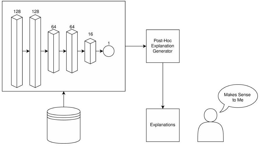
تتمثل هذه الطرق في السعي لتفسير آليات نموذج تم تدريبه بالفعل. كما أوضح سوكول وآخرون باختصار، فإن القابلية للتفسير تتعلق بمخرجات النموذج. من منظور تحليلي أكثر، تشمل الذكاء الاصطناعي القابل للتفسير بشكل أساسي استراتيجيات ما بعد التفسير لتسليط الضوء على النماذج الغامضة، المعروفة بصندوق الأسود. يتم توضيح هذا النموذج في الشكل 1، حيث يتم بناء تفسيرات النموذج لتعزيز فهم المستخدم.
الشكل 1. تصور دورة تصميم الذكاء الاصطناعي القابل للتفسير
أ: غير معتمد على النموذج ونموذج محدد.
يمكن تصنيف الطرق القابلة للتفسير بناءً على ملاءمتها لمعالجة أنواع مختلفة من نماذج الصندوق الأسود. تُسمى الطرق التي تنطبق على النماذج بغض النظر عن هيكلها بالطرق غير المعتمدة على النموذج. تشمل الطرق الشائعة التي تندرج تحت هذه الفئة تفسيرات شابلي الإضافية (SHAP) [23] وتفسيرات النماذج القابلة للتفسير محليًا وغير المعتمدة على النموذج (LIME) [24]. يتم وصف هذه الطرق وطرق أخرى غير معتمدة على النموذج في القسم V-A. يُعرف عكس هذه الطرق بالطرق المعتمدة على النموذج. تم تصميم الطرق المعتمدة على النموذج مثل رسم تنشيط الفئة (CAM) [25] لشبكات الأعصاب التلافيفية (CNNs) للاستفادة من الهيكل الموجود بالفعل لتوفير التفسير. يتم وصف هذه الطرق وغيرها في القسم V-B.

b: التفسيرات المحلية والتفسيرات العالمية.

طريقة أخرى لتصنيف الطرق القابلة للتفسير هي من خلال نطاق التفسير. يتم وصف هذه النطاقات عادةً إما محليًا أو عالميًا. تهدف التفسيرات المحلية إلى تفسير سلوك النموذج لنقطة بيانات واحدة. توفر التفسيرات العالمية تبريرًا يمثل سلوك النموذج لأي نقطة بيانات.

c: مثال على XAI

لتقديم مثال ملموس على XAI، قد يرغب الباحث في استخدام شبكة عصبية طويلة وقصيرة الأمد لتحليل السلاسل الزمنية بسبب قدراتها في النمذجة الزمنية [1]، [6]. النماذج الشائعة في التعلم العميق مثل هذه ليست قابلة للتفسير بشكل شائع، لذا لجعلها قابلة للتفسير، قد يفكر الباحث في استخدام نموذج أبسط، أي الانحدار الخطي،
شجرة القرار، إلخ، لتكون بمثابة بديل للتفسيرات اللاحقة. سيتم تقديم هذه التفسيرات بعد ذلك للمستخدم/المطور/المعنيين لشرح سلوك هيكل الصندوق الأسود الكامن بشكل أفضل.

2) التعلم الآلي القابل للتفسير

يصف التعلم الآلي القابل للتفسير (iML) نماذج التعلم الآلي التي تُعرف بالصناديق البيضاء أو الرمادية [12]، ويتم فرض قابليتها للتفسير من خلال قيود هيكلية أو وظيفية. بين الاثنين، تجعل القيود الهيكلية النماذج بسيطة بما يكفي لفهمها، بينما تحاول القيود الفيزيائية تقديم حسابات النموذج من حيث الميزات الواقعية. بينما يركز XAI على مخرجات النموذج، يركز iML على النموذج نفسه [19]. وقد تم الإشارة إلى ذلك أيضًا على أنه قابلية التفسير الجوهرية لتمييزه عن طرق التفسير اللاحقة [22]، [26]. كما يلي، ستعادل هذه المقالة iML بالنماذج القابلة للتفسير جوهريًا من خلال طرق القيود الهيكلية، والارتباطات الفيزيائية، إلخ. يمكن رؤية ذلك في الشكل 2، حيث لا حاجة لترجمة النموذج من خلال طريقة قابلة للتفسير.
الشكل 2. تصور دورة تصميم التعلم الآلي القابل للتفسير
كمثال ملموس، قد يكون لدى الباحث مشكلة يمكن أن تستفيد من مصنف الانحدار اللوجستي البسيط. مع مثل هذه البنية البسيطة، سيكون النموذج نفسه قابلاً للتفسير حيث سيكون من الواضح ما المدخلات التي تؤثر على أي المخرجات. يمكن للمرء أيضًا استنتاج المعادلة الشاملة إذا كان النموذج بسيطًا بما يكفي. هذا يوضح القابلية للتفسير الجوهرية.

B. الصيانة التنبؤية

الصيانة التنبؤية (PdM) هي فئة فرعية من التنبؤات وإدارة الصحة (PHM) التي شهدت اهتمامًا واسعًا في السنوات الأخيرة [1]، [22]، [27]، [28]. تستخدم PdM الذكاء الاصطناعي ومعلومات الفشل السابقة من الأنظمة الميكانيكية للتنبؤ بحدوث عطل أو توقف في المستقبل [1]، [6]، [29]. يتم تنفيذ PdM باستخدام مجموعة متنوعة من الأدوات، بما في ذلك اكتشاف الشذوذ، وتشخيص الأعطال والتنبؤ [22]، [28].
يتميز اكتشاف الشذوذ وتشخيص الأعطال بفارق واضح. بينما يهدف اكتشاف الشذوذ إلى تحديد ما إذا كان قد حدث عطل أم لا، يهدف تشخيص الأعطال إلى تحديد سبب العطل [28]، [30]. هذا يعني أن اكتشاف الشذوذ يمكن اعتباره مشكلة تصنيف ثنائية، ويمكن اعتبار تشخيص الأعطال امتدادًا لاكتشاف الشذوذ إلى مشكلة تصنيف متعددة. أخيرًا،

يتعامل التنبؤ مع توقع العمر المتبقي المفيد (RUL) أو الوقت حتى الفشل [1]، [6]، [28]. هذا يضع التنبؤ في نطاق مشاكل الانحدار. الآن بعد أن تم تعريف هذه المصطلحات وتصنيفها إلى مشاكلها المختلفة، يمكننا مناقشة البحث المنهجي المتوافق مع PRISMA الذي قمنا به.
استخدمنا بيان العناصر المفضلة للإبلاغ عن المراجعات المنهجية والتحليلات التلوية (PRISMA) 2020 [31]، [32] لوضع منهجية منظمة لأداء مراجعة الأدبيات. يمكن رؤية العملية الكاملة في الشكل 3

A. التعرف

في تحديد قواعد البيانات المحتملة، ركزنا على ناشري علوم الكمبيوتر الشائعين بالإضافة إلى ناشري العلوم العامة. استخدمنا قواعد البيانات التالية للبحث في الأدبيات: IEEE Xplore، مكتبة ACM الرقمية، ScienceDirect وScopus، والتي تم الوصول إليها جميعًا في 21 يونيو 2023. لالتقاط أكبر قدر ممكن، بحثنا في العناوين والكلمات الرئيسية والملخصات مع وضع فكرتين في الاعتبار: XAI و و .
في الحالة الأولى استخدمنا القابل للتفسير القابل للتفسير أو xai لالتقاط المجموعة الأولى من الأوراق. يجب أن تجمع هذه الأوراق مع عبارات شائعة مثل الذكاء الاصطناعي القابل للتفسير، التعلم الآلي القابل للتفسير، التعلم الآلي القابل للتفسير،
XAI، إلخ. لالتقاط جانب PdM، قدمنا كلمات أكثر وضوحًا لتمثيل مجال البحث بشكل أفضل. استخدمنا prognos* أو diagnos* أو RUL أو العمر المتبقي المفيد الصيانة التنبؤية أو الاكتشاف. سيلتقط هذا أفكارًا مثل التنبؤ، التنبؤات، التشخيص، التشخيصات، الاكتشاف، إلخ.
في البحث، تظهر كلمات مثل التنبؤ والتشخيص في المقالات المتعلقة بالطب. هذا منطقي حيث يمكن للكثيرين أن يشهدوا أنهم سيذهبون إلى طبيبهم للحصول على تشخيص. لتقليل إدراج الأدبيات الطبية، تم ضبط ScienceDirect وScopus للنظر في المقالات المتعلقة بالهندسة وعلوم الكمبيوتر فقط. حتى مع هذا الاختيار، كانت مجموعة البحث الأولية 6932 مقالة.
لم يكن هذا التحديد للأوراق فعالًا كما توقعنا في البداية حيث تم فحص العناوين والكلمات الرئيسية والملخصات فقط. قبل إزالة التكرارات، قمنا أيضًا بإزالة المقالات التي لم تذكر الصيانة التنبؤية داخل المقالة. بعد إزالة تلك الأوراق والتكرارات، بدأت عملية الفحص الأولي بـ 296 مقالة.

B. معايير الاستبعاد والفحص

شملت عمليات الفحص الأولية لدينا تصفح الملخصات والأهداف الرئيسية والاستنتاجات والصور للمقالات. استخدمت هذه الفحوصات الأولية معايير الاستبعاد التالية:
  1. لا يعد XAI أو iML محورًا رئيسيًا للمقال.
  2. المقالات ليست دراسات حالة لـ PdM.
  3. لا يتم تقديم أي تفسير أو تفسير.
تظهر الحاجة إلى المعايير الأولين بوضوح. ستذكر العديد من المقالات أحد مصطلحات البحث من XAI/iML، لكنها لن تقع في هذه الفئة من العمل ( ). سيظهر هذا بشكل رئيسي كاستخدام كلمات قابلة للتفسير أو قابلة للتفسير في جملة من الملخص. بالمثل، بالنسبة لدراسات حالة PdM، تذكر العديد من المقالات التشخيص، وما إلى ذلك، في جملة دون أن تكون محور المقال ( ). ومع ذلك، تحتاج المعايير الثالثة إلى تفسير أكثر عمقًا.
عند الإشارة إلى أن هيكلًا ما قابل للتفسير أو قابل للتفسير، يتم زرع توقع معين في ذهن القارئ. ينطبق هذا على أي مفهوم سواء كان متعلقًا بعلوم الكمبيوتر أم لا. واحدة من التوقعات التي اتفقنا عليها كانت تقديم دليل على القابلية للتفسير أو القابلية للتفسير. سيتطلب هذا التفسير من الطريقة القابلة للتفسير أو التفسير الجوهري للنموذج القابل للتفسير. مع وضع هذا التوقع في الاعتبار، تمت إزالة بعض المقالات ( ) قبل الفحص المتعمق بسبب ذكر طريقة تفسيرية دون أي مخرجات للطريقة المذكورة. هذا أنهى مجموعة الفحص بـ 116 مقالة تم السعي لاسترجاعها. لم يتم استرجاع ثلاث منها بواسطة مواردنا. عند الفحص الإضافي، يبدو أن تلك المقالات الثلاث تؤدي إلى روابط ميتة.
للتقييم النهائي للأهلية، تمت قراءة جميع الموارد. كانت العديد من المقالات التي تم استبعادها غير متاحة خارج عرض صغير. من بين المقالات المتبقية البالغ عددها 113، تم استبعاد 11 لأسباب التالية:
الشكل 4. المقالات المنشورة سنويًا في نتائج شمولنا
الشكل 5. اتجاه بحث جوجل لـ PdM و XAI و iML من سنوات مقالتنا
  • ثلاثة يذكرون XAI/iML في الملخص لكنهم لا يستخدمون أي طرق يمكننا العثور عليها.
  • اثنان لم يكونا لا XAI ولا iML. تذكر هذه المصطلحات البحثية في الملخصات، لكنها لا تبني عليها.
  • ثلاثة لا يقدمون أي تفسيرات لطريقتهم التفسيرية.
  • يذكر اثنان PdM في الملخص لكن لا يركزان على PdM في تجربة.
  • لم تكن واحدة دراسة حالة.

ج. الشمولية

بعد مراجعة دقيقة للمقالات، قمنا بتحديد مجموعة من 102 مقالة. يتم الآن مناقشة نتائجنا وهذه المقالات في القسم الرابع.

IV. نتائج البحث

لرسم صورة شاملة لنتائجنا، يوضح الشكل 4 توزيع مجموعة الإدراج لدينا حسب السنة. يظهر هذا اتجاهًا واضحًا متزايدًا في المنشورات يمكن تفسيره بعدة عوامل محتملة. أولاً، تستمر شعبية الصيانة التنبؤية في الزيادة، كما هو موضح في [1] وفي الشكل 5، مع انتقالنا إلى عالم يركز على البيانات الكبيرة في الصناعة. يوفر هذا المزيد من الفرص لتنفيذ هذه الهياكل العصبية الكبيرة والمعقدة جدًا لاتخاذ قرارات مهمة. تؤدي أهمية هذه القرارات إلى سبب ثانٍ لزيادة الأهمية، وهو الثقة.
الشكل 6. توزيع XAI و IML في نتائج البحث
تناقش العديد من المقالات أهمية زيادة ثقة المستخدمين في النموذج مع تقليل التحيز في النماذج السوداء [33]-[36]. يعرف روجات وآخرون الثقة بأنها تتحقق عندما يتمكن النموذج من تفسير قراراته بشكل فعال لشخص ما [18]. سيتطلب ذلك نوعًا من البنية القابلة للتفسير أو القابلة للتفسير بطبيعتها التي يمكن أن تعطي المستخدمين رؤى. علاوة على ذلك، يذكر فولرت وآخرون [22] أن الثقة هي شرط أساسي لتطبيق ناجح يعتمد على البيانات.
عند النظر إلى الشكل 6، تعكس نتائجنا الفكرة القائلة بأن XAI أكثر شعبية قليلاً من iML في PdM. قد يكون أحد الأسباب المحتملة هو الرغبة في الاستفادة من مزايا النماذج المعقدة. تستخدم العديد من المقالات هياكل مثل الشبكات العصبية التلافيفية العميقة [37] أو الشبكات العصبية ذات الذاكرة الطويلة والقصيرة [38] بسبب أدائها العالي في التطبيق. مع الطبيعة الغامضة لهذه النماذج، يحتاج هؤلاء الباحثون إلى طرق قابلة للتفسير بعد الحدث. يبدو أن هذه الرغبة في XAI بدلاً من iML تؤثر على مهام PdM معينة أكثر من غيرها.
تم تصنيف المقالات وفقًا لمهمة PdM في الشكل 7، وتم تمييزها بشكل أكبر إلى XAI و iML ضمن المهام في الشكل 8. تعكس مجموعة مقالاتنا اكتشاف الشذوذ كمهمة رئيسية تستخدم XAI و iML. تشخيص الأعطال والتنبؤ متساويان تقريبًا في عدد المقالات المنشورة ضمن هذه المجموعة؛ ومع ذلك، يظهر الشكل 8 أن الاهتمام بـ XAI و iML معكوس في هذه المجموعات. باختصار، يركز التنبؤ على XAI، بينما يركز التشخيص على iML. الآن نصف العديد من الطرق التي تم تطبيقها على مجموعات البيانات المتنوعة الموضحة في الجدول 1. هذه الطرق مقسمة بين القسم V لطرق XAI والقسم VI لطرق iML. بالإضافة إلى ذلك، يمكن العثور على مقالات محددة ذات اهتمام في الجدول 4.

V. الذكاء الاصطناعي القابل للتفسير في الصيانة التنبؤية

تلتقط XAI في الصيانة التنبؤية مجموعة واسعة من الطرق التي يمكن تصنيفها بعدة طرق. لتجنب تكرار المعلومات، تم تقسيم الطرق إلى ثلاثة أقسام فرعية: غير مرتبطة بالنموذج، مرتبطة بالنموذج، ومجموعة.

أ. غير معتمد على النموذج

يصف هذا القسم الطرق القابلة للتفسير في مجموعتنا، كما هو موضح في الجدول 2، التي يمكن تطبيقها على أي بنية.
الشكل 7. الأوراق البحثية حول كشف الشذوذ (AD)، تشخيص الأعطال (FD)، والتنبؤ (Prog)
الشكل 8. الانقسام بين XAI و iML حسب فئة الصيانة التنبؤية
تُعرف هذه الطرق بشكل غير رسمي بأنها طرق تفسيرية غير مرتبطة بالنموذج [149]. يمكن تطبيق هذه الطرق الموجودة في هذا القسم على أي بنية وتتكون من SHAP في القسم V-A1 وLIME في القسم V-A2 وطرق إضافية ذات صلة.
  1. تفسيرات شابلي الإضافية (SHAP).
تم تقديم قيم SHAP بواسطة لوندبرغ وآخرين كقياس موحد لأهمية الميزات [23]. تعتمد SHAP على ثلاث خصائص مشتركة مع تقدير قيمة شابلي الكلاسيكية: الدقة المحلية، والافتقار، والاتساق. تشير الدقة المحلية إلى قدرة المدخلات المبسطة على مطابقة مخرجات المدخلات من البيانات على الأقل. يشير الافتقار إلى الميزات التي تفتقر إليها المدخلات المبسطة. باختصار، هذا يعني أنه إذا كانت ميزة ما غير مفيدة للتفسير، فهي غير مفيدة للنموذج. أخيرًا، يجلب الاتساق الفكرة القائلة بأن أهمية ميزة ما يجب أن تظل كما هي أو تزداد بغض النظر عن الميزات الأخرى.
حتى الآن، تُعتبر SHAP الطريقة الأكثر استخدامًا التي تم رؤيتها في عيّنتنا. علاوة على ذلك، تُعد SHAP واحدة من الطرق القليلة التي تم تطبيقها على مشاكل كشف الشذوذ [72]، [106][108]، تشخيص الأعطال [130]، [134]، والتنبؤ [75]، [77]، [112]. من المحتمل أن يكون ذلك بسبب تنوعها الواسع كطريقة مستقلة عن النموذج يمكن أن تقدم تفسيرات عالمية.
أنشأ ستورتيwagen وآخرون [134] إطارًا لتشخيص الأعطال يتكون من ثلاثة أجزاء: جمع البيانات، التنبؤ-
الجدول 1. مجموعات البيانات من البحث في الأدبيات
مجموعات البيانات مقالات
محامل و PRONOSTIA [39]، 40] |41|-|53
[33]، [37]، [54]، |55]
المركبات أو نظام فرعي للمركبة [56]-|68
CMAPSS [69] [35]-|37], |70|-|79|
[80]
أعطال وآخطاء الآلات العامة 81 [42]، [48]، |82|-|86]
قطارات [٣٤]، |٨٧-|٩٢
صناديق التروس [93] |42|، 45، 48، |94|
مجموعة بيانات اصطناعية [٤٤، ٩٥، ٩٦
الصلب المدرفل على الساخن أو البارد [72]، |95|، |97|
مضخة ميكانيكية [98-|100]
طائرة [52],101
ألعاب الملاهي [102],103
مسارعات الجسيمات [104, 1105
مصنع كيميائي [١٠٦، ١٠٧
بحري [108-110
أشباه الموصلات |111| |112|, 113
مكيفات الهواء ٥٦
الأقراص الصلبة [114] [٣٨، [٧٠]، |١١٥]
عملية تينيسي إيستمان |116 70
آلات الضغط ١٠٣
مستودع تعلم الآلة UCI [117] 1118
توربينات الرياح [119] [120]-|122
محولات |123
بطاريات الليثيوم أيون [124] [٣٧، |١٢٥|، |١٢٦|]
سخانات 127
بيانات التحكم الرقمي بالكمبيوتر 128
الأقمشة ١٢٩
آلات بثق البلاستيك ١٣٠
آلة الضغط 131
آلات الفحم 132
ثلاجات ١١٣٣
ضواغط الغاز 134
أنظمة هيدروليكية 135
أفران صناعة الحديد 1136
أدوات القطع ١٣٧
خطوط الطاقة [138] ١٣٩
معدات الاتصالات ١٤٠
مضخة مياه 141
معدات حفر النفط 142
صمامات تعمل بالملف اللولبي 143
نواقل الفحم ١٤٤
أجهزة مراقبة درجة الحرارة 145
وحدة التقطير 146
أنابيب المياه [147] 148
الأخت، والتشخيص. من المهم أنه في مرحلة جمع البيانات، تلقوا التقارير المرتبطة بالأعطال. استخدم قسم التنبؤ خوارزمية XGBoost لاكتشاف حدوث عطل. استخدم التشخيص SHAP لتحديد الميزات المهمة لنتيجة XGBoost. يتم التحقق من هذه الميزات باستخدام التقارير التي ترافق العطل.
اقترح تشوي وآخرون [107] طريقة للكشف عن الشذوذ غير الخاضع للإشراف القابل للتفسير للتنبؤ بإيقاف الأنظمة في العمليات الكيميائية. تتكون طريقتهم مما يسمونه إطار عمل مستقل عن الفترة وإطار عمل متكامل مع الفترة. بحث الإطار المستقل عن الفترة عن أفضل نموذج للكشف عن الشذوذ وطبق الطريقة القابلة للتفسير. في الإطار المتكامل مع الفترة، طبقوا المعلومات في الوقت الحقيقي على النموذج المختار من الإطار السابق. وجدوا أن غابة العزل قدمت أفضل النتائج في الإطار المستقل عن الفترة بناءً على
الجدول 2. الطرق القابلة للتفسير من الأدبيات
طريقة مقالات
قيم شابلي V-A1
لايم V-A2
أهمية الميزة
LRP V-A4 القائم على القواعد V-A5
كام وجرادكام V-B1
سوروجيت V-A6
التصور V-A9
DIFFI V-B2
التدرجات المتكاملة (V-A7)
استدلال سببي V-AB
ACME V-A10
الإحصائيات V-A11
SmoothGrad V-A12
الافتراضات المضادة V-A13
ليون فورست V-B3
اشرح لي كأنني في الخامسة V-A14
خرائط البروز (V-B4)
أركانا V-B5
[72]، [95]، [106|-|108|، [130]، [132]
[36]-[38], [42], [66], [75]-[77], [112], [131], [134]
[35]-|38|، [44]، [50]، [51]، [54]، [61]، [66]، [76]، 84]
[٣٤]، [٥٤]، [٦٧]، [٨٥]، [٨٦]، [٩٢]، [١٠٤]، [١١٠]، |١٣٧|، |١٣٩|
٣٧، ٤٤، ٦٨، [١٠٥]، [١٢٦]
65، 70، 71، 73
٣٧، ٤٤، ٤٨، ٦٣،
|82|، |89|، |95|، |40|
٤٧، |٧٤، ١٠٩، ١٢٩
[42، 102]، 128]
94، |131
٨٨
١٠٣]
٥٩
[13]
97
96
51
37
[120]
عدد الإغلاقات غير المخطط لها التي تم اكتشافها، وقد استخدموا SHAP كوسيلة فعالة لقياس تحليل السبب الجذري.
قام غاشي وآخرون [112] بإجراء صيانة تنبؤية على نظام متعدد المكونات. كان هدفهم هو نمذجة الاعتماد المتبادل وتقييم أهمية الاعتماد المتبادل. قبل تدريب نموذج الغابة العشوائية الخاص بهم، استخدموا الاستكشاف البصري لدراسة الاعتماد المتبادل. استخدموا طريقتين لتبرير استخدام الاعتماد المتبادل: الإحصائيات وXAI. استخدموا اختبار كاي-تربيع لإظهار أن أداء نموذج مع الاعتماد المتبادل أفضل ( ). عند تطبيق SHAP على الغابة العشوائية، أظهروا أن متغيرات الاعتماد المتبادل كانت عادةً من بين أهم ميزات الشرح. هذا يضيف مصداقية لـ SHAP كطريقة قابلة للتفسير من حيث دقة شروحاتها.
2) تفسيرات نموذجية قابلة للتفسير محليًا (LIME). تم تقديم LIME من قبل ريبيرو وآخرون كوسيلة لشرح أي نموذج باستخدام تمثيل محلي حول التنبؤ [24]. يتم ذلك عن طريق أخذ عينات حول بيانات الإدخال المعطاة وتدريب نموذج خطي باستخدام البيانات المأخوذة. من خلال القيام بذلك، يمكنهم توليد تفسير يتوافق مع ذلك التنبؤ بينما يستخدمون فقط المعلومات المستمدة من النموذج الأصلي.
قام بروتوباباداكيس وآخرون [35] بحساب RUL كما تم تطبيقه على مجموعة بيانات CMAPSS لمحركات التوربين. حاولوا في البداية إجراء تنبؤ بـ RUL باستخدام نموذجين، غابة عشوائية وشبكة عصبية عميقة. وجدوا أن الغابة العشوائية كانت أداؤها ضعيفًا، مما سيؤدي إلى شروحات ضعيفة. حققت شبكتهم العصبية العميقة أداءً عاليًا، لذا طبقوا LIME. قارنوا بين تفسيرين لـ LIME، واحد لحياة مبكرة وآخر لحياة متأخرة مع عطل محدد. وجدوا أن LIME كانت قادرة على تصنيف الميزات المهمة لـ
الأعطال التي تعكس الأعطال الفيزيائية. بالإضافة إلى ذلك، أظهروا أن LIME ستواجه صعوبة أكبر في تصنيف الميزات المهمة عندما تم تطبيقها على مقاطع بدون أعطال حيث يمكن أن يحدث أي شيء في المستقبل.
ناقش الله بخش وآخرون [92] عدة مصنفات قائمة على الأشجار للتنبؤ بالحاجة إلى أحداث الصيانة، أي، اكتشاف الشذوذ، لمفاتيح القطارات. من مجموعة مصنفاتهم القائمة على الأشجار، بما في ذلك شجرة القرار، الغابة العشوائية، وشجرة معززة بالتدرج، حددوا الشجرة المعززة بالتدرج كالأكثر دقة بين النماذج عند التنبؤ ما إذا كانت ستحدث مشكلة. في اختبار منفصل، جعلوا نفس النماذج تتنبأ بأنواع معينة من الشذوذ. في هذه التجربة، تفوقت الغابة العشوائية على البقية. من أجل القابلية للتفسير، طبقوا LIME للتعلم من مخرجات الغابة العشوائية. يعتزم الباحثون أن تساعد المخرجات من LIME في بناء الثقة في النموذج لخبراء المجال وصانعي القرار

3) أهمية الميزات.

تشير أهمية الميزات إلى فكرة أن بعض ميزات الإدخال لها تأثير أكبر على المخرجات من غيرها. على سبيل المثال، عند تحديد ما إذا كانت الصورة كلبًا، فإن الخلفية التي لا تحتوي على بكسلات من الكلب ستكون أقل أهمية من البكسلات التي تحتوي على الكلب. عادةً ما يتم تقييم أهمية الميزات باستخدام تقنيات مثل SHAP وLIME، ولكن توجد طرق متنوعة في الأدبيات.
لقد طبق العديد من الباحثين طرقًا مختلفة لحساب أهمية الميزات. تناول بكدي وآخرون [110] الصيانة التنبؤية لأنظمة دفع السفن. جمعوا بين نماذج الغابة العشوائية المتوازنة والتعلم متعدد الحالات لتحقيق معدل إيجابي حقيقي مرتفع تم شرحه بعد ذلك عبر أهمية ميزات جيني. كما طبق شميتز وآخرون [137] أهمية ميزات جيني للتحقق من مفسر الشجرة [150] لمصنف الغابة العشوائية الخاص بهم.
قام باحثون آخرون بترتيب ميزاتهم بطرق مختلفة. قام مانكو وآخرون [34] بإجراء تنبؤ بالأعطال لتدريب الأنظمة حيث قاموا بترتيب خطوات الوقت حسب مدى شذوذها ضمن نافذة زمنية. تم إجراء هذا الترتيب من خلال نمذجة خليط الاحتمالية السابقة للاتجاه مع احتمال أن يكون الاتجاه سلوكًا طبيعيًا. طبق ماركاتو وآخرون [104] اكتشاف الشذوذ على مسرعات الجسيمات حيث تم استخدام أهمية الميزات المعتمدة على التبديل لتوجيه تطوير النموذج بشكل أكبر.
أخيرًا، اقترح فورونوف وآخرون [67] وغاسيمخاني وآخرون [86] طرقًا مختلفة لحساب أهمية الميزات التي تتناول مشاكل مختلفة. اقترح فورونوف وآخرون محدد متغيرات قائم على الغابة يسمى توزيع عمق المتغيرات (VDD) الذي تناول مشكلة الاعتماد المتبادل للمتغيرات من خلال تجميع الميزات. ظهرت الميزات المهمة في مجموعات متعددة. طور غاسيمخاني وآخرون K-Star المتوازن للتعامل مع مشكلة عدم التوازن الموجودة عادة في الصيانة التنبؤية. لإضافة القابلية للتفسير، طبقوا اختبار كاي-تربيع لتحديد الميزات المهمة في فشل الآلة.
4) انتشار الصلة على مستوى الطبقة (LRP).
تم تقديم LRP من قبل باخ وآخرون [151] كطريقة قابلة للتفسير تفترض أن المصنف يمكن تفكيكه إلى عدة طبقات من الحساب. يعمل LRP مع مفهوم درجة الصلة التي تقيس مدى أهمية ميزة ما لمخرج. يعمل LRP عن طريق استقراء الصلة إلى طبقة الإدخال من خلال التحرك للخلف عبر الهيكل بدءًا من طبقة المخرج. يمكن بعد ذلك قياس أهمية ميزة الإدخال كمجموع للميزات التي تؤثر عليها عبر الهيكل.
يعتبر LRP من الفئة غير المعتمدة على النموذج والتي يمكن رؤيتها في حالات الاستخدام في الأدبيات. طبق فالسبرغر وآخرون [105] LRP على هياكل متعددة بما في ذلك kNN، الغابة العشوائية، ونماذج قائمة على CNN. من خلال LRP، وجدوا أن هياكل CNN كانت تتعلم ميزات مهمة مما أدى إلى أداء أعلى. قام هان وآخرون [68] بإجراء تشخيص للأعطال للمحركات باستخدام النموذج البارز LeNet [152]. من خلال استخدام LRP، تمكنوا من جلب القابلية للتفسير إلى هيكل بارز.
اقترح وانغ وآخرون [126] طريقة لاستخدام القابلية للتفسير كوسيلة لدفع عملية التدريب. استخدموا LRP لحساب أهمية الميزات لبيانات التدريب. تم تضمين حسابات الأهمية لتحسين أداء النموذج. قدموا هذا النهج المدفوع بالقابلية للتفسير لمشكلة بطاريات الشيخوخة، وأظهروا دقته الممتازة عند مقارنتها بنهج مدفوع بالبيانات.

5) المفسرات القائمة على القواعد.

تستخدم المفسرات القائمة على القواعد مزيجًا من النموذج الأسود وبيانات التدريب لإنشاء سلسلة من قواعد IF-THEN. يتم إنشاء هذه القواعد عمومًا باستخدام المنطق التوافقي (ANDs، ORs، وNOTs) لدمج الميزات في جزء IF من القواعد. يتم ملء جزء THEN من القواعد بالنتيجة من النموذج، عادةً فئة أو قيمة متوقعة. ثم يتم تقديم القواعد كتفسيرات أو قد تُستخدم كبديل للنموذج الأسود نفسه.
حتى في المفسرات القائمة على القواعد، هناك العديد من الطرق التي تم استخدامها. اقترح وو وآخرون [71] إطار K-PdM (PDM الموجه نحو KPI)، وهو نموذج HMM قائم على التجمع يعتمد على مؤشرات الأداء الرئيسية (KPIs). KPI هو متجه لميزة واحدة من التدهور الدقيق، ومجموعة من KPIs تعكس صحة الآلة. تم نمذجة الصحة كنموذج HMM لكل KPI. تم تحويل هذه النماذج HMM إلى نظام استدلال قائم على القواعد من أجل القابلية للتفسير.
أظهر برونيلو وآخرون [70]، [73] مرتين أن المنطق الزمني يمكن استخدامه في اكتشاف الشذوذ. أولاً، أظهروا أنه يمكن إضافة المنطق الزمني الخطي إلى نظام عبر الإنترنت لمراقبة الأعطال [73]. مرة أخرى، أظهروا أن المنطق الزمني يمكن استخدامه في نهج مختلف لنفس المشكلة. أنشأ برونيلو وآخرون [70] أشجار بناء جملة استخدمت عبارة منطق زمني إشارة محدودة. تم تعديل الأشجار باستخدام نهج تطوري للتنبؤ بالفشل في محرك Blackblaze Hard Drive [114]، وعملية تينيسي إيستمان [116]، ومجموعة بيانات CMAPSS [69]، وهي مجموعات بيانات مستخدمة بشكل شائع لصيانة محركات الأقراص الصلبة والعمليات الكهربائية و
محركات التوربين. أدت هذه الطريقة إلى أداء رائع مع تفسيرات قائمة على القواعد.
طبق ريبيرو وآخرون [65] الذكاء الاصطناعي القابل للتفسير (XAI) على عملية التعلم عبر الإنترنت باستخدام مشفر طويل وقصير المدى (LSTMAE) لنمذجة أعطال النقل العام. في الوقت نفسه، تعلم نظام المؤلفين قواعد الانحدار التي تفسر مخرجات النموذج. بينما كان نظامهم يتعلم كيفية رسم الشذوذ، تم إدخال مخرجات نموذجهم إلى خوارزمية تعلم قواعد التدفق (AMRules). طبقوا طريقتهم على أربعة مجموعات بيانات للنقل العام، وقدموا تفسيرات قائمة على القواعد العالمية والمحلية المستخدمة في نظامهم.

6) نماذج الوكلاء.

النماذج البديلة هي نماذج أبسط تُستخدم لتمثيل نماذج أكثر تعقيدًا. تأخذ هذه النماذج البديلة عمومًا شكل أشجار قرار بسيطة ونماذج انحدار خطي/لوجستي. الطبيعة البسيطة لهذه النماذج تجعلها قابلة للتفسير؛ ومع ذلك، فإن استخدامها له قابلية تفسير كطريقة قابلة للتفسير لنموذج صندوق أسود.
عند استخدام نموذج بديل كطريقة قابلة للتفسير، يجب أن يكون النموذج البديل قابلاً للتفسير بشكل جوهري للسماح بجمع تفسير من النموذج الرئيسي. استخدم غلوك وآخرون [82] نموذجين من ARIMA لشرح نموذج الغابة العشوائية. تعلم نموذج ARIMA الأول نفس البيانات التي تعلمها نموذج الغابة العشوائية، بينما تعلم نموذج ARIMA الثاني الأخطاء المتبقية من نموذج الغابة العشوائية. في حين أن نموذج الغابة العشوائية ليس قابلاً للتفسير، يمكن للنموذجين من ARIMA أن يظهرا ما يمكن وما لا يمكن أن يتعلمه نموذج الغابة العشوائية.
اقترح زانغ وآخرون [140] استخراج قاعدة ارتباط الإنذار بالخلل استنادًا إلى أهمية الميزات وأشجار القرار. بدأت عمليتهم بغابة عشوائية موزونة. تم إجراء اختيار الميزات لجمع الميزات المهمة في الحالة الشاذة. تم استخدام هذه الميزات لإنشاء سلسلة من أشجار القرار C4.5 التي نمذجة ميزات مختلفة. بمجرد تدريب غابتهم العشوائية وتوقع خلل، يمكن استخدام شجرة القرار ذات الدقة الأعلى لاستنتاج تفسير للخلل.
اختبر إيراندونيا وآخرون [89] الذكاء الاصطناعي القابل للتفسير في الحوسبة الطرفية مع جميع النماذج الممكنة فيH2O.aiاستخدمت AutoML الخاصة بهم لأداء تشخيص الأعطال. بعد تحديد الهياكل المثلى، قاموا بتدريب نموذج شجرة قرار بديل لإضافة قابلية التفسير إلى عملية AutoML الخاصة بهم. من خلال تحسين الأجهزة والدقة، أظهروا أن الصيانة التنبؤية القابلة للتفسير يمكن أن تحدث نظريًا على أجهزة الحوسبة الطرفية.

7) التدرجات المتكاملة.

تم تقديم التدرجات المتكاملة بواسطة سونداراجان وآخرين [153] لنسب توقعات بنية عميقة إلى ميزات إدخالها. يقدمون اثنين من المسلمات، الحساسية وثبات التنفيذ، لبناء طريقتهم القابلة للتفسير. يتم تحقيق الحساسية إذا كان لكل إدخال وقاعدة تختلف في ميزة واحدة ولكن لديها توقعات مختلفة، فيجب أن تُعطى الميزة المختلفة نسبة غير صفرية. يعني ثبات التنفيذ أن النسب تكون دائمًا متطابقة-
تُحسب التدرجات المتكاملة من خلال جمعات صغيرة عبر تدرجات الطبقات، مع وضع هذه البديهيات في الاعتبار.
قدم حاجاتو وآخرون [94] إطار عمل PredMaX للصيانة التنبؤية الذي حدد الأجزاء الحساسة من الآلات وقام بتجميع الفترات الزمنية. يعمل في خطوتين: تم تطبيق مشفر تلقائي عميق على البيانات، وتم إجراء التجميع في الفضاء الكامن في المشفر التلقائي. من التجمعات، أظهروا أي القنوات تساهم في الانتقال من الحالة الطبيعية إلى الحالة غير الطبيعية. بالإضافة إلى ذلك، تم استخدام تقنية التدرجات المدمجة لاستخراج قنوات المستشعر ذات الصلة لجزء الآلة المعطل.

8) الاستدلال السببي.

تتجاوز السببية مفهوم الاعتماد الإحصائي حيث تظهر علاقة حقيقية بين متغيرين أو أكثر [154]. يمكن قياس السببية من خلال قوة السببية التي تقيس التغير في توزيع المتغيرات عندما يتم تغيير متغير واحد [154]. السببية ليست سمة سهلة للتحليل حيث يمكن اكتشافها حقًا فقط من خلال الملاحظات المتكررة لظاهرة تحدث نتيجة لحدث ما؛ ومع ذلك، كانت الاستدلالات السببية طريقة من طرق الذكاء الاصطناعي القابل للتفسير التي استخدمها بعض الباحثين.
صمم تريلا وآخرون [88] إطار عمل لاكتشاف الشذوذ يعتمد على مشفر تلقائي متغير لإزالة الضوضاء (VAE) وشبكة عصبية متعددة الطبقات (MLP). قاموا باستخراج أنماط داخل النظام الفرعي وبين الأنظمة الفرعية من خلال تحويل بيانات السلاسل الزمنية إلى فوكسيلا. قام الـ VAE بتعميم التضمينات. وأخيرًا، تم استخدام الـ MLP لإنشاء دالة احتمالية تشخيصية سلسة. طبقوا طريقتهم على مجموعة بيانات الحركة واستخدموا الاستدلال السببي عبر خوارزمية بيتر-كلارك للإجابة على السؤال “هل تعلم الـ VAE علاقات السبب والنتيجة؟” وجدوا أن الـ VAE يمكن أن يوصف في أفضل حالاته بأنه نمذجة لعلاقة ارتباط، لكن هذه القيود كانت تعزى بشكل رئيسي إلى محدودية توفر البيانات.

9) التصور.

تقنيات التصور لا تتخذ أي شكل محدد. بشكل عام، تأخذ هذه التصورات شكل تصور الأوزان؛ ومع ذلك، يمكن أن تأخذ أيضًا شكل تصور أمثلة محددة. في كلتا الحالتين، تفيد هذه الطرق المستخدمين من خلال تقديم صورة توضح للمستخدم كيفية عمل المعمارية من الداخل.
يمكن استخدام التصورات بطرق عديدة لزيادة الفهم. استخدم ميكالوسكا وآخرون [109] التصورات لمقارنة البيانات الصحية والشاذة. استخدم كوستا وآخرون [74] التصورات مع مشفر تكراري متغير. يظهرون أن الفضاء الكامن الذي أنشأه المشفر يمكن أن يضيف إلى الفهم. عندما تمر بيانات الإدخال ذات القيم المتبقية المشابهة عبر المشفر، يظهرون أن الفضاءات الكامنة متشابهة لتلك التي لها قيم متبقية مشابهة.
سعى شين وآخرون 47 إلى معالجة تشخيص أعطال المحامل من خلال نموذج جديد يسمى الشبكة المتبقية ذاتية المعايرة المعدلة باستخدام تحويل فورييه القصير الزمني اللوغاريتمي (log-STFTMSCResNet). يقوم تحويل فورييه القصير الزمني باستخراج ميزات الزمن-التردد من الإشارات الخام للاحتفاظ بالمعنى الفيزيائي لتوقيعات الأعطال.
الشكل 9. استخدام طرق الذكاء الاصطناعي القابل للتفسير
التي تم تصورها من أجل التفسير. يتم استخدام MSCResNet لتوسيع مجال الاستقبال دون إدخال المزيد من المعلمات. مع الجمع بين الاثنين، يهدفون إلى تحقيق دقة عالية حتى في ظل ظروف العمل غير المعروفة. قاموا بمقارنة نموذجهم مع نماذج شائعة مثل LSTM وResNet18. أداء log-STFT-MSCResNet كان من بين الأفضل حتى في ظل ظروف العمل غير المعروفة، وكان لديه عدد قليل من الميزات ووقت تدريب أقصر من الآخرين.

10) تفسيرات نموذجية غير محددة متسارعة (ACME).

تم تقديم ACME بواسطة Dandolo وآخرين [155] كطريقة لتوليد مقاييس أهمية الميزات المحلية والعالمية بسرعة استنادًا إلى اضطرابات البيانات. بالنسبة للتفسيرات العالمية، يأخذون متجهًا يحمل متوسط كل ميزة عبر مجموعة البيانات بأكملها؛ يُعرف هذا باسم متجه الأساس. ثم يتم إنشاء مصفوفة كميّة متغيرة تحتوي على الكميات المختلفة للميزات. تُستخدم هذه المصفوفة لجمع التنبؤات التي تمثل كل كميّة. وأخيرًا، يتم حساب أهمية الميزات العالمية لكل ميزة من خلال حساب التأثير المعياري عبر كل كميّة. للحصول على تفسير محلي، يتم استبدال متجه الأساس بنقطة البيانات المحددة التي يُراد تفسيرها.
طبق أنيلو وآخرون [103] ACME على مشكلة اكتشاف الشذوذ لمقارنتها بـ SHAP. استخدموا غابة العزل لاكتشاف الشذوذ لأنها تُستخدم عادةً لاكتشاف القيم الشاذة أو الشذوذ. تم استخدام درجة الشذوذ كعلامة لسلسلة الزمن لتمثيل المشكلة كمهام انحدار مما يسمح بتطبيق ACME. بعد تطبيق SHAP و ACME على مجموعة بيانات الأفعوانية ومجموعة بيانات آلة الضغط، وجدوا تسريعًا كبيرًا.
باستخدام ACME مع جميع البيانات بينما سيكون SHAP أبطأ حتى مع الوصول إلى من البيانات.
11) الإحصائيات.
كطريقة للتفسير المطبقة على مشكلة الصيانة التنبؤية، يمكن استخدام الاختبارات الإحصائية لمقارنة توزيع الميزات بين الفئات المختلفة.
طور فان وآخرون [59] طرق تعلم الآلة التي تستفيد من المعرفة الفيزيائية لزيادة القابلية للتفسير. كانت دراستهم حالة اكتشاف الأعطال المتعلقة بالتسرب في أنظمة الهواء في المركبات. طبقوا ثلاث معادلات فيزيائية على بياناتهم التي كانت ستقوم بنمذجة تسرب الهواء. علاوة على ذلك، استخدموا تلك البيانات في بيانات التدريب لنماذج kNN وMLP الخاصة بهم. أظهرت النتائج أن النماذج المدعومة بالفيزياء تفوقت على النماذج غير المدعومة.
12) تدرجات سلسة (SmoothGrad).
تم تطوير SmoothGrad بواسطة Smilkov وآخرين [156] لإنتاج خريطة حساسية تعتمد على التدرج. الفكرة وراء SmoothGrad تتضمن اشتقاق النموذج التنبؤي بالنسبة للإدخال. هذه الاشتقاق ينشئ خريطة حساسية تمثل مدى تأثير تغيير في كل بكسل من الإدخال على التصنيف [156]. علاوة على ذلك، يمكن أن تُظهر هذه الخريطة الحساسية بشكل مثالي المناطق التي تعتبر أساسية للتنبؤ.
13) الافتراضات المضادة.
تم تقديم العوامل المضادة للواقع بواسطة واتشر وآخرون [157] لتوفير بيانات حول الفروقات اللازمة لتحقيق النتيجة المرغوبة. تعمل هذه الطريقة أيضًا من خلال توفير
تفسير لنتيجة النموذج، لكن هذه القدرة الإضافية تجعل العوامل المضادة فريدة جدًا في مجال طرق الذكاء الاصطناعي القابلة للتفسير.
طور جاكوبوفسكي وآخرون [97] حلاً للصيانة التنبؤية لعملية الدرفلة الباردة الصناعية. استخدموا خوارزمية شبه مشروطة تعتمد على مشفر تلقائي مستند إلى الفيزياء (PIAE). تم إبلاغ هذه البنية بالفيزياء من خلال تطبيق قائمة من المعادلات في بداية بيانات الإدخال الخاصة بهم. تم إلحاق ناتج المعادلات ببيانات الإدخال لمشفرهم التلقائي. أثبت نموذجهم أنه أكثر دقة من مشفر تلقائي أساسي. بينما يحتوي PIAE على بعض الجوانب القابلة للتفسير بالفعل، فقد طبقوا العوامل المضادة كطريقة للتفسير لإظهار الميزات المهمة من قرارات خوارزميتهم.

14) اشرح لي كأني في الخامسة (ELI5).

ELI5 هي طريقة شائعة من Github [158] يتم صيانتها بواسطة المستخدم TeamHG-Memex و 15 مساهمًا آخر. تركز هذه المكتبة في بايثون على شرح أوزان النموذج، والتي تعمل أيضًا كطريقة لحساب أهمية الميزات. بينما تحافظ على الطرق الأصلية، توفر ELI5 أيضًا تنفيذات لطرق أخرى لشرح النتائج.

ب. نموذج محدد

تصف هذه القسم الطرق القابلة للتفسير في مجموعتنا التي تعتمد التفسيرات على خصائص الهيكل المعماري الذي تهدف إلى شرحه. تُعرف هذه الطرق بأنها محددة النموذج [149]. هنا نناقش الطرق التي تستفيد من الهيكل لتوليد التفسيرات مثل CAM وGradCAM في القسم V-B1. DIFFI في القسم V-B2 والمزيد.

1) رسم تفعيل الفئة (CAM) ورسم تفعيل الفئة المدعوم بالتدرج (GradCAM).

تم تقديم CAM بواسطة زو وآخرين [25] كطريقة للتفسير العالمي لشبكات الأعصاب التلافيفية (CNN). الخريطة التي يتم إنشاؤها تشير إلى مناطق الصورة التي تستخدمها CNN لتحديد الفئة المستهدفة. يقوم CAM بذلك من خلال استخدام طبقة التجميع المتوسط العالمي (GAP) في بنية CNN التي تخرج المتوسط المكاني لخريطة الميزات في الطبقة النهائية. يتم ربط البكسلات ذات القيم الأعلى بالبكسلات في الصورة المرتبطة بتسمية الفئة. بالإضافة إلى ذلك، قام سيلفراجو وآخرون [159] بتوسيع CAM إلى GradCAM من خلال استخدام معلومات التدرج المتجهة إلى آخر طبقة تلافيفية لفهم أهمية الميزات.
تم التحقق من GradCAM من خلال دراسات مختلفة عبر المقارنة والمقاييس. يركز مي وآخرون [44] على إمكانية تفسير الذكاء الاصطناعي القابل للتفسير (XAI) لشرح شبكة الأعصاب التلافيفية (CNN). لقد بحثوا في GradCAM وLRP وLIME كطرق لشرح شبكة الأعصاب التلافيفية لاكتشاف الشذوذ. وجدوا ميزات غير قابلة للتمييز تم تسليط الضوء عليها بواسطة LRP، ووجدوا ميزات غير مهمة تم تسليط الضوء عليها بواسطة LIME. كان GradCAM قادرًا على تسليط الضوء على الميزات المهمة التي قاموا بتصنيفها قبل تدريب شبكة الأعصاب التلافيفية. قد يشير هذا إلى أن الطرق المحددة للنموذج تتفوق على الطرق غير المحددة للنموذج عندما يكون ذلك ممكنًا.
يقدم سوليس-مارتن وآخرون [37] مقارنة بين LIME وSHAP وLRP وSaliency Maps الخاصة بالصورة وGradCAM كما تم تطبيقها على مجموعات بيانات الصيانة التنبؤية مثل CMAPSS والبطاريات. يحددون ثمانية مقاييس للمقارنة: الهوية، القابلية للفصل، الاستقرار، الانتقائية، التماسك، الاكتمال، التوافق والذكاء، وهو تقييم اقترحه المؤلفون. عند مقارنة الطرق المختلفة كما تم تطبيقها على بنية CNN، كانت GradCAM الأفضل من حيث المقاييس التسعة.
يقترح أو وآخرون [63] إطار عمل لاكتشاف الأعطال وتشخيصها يتكون من شبكة عصبية تلافيفية أحادية الأبعاد لاكتشاف الأعطال، وخرائط تنشيط الفئات لتشخيص الأعطال (طريقة قابلة للتفسير) و VAE لتنفيذ ملاحظات المستخدم. تستخدم الشبكة العصبية طبقة GAP كطبقة إخراج نظرًا لقدرتها على الحفاظ على المعلومات الزمنية. وهذا يسمح لهم أيضًا باستخدام CAM كطريقة قابلة للتفسير بدلاً من GradCAM. يتم استخدام VAE بمبدأ منطق القمامة في الداخل، قمامة في الخارج لتقليل عدد الإيجابيات الكاذبة والسلبيات الكاذبة التي ستُعرض على المستخدمين. للتحقق من طريقتهم، يطبقونها على مجموعة بيانات فورد موتور، وهي مجموعة بيانات لمحرك السيارة تحتوي على كمية من البيانات الضوضائية. يظهرون أن نموذجهم دقيق حتى في البيانات الضوضائية، ويظهرون أن VAE يزيد من دقتهم. كما يظهرون عبر CAM أن البيانات الشاذة قابلة للفصل خطيًا، وهو ما يوجد في VAE.
2) أهمية الميزات المستندة إلى عمق غابة العزل (DIFFI). تم تقديم DIFFI بواسطة كارليتي وآخرين [160] كطريقة قابلة للتفسير لغابات العزل. غابات العزل هي مجموعة من أشجار العزل التي تتعلم النقاط الشاذة من خلال عزلها عن النقاط العادية. يعتمد DIFFI على فرضيتين لتعريف أهمية الميزات حيث يجب أن: تؤدي إلى عزل النقاط الشاذة عند عمق صغير (أي، بالقرب من الجذر) وتنتج عدم توازن أعلى على النقاط الشاذة بينما تكون عديمة الفائدة على النقاط العادية [160]. ستسمح هذه الفرضيات بتقديم تفسيرات للبيانات الشاذة مما سيمكن من تقديم تفسيرات للنقاط الشاذة أو البيانات المعيبة.
قام برنو وآخرون [102] بتنفيذ كشف الشذوذ للرحلات الآلية في حدائق الترفيه. قدموا فكرة توفير ميزات محددة تركز على الشذوذ من خلال تقسيم بياناتهم إلى مجموعة متعددة المتغيرات والعديد من المجموعات أحادية المتغير بناءً على معرفة سابقة. استخدموا غابة العزل لنمذجة السلاسل الزمنية متعددة المتغيرات مع DIFFI لشرح الناتج. قاموا بنمذجة السلاسل الزمنية أحادية المتغير باستخدام شبكة غاز عصبية تنمو عند الحاجة (GWR). تم استخدام التحليل متعدد المتغيرات لتحديد الشذوذ داخل معظم المتغيرات، وتم استخدام الشروحات لترتيب الميزات التي تسبب الشذوذ.
صمم لورينتي وآخرون [128] خط أنابيب للكشف عن الشذوذ القابل للتفسير وغير الخاضع للإشراف يعرف باسم الكشف المستمر عن الشذوذ في عمليات التشغيل (CUADMO). يتكون CUAD-MO من 4 أجزاء: تقسيم البيانات واستخراج الميزات، اختيار الميزات غير الخاضع للإشراف من خلال تحليل مكون الاختيار الأمامي (FSCA)، الكشف عن الشذوذ عبر غابة العزل، والتفسير اللاحق عبر DIFFI. كان استخراج الميزات لديهم يتكون من إضافة إحصائيات أساسية.
واللحظات العليا للإشارات مثل الكورتوز. تقوم FSCA باختيار الميزات بشكل تكراري لزيادة مقدار التباين المفسر. أخيرًا، يتم استخدام غابة العزل لاكتشاف القيم الشاذة التي يتم التعامل معها كأحداث خاطئة. يتم شرح هذه من خلال DIFFI. لقد طبقوا طريقتهم على سنتين من بيانات التحكم الرقمي بالحاسوب مما أسفر عن معدل الدقة.

3) غابات الأسد.

تم تقديم LionForests بواسطة مولاس وآخرين [161] كطريقة تفسير محلية محددة للغابات العشوائية. تتبع طريقتهم هذه الخطوات: تقدير الحد الأدنى من المسارات للحصول على الإجابة الدقيقة، تقليل المسارات من خلال قواعد الارتباط، التجميع، الاختيار العشوائي أو الاختيار القائم على التوزيع، استخراج نطاقات الميزات، التعامل مع الميزات الفئوية، تأليف التفسير، وتصوير نطاقات الميزات. مخرجات طريقتهم هي التفسيرات في شكل قواعد IF-THEN وتصوير الميزات.
هدف ميلوناس وآخرون [96] إلى تخفيف الطبيعة غير القابلة للتفسير للغابات العشوائية من خلال تطبيق نسخة موسعة من LionForests على تشخيص الأعطال. قاموا بتوسيع LionForests إلى مجال التصنيف متعدد التسميات من خلال تطبيق ثلاث استراتيجيات مختلفة: تسمية واحدة، مجموعة التسمية المتوقعة، ومجموعات التسمية. تهدف التسمية الواحدة إلى تفسير كل توقع فردي (محلي)؛ تهدف مجموعة التسمية المتوقعة إلى تفسير جميع التوقعات (عالمي)؛ وتهدف مجموعات التسمية إلى التفسير بناءً على مجموعات التوقعات التي تظهر بشكل متكرر. مع توسعهم، تركز انتباههم على مجموعات بيانات متعددة لفشل الآلات، ولكن بشكل خاص على مجموعة بيانات AI4I [162]. استخدموا مقاييس الدقة مثل الدقة، وقدموا مقاييس لتفسيراتهم مثل طول التفسيرات وتغطية البيانات. واحدة من العناصر الأكثر بروزًا في عملهم تتعلق بمقارنة خوارزمية XAI الخاصة بهم مع خوارزميات أخرى، وهي البدائل العالمية والمحلية وAnchors.

4) خرائط البروز.

تم تقديم خرائط البروز بواسطة سيمونيان وآخرين [163] كطريقة لشرح مخرجات الشبكات العصبية التلافيفية (CNN). بالنظر إلى مدخل ونموذج، تقوم خرائط البروز بترتيب بكسلات المدخل بناءً على تأثيرها على مخرج النموذج. يتم ذلك من خلال تقريب المخرج بدالة خطية في جوار المدخل باستخدام مشتق دالة التقييم بالنسبة للمدخل. هذا التقريب هو خريطة البروز.

5) تحليل السبب الجذري للانحرافات القائم على التشفير التلقائي (ARCANA).

تم تقديم ARCANA بواسطة Roelofs وآخرون [120]. لقد لاحظوا أن الشبكات التلقائية كانت طريقة شائعة لاكتشاف الشذوذ في مجالهم المستهدف، وهو توربينات الرياح؛ ومع ذلك، فإن الشبكات التلقائية بمفردها ليست قابلة للتفسير. للتغلب على هذه المشكلة في قابلية التفسير، قاموا بتنفيذ ARCANA كوسيلة لشرح سبب خطأ إعادة البناء لشبكة تلقائية. تعمل ARCANA من خلال تقليل دالة خسارة تعتمد على إعادة البناء. على عكس قياس
الفرق بين ناتج المشفر التلقائي والمدخلات، يضيفون هذا المتجه المنحاز إلى بيانات المدخلات للحصول على مدخلات مصححة. علاوة على ذلك، يظهر المنحاز ميزات “غير صحيحة” بناءً على الناتج؛ لذلك، يمكن أن يفسر المنحاز سلوك المشفر التلقائي من خلال إظهار الميزات التي تجعل الناتج شاذًا.
رويلوفس وآخرون [120] يستخدمون أيضًا طريقتهم لاكتشاف الشذوذ وتحليل الأسباب الجذرية لتوربينات الرياح. يؤكدون أن ARCANA يوفر الميزة الأكثر أهمية التي تسبب المشكلات مع توربيناتهم. يتم ذلك من خلال قياس خطأ إعادة بناء الميزات أولاً. عند تنفيذ ARCANA، تكون الميزة التي تظهر بأكبر أهمية هي نفس الميزة التي تحتوي على أكبر خطأ. ثم يظهرون أنه حتى عندما لا تظهر الميزة في خطأ إعادة البناء، فإن ARCANA قادر على العثور على أهمية الميزات في المستشعرات التي تنطبق على الشذوذ المعروف.

ج. دمج الطرق

يتناول هذا القسم الأعمال التي استخدمت طرقًا متعددة للتفسير. تم استخدام بعض هذه الأعمال فقط لتدوين الفروق بين الطرق القابلة للتفسير المختلفة. بينما قارن أعمال أخرى الطرق لتحديد الطريقة الأفضل. يستعرض هذا القسم الأعمال التي تجمع بين طرق متعددة دون أن تهدف إلى إعلان طريقة واحدة كأفضل من الأخرى.
يمكن استخدام طرق متعددة قابلة للتفسير بطريقة متراكمة أو بطريقة متزامنة. تتضمن الطريقة المتراكمة استخدام طرق قابلة للتفسير بشكل متسلسل. في دراسة جاكوبوفسكي وآخرون [95]، أنشأوا مشفرًا تلقائيًا شبهًا للكشف عن الشذوذ القابل للتفسير. تم استخدام نموذج بديل لـ XGBoost كوسيلة لتبسيط النموذج الأصلي. لقد حققوا مستوى عالٍ من احصل على النتيجة باستخدام نموذج XGBoost مع إضافة الشرح من خلال TreeExplainer (SHAP).
في الأدبيات، يظهر استخدام متزامن للطرق القابلة للتفسير بشكل أكثر شيوعًا حيث يحصل المؤلفون على تفسيرات متعددة من طرق مختلفة. وجد خان وآخرون [36] أفضل بنية لمشكلتهم في توقع العمر المتبقي (RUL) بين: الغابة العشوائية، SVM، تعزيز التدرج، شبكة GLM المرنة، ومُرجع MLP. بعد رؤية أن مُرجع MLP لديه أفضل أداء، استخدموا LIME وSHAP لتفسير الناتج. لم تكن LIME وSHAP لديهما نفس التفسيرات، لكنهما كانتا لديهما تفسيرات مشابهة. وبالمثل، أجرى جاكوبوفسكي وآخرون [76] تجربة لاختبار خمس بنى واستخدام SHAP وLIME كمفسرين. وجدوا أن SHAP وLIME كان لديهما تفسيرات مختلفة عبر البنى العصبية المختلفة مما يشير إلى وجود قلق بشأن الدقة بين البنى.
مثل السابقتين، قام سيراديا وآخرون [51] بإجراء توقع العمر المتبقي المفيد على منصة اختبار المحامل. اختبروا ستة نماذج مختلفة ووجدوا أن نموذج الغابة العشوائية هو الأفضل. ثم استخدموا طريقتين للتفسير (ELI5 و LIME) لإظهار الأهمية العالمية والمحلية للميزات في تطوير النموذج. قام بريتو وآخرون [42] بإجراء تجربة كبيرة طبقت العديد من خوارزميات التعلم غير المشرف للكشف عن الأعطال وتشخيصها. أظهروا أن Local-DIFFI و SHAP بدوا الأكثر استخدامًا.
اتفاق حول الشرح لنتيجة النموذج، لكنهم لم يتقدموا أكثر في السؤال عن أيهما أفضل.
ركز فيرارو وآخرون [38] على تحليل فعالية طرق الشرح على توقعات نموذج قائم على الشبكات العصبية المتكررة لتوقع العمر المتبقي. من الجدير بالذكر أن النموذج حقق أداءً جيدًا، لكن التركيز كان على طرق الشرح SHAP وLIME. تم إجراء تحليل كمي باستخدام ثلاثة مقاييس: الهوية، الاستقرار، والانفصال. أظهر ذلك: (1) لم يكن LIME قادرًا على تقديم تفسيرات متطابقة للحالات المتطابقة؛ (2) قدم LIME، أكثر من SHAP، تفسيرات مشابهة للحالات في نفس الفئة؛ و(3) كان LIME وSHAP قادرين على تقديم تفسيرات مختلفة للحالات في فئات مختلفة.
لي وآخرون [66] هدفوا إلى دمج القابلية للتفسير في بيئة AutoML المستخدمة لبيانات المركبات. قاموا باختبار أربع منصات AutoML مختلفة: AutoSklearn، TPOT، ، و AutoKeras. قاموا بإجراء تجربتين مختلفتين حيث قدموا مقاطع فرعية مختلفة من مجموعة بياناتهم، مما أسفر عن أداء TPOT الأفضل من حيث الدقة. أخيرًا، قاموا بتطبيق LIME و SHAP على النموذج الناتج لشرح عينة محلية والنموذج بالكامل. تؤدي أعمالهم إلى تحديد سير عمل لنظام صيانة تنبؤية تلقائية يتضمن قابلية التفسير.

VI. التعلم الآلي القابل للتفسير في الصيانة التنبؤية

تشمل تعلم الآلة القابل للتفسير (iML) العديد من الطرق التي يمكن فهم آليات عملها دون الحاجة إلى طريقة لاحقة لتوليد التفسير. يمكن تفسير هذه الطرق من قبل الجمهور المستهدف دون الحاجة إلى طرق منفصلة تعمل كترجمة بين النموذج والشخص. تتكون طرق iML بشكل أساسي من هياكل يمكن أن تحتوي على مخرجات قابلة للقراءة من قبل البشر مثل الأنظمة القائمة على القواعد، والتمثيلات البصرية البسيطة مثل أشجار القرار والشبكات البسيطة أو الخرائط الفيزيائية التي يمكن فهمها من قبل المستخدم.

أ. انتباه.

تم تقديم الانتباه بواسطة فاسواني وآخرين [164] كطريقة لمعالجة اللغة الطبيعية. يتم توسيع هذه الوحدة من الانتباه لتقديم بنية المحول التي أدت إلى العديد من النماذج الشهيرة مثل GPT. يمكن تصور الأوزان من وحدات الانتباه للسماح بتفسير الجوانب التي تركز عليها البنية.
تناول شيا وآخرون [58] وحفيظ وآخرون [64] تشخيص الأعطال القابل للتفسير بطريقتين منفصلتين. نظر شيا وآخرون في الانتباه الهرمي من خلال تجميع الميزات حسب الأنظمة والأنظمة الفرعية. استخدموا مشفرات BiLSTM مع الانتباه للحصول على ميزات مهمة حيث أضافت مكونات الانتباه قابلية التفسير. أنشأ حفيظ وآخرون بنية تُعرف باسم DTCEncoder لتعلم تمثيلات منخفضة المستوى من تسلسلات متعددة المتغيرات مع الانتباه. استخدمت رموز الأعطال التشخيصية (DTC) الموجودة عادة في مشاكل الصيانة التنبؤية كعلامة فئة لتشخيص الأعطال. تم استخدام طبقات كثيفة لترجمة الفضاء الكامن المشفر من DTCEncoder إلى توزيع احتمالي لمختلف رموز الأعطال التشخيصية. تم تعلم الفضاء الكامن باستخدام الانتباه.
آليات ويمكن استخدامها لإضافة قابلية التفسير لسبب إخراج الشبكة لـ DTC.
للتنبؤ بالأخطاء القابلة للتفسير، اقترح وانغ وآخرون [56] طريقة من مرحلتين تعتمد على اكتشاف الشذوذ وتراكم الشذوذ. تم إنشاء وحدة اكتشاف الشذوذ باستخدام CT-GAN لتدريب مميز على بيانات محدودة، أي الأخطاء. تم إدخال درجات الشذوذ من CT-GAN إلى وحدة تراكم الشذوذ المعتمدة على Attention-LSTM. وقد نمذجة الاعتماديات الزمنية لدرجات الشذوذ بينما تم استخدام آلية الانتباه لإعطاء أهمية لشذوذات مختلفة في خطوات زمنية مختلفة. يتفوق نموذجهم على نماذج مثل SVM وLSTM في التنبؤ وDTW في التصنيف.
لم يكن اهتمام شيو وآخرون [133] مقتصرًا على اكتشاف الشذوذ، بل أيضًا على اكتشاف المؤشرات السابقة للشذوذ، وهي الأعراض المبكرة لشذوذ قادم. وقد جادلوا بأن اكتشاف المؤشرات السابقة مفيد للتنبؤ المبكر بالشذوذ لفهم أفضل لمتى وأي نوع من الشذوذ سيحدث. اقترحوا نهج التعلم المتباين متعدد الحالات مع الانتباه المزدوج (MCDA) لمعالجة مشكلة اكتشاف المؤشرات السابقة للشذوذ. جمع MCDA بين التعلم متعدد الحالات وLSTM المعتمد على المصفوفات مع الارتباط الزمني لتعلم المؤشرات السابقة. بالإضافة إلى ذلك، أنتجت وحدة الانتباه المزدوج نتائج قابلة للتفسير. كان لهذا النهج نتائج دقيقة عالية، وقدم آلية الانتباه الخاصة بهم متغيرات تفسر النتائج. من المهم أنهم تحققوا من هذه التفسيرات مع خبراء المجال.

ب. قائم على الضبابية.

تم تقديم المنطق الضبابي من قبل الدكتور لوتفي زاده [165] كوسيلة لفهم نمط التفكير التقريبي بدلاً من الدقيق. وفقًا لهذا النموذج التقريبي للفهم، ستأتي جميع المعرفة مع درجة من الثقة بدلاً من أن تكون العبارة في فئة. يضيف هذا بعض المكونات المثيرة والمفيدة لتعلم الآلة حيث يمكن استخدام هذه الفئات الوسيطة بطريقة تختلف عن وجود كل المعلومات ضمن فئة واحدة فقط.
تطبق الطرق المعتمدة على المنطق الضبابي المنطق الضبابي بطرق مختلفة. استخدم لوغوفر وآخرون [53] وكوثاماسو وآخرون [52] المنطق الضبابي من النوع 1. اقترح لوغوفر وآخرون إطارًا لتعلم التمثيل يعتمد على نقل المصنفات الضبابية. تطابق التعلم المنقول التوزيعات بين بيانات المصدر والمهمة المستهدفة باستخدام تفعيل القواعد الضبابية. تم ذلك من خلال تغذية النموذج بجميع بيانات المصدر والبيانات الصحية من المجال المستهدف. من خلال هذا التدريب، صنف النموذج بيانات صحية وغير صحية غير مرئية من المهمة المستهدفة. لم يتفوق نموذجهم على جميع نماذج الصندوق الأسود؛ ومع ذلك، كان في المراتب العليا من الأداء مع تقديمه للقدرة على التفسير للمستخدم.
بالإضافة إلى ذلك، قدم كوثاماسو وآخرون [52] نهج نمذجة عصبية ضبابية من نوع مانداني لحالتين من الاستخدام، وهما اكتشاف أعطال المحامل وتشخيص أعطال محركات الطائرات. اختاروا هذا النموذج لأنه يتمتع بخصائص التكيف والمرونة والوضوح والصلابة. يتكون نموذجهم من خمس طبقات: المدخلات، مدخلات المصطلحات اللغوية، القواعد، مخرجات المصطلحات اللغوية، و
الشكل 10. استخدام طرق iML
إزالة الغموض. نظرًا لأن القواعد يمكن أن تصبح غير مميزة من خلال التدريب، فقد استخدموا معلومات كولباك-لايبلر المتوسطة لتنقيح القواعد.
يمكن أن تأخذ الطرق المعتمدة على المنطق الضبابي أيضًا شكل منطق ضبابي من الدرجة العليا كما هو موضح من قبل أوباساني وآخرين [123]، [141]. لقد اقترحوا نظام منطق ضبابي من النوع 2 لتوقع الأعطال للسماح بالتفسير [123]. بالإضافة إلى ذلك، تم استخدام خوارزمية التطور Big-Bang Big-Crunch (BB-BC) لتحسين عدد المقدمات في نظامهم للمنطق الضبابي. تم تحسين ذلك لتقليل RMSE لنظامهم. كان نظامهم قادرًا على الحصول على RMSE منخفض جدًا مع 100 قاعدة وست مقدمات لكل قاعدة.
قام أوباساني وآخرون [141] بتوسيع عملهم السابق [123] ليشمل معظم الأخطاء التي يمكن أن تحدث بالإضافة إلى اقتراح إطار عمل قابل للتفسير. بينما يُعتبر الحفاظ على الدقة مع المزيد من الأخطاء أمرًا جديرًا بالاهتمام، كانت قياسات التجربة لثقة المستخدمين فريدة من نوعها مقارنة بالأدبيات. لقد لاحظوا أن وافق أو وافق بشدة من المستجيبين على وجود ثقة في النظام القابل للتفسير. تُعزى هذه الثقة إلى الإطار القابل للتفسير والطبيعة القابلة للتفسير لهندستهم؛ علاوة على ذلك، يُلاحظ أن الواجهة توفر رؤى مفيدة للمستخدمين من شأنها تقليل وقت تعطل الأصول.

ج. قائمة على المعرفة.

في هذه الورقة، تشمل الأساليب المعتمدة على المعرفة طرقًا مثل الرسوم البيانية المعرفية، والأنظمة المعتمدة على المعرفة، والرسوم البيانية المعرفية، وما إلى ذلك. تركز الأساليب المعتمدة على المعرفة على تمثيل رمزي للبيانات التي يمكن العثور عليها في مصدر البيانات. تتكون هذه التمثيلات من اتصالات.
بين الميزات المختلفة حيث تأخذ الروابط شكل رابط عند مناقشة الرسوم البيانية أو قواعد الإنتاج عند مناقشة أنظمة الإنتاج. تنتج هذه الطرق تفسيرًا من خلال توفير هذه الاتصالات داخل الميزات، عادةً في شكل لغة طبيعية.
اقترح شيا وآخرون 142 رسمًا بيانيًا للمعرفة موجهًا للصيانة لتطبيقه في الصيانة التنبؤية لمعدات حفر النفط. بمجرد أن حصلوا على رسم المعرفة الموجه للصيانة، تم استخدام شبكة التلافيف العلائقية المضغوطة المعتمدة على الانتباه (ACRGCN) للتنبؤ بالحلول لمختلف الأعطال من خلال التنبؤ بالروابط بين المعرفة. كما أن هذه الطريقة فسرت الأعطال بفضل رسم المعرفة الذي يربط بين الأعراض المختلفة ومتطلبات الصيانة. على الرغم من أن رسومات المعرفة تتمتع بتفسير داخلي، إلا أنهم أنشأوا نظام سؤال وجواب يسمح للمستخدم بالاستعلام عن الرسم.
قام ساليدو وآخرون [99] بإنشاء نظام تشخيص ضبابي يعتمد على الشبكات المعتمدة على المعرفة (KBN) والخوارزميات الجينية (GA). قامت KBN بإنشاء قواعد ضبابية باستخدام التعلم العصبي حيث تكون المدخلات هي الميزات والطبقات التالية هي خلايا عصبية من نوع OR وخلايا عصبية من نوع AND. لتحديد العدد الأمثل من الخلايا العصبية، استخدموا GA. ومن المهم في GA الخاص بهم أنهم أضافوا مقياسًا لقياس بساطة قواعدهم من خلال جعل القواعد أكثر اختصارًا. مع هيكلهم، تمكنوا من 1) اكتشاف عطل و 2) شرح العطل باستخدام قاعدة IF-THEN التي يمكن استخدامها كطريقة لتحليل السبب الجذري.
قام كاو وآخرون [113] بإنشاء نهج يعتمد على أنظمة قائمة على المعرفة لتوقع الشذوذ. تم تقسيم طريقتهم إلى ثلاثة أجزاء: تقليم قاعدة قواعد السجلات، دمج قواعد الخبراء، والصيانة التنبؤية. تقليم
يتكون قاعدة قواعد السجل من استخراج القواعد من خلال تعدين السجل المتكرر، وترجمة القواعد إلى قواعد SWRL، واستخدام الدقة (عدد القواعد الصحيحة) والتغطية (عدد القواعد الصحيحة الشاملة) لاختيار أفضل القواعد جودة. شملت عملية دمج قواعد الخبراء تلقي المدخلات من الخبراء وتطبيق نفس القيود على قواعدهم. أخيرًا، تم استخدام القواعد لتوقع الشذوذ في أشباه الموصلات.
الجدول 3. الطرق القابلة للتفسير من الأدبيات
طريقة مقالات
انتباه VI-A |56|، |58|، |64|، |78|، 133
فوزي VI-B
١٣٣
[52]، |53|، |123|، ||41
VI-C المعتمد على المعرفة 99، 1131، 142
الشبكات النادرة (VI-M) ٤٦، ١٠٠، ١٢١
مرشحات قابلة للتفسير VI-D ٤٥، ٤٩، [٦٠]
شجرة القرار VI-E [٥٧، |١٥]
شجرة العيوب (VI-F) 79، 127
القيود الفيزيائية VI-G ٩٨، ١٤٣
النموذج الإحصائي VI-H 41، |55
شبكات الانتباه البيانية VI-I 87
نموذج المزيج الغاوسي VI-J 125]
آلة التعزيز القابلة للتفسير (VI-K) 76
نموذج ماركوف المخفي VI-L 80
نموذج أولي VI-N 62
منطق الإشارة الزمنية VI-O 136
التوأم الرقمي VI-P 144]
نموذج الحياة الرمزي VI-Q 33
نموذج الجمع العام (VI-R) 43
MTS (VI-S) 118
أقرب الجيران k- VI-T 145
تفسيرات قائمة على القواعد VI-U. 146]

D. المرشحات القابلة للتفسير.

المرشحات القابلة للتفسير هي مفهوم يجلب أشكال موجية محددة إلى بنية CNN كوسيلة لإظهار ما الإشارات التي يتم تعلمها. كما تم شرحه في رافانيلي وبنغيو [166]، يبدو أن الطبقة الأولى من CNN مهمة لنماذج CNN المعتمدة على الموجات. باستخدام هذه المرشحات القابلة للتفسير التي تأخذ شكل الموجات الشائعة، يمكن للمرء أن يبدأ في فهم سلوك CNN إذا فهم سلوك الموجة.
لي وآخرون [45] هدفوا إلى تحسين الطرق المعتمدة على CNN لـ PHM من خلال معالجة مشكلة الصندوق الأسود. اقترحوا طبقة التحويل الموجي المستمر (CWC) التي تم تصميمها لجعل الطبقة الأولى من CNN قابلة للتفسير. يتم ذلك باستخدام مكتبة من المرشحات التي لها معاني فيزيائية والتي يتم دمجها على إشارة الإدخال. يمكن التنقل عبر هذه الدمج على طول السلسلة وإسقاطها في بعدين زمني ومقياس. تمت مقارنة أدائها مع CNN مع موجات مختلفة، وكانت نتائجهم مزدوجة. أولاً، أظهرت أداء CNN مع طبقة CWC أداءً أفضل من CNN بدونها. أخيرًا، تعلمت CWC شكل موجة محدد جيدًا بينما تعلمت الأخرى ما بدا أنه تمثيل ضوضائي وغير قابل للتفسير.
لي وآخرون [45] بنوا على عملهم السابق من خلال فحص الأخطاء المركبة. صمموا إطارًا قابلاً للتفسير يسمى شبكة الكبسولة الموجية (WavCapsNet) التي تستخدم
التتبع العكسي. تحتوي هذه الشبكة على 1) معنى قابل للتفسير من طبقة التحويل الموجي، 2) طبقات كبسولة تسمح بفصل الخطأ المركب، و3) تتبع عكسي يساعد في تفسير المخرجات من خلال التركيز على العلاقات بين الميزات وظروف الصحة. لم يكن إطارهم قادرًا فقط على تحقيق دقة عالية في جميع الظروف، بما في ذلك الأخطاء المركبة، ولكنهم أظهروا أيضًا أن طريقة التتبع العكسي يمكن أن تفصل طبقات الكبسولة بشكل فعال.
بن وآخرون [49] اقترحوا بنية جديدة، SincNet، التي تتدرب مباشرة على إشارات الاهتزاز الخام لتشخيص أخطاء المحامل. استخدمت بنيتهم مرشحات رقمية قابلة للتفسير لبنى CNN. قاموا بتقليل عدد المعلمات القابلة للتدريب واستخراج تمثيلات ذات معنى من خلال جعل الوظائف المحددة مسبقًا تعمل كتحويل. عند مقارنة الأداء مع CNN، كان لدى SincNet دقة أعلى وبلغت التقارب بشكل أسرع.

E. أشجار القرار.

تشمل أشجار القرار كل من أشجار التصنيف وأشجار الانحدار التي تعود إلى أول خوارزمية شجرة انحدار اقترحها مورغان وسونغكويست [167]. تنشئ أشجار القرار بنية قائمة على الشجرة حيث يتم تقسيم كل مجموعة من الأطفال لكل عقدة باستخدام ميزة. لإنتاج مخرج، تبدأ خوارزمية شجرة القرار من جذر الشجرة وتتابع أسفل الشجرة من خلال تقييم الميزة المستخدمة في التقسيم. يتوافق المخرج مع العقدة النهائية التي تصل إليها أشجار القرار في مسارها.
أم رام وآخرون [115] استخدموا نوعين من أشجار القرار، أشجار التصنيف المثلى [168] وأشجار البقاء المثلى [169]. كانت أهدافهم تشمل التنبؤ بالعمر المتبقي للصحة طويلة الأجل للأقراص الصلبة، والتنبؤ بالعمر المتبقي للصحة قصيرة الأجل للأقراص الصلبة، والتنبؤ بتصنيف الفشل في الصحة قصيرة الأجل للأقراص الصلبة وإجراء تجارب مماثلة بمعلومات محدودة. أظهرت نتائجهم أنهم يمكنهم جمع نتائج أفضل باستخدام نماذج منفصلة للمهام بدلاً من استخدام نموذج واحد. كما أظهروا أن الطرق القابلة للتفسير تشارك العديد من الميزات المهمة للمهام المختلفة.
باندا وآخرون [57] هدفوا إلى معالجة مشكلة الصيانة التنبؤية للمركبات التجارية من خلال تصميم إطار تعلم آلي قابل للتفسير. لتبسيط مشكلتهم، نظروا فقط في نظام ضاغط الهواء. من خلال النظر في نظام ضاغط الهواء، أجروا تجربة واسعة حللت تكوينات مختلفة من النماذج والبيانات. كان أداء نموذج C5.0 مع التعزيز هو الأفضل، وأدى تضمين رموز الأعطال التشخيصية مع بيانات المستشعر إلى رفع مقاييس الأداء.
سيمونز وآخرون [139] جادلوا بأن ديناميات السلاسل الزمنية في حد ذاتها تميز الصحة أو الفشل. بالإضافة إلى ذلك، فإن الديناميات قابلة للتفسير لأنها مشتقة مباشرة من المعلومات. تم ترجمة هذه الأفكار إلى مجال تعدين البيانات من خلال إنشاء ميزات تمثل سلاسل زمنية أقصر في المجالات الزمنية والمكانية والمختلطة. مرت الميزات بعملية اختيار قائمة على الرتبة التي جمعت الميزات التي كانت إحصائيًا
مختلفة بين الفئات. تم استخدام هذه الميزات لتدريب آلة تعزيز التدرج الخفيف (LightGBM) وهي نوع من شجرة قرار تعزيز التدرج التي قدمها كي وآخرون [170]. تتيح هذه الطريقة المراقبة المستمرة لأهمية الميزات أثناء التدريب والتي يمكن استخدامها لتفسير النتائج.

F. أشجار الأخطاء.

تم تقديم أشجار الأخطاء من قبل H.A. واتسون في مختبرات بيل في عام 1961 [171]. تم تقديم أشجار الأخطاء كنموذج مفهوم يمكنه تعلم الأنظمة المعقدة وإجراء تحليل السبب الجذري. إنها هياكل شبيهة بالأشجار تتكون من أنواع مختلفة من العقد: أحداث أساسية، أحداث بوابة، أحداث شرطية، وأحداث نقل. الأحداث الأساسية هي العقد التي تمثل إما حدث فشل أو حدث تشغيل طبيعي. أحداث البوابة هي العقد التي تجمع المنطق وتتكون من AND و OR و Inhibit و Priority و Exclusive OR. تمثل الأحداث الشرطية الشروط التي يجب أن تحدث لحدوث حدث بوابة. أحداث النقل هي العقد التي تشير إلى مكان آخر في الشجرة. مع كل هذه البوابات، تستطيع أشجار الأخطاء تعلم الأسباب الجذرية لمختلف الأخطاء التي يمكن أن تحدث في نظام.
فيركويل وآخرون [127] لاحظوا أن أشجار الأخطاء تُصنع عبر تدخل بشري. مع فكرة أتمتة العملية، طبقوا شجرة C4.5 مع LIFT لإنشاء أشجار أخطاء للسخانات المنزلية. تُستخدم C4.5 لتعلم عتبات الفشل لبيانات المستشعر. ينشئ LIFT أشجار الأخطاء في عملية تكرارية باستخدام الميزات المتعلمة. بينما لا يقدمون مقياس أداء، يلاحظون أن طريقتهم قد لا تكون مثالية لأسباب تتعلق بتبسيط المشكلة واستخدام خوارزمية جشعة. ومع ذلك، أعرب خبراء المجال عن آرائهم حول التفسيرات المقدمة بشكل إيجابي.
واجين وآخرون [79] استخدموا أشجار الأخطاء لإجراء تحليل سببية زمنية قابلة للتفسير. كانت منهجيتهم تتكون من بناء عدة أشجار منطقية لكل مجموعة فرعية من البيانات. تم تجميع هذه الأشجار المنطقية في شجرة خطأ واحدة تمثل الأشجار المتعددة. قاموا بإجراء تحليل سبب زمني قابل للتفسير من خلال المرور عبر كل متغير في شجرة الخطأ. من خلال التنقل عبر شجرة الخطأ، تمكنوا من استنتاج قواعد يمكن أن نمذج السببية عبر الزمن نحو الأخطاء.

G. القيود الفيزيائية.

تُستخدم القيود الفيزيائية لجلب القيود الواقعية إلى النماذج المعتمدة على البيانات. يمكن أن يكون ذلك في شكل رسم خرائط الإدخال والإخراج للهياكل إلى مكونات فيزيائية، أو بشكل أكثر شيوعًا، استخدام معلومات أو معادلات فيزيائية معروفة حول النظام الواقعي في بنية نموذجهم بطريقة ما.
يمكن رؤية طرق تطبيق القيود الفيزيائية في أشكال مختلفة، وهي النهج المعتمدة على النموذج والنهج المستندة إلى الفيزياء، والتي تحتاج إلى التمييز. تم إنشاء النهج المعتمدة على النموذج لنمذجة نظام دون تدريب شبكة بالبيانات المقدمة، منفصلة عن النماذج المعتمدة على البيانات [143]. تحتوي هذه النهج المعتمدة على النموذج على قيود فيزيائية لأنها يجب أن نمذج الخصائص الرياضية للنظام. تهدف النماذج المستندة إلى الفيزياء
إلى دمج النهج المعتمدة على النموذج والنهج المعتمدة على البيانات من خلال إرفاق الخصائص الرياضية للنظام بالبيانات في النهج المعتمدة على البيانات [98].
قام تود وآخرون [143] بتنفيذ نهج قائم على نموذج من المبادئ الأساسية لتقييم صحة الصمامات التي تعمل بالملف اللولبي. مقارنةً بالنماذج الأخرى القائمة على المبادئ الأساسية، يأخذ نموذجهم المحسن في الاعتبار تأثيرات التدهور الأخرى، وهي تدهور حلقة التظليل والتآكل الميكانيكي. تستخرج الطريقة ثلاثة مؤشرات حالة مما يسمح لهم بالكشف عن إشارات مشكلة يمكن ربطها مباشرة بالمكونات الفيزيائية من خلال نموذجهم.
قام وانغ وآخرون [55] بإجراء تشخيص للأعطال في توربينات الرياح. كانت طريقتهم طريقة عبر الإنترنت اكتشفت مشكلات في المحامل. بالتزامن مع المعادلات التي تمثل الجوانب الفيزيائية للمحامل، اكتشفوا مشكلات تتعلق بالفراغ في المحامل مع قابلية تفسير عالية. أظهرت تفسيراتهم بشكل خاص الترددات المختلفة حول الميزات الفيزيائية للمحامل.
يقترح شيو وآخرون [98] شبكة عصبية متغيرة مقيدة بالفيزياء (PCVNN) كما تم تطبيقها على مضخات التروس الخارجية. تعتبر PCVNN مشفرة تلقائية غير متناسقة مستندة إلى الفيزياء حيث تكون المشفر عبارة عن شبكة CNN مكدسة، وBiLSTM، وشبكة انتباه بينما يكون المفكك نموذجًا فيزيائيًا توليديًا. سيسمح ذلك لشبكة عصبية بتعلم البيانات، وسيسمح للنموذج الفيزيائي بتمثيل الأنماط المتعلمة بطريقة تتماشى مع فيزياء المشكلة.

H. الطرق الإحصائية.

تستخدم الطرق الإحصائية لشرح من خلال تحليل ميزات مختلفة عبر فئات مختلفة باستخدام اختبارات إحصائية، مثل اختبار t لستودنت [172]، واختبار كاي تربيع لبييرسون [173]، إلخ.
اقترح ياو وآخرون [41] إطار عمل مع نهج قابل للتفسير وآلي يتكون فقط من معالجة إحصائية. اقترحت طريقتهم مقياس الكورتوزيس-الطاقة لتعريف نطاقات فرعية رئيسية، ومؤشر صحة جديد لهذه النطاقات الفرعية، واستراتيجية إنذار إحصائي مشترك وتحديد الأعطال. بالإضافة إلى ذلك، اقترحوا استراتيجية تقسيم مراحل الصحة لتقييم مرحلة الصحة وتحليل نمط التدهور. تضمنت هذه الطريقة تحليل البيانات في مجال التردد الزمني وقمع المكونات المزعجة مثل الضوضاء. كانت هذه التحليلات قادرة على المساعدة في تشكيل النطاقات الفرعية لمراقبة الحالة الحالية. إذا فشلت في الاختبارات الإحصائية، يتم الكشف عن شذوذ. اختبروا طريقتهم على مجموعة بيانات المحامل الدوارة PHM 2012، وأبلغوا عن إيجابيات كاذبة منخفضة جدًا.

I. شبكات انتباه الرسم البياني (GATS).

تم تقديم GATs بواسطة فيليفيكوفيتش وآخرون [174] كطريقة لدمج طبقات الانتباه الذاتي مع بيانات هيكل الرسم البياني. يتم ذلك من خلال تطبيق طبقات الانتباه حيث يمكن للعقد أن تحضر الأحياء الكاملة من العقد السابقة في الرسم البياني. بينما يأتي هذا مع العديد من الفوائد، فإن الفائدتين الرئيسيتين تأتيان من الفوائد التي تحصل عليها الهياكل الأخرى من آليات الانتباه وسحب الحاجة إلى معرفة مسبقة بهيكل الرسم البياني.
الجدول 4. أمثلة على المقالات من عينة السكان
العنوان الهدف المساهمة
أثر الاعتماد المتبادل: منظور نظام متعدد المكونات نحو الصيانة التنبؤية المعتمدة على التعلم الآلي وXAI [112] تنفيذ الصيانة التنبؤية من خلال نمذجة الاعتماد المتبادل واختبار أهميتها أظهر مع دلالة إحصائية أن نمذجة الاعتماد المتبادل تزيد من أداء وفهم النموذج
تقدير العمر المتبقي القابل للتفسير والمساعد بالذكاء الاصطناعي لمحركات الطائرات [35] حساب RUL لمجموعة بيانات CMAPSS لمحركات التوربينات مع LIME لشرح الأداء أظهر أن LIME كان أداؤه ضعيفًا عند تطبيقه على مقاطع بدون أعطال ولكنه كان جيدًا عند تصنيف الميزات مع تسلسلات فاشلة
تحسين النموذج المدفوع بالشرح لتقدير SOH لبطارية الليثيوم أيون [126] تنفيذ الصيانة التنبؤية من خلال تضمين الشروحات في حلقة التدريب قدم فكرة التدريب المدفوع بالشرح للصيانة التنبؤية
شرح الشذوذ عبر الإنترنت: دراسة حالة على الصيانة التنبؤية [65] تطبيق طرق XAI على عملية التعلم عبر الإنترنت أظهر أن الشروحات المحلية والعالمية يمكن إضافتها إلى نموذج التعلم عبر الإنترنت
شرح غابة عشوائية مع فرق نموذجين ARIMA في سيناريو اكتشاف الأعطال الصناعية [82] استخدام نموذجين ARIMA بديلين لشرح قدرات نموذج الغابة العشوائية قدم طريقة لوضع نموذج بين بديلين لإظهار أين يفشل النموذج في الأداء الجيد
اقتراح قائم على الذكاء الحدي لتشخيص سعة التداخل على متن القطار [89] اختبار XAI على الحوسبة الحدي لتشخيص الأعطال قدم طريقة لتنفيذ XAI في مثال الحوسبة الحدي مقترنًا بمكتبات AutoML
خوارزميات الذكاء الاصطناعي القابلة للتفسير لاكتشاف الأعطال المستندة إلى الاهتزاز: طرق متكيفة مع حالات الاستخدام وتقييم نقدي [44] اكتشاف إمكانية طرق XAI في شرح مخرجات هياكل CNN أظهر LRP ميزات غير قابلة للتمييز، وأظهر LIME ميزات غير مهمة، وأظهر GradCAM الميزات المهمة
حول صحة XAI في التنبؤات وإدارة الصحة (PHM) [37] مقارنة طرق XAI المختلفة لمجموعة بيانات CMAPSS وبطارية الليثيوم أيون أظهر مقاييس مختلفة لمقارنة الشروحات التي تم إنشاؤها بواسطة طرق XAI المختلفة وأظهر أن GradCAM كان الأفضل في أداءه على هياكل CNN
تفسير تقديرات العمر المتبقي القابل للتفسير بالجمع بين الذكاء الاصطناعي القابل للتفسير والمعرفة الميدانية في الآلات الصناعية [51] تنفيذ RUL للمحامل من خلال نماذج وأساليب تفسيرية متعددة مختلفة أظهر أهمية تطبيق الشروحات العالمية والمحلية لتفسير أداء النماذج من جميع الجوانب
تقييم أدوات الذكاء الاصطناعي القابلة للتفسير لصيانة محركات الأقراص الصلبة التنبؤية [38] تحليل فعالية طرق الشرح لنماذج الشبكات العصبية المتكررة لتنبؤ RUL استخدمت ثلاث مقاييس لمقارنة الشروحات من LIME وSHAP وأظهرت أين يتألق كل منها على الآخر
نظام صيانة تنبؤية تلقائي وقابل للتفسير [66] هدفت إلى دمج القابلية للتفسير في بيئة AutoML عرفت سير عمل لنظام صيانة تنبؤية تلقائي قابل للتفسير
DTCEncoder: هيكل سكين الجيش السويسري لاستكشاف DTC، التنبؤ، البحث وتفسير النموذج [64] تنفيذ اكتشاف الأعطال من خلال تصنيف DTCs صممت DTCEncoder التي تستخدم آلية انتباه لتوفير مساحة خفية قابلة للتفسير حول سبب إخراج DTC
تعلم متباين عميق متعدد الحالات مع انتباه مزدوج لاكتشاف الشذوذ [133] تنفيذ اكتشاف الشذوذ واكتشاف سلف الشذوذ نفذت اكتشاف سلف الشذوذ من خلال التعلم متعدد الحالات مع شروحات تم التحقق منها من خلال خبراء المجال
نظام ذكاء اصطناعي قابل للتفسير قائم على الضبابية من النوع 2 للصيانة التنبؤية في صناعة ضخ المياه [141] استخدام خوارزمية تطورية لتحسين نظام المنطق الضبابي الخاص بهم لتنبؤ الأعطال استخدم نظام منطق ضبابي من النوع 2 وتحسين تطوري لتوليد قواعد ضبابية لتنبؤ الأعطال
Waveletkernelnet: شبكة عصبية عميقة قابلة للتفسير للتشخيص الذكي الصناعي [45] تحسين طرق قائمة على CNN للصيانة الصحية صممت التحويلة الموجية المستمرة لإضافة تفسيرات فيزيائية إلى الطبقة الأولى من هياكل CNN
شبكات متفرقة مقيدة لتشخيص أعطال المحامل الدوارة [46] تنفيذ اكتشاف الأعطال باستخدام شبكة متفرقة استكشفت فضاء التردد المتقطع المقيد واستخدمت التحويل إلى هذه المساحة لتدريب شبكة من طبقتين تؤدي بشكل متساوٍ مع CNN-LSTM
تعلم تسلسلي قابل للتفسير وقابل للتوجيه عبر النماذج الأولية [62] بناء نموذج تعلم عميق مع قابلية تفسير مدمجة لتشخيص الأعطال عبر DTCs قدمت شبكة تسلسل النموذج الأولي (ProSeNet) التي تستخدم تشابه النموذج الأولي في تدريب الشبكة وأكدت قابلية تفسير نهجهم من خلال دراسة مستخدمين على Amazon MTurk
قواعد سببية وقابلة للتفسير لتحليل السلاسل الزمنية [146] تنفيذ الصيانة التنبؤية مع الاستفادة من القواعد السببية للتفسيرات صممت خوارزمية APriori لتقاطع الحالة للصيانة التنبؤية والتي أظهرت أن الأداء الأعلى يحدث عند وجود قواعد مضافة ومطروحة على المخرجات
صمم ليو وآخرون [87] إطارًا لاكتشاف الأخطاء يعتمد على شبكة الالتفاف البيانية وشبكات الانتباه البيانية. يقترحون Causal-GAT. يتكون CausalGAT من جزئين: بناء الرسم البياني السببي وDC-Attention لاستخراج الميزات والاكتشاف. يستخدم بناء الرسم البياني السببي طرق اكتشاف السببية و/أو الخبرة السابقة لترميز متغيرات المراقبة إلى
رسم بياني موجه غير دوري. يقوم انتباه السبب المفكك (DC-Attention) بتجميع المتغيرات السببية لتوليد تمثيلات المتغيرات التأثيرية. يقوم انتباه DC-Attention بإخراج حالة النظام (معطلة أو غير معطلة). ثم يستخدمون دالة خسارة مخصصة تحسب المسافة بين الدعم الحالي للتمثيلات ودعمه المفكك نظريًا.

نموذج المزيج الغاوسي.

كما وصف رينولدز [175]، فإن نماذج المزيج الغاوسي (GMMs) هي دالة كثافة احتمالية مصممة كمجموع وزني لكثافات المكونات الغاوسية. يتم إنشاء كثافات المكونات باستخدام متجه المتوسط ومصفوفة التباين للبيانات بينما يتم تقدير أوزان المزيج. تُستخدم GMMs بشكل شائع بسبب قدرتها على تمثيل المعلومات من خلال مجموعة منفصلة من الدوال الغاوسية لتحسين نمذجة التوزيعات الأكبر. يمكن تصنيف هذه النماذج على أنها قابلة للتفسير حيث تمثل النماذج مباشرة توزيعات الميزات. يمكن بعد ذلك استخدام هذه النماذج مباشرة لشرح الميزات.
قام تشالودي وآخرون [125] بإجراء تحليل البقاء باستخدام توزيع ويبل من خلال تمثيل إشارات التشغيل كنماذج خليط غاوسي ومعلمات نموذج ويبل عبر التجميع. بشكل محدد، استخدمت طريقتهم خوارزمية التوقع-التعظيم التي تتكون من جزئين. حددت خطوة التوقع احتمال انتماء نقطة البيانات إلى أي مجموعة معينة بالنظر إلى وقت البقاء والمعلمات مع افتراض أن التجميع صحيح. قامت خطوة التعظيم بتحديث المعلمات لنماذج الخليط الغاوسي وتوزيع ويبل لتمثيل البيانات بشكل أفضل. عند تطبيق طريقتهم على بطاريات الليثيوم أيون، مثلوا توزيعات البطاريات غير الصحية بدقة كبيرة بينما كانت البطاريات الصحية ممثلة بشكل أقل دقة. حدث ذلك بسبب الفئة الكبيرة من البيانات الصحية التي كان من الصعب تمثيلها في نموذج صغير واحد بينما كانت البيانات غير الصحية يمكن تمثيلها بسهولة عند عزلها.

آلة التعزيز القابلة للتفسير (EBM).

تم تقديم EBM بواسطة نوري وآخرين [176] كنموذج زجاجي، وهو مصطلح آخر للنموذج القابل للتفسير، بدقة مشابهة لتلك الخاصة بخوارزميات الصندوق الأسود المتطورة. EBM هو نوع من النماذج المضافة العامة التي تتعلم وظيفة كل ميزة باستخدام تقنيات مثل التجميع. بالإضافة إلى ذلك، يمكنه اكتشاف التفاعلات بين الميزات وإدراج تلك الأزواج من المصطلحات من خلال تعلم وظائف تركيبات الميزات. نظرًا لطبيعته كنموذج مضاف، يمكن تفسير الميزات من خلال تأثيرها على النتيجة.

نموذج ماركوف المخفي.

تم تقديم نماذج ماركوف المخفية (HMMs) بواسطة باوم وبيترى [177] ويمكن وصفها بأنها خوارزمية إحصائية في فضاء الحالة [29]. تمثل نماذج ماركوف المخفية التعلم كعملية إحصائية تنتقل بين الحالات، وتمثل المخرجات كحالات منفصلة تمتد من الحالات الانتقالية. كنموذج إحصائي، يمكن لنماذج ماركوف المخفية تمييز الحالات المخفية من البيانات التي قد لا تكون واضحة بسهولة. كما أنها قادرة على تعلم تركيبات بيانات المستشعر، واستغلال المتغيرات المربكة، وتنفيذ تقليل الأبعاد لتبسيط تعقيد البيانات. [80].
جمع عباس وآخرون [80] بين نموذج ماركوف المخفي المدخلات-المخرجات والتعلم المعزز لاتخاذ قرارات صيانة قابلة للتفسير. كانت طريقتهم الهرمية تتكون من خطوتين. يقوم نموذج ماركوف المخفي المدخلات-المخرجات بترشيح البيانات واكتشاف حالات الفشل. بمجرد اكتشاف حالة الفشل، يتم استخدام التعلم المعزز العميق.
تعلم الوكيل التعليمي سياسة للصيانة بناءً على الأعطال. التحدي الأول في هذا النهج يتضمن تمثيل الصيانة التنبؤية كمشكلة تعلم معزز. يتم ذلك من خلال تمثيل الإجراءات المحتملة كالإبقاء، الإصلاح، أو الاستبدال، وإنشاء دالة مكافأة بناءً على الإبقاء، الاستبدال المبكر والاستبدال بعد الفشل، وقياس التكلفة بناءً على هذه الدوال المكافأة. يتم استخدام نموذج ماركوف المخفي لتفسير مخرجات نموذجهم من خلال ملاحظة الميزات التي أدت بالنموذج إلى اكتشاف حالة الفشل.

شبكات متفرقة.

الشبكات النادرة هي شبكات عصبية محدودة في هيكلها. تعتبر الشبكات العصبية العميقة الكبيرة نماذج غير شفافة بطبيعتها؛ ومع ذلك، يمكن أن تأخذ النماذج القابلة للتفسير شكل نماذج شبكات عصبية بسيطة جداً مثل نماذج الانحدار الخطي أو نماذج الانحدار اللوجستي. نظرًا لأن النماذج بسيطة، يمكن رؤية تأثيرات ميزات الإدخال كما يتم تمريرها عبر الشبكة.
استخدمت بيريتا وآخرون [121] نموذجين مختلفين للصيانة التنبؤية: نموذج انحدار معزز بالتدرج لنمذجة البيانات العادية وغابة عزل لنمذجة بيانات الأعطال. يتم دمج ناتج هذه النماذج مع متوسط قراءات درجة الحرارة لإنشاء درجة فشل. يثني المؤلفون على بساطة الخوارزميات كمصدر للقدرة على التفسير في طريقتهم.
استكشف بوه وآخرون [46] مجال تردد جديد يسمونه مجال التردد النادر المقيد (RSFDS) لعيوب المحامل الدوارة. يقوم RSFDS بتفكيك الميزات إلى مساحة تتكون من نقاط حقيقية وتخيلية. هذه المساحة قادرة على تصور الحدود التي لها معاني فيزيائية للعيوب. يستخدمون شبكة عصبية بسيطة من طبقتين لهذه النقاط، ويحققون أداءً عاليًا يعادل أداء CNN-LSTM مع استخدام أقل للذاكرة ووحدة المعالجة المركزية.
اقترح لانغون وآخرون [100] نموذجًا لتوقع الشذوذ القابل للتفسير استنادًا إلى نموذج الانحدار اللوجستي مع تنظيم الشبكة المرنة. تتكون طريقتهم من 3 خطوات: إعداد البيانات، التعلم وتنقيح نموذج التوقع. في مرحلة إعداد البيانات، يقومون بتصنيف البيانات باستخدام الإحصائيات المضمنة، وتطبيق تقسيم البيانات إلى نوافذ، وأخيرًا وضع علامة على النوافذ كأنها شاذة أو غير شاذة. تتكون مرحلة التعلم من تعلم الميزات ذات الصلة من البيانات المقسمة إلى نوافذ. يشمل ذلك النظر في توزيعات الميزات عبر حالات الفشل وغير الفشل وقياس المسافة وفقًا لمقياس كولموغوروف-سميرنوف. تتكون مرحلة تنقيح نموذج التوقع من تدريب واستخدام نموذج الانحدار اللوجستي. بالتزامن مع تنظيم الشبكة المرنة، اختار هذا النموذج مجموعة أصغر من البيانات الأصلية ويعكس الارتباطات بين المتغيرات. طبقوا طريقتهم على مضخة دفع في مصنع كيميائي وحققوا درجات جيدة ومتسقة نسبيًا.

ن. تعلم النموذج الأولي.

تعلم النموذج الأولي، كما وصفه مينغ وآخرون [62]، هو شكل من أشكال التفكير القائم على الحالات الذي يحدد ناتج مدخل معين.
من خلال المقارنة مع مثال تمثيلي. تحديد أفضل النماذج الأولية هو مشكلة بحد ذاته، لكن القابلية للتفسير التي يجلبها واضحة. سيكون ناتج إدخال محدد مشابهًا لناتج أقرب نموذج أولي له؛ لذلك، فإن السبب وراء أن بيانات الإدخال لها ناتج معين هو بسبب ناتج قطعة بيانات مشابهة جدًا. وهذا يجلب القابلية للتفسير من خلال المقارنة مع النموذج الأولي.
استخدم مينغ وآخرون [62] مفهوم تعلم النماذج الأولية لبناء نموذج تعلم عميق مع قابلية تفسير مدمجة. قدموا شبكة تسلسل النموذج الأولي (ProSeNet) لمشكلة تصنيف متعددة الفئات لتشخيص الأعطال عبر رموز الأعطال التشخيصية. يتكون النموذج من مشفر تسلسلي يعتمد على بنية متكررة. يتم إدخال الحالة المخفية في طبقة نموذج أولي تحدد مدى تشابه الحالة المخفية مع النماذج الأولية في شكل متجه تشابه. ثم تقوم الشبكة بإخراج احتمال التنبؤ للفئات المختلفة بناءً على متجه التشابه. يمكن تصور القابلية للتفسير من خلال النماذج الأولية الأكثر تشابهًا مع المدخلات. برروا قابلية تفسير نموذجهم باستخدام Amazon MTurk واستطلاع آراء المستخدمين حول القابلية للتفسير. كما درسوا كيف سيؤثر إدخال المعرفة البشرية على القابلية للتفسير. أظهروا أن تضمين التعليقات البشرية قد حسن من قابلية تفسير شبكتهم في دراسة لاحقة لمستخدمين مختلفين من Amazon MTurk.

O. منطق الإشارة الزمنية (STL).

تم تقديمه من قبل مالير ونيتشوفيتش [178]، STL كنوع من المنطق الزمني الذي يستخدم للإشارات ذات القيم الحقيقية في الزمن الكثيف. يتم تعريف STL كعبارات على المقترحات الذرية. تتشكل هذه القواعد STL من خلال تطبيق مرشحات بوليانية على هذه المقترحات الذرية التي تحول إشارة إلى إشارة بوليانية. يتضمن ذلك النظر في: المرشح الذي يتم تطبيقه، طول الإشارة، أخذ عينات من الإشارة وأي عينات إضافية مرغوبة. نشير إلى القارئ إلى مالير ونيتشوفيتش [178] القسم 4 للحصول على مثال.
أجرى تشين وآخرون [136] تشخيص الأعطال على فرن باستخدام إنترنت الأشياء، التعلم المعزز، ومنطق الإشارة الزمنية. تأخذ خوارزميتهم قواعد STL وبيانات الإدخال المسمى، وتخرج صيغة STL المثلى. يختار الوكيل صيغة من الأجندة ويضيفها إلى مخطط بناءً على السياسة الحالية. يقوم المقيم بتقييم أداء الصيغة على المدخلات. يقوم المتعلم بتحديث دالة السياسة وفقًا للأداء. يتم تحديث الأجندة بناءً على الصيغ في المخطط. يستخدمون MDP لبناء الصيغ المعتمدة على الأجندة بينما يحل التعلم المعزز المشكلة. يطبقون طريقتهم على عدة أعطال مما يظهر نتائج قوية، أوقات تشغيل سريعة، وأداء ذو دلالة إحصائية.

P. التوأم الرقمي.

نشأت التوائم الرقمية في عام 2002 كما وصفها غريفز وفيكرز [179] كوسيلة لإنشاء بناء رقمي يصف نظامًا ماديًا. علاوة على ذلك، تتكون التوائم الرقمية من نظامين: نظام مادي يتم تمثيله بواسطة
الأصل ونظام رقمي يحمل المعلومات حول النظام المادي. باستخدام التوائم الرقمية، يمكن للمرء مراقبة أداء النظام المادي دون الحاجة إلى مراقبة الأصل فعليًا.
اقترح محموديان وآخرون [144] استخدام توأم رقمي لمراقبة بنية الناقل. يتكون توأمهم الرقمي من أخذ بيانات حقيقية من مستشعرات مختلفة ومحاكاة البيانات. تتم مقارنة هذه البيانات مع البيانات الحقيقية لضمان اتساق البيانات. يمكن لتوأمهم الرقمي عرض المعلومات المختلفة وكذلك تلقي مدخلات من المستخدمين لتقييم التفسيرات المقدمة. إذا تم اعتبارها غير صالحة، يمكن للتوأم الرقمي إجراء محاكاة حول تلك البيانات لزيادة دقتها.

Q. نموذج الحياة الرمزي.

تهدف نماذج الحياة الرمزية إلى تخفيف تأثير الصندوق الأسود من خلال نمذجة العملية المتعلمة عن طريق رسم العلاقات والنتائج. نماذج الحياة الرمزية هي شكل من أشكال الانحدار الرمزي القائم على البرمجة الجينية. هذه الطريقة تنشئ تمثيل شجري لمعادلة حيث تمثل العقدة مدخلًا، تعبيرًا رياضيًا أو رقمًا. يتم العثور على ناتج الشجرة المعطاة مدخلًا من خلال التنقل في الشجرة وأداء التعبيرات الرياضية مع توسيع العقد. يتم استخدام الخوارزمية الجينية لإجراء عمليات تقاطع وتحولات بناءً على الدوال الرياضية المختلفة والأرقام حيث الهدف هو زيادة أداء الشجرة على مجموعة بيانات معينة. لمزيد من المعلومات التفصيلية، نوصي بأوغوستو وباربوسا [180].
اقترح دينغ وآخرون [33] استخدام نماذج الحياة الرمزية، وبشكل محدد النهج الرمزي التكيفي الهيكلي الديناميكي (DSASA)، كوسيلة لنمذجة RUL. يجمع DSASA بين طرق نماذج الحياة الرمزية المتطورة مع هيكل طرق التكيف. يتم إنشاء نموذج حياة رمزي أولي من خوارزمية برمجة جينية وبيانات التشغيل حتى الفشل. يتبع ذلك التعديل الديناميكي لنماذج الحياة بناءً على الأداء على المعلومات في الوقت الحقيقي. هذا ينشئ مجموعات من النماذج المحسنة التي يمكن استخدامها جميعًا للتنبؤ. نماذج الحياة قابلة للتفسير حيث أنها نماذج بسيطة تعمل بناءً على القيود الفيزيائية.

R. النموذج الإضافي العام (GAM).

تم تقديمه من قبل هاستي وتيبشيراني [181]، تعتبر GAMs وسيلة لتقدير دالة من خلال جمع قائمة من الدوال غير الخطية بطريقة تكرارية بحيث تصبح أفضل مع نماذج محلية دقيقة بدلاً من نموذج عالمي شامل. يتم تنعيم هذه النماذج المحلية باستخدام سلسلة من دوال التنعيم. بالإضافة إلى ذلك، فإن هذه النماذج المحلية مستقلة عن بعضها البعض حيث يتم تدريبها باستخدام ميزات فردية. تسمح هذه النماذج المحلية بالقابلية للتفسير وكذلك الأهمية المتعلقة بتأثيراتها على نتيجة GAM.
قدم يانغ وآخرون [43] عملية Gaussian الضعيفة المعروفة بالضوضاء كوسيلة لحل مشاكل القابلية للتوسع وحساسية الضوضاء في عمليات Gaussian العادية. بناءً على خوارزمية NASGP الخاصة بهم، طوروا GAM قابلاً للتفسير يستخدم نوى إضافية وميزات فردية. طبقوا طريقتهم على تحدي بيانات IEEE PHM 2012 في أشكال
لتنبؤ RUL وتشخيص الأعطال. أدت طريقتهم بشكل جيد مقارنة بالطرق الأخرى وسمحت بمستوى من القابلية للتفسير.

S. نظام ماهالانوبس-تاجوتشي (MTS).

تم تقديم MTS من قبل تاجوتشي وجوجولوم [182] كطريقة للتشخيص والتنبؤ. تعتمد هذه الطريقة قوتها التمييزية على حساب مسافة ماهالانوبس؛ لا يمكن أن تعمل هذه الطريقة بشكل عملي إذا لم يكن بالإمكان تمييز الفئات بهذه الطريقة. يتم تقليل فضاء الميزات عبر المصفوفات المتعامدة ونسب الإشارة إلى الضوضاء. تحتوي المصفوفة المتعامدة على مجموعات فرعية مختلفة من الميزات. تقيس نسبة الإشارة إلى الضوضاء شذوذ الميزة. أخيرًا، يتم تعظيم مسافة ماهالانوبس من خلال تضمين الميزات التي تزيد نسبة الإشارة إلى الضوضاء المسافة. يمكن اعتبار هذه المسافة المعظمة كسبب للتشخيص، والذي يتم تحديده من خلال الميزات المستخدمة لحساب المسافة.
قدم سكوت وآخرون [118] استخدام نظام ماهالانوبس-تاجوتشي لاكتشاف الأعطال. يستخدم MTS مسافة ماهالانوبس، والمصفوفات المتعامدة، ونسب الإشارة إلى الضوضاء للتشخيص والتنبؤ متعدد المتغيرات. يمثل فضاء ماهالانوبس العمليات المستقرة ويعطي الفرق بين الملاحظة والمستقرة. يتم استخدام المصفوفات المتعامدة ونسبة الإشارة إلى الضوضاء لتشخيص أو تحديد المتغيرات المسؤولة عن العطل. كانت هذه الطريقة قادرة على اكتشاف حوالي من الأعطال المختبرة.

T. الجيران الأقرب K (KNN).

تم تقديم kNN في الأصل في عام 1951 من قبل فيكس وهودجز [183]، وهو خوارزمية تعلم تحت الإشراف تعتمد على تجميع بيانات الإدخال مع k من أكثر البيانات المدخلة تشابهًا. يمثل بيانات الإدخال كفضاء ميزات كبير. يتم تمثيل ناتج بعض بيانات الإدخال بمكانه في فضاء الميزات بالنسبة لأقرب k نقاط بيانات أخرى. تؤدي قيم k الصغيرة إلى اعتبار أقل لقيمة الناتج لبيانات الإدخال؛ ومع ذلك، فإنها تؤدي أيضًا إلى ناتج أكثر تحديدًا. تؤدي قيم k الأكبر إلى اعتبار المزيد من القيم عند تحديد الناتج؛ ومع ذلك، فإن قيم k الكبيرة جدًا ستجعل الناتج أقل معنى.
استخدم كونوفالينكو وآخرون [145] خوارزمية kNN المعدلة لتوليد دعم القرار لتنبيهات درجة الحرارة. لقد تناولوا ثلاث مشكلات مرتبطة بـ kNN: (1) الصعوبة المرتبطة بالمناطق النادرة؛ (2) العمى لحدود الفئات مما يؤدي إلى تصنيفات خاطئة؛ و (3) الحساسية لتداخل الفئات. تم معالجة هذه المشكلات من خلال إضافة مبادئ التشابه المحلي وتجانس الجوار. يشير التشابه المحلي إلى الفكرة القائلة بأن البيانات الجديدة أقرب إلى عينات التدريب ذات نفس تصنيف الفئة. تجانس الجوار هو الفكرة التي تفيد بأن البيانات الجديدة تقع في حي حيث يمثل تصنيف الفئة الأغلبية. هذه الطريقة قابلة للتفسير من خلال قدرتها على فصل فئات البيانات على رسم بياني ذو أبعاد صغيرة.

U. التفسيرات القائمة على القواعد.

على غرار المفسرين القائمين على القواعد المقدمة في V-A، تتضمن التفسيرات القائمة على القواعد استخدام قواعد يتم تعلمها من البيانات. على عكس المفسرين القائمين على القواعد، تزيل التفسيرات القائمة على القواعد الصندوق الأسود من المشكلة. وهذا يسمح للقواعد بالتعلم مباشرة من المعلومات بدلاً من التعلم من نموذج الصندوق الأسود والبيانات.
اقترح ذهوا وآخرون [146] نهجًا جديدًا يجمع بين تصميم بحث حالة التقاطع مع تعدين البيانات Apriori. أسفر هذا الجمع عن خوارزمية Case-crossover APriori (CAP) لشرح قواعد الارتباط والسببية. يصف تصميم حالة التقاطع طريقة إعداد المشكلة. لقد تجاهلوا مجموعة البيانات التي لا يحدث فيها شيء خاطئ، وركزوا على الموضوعات التي تغيرت فيها الفئة. في حالة الصيانة التنبؤية، سيكون تغيير الفئة من بيانات صحية إلى بيانات فشل. ينظر تصميم حالة التقاطع إلى الفترة التي تسبق تغيير الفئة كمجموعة تحكم، وينظر إلى اللحظات التي تسبق تغيير الفئة كفترة حالة. يتم دمج هذه النقاط البيانية مع تعدين قواعد الارتباط APriori لاستخراج قواعد سببية. يمكن أن تكون هذه القواعد السببية مضافة (تنبؤية للحقيقة) وطرحية (تنبؤية للباطل). تظهر نتائجهم أن كلا من القواعد المضافة والطرحية تساعد في الأداء، وتظهر أن خوارزميتهم تتفوق على الغابة العشوائية في نفس المشكلة.

VII. التحديات والاتجاهات البحثية للصيانة التنبؤية القابلة للتفسير

تم استخدام XAI و iML بنجاح في الصيانة التنبؤية في العديد من الحالات. أظهر الباحثون أن هذه الطرق يمكن أن تضيف إلى التنبؤ بطريقة يمكن استخدامها لتحليل الأسباب الجذرية، والتحقق من الأخطاء، وما إلى ذلك. يركز معظم البحث على إضافة القابلية للتفسير إلى مشكلة معقدة وغير قابلة للتفسير. بينما يعد جانبًا مهمًا من هذا المجال الدراسي، هناك جوانب متعددة للمشكلة التي عادة ما تكون غير ممثلة بشكل كافٍ.

A. غرض التفسيرات

تخدم جميع التفسيرات غرضًا واحدًا شاملًا: إنتاج أسباب تجعل وظيفة النموذج مفهومة. لقد اتخذت هذه المعلومات شكل تصورات لتوزيعات البيانات، وتصورات لرسوم أهمية الميزات، وقواعد تنبؤية، وما إلى ذلك؛ ومع ذلك، فإن المعلومات ليست محددة لجمهور مستهدف. لتأكيد ما قاله نيوبان وآخرون [15]، “التفسيرات لا تُصمم حول أصحاب المصلحة”. ليس فقط أن التفسيرات لا تُصمم لأصحاب المصلحة، ولكن أيضًا العديد من التفسيرات لا تحتوي على جمهور مستهدف خارج الجمهور الضمني لمصمم النموذج.
يقدم باريدو أرييتا وآخرون [184] قائمة بالجماهير المحتملة التي يمكن أن تستهدفها XAI. بينما يتناولون المزيد من التفاصيل، يمكن أن تكون بعض الجماهير المستهدفة المحتملة، خاصة للصيانة التنبؤية، هي علماء البيانات والمطورين الذين ينشئون النظام التنبؤي، ومديري المشاريع وأصحاب المصلحة في المشروع، أو حتى الفنيين الذين يعملون على الأنظمة الفيزيائية. قد يحتاج هؤلاء الأشخاص المختلفون إلى أنواع مختلفة من التفسيرات تتراوح من المزيد من التفسيرات المتعلقة بـ
المجالات الفيزيائية والزمنية إلى معلومات مجردة على مستوى أعلى.
الجدول 5. مقاييس تقييم التفسير من 185. 189
المقاييس وجهة النظر الوصف
D موضوعي الفرق بين أداء النموذج وأداء التفسير
R موضوعي عدد القواعد في التفسيرات
F موضوعي عدد الميزات في التفسير
S موضوعي استقرار التفسير
الحساسية موضوعي قياس الدرجة التي تتأثر بها التفسيرات بالتغييرات الصغيرة في نقاط الاختبار
الصلابة موضوعي يجب أن تكون المدخلات المماثلة لها تفسيرات مماثلة
التزايدية موضوعي يجب أن تكون نسب الميزات تزايدية؛ وإلا، فإن الأهمية الصحيحة لا تُحسب
صحة التفسير موضوعي الحساسية والولاء
الولاء موضوعي تصف التفسيرات النموذج بشكل صحيح؛ الميزات ونسبها مرتبطة
العمومية موضوعي مدى إبلاغ تفسير واحد عن الآخرين
الثقة ذاتي يتم قياسها من خلال استبيانات المستخدمين
الفعالية ذاتي تقيس فائدة التفسيرات
الرضا ذاتي سهولة الاستخدام

B. تقييم التفسيرات

في الأدبيات المقدمة أعلاه، هناك أكثر من عشرة مقاييس تقييم مختلفة لأداء خوارزميات التعلم الآلي، بما في ذلك RMSE و MAPE و FP، وما إلى ذلك. يظهر هذا أن المجال قد توصل بشكل جماعي إلى اتفاق حول كيفية قياس الأداء بطريقة ذات مغزى. لم يتلق تقييم التفسيرات نفس القدر من الاهتمام مثل أداء الخوارزمية على الرغم من أنه تم العمل على تعريف هذه المقاييس المختلفة، وبعضها موجود في الجدول 5.
يقدم ميلر [185] واحدة من أكثر الأوصاف عمقًا لاحتياجات مختلف الأشخاص بشأن التفسيرات. قدم ميلر العديد من التمثيلات النظرية للتفسير بما في ذلك التفسيرات العلمية وتفسيرات البيانات. كما يقدمون المزيد من المعلومات بما في ذلك مستويات التفسير التي قد تكون قابلة للتطبيق على أنواع مختلفة من المستخدمين، وهياكل التفسير التي قد تؤثر على قوة التفسيرات، والمزيد.
يقدم كورواما وغروزا [186] 37 مقياسًا مختلفًا لقياس فعالية التفسير. تتراوح الطرق من الأنواع الموضوعية إلى الأنواع الذاتية. يتضمن كل أسلوب الخاصية التي يقيسها وما إذا كان هناك تنفيذ منهجي.
يقدم سيسك وآخرون [187] الحالة لتقييمات موجهة نحو الإنسان وتقييمات موضوعية للطرق القابلة للتفسير. تهدف تقييماتهم الموجهة نحو الإنسان إلى تقسيم المستخدمين بناءً على رغباتهم من الأنظمة القابلة للتفسير. تشمل المقاييس الموضوعية المقدمة العديد من جوانب التفسيرات بما في ذلك عدد القواعد وعدد الميزات.
الشكل 11. الجماهير المحتملة للصيانة التنبؤية القابلة للتفسير. الأيقونات مأخوذة من
يقترح كادير وآخرون [188] تصنيفًا لتقييمات XAI كما ظهرت في الأدبيات. لقد حددوا 28 مقياسًا مختلفًا من خلال بحثهم في الأدبيات. يتم تقسيم هذه المقاييس إلى تصنيف حول كيفية إجراء التحليل. مثال على ذلك سيكون تحليل الحساسية للتفسيرات المحلية. يتم تقسيم تحليل الحساسية إلى إزالة الميزات وإضافة الميزات. يتضمن كل من هذه الفئات العديد من الطرق التي تم استخدامها.
يعبّر هوفمان وآخرون [189] عن أهمية التفسيرات عالية الجودة في XAI. إذا تم استقبال التفسيرات بشكل جيد وكانت صالحة، سيكون المستخدم مجهزًا بشكل أفضل للثقة واستخدام نظام يستخدم عملية XAI. وهذا يسمح بالعديد من مجالات التقييم بما في ذلك جودة التفسير، والرضا الذي تقدمه التفسيرات للمستخدمين، وفهم المستخدم، والفضول الذي يحفز المستخدم، والثقة والاعتماد الذي يمتلكه المستخدم مع الذكاء الاصطناعي، وأداء نظام الإنسان-XAI. يقدمون طرقًا لقياس هذه المقاييس المتاحة بسهولة.

C. إضافة مشاركة الإنسان

الجمهور المستهدف من نظام قابل للتفسير هو موضوع إنساني سواء كان عالم بيانات أو صاحب مصلحة أو مهندس أو غيره. تلبية احتياجات أنواع مختلفة من مستخدمي نظام قابل للتفسير هي منطقة بحث مهمة تفتقر حاليًا. كما هو موضح في الشكل 11، فإن الأشخاص المختلفين في نفس المهمة لديهم أهداف ورغبات مختلفة من الصيانة التنبؤية. بينما سيكون تعويض هذه الاختلافات صعبًا، نقترح طريقة لتحقيق ذلك، مع الفوائد الناتجة.
أولاً، يجب تحديد جمهور مستهدف للنظام القابل للتفسير، مع التأكد من استخدام عينة سكانية بحجم إحصائي كبير. تقديم المعلومات لهذه العينة السكانية سيجلب العديد من الفوائد لمجال XAI ككل. تشمل هذه الفوائد: جعل المزيد من مقاييس الجودة متاحة، مما يسمح للباحثين بالتفريق بين المعلومات الأكثر أو الأقل فائدة، وجلب المزيد من الانتباه إلى التفسيرات القابلة للتخصيص حسب نوع المستخدم. ستدفع هذه الأمور مجال XAI إلى الأمام وكذلك تدفع مجال
الصيانة التنبؤية نحو بيئة تعاون بين الإنسان والذكاء الاصطناعي.

د. قيود الدراسة

تركز هذه الدراسة على كمية صغيرة من الأدبيات المحتملة في XAI و iML. بينما تعكس هذه الدراسة العمل المنجز كما ينطبق على الصيانة التنبؤية، إلا أنها لا تعكس العديد من خوارزميات XAI و iML المطبقة الموجودة. كما أنها لا تعكس جميع خوارزميات ML القابلة للتطبيق التي تم تطويرها في سياق الصيانة التنبؤية. بينما لا نرى في ذلك ضررًا للمقال المقدم، نلاحظ أن هناك عددًا من الطرق الشائعة التي قد يكون القارئ على دراية بها والتي ليست موجودة.

ثامناً. الخاتمة

على مدار العقد الماضي، احتلت الصيانة التنبؤية وجودًا كبيرًا في مجال أبحاث تعلم الآلة. مع تقدمنا نحو أنظمة ميكانيكية معقدة ذات اعتمادات متبادلة نكافح لشرحها، تتيح لنا الصيانة التنبؤية تفكيك الغموض حول ما قد يسير بشكل خاطئ في النظام. العديد من هذه الأساليب تقربنا من فهم النظام بينما نبني نظامًا جديدًا نحتاج إلى فهمه. تهدف الصيانة التنبؤية القابلة للتفسير والصيانة التنبؤية القابلة للفهم إلى كسر هذه الجدران الجديدة لتقريبنا من فهم واضح للنظام الميكانيكي.
في هذه المراجعة، قدمنا مجموعة واسعة من الأساليب التي تُستخدم لمعالجة مشكلة القابلية للتفسير. تم تقسيم هذه الأساليب إلى نهج XAI و iML. في كتابتنا، تم تقسيم XAI إلى نهج غير معتمد على النموذج مثل SHAP و LIME و LRP، ونهج محدد بالنموذج مثل GradCAM و DIFFI. تطبق نهج iML جميعها طرقًا مختلفة لتطبيق نماذج قابلة للتفسير بطبيعتها على مشكلة الصيانة التنبؤية.
أظهرت مراجعتنا المنهجية لـ XAI و iML كما تم تطبيقها على الصيانة التنبؤية بعض النقاط الضعيفة في المجال التي يمكن معالجتها. على وجه الخصوص، هناك نقص في استخدام مقاييس التفسيرات في الصيانة التنبؤية. أظهر مجال XAI عددًا من المقاييس التي لا تحتاج حتى إلى عرض التفسيرات على الجمهور المستهدف من الأنظمة القابلة للتفسير. قدمنا قائمة بالمقاييس المحتملة الموجودة في الأدبيات التي يمكن تطبيقها على هذا المجال.
أخيرًا، قدمنا وصفًا قصيرًا لكيفية إدخال البشر في تقييم الأساليب القابلة للتفسير والفهم. بعد تحديد الجمهور المستهدف، يمكن للباحثين جمع عينة بحجم إحصائي كبير من ذلك الجمهور. سيوفر تقديم التفسيرات لتلك العينة ملاحظات ويسمح للمجال بالتقدم نحو تفسيرات محددة من قبل الإنسان.

REFERENCES

[1] S. B. Ramezani, L. Cummins, B. Killen, R. Carley, A. Amirlatifi, S. Rahimi, M. Seale, and L. Bian, “Scalability, explainability and performance of data-driven algorithms in predicting the remaining useful life: A comprehensive review,” IEEE Access, 2023.
[2] J. Leng, W. Sha, B. Wang, P. Zheng, C. Zhuang, Q. Liu, T. Wuest, D. Mourtzis, and L. Wang, “Industry 5.0: Prospect and retrospect,” Journal of Manufacturing Systems, vol. 65, pp. 279-295, Oct. 2022.
[3] F. Longo, A. Padovano, and S. Umbrello, “Value-Oriented and ethical technology engineering in industry 5.0: A Human-Centric perspective for the design of the factory of the future,” NATO Adv. Sci. Inst. Ser. E Appl. Sci., vol. 10, no. 12, p. 4182, Jun. 2020.
[4] S. Nahavandi, “Industry 5.0-a Human-Centric solution,” Sustain. Sci. Pract. Policy, vol. 11, no. 16, p. 4371, Aug. 2019.
[5] A. Lavopa and M. Delera, “What is the Fourth Industrial Revolution? | Industrial Analytics Platform,” 2021. [Online]. Available: https: //iap.unido.org/articles/what-fourth-industrial-revolution
[6] L. Cummins, B. Killen, K. Thomas, P. Barrett, S. Rahimi, and M. Seale, “Deep learning approaches to remaining useful life prediction: A survey,” in 2021 IEEE Symposium Series on Computational Intelligence (SSCI), 2021, pp. 1-9.
[7] T. Speith, “A review of taxonomies of explainable artificial intelligence (xai) methods,” in Proceedings of the 2022 ACM Conference on Fairness, Accountability, and Transparency, 2022, pp. 2239-2250.
[8] J. Zhou, A. H. Gandomi, F. Chen, and A. Holzinger, “Evaluating the quality of machine learning explanations: A survey on methods and metrics,” Electronics, vol. 10, no. 5, p. 593, 2021.
[9] M. Nauta, J. Trienes, S. Pathak, E. Nguyen, M. Peters, Y. Schmitt, J. Schlötterer, M. van Keulen, and C. Seifert, “From anecdotal evidence to quantitative evaluation methods: A systematic review on evaluating explainable ai,” ACM Computing Surveys, 2022.
[10] Y. Rong, T. Leemann, T.-t. Nguyen, L. Fiedler, T. Seidel, G. Kasneci, and E. Kasneci, “Towards human-centered explainable ai: user studies for model explanations,” arXiv preprint arXiv:2210.11584, 2022.
[11] J. Sharma, M. L. Mittal, and G. Soni, “Condition-based maintenance using machine learning and role of interpretability: a review,” International Journal of System Assurance Engineering and Management, Dec. 2022.
[12] R. Marcinkevičs and J. E. Vogt, “Interpretable and explainable machine learning: A methods-centric overview with concrete examples,” Wiley Interdisciplinary Reviews: Data Mining and Knowledge Discovery, p. e1493, 2023.
[13] M. Clinciu and H. Hastie, “A survey of explainable ai terminology,” in Proceedings of the 1st workshop on interactive natural language technology for explainable artificial intelligence (NLAXAI 2019), 2019, pp. 8-13.
[14] S. S. Kim, E. A. Watkins, O. Russakovsky, R. Fong, and A. MonroyHernández, “” help me help the ai”: Understanding how explainability can support human-ai interaction,” in Proceedings of the 2023 CHI Conference on Human Factors in Computing Systems, 2023, pp. 1-17.
[15] S. Neupane, J. Ables, W. Anderson, S. Mittal, and others, “Explainable intrusion detection systems (x-ids): A survey of current methods, challenges, and opportunities,” IEEE, 2022.
[16] A. K. M. Nor, S. R. Pedapati, M. Muhammad, and V. Leiva, “Overview of explainable artificial intelligence for prognostic and health management of industrial assets based on preferred reporting items for systematic reviews and Meta-Analyses,” Sensors, vol. 21, no. 23, Dec. 2021.
[17] S. Ali, T. Abuhmed, S. El-Sappagh, K. Muhammad, J. M. Alonso-Moral, R. Confalonieri, R. Guidotti, J. D. Ser, N. Díaz-Rodríguez, and F. Herrera, “Explainable artificial intelligence (XAI): What we know and what is left to attain trustworthy artificial intelligence,” Inf. Fusion, p. 101805, Apr. 2023.
[18] T. Rojat, R. Puget, D. Filliat, J. Del Ser, R. Gelin, and N. Díaz-Rodríguez, “Explainable artificial intelligence (xai) on timeseries data: A survey,” arXiv preprint arXiv:2104.00950, 2021.
[19] K. Sokol and P. Flach, “Explainability is in the mind of the beholder: Establishing the foundations of explainable artificial intelligence,” arXiv preprint arXiv:2112.14466, 2021.
[20] T. A. Schoonderwoerd, W. Jorritsma, M. A. Neerincx, and K. Van Den Bosch, “Human-centered xai: Developing design patterns for explanations of clinical decision support systems,” International Journal of Human-Computer Studies, vol. 154, p. 102684, 2021.
[21] P. Lopes, E. Silva, C. Braga, T. Oliveira, and L. Rosado, “Xai systems evaluation: A review of human and computer-centred methods,” Applied Sciences, vol. 12, no. 19, p. 9423, 2022.
[22] S. Vollert, M. Atzmueller, and A. Theissler, “Interpretable machine learning: A brief survey from the predictive maintenance perspective,” in 2021 26th IEEE International Conference on Emerging Technologies and Factory Automation (ETFA). ieeexplore.ieee.org, Sep. 2021, pp. 01-08.
[23] S. M. Lundberg and S.-I. Lee, “A unified approach to interpreting model predictions,” Advances in neural information processing systems, vol. 30, 2017.
[24] M. T. Ribeiro, S. Singh, and C. Guestrin, “” why should i trust you?” explaining the predictions of any classifier,” in Proceedings of the 22nd ACM SIGKDD international conference on knowledge discovery and data mining, 2016, pp. 1135-1144.
[25] B. Zhou, A. Khosla, A. Lapedriza, A. Oliva, and A. Torralba, “Learning deep features for discriminative localization,” in 2016 IEEE Conference on Computer Vision and Pattern Recognition (CVPR). IEEE, Jun. 2016, pp. 2921-2929.
[26] C. Molnar, Interpretable machine learning. Lulu. com, 2020.
[27] S. B. Ramezani, L. Cummins, B. Killen, R. Carley, S. Rahimi, and M. Seale, “Similarity based methods for faulty pattern detection in predictive maintenance,” in 2021 International Conference on Computational Science and Computational Intelligence (CSCI), 2021, pp. 207-213.
[28] Y. Wen, F. Rahman, H. Xu, and T.-L. B. Tseng, “Recent advances and trends of predictive maintenance from data-driven machine prognostics perspective,” Measurement, vol. 187, p. 110276, Jan. 2022.
[29] S. B. Ramezani, B. Killen, L. Cummins, S. Rahimi, A. Amirlatifi, and M. Seale, “A survey of hmm-based algorithms in machinery fault prediction,” in 2021 IEEE Symposium Series on Computational Intelligence (SSCI), 2021, pp. 1-9.
[30] K. L. Tsui, N. Chen, Q. Zhou, Y. Hai, W. Wang et al., “Prognostics and health management: A review on data driven approaches,” Mathematical Problems in Engineering, vol. 2015, 2015.
[31] M. J. Page, D. Moher, P. M. Bossuyt, I. Boutron, T. C. Hoffmann, C. D. Mulrow, L. Shamseer, J. M. Tetzlaff, E. A. Akl, S. E. Brennan et al., “Prisma 2020 explanation and elaboration: updated guidance and exemplars for reporting systematic reviews,” bmj, vol. 372, 2021.
[32] N. R. Haddaway, M. J. Page, C. C. Pritchard, and L. A. McGuinness, “Prisma2020: An r package and shiny app for producing prisma 2020compliant flow diagrams, with interactivity for optimised digital transparency and open synthesis,” Campbell Systematic Reviews, vol. 18, no. 2, p. e1230, 2022.
[33] P. Ding, M. Jia, and H. Wang, “A dynamic structure-adaptive symbolic approach for slewing bearings’ life prediction under variable working conditions,” Structural Health Monitoring, vol. 20, no. 1, pp. 273-302, Jan. 2021.
[34] G. Manco, E. Ritacco, P. Rullo, L. Gallucci, W. Astill, D. Kimber, and M. Antonelli, “Fault detection and explanation through big data analysis on sensor streams,” Expert Systems with Applications, vol. 87, pp. 141156, 2017.
[35] G. Protopapadakis and A. I. Kalfas, “Explainable and interpretable AIAssisted remaining useful life estimation for aeroengines,” ASME Turbo Expo 2022: Turbomachinery Technical Conference and Exposition, p. V002T05A002, Oct. 2022.
[36] T. Khan, K. Ahmad, J. Khan, I. Khan, and N. Ahmad, “An explainable regression framework for predicting remaining useful life of machines,” in 2022 27th International Conference on Automation and Computing (ICAC). IEEE, 2022, pp. 1-6.
[37] D. Solís-Martín, J. Galán-Páez, and J. Borrego-Díaz, “On the soundness of XAI in prognostics and health management (PHM),” Information, vol. 14, no. 5, p. 256, Apr. 2023.
[38] A. Ferraro, A. Galli, V. Moscato, and G. Sperlì, “Evaluating explainable artificial intelligence tools for hard disk drive predictive maintenance,” Artificial Intelligence Review, vol. 56, no. 7, pp. 7279-7314, Jul. 2023.
[39] P. Nectoux, R. Gouriveau, K. Medjaher, E. Ramasso, B. Chebel-Morello, N. Zerhouni, and C. Varnier, “Pronostia: An experimental platform for bearings accelerated degradation tests.” in IEEE International Conference on Prognostics and Health Management, PHM’12. IEEE Catalog Number: CPF12PHM-CDR, 2012, pp. 1-8.
[40] H. Qiu, J. Lee, J. Lin, and G. Yu, “Wavelet filter-based weak signature detection method and its application on rolling element bearing prognostics,” Journal of Sound and Vibration, vol. 289, no. 4, pp. 1066-1090, 2006. [Online]. Available: https://www.sciencedirect.com/ science/article/pii/S0022460X0500221X
[41] R. Yao, H. Jiang, C. Yang, H. Zhu, and C. Liu, “An integrated framework via key-spectrum entropy and statistical properties for bearing dynamic health monitoring and performance degradation assessment,” Mechanical Systems and Signal Processing, vol. 187, p. 109955, 2023.
[42] L. C. Brito, G. A. Susto, J. N. Brito, and M. A. Duarte, “An explainable artificial intelligence approach for unsupervised fault detection and diagnosis in rotating machinery,” Mechanical Systems and Signal Processing, vol. 163, p. 108105, 2022.
[43] J. Yang, Z. Yue, and Y. Yuan, “Noise-aware sparse gaussian processes and application to reliable industrial machinery health monitoring,” IEEE
Transactions on Industrial Informatics, vol. 19, no. 4, pp. 5995-6005, 2022.
[44] O. Mey and D. Neufeld, “Explainable ai algorithms for vibration data-based fault detection: Use case-adadpted methods and critical evaluation,” Sensors, vol. 22, no. 23, 2022. [Online]. Available: https://www.mdpi.com/1424-8220/22/23/9037
[45] T. Li, Z. Zhao, C. Sun, L. Cheng, X. Chen, R. Yan, and R. X. Gao, “Waveletkernelnet: An interpretable deep neural network for industrial intelligent diagnosis,” IEEE Transactions on Systems, Man, and Cybernetics: Systems, vol. 52, no. 4, pp. 2302-2312, 2022.
[46] H. Pu, K. Zhang, and Y. An, “Restricted sparse networks for rolling bearing fault diagnosis,” IEEE Transactions on Industrial Informatics, pp. 1-11, 2023.
[47] G. Xin, Z. Li, L. Jia, Q. Zhong, H. Dong, N. Hamzaoui, and J. Antoni, “Fault diagnosis of wheelset bearings in high-speed trains using logarithmic short-time fourier transform and modified self-calibrated residual network,” IEEE Transactions on Industrial Informatics, vol. 18, no. 10, pp. 7285-7295, 2022.
[48] L. C. Brito, G. A. Susto, J. N. Brito, and M. A. V. Duarte, “Fault diagnosis using explainable ai: A transfer learning-based approach for rotating machinery exploiting augmented synthetic data,” Expert Systems with Applications, vol. 232, p. 120860, 2023. [Online]. Available: https://www.sciencedirect.com/science/article/pii/S0957417423013623
[49] F. Ben Abid, M. Sallem, and A. Braham, “An end-to-end bearing fault diagnosis and severity assessment with interpretable deep learning.” Journal of Electrical Systems, vol. 18, no. 4, 2022.
[50] D. C. Sanakkayala, V. Varadarajan, N. Kumar, Karan, G. Soni, P. Kamat, S. Kumar, S. Patil, and K. Kotecha, “Explainable ai for bearing fault prognosis using deep learning techniques,” Micromachines, vol. 13, no. 9, p. 1471, 2022.
[51] O. Serradilla, E. Zugasti, C. Cernuda, A. Aranburu, J. R. de Okariz, and U. Zurutuza, “Interpreting remaining useful life estimations combining explainable artificial intelligence and domain knowledge in industrial machinery,” in 2020 IEEE international conference on fuzzy systems (FUZZ-IEEE). IEEE, 2020, pp. 1-8.
[52] R. Kothamasu and S. H. Huang, “Adaptive mamdani fuzzy model for condition-based maintenance,” Fuzzy sets and Systems, vol. 158, no. 24, pp. 2715-2733, 2007.
[53] E. Lughofer, P. Zorn, and E. Marth, “Transfer learning of fuzzy classifiers for optimized joint representation of simulated and measured data in anomaly detection of motor phase currents,” Applied Soft Computing, vol. 124, p. 109013, 2022.
[54] A. L. Alfeo, M. G. C. A. Cimino, and G. Vaglini, “Degradation stage classification via interpretable feature learning,” Journal of Manufacturing Systems, vol. 62, pp. 972-983, Jan. 2022.
[55] J. Wang, M. Xu, C. Zhang, B. Huang, and F. Gu, “Online bearing clearance monitoring based on an accurate vibration analysis,” Energies, vol. 13, no. 2, p. 389, 2020.
[56] W. Wang, Z. Peng, S. Wang, H. Li, M. Liu, L. Xue, and N. Zhang, “Ifpadac: A two-stage interpretable fault prediction model for multivariate time series,” in 2021 22nd IEEE International Conference on Mobile Data Management (MDM). IEEE, 2021, pp. 29-38.
[57] C. Panda and T. R. Singh, “Ml-based vehicle downtime reduction: A case of air compressor failure detection,” Engineering Applications of Artificial Intelligence, vol. 122, p. 106031, 2023.
[58] S. Xia, X. Zhou, H. Shi, S. Li, and C. Xu, “A fault diagnosis method with multi-source data fusion based on hierarchical attention for auv,” Ocean Engineering, vol. 266, p. 112595, 2022.
[59] Y. Fan, H. Sarmadi, and S. Nowaczyk, “Incorporating physics-based models into data driven approaches for air leak detection in city buses,” in Joint European Conference on Machine Learning and Knowledge Discovery in Databases. Springer, 2022, pp. 438-450.
[60] W. Li, H. Lan, J. Chen, K. Feng, and R. Huang, “Wavcapsnet: An interpretable intelligent compound fault diagnosis method by backward tracking,” IEEE Transactions on Instrumentation and Measurement, vol. 72, pp. 1-11, 2023.
[61] G. B. Jang and S. B. Cho, “Anomaly detection of 2.41 diesel engine using one-class svm with variational autoencoder,” in Proc. Annual Conference of the Prognostics and Health Management Society, vol. 11, no. 1, 2019.
[62] Y. Ming, P. Xu, H. Qu, and L. Ren, “Interpretable and steerable sequence learning via prototypes,” in Proceedings of the 25th ACM SIGKDD International Conference on Knowledge Discovery & Data Mining, 2019, pp. 903-913.
[63] C. Oh, J. Moon, and J. Jeong, “Explainable process monitoring based on class activation map: Garbage in, garbage out,” in IoT Streams for DataDriven Predictive Maintenance and IoT, Edge, and Mobile for Embedded Machine Learning, J. Gama, S. Pashami, A. Bifet, M. Sayed-Mouchawe, H. Fröning, F. Pernkopf, G. Schiele, and M. Blott, Eds. Cham: Springer International Publishing, 2020, pp. 93-105.
[64] A. B. Hafeez, E. Alonso, and A. Riaz, “Dtcencoder: A swiss army knife architecture for dtc exploration, prediction, search and model interpretation,” in 2022 21st IEEE International Conference on Machine Learning and Applications (ICMLA). IEEE, 2022, pp. 519-524.
[65] R. P. Ribeiro, S. M. Mastelini, N. Davari, E. Aminian, B. Veloso, and J. Gama, “Online anomaly explanation: A case study on predictive maintenance,” in Joint European Conference on Machine Learning and Knowledge Discovery in Databases. Springer, 2022, pp. 383-399.
[66] X. Li, Y. Sun, and W. Yu, “Automatic and interpretable predictive maintenance system,” in SAE Technical Paper Series, no. 2021-01-0247. 400 Commonwealth Drive, Warrendale, PA, United States: SAE International, Apr. 2021.
[67] S. Voronov, D. Jung, and E. Frisk, “A forest-based algorithm for selecting informative variables using variable depth distribution,” Engineering Applications of Artificial Intelligence, vol. 97, p. 104073, 2021.
[68] J.-H. Han, S.-U. Park, and S.-K. Hong, “A study on the effectiveness of current data in motor mechanical fault diagnosis using XAI,” Journal of Electrical Engineering & Technology, vol. 17, no. 6, pp. 3329-3335, Nov. 2022.
[69] A. Saxena and K. Goebel, “Turbofan engine degradation simulation data set,” NASA ames prognostics data repository, vol. 18, 2008.
[70] A. Brunello, D. Della Monica, A. Montanari, N. Saccomanno, and A. Urgolo, “Monitors that learn from failures: Pairing stl and genetic programming,” IEEE Access, 2023.
[71] Z. Wu, H. Luo, Y. Yang, P. Lv, X. Zhu, Y. Ji, and B. Wu, “K-pdm: Kpioriented machinery deterioration estimation framework for predictive maintenance using cluster-based hidden markov model,” IEEE Access, vol. 6, pp. 41676-41687, 2018.
[72] J. Jakubowski, P. Stanisz, S. Bobek, and G. J. Nalepa, “Anomaly detection in asset degradation process using variational autoencoder and explanations,” Sensors, vol. 22, no. 1, p. 291, 2021.
[73] A. Brunello, D. Della Monica, A. Montanari, and A. Urgolo, “Learning how to monitor: Pairing monitoring and learning for online system verification.” in OVERLAY, 2020, pp. 83-88.
[74] N. Costa and L. Sánchez, “Variational encoding approach for interpretable assessment of remaining useful life estimation,” Reliability Engineering & System Safety, vol. 222, p. 108353, 2022.
[75] M. Sayed-Mouchaweh and L. Rajaoarisoa, “Explainable decision support tool for iot predictive maintenance within the context of industry 4.0,” in 2022 21st IEEE International Conference on Machine Learning and Applications (ICMLA). IEEE, 2022, pp. 1492-1497.
[76] J. Jakubowski, P. Stanisz, S. Bobek, and G. J. Nalepa, “Performance of explainable AI methods in asset failure prediction,” in Computational Science – ICCS 2022. Springer International Publishing, 2022, pp. 472485.
[77] E. Kononov, A. Klyuev, and M. Tashkinov, “Prediction of technical state of mechanical systems based on interpretive neural network model,” Sensors, vol. 23, no. 4, Feb. 2023.
[78] T. Jing, P. Zheng, L. Xia, and T. Liu, “Transformer-based hierarchical latent space VAE for interpretable remaining useful life prediction,” Advanced Engineering Informatics, vol. 54, p. 101781, Oct. 2022.
[79] K. Waghen and M.-S. Ouali, “A Data-Driven fault tree for a time causality analysis in an aging system,” Algorithms, vol. 15, no. 6, p. 178, May 2022.
[80] A. N. Abbas, G. C. Chasparis, and J. D. Kelleher, “Interpretable InputOutput hidden markov Model-Based deep reinforcement learning for the predictive maintenance of turbofan engines,” in Big Data Analytics and Knowledge Discovery. Springer International Publishing, 2022, pp. 133148.
[81] J. Brito and R. Pederiva, “Using artificial intelligence tools to detect problems in induction motors,” in Proceedings of the 1st International Conference on Soft Computing and Intelligent Systems (International Session of 8th SOFT Fuzzy Systems Symposium) and 3rd International Symposium on Advanced Intelligent Systems (SCIS and ISIS 2002), vol. 1, 2002, pp. 1-6.
[82] A.-C. Glock, “Explaining a random forest with the difference of two arima models in an industrial fault detection scenario,” Procedia Computer Science, vol. 180, pp. 476-481, 2021.
[83] S. Matzka, “Explainable artificial intelligence for predictive maintenance applications,” in 2020 third international conference on artificial intelligence for industries (ai4i). IEEE, 2020, pp. 69-74.
[84] A. Torcianti and S. Matzka, “Explainable artificial intelligence for predictive maintenance applications using a local surrogate model,” in 2021 4th International Conference on Artificial Intelligence for Industries (AI4I). IEEE, 2021, pp. 86-88.
[85] Y. Remil, A. Bendimerad, M. Plantevit, C. Robardet, and M. Kaytoue, “Interpretable summaries of black box incident triaging with subgroup discovery,” in 2021 IEEE 8th International Conference on Data Science and Advanced Analytics (DSAA), Oct. 2021, pp. 1-10.
[86] B. Ghasemkhani, O. Aktas, and D. Birant, “Balanced K-Star: An explainable machine learning method for Internet-of-Things-Enabled predictive maintenance in manufacturing,” Machines, vol. 11, no. 3, p. 322, Feb. 2023.
[87] J. Liu, S. Zheng, and C. Wang, “Causal graph attention network with disentangled representations for complex systems fault detection,” Reliability Engineering & System Safety, vol. 235, p. 109232, 2023.
[88] A. Trilla, N. Mijatovic, and X. Vilasis-Cardona, “Unsupervised probabilistic anomaly detection over nominal subsystem events through a hierarchical variational autoencoder,” International Journal of Prognostics and Health Management, vol. 14, no. 1, 2023.
[89] I. Errandonea, P. Ciáurriz, U. Alvarado, S. Beltrán, and S. Arrizabalaga, “Edge intelligence-based proposal for onboard catenary stagger amplitude diagnosis,” Computers in Industry, vol. 144, p. 103781, 2023. [Online]. Available: https://www.sciencedirect.com/science/article/pii/ S0166361522001774
[90] B. Steenwinckel, D. De Paepe, S. V. Hautte, P. Heyvaert, M. Bentefrit, P. Moens, A. Dimou, B. Van Den Bossche, F. De Turck, S. Van Hoecke et al., “Flags: A methodology for adaptive anomaly detection and root cause analysis on sensor data streams by fusing expert knowledge with machine learning,” Future Generation Computer Systems, vol. 116, pp. 30-48, 2021.
[91] H. Li, D. Parikh, Q. He, B. Qian, Z. Li, D. Fang, and A. Hampapur, “Improving rail network velocity: A machine learning approach to predictive maintenance,” Transportation Research Part C: Emerging Technologies, vol. 45, pp. 17-26, 2014.
[92] Z. Allah Bukhsh, A. Saeed, I. Stipanovic, and A. G. Doree, “Predictive maintenance using tree-based classification techniques: A case of railway switches,” Transp. Res. Part C: Emerg. Technol., vol. 101, pp. 35-54, Apr. 2019.
[93] P. Cao, S. Zhang, and J. Tang, “Preprocessing-free gear fault diagnosis using small datasets with deep convolutional neural network-based transfer learning,” IEEE Access, vol. 6, pp. 26241-26253, 2018.
[94] G. Hajgató, R. Wéber, B. Szilágyi, B. Tóthpál, B. Gyires-Tóth, and C. Hős, “PredMaX: Predictive maintenance with explainable deep convolutional autoencoders,” Advanced Engineering Informatics, vol. 54, p. 101778, Oct. 2022.
[95] J. Jakubowski, P. Stanisz, S. Bobek, and G. J. Nalepa, “Explainable anomaly detection for hot-rolling industrial process,” in 2021 IEEE 8th International Conference on Data Science and Advanced Analytics (DSAA). IEEE, 2021, pp. 1-10.
[96] N. Mylonas, I. Mollas, N. Bassiliades, and G. Tsoumakas, “Local multilabel explanations for random forest,” in Joint European Conference on Machine Learning and Knowledge Discovery in Databases. Springer, 2022, pp. 369-384.
[97] J. Jakubowski, P. Stanisz, S. Bobek, and G. J. Nalepa, “Roll wear prediction in strip cold rolling with physics-informed autoencoder and counterfactual explanations,” in 2022 IEEE 9th International Conference on Data Science and Advanced Analytics (DSAA). IEEE, 2022, pp. 1-10.
[98] W. Xu, Z. Zhou, T. Li, C. Sun, X. Chen, and R. Yan, “Physics-constraint variational neural network for wear state assessment of external gear pump,” IEEE Transactions on Neural Networks and Learning Systems, 2022.
[99] J. M. F. Salido and S. Murakami, “A comparison of two learning mechanisms for the automatic design of fuzzy diagnosis systems for rotating machinery,” Applied Soft Computing, vol. 4, no. 4, pp. 413-422, 2004.
[100] R. Langone, A. Cuzzocrea, and N. Skantzos, “Interpretable anomaly prediction: Predicting anomalous behavior in industry 4.0 settings via regularized logistic regression tools,” Data & Knowledge Engineering, vol. 130, p. 101850, 2020.
[101] V. M. Janakiraman, “Explaining aviation safety incidents using deep temporal multiple instance learning,” in Proceedings of the 24th ACM
SIGKDD International Conference on Knowledge Discovery & Data Mining, 2018, pp. 406-415.
[102] M. Berno, M. Canil, N. Chiarello, L. Piazzon, F. Berti, F. Ferrari, A. Zaupa, N. Ferro, M. Rossi, and G. A. Susto, “A machine learning-based approach for advanced monitoring of automated equipment for the entertainment industry,” in 2021 IEEE International Workshop on Metrology for Industry 4.0 & IoT (MetroInd4. 0&IoT). IEEE, 2021, pp. 386-391.
[103] E. Anello, C. Masiero, F. Ferro, F. Ferrari, B. Mukaj, A. Beghi, and G. A. Susto, “Anomaly detection for the industrial internet of things: an unsupervised approach for fast root cause analysis,” in 2022 IEEE Conference on Control Technology and Applications (CCTA). IEEE, 2022, pp. 1366-1371.
[104] D. Marcato, G. Arena, D. Bortolato, F. Gelain, V. Martinelli, E. Munaron, M. Roetta, G. Savarese, and G. A. Susto, “Machine learning-based anomaly detection for particle accelerators,” in 2021 IEEE Conference on Control Technology and Applications (CCTA). IEEE, 2021, pp. 240246.
[105] L. Felsberger, A. Apollonio, T. Cartier-Michaud, A. Müller, B. Todd, and D. Kranzlmüller, “Explainable deep learning for fault prognostics in complex systems: A particle accelerator use-case,” in Machine Learning and Knowledge Extraction: 4th IFIP TC 5, TC 12, WG 8.4, WG 8.9, WG 12.9 International Cross-Domain Conference, CD-MAKE 2020, Dublin, Ireland, August 25-28, 2020, Proceedings 4. Springer, 2020, pp. 139158.
[106] P. Bellini, D. Cenni, L. A. I. Palesi, P. Nesi, and G. Pantaleo, “A deep learning approach for short term prediction of industrial plant working status,” in 2021 IEEE Seventh International Conference on Big Data Computing Service and Applications (BigDataService). IEEE, 2021, pp. 9-16.
[107] H. Choi, D. Kim, J. Kim, J. Kim, and P. Kang, “Explainable anomaly detection framework for predictive maintenance in manufacturing systems,” Applied Soft Computing, vol. 125, p. 109147, 2022.
[108] D. Kim, G. Antariksa, M. P. Handayani, S. Lee, and J. Lee, “Explainable anomaly detection framework for maritime main engine sensor data,” Sensors, vol. 21, no. 15, p. 5200, 2021.
[109] K. Michałowska, S. Riemer-Sørensen, C. Sterud, and O. M. Hjellset, “Anomaly detection with unknown anomalies: Application to maritime machinery,” IFAC-PapersOnLine, vol. 54, no. 16, pp. 105-111, 2021.
[110] A. Bakdi, N. B. Kristensen, and M. Stakkeland, “Multiple instance learning with random forest for event logs analysis and predictive maintenance in ship electric propulsion system,” IEEE Trans. Ind. Inf., vol. 18, no. 11, pp. 7718-7728, Nov. 2022.
[111] M. McCann and A. Johnston, “SECOM,” UCI Machine Learning Repository, 2008, DOI: https://doi.org/10.24432/C54305.
[112] M. Gashi, B. Mutlu, and S. Thalmann, “Impact of interdependencies: Multi-component system perspective toward predictive maintenance based on machine learning and xai,” Applied Sciences, vol. 13, no. 5, p. 3088, 2023.
[113] Q. Cao, C. Zanni-Merk, A. Samet, F. d. B. de Beuvron, and C. Reich, “Using rule quality measures for rule base refinement in knowledgebased predictive maintenance systems,” Cybernetics and Systems, vol. 51, no. 2, pp. 161-176, 2020.
[114] A. Klein, “Hard drive failure rates: A look at drive reliability,” Jul 2021. [Online]. Available: https://www.backblaze.com/blog/ backblaze-hard-drive-stats-q1-2020/
[115] M. Amram, J. Dunn, J. J. Toledano, and Y. D. Zhuo, “Interpretable predictive maintenance for hard drives,” Machine Learning with Applications, vol. 5, p. 100042, Sep. 2021.
[116] I. Katser, V. Kozitsin, V. Lobachev, and I. Maksimov, “Unsupervised offline changepoint detection ensembles,” Applied Sciences, vol. 11, no. 9, p. 4280, 2021.
[117] D. Dua and C. Graff, “Uci machine learning repository,” 2017. [Online]. Available: http://archive.ics.uci.edu/ml
[118] K. Scott, D. Kakde, S. Peredriy, and A. Chaudhuri, “Computational enhancements to the mahalanobis-taguchi system to improve fault detection and diagnostics,” in 2023 Annual Reliability and Maintainability Symposium (RAMS). IEEE, 2023, pp. 1-7.
[119] K. S. Hansen, N. Vasiljevic, and S. A. Sørensen, “Wind farm measurements,” May 2021. [Online]. Available: https://data.dtu.dk/ collections/Wind_Farm_measurements/5405418/3
[120] C. M. Roelofs, M.-A. Lutz, S. Faulstich, and S. Vogt, “Autoencoder-based anomaly root cause analysis for wind turbines,” Energy and AI, vol. 4, p. 100065, 2021.
[121] M. Beretta, A. Julian, J. Sepulveda, J. Cusidó, and O. Porro, “An ensemble learning solution for predictive maintenance of wind turbines main bearing,” Sensors, vol. 21, no. 4, Feb. 2021.
[122] M. Beretta, Y. Vidal, J. Sepulveda, O. Porro, and J. Cusidó, “Improved ensemble learning for wind turbine main bearing fault diagnosis,” Applied Sciences, vol. 11, no. 16, 2021. [Online]. Available: https: //www.mdpi.com/2076-3417/11/16/7523
[123] S. J. Upasane, H. Hagras, M. H. Anisi, S. Savill, I. Taylor, and K. Manousakis, “A big bang-big crunch type-2 fuzzy logic system for explainable predictive maintenance,” in 2021 IEEE International Conference on Fuzzy Systems (FUZZ-IEEE). IEEE, 2021, pp. 1-8.
[124] P. M. Attia, A. Grover, N. Jin, K. A. Severson, T. M. Markov, Y.-H. Liao, M. H. Chen, B. Cheong, N. Perkins, Z. Yang et al., “Closedloop optimization of fast-charging protocols for batteries with machine learning,” Nature, vol. 578, no. 7795, pp. 397-402, 2020.
[125] R. Csalódi, Z. Bagyura, and J. Abonyi, “Mixture of survival analysis models-cluster-weighted weibull distributions,” IEEE Access, vol. 9, pp. 152288-152299, 2021.
[126] F. Wang, Z. Zhao, Z. Zhai, Z. Shang, R. Yan, and X. Chen, “Explainability-driven model improvement for SOH estimation of lithium-ion battery,” Reliab. Eng. Syst. Saf., vol. 232, p. 109046, Apr. 2023.
[127] B. Verkuil, C. E. Budde, and D. Bucur, “Automated fault tree learning from continuous-valued sensor data: a case study on domestic heaters,” arXiv preprint arXiv:2203.07374, 2022.
[128] L. Lorenti, G. De Rossi, A. Annoni, S. Rigutto, and G. A. Susto, “Cuadmo: Continuos unsupervised anomaly detection on machining operations,” in 2022 IEEE Conference on Control Technology and Applications (CCTA). IEEE, 2022, pp. 881-886.
[129] B. A. ugli Olimov, K. C. Veluvolu, A. Paul, and J. Kim, “Uzadl: Anomaly detection and localization using graph laplacian matrix-based unsupervised learning method,” Computers & Industrial Engineering, vol. 171, p. 108313, 2022.
[130] A. Lourenço, M. Fernandes, A. Canito, A. Almeida, and G. Marreiros, “Using an explainable machine learning approach to minimize opportunistic maintenance interventions,” in International Conference on Practical Applications of Agents and Multi-Agent Systems. Springer, 2022, pp. 41-54.
[131] O. Serradilla, E. Zugasti, J. Ramirez de Okariz, J. Rodriguez, and U. Zurutuza, “Adaptable and explainable predictive maintenance: Semisupervised deep learning for anomaly detection and diagnosis in press machine data,” Applied Sciences, vol. 11, no. 16, p. 7376, 2021.
[132] M. Hermansa, M. Kozielski, M. Michalak, K. Szczyrba, Ł. Wróbel, and M. Sikora, “Sensor-based predictive maintenance with reduction of false alarms-a case study in heavy industry,” Sensors, vol. 22, no. 1, p. 226, 2021.
[133] D. Xu, W. Cheng, J. Ni, D. Luo, M. Natsumeda, D. Song, B. Zong, H. Chen, and X. Zhang, “Deep multi-instance contrastive learning with dual attention for anomaly precursor detection,” in Proceedings of the 2021 SIAM International Conference on Data Mining (SDM). SIAM, 2021, pp. 91-99.
[134] B. Steurtewagen and D. Van den Poel, “Adding interpretability to predictive maintenance by machine learning on sensor data,” Computers & Chemical Engineering, vol. 152, p. 107381, 2021.
[135] A. T. Keleko, B. Kamsu-Foguem, R. H. Ngouna, and A. Tongne, “Health condition monitoring of a complex hydraulic system using deep neural network and deepshap explainable xai,” Advances in Engineering Software, vol. 175, p. 103339, 2023.
[136] G. Chen, M. Liu, and Z. Kong, “Temporal-logic-based semantic fault diagnosis with time-series data from industrial internet of things,” IEEE Transactions on Industrial Electronics, vol. 68, no. 5, pp. 4393-4403, 2020.
[137] A. Schmetz, C. Vahl, Z. Zhen, D. Reibert, S. Mayer, D. Zontar, J. Garcke, and C. Brecher, “Decision support by interpretable machine learning in acoustic emission based cutting tool wear prediction,” in 2021 IEEE International Conference on Industrial Engineering and Engineering Management (IEEM). ieeexplore.ieee.org, Dec. 2021, pp. 629-633.
[138] T. V. Addison Howard, Sohier Dane, “Vsb power line fault detection,” 2018. [Online]. Available: https://kaggle.com/competitions/ vsb-power-line-fault-detection
[139] S. Simmons, L. Jarvis, D. Dempsey, and A. W. Kempa-Liehr, “Data mining on extremely long Time-Series,” in 2021 International Conference on Data Mining Workshops (ICDMW), Dec. 2021, pp. 1057-1066.
[140] Y. Zhang, P. Wang, K. Liang, Y. He, and S. Ma, “An alarm and fault association rule extraction method for power equipment based on explainable decision tree,” in 2021 11th International Conference on Power and Energy Systems (ICPES), Dec. 2021, pp. 442-446.
[141] S. J. Upasane, H. Hagras, M. H. Anisi, S. Savill, I. Taylor, and K. Manousakis, “A type-2 fuzzy based explainable AI system for predictive maintenance within the water pumping industry,” IEEE Transactions on Artificial Intelligence, pp. 1-14, 2023.
[142] L. Xia, Y. Liang, J. Leng, and P. Zheng, “Maintenance planning recommendation of complex industrial equipment based on knowledge graph and graph neural network,” Reliab. Eng. Syst. Saf., vol. 232, p. 109068, Apr. 2023.
[143] G. Tod, A. P. Ompusunggu, and E. Hostens, “An improved first-principle model of AC powered solenoid operated valves for maintenance applications,” ISA Trans., vol. 135, pp. 551-566, Apr. 2023.
[144] M. Mahmoodian, F. Shahrivar, S. Setunge, and S. Mazaheri, “Development of digital twin for intelligent maintenance of civil infrastructure,” Sustain. Sci. Pract. Policy, vol. 14, no. 14, p. 8664, Jul. 2022.
[145] I. Konovalenko and A. Ludwig, “Generating decision support for alarm processing in cold supply chains using a hybrid algorithm,” Expert Systems with Applications, vol. 190, p. 116208, 2022.
[146] A. Dhaou, A. Bertoncello, S. Gourvénec, J. Garnier, and E. Le Pennec, “Causal and interpretable rules for time series analysis,” in Proceedings of the 27th ACM SIGKDD Conference on Knowledge Discovery & Data Mining, ser. KDD ’21. New York, NY, USA: Association for Computing Machinery, Aug. 2021, pp. 2764-2772.
[147] [Online]. Available: https://catalogue.data.wa.gov.au/dataset/ water-pipe-wcorp-002
[148] P. Castle, J. Ham, M. Hodkiewicz, and A. Polpo, “Interpretable survival models for predictive maintenance,” in 30th European Safety and Reliability Conference and 15th Probabilistic Safety Assessment and Management Conference. research-repository.uwa.edu.au, 2020, pp. 3392-3399.
[149] V. Belle and I. Papantonis, “Principles and practice of explainable machine learning,” Front Big Data, vol. 4, p. 688969, Jul. 2021.
[150] A. Saabas, “Interpreting random forests,” Oct 2014. [Online]. Available: http://blog.datadive.net/interpreting-random-forests/
[151] S. Bach, A. Binder, G. Montavon, F. Klauschen, K.-R. Müller, and W. Samek, “On Pixel-Wise explanations for Non-Linear classifier decisions by Layer-Wise relevance propagation,” PLoS One, vol. 10, no. 7, p. e0130140, Jul. 2015.
[152] Y. LeCun, L. Bottou, Y. Bengio, and P. Haffner, “Gradient-based learning applied to document recognition,” Proceedings of the IEEE, vol. 86, no. 11, pp. 2278-2324, 1998.
[153] M. Sundararajan, A. Taly, and Q. Yan, “Axiomatic attribution for deep networks,” in Proceedings of the 34th International Conference on Machine Learning, ser. Proceedings of Machine Learning Research, D. Precup and Y. W. Teh, Eds., vol. 70. PMLR, 2017, pp. 3319-3328.
[154] D. Janzing, D. Balduzzi, M. Grosse-Wentrup, and B. Schölkopf, “Quantifying causal influences,” aos, vol. 41, no. 5, pp. 2324-2358, Oct. 2013.
[155] D. Dandolo, C. Masiero, M. Carletti, D. Dalle Pezze, and G. A. Susto, “AcME-Accelerated model-agnostic explanations: Fast whitening of the machine-learning black box,” Expert Syst. Appl., vol. 214, p. 119115, Mar. 2023.
[156] D. Smilkov, N. Thorat, B. Kim, F. Viégas, and M. Wattenberg, “Smoothgrad: removing noise by adding noise,” arXiv preprint arXiv:1706.03825, 2017.
[157] S. Wachter, B. Mittelstadt, and C. Russell, “Counterfactual explanations without opening the black box: Automated decisions and the GDPR,” Harv. JL & Tech., 2017.
[158] TeamHG-Memex, “Teamhg-memex/eli5: A library for debugging/inspecting machine learning classifiers and explaining their predictions.” [Online]. Available: https://github.com/TeamHG-Memex/eli5
[159] R. R. Selvaraju, M. Cogswell, A. Das, R. Vedantam, D. Parikh, and D. Batra, “Grad-CAM: Visual explanations from deep networks via gradientbased localization,” Int. J. Comput. Vis., vol. 128, no. 2, pp. 336-359, Feb. 2020.
[160] M. Carletti, M. Terzi, and G. A. Susto, “Interpretable anomaly detection with DIFFI: Depth-based feature importance of isolation forest,” Eng. Appl. Artif. Intell., vol. 119, p. 105730, Mar. 2023.
[161] I. Mollas, N. Bassiliades, and G. Tsoumakas, “Conclusive local interpretation rules for random forests,” Data Min. Knowl. Discov., vol. 36, no. 4, pp. 1521-1574, Jul. 2022.
[162] “AI4I 2020 Predictive Maintenance Dataset,” UCI Machine Learning Repository, 2020, DOI: https://doi.org/10.24432/C5HS5C.
[163] K. Simonyan, A. Vedaldi, and A. Zisserman, “Deep inside convolutional networks: Visualising image classification models and saliency maps,” arXiv preprint arXiv:1312.6034, 2013.
[164] Vaswani, Shazeer, Parmar, and others, “Attention is all you need,” Adv. Neural Inf. Process. Syst., 2017.
[165] L. A. Zadeh, “Fuzzy logic,” Computer, vol. 21, no. 4, pp. 83-93, Apr. 1988.
[166] M. Ravanelli and Y. Bengio, “Speaker recognition from raw waveform with sincnet,” in 2018 IEEE spoken language technology workshop (SLT). IEEE, 2018, pp. 1021-1028.
[167] J. N. Morgan and J. A. Sonquist, “Problems in the analysis of survey data, and a proposal,” Journal of the American statistical association, vol. 58, no. 302, pp. 415-434, 1963.
[168] D. Bertsimas and J. Dunn, “Optimal classification trees,” Machine Learning, vol. 106, pp. 1039-1082, 2017.
[169] D. Bertsimas, J. Dunn, E. Gibson, and A. Orfanoudaki, “Optimal survival trees,” Machine Learning, vol. 111, no. 8, pp. 2951-3023, 2022.
[170] G. Ke, Q. Meng, T. Finley, T. Wang, W. Chen, W. Ma, Q. Ye, and T.Y. Liu, “Lightgbm: A highly efficient gradient boosting decision tree,” Advances in neural information processing systems, vol. 30, 2017.
[171] H. A. Watson et al., “Launch control safety study,” Bell labs, 1961.
[172] Student, “The probable error of a mean,” Biometrika, vol. 6, no. 1, pp. 1-25, 1908.
[173] K. Pearson, “X. on the criterion that a given system of deviations from the probable in the case of a correlated system of variables is such that it can be reasonably supposed to have arisen from random sampling,” The London, Edinburgh, and Dublin Philosophical Magazine and Journal of Science, vol. 50, no. 302, pp. 157-175, 1900.
[174] P. Veličković, G. Cucurull, A. Casanova, A. Romero, P. Lio, and Y. Bengio, “Graph attention networks,” arXiv preprint arXiv:1710.10903, 2017.
[175] D. A. Reynolds et al., “Gaussian mixture models.” Encyclopedia of biometrics, vol. 741, no. 659-663, 2009.
[176] H. Nori, S. Jenkins, P. Koch, and R. Caruana, “Interpretml: A unified framework for machine learning interpretability,” arXiv preprint arXiv:1909.09223, 2019.
[177] L. E. Baum and T. Petrie, “Statistical inference for probabilistic functions of finite state markov chains,” The annals of mathematical statistics, vol. 37, no. 6, pp. 1554-1563, 1966.
[178] O. Maler and D. Nickovic, “Monitoring temporal properties of continuous signals,” in International Symposium on Formal Techniques in RealTime and Fault-Tolerant Systems. Springer, 2004, pp. 152-166.
[179] M. Grieves and J. Vickers, “Digital twin: Mitigating unpredictable, undesirable emergent behavior in complex systems,” Transdisciplinary perspectives on complex systems: New findings and approaches, pp. 85113, 2017.
[180] D. A. Augusto and H. J. Barbosa, “Symbolic regression via genetic programming,” in Proceedings. Vol. 1. Sixth Brazilian symposium on neural networks. IEEE, 2000, pp. 173-178.
[181] T. Hastie and R. Tibshirani, “Generalized additive models,” Stat. Sci., vol. 1, no. 3, pp. 297-310, Aug. 1986.
[182] G. Taguchi, G. Taguchi, and R. Jugulum, The Mahalanobis-Taguchi strategy: A pattern technology system. John Wiley & Sons, 2002.
[183] E. Fix and J. L. Hodges, “Discriminatory analysis. nonparametric discrimination: Consistency properties,” International Statistical Review/Revue Internationale de Statistique, vol. 57, no. 3, pp. 238-247, 1989.
[184] A. Barredo Arrieta, N. Díaz-Rodríguez, J. Del Ser, A. Bennetot, S. Tabik, A. Barbado, S. Garcia, S. Gil-Lopez, D. Molina, R. Benjamins, R. Chatila, and F. Herrera, “Explainable artificial intelligence (XAI): Concepts, taxonomies, opportunities and challenges toward responsible AI,” Inf. Fusion, vol. 58, pp. 82-115, Jun. 2020.
[185] T. Miller, “Explanation in artificial intelligence: Insights from the social sciences,” Artif. Intell., vol. 267, pp. 1-38, Feb. 2019.
[186] L. Coroama and A. Groza, “Evaluation metrics in explainable artificial intelligence (xai),” in International Conference on Advanced Research in Technologies, Information, Innovation and Sustainability. Springer, 2022, pp. 401-413.
[187] M. Sisk, M. Majlis, C. Page, and A. Yazdinejad, “Analyzing xai metrics: Summary of the literature review,” TechRxiv preprint techrxiv.21262041.v1, 2022.
[188] M. A. Kadir, A. Mosavi, and D. Sonntag, “Assessing xai: Unveiling evaluation metrics for local explanation, taxonomies, key concepts, and practical applications,” engrXiv preprint, 2023.
[189] R. R. Hoffman, S. T. Mueller, G. Klein, and J. Litman, “Metrics for explainable ai: Challenges and prospects,” arXiv preprint arXiv:1812.04608, 2018.
LOGAN CUMMINS (Member, IEEE) received

their B.S. degree in Computer Science and Engineering from Mississippi State University. They are currently pursuing a Ph.D degree in Computer Science at Mississippi State University with a minor in Cognitive Science.
They are a Graduate Research Assistant with the Predictive Analytics and Technology Integration (PATENT) Laboratory in collaboration with the Institute for Systems Engineering Research. Additionally, they perform research with the Social Therapeutic and Robotic Systems (STaRS) research lab. Their research interests include explainable artificial intelligence and its applications, cognitive science, and humancomputer interactions as applied to human-agent teamming. They are a member of ACM and IEEE at Mississippi State University.
ALEXANDER SOMMERS (Member, IEEE) re-

ceived his B.S. in Computer Science from Saint Vincent Collage and his M.S. in Computer Science from Southern Illinois University. He is pursuing A Ph.D. in Computer Science at Mississippi State University with a concentration in machine learning.
He is a Graduate Research Assistant in the Predictive Analytics and Technology Integration Laboratory (PATENT Lab), in collaboration with the Institute for Systems Engineering Research. His work concerns synthetic time-series generation and remaining-useful-life prediction. His interests are the application of machine learning to reliability engineering and lacuna discovery respectively. He is a member of IEEE and ACM.
SOMAYEH BAKHTIARI RAMEZANI (Member,

IEEE) received the B.S. degree in computer engineering and the M.S. degree in information technology engineering from the Iran University of Science and Technology, in 2004 and 2008, respectively. She is currently pursuing the Ph.D. degree in computer science with Mississippi State University.
She is a Graduate Research Assistant with the Predictive Analytics and Technology Integration (PATENT) Laboratory in collaboration with the Institute for Systems Engineering Research. Prior to joining Mississippi State University, in 2019, she was with several companies in the energy and healthcare sectors as an HPC programmer and a data scientist. She is a 2021 SIGHPC Computational and Data Science Fellow. Her research interests include probabilistic modeling and optimization of dynamic systems, the application of ML, quantum computation, and time-series segmentation in the healthcare sector. She is a member of an ACM, the President of the ACM-W Student Chapter at Mississippi State University, and the Chair of the IEEE-WIE AG Mississippi section.
SUDIP MITTAL (Member, IEEE) is an Assistant Professor in the Department of Computer Science & Engineering at the Mississippi State University. He graduated with a Ph.D. in Computer Science from the University of Maryland Baltimore County in 2019. His primary research interests are cybersecurity and artificial intelligence. Mittal’s goal is to develop the next generation of cyber defense systems that help protect various organizations and people. At Mississippi State, he leads the Secure and Trustworthy Cyberspace (SECRETS) Lab and has published over 80 journals and conference papers in leading cybersecurity and AI venues. Mittal has received funding from the NSF, USAF, USACE, and various other Department of Defense programs. He also serves as a Program Committee member or Program Chair of leading AI and cybersecurity conferences and workshops. Mittal’s work has been cited in the LA times, Business Insider, WIRED, the Cyberwire, and other venues. He is a member of the ACM and IEEE.
JOSEPH JABOUR received his B. S. of Computer Science from the University of Mississippi in 2019, and is currently pursuing an M. S. of Computer Science from Mississippi State University.
He is a Computer Scientist at the Information Technology Lab (ITL) of the Engineering Research and Development Center (ERDC) in Vicksburg, MS. He began working at the ERDC in 2019, and he has pursued research in the field of Artificial Intelligence and Machine Learning. Additionally, he has performed a significant amount of work in the fields of Data Visualization, Digital Twins, and many other forms of research. He has since presented at several nationally recognized conferences, has held a vice chair position in the ERDC Association of Computing Machinery, and is currently a facilitator of the ERDC ITL Field Training Exercise based off of leadership principles from the Echelon Front. He has received awards for his research and development including but not limited to the ERDC Award for Outstanding Innovation in Research and Development. He seeks to push past the forefront of technological development and innovation and endeavors to identify and implement solutions to our nation’s leading causes of concern.
MARIA SEALE received the B.S. degree in computer science from the University of Southern Mississippi, in 1987, and the M.S. and Ph.D. degrees in computer science from Tulane University, in 1992 and 1995, respectively.
Prior to joining the Information Technology Laboratory, U.S. Army Engineer Research and Development Center (ERDC), in 2016, she held positions with the Institute for Naval Oceanography, the U.S. Naval Research Laboratory, and various private companies, as well as a tenured Associate Professorship with the University of Southern Mississippi. At ERDC, she has been involved with research in making scalable machine learning algorithms available on highperformance computing platforms and expanding the center’s capabilities to manage and analyze very large data sets. Her research interests include natural language processing, machine learning, natural computing, highperformance data analytics, and prognostics and health management for engineered systems. She is a member of the Prognostics and Health Management Society, the American Society of Mechanical Engineers, and the Association of Computing Machinery.
SHAHRAM RAHIMI (Member, IEEE) is currently a Professor and the Head of the Department of Computer Science and Engineering, Mississippi State University. Prior to that, he led the Department of Computer Science, Southern Illinois University, for five years. He is also a recognized leader in the area of artificial and computational intelligence, with over 220 peer-reviewed publications and a few patents or pending patents in this area.
He is a member of the IEEE New Standards Committee in Computational Intelligence. He provides advice to staff and administration at the federal government on predictive analytics for foreign policy. He was a recipient of the 2016 Illinois Rising Star Award from ISBA, selected among 100s of highly qualified candidates. His intelligent algorithm for patient flow optimization and hospital staffing is currently used in over 1000 emergency departments across the nation. He was named one of the top ten AI technology for healthcare, in 2018, by HealthTech Magazine. He has secured over of federal and industry funding as a PI or a co-PI in the last 20 years. He has also organized 15 conferences and workshops in the areas of computational intelligence and multi-agent systems over the past two decades. He has served as the Editor-in-Chief for two leading computational intelligence journals and is on the editorial board of several other journals.


Journal: IEEE Access, Volume: 12
DOI: https://doi.org/10.1109/access.2024.3391130
Publication Date: 2024-01-01

Explainable Predictive Maintenance: A Survey of Current Methods, Challenges and Opportunities

LOGAN CUMMINS , ALEX SOMMERS , SOMAYEH BAKHTIARI RAMEZANI , SUDIP MITTAL , JOSEPH JABOUR , MARIA SEALE and SHAHRAM RAHIMI Department of Computer Science and Engineering, Mississippi State University, Mississippi State, MS 39762 USA U.S. Army Engineer Research and Development Center (ERDC), Vicksburg, MS, 39180, MSCorresponding author: Logan Cummins (e-mail: nlc123@cavs.msstate.edu).

This work by the Mississippi State University was financially supported by the U.S. Department of Defense (DoD) High Performance Computing Modernization Program, through the US Army Engineering Research and Development Center (ERDC) (#W912HZ21C0014).
The views and conclusions contained herein are those of the authors and should not be interpreted as necessarily representing the official policies or endorsements, either expressed or implied, of the U.S. Army ERDC or the U.S. DoD. Authors would also like to thank
Mississippi State University’s Predictive Analytics and Technology Integration (PATENT) Laboratory for its support.

Abstract

Predictive maintenance is a well studied collection of techniques that aims to prolong the life of a mechanical system by using artificial intelligence and machine learning to predict the optimal time to perform maintenance. The methods allow maintainers of systems and hardware to reduce financial and time costs of upkeep. As these methods are adopted for more serious and potentially life-threatening applications, the human operators need trust the predictive system. This attracts the field of Explainable AI (XAI) to introduce explainability and interpretability into the predictive system. XAI brings methods to the field of predictive maintenance that can amplify trust in the users while maintaining well-performing systems. This survey on explainable predictive maintenance (XPM) discusses and presents the current methods of XAI as applied to predictive maintenance while following the Preferred Reporting Items for Systematic Reviews and Meta-Analyses (PRISMA) 2020 guidelines. We categorize the different XPM methods into groups that follow the XAI literature. Additionally, we include current challenges and a discussion on future research directions in XPM.

INDEX TERMS eXplainable Artificial Intelligence, XAI, Predictive Maintenance, Industry 4.0, Industry 5.0, Interpretable Machine Learning, PRISMA

I. INTRODUCTION

The history of technological advancements within the past couple of hundred years is well documented. These centuries and decades can be categorized into what is described as revolutions, i.e. Industrial Revolutions [1]. The most recent of these is agreed to be known as the fourth industrial revolution or Industry .
Industry 4.0 is categorized by bridging the gap between machinery through hardware and software connectivity [5]. This revolution is characterized by the inclusion of humanmachine interfaces, AI, and internet of things technologies [5]. Through these technologies, we can become more automated and efficient with new challenges that come with big data and cyber-physical systems. One of the problems created from this revolution has centered around the optimization of mechanical systems.
One method of optimizing mechanical systems is to minimize the downtime the system may suffer from due to breakdowns and repairs. To tackle this level of optimization, researchers of Industry 4.0 have developed the field of predic-
tive maintenance ( Pd M ). PdM encompasses many different problems in the field of maintenance, but an overarching representation of PdM involves monitoring the system as it is in the present and alerting for any potential problems such as a specific anomaly or time until failure [1], [6]. While this problem that exists in the cyber-physical realm has been well studied from the perspective of deep learning models, statistical models, and more, the people that get impacted by these systems have had considerably less attention. This change of focus leads us into the fifth industrial revolution or Industry 5.0.
While the mechanical systems were the focus of the fourth industrial revolution, human-centered challenges have become the focus of the fifth revolution. As described by Leng et al. [2], humans must be important in the processes related to these important decision-making systems. Nahavandi et al. [4] illustrates Industry 5.0 in the realm of a factory line. The human performs a task that is assisted by an artificial intelligent agent that can increase the productivity of the human.
As these systems are moving the focus away from mechanics and towards humans, a different area must be brought to the forefront. The way to address human-centered processes can be derived from the fields of eXplainable AI (XAI) and Interpretable Machine Learning (iML). XAI and iML are extensively researched from multiple fields on a wide array of problems including the various problems in PdM. Our article’s main contribution involves using the Preferred Reporting Items for Systematic Reviews and Meta-Analyses statement to organize the XAI and iML works applied to PdM . We also describe and categorize the different methods, note challenges found in PdM and provide key aspects to keep the field of Explainable Predictive Maintenance (XPM) moving forward.
The article is organized in the following manner. In Section III important information surrounding explainability, Interpretable Machine Learning, and predictive maintenance are described. Section III describes the literature search performed including identification, screening, and inclusion. In Sections IV|Vland VI the results of the literature review are categorized and discussed in detail. Section VII discusses challenges in the field that remain to be addressed, and Section VIII provides our closing remarks.

II. BACKGROUND

To accommodate readers of varying backgrounds, we briefly explain a couple of key topics needed for understanding the importance of this research, namely Explainable Artificial Intelligence (XAI), Interpretable Machine Learning (iML), and Predictive Maintenance ( PdM ). We will also discuss the distinction between XAI and iML to inform the readers of the perspective with which we evaluated the literature.

A. EXPLAINABILITY AND INTERPRETABILITY IN ARTIFICIAL INTELLIGENCE

The fine distinction between explainability and interpretability in the context of AI and ML has raised considerable debate [7]. While several researchers argue that the terms are synonymous, viewing them as interchangeable to simplify discussions [8]-[11], others assert that they capture distinct concepts [12]-[19]. Interestingly, a third perspective points out that one term is a subset of the other, adding another layer to the discourse [20]-[22].
To ensure clarity and coherence in this article, we consider that explainability and interpretability are related yet distinct. While there exists a certain degree of overlap, they emphasize different facets of machine learning.

1) Explainable Artificial Intelligence

The rapidly growing field of eXplainable Artificial Intelligence (XAI) aims to demystify AI systems by clarifying their reasoning mechanisms and subsequent outputs [7]. XAI methodologies can typically be classified based on features such as the scope of explanation-whether global or lo-cal-and the techniques employed for generating explanations, like feature perturbation. A unifying theme across
these methods is the endeavor to interpret the workings of an already-trained model. As Sokol et al. succinctly put it, explainability is for the model’s output [19]. From a more analytical standpoint, XAI predominantly encompasses posthoc strategies to shed light on otherwise opaque, black-box models [16]. This paradigm is illustrated in Figure 1, where a model’s explanations are constructed to enhance user comprehension.
FIGURE 1. Visualization of XAI Design Cycle
a: Model-Agnostic and Model-Specific.
Explainable methods can be categorized based on their suitability for addressing various types of black-box models. Methods that are applicable to models regardless of their architecture are called model-agnostic. Common methods that fall into this category are Shapley Additive Explanations (SHAP) [23] and Local Interpretable Model-agnostic Explanations (LIME) [24]. These methods and additional modelagnostic methods are described in Section V-A. The opposite of these methods are known as model-specific. Modelspecific methods such as Class Activation Mapping (CAM) [25] for Convolutional Neural Networks (CNNs) are designed to take advantage of the architecture already to provide explainability. These methods and others are described in Section V-B.

b: Local Explanations and Global Explanations.

Another way of classifying explainable methods is by the scope of the explaination. These scopes are commonly described as either local or global. Local explanations aim at explaining the model’s behavior for a single data point. Global explanations provide reasoning that represents the model’s behavior for any data point.

c: XAI Example

To give a concrete example of XAI, a researcher may want to use a Long Short-Term Memory neural network for timeseries analysis due to its temporal modeling capabilities [1], [6]. Common deep learning models like this one are not commonly interpretable, so to make it explainable, the researcher might consider using a simpler model, i.e., linear regression,
decision tree, etc., to serve as a surrogate for post-hoc explanations. These explanations would then be presented to the user/developer/stakeholder to better explain the behavior of an inherent black-box architecture.

2) Interpretable Machine Learning

Interpretable Machine Learning (iML) describes ML models that are referred to as white- or gray-boxes [12], and their interpretability is enforced by architectural or functional constraints. Between the two, architectural constraints make models simple enough to understand, while physical constraints attempt to cast the model’s computations in terms of real-world features. While XAI focuses on the model’s output, iML focuses on the model itself [19]. This has also been stated as intrinsic interpretability as to separate it from post-hoc explainability methods [22], [26]. As follows, this article will equate iML with models that are intrinsically interpretable through methods of structural constraints, physical bindings, etc. This can be seen in Figure 2, where there is no need for translating the model through an explainable method.
FIGURE 2. Visualization of interpretable ML Design Cycle
For a concrete example, a researcher may have a problem that could benefit from a simple logistic regression classifier. With such a simple architecture, the network itself would be interpretable as it would be clear what inputs affect what outputs. One could also extrapolate the overarching equation if the network is simple enough. This illustrates inherent interpretability.

B. PREDICTIVE MAINTENANCE

Predictive maintenance ( PdM ) is a subcategory of prognostics and health management (PHM) that has seen widespread attention in recent years [1], [22], [27], [28]. PdM utilizes AI and previous failure information from mechanical systems to predict a fault or downtime in the future [1], [6], [29]. PdM is implemented with a variety of tools, including anomaly detection, fault diagnosis and prognosis [22], [28].
Anomaly detection and fault diagnosis have a very distinct difference. Whereas anomaly detection aims at determining whether a fault occured or not, fault diagnosis aims to identify the cause of a fault [28], [30]. This means that anomaly detection can be thought of as a binary classification problem, and fault diagnosis can be thought of as an extension of anomaly detection to a multi-classification problem. Finally, prognosis

deals with predicting the remaining useful life (RUL) or time until failure [1], [6], [28]. This puts prognosis in the domain of regression problems. Now that these terms are defined and categorized into their different problems, we can discuss the PRISMA compliant systematic search that we performed.
We utilized the Preferred Reporting Items for Systematic Reviews and Meta-Analyses (PRISMA) 2020 statement [31], [32] to layout a systemized methodology of performing a literature review. The full process can be seen in Fig. 3

A. IDENTIFICATION

In identifying the potential databases, we focused on popular computer science publishers as well as general scientific publishers. We utilized the following databases for literature searches: IEEE Xplore, ACM Digital Library, ScienceDirect and Scopus, all of which were accessed on June 21, 2023. To capture as much as we could, we searched titles, keywords, and abstracts with two ideas in mind: XAI and and .
In the former case we used explainable interpretable OR xai to capture the first grouping of papers. This should gather papers with common phrases like explainable artificial intelligence, explainable machine learning, interpretable ML,
XAI, etc. To capture the PdM aspect, we provided more explicit words so as to represent the research area better. We used prognos* OR diagnos* OR RUL OR remaining useful life predictive maintenance or detection. This would capture ideas such as prognosis, prognostics, diagnosis, diagnostics, detection, etc.
In research, words like prognosis and diagnosis appear in medically related articles. This makes sense as many can attest that they would go to their physician for a diagnosis. To minimize the inclusion of medical literature, ScienceDirect and Scopus were set to look at Engineering and Computer Science related articles only. Even with this selection, the initial pool of research was 6932 articles.
This narrowing down of papers was not as effective as we initially expected as only the titles, keywords, and abstracts were checked. Prior to removing duplicates, we also removed articles that did not mention predictive maintenance inside of the article. After removing those papers and duplicates, the initial screening started with 296 articles.

B. EXCLUSION CRITERIA AND SCREENING

Our initial screenings involved skimming through the abstracts, main objectives, conclusions, and images of the articles. These initial screenings utilized the following exclusion criteria:
  1. Neither XAI nor iML are a main focus of the article.
  2. Articles are not PdM case studies.
  3. No explanation or interpretation is provided.
The need for the first tow criteria is easily apparent. Many articles would mention one of the search terms from XAI/iML, but they would not fall into this category of work ( ). This would mainly emerge as using the words explainable or interpretable in a sentence of the abstract. Similarly, to the PdM case studies, many articles mention diagnosis, and such, in a sentence without it being the focus of the article ( ). However, the third criterion needs a more in-depth explanation.
When stating that an architecture is interpretable or explainable, a certain expectation is implanted in the reader’s mind. This applies to any concept whether it be computer science related or not. One of the expectations that we agreed upon was providing proof of interpretability or explainability. This would necessitate the explanation from the explainable method or the inherent interpretation of the interpretable model. With this expectation in mind, a few articles ( ) were removed before in-depth screening due to a mention of an explanatory method without any output of the said method. This finalized a screening population of 116 articles which were sought for retrieval. Three were not retrieved by our resources. Upon further examination, those three articles seem to lead to dead URLs.
For final assessment of eligibility, all of the resources were read. Many of the articles that were excluded were not available outside of a small preview. Of the remaining 113 articles, 11 were excluded for the following reasons:
FIGURE 4. Articles published per year in our inclusion results
FIGURE 5. Google Search Trend for PdM, XAI, and iML from our article years
  • Three mention XAI/iML in the abstract but do not utilize any methods that we could find.
  • Two were neither XAI nor iML. These mention search terms in the abstracts, but do not build on them.
  • Three offer no interpretations of their interpretive method.
  • Two mention PdM in the abstract but do not focus on PdM in an experiment.
  • One was not a case study.

C. INCLUSION

After careful review of the articles, we finalized a population of 102 articles. Our findings and these articles are now discussed in Section IV

IV. SEARCH RESULTS

To paint an overarching picture of our results, Fig. 4 shows a break-down of our inclusion population grouped by year. This shows a clear increasing trajectory in publications that can be explained by a few potential factors. Firstly, the popularity of predictive maintenance continues to increase, as shown in [1] and in Fig. 5, as we move to a big-data centric world in industry. This provides more opportunities to implement these very large and very complex neural architectures for making important decisions. The importance of these decisions leads to a second reason for increasing importance, trust.
FIGURE 6. Distribution of XAI and IML in the search results
Many articles discuss the importance of increasing the trust of the users in the model while decreasing the bias in blackbox models [33]-[36]. Rojat et al. define trust as achieved once a model can effectively explain its decisions to a person [18]. This would necessitate some sort of explainable or inherently interpretable architecture that could give the users insight. Furthermore, Vollert et al. [22] even state that trust is a prerequisite for a successful data-driven application.
Looking at Fig. 6, our findings reflect the idea that XAI is slightly more popular than iML in PdM. One potential reason could be the desire to make use of the benefits from complex models. Many of the articles utilize architectures such as Deep Convolutional Neural Networks [37] or Long Short-term Memory Neural Networks [38] due to their high performance in the application. With the inherent black-box nature of these models, these researchers need post-hoc explainable methods. This desire for XAI over iML seems to be affecting specific PdM tasks more than others.
The articles are categorized according to PdM task in Fig. 7. and those are further distinguished into XAI and iML within tasks in Fig. 8. Our article population reflects anomaly detection as the main task that utilizes XAI and iML. Fault diagnosis and prognosis are virtually the same in number of articles published within this population; however, Fig. 8 shows that the interest in XAI and iML are reversed in these groups. Succinctly, prognosis focuses on XAI, while diagnosis focuses on iML. We now describe the many methods that were applied to the varying datasets seen in Table 1 These methods are split between section V for XAI methods and section VI for iML methods. Additionally, specific articles of interest can be found in Table4.

V. EXPLAINABLE AI IN PREDICTIVE MAINTENANCE

XAI in predictive maintenance captures a wide range of methods that can be categorized in several ways. To not repeat information, the methods are broken up into three subsections: model-agnostic, model-specific, and combination.

A. MODEL-AGNOSTIC

This section describes the explainable methods in our population, seen in Table 2, that could be applied to any architecture.
FIGURE 7. Papers per Anomaly Detection (AD), Fault Diagnosis (FD), and Prognosis (Prog)
FIGURE 8. Split between XAI and iML per category of predictive maintenance
These methods are colloquially known as model-agnostic explainable methods [149]. These methods found in this section can be applied to any architecture and consist of SHAP in Section V-A1. LIME in Section V-A2 and additional related methods.
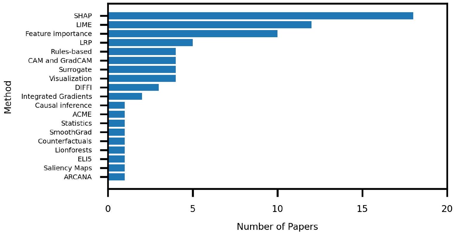
  1. Shapley Additive Explanations (SHAP).
SHAP values were introduced by Lundberge et al. as a unified measure of feature importance [23]. SHAP is based on three properties that are shared with classical Shapley value estimation: local accuracy, missingness, and consistency. Local accuracy refers to the ability of the simplified input to at least match the output of the input from the data. Missingness refers to the features that are missing from the simplified input. Succinctly, this states that if a feature is not useful to the explanation, then it is not useful to the model. Finally, consistency brings the idea that the importance of a feature should stay the same or increase regardless of the other features.
By far, SHAP is the most used method seen in our sample. Moreover, SHAP is one of the few methods that has been applied to the problems of anomaly detection [72], [106][108], [132], fault diagnosis [130], [134], and prognosis [75], [77], [112]. This is likely due to its wide versatility as a modelagnostic method that can provide global explanations.
Steurtewagen et al. [134] created a framework for fault diagnosis that consists of three parts: data collection, progno-
TABLE 1. Datasets from the Literature Search
Datasets Articles
Bearings and PRONOSTIA [39], 40] |41|-|53
[33], [37], [54], |55]
Vehicles or vehicle subsystem [56]-|68
CMAPSS [69] [35]-|37], |70|-|79|
[80]
General Machine Faults and Failures 81 [42], [48], |82|-|86]
Trains [34], |87-|92
Gearboxes [93] |42|, 45, 48, |94|
Artificial Dataset [44, 95, 96
Hot or Cold Rolling Steel [72], |95|, |97]
Mechanical Pump [98-|100]
Aircraft [52],101
Amusement Park Rides [102],103
Particle Accelerators [104, 1105
Chemical plant [106, 107
Maritime [108-110
Semi-conductors |111| |112|, 113
Air Conditioners 56
Hard Drives [114] [38, [70], |115]
Tennessee Eastman Process |116 70
Compacting Machines 103
UCI Machine Learning Repository [117] 1118
Wind Turbines [119] [120]-|122
Transducers |123
Lithium-ion Batteries [124] [37, |125|, |126]
Heaters 127
Computer Numerical Control data 128
Textiles 129
Plastic Extruders 130
Press Machine 131
Coal Machinery 132
Refrigerators 1133
Gas Compressors 134
Hydraulic Systems 135
Iron Making Furnaces 1136
Cutting Tools 137
Power Lines [138] 139
Communication Equipment 140
Water Pump 141
Oil Drilling Equipment 142
Solenoid operated valves 143
Coal Conveyors 144
Temperature Monitoring Devices 145
Distillation Unit 146
Water Pipes [147] 148
sis, and diagnosis. Importantly, in the data collection phase, they received the reports that were associated with the faults. The prognosis section used an XGBoost algorithm to detect a fault occurring. The diagnosis utilized SHAP to determine the features that are important to the output of XGBoost. These features are validated using the reports that accompany the fault.
Choi et al. [107] proposed a method for explainable unsupervised anomaly detection to predict system shutdowns for chemical processes. Their method consisted of what they call a period-independent framework and a period-integrated framework. The period-independent framework searched for the best anomaly detection model and applied the explainable method. In the period-integrated framework, they applied real-time information to the model chosen from the previous framework. They found that the isolation forest provided the best results in the period-independent framework based on the
TABLE 2. Explainable Methods from the Literature
Method Articles
Shapley Values V-A1
LIME V-A2
Feature Importance
LRP V-A4 Rule-based V-A5
CAM and GradCAM V-B1
Surrogate V-A6
Visualization V-A9
DIFFI V-B2
Integrated Gradients (V-A7)
Causal Inference V-AB
ACME V-A10
Statistics V-A11
SmoothGrad V-A12
Counterfactuals V-A13
LionForests V-B3
ELI5 V-A14
Saliency Maps (V-B4)
ARCANA V-B5
[72], [95], [106|-|108|, [130], [132]
[36]-[38], [42], [66], [75]-|77], |112], [131], [134]
[35]-|38|, [44], [50], [51], [54], [61], [66], [76], 84]
[34], [54], [67], [85], [86], [92], [104], [110], |137|, |139|
37, 44, 68, [105], [126]
65, 70, 71, 73
37, 44, 48, 63,
|82|, |89|, |95|, |40|
47, |74, 109, 129
[42, 102], 128]
94, |131
88
103]
59
[13]
97
96
51
37
[120]
number of unplanned shutdowns detected, and they utilized show SHAP as an effective way of measuring root cause analysis.
Gashi et al. [112] conducted predictive maintenance on a multi-component system. Their objective was to model interdependencies and assess the significance of the interdependencies. Prior to training their Random Forest model, they used visual exploration to study interdependencies. They used two methods to justify the use of interdependencies: statistics and XAI. They used chi-squared testing to show that the performance of a model with interdependencies is better ( ). When applying SHAP to the random forest, they showed that the interdependency variables were usually among the top explainer features. This adds validity to SHAP as an explainable method in terms of the accuracy of its explanations.
2) Local Interpretable Model-agnostic Explanations (LIME). LIME was introduced by Ribeiro et al. as a way of explaining any model using a local representation around the prediction [24]. This is done by sampling around the given input data and training a linear model with the sampled data. In doing this, they can generate an explanation that is faithful to that prediction while using only information gained from the original model.
Protopapadakis et al. [35] computed the RUL as applied to the CMAPSS turbofan dataset. They initially attempted to perform RUL prediction with two models, a random forest and a deep neural network. They found the random forest to perform poorly, which would lead to poor explanations. Their deep neural network achieved high performance, so they applied LIME. They compared two LIME explanations, one for early life and one for late life with a specific fault. They found that LIME was able to label the important features for
failures that reflected the physical faults. Additionally, they showed that LIME would have a more difficult time labeling the important features when it was applied to segments with no faults as anything could occur in the future.
Allah Bukhsh et al. [92] discussed multiple tree-based classifiers for predicting the need for maintenance events, i.e., anomaly detection, for train switches. From their pool of treebased classifiers, including decision tree, random forest, and gradient boosted tree, they identified gradient boosted tree as the most accurate amongst the models when predicting if a problem would occur. In a separate test, they had the same models predict specific types of anomalies. In this experiment, random forest outperformed the rest. For interpretability, they implemented LIME to learn from the outputs of the random forest. The researchers intend that the output from LIME will help establish trust in the model for domain experts and decision makers

3) Feature Importance.

Feature importance refers to the idea that some of the input features have more influence on the output than others. For example, when determining if an image is a dog, the background that has no pixels of the dog would potentially be less important than the pixels with the dog. Feature importance is typically assessed using techniques like SHAP and LIME, but various approaches exist in the literature.
Many researchers have applied different methods of feature importance calculations. Bakdi et al. 110] tackled predictive maintenance for ship propulsion systems. They combined balanced random forest models and multi-instance learning to achieve a high true positive rate which was then explained via Gini feature importance. Schmetz et al. [137] also applied Gini feature importance to verify a Tree Interpreter [150] for their random forest classifier.
Other researchers have ranked their features in different ways. Manco et al. [34] performed fault prediction to train systems where they ranked time steps by how anomalous they were within a time window. This ranking was performed by mixture modeling of the prior probability of the trend with the probability of the trend being normal behavior. Marcato et al. [104] applied anomaly detection to particle accelerators where permutation-based feature importance to guide further model development.
Finally, Voronov et al. [67] and Ghasemkhani et al. [86] each proposed different methods of calculating feature importance that tackle different problems. Voronov et al. proposed a forest-based variable selector called Variable Depth Distribution (VDD) that addressed the issue of variable interdependencies through clustering of features. The important features appeared in multiple clusters. Ghasemkhani et al. developed Balanced K-Star to deal with the imbalance problem commonly found in predictive maintenance. To add explainability, they applied chi-square to determine the important features in the machine failure.
4) Layer-wise Relevance Propagation (LRP).
LRP was introduced by Bach et al. 151 as an explainable method that assumes that a classifier can be decomposed into several layers of computation. LRP works with the concept of a relevance score that measures how important a feature is to an output. LRP works by extrapolating the relevance to the input layer by moving backwards through the architecture starting at the output layer. The importance of an input feature can then be measured as a summation of features it impacts through the architecture.
LRP falls into the category of model-agnostic which can be seen in the use-cases in the literature. Felsberger et al. [105] applied LRP to multiple architectures including kNN, random forest, and CNN-based models. Through LRP, they found that the CNN architectures were learning important features which led to higher performance. Han et al. [68] performed fault diagnosis for motors using the notable model LeNet [152]. Through the use of LRP, they were able to bring explainability to a notable architecture.
Wang et al. [126] proposed a method of using explainability as a method of driving the training process. They utilized LRP to calculate feature importance for the training data. The importance calculations were embedded for optimizing the model’s performance. They introduced this explainabilitydriven approach to the problem of aging batteries, and showed its superb accuracy when compared to a data-driven approach.

5) Rule-based Explainers.

Rule-based explainers use a combination of the black-box model and the training data to create a series of IF-THEN rules. These rules are generally created using combinatorial logic (ANDs, ORs, and NOTs) to combine the features in the IF portion of the rules. The THEN portion of the rules are populated by the result from the model, usually a class or a predicted value. The rules are then presented as explanations or may be used as a replacement for the black-box model itself.
Even in rule-based explainers, there are numerous methods that have been used. Wu et al. [71] proposed the K-PdM (KPIoriented PDM) framework, a cluster-based HMM based on key performance indicators (KPIs). A KPI is a vector of one feature of fine-grained deterioration, and a combination of KPIs reflect the health of a machine. The health was modeled as an HMM for each KPI. These HMMs were converted into a rule-based reasoning system for explainability.
Brunello et al. [70], [73] showed twice that temporal logic can be used in anomaly detection. Firstly, they showed that linear temporal logic could be added to an online system for monitoring failures [73]. They again showed that temporal logic could be used in a different approach to the same problem. Brunello et al. [70] created syntax trees that utilized bounded signal temporal logic statement. The trees were altered using an evolutionary approach to predict failure in Blackblaze Hard Drive [114], Tennessee Eastman Process [116], and CMAPSS [69] datasets, commononly used datasets for PdM of hard drives, electrical processes and
turbofans. This method led to great performance with rulebased explanations.
Ribeiro et al. [65] applied XAI to the online learning process using a Long Short-term Memory AutoEncoder (LSTMAE) for modeling public transport faults. Simultaneously, the authors’ system learned regression rules that explained the outputs of the model. While their system was learning to map the anomalies, the output of their model was fed into Adaptive Model Rules (AMRules), a stream rule learning algorithm. They applied their method to four public transport datasets, and they output their global and local rule-based explanations given used in their system.

6) Surrogate Models.

Surrogate models are simpler models that are used to represent more complex models. These surrogate models generally take the form of simple decision trees and linear/logistic regression models. The simplistic nature of these models makes them interpretable; however, their use has their interpretability as an explainable method for a black-box model.
When utilizing a surrogate model as an explainable method, the surrogate model must be inherently interpretable as a way of allowing an explanation to be gathered from the main model. Glock et al. [82] utilized two ARIMA models to explain a random forest model. One ARIMA model learned the same data as the random forest, and the second ARIMA model learned the residual errors from the random forest. While the random forest is not explainable, the two ARIMA models could show what the random forest could and could not learn.
Zhang et al. [140] proposed an alarm-fault association rule extraction based on feature importance and decision trees. Their process started with a weighted-random forest. Feature selection was performed to gather the important features in the abnormal state. These features were used to create a series of C4.5 decision trees that model different features. Once their random forest was trained and predicted a fault, the decision tree with the highest accuracy could be used to extrapolate an explanation of the fault.
Errandonea et al. [89] tested XAI on edge computing with all possible models in H2O.ai‘s AutoML to perform their fault diagnosis. After determining the optimal architectures, they trained a decision tree surrogate model to add explainability to their autoML process. By optimizing hardware and accuracy, they showed that explainable predictive maintenance could theoretically occur on edge computing devices.

7) Integrated Gradients.

Integrated gradients was introduced by Sundararajan et al. [153] to attribute the prediction of a deep architecture to its input features. They introduce two axioms, sensitivity and implementation invariance, to build their explainable method. Sensitivity is achieved if for every input and baseline that differ in one feature but have different predictions then the differing feature should be given a non-zero attribution. Implementation invariance means attributions are always iden-
tical for two functionally equivalent networks. With these axioms in mind, the integrated gradients are calculated via small summations through the layers’ gradients.
Hajgato et al. [94] introduced the PredMaX framework for predictive maintenance which identified sensitive machine parts and clustered time periods. It works in two steps: a deep convolutional autoencoder was applied to the data, and clustering was performed on the latent space in the autoencoder. From the clusters, they showed which channels contribute to the transition from normal to abnormal. Additionally, the integrated gradients technique was used to extract the relevant sensor channels for a malfunctioning machine part.

8) Causal Inference.

Causality goes beyond the notion of statistics dependencies as it shows a true relationship between two or more variables [154]. Causality can be measured in causal strength which measures the change in distribution of variables when one variable has been changed [154]. Causality is not an easy quality to analyze as it can only be truly discovered by repeated observations of a phenomenon occurring given an event; however, causal inference has been a method of XAI that some researchers have utilized.
Trilla et al. [88] designed an anomaly detection framework based around a denoising variational autoencoder (VAE) and an MLP. They extracted intra-subsystem and inter-subsystem patterns by making the time series data into voxels. The VAE generalized the embeddings. Finally the MLP was used to create a smooth diagnosis probabilistic function. They applied their method on a locomotion dataset and utilized causal inference via the Peter-Clark algorithm to answer the question “Did the VAE learn cause-effect relationships?” They found that the VAE could at best be described as modeling a correlation relationship, but this limitation was mainly attributed to limited data availability.

9) Visualization.

Visualization techniques do not take any one specific form. Generally, these visualizations take the form of visualizing weights; however they may also take the form of visualizing specific examples. Whatever the case, these methods benefit the users by providing an image enlightens the user to the inner workings of the architecture.
Visualizations can be utilized in many ways for explainability. Michalowska et al. [109] use visualizations to compare healthy and anomalous data. Costa et al. [74] utilized visualizations coupled with a recurrent variational encoder. They show that the latent space created by the encoder can add explainability. When input data with similar RULs pass through the encoder, they show the latent spaces are similar for those with similar RULs.
Xin et al. 47 aimed to address bearing fault diagnosis via a novel model named logarithmic-short-time Fourier transform modified self-calibrated residual network (log-STFTMSCResNet). The STFT extracts time-frequency features from raw signals to retain physical meaning of fault signatures
FIGURE 9. Use of XAI Methods
which are visualized for explainability. The MSCResNet is used to enlarge the receptive field without introducing more parameters. With the combination of the two, they aim to have high accuracy even under unknown working conditions. They compared their model to popular models such as LSTM and ResNet18. log-STFT-MSCResNet performed among the best even under unknown working conditions, had a small number of features and had a shorter training time than the others.

10) Accelerated Model-agnostic Explanations (ACME).

ACME was introduced by Dandolo et al. [155] as a method of quickly generating local and global feature importance measures based on perturbations of the data. For global explanations, they take a vector that holds the mean of each feature through the entire dataset; this is known as the baseline vector. Then a variable-quantile matrix is created that holds the different quantiles of the features. This matrix is used to gather predictions that would represent each quantile. The global feature importance is finally calculated for each feature by computing the standardized effect over each quantile. To get a local explanation, the baseline vector is replaced with the specific data point that is meant for explaining.
Anello et al. [103] applied ACME to the problem of anomaly detection to compare it to SHAP. They utilized isolation forest to detect anomalies as it is commonly used for detecting outliers or anomalies. An anomaly score was used as a label for the time series to represent the problem as a regression task which allows ACME to be applied. After applying SHAP and ACME to a roller coaster dataset and a compacting machine dataset, they found a drastic speed up
by using ACME with all of the data while SHAP would be slower even with access to of the data.
11) Statistics.
As a method of explaination applied to the problem of predictive maintenance, statistical tests can be used to compare the distribution of the features between different classes.
Fan et al. [59] developed ML methods that take advantage of physics knowledge for added interpretability. Their case study was fault detection of leak-related faults in vehicle air systems. They applied three physics equations to their data that would model the air leakage. Moreover, they used that data in the training data of their kNN and MLP models. Results showed that the physics-assisted models to outperform the non-assisted models.
12) Smooth Gradients (SmoothGrad).
SmoothGrad was developed by Smilkov et al. [156] to produce a gradient-based sensitivity map. The intuition behind SmoothGrad involves differentiating the predicting model with respect to the input. This derivative creates a sensitivity map that represents how much difference a change in each pixel of the input would make to the classification [156]. Moreover, this sensitivity map can ideally show regions that are key to the prediction.
13) Counterfactuals.
Counterfactuals were introduced by Wachter et al. [157] to provide statements of the differences needed to gain the desirable outcome. This method also works by providing
an explanation for the output of the model, but this extra capability makes counterfactuals very unique in realm of XAI methods.
Jakubowski et al. [97] developed a predictive maintenance solution for an industrial cold rolling operation. They utilize a semi-supervised algorithm based on the Physics-Informed Auto-Encoder (PIAE). This architecture was physics-informed by applying a list of equations at the beginning of their input data. The output of the equations was appended to the input data of their AE. Their model proved to be more accurate than a base AE. While PIAE has some interpretable aspects already, they applied counterfactuals as an explainability method to show the important features from their algorithm’s decisions.

14) Explain Like I’m 5 (ELI5).

ELI5 is a popular method from Github [158] maintained by the user TeamHG-Memex and 15 other contributors. This Python library focuses on explaining the weights of a model which also serves as a method for calculating feature importance. While maintaining original methods, ELI5 also provides other explainability method implementations.

B. MODEL-SPECIFIC

This section describes the explainable methods in our population that base the explanations on the properties of the architecture it intends to explain. These methods are known as model-specific [149]. Here we discuss methods that take advantage of the architecture for generating explanations such as CAM and GradCAM in Section V-B1. DIFFI in Section V-B2 and more.

1) Class Activation Mapping (CAM) and Gradient-weighted Cam (GradCAM).

CAM was introduced by Zhou et al. [25] as a method of global explainability for convolutional neural networks (CNN). The map that is created indicates the image regions that are used by the CNN to identify the target category. CAM does this by utilizing a global average pooling (GAP) layer in the CNN architecture which outputs the spatial average of the feature map of the final layer. The pixels with higher values are associated with the pixels in the image associated with the class label. Additionally, Selvaraju et al. [159] extend CAM to GradCAM by using the gradient information going into the last convolutional layer to understand the importance of the features.
GradCAM has been validated through different studies via comparison and metrics. Mey et al. [44] focuses on the plausibility of XAI for explaining a CNN. They investigated GradCAM, LRP and LIME as methods of explaining a CNN for anomaly detection. They found non-distinguishable features highlighted by LRP, and they found unimportant features highlighted by LIME. GradCAM was able to highlight the important features that they labeled prior to CNN training. This could point towards model-specific methods outperforming model-agnostic methods when applicable.
Solis-Martin et al. [37] present a comparison on LIME, SHAP, LRP, Image-Specific Class Saliency (Saliency Maps) and GradCAM as applied to predictive maintenance datasets such as CMAPSS and batteries. They identify eight metrics for comparison: identity, separability, stability, selectivity, coherence, completeness, congruence and acumen, an evaluation proposed by the authors. When comparing the different methods as applied to a CNN architecture, GradCAM performed the best in regards to the nine metrics.
Oh et al. [63] propose a fault detection and diagnosis framework that consists of a 1D-CNN for fault detection, class activation maps for fault diagnosis (explainable method) and VAE for implementing user feedback. The CNN utilizes a GAP layer as the output layer due to its ability to maintain the temporal information. This also allows them to use CAM as an explainable method as opposed to GradCAM. The VAE is utilized with the principle of Garbage-In, Garbage-Out logic to minimize the amount of false positives and negatives that would be presented to the users. To verify their method, they apply it to the Ford Motor dataset which is a vehicle engine dataset that contains an amount of noisy data. They show that their model is accurate even in noisy data, and they show that the VAE increases their accuracy. They also show via CAM that the anomalous data is linearly separable, which is found in the VAE.
2) Depth-based Isolation Forrest Feature Importance (DIFFI). DIFFI was introduced by Carletti et al. [160] as an explanable method for isolation forests. Isolation forests are an ensemble of isolation trees which learn outliers by isolating them from the inliers. DIFFI relies on two hypotheses to define feature importance where a feature must: induce the isolation of anomalous data points at small depth (i.e., close to the root) and produce a higher imbalance on anomalous data points while being useless on regular points [160]. These hypotheses would allow explanations for anomalous data which would allow for explanations of outliers or faulty data.
Berno et al. 102] performed anomaly detection for automated rides at entertainment parks. They introduced the idea of providing extra focus specific features by splitting their data into a multivariate set and many univariate sets based on a prior knowledge. They utilized isloation forest to model the multivariate time series with DIFFI explaining the output. They modeled the univariate time series with a Growing When Required (GWR) neural gas network. The multivariate analysis was used for determining anomalies within most of the variables, and the explanations were used to rank the features causing the anomaly.
Lorenti et al. [128] designed an unsupervised interpretable anomaly detection pipeline known as Continuous Unsupervised Anomaly Detection on Machining Operations (CUADMO). CUAD-MO consists of 4 parts: data segmentation and feature extraction, unsupervised feature selection via Forward Selection Component Analysis (FSCA), anomaly detection via Isolation Forest, and post-hoc explainability via DIFFI. Their feature extraction consisted of adding basic statistics
and higher order moments of the signals such as Kurtosis. FSCA iteratively selects features to maximize the amount of variance explained. Finally, the Isolation Forest is used to detect outliers which are handled as faulty events. These are explained via DIFFI. They applied their method to 2 years of computer numerical control data resulting in a precision rate.

3) LionForests.

LionForests were introduced by Mollas et al. [161] as a local explanation method specifically for random forests. Their method follows these steps: estimating the minimum number of paths for the accurate answer, reducing the paths through association rules, clustering, random selection or distributionbased selection, extracting the feature-ranges, categorical handling of features, composing the interpretation, and visualizing the feature ranges. The outputs of their method are the interpretations in the form of IF-THEN rules and visualizations of the features.
Mylonas et al. [96] aimed to alleviate the non-explainable nature of random forest by applying an expanded version of LionForests to fault diagnosis. They expanded LionForests into the realm of multi-label classification by applying three different strategies: single label, predicted labelset, and label subsets. Single label aims at explaining every individual prediction (local); predicted labelset aims at explaining all predictions (global); and label subsets aim at explaining based on frequently appearing subsets of predictions. With their expansion, their attention is focused on multiple machine failure datasets, but specifically the AI4I dataset [162]. They utilized accuracy metrics such as precision, and they provided metrics for their explanations such as length of explanations and coverage of data. One of the more notable elements of their work involves comparing their XAI algorithm to other algorithms, namely global and local surrogates and Anchors.

4) Saliency Maps.

Saliency maps were introduced by Simonyan et al. [163] as a method for explaining CNN outputs. Given an input and a model, saliency maps rank the pixels of the input based on their influence on the output of the model. This is done by approximating the output with a linear function in the neighborhood of the input by using the derivative of the scoring function with respect to the input. This approximation is the saliency map.

5) Autoencoder-based Anomaly Root Cause Analysis (ARCANA).

ARCANA was introduced by Roelofs et al. [120]. They noticed that autoencoders were a popular method of detecting anomalies in their target domain, wind turbines; however by themselves, autoencoders are not interpretable. To overcome this lack of interpretability, they implement ARCANA as a way of explaining the cause of the reconstruction error of an autoencoder. ARCANA works by minimizing a loss function that is based on reconstruction. As opposed to measuring
the difference between the output of the autoencoder and the input, they add this bias vector to the input data as to have a corrected input. Moreover, the bias shows “incorrect” features based on the output; therefore, the bias would explain the behavior of the autoencoder by showing which features are making the output anomalous.
Roelofs et al. [120] also utilize their method for anomaly detection and root cause analysis for wind turbines. They verify that ARCANA provides the most important feature causing the issues with their wind turbines. This method is done by firstly measuring the features reconstruction error. When performing ARCANA, the feature that shows the most importance is the same feature with the largest error. They then show that even when the feature does not appear in the reconstruction error, ARCANA is able to find feature importance in sensors that are applicable to known anomalies.

C. COMBINATION OF METHODS

This section describes the works that used multiple explainability methods. Some of these works were utilized to just note the differences between the different explainable methods. Other works compared the methods as to determine the better method. This section reviews the works that combine multiple methods without aiming to declare one method as better than another.
Utilizing multiple explainable methods can be used in a stacked manner or in a simultaneous manner. The stacked manner involves using explainable methods sequentially. In Jakubowski et al. [95] they created a quasi-autoencoder for explainable anomaly detection. A surrogate model of XGBoost was used as a way of simplifying the original model. They achieved a high score using this XGBoost model while adding explainability via TreeExplainer (SHAP).
More commonly, a simultaneous utilization of explainable methods appears in the literature where the authors obtain multiple explanations from different methods. Khan et al. [36] found the best architecture for their problem of RUL prediction amongst: random forest, SVM, gradient boosting, elastic net GLM and an MLP regressor. After seeing the MLP regressor to have the best performance, they used LIME and SHAP to explain the output. LIME and SHAP did not have the same explanations, but they had similar explanations. Similarly, Jakubowski et al. [76] performed an experiment testing five architectures and using SHAP and LIME as explainers. The found that SHAP and LIME had different explanations throughout the different neural architectures suggesting a fidelity concern between architectures.
Like the prior two, Serradilla et al. [51] performed remaining useful life prediction on a bushings testbed. They tested six different models and determined random forest regressor to be the best. They then utilize two explainability methods (ELI5 and LIME) to show global and local feature importance of driving model development. Brito et al. [42] performed a large experiment that applied many unsupervised learning algorithms for fault detection and fault diagnosis. They showed that Local-DIFFI and SHAP seemed to be mostly in
agreement about the explanation for the model’s output, but they did not move further in asking which is better.
Ferraro et al. [38] focused on analyzing the effectiveness of explainability methods on the predictions of a recurrent neural network based model for RUL prediction. Notably, the model performed well, but the focus was on the explainable methods SHAP and LIME. A quantitative analysis was performed using three metrics: identity, stability and separability. This showed: (1) LIME was unable to give identical explanations for identical instances; (2) LIME more than SHAP gave similar explanations to instances in the same class; and (3) LIME and SHAP were able to give different explanations for instances in different classes.
Li et al. [66] aimed at integrating explainability into an AutoML environment used for vehicle data. They tested four different AutoML platforms: AutoSklearn, TPOT, , and AutoKeras. They performed two different experiments where they provided different subsections of their dataset with both resulting in TPOT performing the best in accuracy. Finally, they apply LIME and SHAP to the resulting model to explain a local sample and the whole model. Their work results in a defined workflow for an automatic predictive maintenance system that includes explainability.

VI. INTERPRETABLE ML IN PREDICTIVE MAINTENANCE
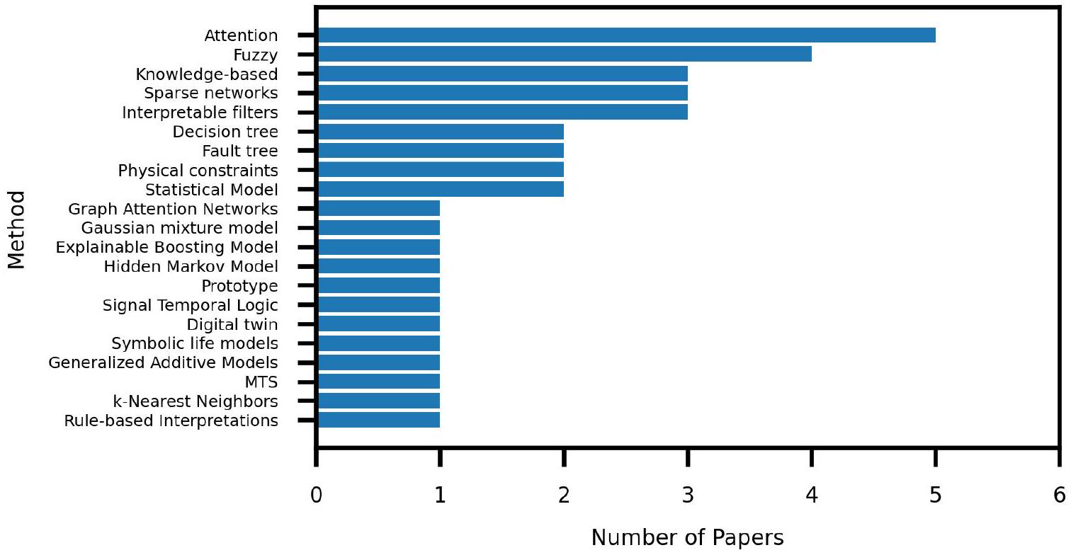
Interpretable machine learning (iML) encompasses many methods whose inner-workings are understandable without requiring a post-hoc method for explanation generation. These methods can be interpreted by the target audience without the need of separate methods to serve as a translator between the model and the person. iML methods namely consist of architectures that can have human-readable outputs such as rule-based systems, simple visual representations such as decision trees and simple networks or physical mappings that are intelligible to the user.

A. ATTENTION.

Attention was introduced by Vaswani et al. [164] as a method of natural language processing. This attention module gets extended to introduce the transformer architecture that has led to many famous models such as GPT. The weights from the attention modules can be visualized to allow interpretation of the aspects the architecture is focusing.
Xia et al. [58] and Hafeez et al. [64] tackled interpretable fault diagnosis in two separate ways. Xia et al. looked at hierarchical attention by grouping the features by systems and subsystems. They utilized BiLSTM encoders with attention to obtain important features where the attention components added interpretability. Hafeez et al. created an architecture known as the DTCEncoder to learn low level representations of multivariate sequences with attention. It utilized the Diagnostic Trouble Codes (DTC) commonly found in predictive maintenance problems as a class label for fault diagnosis. Dense layers were used to translate the encoded latent space from DTCEncoder into a probability distribution for the different DTCs. The latent space was learned using attention
mechanisms and could be used to add interpretability of why the network output the DTC.
For interpretable fault prediction, Wang et al. [56] proposed a two-stage method based on anomaly detection and anomaly accumulation. The anomaly detection module was made using a CT-GAN to train a discriminator on limited data, i.e., faults. The anomaly scores from the CT-GAN were fed into the anomaly accumulation module based on an Attention-LSTM. This modeled the temporal dependencies of the anomaly scores while the attention mechanism was used to give importance to different anomalies at different time steps. Their model outperforms models such as SVM and LSTM on prediction and DTW on classification.
Xu et al. [133] was not only interested in anomaly detection, but also anomaly precursor detection, early symptoms of an upcoming anomaly. They argued that detecting precursors is useful for early prediction of anomalies to better understand when and what kind of anomaly will occur. They proposed Multi-instance Contrastive learning approach with Dual Attention (MCDA) to tackle the problem of anomaly precursor detection. MCDA combined multi-instance learning and tensorized LSTM with time-dependent correlation to learn the precursors. Additionally, the dual-attention module produced their interpretable results. This approach had high accuracy results, and their attention mechanism provided variables which are explanatory for the results. Importantly, they verified these explanations with domain experts.

B. FUZZY-BASED.

Fuzzy logic was introduced by Dr. Lofti Zadeh [165] as a way of understanding the approximate mode of reasoning as opposed to the exact. Following this approximate model of understanding, all knowledge would come with a degree of confidence as opposed to a statement being in a category. This adds some interesting and useful components to machine learning as these in-between categories can be utilized in a way that is different from having all information fall strictly into one category.
Fuzzy-based methods apply fuzzy logic in different ways. Lughofer et al. [53] and Kothamasu et al. [52] used type 1 fuzzy logic. Lughofer et al. proposed a framework of representation learning based on transfer of fuzzy classifiers. The transfer learning matched the distributions between the source data and the target task using fuzzy rule activation. This was done by feeding the model all of the source data and the healthy data from the target domain. Through this training, the model classified unseen healthy and unhealthy data from the target task. Their model did not outperform all black box models; however, it was in the upper ranks of performance while bringing interpretability to the user.
Additionally, Kothamasu et al. [52] presented a Mamdani neuro-fuzzy modeling approach for two use cases, bearing fault detection and aircraft engine fault diagnosis. They chose this model as it has the characteristics of being adaptive, flexible, lucid, and robust. Their model consists of five layers: input, linguistic term input, rules, linguistic terms output, and
FIGURE 10. Use of iML Methods
defuzzification. As the rules can become undistinguisable through training, they utilized Kullback-Leibler mean information to refine the rules.
Fuzzy-based methods can also take the form of higherorder fuzzy logic as seen by Upasane et al. [123], [141]. They proposed a type 2 fuzzy logic system for fault prediction to allow interpretability [123]. Additionally, the Big-Bang Big-Crunch (BB-BC) evolutionary algorithm was used for optimizing the number of antecedents of their fuzzy logic system. This was optimized for minimizing the RMSE of their system. Their system was able to get a very low RMSE with 100 rules and six antecedents per rule.
Upasane et al. [141] extended their previous work [123] to include most of the faults that can occur as well as proposing an explainable framework. While maintaining accuracy with more faults is noteworthy, the experiment’s measurement of users’ trust was quite unique compared to the literature. They observed that of the respondents agreed or strongly agreed with having trust in the interpretable system. This trust is attributed to the explainable framework and interpretable nature of their architecture; moreover, the interface is noted to provide helpful insights to the users that would minimize downtime of the assets.

C. KNOWLEDGE-BASED.

In this paper, knowledge-based approaches include methods such as knowledge-graphs, knowledge-based systems, knowledge graphs, etc. Knowledge-based approaches focus on a symbolic representation of the data that one can find in a source of data. These representations consist of connections
between different features where the links take the form of a link when discussing graphs or production rules when discussing production systems. These methods produce interpretation by providing these connections within the features, usually in the form of natural language.
Xia et al. 142 proposed a maintenance-oriented knowledge graph to apply for predictive maintenance of oil drilling equipment. Once they had the maintenance-oriented knowledge graph, an attention-based compressed relational graph convolutional network (ACRGCN) was used to predict solutions for different faults by predicting links between knowledge. This method also explained faults due to its knowledgegraph that maps different symptoms and maintenance requirements. Even though knowledge-graphs have inherent interpretability, they created a question-answer system that allowed the user to query the graph.
Salido et al. [99] created a fuzzy diagnosis system based on knowledge-based networks (KBN) and genetic algorithms (GA). The KBN constructed fuzzy rules using neural learning where the input is the features and the following layers are OR neurons and AND neurons. To determine the optimal number of neurons, they used a GA. Importantly in their GA, they added a metric to measure simplicity of their rules by making more concise rules. With their architecture, they could 1 ) detect a fault and 2) explain the fault using an IF-THEN rule which can be used as a method of root cause analysis.
Cao et al. 113] created an approach based on knowledgebased systems for anomaly prediction. Their method is broken into three parts: pruning of chronicle rule base, integration of expert rules, and predictive maintenance. Pruning of
chronicle rule base consists of mining the rules with frequent chronicle mining, translating the rules into SWRL rules, and using accuracy (how many true rules) and coverage (how many true encompassing rules) to select the best quality rules. The integration of expert rules involved receiving input from the experts and placing the same restrictions on their rules. Finally, the rules were used for anomaly prediction of semiconductors.
TABLE 3. Interpretable Methods from the Literature
Method Articles
Attention VI-A |56|, |58|, |64|, |78|, 133
Fuzzy VI-B
133
[52], |53|, |123|, ||41
Knowledge-based VI-C 99, 1131, 142
Sparse Networks (VI-M) 46, 100, 121
Interpretable Filters VI-D 45, 49, [60]
Decision Tree VI-E [57, |15]
Fault Tree (VI-F) 79, 127
Physical Constraints VI-G 98, 143
Statistical Model VI-H 41, |55
Graph Attention Networks VI-I 87
Gaussian Mixture Model VI-J 125]
Explainable Boosting Machıne (VI-K) 76
Hidden Markov Model VI-L 80
Prototype VI-N 62
Signal Temporal Logic VI-O 136
Digital Twin VI-P 144]
Symbolic Life Model VI-Q 33
Generalized Additive Model (VI-R) 43
MTS (VI-S) 118
k-Nearest Neighbors VI-T 145
Rule-based Interpretations VI-U. 146]

D. INTERPRETABLE FILTERS.

Interpretable filters are a concept that brings specific waveforms to a CNN architecture as a way of showing what signals are being learned. As explained in Ravanelli and Bengio [166], the first layer of a CNN appears to be important for waveform-based CNNs. In using these interpretable filters that take the form of common waveforms, one can begin to understand the behavior of the CNN if one understands the behavior of the waveform.
Li et al. [45] aimed to improve CNN-based methods for PHM by addressing the black box problem. They proposed the Continuous Wavelet Convolution (CWC) layer which is designed to make the first layer of a CNN interpretable. It does this by using a library of filters that have physical meanings which are convolved on the input signal. These convolutions can be traversed along the series and projected into a two-dimensional time and scale dimension. Its performance was compared with a CNN with different wavelets, and their findings were two-fold. Firstly, the performance of the CNN with a CWC layer showed better performance than a CNN without. Lastly, the CWC learned a well-defined waveform while the one without learned what looked to be a noisy and uninterpretable representation.
Li et al. [45] built on their previous work by examining compound faults. They designed an interpretable framework called wavelet capsule network (WavCapsNet) which utilizes
backward tracking. This network has 1) interpretable meaning from the wavelet kernel convolutional layer, 2) capsule layers that allow decoupling of the compound fault, and 3) backward tracking which helps interpret output by focusing on the relationships between the features and health conditions. Not only was their framework able to achieve high accuracy on all conditions, including compound faults, but also they showed that the backward tracking method can decouple the capsule layers effectively.
Ben et al. [49] proposed a new architecture, SincNet, that trains directly on the raw vibration signals to diagnose bearing faults. Their architecture utilized interpretable digital filters for CNN architectures. They reduced the number of trainable parameters and extracted meaningful representations by having the predefined functions serve as the convolution. When comparing the performance to a CNN, the SincNet had a higher precision and reached convergence faster.

E. DECISION TREES.

Decision trees encompass both classification and regression trees that date back to the first regression tree algorithm proposed by Morgan and Songquist [167]. Decision trees create a tree-based architecture where each set of children of each node is split using a feature. To produce an output, a decision tree algorithm starts at the root of the tree and proceeds down the tree by evaluating the feature that is used for splitting. The output corresponds to the final leaf node that the decision trees reaches on its path.
Amram et al. 115] utilized two types of decision trees, optimal classification trees [168] and optimal survival trees [169]. Their goals included predicting the RUL of long-term health of hard drives, predicting RUL of the short-term health of hard drives, predicting failure classification in short-term health of the hard drives and performing similar experiments with limited information. Their results showed that they could gather better results using separate models for the tasks as opposed to using one model. They also showed the interpretable methods shared many of the important features for the different tasks.
Panda et al. [57] aimed at tackling the problem of commercial vehicle predictive maintenance by designing an interpretable ML framework. To simplify their problem, they solely looked at the air compressor system. By looking at the air compressor system, they ran a broad experiment that analyzed different configurations of models and data. The C5.0 with boosting model performed the best, and the inclusion of Diagnostic Trouble Codes with the sensor data raised the performance metrics.
Simmons et al. [139] argued that the dynamics of a timeseries are in themselves discriminative of health or failure. Additionally, the dynamics are interpretable because they are derived directly from the information. These ideas were translated into the data mining domain by creating features that represent shorter time series in the temporal, spatial, and mixed domains. The features went through a rank-based selection process which gathered features that were statistically
different between classes. These features were used to train a Light Gradient Boosting Machine (LightGBM) which is a type of gradient boosting decision tree introduced by Ke et al. [170]. This method allows for constant monitoring of feature importance during training which can be used for interpreting the results.

F. FAULT TREES.

Fault trees were introduced by H.A. Watson at Bell Labs in 1961 [171]. Fault trees were introduced as an understandable model that can learn complex systems and perform root cause analysis. They are tree-like structures that are created using different types of nodes: basic events, gate events, condition events, and transfer events. Basic events are the nodes that represent either a failure event or a normal operating event. Gate events are the logic combining nodes and consists of AND, OR, Inhibit, Priority and Exclusive OR. Condition events represent conditions that must occur for a gate event to occur. Transfer events are nodes that point to somewhere else in the tree. With all of these gates, fault trees are able to learn root causes for different faults that can occur in a system.
Verkuil et al. [127] noticed that fault trees are made via human intervention. With the idea of automating the process, they applied the C4.5 tree combined with LIFT to create fault trees for domestic heaters. C4.5 is used to learn the failure thresholds of the sensor data. LIFT creates fault trees in an iterative process using the learned features. While they do not provide a performance metric, they note that their method cannot be optimal for the reasons of oversimplifying the problem and using a greedy heuristic. However, domain experts weighed in on the explanations provided in a positive manner.
Waghen et al. [79] utilized fault trees to perform interpretable time causality analysis. Their methodology consisted of building multiple logic trees for each subset of data. These logic trees were aggregated into one fault tree representing the multiple trees. They performed interpretatable time cause analysis by going through each variable in the fault tree. By traversing the fault tree, they were able to extrapolate rules that can model the causality through time towards faults.

G. PHYSICAL CONSTRAINTS.

Physical constraints are used to bring real-life limitations to the data-driven models. This can be in the form of mapping the input and output of the architectures to physical components, or more commonly, utilizing known physics information or equations about the real-life system in the architecture of their model in some way.
The methods of applying physical constraints can be seen in different forms, namely model-based approaches and physics-informed approaches, which need to be differentiated. Model-based approaches are created to model a system without the training of a network with the data provided, separate from data-based models [143]. These model-based approaches have physical constraints as they have to model the mathematical properties of the system. Physics-informed
models aim to combine model-based and data-driven approaches by attaching the mathematical properties of the system to the data in data-driven approaches [98].
Tod et al. [143] implemented a first-principle model-based approach to assess the health of solenoid operated valves. Compared to other first-principle models, their improved model takes other degradation effects into account, namely shading ring degradation and mechanical wear. The method extracts three condition indicators which allows them to detect problematic signals that can be directly mapped to physical components through their model.
Wang et al. [55] performed fault diagnostics of wind turbines. Their method was an online method that detected issues with bearings. Coupled with equations that represent the physical aspects of the bearings, they detected issues surrounding clearance of the bearings with high interpretability. Their interpretation specifically showed the different frequencies around the physical features of the bearings.
Xu et al. [98] propose the physics-constraint variational neural network (PCVNN) as applied to external gear pumps. The PCVNN is physics-informed asymmetric autoencoder where the encoder is a stacked CNN, BiLSTM, Attention network while the decoder is a generative physical model. This would allow for an NN to learn the data, and it would allow the physical model to represent the learned patterns in a way that is consistent with the physics of the problem.

H. STATISTICAL METHODS.

Statistical methods are using for explaining by analyzing different features along different classes using statistical tests, such as Student’s t-test [172], Pearson’s chi-squared test [173], etc.
Yao et al. [41] proposed a framework with interpretable and automatic approaches that consisted of solely statistical processing. Their method proposed kurtosis-energy metric to define key sub-bands, a new health index of these sub-bands, a joint statistical alarm and fault identification strategy. Additionally, they proposed a health phase segmentation strategy for health phase assessment and degradation pattern analysis. This method involved analyzing the data on the timefrequency domain and suppressing the disturbing components such as noise. This analysis was able to help form the subbands for monitoring the current state. If it fails statistical tests, then an anomaly is detected. They tested their method on the PHM 2012 rolling bearing dataset, and they reported very low false positives.

I. GRAPH ATTENTION NETWORKS (GATS).

GATs were introduced by Velivckovic et al. [174] as a way of combining self-attention layers with graph-structured data. This is done by applying attention layers where nodes can attend whole neighborhoods of previous graph nodes. While this comes with many benefits, the main two come from the benefits that other architectures gain from attention mechanisms and the retraction of needing prior knowledge of the graph structure.
TABLE 4. Examples of Articles from Sample Population
Title Objective Contribution
Impact of Interdependencies: Multi-Component System Perspective Toward Predictive Maintenance Based on Machine Learning and XAI [112] Perform predictive maintenance by modeling interdependencies and test their importance Showed with statistical significance that interdependency modeling increases performance and understandability of a model
Explainable and Interpretable AI-Assisted Remaining Useful Life Estimation for Aeroengines [35] Compute RUL of the CMAPSS turbofan dataset with LIME explaining the performance Showed that LIME performed poorly when applied to segments with no faults but performed well when labeling features with failing sequences
Explainability-driven Model Improvement for SOH Estimation of Lithium-ion Battery [126] Perform predictive maintenance by embedding explanations into the training loop Introduced the idea of explainability-driven training for predictive maintenance
Online Anomaly Explanation: A Case Study on Predictive Maintenance [65] Apply XAI methods to the online learning process Showed that local and global explanations could be added into the online learning paradigm
Explaining a Random Forest with the Difference of Two ARIMA Models in an Industrial Fault Detection Scenario [82] Utilize two ARIMA surrogate models to explain the capabilities of a random forest model Introduced a method of sandwiching a model between two surrogates to show where a model fails to perform well
Edge Intelligence-based Proposal for Onboard Catenary Stagger Amplitude Diagnosis [89] Test XAI on edge computing for fault diagnosis Provided a method of performing XAI in an edge computing example coupled with AutoML libraries
Explainable AI Algorithms for Vibration Databased Fault Detection: Use Case-adapted Methods and Critical Evaluation [44] Discover the plausibility of XAI methods explaining the output of CNN architectures LRP showed non-distinguishable features, LIME showed unimportant features, and GradCAM showed the important features
On the Soundness of XAI in Prognostics and Health Management (PHM) [37] Compare different XAI methods for the CMAPSS and lithium-ion battery dataset Showed different metrics for comparing explanations generated by different XAI methods and showed GradCAM to perform the best on CNN architectures
Interpreting Remaining Useful Life Estimations Combining Explainable Artificial Intelligence and Domain Knowledge in Industrial Machinery [51] Perform RUL of bushings through multiple different models and explanatory methods Showed the importance of applying global and local explanations to interpret performances of models from all aspects
Evaluating Explainable Artificial Intelligence Tools for Hard Disk Drive Predictive Maintenance [38] Analyze the effectiveness of explainability methods for recurrent neural network based models for RUL prediction Utilized three metrics to compare explanations from LIME and SHAP and showed where each of them shine over the others
Automatic and Interpretable Predictive Maintenance System [66] Aimed to integrate explainability into an AutoML environment Defined a workflow for an automatic explainable predictive maintenance system
DTCEncoder: A Swiss Army Knife Architecture for DTC Exploration, Prediction, Search and Model interpretation [64] Perform fault detection by classifying DTCs Designed the DTCEncoder that utilizes an attention mechanism to provide an interpretable latent space as to why the a DTC is output
Deep Multi-Instance Contrastive Learning with Dual Attention for Anomaly Precursor Detection [133] Perform anomaly detection and anomaly precursor detection Performed anomaly precursor detection through multi-instance learning with verified explanations through domain experts
A Type-2 Fuzzy Based Explainable AI System for Predictive Maintenance Within the Water Pumping Industry [141] Utilize an evolutionary algorithm to optimize their fuzzy logic system for fault prediction Used a type 2 fuzzy logic system and evolutionary optimization to generate fuzzy rules for fault prediction
Waveletkernelnet: An Interpretable Deep Neural Network for Industrial Intelligent Diagnosis [45] Improve CNN-based methods for PHM Designed the Continuous Wavelet Convolution to add physical interpretations to the first layer of CNN architectures
Restricted Sparse Networks for Rolling Bearing Fault Diagnosis, [46] Perform fault detection using a sparse network Explored the Restricted-Sparse Frequency Domain Space and used the transform into this space to train a two-layer network that performs equal to a CNN-LSTM
Interpretable and Steerable Sequence Learning via Prototypes [62] Construct a deep learning model with built-in interpretability for fault diagnosis via DTCs Introduced Prototype Sequence Network (ProSeNet) which uses prototype similarity in the training of the network and justified the interpretability of their approach via a user study on Amazon MTurk
Causal and Interpretable Rules for Time Series Analysis [146] Perform predictive maintenance while utilizing causal rules for explanations Designed Case-crossover APriori algorithm for predictive maintenance which showed both higher performance occurs when having rules that are additive and subtractive to an output
Liu et al. [87] designed a framework for fault detection based around the Graph Convolutional Network and Graph Attention Networks. They propose the Causal-GAT. CausalGAT is comprised of two parts: causal graph construction and DC-Attention for extracting features and detection. The causal graph construction uses causal discovery methods and/or prior expertise to encode monitoring variables into a
directed acyclic graph. The Disentangled Causal Attention (DC-Attention) aggregates the causal variables for generating representations of the effect variables. The DC-Attention outputs the system status (faulty or not faulty). They then utilize a custom loss function that calculates the distance between the current support of representations and its theoretically disentangled support.

J. GAUSSIAN MIXTURE MODEL.

As described by Reynolds [175], Gaussian mixture models (GMMs) is a probability density function designed as a weighted sum of Gaussian component densities. The component densities are created using the mean vector and covariance matrix of the data while the mixture weights are estimated. GMMs are commonly used due to their capability of representing information via a discrete set of Gaussian functions to improve modeling of larger distributions. These models can be labeled as interpretable as the models directly represent the distributions of the features. These models can then be directly used to explain the features.
Csalodi et al. [125] performed survival analysis via a Weibull distribution by representing the operation signals as a Gaussian mixture models and the parameters of the Weibull model via clustering. Specifically, their method used an expectation-maximization algorithm which consists of two parts. The expectation step determined the probability that a data point belongs to any cluster given the survival time and parameters while assuming the clustering is correct. The maximization step updated the parameters for the Gaussian mixture models and the Weibell distribution to better represent the data. When applying their method to lithium-ion batteries, they represented distributions of unhealthy batteries quite accurately while healthy batteries were less wellrepresented. This occurred due to the large category of healthy data which was harder to represent in one small model while the unhealthy data could be easily represented when isolated.

K. EXPLAINABLE BOOSTING MACHINE (EBM).

EBM were introduced by Nori et al. [176] as a glassbox model, another term for interpretable model, with similar accuracy to that of state-of-the-art blackbox algorithms. EBM is a type of generalized additive model that learns each feature’s function using techniques such as bagging. Additionally, it can detect interactions between features and include those pairs of terms by learning functions of combinations of features. Because of its nature as an additive model, the features can be explained by their impact on the outcome.

L. HIDDEN MARKOV MODEL.

HMMs were introduced by Baum and Petrie [177] and can be described as a statistical state-space algorithm [29]. HMMs represent the learning as a statistical process that transitions between states, and HMMs represent the output as separate states that extend from the transitional states. HMMs, as a statistical process, can discern hidden states from the data that may not be readily apparent. They are also capable of learning combinations of sensor data, leveraging confounding variables, and executing dimensionality reduction to simplify the complexity of the data. [80].
Abbas et al. [80] combined the input-output HMM with reinforcement learning to make interpretable maintenance decisions. Their hierarchical method consisted of two steps. The input-output HMM filters the data and detects failure states. Once the failure state was detected, the deep reinforcement
learning agent learned a policy for maintenance based on the failures. The first challenge of this approach involves representing predictive maintenance as a reinforcement learning problem. This is done by representing the potential actions as hold, repair, or replace, creating a reward function based on holding, early replacement and replacement after failure, and measuring the cost based on these reward functions. The HMM is used for interpreting the output of their model by observing the features that led the model into detecting a failure state.

M. SPARSE NETWORKS.

Sparse networks are neural networks that are limited in their architecture. Large deep neural networks are inherently blackbox models; however, interpretable whitebox models can take the form of very simple neural network models such as linear regression or logistic regression models. As the models are simple, the impacts of the input features can be seen as they are propagated through the network.
Beretta et al. [121] utilized two different models for predictive maintenance: a gradient-boosting regressor to model the normal data and an isolation forest to model the fault data. The output of these are merged with a mean average of the temperature readings to create a score of failure. The authors praise the simplicity of the algorithms as the source of interpretability in their method.
Pu et al. [46] explored a new frequency domain space they call the restricted sparse frequency domain space (RSFDS) for rolling bearing faults. The RSFDS breaks down the features into a space that is made of real and imaginary points. This space is able to visualize boundaries that have physical meanings to the faults. They use a simple two-layer neural network to these points, and they achieve high performance equal to that of a CNN-LSTM with less memory and CPU usage.
Langone et al. [100] proposed a model for interpretable anomaly prediction based on a logistic regression model with elastic net regularization. Their method is made of 3 steps: data preparation, learning and refinement of the prediction model. In the data preparation phase, they categorize the data using included statistics, apply windowing to the data, and finally mark the windows as either being anomalous or not. The learning phase consists of learning the relevant features from the windowed data. This includes considering the feature distributions across failures and non-failures and measuring the distance according to the Kolmogorov-Smirnov metric. The refinement of prediction model phase consists of the training and utilization of the logistic regression model. Coupled with elastic net regularization, this model selected a smaller subset of the original data and captures the variable correlations. They applied their method to a plunger pump in a chemical plant and produced relative good and consistent scores.

N. PROTOTYPE LEARNING.

Prototype learning, as described by Ming et al. [62], is a form of case-based reasoning that determines the output of an input
by comparison to a representative example. Determining the best prototypes is a problem itself, but the interpretability it bring is apparent. The output of a specified input would be similar to its most similar prototype’s output; therefore, the reason that the input data has a certain output is due to the output of a very similar piece of data. This brings interpretability via comparison to the prototype.
Ming et al. 62] used the concept of prototype learning to construct a deep learning model with built-in interpretability. They introduced the prototype sequence network (ProSeNet) for a multi-class classification problem of fault diagnosis via diagnostic trouble codes. The model consists of a sequence encoder that is based on a recurrent architecture. The hidden state is fed into a prototype layer that determines how similar the hidden state is to prototypes in the form of a similarity vector. The network then outputs a prediction probability for the different classes based on the similarity vector. Interpretability can be conceived via the prototypes that are most similar to the input. They justified the interpretability of their model by using Amazon MTurk and surveying the users about the interpretability. They also studied how the input of human knowledge would affect the interpretability. They showed that including the human feedback improved the interpretability of their network in a post-study of different Amazon MTurk users.

O. SIGNAL TEMPORAL LOGIC (STL).

Introduced by Maler and Nichovic [178], STL as a type of temporal logic that is used for dense-time real-valued signals. STL is defined as predicates over atomic propositions. These STL rules are formed by applying Boolean filters for these atomic propositions that transforms a signal into a Boolean signal. This involves considering: the filter that is being applied, the length of the signal, the sampling of the signal and any additional desired samples. We refer the reader to Maler and Nichovic [178] Section 4 for an example.
Chen et al. [136] performed fault diagnosis on a furnace using internet-of-things, reinforcement learning, and signal temporal logic. Their algorithm takes in the STL grammar and labeled input data, and it outputs an optimal STL formula. The agent chooses a formula from the agenda and adds it to a chart based on the current policy. The evaluator evaluates the performance of the formula on the input. The learner updates the policy function according to the performance. The agenda is updated based on the formulas in the chart. They utilize an MDP to construct the agenda-based formulas while the reinforcement learning solves the problem. They apply their method to multiple faults demonstrating good robustness results, fast runtimes, and statistically significant performances.

P. DIGITAL TWIN.

Digital twins originated in 2002 as described by Grieves and Vickers [179] as a way of creating a digital construct that describes a physical system. Moreover, digital twins consist of two systems: a physical system that is represented by the
asset and a digital system that holds the information about the physical system. Using digital twins, one can observe the performance of the physical system without having the physically observe the asset.
Mahmoodian et al. [144] proposed the use of a digital twin to monitor the infrastructure of a conveyor. Their digital twin consists of taking in real data from different sensors and simulating the data. This data is compared to the real time data to ensure the data is consistent. Their digital twin can display the different information as well as receive input from the users to rate the explanations given. If it is seen as not valid, the digital twin can run simulations surrounding that data to increase its accuracy.

Q. SYMBOLIC LIFE MODEL.

Symbolic life models aim to alleviate the black box effect by modeling the process learned by mapping relationships and results. Symbolic life models are a form of symbolic regression based on genetic programming. This method creates a tree representation of an equation where the nodes are an input, a mathematical expression or a number. The output of the tree given an input is found by traversing the tree and performing the mathematical expressions as nodes are expanded. The genetic algorithm is used to perform crossovers and mutations based on the different mathematical functions and numbers where the goal is to maximize the tree’s performance on a given dataset. For more detailed information, we recommend Augusto and Barbosa [180].
Ding et al. [33] proposed the use of symbolic life models, specifically dynamic structure-adaptive symbolic approach (DSASA), as a way of modeling RUL. DSASA combines the evolving methods of symbolic life models with the structure of adaption methods. An initial symbolic life model is created from a genetic programming algorithm and run-to-failure data. This is followed by the dynamic adjustment to the life models based on the performance on real-time information. This creates groups of improved models that can all be used for prediction. The life models are interpretable as they are simple models that perform based on the physical constraints.

R. GENERALIZED ADDITIVE MODEL (GAM).

Introduced by Hastie and Tibshirani [181], GAMs are a way of estimating a function by summing a list of nonlinear functions in an iterative manner as to become better with accurate local models as opposed to an overarching global model. These local models are smoothed using a series of smoothing functions. Additionally, these local models are independent of one another as they are trained using single features. These local models allow for interpretability as well as importance related to their impacts on the outcome of the GAM.
Yang et al. [43] introduced the Noise-Aware Sparse Gaussian Process as a way of solving the scalability and noise sensitivity issues of normal Guassian Processes. Based on their NASGP algorithm, they developed an interpretable GAM that uses additive kernels and individual features. They applied their method to the IEEE PHM 2012 data challenge in forms
of RUL prediction and fault diagnosis. Their method performed well in comparison to other methods and allowed a level of interpretability.

S. MAHALANOBIS-TAGUCHI SYSTEM (MTS).

MTS was introduced by Taguchi and Jugulum [182] as a diagnosis and forecasting method. This method bases its discriminative power on the Mahalanobis distance calculation; this method cannot feasibly work if the classes cannot be distinguished this way. The feature space is reduced via orthogonal arrays and signal-to-noise ratios. The orthogonal array contains different subsets of the features. The signal-tonoise ratio measures the abnormality of the feature. Finally, the Mahalanobis distance is maximized by only including the features whose signal-to-noise ratio increases the distance. This maximized distance can be seen as the reason for a diagnosis, which is determined by the features that are used to calculate the distance.
Scott et al. [118] introduced use of the MahalanobisTaguchi system for fault detection. MTS utilizes Mahalanobis distance, orthogonal arrays, and signal-to-noise ratios for multivariate diagnosis and prediction. The Mahalanobis space represents the stable operations andyields the difference of an observation from stable. The orthogonal arrays and signal-tonoise ratio is used to diagnose or identify variables responsible for the fault. This method was able to detect roughly of the faults tested.

T. K-NEAREST NEIGHBORS (KNN).

Originally introduced in 1951 by Fix and Hodges [183], kNN is a supervised learning algorithm that is based on grouping input data with the k most similar other pieces of input data. It represents the input data as a large feature space. The output of some input data is represented by its place in the feature space in relation to the k closest other data points. Small k values lead to less consideration for the output value of the input data; however, it also leads to a more specific output. Larger k values lead to considering more values when determining the output; however, too large k values will make the output less meaningful.
Konovalenko et al. [145] used a modified kNN algorithm for generating decision support of temperature alarms. They tackled three problems associated with kNN : (1) the difficulty associated with sparse regions; (2) the blindness to class boundaries leading to misclassifications; and (3) sensitivity to class overlap. These problems were addressed by adding principles of local similarity and neighborhood homogeneity. Local similarity refers to the idea that a new data is closer to training samples with the same class label. Neighborhood homogeneity is the idea that new data falls into a neighborhood where the class label represents the majority. This method is interpretable through its ability to separate classes of data on a small dimensional graph.

U. RULE-BASED INTERPRETATIONS.

Similar to rule-based explainers presented in V-A rule-based interpretations involve utilizing rules that are learned from the data. Unlike the rule-based explainers, rule-based interpretations remove the black-box from the problem. This allows the rules to be directly learn from the information as opposed to learning from the black-box model and the data.
Dhaou et al. [146] proposed a novel approach that combines case-crossover research design with Apriori data mining. This combination resulted in the Case-crossover APriori (CAP) algorithm for association and causal rules explanation. The case-crossover design describes the way of setting up the problem. They ignored the group of data where nothing goes wrong, and they focused on the subjects that have the class change. In the case of predictive maintenance, a class change would be from healthy to failure data. The case-crossover design looks at the period prior to class change as the control group, and it looks at moments before the class change as the case period. These data points are combined with Association Rule Mining APriori to extract causal rules. These causal rules can be both additive (predictive of truth) and subtractive (predictive of falsehood). Their results show that both additive and subtractive rules help with performance, and they show their algorithm to outperform random forest on the same problem.

VII. CHALLENGES AND RESEARCH DIRECTIONS OF EXPLAINABLE PREDICTIVE MAINTENANCE

XAI and iML have been successfully utilized in predictive maintenance on many accounts. Researchers have shown that these methods can add to a prediction in a way that can be used for root cause analysis, validation of faults, etc. The main focus of much of the research focuses on adding explainability to a complex and unexplainable problem. While an important aspect of this field of study, there are multiple facets to the problem that generally go under-represented.

A. PURPOSE OF THE EXPLANATIONS

All explanations serve one overarching purpose: produce reasons that make the model’s functioning understandable. This information transfer has taken form in visualizations of data distributions, visualizations of feature importance graphs, predictive rules, etc; however, the information is not specific to a target audience. To echo Neupane et al. [15], “explanations are not being designed around stakeholders”. Not only are the explanations not being designed for stakeholders, but also many explanations do not have a target audience outside of the implicit audience of the model’s designer.
Barredo Arrieta et al. [184] provides a list of potential audiences XAI can target. While they go into more detail, some potential target audiences, especially for predictive maintenance, could be the data scientists and developers creating the predictive system, the project managers and stakeholders in the project, or even the mechanics working on the physical systems. These different people may need different types of explanations ranging from more explanations relating to the
physical and time domains to higher level abstract information.
TABLE 5. Explanation Evaluation Metrics from 185. 189
Metrics Viewpoint Description
D Objective Difference between the model’s performance and the explanation’s performance
R Objective Number of rules in explanations
F Objective Number of features in explanation
S Objective The stability of the explanation
Sensitivity Objective Measure the degree in which explanations are affected by small changes to the test points
Robustness Objective Similar inputs should have similar explanations
Monotonicity Objective Feature attributions should be monotonic; otherwise, the correct importance is not calculated
Explanation correctness Objective Sensitivity and Fidelity
Fidelity Objective Explanations correctly describe the model; features and their attribution are correlated
Generalizability Objective How much one explanation informs about others
Trust Subjective Measured through user questionnaires
Effectiveness Subjective Measures the usefulness of the explanations
Satisfaction Subjective Ease of use

B. EVALUATION OF THE EXPLANATIONS

In the literature presented above, there are over ten different evaluation metrics for the performance of the machine learning algorithms, including RMSE, MAPE, FP, etc. This shows that the field has collectively come to an agreement on how we should measure performance in a meaningful way. The evaluation of the explanations has not received the same attention as the performance of the algorithm even though work has been done in defining these different metrics, some of which are seen in Table 5
Miller [185] provides one of the most in-depth descriptions of various people’s needs regarding explanations. Miller has provided many theoretical representations for explanation including scientific explanations and data explanations. They also provide much more information including levels of explanation that could be applicable to different types of users, structures of explanations that could impact the power of the explanations, and more.
Coroama and Groza [186] present 37 different metrics for measuring the effectiveness of an explanation. The methods range from objective to subjective types. Each method includes the property it measures and whether there is a systemic implementation.
Sisk et al. [187] present the case for human-centered evaluations and objective evaluations for explainable methods. Their human-centered evaluations aim at partitioning the users based on their wants from explainable systems. The objective metrics provided involve many aspects of the explanations including number of rules and number of features.
FIGURE 11. Potential Audiences of Explainable Predictive Maintenance. Icons taken from
Kadir et al. [188] propose a taxonomy of XAI evaluations as they appeared in the literature. They identified 28 different metrics through their literature search. These metrics are broken down into a taxonomy of how the analysis is performed. An example would be sensitivity analysis for local explanations. Sensitivity analysis is broken down into the removal of features and the addition of features. Each of these categories then includes many methods that were used.
Hoffman et al. [189] express the importance of high quality explanations in XAI. If explanations are received well and are valid, a user would be better equipped to trust and use a system that employes the XAI process. This allows for multiple areas of evaluations including the goodness of the explanation, the satisfaction the explanations provided to the users, the comprehension of the user, the curiosity that motivates the user, the trust and reliance the user has with the AI, and the performance of the human-XAI system. They provide methods for measuring these metrics that are readily available.

C. ADDITION OF HUMAN INVOLVEMENT

The target audience of an explainable system is a human subject whether a data scientist, a stakeholder, an engineer, or other. Addressing the needs of different types of users of an explainable system is an important area of research that is currently lacking. As seen in Fig. 11, different people on the same task have different goals and desires from predictive maintenance. While compensating for these differences would be difficult, we suggest a way to accomplish this, together with the resulting benefits.
First, a target audience for the explainable system should be identified, ensuring that a sample population of statistically significant size is used. Presenting the information to this sample population would bring many benefits to the XAI field as a whole. These include: making more quality metrics available, allowing researchers to discern which information is more or less useful, and bringing more attention to customizable explanations via the type of user. These would push the field of XAI forward as well as push the field of
predictive maintenance forward towards a human-AI teaming environment.

D. STUDY LIMITATIONS

This study focuses on a small amount of potential XAI and iML literature. While this survey reflects the work done as applied to predictive maintenance, it does not reflect many of the applied XAI and iML algorithms that exist. It also does not reflect all of the applicable ML algorithms developed within the context of predictive maintenance. While we do not see this as a detriment to the article presented, we do note that there are a number of popular methods of which the reader may be aware that are not present.

VIII. CONCLUSION

Over the last decade, predictive maintenance has occupied a considerable presence in the field of machine learning research. As we move towards complex mechanical systems with interdependencies that we struggle to explain, predictive maintenance allows us to break down the mysticality of what could potentially go wrong in the system. Many of these approaches move us closer to understanding the system while building a new system that we need to comprehend. Explainable predictive maintenance and interpretable predictive maintenance aim at breaking down these new walls to bring us closer to a clear understanding of the mechanical system.
In this review, we provided a wide range of methods that are being used to tackle the problem of explainability. These methods are broken down in XAI and iML approaches. In our writing, XAI was broken-up into model-agnostic approaches like SHAP, LIME and LRP, and model-specific approaches like GradCAM and DIFFI. iML approaches all apply different methods of applying inherently interpretable models to the problem of predictive maintenance.
Our systematic review of XAI and iML as applied to predictive maintenance showed some weak points in the field that can be addressed. Namely, there is a lack of utilization of metrics of explanations in predictive maintenance. The field of XAI has shown a number of metrics that do not even need to show the explanations to the target audience of the explainable systems. We provided a list of potential metrics found in the literature that can be applied to this domain.
Lastly, we provided a short description of how humans can be brought into the evaluation of explainable and interpretable methods. After defining the target audience, researchers can gather a statistically significant sized sample of that audience. Providing the explanations to that sample would give feedback and allow the field to push towards human-specified explanations.

REFERENCES

[1] S. B. Ramezani, L. Cummins, B. Killen, R. Carley, A. Amirlatifi, S. Rahimi, M. Seale, and L. Bian, “Scalability, explainability and performance of data-driven algorithms in predicting the remaining useful life: A comprehensive review,” IEEE Access, 2023.
[2] J. Leng, W. Sha, B. Wang, P. Zheng, C. Zhuang, Q. Liu, T. Wuest, D. Mourtzis, and L. Wang, “Industry 5.0: Prospect and retrospect,” Journal of Manufacturing Systems, vol. 65, pp. 279-295, Oct. 2022.
[3] F. Longo, A. Padovano, and S. Umbrello, “Value-Oriented and ethical technology engineering in industry 5.0: A Human-Centric perspective for the design of the factory of the future,” NATO Adv. Sci. Inst. Ser. E Appl. Sci., vol. 10, no. 12, p. 4182, Jun. 2020.
[4] S. Nahavandi, “Industry 5.0-a Human-Centric solution,” Sustain. Sci. Pract. Policy, vol. 11, no. 16, p. 4371, Aug. 2019.
[5] A. Lavopa and M. Delera, “What is the Fourth Industrial Revolution? | Industrial Analytics Platform,” 2021. [Online]. Available: https: //iap.unido.org/articles/what-fourth-industrial-revolution
[6] L. Cummins, B. Killen, K. Thomas, P. Barrett, S. Rahimi, and M. Seale, “Deep learning approaches to remaining useful life prediction: A survey,” in 2021 IEEE Symposium Series on Computational Intelligence (SSCI), 2021, pp. 1-9.
[7] T. Speith, “A review of taxonomies of explainable artificial intelligence (xai) methods,” in Proceedings of the 2022 ACM Conference on Fairness, Accountability, and Transparency, 2022, pp. 2239-2250.
[8] J. Zhou, A. H. Gandomi, F. Chen, and A. Holzinger, “Evaluating the quality of machine learning explanations: A survey on methods and metrics,” Electronics, vol. 10, no. 5, p. 593, 2021.
[9] M. Nauta, J. Trienes, S. Pathak, E. Nguyen, M. Peters, Y. Schmitt, J. Schlötterer, M. van Keulen, and C. Seifert, “From anecdotal evidence to quantitative evaluation methods: A systematic review on evaluating explainable ai,” ACM Computing Surveys, 2022.
[10] Y. Rong, T. Leemann, T.-t. Nguyen, L. Fiedler, T. Seidel, G. Kasneci, and E. Kasneci, “Towards human-centered explainable ai: user studies for model explanations,” arXiv preprint arXiv:2210.11584, 2022.
[11] J. Sharma, M. L. Mittal, and G. Soni, “Condition-based maintenance using machine learning and role of interpretability: a review,” International Journal of System Assurance Engineering and Management, Dec. 2022.
[12] R. Marcinkevičs and J. E. Vogt, “Interpretable and explainable machine learning: A methods-centric overview with concrete examples,” Wiley Interdisciplinary Reviews: Data Mining and Knowledge Discovery, p. e1493, 2023.
[13] M. Clinciu and H. Hastie, “A survey of explainable ai terminology,” in Proceedings of the 1st workshop on interactive natural language technology for explainable artificial intelligence (NLAXAI 2019), 2019, pp. 8-13.
[14] S. S. Kim, E. A. Watkins, O. Russakovsky, R. Fong, and A. MonroyHernández, “” help me help the ai”: Understanding how explainability can support human-ai interaction,” in Proceedings of the 2023 CHI Conference on Human Factors in Computing Systems, 2023, pp. 1-17.
[15] S. Neupane, J. Ables, W. Anderson, S. Mittal, and others, “Explainable intrusion detection systems (x-ids): A survey of current methods, challenges, and opportunities,” IEEE, 2022.
[16] A. K. M. Nor, S. R. Pedapati, M. Muhammad, and V. Leiva, “Overview of explainable artificial intelligence for prognostic and health management of industrial assets based on preferred reporting items for systematic reviews and Meta-Analyses,” Sensors, vol. 21, no. 23, Dec. 2021.
[17] S. Ali, T. Abuhmed, S. El-Sappagh, K. Muhammad, J. M. Alonso-Moral, R. Confalonieri, R. Guidotti, J. D. Ser, N. Díaz-Rodríguez, and F. Herrera, “Explainable artificial intelligence (XAI): What we know and what is left to attain trustworthy artificial intelligence,” Inf. Fusion, p. 101805, Apr. 2023.
[18] T. Rojat, R. Puget, D. Filliat, J. Del Ser, R. Gelin, and N. Díaz-Rodríguez, “Explainable artificial intelligence (xai) on timeseries data: A survey,” arXiv preprint arXiv:2104.00950, 2021.
[19] K. Sokol and P. Flach, “Explainability is in the mind of the beholder: Establishing the foundations of explainable artificial intelligence,” arXiv preprint arXiv:2112.14466, 2021.
[20] T. A. Schoonderwoerd, W. Jorritsma, M. A. Neerincx, and K. Van Den Bosch, “Human-centered xai: Developing design patterns for explanations of clinical decision support systems,” International Journal of Human-Computer Studies, vol. 154, p. 102684, 2021.
[21] P. Lopes, E. Silva, C. Braga, T. Oliveira, and L. Rosado, “Xai systems evaluation: A review of human and computer-centred methods,” Applied Sciences, vol. 12, no. 19, p. 9423, 2022.
[22] S. Vollert, M. Atzmueller, and A. Theissler, “Interpretable machine learning: A brief survey from the predictive maintenance perspective,” in 2021 26th IEEE International Conference on Emerging Technologies and Factory Automation (ETFA). ieeexplore.ieee.org, Sep. 2021, pp. 01-08.
[23] S. M. Lundberg and S.-I. Lee, “A unified approach to interpreting model predictions,” Advances in neural information processing systems, vol. 30, 2017.
[24] M. T. Ribeiro, S. Singh, and C. Guestrin, “” why should i trust you?” explaining the predictions of any classifier,” in Proceedings of the 22nd ACM SIGKDD international conference on knowledge discovery and data mining, 2016, pp. 1135-1144.
[25] B. Zhou, A. Khosla, A. Lapedriza, A. Oliva, and A. Torralba, “Learning deep features for discriminative localization,” in 2016 IEEE Conference on Computer Vision and Pattern Recognition (CVPR). IEEE, Jun. 2016, pp. 2921-2929.
[26] C. Molnar, Interpretable machine learning. Lulu. com, 2020.
[27] S. B. Ramezani, L. Cummins, B. Killen, R. Carley, S. Rahimi, and M. Seale, “Similarity based methods for faulty pattern detection in predictive maintenance,” in 2021 International Conference on Computational Science and Computational Intelligence (CSCI), 2021, pp. 207-213.
[28] Y. Wen, F. Rahman, H. Xu, and T.-L. B. Tseng, “Recent advances and trends of predictive maintenance from data-driven machine prognostics perspective,” Measurement, vol. 187, p. 110276, Jan. 2022.
[29] S. B. Ramezani, B. Killen, L. Cummins, S. Rahimi, A. Amirlatifi, and M. Seale, “A survey of hmm-based algorithms in machinery fault prediction,” in 2021 IEEE Symposium Series on Computational Intelligence (SSCI), 2021, pp. 1-9.
[30] K. L. Tsui, N. Chen, Q. Zhou, Y. Hai, W. Wang et al., “Prognostics and health management: A review on data driven approaches,” Mathematical Problems in Engineering, vol. 2015, 2015.
[31] M. J. Page, D. Moher, P. M. Bossuyt, I. Boutron, T. C. Hoffmann, C. D. Mulrow, L. Shamseer, J. M. Tetzlaff, E. A. Akl, S. E. Brennan et al., “Prisma 2020 explanation and elaboration: updated guidance and exemplars for reporting systematic reviews,” bmj, vol. 372, 2021.
[32] N. R. Haddaway, M. J. Page, C. C. Pritchard, and L. A. McGuinness, “Prisma2020: An r package and shiny app for producing prisma 2020compliant flow diagrams, with interactivity for optimised digital transparency and open synthesis,” Campbell Systematic Reviews, vol. 18, no. 2, p. e1230, 2022.
[33] P. Ding, M. Jia, and H. Wang, “A dynamic structure-adaptive symbolic approach for slewing bearings’ life prediction under variable working conditions,” Structural Health Monitoring, vol. 20, no. 1, pp. 273-302, Jan. 2021.
[34] G. Manco, E. Ritacco, P. Rullo, L. Gallucci, W. Astill, D. Kimber, and M. Antonelli, “Fault detection and explanation through big data analysis on sensor streams,” Expert Systems with Applications, vol. 87, pp. 141156, 2017.
[35] G. Protopapadakis and A. I. Kalfas, “Explainable and interpretable AIAssisted remaining useful life estimation for aeroengines,” ASME Turbo Expo 2022: Turbomachinery Technical Conference and Exposition, p. V002T05A002, Oct. 2022.
[36] T. Khan, K. Ahmad, J. Khan, I. Khan, and N. Ahmad, “An explainable regression framework for predicting remaining useful life of machines,” in 2022 27th International Conference on Automation and Computing (ICAC). IEEE, 2022, pp. 1-6.
[37] D. Solís-Martín, J. Galán-Páez, and J. Borrego-Díaz, “On the soundness of XAI in prognostics and health management (PHM),” Information, vol. 14, no. 5, p. 256, Apr. 2023.
[38] A. Ferraro, A. Galli, V. Moscato, and G. Sperlì, “Evaluating explainable artificial intelligence tools for hard disk drive predictive maintenance,” Artificial Intelligence Review, vol. 56, no. 7, pp. 7279-7314, Jul. 2023.
[39] P. Nectoux, R. Gouriveau, K. Medjaher, E. Ramasso, B. Chebel-Morello, N. Zerhouni, and C. Varnier, “Pronostia: An experimental platform for bearings accelerated degradation tests.” in IEEE International Conference on Prognostics and Health Management, PHM’12. IEEE Catalog Number: CPF12PHM-CDR, 2012, pp. 1-8.
[40] H. Qiu, J. Lee, J. Lin, and G. Yu, “Wavelet filter-based weak signature detection method and its application on rolling element bearing prognostics,” Journal of Sound and Vibration, vol. 289, no. 4, pp. 1066-1090, 2006. [Online]. Available: https://www.sciencedirect.com/ science/article/pii/S0022460X0500221X
[41] R. Yao, H. Jiang, C. Yang, H. Zhu, and C. Liu, “An integrated framework via key-spectrum entropy and statistical properties for bearing dynamic health monitoring and performance degradation assessment,” Mechanical Systems and Signal Processing, vol. 187, p. 109955, 2023.
[42] L. C. Brito, G. A. Susto, J. N. Brito, and M. A. Duarte, “An explainable artificial intelligence approach for unsupervised fault detection and diagnosis in rotating machinery,” Mechanical Systems and Signal Processing, vol. 163, p. 108105, 2022.
[43] J. Yang, Z. Yue, and Y. Yuan, “Noise-aware sparse gaussian processes and application to reliable industrial machinery health monitoring,” IEEE
Transactions on Industrial Informatics, vol. 19, no. 4, pp. 5995-6005, 2022.
[44] O. Mey and D. Neufeld, “Explainable ai algorithms for vibration data-based fault detection: Use case-adadpted methods and critical evaluation,” Sensors, vol. 22, no. 23, 2022. [Online]. Available: https://www.mdpi.com/1424-8220/22/23/9037
[45] T. Li, Z. Zhao, C. Sun, L. Cheng, X. Chen, R. Yan, and R. X. Gao, “Waveletkernelnet: An interpretable deep neural network for industrial intelligent diagnosis,” IEEE Transactions on Systems, Man, and Cybernetics: Systems, vol. 52, no. 4, pp. 2302-2312, 2022.
[46] H. Pu, K. Zhang, and Y. An, “Restricted sparse networks for rolling bearing fault diagnosis,” IEEE Transactions on Industrial Informatics, pp. 1-11, 2023.
[47] G. Xin, Z. Li, L. Jia, Q. Zhong, H. Dong, N. Hamzaoui, and J. Antoni, “Fault diagnosis of wheelset bearings in high-speed trains using logarithmic short-time fourier transform and modified self-calibrated residual network,” IEEE Transactions on Industrial Informatics, vol. 18, no. 10, pp. 7285-7295, 2022.
[48] L. C. Brito, G. A. Susto, J. N. Brito, and M. A. V. Duarte, “Fault diagnosis using explainable ai: A transfer learning-based approach for rotating machinery exploiting augmented synthetic data,” Expert Systems with Applications, vol. 232, p. 120860, 2023. [Online]. Available: https://www.sciencedirect.com/science/article/pii/S0957417423013623
[49] F. Ben Abid, M. Sallem, and A. Braham, “An end-to-end bearing fault diagnosis and severity assessment with interpretable deep learning.” Journal of Electrical Systems, vol. 18, no. 4, 2022.
[50] D. C. Sanakkayala, V. Varadarajan, N. Kumar, Karan, G. Soni, P. Kamat, S. Kumar, S. Patil, and K. Kotecha, “Explainable ai for bearing fault prognosis using deep learning techniques,” Micromachines, vol. 13, no. 9, p. 1471, 2022.
[51] O. Serradilla, E. Zugasti, C. Cernuda, A. Aranburu, J. R. de Okariz, and U. Zurutuza, “Interpreting remaining useful life estimations combining explainable artificial intelligence and domain knowledge in industrial machinery,” in 2020 IEEE international conference on fuzzy systems (FUZZ-IEEE). IEEE, 2020, pp. 1-8.
[52] R. Kothamasu and S. H. Huang, “Adaptive mamdani fuzzy model for condition-based maintenance,” Fuzzy sets and Systems, vol. 158, no. 24, pp. 2715-2733, 2007.
[53] E. Lughofer, P. Zorn, and E. Marth, “Transfer learning of fuzzy classifiers for optimized joint representation of simulated and measured data in anomaly detection of motor phase currents,” Applied Soft Computing, vol. 124, p. 109013, 2022.
[54] A. L. Alfeo, M. G. C. A. Cimino, and G. Vaglini, “Degradation stage classification via interpretable feature learning,” Journal of Manufacturing Systems, vol. 62, pp. 972-983, Jan. 2022.
[55] J. Wang, M. Xu, C. Zhang, B. Huang, and F. Gu, “Online bearing clearance monitoring based on an accurate vibration analysis,” Energies, vol. 13, no. 2, p. 389, 2020.
[56] W. Wang, Z. Peng, S. Wang, H. Li, M. Liu, L. Xue, and N. Zhang, “Ifpadac: A two-stage interpretable fault prediction model for multivariate time series,” in 2021 22nd IEEE International Conference on Mobile Data Management (MDM). IEEE, 2021, pp. 29-38.
[57] C. Panda and T. R. Singh, “Ml-based vehicle downtime reduction: A case of air compressor failure detection,” Engineering Applications of Artificial Intelligence, vol. 122, p. 106031, 2023.
[58] S. Xia, X. Zhou, H. Shi, S. Li, and C. Xu, “A fault diagnosis method with multi-source data fusion based on hierarchical attention for auv,” Ocean Engineering, vol. 266, p. 112595, 2022.
[59] Y. Fan, H. Sarmadi, and S. Nowaczyk, “Incorporating physics-based models into data driven approaches for air leak detection in city buses,” in Joint European Conference on Machine Learning and Knowledge Discovery in Databases. Springer, 2022, pp. 438-450.
[60] W. Li, H. Lan, J. Chen, K. Feng, and R. Huang, “Wavcapsnet: An interpretable intelligent compound fault diagnosis method by backward tracking,” IEEE Transactions on Instrumentation and Measurement, vol. 72, pp. 1-11, 2023.
[61] G. B. Jang and S. B. Cho, “Anomaly detection of 2.41 diesel engine using one-class svm with variational autoencoder,” in Proc. Annual Conference of the Prognostics and Health Management Society, vol. 11, no. 1, 2019.
[62] Y. Ming, P. Xu, H. Qu, and L. Ren, “Interpretable and steerable sequence learning via prototypes,” in Proceedings of the 25th ACM SIGKDD International Conference on Knowledge Discovery & Data Mining, 2019, pp. 903-913.
[63] C. Oh, J. Moon, and J. Jeong, “Explainable process monitoring based on class activation map: Garbage in, garbage out,” in IoT Streams for DataDriven Predictive Maintenance and IoT, Edge, and Mobile for Embedded Machine Learning, J. Gama, S. Pashami, A. Bifet, M. Sayed-Mouchawe, H. Fröning, F. Pernkopf, G. Schiele, and M. Blott, Eds. Cham: Springer International Publishing, 2020, pp. 93-105.
[64] A. B. Hafeez, E. Alonso, and A. Riaz, “Dtcencoder: A swiss army knife architecture for dtc exploration, prediction, search and model interpretation,” in 2022 21st IEEE International Conference on Machine Learning and Applications (ICMLA). IEEE, 2022, pp. 519-524.
[65] R. P. Ribeiro, S. M. Mastelini, N. Davari, E. Aminian, B. Veloso, and J. Gama, “Online anomaly explanation: A case study on predictive maintenance,” in Joint European Conference on Machine Learning and Knowledge Discovery in Databases. Springer, 2022, pp. 383-399.
[66] X. Li, Y. Sun, and W. Yu, “Automatic and interpretable predictive maintenance system,” in SAE Technical Paper Series, no. 2021-01-0247. 400 Commonwealth Drive, Warrendale, PA, United States: SAE International, Apr. 2021.
[67] S. Voronov, D. Jung, and E. Frisk, “A forest-based algorithm for selecting informative variables using variable depth distribution,” Engineering Applications of Artificial Intelligence, vol. 97, p. 104073, 2021.
[68] J.-H. Han, S.-U. Park, and S.-K. Hong, “A study on the effectiveness of current data in motor mechanical fault diagnosis using XAI,” Journal of Electrical Engineering & Technology, vol. 17, no. 6, pp. 3329-3335, Nov. 2022.
[69] A. Saxena and K. Goebel, “Turbofan engine degradation simulation data set,” NASA ames prognostics data repository, vol. 18, 2008.
[70] A. Brunello, D. Della Monica, A. Montanari, N. Saccomanno, and A. Urgolo, “Monitors that learn from failures: Pairing stl and genetic programming,” IEEE Access, 2023.
[71] Z. Wu, H. Luo, Y. Yang, P. Lv, X. Zhu, Y. Ji, and B. Wu, “K-pdm: Kpioriented machinery deterioration estimation framework for predictive maintenance using cluster-based hidden markov model,” IEEE Access, vol. 6, pp. 41676-41687, 2018.
[72] J. Jakubowski, P. Stanisz, S. Bobek, and G. J. Nalepa, “Anomaly detection in asset degradation process using variational autoencoder and explanations,” Sensors, vol. 22, no. 1, p. 291, 2021.
[73] A. Brunello, D. Della Monica, A. Montanari, and A. Urgolo, “Learning how to monitor: Pairing monitoring and learning for online system verification.” in OVERLAY, 2020, pp. 83-88.
[74] N. Costa and L. Sánchez, “Variational encoding approach for interpretable assessment of remaining useful life estimation,” Reliability Engineering & System Safety, vol. 222, p. 108353, 2022.
[75] M. Sayed-Mouchaweh and L. Rajaoarisoa, “Explainable decision support tool for iot predictive maintenance within the context of industry 4.0,” in 2022 21st IEEE International Conference on Machine Learning and Applications (ICMLA). IEEE, 2022, pp. 1492-1497.
[76] J. Jakubowski, P. Stanisz, S. Bobek, and G. J. Nalepa, “Performance of explainable AI methods in asset failure prediction,” in Computational Science – ICCS 2022. Springer International Publishing, 2022, pp. 472485.
[77] E. Kononov, A. Klyuev, and M. Tashkinov, “Prediction of technical state of mechanical systems based on interpretive neural network model,” Sensors, vol. 23, no. 4, Feb. 2023.
[78] T. Jing, P. Zheng, L. Xia, and T. Liu, “Transformer-based hierarchical latent space VAE for interpretable remaining useful life prediction,” Advanced Engineering Informatics, vol. 54, p. 101781, Oct. 2022.
[79] K. Waghen and M.-S. Ouali, “A Data-Driven fault tree for a time causality analysis in an aging system,” Algorithms, vol. 15, no. 6, p. 178, May 2022.
[80] A. N. Abbas, G. C. Chasparis, and J. D. Kelleher, “Interpretable InputOutput hidden markov Model-Based deep reinforcement learning for the predictive maintenance of turbofan engines,” in Big Data Analytics and Knowledge Discovery. Springer International Publishing, 2022, pp. 133148.
[81] J. Brito and R. Pederiva, “Using artificial intelligence tools to detect problems in induction motors,” in Proceedings of the 1st International Conference on Soft Computing and Intelligent Systems (International Session of 8th SOFT Fuzzy Systems Symposium) and 3rd International Symposium on Advanced Intelligent Systems (SCIS and ISIS 2002), vol. 1, 2002, pp. 1-6.
[82] A.-C. Glock, “Explaining a random forest with the difference of two arima models in an industrial fault detection scenario,” Procedia Computer Science, vol. 180, pp. 476-481, 2021.
[83] S. Matzka, “Explainable artificial intelligence for predictive maintenance applications,” in 2020 third international conference on artificial intelligence for industries (ai4i). IEEE, 2020, pp. 69-74.
[84] A. Torcianti and S. Matzka, “Explainable artificial intelligence for predictive maintenance applications using a local surrogate model,” in 2021 4th International Conference on Artificial Intelligence for Industries (AI4I). IEEE, 2021, pp. 86-88.
[85] Y. Remil, A. Bendimerad, M. Plantevit, C. Robardet, and M. Kaytoue, “Interpretable summaries of black box incident triaging with subgroup discovery,” in 2021 IEEE 8th International Conference on Data Science and Advanced Analytics (DSAA), Oct. 2021, pp. 1-10.
[86] B. Ghasemkhani, O. Aktas, and D. Birant, “Balanced K-Star: An explainable machine learning method for Internet-of-Things-Enabled predictive maintenance in manufacturing,” Machines, vol. 11, no. 3, p. 322, Feb. 2023.
[87] J. Liu, S. Zheng, and C. Wang, “Causal graph attention network with disentangled representations for complex systems fault detection,” Reliability Engineering & System Safety, vol. 235, p. 109232, 2023.
[88] A. Trilla, N. Mijatovic, and X. Vilasis-Cardona, “Unsupervised probabilistic anomaly detection over nominal subsystem events through a hierarchical variational autoencoder,” International Journal of Prognostics and Health Management, vol. 14, no. 1, 2023.
[89] I. Errandonea, P. Ciáurriz, U. Alvarado, S. Beltrán, and S. Arrizabalaga, “Edge intelligence-based proposal for onboard catenary stagger amplitude diagnosis,” Computers in Industry, vol. 144, p. 103781, 2023. [Online]. Available: https://www.sciencedirect.com/science/article/pii/ S0166361522001774
[90] B. Steenwinckel, D. De Paepe, S. V. Hautte, P. Heyvaert, M. Bentefrit, P. Moens, A. Dimou, B. Van Den Bossche, F. De Turck, S. Van Hoecke et al., “Flags: A methodology for adaptive anomaly detection and root cause analysis on sensor data streams by fusing expert knowledge with machine learning,” Future Generation Computer Systems, vol. 116, pp. 30-48, 2021.
[91] H. Li, D. Parikh, Q. He, B. Qian, Z. Li, D. Fang, and A. Hampapur, “Improving rail network velocity: A machine learning approach to predictive maintenance,” Transportation Research Part C: Emerging Technologies, vol. 45, pp. 17-26, 2014.
[92] Z. Allah Bukhsh, A. Saeed, I. Stipanovic, and A. G. Doree, “Predictive maintenance using tree-based classification techniques: A case of railway switches,” Transp. Res. Part C: Emerg. Technol., vol. 101, pp. 35-54, Apr. 2019.
[93] P. Cao, S. Zhang, and J. Tang, “Preprocessing-free gear fault diagnosis using small datasets with deep convolutional neural network-based transfer learning,” IEEE Access, vol. 6, pp. 26241-26253, 2018.
[94] G. Hajgató, R. Wéber, B. Szilágyi, B. Tóthpál, B. Gyires-Tóth, and C. Hős, “PredMaX: Predictive maintenance with explainable deep convolutional autoencoders,” Advanced Engineering Informatics, vol. 54, p. 101778, Oct. 2022.
[95] J. Jakubowski, P. Stanisz, S. Bobek, and G. J. Nalepa, “Explainable anomaly detection for hot-rolling industrial process,” in 2021 IEEE 8th International Conference on Data Science and Advanced Analytics (DSAA). IEEE, 2021, pp. 1-10.
[96] N. Mylonas, I. Mollas, N. Bassiliades, and G. Tsoumakas, “Local multilabel explanations for random forest,” in Joint European Conference on Machine Learning and Knowledge Discovery in Databases. Springer, 2022, pp. 369-384.
[97] J. Jakubowski, P. Stanisz, S. Bobek, and G. J. Nalepa, “Roll wear prediction in strip cold rolling with physics-informed autoencoder and counterfactual explanations,” in 2022 IEEE 9th International Conference on Data Science and Advanced Analytics (DSAA). IEEE, 2022, pp. 1-10.
[98] W. Xu, Z. Zhou, T. Li, C. Sun, X. Chen, and R. Yan, “Physics-constraint variational neural network for wear state assessment of external gear pump,” IEEE Transactions on Neural Networks and Learning Systems, 2022.
[99] J. M. F. Salido and S. Murakami, “A comparison of two learning mechanisms for the automatic design of fuzzy diagnosis systems for rotating machinery,” Applied Soft Computing, vol. 4, no. 4, pp. 413-422, 2004.
[100] R. Langone, A. Cuzzocrea, and N. Skantzos, “Interpretable anomaly prediction: Predicting anomalous behavior in industry 4.0 settings via regularized logistic regression tools,” Data & Knowledge Engineering, vol. 130, p. 101850, 2020.
[101] V. M. Janakiraman, “Explaining aviation safety incidents using deep temporal multiple instance learning,” in Proceedings of the 24th ACM
SIGKDD International Conference on Knowledge Discovery & Data Mining, 2018, pp. 406-415.
[102] M. Berno, M. Canil, N. Chiarello, L. Piazzon, F. Berti, F. Ferrari, A. Zaupa, N. Ferro, M. Rossi, and G. A. Susto, “A machine learning-based approach for advanced monitoring of automated equipment for the entertainment industry,” in 2021 IEEE International Workshop on Metrology for Industry 4.0 & IoT (MetroInd4. 0&IoT). IEEE, 2021, pp. 386-391.
[103] E. Anello, C. Masiero, F. Ferro, F. Ferrari, B. Mukaj, A. Beghi, and G. A. Susto, “Anomaly detection for the industrial internet of things: an unsupervised approach for fast root cause analysis,” in 2022 IEEE Conference on Control Technology and Applications (CCTA). IEEE, 2022, pp. 1366-1371.
[104] D. Marcato, G. Arena, D. Bortolato, F. Gelain, V. Martinelli, E. Munaron, M. Roetta, G. Savarese, and G. A. Susto, “Machine learning-based anomaly detection for particle accelerators,” in 2021 IEEE Conference on Control Technology and Applications (CCTA). IEEE, 2021, pp. 240246.
[105] L. Felsberger, A. Apollonio, T. Cartier-Michaud, A. Müller, B. Todd, and D. Kranzlmüller, “Explainable deep learning for fault prognostics in complex systems: A particle accelerator use-case,” in Machine Learning and Knowledge Extraction: 4th IFIP TC 5, TC 12, WG 8.4, WG 8.9, WG 12.9 International Cross-Domain Conference, CD-MAKE 2020, Dublin, Ireland, August 25-28, 2020, Proceedings 4. Springer, 2020, pp. 139158.
[106] P. Bellini, D. Cenni, L. A. I. Palesi, P. Nesi, and G. Pantaleo, “A deep learning approach for short term prediction of industrial plant working status,” in 2021 IEEE Seventh International Conference on Big Data Computing Service and Applications (BigDataService). IEEE, 2021, pp. 9-16.
[107] H. Choi, D. Kim, J. Kim, J. Kim, and P. Kang, “Explainable anomaly detection framework for predictive maintenance in manufacturing systems,” Applied Soft Computing, vol. 125, p. 109147, 2022.
[108] D. Kim, G. Antariksa, M. P. Handayani, S. Lee, and J. Lee, “Explainable anomaly detection framework for maritime main engine sensor data,” Sensors, vol. 21, no. 15, p. 5200, 2021.
[109] K. Michałowska, S. Riemer-Sørensen, C. Sterud, and O. M. Hjellset, “Anomaly detection with unknown anomalies: Application to maritime machinery,” IFAC-PapersOnLine, vol. 54, no. 16, pp. 105-111, 2021.
[110] A. Bakdi, N. B. Kristensen, and M. Stakkeland, “Multiple instance learning with random forest for event logs analysis and predictive maintenance in ship electric propulsion system,” IEEE Trans. Ind. Inf., vol. 18, no. 11, pp. 7718-7728, Nov. 2022.
[111] M. McCann and A. Johnston, “SECOM,” UCI Machine Learning Repository, 2008, DOI: https://doi.org/10.24432/C54305.
[112] M. Gashi, B. Mutlu, and S. Thalmann, “Impact of interdependencies: Multi-component system perspective toward predictive maintenance based on machine learning and xai,” Applied Sciences, vol. 13, no. 5, p. 3088, 2023.
[113] Q. Cao, C. Zanni-Merk, A. Samet, F. d. B. de Beuvron, and C. Reich, “Using rule quality measures for rule base refinement in knowledgebased predictive maintenance systems,” Cybernetics and Systems, vol. 51, no. 2, pp. 161-176, 2020.
[114] A. Klein, “Hard drive failure rates: A look at drive reliability,” Jul 2021. [Online]. Available: https://www.backblaze.com/blog/ backblaze-hard-drive-stats-q1-2020/
[115] M. Amram, J. Dunn, J. J. Toledano, and Y. D. Zhuo, “Interpretable predictive maintenance for hard drives,” Machine Learning with Applications, vol. 5, p. 100042, Sep. 2021.
[116] I. Katser, V. Kozitsin, V. Lobachev, and I. Maksimov, “Unsupervised offline changepoint detection ensembles,” Applied Sciences, vol. 11, no. 9, p. 4280, 2021.
[117] D. Dua and C. Graff, “Uci machine learning repository,” 2017. [Online]. Available: http://archive.ics.uci.edu/ml
[118] K. Scott, D. Kakde, S. Peredriy, and A. Chaudhuri, “Computational enhancements to the mahalanobis-taguchi system to improve fault detection and diagnostics,” in 2023 Annual Reliability and Maintainability Symposium (RAMS). IEEE, 2023, pp. 1-7.
[119] K. S. Hansen, N. Vasiljevic, and S. A. Sørensen, “Wind farm measurements,” May 2021. [Online]. Available: https://data.dtu.dk/ collections/Wind_Farm_measurements/5405418/3
[120] C. M. Roelofs, M.-A. Lutz, S. Faulstich, and S. Vogt, “Autoencoder-based anomaly root cause analysis for wind turbines,” Energy and AI, vol. 4, p. 100065, 2021.
[121] M. Beretta, A. Julian, J. Sepulveda, J. Cusidó, and O. Porro, “An ensemble learning solution for predictive maintenance of wind turbines main bearing,” Sensors, vol. 21, no. 4, Feb. 2021.
[122] M. Beretta, Y. Vidal, J. Sepulveda, O. Porro, and J. Cusidó, “Improved ensemble learning for wind turbine main bearing fault diagnosis,” Applied Sciences, vol. 11, no. 16, 2021. [Online]. Available: https: //www.mdpi.com/2076-3417/11/16/7523
[123] S. J. Upasane, H. Hagras, M. H. Anisi, S. Savill, I. Taylor, and K. Manousakis, “A big bang-big crunch type-2 fuzzy logic system for explainable predictive maintenance,” in 2021 IEEE International Conference on Fuzzy Systems (FUZZ-IEEE). IEEE, 2021, pp. 1-8.
[124] P. M. Attia, A. Grover, N. Jin, K. A. Severson, T. M. Markov, Y.-H. Liao, M. H. Chen, B. Cheong, N. Perkins, Z. Yang et al., “Closedloop optimization of fast-charging protocols for batteries with machine learning,” Nature, vol. 578, no. 7795, pp. 397-402, 2020.
[125] R. Csalódi, Z. Bagyura, and J. Abonyi, “Mixture of survival analysis models-cluster-weighted weibull distributions,” IEEE Access, vol. 9, pp. 152288-152299, 2021.
[126] F. Wang, Z. Zhao, Z. Zhai, Z. Shang, R. Yan, and X. Chen, “Explainability-driven model improvement for SOH estimation of lithium-ion battery,” Reliab. Eng. Syst. Saf., vol. 232, p. 109046, Apr. 2023.
[127] B. Verkuil, C. E. Budde, and D. Bucur, “Automated fault tree learning from continuous-valued sensor data: a case study on domestic heaters,” arXiv preprint arXiv:2203.07374, 2022.
[128] L. Lorenti, G. De Rossi, A. Annoni, S. Rigutto, and G. A. Susto, “Cuadmo: Continuos unsupervised anomaly detection on machining operations,” in 2022 IEEE Conference on Control Technology and Applications (CCTA). IEEE, 2022, pp. 881-886.
[129] B. A. ugli Olimov, K. C. Veluvolu, A. Paul, and J. Kim, “Uzadl: Anomaly detection and localization using graph laplacian matrix-based unsupervised learning method,” Computers & Industrial Engineering, vol. 171, p. 108313, 2022.
[130] A. Lourenço, M. Fernandes, A. Canito, A. Almeida, and G. Marreiros, “Using an explainable machine learning approach to minimize opportunistic maintenance interventions,” in International Conference on Practical Applications of Agents and Multi-Agent Systems. Springer, 2022, pp. 41-54.
[131] O. Serradilla, E. Zugasti, J. Ramirez de Okariz, J. Rodriguez, and U. Zurutuza, “Adaptable and explainable predictive maintenance: Semisupervised deep learning for anomaly detection and diagnosis in press machine data,” Applied Sciences, vol. 11, no. 16, p. 7376, 2021.
[132] M. Hermansa, M. Kozielski, M. Michalak, K. Szczyrba, Ł. Wróbel, and M. Sikora, “Sensor-based predictive maintenance with reduction of false alarms-a case study in heavy industry,” Sensors, vol. 22, no. 1, p. 226, 2021.
[133] D. Xu, W. Cheng, J. Ni, D. Luo, M. Natsumeda, D. Song, B. Zong, H. Chen, and X. Zhang, “Deep multi-instance contrastive learning with dual attention for anomaly precursor detection,” in Proceedings of the 2021 SIAM International Conference on Data Mining (SDM). SIAM, 2021, pp. 91-99.
[134] B. Steurtewagen and D. Van den Poel, “Adding interpretability to predictive maintenance by machine learning on sensor data,” Computers & Chemical Engineering, vol. 152, p. 107381, 2021.
[135] A. T. Keleko, B. Kamsu-Foguem, R. H. Ngouna, and A. Tongne, “Health condition monitoring of a complex hydraulic system using deep neural network and deepshap explainable xai,” Advances in Engineering Software, vol. 175, p. 103339, 2023.
[136] G. Chen, M. Liu, and Z. Kong, “Temporal-logic-based semantic fault diagnosis with time-series data from industrial internet of things,” IEEE Transactions on Industrial Electronics, vol. 68, no. 5, pp. 4393-4403, 2020.
[137] A. Schmetz, C. Vahl, Z. Zhen, D. Reibert, S. Mayer, D. Zontar, J. Garcke, and C. Brecher, “Decision support by interpretable machine learning in acoustic emission based cutting tool wear prediction,” in 2021 IEEE International Conference on Industrial Engineering and Engineering Management (IEEM). ieeexplore.ieee.org, Dec. 2021, pp. 629-633.
[138] T. V. Addison Howard, Sohier Dane, “Vsb power line fault detection,” 2018. [Online]. Available: https://kaggle.com/competitions/ vsb-power-line-fault-detection
[139] S. Simmons, L. Jarvis, D. Dempsey, and A. W. Kempa-Liehr, “Data mining on extremely long Time-Series,” in 2021 International Conference on Data Mining Workshops (ICDMW), Dec. 2021, pp. 1057-1066.
[140] Y. Zhang, P. Wang, K. Liang, Y. He, and S. Ma, “An alarm and fault association rule extraction method for power equipment based on explainable decision tree,” in 2021 11th International Conference on Power and Energy Systems (ICPES), Dec. 2021, pp. 442-446.
[141] S. J. Upasane, H. Hagras, M. H. Anisi, S. Savill, I. Taylor, and K. Manousakis, “A type-2 fuzzy based explainable AI system for predictive maintenance within the water pumping industry,” IEEE Transactions on Artificial Intelligence, pp. 1-14, 2023.
[142] L. Xia, Y. Liang, J. Leng, and P. Zheng, “Maintenance planning recommendation of complex industrial equipment based on knowledge graph and graph neural network,” Reliab. Eng. Syst. Saf., vol. 232, p. 109068, Apr. 2023.
[143] G. Tod, A. P. Ompusunggu, and E. Hostens, “An improved first-principle model of AC powered solenoid operated valves for maintenance applications,” ISA Trans., vol. 135, pp. 551-566, Apr. 2023.
[144] M. Mahmoodian, F. Shahrivar, S. Setunge, and S. Mazaheri, “Development of digital twin for intelligent maintenance of civil infrastructure,” Sustain. Sci. Pract. Policy, vol. 14, no. 14, p. 8664, Jul. 2022.
[145] I. Konovalenko and A. Ludwig, “Generating decision support for alarm processing in cold supply chains using a hybrid algorithm,” Expert Systems with Applications, vol. 190, p. 116208, 2022.
[146] A. Dhaou, A. Bertoncello, S. Gourvénec, J. Garnier, and E. Le Pennec, “Causal and interpretable rules for time series analysis,” in Proceedings of the 27th ACM SIGKDD Conference on Knowledge Discovery & Data Mining, ser. KDD ’21. New York, NY, USA: Association for Computing Machinery, Aug. 2021, pp. 2764-2772.
[147] [Online]. Available: https://catalogue.data.wa.gov.au/dataset/ water-pipe-wcorp-002
[148] P. Castle, J. Ham, M. Hodkiewicz, and A. Polpo, “Interpretable survival models for predictive maintenance,” in 30th European Safety and Reliability Conference and 15th Probabilistic Safety Assessment and Management Conference. research-repository.uwa.edu.au, 2020, pp. 3392-3399.
[149] V. Belle and I. Papantonis, “Principles and practice of explainable machine learning,” Front Big Data, vol. 4, p. 688969, Jul. 2021.
[150] A. Saabas, “Interpreting random forests,” Oct 2014. [Online]. Available: http://blog.datadive.net/interpreting-random-forests/
[151] S. Bach, A. Binder, G. Montavon, F. Klauschen, K.-R. Müller, and W. Samek, “On Pixel-Wise explanations for Non-Linear classifier decisions by Layer-Wise relevance propagation,” PLoS One, vol. 10, no. 7, p. e0130140, Jul. 2015.
[152] Y. LeCun, L. Bottou, Y. Bengio, and P. Haffner, “Gradient-based learning applied to document recognition,” Proceedings of the IEEE, vol. 86, no. 11, pp. 2278-2324, 1998.
[153] M. Sundararajan, A. Taly, and Q. Yan, “Axiomatic attribution for deep networks,” in Proceedings of the 34th International Conference on Machine Learning, ser. Proceedings of Machine Learning Research, D. Precup and Y. W. Teh, Eds., vol. 70. PMLR, 2017, pp. 3319-3328.
[154] D. Janzing, D. Balduzzi, M. Grosse-Wentrup, and B. Schölkopf, “Quantifying causal influences,” aos, vol. 41, no. 5, pp. 2324-2358, Oct. 2013.
[155] D. Dandolo, C. Masiero, M. Carletti, D. Dalle Pezze, and G. A. Susto, “AcME-Accelerated model-agnostic explanations: Fast whitening of the machine-learning black box,” Expert Syst. Appl., vol. 214, p. 119115, Mar. 2023.
[156] D. Smilkov, N. Thorat, B. Kim, F. Viégas, and M. Wattenberg, “Smoothgrad: removing noise by adding noise,” arXiv preprint arXiv:1706.03825, 2017.
[157] S. Wachter, B. Mittelstadt, and C. Russell, “Counterfactual explanations without opening the black box: Automated decisions and the GDPR,” Harv. JL & Tech., 2017.
[158] TeamHG-Memex, “Teamhg-memex/eli5: A library for debugging/inspecting machine learning classifiers and explaining their predictions.” [Online]. Available: https://github.com/TeamHG-Memex/eli5
[159] R. R. Selvaraju, M. Cogswell, A. Das, R. Vedantam, D. Parikh, and D. Batra, “Grad-CAM: Visual explanations from deep networks via gradientbased localization,” Int. J. Comput. Vis., vol. 128, no. 2, pp. 336-359, Feb. 2020.
[160] M. Carletti, M. Terzi, and G. A. Susto, “Interpretable anomaly detection with DIFFI: Depth-based feature importance of isolation forest,” Eng. Appl. Artif. Intell., vol. 119, p. 105730, Mar. 2023.
[161] I. Mollas, N. Bassiliades, and G. Tsoumakas, “Conclusive local interpretation rules for random forests,” Data Min. Knowl. Discov., vol. 36, no. 4, pp. 1521-1574, Jul. 2022.
[162] “AI4I 2020 Predictive Maintenance Dataset,” UCI Machine Learning Repository, 2020, DOI: https://doi.org/10.24432/C5HS5C.
[163] K. Simonyan, A. Vedaldi, and A. Zisserman, “Deep inside convolutional networks: Visualising image classification models and saliency maps,” arXiv preprint arXiv:1312.6034, 2013.
[164] Vaswani, Shazeer, Parmar, and others, “Attention is all you need,” Adv. Neural Inf. Process. Syst., 2017.
[165] L. A. Zadeh, “Fuzzy logic,” Computer, vol. 21, no. 4, pp. 83-93, Apr. 1988.
[166] M. Ravanelli and Y. Bengio, “Speaker recognition from raw waveform with sincnet,” in 2018 IEEE spoken language technology workshop (SLT). IEEE, 2018, pp. 1021-1028.
[167] J. N. Morgan and J. A. Sonquist, “Problems in the analysis of survey data, and a proposal,” Journal of the American statistical association, vol. 58, no. 302, pp. 415-434, 1963.
[168] D. Bertsimas and J. Dunn, “Optimal classification trees,” Machine Learning, vol. 106, pp. 1039-1082, 2017.
[169] D. Bertsimas, J. Dunn, E. Gibson, and A. Orfanoudaki, “Optimal survival trees,” Machine Learning, vol. 111, no. 8, pp. 2951-3023, 2022.
[170] G. Ke, Q. Meng, T. Finley, T. Wang, W. Chen, W. Ma, Q. Ye, and T.Y. Liu, “Lightgbm: A highly efficient gradient boosting decision tree,” Advances in neural information processing systems, vol. 30, 2017.
[171] H. A. Watson et al., “Launch control safety study,” Bell labs, 1961.
[172] Student, “The probable error of a mean,” Biometrika, vol. 6, no. 1, pp. 1-25, 1908.
[173] K. Pearson, “X. on the criterion that a given system of deviations from the probable in the case of a correlated system of variables is such that it can be reasonably supposed to have arisen from random sampling,” The London, Edinburgh, and Dublin Philosophical Magazine and Journal of Science, vol. 50, no. 302, pp. 157-175, 1900.
[174] P. Veličković, G. Cucurull, A. Casanova, A. Romero, P. Lio, and Y. Bengio, “Graph attention networks,” arXiv preprint arXiv:1710.10903, 2017.
[175] D. A. Reynolds et al., “Gaussian mixture models.” Encyclopedia of biometrics, vol. 741, no. 659-663, 2009.
[176] H. Nori, S. Jenkins, P. Koch, and R. Caruana, “Interpretml: A unified framework for machine learning interpretability,” arXiv preprint arXiv:1909.09223, 2019.
[177] L. E. Baum and T. Petrie, “Statistical inference for probabilistic functions of finite state markov chains,” The annals of mathematical statistics, vol. 37, no. 6, pp. 1554-1563, 1966.
[178] O. Maler and D. Nickovic, “Monitoring temporal properties of continuous signals,” in International Symposium on Formal Techniques in RealTime and Fault-Tolerant Systems. Springer, 2004, pp. 152-166.
[179] M. Grieves and J. Vickers, “Digital twin: Mitigating unpredictable, undesirable emergent behavior in complex systems,” Transdisciplinary perspectives on complex systems: New findings and approaches, pp. 85113, 2017.
[180] D. A. Augusto and H. J. Barbosa, “Symbolic regression via genetic programming,” in Proceedings. Vol. 1. Sixth Brazilian symposium on neural networks. IEEE, 2000, pp. 173-178.
[181] T. Hastie and R. Tibshirani, “Generalized additive models,” Stat. Sci., vol. 1, no. 3, pp. 297-310, Aug. 1986.
[182] G. Taguchi, G. Taguchi, and R. Jugulum, The Mahalanobis-Taguchi strategy: A pattern technology system. John Wiley & Sons, 2002.
[183] E. Fix and J. L. Hodges, “Discriminatory analysis. nonparametric discrimination: Consistency properties,” International Statistical Review/Revue Internationale de Statistique, vol. 57, no. 3, pp. 238-247, 1989.
[184] A. Barredo Arrieta, N. Díaz-Rodríguez, J. Del Ser, A. Bennetot, S. Tabik, A. Barbado, S. Garcia, S. Gil-Lopez, D. Molina, R. Benjamins, R. Chatila, and F. Herrera, “Explainable artificial intelligence (XAI): Concepts, taxonomies, opportunities and challenges toward responsible AI,” Inf. Fusion, vol. 58, pp. 82-115, Jun. 2020.
[185] T. Miller, “Explanation in artificial intelligence: Insights from the social sciences,” Artif. Intell., vol. 267, pp. 1-38, Feb. 2019.
[186] L. Coroama and A. Groza, “Evaluation metrics in explainable artificial intelligence (xai),” in International Conference on Advanced Research in Technologies, Information, Innovation and Sustainability. Springer, 2022, pp. 401-413.
[187] M. Sisk, M. Majlis, C. Page, and A. Yazdinejad, “Analyzing xai metrics: Summary of the literature review,” TechRxiv preprint techrxiv.21262041.v1, 2022.
[188] M. A. Kadir, A. Mosavi, and D. Sonntag, “Assessing xai: Unveiling evaluation metrics for local explanation, taxonomies, key concepts, and practical applications,” engrXiv preprint, 2023.
[189] R. R. Hoffman, S. T. Mueller, G. Klein, and J. Litman, “Metrics for explainable ai: Challenges and prospects,” arXiv preprint arXiv:1812.04608, 2018.
LOGAN CUMMINS (Member, IEEE) received

their B.S. degree in Computer Science and Engineering from Mississippi State University. They are currently pursuing a Ph.D degree in Computer Science at Mississippi State University with a minor in Cognitive Science.
They are a Graduate Research Assistant with the Predictive Analytics and Technology Integration (PATENT) Laboratory in collaboration with the Institute for Systems Engineering Research. Additionally, they perform research with the Social Therapeutic and Robotic Systems (STaRS) research lab. Their research interests include explainable artificial intelligence and its applications, cognitive science, and humancomputer interactions as applied to human-agent teamming. They are a member of ACM and IEEE at Mississippi State University.
ALEXANDER SOMMERS (Member, IEEE) re-

ceived his B.S. in Computer Science from Saint Vincent Collage and his M.S. in Computer Science from Southern Illinois University. He is pursuing A Ph.D. in Computer Science at Mississippi State University with a concentration in machine learning.
He is a Graduate Research Assistant in the Predictive Analytics and Technology Integration Laboratory (PATENT Lab), in collaboration with the Institute for Systems Engineering Research. His work concerns synthetic time-series generation and remaining-useful-life prediction. His interests are the application of machine learning to reliability engineering and lacuna discovery respectively. He is a member of IEEE and ACM.
SOMAYEH BAKHTIARI RAMEZANI (Member,

IEEE) received the B.S. degree in computer engineering and the M.S. degree in information technology engineering from the Iran University of Science and Technology, in 2004 and 2008, respectively. She is currently pursuing the Ph.D. degree in computer science with Mississippi State University.
She is a Graduate Research Assistant with the Predictive Analytics and Technology Integration (PATENT) Laboratory in collaboration with the Institute for Systems Engineering Research. Prior to joining Mississippi State University, in 2019, she was with several companies in the energy and healthcare sectors as an HPC programmer and a data scientist. She is a 2021 SIGHPC Computational and Data Science Fellow. Her research interests include probabilistic modeling and optimization of dynamic systems, the application of ML, quantum computation, and time-series segmentation in the healthcare sector. She is a member of an ACM, the President of the ACM-W Student Chapter at Mississippi State University, and the Chair of the IEEE-WIE AG Mississippi section.
SUDIP MITTAL (Member, IEEE) is an Assistant Professor in the Department of Computer Science & Engineering at the Mississippi State University. He graduated with a Ph.D. in Computer Science from the University of Maryland Baltimore County in 2019. His primary research interests are cybersecurity and artificial intelligence. Mittal’s goal is to develop the next generation of cyber defense systems that help protect various organizations and people. At Mississippi State, he leads the Secure and Trustworthy Cyberspace (SECRETS) Lab and has published over 80 journals and conference papers in leading cybersecurity and AI venues. Mittal has received funding from the NSF, USAF, USACE, and various other Department of Defense programs. He also serves as a Program Committee member or Program Chair of leading AI and cybersecurity conferences and workshops. Mittal’s work has been cited in the LA times, Business Insider, WIRED, the Cyberwire, and other venues. He is a member of the ACM and IEEE.
JOSEPH JABOUR received his B. S. of Computer Science from the University of Mississippi in 2019, and is currently pursuing an M. S. of Computer Science from Mississippi State University.
He is a Computer Scientist at the Information Technology Lab (ITL) of the Engineering Research and Development Center (ERDC) in Vicksburg, MS. He began working at the ERDC in 2019, and he has pursued research in the field of Artificial Intelligence and Machine Learning. Additionally, he has performed a significant amount of work in the fields of Data Visualization, Digital Twins, and many other forms of research. He has since presented at several nationally recognized conferences, has held a vice chair position in the ERDC Association of Computing Machinery, and is currently a facilitator of the ERDC ITL Field Training Exercise based off of leadership principles from the Echelon Front. He has received awards for his research and development including but not limited to the ERDC Award for Outstanding Innovation in Research and Development. He seeks to push past the forefront of technological development and innovation and endeavors to identify and implement solutions to our nation’s leading causes of concern.
MARIA SEALE received the B.S. degree in computer science from the University of Southern Mississippi, in 1987, and the M.S. and Ph.D. degrees in computer science from Tulane University, in 1992 and 1995, respectively.
Prior to joining the Information Technology Laboratory, U.S. Army Engineer Research and Development Center (ERDC), in 2016, she held positions with the Institute for Naval Oceanography, the U.S. Naval Research Laboratory, and various private companies, as well as a tenured Associate Professorship with the University of Southern Mississippi. At ERDC, she has been involved with research in making scalable machine learning algorithms available on highperformance computing platforms and expanding the center’s capabilities to manage and analyze very large data sets. Her research interests include natural language processing, machine learning, natural computing, highperformance data analytics, and prognostics and health management for engineered systems. She is a member of the Prognostics and Health Management Society, the American Society of Mechanical Engineers, and the Association of Computing Machinery.
SHAHRAM RAHIMI (Member, IEEE) is currently a Professor and the Head of the Department of Computer Science and Engineering, Mississippi State University. Prior to that, he led the Department of Computer Science, Southern Illinois University, for five years. He is also a recognized leader in the area of artificial and computational intelligence, with over 220 peer-reviewed publications and a few patents or pending patents in this area.
He is a member of the IEEE New Standards Committee in Computational Intelligence. He provides advice to staff and administration at the federal government on predictive analytics for foreign policy. He was a recipient of the 2016 Illinois Rising Star Award from ISBA, selected among 100s of highly qualified candidates. His intelligent algorithm for patient flow optimization and hospital staffing is currently used in over 1000 emergency departments across the nation. He was named one of the top ten AI technology for healthcare, in 2018, by HealthTech Magazine. He has secured over of federal and industry funding as a PI or a co-PI in the last 20 years. He has also organized 15 conferences and workshops in the areas of computational intelligence and multi-agent systems over the past two decades. He has served as the Editor-in-Chief for two leading computational intelligence journals and is on the editorial board of several other journals.