النتائج الأولى لتلسكوب أفق الحدث الخاص بساجيتاريوس A*. السابع. استقطاب الحلقة First Sagittarius A* Event Horizon Telescope Results. VII. Polarization of the Ring
هذا العمل مقدم لكم من جامعة جنوب الدنمارك. ما لم يُذكر خلاف ذلك، فقد تم مشاركته وفقًا للشروط الخاصة بالأرشفة الذاتية. إذا لم يتم ذكر ترخيص آخر، تنطبق هذه الشروط:
يمكنك تنزيل هذا العمل للاستخدام الشخصي فقط.
لا يجوز لك توزيع المادة بشكل إضافي أو استخدامها لأي نشاط يهدف إلى الربح أو لتحقيق مكاسب تجارية.
يمكنك توزيع عنوان URL الذي يحدد هذه النسخة المفتوحة الوصول بحرية
إذا كنت تعتقد أن هذا المستند ينتهك حقوق الطبع والنشر، يرجى الاتصال بنا مع تقديم التفاصيل وسنقوم بالتحقيق في ادعائك. يرجى توجيه جميع الاستفسارات إلىpuresupport@bib.sdu.dk
النتائج الأولى لتلسكوب أفق الحدث الخاص بساجيتاريوس A*. السابع. استقطاب الحلقة
تعاون تلسكوب أفق الحدث(انظر نهاية النص للحصول على القائمة الكاملة للمؤلفين.)
استلم في 4 يناير 2024؛ تم تنقيحه في 5 فبراير 2024؛ تم قبوله في 18 فبراير 2024؛ نُشر في 27 مارس 2024
الملخص
قام تلسكوب أفق الحدث بمراقبة منطقة انبعاث السنكروترون على نطاق الأفق حول الثقب الأسود الهائل في مركز المجرة، القوس A* (Sgr A*)، في عام 2017. كشفت هذه الملاحظات عن شكل حلقي سميك ومشرق بقطركشفت عن عدم تماثل في السطوع الأفقى المتواضع، متسقة مع المظهر المتوقع لثقب أسود بكتلة. من هذه الملاحظات، نقدم أول صور قطبية خطية ودائرية مفصولة لـتظهر صور الاستقطاب الخطي أن حلقة الانبعاث مستقطبة بشكل كبير، حيث تعرض نمط زاوية استقطاب متجه كهربائي حلزوني بارز مع ذروة استقطاب كسري منفي الجزء الغربي من الحلقة. تتميز صور الاستقطاب الدائري بشكل معتدل (هيكل ثنائي القطب المستقطب على طول حلقة الانبعاث، مع استقطاب دائري سالب في المنطقة الغربية واستقطاب دائري موجب في المنطقة الشرقية، على الرغم من أن طرقنا تظهر اختلافًا أقوى مقارنة بالاستقطاب الخطي. نقوم بتحليل البيانات باستخدام عدة طرق تصوير ونمذجة مستقلة، يتم التحقق من صحة كل منها باستخدام مجموعة موحدة من مجموعات البيانات الاصطناعية. بينما تظل التوزيعات المكانية التفصيلية للاستقطاب الخطي على طول الحلقة غير مؤكدة بسبب التغيرات الجوهرية في المصدر، فإن هيكل الاستقطاب الحلزوني قوي تجاه الخيارات المنهجية. توفر درجة واتجاه الاستقطاب الخطي قيودًا صارمة على الثقب الأسود والحقول المغناطيسية المحيطة به، والتي نناقشها في منشور مرفق.
مفاهيم المعجم الموحد لعلم الفلك: الثقوب السوداء (162)؛ الثقوب السوداء العملاقة (1663)؛ الاستقطاب (1278)؛ التداخل الراديوي (1346)؛ التداخل طويل المدى جداً (1769)؛ مركز المجرة (565)
1. المقدمة
تعاون تلسكوب أفق الحدث (EHT)، باستخدام تقنية التداخل القائم على قاعدة طويلة جدًا (VLBI) عند تردد 230 غيغاهرتز، نشر مؤخرًا أول صور مفصلة للثقب الأسود الضخم في مركز المجرة، القوس A* (Sgr A*). كشفت التحليلات باستخدام مجموعة متنوعة من طرق التصوير والنمذجة الهندسية عن حلقة انبعاث ساطعة مرتبطة بتدفق التراكم الداخلي مع وجود انخفاض في السطوع المركزي المرتبط بتأثير العدسة الجاذبية، والانزياح الأحمر، والتقاط الضوء بواسطة الثقب الأسود (تعاون تلسكوب أفق الحدث وآخرون 2022أ، 2022ب، 2022ج، 2022د، 2022هـ، 2022و، فيما بعد الأوراق I-VI). نظرًا لأن Sgr A* يتعرض لتشتت كبير من الوسط بين النجمي المؤين ويظهر تقلبات سريعة (داخل الساعة)، استخدمت هذه التحليلات مجموعة من الأساليب الجديدة لمعالجة كلا التأثيرين على شكل الانبعاث (انظر الأوراق II، III، وIV). أدت هذه التحديات، التي لم تكن ذات صلة بملاحظات EHT لـ Messier 87* (M87*؛ تعاون تلسكوب أفق الحدث وآخرون 2019أ، 2019ب، 2019ج، 2019د، 2019هـ، 2019و، فيما بعد M87* الأوراق I-VI)، إلى عدم اليقين الكبير في الصورة الناتجة، خاصة في ملف انبعاث الزاوية. ومع ذلك، كما نوقش في الورقة V، فإن قطر حلقة الانبعاث في Sgr A* يتماشى مع التوقعات لثقب أسود بكتلةيقع على بعد (على سبيل المثال، فالك وآخرون 2000؛ برودرِك ولوب 2005)، كما تم استنتاجه من الملاحظات عند أطوال موجية تحت الحمراء لـ
يمكن استخدام المحتوى الأصلي من هذا العمل بموجب شروط رخصة المشاع الإبداعي النسب 4.0. يجب أن تحافظ أي توزيع إضافي لهذا العمل على النسبة للمؤلفين وعنوان العمل، واستشهاد المجلة ورقم DOI. مدارات نجمية فردية على مقاييس منأشعة شوارزشيلد (دو وآخرون 2019؛ تعاون الجاذبية وآخرون 2022).
تتوافق صور EHT بشكل عام مع المحاكاة العددية لتدفق الانجذاب الساخن، غير الفعال إشعاعيًا، والذي يكون أقل بكثير من حد إيدينغتون.; الورقة الخامسة). بينما جاءت الأدلة الأولية لمعدل تراكم منخفض من طيف الراديو وتحت الملليمتر لـ Sgr A* في الكثافة الكلية (على سبيل المثال، فالك et al. 1993؛ نارايان et al. 1995؛ يوان et al. 2003)، جاءت أقوى الأدلة من الملاحظات القطبية عند أطوال موجية راديوية وتحت الملليمتر. كانت أول قياسات قطبية لـتمت في الاستقطاب الدائري (باور وفالك 1999ب).بعد هذه الاكتشافات، أظهرت القياسات الأولية للاستقطاب الخطي (Aitken et al. 2000؛ Bower et al. 2003) أن معدل الانجذاب يجب أن يكونلتجنب الاستقطاب من خلال دوران فاراداي (على سبيل المثال، أغول 2000؛ كواترت وغروزينوف 2000). مكنت الملاحظات اللاحقة التي أجريت في نفس الوقت عند 227 و343 غيغاهرتز من قياس مقدار دوران فاراداي (RM)، RM~-5 (Marrone وآخرون 2007)، مما يدعم معدل التراكم المنخفض ويوفر قيودًا أكثر دقة على نماذج تدفق التراكم. كشفت دراسات منحنى الضوء القطبي لـ Sgr A* أيضًا عن تباين داخلي في الاستقطاب الخطي (Marrone 2006؛ Marrone وآخرون 2008)، والاستقطاب الدائري (Bower وآخرون 2002)، وRM (Bower وآخرون 2018). تظهر التغيرات القطبية أحيانًا لمحات من الحلقات في ستوكزطائرة تفضل الحركة في اتجاه عقارب الساعة، على الرغم من أن الحركة في الاتجاه المعاكس لعقارب الساعة تُلاحظ أيضًا بانتظام (مارون وآخرون 2006ب؛ مارون 2006).
قياسات الاستقطاب غير المحلولة لـتمت أيضًا ملاحظات عند أطوال موجية قريبة من الأشعة تحت الحمراء، تظهر نسبة استقطاب خطي عالية مع تباين خلال ساعات أثناء الانفجارات (مثل، غينزل وآخرون 2003؛ إيكارت وآخرون 2006؛ تريبي وآخرون 2007). مؤخرًا، أنتجت مجموعة GRAVITY ملاحظات استقطابية لمركز المجرة في الأشعة تحت الحمراء القريبة باستخدام تداخل التلسكوب الكبير جدًا (VLTI؛ مجموعة Gravity وآخرون 2017). أنتجت هذه الملاحظات قياسات فلكية تشير إلى حركة في اتجاه عقارب الساعة في السماء (مجموعة Gravity وآخرون 2018، 2023)؛ وكان تباين الاستقطاب المتكامل المرتبط متسقًا مع نماذج تتضمن تدفقًا متواضع الميل من المادة وقوى مغناطيسية قوية (مجموعة Gravity وآخرون 2020). تدعم الدراسات الحديثة لمنحنيات الضوء المستقطب التي أجراها ويلغوس وآخرون (2022ب) عند 230 غيغاهرتز أيضًا الحركة في اتجاه عقارب الساعة بالقرب من الثقب الأسود، المرتبطة بانفجار أشعة سينية (الورقة الثانية؛ ويلغوس وآخرون 2022أ).
حتى الآن، فإن القياسات القطبية المكانية الوحيدة لـ Sgr A* جاءت من ملاحظات EHT السابقة عند تردد 230 غيغاهرتز باستخدام مصفوفة مكونة من ثلاثة عناصر (جونستون وآخرون 2015). وجدت هذه الملاحظات زيادة حادة في الاستقطاب النسبي التداخلي المقاس على خطوط القاعدة الطويلة، أحيانًا تتجاوز الواحد، مما يدل على انبعاث سينكروترون ناتج عن مجالات مغناطيسية مرتبة جزئيًا على مقاييس تصل إلى عدة أشعة شوارزشيلد (انظر أيضًا غولد وآخرون 2017). كما كشفت هذه الملاحظات عن تباين داخلي في الاستقطاب النسبي التداخلي على خطوط القاعدة الطويلة، مما يشير إلى منطقة انبعاث مضغوطة وديناميكية للغاية. ومع ذلك، لم تكن هذه الملاحظات تحتوي على تغطية كافية لخطوط القاعدة لإنتاج صور.
في هذه الورقة نقدم أول صور ذات دقة مكانية على نطاق الأفق لـ Sgr A* في الاستقطاب الخطي والدائري، باستخدام ملاحظات EHT التي تم أخذها في أبريل 2017 بتردد 230 غيغاهرتز. في القسم 2 نقدم نظرة عامة على ملاحظات EHT لعام 2017 ومعالجة البيانات. في القسم 3 نناقش خصائص مجموعة بيانات Sgr A*، وفي القسم 4 نناقش دراسات التخفيف لثلاثة-التحديات المحددة للتحليل. في القسم 5 نقدم نظرة عامة على طرق التحليل، وفي القسم 6 نقدم صور الاستقطاب الخطي والدائري لـفي القسمين 7 و 8 نقدم مناقشة للنتائج واستنتاجاتنا الرئيسية، على التوالي. مشابهًا للتحليل القطبي لـ M87* (تعاون تلسكوب أفق الحدث وآخرون 2021a، 2021b، 2023a، فيما بعد أوراق M87* VII-IX)، توفر الصور القطبية لانبعاث السنكروترون من الجوار المباشر لأفق الحدث للثقب الأسود أداة غنية لاستكشاف فيزياء التراكم والزمن-المكان، والتي نناقشها بشكل منفصل في ورقة مرافقة (تعاون تلسكوب أفق الحدث وآخرون 2024، فيما بعد الورقة VIII).
2. الملاحظات ومعالجة البيانات
رصدت EHT Sgr A* في 5 و 6 و 7 و 10 و 11 أبريل 2017. كانت المراصد المشاركة في حملة 2017 هي مصفوفة أتاكاما الكبيرة للمليمتر/ما دون المليمتر (ALMA) وتجربة أتاكاما بايثفايندر (APEX) في صحراء أتاكاما في تشيلي، وتلسكوب جيمس كلارك ماكسويل (JCMT) ومصفوفة ما دون المليمتر (SMA) في ماونا كيا في هاواي، وتلسكوب ما دون المليمتر (SMT) على جبل غراهام في أريزونا، وتلسكوب IRAM 30 م (PV) على بيكو فيليتا في إسبانيا، وتلسكوب المليمتر الكبير ألفونسو سيرانو (LMT) على سييرا نيجرا في المكسيك، وتلسكوب القطب الجنوبي (SPT) في القارة القطبية الجنوبية (ورقة M87* II). كانت ملاحظات Sgr A* متداخلة مع تتناول هذه الرسالة ملاحظات Sgr A* في 6 و7 أبريل 2017، والتي شاركت فيها ALMA وكانت مستويات التغير فيها منخفضة مقارنة بالأيام الأخرى الملاحظة (الورقة II).
تم تسجيل بيانات VLBI في قطبيتين ونطاقي تردد. سجلت جميع المراصد نطاقين تردديين بعرض 2 غيغاهرتز مركزيين عند 227.1 و229.1 غيغاهرتز، والتي نشير إليها هنا بالنطاق المنخفض والنطاق العالي، على التوالي. تم تقديم وصف أكثر تفصيلاً لإعداد EHT في الورقة الثانية عن M87*. باستثناء ALMA وJCMT، سجلت جميع المراصد كل من الاستقطاب الدائري الأيمن (RCP) والاستقطاب الدائري الأيسر (LCP). سجلت ALMA استقطاباً خطياً مزدوجاً، والذي تم تحويله لاحقاً إلى استقطاب دائري باستخدام حزمة البرمجيات PolConvert (Martí-Vidal et al. 2016). سجلت JCMT فقط RCP في 5 و6 و7 أبريل وLCP في 10 و11 أبريل.
بعد ربط البيانات المسجلة من جميع التلسكوبات، قمنا بتصحيح تأثيرات نطاق الأدوات والاضطرابات الطورية من الغلاف الجوي للأرض باستخدام خوارزميات ملائمة الحواف المعتمدة (M87* الورقة الثالثة). تم إجراء هذه المعايرة باستخدام خطي برمجيات منفصلين: rPICARD المعتمد على CASA (جانسن وآخرون 2019) وEHTHOPS المعتمد على HOPS (بلاكبيرن وآخرون 2019). بعد إزالة التغيرات الطورية الجوية، يمكن متوسط البيانات بشكل متماسك زمنياً لزيادة نسبة الإشارة إلى الضوضاء.قمنا أيضًا بتصحيح انحرافات الطور والتأخير للأدوات RCP و LCP من خلال الإشارة إلى حلول الحواف إلى ALMA المرحل (Martí-Vidal et al. 2016؛ Matthews et al. 2018؛ Goddi et al. 2019). ثم تم معايرة البيانات من حيث السعة باستخدام قياسات محددة للمحطة لكثافة التدفق المكافئ للنظام ومتوسط الوقت في مقاطع مدتها 10 ثوانٍ (M87* Paper III؛ Paper II). أخيرًا، تم “معايرة الشبكة” للمحطات التي لديها شريك متواجد في نفس الموقع (أي ALMA و APEX و SMA و JCMT) لتحسين دقة معايرة السعة بشكل أكبر (M87* Paper III؛ Blackburn et al. 2019). تقدم معايرة Sgr A* تحديات فريدة بسبب طبيعته المتغيرة مع الزمن والانبعاث الممتد على مقاييس الأرك ثانية، مما يمكن أن يؤثر على سعات الرؤية للخطوط الأساسية ضمن الشبكات المحلية مثل ALMA و SMA. يصف Wielgus et al. (2022a) التقنيات المستخدمة لتقدير كثافة التدفق المتغيرة مع الزمن لـ Sgr A* للتغلب على هذه التحديات أثناء المعايرة. تم استيفاء تصحيحات سعة الكسب للمحطات المتبقية من الحلول المستمدة من أهداف المعايرة، J1924-2914 و NRAO 530 (Paper II).
الهدف الرئيسي من المعايرة القطبية اللاحقة هو تصحيح تسرب القطبية الزائف. لم تكن هذه الخطوة جزءًا من تحليل بيانات الكثافة الكلية الأولية (الورقة الأولى)، حيث كان تأثير التسرب على ستوكيسالمكون ضئيل (الأوراق III و IV). ومع ذلك، فإن هذا التأثير قد يكون له أهمية كبيرة في تحليل الاستقطاب الخطي والدائري. لذلك، نستخدم نفس إجراءات المعايرة المستخدمة لـ M87* (ورقة M87* VII) لتحليل البيانات القطبية لـ Sgr A*. نظرًا لأن تسرب الاستقطاب هو تأثير آلي، فإنمن المتوقع أن تكون معاملات المدى الطويل، التي تقيس تأثير التسرب على البيانات، مستقرة على مدى زمن الحملة الرصدية لـ EHT.الأسبوع) ولديها نفس القيم لجميع المصادر الملاحظة. ALMA هو استثناء لأن تسربه القطبي يتم تصحيحه أولاً باستخدام معايرة متعددة المصادر كجزء من إجراء PolConvert، و
الجدول 1 المتوسط اليومي-شروط ALMA المستمدة من خلال طريقة المصادر المتعددة داخل الموقع
تاريخ
فرقة
(%)
5 أبريل
منخفض
عالي
6 أبريل
منخفض
عالي
7 أبريل
منخفض
عالي
10 أبريل
منخفض
عالي
11 أبريل
منخفض
عالي
ملاحظة. الـيُفترض أن تكون الشكوك على المدى الطويل موزعة كغوسي دائري في المستوى المركب.
تتأثر بيانات VLBI فقط بالتسرب المتبقي الذي يمكن أن يتغير من يوم لآخر. بالنظر إلى هذه الاعتبارات، نقوم بتطبيق -الشروط لمجموعات بيانات Sgr A*. بالنسبة للمحطات التي لديها شريك متواجد في نفس الموقع، نستخدم القيم المستمدة من خلال ملاءمة المصادر المتعددة باستخدام polsolve (Martí-Vidal et al. 2021) في الملحق D من ورقة M87* VII، كما هو موضح في الجداول 1 و 2. بالنسبة لجميع المحطات الأخرى باستثناء SPT، فإن القيم المعتمدة الموضحة في الجدول 3 تستند إلى نطاقات D-term الخاصة بـ M87* المبلغ عنها في الملحق E من ورقة M87* VII كما هو ملخص في Issaoun et al. (2022). SPT-يُفترض أن تكون الحدود صفرًا، بما يتماشى مع القيود الناتجة عن تحليل المعايرات المرافقة J1924-2914 و NRAO 530 (Issaoun et al. 2022; Jorstad et al. 2023)، والتي لها مجموعة متطابقة منتم دمج الشروط والتحقق منها من خلال اختبارات التناسق.
أخيرًا، المعايرة الدقيقة للأنظمة المعقدةنسب الكسب ذات صلة بشكل خاص بالاستقطاب الدائري (ستوكزتحليل. في هذا العمل نتبنى نهج المعايرة الذاتية الذي يفترض. هذه الطريقة أكثر تحفظًا فيما يتعلق بالكشف المحتمل عن الاستقطاب الدائري مقارنةً بالنهج الأساسي الم discussed في الملحق A من ورقة M87* IX. ومع ذلك، فإن هذه المعايرة تسمح باستعادة كاملة لشكل الاستقطاب الدائري المقيد بكميات إغلاق تداخلية قوية؛ انظر أيضًا رويلوفز وآخرون (2023).
3. خصائص البيانات
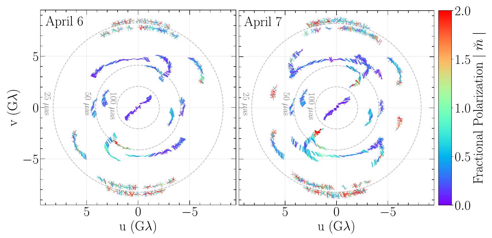
في الشكل 1، نعرض الـالتغطية واستقطاب التداخل منخفض التردد لملاحظات 6 و7 أبريل 2017 لـ Sgr A* كدالة لـ ( ) بعد معايرة المدى. الألوان ترمز إلى سعة الاستقطاب الكسرى المعقدة.في مجال الرؤية، تم متوسطه زمنياً بشكل متماسك في مقاطع مدتها 120 ثانية. وفقاً لجونسون وآخرين (2015)، نعرف نسبة الاستقطاب الجزئي في مجال الرؤية على أنها
أين، و تم أخذ عينات من معلمات ستوكز في مجال الرؤية. Sgr A* مستقطب بشكل معتدل في معظم الخطوط الأساسية،تحتوي نقاط البيانات على خطوط الأساس تشيلي-إل إم تي وتشيلي-هاواي في 7 أبريل 2017 على استقطاب جزئي مرتفع جداً،“، الذي يحدث في ( ) المسافات حيث ستوكيس تقترب السعات من حد أدنى عميق. نجد أيضًا أن نسب الاستقطاب في الأوقات القصيرة ( ) الخطوط الأساسية هي
الجدول 2 متوسط الحملة-مصطلحات APEX و JCMT و SMA المستمدة من طريقة المصادر المتعددة داخل الموقع
محطة
أبيكس
JCMT
SMA
ملاحظة. الـيُفترض أن تكون الشكوك على المدى الطويل موزعة كغوسي دائري في المستوى المركب.
الجدول 3 معايرة التسرب-الشروط المفترضة للمحطات التي لا تحتوي على موقع مشترك
محطة
LMT
SMT
PV
مماثلة لتلك التي لوحظت في عام 2013 بواسطة جونسون وآخرون (2015)؛ انظر الشكل 2.
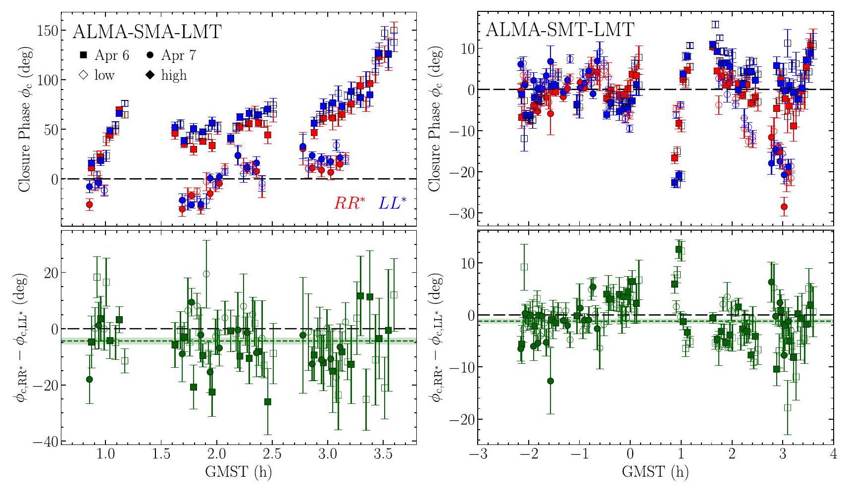
تظهر الشكل 3 مرحلة منتجات تتبع الإغلاق المرافقة على مربعين (ALMA-APEX-LMT-SMT و ALMA-LMT-SMA-SMT، مرتبة كما هو محدد في Broderick & Pesce 2020) لملاحظات Sgr A* في 6 و 7 أبريل 2017. تتبع الإغلاق هي كميات محصنة ضد مكاسب المحطات المعقدة وتسربات الاستقطاب. تنحرف منتجات تتبع الإغلاق المرافقة عن الواحد (أي، تنحرف مراحلها عن الصفر) فقط في وجود هياكل استقطاب غير متجانسة، وبالتالي فهي مؤشرات واضحة لاستقطاب المصدر (Broderick & Pesce 2020). نلاحظ انحرافات كبيرة عن الصفر في الشكل 3، مما يشير إلى أنلديها بنية استقطابية غير متجانسة وموزعة مكانيًا. القيم المختلفة إحصائيًا لمنتجات أثر الإغلاق المرافقة على نفس الأرباع بين 6 أبريل 2017 و7 أبريل تشير بشكل أكبر إلى أن البنية الاستقطابية فيهو متغير الزمن.
في الشكل 4 (الألواح العلوية)، نعرض الـ و مراحل الإغلاق على مثلثين يتمتعان بنسب إشارة إلى ضوضاء عالية بشكل خاص. الانحرافات الكبيرة عن الصفر هي نتيجة لهياكل مفككة وغير متكافئة في و يظهر الفرق في مرحلة الإغلاق بين منتجين الارتباط في اللوحات السفلية، مع عرض متوسط فرق مرحلة الإغلاق كحزام أخضر.عدم اليقين في تقدير المتوسط)، الذي ينحرف عن الصفر وبالتالي يشير إلى وجود إشارة استقطاب دائري، كما هو الحال بالنسبة لـ M87* (ورقة M87* IX). لأن تأثيرات تسرب الاستقطاب غير المصححة المتبقية تدخل في المستوى لمنتجات الارتباط ذات اليدين المتوازيتين، نتوقع الفرق بين و تكون مراحل الإغلاق مهيمنة بواسطة ستوكز الجوهريإشارة بدلاً من النظاميات الآلية. في الواقع، كشفت دراسة النظاميات في البيانات في الورقة الثانية عن وجود “ضوضاء” زائدة منكميات الإغلاق في بيانات Sgr A* مقارنة بمصادر أخرى، على الأرجح بسبب وجود استقطاب دائري داخلي في المصدر.
4. التخفيف من التباين، والتشتت، ودوران فاراداي في بيانات Sgr A*
بالمقارنة مع التحليل القطبي لـ M87* (ورقة M87* السابعة)، هناك تحديات إضافية في بيانات Sgr A* تزيد من صعوبة إعادة بناء الصور. التأثيرات
الشكل 1. الـالتغطية لملاحظات EHT في 6 أبريل (يسار) و7 أبريل (يمين) لـ Sgr A* خلال حملة 2017. لون نقاط البيانات يشفر سعة الاستقطاب الكسرية.في النطاق من 0 إلى 2، واتجاه العلامة يشفر اتجاه الاستقطاب المقاسالبيانات المعروضة مشتقة من الرؤى ذات النطاق المنخفض بعد تقليل البيانات وتم تطبيق المعايرة على المدى الطويل الموضحة في القسم 2. يتم حساب متوسط النقاط البيانية بشكل متماسك على مدى 120 ثانية. النسب العالية من الاستقطاب في أطراف بعض مسارات الخط الأساسي تعود إلى انخفاضبينما يستكشفون الحد الأدنى من الكثافة الكلية.
الشكل 2. مقارنة الاستقطاب الخطي الجزئي الذي تم ملاحظته في ملاحظات EHT السابقة في 21 مارس 2013 (اللوحة اليسرى؛ جونسون وآخرون 2015) ومقاييس مكانية مماثلة في ملاحظاتنا في 7 أبريل 2017 (اللوحة اليمنى). اللوحة الخاصة بسنة 2017 هي تكبير للوحة اليمنى من الشكل 1، مع نطاق سعة شريط الألوان من جونسون وآخرون (2015).
الشكل 3. مراحل منتج إغلاق الاقتران على مربعين لمرصد Sgr A* في 6 و 7 أبريل. تم حساب نقاط البيانات بشكل متماسك عبر كلا نطاقي الترددات وفي الزمن على مدى 120 ثانية. تشير المراحل غير الصفرية إلى أن المصدر لديه هيكل قطبي غير متجانس ومفصول مكانيًا.
الشكل 4. مراحل الإغلاق الملاحظة على مثلثات ALMA-SMA-LMT (يسار) وALMA-SMT-LMT (يمين) خلال ملاحظات Sgr A* في 6 أبريل (مربعات) و7 أبريل (دوائر). تشير العلامات المفتوحة والمملوءة إلى بيانات النطاق المنخفض والعالي، على التوالي. الأعلى: مراحل الإغلاق المكونة من الرؤى المتوسطة المأخوذة من المسح لكلا الفترتين،باللون الأحمر،باللون الأزرق. الأسفل: فرق مراحل الإغلاق بين و مستوى الصفر من فرق الإغلاق (أي، لاتم الكشف عنه) يتم تمييزه بخط متقطع أسود. الشريط الأخضر الفاتح يظهر المتوسطفرق.
من التشتت بين النجوم على طول خط الرؤية إلى مركز المجرة وتغير الزمن للمصدر على المدى القصير (تمت دراسة وتخفيف الأطر الزمنية (بالدقائق) في ستوكالتحليلات (الأوراق II و III و IV). نناقش كيف تتجلى التباين والتشتت في البيانات القطبية في الأقسام 4.1 و 4.2، على التوالي. في القسم 4.3، نناقش التأثيرات الإضافية لدوران فاراداي على النتائج وكيف تؤثر هذه على التفسير النظري.
4.1. التغير الزمني الجوهري
4.1.1. تباين ستوكز I
خلال حملة المراقبة EHT في عام 2017، أظهر Sgr A* ستوكزالتغير عبر مجموعة واسعة من مقاييس الزمن. يظهر منحنى الضوء المتكامل من المصدر خلال هذه الفترة تغيرًا من الدقائق إلى أطول مقاييس الزمن التي تم استكشافها. )، مع طيف طاقة زمنية “حمراء” (أي، تباين أكبر على مقاييس زمنية أطول؛ ويلغوس وآخرون 2022a). كما أن التباين الهيكلي موجود أيضًا على مقاييس مكانية قابلة للمقارنة مع ظل الثقب الأسود، ويظهر مباشرة في سعات الرؤية وكميات الإغلاق (الأوراق II و IV).
تغيركان متوقعًا نظريًا؛ المقياس الزمني الديناميكي بالقرب من أفق الحدث لـ هو ، والتقلبات المرصودة في السطوع هي نتائج طبيعية للهياكل المضطربة التي تتنبأ بها محاكاة الديناميكا المائية المغناطيسية العامة النسبية (GRMHD) (الورقة الخامسة). تؤكد دراسة مكتبة محاكاة EHT أن طيف القدرة الزمكانية للتغير (أي، التقلبات حول الصورة المتوسطة) في محاكاة GRMHD يتم تقريبه بشكل جيد بشكل عالمي بواسطة طيف كسر متناسق أسطوانيًا. القانون في كل من الأبعاد المكانية والزمنية (جورجييف وآخرون 2022). تهيمن هذه القوانين على أكبر المقاييس المكانية وأطول المقاييس الزمنية، أي أنها تظهر كثافة طيفية حمراء. ونتيجة لذلك، في محاكاة GRMHD، يمكن القضاء على الجزء الأكبر من التباين من خلال تطبيع الكثافة الإجمالية لإطارات الصور الفردية (ويلغوس وآخرون 2022أ). بعد تطبيع منحنى الضوء، يصل طيف الطاقة داخل الليلة إلى ذروته عند طول قاعدة ( ).
أدوات لقياس وتخفيف تأثير ستوكتم تطوير التباين في Sgr A* استنادًا إلى العالمية الملحوظة في محاكاة GRMHD (Broderick et al. 2022). تم تقدير طيف القوة المكاني من خلال حساب المتوسطات والتباينات لسعات الرؤية عبر نطاقات التردد والأيام في بقع من ( ) الطائرة بعد تطبيع منحنى الضوء وأداء إزالة الانحياز الخطي (انظر القسم 4 من برويدرِك وآخرون 2022). تستفيد هذه العملية من الطبيعة المدمجة لـ Sgr A*، وتستخدم التقريب المكاني المتساوي المتوقع من محاكاة GRMHD (جورجييف وآخرون 2022)، وتدمج تقديرات عدم اليقين التي تشمل المساهمات من الخطأ الإحصائي (أي، الضوضاء الحرارية)، وأ amplitudes الكسب، وعبارات التسرب ( -الشروط). نظرًا لأن عدد نقاط البيانات في أي نطاق من أطوال الأساس يمكن أن يكون صغيرًا، فإن هذه المقدرة قد تعاني من تحيزات معروفة يمكن تصحيحها من خلال المعايرة باستخدام مجموعات بيانات وهمية مناسبة (الورقة الرابعة). عند القيام بذلك، تتطابق التقديرات التجريبية الناتجة عن طيف قوة التباين الهيكلي مع تلك الناتجة من محاكاة GRMHD من حيث السعة والشكل (الورقة الخامسة).
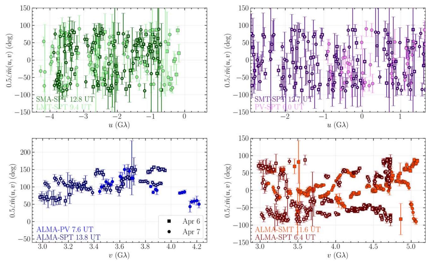
الشكل 5. مرحلةعلى المعبر والمسارات التالية المحددة في الورقة الرابعة، خلال التي نفس ( ) يتم أخذ عينات من المواقع في أوقات مختلفة بواسطة خطوط أساسية مختلفة في 6 أبريل 2017 (مربعات) و7 (دوائر). يتم وضع الطوابع الزمنية المركزية لكل مسار باللون المقابل (انظر الشكل 2 من الورقة الرابعة لمواقع المسارات الدقيقة في ( تمت معالجة جميع البيانات بشكل متسق على مقاييس زمنية تبلغ 120 ثانية لتوضيح التغيرات على المدى القصير. لم يتم إضافة أي عدم يقين منهجي إضافي.
تم التخفيف من التباين الهيكلي داخل الساعة لـ Sgr A* في الورقة الثالثة على ثلاث مراحل. أولاً، تم تطبيع الرؤية المعقدة وفقًا لمنحنى الضوء (Wielgus et al. 2022a)، مما أزال أكبر مكون من التباين وقمع جميع المكونات المرتبطة. ثانيًا، تم إدخال القوة الإضافية للتباين، المستنتجة من تقدير التباين التجريبي، كخطأ إحصائي إضافي حول هيكل الصورة المتوسطة. حيث كانت شدة هذا المكون الإضافي غير مؤكدة، تم استقصاء مستوى “الضوضاء” الزائدة كجزء من استكشاف التصوير والنمذجة. ثالثًا، تم تقدير عدم اليقين الإضافي اللازم من خلال “نمذجة الضوضاء”، وهو التوافق المباشر لنموذج متزامن للصورة المتوسطة ونموذج قانون القوة المكسور المعلم للخصائص الإحصائية للتباين غير المودل (Broderick et al. 2022; Paper IV).
4.1.2. التغير القطبي
متسق مع التوقعات التاريخية (مثل، باور وآخرون 2002؛ مارون وآخرون 2006أ)، خلال حملة EHT لعام 2017، أظهر Sgr A* تباينًا قطبيًا كبيرًا. هذا التباين يُشير إليه بشدة التغيرات السريعة.في اتجاه الاستقطاب المقاس في الشكل 1. كما يتم عرض التغير بشكل صريح في الشكل 5 للمسارات المتقاطعة واللاحقة المحددة في الورقة الرابعة – مقاطع من المسارات الأساسية التي تتداخل بشكل كبير في أوقات المراقبة المختلفة طوال الليل – والتي تحدث فيها تقلبات كبيرة في اتجاه الاستقطاب.
موجود على مقاييس الزمن“، بما في ذلك الفروق الكبيرة بين 6 و 7 أبريل 2017. كما يُشير التباين القطبي بشكل مشابه إلى التغيرات السريعة في منتجات تتبع الإغلاق المترافق الموضحة في الشكل 3، ويتم توضيحه بشكل صريح من خلال المقارنة بين أيام الملاحظة. بالنسبة لكلا الرباعيات الموضحة في الشكل 3، يتغير طور منتجات تتبع الإغلاق المترافق بـعلى مقاييس زمنية تصل إلى عشرات الدقائق، وعلى مقاييس زمنية مشابهة للتغيرات الملحوظة في ستوكزلكن أقل في الحجم.
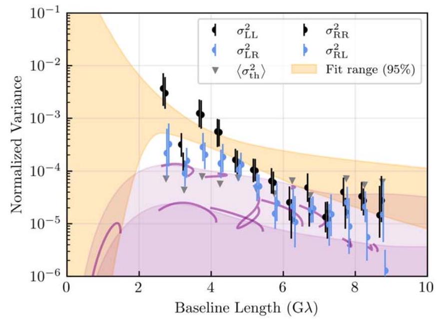
لتقييم درجة التباين القطبي بشكل كمي، نقوم بتوسيع التقدير التجريبي المستخدم لستوكزمن برويدرِك وآخرون (2022) إلى منتجات الارتباط المستقل بين اليدين المتوازيتين واليدين المتقاطعتين. بعد تطبيق مصطلحات التسرب المحددة بواسطة المعاير، تكون الإجراءات مشابهة لتلك الموجودة في الورقة الرابعة: يتم حساب متوسط الرؤية على أساس المسح وتطبيع منحنى الضوء، ويتم حساب المتوسط والتباين داخل البقع بعد إزالة الاتجاه الخطي ومتوسط الزاوية، وتُقدّر الشكوك من خلال أخذ عينات مونت كارلو للشكوك الإحصائية، والمكاسب المعقدة، والتسربات. يتم توليد تقديرات طيف الطاقة المتوسطة الزاوية بشكل مستقل لـ، و تظهر النتائج بعد دمج بيانات 6 و 7 أبريل 2017 في الشكل 6 لكل يد بشكل مستقل.
طيف الطاقة المتوازي المقدر تجريبياً و ) لا يمكن تمييزها إحصائيًا عن بعضها البعض وعن تلك المرتبطة بـ Stokes الخاصة بها نظير. هذه الشبه يوحي بأن التغير المطلق في ستوكزعلىكما أنه صغير مقارنة بالتغير في ستوكزعمليًا، يعني ذلك أن التباين في الأيدي المتوازية يمكن تقليله بشكل فعال باستخدام النموذج في الأوراق الثالثة والرابعة لـ و بشكل فردي.
طيف القوة المتقاطع و ) غير قابلة للتمييز إحصائيًا عن بعضها البعض. في غياب التسرب غير المصحح، فإن هذا متوقع من حيث البناء وبالتالي يوفر ثقة إضافية في ما يُستنتج من المعاير-الشروط. والأهم من ذلك، أن طيف القوة المتقاطع يشترك في الشكل مع تلك المرتبطة بالأيدي المتوازية، على الرغم من إعادة قياسها تقريبًامن سعة اليدين المتوازيتين.
كما في الأوراق الثالثة والرابعة، نستخدم عدة استراتيجيات لتخفيف التباين عند نمذجة أو تصوير بيانات Sgr A*. يمكن تقسيم هذه الاستراتيجيات إلى فئتين عامتين: بعد التهميش: يتم إعادة بناء صور متعددة على مجموعات فرعية من البيانات التي تمتد لفترات زمنية قصيرة بما يكفي يمكن تجاهل التباين، ثم يتم دمجها لاحقًا لإنتاج صورة “متوسطة” واحدة. قبل التهميش: يتم ملاءمة صورة واحدة لمجموعة البيانات الكاملة، مع إضافة ضوضاء إضافية لتفسير الانحرافات في الرؤى بسبب التباين الهيكلي بالإضافة إلى المكونات الإحصائية والنظامية. لطرق ما قبل التهميش، نستخدم طيف القدرة المتغير القطبي التجريبي بطريقة مشابهة لما هو مذكور في الورقة الثالثة، مع تعديلها لإعادة البناء القطبي. كما هو الحال مع ستوكزنقوم بتطبيع جميع نواتج الارتباط بواسطة ستوكزمنحنى الضوء لتقليل تأثير التغيرات المرتبطة على نطاق واسع. ثم يتم إضافة خطأ إحصائي إضافي وفقًا لنموذج القوة المكسورة بشكل تربيعي إلى كل منتج ارتباط، مع تلقي الأيدي المتوازية نفس الضوضاء الإضافية كما تم تطبيقها على ستوكز.وتلقي الأيدي المتقاطعة مبلغًا يتم تقليصه بنسبة ثابتة.
بالنسبة لـ Sgr A*، فإن نسبة تباين اليد المتوازية/اليد المتقاطعة هيأي، يتم إضافة نصف الضوضاء فقط بشكل مطلق إلى الأيدي المتقاطعة مقارنة بتلك المضافة إلى الأيدي المتوازية.اعتمادًا على طريقة إعادة بناء الصورة القطبية، يتم استقصاء معلمات نموذج الضوضاء الإضافية أو إعادة بنائها مباشرة (انظر الملحق أ). علاوة على ذلك، تعتمد قيمة نسبة التباين هذه على خصائص المصدر ويمكن أن تكون أصغر بكثير أو أكبر لمجموعات بيانات أخرى (مثل مجموعات البيانات الاصطناعية التي تم مناقشتها في الملحق ب) مما تم العثور عليه لـاعتمادًا على كل من نسبة الاستقطاب ودرجة التغير.
4.2. التشتت بين النجوم
عند أطوال موجات الراديو، صورةيتشتت بشكل كبير بواسطة البلازما بين النجوم المؤينة على طول خط الرؤية. على وجه الخصوص، تؤدي عدم تجانس الكثافة إلى مؤشر انكسار متغير، مع تقلبات في الطور عبر الصورة تتغير مع الزمن وطول الموجة المراقب.للنقاش التفصيلي وملخص تاريخي عن تشتت Sgr A*، انظر Psaltis وآخرون (2018) وJohnson وآخرون (2018).
تسبب تأثيرات التشتت بشكل أساسي في عدم التجانس على مقاييس مكانية متباعدة على نطاق واسع. ينشأ التشتت “الانكساري” من تقلبات على مقاييس مكانية منوينتج عنه تشويش الصورة باستخدام نواة تقريبية غاوسية. “التشتت الانكساري” ينشأ من تقلبات على مقاييس مكانية منوينتج عن ذلك تشويه غير منتظم للصورة لا يتوافق مع الالتفاف. من حيث الرؤية التداخلية، فإن الإشارة
الشكل 6. تقديرات غير مرتبطة بالنموذج للتباين الزائد المتوسط الزاوي لدرجات وضوح اليد المتوازية واليد المتقاطعة، بعد إزالة ذلك من الأخطاء الإحصائية المبلغ عنها، كدالة لطول القاعدة. تم الحصول على تقديرات غير معلمية عبر 6 و7 أبريل، باستخدام بيانات النطاق العالي والمنخفض. تشير القضبان الخطأ إلى عدم اليقين المرتبط بالأخطاء الحرارية، واختلاف مكاسب المحطات، وتسرب الاستقطاب. تُظهر الأخطاء الحرارية المتوسطة الزاوية مثلثات رمادية وتوفر حدًا أدنى تقريبيًا على نطاق تقديرات التباين الدقيقة. للمقارنة، تُظهر مقادير التباين الناتج عن التشتت الانكساري باللون الأرجواني على المحاور الثانوية (الأعلى) والرئيسية (الأسفل) لنواة التشتت الانكساري (انظر القسم 4 من الورقة III)؛ يُظهر التباين على المسارات الفردية في 7 أبريل بواسطة الخطوط الأرجوانية الصلبة. تشير الشريط البرتقالي إلى النطاق المئوي الخامس والتسعين لتناسبات القوة المكسورة على ستوكز.التباينات الزائدة من الورقة الرابعة.
على الخطوط الأساسية الطويلة، يتم قمعها بشكل أسي بواسطة تشويش الانكسار ولكنها تحتفظ بمساهمة إضافية من “الضوضاء” الانكسارية (غودمان ونارايان 1989؛ نارايان وغودمان 1989؛ جونسون وآخرون 2015؛ جونسون ونارايان 2016). في هذه الورقة، نتبع النهج المستخدم في الأوراق السابقة في هذه السلسلة و”نزيل التشويش” من بياناتنا قبل التصوير (انظر، على سبيل المثال، فيش وآخرون 2014)، حيث نقوم بقسمة كل قياس على نواة التشتت المترافقة فورييه على خطه الأساسي؛ نستخدم معلمات نواة التشتت من جونسون وآخرون (2018)، التي تم تقديرها باستخدام قياسات تاريخية لـ Sgr A* وتم التحقق منها من خلال قياسات لاحقة (عيسى وآخرون 2019، 2021؛ تشو وآخرون 2022). انظر الورقة الثانية لمزيد من التفاصيل حول تأثيرات التشتت بين النجوم لبيانات EHT Sgr A*.
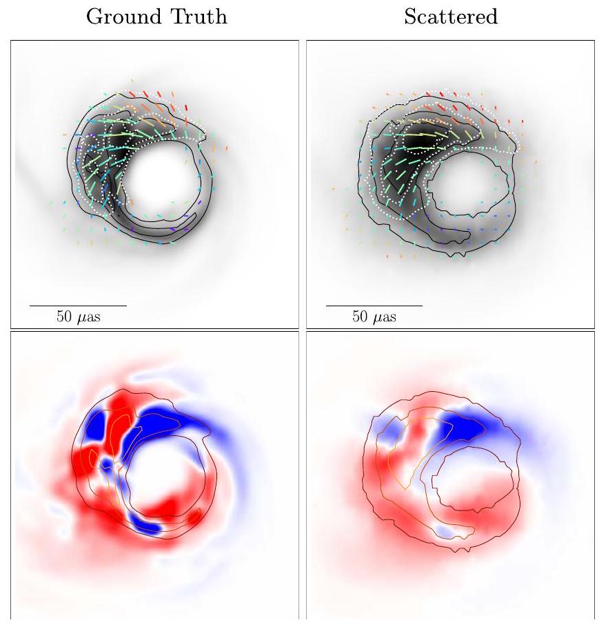
لأن الوسط بين النجمي المؤين ليس له تأثير كبير في التشتت (على سبيل المثال، تومسون وآخرون 2017؛ ني وآخرون 2022)، فإن تأثيرات التشتت على الملاحظات القطبية يمكن أن تكون خفيفة. على سبيل المثال، فإن الاستقطاب النسبي في التداخل لا يتأثر بالتشويش الناتج عن الانكسار؛ وخصائص الصورة المدمجة الأخرى، مثل الوضع المتناظر دورانيًا (التي نقوم بتحليلها بشكل موسع في الورقة الثامنة، تتأثر فقط بشكل طفيف بالتشويش (بالومبو وآخرون 2020). بشكل عام، فإن الاستقطاب النسبي التداخلي يتأثر بشكل ضعيف لأي قاعدة يكون فيها الضجيج الانكساري صغيرًا مقارنةً بسعة الإشارة (انظر، على سبيل المثال، ريكارتي وآخرون 2023). علاوة على ذلك، نظرًا لأن شعاع EHT Comparable إلى حجم نواة التشويش الانكساري، فإن آثار التشتت على الصورة المستقطبة لـمن المتوقع أن تكون خفيفة عند مشاهدتها بدقة EHT. الشكل 7 يظهر أمثلة على الصور المتناثرة لمحاكاة GRMHD في الاستقطاب الخطي والدائري.
تظهر الجدول 4 قيم الكميات الصورية المفيدة في تمييز النماذج القطبية في الصور غير المتناثرة، والمتناثرة، والمشوشة لمحاكاة GRMHD المعروضة عند 230 جيجاهرتز.
الشكل 7. مقارنة لصور محاكاة GRMHD في الاستقطاب الخطي (الأعلى) والدائري (الأسفل) مع وبدون تأثيرات تشتت بين النجوم. الكميات القابلة للقياس المرتبطة موضحة في الجدول 4. لأغراض العرض، تم تشويش الصور غير المتشتتة بشكل طفيف.كشعاع غاوسي دائري، أصغر بكثير من دقة أداة EHT. الأعلى: يتم عرض الكثافة الكلية في مقياس رمادي، وتوضح علامات الاستقطاب EVPA، حيث يكون طول العلامة متناسبًا مع مقدار كثافة الاستقطاب الخطي، ويشير اللون إلى النسبة المئوية للاستقطاب الخطي. مستويات الخطوط المنقطة تت correspond إلى كثافات الاستقطاب الخطي لـ، و ذروة الاستقطاب. يتم إجراء قصات لاستبعاد جميع المناطق في الصور حيث ستوكيسذروة السطوع ومن ذروة السطوع المستقطب. الأسفل: يتم الإشارة إلى الكثافة الكلية في خطوط متدرجة ملونة، و ستوكزيتم الإشارة إلى السطوع في خريطة الألوان المتباينة، حيث يشير الأحمر/الأزرق إلى علامة إيجابية/سلبية.
نحدد كسور الاستقطاب الخطي والدائري المتكاملة بالصورة على أنها
حيث يكون المجموع على البكسلات المفهرسة بواسطةنقوم أيضًا بقياس كسور الاستقطاب الخطي والدائري المتوسطة للصورة. و عبر الصور:
لاحظ أن هذه الكميات تعتمد على دقة الصورة؛ ستحتوي صور GRMHD عالية الدقة على نسب استقطاب أكبر بشكل منهجي من نظيراتها من إعادة بناء الصور. جميع الصور المستخدمة في التحليلات في هذه الورقة والورقة المرافقة الثامنة قد تم تشويشها إلى دقة فعالة منوفقًا لبالومبو وآخرون (2020)،
الجدول 4 كميات الصورة ذات الاهتمام المحسوبة على لقطة من محاكاة GRMHD مع وبدون تأثيرات تشتت بين النجوم
بارام.
جوهرية
مبهم
مبعثر ومشوش
(%)
٤.٧٢
٤.٧٢
٤.٦٢
0.33
0.33
0.35
٤٩.٦٦
٣١.٩٧
31.82
٢.٢٦
0.91
0.93
0.14
0.14
0.14
0.34
0.30
0.29
(درجة)
93.8
92.5
92.4
2.43
2.15
2.14
ملاحظة. محاكاة GRMHD هي نموذج قرص محاصر مغناطيسيًا مع، و تمت مشاهدته في الميل قبل وبعد تشتت النجوم بين النجوم (تعاون تلسكوب أفق الحدث وآخرون 2022e). في العمود الأوسط، الصورة مشوشة بواسطة كحزمة غاوسية دائرية. في العمود الأيمن، يتم تطبيق تأثيرات التشتت المحاكاة، مما ينتج عنه تشويش تداخلي على مقاييس تحت الحزمة. يتم إجراء تشويش غاوسي دائري إضافي للوصول إلىمثل دقة التصوير. مجال الرؤية وحجم البكسل هما نفس الشيء في كل حالة. نحن أيضًا نحسب المعقدالأوضاع، التي هي تحللات فورييه لهيكل الاستقطاب الخطي:
أين ( ) هي إحداثيات قطبية في مستوى الصورة و هو كثافة التدفق الكلي في الصورة. الـ الوضع هو أبسط وضع غير متماثل، بينما هو أبسط وضع متماثل دوراني. على وجه الخصوص، هو استقصاء ليدوية وزاوية الميل للالتواء العام لنمط زاوية استقطاب المتجه الكهربائي (EVPA)، حيثتشير إلى نمط EVPA شعاعي وتشير إلى نمط EVPA حلقي في الصورة.
الكميات المدمجة بالصورة مثلتتغير قليلاً جداً، بينما الكميات المحددة مثلتتضاءل بشكل كبير بسبب تشويش التشتت الناتج عن التشتت. ومن الجدير بالذكر أن الكميات الشكلية ذات الدقة المنخفضة مثل و تكاد تكون غير متأثرة تمامًا، خاصة في الطور، على الرغم من أن الأوضاع ذات الرتبة الأعلى ستكون أكثر اضطرابًا. ومع ذلك، فإن الحجم الفعال لنواة التشتت، كما هو، أدناه دقة الأداة الفعالة لـ، وبالتالي فإن وجود التشتت ليس ملوثًا كبيرًا لكميات الصورة ذات الاهتمام.
4.3. دوران فاراداي
عندما تنتشر الإشعاعات عبر وسط مغناطيسي، يتأثر حالة الاستقطاب بتأثيرات فاراداي. والأهم من ذلك، أن EVPA يتغير بسبب دوران فاراداي، الذي يمكن قياسه باستخدام RM. يمكن وصف RM على أنه
فرق في قياسات EVPAsبين نطاقات التردد التي تتوافق مع الأطوال الموجية (على سبيل المثال، برينتجنز ودي بروين 2005). RM كبير من تم قياسه في Sgr A* عند 230 جيجاهرتز. بينما تتقلب القيمة المقاسة لـ RM بشكل كبير، إلا أن الإشارة السلبية الملحوظة ظلت ثابتة لعقود (على سبيل المثال، باور وآخرون 2018؛ ويلغوس وآخرون 2024). قياسات RM التفصيلية من ALMA كشبكة تداخلية مرتبطة بالعناصر متاحة لفترات المراقبة الدقيقة لـ EHT، والتي تشير إلى قيم تتماشى مع البيانات التاريخية (غودي وآخرون 2021؛ ويلغوس وآخرون 2022ب، 2024)؛ انظر الجدول 5.
إذا كان من الممكن بثقة نسب RM بالكامل إلى شاشة فاراداي خارجية تقع بين المصدر المدمج المنبعث والأرض، فيمكن استعادة نمط EVPA الجوهري ببساطة عن طريق “إعادة تدوير” علامات EVPA بمقدار. بالنسبة لهذه الملاحظات، فإن قياس RM بافتراض وجود شاشة خارجية بالكامل يؤدي إلى تدوير الـ EVPAs المرصودة بحوالي (الجدول 5) في اتجاه عقارب الساعة قبل مقارنتها بالنماذج النظرية لتدفق التراكم بالقرب من أفق حدث الثقب الأسود. يتم دعم الطابع الخارجي لشاشة فاراداي من خلال استمرار إشارة RM على مدى فترات زمنية طويلة، حيث نتوقع حدوث انعكاسات متكررة للإشارة في تدفق التراكم المضطرب بالقرب من أفق الحدث (ريكارت وآخرون 2020؛ ريسلر وآخرون 2023). من ناحية أخرى، أفاد ويغلس وآخرون (2022ب) بتدوين فاراداي الزمني، مع تقلب RM المستنتج بمقدار يصل إلى على مقاييس زمنية دون الساعة. تشير هذه النتائج إلى أن جزءًا على الأقل من دوران فاراداي ناتج عن شاشة فاراداي داخلية متزامنة مع المنطقة المضيئة المدمجة المرصودة (ويلغوس وآخرون 2024). في هذه الحالة، لا يتطلب الأمر أي تعديل لزاوية الاستقطاب قبل مقارنة النماذج بالملاحظات، حيث يجب أن تأخذ النماذج النظرية لمنطقة الانبعاث المدمجة في الاعتبار دوران فاراداي المرصود بالكامل.
يمكن أن تتضمن صورة التوافق شاشة فاراداي خارجية تتغير ببطء للحفاظ على إشارة ثابتة على المقاييس الزمنية ذات الصلة بالإضافة إلى شاشة فاراداي داخلية من نفس الحجم لشرح التغير السريع في الزمن (ريسلي وآخرون 2023). في هذه الصورة، يكون من المبرر تدوير علامات EVPA بواسطة الوسيط RM المقاس لمراقبة معينة، حيث إن مدة ليلة المراقبة أطول بكثير من المقياس الزمني الديناميكي بالقرب من أفق الحدث.. علاوة على ذلك، بسبب التغير السريع في RM الذي تم قياسه بواسطة ALMA (ويلغوس وآخرون 2022ب)، فإن مقدار فساد EVPA يتغير مع مرور الوقت بحوالي (الجدول 5). هذا يزيد من عدم اليقين في هيكل EVPA المستنتج في الصور المعاد بناؤها ويمكن أن يتم التقاطه في تقديرات مدفوعة بالبيانات لتغيرات الاستقطاب التي تم مناقشتها في القسم 4.1.2. هذه الاعتبارات حاسمة للتفسير النظري لنتائج EHT، ونحقق في تأثير دوران فاراداي بمزيد من التفصيل باستخدام المحاكاة في الورقة الثامنة.
5. الطرق
في هذا القسم، نقدم ملخصًا للطرق المستخدمة في نتائج الاستقطاب لـ Sgr A*. نقوم بإجراء نمذجة هندسية للمصدر باستخدام طريقة ملاءمة نموذج الحلقة اللحظية (الورقة الرابعة؛ رويلوفز وآخرون 2023). نستخدم أيضًا ثلاث طرق تصوير: إطار التصوير بايزي THEMIS (برودرِك وآخرون 2020، 2020c) وطرق الاحتمالية القصوى المنتظمة (RML) مثل eht-imaging (تشايل وآخرون 2016، 2018) وDoG-HiT (مولر ولوبانوف 2022). هذه الطرق تختلف جوهريًا عن بعضها البعض في كيفية تعاملها مع التغيرات الداخلية للمصدر. هنا نلخص الخصائص الرئيسية للطريقة؛ يمكن العثور على أوصاف أكثر تفصيلًا في الملحق A.
كاستمرار للتحليل الذي تم إجراؤه في الأوراق المرافقة للشدّة الكلية (الأوراق III و IV)، نقوم بنمذجة هيكل الاستقطاب فوق شكل الحلقة، المستنتج من خلال تحليل ملاحظات الشدّة الكلية. للمساعدة
الجدول 5 متوسط قياس الدوران لـ Sgr A* المستخلص من منحنيات الضوء التداخلية لـ ALMA (ويلغوس وآخرون 2022b)
ملاحظات
RM ( )
EVPA (درجة)
6 أبريل
7 أبريل
11 أبريل
6، 7 أبريل
جميع الأيام
ملاحظة. تقديرات الخطأ تتعلق بـتم تقييم التغيير في EVPA عند 228.1 غيغاهرتز. في خطوة إعادة بناء الكثافة الكلية، تستخدم طرق التصوير RMLمجموعات البيانات التي تم معايرتها ذاتيًا إلى الصورة المتوسطة الموثوقة المزالة الضبابية الناتجة عن إجراء تجميع الصور في القسم 7.2 من الورقة الثالثة. تم عرض اختبارات تأثير أوضاع تجمع الحلقات المختلفة على إعادة بناء الهيكل القطبي، والتي تكون ضئيلة، في الملحق C. لا تستخدم طرق THEMIS وsnapshot m-ring البيانات المعايرة ذاتيًا وتقوم بمعايرتها ذاتيًا بالتزامن مع ملاءمة البيانات. جميع الطرق تستخدم بيانات تم تم معايرة المدى الزمني، وتطبيع منحنى الضوء، وإزالة الضبابية لمواجهة آثار التشتت الانكساري وتحديد ميزانية الضوضاء المناسبة للشدة الكلية والاستقطاب وفقًا لدراسات التغير الموضحة في القسم 4.1.
5.1. نمذجة حلقة اللقطة
باستخدام طريقة نمذجة حلقة م لحظية، نقوم بتطبيق نموذج هندسي قطبي (“حلقة م”؛ انظر الملحق أ للتفاصيل) على لقطات مدتها دقيقتان من مجموعات بياناتنا (الورقة الرابعة؛ رويليفز وآخرون 2023). نحن نستخدم فقط اللقطات التي تحتوي على 10 رؤى على الأقل و60 ثانية من وقت التكامل المتماسك. بعد متوسط الوقت للقطات إلىتُضاف amplitudes الرؤية إلى ميزانية الضوضاء الحرارية لتمثيل الشكوك النظامية. نقوم بتثبيت معلمات التسرب على الحلول المحددة مسبقًا من تحليل EHT القطبي لـ M87*؛ انظر القسم 2. بالنسبة لملاءمات الاستقطاب الخطي لدينا، نقوم بملاءمة نموذج الحلقة m لدينا إلى مراحل الإغلاق، amplitudes الإغلاق، ونسبة الاستقطاب الخطي في مجال الرؤية.لكل لقطة بشكل مستقل (أي أنه لا يُفترض وجود ارتباطات زمنية). بالنسبة لتناسبات الاستقطاب الدائري لدينا، نقوم بتثبيت معلمات الاستقطاب الخطي على تقديرات الحد الأقصى الاحتمالي (MAP) ونتناسب مع مراحل الإغلاق لليد المتوازية وسعات الإغلاق (أي أننا نتناسب مع و منتجات الإغلاق). نحن نستكشف أيضًا التوافق معنسب الرؤية. جميع هذه المنتجات البيانية قوية أمام مكاسب المحطات المضاعفة، باستثناءنسب الرؤية، التي قد تتأثر بالبقايانسب المكاسب (انظر أيضًا الاختبارات التي أجريت في رويلوفس وآخرون 2023). بعد ملاءمة كل لقطة من كل يوم ونطاق ترددي، نقوم بدمج جميع التوزيعات اللاحقة في توزيع لاحق واحد باستخدام نظام متوسط بايزي (الورقة الرابعة).
5.2. ثيميس
كما هو موضح في Broderick et al. (2020) وM87* Paper VII، يتكون نموذج صورة THEMIS من مجموعة مستطيلة من نقاط التحكم، تمتد عبر منحنى بيكوبي. اتجاه الصورة ومجال الرؤية هما معلمتان حرتان وتتكيفان ديناميكيًا أثناء إعادة بناء الصورة لاختيار دقة فعالة. يتم تحديد دقة الشبكة عن طريق تعظيم الأدلة البايزية على بعد الشبكة؛ عادةً ما تكون هذه صغيرة بسبب العدد المحدود من عناصر دقة EHT عبر Sgr A*، ونستخدم راستر قائم على ستوكالدراسة في الورقة الثالثة. يتكون نموذج الصورة القطبية الكامل من أربعة شبكات متطابقة الحجم والتوجه تحدد الكثافة الكلية، ونسبة الاستقطاب، وزاوية الاستقطاب الكهربائية، وستوكز.كما هو موضح في برويدرِك وآخرون (2022) والقسم 4.1.2، يتم التخفيف من تباين المصدر الداخلي من خلال نمذجة مساهمة إضافية تعتمد على خط الأساس في عدم اليقين في البيانات. يتكون نموذج عدم اليقين من مكونات تتوافق مع ضوضاء التباين، وضوضاء التشتت الانكساري، وميزانية الخطأ المنهجي (انظر، على سبيل المثال، الورقة الرابعة).
إعادة بناء THEMIS تتناسب مباشرة مع الرؤية المعقدة المتوسطة للمسح )، بعد تطبيع منحنى الضوء كما هو موضح في القسم 4.1.2، تم دمجه عبر النطاقات وفي 6 و 7 أبريل 2017. بالتزامن مع توليد الصور، يتم استرداد مصطلحات التسرب والمكاسب المعقدة. لتجنب التعقيدات الناتجة عن التغيرات المحتملة من ليلة إلى أخرى في -الشروط في ALMA وSMA، نقوم بتناسب البيانات التي تم تصحيحها مسبقًا باستخدام تسريبات ورقة M87* السابعة. ومع ذلك، أثناء التناسب،-المصطلحات التي تظل ثابتة عبر كلا يومي الملاحظة والأشرطة العالية والمنخفضة يتم الحصول عليها من Sgr A* فقط ولا تتضمن تقديرات تسرب سابقة من إعادة بناء مصادر أخرى. يتم إعادة بناء مكاسب المحطات المعقدة بشكل مستقل على المسحات وعبر الأشرطة ولكنها مقيدة بأن تكون وحدة.نسب المكاسب. تم الإبلاغ عن اختبارات البيانات الاصطناعية في ورقة M87* IX حول ستوكزفي M87* أظهر أنتنتج الفجوات في المكاسب التي تزيد عن بضع نقاط مئوية ملاءمات أسوأ بشكل ملحوظ من تلك التي تحتوي على فجوات أصغر. أنتجت صور THEMIS ملاءمات عالية الجودة لبيانات EHT؛ وبالتالي،من المتوقع أن تكون مكاسب التعويضات صغيرة جداً.
نتيجة ملاءمات THEMIS هي تقريبا توزيع خلفي يتكون من مجموعة من الصور التي يمكن استخدامها للتفسير البايزي. لمزيد من التفاصيل حول بناء الاحتمالات، والعينة، ومعايير تقارب السلسلة، انظر الملحق A والمراجع المذكورة هناك.
5.3. تصوير Eht
حزمة التصوير EHT (Chael et al. 2016, 2018) هي خوارزمية تصوير تعتمد على البكسل. يتم إجراء إعادة البناء من خلال تقليل دالة الهدف عبر الانحدار التدرجي. تم بناء هذه الدالة الهدف مع مصطلحات جودة الملاءمة ومصطلحات المنظم التي تفضل أو تعاقب خصائص الصورة المحددة. بالنسبة لإعادة بناء الصور المستقطبة، نتبنى منهجية مشابهة جدًا لتصوير الاستقطاب لـ M87*، الموضحة في الملحق C من ورقة M87* VII. نظرًا لأن التسرب قد تم تصحيحه بالفعل في بيانات Sgr A* من تحليل M87*، يتم حذف هذه الخطوة. نستخدم البيانات التي تم معايرتها ذاتيًا لصورة الكثافة الكلية المرجعية كنقاط بيانات البداية لدينا. هذه البيانات تم معايرتها ذاتيًا لصورة غير مشوشة، لذا لا يتم إجراء أي تخفيف للتشتت كجزء من إجراءاتنا. نقوم بمتوسط البيانات بشكل متماسك لمدة 120 ثانية، ونجمع النطاقات العالية والمنخفضة في مجموعة بيانات واحدة، ونعيد بناء صورة واحدة لكل يوم ملاحظة في 6 و 7 أبريل. نضيف ميزانية ضوضاء منهجية جزئية من بناءً على استكشاف معلمات الكثافة الكلية (انظر الجدول 4 من ورقة III). نضيف أيضًا ميزانية ضوضاء التغير المحددة في جهود الكثافة الكلية في مربع إلى عدم اليقين لكل نقطة رؤية (انظر القسم 3.2.2 من ورقة III)، مما يقلل من
الميزانية المطبقة على رؤى اليد المتقاطعة بناءً على تقييم التغير الاستقطابي في القسم 4.1.2.
كخطوة أولى، نقوم بإعادة بناء صورة الكثافة الكلية الابتدائية من خلال التوافق مع مراحل الإغلاق لليدين المتوازيتين، وسعات الإغلاق، وسعات الرؤية. يتم الاحتفاظ بهذه الصورة الكثافة الكلية ثابتة أثناء التصوير الاستقطابي، مما يحدد المناطق التي يُسمح فيها بكثافة الاستقطاب. يتم التصوير من خلال جولات تكرارية من الانحدار التدرجي. في كل تكرار، يتم تشويش الصورة الناتجة باستخدام كحزمة غاوسية وتستخدم كصورة أولية للجولة التالية، وتزداد الأوزان على مصطلحات البيانات. يتم إجراء التصوير الاستقطابي الخطي والتصوير الاستقطابي الدائري بشكل منفصل. بالنسبة للاستقطاب الخطي، نقوم بتوافق الرؤية الاستقطابية ونسبة الرؤية الاستقطابية في مجال الرؤية . بالنسبة للاستقطاب الدائري، نقوم بتوافق الرؤى المعايرة ذاتيًا ومراحل الإغلاق لليدين المتوازيتين وسعات الإغلاق، ونحل للحصول على مكاسب معقدة يمينًا ويسارًا بشكل مستقل.
5.4. DoG-HiT
حزمة DoG-HiT (Müller & Lobanov 2022، 2023a، 2023b) هي خوارزمية تصوير تعتمد على الموجات تستخدم الاستشعار الضاغط. يقوم DoG-HiT بتوافق مصطلحات البيانات مع افتراض أن هيكل الصورة يتم تمثيله بشكل نادر بعدد قليل من الموجات. بالنسبة للتحليل الاستقطابي والديناميكي، نتبع الوصف المقدم في Müller & Lobanov (2023b). مشابهًا للإجراء الخاص بتصوير EHT الموضح في القسم 5.3، نستخدم مجموعة البيانات المتوسطة، والمعايرة ذاتيًا، والمصححة للتسرب كنقطة انطلاق. لم يتم تطبيق أي تخفيف للتشتت كجزء من الإجراء. نضيف ميزانية ضوضاء منهجية جزئية من إلى الرؤى المتوسطة التي تم متوسطها لمدة 120 ثانية.
أولاً، نستعيد صورة ستوكيس المتوسطة باستخدام DoG-HiT، فقط نتوافق مع مراحل الإغلاق وسعات الإغلاق المحسوبة من رؤى ستوكيس . نقوم بمعايرة المكاسب المتبقية لهذه الصورة على فترات مدتها 10 دقائق، ونستخرج الدعم متعدد الدرجات، أي مجموعة من معاملات الموجات المهمة، من الصورة المتوسطة. يحدد الدعم متعدد الدرجات المقاييس المكانية والمواقع للتصوير الديناميكي والاستقطابي حيث يُسمح بالإشعاع. بعد ذلك، نقوم بإنشاء صورة استقطابية متوسطة من خلال توافق الرؤى الاستقطابية و ، لكننا نسمح فقط لمعاملات الموجات في الدعم متعدد الدرجات بالتغير. في إجراء تكراري، نقوم بحل لمصطلحات المتبقية. أخيرًا، نقوم بتقسيم الملاحظة إلى إطارات مدتها 30 دقيقة ونتوافق مع الرؤى الكثافة الكلية والاستقطابية في كل إطار بشكل مستقل بدءًا من الصور المتوسطة، لكننا نغير فقط معاملات الموجات في الدعم متعدد الدرجات. نقوم بمتوسط الإطارات المستعادة بشكل موحد لتحقيق صورة ثابتة نهائية. يتم تنفيذ الإجراء بالكامل لكلا يومي الملاحظات بشكل مستقل وأخيرًا يتم متوسطها.
5.5. اختبارات البيانات الاصطناعية
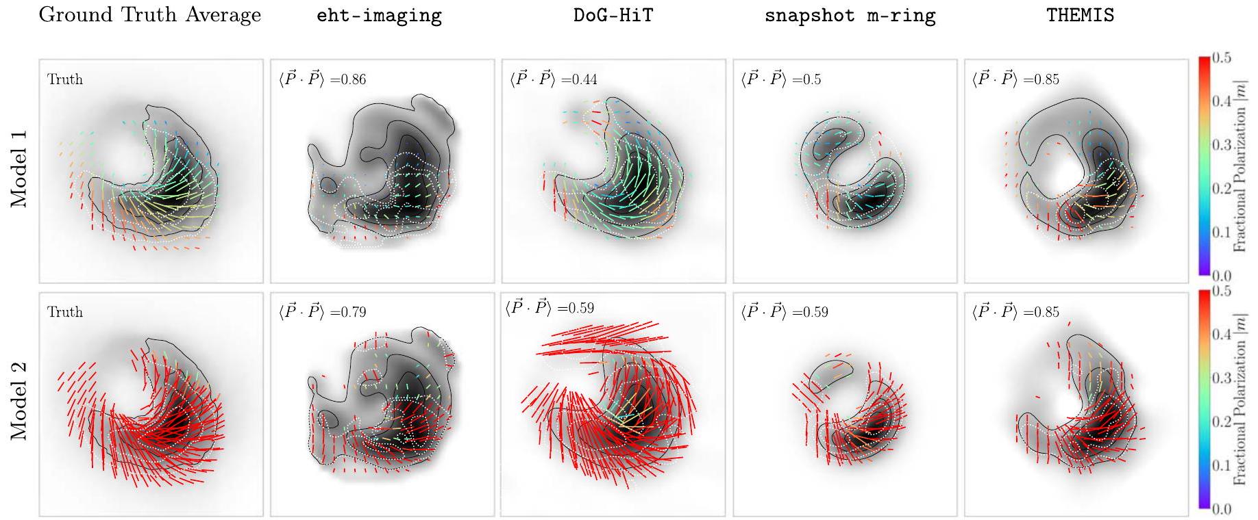
تم التحقق من جميع الطرق ضد مجموعات بيانات اصطناعية تحاكي خصائص Sgr A*، والتي تم تقديم نتائجها بالتفصيل في الملحق B. تم اختيار نموذجين من GRMHD من مجموعة النماذج النظرية لـ Sgr A* التي تحاكي كل من خصائص الكثافة الكلية والاستقطاب. يحتوي أحد النماذج على استقطاب خطي إجمالي أقل من Sgr A* ولكنه يحتوي على نسبة تغير مشابهة لليد المتقاطعة مقارنة برؤى اليد المتوازية، بينما يحتوي النموذج الآخر على نسبة استقطاب خطي إجمالي مشابهة لتلك الخاصة بـ ولكنه يحتوي على نسبة تغير أعلى لليد المتقاطعة مقارنة بـ
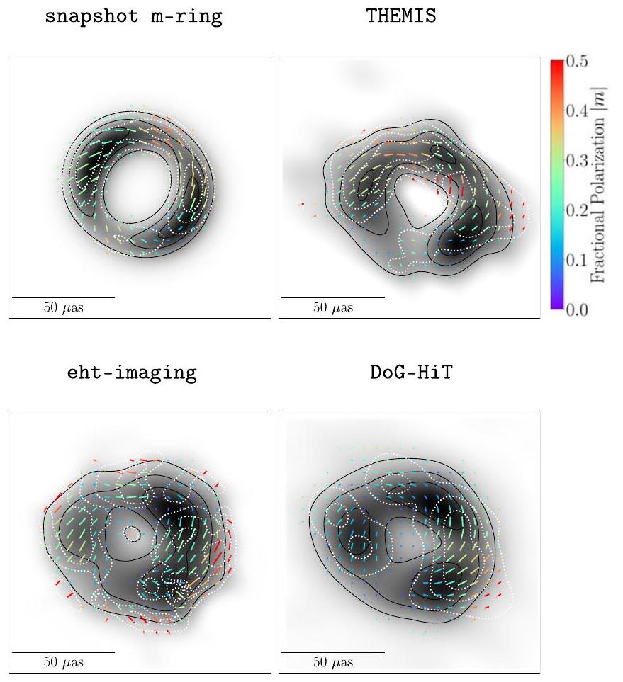
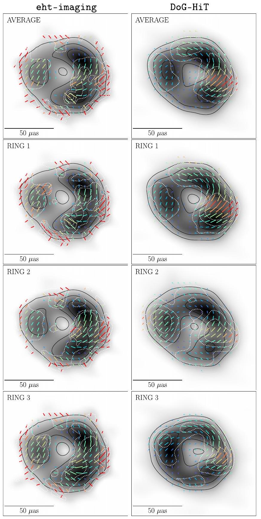
الشكل 8. صور استقطابية خطية لـ Sgr A* من الملاحظات المجمعة في 6 و 7 أبريل 2017 مع طرق النمذجة الأساسية m-ring و THEMIS وطرق التحقق من صحة التصوير EHT و DoG-HiT. يتم عرض الصورة المتوسطة اللاحقة لطرق الاستكشاف اللاحقة. يتم عرض الكثافة الكلية في مقياس رمادي، وتشير علامات الاستقطاب إلى EVPA، وطول العلامة متناسب مع مقدار كثافة الاستقطاب الخطي، واللون يشير إلى الاستقطاب الخطي الجزئي. تحدد الخطوط المنقطة البيضاء كثافة الاستقطاب الخطي، والتي تتوافق مع و من ذروة الاستقطاب. لقد قمنا بإخفاء جميع المناطق التي تحتوي على ستوكيس من ذروة السطوع، وقد قمنا أيضًا بإخفاء جميع المناطق التي تحتوي على من ذروة السطوع المستقطب، حيث . نطاق شريط الألوان ثابت لجميع الألواح.
الأيدي المتوازية. كما تم مناقشته في ورقة V، فإن التغير في محاكاة GRMHD عمومًا أعلى من Sgr A، مما يجعل البيانات الاصطناعية أكثر تحديًا لإعادة البناء من البيانات الحقيقية. جميع الطرق قادرة على إعادة بناء هيكل الاستقطاب الخطي للنموذجين، بينما تحقق طرق THEMIS ونمذجة m-ring نتائج أفضل في إعادة بناء هيكل الاستقطاب الدائري. نظرًا لأن THEMIS ونمذجة m-ring يقومان بإجراء استكشاف لاحق كجزء من منهجياتهما، فإنهما يوفران توزيعات لاحقة ضيقة وعدم اليقين المقاس على كميات الاستقطاب الخطي والدائري الفردية. وبالتالي، يتم اختيار هذين الطريقتين كطرق أساسية للتحليل والتفسير النظري، بينما يتم تقديم طريقتي RML كطرق تحقق إضافية.
6. النتائج
6.1. الاستقطاب الخطي
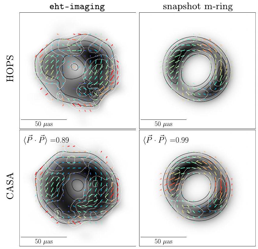
في الشكل 8، نقدم صور Sgr A* الاستقطابية الخطية التي تم إنتاجها بواسطة كل طريقة، مع دمج النطاقات وأيام الملاحظة. يتم إنتاج النتائج الرئيسية باستخدام بيانات تمت معالجتها من خلال خط أنابيب EHT-HOPS، وتُعرض اختبارات التناسق مع خط أنابيب CASA rPICARD في الملحق D. تنتج طريقة التصوير البايزية THEMIS صورة متوسطة من العديد من السحوبات الفردية اللاحقة مع كلا اليومين و
الشكل 9. صور استقطابية لـ Sgr A* من الشكل 8، ولكن مع دوران EVPAs بمقدار 46.0 درجة لأخذ في الاعتبار دوران فاراداي الوسيط في مجموعة بيانات 6 و 7 أبريل المجمعة (الجدول 5). نطاق شريط الألوان ثابت لجميع الألواح.
النطاقات المدمجة في مجموعة بيانات واحدة. تنتج طريقة النمذجة السريعة صورة متوسطة من خلال دمج لقطات فردية مجمعة عبر كلا اليومين باستخدام المتوسط اللاحق البايزي. نظرًا لأن m-ring هو نموذج هندسي بسيط، فإن الهيكل يبدو أقل ضوضاءً من الطرق الأخرى. تنتج طرق التصوير RML EHT و DoG-HiT صورًا مجمعة حسب النطاق لكل يوم؛ نحن هنا نعرض الصورة المتوسطة على مدى يومين (أي، صور 6 و 7 أبريل متوسطة معًا بعد التصوير). في الشكل 9، نقدم نفس الصور ولكن مع دوران EVPAs بزاوية ثابتة لأخذ في الاعتبار دوران فاراداي الوسيط في مجموعة بيانات 6 و 7 أبريل المجمعة، مما يتوافق مع دوران عقارب الساعة لـ EVPA بمقدار 46.0 درجة، كما تم مناقشته في القسم 4.3.
حلقة انبعاث Sgr A* مستقطبة تقريبًا بالكامل، مع ذروة استقطاب جزئي تبلغ عند كدقة في المنطقة الغربية من الحلقة. يظهر نموذج m-ring ذروة شمال غرب أكثر بروزًا بسبب تناظر النموذج الوضع؛ انظر الملحق أ. نمط انبعاث EVPA المستقطب على طول الحلقة هو تقريبًا أزيموثالي مع اتجاه عكس عقارب الساعة الذي يظل ثابتًا عبر الزمن والتردد وطريقة التحليل.
في الشكل 10، نعرض متوسط الصور الأربعة للطرق التي تجمع بين النطاقات والأيام الموضحة في الشكل 8. يتم إجراء المتوسط بشكل مستقل لكل توزيع كثافة ستوكيس. نظرًا لأن صورة الحلقة m تحتوي على نسبة استقطاب صافي أقل (نتيجة لتغيرات EVPAs في المتوسط اللحظي)، فإن نسبة الاستقطاب القصوى في الصورة المتوسطة أقل من تلك الخاصة بالطرق الفردية. تُعتمد هذه الصورة كممثل محافظ للهيكل العام لاستقطاب Sgr A* الخطي، بينما تُستخدم صور الطرق الفردية للمقارنات الكمية والتفسير النظري؛ انظر القسم 7 والمقالة الثامنة.
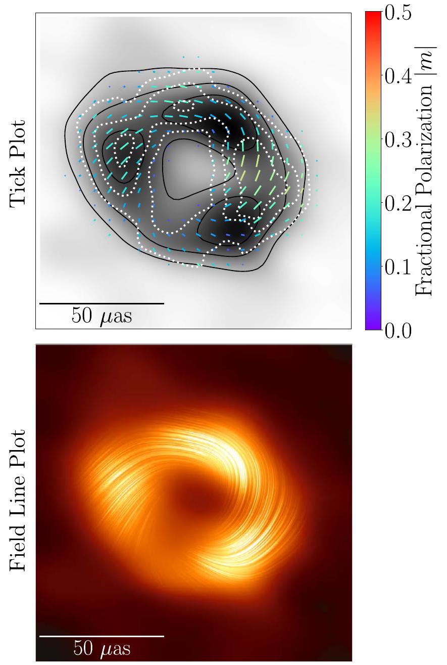
الشكل 10. الأعلى: صورة الاستقطاب الخطي لـ Sagittarius A*. هذه الصورة هي متوسط النطاق واليوم والطريقة لاستقطاب الهيكل الخطي المعاد بناؤه من ملاحظات EHT في 6 و7 أبريل 2017. خيارات العرض مشابهة للشكل 8. الأسفل: خطوط “المجال” للاستقطاب مرسومة فوق صورة الكثافة الكلية الأساسية. من خلال اعتبار الاستقطاب الخطي كحقل متجه، تمثل الخطوط المتعرجة في الصور خطوط تدفق هذا الحقل وبالتالي تتبع أنماط EVPA في الصورة. لتسليط الضوء على المناطق ذات اكتشافات الاستقطاب الأقوى، قمنا بتعديل طول وشفافية هذه الخطوط كمتوسط مربع الكثافة المستقطبة. هذه التصور مستوحى جزئيًا من تمثيلات تكامل الخطوط (Cabral & Leedom 1993) للحقول المتجهة. تم وضع هيكل الاستقطاب الخطي المتوسط فوق صورة الكثافة الكلية المتوسطة المرجعية من الورقة الأولى.
6.2. الاستقطاب الدائري
في الشكل 11، نقدم صور الاستقطاب الدائري التي تم إنتاجها بواسطة كل طريقة، مع دمج النطاقات وأيام المراقبة. في خريطة الألوان المختارة، يتوافق اللون الأحمر مع كثافة التدفق المستقطب دائريًا الموجبة، بينما يتوافق اللون الأزرق مع الكثافة السالبة، مع وجود خطوط الكنتور التي تشير إلى ستوكز.السطوع. كما هو موضح في اختبارات البيانات الاصطناعية في الملحق ب، فإن هيكل الاستقطاب الدائري متسق بالنسبة لطرق استكشاف حلقة الصورة اللحظية m -ring وTHEMIS، بينما تظهر طرق التصوير RML بعض الاختلافات. جميع الطرق ترى استقطاب دائري سلبي بارز في الجزء الغربي من الحلقة، بينما تستعيد فقط طرق الحلقة اللحظية m-ring وTHEMIS استقطاب دائري إيجابي في المنطقة الشمالية الشرقية من الحلقة. تجد طرق m-ring وTHEMIS ذروة الاستقطاب الدائري الإيجابي والسلبي النسبي عند
الشكل 11. صور الاستقطاب الدائري لـ Sgr A* من الملاحظات المجمعة في 6 و 7 أبريل 2017 باستخدام الطرق الأساسية لنمذجة حلقة m-اللحظية وTHEMIS وطرق التحقق eht-imaging وDoG-HiT. يتم عرض الصورة المتوسطة اللاحقة لطرق الاستكشاف اللاحقة. يتم الإشارة إلى الكثافة الكلية في خطوط متساوية ملونة على مقياس خطي عند، و ذروة السطوع. ستوكزيتم الإشارة إلى السطوع في خريطة الألوان المتباينة، حيث يشير الأحمر/الأزرق إلى علامة إيجابية/سلبية. نطاق شريط الألوان ثابت لجميع الألواح.
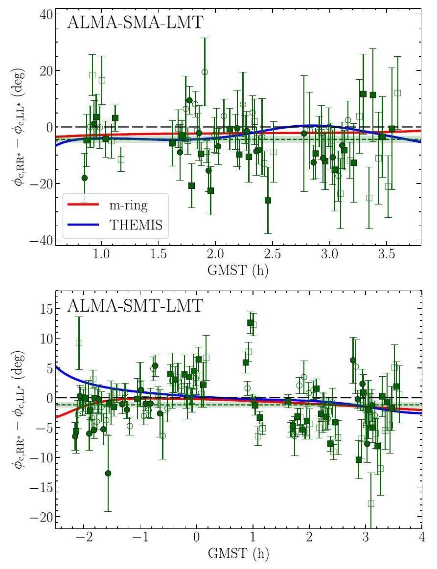
مستوى. من الجدير بالذكر أن قمم خط انبعاث الاستقطاب الدائري تتماشى مع القمم في الكثافة الكلية. وبالتالي، فإن القياسات الجزئية تعتمد بشكل كبير على ميل الطرق الفردية لتفضيل كثافة تدفق أكبر أو أقل في المناطق المدمجة. الهيكل الثنائي القطب المستعاد على طول الحلقة في طرق THEMIS وm-ring يتماشى مع البيانات. على وجه الخصوص، تتنبأ كل من نماذج m-ring وTHEMIS بقيم صغيرة وسلبية في الغالب. و اختلافات مراحل الإغلاق على مثلثات ذات نسبة إشارة إلى ضوضاء عالية (انظر الشكل 12) وهي متوافقة بشكل عام مع القيم المتوسطة المقدرة المشار إليها بالأشرطة الخضراء. تم إجراء ملاءمات إضافية للحلقات m باستخدام قيم أعلى-أنماط ( ) تفضل أيضًا الهيكل المتماثل على طول الحلقة ولكنها تظهر عدم يقين أكبر بكثير في الهيكل من نموذج الملاءمة الموضح هنا. بالإضافة إلى ذلك، فإن الأدلة البايزية للملاءمات من الدرجة الأعلى أقل بكثير من تلك الخاصة بـيتناسب، مما يشير إلى أن البيانات لا تدعم وجود أوضاع أكثر تعقيدًا من ثنائي القطب. تبدو البيانات تدفع جميع الطرق نحو هيكل بسيط متماثل، مما يدل على الحاجة إلى ستوكز عالية.في المناطق المدمجة على الحلقة بناءً على اكتشافات VLBI مع الحفاظ على مستوى الاستقطاب الدائري المتكامل للصورة بالقرب من الصفر، بما يتماشى مع قياسات ALMA. نظرًا لوجود عدم اليقين المتبقي في تفاصيل ستوكزالهيكل على طول الحلقة، الخصائص الهيكلية لستوكلا تُستخدم للتفسير النظري في الورقة المرافقة الثامنة.
7. المناقشة
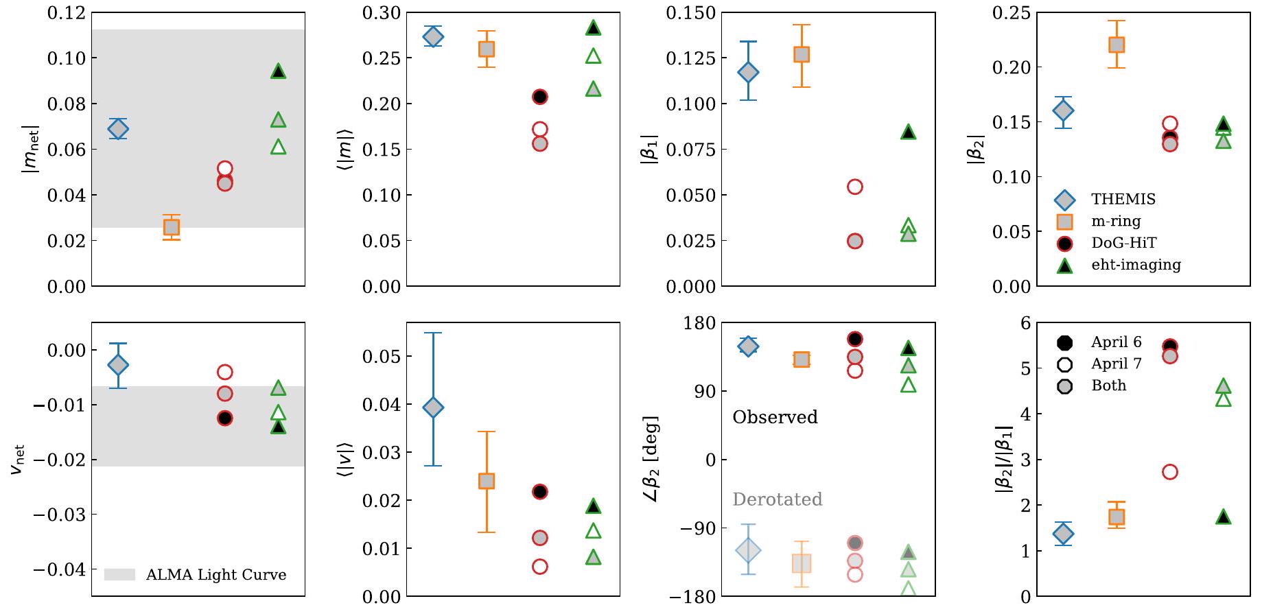
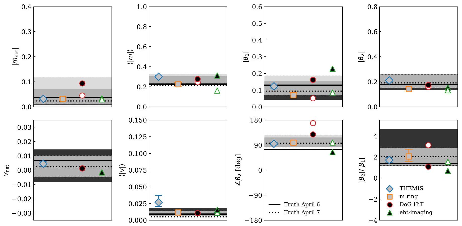
نستخلص ثمانية قيود رصدية من الصور المعاد بناؤها لـ Sgr A*، وهذه موضحة في الشكل 13. نظرًا لأن
الشكل 12. فرق مراحل الإغلاق بين و الرؤى، التي تم رصدها على مثلثات ALMA-SMA-LMT (الأعلى) وALMA-SMT-LMT (الأسفل) في 6 أبريل (مربعات) و7 أبريل (دوائر). تشير العلامات المفتوحة والمملوءة إلى بيانات النطاق المنخفض والعالي، على التوالي. تتبع الرسوم البيانية اللوحات السفلية من الشكل 4. كما تم تقديم التوقعات من النماذج الموضحة في الشكل 11 (الخطوط الصلبة الحمراء والزرقاء). وهي متسقة إلى حد كبير مع اختلافات المرحلة المغلقة المقاسة الصغيرة والسلبية في الغالب.
نمذجة حلقة الصورة الفورية وطرق THEMIS كلاهما يوفر توزيعات بايزيان الخلفية، وأشرطة الخطأ التي تمثلتظهر فترات الثقة من السحوبات العشوائية اللاحقة. المجمعةتُستخدم فترات الثقة من هذين الطريقتين، الموضحتين في الجدول 6، في الورقة الثامنة للتفسير النظري. لا توفر طرق التصوير RML مثل ehtimaging وDoG-HiT مثل هذه التوزيعات، ولكنها موضحة في الشكل 13 كتحقق إضافي من اتساق طرق إعادة بناء الصور ذات المنهجيات المختلفة جداً. يتم تقديم مزيد من التفاصيل حول الطرق الفردية في الملحق A. نلاحظ أن كلا طريقتي استكشاف الخلفية تعالجان التباين بشكل مختلف: حيث يقوم نموذج الحلقة اللحظي m -ring بملاءمة نموذج حلقة مقيد هيكلياً لقطات بيانات فردية مدتها دقيقتان، بينما يقوم تصوير THEMIS Bayesian بإعادة بناء مجموعة من الصور الثابتة من مجموعة بيانات مدتها يومان مع ميزانية ضوضاء تأخذ في الاعتبار التباين. على الرغم من اختلافاتهما الخوارزمية الكبيرة، فإن هاتين الطريقتين تؤديان بشكل أفضل في اختبارات البيانات الاصطناعية المقدمة في الملحق B وتنتجان نتائج متشابهة جداً.
في الألواح الأكثر يسارًا من الشكل 13، يتم عرض النسب الصافية المدمجة للقطبية الخطية والدائرية و منتتم مقارنة إعادة البناء مع النطاقات من منحنيات الضوء باستخدام تقنية التداخل المترية-ALMA مع اعتبار Sgr A* كمصدر نقطة غير محلول من Wielgus et al. (2022a). بشكل عام، جميع الطرق تتماشى بشكل عام مع نطاقات ALMA، على الرغم من أنه لا يجب أن يكون هذا هو الحال بالضرورة. بينما تتوافق النطاقات لمنحنيات الضوء ALMA مع القياسات الفورية لـ و ، الـ و من إعادة بناء صورنا تتوافق مع متوسطات ليلية واحدة أو اثنتين، كما هو موضح. نلاحظ أن THEMIS ونموذج الحلقة m لا يتفقان علىتنتج الصور الفردية الملتقطة من طريقة الحلقة m قيمًا أعلى بكثير منالأسفلفي صورة الحلقة المتوسطة قد يكون ذلك نتيجة لتجمع إلغاءات الهيكل المتغير مع الزمن ومشكلات تحديد النموذج مما يؤدي إلى انزياحات في الطور للملاءمة. (انظر الملحق أ للحصول على التفاصيل).
نحن نقيس أيضًا كسور الاستقطاب الخطي والدائري المتوسطة للصورة و عبر الصور المعاد بناؤها. لـعلى وجه الخصوص، نلاحظ اتساقًا كبيرًا بين طريقتي الاستكشاف الخلفي، مما يؤدي إلى قيود صارمة للنماذج النظرية في الورقة الثامنة. متحيز بشكل كبير نحو الأعلى عندما فقير، يتم تفسير هذه الكمية كحد أعلى، كما في الدراسات السابقة لـ M87* (ورقة M87* IX). نذكر أن كلا و تعتمد على الدقة؛ على عكس الدراسات السابقة (M87* الورقة الثامنة؛ M87* الورقة التاسعة)، لا نقوم بتطبيق أي تشويش بعد إعادة بناء الصورة قبل حساب هذه الكميات.
في اللوحة السفلية من العمود الثالث في الشكل 13، الـالمقاسة عبر الطرق تبقى بعيدة عن 0 باستمرار، مما يعني أن أنماط EVPA الدائرية أكثر من الأنماط الشعاعية في الصور المعاد بناؤها لـمع الأخذ في الاعتبار RM ثابت مع افتراض وجود شاشة فاراداي خارجية، يتم إزالة دوران نمط EVPA بواسطة، مما أدى إلى من الإشارة المعاكسة (النقاط الباهتة في لوحة). بينما تصحيح RM يقلب اتجاه نمط EVPA (انظر الأشكال 8-9) وبالتالي يشكل نظامًا منهجيًا كبيرًا للمقارنات مع النماذج النظرية، تظل أنماط EVPA عبر الطرق دائرية جدًا.أقرب إلىمن; بالومبو وآخرون 2020).
8. الاستنتاجات والملخص
قدمنا التصوير القطبي الخطي والدائري لملاحظات EHT في 6 و7 أبريل 2017 لثقبنا الأسود في مركز المجرة Sgr A* على مقاييس أفق الحدث عند تردد 230 غيغاهرتز. يعتمد تحليلنا على نتائج شكل الحلقة الكلية المقدمة في الأوراق I-VI واستخدمت معايرة التسرب المستمدة من الورقة VII لمجرة M87*. استخدمنا أربع طرق متميزة في التحليل القطبي: طريقتان لاستكشاف ما بعد (إحداهما تصوير بايزي والأخرى نمذجة لقطات) للتحليل الأساسي وطريقتان لتصوير RML للتحقق. تم اختبار جميع الطرق على بيانات اصطناعية مصممة لتقليد خصائص قطبية محددة لـ Sgr A*. عند تطبيقها على بيانات EHT لـ Sgr A*، أظهرت جميع الطرق أن حلقة الانبعاث مستقطبة بشدة، مع ذروة الاستقطاب الخطي النسبي لـفي المنطقة الغربية من الحلقة. بينما التوزيع المكاني التفصيلي للاستقطاب الخطي على طول الحلقة غير مؤكد بسبب التغيرات الذاتية لـ Sgr A* (كما كان الحال بالنسبة لنتائج الكثافة الكلية)، لاحظنا هيكل استقطاب حلزوني متماسك عبر جزء كبير من الحلقة وهو قوي أمام الخيارات المنهجية. تفضل إعادة بناء الاستقطاب الدائري من طرق الاستكشاف اللاحقة، التي أدت بشكل أفضل في الاختبارات الاصطناعية، هيكل ثنائي القطب على طول الحلقة، مع انبعاث استقطاب دائري سالب في الغرب من الحلقة (الذي تم استعادته أيضًا بواسطة طرق تصوير RML) وانبعاث إيجابي مقيد في الغالب إلى الشمال الشرقي، مع قيم مطلقة قصوى هيمن ستوك
الشكل 13. مقارنات الكميات القطبية الخطية والدائرية المقاسة من إعادة بناء Sgr A* عبر الطرق. بالنسبة لطرق التصوير RML، تمثل الرموز المملوءة والمفتوحة نتائج 6 و 7 أبريل، على التوالي. تمثل الرموز الرمادية المتوسطات على مدى يومين. تمثل أشرطة الخطأ لطرق التصوير المقطعي m-ring و THEMIS Bayesian نطاق الثقة من توزيعات الخلفية المجمعة اليومية. المنطقة المظللة تتوافق مع النطاقات من النسبة المئوية الخامسة إلى الخامسة والتسعين من منحنيات الضوء القطبي الخطي والدائري الخاصة بـ ALMA فقط من Wielgus et al. (2022b). طريقة الحلقة m لا تعيد قياسًا لـلأنها تثبت القيمة عند متوسط قياس ALMA قبل التوفيق. استنادًا إلى أدائها في اختبارات البيانات الاصطناعية والتوزيعات الكمية، تُستخدم النتائج من طرق حلقة m -snapshot وTHEMIS للمقارنات النظرية في الورقة المرافقة VIII.
الجدول 6 القيود القطبية المستمدة من الطرق الأساسية THEMIS ونمذجة حلقة Snapshot
قابل للملاحظة
لقطة m-ring
ثيميس
مُدمَج
(2.0, 3.1)
(6.5, 7.3)
(2.0, 7.3)
…
(-0.7, 0.12)
(-0.7, 0.12)
(1.4, 1.8)
(2.7, 5.5)
(0.0, 5.5)
(0.11, 0.14)
(0.10, 0.13)
(0.10, 0.14)
(0.20, 0.24)
(0.14, 0.17)
(0.14, 0.24)
(درجة) (كما لوحظ)
(درجة) (RM المعكوس)
(-168, -108)
(-151، -85)
(-168, -85)
(1.5, 2.1)
(1.1، 1.6)
(1.1، 2.1)
ملاحظة. توفر هاتان الطريقتان كل منهما توزيعات لاحقة، منهاتُذكر مناطق الثقة. تفترض عملية إزالة الدوران أن الوسيط RM يمكن أن يُعزى إلى شاشة فاراداي خارجية، حيث يتم اعتماد تردد 228.1 غيغاهرتز.يتم اعتبار النطاق كحد أعلى. تُستخدم القيود المجمعة للتفسير النظري المقدم في الورقة الثامنة. الإصدار في نفس المواقع. على الرغم من أن كلا طريقتي الاستكشاف الخلفي لدينا تعيد إنتاج ثنائي القطب على طول الحلقة، إلا أننا نعتبر أن هيكل الاستقطاب الدائري أكثر عدم يقين نظرًا للاختلاف الأقوى بين الطريقتين مقارنة بإعادة بناء الاستقطاب الخطي.
لقد وفرت دقة وحساسية تلسكوب أفق الحدث صورًا قطبية على نطاق الأفق لـ Sgr A*، مما مكن لأول مرة من إعادة بناء هندسة المجال المغناطيسي في محيط أفق الحدث لثقبنا الأسود الهائل في مركز المجرة. يتم تقديم مناقشة للتفسير الفيزيائي لهذه النتائج في الورقة الثامنة.
شكر وتقدير
تشكر مجموعة تلسكوب أفق الحدث المنظمات والبرامج التالية: أكاديمية سينيكا؛ أكاديمية فنلندا (المشاريع 274477، 284495، 312496، 315721)؛ الوكالة الوطنية للبحث والتطوير (ANID)، تشيلي عبر NCN19 (TITANs)، فوندسيكت 1221421، و BASAL FB210003؛ مؤسسة ألكسندر فون هومبولت؛ زمالة ألفريد ب. سلون للبحث؛ أليغرو، مركز ALMA الإقليمي الأوروبي في هولندا، شبكة الأبحاث الفلكية NL NOVA ومعاهد الفلك في جامعة أمستردام، جامعة لايدن، وجامعة رادبود؛ صندوق تطوير ALMA في أمريكا الشمالية؛ برنامج الفيزياء الفلكية والفيزياء عالية الطاقة من MCIN (بتمويل من الاتحاد الأوروبي NextGenerationEU، PRTR-C17I1)؛ مبادرة الثقب الأسود، التي تمولها منح من مؤسسة جون تمبلتون (60477، 61497، 62286) ومؤسسة غوردون وبيتي مور (منحة GBMF-8273) – على الرغم من أن الآراء المعبر عنها في هذا العمل هي آراء المؤلف ولا تعكس بالضرورة آراء هذه المؤسسات؛ مؤسسة برينسون؛ مؤسسة “لا كايسا” (ID 100010434) من خلال رموز الزمالة LCF/BQ/DI22/11940027 و LCF/BQ/DI22/11940030؛ تشاندرا DD718089X و TM6-17006X؛ مجلس المنح الدراسية في الصين؛ زمالات مؤسسة العلوم ما بعد الدكتوراه في الصين (2020M671266، 2022M712084)؛ المجلس الوطني للعلوم الإنسانية والعلوم والتكنولوجيا (CONAHCYT، المكسيك، المشاريع U0004-246083، U0004-259839، F0003-272050، M0037279006، F0003-281692، 104497، 275201، 263356)؛ منحة كولفوتورو؛ وزارة الاقتصاد والمعرفة والشركات والجامعة في حكومة الأندلس (منحة P18-FR-1769)؛ المجلس الأعلى للبحوث العلمية (منحة 2019AEP112)؛ عائلة ديلاني عبر ديلاني
كرسي عائلة جون أ. ويلر في معهد بيريمتر؛ المديرية العامة لشؤون الموظفين الأكاديميين – الجامعة الوطنية المستقلة في المكسيك (DGAPA-UNAM، المشاريع IN112820 و IN108324)؛ منظمة الأبحاث العلمية الهولندية (NWO) لجائزة VICI (المنحة 639.043.513)، المنحة OCENW.KLEIN.113، وكونسورتيوم الثقوب السوداء الهولندي (مع المشروع رقم NWA 1292.19.202) من برنامج البحث أجندة العلوم الوطنية؛ الحواسيب الفائقة الوطنية الهولندية، كارتيسيوس وسنليوس (منحة NWO 2021.013)؛ زمالة EACOA الممنوحة من قبل جمعية المراصد الأساسية لشرق آسيا، والتي تتكون من معهد أكاديميا سينيكا لعلم الفلك والفيزياء الفلكية، المرصد الفلكي الوطني في اليابان، مركز العلوم الفلكية الضخمة، الأكاديمية الصينية للعلوم، ومعهد كوريا لعلم الفلك وعلوم الفضاء؛ منحة التعاون من المجلس الأوروبي للبحث (ERC) “BlackHoleCam: تصوير أفق الحدث للثقوب السوداء” (المنحة 610058)؛ برنامج الأبحاث والابتكار Horizon 2020 للاتحاد الأوروبي بموجب اتفاقيات المنح RadioNet (رقم 730562) وM2FINDERS (رقم 101018682)؛ برنامج منح Horizon ERC Grants 2021 بموجب اتفاقية المنحة رقم 101040021؛ المجلس الأوروبي للبحث من أجل منحة متقدمة “JETSET: إطلاق، انتشار وإصدار النفاثات النسبية من الاندماجات الثنائية وعبر مقاييس الكتلة” (رقم المنحة 884631)؛ FAPESP (مؤسسة دعم الأبحاث في ولاية ساو باولو) بموجب المنحة 2021/01183-8؛ صندوق CAS-ANID رقم CAS220010؛ حكومة فالنسيا (المنح APOSTD/2018/177 وASFAE/2022/018) وبرنامج GenT (المشروع CIDEGENT/2018/021)؛ مؤسسة غوردون وبيتي مور (GBMF-3561، GBMF5278، GBMF-10423)؛ معهد الدراسات المتقدمة؛ المعهد الوطني للفيزياء النووية (INFN) قسم نابولي، مبادرات محددة TEONGRAV؛ المدرسة الدولية ماكس بلانك للبحث في علم الفلك والفيزياء الفلكية في جامعات بون وكولونيا؛ منحة بحث DFG “فيزياء النفاثات على مقاييس الأفق وما بعدها” (رقم المنحة 443220636)؛ زمالة ما بعد الدكتوراه المشتركة بين كولومبيا/فلاتيرون (البحث في معهد فلاتيرون مدعوم من مؤسسة سيمونز)؛ وزارة التعليم اليابانية، الثقافة، الرياضة، العلوم والتكنولوجيا (MEXT؛ المنحة JPMXP1020200109)؛ منحة JSPS من جمعية تعزيز العلوم اليابانية (JSPS) للزمالة البحثية (JP17J08829)؛ المعهد المشترك للعلوم الأساسية الحاسوبية، اليابان؛ برنامج البحث الرئيسي للعلوم الحدودية، الأكاديمية الصينية للعلوم (CAS، المنح QYZDJ-SSW-SLH057، QYZDJ-SSW-SYS008، ZDBS-LY-SLH011)؛ زمالة Leverhulme Trust للبحث المبكر؛ جمعية ماكس بلانك (MPG)؛ مجموعة شراكة ماكس بلانك من MPG وCAS؛ MEXT/JSPS KAKENHI (المنح 18KK0090، JP21H01137، JP18H03721، JP18K13594، 18K03709، JP19K14761، 18H01245، 25120007، 23K03453)؛ مشاريع البحث MICINN PID2019-108995GB-C22، PID2022-140888NB-C22؛ صندوق المبادرات الدولية للعلوم والتكنولوجيا في MIT (MISTI)؛ وزارة العلوم والتكنولوجيا (MOST) في تايوان (103-2119-M-001-010-MY2، 105-2112-M-001-025-MY3، 105-2119-M-001-042، 106-2112-M-001-011، 106-2119-M-001-013، 106-2119-M-001-027، 106-2923-M-001-005، 107-2119-M-001-017، 107-2119-M-001-020، 107-2119-M-001-041، 107-2119-M-110-005، 107-2923-M-001-009، 108-2112-M-001-048، 108-2112-M-001-051، 108-2923-M-001002، 109-2112-M-001-025، 109-2124-M-001-005، 109-2923-M-001-001، 110-2112-M-003-007-MY2، 110-2112-M-001-033، 110-2124-M-001-007، و110-2923-M-001-001)؛ وزارة
التعليم (MoE) في تايوان برنامج يوشان للعلماء الشباب؛ قسم الفيزياء، المركز الوطني للعلوم النظرية في تايوان؛ إدارة الطيران والفضاء الوطنية (ناسا، منحة الباحث الضيف في فيرمي 80NSSC20K1567، منحة برنامج نظرية الفيزياء الفلكية في ناسا 80NSSC20K0527، جائزة ناسا NuSTAR 80NSSC20K0645)؛ منح زمالة هابل من ناسا HST-HF2-51431.001-A، HST-HF2-51482.001-A الممنوحة من قبل معهد علوم التلسكوب الفضائي، الذي تديره جمعية الجامعات للبحث في علم الفلك، Inc.، لصالح ناسا، بموجب العقد NAS5-26555؛ المعهد الوطني للعلوم الطبيعية (NINS) في اليابان؛ البرنامج الوطني الرئيسي للبحث والتطوير في الصين (المنح 2016YFA0400704، 2017YFA0402703، 2016YFA0400702)؛ مجلس العلوم والتكنولوجيا الوطني (NSTC، المنح NSTC 111-2112-M-001-041، NSTC 111-2124-M-001-005، NSTC 112-2124-M-001-014)؛ مؤسسة العلوم الوطنية الأمريكية (NSF، المنح AST-0096454، AST0352953، AST-0521233، AST-0705062، AST-0905844، AST0922984، AST-1126433، OIA-1126433، AST-1140030، DGE1144085، AST-1207704، AST-1207730، AST-1207752، MRI-1228509، OPP-1248097، AST-1310896، AST-1440254، AST-1555365، AST-1614868، AST-1615796، AST-1715061، AST-1716327، AST-1726637، OISE-1743747، AST-1743747، AST-1816420، AST-1952099، AST-1935980، AST-2034306، AST-2205908، AST-2307887)؛ زمالة ما بعد الدكتوراه في علم الفلك والفيزياء الفلكية من NSF (AST-1903847)؛ مؤسسة العلوم الطبيعية في الصين (المنح 11650110427، 10625314، 11721303، 11725312، 11873028، 11933007، 11991052، 11991053، 12192220، 12192223، 12273022، 12325302، 12303021)؛ مجلس الأبحاث الطبيعية والهندسية في كندا (NSERC، بما في ذلك منحة اكتشاف ومنحة NSERC ألكسندر غراهام بيل لبرنامج الدكتوراه)؛ برنامج المواهب الشابة الوطني في الصين؛ مؤسسة البحث الوطنية في كوريا (منحة زمالة الدكتوراه العالمية: المنح NRF2015H1A2A1033752، برنامج زمالة البحث في كوريا: NRF-2015H1D3A1066561، برنامج Brain Pool: 2019H1D3A1A01102564، منحة دعم البحث الأساسي 2019R1F1A1059721، 2021R1A6A3A01086420، 2022R1C1C1005255، 2022R1F1A107515)؛ المدرسة البحثية الهولندية لعلم الفلك (NOVA) معهد افتراضي للاكتساب (VIA) زمالات ما بعد الدكتوراه؛ NOIRLab، الذي تديره جمعية الجامعات للبحث في علم الفلك (AURA) بموجب اتفاق تعاوني مع مؤسسة العلوم الوطنية؛ مرصد أونسالا الفضائي (OSO) البنية التحتية الوطنية، لتوفير مرافقه/الدعم الرصدي (يتلقى OSO تمويلاً من خلال مجلس الأبحاث السويدي بموجب المنحة 2017-00648)؛ معهد بيريمتر للفيزياء النظرية (البحث في معهد بيريمتر مدعوم من حكومة كندا من خلال وزارة الابتكار والعلوم والتنمية الاقتصادية ومن قبل مقاطعة أونتاريو من خلال وزارة البحث والابتكار والعلوم)؛ مبادرة جاذبية برينستون؛ وزارة العلوم والابتكار الإسبانية (المنح PGC2018-098915-B-C21، AYA2016-80889-P، PID2019-108995GB-C21، PID2020-117404GB-C21)؛ جامعة بريتوريا للمساعدة المالية في توفير عقد خادم الكلاستر الجديد وسوبرمايكرو (الولايات المتحدة) منحة SEEDING المعتمدة نحو هذه العقد في 2020؛ برنامج توجيه بلدية شنغهاي للبحث الأساسي للعلماء الدوليين (رقم المنحة 22JC1410600)؛ برنامج شنغهاي التجريبي للبحث الأساسي، الأكاديمية الصينية للعلوم، فرع شنغهاي (JCYJ-SHFY-2021-013)؛ الوكالة
المدنية للبحث في وزارة التعليم الإسبانية MCIU من خلال جائزة “مركز التميز سيفيرو أوتشوا” لمعهد أستروفísica دي أندلوسيا (SEV-2017-0709)؛ وزارة العلوم والابتكار الإسبانية منحة CEX2021-001131-S الممولة من MCIN/AEI/10.13039/501100011033؛ جائزة سبينوزا SPI 78-409؛ مبادرة كراسي البحث في جنوب أفريقيا، من خلال المرصد الفلكي الإذاعي في جنوب أفريقيا (SARAO، رقم المنحة 77948)، وهو مرفق تابع لمؤسسة البحث الوطنية (NRF)، وهي وكالة تابعة لوزارة العلوم والابتكار (DSI) في جنوب أفريقيا؛ مؤسسة توراي للعلوم؛ مجلس الأبحاث السويدي (VR)؛ مجلس مرافق العلوم والتكنولوجيا في المملكة المتحدة (رقم المنحة ST/X508329/1)؛ وزارة الطاقة الأمريكية (USDOE) من خلال مختبر لوس ألاموس الوطني (الذي تديره Triad National Security، LLC، لصالح إدارة الأمن النووي الوطني في USDOE، العقد 89233218CNA000001)؛ وزمالة جائزة YCAA ما بعد الدكتوراه.
نشكر موظفي المراصد المشاركة ومراكز الارتباط والمؤسسات على دعمهم الحماسي. تستخدم هذه الورقة البيانات التالية من ALMA: ADS/JAO. ALMA#2016.1.01154.V. ALMA هو شراكة بين المرصد الجنوبي الأوروبي (ESO؛ أوروبا، ممثلة بدولها الأعضاء)، NSF، والمعاهد الوطنية للعلوم الطبيعية في اليابان، جنبًا إلى جنب مع المجلس الوطني للبحوث (كندا)، وزارة العلوم والتكنولوجيا (MOST؛ تايوان)، معهد أكاديميا سينيكا لعلم الفلك والفيزياء الفلكية (ASIAA؛ تايوان)، ومعهد كوريا لعلم الفلك وعلوم الفضاء (KASI؛ جمهورية كوريا)، بالتعاون مع جمهورية تشيلي. يتم تشغيل المرصد المشترك ALMA بواسطة ESO، والجامعات المرتبطة، Inc. (AUI)/NRAO، والمرصد الفلكي الوطني في اليابان (NAOJ). تعتبر NRAO منشأة تابعة لـ NSF تعمل بموجب اتفاقية تعاونية مع AUI. استخدمت هذه الدراسة موارد منشأة أوك ريدج للحوسبة القيادية في مختبر أوك ريدج الوطني، المدعومة من مكتب العلوم التابع لوزارة الطاقة الأمريكية بموجب العقد رقم DE-AC0500OR22725؛ وبنية ASTROVIVES FEDER التحتية، برمز المشروع IDIFEDER-2021-086؛ ومجموعة الحوسبة لمراصد VLBI في شنغهاي المدعومة من الصندوق الخاص لعلم الفلك من وزارة المالية في الصين. كما نشكر مركز علم الفلك الحسابي، المرصد الفلكي الوطني في اليابان. تم دعم هذا العمل من قبل FAPESP (مؤسسة دعم البحث في ولاية ساو باولو) بموجب المنحة 2021/01183-8.
APEX هو تعاون بين معهد ماكس بلانك لعلم الفلك الراديوي (ألمانيا)، ومنظمة ESO، ومرصد أونسالا الفضائي (السويد). SMA هو مشروع مشترك بين SAO وASIAA ويموّل من قبل مؤسسة سميثسونيان وأكاديمية سينيكا. يتم تشغيل JCMT بواسطة المرصد الشرقي الآسيوي نيابة عن NAOJ وASIAA وKASI، بالإضافة إلى وزارة المالية في الصين، والأكاديمية الصينية للعلوم، والبرنامج الوطني الرئيسي للبحث والتطوير (رقم 2017YFA0402700) في الصين ومنحة مؤسسة العلوم الطبيعية في الصين 11873028. يتم توفير دعم تمويلي إضافي لـ JCMT من قبل مجلس مرافق العلوم والتكنولوجيا (المملكة المتحدة) والجامعات المشاركة في المملكة المتحدة وكندا. LMT هو مشروع تديره المعهد الوطني لعلم الفلك والبصريات والإلكترونيات (المكسيك) وجامعة ماساتشوستس في أمهيرست (الولايات المتحدة الأمريكية). يتم تشغيل تلسكوب IRAM 30 م على بيكو فيليتا، إسبانيا بواسطة IRAM ومدعوم من CNRS (المركز الوطني للبحث العلمي، فرنسا)، وMPG (جمعية ماكس بلانك، ألمانيا)، وIGN (المعهد الجغرافي).
تدير المرصد الإذاعي في أريزونا، وهو جزء من مرصد ستيوارد التابع لجامعة أريزونا، نظام SMT، بدعم مالي من عمليات الدولة في أريزونا ودعم مالي لتطوير الأدوات من NSF. يتم توفير الدعم لمشاركة SPT في EHT من قبل المؤسسة الوطنية للعلوم من خلال الجائزة OPP-1852617 لجامعة شيكاغو. كما يتم توفير دعم جزئي من معهد كافلي لفيزياء الكون في جامعة شيكاغو. تم توفير مذبذب الهيدروجين SPT على سبيل الإعارة من GLT، بفضل ASIAA.
استخدم هذا العمل بيئة اكتشاف العلوم والهندسة المتطرفة (XSEDE)، المدعومة من منحة NSF رقم ACI-1548562، وCyVerse، المدعومة من منح NSF رقم DBI-0735191، DBI1265383، وDBI-1743442. تم تخصيص موارد XSEDE Stampede2 في TACC من خلال TG-AST170024 وTG-AST080026N. تم تخصيص موارد XSEDE JetStream في PTI وTACC من خلال AST170028. هذا البحث هو جزء من مشروع الحوسبة Frontera في مركز تكساس المتقدم للحوسبة من خلال تخصيص شراكات المجتمع الكبيرة Frontera رقم AST20023. تم تمكين Frontera بفضل منحة مؤسسة العلوم الوطنية رقم OAC-1818253. تم إجراء هذا البحث باستخدام الخدمات المقدمة من اتحاد OSG (Pordes et al. 2007؛ Sfiligoi et al. 2009) المدعوم من منح مؤسسة العلوم الوطنية رقم 2030508 و1836650. تم استخدام عمل إضافي باستخدام ABACUS2.0، الذي هو جزء من مركز eScience في جامعة جنوب الدنمارك، وعناقيد كالتورن الفلكية الهجينة (مشاريع Conicyt Programa de Astronomia Fondo Quimal QUIMAL170001، Conicyt PIA ACT172033، Fondecyt Iniciacion 11170268، Quimal 220002). تم إجراء محاكاة أيضًا على عنقود SuperMUC في LRZ في غارشينغ، وعلى عنقود LOEWE في CSC في فرانكفورت، وعلى عنقود HazelHen في HLRS في شتوتغارت، وعلى Pi2.0 وSiyuan Mark-I في جامعة شنغهاي جياو تونغ. يتم الاعتراف بالموارد الحاسوبية لمركز تكنولوجيا المعلومات الفنلندي للعلوم (CSC) ومشروع البنية التحتية للكفاءة الحاسوبية الفنلندية (FCCI). تم تمكين هذا البحث جزئيًا من خلال الدعم المقدم من Compute Ontario (http:// computeontario.ca), حساب كيبك (http://www.calculquebec.ca) وحساب كندا (http://www.computecanada.ca).
لقد تلقت EHTC تبرعات سخية من شرائح FPGA من شركة Xilinx، بموجب برنامج جامعة Xilinx. استفادت EHTC من التكنولوجيا التي تم مشاركتها بموجب ترخيص مفتوح المصدر من قبل التعاون لأبحاث معالجة إشارات الفلك والإلكترونيات (CASPER). تعبر مشروع EHT عن امتنانها لـ T4Science وMicrosemi لمساعدتهما في مجال الماسرات الهيدروجينية. استخدمت هذه الأبحاث نظام بيانات الفلك التابع لناسا. نعرب عن شكرنا للدعم المقدم من الطاقم الموسع لـ ALMA، منذ بداية مشروع تنسيق ALMA وحتى الحملات الرصدية في عامي 2017 و2018. نود أن نشكر A. Deller وW. Brisken على الدعم الخاص بـ EHT في استخدام DiFX. نشكر مارتن شيبرد على إضافة ميزات إضافية في برنامج Difmap التي تم استخدامها لنتائج التصوير CLEAN المقدمة في هذه الورقة. نعترف بأهمية ماونا كيا، حيث تقع محطات EHT SMA وJCMT، بالنسبة للشعب الأصلي في هاواي.
في النمذجة الهندسية، يتم وصف هيكل المصدر بواسطة نموذج منخفض الأبعاد يتم ملاءمته مع البيانات الملاحظة. النمذجة الهندسية عادة ما تكون سريعة، حيث يمكن إجراء عمليات مثل تحويل فورييه وحساب التدرج بشكل تحليلي. غالبًا ما تتوافق معلمات النموذج الهندسي مباشرة مع معلمات هيكل المصدر ذات الأهمية (مثل قطر الحلقة، السماكة، وعدم التماثل). من ناحية أخرى، تعاني النمذجة الهندسية من مشكلة تحديد النموذج بشكل خاطئ: عادةً ما لا يلتقط النموذج الهندسي جميع ميزات الصورة الأساسية، حتى لو كانت الدقة الزاوية محدودة. ومع ذلك، من خلال تقييد فضاء معلمات مجال الصورة، يمكن للنمذجة الهندسية تقييد الهيكل منخفض الترتيب للصورة في الأنظمة التي تواجه فيها طرق التصوير صعوبات بسبب العديد من درجات الحرية (قيم بكسل الصورة). لذلك، تعتبر النمذجة الهندسية مفيدة بشكل خاص لمجموعات البيانات ذات التغطية الأساسية النادرة و/أو بيانات ذات نسبة إشارة إلى ضوضاء منخفضة.
في تحليل بيانات EHT، تم استخدام النمذجة الهندسية لتقييد هيكل مقياس أفق الحدث لـ M87* في ستوك الكامل (M87* الورقة السادسة؛ ويلغوس وآخرون 2022a؛ M87* الورقة التاسعة؛ رويلاف وآخرون 2023) وهيكل مقياس أفق الحدث لـ Sgr A* في الكثافة الكلية (الورقة الرابعة). بالنسبة لبيانات EHT لـ Sgr A*، توفر النمذجة الهندسية اللحظية وسيلة للتخفيف من التغير السريع في المصدر. في النمذجة اللحظية، يتم تقسيم مجموعة البيانات إلى لقطات قصيرة (دقيقتان) يتم ملاءمتها بشكل مستقل مع النموذج الهندسي. ثم يتم دمج نتائج اللقطات باستخدام نموذج هرمي بايزي للحصول على تقدير لاحق لهياكل الصورة المتوسطة؛ انظر الورقة الرابعة للحصول على التفاصيل. في هذا العمل، نستخدم النمذجة الهندسية اللحظية بالاشتراك مع هذه الإجراء المتوسط البايزي لتقييد هيكل Sgr A* في ستوك الكامل.
كما في الورقة الرابعة والورقة التاسعة لمجرة M87*، نموذجنا الهندسي المختار هو نموذج الحلقة m. يقوم نموذج الحلقة m بتمثيل هيكل مجال الصورة كحلقة بقطرعرض (FWHM)، وهي بنية أفقية محددة بواسطة أوضاع فورييه في الكثافة الكلية، الاستقطاب الخطي، والاستقطاب الدائري (جونستون وآخرون 2020؛ الورقة الرابعة؛ رويليفز وآخرون 2023). في الكثافة الكلية وإحداثيات الصورة القطبية، تأخذ حلقة m الشكل
هنا هو توزيع دلتا ديراك، و هي معاملات فورييه التي تحدد الهيكل الزاوي. لقد قمنا بتعيينلكييعطي الكثافة الكلية للتدفق للحلقة. كلما زاد ترتيب الحلقة mيمكن نمذجة الهياكل الأفقية الأكثر تعقيدًا. يتم إدخال سمك نهائي عن طريق تشويش الحلقة m باستخدام نواة غاوسية دائرية مع عرض نصف الحد الأقصى.على عكس الورقة الرابعة، لا نضيف مكون أرضي غاوسي إلى نموذج الحلقة m لدينا.
هيكل الاستقطاب الخطيوبنية الاستقطاب الدائريمُعَامَلَة بشكل مشابه، مع الهيكل الزاوي المحدد بواسطة و على التوالي. نظرًا لأن هياكل الكثافة الكلية والاستقطاب الدائري هي قيم حقيقية، و . بالمقابل، فإن هياكل الاستقطاب الخطي لها قيم معقدة، وبالتالي نقوم بتناسب و بشكل مستقل. يتم الإشارة إلى أوامر الحلقة m في الاستقطاب الخطي والدائري بـ و ، على التوالي. يتم إعطاء النسب الصافية للاستقطاب الخطي والدائري بواسطة و ، على التوالي. وبالتالي، يتم تحديد هيكل الاستقطاب في مصطلحات نسبية ويمكن تحويله إلى كثافات مستقطبة من خلال الضرب فيفي المعادلة (A1).
قبل تركيب نموذج الحلقة m في ستوك الكامل على Sgr A*، نقوم بمعالجة البيانات عن طريق إضافةالضوضاء النظامية الجزئية على الرؤى، وإزالة الضبابية للتخفيف من آثار التشتت بين النجوم، ومعايرة التسرب، وتطبيع منحنيات الضوء للبيانات وتقسيم البيانات إلى لقطات مدتها دقيقتان. نحن نناسب فقط اللقطات التي تحتوي على بيانات على الأقل من 10 خطوط أساسية ووقت تكامل متماسك لا يقل عن 60 ثانية. نظرًا لأن كل لقطة يتم ملاءمتها بشكل مستقل، فلا حاجة لإدخال ميزانية ضوضاء إضافية تمثل تباين المصدر الداخلي. وفقًا لـ Roelofs et al. (2023)، نقوم أولاً بملاءمة هيكل الكثافة الكلية والاستقطاب الخطي لزوايا الإغلاق ذات اليدين المتوازيتين، وأطوال الإغلاق، والاستقطاب الخطي الجزئي في مجال الرؤية.. هذه المنتجات البيانية غير متغيرة أمام تشوهات الكسب المعقدة باستثناء اعتماد نسبة الكسب على. ثم نقوم بتثبيت معلمات الاستقطاب الخطي على تقديرات MAP ونقوم بتناسب هيكل الكثافة الكلية والاستقطاب الدائري إما مع اليدين المتوازيتين المنفصلتين ( و مراحل الإغلاق وسعات الإغلاق أو إلىنسب الرؤية. نظرًا لأن منتجات الإغلاق لا يمكن أن تقيدنحن نصلحإلى القيمة المتوسطة من منحنى ضوء ALMA. الـالمنتج البياني حساس للبقايانسب المكاسب التي قد تكون موجودة في بياناتنا (انظر رويلوفز وآخرون 2023، لمزيد من التفاصيل). وبالتحفظ، نقدم لذلك ملاءماتنا التي تعتمد فقط على الإغلاق في الشكل 11 ونعلق علىيتناسب أدناه. نحن نحدد، و لكل الملاءمات المقدمة في هذا العمل. هذه هي أقصى أوامر m التي تنتج نتائج معقولة بناءً على الأداء في اختبارات البيانات الاصطناعية، والتحقيق في الأدلة البايزية (انظر أيضًا الورقة الرابعة)، واستقرار نتائج الملاءمة مع زيادة أوامر m. يتم إجراء جميع الملاءمات باستخدام eht-imaging، باستخدام dynesty (Speagle 2020) لاستكشاف الخلفيات.
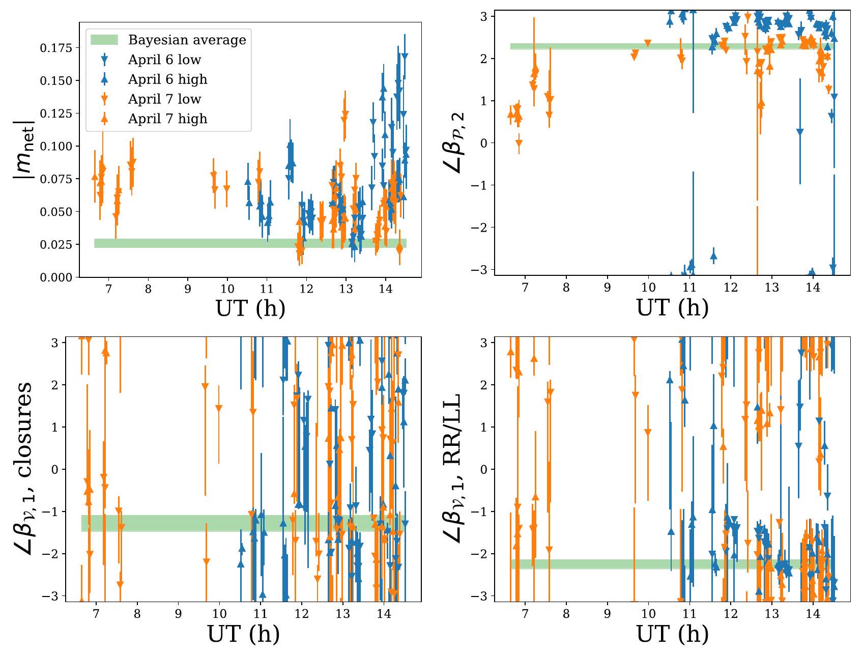
الشكل 14 يظهرنطاقات ما بعد التوزيع للصور الفوتوغرافية في جميع الأيام والأشرطة، لعدد من معلمات الاستقطاب المثيرة للاهتمام. كما يتم الإشارة إلى نطاق ما بعد التوزيع المتوسط البايزي بواسطة الأشرطة الخضراء.يتراوح بين و للقطات الفردية، والمتوسط البايزي في الطرف الأدنى من هذا النطاق. إجراء المتوسط البايزي يقوم تقريبًا بأداء متوسط معقد على معلمات معقدة، بحيث تكون القيم المطلقة الناتجة عادةً أقل من اللقطات الفردية بسبب التغيرات الزاوية (في هذه الحالة المتعلقة بـ EVPA الصافي). بالإضافة إلى ذلك، نجد أن نموذج الحلقة m لا يتناسب مع الخط الأساسي الصفري.مرحلة جيدة لجميع اللقطات. تؤدي هذه الانحرافات الصفرية في المرحلة إلى انتشار أكبر في القيم الملائمة.الطور عبر اللقطات أكثر مما هو متوقع من قياسات الصفر الأساسية، مما يؤدي إلى سعة أقل بعد المتوسط البايزي. من المحتمل أن تكون الانحرافات في الطور ناتجة عن مزيج من عدم تحديد النموذج بشكل صحيح والاختلافات بين الخطوط الأساسية. يتم ملاءمة نقاط البيانات ذات نسبة الإشارة إلى الضوضاء العالية بشكل جيد على الخطوط الأساسية المتوسطة، بينما يتم ملاءمة النقاط ذات نسبة الإشارة إلى الضوضاء المنخفضة بشكل أقل جودة على الخطوط الأساسية القصيرة.على الخطوط الأساسية القصيرة منخفض لأن
الشكل 14. لقطات من التوزيعات الخلفية لـ m-ringنطاقات) لبارامترات الاستقطاب الخطي و (الصف العلوي) ومعامل الاستقطاب الدائري (أي، ستوكز من الدرجة الأولى التوجيه) للتناسب مع كميات الإغلاق ونسب رؤية RR/LL (الصف السفلي). تشير الأشرطة الخضراء إلىنطاقات الوقت والبنية المتوسطة للفرقة المحسوبة باستخدام إجراء التقدير البايزي لدينا. نظرًا لأن هذا الإجراء ينتج تقريبًا متوسطًا معقدًا، فإن السعات الناتجة عن الكميات المعقدة مثلتميل إلى أن تكون أقل من تلك الخاصة باللقطات الفردية.
نسبة الاستقطاب الكلي، وتزداد الفروق بسبب إضافة الضوضاء النظامية (وهي نسبة ثابتة من سعات الرؤية). مستقر نسبيًا بين اللقطات، مع انحراف منهجي بين اليومين. (الصف السفلي)، والذي يمثل التوجه من الدرجة الأولى لانبعاث الاستقطاب الدائري، يكون غير مقيد نسبيًا للصور الفردية عند التوافق فقط مع منتجات الإغلاق ذات اليد المتوازية (اللوحة السفلى اليسرى)، على الرغم من أن إجراء التقدير البايزي يشير إلى توجه مفضل يتماشى تقريبًا مع طرق أخرى (الشكل 11). تشير تفضيلات أوضح لعدم التماثل تقريبًا من الشمال الغربي إلى الجنوب الشرقي إلى يتناسب (اللوحة السفلية اليمنى). منذ أنالمتوسط البايزي لـوتتناقض التركيبات النهائية بشكل رسمي عندمستوى (على الرغم من أنهم ضمن ربع من بعضهم البعض) وقد تتأثر القياسات بمخلفات غير معروفةنسب المكاسب، نستخدم فقط التناسبات المغلقة لنطاقات المعلمات المبلغ عنها والتفسير النظري (على سبيل المثال، الجدول 6، الشكل 13).
أ.2. ثيميس
حزمة THEMIS هي إطار بايزي مصمم لتحليل بيانات EHT (برودريك وآخرون 2020c). توفر مجموعة موحدة ومختبرة جيدًا من الأدوات المستقلة لمعالجة الأنظمة القائمة على المحطات والأنظمة الفلكية، بما في ذلك المعقدة. تقدير تسرب الاستقطاب لإعادة بناء الكسب-الشروط)، ونماذج التشتت بين النجوم. يوفر THEMIS عددًا من طرق أخذ العينات اللاحقة، حيث أن الناتج الأكثر شيوعًا هو سلسلة ماركوف مونت كارلو (MCMC) التي تدعم التفسير البايزي اللاحق. في حالة نماذج التصوير (برودريك وآخرون 2020)، تسمح هذه النتائج بتفسيرات بايزية لميزات الصورة.
يتناسب THEMIS مع الرؤى المعقدة لليدين المتوازيتين واليدين المتقاطعتين. قبل التناسب، يتم معايرة البيانات كما هو موضح في القسم 2، ومتوسطها عبر المسح، ويتم تطبيعها بواسطة ستوكز.منحنى الضوء، كما هو موصوف في الأوراق الثالثة والرابعة. تقديرات المعاير للزيادات المعقدة وتُطبق الشروط، وبالتالي فإن تقديرات THEMIS هي تصحيحات إضافية لكل منها. يتم ملاءمة بيانات النطاق العالي والمنخفض من 6 و7 أبريل في وقت واحد، مما يضمن تلبية الافتراضات الأساسية لإعادة بناء التغيرات (انظر Broderick et al. 2022).
نموذج الصورة القطبية في THEMIS يعتمد على ستوكزنموذج التصوير المقدم في برويدرِك وآخرون (2020) والذي تم استخدامه سابقًا في الورقة السابعة والورقة التاسعة عن M87*. يتم إعادة بناء أربعة مجالات في الوقت نفسه:
ستوكزخريطة؛
نسبة الاستقطاب الكلي؛
استقطاب خطي EVPA؛ و
كسر التدفق المستقطب المرتبط بـ ستوكز،
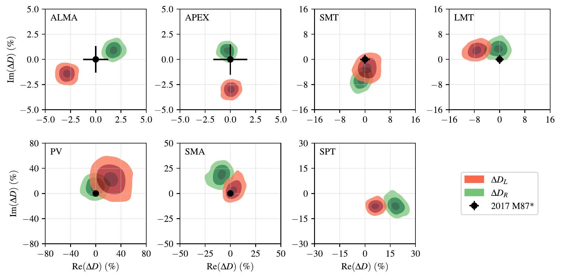
الشكل 15. التوزيعات الخلفية لتصحيحات مصطلح التسرب، المطبقة بعد المعايرة باستخدام مصطلحات D لعام 2017 لمصدر M87*، التي تم الحصول عليها بواسطة THEMIS من خلال التوافق مع بيانات 6 و7 أبريل 2017 على Sgr A* فقط (أي، دون النظر في معايرات أخرى). تظهر الخطوط المتساوية، و المناطق التراكمية. للمقارنة،تشير القضبان السوداء إلى عدم اليقين من قيم THEMIS 2017 M87*. القيود الأضعف بشكل ملحوظ على IRAM 30 م (PV) وSMA-المصطلحات هي نتائج مباشرة لتغطية الزاوية المتوازية الأقل نسبياً خلال ملاحظات Sgr A*. وبالمثل، لأن M87* غير مرئي من القطب الجنوبي، فإن SPT ليس لديه نقطة مقارنة.
كل منها ممثلة بعدد ثابت من نقاط التحكم الموجودة على شبكة مستطيلة مع الأولويات كما هو مذكور في ورقة M87* VII وورقة M87* IX، والتي يتم من خلالها استيفاء الصورة عبر منحنى بيكوبي. انظر برويدرِك وآخرون (2020). مجال الرؤية على المحورين من الشبكة واتجاه الشبكة هما معلمات نموذجية ومسموح لهما بالتغير. يتم تطبيق التشتت الانكساري مباشرة على الرؤى المرتبطة، مع افتراض نموذج التشتت في جونسن وآخرون (2018)، مع معلمات التشتت الافتراضية من إيساوان وآخرون (2021). يتم إعادة بناء المكاسب المعقدة بشكل مستقل حسب المسح كما هو موضح في الورقة الثالثة. يتم حل تسرب الاستقطاب باستخدام البيانات فقط، مع أولويات ثابتة على الفترةعلى المكونات الحقيقية والخيالية لليسار واليمين-شروط لكل محطة.
يتم التخفيف من التغيرات داخل الساعة لـ Sgr A* من خلال النمذجة الصريحة للتقلبات الإضافية حول الصورة المتوسطة كما هو موضح في Broderick et al. (2022)، المعدلة كما هو موضح في القسم 4.1.2. في الوقت نفسه، يتم تخصيص مساهمات إضافية لميزانية عدم اليقين الزائد لحساب ضوضاء التشتت الانكساري والأخطاء النظامية (مثل الأخطاء غير المغلقة)، كما هو موضح في الورقة الرابعة. باستثناء تباين اليد المتوازية/اليد المتقاطعة، الذي يتم تثبيته عند القيمة التي تشير إليها طيف الطاقة المقدرة تجريبياً، يُسمح لجميع المعلمات الأخرى في نموذج عدم اليقين بالتغير أثناء إعادة بناء الصورة (انظر الأوراق الثالثة والرابعة لمزيد من التفاصيل).
لضمان أخذ عينات فعالة من التوزيع الخلفي، نستخدم نظام التبريد المتوازي المتباين الفردي-الزوجي، حيث يتم استكشاف كل مستوى من مستويات التبريد عبر خوارزمية هاملتونية مونت كارلو NUTS التي تم تنفيذها بواسطة حزمة ستان (كاربانتر وآخرون 2017؛ سيد وآخرون 2019). لقد تم إثبات أن هذه العينة فعالة في التقاط التوزيعات الخلفية متعددة الأنماط (انظر، على سبيل المثال، ورقة M87* السابعة؛ الورقة الرابعة). يتم تقييم تقارب السلسلة من خلال الفحص البصري لآثار المعلمات والسلسلة الكمية. الإحصائيات، بما في ذلك وقت الارتباط الذاتي المتكامل، مقسوم-وتوزيعات رتبة المعلمات (Vehtari et al. 2019)، وعادة ما يتطلبخطوات MCMC. يتم اختيار عدد مستويات التخفيف لضمان التواصل الفعال بين مستويات الحرارة الأعلى والأدنى، وهنا عادةً ما يكون 65 بسبب الطبيعة المعقدة للنموذج.
ثلاثة مصادر رئيسية إضافية من عدم اليقين المنهجي التي تم استكشافها بواسطة صورة THEMIS القطبية هي تأثير تصحيحات التسرب، مكاسب المحطات، و ستوكز الأساسية.صورة.تصحيحات المدى القصير بالنسبة للقيم المستنتجة من المعاير المستندة إلى بيانات THEMIS (المستمدة من بيانات Sgr A* فقط) موضحة في الشكل 15 بالمقارنة مع الأحجام المستنتجة من إعادة بناء THEMIS القطبية لبيانات M87* في 11 أبريل (ورقة M87* السابعة). معظم التصحيحات تتماشى مع كونها صغيرة. )، مع الشكوك الكبيرة ( ) عند PV وSMA تشير إلى ضعف تغطية الزاوية المتوازية لـ Sgr A* في تلك المحطات. ومع ذلك، فإن الصور قوية حتى أمام -الشروط، مما يشير إلى أن الهيكل القطبي النهائي قوي أمام معايرة التسرب. التأثير الأدنى لـ-الشروط المتعلقة بالهيكل القطبي متوافقة أيضًا مع النتائج في الملحق H من ورقة M87* VII التي تقيم تأثيرها على الصور القطبية لثقب أسود M87* الثابت. تشير فحص إعادة بناء الكسب المعقد إلى وجود انحرافات صغيرة فقط عن مكاسب المعايرة المفترضة التي تم تطبيقها قبل التحليل: بالنسبة لـ ALMA و APEX و SMA، فإن تصحيحات سعة الكسب تكون من حيث; بالنسبة لـ SMT و PV فهي من الدرجة ; وبالنسبة لـ LMT و SPT فهي تقريبًا . تم تهيئة سلاسل MCMC لـ Sgr A* باستخدام ستوكزصورة من الورقة الثالثة لتقليل الوقت اللازم لتقارب MCMC. بالنسبة لاختبارات البيانات المحاكاة، تم تهيئة سلاسل MCMC باستخدام ستوكزالصور ومع توزيع غاوسي منتشر بحجم تقريبي كما تشير إليه تحليلات رؤية اللحظة الثانية، حيث تتقارب الحالتان إلى نفس التوزيعات الخلفية. توفير الثقة بأن التهيئة المحددة ليست مهمة. بالنسبة لـ Sgr A*، تم العثور على أوضاع متعددة متشابهة نوعيًا، تختلف بشكل طفيف في توزيع التدفق حول الحلقة وبنية الانبعاث المنتشر الممتد.
أ.3. التصوير الكهربائي
حزمة التصوير EHT (Chael et al. 2016، 2018) تعيد بناء الصور القطبية عبر RML. يقوم EHT-imaging بحل صورةعن طريق تقليل دالة الهدف عبر الانحدار التدرجي. دالة الهدف التي تم تقليلهاهو مجموع مرجح للبيانات المخفضةمصطلحات احتمالية السجل وعبارات التنظيم التي تفضل أو تعاقب خصائص الصورة المحددة:
لذا يتطلب تصوير RML تحسين أوزان “الهايبر بارامتر”. و في المعادلة (A2) لاستعادة الصور عالية الدقة. هنا نصف مصطلحات البيانات والمُنظّمات التي نستخدمها في التصوير القطبي.
بالنسبة لإعادة بناء الصور المستقطبة، نتبع الطريقة الموضحة في تشايل وآخرون (2016) والملحق C من ورقة M87* VII. الاختلاف الرئيسي الوحيد مع تحليل الاستقطاب لـ M87* هو استبعاد الـ-خطوات حل المدى الطويل، لأن بيانات Sgr A* تم تصحيح تسربها بناءً على تحليل M87* (والمعاير). نبدأ ببيانات مصححة من التسرب تم ضبطها باستخدام مكاسب السعة والطور الزمنية المعتمدة على المحطة، باستخدام الصورة المتوسطة الثابتة من الورقة الثالثة. يتم متوسط البيانات زمنياً إلى 120 ثانية، ميزانية ضوضاء منهجية منيتم تطبيقه، ويتم إضافة ميزانية الضوضاء بشكل متعامد إلى عدم اليقين في الرؤى وفقًا لدراسات التغير التي تم مناقشتها في القسم 4.1. ثم نقوم بإعادة بناء ستوكزصورة باستخدام معلمات المجموعة العليا لتصوير EHT التي تم تطويرها في الورقة الثالثة. نحن نثبت مجال رؤية الصورة عندكـ و احسب الكثافات على شبكة منبكسلات. بعد ذلك نقوم بإعادة ضبط مكاسب السعة والطور للمحطة (على افتراضإلى ستوك النهائي لديناصورة. باستخدام هذه الصورة كمرجع للتصوير القطبي، نقوم بعد ذلك بإعادة بناء صور الاستقطاب الخطي والدائري بشكل منفصل.
لإعادة بناء صورة الاستقطاب الخطي، تتضمن دالة الهدف في المعادلة (A2) احتمالين لوغاريتميين.الشروط: واحدة محسوبة باستخدام رؤية الاستقطاب RL*، وواحد يستخدم نسبة الاستقطاب في مجال الرؤيةمناعة من معظم أخطاء زيادة المحطة المتبقية الناتجة عن ستوكزالتصوير باستثناءنسبة الكسب، بينماليس كذلك. نحن نستخدم منظمان لكثافة التدفق القطبي: المنظم هولداوي-واردل (هولداوي وواردل 1990) (المعادلة (13) من تشايل وآخرون 2016) تفضل بكسلات الصورة التي تأخذ قيمة أقل من (الاستقطاب الأقصى النظري لإشعاع السنكروترون)، ومُنظِّم التباين الكلي (TV) (Rudin et al. 1992) يعاقب على التدرجات الكبيرة بين البيكسلات في كل من الأجزاء الحقيقية والتخييلية من توزيع سطوع الاستقطاب المعقد (المعادلة (15) من Chael et al. 2016). وبالتالي، فإن دالة الهدف للاستقطاب الخطي هي
تحدد الأوزان النسبية بين قيود البيانات وعبارات التنظيم بواسطة أربعة معلمات فرعية , , و. نحن نحل توزيع التدفق المستقطب الذي
يقلل من المعادلة (A3) المعلمة بواسطة الاستقطاب النسبي و EVPA في كل بكسل. يتم تثبيت صورة ستوكز في خطوة التصوير الاستقطابي وتحدد المنطقة التي يُسمح فيها بتدفق الاستقطاب. نعيد بدء عملية الانحدار التدرجي عدة مرات، باستخدام مخرجات الجولة السابقة من التصوير المموهة بواسطة كدالة غاوسية كنقطة البداية الجديدة ونتكرر عبر جولات التصوير بزيادة الأوزان على و. نحتفظ بالبيانات الأساسية والمكاسب ثابتة.
لتصوير ستوكز , يقوم eht-imaging مرة أخرى بتثبيت صورة ستوكز ويحل من أجل الاستقطاب الدائري النسبي في كل بكسل عن طريق التوافق مع الرؤية الذاتية. يتم تحديد نسبة الاستقطاب الدائري ضمن النطاق من خلال تغيير المتغيرات بين الاستقطاب النسبي للبكسل والكمية المحلولة في الانحدار التدرجي. تشمل دالة الهدف للاستقطاب الدائري مُنظمًا للتغير الكلي على خريطة و مُنظمًا للندرة (على سبيل المثال، Akiyama et al. 2017)، وكلاهما يأخذ نفس الشكل كما في تصوير الكثافة الكلية (Chael et al. 2016). نقوم مرة أخرى بتصوير في جولات متعددة ونقوم بإجراء التحقق الذاتي التكراري، هذه المرة نحل من أجل المكاسب المعقدة اليمنى واليسرى بشكل مستقل لأخذ في الاعتبار انحرافات المكاسب الاستقطابية النسبية. يتم الاحتفاظ بـ -المصطلحات ثابتة أثناء تصوير ستوكز .
A.4. DoG-HiT
تتكون عملية DoG-HiT من خطوتين. في الخطوة الأولى، نستخدم خوارزمية DoG-HiT (Müller & Lobanov 2022) لتقريب صورة كثافة كلية ثابتة واستنتاج دعم متعدد الدقة (مجموعة من معاملات الموجات ذات الأهمية الإحصائية). في الخطوة الثانية، نستخدم هذه المعلومات السابقة لاستراتيجية تصوير دعم متعدد الدقة الموضحة في Müller & Lobanov (2023b) لإضافة الاستقطاب الخطي وحل الديناميات.
يقوم DoG-HiT بنمذجة الصورة بواسطة مجموعة من دوال الأساس متعددة المتغيرات (Müller & Lobanov 2022). تُعرف المصفوفة التي تحتوي على جميع دوال الأساس عادةً باسم القاموس، ونشير إليها بـ لبقية هذه المناقشة. يتم تعريف خريطة الكثافة الكلية على أنها ، حيث هو مصفوفة معاملات الموجات. يتم اختيار العرض المتجه والاتجاهات الزاوية للموجات بناءً على تغطية ()، بحيث تفصل الميزات الهيكلية للصورة التي تم قياسها (المغطاة بالملاحظات) وتلك التي تكون حساسة بشكل أساسي للفجوات في تغطية (). لتحقيق هذا الهدف، قمنا بتطوير قواميس خاصة من الموجات، أو اختلافات دوال بيسل البيضاوية واختلافات دوال غاوس البيضاوية؛ انظر Müller & Lobanov (2023a) لمزيد من التفاصيل. نستخدم صيغة تنظيم تعزز الندرة التي تشبه المعادلة (A2) باستثناء أن منتجات البيانات التي يتم توافقها هي مراحل الإغلاق وأطوال الإغلاق التي تم بناؤها من رؤى ستوكز ()، ونحل من أجل معاملات الموجات بدلاً من الصورة:
حيث هو معلمة التنظيم و هو قيد تدفق إجمالي بكثافة تدفق مضغوط . في هذا الإطار، تحاول إعادة بناء DoG-HiT استعادة صورة كثافة كلية مع تقليل الخيارات المعتمدة على المستخدم، أي، باستخدام فقط مصطلحات البيانات للصورة الثابتة ذات الكثافة الكلية التي تكون قوية
ضد التحقق الذاتي، واختيار مدفوع بالبيانات لمصطلح التنظيم. لقد تم إثبات أن بيانات EHT كافية لتقييد التصوير فقط بالإغلاق للصورة ذات الكثافة الكلية (على سبيل المثال، Chael et al. 2018؛ M87* الورقة IV؛ الورقة III؛ Müller et al. 2023).
في الخطوة الثانية، نتناول الديناميات والاستقطاب. أثناء توافق نموذج DoG-HiT الثابت (ستوكز ) مع الرؤى المرصودة، يتم قمع معاملات الموجات التي تكون حساسة بشكل أساسي للمقاييس المكانية المرتبطة بالفجوات في تغطية (). تُستخدم هذه المعلومات السابقة لإعادة بناء مجموعات البيانات الاستقطابية والمتغيرة زمنياً من خلال إجراء تقليل مقيد، أي، نقوم بتوافق الرؤى الاستقطابية الكاملة لستوكز بشكل مستقل لكل إطار ولكن نغير فقط المعاملات في دعم متعدد الدقة (Müller & Lobanov 2023b)، من خلال تقليل و لكل لقطة.
بالنسبة لتحليل ستوكز الثابت لمصدر متغير زمنياً ، نستخدم الصورة المتوسطة المرجعية من تحليل الكثافة الكلية (الورقة III) كحدس أولي، نقوم بالتحقق الذاتي لمجموعة البيانات إلى هذا النموذج، نضيف ضوضاء منهجية بمستوى في كل قاعدة، ونحسب دعم متعدد الدقة مع الجولة الرئيسية للتصوير DoG-HiT من خلال تقسيم للأمام والخلف (Müller & Lobanov 2022). بالنسبة للتحليل الاستقطابي والديناميكي، نستعيد أولاً صور ستوكز المتوسطة و عبر إجراء التقليل المقيد الموضح أعلاه. يتم تعيين عدد التكرارات يدويًا إلى 1000 تكرار. أخيرًا، نقوم بتقسيم مجموعات البيانات في إطارات مدتها 30 دقيقة ونستعيد الصورة المستقطبة الخطية في كل إطار بشكل مستقل. لكل إطار، تُستخدم الصورة الاستقطابية المتوسطة كحدس أولي لنهج الانحدار المتعدد المتغيرات مع حجم خطوة صغير. يتم متوسط إطارات إعادة بناء هذه اللقطة بشكل موحد وتقديمها كنتائج نهائية لـ DoG-HiT.
الملحق ب اختبارات البيانات الاصطناعية
في تصوير VLBI، يتم عادةً تعيين المعلمات الحرة ضمن طريقة التحليل بواسطة المستخدم بناءً على الخبرة السابقة مع مجموعات بيانات مماثلة. لاختيار معلمات الطريقة القادرة على إعادة بناء صور عالية الدقة، نقوم بإجراء دراسات استكشافية لمساحات المعلمات على بيانات اصطناعية مختارة لتقليد سلوك Sgr A*. يتم تطبيق أفضل مجموعة من المعلمات لكل طريقة على بيانات EHT الخاصة بـ Sgr A*.
تتكون مجموعات البيانات الاصطناعية المستخدمة في هذه الدراسة من ثمانية ملاحظات اصطناعية لـ EHT باستخدام تغطية Sgr A* المناظرة في 6 و 7 أبريل () الناتجة عن محاكاة MAD KHARMA GRMHD، التي تحتوي على مجموعة نموذجية من المعلمات مشابهة لسلوك Sgr A* في الكثافة الكلية (الورقة V). مجموعات بيانات 6 و 7 أبريل هي من نطاقين زمنيين متميزين من نفس محاكاة GRMHD. النموذج 1 هو المحاكاة الأصلية لـ GRMHD مع و . كلا هذين القيمتين أصغر من حيث الحجم مما لوحظ لـ Sgr A*، لكن هذا النموذج ينتج درجة مماثلة من تباين الاستقطاب: من تباين الكثافة الكلية مقارنة بـ لـ Sgr A* (أي، نسبة تباين اليد المتوازية/اليد المتقاطعة من ; انظر القسم 4.1 لطريقة القياس ونتائج Sgr A*). بينما ينتج النموذج 1 مستوى معقول من تباين الاستقطاب، فإن حقيقة أنه ينتج أقل من النسب الكلية للاستقطاب الخطي والدائري تؤدي إلى نتائج متشائمة من حيث المستقطب. لذلك، نحن أيضًا
نضم النموذج 2، المحاكاة GRMHD المعاد قياسها بحيث تتطابق النسب المتوسطة للاستقطاب الخطي والدائري مع تلك المقاسة في Sgr A*، . تؤدي هذه المعايرة إلى درجة من تباين الاستقطاب أكبر من تلك في الكثافة الكلية في النموذج 2. وبالتالي، مقارنةً بـ Sgr A* نفسها، ينتج النموذج 1 كمية معقولة من التباين ولكن مع القليل جدًا من الاستقطاب، بينما ينتج النموذج 2 نسب استقطاب معقولة مع الكثير من التباين. كلا النموذجين ملوثان بأفضل نموذج حالي لشاشة تشتت Sgr A* (Johnson et al. 2018؛ Psaltis et al. 2018؛ Issaoun et al. 2021). من المتوقع أن تعيد هذه النماذج GRMHD إنتاج سلوكيات الاستقطاب لبيانات Sgr A* الحقيقية، أي، أنماط EVPA المتغيرة ببطء، وتباين استقطاب مشابه للنموذج 1، ودرجة استقطاب مشابهة للنموذج 2، مع حمل خصائص تجعلها أكثر تحديًا لإعادة البناء، أي، تباين هيكلي أعلى في الكثافة الكلية بشكل عام، ودرجة استقطاب أقل للنموذج 1، وتباين استقطاب أعلى للنموذج 2.
تُعرض الصور المتوسطة للاستقطاب الخطي والدائري لنماذج المصدر في الأعمدة الأولى من الأشكال 16 و17، على التوالي. يتم توليد مجموعات البيانات الاصطناعية باستخدام الروتينات في eht-imaging. نتبع إجراء توليد البيانات الاصطناعية في القسم 4.3 من ورقة M87* VII، حيث نقوم بأخذ عينات من الرؤى على خطوط قاعدة EHT ونعرضها للضوضاء الحرارية، وانحرافات الكسب المعقد، ومصطلحات تسرب الاستقطاب. من أجل التوافق مع تحليل Sgr A*، نقوم بعد ذلك بتصحيح البيانات الاصطناعية باستخدام مصطلحات D المستمدة من M87*؛ انظر القسم 2. نقوم أيضًا بتوليد صور الكثافة الكلية باستخدام برنامج SMILI (Akiyama et al. 2017) باستخدام معاييره العليا من الورقة III. تُستخدم صور الكثافة الكلية من SMILI بعد ذلك لمعايرة البيانات الاصطناعية قبل التصوير باستخدام ehtimaging وDoG-HiT. هذا مشابه للإجراء المستخدم في تصوير الاستقطاب لـ M87* في ورقة M87* VII للحفاظ على تصوير الكثافة الكلية مستقلًا عن الإجراءات الاستقطابية. لا تستخدم طرق استكشاف الخلفية البيانات المعايرة ذاتيًا، كما هو الحال في تحليل Sgr A*.
نقدم إعادة بناء الاستقطاب الخطي للنموذجين في الشكل 16. لكل طريقة، نعرض النتائج المتوسطة على مدى يومين (6 و7 أبريل) وعلى نطاقين (منخفض وعالي)، مع الإشارة إلى التداخل المنظم في هيكل الاستقطاب الخطي بين الصورة المعاد بناؤها والواقع في الزاوية العليا اليسرى. نقوم بتحديد هذا التداخل من حيث معامل الارتباط بين صور الاستقطاب الخطي المعاد بناؤها وصور الاستقطاب الخطي الحقيقية، المموهة إلى دقة فعالة منكما هو موصوف في الورقة السابعة M87*، حيث
تم اختيار الجزء الحقيقي لقياس درجة محاذاة متجهات الاستقطاب.نقدم إعادة بناء الاستقطاب الدائري للنموذجين في الشكل 17، مع دمج كلا اليومين والنطاقين. كما نقوم بتحديد تداخل مُعَدل بين الصور المعاد بناؤها للاستقطاب الدائري وصور الحقيقة الأرضية، حيث
هذه المقياس حساس جدًا للبنية المنتشرة، التي تكون أكثر وضوحًا في صور الاستقطاب الدائري، مما يؤدي إلى تداخل أسوأ في إعادة بناء الاستقطاب الدائري عبر الطرق مقارنةً بـ
الشكل 16. صور الاستقطاب الخطي للنماذج الاصطناعية عبر جميع الطرق، تجمع بين كلا اليومين والنطاقات. نتائج استكشاف الخلفية هي متوسطات التوزيعات الخلفية للصور. النموذج 1 هو نموذج منخفض الاستقطاب ومنخفض التباين؛ النموذج 2 هو نموذج عالي الاستقطاب وعالي التباين. معامل الارتباطالمقارنة مع الحقيقة الأرضية المرتبطة تظهر في الزاوية العليا اليسرى من كل إعادة بناء. نظام العرض مشابه لذلك في الشكل 8.
الشكل 17. صور الاستقطاب الدائري للنماذج الاصطناعية الاثنين عبر جميع الطرق، مع دمج كلا اليومين والنطاقات. نتائج استكشاف الخلفية هي متوسطات التوزيعات الخلفية للصور. معامل الارتباطالمقارنة مع الحقيقة الأرضية المرتبطة تظهر في الزاوية العليا اليسرى من كل إعادة بناء. نظام العرض مشابه لذلك في الشكل 11.
الاستقطاب الخطي. الكميات المقاسة المعروضة في الشكل 18 تعمل كمقياس إضافي لمدى دقة إعادة البناء.
نلاحظ أنه بالنسبة لنمذجة حلقة اللقطة، يتم بناء الصورة المتوسطة من السحوبات اللاحقة من إعادة بناء اللقطات الفردية، لذا فإن هذه الصورة المتوسطة لا يُتوقع أن تتناسب مع الصورة المتوسطة للحقيقة الأرضية. يتم إظهار التناسق بشكل أفضل من خلال الكميات القابلة للقياس من التوزيع اللاحق بالكامل. يتم عرض مقارنة الكميات القطبية القابلة للقياس مع الحقيقة الأرضية في الشكل 18. لأن و تعتمد على الدقة، نحن نطبق ك kernel التمويه الغاوسي لمحاكاة GRMHD قبل حساب قيم الحقيقة. جميع الطرق هي بشكل عام قادر على استعادة الكميات ذات الاهتمام. طرق الاستكشاف البعدية، نمذجة حلقة اللقطة وTHEMIS، تؤدي بشكل جيد بالمقارنة، وأفضل من طرق تصوير RML. تواجه DoG-HiT أكبر صعوبة في إعادة بناء البيانات الاصطناعية نتيجة لافتراضاتها الضعيفة نسبيًا حول توزيع الانبعاث (فهي لا تفرض أو استنادًا إلى أداء البيانات الاصطناعية والتوزيعات اللاحقة المقدمة لقياس عدم اليقين، ستُستخدم نتائج حلقة m و THEMIS Sgr A* كقيود نظرية، بينما توفر نتائج التصوير هنا فحصًا للتناسق باستخدام منهجيات مختلفة بطبيعتها.
النموذج 1
النموذج 2
الشكل 18. مقارنات الكميات القطبية الخطية والدائرية المقاسة من الطرق الفردية وصور المتوسط الحقيقي للأفلام GRMHD. تظهر النتائج للنموذج 1 في الألواح الثمانية العلوية، وتظهر النتائج للنموذج 2 في الألواح الثمانية السفلية. بالنسبة لطرق تصوير RML، تمثل الرموز المملوءة والفارغة نتائج 6 و7 أبريل، على التوالي. تمثل أشرطة الخطأ لطرق حلقة m-اللحظية وTHEMISنطاق الثقة من توزيعات الخلفية المجمعة لليوم. تم تمثيل القيم الحقيقية كخطوط ممتلئة ومتقطعة ليومي 6 و7 أبريل، على التوالي. بالنسبة لـ DoG-HiT، الذي لا يفرض بشكل نشط أو نقوم بإخفاء أي بكسلات تكون أقل منمن شدة الذروة قبل حساب هذه الكميات. يتم تشويش صور GRMHD الحقيقية باستخدام Gaussian دائري.كما هو الحال بالنسبة للنماذج النظرية مقارنةً بـ Sgr A* في الورقة الثامنة. تمثل الخطوط الأفقية قيم الحقيقة للصورة المتوسطة، بينما تمثل المناطق المظللة المناطق من النسبة المئوية الخامسة إلى الخامسة والتسعين التي تغطيها اللقطات الفردية ليومي المراقبة. لا توجد قيمة حلقة m مقاسة لـلأن الطريقة تثبتها على قيمة مستنتجة من منحنى ضوء ALMA.
الملحق ج: ستوكاعتماد
في هذا الملحق، نصف اختبارًا مستهدفًا لاعتماد النتائج القطبية على ستوكز الأساسية.الهيكل. حددت الورقة الثالثة أربعة تجمعات من الإجمالي-
الشكل 19. صور الاستقطاب لـ Sgr A* بتاريخ 7 أبريل 2017 باستخدام تصوير eht (يسار) و DoG-HiT (يمين)، حيث يتم استخدام ستوكز الأساسيةالصورة (باللون الرمادي) المستخدمة في المعايرة الذاتية تم اختيارها من الصورة المتوسطة التمثيلية العامة ومتوسطات الثلاث مجموعات الحلقية في الورقة الثالثة. نظام العرض مشابه لذلك في الشكل 8.
الجدول 7 معامل الارتباط الطبيعي بين هيكل الاستقطاب في وضعيات الحلقة بتاريخ 7 أبريل وذلك للصورة المتوسطة في الشكل 19، لكل من تصوير eht وDoG-HiT
وضع الرنين
تصوير EHT
دوغ-هيت
الخاتم 1
0.93
0.97
الخاتم 2
0.88
0.85
الخاتم 3
0.92
0.90
هيكل الكثافة في الصور العليا المعاد بناؤها لـ Sgr A*. من بين هذه المجموعات الأربع، تحتوي ثلاث منها على شكل حلقي واضح مع أنماط كثافة متغيرة على طول الحلقة. هنا نفترض أنلها شكل حلقي، ونختبر اختيار وضع الحلقة الأساسية في التصوير القطبي.
في الشكل 19، نعرض الصور المعاد بناؤها ليوم 7 أبريل باستخدام كل من تصوير EHT وDoG-HiT – وهما البرنامجان اللذان يستخدمان بيانات تم معايرتها ذاتيًا باستخدام صورة الكثافة الإجمالية المتوسطة عبر أوضاع الحلقة المختلفة. في الجدول 7، نعرض التداخل المنظم بين الهياكل القطبية لأوضاع الحلقة وتلك الخاصة بالصورة المتوسطة المستخدمة في المعايرة الذاتية للنتائج الرئيسية. بينما يختلف توزيع الكثافة الإجمالية على طول الحلقة، تظهر بنية الاستقطاب استقرارًا عبر أوضاع الحلقة. وبالتالي، فإن الخصائص الرئيسية للاستقطاب غير حساسة لوضع الحلقة الكثافة الإجمالية الأساسي.
الملحق د: اعتماد خط أنابيب المعايرة
بينما تستخدم النتائج الرئيسية في هذا العمل خط أنابيب EHT-HOPS (بلاكبيرن وآخرون 2019)، نقوم بإجراء فحوصات إضافية ضد بيانات خط أنابيب CASA rPICARD (يانسن وآخرون 2019). في الشكل 20، نقارن إعادة بناء Sgr A* من بيانات HOPS و CASA لأيام المراقبة 6 و 7 أبريل 2017 باستخدام نصوص تحليل متطابقة مع طريقة تصوير RML واحدة (تصوير eht) وطريقة استكشاف posterior واحدة (نمذجة m-ring اللحظية). نحسب الارتباط المتقاطع للاستقطاب بين صور خطي تقليل البيانات، الموضحة في الزاوية العلوية اليسرى من لوحات CASA، ونجد توافقًا جيدًا. بينما تظهر صور الكثافة الكلية بعض التباين بسبب اختلافات البيانات، فإن نفس هيكل الاستقطاب الخطي لصور CASA موجود على جزء كبير من الحلقة، مع نمط EVPA قريب من الأفق. في الشكل 21، نقارن إعادة بناء m-ring اللحظية وتصوير eht للاستقطاب الدائري في Sgr A* باستخدام بيانات HOPS و CASA. بالنسبة لطريقة m-ring اللحظية، فإن الهيكل ثنائي القطب على طول الحلقة، مع منطقة غربية سلبية ومنطقة شرقية إيجابية، متسق لكلا خطي الأنابيب. تفضل إعادة بناء تصوير eht بشكل عام الاستقطاب الدائري السلبي، لكن الموقع يختلف بسبب التباين في البيانات. بناءً على ثقتنا في كل طريقة إعادة بناء من اختبارات البيانات الاصطناعية، فإن الاستنتاجات الرئيسية عمومًا قوية أمام الاختلافات في المعايرة وطرق التقليل.
الشكل 20. مقارنات لإعادة البناء باستخدام تصوير EHT ونمذجة حلقة اللقطة باستخدام خطوط تقليل HOPS (Blackburn et al. 2019) وCASA (Janssen et al. 2019) التي تجمع بين الأيام والأطياف. صور HOPS هي تلك المعروضة والمستخدمة في النص الرئيسي لهذا العمل. لكل صورة من صور CASA، يتم حساب الارتباط المتقاطع القطبي مقابل الصورة المعادلة من HOPS. نظام العرض مشابه لذلك في الشكل 8.
الشكل 21. مقارنات لإعادة بناء الاستقطاب الدائري مع تصوير EHT ونمذجة حلقة اللحظة باستخدام خطوط تقليل HOPS (في الأعلى) و CASA (في الأسفل) التي تجمع بين الأيام والنطاقات. نظام العرض مشابه لذلك في الشكل 11.
The Astropy Collaboration, Robitaille, T. P., Tollerud, E. J., et al. 2013, A&A, 558, A33
Blackburn, L., Chan, C.-k., Crew, G. B., et al. 2019, ApJ, 882, 23
Bower, G. C., Backer, D. C., Zhao, J.-H., Goss, M., & Falcke, H. 1999a, ApJ, 521, 582
Bower, G. C., Broderick, A., Dexter, J., et al. 2018, ApJ, 868, 101
Bower, G. C., Falcke, H., & Backer, D. C. 1999b, ApJL, 523, L29
Bower, G. C., Falcke, H., Sault, R. J., & Backer, D. C. 2002, ApJL, 571, 843
Bower, G. C., Wright, M. C. H., Backer, D. C., & Falcke, H. 1999c, ApJ, 527, 851
Bower, G. C., Wright, M. C. H., Falcke, H., & Backer, D. C. 2003, ApJL, 588, 331
Brentjens, M. A., & de Bruyn, A. G. 2005, A&A, 441, 1217
Broderick, A. E., Gold, R., Georgiev, B., et al. 2022, ApJL, 930, L21
Broderick, A. E., Gold, R., Karami, M., et al. 2020c, ApJ, 897, 139
Broderick, A. E., & Loeb, A. 2005, MNRAS, 363, 353
Broderick, A. E., & Pesce, D. W. 2020, ApJ, 904, 126
Broderick, A. E., Pesce, D. W., Tiede, P., Pu, H.-Y., & Gold, R. 2020, ApJ, 898, 9
Cabral, B., & Leedom, L. C. 1993, Proceedings of the 20th Annual Conference on Computer Graphics and Interactive Techniques SIGGRAPH ’93 (New York: Association for Computing Machinery), 263
Carpenter, B., Gelman, A., Hoffman, M. D., et al. 2017, J. Stat. Softw., 76, 1
Chael, A. A., Johnson, M. D., Bouman, K. L., et al. 2018, ApJ, 857, 23
Chael, A. A., Johnson, M. D., Narayan, R., et al. 2016, ApJ, 829, 11
Cho, I., Zhao, G.-Y., Kawashima, T., et al. 2022, ApJ, 926, 108
Deller, A. T., Brisken, W. F., Phillips, C. J., et al. 2011, PASP, 123, 275
Do, T., Hees, A., Ghez, A., et al. 2019, Sci, 365, 664
Eckart, A., Schödel, R., Meyer, L., et al. 2006, A&A, 455, 1
Event Horizon Telescope Collaboration, Akiyama, K., Alberdi, A., et al. 2019a, ApJL, 875, L1
Event Horizon Telescope Collaboration, Akiyama, K., Alberdi, A., et al. 2019b, ApJL, 875, L2
Event Horizon Telescope Collaboration, Akiyama, K., Alberdi, A., et al. 2019c, ApJL, 875, L3
Event Horizon Telescope Collaboration, Akiyama, K., Alberdi, A., et al. 2019d, ApJL, 875, L4
Event Horizon Telescope Collaboration, Akiyama, K., Alberdi, A., et al. 2019e, ApJL, 875, L5
Event Horizon Telescope Collaboration, Akiyama, K., Alberdi, A., et al. 2019f, ApJL, 875, L6
Event Horizon Telescope Collaboration, Akiyama, K., Alberdi, A., et al. 2021a, ApJL, 910, L12
Event Horizon Telescope Collaboration, Akiyama, K., Alberdi, A., et al. 2021b, ApJL, 910, L13
Event Horizon Telescope Collaboration, Akiyama, K., Alberdi, A., et al. 2022a, ApJL, 930, L12
Event Horizon Telescope Collaboration, Akiyama, K., Alberdi, A., et al. 2022b, ApJL, 930, L13
Event Horizon Telescope Collaboration, Akiyama, K., Alberdi, A., et al. 2022c, ApJL, 930, L14
Event Horizon Telescope Collaboration, Akiyama, K., Alberdi, A., et al. 2022d, ApJL, 930, L15
Event Horizon Telescope Collaboration, Akiyama, K., Alberdi, A., et al. 2022e, ApJL, 930, L16
Event Horizon Telescope Collaboration, Akiyama, K., Alberdi, A., et al. 2022f, ApJL, 930, L17
Event Horizon Telescope Collaboration, Akiyama, K., Alberdi, A., et al. 2023a, ApJL, 957, L20
Event Horizon Telescope Collaboration, Akiyama, K., Alberdi, A., et al. 2024, ApJL, 964, L26
Falcke, H., Mannheim, K., & Biermann, P. L. 1993, A&A, 278, L1
Falcke, H., Melia, F., & Agol, E. 2000, ApJL, 528, L13
Fish, V. L., Johnson, M. D., Lu, R.-S., et al. 2014, ApJ, 795, 134
Genzel, R., Schödel, R., Ott, T., et al. 2003, Natur, 425, 934
Georgiev, B., Pesce, D. W., Broderick, A. E., et al. 2022, ApJL, 930, L20
Goddi, C., Martí-Vidal, I., Messias, H., et al. 2019, PASP, 131, 075003
Goddi, C., Martí-Vidal, I., Messias, H., et al. 2021, ApJL, 910, L14
Gold, R., McKinney, J. C., Johnson, M. D., & Doeleman, S. S. 2017, ApJ, 837, 180
Goodman, J., & Narayan, R. 1989, MNRAS, 238, 995
Gravity Collaboration, Abuter, R., Accardo, M., et al. 2017, A&A, 602, A94
Gravity Collaboration, Abuter, R., Aimar, N., et al. 2022, A&A, 657, L12
Gravity Collaboration, Abuter, R., Aimar, N., et al. 2023, A&A, 677, L10
Gravity Collaboration, Abuter, R., Amorim, A., et al. 2018, A&A, 618, L10
Gravity Collaboration, Jiménez-Rosales, A., Dexter, J., et al. 2020, A&A, 643, A56
Harris, C. R., Millman, K. J., van der Walt, S. J., et al. 2020, Natur, 585, 357
Holdaway, M. A., & Wardle, J. F. C. 1990, Proc. SPIE, 1351, 714
Hunter, J. D. 2007, CSE, 9, 90
Issaoun, S., Johnson, M. D., Blackburn, L., et al. 2019, ApJ, 871, 30
Issaoun, S., Johnson, M. D., Blackburn, L., et al. 2021, ApJ, 915, 99
Issaoun, S., Wielgus, M., Jorstad, S., et al. 2022, ApJ, 934, 145
Janssen, M., Goddi, C., Falcke, H., et al. 2018, in 14th European VLBI Network Symp. & Users Meeting (EVN 2018) (Trieste: SISSA), 80
Janssen, M., Goddi, C., van Bemmel, I. M., et al. 2019, A&A, 626, A75
Johnson, M. D., Fish, V. L., Doeleman, S. S., et al. 2015, Sci, 350, 1242
Johnson, M. D., Lupsasca, A., Strominger, A., et al. 2020, SciA, 6, eaaz1310
Johnson, M. D., & Narayan, R. 2016, ApJ, 826, 170
Johnson, M. D., Narayan, R., Psaltis, D., et al. 2018, ApJ, 865, 104
Jones, E., Oliphant, T., Peterson, P., et al. 2001, SciPy: Open source scientific tools for Python
Jorstad, S., Wielgus, M., Lico, R., et al. 2023, ApJ, 943, 170
Kluyver, T., Ragan-Kelley, B., Pérez, F., et al. 2016, in Positioning and Power in Academic Publishing: Players, Agents and Agendas, ed. F. Loizides & B. Schmidt (Amsterdam: IOS Press), 90
Marrone, D. P. 2006, PhD thesis, Harvard Univ.
Marrone, D. P., Baganoff, F. K., Morris, M. R., et al. 2008, ApJ, 682, 373
Marrone, D. P., Moran, J. M., Zhao, J., & Rao, R. 2007, ApJ, 654, L57
Marrone, D. P., Moran, J. M., Zhao, J.-H., & Rao, R. 2006a, ApJ, 640, 308
Marrone, D. P., Moran, J. M., Zhao, J.-H., & Rao, R. 2006b, JPhCS, 54, 354
Martí-Vidal, I., Mus, A., Janssen, M., de Vicente, P., & González, J. 2021, A&A, 646, A52
Martí-Vidal, I., Roy, A., Conway, J., & Zensus, A. J. 2016, A&A, 587, A143
Matthews, L. D., Crew, G. B., Doeleman, S. S., et al. 2018, PASP, 130, 015002
McKinney, W. 2010, in Proc. of the 9th Python in Science Conf., ed. S. van der Walt & J. Millman, 51
McMullin, J. P., Waters, B., Schiebel, D., Young, W., & Golap, K. 2007, in ASP Conf. Ser. 376, Astronomical Data Analysis Software and Systems XVI, ed. R. A. Shaw, F. Hill, & D. J. Bell (San Francisco, CA: ASP), 127
Müller, H., & Lobanov, A. P. 2022, A&A, 666, A137
Müller, H., & Lobanov, A. P. 2023a, A&A, 672, A26
Müller, H., & Lobanov, A. P. 2023b, A&A, 673, A151
Müller, H., Mus, A., & Lobanov, A. 2023, A&A, 675, A60
Muñoz, D. J., Marrone, D. P., Moran, J. M., & Rao, R. 2012, ApJ, 745, 115
Narayan, R., & Goodman, J. 1989, MNRAS, 238, 963
Narayan, R., Yi, I., & Mahadevan, R. 1995, Natur, 374, 623
Ni, C., Broderick, A. E., & Gold, R. 2022, ApJ, 940, 149
Palumbo, D. C. M., Wong, G. N., & Prather, B. S. 2020, ApJ, 894, 156
Pordes, R., Petravick, D., Kramer, B., et al. 2007, JPhCS, 78, 012057
Psaltis, D., Johnson, M., Narayan, R., et al. 2018, arXiv:1805.01242
Quataert, E., & Gruzinov, A. 2000, ApJ, 545, 842
Ressler, S. M., White, C. J., & Quataert, E. 2023, MNRAS, 521, 4277
Ricarte, A., Johnson, M. D., Kovalev, Y. Y., Palumbo, D. C. M., & Emami, R. 2023, Galax, 11, 5
Ricarte, A., Prather, B. S., Wong, G. N., et al. 2020, MNRAS, 498, 5468
Roelofs, F., Johnson, M. D., Chael, A., et al. 2023, ApJL, 957, L21
Rudin, L. I., Osher, S., & Fatemi, E. 1992, PhyD, 60, 259
Sfiligoi, I., Bradley, D. C., Holzman, B., et al. 2009, in 2009 WRI World Congress on Computer Science and Information Engineering, 2 (Piscataway. NJ: IEEE), 428
Speagle, J. S. 2020, MNRAS, 493, 3132
Syed, S., Bouchard-Côté, A., Deligiannidis, G., & Doucet, A. 2019, arXiv:1905.02939
Thompson, A. R., Moran, J. M., & Swenson, G. W., Jr 2017, Interferometry and Synthesis in Radio Astronomy, 3rd ed. (Berlin: Springer)
Trippe, S., Paumard, T., Ott, T., et al. 2007, MNRAS, 375, 764
Vehtari, A., Gelman, A., Simpson, D., Carpenter, B., & Bürkner, P.-C. 2019, arXiv:1903.08008
Whitney, A. R., Cappallo, R., Aldrich, W., et al. 2004, RaSc, 39, RS1007
Wielgus, M., Issaoun, S., Martí-Vidal, I., et al. 2024, A&A, 682, A97
Wielgus, M., Marchili, N., Martí-Vidal, I., et al. 2022a, ApJL, 930, L19
Wielgus, M., Moscibrodzka, M., Vos, J., et al. 2022b, A&A, 665, L6
Yuan, F., Quataert, E., & Narayan, R. 2003, ApJ, 598, 301
Kazunori Akiyama (D),Antxon Alberdi (D),Walter Alef ,Juan Carlos Algaba (D),Richard Anantua (D),Keiichi Asada (D), Rebecca Azulay (D),Uwe Bach (D),Anne-Kathrin Baczko (D),David Ball ,Mislav Balokovic (D), Bidisha Bandyopadhyay (D),John Barrett (D),Michi Bauböck (D),Bradford A.Benson (D),Dan Bintley , Lindy Blackburn (D),Raymond Blundell (D),Katherine L.Bouman (D),Geoffrey C.Bower (D),Hope Boyce (D), Michael Bremer ,Christiaan D.Brinkerink (D),Roger Brissenden (D),Silke Britzen (D),Avery E.Broderick (D), Dominique Broguiere (D),Thomas Bronzwaer (D),Sandra Bustamante (D),Do-Young Byun (D), John E.Carlstrom (D),Chiara Ceccobello (D),Andrew Chael (D),Chi-kwan Chan (D),Dominic O.Chang (D), Koushik Chatterjee (D),Shami Chatterjee (D),Ming-Tang Chen (D),Yongjun Chen(陈永军)(D),Xiaopeng Cheng (D), Ilje Cho (D),Pierre Christian (D),Nicholas S.Conroy (D),John E.Conway (D),James M.Cordes (D), Thomas M.Crawford (D),Geoffrey B.Crew (D),Alejandro Cruz-Osorio (ID),Yuzhu Cui 崔玉竹)(ID),Rohan Dahale (D), Jordy Davelaar (D),Mariafelicia De Laurentis (D),Roger Deane (D),Jessica Dempsey (D), Gregory Desvignes (D),Jason Dexter (D),Vedant Dhruv (D),Indu K.Dihingia (D),Sheperd S.Doeleman (D), Sean Taylor Dougal (D),Sergio A.Dzib (D),Ralph P.Eatough (D),Razieh Emami (D),Heino Falcke (D),Joseph Farah (D), Vincent L.Fish (D),Edward Fomalont (D),H.Alyson Ford (D),Marianna Foschi (D),Raquel Fraga-Encinas (D), William T.Freeman ,Per Friberg (D),Christian M.Fromm (D),Antonio Fuentes (D),Peter Galison (D), Charles F.Gammie (D),Roberto García (D),Olivier Gentaz (D),Boris Georgiev (D),Ciriaco Goddi (D), Roman Gold (D),Arturo I.Gómez-Ruiz (D),José L.Gómez (D),Minfeng Gu(顾敏峰)(D),Mark Gurwell (D), Kazuhiro Hada (D),Daryl Haggard (D),Kari Haworth ,Michael H.Hecht (D),Ronald Hesper (D),Dirk Heumann (D), Luis C.Ho(何子山)(Daul Ho (D),Mareki Honma (D),Chih-Wei L.Huang (D),Lei Huang(黄磊)(D), David H.Hughes ,Shiro Ikeda (D),C.M.Violette Impellizzeri (D),Makoto Inoue (D),Sara Issaoun (D), David J.James (D),Buell T.Jannuzi (D),Michael Janssen (D),Britton Jeter (D),Wu Jiang(江悟)(D), Alejandra Jiménez-Rosales (D),Michael D.Johnson (D,Svetlana Jorstad (D),Abhishek V.Joshi (D),Taehyun Jung (D), Mansour Karami (D),Ramesh Karuppusamy (D),Tomohisa Kawashima (D),Garrett K.Keating (D),Mark Kettenis (D), Dong-Jin Kim (D),Jae-Young Kim (D),Jongsoo Kim (D),Junhan Kim (D),Motoki Kino (D),Jun Yi Koay (D), Prashant Kocherlakota (D),Yutaro Kofuji ,Patrick M.Koch (D),Shoko Koyama (D),Carsten Kramer (D), Joana A.Kramer (D),Michael Kramer (D),Thomas P.Krichbaum (D),Cheng-Yu Kuo (D),Noemi La Bella (D),Tod R.Lauer (D), Daeyoung Lee (D),Sang-Sung Lee (D),Po Kin Leung (D),Aviad Levis (D),Zhiyuan Li(李志远)(D),Rocco Lico (D), Greg Lindahl (D),Michael Lindqvist (D),Mikhail Lisakov (D),Jun Liu (D),Kuo Liu (D),Elisabetta Liuzzo (D), Wen-Ping Lo (D),Andrei P.Lobanov (D),Laurent Loinard (D),Colin J.Lonsdale (D),Amy E.Lowitz (D),Ru-Sen Lu (路如森)(DD),Nicholas R.MacDonald (D),Jirong Mao(毛基荣)(D),Nicola Marchili (D),Sera Markoff (D), Daniel P.Marrone (B),Alan P.Marscher (BD,Iván Martí-Vidal (BD),Satoki Matsushita (D),Lynn D.Matthews (D), Lia Medeiros (D),Karl M.Menten (D),Daniel Michalik (D),Izumi Mizuno (D),Yosuke Mizuno (D), James M.Moran (D),Kotaro Moriyama (D),Monika Moscibrodzka (D),Wanga Mulaudzi (D),Cornelia Müller (D), Hendrik Müller (D),Alejandro Mus (D),Gibwa Musoke (D),Ioannis Myserlis (D),Andrew Nadolski (D), Hiroshi Nagai (D),Neil M.Nagar (D),Masanori Nakamura (D),Gopal Narayanan (D),Iniyan Natarajan (D), Antonios Nathanail (D),Santiago Navarro Fuentes ,Joey Neilsen (D),Roberto Neri (D),Chunchong (D), Aristeidis Noutsos (D),Michael A.Nowak (D),Junghwan Oh (D),Hiroki Okino (D),Hèctor Olivares (D), Gisela N.Ortiz-León (D),Tomoaki Oyama (D),Feryal Özel (D),Daniel C.M.Palumbo (D),Georgios Filippos Paraschos (D), Jongho Park (D),Harriet Parsons (D),Nimesh Patel (D),Ue-Li Pen (D),Dominic W.Pesce (D),Vincent Piétu , Richard Plambeck (D),Aleksandar PopStefanija ,Oliver Porth (D),Felix M.Pötzl (D),Ben Prather (D), Jorge A.Preciado-López (D),Dimitrios Psaltis (D),Hung-Yi Pu (D),Venkatessh Ramakrishnan (D), Ramprasad Rao (D),Mark G.Rawlings (BD,Alexander W.Raymond (D),Luciano Rezzolla (D),Angelo Ricarte (D), Bart Ripperda (D),Freek Roelofs (D),Alan Rogers (D),Cristina Romero-Cañizales (D),Eduardo Ros (D), Arash Roshanineshat (D),Helge Rottmann ,Alan L.Roy (D),Ignacio Ruiz (D),Chet Ruszczyk (D),Kazi L.J.Rygl (D), Salvador Sánchez (D),David Sánchez-Argüelles (D),Miguel Sánchez-Portal (D),Mahito Sasada (D), Kaushik Satapathy (D),Tuomas Savolainen (D),F.Peter Schloerb ,Jonathan Schonfeld (D),Karl-Friedrich Schuster (D), Lijing Shao (D),Zhiqiang Shen(沈志强)(D),Des Small (D),Bong Won Sohn (D),Jason SooHoo (D), León David Sosapanta Salas (D),Kamal Souccar (D),Joshua S.Stanway (D),He Sun(孙赫)(D),Fumie Tazaki (D), Alexandra J.Tetarenko (D),Paul Tiede (D),Remo P.J.Tilanus (D),Michael Titus (D),Pablo Torne (D), Teresa Toscano (D),Efthalia Traianou (D),Tyler Trent ,Sascha Trippe (D),Matthew Turk (D),Ilse van Bemmel (D), Huib Jan van Langevelde (D),Daniel R.van Rossum (D),Jesse Vos (D),Jan Wagner (D),Derek Ward-Thompson (D), John Wardle (DI),Jasmin E.Washington (D),Jonathan Weintroub (D),Robert Wharton (D),Maciek Wielgus (D),Kaj Wiik (D), Gunther Witzel (D),Michael F.Wondrak (D),George N.Wong (D),Qingwen Wu(吴庆文)(DD,Nitika Yadlapalli (D), Paul Yamaguchi (D),Aristomenis Yfantis (D),Doosoo Yoon (D),Andrè Young (D),Ken Young (D),Ziri Younsi (D), Netherlands Organisation for Scientific Research (NWO), Postbus 93138, 2509 AC Den Haag, The Netherlands Department of Physics and Astronomy, Seoul National University, Gwanak-gu, Seoul 08826, Republic of Korea University of New Mexico, Department of Physics and Astronomy, Albuquerque, NM 87131, USA Physics Department, Brandeis University, 415 South Street, Waltham, MA 02453, USA Tuorla Observatory, Department of Physics and Astronomy, University of Turku, Finland Radboud Excellence Fellow of Radboud University, Nijmegen, The Netherlands School of Natural Sciences, Institute for Advanced Study, 1 Einstein Drive, Princeton, NJ 08540, USA School of Physics, Huazhong University of Science and Technology, Wuhan, Hubei, 430074, People’s Republic of China Mullard Space Science Laboratory, University College London, Holmbury St. Mary, Dorking, Surrey, RH5 6NT, UK Center for Astronomy and Astrophysics and Department of Physics, Fudan University, Shanghai 200438, People’s Republic of China Astronomy Department, University of Science and Technology of China, Hefei 230026, People’s Republic of China Department of Physics and Astronomy, Michigan State University, 567 Wilson Rd., East Lansing, MI 48824, USA
has a circular polarization fraction exceeding the linear polarization fraction at frequencies (e.g., Bower et al. 1999a, 1999c; Muñoz et al. 2012).
Because the empirical variability power spectra estimates are made after light-curve normalization, they do not suffer from the apparent excess of variability in GRMHD simulation light curves over that seen in Sgr A* by the EHT in 2017 (Paper V; Georgiev et al. 2022).
157 While image structure may also induce variations in , for sources smaller than as the visibilities are smoothed on scales in the ( ) plane. Thus, in the absence of an extended highly polarized component, variations on smaller ( ) scales are evidence for temporal variability in the source.
Note that this difference in variances does not imply that the fractional polarimetric variability is less than that of Stokes , because the fractional polarimetric variability also depends on the degree of polarization.
First Sagittarius A* Event Horizon Telescope Results. VII. Polarization of the Ring
Akiyama, Kazunori; Alberdi, Antxon; Alef, Walter; Algaba, Juan Carlos; Anantua, Richard; Asada, Keiichi; Azulay, Rebecca; Bach, Uwe; Baczko, Anne Kathrin; Ball, David; Baloković, Mislav; Bandyopadhyay, Bidisha; Barrett, John; Bauböck, Michi; Benson, Bradford A.; Bintley, Dan; Blackburn, Lindy; Blundell, Raymond; Bouman, Katherine L.; Bower, Geoffrey C.; Boyce, Hope; Bremer, Michael; Brinkerink, Christiaan D.; Brissenden, Roger; Britzen, Silke; Broderick, Avery E.; Broguiere, Dominique; Bronzwaer, Thomas; Bustamante, Sandra; Byun, Do Young; Carlstrom, John E.; Ceccobello, Chiara; Chael, Andrew; Chan, Chi Kwan; Chang, Dominic O.; Chatterjee, Koushik; Chatterjee, Shami; Chen, Ming Tang; Chen, Yongjun; Cheng, Xiaopeng; Cho, Ilje; Christian, Pierre; Conroy, Nicholas S.; Conway, John E.; Cordes, James M.; Crawford, Thomas M.; Crew, Geoffrey B.; Cruz-Osorio, Alejandro; Cui, Yuzhu; Gold, Roman; The Event Horizon Telescope Collaboration
Published in:
Astrophysical Journal Letters
DOI:
10.3847/2041-8213/ad2df0
Publication date:
2024
Document version:
Final published version
Document license:
CC BY
Citation for pulished version (APA):
Akiyama, K., Alberdi, A., Alef, W., Algaba, J. C., Anantua, R., Asada, K., Azulay, R., Bach, U., Baczko, A. K., Ball, D., Baloković, M., Bandyopadhyay, B., Barrett, J., Bauböck, M., Benson, B. A., Bintley, D., Blackburn, L., Blundell, R., Bouman, K. L., … The Event Horizon Telescope Collaboration (2024). First Sagittarius A* Event Horizon Telescope Results. VII. Polarization of the Ring. Astrophysical Journal Letters, 964(2), Article L25. https://doi.org/10.3847/2041-8213/ad2df0
Terms of use
This work is brought to you by the University of Southern Denmark.
Unless otherwise specified it has been shared according to the terms for self-archiving.
If no other license is stated, these terms apply:
You may download this work for personal use only.
You may not further distribute the material or use it for any profit-making activity or commercial gain
You may freely distribute the URL identifying this open access version
If you believe that this document breaches copyright please contact us providing details and we will investigate your claim.
Please direct all enquiries to puresupport@bib.sdu.dk
First Sagittarius A* Event Horizon Telescope Results. VII. Polarization of the Ring
The Event Horizon Telescope Collaboration(See the end matter for the full list of authors.)
Received 2024 January 4; revised 2024 February 5; accepted 2024 February 18; published 2024 March 27
Abstract
The Event Horizon Telescope observed the horizon-scale synchrotron emission region around the Galactic center supermassive black hole, Sagittarius A* (Sgr A*), in 2017. These observations revealed a bright, thick ring morphology with a diameter of as and modest azimuthal brightness asymmetry, consistent with the expected appearance of a black hole with mass . From these observations, we present the first resolved linear and circular polarimetric images of . The linear polarization images demonstrate that the emission ring is highly polarized, exhibiting a prominent spiral electric vector polarization angle pattern with a peak fractional polarization of in the western portion of the ring. The circular polarization images feature a modestly ( ) polarized dipole structure along the emission ring, with negative circular polarization in the western region and positive circular polarization in the eastern region, although our methods exhibit stronger disagreement than for linear polarization. We analyze the data using multiple independent imaging and modeling methods, each of which is validated using a standardized suite of synthetic data sets. While the detailed spatial distribution of the linear polarization along the ring remains uncertain owing to the intrinsic variability of the source, the spiraling polarization structure is robust to methodological choices. The degree and orientation of the linear polarization provide stringent constraints for the black hole and its surrounding magnetic fields, which we discuss in an accompanying publication.
Unified Astronomy Thesaurus concepts: Black holes (162); Supermassive black holes (1663); Polarimetry (1278); Radio interferometry (1346); Very long baseline interferometry (1769); Galactic center (565)
1. Introduction
The Event Horizon Telescope (EHT) Collaboration, using the technique of very long baseline interferometry (VLBI) at 230 GHz , recently published the first resolved images of the supermassive black hole at the Galactic center, Sagittarius A* (Sgr A*). Analyses using a variety of imaging and geometrical modeling methods revealed a bright emission ring associated with the inner accretion flow together with a dark central brightness depression associated with gravitational lensing, redshift, and light capture by the black hole (Event Horizon Telescope Collaboration et al. 2022a, 2022b, 2022c, 2022d, 2022e, 2022f, hereafter Papers I-VI). Because Sgr A* is heavily scattered by the intervening ionized interstellar medium and exhibits rapid (intrahour) intrinsic variability, these analyses employed a series of novel approaches to address both effects on the emission morphology (see Papers II, III, and IV). These challenges, which were not relevant for EHT observations of Messier 87* (M87*; Event Horizon Telescope Collaboration et al. 2019a, 2019b, 2019c, 2019d, 2019e, 2019f, hereafter M87* Papers I-VI), led to substantial uncertainty in the resulting image, particularly in the azimuthal emission profile. Nevertheless, as discussed in Paper V, the diameter of the emission ring in Sgr A* is consistent with expectations for a black hole with a mass of located at a distance of (e.g., Falcke et al. 2000; Broderick & Loeb 2005), as inferred by observations at infrared wavelengths of
Original content from this work may be used under the terms of the Creative Commons Attribution 4.0 licence. Any further distribution of this work must maintain attribution to the author(s) and the title of the work, journal citation and DOI.
individual stellar orbits on scales of Schwarzschild radii (Do et al. 2019; Gravity Collaboration et al. 2022).
The EHT images are broadly consistent with numerical simulations of a hot, radiatively inefficient, and highly subEddington accretion flow ( ; Paper V). While initial evidence for a low accretion rate came from the radio and submillimeter spectrum of Sgr A* in total intensity (e.g., Falcke et al. 1993; Narayan et al. 1995; Yuan et al. 2003), the strongest evidence has come from polarimetric observations at radio and submillimeter wavelengths. The first polarized measurements of were made in circular polarization (Bower & Falcke 1999b). Following these detections, initial measurements of linear polarization (Aitken et al. 2000; Bower et al. 2003) demonstrated that the accretion rate must be to avoid depolarization through Faraday rotation (e.g., Agol 2000; Quataert & Gruzinov 2000). Subsequent observations performed simultaneously at 227 and 343 GHz enabled measurements of the Faraday rotation measure (RM), RM~-5 (Marrone et al. 2007), substantiating the low accretion rate and providing tighter constraints on models of the accretion flow. Studies of the polarimetric light curve of Sgr A* also revealed intrahour variability in the linear polarization (Marrone 2006; Marrone et al. 2008), circular polarization (Bower et al. 2002), and RM (Bower et al. 2018). The polarimetric variations occasionally show hints of loops in the Stokes plane with a preference for clockwise motion, although counterclockwise motion is also regularly observed (Marrone et al. 2006b; Marrone 2006).
Unresolved polarimetric measurements of have also been made at near-infrared wavelengths, showing high fractional linear polarization with intrahour variability during flares (e.g., Genzel et al. 2003; Eckart et al. 2006; Trippe et al. 2007). Recently, the GRAVITY Collaboration produced polarimetric observations of the Galactic center in the nearinfrared with the Very Large Telescope Interferometer (VLTI; Gravity Collaboration et al. 2017). These observations produced astrometric measurements suggestive of clockwise motion on the sky (Gravity Collaboration et al. 2018, 2023); the associated integrated polarization variability was consistent with models with a modestly inclined accretion flow and strong magnetic fields (Gravity Collaboration et al. 2020). The recent polarized light-curve studies by Wielgus et al. (2022b) at 230 GHz also support clockwise motion near the black hole, associated with an X-ray flare (Paper II; Wielgus et al. 2022a).
To date, the only spatially resolved polarimetric measurements of Sgr A* have come from precursor EHT observations at 230 GHz with a three-element array (Johnson et al. 2015). These observations found a sharp increase in the interferometric fractional polarization measured on long baselines, sometimes exceeding unity, indicative of synchrotron emission produced by partially ordered magnetic fields on scales of a few Schwarzschild radii (see also Gold et al. 2017). These observations also revealed intrahour variability in the interferometric fractional polarization on long baselines, indicating a compact and highly dynamic emission region. However, these observations did not have sufficient baseline coverage to produce images.
In this paper we present the first spatially resolved horizonscale images of Sgr A* in linear and circular polarization, using EHT observations taken in 2017 April at a frequency of 230 GHz . In Section 2 we give an overview of the 2017 EHT observations and data processing. In Section 3 we discuss properties of the Sgr A* data set, and in Section 4 we discuss mitigation studies of three -specific challenges to the analysis. In Section 5 we give an overview of the analysis methods, and in Section 6 we present the linear and circular polarization images of . In Sections 7 and 8 we provide a discussion of the results and our main conclusions, respectively. Similar to the polarimetric analysis of M87* (Event Horizon Telescope Collaboration et al. 2021a, 2021b, 2023a, hereafter M87* Papers VII-IX), the polarized images of synchrotron emission from the immediate vicinity of the black hole event horizon provide a rich probe of the accretion physics and spacetime, which we discuss separately in an accompanying paper (Event Horizon Telescope Collaboration et al. 2024, hereafter Paper VIII).
2. Observations and Data Processing
The EHT observed Sgr A* on 2017 April 5, 6, 7, 10, and 11. The observatories participating in the 2017 campaign were the phased Atacama Large Millimeter/submillimeter Array (ALMA) and the Atacama Pathfinder Experiment (APEX) in the Atacama Desert in Chile, the James Clerk Maxwell Telescope (JCMT) and the phased Submillimeter Array (SMA) on Maunakea in Hawai’i, the Submillimeter Telescope (SMT) on Mt. Graham in Arizona, the IRAM 30 m (PV) telescope on Pico Veleta in Spain, the Large Millimeter Telescope Alfonso Serrano (LMT) on the Sierra Negra in Mexico, and the South Pole Telescope (SPT) in Antarctica (M87* Paper II). Sgr A* observations were interleaved with
those of two calibrator sources, the quasars J1924-2914 and NRAO 530. Scientific analyses of EHT observations of these two calibrators are presented in Issaoun et al. (2022) and Jorstad et al. (2023), respectively. This letter focuses on Sgr A* observations on 2017 April 6 and 7, which have ALMA participation and low levels of variability in the source compared to the other observed days (Paper II).
The VLBI data were recorded in two polarizations and two frequency bands. All observatories recorded two 2 GHz -wide frequency bands centered at 227.1 and 229.1 GHz , to which we refer here as low and high band, respectively. A more detailed description of the EHT setup is presented in M87* Paper II. With the exception of ALMA and JCMT, all observatories recorded both right-circular polarization (RCP) and left-circular polarization (LCP). ALMA recorded dual linear polarization, which was later converted to circular polarization using the PolConvert software package (Martí-Vidal et al. 2016). JCMT recorded only RCP on April 5, 6, and 7 and LCP on April 10 and 11.
After correlating the recorded data from all telescopes, we corrected for instrumental bandpass effects and phase turbulence from Earth’s atmosphere using established fringe-fitting algorithms (M87* Paper III). This calibration was carried out using two separate software pipelines: the CASA-based rPICARD (Janssen et al. 2019) and the HOPS-based EHTHOPS (Blackburn et al. 2019). After the atmospheric phase variations are removed, the data can be coherently averaged in time to increase the signal-to-noise ratio ( ). We also corrected for instrumental RCP and LCP phase and delay offsets by referencing the fringe solutions to phased ALMA (Martí-Vidal et al. 2016; Matthews et al. 2018; Goddi et al. 2019). The data were then amplitude-calibrated using stationspecific measurements of the system equivalent flux density and time-averaged in 10 s segments (M87* Paper III; Paper II). Finally, stations with a colocated partner (i.e., ALMA, APEX, SMA, and JCMT) were “network-calibrated” to further improve the amplitude calibration accuracy (M87* Paper III; Blackburn et al. 2019). Calibrating Sgr A* presents unique challenges owing to its time-varying nature and extended emission on arcsecond scales, which can affect visibility amplitudes for baselines within local arrays like ALMA and SMA. Wielgus et al. (2022a) describe the techniques used to estimate the time-resolved flux density of Sgr A* to overcome these challenges during calibration. Gain amplitude corrections for the remaining stations were interpolated from solutions derived on the calibrator targets, J1924-2914 and NRAO 530 (Paper II).
The main goal of the subsequent polarimetric calibration is the correction of spurious polarimetric leakage. This step was not part of the initial total-intensity data analysis (Paper I), as the impact of leakage on the Stokes component is negligible (Papers III and IV). Nonetheless, this effect is potentially significant for the analysis of linear and circular polarization. Hence, we employ the same calibration procedures used for M87* (M87* Paper VII) for the polarimetric analysis of the Sgr A* data. Since polarimetric leakage is an instrumental effect, the -term coefficients, quantifying the impact of leakage on the data, are expected to be stable on timescales of the EHT observing campaign ( week) and have the same values for all observed sources. ALMA is an exception because its polarimetric leakage is first corrected using multisource calibration as part of the PolConvert procedure, and the
Table 1
Daily Average -terms for ALMA Derived Via the Multisource Intrasite Method
Date
Band
(%)
Apr 5
low
high
Apr 6
low
high
Apr 7
low
high
Apr 10
low
high
Apr 11
low
high
Note. The -term uncertainties are assumed to be distributed as circular Gaussians in the complex plane.
VLBI data are only impacted by residual leakage that can vary from day to day. Given these considerations, we apply precalculated -terms to the Sgr A* data sets. For the stations with a colocated partner we use values derived through polsolve multisource fitting (Martí-Vidal et al. 2021) in Appendix D of M87* Paper VII, as shown in Tables 1 and 2. For all other stations except SPT, the adopted values shown in Table 3 are based on the M87* D-term ranges reported in Appendix E of M87* Paper VII as summarized in Issaoun et al. (2022). The SPT -terms are assumed to be zero, consistent with the constraints from the analysis of the companion calibrators J1924-2914 and NRAO 530 (Issaoun et al. 2022; Jorstad et al. 2023), for which an identical set of -terms was incorporated and verified through consistency tests.
Finally, accurate calibration of complex gain ratios is relevant particularly for circular polarization (Stokes ) analysis. In this work we take a self-calibration approach that assumes . This method is more conservative regarding the potential detection of circular polarization than the primary approach discussed in Appendix A of M87* Paper IX. Nonetheless, this calibration allows for a full recovery of circular polarization morphology constrained by robust interferometric closure quantities; see also Roelofs et al. (2023).
3. Data Properties
In Figure 1, we show the coverage and low-band interferometric polarization of the 2017 April 6 and 7 observations of Sgr A* as a function of ( ) after -term calibration. The colors encode the amplitude of the complex fractional polarization in the visibility domain, coherently time-averaged in 120 s segments. Following Johnson et al. (2015), we define the visibility-domain fractional polarization as
where , and are the visibility-domain Stokes parameters sampled. Sgr A* is moderately polarized on most baselines, . Data points on the Chile-LMT and Chile-Hawai’i baselines for 2017 April 7 have very high fractional polarization, , that occurs at ( ) spacings where the Stokes amplitudes approach a deep minimum. We also find that the polarization fractions on short ( ) baselines are
Table 2
Campaign-average -terms for APEX, JCMT, and SMA Derived via the Multisource Intrasite Method
Station
APEX
JCMT
SMA
Note. The -term uncertainties are assumed to be distributed as circular Gaussians in the complex plane.
Table 3
Leakage Calibration -terms Assumed for Stations without a Colocated Site
Station
LMT
SMT
PV
similar to those observed in 2013 by Johnson et al. (2015); see Figure 2.
Figure 3 shows the phase of the conjugate closure trace products on two quadrangles (ALMA-APEX-LMT-SMT and ALMA-LMT-SMA-SMT, ordered as specified in Broderick & Pesce 2020) for the 2017 April 6 and 7 observations of Sgr A*. Closure traces are quantities immune to complex station gains and polarimetric leakages. Conjugate closure trace products deviate from unity (i.e., their phases deviate from zero) only in the presence of nonuniform polarization structures, and they are therefore clear indicators of source polarization (Broderick & Pesce 2020). We note significant deviations from zero in Figure 3, indicating that has spatially resolved, nonuniform polarization structure. Statistically different values of the conjugate closure trace products on the same quadrangles between 2017 April 6 and April 7 further indicate that the polarization structure in is time variable.
In Figure 4 (top panels), we show the and closure phases on two triangles with particularly high S/N. Significant deviations from zero are a consequence of resolved and asymmetric structure in and . The difference in closure phase between the two correlation products is shown in the bottom panels, with the average closure phase difference shown as a green band ( uncertainty in the estimate of the mean), which deviates from zero and thus indicates the presence of a circular polarization signal, as is the case for M87* (M87* Paper IX). Because the effects of residual uncorrected polarization leakage enter in at the level for the parallel-hand correlation products, we expect the difference between and closure phases to be dominated by intrinsic Stokes signal rather than by instrumental systematics. In fact, the study of systematics in the data in Paper II revealed an excess “noise” of closure quantities in the Sgr A* data compared to other sources, likely due to the presence of intrinsic circular polarization in the source.
4. Mitigation of Variability, Scattering, and Faraday Rotation in the Sgr A* Data
In comparison to the polarimetric analysis of M87* (M87* Paper VII), there are additional challenges in the Sgr A* data that increase the difficulty of reconstructing images. The effects
Figure 1. The coverage for the April 6 (left) and April 7 (right) EHT observations of Sgr A* during the 2017 campaign. The color of the data points encodes the fractional polarization amplitude in the range from 0 to 2 , and the tick direction encodes the measured polarization direction . The data shown are derived from low-band visibilities after the data reduction and -term calibration described in Section 2 have been applied. The data points are coherently averaged over 120 s . High polarization fractions at the tails of certain baseline tracks are due to low , as they probe total-intensity minima.
Figure 2. Comparison of the fractional linear polarization observed in precursor EHT observations on 2013 March 21 (left panel; Johnson et al. 2015) and similar spatial scales in our 2017 April 7 observations (right panel). The 2017 panel is a zoom-in of the right panel of Figure 1, with the color-bar amplitude range from Johnson et al. (2015).
Figure 3. Conjugate closure trace product phases on two quadrangles for the April 6 and 7 observations of Sgr A*. The data points are coherently averaged across both frequency bands and in time over 120 s. Nonzero phases indicate that the source has spatially resolved and nonuniform polarized structure.
Figure 4. Closure phases observed on the ALMA-SMA-LMT (left) and ALMA-SMT-LMT (right) triangles during Sgr A* observations on April 6 (squares) and April 7 (circles). Open and filled markers denote low- and high-band data, respectively. Top: closure phases constructed from scan-averaged visibilities for both epochs, in red, in blue. Bottom: difference of closure phases between and . The zero level of the closure difference (i.e., no detected) is marked with a black dashed line. The light-green band shows the average difference.
of interstellar scattering along the line of sight to the Galactic center and the source’s time variability on short ( minutes) timescales have been studied and mitigated in the Stokes analyses (Papers II, III, and IV). We discuss how the variability and scattering manifest in the polarimetric data in Sections 4.1 and 4.2, respectively. In Section 4.3, we discuss the additional effects of Faraday rotation on the results and how these inform theoretical interpretation.
4.1. Intrinsic Time Variability
4.1.1. Stokes I Variability
During the 2017 EHT observing campaign, Sgr A* exhibited Stokes variability across a wide range of timescales. The compact source-integrated light curve during this period exhibits variability from minutes to the longest timescales probed ( ), with a “red” temporal power spectrum (i.e., larger variability on longer timescales; Wielgus et al. 2022a). Structural variability is also present on spatial scales comparable to that of the black hole shadow, appearing directly in visibility amplitudes and closure quantities (Papers II and IV).
The variability of was theoretically anticipated; the dynamical timescale near the event horizon of is , and the observed brightness fluctuations are natural consequences of the turbulent structures predicted by numerical general relativistic magnetohydrodynamic (GRMHD) simulations (Paper V). A survey of the EHT simulation library confirms that the spatiotemporal power spectrum of the variability (i.e., fluctuations about the mean image) in the GRMHD simulations is universally well approximated by a cylindrically symmetric, broken power
law in both the spatial and temporal dimensions (Georgiev et al. 2022). These power laws are dominated by the largest spatial and longest temporal scales, i.e., they exhibit a “red””red” power spectral density. As a consequence, in the GRMHD simulations, the bulk of the variability can be eliminated by normalizing the total intensity of individual image frames (Wielgus et al. 2022a). After light-curve normalization, the intranight power spectrum peaks at a baseline length of ( ).
Tools for measuring and mitigating the Stokes variability in Sgr A* have been developed based on the universality observed in GRMHD simulations (Broderick et al. 2022). The spatial power spectra have been estimated by computing means and variances of visibility amplitudes across frequency bands and days in patches of the ( ) plane after light-curve normalization and performing linear debiasing (see Section 4 of Broderick et al. 2022). This procedure leverages the compact nature of Sgr A*, makes use of the approximate spatial isotropy anticipated from the GRMHD simulations (Georgiev et al. 2022), and incorporates estimates of the uncertainty that include contributions from the statistical error (i.e., thermal noise), gain amplitudes, and leakage terms ( -terms). Because the number of data points in any range of baseline lengths can be small, this estimator can suffer from known biases that may be corrected via calibration with appropriate mock data sets (Paper IV). Upon doing so, the resulting empirical estimates of the structural variability power spectrum match those from GRMHD simulations in amplitude and shape (Paper V).
Figure 5. Phase of on the crossing and following tracks identified in Paper IV, during which the same ( ) positions are sampled at different times by different baselines on 2017 April 6 (squares) and 7 (circles). The central time stamps for each track are labeled in the corresponding colors (see Figure 2 of Paper IV for exact track locations in the ( ) plane). All data have been coherently averaged on 120 s timescales to illustrate short-timescale variability. No additional systematic uncertainty has been added.
The intrahour structural variability of Sgr A* was mitigated in Paper III in three stages. First, the complex visibilities were light-curve normalized (Wielgus et al. 2022a), eliminating the largest component of the variability and suppressing all correlated components. Second, the additional variability power, inferred from the empirical variability estimate, was introduced as an additional statistical error about a mean image structure. Where the magnitude of this additional component was uncertain, the level of excess “noise” was surveyed as part of the imaging and modeling exploration. Third, the additional uncertainty necessary was estimated via “noise-modeling,” the direct fitting of a simultaneous model for the mean image and a parameterized, broken power-law model for the statistical properties of the otherwise unmodeled variability (Broderick et al. 2022; Paper IV).
4.1.2. Polarimetric Variability
Consistent with historical expectations (e.g., Bower et al. 2002; Marrone et al. 2006a), during the 2017 EHT campaign Sgr A* exhibited significant polarimetric variability. This variability is strongly implied by the rapid fluctuations in the measured polarization direction in Figure 1. Variability is also shown explicitly in Figure 5 for the crossing and following tracks identified in Paper IV-segments of baseline tracks that substantially overlap at different observing times throughout the night-for which large polarization direction swings are
present on timescales , including large differences between 2017 April 6 and 7. Polarimetric variability is similarly implied by the rapid variations in the conjugate closure trace products shown in Figure 3, and it is shown explicitly by the comparison between observation days. For both of the quadrangles shown in Figure 3, the phase of the conjugate closure trace products varies by on timescales of tens of minutes, on similar timescales to the variability observed in Stokes but lower in magnitude.
To quantitatively assess the degree of polarimetric variability, we extend the empirical estimate used for Stokes from Broderick et al. (2022) to the independent parallel-hand and cross-hand correlation products. Following the application of calibrator-determined leakage terms, the procedure is similar to that in Paper IV: visibilities are scan-averaged and light-curve normalized, the mean and variance within patches are computed after linear detrending and azimuthally averaged, and uncertainties are estimated via Monte Carlo sampling of the statistical uncertainties, complex gains, and leakages. Estimates of the azimuthally averaged power spectra are independently generated for , and . The results after combining the 2017 April 6 and April 7 data are shown in Figure 6 for each hand independently.
The empirically estimated parallel-hand power spectra and ) are statistically indistinguishable from each other and from those associated with their Stokes counterpart. This similarity implies that the absolute variability in Stokes on as is small in comparison to the variability in Stokes . Practically, it implies that variability in the parallel hands may be mitigated effectively using the model in Papers III and IV for and individually.
The cross-hand power spectra ( and ) are statistically indistinguishable from each other. In the absence of uncorrected leakage, this is expected by construction and thus provides additional confidence in the calibrator-implied -terms. More importantly, the cross-hand power spectra share the shape of those associated with the parallel hands, though rescaled to approximately of the parallel-hand amplitude.
As in Papers III and IV, we employ multiple variability mitigation schemes when modeling or imaging the Sgr A* data. These may be segregated into two general categories:
Post-marginalization: Multiple images are reconstructed on subsets of the data that span sufficiently short periods of time that variability may be ignored, and they are subsequently combined to yield a single “average” image. Pre-marginalization: A single image is fit to the entire data set, with additional noise added to account for the deviations in the visibilities due to the structural variability in addition to the statistical and systematic components.
For the pre-marginalization methods, we make use of the empirical polarimetric variability power spectra in a way similar to Paper III, modified for polarimetric reconstructions. As with Stokes , we normalize all correlation products by the Stokes light curve to reduce the impact of large-scale correlated variability. Additional statistical error following the broken power-law model is then added in quadrature to each correlation product, with the parallel hands receiving the same additional noise as applied to Stokes and cross-hands receiving an amount that is reduced by a fixed fraction.
For Sgr A* the parallel-hand/cross-hand variance ratio is , i.e., half as much noise is added in an absolute sense to the cross-hands as that added to the parallel hands. Depending on the polarimetric image reconstruction method, parameters of the additional noise model are surveyed or directly reconstructed (see Appendix A). Moreover, the value of this variance ratio depends on the source properties and can be both much smaller and larger for other data sets (e.g., the synthetic data sets discussed in Appendix B) than found for , depending on both the polarization fraction and degree of variability.
4.2. Interstellar Scattering
At radio wavelengths, the image of is heavily scattered by ionized interstellar plasma along the line of sight. In particular, density inhomogeneities result in a variable index of refraction, with corresponding phase fluctuations across an image that vary with time and observing wavelength ( ). For detailed discussion and a historical summary of the scattering of Sgr A*, see Psaltis et al. (2018) and Johnson et al. (2018).
The effects of scattering are predominantly caused by inhomogeneities on two widely separated spatial scales. “Diffractive” scattering arises from fluctuations on spatial scales of and results in blurring of the image with an approximately Gaussian kernel. “Refractive” scattering arises from fluctuations on spatial scales of and results in irregular distortion of the image that does not correspond to a convolution. In terms of interferometric visibilities, the signal
Figure 6. Model-agnostic estimates of the azimuthally averaged excess variance of the parallel-hand and cross-hand visibility amplitudes, after removing that from the reported statistical errors, as a function of baseline length. Nonparametric estimates are obtained across April 6 and 7, using both high- and low-band data. Uncertainties associated with the thermal errors, uncertain station gains, and polarization leakage are indicated by the error bars. Azimuthally averaged thermal errors are shown by the gray triangles and provide an approximate lower limit on the range of accurate variance estimates. For comparison, the magnitudes of the variance induced by refractive scattering are shown in purple along the minor (top) and major (bottom) axes of the diffractive scattering kernel (see Section 4 of Paper III); the variance along individual tracks on April 7 is shown by the solid purple lines. The orange band indicates the 95th percentile range of broken power-law fits to the Stokes excess variances from Paper IV.
on long baselines is exponentially suppressed by diffractive blurring but retains an additive contribution from refractive “noise” (Goodman & Narayan 1989; Narayan & Goodman 1989; Johnson et al. 2015; Johnson & Narayan 2016). In this paper, we follow the approach used in previous papers in this series and “deblur” our data before imaging (see, e.g., Fish et al. 2014), dividing each measurement by the Fourierconjugate scattering kernel on its baseline; we use the scattering kernel parameters from Johnson et al. (2018), which have been estimated using historical measurements of Sgr A* and validated by subsequent measurements (Issaoun et al. 2019, 2021; Cho et al. 2022). See Paper II for more details on the effects of interstellar scattering for EHT Sgr A* data.
Because the ionized interstellar medium is not significantly birefringent (e.g., Thompson et al. 2017; Ni et al. 2022), the effects of scattering on polarimetric observables can be mild. For example, interferometric fractional polarization is invariant to diffractive blurring; other image-integrated properties, such as the rotationally symmetric mode ( ) that we analyze extensively in Paper VIII, are only mildly affected by blurring (Palumbo et al. 2020). In general, the interferometric fractional polarization is only weakly affected for any baseline on which refractive noise is small compared to the signal amplitude (see, e.g., Ricarte et al. 2023). Moreover, because the beam of the EHT is comparable to the size of the diffractive blurring kernel, the effects of scattering on the polarized image of are expected to be mild when viewed at the resolution of the EHT. Figure 7 shows example scattered images of GRMHD simulations in linear and circular polarization.
Table 4 shows the values of the image quantities useful in polarimetric model discrimination in unscattered, scattered, and blurred images of a GRMHD simulation viewed at 230 GHz .
Figure 7. A comparison of GRMHD simulation snapshots in linear (top) and circular (bottom) polarization with and without the effects of interstellar scattering. Associated measurable quantities are given in Table 4. For display purposes the unscattered snapshots are blurred with a small as circular Gaussian beam, much smaller than the EHT instrument resolution. Top: total intensity is shown in gray scale, polarization ticks indicate the EVPA, the tick length is proportional to the linear polarization intensity magnitude, and color indicates fractional linear polarization. The dotted contour levels correspond to linearly polarized intensities of , and of the polarization peak. Cuts are made to omit all regions in the images where Stokes of the peak brightness and of the peak polarized brightness. Bottom: total intensity is indicated in colored linear-scale contours, and the Stokes brightness is indicated in the diverging color map, with red/blue indicating a positive/negative sign.
We define the image-integrated net linear and circular polarization fractions as
where the sum is over the pixels indexed by . We also measure the image-averaged linear and circular polarization fractions and across the images:
Note that these quantities depend on the resolution of the image; high-resolution GRMHD images will have systematically larger polarization fractions than their counterpart image reconstructions. All images used for analyses in this paper and the companion Paper VIII have been blurred to an effective resolution of . Following Palumbo et al. (2020),
Table 4
Image Quantities of Interest Computed on a Snapshot of a GRMHD Simulation with and without Interstellar Scattering Effects
Param.
Intrinsic
Blurred
Scattered and Blurred
(%)
4.72
4.72
4.62
0.33
0.33
0.35
49.66
31.97
31.82
2.26
0.91
0.93
0.14
0.14
0.14
0.34
0.30
0.29
(deg)
93.8
92.5
92.4
2.43
2.15
2.14
Note. The GRMHD simulation is a magnetically arrested disk model with , and viewed at inclination before and after interstellar scattering (Event Horizon Telescope Collaboration et al. 2022e). In the middle column, the image is blurred by a as circular Gaussian beam. In the right column, the simulated effects of scattering are applied, which produces diffractive blurring at sub-beam scales. Additional circular Gaussian blurring is performed to reach the as imaging resolution. The field of view and pixel size are the same in each case.
we also compute complex modes, which are Fourier decompositions of the linear polarization structure:
where ( ) are polar coordinates in the image plane and is the total flux density in the image. The mode is the simplest asymmetric mode, while is the simplest rotationally symmetric mode. In particular, is a probe of the handedness and pitch angle of the overall twist of the electric vector polarization angle (EVPA) pattern, where indicates a radial EVPA pattern and indicates a toroidal EVPA pattern on the image.
Image-integrated quantities such as change very little, while resolved quantities such as are significantly diminished by the diffractive blurring depolarization caused by scattering. Notably, low-resolution morphological quantities like and are almost completely unaffected, particularly in phase, though higher-order modes would be more disrupted. However, the effective size of the scattering kernel, as, is below the effective instrument resolution of , and so the presence of scattering is not a large contaminant of the image quantities of interest.
4.3. Faraday Rotation
As radiation propagates through a magnetized medium, the polarization state is affected by Faraday effects. Most notably, the EVPA changes because of Faraday rotation, quantifiable with an RM. The RM can be characterized as
a difference in measured EVPAs between the frequency bands corresponding to wavelengths (e.g., Brentjens & de Bruyn 2005). A large RM of has been measured in Sgr A* at 230 GHz . While the measured value of RM fluctuates significantly, the observed negative sign has remained consistent for decades (e.g., Bower et al. 2018; Wielgus et al. 2024). Detailed RM measurements from ALMA
as a connected-element interferometric array are available for the exact EHT observing epochs, which indicate values consistent with historical data (Goddi et al. 2021; Wielgus et al. 2022b, 2024); see Table 5.
If the entire RM can be confidently attributed to an external Faraday screen located between the emitting compact source and Earth, then the intrinsic EVPA pattern can be recovered by simply “derotating” EVPA ticks by an amount . For these observations, the measured RM assuming an entirely external screen leads to rotating the observed EVPAs by approximately (Table 5) clockwise before comparing them to theoretical models of the accretion flow near the black hole event horizon. The external character of the Faraday screen is supported by the persistence of the RM sign over long timescales, since we would expect frequent sign reversals in the turbulent accretion flow near the event horizon (Ricarte et al. 2020; Ressler et al. 2023). On the other hand, Wielgus et al. (2022b) reported time-resolved Faraday rotation, with the inferred RM fluctuating by up to on subhour timescales. These results point toward at least some of the Faraday rotation being due to an internal Faraday screen cospatial with the observed compact emitting region (Wielgus et al. 2024). In this limit, no EVPA derotation is required before comparing models to observations, as the theoretical models of the compact emission zone should fully account for the observed Faraday rotation.
A concordance picture could involve a slowly varying external Faraday screen to maintain a constant sign on relevant timescales in addition to an internal Faraday screen of a similar magnitude to explain the rapid time variability (Ressler et al. 2023). In this picture, it is justified to derotate the EVPA ticks by the median RM measured for a given observation, as the duration of the observing night is much longer than the dynamical timescale near the event horizon of . Furthermore, because of the rapid variability of the RM measured by ALMA (Wielgus et al. 2022b), the amount of EVPA corruption changes in time by about (Table 5). This further inflates uncertainties of the inferred EVPA structure in the reconstructed images and can be captured in data-driven estimates of polarimetric variability discussed in Section 4.1.2. These considerations are crucial for theoretical interpretation of the EHT results, and we investigate the impact of Faraday rotation in more detail using simulations in Paper VIII.
5. Methods
In this section, we present a summary of the methods used for the Sgr A* polarimetry results. We carry out geometric modeling of the source with a snapshot m-ring model fitting method (Paper IV; Roelofs et al. 2023). We additionally use three imaging methods: the Bayesian imaging framework THEMIS (Broderick et al. 2020, 2020c) and the regularized maximum likelihood (RML) methods eht-imaging (Chael et al. 2016, 2018) and DoG-HiT (Müller & Lobanov 2022). These methods are inherently different from one another in how they handle the intrinsic variability of the source. We summarize here the main method characteristics; more detailed descriptions can be found in Appendix A.
As a continuation of the analysis performed in the totalintensity companion papers (Papers III and IV), we model the polarization structure on top of a ring morphology, inferred through the analysis of the total-intensity observations. To aid
Table 5
Median Rotation Measure of Sgr A* Obtained from the ALMA Interferometric Light Curves (Wielgus et al. 2022b)
Observations
RM ( )
EVPA (deg)
April 6
April 7
April 11
April 6, 7
All Days
Note. The error estimates correspond to of the distribution. The change in EVPA is evaluated at 228.1 GHz .
in the total-intensity reconstruction step, the RML imaging methods use data sets that have been self-calibrated to the fiducial average deblurred total-intensity image produced with the image clustering procedure in Section 7.2 of Paper III. Tests of the effect of the various ring cluster modes on the polarimetric structure reconstructions, which is minimal, are shown in Appendix C. The THEMIS and snapshot m-ring methods do not use the self-calibrated data and do their own self-calibration simultaneously with the data fitting. All methods make use of data that have been -term calibrated, light-curve normalized, and deblurred to counter the effects of diffractive scattering and prescribe an appropriate totalintensity and polarization noise budget following the variability studies described in Section 4.1.
5.1. Snapshot m-ring Modeling
With the snapshot m-ring modeling method, we fit a polarimetric geometric model (“m-ring”; see Appendix A for details) to 2 -minute snapshots from our data sets (Paper IV; Roelofs et al. 2023). We only use snapshots with at least 10 visibilities and 60 s of coherent integration time. After timeaveraging the snapshots to of the visibility amplitudes are added to the thermal noise budget in order to represent systematic uncertainties. We fix the leakage parameters to the predetermined solutions from the EHT polarimetric M87* analysis; see Section 2. For our linear polarization fits, we fit our m-ring model to closure phases, closure amplitudes, and the visibility-domain fractional linear polarization for each snapshot independently (i.e., no temporal correlations are assumed). For our circular polarization fits, we fix the linear polarization parameters to the maximum a posteriori (MAP) estimates and fit to the parallel-hand closure phases and closure amplitudes (i.e., we fit to the separate and closure products). We also explore fits to visibility ratios. All these data products are robust to multiplicative station gains, except the visibility ratios, which may be affected by residual gain ratios (see also tests carried out in Roelofs et al. 2023). After fitting each snapshot from each day and frequency band, we combine all posteriors to a single posterior using a Bayesian averaging scheme (Paper IV).
5.2. THEMIS
As described in Broderick et al. (2020) and M87* Paper VII, the THEMIS image model consists of a rectilinear set of control points, spanned via a bicubic spline. Raster orientation and field of view are free parameters and dynamically adjust during
image reconstruction to choose an effective resolution. Raster resolution is determined by maximizing the Bayesian evidence over the raster dimension; typically, this is small owing to the limited number of EHT resolution elements across Sgr A*, and we make use of a raster based on the Stokes study in Paper III. The full polarimetric image model consists of four identically sized and oriented rasters that specify the total intensity, polarization fraction, EVPA, and Stokes . As described in Broderick et al. (2022) and Section 4.1.2, intrinsic source variability is mitigated via the modeling of a parameterized additional baseline-dependent contribution to the data uncertainties. The uncertainty model is composed of components that correspond to the variability noise, the refractive scattering noise, and the systematic error budget (see, e.g., Paper IV).
THEMIS reconstructions are fit directly to the scan-averaged complex visibilities ( ), after light-curve normalization as described in Section 4.1.2, combined across bands and 2017 April 6 and 7. Simultaneous with image generation, leakage terms and complex gains are recovered. To avoid complications from potential night-to-night variations in the -terms at ALMA and SMA, we fit data that are precorrected using the M87* Paper VII leakages. However, during fitting, -terms that are constant across both observation days and high and low bands are obtained from Sgr A* alone and do not further incorporate prior leakage estimates from other source reconstructions. Complex station gains are reconstructed independently on scans and across bands but are restricted to have unit gain ratios. Synthetic data tests reported in M87* Paper IX on Stokes in M87* showed that gain discrepancies of more than a few percent produced fits noticeably worse than those with smaller discrepancies. THEMIS images produced good-quality fits to EHT data; thus, gain offsets are expected to be very small.
The result of THEMIS fits is an approximate posterior composed of a set of images that may be used for Bayesian interpretation. For more details on likelihood construction, sampling, and chain convergence criteria see Appendix A and references therein.
5.3. Eht-imaging
The eht-imaging (Chael et al. 2016, 2018) package is a pixel-based RML imaging algorithm. Reconstructions are done via minimization of an objective function through gradient descent. This objective function is constructed with goodness-of-fit terms and regularizer terms that favor or penalize specific image properties. For polarized image reconstructions, we adopt a very similar methodology to the polarimetric imaging of M87*, described in Appendix C of M87* Paper VII. Since leakage is already corrected in the Sgr A* data from the M87* analysis, this step is omitted. We use the data self-calibrated to the fiducial total-intensity image as our starting data sets. These data are self-calibrated to a deblurred image, so no scattering mitigation is done as part of our procedure. We coherently average the data for 120 s , combine high and low bands into a single data set, and reconstruct one image per observing day for April 6 and 7. We add a fractional systematic noise budget of based on the total-intensity parameter exploration (see Table 4 of Paper III). We also add the variability noise budget determined in the total-intensity efforts in quadrature to the uncertainty of each visibility point (see Section 3.2.2 of Paper III), halving the
budget applied to cross-hand visibilities based on the polarimetric variability assessment in Section 4.1.2.
As a first step, we reconstruct a starting total-intensity image by fitting to parallel-hand closure phases, closure amplitudes, and visibility amplitudes. This total-intensity image is then kept fixed during the polarimetric imaging, defining the regions where polarimetric intensity is allowed. The imaging is done via iterative rounds of gradient descent. At each iteration, the output image is blurred with a as Gaussian beam and used as the initial image for the next round, and the weights on the data terms are increased. Linear polarimetric imaging and circular polarimetric imaging are done separately. For linear polarization, we fit the polarimetric visibility and the visibility-domain polarimetric ratio . For circular polarization, we fit the self-calibrated visibilities and the parallel-hand closure phases and closure amplitudes, and we solve for right and left complex gains independently.
5.4. DoG-HiT
The DoG-HiT package (Müller & Lobanov 2022, 2023a, 2023b) is a wavelet-based imaging algorithm that uses compressive sensing. DoG-HiT fits the data terms while assuming that the image structure is sparsely represented by a small number of wavelets. For the polarimetric and dynamic analysis we follow the description presented in Müller & Lobanov (2023b). Similar to the procedure for eht-imaging outlined in Section 5.3, we use the band-averaged, selfcalibrated, and leakage-corrected data set as a starting point. No scattering mitigation was applied as part of the procedure. We add a fractional systematic noise budget of to the 120 s averaged visibilities.
First, we recover a mean Stokes image with DoG-HiT, only fitting to the closure phases and closure amplitudes computed from the Stokes visibilities. We self-calibrate residual gains to this image on 10 -minute intervals, and we derive the multiresolution support, i.e., the set of significant wavelet coefficients, from the mean image. The multiresolution support fixes the spatial scales and positions for the dynamic and polarimetric imaging where emission is allowed. Next, we construct a mean polarimetric image by fitting the polarimetric visibilities and , but we only allow wavelet coefficients in the multiresolution support to vary. In an iterative procedure, we solve for residual terms. Finally, we cut the observation into frames of 30 minutes and fit the total-intensity and polarimetric visibilities in each frame independently starting from the mean images, but we only vary wavelet coefficients in the multiresolution support. We average the recovered frames uniformly to achieve a final static image. The whole procedure is carried out for both days of observations independently and finally averaged.
5.5. Synthetic Data Tests
All methods are validated against synthetic data sets that mimic properties of Sgr A*, the results of which are presented in detail in Appendix B. Two GRMHD models are chosen from the passing set of Sgr A* theoretical models that mimic both total-intensity and polarization properties of the source. One model has lower total linear polarization than Sgr A* but has a similar variability ratio of the cross-hand compared to the parallel-hand visibilities, while the other model has a total linear polarization fraction similar to that of but has a higher variability ratio of the cross-hands compared to the
Figure 8. Linear polarimetric images of Sgr A* from the combined 2017 April 6 and 7 observations with the primary methods snapshot m-ring modeling and THEMIS and the validation methods eht-imaging and DoG-HiT. The posterior-average image is shown for the posterior exploration methods. Total intensity is shown in gray scale, polarization ticks indicate the EVPA, the tick length is proportional to the linear polarization intensity magnitude, and color indicates fractional linear polarization. The white dotted contours mark the linear polarized intensity, corresponding to , and of the polarization peak. We have masked out all regions in which Stokes of the peak brightness, and we have similarly masked out all regions in which of the peak polarized brightness, where . The colorbar range is fixed for all panels.
parallel hands. As discussed in Paper V, the variability in the GRMHD simulations is generally higher than for Sgr A , making synthetic data more challenging to reconstruct than the real data. All methods are able to reconstruct the linear polarization structure of the two models, while THEMIS and the snapshot m-ring modeling methods fare better in reconstructing the circular polarization structure. Since THEMIS and m-ring modeling both carry out posterior exploration as part of their methodologies, they provide tight posterior distributions and measured uncertainties on individual linear and circular polarization quantities. These two methods are thus selected as the primary methods for analysis and theoretical interpretation, while the two RML methods are presented as additional validation methods.
6. Results
6.1. Linear Polarization
In Figure 8, we present the Sgr A* linear polarimetric images produced by each method, combining bands and observing days. The main results are produced using data processed through the EHT-HOPS pipeline, and consistency tests with the CASA rPICARD pipeline are presented in Appendix D. The Bayesian imaging method THEMIS produces an average image from many individual posterior draws with both days and
Figure 9. Polarimetric images of Sgr A* from Figure 8, but with EVPAs rotated by 46.0 deg to account for the median Faraday rotation in the combined April 6 and 7 data set (Table 5). The color-bar range is fixed for all panels.
bands combined into one data set. The snapshot modeling method produces an average image by combining individual band-combined snapshots across both days using Bayesian posterior averaging. Because the m-ring is a simple geometric model, the structure appears less noisy than the other methods. The RML imaging methods eht-imaging and DoG-HiT produce band-combined images per day; we display here the average image over 2 days (i.e., the April 6 and 7 images averaged together after imaging). In Figure 9, we present the same images but with EVPAs rotated by a constant angle to account for the median Faraday rotation in the combined April 6 and 7 data set, corresponding to a clockwise rotation of the EVPA by 46.0 deg , as discussed in Section 4.3.
The Sgr A* emission ring is almost entirely polarized, with a peak fractional polarization of at as resolution in the western region of the ring. The m-ring model shows a more prominent northwest peak due to the symmetry of the model mode; see Appendix A. The polarized emission EVPA pattern along the ring is nearly azimuthal with a counterclockwise handedness that is robust across time, frequency, and analysis method.
In Figure 10, we show the average of the four method images combining bands and days shown in Figure 8. The averaging is done independently for each Stokes intensity distribution. Due to the m-ring image having lower net polarization fraction (an effect of the variability of the EVPAs in snapshot averaging), the peak polarization fraction in the average image is lower than those of individual methods. This image is adopted as the conservative representation of the overall Sgr A* linear polarization structure, while individual method images are used for quantitative comparisons and theoretical interpretation; see Section 7 and Paper VIII.
Figure 10. Top: linear polarization image of Sagittarius A*. This image is the band, day, and method average of the linear polarization structure reconstructed from 2017 April 6 and 7 EHT observations. The display choices are analogous to Figure 8. Bottom: polarization “field lines” plotted atop an underlying totalintensity image. Treating the linear polarization as a vector field, the sweeping lines in the images represent streamlines of this field and thus trace the EVPA patterns in the image. To emphasize the regions with stronger polarization detections, we have scaled the length and opacity of these streamlines as the square of the polarized intensity. This visualization is inspired in part by line integral convolution (Cabral & Leedom 1993) representations of vector fields. The average linear polarization structure is overlaid on the fiducial average total-intensity image from Paper I.
6.2. Circular Polarization
In Figure 11, we present the circular polarization images produced by each method, combining bands and observing days. In the chosen color map, red and blue correspond to positive and negative circular-polarized flux density, respectively, with contours indicating the Stokes brightness. As in the synthetic data tests shown in Appendix B, the circular polarization structure is consistent for the snapshot m -ring and THEMIS posterior exploration methods, while the RML imaging methods show some differences. All methods see prominent negative circular polarization in the western portion of the ring, while only the snapshot m-ring and THEMIS methods recover positive circular polarization in the northeast region of the ring. The m -ring and THEMIS methods find peak fractional positive and negative circular polarization at the
Figure 11. Circular polarimetric images of Sgr A* from the combined 2017 April 6 and 7 observations with the primary methods snapshot m-ring modeling and THEMIS and the validation methods eht-imaging and DoG-HiT. The posterior-average image is shown for the posterior exploration methods. Total intensity is indicated in colored linear-scale contours at , and of the peak brightness. The Stokes brightness is indicated in the diverging color map, with red/blue indicating a positive/negative sign. The color-bar range is fixed for all panels.
level. It is worth noting that the peaks of the circular polarization emission line up with the peaks in total intensity. Thus, fractional measurements strongly depend on the tendency of individual methods to prefer more or less flux density in compact regions. The recovered dipole structure along the ring in the THEMIS and m-ring methods is consistent with the data. In particular both m-ring and THEMIS models predict small and mostly negative and closure phase differences on high-S/N triangles (see Figure 12) and are broadly consistent with the estimated mean values indicated with green bands. Additional m-ring fits carried out with higher -modes ( ) also prefer symmetric structure along the ring but exhibit significantly more uncertainty in the structure than the mode fit shown here. In addition, the Bayesian evidence for the higher-order fits is substantially lower than for the fits, indicating that the data do not support the presence of modes that are more complex than a dipole. The data appear to drive all methods toward simple symmetric structure, indicative of a need for high Stokes in compact regions on the ring based on the VLBI detections while still keeping an imageintegrated circular polarization level near zero, consistent with ALMA measurements. Given the remaining uncertainty in the detailed Stokes structure along the ring, structural properties of Stokes are not used for the theoretical interpretation in the companion Paper VIII.
7. Discussion
We derive eight observational constraints from reconstructed images of Sgr A*, and these are shown in Figure 13. Since the
Figure 12. Difference of closure phases between and visibilities, observed on the ALMA-SMA-LMT (top) and ALMA-SMT-LMT (bottom) triangles on April 6 (squares) and April 7 (circles). Open and filled markers denote low- and high-band data, respectively. The plots follow the bottom panels of Figure 4. Predictions from the models shown in Figure 11 are also given (red and blue solid lines). They are mostly consistent with small and predominantly negative measured closure phase differences.
snapshot m-ring modeling and THEMIS methods both provide Bayesian posterior distributions, error bars representing the confidence intervals from random posterior draws are shown. The combined confidence intervals from these two methods, shown in Table 6, are used in Paper VIII for theoretical interpretation. The RML imaging methods ehtimaging and DoG-HiT do not provide such distributions, but they are shown in Figure 13 as additional consistency checks from image reconstruction methods with very different methodologies. More detail on the individual methods is provided in Appendix A. We note that both posterior exploration methods treat variability differently: the snapshot m -ring modeling fits a structurally restricted ring model to individual 2 -minute data snapshots, while THEMIS Bayesian imaging reconstructs a collection of static images from the entire 2-day data set with a noise budget accounting for variability. Despite their substantial algorithmic differences, these two methods perform best on the synthetic data tests presented in Appendix B and yield very similar results.
In the leftmost panels of Figure 13, the image-integrated net linear and circular polarization fractions and from the reconstructions are compared to ranges from interfero-metric-ALMA light curves treating Sgr A* as an unresolved point source from Wielgus et al. (2022a). In general, all
methods are broadly consistent with ALMA ranges, although this need not necessarily have been the case. While the ranges for ALMA light curves correspond to instantaneous measurements of and , the and from our image reconstructions correspond to one or two night averages, as indicated. We note that THEMIS and the m-ring model do not agree on . Individual snapshot images from the m-ring method yield much higher values of . The lower in the averaged m-ring image may be due to a combination of cancellations of time-varying structure and model misspecification issues leading to phase offsets of the fitted (see Appendix A for details).
We also measure the image-averaged linear and circular polarization fractions and across the reconstructed images. For in particular, we note great consistency between the two posterior exploration methods, leading to stringent constraints for theoretical models in Paper VIII. Since is significantly biased upward when the is poor, this quantity is interpreted as an upper limit, as in previous studies of M87* (M87* Paper IX). We recall that both and are resolution dependent; unlike in past studies (M87* Paper VIII; M87* Paper IX), we do not apply any blurring after image reconstruction before computing these quantities.
In the bottom panel of the third column of Figure 13, the measured across methods is consistently far from 0 , implying more toroidal than radial EVPA patterns in the reconstructed images of . Accounting for a constant RM assuming an external Faraday screen, the EVPA pattern is derotated by , leading to a large of the opposite sign (the faded points in the panel). While the RM correction flips the handedness of the EVPA pattern (see Figures 8-9) and thus poses a significant systematic for comparisons to theoretical models, the EVPA patterns across methods remain very toroidal ( is closer to than ; Palumbo et al. 2020).
8. Conclusions and Summary
We presented the linear and circular polarimetric imaging of the EHT 2017 April 6 and 7 observations of our Galactic center black hole Sgr A* on event horizon scales at 230 GHz . Our analysis builds on the total-intensity ring morphology results presented in Papers I-VI and made use of the leakage calibration derived in M87* Paper VII. We employed four distinct methods in the polarimetric analysis: two posterior exploration (one Bayesian imaging and one snapshot modeling) methods for primary analysis and two RML imaging methods for validation. All methods were tested on synthetic data designed to mimic specific polarimetric characteristics of Sgr A*. When applied to the EHT Sgr A* data, all methods showed that the emission ring is highly polarized, with a peak fractional linear polarization of in the western region of the ring. While the detailed spatial distribution of the linear polarization along the ring is uncertain owing to the intrinsic variability of Sgr A* (as was the case for the total-intensity results), we observed a coherent spiraling polarization structure across a large portion of the ring that is robust to methodological choices. The circular polarization reconstructions from the posterior exploration methods, which performed best on the synthetic tests, prefer a dipole structure along the ring, with negative circular polarization emission on the west of the ring (also recovered by the RML imaging methods) and positive emission mostly constrained to the northeast, with peak absolute values that are of the Stokes
Figure 13. Comparisons of the measured linear and circular polarimetric quantities from the Sgr A* reconstructions across methods. For the RML imaging methods, the filled and open symbols represent the April 6 and 7 results, respectively. The gray symbols represent the 2 -day averages. The error bars for the snapshot m -ring and THEMIS Bayesian imaging methods represent the confidence range from the day-combined posterior distributions. The shaded region corresponds to the 5th to 95th percentile regions from ALMA-only linear and circular polarization light curves from Wielgus et al. (2022b). The m-ring method does not return a measurement for because it fixes the value to the ALMA mean measurement before fitting. Based on their performance on the synthetic data tests and quantified distributions, the results from the snapshot m -ring and THEMIS methods are used for theoretical comparisons in the companion Paper VIII.
Table 6
Polarimetric Constraints Derived from the Primary Methods THEMIS and Snapshot m-ring Modeling
Observable
Snapshot m-ring
THEMIS
Combined
(2.0, 3.1)
(6.5, 7.3)
(2.0, 7.3)
…
(-0.7, 0.12)
(-0.7, 0.12)
(1.4, 1.8)
(2.7, 5.5)
(0.0, 5.5)
(0.11, 0.14)
(0.10, 0.13)
(0.10, 0.14)
(0.20, 0.24)
(0.14, 0.17)
(0.14, 0.24)
(deg) (as observed)
(deg) (RM derotated)
(-168, -108)
(-151, -85)
(-168, -85)
(1.5, 2.1)
(1.1, 1.6)
(1.1, 2.1)
Note. These two methods each provide posteriors, from which confidence regions are quoted. Derotation assumes that the median RM can be attributed to an external Faraday screen, for which a frequency of 228.1 GHz is adopted. The range is treated as an upper limit. The combined constraints are used for the theoretical interpretation presented in Paper VIII.
emission in the same locations. Although both our posterior exploration methods reproduce a dipole along the ring, we deem the circular polarization structure more uncertain given the stronger disagreement between methods compared to the linear polarization reconstructions.
The resolution and sensitivity of the EHT have provided horizon-scale polarimetric images of Sgr A*, enabling for the first time a reconstruction of the magnetic field geometry in the vicinity of our Galactic center supermassive black hole’s event horizon. A discussion of the physical interpretation of these results is presented in Paper VIII.
Acknowledgments
The Event Horizon Telescope Collaboration thanks the following organizations and programs: the Academia Sinica; the Academy of Finland (projects 274477, 284495, 312496, 315721); the Agencia Nacional de Investigación y Desarrollo (ANID), Chile via NCN19 (TITANs), Fondecyt 1221421, and BASAL FB210003; the Alexander von Humboldt Stiftung; an Alfred P. Sloan Research Fellowship; Allegro, the European ALMA Regional Centre node in the Netherlands, the NL astronomy research network NOVA and the astronomy institutes of the University of Amsterdam, Leiden University, and Radboud University; the ALMA North America Development Fund; the Astrophysics and High Energy Physics program by MCIN (with funding from European Union NextGenerationEU, PRTR-C17I1); the Black Hole Initiative, which is funded by grants from the John Templeton Foundation (60477, 61497, 62286) and the Gordon and Betty Moore Foundation (grant GBMF-8273)-although the opinions expressed in this work are those of the author and do not necessarily reflect the views of these Foundations; the Brinson Foundation; “la Caixa” Foundation (ID 100010434) through fellowship codes LCF/BQ/DI22/ 11940027 and LCF/BQ/DI22/11940030; Chandra DD718089X and TM6-17006X; the China Scholarship Council; the China Postdoctoral Science Foundation fellowships (2020M671266, 2022M712084); Consejo Nacional de Humanidades, Ciencia y Tecnología (CONAHCYT, Mexico, projects U0004-246083, U0004-259839, F0003-272050, M0037279006, F0003-281692, 104497, 275201, 263356); the Colfuturo Scholarship; the Consejería de Economía, Conocimiento, Empresas y Universidad of the Junta de Andalucía (grant P18-FR-1769); the Consejo Superior de Investigaciones Científicas (grant 2019AEP112); the Delaney Family via the Delaney
Family John A. Wheeler Chair at Perimeter Institute; Dirección General de Asuntos del Personal Acadëmico-Universidad Nacional Autónoma de Mèxico (DGAPA-UNAM, projects IN112820 and IN108324); the Dutch Organization for Scientific Research (NWO) for the VICI award (grant 639.043.513), the grant OCENW.KLEIN.113, and the Dutch Black Hole Consortium (with project No. NWA 1292.19.202) of the research program the National Science Agenda; the Dutch National Supercomputers, Cartesius and Snellius (NWO grant 2021.013); the EACOA Fellowship awarded by the East Asia Core Observatories Association, which consists of the Academia Sinica Institute of Astronomy and Astrophysics, the National Astronomical Observatory of Japan, Center for Astronomical Mega-Science, Chinese Academy of Sciences, and the Korea Astronomy and Space Science Institute; the European Research Council (ERC) Synergy grant “BlackHoleCam: Imaging the Event Horizon of Black Holes” (grant 610058); the European Union’s Horizon 2020 research and innovation program under grant agreements RadioNet (No. 730562) and M2FINDERS (No. 101018682); the Horizon ERC Grants 2021 program under grant agreement No. 101040021; the European Research Council for advanced grant “JETSET: Launching, propagation and emission of relativistic jets from binary mergers and across mass scales” (grant No. 884631); the FAPESP (Fundaç ao de Amparo á Pesquisa do Estado de S ao Paulo) under grant 2021/ 01183-8; the Fondo CAS-ANID folio CAS220010; the Generalitat Valenciana (grants APOSTD/2018/177 and ASFAE/2022/ 018) and GenT Program (project CIDEGENT/2018/021); the Gordon and Betty Moore Foundation (GBMF-3561, GBMF5278, GBMF-10423); the Institute for Advanced Study; the Istituto Nazionale di Fisica Nucleare (INFN) sezione di Napoli, iniziative specifiche TEONGRAV; the International Max Planck Research School for Astronomy and Astrophysics at the Universities of Bonn and Cologne; DFG research grant “Jet physics on horizon scales and beyond” (grant No. 443220636); Joint Columbia/Flatiron Postdoctoral Fellowship (research at the Flatiron Institute is supported by the Simons Foundation); the Japan Ministry of Education, Culture, Sports, Science and Technology (MEXT; grant JPMXP1020200109); the Japan Society for the Promotion of Science (JSPS) grant-in-aid for JSPS Research Fellowship (JP17J08829); the Joint Institute for Computational Fundamental Science, Japan; the Key Research Program of Frontier Sciences, Chinese Academy of Sciences (CAS, grants QYZDJ-SSW-SLH057, QYZDJ-SSW-SYS008, ZDBS-LY-SLH011); the Leverhulme Trust Early Career Research Fellowship; the Max-Planck-Gesellschaft (MPG); the Max Planck Partner Group of the MPG and the CAS; the MEXT/JSPS KAKENHI (grants 18KK0090, JP21H01137, JP18H03721, JP18K13594, 18K03709, JP19K14761, 18H01245, 25120007, 23K03453); the MICINN Research Projects PID2019-108995GB-C22, PID2022-140888NB-C22; the MIT International Science and Technology Initiatives (MISTI) Funds; the Ministry of Science and Technology (MOST) of Taiwan (103-2119-M-001-010-MY2, 105-2112-M-001-025-MY3, 105-2119-M-001-042, 106-2112-M-001-011, 106-2119-M-001-013, 106-2119-M-001-027, 106-2923-M-001-005, 107-2119-M-001-017, 107-2119-M-001-020, 107-2119-M-001-041, 107-2119-M-110-005, 107-2923-M-001-009, 108-2112-M-001-048, 108-2112-M-001-051, 108-2923-M-001002, 109-2112-M-001-025, 109-2124-M-001-005, 109-2923-M-001-001, 110-2112-M-003-007-MY2, 110-2112-M-001-033, 110-2124-M-001-007, and 110-2923-M-001-001); the Ministry
of Education (MoE) of Taiwan Yushan Young Scholar Program; the Physics Division, National Center for Theoretical Sciences of Taiwan; the National Aeronautics and Space Administration (NASA, Fermi Guest Investigator grant 80NSSC20K1567, NASA Astrophysics Theory Program grant 80NSSC20K0527, NASA NuSTAR award 80NSSC20K0645); NASA Hubble Fellowship grants HST-HF2-51431.001-A, HST-HF2-51482.001-A awarded by the Space Telescope Science Institute, which is operated by the Association of Universities for Research in Astronomy, Inc., for NASA, under contract NAS5-26555; the National Institute of Natural Sciences (NINS) of Japan; the National Key Research and Development Program of China (grant 2016YFA0400704, 2017YFA0402703, 2016YFA0400702); the National Science and Technology Council (NSTC, grants NSTC 111-2112-M-001-041, NSTC 111-2124-M-001-005, NSTC 112-2124-M-001-014); the US National Science Foundation (NSF, grants AST-0096454, AST0352953, AST-0521233, AST-0705062, AST-0905844, AST0922984, AST-1126433, OIA-1126433, AST-1140030, DGE1144085, AST-1207704, AST-1207730, AST-1207752, MRI-1228509, OPP-1248097, AST-1310896, AST-1440254, AST-1555365, AST-1614868, AST-1615796, AST-1715061, AST-1716327, AST- 1726637, OISE-1743747, AST-1743747, AST-1816420, AST-1952099, AST-1935980, AST-2034306, AST-2205908, AST-2307887); NSF Astronomy and Astrophysics Postdoctoral Fellowship (AST-1903847); the Natural Science Foundation of China (grants 11650110427, 10625314, 11721303, 11725312, 11873028, 11933007, 11991052, 11991053, 12192220, 12192223, 12273022, 12325302, 12303021); the Natural Sciences and Engineering Research Council of Canada (NSERC, including a Discovery grant and the NSERC Alexander Graham Bell Canada Graduate ScholarshipsDoctoral Program); the National Youth Thousand Talents Program of China; the National Research Foundation of Korea (the Global PhD Fellowship grant: grants NRF2015H1A2A1033752, the Korea Research Fellowship Program: NRF-2015H1D3A1066561, Brain Pool Program: 2019H1D3A1A01102564, Basic Research Support grant 2019R1F1A1059721, 2021R1A6A3A01086420, 2022R1C1C1005255, 2022R1F1A107515); Netherlands Research School for Astronomy (NOVA) Virtual Institute of Accretion (VIA) postdoctoral fellowships; NOIRLab, which is managed by the Association of Universities for Research in Astronomy (AURA) under a cooperative agreement with the National Science Foundation; Onsala Space Observatory (OSO) national infrastructure, for the provisioning of its facilities/observational support (OSO receives funding through the Swedish Research Council under grant 2017-00648); the Perimeter Institute for Theoretical Physics (research at Perimeter Institute is supported by the Government of Canada through the Department of Innovation, Science and Economic Development and by the Province of Ontario through the Ministry of Research, Innovation and Science); the Princeton Gravity Initiative; the Spanish Ministerio de Ciencia e Innovación (grants PGC2018-098915-B-C21, AYA2016-80889-P, PID2019-108995GB-C21, PID2020-117404GB-C21); the University of Pretoria for financial aid in the provision of the new Cluster Server nodes and SuperMicro (USA) for a SEEDING grant approved toward these nodes in 2020; the Shanghai Municipality orientation program of basic research for international scientists (grant no. 22JC1410600); the Shanghai Pilot Program for Basic Research, Chinese Academy of Science, Shanghai Branch (JCYJ-SHFY-2021-013); the State
Agency for Research of the Spanish MCIU through the “Center of Excellence Severo Ochoa” award for the Instituto de Astrofísica de Andalucía (SEV-2017-0709); the Spanish Ministry for Science and Innovation grant CEX2021-001131-S funded by MCIN/AEI/10.13039/501100011033; the Spinoza Prize SPI 78-409; the South African Research Chairs Initiative, through the South African Radio Astronomy Observatory (SARAO, grant ID 77948), which is a facility of the National Research Foundation (NRF), an agency of the Department of Science and Innovation (DSI) of South Africa; the Toray Science Foundation; the Swedish Research Council (VR); the UK Science and Technology Facilities Council (grant no. ST/ X508329/1); the US Department of Energy (USDOE) through the Los Alamos National Laboratory (operated by Triad National Security, LLC, for the National Nuclear Security Administration of the USDOE, contract 89233218CNA000001); and the YCAA Prize Postdoctoral Fellowship.
We thank the staff at the participating observatories, correlation centers, and institutions for their enthusiastic support. This paper makes use of the following ALMA data: ADS/JAO. ALMA#2016.1.01154.V. ALMA is a partnership of the European Southern Observatory (ESO; Europe, representing its member states), NSF, and National Institutes of Natural Sciences of Japan, together with National Research Council (Canada), Ministry of Science and Technology (MOST; Taiwan), Academia Sinica Institute of Astronomy and Astrophysics (ASIAA; Taiwan), and Korea Astronomy and Space Science Institute (KASI; Republic of Korea), in cooperation with the Republic of Chile. The Joint ALMA Observatory is operated by ESO, Associated Universities, Inc. (AUI)/NRAO, and the National Astronomical Observatory of Japan (NAOJ). The NRAO is a facility of the NSF operated under cooperative agreement by AUI. This research used resources of the Oak Ridge Leadership Computing Facility at the Oak Ridge National Laboratory, which is supported by the Office of Science of the U.S. Department of Energy under contract No. DE-AC0500OR22725; the ASTROVIVES FEDER infrastructure, with project code IDIFEDER-2021-086; and the computing cluster of Shanghai VLBI correlator supported by the Special Fund for Astronomy from the Ministry of Finance in China. We also thank the Center for Computational Astrophysics, National Astronomical Observatory of Japan. This work was supported by FAPESP (Fundacao de Amparo a Pesquisa do Estado de Sao Paulo) under grant 2021/01183-8.
APEX is a collaboration between the Max-Planck-Institut für Radioastronomie (Germany), ESO, and the Onsala Space Observatory (Sweden). The SMA is a joint project between the SAO and ASIAA and is funded by the Smithsonian Institution and the Academia Sinica. The JCMT is operated by the East Asian Observatory on behalf of the NAOJ, ASIAA, and KASI, as well as the Ministry of Finance of China, Chinese Academy of Sciences, and the National Key Research and Development Program (No. 2017YFA0402700) of China and Natural Science Foundation of China grant 11873028. Additional funding support for the JCMT is provided by the Science and Technologies Facility Council (UK) and participating universities in the UK and Canada. The LMT is a project operated by the Instituto Nacional de Astrófisica, Óptica, y Electrónica (Mexico) and the University of Massachusetts at Amherst (USA). The IRAM 30 m telescope on Pico Veleta, Spain is operated by IRAM and supported by CNRS (Centre National de la Recherche Scientifique, France), MPG (Max-PlanckGesellschaft, Germany), and IGN (Instituto Geográfico
Nacional, Spain). The SMT is operated by the Arizona Radio Observatory, a part of the Steward Observatory of the University of Arizona, with financial support of operations from the State of Arizona and financial support for instrumentation development from the NSF. Support for SPT participation in the EHT is provided by the National Science Foundation through award OPP-1852617 to the University of Chicago. Partial support is also provided by the Kavli Institute of Cosmological Physics at the University of Chicago. The SPT hydrogen maser was provided on loan from the GLT, courtesy of ASIAA.
This work used the Extreme Science and Engineering Discovery Environment (XSEDE), supported by NSF grant ACI-1548562, and CyVerse, supported by NSF grants DBI-0735191, DBI1265383, and DBI-1743442. XSEDE Stampede2 resource at TACC was allocated through TG-AST170024 and TGAST080026N. XSEDE JetStream resource at PTI and TACC was allocated through AST170028. This research is part of the Frontera computing project at the Texas Advanced Computing Center through the Frontera Large-Scale Community Partnerships allocation AST20023. Frontera is made possible by National Science Foundation award OAC-1818253. This research was done using services provided by the OSG Consortium (Pordes et al. 2007; Sfiligoi et al. 2009) supported by the National Science Foundation award Nos. 2030508 and 1836650. Additional work used ABACUS2.0, which is part of the eScience center at Southern Denmark University, and the Kultrun Astronomy Hybrid Cluster (projects Conicyt Programa de Astronomia Fondo Quimal QUIMAL170001, Conicyt PIA ACT172033, Fondecyt Iniciacion 11170268, Quimal 220002). Simulations were also performed on the SuperMUC cluster at the LRZ in Garching, on the LOEWE cluster in CSC in Frankfurt, on the HazelHen cluster at the HLRS in Stuttgart, and on the Pi2.0 and Siyuan Mark-I at Shanghai Jiao Tong University. The computer resources of the Finnish IT Center for Science (CSC) and the Finnish Computing Competence Infrastructure (FCCI) project are acknowledged. This research was enabled in part by support provided by Compute Ontario (http:// computeontario.ca), Calcul Quebec (http://www.calculquebec.ca), and Compute Canada (http://www.computecanada.ca).
The EHTC has received generous donations of FPGA chips from Xilinx Inc., under the Xilinx University Program. The EHTC has benefited from technology shared under opensource license by the Collaboration for Astronomy Signal Processing and Electronics Research (CASPER). The EHT project is grateful to T4Science and Microsemi for their assistance with hydrogen masers. This research has made use of NASA’s Astrophysics Data System. We gratefully acknowledge the support provided by the extended staff of the ALMA, from the inception of the ALMA Phasing Project through the observational campaigns of 2017 and 2018. We would like to thank A. Deller and W. Brisken for EHT-specific support with the use of DiFX. We thank Martin Shepherd for the addition of extra features in the Difmap software that were used for the CLEAN imaging results presented in this paper. We acknowledge the significance that Maunakea, where the SMA and JCMT EHT stations are located, has for the indigenous Hawaiian people.
Software: DiFX (Deller et al. 2011), CALC, PolConvert (Martí-Vidal et al. 2016), HOPS (Whitney et al. 2004), EHTHOPS Pipeline (Blackburn et al. 2019), CASA (McMullin
et al. 2007), rPICARD (Janssen et al. 2018, 2019), ehtimaging (Chael et al. 2016), DoG-HiT (Müller & Lobanov 2022), THEMIS (Broderick et al. 2020c), Numpy (Harris et al. 2020), Scipy (Jones et al. 2001), Pandas (McKinney 2010), Astropy (The Astropy Collaboration et al. 2013, 2018), Jupyter (Kluyver et al. 2016), Matplotlib (Hunter 2007).
Appendix A Method Details
A.1. M-ring Snapshot Modeling
In geometric modeling, the source structure is described by a low-dimensional model that is fit to the observational data. Geometric modeling is generally fast, since operations like the Fourier transform and gradient computation can be performed analytically. The geometric model parameters often directly correspond to source structure parameters of interest (e.g., ring diameter, thickness, and asymmetry). On the other hand, geometric modeling suffers from the issue of model misspecification: a geometric model typically does not capture all underlying image features, even if the angular resolution is limited. However, by restricting the image-domain parameter space, geometric modeling can constrain the low-order image structure in regimes where imaging methods encounter difficulties because of the many degrees of freedom (image pixel values). Geometric modeling is therefore particularly useful for data sets with sparse baseline coverage and/or low-S/N data.
In the analysis of EHT data, geometric modeling has been used to constrain the event horizon scale structure of M87* in full Stokes (M87* Paper VI; Wielgus et al. 2022a; M87* Paper IX; Roelofs et al. 2023) and the event horizon scale structure of Sgr A* in total intensity (Paper IV). For EHT data of Sgr A*, snapshot geometric modeling provides a way to mitigate rapid source variability. In snapshot modeling, the data set is split up into short ( 2 -minute) snapshots fitted independently with the geometric model. The snapshot results are then combined using a Bayesian hierarchical model in order to obtain a posterior for the average image structure; see Paper IV for details. In this work, we use snapshot geometric modeling in combination with this Bayesian averaging procedure to constrain the structure of Sgr A* in full Stokes.
Like in Paper IV and M87* Paper IX, our geometric model of choice is the m-ring model. The m-ring model parameterizes the image-domain structure as a ring with diameter , width (FWHM) , and an azimuthal structure set by Fourier modes in total intensity, linear polarization, and circular polarization (Johnson et al. 2020; Paper IV; Roelofs et al. 2023). In totalintensity and polar image coordinates, the m-ring has the form
Here is the Dirac delta distribution, and the are the Fourier coefficients setting the azimuthal structure. We have set so that gives the total flux density of the ring. The higher the m-ring order , the more complex azimuthal structures can be modeled. A finite thickness is introduced by blurring the m-ring using a circular Gaussian kernel with FWHM . Unlike Paper IV, we do not add a Gaussian floor component to our m-ring model.
The linear polarization structure and the circular polarization structure are parameterized analogously,
with the azimuthal structure set by and , respectively. Since the total-intensity and circular polarization structures are real-valued, and . In contrast, the linear polarization structures are complex-valued, and thus we fit and independently. The m-ring orders in linear and circular polarization are indicated with and , respectively. The net linear and circular polarization fractions are given by and , respectively. The polarization structure is thus parameterized in fractional terms and can be converted to polarized intensities via multiplication by in Equation (A1).
Before fitting the m-ring model in full Stokes to Sgr A*, we preprocess the data by adding fractional systematic noise to the visibilities, deblurring to mitigate the effects of interstellar scattering, leakage-calibrating, and light-curve-normalizing the data and splitting the data into 2 -minute snapshots. We only fit to snapshots with data on at least 10 baselines and with a coherent integration time of at least 60 s . Since each snapshot is fit independently, there is no need for the introduction of an additional noise budget representing intrinsic source variability. Following Roelofs et al. (2023), we first fit the total-intensity and linear polarization structure to parallel-hand closure phases, closure amplitudes, and the visibility-domain fractional linear polarization . These data products are invariant to complex gain corruptions except for an gain ratio dependence of . We then fix the linear polarization parameters to the MAP estimates and fit the total-intensity and circular polarization structure either to the separate parallel-hand ( and ) closure phases and closure amplitudes or to the visibility ratios. Since the closure products cannot constrain , we fix to the mean value from the ALMA light curve . The data product is sensitive to residual gain ratios that may be present in our data (see Roelofs et al. 2023, for details). Erring on the conservative side, we therefore present our closure-only fits in Figure 11 and comment on our fits below. We set , and for all fits presented in this work. These are the maximum m-orders that produce reasonable results based on performance on synthetic data tests, an investigation of the Bayesian evidence (see also Paper IV), and the stability of the fit results as the m-orders are increased. All fitting is done with eht-imaging, using dynesty (Speagle 2020) for posterior exploration.
Figure 14 shows posterior ranges for snapshots on all days and bands, for a few polarization parameters of interest. The Bayesian average posterior range is also indicated by the green bands. ranges between and for the individual snapshots, and the Bayesian average is at the lower end of this range. The Bayesian averaging procedure approximately performs a complex average on complex parameters, so that the resulting absolute values are usually lower than the individual snapshots because of angular variations (in this case related to the net EVPA). In addition, we find that the m-ring model does not fit the zero-baseline phase well for all snapshots. These zero-baseline phase offsets result in a larger spread on the fitted phase across snapshots than what is expected from the zero-baseline measurements, leading to a lower amplitude after Bayesian averaging. The phase offsets are likely caused by a combination of model misspecification and differences between baselines. High-S/N data points on intermediate baselines are fit well, while lower-S/N points on short baselines are fit more poorly. The on short baselines is low because of the low
Figure 14. Snapshot m-ring posteriors ( ranges) for linear polarization parameters and (top row) and circular polarization parameter (i.e., the first-order Stokes orientation) for fits to closure quantities and RR/LL visibility ratios (bottom row). The green bands indicate the ranges for the time and bandaveraged structure computed using our Bayesian averaging procedure. Since this procedure approximately produces a complex average, the resulting amplitudes of complex quantities like tend to be lower than those of individual snapshots.
total polarization fraction, and the differences are amplified by the addition of systematic noise (which is a fixed fraction of the visibility amplitudes). is relatively stable between snapshots, with a systematic offset between the 2 days. (bottom row), which is the firstorder orientation of the circular polarization emission, is relatively unconstrained for individual snapshots when fitting only to the parallel-hand closure products (bottom left panel), although the Bayesian averaging procedure indicates a preferred orientation that is roughly consistent with other methods (Figure 11). A clearer preference for an approximately northwest-southeast asymmetry is indicated by the fits (bottom right panel). Since the Bayesian average of the and closure fits are formally inconsistent at the level (although they are within a quadrant of each other) and the fits may be affected by unknown residual gain ratios, we only use the closure fits for our reported parameter ranges and theoretical interpretation (e.g., Table 6, Figure 13).
A.2. THEMIS
The THEMIS package is a Bayesian framework designed for the analysis of EHT data (Broderick et al. 2020c). It provides a well-tested, uniform set of independent tools for addressing station-based and astrophysical systematics, including complex
gain reconstruction, polarimetric leakage estimation ( -terms), and interstellar scattering models. THEMIS provides a number of posterior sampling methods, for which the most common output is a Markov Chain Monte Carlo (MCMC) chain that supports subsequent Bayesian interpretation. In the case of imaging models (Broderick et al. 2020), these posteriors permit Bayesian interpretations of image features.
THEMIS fits the complex parallel-hand and cross-hand visibilities. Prior to fitting, the data are calibrated as described in Section 2, scan-averaged, and normalized by the Stokes light curve, as described in Papers III and IV. The calibrator estimates of the complex gains and -terms are applied, and thus THEMIS estimates are additional corrections to each. Highand low-band data from April 6 and 7 are fit simultaneously, ensuring that the underlying assumptions of the variability reconstruction are satisfied (see Broderick et al. 2022).
The polarimetric image model in THEMIS is based on the Stokes imaging model presented in Broderick et al. (2020) and previously used in M87* Paper VII and M87* Paper IX. Four fields are simultaneously reconstructed:
the Stokes map;
the total polarization fraction;
the linear polarization EVPA; and
the fraction of polarized flux associated with Stokes ,
Figure 15. Posteriors of the leakage term corrections, applied after calibration with the 2017 M87* D-terms, obtained by THEMIS via fitting to the 2017 April 6 and 7 data on Sgr A* alone (i.e., without considering other calibrators). Contours show , and cumulative regions. For comparison, the uncertainties from the THEMIS 2017 M87* values are indicated by the black error bars. The substantially weaker constraints on the IRAM 30 m (PV) and SMA -terms are direct consequences of the relatively poorer parallactic angle coverage during the Sgr A* observations. Similarly, because M87* is not visible from the south pole, the SPT has no comparison point.
each of which is represented by a fixed number of control points located on a rectilinear raster with priors as stated in M87* Paper VII and M87* Paper IX, between which the image is interpolated via a bicubic spline; see Broderick et al. (2020). The field of view along the two axes of the raster and the raster orientation are model parameters and permitted to vary. Diffractive scattering is applied directly to the associated visibilities, assuming the scattering model in Johnson et al. (2018), with the default scattering parameters from Issaoun et al. (2021). Complex gains are reconstructed independently by scan as described in Paper III. Polarization leakage is solved for using the data alone, with flat priors on the interval on real and imaginary components of the left and right -terms for each station.
The intrahour variability of Sgr A* is mitigated via explicit modeling of the additional fluctuations about the mean image as described in Broderick et al. (2022), modified as described in Section 4.1.2. Simultaneously, additional contributions to the excess uncertainty budget are allocated to account for the refractive scattering noise and systematic (e.g., nonclosing) errors, as described in Paper IV. With the exception of the parallel-hand/cross-hand variance, which is held fixed at the value implied by the empirically estimated power spectra, all other parameters in the uncertainty model are permitted to vary during image reconstruction (see Papers III and IV for details).
To ensure efficient sampling of the posterior, we use the differential even-odd parallel tempering scheme with each tempering level explored via the Hamiltonian Monte Carlo NUTS algorithm implemented by the Stan package (Carpenter et al. 2017; Syed et al. 2019). This sampler has been demonstrated to effectively capture multimodal posteriors (see, e.g., M87* Paper VII; Paper IV). Chain convergence is assessed by visual inspection of parameter traces and quantitative chain
statistics, including the integrated autocorrelation time, split- , and parameter rank distributions (Vehtari et al. 2019), and typically requires MCMC steps. The number of tempering levels is chosen to ensure efficient communication between the highest- and lowest-temperature levels, here typically 65 due to the complicated nature of the model.
Three key additional systematic uncertainties explored by the THEMIS polarimetric image posterior are the impact of leakage corrections, station gains, and the underlying Stokes image. -term corrections relative to the calibrator-implied values from the THEMIS posterior (obtained from the Sgr A* data alone) are shown in Figure 15 in comparison to the sizes implied by THEMIS polarimetric reconstructions of the April 11 M87* data (M87* Paper VII). Most corrections are consistent with being small ( ), with the large uncertainties ( ) at PV and SMA indicative of the poor parallactic angle coverage of Sgr A* at those stations. Regardless, the images are robust to even large -terms, indicating that the final polarimetric structure is robust to the leakage calibration. The minimal impact of -terms on polarimetric structure is also consistent with the findings in Appendix H of M87* Paper VII assessing their effect on polarimetric images of the static M87* black hole. Inspection of the complex gain reconstructions indicates only small deviations from the calibrator-implied gains applied before analysis: for ALMA, APEX, and SMA the gain amplitude corrections are of order ; for SMT and PV they are of order ; and for LMT and SPT they are roughly . Sgr A* MCMC chains were initialized using the Stokes image from Paper III to decrease time to MCMC convergence. For the simulated data tests the MCMC chains were initialized both with Stokes images and with a diffuse Gaussian of approximately the size implied by second-moment visibility analyses, with both cases converging to the same posteriors,
providing confidence that the particular initialization is unimportant. For Sgr A*, multiple qualitatively similar modes are found, differing subtly in the distribution of flux about the ring and the structure of the extended diffuse emission.
A.3. Eht-imaging
The eht-imaging (Chael et al. 2016, 2018) package reconstructs polarimetric images via RML. eht-imaging solves for an image by minimizing an objective function via gradient descent. The minimized objective function is a weighted sum of data reduced log-likelihood terms and regularizer terms that favor or penalize specific image properties:
RML imaging thus requires optimizing the “hyperparameter” weights and in Equation (A2) to recover high-fidelity images. Here we describe the data terms and regularizers we use for polarimetric imaging.
For polarized image reconstructions, we follow the method laid out in Chael et al. (2016) and Appendix C of M87* Paper VII. The only major difference with the M87* polarimetric analysis is the exclusion of the -term solving steps, because the Sgr A* data are leakage corrected following the M87* (and calibrator) analysis. We start with leakagecalibrated data that have had the overall time-dependent station amplitude and phase gains calibrated using the static average image from Paper III. The data are time averaged to 120 s , a systematic noise budget of is applied, and a noise budget is added in quadrature to the uncertainties on the visibilities following the variability studies discussed in Section 4.1. We then reconstruct a Stokes image using top-set parameters for eht-imaging developed in Paper III. We fix the image field of view at as and solve for the intensities on a grid of pixels. We next (re-)self-calibrate the station amplitude and phase gains (assuming ) to our final Stokes image. Using this image as the prior for polarimetric imaging, we then reconstruct linear and circular polarization images separately.
For linear polarization image reconstruction, the objective function in Equation (A2) includes two log-likelihood terms: one computed using the RL* polarimetric visibility , and one using the visibility-domain polarimetric ratio is immune to most residual station gain errors left over from Stokes imaging except for gain ratio, while is not. We use two regularizers for polarized flux density: the Holdaway-Wardle (Holdaway & Wardle 1990) regularizer (Equation (13) of Chael et al. 2016) prefers image pixels that take a value less than (the theoretical maximum polarization for synchrotron radiation), and the total variation (TV) regularizer (Rudin et al. 1992) penalizes large pixel-to-pixel image gradients in both the real and imaginary parts of the complex polarization brightness distribution (Equation (15) of Chael et al. 2016). The linear polarization objective function is thus
The relative weighting between the data constraints and the regularizer terms is set by the four hyperparameters , , and . We solve for the polarized flux distribution that
minimizes Equation (A3) parameterized by the fractional polarization and EVPA in each pixel. The Stokes image is fixed in the polarimetric imaging step and defines the region where polarimetric flux is allowed. We restart the gradient descent process several times, using the output of the previous round of imaging blurred by a as Gaussian kernel as the new initial point and iterating through imaging rounds by increasing the weights on and . We keep the underlying data and gains fixed.
For imaging Stokes , eht-imaging again fixes the Stokes image and solves for the fractional circular polarization in each pixel by fitting to self-calibrated visibilities. The circular polarization fraction is limited to the range by means of a change of variables between the pixel fractional polarization and the quantity solved for in gradient descent. The circular polarization objective function includes a total variation regularizer on the map and an sparsity regularizer (e.g., Akiyama et al. 2017), both of which take the same form as in total-intensity imaging (Chael et al. 2016). We again image in multiple rounds and perform iterative self-calibration, this time solving for right and left complex gains independently to account for relative polarimetric gain offsets. The -terms are kept fixed during Stokes imaging.
A.4. DoG-HiT
The DoG-HiT procedure consists of two steps. In the first step we utilize the DoG-HiT algorithm (Müller & Lobanov 2022) to approximate a static total-intensity image and derive the multiresolution support (the set of statistically significant wavelet coefficients). In the second step, we utilize this prior information for the multiresolution support imaging strategy described in Müller & Lobanov (2023b) to add linear polarimetry and solve for the dynamics.
DoG-HiT models the image by a set of multiscalar basis functions (Müller & Lobanov 2022). The matrix containing all basis functions is commonly referred to as a dictionary, and we denote it as for the rest of this discussion. The total-intensity map is defined as , where is the array of wavelet coefficients. The scalar widths and angular orientations of the wavelets are selected based on the ( ) coverage, such that they separate the image structural features that are measured (covered by observations) and those that are mainly sensitive to the gaps in the ( ) coverage. To achieve this goal, we developed special dictionaries of wavelets, or differences of elliptical Bessel functions and differences of elliptical Gaussian functions; see Müller & Lobanov (2023a) for more details. We use a sparsity-promoting regularization formalism that is analogous to Equation (A2) except that the data products being fit are closure phases and closure amplitudes that are constructed from the Stokes visibilities ( ), and we solve for the wavelet coefficients rather than the image:
where is the regularization parameter and is a total flux constraint with a compact flux density . In this framework, DoG-HiT reconstruction attempts to recover a total-intensity image while minimizing user-based choices, i.e., by using only data terms for the static total-intensity image that are robust
against the self-calibration, and a data-driven choice of the regularization term. It has been demonstrated that EHT data are constraining enough for closure-only imaging of the totalintensity image (e.g., Chael et al. 2018; M87* Paper IV; Paper III; Müller et al. 2023).
In a second step, we address the dynamics and the polarimetry. During the fitting of the static DoG-HiT (Stokes ) model to the observed visibilities, wavelets that are sensitive primarily to spatial scales associated with gaps in the ( ) coverage have their coefficients suppressed. This prior information is used for the reconstruction of polarimetric and time-variable data sets by a constrained minimization procedure, i.e., we fit the full Stokes polarimetric visibilities independently for every frame but only vary the coefficients in the multiresolution support (Müller & Lobanov 2023b), by minimizing and for every snapshot.
For the Stokes static analysis of the time-variable source , we use the fiducial average image from the totalintensity analysis (Paper III) as an initial guess, self-calibrate the data set to this model, add systematic noise at a level of at every baseline, and calculate the multiresolution support with the main imaging round of DoG-HiT by forward-backward splitting (Müller & Lobanov 2022). For the polarimetric and dynamic analysis, we first recover mean Stokes , and images via the constrained minimization procedure outlined above. The number of iterations is manually set to 1000 iterations. Finally, we segment the data sets in frames of 30 minutes and recover the linear polarized image in every frame independently. For each frame, the mean polarimetric image is used as an initial guess for a multiscalar gradient descent approach with a small step size. The frames of this snapshot reconstruction are uniformly averaged and presented as final results of DoG-HiT.
Appendix B Synthetic Data Tests
In VLBI imaging, free parameters within an analysis method are typically set by the user based on previous experience with similar data sets. To select method parameters able to reconstruct high-fidelity images, we carry out exploratory studies of the parameter spaces on synthetic data selected to mimic the behavior of Sgr A*. The best-performing set of parameters for each method is then applied to the Sgr A* EHT data.
The synthetic data sets used for this study consist of eight synthetic EHT observations using the Sgr A* April 6 and 7 equivalent low- and high-band ( ) coverage generated from an MAD KHARMA GRMHD simulation, which has a typical set of parameters similar to Sgr A* behavior in total intensity (Paper V). The April 6 and 7 data sets are from two distinct time ranges of the same GRMHD simulation. Model 1 is the original GRMHD simulation with and . Both of these values are smaller in magnitude than observed for Sgr A*, but this model produces a comparable degree of polarization variability: of total-intensity variability in comparison to for Sgr A* (i.e., a parallel-hand/cross-hand variance ratio of ; see Section 4.1 for the measurement method and Sgr A* results). While Model 1 produces a reasonable level of polarization variability, the fact that it underproduces the net linear and circular polarization fractions leads to pessimistic results in terms of the polarized . Therefore, we also
include Model 2, the GRMHD simulation rescaled so the timeaveraged linear and circular polarization fractions match those measured in Sgr A*, . This rescaling results in a degree of polarization variability larger than that in total intensity in Model 2. Thus, compared to Sgr A* itself, Model 1 produces a reasonable amount of variability but with too little polarization, while Model 2 produces reasonable polarization fractions with too much variability. Both models are corrupted with the current best model for the Sgr A* scattering screen (Johnson et al. 2018; Psaltis et al. 2018; Issaoun et al. 2021). These GRMHD models are expected to reproduce polarimetric behaviors of the real Sgr A* data, i.e., slow-varying EVPA patterns, similar polarization variability for Model 1, and similar polarization degree for Model 2, while carrying characteristics that make them inherently more challenging to reconstruct, i.e., higher structural variability in total intensity overall, lower polarization degree for Model 1, and higher polarization variability for Model 2.
The average linear and circular polarization images of the source models are displayed in the first columns of Figures 16 and 17, respectively. The synthetic data sets are generated using routines in eht-imaging. We follow the synthetic data generation procedure in Section 4.3 of M87* Paper VII, sampling visibilities on EHT baselines and corrupting with thermal noise, complex gain offsets, and polarimetric leakage terms. For consistency with the Sgr A* analysis, we then correct the synthetic data with the M87*-derived D-terms; see Section 2. We also generate total-intensity images with the SMILI software (Akiyama et al. 2017) using its top-set parameters from Paper III. The SMILI total-intensity images are then used to self-calibrate the synthetic data before imaging with ehtimaging and DoG-HiT. This is analogous to the procedure for M87* polarimetric imaging in M87* Paper VII to keep the totalintensity imaging independent from the polarimetric procedures. The posterior exploration methods do not use the self-calibrated data, as is the case for the Sgr A* analysis.
We present the linear polarization reconstructions of the two models in Figure 16. For each method we display the 2-day (April 6 and 7) and two-band (low and high) average results, indicating the normalized overlap in the linear polarization structure between the reconstructed image and the ground truth in the upper left corner. We quantify this overlap in terms of a correlation coefficient between the reconstructed and groundtruth linear polarization images, blurred to an effective resolution of , as described in M87* Paper VII, where
The real part is chosen to measure the degree of alignment of the polarization vectors . We present the circular polarization reconstructions of the two models in Figure 17, combining both days and bands. We also quantify a normalized overlap between the reconstructed and ground-truth circular polarization images, where
This metric is very sensitive to diffuse structure, which is more prominent in the circular polarization images, thus leading to worse overlap in circular polarization reconstruction across methods than
Figure 16. Linear polarimetric images of synthetic models across all methods, combining both days and bands. The posterior exploration results are means of the posterior distributions of images. Model 1 is a low-polarization and low-variability model; Model 2 is a high-polarization and high-variability model. The correlation coefficient comparing to the associated ground truth is shown in the upper left corner of each reconstruction. The display scheme is analogous to that of Figure 8.
Figure 17. Circular polarimetric images of the two synthetic models across all methods, combining both days and bands. The posterior exploration results are means of the posterior distributions of images. The correlation coefficient comparing to the associated ground truth is shown in the upper left corner of each reconstruction. The display scheme is analogous to that of Figure 11.
linear polarization. The measured quantities presented in Figure 18 serve as an additional metric for reconstruction fidelity.
We note that for the snapshot m-ring modeling the mean image from posterior draws is constructed from the individual snapshot reconstructions, and so this mean image is not expected to fit the mean ground-truth image. Consistency is better shown via the measurable quantities from the entire posterior distribution. A comparison of the measurable polarimetric quantities to the ground truth is shown in Figure 18. Because and are resolution dependent, we apply a as Gaussian blurring kernel to the GRMHD simulations before computing truth values. All methods are
generally able to recover the quantities of interest. The two posterior exploration methods, the snapshot m-ring modeling and THEMIS, perform comparably well, and better than the RML imaging methods. DoG-HiT has the most difficulty reconstructing the synthetic data as a consequence of its relatively weak assumptions on the distribution of the emission (it does not enforce or ). Based on the synthetic data performance and provided posterior distributions to quantify uncertainty, the m-ring and THEMIS Sgr A* results will be used for theoretical constraints, while the imaging results provide here a consistency check using inherently different methodologies.
Model 1
Model 2
Figure 18. Comparisons of the measured linear and circular polarimetric quantities from the individual methods and the ground-truth average images of the GRMHD movies. The results for Model 1 are shown in the top eight panels, and the results for Model 2 are shown in the bottom eight panels. For the RML imaging methods, the filled and open symbols represent the April 6 and 7 results, respectively. The error bars for the snapshot m-ring and THEMIS methods represent the confidence range from the day-combined posterior distributions. The ground-truth values are represented as filled and dashed lines for April 6 and 7, respectively. For DoG-HiT, which does not actively enforce or , we mask out any pixels that are below of the peak intensity before calculating these quantities. The groundtruth GRMHD average images are blurred with a circular Gaussian as beam, as is done for the theory models compared to Sgr A* in Paper VIII. Horizontal lines represent the truth values for the average image, while shaded regions represent the 5th to 95th percentile regions spanned by individual snapshots for the two observing days. There is no measured m-ring value for because the method fixes it to a value inferred from the ALMA light curve.
Appendix C Stokes Dependence
In this appendix, we describe a targeted test of the dependence of the polarimetric results on the underlying Stokes structure. Paper III identified four clusters of total-
Figure 19. 2017 April 7 polarimetric images of Sgr A* with eht-imaging (left) and DoG-HiT (right), where the underlying Stokes image (in gray scale) used in the self-calibration is chosen from the overall representative average image and the averages from the three ring clusters in Paper III. The display scheme is analogous to that of Figure 8.
Table 7
The Normalized Correlation Coefficient between the April 7 Polarization Structure in the Ring Modes and That of the Average Image in Figure 19, for Both eht-imaging and DoG-HiT
Ring Mode
eht-imaging
DoG-HiT
Ring 1
0.93
0.97
Ring 2
0.88
0.85
Ring 3
0.92
0.90
intensity structure in the top-set images reconstructed for Sgr A*. Among these four clusters, three have a clear ring morphology with varying intensity patterns along the ring. Here we assume that has a ring morphology, and we test the choice of underlying ring mode in the polarimetric imaging.
In Figure 19, we show the reconstructed images for April 7 with both eht-imaging and DoG-HiT-the two softwares that make use of data that have been self-calibrated using the average total-intensity image-across the different totalintensity ring modes. In Table 7, we show the normalized overlap between the polarimetric structures of the ring modes and that of the average image used in the self-calibration for the primary results. While the total-intensity distribution along the ring differs, the polarization structure shows stability across ring modes. The main polarization properties are thus insensitive to the underlying total-intensity ring mode.
Appendix D Calibration Pipeline Dependence
While the main results in this work use the EHT-HOPS pipeline (Blackburn et al. 2019), we perform additional checks against the CASA rPICARD pipeline (Janssen et al. 2019) data. In Figure 20, we compare Sgr A* reconstructions from HOPS and CASA data for the 2017 April 6 and 7 observing days using identical analysis scripts with one RML imaging method (eht-imaging) and one posterior exploration method (snapshot m-ring modeling). We compute the polarization cross-correlation between the two reduction pipeline images, shown in the upper left corner of the CASA panels, and find good consistency. While the total-intensity images show some variation due to data differences, the same linear polarization structure for the CASA images is present on a large fraction of the ring, with a near-azimuthal EVPA pattern. In Figure 21, we compare the snapshot m-ring and eht-imaging reconstructions of the circular polarization in Sgr A* using HOPS and CASA data. For the snapshot m-ring method, the dipole structure along the ring, with a negative western region and a positive eastern region, is consistent for both pipelines. The eht-imaging reconstructions both prefer predominantly negative circular polarization, but the location differs owing to the variability in the data. Based on our confidence in each reconstruction method from the synthetic data tests, the main conclusions are generally robust to differences in calibration and reduction pathways.
Figure 20.Comparisons of reconstructions with eht-imaging and snapshot m-ring modeling using the HOPS(Blackburn et al.2019)and CASA(Janssen et al.2019)reduction pipelines combining days and bands.The HOPS images are those presented and used in the main body of this work.For each CASA image,the polarimetric cross-correlation is calculated against the equivalent HOPS image.The display scheme is analogous to that of Figure 8.
Figure 21.Comparisons of circular polarization reconstructions with eht- imaging and snapshot m-ring modeling using the HOPS(top)and CASA (bottom)reduction pipelines combining days and bands.The display scheme is analogous to that of Figure 11.
The Astropy Collaboration, Robitaille, T. P., Tollerud, E. J., et al. 2013, A&A, 558, A33
Blackburn, L., Chan, C.-k., Crew, G. B., et al. 2019, ApJ, 882, 23
Bower, G. C., Backer, D. C., Zhao, J.-H., Goss, M., & Falcke, H. 1999a, ApJ, 521, 582
Bower, G. C., Broderick, A., Dexter, J., et al. 2018, ApJ, 868, 101
Bower, G. C., Falcke, H., & Backer, D. C. 1999b, ApJL, 523, L29
Bower, G. C., Falcke, H., Sault, R. J., & Backer, D. C. 2002, ApJL, 571, 843
Bower, G. C., Wright, M. C. H., Backer, D. C., & Falcke, H. 1999c, ApJ, 527, 851
Bower, G. C., Wright, M. C. H., Falcke, H., & Backer, D. C. 2003, ApJL, 588, 331
Brentjens, M. A., & de Bruyn, A. G. 2005, A&A, 441, 1217
Broderick, A. E., Gold, R., Georgiev, B., et al. 2022, ApJL, 930, L21
Broderick, A. E., Gold, R., Karami, M., et al. 2020c, ApJ, 897, 139
Broderick, A. E., & Loeb, A. 2005, MNRAS, 363, 353
Broderick, A. E., & Pesce, D. W. 2020, ApJ, 904, 126
Broderick, A. E., Pesce, D. W., Tiede, P., Pu, H.-Y., & Gold, R. 2020, ApJ, 898, 9
Cabral, B., & Leedom, L. C. 1993, Proceedings of the 20th Annual Conference on Computer Graphics and Interactive Techniques SIGGRAPH ’93 (New York: Association for Computing Machinery), 263
Carpenter, B., Gelman, A., Hoffman, M. D., et al. 2017, J. Stat. Softw., 76, 1
Chael, A. A., Johnson, M. D., Bouman, K. L., et al. 2018, ApJ, 857, 23
Chael, A. A., Johnson, M. D., Narayan, R., et al. 2016, ApJ, 829, 11
Cho, I., Zhao, G.-Y., Kawashima, T., et al. 2022, ApJ, 926, 108
Deller, A. T., Brisken, W. F., Phillips, C. J., et al. 2011, PASP, 123, 275
Do, T., Hees, A., Ghez, A., et al. 2019, Sci, 365, 664
Eckart, A., Schödel, R., Meyer, L., et al. 2006, A&A, 455, 1
Event Horizon Telescope Collaboration, Akiyama, K., Alberdi, A., et al. 2019a, ApJL, 875, L1
Event Horizon Telescope Collaboration, Akiyama, K., Alberdi, A., et al. 2019b, ApJL, 875, L2
Event Horizon Telescope Collaboration, Akiyama, K., Alberdi, A., et al. 2019c, ApJL, 875, L3
Event Horizon Telescope Collaboration, Akiyama, K., Alberdi, A., et al. 2019d, ApJL, 875, L4
Event Horizon Telescope Collaboration, Akiyama, K., Alberdi, A., et al. 2019e, ApJL, 875, L5
Event Horizon Telescope Collaboration, Akiyama, K., Alberdi, A., et al. 2019f, ApJL, 875, L6
Event Horizon Telescope Collaboration, Akiyama, K., Alberdi, A., et al. 2021a, ApJL, 910, L12
Event Horizon Telescope Collaboration, Akiyama, K., Alberdi, A., et al. 2021b, ApJL, 910, L13
Event Horizon Telescope Collaboration, Akiyama, K., Alberdi, A., et al. 2022a, ApJL, 930, L12
Event Horizon Telescope Collaboration, Akiyama, K., Alberdi, A., et al. 2022b, ApJL, 930, L13
Event Horizon Telescope Collaboration, Akiyama, K., Alberdi, A., et al. 2022c, ApJL, 930, L14
Event Horizon Telescope Collaboration, Akiyama, K., Alberdi, A., et al. 2022d, ApJL, 930, L15
Event Horizon Telescope Collaboration, Akiyama, K., Alberdi, A., et al. 2022e, ApJL, 930, L16
Event Horizon Telescope Collaboration, Akiyama, K., Alberdi, A., et al. 2022f, ApJL, 930, L17
Event Horizon Telescope Collaboration, Akiyama, K., Alberdi, A., et al. 2023a, ApJL, 957, L20
Event Horizon Telescope Collaboration, Akiyama, K., Alberdi, A., et al. 2024, ApJL, 964, L26
Falcke, H., Mannheim, K., & Biermann, P. L. 1993, A&A, 278, L1
Falcke, H., Melia, F., & Agol, E. 2000, ApJL, 528, L13
Fish, V. L., Johnson, M. D., Lu, R.-S., et al. 2014, ApJ, 795, 134
Genzel, R., Schödel, R., Ott, T., et al. 2003, Natur, 425, 934
Georgiev, B., Pesce, D. W., Broderick, A. E., et al. 2022, ApJL, 930, L20
Goddi, C., Martí-Vidal, I., Messias, H., et al. 2019, PASP, 131, 075003
Goddi, C., Martí-Vidal, I., Messias, H., et al. 2021, ApJL, 910, L14
Gold, R., McKinney, J. C., Johnson, M. D., & Doeleman, S. S. 2017, ApJ, 837, 180
Goodman, J., & Narayan, R. 1989, MNRAS, 238, 995
Gravity Collaboration, Abuter, R., Accardo, M., et al. 2017, A&A, 602, A94
Gravity Collaboration, Abuter, R., Aimar, N., et al. 2022, A&A, 657, L12
Gravity Collaboration, Abuter, R., Aimar, N., et al. 2023, A&A, 677, L10
Gravity Collaboration, Abuter, R., Amorim, A., et al. 2018, A&A, 618, L10
Gravity Collaboration, Jiménez-Rosales, A., Dexter, J., et al. 2020, A&A, 643, A56
Harris, C. R., Millman, K. J., van der Walt, S. J., et al. 2020, Natur, 585, 357
Holdaway, M. A., & Wardle, J. F. C. 1990, Proc. SPIE, 1351, 714
Hunter, J. D. 2007, CSE, 9, 90
Issaoun, S., Johnson, M. D., Blackburn, L., et al. 2019, ApJ, 871, 30
Issaoun, S., Johnson, M. D., Blackburn, L., et al. 2021, ApJ, 915, 99
Issaoun, S., Wielgus, M., Jorstad, S., et al. 2022, ApJ, 934, 145
Janssen, M., Goddi, C., Falcke, H., et al. 2018, in 14th European VLBI Network Symp. & Users Meeting (EVN 2018) (Trieste: SISSA), 80
Janssen, M., Goddi, C., van Bemmel, I. M., et al. 2019, A&A, 626, A75
Johnson, M. D., Fish, V. L., Doeleman, S. S., et al. 2015, Sci, 350, 1242
Johnson, M. D., Lupsasca, A., Strominger, A., et al. 2020, SciA, 6, eaaz1310
Johnson, M. D., & Narayan, R. 2016, ApJ, 826, 170
Johnson, M. D., Narayan, R., Psaltis, D., et al. 2018, ApJ, 865, 104
Jones, E., Oliphant, T., Peterson, P., et al. 2001, SciPy: Open source scientific tools for Python
Jorstad, S., Wielgus, M., Lico, R., et al. 2023, ApJ, 943, 170
Kluyver, T., Ragan-Kelley, B., Pérez, F., et al. 2016, in Positioning and Power in Academic Publishing: Players, Agents and Agendas, ed. F. Loizides & B. Schmidt (Amsterdam: IOS Press), 90
Marrone, D. P. 2006, PhD thesis, Harvard Univ.
Marrone, D. P., Baganoff, F. K., Morris, M. R., et al. 2008, ApJ, 682, 373
Marrone, D. P., Moran, J. M., Zhao, J., & Rao, R. 2007, ApJ, 654, L57
Marrone, D. P., Moran, J. M., Zhao, J.-H., & Rao, R. 2006a, ApJ, 640, 308
Marrone, D. P., Moran, J. M., Zhao, J.-H., & Rao, R. 2006b, JPhCS, 54, 354
Martí-Vidal, I., Mus, A., Janssen, M., de Vicente, P., & González, J. 2021, A&A, 646, A52
Martí-Vidal, I., Roy, A., Conway, J., & Zensus, A. J. 2016, A&A, 587, A143
Matthews, L. D., Crew, G. B., Doeleman, S. S., et al. 2018, PASP, 130, 015002
McKinney, W. 2010, in Proc. of the 9th Python in Science Conf., ed. S. van der Walt & J. Millman, 51
McMullin, J. P., Waters, B., Schiebel, D., Young, W., & Golap, K. 2007, in ASP Conf. Ser. 376, Astronomical Data Analysis Software and Systems XVI, ed. R. A. Shaw, F. Hill, & D. J. Bell (San Francisco, CA: ASP), 127
Müller, H., & Lobanov, A. P. 2022, A&A, 666, A137
Müller, H., & Lobanov, A. P. 2023a, A&A, 672, A26
Müller, H., & Lobanov, A. P. 2023b, A&A, 673, A151
Müller, H., Mus, A., & Lobanov, A. 2023, A&A, 675, A60
Muñoz, D. J., Marrone, D. P., Moran, J. M., & Rao, R. 2012, ApJ, 745, 115
Narayan, R., & Goodman, J. 1989, MNRAS, 238, 963
Narayan, R., Yi, I., & Mahadevan, R. 1995, Natur, 374, 623
Ni, C., Broderick, A. E., & Gold, R. 2022, ApJ, 940, 149
Palumbo, D. C. M., Wong, G. N., & Prather, B. S. 2020, ApJ, 894, 156
Pordes, R., Petravick, D., Kramer, B., et al. 2007, JPhCS, 78, 012057
Psaltis, D., Johnson, M., Narayan, R., et al. 2018, arXiv:1805.01242
Quataert, E., & Gruzinov, A. 2000, ApJ, 545, 842
Ressler, S. M., White, C. J., & Quataert, E. 2023, MNRAS, 521, 4277
Ricarte, A., Johnson, M. D., Kovalev, Y. Y., Palumbo, D. C. M., & Emami, R. 2023, Galax, 11, 5
Ricarte, A., Prather, B. S., Wong, G. N., et al. 2020, MNRAS, 498, 5468
Roelofs, F., Johnson, M. D., Chael, A., et al. 2023, ApJL, 957, L21
Rudin, L. I., Osher, S., & Fatemi, E. 1992, PhyD, 60, 259
Sfiligoi, I., Bradley, D. C., Holzman, B., et al. 2009, in 2009 WRI World Congress on Computer Science and Information Engineering, 2 (Piscataway. NJ: IEEE), 428
Speagle, J. S. 2020, MNRAS, 493, 3132
Syed, S., Bouchard-Côté, A., Deligiannidis, G., & Doucet, A. 2019, arXiv:1905.02939
Thompson, A. R., Moran, J. M., & Swenson, G. W., Jr 2017, Interferometry and Synthesis in Radio Astronomy, 3rd ed. (Berlin: Springer)
Trippe, S., Paumard, T., Ott, T., et al. 2007, MNRAS, 375, 764
Vehtari, A., Gelman, A., Simpson, D., Carpenter, B., & Bürkner, P.-C. 2019, arXiv:1903.08008
Whitney, A. R., Cappallo, R., Aldrich, W., et al. 2004, RaSc, 39, RS1007
Wielgus, M., Issaoun, S., Martí-Vidal, I., et al. 2024, A&A, 682, A97
Wielgus, M., Marchili, N., Martí-Vidal, I., et al. 2022a, ApJL, 930, L19
Wielgus, M., Moscibrodzka, M., Vos, J., et al. 2022b, A&A, 665, L6
Yuan, F., Quataert, E., & Narayan, R. 2003, ApJ, 598, 301
Kazunori Akiyama (D),Antxon Alberdi (D),Walter Alef ,Juan Carlos Algaba (D),Richard Anantua (D),Keiichi Asada (D), Rebecca Azulay (D),Uwe Bach (D),Anne-Kathrin Baczko (D),David Ball ,Mislav Balokovic (D), Bidisha Bandyopadhyay (D),John Barrett (D),Michi Bauböck (D),Bradford A.Benson (D),Dan Bintley , Lindy Blackburn (D),Raymond Blundell (D),Katherine L.Bouman (D),Geoffrey C.Bower (D),Hope Boyce (D), Michael Bremer ,Christiaan D.Brinkerink (D),Roger Brissenden (D),Silke Britzen (D),Avery E.Broderick (D), Dominique Broguiere (D),Thomas Bronzwaer (D),Sandra Bustamante (D),Do-Young Byun (D), John E.Carlstrom (D),Chiara Ceccobello (D),Andrew Chael (D),Chi-kwan Chan (D),Dominic O.Chang (D), Koushik Chatterjee (D),Shami Chatterjee (D),Ming-Tang Chen (D),Yongjun Chen(陈永军)(D),Xiaopeng Cheng (D), Ilje Cho (D),Pierre Christian (D),Nicholas S.Conroy (D),John E.Conway (D),James M.Cordes (D), Thomas M.Crawford (D),Geoffrey B.Crew (D),Alejandro Cruz-Osorio (ID),Yuzhu Cui 崔玉竹)(ID),Rohan Dahale (D), Jordy Davelaar (D),Mariafelicia De Laurentis (D),Roger Deane (D),Jessica Dempsey (D), Gregory Desvignes (D),Jason Dexter (D),Vedant Dhruv (D),Indu K.Dihingia (D),Sheperd S.Doeleman (D), Sean Taylor Dougal (D),Sergio A.Dzib (D),Ralph P.Eatough (D),Razieh Emami (D),Heino Falcke (D),Joseph Farah (D), Vincent L.Fish (D),Edward Fomalont (D),H.Alyson Ford (D),Marianna Foschi (D),Raquel Fraga-Encinas (D), William T.Freeman ,Per Friberg (D),Christian M.Fromm (D),Antonio Fuentes (D),Peter Galison (D), Charles F.Gammie (D),Roberto García (D),Olivier Gentaz (D),Boris Georgiev (D),Ciriaco Goddi (D), Roman Gold (D),Arturo I.Gómez-Ruiz (D),José L.Gómez (D),Minfeng Gu(顾敏峰)(D),Mark Gurwell (D), Kazuhiro Hada (D),Daryl Haggard (D),Kari Haworth ,Michael H.Hecht (D),Ronald Hesper (D),Dirk Heumann (D), Luis C.Ho(何子山)(Daul Ho (D),Mareki Honma (D),Chih-Wei L.Huang (D),Lei Huang(黄磊)(D), David H.Hughes ,Shiro Ikeda (D),C.M.Violette Impellizzeri (D),Makoto Inoue (D),Sara Issaoun (D), David J.James (D),Buell T.Jannuzi (D),Michael Janssen (D),Britton Jeter (D),Wu Jiang(江悟)(D), Alejandra Jiménez-Rosales (D),Michael D.Johnson (D,Svetlana Jorstad (D),Abhishek V.Joshi (D),Taehyun Jung (D), Mansour Karami (D),Ramesh Karuppusamy (D),Tomohisa Kawashima (D),Garrett K.Keating (D),Mark Kettenis (D), Dong-Jin Kim (D),Jae-Young Kim (D),Jongsoo Kim (D),Junhan Kim (D),Motoki Kino (D),Jun Yi Koay (D), Prashant Kocherlakota (D),Yutaro Kofuji ,Patrick M.Koch (D),Shoko Koyama (D),Carsten Kramer (D), Joana A.Kramer (D),Michael Kramer (D),Thomas P.Krichbaum (D),Cheng-Yu Kuo (D),Noemi La Bella (D),Tod R.Lauer (D), Daeyoung Lee (D),Sang-Sung Lee (D),Po Kin Leung (D),Aviad Levis (D),Zhiyuan Li(李志远)(D),Rocco Lico (D), Greg Lindahl (D),Michael Lindqvist (D),Mikhail Lisakov (D),Jun Liu (D),Kuo Liu (D),Elisabetta Liuzzo (D), Wen-Ping Lo (D),Andrei P.Lobanov (D),Laurent Loinard (D),Colin J.Lonsdale (D),Amy E.Lowitz (D),Ru-Sen Lu (路如森)(DD),Nicholas R.MacDonald (D),Jirong Mao(毛基荣)(D),Nicola Marchili (D),Sera Markoff (D), Daniel P.Marrone (B),Alan P.Marscher (BD,Iván Martí-Vidal (BD),Satoki Matsushita (D),Lynn D.Matthews (D), Lia Medeiros (D),Karl M.Menten (D),Daniel Michalik (D),Izumi Mizuno (D),Yosuke Mizuno (D), James M.Moran (D),Kotaro Moriyama (D),Monika Moscibrodzka (D),Wanga Mulaudzi (D),Cornelia Müller (D), Hendrik Müller (D),Alejandro Mus (D),Gibwa Musoke (D),Ioannis Myserlis (D),Andrew Nadolski (D), Hiroshi Nagai (D),Neil M.Nagar (D),Masanori Nakamura (D),Gopal Narayanan (D),Iniyan Natarajan (D), Antonios Nathanail (D),Santiago Navarro Fuentes ,Joey Neilsen (D),Roberto Neri (D),Chunchong (D), Aristeidis Noutsos (D),Michael A.Nowak (D),Junghwan Oh (D),Hiroki Okino (D),Hèctor Olivares (D), Gisela N.Ortiz-León (D),Tomoaki Oyama (D),Feryal Özel (D),Daniel C.M.Palumbo (D),Georgios Filippos Paraschos (D), Jongho Park (D),Harriet Parsons (D),Nimesh Patel (D),Ue-Li Pen (D),Dominic W.Pesce (D),Vincent Piétu , Richard Plambeck (D),Aleksandar PopStefanija ,Oliver Porth (D),Felix M.Pötzl (D),Ben Prather (D), Jorge A.Preciado-López (D),Dimitrios Psaltis (D),Hung-Yi Pu (D),Venkatessh Ramakrishnan (D), Ramprasad Rao (D),Mark G.Rawlings (BD,Alexander W.Raymond (D),Luciano Rezzolla (D),Angelo Ricarte (D), Bart Ripperda (D),Freek Roelofs (D),Alan Rogers (D),Cristina Romero-Cañizales (D),Eduardo Ros (D), Arash Roshanineshat (D),Helge Rottmann ,Alan L.Roy (D),Ignacio Ruiz (D),Chet Ruszczyk (D),Kazi L.J.Rygl (D), Salvador Sánchez (D),David Sánchez-Argüelles (D),Miguel Sánchez-Portal (D),Mahito Sasada (D), Kaushik Satapathy (D),Tuomas Savolainen (D),F.Peter Schloerb ,Jonathan Schonfeld (D),Karl-Friedrich Schuster (D), Lijing Shao (D),Zhiqiang Shen(沈志强)(D),Des Small (D),Bong Won Sohn (D),Jason SooHoo (D), León David Sosapanta Salas (D),Kamal Souccar (D),Joshua S.Stanway (D),He Sun(孙赫)(D),Fumie Tazaki (D), Alexandra J.Tetarenko (D),Paul Tiede (D),Remo P.J.Tilanus (D),Michael Titus (D),Pablo Torne (D), Teresa Toscano (D),Efthalia Traianou (D),Tyler Trent ,Sascha Trippe (D),Matthew Turk (D),Ilse van Bemmel (D), Huib Jan van Langevelde (D),Daniel R.van Rossum (D),Jesse Vos (D),Jan Wagner (D),Derek Ward-Thompson (D), John Wardle (DI),Jasmin E.Washington (D),Jonathan Weintroub (D),Robert Wharton (D),Maciek Wielgus (D),Kaj Wiik (D), Gunther Witzel (D),Michael F.Wondrak (D),George N.Wong (D),Qingwen Wu(吴庆文)(DD,Nitika Yadlapalli (D), Paul Yamaguchi (D),Aristomenis Yfantis (D),Doosoo Yoon (D),Andrè Young (D),Ken Young (D),Ziri Younsi (D), Netherlands Organisation for Scientific Research (NWO), Postbus 93138, 2509 AC Den Haag, The Netherlands Department of Physics and Astronomy, Seoul National University, Gwanak-gu, Seoul 08826, Republic of Korea University of New Mexico, Department of Physics and Astronomy, Albuquerque, NM 87131, USA Physics Department, Brandeis University, 415 South Street, Waltham, MA 02453, USA Tuorla Observatory, Department of Physics and Astronomy, University of Turku, Finland Radboud Excellence Fellow of Radboud University, Nijmegen, The Netherlands School of Natural Sciences, Institute for Advanced Study, 1 Einstein Drive, Princeton, NJ 08540, USA School of Physics, Huazhong University of Science and Technology, Wuhan, Hubei, 430074, People’s Republic of China Mullard Space Science Laboratory, University College London, Holmbury St. Mary, Dorking, Surrey, RH5 6NT, UK Center for Astronomy and Astrophysics and Department of Physics, Fudan University, Shanghai 200438, People’s Republic of China Astronomy Department, University of Science and Technology of China, Hefei 230026, People’s Republic of China Department of Physics and Astronomy, Michigan State University, 567 Wilson Rd., East Lansing, MI 48824, USA
has a circular polarization fraction exceeding the linear polarization fraction at frequencies (e.g., Bower et al. 1999a, 1999c; Muñoz et al. 2012).
Because the empirical variability power spectra estimates are made after light-curve normalization, they do not suffer from the apparent excess of variability in GRMHD simulation light curves over that seen in Sgr A* by the EHT in 2017 (Paper V; Georgiev et al. 2022).
157 While image structure may also induce variations in , for sources smaller than as the visibilities are smoothed on scales in the ( ) plane. Thus, in the absence of an extended highly polarized component, variations on smaller ( ) scales are evidence for temporal variability in the source.
Note that this difference in variances does not imply that the fractional polarimetric variability is less than that of Stokes , because the fractional polarimetric variability also depends on the degree of polarization.