النتائج الأولى لتلسكوب أفق الحدث الخاص بساجيتاريوس A*. الثامن. التفسير الفيزيائي للحلقة المستقطبة First Sagittarius A* Event Horizon Telescope Results. VIII. Physical Interpretation of the Polarized Ring

المجلة: The Astrophysical Journal Letters، المجلد: 964، العدد: 2
DOI: https://doi.org/10.3847/2041-8213/ad2df1
تاريخ النشر: 2024-03-27

SDU-

جامعة جنوب الدنمارك

النتائج الأولى لتلسكوب أفق الحدث الخاص بساجيتاريوس A*. الثامن. التفسير الفيزيائي للحلقة المستقطبة

أكياما، كازونوري؛ ألبيردي، أنتون؛ أليف، والتر؛ ألغابا، خوان كارلوس؛ أنانتوا، ريتشارد؛ أسادا، كييشي؛ أزولاي، ريبكا؛ باخ، أوي؛ باتسكو، آن كاثرين؛ بال، ديفيد؛ بالوكوفيتش، ميسلاف؛ بانديوبادياي، بيديشا؛ بارنت، جون؛ باوبوك، ميشي؛ بنسون، برادفورد أ؛ بينتلي، دان؛ بلاكبيرن، ليندي؛ بلونديل، رايموند؛ بومان، كاثرين ل؛ باور، جيفري سي؛ بويز، هوب؛ بريمر، مايكل؛ برينكيرينك، كريستيان د؛ بريسنن، روجر؛ بريتزن، سيلكي؛ برودرريك، أفيري إي؛ بروغوير، دومينيك؛ برونزوير، توماس؛ بوستامانتي، ساندرا؛ بيون، دو يونغ؛ كارلستروم، جون إي؛ تشيكوبيلو، كيارا؛ تشايل، أندرو؛ تشان، تشي كوان؛ تشانغ، دومينيك أو؛ تشاترجي، كوشيك؛ تشاترجي، شامي؛ تشين، مينغ تانغ؛ تشين، يونغجون؛ تشينغ، شياوبينغ؛ تشو، إيلجي؛ كريستيان، بيير؛ كونروي، نيكولاس إس؛ كونواي، جون إي؛ كوردس، جيمس إم؛ كراوفورد، توماس إم؛ كرو، جيفري ب؛ كروز-أوسوريو، أليخاندرو؛ كوي، يوزهو؛ غولد، رومان؛ تعاون تلسكوب أفق الحدث
نُشر في:
رسائل مجلة الفيزياء الفلكية
معرف الوثيقة الرقمي:
10.3847/2041-8213/ad2df1
تاريخ النشر:
2024
نسخة الوثيقة:
النسخة النهائية المنشورة
ترخيص الوثيقة:
CC BY
استشهاد بالإصدار المنشور (APA):
أكياما، ك.، ألبيردي، أ.، أليف، و.، ألغابا، ج. س.، أنانتوا، ر.، أسادا، ك.، أزولاي، ر.، باخ، أ.، باتسكو، أ. ك.، بال، د.، بالوكوفيتش، م.، بانديوبادياي، ب.، بارّيت، ج.، باوبوك، م.، بنسون، ب. أ.، بينتلي، د.، بلاكبيرن، ل.، بلونديل، ر.، بومان، ك. ل.، … تعاون تلسكوب أفق الحدث (2024). النتائج الأولى لتلسكوب أفق الحدث في القوس A*. الثامن. التفسير الفيزيائي للحلقة المستقطبة. رسائل المجلة الفلكية، 964(2)، المقال L26.https://doi.org/10.3847/2041-8213/ad2df1

شروط الاستخدام

هذا العمل مقدم لكم من جامعة جنوب الدنمارك.
ما لم يُذكر خلاف ذلك، فقد تم مشاركته وفقًا للشروط الخاصة بالأرشفة الذاتية.
إذا لم يتم ذكر ترخيص آخر، تنطبق هذه الشروط:
  • يمكنك تنزيل هذا العمل للاستخدام الشخصي فقط.
  • لا يجوز لك توزيع المادة بشكل إضافي أو استخدامها لأي نشاط يهدف إلى الربح أو لتحقيق مكاسب تجارية.
  • يمكنك توزيع عنوان URL الذي يحدد هذه النسخة المفتوحة الوصول بحرية
إذا كنت تعتقد أن هذا المستند ينتهك حقوق الطبع والنشر، يرجى الاتصال بنا مع تقديم التفاصيل وسنقوم بالتحقيق في ادعائك.
يرجى توجيه جميع الاستفسارات إلىpuresupport@bib.sdu.dk

النتائج الأولى لتلسكوب أفق الحدث الخاص بساجيتاريوس A*. الثامن. التفسير الفيزيائي للحلقة المستقطبة

تعاون تلسكوب أفق الحدث(انظر نهاية النص للحصول على القائمة الكاملة للمؤلفين.)

استلم في 4 يناير 2024؛ تم تنقيحه في 16 فبراير 2024؛ تم قبوله في 17 فبراير 2024؛ نُشر في 27 مارس 2024

الملخص

في ورقة مرافقة، نقدم أول صورة قطبية موضوعة مكانيًا لقوس قزح. على مقاييس أفق الحدث، تم التقاطها باستخدام تلسكوب أفق الحدث، وهو مصفوفة عالمية للتداخل طويل المدى تعمل بطول موجي قدره 1.3 مم. هنا نقوم بتفسير هذه الصورة باستخدام نماذج تحليلية بسيطة ومحاكاة ديناميكا الموائع المغناطيسية النسبية العامة (GRMHD) العددية. إن نسبة الاستقطاب الخطي الكبيرة المكانية المحللة ، تصل إلى ) هو أقوى قيد على فضاء المعلمات، مما يفضل النماذج التي لا تتعرض لتخفيف فاراداي بشكل مفرط. مشابهة لدراساتنا حول M87*، تعزز القيود القطبية تفضيل نماذج GRMHD التي تحتوي على مجالات مغناطيسية ذات أهمية ديناميكية. على الرغم من أن الشكل الحلزوني لنمط الاستقطاب معروف بأنه يقيد زاوية الدوران وزاوية الميل، فإن قياس الدوران المتغير زمنياً (RM) لـ Sgr A* (ما يعادل تدوير عند 228 غيغاهرتز) يحد من فائدته الحالية كقيد. إذا نسبنا RM إلى دوران فاراداي الداخلي، فإن حركة المادة المتراكمة يُستنتج أنها عكس عقارب الساعة، على عكس الاستنتاجات المستندة إلى الومضات المستقطبة التاريخية، ولا يوجد نموذج يلبي جميع القيود القطبية وقيود الكثافة الكلية. من ناحية أخرى، إذا نسبنا RM المتوسط إلى شاشة فاراداي الخارجية، فإن حركة المادة المتراكمة يُستنتج أنها مع عقارب الساعة، ونموذج واحد يمر بجميع القيود المفروضة على الكثافة الكلية والقيود القطبية: نموذج مع مجالات مغناطيسية قوية، ومعامل دوران قدره 0.94، وزاوية ميل. نناقش كيف ستساهم تكنولوجيا 345 غيغاهرتز والتصوير الديناميكي في تقليل عدم اليقين الحالي لدينا وتوفير قيود إضافية على الثقب الأسود وتدفقه التراكمي.

مفاهيم المعجم الموحد لعلم الفلك: الثقوب السوداء (162)؛ الثقوب السوداء العملاقة (1663)؛ فيزياء الثقوب السوداء (159)؛ مركز المجرة (565)؛ التداخل الراديوي (1346)؛ الاستقطاب (1278)؛ الديناميكا الماغنتوهيدروديناميكية (1964)
مواد داعمة: مجموعة من الأشكال

1. المقدمة

الإشعاع الناتج عن السنكروترون من البلازما القريبة من الثقوب السوداء الضخمة يوفر مصدرًا حاسمًا لفهم العمليات الفيزيائية التي تحرك التراكم والتدفق في نوى المجرات. إنه مستقطب بطبيعته، حيث توفر كل من الاستقطاب الخطي والاستقطاب الدائري معلومات عن كثافة البلازما المنبعثة ودرجة حرارتها وتركيبها ومجالها المغناطيسي. في إطار الراحة للسائل المنبعث، يكون اتجاه الاستقطاب الخطي عموديًا على المجالات المغناطيسية المحلية، لذا تلتقط صور الاستقطاب الخطي هيكل المجال المغناطيسي المسقط عموديًا على خط الرؤية. أي بلازما مغناطيسية على طول خط الرؤية تضيف تأثيرات قطبية إضافية عبر دوران فاراداي، الذي يدور مستوى الاستقطاب الخطي مع الاعتماد، حيث هو الطول الموجي الملاحظ، وتحويل فاراداي، الذي يبادل بين حالات الاستقطاب الخطي والدائري. أخيرًا، بالنسبة للإشعاع بالقرب من الثقب الأسود، فإن الاستقطاب يخضع للدوران غير اللوني نتيجة الانتشار في الزمكان المنحني.
مؤخراً، نشرت مجموعة تلسكوب أفق الحدث (EHT) صوراً للثقب الأسود الضخم في مركز المجرة، القوس A* (Sgr A*؛ تلسكوب أفق الحدث)
برنامج زمالة هابل التابع لناسا، زميل أينشتاين.
يمكن استخدام المحتوى الأصلي من هذا العمل بموجب شروط رخصة المشاع الإبداعي النسب 4.0. يجب أن تحافظ أي توزيع إضافي لهذا العمل على النسبة للمؤلفين وعنوان العمل، واستشهاد المجلة ورقم DOI.
التعاون وآخرون 2022أ، 2022ب، 2022ج، 2022د، 2022هـ، 2022و، هنا بعد الأوراق I-VI). كشفت هذه الصور عن حلقة انبعاث ساطعة تحيط بانخفاض سطوع مركزي (“الظل الظاهر”)، متوافقة مع المظهر المتوقع لثقب أسود كير مع كتلة الذي يجمع فقط تدفقًا ضئيلًا من المادة مقارنةً بتلك التي تم التقاطها عند نصف قطر بوندي بطريقة غير فعالة إشعاعيًا (على سبيل المثال، هيلبرت 1917؛ باردين 1973؛ لومينيه 1979؛ ياروزينسكي وكوربيفسكي 1997؛ فالك وآخرون 2000). توفر المقارنات بين قياسات EHT والمحاكاة العددية تقديرات لمعدل تراكم الكتلة. وإضاءة تكون (انظر، على سبيل المثال، الورقة الخامسة، والمراجع المذكورة هناك). هنا هو معدل تراكم الكتلة في بوندي و هو سطوع إيدينغتون، مع ، و كونها ثابت الجاذبية، سرعة الضوء، كتلة البروتون، ومقطع طومسون، على التوالي. سابقًا، قدمت قياسات الانبعاث المستقطب خطيًا بالقرب من Sgr A* دليلًا قويًا على هذه الحالة المنخفضة من الاقتران (على سبيل المثال، أغول 2000؛ كواتارت وغروزينوف 2000). بالإضافة إلى ذلك، فإن شكل حلقة الانبعاث، بما في ذلك عدم وجود عدم تماثل ملحوظ في السطوع في صور EHT، يفضل زاوية رؤية في Sgr A* تكون عند ميل منخفض إلى معتدل. بالنسبة إلى الزخم الزاوي لتدفق التراكم الداخلي (انظر، على سبيل المثال، الشكل 9 في الورقة الخامسة).
تقرير تعاون تلسكوب أفق الحدث وآخرون (2024، فيما بعد الورقة السابعة) عن أول صور مستقطبة لـ Sgr A*، باستخدام ملاحظات EHT عند 230 غيغاهرتز التي تم أخذها في عام 2017. تظهر هذه الصور نمط استقطاب حلزوني بارز في حلقة الانبعاث.
الذي يتمتع باستقرار زمني، مستقطب خطيًا بقوة ( )، وتسيطر عليها بنية متناظرة حول المحور. كل من متوسط نسبة الاستقطاب للصورة ( ) ونسبة الاستقطاب المحلولة ( ) أعلى بكثير في Sgr A* مقارنة بملاحظات EHT لـ M87* (تعاون تلسكوب أفق الحدث وآخرون 2021a، فيما بعد ورقة M87* VII). في M87*، تم تفسير نمط الاستقطاب هذا بواسطة مجالات مغناطيسية متماسكة وديناميكية، تم إلغاء استقطابها بواسطة تأثيرات فاراداي (تعاون تلسكوب أفق الحدث وآخرون 2021b، فيما بعد ورقة M87* VIII).
في هذه الورقة، نقدم النمذجة النظرية والتفسير المرافق للورقة VII. في القسم 2، نلخص القيود الجديدة للملاحظات الاستقطابية على Sgr A*. في القسم 3، نقدم حججًا عامة حول ما تعنيه هذه القيود بالنسبة لـ Sgr A* من خلال المقارنة مع ثلاثة نماذج بسيطة: نماذج فيزيائية ذات منطقة واحدة لتقييم خصائص البلازما، نماذج حلقية هندسية لتقييم درجة التماسك في الصورة المستقطبة، ونماذج انبعاث شبه تحليلية لتقييم التفاعل بين الزمكان ومعلمات الانبعاث في تحديد هيكل الصورة المستقطبة. في القسم 4، نصف مكتبة كبيرة من محاكاة الديناميكا المغناطيسية النسبية العامة (GRMHD) لـ Sgr A*. في القسم 5، نقيم أي من هذه النماذج GRMHD متوافقة مع القيود الملاحظة. في القسم 6، نلخص نتائجنا ونصف الآفاق لتحسين القيود من الملاحظات المستقبلية لـ Sgr A*.

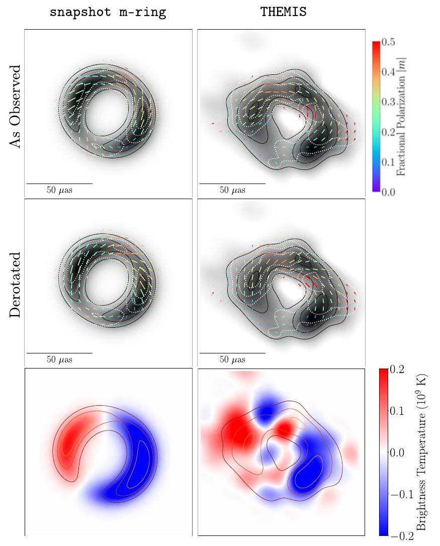
2. ملخص الملاحظات الاستقطابية

في الورقة VII، تم بناء صور استقطابية ثابتة من بيانات Sgr A* EHT المأخوذة في 6 و7 أبريل 2017 بين 226.1 و230.1 غيغاهرتز (انظر القسم 2 من الورقة VII لمزيد من التفاصيل). للتفسير النظري، نتبنى ثمانية قيود ملاحظة مستمدة من الصور التي تم إنشاؤها بواسطة طرق THEMIS وإعادة بناء الحلقة m (لاحظ أن “m” هو رقم الوضع الزاوي هنا، وليس نسبة الاستقطاب؛ انظر جونسون وآخرون 2020). من بين الطرق الأربعة المدرجة في الورقة VII، هذه هي الطرق الوحيدة التي توفر تقديرات بايزي، والتي نحسب منها فترات الثقة. هذه الطرق تتبنى افتراضات مختلفة تمامًا، وفي بعض النواحي، تحدد التباين المكاني والزماني المحتمل. باختصار، طريقة الحلقة m تناسب نموذج حلقة لكل لقطة بشكل مستقل، لكن التباين المكاني المسموح به محدود جدًا من حيث البناء ( للحدة الكلية، للاستقطاب الخطي، و للاستقطاب الدائري). بالمقابل، تحاول THEMIS تحسين صورة ثابتة واحدة تتماشى مع البيانات الكاملة على مر الزمن، مع ميزانية ضوضاء تُعزى إلى التباين الزمني. على الرغم من الفروق الكبيرة بين هذه النماذج، فإنها تستعيد كميات الصورة الرئيسية بدقة مماثلة في اختبارات البيانات الاصطناعية وتصل إلى ملاحظات متسقة إلى حد كبير (الورقة VII).
طوال هذا العمل، يمثل قياس الدوران الكبير والمتغير الزمني (RM) لـ Sgr A* عدم يقين منهجي كبير. يُعرف بأنه ، حيث هو زاوية موضع المتجه الكهربائي (EVPA)، قد ينشأ RM لـ Sgr A* من دوران فاراداي الداخلي إلى المنطقة المنبعثة، أو شاشة خارجية، أو تغييرات في البلازما التي تم استكشافها كدالة لعمق الضوء، أو مجموعة من هذه التأثيرات. من خلال فحص منحنيات الضوء المستقطبة لنفس اليومين كما في ملاحظات EHT لدينا، توصل ويلغوس وآخرون (2024) إلى . نحتفظ بمناقشة مطولة حول RM لـ Sgr A* في كل من الملاحظات والنظرية في الملحق C. باختصار، فإن نسبة RM
الجدول 1
قيود استقطابية مستمدة من إعادة البناء الثابت لـ Sgr A*
قابل للملاحظة حلقة m THEMIS مجتمعة
(%) (2.0، 3.1) (6.5، 7.3) (2.0، 7.3)
(-0.7، 0.12) (-0.7، 0.12)
(1.4، 1.8) (2.7، 5.5) (0.0، 5.5)
(0.11، 0.14) (0.10، 0.13) (0.10، 0.14)
(0.20، 0.24) (0.14، 0.17) (0.14، 0.24)
(درجة) (كما لوحظ)
(درجة) (RM المعكوس) (-168، -108) (-151، -85) (-168، -85)
(1.5، 2.1) (1.1، 1.6) (1.1، 2.1)
ملاحظة. توفر هاتان الطريقتان كل منهما تقديرات، منها يتم اقتباس مناطق الثقة. كقيود على نماذجنا، نتبنى بحذر الحد الأدنى والحد الأقصى من هذه مناطق الثقة من كلا الطريقتين مجتمعتين (العمود الأيمن)، باستثناء ، الذي يُعتبر حدًا أعلى. تفترض المعكوسة أن RM المتوسطة يمكن أن تُعزى إلى شاشة فاراداي خارجية، والتي يتم اعتماد تردد 228.1 غيغاهرتز لها.
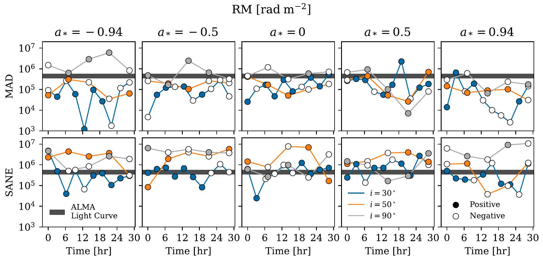
الذي يمكن أن يُعزى إلى شاشة فاراداي خارجية لا يزال غير محلول. وبالتالي، طوال هذا العمل نعتبر إحصائيات الصورة المستعادة مع وبدون عكس RM. يتوافق عكس الصورة مع تفسير حيث يتم إرجاع RM المتوسط الزمني إلى شاشة فاراداي خارجية مستقرة نسبيًا، منفصلة عن نماذجنا، والتي يمكن تصحيحها. الامتناع عن القيام بذلك يتوافق مع تفسير يتم فيه توليد كل RM داخليًا، ضمن نماذجنا. يمكن لمحاكاة GRMHD لدينا إعادة إنتاج التباين اليومي لـ RM، ولكن ليس استقراره في الإشارة (انظر الملحق C).
لكل من هذه الطرق، تم حساب ثمانية قيود ملاحظة تم استكشافها في هذه الورقة، المدرجة في الجدول 1. لتوليد هذه النطاقات، تم إنشاء كمية كبيرة من الصور المتوافقة مع البيانات من توزيع تقديرات كل طريقة. قمنا بحساب القيم القابلة للملاحظة ذات الصلة لكل من هذه الصور ثم استنتجنا مناطق الثقة. لا توفر طريقة الحلقة m قيمًا مستقلة لـ ، والتي يتم تثبيتها على القيمة المتوسطة المستنتجة من ALMA لتحليل الاستقطاب الدائري (انظر الورقة VII). عند دمج الطريقتين للتفسير النظري، نتبنى الحد الأدنى والحد الأقصى من اتحاد كلا مناطق الثقة (انظر الشكل 10 في الورقة VII للتصور).
تشير الكميات و إلى الاستقطاب الخطي والدائري الصافي الذي يمكن استنتاجه من قياس غير محدد مكانيًا للصورة المتوسطة الزمنية. يتم إعطاؤها بواسطة
حيث تشير إلى مجموع كل بكسل . بالنسبة لمنحنيات الضوء المحللة زمنياً، والتي تختلف عن القيم المستنتجة من إعادة بناء صورتنا الثابتة، يجد ويلغوس وآخرون (2022b، 2024) و ، على التوالي، حيث نقتبس المركزية للقيم الملاحظة خلال نفس اليومين من الملاحظة. من المثير للاهتمام، نجد أن طريقة الحلقة m تصل إلى قيم
أقل بكثير من مقارنة بـ THEMIS، والتي قد تُعزى إلى إلغاء زمني لأنماط EVPA المتقلبة.
تتعلق بقية قيودنا بكميات هيكلية، بدءًا من و ، نسبة الاستقطاب الخطي والدائري المتوسطة للصورة. يتم إعطاؤها بواسطة
لاحظ أن هذه الكميات تعتمد على الدقة الفعالة لصورنا. طوال هذا العمل، نقتبس القيم من محاكاة لدينا تتوافق مع كدقة لمحاكاة دقة EHT. نتعامل مع نسبة الاستقطاب الدائري المحلولة كحد أعلى، وبالتالي يمتد النطاق المدمج إلى 0 في الجدول 1. ويرجع ذلك إلى أن الصور المستقطبة دائريًا المقدمة في الورقة VII تظهر اختلافات هيكلية نُعزى إلى الضوضاء (انظر أيضًا تعاون تلسكوب أفق الحدث وآخرون 2023، فيما بعد ورقة M87* IX). بسبب الحجم المطلق المتأصل في تعريف هذه الكمية، فإنه يكون متحيزًا بشكل مرتفع عندما تكون نسبة الإشارة إلى الضوضاء منخفضة جدًا.
تشير أوضاع المعقدة إلى تفكيك فورييه لهيكل الاستقطاب الخطي، حيث تشير إلى عدد المرات التي تدور فيها علامة EVPA مع الزاوية (بالومبو وآخرون 2020). يتم تعريف هذه المعاملات بواسطة
حيث و تشير إلى الإحداثيات القطبية في الصورة و . الوضع غير المتغير بالدوران، ، له اتصالات طبيعية مع ما نعتقد أنه هياكل قرص/نفاث متناظرة زاويًا، وبشكل خاص هندسة المجال المغناطيسي. يشفر اتساعه قوة هذا الوضع، بينما يشفر طوره زاوية الميل ويد اليمين لعلامات EVPA. نلاحظ أقرب إلى من ، مما يتوافق مع أنماط العلامات التي هي أكثر شكلًا دائريًا من شعاعي.
عند النظر في القيود الملاحظة بدون عكس RM، نتبنى ببساطة نطاق كما لوحظ في السماء. عند النظر في القيود الملاحظة مع عكس RM، نقوم بعكس على افتراض أن هناك شاشة فاراداي خارجية بيننا وبين المنطقة المنبعثة التي يمكننا وصفها بواسطة RM المتوسطة على مر الزمن. نظرًا لأن تعتمد على ضعف EVPA، نضيف لذلك إلى ، حيث هو RM المتوسطة الملاحظة في 6 و7 أبريل. وبالتالي، يمتد النطاق على تم تحويله بشكل كبير بواسطة شاشة فاراداي بواسطة تطبيق هذا الإزالة للدوران يؤدي إلى تغيير و توسيع القيد.
تم رسم الصور المتوسطة من التوزيعات الخلفية التي تم إنشاؤها بواسطة كل طريقة في الشكل 1. يتم عرض مجموعتين من الصور المستقطبة خطيًا، تتوافق مع الصور بدون دوران وبتدوير، على التوالي. لاحظ أن التدوير يعكس اتجاه لولب الاستقطاب، مما له آثار مهمة على هيكل التدفق. في الصفين الأولين، يتم عرض الكثافة الكلية بتدرج الرمادي، مع رسم خطوط الكنتور عند ، ، و من ذروة السطوع. تتكرر هذه الخطوط في الصف السفلي. في الصفين العلوي والوسيط،
الشكل 1. صور مستقطبة لـ Sgr A* المستخدمة للتفسير الفيزيائي في هذا العمل. تم تضمين طريقتين من الورقة السابعة، حلقة الصورة اللحظية وTHEMIS. الأعلى والوسط: يتم عرض الكثافة الكلية بتدرج الرمادي، وتوضح علامات الاستقطاب اتجاه الاستقطاب الكهربائي، وطول العلامة يتناسب مع مقدار شدة الاستقطاب الخطي، واللون يشير إلى النسبة المئوية للاستقطاب الخطي. مستويات الخطوط المنقطة تت correspond إلى شدة الاستقطاب الخطي لـ ، و قمة الاستقطاب. تشير مستويات الخطوط الصلبة إلى الكثافة الكلية عند ، و ذروة السطوع. الصف العلوي يعرض صورًا بدون دوران، والصف الأوسط يعرض صورًا مع دوران قدره 46.0 درجة لأخذ دوران فاراداي في الاعتبار. الأسفل: يتم الإشارة إلى الكثافة الكلية في خطوط ملونة صلبة عند ، و ذروة السطوع، و ستوكز يتم الإشارة إلى السطوع في خريطة الألوان المتباينة، حيث يشير الأحمر/الأزرق إلى علامة إيجابية/سلبية.
تشفّر العلامات الملونة الاستقطاب الخطي، حيث يتناسب الطول مع إجمالي شدة الاستقطاب الخطي، ويتناسب اللون مع الاستقطاب النسبي. تُمثل الخطوط البيضاء المتقطعة شدة الاستقطاب الخطي بدلاً من الشدة الكلية.
أخيرًا، نقوم أيضًا بحساب أبسط وضع غير متناظر دورانيًا، ، كاستقصاء لعدم التماثل في الاستقطاب. مرة أخرى، يشفر قوة هذا الوضع، ونستخدم كاستكشاف للتناظر الدوراني. نظرًا لعدم وجود محور واضح (مثل محور الدوران) لتعريفه نحن لا ندرس . نحن أيضًا نمتنع عن حساب الترتيبات العليا الأوضاع، التي من المرجح أن تكون حساسة لتقلبات الضوضاء على نطاق أصغر.

3. النماذج التحليلية

كما تم مناقشته في القسم السابق، فإن الصورة المستقطبة خطيًا لـ Sgr A* تظهر ثلاث ميزات بارزة:
  1. لديها نسبة استقطاب كبيرة محسوبة من ، مع ذروة ، أعلى بكثير من M87*.
  2. هيكل الاستقطاب الخطي منظم للغاية.
  3. تظهر البنية المرتبة درجة عالية من التناظر الدوراني، الذي يبدو أنه يلتف نحو الداخل مع
الشكل 2. مساحة المعلمات المسموح بها في كثافة عدد الإلكترونات ) ودرجة حرارة الإلكترون غير البعدية ( ) لنموذج المنطقة الواحدة الموصوف في القسم 3.1. تتوافق الألواح مع قيم مختلفة مفترضة للبلازما نحن نطلب أن تكون كثافة التدفق الكلي (المنطقة الرمادية) وعمق البصريات (المنطقة الخضراء). يتم عرض شدة الحقول المغناطيسية المقابلة كخطوط حمراء منقطة. باللون الأزرق، نرسم المنطقة السميكة لفاراداي، على عكس M87*، نجد أن النموذج رقيق فارياد في أي مكان يوجد فيه تقاطع بين قيودنا الاثنين.
الاتجاه المعاكس لعقارب الساعة بعد التدوير بواسطة RM الظاهر، أو في اتجاه عقارب الساعة دون التدوير.
قبل استكشاف نماذج GRMHD الأكثر اكتمالاً من الناحية الفيزيائية، نوضح أن كل من هذه الميزات يمكن فهمها في سياق نماذج تحليلية بسيطة.

3.1. نمذجة منطقة واحدة

نستخدم الافتراضات الأساسية الموصوفة في الورقة الخامسة التي تفيد بأن Sgr A* هو ثقب أسود يتراكم عليه المادة مع نسبة إيدينغتون صغيرة للغاية ونتبع الورقة الثامنة الخاصة بـ M87* لتضمين الاستقطاب. هذا النموذج المستقطب ذو المنطقة الواحدة يثبت صحة النماذج العددية الأكثر تعقيدًا المعروضة لاحقًا في هذه الورقة ويقدم تفسيرًا طبيعيًا لنسبة الاستقطاب العالية لـ Sgr A* مقارنة بـ M87*.
نحن نمذج تدفق التراكم حول كرات متجانسة من البلازما ذات نصف قطر ، حيث ، مقارنة بالحجم الملحوظ لـ عند 230 جيجاهرتز (الأوراق III و IV)، مع حقل مغناطيسي موحد موجه في اتجاه مرجعي الميل بالنسبة لخط الرؤية. تعتمد نتائج نموذجنا ذو المنطقة الواحدة بشكل ضعيف فقط على اتجاه المجال. لاحظ أن سرعة البلازما والانزياح الجاذبي مهملان.
في الورقة الخامسة، افترضنا أن البلازما رقيقة بصريًا، ونسبة درجة حرارة الأيونات إلى الإلكترونات هي 3، وأن الأيونات تحت الفيرالية بعامل 3، والبلازما اعتماد قيود التدفق الملاحظ (ويلغوس وآخرون 2022أ)، حصلنا على الحل الذاتي المتسق و باستخدام هذا الحل، يمكننا تقدير قوة دوران فاراداي عند 230 جيجاهرتز مع العمق البصري لدوران فاراداي. :
أين هو معامل دوران فاراداي (على سبيل المثال، جونز وهاردي 1979). بالمقابل، توصلت نماذج مماثلة إلى لـ M87* (ورقة M87* الثامنة). القيمة المستنتجة لـ Sgr A* تشير إلى أن دوران فاراداي الداخلي
قد لا تكون قابلة للتجاهل (انظر أيضًا ويلغس وآخرون 2024)، لكنها قد لا تؤدي بالضرورة إلى إزالة استقطاب كبيرة.
من خلال تضمين تأثيرات العمق البصري واستخدام انبعاث وتوصيل السنكروترون المستقطب وفقًا لدكستر (2016)، نقوم بتخفيف بعض الافتراضات، مثل نسب درجات حرارة الأيونات والإلكترونات وعامل الفيريل، ونرسم مساحة المعلمات المسموح بها كما في ورقة M87* الثامنة. على وجه التحديد،
  1. نحن نخفف قيود التدفق إلى لتضمين تأثير التباين؛ و
  2. نحن نحتاج إلى نفس الافتراض أن رقيق بصريًا، أي، .
المتطلبات المذكورة أعلاه محددة بالمناطق الرمادية والخضراء في الشكل 2، على التوالي. تُظهر خطوط الكنتور المنقطة الحمراء شدة الحقل المغناطيسي، وتفترض الألواح المختلفة بلازما مختلفة. . باللون الأزرق، نرسم الخط المحيط الذي يتوافق مع ، حيث يصبح الاستقطاب الداخلي لفاراداي أكثر أهمية. على عكس M87* (انظر الشكل 2 من ورقة M87* VIII)، نجد أن المناطق التي يتم فيها تلبية قيود التدفق الكلي والقيود الشفافة بصريًا تحدث فقط في مناطق رقيقة لفاراداي من فضاء المعلمات. نلاحظ أن هذا يتوافق مع قياسات RM متعددة الترددات التي تقترح (ويلغوس وآخرون 2024). مرة أخرى، هذا يكفي لتدوير نمط EVPA بشكل ملحوظ، لكنه ليس كافيًا للتسبب في إزالة الاستقطاب بشكل كبير.
باختصار، تتطلب قيود التدفق الكلي وعمق البصريات لـ Sgr A* عمق فاراداي صغير، مما يفسر القيم الكبيرة المستنتجة لـ .

3.2. الاستقطاب المنظم: الحقول المنظمة

لأن إزالة الاستقطاب الشعاعي يمكن أن تقلل فقط من الكسر الاستقطابي الملحوظ، فإن قياسات الاستقطاب الخطي على مقاييس زاوية مختلفة توفر معلومات حول درجة النظام في الاستقطاب الأساسي. من الناحية النظرية، قد يكون من الممكن أن يكون المجال المغناطيسي الأساسي متشابكًا بشكل كبير على مقاييس أصغر بكثير من الشعاع. ومع ذلك، فإن مجموعة من غير المحلولة ( ) وبدقة EHT تقيس قياسات الاستقطاب الخطي درجة النظام في نمط الاستقطاب الحقيقي الأساسي على
الشكل 3. مجموعة غير محلولة ( ) وبدقة EHT ( قياسات الاستقطاب الخطي (عند كقياس) يقيّد درجة النظام في صورة الاستقطاب الأساسية. في هذا المثال التخطيطي، يحتوي حلقة m المستقطبة على استقطاب صافي ثابت، (المشار إليه بالخط المنقط الأسود)، جنبًا إلى جنب مع وضع واحد مستقطب بقوة في ترتيب أعلى، ، الذي يتحكم في درجة الفوضى. للقيم الصغيرة من ، الصورة الناتجة مرتبة جداً، مع يتجاوز القيمة التي لاحظناها لـ Sgr A* (المشار إليها بالشريط الأصفر العلوي). بالنسبة للقيم الكبيرة لـ ، الصورة الناتجة غير مرتبة للغاية، حيث أن استقطاب الشعاع يقضي على هيكل الصورة المستقطب بشدة. في هذا المثال، يجب أن تكون المجالات مرتبة بشكل كبير لتكون متوافقة مع ملاحظاتنا عن ، مع هيكل قطبي متماسك على مقاييس الـ وضع، يتوافق مع مقاييس الزاوية لـ .
مقاييس أصغر من حجم شعاعنا، مما يمنع وجود اضطراب غير محدد مكانيًا بشكل كبير.
كنموذج لعبة بسيط، قمنا بتحليل حلقة دائرية رقيقة مع استقطاب محصور في وضعين فوريير أزيموثيين، تم تمييزهما بمؤشر أولاً، نضيف ثابتاً ( وضع يحدد . نحن نثبت سعة هذا الوضع لتكون 0.07 لتتناسب مع الملاحظات غير المحلولة لـ . بعد ذلك، نضيف وضعًا ثانيًا مع مؤشر متغير وسعة 0.7، مشابهة لقمة الاستقطاب النسبي المتوقع لإشعاع السينكروترون. من خلال تغيير ، يمكننا تقييم درجة التماسك المسموح بها في استقطاب Sgr A* بشكل تقريبي.
تظهر الشكل 3 الاستقطاب النسبي المحلول بدقة زاوية قدرها كدالة لمؤشر الوضع الثانوي . سيكون لكل من حقل الاستقطاب المنظم تمامًا ( ) وحقل الاستقطاب غير المنظم بشدة ( ) . بالنسبة للأول، لا يوجد تدهور في الشعاع؛ بالنسبة للأخير، فإن تدهور الشعاع يقضي على كل الطاقة المستقطبة على المقياس الصغير، حتى عند دقة EHT. ومن ثم، فإن القيمة العالية لـ بالنسبة لـ التي نلاحظها هي تشخيص قوي للبنية المستقطبة المتماسكة.
كما هو متوقع، فإن القيم الصغيرة لـ تنتج كسور استقطاب محلولة مرتفعة جدًا، بينما القيم الكبيرة لـ تنتج كسور استقطاب محلولة منخفضة جدًا. العديد من التأثيرات التي لم يتم تضمينها في هذا النموذج البسيط يمكن أن تقلل من الاستقطاب النسبي المحلول – قد تكون سعة بنية الاستقطاب على المقياس الصغير أقل بكثير من الحد الأقصى للسينكروترون (على سبيل المثال، بسبب عمق بصري أو تدهور فاراداي)، قد يكون هناك مزيج من أكثر من اثنين من
الأوضاع، وقد تكون هناك بنية استقطاب شعاعية تسبب تدهور الشعاع. ومن ثم، يوفر هذا المثال حدًا أدنى محافظًا على مقياس البنية المستقطبة المتماسكة. لتكون متسقة مع قياساتنا لـ Sgr A*، نحتاج إلى ، مما يتوافق مع بنية على مقاييس زاوية من كما. هنا ، حيث هو المسافة و هو نصف قطر حلقة الإشعاع التقريبية في Sgr A*. ومن ثم، حتى بدون نمذجة مفصلة، نتوقع أن الاستقطاب الأساسي في Sgr A* منظم للغاية، مع طاقة كبيرة على مقاييس زاوية من أو أكثر. أي أن الكسر الكبير للاستقطاب المحلول يعني ترتيب نسبي لنمط المجال المغناطيسي على مقاييس أقل من حجم الشعاع.

3.3. فك تشفير شكل الاستقطاب

تمكن النماذج شبه التحليلية من التحقيق في تأثيرات معلمات النموذج على الصور بتكلفة حسابية منخفضة. على سبيل المثال، تم استخدام النماذج شبه التحليلية لتدفقات الانجذاب غير الفعالة إشعاعيًا لعقود للحصول على رؤى قابلة للتعامل ولكن مدفوعة جسديًا حول تدفقات الانجذاب (برومايلي وآخرون 2001؛ برودريك وآخرون 2009، 2011، 2014، 2016؛ بو وآخرون 2016؛ بو وبرودريك 2018؛ فينسنت وآخرون 2022). هنا نستكشف نموذجًا بسيطًا جدًا، KerrBAM (أو نمذجة الانجذاب البايزية لكير)، وهو نموذج شبه تحليلي لإشعاع السينكروترون المحيطي، المحوري حول ثقب أسود كير (بالومبو وآخرون 2022). يقوم هذا الإطار النمذجي بإجراء تتبع للأشعة في فضاء كير الزمني لإنتاج صورة نموذجية تفترض حلقة استقطاب مع سرعة سائلة محددة، وهيكل مجال مغناطيسي، وملف إشعاع شعاعي. هنا نستخدم هذا النموذج البسيط لتوضيح تأثيرات الميل والدوران على بنية الصورة المستقطبة.
كنقطة انطلاق، نقوم بمتوسط المجالات المغناطيسية ومجالات السرعة في ثلاث محاكيات KHARMA GRMHD (سيتم مناقشتها في القسم 4) في كل من الزمن والزوايا. نحدد حلقة من الإشعاع مركزة عند نصف قطر ونستخدم قيم سرعة السائل وهيكل المجال المغناطيسي المستخرجة من مستوى GRMHD في هذا نصف القطر. لإعطاء حلقة الإشعاع عرضًا محدودًا بشكل واقعي، يتم توزيع الإشعاع في توزيع غاوسي يمتد تقريبًا ، مع الحفاظ على ثوابت السرعة والمتجهات المغناطيسية. مع هذه القيم، يتمكن KerrBAM من التقاط تأثيرات الإشعاع، وسحب الإطار، والتكبير على الصورة الناتجة. لاحظ أن هذا النموذج يستبعد المساهمة المحتملة للإشعاع من المستوى الأوسط (على سبيل المثال، فالك وآخرون 1993؛ ماركوف وآخرون 2007).
لثلاثة أقراص مغناطيسية محبوسة (MADs) مع دوران ، و +0.94، نرسم عدة كميات استقطابية مثيرة للاهتمام (العمود الأيسر) وصور نماذجها (الأعمدة التالية) في الشكل 4. جنبًا إلى جنب مع الملاحظات الاستقطابية، نضع قيودنا باللون الرمادي، حيث بالنسبة لـ يتم عرض النطاق بدون دوران RM كمنطقة مخططة. نظرًا لأن هذا النموذج يضع الإشعاع بالضبط عند المستوى الأوسط من خلال البناء، فإن الصور المنتجة عند الميل القريب جدًا من مضللة وبالتالي لا يتم تضمينها. لا تتضمن وصفة KerrBAM تأثيرات فاراداي، حيث يتم نمذجة عمق بصري بشكل تقريبي (في هذه الحالة تطبيق عمق بصري يعبر عن المستوى الأوسط المطبق بشكل موحد على
الشكل 4. العمود الأيسر: كميات الصورة المحددة من نماذج KerrBAM التحليلية المبسطة التي تم تقييمها باستخدام سرعات السوائل المغناطيسية وحقولها من ثلاث دورانات. في هذا الشكل والأشكال التالية، نرسم قيودنا الملاحظات كأشرطة رمادية للرجوع إليها، مع قيود قبل دوران RM المعروضة كمنطقة مخططة. نستخدم هذا النموذج لفهم الاتجاهات الرئيسية، لكننا نحذر من أن نماذج GRMHD الأكثر اكتمالًا جسديًا ضرورية للمقارنة الكمية. الأعمدة الثلاثة اليمنى: صور KerrBAM المقابلة التي تم تقييمها عند أربعة ميول نموذجية.
، و ) ويفترض نموذج إشعاع محدد مسبقًا محصور في المستوى الأوسط، لذا فإن التوافق التفصيلي مع نماذج GRMHD ليس متوقعًا ولا يتحقق. ومع ذلك، فإن هذا النموذج مفيد لفهم عدة اتجاهات نوعية في مكتبة GRMHD الخاصة بنا التي تم إعادة إنتاجها بنجاح.
أولاً، يتم تقليل الاستقطاب الصافي عند الميل المنخفض، حيث يتسبب تناظر تدفق الانجذاب في إلغاء الاستقطاب في الصورة المجمعة. سعة الوضع الثابت الدوراني دائمًا مرتفعة، بسبب التناظر الزاوي الأساسي للنظام. في الوقت نفسه، تكون سعة أقوى عند الميول الأعلى، حيث إنها حساسة للاختلافات في الصورة المستقطبة. أخيرًا، نحن
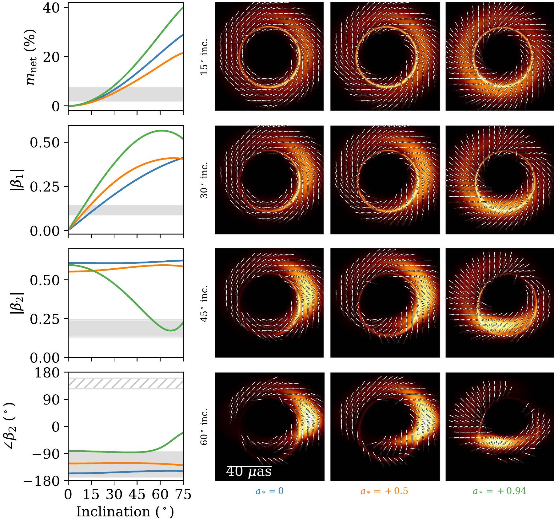
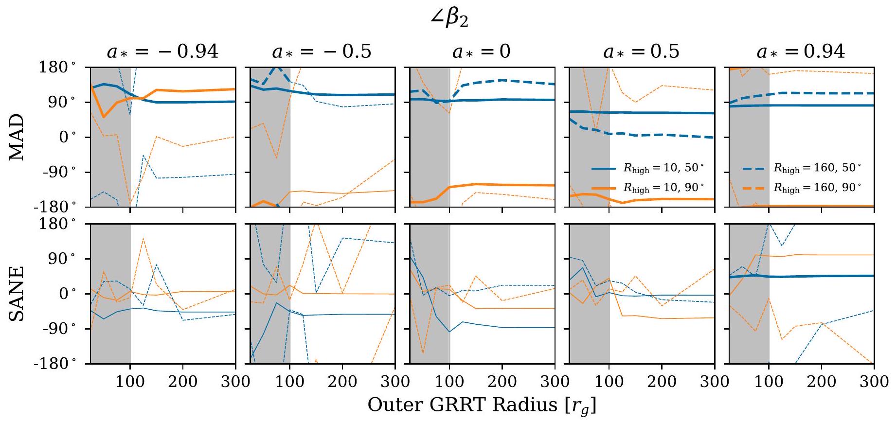
نسلط الضوء على اعتماد الدوران لـ ، والذي يظهر هذا النمذجة أنه مدفوع بتطور هيكل المجال المغناطيسي والسرعة في محاكيات GRMHD بسبب سحب الإطار (انظر أيضًا ريكارتي وآخرون 2022؛ تشايل وآخرون 2023؛ إمامي وآخرون 2023ب). يحتوي نموذج على ، مما يتوافق مع نمط EVPA حلقي للغاية وبالتالي مجالات مغناطيسية شعاعية. في الوقت نفسه، تكتسب نماذج الدوران الأعلى بسبب هياكل EVPA الحلزونية الأكثر. من المثير للاهتمام أن تظل مستقرة بشكل ملحوظ مع الميل، على الرغم من أن بنية الصورة العامة تبدو أنها تتطور بشكل كبير بالعين.
تظهر هذه الاستكشافات أن بعض من أبرز الميزات النوعية للصورة المستقطبة يمكن تتبعها
الجدول 2
ملخص لمكتبة محاكاة Sgr A* GRMHD المستخدمة في هذا العمل
الإعداد GRMHD GRRT الوضع الدقة
الحلقة KHARMA IPOLE MAD/SANE 50,000 1000
الحلقة BHAC RAPTOR MAD/SANE 30,000 3333
الحلقة H-AMR IPOLE MAD/SANE 35,000 1000/200
ملاحظة. العمود الأخير هو ، مع إحداثيات متزايدة في نصف القطر، متزايدة في الزاوية القطبية ، و متناسبة مع الطول . يتم إعطاء الأوقات بوحدات من ونصف الأقطار بوحدات من . قد يتم اعتماد إعدادات مختلفة لنماذج MAD مقارنة بنماذج SANE، كما هو موضح بواسطة .
إلى الخصائص الأساسية للسائل وفضاء الزمن (هيكل المجال المغناطيسي والدوران) دون الحاجة إلى استدعاء جوانب أكثر عدم اليقين من نماذج GRMHD مثل دوران فاراداي، ونسبة درجة حرارة الإلكترون إلى الأيون، ودالة توزيع الإلكترون. ومع ذلك، لا تزال الحسابات الأكثر اكتمالًا جسديًا مع محاكيات GRMHD التي تتضمن هذه التأثيرات بشكل ذاتي ضرورية للمقارنة الكمية.

4. نماذج GRMHD

بينما توفر النماذج شبه التحليلية رؤى نوعية وحدس حول تدفقات تراكم الثقوب السوداء، إلا أنها لا تفرض قوانين الحفظ أو تلتقط الظواهر الزمنية مثل الاضطراب والصدمات التي تلعب دورًا حاسمًا في تحديد الهيكل التفصيلي للنظام. وبالتالي، نقوم بإنشاء نماذج مصدر ديناميكية باستخدام محاكاة GRMHD العددية المثالية. يبدو أن تقريب السوائل يتعارض مع حقيقة أن معدل تصادمات كولوم صغير، مما يؤدي إلى مسارات حرة متوسطة تتجاوز حجم النظام، مما يعني أن معالجة كينتيك خالية من التصادمات قد تكون ضرورية (ماهديان وكواترت 1997). ومع ذلك، يمكن أن تنتج عدم استقرار كينتيك عدم تجانسات صغيرة في المجال المغناطيسي التي تنتج فعالية تصادمية من خلال تفاعلات الجسيمات والموجات (كونز وآخرون 2014؛ ريكويلمي وآخرون 2015؛ سيروني ونارين 2015؛ ميران وآخرون 2019). نفترض ضمنيًا أن التأثيرات الإشعاعية مثل التبريد ليست مهمة ديناميكيًا لتطور السائل. هذه الفرضية مدفوعة جيدًا نظرًا لانخفاض معدل التراكم. الذي تكون فيه فترة التبريد الإشعاعي طويلة مقارنة بفترة التراكم (ديبي وآخرون 2012؛ رايان وآخرون 2017؛ تشايل وآخرون 2018؛ بورت وآخرون 2019؛ ولكن انظر أيضًا يون وآخرون 2020).
في الورقة الخامسة، لمقارنة شدة الإشعاع الكلي مع قيود EHT ومتعددة الأطياف، قمنا بإنشاء مجموعة من الصور المستمدة من GRMHD تأخذ عينات من مجموعة من الظروف الأولية والمعلمات لدرجة حرارة الإلكترون ودالة التوزيع. نحن نبسط استكشافنا في هذا العمل، مقيدين أنفسنا بمحاكاة ذات ظروف أولية على شكل حلقة غير مائلة، ودوال توزيع إلكترونية حرارية نسبية (eDFs) تفتقر إلى المساهمات غير الحرارية، ودرجات حرارة إلكترونية محددة عبر Mościbrodzka وآخرون (2016). الوصفة (انظر المعادلة (8) أدناه). يتم تلخيص خصائص محاكاة GRMHD الخاصة بنا في الجدول 2. يتم دمج النقل الإشعاعي ضمن نصف قطر ، مع تجاهل صريح للمواد في المناطق ذات المغناطيسية العالية مع ، حيث يتم حقن كثافة الكتلة بشكل مصطنع للحفاظ على استقرار المحاكاة. نقوم باختبار تأثير اختياراتنا لنصف قطر التكامل الخارجي، قطع، و eDF في الملحقات D-F، على التوالي. بينما تعتبر الانحرافات عن هذه الافتراضات مثيرة للاهتمام و
الجدول 3
ملخص المعلمات التي تم أخذ عينات منها بواسطة مكتبات GRMHD الخاصة بنا
معامل القيم
حالة المجال المغناطيسي مجنون، عاقل
-0.94، -0.5، 0.0، 0.5، 0.94
(درجة) 10، 30، 50، 70، 90، 110، 130، 150، 170
1، 10، 40، 160
قطبية المجال المغناطيسي محاذاة، مقلوب
ملاحظة. نحن نأخذ عينة خشنة من فضاء المعلمات ذو الأبعاد الخمسة. لكل مجموعة من المعلمات ولكل من رموز KHARMA و BHAC، نقوم بتتبع الأشعة لما يعادل 10 ليالٍ من الملاحظات.
من الناحية الجسدية، نؤجل التحقيق الشامل في هذه المواضيع إلى أعمال مستقبلية.
تقوم مكتبة GRMHD الخاصة بنا بأخذ عينات من فضاء معلمات ذو خمسة أبعاد. المعلمة الأولى هي حالة المجال المغناطيسي، إما نموذج MAD (بيسنوفتاي-كوجان ورزمايكين 1976؛ إيغومينشيف وآخرون 2003؛ نارايان وآخرون 2003؛ تشيكهوفسكوي وآخرون 2011) أو نموذج التطور القياسي والعادي (SANE) (دي فيلييرز وآخرون 2003؛ غامي وآخرون 2003؛ نارايان وآخرون 2012؛ سادوسكي وآخرون 2013). تصف هذه النماذج الحالات التي يكون فيها التدفق المغناطيسي الذي يخترق الأفق لمعدل تراكم معين قد تشبع وأصبح ذا أهمية ديناميكية (MAD) أو لا (SANE). الثانية هي دوران الثقب الأسود، الذي نرمز له بـ حيث تشير العلامة السلبية إلى قرص متراجع بالنسبة إلى متجه الدوران. والثالث هو الميل، الذي يأخذ عينات بشكل موحد بدلاً من فقط كما تم التحقيق فيه في الورقة الخامسة، لأن دوران فاراداي وانبعاث الاستقطاب الدائري يكسران التماثل عند اعتبار الاستقطاب. معلمنا الرابع هو الذي يحدد القيمة التقريبية لنسبة درجة حرارة الأيونات إلى الإلكترونات كالبلازما (موستشيبروتسكا وآخرون 2016). بالتحديد،
أين و هي درجات حرارة الأيونات والإلكترونات، على التوالي. بينما كانت الأهمية المحتملة لتبريد الإلكترونات لمصدر M87* تحفز النماذج التي تحتوي على إلكترونات أكثر برودة، هنا نأخذ في الاعتبار فقط بسبب النسبة الأصغر بكثير من إيدينغتون لـ أخيرًا، المعامل الخامس لدينا هو قطبية المجال المغناطيسي بالنسبة إلى متجه الزخم الزاوي للقرص، سواء كانت متوافقة أو معكوسة، مما يؤثر على اتجاه دوران فاراداي ويد الازدواجية للإشعاع المستقطب دائريًا. هذه الدرجة الأخيرة من الحرية تهم فقط في نقل الإشعاع المستقطب وتم تجاهلها في الورقة الخامسة. نحن ننتج مكتبة من الصور لكل مجموعة من هذه المعاملات، كما هو موضح في الجدول 3.
الشكل 5. معرض لمحاكاة متوسطة زمنياً في مكتبتنا. يعرض كل لوح محاكاة متوسطة زمنياً ومشوشة (مع كـ نواة غاوسي بعرض نصف القمة (FWHM) MAD نماذج متراصة عند ثلاث زوايا مختلفة. يعرض اللوح الأول من كل مجموعة الكثافة الكلية والاستقطاب الخطي، بينما يعرض اللوح الثاني من كل مجموعة الكثافة الكلية والاستقطاب الدائري. طول العلامات يحدد كثافة التدفق المستقطب الكلي في بكسل معين، بينما تتدرج ألوانها مع نسبة الاستقطاب. تم تتبع نماذج H-AMR باستخدام الأشعة فقط لمجموعة فرعية من النماذج للمقارنة ولا تستخدم للتقييم.
نحتفظ باستخدام رموز متعددة لتقييم الفروق النظامية العددية. من أجل التسجيل، نقوم بإنشاء مكتبات تمتد ما يعادل حوالي 108 ساعة من الملاحظات الليلية للتركيبات المعلمية المدرجة في الجدول 3 باستخدام مجموعتين من الأكواد: KHARMA (Prather وآخرون 2021) + IPOLE (موشيبروتسكا وغامي 2018) و BHAC (بورت وآخرون 2017؛ أوليفاريس وآخرون 2019) + رابتر (برونزوير وآخرون 2018، 2020)، حيث يتوافق الرمز الأول والثاني في كل زوج مع GRMHD و GRRT، على التوالي. كتحقق إضافي من التناسق، يتم إنشاء مجموعة ثالثة باستخدام H-AMR (ليزكا وآخرون 2022) + IPOLE لمجموعة فرعية من فضاء المعلمات (فقط حقول متوافقة، و ) التي لا نستخدمها للتسجيل.
يتم تهيئة كل محاكاة مع حلقة من الغاز في توازن هيدرو ديناميكي مع زخم زاوي ثابت (فيش بون ومونكريف 1976). يتم إزعاج هذه الحلقات بحقل مغناطيسي ضعيف، قطبي. تختلف المحاكاة في نصف قطرها الابتدائي لأقصى ضغط (من إلى ) ومؤشر الأديباتيك، . تختلف الرموز في اختيارها لـ لأن ينطبق على سائل من الإلكترونات النسبية و ينطبق ذلك على سائل من الأيونات غير النسبية، ولكن يتم تطوير سائل واحد فقط في هذه النماذج. اعتمادًا على حجم الحلقة وتكوين المجال المغناطيسي الأولي، تتطور المحاكاة إلى حالة MAD أو SANE (انظر، على سبيل المثال، وونغ وآخرون 2022).
في الشكل 5، نعرض مجموعة من لقطات GRMHD المتوسطة زمنياً من مكتبتنا، مشوشة إلى دقة EHT باستخدام نواة التمويه الغاوسي مع عرض كامل عند نصف الحد الأقصى (FWHM) من في اللوحة اليسرى من كل مجموعة، نرسم الكثافة الكلية بتدرج الرمادي والاستقطاب الخطي المحلّل كعلامات ملونة. في اللوحة اليمنى من كل مجموعة، نرسم الاستقطاب الدائري من الأزرق إلى
أحمر مع خطوط كثافة إجمالية. كل لوحة مُعَيرة بشكل فردي بحيث تمتد خرائط الألوان من 0 إلى الحد الأقصى على اليسار و على اليمين. كل من هذه النماذج هو MAD محاكاة المجال المتماسك، تم حسابها باستخدام رموز مختلفة كما هو موضح أعلاه.
تظهر الرموز توافقًا من حيث الكثافة الكلية والشكل المستقطب، لكنها تختلف بعض الشيء في درجة الاستقطاب. مع زيادة الميل، تصبح صورة الكثافة الكلية أكثر عدم تماثل بسبب تأثير دوبلر (على سبيل المثال، فالك وآخرون 2000؛ ميديروس وآخرون 2022؛ الورقة الخامسة). وينطبق الشيء نفسه على الاستقطاب، الذي يتأثر أيضًا بتدرج إزالة الاستقطاب بفاراداي (انظر الملحق A.3). يتم تشفير هندسة المجال المغناطيسي كما تم أخذها من خلال الأشعة الضوئية المنحرفة في صورة الاستقطاب الدائري. على وجه الخصوص، تعرض الصور الجانبية في الاستقطاب الدائري انعكاسات في الإشارة على طول كل من المحور الأفقي والرأسي بسبب تقلبات في اتجاه المجال المغناطيسي على خط الرؤية، وتختفي هذه الإشارة مع انخفاض زاوية الرؤية (ريكارت وآخرون 2021؛ تسونيتو وآخرون 2021).

5. تقييم نموذج GRMHD

نقدم منهجية جديدة لتقييم كل من نماذج GRMHD الخاصة بنا باستخدام القيود القطبية الثمانية في الجدول 1. تعمل خطة التقييم الجديدة لدينا على صور GRMHD المتوسطة زمنياً وتحاول استيعاب التباينات بين الأكواد. لاحظ أننا ندرج فقط الكميات المستنتجة من صورنا القطبية في هذه القيود، ولكننا سنناقش المقارنات مع الكثافة الكلية والقيود متعددة الترددات المستمدة في الورقة الخامسة.
  1. أولاً، يتم تقسيم كل سلسلة زمنية من الصور إلى 10 نوافذ، كل منها بمدة 1500 مللي ثانية. داخل كل نافذة، نقوم بإنتاج صورة متوسطة زمنياً عن طريق حساب متوسط كل من معلمات ستوك. ثم، نقوم بتشويش الصورة المتوسطة باستخدام نواة غاوسية بمتوسط عرض كامل (FWHM) من كما وحساب كل من الثمانية المتغيرات القابلة للرصد للتسجيل.
قيود بدون
الشكل 6. القيود القطبية المجمعة على مكتبة نموذج GRMHD باستثناء تفشل النماذج البرتقالية، بينما تنجح النماذج الخضراء في الزاويتين المعطاة والمكملة، وتنجح المناطق الزرقاء فقط مع الزاوية المعطاة أو المكملة كما هو موضح. يتم رسم نماذج SANE في النصف العلوي، بينما يتم رسم نماذج MAD في النصف السفلي. تتوافق الأعمدة المختلفة مع دوران مختلف من -0.94 إلى 0.94. داخل كل شريحة، يتوافق الاتجاه الشعاعي مع واتجاه الزاوية الأفقية يتوافق مع ميل المراقب.
2. لكل مجموعة من المعلمات، نقوم بدمج قيم المتغيرات القابلة للرصد التي تتنبأ بها رموز KHARMA و BHAC. نظرًا لوجود 10 نوافذ ومجموعتين من الرموز، فإن هذا يؤدي إلى 20 عينة مختلفة. من هذه القيم، نحسب الكوانتيلات لكل ملاحظة لالتقاط تباين الوقت.
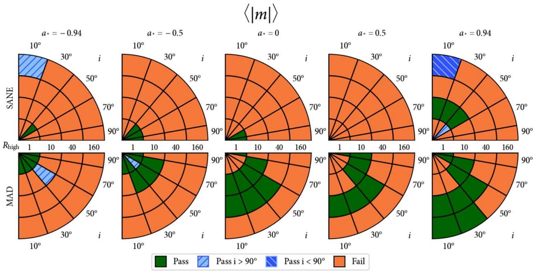
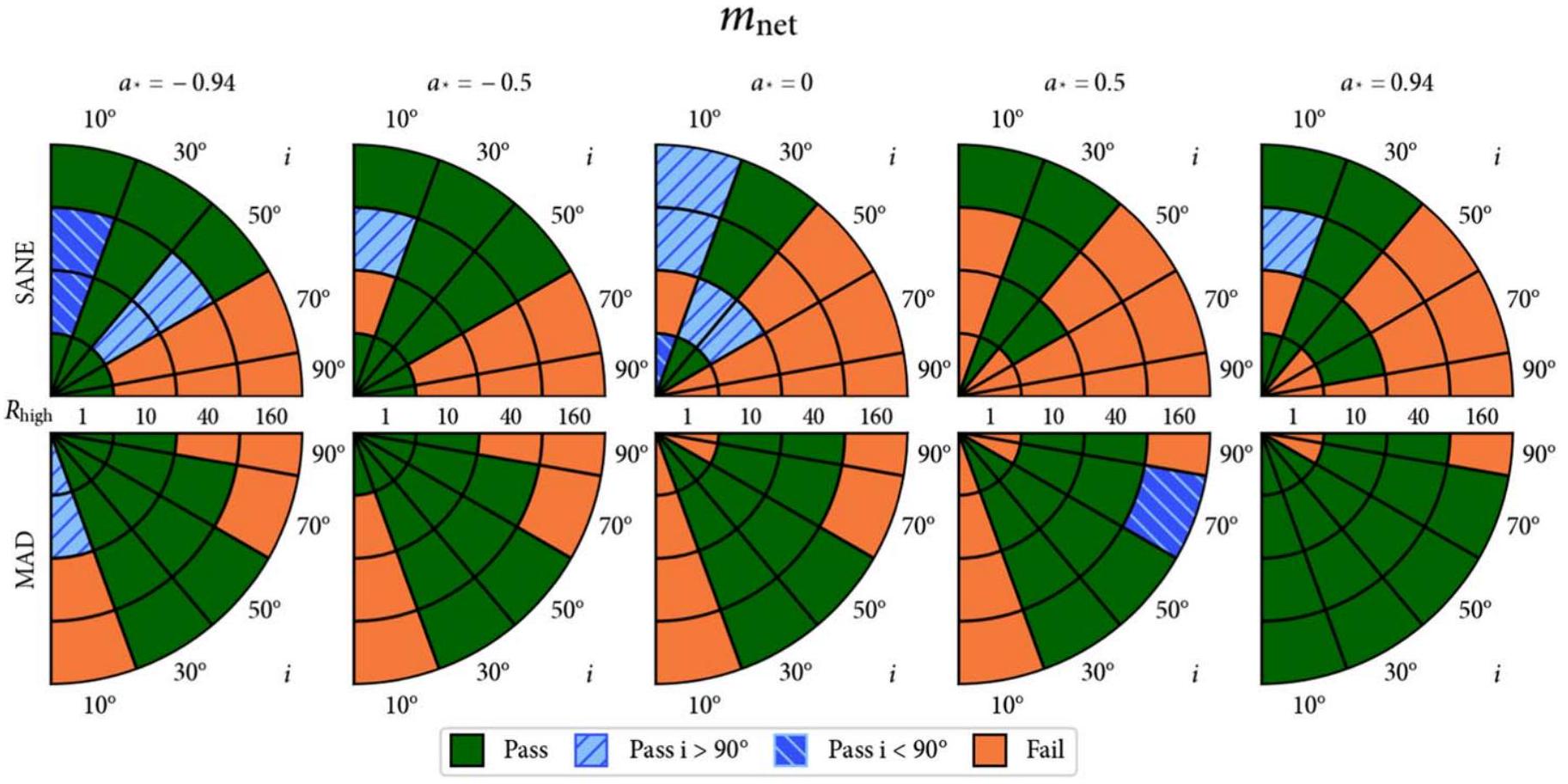
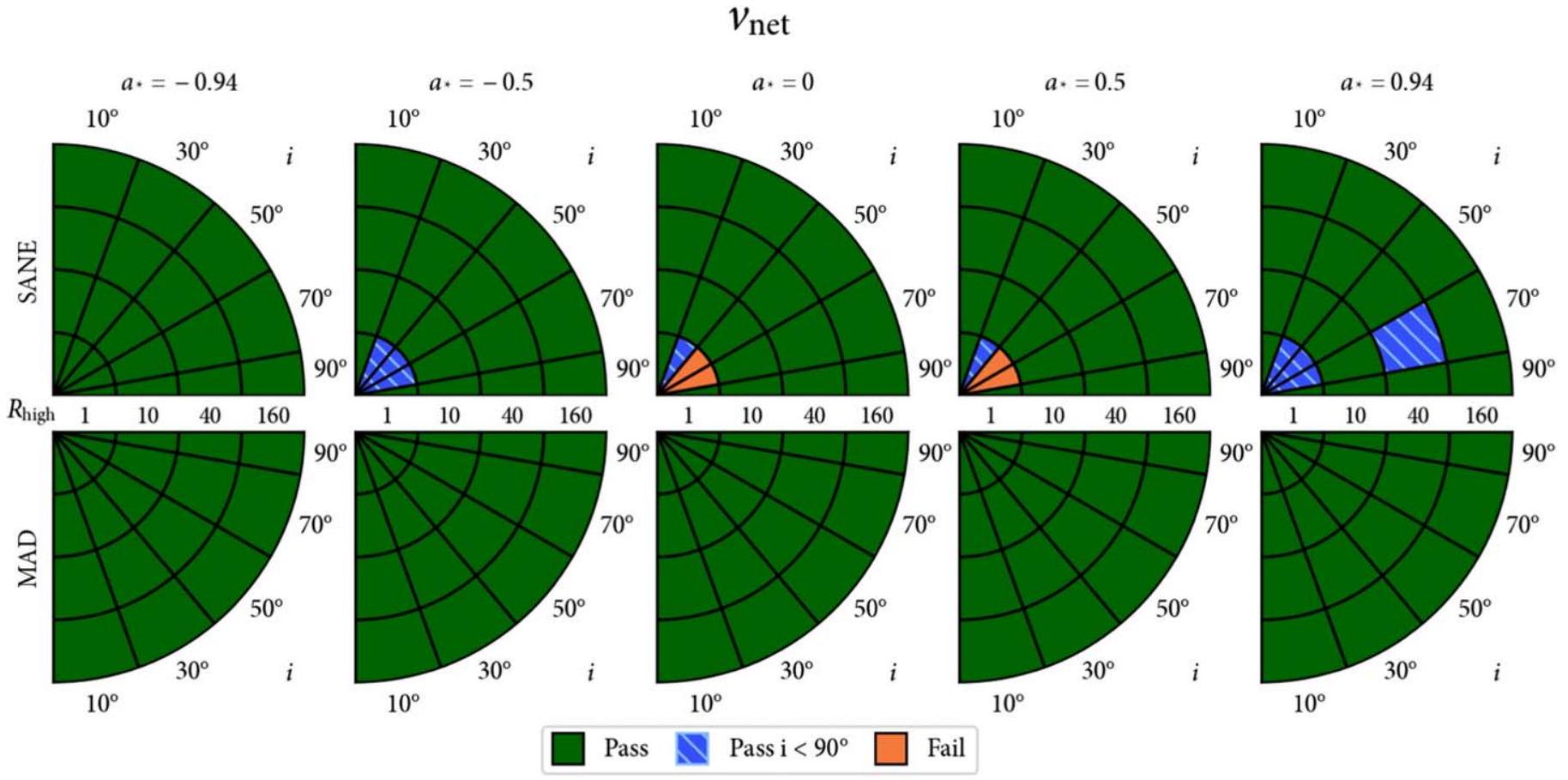
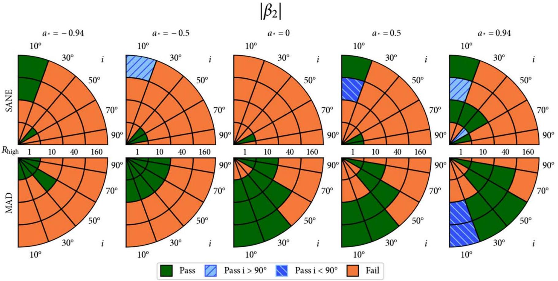
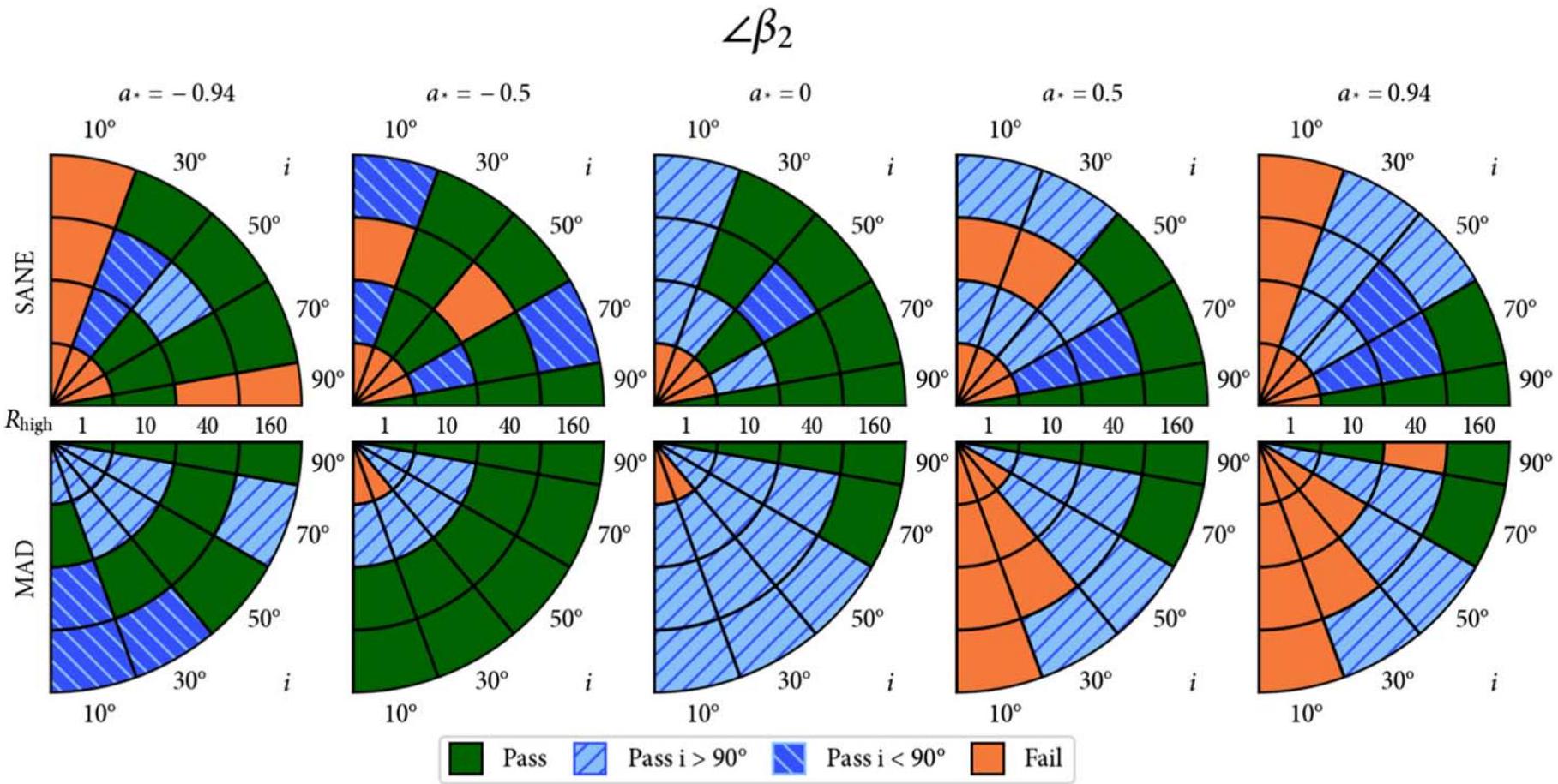
3. ينجح النموذج في تجاوز قيد الملاحظة الفردية إذا كان هناك تداخل بينه وبين منطقة الكوانتيل وتلك الخاصة بالملاحظات. ينجح النموذج في تلبية مجموعة من القيود الملاحظية إذا اجتاز جميع القيود في المجموعة في الوقت نفسه.
أهم الفروق مقارنة بنظام التقييم المستخدم في الورقة الخامسة هي أن هذا النظام الجديد يعمل على الصور المتوسطة زمنياً ويجمع النتائج من عدة أكواد في نطاق نظري واحد. قمنا باختبار إجراء التقييم باستخدام مجموعة محاكاة واحدة في كل مرة. نظرًا لأن درجات حرارة الإلكترونات في نموذج KHARMA تُعطى بشكل منهجي أعلى من تلك الخاصة بنماذج BHAC (انظر الملحق H)، فإن نماذج KHARMA تمرر نماذج ذات أكبر هناك المزيد من الاختلاف بين الرموز لنماذج SANE مقارنة بنماذج MAD. القيود التي يوجد بها أكبر قدر من الاختلاف بين الرمزين هي ، و ، حيث استبعدت محاكاة KHARMA نماذج SANE أكثر من محاكاة BHAC في كل حالة.
كل من القيود الرصدية لها ارتباطات معروفة مع الفيزياء الأساسية. وللاختصار، نؤجل استكشافًا تعليميًا لكيفية تأثير كل من معلماتنا الحرة.
يتم طباعة على الملاحظات في الملحق أ. ندرس كيف يؤثر كل قيد فردي على اختيار النموذج في الملحق ب. هنا نلخص نتائج التقييم على أعلى مستوى، أولاً باستبعاد ثم بما في ذلك إما كما لوحظ أو بعد إجراء دوران RM.

5.1. القيود المستقلة عن إدارة المخاطر

في الشكل 6، نرسم جدول النجاح/الفشل الذي يجمع جميع القيود القطبية، باستثناء . تجمع هذه الرسوم البيانية بين كلا قطبي المجال المغناطيسي، موضحة مرورًا طالما أن أيًا من القطبين يمر. هذه الجداول تختلف قليلاً ولكن ليس بشكل منهجي كدالة لقطبية المجال المغناطيسي.
نجد أن القيد الصارم على هو الأكثر قوة، حيث يقود معظم الاتجاهات الموضحة في هذه الصورة. إنه أكثر تقييدًا لمساحة المعلمات من ، والتي تتطلب نطاقًا أكبر بكثير ( مسموح. الـ تستبعد القيود بعض النماذج الإضافية التي تكون عادةً على الحافة، لكنها لا توفر الكثير من القوة التقييدية الإضافية لأن و مرتبطان. بدون تظهر الشكل 6 عدم وجود تفضيل كبير بين و نماذج.
بينما كانت قيود شدة إجمالي لدينا عمومًا تفضل القيم الأكبر من (بسبب القيود متعددة الأطوال الموجية إلى حد كبير؛ الورقة الخامسة)، تفضل قيودنا الاستقطابية عادةً قيمًا أكثر اعتدالًا. وذلك لأن القيم الأكبر من عادة ما تؤدي إلى أعماق دوران فاراداي الداخلية الأكبر (انظر الملحق A.4)، وهو المحرك الفيزيائي الأكثر أهمية لفقدان الاستقطاب في نماذجنا. ومع ذلك، فإن هناك اتجاهًا مثيرًا للاهتمام فيما يتعلق بالدوران يسمح لأحد أفضل النماذج في الورقة V بالاستمرار في النجاح مع . هذا هو MAD نموذج. تحتوي نماذج MAD ذات الدوران الأكبر على أعماق دوران فاراداي أصغر (انظر
جميع القيود القطبية
الشكل 7. نفس الشكل 6، ولكن مع تضمين القيد على الطور لـ بدون دوران RM. فقط النماذج ذات الحركة المعاكسة لجهة عقارب الساعة ( لا يوجد نموذج يفي بجميع القيود القطبية وقيود الكثافة الكلية المستخدمة في الورقة الخامسة.
الملحق H)، مما يسمح لهم بتمرير قيود للقيم الأكبر من نُشير إلى الملحق ب للحصول على تحليل أكثر تفصيلاً لكل قيد تم النظر فيه بشكل فردي.

5.2. القيود بما في ذلك بدون إزالة دوران RM

أولاً، نناقش الـ القيود إذا لم يتم تنفيذ إعادة دوران RM. من الممكن أن يُعزى RM بالكامل إلى دوران فاراداي الذي تم التقاطه داخل مجال محاكاة لدينا. نماذج GRMHD قادرة على إنتاج الحجم الصحيح لـ RM من دوران فاراداي على مقاييس أفق الحدث، لكنها تميل إلى إنتاج تقلبات في إشارة RM غير متسقة مع عقود من ملاحظات Sgr A* التي تنتج قيم سلبية لـ RM (Ricarte et al. 2020؛ M87* Paper VII؛ Wielgus et al. 2024). ومع ذلك، من الممكن أن تكون هذه المشكلة مرتبطة بالاختلاف الزائد في نماذجنا التي تم تحديدها في الورقة V. نحن نناقش المزيد من الشكوك المحيطة بتفسيرنا لـ RM في الملحق C.
إذا تم نسب RM بالكامل إلى دوران فاراداي الداخلي، فإن قيدنا على يمتد عبر الفترة إضافة هذا القيد إلى الشكل 6 ينتج الشكل 7. اختيار لـ ينشأ ذلك لأن اتجاه لولب الاستقطاب هو عكس اتجاه المجال المغناطيسي، الذي يرث اتجاه الغاز المتدفق والغاز المنبعث (انظر القسم 3.3 والملحق A.3). وهذا يتوافق مع الحركة عكس عقارب الساعة، مما يتعارض مع تفسيرات النقاط الساخنة للومضات المستقطبة سواء في الأشعة تحت الحمراء القريبة (NIR؛ تعاون GRAVITY وآخرون 2018، 2020a، 2020b) أو في المليمتر الفرعي (فوس وآخرون 2022؛ ويلغوس وآخرون 2022b). أي أن التوافق مع الحركة مع عقارب الساعة سيتطلب إذا افترضنا أن تتبع خطوط المجال المغناطيسي مع تدفق بوانتينغ الخارج (تشايل وآخرون 2023)، وهو ما لا يتوافق مع الشكل القطبي الخطي كما لوحظ في السماء.
بدون دوران RM، لا يمكن لأي نموذج أن يمر في الوقت نفسه بجميع قيود الكثافة الكلية والقيود القطبية. وذلك لأن نموذج الرهان الأفضل في الورقة V ينتج نمط EVPA يكون شعاعياً جداً (انظر الملحق A.2). جميع النماذج التي تتجاوز قيود الاستقطاب لدينا في الشكل 7 تفشل في تلبية قيود متعددة على الكثافة الكلية. على وجه الخصوص، جميع النماذج الثمانية الموضحة في الشكل 7 تنتج تدفقاً زائداً في الأشعة تحت الحمراء لتتناسب مع الملاحظات، وجميعها باستثناء نموذج SANE في تنتج بشكل مفرط تدفق الأشعة السينية (الورقة الخامسة). كلاهما فشل خطير، حيث أن كل من تدفقات الأشعة تحت الحمراء والأشعة السينية المقدرة بواسطة نماذجنا هي حدود دنيا بسبب نقص الإلكترونات غير الحرارية وحجم المحاكاة الصغير بالنسبة لمنطقة انبعاث الأشعة السينية. خمسة من النماذج تفشل أيضًا في مطابقة الحجم المرصود وتدفق المصدر عند 86 غيغاهرتز (إيساoun وآخرون 2019). جميع هذه النماذج تفشل أيضًا في تلبية شرط هيكلي واحد على الأقل من حيث الكثافة الكلية (اختبارات شكل الحلقة وارتفاع الرؤية في الورقة الخامسة). في الختام، لا يمكننا العثور على نموذج متوافق لـ Sgr A* دون تدوير RM.

5.3. القيود بما في ذلك مع إزالة RM

بدلاً من ذلك، في هذا القسم نفسر متوسط RM كدرع فاراداي خارجي، مما يحفز عملية التدوير. كما تم مناقشته في القسم 2، يعتمد على ضعف RM، والذي له قيمة متوسطة من تم الحصول عليه. وهذا قد يؤدي إلى تحول في من إذا تم تفسير هذا RM كدرع فاراداي خارجي. في هذه الصورة، يفسر الدرع الخارجي المستقر نسبيًا الإشارة الثابتة لـ RM التي تم ملاحظتها لعقود (ومع ذلك مع تباين على مستوى ثم، مكون إضافي على مقاييس أفق الحدث، والذي تم تضمينه بالفعل بشكل ذاتي في نماذجنا، يفسر التغير الزمني دون الساعة.
إذا تم اعتبار متوسط RM ليوم معين بالكامل على أنه ناتج عن شاشة خارجية، فإن قيودنا على يمتد ( ).
جميع القيود القطبية
الشكل 8. نفس الشكل 6، ولكن مع تضمين القيد على طور مع دوران RM. فقط النماذج ذات الحركة في اتجاه عقارب الساعة ( ) تمر. نموذج أفضل من الورقة V يمر بجميع قيود الكثافة الكلية والقيود القطبية: MAD متماسك.
إضافة هذا القيد إلى الشكل 6 ينتج الشكل 8. يتطلب إجراء هذا القطع زوايا ميل ، والتي تتوافق مع الحركة في اتجاه عقارب الساعة في السماء، والتي تتفق الآن مع النماذج المذكورة سابقًا للومضات المستقطبة في NIR وتحت المليمتر.
مع دوران RM، يمر أحد أفضل النماذج من تحليل الكثافة الكلية بجميع قيود الكثافة الكلية والقيود القطبية المطبقة. هذا هو نموذج MAD ، متماسك. كان النموذج الثاني الأفضل من الورقة V لديه ومعلمات متطابقة بخلاف ذلك. هذا النموذج الثاني يمر بجميع القيود باستثناء ، والتي ينتج عنها أقل من المطلوب بنسبة . لكي يمر نموذج الأفضل، يجب أن يأتي على الأقل من RM المقاسة من شاشة خارجية. من الجدير بالذكر أن النموذج الأفضل يفشل إذا تم تفسير RM الأصغر المقاسة عند 86 غيغاهرتز قبل بضعة أيام، (ويلغوس وآخرون 2024)، بدلاً من ذلك على أنه الشاشة الخارجية.
في الشكل 9، نعرض النموذج الأفضل (BHAC المعروض) الذي ينجو مع دوران RM. في العمودين الأيسر، نرسم صورته القطبية الكاملة بأسلوب الشكل 5. لا يتم تطبيق أي تشويش في العمود الأيسر، ويتم تطبيق كـ FWHM نواة غاوسية على الصورة في العمود الثاني لتقريب دقة EHT. يتميز هذا النموذج بحلقة فوتون ساطعة، وفي صورتنا بدون تشويش، نتجنب خطوط كثافة الكثافة الكلية من خريطة الاستقطاب الدائري لكشف عكس إشارة حلقة الفوتون (المناقشة في موشيبروتسكا وآخرون 2021؛ ريكارتي وآخرون 2021).
على اليمين، ننتج خريطة لكثافة الانبعاث المرصود في محاكاة KHARMA المعادلة (باستخدام إحداثيات كير-شيلد). يتم تطبيع خريطة كثافة الانبعاث بحيث تكون قيمتها القصوى واحدة، ويتم تصورها في مقياس لوغاريتمي مع 3 أوامر من الحجم في النطاق الديناميكي. يتم الإشارة إلى خط نظرنا بواسطة السهم الأخضر، وتحيط كونتور بيضاء بالانبعاث الكلي. يكشف هذا أنه بينما يكون الانبعاث في ذروته عند نصف قطر صغير بالقرب من مستوى القرص، فإن جزءًا كبيرًا من الانبعاث ينشأ من
منطقة قمع نفاثة أكثر انتشارًا. حساب نصف قطر الانبعاث المميز الموزون بالانبعاث ، حيث هو كثافة الانبعاث و هو نصف القطر في الإحداثيات الأسطوانية، نجد . نلاحظ أن خياراتنا لتضمين وظائف توزيع الإلكترونات الحرارية فقط واستبعاد المناطق التي تحتوي على في هذا العمل تقلل من المساهمة المحتملة لنفاثة في الانبعاث الكلي (على سبيل المثال، الشكل 12 من فروم وآخرون 2022). قد تكون مكون نفاث كبير ضروريًا لإعادة إنتاج مؤشر الطيف المسطح عند هذه الترددات (فالك وآخرون 1993؛ فالك وماركوف 2000؛ موشيبروتسكا وفالك 2013).
عند نصف قطر ، نحسب متوسط قوة المجال المغناطيسي الموزون بالكتلة ، حيث يتوافق النطاق المذكور هنا مع القيم من النسبة المئوية 16 إلى 84 التي تم الحصول عليها في سلسلة الزمن. تتفق هذه القيمة بشكل معقول مع نموذج المنطقة الواحدة الذي تم مناقشته في القسم 3.1، على الرغم من أننا نلاحظ أن هذه القيمة تتطور بشكل كبير مع نصف القطر، حيث تصل إلى عند نصف قطر و عند الأفق.
ينتج هذا النموذج قوة تدفق قدرها ولديه معدل تراكم قدره . يتمتع هذا النموذج بكفاءة نفاثة كبيرة جدًا تبلغ حوالي مدعومًا بآلية بلاندفورد وزنايك (1977). ومع ذلك، على الرغم من كفاءته، فإن قوة النفاثة ليست عالية بما يكفي لتوقع تأثيرات عالمية على تطور مجرتنا (على سبيل المثال، سو وآخرون 2021).

6. المناقشة والاستنتاج

تظهر الصورة المستقطبة الأولى لـ Sgr A* على مقاييس أفق الحدث نسبة استقطاب عالية تم حلها قدرها ونمط EVPA منظم ومتماثل دوراني. من خلال الحجج شبه التحليلية والمقارنات مع محاكاة GRMHD، نصل إلى الاستنتاجات التالية:
  1. تشير نسبة الاستقطاب العالية التي تم حلها إلى أن المجال المغناطيسي على مقاييس أفق الحدث لا يمكن أن يكون متشابكًا جدًا على مقاييس أصغر من الشعاع، ولا يمكن أن تضيف دوران فاراداي
الشكل 9. النموذج الأفضل لـ Sgr A*: MAD متماسك. في العمودين الأيسر، نرسم صورته المحاكاة بأسلوب الشكل 5. الصور في العمود الأول غير مشوشة، والصور في العمود الثاني مشوشة مع غاوسي ب FWHM قدره كما، تقارب دقة EHT. في اللوحة اليمنى، نقدم خريطة للانبعاث في هذا النموذج. تحيط الكونتور البيضاء بالانبعاث الكلي، والدائرة البيضاء المنقطة تحدد الأفق، والسهم الأخضر يشير إلى زاوية رؤيتنا. بينما يصل الانبعاث إلى ذروته بالقرب من الثقب الأسود في المستوى، فإن جزءًا كبيرًا من الانبعاث ينشأ من منطقة أكثر انتشارًا، بما في ذلك غلاف النفاثة.
يضيف الدوران الكثير من الفوضى الإضافية إلى هيكل EVPA. يمكن أن يُعزى التباين بين نسب الاستقطاب الخطية المحلولة مكانيًا ( ) وغير المحلولة ( ) إلى الإلغاءات بسبب الطبيعة المتماثلة للصورة.
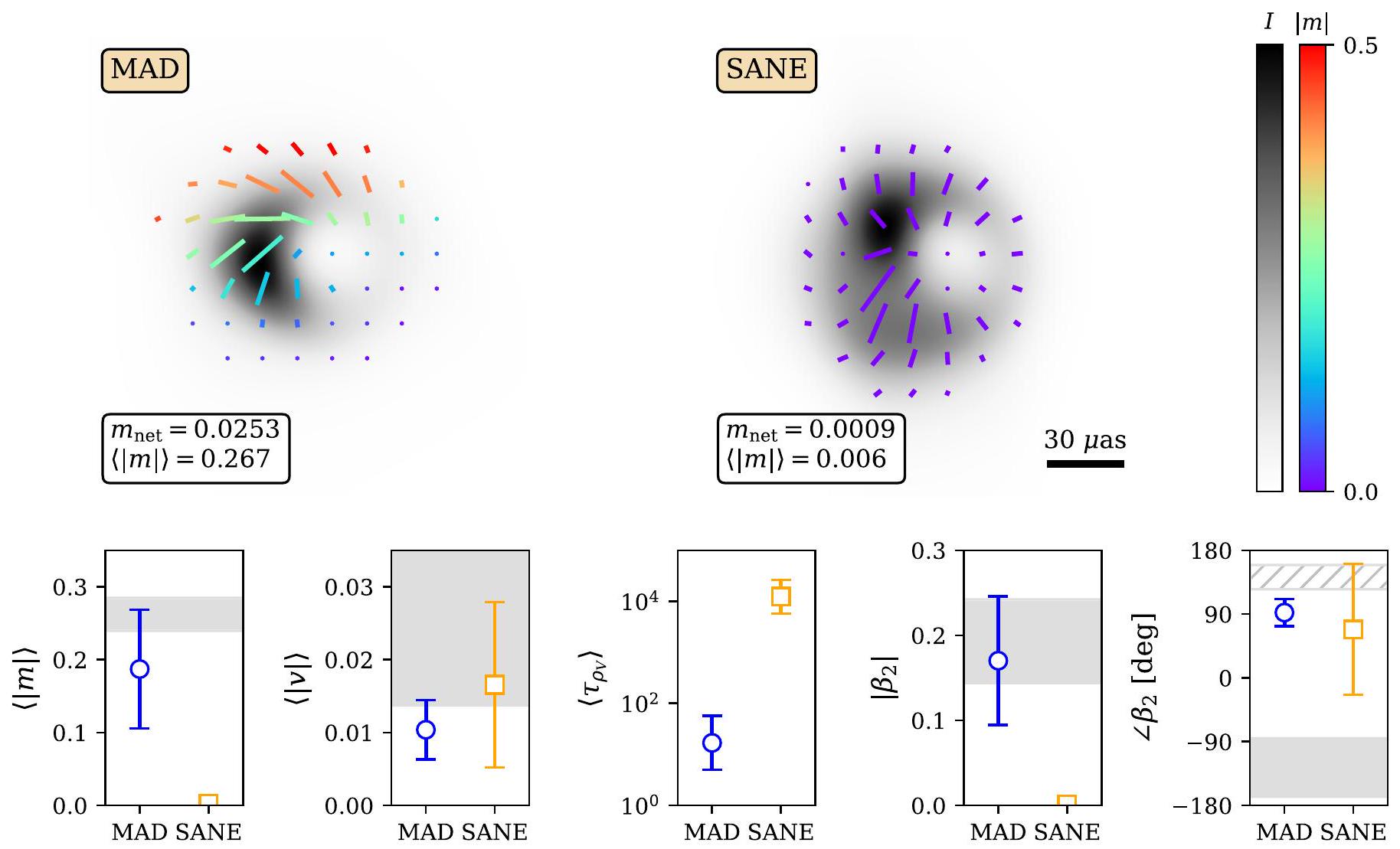
2. مدفوعة في الغالب بنسبة الاستقطاب المحلولة مكانيًا، تفضل قيودنا بشدة نماذج MAD على نظرائها SANE، كما في ورقة M87* VIII.
3. إذا اعتمدنا على دوران فاراداي الداخلي لإنتاج RM المرصود ولم نقم بإجراء دوران، فلا يوجد نموذج يمر بجميع قيود الكثافة الكلية والقيود القطبية.
4. من ناحية أخرى، إذا افترضنا أن RM يمكن أن يُعزى إلى شاشة خارجية وقمنا بدوران نمط EVPA، فإننا نجد نموذجًا واحدًا يمر بجميع قيود الكثافة الكلية والقيود القطبية المطبقة: MAD متماسك.
بينما حققت محاكاة GRMHD المثالية لدينا التي تحتوي فقط على توزيعات الإلكترونات الحرارية نجاحًا ملحوظًا في إعادة إنتاج العديد من الكميات المرصودة لـ Sgr A*، إلا أنها لا تزال تحتوي على العديد من العيوب المعروفة. معظم هذه النماذج تفرط في تقدير التغير الزمني، بما في ذلك النموذج الأفضل (الورقة V)، ونحذر من أن القيم المستنتجة من نموذجنا الأفضل لا ينبغي تفسيرها على أنها قياسات. تشمل المناطق المعروفة التي يمكن تحسين هذه المحاكاة فيها ما يلي:
  1. الظروف الأولية: جميع محاكياتنا تبدأ بتوريات إما متوافقة تمامًا أو متعارضة مع محور الزخم الزاوي للثقب الأسود. تتمتع المحاكيات التي تغذي الثقب الأسود عبر الرياح النجمية بخصائص تغير مختلفة (مورشيكوفا وآخرون 2022) ويمكن أن تتنبأ بشكل ذاتي بشاشة فاراداي خارجية (ريسلي وآخرون 2019، 2023).
نماذج الأقراص المائلة (على سبيل المثال، فراجيل وآخرون 2007؛ ليسكا وآخرون 2018؛ تشاترجي وآخرون 2020) قد تؤدي إلى خصائص دوران فاراداي مختلفة بسبب هندستها عند نصف قطر كبير.
2. الديناميكا الحرارية للإلكترونات: الوصفة التي اعتمدناها من موشيبروتسكا وآخرون (2016) لتحديد درجة حرارة الإلكترون تلتقط بشكل عام الاتجاهات التي تُرى في المحاكاة الحركية التي تُعالج بشكل صريح التسخين والتبريد (على سبيل المثال، تشايل وآخرون 2018؛ ديكستر وآخرون 2020؛ ميزونو وآخرون 2021؛ ديهينغيا وآخرون 2023) ولكنها لا تعيد إنتاجها بتفاصيل كثيرة. بشكل عام، يُعتقد أن هناك مساهمة غير حرارية في وظيفة توزيع الإلكترونات ضرورية لإعادة إنتاج توزيع الطاقة الطيفية (أوزيل وآخرون 2000؛ ماركوف وآخرون 2001؛ دافيلار وآخرون 2018) ويتم التنبؤ بها بشكل طبيعي من خلال محاكاة الجسيمات في الخلايا (كونز وآخرون 2016؛ بال وآخرون 2018). يمكن أن يكون لوظائف توزيع الإلكترونات غير الحرارية تأثيرات كبيرة على كل من الكثافة الكلية والخصائص المستقطبة (على سبيل المثال، ماركوف وآخرون 2001؛ ماو وآخرون 2017؛ دافيلار وآخرون 2018؛ كروز-أوسوريو وآخرون 2022؛ فروم وآخرون 2022؛ الورقة V) وهي طريق واعد لمواصلة الاستكشاف النظري.
3. تركيبة البلازما: يوضح وونغ وغامي (2022) أن النماذج التي تتغذى بالهيليوم بدلاً من الهيدروجين قد تكون لها أشكال انبعاث مختلفة بشكل كبير، تميل نحو درجات حرارة أعلى وكثافات أقل وبالتالي نسب استقطاب أعلى. في الوقت نفسه، يمكن أن تؤثر وجود أزواج الإلكترون-البوزيترون بشكل كبير على تأثيرات فاراداي، مما يؤدي إلى توقيعات محتملة في كل من الاستقطاب الخطي والدائري التي لم يتم استكشافها بالكامل (أنانتوا وآخرون 2020؛ إمامي وآخرون 2021، 2023أ؛ ورقة M87* IX).
ستكون هناك عدة تطورات جارية ضمن EHT لها تأثير كبير على اختبار تفسيرنا الحالي، خاصة الاستكشافات في الزمن والتردد. هناك جهد مستمر لإنتاج أفلام ديناميكية لـ Sgr A*، على الرغم من التحديات الناتجة عن تغطية لقطات نادرة جدًا ( ) (تييد وآخرون 2020؛ فرح وآخرون 2022؛ ليفيس وآخرون 2023). ستوفر قياسات السرعة الزاوية الظاهرة أو ربما حركة النقاط الساخنة قيودًا إضافية على الدوران والميل (وييلغوس وآخرون 2022ب؛ كونروي وآخرون 2023). إن إعادة البناء الديناميكي والنمذجة الهندسية لهذه البيانات بواسطة كنولمولر وآخرون (2023) تتماشى مع الميل المستنتج والحركة في اتجاه عقارب الساعة لنموذجنا الأفضل. على مدى فترات زمنية أطول (من سنوات)، سيكون من المهم الحصول على متوسطات لكميات مثل ، التي تتغير قليلاً في نماذجنا بسبب ارتباطها الوثيق مع دوران الثقب الأسود.
في مجال التردد، ستتضمن مجموعات بيانات EHT المستقبلية بيانات بتردد 345 غيغاهرتز. إن اعتماد الطول الموجي على شاشة التشتت نحو مركز المجرة يعيق تصوير Sgr A* عند الترددات المنخفضة تحت 86 غيغاهرتز (جونسن وآخرون 2018؛ إيساوان وآخرون 2019، 2021). بمفردها، ستخفف صورة مستقطبة بتردد 345 غيغاهرتز بالفعل من واحدة من أكبر عدم اليقين النظامي لدينا، RM؛ ستنخفض إجمالي دوران EVPA بمقدار 2، حيث إنه يتناسب مع . ستتمتع هذه الصور أيضًا بدقة أعلى جوهريًا بمقدار . قد تمكن الملاحظات المتزامنة ثنائية النطاق من إنتاج خرائط RM، والتي ستكون أفضل أداة لدينا لوصف شاشة فاراداي وتوضيح نهجنا نحو إزالة الدوران. إذا كان RM ينشأ حقًا من شاشة فاراداي خارجية ولم يتغير مصدر الانبعاث بشكل كبير، فعند 345 غيغاهرتز يجب أن نلاحظ دوران EVPA موحد مكانيًا بمقدار في اتجاه عقارب الساعة بالنسبة لصورتنا عند 230 غيغاهرتز (تقريبًا في منتصف الصفين العلويين في الشكل 1). في الوقت نفسه، قد يظهر RM بسبب دوران فاراداي الداخلي مزيدًا من التباين المكاني وقد يتسبب في تقلبات محتملة بسبب الاضطراب في تدفق التراكم الداخلي (ريكارتي وآخرون 2020).
نظرًا لشساعة مساحة المعلمات والنمذجة المتاحة للتفسير النظري، نتوقع أن تستمر الصورة المستقطبة لـ Sgr A* في تقييد النماذج للعديد من الدراسات القادمة. ستستمر مجموعة بيانات EHT المتزايدة في تحدي النماذج النظرية وتوفير رؤى حول طبيعة الثقوب السوداء، والتراكم، وفيزياء البلازما.

الشكر والتقدير

تشكر تعاون تلسكوب أفق الحدث المنظمات والبرامج التالية: أكاديمية سينيكا؛ أكاديمية فنلندا (المشاريع 274477، 284495، 312496، 315721)؛ الوكالة الوطنية للبحث والتطوير (ANID)، تشيلي عبر NCN19_058 (TITANs)، فوندسيتي 1221421 و BASAL FB210003؛ مؤسسة ألكسندر فون هومبولت؛ زمالة أبحاث ألفريد ب. سلون؛ أليغرو، مركز ALMA الإقليمي الأوروبي في هولندا، شبكة أبحاث الفلك NL NOVA ومعاهد الفلك في جامعة أمستردام، جامعة لايدن، وجامعة رادبود؛ صندوق تطوير ALMA في أمريكا الشمالية؛ برنامج الفيزياء الفلكية والفيزياء عالية الطاقة من MCIN (بتمويل من الاتحاد الأوروبي NextGenerationEU، PRTR-C17I1)؛ مبادرة الثقب الأسود، التي تمولها منح من مؤسسة جون تمبلتون (60477، 61497، 62286) ومؤسسة غوردون وبيتي مور (منحة GBMF-8273)- على الرغم من أن الآراء المعبر عنها في هذا العمل هي آراء المؤلف ولا تعكس بالضرورة آراء هذه المؤسسات؛ مؤسسة برينسون
؛ مؤسسة “لا كايسا” (ID 100010434) من خلال رموز الزمالة LCF/BQ/DI22/11940027 و LCF/BQ/DI22/ 11940030؛ تشاندرا DD7-18089X و TM6-17006X؛ مجلس المنح الدراسية في الصين؛ زمالات مجلس العلوم ما بعد الدكتوراه في الصين (2020M671266، 2022M712084)؛ المجلس الوطني للعلوم الإنسانية والعلوم والتكنولوجيا (CONAHCYT، المكسيك، المشاريع U0004-246083، U0004-259839، F0003-272050، M0037279006، F0003-281692، 104497، 275201، 263356)؛ منحة كولفوتورو؛ وزارة الاقتصاد والمعرفة والشركات والجامعة في حكومة الأندلس (منحة P18-FR-1769)؛ المجلس الأعلى للبحوث العلمية (منحة 2019AEP112)؛ عائلة ديلاني عبر كرسي جون أ. ويلر في معهد بيريمتر؛ الإدارة العامة لشؤون الموظفين الأكاديميين – الجامعة الوطنية المستقلة في المكسيك (DGAPA-UNAM، المشاريع IN112820 و IN108324)؛ المنظمة الهولندية للبحث العلمي (NWO) لجائزة VICI (منحة 639.043.513)، منحة OCENW.KLEIN.113، وكونسورتيوم الثقوب السوداء الهولندي (مع المشروع رقم NWA 1292.19.202) من برنامج البحث أجندة العلوم الوطنية؛ الحواسيب الفائقة الوطنية الهولندية، كارتيسيوس وسنليوس (منحة NWO 2021.013)؛ زمالة EACOA الممنوحة من قبل جمعية المراصد الأساسية في شرق آسيا، التي تتكون من معهد سينيكا لعلم الفلك والفيزياء الفلكية، المرصد الفلكي الوطني في اليابان، مركز العلوم الفلكية الضخمة، الأكاديمية الصينية للعلوم، ومعهد علوم الفضاء والفلك الكوري؛ منحة التعاون الأوروبي للبحث (ERC) منحة التآزر “BlackHoleCam: تصوير أفق الحدث للثقوب السوداء” (منحة 610058)؛ برنامج البحث والابتكار Horizon 2020 للاتحاد الأوروبي بموجب اتفاقيات المنح RadioNet (رقم 730562) و M2FINDERS (رقم 101018682)؛ برنامج منح Horizon ERC Grants 2021 بموجب اتفاقية المنحة رقم 101040021؛ المجلس الأوروبي للبحث من أجل منحة متقدمة “JETSET: إطلاق، انتشار وانبعاث النفاثات النسبية من الاندماجات الثنائية وعبر مقاييس الكتلة” (منحة رقم 884631)؛ FAPESP (مؤسسة دعم البحث في ولاية ساو باولو) بموجب منحة 2021/01183-8؛ صندوق CASANID رقم CAS220010؛ حكومة فالنسيا (المنح APOSTD/2018/177 و ASFAE/2022/018) وبرنامج GenT (المشروع CIDEGENT/2018/021)؛ مؤسسة غوردون وبيتي مور (GBMF-3561، GBMF-5278، GBMF-10423)؛ معهد الدراسات المتقدمة؛ المعهد الوطني للفيزياء النووية (INFN) قسم نابولي، مبادرات محددة TEONGRAV؛ المدرسة الدولية ماكس بلانك للبحث في علم الفلك والفيزياء الفلكية في جامعات بون وكولونيا؛ منحة بحث DFG “فيزياء النفاثات على مقاييس الأفق وما بعدها” (منحة رقم 443220636)؛ زمالة ما بعد الدكتوراه المشتركة بين كولومبيا/فلاتيرون (البحث في معهد فلاتيرون مدعوم من مؤسسة سيمونز)؛ وزارة التعليم والثقافة والرياضة والعلوم والتكنولوجيا في اليابان (MEXT؛ منحة JPMXP1020200109)؛ منحة جمعية اليابان لتعزيز العلوم (JSPS) منحة دعم الأبحاث لزمالة JSPS (JP17J08829)؛ المعهد المشترك للعلوم الأساسية الحاسوبية، اليابان؛ برنامج البحث الرئيسي للعلوم الحدودية، الأكاديمية الصينية للعلوم (CAS، المنح QYZDJ-SSWSLH057، QYZDJ-SSW-SYS008، ZDBS-LY-SLH011)؛ زمالة Leverhulme Trust للبحث المبكر؛ جمعية ماكس بلانك (MPG)؛ مجموعة شراكة ماكس بلانك من MPG وCAS؛ MEXT/JSPS KAKENHI (المنح 18KK0090، JP21H01137، JP18H03721، JP18K13594، 18K03709، JP19K14761، 18H01245، 25120007، 23K03453)؛ مشاريع البحث MICINN PID2019-108995GB-C22 و PID2022-140888NB-C22؛ MIT العلوم والتكنولوجيا الدولية
“صناديق المبادرات (MISTI)؛ وزارة العلوم والتكنولوجيا (MOST) في تايوان (103-2119-M-001-010-MY2، 105-2112-M-001-025-MY3، 105-2119-M-001-042، 106-2112-M-001-011، 106-2119-M-001-013، 106-2119-M-001-027، 106-2923-M-001-005، 107-2119-M-001-017، 107-2119-M-001-020، 107-2119-M-001041، 107-2119-M-110-005، 107-2923-M-001-009، 108-2112-M-001-048، 108-2112-M-001-051، 108-2923-M-001-002، 109-2112-M-001-025، 109-2124-M-001-005، 109-2923-M-001-001، 110-2112-M-003-007-MY2، 110-2112-M-001-033، 110-2124-M-001007، و110-2923-M-001-001)؛ وزارة التعليم (MoE) في تايوان برنامج يوشان للباحثين الشباب؛ قسم الفيزياء، المركز الوطني للعلوم النظرية في تايوان؛ إدارة الطيران والفضاء الوطنية (NASA، منحة الباحث الضيف في فيرمي 80NSSC20K1567، منحة برنامج نظرية علم الفلك 80NSSC20K0527، جائزة NASA NuSTAR 80NSSC20K0645)؛ منح زمالة هابل من NASA HST-HF2-51431.001-A وHST-HF2-51482.001-A الممنوحة من معهد علوم التلسكوب الفضائي، الذي تديره جمعية الجامعات للبحث في علم الفلك، Inc.، لصالح NASA، بموجب عقد NAS5-26555؛ المعهد الوطني للعلوم الطبيعية (NINS) في اليابان؛ البرنامج الوطني الرئيسي للبحث والتطوير في الصين (منحة 2016YFA0400704، 2017YFA0402703، 2016YFA0400702)؛ مجلس العلوم والتكنولوجيا الوطني (NSTC، منح NSTC 111-2112-M-001-041، NSTC 111-2124-M-001-005، NSTC 112-2124-M-001-014)؛ مؤسسة العلوم الوطنية الأمريكية (NSF، منح AST-0096454، AST-0352953، AST0521233، AST-0705062، AST-0905844، AST-0922984، AST1126433، OIA-1126433، AST-1140030، DGE-1144085، AST1207704، AST-1207730، AST-1207752، MRI-1228509، OPP1248097، AST-1310896، AST-1440254، AST-1555365، AST1614868، AST-1615796، AST-1715061، AST-1716327، AST-1726637، OISE-1743747، AST-1743747، AST-1816420، AST1952099، AST-1935980، AST-2034306، AST-2205908، AST2307887)؛ زمالة ما بعد الدكتوراه في علم الفلك وعلم الفلك من NSF (AST-1903847)؛ مؤسسة العلوم الطبيعية في الصين (المنح 11650110427، 10625314، 11721303، 11725312، 11873028، 11933007، 11991052، 11991053، 12192220، 12192223، 12273022، 12325302، و12303021)؛ مجلس الأبحاث في العلوم الطبيعية والهندسة في كندا (NSERC، بما في ذلك منحة اكتشاف ومنح برنامج ألكسندر غراهام بيل للدراسات العليا – برنامج الدكتوراه)؛ برنامج المواهب الوطنية للشباب في الصين؛ مؤسسة البحث الوطنية في كوريا (منحة زمالة الدكتوراه العالمية: المنح NRF-2015H1A2A1033752، برنامج زمالة البحث في كوريا: NRF-2015H1D3A1066561، برنامج Brain Pool: 2019H1D3A1A01102564، منحة دعم البحث الأساسي 2019R1F1A1059721، 2021R1A6A3A01086420، 2022R1C1C1005255، 2022R1F1A1075115)؛ المدرسة البحثية الهولندية لعلم الفلك (NOVA) معهد افتراضي للاكتساب (VIA) زمالات ما بعد الدكتوراه؛ NOIRLab، الذي تديره جمعية الجامعات للبحث في علم الفلك (AURA) بموجب اتفاق تعاوني مع مؤسسة العلوم الوطنية؛ مرصد أونسالا الفضائي (OSO) البنية التحتية الوطنية، لتوفير مرافقه/ الدعم الرصدي (يتلقى OSO تمويلاً من خلال مجلس البحث السويدي بموجب منحة 2017-00648)؛ معهد بيريمتر للفيزياء النظرية (يتم دعم البحث
جامعة بريتوريا للمساعدة المالية في توفير عقد خادم الكتلة الجديدة وسوبرمايكرو (الولايات المتحدة الأمريكية) من أجل منحة تمويل تم الموافقة عليها لهذه العقد في عام 2020؛ برنامج توجيه بلدية شنغهاي للبحث الأساسي للعلماء الدوليين (رقم المنحة 22JC1410600)؛ برنامج شنغهاي التجريبي للبحث الأساسي، الأكاديمية الصينية للعلوم، فرع شنغهاي (JCYJ-SHFY-2021-013)؛ الوكالة الحكومية للبحث في وزارة التعليم الإسبانية من خلال جائزة “مركز التميز سيفيرو أوتشوا” لمعهد أستروفزياء الأندلس (SEV-2017-0709)؛ منحة وزارة العلوم والابتكار الإسبانية CEX2021-001131-S الممولة من MCIN/AEI/10.13039/501100011033؛ جائزة سبينوزا SPI 78-409؛ مبادرة كراسي البحث في جنوب أفريقيا، من خلال مرصد جنوب أفريقيا لرصد الراديو (SARAO، رقم المنحة 77948)، وهو مرفق تابع لمؤسسة البحث الوطنية (NRF)، وهي وكالة تابعة لوزارة العلوم والابتكار (DSI) في جنوب أفريقيا؛ مؤسسة توراي للعلوم؛ المجلس السويدي للبحث (VR)؛ مجلس العلوم والتكنولوجيا في المملكة المتحدة (رقم المنحة ST/X508329/1)؛ وزارة الطاقة الأمريكية (USDOE) من خلال مختبر لوس ألاموس الوطني (الذي تديره شركة ترياد للأمن الوطني، LLC، لصالح إدارة الأمن النووي في USDOE، العقد 89233218CNA000001)؛ وزمالة ما بعد الدكتوراه لجائزة YCAA.
نشكر موظفي المراصد المشاركة ومراكز الارتباط والمؤسسات على دعمهم الحماسي. تستخدم هذه الورقة البيانات التالية من ALMA: ADS/JAO.ALMA#2016.1.01154.V. ALMA هو شراكة بين المرصد الجنوبي الأوروبي (ESO؛ أوروبا، ممثلة بدولها الأعضاء)، NSF، والمعاهد الوطنية للعلوم الطبيعية في اليابان، جنبًا إلى جنب مع المجلس الوطني للبحوث (كندا)، وزارة العلوم والتكنولوجيا (MOST؛ تايوان)، معهد أكاديميا سينيكا لعلم الفلك والفيزياء الفلكية (ASIAA؛ تايوان)، ومعهد كوريا لعلم الفلك وعلوم الفضاء (KASI؛ جمهورية كوريا)، بالتعاون مع جمهورية تشيلي. يتم تشغيل المرصد المشترك ALMA بواسطة ESO، والجامعات المرتبطة، Inc. (AUI)/NRAO، والمرصد الفلكي الوطني في اليابان (NAOJ). NRAO هو مرفق تابع لـ NSF يتم تشغيله بموجب اتفاقية تعاونية من قبل AUI. استخدمت هذه الدراسة موارد منشأة أوك ريدج للحوسبة القيادية في مختبر أوك ريدج الوطني، المدعوم من مكتب العلوم التابع لوزارة الطاقة الأمريكية بموجب العقد رقم DE-AC05-00OR22725؛ وبنية ASTROVIVES FEDER التحتية، برمز المشروع IDIFEDER-2021086؛ ومجموعة الحوسبة لمراصد VLBI في شنغهاي المدعومة من الصندوق الخاص لعلم الفلك من وزارة المالية في الصين. نشكر أيضًا مركز علم الفلك الحسابي، المرصد الفلكي الوطني في اليابان. تم دعم هذا العمل من قبل FAPESP (مؤسسة دعم البحث في ولاية ساو باولو) بموجب المنحة 2021/01183-8.
APEX هو تعاون بين معهد ماكس بلانك لعلم الفلك الراديوي (ألمانيا)، ومنظمة ESO، ومرصد أونسالا الفضائي (السويد). SMA هو مشروع مشترك بين SAO وASIAA ويموّل من قبل مؤسسة سميثسونيان وأكاديمية سينكا. يتم تشغيل JCMT بواسطة المرصد الشرقي الآسيوي نيابة عن NAOJ وASIAA وKASI، بالإضافة إلى وزارة المالية في الصين، والأكاديمية الصينية للعلوم، وبرنامج البحث والتطوير الوطني الرئيسي (رقم 2017YFA0402700) في الصين ومنحة مؤسسة العلوم الطبيعية في الصين 11873028. دعم إضافي للتمويل
يتم توفير الدعم لمشروع JCMT من قبل مجلس مرافق العلوم والتكنولوجيا (المملكة المتحدة) والجامعات المشاركة في المملكة المتحدة وكندا. مشروع LMT يتم تشغيله بواسطة المعهد الوطني لعلم الفلك والبصريات والإلكترونيات (المكسيك) وجامعة ماساتشوستس في أمهرست (الولايات المتحدة الأمريكية). يتم تشغيل تلسكوب IRAM بقطر 30 متر على بيكو فيليتا، إسبانيا، بواسطة IRAM وبدعم من CNRS (المركز الوطني للبحث العلمي، فرنسا) وMPG (جمعية ماكس بلانك، ألمانيا) وIGN (المعهد الجغرافي الوطني، إسبانيا). يتم تشغيل SMT بواسطة مرصد أريزونا الراديوي، وهو جزء من مرصد ستيوارد التابع لجامعة أريزونا، مع دعم مالي للعمليات من ولاية أريزونا ودعم مالي لتطوير الأدوات من NSF. يتم توفير الدعم لمشاركة SPT في EHT من قبل المؤسسة الوطنية للعلوم من خلال منحة OPP-1852617 لجامعة شيكاغو. كما يتم توفير دعم جزئي من معهد كافلي لفيزياء الكون في جامعة شيكاغو. تم توفير ماسر الهيدروجين SPT كقرض من GLT، بفضل ASIAA.
استخدم هذا العمل بيئة اكتشاف العلوم والهندسة المتطرفة (XSEDE)، المدعومة من منحة NSF رقم ACI-1548562، وCyVerse، المدعومة من منح NSF رقم DBI-0735191، DBI1265383، وDBI-1743442. تم تخصيص موارد XSEDE Stampede2 في TACC من خلال TG-AST170024 وTG-AST080026N. تم تخصيص موارد XSEDE JetStream في PTI وTACC من خلال AST170028. هذا البحث هو جزء من مشروع الحوسبة Frontera في مركز تكساس المتقدم للحوسبة من خلال تخصيص شراكات المجتمع الكبيرة Frontera رقم AST20023. تم تمكين Frontera بفضل منحة مؤسسة العلوم الوطنية رقم OAC-1818253. تم إجراء هذا البحث باستخدام الخدمات المقدمة من اتحاد OSG (Pordes et al. 2007؛ Sfiligoi et al. 2009) المدعوم من منح مؤسسة العلوم الوطنية رقم 2030508 و1836650. تم استخدام عمل إضافي مع ABACUS2.0، الذي هو جزء من مركز eScience في جامعة جنوب الدنمارك، ومجموعة Kultrun الفلكية الهجينة (المشاريع Conicyt Programa de Astronomia Fondo Quimal QUIMAL170001، Conicyt PIA ACT172033، Fondecyt Iniciacion 11170268، Quimal 220002). تم إجراء محاكاة أيضًا على مجموعة SuperMUC في LRZ في غارشينغ، وعلى مجموعة LOEWE في CSC في فرانكفورت، وعلى مجموعة HazelHen في HLRS في شتوتغارت، وعلى Pi2.0 وSiyuan Mark-I في جامعة شنغهاي جياو تونغ. يتم الاعتراف بالموارد الحاسوبية لمركز تكنولوجيا المعلومات الفنلندي للعلوم (CSC) ومشروع البنية التحتية للكفاءة الحاسوبية الفنلندية (FCCI). تم تمكين هذا البحث جزئيًا من خلال الدعم المقدم من Compute Ontario (http:// computeontario.ca), حساب كيبك (http://www.calculquebec.ca) وحساب كندا (http://www.computecanada.ca).
لقد تلقى مركز EHTC تبرعات سخية من شرائح FPGA من شركة Xilinx Inc.، في إطار برنامج جامعة Xilinx. لقد استفاد مركز EHTC من التكنولوجيا التي تم مشاركتها بموجب ترخيص مفتوح المصدر من قبل التعاون في معالجة إشارات الفلك والبحث في الإلكترونيات (CASPER). نحن ممتنون لمشروع EHT لشركة T4Science وMicrosemi لمساعدتهما في مجال الماسرات الهيدروجينية. لقد استخدمت هذه الأبحاث نظام بيانات الفيزياء الفلكية التابع لناسا. نحن نقدر الدعم المقدم من الطاقم الموسع لمشروع ALMA، منذ بداية مشروع تنسيق ALMA وحتى الحملات الرصدية في عامي 2017 و2018. نود أن نشكر A. Deller وW. Brisken على الدعم الخاص بمشروع EHT في استخدام DiFX. نشكر مارتن شيبرد على إضافة ميزات إضافية في برنامج Difmap التي تم استخدامها لنتائج التصوير CLEAN المقدمة في هذه الورقة. نحن نعترف بأهمية ماونا كيا، حيث يقع SMA و
تقع محطات JCMT EHT، لها أهمية كبيرة بالنسبة للشعب هاواي الأصلي.
البرمجيات: eht-imaging (Chael et al. 2016)، Numpy (Harris et al. 2020)، Scipy (Jones et al. 2001)، Pandas (McKinney 2010)، Astropy (The Astropy Collaboration et al 2013، 2018)، Jupyter (Kluyver et al. 2016)، Matplotlib (Hunter 2007)، THEMIS (Broderick et al. 2020)، IPOLE (Noble et al. 2007؛ Mościbrodzka & Gammie 2018)، KHARMA (Prather et al. 2021)، BHAC (Porth et al. 2017؛ Olivares et al. 2019)، H-AMR (Liska et al. 2022)، RAPTOR (Bronzwaer et al. 2018، 2020)، KerrBAM (Palumbo et al. 2022).

الملحق أ
الاتجاهات الرئيسية: ربط النظرية بالملاحظات

باستخدام نماذجنا GRMHD، نستكشف فضاءً بارامترًا ذا خمسة أبعاد، مقيدًا بثمانية جوانب قابلة للرصد من الصورة المستقطبة التي نعتقد أنها مرتبطة بالنماذج بطرق مفهومة فيزيائيًا. أدناه، نبرز الاتجاهات الأكثر بروزًا في مكتبة الصور المحاكاة لدينا لشرح أصولها الفيزيائية. نركز على أمثلة توضيحية في هذا الملحق، لكننا نقدم توزيعات شاملة للمتغيرات القابلة للرصد المحسوبة من نماذجنا GRMHD في الملحق H.

أ.1. حالة المجال المغناطيسي

بناءً على ذلك، تحتوي نماذج SANE على مجالات مغناطيسية أضعف بالقرب من الأفق مقارنةً بنظيراتها MAD عند معدل تراكم معين. ونتيجة لذلك، بمجرد إعادة قياس السائل لإعادة إنتاج التدفق الملحوظ في المليمتر، عادةً ما تحتوي نماذج SANE على كثافات كتلة أكبر. وهذا يترجم مباشرةً إلى عمق دوران فاراداي أكبر، والذي يرتبط مباشرةً بتشويش/إزالة الاستقطاب لصور نموذج EHT (Mościbrodzka et al. 2017؛ Jiménez-Rosales & Dexter 2018؛ Ricarte et al. 2020؛ M87* Paper IX). نماذج SANE لدينا أيضًا أبرد (Paper V)، مما يزيد من كفاءة دوران فاراداي (Jones & O’Dell 1977؛ Quataert & Gruzinov 2000).
في الشكل 10، نستكشف الفروقات بين نماذج MAD و SANE لدينا مع الثابت وحقول متراصة. في الألواح العلوية، نرسم صور KHARMA المتوسطة زمنياً في الكثافة الكلية والاستقطاب الخطي، مشوشة إلى دقة في الألواح السفلية، نقارن الفروق في نسبة الاستقطاب الخطي والدائري المحللة، وعمق دوران فاراداي، و . في هذه الرسوم البيانية والرسوم التالية في هذا القسم، نعرض نطاقات الخطأ النظرية التي تم حسابها بناءً على الفروق بين الأكواد، وتغير الوقت، والجيران الأقرب في فضاء المعلمات. يتم تقديم تفاصيل كيفية حساب هذه الأشرطة الخطأ النظرية في القسم 5.
هنا نرى أن نموذج SANE لديه نسبة استقطاب خطي أقل بكثير و )، والذي يمكن أن يُعزى إلى عمق فاراداي أكبر بكثير تؤدي أعماق فاراداي الأكبر بكثير في نماذج SANE مقارنةً بنماذج MAD المعادلة إلى معظم الاختلافات بين هاتين الفئتين من النماذج. يمكن لنماذج SANE أيضًا إنتاج استقطاب دائري أكبر. بفضل تحويل فاراداي (M87* الورقة التاسعة). أظهر بالومبو وآخرون (2020) أن هو تمييز قوي بين نماذج MAD و SANE لـ M87*. كما هو متوقع، أكبر بكثير لنموذج MAD مقارنة بنموذج SANE
الشكل 10. مقارنة بين MAD و SANE نماذج متوافقة (صور KHARMA المرسومة). كما هو موضح في الشكل 5، تتناسب أطوال العلامات مع التدفق المستقطب في كل بكسل، مع تطبيع كل نموذج بشكل فردي. يتم عرض مجموعة من الملاحظات الاستقطابية مع أشرطة خطأ نظرية، جنبًا إلى جنب مع قيودنا الملاحظة باللون الرمادي. القيد على قبل دوران RM يتم إظهاره بشريط مخطط بدلاً من شريط مملوء. مع تثبيت المعلمات الأخرى، عادةً ما تحتوي نماذج SANE على استقطاب خطي منخفض بسبب أعماق فاراداي الأعلى ويمكن أن تصل أحيانًا إلى قيم كبيرة من الاستقطاب الدائري. تؤدي أعماق فاراداي الكبيرة في SANEs إلى قيم أقل من و .
نموذج. من المثير للاهتمام أنه بينما تظهر نماذج SANE لـ M87* عادةً ، وبما يتوافق مع أنماط EVPA الشعاعية، يكتسب نمط EVPA في هذا النموذج SANE بعض الالتواء بسبب وجود نفاث مائل للأمام نراه في الإسقاط (الزاوية العلوية اليسرى).

أ.2. دوران

إن دوران الثقب الأسود هو كمية مثيرة للاهتمام بشكل خاص لتقييدها نظرًا لتداعياتها على تجميعها الكوني وعمليات التغذية الراجعة. وقد استكشفت عدد من الدراسات المتعلقة بتلسكوب أفق الحدث مؤخرًا توقيعات الدوران، وقد أظهرت بنية الاستقطاب الخطي المحلولة أنها واحدة من أكثر الأدوات الواعدة والمتاحة (بالومبو وآخرون 2020؛ تشايل وآخرون 2023؛ إمامي وآخرون 2023ب؛ كيو وآخرون 2023؛ ريكارتي وآخرون 2023).
في الشكل 11، نرسم الطور والسعة لـ كدالة للدوران لمجموعة فرعية من نماذج MAD المعكوسة. يدور القرص الخارجي للاكتساب في اتجاه عكس عقارب الساعة في السماء لـ وفي اتجاه عقارب الساعة في السماء لـ ، وهو ما ينعكس في إشارة (أو بالأحرى، إشارة مكونه التخيلي). كما تم مناقشته في القسم 3.3، يتطور مع الدوران بسبب سحب الإطار، مما يؤدي إلى تغييرات في المجال المغناطيسي وبنية السرعة (بالومبو وآخرون 2020؛ تعاون تلسكوب أفق الحدث وآخرون 2021ب؛ ريكارتي وآخرون 2022؛ تشايل وآخرون 2023؛ إيمامي وآخرون 2023ب؛ تشيو وآخرون 2023). النماذج الأكثر دورانًا في الاتجاه الأمامي تكتسب مكونًا قويًا من المجال المغناطيسي الأفقي، مما يؤدي إلى أنماط EVPA أكثر شعاعية ( أقرب إلى ). أخيرًا، أقوى للنماذج المتناظرة والمنظمة
من النماذج العكسية الأكثر فوضى (انظر أيضًا تشيو وآخرون 2023).

A.3. الميل

ميل يعتبر ذا أهمية خاصة لأن نشاطه المتألق المستقطب يمكن تفسيره بنموذج نقطة ساخنة مستقطبة يفضل زاوية رؤية تقريبًا من الأمام (تعاون جرافيتي وآخرون 2020أ، 2020ب؛ ويلغوس وآخرون 2022ب). بالإضافة إلى ذلك، من المهم معرفة ما إذا كان محور الزاوية الزاوية للقرص أو BH يتماشى مع أي هيكل في بيئته.
يتم طباعة الميل على الصورة المستقطبة بطرق متنوعة، ونرسم معظم مشاهداتنا القطبية كدالة للميل في الشكل 12. هنا يتم اعتبار نماذج MAD ، ، تنتج هذه النماذج صورًا متناظرة دورانيًا عند مشاهدتها من الأمام، وبالتالي يؤدي الإلغاء إلى سلوك معكوس لـ و ، حيث ينخفض الأخير مع الميل بسبب إزالة الاستقطاب فاراداي. بشكل بديهي، ، سعة الوضع الثابت الدوراني، هي الأقوى لزوايا الرؤية من الأمام والأضعف لزوايا الرؤية من الجانب. في الوقت نفسه، فإن الوضع غير المتناظر يمتلك أكبر سعة للميل المتوسط. يتم ترميز اتجاه لولبية الاستقطاب الخطي مباشرة في ، وبالتالي نرى أن لـ و لـ . أخيرًا،
حساس لما إذا كان المجال القطبي موجهًا نحونا أو بعيدًا عنا، لكن لاحظ أنه ليس مضادًا تمامًا. الشكل 11. هيكل الاستقطاب الخطي المتناظر دورانيًا كدالة للدوران، محصور في الطور والسعة لـ . لهذا الرسم، تم تضمين نماذج MAD ، المعكوسة، مع إما باللون الأزرق أو
باللون الأحمر. يتم عرض قيودنا الملاحظة كأشرطة رمادية، ويتم عرض القيد قبل إزالة دوران RM كمنطقة مخططة. في هذه الشريحة من فضاء المعلمات، تميل النماذج الأمامية ذات قيم الدوران الكبيرة جدًا إلى إنتاج أنماط استقطاب متناظرة جدًا في الاتجاه الأفقي وموجهة شعاعيًا مقارنة بملاحظاتنا. الشكل 12. مجموعة من المشاهدات القطبية المرسومة كدالة للميل في شريحة من فضاء المعلمات لدينا تتوافق مع نماذج المعكوسة. في نماذج مرتبة جدًا مثل هذه، يؤدي التناظر والإلغاء إلى أصغر كسور استقطاب خطي صافي لزوايا الرؤية من الأمام في نفس الوقت الذي تكون فيه كسور الاستقطاب الخطي المحلولة هي الأعلى. في هذا النموذج، ترمز إلى اتجاه الحركة، و
ترمز إلى اتجاه المجال المغناطيسي بالنسبة لخط الرؤية. حوالي

بسبب المساهمات من تحويل فاراداي (ريكارتي وآخرون 2021). A.4.

(درجة حرارة الإلكترون) كما هو موصوف في القسم 4، يحدد نسبة درجة حرارة الأيون إلى الإلكترون كبلasma (موسكيبرودزكا وآخرون 2016). زيادة مع تثبيت جميع المعلمات الأخرى تجعل الإلكترونات في نموذج معين أكثر برودة وأقل كفاءة في الانبعاث. وبالتالي، تميل النماذج ذات الأكبر إلى أن تكون لها قيم أكبر من عند إعادة قياسها لتحقيق نفس تدفق الهدف. نتيجة لذلك، فإن زيادة
تزيد بشكل غير مباشر من عمق دوران فاراداي (موسكيبرودزكا وآخرون 2017؛ خيمينيز-روساليس وديكستر 2018؛ ريكارتي وآخرون 2020؛ M87* الورقة الثامنة). زيادة تؤدي أيضًا إلى تحويل الانبعاث بعيدًا عن المستوى الأوسط وتركيزه نحو منطقة قمع النفاث (الورقة الخامسة؛ وونغ وآخرون 2022). هذا التأثير أضعف بكثير بالنسبة لـ MADs مقارنة بـ SANEs، حيث أن نماذج MAD تحتوي بطبيعتها على بلازما أصغر
على مقاييس الأفق. في الشكل 13، نرسم نماذج المجال المتراصف BHAC MAD ، كدالة لـ ، بالإضافة إلى العديد من مشاهداتهم للاستقطاب الخطي. تفسر زيادة إزالة الاستقطاب فاراداي الانخفاضات في و مع . ينمو الاستقطاب بشكل أكثر عدم تناظر كلما زادت
لأنه عند هذا الميل يكون المستوى الأوسط السميك فاراداي في النصف العلوي من الصورة. هذا، جنبًا إلى جنب مع الشكل 13. صور متوسطة زمنية ومجموعة من المشاهدات القطبية كدالة لـ ، لشريحة من فضاء المعلمات لدينا تتوافق مع نماذج MAD المتراصفة (تم رسم صور BHAC). في هذه الشريحة من فضاء المعلمات، يكون لدوران فاراداي تأثير واضح، حيث أن زيادة تؤدي إلى كسور استقطاب خطي أصغر و بالمثل. عند هذا الميل، تمر خطوط الرؤية في الجزء العلوي من الصورة عبر المستوى الأوسط السميك فاراداي، مما يزيد من عدم تناظر الاستقطاب كلما زادت ، وهو ما ينعكس في . يؤدي كل من دوران فاراداي لخط الرؤية وتغيير مناطق الانبعاث إلى اتجاه في
. الشكل 14. تأثير عكس قطبية المجال المغناطيسي على نموذج KHARMA MAD
المتوسط الزمني. في النقل الإشعاعي، تنقلب اتجاهات دوران فاراداي والانبعاث المستقطب دائريًا عندما ينقلب المجال المغناطيسي. يمكن أن يؤدي ذلك إلى تغييرات في أشكال كل من الصور المستقطبة خطيًا ودائريًا. زيادة دوران فاراداي الذي يدور قليلاً عقارب الساعة، يؤدي إلى تحول في . بالإضافة إلى ذلك،

ينخفض كلما زاد عدم تناظر الاستقطاب.

A.5. قطبية المجال المغناطيسي في GRMHD المثالي، فإن المعادلات التي تحكم تطور سائل مغناطيسي غير متغيرة عند قلب إشارة اتجاه المجال المغناطيسي. ومع ذلك، فإن معادلات GRRT ليست كذلك، مما يؤدي إلى توقيعات استقطابية محتملة لاتجاه المجال القطبي. عند إجراء النقل الإشعاعي، (الاستقطاب الدائري الجوهري للإشعاع المنبعث) و
(دوران فاراداي) حساسة كل منهما لاتجاه المجال بالنسبة لـ الموجة الفوتونية. تشير ستوكز السلبية تاريخيًا لـ Sgr A* إلى وجود مجال مغناطيسي موجه بعيدًا عنا. ومع ذلك، تناقش الورقة M87* IX كيف يمكن أن يكون لقلب اتجاه المجال المغناطيسي تأثيرات غير تافهة على الصورة المستقطبة دائريًا (تجاوز قلب الإشارة البسيط) وتأثيرات ملحوظة على
بسبب تأثيرات فاراداي (انظر أيضًا ريكارتي وآخرون 2021؛ إيمامي وآخرون 2023ب). في الشكل 14، نبرز الفروق بين نماذج المجال المتراصف والمعكوسة لنماذج KHARMA MAD المتوسطة الزمنية. يتم تشويش كل نموذج باستخدام كشعاع غاوسي FWHM كما هو موضح في الكثافة الكلية وعلامات الاستقطاب الخطي على اليسار والدوائر الاستقطابية والكثافة الكلية على اليمين. نكتب و لكل نموذج في الزاوية السفلية اليسرى، مما يكشف عن اختلافات كبيرة وغير متوقعة، مما يحفز
تتبع الأشعة المستقلة لكل قطبية مجال مغناطيسي. في الاستقطاب الخطي، يأتي الاختلاف من عكس الاتجاه الذي يحول دوران فاراداي نمط EVPA. حجم هذا التأثير أكبر من ذلك المبلغ عنه في الورقة M87* IX لأن نماذج M87* موجهة تقريبًا بالكامل من الأمام، تُشاهد من خلال قمع مفرغ (ريكارتي وآخرون 2020). يمكن أن تجمع نماذج Sgr A* عمق دوران فاراداي أكبر حيث يمر الإشعاع عبر المزيد من القرص عند زوايا ميل أكبر. في الاستقطاب الدائري، يتميز هذا النموذج بشكل أساسي بقلب إشارة عام، لكن هذا ليس موحدًا عبر الصورة، مما يؤدي إلى اختلاف صغير في . وذلك لأن معامل تحويل فاراداي، الذي يتبادل الاستقطاب الخطي والدائري، غير متغير عند قلب إشارة اتجاه المجال المغناطيسي.

الملحق ب تأثيرات القيود الملاحظة الفردية

في القسم 5، قمنا بتضمين مجموعة محدودة من الرسوم البيانية التي تعكس أي من نماذجنا اجتازت كل من القيود الملاحظة الاستقطابية على Sgr A*. هنا نقوم بتفصيل تأثير كل قيد بشكل فردي.
في الشكل 15، نرسم تأثير القيود، التي نجد أنها الأكثر أهمية لاختيار النموذج. مقارنةً بالقيود الأخرى، يتم قياسه بدقة نسبية، وتوافق الطريقتان بشكل جيد جداً. يفسر عمق دوران فاراداي الاتجاهات في هذه الشكل (انظر الملحق H). يميل حدوث المزيد من إزالة الاستقطاب بفعل فاراداي إذا أكبر، إذا كانت الميل أكبر، أو إذا كان النموذج SANE. من النماذج التي تفشل في القيود، معظمها مفرط الاستقطاب، لكن بعض القليل- نماذج الدوران العالي، المواجهة للوجه، مستبعدة لتوقع قيم التي تكون كبيرة جدًا. نجد أن أكثر تقييدًا بكثير من (الشكل 16)، الذي يتم قياسه بدقة أقل بكثير. تذكر أن هو
أقل بكثير (وأقل توافقًا مع منحنى الضوء) في نموذج الحلقة m مقارنةً بـ THEMIS. نجد أنه إذا كانت القيم الأعلى والأكثر تماسكًا إذا تم اعتماد القيد من THEMIS بمفرده، فإن ذلك كان سيستبعد العديد من النماذج المواجهة (الموضحة في القسم 3.3 والملحق A.3)، بما في ذلك نموذج الرهان الأفضل.
قيود الاستقطاب الدائري لدينا ليست مؤثرة للغاية. حدنا الأعلى على لا يستبعد أي نماذج (الشكل 17)، حيث تنتج جميع نماذج GRMHD أقل من الحد الأعلى (مماثل لـ M87* الورقة التاسعة). قيدنا على ليس له تأثير كبير أيضًا (الشكل 18)، ولكن على الرغم من عدم ظهوره مع مخطط الرسم الخاص بنا، فإنه يستبعد العديد من النماذج العكسية التي تحتوي على مجالات متراصة. هذه النماذج تنتج بشكل تفضيلي نتائج إيجابية. بينما تنتج عقود من الملاحظات على Sgr A* .
قيودنا على (الشكل 19)، (الشكل 20)، و (الشكل 21) لها تأثير كبير، لكنها مرتبطة ببعضها البعض و . مقارنة بـ كما يستبعد بعض النماذج. النسبة ليس مقيدًا جدًا، حيث أن معظم النماذج تنتج بشكل طبيعي ، بما يتماشى مع الملاحظات. بينما أنتجت بعض الطرق في الورقة السابعة نسبًا تصل إلى التي كانت ستدفع اختيارنا نحو زوايا أكثر مواجهة، إلا أن الطريقتين المحتفظ بهما في هذه الورقة أنتجتا قيمًا أكثر تواضعًا. ومن المثير للاهتمام أن بعض النماذج المواجهة تم استبعادها لأنها كانت مهيمنة بشكل كبير على الوضع المتناظر دورانيًا.
أخيرًا، نعتبر تأثير كلاهما مع وبدون دوران RM في الشكلين 22 و23، على التوالي. في كلتا الحالتين، من المرجح أن تفشل النماذج التي تحتوي على أنماط EVPA شعاعية تفضيلية، مثل نماذج MAD المتقدمة من الأمام (انظر الملحق A.2). مع الدوران، ينتج عن هذا القيد تفضيل للحركة في اتجاه عقارب الساعة في السماء ( بدون إزالة الدوران، يكون العكس صحيحًا، ويفشل المزيد من النماذج بشكل كامل لأن القيد أكثر صرامة.
الشكل 15. التأثير الفردي لـ قيود على اختيار النموذج. هذه القيود الصارمة هي الأكثر إفادة لدينا، حيث تستبعد النماذج التي تكون إما مفرطة أو غير كافية في الاستقطاب فاراداي.
الشكل 16. التأثير الفردي لـ قيود على اختيار النموذج. هذا أقل تأثيرًا من ، في الغالب لأن النطاق المسموح به أكبر بكثير.
الشكل 17. التأثير الفردي لـ قيود على اختيار النموذج، والتي تُعتبر كحد أقصى. جميع النماذج تنتج بشكل طبيعي نسب استقطاب دائري مُحلل أصغر من هذه القيود.
الشكل 18. التأثير الفردي لـ قيود على اختيار النموذج. هذا ليس مقيدًا جدًا، لكنه يستبعد النماذج التي تتوزع فيها مائلة نحو القيم الإيجابية.
الشكل 19. التأثير الفردي لـ قيود على اختيار النموذج.
الشكل 20. التأثير الفردي لـ قيود على اختيار النموذج. هذه الملاحظة مرتبطة بـ ويتصرّف بشكل مشابه.
الشكل 21. التأثير الفردي لـ قيود على اختيار النموذج. هذا يستبعد فقط بعض النماذج المواجهة التي تتمتع بتماثل دوراني مفرط.
الشكل 22. التأثير الفردي لـ قيود مع دوران RM. هذه القيود تنتج تفضيل لـ .
الشكل 23. التأثير الفردي لـ قيود بدون إزالة دوران RM. بالمقارنة مع الشكل 22، هناك عدد أقل من النماذج التي تمر والآن هناك تفضيل لـ .

الملحق ج قياس الدوران

إن RM لـ Sgr A* هو عدم يقين منهجي كبير في عملنا، يؤثر على تفسيرنا لـ يتم تعريف RM على أنه
أين هو EVPA و هو الطول الموجي. إذا لم يتغير EVPA للإشعاع المستقطب بشكل جوهري مع
إذا كانت الطول الموجي (بسبب العمق البصري) ، وكان الانبعاث المستقطب يقع بالكامل خلف شاشة فاراداي التي تكون موحدة بالنسبة لحجم منطقة الانبعاث ، فإن RM مرتبط بتكامل مسار على طول خط البصر عبر
الشكل 24. RM كدالة للوقت لعدد من لقطات نموذج KHARMA، كل منها مع وحقول مغناطيسية متراصة. يمكن لنماذجنا أن تعيد تقريبًا إنتاج الحجم الملحوظ لـ RM ولكنها تتنبأ بتقلبات سريعة في الإشارة (علامات ملونة مقابل علامات بيضاء) التي لم تُلاحظ.
أين هو كثافة عدد الإلكترونات، هل المجال المغناطيسي المحلي موازٍ لمتجه موجة الفوتون، و ، وهو عامل يسبب انخفاض الكفاءة حيث تصبح الإلكترونات نسبية للغاية (جونز وأوديل 1977). إذا كانت الفرضيتان أعلاه صحيحتين، فيمكن استعادة نمط EVPA “الجوهرية” بسهولة عن طريق تدوير EVPA .
لقد أظهر Sgr A* علامة ثابتة من RM لعقود (Bower et al. 2018)، مما يدعم تفسير وجود شاشة فاراداي خارجية مستقرة. تتنبأ محاكاة GRMHD التي تشمل RM من مقاييس أفق الحدث بتقلبات علامة شاملة على مقاييس زمنية دون الساعة والتي لم تُلاحظ (Ricarte et al. 2020؛ Ressler et al. 2023؛ Wielgus et al. 2024). من ناحية أخرى، يظهر Sgr A* عدم- تطور الـ EVPA عند مقارنة نطاقي 86 غيغاهرتز و230 غيغاهرتز. عند 86 غيغاهرتز، فإن الـ RM في أيام قريبة من ملاحظاتنا هو فقط مقارنة بـ عند 230 غيغاهرتز (ويلغوس وآخرون 2024). بالإضافة إلى التغير الزمني الذي يقل عن ساعة، يشير هذا إلى أن جزءًا على الأقل من RM يجب أن يأتي أيضًا من دوران فاراداي الداخلي على مقاييس أفق الحدث.
إن التنبؤ بدقة بالـ RM مباشرة لجميع محاكيات GRMHD الخاصة بنا سيزيد من التكلفة الحاسوبية بمقدار عدة مرات (أكثر من 2) مع البرمجيات المستخدمة في هذا العمل. وذلك لأن تتبع الأشعة يجب أن يتم عند ترددات مختلفة بمسافات غير متساوية لحل مشكلة الالتفاف المحتمل للطور و سلوك الـ EVPA. ومع ذلك، نقوم بفحص الـ RM لعدد من اللقطات لنماذجنا في الشكل 24، حيث يتم تقدير الـ RM عن طريق تتبع الأشعة عند ، و229 غيغاهرتز (محاكاة الملاحظات) ثم التوفيق للانحدار تم رسم نماذج MAD في الصف العلوي، ونماذج SANE في الصف السفلي. يتم عرض ثلاث زوايا ميل: باللون الأزرق، باللون البرتقالي، و باللون الرمادي. جميع النماذج في وفي تكوين حقل متماسك. لاحظ أن هذه المحاكاة تشمل فقط المواد داخل لكن المحاكاة من البداية لتراكم Sgr A* من النجوم
تشير الرياح إلى أن شاشة فاراداي الثابتة يمكن أن تكون موجودة عند أنصاف أقطار أكبر حتى.
نجد أن معظم نماذجنا تنتج بشكل طبيعي في نقطة واحدة على الأقل في الزمن، بما يتماشى تقريبًا مع القيمة الملحوظة. نماذج SANE، بالإضافة إلى MADs في تميل إلى قيم أكبر، مشابهة لنماذج M87* (Ricarte et al. 2020). ومع ذلك، كما في الأعمال السابقة، يتغير إشارة RM في كل نموذج على الأقل مرة واحدة. ومن المثير للاهتمام، أننا نجد قيم RM مشابهة من حيث ترتيب الحجم إذا تم إيقاف دوران فاراداي بشكل صريح أثناء تتبع الأشعة. ) في بعض من هذه النماذج. وهذا يشير إلى أن تطور مصدر الانبعاث كدالة للتردد قد يساهم في RM المستنتج وتغيره.
تتوافق نتائجنا في الشكل 24 بشكل عام مع تفسير حيث أن التغير السريع في الوقت لـ RM ناتج عن التغيرات على مقاييس أفق الحدث، ولكن يتم الحفاظ على استقرار الإشارة بواسطة شاشة فاراداي خارجية على طول خط الرؤية، مما يحفز عملية إزالة الدوران. . من ناحية أخرى، قد يكون من الممكن أيضًا أن جميع الـ RM تنشأ من مقاييس أفق الحدث، وأن نماذج GRMHD لدينا تتنبأ بزيادة في التغير في RM بنفس الطريقة التي تتنبأ بها بزيادة في التغير في الكثافة الكلية (الورقة الخامسة). لحل هذه المشكلة، سيكون تصوير Sgr A* بتردد 345 غيغاهرتز أمرًا حاسمًا؛ حيث أن 345 غيغاهرتز أقل تأثرًا بتدوير فاراداي بعامل . بالإضافة إلى ذلك، ستساعد خرائط RM التي تم إنتاجها من خلال التصوير المتعدد الترددات المتزامن في تحديد طبيعة شاشة فاراداي.

الملحق د تأثير نصف قطر التكامل الخارجي

على الرغم من أننا واثقون من أن معظم الانبعاثات في نماذجنا تنشأ بالقرب من أفق الحدث يمكن أن تنشأ دوران فاراداي عند نصف قطر أكبر بكثير في نماذجنا، خاصة مع زيادة الميل (ديكستر وآخرون 2020؛ ريكارتي وآخرون 2020). هذه المشكلة تكون خاصة لأن المادة عند هذه الأنصاف قد لا تكون قد حصلت على الوقت الكافي في المحاكاة للوصول إلى التوازن. هذه القلق أكثر
الشكل 25. كنتيجة لدالة نصف قطر التكامل الخارجي لمجموعة من نماذج KHARMA. تتضمن GRRT في عملنا المواد في ، مشفرة بواسطة الشريط الرمادي. تنتقل الخطوط من السميك إلى الرقيق عند أول نصف قطر حيث . لنماذج مع عادة ما يتقارب بواسطة .
أهم لدراسات Sgr A* مقارنة بـ M87* لأننا نرى M87* بزاوية ميل تبلغ فقط من خلال قمع مفرغ.
نختبر تأثير نصف قطر تكامل نقل الإشعاع الخارجي في الشكل 25، حيث نقوم بتتبع الأشعة لعدد من لقطات KHARMA عند مجموعة متنوعة من الأنصاف التي تتراوح من إلى . نحن نركز على التي يجب أن تتأثر مباشرة بتدوير فاراداي على نطاقات واسعة. زوايا الميل لكل من و تعتبر، مع قيم كل من 10 و 160. لحسن الحظ، نجد أن يبدو أنه قد تقارب لمعظم هذه النماذج قبل ، حيث نقوم بإجراء تتبع الأشعة في هذه الورقة. نجد أن النماذج التي تظهر تطورًا كبيرًا مع نصف قطر التكامل الخارجي جميعها تنتج أقل من الملاحظ. لاحظ أن نماذج SANE عند ميول مع هي النماذج الأكثر سمكًا من حيث فاراداي في مكتبتنا. النماذج عند و/أو مرتفع يبدو أن لديها أكبر تطور فيما يتعلق بنصف القطر التكامل. وهذا يتماشى مع التوقعات بأن الزوايا الأعلى والانحدارات الأعلى ستزيد القيم من مقدار دوران فاراداي بسبب مرور المزيد من الفوتونات عبر مناطق كثيفة وباردة في مجال الديناميكا المغناطيسية النسبية.
بينما يبدو أنه يظهر تطورًا لبعض النماذج، بينما تتقارب مقاييس الاستقطاب الأخرى بشكل جيد وتظهر تغيرًا طفيفًا لجميع النماذج عبر نصف قطر التكامل. ومع ذلك، على الرغم من أننا تحققنا من خطوة GRRT، تذكر أن نماذج GRMHD لدينا متقاربة فقط ضمن نظرًا للقيود الحسابية. سيكون الاستكشاف باستخدام المحاكاة التي تكون صالحة لأشعة أكبر والتي قد تنتج شاشة فاراداي خارجية بشكل متسق ذاتيًا (على سبيل المثال، ريسلر وآخرون 2023) طريقًا مثيرًا للتحليل في المستقبل.

الملحق E

أثر قطع مركز النفاثة “)

يتم ملء القمع القطبي في محاكاة GRMHD بخطوط المجال التي تخترق الأفق ويُعتقد أنها تحتوي على بلازما بكثافة أقل بمقدار عدة درجات من الكثافة مقارنة بقرص السقوط.
وبالمثل، مغنطة القمع يُعتقد أنه أكبر بكثير من المغنطة في القرص. نظرًا لوجود عدد قليل جدًا من الجسيمات المنبعثة في القمع، من المتوقع أن تكون مساهمتها في الصورة العامة ضئيلة. في الممارسة العملية، للحفاظ على استقرار تطور GRMHD العددي، لا يُسمح بافتراض قيم واقعية، بل يتم تحديدها عند قيم معتدلة. عن طريق حقن الكتلة بشكل اصطناعي (على سبيل المثال، بورت وآخرون 2019). لذلك، لا يمكننا الوثوق بكثافة الكتلة المتضخمة في هذه المنطقة. على افتراض أن الانبعاث في يجب أن تكون القناة في الواقع ضئيلة، نتبع الممارسة الشائعة ونحدد جميع معاملات نقل الإشعاع إلى الصفر عندما تتجاوز المغنطة قيمة حرجة. . هذا الخيار آمن فقط عندما لا يكون هناك تتكون المناطق بشكل طبيعي في القرص وعندما يكون خلط بلازما القرص والقمع عند جدار النفاثة غير فعال. في هذه الحالة، يكون التدرج في المغنطة حادًا مما يعني أنه سواء اعتمدنا على أو، على سبيل المثال، لا تؤثر على النتائج. في الواقع، ومع ذلك، يمكن أن تؤدي تأثيرات الدقة المحدودة في محاكاة GRMHD، والاضطرابات المتبادلة المحلولة، وإمكانية وجود مغنطة قوية في القرص إلى اعتماد على قيمة العتبة المعتمدة.
باستخدام بيانات BHAC/RAPTOR، قمنا بإجراء فحوصات عشوائية باستخدام نموذجين من “أفضل الخيارات” حيث قمنا بزيادة العتبة إلى النموذج 1 هو MAD ، متماسك، والنموذج 2 هو MAD ، متوافقة. في كلتا الحالتين، تتغير القيود فقط بنسبة قليلة، على سبيل المثال، في النموذج 2، المتوسط تغيرت المرحلة من إلى وانخفض متوسط الاستقطاب الصافي من إلى في النموذج 1، التغيير في المتوسط المرحلة أكبر إلى حد ما (تنتقل من إلى )، لكنها لا تزال صغيرة مقارنة بالانتشار العام للتوزيعات. هذا يظهر أن النتائج المتعلقة بالانبعاثات تحت المليمتر المستقطبة قوية جدًا ضد التغير في القيمة المعتمدة لـ ولا تهيمن الانبعاثات عند أو داخل القمع المغناطيسي العالي على النموذج.

الملحق F تأثير الإلكترونات غير الحرارية

على مدار هذا العمل، اعتبرنا فقط eDFs الحرارية عند تنفيذ GRRT. هنا نستكشف بإيجاز تأثير الإلكترونات غير الحرارية على الخصائص الاستقطابية لنموذج GRMHD واحد: MAD. متوافقة. يتم استكشاف وصفتين غير حراريتين:
  1. متغير : في كل خلية، التوزيع (فاسيليونس 1968؛ شياو 2006) يُطبق، باستخدام وصفة مستمدة من محاكاة الجسيمات في الخلايا (بال et al. 2018؛ دافيلار et al. 2019).
  2. ” : أ توزيع بقيمة ثابتة من يتم تطبيقه عالميًا (Davelaar et al. 2018).
نقوم بتتبع الأشعة لـ 300 لقطة لكل من هذه الحالات ونقارنها بلقطات النموذج الحراري. يتم الحفاظ على معدل التراكم ثابتًا، لكننا نجد أن كثافة التدفق المتوسطة هي 2.3 جي. وا في جميع الحالات. في الشكل 26، نرسم مجموعة من الكميات القطبية لهذه النماذج. يتم وضع كل علامة عند الوسيط، وتمتد أشرطة الخطأ إلى النسب المئوية 16 و84. بشكل عام، نجد فقط اختلافات طفيفة بين هذه النماذج المختلفة لـ eDF. نجد أن تراجعات في نماذج eDF غير الحرارية، تتزامن مع زيادات في عمق دوران فاراداي (2.2، 4.2، و6.3 للحرارية، متغيرة ، و النماذج، على التوالي). من المثير للاهتمام، تبديل الإشارة في نموذج، بينما يختلف فقط قليلاً، بسبب ارتباطه مع هندسة المجال الأساسية. بشكل عام، ستكون الصور التي تحتوي على eDFs غير الحرارية مفيدة للدراسة في الأعمال المستقبلية.
الشكل 26. مقارنة بين eDFs الحرارية وغير الحرارية لـ MAD نماذج متوافقة. التغيرات في توزيعات الكميات القطبية تحفز الاستكشاف المستقبلي في هذا المجال.

الملحق ج: نظام تسجيل تفسيري

مع نماذجنا GRMHD، نقوم بأخذ عينات خشنة من فضاء المعلمات ذو الأبعاد الخمسة. هنا نستكشف إمكانية أن هذه العينات النادرة تفوت نماذج محتملة من خلال إجراء تقييم باستخدام حدود خطأ نظرية موسعة. نحن نتخيل كل مجموعة من ، و كحجم في فضاء المعلمات ثلاثي الأبعاد. لكل جار في فضاء المعلمات، إذا كان كوانتيلات الـ
إذا لم تتداخل الجيران، نقوم بالتداخل الخطي للنطاقات السفلية والعلوية لكل observable إلى النقاط الوسطى لأقرب الجيران. تساعد هذه الخطة في التخفيف من العينة النادرة، ولكن كما نناقش، قد تؤدي إلى إيجابيات زائفة إذا تطورت observables بسرعة بين النماذج المجاورة. بالإضافة إلى ذلك، تفشل هذه المنهجية في اعتبار التطور المرتبط بين observables.
في الشكلين 27 و28، نعرض نتائج نظام تسجيلنا التداخلي مع الأخذ في الاعتبار جميع القياسات القطبية.
جميع القيود القطبية
الشكل 27. نفس الشكل 7، ولكن باستخدام نظام التقييم التداخلي الموصوف في الملحق G.
جميع القيود القطبية
الشكل 28. نفس الشكل 8، ولكن باستخدام نظام التقييم التداخلي الموضح في الملحق G.
الشكل 29. توزيعات المتغيرات القابلة للرصد لعدد من نماذج SANE التي تم تتبعها بالأشعة بدقة أعلى في بين 1 و 10. هذه تتوافق مع KHARMA SANE نماذج متوافقة. نجد تطورًا سريعًا في هذا الجزء من فضاء المعلمات.
القيود بدون ومع دوران RM، على التوالي. كما هو متوقع، تمر العديد من النماذج في كلا الحالتين. التفضيل للحركة في اتجاه عقارب الساعة مع الدوران أو الحركة في الاتجاه المعاكس بدون دوران أقل دراماتيكية مع هذه الخطة. بدون دوران، لا تزال كلا من أفضل النماذج تفشل. مع الدوران، النموذج الثاني الأفضل من الورقة V، MAD ، يمر أيضًا في هذه الخطة. بدون التداخل، كان هذا النموذج قد فشل فقط من خلال إنتاج القليل جدًا .
هذه الخطة التقييمية التداخلية لا تنتج تفضيلاً واضحاً لنماذج MAD على نماذج SANE. نجد أن هذا الاختلاف ناتج عن قصور في هذه الطريقة: نماذج SANE تتطور بسرعة كبيرة مع ، خاصة بين و ، مما يؤدي إلى وجود هوامش خطأ نظرية كبيرة جدًا. نستكشف مثالًا واحدًا في الشكل 29، حيث مجموعة من KHARMA SANE نماذج الحقل المتراصفة يتم تتبعها بالأشعة عند القيم المتوسطة لـ تم رسم كل من الملاحظات القطبية الثمانية لدينا، ونقوم بتحسين فهمنا للتطور السريع في هذه المعلمات مع تحدث تفاعل ملحوظ في مخطط الاستيفاء لدينا مع و ، اثنان من أكثر الملاحظات تقييدًا لدينا. نرى أنه في النموذج ينتج بشكل مفرط لكنها تفشل في إعادة إنتاج ، وهو ما يعتبر دائريًا جدًا. في الوقت نفسه، نماذج SANE مع لديها منخفضة جداً وتوزيع منتظم تسمح الاستيفاء للنماذج في هذه المنطقة بالمرور لأن نظام التقييم لدينا يقترح أنه قد يكون هناك نموذج بوسيط. الذي يحتوي على كلا من الصحيح وصحيح . ومع ذلك، مع دقة أفضل في لا نجد نموذجًا فرديًا يمكن أن ينجح. بشكل عام، تُظهر هذه التجربة أن استنتاجاتنا الرئيسية من غير المحتمل أن تكون مدفوعة بعينة البيانات المحدودة التي لدينا من فضاء المعلمات.

الملحق H توزيعات الملاحظات في GRMHD

لتصور اتجاهات ثمانية من الملاحظات لدينا في فضاء المعلمات الخماسي الأبعاد الذي نستكشفه، نقدم رسومات “الكمان” لملاحظاتنا من نماذجنا كمجموعة من الأشكال، النسخة الكاملة منها متاحة في المجلة الإلكترونية. في كل شكل، نعتبر ملاحظة واحدة وحالة حقل مغناطيسي واحدة (إما نماذج MAD أو SANE). شكل واحد، توزيعات لنماذج MAD، كما هو موضح في الشكل 30. يتم عرض دورات مختلفة في أعمدة مختلفة، وقيم مختلفة من مُعروضة في صفوف مختلفة. داخل كل لوحة، نرسم التوزيعات كدالة للزاوية، حيث تم تضمين خمسة فقط من التسع زوايا التي تم تتبعها في هذا العمل لتحسين قابلية القراءة. تُعرض نماذج الحقل المتراصف على اليسار، وتُعرض نماذج الحقل المعكوس على اليمين. عادةً ما تكون التوزيعات ذات قطبية المجال المغناطيسي المعاكسة مشابهة جدًا، مع الاستثناءات الملحوظة لـ وأكثر دقة، لإظهار الاتفاق أو الاختلاف النسبي بين الرموز، نقوم برسم نماذج BHAC باللون الأحمر ونماذج KHARMA باللون الأزرق. تُعرض نماذج H-AMR، التي تم تتبعها بالأشعة لمجموعة فرعية من النماذج فقط للمقارنة هنا وليس للتقييم، كأشكال متقطعة عندما تكون متاحة. أخيرًا، تُظهر القيود الرصدية باللون الرمادي، حيث، كما هو معتاد، النطاق المسموح به لـ بدون دوران RM يظهر كمنطقة مخططة.
مجموعة الرسوم البيانية الأخيرة لدينا، توزيعات عمق دوران فاراداي لا يمكن ملاحظتها بشكل مباشر ولكنها تؤثر على العديد من الاتجاهات الفيزيائية لدينا، بالإضافة إلى الاختلافات بين الأكواد. لمناقشة مفصلة حول الاتجاهات الفيزيائية الموجودة في هذه الأشكال، نوجه القراء إلى الملحق أ.
الشكل 30. توزيعات الملاحظات لنماذج MAD أو SANE. دوران الثقب الأسود يختلف في كل عمود، و يختلف في كل صف. الميل يختلف على طول -المحور. تُظهر محاكاة BHAC و KHARMA GRMHD باللونين الأحمر والأزرق في كل حالة، على التوالي، مع عرض H-AMR كمنحنى متقطع. التوزيعات الموضوعة على اليسار تمثل حقولًا مغناطيسية متراصة، بينما تلك الموضوعة على اليمين تمثل حقولًا مغناطيسية معكوسة. يتم عرض قيودنا الرصدية باللون الرمادي. مجموعة الأشكال الكاملة (18 صورة) متاحة في المجلة الإلكترونية.
(مجموعة الأشكال الكاملة (18 صورة) متاحة.)
تؤدي الاختلافات بين نماذج KHARMA و BHAC إلى تضخيم أخطاءنا النظرية في القسم 5. نجد أن جزءًا على الأقل من هذه الاختلافات ينشأ من التقريبات الفيزيائية المتعلقة بتعيين درجة حرارة الإلكترون أثناء GRRT. يتم تطوير سائل واحد بمؤشر أديباتيكي واحد في أكواد GRMHD الخاصة بنا، لكنه يمثل كل من الإلكترونات النسبية (بمؤشر أديباتيكي قدره 4/3) والأيونات غير النسبية (بمؤشر أديباتيكي قدره ). خلال خطوة GRRT من
في الحسابات، تكون درجة حرارة الإلكترون هي الوحيدة ذات الصلة للإشعاع السنكروتروني الذي نلاحظه. عند تعيين درجات حرارة الإلكترون، تعتمد RAPTOR (انظر، على سبيل المثال، دافيلار وآخرون 2018)
أين هو درجة حرارة الإلكترون، هو الطاقة الداخلية، و المعطاة بواسطة المعادلة (8). في هذه الأثناء، IPOLE
يُفسر الفرق في المؤشرات الأديباتية من خلال اعتماد
أين و .المعادلة (H2) مبررة من الناحية الفيزيائية، لكنها تضحي بالتناسق الداخلي مع محاكاة GRMHD، حيث يوجد سائل واحد مع تطورت (Wong et al. 2022). عندما نحدد في المعادلة (H2)، نستعيد المعادلة (H1) المستخدمة من قبل RAPTOR. درجات حرارة الإلكترون التي تحددها RAPTOR تكون بشكل منهجي أبرد، ساخن مثل وصفة IPOLE في و ساخن مثل هذا يفسر الأعماق فاراداي الأكبر بشكل منهجي في نماذج BHAC لدينا مقارنةً بكل من KHARMA وH-AMR، واللذان يتم تتبعهما بالأشعة باستخدام IPOLE.
تظهر اختلافات أكبر بين نماذج SANE مقارنةً بنماذج MAD. لا يُعتقد أن هناك نموذج SANE فريد، ومن المعروف أن الاختلافات تحدث على مستوى سائل GRMHD (Porth et al. 2019).

معرفات ORCID

كازونوري أكيياما © https://orcid.org/0000-0002-9475-4254 أنتون ألبيردي © https://orcid.org/0000-0002-9371-1033 خوان كارلوس ألغابا © https://orcid.org/0000-0001-6993-1696 ريتشارد أنانتوا © https://orcid.org/0000-0003-3457-7660 كييشي أسا دا © https://orcid.org/0000-0001-6988-8763 ربيكا أزولاي (1) https://orcid.org/0000-0002-2200-5393 أوفي باخ © https://orcid.org/0000-0002-7722-8412 آن-كاثرين باكزو © https://orcid.org/0000-0003-3090-3975
ميسلاف بالوكوفيتش © https://orcid.org/0000-0003-0476-6647 بيديشا بانديوبادياي © https://orcid.org/0000-0002-2138-8564
جون بارنت © https://orcid.org/0000-0002-9290-0764
ميشي باوبوك © https://orcid.org/0000-0002-5518-2812
برادفورد أ. بنسون © https://orcid.org/0000-0002-5108-6823
ليندي بلاكبيرن © https://orcid.org/0000-0002-9030-642X
رايموند بلونديل © https://orcid.org/0000-0002-5929-5857
كاترين ل. بومان © https://orcid.org/0000-0003-0077-4367
جيفري سي. باور © https://orcid.org/0000-0003-4056-9982
أمل بويز © https://orcid.org/0000-0002-6530-5783
كريستيان د. برينكيرينك © https://orcid.org/0000-0002-2322-0749
روجر بريسيندن © https://orcid.org/0000-0002-2556-0894
سيلكي بريتزن © https://orcid.org/0000-0001-9240-6734
أفيري إي. برودريك © https://orcid.org/0000-0002-3351-760X
دومينيك بروجيير © https://orcid.org/0000-0001-9151-6683
توماس برونزوير © https://orcid.org/0000-0003-1151-3971
ساندرا بوستامانتي © https://orcid.org/0000-0001-6169-1894
دو-يونغ بيون © https://orcid.org/0000-0003-1157-4109
جون إي. كارلستروم © https://orcid.org/0000-0002-2044-7665
كيارا تشيكوبيللو © https://orcid.org/0000-0002-4767-9925
أندرو تشايل © https://orcid.org/0000-0003-2966-6220
تشان تشي-كوان © https://orcid.org/0000-0001-6337-6126
دومينيك أو. تشانغ © https://orcid.org/0000-0001-9939-5257
كوشيك تشاتيرجي © https://orcid.org/0000-0002-2825-3590
شامي شاتيرجي (10) https://orcid.org/0000-0002-2878-1502
مينغ-تشانغ تشين © https://orcid.org/0000-0001-6573-3318
يونغجون تشين (陈永军) © https://orcid.org/0000-0001-5650-6770
شياوبينغ تشينغ © https://orcid.org/0000-0003-4407-9868
إلجي تشو © https://orcid.org/0000-0001-6083-7521
بيير كريستيان © https://orcid.org/0000-0001-6820-9941
نيكولاس س. كونروي © https://orcid.org/0000-0003-2886-2377
جون إي. كونواي © https://orcid.org/0000-0003-2448-9181
جيمس م. كوردس © https://orcid.org/0000-0002-4049-1882
توماس م. كروفورد © https://orcid.org/0000-0001-9000-5013
جيفري ب. كرو © https://orcid.org/0000-0002-2079-3189
أليخاندرو كروز-أوسوريو © https://orcid.org/0000-0002-3945-6342
يوزهو تسوي (崔玉竹) (10 https://orcid.org/0000-0001-6311-4345
روهان داهالي © https://orcid.org/0000-0001-6982-9034
جوردي دافيلار © https://orcid.org/0000-0002-2685-2434
ماريافيليتشا دي لورينتيس © https://orcid.org/0000-0002-9945-682X
روجر دين © https://orcid.org/0000-0003-1027-5043
جيسيكا ديمبسي © https://orcid.org/0000-0003-1269-9667
غريغوري ديفينس © https://orcid.org/0000-0003-3922-4055
جيسون ديكستر © https://orcid.org/0000-0003-3903-0373
فيدانت دهرُف © https://orcid.org/0000-0001-6765-877X
إندو ك. ديهينغيا © https://orcid.org/0000-0002-4064-0446
شيبرد س. دويلمان © https://orcid.org/0000-0002-9031-0904
شون دوغال © https://orcid.org/0000-0002-3769-1314
سيرجيو أ. دزيب © https://orcid.org/0000-0001-6010-6200
“رالف ب. إيتو” © https://orcid.org/0000-0001-6196-4135
رازيه إمامي © https://orcid.org/0000-0002-2791-5011
هاينو فالك © https://orcid.org/0000-0002-2526-6724
جوزيف فارة © https://orcid.org/0000-0003-4914-5625
فينسنت ل. فيش © https://orcid.org/0000-0002-7128-9345
إدوارد فومالونت © https://orcid.org/0000-0002-9036-2747
H. أليسون فورد © https://orcid.org/0000-0002-9797-0972
ماريانا فوشي © https://orcid.org/0000-0001-8147-4993
راكيل فراجا-إنسinas © https://orcid.org/0000-0002-5222-1361
بواسطة فريبيرغ © https://orcid.org/0000-0002-8010-8454 كريستيان م. فروم © https://orcid.org/0000-0002-1827-1656
أنطونيو فوانتس © https://orcid.org/0000-0002-8773-4933
بيتر جاليزون (10) https://orcid.org/0000-0002-6429-3872
تشارلز ف. غامي © https://orcid.org/0000-0001-7451-8935
روبرتو غارسيا © https://orcid.org/0000-0002-6584-7443
أوليفييه جينتاز © https://orcid.org/0000-0002-0115-4605
بوريس جورجييف (DL) https://orcid.org/0000-0002-3586-6424
سيرياكو جودي (ب) https://orcid.org/0000-0002-2542-7743
ذهب روماني © https://orcid.org/0000-0003-2492-1966
أرتورو إ. غوميز-رويز © https://orcid.org/0000-0001-9395-1670
خوسيه ل. غوميز © https://orcid.org/0000-0003-4190-7613
مينفينغ غو (顾敏峰) © https://orcid.org/0000-0002-4455-6946
مارك غورويل © https://orcid.org/0000-0003-0685-3621
كازوهيرو هادا © https://orcid.org/0000-0001-6906-772X
داريل هاجارد © https://orcid.org/0000-0001-6803-2138
مايكل هـ. هيكت © https://orcid.org/0000-0002-4114-4583
رونالد هيسبر © https://orcid.org/0000-0003-1918-6098
ديرك هومان © https://orcid.org/0000-0002-7671-0047 لويس سي. هو (何子山) © https://orcid.org/0000-0001-6947-5846
بول هو © https://orcid.org/0000-0002-3412-4306
ماركي هونما © https://orcid.org/0000-0003-4058-9000
تشih-Wei L.Huang © https://orcid.org/0000-0001-5641-3953
Lei Huang(黄磊)© https://orcid.org/0000-0002-1923-227X
شيروا إيكيدا © https://orcid.org/0000-0002-2462-1448
سي. إم. فيوليت إمبليزيري © https://orcid.org/0000-0002-3443-2472
ماكوتو إينو © https://orcid.org/0000-0001-5037-3989
سارة عيساوي © https://orcid.org/0000-0002-5297-921X
ديفيد ج. جيمس © https://orcid.org/0000-0001-5160-4486
بويل ت. جانوزي © https://orcid.org/0000-0002-1578-6582
مايكل يانسن © https://orcid.org/0000-0001-8685-6544
بريتون جيتر © https://orcid.org/0000-0003-2847-1712
وو جيانغ (江悟) © https://orcid.org/0000-0001-7369-3539
أليخاندرا خيمينيز-روساليس © https://orcid.org/0000-0002-2662-3754
مايكل دي. جونسون (10) https://orcid.org/0000-0002-4120-3029
سفيتلانا يورستاد © https://orcid.org/0000-0001-6158-1708
أبهيشيك ف. جوشي © https://orcid.org/0000-0002-2514-5965
تايهيون جونغ © https://orcid.org/0000-0001-7003-8643
منصور كرامي © https://orcid.org/0000-0001-7387-9333
راميش كاروبوسامي © https://orcid.org/0000-0002-5307-2919
توموهيسا كاواشيما © https://orcid.org/0000-0001-8527-0496
غاريت ك. كيتينغ © https://orcid.org/0000-0002-3490-146X
مارك كيتينيس © https://orcid.org/0000-0002-6156-5617
دونغ-جين كيم © https://orcid.org/0000-0002-7038-2118
جاى-يونغ كيم © https://orcid.org/0000-0001-8229-7183
جونغسو كيم © https://orcid.org/0000-0002-1229-0426
جونهان كيم © https://orcid.org/0000-0002-4274-9373
موتوكي كينو © https://orcid.org/0000-0002-2709-7338
جون يي كواي © https://orcid.org/0000-0002-7029-6658
براشانت كوتشريلاغوتا © https://orcid.org/0000-0001-7386-7439
باتريك م. كوتش © https://orcid.org/0000-0003-2777-5861
شوكو كوياما © https://orcid.org/0000-0002-3723-3372
كارستن كرامر © https://orcid.org/0000-0002-4908-4925
جوانا أ. كرامر © https://orcid.org/0009-0003-3011-0454
مايكل كرامر © https://orcid.org/0000-0002-4175-2271
توماس ب. كريتشباوم © https://orcid.org/0000-0002-4892-9586
تشينغ-يو كوو © https://orcid.org/0000-0001-6211-5581
نوييمي لا بيلا © https://orcid.org/0000-0002-8116-9427
تود ر. لاور © https://orcid.org/0000-0003-3234-7247
دايونغ لي © https://orcid.org/0000-0002-3350-5588
سانغ-سونغ لي © https://orcid.org/0000-0002-6269-594X
بو كين ليونغ © https://orcid.org/0000-0002-8802-8256
أفياد ليفيس © https://orcid.org/0000-0001-7307-632X
Zhiyuan Li(李志远)© https://orcid.org/0000-0003-0355-6437
روكو ليكو © https://orcid.org/0000-0001-7361-2460
غريغ لينداهل © https://orcid.org/0000-0002-6100-4772
مايكل ليندكفيست (1) https://orcid.org/0000-0002-3669-0715
ميخائيل ليساكوڤ © https://orcid.org/0000-0001-6088-3819
جون ليو (刘俊) © https://orcid.org/0000-0002-7615-7499
كيو ليو © https://orcid.org/0000-0002-2953-7376
إليزابيتا ليوزو © https://orcid.org/0000-0003-0995-5201
Wen-Ping Lo © https://orcid.org/0000-0003-1869-2503
أندريه ب. لوغانوف © https://orcid.org/0000-0003-1622-1484
لوران لوينارد © https://orcid.org/0000-0002-5635-3345
كولين ج. لونزديل © https://orcid.org/0000-0003-4062-4654
أيمي إي. لوويتز © https://orcid.org/0000-0002-4747-4276
رو-سن لو (路如森) (10) https://orcid.org/0000-0002-7692-7967
نيكولاس ر. ماكدونالد © https://orcid.org/0000-0002-6684-8691
جيرونغ ماو (毛基荣) © https://orcid.org/0000-0002-7077-7195
نيكولا ماركيلي (10) https://orcid.org/0000-0002-5523-7588
سيرا ماركوف © https://orcid.org/0000-0001-9564-0876
دانيال ب. مارون © https://orcid.org/0000-0002-2367-1080
آلان ب. مارشر © https://orcid.org/0000-0001-7396-3332
إيفان مارتí-فيدال © https://orcid.org/0000-0003-3708-9611
ساتوكي ماتسوشيتا © https://orcid.org/0000-0002-2127-7880
لين دي. ماثيوز © https://orcid.org/0000-0002-3728-8082
ليا ميديروس © https://orcid.org/0000-0003-2342-6728
كارل م. منتن © https://orcid.org/0000-0001-6459-0669
دانيال ميشاليك © https://orcid.org/0000-0002-7618-6556
إيزومي ميزونو © https://orcid.org/0000-0002-7210-6264
يوسكي ميزونو © https://orcid.org/0000-0002-8131-6730
جيمس م. موران (ب) https://orcid.org/0000-0002-3882-4414
كوتارو موريياما (10) https://orcid.org/0000-0003-1364-3761
مونيكا موسكيبرودسكا © https://orcid.org/0000-0002-4661-6332
Wanga Mulaudzi © https://orcid.org/0000-0003-4514-625X
كورنيليا مولر (1) https://orcid.org/0000-0002-2739-2994
هندريك مولر © https://orcid.org/0000-0002-9250-0197
أليخاندرو موس © https://orcid.org/0000-0003-0329-6874
جيبوا موسوكه (10) https://orcid.org/0000-0003-1984-189X
يوأنيس ميسيرليس © https://orcid.org/0000-0003-3025-9497
أندرو نادولسكي (ب) https://orcid.org/0000-0001-9479-9957
هيروشي ناغاي © https://orcid.org/0000-0003-0292-3645
نيل م. ناغار © https://orcid.org/0000-0001-6920-662X
ماسونوري ناكامورا © https://orcid.org/0000-0001-6081-2420
غوبال نارايانان © https://orcid.org/0000-0002-4723-6569
إينيان ناتاراجان © https://orcid.org/0000-0001-8242-4373
أنطونيوس ناثانيل © https://orcid.org/0000-0002-1655-9912
جوي نيلسن © https://orcid.org/0000-0002-8247-786X
روبرتو نيري © https://orcid.org/0000-0002-7176-4046
تشونغ نين © https://orcid.org/0000-0003-1361-5699
أريستيديس نوتسوس © https://orcid.org/0000-0002-4151-3860
مايكل أ. نواك © https://orcid.org/0000-0001-6923-1315
جونغوان أوه © https://orcid.org/0000-0002-4991-9638
هيروكي أوكينو © https://orcid.org/0000-0003-3779-2016
هيكتور أوليفاريس © https://orcid.org/0000-0001-6833-7580
جيزيلا ن. أورتيز – ليون © https://orcid.org/0000-0002-
2863-676X
توموآكي أوياما © https://orcid.org/0000-0003-4046-2923
فريال أوزيل © https://orcid.org/0000-0003-4413-1523
دانيال سي. إم. بالومبو © https://orcid.org/0000-0002-7179-3816
جورجيوس فيليبوس باراشوس © https://orcid.org/0000-0001-6757-3098
جونغهو بارك © https://orcid.org/0000-0001-6558-9053
هاريت بارسونز © https://orcid.org/0000-0002-6327-3423
نيمش باتيل © https://orcid.org/0000-0002-6021-9421
يوي-لي بن © https://orcid.org/0000-0003-2155-9578
دومينيك و. بيسك © https://orcid.org/0000-0002-5278-9221
ريتشارد بلومبيك © https://orcid.org/0000-0001-6765-9609
أوليفر بورت © https://orcid.org/0000-0002-4584-2557
فليكس م. بوتزل © https://orcid.org/0000-0002-6579-8311
بن براثر © https://orcid.org/0000-0002-0393-7734
خورخي أ. بريسيادو-لوبيز © https://orcid.org/0000-0002-4146-0113
ديميتريوس بسالتيس © https://orcid.org/0000-0003-1035-3240
هونغ-ي بوه © https://orcid.org/0000-0001-9270-8812
فينكاتيش راماكريشنان © https://orcid.org/0000-0002-9248-086X
رامبراساد راو © https://orcid.org/0000-0002-1407-7944
مارك ج. رولينغز © https://orcid.org/0000-0002-6529-202X
ألكسندر و. ريموند © https://orcid.org/0000-0002-5779-4767
لوتشيانو ريزولا © https://orcid.org/0000-0002-1330-7103
أنجيلو ريكارتي (10) https://orcid.org/0000-0001-5287-0452
بارت ريبيردا © https://orcid.org/0000-0002-7301-3908
فريك رويلافز © https://orcid.org/0000-0001-5461-3687
آلان روجرز © https://orcid.org/0000-0003-1941-7458
كريستينا روميرو-كانيزالس © https://orcid.org/0000-0001-6301-9073
إدواردو روس © https://orcid.org/0000-0001-9503-4892
أراش روشاني نشات © https://orcid.org/0000-0002-8280-9238
آلان ل. روي © https://orcid.org/0000-0002-1931-0135
إغناسيو رويز © https://orcid.org/0000-0002-0965-5463
تشيت روسزك © https://orcid.org/0000-0001-7278-9707
كازي ل. ج. ريجيل © https://orcid.org/0000-0003-4146-9043
سالڤادور سانشيز © https://orcid.org/0000-0002-8042-5951
ديفيد سانشيز-أرجويلس (1) https://orcid.org/0000-0002-7344-9920
ميغيل سانشيز-بورتال © https://orcid.org/0000-0003-0981-9664
ماهيتو ساسادا © https://orcid.org/0000-0001-5946-9960
كاوشيك ساتاباثي © https://orcid.org/0000-0003-0433-3585
توماس سافولاينن © https://orcid.org/0000-0001-6214-1085
جوناثان شونفيلد © https://orcid.org/0000-0002-8909-2401
كارل-فريدريش شوشتر © https://orcid.org/0000-0003-2890-9454
ليجينغ شاو © https://orcid.org/0000-0002-1334-8853
زهيكيانغ شين (沈志强) © https://orcid.org/0000-0003-3540-8746
ديز سمول (1) https://orcid.org/0000-0003-3723-5404
بونغ وون سون © https://orcid.org/0000-0002-4148-8378
جيسون سوهو © https://orcid.org/0000-0003-1938-0720
ليون دافيد سوسابانتا سالاس © https://orcid.org/0000-0003-1979-6363
كمال سوكار © https://orcid.org/0000-0001-7915-5272
جوشوا س. ستانواي © https://orcid.org/0009-0003-7659-4642
هي صن (سون هي) © https://orcid.org/0000-0003-1526-6787
فومي تزاكي © https://orcid.org/0000-0003-0236-0600
ألكسندرا ج. تيتارينكو © https://orcid.org/0000-0003-3906-4354
بول تيد © https://orcid.org/0000-0003-3826-5648
ريمو ب. ج. تيلاينس © https://orcid.org/0000-0002-6514-553X
مايكل تيتوس © https://orcid.org/0000-0001-9001-3275
بابلو تورني © https://orcid.org/0000-0001-8700-6058
تيريزا توسكاني © https://orcid.org/0000-0003-3658-7862
إفثاليا تريانوس (ب) https://orcid.org/0000-0002-1209-6500
ساسشا تريبي © https://orcid.org/0000-0003-0465-1559
ماثيو ترك © https://orcid.org/0000-0002-5294-0198
إلسه فان بيميل © https://orcid.org/0000-0001-5473-2950
هوib جان فان لانغفيلدي © https://orcid.org/0000-0002-0230-5946
دانيال ر. فان روسوم © https://orcid.org/0000-0001-7772-6131
جيسي فوس © https://orcid.org/0000-0003-3349-7394
جان فاغنر © https://orcid.org/0000-0003-1105-6109
ديريك وورد-تومسون © https://orcid.org/0000-0003-1140-2761
جون ووردل © https://orcid.org/0000-0002-8960-2942
ياسمين إي. واشنطن © https://orcid.org/0000-0002-7046-0470
جوناثان وينتراب © https://orcid.org/0000-0002-4603-5204
روبرت وارتون © https://orcid.org/0000-0002-7416-5209
ماسيك فيلجوس © https://orcid.org/0000-0002-8635-4242
كاج ويك © https://orcid.org/0000-0002-0862-3398
غونتر ويتزل © https://orcid.org/0000-0003-2618-797X
مايكل ف. ووندراك © https://orcid.org/0000-0002-6894-1072
جورج ن. وونغ © https://orcid.org/0000-0001-6952-2147
تشينغ وين وو (吴庆文) © https://orcid.org/0000-0003-4773-4987
نيتيكا يادلابالي © https://orcid.org/0000-0003-3255-4617
بول ياماغوتشي © https://orcid.org/0000-0002-6017-8199
أريستومينيس إيفانتيس © https://orcid.org/0000-0002-3244-7072
دو سيو يون © https://orcid.org/0000-0001-8694-8166
أندريه يونغ © https://orcid.org/0000-0003-0000-2682
كن يونغ © https://orcid.org/0000-0002-3666-4920
زيري يونس © https://orcid.org/0000-0001-9283-1191
وي يوي (于威) (10) https://orcid.org/0000-0002-5168-6052
فنج يوان (袁峰) © https://orcid.org/0000-0003-3564-6437
ي-في يوان (袁业飞) © https://orcid.org/0000-0002-7330-4756
ج. أنطون زينسوس © https://orcid.org/0000-0001-7470-3321
شوو زانغ © https://orcid.org/0000-0002-2967-790X
غوانغ-ياو تشاو © https://orcid.org/0000-0002-4417-1659
شان-شان تشاو (赵杉杉) (10 https://orcid.org/0000-0002-9774-3606
مهدي نجفي – زيازي © https://orcid.org/0009-0008-0922-3995

References

Agol,E.2000,ApJL,538,L121
Anantua,R.,Emami,R.,Loeb,A.,&Chael,A.2020,ApJ,896, 30
The Astropy Collaboration,Robitaille,T.P.,Tollerud,E.J.,et al.2013,A&A, 558,A33
Ball,D.,Sironi,L.,&Özel,F.2018,ApJ,862, 80
Bardeen,J.M.1973,Les Astres Occlus(New York:Gordon &Breach), 215
Bisnovatyi-Kogan,G.S.,&Ruzmaikin,A.A.1976,Ap&SS,42, 401
Blandford,R.D.,&Znajek,R.L.1977,MNRAS,179, 433
Bower,G.C.,Broderick,A.,Dexter,J.,et al.2018,ApJ,868, 101
Broderick,A.E.,Fish,V.L.,Doeleman,S.S.,&Loeb,A.2009,ApJ,697, 45
Broderick,A.E.,Fish,V.L.,Doeleman,S.S.,&Loeb,A.2011,ApJ,735, 110
Broderick,A.E.,Fish,V.L.,Johnson,M.D.,et al.2016,ApJ,820, 137
Broderick,A.E.,Gold,R.,Karami,M.,et al.2020,ApJ,897, 139
Broderick,A.E.,Johannsen,T.,Loeb,A.,&Psaltis,D.2014,ApJ,784, 7
Bromley,B.C.,Melia,F.,&Liu,S.2001,ApJL,555,L83
Bronzwaer,T.,Davelaar,J.,Younsi,Z.,et al.2018,A&A,613,A2
Bronzwaer,T.,Younsi,Z.,Davelaar,J.,&Falcke,H.2020,A&A,641,A126
Chael,A.,Lupsasca,A.,Wong,G.N.,&Quataert,E.2023,ApJ,958, 65
Chael,A.,Rowan,M.,Narayan,R.,Johnson,M.,&Sironi,L.2018,MNRAS, 478, 5209
Chael,A.A.,Johnson,M.D.,Narayan,R.,et al.2016,ApJ,829, 11
Chatterjee,K.,Younsi,Z.,Liska,M.,et al.2020,MNRAS,499, 362
Conroy, N. S., Bauböck, M., Dhruv, V., et al. 2023, ApJ, 951, 46
Cruz-Osorio, A., Fromm, C. M., Mizuno, Y., et al. 2022, NatAs, 6, 103
Davelaar, J., Mościbrodzka, M., Bronzwaer, T., & Falcke, H. 2018, A&A, 612, A34
Davelaar, J., Olivares, H., Porth, O., et al. 2019, A&A, 632, A2
De Villiers, J.-P., Hawley, J. F., & Krolik, J. H. 2003, ApJ, 599, 1238
Dexter, J. 2016, MNRAS, 462, 115
Dexter, J., Jiménez-Rosales, A., Ressler, S. M., et al. 2020, MNRAS, 494, 4168
Dibi, S., Drappeau, S., Fragile, P. C., Markoff, S., & Dexter, J. 2012, MNRAS, 426, 1928
Dihingia, I. K., Mizuno, Y., Fromm, C. M., & Rezzolla, L. 2023, MNRAS, 518, 405
Emami, R., Anantua, R., Chael, A. A., & Loeb, A. 2021, ApJ, 923, 272
Emami, R., Anantua, R., Ricarte, A., et al. 2023a, Galax, 11, 11
Emami, R., Ricarte, A., Wong, G. N., et al. 2023b, ApJ, 950, 38
Event Horizon Telescope Collaboration, Akiyama, K., Alberdi, A., et al. 2022a, ApJL, 930, L12
Event Horizon Telescope Collaboration, Akiyama, K., Alberdi, A., et al. 2022b, ApJL, 930, L13
Event Horizon Telescope Collaboration, Akiyama, K., Alberdi, A., et al. 2022c, ApJL, 930, L14
Event Horizon Telescope Collaboration, Akiyama, K., Alberdi, A., et al. 2022d, ApJL, 930, L15
Event Horizon Telescope Collaboration, Akiyama, K., Alberdi, A., et al. 2022e, ApJL, 930, L16
Event Horizon Telescope Collaboration, Akiyama, K., Alberdi, A., et al. 2022f, ApJL, 930, L17
Event Horizon Telescope Collaboration, Akiyama, K., Alberdi, A., et al. 2023, ApJL, 957, L20
Event Horizon Telescope Collaboration, Akiyama, K., Alberdi, A., et al. 2024, ApJL, 964, L25
Event Horizon Telescope Collaboration, Akiyama, K., Algaba, J. C., et al. 2021a, ApJL, 910, L12
Event Horizon Telescope Collaboration, Akiyama, K., Algaba, J. C., et al. 2021b, ApJL, 910, L13
Falcke, H., Mannheim, K., & Biermann, P. L. 1993, A&A, 278, L1
Falcke, H., & Markoff, S. 2000, A&A, 362, 113
Falcke, H., Melia, F., & Agol, E. 2000, ApJL, 528, L13
Farah, J., Galison, P., Akiyama, K., et al. 2022, ApJL, 930, L18
Fishbone, L. G., & Moncrief, V. 1976, ApJ, 207, 962
Fragile, P. C., Blaes, O. M., Anninos, P., & Salmonson, J. D. 2007, ApJ, 668, 417
Fromm, C. M., Cruz-Osorio, A., Mizuno, Y., et al. 2022, A&A, 660, A107
Gammie, C. F., McKinney, J. C., & Tóth, G. 2003, ApJ, 589, 444
GRAVITY Collaboration, Abuter, R., Amorim, A., et al. 2018, A&A, 618, L10
GRAVITY Collaboration, Bauböck, M., Dexter, J., et al. 2020a, A&A, 635, A143
GRAVITY Collaboration, Jiménez-Rosales, A., Dexter, J., et al. 2020b, A&A, 643, A56
Harris, C. R., Millman, K. J., van der Walt, S. J., et al. 2020, Natur, 585, 357
Hilbert, D. 1917, Nachrichten von der Königlichen Gesellschaft der Wissenschaften zu Göttingen-Mathematisch-physikalische Klasse (Berlin: Weidmannsche Buchhandlung), 53
Hunter, J. D. 2007, CSE, 9, 90
Igumenshchev, I. V., Narayan, R., & Abramowicz, M. A. 2003, ApJ, 592, 1042
Issaoun, S., Johnson, M. D., Blackburn, L., et al. 2019, ApJ, 871, 30
Issaoun, S., Johnson, M. D., Blackburn, L., et al. 2021, ApJ, 915, 99
Jaroszynski, M., & Kurpiewski, A. 1997, A&A, 326, 419
Jiménez-Rosales, A., & Dexter, J. 2018, MNRAS, 478, 1875
Johnson, M. D., Lupsasca, A., Strominger, A., et al. 2020, SciA, 6, eaaz1310
Johnson, M. D., Narayan, R., Psaltis, D., et al. 2018, ApJ, 865, 104
Jones, E., Oliphant, T., Peterson, P., et al. 2001, SciPy: Open Source Scientific Tools for Python, http://www.scipy.org/
Jones, T. W., & Hardee, P. E. 1979, ApJ, 228, 268
Jones, T. W., & O’Dell, S. L. 1977, ApJ, 214, 522
Kluyver, T., Ragan-Kelley, B., Pérez, F., et al. 2016, in Positioning and Power in Academic Publishing: Players, Agents and Agendas, ed. F. Loizides & B. Schmidt (Amsterdam: IOS Press), 87
Knollmüller, J., Arras, P., & Enßlin, T. 2023, arXiv:2310.16889
Kunz, M. W., Schekochihin, A. A., & Stone, J. M. 2014, PhRvL, 112, 205003
Kunz, M. W., Stone, J. M., & Quataert, E. 2016, PhRvL, 117, 235101
Levis, A., Chael, A. A., Bouman, K. L., Wielgus, M., & Srinivasan, P. P. 2023, arXiv:2310.07687
Liska, M., Hesp, C., Tchekhovskoy, A., et al. 2018, MNRAS, 474, L81
Liska, M. T. P., Chatterjee, K., Issa, D., et al. 2022, ApJS, 263, 26
Luminet, J.-P. 1979, A&A, 75, 228
Mahadevan, R., & Quataert, E. 1997, ApJ, 490, 605
Mao, S. A., Dexter, J., & Quataert, E. 2017, MNRAS, 466, 4307
Markoff, S., Bower, G. C., & Falcke, H. 2007, MNRAS, 379, 1519
Markoff, S., Falcke, H., Yuan, F., & Biermann, P. L. 2001, A&A, 379, L13
McKinney, W. 2010, in Proc. 9th Python in Science Conf., ed. S. van der Walt & J. Millman, 51
Medeiros, L., Chan, C.-K., Narayan, R., Özel, F., & Psaltis, D. 2022, ApJ, 924, 46
Meyrand, R., Kanekar, A., Dorland, W., & Schekochihin, A. A. 2019, PNAS, 116, 1185
Mizuno, Y., Fromm, C. M., Younsi, Z., et al. 2021, MNRAS, 506, 741
Mościbrodzka, M., Dexter, J., Davelaar, J., & Falcke, H. 2017, MNRAS, 468, 2214
Mościbrodzka, M., & Falcke, H. 2013, A&A, 559, L3
Mościbrodzka, M., Falcke, H., & Shiokawa, H. 2016, A&A, 586, A38
Mościbrodzka, M., & Gammie, C. F. 2018, MNRAS, 475, 43
Mościbrodzka, M., Janiuk, A., & De Laurentis, M. 2021, MNRAS, 508, 4282
Murchikova, L., White, C. J., & Ressler, S. M. 2022, ApJL, 932, L21
Narayan, R., Igumenshchev, I. V., & Abramowicz, M. A. 2003, PASJ, 55, L69
Narayan, R., Sądowski, A., Penna, R. F., & Kulkarni, A. K. 2012, MNRAS, 426, 3241
Noble, S. C., Leung, P. K., Gammie, C. F., & Book, L. G. 2007, CQGra, 24, S259
Olivares, H., Porth, O., Davelaar, J., et al. 2019, A&A, 629, A61
Özel, F., Psaltis, D., & Narayan, R. 2000, ApJ, 541, 234
Palumbo, D. C. M., Gelles, Z., Tiede, P., et al. 2022, ApJ, 939, 107
Palumbo, D. C. M., Wong, G. N., & Prather, B. S. 2020, ApJ, 894, 156
Pordes, R., Petravick, D., Kramer, B., et al. 2007, JPhCS, 78, 012057
Porth, O., Chatterjee, K., Narayan, R., et al. 2019, ApJS, 243, 26
Porth, O., Olivares, H., Mizuno, Y., et al. 2017, ComAC, 4, 1
Prather, B., Wong, G., Dhruv, V., et al. 2021, JOSS, 6, 3336
Pu, H.-Y., Akiyama, K., & Asada, K. 2016, ApJ, 831, 4
Pu, H.-Y., & Broderick, A. E. 2018, ApJ, 863, 148
Qiu, R., Ricarte, A., Narayan, R., et al. 2023, MNRAS, 520, 4867
Quataert, E., & Gruzinov, A. 2000, ApJ, 545, 842
Ressler, S. M., Quataert, E., & Stone, J. M. 2019, MNRAS, 482, L123
Ressler, S. M., White, C. J., & Quataert, E. 2023, MNRAS, 521, 4277
Ricarte, A., Palumbo, D. C. M., Narayan, R., Roelofs, F., & Emami, R. 2022, ApJL, 941, L12
Ricarte, A., Prather, B. S., Wong, G. N., et al. 2020, MNRAS, 498, 5468
Ricarte, A., Qiu, R., & Narayan, R. 2021, MNRAS, 505, 523
Ricarte, A., Tiede, P., Emami, R., Tamar, A., & Natarajan, P. 2023, Galax, 11, 6
Riquelme, M. A., Quataert, E., & Verscharen, D. 2015, ApJ, 800, 27
Ryan, B. R., Ressler, S. M., Dolence, J. C., et al. 2017, ApJL, 844, L24
Sądowski, A., Narayan, R., Penna, R., & Zhu, Y. 2013, MNRAS, 436, 3856
Sfiligoi, I., Bradley, D. C., Holzman, B., et al. 2009, in 2009 WRI World Congress on Computer Science and Information Engineering 2 (New York: IEEE), 428
Sironi, L., & Narayan, R. 2015, ApJ, 800, 88
Su, K.-Y., Hopkins, P. F., Bryan, G. L., et al. 2021, MNRAS, 507, 175
Tchekhovskoy, A., Narayan, R., & McKinney, J. C. 2011, MNRAS, 418, L79
The Astropy Collaboration, Price-Whelan, A. M., Sipőcz, B. M., et al. 2018, AJ, 156, 123
Tiede, P., Pu, H.-Y., Broderick, A. E., et al. 2020, ApJ, 892, 132
Tsunetoe, Y., Mineshige, S., Ohsuga, K., Kawashima, T., & Akiyama, K. 2021, PASJ, 73, 912
Vasyliunas, V. M. 1968, JGR, 73, 2839
Vincent, F. H., Gralla, S. E., Lupsasca, A., & Wielgus, M. 2022, A&A, 667, A170
Vos, J., Mościbrodzka, M. A., & Wielgus, M. 2022, A&A, 668, A185
Wielgus, M., Issaoun, S., Martí-Vidal, I., et al. 2024, A&A, 682, A97
Wielgus, M., Marchili, N., Martí-Vidal, I., et al. 2022a, ApJL, 930, L19
Wielgus, M., Moscibrodzka, M., Vos, J., et al. 2022b, A&A, 665, L6
Wong, G. N., & Gammie, C. F. 2022, ApJ, 937, 60
Wong, G. N., Prather, B. S., Dhruv, V., et al. 2022, ApJS, 259, 64
Xiao, F. 2006, PPCF, 48, 203
Yoon, D., Chatterjee, K., Markoff, S. B., et al. 2020, MNRAS, 499, 3178

تعاون تلسكوب أفق الحدث،


منظمة هولندا للبحث العلمي (NWO)، صندوق بريد 93138، 2509 AC لاهاي، هولندا
قسم الفيزياء وعلم الفلك، جامعة سيول الوطنية، غواناك-غو، سيول 08826، جمهورية كوريا
جامعة نيو مكسيكو، قسم الفيزياء وعلم الفلك، ألبوكيركي، نيو مكسيكو 87131، الولايات المتحدة الأمريكية
قسم الفيزياء، جامعة برانديز، 415 شارع ساوث، وولثام، ماساتشوستس 02453، الولايات المتحدة الأمريكية
مرصد تيوورلا، قسم الفيزياء وعلم الفلك، جامعة توركو، فنلندا
زميل التميز في جامعة رادبود، نيميخن، هولندا
مدرسة العلوم الطبيعية، معهد الدراسات المتقدمة، 1 طريق أينشتاين، برينستون، نيو جيرسي 08540، الولايات المتحدة الأمريكية
مدرسة الفيزياء، جامعة هوازونغ للعلوم والتكنولوجيا، ووهان، هوبي، 430074، جمهورية الصين الشعبية
مختبر مولارد لعلوم الفضاء، كلية جامعة لندن، هولمبوري سانت ماري، دوركينغ، ساري، RH5 6NT، المملكة المتحدة
مركز الفلك والفيزياء الفلكية وقسم الفيزياء، جامعة فودان، شنغهاي 200438، جمهورية الصين الشعبية
قسم الفلك، جامعة العلوم والتكنولوجيا في الصين، هيفي 230026، جمهورية الصين الشعبية
قسم الفيزياء وعلم الفلك، جامعة ولاية ميشيغان، 567 طريق ويلسون، إيست لانسنج، ميشيغان 48824، الولايات المتحدة الأمريكية

  1. هذا النموذج من اللعبة يعادل نموذج “حلقة م” المستخدم في الورقة السابعة، لكننا نضع علامة باستخدام المؤشر ” هنا لتجنب الغموض.
  2. بدلاً من مكونات الرباعي، نقوم بمتوسط الازدواج هودج لمتنسور فاراداي ثم نعيد بناء متجه المجال المغناطيسي المتوسط من الشرط .
    تُحسب السرعة في إطار المراقب الذي يمتلك زخم زاوي صفري باستخدام إحداثيات بوير-لينكويست، بينما يُحسب المجال المغناطيسي في إطار السائل.
  3. لـ لتجنب المشاكل المتعلقة بلف المرحلة، نقوم بترجمة الزوايا إلى متجهات وحدة في المستوى المركب المركز عند 0 قبل الحساب. النسب المئوية ثم نترجم مرة أخرى. إذا كانت قيمة المتوسط لهذه المتجهات الوحدة أقل من 0.05، نقوم بتحديد النطاقات السفلية والعلوية لـ إلى و ، على التوالي. يحدث هذا بشكل أساسي عندما يكون النموذج مفككًا لدرجة أن توزيعها تقريبا متساوي.
  4. يتم الحصول على عمق دوران فاراداي من خلال تكامل معامل نقل الإشعاع لدوران فاراداي، على طول كل جيوديسيا، ثم إجراء متوسط مرجح بالشدة عبر الصورة (انظر، على سبيل المثال، ورقة M87* الثامنة).
  5. 165 لنموذج حقل متماسك مع المجال القطبي موجه بعيدًا عنا، مما يؤدي إلى انزياح منهجي في اتجاه عقارب الساعة.

Journal: The Astrophysical Journal Letters, Volume: 964, Issue: 2
DOI: https://doi.org/10.3847/2041-8213/ad2df1
Publication Date: 2024-03-27

SDU-

University of Southern Denmark

First Sagittarius A* Event Horizon Telescope Results. VIII. Physical Interpretation of the Polarized Ring

Akiyama, Kazunori; Alberdi, Antxon; Alef, Walter; Algaba, Juan Carlos; Anantua, Richard; Asada, Keiichi; Azulay, Rebecca; Bach, Uwe; Baczko, Anne Kathrin; Ball, David; Baloković, Mislav; Bandyopadhyay, Bidisha; Barrett, John; Bauböck, Michi; Benson, Bradford A.; Bintley, Dan; Blackburn, Lindy; Blundell, Raymond; Bouman, Katherine L.; Bower, Geoffrey C.; Boyce, Hope; Bremer, Michael; Brinkerink, Christiaan D.; Brissenden, Roger; Britzen, Silke; Broderick, Avery E.; Broguiere, Dominique; Bronzwaer, Thomas; Bustamante, Sandra; Byun, Do Young; Carlstrom, John E.; Ceccobello, Chiara; Chael, Andrew; Chan, Chi Kwan; Chang, Dominic O.; Chatterjee, Koushik; Chatterjee, Shami; Chen, Ming Tang; Chen, Yongjun; Cheng, Xiaopeng; Cho, Ilje; Christian, Pierre; Conroy, Nicholas S.; Conway, John E.; Cordes, James M.; Crawford, Thomas M.; Crew, Geoffrey B.; Cruz-Osorio, Alejandro; Cui, Yuzhu; Gold, Roman; The Event Horizon Telescope Collaboration
Published in:
Astrophysical Journal Letters
DOI:
10.3847/2041-8213/ad2df1
Publication date:
2024
Document version:
Final published version
Document license:
CC BY
Citation for pulished version (APA):
Akiyama, K., Alberdi, A., Alef, W., Algaba, J. C., Anantua, R., Asada, K., Azulay, R., Bach, U., Baczko, A. K., Ball, D., Baloković, M., Bandyopadhyay, B., Barrett, J., Bauböck, M., Benson, B. A., Bintley, D., Blackburn, L., Blundell, R., Bouman, K. L., … The Event Horizon Telescope Collaboration (2024). First Sagittarius A* Event Horizon Telescope Results. VIII. Physical Interpretation of the Polarized Ring. Astrophysical Journal Letters, 964(2), Article L26. https://doi.org/10.3847/2041-8213/ad2df1

Terms of use

This work is brought to you by the University of Southern Denmark.
Unless otherwise specified it has been shared according to the terms for self-archiving.
If no other license is stated, these terms apply:
  • You may download this work for personal use only.
  • You may not further distribute the material or use it for any profit-making activity or commercial gain
  • You may freely distribute the URL identifying this open access version
If you believe that this document breaches copyright please contact us providing details and we will investigate your claim.
Please direct all enquiries to puresupport@bib.sdu.dk

First Sagittarius A* Event Horizon Telescope Results. VIII. Physical Interpretation of the Polarized Ring

The Event Horizon Telescope Collaboration(See the end matter for the full list of authors.)

Received 2024 January 4; revised 2024 February 16; accepted 2024 February 17; published 2024 March 27

Abstract

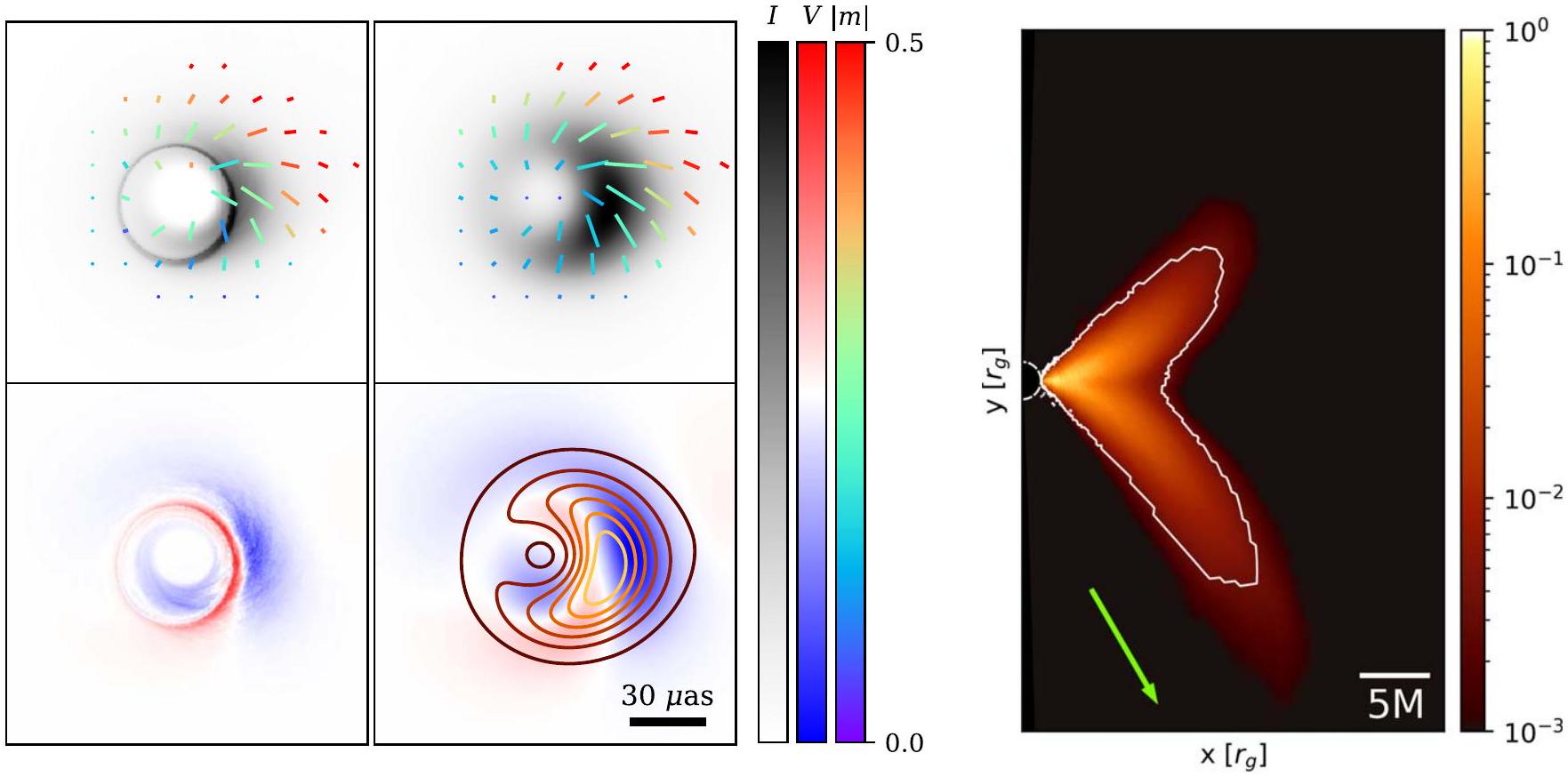
In a companion paper, we present the first spatially resolved polarized image of Sagittarius on event horizon scales, captured using the Event Horizon Telescope, a global very long baseline interferometric array operating at a wavelength of 1.3 mm . Here we interpret this image using both simple analytic models and numerical general relativistic magnetohydrodynamic (GRMHD) simulations. The large spatially resolved linear polarization fraction ( , peaking at ) is the most stringent constraint on parameter space, disfavoring models that are too Faraday depolarized. Similar to our studies of M87*, polarimetric constraints reinforce a preference for GRMHD models with dynamically important magnetic fields. Although the spiral morphology of the polarization pattern is known to constrain the spin and inclination angle, the time-variable rotation measure (RM) of Sgr A* (equivalent to rotation at 228 GHz ) limits its present utility as a constraint. If we attribute the RM to internal Faraday rotation, then the motion of accreting material is inferred to be counterclockwise, contrary to inferences based on historical polarized flares, and no model satisfies all polarimetric and total intensity constraints. On the other hand, if we attribute the mean RM to an external Faraday screen, then the motion of accreting material is inferred to be clockwise, and one model passes all applied total intensity and polarimetric constraints: a model with strong magnetic fields, a spin parameter of 0.94 , and an inclination of . We discuss how future 345 GHz and dynamical imaging will mitigate our present uncertainties and provide additional constraints on the black hole and its accretion flow.

Unified Astronomy Thesaurus concepts: Black holes (162); Supermassive black holes (1663); Black hole physics (159); Galactic center (565); Radio interferometry (1346); Polarimetry (1278); Magnetohydrodynamics (1964)
Supporting material: figure set

1. Introduction

Synchrotron emission from the plasma near supermassive black holes (BHs) provides a crucial source of insight into the physical processes that drive accretion and outflow in galactic cores. It is intrinsically polarized, and both linear polarization and circular polarization provide information about the emitting plasma’s density, temperature, composition, and magnetic field. In the rest frame of the emitting fluid, the linear polarization direction is orthogonal to the local magnetic fields, so images of linear polarization capture the projected magnetic field structure perpendicular to the line of sight. Any magnetized plasma along the line of sight imparts additional polarimetric effects via Faraday rotation, which rotates the plane of linear polarization with a dependence, where is the observing wavelength, and Faraday conversion, which exchanges linear and circular polarization states. Finally, for emission near a BH, the polarization is subject to achromatic rotation from propagation in a curved spacetime.
Recently, the Event Horizon Telescope (EHT) Collaboration published images of the supermassive BH at the Galactic center, Sagittarius A* (Sgr A*; Event Horizon Telescope
NASA Hubble Fellowship Program, Einstein Fellow.
Original content from this work may be used under the terms of the Creative Commons Attribution 4.0 licence. Any further distribution of this work must maintain attribution to the author(s) and the title of the work, journal citation and DOI.
Collaboration et al. 2022a, 2022b, 2022c, 2022d, 2022e, 2022f, hereafter Papers I-VI). These images revealed a bright emission ring encircling a central brightness depression (the “apparent shadow”), consistent with the expected appearance of a Kerr BH with a mass that is only accreting a trickle of material relative to that captured at the Bondi radius in a radiatively inefficient manner (e.g., Hilbert 1917; Bardeen 1973; Luminet 1979; Jaroszynski & Kurpiewski 1997; Falcke et al. 2000). Comparisons of the EHT measurements with numerical simulations provide estimates of the mass accretion rate and a luminosity that is (see, e.g., Paper V, and references therein). Here is the Bondi mass accretion rate and is the Eddington luminosity, with , and being the gravitational constant, speed of light, proton mass, and Thomson cross section, respectively. Previously, measurements of linearly polarized emission near Sgr A* gave strong evidence for this low accretion state (e.g., Agol 2000; Quataert & Gruzinov 2000). In addition, the emission ring morphology, including the lack of a pronounced brightness asymmetry in EHT images, favors a viewing angle in Sgr A* that is at a low to moderate inclination ( ) relative to the angular momentum of the inner accretion flow (see, e.g., Figure 9 in Paper V).
Event Horizon Telescope Collaboration et al. (2024, hereafter Paper VII) reports the first polarized images of Sgr A*, using EHT observations at 230 GHz taken in 2017. These images show a prominent spiral polarization pattern in the emission ring
that is temporally stable, strongly linearly polarized ( ), and dominated by azimuthally symmetric structure. Both the imageaveraged polarization fraction ( ) and the resolved polarization fraction ( ) are significantly higher in Sgr A* than in the EHT’s observations of M87* (Event Horizon Telescope Collaboration et al. 2021a, hereafter M87* Paper VII). In M87*, this polarization pattern was explained by coherent and dynamically important magnetic fields, depolarized by Faraday effects (Event Horizon Telescope Collaboration et al. 2021b, hereafter M87* Paper VIII).
In this paper, we provide the theoretical modeling and interpretation to accompany Paper VII. In Section 2, we summarize the new polarimetric observational constraints on Sgr A*. In Section 3, we provide general arguments about what these constraints imply for Sgr A* through comparison with three simple models: one-zone physical models to evaluate the plasma properties, geometrical ring models to evaluate the degree of coherence in the polarized image, and semianalytic emission models to evaluate the interplay between spacetime and emission parameters in determining polarized image structure. In Section 4, we describe a large library of general relativistic magnetohydrodynamic (GRMHD) simulations for Sgr A*. In Section 5, we evaluate which of these GRMHD models are compatible with the observational constraints. In Section 6, we summarize our findings and describe the prospects for improved constraints from future observations of Sgr A*.

2. Summary of Polarimetric Observations

In Paper VII, static polarimetric images are constructed from the Sgr A* EHT data taken on 2017 April 6th and 7 between 226.1 and 230.1 GHz (see Section 2 of Paper VII for more details). For theoretical interpretation, we adopt eight observational constraints derived from images generated by the THEMIS and the m-ring reconstruction methods (note that “m” is the azimuthal/angular mode number here, not polarization fraction; see Johnson et al. 2020). Of the four methods included in Paper VII, these are the only methods that provide Bayesian posteriors, from which we compute confidence intervals. These methods make drastically different assumptions and, in a sense, bracket the possible spatial and temporal variability. In brief, the m-ring method fits a ring model to each snapshot independently, but the allowed spatial variability is very limited by construction ( for total intensity, for linear polarization, and for circular polarization). In contrast, THEMIS attempts to optimize a single static image most consistent with the full data over time, with a noise budget attributed to time variability. Despite the vast differences between these models, they recover key image quantities with similar accuracy in synthetic data tests and arrive at mostly consistent observables (Paper VII).
Throughout this work, the large and time-variable rotation measure (RM) of Sgr A* poses a significant systematic uncertainty. Defined as , where is the electric vector position angle (EVPA), the RM of Sgr A* may originate from Faraday rotation internal to the emitting region, an external screen, changes in the plasma probed as a function of optical depth, or a combination of these effects. Examining the polarized light curves for the same 2 days as our EHT observations, Wielgus et al. (2024) arrive at . We reserve a lengthy discussion of the RM of Sgr A* in both observations and theory for Appendix C. In summary, the fraction of the RM
Table 1
Polarimetric Constraints Derived from the Static Reconstruction of Sgr A*
Observable m-ring THEMIS Combined
(%) (2.0, 3.1) (6.5, 7.3) (2.0, 7.3)
(-0.7, 0.12) (-0.7, 0.12)
(1.4, 1.8) (2.7, 5.5) (0.0, 5.5)
(0.11, 0.14) (0.10, 0.13) (0.10, 0.14)
(0.20, 0.24) (0.14, 0.17) (0.14, 0.24)
(deg) (as observed)
(deg) (RM derotated) (-168, -108) (-151, -85) (-168, -85)
(1.5, 2.1) (1.1, 1.6) (1.1, 2.1)
Note. These two methods each provide posteriors, from which confidence regions are quoted. As constraints on our models, we conservatively adopt the minimum and maximum of these confidence regions from both of these methods combined (rightmost column), with the exception of , which is treated as an upper limit. Derotation assumes that the mean RM can be attributed to an external Faraday screen, for which a frequency of 228.1 GHz is adopted.
that can be attributed to an external Faraday screen is currently unresolved. Thus, throughout this work we consider the recovered image statistics both with and without RM derotation. Derotating the image corresponds to an interpretation where the time-averaged RM is attributed to a relatively stable external Faraday screen, separate from our models, which can be corrected for. Refraining from doing so corresponds to an interpretation in which all of the RM is generated internally, within our models. Our GRMHD simulations can reproduce the intraday variability of the RM, but not its stability of sign (see Appendix C).
For each of these methods, eight observational constraints explored in this paper are computed, listed in Table 1. To generate these ranges, a large quantity of images consistent with the data were generated from each method’s posterior distribution. We computed the relevant observables for each of these images and then inferred confidence regions. The m -ring method does not provide independent values of , which is fixed to the mean ALMA-inferred value for circular polarization analysis (see Paper VII). When combining the two methods for theoretical interpretation, we adopt the minimum and maximum of the union of both confidence regions (see Figure 10 in Paper VII for a visualization).
The quantities and correspond to the net linear and circular polarization that would be inferred from a spatially unresolved measurement for the time-averaged image. These are given by
where denotes a summation over each pixel . For the timeresolved light curves, which are distinct from the values inferred from our static image reconstructions, Wielgus et al. (2022b, 2024) find and , respectively, where we quote the central of the values observed during the same 2 days of observation. Interestingly, we find that the m-ring method arrives at much
lower values of than THEMIS, which may be attributable to temporal cancellations of fluctuating EVPA patterns.
The remainder of our constraints are structural quantities, beginning with and , the image-averaged linear and circular polarization fraction. These are given by
Note that these quantities depend on the effective resolution of our images. Throughout this work we quote values from our simulations corresponding to as resolution to mimic EHT resolution. We treat the resolved circular polarization fraction as an upper limit, and thus the combined range extends to 0 in Table 1. This is due to the fact that the circularly polarized images presented in Paper VII show structural differences that we attribute to noise (see also Event Horizon Telescope Collaboration et al. 2023, hereafter M87* Paper IX). Because of the absolute magnitude inherent to the definition of this quantity, it is biased high when the signal-to-noise ratio is too low.
Complex modes correspond to Fourier decompositions of the linear polarization structure, where refers to the number of times that an EVPA tick rotates with azimuth (Palumbo et al. 2020). These coefficients are defined by
where and correspond to polar coordinates in the image and . The rotationally invariant mode, , has natural connections to what we believe are azimuthally symmetric disk/jet structures, in particular the magnetic field geometry. Its amplitude encodes the strength of this mode, while its phase encodes the pitch angle and handedness of EVPA ticks. We observe closer to than , which corresponds to tick patterns that are more toroidal than radial.
When considering observational constraints without RM derotation, we simply adopt the range of as observed on the sky. When considering observational constraints with RM derotation, we derotate assuming that there is an external Faraday screen between us and the emitting region that we can characterize by the mean RM over time. Since depends on twice the EVPA, we therefore add to , where is the mean RM observed on April 6 and 7. Therefore, the range on had been significantly shifted by the Faraday screen by deg. Applying this derotation both shifts and broadens the constraint.
Mean images from the posterior distributions generated by each method are plotted in Figure 1. Two sets of linearly polarized images are shown, corresponding to images without and with derotation, respectively. Note that derotation reverses the handedness of the polarization spiral, which has important implications for the flow structure. In the first two rows, total intensity is shown in gray scale, with contours drawn at , , and of the peak brightness. These same contours are repeated in the bottom row. In the top and middle rows, the
Figure 1. Polarized images of Sgr A* used for physical interpretation in this work. Two methods from Paper VII, snapshot m-ring and THEMIS, are included. Top and middle: total intensity is shown in gray scale, polarization ticks indicate the EVPA, the tick length is proportional to the linear polarization intensity magnitude, and color indicates fractional linear polarization. The dotted contour levels correspond to linearly polarized intensities of , and of the polarization peak. The solid contour levels indicate total intensity at , and of the peak brightness. The top row shows images without derotation, and the middle row shows images with a derotation of 46.0 deg to account for Faraday rotation. Bottom: total intensity is indicated in solid colored contours at , and of the peak brightness, and the Stokes brightness is indicated in the diverging color map, with red/blue indicating a positive/negative sign.
colored ticks encode linear polarization, where the length scales with the total linearly polarized intensity and the color scales with the fractional polarization. The dashed white contours plot the linearly polarized intensity rather than the total intensity.
Finally, we also compute the simplest nonrotationally symmetric mode, , as a probe of polarization asymmetry. Again, encodes the strength of this mode, and we use as a probe of rotational symmetry. Since there is no clear axis (such as the spin axis) to define , we do not study . We also refrain from computing higher-order modes, which are more likely to be sensitive to smaller-scale noise fluctuations.

3. Analytic Models

As discussed in the previous section, the linearly polarized image of Sgr A* exhibits three salient features:
  1. It has a large resolved polarization fraction of , with a peak of , much higher than M87*.
  2. The linear polarization structure is highly ordered.
  3. The ordered structure exhibits a high degree of rotational symmetry, which appears to spiral inward with
Figure 2. Allowed parameter space in electron number density ( ) and dimensionless electron temperature ( ) for the one-zone model described in Section 3.1. The panels correspond to different assumed values of plasma . We require that the total flux density (gray region) and optical depth (green region). Corresponding magnetic field strengths are shown as red dotted lines. In blue, we plot the Faraday thick region, . Unlike for M87*, we find that the model is Faraday thin wherever there is intersection between our two constraints.
counterclockwise handedness after derotating by the apparent RM, or clockwise without derotating.
Before exploring more physically complete GRMHD models, we demonstrate that each of these features can be understood in the context of simple analytic models.

3.1. One-zone Modeling

We use the basic assumptions described in Paper V that Sgr A* is an accreting BH with extremely small Eddington ratio and follow M87* Paper VIII to include polarimetry. This polarized one-zone model validates the more complicated numerical models shown later in this paper and offers a natural explanation for the high polarization fraction of Sgr A* relative to M87*.
We model the accretion flow around as a uniform sphere of plasma with radius , where , comparable to the observed size of at 230 GHz (Papers III and IV), with uniform magnetic field oriented at a fiducial inclination relative to the line of sight. The outcomes of our one-zone model depend only weakly on the field orientation. Note that the plasma velocity and the gravitational redshift are neglected.
In Paper V, we assumed that the plasma is optically thin, the ion-electron temperature ratio is 3 , the ions are subvirial by a factor of 3 , and plasma . Adopting the observational flux constraint (Wielgus et al. 2022a), we obtained the self-consistent solution and . Using this solution, we can estimate the strength of the Faraday rotation at 230 GHz with the optical depth to Faraday rotation :
where is the Faraday rotation coefficient (e.g., Jones & Hardee 1979). In contrast, similar modeling arrived at for M87* (M87* Paper VIII). The value inferred for Sgr A* suggests that the internal Faraday rotation
may not be negligible (see also Wielgus et al. 2024), but it also may not necessarily lead to substantial depolarization.
By including optical depth effects and using the Dexter (2016) polarized synchrotron emission and transfer coefficients, we relax some assumptions, such as ion-electron temperature ratios and virial factor, and plot the allowed parameter space as in M87* Paper VIII. Specifically,
  1. we relax the flux constraint to to include the effect of variability; and
  2. we require the same assumption that is optically thin, i.e., .
The above requirements are marked by the gray and green regions in Figure 2, respectively. The magnetic field strengths are shown as red dotted contour lines, and the different panels assume different plasma . In blue, we plot the contour corresponding to , beyond which internal Faraday depolarization becomes increasingly important. Unlike for M87* (see Figure 2 of M87* Paper VIII), we find that the regions where the total flux and optically thin constraints are satisfied only occur in Faraday thin regions of parameter space. We note that this is compatible with multifrequency RM measurements that suggest (Wielgus et al. 2024). Again, this is enough to noticeably rotate the EVPA pattern, but not enough to cause substantial depolarization.
In summary, the total flux and optical depth constraints of Sgr A* naturally require small Faraday depths, which explains the large inferred values of .

3.2. Ordered Polarization: Ordered Fields

Because beam depolarization can only decrease the observed polarization fraction, measurements of the linear polarization at varying angular scales provide information about the degree of order in the underlying polarization. A priori, it could be possible that the the underlying magnetic field is significantly tangled on scales much smaller than the beam. However, the combination of unresolved ( ) and EHT-resolved linear polarization measurements constrains the degree of order in the true, underlying polarization pattern on
Figure 3. The combination of unresolved ( ) and EHT-resolved ( ) linear polarization measurements (at as resolution) constrains the degree of order in the underlying polarization image. In this schematic example, a polarized m -ring has a fixed net polarization, (denoted with the black dashed line), together with a single strongly polarized mode at higher order, , that controls the degree of disorder. For small values of , the resulting image is too ordered, with exceeding our observed value for Sgr A* (denoted with the upper yellow band). For large values of , the resulting image is too disordered, with beam depolarization eliminating the highly polarized image structure. In this example, the fields must be substantially ordered to be consistent with our observations of , with polarized structure that is coherent on scales of the mode, corresponding to angular scales of .
scales smaller than our beam size, disallowing significant spatially unresolved disorder.
As a simple toy model, we analyzed a thin, circular ring with polarization confined to two azimuthal Fourier modes, labeled with index First, we include a constant ( ) mode that defines . We fix the amplitude of this mode to be 0.07 to match unresolved observations of . Next, we add a second mode with varying index and an amplitude of 0.7 , similar to the peak fractional polarization expected for synchrotron emission. By varying , we can crudely assess the allowed degree of coherence in the polarization of Sgr A*.
Figure 3 shows the resolved fractional polarization at an angular resolution of as as a function of the secondary mode index . Both a perfectly ordered polarization field ( ) and a highly disordered polarization field ( ) will have . For the former, there is no beam depolarization; for the latter, the beam depolarization eliminates all small-scale polarized power, even at the resolution of the EHT. Hence, the high value of relative to that we observe is a powerful diagnostic of coherent polarized structure.
As expected, small values of produce resolved polarization fractions that are too high, while large values of produce resolved polarization fractions that are too low. Many effects that are not included in this toy model could further decrease the resolved fractional polarization-the amplitude of the small-scale polarization structure could be significantly less than the synchrotron maximum (e.g., from optical depth or Faraday depolarization), there could be a mix of more than two
modes, and there could be radial polarization structure that causes beam depolarization. Hence, this example provides a conservative lower limit on the scale of coherent polarized structure. To be consistent with our measurements of Sgr A*, we require , corresponding to structure on angular scales of as. Here , where is the distance and is the approximate radius of the emission ring in Sgr A*. Hence, even without detailed modeling, we anticipate that the underlying polarization in Sgr A* is highly ordered, with significant power on azimuthal scales of or more. That is, the large resolved polarization fraction implies relative order of the magnetic field pattern on scales below the beam size.

3.3. Decoding the Polarization Morphology

Semianalytic models enable computationally inexpensive investigation of the effects of model parameters on images. For example, semianalytic models of radiatively inefficient accretion flows have been used for decades to gain tractable yet physically motivated insights into accretion flows (Bromley et al. 2001; Broderick et al. 2009, 2011, 2014, 2016; Pu et al. 2016; Pu & Broderick 2018; Vincent et al. 2022). Here we explore a very simple model, KerrBAM (or Kerr Bayesian Accretion Modeling), a semianalytic model for equatorial, axisymmetric synchrotron emission around a Kerr BH (Palumbo et al. 2022). This modeling framework carries out ray-tracing in a Kerr spacetime to produce a model image assuming an equatorial ring of emission with a specified fluid velocity, magnetic field geometry, and radial emission profile. Here we use this simple model to illustrate the effects of inclination and spin on polarized image structure.
As our starting point, we average magnetic fields and velocity fields in three KHARMA GRMHD simulations (to be discussed in Section 4) in both time and azimuth. We specify a ring of emission centered at a radius of and use the values of the fluid velocity and magnetic field extracted from the GRMHD midplane at this radius. To give the emission ring a realistically finite width, the emission is spread in a Gaussian spanning approximately , keeping the velocity and magnetic field vectors constant. With these values, KerrBAM is able to capture the effects of beaming, frame dragging, and lensing on the resultant image. Note that this model excludes the likely contribution of emission off the midplane (e.g., Falcke et al. 1993; Markoff et al. 2007).
For three different magnetically arrested disks (MADs) with spins of , and +0.94 , we plot several polarimetric quantities of interest (leftmost column) and their model images (subsequent columns) in Figure 4. Along with the polarimetric observables, we overlay our constraints in gray, where for the range without RM derotation is shown as a hatched region. Since this model places emission exactly at the midplane by construction, images produced at inclinations too close to are misleading and therefore not included. The KerrBAM prescription does not include Faraday effects, only crudely modeling optical depth (in this case applying a midplanenormal crossing optical depth applied uniformly to
Figure 4. Left column: image quantities determined from simplified analytic KerrBAM models evaluated using MAD GRMHD fluid velocities and magnetic fields of three spins. In this and subsequent figures, we plot our observational constraints as gray bands for reference, with the constraint prior to RM derotation shown as a hatched region. We use this model to understand key trends, but we caution that more physically complete GRMHD models are necessary for quantitative comparison. Right three columns: corresponding KerrBAM images evaluated at four example inclinations.
, and ) and assuming a prespecified emission model confined to the midplane, so detailed agreement with the GRMHD models is neither expected nor achieved. Nevertheless, this model is useful for understanding several qualitative trends in our GRMHD library that are successfully reproduced.
First, the net polarization is minimized at low inclination, since the symmetry of the accretion flow causes cancellation of polarization in the integrated image. The amplitude of the rotationally invariant mode is always high, due to the underlying azimuthal symmetry of the system. Meanwhile, the amplitude of is stronger at higher inclinations, as it is sensitive to asymmetries in the polarized image. Finally, we
highlight the spin dependence of , which this modeling demonstrates is driven by the evolution of the magnetic field and velocity structure in the GRMHD simulations due to frame dragging (see also Ricarte et al. 2022; Chael et al. 2023; Emami et al. 2023b). The model has , corresponding to a very toroidal EVPA pattern and thus radial magnetic fields. Meanwhile, the higher spin models acquire owing to their more spiral EVPA structures. Interestingly, remains strikingly stable with inclination, although the overall image structure appears to evolve substantially by eye.
This exploration shows that some of the most salient qualitative features of the polarized image can be traced back
Table 2
Summary of the Sgr A* GRMHD Simulation Library Used in This Work
Setup GRMHD GRRT Mode Resolution
Torus KHARMA IPOLE MAD/SANE 50,000 1000
Torus BHAC RAPTOR MAD/SANE 30,000 3333
Torus H-AMR IPOLE MAD/SANE 35,000 1000/200
Note. The last column is , with coordinate monotonic in radius, monotonic in colatitude , and proportional to longitude . Times are given in units of and radii in units of . Different settings may be adopted for MAD models compared to SANE ones, as denoted by a .
to fundamental properties of the fluid and spacetime (magnetic field geometry and spin) without necessarily invoking more uncertain aspects of GRMHD models such as Faraday rotation, the electron-to-ion temperature ratio, and the electron distribution function. However, more physically complete calculations with GRMHD simulations that include these effects selfconsistently are still necessary for quantitative comparison.

4. GRMHD Models

While semianalytic models provide qualitative insights and intuition about BH accretion flows, they do not enforce conservation laws or capture time-dependent phenomena such as turbulence and shocks that play a crucial role in determining the detailed system structure. Thus, we generate dynamical source models using numerical ideal GRMHD simulations. A fluid approximation would appear to conflict with the fact that the rate of Coulomb collisions is small, leading to mean free paths well exceeding the system size, implying that a collisionless kinetic treatment of the plasma may be necessary (Mahadevan & Quataert 1997). However, kinetic instabilities can produce small-scale inhomogeneities in the magnetic field that produce an effective collisionality through particle-wave interactions (Kunz et al. 2014; Riquelme et al. 2015; Sironi & Narayan 2015; Meyrand et al. 2019). We implicitly assume that radiative effects like cooling are not dynamically important for the fluid evolution. This assumption is well motivated given the low accretion rate of , for which the radiative cooling timescale is long compared to the accretion timescale (Dibi et al. 2012; Ryan et al. 2017; Chael et al. 2018; Porth et al. 2019; but see also Yoon et al. 2020).
In Paper V, to compare with total intensity EHT and multiwavelength constraints, we generated a suite of GRMHD-derived images sampling a range of initial conditions and parameterizations of the electron temperature and distribution function. We simplify our exploration in this work, limiting ourselves to simulations with untilted toruslike initial conditions, relativistic thermal electron distribution functions (eDFs) lacking nonthermal contributions, and electron temperatures prescribed via the Mościbrodzka et al. (2016) prescription (see Equation (8) below). The properties of our GRMHD simulations are summarized in Table 2. Radiative transfer is integrated within a radius of , explicitly ignoring material in highly magnetized regions with , within which mass density is artificially injected to keep the simulation stable. We briefly test the impact of our choices of outer integration radius, the cut, and the eDF in Appendices D-F, respectively. While departures from these assumptions are both interesting and
Table 3
Summary of Parameters Sampled by Our GRMHD Libraries
Parameter Values
Magnetic field state MAD, SANE
-0.94, -0.5, 0.0, 0.5, 0.94
(deg) 10, 30, 50, 70, 90, 110, 130, 150, 170
1, 10, 40, 160
Magnetic field polarity Aligned, Reversed
Note. We coarsely sample a five-dimensional parameter space. For each combination of parameters and for each of the KHARMA and BHAC codes, we ray-trace the equivalent of 10 nights of observations.
physically justified, we defer a thorough investigation of these topics to future work.
Our GRMHD library samples a five-dimensional parameter space. The first parameter is the magnetic field state, either an MAD model (Bisnovatyi-Kogan & Ruzmaikin 1976; Igumenshchev et al. 2003; Narayan et al. 2003; Tchekhovskoy et al. 2011) or a standard and normal evolution (SANE) model (De Villiers et al. 2003; Gammie et al. 2003; Narayan et al. 2012; Sądowski et al. 2013). These describe models in which the magnetic flux threading the horizon for a given accretion rate has saturated and become dynamically important (MAD) or not (SANE). The second is the BH spin, which we denote as , where a negative sign indicates a retrograde disk with respect to the spin vector. Third is the inclination, which uniformly samples , instead of only as probed in Paper V, because Faraday rotation and emission of circular polarization break the symmetry when polarization is considered. Our fourth parameter is , which sets the asymptotic value of the ion-to-electron temperature ratio as plasma (Mościbrodzka et al. 2016). Specifically,
where and are the ion and electron temperatures, respectively. While the potential importance of electron cooling for M87* motivated models with cooler electrons, , here we only consider owing to the much smaller Eddington ratio of . Finally, our fifth parameter is the magnetic field polarity with respect to the angular momentum vector of the disk, either aligned or reversed, which affects the direction of Faraday rotation and the handedness of circularly polarized emission. This last degree of freedom only matters for polarized radiative transfer and was ignored in Paper V. We produce a library of images for each combination of these parameters, tabulated in Table 3.
Figure 5. Gallery of example time-averaged simulations in our library. Each panel displays a time-averaged and blurred (with a as FWHM Gaussian kernel) MAD aligned models at three different inclinations. The first panel of each set displays total intensity and linear polarization, while the second panel of each set displays total intensity and circular polarization. Tick lengths scale the total polarized flux density in a given pixel, while their colors scale with the polarization fraction. H-AMR models are ray-traced only for a subset of models for comparison and are not used for scoring.
We retain the use of multiple codes to assess numerical systematic differences. For scoring, we generate libraries spanning , equivalent to about 108 hr nights of observation for the parameter combinations listed in Table 3 using two code combinations: KHARMA (Prather et al. 2021) + IPOLE (Mościbrodzka & Gammie 2018) and BHAC (Porth et al. 2017; Olivares et al. 2019) + RAPTOR (Bronzwaer et al. 2018, 2020), where the first and second codes in each pair correspond to GRMHD and GRRT, respectively. As a further consistency check, a third set is generated with H-AMR (Liska et al. 2022) + IPOLE for a subset of parameter space (only , aligned fields, and ) that we do not use for scoring.
Each simulation is initialized with a torus of gas in constant angular momentum hydrodynamic equilibrium (Fishbone & Moncrief 1976). These tori are perturbed with a weak, poloidal magnetic field. The simulations vary in their initial radius of maximum pressure (from to ) and adiabatic index, . Codes differ in their choice of because applies to a fluid of relativistic electrons and applies to a fluid of nonrelativistic ions, but only one fluid is evolved in these models. Depending on the torus size and initial magnetic field configuration, the simulations develop into an MAD or SANE state (see, e.g., Wong et al. 2022).
In Figure 5, we plot a selection of time-averaged GRMHD snapshots from our library, blurred to EHT resolution using a Gaussian convolution kernel with an FWHM of . In the left panel of each set we plot total intensity in gray scale and the resolved linear polarization as colored ticks. In the right panel of each set, we plot the circular polarization from blue to
red with total intensity contours. Each panel is individually normalized such that the color maps span from 0 to the max on the left and on the right. Each of these models is an MAD aligned field simulation, computed with different codes as indicated above.
The codes exhibit agreement in terms of total intensity and polarized morphology but differ somewhat in the degree of polarization. As the inclination grows, the total intensity image becomes more asymmetric owing to Doppler beaming (e.g., Falcke et al. 2000; Medeiros et al. 2022; Paper V). The same holds true for the polarization, which is further affected by a Faraday depolarization gradient (see Appendix A.3). The magnetic field geometry as sampled by deflected light rays is encoded in the image of circular polarization. In particular, edge-on images in circular polarization exhibit sign inversions along both a horizontal and vertical axis due to flips in the line-of-sight magnetic field direction, and this signal disappears as the viewing angle decreases (Ricarte et al. 2021; Tsunetoe et al. 2021).

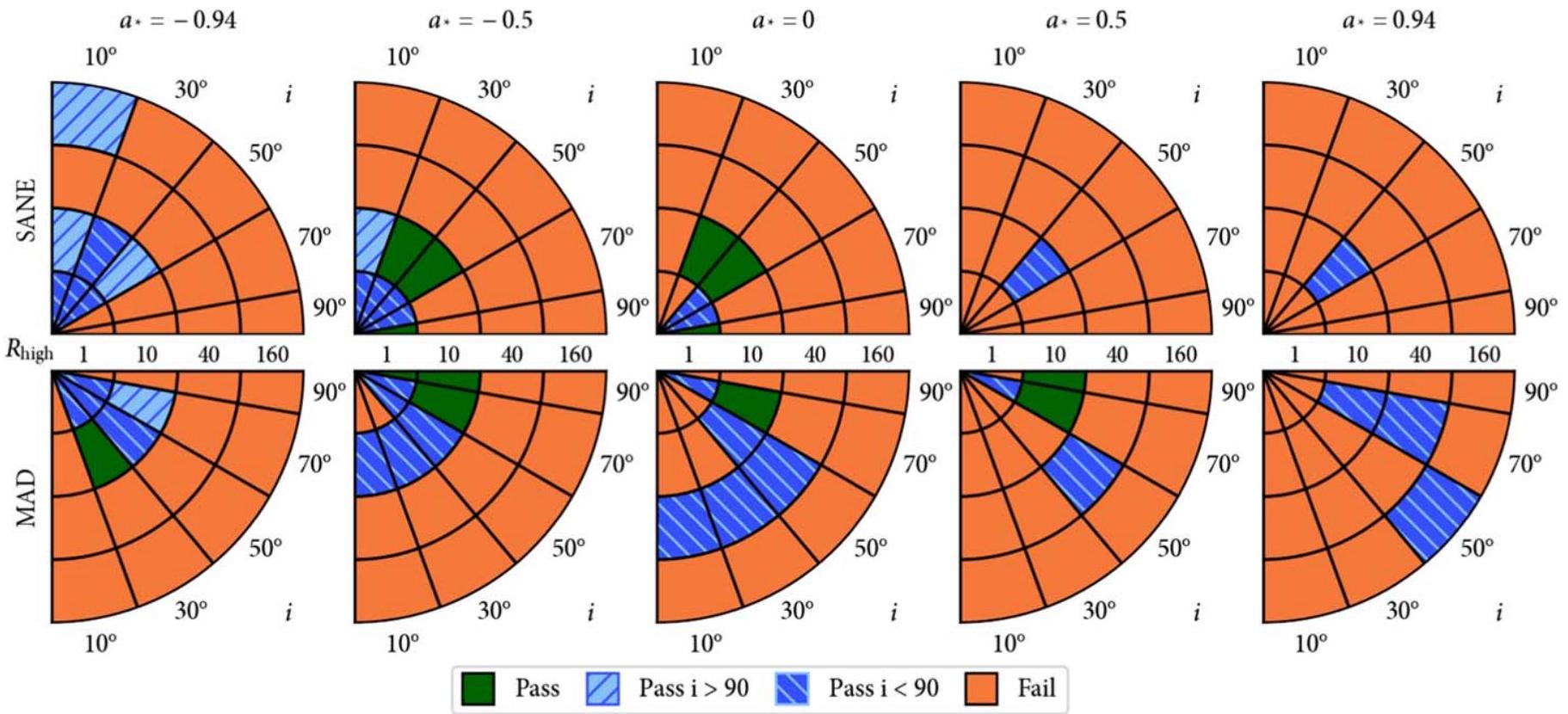
5. GRMHD Model Scoring

We introduce a novel methodology to score each of our GRMHD models using the eight polarimetric constraints in Table 1. Our new scoring scheme acts on time-averaged GRMHD images and attempts to accommodate variations between codes. Note that we only include quantities inferred from our polarimetric images in these constraints, but we will discuss comparisons with total intensity and multifrequency constraints derived in Paper V.
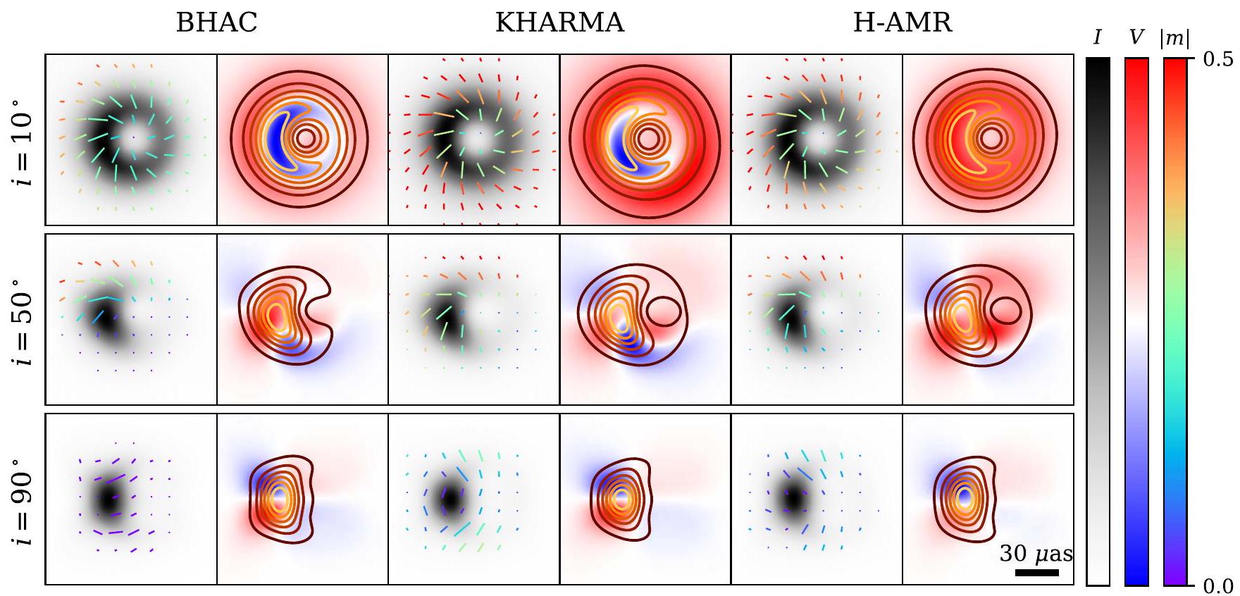
  1. First, each model time series of images is split into 10 windows, each with 1500 M duration. Within each window, we produce a time-averaged image by averaging each of the Stokes parameters. Then, we blur the average image with a Gaussian kernel with an FWHM of as and compute each of the eight observables for scoring.
Constraints Without
Figure 6. Combined polarimetric constraints on the GRMHD model library excluding . Orange models fail, green models pass at both the given and its supplementary angle, and blue regions only pass with the given or supplementary angle as indicated. SANE models are plotted on the top half, and MAD models are plotted on the bottom half. Different columns correspond to different spins from -0.94 to 0.94 . Within each wedge, the radial direction corresponds to and the azimuthal direction corresponds to observer inclination.
2. For each combination of parameters, we combine the values of the observables predicted by the KHARMA and BHAC codes. Since there are 10 windows and two sets of codes, this results in 20 different samples. From these values, we compute the quantiles of each observable to capture the time variability.
3. A model passes an individual observational constraint if there is overlap between its quantile region and that of the observations. A model passes a set of observational constraints if it passes all of the constraints in the set simultaneously.
The most important differences compared to the scoring system utilized in Paper V are that this new system operates on time-averaged images and combines the results from multiple codes into a single theoretical range. We tested performing scoring using only one simulation set at a time. Since KHARMA model electron temperatures are assigned systematically hotter than those of the BHAC models (see Appendix H), KHARMA passes models with larger . There is more disagreement between the codes for SANE models than for MAD models. The constraints with the most disagreement between the two codes are , and , with the KHARMA simulations ruling out more SANE models than the BHAC simulations in each case.
Each of the observational constraints has known connections with the underlying physics. For brevity, we defer a pedagogical exploration of how each of our free parameters
is imprinted onto the observables to Appendix A. We study how each individual constraint affects model selection in Appendix B. Here we summarize the highest-level scoring results, first excluding and then including either as observed or after performing RM derotation.

5.1. Constraints Independent of RM

In Figure 6, we plot a pass/fail table combining all polarimetric constraints, with the exception of . These plots combine both polarities of the magnetic field, showing a pass as long as either polarity passes. These tables are slightly but not systematically different as a function of magnetic field polarity.
We find that the tight constraint on is the most powerful, driving most of the trends shown in this figure. It is much more constraining on parameter space than , for which a much larger range ( ) is allowed. The constraint rules out a few additional typically edge-on models, but it does not provide too much more additional constraining power because and are correlated. Without , Figure 6 reveals no significant preference between and models.
While our total intensity constraints generally favored larger values of (due largely to multiwavelength constraints; Paper V), our polarimetric constraints usually prefer more moderate values. This is because larger values of usually lead to larger internal Faraday rotation depths (see Appendix A.4), which is the most important physical driver of depolarization in our models. However, an interesting trend with respect to spin allows one of the best-bet models of Paper V to continue to pass with . This is the MAD model. MAD models with larger spin have smaller Faraday rotation depths (see
All Polarimetric Constraints
Figure 7. Same as Figure 6, but including the constraint on the phase of without RM derotation. Only models with counterclockwise motion ( ) pass. There is no model that passes all polarimetric and total intensity constraints utilized in Paper V.
Appendix H), allowing them to pass the constraint for larger values of . We refer readers to Appendix B for a more detailed breakdown of each constraint considered individually.

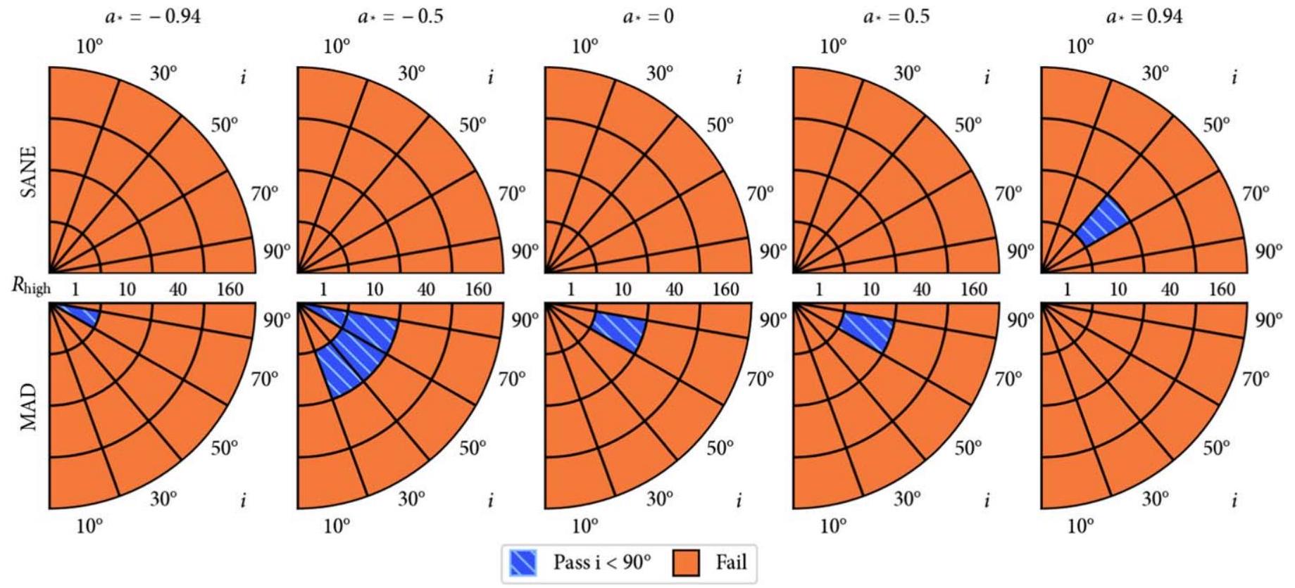
5.2. Constraints Including without RM Derotation

First, we discuss the constraint if RM derotation is not performed. It is possible that the RM may be attributed entirely to Faraday rotation captured within our simulation domain. GRMHD models are capable of producing the correct magnitude of RM from Faraday rotation on event horizon scales, but they tend to produce RM sign flips that are not consistent with decades of Sgr A* observations that produce negative values of the RM (Ricarte et al. 2020; M87* Paper VII; Wielgus et al. 2024). However, it is possible that this problem is related to the excess variability in our models identified in Paper V. We further discuss the uncertainties surrounding our interpretation of the RM in Appendix C.
If one attributes the RM entirely to internal Faraday rotation, then our constraint on spans the interval . Adding this constraint to Figure 6 results in Figure 7. A selection for arises because the handedness of the polarization spiral is opposite that of the magnetic field, which inherits the handedness of the inflowing and emitting gas (see Section 3.3 and Appendix A.3). This corresponds to counterclockwise motion, which disagrees with hot spot interpretations of polarized flares both in the near-IR (NIR; GRAVITY Collaboration et al. 2018, 2020a, 2020b) and in the submillimeter (Vos et al. 2022; Wielgus et al. 2022b). That is, consistency with clockwise motion would require if we assume that traces magnetic field lines with outgoing Poynting flux (Chael et al. 2023), which does not agree with the linearly polarized morphology as observed on the sky.
Without RM derotation, no model can simultaneously pass all total intensity and polarimetric constraints. This is because the best-bet model of Paper V produces an EVPA pattern that is too radial (see Appendix A.2). All models that pass our polarization constraints in Figure 7 fail multiple constraints on the total intensity. In particular, all eight models shown in Figure 7 produce too much flux in the infrared to match observations, and all but the SANE model at overproduce the X-ray flux (Paper V). Both of these are serious failures, as both the IR and X-ray fluxes estimated by our models are lower limits owing to our lack of nonthermal electrons and small simulation domain relative to the X-rayemitting area. Five of the models additionally fail to match the observed size and flux of the source at 86 GHz (Issaoun et al. 2019). All of these models also fail at least one total intensity structural constraint (m-ring and visibility amplitude morphology tests in Paper V). In conclusion, we cannot find a concordance model of Sgr A* without RM derotation.

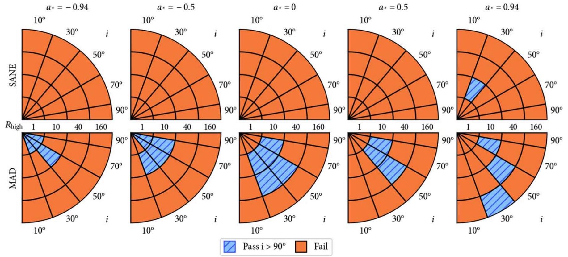
5.3. Constraints Including with RM Derotation

Alternatively, in this section we interpret the mean RM as an external Faraday screen, motivating derotation. As discussed in Section 2, depends on twice the RM, for which a mean value of has been obtained. This potentially results in a shift in of if this RM is interpreted as an external Faraday screen. In this picture, a relatively stable external screen explains the constant sign of RM that has been observed for decades (nevertheless with variation on the order of ). Then, an additional component on event horizon scales, which is already included self-consistently in our models, explains the subhour time variability.
If one attributes the mean RM of a given day entirely to an external screen, then our constraint on spans ( ).
All Polarimetric Constraints
Figure 8. Same as Figure 6, but including the constraint on the phase of with RM derotation. Only models with clockwise motion ( ) pass. A best-bet model from Paper V passes all total intensity and polarimetric constraints: MAD aligned.
Adding this constraint to Figure 6 results in Figure 8. Performing this cut requires inclination angles , corresponding to clockwise motion on the sky, which now agrees with the aforementioned models of polarized NIR and submillimeter flares.
With RM derotation, one of the best-bet models from our total intensity analysis passes all applied total intensity and polarimetric constraints. This is the MAD , aligned model. The second best-bet model from Paper V had and otherwise identical parameters. This second model passes all constraints except , which it underproduces by . In order for the best-bet model to pass, at least of the measured RM must arise from an external screen. Notably, the best-bet model fails if the smaller RM measured at 86 GHz a few days prior, (Wielgus et al. 2024), is instead interpreted as the external screen.
In Figure 9, we visualize the best-bet model (BHAC shown) that survives with RM derotation. In the left two columns, we plot its full polarimetric image in the style of Figure 5. No blurring is applied in the leftmost column, and a as FWHM Gaussian kernel is convolved with the image in the second column to approximate EHT resolution. This model features a bright photon ring, and in our image without blurring, we omit total intensity contours from the circular polarization map to reveal a photon ring sign inversion (discussed in Mościbrodzka et al. 2021; Ricarte et al. 2021).
On the right, we produce a map of the density of the observed emission in the equivalent KHARMA simulation (using Kerr-Schild coordinates). The emission density map is normalized such that its peak value is unity, and it is visualized in logarithmic scale with 3 orders of magnitude in dynamic range. Our line of sight is indicated by the green arrow, and a white contour encloses of the total emission. This reveals that while the emission is peaked at small radius near the disk midplane, a substantial fraction of the emission originates from
a more diffuse jet funnel region. Computing an emissionweighted characteristic emission radius , where is the emission density and is the radius in cylindrical coordinates, we find . We note that our choices to include only thermal electron distribution functions and cut out regions with in this work minimize the potential contribution of a jet to the total emission (e.g., Figure 12 of Fromm et al. 2022). A significant jet component may be necessary to reproduce the flat spectral index at these frequencies (Falcke et al. 1993; Falcke & Markoff 2000; Mościbrodzka & Falcke 2013).
At a radius of , we compute a mass-weighted average magnetic field strength of , where the range quoted here corresponds to the 16th to 84th percentile values obtained in the time series. This value agrees reasonably well with the onezone model discussed in Section 3.1, although we note that this value evolves substantially with radius, reaching at a radius of and at the horizon.
This model produces an outflow power of and has an accretion rate of . This model has a very large jet efficiency of approximately powered by the Blandford & Znajek (1977) mechanism. Yet despite its efficiently, the jet’s power is not high enough to expect global effects on the evolution of our Galaxy (e.g., Su et al. 2021).

6. Discussion and Conclusion

The first polarized image of Sgr A* on event horizon scales exhibits a high resolved polarization fraction of and an ordered, rotationally symmetric EVPA pattern. Through semianalytic arguments and comparisons to GRMHD simulations, we come to the following conclusions:
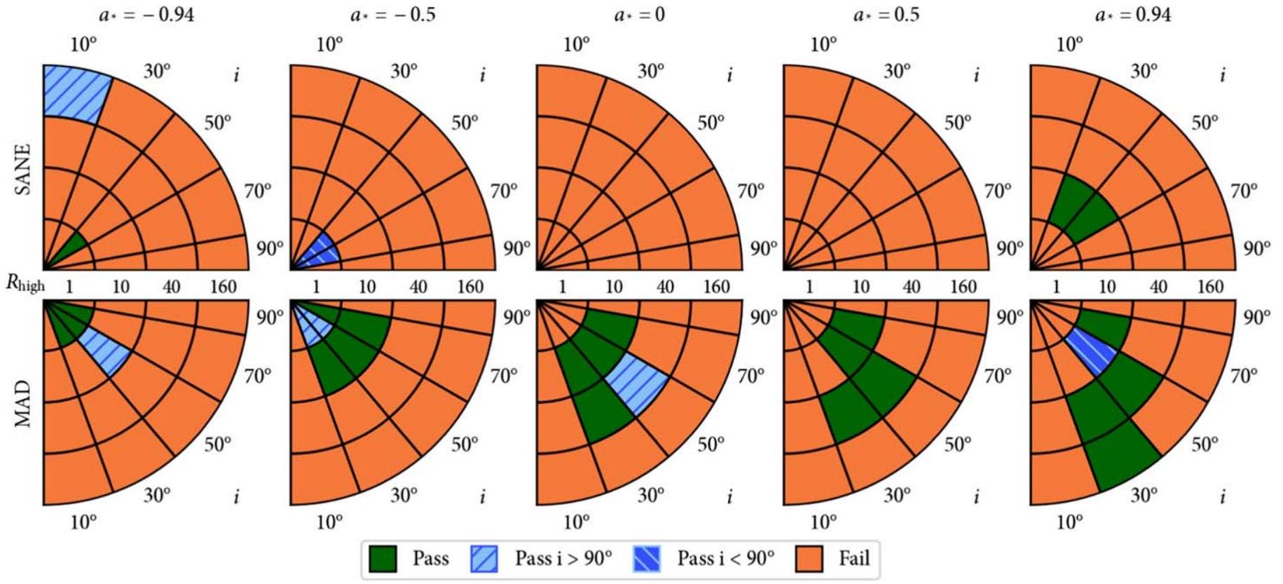
  1. The large resolved polarization fraction implies that the magnetic field on event horizon scales cannot be very tangled on scales smaller than beam, nor can Faraday
Figure 9. The best-bet model of Sgr A*: MAD aligned. In the left two columns, we plot its simulated image in the style of Figure 5. Images in the first column are unblurred, and images in the second column are blurred with a Gaussian with an FWHM of as, approximating EHT resolution. In the right panel, we provide a map of the emission in this model. The white contour encloses of the total emission, the dashed white circle demarcates the horizon, and the green arrow indicates our viewing angle. While the emission peaks close to the BH in the midplane, a significant fraction of emission originates from a more diffuse region, including the jet sheath.
rotation add too much additional disorder to the EVPA structure. The disparity between the spatially resolved ( ) and unresolved ( ) linear polarization fractions can be attributed to cancellations due to the symmetric nature of the image.
2. Driven mostly by the spatially resolved polarization fraction, our constraints strongly favor MAD models over their SANE counterparts, as in M87* Paper VIII.
3. If we rely on internal Faraday rotation to produce the observed RM and do not perform derotation, then there is no model that passes all total intensity and polarimetric constraints.
4. On the other hand, if we assume that the RM can be attributed to an external screen and derotate the EVPA pattern, then we find one model that passes all applied total intensity and polarimetric constraints: MAD aligned.
While our ideal GRMHD simulations containing only thermal electron distributions have done remarkably well at reproducing many of the observed quantities of Sgr A*, they nevertheless have many known imperfections. Most of these models overestimate time variability, including the best-bet model (Paper V), and we caution that the values inferred from our best-bet model should not be interpreted as measurements. Known areas where these simulations can be improved include the following:
  1. Initial Conditions: All of our simulations are initialized with tori that are either perfectly aligned or antialigned with the BH angular momentum axis. Simulations feeding the BH via stellar winds have different variability characteristics (Murchikova et al. 2022) and can self-consistently predict an external Faraday screen (Ressler et al. 2019, 2023).
Tilted disk models (e.g., Fragile et al. 2007; Liska et al. 2018; Chatterjee et al. 2020) may lead to different Faraday rotation characteristics owing to their geometry at large radii.
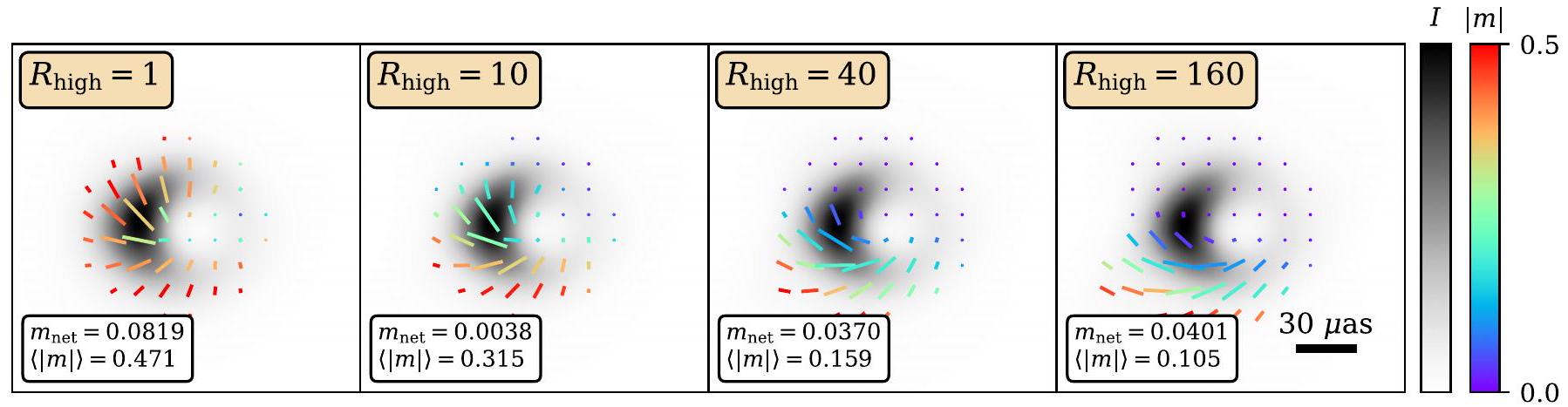
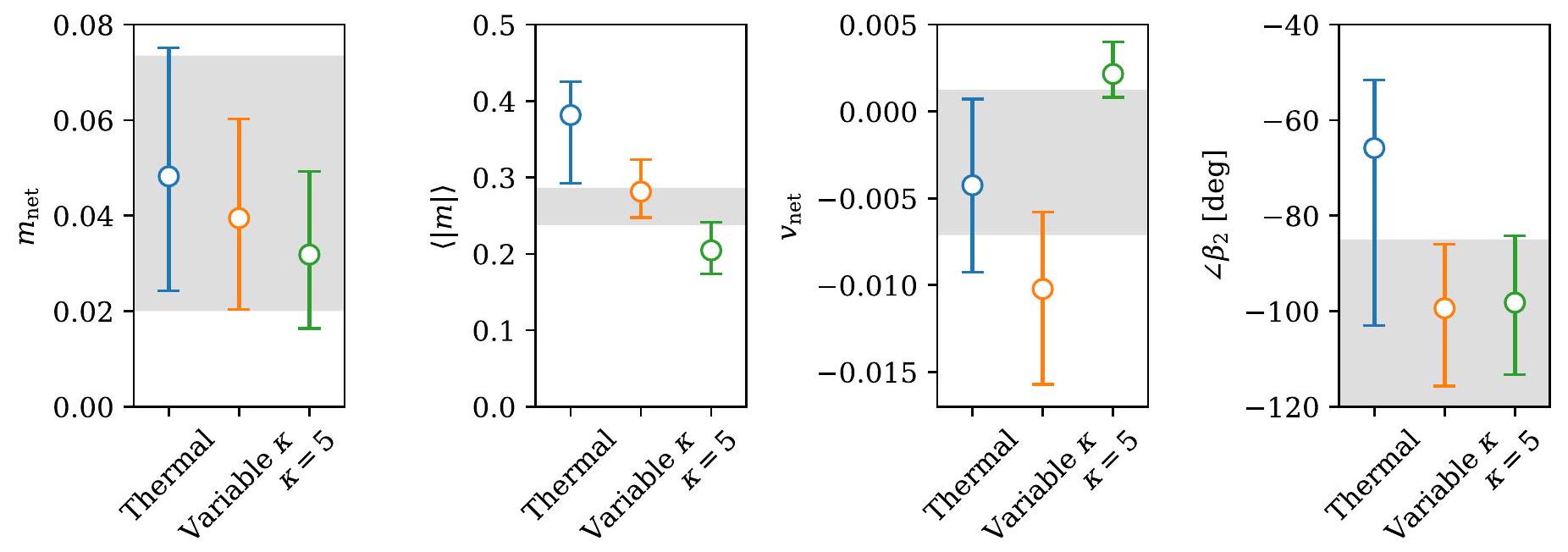
2. Electron Thermodynamics: The Mościbrodzka et al. (2016) prescription that we adopt to set the electron temperature broadly captures the trends seen in kinetic simulations that explicitly model heating and cooling (e.g., Chael et al. 2018; Dexter et al. 2020; Mizuno et al. 2021; Dihingia et al. 2023) but does not reproduce them in much detail. More generally, a nonthermal contribution to the electron distribution function is believed to be necessary to reproduce the spectral energy distribution (Özel et al. 2000; Markoff et al. 2001; Davelaar et al. 2018) and is naturally predicted by particle-in-cell simulations (Kunz et al. 2016; Ball et al. 2018). Nonthermal electron distribution functions can have significant impacts on both total intensity and polarized properties (e.g., Markoff et al. 2001; Mao et al. 2017; Davelaar et al. 2018; Cruz-Osorio et al. 2022; Fromm et al. 2022; Paper V) and are a promising avenue to continue theoretical exploration.
3. Plasma Composition: Wong & Gammie (2022) demonstrate that models fed by helium rather than hydrogen may have substantially different emission morphologies, tending toward higher temperatures and lower densities and thus higher polarization fractions. Meanwhile, the presence of electron-positron pairs can significantly alter Faraday effects, leading to potential signatures in both linear and circular polarization that have not been fully explored (Anantua et al. 2020; Emami et al. 2021, 2023a; M87* Paper IX).
Several ongoing developments within the EHT will be impactful for testing our present interpretation, especially explorations in time and frequency. An effort is ongoing to produce dynamical movies of Sgr A*, despite the challenges of very sparse snapshot ( ) coverage (Tiede et al. 2020; Farah et al. 2022; Levis et al. 2023). Measurements of the apparent angular velocity or potentially the motion of hot spots will provide additional constraints on spin and inclination (Wielgus et al. 2022b; Conroy et al. 2023). The dynamic reconstruction and geometric modeling of these data by Knollmüller et al. (2023) are consistent with the inferred inclination and clockwise motion of our best-bet model. On longer timescales (of years), it will be important to obtain averages of quantities such as , which varies little in our models owing to its tight link with BH spin.
In the frequency domain, future EHT data sets will include 345 GHz data. The wavelength dependence of the scattering screen toward the Galactic center inhibits imaging of Sgr A* at lower frequencies below 86 GHz (Johnson et al. 2018; Issaoun et al. 2019, 2021). On its own, a 345 GHz polarized image would already strongly mitigate one of our largest systematic uncertainties, the RM; the total EVPA rotation would decrease by a factor of 2 , as it is proportional to . These images will also have intrinsically higher resolution by a factor of . Simultaneous dual-band observations could enable the production of RM maps, which would be our best tool for characterizing the Faraday screen and disambiguating our approach to derotation. If the RM truly originates from an external Faraday screen and the emission origin does not significantly change, then at 345 GHz we should observe a spatially uniform EVPA rotation of clockwise relative to our 230 GHz image (roughly halfway between the top two rows in Figure 1). Meanwhile, RM due to internal Faraday rotation may exhibit more spatial variation and potentially sign flips owing to turbulence in the inner accretion flow (Ricarte et al. 2020).
Given the vastness of parameter and modeling space available to theoretical interpretation, we expect the polarized image of Sgr A* to continue to constrain models for many studies to come. This growing EHT data set will continue to challenge theoretical models and provide insights into the nature of BHs, accretion, and plasma physics.

Acknowledgments

The Event Horizon Telescope Collaboration thanks the following organizations and programs: the Academia Sinica; the Academy of Finland (projects 274477, 284495, 312496, 315721); the Agencia Nacional de Investigación y Desarrollo (ANID), Chile via NCN19_058 (TITANs), Fondecyt 1221421 and BASAL FB210003; the Alexander von Humboldt Stiftung; an Alfred P. Sloan Research Fellowship; Allegro, the European ALMA Regional Centre node in the Netherlands, the NL astronomy research network NOVA and the astronomy institutes of the University of Amsterdam, Leiden University, and Radboud University; the ALMA North America Development Fund; the Astrophysics and High Energy Physics program by MCIN (with funding from European Union NextGenerationEU, PRTR-C17I1); the Black Hole Initiative, which is funded by grants from the John Templeton Foundation (60477, 61497, 62286) and the Gordon and Betty Moore Foundation (Grant GBMF-8273)-although the opinions expressed in this work are those of the author and do not necessarily reflect the views of these Foundations; the Brinson
Foundation; “la Caixa” Foundation (ID 100010434) through fellowship codes LCF/BQ/DI22/11940027 and LCF/BQ/DI22/ 11940030; Chandra DD7-18089X and TM6-17006X; the China Scholarship Council; the China Postdoctoral Science Foundation fellowships (2020M671266, 2022M712084); Consejo Nacional de Humanidades, Ciencia y Tecnología (CONAHCYT, Mexico, projects U0004-246083, U0004-259839, F0003-272050, M0037279006, F0003-281692, 104497, 275201, 263356); the Colfuturo Scholarship; the Consejería de Economía, Conocimiento, Empresas y Universidad of the Junta de Andalucía (grant P18-FR-1769); the Consejo Superior de Investigaciones Científicas (grant 2019AEP112); the Delaney Family via the Delaney Family John A. Wheeler Chair at Perimeter Institute; Dirección General de Asuntos del Personal Académico-Universidad Nacional Autónoma de México (DGAPA-UNAM, projects IN112820 and IN108324); the Dutch Organization for Scientific Research (NWO) for the VICI award (grant 639.043.513), the grant OCENW.KLEIN.113, and the Dutch Black Hole Consortium (with project No. NWA 1292.19.202) of the research program the National Science Agenda; the Dutch National Supercomputers, Cartesius and Snellius (NWO grant 2021.013); the EACOA Fellowship awarded by the East Asia Core Observatories Association, which consists of the Academia Sinica Institute of Astronomy and Astrophysics, the National Astronomical Observatory of Japan, Center for Astronomical Mega-Science, Chinese Academy of Sciences, and the Korea Astronomy and Space Science Institute; the European Research Council (ERC) Synergy Grant “BlackHoleCam: Imaging the Event Horizon of Black Holes” (grant 610058); the European Union’s Horizon 2020 research and innovation program under grant agreements RadioNet (No. 730562) and M2FINDERS (No. 101018682); the Horizon ERC Grants 2021 program under grant agreement No. 101040021; the European Research Council for advanced grant “JETSET: Launching, propagation and emission of relativistic jets from binary mergers and across mass scales” (grant No. 884631); the FAPESP (Fundação de Amparo á Pesquisa do Estado de São Paulo) under grant 2021/01183-8; the Fondo CASANID folio CAS220010; the Generalitat Valenciana (grants APOSTD/2018/177 and ASFAE/2022/018) and GenT Program (project CIDEGENT/2018/021); the Gordon and Betty Moore Foundation (GBMF-3561, GBMF-5278, GBMF-10423); the Institute for Advanced Study; the Istituto Nazionale di Fisica Nucleare (INFN) sezione di Napoli, iniziative specifiche TEONGRAV; the International Max Planck Research School for Astronomy and Astrophysics at the Universities of Bonn and Cologne; DFG research grant “Jet physics on horizon scales and beyond” (grant No. 443220636); Joint Columbia/Flatiron Postdoctoral Fellowship (research at the Flatiron Institute is supported by the Simons Foundation); the Japan Ministry of Education, Culture, Sports, Science and Technology (MEXT; grant JPMXP1020200109); the Japan Society for the Promotion of Science (JSPS) Grant-in-Aid for JSPS Research Fellowship (JP17J08829); the Joint Institute for Computational Fundamental Science, Japan; the Key Research Program of Frontier Sciences, Chinese Academy of Sciences (CAS, grants QYZDJ-SSWSLH057, QYZDJ-SSW-SYS008, ZDBS-LY-SLH011); the Leverhulme Trust Early Career Research Fellowship; the Max-Planck-Gesellschaft (MPG); the Max Planck Partner Group of the MPG and the CAS; the MEXT/JSPS KAKENHI (grants 18KK0090, JP21H01137, JP18H03721, JP18K13594, 18K03709, JP19K14761, 18H01245, 25120007, 23K03453); the MICINN Research Projects PID2019-108995GB-C22 and PID2022-140888NB-C22; the MIT International Science and Technology
Initiatives (MISTI) Funds; the Ministry of Science and Technology (MOST) of Taiwan (103-2119-M-001-010-MY2, 105-2112-M-001-025-MY3, 105-2119-M-001-042, 106-2112-M-001-011, 106-2119-M-001-013, 106-2119-M-001-027, 106-2923-M-001-005, 107-2119-M-001-017, 107-2119-M-001-020, 107-2119-M-001041, 107-2119-M-110-005, 107-2923-M-001-009, 108-2112-M-001-048, 108-2112-M-001-051, 108-2923-M-001-002, 109-2112-M-001-025, 109-2124-M-001-005, 109-2923-M-001-001, 110-2112-M-003-007-MY2, 110-2112-M-001-033, 110-2124-M-001007, and 110-2923-M-001-001); the Ministry of Education (MoE) of Taiwan Yushan Young Scholar Program; the Physics Division, National Center for Theoretical Sciences of Taiwan; the National Aeronautics and Space Administration (NASA, Fermi Guest Investigator grant 80NSSC20K1567, NASA Astrophysics Theory Program grant 80NSSC20K0527, NASA NuSTAR award 80NSSC20K0645); NASA Hubble Fellowship grants HST-HF2-51431.001-A and HST-HF2-51482.001-A awarded by the Space Telescope Science Institute, which is operated by the Association of Universities for Research in Astronomy, Inc., for NASA, under contract NAS5-26555; the National Institute of Natural Sciences (NINS) of Japan; the National Key Research and Development Program of China (grant 2016YFA0400704, 2017YFA0402703, 2016YFA0400702); the National Science and Technology Council (NSTC, grants NSTC 111-2112-M-001-041, NSTC 111-2124-M-001-005, NSTC 112-2124-M-001-014); the US National Science Foundation (NSF, grants AST-0096454, AST-0352953, AST0521233, AST-0705062, AST-0905844, AST-0922984, AST1126433, OIA-1126433, AST-1140030, DGE-1144085, AST1207704, AST-1207730, AST-1207752, MRI-1228509, OPP1248097, AST-1310896, AST-1440254, AST-1555365, AST1614868, AST-1615796, AST-1715061, AST-1716327, AST-1726637,OISE-1743747, AST-1743747, AST-1816420, AST1952099, AST-1935980, AST-2034306, AST-2205908, AST2307887); NSF Astronomy and Astrophysics Postdoctoral Fellowship (AST-1903847); the Natural Science Foundation of China (grants 11650110427, 10625314, 11721303, 11725312, 11873028, 11933007, 11991052, 11991053, 12192220, 12192223, 12273022, 12325302, and 12303021); the Natural Sciences and Engineering Research Council of Canada (NSERC, including a Discovery Grant and the NSERC Alexander Graham Bell Canada Graduate Scholarships-Doctoral Program); the National Youth Thousand Talents Program of China; the National Research Foundation of Korea (the Global PhD Fellowship Grant: grants NRF-2015H1A2A1033752, the Korea Research Fellowship Program: NRF-2015H1D3A1066561, Brain Pool Program: 2019H1D3A1A01102564, Basic Research Support Grant 2019R1F1A1059721, 2021R1A6A3A01086420, 2022R1C1C1005255, 2022R1F1A1075115); Netherlands Research School for Astronomy (NOVA) Virtual Institute of Accretion (VIA) postdoctoral fellowships; NOIRLab, which is managed by the Association of Universities for Research in Astronomy (AURA) under a cooperative agreement with the National Science Foundation; Onsala Space Observatory (OSO) national infrastructure, for the provisioning of its facilities/ observational support (OSO receives funding through the Swedish Research Council under grant 2017-00648); the Perimeter Institute for Theoretical Physics (research at Perimeter Institute is supported by the Government of Canada through the Department of Innovation, Science and Economic Development and by the Province of Ontario through the Ministry of Research, Innovation and Science); the Princeton Gravity Initiative; the Spanish Ministerio de Ciencia e Innovación (grants PGC2018-098915-B-
C21, AYA2016-80889-P, PID2019-108995GB-C21, PID2020-117404GB-C21); the University of Pretoria for financial aid in the provision of the new Cluster Server nodes and SuperMicro (USA) for a SEEDING GRANT approved toward these nodes in 2020; the Shanghai Municipality orientation program of basic research for international scientists (grant No. 22JC1410600); the Shanghai Pilot Program for Basic Research, Chinese Academy of Science, Shanghai Branch (JCYJ-SHFY-2021-013); the State Agency for Research of the Spanish MCIU through the “Center of Excellence Severo Ochoa” award for the Instituto de Astrofísica de Andalucía (SEV-2017-0709); the Spanish Ministry for Science and Innovation grant CEX2021-001131-S funded by MCIN/AEI/10.13039/ 501100011033; the Spinoza Prize SPI 78-409; the South African Research Chairs Initiative, through the South African Radio Astronomy Observatory (SARAO, grant ID 77948), which is a facility of the National Research Foundation (NRF), an agency of the Department of Science and Innovation (DSI) of South Africa; the Toray Science Foundation; the Swedish Research Council (VR); the UK Science and Technology Facilities Council (grant No. ST/X508329/1); the US Department of Energy (USDOE) through the Los Alamos National Laboratory (operated by Triad National Security, LLC, for the National Nuclear Security Administration of the USDOE, contract 89233218CNA000001); and the YCAA Prize Postdoctoral Fellowship.
We thank the staff at the participating observatories, correlation centers, and institutions for their enthusiastic support. This paper makes use of the following ALMA data: ADS/JAO.ALMA#2016.1.01154.V. ALMA is a partnership of the European Southern Observatory (ESO; Europe, representing its member states), NSF, and National Institutes of Natural Sciences of Japan, together with National Research Council (Canada), Ministry of Science and Technology (MOST; Taiwan), Academia Sinica Institute of Astronomy and Astrophysics (ASIAA; Taiwan), and Korea Astronomy and Space Science Institute (KASI; Republic of Korea), in cooperation with the Republic of Chile. The Joint ALMA Observatory is operated by ESO, Associated Universities, Inc. (AUI)/NRAO, and the National Astronomical Observatory of Japan (NAOJ). The NRAO is a facility of the NSF operated under cooperative agreement by AUI. This research used resources of the Oak Ridge Leadership Computing Facility at the Oak Ridge National Laboratory, which is supported by the Office of Science of the U.S. Department of Energy under contract No. DE-AC05-00OR22725; the ASTROVIVES FEDER infrastructure, with project code IDIFEDER-2021086; and the computing cluster of Shanghai VLBI correlator supported by the Special Fund for Astronomy from the Ministry of Finance in China. We also thank the Center for Computational Astrophysics, National Astronomical Observatory of Japan. This work was supported by FAPESP (Fundacao de Amparo a Pesquisa do Estado de Sao Paulo) under grant 2021/01183-8.
APEX is a collaboration between the Max-Planck-Institut für Radioastronomie (Germany), ESO, and the Onsala Space Observatory (Sweden). The SMA is a joint project between the SAO and ASIAA and is funded by the Smithsonian Institution and the Academia Sinica. The JCMT is operated by the East Asian Observatory on behalf of the NAOJ, ASIAA, and KASI, as well as the Ministry of Finance of China, Chinese Academy of Sciences, and the National Key Research and Development Program (No. 2017YFA0402700) of China and Natural Science Foundation of China grant 11873028. Additional funding support
for the JCMT is provided by the Science and Technologies Facility Council (UK) and participating universities in the UK and Canada. The LMT is a project operated by the Instituto Nacional de Astrófisica, Óptica, y Electrónica (Mexico) and the University of Massachusetts at Amherst (USA). The IRAM 30 m telescope on Pico Veleta, Spain, is operated by IRAM and supported by CNRS (Centre National de la Recherche Scientifique, France), MPG (Max-Planck-Gesellschaft, Germany), and IGN (Instituto Geográfico Nacional, Spain). The SMT is operated by the Arizona Radio Observatory, a part of the Steward Observatory of the University of Arizona, with financial support of operations from the State of Arizona and financial support for instrumentation development from the NSF. Support for SPT participation in the EHT is provided by the National Science Foundation through award OPP-1852617 to the University of Chicago. Partial support is also provided by the Kavli Institute of Cosmological Physics at the University of Chicago. The SPT hydrogen maser was provided on loan from the GLT, courtesy of ASIAA.
This work used the Extreme Science and Engineering Discovery Environment (XSEDE), supported by NSF grant ACI-1548562, and CyVerse, supported by NSF grants DBI-0735191, DBI1265383, and DBI-1743442. XSEDE Stampede2 resource at TACC was allocated through TG-AST170024 and TGAST080026N. XSEDE JetStream resource at PTI and TACC was allocated through AST170028. This research is part of the Frontera computing project at the Texas Advanced Computing Center through the Frontera Large-Scale Community Partnerships allocation AST20023. Frontera is made possible by National Science Foundation award OAC-1818253. This research was done using services provided by the OSG Consortium (Pordes et al. 2007; Sfiligoi et al. 2009) supported by the National Science Foundation award Nos. 2030508 and 1836650. Additional work used ABACUS2.0, which is part of the eScience center at Southern Denmark University, and the Kultrun Astronomy Hybrid Cluster (projects Conicyt Programa de Astronomia Fondo Quimal QUIMAL170001, Conicyt PIA ACT172033, Fondecyt Iniciacion 11170268, Quimal 220002). Simulations were also performed on the SuperMUC cluster at the LRZ in Garching, on the LOEWE cluster in CSC in Frankfurt, on the HazelHen cluster at the HLRS in Stuttgart, and on the Pi2.0 and Siyuan Mark-I at Shanghai Jiao Tong University. The computer resources of the Finnish IT Center for Science (CSC) and the Finnish Computing Competence Infrastructure (FCCI) project are acknowledged. This research was enabled in part by support provided by Compute Ontario (http:// computeontario.ca), Calcul Quebec (http://www.calculquebec.ca), and Compute Canada (http://www.computecanada.ca).
The EHTC has received generous donations of FPGA chips from Xilinx Inc., under the Xilinx University Program. The EHTC has benefited from technology shared under opensource license by the Collaboration for Astronomy Signal Processing and Electronics Research (CASPER). The EHT project is grateful to T4Science and Microsemi for their assistance with hydrogen masers. This research has made use of NASA’s Astrophysics Data System. We gratefully acknowledge the support provided by the extended staff of the ALMA, from the inception of the ALMA Phasing Project through the observational campaigns of 2017 and 2018. We would like to thank A. Deller and W. Brisken for EHT-specific support with the use of DiFX. We thank Martin Shepherd for the addition of extra features in the Difmap software that were used for the CLEAN imaging results presented in this paper. We acknowledge the significance that Maunakea, where the SMA and
JCMT EHT stations are located, has for the indigenous Hawaiian people.
Software: eht-imaging (Chael et al. 2016), Numpy (Harris et al. 2020), Scipy (Jones et al. 2001), Pandas (McKinney 2010), Astropy (The Astropy Collaboration et al 2013, 2018), Jupyter (Kluyver et al. 2016), Matplotlib (Hunter 2007), THEMIS (Broderick et al. 2020), IPOLE (Noble et al. 2007; Mościbrodzka & Gammie 2018), KHARMA (Prather et al. 2021), BHAC (Porth et al. 2017; Olivares et al. 2019), H-AMR (Liska et al. 2022), RAPTOR (Bronzwaer et al. 2018, 2020), KerrBAM (Palumbo et al. 2022).

Appendix A
Key Trends: Bridging Theory and Observations

Using our GRMHD models, we explore a five-dimensional parameter space, constrained by eight observable aspects of the polarized image that we believe are tied to the models in physically understood ways. Below, we highlight the most salient trends in our simulated image library to explain their physical origins. We focus on illustrative examples in this appendix, but we provide exhaustive distributions of observables calculated from our GRMHD models in Appendix H.

A.1. Magnetic Field State
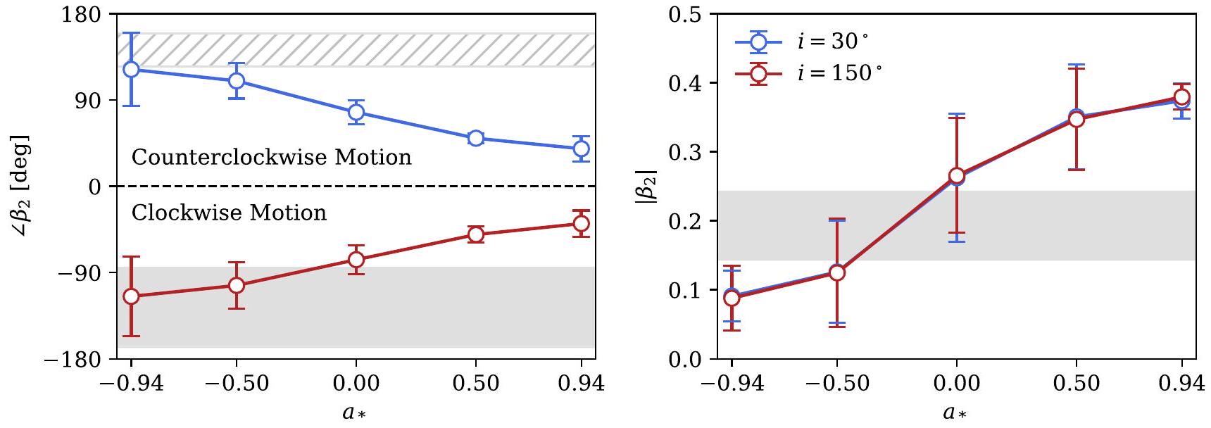
By construction, SANE models have weaker magnetic fields near the horizon than their MAD counterparts at a given accretion rate. As a result, once the fluid is rescaled to reproduce the observed millimeter flux, SANE models usually have larger mass densities. This translates directly to a larger Faraday rotation depth, which is directly implicated for scrambling/depolarizing EHT model images (Mościbrodzka et al. 2017; Jiménez-Rosales & Dexter 2018; Ricarte et al. 2020; M87* Paper IX). Our SANE models are also colder (Paper V), which further increases the efficiency of Faraday rotation (Jones & O’Dell 1977; Quataert & Gruzinov 2000).
In Figure 10, we explore the differences between our MAD and SANE models with fixed and aligned fields. In the top panels, we plot the time-averaged KHARMA images in total intensity and linear polarization, blurred to a resolution of . In the bottom panels, we compare differences in resolved linear and circular polarization fraction, Faraday rotation depth, and . In these and the following plots in this section, we display theoretical error ranges that are calculated based on differences between codes, time variability, and nearest neighbors in parameter space. The details of how these theoretical error bars are calculated are provided in Section 5.
Here we see that the SANE model has much lower linear polarization fraction ( and ), which can be attributed to a much larger Faraday depth Much larger Faraday depths in SANE models than their equivalent MADs drive most of the differences between these two classes of models. SANE models can also produce larger circular polarization ( ) owing to Faraday conversion (M87* Paper IX). Palumbo et al. (2020) showed that is a strong discriminant between MAD and SANE models of M87*. As expected, is significantly larger for the MAD model than for the SANE
Figure 10. Comparison of the MAD and SANE aligned models (KHARMA images plotted). As in Figure 5, the lengths of the ticks scale with the polarized flux in each pixel, normalized for each model individually. A selection of polarimetric observables are shown with theoretical error bars, along with our observational constraints in gray. The constraint on prior to RM derotation is shown with a hatched band instead of a filled band. With other parameters held fixed, SANE models typically have lower resolved linear polarization owing to higher Faraday depths and can sometimes reach large values of circular polarization. Large Faraday depths in SANEs result in lower values of and .
model. Interestingly, while SANE models of M87* usually exhibit , corresponding to radial EVPA patterns, the EVPA pattern in this SANE model acquires some twist owing to a tilted forward jet that we view in projection (top left).

A.2. Spin

The BH spin is a particularly interesting quantity to constrain owing to implications for its cosmic assembly and feedback processes. A number of EHT-related studies have recently explored signatures of spin, and resolved linear polarization structure has been shown to be one of the most promising and accessible probes (Palumbo et al. 2020; Chael et al. 2023; Emami et al. 2023b; Qiu et al. 2023; Ricarte et al. 2023).
In Figure 11, we plot the phase and amplitude of as a function of spin for the subset of the MAD reversed models. The outer accretion disk rotates counterclockwise on the sky for and clockwise on the sky for , which is reflected by the sign of (or rather, the sign of its imaginary component). As discussed in Section 3.3, evolves with spin owing to frame dragging, which results in changes in the magnetic field and velocity structure (Palumbo et al. 2020; Event Horizon Telescope Collaboration et al. 2021b; Ricarte et al. 2022; Chael et al. 2023; Emami et al. 2023b; Qiu et al. 2023). The most highly spinning prograde models acquire a strong azimuthal magnetic field component, resulting in more radial EVPA patterns ( closer to ). Finally, is stronger for symmetric and ordered
progrades than for their messier retrograde counterparts (see also Qiu et al. 2023).

A.3. Inclination

The inclination of is of particular interest because its polarized flaring activity can be interpreted with a polarized hot spot model that favors a relatively face-on viewing angle (GRAVITY Collaboration et al. 2020a, 2020b; Wielgus et al. 2022b). In addition, it is of interest whether or not the accretion disk or BH angular momentum axes align with any structure in its environment.
Inclination is imprinted on the polarized image in a variety of ways, and we plot most of our polarimetric observables as a function of inclination in Figure 12. Here MAD , models are considered. These models produce rotationally symmetric images when viewed face-on, and thus cancellation leads to opposite behavior of and , the latter of which decreases with inclination owing to Faraday depolarization. Intuitively, , the amplitude of the rotationally invariant mode, is strongest for face-on viewing angles and weakest for edge-on viewing angles. Meanwhile, the asymmetric mode has the largest amplitude for intermediate inclinations. The handedness of the linear polarization spiral is directly encoded in , and thus we see that for and for . Finally, is sensitive to whether the poloidal field is pointed toward us or away from us, but note that it is not perfectly antisymmetric
Figure 11. Rotationally symmetric linear polarization structure as a function of spin, encapsulated in the phase and amplitude of . For this plot, MAD , reversed models are included, with either in blue or in red. Our observational constraints are shown as gray bands, and the constraint prior to RM derotation is shown as a hatched region. In this slice of parameter space, prograde models with spin values that are too large tend to produce polarization patterns that are too azimuthally symmetric and radially oriented compared to our observations.
Figure 12. A selection of polarimetric observables plotted as a function of inclination in a slice of our parameter space corresponding to reversed models. In very ordered models such as this one, symmetry and cancellation lead to the smallest net linear polarization fractions for face-on viewing angles at the same time that the resolved linear polarization fraction is highest. In this model, encodes the direction of motion, and encodes the direction of the magnetic field with respect to the line of sight.
about owing to contributions from Faraday conversion (Ricarte et al. 2021).

A.4. (Electron Temperature)

As described in Section 4, sets the ratio of ion-toelectron temperature as plasma (Mościbrodzka et al. 2016). Increasing while fixing all other parameters makes the electrons of a given model cooler and less efficient emitters. Thus, models with larger tend to have larger values of when rescaled to achieve the same target flux. As a result, increasing indirectly increases the Faraday rotation depth (Mościbrodzka et al. 2017; Jiménez-Rosales & Dexter 2018;
Ricarte et al. 2020; M87* Paper VIII). Increasing also shifts emission away from the midplane and concentrates it toward the jet funnel region (Paper V; Wong et al. 2022). This effect is much weaker for MADs than for SANEs, since MAD models intrinsically have smaller plasma on horizon scales.
In Figure 13, we plot time-averaged BHAC MAD , aligned field models as a function of , as well as several of their linear polarization observables. Increasing Faraday depolarization explains the declines in and with . The polarization grows more asymmetric as increases, because at this inclination the Faraday thick midplane is at the top half of the image. This, combined with
Figure 13. Time-averaged images and a selection of polarimetric observables as a function of , for the slice of our parameter space corresponding to MAD aligned models (BHAC images plotted). In this slice of parameter space, Faraday rotation has a clear effect, since increasing leads to smaller linear polarization fractions and correspondingly . At this inclination, sight lines at the top of the image pass through the Faraday thick-disk midplane, increasing the polarization asymmetry as increases, which is reflected in . Both line-of-sight Faraday rotation and changing emission regions lead to a trend in .
Figure 14. Impact of reversing the polarity of the magnetic field on the time-averaged KHARMA MAD model. In radiative transfer, the handedness of Faraday rotation and intrinsic circularly polarized emission flip sign when the magnetic field flipped. This can lead to changes in the morphologies of both linearly and circularly polarized images.
increased Faraday rotation that slightly turns ticks clockwise, leads to a shift in . In addition, decreases as the polarization grows more asymmetric.

A.5. Magnetic Field Polarity

In ideal GRMHD, the equations governing the evolution of a magnetized fluid are invariant to a sign flip of the magnetic field direction. However, the equations of GRRT are not, leading to potential polarimetric signatures of the poloidal field direction. When performing radiative transfer, (intrinsic circular polarization of emitted radiation) and (Faraday rotation) are each sensitive to the direction of the field with
respect to the photon wavevector. The historically negative Stokes of Sgr A* is suggestive of a magnetic field oriented away from us. However, M87* Paper IX discusses how flipping the magnetic field direction can have nontrivial effects on the circularly polarized image (beyond a simple sign flip) and noticeable effects on due to Faraday effects (see also Ricarte et al. 2021; Emami et al. 2023b).
In Figure 14, we highlight the differences between aligned and reversed field models for the time-averaged KHARMA MAD models. Each model is blurred with a as FWHM Gaussian beam shown in total intensity and linear polarization ticks on the left and circular polarization and total intensity contours on the right. We write and for each model in the lower left corner, revealing significant and unpredictable differences, motivating independent
ray-tracing for each magnetic field polarity. In linear polarization, the difference comes from reversing the direction that Faraday rotation shifts the EVPA pattern. The magnitude of this effect is larger than that reported in M87* Paper IX because M87* models are oriented almost completely face-on, viewed through an evacuated funnel (Ricarte et al. 2020). Models of Sgr A* can accumulate larger Faraday rotation depths as radiation passes through more of the disk at larger inclinations. In circular polarization, this particular model is mostly characterized by an overall sign flip, but this is not uniform across the image, leading to a small difference in . This is because the coefficient of Faraday conversion, which exchanges linear and circular polarization, is invariant to a sign flip in the magnetic field direction.

Appendix B Impacts of Individual Observational Constraints

In Section 5, we included a limited selection of plots reflecting which of our models passed each of the polarimetric observational constraints on Sgr A*. Here we break down the impact of each constraint individually.
In Figure 15, we plot the impact of our constraint, which we find is the most important for model selection. Compared to the other constraints, is measured relatively precisely and the two methods agree very well. The Faraday rotation depth explains the trends in this figure (see Appendix H). More Faraday depolarization tends to occur if is larger, if the inclination is larger, or if the model is SANE. Of the models that fail the constraint, most are too depolarized, but some low- , high-spin, face-on models are ruled out for predicting values of that are too large. We find that is much more constraining than (Figure 16), which is measured much less precisely. Recall that is
substantially lower (and less consistent with the light curve) in the m-ring model than THEMIS. We find that if the higher and tighter constraint from THEMIS had been adopted on its own, then this would have ruled out many face-on models (explained in Section 3.3 and Appendix A.3), including the best-bet model.
Our circular polarization constraints are not very impactful. Our upper limit on rules out no models (Figure 17), as all GRMHD models produce lower than the upper limit (similar to M87* Paper IX). Our constraint on is also not very impactful (Figure 18), but while not visible with our plotting scheme, it does rule out many retrograde models that have aligned fields. These models produce preferentially positive , while decades of Sgr A* observations produce .
Our constraints on (Figure 19), (Figure 20), and (Figure 21) are impactful, but they are correlated with each other and . Compared to additionally rules out some models. The ratio is not very constraining, as most models naturally produce , in agreement with the observations. While some methods in Paper VII produced ratios up to , which would have pushed our selection toward more face-on inclinations, the two methods retained in this paper produced more modest values. Interestingly, a few face-on models are ruled out for being too dominated by the rotationally symmetric mode.
Finally, we consider the effect of both with and without RM derotation in Figures 22 and 23, respectively. In either case, models with preferentially radial EVPA patterns are most likely to fail, such as face-on prograde MAD models (see Appendix A.2). With derotation, this constraint produces a preference for clockwise motion on the sky ( ). Without derotation, the opposite is true, and more models fail outright since the constraint is tighter.
Figure 15. Individual impact of our constraint on model selection. This tight constraint is our most informative, ruling out models that are either overly or insufficiently Faraday depolarized.
Figure 16. Individual impact of our constraint on model selection. This is less impactful than , mostly because the allowed range is much larger.
Figure 17. Individual impact of our constraint on model selection, which is treated as an upper limit. All models naturally produce smaller resolved circular polarization fractions than this constraint.
Figure 18. Individual impact of our constraint on model selection. This is not very constraining, but it does rule out models whose distributions of are skewed toward positive values.
Figure 19. Individual impact of our constraint on model selection.
Figure 20. Individual impact of our constraint on model selection. This observable is correlated with and behaves similarly.
Figure 21. Individual impact of our constraint on model selection. This only rules out a few face-on models that are too rotationally symmetric.
Figure 22. Individual impact of our constraint with RM derotation. This constraint produces a preference for .
Figure 23. Individual impact of our constraint without RM derotation. Compared to Figure 22, fewer models pass and there is now a preference for .

Appendix C Rotation Measure

The RM of Sgr A* is a significant systematic uncertainty in our work, affecting our interpretation of . The RM is defined as
where is the EVPA and is the wavelength. If the EVPA of the polarized emission does not intrinsically change with
wavelength (due to optical depth), and the polarized emission is situated entirely behind a Faraday screen that is uniform relative to the size of the emitting region, then the RM is related to a path integral along the line of sight via
Figure 24. RM as a function of time for a selection of KHARMA model snapshots, each with and aligned magnetic fields. Our models can roughly reproduce the observed magnitude of the RM but predict rapid sign flips (colored vs. white markers) that are not observed.
where is the electron number density, is the local magnetic field parallel to the photon wavevector, and , a factor causing lower efficiency as electrons become too relativistic (Jones & O’Dell 1977). If the two assumptions above are correct, then the “intrinsic” EVPA pattern can be easily recovered by derotating the EVPA by .
Sgr A* has exhibited a constant sign of RM for decades (Bower et al. 2018), which supports the interpretation of a stable external Faraday screen. GRMHD simulations including RM from event horizon scales predict ubiquitous sign flips on subhour timescales that are not observed (Ricarte et al. 2020; Ressler et al. 2023; Wielgus et al. 2024). On the other hand, Sgr A* exhibits non- evolution of the EVPA when comparing the 86 GHz and 230 GHz bands. At 86 GHz , the RM on nearly simultaneous days to our observations is only compared to at 230 GHz (Wielgus et al. 2024). In addition to subhour time variability, this suggests that at least some of the RM must also come from internal Faraday rotation on event horizon scales.
Carefully predicting the RM directly for all of our GRMHD simulations would increase the computational cost by factors of a few (more than 2) with the software utilized in this work. This is because ray-tracing must be performed at different frequencies at nonuniform spacings to resolve potential phase wrapping and non- behavior of the EVPA. Nevertheless, we check the RM for a few snapshots of our models in Figure 24, where the RM is estimated by ray-tracing at , and 229 GHz (emulating observations) and then fitting for the slope . MAD models are plotted in the top row, and SANE models are plotted in the bottom row. Three inclinations are shown: in blue, in orange, and in gray. All models are at and in an aligned field configuration. Note that these simulations only include material within , but ab initio simulations of the accretion of Sgr A* from stellar
winds suggest that a steady Faraday screen could potentially be situated at even larger radii (Ressler et al. 2019, 2023).
We find that most of our models naturally produce at at least one point in time, in rough agreement with the observed value. The SANE models, as well as the MADs at , tend toward larger values, similar to models of M87* (Ricarte et al. 2020). However, as in previous works, the RM flips sign in every model at least once. Interestingly, we find similar order-of-magnitude values of RM if Faraday rotation is explicitly switched off during ray-tracing ( ) in some of these models. This suggests that evolving emission origin as a function of frequency may contribute to the inferred RM and its variability.
Our findings in Figure 24 are broadly consistent with an interpretation wherein the rapid time variability of RM is caused by variability on event horizon scales, but the stability of sign is maintained by an external Faraday screen along the line of sight, motivating derotation of . On the other hand, it may also be possible that all of the RM originates from event horizon scales, and our GRMHD models overpredict the variability in RM in the same way that they overpredict variability in total intensity (Paper V). To resolve this, 345 GHz imaging of Sgr A* will be critical; 345 GHz is less affected by Faraday rotation by a factor of . In addition, RM maps produced via simultaneous multifrequency imaging will help determine the nature of the Faraday screen.

Appendix D Impact of Outer Integration Radius

Although we are confident that most of the emission in our models originates close to the event horizon ( ), Faraday rotation can originate at much larger radius in our models, more so as the inclination increases (Dexter et al. 2020; Ricarte et al. 2020). This is especially problematic because material at these radii may not have had enough time in the simulation to reach equilibrium. This concern is more
Figure 25. as a function of outer integration radius for a selection of KHARMA models. The GRRT in our work includes material at , encoded by the gray band. Lines transition from thick to thin at the first radius at which . For models with typically converges by .
important for studies of Sgr A* than for M87* because we view M87* at an inclination of only through an evacuated funnel.
We test the impact of the outer radiative transfer integration radius in Figure 25, where we ray-trace a few KHARMA snapshots at a variety of radii ranging from to . We focus on , which should be directly affected by Faraday rotation on large scales. Inclinations of both and are considered, with values of both 10 and 160 . Fortunately, we find that appears to have converged for most of these models before , where we perform the ray-tracing in this paper. We find that the models that do exhibit substantial evolution with outer integration radius all produce lower than observed. Note that SANE models at inclinations with are the most Faraday-thick models in our library. Models at and/or high appear to have the most evolution with respect to the integration radius. This is consistent with the expectation that higher inclinations and higher values will increase the amount of Faraday rotation owing to more photons traveling through dense, cold regions in the GRMHD domain.
While appears to show evolution for some models, the other polarimetry metrics are well converged and show minimal change for all models across integration radius. However, although we have checked the GRRT step, recall that our GRMHD models are only converged within owing to computational limitations. Exploration with simulations that are valid to larger radii that may produce an external Faraday screen self-consistently (e.g., Ressler et al. 2023) would be an interesting avenue for future analysis.

Appendix E

Impact of Cutting Jet Center (” “)

The polar funnel in the GRMHD simulations is filled with horizon-penetrating field lines and thought to contain plasma with orders of magnitude lower density than the accretion disk.
By the same token, the funnel magnetization is believed to be much larger than the magnetization in the disk. Since there are very few emitting particles in the funnel, its contribution to the overall image is expected to be negligible. In practice, to keep the numerical GRMHD evolution stable, is not allowed to assume realistic values but is instead capped at moderate values by artificially injecting mass (e.g., Porth et al. 2019). Hence, we cannot trust the inflated mass density in this region. Assuming that emission in the funnel should in reality be negligible, we follow the common practice and set all radiation transport coefficients to zero when the magnetization exceeds a critical value . This choice is only safe when no regions form naturally in the disk and when the mixing of disk and funnel plasma at the jet wall is inefficient. In this case the gradient in magnetization is steep which means that whether we adopt or, e.g., does not affect the results. In reality, however, finite-resolution effects in the GRMHD simulations, resolved interchange instabilities, and potentially strong disk magnetization can cause a dependence on the adopted threshold value.
Using the BHAC/RAPTOR data, we have carried out spot checks with two “best-bet” models whereby we increase the threshold to model 1 is MAD , aligned, and model 2 is MAD , aligned. In either case, the constraints change only by a few percent, e.g., in model 2 the average phase changed from to and the average net polarization went down from to . In model 1 , the change in average phase is somewhat larger (going from to ), but still small compared to the overall spread of the distributions. This shows that the results on polarized submillimeter emission are quite robust against change in the adopted value of the and emission at or within the highly magnetized funnel does not dominate in the model.

Appendix F Impact of Nonthermal Electrons

Throughout this work, we have considered only thermal eDFs when performing GRRT. Here we briefly explore the impact of nonthermal electrons in the polarimetric properties of one GRMHD model: MAD aligned. Two nonthermal prescriptions are explored:
  1. Variable : In each cell, a distribution (Vasyliunas 1968; Xiao 2006) is applied, using a prescription originating from particle-in-cell simulations (Ball et al. 2018; Davelaar et al. 2019).
  2. : A distribution with a constant value of is applied globally (Davelaar et al. 2018).
We ray-trace 300 snapshots for each of these cases and compare with the thermal model snapshots. The accretion rate is kept fixed, but we find that the average flux density is 2.3 Jy for all cases. In Figure 26, we plot a selection of polarimetric quantities for these models. Each marker is placed at the median, and the error bars extend to the 16th and 84th percentiles. Overall, we find only subtle differences between these different eDF models. We find that declines in the nonthermal eDF models, coincident with increases in the Faraday rotation depth (2.2, 4.2, and 6.3 for thermal, Variable , and models, respectively). Interestingly, switches sign in the model, while varies only slightly, due to its link with the underlying field geometry. Overall, images with nonthermal eDFs will be useful to study in future work.
Figure 26. Comparison of thermal and nonthermal eDFs for MAD aligned models. Changes in the distributions of polarimetric quantities motivate future exploration in this area.

Appendix G An Interpolative Scoring Scheme

With our GRMHD models, we coarsely sample a fivedimensional parameter space. Here we investigate the possibility that this sparse sampling misses potentially passing models by performing scoring using expanded theoretical error bars. We conceptualize each combination of , and as a volume in three-dimensional parameter space. For each neighbor in parameter space, if the quantiles of the
neighbor do not overlap, we linearly interpolate the lower and upper ranges of each observable to the midpoints of their nearest neighbors. This scheme helps mitigate sparse sampling but, as we discuss, may lead to false positives if observables evolve rapidly between adjacent models. In addition, this methodology fails to consider correlated evolution between observables.
In Figures 27 and 28, we show the results of our interpolative scoring scheme considering all polarimetric
All Polarimetric Constraints
Figure 27. Same as Figure 7, but using the interpolative scoring scheme described in Appendix G.
All Polarimetric Constraints
Figure 28. Same as Figure 8, but using the interpolative scoring scheme described in Appendix G.
Figure 29. Distributions of observables for a selection of SANE models ray-traced with greater resolution in between 1 and 10. These correspond to KHARMA SANE aligned models. We find rapid evolution in this part of parameter space.
constraints without and with RM derotation, respectively. As expected, many more models pass in both cases. The preference for clockwise motion with derotation or counterclockwise motion without derotation is less dramatic with this scheme. Without derotation, both best-bet models still fail. With derotation, the second best-bet model from Paper V, MAD , also passes in this scheme. Without interpolation, this model had only failed by producing too little .
This interpolative scoring scheme does not produce as clear of a preference for MAD over SANE models. We find that this difference is driven by a shortcoming of this method: SANE models evolve very rapidly with , especially between and , leading to very large theoretical error bars. We explore one example in Figure 29, where a set of KHARMA SANE aligned field models are ray-traced at intermediate values of . Each of our eight polarimetric observables is plotted, and we better resolve the rapid evolution in these parameters with . A noteworthy interaction occurs in our interpolation scheme with and , two of our most constraining observables. We see that at the model overproduces but fails to reproduce , which is too radial. Meanwhile, SANE models with have too low and a uniformly distributed . Interpolation allows models in this region to pass because our scoring system suggests that there might be a model with intermediate that has both a correct and a correct . However, with better resolution in , we do not find an individual model that would pass. Overall, this exercise shows that our main conclusions are not likely driven by our sparse sampling of parameter space.

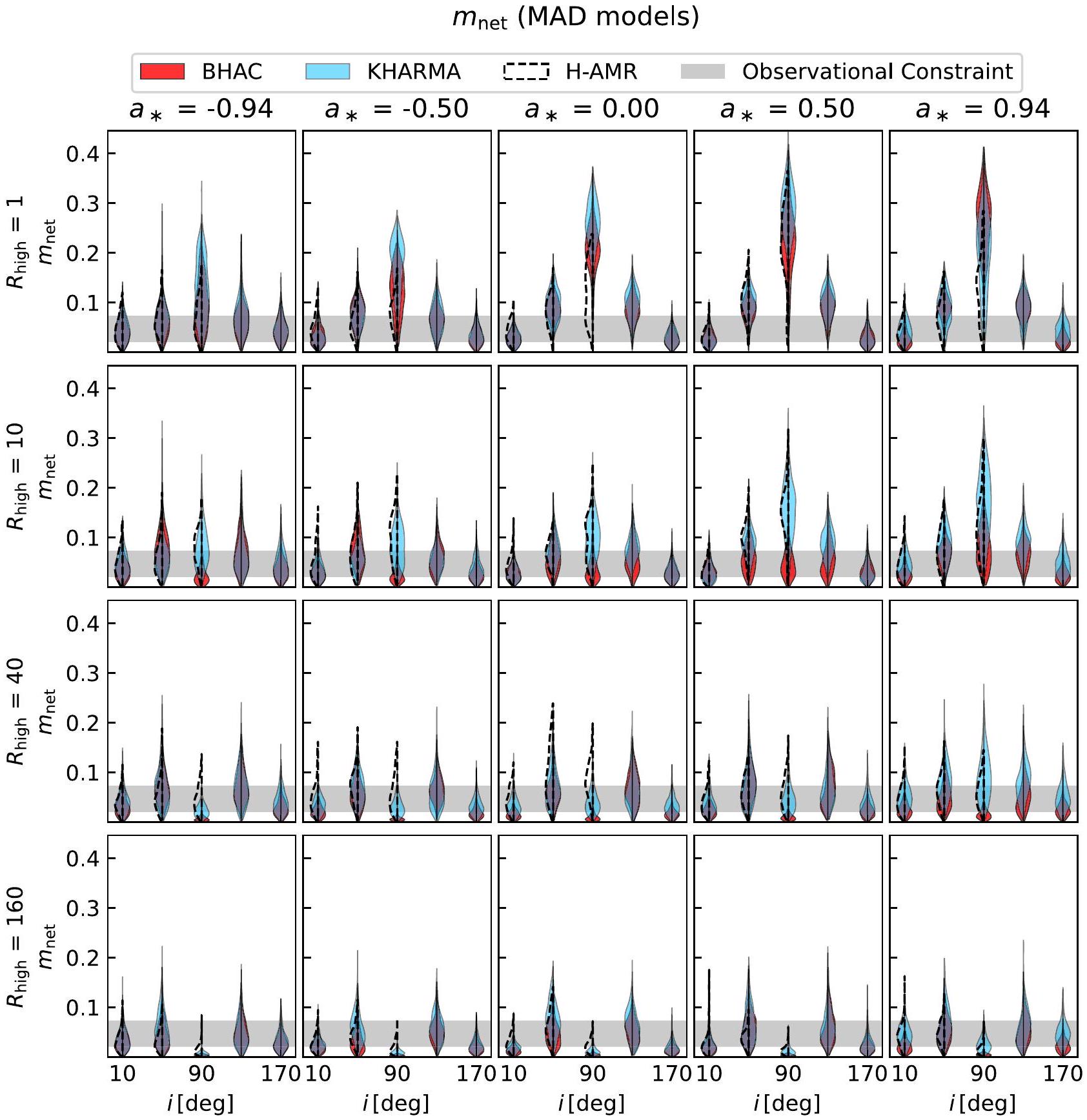
Appendix H GRMHD Observable Distributions

To visualize trends of our eight observables in the fivedimensional parameter space that we explore, we provide “violin” plots of our observables from our models as a figure set, the complete version of which is available in the online journal. In each figure, we consider one observable and one magnetic field state (either MAD or SANE models). One figure, the distributions of for MAD models, is shown in Figure 30. Different spins are shown in different columns, and different values of are shown in different rows. Within each panel, we plot distributions as a function of inclination, where only five of the nine inclinations ray-traced in this work are included to improve readability. Aligned field models are shown on the left, and reversed field models are shown on the right. The distributions with opposite magnetic field polarity are usually very similar, with the notable exceptions of and, more subtly, . To display the relative agreement or disagreement between codes, we plot BHAC models in red and KHARMA models in blue. H-AMR models, which are raytraced for a subset of models only for comparison here and not for scoring, are displayed as dashed distributions when available. Finally, the observational constraints are shown in gray, where, as usual, the allowed range for without RM derotation is shown as a hatched region.
Our last set of plots, distributions of the Faraday rotation depth , are not directly observable but drive many of our physical trends, as well as differences between codes. For a detailed discussion of the physical trends present in these figures, we refer readers to Appendix A.
Figure 30. Distributions of observables for either MAD or SANE models. BH spin varies in each column, and varies in each row. Inclination varies along the -axis. BHAC and KHARMA GRMHD simulations are shown in red and blue in each case, respectively, with H-AMR shown as a dashed curve. Distributions plotted on the left represent aligned magnetic fields, while those plotted on the right represent reversed magnetic fields. Our observational constraint is shown in gray. The complete figure set ( 18 images) is available in the online journal.
(The complete figure set (18 images) is available.)
Differences between our KHARMA and BHAC models inflate our theoretical error bars in Section 5. We find that at least part of these differences arise from physical approximations regarding the assignment of electron temperature during the GRRT. One fluid with a single adiabatic index is evolved in our GRMHD codes, but it represents both relativistic electrons (with an adiabatic index of 4/3) and nonrelativistic ions (with an adiabatic index of ). During the GRRT step of our
calculations, only the electron temperature is relevant for the synchrotron emission that we observe. When assigning electron temperatures, RAPTOR adopts (see, e.g., Davelaar et al. 2018)
where is the electron temperature, is the internal energy, and given by Equation (8). Meanwhile, IPOLE
accounts for the difference in adiabatic indices by adopting
where and .Equation(H2)is physically justified,but it sacrifices internal consistency with the GRMHD simulations,where a single fluid with is evolved (Wong et al.2022).When we set in Equation(H2),we recover Equation(H1)used by RAPTOR. Electron temperatures assigned by RAPTOR are systematically colder, as hot as the IPOLE prescription at ,and as hot as .This explains the systematically larger Faraday depths in our BHAC models relative to both KHARMA and H-AMR,which are both ray-traced with IPOLE.
Larger differences are seen between SANE models than MADs.A unique SANE model is not believed to exist,and differences are known to occur at the GRMHD fluid level (Porth et al.2019).

ORCID iDs

Kazunori Akiyama © https://orcid.org/0000-0002-9475-4254 Antxon Alberdi © https://orcid.org/0000-0002-9371-1033 Juan Carlos Algaba © https://orcid.org/0000-0001-6993-1696 Richard Anantua © https://orcid.org/0000-0003-3457-7660 Keiichi Asada © https://orcid.org/0000-0001-6988-8763 Rebecca Azulay(1)https://orcid.org/0000-0002-2200-5393 Uwe Bach © https://orcid.org/0000-0002-7722-8412 Anne-Kathrin Baczko © https://orcid.org/0000-0003- 3090-3975
Mislav Baloković © https://orcid.org/0000-0003-0476-6647 Bidisha Bandyopadhyay © https://orcid.org/0000-0002- 2138-8564
John Barrett © https://orcid.org/0000-0002-9290-0764
Michi Bauböck © https://orcid.org/0000-0002-5518-2812
Bradford A.Benson © https://orcid.org/0000-0002- 5108-6823
Lindy Blackburn © https://orcid.org/0000-0002-9030-642X
Raymond Blundell © https://orcid.org/0000-0002-5929-5857
Katherine L.Bouman © https://orcid.org/0000-0003- 0077-4367
Geoffrey C.Bower © https://orcid.org/0000-0003-4056-9982
Hope Boyce © https://orcid.org/0000-0002-6530-5783
Christiaan D.Brinkerink © https://orcid.org/0000-0002- 2322-0749
Roger Brissenden © https://orcid.org/0000-0002-2556-0894
Silke Britzen © https://orcid.org/0000-0001-9240-6734
Avery E.Broderick © https://orcid.org/0000-0002- 3351-760X
Dominique Broguiere © https://orcid.org/0000-0001- 9151-6683
Thomas Bronzwaer © https://orcid.org/0000-0003-1151-3971
Sandra Bustamante © https://orcid.org/0000-0001-6169-1894
Do-Young Byun © https://orcid.org/0000-0003-1157-4109
John E.Carlstrom © https://orcid.org/0000-0002-2044-7665
Chiara Ceccobello © https://orcid.org/0000-0002-4767-9925
Andrew Chael © https://orcid.org/0000-0003-2966-6220
Chi-kwan Chan © https://orcid.org/0000-0001-6337-6126
Dominic O.Chang © https://orcid.org/0000-0001-9939-5257
Koushik Chatterjee © https://orcid.org/0000-0002-2825-3590
Shami Chatterjee(10)https://orcid.org/0000-0002-2878-1502
Ming-Tang Chen © https://orcid.org/0000-0001-6573-3318
Yongjun Chen(陈永军)© https://orcid.org/0000-0001- 5650-6770
Xiaopeng Cheng © https://orcid.org/0000-0003-4407-9868
Ilje Cho © https://orcid.org/0000-0001-6083-7521
Pierre Christian © https://orcid.org/0000-0001-6820-9941
Nicholas S.Conroy © https://orcid.org/0000-0003-2886-2377
John E.Conway © https://orcid.org/0000-0003-2448-9181
James M.Cordes © https://orcid.org/0000-0002-4049-1882
Thomas M.Crawford © https://orcid.org/0000-0001- 9000-5013
Geoffrey B.Crew © https://orcid.org/0000-0002-2079-3189
Alejandro Cruz-Osorio © https://orcid.org/0000-0002- 3945-6342
Yuzhu Cui(崔玉竹)(10 https://orcid.org/0000-0001- 6311-4345
Rohan Dahale © https://orcid.org/0000-0001-6982-9034
Jordy Davelaar © https://orcid.org/0000-0002-2685-2434
Mariafelicia De Laurentis © https://orcid.org/0000-0002- 9945-682X
Roger Deane © https://orcid.org/0000-0003-1027-5043
Jessica Dempsey © https://orcid.org/0000-0003-1269-9667
Gregory Desvignes © https://orcid.org/0000-0003-3922-4055
Jason Dexter © https://orcid.org/0000-0003-3903-0373
Vedant Dhruv © https://orcid.org/0000-0001-6765-877X
Indu K.Dihingia © https://orcid.org/0000-0002-4064-0446
Sheperd S.Doeleman © https://orcid.org/0000-0002- 9031-0904
Sean Dougall © https://orcid.org/0000-0002-3769-1314
Sergio A.Dzib © https://orcid.org/0000-0001-6010-6200
Ralph P.Eatough © https://orcid.org/0000-0001-6196-4135
Razieh Emami © https://orcid.org/0000-0002-2791-5011
Heino Falcke © https://orcid.org/0000-0002-2526-6724
Joseph Farah © https://orcid.org/0000-0003-4914-5625
Vincent L.Fish © https://orcid.org/0000-0002-7128-9345
Edward Fomalont © https://orcid.org/0000-0002-9036-2747
H.Alyson Ford © https://orcid.org/0000-0002-9797-0972
Marianna Foschi © https://orcid.org/0000-0001-8147-4993
Raquel Fraga-Encinas © https://orcid.org/0000-0002- 5222-1361
Per Friberg © https://orcid.org/0000-0002-8010-8454 Christian M.Fromm © https://orcid.org/0000-0002- 1827-1656
Antonio Fuentes © https://orcid.org/0000-0002-8773-4933
Peter Galison(10)https://orcid.org/0000-0002-6429-3872
Charles F.Gammie © https://orcid.org/0000-0001-7451-8935
Roberto García © https://orcid.org/0000-0002-6584-7443
Olivier Gentaz © https://orcid.org/0000-0002-0115-4605
Boris Georgiev(DL)https://orcid.org/0000-0002-3586-6424
Ciriaco Goddi(B)https://orcid.org/0000-0002-2542-7743
Roman Gold © https://orcid.org/0000-0003-2492-1966
Arturo I.Gómez-Ruiz © https://orcid.org/0000-0001- 9395-1670
José L.Gómez © https://orcid.org/0000-0003-4190-7613
Minfeng Gu(顾敏峰)© https://orcid.org/0000-0002- 4455-6946
Mark Gurwell © https://orcid.org/0000-0003-0685-3621
Kazuhiro Hada © https://orcid.org/0000-0001-6906-772X
Daryl Haggard © https://orcid.org/0000-0001-6803-2138
Michael H.Hecht © https://orcid.org/0000-0002-4114-4583
Ronald Hesper © https://orcid.org/0000-0003-1918-6098
Dirk Heumann © https://orcid.org/0000-0002-7671-0047 Luis C.Ho(何子山)© https://orcid.org/0000-0001- 6947-5846
Paul Ho © https://orcid.org/0000-0002-3412-4306
Mareki Honma © https://orcid.org/0000-0003-4058-9000
Chih-Wei L.Huang © https://orcid.org/0000-0001-5641-3953
Lei Huang(黄磊)© https://orcid.org/0000-0002-1923-227X
Shiro Ikeda © https://orcid.org/0000-0002-2462-1448
C.M.Violette Impellizzeri © https://orcid.org/0000-0002- 3443-2472
Makoto Inoue © https://orcid.org/0000-0001-5037-3989
Sara Issaoun © https://orcid.org/0000-0002-5297-921X
David J.James © https://orcid.org/0000-0001-5160-4486
Buell T.Jannuzi © https://orcid.org/0000-0002-1578-6582
Michael Janssen © https://orcid.org/0000-0001-8685-6544
Britton Jeter © https://orcid.org/0000-0003-2847-1712
Wu Jiang(江悟)© https://orcid.org/0000-0001-7369-3539
Alejandra Jiménez-Rosales © https://orcid.org/0000-0002- 2662-3754
Michael D.Johnson(10)https://orcid.org/0000-0002-4120- 3029
Svetlana Jorstad © https://orcid.org/0000-0001-6158-1708
Abhishek V.Joshi © https://orcid.org/0000-0002-2514-5965
Taehyun Jung © https://orcid.org/0000-0001-7003-8643
Mansour Karami © https://orcid.org/0000-0001-7387-9333
Ramesh Karuppusamy © https://orcid.org/0000-0002- 5307-2919
Tomohisa Kawashima © https://orcid.org/0000-0001- 8527-0496
Garrett K.Keating © https://orcid.org/0000-0002-3490-146X
Mark Kettenis © https://orcid.org/0000-0002-6156-5617
Dong-Jin Kim © https://orcid.org/0000-0002-7038-2118
Jae-Young Kim © https://orcid.org/0000-0001-8229-7183
Jongsoo Kim © https://orcid.org/0000-0002-1229-0426
Junhan Kim © https://orcid.org/0000-0002-4274-9373
Motoki Kino © https://orcid.org/0000-0002-2709-7338
Jun Yi Koay © https://orcid.org/0000-0002-7029-6658
Prashant Kocherlakota © https://orcid.org/0000-0001- 7386-7439
Patrick M.Koch © https://orcid.org/0000-0003-2777-5861
Shoko Koyama © https://orcid.org/0000-0002-3723-3372
Carsten Kramer © https://orcid.org/0000-0002-4908-4925
Joana A.Kramer © https://orcid.org/0009-0003-3011-0454
Michael Kramer © https://orcid.org/0000-0002-4175-2271
Thomas P.Krichbaum © https://orcid.org/0000-0002- 4892-9586
Cheng-Yu Kuo © https://orcid.org/0000-0001-6211-5581
Noemi La Bella © https://orcid.org/0000-0002-8116-9427
Tod R.Lauer © https://orcid.org/0000-0003-3234-7247
Daeyoung Lee © https://orcid.org/0000-0002-3350-5588
Sang-Sung Lee © https://orcid.org/0000-0002-6269-594X
Po Kin Leung © https://orcid.org/0000-0002-8802-8256
Aviad Levis © https://orcid.org/0000-0001-7307-632X
Zhiyuan Li(李志远)© https://orcid.org/0000-0003- 0355-6437
Rocco Lico © https://orcid.org/0000-0001-7361-2460
Greg Lindahl © https://orcid.org/0000-0002-6100-4772
Michael Lindqvist(1)https://orcid.org/0000-0002-3669-0715
Mikhail Lisakov © https://orcid.org/0000-0001-6088-3819
Jun Liu(刘俊)© https://orcid.org/0000-0002-7615-7499
Kuo Liu © https://orcid.org/0000-0002-2953-7376
Elisabetta Liuzzo © https://orcid.org/0000-0003-0995-5201
Wen-Ping Lo © https://orcid.org/0000-0003-1869-2503
Andrei P.Lobanov © https://orcid.org/0000-0003-1622-1484
Laurent Loinard © https://orcid.org/0000-0002-5635-3345
Colin J.Lonsdale © https://orcid.org/0000-0003-4062-4654
Amy E.Lowitz © https://orcid.org/0000-0002-4747-4276
Ru-Sen Lu(路如森)(10)https://orcid.org/0000-0002- 7692-7967
Nicholas R.MacDonald © https://orcid.org/0000-0002- 6684-8691
Jirong Mao(毛基荣)© https://orcid.org/0000-0002- 7077-7195
Nicola Marchili(10)https://orcid.org/0000-0002-5523-7588
Sera Markoff © https://orcid.org/0000-0001-9564-0876
Daniel P.Marrone © https://orcid.org/0000-0002-2367-1080
Alan P.Marscher © https://orcid.org/0000-0001-7396-3332
Iván Martí-Vidal © https://orcid.org/0000-0003-3708-9611
Satoki Matsushita © https://orcid.org/0000-0002-2127-7880
Lynn D.Matthews © https://orcid.org/0000-0002-3728-8082
Lia Medeiros © https://orcid.org/0000-0003-2342-6728
Karl M.Menten © https://orcid.org/0000-0001-6459-0669
Daniel Michalik © https://orcid.org/0000-0002-7618-6556
Izumi Mizuno © https://orcid.org/0000-0002-7210-6264
Yosuke Mizuno © https://orcid.org/0000-0002-8131-6730
James M.Moran(B)https://orcid.org/0000-0002-3882-4414
Kotaro Moriyama(10)https://orcid.org/0000-0003-1364-3761
Monika Moscibrodzka © https://orcid.org/0000-0002- 4661-6332
Wanga Mulaudzi © https://orcid.org/0000-0003-4514-625X
Cornelia Müller(1)https://orcid.org/0000-0002-2739-2994
Hendrik Müller © https://orcid.org/0000-0002-9250-0197
Alejandro Mus © https://orcid.org/0000-0003-0329-6874
Gibwa Musoke(10)https://orcid.org/0000-0003-1984-189X
Ioannis Myserlis © https://orcid.org/0000-0003-3025-9497
Andrew Nadolski(B)https://orcid.org/0000-0001-9479-9957
Hiroshi Nagai © https://orcid.org/0000-0003-0292-3645
Neil M.Nagar © https://orcid.org/0000-0001-6920-662X
Masanori Nakamura © https://orcid.org/0000-0001- 6081-2420
Gopal Narayanan © https://orcid.org/0000-0002-4723-6569
Iniyan Natarajan © https://orcid.org/0000-0001-8242-4373
Antonios Nathanail © https://orcid.org/0000-0002-1655-9912
Joey Neilsen © https://orcid.org/0000-0002-8247-786X
Roberto Neri © https://orcid.org/0000-0002-7176-4046
Chunchong Ni © https://orcid.org/0000-0003-1361-5699
Aristeidis Noutsos © https://orcid.org/0000-0002-4151-3860
Michael A.Nowak © https://orcid.org/0000-0001-6923-1315
Junghwan Oh © https://orcid.org/0000-0002-4991-9638
Hiroki Okino © https://orcid.org/0000-0003-3779-2016
Héctor Olivares © https://orcid.org/0000-0001-6833-7580
Gisela N.Ortiz-León © https://orcid.org/0000-0002-
2863-676X
Tomoaki Oyama © https://orcid.org/0000-0003-4046-2923
Feryal Özel © https://orcid.org/0000-0003-4413-1523
Daniel C.M.Palumbo © https://orcid.org/0000-0002- 7179-3816
Georgios Filippos Paraschos © https://orcid.org/0000-0001- 6757-3098
Jongho Park © https://orcid.org/0000-0001-6558-9053
Harriet Parsons © https://orcid.org/0000-0002-6327-3423
Nimesh Patel © https://orcid.org/0000-0002-6021-9421
Ue-Li Pen © https://orcid.org/0000-0003-2155-9578
Dominic W.Pesce © https://orcid.org/0000-0002-5278-9221
Richard Plambeck © https://orcid.org/0000-0001-6765-9609
Oliver Porth © https://orcid.org/0000-0002-4584-2557
Felix M.Pötzl © https://orcid.org/0000-0002-6579-8311
Ben Prather © https://orcid.org/0000-0002-0393-7734
Jorge A.Preciado-López © https://orcid.org/0000-0002- 4146-0113
Dimitrios Psaltis © https://orcid.org/0000-0003-1035-3240
Hung-Yi Pu © https://orcid.org/0000-0001-9270-8812
Venkatessh Ramakrishnan © https://orcid.org/0000-0002- 9248-086X
Ramprasad Rao © https://orcid.org/0000-0002-1407-7944
Mark G.Rawlings © https://orcid.org/0000-0002-6529-202X
Alexander W.Raymond © https://orcid.org/0000-0002- 5779-4767
Luciano Rezzolla © https://orcid.org/0000-0002-1330-7103
Angelo Ricarte(10)https://orcid.org/0000-0001-5287-0452
Bart Ripperda © https://orcid.org/0000-0002-7301-3908
Freek Roelofs © https://orcid.org/0000-0001-5461-3687
Alan Rogers © https://orcid.org/0000-0003-1941-7458
Cristina Romero-Cañizales © https://orcid.org/0000-0001- 6301-9073
Eduardo Ros © https://orcid.org/0000-0001-9503-4892
Arash Roshanineshat © https://orcid.org/0000-0002- 8280-9238
Alan L.Roy © https://orcid.org/0000-0002-1931-0135
Ignacio Ruiz © https://orcid.org/0000-0002-0965-5463
Chet Ruszczyk © https://orcid.org/0000-0001-7278-9707
Kazi L.J.Rygl © https://orcid.org/0000-0003-4146-9043
Salvador Sánchez © https://orcid.org/0000-0002-8042-5951
David Sánchez-Argüelles(1)https://orcid.org/0000-0002- 7344-9920
Miguel Sánchez-Portal © https://orcid.org/0000-0003- 0981-9664
Mahito Sasada © https://orcid.org/0000-0001-5946-9960
Kaushik Satapathy © https://orcid.org/0000-0003-0433-3585
Tuomas Savolainen © https://orcid.org/0000-0001-6214-1085
Jonathan Schonfeld © https://orcid.org/0000-0002-8909-2401
Karl-Friedrich Schuster © https://orcid.org/0000-0003- 2890-9454
Lijing Shao © https://orcid.org/0000-0002-1334-8853
Zhiqiang Shen(沈志强)© https://orcid.org/0000-0003- 3540-8746
Des Small(1)https://orcid.org/0000-0003-3723-5404
Bong Won Sohn © https://orcid.org/0000-0002-4148-8378
Jason SooHoo © https://orcid.org/0000-0003-1938-0720
León David Sosapanta Salas © https://orcid.org/0000-0003- 1979-6363
Kamal Souccar © https://orcid.org/0000-0001-7915-5272
Joshua S.Stanway © https://orcid.org/0009-0003-7659-4642
He Sun(孙赫)© https://orcid.org/0000-0003-1526-6787
Fumie Tazaki © https://orcid.org/0000-0003-0236-0600
Alexandra J.Tetarenko © https://orcid.org/0000-0003- 3906-4354
Paul Tiede © https://orcid.org/0000-0003-3826-5648
Remo P.J.Tilanus © https://orcid.org/0000-0002-6514-553X
Michael Titus © https://orcid.org/0000-0001-9001-3275
Pablo Torne © https://orcid.org/0000-0001-8700-6058
Teresa Toscano © https://orcid.org/0000-0003-3658-7862
Efthalia Traianou(B)https://orcid.org/0000-0002-1209-6500
Sascha Trippe © https://orcid.org/0000-0003-0465-1559
Matthew Turk © https://orcid.org/0000-0002-5294-0198
Ilse van Bemmel © https://orcid.org/0000-0001-5473-2950
Huib Jan van Langevelde © https://orcid.org/0000-0002- 0230-5946
Daniel R.van Rossum © https://orcid.org/0000-0001- 7772-6131
Jesse Vos © https://orcid.org/0000-0003-3349-7394
Jan Wagner © https://orcid.org/0000-0003-1105-6109
Derek Ward-Thompson © https://orcid.org/0000-0003- 1140-2761
John Wardle © https://orcid.org/0000-0002-8960-2942
Jasmin E.Washington © https://orcid.org/0000-0002- 7046-0470
Jonathan Weintroub © https://orcid.org/0000-0002- 4603-5204
Robert Wharton © https://orcid.org/0000-0002-7416-5209
Maciek Wielgus © https://orcid.org/0000-0002-8635-4242
Kaj Wiik © https://orcid.org/0000-0002-0862-3398
Gunther Witzel © https://orcid.org/0000-0003-2618-797X
Michael F.Wondrak © https://orcid.org/0000-0002- 6894-1072
George N.Wong © https://orcid.org/0000-0001-6952-2147
Qingwen Wu(吴庆文)© https://orcid.org/0000-0003-4773- 4987
Nitika Yadlapalli © https://orcid.org/0000-0003-3255-4617
Paul Yamaguchi © https://orcid.org/0000-0002-6017-8199
Aristomenis Yfantis © https://orcid.org/0000-0002- 3244-7072
Doosoo Yoon © https://orcid.org/0000-0001-8694-8166
André Young © https://orcid.org/0000-0003-0000-2682
Ken Young © https://orcid.org/0000-0002-3666-4920
Ziri Younsi © https://orcid.org/0000-0001-9283-1191
Wei Yu(于威)(10)https://orcid.org/0000-0002-5168-6052
Feng Yuan(袁峰)© https://orcid.org/0000-0003-3564-6437
Ye-Fei Yuan(袁业飞)© https://orcid.org/0000-0002-7330- 4756
J.Anton Zensus © https://orcid.org/0000-0001-7470-3321
Shuo Zhang © https://orcid.org/0000-0002-2967-790X
Guang-Yao Zhao © https://orcid.org/0000-0002-4417-1659
Shan-Shan Zhao(赵杉杉)(10 https://orcid.org/0000-0002- 9774-3606
Mahdi Najafi-Ziyazi © https://orcid.org/0009-0008- 0922-3995

References

Agol,E.2000,ApJL,538,L121
Anantua,R.,Emami,R.,Loeb,A.,&Chael,A.2020,ApJ,896, 30
The Astropy Collaboration,Robitaille,T.P.,Tollerud,E.J.,et al.2013,A&A, 558,A33
Ball,D.,Sironi,L.,&Özel,F.2018,ApJ,862, 80
Bardeen,J.M.1973,Les Astres Occlus(New York:Gordon &Breach), 215
Bisnovatyi-Kogan,G.S.,&Ruzmaikin,A.A.1976,Ap&SS,42, 401
Blandford,R.D.,&Znajek,R.L.1977,MNRAS,179, 433
Bower,G.C.,Broderick,A.,Dexter,J.,et al.2018,ApJ,868, 101
Broderick,A.E.,Fish,V.L.,Doeleman,S.S.,&Loeb,A.2009,ApJ,697, 45
Broderick,A.E.,Fish,V.L.,Doeleman,S.S.,&Loeb,A.2011,ApJ,735, 110
Broderick,A.E.,Fish,V.L.,Johnson,M.D.,et al.2016,ApJ,820, 137
Broderick,A.E.,Gold,R.,Karami,M.,et al.2020,ApJ,897, 139
Broderick,A.E.,Johannsen,T.,Loeb,A.,&Psaltis,D.2014,ApJ,784, 7
Bromley,B.C.,Melia,F.,&Liu,S.2001,ApJL,555,L83
Bronzwaer,T.,Davelaar,J.,Younsi,Z.,et al.2018,A&A,613,A2
Bronzwaer,T.,Younsi,Z.,Davelaar,J.,&Falcke,H.2020,A&A,641,A126
Chael,A.,Lupsasca,A.,Wong,G.N.,&Quataert,E.2023,ApJ,958, 65
Chael,A.,Rowan,M.,Narayan,R.,Johnson,M.,&Sironi,L.2018,MNRAS, 478, 5209
Chael,A.A.,Johnson,M.D.,Narayan,R.,et al.2016,ApJ,829, 11
Chatterjee,K.,Younsi,Z.,Liska,M.,et al.2020,MNRAS,499, 362
Conroy, N. S., Bauböck, M., Dhruv, V., et al. 2023, ApJ, 951, 46
Cruz-Osorio, A., Fromm, C. M., Mizuno, Y., et al. 2022, NatAs, 6, 103
Davelaar, J., Mościbrodzka, M., Bronzwaer, T., & Falcke, H. 2018, A&A, 612, A34
Davelaar, J., Olivares, H., Porth, O., et al. 2019, A&A, 632, A2
De Villiers, J.-P., Hawley, J. F., & Krolik, J. H. 2003, ApJ, 599, 1238
Dexter, J. 2016, MNRAS, 462, 115
Dexter, J., Jiménez-Rosales, A., Ressler, S. M., et al. 2020, MNRAS, 494, 4168
Dibi, S., Drappeau, S., Fragile, P. C., Markoff, S., & Dexter, J. 2012, MNRAS, 426, 1928
Dihingia, I. K., Mizuno, Y., Fromm, C. M., & Rezzolla, L. 2023, MNRAS, 518, 405
Emami, R., Anantua, R., Chael, A. A., & Loeb, A. 2021, ApJ, 923, 272
Emami, R., Anantua, R., Ricarte, A., et al. 2023a, Galax, 11, 11
Emami, R., Ricarte, A., Wong, G. N., et al. 2023b, ApJ, 950, 38
Event Horizon Telescope Collaboration, Akiyama, K., Alberdi, A., et al. 2022a, ApJL, 930, L12
Event Horizon Telescope Collaboration, Akiyama, K., Alberdi, A., et al. 2022b, ApJL, 930, L13
Event Horizon Telescope Collaboration, Akiyama, K., Alberdi, A., et al. 2022c, ApJL, 930, L14
Event Horizon Telescope Collaboration, Akiyama, K., Alberdi, A., et al. 2022d, ApJL, 930, L15
Event Horizon Telescope Collaboration, Akiyama, K., Alberdi, A., et al. 2022e, ApJL, 930, L16
Event Horizon Telescope Collaboration, Akiyama, K., Alberdi, A., et al. 2022f, ApJL, 930, L17
Event Horizon Telescope Collaboration, Akiyama, K., Alberdi, A., et al. 2023, ApJL, 957, L20
Event Horizon Telescope Collaboration, Akiyama, K., Alberdi, A., et al. 2024, ApJL, 964, L25
Event Horizon Telescope Collaboration, Akiyama, K., Algaba, J. C., et al. 2021a, ApJL, 910, L12
Event Horizon Telescope Collaboration, Akiyama, K., Algaba, J. C., et al. 2021b, ApJL, 910, L13
Falcke, H., Mannheim, K., & Biermann, P. L. 1993, A&A, 278, L1
Falcke, H., & Markoff, S. 2000, A&A, 362, 113
Falcke, H., Melia, F., & Agol, E. 2000, ApJL, 528, L13
Farah, J., Galison, P., Akiyama, K., et al. 2022, ApJL, 930, L18
Fishbone, L. G., & Moncrief, V. 1976, ApJ, 207, 962
Fragile, P. C., Blaes, O. M., Anninos, P., & Salmonson, J. D. 2007, ApJ, 668, 417
Fromm, C. M., Cruz-Osorio, A., Mizuno, Y., et al. 2022, A&A, 660, A107
Gammie, C. F., McKinney, J. C., & Tóth, G. 2003, ApJ, 589, 444
GRAVITY Collaboration, Abuter, R., Amorim, A., et al. 2018, A&A, 618, L10
GRAVITY Collaboration, Bauböck, M., Dexter, J., et al. 2020a, A&A, 635, A143
GRAVITY Collaboration, Jiménez-Rosales, A., Dexter, J., et al. 2020b, A&A, 643, A56
Harris, C. R., Millman, K. J., van der Walt, S. J., et al. 2020, Natur, 585, 357
Hilbert, D. 1917, Nachrichten von der Königlichen Gesellschaft der Wissenschaften zu Göttingen-Mathematisch-physikalische Klasse (Berlin: Weidmannsche Buchhandlung), 53
Hunter, J. D. 2007, CSE, 9, 90
Igumenshchev, I. V., Narayan, R., & Abramowicz, M. A. 2003, ApJ, 592, 1042
Issaoun, S., Johnson, M. D., Blackburn, L., et al. 2019, ApJ, 871, 30
Issaoun, S., Johnson, M. D., Blackburn, L., et al. 2021, ApJ, 915, 99
Jaroszynski, M., & Kurpiewski, A. 1997, A&A, 326, 419
Jiménez-Rosales, A., & Dexter, J. 2018, MNRAS, 478, 1875
Johnson, M. D., Lupsasca, A., Strominger, A., et al. 2020, SciA, 6, eaaz1310
Johnson, M. D., Narayan, R., Psaltis, D., et al. 2018, ApJ, 865, 104
Jones, E., Oliphant, T., Peterson, P., et al. 2001, SciPy: Open Source Scientific Tools for Python, http://www.scipy.org/
Jones, T. W., & Hardee, P. E. 1979, ApJ, 228, 268
Jones, T. W., & O’Dell, S. L. 1977, ApJ, 214, 522
Kluyver, T., Ragan-Kelley, B., Pérez, F., et al. 2016, in Positioning and Power in Academic Publishing: Players, Agents and Agendas, ed. F. Loizides & B. Schmidt (Amsterdam: IOS Press), 87
Knollmüller, J., Arras, P., & Enßlin, T. 2023, arXiv:2310.16889
Kunz, M. W., Schekochihin, A. A., & Stone, J. M. 2014, PhRvL, 112, 205003
Kunz, M. W., Stone, J. M., & Quataert, E. 2016, PhRvL, 117, 235101
Levis, A., Chael, A. A., Bouman, K. L., Wielgus, M., & Srinivasan, P. P. 2023, arXiv:2310.07687
Liska, M., Hesp, C., Tchekhovskoy, A., et al. 2018, MNRAS, 474, L81
Liska, M. T. P., Chatterjee, K., Issa, D., et al. 2022, ApJS, 263, 26
Luminet, J.-P. 1979, A&A, 75, 228
Mahadevan, R., & Quataert, E. 1997, ApJ, 490, 605
Mao, S. A., Dexter, J., & Quataert, E. 2017, MNRAS, 466, 4307
Markoff, S., Bower, G. C., & Falcke, H. 2007, MNRAS, 379, 1519
Markoff, S., Falcke, H., Yuan, F., & Biermann, P. L. 2001, A&A, 379, L13
McKinney, W. 2010, in Proc. 9th Python in Science Conf., ed. S. van der Walt & J. Millman, 51
Medeiros, L., Chan, C.-K., Narayan, R., Özel, F., & Psaltis, D. 2022, ApJ, 924, 46
Meyrand, R., Kanekar, A., Dorland, W., & Schekochihin, A. A. 2019, PNAS, 116, 1185
Mizuno, Y., Fromm, C. M., Younsi, Z., et al. 2021, MNRAS, 506, 741
Mościbrodzka, M., Dexter, J., Davelaar, J., & Falcke, H. 2017, MNRAS, 468, 2214
Mościbrodzka, M., & Falcke, H. 2013, A&A, 559, L3
Mościbrodzka, M., Falcke, H., & Shiokawa, H. 2016, A&A, 586, A38
Mościbrodzka, M., & Gammie, C. F. 2018, MNRAS, 475, 43
Mościbrodzka, M., Janiuk, A., & De Laurentis, M. 2021, MNRAS, 508, 4282
Murchikova, L., White, C. J., & Ressler, S. M. 2022, ApJL, 932, L21
Narayan, R., Igumenshchev, I. V., & Abramowicz, M. A. 2003, PASJ, 55, L69
Narayan, R., Sądowski, A., Penna, R. F., & Kulkarni, A. K. 2012, MNRAS, 426, 3241
Noble, S. C., Leung, P. K., Gammie, C. F., & Book, L. G. 2007, CQGra, 24, S259
Olivares, H., Porth, O., Davelaar, J., et al. 2019, A&A, 629, A61
Özel, F., Psaltis, D., & Narayan, R. 2000, ApJ, 541, 234
Palumbo, D. C. M., Gelles, Z., Tiede, P., et al. 2022, ApJ, 939, 107
Palumbo, D. C. M., Wong, G. N., & Prather, B. S. 2020, ApJ, 894, 156
Pordes, R., Petravick, D., Kramer, B., et al. 2007, JPhCS, 78, 012057
Porth, O., Chatterjee, K., Narayan, R., et al. 2019, ApJS, 243, 26
Porth, O., Olivares, H., Mizuno, Y., et al. 2017, ComAC, 4, 1
Prather, B., Wong, G., Dhruv, V., et al. 2021, JOSS, 6, 3336
Pu, H.-Y., Akiyama, K., & Asada, K. 2016, ApJ, 831, 4
Pu, H.-Y., & Broderick, A. E. 2018, ApJ, 863, 148
Qiu, R., Ricarte, A., Narayan, R., et al. 2023, MNRAS, 520, 4867
Quataert, E., & Gruzinov, A. 2000, ApJ, 545, 842
Ressler, S. M., Quataert, E., & Stone, J. M. 2019, MNRAS, 482, L123
Ressler, S. M., White, C. J., & Quataert, E. 2023, MNRAS, 521, 4277
Ricarte, A., Palumbo, D. C. M., Narayan, R., Roelofs, F., & Emami, R. 2022, ApJL, 941, L12
Ricarte, A., Prather, B. S., Wong, G. N., et al. 2020, MNRAS, 498, 5468
Ricarte, A., Qiu, R., & Narayan, R. 2021, MNRAS, 505, 523
Ricarte, A., Tiede, P., Emami, R., Tamar, A., & Natarajan, P. 2023, Galax, 11, 6
Riquelme, M. A., Quataert, E., & Verscharen, D. 2015, ApJ, 800, 27
Ryan, B. R., Ressler, S. M., Dolence, J. C., et al. 2017, ApJL, 844, L24
Sądowski, A., Narayan, R., Penna, R., & Zhu, Y. 2013, MNRAS, 436, 3856
Sfiligoi, I., Bradley, D. C., Holzman, B., et al. 2009, in 2009 WRI World Congress on Computer Science and Information Engineering 2 (New York: IEEE), 428
Sironi, L., & Narayan, R. 2015, ApJ, 800, 88
Su, K.-Y., Hopkins, P. F., Bryan, G. L., et al. 2021, MNRAS, 507, 175
Tchekhovskoy, A., Narayan, R., & McKinney, J. C. 2011, MNRAS, 418, L79
The Astropy Collaboration, Price-Whelan, A. M., Sipőcz, B. M., et al. 2018, AJ, 156, 123
Tiede, P., Pu, H.-Y., Broderick, A. E., et al. 2020, ApJ, 892, 132
Tsunetoe, Y., Mineshige, S., Ohsuga, K., Kawashima, T., & Akiyama, K. 2021, PASJ, 73, 912
Vasyliunas, V. M. 1968, JGR, 73, 2839
Vincent, F. H., Gralla, S. E., Lupsasca, A., & Wielgus, M. 2022, A&A, 667, A170
Vos, J., Mościbrodzka, M. A., & Wielgus, M. 2022, A&A, 668, A185
Wielgus, M., Issaoun, S., Martí-Vidal, I., et al. 2024, A&A, 682, A97
Wielgus, M., Marchili, N., Martí-Vidal, I., et al. 2022a, ApJL, 930, L19
Wielgus, M., Moscibrodzka, M., Vos, J., et al. 2022b, A&A, 665, L6
Wong, G. N., & Gammie, C. F. 2022, ApJ, 937, 60
Wong, G. N., Prather, B. S., Dhruv, V., et al. 2022, ApJS, 259, 64
Xiao, F. 2006, PPCF, 48, 203
Yoon, D., Chatterjee, K., Markoff, S. B., et al. 2020, MNRAS, 499, 3178

The Event Horizon Telescope Collaboration,


Netherlands Organisation for Scientific Research (NWO), Postbus 93138, 2509 AC Den Haag, The Netherlands
Department of Physics and Astronomy, Seoul National University, Gwanak-gu, Seoul 08826, Republic of Korea
University of New Mexico, Department of Physics and Astronomy, Albuquerque, NM 87131, USA
Physics Department, Brandeis University, 415 South Street, Waltham, MA 02453, USA
Tuorla Observatory, Department of Physics and Astronomy, University of Turku, Finland
Radboud Excellence Fellow of Radboud University, Nijmegen, The Netherlands
School of Natural Sciences, Institute for Advanced Study, 1 Einstein Drive, Princeton, NJ 08540, USA
School of Physics, Huazhong University of Science and Technology, Wuhan, Hubei, 430074, People’s Republic of China
Mullard Space Science Laboratory, University College London, Holmbury St. Mary, Dorking, Surrey, RH5 6NT, UK
Center for Astronomy and Astrophysics and Department of Physics, Fudan University, Shanghai 200438, People’s Republic of China
Astronomy Department, University of Science and Technology of China, Hefei 230026, People’s Republic of China
Department of Physics and Astronomy, Michigan State University, 567 Wilson Road, East Lansing, MI 48824, USA

  1. This toy model is equivalent to the “m-ring” model used in Paper VII, but we label with the index ” ” here to avoid ambiguities.
  2. Rather than four-vector components, we average the Hodge dual of the Faraday tensor and then reconstruct the averaged magnetic field vector from the condition .
    The velocity is computed in the frame of the zero angular momentum observer in Boyer-Lindquist coordinates, while the magnetic field is computed in the fluid frame.
  3. For , to evade problems with phase wrapping, we translate angles into unit vectors in the complex plane centered at 0 before computing quantiles and then translate back. If the magnitude of the mean of these unit vectors is less than 0.05 , we set the lower and upper ranges of to and , respectively. This occurs predominantly when a model is so depolarized that its is approximately uniformly distributed.
  4. Faraday rotation depth is obtained by integrating the radiative transfer coefficient of Faraday rotation, , along each geodesic, and then performing an intensity-weighted average across the image (see, e.g., M87* Paper VIII).
  5. 165 For an aligned field model with , the poloidal field is pointed away from us, leading to a systematic clockwise shift.