المجلة: Scientific Reports، المجلد: 15، العدد: 1
DOI: https://doi.org/10.1038/s41598-024-84386-0
PMID: https://pubmed.ncbi.nlm.nih.gov/39789043
تاريخ النشر: 2025-01-09
DOI: https://doi.org/10.1038/s41598-024-84386-0
PMID: https://pubmed.ncbi.nlm.nih.gov/39789043
تاريخ النشر: 2025-01-09
تقارير علمية
مفتوح
تحليل أورام الدماغ باستخدام التصوير بالرنين المغناطيسي المدمج مع التعلم العميق: استخراج الميزات، والتقسيم، وتوقع البقاء باستخدام الشبكات المكررة والشبكات الحجمية
أكثر أشكال الأورام الخبيثة شيوعًا التي تنشأ في الدماغ تُعرف باسم الأورام الدبقية. من أجل تشخيصها وعلاجها وتحديد عوامل الخطر، من الضروري أن يكون هناك تقسيم دقيق وموثوق للأورام، بالإضافة إلى تقدير معدل بقاء المرضى بشكل عام. لذلك، قدمنا نهجًا للتعلم العميق يستخدم مجموعة من صور الرنين المغناطيسي لتقسيم أورام الدماغ بدقة وتوقع البقاء في المرضى الذين يعانون من الأورام الدبقية. لضمان تقسيم قوي وموثوق للأورام، نستخدم هياكل الشبكات العصبية الالتفافية الحجمية ثنائية الأبعاد التي تستخدم قاعدة الأغلبية. تساعد هذه الطريقة في تقليل انحياز النموذج بشكل كبير وتحسين الأداء. بالإضافة إلى ذلك، من أجل توقع معدلات البقاء، نستخرج ميزات إشعاعية من مناطق الأورام التي تم تقسيمها، ثم نستخدم شبكة عصبية مكررة ثلاثية الأبعاد مستوحاة من التعلم العميق لتحديد الميزات الأكثر فعالية. كان النموذج المقدم في هذه الدراسة ناجحًا في تقسيم أورام الدماغ وتوقع نتائج الأورام المعززة والأورام المعززة الحقيقية. تم تقييم النموذج باستخدام مجموعة بيانات معايير BRATS2020، وكانت النتائج التي تم الحصول عليها مرضية وواعدة.
الكلمات الرئيسية: ورم دماغي، التصوير بالرنين المغناطيسي، استخراج الميزات، التقسيم، توقع أيام البقاء، التعلم العميق، شبكة عصبية مكررة ثلاثية الأبعاد، شبكة التلافيف الحجمية ثنائية الأبعاد
يلعب التصوير بالرنين المغناطيسي دورًا حاسمًا في التصوير السريري حيث يوفر معلومات موثوقة وقابلة للقياس للتشخيص. يُستخدم لأغراض متعددة مثل تصوير الجهاز العضلي الهيكلي، والجهاز القلبي الوعائي، وخاصة الجهاز العصبي المركزي والأنظمة العصبية الفرعية. يتمتع التصوير بالرنين المغناطيسي بمزايا كبيرة مقارنة بأساليب التصوير الطبي التقليدية
أورام الدماغ هي حالات نادرة تنشأ من نمو خلايا خبيثة يمكن أن تنشأ من أي مكان في الدماغ
طورت جمعية أورام الدماغ الأمريكية ومنظمة الصحة العالمية
بسرعة، تنمو الأورام منخفضة الدرجة، مثل الأورام الدبقية من الدرجة الأولى والثانية، بشكل أبطأ
لقد خضعت الطبعة الخامسة من الكتاب الأزرق، الذي هو تحديث من الطبعة الرابعة (الشكل 1) الصادرة في عام 2016، لتغييرات كبيرة في تصنيف الأورام الدبقية، والأورام العصبية الدبقية والعصبية، والأورام الجنينية. قدمت الطبعة الجديدة 14 ورمًا دبقيًا جديدًا تم التعرف عليه. علاوة على ذلك، يتم الآن تصنيف الأورام الدبقية المنتشرة من قبل منظمة الصحة العالمية كأورام من نوع البالغين أو الأطفال
يمكن علاج الأورام الحميدة منخفضة الدرجة، مثل الأورام الدبقية من الدرجة الأولى والثانية، من خلال الإزالة الجراحية الكاملة. من ناحية أخرى، يمكن علاج الأورام الدماغية الخبيثة من الدرجة الثالثة والرابعة من خلال مزيج من الإشعاع، والعلاج الكيميائي، أو كليهما. يمكن العثور على الأورام الدبقية الخبيثة، بما في ذلك الأستروسيتومات غير المتمايزة، في كل من الأورام من الدرجة الثالثة والرابعة
يعد تقسيم الصور الطبية ضروريًا لعزل أنسجة الأورام الملوثة. يتضمن التقسيم تقسيم الصورة إلى أجزاء أو كتل متميزة بناءً على ميزات مشتركة مثل اللون، والملمس، والتباين، والسطوع، والحدود، ومستويات الرمادي. تُستخدم صور الرنين المغناطيسي أو تقنيات التصوير الأخرى لتقسيم أورام الدماغ إلى أورام صلبة، والتي قد تشمل السائل النخاعي، والمواد الرمادية (GM)، والمواد البيضاء (WM)، بالإضافة إلى فصلها عن أنسجة الجهاز العصبي المركزي والوذمة (CSF)
تتناول هذه الدراسة أو البحث في التصوير الطبي تحليل بيانات أورام الدماغ المستمدة من صور الرنين المغناطيسي (التصوير بالرنين المغناطيسي). الهدف من هذه الدراسة هو استخراج ميزات ذات مغزى من صور أورام الدماغ، وتقسيم مناطق الورم، وتوقع أيام البقاء للمرضى باستخدام مجموعة من تقنيات التعلم العميق. تستخدم الدراسة مجموعة معينة من التقنيات لتحقيق أهدافها، وهي شبكة تلافيف حجمية ثنائية الأبعاد وشبكة عصبية مكررة ثلاثية الأبعاد مستوحاة من التعلم العميق. يعد التصوير بالرنين المغناطيسي طريقة تصوير غير جراحية تقدم تفاصيل شاملة عن التشريح الداخلي للدماغ، بما في ذلك الأورام. استخراج الميزات هو عملية أخذ الميزات ذات الصلة من صور أورام الدماغ. من بين الصفات التي يمكن استخدامها لتمييز مناطق الأورام عن الأنسجة الدماغية السليمة تشمل الشكل، والملمس، والكثافة، وغيرها من الخصائص المميزة. يتم تحديد مواقع الأورام داخل صور الرنين المغناطيسي وتحديدها بواسطة إجراء يُعرف بالتقسيم. هذه العملية ضرورية لفصل الورم عن الأنسجة السليمة المحيطة وعزل المنطقة المتأثرة. في هذه الدراسة، تم استخدام هيكل شبكة عصبية آخر
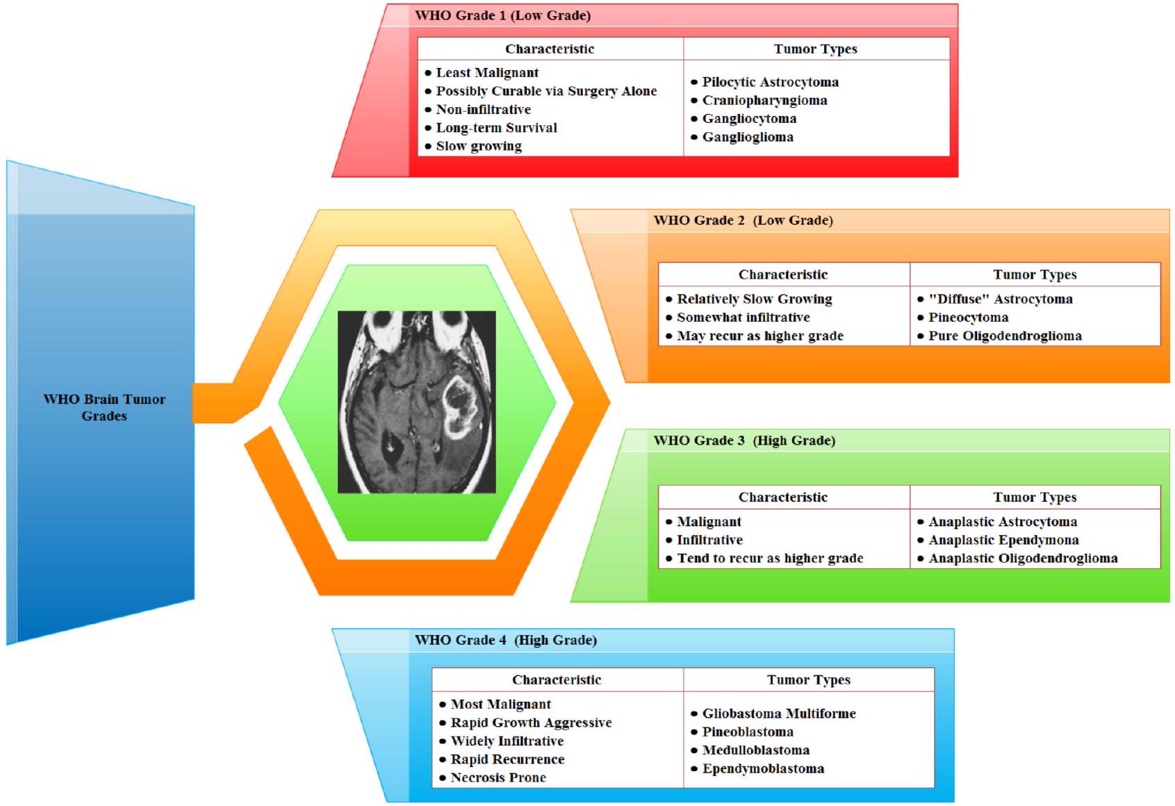
الشكل 1. تصنيف الأورام الدبقية في الطبعة الرابعة من منظمة الصحة العالمية
المستخدمة هي شبكة التلافيف الحجمية ثنائية الأبعاد. لمعالجة مناطق الورم المقسمة وتوقع أيام البقاء، من المحتمل أن تستخدم طبقات تلافيف ثنائية الأبعاد. يمكن أن تستخرج الشبكة العصبية المكررة تمثيلات ذات مغزى من بيانات الورم من خلال استخدام تقنيات التعلم العميق. تحلل هذه الدراسة بيانات أورام الدماغ من صور الرنين المغناطيسي باستخدام خوارزميات التعلم العميق المتطورة. تحاول الدراسة توقع أيام بقاء المرضى من خلال استخدام نماذج تنبؤية، وتقسيم مواقع الأورام، واستخراج الخصائص المهمة، مما سيوفر معلومات هامة لاتخاذ القرارات السريرية.
تستخدم هذه الدراسة مجموعة متنوعة من أنماط التصوير بالرنين المغناطيسي (MRI)، بما في ذلك التصوير بالرنين المغناطيسي المعتمد على استعادة الانعكاس السائل، والتصوير بالرنين المغناطيسي المعتمد على كثافة البروتون، والتصوير بالرنين المغناطيسي المعتمد على T2، والتصوير بالرنين المغناطيسي المعتمد على T1، لتحديد أورام الدماغ. يعتمد العلاج الفعال لأورام الدماغ على الكشف المبكر. يتطلب الأمر دراسة إشعاعية عندما يكون هناك اشتباه سريري في وجود ورم دماغي لتحديد الموقع الدقيق، ومدى التأثير على المناطق المجاورة. بناءً على هذه المعلومات، يمكن تحديد العلاج الأنسب، سواء كان جراحة، أو علاج إشعاعي، أو علاج كيميائي. يمكن أن يزيد الكشف المبكر عن الورم بشكل كبير من فرص بقاء المريض. يوضح الشكل 2 التصور لفحص الرنين المغناطيسي متعدد الأنماط للدماغ.
يمكن سرد المساهمة الكبيرة التي قدمتها الدراسة البحثية المعنية كما يلي:
- من المحتمل أن تسهم الورقة في مجال تحليل أورام الدماغ من خلال اقتراح منهجية تتضمن استخراج ميزات ذات مغزى بمساعدة الشبكة العصبية المكررة من صور الرنين المغناطيسي للدماغ. هذه خطوة حاسمة في تشخيص وفهم أورام الدماغ.
- شبكات الالتفاف الحجمية، التي تعالج البيانات ثلاثية الأبعاد، ذات صلة خاصة بتحليل الصور الطبية مثل فحوصات الرنين المغناطيسي. يقدم هذا البحث طرقًا لاستخدام مثل هذه الشبكات لتقسيم أورام الدماغ بدقة وكفاءة.
- تنبؤ أيام البقاء بناءً على الصور الطبية وبيانات المرضى هو مهمة صعبة لها تداعيات سريرية كبيرة. قد تسهم الورقة من خلال اقتراح نموذج قائم على التعلم العميق يتنبأ بنتائج البقاء، مما يمكن أن يساعد المتخصصين الطبيين في تخطيط العلاج وإدارة المرضى.
بقية هذه المقالة منظمة كما هو موضح في الشكل 3 على النحو التالي. القسم العمل المتعلق يقدم مراجعة للأبحاث السابقة ذات الصلة. في القسم المواد والمنهجية المعدلة، نستعرض المواد والمنهجية التي استخدمناها في دراستنا. القسم قياس المعلمات والنتائج التجريبية مخصص لتقديم المعلمات القياسية والنتائج التجريبية. القسم المناقشة يتضمن مناقشة لنتائجنا ومقارنة مع النماذج الموجودة. أخيرًا، في القسم الخاتمة، نختتم عملنا بأفكار ختامية واقتراحات للتحسينات المستقبلية.
الأعمال ذات الصلة
البحث
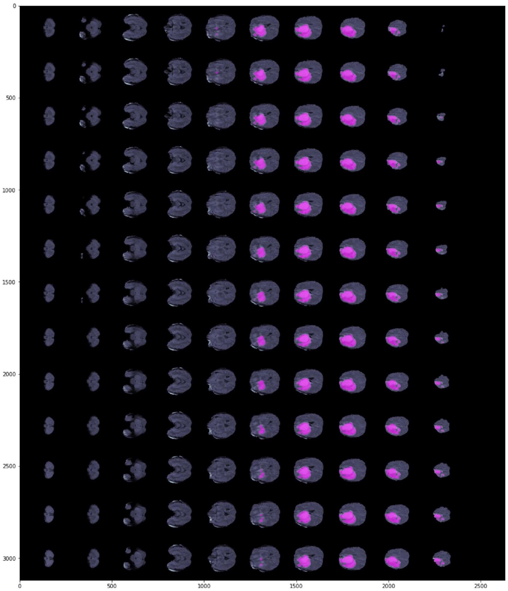
مسحات متعددة الأنماط – البيانات | قناع مقسم يدويًا – الهدف
الشكل 2. تصور لفحص متعدد الأنماط لتصوير الرنين المغناطيسي للدماغ.
الشكل 3. تنظيم الورقة.
وتمت مقارنة نماذج Vanilla Unet مع نموذج UnetResNext-50 بالإضافة إلى الأساليب المتطورة. درجة DICE لنموذج UnetResNext-50 هي 95.73، ولديه
تم استخدام شبكة عصبية تلافيفية (CNN) في الدراسة
معدل الدقة
معدل الدقة
هدف البحث المبلغ عنه في المنشور
المقال
تمت دراسة عدة تقنيات لاستخراج الميزات وتصنيف صور الرنين المغناطيسي في هذا العمل.
هذه الدراسة
الشبكات العصبية هي تقنية أخرى تم اقتراحها في هذا المجال.
وفقًا للدراسات
تُقدم الورقة استراتيجية لتصنيف أورام الدماغ باستخدام مزيج من تحليل المكونات الرئيسية، ونواة RBF، وخوارزميات SVM.
يمكن تقسيم أورام الدماغ وتصنيفها بدقة باستخدام تقنية موصوفة في
لكشف عن سرطانات الدماغ في صور الرنين المغناطيسي، يجمع B-CNN
الهدف الرئيسي من الدراسة الموصوفة في
مع بوابات الانتباه في نموذج U-Net الحالي. تُستخدم مسارات البداية المتبقية لربط خرائط ميزات الترميز وفك التشفير لتقليل المسافة بينها. كما يتم معالجة مشكلة عدم توازن الفئات باستخدام مزيج من دالة خسارة الانتروبيا المتقاطعة، وGDL، ودوال خسارة Tversky المركزة.
مع بوابات الانتباه في نموذج U-Net الحالي. تُستخدم مسارات البداية المتبقية لربط خرائط ميزات الترميز وفك التشفير لتقليل المسافة بينها. كما يتم معالجة مشكلة عدم توازن الفئات باستخدام مزيج من دالة خسارة الانتروبيا المتقاطعة، وGDL، ودوال خسارة Tversky المركزة.
تم تقديم نهج آخر لتصنيف سرطان الدماغ في
في هذا البحث
تتمثل هذه الدراسة
استنادًا إلى تحليل الأبحاث ذات الصلة، تم تحديد القيود التالية:
- يمكن أن تظهر أورام الدماغ مجموعة واسعة من الخصائص تشمل الحجم، والشكل، والملمس، والشدة. يمكن أن يشكل التعامل مع هذا التنوع بشكل فعال في طرق استخراج الميزات والتقسيم تحديات.
- تكون الصور الطبية، مثل مسحات الرنين المغناطيسي، عرضة لوجود اضطرابات وفنون، مما قد يؤثر على دقة تقنيات التقسيم. علاوة على ذلك، يتم الحصول على صور أورام الدماغ باستخدام تسلسلات رنين مغناطيسي مميزة (مثل T1-weighted، T2-weighted، FLAIR)، كل منها يوفر معلومات مميزة.
- يمكن أن تعقد التباين بين أوضاع التصوير المختلفة عملية التقسيم. في السيناريوهات التي تتسلل فيها الأورام إلى الأنسجة السليمة، يمكن أن تكون حدود الورم غير واضحة، مما يجعل تحديد الحدود بدقة مشكلة.
- تنبؤ البقاء على قيد الحياة لدى مرضى أورام الدماغ هو مسعى معقد مصحوب بعدد من الصعوبات. إن الاختيار الدقيق للميزات ذات الصلة لتوقع البقاء هو أمر بالغ الأهمية. ومع ذلك، فإن تحديد الميزات الأكثر إفادة من مزيج غير متجانس من البيانات السريرية وصور الأشعة يمكن أن يكون معقدًا.
استخدمت هذه الورقة نهجًا هجينًا يستخدم شبكة عصبية مكررة ثلاثية الأبعاد مستوحاة من التعلم العميق وشبكة تلافيفية حجمية ثنائية الأبعاد لاستخراج الميزات والتقسيم لتوقع بقاء المرضى. استنادًا إلى النتائج، يقترح الباحثون أن طريقتهم مناسبة للتكامل مع أنظمة دعم القرار السريري لمساعدة المتخصصين الطبيين أو أطباء الأشعة في الفحص الأولي والتشخيص.
المواد والمنهجية المعدلة لتحديد مجموعة بيانات الصور
في هذا البحث، نقيم فعالية طريقة استخراج الميزات والتقسيم المقترحة باستخدام مجموعة بيانات BraTS2020، التي تتكون من 368 مسحة رنين مغناطيسي للدماغ مع تسميات، كل منها بحجم
يتم عرض تصور صور الرنين المغناطيسي وأقنعتها باستخدام قيم صورة فريدة، وقيم دنيا وعليا، وقيم قناع فريدة في الشكل 5. بالنسبة لمجموعة بيانات صور الرنين المغناطيسي المستخدمة في هذه الدراسة، كان لدى صورة واحدة 1202 قيمة فريدة، مع قيم صورة دنيا وعليا تبلغ 0 و1. تم إعطاء عدد قيم القناع الفريدة كـ (array ([0., 1.], dtype
الشكل 4. تصور أوضاع التصوير: T1C (T1-weighted المعزز بالتباين)، T1 (T1-weighted)، FLAIR (استعادة التخفيف السائل)، T2 (T2-weighted).
الشكل 5. تصور صورة الرنين المغناطيسي والقناع.
المعالجة المسبقة
الهدف الرئيسي من المعالجة المسبقة هو تحسين وضوح صور الرنين المغناطيسي وتحويلها إلى تنسيق يمكن معالجته بواسطة البشر أو أنظمة التعلم الآلي. كما تحسن المعالجة المسبقة الجودة البصرية لصور الرنين المغناطيسي من خلال تعزيز نسبة الإشارة إلى الضوضاء، وإزالة العناصر الخلفية غير المرغوب فيها والضوضاء، وتنعيم داخل المناطق، والحفاظ على حوافها. تحتوي مجموعة بيانات BRATS 2020 على 368 صورة رنين مغناطيسي بتنسيق nii. نظرًا لقيود الذاكرة، استخدمت هذه الدراسة 150 صورة رنين مغناطيسي للتجربة، والتي تم تقسيمها إلى ثلاثة أجزاء للتدريب والاختبار والتحقق (
مع استخراج الميزات. تم استخدام تقنية قياس MinMax لإجراء التطبيع. يتشارك التطبيع والتوحيد نفس المفهوم الأساسي المتمثل في ضبط المتغيرات التي يتم تقييمها على مقاييس مختلفة لمنع التحيز في ملاءمة النموذج ووظائف التعلم. لذلك، يتم عادةً إجراء التطبيع على مستوى الميزات، مثل قياس MinMax، قبل ملاءمة النموذج. في قياس MinMax، يتم تحويل المتغيرات المدخلة إلى النطاق [ 0،1 ]، حيث تكون 0 و1 هي القيم القصوى والدنيا لكل ميزة/متغير. يتم إعطاء الصيغة الرياضية لقياس minmax في المعادلة 1.
مع استخراج الميزات. تم استخدام تقنية قياس MinMax لإجراء التطبيع. يتشارك التطبيع والتوحيد نفس المفهوم الأساسي المتمثل في ضبط المتغيرات التي يتم تقييمها على مقاييس مختلفة لمنع التحيز في ملاءمة النموذج ووظائف التعلم. لذلك، يتم عادةً إجراء التطبيع على مستوى الميزات، مثل قياس MinMax، قبل ملاءمة النموذج. في قياس MinMax، يتم تحويل المتغيرات المدخلة إلى النطاق [ 0،1 ]، حيث تكون 0 و1 هي القيم القصوى والدنيا لكل ميزة/متغير. يتم إعطاء الصيغة الرياضية لقياس minmax في المعادلة 1.
تُعرف نماذج التعلم العميق بأدائها الاستثنائي، لكنها تأتي مع بعض العيوب. أحدها هو أنها عرضة للضوضاء، مما يعني أن هناك حاجة إلى معالجة مسبقة شاملة لكل إدخال مرئي. لتطبيع صور الرنين المغناطيسي مع جميع الخصائص، تم اتباع خطوات المعالجة المسبقة لعمليات التقسيم والكشف الموضحة في الشكل 6.
الخطوة 1. للبدء، تحتوي جميع الأنماط والحقيقة الأساسية على أحجام ثلاثية الأبعاد لها أبعاد
الخطوة 2. يؤدي تقطيع هذه الأحجام إلى 155 صورة ثنائية الأبعاد بقياس
الخطوة 3. من كل حجم، يتم اختيار 90 جزءًا تتراوح من 30 إلى 120.
الخطوة 4. أخيرًا، يتم تقليل كل نمط من أنماط الرنين المغناطيسي إلى أبعاد
يمثل الشكل 7 الرسم البياني للتوزيع للتدريب والاختبار والتحقق.
الخطوة 2. يؤدي تقطيع هذه الأحجام إلى 155 صورة ثنائية الأبعاد بقياس
الخطوة 3. من كل حجم، يتم اختيار 90 جزءًا تتراوح من 30 إلى 120.
الخطوة 4. أخيرًا، يتم تقليل كل نمط من أنماط الرنين المغناطيسي إلى أبعاد
يمثل الشكل 7 الرسم البياني للتوزيع للتدريب والاختبار والتحقق.
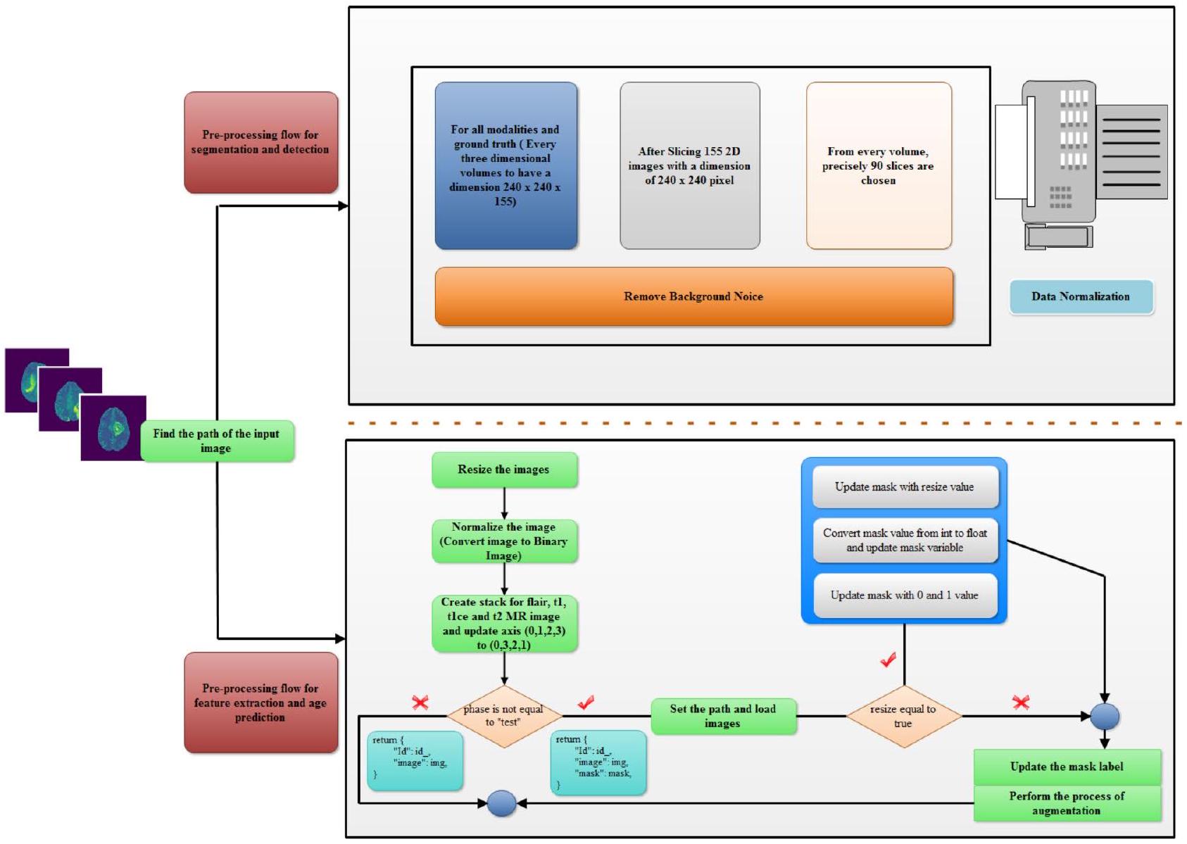
الشكل 6. سير العمل للمعالجة المسبقة.
توزيع بيانات صورة الرنين المغناطيسي BRATS 2020
الشكل 7. الرسم البياني للتوزيع لمجموعة بيانات BRATS 2020.
الكود الزائف لتنفيذ الفئة لمجموعة بيانات BRATS – المعالجة المسبقة لعملية استخراج الميزات
الوصف: هنا مجموعة البيانات هي مجموعة من صور الرنين المغناطيسي التي ستستخدم في عملية المعالجة المسبقة
التهيئة (مثيل من الفئة، إطار البيانات، المرحلة، عملية تغيير الحجم)
الوصف: هنا ستتم عملية التهيئة للمعالجة المسبقة
تعيين مثيل من الفئة
تعيين المرحلة لمجموعة البيانات
تعيين متغير التAugmentation للتهيئة مع استدعاء الدالة للمرحلة المعطاة
تعيين أنواع البيانات لصور مجموعة البيانات
تعيين متغير تغيير الحجم للصور
تعيين المرحلة لمجموعة البيانات
تعيين متغير التAugmentation للتهيئة مع استدعاء الدالة للمرحلة المعطاة
تعيين أنواع البيانات لصور مجموعة البيانات
تعيين متغير تغيير الحجم للصور
الطول (مثيل من الفئة)
الوصف: هنا للعثور على الشكل في إطار البيانات
إرجاع قيمة الشكل في إطار البيانات
Fetch_Images(مثيل من الفئة، معرف للصور)
تعيين معرف لموقع صور BRATS
تعيين root_path لجلب القيمة
تعيين متغير للصور لتحميل جميع الأنماط
لكل data_type في class_instance.data_types
تعيين image_path حسب أنواع البيانات المعطاة
تعيين متغير img لتحميل الصور من image_path
إذا كانت class_instance.resize صحيحة، إذن
تحديث img بحجم الصورة الجديد
تحميل القيمة في img بعد استدعاء دالة class_instance.normalize مع القيمة المعطاة كمعامل
إضافة جميع الصور
إنشاء كومة للصور
تحديث المحور
إذا كانت class_instance.phase لا تساوي القيمة المرسلة، إذن
تعيين متغير mask_path باستخدام قيمة .seg لصورة الرنين المغناطيسي
تعيين متغير mask لتحميل القيمة المقسمة
إذا كانت class_instance.resize صحيحة، إذن
تحديث mask بقيمة تغيير الحجم
تحويل قيمة mask من int إلى float وتحديث متغير mask
تحديث mask بقيمة 0 و 1
استدعاء الدالة لتحديث تسمية mask
تنفيذ عملية التAugmentation
تعيين img و mask لقيمة الصورة و mask المعززة
إرجاع قيمة المعرف والصورة و mask
إرجاع المعرف والصورة
تحديث mask بقيمة 0 و 1
استدعاء الدالة لتحديث تسمية mask
تنفيذ عملية التAugmentation
تعيين img و mask لقيمة الصورة و mask المعززة
إرجاع قيمة المعرف والصورة و mask
إرجاع المعرف والصورة
Load_Images(class_instance، مسار الملف)
الوصف: هذه الدالة لتحميل جميع الصور وتحويلها إلى شكل مصفوفة
تعيين متغير البيانات لتحميل قيمة مسار الملف
تحديث متغير البيانات بعد تحويله إلى مصفوفة
إرجاع قيمة البيانات
تعيين متغير البيانات لتحميل قيمة مسار الملف
تحديث متغير البيانات بعد تحويله إلى مصفوفة
إرجاع قيمة البيانات
Normalize_data(class_instance، البيانات كشكل مصفوفة)
الوصف: هذه الدالة مخصصة لتطبيع البيانات وفقًا للقيمة الدنيا والقصوى للصور
تعيين datamin للقيمة الدنيا للبيانات
إرجاع قيمة التعبير [(data – datamin)/(max(data) – datamin]
إرجاع قيمة التعبير [(data – datamin)/(max(data) – datamin]
Preprocess_label_mask(class_instance، mask كمصفوفة)
الوصف: تحديث قيمة mask لكائن WT و TC و ET
تحديث قيمة mask للورم الكلي بقيمة 0 و 1
تحديث قيمة mask لنواة الورم بقيمة 0 و 1
تحديث قيمة mask للورم المعزز بقيمة 0 و 1
إنشاء كومة لقيمة mask لـ WT و TC و ET
تحديث المحور لقيمة mask
إرجاع قيمة mask
تحديث قيمة mask للورم الكلي بقيمة 0 و 1
تحديث قيمة mask لنواة الورم بقيمة 0 و 1
تحديث قيمة mask للورم المعزز بقيمة 0 و 1
إنشاء كومة لقيمة mask لـ WT و TC و ET
تحديث المحور لقيمة mask
إرجاع قيمة mask
بنية الشبكة وطريقة التدريب لاستخراج الميزات والتقسيم والكشف
منهجية الشبكة العصبية المكررة ثلاثية الأبعاد
الشبكة العصبية المكررة هي نوع من الشبكات العصبية التغذوية التي تعيد بناء المخرجات باستخدام نفس المدخلات. أولاً، تقلل من أبعاد المدخلات ثم تنشئ المخرجات بناءً على تلك التمثيلات. تُستخدم الشبكة العصبية المكررة بشكل متكرر للتعلم غير المراقب لأنها يمكن أن تساعد في تحديد العلاقات الخفية داخل البيانات وتقديمها في شكل أكثر إيجازًا. من خلال تحويل مشكلات التعلم غير المراقب إلى خوارزميات التعلم المراقب، يمكن تدريب الشبكة العصبية المكررة لتحديد الأنماط داخل البيانات.
تُمرر المدخلات إلى المخرجات، وتقوم شبكة التشفير بضغط المدخلات إلى شكل مشفر أصغر. في الوقت نفسه، تقوم شبكة فك التشفير بفك تشفير التشفير لإعادة بناء المدخلات
تُمرر المدخلات إلى المخرجات، وتقوم شبكة التشفير بضغط المدخلات إلى شكل مشفر أصغر. في الوقت نفسه، تقوم شبكة فك التشفير بفك تشفير التشفير لإعادة بناء المدخلات
تولد طبقة التشفير نسخة ذات أبعاد أقل من المعلومات، مما يكشف عن اتصالات معقدة ومثيرة للاهتمام داخل البيانات. يوضح الشكل 8 مكونات الشبكة العصبية المكررة.
- المشفّر: المكون الشبكي المعروف باسم المشفر يستقبل المدخلات وينشئ تشفيرًا بأبعاد أقل يُعرف باسم المشفر.
- نقطة الاختناق: الطبقة المخفية ذات الأبعاد الأقل هي مصدر التشفير. يتم تقليل عدد العقد الموجودة في طبقة نقطة الاختناق، كما تحدد كيفية تشفير المدخلات من حيث الأبعاد.
- فك التشفير: يستقبل فك التشفير المدخلات ويعيد بناءها باستخدام التشفير.
الهايبر بارامترات:
- حجم الكود: يشير إلى عدد عقد الطبقة الوسيطة، حيث تؤدي العقد الأقل إلى مزيد من الضغط.
- عدد الطبقات: يوضح عدد الطبقات التي تشكل الشبكة لفك التشفير والمشفّر.
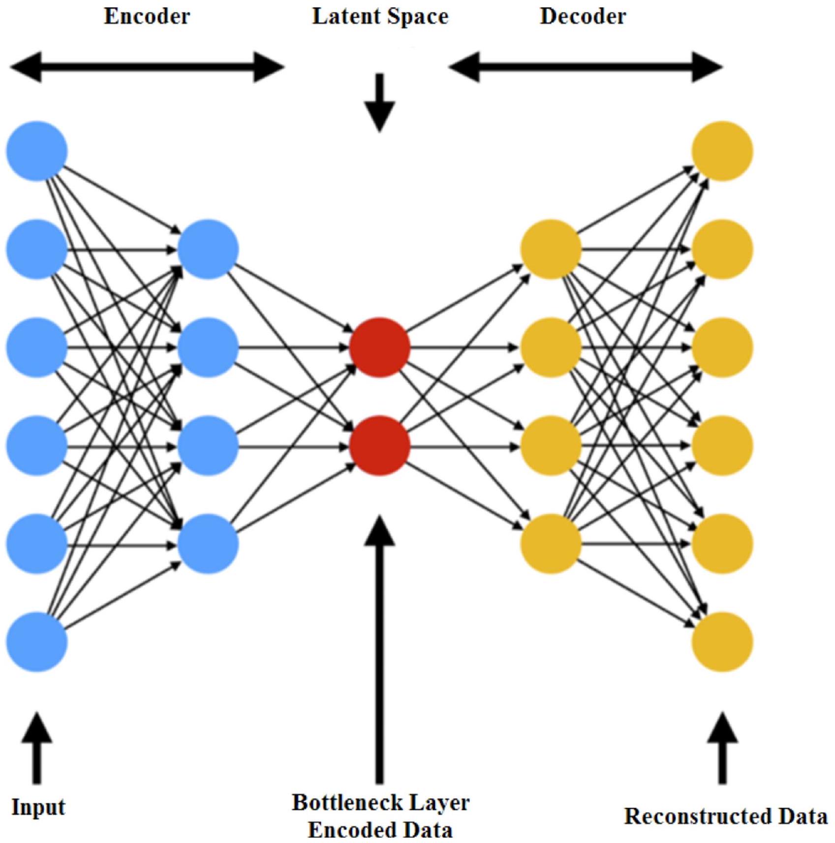
الشكل 8. مكون الشبكة العصبية المكررة مع الفضاء الكامن
- عدد العقد لكل طبقة: الشبكة العصبية المكررة الموضحة في الصورة السابقة هي شبكة تشفير متراكمة، مما يعني أن عدد العقد لكل طبقة ينمو في فك التشفير المتماثل بينما ينخفض في الطبقات التالية من المشفر.
- دالة الخسارة: تُستخدم دالة الانتروبيا المتقاطعة عادةً إذا كانت قيم المدخلات ضمن النطاق
، وإلا يجب استخدام متوسط الخطأ التربيعي.
وفقًا للعناصر التالية، يتم وصف الشبكة العصبية المكررة: فضاءات التعليمات المفككة
هناك مكونان رئيسيان من الوظائف التي تم تهيئتها: عائلة المشفرين
غالبًا ما نكتب
عادةً ما يتم استخدام الإدراك متعدد الطبقات لتصميم كل من المشفر وفك التشفير. كمثال، المشفر MLP ذو الطبقة الواحدة
تشير مصطلح “الوزن” إلى مصفوفة ممثلة بـ W، و”التحيز” يشير إلى متجه يُشار إليه بـ b، و”دالة التنشيط”، التي يُرمز إليها بـ
تدريب الشبكة العصبية المكررة
يتكون تدريب الشبكة العصبية المكررة ثلاثية الأبعاد المقترحة من مجرد مجموعة من عاملين بمفردها. يحتاج التدريب إلى مهمة من أجل تقييم جودته. يتم استخدام توزيع احتمالي مرجعي
تتيح لنا هذه العناصر بناء دالة خسارة الشبكة العصبية المكررة على النحو التالي
تكون الشبكة العصبية المكررة المقدمة للمهمة المفترضة (
المكونان الرئيسيان للشبكة العصبية المكررة هما مشفر يقوم بتحويل الاتصال إلى كود ومفكك يقوم باستخراج المعلومات من الكود. تحدد دالة جودة الاسترداد d “قريب من المثالي” كالأداء الذي يمكن أن تحققه شبكة عصبية مكررة مثالية من حيث الاستعادة.
التفسير
يوضح الشكل 9 كيف تفسر الشبكة العصبية المكررة ثلاثية الأبعاد لاستخراج الميزات النموذج؛ يتم عرض النموذج بعد أن خضعت المدخلات للمعالجة المسبقة والتطبيع، ولدى المشفر ثلاث طبقات تلافيفية، وثلاث طبقات تجميع، وطبقة خطية واحدة.
الخطوة 1 – التهيئة لتمثيل التشفير تكون على هذا النحو
الخطوة 2 – التهيئة لتمثيل فك التشفير تكون على هذا النحو
الخطوة 3 – لتنفيذ عملية ترميز إطار البيانات:
بعد عملية الطبقات المذكورة أعلاه، يعود نموذج الشبكة العصبية المكررة ثلاثية الأبعاد بالميزات التي سيتم فك تشفيرها في الخطوات التالية.
الخطوة 4 – هيكل الطبقات لفك التشفير وفقًا للميزات العائدة باستخدام فك الالتواء وعدم التجميع مثل ذلك:
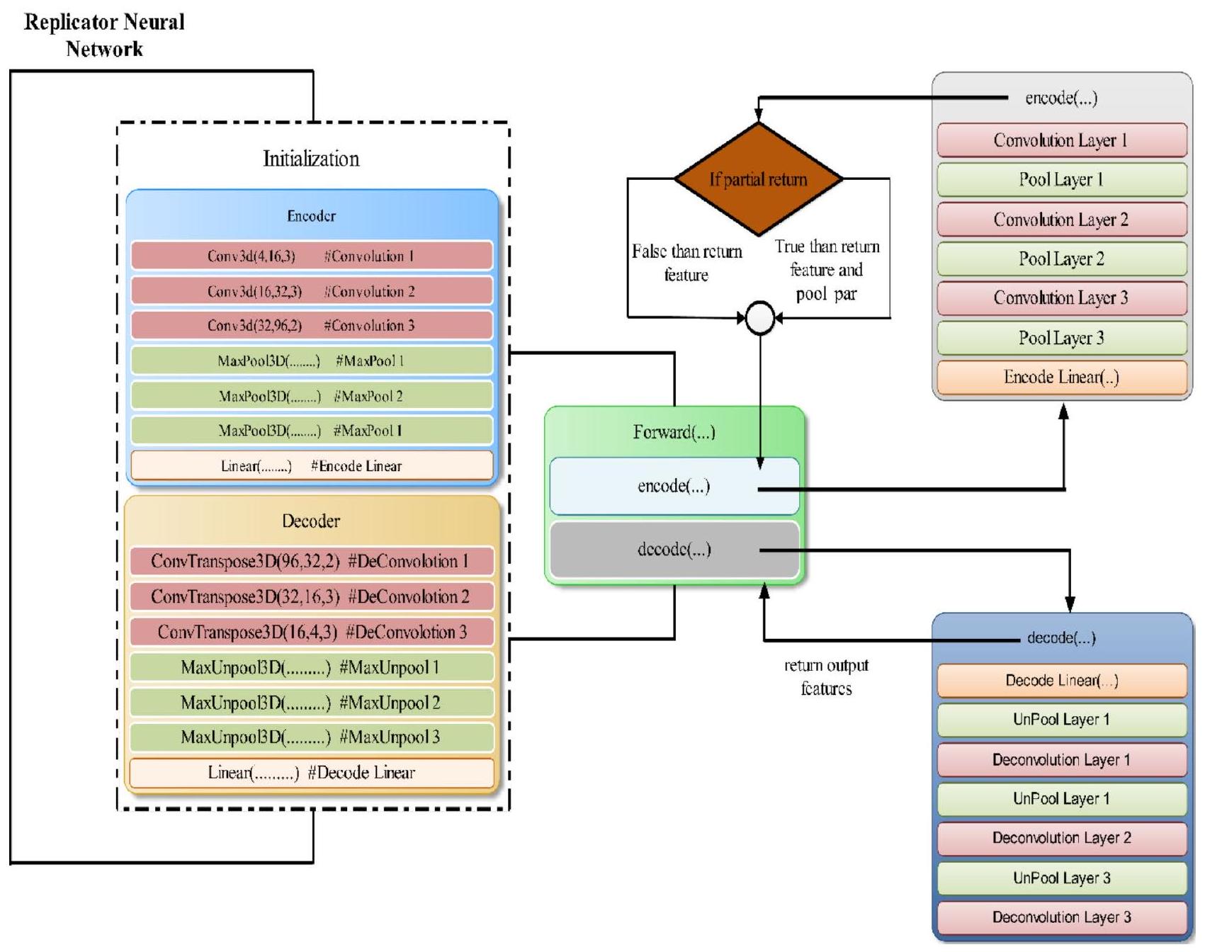
الشكل 9. تدفق عمل الشبكة العصبية المكررة ثلاثية الأبعاد.
Decoding_Linear → unpool $1 rightarrow$ deconv $1 rightarrow$ unpool $2 rightarrow$ deconv $2 rightarrow$ unpool $3 rightarrow$ deconv 3
منهجية الشبكة العصبية الالتفافية الحجمية ثنائية الأبعاد لتجزئة واكتشاف الورم
يوضح الشكل 10 تصور شبكتنا العصبية الالتفافية. تُستخدم العمليات الالتفافية لاستخراج الميزات من المعلومات، وبعد كل مرحلة، يتم تقليل دقة البيانات باستخدام خطوة مناسبة. الجانب الأيسر من الشبكة يضغط الإشارة، بينما الجانب الأيمن يفك ضغطها حتى تعود إلى حجمها الأصلي.
الجانب الأيسر من الشبكة.
في هذه الشبكة، يتعامل القسم الأيسر مع دقات مختلفة من بيانات الإدخال. تستخدم المراحل الثلاث الأولى طبقات التفاف لتحديد وظيفة متبقية، يتم تدريبها باستخدام إدخال من كل مرحلة، ثم تتم معالجتها بشكل غير خطي. تضمن هذه الوظيفة المتبقية التقارب، وهو ما لا يمكن تحقيقه في الشبكات التعليمية التقليدية بدون كتل متبقية. تستخدم عملية الالتفاف نواة حجمية بحجم فوكسي.
تلعب الوظيفة المتبقية دورًا محوريًا في تعزيز تقارب الشبكات العصبية العميقة، ويمكن فهم فعاليتها بشكل أفضل عند مقارنتها بمسار الضغط في شبكة الالتفاف الحجمية. في مثل هذه الشبكات، يقلل مسار الضغط من الدقة باستخدام الالتفافات بخطوة 2 و
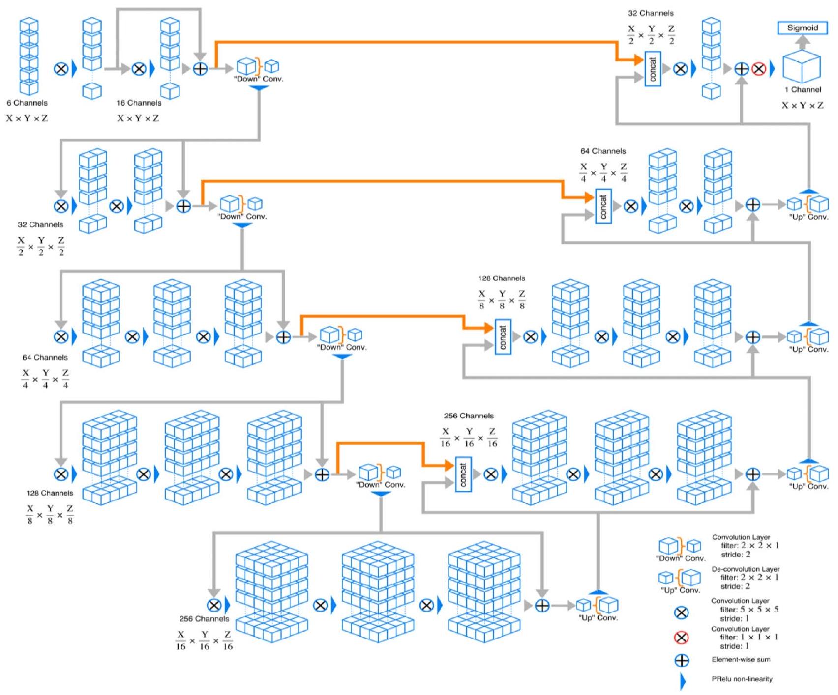
الشكل 10. هيكل الشبكة لشبكة الالتفاف الحجمية ثنائية الأبعاد.
إعادة صياغة المهمة إلى تعلم المتبقيات – الفروق بين المدخلات والمخرجات – بدلاً من التحولات الكاملة. تجعل هذه التبسيط الشبكة أكثر سهولة في التحسين، تمامًا كما أن تقليل العينة في مسار الضغط يوسع تركيز الشبكة. تسرع هذه الآلية أيضًا عملية التقارب، مما يسمح للشبكة بالتدريب بشكل أكثر كفاءة وفعالية. بشكل عام، تسهل الوظيفة المتبقية تقاربًا أفضل من خلال استقرار الانحدارات، وتبسيط التعلم، ومنع التدهور في الشبكات العميقة، وتحسين عملية التدريب.
يقلل هيكل الشبكة العصبية المكررة (RNN) من استخدام الذاكرة من خلال عدة آليات رئيسية. يقوم بترميز البيانات بكفاءة إلى تمثيل منخفض الأبعاد، مما يضغط بشكل كبير على بيانات الإدخال ويقلل من حجم التنشيطات الوسيطة. تتطلب عملية الترميز هذه موارد أقل مقارنةً بالبيانات الأصلية عالية الأبعاد. تستخدم الشبكة أيضًا مشاركة الوزن عبر الطبقات، مما يقلل من العدد الإجمالي للمعلمات التي تحتاج إلى التخزين. خلال التدريب، تمتد هذه الكفاءة إلى تقليل تخزين التنشيط ومتطلبات ذاكرة الانتشار العكسي الأكثر قابلية للإدارة.
الجانب الأيمن من الشبكة.
من خلال استخراج الميزات وزيادة التغطية الجغرافية لخرائط الميزات ذات الدقة المنخفضة، تحاول الشبكة جمع وتوليف البيانات اللازمة لإنتاج تجزئة حجمية ذات قناتين. يتم زيادة حجم إدخال كل مستوى باستخدام إجراء فك الالتواء، والذي يرافقه من عملية التفاف واحدة إلى ثلاث عمليات، كل منها تحتوي على نصف عدد 555 نواة مثل الطبقة التي تسبقها. تمامًا كما يتم تعليم النصف الأيسر من الشبكة، يتم تعليم الوظيفة المتبقية. يتم إنتاج خريطتين ميزات بنفس حجم الحجم المصدر وقوة نواة 111 من قبل آخر طبقة التفاف. يتم تقسيم المناطق الخلفية والأمامية بشكل احتمالي إلى هاتين الخريطتين الناتجتين باستخدام طريقة فوكسي ناعمة.
الاتصال الأفقي.
تخسر عملية الضغط في الشبكة العصبية الالتفافية معلومات الموقع، كما هو موضح في الجانب الأيسر. لحل هذه المشكلة، يتم دمج الاتصالات الأفقية لنقل العناصر من المراحل المبكرة من القسم الأيسر للشبكة العصبية الالتفافية إلى الجزء الأيمن. لا يعزز هذا فقط دقة توقع الشكل النهائي ولكن أيضًا يوفر
معلومات موضع دقيقة للمكون الأيمن. من خلال دمج هذه الاتصالات، يتم تسريع وقت التقارب للنموذج.
معلومات موضع دقيقة للمكون الأيمن. من خلال دمج هذه الاتصالات، يتم تسريع وقت التقارب للنموذج.
خطوة من تدفق العملية.
الخطوة 1 صورة الإدخال لمعالجة البيانات المسبقة
- كل حجم ثلاثي الأبعاد بحجم
متاح لجميع الأنماط والحقيقة الأرضية. - بعد التحويل إلى صور ثنائية الأبعاد، سيكون هناك 155 صورة، كل منها بأبعاد
بكسل. - من بين هذه الشرائح الـ 155، يتم اختيار 90 شريحة تتراوح من 30 إلى 120 من كل حجم.
- يتم تقليم جميع أنماط التصوير بالرنين المغناطيسي إلى
بكسل لإزالة ضوضاء الخلفية.
الخطوة 2 عملية تطبيع البيانات
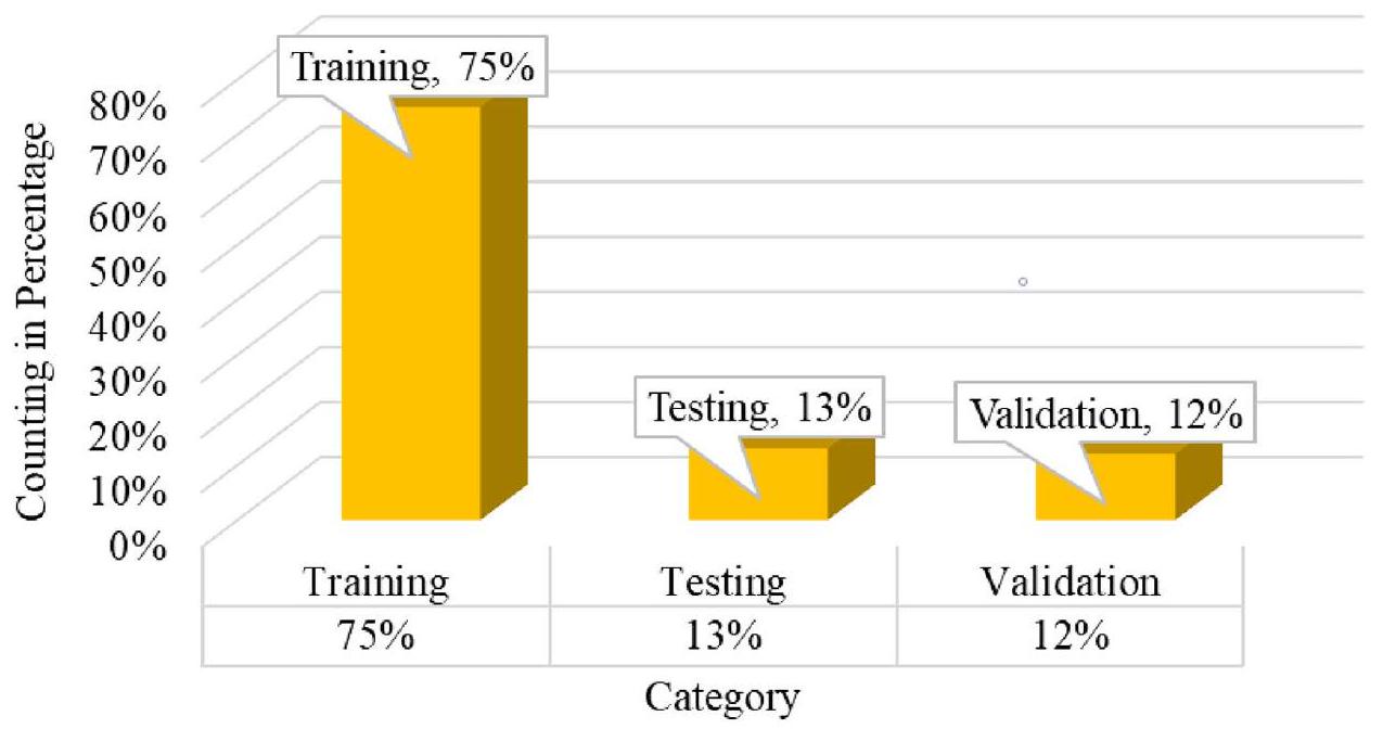
الخطوة 3 تقسيم البيانات المعيارية 75% بيانات التدريب، 13% بيانات الاختبار، 12% بيانات التحقق
الخطوة 4 تطبيق نموذج V-Net ثنائي الأبعاد (عملية الترميز وفك التشفير على البيانات المعيارية)
الخطوة 5 تطبيق نموذج التدريب على بيانات الاختبار وبيانات التحقق
الخطوة 3 تقسيم البيانات المعيارية 75% بيانات التدريب، 13% بيانات الاختبار، 12% بيانات التحقق
الخطوة 4 تطبيق نموذج V-Net ثنائي الأبعاد (عملية الترميز وفك التشفير على البيانات المعيارية)
الخطوة 5 تطبيق نموذج التدريب على بيانات الاختبار وبيانات التحقق
- العثور على معامل دايس
- العثور على الدقة
- العثور على قيمة الخسارة
الخطوة 6 التحقق من النتيجة للتنبؤ
تُستخدم وحدة الخطية المعادلة البارامترية (PReLU) كدالة تنشيط في الشبكات العصبية العميقة لمعالجة بعض القيود في دوال التنشيط التقليدية، مثل ReLU. تقدم PReLU معلمة صغيرة قابلة للتعلم للانحدار السلبي لدالة التنشيط، مما يسمح لها بتعلم أفضل انحدار بشكل تكيفي أثناء التدريب.
تُعرف PReLU على أنها
كيف تحسن PReLU أداء النموذج:
- تجنب الخلايا العصبية الميتة: من خلال السماح بانحدار صغير للقيم السلبية، تمنع PReLU الخلايا العصبية من أن تصبح غير نشطة، مما يضمن أن جميع الخلايا العصبية يمكن أن تساهم في التعلم طوال عملية التدريب. يساعد ذلك في الحفاظ على مجموعة أكثر تنوعًا من الميزات ويمنع الشبكة من أن تصبح نادرة جدًا.
- تعزيز التعلم: تعني قابلية التكيف لـ PReLU أن الشبكة يمكن أن تتعلم أفضل انحدار للقيم السلبية أثناء التدريب. يمكن أن تؤدي هذه المرونة إلى أداء أفضل للنموذج حيث تقوم الشبكة بتحسين دالة التنشيط الخاصة بها للمهمة المعطاة، مما يحسن قدرتها على التقاط الأنماط والعلاقات المعقدة في البيانات.
- تحسين تدفق الانحدار: تساعد الانحدارات غير الصفرية للمدخلات السلبية في الحفاظ على تدفق انحدار أكثر استقرارًا وفعالية أثناء الانتشار العكسي. تساعد هذه الاستقرار في تحديث الأوزان بشكل أكثر اتساقًا، مما يمكن أن يسرع من التقارب ويحسن كفاءة التدريب العامة.
- زيادة سعة النموذج: تزيد قدرة PReLU على تعلم انحدارات مختلفة للمدخلات الإيجابية والسلبية بشكل فعال من قدرة الشبكة على نمذجة الوظائف المعقدة. تسمح هذه المرونة المعززة للشبكة بالتكيف مع بيانات التدريب بدقة أكبر والتعميم بشكل أفضل على البيانات غير المرئية.
قياس المعلمات والنتائج التجريبية
تشير استخراج الميزات إلى التقنية المستخدمة للحصول على بيانات أكثر تفصيلاً حول الصورة، مثل نسيجها وشكلها وتباينها ولونها. يعتبر تحليل النسيج جانبًا حيويًا لكل من أنظمة التعلم الآلي والإدراك البصري البشري. من خلال اختيار الميزات المهمة، يمكن أن يعزز بشكل فعال دقة النظام التشخيصي. يمكن أن تكون الملاحظات والتحليلات النسيجية مفيدة في تقييم المراحل المختلفة للأورام (تصنيف الأورام) وللتشخيص. يتم تقديم الصيغة لبعض الجوانب الإحصائية ذات الصلة ونتائج التجارب أدناه.
المتوسط (M): يتم تحديد متوسط الجسم من خلال ضرب مجموع جميع قيم البكسل في الجسم بعدد البكسلات الكلي الموجودة في الجسم.
نتيجة تجريبية للمتوسط لمجموعة بيانات BRATS 2020 مع وزن t1 ووزن t1ce ووزن t2 وflair موضحة في الشكل 11.
الانحراف (Skn) الانحراف هو مقياس للتناظر أو عدمه. تعريف الانحراف لمتغير عشوائي X، يُمثل كـ
حيث SD هو الانحراف المعياري وسيتم تقييمه بهذه الطريقة
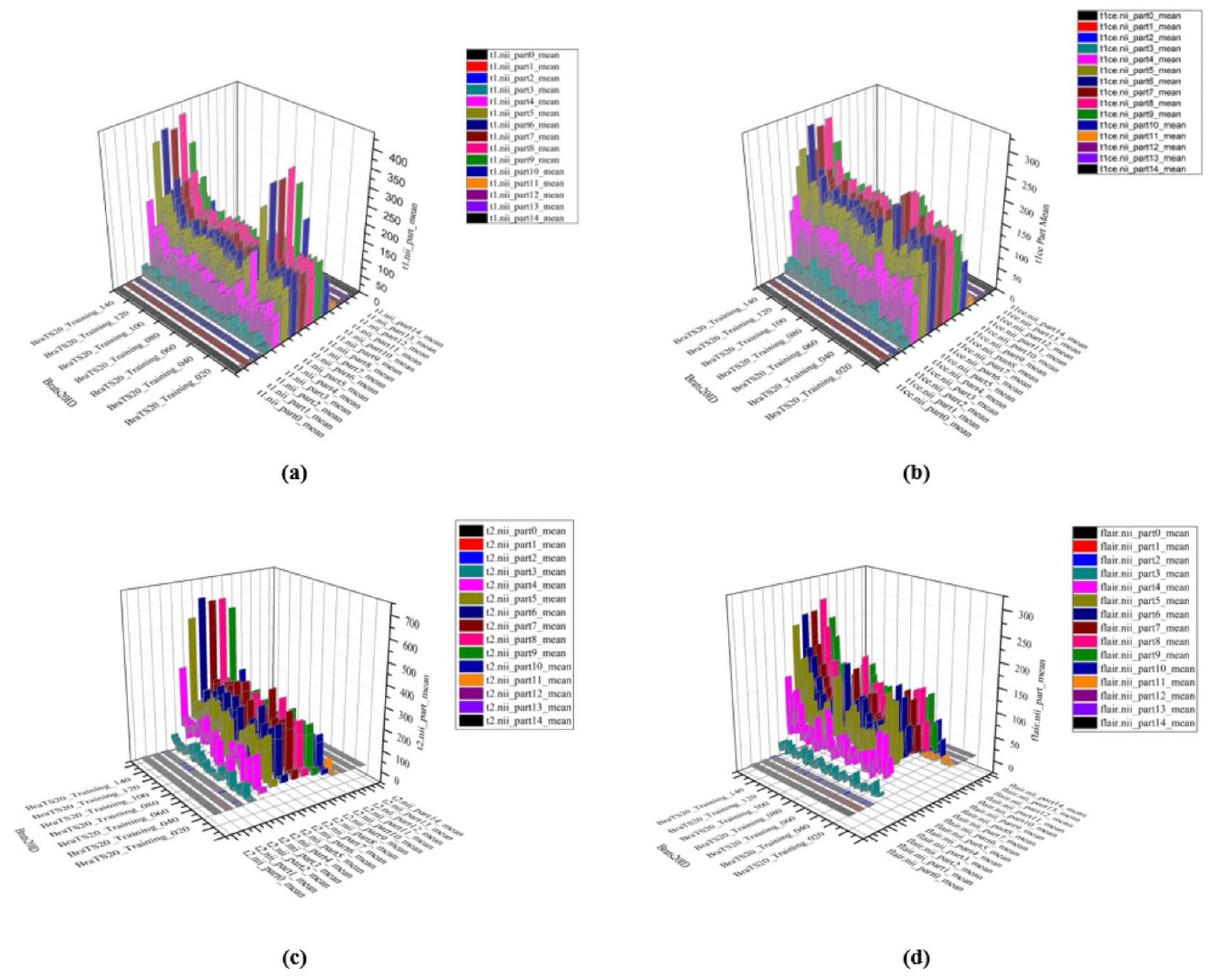
الشكل 11. نتيجة تجريبية للقيمة المتوسطة لمجموعة بيانات BRATS2020 MRI (أ) قيم الوزن t1 (ب) قيم الوزن t1ce (ج) قيمة الوزن t2 (د) قيمة flair.
نتيجة تجريبية للانحراف في مجموعة بيانات BRATS 2020 مع وزن t1 ووزن t1ce ووزن t2 وflair موضحة في الشكل 12a.
الكورتوز (Krt) يصف معلم الكورتوز شكل توزيع الاحتمالات لمتغير عشوائي. بالنسبة للمعرف العشوائي X، يتم تعريف الكورتوز على أنه
نتيجة تجريبية للكورتوزيس لمجموعة بيانات BRATS 2020 مع وزن t1 ووزن t1ce ووزن t2 وflair موضحة في الشكل 12b.
فرق الانحراف: يقيس فرق الانحراف التفاوت في عدم التماثل بين توزيعين احتماليين أو مجموعتين من البيانات. الانحراف نفسه يقيس مدى انحراف التوزيع عن التماثل حول متوسطه: الانحراف الإيجابي يشير إلى ذيل أطول على اليمين، بينما الانحراف السلبي يشير إلى ذيل أطول على اليسار. من خلال حساب الفرق في الانحراف بين مجموعتين من البيانات، يوفر فرق الانحراف رؤى حول كيفية مقارنة عدم تماثلهما. الشكل 12c يظهر النتيجة التجريبية لفرق الانحرافات لمجموعة بيانات BRATS 2020 مع وزن t1، وزن t1ce، وزن t2 وflair.
المسافة المكثفة هي مفهوم يُستخدم لقياس الفرق النسبي أو التشابه بين نقاط البيانات أو التوزيعات مع التحكم في المقياس والحجم. على عكس مقاييس المسافة التقليدية، التي غالبًا ما
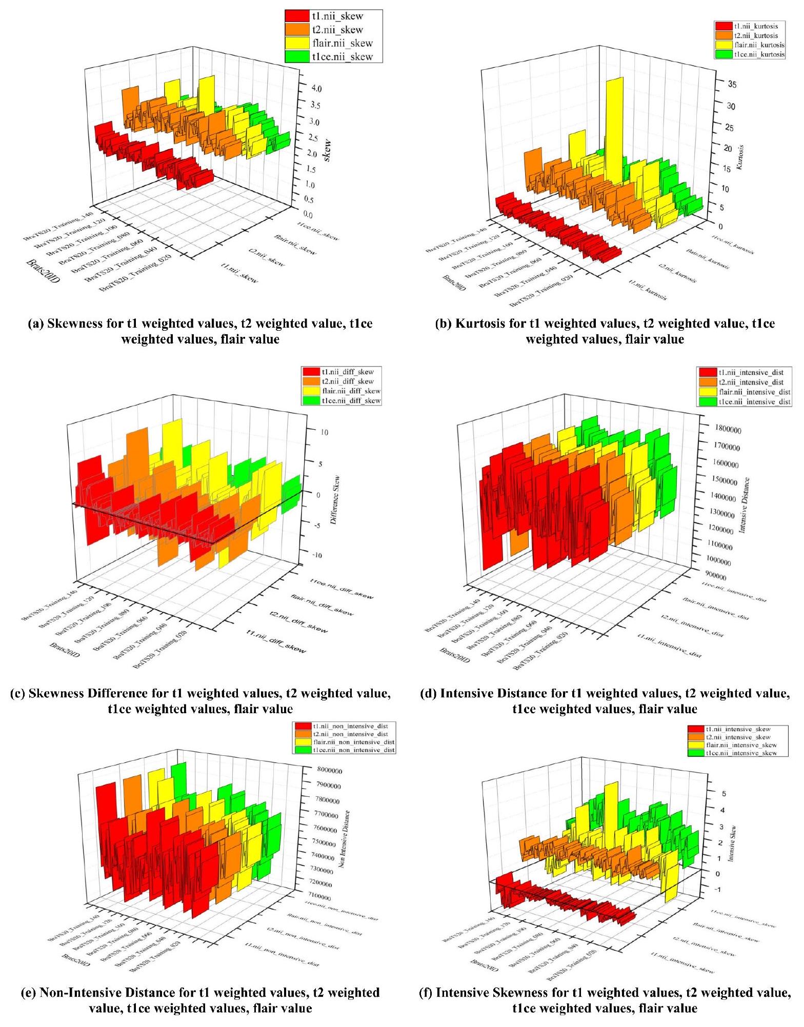
الشكل 12. رسم بياني لقيمة الميزات للانحراف، والتفرطح، والاختلافات الشديدة.
تأخذ الفروق المطلقة في الاعتبار وقد تتأثر بمقياس البيانات، بينما تركز المسافة المكثفة على الخصائص الجوهرية للبيانات من خلال تطبيعها أو تعديلها لتأثيرات المقياس.
تظهر الشكل 12d النتيجة التجريبية للتوزيع المكثف لمجموعة بيانات BRATS 2020 مع وزن t1، وزن t1ce، وزن t2 و flair.
المسافة غير المكثفة عن بُعد هي مفهوم يُستخدم لقياس المسافة بين نقاط البيانات أو التوزيعات دون الأخذ في الاعتبار التعديلات على المقياس أو التباين. على عكس المسافة المكثفة، التي تقوم بتطبيع المقياس لضمان مقارنات عادلة، تأخذ المسافة غير المكثفة في الاعتبار الفروقات الخام بين القيم أو الميزات مباشرة. لا يقوم هذا النهج بتعديل حجم أو توزيع البيانات، مما يجعله حساسًا للقيم المطلقة والمقياس. تُظهر الشكل 12e النتيجة التجريبية للتوزيع غير المكثف لمجموعة بيانات BRATS 2020 مع وزن t1 ووزن t1ce ووزن t2 وflair.
الانحراف المكثف هو قياس الانحراف لبيانات التوزيع المكثف. توضح الشكل 12f النتيجة التجريبية للانحراف المكثف لمجموعة بيانات BRATS 2020 مع وزن t1 ووزن t1ce ووزن t2 وflair.
الانحراف غير المكثف هو قياس الانحراف للبيانات ذات التوزيع غير المكثف. الشكل 13أ يظهر النتيجة التجريبية للانحراف غير المكثف لمجموعة بيانات BRATS 2020 مع وزن t1، وزن t1ce، وزن t2 وflair.
فرق الانحراف الكثيف للبيانات يقيم التباين الخام في الانحراف بين مجموعتين من البيانات، مما يعكس اختلافات عدم التماثل دون تعديل للقياس أو التطبيع. توضح الشكل 13b النتيجة التجريبية لفرق الانحراف الكثيف لمجموعة بيانات BRATS 2020 مع وزن t1 ووزن t1ce ووزن t2 وflair.
فرق انحراف البيانات غير الكثيفة هو الفرق بين انحراف البيانات والانحراف غير الكثيف. توضح الشكل 13c النتيجة التجريبية لفرق انحراف البيانات غير الكثيفة لمجموعة بيانات BRATS 2020 مع وزن t 1، وزن t 1 ce، وزن t 2 و flair.
الميزات الكامنة مجموعة من الكائنات مدمجة داخل فضاء متعدد الأبعاد يُعرف غالبًا بفضاء الميزات الكامنة أو فضاء التضمين (الشكل 13d). في الفضاء الكامن، يتم وضع العناصر الأكثر تشابهًا مع بعضها البعض بالقرب من بعضها. ببساطة، الفضاء الكامن هو تمثيل للبيانات المضغوطة، حيث تقع نقاط البيانات المتشابهة بالقرب من بعضها. الفضاء الكامن مفيد لاكتشاف تصورات أكثر بساطة للتحليل وكذلك لتعلم ميزات البيانات.
لتحقيق نتائج تقييم أفضل على صور الرنين المغناطيسي للدماغ، هناك حاجة إلى معايير تقييم جودة إضافية إلى المعايير المذكورة أدناه لتجزئة الصور.
الخسارة: طريقة لتقييم مدى فعالية برنامجك في نمذجة مجموعة البيانات الخاصة بك هي من خلال دالة الخسارة. إنها دالة رياضية لبارامترات خوارزمية التعلم العميق. في هذا العمل المقترح، يتم قياس أداء نموذج التقسيم من خلال خسارة الانتروبيا المتقاطعة. الرقم بين 0 و 1 يمثل الخسارة (أو الخطأ)، حيث يمثل 0 النموذج المثالي. بشكل عام، الهدف هو جعل نموذجك قريبًا من 0 قدر الإمكان. باستخدام الانتروبيا المتقاطعة، يمكننا قياس الخطأ (أو الفرق) بين توزيعين احتماليين.
على سبيل المثال، يتم توفير الانتروبيا المتقاطعة في سياق التصنيف الثنائي بواسطة:
حيث، p هو الاحتمال المتوقع و y هو المؤشر.
الدقة: هي إحصائية تُستخدم لتقييم فعالية النموذج عبر جميع الفئات. تكون مفيدة جدًا عندما تُعطى كل فئة وزنًا متساويًا. لحساب الدقة، يتم قسمة العدد الإجمالي للتخمينات الصحيحة على العدد الإجمالي للتوقعات.
الدقة: هي إحصائية تُستخدم لتقييم فعالية النموذج عبر جميع الفئات. تكون مفيدة جدًا عندما تُعطى كل فئة وزنًا متساويًا. لحساب الدقة، يتم قسمة العدد الإجمالي للتخمينات الصحيحة على العدد الإجمالي للتوقعات.
متوسط IOU: يحسب متوسط التقاطع على الاتحاد (MeanIoU) نسبة التداخل بين صندوقين محيطين إلى اتحاد مساحات الصناديق. تحتوي التنبؤات والحقائق الأرضية ضمن هذه الصناديق المحيطة. يمكن استخدام هذه المقياس لأي نهج يتنبأ بالصناديق المحيطة. صيغته الرياضية هي:
معامل ديس: تم استخدام معامل التشابه ديس (DSC) كمعيار للتحقق الإحصائي لتقييم تكرارية تقسيمات البشر ودقة تداخل المساحات لتقسيمات الصور بالرسم الاحتمالي الآلي لصور الرنين المغناطيسي. يقيس هذا المعامل مدى تشابه صورتين من خلال قسمة العدد الإجمالي للبكسلات في الصورتين على مساحة التداخل بين الصورتين المقسمتين.
الدقة: يتم قياس دقة النموذج من خلال نسبة العينات الإيجابية التي تم تصنيفها بشكل صحيح من جميع العينات التي تم تصنيفها على أنها إيجابية، بغض النظر عما إذا كانت مصنفة بشكل صحيح أو غير صحيح. من ناحية أخرى، تقيم الدقة مدى فعالية النموذج في تحديد عينة على أنها إيجابية.
الشكل 13. قيم رسم الميزة للانحراف غير المكثف، والانحراف المكثف، واختلافات الانحراف غير المكثف، والميزات الكامنة.
يرتفع المقام وتصبح الدقة منخفضة عندما يقوم النموذج بعمل العديد من التصنيفات الإيجابية الخاطئة أو عدد قليل من التصنيفات الإيجابية الصحيحة. ومع ذلك، تكون الدقة عالية عندما:
- يتم إجراء العديد من التصنيفات الإيجابية الدقيقة بواسطة النموذج (زيادة عدد الإيجابيات الحقيقية).
- يتم إجراء تصنيفات إيجابية أقل عدم دقة بواسطة النموذج (تقليل الإيجابيات الكاذبة).
الشكل 14. رسم تقييم كل عصر.
- التعميم عبر مجموعات سكانية متنوعة: قد يواجه النموذج صعوبة في التعميم بشكل جيد عبر مجموعات المرضى المتنوعة بسبب الاختلافات في خصائص الأورام والعوامل الوراثية وبروتوكولات العلاج. قد تؤدي هذه القيود إلى تقليل دقة النموذج عند تطبيقه على مجموعات المرضى الجديدة أو الممثلة تمثيلاً ناقصاً.
- مشكلات القابلية للتفسير: تعمل نماذج التعلم العميق، بما في ذلك الشبكات العصبية المكررة وشبكات الالتفاف الحجمية، غالبًا كـ “صناديق سوداء”، مما يجعل من الصعب فهم الأسباب وراء توقعاتها. يمكن أن تكون هذه القابلية المحدودة للتفسير عائقًا أمام الاعتماد السريري، حيث يحتاج الأطباء إلى الثقة والتحقق من مخرجات النموذج.
الشكل 15. يمكن تمثيل توقع النموذج بعد تقسيم الصورة إلى أجزاء في ثلاثة أشكال: (أ) صورة الورم الأصلية، (ب) منطقة الورم المتوقعة بواسطة النموذج، و(ج) منطقة الورم الحقيقية كما هو موضح في صور الحقيقة الأرضية.
- التحقق المحدود في البيئات الواقعية: بينما قد يؤدي هذا النهج بشكل جيد في بيئات البحث المنضبطة، إلا أنه قد لا يكون موثقًا بشكل واسع في بيئات سريرية متنوعة في العالم الحقيقي. قد يحد هذا الفجوة في التحقق من قابليته للتطبيق الفوري في الممارسة السريرية اليومية.
- المخاوف التنظيمية والأخلاقية: يثير استخدام نماذج الذكاء الاصطناعي المتقدمة في الرعاية الصحية قضايا تنظيمية وأخلاقية، بما في ذلك خصوصية المرضى، وأمان البيانات، والحاجة إلى التحقق الصارم قبل النشر السريري. إن التنقل عبر هذه المخاوف أمر ضروري ولكنه قد يكون تحديًا.
توزيع الأعمار المدورة في البيانات
الشكل 16. توزيع الأعمار المدورة في BRATS2020.
توزيع الأيام الباقية المستديرة في البيانات
الشكل 17. توزيع أيام البقاء المستديرة للمرضى كما هو موضح في BRATS 2020.
| خسارة | دقة | متوسط تقاطع الاتحاد | معامل دايس | دقة | |
| نتيجة التدريب | 0.097695 | 0.995166 | 0.616957 | 0.902311 | 0.995193 |
| نتيجة التحقق | 0.108875 | 0.994494 | 0.637059 | 0.891475 | 0.994538 |
| نتيجة الاختبار | 0.109715 | 0.994260 | 0.623013 | 0.889182 | 0.994220 |
الجدول 1. تقرير التقييم.
| مرجع | النموذج المستخدم | دقة | دي إس سي | خصوصية | حساسية |
| 1 | TPUAR-NET | – | 0.89 | 0.99 | – |
| ٦ | LDI-المعاني + المعلومات المتبادلة + تحليل القيم الفردية مع تقليل الأبعاد + SVM | 0.9102 | – | 0.9426 | 0.93 |
| ١٣ | في جي جي – 16 | – | 0.8892 | 0.9948 | 0.9 |
| 14 | شبكة CNN المعتمدة على U-Net | – | 0.878 | 0.993 | 0.87 |
| 26 | شبكة عصبية تلافيفية عميقة | – | 0.88 | 0.89 | 0.89 |
| 27 | 3D-يونت | – | 0.86 | 0.99 | 0.89 |
| ٢٨ | شبكة عصبية تلافيفية عميقة | – | 0.87 | 0.94 | 0.82 |
| 30 | وسائل فuzzy C Means الاحتمالية الكسرية (Fr-pFCM) + شبكة الاعتقاد العميق المعتمدة على تحسين سرب الحيتان والقطط (WCSO-DBN) | 0.923 | – | 0.96 | 0.84 |
| ٣٦ | وسائل فوزي الخاصة | – | 0.86 | – | 0.89 |
| ٣٤ | ريزنت 50 المحسن مع جرايدكام | 0.985 | – | – | 0.888 |
| ٣٩ | DeepMRSeg الأمثل + SPO + GAN + CAViaR-SPO. | 0.917 | – | 0.925 | 0.8884 |
| 41 | سي إن إن | – | 0.88 | – | 0.88 |
| ٤٨ | شبكة التوصيل العصبي المدفوعة بالتناظر | – | 0.87 | – | 0.928 |
| ٤٩ | التجميع الضبابي البايزي، تحويل التشتت (ST)، مقاييس نظرية المعلومات، تقنية الانحدار السلس، DAE | 0.985 | – | 0.995 | 0.95 |
| 52 | شبكة عصبية تلافيفية مصنوعة يدويًا | 0.95 | 0.91 | 0.96 | – |
| ٥٥ | شبكة متصلة على شكل حرف U عبر المستويات (CLCU-Net) | – | 0.885 | – | 0.96 |
| ٥٩ | شبكة عصبية تلافيفية كاملة + حقول عشوائية شرطية | – | 0.84 | – | – |
| المنهجية المقترحة | 0.9951 | 0.9023 | 0.9980 | 0.9950 |
الجدول 2. تحليل مقارن لتقنيات تقسيم أورام الدماغ في مجموعة بيانات BRATS المختلفة.
تنفيذ نهج استخراج ميزات ورم الدماغ القائم على التصوير بالرنين المغناطيسي، والتقسيم، وتوقع أيام البقاء باستخدام شبكة عصبية مقلدة مستوحاة من التعلم العميق وشبكة الالتفاف الحجمية يواجه عدة تحديات:
- تباين البيانات: يمكن أن تختلف بيانات الرنين المغناطيسي بشكل كبير عبر آلات وبروتوكولات ومؤسسات مختلفة. يمكن أن تؤثر هذه التباينات على أداء النموذج والتعميم، مما يتطلب تقنيات معالجة مسبقة وتطبيع قوية.
- تعقيد النموذج والحمل الحسابي: يمكن أن يكون الاستخدام المشترك لشبكة الأعصاب المكررة وشبكة الالتفاف الحجمية مكثفًا من الناحية الحسابية، خاصة عند معالجة مسحات الرنين المغناطيسي ثلاثية الأبعاد الكبيرة وعالية الدقة. إن ضمان تدريب واستدلال فعالين دون التضحية بالدقة هو تحدٍ رئيسي.
- بيانات مشروحة محدودة: تتطلب عملية تقسيم الأورام بدقة وتوقع البقاء على قيد الحياة مجموعات بيانات مشروحة جيدًا، والتي قد تكون نادرة. يمكن أن يحد نقص البيانات المعلّمة الكافية للتدريب من قدرة النموذج على التعميم، مما يجعل تقنيات مثل زيادة البيانات أو توليد البيانات الاصطناعية أمرًا حيويًا.
- الاندماج في سير العمل السريري: يتطلب تنفيذ هذا النهج في البيئات السريرية الواقعية دمج النموذج في أنظمة التصوير الطبي الحالية وضمان توافقه بسلاسة مع سير عمل الأطباء. يتطلب ذلك اعتبارات دقيقة لتصميم واجهة المستخدم وقدرات المعالجة في الوقت الحقيقي.
- قابلية التفسير والموثوقية: يحتاج الأطباء إلى الثقة في توقعات النموذج، خاصة في القرارات الحرجة مثل توقع البقاء. سيكون من الضروري ضمان أن تكون مخرجات النموذج قابلة للتفسير وتقديم رؤى حول كيفية إجراء التوقعات من أجل اعتمادها في الممارسة السريرية.
- الامتثال التنظيمي والتحقق: يجب أن يتوافق النموذج مع معايير تنظيمية صارمة وأن يخضع للتحقق الدقيق قبل استخدامه في البيئات السريرية. إن ضمان الامتثال للوائح الرعاية الصحية وإظهار سلامة وفعالية النموذج يمثلان عقبات كبيرة.
تواجه أنظمة التصوير الطبي الحالية العديد من القضايا العملية والمحتملة التي تؤثر على فعاليتها واندماجها في الممارسة السريرية:
- قابلية التوسع: تعاني العديد من أنظمة التصوير الطبي من صعوبة التوسع مع زيادة حجم البيانات وتعقيدها. مع تقدم تكنولوجيا التصوير، يجب أن تتمكن الأنظمة من التعامل مع مجموعات بيانات أكبر وأعلى دقة، مما قد يضغط على البنية التحتية الحالية ويتطلب ترقيات كبيرة.
- تحديات التكامل: غالبًا ما تعمل أنظمة التصوير الحالية بشكل معزول، مما يجعل من الصعب دمج التقنيات أو التحديثات الجديدة. يمكن أن يؤدي ذلك إلى تدفقات عمل مجزأة وعدم كفاءة، حيث قد لا تتصل الأدوات الجديدة بسلاسة مع الأنظمة القديمة، مما يعقد إدارة البيانات وتحليلها.
- توافق البيانات: قد تستخدم أنماط وأنظمة التصوير المختلفة تنسيقات و معايير ملفات متنوعة، مما يخلق مشاكل في توافق البيانات. يمكن أن تعيق هذه الافتقار إلى التوحيد القياسي تبادل المعلومات بين الأنظمة وتقلل من القدرة على إجراء تحليلات شاملة.
- واجهة المستخدم وتدفق العمل: تحتوي العديد من الأنظمة الحالية على واجهات مستخدم معقدة أو قديمة قد يكون من الصعب التنقل فيها. يمكن أن يؤثر ذلك على الراحة وكفاءة إجراءات التصوير، مما يؤدي إلى زيادة أوقات التدريب وإمكانية حدوث أخطاء في تفسير الصور.
- سرعة المعالجة والتخزين: تولد الصور عالية الدقة والصور ثلاثية الأبعاد كميات كبيرة من البيانات، مما يتطلب قوة معالجة كبيرة وسعة تخزين. قد تواجه الأنظمة الحالية صعوبة في سرعة المعالجة وتخزين البيانات، مما يؤدي إلى تأخيرات واحتماعية حدوث اختناقات في سير العمل السريري.
- التشغيل البيني: ضمان أن تعمل أنظمة التصوير بشكل جيد مع تقنيات الرعاية الصحية الأخرى، مثل السجلات الصحية الإلكترونية (EHRs) وأدوات التشخيص، أمر حاسم لتجربة رعاية مرضى متكاملة. قد تكون الأنظمة الحالية ذات تشغيل بيني محدود، مما يجعل من الصعب دمج بيانات التصوير مع معلومات سريرية أخرى.
يمكن أن يؤدي دمج المنهجية المقترحة في سير العمل السريرية إلى تعزيز دقة التشخيص وتحسين رعاية المرضى من خلال تبسيط وأتمتة العمليات الرئيسية. يضمن التكامل السلس مع أنظمة التصوير الطبي الحالية والسجلات الصحية الإلكترونية التوافق ويقلل من الاضطرابات. يمكن أن تحسن الخوارزميات المتقدمة للمنهجية من تحديد الأورام وتحديد موقعها، مما يؤدي إلى تشخيصات أكثر دقة وعلاجات أفضل استهدافًا. تقلل أتمتة المهام الروتينية، مثل معالجة الصور وتحليلها، من عبء العمل وتقلل من الأخطاء البشرية، مما يسمح للأطباء بالتركيز على تفسير النتائج. توفر قدرات التحليل في الوقت الحقيقي تغذية راجعة فورية أثناء إجراءات التصوير، مما يسهل التعديلات السريعة والقرارات الأكثر استنارة. تقدم أدوات إدارة البيانات والتصور المحسنة رؤى أوضح ومعلومات شاملة للأطباء. يضمن التدريب والدعم الفعالين للمهنيين الصحيين اعتمادًا ناجحًا واستخدامًا للمنهجية الجديدة. بالإضافة إلى ذلك، تساعد آليات مراقبة الجودة والتغذية الراجعة المستمرة في تحسين المنهجية، مما يحافظ على معايير عالية من الدقة والموثوقية. يؤدي هذا التكامل في النهاية إلى تحسين العمليات التشخيصية ورعاية المرضى، مما يساهم في تحسين النتائج السريرية.
الخاتمة
شملت هذه الدراسة استخدام التصوير بالرنين المغناطيسي (MRI) للدماغ لتمييز بين الأنسجة الطبيعية للدماغ وأنسجة الأورام، وخاصة الأورام الدبقية. من المهم تحديد مواقع الأورام الدماغية بدقة لتشخيصها وعلاجها بشكل صحيح وتقدير معدل بقاء المريض بشكل عام. لتحقيق ذلك، استخدم الباحثون نهج التعلم العميق باستخدام مجموعة من مسحات الرنين المغناطيسي. استخدموا بنية شبكة الالتفاف الحجمية ثنائية الأبعاد مع قاعدة الأغلبية لضمان تقسيم موثوق للأورام وتحسين الأداء. كما استخرج الباحثون ميزات إشعاعية من مناطق الأورام المقسمة واستخدموا شبكة عصبية ثلاثية الأبعاد مستوحاة من التعلم العميق لتحديد الميزات الأكثر فعالية في التنبؤ بمعدلات البقاء. بالمقارنة مع التعرف اليدوي من قبل المتخصصين السريريين، أظهرت النتائج أن النموذج فصل بدقة بين أورام الدماغ وتنبأ بمصير الأورام المعززة الحقيقية. توفر المنهجية المقترحة اكتشافًا دقيقًا وسريعًا لأورام الدماغ وتحديدًا دقيقًا لموقع الورم. تعتبر نتائج الدراسة حاسمة للممارسة السريرية، حيث تقدم رؤى يمكن أن تعزز رعاية المرضى ونتائجهم. من خلال دمج هذه النتائج، يمكن للأطباء تحسين فعالية العلاج وتخصيص التدخلات، مما يؤدي إلى إدارة أفضل للمرضى ونتائج صحية أفضل. يعد التعرف الدقيق وتحديد موقع أورام الدماغ أمرًا حيويًا لتحسين التشخيص وتخطيط العلاج. يضمن الكشف الدقيق أن الأورام يتم التعرف عليها بشكل صحيح، مما يمكّن استراتيجيات العلاج المستهدفة. يساعد التحديد الدقيق في تخطيط التدخلات الجراحية والعلاجات الأخرى، مما يقلل من الأضرار التي تلحق بأنسجة الدماغ السليمة. بشكل عام، تؤدي هذه التطورات إلى علاج أكثر فعالية، ونتائج أفضل، ورعاية مرضى محسنة. يمكن أن تركز الأبحاث المستقبلية حول هذا النهج على دمج البيانات متعددة الوسائط، مثل الجينات وأنواع التصوير الأخرى، لتحسين دقة التنبؤ. سيساهم تطوير نماذج علاجية مخصصة وتحسين المعالجة في الوقت الحقيقي في تعزيز الفائدة السريرية. يمكن استكشاف التعلم المنقول لتحسين القابلية للتعميم عبر مجموعات سكانية متنوعة وإعدادات التصوير بالرنين المغناطيسي.
توفر البيانات
سيقدم المؤلف المراسل المعلومات المستخدمة لدعم نتائج هذه الدراسة عند الطلب.
تاريخ الاستلام: 21 أبريل 2024؛ تاريخ القبول: 23 ديسمبر 2024
تم النشر عبر الإنترنت: 09 يناير 2025
تم النشر عبر الإنترنت: 09 يناير 2025
References
- Abd-Ellah, M. K., Khalaf, A. A. M., Awad, A. I. & Hamed, H. F. A. TPUAR-Net: two parallel U-Net with asymmetric residual-based deep convolutional neural network for Brain Tumor Segmentation. In (eds Karray, F., Campilho, A. & Yu, A.) Image Analysis and Recognition (106-116). Springer International Publishing. (2019).
- Abdel-Maksoud, E., Elmogy, M. & Al-Awadi, R. Brain tumor segmentation based on a hybrid clustering technique. Egypt. Inf. J. 16 (1), 71-81. https://doi.org/10.1016/j.eij.2015.01.003 (2015).
- Abdollahi, A., Pradhan, B. & Alamri, A. VNet: an end-to-end fully convolutional neural network for road extraction from HighResolution Remote Sensing Data. IEEE Access. 8, 179424-179436. https://doi.org/10.1109/access.2020.3026658 (2020).
- AboElenein, N. M., Piao, S., Noor, A. & Ahmed, P. N. MIRAU-Net: an improved neural network based on U-Net for gliomas segmentation. Sig. Process. Image Commun. 101, 116553. https://doi.org/10.1016/j.image.2021.116553 (2022).
- Ain, Q., Jaffar, M. A. & Choi, T. S. Fuzzy anisotropic diffusion-based segmentation and texture based ensemble classification of brain tumor. Appl. Soft Comput. 21, 330-340. https://doi.org/10.1016/j.asoc.2014.03.019 (2014).
- Al-Saffar, Z. A. & Yildirim, T. A hybrid approach based on multiple eigenvalues selection (MES) for the automated grading of a brain tumor using MRI. Comput. Methods Programs Biomed. 201, 105945. https://doi.org/10.1016/j.cmpb.2021.105945 (2021).
- American Brain Tumor Association. http://www.abta.org
- Amin, J. et al. Brain tumor detection by using stacked autoencoders in Deep Learning. J. Med. Syst. 44 (2), 32. https://doi.org/10.1 007/s10916-019-1483-2 (2019).
- Ayadi, W., Elhamzi, W., Charfi, I. & Atri, M. A hybrid feature extraction approach for brain MRI classification based on bag-ofwords. Biomed. Signal Process. Control. 48, 144-152. https://doi.org/10.1016/j.bspc.2018.10.010 (2019).
- Bahadure, N. B., Ray, A. K. & Thethi, H. P. Image Analysis for MRI Based Brain Tumor Detection and Feature Extraction Using Biologically Inspired BWT and SVM. International Journal of Biomedical Imaging, 2017, 9749108. (2017). https://doi.org/10.115 5/2017/9749108
- Bashir-Gonbadi, F. & Khotanlou, H. Brain tumor classification using deep convolutional autoencoder-based neural network: multi-task approach. Multimedia Tools Appl. 80 (13), 19909-19929. https://doi.org/10.1007/s11042-021-10637-1 (2021).
- Caban, J. J., Yao, J. & Mollura, D. J. Enhancing image analytic tools by fusing quantitative physiological values with image features. J. Digit. Imaging. 25 (4), 550-557. https://doi.org/10.1007/s10278-011-9449-z (2012).
- Cabezas, M., Valverde, S., González-Villà, S., Clérigues, A., Salem, M., Kushibar,K., … Lladó, X, 2018. Survival prediction using ensemble tumor segmentation and transfer learning. arXiv preprint arXiv:1810.04274.
- Caver, E., Liu, C., Zong, W., Dai, Z. & Wen, N. Automatic Brain Tumor Segmentation Using a U-net Neural Network. PreConference Proceedings of the 7th MICCAI BraTS Challenge; 63. (2018).
- Chaddad, A. Automated Feature Extraction in Brain Tumor by Magnetic Resonance Imaging Using Gaussian Mixture Models. International Journal of Biomedical Imaging, 2015, 868031. (2015). https://doi.org/10.1155/2015/868031
- Chawla, R. et al. Brain tumor recognition using an integrated bat algorithm with a convolutional neural network approach. Measurement: Sens. 24, 100426. https://doi.org/10.1016/j.measen.2022.100426 (2022).
- Chen, S. & Guo, W. Auto-Encoders in Deep Learning-A Review with New Perspectives. Mathematics, 11(8), 1777. MDPI AG. (2023). Retrieved from https://doi.org/10.3390/math11081777
- Cui, W., Wang, Y., Fan, Y., Feng, Y. & Lei, T. Localized FCM clustering with spatial information for Medical Image Segmentation and Bias Field Estimation. Int. J. Biomed. Imaging. 2013 (930301). https://doi.org/10.1155/2013/930301 (2013).
- Damodaran, S. & Raghavan, D. Combining tissue segmentation and neural network for brain tumor detection. Int. Arab. J. Inform. Technol. 12, 42-52 (2015).
- Deepak, S. & Ameer, P. M. Retrieval of brain MRI with tumor using contrastive loss based similarity on GoogLeNet encodings. Comput. Biol. Med. 125, 103993. https://doi.org/10.1016/j.compbiomed.2020.103993 (2020).
- Demirhan, A., Toru, M. & Guler, I. Segmentation of tumor and edema along with healthy tissues of brain using wavelets and neural networks. IEEE J. Biomedical Health Inf. 19 (4), 1451-1458. https://doi.org/10.1109/JBHI.2014.2360515 (2015).
- Gull, S., Akbar, S., Hassan, S. A., Rehman, A. & Sadad, T. Automated brain tumor segmentation and classification through MRI images. In (eds Liatsis, P., Hussain, A., Mostafa, S. A. & Al-Jumeily, D.) Emerging Technology Trends in Internet of Things and Computing (182-194). Springer International Publishing. (2022).
- Guo, L. et al. Tumor detection in MR images using one-class Immune Feature Weighted SVMs. IEEE Trans. Magn. 47 (10), 3849-3852. https://doi.org/10.1109/TMAG.2011.2158520 (2011).
- Gupta, N., Bhatele, P. & Khanna, P. Glioma detection on brain MRIs using texture and morphological features with ensemble learning. Biomed. Signal Process. Control. 47, 115-125. https://doi.org/10.1016/j.bspc.2018.06.003 (2019).
- Habib, H., Amin, R., Ahmed, B. & Hannan, A. Hybrid algorithms for brain tumor segmentation, classification and feature extraction. J. Ambient Intell. Humaniz. Comput. 13 (5), 2763-2784. https://doi.org/10.1007/s12652-021-03544-8 (2022).
- Havaei, M. et al. Brain tumor segmentation with deep neural networks. Med. Image. Anal. 35, 18-31. https://doi.org/10.1016/j.me dia.2016.05.004 (2017).
- Hu, X. & Piraud, M. Multi-level Activation for Segmentation of Hierarchically-nested Classes on 3D-UNet. Pre-Conference Proceedings of the 7th MICCAI BraTS Challenge.; 188. (2018).
- Hussain, S., Anwar, S. M. & Majid, M. Segmentation of glioma tumors in brain using deep convolutional neural network. Neurocomputing 282, 248-261. https://doi.org/10.1016/j.neucom.2017.12.032 (2018).
- Jemimma, T. A. & Raj, Y. J. V. Significant LOOP with clustering approach and optimization enabled deep learning classifier for the brain tumor segmentation and classification. Multimedia Tools Appl. 81 (2), 2365-2391. https://doi.org/10.1007/s11042-021-1159 1-8 (2022).
- Jemimma, T. A. & Vetharaj, Y. J. Fractional probabilistic fuzzy clustering and optimization based brain tumor segmentation and classification. Multimedia Tools Appl. 81 (13), 17889-17918. https://doi.org/10.1007/s11042-022-11969-2 (2022).
- Kapila, D. & Bhagat, N. Efficient feature selection technique for brain tumor classification utilizing hybrid fruit fly based abc and ann algorithm. Materials Today: Proceedings, 51, 12-20. (2022). https://doi.org/10.1016/j.matpr.2021.04.089
- Kay, S. et al. Integrating Autoencoder and Heteroscedastic Noise Neural Networks for the Batch Process Soft-Sensor Design. Ind. Eng. Chem. Res., 61(36), 13559-13569. https://doi.org/10.1021/acs.iecr.2c01789 (2022).
- Kong, Y., Deng, Y. & Dai, Q. Discriminative clustering and feature selection for Brain MRI Segmentation. IEEE. Signal. Process. Lett. 22 (5), 573-577. https://doi.org/10.1109/LSP.2014.2364612 (2015).
- Kumar, M. M. M. R. M. T., Guluwadi, V. & S Enhancing brain tumor detection in MRI images through explainable AI using GradCAM with Resnet 50. BMC Med. Imaging. 24 https://doi.org/10.1186/s12880-024-01292-7 (2024).
- Kumar, P. & Vijayakumar, B. Brain Tumour Mr Image Segmentation and classification using by PCA and RBF Kernel based support Vector Machine. Middle-East J. Sci. Res. 23 (9), 2106-2116. https://doi.org/10.5829/idosi.mejsr.2015.23.09.22458 (2015).
- Li, Q. et al. Glioma segmentation with a unified algorithm in Multimodal MRI images. IEEE Access. 6, 9543-9553. https://doi.org /10.1109/ACCESS.2018.2807698 (2018).
- Louis, D. N. et al. The 2016 World Health Organization Classification of Tumors of the Central Nervous System: a summary. Acta Neuropathol. 131 (6), 803-820. https://doi.org/10.1007/s00401-016-1545-1 (2016).
- Maji, D., Sigedar, P. & Singh, M. Attention Res-UNet with guided decoder for semantic segmentation of brain tumors. Biomed. Signal Process. Control. 71, 103077. https://doi.org/10.1016/j.bspc. 2021.103077 (2022).
- Neelima, G., Chigurukota, D. R., Maram, B. & Girirajan, B. Optimal DeepMRSeg based tumor segmentation with GAN for brain tumor classification. Biomed. Signal Process. Control. 74, 103537. https://doi.org/10.1016/j.bspc. 2022.103537 (2022).
- Osborn, A. G., Louis, D. N., Poussaint, T. Y., Linscott, L. L. & Salzman, K. L. The 2021 World Health Organization Classification of Tumors of the Central Nervous System: what neuroradiologists need to know. Am. J. Neuroradiol. https://doi.org/10.3174/ajnr.A7 462 (2022).
- Pereira, S., Pinto, A., Alves, V. & Silva, C. A. Brain tumor segmentation using Convolutional neural networks in MRI images. IEEE Trans. Med. Imaging. 35 (5), 1240-1251. https://doi.org/10.1109/TMI.2016.2538465 (2016).
- Rai, H. M., Chatterjee, K. & Dashkevich, S. Automatic and accurate abnormality detection from brain MR images using a novel hybrid UnetResNext-50 deep CNN model. Biomed. Signal Process. Control. 66, 102477. https://doi.org/10.1016/j.bspc.2021.102477 (2021).
- Rastogi, D., Johri, P. & Tiwari, V. Brain tumor detection and localization: an inception V3 – based classification followed by RESUNET-Based Segmentation Approach. Int. J. Math. Eng. Manage. Sci. 8, 336-352. https://doi.org/10.33889/ijmems.2023.8.2.020 (2023b).
- Sachdeva, J., Kumar, V., Gupta, I., Khandelwal, N. & Ahuja, C. K. Segmentation, feature extraction, and Multiclass Brain Tumor classification. J. Digit. Imaging. 26 (6), 1141-1150. https://doi.org/10.1007/s10278-013-9600-0 (2013).
- Sachdeva, J., Kumar, V., Gupta, I., Khandelwal, N. & Ahuja, C. K. A package-SFERCB-Segmentation, feature extraction, reduction and classification analysis by both SVM and ANN for brain tumors. Appl. Soft Comput. 47, 151-167. https://doi.org/10.1016/j.aso c.2016.05.020 (2016).
- Salem, A. B. M. An Automatic Classification of Brain Tumors through MRI Using Support Vector Machine. (2016).
- Sharma, N. et al. Segmentation and classification of medical images using texture-primitive features: application of BAM-type artificial neural network. J. Med. Phys. 33 (3), 119-126. https://doi.org/10.4103/0971-6203.42763 (2008).
- Shen, H., Zhang, J. & Zheng, W. Efficient symmetry-driven fully convolutional network for multimodal brain tumor segmentation. 2017 IEEE Int. Conf. Image Process. (ICIP). 3864-3868. https://doi.org/10.1109/ICIP. 2017.8297006 (2017).
- Siva Raja, P. M. & rani, A. V. Brain tumor classification using a hybrid deep autoencoder with bayesian fuzzy clustering-based segmentation approach. Biocybernetics Biomedical Eng. 40 (1), 440-453. https://doi.org/10.1016/j.bbe.2020.01.006 (2020).
- Tong, J., Zhao, Y., Zhang, P., Chen, L. & Jiang, L. MRI brain tumor segmentation based on texture features and kernel sparse coding. Biomed. Signal Process. Control. 47, 387-392. https://doi.org/10.1016/j.bspc.2018.06.001 (2019).
- Torheim, T. et al. Classification of dynamic contrast enhanced MR images of cervical cancers using texture analysis and support Vector machines. IEEE Trans. Med. Imaging. 33 (8), 1648-1656. https://doi.org/10.1109/TMI.2014.2321024 (2014).
- Ullah, F. et al. Brain tumor segmentation from MRI images using handcrafted convolutional neural network. Diagnostics 13, 2650. https://doi.org/10.3390/diagnostics13162650 (2023).
- Varuna Shree, N. & Kumar, T. N. R. Identification and classification of brain tumor MRI images with feature extraction using DWT and probabilistic neural network. Brain Inf. 5 (1), 23-30. https://doi.org/10.1007/s40708-017-0075-5 (2018).
- Wang, G., Xu, J., Dong, Q. & Pan, Z. Active contour model coupling with higher order diffusion for medical image segmentation. International Journal of Biomedical Imaging, 2014, 237648. (2014). https://doi.org/10.1155/2014/237648
- Wang, Y. L., Zhao, Z. J., Hu, S. Y. & Chang, F. L. CLCU-Net: cross-level connected U-shaped network with selective feature aggregation attention module for brain tumor segmentation. Comput. Methods Programs Biomed. 207, 106154. https://doi.org/10. 1016/j.cmpb.2021.106154 (2021).
- Yang, F., Thomas, M. A., Dehdashti, F. & Grigsby, P. W. Temporal analysis of intratumoral metabolic heterogeneity characterized by textural features in cervical cancer. Eur. J. Nucl. Med. Mol. Imaging. 40 (5), 716-727. https://doi.org/10.1007/s00259-012-2332-4 (2013).
- Yao, J., Chen, J. & Chow, C. Breast Tumor Analysis in dynamic contrast enhanced MRI using texture features and Wavelet Transform. IEEE J. Selec. Topics Signal Process. 3 (1), 94-100. https://doi.org/10.1109/JSTSP.2008.2011110 (2009).
- Zanaty, E. Determination of Gray Matter (GM) and White Matter (WM) volume in Brain magnetic resonance images (MRI). Int. J. Comput. Appl. 45, 975-981 (2012).
- Zhao, X. et al. A deep learning model integrating FCNNs and CRFs for brain tumor segmentation. Med. Image. Anal. 43, 98-111. https://doi.org/10.1016/j.media.2017.10.002 (2018).
مساهمات المؤلفين
اقترح D.R. وM.D. وS.K. وJ.K. وP.F. وA.A.K. الفكرة تحت إشراف P.J. وG.E. علاوة على ذلك، ساهم D.R. وJ.K. وM.D. وS.K. وP.F. وA.A.K. في المحاكاة التجريبية والتصميم، بينما عمل P.J. وG.E. وA.A.K. على النمذجة الرياضية. أيضًا، كتب D.R. وM.D. وS.K. وP.F. وA.A.K. المخطوطة تحت الاقتراحات المثمرة لـ J.K. وP.J. وG.E. قرأ جميع المؤلفين ووافقوا على النسخة المنشورة من المخطوطة.
الإعلانات
المصالح المتنافسة
يعلن المؤلفون عدم وجود مصالح متنافسة.
معلومات إضافية
يجب توجيه المراسلات والطلبات للحصول على المواد إلى A.A.K. أو J.K.
معلومات إعادة الطبع والتصاريح متاحة على www.nature.com/reprints.
ملاحظة الناشر تظل Springer Nature محايدة فيما يتعلق بالمطالبات القضائية في الخرائط المنشورة والانتماءات المؤسسية.
معلومات إعادة الطبع والتصاريح متاحة على www.nature.com/reprints.
ملاحظة الناشر تظل Springer Nature محايدة فيما يتعلق بالمطالبات القضائية في الخرائط المنشورة والانتماءات المؤسسية.
الوصول المفتوح هذه المقالة مرخصة بموجب رخصة المشاع الإبداعي للاستخدام غير التجاري، والتي تسمح بأي استخدام غير تجاري، ومشاركة، وتوزيع، وإعادة إنتاج في أي وسيلة أو تنسيق، طالما أنك تعطي الائتمان المناسب للمؤلفين الأصليين والمصدر، وتوفر رابطًا لرخصة المشاع الإبداعي، وتوضح إذا قمت بتعديل المادة المرخصة. ليس لديك إذن بموجب هذه الرخصة لمشاركة المواد المعدلة المشتقة من هذه المقالة أو أجزاء منها. الصور أو المواد الأخرى من طرف ثالث في هذه المقالة مشمولة في رخصة المشاع الإبداعي للمقالة، ما لم يُشار إلى خلاف ذلك في سطر ائتمان للمادة. إذا لم تكن المادة مشمولة في رخصة المشاع الإبداعي للمقالة وكان استخدامك المقصود غير مسموح به بموجب اللوائح القانونية أو يتجاوز الاستخدام المسموح به، ستحتاج إلى الحصول على إذن مباشرة من صاحب حقوق الطبع والنشر. لعرض نسخة من هذه الرخصة، قم بزيارة http://creativecommo ns.org/licenses/by-nc-nd/4.0/.
© المؤلفون 2025
© المؤلفون 2025
مدرسة علوم الحاسوب والهندسة، جامعة IILM، غرايتر نويدا، نويدا 201306، UP، الهند. SCSE، جامعة غالغوتيا، غرايتر نويدا، نويدا 203201، UP، الهند. قسم الهندسة المدنية والبيئية والميكانيكية، جامعة ترينتو، ترينتو 38100، إيطاليا. مختبر الإشعاعيات، قسم الاقتصاد والإدارة، جامعة ترينتو، ترينتو 38100، إيطاليا. قسم علوم الحاسوب والرياضيات، الجامعة الأمريكية اللبنانية، بيروت، لبنان. كلية نوروف، كريستيانساند 4612، النرويج. قسم الهندسة، جامعة سيمبسون، كاليفورنيا 96003، الولايات المتحدة الأمريكية. وحدة الأشعة العصبية، مستشفى سانتا تشيارا، الوكالة الإقليمية للخدمات الصحية، ترينتو 38100، إيطاليا. قسم هندسة الحاسوب، جامعة إينه، إنشيون، جمهورية كوريا. البريد الإلكتروني: arfat_ahmad_khan@yahoo.com; jekim@inha.ac.kr
Journal: Scientific Reports, Volume: 15, Issue: 1
DOI: https://doi.org/10.1038/s41598-024-84386-0
PMID: https://pubmed.ncbi.nlm.nih.gov/39789043
Publication Date: 2025-01-09
DOI: https://doi.org/10.1038/s41598-024-84386-0
PMID: https://pubmed.ncbi.nlm.nih.gov/39789043
Publication Date: 2025-01-09
scientific reports
OPEN
Deep learning-integrated MRI brain tumor analysis: feature extraction, segmentation, and Survival Prediction using Replicator and volumetric networks
The most prevalent form of malignant tumors that originate in the brain are known as gliomas. In order to diagnose, treat, and identify risk factors, it is crucial to have precise and resilient segmentation of the tumors, along with an estimation of the patients’ overall survival rate. Therefore, we have introduced a deep learning approach that employs a combination of MRI scans to accurately segment brain tumors and predict survival in patients with gliomas. To ensure strong and reliable tumor segmentation, we employ 2D volumetric convolution neural network architectures that utilize a majority rule. This method helps to significantly decrease model bias and improve performance. Additionally, in order to predict survival rates, we extract radiomic features from the tumor regions that have been segmented, and then use a Deep Learning Inspired 3D replicator neural network to identify the most effective features. The model presented in this study was successful in segmenting brain tumors and predicting the outcome of enhancing tumor and real enhancing tumor. The model was evaluated using the BRATS2020 benchmarks dataset, and the obtained results are quite satisfactory and promising.
Keywords Brain tumor, Magnetic resonance imaging, Feature extraction, Segmentation, Survival days prediction, Deep learning, 3D replicator neural network, 2D volumetric Convolutional Network
MRI plays a crucial role in clinical imaging as it provides reliable and measurable information for diagnosis. It is used for various purposes such as imaging the musculoskeletal system, cardiovascular system, and particularly the central nervous system and neurological subsystems. MRI has significant advantages over conventional medical imaging methods
Brain tumours are uncommon conditions that arise from growths of malignant cells that can originate anywhere in the brain
The American Brain Tumour Society and the World Health Organisation
quickly, low-grade tumours, such as grade I and II gliomas, grow more slowly
The 5th edition of the blue book, which is an update from the 4th edition (Fig. 1) released in 2016, has undergone major changes in the classification of gliomas, glioneuronal and neuronal tumors, and embryonal tumors. The new edition has introduced 14 newly identified gliomas and glioneuronal tumors. Furthermore, diffuse gliomas are now classified by the WHO as either adult or paediatric-type neoplasms
Low-grade benign tumors, such as grade I and II gliomas, can be treated by complete surgical removal. On the other hand, malignant brain tumors of grade III and IV can be cured through a combination of radiation, chemotherapy, or both. Malignant gliomas, including anaplastic astrocytoma’s, can be found in both grade III and grade IV tumors
Medical image segmentation is necessary to isolate contaminated tumour tissues. Segmentation involves dividing an image into distinct parts or blocks based on shared features like colour, texture, contrast, brightness, boundaries, and greyscale levels. MR images or other imaging techniques are utilized for segmenting brain tumors into solid tumors, which may include cerebrospinal fluid, grey matter (GM), and white matter (WM), as well as separating them from central nervous system tissues and edema (CSF)
This research or medical imaging study that focuses on the analysis of brain tumor data obtained from MRI (Magnetic Resonance Imaging) scans. The objective of this study is to extract meaningful features from brain tumor images, segment the tumor regions, and predict the survival days of patients using a combination of deep learning techniques. The study employs a particular set of techniques to achieve its objectives, specifically a 2D volumetric convolutional network and a 3D replicator neural network influenced by deep learning. An MRI is a non-invasive imaging method that offers comprehensive details on the interior anatomy of the brain, including tumours. Feature extraction is the process of taking pertinent features out of the pictures of brain tumours. Among the traits that can be used to distinguish tumour areas from healthy brain tissue include form, texture, intensity, and other distinguishing qualities. Tumour locations within the MRI images are identified and delineated by a procedure known as segmentation. This process is essential for separating the tumour from the surrounding healthy tissue and isolating the affected region. In this study, another neural network architecture
Fig. 1. WHO 4th Edition Glioma’s Grading
used is the 2D Volumetric Convolutional Network. To process the divided tumour zones and forecast survival days, it probably makes use of 2D convolutional layers. The replicator neural network can effectively extract meaningful representations from the tumour data by utilising deep learning techniques. This study analyses brain tumour data from MRI images using cutting-edge deep learning algorithms. The study attempts to forecast patients’ survival days by using predictive models, segmenting tumour locations, and extracting significant characteristics, which will provide important information for clinical decision-making.
This study employs a variety of magnetic resonance imaging (MRI) patterns, including fluid-attenuated inversion recovery-weighted MRI, proton density weighted MRI, T2-weighted MRI, and T1-weighted MRI, to identify brain tumours. Effective treatment for brain tumours depends on early detection. Radiological study is required when there is a clinical suspicion of a brain tumour in order to pinpoint the exact location, extent, and influence on adjacent regions. Based on this information, the most suitable treatment, whether it be surgery, radiation therapy, or chemotherapy, can be determined. Early detection of a tumour can significantly increase the chances of patient survival. Figure 2 illustrates the visualization for multimodal scan of brain MRI.
The significant contribution introduced by the research study under consideration can be listed as follows:
- The paper likely contributes to the field of brain tumor analysis by proposing a methodology that involves extracting meaningful features with the help from Replicator Neural Network from MRI images of the brain. This is a critical step in diagnosing and understanding brain tumors.
- Volumetric Convolution Networks, which process 3D data, are particularly relevant for medical image analysis like MRI scans. This paper introduces ways to utilize such networks to segment brain tumors accurately and efficiently.
- Predicting survival days based on medical images and patient data is a challenging task with significant clinical implications. The paper might contribute by proposing a deep learning-based model that predicts survival outcomes, which could assist medical professionals in treatment planning and patient management.
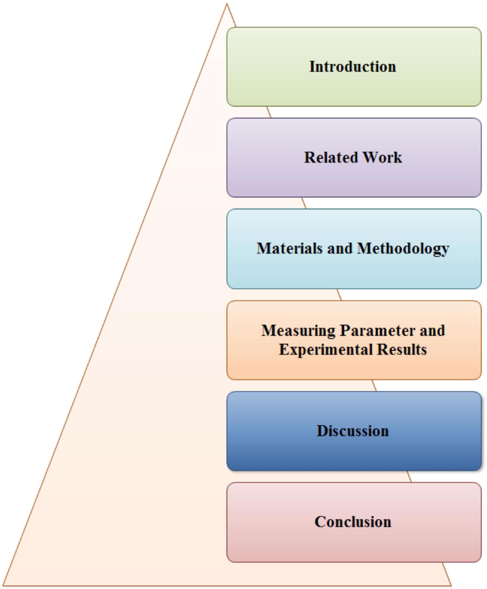
The rest of this article is organized Fig. 3 as follows. Section Related work provides a review of relevant previous research. In Sect. Materials and methodology adapted, we outline the materials and methodology that we used in our study. Section Measuring parameter and experimental results is dedicated to presenting the measuring parameters and experimental results. Section Discussion includes a discussion of our findings and a comparison with existing models. Finally, in Sect. Conclusion, we wrap up our work with concluding thoughts and suggestions for future improvements.
Related work
The research
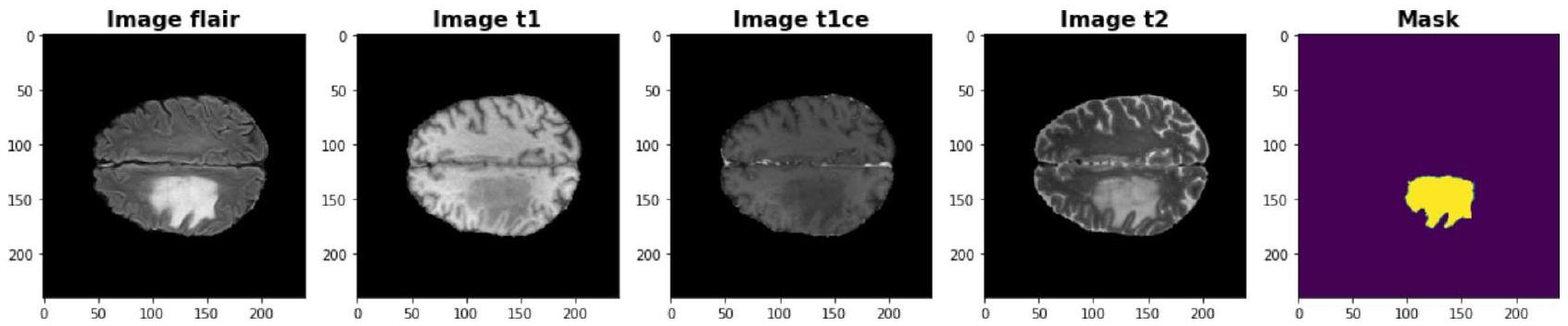
Multimodal Scans – Data | Manually-Segmented mask – Target
Fig. 2. Visualization for multimodal scan of brain MRI.
Fig. 3. Organization of the paper.
and Vanilla Unet models are contrasted with the UnetResNext-50 model as well as cutting-edge methods. The DICE score for the UnetResNext-50 model is 95.73 , and it has a
A convolutional neural network (CNN) is employed in study
accuracy rate of
accuracy rate of
The goal of the research reported in the publication
The article
Several techniques for feature extraction and categorisation of MR images are investigated in this work
This study
Neural networks are another technique that has been proposed in this field
According to studies
A strategy for categorising brain tumours utilising a mix of PCA, RBF kernel, and SVM algorithms is presented in the paper
Brain tumours may be precisely segmented and categorised using a technique described in
For the detection of brain cancers in MRI images, B-CNN
The main aim of the study discussed in
modules with attention gates into the existing U-Net model. Inception Residual paths are used to connect encoder and decoder feature maps to reduce the distance between them. The problem of class imbalance is also tackled using a combination of weight cross-entropy, GDL, and focused Tversky loss functions.
modules with attention gates into the existing U-Net model. Inception Residual paths are used to connect encoder and decoder feature maps to reduce the distance between them. The problem of class imbalance is also tackled using a combination of weight cross-entropy, GDL, and focused Tversky loss functions.
Another approach for brain cancer classification is presented in
In this research
This study
Based on the analysis of related research, the following limitations have been identified:
- Brain tumors can manifest a wide range of characteristics encompassing size, morphology, texture, and intensity. Coping with this diversity effectively in feature extraction and segmentation methods can pose challenges.
- Medical images, such as MRI scans, are susceptible to the presence of disturbances and artifacts, potentially impacting the precision of segmentation techniques. Moreover, brain tumor images are obtained using distinct MRI sequences (e.g., T1-weighted, T2-weighted, FLAIR), each yielding distinct information.
- The variability between different imaging modalities can complicate the segmentation process. In scenarios where tumors infiltrate healthy tissue, the delineation of tumor boundaries can be indistinct, rendering the accurate determination of boundaries problematic.
- The prediction of survival in brain tumor patients is an intricate endeavour accompanied by a multitude of difficulties. The accurate selection of pertinent features for survival prediction is of utmost importance. However, the identification of the most informative features from a heterogeneous amalgamation of clinical and imaging data can be intricate.
This paper employed a hybrid approach that uses a 3D Replicator Neural Network inspired by deep learning and 2D Volumetric Convolutional Network for feature extraction and segmentation to predict patient survival. Based on the findings, the researchers propose that their method is suitable for integration with clinical decision support systems to assist medical professionals or radiologists in initial screening and diagnosis.
Materials and methodology adapted Specification of image dataset
In this research, we evaluate the efficacy of our proposed method’s feature extraction and segmentation using the BraTS2020 dataset, which consists of 368 brain MRI scans with labels, each having dimensions of
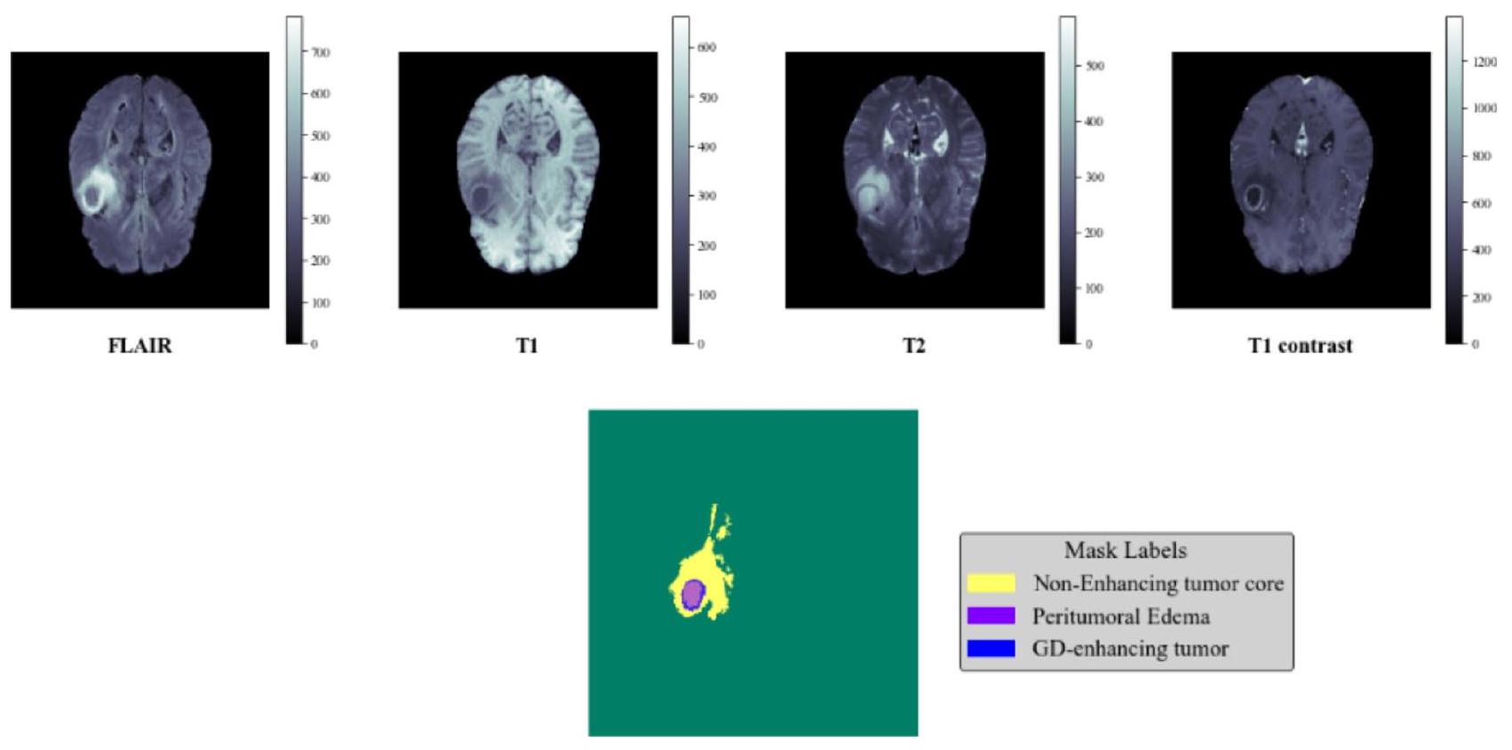
The visualization of MR images and their masks using unique image values, minimum and maximum values, and unique mask values is shown in Fig. 5. For the MR image dataset used in this study, one image had 1202 unique values, with minimum and maximum image values of 0 and 1 . The number of unique mask values was given as (array ([0., 1.], dtype
Fig. 4. Visualization of imaging modalities: T1C (contrast enhanced T1-weighted), T1 (T1-weighted), FLAIR (Fluid Attenuation Inversion Recovery), T2 (T2-weighted).
Fig. 5. Visualization of MR image and mask.
Preprocessing
The primary objective of pre-processing is to improve the clarity of MR images and convert them into a format that can be processed by humans or machine learning systems. Pre-processing also improves the visual quality of MR images by enhancing their signal-to-noise ratio, eliminating unwanted background elements and noise, smoothing the interior of regions, and maintaining their edges. The BRATS 2020 dataset contains 368 MR images in nii format. Due to memory limitations, this study used 150 MR images for the experiment, which were divided into three parts for training, testing, and validation (
with feature extraction. The MinMax scaling technique was used to perform normalization. Normalization and standardization share the same basic concept of adjusting variables assessed at different scales to prevent bias in model fitting and learning functions. Therefore, feature-wise normalization, such as MinMax Scaling, is typically done before model fitting. In MinMax scaling, input variables are transformed to the range [ 0,1 ], with 0 and 1 being the maximum and minimum values for each feature/variable. The mathematical formulation for the minmax scaling is given by Eq. 1.
with feature extraction. The MinMax scaling technique was used to perform normalization. Normalization and standardization share the same basic concept of adjusting variables assessed at different scales to prevent bias in model fitting and learning functions. Therefore, feature-wise normalization, such as MinMax Scaling, is typically done before model fitting. In MinMax scaling, input variables are transformed to the range [ 0,1 ], with 0 and 1 being the maximum and minimum values for each feature/variable. The mathematical formulation for the minmax scaling is given by Eq. 1.
Deep learning models are known for their exceptional performance, but they do come with a few drawbacks. One of them is that they are susceptible to noise, which means that extensive pre-processing is required for every input visualize. To normalize MRI images with all characteristics, the pre-processing steps for segmentation and detection operations shown in Fig. 6 were followed.
Step 1. To begin with, all the modalities and ground truth contain 3D volumes that have a dimension of
Step 2. Slicing these volumes results in 155 2D images with a measurement of
Step 3. From each size, 90 portions ranging from 30 to 120 are selected.
Step 4. Finally, each MRI modality is reduced to a dimension of
Figure 7 represent the distribution graph for training, testing and validation.
Step 2. Slicing these volumes results in 155 2D images with a measurement of
Step 3. From each size, 90 portions ranging from 30 to 120 are selected.
Step 4. Finally, each MRI modality is reduced to a dimension of
Figure 7 represent the distribution graph for training, testing and validation.
Fig. 6. Work flow for pre-processing.
BRATS 2020 MR Image Data Distribution
Fig. 7. Distribution graph for BRATS 2020 Dataset.
Pseudocode of class implementation for BRATS Dataset – Pre-processing for feature extraction process
Description: Here Dataset is a set of MR image that will used in the process of preprocessing
Initialization (instance of class, dataframe, phase, resize operation)
Description: Here the process of initialization will be acquired for preprocessing
Set instance of class
Set phase for dataset
Set Augmentation variable to initialize with calling the function for given phase
Set data_types for dataset images
Set resize variable for images
Set phase for dataset
Set Augmentation variable to initialize with calling the function for given phase
Set data_types for dataset images
Set resize variable for images
Length (instance of class)
Description: Here to find the shape in dataframe
Return the value of shape in dataframe
Fetch_Images(instance of the class, id for images)
Set id for the location of BRATS images
Set root_path to fatch the value
Set variable for images to load all the modalities
for data_type in class_instance.data_types
Set image_path as per given datatypes
Set variable img to load images from image_path
if class instance.resize is true then
Update the img with new image size
Load value in img after the calling class_instance.normalize function with given img value as a pareameter
Append all the images
Create a stack for the images
Update the axis
if class_instance.phase not equal to the passed value then
Set variable for the mask_path using the .seg value of MR image
Set variable mask for the loading of segmented value
if class_instance.resize is true then
Update mask with resize value
Convert mask value from int to float and update mask variable
Update mask with 0 and 1 value
Call the function to update the mask label
Perform the operation of augmentation
Set img and mask for augmented value of image and mask
Return value of id, image and mask
Return id and image
Update mask with 0 and 1 value
Call the function to update the mask label
Perform the operation of augmentation
Set img and mask for augmented value of image and mask
Return value of id, image and mask
Return id and image
Load_Images(class_instance, path of the file)
Description: This function to load all the images and convert into array form
Set data variable to load value of file path
Update data variable after converting into array
Return data value
Set data variable to load value of file path
Update data variable after converting into array
Return data value
Normalize_data(class_instance, data as array form)
Description: This function dedicated to normalize the data as per min and max value of images
Set datamin for minimum value of the data
Return value of the expression [(data – datamin)/(max(data) – datamin]
Return value of the expression [(data – datamin)/(max(data) – datamin]
Preprocess_label_mask(class_instance, mask as an array)
Description: Update mask value for the object of WT, TC and ET
Update mask value for Whole Tumor with the value of 0 and 1
Update mask value for Tumor Core with the value of 0 and 1
Update mask value for Enhanced Tumor with the value of 0 and 1
Create a stack for WT, TC and ET mask value
Update the axis for mask value
Return value of the mask
Update mask value for Whole Tumor with the value of 0 and 1
Update mask value for Tumor Core with the value of 0 and 1
Update mask value for Enhanced Tumor with the value of 0 and 1
Create a stack for WT, TC and ET mask value
Update the axis for mask value
Return value of the mask
Network architecture and training approach for feature extraction, segmentation and detection
3D replicator neural network methodology
A replicator neural network is a type of feedforward neural network that reconstructs the output using the same input. It first reduces the input’s dimension and then creates the output based on that representation. Replicator Neural Network is frequently used for unsupervised learning because they can help identify hidden relationships within data and present them in a more concise format. By transforming unsupervised learning issues into supervised learning algorithms, replicator neural network can be trained to identify patterns within data. The
input is passed through to the output, and an encoder network compresses the input into a smaller encoded form. Meanwhile, a decoder network decodes the encoding to reconstruct the input
input is passed through to the output, and an encoder network compresses the input into a smaller encoded form. Meanwhile, a decoder network decodes the encoding to reconstruct the input
The encoder layer generates a lower-dimensional version of the information, revealing complex and fascinating connections within the data. Figure 8 outlines the components of a replicator neural network.
- Encoder: The network component known as the encoder receives input and creates a lower-dimensional encoding which is known as the encoder.
- Bottleneck: The lower-dimensional hidden layer is the source of the encoding. The number of nodes present in the bottleneck layer is reduced, and it also determines how the input is encoded in terms of dimension.
- Decoder: The decoder receives the input and reconstructs it using the encoding.
Hyperparameters:
- Code Size: Signifies the number of intermediate layer nodes, where fewer nodes lead to more compression.
- Number of Layers: Depicts the number of layers that compose the network for the decoder and encoder.
Fig. 8. Component of Replicator Neural Network with Latent Space
- Number of nodes per layer: The replicator neural network shown in the previous image is a stacked encoding network, meaning that the number of nodes per layer grows in the symmetric decoder while decreasing in the succeeding layers of the encoder.
- Loss Function: Cross entropy is commonly used if the input values are within the range
, otherwise Mean Squared Error should be used.
According to the following elements, replicator neural network is described: The spaces of decoded instructions
There are two primary components of functions that have been parametrized: the encoder family
We often write
Typically, multilayer perception is used to design both the encoder and the decoder. As an illustration, the one-layer MLP encoder
The term “weight” refers to a matrix represented by W , “bias” refers to a vector indicated by b, and “activation function,” denoted by
Training a replicator neural network
The training of proposed 3D replicator neural network consists of just a bundle of two factors on its own. Training needs an assignment in order to assess its quality. A benchmark probability distribution
These enable us to construct the replicator neural network’s loss function as
The presented replicator neural network for the assumed job (
The two primary components of replicator neural network are an encoder that converts a communication to a code and a decoder that extracts the information from the code. The recovery quality function d defines “near to perfect” as the performance that an ideal replicator neural network may achieve in terms of restoration.
Interpretation
Figure 9 illustrates how the 3D Replicator Neural Network for feature extraction interprets the model; the model is displayed after input has undergone pre-processing and normalisation, and the encoder has three convolutional layers, three pooling layers, and one linear layer.
Step 1 – Initialization for encoding representation is like that
Step 2 – Initialization for decoding representation is like that
Step 3 – To perform the operation of Encoding the data frame:
After the process of the above mention layers, the Replicator Neural Network 3D model returns the features that will be decoded by the next steps.
Step 4 – The layering structure for the decoding as per the return features using deconvolution and unpooling like that:
Fig. 9. 3D replicator neural network working flow.
Decoding_Linear → unpool $1 rightarrow$ deconv $1 rightarrow$ unpool $2 rightarrow$ deconv $2 rightarrow$ unpool $3 rightarrow$ deconv 3
2D Volumetric convolutional network methodology for segmentation and detection the tumor
The Fig. 10 illustration shows our conceptual convolutional neural network. Convolutional operations are utilized to extract features from the information, and after each stage, the data’s resolution is reduced using an appropriate stride. The left side of the network compresses the signal, while the right side uncompresses it until it returns to its initial size
Left side of Network.
In this network, the left section handles different resolutions of the input data. The first three stages use convolutional layers to identify a residual function, which is trained using input from each phase, and then nonlinearly processed. This residual function ensures convergence, which is not possible in conventional learning networks without residual blocks. The convolutional operation uses a volumetric kernel with a voxel size of
The residual function plays a pivotal role in enhancing the convergence of deep neural networks, and its effectiveness can be better understood when compared to the compression path in a volumetric convolutional network. In such networks, the compression path reduces resolution using convolutions with a stride of 2 and
Fig. 10. Network Architecture for 2D Volumetric Convolutional Network
reformulating the task into learning residuals-differences between the input and the output-rather than full transformations. This simplification makes it easier for the network to optimize, much like how down-sampling in the compression path broadens the network’s focus. This mechanism also accelerates the convergence process, allowing the network to train more efficiently and effectively. Overall, the residual function facilitates better convergence by stabilizing gradients, simplifying learning, preventing degradation in deep networks, and optimizing the training process.
The Replicator Neural Network (RNN) architecture reduces memory usage through several key mechanisms. It efficiently encodes data into a lower-dimensional representation, significantly compressing the input data and reducing the size of intermediate activations. This encoding process requires fewer resources compared to the original high-dimensional data. The network also employs weight sharing across layers, which minimizes the total number of parameters that need to be stored. During training, this efficiency extends to reduced activation storage and more manageable backpropagation memory requirements.
Right Side of Network.
By extracting features and increasing the geographic coverage of the lower resolution feature maps, the network tries to collect and synthesise the necessary data for producing a two-channel volumetric segmentation. Each level’s input size is increased using a deconvolution procedure, which is accompanied by one to three convolution operation that each have half as many 555 kernels as the layer before them. Similar to how the left half of the network is taught, so is the residual function. Two feature maps with the identical size as the source volume and 111 kernel strengths are produced by the last convolutional layer. The background and foreground areas are probabilistically divided into these two output feature maps using a soft-max voxel-wise method.
Horizontal Connection.
The compression process of the CNN loses location information, as depicted on the left side. To resolve this issue, horizontal connections are incorporated to transmit elements from the early stages of the CNN’s left section to the right portion. This not only enhances the accuracy of the final contour prediction but also provides
precise position information to the right component. By incorporating these connections, the convergence time of the model is accelerated.
precise position information to the right component. By incorporating these connections, the convergence time of the model is accelerated.
Step of Process Flow.
Step 1 Input Image for Data Pre-processing
- Each 3D volume of size
is available for all modalities and ground truth. - After converting into 2D pictures, there will be 155 images, each with dimensions of
pixels. - Out of these 155 slices, only 90 slices ranging from 30 to 120 are selected from each volume.
- All MRI modalities are trimmed to
pixels to remove the background noise.
Step 2 Process of Data Normalization
Step 3 Splitting the normalized data 75% Training Data, 13% Testing Data, 12% Validation Data
Step 4 Apply 2D V-Net Model (Encoding and Decoding process on normalized Data)
Step 5 Applying Training model into Testing Data and Validation Data
Step 3 Splitting the normalized data 75% Training Data, 13% Testing Data, 12% Validation Data
Step 4 Apply 2D V-Net Model (Encoding and Decoding process on normalized Data)
Step 5 Applying Training model into Testing Data and Validation Data
- Find Dice coefficient
- Find Accuracy
- Find Loss Value
Step 6 Verify the result for prediction
The Parametric Rectified Linear Unit (PReLU) is used as the activation function in deep neural networks to address certain limitations of traditional activation functions, such as ReLU. PReLU introduces a small, learnable parameter for the negative slope of the activation function, allowing it to adaptively learn the best slope during training.
PReLU is defined as
How PReLU Improves Model Performance:
- Avoiding Dead Neurons: By allowing a small gradient for negative values, PReLU prevents neurons from becoming inactive, ensuring that all neurons can contribute to learning throughout the training process. This helps maintain a more diverse set of features and prevents the network from becoming too sparse.
- Enhancing Learning: The adaptability of PReLU means that the network can learn the most effective slope for negative values during training. This flexibility can lead to better model performance as the network optimizes its activation function for the given task, improving its ability to capture complex patterns and relationships in the data.
- Improving Gradient Flow: The non-zero gradients for negative inputs help maintain a more stable and effective gradient flow during backpropagation. This stability aids in more consistent weight updates, which can accelerate convergence and improve overall training efficiency.
- Increased Model Capacity: PReLU’s ability to learn different slopes for positive and negative inputs effectively increases the network’s capacity to model complex functions. This enhanced flexibility allows the network to fit the training data more accurately and generalize better to unseen data.
Measuring parameter and experimental results
Feature extraction refers to the technique of obtaining more detailed data about an image, such as its texture, shape, contrast, and color. Texture analysis is a vital aspect of both machine learning systems and human visual perception. By selecting significant features, it can effectively enhance the accuracy of the diagnostic system. Textural observations and analysis can be beneficial in evaluating the different stages of tumours (tumour staging) and for diagnosis. The formula for some relevant statistical aspects and the results of the experiments are provided below.
Mean (M): The mean of the object is determined using, by multiplying the sum of all the pixel values in an object by the overall number of pixels present in the object.
Experimental result of mean for the BRATS 2020 dataset with t1 weighted, t1ce weighted, t2 weighted and flair is shown in Fig. 11.
Skewness (Skn) Skewness is a metric for symmetry or lack thereof. The definition of the skewness of an arbitrary variable X , represented as
Where SD is standard deviation and will be evaluated like that
Fig. 11. Mean value experimental result for BRATS2020 MRI Dataset (a) t1 weighted values (b) t1ce weighted values (c) t2 weighted value (d) flair value.
Experimental result of Skewness for the BRATS 2020 dataset with t1 weighted, t1ce weighted, t2 weighted and flair is shown in Fig. 12a.
Kutosis (Krt) The Kurtosis parameter describes the probability distribution’s form for a random variable. For the random identifier X , the Kurtosis is identified as
Experimental result of Kurtosis for the BRATS 2020 dataset with t1 weighted, t1ce weighted, t2 weighted and flair is shown in Fig. 12b.
Skewness Difference: Skewness Difference measures the disparity in asymmetry between two probability distributions or datasets. Skewness itself quantifies how a distribution deviates from symmetry around its mean: positive skewness indicates a longer tail on the right, while negative skewness suggests a longer tail on the left. By calculating the difference in skewness between two datasets, Skewness Difference provides insight into how their asymmetries compare. Figure 12c shows the experimental result of skewness differences for the BRATS 2020 dataset with t1 weighted, t1ce weighted, t2 weighted and flair.
Intensive Distance Intensive Distance is a concept used to measure the relative difference or similarity between data points or distributions while controlling for scale and size. Unlike traditional distance metrics, which often
Fig. 12. Features Value Graph for Skewness, Kurtosis, Intensive Differences.
consider absolute differences and may be influenced by the scale of data, Intensive Distance focuses on the inherent characteristics of the data by normalizing or adjusting for scale effects.
Figure 12d shows the experimental result of intensive distribution for the BRATS 2020 dataset with t1 weighted, t1ce weighted, t2 weighted and flair.
Non-intensive Distance Non-Intensive Distance is a concept used to measure the distance between data points or distributions without accounting for scale or variability adjustments. Unlike Intensive Distance, which normalizes for scale to ensure equitable comparisons, Non-Intensive Distance considers the raw differences between values or features directly. This approach does not adjust for the size or distribution of the data, making it sensitive to absolute values and scale. Figure 12e shows the experimental result of non-intensive distribution for the BRATS 2020 data set with t1 weighted, t1ce weighted, t2 weighted and flair.
Intensive skewness It is the measurement of skewness for intensive distribution data. Figure 12f shows the experimental result of intensive skewness for the BRATS 2020 dataset with t1 weighted, t1ce weighted, t2 weighted and flair.
Non-intensive Skewness It is the measurement of skewness for non-intensive distribution data. Figure 13a shows the experimental result of non-intensive skewness for the BRATS 2020 dataset with t1 weighted, t1ce weighted, t 2 weighted and flair.
Data intensive skewness difference It evaluates the raw disparity in skewness between two datasets, reflecting the asymmetry differences without adjusting for scale or normalization. Figure 13b show the experimental result of Intensive Skewness Difference for the BRATS 2020 data set with t1 weighted, t1ce weighted, t2 weighted and flair.
Data non-intensive skewness difference It is the difference between data skewness and non-intensive skewness. Figure 13c shows the experimental result of data non-intensive skewness Difference for the BRATS 2020 data set with t 1 weighted, t 1 ce weighted, t 2 weighted and flair.
Latent feature A set of objects is embedded within a multidimensional in a latent space, often referred to as a latent feature space or embedding space (Fig. 13d). In the latent space, the items that are more similar to one another are placed closer to one another. Simply said, the latent space is a depiction of compressed data, where like data points are located near to one another. Latent space is helpful for discovering more straightforward visualisations for analysis as well as for learning data features.
To achieve better evaluation results on brain MR images, additional quality evaluation parameters to the one below mentioned are also required for segmentation.
Loss: A way to assess how effectively your programme models your dataset is via the Loss function. It is a mathematical function of the deep learning algorithm’s parameters. In this proposed work, performance of a segmentation model is measured by cross entropy loss. A number between 0 and 1 represents the loss (or error), with 0 representing the ideal model. Generally speaking, the objective is to bring your model as close to 0 as you can. Using cross entropy, we can measure the error (or difference) between two probability distributions.
Cross-entropy, for instance, in the context of Binary Classification is provided by:
Where, p is the predicted probability and y is the indicator.
Accuracy: A statistic used to assess the model’s effectiveness across all classes is accuracy. When each class is given equal weight, it is very helpful. To determine accuracy, divide the total number of correct guesses by the total number of forecasts.
Accuracy: A statistic used to assess the model’s effectiveness across all classes is accuracy. When each class is given equal weight, it is very helpful. To determine accuracy, divide the total number of correct guesses by the total number of forecasts.
MeanIOU: Mean Intersection over Union (MeanIoU) calculates the proportion of the overlap between two bounding boxes to the union of the areas of the boxes. The prediction and the ground truth are contained within these bounding boxes. This metric can be used for any approach that predicts bounding boxes. Its mathematical formulation is:
Dice Coefficient: The Dice similarity coefficient (DSC) was employed as a statistical validation metric to assess the repeatability of human segmentations and the spatial overlap accuracy of automated probabilistic fractional segmentation of MR images. This coefficient measures how similar two images are by dividing the total number of pixels in both images by the area of overlap between the two segmented images.
Precision: The model’s accuracy is measured by the percentage of Positive samples that were correctly classified out of all samples that were classified as Positive, regardless of whether they were classified correctly or incorrectly. Precision, on the other hand, evaluates how effectively the model identifies a sample as positive.
Fig. 13. The feature graph values for non-intensive skewness, intensive skewness, non-intensive skew differences, and latent features.
The denominator rises and the precision becomes low when the model makes many wrong Positive classifications or few correct Positive classifications. However, the precision is high when:
- Numerous accurate Positive classifications are made by the model (maximize True Positive).
- Less inaccurate Positive classifications are made by the model (minimize False Positive).
Fig. 14. Evaluation Graph Epoch by Epoch.
- Generalization Across Diverse Populations: The model may struggle to generalize well across diverse patient populations due to differences in tumor characteristics, genetic factors, and treatment protocols. This limitation could reduce the model’s accuracy when applied to new or underrepresented patient groups.
- Interpretability Issues: Deep learning models, including Replicator Neural Networks and Volumetric Convolution Networks, often operate as “black boxes,” making it difficult to understand the rationale behind their predictions. This lack of interpretability can be a barrier to clinical adoption, as clinicians need to trust and verify the model’s outputs.
Fig. 15. The model’s prediction after dividing the image into segments can be represented in three forms: (a) the original tumor image, (b) the tumor region predicted by the model, and (c) the real tumor region as shown in the ground truth images.
- Limited Validation in Real-World Settings: While the approach may perform well in controlled research environments, it might not be extensively validated in diverse, real-world clinical settings. This gap in validation could limit its immediate applicability in everyday clinical practice.
- Regulatory and Ethical Concerns: The use of advanced AI models in healthcare raises regulatory and ethical issues, including patient privacy, data security, and the need for stringent validation before clinical deployment. Navigating these concerns is essential but can be challenging.
Distribution of rounded Ages in data
Fig. 16. Distribution of Rounded Ages in BRATS2020.
Distribution of rounded Survival_days in data
Fig. 17. Distribution of rounded Survival Days of patient as given in BRATS 2020.
| Loss | Accuracy | MeanIoU | Dice Coefficient | Precision | |
| Train Result | 0.097695 | 0.995166 | 0.616957 | 0.902311 | 0.995193 |
| Validation Result | 0.108875 | 0.994494 | 0.637059 | 0.891475 | 0.994538 |
| Test Result | 0.109715 | 0.994260 | 0.623013 | 0.889182 | 0.994220 |
Table 1. Evaluation report.
| Reference | Model Used | Accuracy | DSC | Specificity | Sensitivity |
| 1 | TPUAR-NET | – | 0.89 | 0.99 | – |
| 6 | LDI-Means + Mutual Information + Singular Value Decomposition With Dimensionality Reduction + SVM | 0.9102 | – | 0.9426 | 0.93 |
| 13 | VGG-16 | – | 0.8892 | 0.9948 | 0.9 |
| 14 | U-Net Based CNN | – | 0.878 | 0.993 | 0.87 |
| 26 | Deep Convolutional Neural Network | – | 0.88 | 0.89 | 0.89 |
| 27 | 3D-UNet | – | 0.86 | 0.99 | 0.89 |
| 28 | Deep Convolutional Neural Network | – | 0.87 | 0.94 | 0.82 |
| 30 | Fractional probabilistic Fuzzy C Means (Fr-pFCM) + Whale-Cat Swarm Optimization based Deep Belief Network (WCSO-DBN) | 0.923 | – | 0.96 | 0.84 |
| 36 | Spectial Fuzzy C Means | – | 0.86 | – | 0.89 |
| 34 | Optimized Resnet50 with Gradcam | 0.985 | – | – | 0.888 |
| 39 | Optimal DeepMRSeg + SPO + GAN + CAViaR-SPO. | 0.917 | – | 0.925 | 0.8884 |
| 41 | CNN | – | 0.88 | – | 0.88 |
| 48 | Symmetric-Driven FCN | – | 0.87 | – | 0.928 |
| 49 | Bayesian fuzzy clustering, Scattering transform (ST), Information-theoretic measures, Softmax Regression technique, DAE | 0.985 | – | 0.995 | 0.95 |
| 52 | Handcrafted Convolutional Neural Network | 0.95 | 0.91 | 0.96 | – |
| 55 | Cross-Level Connected U-Shaped Network (CLCU-Net | – | 0.885 | – | 0.96 |
| 59 | FCNN + Conditional Random Fields | – | 0.84 | – | – |
| Proposed Methodology | 0.9951 | 0.9023 | 0.9980 | 0.9950 |
Table 2. Comparative analysis of the various BRATS dataset brain tumour segmentation techniques.
Implementing the MRI-based brain tumor feature extraction, segmentation, and survival days prediction approach using a Deep Learning Inspired Replicator Neural Network and Volumetric Convolution Network presents several challenges:
- Data Heterogeneity: MRI data can vary significantly across different machines, protocols, and institutions. This variability can affect model performance and generalization, necessitating robust preprocessing and normalization techniques.
- Model Complexity and Computational Load: The combined use of a Replicator Neural Network and Volumetric Convolution Network can be computationally intensive, especially when processing large, high-resolution 3D MRI scans. Ensuring efficient training and inference without sacrificing accuracy is a key challenge.
- Limited Annotated Data: Accurate tumor segmentation and survival prediction require well-annotated datasets, which can be scarce. The lack of sufficient labeled data for training can limit the model’s ability to generalize, making techniques like data augmentation or synthetic data generation crucial.
- Integration into Clinical Workflows: Deploying this approach in real-world clinical settings involves integrating the model into existing medical imaging systems and ensuring it fits seamlessly into the clinician’s workflow. This requires careful consideration of user interface design and real-time processing capabilities.
- Interpretability and Trustworthiness: Clinicians need to trust the model’s predictions, particularly in critical decisions like survival prediction. Ensuring the model’s outputs are interpretable and providing insights into how predictions are made will be vital for adoption in clinical practice.
- Regulatory Compliance and Validation: The model must meet stringent regulatory standards and undergo rigorous validation before being used in clinical environments. Ensuring compliance with healthcare regulations and demonstrating the model’s safety and efficacy are significant hurdles.
Existing medical imaging systems face several practical and potential issues that impact their effectiveness and integration into clinical practice:
- Scalability: Many medical imaging systems struggle to scale with increasing data volumes and complexity. As imaging technology advances, systems must handle larger and higher-resolution datasets, which can strain existing infrastructure and require significant upgrades.
- Integration Challenges: Existing imaging systems often operate in isolation, making it difficult to integrate new technologies or updates. This can lead to fragmented workflows and inefficiencies, as new tools may not seamlessly connect with legacy systems, complicating data management and analysis.
- Data Compatibility: Different imaging modalities and systems may use various file formats and standards, creating issues with data compatibility. This lack of standardization can hinder the exchange of information between systems and reduce the ability to perform comprehensive analyses.
- User Interface and Workflow: Many existing systems have complex or outdated user interfaces that can be difficult to navigate. This can affect the convenience and efficiency of imaging procedures, leading to longer training times and potential errors in image interpretation.
- Processing Speed and Storage: High-resolution and 3D imaging generate large amounts of data, requiring significant processing power and storage capacity. Existing systems may struggle with processing speed and data storage, leading to delays and potential bottlenecks in clinical workflows.
- Interoperability: Ensuring that imaging systems work well with other healthcare technologies, such as electronic health records (EHRs) and diagnostic tools, is crucial for a cohesive patient care experience. Existing systems may have limited interoperability, making it challenging to integrate imaging data with other clinical information.
Integrating the proposed methodology into clinical workflows can enhance diagnostic accuracy and optimize patient care by streamlining and automating key processes. Seamless integration with existing medical imaging systems and electronic health records ensures compatibility and reduces disruptions. The methodology’s advanced algorithms can improve tumor identification and localization, leading to more precise diagnoses and better-targeted treatments. Automation of routine tasks, such as image preprocessing and analysis, reduces workload and minimizes human error, allowing clinicians to focus on interpreting results. Real-time analysis capabilities provide immediate feedback during imaging procedures, facilitating quicker adjustments and more informed decisions. Enhanced data management and visualization tools offer clearer insights and comprehensive information for clinicians. Effective training and support for healthcare professionals ensure successful adoption and use of the new methodology. Additionally, quality control mechanisms and ongoing feedback help refine the methodology, maintaining high standards of accuracy and reliability. This integration ultimately improves diagnostic processes and patient care, contributing to better clinical outcomes.
Conclusion
This study involved using magnetic resonance imaging (MRI) of the brain to distinguish between normal brain tissue and tumor tissue, specifically gliomas. It is important to accurately identify and locate brain tumors to properly diagnose, treat, and estimate the patient’s overall survival rate. To achieve this, the researchers employed a deep learning approach using a combination of MRI scans. They used a 2D Volumetric Convolutional Network architecture with a majority rule to ensure reliable tumor segmentation and improve performance. The researchers also extracted radiomic features from the segmented tumor regions and used a Deep Learning Inspired 3D Replicator neural network to identify the most effective features for predicting survival rates. In comparison to manual identification by clinical specialists, the findings demonstrated that the model accurately segregated brain tumours and forecasted the fate of enhancing and genuine enhancing tumours. The proposed methodology provides an accurate and speedy detection of brain tumors and precise location of the tumour. The study’s findings are crucial for clinical practice, offering insights that can enhance patient care and outcomes. By integrating these results, clinicians can improve treatment effectiveness and tailor interventions, leading to better patient management and health outcomes. Accurate identification and localization of brain tumors are critical for improving diagnosis and treatment planning. Precise detection ensures that tumors are correctly identified, enabling targeted treatment strategies. Accurate localization helps in planning surgical interventions and other therapies, minimizing damage to healthy brain tissue. Overall, these advancements lead to more effective treatment, better outcomes, and improved patient care. Future research on this approach could focus on integrating multimodal data, such as genetics and other imaging types, to improve prediction accuracy. Developing personalized treatment models and optimizing for real-time processing would enhance clinical utility. Transfer learning could be explored to improve generalizability across diverse populations and MRI settings.
Data availability
The corresponding author will give the information used to back up the findings of this investigation upon request.
Received: 21 April 2024; Accepted: 23 December 2024
Published online: 09 January 2025
Published online: 09 January 2025
References
- Abd-Ellah, M. K., Khalaf, A. A. M., Awad, A. I. & Hamed, H. F. A. TPUAR-Net: two parallel U-Net with asymmetric residual-based deep convolutional neural network for Brain Tumor Segmentation. In (eds Karray, F., Campilho, A. & Yu, A.) Image Analysis and Recognition (106-116). Springer International Publishing. (2019).
- Abdel-Maksoud, E., Elmogy, M. & Al-Awadi, R. Brain tumor segmentation based on a hybrid clustering technique. Egypt. Inf. J. 16 (1), 71-81. https://doi.org/10.1016/j.eij.2015.01.003 (2015).
- Abdollahi, A., Pradhan, B. & Alamri, A. VNet: an end-to-end fully convolutional neural network for road extraction from HighResolution Remote Sensing Data. IEEE Access. 8, 179424-179436. https://doi.org/10.1109/access.2020.3026658 (2020).
- AboElenein, N. M., Piao, S., Noor, A. & Ahmed, P. N. MIRAU-Net: an improved neural network based on U-Net for gliomas segmentation. Sig. Process. Image Commun. 101, 116553. https://doi.org/10.1016/j.image.2021.116553 (2022).
- Ain, Q., Jaffar, M. A. & Choi, T. S. Fuzzy anisotropic diffusion-based segmentation and texture based ensemble classification of brain tumor. Appl. Soft Comput. 21, 330-340. https://doi.org/10.1016/j.asoc.2014.03.019 (2014).
- Al-Saffar, Z. A. & Yildirim, T. A hybrid approach based on multiple eigenvalues selection (MES) for the automated grading of a brain tumor using MRI. Comput. Methods Programs Biomed. 201, 105945. https://doi.org/10.1016/j.cmpb.2021.105945 (2021).
- American Brain Tumor Association. http://www.abta.org
- Amin, J. et al. Brain tumor detection by using stacked autoencoders in Deep Learning. J. Med. Syst. 44 (2), 32. https://doi.org/10.1 007/s10916-019-1483-2 (2019).
- Ayadi, W., Elhamzi, W., Charfi, I. & Atri, M. A hybrid feature extraction approach for brain MRI classification based on bag-ofwords. Biomed. Signal Process. Control. 48, 144-152. https://doi.org/10.1016/j.bspc.2018.10.010 (2019).
- Bahadure, N. B., Ray, A. K. & Thethi, H. P. Image Analysis for MRI Based Brain Tumor Detection and Feature Extraction Using Biologically Inspired BWT and SVM. International Journal of Biomedical Imaging, 2017, 9749108. (2017). https://doi.org/10.115 5/2017/9749108
- Bashir-Gonbadi, F. & Khotanlou, H. Brain tumor classification using deep convolutional autoencoder-based neural network: multi-task approach. Multimedia Tools Appl. 80 (13), 19909-19929. https://doi.org/10.1007/s11042-021-10637-1 (2021).
- Caban, J. J., Yao, J. & Mollura, D. J. Enhancing image analytic tools by fusing quantitative physiological values with image features. J. Digit. Imaging. 25 (4), 550-557. https://doi.org/10.1007/s10278-011-9449-z (2012).
- Cabezas, M., Valverde, S., González-Villà, S., Clérigues, A., Salem, M., Kushibar,K., … Lladó, X, 2018. Survival prediction using ensemble tumor segmentation and transfer learning. arXiv preprint arXiv:1810.04274.
- Caver, E., Liu, C., Zong, W., Dai, Z. & Wen, N. Automatic Brain Tumor Segmentation Using a U-net Neural Network. PreConference Proceedings of the 7th MICCAI BraTS Challenge; 63. (2018).
- Chaddad, A. Automated Feature Extraction in Brain Tumor by Magnetic Resonance Imaging Using Gaussian Mixture Models. International Journal of Biomedical Imaging, 2015, 868031. (2015). https://doi.org/10.1155/2015/868031
- Chawla, R. et al. Brain tumor recognition using an integrated bat algorithm with a convolutional neural network approach. Measurement: Sens. 24, 100426. https://doi.org/10.1016/j.measen.2022.100426 (2022).
- Chen, S. & Guo, W. Auto-Encoders in Deep Learning-A Review with New Perspectives. Mathematics, 11(8), 1777. MDPI AG. (2023). Retrieved from https://doi.org/10.3390/math11081777
- Cui, W., Wang, Y., Fan, Y., Feng, Y. & Lei, T. Localized FCM clustering with spatial information for Medical Image Segmentation and Bias Field Estimation. Int. J. Biomed. Imaging. 2013 (930301). https://doi.org/10.1155/2013/930301 (2013).
- Damodaran, S. & Raghavan, D. Combining tissue segmentation and neural network for brain tumor detection. Int. Arab. J. Inform. Technol. 12, 42-52 (2015).
- Deepak, S. & Ameer, P. M. Retrieval of brain MRI with tumor using contrastive loss based similarity on GoogLeNet encodings. Comput. Biol. Med. 125, 103993. https://doi.org/10.1016/j.compbiomed.2020.103993 (2020).
- Demirhan, A., Toru, M. & Guler, I. Segmentation of tumor and edema along with healthy tissues of brain using wavelets and neural networks. IEEE J. Biomedical Health Inf. 19 (4), 1451-1458. https://doi.org/10.1109/JBHI.2014.2360515 (2015).
- Gull, S., Akbar, S., Hassan, S. A., Rehman, A. & Sadad, T. Automated brain tumor segmentation and classification through MRI images. In (eds Liatsis, P., Hussain, A., Mostafa, S. A. & Al-Jumeily, D.) Emerging Technology Trends in Internet of Things and Computing (182-194). Springer International Publishing. (2022).
- Guo, L. et al. Tumor detection in MR images using one-class Immune Feature Weighted SVMs. IEEE Trans. Magn. 47 (10), 3849-3852. https://doi.org/10.1109/TMAG.2011.2158520 (2011).
- Gupta, N., Bhatele, P. & Khanna, P. Glioma detection on brain MRIs using texture and morphological features with ensemble learning. Biomed. Signal Process. Control. 47, 115-125. https://doi.org/10.1016/j.bspc.2018.06.003 (2019).
- Habib, H., Amin, R., Ahmed, B. & Hannan, A. Hybrid algorithms for brain tumor segmentation, classification and feature extraction. J. Ambient Intell. Humaniz. Comput. 13 (5), 2763-2784. https://doi.org/10.1007/s12652-021-03544-8 (2022).
- Havaei, M. et al. Brain tumor segmentation with deep neural networks. Med. Image. Anal. 35, 18-31. https://doi.org/10.1016/j.me dia.2016.05.004 (2017).
- Hu, X. & Piraud, M. Multi-level Activation for Segmentation of Hierarchically-nested Classes on 3D-UNet. Pre-Conference Proceedings of the 7th MICCAI BraTS Challenge.; 188. (2018).
- Hussain, S., Anwar, S. M. & Majid, M. Segmentation of glioma tumors in brain using deep convolutional neural network. Neurocomputing 282, 248-261. https://doi.org/10.1016/j.neucom.2017.12.032 (2018).
- Jemimma, T. A. & Raj, Y. J. V. Significant LOOP with clustering approach and optimization enabled deep learning classifier for the brain tumor segmentation and classification. Multimedia Tools Appl. 81 (2), 2365-2391. https://doi.org/10.1007/s11042-021-1159 1-8 (2022).
- Jemimma, T. A. & Vetharaj, Y. J. Fractional probabilistic fuzzy clustering and optimization based brain tumor segmentation and classification. Multimedia Tools Appl. 81 (13), 17889-17918. https://doi.org/10.1007/s11042-022-11969-2 (2022).
- Kapila, D. & Bhagat, N. Efficient feature selection technique for brain tumor classification utilizing hybrid fruit fly based abc and ann algorithm. Materials Today: Proceedings, 51, 12-20. (2022). https://doi.org/10.1016/j.matpr.2021.04.089
- Kay, S. et al. Integrating Autoencoder and Heteroscedastic Noise Neural Networks for the Batch Process Soft-Sensor Design. Ind. Eng. Chem. Res., 61(36), 13559-13569. https://doi.org/10.1021/acs.iecr.2c01789 (2022).
- Kong, Y., Deng, Y. & Dai, Q. Discriminative clustering and feature selection for Brain MRI Segmentation. IEEE. Signal. Process. Lett. 22 (5), 573-577. https://doi.org/10.1109/LSP.2014.2364612 (2015).
- Kumar, M. M. M. R. M. T., Guluwadi, V. & S Enhancing brain tumor detection in MRI images through explainable AI using GradCAM with Resnet 50. BMC Med. Imaging. 24 https://doi.org/10.1186/s12880-024-01292-7 (2024).
- Kumar, P. & Vijayakumar, B. Brain Tumour Mr Image Segmentation and classification using by PCA and RBF Kernel based support Vector Machine. Middle-East J. Sci. Res. 23 (9), 2106-2116. https://doi.org/10.5829/idosi.mejsr.2015.23.09.22458 (2015).
- Li, Q. et al. Glioma segmentation with a unified algorithm in Multimodal MRI images. IEEE Access. 6, 9543-9553. https://doi.org /10.1109/ACCESS.2018.2807698 (2018).
- Louis, D. N. et al. The 2016 World Health Organization Classification of Tumors of the Central Nervous System: a summary. Acta Neuropathol. 131 (6), 803-820. https://doi.org/10.1007/s00401-016-1545-1 (2016).
- Maji, D., Sigedar, P. & Singh, M. Attention Res-UNet with guided decoder for semantic segmentation of brain tumors. Biomed. Signal Process. Control. 71, 103077. https://doi.org/10.1016/j.bspc. 2021.103077 (2022).
- Neelima, G., Chigurukota, D. R., Maram, B. & Girirajan, B. Optimal DeepMRSeg based tumor segmentation with GAN for brain tumor classification. Biomed. Signal Process. Control. 74, 103537. https://doi.org/10.1016/j.bspc. 2022.103537 (2022).
- Osborn, A. G., Louis, D. N., Poussaint, T. Y., Linscott, L. L. & Salzman, K. L. The 2021 World Health Organization Classification of Tumors of the Central Nervous System: what neuroradiologists need to know. Am. J. Neuroradiol. https://doi.org/10.3174/ajnr.A7 462 (2022).
- Pereira, S., Pinto, A., Alves, V. & Silva, C. A. Brain tumor segmentation using Convolutional neural networks in MRI images. IEEE Trans. Med. Imaging. 35 (5), 1240-1251. https://doi.org/10.1109/TMI.2016.2538465 (2016).
- Rai, H. M., Chatterjee, K. & Dashkevich, S. Automatic and accurate abnormality detection from brain MR images using a novel hybrid UnetResNext-50 deep CNN model. Biomed. Signal Process. Control. 66, 102477. https://doi.org/10.1016/j.bspc.2021.102477 (2021).
- Rastogi, D., Johri, P. & Tiwari, V. Brain tumor detection and localization: an inception V3 – based classification followed by RESUNET-Based Segmentation Approach. Int. J. Math. Eng. Manage. Sci. 8, 336-352. https://doi.org/10.33889/ijmems.2023.8.2.020 (2023b).
- Sachdeva, J., Kumar, V., Gupta, I., Khandelwal, N. & Ahuja, C. K. Segmentation, feature extraction, and Multiclass Brain Tumor classification. J. Digit. Imaging. 26 (6), 1141-1150. https://doi.org/10.1007/s10278-013-9600-0 (2013).
- Sachdeva, J., Kumar, V., Gupta, I., Khandelwal, N. & Ahuja, C. K. A package-SFERCB-Segmentation, feature extraction, reduction and classification analysis by both SVM and ANN for brain tumors. Appl. Soft Comput. 47, 151-167. https://doi.org/10.1016/j.aso c.2016.05.020 (2016).
- Salem, A. B. M. An Automatic Classification of Brain Tumors through MRI Using Support Vector Machine. (2016).
- Sharma, N. et al. Segmentation and classification of medical images using texture-primitive features: application of BAM-type artificial neural network. J. Med. Phys. 33 (3), 119-126. https://doi.org/10.4103/0971-6203.42763 (2008).
- Shen, H., Zhang, J. & Zheng, W. Efficient symmetry-driven fully convolutional network for multimodal brain tumor segmentation. 2017 IEEE Int. Conf. Image Process. (ICIP). 3864-3868. https://doi.org/10.1109/ICIP. 2017.8297006 (2017).
- Siva Raja, P. M. & rani, A. V. Brain tumor classification using a hybrid deep autoencoder with bayesian fuzzy clustering-based segmentation approach. Biocybernetics Biomedical Eng. 40 (1), 440-453. https://doi.org/10.1016/j.bbe.2020.01.006 (2020).
- Tong, J., Zhao, Y., Zhang, P., Chen, L. & Jiang, L. MRI brain tumor segmentation based on texture features and kernel sparse coding. Biomed. Signal Process. Control. 47, 387-392. https://doi.org/10.1016/j.bspc.2018.06.001 (2019).
- Torheim, T. et al. Classification of dynamic contrast enhanced MR images of cervical cancers using texture analysis and support Vector machines. IEEE Trans. Med. Imaging. 33 (8), 1648-1656. https://doi.org/10.1109/TMI.2014.2321024 (2014).
- Ullah, F. et al. Brain tumor segmentation from MRI images using handcrafted convolutional neural network. Diagnostics 13, 2650. https://doi.org/10.3390/diagnostics13162650 (2023).
- Varuna Shree, N. & Kumar, T. N. R. Identification and classification of brain tumor MRI images with feature extraction using DWT and probabilistic neural network. Brain Inf. 5 (1), 23-30. https://doi.org/10.1007/s40708-017-0075-5 (2018).
- Wang, G., Xu, J., Dong, Q. & Pan, Z. Active contour model coupling with higher order diffusion for medical image segmentation. International Journal of Biomedical Imaging, 2014, 237648. (2014). https://doi.org/10.1155/2014/237648
- Wang, Y. L., Zhao, Z. J., Hu, S. Y. & Chang, F. L. CLCU-Net: cross-level connected U-shaped network with selective feature aggregation attention module for brain tumor segmentation. Comput. Methods Programs Biomed. 207, 106154. https://doi.org/10. 1016/j.cmpb.2021.106154 (2021).
- Yang, F., Thomas, M. A., Dehdashti, F. & Grigsby, P. W. Temporal analysis of intratumoral metabolic heterogeneity characterized by textural features in cervical cancer. Eur. J. Nucl. Med. Mol. Imaging. 40 (5), 716-727. https://doi.org/10.1007/s00259-012-2332-4 (2013).
- Yao, J., Chen, J. & Chow, C. Breast Tumor Analysis in dynamic contrast enhanced MRI using texture features and Wavelet Transform. IEEE J. Selec. Topics Signal Process. 3 (1), 94-100. https://doi.org/10.1109/JSTSP.2008.2011110 (2009).
- Zanaty, E. Determination of Gray Matter (GM) and White Matter (WM) volume in Brain magnetic resonance images (MRI). Int. J. Comput. Appl. 45, 975-981 (2012).
- Zhao, X. et al. A deep learning model integrating FCNNs and CRFs for brain tumor segmentation. Med. Image. Anal. 43, 98-111. https://doi.org/10.1016/j.media.2017.10.002 (2018).
Author contributions
D.R., M.D., S.K., J.K., P.F. and A.A.K. proposed the idea under the supervision of the P.J., and G.E. Moreover, D.R., J.K, M.D., S.K., P.F. and A.A.K. contributed in the experimental simulations and designing, while P.J., G.E. and A.A.K. worked on the mathematical modeling. Also, D.R., M.D., S.K., P.F. and A.A.K. wrote the manuscript under the fruitful suggestions of J.K., P.J., G.E. All authors have read and agreed to the published version of the manuscript.
Declarations
Competing interests
The authors declare no competing interests.
Additional information
Correspondence and requests for materials should be addressed to A.A.K. or J.K.
Reprints and permissions information is available at www.nature.com/reprints.
Publisher’s note Springer Nature remains neutral with regard to jurisdictional claims in published maps and institutional affiliations.
Reprints and permissions information is available at www.nature.com/reprints.
Publisher’s note Springer Nature remains neutral with regard to jurisdictional claims in published maps and institutional affiliations.
Open Access This article is licensed under a Creative Commons Attribution-NonCommercial-NoDerivatives 4.0 International License, which permits any non-commercial use, sharing, distribution and reproduction in any medium or format, as long as you give appropriate credit to the original author(s) and the source, provide a link to the Creative Commons licence, and indicate if you modified the licensed material. You do not have permission under this licence to share adapted material derived from this article or parts of it. The images or other third party material in this article are included in the article’s Creative Commons licence, unless indicated otherwise in a credit line to the material. If material is not included in the article’s Creative Commons licence and your intended use is not permitted by statutory regulation or exceeds the permitted use, you will need to obtain permission directly from the copyright holder. To view a copy of this licence, visit http://creativecommo ns.org/licenses/by-nc-nd/4.0/.
© The Author(s) 2025
© The Author(s) 2025
School of Computer Science and Engineering, IILM University, Greater Noida, Noida 201306, UP, India. SCSE, Galgotias University, Greater Noida, Noida 203201, UP, India. Department of Civil, Environmental, Mechanical Engineering University of Trento, Trento 38100, Italy. Radiomics Laboratory, Department of Economy and Management, University of Trento, Trento 38100, Italy. Department of Computer Science and Mathematics, Lebanese American University, Beirut, Lebanon. Noroff University College, Kristiansand 4612, Norway. Department of Engineering, Simpson University, California 96003, USA. Neuroradiology Unit, Santa Chiara Hospital, Azienda provinciale per i servizi sanitari, Trento 38100, Italy. Department of Computer Engineering, Inha University, Incheon, Republic of Korea. email: arfat_ahmad_khan@yahoo.com; jekim@inha.ac.kr