تحليل العوامل متعددة الجسيمات وصلابة نظرية الأوتار
نيما أركاني-هامد،كليفورد تشيونغ،كارولينا فيغيريدو،وغرانت ن. ريمانمدرسة العلوم الطبيعية، معهد الدراسات المتقدمة، برينستون، نيو جيرسي 08540معهد والتر بيرك للفيزياء النظرية، معهد كاليفورنيا للتكنولوجيا، باسادينا، كاليفورنيا 91125قسم الفيزياء، جامعة برينستون، برينستون، نيو جيرسي 08540مركز علم الكونيات وفيزياء الجسيمات، قسم الفيزياء، جامعة نيويورك، نيويورك، نيويورك 10003
الملخص
هل تحدد نظرية الأوتار بشكل فريد من خلال التناسق الذاتي؟ يبدو أن السببية والوحدوية تسمحان بتعدد من التشوهات المفترضة، على الأقل على مستوى تشتت الجسيمات من اثنين إلى اثنين. مدفوعين بهذا السؤال، نبدأ استكشافًا منهجيًا للقيود المفروضة على التشتت من تحليل العوامل الأعلى، والذي يفرض قواعد جمع صارمة بشكل استثنائي على البقايا والطيف المحدد بواسطة سعة معينة. تستبعد هذه الحدود بسهولة العديد من التشوهات المقترحة للوتر: أبسط السعات “المخصصة” ذات الكتل القابلة للتعديل وعائلة من الدوال المعدلة للأوتار من “الهندسة الثنائية”. بينما يمر الوتر نفسه بجميع الاختبارات، يستخرج نظامنا مباشرة السعات الثلاثية للأوضاع المنخفضة للوتر دون مساعدة من مشغلات رأس العالم.
المقدمة.- تظهر سعات التشتت في نظرية الأوتار مجموعة من الميزات التي تبدو مستحيلة في الوقت نفسه. من ناحية، تقدم دليلاً على المبدأ حول كيفية استقراء الجاذبية الكمومية بشكل متسق إلى طاقات فوق عالية، متجاوزة نطاق صلاحية النسبية العامة. بشكل معجزي، تحقق كل هذا مع الحفاظ على السببية، التي تفرض أن التشتت المرن عالي الطاقة محدود بشكل متعدد الحدود في طاقة مركز الكتلة عند معلمة تأثير ثابتة [ 7]. علاوة على ذلك، تستخدم سعات الأوتار بشكل حاسم حالات الدوران الأعلى، التي تشتهر بعدم التناسق في العزلة ولكنها تظهر معًا في برج لا نهائي يتآمر بشكل معقد للحفاظ على الوحدوية.
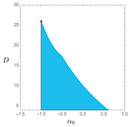
هذه الشروط صارمة لدرجة أنه قد يتساءل المرء عما إذا كانت سعات الأوتار تحدد بشكل فريد من خلال هذه المجموعة من القيود. شهدت السنوات الأخيرة زيادة في الاهتمام بهذا السؤال في أبسط سياق لتشتت النقاط الأربع [6-13]. حتى في الأشهر القليلة الماضية، ظهرت مجموعة مذهلة من مثل هذه الاقتراحات في الأدبيات [12-22]، بعضها يعيد زيارة العمل الرائد في المرجع [23]. بشكل مفاجئ، كانت النتيجة العامة سلبية: من الممكن تشويه سعة فينيزيانو للنقاط الأربع [24] للوتر المفتوح بطرق عديدة لا تزال تتوافق مع هذه القيود الفيزيائية. حتى عند النقاط الأربع، لا تزال الوحدوية الجزئية تسمح بمجموعة من المعلمات المتسقة [25]، على الرغم من أن الشهيرة لنظرية الأوتار لا تزال تأخذ دلالة خاصة، كما هو موضح في الشكل 1.
من الطبيعي أن نسأل عما إذا كانت هذه الحرية الهائلة تستمر بعد تشتت النقاط الأربع. ومع ذلك، فإن الحدود -نقطة من التشتت ظلت منطقة غير مستكشفة إلى حد كبير حتى العام الماضي أو نحو ذلك.
على سبيل المثال، تم اقتراح فئة واسعة من التعميمات لسعات الأوتار ذات النقاط -التي تظهر “مخصصة”، أو طيفًا قابلًا للتعديل تمامًا. كما في نظرية الأوتار، تصف هذه السعات المخصصة برجًا لا نهائيًا من الدورانات الأعلى التي تظهر ازدواجية القناة. عند النقاط الأربع، هناك أدلة على أن نماذج معينة، على الأقل في بعض مناطق فضاء المعلمات، هي سببية ووحدوية. علاوة على ذلك، عند النقطة تكون هذه السعات متسقة مع التحليل على
الشكل 1. تحدد الوحدوية الجزئية سعة الوتر المفتوح ذات النقاط الأربع مع تقاطع ريج، في أبعاد الزمكان إلى المنطقة المسموح بها باللون الأزرق. يتوافق الوتر البوزوني مع القمة عند و .
أقطاب الحالة المتبادلة الأقل.
تطور بارز آخر هو نهج جديد لتشتت النقاط الذي ينطبق على نظرية الأوتار ولكن أيضًا على نظريات الحقول الكمومية مثل نظرية و نظرية يانغ-ميلز في جميع أوامر توسيع ‘ت هوفت. في هذا الإطار، يتم وصف سعات النقاط بواسطة تكامل بسيط على مجموعة من المتغيرات المساعدة التي هي أبناء عمومة رياضية للمعلمات المعتادة التي تحدد تمثيل كوبا-نيلسن لسعات الأوتار. بشكل ملائم، يستوعب هذا النظام تشويهًا طبيعيًا لسعة الوتر ذات النقاط من خلال إدخال عامل شكل مضاعف في الدالة. يمكن تصميم هذه الدالة بسهولة لضمان التحليل على الأقطاب عديمة الكتلة.
النتيجة من هذه النتائج هي نوع من الصدمة: لقد انتقلنا من الحدس الساذج بأن تشتت الأوتار ذات النقاط فريد إلى إحراج من الثروات في التشوهات المتسقة المفترضة! هذا مثير ومزعج في نفس الوقت. لكن هل هذه الحرية حقيقية؟
في هذه الورقة سنجادل بأنها ليست كذلك، بسبب القيود المفروضة من التحليل على الأقطاب الكتلية إلى مجموعة متسقة من السعات الثلاثية.
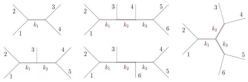
الشكل 2. التحليل المتسق في هذه القنوات كافٍ لاستبعاد فئة هائلة من السعات المفترضة. عكس عقارب الساعة من أعلى اليسار: نصف سلم من أربع وخمس نقاط؛ نصف سلم ملتوي من ست نقاط، نجمة، ونصف سلم.
هذه الحالة مقيدة بشكل مذهل. التحليل في تشتت النقاط الأربع والخمس والست كافٍ لهزيمة أبسط نموذج مخصص وكذلك فئة كبيرة من البنى الطبيعية . تتطلب هذه الاستبعادات فقط اعتبار المتجهات والسكالار المتبادلة في الطوبولوجيات الموضحة في الشكل 2. على طول الطريق، سنقدم تقنيات مفيدة لحساب البقايا على الأقطاب الكتلية ونلخص مجموعة جديدة من قواعد الجمع البسيطة التي تقيد مباشرة البقايا والطيف الكتلي لأي سعة مفترضة ذات النقاط .
بالطبع، تلبي سعات النقاط من نظرية الأوتار القيود من التحليل على الأقطاب الكتلية. لكن نتيجة هذه الفحص هي أننا يمكننا استخراج السعات الثلاثية مباشرة – الثوابت المرتبطة وكل شيء – مباشرة من السعات ذات النقاط الأعلى.
تمهيد.- إن قوة القيود الناتجة عن التحليل واضحة بالفعل عند النقاط المنخفضة. كمثال بسيط على هذا النهج، دعونا نعتبر باختصار سعات التاكيون على مستوى الشجرة للوتر البوزوني. تشتهر هذه السعات بعرض طيف خطي ، حيث هو عدد صحيح غير سالب يحدد كل مستوى من الوتر، الذي يدعم أوضاع الدوران . من خلال تحليل سعة الوتر ذات النقاط الأربع على المستويات و 1، نحصل على البقايا
حيث هي المتغيرات الماندلستام المسطحة في التوقيع الأكثر إيجابية. هنا يتم إنشاؤه بواسطة سكالار عند المستوى و يتم إنشاؤه بواسطة سكالار ومتجه عند المستوى .
بعد ذلك، نقارن هذه البقايا مع بقايا افتراضية مستمدة من مجموعة من سعات ثلاثية على السطح تصف تفاعل الجسيمات الثلاثة عند المستويات من الدورانات . بشكل صريح،
ثم نستخرج رؤوس فينمان المقابلة ونلصقها معًا للحصول على البقايا الافتراضية،
مساواة المعادلات (1) و (3)، وبالتالي نحدد – حتى العلامات غير الفيزيائية – الثوابت المرتبطة بالنظرية.
من الثوابت المرتبطة المربعة في المعادلة (3)، نرى أن البناء أعلاه هو ببساطة إعادة صياغة الشرط المعتاد للإيجابية في تشتت النقاط الأربع. ومع ذلك، نظرًا لأننا حددنا السعات الثلاثية، يمكننا إعادة إدخال هذه النتائج في البقايا ذات النقاط الأعلى للحصول على حدود جديدة.
على سبيل المثال، فإن بقايا السعة ذات النقاط الخمس، عند المستوى لكلا الناقلين الداخليين، هي
بينما البقايا الافتراضية المقابلة هي
هنا و تم تثبيتهما عند النقطة الأربع، وقد عرفنا السعات الافتراضية الإضافية،
تحدد البقايا في المعادلات (3) و (5) الفضاء المتسق المسموح به من خلال التحليل وطيفنا المفترض. ومن ثم، يمكن استخدامها لتحديد الثوابت المرتبطة بالنظرية أو، بالعكس، لاستبعاد سعة مفترضة غير متوافقة مع التحليل.
الإجراء العام.- التحليل أعلاه يمكن تعميمه على أي دوران وعدد من الجسيمات الخارجية. كما سنرى، فإن قيود التحليل الناتجة عن تبادل السكالار والناقل في تشتت النقاط الأربع والخمس والست كافية لتقليل مساحة الأمبليتودات المتسقة بشكل كبير! دعونا الآن نصف الإجراء العام لبناء هذه البقايا الافتراضية.
أولاً، نأخذ طيفًا مختارًا من الكتل والدوران كمدخل. من أجل التوضيح، نفترض طيفًا متصلًا باستمرار مع طيف الخيط: عدد صحيح واحد عند المستوىوعدد فردي من القيم العددية والمتجهات على المستوى، دون أي انحلال. ومع ذلك، سنفترض عدم وجود أي شيء مسبق حول القيم الدقيقة للكتل أو الثوابت التفاعلية للنظرية. على مدار النص، سننظر في الأمبليود التي تكون فيها الحالات الخارجية هي المتجهات الملونة ذات الكتلةعلى المستوى.
ثانياً، نقوم بإحصاء جميع الأمبليتودات الثلاثية النقاط على السطح لهذه الحالات. تم إعطاء الأمبليتودات الثلاثية النقاط على السطح لعدد صفر أو واحد أو اثنين من المتجهات الخارجية في المعادلتين (2) و (6). أما الأمبليتود لثلاثة متجهات فهو [26].
هنا تتوافق الحدود الأولى والثانية مع رأس يانغ-ميلز الثلاثي ورأس بوزون القياس الثلاثي الشاذ، على التوالي. من الأم amplitudes المذكورة أعلاه، من السهل اشتقاق رؤوس فاينمان المقابلة.
أخيرًا، لبناء بقايا الأنزاتس، نقوم بلصق هذه الرؤوس فينمان معًا باستخدام ناقلات فينمان للسكالار والمتجهات. البسط للثاني هو، حيث على القطع. لاحظ أنه لا يوجد اعتماد على بعد الزمكانفي الناقلات السلمية والناقلات المتجهة. علاوة على ذلك، فإن آثار المقياس لا تظهر في مستوى الشجرة، لذا فإن الحدود التي نواجهها ستكون-مستقل. أمثلة.- في هذا القسم نحسب البقايا لمختلف الأمبليودات ذات النقاط العليا ونقارنها مباشرة بالبقايا التي تم بناؤها باستخدام الإجراء العام الموضح أعلاه. كما سنرى، فإن القيود الناتجة عن تحليل النقاط العليا قوية للغاية. أ amplitudes. للبدء، اعتبر المستوى القياسي-عامل كوبا-نيلسن [27-29]،
الذي نشير إليه باسم “سعة الخيط” في استخدام طفيف للترميز [30]. هناهي الزخمات الخارجية،هي النماذج المدمجة على القرص، وهناك اختلافات. يتم تعريف طيف الدول بـنظرًا لأن الأرجل الخارجية لسمات السلسلة مرتبة بشكل مسطح، فإن جميع قنوات التحلل تظهر كأقطاب بسيطة في المتغيرات الماندلستام المسطحة.تم تعريفها سابقًا. بشكل مريح، هذهتشكل المتغيرات أساسًا أدنى للجميع-نقاط متغيرات مانديليشتام. لجعل هذا الاعتماد واضحًا، نعيد صياغة المعادلة (8) من حيث نسب التقاطع الثابتةوفي هذه الحالة، تصبح سعة الخيط
لاحظ أنه عند الانتقال من المعادلة (8) إلى المعادلة (9) قمنا بتحويل المتغيرات الماندلستام المستوية بواسطة تقاطع ريج غير متغير.، لذا فإن السعة تحتوي تلقائيًا على تفردات عند والطيف هو .
التفي المتغيرات بالعلاقات غير التافهة،
أين ( ) يتوافق مع جميع الأوتار لـ -جون الذي يتقاطع مع الوتر. هذه المعادلات تقبل ( فضاء الحلول ذي الأبعاد )-المعلمة بدقة بواسطة المعاملاتلورقة العالم المثبتة بواسطة المقياس.
استخدام التقليديالمتغيرات، من الصعب استخراج المتبقيات عند مستويات عشوائية. لكن السبب الوجودي لـالمتغيرات هي لإظهار جميع التفردات بشكل شفاف، مما يمنحنا طريقة بسيطة وصريحة لاستخراج بقايا عشوائية. يتم ذلك بسهولة أكبر من خلال تغيير المتغيرات إلى إحداثيات إيجابية، حيث تأخذ السعة الشكل
هنا كلمرتبط وتريظهر في بعض اختيارات التثليثمن-جون. خوارزمية بسيطة تعبر عنمن حيث [32]. في هذه الصورة، الانفرادياتالأوتار في التثليثمرتبطة بالتباعد اللوغاريتمي للتكامل بالقرب منالتكامل يتباعد لـويجب أن يتم تعريفها من خلال الاستمرار التحليلي، حيث تتطور بالفعل الأقطاب عندما هو عدد صحيح سالب. بالنسبة لـ الدالة المتكاملة تحتوي على قطع فرعية في. ومع ذلك، عندما يكون كل، بدلاً من ذلك يحتوي الدالة المتكاملة على أقطاب عنديتم حساب بقايا التكامل عند القطب بواسطة بقايا الدالة المدخلة عند.
باختصار، الخوارزمية لحساب الباقي المرتبط بأي رسم بياني أو تقسيم مثلثيثم يكون الأمر بسيطًا: استخدم التمثيل الإيجابي المرتبط بـ في المعادلة (11)، اضبط ، واحسب بقايا الدالة المتكاملة عند .
من خلال هذه العملية، نقوم بحساب جميع البقايا لأمبليودات الأوتار ذات الأربع والخمس والست نقاط على قنوات التحلل القصوى التي يتم فيها تحديد جميع الأرجل الداخلية إلى مستويات.. ثم نقارن هذه البقايا النصية بالبقايا التي تم بناؤها من خلال لصق أمبليتات ثلاثية النقاط عشوائية مع تفاعلات حقيقية. ومن المRemarkably، لأي قيمة من قيمة تقاطع ريج.، فإن سعة الخيط متوافقة تمامًا مع هذه الشروط الخاصة بالتفكيك. كنتاج فوري لهذه التمرين، نستخرج السعات الثلاثية النقاط الصريحة لنظرية الأوتار للمستويات (أي، الكتل أو ) ويدور ، كما هو موضح في الجدول أدناه. قمنا ببناء هذه الاقترانات بشكل فريد من تحليل متسق لاهتزازات الأوتار ذات النقاط الأعلى، دون استخدام مشغلات رأس السطح. من السهل حساب جميع اهتزازات الثلاث نقاط للأوتار من خلال تعميم هذا النهج إلى مستويات أعلى، مع مراعاة اعتبارات الانحلال، التي نتركها للعمل المستقبلي.
( )
سعة ثلاث نقاط
(0، 0، 0)
(0، 0، 0)
1
(1, 0, 0)
(0، 0، 0)
(1, 0, 0)
(1, 0, 0)
(1, 1, 0)
(0، 0، 0)
(1, 1, 0)
(1, 0, 0)
(1, 1, 0)
(1, 1, 0)
(1, 1, 1)
(0، 0، 0)
(1, 1, 1)
(1, 0, 0)
(1, 1, 1)
(1, 1, 0)
(1, 1, 1)
(1, 1, 1)
أطياف مخصصة. بعد ذلك، دعونا نوضح كيف تفرض التحليل المتسق قيودًا صارمة على الأطياف المخصصة المحددة في المرجع [14]. من أجل التوضيح، نركز على أبسط نسخة من هذه الأطياف ذات الطيف غير الخطي، والتي تت correspond إلىفي التسمية الواردة في تلك الورقة.
لهذا السعة، طيف الرنين عند المستوىيتم تعريفه بواسطة كثير الحدود غير الخطي النسبي، حيث هي معلمات تلبي. المقابلنقطة السعة المخصصة هي ببساطة مجموع على السعات المعتادة للخيوط،
أينوفي كل حد من حدود مانديستام المسطحتم تأليفه باستخدام دالة غير خطيةالمتوسط عبر فروع الجذر التربيعي، لكل مؤشر، يضمن أن السعة الناتجة خالية من قطع الفروع ولها بقايا متعددة الحدود. لاختيارات مناسبة منأظهرت المرجع [14] أن سعة النقاط الأربعة تمتلك تمثيلًا رنينيًا مزدوجًا وهي متوافقة مع وحدة الموجات الجزئية. العامليصلح التطبيع القياسي للمستوىالدول الخارجية، لذا فإن السعة المخصصة تتفكك تلقائيًا عند تبادل تلك الدول. التفكيك الصحيح على الدول عند مستويات أعلىومع ذلك، لم يتم ضمان ذلك بعد.
يتم حساب بقايا السعات المخصصة من خلال استخراج بقايا سعة الخيط باستخدام المعادلة (11) وإدخالها في المعادلة (12). يتم مقارنة بقايا السعات المخصصة الناتجة مع بقايا الأنزات عند النقاط الأربعة والخمسة والستة للمستوىنجد أنه باستثناء بعض النظريات التافهة ذات التفاعلات النقطية البحتة، لا توجد قيم لـالتي تتماشى مع التحليل. بينما عائلة ذات معلمة واحدة معتفي بالفعل بمتطلبات التحليل للعوامل الخاصة بالسلالم النصفية، لكنها تفشل بالنسبة للسلم النصفى الملتوي ذو النقاط الستة الموضح في الشكل 2.
لذا، فإن أبسط الأمبليتودات المخصصة غير متوافقة مع التحليل إلى عدد حقيقي واحد على المستوىوعدد قياسي مفرد ومتجه عندلا يزال سؤالاً مفتوحاً ما إذا كان يمكن تجاوز هذه الحدود في الفئة الأوسع من الأمبليودات المخصصة [14]، أو ربما من خلال تضمين التكرار.
تكامل السلسلة المشوهة. الميزة الحاسمة في المعادلة (11) هي أنها تجعل التحليل على المستوىالأقطاب واضحة. عندماالتكامل يطور قطبًا بالقرب من. بسبب الطابع “الثنائي” للمعادلة (10)، الحد يرسللأجل الأوتارذلك الصليب. ومن ثميتم تحليلها بطريقة تعكس السعة. وهذا يشير إلى فئة أكثر عمومية من الدوال التي تظهر مستوىتحليل: ببساطة اضرب فيتكامل النقطة بواسطة عامل الشكلمصمم ليتم تحليله إلى حاصل ضرب عوامل ذات نقاط أدنى عندمامن الطبيعي أن نقتصر على كثيرات الحدود المحدودةللحفاظ على سلوك ريج الذي يتميز به أمواج الأوتار.
دعنا نحدد عائلة بسيطة من التشوهات، مُعلمة بواسطة عدد صحيح الذي يحدد -أضلاعداخل الزخم-غون. ثم نحدد
أين ( ) مجموعات على جميع أزواج الرؤوس في ونأخذ. المعامل يُسيطر على التشوه بعيدًا عن سعة السلسلة الأصلية.
لاحظ أنه إذا كانت وتريتقاطعيجب أن يتقاطع مع واحد على الأقل من الأوتار داخل. لذلك، في قناة التحليل حيث ، ناتج ( ) تختفي بسبب المعادلة (10)، مما يترك لنا حاصل الضرب على جميع الـ التي لا تتقاطع، لذا فإن التحليل عند المستوىثم يتبع.
لتحليلنا، نأخذ في الاعتبار و الأمبليتودات، التي نطلق عليها اسم “تشوهات مثلثية” و”تشوهات رباعية”، على التوالي. في كلا الحالتين، الأمبليتودات ثلاثية النقاط عند المستوى يتم إصلاحها تمامًا بواسطة تشتت النقاط الأربعة والخمسة. من خلال إعادة إدخال هذه الروابط في أمبليودات النقاط الأعلى، نجد أنه إذا ثم إن بقايا النقاط الست لكل من المثلث والمربع متسقة بالنسبة للمدرجات نصفية النقاط الأربعة والخمسة والستة، لكنها غير متسقة بالنسبة لتوبولوجيا المدرج نصف الملتوي الموضحة في الشكل 2. وبالتالي، يتم استبعاد كل من نماذج المثلث والمربع [34].
بشكل طريف، يمكن استبعاد تشوه المثلث عند النقاط الأربعة عبر وحدة الموجة الجزئية، على الرغم من التكلفة الكبيرة. عند حساب توسيع الموجة الجزئية على متعددات جينغنباور، نجد أنه بالنسبة للقيم غير الصفريةالموجة الجزئية السلبية الأولى تكون عند الدوران 0 أو 1، ولكن عند مستوى مرتفع جداًتوضح هذه الفجوة الدرامية في الجهد قوة تحليل العوامل ذات النقاط الأعلى. قواعد الجمع.- تفرض عملية التحليل لعوامل النقاط الأعلى مجموعة من قواعد الجمع غير الخطية التي تعتمد على الكتل والمعاملات العددية لبقايا سعة مفترضة. تتمتع هذه القواعد بميزة واضحة تتمثل في أنها يمكن استخدامها لإزالة النظريات غير المتسقة بشكل واضح دون اللجوء إلى الإجراء المرهق المتمثل في لصق سعات ثلاثية النقاط المفترضة معًا.
لهذا الغرض، دعنا نحدد معلمة عامة للبقايا الناتجة عن بقايا الاقتراح للترابطات التعسفية. على سبيل المثال، بقايا نصف السلم العامة ذات الأربع نقاط عند المستوىهم
بينما في النقطة الخامسة هم
هناتُحدد بقايا النقاط بالكامل بواسطة المعاملات العددية، حيث أن الرموز السفليةتشير إلى المستويات التي تم تحديد كل ساق داخلية عليها والرموز العلويةتشير إلى قوة كل متغير مانديستامترتيبيتم تعريفه بواسطة الترتيب المعجمي لـالكتابات السفلية فيالتي تظهر في بقايا معينة [35]. لاحظ أنتفي المعاملات بالهويات المطلوبة من قبل التحويلات المتناظرة، لذا على سبيل المثال،.
نظرًا لأن بقايا الأنزاتز تُبنى عن طريق لصق مقادير ثلاثية النقاط بشكل عشوائي، فهي متعددة الحدود فيمع علاقات دقيقة جدًا تربط بين المعاملات العددية لكل هيكل حركي. تتوافق هذه الشروط مع مجموعة من قواعد الجمع غير الخطية التي تربط بينمعاملات مع طيف الكتلةالتي نقوم الآن بتلخيصها لبقايا من أربع وخمس وست نقاط تم حسابها على مستويات.
قواعد مجموع النقاط الأربعة. بالنسبة للبقايا العامة ذات النقاط الأربعة في المعادلة (14)، يمكننا المقارنة مع بقايا الفرضية لاستخراج السعات الثلاثية المقابلة.
على الفور، تشير حقيقة ثوابت الاقتران إلى عدم المساواة في معاملات البقايا،
حيث إن عدم تشبع المتباينتين الأولى والثانية لأننا نفترض وجود ارتباطات غير صفرية لكل من السكالار والفيكتور.
قواعد مجموع النقاط الخمس. للحصول على قواعد المجموع عند النقطة الخامسة، نقوم بإدخال السعات الثلاثية في المعادلة (16) مرة أخرى في بقايا الفرضية ونقارن مرة أخرى مع البقايا العامة في المعادلة (15). من خلال القيام بذلك، يتم تحديد العديد من السعات الثلاثية الأخرى.
بالإضافة إلى قواعد المجموعات،
انظر الملحق أ. للمجموعات المماثلة لقواعد التحليل المتسق عند النقاط الست.
نقاش.- في هذه الورقة، جادلنا بأن التحليل المتسق هو قيد صارم بشكل ملحوظ على تشتت الجسيمات المتعددة. تحليلنا ليس شاملاً بأي حال من الأحوال، بل هو بمثابة دعوة لاستكشاف هذه المجموعة الغنية من شروط الاتساق الجديدة ذات النقاط الأعلى. هناك العديد من الأسئلة التي أثارتها ملاحظاتنا الأولية بشكل مباشر.
على سبيل المثال، من المبرر تمامًا أن نسأل عما إذا كانت هناك أي تشوهات معروفة لـ-نقطة السعة التي تلبي فعليًا التحليل المتسق. تشمل بعض المرشحات الطبيعية السعات المصممة خصيصًا ذات الطيف غير الخطي بشكل أكبر، بالإضافة إلى غيرها منتشوهات دالة التكامل للوتر.
منتج جانبي مريح من تحليلنا هو أننا يمكننا استخراج الاقترانات الثلاثية النقاط من الخيط مباشرة.-نقاط تشتت الأمواج. سيكون من المثير جداً استخدام هذه الأداة للتعرف على بنية التفاعلات وكثافة الحالات في الخيط مباشرة من الأمواج نفسها. هذه الخطوط من التحقيقات وما يرتبط بها تحمل وعداً برؤى جديدة أساسية حول سؤال ما إذا كان هناك شيء ما يجعل نظرية الأوتار مميزة.
الشكر: نشكر ديفيد غروس وآرون هيلمان على المناقشات المفيدة. يتم دعم ن.أ.هـ. من قبل وزارة الطاقة (المنحة رقم DE-SC0009988)، ومن قبل تعاون سيمونز في الهولوجرافيا السماوية، وتم توفير دعم إضافي من خلال برنامج كارل ب. فاينبرغ متعدد التخصصات في الابتكار في IAS. يتم دعم ج.ج. من قبل وزارة الطاقة (المنحة رقم DESC0011632) ومن قبل معهد والتر بيرك للفيزياء النظرية. يتم دعم ج.ف. من قبل FCT/البرتغال (المنحة رقم2023.01221.BD). يتم دعم G.N.R. من خلال زمالة جيمس آرثر لما بعد الدكتوراه في جامعة نيويورك.
قواعد مجموع النقاط الستة
نقوم ببناء قواعد مجموع عامة لتفكيك متسق لجميع مخططات النقاط الستة على المستوياتلتسهيل الاستخدام، نقدم أيضًا هذه النتائج في ملف نصي إضافي.
نقوم أولاً بإجراء حساب التحليل للعوامل لرسم السلم نصف الست نقاط الموضح في الشكل 2 من الرسالة من خلال حساب البقايا الملصقة ومقارنتها مع بقايا فرضية ست نقاط محددة بشكل عشوائي بواسطةمعاملات
التي تلبي التحويلات الانعكاسية. هنا، نحن نقوم بتحليل على الـ ( ) = قناة. نجد قواعد جمع مستقلة عن الكتلة،
بالإضافة إلى قواعد المجموع المعتمدة على الكتلة،
بالنسبة لمخطط السلم الملتوي ذو النقاط الستة الموضح في الشكل 2، نحدد بقايا جديدة من نوع الأنزات.من حيث المعاملات،
التي تلبي تماثلات الدوران. هنا، نحن نقوم بتحليل على ( نجد قواعد جمع مستقلة عن الكتلة تربط بين معاملات نصف السلم والمعاملات الملتوية لنصف السلم،
بالإضافة إلى قواعد المجموع المعتمدة على الكتلة،
بالنسبة للتوبولوجيا المتبقية النهائية، مخطط النجمة ذات الست نقاط في الشكل 2، نحدد بقايا الأنزات.من حيث المعاملات،
التي تلبي تماثلات الدوران والانعكاس. هنا، نحن نقوم بتحليل العوامل على القناة. بسبب التناظرات المعززة لرسم النجوم، تفرض عملية التحليل المتسقة قائمة أقصر من قواعد الجمع،
[1] أ. مارتن، “تمديد مجال التحليل البديهي لامتصاص الأمواج بواسطة الوحدة. 1.،” نيوفو كيم. أ 42 (1965) 930. [2] ي. س. جين وأ. مارتن، “عدد الطرحات في علاقات الانتشار ذات النقل الثابت،” فيزيكال ريفيو 135 (1964) B1375. [3] ر. ج. إيدن، “نظريات حول تصادمات الطاقة العالية للجسيمات الأولية،” مراجعة الفيزياء الحديثة 43 (1971) 1535. [4] أ. آدامز، ن. أركاني-حميد، س. دوبوفسكي، أ. نيكوليس، و ر. راتاتزي، “السببية، التحليلية و عائق الأشعة تحت الحمراء لإكمال الأشعة فوق البنفسجية،” JHEP 10 (2006) 014، arXiv:hep-th/0602178. [5] ك. هارينغ وأ. زيبودوف، “حدود ريج الجاذبية،” arXiv:2202.08280 [hep-th]. [6] ن. أركاني-حميد، ت.-س. هوانغ، وي.-ت. هوانغ، “الهيكل EFT”، JHEP 05 (2021) 259، arXiv:2012.15849 [hep-th]. [7] X. O. Camanho، J. D. Edelstein، J. Maldacena، و A. Zhiboedov، “قيود السببية على التصحيحات لاقتران الجرافيتون ثلاثي النقاط،” JHEP 02 (2016) 020، arXiv:1407.5597 [hep-th]. [8] س. كارون-هوت، ز. كومارجودسكي، أ. سيفر، وأ. زيبودوف، “الأوتار من الدوران العالي الضخم: التفرد الأسيمبتيكي لامبلي فينيزيانو،” JHEP 10 (2017) 026، arXiv:1607.04253 [hep-th]. [9] ن. أركاني-حميد، ل. إبرهاردت، ي.-ت. هوانغ، و س. ميزيرا، “حول وحدة مستوى الشجرة من مضاعفات الأوتار- “تودس،” JHEP 02 (2022) 197، arXiv:2201.11575 [hep-th]. [10] ل. ف. ألداي، ت. هانسن، وج. أ. سيلفا، “أدس فيراسورو شابيرو من فترات ذات قيمة واحدة،” JHEP 12 (2022) 010، arXiv:2209.06223 [hep-th]. [11] ج. بيرمان، هـ. إلفانغ، و أ. هيردرشي، “تسطيح هيدران EFT: حدود الإيجابية الفائقة والبحث عن نظرية الأوتار،” arXiv:2310.10729 [hep-th]. [12] سي. تشيونغ وجي. إن. ريمان، “تباينات فينيزيانو: ما مدى تميز سعات الأوتار؟”، JHEP 01 (2023) 122، arXiv:2210.12163 [hep-th]. [13] سي. تشيونغ وجي. إن. ريمان، “ديناميات خيطية من انطلاق الأمبليتودات،” فيزيكال ريفيو دي 108 (2023) 026011، arXiv:2302.12263 [hep-th]. [14] سي. تشيونغ وجي. إن. ريمان، “رنين مزدوج مخصص،” فيزيكس ريفيو دي 108 (2023) 086009، arXiv:2308.03833 [hep-th]. [15] ك. هارينغ وأ. زيبودوف، “دليل مصفوفة S الخيطية: أقصى دوران ونعومة سوبر بولينوم”، arXiv:2311.13631 [hep-th]. [16] ي.-ت. هوانغ و ج. ن. ريمان، “أمبليتود الجاذبية المكتملة بالأشعة فوق البنفسجية ومنتج الثلاثي،” فيزيكس ريفيو د 106 (2022) L021902، arXiv:2203.00696 [hep-th]. [17] ج. مالداسينَا و ج. ن. ريمين، “أمبليتات نقاط التراكم في نظرية الأوتار،” (2022) 152، arXiv:2207.06426 [hep-th]. [18] ن. جيسر و ل. و. ليندواسر، “أمبليتودات فينيزيانو وفيراسورو المعممة،” JHEP 04 (2023)
031، arXiv:2210.14920 [hep-th]. [19] ن. جيسر، “خباز-كون-رومان“-نقطة السعة وحدود نظرية الحقل الدقيقة لسعة كون،” arXiv:2311.04130 [hep-th]. [20] ر. بهاردواج، س. دي، م. سبرادلين، و أ. فولوفيتش، “حول وحدة أمبليت كيون،” JHEP 08 (2023) 082، arXiv:2212.00764 [hep-th]. [21] ر. بهاردواج و س. دي، “أمبليتودات رنينية مزدوجة من التواءات درينفيلد،” arXiv:2309.07214 [hep-th]. [22] سي. بي. جيبسن، “خفض سعة الكوان،” JHEP (2023) 114، arXiv:2303.02149 [hep-th]. [23] د. د. كون، “تفرد تمثيل فينيزيانو،” فيز. ليت. ب 29 (1969) 669. [24] ج. فينيسيو، “بناء أمبليتود متقاطع متماثل، يتصرف وفقًا لرج، لمسارات ترتفع خطيًا،” نيوفو كيم. أ 57 (1968) 190. [25] التطبيق الساذج لوحدة الموجات الجزئية قد يوحي بأن الإيجابية عنديتطلب. ومع ذلك، بالنسبة لـالمتبادلةيتطلب الوضع طاقة أقل من طاقة مركز الكتلة للظهور. ومن ثم، فإن قناة التحليل هذه غير متاحة ولا ينطبق حد الإيجابية. [26] لاحظ أن سعة النقطة الثلاثيةلديه ترتيب داخلي في أرجلها الخارجية محدد بواسطة ترتيب الألوان في الرسم. ومن ثم، فإن ترتيب الأرجل في اتجاه عقارب الساعة مقابل عكس اتجاه عقارب الساعة في سعة ثلاثية النقاط مرتبط بتغيير محتمل في الإشارة. على وجه الخصوص، تلتقط سعة ثلاثية النقاط الإشارةعندما يتم تبديل أي مؤشرين. [27] م. ب. غرين، ج. هـ. شوارز، وإي. ويتن، نظرية الأوتار الفائقة. 1987. [28] ج. بولتشينسكي، نظرية الأوتار. مطبعة جامعة كامبريدج، 1998. [29] ك. بيكر، م. بيكر، وج. هـ. شوارز، نظرية الأوتار ونظرية M: مقدمة حديثة. [30] تلعب هذه التكاملات على سطح العالم دورًا مهمًا في وصف جميع سعات الأوتار المفتوحة على مستوى الشجرة: جميع التكاملات المعتمدة على موبايوس التي تم “لفها” بواسطة كوبا-
يمكن كتابة عامل نيلسن كتركيب خطي من تكاملات من هذا الشكل مأخوذة على أساس من ! ترتيبات ألوان مختلفة. وهي مرتبطة أيضًا بأمبليودات مشهورة في نظرية الأوتار. على سبيل المثال، مع تحول حركي بسيط، تأخذ أمبليود جميع التاكيونات في الأوتار البوزونية هذا الشكل. بالإضافة إلى ذلك، تم اقتراح هذا الكائن كنظرية متسقة ذاتيًا في حد ذاتها، تُسمى -نظرية. أخيرًا، عند أربع نقاط، يتم إعطاء سعة الغلوون في نظرية الأوتار الفائقة بواسطة هذا العامل مضروبًا في عامل بسيط.. [31] نعمل في وحدات حيث مقياس الوتر هو. [32] ن. أركاني-هامد، هـ. فروست، ج. سالفاتوري، ب.-ج. بلاموندون، و هـ. توماس، “تشتت جميع الحلقات كمشكلة عدّ”، arXiv:2309.15913 [hep-th]. [33] لاحظ أن سلوك هذه الدالة المدمجة يختلف عن التكامل، أي السعة نفسها، التي هي ميرومافورم في. [34] يسمح التحليل المتسق تقنيًا بتشويه مثلث مع الاختيار الغريب لـ. بالنسبة لهذا الاختيار، تختفي جميع بقايا النقاط الأربعة والخمسة والستة عند المستويات ، وهو الحد الذي وصلنا إليه في تحليلنا. ومع ذلك، يتم استبعاد هذا الإعداد بواسطة وحدة الموجة الجزئية ذات الأربع نقاط على المستوى. [35] على سبيل المثال، بالنسبة لمخطط نصف السلم ذو النقاط الخمس، نحن نقوم بتحليل العوامل على القناة. يمكن أن تعتمد المتبقيات على المتغيرات الماندلستام المستوية المتبقية، والتي تكون بالترتيب القاموسي هي ( ). على الـالقناة، معامل هو . في الملحق أ، نقدم قواعد جمع النقاط الست لجميع الطوبولوجيات. على سبيل المثال، بالنسبة للدرج نصف الست نقاط، نقوم بتفكيك على القناة. المتغيرات الماندلستام المسطحة المتبقية، بترتيب قواميس، هي ( )، لذا فإن المعامل، في الـ بقايا، من هو لاحظ أن مجموع أعداد المؤشرات السفلية والعلوية يساوي دائمًا العدد الإجمالي لمتغيرات مانديستام المسطحة،.
Multiparticle Factorization and the Rigidity of String Theory
Nima Arkani-Hamed, Clifford Cheung, Carolina Figueiredo, and Grant N. Remmen School of Natural Sciences, Institute for Advanced Study, Princeton, NJ 08540 Walter Burke Institute for Theoretical Physics, California Institute of Technology, Pasadena, CA 91125 Department of Physics, Princeton University, Princeton, NJ 08540 Center for Cosmology and Particle Physics, Department of Physics, New York University, New York, NY 10003
Abstract
Is string theory uniquely determined by self-consistency? Causality and unitarity seemingly permit a multitude of putative deformations, at least at the level of two-to-two scattering. Motivated by this question, we initiate a systematic exploration of the constraints on scattering from higher-point factorization, which imposes extraordinarily restrictive sum rules on the residues and spectra defined by a given amplitude. These bounds handily exclude several proposed deformations of the string: the simplest “bespoke” amplitudes with tunable masses and a family of modified string integrands from “binary geometry.” While the string itself passes all tests, our formalism directly extracts the three-point amplitudes for the low-lying string modes without the aid of worldsheet vertex operators.
Introduction.-The scattering amplitudes of string theory exhibit a litany of seemingly impossible features simultaneously. On the one hand, they offer a proof of principle for how to consistently extrapolate quantum gravity to ultrahigh energies, past the regime of validity of general relativity. Miraculously, they achieve all this while preserving causality, which mandates that high-energy elastic scattering is polynomially bounded in the center-of-mass energy at fixed impact parameter [ 7]. Furthermore, string amplitudes make crucial use of higher-spin states, which are famously inconsistent in isolation but appear together in an infinite tower that elaborately conspires to maintain unitarity.
These conditions are so stringent that one might wonder whether string amplitudes are uniquely determined by this panoply of constraints. Recent years have witnessed a surge of interest in this question in the very simplest context of four-point scattering [6-13]. Even in just the past few months, a dizzying array of such proposals has made an appearance in the literature [12-22], some revisiting the seminal work of Ref. [23]. Rather surprisingly, the broad conclusion has been negative: it is possible to deform the four-point Veneziano amplitude [24] of the open string in many ways that still conform to these physical constraints. Even at four points, partial wave unitarity still allows for a range of consistent parameters [25], though the famous of string theory still takes on special significance, as shown in Fig. 1.
It is natural to ask whether this immense freedom persists beyond four-point scattering. However, the -point frontier of scattering has remained largely uncharted territory until the past year or so.
For example, a vast class of generalizations of -point string amplitudes has been recently proposed [14] that exhibit a “bespoke,” or completely tunable, arbitrary spectrum. Like in string theory, these bespoke amplitudes describe an infinite tower of higher spins exhibiting channel duality. At four points, there is evidence that specific models, at least in certain regions of parameter space, are causal and unitary. Furthermore, at point these amplitudes are consistent with factorization on the
Figure 1. Partial wave unitarity constrains the four-point open string amplitude with Regge intercept in spacetime dimensions to the allowed region in blue. The bosonic string corresponds to the cusp at and .
poles of the lowest-lying exchanged state.
Another salient development is a new approach to point scattering that applies to string theory but also quantum field theories like theory and Yang-Mills theory at all orders in the ‘t Hooft expansion. In this framework, -point amplitudes are described by a simple integral over a set of auxiliary variables that are the mathematical cousins of the usual moduli that define the Koba-Nielsen representation of string amplitudes. Conveniently, this formalism accommodates a natural deformation of the -point string amplitude through the introduction of a multiplicative form factor into the integrand. This function can be straightforwardly engineered so as to ensure factorization on massless poles.
The upshot of these results is a bit of whiplash: we have gone from the naive intuition that -point string scattering is unique to an embarrassment of riches in putative consistent deformations! This is exciting and disturbing in equal parts. But is this freedom genuine?
In this paper we will argue that it is not, on account of the constraints imposed by factorization on massive poles onto a self-consistent set of three-point amplitudes.
Figure 2. Consistent factorization in these channels is sufficient to rule out an enormous class of putative amplitudes. Counterclockwise from top left: four- and five-point halfladder; six-point twisted half-ladder, star, and half-ladder.
This condition is amazingly restrictive. Factorization in four-, five-, and six-point scattering is sufficient to vanquish the very simplest bespoke model as well as a large class of natural constructions. These exclusions only require the consideration of scalars and vectors exchanged in the topologies depicted in Fig. 2. Along the way, we will introduce useful techniques for computing residues on massive poles and summarize a new set of simple sum rules that directly constrain the residues and mass spectrum of any putative -point amplitude.
Of course, the -point amplitudes of string theory satisfy the constraints from factorization on massive poles. But a corollary of this check is that we can directly extract the three-point amplitudes-coupling constants and all-directly from the higher-point amplitudes.
Warmup.-The constraining power of factorization is already evident at low point. As a simple illustration of this approach, let us briefly consider the tree-level tachyon amplitudes of the bosonic string. These amplitudes famously exhibit a linear spectrum , where is a nonnegative integer labeling each level of the string, which supports modes of spin . Factorizing the four-point string amplitude onto levels and 1 , we obtain the residues
where are the planar Mandelstam invariants in mostly-plus signature. Here is generated by a scalar at level and is generated by a scalar and a vector at level .
Next, we compare these residues against an ansatz residue derived from a set of ansatz three-point on-shell amplitudes describing the three-particle interaction of the states at levels of spins . Explicitly,
We then extract the corresponding Feynman vertices and glue them together to obtain the ansatz residues,
Equating Eqs. (1) and (3), we thus determine – up to unphysical signs – the coupling constants of the theory.
From squared coupling constants in Eq. (3), we see that the above construction is simply a restatement of the usual condition of positivity in four-point scattering. However, since we have determined the three-point amplitudes, we can feed these results back into higher-point residues to obtain new bounds.
For example, the five-point residue of the string amplitude, at level for both internal propagators, is
while the corresponding ansatz residue is
Here and were fixed at four point, and we have defined the additional ansatz amplitudes,
The residues in Eqs. (3) and (5) parameterize the consistent space allowed by factorization and our assumed spectrum. Hence, they can be used to fix the couplings of the theory or, conversely, rule out a putative amplitude that is incompatible with factorization.
General Procedure.-The above analysis generalizes to any spin and number of external particles. As we will see, however, factorization constraints from scalar and vector exchange in four-, five-, and six-point scattering are sufficient to dramatically reduce the space of consistent scattering amplitudes! Let us now describe the general procedure for constructing these ansatz residues.
First, we take a chosen spectrum of masses and spins as an input. For concreteness, we assume a spectrum that is continuously connected to that of the string: a single scalar at level and a single scalar and vector at level , with no degeneracy. However, we will assume nothing a priori about the precise values of the masses or the coupling constants of the theory. Throughout, we will consider amplitudes in which the external states are the colored scalars of mass at level .
Second, we enumerate all three-point on-shell amplitudes for these states. The on-shell three-point amplitudes for zero, one, or two external vectors were given in Eqs. (2) and (6). The amplitude for three vectors is [26]
Here the first and second terms correspond to the YangMills cubic vertex and anomalous triple gauge boson vertex, respectively. From the above amplitudes it is easy to derive the corresponding Feynman vertices.
Finally, to build the ansatz residue we glue these Feynman vertices together with the Feynman propagators for scalars and vectors. The numerator for the latter is , where on the cut. Note that there is no dependence on the spacetime dimension in the scalar and vector propagators. Furthermore, traces of the metric do not appear at tree level, so the bounds we encounter will be -independent.
Examples.-In this section we compute the residues for various higher-point amplitudes and compare them directly to the residues constructed using the general procedure outlined above. As we will see, constraints from higher-point factorization are exceedingly powerful.
String Amplitudes. To begin, consider the standard treelevel -point Koba-Nielsen factor [27-29],
which we refer to as a “string amplitude” in a slight abuse of notation [30]. Here are the external momenta, are moduli integrated over the disc, and are their differences. The spectrum of states is defined by . Since the external legs of the string amplitude are planar-ordered, all factorization channels appear as simple poles in the planar Mandelstam invariants defined previously. Conveniently, these variables form a minimal basis for all -point Mandelstam invariants. To make this dependence manifest, we recast Eq. (8) in terms of the invariant crossratios, , in which case the string amplitude becomes
Note that in going from Eq. (8) to Eq. (9) we have shifted the planar Mandelstam invariants by a constant Regge intercept , so the amplitude automatically has singularities at and the spectrum is .
The variables satisfy the nontrivial relations,
where ( ) corresponds to all chords of the -gon that intersect the chord . These equations admit an ( )-dimensional space of solutions parameterized precisely by the moduli of the gauge-fixed worldsheet.
Using traditional variables, it is challenging to extract the residues at arbitrary levels. But the raison d’être of the variables is to transparently manifest all singularities, giving us a simple and explicit way to extract arbitrary residues. This is most easily done by a change of variables to positive coordinates, where the amplitude takes the form
Here each is associated with a chord appearing in some choice of triangulation of the -gon. A simple algorithm expresses in terms of [32]. In this form the singularities of chords in the triangulation are associated with the logarithmic divergence of the integral near . The integral diverges for and must be defined by analytic continuation, indeed developing poles when is a negative integer. For generic the integrand has branch cuts in . However, when all , the integrand instead has poles at . The residue of the integral on the pole is computed by the residue of the integrand at .
In summary, the algorithm for computing the residue associated with any diagram or triangulation is then simple: use the positive parameterization associated with in Eq. (11), set the , and compute the residue of the integrand at .
With this procedure we straightforwardly compute all residues of the four-, five-, and six-point string amplitudes on the maximal factorization channels on which all internal legs are localized to levels . We then compare these string residues to the ansatz residues constructed from gluing together arbitrary three-point amplitudes with real couplings. Remarkably, for any value of the Regge intercept , the string amplitude is perfectly consistent with these factorization conditions. As an immediate byproduct of this exercise, we extract the explicit three-point amplitudes of string theory for levels (i.e., masses or ) and spins , given in the table below. We constructed these couplings uniquely from consistent factorization of higher-point string amplitudes, without making use of worldsheet vertex operators. It is straightforward to compute all three-point amplitudes of the string by generalizing this approach to higher levels, modulo considerations of degeneracy, which we leave to future work.
( )
three-point amplitude
(0, 0, 0)
(0, 0, 0)
1
(1, 0, 0)
(0, 0, 0)
(1, 0, 0)
(1, 0, 0)
(1, 1, 0)
(0, 0, 0)
(1, 1, 0)
(1, 0, 0)
(1, 1, 0)
(1, 1, 0)
(1, 1, 1)
(0, 0, 0)
(1, 1, 1)
(1, 0, 0)
(1, 1, 1)
(1, 1, 0)
(1, 1, 1)
(1, 1, 1)
Bespoke Amplitudes. Next, let us demonstrate how consistent factorization imposes stringent constraints on the bespoke amplitudes defined in Ref. [14]. For concreteness, we focus on the very simplest version of these amplitudes with a nonlinear spectrum, corresponding to in the nomenclature of that paper.
For this amplitude, the spectrum of resonances at level is defined by the nonlinear rational polynomial , where are parameters satisfying . The corresponding point bespoke amplitude is simply a sum over the usual string amplitudes,
where and in each term the planar Mandelstam has been composed with a nonlinear function . The average over square root branches, for each index , ensures that the resulting amplitude is free of branch cuts and has polynomial residues. For appropriate choices of , Ref. [14] showed that the four-point amplitude possesses a dual resonant representation and is consistent with partial wave unitarity. The factor fixes the canonical normalization of level external states, so the bespoke amplitude automatically factorizes on the exchange of those states. Proper factorization on states at higher , however, is not yet guaranteed.
The residues of the bespoke amplitudes are computed by extracting the residues of the string amplitude using Eq. (11) and inserting them into Eq. (12). Comparing the resulting bespoke residues against the ansatz residues at four, five, and six point for level , we find that modulo some trivial theories with purely scalar interactions, there are no values of that are consistent with factorization. While a one-parameter family with does indeed satisfy the factorization constraints for the half-ladders, it fails for the six-point twisted half-ladder depicted in Fig. 2.
Thus, the very simplest bespoke amplitudes are inconsistent with factorization onto a single scalar at level and a single scalar and vector at . It remains an open question whether these bounds can be evaded in the broader class of bespoke amplitudes [14], or perhaps by including degeneracy.
Deformed String Integrand. The critical feature of Eq. (11) is that it makes factorization on the level poles obvious. When the integral develops a pole near . Because of the “binary” character of Eq. (10), the limit sends for the chords that cross . Hence factorizes in a way that mirrors the amplitude. This suggests a more general class of functions that exhibit level factorization: simply multiply the -point integrand by a form factor engineered to factorize into the product of lower-point factors
when . It is natural to restrict to a finite polynomial to preserve the Regge behavior characteristic of string amplitudes.
Let us define a simple family of deformations, parameterized by an integer that defines an -gon inside the momentum -gon. We then define
where ( ) sums over all pairs of vertices in and we take . The parameter controls the deformation away from the original string amplitude.
Note that if a chord intersects , it must intersect at least one of the chords inside . Therefore, on a factorization channel where , the product of ( ) vanishes on account of Eq. (10), leaving us with the product over all the that do not intersect , so factorization at level then follows.
For our analysis, we consider the and amplitudes, which we dub the “triangle” and “quadrilateral” deformations, respectively. In both cases, threepoint amplitudes at level are completely fixed by four- and five-point scattering. Feeding these couplings back into higher-point amplitudes, we find that if then the six-point residues for both the triangle and quadrilateral are consistent for the four-, five-, and six-point half-ladders but inconsistent for the twisted half-ladder topology shown in Fig. 2. Hence, both the triangle and quadrilateral models are ruled out [34].
Amusingly, the triangle deformation can actually be ruled out at four point via partial wave unitarity, though at great cost. Computing the partial wave expansion on the Gegenbauer polynomials, we find that for nonzero , the first negative partial wave is at spin 0 or 1 , but at very high level . This dramatic difference in effort illustrates the power of higher-point factorization.
Sum Rules.-Higher-point factorization imposes a set of nonlinear sum rules that depend on the masses and the numerical coefficients of the residues of a putative amplitude. These sum rules have the distinct advantage that they can be used to cleanly eliminate inconsistent theories without resorting to the laborious procedure of gluing together ansatz three-point amplitudes.
To this end, let us define a general parameterization of the residues output by the ansatz residue for arbitrary couplings. For example, the general four-point half-ladder residues at level are
while at five point they are
Here -point residues are fully characterized by the numerical coefficients , where the subscripts denote the levels on which each internal leg has been localized and the superscripts denote the power of each Mandelstam invariant . The ordering of is defined by the lexicographic order of the subscripts in that appear in a given residue [35]. Note that the coefficients satisfy identities required by the flip isometries, so for example, .
Since the ansatz residue is constructed by gluing together arbitrary three-point amplitudes, it is a polynomial in with very precise relations linking the numerical coefficients of each kinematic structure. These conditions correspond to a set of nonlinear sum rules that relate the coefficients with the mass spectrum , which we now summarize for four-, five-, and six-point residues computed at levels .
Four-Point Sum Rules. For the general four-point residue in Eq. (14), we can compare to the ansatz residue to extract the corresponding three-point amplitudes,
Immediately, the reality of the coupling constants imply inequalities on the residue coefficients,
where the first and second inequalities are not saturated because we assume that there are nonzero couplings to both the scalar and the vector.
Five-Point Sum Rules. To obtain the sum rules at five point, we plug the three-point amplitudes in Eq. (16) back into the ansatz residue and again compare with the general residue in Eq. (15). Doing so fixes several more three-point amplitudes,
as well as the sum rules,
See App. I for the analogous sum rules for consistent factorization at six point.
Discussion.-In this paper we have argued that consistent factorization is a remarkably stringent constraint on multiparticle scattering. Our analysis is by no means exhaustive, but rather intended as an invitation to explore this rich set of novel higher-point consistency conditions. There are many questions directly spurred by our preliminary observations.
For example, it is well motivated to ask whether there are any known deformations of the -point amplitude that actually satisfy consistent factorization. Some natural candidates include bespoke amplitudes with more highly nonlinear spectra, as well as other deformations of the string integrand.
A convenient byproduct of our analysis is that we can mechanically extract the three-point couplings of the string directly from the -point scattering amplitudes. It would be very interesting to use this tool to learn about the structure of interactions and density of states of the string directly from the amplitudes themselves. These and related lines of investigation hold the promise of fundamental new insights into the question of whatif anything-makes string theory special.
Acknowledgments: We thank David Gross and Aaron Hillman for useful discussions. N.A.H. is supported by the DOE (Grant No. DE-SC0009988), by the Simons Collaboration on Celestial Holography, and further support was made possible by the Carl B. Feinberg cross-disciplinary program in innovation at the IAS. C.C. is supported by the DOE (Grant No. DESC0011632) and by the Walter Burke Institute for Theoretical Physics. C.F. is supported by FCT/Portugal (Grant No. 2023.01221.BD). G.N.R. is supported by the James Arthur Postdoctoral Fellowship at New York University.
I. SIX-POINT SUM RULES
We construct general sum rules for consistent factorization of all six-point diagrams at levels . For ease of use, we also provide these results in a supplementary text file.
We first perform the factorization calculation for the six-point half-ladder diagram depicted in Fig. 2 of the Letter by computing the glued residues and comparing against an arbitrary six-point ansatz residue parameterized by the coefficients,
which satisfy the flip isometries . Here, we are factorizing on the ( ) = channel. We find mass-independent sum rules,
along with mass-dependent sum rules,
For the six-point twisted half-ladder diagram shown in Fig. 2, we define a new ansatz residue in terms of coefficients ,
which satisfy the rotation isometries . Here, we are factorizing on the ( ) channel. We find mass-independent sum rules relating the half-ladder and twisted half-ladder coefficients,
along with mass-dependent sum rules,
For the final remaining topology, the six-point star diagram in Fig. 2, we define an ansatz residue in terms of coefficients ,
which satisfy the rotation and flip isometries . Here, we are factorizing on the channel. Due to the enhanced symmetries of the star diagram, consistent factorization imposes a shorter list of sum rules,
[1] A. Martin, “Extension of the axiomatic analyticity domain of scattering amplitudes by unitarity. 1.,” Nuovo Cim. A 42 (1965) 930.
[2] Y. S. Jin and A. Martin, “Number of Subtractions in Fixed-Transfer Dispersion Relations,” Phys. Rev. 135 (1964) B1375.
[3] R. J. Eden, “Theorems on High Energy Collisions of Elementary Particles,” Rev. Mod. Phys. 43 (1971) 1535.
[4] A. Adams, N. Arkani-Hamed, S. Dubovsky, A. Nicolis, and R. Rattazzi, “Causality, analyticity and an IR obstruction to UV completion,” JHEP 10 (2006) 014, arXiv:hep-th/0602178.
[5] K. Häring and A. Zhiboedov, “Gravitational Regge bounds,” arXiv:2202.08280 [hep-th].
[6] N. Arkani-Hamed, T.-C. Huang, and Y.-t. Huang, “The EFT-hedron,” JHEP 05 (2021) 259, arXiv:2012.15849 [hep-th].
[7] X. O. Camanho, J. D. Edelstein, J. Maldacena, and A. Zhiboedov, “Causality constraints on corrections to the graviton three-point coupling,” JHEP 02 (2016) 020, arXiv:1407.5597 [hep-th].
[8] S. Caron-Huot, Z. Komargodski, A. Sever, and A. Zhiboedov, “Strings from massive higher spins: the asymptotic uniqueness of the Veneziano amplitude,” JHEP 10 (2017) 026, arXiv:1607.04253 [hep-th].
[9] N. Arkani-Hamed, L. Eberhardt, Y.-t. Huang, and S. Mizera, “On unitarity of tree-level string ampli-
tudes,” JHEP 02 (2022) 197, arXiv:2201.11575 [hep-th].
[10] L. F. Alday, T. Hansen, and J. A. Silva, “AdS VirasoroShapiro from single-valued periods,” JHEP 12 (2022) 010, arXiv:2209.06223 [hep-th].
[11] J. Berman, H. Elvang, and A. Herderschee, “Flattening of the EFT-Hedron: Supersymmetric Positivity Bounds and the Search for String Theory,” arXiv:2310.10729 [hep-th].
[12] C. Cheung and G. N. Remmen, “Veneziano variations: how unique are string amplitudes?,” JHEP 01 (2023) 122, arXiv:2210.12163 [hep-th].
[13] C. Cheung and G. N. Remmen, “Stringy dynamics from an amplitudes bootstrap,” Phys. Rev. D 108 (2023) 026011, arXiv:2302.12263 [hep-th].
[14] C. Cheung and G. N. Remmen, “Bespoke dual resonance,” Phys. Rev. D 108 (2023) 086009, arXiv:2308.03833 [hep-th].
[15] K. Häring and A. Zhiboedov, “The Stringy S-matrix Bootstrap: Maximal Spin and Superpolynomial Softness,” arXiv:2311.13631 [hep-th].
[16] Y.-t. Huang and G. N. Remmen, “UV-complete gravity amplitudes and the triple product,” Phys. Rev. D 106 (2022) L021902, arXiv:2203.00696 [hep-th].
[17] J. Maldacena and G. N. Remmen, “Accumulation-point amplitudes in string theory,” (2022) 152, arXiv:2207.06426 [hep-th].
[18] N. Geiser and L. W. Lindwasser, “Generalized Veneziano and Virasoro amplitudes,” JHEP 04 (2023)
031, arXiv:2210.14920 [hep-th].
[19] N. Geiser, “The Baker-Coon-Romans -point amplitude and an exact field theory limit of the Coon amplitude,” arXiv:2311.04130 [hep-th].
[20] R. Bhardwaj, S. De, M. Spradlin, and A. Volovich, “On unitarity of the Coon amplitude,” JHEP 08 (2023) 082, arXiv:2212.00764 [hep-th].
[21] R. Bhardwaj and S. De, “Dual resonant amplitudes from Drinfel’d twists,” arXiv:2309.07214 [hep-th].
[22] C. B. Jepsen, “Cutting the Coon amplitude,” JHEP (2023) 114, arXiv:2303.02149 [hep-th].
[23] D. D. Coon, “Uniqueness of the Veneziano representation,” Phys. Lett. B 29 (1969) 669.
[24] G. Veneziano, “Construction of a crossing-symmetric, Regge-behaved amplitude for linearly rising trajectories,” Nuovo Cim. A 57 (1968) 190.
[25] Naive application of partial wave unitarity would suggest that positivity at requires . However, for the exchanged mode requires less energy than the center-of-mass energy to go onshell. Hence, this factorization channel is inaccessible and the positivity bound does not apply.
[26] Note that the three-point amplitude has an intrinsic ordering in its external legs fixed by the color ordering of the diagram. Hence, the clockwise vs. counterclockwise ordering of legs on a given three-point amplitude is related by a possible sign flip. In particular, a three-point amplitude picks up the sign when any two indices are swapped.
[27] M. B. Green, J. H. Schwarz, and E. Witten, Superstring Theory. 1987.
[28] J. Polchinski, String Theory. Cambridge University Press, 1998.
[29] K. Becker, M. Becker, and J. H. Schwarz, String Theory and M-theory: A Modern Introduction.
[30] These worldsheet integrals play an important role in describing all open string amplitudes at tree level: all Möbius invariant integrals “twisted” by the Koba-
Nielsen factor can be written as a linear combination of integrals of this form taken over a basis of ! different color orderings. They are also directly related to famous amplitudes in string theory. For instance, with a simple kinematic shift, the all-tachyon amplitude of the bosonic string takes this form. In addition, this object has been proposed as a self-consistent theory in and of itself, dubbed -theory. Finally, at four points, the gluon amplitude in superstring theory is given by this factor times a simple prefactor .
[31] We work in units where the string scale is .
[32] N. Arkani-Hamed, H. Frost, G. Salvatori, P.-G. Plamondon, and H. Thomas, “All Loop Scattering as a Counting Problem,” arXiv:2309.15913 [hep-th].
[33] Note that this integrand behavior is distinct from the integral, i.e., the amplitude itself, which is meromorphic in .
[34] Consistent factorization technically allows for a triangle deformation with the peculiar choice of . For this choice, all four-, five-, and six-point residues vanish at levels , which is as far as we have taken our analysis. Nevertheless, this setup is ruled out by fourpoint partial wave unitarity at level .
[35] For example, for the five-point half-ladder diagram, we are factorizing on the channel. The residues can depend on the remaining planar Mandelstam variables, which in lexicographic order are ( ). On the channel, the coefficient of is . In App. I, we give the six-point sum rules for all topologies. For example, for the six-point half-ladder, we factorize on the channel. The remaining planar Mandelstam variables, in lexicographic order, are ( ), so the coefficient, in the residue, of is . Note that the sum of the numbers of lower and upper indices always equals the total number of planar Mandelstam variables, .