تحليل طيفي UNCOVER يؤكد الانتشار المفاجئ للنوى المجرية النشطة في المصادر الحمراء عند z > 5 UNCOVER Spectroscopy Confirms the Surprising Ubiquity of Active Galactic Nuclei in Red Sources at z > 5
ملاحظة هامة: يُنصح بالرجوع إلى نسخة الناشر (PDF الخاص بالناشر) إذا كنت ترغب في الاقتباس منها. يرجى التحقق من نسخة الوثيقة أدناه.
إصدار الوثيقة نسخة الناشر بصيغة PDF، والمعروفة أيضًا باسم النسخة المسجلة
تاريخ النشر: 2024
رابط للنشر في قاعدة بيانات أبحاث جامعة غرونينغن/UMCG
استشهاد بالإصدار المنشور (APA): جرين، ج. إ.، لابي، إ.، غولدينغ، أ. د.، فورتاك، ل. ج.، شيميرينسكا، إ.، كوكوريف، ف.، دايال، ب.، فولونتيري، م.، ويليامز، ج. ج.، وانغ، ب.، سيتون، د. ج.، بورغاسر، أ. ج.، بيزانسون، ر.، أتيك، ح.، برامر، ج.، كاتلر، س. إ.، فيلدمان، ر.، فوجيموتو، س.، غلازبروك، ك.، … زيتري، أ. (2024). تأكيد طيف UNCOVER على الانتشار المفاجئ للنوى المجرية النشطة في المصادر الحمراء عند z > 5. مجلة الفيزياء الفلكية، 964(1)، المقال 39.https://doi.org/10.3847/1538-4357/ad1e5f
حقوق الطبع والنشر
بخلاف الاستخدام الشخصي البحت، لا يُسمح بتحميل أو إعادة توجيه/توزيع النص أو جزء منه دون موافقة المؤلفين و/أو أصحاب حقوق الطبع والنشر، ما لم يكن العمل تحت ترخيص محتوى مفتوح (مثل رخصة المشاع الإبداعي).
تأكيد طيف UNCOVER على الانتشار المفاجئ للنوى المجرية النشطة في المصادر الحمراء في
جيني إي. غرين(D)إيفو لابي(D)، آندي دي. غولدينغ(D)، لوكاس ج. فورتاك(D)إيرينا شيميرينسكا(D),فاسيلي كوكوريف(D), براتيكا دايال(D)مارطا فولونتيري(D)، كريستينا سي. ويليامز(D),وانغ بينغجيه(王冰洁)(D)، ديفيد ج. سيتون(D)، آدم ج. بورغاسر(D)راشيل بيزانسون(D),حكيم أتيك(D)غابرييل برامر(D)، سام إي. كاتلر(D)روبرت فيلدمان(D)، سيجي فوجيموتو(D)، كارل غلازبروك(D)، آنا دي غراف(D),غوراف خولار(D)، جويل ليجا(D)، دانييلو ماركيزيني(D)، مايكل ف. ماسيدا(D)، يوري ماتهي(D)، تيم ب. ميلر(D)روهان ب. نايدو(D)، ثيميا ناناياكارا(D)، باسكال أ. أوش(D)ريتشارد بان(D)، كيسي بابوفيتش(D)، سيدونا إتش. برايس(D)، بيتر فان دوكوم(D)، جون ر. ويفر(D)، كاثرين إي. ويتاكر(D)، وآدي زيتري(د)قسم العلوم الفلكية، جامعة برينستون، 4 شارع آيفي، برينستون، نيوجيرسي 08544، الولايات المتحدة الأمريكيةمركز الفيزياء الفلكية والحوسبة الفائقة، جامعة سوينبرن للتكنولوجيا، ملبورن، فيكتوريا 3122، أسترالياقسم الفيزياء، جامعة بن غوريون في النقب، صندوق بريد 653، بئر السبع 84105، إسرائيلمعهد astrophysique في باريس، CNRS، جامعة السوربون، 98bis بوليفارد أراجو، F-75014 باريس، فرنسامعهد كابتين الفلكي، جامعة غرونينغن، 9700 AV غرونينغن، هولندامختبر الأبحاث الوطنية للعلم الفلك البصري – تحت الأحمر، 950 شارع تشيري شمال، توكسون، أريزونا 85719، الولايات المتحدة الأمريكيةمرصد ستيوارد، جامعة أريزونا، 933 شمال شارع الكرز، توكسون، AZ 85721، الولايات المتحدة الأمريكيةقسم علم الفلك \ وعلم الفلك النجمي، جامعة ولاية بنسلفانيا، جامعة بارك، بنسلفانيا 16802، الولايات المتحدة الأمريكيةمعهد العلوم الحاسوبية وعلوم البيانات، جامعة ولاية بنسلفانيا، بارك الجامعة، بنسلفانيا 16802، الولايات المتحدة الأمريكيةمعهد الجاذبية والكون، جامعة ولاية بنسلفانيا، بارك الجامعة، بنسلفانيا 16802، الولايات المتحدة الأمريكيةقسم علم الفلك \ وعلم الفلك النجمي، جامعة كاليفورنيا سان دييغو، لا جولا، كاليفورنيا 92093، الولايات المتحدة الأمريكيةقسم الفيزياء وعلم الفلك ومركز أبحاث الفيزياء التطبيقية، جامعة بيتسبرغ، بيتسبرغ، بنسلفانيا 15260، الولايات المتحدة الأمريكيةمركز فجر كوني (DAWN)، معهد نيلز بور، جامعة كوبنهاغن، جاجتفي 128، كوبنهاغن ن، DK-2200، الدنماركقسم الفلك، جامعة ماساتشوستس، أمهرست، MA 01003، الولايات المتحدة الأمريكيةمعهد العلوم الحاسوبية، جامعة زيورخ، زيورخ CH-8057، سويسراقسم الفلك، جامعة تكساس في أوستن، أوستن، تكساس 78712، الولايات المتحدة الأمريكيةمركز الفيزياء الفلكية والحوسبة الفائقة، جامعة سوينبرن للتكنولوجيا، صندوق بريد 218، هاوثورن، فيكتوريا 3122، أستراليامعهد ماكس بلانك لعلم الفلك، كونيغشتول 17، د-69117 هايدلبرغ، ألمانياقسم الفيزياء والفلك، جامعة تافتس، 574 شارع بوسطن، ميدفورد، ماساتشوستس 02155، الولايات المتحدة الأمريكيةقسم الفلك، جامعة ويسكونسن – ماديسون، 475 شارع تشارتر شمال، ماديسون، WI 53706 الولايات المتحدة الأمريكيةقسم الفيزياء، ETH زيورخ، شارع وولفغانغ باولي 27، 8093 زيورخ، سويسرامعهد العلوم والتكنولوجيا النمساوي (IST Austria)، الحرم الجامعي 1، كلوسنبرغ، النمساقسم الفلك، جامعة ييل، نيو هافن، كونيتيكت 06511، الولايات المتحدة الأمريكيةمركز الاستكشاف والبحث بين التخصصات في علم الفلك (CIERA) وقسم الفيزياء وعلم الفلك، جامعة نورث وسترن، إلينوي 60201، الولايات المتحدة الأمريكيةمعهد ميت كافلي لعلم الفلك وبحوث الفضاء، 77 شارع ماساتشوستس، كامبريدج، MA 02139، الولايات المتحدة الأمريكيةقسم الفلك، جامعة جنيف، طريق بيغاسي 51، 1290 فيرسو، سويسراقسم الفيزياء وعلم الفلك، جامعة تكساس A&M، كوليج ستيشن، تكساس 77843-4242 الولايات المتحدة الأمريكيةمعهد جورج ب. وسينثيا وودز ميتشل للفيزياء الأساسية وعلم الفلك، جامعة تكساس A&M، كوليدج ستيشن، تكساس 77843-4242 الولايات المتحدة الأمريكيةقسم الفلك، جامعة ييل، 52 شارع هيلهاوس، نيو هافن، كونيتيكت 06511، الولايات المتحدة الأمريكيةمركز فجر الكون (داون)، الدنماركاستلم في 11 سبتمبر 2023؛ تم تنقيحه في 9 يناير 2024؛ تم قبوله في 13 يناير 2024؛ نشر في 13 مارس 2024
الملخص
تلسكوب جيمس ويب الفضائي يكشف عن مجموعة جديدة من نوى المجرات النشطة ذات الخطوط العريضة الملوثة بالغبار عند انزياحات حمراءهنا نقدم طيفية NIRSpec / Prism العميقة من برنامج Cycle 1 Treasury Ultradeep NIRSpec و NIRCam Observations قبل عصر إعادة التأين (UNCOVER) لـ 15 مرشحًا من AGN تم اختيارهم ليكونوا مضغوطين، مع استمرارية حمراء في الإطار الزمني البصري ولكن مع منحدرات زرقاء في الأشعة فوق البنفسجية. من قياسات NIRCam الفوتومترية وحدها، كان من الممكن أن تهيمن عليها تشكيل النجوم الغبارية أو AGN. هنا نوضح أن الغالبية العظمى من المصادر الحمراء المضغوطة في UNCOVER هي AGN متأثرة بالغبار:إظهار دليل قاطع لخطوط عريضةمع عرض نطاق كامل عند نصف الحد الأقصىالبيانات الحالية غير حاسمة، وهي نجوم قزم بني. نقترح معيارًا فوتومتريًا محدثًا لاختيار الأحمرالذي يستثني الأقزام البنية ومن المتوقع أن ينتجAGN. بشكل ملحوظ، بين جميعالمجرات مع F277W-F444Wفي UNCOVER على الأقلهي AGN بغض النظر عن الكثافة، تتسلق إلى ما لا يقل عنللمصادر التي لديها F277W-F444W>1.6. تمتلك AGN المؤكدة كتل ثقوب سوداء منبينما تضيء أشعة UV الخاصة بهمالمغ)منخفضة مقارنةً بـ AGN المختارة بواسطة UV في هذه الفترات، مما يتماشى مع مستوى النسبة المئوية
الضوء المتناثر من AGN أو مستويات منخفضة من تشكيل النجوم غير المحجوب، فإن اللمعان الكلي المستنتج هو نموذجياً لـ الثقوب السوداء تشع عند حد إيدينغتون. كثافات الأعداد مرتفعة بشكل مدهش عندأكثر شيوعًا بمقدار مرات من أضعف الكوازارات المختارة بالأشعة فوق البنفسجية، مع الأخذ في الاعتبارمن المجرات المختارة بالأشعة فوق البنفسجية. بينما تشير خفوتها في الأشعة فوق البنفسجية إلى أنها قد لا تساهم بشكل كبير في إعادة التأين، فإن انتشارها يطرح تحديات لنماذج نمو الثقوب السوداء. مفاهيم المعجم الفلكي الموحد: نوى المجرات النشطة (16)؛ المجرات ذات الانزياح الأحمر العالي (734)
1. المقدمة
على مدار العقد الماضي، اكتشفت المسوحات الواسعة النطاق مئات من النوى المجرية النشطة اللامعة بالأشعة فوق البنفسجية (AGN) في (على سبيل المثال، مورتلوك وآخرون 2011؛ بانادوس وآخرون 2018؛ فان وآخرون 2019؛ وانغ وآخرون 2021؛ فان وآخرون 2023؛ هاريكان وآخرون 2022). على عكس الانزياحات الحمراء المنخفضة، فإن كثافات الأعداد لـ AGN المختارة بالأشعة فوق البنفسجية في لا تعتمد بشكل قوي على السطوع لـأضعف من (ماتسوكا وآخرون 2018، 2023)، بينما يرتفع دالة سطوع المجرة بشكل حاد، بحيث تكون AGN المختارة بالأشعة فوق البنفسجية أضعف منماكياجسكان المجرة في الانزياح الأحمر العالي. تحديد ما إذا كان نمو الثقوب السوداء يسبق أو يتأخر عن نمو المجرة في هذه الفترات له تداعيات مهمة على زرع وتطور الثقوب السوداء والمجرات (على سبيل المثال، فولونتيري ورينيس 2016؛ دايال وآخرون 2019؛ غرين وآخرون 2020؛ إينايشي وآخرون 2020؛ زانغ وآخرون 2023أ)، وعلى مصادر إعادة التأين (على سبيل المثال، مادو وهااردت 2015؛ دايال وآخرون 2020؛ تريبيتش وآخرون 2023)، وربما على مصادر الموجات الجاذبية (على سبيل المثال، أمارو-سيواني وآخرون 2023؛ سومالوار ورافي 2023).
مع ظهور تلسكوب جيمس ويب الفضائي (JWST؛ غاردنر وآخرون 2023)، بدأنا في تحديد الأجسام النشطة الخافتة في الأشعة فوق البنفسجية التي كانت مفقودة حتى الآن. تم اكتشافها من خلال خطوط بالمر العريضة (أوبلر وآخرون 2023؛ بارو وآخرون 2023؛ هاريكان وآخرون 2023؛ كوتسيفسكي وآخرون 2023؛ لارسون وآخرون 2023؛ مايونينو وآخرون 2023؛ ماثي وآخرون 2023؛ أوش وآخرون 2023)، ومن اللون والشكل (إندسلي وآخرون 2022؛ أونو وآخرون 2023؛ فورتاك وآخرون 2023أ؛ هاينلاين وآخرون 2023أ؛ ليونغ وآخرون 2023؛ أونو وآخرون 2023؛ يانغ وآخرون 2023)، ومن انبعاث الأشعة السينية (بوغدان وآخرون 2024؛ غولدينغ وآخرون 2023). كثافة عدد هذه المصادر المختارة بواسطة JWST تقدر بحوالي بضع في المئة من عدد سكان المجرات، وعلى الرغم من أنها خافتة في الأشعة فوق البنفسجية، إلا أن اللمعان الكلي الضمني لها يمتد عبر نطاق واسع ( )، مما يعني مجموعة واسعة من .
تعتبر مجموعة AGN المختارة بواسطة JWST فرعية مثيرة للاهتمام ولونها أحمر إلى حد كبير (على سبيل المثال،; انظر أيضًا فوجيموتو وآخرون 2022؛ فورتاك وآخرون 2023أ). على سبيل المثال، حدد ماثي وآخرون (2023) طيفيًا عينة من AGN ذات الخطوط العريضة التي تظهر جميعها كـ “نقاط حمراء صغيرة” مع استمرارية حمراء شديدة في الإطار الزمني البصري (انظر أيضًا كوتسيفسكي وآخرون 2023). تظهر عينات أخرى مختارة بواسطة JWST والخطوط العريضة نسبًا حمراء كبيرة من (هاريكان وآخرون 2023؛ مايولينو وآخرون 2023). نلاحظ أنه بالنسبة لـتعتبر الاختيارات المعتمدة على تلسكوب جيمس ويب الفضائي (JWST) عند أطوال موجية أكثر زُرقة في إطار الراحة مقارنةً بالطرق السابقة المعتمدة على الأشعة تحت الحمراء المتوسطة (مثل، ستيرن وآخرون 2005؛ دونلي وآخرون 2012؛ أسيف وآخرون 2013). عند الانزياح الأحمر المنخفض، تُعرف AGN ذات الخطوط العريضة المتأثرة بالاحمرار (مثل، غليكمان وآخرون 2012؛ بانيرجي وآخرون 2015)، لكنها تمتلك توزيعات طاقة طيفية (SEDs) خاصة، مع كل من استمرارية بصرية حمراء حادة ومكون إضافي من الأشعة فوق البنفسجية، والتي تعتبر نادرة جداً عند الانزياح الأحمر المنخفض (مثل، نوبوريغوتشي وآخرون 2019).
ما لم يكن واضحًا حتى الآن هو ما إذا كانت عينة مختارة فوتومتريًا من مصادر حمراء مدمجة تحتوي على مكون UV كبير تهيمن عليها أيضًا AGN، أو ما إذا كانت قد تكون مدفوعة بتكوين النجوم (Akins et al. 2023; Barro et al. 2023; Maiolino et al. 2023). مؤخرًا، قمنا (Labbé et al. 2023a؛ L23 فيما بعد) بنشر عينة فوتومترية كبيرة من المصادر الحمراء المدمجة من برنامج JWST للدورة 1، الملاحظات العميقة للغاية باستخدام NIRSpec وNIRCam قبل عصر إعادة التأين (UNCOVER؛ Bezanson et al. 2022). لقد حصلنا الآن على طيف NIRSpec متابعة لـ 15 من 40 مجرة تم تقديمها في L23. هنا، نستكشف طبيعة العينة، ونظهر أن اختيارنا يوفر بالفعل عائدًا مرتفعًا جدًا من.
نقدم بيانات UNCOVER في القسم 2، ونراجع الاختيار الفوتومتري في القسم 3. التحليل الطيفي، وبشكل خاص تحديد النطاق العريضخطوط الانبعاث، يتم تقديمها في القسم 4. نقدم اختيارًا منقحًا للمصادر الحمراء المدمجة في القسم 5، وننظر في الآثار الفيزيائية لنتائجنا في القسم 6. طوال الوقت، نفترض كونًا متوافقًا مع، ، و (هينشو وآخرون 2013).
2. البيانات، العينة، والمتابعة الطيفية
في هذا القسم، نصف بإيجاز مسح UNCOVER (القسم 2.1 بيزانسون وآخرون 2022) وتجميع الغالق الصغير (MSA)/طيف PRISM والاختزالات في القسم 2.2. لقد جاءت العديد من النتائج المثيرة بالفعل من طيف PRISM للمصادر الحمراء المدمجة، بما في ذلك صورة ثلاثية. (Furtak وآخرون 2023ب)، AGN ذو خطوط عريضة في (فوجيموتو وآخرون 2023أ؛ كوكوريف وآخرون 2023)، وثلاثة أقزام بنية تظهر أطياف طيفية مشابهة لأشعة غاما الحمراء (بورغاسر وآخرون 2024؛ لانجروودي وهجورث 2023). لقد أبلغنا أيضًا عن اثنين من المجرات (وانغ وآخرون 2023)، وبعض من أضعف الأهداف المعروفة في عصر إعادة التأين (أتيك وآخرون 2023أ).
2.1. فوتومترية UNCOVER
تم إجراء بحثنا باستخدام برنامج الخزانة JWST الدورة 1 UNCOVER (بيزانسون وآخرون 2022). تم الانتهاء من تصوير UNCOVER في نوفمبر 2022، والذي يتضمن تصويرًا فائق العمق (تصوير المغناطيسيفي تجمع المجرات A2744. هذا التجمع المدروس جيدًا في مجال الحدود (Lotz et al. 2017) عنديمتلك واحدة من أكبر مناطق التكبير العالي المعروفة للعناقيد، وبالتالي كان هدفًا ممتازًا للدراسات العميقة (لكل فلتر) التصوير عبر سبعة فلاتر NIRCam (F115W، F150W، F200W، F277W، F356W، F410M، وF444W). العمق الاسمييمكن أن تصل المجرة بشكل مريح إلى مصادر خافتة تصل إلى 31.5 مغ بمساعدة التكبير. تم إتاحة كتالوجات الفوتومترية (ويفر وآخرون 2024) بما في ذلك بيانات تلسكوب هابل الفضائي (HST) للجمهور، كما أن نموذج العدسة متاح أيضًا للجمهور (فورتاك وآخرون 2023c). يعتمد الاختيار الأولي للأجسام على صور وكتالوجات إصدار بيانات UNCOVER 1 (ويفر وآخرون 2024).
يقدم فوجيموتو وآخرون (2023ب) بيانات عميقة من مصفوفة أتاكاما الكبيرة للمليمتر/دون المليمتر (ALMA) بتردد 1.2 مم. تصوير A2744. تم الحصول على خريطة أوسع وأعمق بتردد 1.2 مم لمنطقة NIRCam UNCOVER بالكامل في الدورة 9 (#2022.1.00073.S؛ س. فوجيموتو 2024، قيد الإعداد)، حيث وصلت إلى حساسية جذر متوسط المربع للاستمراريةفي أعمق المناطق. يتم استخراج الفوتومترية المعتمدة على الأولويات لجميع المصادر من خلال قياس تدفق ALMA في خريطة الدقة الطبيعية (الحزمة !” ! 8 ) في مواقع NIRCam.
تتمتع منطقة UNCOVER أيضًا بتغطية كاملة مع تصوير بالأشعة السينية بدقة مكانية عالية باستخدام كاشف Chandra ACISI، والذي عند الانتهاء منه سيكون لديه السيدة العمق (PI: أ. بوغدان). تم استخدام بيانات الأشعة السينية هذه بالفعل لتحديد أعلى AGN بالأشعة السينية من حيث الانزياح الأحمر حتى الآن، UHZ1، الذي تم تأكيده طيفياً عند (بودان وآخرون 2024؛ غولدينغ وآخرون 2023).
2.2. طيفية PRISM والتقليصات
2.2.1. إعداد المراقبة MSA
تمت ملاحظة جميع الأهداف الطيفية السبعة عشر من خلال برنامج المتابعة MSA لمجال UNCOVER JWST A2744 (Bezanson et al. 2022). تم أخذ ملاحظات UNCOVER NIRSpec/PRISM على مدى سبع تكوينات MSA. استخدمت هذه الملاحظات نمط تذبذب “2-POINT-WITH-NIRCam-SIZE2” ونمط إزاحة شق ثلاثي عند زاوية فتحة.تم وصف التصميم الرصدي للمكون الفوتومتري بالتفصيل في بيزانسون وآخرون (2022)، وتم وصف الكتالوج بواسطة ويفر وآخرون (2024)، وتم استكشاف الانزياحات الحمراء الفوتومترية بعمق من قبل وانغ وآخرون (2024)، وتم شرح تصميم التجربة الطيفية والاختزالات بواسطة س. هـ. برايس وآخرون (2024، قيد الإعداد).
2.2.2. تقليل بيانات NIRSpec/PRISM
يتم تنفيذ تقليل البيانات باستخدام msaexp (الإصدار 0.6.10؛ برامر 2022)، بدءًا من المنتجات من المستوى 2 التي تم تنزيلها من MAST.ثم يقوم msaexp بتصحيح لـالضوضاء، الأقنعة، كرات الثلج، وإزالة التحيز إطارًا بإطار. يتم استخدام خط أنابيب تقليل JWST لتطبيق تصحيح نظام الإحداثيات العالمي لتحديد كل شق، ثم لأداء تصحيح السطح وتطبيق تصحيحات فوتومترية. يتم استخراج الشقوق ثنائية الأبعاد ورشها على شبكة مشتركة لصنع طيف ثنائي الأبعاد مكدس ومتحول عموديًا، حيث يتم تطبيق طرح الخلفية المحلية. تستخدم عملية الاستخراج المثلى نموذج غاوسي على الطيف المنهار مع مركز وعرض حر (على سبيل المثال، هورن 1986). لمعايرة تدفق الطيف، يتم دمج الطيف الأحادي المستخرج أحادي البعد مع الفلاتر العريضة/متوسطة النطاق، ثم نقارن مع الفوتومترية الكلية (ويفر وآخرون 2024)، ونقوم بنمذجة التصحيح الخطي المعتمد على الطول الموجي باستخدام كثيرات الحدود من الدرجة الأولى. سيتم تقديم البيانات المخفضة في S. H. Price وآخرون (2024، قيد الإعداد).
2.3. التكبير الجاذبي
خلال هذه الدراسة، نستخدم النسخة الأحدث (الإصدار 1.1) من نموذج العدسة القوية لـ Furtak وآخرون (2023c) لـ A2744.تم بناء نموذج العدسة القوية البارامترية باستخدام نسخة محدثة من الطريقة البارامترية لـ Zitrin وآخرون (2015) (Pascale وآخرون 2022؛ Furtak وآخرون 2023c) ويشمل 421
عناقيد المجرات الأعضاء وخمسة هالات مظلمة على نطاق العنقود. تم تحديث الإصدار 1.1 بخمسة أنظمة صور متعددة جديدة وزيادات طيفية إضافية (بيرغاميني وآخرون 2023)، وبالتالي فهو مقيد بـ 141 صورة متعددة تنتمي إلى 48 مصدرًا عبر عدة كتل رئيسية من العنقود. خطأ إعادة إنتاج صورة مستوى العدسة النهائي هونحسب التكبيرات وعدم اليقين المرتبط بها لعينة لدينا عند موقع كل جسم والانزياح الأحمر الطيفي.
3. عينة فوتومترية وطيفية
أولاً، نستعرض بإيجاز الخصائص الأساسية لعينة AGN المختارة فوتومترياً (القسم 3.1؛ L23)، ثم نلخص الأجسام المستهدفة لقياسات الطيف MSA/PRISM.
3.1. عينة من المصادر الحمراء المدمجة
نبني العينة الفوتومترية لمرشحي AGN في عدد من الخطوات الرئيسية. أولاً، نختار المصادر المدمجة والحمراء، مع تطبيق قصات اللون والشكل التالية. مع نسبة الإشارة إلى الضوضاء ( ) في و داخلفتحة، نختار المصادر التي هي (أحمر1 |أحمر2) ومضغوطة، حيث
و
لـمقاس داخلفتحة القطر. تتكون هذه العينة الأولية من 40 مصدرًا، وهي عينة “الأحمر المضغوط”. نعرض الاختيار الكامل في الشكل 1؛ الاختلاف الرئيسي بين red1 و red2 هو أن red2 يفضل المجرات ذات الانزياح الأحمر الأعلى بسبب الفلاتر الأكثر احمرارًا المستخدمة. تمثل عينة red2من العينة الفوتومترية وقد كانت محور المتابعة الطيفية، مما يمثلمن أهدافنا الطيفية.
للسياق، فإن معايير لون L23، وبالتحديد red2، المستخدمة لاختيار العينة الحمراء المدمجة مشابهة لتلك التي استخدمها لابيه وآخرون (2023ب) لاختيار الأطياف الطيفية ‘على شكل V’ كمرشحين للمجرات الضخمة في عصور مشابهة، ولكن مع تمييز مهم. تتكون معايير red2 من مجموعة أكثر صرامة من القطوع لضمان أن المصادر تهيمن عليها النقاط وتظهر لونين أحمرين متتاليين في مرشحات NIRCam ذات الطول الموجي الطويل (LW)، مما يفضل المصادر ذات انحدارات الاستمرارية الحمراء بدلاً من المساهمات من خطوط الانبعاث أو كسر الاستمرارية. يتم مناقشة التداخل بين العينات في القسم 5.
كخطوة نهائية، حددت L23 عينة “نظيفة” من 17 كائنًا مع الاحتفاظ فقط بالمصادر التي أظهرت ملاءمة الصورة ثنائية الأبعاد في F356W.من الضوء المقيم في مكون موسع حيث أشار ملاءمة SED إلى أن الأطياف واسعة النطاق لا يمكن ملاءمتها بدون مكون AGN.
في nearly جميع الحالات، تكون الأهداف ذات الأولوية القصوى هي تلك التي لديها حدود ALMA عميقة، لأنه في هذه الحالات يمكننا فعليًا استبعاد تكوين النجوم الغني بالغبار كمصدر للاستمرارية الحمراء.
الشكل 1. اليسار: اختيار الألوان الأساسية المستخدم لاختيار المصادر الحمراء المدمجة. نعرض العينة الكاملة المكونة من 40 مصدرًا أحمر مدمج (دوائر مفتوحة)، و17 هدفًا نظيفًا (أصفر)، والمصادر المستهدفة طيفيًا (النقاط السوداء هي تلك التي تم رصدها باستخدام MSA). مقارنة بين الانزياحات الحمراء الفوتومترية المقاسة من فوتومترية NIRCam باستخدام قوالب مخصصة من L23، مقارنةً مع الانزياحات الحمراء الطيفية. يتم الإشارة إلى الأقزام البنية بالنجوم.
الجدول 1 عينة
MSAID (1)
ر.ع. (2)
إعلان (3)
(٤)
(5)
(6)
(7)
F444W (8)
F277 – F444 (9)
F277 – F356 (10)
Flg (11)
MSA (12)
(13)
2008
٣.٥٩٢٤٢٣
-30.432828
6.74
1.69
1.68
1.72
٢٧.٣
1.39
1.06
0
1
٢.٧
4286
3.619202
-30.423270
٥.٨٤
1.62
1.61
1.64
٢٤.٨
2.03
1.19
0
2
2.7
10686
٣.٥٥٠٨٣٨
-30.406598
٥.٠٥
1.44
1.45
1.47
٢٤.٣
1.05
0.49
1
1
2.7
٣.٥٧٩٨٢٩
-30.401570
7.04
6.15
٥.٩٦
6.69
٢٥.٠
2.66
1.89
1
2، 3، 5، 6، 7
17.4
13821
٣.٦٢٠٦٠٧
-30.399951
6.34
1.59
1.57
1.61
٢٥.٠
2.33
1.40
1
1
2.7
٣.٥٨٣٥٣٤
-30.396678
7.04
7.29
٥.٧٨
٧:٣٠
٢٥.٣
٢.٤٥
1.71
1
2، 3، 6
9.9
٣.٥٩٧٢٠٣
-30.394330
7.04
٣.٥٥
3.38
٣.٧٠
٢٦.٣
1.97
1.26
1
1، 5، 6، 7
14.7
20466
٣.٦٤٠٤٠٩
-30.386437
٨.٥٠
1.33
1.31
1.34
٢٦.٢
1.92
0.72
1
2
2.7
23608
3.542815
-30.380646
٥.٨٠
2.07
2.07
2.13
٢٤.٩
0.79
0.88
0
٣
2.7
٢٨٨٧٦
٣.٥٦٩٥٩٦
-30.373222
7.04
٢.٧٠
2.60
2.73
٢٦.٨
2.10
1.49
1
1، 4
6.4
٣٢٢٦٥
٣.٥٣٧٥٣٠
-30.370168
…
…
…
…
٢٧.٣
0.97
0.68
1
٣، ٥، ٦، ٧
14.7
٣٣٤٣٧
٣.٥٤٦٤١٩
-30.366245
…
…
…
…
٢٧.٠
2.06
0.97
1
٣، ٥، ٦، ٧
14.7
٣٥٤٨٨
3.578984
-30.362598
6.26
3.38
٣.١٤
3.74
٢٤.٥
0.83
0.99
0
1
٢.٧
38108
٣.٥٣٠٠٠٩
-30.358013
٤.٩٦
1.59
1.58
1.62
٢٤.٧
1.06
0.83
1
٤
3.7
٣٩٢٤٣
٣.٥١٣٨٩٤
-30.356024
…
…
…
…
٢٥.٦
3.63
1.53
1
٤
3.7
41225
٣.٥٣٣٩٩٤
-30.353308
6.76
1.50
1.49
1.53
٢٥.٩
1.13
0.71
1
٤
3.7
٤٥٩٢٤
٣.٥٨٤٧٥٨
-30.343630
٤.٤٦
1.59
1.58
1.65
٢٢.١
0.54
0.94
1
٤، ٥، ٦، ٧
15.7
ملاحظة. جدول بالأجسام التي تلبي (red1|red2) ومضغوطة. العمود (1): معرف MSA. العمود (2): الصعود المستقيم. العمود (3): الانحدار. العمود (4): الانزياح الأحمر الطيفي. العمود (5): التكبير الكلي (استنادًا إلى نموذج العدسات القوية v1.1 UNCOVER (انظر القسم 2.3). العمود (6): التكبيرقيمة منخفضة. العمود (7): التكبيرقيمة عالية. العمود (8): سطوع F444W. العمود (9): لون F277W – F444W (سطوع). العمود (10): لون F277W – F356W (سطوع). العمود (11): علامة لعينة الفوتومترية ذات الأولوية العالية. العمود (12): رقم MSA (1-7). العمود (13): إجمالي وقت التعرض (ساعات). الصور الثلاثة للـ AGN الأحمر متعدد الصور المقدمة في Furtak et al. (2023a، 2023b). ما لم نقم باستدعاء غبار أكثر سخونة بكثير مما يُرى عند هذه (أو أي) انزياح أحمر. ومع ذلك، فقطالأهداف التي تغطيها ALMA تفضل حلول SED بدون مكون AGN، لذا سنفترض أن العينة المختارة بالألوان من NIRCam تمثل إلى حد كبير العينة المختارة بناءً على SED. سنناقش عائد AGN تحت قطع مختلفة في القسم 5.
3.2. عينة طيفية
في تصميم أقنعة MSA PRISM، أعطينا الأولوية لمراقبة المصادر الحمراء المدمجة من L23. حصلنا على طيف لمعظم ( ) من الأهداف ذات الأولوية القصوى، كما هو موضح في الشكل 1 (انظر أيضًا الجدول 1).
4. التحليل الطيفي
استهدفنا باستخدام NIRSpec/PRISM 17 مصدرًا تم تحديده فوتوغرافيًا في فوتومترية UNCOVER (L23). من بين هذه المصادر، 14 هي مصادر خارج مجرتنا وثلاثة منها تبين أنها أقزام بنية باردة (Burgasser et al. 2024). تم تأكيد ثلاثة من المصادر الخارجية على أنها صور متعددة العدسات لنفس المصدر، A2744-QSO1 (Furtak et al. 2023a, 2023b)، مما يترك 12 مصدرًا غير نجمي فريد. جميعها لها انزياحات حمراء.. بشكل عام، كانت الانزياحات الحمراء الفوتومترية دقيقة (الشكل 1)، مع انحراف وسطي فيمن و لكن بالنسبة لبعض الأجسام، تم تقدير الانزياح الأحمر بشكل غير كافٍ (على سبيل المثال، كوكوريف وآخرون 2023)، بسبب الانحلال بين الانزياحات الحمراء حيث [O III] أوفي نطاقات F410M أو F444W.
الهدف الرئيسي من هذه الورقة هو تحديد طبيعة هذه المصادر. استنادًا إلى خصائصها الفريدة – الاستمرارية فوق البنفسجية المكتشفة، الاستمرارية البصرية الحمراء، غير المكتشفة بواسطة ALMA، والتركيز المكاني – اقترحنا، بناءً على ملاءمة SED، أن المصادر من المحتمل أن تكون AGN. نحن الآن نسأل ما إذا كانت الأطياف تقدم دليلًا على وجود ثقب أسود يتراكم. الدليل الرئيسي الذي سنقدمه هو في شكل خطوط بالمر العريضة، التي كانت منذ فترة طويلة توقيعًا مقبولًا للغاز الذي يدور حول ثقب أسود مركزي في منطقة الخطوط العريضة (على سبيل المثال، أوستربروك 1977).
4.1. ملاءمة الخط
من تغطيتنا الواسعة للطيف، من 1 إلىنحن نغطي منإلى خطوط بالمر في. الطيف غني جداً، على الرغم من أنه عند مستويات منخفضة نسبياً ( ) التشتت. في هذا القسم، سنركز فقط على ملاءمة خطوط الانبعاث الضوئي القوية، و[N II] . لاحظ أنه بسبب يقع في أقصى نهاية الطيف الحمراء، لدينا دقة طيفية كافية لنمذجة خطوط [N II] بشكل منفصل عن .
في جميع الحالات، نقوم بنمذجة الخطوط المحظورة الضيقة بعرض سرعة واحد، ونسب ثنائيات [O III] و [N II] ثابتة على. نحن نمثل الاستمرارية كقانون قوة، مُعَدل عند. ثم نقوم بإجراء ملاءمتين مختلفتين لـ III II معقد. في جميع الحالات، ترتبط السرعات الشعاعية لجميع الخطوط معًا. أولاً، نقوم بإجراء ملاءمة لخطوط النطاق الضيق فقط، حيث يتم تثبيت جميع الخطوط على نفس عرض السرعة، مع أولوية عريضة مسطحة على العرض حتى. ثم نقوم بإجراء ملاءمة ذات مكونين مع مكونات ضيقة وعريضة لخطوط بالمر. في هذه الملاءمة، يتم تثبيت جميع الخطوط الضيقة في عرض السرعة وتناسبها ضمن نطاق ضيق مسبقاً (نسبة الضيقتدفق مناسب ضمن نطاق سابق منتحت فرضية إعادة التركيب من النوع B (أوستربروك 1989). واسع و تُركب التدفقات بشكل مستقل، وعرضمقيد بأن يقع ضمن عامل 2 منفي الملاءمة الأولى، نقيد ثمانية معلمات حرة (بما في ذلك استمرارية القوة) وفي النموذج الثاني نضيف أربعة معلمات حرة إضافية.
ثم يتم نمذجة كل نموذج من خلال الأداة قبل حساب الاحتمالية. نستخدم التوسيع الآلي المتوقع قبل الإطلاق من JDOX (جاكوبسن وآخرون 2022)، ولكن نظرًا لأن أهدافنا هي في تعريفها مصادر نقطية، فإن الدقة أفضل بكثير من الدقة الاسمية لشق مضاء بشكل موحد (بما يصل إلى عامل 2؛ دي غراف وآخرون 2023). من ناحية أخرى، فإن تصحيح ودمج الأطياف يؤدي إلى توسيع إضافي بسبب حجم البكسل الكبير نسبيًا مقارنةً بدالة انتشار النقطة للأداة. لذلك، نزيد الدقة الاسمية بعامل موحد محافظ قدره 1.3، ولكن نحذر من أننا بعد ذلك نتجاهل أي اعتماد لطول الموجة على عامل التصحيح لدالة انتشار الخط. التأثير على عرض الخطوط العريضة المستنتجة ضئيل، ولكن العروض المستنتجة لمكونات الخطوط الضيقة تعاني من عدم يقين منهجي. بالنسبة للتناسب، نحدد شبكة طول موجة متغيرة تتجاوز الدقة الأصلية بعامل 4، ونقوم بدمج النموذج مع التوسيع الآلي، ثم نعيد أخذ العينات على شبكة طول الموجة مع الحفاظ على التدفق.
تم تقديم المجموعة الكاملة من الملاءمات الضيقة فقط وملاءمات المكونين في الشكلين 2 و 3، بينما تم تقديم ملاءمات الاستمرارية في
الجدول 2، وتُعرض المعلمات في الجدول 3. لاستكشاف تأثير التداخل بين الخطوط العريضة والضيقة، نقوم بإجراء ملاءمة مكونين إضافية حيث نثبت تناقص بالمر ليكون بين، الذي يتوافق مع المشتق من الاستمرارية 1.5 مغ كما هو موضح في ملاءماتنا الأكثر تحفظًا (القسم 4.4). نجد أنه في جميع الحالات ما عدا واحدة، فإن القيم المستنتجةالعرض يتفق ضمنمن ملاءماتنا الائتمانية. في حالة MSAID23608، التي تحتوي على مكون خط ضيق قوي جداً، فإن النطاق الواسعيقل العرض إلىلذا، نحن واثقون من أن عرض خطوطنا الواسعة بشكل عام قوي ضد التدهور مع المكونات الضيقة.
4.2. تحديد خطوط بالمر العريضة
تم تحديد هدفين (A2744-QSO1 و MSAID20466) سابقًا كأجسام نشطة ذات خطوط طيفية عريضة قوية (Furtak et al. 2023b; Kokorev et al. 2023). هنا نقوم بفحص الأجسام العشرة المتبقية، بعد إزالة الثلاثة الأقزام البنية. الغالبية العظمى من أهدافنا تقع في، مما يعني أن يقع بالكامل في الطيف. نظرًا للاحتباس الكبير للغبار، نركز بشكل حصري على تحديد النطاق الواسع ، نظرًا لما يُعطى من تناقصات بالمر النموذجيةلدينا مستوى أعلى بشكل كبيرفيمن.
لتحديد المصادر التي تحتوي على خطوط عريضة، نطبق المعايير الثلاثة التالية. أولاً، نصر على أن تحسين الملاءمة فيكن أفضل منلأربعة درجات حرية إضافية) بين الملاءمات الضيقة فقط والملاءمات ذات المكونين (تمت إزالة MSAID2008 وMSAID35488 في هذه الخطوة). ثانيًا، نطلب أن يكون المكونان الواسعانلديها عرض نطاق نصف أقصى. نحن نختاركحد محافظ، مقارنةً بالثنائية الشكل عندتم تحديده بواسطة هاو وآخرون (2005). أخيرًا، نقوم بإزالة أي كائن يحتوي على كشف خط عريض، حيثيتم قياسه على أنهالتوزيع من العينة المتداخلة (تمت إزالة MSAID10686 في هذه الخطوة). جميع الكائنات لديهاضيق [O III] والكشف. يمكن أن تظهر الأهداف “الثقوب السوداء غير المؤكدة” أدلة على خطوط انبعاث واسعة مع دقة طيفية أعلى (وفي حالة واحدة تغطية كاملة لـبشكل محدد، تم تحديد العديد من الخطوط العريضة الضعيفة ولكن المهمة جدًا في طيف JWST عالي الدقة (على سبيل المثال، هاريكان وآخرون 2023؛ لارسون وآخرون 2023؛ مايونينو وآخرون 2023). لم نتمكن من تحديد مثل هذه الخطوط في بياناتنا، لذا نحتفظ بتسمية “غير مؤكدة” للأجسام الثلاثة المتبقية. لا نبلغ عن تدفقات الخطوط العريضة أو كتل الثقوب السوداء للأهداف غير المؤكدة.
سؤال آخر هو ما إذا كانت الخطوط العريضة قد تنشأ من التدفقات الخارجة، بدلاً من منطقة الخطوط العريضة في AGN. من الصحيح أن التدفقات الخارجةلقد تم رؤيتها في خطوط ضيقة مسموح بها وممنوعة في AGN مضيئة جداً (ومحمرة) في (على سبيل المثال، زاكامسكا وآخرون 2016). ومع ذلك، بينما لا نملك قياسات قوية لعرض الخطوط الضيقة، نعلم أنها لذا فإن الخطوط المسموح بها الواسعة تنشأ تقريبًا بشكل مؤكد من منطقة الخطوط الواسعة.
4.3. خطوط انبعاث أخرى
نحن لا نقدم ملاءمات شاملة لخطوط الانبعاث فوق البنفسجي الأخرى في هذا العمل. ومع ذلك، قمنا بإجراء بحث عن الخط الممنوع.. يُعتبر هذا الخط مؤشراً محتملاً لنشاط AGN، نظراً لإمكاناته الأيونية التي تبلغ 95 إلكترون فولت، على الرغم من أنه تم نسبه أيضاً إلى نجوم وولف-رايت و/أو الصدمات في حالات مختلفة (مثل، أبيل وساتيابال 2008؛ إيزوتوف وآخرون 2012؛ ليونغ وآخرون 2021). نحن نجد فقط أدلة قوية لـ [ Ne V ]
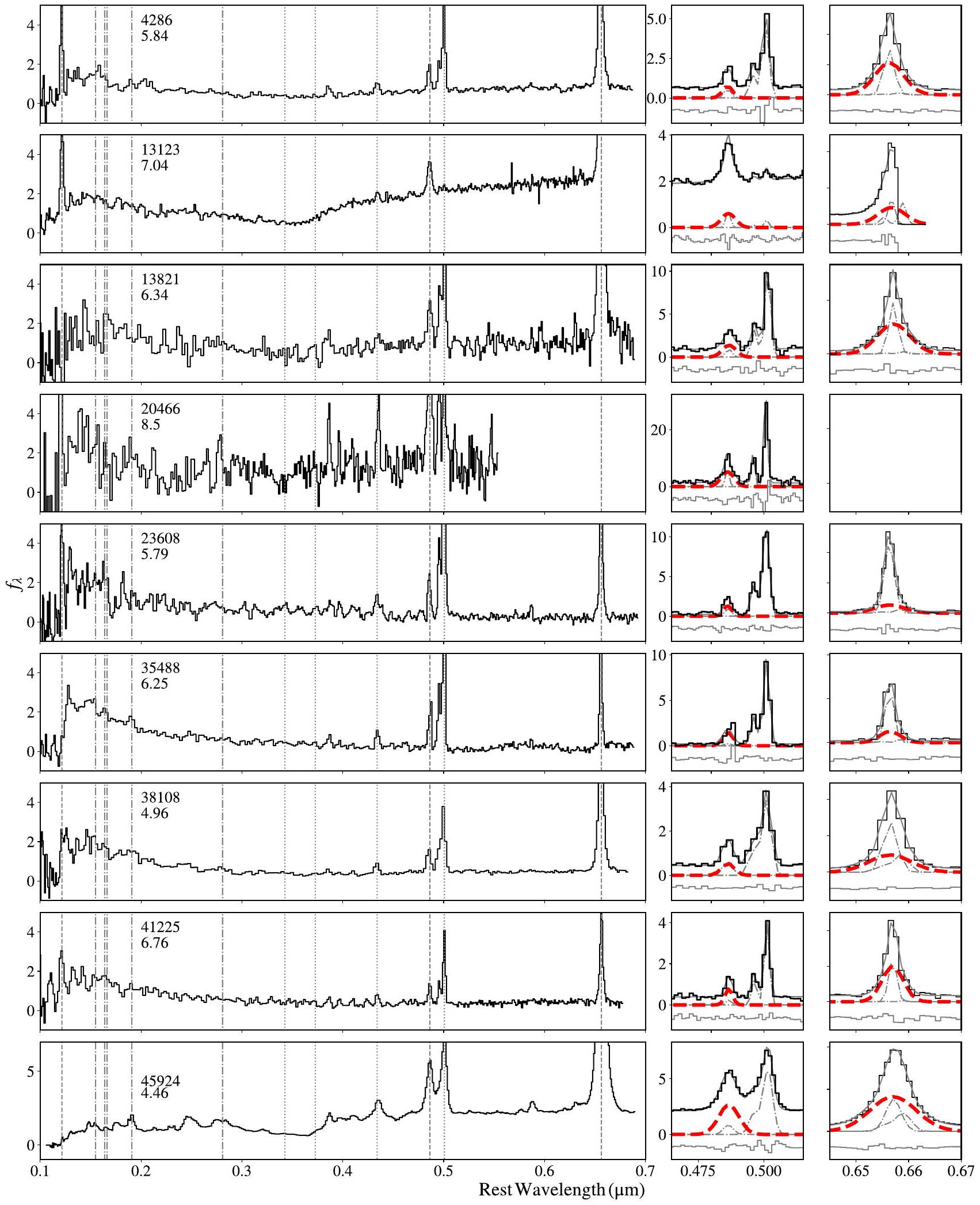
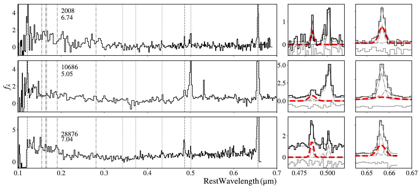
الشكل 2. اليسار: طيف NIRSpec/PRISM لتسعة AGN ذات خطوط عريضة مؤكدة في العينة. تم رسم الأطياف في طول الموجة في إطار الراحة وتم تطبيعها عند. تشير الخطوط العمودية إلى أطوال الموجات الخاصة بخطوط الهيدروجين في حالة السكون (، و ) كخطوط متقطعة، خطوط معدنية عريضة مسموح بها ( C IV هو الثانيأو III ، C III] و Mg II ) كخطوط منقطة وممنوعة ( [Ne V] ، [O III] ، [O III] [لاحظ أن هذا مدمج مع ]، و [O III] ) كخطوط منقطة. في حالة MSAID13123، نحن في الواقع نرسم الطيف المدمج عبر جميع الصور الثلاث من Furtak et al. (2023b). الوسط: التوافقات مع III المنطقة الطيفية. نعرض البيانات (هيستوغرام أسود)، النموذج الكامل (رمادي صلب)، التناسبات ذات الخطوط الضيقة (منقطة-مكسورة)، والتناسبات ذات الخطوط العريضة (مكسورة حمراء سميكة). اليمين: التناسبات إلى II المنطقة، حيث تكون الخطوط هي نفسها كما فيالمنطقة. نحن بحاجة فقط إلى مكون [N II] كبير في بعض الحالات.
الشكل 3. اليسار: طيف NIRSpec/PRISM للـ AGN ذو الخطوط العريضة غير المؤكدة في العينة. تم رسم الأطياف في إطار الراحة وتم تطبيعها عند. تشير الخطوط العمودية إلى أطوال الموجات في إطار الراحة لخطوط الهيدروجين (، و ) كخطوط متقطعة، خطوط معدنية عريضة مسموح بها ( C IV II أو III] ، C III] و Mg II ) كخطوط منقطة، وخطوط محظورة ([O III] ، [O III] [لاحظ أن هذا مدمج مع ] و [O III] ) كخطوط منقطة. الوسط: يتناسب مع III المنطقة الطيفية. نعرض البيانات (هيستوغرام أسود)، النموذج الكامل (رمادي صلب)، التناسبات ذات الخطوط الضيقة (منقطة متقطعة)، والتناسبات ذات الخطوط العريضة (متقطع أحمر سميك). اليمين: التناسبات إلى II المنطقة، حيث تكون الخطوط هي نفسها كما فيالمنطقة. لاحظ أنه في حالة MSAID13123، فإن الانزياح الأحمر لـيقطعخط
الجدول 2 توافقات الاستمرارية
MSAID
(1)
(2)
(3)
(4)
(5)
(6)
(7)
2008
٤٣.٥
٤٣.٧
4286
٤٤.٦
٤٤.٧
١٠٦٨٦
٤٤.٩
٤٤.٣
٤٤.٤
٤٣.٨
13821
٤٤.٢
٤٤.٥
٤٤.٥
٤٤.٩
23608
٤٣.٥
٤٣.٥
28876
٤٤.١
٤٣.٩
٣٥٤٨٨
٤٤.٢
٤٤.١
38108
٤٤.٧
٤٤.٧
41225
٤٥.٠
٤٤.٧
٤٥٩٢٤
٤٤.٩
٤٥.٣
ملاحظات. جدول قياسات الاستمرارية من طيف PRISM. الأعلىطيف الجسم الثلاثي الصورة من فورتاك وآخرون (2023ب).مشتق من تراجع بالمر لهذا المصدر. الـ AGN ذو الخطوط العريضة الذي ناقشه كوكوريف وآخرون (2023). في هذه الحالةتستمد القياسات من تناقص بالمر وتناسب طيفي كامل، بينمافي العمود (7) مستمد منافتراض نسبة من. العمود (1): معرف MSA. العمود (2): الميل البصريمناسب نحو الأحمر من. العمود (3): ميل الأشعة فوق البنفسجيةمناسب نحو الأزرق من. العمود (4): (mag) مقدر من ميل الاستمرارية بافتراض ميل قانون القوة للـ AGN الداخلي وقانون احمرار SMC. العمود (5): (mag) مقدر من ميل الاستمرارية بافتراض ميل قانون القوة للـ AGN الداخلي كما تم ملاءمته لمكون الأشعة فوق البنفسجية من الطيف وقانون احمرار SMC. العمود (6): اللمعان بعد إزالة التخفيف والاحمرار عند (وحدات الإرج ) كما تم تقديره من الاستمرارية المقاسة و من العمود (5). العمود (7): اللمعان المقلل والمصحح من الاحمرار في (وحدات من إرج ثانية ) كما تم تقديره من القياس السطوع ومن العمود (5). في المصدر 45924، الذي يعد بالفعل مرشحًا قويًا جدًا لـ AGN بفضل عرض خطه العريض من FWHM (H ) . منذ عادةً ما يكونقوة [OIII]، ومع الأخذ في الاعتبار الاحمرار القوي، فإن عدم الكشف هذا ليس مفاجئًا (نتزر 1990). نحن أيضًا نحاول تحليل [O III] و خطوط الانبعاث، التي قد توفر أيضًا أدلة داعمة على الإثارة بواسطة نجم نشط (AGN) (باسكين ولور 2005؛ بينيت وآخرون 2022). ومع ذلك، نظرًا لدقة طيفنا، لا نحقق تحليلات موثوقة لأي من المرشحين غير المؤكدين لنجم نشط.
4.4. تناقص بالمر وانحدارات الطيف المستمر
من خلال الاختيار، تحتوي أهدافنا على استمراريات حمراء شديدة الانحدار. مع الأطياف، لدينا قيود جيدة على كل من المنحدرات فوق البنفسجية والبصرية، والتي نشير إليها بـ و بالنسبة للمصادر الواسعة النطاق المؤكدة وغير المؤكدة، نجد و على التوالي. المرشحات غير المؤكدة لـ AGN أكثر زرقة في إطار الأشعة فوق البنفسجية مقارنة بمتوسط AGN في عينتنا، لكن جميع الأهداف تقع في الطرف الأكثر احمرارًا مما هو مُشاهد. للمجرات المختارة بواسطة F444W مع (Bouwens وآخرون 2016؛ Bhatawdekar وConselice 2021؛ Nanayakkara وآخرون 2023؛ Topping وآخرون 2023). المنحدرات البصرية حمراء بطبيعتها، مع و للعينات غير المؤكدة وعينات AGN، على التوالي (الجدول 2).
نحن الآن نحاول تقدير احمرار الغبار. بشكل اسمي، نقيس تناقص بالمر من ملاءمات خطوط بالمر الضيقة (التي تتراوح من 4 إلى 15)، مما يعنينظرًا للانحلال مع خطوط بالمر العريضة، فإن تناقصات بالمر عمومًا ليست محددة بشكل جيد. يمكن أن تؤدي التغييرات الصغيرة في ملاءمات الخطوط العريضة إلى تقلبات كبيرة في تناقصات بالمر. لاحظ أننا لا نثق في تناقصات بالمر ذات الخطوط العريضة، حيث يمكن أن تؤدي الامتصاص الذاتي في منطقة الخطوط العريضة أيضًا إلى تغيير.إلىنسبة (كورستا وغود 2004). وبالتالي، نستند في تقديراتنا للاحتراق على انحدارات الاستمرارية.
نقوم بتناسب الجوانب فوق البنفسجية والبصرية من الطيف بشكل منفصل لاشتقاق و كقوانين القوة فيللاستدلال على احمرار الغبار، يجب أن نفترض شكل طيفي جوهري (غير محمر). جميع تقديراتنا لـنفترض أن الطيف الأحمر يهيمن عليه ضوء AGN (انظر القسم 6). نستخدم نموذجين لـ AGN. أولاً، نستخدم قوالب AGN المركبة من مسح سلوين الرقمي للسماء (SDSS؛ يورك وآخرون 2000) من فاندن بيرك وآخرون (2001). الميل المركب لديهفي الأشعة فوق البنفسجية. ميل الأشعة فوق البنفسجية لنموذج SDSS يتماشى مع العديد من الأعمال الأخرى (مثل، ديفيس وآخرون 2007)، ويبدو أنه مستمر على مدى واسع من الانزياح الأحمر (تمبل وآخرون 2021). ثم يحدث انقطاع في نموذج SDSS إلىفي إطار الراحة البصرية عندقد يكون المنحدر الأكثر احمرارًا تغييرًا طيفيًا جوهريًا، أو تأثير ضوء المجرة نحو الأحمر منانكسار، والذي يصعب تحديده بشكل موثوق. لذلك، نقوم بتطبيق نموذج SDSS-QSO بشكل مستقل على كل طيف في النطاق و (لتجنب الانقطاع الملحوظ الذي يظهر في العديد من الأطياف). في كل حالة، نسمح بمعامل انقراض حر يتميز بمنحنى احمرار SMC (غوردون وآخرون 2003).
نقوم أيضًا بإجراء ملاءمة ثانية أكثر حيادية حيث نقوم بملاءمة ميل الأشعة فوق البنفسجية في إطار الزمان مباشرةً مع افتراض، ثم نفترض أن هذا الميل التجريبي ينطبق على النطاق الطيفي الكامل. في حالة أن انبعاث الأشعة فوق البنفسجية ينشأ من الضوء المتناثر، يجب أن يصف ميل طيفي واحد كل من الميل المتناثر والميل الجوهري. نحن نسمح بوجود معلمين حرين إضافيين، يؤثر على شيء مشابه لـ SMC بلون محمرمكون لوصف الطرف الأحمر من الطيف، ونسبة الضوء المتناثر بدون احمرار ( ) التي تصف جزء الأشعة فوق البنفسجية في إطار الزمان للنموذج النهائي بحيث .
تم جدولته كـ ‘الاحمرار المستمد من نموذج SDSS’بسبب ميل الطيف المركب في إطار الراحة البصرية. يتم الإشارة إلى الملاءمة التجريبية غير المتحيزة على أنهاتناسب لأننا نتناسب مباشرةً من أجللذا فإن هذين القيمتين للاحتراق يحددان نطاقًا معقولًا لمستويات الاحتراق، ويتم تقديمهما في الجدول 2.
نجد أنه على الرغم من أن مستوى التدفق في الأشعة فوق البنفسجية مخفف مقارنةً بنموذج AGN القياسي، إلا أن انحدارات الأشعة فوق البنفسجية مشابهة جدًا لانحدار الأشعة فوق البنفسجية غير المظلمة لنموذج AGN الخاص بـ SDSS. . تتغير انحدارات الإشعاع البصري في إطار الراحة بشكل أكبر. في القسم 6.1، سنناقش أصل انبعاث الأشعة فوق البنفسجية.
5. نسبة عالية من AGN في العينات الفوتومترية الحمراء
مع وجود الأطياف في متناول اليد، يمكننا استكشاف التركيبة السكانية للمصادر الحمراء عند الانزياح الأحمر العالي، بالإضافة إلى وضع معايير اختيار ضوئية محسّنة للبحث في المستقبل.
5.1. العائد والملوثات
من بين 17 هدفًا من L23 مع طيف UNCOVER PRISM، يوجد 11 هدفًا لديها دليل واضح على وجود خطوط انبعاث عريضة، بما في ذلك ثلاثة منها هي صور متعددة لنفس الهدف (Furtak et al. 2023b). ثلاثة أهداف لا تظهر دليلًا واضحًا على خطوط انبعاث عريضة، وثلاثة أخرى هي أقزام بنية (Burgasser et al. 2024). لذلكمن العينة تم تأكيدها كأجرام نشطة واسعة الخط. مع الأخذ في الاعتبار المصدر الذي تم عدسه عدة مرات، فإن نسبة الأجرام النشطة المؤكدة بين الأجسام الخارجية المستهدفة في عينتنا هي. هذه فقط نسبة من AGN للمعايير المحددة للون والكثافة التي طبقناها (انظر المزيد من التفاصيل في القسم 5.2)، وليست كامل مجموعة المجرات.
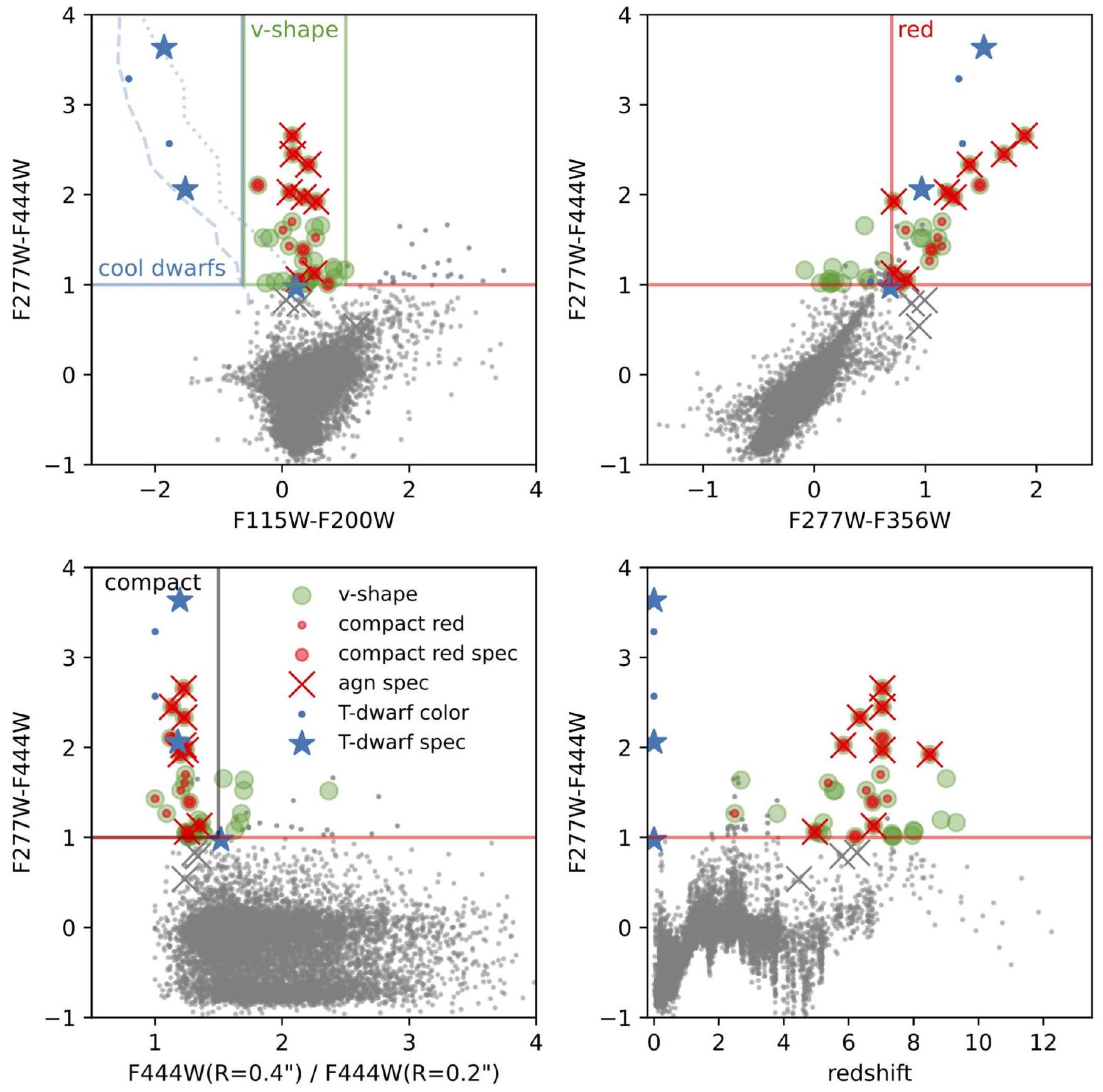
أحد الملوثات الواضحة هو النجوم القزمة البنية. قطع اللون البسيط، باستبعاد جميع المصادر الأكثر زرقة من F115W-F200W (الصندوق الأزرق في الشكل 4)، سيزيل الغالبية العظمى من الأقزام البنية من اختيارات المجرات ذات الزاوية العالية في الحقول العميقة ذات العرض العالي (انظر أيضًا لانجرودي وهجورث 2023). استنادًا إلى المحاكاة من بورغاسر وآخرون (2024) في منطقة UNCOVER نتوقع الأقزام البنية ذات الهالة منخفضة المعدنية، المتوقع أن تكون لديها ألوان F150W – F200W الأكثر زُرقة (انظر الشكل 4). ستبقى بعض الملوثات بألوان أكثر احمرارًا:من المتوقع أن توجد الأقزام البنية الغنية بالمعادن في القرص الرقيق المجري. يجب أن تكون الأقزام البنية ذات المعدل العالي من المعادن في القرص الرقيق ساطعة، F444 < 24 مغ، حيث إن الارتفاع العمودي المحدود للقرص سيقيد هذه الأقزام البنية لتكون ضمن بضع مئات من فرسخ فلكي. يمكن تعريف فلتر أكثر دقة من نموذج أكبر و/أو عينة قالب. ستسمح البيانات القادمة من النطاق المتوسط (GO-4111؛ PI: W. Suess) بتحديد الأقزام البنية بشكل أنظف.
5.2. تحديث الاختيارات الفوتومترية للمجرات ذات الانزياح الأحمر العالي و
هنا نحدد معايير NIRCam المحدثة فقط للاختيارات من L23 وLabbé وآخرون (2023b). على وجه التحديد، نبدأ بنفس و تقطع المجلات كما في السابق. ثم، نقوم بتعريف اختيار لون على شكل “v” لمحاكاة ما قام به لابي وآخرون (2023ب)، المصمم للعثور على مرشحات من المجرات الضخمة ذات الانزياح الأحمر العالي.
الفرق الرئيسي بالنسبة لـ Labbé et al. (2023b) هو استخدام F115W-F200W بدلاً من F150W-F200W، وحد أزرق لتسهيل إزالة الأقزام البنية. بالإضافة إلى ذلك، نظرًا لعدم توفر تغطية عميقة لكاميرا المسح المتقدمة (ACS)، نتخلى عن معيار عدم الكشف البصري HST/ACS، مما يتيح توسيع الاختيار نحو انزياحات حمراء أقل.. ينتج هذا الاختيار 31 مصدرًا فريدًا في UNCOVER وهو فعال وكامل في تحديد المجرات ذات الانزياح الأحمر العالي بألوان بصرية حمراء في إطار الراحة. الوسيط و المصادر لديها (انظر الشكل 4). تم استهداف 15 مصدرًا باستخدام طيفية UNCOVER PRISM، تم تقديم 11 منها في هذه الورقة وأربعة أخرى تم تقديمها في S. H. Price وآخرون (2024، قيد الإعداد). جميعها في . مصدر واحد فقط مع
الجدول 3يتناسب
MSAID (1)
(2)
عرض نصف الحد الأقصى (3)
(٤)
(5)
(6)
(7)
(8)
(9)
2008
94
94
4286
٨٠٧
٣٦١
٤٣.٤
10686
٣٣٢
٢٩٦
…
…
…
42.7
13821
٤٦١
٢٤٨
٤٣.٣
٤٨١٧
410
٤٣.٨
23608
٤٠٩
٣٤١
42.3
28876
٢٦٥
٢٦٥
…
٣٥٤٨٨
١١٢٣
976
42.8
38108
671
215
٤٣.٤
41225
539
٤٣٥
٤٣.٥
٤٥٩٢٤
1621505
90681
٤٤.٠
ملاحظة. جدول لـالقياسات من طيفية PRISM.هو الأعلىطيف الجسم الثلاثي الصورة من فورتاك وآخرون (2023ب)، بينما هو AGN ذات الخطوط العريضة من كوكوريف وآخرون (2023). العمود (1): معرف MSA. العمود (2): FWHM(Hنمط ضيق فقط (وحدات من ). العمود (3): FWHM(Hنظام مزدوج المكونات واسع القياس (وحدات من ). (ب) يتم قياسه من (كوكوريف وآخرون 2023). العمود (4): الملاحظاتتدفق، ملاءمة عريضة ذات مكونين (وحدات من ). (ب) يتم قياسه من (كوكوريف وآخرون 2023). العمود (5): (ضيق فقط). العمود (6): (مكونان). العمود (7): مصغر ومصحح اللونالسطوع (وحدات من إرج) )، باستخدام من الجدول 2. فقط الأجسام ذات الخطوط العريضة المحددة لديهاالأضاءة المدرجة. العمود (8): كتلة الثقب الأسود، باستخدامعرض الخط والسطوع. الأخطاء تأخذ في الاعتبار أخطاء عرض الخط وقيمتين من التعتيم. قد لا تحتوي بعض المصادر علىمدرج. العمود (9): لوغاريتم اللمعان البولومتري (وحدات من إرج) )، المقدرة من السطوع. الأخطاء تأخذ في الاعتبار قيمتي الاحمرار وعدم اليقين في التصحيح الكلّي. فيلا يفي باختيار الشكل v.
من المRemarkably، مع هذا الاختيار اللوني وحده، على الأقلمن الأجسام تم تحديدها طيفياً كأجسام نشطة، مما يتوافق مع حوالي ثلث جميعفينتوقع أن هناك العديد من المجرات غير النشطة في العينة أيضًا. معظم الأجسام التي وجدها لابي وآخرون (2023ب) في مجال CEERS تم حلها مكانيًا في الأشعة فوق البنفسجية في إطار الزمان، مع كثافات مشابهة لقلوب المجرات الإهليلجية في الوقت الحاضر (باجن وآخرون 2023). من بين أربع مجرات تم تحليل طيفها في تلك العينة، وُجد أن واحدة منها هي مصدر نشط واسع الخطوط باللون الأحمر (كوتسيفسكي وآخرون 2023). ستحلل طيف الدورة الثانية (البرنامج JWST-GO-4106، الباحث الرئيسي: إ. نيلسون) النسبة المئوية من هذه الأجسام المختارة حسب اللون ولكن المحللة مكانيًا التي تظهر دلائل على نشاط AGN. يجب أن نؤكد أن هذه المصادر الحمراء، سواء كانت مجرات أو مدفوعة بـ AGN، لا تزال تشكل نسبة صغيرة من سكان المجرات في هذه الحقبة؛ سنحاول تقدير كثافة عدد AGN الحمراء المدمجة في القسم 6.2.
لاختيار AGN الحمراء بشكل أكثر تحديدًا بطريقة مشابهة لاختيار red2 في L23، نضيف معيار لون أحمر إضافي ومعيار الكثافة مقارنةً بمعيار الشكل V:
أحمر مدمج
حيث أن F277W – F356W الإضافي > 0.7 يسهل اختيار SEDs ذات انحدارات مستمرة حمراء، بدلاً من الانكسارات أو خطوط الانبعاث (الشكل 4، أعلى اليمين)، ومعيار الكثافة يساعد في استهداف المصادر التي تهيمن عليها النقاط (الشكل 4، أسفل اليسار). هذه القصات الإضافية تزيل حوالي 50% من الأهداف على شكل V. الاختلافات الرئيسية مقارنة بـ L23 هيإزالة الأقزام البنية وقطع أكثر صرامة قليلاً من تلك الموجودة في L23.
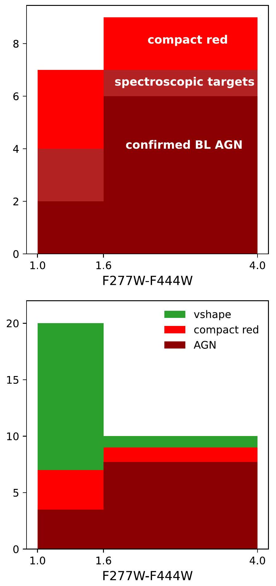
بين هذا الاختيار الأكثر صرامة الذي يركز على AGN، نجد على الأقلهي AGN. نسبة AGN هي دالة للون F277W – F444W (الشكل 5). الغالبية العظمى من العينة الأوسع من المجرات على شكل V لديها. لذلك، يمكن إجراء اختيار بديل عالي العائد من AGN عن طريق الاختيار بواسطة . في هذه الحالة،من المجرات هي AGN، بينمامن المجرات الحمراء المدمجة هي AGN (انظر أيضًا بارو وآخرون 2023).
باختصار، بينالمجرات ذات الألوان الحمراءو F277W-F444W > 1)، على الأقل ثلثها هي AGN. جعل معايير الكثافة واللون أكثر صرامة، أو ببساطة القطع عند F277W-F444Wيمكن أن ينتج عننسبة AGN.
6. طبيعة “النقاط الحمراء الصغيرة”
الآن نركز بشكل حصري على AGN ذات الخطوط العريضة المؤكدة، نستكشف خصائصها، بما في ذلك SEDs، وظائف اللمعان، وكتل الثقوب السوداء.
6.1. أصل الاستمرارية
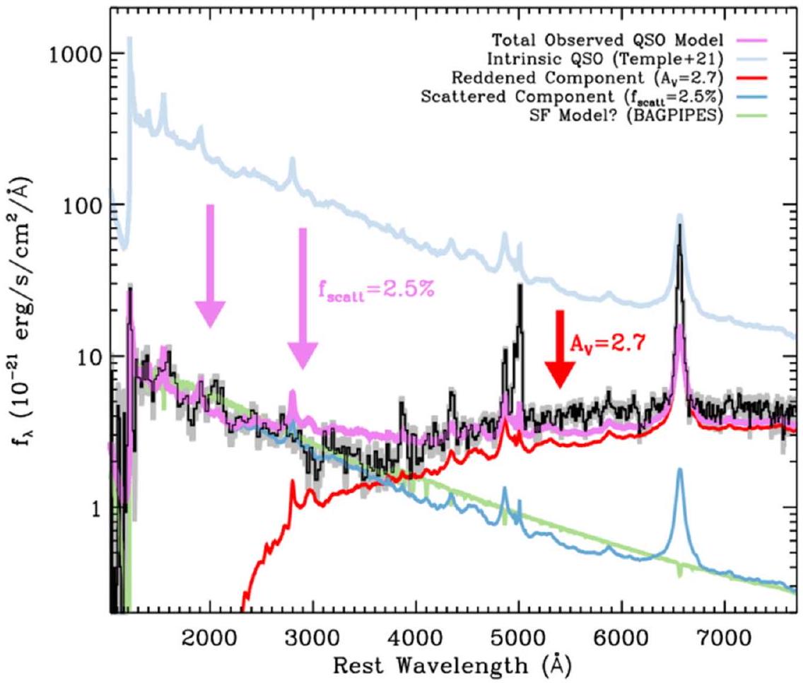
تم اختيار الأجسام الحمراء المدمجة فوتومترياً ليس فقط لوجود استمرارية حمراء في الإطار الزمني البصري، ولكن أيضاً لوجود انبعاثات فوق بنفسجية قابلة للاكتشاف. من خلال ملاءمة نموذجية للبيانات الضوئية فقط، توصلنا إلى استنتاج أن الاستمرارية الحمراء كانت على الأرجح مهيمنة بواسطة ضوء AGN المتأثر بالاحمرار. مع الطيف، نسأل الآن عما إذا كان من الممكن تمييز أصل الاستمرارية البصرية فوق الإطار الزمني والاستمرارية فوق البنفسجية بشكل أكثر مباشرة. نحن نوضح الطرق المختلفة لنمذجة الطيف مع مثال واحد في الشكل 6. سنؤجل النمذجة الكاملة لـ SED إلى عمل مستقبلي، حيث سيتطلب ذلك استغلال كل من الاستمراريات وخطوط الانبعاث.
في الإطار الزمني البصري، نرى على الفور أن المنحدرات الحمراء المرصودة تهيمن عليها الاستمرارية، ولا تنشأ من خطوط انبعاث ذات عرض مكافئ عالٍ (انظر الاحتمالات في Furtak et al. 2023a؛ Endsley et al. 2023). المنحدرات البصرية في الإطار الزمني متوافقة مع نموذج AGN المظلم أو تكوين النجوم المغبر، كما تم الاستنتاج من التناسب الضوئي. ومع ذلك، توفر خطوط الانبعاث العريضة دليلاً إضافياً. يمكننا حساب
الشكل 4. AGN في سياق المجرات الحمراء ذات الانزياح الأحمر العالي. النقاط الرمادية هي من كتالوج UNCOVER لـ F444Wماج و F444W S/N. أعلى اليسار: اختيار ثنائي الألوان NIRCam F115W – F200W مقابل F277W – F444W يحدد المجرات مثل تلك الموجودة في Labbé et al. (2023b) التي تحتوي على استمرارية فوق بنفسجية زرقاء في إطار الراحة واستمرارية بصرية حمراء في إطار الراحة (“شكل v” SED). عينة المرشحين للـ AGN في L23 هي مجموعة فرعية من ذلك ( )، تم اختيارها أيضًا للحصول على استمرارية بصرية حمراء مائلة من خلال قطع في فلترين متجاورين (أعلى اليمين)، وحجم مضغوط (أسفل اليسار)، باستخدام نسبة تدفقات الفتحة كبديل للحجم. عادةً ما تحتوي الملوثات من النجوم القزمة البنية على F115W – F200W أزرق أكثر من المجرات، وبالتالي يمكن عزلها. تم رسم مسارات الألوان الاصطناعية من نماذج الغلاف الجوي للنجوم القزمة البنية LOWZ (Meisner et al. 2021) فوقها لـ والطاقة الشمسيةو -1.5. معيار الشكل V وحده فعال جداً في الاختيار لـالمجرات. تعتبر مجموعة تشمل المعايير المدمجة والحمراء فعالة في اختيار AGN الحمراء.
الاستمرارية المتوقعة بالنظر إلى ما تم ملاحظتهالسطوع (غرين وهو 2005) وقياس الاحمرار. يمكننا أيضًا حساب الاستمرارية المرصودة مباشرة. يجب أن يتطابق الاثنان.نحن نضم الاثنينالقيم، استنادًا إلى الاستمرارية ولكن باستخدام نفس، في الجدول 2. بينما -مشتق
تميل القيم إلى أن تكون أعلى قليلاً، وهم يتفقون ضمن عامل 2، مما يشير إلى أن النطاق الواسعتُعتبر EWs قابلة للمقارنة مع عينة المعايرة ذات الانزياح الأحمر المنخفض من غرين وهو (2005). الـ Hتكون قيم EWs الناتجة عن تكوين النجوم النقي أعلى بكثير بالنسبة للمجرات الضخمة المليئة بالغبار عند الانزياح الأحمر المنخفض (Fumagalli et al. 2012; Whitaker et al. 2014). نظرًا لاكتشاف النطاق الواسعونسب شبيهة بـ AGNإلى الاستمرارية، نستنتج أن الإشعاع الضوئي في إطار الراحة يهيمن عليه AGN.
المكون السائد من AGN هو الاستمرارية الحمراء، ونظرًا لـالذي نستنتج، يمكننا
الشكل 5. توزيع أنواع الأجسام كدالة للون F277W – F444W. تُظهر اللوحة العلوية العينة المختارة بواسطة NIRCam والتي تتميز بالكثافة واللون الأحمر، وعدد الأهداف الطيفية، وAGN المؤكدين من نوع BL. تُظهر اللوحة السفلية الأهداف المختارة بواسطة قطع اللون الثنائي “على شكل V” (باللون الأخضر)، من بينهافيعدد المصادر المدمجة والمختارة باللون الأحمر (أحمر)، والعدد المقدر من AGN (أحمر داكن).
لم يتم الكشف عن هذا المكون في الأشعة فوق البنفسجية (انظر الشكل 6). بدلاً من ذلك، يجب علينا استدعاء مكون ثانٍ، وهو أكثر سطوعًا من طيف AGN المائل نحو الأحمر النقي، ولكنه لا يزال يمثل فقط بضع في المئة من AGN غير المائل نحو الأحمر (الأزرق). المصدران المحتملان لهذا المكون الثاني الذي ينبعث منه الأشعة فوق البنفسجية هما إما تكوين النجوم من المضيف أو بعض النسبة الصغيرة من الفوتونات من قرص تراكم، سواء من خلال التشتت أو التسرب المباشر. للأسف، لا يمكننا تحديد مصدر الأشعة فوق البنفسجية بشكل قاطع بناءً على الميل الطيفي فقط. إن ميول الأشعة فوق البنفسجية في إطار الراحة متسقة تمامًا مع الميول الملحوظة للأجسام النشطة الزرقاء.، وفي بعض الحالات من المحتمل أن تكون هناك خطوط UV واسعة. مع بيانات ذات دقة أعلى، سيكون هذا دليلاً قاطعاً على هيمنة ضوء AGN في الأشعة فوق البنفسجية. بدلاً من ذلك، يمكن أن تكون متوافقة مع الطرف الأحمر منالمجرات (على سبيل المثال، Bouwens وآخرون 2016؛ Bhatawdekar وConselice 2021)، وخاصة تلك المختارة عند F444W (على سبيل المثال، Nanayakkara وآخرون 2023؛ Topping وآخرون 2023).
لاستكشاف أصل الأشعة فوق البنفسجية بشكل أعمق، يمكننا أن نسأل ما هي اللمعان فوق البنفسجي الذي نتوقعه بالنظر إلى الجوهراللمعان. نحن نحدد نطاق المعقولباستخدام الميلين المفترضين للـ AGN، وعلى مدى تلك النطاق نجد أن الملاحظات هو في المئة أو نسبة من القيمة الجوهرية المتوقعة، اعتمادًا على ما إذا كنا نفترض أو ، على التوالي. يمكن بسهولة تفسير الأول من خلال مكون AGN متناثر (أو مُرسل مباشرة)، بينمامن المحتمل أن تكون النسب مرتفعة جدًا لتشتت AGN النقي (على سبيل المثال، ليو وآخرون 2009). في مثل هذه الحالات، نفضل أن يكون هناك مساهمة من تكوين النجوم في الأشعة فوق البنفسجية. نختار عدم ملاءمة الأشعة فوق البنفسجية بمفردها، لأنها تتمتع بحساسية محدودة لكتلة النجوم، ولكن تحويلها بشكل ساذجقياسات لمعدلات تشكيل النجوم، وبدون افتراض أن كل الأشعة فوق البنفسجية ناتجة عن تشكيل النجوم، نجد معدلات تشكيل نجوم متوسطة قدرها. من حيث نتوقع أن يكون أقل بمعدل 10-1000 مرةالسطوع لمعدل تكوين النجوم هذا أكثر مما نقيسه في الخطوط العريضة. من ناحية أخرى، يبدو أن هذا المستوى من تكوين النجوم معقول وصعب الاستبعاد من قياسات أخرى. من حيث المبدأ، يمكن أن تميز خطوط الانبعاث فوق البنفسجية الأصول فوق البنفسجية؛ هناك حاجة إلى بيانات عالية الدقة لهذا الغرض.
بشكل عام، نستنتج أن الاستمرارية البصرية في إطار الراحة تهيمن عليها استمرارية AGN ذات الخطوط العريضة المليئة بالغبار، وأن هناك حاجة إلى مزيد من العمل لتحديد مصدر انبعاث الأشعة فوق البنفسجية بشكل قاطع. أخيرًا، نلاحظ أيضًا أن كائنين، MSAID45924 و A2744-QSO1 (MSAID13123 في هذا العمل) اللذان يظهران ثلاث صور، كلاهما يحتويان على انكسارات طيفية غير عادية لا يمكن نمذجتها بسهولة باستخدام أي نموذج AGN. نترك في العمل المستقبلي ملاءمة أكثر شمولاً لاستمرارياتهما، لمحاولة فهم طبيعة انكساراتهما الشديدة.
6.2. دوال اللمعان
نقوم الآن بحساب دالة اللمعان في إطار الراحة للأشعة فوق البنفسجية للأجسام النشطة ذات الإشعاع الأحمر عند الانزياحات العالية استنادًا إلى العينة الطيفية فقط. نظرًا لأن A2744 هو مجال عدسي قوي، يجب أخذ تشويه العدسة في الاعتبار عند حساب حجم كل حاوية لمعان. لحساب الأحجام، نتبع طريقة النمذجة الأمامية المستخدمة في حقول هابل الحدودية بواسطة Atek وآخرون (2018): يتم تقييم اكتمال العينة من خلال سلسلة من محاكاة الاكتمال حيث نقوم بتعبئة مستوى المصدر بأجسام نشطة حمراء وهمية باستخدام طيف L23، مع تطبيعها إلى لمعات فوق بنفسجية وانزياحات عشوائية. ثم يتم انحرافها إلى مستوى العدسة باستخدام خرائط الانحراف لنموذج العدسة القوية UNCOVER (انظر القسم 2.3) وتضاف إلى الموزاييك التي نعيد تشغيل روتينات الكشف عليها ونقيم نسبة المصادر المستعادة لاستنتاج دالة الاختيار.يرجى ملاحظة أن تفاصيل طرق محاكاة الاكتمال لدينا ستُنشر في I. Chemerynska وآخرون (2024، قيد الإعداد). الاختيار
الشكل 6. نحن نوضح نموذجنا المفضل للمنحدرات الحمراء والأشعة فوق البنفسجية المحددة التي نراها في أجسامنا باستخدام MSAID4286. إن الاستمرارية الداخلية للـ AGN (الحمراء) متأثرة بشدة بالاحمرار. وبالتالي، لا يمكن تفسير المكون فوق البنفسجي من خلال الاستمرارية الأساسية للـ AGN. هنا، نستكشف إمكانية أن يأتي الضوء فوق البنفسجي من الضوء المتناثر، عندمن الأشعة فوق البنفسجية الجوهرية (موضحة بشكل تخطيطي باللون الأزرق الفاتح). للتوضيح، نعرض هنا نموذج تمبل وآخرون (2021). ومع ذلك، نحقق تناسبًا أفضل عندما نستخدم ميل الأشعة فوق البنفسجية المرصود كشكل AGN ذو القوة القانونية الجوهرية. كما نعرض أيضًا تناسبًا لسكان النجوم على الجانب فوق البنفسجي من الطيف باستخدام Bagpipes (كارنل وآخرون 2018، 2019)، مرة أخرى لتوضيح أنه مع معدلات متوسطة لتكوين النجوم تبلغ بضع كتل شمسية في السنة، ومن الممكن أيضًا ملاءمة ميل الطيف المستمر للأشعة فوق البنفسجية مع ضوء النجوم. تشير “؟” إلى المساهمة غير المؤكدة في توزيع الطاقة الطيفية الناتجة عن تكوين النجوم.
تُستخدم الدالة لوزن عنصر الحجم المتحرك، والذي يتم دمجه بعد ذلك على منطقة مستوى المصدر ذات التكبير الكافي المطلوب لاكتشاف كل كائن في جميع النطاقات المعطاة لأعماق فسيفساء UNCOVER (انظر المعادلة (2) في Atek et al. 2018) للحصول على الحجم الفعال الذي تم استكشافه بواسطة UNCOVER. لاحظ أنه نظرًا لأن اكتشاف مصادر UNCOVER يتم في نطاقات LW المجمعة (انظر، على سبيل المثال، Weaver et al. 2024) حيث تكون الكائنات الحمراء المدمجة هي الأكثر سطوعًا، فإن عينتنا مكتملة حتىالمغ و الأجسام الأكثر سطوعًا منلا تحتاج بالضرورة إلى أن تكون مكبرة من أجل اكتشافها بالنظر إلى أعماق UNCOVER المذكورة في ويفر وآخرون (2024). تم تقسيم عينتنا إلى صناديق سطوع الأشعة فوق البنفسجية بعرض 0.5 مغ. تم اشتقاق عدم اليقين في عدد العد من خلال رسمإضاءة عشوائية من كل كائنتوزيع الخطأ وإعادة تجميع دالة اللمعان في كل مرة للسماح للأجسام بتغيير فئة اللمعان. يتم أخذ عدم اليقين في التكبير في الاعتبار عند حساب عدم اليقين في لمعان الأشعة فوق البنفسجية.
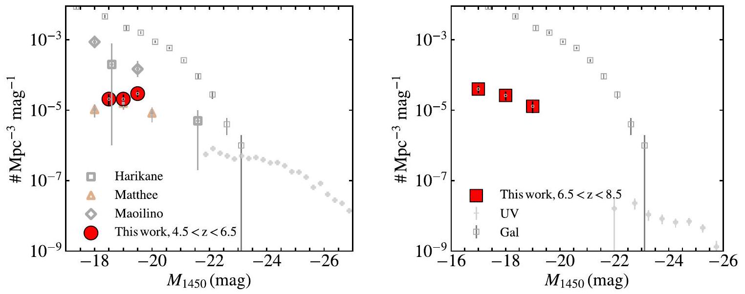
تُعرض دوال اللمعان فوق البنفسجي الناتجة في فئتي الانزياح الأحمر في الجدول 4 والشكل 7. كما تم توضيحه أعلاه، تمثل العينة الطيفية مؤشراً محافظاً ولكنه دقيق إلى حد ما لوظيفة اللمعان الحقيقية لوكالات AGN ذات الخطوط العريضة الحمراء. نحن نؤكد النتيجة من L23 أن كثافات العدد لهذه الوكالات AGN المختارة باللون الأحمر أعلى بحوالي درجتين من حيث الحجم مقارنةً بالوكالات AGN المختارة فوق البنفسجية عند أحجام مماثلة. الكثافة العددية التي نجدها قابلة للمقارنة أيضاً مع ما تم استنتاجه لعينات AGN الحمراء المتوسطة اللمعان في (بارو وآخرون 2023؛ كوتسيفسكي وآخرون 2023؛ ماثي وآخرون 2023)، ويأخذ في الاعتبار من مجموعة AGN العامة ذات الخطوط العريضة كما تم اختيارها بواسطة JWST (هاريكان وآخرون 2023؛ مايونينو وآخرون 2023).
الجدول 4 وظائف اللمعان في الأشعة فوق البنفسجية في إطار الراحة لعينة AGN الحمراء لدينا
( )
عينة
-19.5
٣
-19.0
٢
-18.5
2
عينة
-19.0
1
-18.0
2
-17.0
2
ملاحظة. تحتوي صناديق سطوع الأشعة فوق البنفسجية على عرض 0.5 مغ.
تعتمد العينات المحددة طيفياً على بيانات NIRSpec عالية الدقة، والتي تشمل AGN ذات الخطوط الأضيق والأنظمة التي لا يهيمن فيها AGN بالضرورة على إجمالي خرج الضوء.
نؤكد أن الضوء فوق البنفسجي هو جزء صغير من إجمالي اللمعان بسبب القيم العالية للاحتجاب وله أصل غير معروف إما من الضوء المنعكس أو المنقول من AGN أو من تكوين النجوم غير المحجوب بمستوى منخفض. وبالتالي، بينما يكون مفيدًا لوضع أهدافنا في السياق، فإن دالة اللمعان فوق البنفسجي لا تصف حقًا الخصائص الفيزيائية لـ AGN في هذه العينة. لهذا السبب، نقدم أيضًا دالة اللمعان الكلي في الجدول 5 والشكل 8. نظرًا لأن اشتقاق الاكتمال كدالة لللمعان الكلي ليس بالأمر السهل وسيتطلب تفاصيل
الشكل 7. دالة اللمعان فوق البنفسجي كما تم قياسها فينظهر دالة اللمعان في صندوقين من الانزياح الأحمر، في دوائر حمراء و في المربعات الحمراء. نقارن مع دوال اللمعان المختارة بالأشعة فوق البنفسجية من Akiyama et al. (2018؛ اليسار) وMatsuoka et al. (2023؛ اليمين). نعرض أيضًا AGN ذات الخطوط العريضة المختارة من JWST من Harikane et al. (2023) وMaiolino et al. (2023) وMatthee et al. (2023). أخيرًا، نقارن مع دالة لمعان المجرات من Bouwens et al. (2017). متسقة مع Harikane et al. (2023)، نجد أن AGN المتأثرة بالاحمرار تمثلمن الأجسام ذات الخطوط العريضة عند هذا الانزياح الأحمر، ونسبة قليلة من سكان المجرات. إن AGN لدينا أكثر عددًا بكثير من تلك المختارة بالأشعة فوق البنفسجية، على الرغم من أن لديها درجات سطوع بولومترية متداخلة.
نموذج SED في محاكاة الاكتمال، نستخدم هنا حقيقة أن عينتنا مكتملة في الغالب من حيث سطوع الأشعة فوق البنفسجية (انظر أعلاه) لتقريب الحجم الفعال لدالة السطوع الكلي من خلال افتراض الحد الأقصىالكمال المستمد أعلاه في كلصندوق (بعرض 1 دكس) وبدون تكبير، أي أن عنصر الحجم الفعال يتم دمجه على كامل منطقة سطح مصدر UNCOVER (انظر Atek وآخرون 2023b؛ Furtak وآخرون 2023c). بينما يُعتبر هذا تقديرًا معقولًا نظرًا لخصائص عيّنتنا، فإن دالة اللمعان الكلي المستمدة بهذه الطريقة تظل حدًا أدنى. من المحتمل أن تكون صناديق اللمعان المنخفضة، على وجه الخصوص، مقدرة بأقل من قيمتها الحقيقية نظرًا لأنها ستكون أكثر حساسية للتكبير.
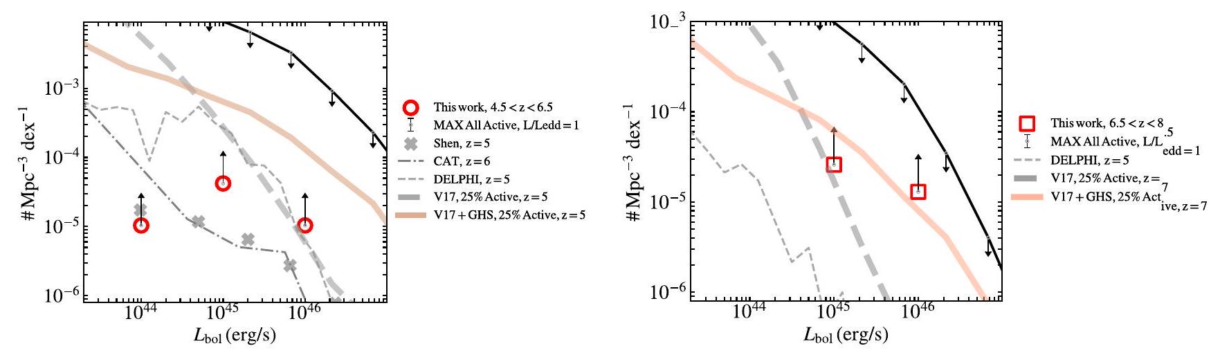
لإرشاد تفسيرنا، نقوم أيضًا بحساب دوال اللمعان البلومتري الثقالي للثقوب السوداء النظرية باستخدام مزيج من الملاحظات ذات الانزياح الأحمر العالي والمنخفض. نحن نعتبر دالة كتلة النجوم في المجرات المستمدة من ضبط دالة كتلة الهالة من أجل إعادة إنتاج دالة كتلة النجوم الملاحظة المتطورة عند (للتفاصيل انظر دايال وجيري 2024). ثم نقوم بتعيين AGN إلى المجرات، من خلال افتراض علاقات التدرج وتوزيعات نسبة إيدينغتون. في نموذج “أقصى” نعتبر علاقة الكتلة بين الثقب الأسود والكتلة النجمية عندمن رينس وفولونتيري (2015)، صالح للمجرات الإهليلجية ذات الكتلة النجمية العالية،، مع تشتت قدره 0.5 دكس، وأن جميع الثقوب السوداء تشع عند سطوع إيدينغتون (الشكل 8، “ماكس”). هذه الخط الحد الأقصى أعلى بكثير من المصادر الحمراء المدمجة المقدمة هنا عند لكن قياساتنا تقترب من النموذج الأقصى في انزياحنا الأحمر الأعلىسلة.
استنادًا إلى الأعمال النظرية السابقة (دوبوا وآخرون 2015؛ باور وآخرون 2017) التي وجدت معدل تراكم إيدينجتون المكبوت للثقوب السوداء في المجرات/الهالات منخفضة الكتلة، نقوم بتحديد معدل تراكم إيدينجتون إلىللهالات ذات الكتل الأقل من. هذه الكبح يخفف من الإنتاج الزائد النموذجي في الطرف الخافت من دالة اللمعان للـ AGN التي توجد عادة في النماذج (Habouzit et al. 2017)، لكنه لا يؤثر على نطاق اللمعان للـ AGN في هذه الورقة. في الواقع، في بعض النماذج التي تظهر كبحًا عند الكتلة المنخفضة، لا تزال الثقوب السوداء تبدو وكأنها تنمو بواسطةإلى كتل الثقوب السوداء المعتدلة الموجودة هنا وفي بحثات أخرى بواسطة تلسكوب جيمس ويب (على سبيل المثال، ترينكا وآخرون 2023). من ناحية أخرى، فإن الإفراط في الإنتاج الذي يحفز هذا
الجدول 5 دوال اللمعان البولومترية لعينة من AGN الحمراء لدينا
إرجع
( )
عينة
٤٤.٠
1
٤٥.٠
٤
٤٦.٠
1
عينة
٤٥.٠
2
٤٦.٠
1
ملاحظة. صناديق البيانات لها عرض 1 دكس. كان التغيير مستندًا إلى وظائف اللمعان للأشعة فوق البنفسجية والأشعة السينية، ويجب إعادة النظر فيه في عصر تلسكوب جيمس ويب (على سبيل المثال، هاريكان وآخرون 2023؛ مايونينو وآخرون 2023).
نحن أيضًا ندرج وظائف اللمعان من النماذج شبه التحليلية التي تنمو فيها الثقوب السوداء بشكل متسق بدءًا من مزيج من البذور الخفيفة والثقيلة (CAT وDelphi، على التوالي؛ Dayal et al. 2019؛ Trinca et al. 2022). الكثافات العددية المتوقعة أقل من تلك المستنتجة من AGN المكتشفة بواسطة JWST، لكن النماذج تم ضبطها لتكرار وظائف اللمعان قبل JWST، والتي تقلل من تقدير الكثافة العددية لـ AGN في هذه العينة. بشكل عام، أنتجت النماذج النظرية عددًا أكبر من AGN الخافتة في الارتفاعات الحمراء العالية مقارنة بما تم ملاحظته قبل JWST (Shen et al. 2020، الشكل 8، رموز “x”). لمجموعة من النتائج، انظر Habouzit et al. (2022).
لاستكشاف ما إذا كان من الممكن إعادة إنتاج كثافات الأعداد المرصودة مع افتراضات معقولة، نعتبر أخيرًا، لنفس دالة كتلة المجرة، مجموعة المعلمات المستخدمة في فولونتيري وآخرون (2017) لإعادة إنتاج أفضل مشتركوظائف اللمعان للأشعة السينية والأشعة فوق البنفسجية للـ AGN المعروفة في ذلك الوقت: العلاقةصالح لAGN ذات اللمعان المعتدل في الهالات ذات الكتلة المنخفضة، مع تباين قدره 0.5 دكس، ونسبة نشاط تبلغ 0.25 وتوزيع لوغاريتمي طبيعي لنسبة إيدينغتون بمتوسط و (الشكل 8، فولونتيري وآخرون 2017؛ V17). نحن نواصل
الشكل 8. دوال اللمعان البولومترية للـ AGNالأعلىالقاع) كما يُستنتج من (الجدول 3). كثافات الأعداد هي حدود دنيا، خاصة عند اللمعان الكروي المنخفض حيث ستكون بحثنا غير حساس بشكل خاص للأجسام التي تهيمن عليها المجرات. نحن ندرج دالة اللمعان الكروي القصوى بافتراض أن كل مجرة تحتوي على ثقب أسود يتراكم ويشع عند حد إيدينغتون الخاص بها وعلاقة كتلة الثقب الأسود-المجرة ذات تطبيع مرتفع. تظهر منحنيان إضافيان بناءً على فولونتيري وآخرون (2017) حالات مع نسبة AGN تبلغ 0.25 وعلاقات كتلة الثقب الأسود-المجرة مع تطبيع أقل وتباين مختلف؛ انظر النص للتفاصيل. المقارنات قبل JWST باللون الرمادي، بما في ذلك نموذج فولونتيري وآخرون (2017) الأصلي، بينما يتم عرض النموذج المحدث لفولونتيري وآخرون (2017) باللون الأحمر للإشارة إلى إلهام JWST. يتم عرض دالة اللمعان الكروي قبل JWST التي جمعها شين وآخرون (2020) (x رمادي). كما تم تضمين دوال اللمعان المستمدة من النماذج شبه التحليلية التي تنمو فيها الثقوب السوداء من البذور كخطوط رمادية (أداة الآثار الكونية (CAT) ودلفي، على التوالي؛ دايال وآخرون 2019؛ ترينكا وآخرون 2022).
اعتبر الملاءمة الواحدة لجميع الثقوب السوداء في غرين وآخرون (2020)مع انتشار لـ واستخدام نفس الكسر النشط وتوزيع نسبة إيدينغتون كما في V17 (الشكل 8، V17 وجرين، سترادر، وهو؛ GHS). مع هذه النماذج نجد أن كثافة عدد AGN يمكن أن تتناسب مع سكان المجرات، مع الأخذ في الاعتبار التشتت في علاقات القياس وكسر نشط يبلغ حوالي لكن مرة أخرى، يتم إنتاج AGN بشكل مفرط مقارنةً بـ Shen وآخرون (2020). في الملخص، كانت النماذج قبل JWST تميل إلى إنتاج AGN بشكل مفرط، بينما يبدو أنه من الممكن إعادة إنتاج كثافات الأعداد الملاحظة بواسطة JWST مع افتراضات معقولة، لكن العديد من التفاصيل (مثل توزيع كتلة الثقب الأسود إلى كتلة المجرة) لا تزال بحاجة إلى دراسة بمزيد من التفصيل.
6.3. كتل الثقوب السوداء
نتبع غرين وهو (2005)، كما تم تحديثه بواسطة رينيس وآخرون (2013)، لحساب كتل الثقوب السوداء بناءً على اللمعان.وسرعةمن الواسعخط. تستند تقديرات كتلة الثقب الأسود ذات الحقبة الواحدة (مثل، شين وآخرون 2019) على افتراض أن منطقة الانبعاث الضوئي الواسعة تعمل كعلامة ديناميكية للثقب الأسود (مثل، بانكوست وآخرون 2014). يتم تقدير حجم منطقة الانبعاث الضوئي الواسعة من سطوع نجم النشاط الكوني (مثل، بينتس وآخرون 2013)، ثم بافتراض التوازن الفيرالي، تتناسب الكتلة الديناميكية معلقد أخذنا قيمة منحيث يكون النموذجي-العامل يتم معايرته على تشتت السرعة للخط بينماتم معايرته إلى عرض الخط الكامل المستخدم هنا (على سبيل المثال، أونكن وآخرون 2004؛ بانكوست وآخرون 2014). بالطبع، لا نعرف ما إذا كانت منطقة الانبعاث الضوئي في توازن فيريالي، ولا نعرف ما إذا كنا نستكشف مجال السرعة عند نصف قطر مشابه لـ “حجم” منطقة الانبعاث الضوئي الذي نقدره من اللمعان (على سبيل المثال، كروليك 2001؛ لينزر وآخرون 2022).
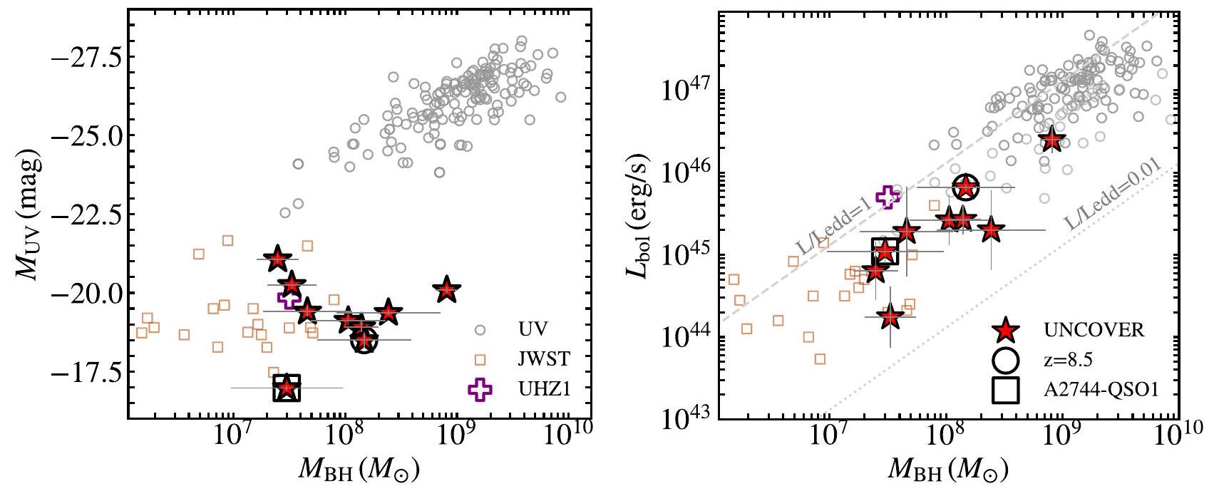
تم رسم كتل الثقوب السوداء مقابل اللمعان فوق البنفسجي و– تم استنتاج اللمعان الكلي في الشكل 9. نقارن المصادر بكل من الكوازارات اللامعة المختارة بالأشعة فوق البنفسجية من مراجعة فان وآخرون (2023) وبالأجسام النشطة ذات اللمعان المعتدل ذات الخطوط العريضة التي تم اكتشافها مؤخرًا باستخدام تلسكوب جيمس ويب (بارو وآخرون 2023؛ هاريكان وآخرون 2023؛ كوتسيفسكي وآخرون 2023؛ ماثي وآخرون 2023). مصادرنا تقع في الطرف الضخم من الأجسام النشطة ذات الخطوط العريضة الموجودة في حقول JWST العميقة، لكنها بالكاد تصل إلى الطرف المنخفض من كتل الثقوب السوداء واللمعان. تم رؤيتها في المصادر النادرة المختارة بالأشعة فوق البنفسجية. ومع ذلك، فإن سطوعها فوق البنفسجي هوأقل من AGN المختارة بواسطة الأشعة فوق البنفسجية عند المقارنة. من المحتمل جداً أن يكون هذا الاختلاف ناتجاً عن حجب الغبار. كما هو موضح في الجانب الأيمن، عندما نستخدم خطوط الانبعاث العريضة مع تصحيح الغبار لتقدير اللمعان الكلي، نجد توافقاً أكبر بكثير في نطاقات اللمعان عند قيمة معينة..
من الجدير بالذكر MSAID45924. هذه المجرة هي الأكثر سطوعًا في العينة. ) وتبرز لجودتها العالية وكتلة الثقب الأسود من يتطلب الموضوع تحليلًا مخصصًا يتجاوز نطاق هذا العمل.
7. المناقشة والملخص
في هذا العمل، نقدم متابعة طيفية باستخدام NIRSpec/PRISM لـ 15 مصدرًا أحمر مضغوط تم اختيارها في مجال UNCOVER A2744. تم تأكيد أن الغالبية العظمى من هذه الأهداف هي AGN معتتميز الأطياف الطيفية في الأشعة فوق البنفسجية/البصرية باستمرار أحمر حاد نحو الإطار الزمني البصري، ولكنها تحتوي أيضًا على مكون فوق بنفسجي غير قابل للإهمال. الإطار الزمني البصري يتماشى مع حالة احمرار.AGN ذات الخطوط العريضة. يتم ملاءمة انحدارات الأشعة فوق البنفسجية بشكل جيد كـ AGN غير المحجوبة في الانحدار، ولكنها مكبوتة بواسطةأوقات بالنسبة لمصدر غير مائل. من بيانات الطيفية منخفضة الدقة المتاحة وبيانات SED العريضة، لا يمكننا استبعاد أن المكون فوق البنفسجي ناتج عن تشكيل نجمي مائل بشكل معتدل بمعدل بضع كتل شمسية في السنة في المضيف. تُعرف AGN بأشكال مماثلة (نوبوريغوتشي وآخرون 2023) في جميع الانزياحات الحمراء (على سبيل المثال، غليكمان وآخرون 2012؛ بانيرجي وآخرون 2015؛ فيليو وآخرون 2016؛ هامن وآخرون 2017؛ آسييف وآخرون 2018؛ بان وآخرون 2021). ومع ذلك، عند، هذه المصادر المحمرة ذات الفائض من الأشعة فوق البنفسجية نادرة؛ يقدر نوبوريغوتشي وآخرون (2019) أنه من بين جميع AGN المحجوبة بالغبار، فقطلديها فائض من الأشعة فوق البنفسجية.
تقوم تلسكوب جيمس ويب الفضائي بكشف عدد كثيف بشكل مدهش من النوى النشطة الحمراء. (انظر أيضًا Harikane et al. 2023؛ Barro et al. 2023؛ Matthee et al. 2023؛ L23). هذه الكثافة العالية غير متوقعة مقارنةً بالمصادر المختارة بواسطة الأشعة فوق البنفسجية، التي تم قياس كثافاتها العددية تقريبًا 100 مرة أقل عند أدنى درجات سطوعها في الأشعة فوق البنفسجية (على سبيل المثال، Matsuoka et al. 2018، 2023)، على الرغم من أن الكثافات بشكل اسمي مشابهة لبعض الاختيارات في الأشعة السينية (Giallongo et al. 2019). ومع ذلك، لم يتم الكشف عن هذه المصادر في الأشعة السينية. على وجه التحديد، بينما Matthee et al. (2023)
الشكل 9. كتلة الثقب الأسود مقابل (يسار) و اللمعان الكلي (يمين) لنجوم AGN ذات الخطوط العريضة (نجوم حمراء) بما في ذلك A2744-QSO1 (Furtak et al. 2023a, 2023b؛ نجمة حمراء ومربع) والمصدر MSAID20466 في (كوكوريف وآخرون 2023؛ نجمة حمراء ودائرة مفتوحة). من أجل السياق، ندرج AGN المختارة بالأشعة فوق البنفسجية مع من Fan وآخرون (2023)، مصادر الخطوط العريضة الأخرى المختارة بواسطة JWST (Harikane وآخرون 2023؛ Maiolino وآخرون 2023؛ Matthee وآخرون 2023)، وAGN المكتشفة بواسطة الأشعة السينية في، UHZ1 (بودان وآخرون 2024؛ غولدينغ وآخرون 2023). لاحظ أن مصادرنا تمتد إلى مستويات عالية بشكل مدهش .
قد تكون الأجسام خافتة جدًا للكشف عنها، ويُستنتج أن المصدر الثلاثي العدسات في حقل UNCOVER أضعف بمقدار 10 مرات في الأشعة السينية مما كان متوقعًا بناءً على الملاحظات البصرية (Furtak et al. 2023b). بالإضافة إلى ذلك، تمثل AGN الحمراء المدمجة جزءًا كبيرًا من جميع المصادر المختارة باللون الأحمر باستخدام JWST. بعد تطبيق قطع لونية بسيطة مصممة لاختيار المجرات الضخمة (كما في Labbé et al. 2023b)، تشير طيفنا إلى أن ثلث الأجسام المختارة على الأقل ستكون AGN. يرتفع هذا الرقم إلى ما يقرب منلأحمر ذيل المصادر )، وهو أيضًا عندما نطبق معيار التراص ونفرض استمرارية قانون القوة الحمراء.
أحد الجوانب المثيرة للاهتمام في هذه المصادر الحمراء المدمجة هو الكتل المنخفضة للمجرات التي تشير إليها أحجامها المدمجة (على سبيل المثال، إيزومي وآخرون 2019؛ فورتاك وآخرون 2023ب؛ كوكوريف وآخرون 2023). بالطبع، نحن نختار فقط المصادر النقطية، مما يوجه العينة بالضرورة نحو تلك التي لديها نسبة عالية من الثقوب السوداء إلى المجرات. علاوة على ذلك، يقترح فولونتيري وآخرون (2023) أن اختيارات الألوان ستحدد بالفعل الثقوب السوداء التي تكون زائدة الكتلة بالنسبة للمجرة بسبب المتطلبات التي تجعل AGN تهيمن على ضوء المجرة. ومع ذلك، فإن الكثافات العددية العالية التي نجدها نحن وآخرون لمثل هذه الأهداف تعني أن جزءًا كبيرًا من سكان الثقوب السوداء من المحتمل أن يكون قد تجاوز مضيفيه؛ هذه المستويات العالية من التشتت مطلوبة أيضًا لمطابقة وظائف اللمعان الكلي (القسم 6.2). تحذير مهم هو بالطبع أننا لا نعرف بعد اللمعان الكلي لهذه المصادر. فهي تعتمد على تفسير يعتمد بشكل كبير على النموذج للطيف الذي يشير إلى احمرار عالي جدًا بسبب الغبار.
بينما من الصحيح أن الكثافات العددية المستنتجة العالية يمكن عمومًا استيعابها بافتراض نسب معقولة من AGN وتدرجات مع السكان المجريين، لا يزال يتعين تفسير النمو الواسع والفعال للثقوب السوداء بدءًا من الظروف الأولية، “البذور”. هناك بعض الطرق لتخيل نمو كثافة كتلة الثقب الأسود الكبيرة في وقت مبكر جدًا. يمكن أن تتشكل بذور الثقوب السوداء بشكل كثيف ( ) كما في نماذج الانهيار المباشر (لوبي وراتسيو 1994؛ بروم و لوبي 2003؛ لوداتو و ناتاراجان 2006؛ بيغيلمان وآخرون 2008؛ فيسبال وآخرون 2014؛ هابوزيت وآخرون 2016) أو في تجمعات النجوم الكثيفة (على سبيل المثال، بورتجيز زوارت وماكميلان 2002؛ أوموكاي وآخرون.
2008؛ ديفيتشي وفولونتيري 2009؛ مابيللي 2016؛ ناتراجان 2021؛ شلايشر وآخرون 2022). مع البذور الثقيلة، من الأسهل نمو الثقب الأسود بشكل أسرع من المجرة (ترينكا وآخرون 2022)، على الرغم من أن النماذج الكلاسيكية لـ “الانهيار المباشر” لا يمكنها تحقيق كثافات عددية عالية من البذور الثقيلة (دايال وآخرون 2019؛ إينايشي وآخرون 2022). تشير المحاكاة الحديثة إلى أن الهالات التي تنمو بسرعة لديها ظروف حيث تتشكل بذور أقل كتلة بعض الشيء،لكن بأعداد أكبر وفي وجود توزيع نجمي كثيف نسبيًا (ريغان وآخرون 2020). ستساعد النماذج التي تستدعي النمو المعزز من تجمعات النجوم المحيطة في نمو البذور في وقت مبكر نسبيًا (على سبيل المثال، ألكسندر وناتاراجان 2014؛ ناتاراجان 2021).
بدلاً من ذلك، يمكن أن تبدأ جميع الثقوب السوداء كبذور خفيفة (Fryer et al. 2001؛ Madau & Rees 2001؛ Bromm & Larson 2004)، مع قدرة بعض منها على النمو بمعدلات فوق إيدينغتون لتكوين كثافة كتلة عالية من الثقوب السوداء (على سبيل المثال، Madau et al. 2014). يُفضل بعض التراكم فوق إيدينغتون، بغض النظر عن نوع البذور، من قبل النموذج شبه التجريبي TRINITY (Zhang et al. 2023b)، الذي يستخدم إحصائيات الهالة وإطار بايزي مدفوع بالملاحظات لنمذجة نمو المجرات والثقوب السوداء بشكل مشترك. في الوقت نفسه، تجد المحاكيات التفصيلية للديناميكا المائية المغناطيسية تدفقات تراكم فوق إيدينغتون قابلة للتطبيق (على سبيل المثال، Jiang et al. 2019).
قد تفسر عملية الاستحواذ فوق إيدينغتون بعض خصائص توزيع الطاقة الطيفية للأجسام الحمراء المدمجة، وخاصة اللمعان المنخفض الظاهر في الأشعة السينية. من الممكن حتى أن يتم تفسير الاستمرارية الحمراء من خلال الاستحواذ فوق إيدينغتون إذا نما تدفق الاستحواذ الداخلي ليصبح كثيفًا بصريًا ولكنه يترك قرصًا خارجيًا. ستخفف عملية الاستحواذ فوق إيدينغتون أيضًا من التوتر مع نموذجنا “الأقصى”، ولكنها ستنتج مزيدًا من اللمعان لكتلة معينة من الثقب الأسود.
قد تأتي تعقيد آخر من الاندماجات. عند الانزياحات الحمراء المنخفضة، يبدو أن AGN ذات الخطوط العريضة الحمراء تقيم بشكل تفضيلي في مضيفين في حالة اندماج (على سبيل المثال، أوروتيا وآخرون 2008). إذا كانت المصادر الحمراء المقدمة هنا تهيمن عليها أيضًا مضيفون في حالة اندماج، فقد يكون من الصعب اكتشاف النظام الاندماجي أكثر من مجرة غير مضطربة بسبب الانقراض المتغير وربما وجود مكون ذو سطوع سطحي منخفض كبير. قد يكون هناك أيضًا حالتين من AGN تغذي الأجسام في بعض الحالات من حيث المبدأ. من الناحية النظرية، فإن كثافات الأعداد للاندماجات الكبرى عند يمكن أن تكون مرتفعة بما يكفي لمطابقة كثافة العدد للمصادر الحمراء المدمجة. مع الأخذ في الاعتبار مقياس الزمن للاندماج المستند إلى التجربةكثافة حجم الاندماج Gyrلـالمجرات من نمذجة الهالة التجريبية (O’Leary وآخرون 2021)، نقوم بتقديرالاندماجات فيمن المحتمل إذن أن يكون هناك علاقة بين تحفيز AGN والاندماج والاحمرار الملحوظ. كما لوحظ في ماتهي وآخرون (2023)، فإن المصادر الحمراء المدمجة تبدو أيضًا متجمعة مع بعضها البعض. يبرز فوجيموتو وآخرون (2023أ) كثافة زائدة محتملة تشير إليها AGN حمراء مدمجة وشيء ساطع في الأشعة فوق البنفسجية تم العثور عليهما معًا في نفس الفقاعة العملاقة المؤينة بقطرمعدل MPC المناسب فيربما يكون هذا التكتل الزائد مرتبطًا بأصل اندماج لهذه المصادر.
سؤال إضافي واضح هو الدور المحتمل لهذه المصادر في إعادة التأين. اعتمادًا على كثافات الأعداد ومعدلات التراكم (التي لا نفهمها جيدًا) للثقوب السوداء مقارنةً بالمجرات التي تشكل النجوم في الطرف الخافت من دالة سطوع الأشعة فوق البنفسجية، يمكن أن تكون قد ساهمت إما بشكل ضئيل (بضع عشرات من النسب المئوية؛ حسن وآخرون 2018؛ دايال وآخرون 2020؛ تريبيتش وآخرون 2021؛ فينكلشتاين وباغلي 2022) أو تهيمن على ميزانية الفوتونات لإعادة التأين (على سبيل المثال، ماداو وهاردت 2015؛ غرازين وآخرون 2018). من المناسب إعادة النظر في دور AGN ذات السطوع المعتدل في إعادة التأين، على الرغم من أن الأجسام الحمراء التي تم النظر فيها هنا قد لا تنتج العديد من الفوتونات المؤينة.
توجد العديد من الألغاز الإضافية التي تثيرها “النقاط الحمراء الصغيرة”، بما في ذلك تجمعها الظاهر، وخصائصها الفريدة في توزيع الطيف الطيفي (استمرارية ضوئية حمراء مميزة، ومكون إضافي للأشعة فوق البنفسجية، وغياب انبعاث الأشعة السينية)، واحتمال عدم وجود مكون كبير من المجرة المضيفة. يبدو أن هذه الكوازارات ذات الخطوط العريضة الحمراء تشكل جزءًا كبيرًا مننسبة AGN ذات الخطوط العريضةبالإضافة إلى نسبة كبيرة من المجرات الحمراء في نفس الحقبة. إنهم جزء مهم من قصة نمو الثقوب السوداء في الأوقات المبكرة.
شكر وتقدير
يقر كل من ج. إ. ج. و أ. د. ج. بالدعم المقدم من منحة NSF/AAG رقم 1007094، كما يقر ج. إ. ج. أيضًا بالدعم من منحة NSF/AAG رقم 1007052. يقر أ. ز. بالدعم المقدم من المنحة رقم 2020750 من مؤسسة العلوم الثنائية الأمريكية-الإسرائيلية (BSF) ومنحة رقم 2109066 من مؤسسة العلوم الوطنية الأمريكية (NSF)، ومن وزارة العلوم والتكنولوجيا الإسرائيلية. يتم تمويل مركز dawn الكوني من قبل مؤسسة الأبحاث الوطنية الدنماركية (DNRF) بموجب المنحة رقم 140. وقد حصل هذا العمل على تمويل من الأمانة السويسرية للتعليم والبحث والابتكار (SERI) بموجب رقم العقد MB22.00072، بالإضافة إلى منحة المشروع من مؤسسة العلوم الوطنية السويسرية (SNSF) من خلال المنحة 200020_207349. يقر ب. د. بالدعم من منحة NWO 016.VIDI.189.162 (“ODIN”) ومن برنامج CO-FUND روزاليند فرانكلين من المفوضية الأوروبية وجامعة غرونينجن. يقر ك. ج. و ت. ن. بالدعم من زمالة لوريت من مجلس الأبحاث الأسترالي FL180100060. يقر ح. أ. و إ. ج. بالدعم من CNES، الذي يركز على مهمة JWST، ومن البرنامج الوطني لعلم الكونيات والمجرات (PNCG) من CNRS/INSU مع INP و IN2P3، الممول من CEA و CNES. يقر ر. ب. ن. بالتمويل من برامج JWST GO-1933 و GO-2279. تم تقديم الدعم لهذا العمل من قبل ناسا من خلال منحة زمالة هابل من ناسا HST-HF2-51515.001-A الممنوحة من معهد علوم التلسكوب الفضائي، الذي تديره جمعية الجامعات للبحث في علم الفلك، بموجب عقد ناسا.
NAS5-26555. يتم دعم أبحاث C.C.W. من قبل NOIRLab، الذي تديره جمعية الجامعات لأبحاث الفلك (AURA) بموجب اتفاق تعاوني مع المؤسسة الوطنية للعلوم. B.W. يعترف بالدعم من JWST-GO-02561.022-A. A.J.B. يعترف بدعم التمويل من منحة NASA/ADAP 21-ADAP21-0187. تم توفير الدعم لهذا العمل من قبل مؤسسة برينسون من خلال منحة زمالة جائزة برينسون. R.P.N. يعترف بالدعم لهذا العمل المقدم من NASA من خلال منحة زمالة هابل NASA HST-HF2-51515.001-A الممنوحة من معهد علوم التلسكوب الفضائي، الذي تديره جمعية الجامعات لأبحاث الفلك، بموجب عقد NASA NAS5-26555. C.P. يشكر مارشا ورالف شيلينغ على الدعم السخي لهذا البحث.
Amaro-Seoane, P., Andrews, J., Arca Sedda, M., et al. 2023, LRR, 26, 2
Assef, R. J., Stern, D., Kochanek, C. S., et al. 2013, ApJ, 772, 26
Assef, R. J., Stern, D., Noirot, G., et al. 2018, ApJS, 234, 23
Atek, H., Labbé, I., Furtak, L. J., et al. 2023a, arXiv:2308.08540
Atek, H., Chemerynska, I., Wang, B., et al. 2023b, MNRAS, 524, 5486
Atek, H., Richard, J., Kneib, J. P., & Schaerer, D. 2018, MNRAS, 479, 5184
Baggen, J. F. W., van Dokkum, P., Labbe, I., et al. 2023, ApJL, 955, L12
Bañados, E., Venemans, B. P., Mazzucchelli, C., et al. 2018, Natur, 553, 473
Banerji, M., Alaghband-Zadeh, S., Hewett, P. C., & McMahon, R. G. 2015, MNRAS, 447, 3368
Barro, G., Perez-Gonzalez, P. G., Kocevski, D. D., et al. 2023, arXiv:2305. 14418
Baskin, A., & Laor, A. 2005, MNRAS, 358, 1043
Begelman, M. C., Rossi, E. M., & Armitage, P. J. 2008, MNRAS, 387, 1649
Bentz, M. C., Denney, K. D., Grier, C. J., et al. 2013, ApJ, 767, 149
Bergamini, P., Acebron, A., Grillo, C., et al. 2023, ApJ, 952, 84
Bezanson, R., Labbe, I., Whitaker, K. E., et al. 2022, arXiv:2212.04026
Bhatawdekar, R., & Conselice, C. J. 2021, ApJ, 909, 144
Binette, L., Villar Martín, M., Magris, C., et al. 2022, RMxAA, 58, 133
Bogdan, A., Goulding, A., Natarajan, P., et al. 2024, NatAs, 8, 126
Bouwens, R. J., Aravena, M., Decarli, R., et al. 2016, ApJ, 833, 72
Bouwens, R. J., Oesch, P. A., Illingworth, G. D., Ellis, R. S., & Stefanon, M. 2017, ApJ, 843, 129
Bower, R. G., Schaye, J., Frenk, C. S., et al. 2017, MNRAS, 465, 32
Brammer, G. 2022, msaexp: NIRSpec analyis tools, v0.3.4, Zenodo, doi:10. 5281/zenodo. 7299500
Bromm, V., & Larson, R. B. 2004, ARA&A, 42, 79
Bromm, V., & Loeb, A. 2003, ApJ, 596, 34
Burgasser, A. J., Gerasimov, R., Bezanson, R., et al. 2024, ApJ, 962, 177
Carnall, A. C., McLure, R. J., Dunlop, J. S., & Davé, R. 2018, MNRAS, 480, 4379
Carnall, A. C., McLure, R. J., Dunlop, J. S., et al. 2019, MNRAS, 490, 417
Croom, S. M., Rhook, K., Corbett, E. A., et al. 2002, MNRAS, 337, 275
Davis, S. W., Woo, J. H., & Blaes, O. M. 2007, ApJ, 668, 682
Dayal, P., & Giri, S. K. 2024, MNRAS, 528, 2784
Dayal, P., Rossi, E. M., Shiralilou, B., et al. 2019, MNRAS, 486, 2336
Dayal, P., Volonteri, M., Choudhury, T. R., et al. 2020, MNRAS, 495, 3065
de Graaff, A., Rix, H. W., Carniani, S., et al. 2023, arXiv:2308.09742
Devecchi, B., & Volonteri, M. 2009, ApJ, 694, 302
Donley, J. L., Koekemoer, A. M., Brusa, M., et al. 2012, ApJ, 748, 142
Dubois, Y., Volonteri, M., Silk, J., et al. 2015, MNRAS, 452, 1502
Endsley, R., Stark, D. P., Lyu, J., et al. 2023, MNRAS, 520, 4609
Endsley, R., Stark, D. P., Whitler, L., et al. 2022, arXiv:2208.14999
Fan, X., Banados, E., & Simcoe, R. A. 2023, ARA&A, 61, 373
Fan, X., Wang, F., Yang, J., et al. 2019, ApJL, 870, L11
Finkelstein, S. L., & Bagley, M. B. 2022, ApJ, 938, 25
Fryer, C. L., Woosley, S. E., & Heger, A. 2001, ApJ, 550, 372
Fujimoto, S., Brammer, G. B., Watson, D., et al. 2022, Natur, 604, 261
Fujimoto, S., Kohno, K., Ouchi, M., et al. 2023b, arXiv:2303.01658
Fujimoto, S., Wang, B., Weaver, J., et al. 2023a, arXiv:2308.11609
Fumagalli, M., Patel, S. G., Franx, M., et al. 2012, ApJL, 757, L22
Furtak, L. J., Labbé, I., Zitrin, A., et al. 2023b, arXiv:2308.05735
Furtak, L. J., Zitrin, A., Plat, A., et al. 2023a, ApJ, 952, 142
Furtak, L. J., Zitrin, A., Weaver, J. R., et al. 2023c, MNRAS, 523, 4568
Gardner, J. P., Mather, J. C., Abbott, R., et al. 2023, PASP, 135, 068001
Giallongo, E., Grazian, A., Fiore, F., et al. 2019, ApJ, 884, 19
Glikman, E., Urrutia, T., Lacy, M., et al. 2012, ApJ, 757, 51
Gordon, K. D., Clayton, G. C., Misselt, K. A., Landolt, A. U., & Wolff, M. J. 2003, ApJ, 594, 279
Goulding, A. D., Greene, J. E., Setton, D. J., et al. 2023, ApJL, 955, L24
Grazian, A., Giallongo, E., Boutsia, K., et al. 2018, A&A, 613, A44
Greene, J. E., & Ho, L. C. 2005, ApJ, 630, 122
Greene, J. E., Strader, J., & Ho, L. C. 2020, ARA&A, 58, 257
Habouzit, M., Somerville, R. S., Li, Y., et al. 2022, MNRAS, 509, 3015
Habouzit, M., Volonteri, M., & Dubois, Y. 2017, MNRAS, 468, 3935
Habouzit, M., Volonteri, M., Latif, M., Dubois, Y., & Peirani, S. 2016, MNRAS, 463, 529
Hainline, K. N., Helton, J. M., Johnson, B. D., et al. 2023b, arXiv:2309.03250
Hainline, K. N., Johnson, B. D., Robertson, B., et al. 2023a, arXiv:2306.02468
Hamann, F., Zakamska, N. L., Ross, N., et al. 2017, MNRAS, 464, 3431
Hao, L., Strauss, M. A., Tremonti, C. A., et al. 2005, AJ, 129, 1783
Harikane, Y., Ono, Y., Ouchi, M., et al. 2022, ApJS, 259, 20
Harikane, Y., Zhang, Y., Nakajima, K., et al. 2023, ApJ, 959, 39
Hassan, S., Davé, R., Mitra, S., et al. 2018, MNRAS, 473, 227
Hinshaw, G., Larson, D., Komatsu, E., et al. 2013, ApJS, 208, 19
Horne, K. 1986, PASP, 98, 609
Inayoshi, K., Onoue, M., Sugahara, Y., Inoue, A. K., & Ho, L. C. 2022, ApJL, 931, L25
Inayoshi, K., Visbal, E., & Haiman, Z. 2020, ARA&A, 58, 27
Izotov, Y. I., Thuan, T. X., & Privon, G. 2012, MNRAS, 427, 1229
Izumi, T., Onoue, M., Matsuoka, Y., et al. 2019, PASJ, 71, 111
Jakobsen, P., Ferruit, P., Alves de Oliveira, C., et al. 2022, A&A, 661, A80
Jiang, Y. F., Stone, J. M., & Davis, S. W. 2019, ApJ, 880, 67
Kocevski, D. D., Onoue, M., Inayoshi, K., et al. 2023, ApJL, 954, L4
Kokorev, V., Fujimoto, S., Labbe, I., et al. 2023, ApJL, 957, L7
Korista, K. T., & Goad, M. R. 2004, ApJ, 606, 749
Krolik, J. H. 2001, ApJ, 551, 72
Labbé, I., Greene, J. E., Bezanson, R., et al. 2023a, arXiv:2306.07320
Labbé, I., van Dokkum, P., Nelson, E., et al. 2023b, Natur, 616, 266
Langeroodi, D., & Hjorth, J. 2023, ApJL, 957, L27
Larson, R. L., Finkelstein, S. L., Kocevski, D. D., et al. 2023, ApJL, 953, L29
Leung, G. C. K., Bagley, M. B., Finkelstein, S. L., et al. 2023, ApJL, 954, L46
Leung, G. C. K., Coil, A. L., Rupke, D. S. N., & Perrotta, S. 2021, ApJ, 914, 17
Linzer, N. B., Goulding, A. D., Greene, J. E., & Hickox, R. C. 2022, ApJ, 937, 65
Liu, X., Zakamska, N. L., Greene, J. E., et al. 2009, ApJ, 702, 1098
Lodato, G., & Natarajan, P. 2006, MNRAS, 371, 1813
Loeb, A., & Rasio, F. A. 1994, ApJ, 432, 52
Lotz, J. M., Koekemoer, A., Coe, D., et al. 2017, ApJ, 837, 97
Madau, P., & Haardt, F. 2015, ApJL, 813, L8
Madau, P., Haardt, F., & Dotti, M. 2014, ApJL, 784, L38
Madau, P., & Rees, M. J. 2001, ApJL, 551, L27
Maiolino, R., Scholtz, J., Curtis-Lake, E., et al. 2023, arXiv:2308.01230
Mapelli, M. 2016, MNRAS, 459, 3432
Matsuoka, Y., Onoue, M., Iwasawa, K., et al. 2023, ApJL, 949, L42
Matsuoka, Y., Strauss, M. A., Kashikawa, N., et al. 2018, ApJ, 869, 150
Matthee, J., Naidu, R. P., Brammer, G., et al. 2023, arXiv:2306.05448
Meisner, A. M., Schneider, A. C., Burgasser, A. J., et al. 2021, ApJ, 915, 120
Mortlock, D. J., Warren, S. J., Venemans, B. P., et al. 2011, Natur, 474, 616
Nanayakkara, T., Glazebrook, K., Jacobs, C., et al. 2023, ApJL, 947, L26
Natarajan, P. 2021, MNRAS, 501, 1413
Netzer, H. 1990, in Active Galactic Nuclei, ed. R. D. Blandford et al. (Berlin: Springer)
Noboriguchi, A., Inoue, A. K., Nagao, T., Toba, Y., & Misawa, T. 2023, ApJL, 959, L14
Noboriguchi, A., Nagao, T., Toba, Y., et al. 2019, ApJ, 876, 132
Oesch, P. A., Brammer, G., Naidu, R. P., et al. 2023, MNRAS, 525, 2864
O’Leary, J. A., Moster, B. P., Naab, T., & Somerville, R. S. 2021, MNRAS, 501, 3215
Omukai, K., Schneider, R., & Haiman, Z. 2008, ApJ, 686, 801
Onken, C. A., Ferrarese, L., Merritt, D., et al. 2004, ApJ, 615, 645
Ono, Y., Harikane, Y., Ouchi, M., et al. 2023, ApJ, 951, 72
Onoue, M., Inayoshi, K., Ding, X., et al. 2023, ApJL, 942, L17
Osterbrock, D. E. 1977, ApJ, 215, 733
Osterbrock, D. E. 1989, Astrophysics of Gaseous Nebulae and Active Galactic Nuclei (Melville, NY: AIP)
Pan, X., Zhou, H., Yang, C., et al. 2021, ApJ, 912, 118
Pancoast, A., Brewer, B. J., Treu, T., et al. 2014, MNRAS, 445, 3073
Pascale, M., Frye, B. L., Diego, J., et al. 2022, ApJL, 938, L6
Portegies Zwart, S. F., & McMillan, S. L. W. 2002, ApJ, 576, 899
Regan, J. A., Wise, J. H., Woods, T. E., et al. 2020, OJAp, 3, 15
Reines, A. E., Greene, J. E., & Geha, M. 2013, ApJ, 775, 116
Reines, A. E., & Volonteri, M. 2015, ApJ, 813, 82
Schleicher, D. R. G., Reinoso, B., Latif, M., et al. 2022, MNRAS, 512, 6192
Shen, X., Hopkins, P. F., Faucher-Giguère, C. A., et al. 2020, MNRAS, 495, 3252
Shen, Y., Wu, J., Jiang, L., et al. 2019, ApJ, 873, 35
Somalwar, J. J., & Ravi, V. 2023, arXiv:2306.00898
Stern, D., Eisenhardt, P., Gorjian, V., et al. 2005, ApJ, 631, 163
Stern, J., & Laor, A. 2012, MNRAS, 423, 600
Temple, M. J., Hewett, P. C., & Banerji, M. 2021, MNRAS, 508, 737
Topping, M. W., Stark, D. P., Endsley, R., et al. 2023, arXiv:2307.08835
Trebitsch, M., Dubois, Y., Volonteri, M., et al. 2021, A&A, 653, A154
Trebitsch, M., Hutter, A., Dayal, P., et al. 2023, MNRAS, 518, 3576
Trinca, A., Schneider, R., Maiolino, R., et al. 2023, MNRAS, 519, 4753
Trinca, A., Schneider, R., Valiante, R., et al. 2022, MNRAS, 511, 616
Übler, H., Maiolino, R., Curtis-Lake, E., et al. 2023, A&A, 677, A145
Urrutia, T., Lacy, M., & Becker, R. H. 2008, ApJ, 674, 80
Vanden Berk, D. E., Richards, G. T., Bauer, A., et al. 2001, AJ, 122, 549
Veilleux, S., Meléndez, M., Tripp, T. M., Hamann, F., & Rupke, D. S. N. 2016, ApJ, 825, 42
Visbal, E., Haiman, Z., & Bryan, G. L. 2014, MNRAS, 445, 1056
Volonteri, M., Habouzit, M., & Colpi, M. 2023, MNRAS, 521, 241
Volonteri, M., & Reines, A. E. 2016, ApJL, 820, L6
Volonteri, M., Reines, A. E., Atek, H., Stark, D. P., & Trebitsch, M. 2017, ApJ, 849, 155
Wang, B., Fujimoto, S., Labbé, I., et al. 2023, ApJL, 957, L34
Wang, B., Leja, J., Labbé, I., et al. 2024, ApJS, 270, 12
Wang, F., Fan, X., Yang, J., et al. 2021, ApJ, 908, 53
Weaver, J. R., Cutler, S. E., Pan, R., et al. 2024, ApJS, 270, 7
Whitaker, K. E., Franx, M., Leja, J., et al. 2014, ApJ, 795, 104
Yang, G., Caputi, K. I., Papovich, C., et al. 2023, ApJL, 950, L5
York, D. G., Adelman, J., Anderson, J. E. J., et al. 2000, AJ, 120, 1579
Zakamska, N. L., Hamann, F., Pâris, I., et al. 2016, MNRAS, 459, 3144
Zhang, H., Behroozi, P., Volonteri, M., et al. 2023a, MNRAS, 523, L69
Zhang, H., Behroozi, P., Volonteri, M., et al. 2023b, MNRAS, 518, 2123
Zitrin, A., Fabris, A., Merten, J., et al. 2015, ApJ, 801, 44
Brinson Prize Fellow. Hubble Fellow. NASA Hubble Fellow.
Comparing to the Greene & Ho (2005) relation is a bit easier than looking at the EW distribution directly, since there may be subtle trends between line EWs and luminosities (e.g., Croom et al. 2002; Stern & Laor 2012) that are fitted for directly by Greene & Ho (2005).
UNCOVER Spectroscopy Confirms the Surprising Ubiquity of Active Galactic Nuclei in Red Sources at z > 5
Greene, Jenny E.; Labbe, Ivo; Goulding, Andy D.; Furtak, Lukas J.; Chemerynska, Iryna; Kokorev, Vasily; Dayal, Pratika; Volonteri, Marta; Williams, Christina C.; Wang, Bingjie
Published in:
Astrophysical Journal
DOI:
10.3847/1538-4357/ad1e5f
IMPORTANT NOTE: You are advised to consult the publisher’s version (publisher’s PDF) if you wish to cite from it. Please check the document version below.
Document Version
Publisher’s PDF, also known as Version of record
Publication date:
2024
Link to publication in University of Groningen/UMCG research database
Citation for published version (APA):
Greene, J. E., Labbe, I., Goulding, A. D., Furtak, L. J., Chemerynska, I., Kokorev, V., Dayal, P., Volonteri, M., Williams, C. C., Wang, B., Setton, D. J., Burgasser, A. J., Bezanson, R., Atek, H., Brammer, G., Cutler, S. E., Feldmann, R., Fujimoto, S., Glazebrook, K., … Zitrin, A. (2024). UNCOVER Spectroscopy Confirms the Surprising Ubiquity of Active Galactic Nuclei in Red Sources at z > 5. Astrophysical Journal, 964(1), Article 39. https://doi.org/10.3847/1538-4357/ad1e5f
Copyright
Other than for strictly personal use, it is not permitted to download or to forward/distribute the text or part of it without the consent of the author(s) and/or copyright holder(s), unless the work is under an open content license (like Creative Commons).
UNCOVER Spectroscopy Confirms the Surprising Ubiquity of Active Galactic Nuclei in Red Sources at
Jenny E.Greene (D),Ivo Labbe (D),Andy D.Goulding (D),Lukas J.Furtak (D),Iryna Chemerynska (D),Vasily Kokorev (D), Pratika Dayal (D),Marta Volonteri (D),Christina C.Williams (D),Bingjie Wang(王冰洁)(D),David J.Setton (D), Adam J.Burgasser (D),Rachel Bezanson (D),Hakim Atek (D),Gabriel Brammer (D),Sam E.Cutler (D),Robert Feldmann (D), Seiji Fujimoto (D),Karl Glazebrook (D),Anna de Graaff (D),Gourav Khullar (D),Joel Leja (D),Danilo Marchesini (D), Michael V.Maseda (D),Jorryt Matthee (D),Tim B.Miller (D),Rohan P.Naidu (D),Themiya Nanayakkara (D), Pascal A.Oesch (D),Richard Pan (D),Casey Papovich (D),Sedona H.Price (D),Pieter van Dokkum (D), John R.Weaver (D),Katherine E.Whitaker (D),and Adi Zitrin (D) Department of Astrophysical Sciences,Princeton University, 4 Ivy Lane,Princeton,NJ 08544,USA Centre for Astrophysics and Supercomputing,Swinburne University of Technology,Melbourne,VIC 3122,Australia Department of Physics,Ben-Gurion University of the Negev,P.O.Box 653,Beer-Sheva 84105,Israel Institut d'Astrophysique de Paris,CNRS,Sorbonne Université,98bis Boulevard Arago,F-75014 Paris,France Kapteyn Astronomical Institute,University of Groningen, 9700 AV Groningen,The Netherlands NSFs National Optical-Infrared Astronomy Research Laboratory, 950 N.Cherry Avenue,Tucson,AZ 85719,USA Steward Observatory,University of Arizona, 933 North Cherry Avenue,Tucson,AZ 85721,USA Department of Astronomy &Astrophysics,The Pennsylvania State University,University Park,PA 16802,USA Institute for Computational &Data Sciences,The Pennsylvania State University,University Park,PA 16802,USA Institute for Gravitation and the Cosmos,The Pennsylvania State University,University Park,PA 16802,USA Department of Astronomy &Astrophysics,UC San Diego,La Jolla,CA 92093,USA Department of Physics and Astronomy and PITT PACC,University of Pittsburgh,Pittsburgh,PA 15260,USA Cosmic Dawn Center(DAWN),Niels Bohr Institute,University of Copenhagen,Jagtvej 128,København N,DK-2200,Denmark Department of Astronomy,University of Massachusetts,Amherst,MA 01003,USA Institute for Computational Science,University of Zurich,Zurich CH-8057,Switzerland Department of Astronomy,The University of Texas at Austin,Austin,TX 78712,USA Centre for Astrophysics and Supercomputing,Swinburne University of Technology,P.O.Box 218,Hawthorn,VIC 3122,Australia Max-Planck-Institut für Astronomie,Königstuhl 17,D-69117 Heidelberg,Germany Department of Physics &Astronomy,Tufts University, 574 Boston Avenue,Medford,MA 02155,USA Department of Astronomy,University of Wisconsin-Madison, 475 N.Charter Street,Madison,WI 53706 USA Department of Physics,ETH Zurich,Wolfgang-Pauli-Strasse 27, 8093 Zurich,Switzerland Institute of Science and Technology Austria(IST Austria),Am Campus 1,Klosterneuburg,Austria Department of Astronomy,Yale University,New Haven,CT 06511,USA Center for Interdisciplinary Exploration and Research in Astrophysics(CIERA)and Department of Physics &Astronomy,Northwestern University,IL 60201,USA MIT Kavli Institute for Astrophysics and Space Research, 77 Massachusetts Avenue,Cambridge,MA 02139,USA Department of Astronomy,University of Geneva,Chemin Pegasi 51, 1290 Versoix,Switzerland Department of Physics and Astronomy,Texas A&M University,College Station,TX 77843-4242 USA George P.and Cynthia Woods Mitchell Institute for Fundamental Physics and Astronomy,Texas A&M University,College Station,TX 77843-4242 USA Astronomy Department,Yale University, 52 Hillhouse Avenue,New Haven,CT 06511,USA Cosmic Dawn Center(DAWN),DenmarkReceived 2023 September 11;revised 2024 January 9;accepted 2024 January 13;published 2024 March 13
Abstract
The James Webb Space Telescope is revealing a new population of dust-reddened broad-line active galactic nuclei (AGN)at redshifts .Here we present deep NIRSpec/Prism spectroscopy from the Cycle 1 Treasury program Ultradeep NIRSpec and NIRCam ObserVations before the Epoch of Reionization(UNCOVER)of 15 AGN candidates selected to be compact,with red continua in the rest-frame optical but with blue slopes in the UV.From NIRCam photometry alone,they could have been dominated by dusty star formation or an AGN.Here we show that the majority of the compact red sources in UNCOVER are dust-reddened AGN: show definitive evidence for broad-line with a FWHM of the current data are inconclusive,and are brown dwarf stars.We propose an updated photometric criterion to select red that excludes brown dwarfs and is expected to yield AGN.Remarkably,among all galaxies with F277W-F444W in UNCOVER at least are AGN regardless of compactness,climbing to at least for sources with F277W-F444W>1.6.The confirmed AGN have black hole masses of .While their UV luminosities ( mag)are low compared to UV-selected AGN at these epochs,consistent with percent-level
scattered AGN light or low levels of unobscured star formation, the inferred bolometric luminosities are typical of black holes radiating at the Eddington limit. The number densities are surprisingly high at times more common than the faintest UV-selected quasars, while accounting for of the UV-selected galaxies. While their UV faintness suggests they may not contribute strongly to reionization, their ubiquity poses challenges to models of black hole growth.
Unified Astronomy Thesaurus concepts: Active galactic nuclei (16); High-redshift galaxies (734)
1. Introduction
Over the past decade, large-area surveys have discovered hundreds of UV-luminous active galactic nuclei (AGN) at (e.g., Mortlock et al. 2011; Bañados et al. 2018; Fan et al. 2019; Wang et al. 2021; Fan et al. 2023; Harikane et al. 2022). Unlike lower redshifts, the number densities of UV-selected AGN at are not strongly luminosity dependent for fainter than (Matsuoka et al. 2018, 2023), while the galaxy luminosity function rises steeply, so that UV-selected AGN fainter than mag make up of the galaxy population at high redshift. Determining whether or not black hole growth is preceding or lagging galaxy growth at these epochs has important implications for the seeding and coevolution of black holes and galaxies (e.g., Volonteri & Reines 2016; Dayal et al. 2019; Greene et al. 2020; Inayoshi et al. 2020; Zhang et al. 2023a), for the sources of reionization (e.g., Madau & Haardt 2015; Dayal et al. 2020; Trebitsch et al. 2023), and potentially for the sources of gravitational waves (e.g., Amaro-Seoane et al. 2023; Somalwar & Ravi 2023).
With the advent of the James Webb Space Telescope (JWST; Gardner et al. 2023), we have begun to identify the heretofore missing UV-faint AGN. They have been discovered through broad Balmer lines (Übler et al. 2023; Barro et al. 2023; Harikane et al. 2023; Kocevski et al. 2023; Larson et al. 2023; Maiolino et al. 2023; Matthee et al. 2023; Oesch et al. 2023), from color and morphology (Endsley et al. 2022; Ono et al. 2023; Furtak et al. 2023a; Hainline et al. 2023a; Leung et al. 2023; Onoue et al. 2023; Yang et al. 2023), and from X-ray emission (Bogdan et al. 2024; Goulding et al. 2023). The number densities of these JWST-selected sources is roughly a few percent of the galaxy population, and while they are UV faint, their implied bolometric luminosities span a broad range ( ), implying a wide range of .
An interesting subcomponent of the JWST-selected AGN population is quite red (e.g., ; see also Fujimoto et al. 2022; Furtak et al. 2023a). For instance, Matthee et al. (2023) spectroscopically identified a sample of broad-line AGN that all appear as “little red dots” with steep red continua in the rest-frame optical (see also Kocevski et al. 2023). Other JWST- and broad-line-selected samples show large red fractions of (Harikane et al. 2023; Maiolino et al. 2023). We note that for , the JWST-based selections are at much bluer rest-frame wavelengths than previous mid-infrared-based methods (e.g., Stern et al. 2005; Donley et al. 2012; Assef et al. 2013). At lower redshift, reddened broad-line AGN are known (e.g., Glikman et al. 2012; Banerji et al. 2015), but they have particular spectral energy distributions (SEDs), with both a steep red optical continuum and an additional UV component, which are quite rare at lower redshift (e.g., Noboriguchi et al. 2019).
What has not been clear to date is whether a photometrically selected sample of compact red sources with a significant UV component is dominated by AGN as well, or whether they may
be powered by star formation (Akins et al. 2023; Barro et al. 2023; Maiolino et al. 2023). Recently, we (Labbé et al. 2023a; L23 hereafter) published a large photometric sample of compact red sources from the Cycle 1 JWST program Ultradeep NIRSpec and NIRCam ObserVations before the Epoch of Reionization (UNCOVER; Bezanson et al. 2022). We have now obtained follow-up NIRSpec spectroscopy for 15 of the 40 galaxies presented in L23. Here, we explore the nature of the sample, and show that our selection indeed provides a very high yield of .
We present the UNCOVER data in Section 2, and review the photometric selection in Section 3. The spectroscopic analysis, and in particular the identification of broad emission lines, is presented in Section 4. We present a revised selection for compact red sources in Section 5, and consider the physical implications of our results in Section 6. Throughout, we assume a concordance cosmology with , , and (Hinshaw et al. 2013).
2. Data, Sample, and Spectroscopic Follow-up
In this section we briefly describe the UNCOVER survey (Section 2.1 Bezanson et al. 2022) and the Micro-Shutter Assembly (MSA)/PRISM spectroscopy and reductions in Section 2.2. Many exciting results have already come from the PRISM spectroscopy of the compact red sources, including a triply imaged (Furtak et al. 2023b), a broad-line AGN at (Fujimoto et al. 2023a; Kokorev et al. 2023), and three brown dwarfs which show similar SEDs as red AGN (Burgasser et al. 2024; Langeroodi & Hjorth 2023). We have also reported two galaxies (Wang et al. 2023), and some of the faintest known targets in the epoch of reionization (Atek et al. 2023a).
2.1. UNCOVER Photometry
Our search is performed using the JWST Cycle 1 Treasury program UNCOVER (Bezanson et al. 2022). UNCOVER imaging was completed in 2022 November, comprising ultradeep ( mag) imaging over in the galaxy cluster A2744. This well-studied Frontier Field cluster (Lotz et al. 2017) at has one of the largest highmagnification areas of known clusters, and thus made an excellent target for deep ( per filter) imaging across seven NIRCam filters (F115W, F150W, F200W, F277W, F356W, F410M, and F444W). The nominal depth mag can comfortably reach sources as faint as 31.5 mag with the help of magnification. Photometric catalogs (Weaver et al. 2024) including existing Hubble Space Telescope (HST) data have been made available to the public, and the lens model is also publicly available (Furtak et al. 2023c). The initial selection of objects is based on the UNCOVER Data Release 1 images and catalogs (Weaver et al. 2024).
Fujimoto et al. (2023b) present deep Atacama Large Millimeter/submillimeter Array (ALMA) 1.2 mm continuum
imaging of A2744. A wider, deeper 1.2 mm map of the full NIRCam UNCOVER area was newly obtained in Cycle 9 (#2022.1.00073.S; S. Fujimoto 2024, in preparation), reaching a continuum rms sensitivity of in the deepest areas. Prior-based photometry is extracted for all sources by measuring the ALMA flux in the natural resolution map (beam !” ! 8 ) at the NIRCam positions.
The UNCOVER region additionally has full coverage with high spatial resolution X-ray imaging using the Chandra ACISI detector, which upon completion will have an Ms depth (PI: A. Bogdan). These X-ray data have already been used to identify the highest-redshift X-ray AGN to date, UHZ1, spectroscopically confirmed at (Bogdan et al. 2024; Goulding et al. 2023).
2.2. PRISM Spectroscopy and Reductions
2.2.1. MSA Observational Setup
All 17 spectroscopic targets were observed with the MSA follow-up program of the UNCOVER JWST field A2744 (Bezanson et al. 2022). The UNCOVER NIRSpec/PRISM observations were taken over seven MSA configurations. These observations employed a “2-POINT-WITH-NIRCam-SIZE2” dither pattern and a three-shutter slit-let nod pattern at an aperture angle . The observational design for the photometric component is described in detail in Bezanson et al. (2022), the catalog is described by Weaver et al. (2024), the photometric redshifts are explored in some depth by Wang et al. (2024), and the spectroscopic experimental design and reductions are explained by S. H. Price et al. (2024, in preparation).
2.2.2. NIRSpec/PRISM Data Reduction
The data reduction is performed with msaexp (v0.6.10; Brammer 2022), beginning from the level 2 products downloaded from MAST. msaexp then corrects for noise, masks snowballs, and removes the bias frame by frame. The JWST reduction pipeline is used to apply a world coordinate system correction to identify each slit, and then to perform flatfielding and to apply photometric corrections. 2D slits are extracted and drizzled onto a common grid to make vertically shifted and stacked 2D spectra, to which a local background subtraction is applied. The optimal extraction uses a Gaussian model on the collapsed spectrum with a free center and width (e.g., Horne 1986). To flux calibrate the spectra, the singlemask extracted 1D spectra are convolved with the broad/ medium-band filters, and then we compare to the total photometry (Weaver et al. 2024), and model the wavelengthdependent linear correction with a first-order polynomial. Reduced data will be presented in S. H. Price et al. (2024, in preparation).
2.3. Gravitational Magnification
Throughout this study we use the latest version ( v 1.1 ) of the Furtak et al. (2023c) strong lensing model of A2744. The parametric strong lensing model was constructed with an updated version of the Zitrin et al. (2015) parametric method (Pascale et al. 2022; Furtak et al. 2023c) and includes 421
cluster member galaxies and five smooth cluster-scale dark matter halos. The v1.1 has been updated with five new multiple image systems and additional spectroscopic redshifts (Bergamini et al. 2023), and is thus constrained with 141 multiple images belonging to 48 sources across the several main clumps of the cluster. The final lens plane image reproduction error is . We compute magnifications and their uncertainties for our sample at each object’s position and spectroscopic redshift.
3. Photometric and Spectroscopic Sample
First, we briefly review the basic properties of the photometrically selected AGN sample (Section 3.1; L23), then we summarize the objects targeted for MSA/PRISM spectroscopy.
3.1. Sample of Red Compact Sources
We build the photometric sample of AGN candidates in a number of key steps. First we select compact and red sources, with the following color and morphology cuts. With a signal-to-noise ratio ( ) in and within a aperture, we select sources that are (red1 |red2) and compact, where
and
for measured within a diameter aperture. This initial sample comprises 40 sources, the “compact red” sample. We show the full selection in Figure 1; the main difference between red1 and red2 is that red2 favors higher-redshift galaxies owing to the redder filters used. The red2 sample accounts for of the photometric sample and has been the focus for spectroscopic follow up, representing of our spectroscopic targets.
For context, the L23 color criteria, specifically red2, used to select the compact red sample are similar to those used by Labbé et al. (2023b) to select “v-shaped” SEDs as candidates for massive galaxies at similar epochs, but with an important distinction. The red2 criteria consist of a more stringent set of cuts to ensure that the sources are point-source dominated and show two red consecutive colors in the long-wavelength (LW) NIRCam filters, thus favoring sources with red continuum slopes rather than contributions from emission lines or a continuum break. The overlap between the samples is discussed in Section 5.
As a final step, L23 identified a “clean” sample of 17 objects keeping only sources where two-dimensional image fitting in F356W indicated of the light residing in an extended component and where SED fitting indicated the broadband SEDs could not be fit without an AGN component.
In nearly all cases, the highest-priority targets are those with deep ALMA limits, because in these cases we can effectively rule out dusty star formation as the origin of the red continuum,
Figure 1. Left: the primary color-color selection used to select the compact red sources. We show the full sample of 40 compact red sources (open circles), the 17 clean targets (yellow), and the spectroscopically targeted sources (black dots are those observed with the MSA). Comparison of the photometric redshifts measured from the NIRCam photometry using custom templates from L23, as compared with the spectroscopic redshifts. The brown dwarfs are indicated with stars.
Table 1
Sample
MSAID (1)
R.A. (2)
Decl. (3)
(4)
(5)
(6)
(7)
F444W (8)
F277 – F444 (9)
F277 – F356 (10)
Flg (11)
MSA (12)
(13)
2008
3.592423
-30.432828
6.74
1.69
1.68
1.72
27.3
1.39
1.06
0
1
2.7
4286
3.619202
-30.423270
5.84
1.62
1.61
1.64
24.8
2.03
1.19
0
2
2.7
10686
3.550838
-30.406598
5.05
1.44
1.45
1.47
24.3
1.05
0.49
1
1
2.7
3.579829
-30.401570
7.04
6.15
5.96
6.69
25.0
2.66
1.89
1
2, 3, 5, 6, 7
17.4
13821
3.620607
-30.399951
6.34
1.59
1.57
1.61
25.0
2.33
1.40
1
1
2.7
3.583534
-30.396678
7.04
7.29
5.78
7.30
25.3
2.45
1.71
1
2, 3, 6
9.9
3.597203
-30.394330
7.04
3.55
3.38
3.70
26.3
1.97
1.26
1
1, 5, 6, 7
14.7
20466
3.640409
-30.386437
8.50
1.33
1.31
1.34
26.2
1.92
0.72
1
2
2.7
23608
3.542815
-30.380646
5.80
2.07
2.07
2.13
24.9
0.79
0.88
0
3
2.7
28876
3.569596
-30.373222
7.04
2.70
2.60
2.73
26.8
2.10
1.49
1
1, 4
6.4
32265
3.537530
-30.370168
…
…
…
…
27.3
0.97
0.68
1
3, 5, 6, 7
14.7
33437
3.546419
-30.366245
…
…
…
…
27.0
2.06
0.97
1
3, 5, 6, 7
14.7
35488
3.578984
-30.362598
6.26
3.38
3.14
3.74
24.5
0.83
0.99
0
1
2.7
38108
3.530009
-30.358013
4.96
1.59
1.58
1.62
24.7
1.06
0.83
1
4
3.7
39243
3.513894
-30.356024
…
…
…
…
25.6
3.63
1.53
1
4
3.7
41225
3.533994
-30.353308
6.76
1.50
1.49
1.53
25.9
1.13
0.71
1
4
3.7
45924
3.584758
-30.343630
4.46
1.59
1.58
1.65
22.1
0.54
0.94
1
4, 5, 6, 7
15.7
Note. Table of objects that satisfy (red1|red2) and compact. Column (1): MSA ID. Column (2): R.A. Column (3): decl. Column (4): spectroscopic redshift. Column (5): total magnification ( ) based on the v1.1 UNCOVER strong lensing model (see Section 2.3). Column (6): magnification low value. Column (7): magnification high value. Column (8): F444W mag. Column (9): F277W – F444W color (mag). Column (10): F277W – F356W color (mag). Column (11): flag for the high-priority photometric sample. Column (12): MSA number (1-7). Column (13): total exposure time (h). The three images of the multiply imaged red AGN presented in Furtak et al. (2023a, 2023b).
unless we were to invoke much hotter dust than is seen at these (or any) redshift. However, only targets with ALMA coverage favored SED solutions without an AGN component, so we will assume that the NIRCam color-selected sample is largely representative of the SED-selected sample. We will discuss the AGN yield under different cuts in Section 5.
3.2. Spectroscopic Sample
In designing the MSA PRISM masks, we prioritized observing the compact red sources from L23. We obtained spectra for most ( ) of the highest-priority targets, as is shown in Figure 1 (see also Table 1).
4. Spectral Analysis
We targeted with the NIRSpec/PRISM 17 sources that were photometrically identified in the UNCOVER photometry (L23). Of these, 14 are extragalactic sources and three turn out to be cool brown dwarfs (Burgasser et al. 2024). Three of the extragalactic sources are confirmed as multiply lensed images of the same source, A2744-QSO1 (Furtak et al. 2023a, 2023b), leaving 12 unique nonstellar sources. All have redshifts . Overall the photometric redshifts were accurate (Figure 1), with a median offset in of and , but for some objects the redshift was underestimated (e.g., Kokorev et al. 2023), due to
degeneracy between redshifts where [O III] or are in the F410M or F444W bands.
The main goal of this paper is to determine the nature of these sources. Based on their unique properties-detected UV continuum, red optical continuum, undetected by ALMA, and spatially compact-we proposed, based on SED fitting, that the sources are likely to be AGN. We now ask whether the spectra provide evidence for an accreting black hole. The main evidence we will present is in the form of broad Balmer lines, which have long been an accepted signature of gas orbiting a central black hole in a broad-line region (e.g., Osterbrock 1977).
4.1. Line Fitting
From our broad wavelength coverage, from 1 to , we cover from to Balmer lines at . The spectra are very rich, albeit at relatively low ( ) dispersion. In this section, we will focus only on fitting the strong optical emission lines , and [N II] . Note that because falls at the reddest end of the spectrum, we have enough spectral resolution to model the [N II] lines separately from .
In all cases we model the narrow forbidden lines with a single velocity width, and the ratios of the [O III] and [N II] doublets are fixed to . We model the continuum as a power law, normalized at . We then perform two different fits to the III II complex. In all fits, the radial velocities of all lines are tied together. First, we perform a narrow-line-only fit, where all the lines are fixed to the same velocity width, with a flat broad prior on the width up to . Then we perform a two-component fit with narrow and broad components to the Balmer lines. In this fit, all narrow lines are fixed in velocity width and fit over a narrow prior range ( ). The ratio of narrow flux is fit over a prior range of under the assumption of case B recombination (Osterbrock 1989). Broad and fluxes are fitted independently, and the width of is constrained to fall within a factor of 2 of . In the first fit we constrain eight free parameters (including a power-law continuum) and in the second model we add four additional free parameters.
Each model is then forward modeled through the instrument before calculating the likelihood. We use the predicted prelaunch instrumental broadening from JDOX (Jakobsen et al. 2022), but because our targets are by definition point sources, the resolution is considerably better than the nominal resolution for a uniformly illuminated slit (by up to a factor 2 ; de Graaff et al. 2023). On the other hand, the rectification and combination of the spectra results in additional broadening due to the relatively large pixel size compared to the instrument point-spread function. We therefore increase the nominal resolution by a conservative, uniform factor of 1.3, but caution that we then neglect any wavelength dependence of the correction factor on the line-spread function. The effect on the inferred broad-line widths is negligible, but the inferred widths for the narrow-line components suffer from a systematic uncertainty. For the fitting, we define a variable wavelength grid that oversamples the native resolution by a factor of 4 , convolve the model with the instrumental broadening, and then resample onto the wavelength grid while preserving the flux.
The full set of narrow-only and two-component fits are presented in Figures 2 and 3, the continuum fits are presented in
Table 2, and the broad parameters are presented in Table 3. To explore the impact of the degeneracy between the broad and narrow lines, we perform an additional two-component fit in which we fix the Balmer decrement to fall between , corresponding to the continuum-derived 1.5 mag as is seen in our more conservative continuum fits (Section 4.4). We find that in all cases but one, the derived width agrees within of our fiducial fits. In the case of MSAID23608, which has a very strong narrow-line component, the broad width decreases to . Thus, we are confident that overall, our broad-line widths are robust to degeneracy with the narrow components.
4.2. Identifying Broad Balmer Lines
Two targets (A2744-QSO1 and MSAID20466) have previously been identified as robust broad-line AGN (Furtak et al. 2023b; Kokorev et al. 2023). We here examine the remaining 10 objects, after removing the three brown dwarfs. The majority of our targets are at , meaning that falls fully in the spectrum. Given the significant dust reddening, we focus exclusively on identifying broad , since given the typical Balmer decrements , we have a substantially higher in than .
To determine which sources have broad lines, we apply the following three criteria. First, we insist that the fit improvement in be better than for four additional degrees of freedom) between the narrow-only and two-component fits (MSAID2008 and MSAID35488 are removed at this step). Second, we require that the two-component broad have a FWHM . We choose as a conservative limit, compared to the bimodality at identified by Hao et al. (2005). Finally, we remove any object with a detection of a broad line, where is measured as the distribution from the nested sampling (MSAID10686 is removed at this step). All objects have narrow [O III] and detections. The “unconfirmed black hole” targets could show evidence of broad emission lines with higher spectral resolution (and in one case complete coverage of ). Specifically, many very significant but weak broad lines have been identified in higher-resolution JWST spectroscopy (e.g., Harikane et al. 2023; Larson et al. 2023; Maiolino et al. 2023). We could not identify such lines in our data, and so we retain a label of “unconfirmed” for the remaining three objects. We do not report broad-line fluxes or black hole masses for the unconfirmed targets.
Another question is whether the broad lines might arise from outflows, rather than the broad-line region of the AGN . It is true that outflows have been seen in narrow permitted and forbidden lines in very luminous (and reddened) AGN at (e.g., Zakamska et al. 2016). However, while we do not have robust measurements of the narrow-line widths, we know that they are , so that the broad permitted lines almost certainly arise from the broad-line region.
4.3. Other Emission Lines
We do not present exhaustive fits of other UV emission lines in this work. However, we did perform a search for the forbidden line . This line is widely accepted as a likely indicator of AGN activity, given its ionization potential of 95 eV , although it has also been attributed to Wolf-Rayet stars and/or shocks in various situations (e.g., Abel & Satyapal 2008; Izotov et al. 2012; Leung et al. 2021). We only find compelling evidence for [ Ne V ]
Figure 2. Left: NIRSpec/PRISM spectra of the nine confirmed broad-line AGN in the sample. Spectra are plotted in rest-frame wavelength and have been normalized at . The vertical lines indicate the rest-fame wavelengths of the hydrogen lines ( , and ) as dashed lines, broad permitted metal lines ( C IV , He II , O III , C III] , and Mg II ) as dashed-dotted lines, and forbidden lines ([Ne V] , [O III] , [O III] [note this is blended with ], and [O III] ) as dotted lines. In the case of MSAID13123, we are actually plotting the coadded spectrum across all three images from Furtak et al. (2023b). Middle: Fits to the III spectral region. We show the data (black histogram), the full model (gray solid), the narrow-line fits (dotted-dashed), and the broad-line fits (thick red dashed). Right: Fits to the II region, where lines are the same as in the region. We only require a significant [ N II] component in a couple of cases.
Figure 3. Left: NIRSpec/PRISM spectra of the unconfirmed broad-line AGN in the sample. Spectra are plotted in the rest frame and have been normalized at . The vertical lines indicate the rest-frame wavelengths of the hydrogen lines ( , and ) as dashed lines, broad permitted metal lines ( C IV II , O III] , C III] , and Mg II ) as dashed-dotted lines, and forbidden lines ([O III] , [O III] [note this is blended with ], and [O III] ) as dotted lines. Middle: Fits to the III spectral region. We show the data (black histogram), the full model (gray solid), the narrow-line fits (dotteddashed), and the broad-line fits (thick red dashed). Right: Fits to the II region, where the lines are the same as in the region. Note that in the case of MSAID13123, the redshift of truncates the line
Table 2
Continuum Fits
MSAID
(1)
(2)
(3)
(4)
(5)
(6)
(7)
2008
43.5
43.7
4286
44.6
44.7
10686
44.9
44.3
44.4
43.8
13821
44.2
44.5
44.5
44.9
23608
43.5
43.5
28876
44.1
43.9
35488
44.2
44.1
38108
44.7
44.7
41225
45.0
44.7
45924
44.9
45.3
Notes. Table of continuum measurements from the PRISM spectroscopy. The highest spectrum of the triply imaged object from Furtak et al. (2023b). The is derived from the Balmer decrement for this source. The broad-line AGN discussed by Kokorev et al. (2023). In this case the measurements are derived from the Balmer decrement and a full spectral fit, while in column (7) is derived from assuming a ratio of . Column (1): MSA ID. Column (2): optical slope , fitted redward of . Column (3): UV slope , fitted blueward of . Column (4): (mag) estimated from the continuum slope assuming an intrinsic AGN power-law slope of and an SMC reddening law. Column (5): (mag) estimated from the continuum slope assuming an intrinsic AGN power-law slope as fitted to the UV component of the spectrum and an SMC reddening law. Column (6): demagnified and dereddened luminosity at (units of erg ) as estimated from the measured continuum and the from column (5). Column (7): demagnified and dereddened luminosity at (units of erg s ) as estimated from the measured luminosity and the from column (5).
in source 45924, which is already a very strong AGN candidate by virtue of its broad line width of FWHM (H ) . Since is typically the strength of [OIII], and considering the strong reddening, this nondetection is not surprising (Netzer 1990). We also attempt to decompose the [O III] and emission lines, which may also provide corroborating evidence for excitation by an AGN (Baskin & Laor 2005; Binette et al. 2022). However, given our spectral resolution, we do not achieve robust decompositions for any of the unconfirmed AGN candidates.
4.4. Balmer Decrement and Continuum Slopes
By selection, our targets contain steep red continua. With the spectra, we have good constraints on both the UV and optical slopes, which we denote as and . For the definitive and unconfirmed broad-line sources, we find and , respectively. The unconfirmed AGN candidates are bluer in the rest-frame UV than the average AGN in our sample, but all the targets are on the redder end of what is seen
for F444W-selected galaxies with (Bouwens et al. 2016; Bhatawdekar & Conselice 2021; Nanayakkara et al. 2023; Topping et al. 2023). The optical slopes are by construction quite red, with and for the AGN and unconfirmed samples, respectively (Table 2).
We now try to estimate the dust reddening. Nominally, we measure the Balmer decrement from the narrow Balmer line fits (ranging from 4 to 15 ), implying . Because of the degeneracy with the broad Balmer lines, the Balmer decrements are not well constrained in general. Small changes in the broad-line fits can lead to large fluctuations in the Balmer decrements. Note that we do not trust broad-line Balmer decrements, since self-absorption in the broad-line region can also change the to ratio (Korista & Goad 2004). We thus base our reddening estimates on the continuum slopes.
We fit the UV and optical sides of the spectra separately to derive and as power laws in . To derive the dust reddening, we must assume an intrinsic (unreddened) spectral shape. All of our determinations of are under the assumption that the red continuum is dominated by AGN light (see Section 6). We take two AGN models. First, we use the Sloan Digital Sky Survey (SDSS; Yorket al. 2000) composite AGN templates from Vanden Berk et al. (2001). The composite slope has in the UV. The UV slope of the SDSS template is consistent with many other works (e.g., Davis et al. 2007), and seems to hold over a wide range of redshift (Temple et al. 2021). The SDSS template then has a break to in the rest-frame optical at . The redder slope could be an intrinsic spectral change, or the impact of galaxy light redward of the break, which is hard to determine robustly. Hence, we fit the SDSS-QSO template independently to each spectrum in the range and (to avoid the observed break seen in several of the spectra). In each case we allow a free extinction parameter characterized by the SMC reddening curve (Gordon et al. 2003).
We also perform a second more agnostic fit in which we fit the rest-frame UV slope directly assuming , and then assume this empirical slope holds over the full spectral range. In the case that the UV emission arises from scattered light, a single spectral slope should describe the scattered and intrinsic slopes. We allow for an additional two free parameters, an affecting an SMC-like reddened component to describe the red end of the spectra, and a zero-reddening scattered light fraction ( ) that describes the rest-frame UV portion of the final model such that .
The reddening derived from the SDSS template is tabulated as due to the rest-frame optical slope of the composite spectrum. The agnostic empirical fit is denoted as , fit because we fit directly for . These two reddening values thus bracket a reasonable range of reddening levels, and are presented in Table 2.
We find that although the flux level in the UV is suppressed compared to the standard AGN template, the UV slopes are very similar to the unreddened UV slope of the SDSS AGN template ( ). The rest-frame optical slopes are more variable. In Section 6.1, we will discuss the origin of the UV emission.
5. High Fraction of AGN in Red Photometric Samples
Our NIRSpec/PRISM spectra confirm the AGN hypothesis for a majority of the objects photometrically selected in L23.
With the spectra in hand, we can explore the demographics of red sources at high redshift, as well as devise refined photometric selection criteria for future searches.
5.1. Yield and Contaminants
Of the 17 targets from L23 with UNCOVER PRISM spectra, 11 have unambiguous evidence for broad emission lines, including three which are multiple images of the same target (Furtak et al. 2023b). Three targets do not show clear evidence for broad emission lines, and a further three are brown dwarfs (Burgasser et al. 2024). Therefore of the sample are confirmed as broad-line AGN. Accounting for the multiply lensed source, the confirmed AGN fraction among the targeted extragalactic objects in our sample is . This is only the fraction of AGN for the specific color and compactness criteria we applied (see more details in Section 5.2), not the full galaxy population.
One obvious contaminant is brown dwarf stars. A simple color cut, excluding all sources bluer than F115W-F200W (blue box in Figure 4), would remove the majority of brown dwarfs from high-z galaxy selections in high-latitude deep fields (see also Langeroodi & Hjorth 2023). Based on the simulations from Burgasser et al. (2024) in the UNCOVER area we expect low-metallicity halo brown dwarfs, expected to have the bluest F150W – F200W colors (see Figure 4). Some contaminants at redder colors would remain: metal-rich brown dwarfs that reside in the Galactic thin disk are expected. The highermetallicity brown dwarfs in the thin disk should be bright, F444 < 24 mag, since the limited vertical scale height of the disk will limit these brown dwarfs to be within a few hundred parsecs. A more refined filter could possibly be defined from a larger model and/or template sample. Upcoming medium-band data (GO-4111; PI: W. Suess) will allow for even cleaner identification of brown dwarfs (Hainline et al. 2023b).
5.2. Updated Photometric Selections of High-redshift Galaxies and
Here we define updated NIRCam-only criteria to the selections of L23 and Labbé et al. (2023b). Specifically, we start with the same and mag cuts as before. Then, we define a “v-shape” color selection to mimic that of Labbé et al. (2023b), designed to find candidate massive high-redshift galaxies
The main difference with respect to Labbé et al. (2023b) is using F115W-F200W rather than F150W-F200W, and a blue limit to facilitate removing brown dwarfs. In addition, since we lack deep Advanced Camera for Surveys (ACS) coverage, we forego the HST/ACS optical nondetection criterion, thereby extending the selection toward lower redshifts . This selection produces 31 unique sources in UNCOVER and is both effective and complete at identifying high-redshift galaxies with red rest-frame optical colors. The median and sources have (see Figure 4). In total 15 sources were targeted with UNCOVER PRISM spectroscopy, 11 presented in this paper and a further four presented in S. H. Price et al. (2024, in preparation). All are at . Only one source with
Table 3 Fits
MSAID (1)
(2)
FWHM (3)
(4)
(5)
(6)
(7)
(8)
(9)
2008
94
94
4286
807
361
43.4
10686
332
296
…
…
…
42.7
13821
461
248
43.3
4817
410
43.8
23608
409
341
42.3
28876
265
265
…
35488
1123
976
42.8
38108
671
215
43.4
41225
539
435
43.5
45924
1621505
90681
44.0
Note. Table of measurements from the PRISM spectroscopy. is the highest spectrum of the triply imaged object from Furtak et al. (2023b), while is the broad-line AGN from Kokorev et al. (2023). Column (1): MSA ID. Column (2): FWHM(H ), narrow-only fit (units of ). Column (3): FWHM(H ), two-component broad fit (units of ). (b) is measured from (Kokorev et al. 2023). Column (4): observed flux, two-component broad fit (units of ). (b) is measured from (Kokorev et al. 2023). Column (5): (narrow only). Column (6): (two component). Column (7): demagnified and dereddened luminosity (units of erg ), using from Table 2. Only definite broad-line objects have luminosities listed. Column (8): black hole mass, using line width and luminosity. The errors account for the line width errors and two reddening values. Some sources may not have an listed. Column (9): logarithm of the bolometric luminosity (units of erg ), estimated from the luminosity. The errors account for the two reddening values and the uncertainty in the bolometric correction. at does not satisfy the v-shape selection.
Remarkably, with this color selection alone, at least of the objects are spectroscopically identified AGN, corresponding to about one-third of all at . We expect there are many inactive galaxies in the sample as well. Most of the Labbé et al. (2023b) objects found in the CEERS field are spatially resolved in the rest-frame UV, with densities similar to the cores of present-day ellipticals (Baggen et al. 2023). Out of four galaxies with spectroscopy in that sample, one was found to be a red broad-line AGN (Kocevski et al. 2023). Cycle 2 spectroscopy (program JWST-GO-4106, PI: E. Nelson) will determine what fraction of these colorselected but spatially resolved objects show evidence for AGN activity. We should emphasize that these red sources, be they galaxy or AGN powered, still constitute a small fraction of the galaxy population at this epoch; we will attempt to quantify the compact red AGN number density in Section 6.2.
To select red AGN more specifically in a similar fashion to the red2 selection of L23, we add an additional red color and compactness criterion compared to the v -shape criterion:
compact red
where the additional F277W – F356W > 0.7 facilitates selecting SEDs with red continuum slopes, rather than breaks or emission lines (Figure 4, top right), and the compactness criterion helps to target point-source-dominated sources (Figure 4, bottom left). These extra cuts remove roughly 50% of the v-shape targets. The main differences compared to L23 are the brown dwarf removal and a slightly more stringent compact cut than in L23.
Among this more stringent AGN-focused selection, we find at least are AGN . The AGN fraction is a function of F277W – F444W color (Figure 5). The majority of the broader sample of v-shape galaxies have . Therefore, an alternative high-yield selection of AGN can be made by selecting by . In this situation, of the galaxies are AGN, while of the compact red galaxies are AGN (see also Barro et al. 2023).
In short, among the galaxies with red colors ( and F277W-F444W > 1), at least one-third are AGN . Making more stringent compactness and color criteria, or simply cutting at F277W-F444W , can yield an AGN fraction.
6. The Nature of the “Little Red Dots”
Now focusing exclusively on the confirmed broad-line AGN, we explore their properties, including SEDs, luminosity functions, and black hole masses.
6.1. Origin of the Continuum
The compact red objects were photometrically selected not only to have a red continuum in the rest-frame optical, but also detectable UV emission. From a template fit to the photometry alone, we came to the conclusion that the red continuum was most likely dominated by reddened AGN light. With the spectra, we now ask whether it is possible to distinguish the origin of the restframe optical and UV continua more directly. We demonstrate the different methods of modeling the spectra with one example in Figure 6. We will defer full SED modeling to a future work, as that will require exploiting both the continua and the emission lines.
In the rest-frame optical, we immediately see that the observed red slopes are continuum dominated, not arising from highequivalent width (EW) emission lines (see possibilities in Furtak et al. 2023a; Endsley et al. 2023). The rest-frame optical slopes are consistent with a reddened AGN template or dusty star formation, as was concluded from the photometric fitting. However, the broad emission lines provide an additional clue. We can calculate the
Figure 4. AGN in the context of high-redshift red galaxies. The gray points are the UNCOVER catalog for F444W mag and F444W S/N . Top left: The NIRCam F115W – F200W vs. F277W – F444W bicolor selection identifies galaxies like those in Labbé et al. (2023b) that have a blue rest-frame UV continuum and red rest-frame optical continuum (“v-shape” SED). The AGN candidate sample of L23 is a subset of that ( ), selected to also have a red optical sloped continuum via a cut in two adjacent filters (top right), and compact size (bottom left), using a ratio of aperture fluxes as a proxy for size. Brown dwarf star contaminants generally have bluer F115W – F200W than galaxies and can therefore be isolated. Overplotted are synthetic color tracks from the LOWZ brown dwarf atmosphere models (Meisner et al. 2021) for and solar and -1.5 . The v-shape criterion alone is very effective at selecting for galaxies. A selection including the compact and red criterion is efficient at selecting red AGN.
expected continuum given the observed luminosity (Greene & Ho 2005) and a measurement of reddening. We can also directly calculate the observed continuum. The two should match. We include the two values, based on the continuum and but using the same , in Table 2. While the -derived
values tend to be a bit higher, they agree to within a factor of 2 , suggesting that the broad EWs are comparable to the lowredshift SDSS calibration sample from Greene & Ho (2005). The H EWs from pure star formation are much higher for dusty massive galaxies at lower redshift (Fumagalli et al. 2012; Whitaker et al. 2014). Given the detection of broad and the AGN-like ratios of to continuum, we conclude that the restframe optical is AGN dominated.
The dominant component from the AGN is the red continuum, and given the that we infer, we could
Figure 5. Distribution of object types as a function of F277W – F444W color. The top panel shows the compact and red NIRCam-selected sample, the number of spectroscopic targets, and the confirmed BL AGN. The bottom panel shows targets selected by the “v-shape” two-color cut (green), of which are at , the number of compact and red-selected sources (red), and the estimated number of AGN (dark red).
not detect that component in the UV (see Figure 6). Instead, we must invoke a second component, which is brighter than the pure reddened AGN spectrum, but still only a few percent of an unreddened (blue) AGN. The two possible origins for this second UV-emitting component are either star formation from the host or some small fraction of the photons from the
accretion disk, whether via scattering or direct leakage. Unfortunately, we cannot make a concrete determination of the origin of the UV based on the spectral slopes alone. The rest-frame UV slopes are quite consistent with the observed slopes of blue AGN with , and in some cases there are likely broad UV lines. With higher-resolution data this would be a smoking gun of AGN light dominating the UV. Alternatively, they could be consistent with the redder end of galaxies (e.g., Bouwens et al. 2016; Bhatawdekar & Conselice 2021), particularly those selected at F444W (e.g., Nanayakkara et al. 2023; Topping et al. 2023).
To explore the UV origin further, we can ask what UV luminosities we would expect given the intrinsic luminosities. We bracket the range of reasonable using the two assumed intrinsic AGN slopes, and over that range we find that the observed is percent or of percent of the expected intrinsic , depending on whether we assume or , respectively. The former can easily be explained by a scattered (or directly transmitted) AGN component, while fractions are likely too high for pure AGN scattering (e.g., Liu et al. 2009). In such cases, we would favor a star formation contribution to the UV. We choose not to fit the UV alone, since it has limited sensitivity to the stellar mass, but naively converting the measurements to star formation rates, and assuming that all the UV arises from star formation, we find average star formation rates of . In terms of , we would expect 10-1000 times less luminosity for this star formation rate than what we measure in the broad lines. On the other hand, this level of star formation seems both plausible and challenging to rule out from other measurements. In principle, the UV emission lines could distinguish the UV origins; higher-resolution data are needed for this purpose.
Overall, we conclude that the rest-frame optical continuum is dominated by a dusty broad-line AGN continuum, and that more work is needed to determine the origin of the UV emission definitively. Finally, we also note that two objects, MSAID45924 and the triply imaged A2744-QSO1 (MSAID13123 in this work), both have rather extraordinary spectral breaks that are not easily modeled with any AGN template. We leave to future work a more exhaustive fitting of their continua, to attempt to understand the nature of their extreme breaks.
6.2. Luminosity Functions
We now compute the rest-frame UV luminosity function of the red AGN at high-redshifts based on the spectroscopic sample alone. Since A2744 is a strong lensing field, the lensing distortion needs to be taken into account when computing the volume of each luminosity bin. To calculate the volumes, we follow the forward-modeling method used in the Hubble Frontier Fields by Atek et al. (2018): the sample completeness is assessed with a series of completeness simulations in which we populate the source plane with mock red AGN using the L23 SED, normalizing it to random UV luminosities and redshifts. These are then deflected into the lens plane with the deflection maps of the UNCOVER strong lensing model (see Section 2.3) and added into the mosaics on which we rerun the detection routines and assess the fraction of recovered sources to derive the selection function . Note that the details of our completeness simulation methods will be published in I. Chemerynska et al. (2024, in preparation). The selection
Figure 6. We illustrate our preferred model for the particular red and UV slopes seen in our objects using MSAID4286. The intrinsic AGN continuum (red) is highly reddened. Thus, the UV component cannot be explained by the primary AGN continuum. Here, we explore the possibility that the UV comes from scattered light, at of the intrinsic UV (shown schematically in light blue). For illustration, we show here the Temple et al. (2021) template. However, we achieve even better fits when we use the observed UV slope as the intrinsic power-law AGN shape. We also overplot a stellar-population fit to the UV side of the spectrum with Bagpipes (Carnall et al. 2018, 2019), again to illustrate that with moderate star formation rates of a few solar masses per year, and mag, it is possible to fit the UV continuum slope with starlight as well. The “?” indicates the uncertain contribution to the SED from star formation.
function is used to weight the comoving volume element, which is then integrated over the source plane area of sufficient magnification required to detect each object in all bands given the UNCOVER mosaic depths (see Equation (2) in Atek et al. 2018) to obtain the effective volume probed by UNCOVER. Note that since the UNCOVER source detection is performed in the stacked LW bands (see, e.g., Weaver et al. 2024) where the compact red objects are the brightest, our sample is complete down to mag and objects brighter than do not necessarily need to be magnified in order to be detected given the UNCOVER depths listed in Weaver et al. (2024). Our sample is binned in UV luminosity bins of 0.5 mag width. The number count uncertainties are derived by drawing random luminosities from each object’s error distribution and rebinning the luminosity function each time to allow objects to change luminosity bin. The uncertainty in magnification is taken into account in the computation of the UV luminosity uncertainties.
The resulting UV luminosity functions in the two redshift bins are presented in Table 4 and Figure 7. As established above, the spectroscopic sample represents a conservative but fairly accurate proxy for the true luminosity function of the reddened broad-line AGN. We confirm the result from L23 that the number densities of these red-selected AGN are higher by roughly 2 orders of magnitude compared to the UV-selected AGN at similar magnitudes. The number density we find is also comparable to what has been inferred for other moderateluminosity red AGN samples at (Barro et al. 2023; Kocevski et al. 2023; Matthee et al. 2023), and accounts for of the general broad-line AGN population as selected with JWST (Harikane et al. 2023; Maiolino et al. 2023).
Table 4
Rest-frame UV Luminosity Functions of Our Sample of Red AGN
( )
sample
-19.5
3
-19.0
2
-18.5
2
sample
-19.0
1
-18.0
2
-17.0
2
Note.The UV luminosity bins have widths of 0.5 mag .
The spectroscopically identified samples rely on higher-resolution NIRSpec data, which are inclusive of AGN with narrower lines and systems where the AGN does not necessarily dominate the total light output.
We emphasize that the UV light is a small fraction of the total luminosity due to the large reddening values and has an unknown origin in either scattered or transmitted AGN light or low-level unobscured star formation. Thus, while useful to put our targets into context, the UV luminosity function does not truly describe the physical properties of the AGN in this sample. For this reason, we also present a bolometric luminosity function in Table 5 and Figure 8. Since the derivation of completeness as a function of bolometric luminosity is not straightforward and would require detailed
Figure 7. UV luminosity function as measured at . We show the luminosity function in two redshift bins, in red circles and in red squares. We compare with the UV-selected luminosity functions from Akiyama et al. (2018; left) and Matsuoka et al. (2023; right). We show other JWST-selected broad-line AGN from Harikane et al. (2023), Maiolino et al. (2023), and Matthee et al. (2023). Finally, we compare with the galaxy luminosity function from Bouwens et al. (2017). Consistent with Harikane et al. (2023), we find that the reddened AGN account for of the broad-line objects at this redshift, and a few percent of the galaxy population. Our AGN are far more numerous than the UV-selected ones, although they have overlapping bolometric luminosities.
SED modeling in the completeness simulations, we here use the fact that our sample is mostly complete in UV luminosity (see above) to approximate the effective volume for the bolometric luminosity function by assuming the maximum completeness derived above in each bin (of width 1 dex) and no magnification, i.e., the effective volume element is integrated over the whole UNCOVER source plane area of (see Atek et al. 2023b; Furtak et al. 2023c). While this is a reasonable approximation given the properties of our sample, the thus derived bolometric luminosity function remains a lower limit. The lower luminosity bins in particular are probably underestimated since these would be more sensitive to magnification.
To guide our interpretation, we also calculate theoretical black hole bolometric luminosity functions using a combination of high- and low-redshift observations. We consider a galaxy stellar mass function derived by tuning the halo mass function in order to reproduce the evolving observed stellar mass function at (for details see Dayal & Giri 2024). We then assign AGN to galaxies, by assuming scaling relations and Eddington ratio distributions. In a “maximal” model we consider the black hole and stellar mass relation at from Reines & Volonteri (2015), valid for high stellar mass elliptical galaxies, , with a scatter of 0.5 dex, and that all black holes radiate at the Eddington luminosity (Figure 8, “Max”). This maximal line is considerably higher than the compact red sources presented here at , but our measurements are getting close to the maximal model in our higher-redshift bin.
Based on previous theoretical works (Dubois et al. 2015; Bower et al. 2017) finding suppressed Eddington accretion rate for black holes in low-mass galaxies/halos, we limit the Eddington accretion rate to for halos with masses below . This suppression eases the typical overproduction of the faint end of the AGN luminosity function generally found in models (Habouzit et al. 2017), but does not affect the luminosity range of the AGN in this paper. In fact, in some models showing suppression at low mass, black holes still appear to grow by to the moderate black hole masses found here and in other JWST searches (e.g., Trinca et al. 2023). On the other hand, the overproduction motivating this
Table 5
Bolometric Luminosity Functions of Our Sample of Red AGN
erg s
( )
sample
44.0
1
45.0
4
46.0
1
sample
45.0
2
46.0
1
Note. The bins have widths of 1 dex .
change was based on UV and X-ray luminosity functions, and should be revisited in the JWST era (e.g., Harikane et al. 2023; Maiolino et al. 2023).
We also include luminosity functions from semianalytical models that grow black holes self-consistently starting from a mixture of light and heavy seeds (CAT and Delphi, respectively; Dayal et al. 2019; Trinca et al. 2022). The predicted number densities are lower than inferred from the JWST-discovered AGN, but the models were tuned to reproduce the pre-JWST luminosity functions, which underestimate the number density of the AGN in this sample. Broadly speaking, theoretical models produced more high-redshift faint AGN than observed preJWST (Shen et al. 2020, Figure 8, “x”symbols). For a compilation of results see Habouzit et al. (2022).
To explore whether it is possible to reproduce the observed number densities with reasonable assumptions, we finally consider, for the same galaxy mass function, the set of parameters used in Volonteri et al. (2017) to reproduce the best joint X-ray and UV AGN luminosity functions known at the time: the relation , valid for moderate-luminosity AGN in low-mass halos, with a scatter of 0.5 dex, an active fraction of 0.25 and a lognormal distribution of the Eddington ratio with mean and (Figure 8, Volonteri et all 2017; V17). We further
Figure 8. Bolometric AGN luminosity functions ( top, bottom) as inferred from (Table 3). The number densities are lower limits, particularly at low bolometric luminosity where our search will be particularly insensitive to galaxy-dominated objects. We include a maximal bolometric luminosity function assuming that every galaxy harbors an accreting black hole radiating at its Eddington limit and a high normalization of the black hole-galaxy mass relation. Two additional curves based on Volonteri et al. (2017) show cases with an AGN fraction of 0.25 and black hole-galaxy mass relations with lower normalization and different scatter; see text for details. Pre-JWST comparisons are in gray, including the original Volonteri et al. (2017) model, while the updated Volonteri et al. (2017) model is shown in red to indicate JWST inspiration. The pre-JWST bolometric luminosity function compiled by Shen et al. (2020) is shown (gray x). The luminosity functions derived in semianalytical models that grow black holes from seeds are also included as gray lines (Cosmic Archaeology Tool (CAT) and Delphi, respectively; Dayal et al. 2019; Trinca et al. 2022).
consider the single fit to all black holes in Greene et al. (2020) , with a scatter of and using the same active fraction and Eddington ratio distribution as V17 (Figure 8, V17 and Greene, Strader, & Ho; GHS). With these models we find that the number density of AGN can be accommodated in relation to the galaxy population, taking into account the scatter in the scaling relations and an active fraction of about , but again overproducing AGN relative to Shen et al. (2020). In summary, pre-JWST models tended to overproduce AGN, while it seems plausible to reproduce the JWST-observed number densities with reasonable assumptions, but many details (like the distribution of black hole to galaxy mass) remain to studied in more detail.
6.3. Black Hole Masses
We follow Greene & Ho (2005), as updated by Reines et al. (2013), to calculate the black hole masses based on the luminosity and velocity of the broad line. These single-epoch black hole mass estimates (e.g., Shen et al. 2019) are based on assuming that the BLR acts as a dynamical tracer of the black hole (e.g., Pancoast et al. 2014). The size of the BLR is estimated from the AGN luminosity (e.g., Bentz et al. 2013), and then assuming virial equilibrium, the dynamical mass scales as . We have taken a value of , where the typical -factor is calibrated to the velocity dispersion of the line while is calibrated to the FWHM used here (e.g., Onken et al. 2004; Pancoast et al. 2014). Of course, we do not know that the BLR is in virial equilibrium, nor do we know whether we probe the velocity field at a comparable radius as the BLR “size” we estimate from the luminosity (e.g., Krolik 2001; Linzer et al. 2022).
The black hole masses are plotted against the UV luminosities and the -inferred bolometric luminosities in Figure 9. We compare the sources both to luminous UVselected quasars from the review of Fan et al. (2023) and to recent moderate-luminosity broad-line AGN discovered with JWST (Barro et al. 2023; Harikane et al. 2023; Kocevski et al. 2023; Matthee et al. 2023). Our sources are on the massive end of the broad-line AGN found in deep JWST fields, but barely reach the low end of the black hole masses and luminosities
seen in the rare UV-selected sources. However, their UV luminosities are lower than the UV-selected AGN at comparable . This difference is very likely due to dust obscuration. As shown on the right-hand side, when we use the broad emission lines with dust correction to estimate the bolometric luminosity, we find much more agreement in the luminosity ranges at a given .
It is worth noting MSAID45924. This galaxy is the brightest in the sample ( ) and stands out for its high and black hole mass of . The object warrants bespoke analysis that is beyond the scope of this work.
7. Discussion and Summary
In this work, we present NIRSpec/PRISM spectroscopic follow up of 15 red, compact sources selected in the UNCOVER A2744 field. The majority of these targets are confirmed to be AGN with . The UV/optical SEDs have a characteristic steep red continuum toward the rest-frame optical but also a nonnegligible UV component. The rest-frame optical is consistent with a reddened ( ) broad-line AGN. The UV slopes are well fit as unobscured AGN in slope, but suppressed by times relative to an unreddened source. From the available low-resolution spectroscopy and broadband SED data, we cannot rule out that the UV component is due to moderately reddened star formation at the level of a few solar masses per year in the host. AGN with similar shapes (Noboriguchi et al. 2023) are known at all redshifts (e.g., Glikman et al. 2012; Banerji et al. 2015; Veilleux et al. 2016; Hamann et al. 2017; Assef et al. 2018; Pan et al. 2021). However, at , these reddened sources with a UV excess are rare; Noboriguchi et al. (2019) estimate that of all the dust-obscured AGN, only have a UV excess.
JWST is uncovering a surprisingly high number density of red AGN at (see also Harikane et al. 2023; Barro et al. 2023; Matthee et al. 2023; L23). This high number density is unexpected compared to UV-selected sources, which have measured number densities nearly 100 times lower at their faintest UV luminosities (e.g., Matsuoka et al. 2018, 2023), although nominally the densities are similar to some X-ray selections (Giallongo et al. 2019). However, these sources are not detected in the X-ray. Specifically, while the Matthee et al. (2023)
Figure 9. Black hole mass vs. (left) and bolometric luminosity (right) for the broad-line AGN (red stars) including A2744-QSO1 (Furtak et al. 2023a, 2023b; red star and square) and the source MSAID20466 at (Kokorev et al. 2023; red star and open circle). For context, we include the UV-selected AGN with from Fan et al. (2023), other JWST-selected broad-line sources (Harikane et al. 2023; Maiolino et al. 2023; Matthee et al. 2023), and the X-ray-detected AGN at , UHZ1 (Bogdan et al. 2024; Goulding et al. 2023). Note that our sources extend to surprisingly high .
objects may be too faint to detect, the triply lensed source in the UNCOVER field is inferred to be 10 times weaker in the X-ray than expected given the optical observations (Furtak et al. 2023b). Additionally, the compact red AGN account for a large fraction of all red-selected sources with JWST. After applying simple color cuts designed to select massive galaxies (as in Labbé et al. 2023b), our spectra imply that at least one-third of the selected objects will be AGN. This number rises to nearly for the reddest tail of sources ( ), and is also when we apply a compactness criterion and enforce a red power-law continuum.
One of the intriguing aspects of these compact red sources is the low galaxy masses that are implied by their compact sizes (e.g., Izumi et al. 2019; Furtak et al. 2023b; Kokorev et al. 2023). Of course, we are selecting only point sources, which necessarily biases the sample toward those with high a black hole to galaxy ratio. Furthermore, Volonteri et al. (2023) suggest that color selections would indeed preferentially identify black holes that are overmassive with respect to the galaxy due to the requirement that the AGN dominate over the galaxy light. However, the high number densities that we and others find for such targets means that a significant fraction of the black hole population is likely to have outgrown their hosts; this high level of scatter is also required to match the bolometric luminosity functions (Section 6.2). An important caveat is of course that we do not yet know the bolometric luminosities of these sources. They rely on a very modeldependent interpretation of the spectra that implies very high dust reddening.
While it is true that the high inferred number densities can be generally accommodated assuming reasonable AGN fractions and scalings with the galaxy population, a widespread efficient growth of black holes starting from initial conditions, “seeds,” remains to be explained. There are a few ways to imagine growing a large enough black hole mass density this early. Black hole seeds could form heavy ( ) as in direct collapse models (Loeb & Rasio 1994; Bromm & Loeb 2003; Lodato & Natarajan 2006; Begelman et al. 2008; Visbal et al. 2014; Habouzit et al. 2016) or in dense star clusters (e.g., Portegies Zwart & McMillan 2002; Omukai et al.
2008; Devecchi & Volonteri 2009; Mapelli 2016; Natarajan 2021; Schleicher et al. 2022). With heavy seeds, it is easier to grow the black hole more rapidly than the galaxy (Trinca et al. 2022), although classic “direct collapse” models cannot make high number densities of heavy seeds (Dayal et al. 2019; Inayoshi et al. 2022). Recent simulations suggest that rapidly growing halos have conditions where somewhat less massive seeds form, , but in larger numbers and in the presence of a relatively dense stellar distribution (Regan et al. 2020). Models invoking boosted growth from surrounding star clusters would then help the seeds grow relatively early (e.g., Alexander & Natarajan 2014; Natarajan 2021).
Alternatively, all of the black holes could start as light seeds (Fryer et al. 2001; Madau & Rees 2001; Bromm & Larson 2004), with some of them able to grow at superEddington rates to make the high mass density of black holes (e.g., Madau et al. 2014). Some super-Eddington accretion, irrespective of the type of seed, is favored by the semiempirical model TRINITY (Zhang et al. 2023b), which uses halo statistics and an observation-driven Bayesian framework to model galaxy and black hole growth jointly. At the same time, detailed magnetohydrodynamical simulations do find viable super-Eddington accretion flows (e.g., Jiang et al. 2019).
Super-Eddington accretion may also explain some of the SED properties of the compact red sources, in particular the apparently low X-ray luminosities. It is even possible that the red continuum could be explained by super-Eddington accretion if the inner accretion flow grows optically thick but leaves an outer disk. Super-Eddington accretion would also alleviate the tension with our “maximal” model, but producing more luminosity for a given black hole mass.
One other complication may come from mergers. At low redshifts, reddened broad-line AGN seem to reside preferentially in merging hosts (e.g., Urrutia et al. 2008). If the red sources presented here were also dominated by merging hosts, then perhaps the merging system may be harder to detect than an undisturbed galaxy due to variable extinction and perhaps a significant low surface brightness component. There could also be two AGN powering the objects in some cases in principle. Notionally, the number densities of major mergers at
could be high enough to match the number density of the compact red sources.Taking an empirically motivated merger timescale Gyr and a merger volume density for galaxies from empirical halo modeling(O'Leary et al.2021),we estimate mergers at .Plausibly then there could be a relationship between AGN triggering,merging,and the observed reddening.As was seen in Matthee et al.(2023),the compact red sources also appear to be clustered with each other. Fujimoto et al.(2023a)highlights a potential overdensity hinted at by a compact red AGN and a UV-bright object found together in the same giant ionized bubble with a radius of proper Mpc at .Perhaps this excess clustering could be related to a merger origin for these sources.
An obvious additional question is the possible role of these sources in reionization.Depending on the(poorly understood) number densities and accretion rates of black holes compared to star-forming galaxies at the faint end of the UV luminosity function,they could either have made a minimal contribution (a few tens of percent;Hassan et al.2018;Dayal et al.2020; Trebitsch et al.2021;Finkelstein &Bagley 2022)or dominate the photon budget for reionization(e.g.,Madau &Haardt 2015; Grazian et al.2018).Revisiting the role of moderate-luminosity AGN in reionization is in order,although the red objects considered here may not produce many ionizing photons.
There are many additional puzzles raised by the"little red dots,"including their apparent clustering,their unique SEDs (characteristic red optical continuum,an additional UV component,and a lack of X-ray emission),and their possible lack of significant host galaxy component.These red broad-line AGN apparently constitute a sizable fraction of broad-line AGN at ,as well as a sizable fraction of red galaxies at the same epoch.They are an important part of the story of black hole growth at early times.
Acknowledgments
J.E.G.and A.D.G acknowledge support from NSF/AAG grant No.1007094,and J.E.G.also acknowledges support from NSF/ AAG grant No.1007052.A.Z.acknowledges support by grant No. 2020750 from the United States-Israel Binational Science Foundation(BSF)and grant No. 2109066 from the United States National Science Foundation(NSF),and by the Ministry of Science &Technology of Israel.The Cosmic Dawn Center is funded by the Danish National Research Foundation(DNRF) under grant No.140.This work has received funding from the Swiss State Secretariat for Education,Research and Innovation (SERI)under contract number MB22.00072,as well as from the Swiss National Science Foundation(SNSF)through project grant 200020_207349.P.D.acknowledges support from the NWO grant 016.VIDI.189.162("ODIN")and from the European Commis- sion's and University of Groningen's CO-FUND Rosalind Franklin program.K.G.and T.N.acknowledge support from Australian Research Council Laureate Fellowship FL180100060. H.A.and I.C.acknowledge support from CNES,focused on the JWST mission,and the Programme National Cosmology and Galaxies(PNCG)of CNRS/INSU with INP and IN2P3,cofunded by CEA and CNES.R.P.N.acknowledges funding from JWST programs GO-1933 and GO-2279.Support for this work was provided by NASA through the NASA Hubble Fellowship grant HST-HF2-51515.001-A awarded by the Space Telescope Science Institute,which is operated by the Association of Universities for Research in Astronomy,Incorporated,under NASA contract
NAS5-26555.The research of C.C.W.is supported by NOIRLab, which is managed by the Association of Universities for Research in Astronomy(AURA)under a cooperative agreement with the National Science Foundation.B.W.acknowledges support from JWST-GO-02561.022-A.A.J.B.acknowledges funding support from NASA/ADAP grant 21-ADAP21-0187.Support for this work was provided by The Brinson Foundation through a Brinson Prize Fellowship grant.R.P.N.acknowledges support for this work provided by NASA through the NASA Hubble Fellowship grant HST-HF2-51515.001-A awarded by the Space Telescope Science Institute,which is operated by the Association of Universities for Research in Astronomy,Incorporated,under NASA contract NAS5-26555.C.P.thanks Marsha and Ralph Schilling for the generous support of this research.
Amaro-Seoane, P., Andrews, J., Arca Sedda, M., et al. 2023, LRR, 26, 2
Assef, R. J., Stern, D., Kochanek, C. S., et al. 2013, ApJ, 772, 26
Assef, R. J., Stern, D., Noirot, G., et al. 2018, ApJS, 234, 23
Atek, H., Labbé, I., Furtak, L. J., et al. 2023a, arXiv:2308.08540
Atek, H., Chemerynska, I., Wang, B., et al. 2023b, MNRAS, 524, 5486
Atek, H., Richard, J., Kneib, J. P., & Schaerer, D. 2018, MNRAS, 479, 5184
Baggen, J. F. W., van Dokkum, P., Labbe, I., et al. 2023, ApJL, 955, L12
Bañados, E., Venemans, B. P., Mazzucchelli, C., et al. 2018, Natur, 553, 473
Banerji, M., Alaghband-Zadeh, S., Hewett, P. C., & McMahon, R. G. 2015, MNRAS, 447, 3368
Barro, G., Perez-Gonzalez, P. G., Kocevski, D. D., et al. 2023, arXiv:2305. 14418
Baskin, A., & Laor, A. 2005, MNRAS, 358, 1043
Begelman, M. C., Rossi, E. M., & Armitage, P. J. 2008, MNRAS, 387, 1649
Bentz, M. C., Denney, K. D., Grier, C. J., et al. 2013, ApJ, 767, 149
Bergamini, P., Acebron, A., Grillo, C., et al. 2023, ApJ, 952, 84
Bezanson, R., Labbe, I., Whitaker, K. E., et al. 2022, arXiv:2212.04026
Bhatawdekar, R., & Conselice, C. J. 2021, ApJ, 909, 144
Binette, L., Villar Martín, M., Magris, C., et al. 2022, RMxAA, 58, 133
Bogdan, A., Goulding, A., Natarajan, P., et al. 2024, NatAs, 8, 126
Bouwens, R. J., Aravena, M., Decarli, R., et al. 2016, ApJ, 833, 72
Bouwens, R. J., Oesch, P. A., Illingworth, G. D., Ellis, R. S., & Stefanon, M. 2017, ApJ, 843, 129
Bower, R. G., Schaye, J., Frenk, C. S., et al. 2017, MNRAS, 465, 32
Brammer, G. 2022, msaexp: NIRSpec analyis tools, v0.3.4, Zenodo, doi:10. 5281/zenodo. 7299500
Bromm, V., & Larson, R. B. 2004, ARA&A, 42, 79
Bromm, V., & Loeb, A. 2003, ApJ, 596, 34
Burgasser, A. J., Gerasimov, R., Bezanson, R., et al. 2024, ApJ, 962, 177
Carnall, A. C., McLure, R. J., Dunlop, J. S., & Davé, R. 2018, MNRAS, 480, 4379
Carnall, A. C., McLure, R. J., Dunlop, J. S., et al. 2019, MNRAS, 490, 417
Croom, S. M., Rhook, K., Corbett, E. A., et al. 2002, MNRAS, 337, 275
Davis, S. W., Woo, J. H., & Blaes, O. M. 2007, ApJ, 668, 682
Dayal, P., & Giri, S. K. 2024, MNRAS, 528, 2784
Dayal, P., Rossi, E. M., Shiralilou, B., et al. 2019, MNRAS, 486, 2336
Dayal, P., Volonteri, M., Choudhury, T. R., et al. 2020, MNRAS, 495, 3065
de Graaff, A., Rix, H. W., Carniani, S., et al. 2023, arXiv:2308.09742
Devecchi, B., & Volonteri, M. 2009, ApJ, 694, 302
Donley, J. L., Koekemoer, A. M., Brusa, M., et al. 2012, ApJ, 748, 142
Dubois, Y., Volonteri, M., Silk, J., et al. 2015, MNRAS, 452, 1502
Endsley, R., Stark, D. P., Lyu, J., et al. 2023, MNRAS, 520, 4609
Endsley, R., Stark, D. P., Whitler, L., et al. 2022, arXiv:2208.14999
Fan, X., Banados, E., & Simcoe, R. A. 2023, ARA&A, 61, 373
Fan, X., Wang, F., Yang, J., et al. 2019, ApJL, 870, L11
Finkelstein, S. L., & Bagley, M. B. 2022, ApJ, 938, 25
Fryer, C. L., Woosley, S. E., & Heger, A. 2001, ApJ, 550, 372
Fujimoto, S., Brammer, G. B., Watson, D., et al. 2022, Natur, 604, 261
Fujimoto, S., Kohno, K., Ouchi, M., et al. 2023b, arXiv:2303.01658
Fujimoto, S., Wang, B., Weaver, J., et al. 2023a, arXiv:2308.11609
Fumagalli, M., Patel, S. G., Franx, M., et al. 2012, ApJL, 757, L22
Furtak, L. J., Labbé, I., Zitrin, A., et al. 2023b, arXiv:2308.05735
Furtak, L. J., Zitrin, A., Plat, A., et al. 2023a, ApJ, 952, 142
Furtak, L. J., Zitrin, A., Weaver, J. R., et al. 2023c, MNRAS, 523, 4568
Gardner, J. P., Mather, J. C., Abbott, R., et al. 2023, PASP, 135, 068001
Giallongo, E., Grazian, A., Fiore, F., et al. 2019, ApJ, 884, 19
Glikman, E., Urrutia, T., Lacy, M., et al. 2012, ApJ, 757, 51
Gordon, K. D., Clayton, G. C., Misselt, K. A., Landolt, A. U., & Wolff, M. J. 2003, ApJ, 594, 279
Goulding, A. D., Greene, J. E., Setton, D. J., et al. 2023, ApJL, 955, L24
Grazian, A., Giallongo, E., Boutsia, K., et al. 2018, A&A, 613, A44
Greene, J. E., & Ho, L. C. 2005, ApJ, 630, 122
Greene, J. E., Strader, J., & Ho, L. C. 2020, ARA&A, 58, 257
Habouzit, M., Somerville, R. S., Li, Y., et al. 2022, MNRAS, 509, 3015
Habouzit, M., Volonteri, M., & Dubois, Y. 2017, MNRAS, 468, 3935
Habouzit, M., Volonteri, M., Latif, M., Dubois, Y., & Peirani, S. 2016, MNRAS, 463, 529
Hainline, K. N., Helton, J. M., Johnson, B. D., et al. 2023b, arXiv:2309.03250
Hainline, K. N., Johnson, B. D., Robertson, B., et al. 2023a, arXiv:2306.02468
Hamann, F., Zakamska, N. L., Ross, N., et al. 2017, MNRAS, 464, 3431
Hao, L., Strauss, M. A., Tremonti, C. A., et al. 2005, AJ, 129, 1783
Harikane, Y., Ono, Y., Ouchi, M., et al. 2022, ApJS, 259, 20
Harikane, Y., Zhang, Y., Nakajima, K., et al. 2023, ApJ, 959, 39
Hassan, S., Davé, R., Mitra, S., et al. 2018, MNRAS, 473, 227
Hinshaw, G., Larson, D., Komatsu, E., et al. 2013, ApJS, 208, 19
Horne, K. 1986, PASP, 98, 609
Inayoshi, K., Onoue, M., Sugahara, Y., Inoue, A. K., & Ho, L. C. 2022, ApJL, 931, L25
Inayoshi, K., Visbal, E., & Haiman, Z. 2020, ARA&A, 58, 27
Izotov, Y. I., Thuan, T. X., & Privon, G. 2012, MNRAS, 427, 1229
Izumi, T., Onoue, M., Matsuoka, Y., et al. 2019, PASJ, 71, 111
Jakobsen, P., Ferruit, P., Alves de Oliveira, C., et al. 2022, A&A, 661, A80
Jiang, Y. F., Stone, J. M., & Davis, S. W. 2019, ApJ, 880, 67
Kocevski, D. D., Onoue, M., Inayoshi, K., et al. 2023, ApJL, 954, L4
Kokorev, V., Fujimoto, S., Labbe, I., et al. 2023, ApJL, 957, L7
Korista, K. T., & Goad, M. R. 2004, ApJ, 606, 749
Krolik, J. H. 2001, ApJ, 551, 72
Labbé, I., Greene, J. E., Bezanson, R., et al. 2023a, arXiv:2306.07320
Labbé, I., van Dokkum, P., Nelson, E., et al. 2023b, Natur, 616, 266
Langeroodi, D., & Hjorth, J. 2023, ApJL, 957, L27
Larson, R. L., Finkelstein, S. L., Kocevski, D. D., et al. 2023, ApJL, 953, L29
Leung, G. C. K., Bagley, M. B., Finkelstein, S. L., et al. 2023, ApJL, 954, L46
Leung, G. C. K., Coil, A. L., Rupke, D. S. N., & Perrotta, S. 2021, ApJ, 914, 17
Linzer, N. B., Goulding, A. D., Greene, J. E., & Hickox, R. C. 2022, ApJ, 937, 65
Liu, X., Zakamska, N. L., Greene, J. E., et al. 2009, ApJ, 702, 1098
Lodato, G., & Natarajan, P. 2006, MNRAS, 371, 1813
Loeb, A., & Rasio, F. A. 1994, ApJ, 432, 52
Lotz, J. M., Koekemoer, A., Coe, D., et al. 2017, ApJ, 837, 97
Madau, P., & Haardt, F. 2015, ApJL, 813, L8
Madau, P., Haardt, F., & Dotti, M. 2014, ApJL, 784, L38
Madau, P., & Rees, M. J. 2001, ApJL, 551, L27
Maiolino, R., Scholtz, J., Curtis-Lake, E., et al. 2023, arXiv:2308.01230
Mapelli, M. 2016, MNRAS, 459, 3432
Matsuoka, Y., Onoue, M., Iwasawa, K., et al. 2023, ApJL, 949, L42
Matsuoka, Y., Strauss, M. A., Kashikawa, N., et al. 2018, ApJ, 869, 150
Matthee, J., Naidu, R. P., Brammer, G., et al. 2023, arXiv:2306.05448
Meisner, A. M., Schneider, A. C., Burgasser, A. J., et al. 2021, ApJ, 915, 120
Mortlock, D. J., Warren, S. J., Venemans, B. P., et al. 2011, Natur, 474, 616
Nanayakkara, T., Glazebrook, K., Jacobs, C., et al. 2023, ApJL, 947, L26
Natarajan, P. 2021, MNRAS, 501, 1413
Netzer, H. 1990, in Active Galactic Nuclei, ed. R. D. Blandford et al. (Berlin: Springer)
Noboriguchi, A., Inoue, A. K., Nagao, T., Toba, Y., & Misawa, T. 2023, ApJL, 959, L14
Noboriguchi, A., Nagao, T., Toba, Y., et al. 2019, ApJ, 876, 132
Oesch, P. A., Brammer, G., Naidu, R. P., et al. 2023, MNRAS, 525, 2864
O’Leary, J. A., Moster, B. P., Naab, T., & Somerville, R. S. 2021, MNRAS, 501, 3215
Omukai, K., Schneider, R., & Haiman, Z. 2008, ApJ, 686, 801
Onken, C. A., Ferrarese, L., Merritt, D., et al. 2004, ApJ, 615, 645
Ono, Y., Harikane, Y., Ouchi, M., et al. 2023, ApJ, 951, 72
Onoue, M., Inayoshi, K., Ding, X., et al. 2023, ApJL, 942, L17
Osterbrock, D. E. 1977, ApJ, 215, 733
Osterbrock, D. E. 1989, Astrophysics of Gaseous Nebulae and Active Galactic Nuclei (Melville, NY: AIP)
Pan, X., Zhou, H., Yang, C., et al. 2021, ApJ, 912, 118
Pancoast, A., Brewer, B. J., Treu, T., et al. 2014, MNRAS, 445, 3073
Pascale, M., Frye, B. L., Diego, J., et al. 2022, ApJL, 938, L6
Portegies Zwart, S. F., & McMillan, S. L. W. 2002, ApJ, 576, 899
Regan, J. A., Wise, J. H., Woods, T. E., et al. 2020, OJAp, 3, 15
Reines, A. E., Greene, J. E., & Geha, M. 2013, ApJ, 775, 116
Reines, A. E., & Volonteri, M. 2015, ApJ, 813, 82
Schleicher, D. R. G., Reinoso, B., Latif, M., et al. 2022, MNRAS, 512, 6192
Shen, X., Hopkins, P. F., Faucher-Giguère, C. A., et al. 2020, MNRAS, 495, 3252
Shen, Y., Wu, J., Jiang, L., et al. 2019, ApJ, 873, 35
Somalwar, J. J., & Ravi, V. 2023, arXiv:2306.00898
Stern, D., Eisenhardt, P., Gorjian, V., et al. 2005, ApJ, 631, 163
Stern, J., & Laor, A. 2012, MNRAS, 423, 600
Temple, M. J., Hewett, P. C., & Banerji, M. 2021, MNRAS, 508, 737
Topping, M. W., Stark, D. P., Endsley, R., et al. 2023, arXiv:2307.08835
Trebitsch, M., Dubois, Y., Volonteri, M., et al. 2021, A&A, 653, A154
Trebitsch, M., Hutter, A., Dayal, P., et al. 2023, MNRAS, 518, 3576
Trinca, A., Schneider, R., Maiolino, R., et al. 2023, MNRAS, 519, 4753
Trinca, A., Schneider, R., Valiante, R., et al. 2022, MNRAS, 511, 616
Übler, H., Maiolino, R., Curtis-Lake, E., et al. 2023, A&A, 677, A145
Urrutia, T., Lacy, M., & Becker, R. H. 2008, ApJ, 674, 80
Vanden Berk, D. E., Richards, G. T., Bauer, A., et al. 2001, AJ, 122, 549
Veilleux, S., Meléndez, M., Tripp, T. M., Hamann, F., & Rupke, D. S. N. 2016, ApJ, 825, 42
Visbal, E., Haiman, Z., & Bryan, G. L. 2014, MNRAS, 445, 1056
Volonteri, M., Habouzit, M., & Colpi, M. 2023, MNRAS, 521, 241
Volonteri, M., & Reines, A. E. 2016, ApJL, 820, L6
Volonteri, M., Reines, A. E., Atek, H., Stark, D. P., & Trebitsch, M. 2017, ApJ, 849, 155
Wang, B., Fujimoto, S., Labbé, I., et al. 2023, ApJL, 957, L34
Wang, B., Leja, J., Labbé, I., et al. 2024, ApJS, 270, 12
Wang, F., Fan, X., Yang, J., et al. 2021, ApJ, 908, 53
Weaver, J. R., Cutler, S. E., Pan, R., et al. 2024, ApJS, 270, 7
Whitaker, K. E., Franx, M., Leja, J., et al. 2014, ApJ, 795, 104
Yang, G., Caputi, K. I., Papovich, C., et al. 2023, ApJL, 950, L5
York, D. G., Adelman, J., Anderson, J. E. J., et al. 2000, AJ, 120, 1579
Zakamska, N. L., Hamann, F., Pâris, I., et al. 2016, MNRAS, 459, 3144
Zhang, H., Behroozi, P., Volonteri, M., et al. 2023a, MNRAS, 523, L69
Zhang, H., Behroozi, P., Volonteri, M., et al. 2023b, MNRAS, 518, 2123
Zitrin, A., Fabris, A., Merten, J., et al. 2015, ApJ, 801, 44
Brinson Prize Fellow. Hubble Fellow. NASA Hubble Fellow.
Comparing to the Greene & Ho (2005) relation is a bit easier than looking at the EW distribution directly, since there may be subtle trends between line EWs and luminosities (e.g., Croom et al. 2002; Stern & Laor 2012) that are fitted for directly by Greene & Ho (2005).