تحليل محدث للكتلة والشعاع لمجموعة بيانات NICER لعامي 2017-2018 للنجم النابض PSR J0030+0451 An Updated Mass–Radius Analysis of the 2017–2018 NICER Data Set of PSR J0030+0451
تحليل محدث للكتلة والشعاع لمجموعة بيانات NICER لعامي 2017-2018 للنجم النابض PSR J0030+0451
سيرينا فينتشيغيرا، توومو سالمي، آنا ل واتس، ديفارشي تشودري، توماس إي رايلي، بول إس راي، سلافكو بوغدانوف، إيف كيني، سيباستيان غييو، ديبتو تشاكرابارتي، وآخرون.
للاستشهاد بهذه النسخة:
سيرينا فينتشيغيرا، توومو سالمي، آنا ل واتس، ديفارشي تشودري، توماس إي رايلي، وآخرون. تحليل محدث للكتلة والشعاع لمجموعة بيانات NICER لعام 2017-2018 من PSR J0030+0451. مجلة الفيزياء الفلكية، 2024، 961 (1)، ص. 62. 10.3847/1538-4357/acfb83 . hal-04196312
HAL هو أرشيف مفتوح متعدد التخصصات لإيداع ونشر الوثائق البحثية العلمية، سواء كانت منشورة أم لا. قد تأتي الوثائق من مؤسسات التعليم والبحث في فرنسا أو في الخارج، أو من مراكز البحث العامة أو الخاصة.
الأرشيف المفتوح متعدد التخصصات HAL مخصص لإيداع ونشر الوثائق العلمية على مستوى البحث، سواء كانت منشورة أم لا، والتي تصدر عن مؤسسات التعليم والبحث الفرنسية أو الأجنبية، أو المختبرات العامة أو الخاصة.
تحليل محدث للكتلة والشعاع لمجموعة بيانات NICER لعام 2017-2018 من PSR J0030+0451
سيرينا فينتشيغيرا (ب)، تومو سالمي (ب)، آنا ل. واتس (ب)، ديفارشي تشودري (ب)، توماس إي. رايلي (ب)، بول س. راي (ب)، سلافكو بوغدانوف (D)، إيف كيني (D)، سيباستيان غيّو (D)، ديبتو تشاكرابارتي (D)، وين سي. جي. هو (D)، دانييلا هوبينكوتن (D)، شارون م. مورسنك (D)، زوروار وادياسينغ (D) ومايكل ت. وولف (د)معهد أنطون بانيكوك لعلم الفلك، جامعة أمستردام، حديقة العلوم 904، 1098XH أمستردام، هولندا؛ s.vinciguerra@uva.nlقسم علوم الفضاء، مختبر أبحاث البحرية الأمريكية، واشنطن، العاصمة 20375، الولايات المتحدة الأمريكيةمختبر الفيزياء الفلكية في كولومبيا، جامعة كولومبيا، 550 غرب 120 شارع، نيويورك، نيويورك 10027، الولايات المتحدة الأمريكيةمعهد البحث في علم الفلك والكواكب، UPS-OMP، CNRS، CNES، 9 شارع الكولونيل روش، صندوق بريد 44346، F-31028 تولوز سيدكس 4، فرنسامعهد كافلي لعلم الفلك وبحوث الفضاء، معهد ماساتشوستس للتكنولوجيا، كامبريدج، MA 02139، الولايات المتحدة الأمريكيةقسم الفيزياء وعلم الفلك، كلية هافرفورد، 370 شارع لانكستر، هافرفورد، بنسلفانيا 19041، الولايات المتحدة الأمريكيةمعهد SRON الهولندي لأبحاث الفضاء، نيلس بوهرويج 4، 2333 CA ليدن، هولنداقسم الفيزياء، جامعة ألبرتا، 4-183 CCIS، إدمونتون، ألبرتا، T6G 2E1، كنداقسم الفلك، جامعة ماريلاند، كوليج بارك، MD 20742، الولايات المتحدة الأمريكيةقسم علوم الفيزياء الفلكية، مركز غودارد لرحلات الفضاء التابع لناسا، غرينبيلت، ماريلاند 20771، الولايات المتحدة الأمريكيةمركز البحث والاستكشاف في علوم الفضاء والتكنولوجيا، ناسا/مركز غودارد للفضاء، غرينبيلت، ماريلاند 20771، الولايات المتحدة الأمريكيةاستلم في 27 يوليو 2023؛ تم تنقيحه في 7 سبتمبر 2023؛ تم قبوله في 18 سبتمبر 2023؛ نُشر في 16 يناير 2024
الملخص
في عام 2019، نشرت تعاون NICER أول كتلة ونصف قطر مستنتج لـ PSR J0030+0451، بفضل ملاحظات NICER، والقيود الناتجة على معادلة الحالة التي تصف المادة الكثيفة. وجدت تحليلات مستقلة اثنتان كتلة قدرهاونصف قطر. كما وجدا أن النقاط الساخنة كانت جميعها تقع في نفس نصف الكرة، مقابل للمراقب، وأن أحدها على الأقل كان له شكل ممدود بشكل ملحوظ. هنا نعيد تحليل مجموعة بيانات NICER نفسها، بتفصيل أكبر، مع دمج تأثيرات مصفوفة استجابة NICER المحدثة واستخدام إطار تحليل مطور. نحن نوسع النماذج المعتمدة ونحلل أيضًا بيانات XMM-Newton بشكل مشترك، مما يمكننا من تقييد أفضل لنسبة العدادات الملاحظة القادمة من PSR J0030 +0451. باستخدام نفس النماذج المستخدمة في المنشورات السابقة، نجد نتائج متسقة، على الرغم من وجود متطلبات استدلال أكثر صرامة. كما نجد هيكل متعدد الأوضاع في السطح الخلفي. يصبح هذا حاسمًا عندما تؤخذ بيانات XMM-Newton في الاعتبار. إن تضمين القيود المقابلة يفضل الحلول الرئيسية التي تم العثور عليها سابقًا، لصالح النماذج الجديدة والأكثر تعقيدًا. هذه النماذج لها كتل وأشعة مستنتجة من و اعتمادًا على النموذج المفترض. تظهر التكوينات التي لا تتطلب أن تكون البقعتان الساخنتان اللتان تولدان الأشعة السينية المرصودة على نفس نصف الكرة، ولا تظهر ميزات ممدودة جدًا، وتشير بدلاً من ذلك إلى وجود تدرجات في درجة الحرارة والحاجة إلى أخذها في الاعتبار.
مفاهيم معجم الفلك الموحد: النجوم النيوترونية (1108)؛ الفيزياء الفلكية النووية (1129)؛ تحليل بيانات الفلك (1858)؛ الفيزياء الفلكية عالية الطاقة (739)؛ علم الفلك بالأشعة السينية (1810) المواد الداعمة: مجموعات الأشكال
1. المقدمة
مستكشف تركيب داخل نجم النيوترون (NICER) هو جهاز مثبت على محطة الفضاء الدولية للكشف عن انبعاثات الأشعة السينية الحرارية الناعمة من النباضات السريعة الدوران (MSPs). من خلال نمذجة هذا الانبعاث، الذي ينشأ من الأقطاب الساخنة، يمكننا استنتاج كتل وأحجام نجوم النيوترون (NS)، وبالتالي تقييد معادلة الحالة (EoS) التي تحكم المادة الكثيفة والباردة. حتى الآن، أصدرت تعاون NICER نتائج لمصدرين: PSR J0030+0451 (ميلر وآخرون 2019؛ رايلي وآخرون 2019) والنباض عالي الكتلة PSR J0740+6620 (ميلر وآخرون 2021؛ رايلي وآخرون 2021؛ سالمي وآخرون 2022).
يتميز انبعاث الأشعة السينية من النجوم النابضة المستهدفة بواسطة NICER بالتذبذبات الناتجة عن التيارات العائدة التي تسخن سطح النجم النيوتروني عند الأقطاب المغناطيسية. خاصة وعامة
يمكن استخدام المحتوى الأصلي من هذا العمل بموجب شروط رخصة المشاع الإبداعي النسب 4.0. يجب أن تحافظ أي توزيع إضافي لهذا العمل على النسبة للمؤلفين وعنوان العمل، واستشهاد المجلة ورقم DOI. تضمن التأثيرات النسبية على انتشار الإشعاع أن الطيف المحلّل حسب الطور للاهتزازات يحمل معلومات عن الزمكان المحيط بالنجم النيوتروني. من خلال نمذجة جميع التأثيرات النسبية ذات الصلة، وهي تقنية تُعرف بنمذجة ملف النبض (PPM)، من الممكن استنتاج الكتلة ونصف القطر (للمقدمة العامة حول PPM، انظر بوغدانوف وآخرون 2019ب، 2021؛ واتس 2019). كمنتج ثانوي للتحليل، تتيح لنا PPM أيضًا استنتاج خصائص (الحجم، الشكل، والموقع) للمناطق الساخنة المنبعثة.
في هذه الورقة، نعيد النظر في المصدر الأول الذي تم إصدار نتائج NICER له، PSR J0030 + 0451، باستخدام محاكاة نبض الأشعة السينية والاستدلال (X-PSI).الحزمة (رايلي وآخرون 2023). تحليلنا هو تحديث لـ (رايلي وآخرون 2019، فيما بعد R19)، والذي تم التحقق منه أيضًا بواسطة أفلي وآخرون (2023) الذين استخدموا X-PSI؛ بينما استخدم التحليل المستقل لميلر وآخرون (2019) خط أنابيب مختلف.
PSR J0030+0451 هو نباض سريع معزول يدور عند، يقع على بعد (أرزوماينيان وآخرون 2018؛ دينغ وآخرون 2023). أول تحليل X-PSI لبيانات NICER
تم العثور على مجموعة من النماذج لحجم وشكل الأقطاب الساخنة لـ PSR J0030+0451 (R19) التي يمكن أن تعيد إنتاج البيانات بشكل جيد. ومع ذلك، عندما تم تصنيف النماذج وفقًا لأدلتها، كان النموذج المفضل هو الذي ينشأ فيه الانبعاث من بقعة ساخنة صغيرة (دائرية) وبقعة ممتدة (على شكل قوس)، تقع في نفس نصف الكرة الدوراني. وجدت تحليل مستقل لنفس البيانات بواسطة ميلر وآخرون (2019)، باستخدام رمز تقدير معلمات مختلف، أشكال بقع ومواقع مشابهة نوعيًا على النجم، على الرغم من أنهم استخدموا البيضاويات بدلاً من الأقواس. أشارت شكل وموقع المناطق الساخنة المنبعثة إلى الحاجة إلى تغييرات عميقة في الصورة القياسية لمجال النجم النيوتروني، حيث كانت غير متوافقة مع ثنائي القطب المركزي الكلاسيكي (بيولوس وآخرون 2019؛ تشين وآخرون 2020؛ كالا باثاراكوس وآخرون 2021).
بالنسبة لنمط الانبعاث المفضل وزاوية الرؤية، كانت الكتلة ونصف القطر المستنتجان من قبل R19 لـ PSR J0030+0451 هي و ، حيث يتم تحديد الشكوك، هنا وفي جميع أنحاء هذا العمل، بحوالي و النسب المئوية في الهامش البعدي أحادي الأبعاد (للمقارنة، استنتج ميلر وآخرون 2019) و ). تم استخدام تقديرات الكتلة ونصف القطر منذ ذلك الحين في مجموعة متنوعة من الدراسات لتقييد معادلة الحالة (انظر، على سبيل المثال، Raaijmakers وآخرون 2021؛ Tang وآخرون 2021؛ Biswas 2022؛ Sabatucci وآخرون 2022؛ Rutherford وآخرون 2023؛ Sun وآخرون 2023). إن حقيقة أن PSR J0030+0451 لديه نصف قطر مستنتج مشابه لذلك المستنتج لـ النجم النابض PSR J0740+6620 (Fonseca وآخرون 2021؛ Miller وآخرون 2021؛ Riley وآخرون 2021؛ Salmi وآخرون 2022)، على الرغم من الكتلة المستنتجة الأقل بكثير، هي ملحوظة بشكل خاص (Raaijmakers وآخرون 2021). يمكن استخدام التحول في نصف القطر مع زيادة الكتلة للتمييز بين نماذج معادلة الحالة (Drischler وآخرون 2021).
إن تحسين موثوقية نتائج PPM من NICER وتحديثها كلما كان ذلك ممكنًا أمر حاسم لتقدم فهمنا لمعادلة الحالة. في ورقة مصاحبة (Vinciguerra وآخرون 2023a، فيما بعد V23a) تم إجراء محاكاة لاستعادة المعلمات، مصممة خصيصًا لـ PSR J0030+0451، لاختبار موثوقية نتائجنا لنماذج النقاط الساخنة المعقدة، وحساسية التغيرات العشوائية وإعدادات الاستدلال. كشفت هذه الدراسة عن بعض الحساسية لتقديرات PPM للضوضاء، وإعدادات التحليل وعمليات العينة العشوائية. آثارها مترابطة: اعتمادًا على تحقيق الضوضاء، قد تكون إعدادات التحليل المحددة كافية أو غير كافية لتأكيد درجة معينة من الاستقرار في النتائج، وبشكل عام، فإن إعدادات التحليل الرخيصة حسابيًا أكثر عرضة للتغير بسبب عمليات العينة العشوائية. كانت النتيجة الرئيسية الأخرى لهذه الدراسة هي وجود هيكل متعدد الأوضاع بوضوح في التقدير. غالبًا ما تكون هذه القيم القصوى للتقدير مختلفة بشكل كبير من حيث الاحتمالات المرتبطة، لذا فهي لا تظهر دائمًا كأشكال متعددة الأوضاع واضحة في الرسوم البيانية للتقدير. أحيانًا قد تكون موجودة كذيول للتوزيعات، وأحيانًا قد يتم محوها تمامًا بواسطة الوضع الرئيسي. ومع ذلك، يمكن أن تكون خصائصها مختلفة بشكل كبير، وقد يؤدي تطبيق قيود مستقلة إلى تغيير أهميتها تمامًا.
نظرًا للقيود في الموارد الحاسوبية، ركزت دراسة المحاكاة V23a على مجموعات بيانات اصطناعية تعتمد فقط على متجهين مختلفين للمعلمات. وهذا يعني أن بعض نتائجها قد لا تكون عامة. على وجه الخصوص، عند مقارنة نتائج V23a مع تلك المبلغ عنها في R19، نلاحظ بعض الاختلافات التي قد تكون مرتبطة بالاختيار المحدد لمتجهات المعلمات. على سبيل المثال، تم العثور على فرق ضئيل في الأدلة
بين النماذج المختلفة من قبل V23a ولكن ليس من قبل R19. كما أفادت V23a أن النماذج المختلفة يمكن أن تستعيد كتلة ونصف قطر متسقين، نظرًا لمجموعة بيانات اصطناعية محددة؛ بينما أظهرت R19 أنه عند تحليل مجموعة بيانات NICER الأصلية، المقدمة في Bogdanov وآخرون (2019a)، فإن استخدام نماذج مختلفة يغير بشكل جذري توزيعات الكتلة ونصف القطر المستنتجة. في هذه الورقة، نطبق ما تعلمناه من V23a ونعيد زيارة PPM لـ PSR J0030 +0451، مع إجراء عدد من التحسينات على التحليل المقدم في R19.
لقد خضعت X-PSI لسلسلة من التحديثات الرئيسية منذ التحليل المقدم في R19: على سبيل المثال، مجموعة نماذج نمط السطح أكثر شمولاً، وأصبح من الممكن الآن إجراء تحليل مشترك مع مجموعات بيانات تم رصدها بواسطة أدوات متعددة. في R19، تم التحقق من الخلفية المستنتجة بعد ذلك ضد القيود المستمدة من ملاحظات XMM-Newton (Bogdanov & Grindlay 2009). في هذه الورقة، ندرج قيود XMM-Newton مباشرة في تحليل الاستدلال، كما تم القيام به لـ PSR J0740+6620 في Miller وآخرون (2021)، Riley وآخرون (2021)، وSalmi وآخرون (2022). مع المزيد من الموارد الحاسوبية، تمكنا أيضًا من إجراء دراسة أوسع وأعلى دقة. وهذا يمكننا من استكشاف موثوقية النتائج بعمق أكبر. تحسين آخر هو نموذج استجابة الأداة لـ NICER، الذي تم تحديثه منذ التحليل المقدم في R19. ما نقدمه هنا هو تحليل لمجموعة بيانات NICER المعدلة (فيما بعد B19v006)، المشتقة من تلك المقدمة في Bogdanov وآخرون (2019a) وتغطي نفس الملاحظات، ولكن تم تعديلها لتكون متوافقة مع أحدث مصفوفة استجابة لـ NICER. وبالتالي، يصبح هذا هو الأساس الذي يجب مقارنة استدلال مجموعات بيانات PSR J0030 +0451 التي تحتوي على ملاحظات جديدة به في النهاية.
أدناه، بالنسبة لاستدلالات PPM لدينا، سننظر في أربعة نماذج مختلفة تصف نظام PSR J0030+0451، مع اعتماد أنماط سطحية أكثر تعقيدًا بشكل متزايد. مع التحليلات التي تعتمد فقط على NICER، نختبر حساسية التقديرات المحددة لافتراضات وإعدادات تحليل مختلفة. كما نتحقق من تأثير عمليات العينة العشوائية، من خلال تكرار (عدة مرات) الاستدلالات التي تم إعدادها بشكل متطابق. نظرًا لمختلف التحليلات التي بدأت مع بيانات NICER فقط، قررنا تعيين أربع عمليات مرجعية، واحدة لكل من النماذج المعتمدة. تُستخدم هذه للنقاش العام وتم تنفيذها بإعدادات تحليل مكلفة حسابيًا؛ ومع ذلك، فإن موثوقية نتائجنا ليست مضمونة دائمًا في هذه الحالة أيضًا. لقد قمنا فقط بإجراء عملية إنتاج واحدة لكل نموذج، عند تحليل بيانات NICER وXMMNewton بشكل مشترك؛ في هذه الحالة، لا توجد حاجة للإشارات المرجعية. نظرًا لأن الاستدلالات المشتركة تتطلب موارد حاسوبية أعلى بكثير، فإن إعدادات التحليل تكون، في معظم الأوقات، أقل مثالية مقارنة بحالة NICER فقط. وبالتالي، فإن التقديرات المقابلة لم تثبت بعد أنها موثوقة. لمساعدتنا وإرشادنا في تفسير نتائجنا، يتم تقديم المزيد من التفاصيل وسياق أوسع في النص الذي يلي.
في القسم 2، نصف النماذج المعتمدة لهذا التحليل وأهم التحديثات على X-PSI منذ تحليل R19. في القسم 3، نحدد الخصائص والتغييرات الأكثر صلة لمجموعات بيانات NICER وXMM-Newton التي تم تحليلها. ثم يتم تقديم نتائج تحليلنا في القسم 4 ومناقشتها في القسم 5. نقدم ملاحظاتنا النهائية في القسم 6.
2. المنهجية: تحديثات X-PSI والإعدادات الرئيسية
في هذا العمل، نستخدم حزمة X-PSI لتحليل انبعاث الأشعة السينية الناتج عن PSR J0030 +0451 والذي تم اكتشافه بواسطة NICER. يتم تسجيل بيانات NICER كأحداث (عد) لكل قناة PI (طاقة الآلة)، حيث يتميز كل حدث بوقت اكتشاف محدد. كما هو موضح في R19، يتم طي البيانات المجمعة على مدى العديد من الدورات الدورانية على فترة دوران MSP المعنية، في حالتنا PSR J0030 +0451، ثم يتم تجميعها في 32 حاوية طور. وبالتالي، فإن البيانات التي تم تحليلها بواسطة X-PSI تأخذ شكل عدد الأحداث (العد) لكل قناة آلية وحاوية طور دوراني.
X-PSI هي حزمة برمجية تقوم بإجراء تقدير المعلمات من خلال نمذجة الانبعاث الحراري الناتج عن سطح NS والذي تم اكتشافه بواسطة NICER، وفقًا للمنهجية الموضحة في Bogdanov وآخرون (2019b)، Riley وآخرون (2019)، Bogdanov وآخرون (2021)، وRiley وآخرون (2021). يتم نمذجة كل نقطة ساخنة على سطح NS بواسطة قباب كروية متداخلة (انظر القسم 2.1 لمزيد من التفاصيل). لأخذ في الاعتبار البئر المحتمل وشكل NS، يعتمد تحليلنا على تتبع الأشعة النسبي الموصوف بواسطة تقريب Schwarzschild المفلطح بالإضافة إلى دوبلر، الذي قدمه Morsink وآخرون (2007) وAlGendy & Morsink (2014). ثم يتم حساب الشدة النهائية عند المراقب مع الأخذ في الاعتبار تأثيرات غلاف NS والوسط بين النجمي. يتم توليد مثل هذه الإشارة لكل متجه معلمات يتم عيّنته بواسطة MULTINEST (Feroz & Hobson 2008؛ Feroz وآخرون 2009، 2019)، الخوارزمية المعتمدة ضمن X-PSI لاستكشاف فضاء معلمات النموذج من خلال خوارزمية عينة متداخلة (Skilling 2004). هذه العملية المحاكاة ضرورية لتحليل الاستدلال لدينا، الذي يقارن بعد ذلك هذه الإشارات الاصطناعية ضد بيانات NICER الفعلية ضمن إطار بايزي.
في هذا العمل، نستخدم إصدارات X-PSI v 0.7 وv 1 (للاستدلال, وv 0.7 .10 -التي تختلف عن بعضها البعض فقط من خلال التحديثات وإصلاحات الأخطاء الطفيفة التي لا يُتوقع أن تؤثر على النتائج- ولما بعد المعالجة). بالمقارنة مع النسخة المستخدمة في R19 (X-PSI v0.1) تتضمن هذه النسخ من X-PSI إمكانية وجود صور متعددة، كما هو موضح في القسم 2.2.3 من رايلي وآخرون (2021). لاحظ أننا لا نتوقع أن تؤثر هذه التعديلات بشكل كبير على نتائجنا، لأنها ذات صلة بقيم الكثافة (للاختصار، نفترض ) ووجدت R19 احتمالية لاحقة ضئيلة للكثافة فوق في جميع النماذج المختبرة (انظر الشكل 19 من تلك الورقة).
2.1. نماذج X-PSI
يمكن العثور على ملخص للطريقة الأساسية التي تستند إليها التحليلات التي تم إجراؤها باستخدام X-PSI وترقياتها وتعديلاتاتها الأخيرة في القسم 2 من V23a. نحن نوسع هذا العرض من خلال تقديم مواصفات تحليل إضافية أدناه والتي تعتبر ضرورية لتقديم مجموعة أوسع من الاختبارات المدرجة في هذا العمل.
2.1.1. الغلاف الجوي والوسط بين النجمي
طوال هذا العمل نفترض أن النقاط الساخنة لـ PSR J0030 + 0451 تحتوي على غلاف هيدروجيني مؤين بالكامل وغير مغناطيسي (هو ولاي 2001؛ هو وهينك 2009). كما في رايلي وآخرون (2021)، سالمي وآخرون (2023)، وV23a، يتم حساب شدة حقل الإشعاع من خلال استيفائه من جدول (موسع مقارنةً بذلك المستخدم في R19)، والذي يعبر عنه لقيم مختلفة من درجة الحرارة الفعالة،
الجاذبية السطحية، طاقة الفوتون، وجيب زاوية الانبعاث المحسوبة من العمود السطحي (للمزيد من التفاصيل، انظر القسم 2.4.1 من R19). يتم تقديم مناقشة مفصلة حول تداعيات هذا الاختيار (والبدائل المحتملة) في سالمي وآخرون (2023)، بشكل خاص لـ PSR J0030 +0451 ومجموعة البيانات التي تم تحليلها هنا. للمرة الأولى، نختبر التأثير المحتمل لإضافة انبعاث محتمل ضمن النطاق من سطح NS، خارج النقاط الساخنة. بالنسبة لهذا الاختبار الأولي، لا زلنا نفترض غلاف هيدروجيني مؤين بالكامل للنقاط الساخنة، ولكننا نقوم بنمذجة الإشعاع الناتج من الجزء المتبقي من السطح كإشعاع جسم أسود، لتقليل التكلفة الحسابية المقابلة. حتى مع هذا التبسيط، يمكن أن يؤدي إضافة مثل هذا المكون إلى زيادة كبيرة في الموارد الحسابية المطلوبة.
تتم محاكاة التأثيرات المخففة التي يمتلكها الوسط بين النجمي عند طاقات مختلفة باستخدام نفس الجداول المحسوبة مسبقًا، استنادًا إلى نموذج tbnew، المستخدم في R19. كما هو موضح في R19، نقوم بمعايرة تأثير الوسط بين النجمي بمتغير واحد، كثافة عمود الهيدروجين المحايد . ثم يتم افتراض وفرة كيميائية أخرى بناءً على ذلك، وفقًا لويلمز وآخرون (2000).
2.1.2. معلمات النقاط الساخنة
لنموذج الإشعاع الحراري للنقاط الساخنة في نطاق NICER، نستخدم نماذج معلمة مدفوعة بالدراسات النظرية للتيارات العائدة وتسخين القطبين في النجوم النابضة المدفوعة بالدوران (هاردينغ ومسلموف 2001، 2011؛ تيموكين وآرونز 2013؛ كالابوثاراكوس وآخرون 2014؛ جرايلا وآخرون 2017؛ لوكهارت وآخرون 2019؛ كالابوثاراكوس وآخرون 2021). على وجه الخصوص، نحدد كل نقطة ساخنة بواحدة أو اثنتين من الأغطية الكروية المتداخلة على سطح NS. واحدة من هذه المكونات دائمًا ما تصدر عند درجة حرارة ثابتة وموحدة؛ يمكن أن تشع الأخرى أيضًا (تشكل نقطة ساخنة بدرجتين حرارة) أو تخفي أشعة X للمكون المصدِر (توسيع نطاق أشكال النقاط الساخنة المحتملة لتشمل الأقواس أو الحلقات).
لقد افترضت تحليلات X-PSI لبيانات NICER دائمًا وجود نقطتين ساخنتين غير متداخلتين، مدفوعة بصلتها النظرية بالأقطاب المغناطيسية وبنية بيانات ملف النبض. نشير إلى هاتين النقطتين الساخنتين على أنهما الأساسية والثانوية. ضمن إطار عمل X-PSI يمكننا تعريف نماذج مختلفة، نظرًا للإعداد الذي تم وصفه للتو. يتم الإبلاغ عن مزيد من التفاصيل حول نظام التسمية المعتمد لنماذجنا وتمثيلها التخطيطي في القسم 2.3.3 والشكل 1 من V23a.
في هذا العمل، نعتمد نماذج متداخلة تصف أنماط السطح بزيادة التعقيد:
: حيث يتم وصف كل من النقطتين الساخنتين (درجة حرارة واحدة؛ ST) بواسطة غطاء كروي واحد. يتم تعريف النقطة الساخنة الأساسية على أنها النقطة الساخنة ذات الزاوية الأقل بالنسبة إلى متجه الزخم الزاوي (محور الدوران)،
2. : حيث يتم وصف النقطة الساخنة الأساسية (ST) بواسطة غطاء كروي واحد والنقطة الساخنة الثانوية (درجة حرارة واحدة بارزة؛ PST) بواسطة مكونين، واحد يصدر وآخر يخفي (انظر الشكل 2 من V23a). ضمن هذا النموذج، للمقارنة، نعتمد كل من الأول المستخدم للتحليلات في R19 والأكثر شمولاً للنقطة الساخنة الأول الموصوف في القسم 2.3.4 من V23a. يسمح الأخير للنقطة الساخنة الموصوفة بغطاء كروي واحد بالتداخل مع المكون المخفي للنقطة الساخنة PST؛
3. : حيث يتم وصف النقطة الساخنة الأساسية (ST) بواسطة غطاء كروي واحد والنقطة الساخنة الثانوية (درجة حرارة مزدوجة بارزة؛ PDT) بواسطة مكونين، كلاهما يصدر؛ و
4. PDT-U: حيث يتم وصف كل من النقطتين الساخنتين بواسطة غطاءين كرويين يصدران. يتم تعريف النقطة الساخنة الأساسية على أنها النقطة الساخنة ذات الزاوية الأقل.
تم وصف الأولين بالتفصيل في V23a؛ يتم تقديم شرح أكثر تفصيلاً عن الآخرين أدناه. اقترحت R19 أن إحدى النقاط الساخنة كانت ممثلة جيدًا بالفعل من خلال وصفنا الأبسط (أي، من خلال مكون دائري بدرجة حرارة موحدة). لهذا السبب، بدءًا من أبسط نموذج تم النظر فيه هنا، ST-U، نبدأ أولاً بزيادة تعقيد وصف واحدة فقط من النقاط الساخنة: أولاً السماح بإنشاء أشكال مختلفة باستخدام نموذج ST+PST، ثم السماح لمكونين دائريين متداخلين بالإشعاع عند درجات حرارة مختلفة، باستخدام نموذج ST+PDT. فقط النموذج الأكثر تعقيدًا، PDT-U يسمح بوصف كلا النقطتين الساخنتين بمثل هذا التعقيد. في هذا المشروع، للمرة الأولى ضمن تحليلات NICER PPM، نأخذ أيضًا في الاعتبار الإشعاع من الجزء المتبقي من سطح NS، مقدمة درجة الحرارة في أماكن أخرى ( )، والتي يمكن إضافتها إلى جميع النماذج.
في الجدول 1، ندرج بإيجاز جميع المعلمات المستخدمة في هذا العمل لوصف نموذج ST-U ( ). ضمن نظام التسمية لدينا، -U، للدلالة على عدم المشاركة، يشير إلى أن قيم معلمات النموذج التي تصف نقطة ساخنة واحدة مستقلة تمامًا عن الأخرى. يتم استخدام الأجزاء السفلية و للإشارة إلى متى تشير معلمة إلى النقطة الساخنة الأساسية أو الثانوية. المعلمات في هذا الجدول بشكل عام شائعة لجميع النماذج المستخدمة في هذه الورقة؛ إذا تم استخدام مكونين لوصف نقطة ساخنة، فإن الكميات أدناه تشير إما إلى الغطاء الكروي الوحيد المصدِر المعني أو – إذا كان كلاهما يشع – إلى المكون المتفوق. الاستثناء الوحيد هو المرحلة ، التي تشير إلى المكون المخفي، إذا كان موجودًا.
عندما يتم نمذجة نقطة ساخنة بواسطة غطاءين كرويين، نحتاج إلى تعريف بعض المعلمات الإضافية. نقسمها إلى حالتين: PST إذا كان مكون واحد فقط يصدر و PDT إذا كان كلاهما يصدر. نصف جميع هذه المعلمات في الجدول 2. يمكن العثور على شرح أكثر تفصيلاً للمعايرة المعتمدة في النماذج التي تستخدم نقاط ساخنة PST و PDT في القسم 2.5.6 من R19.
في هذا العمل، على عكس R19 و V23a، نقوم بدمج بيانات XMM-Newton بشكل متماسك في بعض تحليلاتنا. XMM-Newton هو تلسكوب تصويري للأشعة السينية. لهذا السبب، فإنه يعمل بشكل أفضل في تحديد الفوتونات التي يتم توليدها بواسطة مصدر معين. إدخال مجموعة البيانات هذه، مع الخلفية المرتبطة بها، ومحاولة ملاءمة بيانات NICER و XMM-Newton في نفس الوقت، يسمح لنا بتقييم أي جزء من الأحداث المسجلة (لكلا مجموعتي البيانات) يأتي فعليًا من PSR J0030+0451 وأيها ناتج عن مساهمات خارجية (انظر القسم 4.2 من رايلي وآخرون 2021 لمزيد من التفاصيل). نحن
الجدول 1
معلمات النموذج المشتركة
الرمز
المعنى
كتلة MSP
نصف القطر الاستوائي لـ MSP
[ك.ب]
مسافة MSP
جيب زاوية الميل، الزاوية بين محور الدوران وخط الرؤية
كثافة عمود الهيدروجين
لوغاريتم درجة حرارة النقطة الساخنة الأساسية
لوغاريتم درجة حرارة النقطة الساخنة الثانوية
[راد]
نصف القطر الزاوي للنقطة الساخنة الأساسية
نصف القطر الزاوي للنقطة الساخنة الثانوية
[راد]
زاوية القطب للنقطة الساخنة الأساسية
[راد]
زاوية القطب للنقطة الساخنة الثانوية
[دورات]
التحول في المرحلة لمركز النقطة الساخنة الأساسية مقارنةً بالمرحلة المرجعية المحددة بواسطة البيانات
[دورات]
تحول الطور لمركز البقعة الساخنة الثانوية مقارنة بالطور المرجعي المحدد بواسطة البيانات بالإضافة إلى نصف دورة
(NICER،أو إكس إم إم-نيوتن،عامل التحجيم المستقل عن الطاقة للمنطقة الفعالة
معامل المساحة الفعالة المقاسة عن بُعد (يستخدم كبديل لـ و )
سجل درجة حرارة السطح المتبقي من MSP (تم اعتماده فقط في بعض التحليلات)
ملاحظات. تعريف المعلمات التي تتشارك بها جميع النماذج المعتمدة في هذا العمل. يمكن العثور على أوصاف أكثر تفصيلاً في القسم 2.3.3 من V23a. يشار إليه فيما بعد ببساطة باسم نصف القطر. وصف أدناه كيف نقوم بنمذجة عدم اليقين في استجابات الأدوات لكل من NICER و XMM-Newton.
نمذجة استجابة الأداة: عندما نقوم بتحليل مجموعة بيانات NICER فقط B19v006، نستخدم نفس المعلمات الموضحة في القسم 2.2 من V23a والموجزة أدناه. لنمذجة عدم اليقين في استجابة الأداة، نتبنى متغيرًا، حيث هو مسافة النباض بالكيلوبارسيك. هو العامل المستقل عن الطاقة الذي يقوم بتعديل مصفوفة الاستجابة المرجعية، وبالتالي المساحة الفعالة الكلية، لأداة توقيت الأشعة السينية NICER (XTI).يمثل التركيبة الوحيدة لـ و التي تكون تحليلاتنا حساسة لها. عندما يتم استخدام مجموعتي بيانات XMM-Newton و NICER، نقوم بدلاً من ذلك بأخذ عينات من، و كما هو موضح في الجدول 1،يمثل عامل القياس المستقل عن الطاقة المطبق على استجابات الأجهزة المرجعية لكاميرتي XMM-Newton: MOS1 و MOS2 (أي، نفترض، والتي قد لا تكون الحالة الفعلية). نحن نتخذ هذا الاختيار للمعاملات لوصف العلاقة بين استجابات أدوات NICER و XMM-Newton كما هو موضح في القسم 2.4 من
الجدول 2 معلمات نموذج إضافية لنقاط الحرارة PST و PDT
رمز
معنى
توقيت المحيط الهادئ
توقيت المحيط الهادئ
نصف قطر منطقة التغطية / التراجع
خط العرض المائل لمنطقة التغطية / التنازل
[راد]
الانحراف الزاوي بين الغلافين
درجة الحرارة في سجل المنطقة المتراجعة
ملاحظات. تعريف المعلمات اللازمة لوصف النقاط الساخنة لـ PST و PDT. يتميز نقطة ساخنة لـ PST بوجود قبة كروية مفقودة وأخرى مشعة، على التوالي، موصوفة أعلاه بالرمز الفرعي و . يتميز نقطة ساخنة PDT بوجود قبة كروية متنازلة وأخرى متفوقة، يتم تمييزهما بالرمز الفرعي و . المعلمات المذكورة في الجدول مع المؤشرات السفليةلذا يُشار إلى خصائص العنصر المُستبعد، بالنسبة لنقطة ساخنة من نوع PST، أو إلى العنصر المُتنازل، بالنسبة لنقطة ساخنة من نوع PDT. في حالة وجود نقطتين ساخنتين، يتم إضافة (أولية) مؤشرات إضافية. أو سوف يشير إلى ما إذا كان المعامل يشير إلى النقطة الساخنة الأساسية أو الثانوية. بالنسبة لمعاملات PST، يمكن العثور على وصف أكثر تفصيلاً في القسم 2.3.4 من V23a. ، حيث تشير العلامات إلى المراحل وتوضح الأرقام السفلية المكون المقابل.
رايلي وآخرون (2021). كما في سالمى وآخرون (2022)، في هذا العمل نتبنى منطقة الفعالية المضغوطة السابقة (انظر القسم 4.2 من رايلي وآخرون 2021).
في هذه الورقة اخترنا تطبيق تقديرات متحفظة للغاية لـالمعلمات. هذه قابلة للمقارنة مع ما تم استخدامه في R19 وأكثر تقييدًا مقارنة بما تم اعتماده لنتائج العنوان لـ Riley et al. (2021)، لكنها لا تزال واسعة بما يكفي للسماح بإجراء اختبارات متابعة، مع اعتماد أخذ العينات حسب الأهمية، مع قيود أكثر صرامة، والتي يمكن أن تعكس بدقة أكبر الفهم الحالي لعدم اليقين في معايرة NICER وXMM-Newton.
2.1.3. الافتراضات والإعدادات
في هذه الورقة، نستخدم نفس الافتراضات والإعدادات التي تم تقديمها في القسم 2.2 من V23a. وتشمل هذه افتراضًا مسطحًا في فضاء معلمات الكتلة ونصف القطر، حيث يتم تطبيق حدود صارمة: يتم تقييد الكتلة لتكون في النطاق3.0بينما يجب أن يكون نصف القطربالمثل مع R19 وV23a وSalmi وآخرون (2022، 2023)، نقوم أيضًا بتحديد الكثافة والجاذبية السطحية. بخلاف R19، نعتمد على قنوات PI الآلية في النطاق [30، 300) ونعتبر أولويات متساوية (مسطحة في جيب التمام) لزاوية الميل.وخطوط العرض للمراكز الساخنة و .
المعلومات السابقة التي تصف المكون الإضافي المنبعث فيونماذج PDT-U مقيدة بشرط التداخل، الذي يفرض تداخلات بين القباب الكروية المتفوقة والقباب الكروية المتنازلة. وبالتالي، فإن هذه الأولويات مرتبطة بقيمة المعلمات التي تصف الشكل والموقع للمكون المتفوق. يتم تنفيذ هذه الاعتمادات بشكل مشابه لنموذج ST+PST، بدءًا من نصف القطر الزاوي للمنطقة المتنازلة. (انظر القسم 2.5.6 من R19 لمزيد من التفاصيل). عند الاستخدام، تكون درجة حرارة المكون الإضافي في مكان آخر
الجدول 3 أهم المعلمات التي تصف إعدادات مولتينست
رمز
معنى
نطاق أو مقياس
افتراضي
SE
كفاءة العينة
عادةً
0.3
إي تي
تحمل الأدلة
عادةً
0.1
LP
نقاط حية
اطلب المئات إلى الآلاف
1000
MM
وضع متعدد/فصل الوضع
تشغيل/إيقاف
إيقاف
ملاحظات. يُستخدم مصطلح “عادةً” للإشارة إلى القيم التي واجهناها في الأدبيات. من خلال “افتراضنا الافتراضي” نعني القيم الافتراضية المستخدمة في تحليلنا ما لم يُذكر خلاف ذلك. القيم الموصى بها من MULTINEST هي 0.5 لتحمل الأدلة و0.3 أو 0.8 لكفاءة العينة، على التوالي، إذا كان الهدف الرئيسي هو حساب الأدلة أو تقدير المعلمات (فيروز وهوبسون 2008؛ بوخنر 2021). لم يتم اقتراح عدد رسمي من النقاط الحية، على الأرجح لأن العدد المناسب يعتمد على المشكلة المطروحة. بالنظر إلى نفس الإعدادات، فإن اعتماد وضع فصل الوضعية يُسهم قليلاً في تدهور دقة النتائج النهائية، حيث لم تعد النقاط الحية تتحرك بكفاءة. الأعداد الأقل لكفاءة العينة وتحمل الأدلة، والأعداد الأعلى من النقاط الحية، تعني دقة أعلى في الحساب؛ ومع ذلك، فإنها تزيد أيضًا بشكل كبير من الموارد الحاسوبية المطلوبة. يتم أخذ عينة بشكل موحد بين الحدود (5.0، 6.5).
في هذا العمل، وكذلك في V23a، نستخدم كل من إعدادات X-PSI عالية الدقة (HR) ومنخفضة الدقة (LR) (المعلمات المحددة التي تعرف هذه الإعدادات وقيمها موضحة في القسم 2.3.1 من V23a). يسمح لنا الأخير بتشغيل نماذج معقدة، مع توفير موارد حسابية كبيرة. وفقًا للنتائج المقدمة في V23a، لا يُتوقع حدوث تغييرات كبيرة في النتائج عند اعتماد إعدادات منخفضة الدقة. أدناه نختبر ما إذا كانت هذه الفرضية صحيحة أيضًا في حالة بيانات NICER الحقيقية.
2.1.4. مولتينست
يجب ربط X-PSI ببرنامج أخذ العينات. في هذا العمل، نستخدم PyMultiNest (Buchner et al. 2014)، وهي مكتبة تتيح لنا التفاعل بسهولة مع MULTINEST. MULTINEST هي تقنية استدلال بايزي وبرنامج يستهدف تقدير الأدلة. من خلال ذلك، يستكشف فضاء المعلمات، مما يسمح بتقدير المعلمات. يتم تقديم مزيد من التفاصيل في القسم 2.4 من V23a؛ في الجدول 3، نقوم بتلخيص الإعدادات الأكثر صلة بالتحليلات التي تم إجراؤها في هذا العمل. إعدادات MULTINEST الافتراضية لدينا هي كما يلي: كفاءة أخذ العينات 0.3؛ تحمل الأدلة 0.1؛ النقاط الحية 1000؛ وفصل الوضع/الوضع المتعدد مغلق (SE 0.3، ET 0.1، LP 1000، MM مغلق). يتم تعديل كفاءة أخذ العينات التي تم تعيينها في البداية داخل X-PSI لأخذ في الاعتبار حجم الهيبركيوب الفعال للمساحة السابقة التي تم النظر فيها في التحليل.
2.2. حالات الاختبار
الهدف الرئيسي من هذه الورقة هو وضع قاعدة أساسية لتحليل مجموعات بيانات PSR J0030+0451 الجديدة القادمة وتفسيرها. يتم دعم ذلك من خلال المحاكاة التي تم تنفيذها في V23a. لتحقيق هذا الهدف، نقوم أولاً بإجراء بعض التجارب الاستكشافية، بهدف اختبار قوة الحلول التي وجدها R19. نحاول أولاً إعادة إنتاج تلك النتائج، باستخدام الإعداد الجديد الذي نصفه هنا. ثم نحقق في تأثير القيود الخلفية، من خلال تضمين بيانات XMM-Newton.
الجدول 4 مجموعة من عمليات الاستدلال التي تم تنفيذها لهذا العمل والخصائص والإعدادات المقابلة
نموذج
إعدادات X-PSI
SE
إي تي
LP
MM
إكس إم إم-نيوتن
ن
ST-U
الموارد البشرية
0.3
0.1
إيقاف
لا
٣
الموارد البشرية
0.3
0.1
إيقاف
لا
1
الموارد البشرية
0.3
0.1
إيقاف
لا
1
الموارد البشرية
0.3
0.1
إيقاف
لا
1
الموارد البشرية
0.1
0.1
إيقاف
لا
1
الموارد البشرية
0.8
0.1
إيقاف
لا
1
الموارد البشرية
0.3
0.001
إيقاف
لا
٣
الموارد البشرية
0.3
0.1
على
لا
1
الموارد البشرية
0.3
0.1
على
نعم
1
الموارد البشرية
0.3
0.1
إيقاف
لا
1
ST+PST
الموارد البشرية
0.1
إيقاف
لا
٣
LR
0.3
0.1
إيقاف
لا
2
الموارد البشرية
0.3
0.1
على
لا
1
ب
LR
0.3
0.1
إيقاف
لا
1
ب
LR
0.3
0.1
على
لا
1
ب
LR
0.8
0.1
إيقاف
نعم
1
LR
0.3
0.1
إيقاف
لا
1
ST+PDT
LR
0.8
0.1
إيقاف
لا
1
LR
0.8
0.1
على
لا
1
LR
0.8
0.1
على
لا
1
LR
0.8
0.1
إيقاف
نعم
1
PDT-U
LR
0.8
0.1
إيقاف
لا
1
LR
0.8
0.1
على
لا
1
LR
0.8
0.1
إيقاف
نعم
1
ملاحظات. العمود الأول يمثل اسم نموذج النقطة الساخنة المعتمد للجري (انظر القسم 2.1.2 والقسم 2.5 من R19). عندما يتبع اسم النموذج التقليدي بـتشمل العملية أيضًا نمذجة درجة حرارة بقية سطح MSP، الخارجي عن نقطتي الحرارة. تصف العمود الثاني ما إذا كانت العملية قد أُجريت بدقة عالية (HR) أو منخفضة (LR) لبعض المعلمات الرئيسية لـ X-PSI. تمثل الأعمدة الأربعة التي تلي ذلك إعدادات MULTINEST كما هو موضح في الجدول 3. يُستخدم العمود السابع للإشارة إلى عمليات الاستدلال حيث تم ملاءمة بيانات NICER وXMM-Newton في نفس الوقت؛ ويظهر العمود الأخير عدد التكرارات المتطابقة لنفس العملية التي أُجريت لاختبار تأثير عمليات العينة العشوائية. تُبرز العمليات المرجعية لهذه الدراسة بالخط العريض. تم استئناف اثنين من هذه الجولات الثلاث بكفاءة أخذ العينات 0.8، كما تم في R19. تم إجراء هذه الجولات مع اعتماد الأولوية المحدثة لـ CoH. نقوم بتحديد ذلك في عمليات الاستدلال لدينا. ننظر في الوجود المحتمل للهياكل متعددة الأوضاع في السطح الخلفي، بالإضافة إلى العيوب المحتملة في التحليل (في ضوء ما تم العثور عليه في V23a).
نظرًا لنطاق هذه الورقة، قررنا التركيز معظم اختباراتنا على النموذجين الأبسط ST-U و ST+PST. تم تحديد الأخير كنموذج مفضل في R19 (وارتبط بنتيجة الكتلة-نصف القطر الرئيسية)؛ بينما وُجد أن الأول هو أبسط نموذج يمكن أن يمثل بيانات PSR J0030+0451 من NICER دون إظهار هياكل واضحة في المتبقيات. باستخدام هذين النموذجين، نختبر متانة قيم المعلمات المستنتجة التي تم الحصول عليها واعتمادها على عمليات العينة العشوائية وإعدادات التحليل. كما نبدأ في استكشاف فضاء المعلمات للنموذجين الأكثر تعقيدًا: ST+PDT و PDT-U. نظرًا لأن V23a كشفت عن وجود هياكل متعددة الأوضاع بارزة في السطح الخلفي، بالنسبة لتحليلات NICER فقط، نقوم هنا بإجراء استنتاج واحد معتمدًا على متغير فصل الأوضاع معنقاط حية لكل نموذج؛ هذه هي عملياتنا المرجعية (لـ NICER فقط). هذه الإعدادات مثبتة (انظر القسم 4.1.2) لتوليد نتائج مستقرة عند استخدام نموذج ST-U؛ ومع ذلك، فإن هذا ليس بالضرورة الحال بالنسبة للنماذج الأكثر تعقيدًا، والتي كان من المكلف حسابيًا إجراء اختبار أكثر تفصيلاً لها. بالنسبة لجميع النماذج الأربعة، نقوم أيضًا بإجراء عملية إنتاج أولية تشمل بيانات XMM-Newton في التحليل.
نلخص جميع التجارب التي تم تنفيذها وإعداداتها في الجدول 4.
3. مجموعات البيانات
3.1. مجموعة بيانات NICER B19v006
لهذا العمل، نستخدم نفس مجموعة البيانات كما في التحليلات الأولية لـ NICER لـ PSR J0030+0451 (ميلر وآخرون 2019؛ رايلي وآخرون 2019)، مع معالجة البيانات كما هو موضح في بودجانوف وآخرون (2019أ، هنا بعد ذلك B19). تحتوي مجموعة البيانات على 1.936 مللي ثانية من وقت التعرض تم جمعها خلال الفترة من 24 يوليو 2017 إلى 9 ديسمبر 2018. ومع ذلك، قمنا بإعادة معايرة الكسب باستخدام أداة nicerpi، وتحديث المعايرة لاستخدام ملف معايرة الكسب 20170601v006. مصفوفات الاستجابة المتطابقة مع هذا الحل للكسب موجودة في ملف NICER CALDB xti20200722. بالمقارنة مع الاستنتاجات المبلغ عنها في R19 (التي شملت أيضًا قنوات الطاقة 25-30)، تحتاج تحليلات مجموعة البيانات المعايرة هذه إلى أن تقتصر على قنوات الطاقة“، حيث أن الإجراء المتبع لإنشاء مجموعة بيانات B19v006 المحدثة من مجموعة بيانات B19 الأصلية يسمح بوجود أخطاء محتملة في المعايرة في هذه القنوات الأدنى المستبعدة. في القسم 5.1 نوضح أن آثار إزالة هذه القنوات طفيفة. وهذا يتماشى مع تحليل ميلر وآخرون (2019)، الذي اعتبر فقط القنواتووجدوا أن هذا الاختيار لم يؤثر على نتائجهم.
3.2. مجموعة بيانات XMM
بيانات XMM-Newton الخاصة بـ PSR J0030+0451 المستخدمة في هذا التحليل (التي تم تقديمها لأول مرة في Bogdanov & Grindlay 2009) هي من ملاحظتين أرشيفيتين تم الحصول عليهما في 19 يونيو 2001 (ObsID 0112320101) و12 ديسمبر 2007 (ObsID 0502290101). نحن نعتبر فقط ملاحظات التصوير في وضع “الإطار الكامل” EPIC MOS1 وMOS2؛ على الرغم من أنها لا تمتلك وقت أخذ عينات كافٍ لحل النبضات من PSR J0030+0451، إلا أنها توفر طيف مصادر موثوق به بمتوسط مرحلة منخفضة الخلفية. لم تُستخدم بيانات EPIC pn التي تم الحصول عليها في وضع “التوقيت”، والتي توفر التصوير في اتجاه واحد فقط من الكاشف، بسبب عدم اليقين الأكبر بكثير في معايرة الأداة في وضع المراقبة هذا. تم إجراء تقليل البيانات واستخراج بيانات EPIC MOS باستخدام برنامج تحليل العلوم (SAS). الإصدار xmmsas_20211130_0941. تم فحص بيانات الحدث بحثًا عن حالات معدلات العد الخلفية العالية والنمط الموصى به ( تم تطبيق مرشحات MOS1/2 وFLAG (0). وقد أسفر ذلك عن 121.2 كيلو ثانية و120.9 كيلو ثانية من التعرض الفعال الكلي لـ MOS1 وMOS2، على التوالي، من دمج كلا الملاحظتين.
4. النتائج
فيما يلي، نقدم نتائج عمليات الاستدلال الموضحة في القسم 2.2 والمختصرة في الجدول 4. نعتبر كل نموذج نقطة ساخنة تم تقديمه في القسم 2.1.2، بدءًا من الأبسط إلى الأكثر تعقيدًا. بالنسبة للأبسط،و ST +PST، نبدأ بتحليلات تقدير المعلمات التي تسمح بمقارنة أسهل مع نتائج R19 ونستكشف حساسيتنا للإعدادات وعمليات العينة العشوائية، كما في V23a. البيانات الرئيسية وروتين المعالجة اللاحقة اللازمة لإعادة إنتاج نتائجنا الرئيسية متاحة على زينودو على doi:10.5281/ zenodo. 8239000 (فينسجويرا وآخرون 2023b).
نظرًا لأن تقدير الكتلة ونصف القطر للنجوم النابضة السريعة هو الهدف العلمي الرئيسي لجهاز NICER، فإننا نركز في هذا القسم بشكل خاص على التوزيعات اللاحقة المستنتجة لهذين المعلمين. كما نعرض التوزيعات اللاحقة للانضغاط، حيث من المتوقع أن تكون تحليلاتنا أكثر حساسية لهذه المجموعة المحددة من الكتلة ونصف القطر.تظهر الرسوم البيانية الزاوية المبلغ عنها في معظم الأشكال التالية التوزيعات الخلفية 1D و2D لهذه المعلمات الثلاث. كما هو الحال في V23a وR19 وRiley et al. (2021) وSalmi et al. (2022)، فإن الشريط الملون الموجود في الرسوم البيانية الخلفية 1D يظهر المنطقة المحصورة داخل و النسب المئوية للتوزيعات الخلفية الهامشية ذات البعد الواحد (تُكتب الوسائط والحدود الدنيا والعليا المقابلة فوق كل توزيع خلفي ذو بعد واحد)، بينما تمثل الخطوط المحيطية في التوزيعات الهامشية ذات البعدين، و المناطق الموثوقة. كما هو موضح في القسم 4 من V23a، تعتمد أدوات المعالجة اللاحقة X-PSI على GetDistتستخدم KDE لتنعيم توزيع العينات الخلفية. في الرسوم البيانية الخلفية ثنائية الأبعاد، قد يؤدي ذلك إلى إدخال تدرجات صناعية في الكثافة، عندما تكون هناك حدود حادة (أكثر تعقيدًا من عتبة على معلمة واحدة) موجودة في السابق. هذا هو، على سبيل المثال، الحال بالنسبة لرسم الكثافة الخلفية ثنائية الأبعاد لنصف القطر والضغط (انظر أيضًا الحاشية 15 من V23a).
في هذا القسم، وكذلك في المناقشة (القسم 5)، من أجل تبسيط توجيه أفكارنا، نشير أحيانًا إلى عينة واحدة، وهي الاحتمالية القصوى للجري أو الوضع المحدد الذي نعتبره. نستخدمها كنقطة مرجعية لوصف بعض خصائص هذه الجزء من التوزيع الخلفي. ومع ذلك، يجب تقييم التعميمات بعناية حيث إن عينة واحدة لا يمكن أن تمثل بالكامل النطاق الكامل من الاحتمالات التي يغطيها وضع التوزيع الخلفي.
4.1.1. إعادة إنتاج نتائج R19
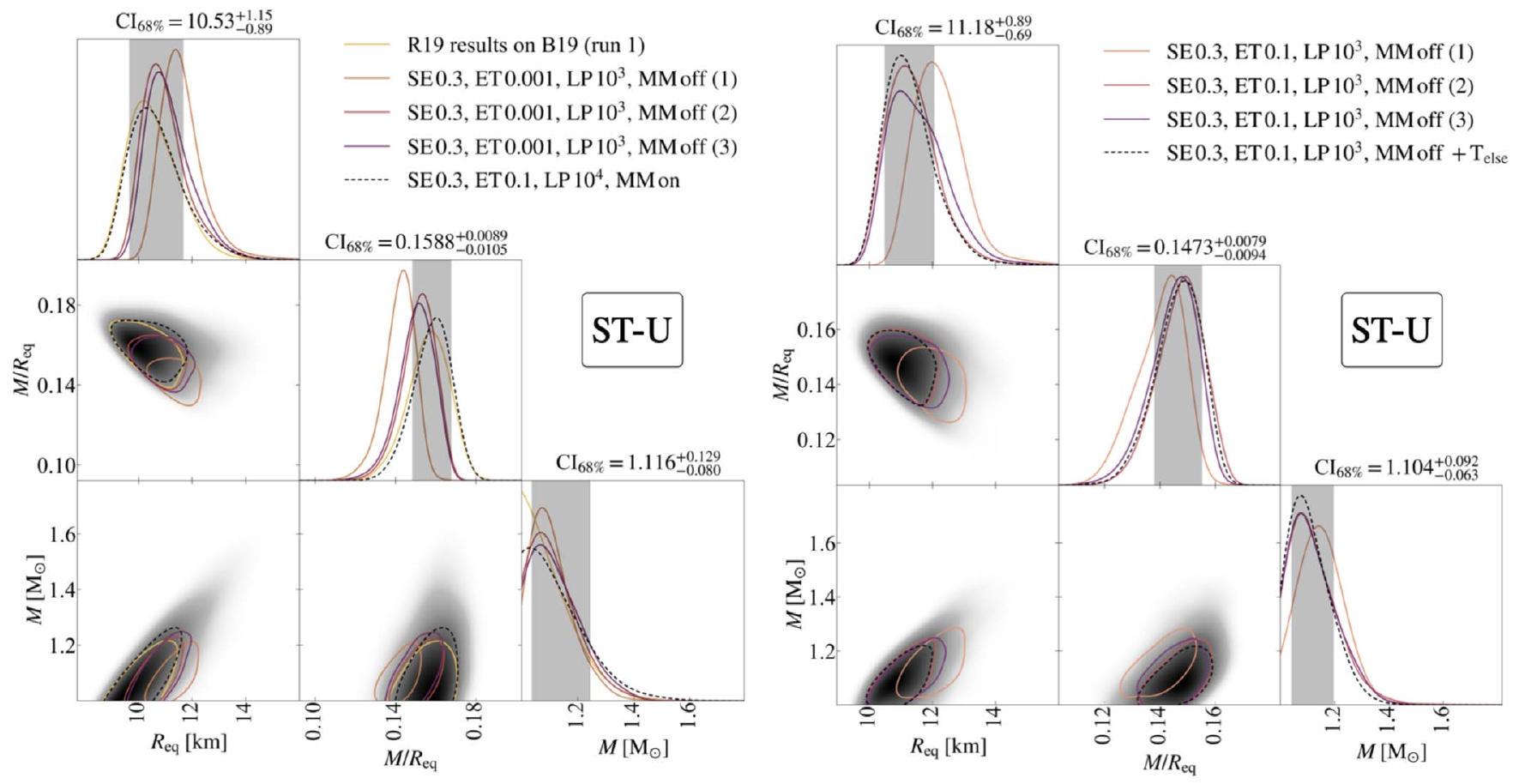
حدد R19 نموذج ST-U كنموذج أبسط يمكن أن يمثل مجموعة بيانات NICER الأصلية لـ PSR J0030+0451 التي تم تحليلها في تلك الورقة. النموذج المستمدفترة موثوقة للكتلة ونصف القطر، بافتراض ST-U، كانت، على التوالي، و . بالنسبة لهذا الاستنتاج، كانت إعدادات MULTINEST المعتمدة لتحليل PSR J0030+0451 هي: SE 0.3، ET 0.001، LP 1000، MM غير مفعل (من الآن فصاعدًا، نشير إلى هذه الإعدادات باسم إعدادات R19 MULTINEST لـمع التوزيعات الخلفية للثلاثة تجارب المختبرة، المتداخلة (انظر، على سبيل المثال، التوزيعات الخلفية للتجربة 1 في اللوحة اليسرى من الشكل 1). ضمن هذا الإطار الجديد (الذي، مقارنةً بالتحليلات في R19، يتضمن مجموعة بيانات NICER محدثة تتكيف مع استجابة أداة NICER الأحدث – بالإضافة إلى برنامج محدث)، نقوم لذلك بإجراء ثلاث تحليلات متطابقة ومستقلة باستخدام نفس إعدادات MULTINEST. يتم الإبلاغ عن التوزيعات الخلفية المستخلصة للكتلة، ونصف القطر، والكثافة في الرسم البياني في الزاوية اليسرى من الشكل 1. تشير تقلبات النتائج المستنتجة من هذه التجارب الثلاث إلى أنه، على عكس ما تم الإبلاغ عنه في R19، في إطار التحليل الحالي لدينا (بما في ذلك جميع التغييرات الموصوفة سابقًا)، فإن هذه الإعدادات غير كافية لاستكشاف فضاء المعلمات بشكل شامل. لهذا السبب، في نفس الرسم البياني، نبلغ أيضًا عن التوزيعات الخلفية لـ SE 0.3، ET 0.1، LP، MM قيد التشغيل، HR تعمل، والتي نعتبرها تمثيلية فعالة لنتائج ST-U في هذا الإطار الجديد (انظر الشكل 2). على الرغم من أننا نلاحظ زيادة طفيفة في القيمة المتوسطة المستنتجة للكتلة ونصف القطر بالإضافة إلى اتساع توزيعاتها اللاحقة، إلا أنها تتفق بشكل جيد مع نتائج R19. إذا بدلاً من التركيز على عمليات الاستدلال معنقاط حية، نركز على النتائج المستمدة هنا باستخدام إعدادات MULTINEST المشابهة لتلك المعتمدة في R19، فإن التوزيعات الخلفية الجديدة لنصف القطر والكتلة أضيق وتظهر وسائط أكبر بكثير (يمكن أن تكون الفروقات في نصف القطر ). نحن نعتبر الـ تشغيل ليكون أكثر قوة لأنه يستكشف فضاء المعلمات بشكل أفضل وأكثر استقرارًا (انظر بالفعل التداخل بين التوزيعات الخلفية مع LPالمبلغ عنه في الشكل 2 والمناقش في القسم 4.1.2.
يظهر الرسم البياني في الزاوية اليمنى من الشكل 1 التوزيعات الخلفية التي تم الحصول عليها باستخدام إعدادات MULTINEST الافتراضية لدينا (SE 0.3، ET، MM إيقاف). ليس من المستغرب، أيضًا في هذه الحالة، حيث يكون متطلب الدقة على تقدير الأدلة أقل، تظهر النتائج بعض التباين. بالإضافة إلى ذلك، في نفس الرسم البياني، نبلغ عن النتائج التي تم الحصول عليها من خلال اعتماد ST-U+T آخر، والذي يتضمن إمكانية أن
الشكل 1. التوزيعات الخلفية لـ ST-U (المُعالجة بواسطة KDEs من GetDist) من تسع جولات استدلال، بالنسبة لنصف القطر، والكتلة، والكثافة. تُظهر الرسم البياني في الزاوية اليسرى النتائج لثلاث جولات استدلال بإعدادات MULTINEST مطابقة لتلك التي اعتمدها R19، ولكن تم الحصول عليها في إطار X-PSI والبيانات الجديد الموضح في الأقسام 2 و3 (الاختلافات مدرجة في القسم 5.1). بالنسبة لجميع هذه الجولات، اعتمدنا إعدادات X-PSI عالية الدقة. للمقارنة، نعرض أيضًا التوزيعات التي تم العثور عليها للجولة بخطوط صفراء صلبة.النموذج، في R19. مع الخطوط السوداء المتقطعة نقدم التوزيعات اللاحقة للخطأ المعياريMM على التشغيل، الذي نعتبره التشغيل المرجعي لنموذج ST-U في هذا العمل. تُظهر الرسم البياني في الزاوية اليمنى النتائج لثلاثة عمليات استدلال باستخدام إعدادات MULTINEST الافتراضية لدينا. كما نبلغ عن توزيعات ما بعد الاستدلال للتشغيل الذي يسمح لكامل سطح MSP بالإشعاع (المعروف باسم ST-U+Telse). كل من الرسمين البيانيين في الزاوية يظهر توزيعات جديدة من أربعة عمليات استدلال، والتي تستخدم إعدادات MULTINEST مختلفة، كما هو موضح في الأسطورة (للتعريفات، انظر القسم 2.1.4). تتبع المنحنيات في تمثيل توزيعات ما بعد الاستدلال ثنائية الأبعاد منطقة موثوقة بنسبة 68%. بالإضافة إلى توزيعات ما بعد الاستدلال أحادية البعد، نبلغ عن فترات موثوقة بنسبة 68% (تمثل المنطقة داخل و النسب المئوية في التوزيع الهامشي ذي البعد الواحد) بدءًا من الوسيط للتوزيعات. تشير هذه القيم، بالإضافة إلى المناطق الملونة، إلى الخطين الأسودين المتقطعين: التشغيل الذي يمكّن من فصل الوضع، في الرسم البياني في الزاوية اليسرى، والتشغيل الذي يعتمد على ST-U+T.النموذج، في الزاوية اليمنى من الرسم.
يمكن أن تصدر السطح بالكامل من النجوم النيوترونية في نطاق حساسية NICER. نجد أن إضافة هذا العنصر الإضافي في النموذج تنتج نتائج متسقة مع عمليات الاستدلال الأخرى التي تم تنفيذها بنفس الإعدادات.
4.1.2. تأثير إعدادات التحليل
تسلط نتائج V23a الضوء على أهمية إعدادات multinEST. بالنسبة لـ ST-U (الأرخص حسابيًا من نماذجنا)، اختبرنا تأثير اعتماد قيم مختلفة من كفاءة العينة أو تحمل الأدلة، بدءًا من إعداداتنا الافتراضية (استنادًا إلى الإعدادات المعتمدة للنماذج الأكثر تعقيدًا من ST-U في R19). يتم الإبلاغ عن التوزيعات البعدية المستنتجة في الزاوية اليسرى من الشكل 2. نحن نبلغ عن ما يلي: باللون الوردي، النتائج لجميع الجولات الثلاث مع إعداداتنا الافتراضية، وباللون البني تلك للجولات الثلاث للاستدلال، التي تم تنفيذها مع ET 0.001، المعروضة بشكل فردي في الرسمين الأيمن والأيسر، على التوالي، من الشكل 1.
في الزاوية اليمنى، نوضح أهمية تحديد عدد كافٍ من النقاط الحية لتغطية مساحة معلمات النموذج بشكل شامل والحصول على حل مستقر. مرة أخرى، نعرض باللون الوردي تقديرات المعلمات لثلاثة جولات استدلال تعتمد على إعدادات MULTINEST الافتراضية لدينا. ثم نعرض التوزيعات البعدية التي تم الحصول عليها، على التوالي، مع الجولات التي تعتمد على 3 آلاف، 6 آلاف، و10 آلاف نقطة حية، مما يوضح التقارب التدريجي نحو قيم أقل قليلاً من الأشعة وزيادة في عدم اليقين. تظهر هذه النتائج أنه في هذا الإعداد (وبعد تثبيت كفاءة العينة عند 0.3 والأدلة نحتاج إلى حد أدنى من النقاط الحية في مكان ما في النطاق (تحمل 0.1)لضمان استكشاف كافٍ لمساحة معلمات النموذج.
في كلا الرسمين في الزاوية، كمرجع، نقوم أيضًا برسم التوزيعات البعدية التي تم الحصول عليها من عملية الاستدلال SE 0.3، ET، MM قيد التشغيل، HR. اعتمادًا على الأخير كمرجع، مع التحذير من إحصائيات الأعداد المنخفضة، تشير هذه النتائج إلى الاستنتاجات التالية:
في هذا الإطار الجديد،النقاط الحية ليست كافية لاستكشاف مساحة معلمات النموذج بشكل شامل؛
يبدو أن واحدًا من كل ثلاثة تجارب يعطي قيمة متوسطة مختلفة بشكل ملحوظ لنصف القطر الخلفي، سواء مع إعدادات MULTINEST الافتراضية لدينا أو مع التغيير في تحمل الأدلة (ET 0.001)؛
مقارنةً عندما نتبنى ET 0.001، يبدو أن إعدادات MULTINEST الافتراضية لدينا (مع ET 0.1) تؤدي إلى تباين أكبر في وسائط نصف القطر والكتلة (لكن أقل في الكثافة)؛ كما أن هذه الوسائط عمومًا أبعد عن القيم المحددة مع SE المرجعي.تشغيل، استنتاج الموارد البشرية؛
ومع ذلك، يبدو أن إعداداتنا الافتراضية تستعيد أيضًا توزيعات أوسع مقارنةً بنظيراتها من ET 0.001؛ حيث يتم استعادة توزيعات أوسع، مرة أخرى مقارنةً بتجارب ET 0.001، أيضًا مع تجربة المرجع ST-U؛
يبدو أن تغيير قيمة كفاءة العينة لا يؤثر بشكل كبير على القيمة الوسيطة للنتائج اللاحقة؛
الشكل 2. توزيعات ST-U الخلفية (المُعالجة بواسطة GetDist KDEs) من 16 تجربة، بالنسبة لنصف القطر، الكثافة، والكتلة. يبرز هذا الشكل تأثير اعتماد إعدادات MULTINEST المختلفة (لجميع هذه التجارب، اعتمدنا إعدادات X-PSI عالية الدقة). في الرسم البياني الأيسر، نعرض النتائج لتسع تجارب استدلال ST-U: توضح، للمشكلة المحددة المطروحة، ما هو تأثير تغيير تحمل الأدلة أو كفاءة العينة، مقارنةً بإعداداتنا الافتراضية. بينما يظهر الرسم البياني في الزاوية اليمنى تأثير زيادة عدد النقاط الحية. كمرجع، في كلا الرسمين البيانيين في الزاوية، نبلغ أيضًا بخطوط سوداء متقطعة التوزيعات الخلفية التي تم الحصول عليها مع SE 0.3، ET 0.1، LPMM في التشغيل؛ الأرقام الموجودة أعلى التوزيعات الخلفية 1D، بالإضافة إلى المناطق المظللة، تشير إلى هذه الجولة من الاستدلال. راجع تعليق الشكل 1 لمزيد من التفاصيل.
ومع ذلك، عند خفضه إلى 0.1، تزداد عرض التوزيعات الخلفية، مما يقترب من القيم التي تم الحصول عليها إذا تم اعتماد عدد أكبر من النقاط الحية؛ و 6. نظرًا لظهور انحياز نحو قيم نصف القطر الأعلى عندماتستخدم النقاط الحية، ويبدو أن إجراء عدة تجارب مع هذا الإعداد من غير المحتمل أن يؤدي إلى نفس النتيجة التي يمكن الحصول عليها من تجربة واحدة مع عدد أكبر من النقاط الحية.
4.1.3. استكشاف النموذج
القيم المختلفة للكتلة ونصف القطر التي تم الحصول عليها من تسلسل نماذج الأنماط السطحية المتداخلة التي تم تحليلها في R19 قد اقترحت بالفعل وجود أوضاع متعددة في سطح الاحتمالية. في هذا العمل، نبرز ونتوسع في هذه النتائج. نركز هنا على التوزيعات البعدية التي تم الحصول عليها باستخدام SE 0.3 و ET 0.1 و LP.تشغيل استنتاج HR ST-U مع MM مفعل. هنا نجد ثلاثة أوضاع في الخلفية، مع انحدارات ومواقع نقاط ساخنة مختلفة بشكل ملحوظ (التكوين الذي يتوافق مع الرئيسي المبلغ عنه في اللوحة (A) من الشكل 3). من المثير للاهتمام أنهم يظهرون نفس أوضاع تكوين النقاط الساخنة كما هو موجود في V23a عند تحليل مجموعة بيانات اصطناعية تم إنتاجها باستخدام نموذج ST+PST (انظر الشكل 8 من V23a لتمثيل بصري). كما في تلك الحالة، فإن الحلول الثانوية الاثنين لها قيم احتمال وأدلة محلية مشابهة، لكنها تؤدي بشكل أسوأ بكثير من الوضع الرئيسي المحدد (الهندسة ذات الاحتمالية القصوى، للتشغيل المعادل ولكن مع MM غير مفعل، تم الإبلاغ عنها في اللوحة (A) من الشكل 3). كما أنها تختلف بشكل ملحوظ عنها في الكتلة المستنتجة ونصف القطر (تم الإبلاغ عن المتوسطات والانحرافات المعيارية المرتبطة بها في الجدول 5).
من الزاوية اليمنى من الشكل 2، يمكننا مقارنة توزيعات الكتلة، ونصف القطر، والكثافة الخلفية لهذه العملية الاستدلالية بتلك التي تم الحصول عليها باستخدام نفس إعدادات MULTINEST ولكن مع تعطيل فصل الوضع. عندما نقوم بتمكين فصل الوضع، تكون التوزيعات الخلفية أضيق قليلاً ولكن بخلاف ذلك فهي متشابهة جداً مع بعضها البعض:فترات موثوقة لنصف قطر PSR J0030+0451، مع وبدون تفعيل فصل الوضع، هي، على التوالي، و ؛ بينما بالنسبة للكتلة هم و بينما يسمح الأخير للنقاط الحية باستكشاف فضاء المعلمات بحرية وبشكل أكثر كفاءة، فإن الأول، وهو تشغيلنا المرجعي لتحليلات ST-U NICER فقط، يتيح لنا تحديد الأنماط في التوزيع الخلفي المستنتج، حتى عندما لا تكون مرئية بالعين.
4.1.4. التحليل المشترك لبيانات NICER و XMM-Newton
في الزاوية اليسرى من الشكل 4، نعرض النتائج الرئيسية من تحليل الاستدلال المشترك بين NICER وXMM-Newton. وهي تشير إلى SEعلى، تم تشغيل HR، وتم الأداء بالإعداد الموصوف في القسم 2. التكوين المرتبط بعينة الاحتمالية القصوى من توزيعها الخلفي موضح في اللوحة (C) من الشكل 3.
تتحرك التوزيعات الخلفية أحادية البعد للكتلة، ونصف القطر، والكثافة إلى قيم أكبر. على وجه الخصوص، تصل التوزيعة بوضوح إلى الحد الأعلى لنصف القطر البالغ 16 كم. نظرًا لأن تحليلنا حساس بشكل خاص للكثافة، من المتوقع أن يقيّد هذا الحد الأعلى لنصف القطر الخلفية الخاصة بالكتلة بشكل غير مباشر أيضًا. تشير الرسم البياني إلى أن قمة الخلفية لنصف القطر قد تتوافق مع أنصاف أقطار أكبر مما تسمح به أولوياتنا (المستندة إلى الأسس الفيزيائية). ومع ذلك، هناك ذيل ممدود للخلفية يتضمن قيمًا أقل بكثير.
الشكل 3. تمثيل الأوضاع الهندسية الرئيسية التي تم العثور عليها من خلال التحليلات المقدمة في هذه الدراسة. تُظهر أنماط السطح من وجهة نظر المراقب (أي، وفقًا للانحدار المستنتج للعينة المحددة المعنية)، عند المرحلة صفر من البيانات. تُرسم النقاط الساخنة على نفس (أو النصف المعاكس) من الكرة الأرضية مقارنة بالمراقب بألوان كاملة (مخففة) وعلامة صليب (دائرية) في المركز. يتغير لون مكونات النقطة الساخنة من الأزرق إلى الأحمر من أعلى إلى أدنى درجة حرارة للنمط السطحي المعني (بدقة أعلى مقارنة بدرجة الحرارة المبلغ عنها في الأسطورة). يُستخدم الأسود لتغطية المكونات. في جميع الحالات، نعرض، كنقطة مرجعية، هندسة النقطة الساخنة المرتبطة بعينة الاحتمالية القصوى لتلك الوضعية المحددة ضمن فترة الاستدلال المعنية. على الرغم من أن هذه العينة الواحدة لا يمكن أن تلتقط مجموعة كاملة من التغيرات الممكنة الموجودة في الوضعية، نأمل بهذه الطريقة أن نقدم إشارة مبسطة ولكن أكثر وضوحًا للتكوينات التي تنتمي إلى الوضعية. تشير اللوحات (A) و(B) إلى التكوينات المرتبطة بالوضعية الرئيسية لـ ST-U (SE 0.3، ET 0.1، LP“، MM إيقاف، HR) و ST+PST (SE 0.3، ER 0.1، LP، نماذج MM على، LR) ، تحليلات NICER فقط. تشير اللوحات (C) و (D) و (E) و (F) إلى التكوينات الموجودة في استنتاجات NICER و XMM-Newton المشتركة. اللوحات (C) و (D) تمثل الأوضاع الرئيسية (C) والثانوية (D) المستمدة من اعتماد النموذج (SE 0.3، ER 0.1، LP 104، MM قيد التشغيل)، بينما تشير اللوحات (E) و (F) إلى الوضع الرئيسي الموجود مع نماذج ST+PDT و PDT-U (SE 0.8، ER 0.1، LP ، إيقاف MM) (للهذين الأخيرين، تم اعتماد إعدادات منخفضة الدقة، LR، X-PSI).
الأشعة. الخلفيات التي تنتمي إلى هذا الذيل تتميز أيضًا بكتل أقل بكثير (انظر توزيع الخلفية ثنائي الأبعاد للكتلة والشعاع)، بما يتماشى بشكل أقرب مع ما تم العثور عليه كالوضع الرئيسي عند تحليل بيانات NICER فقط. هذا الذيل في الخلفية الشعاعية للاستنتاج المشترك بين NICER وXMM-Newton يتوافق مع الوضع الثانوي الذي وجده العينة، والذي تم الإبلاغ عن تكوينه في اللوحة (D) من الشكل 3. تم الإبلاغ عن المتوسط والانحراف المعياري لهذه القمة الثانوية في الخلفية، بالإضافة إلى القمة الرئيسية، في آخر عمودين من الجدول 5. كلا الوضعين يظهران توزيع خلفية للانضغاط يصل إلى قيم أعلى بكثير مقارنةً بالنتائج التي تم الحصول عليها عند تحليل بيانات NICER فقط. إن تضمين بيانات XMM-Newton في عملية الاستنتاج يحد من مساهمة الخلفية (انظر الشكل 5)، مقارنةً بما يتم استنتاجه من بيانات NICER وحدها. لتعويض الانخفاض في الخلفية غير النابضة، يزداد الانضغاط المستنتج، مما يخلق إشارة غير نابضة أكبر تنشأ من النجم (على الرغم من أن المنطق نفسه تم تطبيقه لشرح النتائج من الاستنتاج المشترك).
تحليلات NICER و XMM-Newton أيضًا في رايلي وآخرون 2021 وسالمي وآخرون 2022 لـ PSR J0740+6620). نفس الاتجاه يظهر لكل من نماذج ST-U و ST+PST.
تؤدي قيم نصف القطر الأعلى والكثافة إلى الحصول على أنصاف أقطار زاوية أقل تصف حجمين للنقاط الساخنة، وتسمح للنقطة الساخنة عند الزاوية القطبية الأعلى (الأقرب إلى القطب) بالتحرك قليلاً نحو خط الاستواء. ومع ذلك، فإن الزوايا القطبية للنقاط الساخنة ليست مقيدة بشكل صارم، مما يؤدي إلى هيكل ثنائي النمط مرئي في التوزيع الخلفي للمعلمات التي تصف خصائص النقاط الساخنة (انظر الشكل 6). ويرجع ذلك إلى الغموض في التسميات الأولية والثانوية المرتبطة بالنقاط الساخنة.نظرًا لأن نصف قطر MSP المستنتج من خلال
الجدول 5 جدول يصف الخصائص الرئيسية للأوضاع الثلاثة المحددة وفقًا لنموذج ST-U
أجمل
نيكر و إكس إم إم
الوضع 1
الوضع 2
الوضع 3
الوضع 1
الوضع 2
-35735
-35758
-٣٥٧٥٧
-42661
-42666
-35788
-35810
-35808
-42714
-42718
تكوين
اللوحة (أ)، الشكل 3
اللوحة الوسطى من الشكل 8، V23a
اللوحة اليمنى في الشكل 8، V23a
اللوحة (ج)، الشكل 3
اللوحة (د)، الشكل 3
ملاحظة. الصفان الأولان يوضحان المتوسطات والانحرافات المعيارية للكتلةونصف القطر الاستوائيالتوزيعات الخلفية؛ يظهر الاثنان الأخيران القيم المقابلة لأقصى احتمال لوغاريتمي وقيم دليل محلي. يصل الوضع الثانوي إلى قيم أكبر قليلاً فقط من تلك الموجودة في بيانات NICER فقط، لا تزال الزوايا الخاصة بالنقاط الساخنة تتناقص، ولكن ليس بنفس القدر كما في الوضع الرئيسي (انظر الشكل 6). تظهر التكوينات الناتجة عن الوضع الرئيسي للاستدلال المشترك بين NICER وXMM-Newton درجات حرارة وزوايا ميل مشابهة جداً لتلك الموجودة في الوضع الرئيسي عند تحليل بيانات NICER فقط. هذا ليس هو الحال بالنسبة للوضع الثانوي، الذي يشير إلى تكوين أكثر قربًا من الحافة، مع جيب التمام للزاوية الميل متوافق مع الصفر. في هذا الإعداد الجديد، تقع النقاط الساخنة بالقرب من خط الاستواء وتتميز بدرجات حرارة أقل بكثير.
4.1.5. تحليل بيانات XMM-نيوتن فقط
تم تحليل بيانات XMM-نيوتن لـ PSR J0030+0451 لأول مرة في دراسة بودغانوف وغريندلاي (2009) في محاولة لاستخراج معلومات حول نصف قطر النجم النيوتروني. في هذا التحليل، الذي استخدم نهجًا تكراريًا، تم افتراض كتلة ثابتة منتم الافتراض فقطكان مسموحًا بالتغيير. تم اعتبار دائرتين ساخنتين فقط بتكوين يعادل نموذج ST-U. بالإضافة إلى ذلك، تم ملاءمة ملف النبض المستخرج من جهاز XMM-Newton EPIC pn (الذي تم استخدامه في بودانوف وغرينلاي 2009، ولكن ليس في هذا العمل؛ انظر القسم 3.2) في نطاقين طاقيين عريضين فقط. و . نظرًا للإحصائيات المحدودة للفوتونات في بيانات XMM-Newton، أسفرت هذه التحليل عن حد أدنى فقط على نصف قطر النجم النيوتروني من (95% ثقة) وقيود واسعة جداً على مواقع النقاط والهندسة، والتي تتماشى بشكل عام مع التكوينات المبلغ عنها في الألواح (C) و(D) من الشكل 3.
باستخدام خط الأنابيب والإجراءات الموضحة في هذه الورقة، فإن تحليل بيانات XMM-Newton فقط يعطي خصائص نقاط ساخنة مقيدة بشكل ضعيف جداً وفترات موثوقة من والكتلة هذه القيم أوسع من القيم المذكورة في بودغانوف وغريندلاي (2009)، على الأرجح لأن بعض الافتراضات قد تم تخفيفها ولم يتم استخدام أي معلومات زمنية. كما أنها أوسع بكثير من التوزيعات اللاحقة المستمدة من بيانات NICER، كما هو متوقع بسبب وقت التعرض الأصغر بكثير لـ XMM-Newton، والمساحة الفعالة، والدقة الزمنية، ودقة الطاقة.
4.2.
4.2.1. إعادة إنتاج نتائج R19 وتحليل تأثير الإعدادات
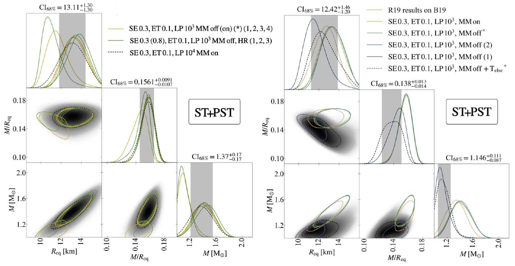
بالنسبة لـ ST+PST، أبلغ R19 عن فترات موثوقة للكتلة ونصف القطر، على التوالي، من و . هذه تم الحصول على النتائج من تشغيل يعتمد على إعدادات MULTINEST التالية: SE 0.3 (0.8)، ET 0.1، LPتم إيقاف MM، حيث زادت كفاءة العينة إلى 0.8 عند استئناف التحليل. في الشكل 7، نعرض التوزيعات اللاحقة المستمدة من تحليل B19v006 باستخدام نموذج ST+PST في إطار الاستدلال الجديد (انظر القسم 2 لمزيد من التفاصيل). تظهر الخطوط الخضراء في الزاوية اليسرى من الرسم النتائج للجولات التي تتطابق قدر الإمكان مع إعدادات التحليل المعتمدة في R19. نلاحظ أن هناك بعض التشتت بين هذه التوزيعات اللاحقة. على وجه الخصوص، فإن القيم الشاذة الرئيسية تجد فقط الوضع الثانوي لسطح posterior (انظر الأقسام 4.2.2 و 5 للسياق والنقاش حول تعدد الأوضاع الخاصة به)؛ وهذا يشبه الوضع الذي تم العثور عليه لـ ST-U وبالتالي يتميز بنصف قطر وكتل أصغر. لا تزال الجولتان الأخريان تظهران بعض التشتت، مما يشير إلى أن إعدادات MULTINEST هذه غير كافية الآن (نظرًا للتغييرات المختلفة في خيارات القنوات، استجابة الأدوات، إلخ مقارنة بـ R19) لاستكشاف فضاء معلمات النموذج. مقارنة بالفترات الموثوقة المقدمة في R19، تظهر التوزيعات اللاحقة الجديدة قيمًا أعلى قليلاً (على الأرجح بسبب الاختلاف في القنوات، حيث تم العثور على نفس الاتجاه في التحليلات الأولية ونُسب إلى نموذج ST-U لإزالة البيانات في القنوات 25-30) وعدم اليقين المماثل. الجولة الوحيدة HR مع SE 0.3 فقط هي جولة الاستدلال، التي تحدد، كأوضاعها الرئيسية، الوضع الثانوي (المشابه لـ ST-U) (تم تمثيل التوزيعات اللاحقة 1D و 2D للكتلة، ونصف القطر، والكثافة في الشكل 7 بواسطة القيم الشاذة الخضراء)؛ كانت التكلفة الحسابية لهذا التحليل ثلاثة إلى أربعة أضعاف تكلفة الجولتين HR الأخريين.
تظهر قطعة الزاوية نفسها أيضًا تأثير خفض دقة إعدادات X-PSI؛ حيث تُظهر المنحنيات الخضراء النتائج الوحيدة التي تم الحصول عليها بدقة عالية للنماذج الأكثر تعقيدًا منتمثل الخطوط الصفراء التوزيعات، المستمدة بدقة منخفضة ولكن مع الإعدادات الأخرى القابلة للمقارنة مباشرة مع تلك التي تم الحصول عليها بدقة عالية. لاحظ أن القيم الشاذة الاثنين تم إنتاجها بنفس البذور الثابتة لـ MULTINEST وPython. باستثناء القيمة الشاذة (التي ترتبط مرة أخرى بتحديد الوضع الثانوي)، يبدو أن الجولات ذات الدقة المنخفضة تتقارب نحو حلول أكثر استقرارًا قليلاً تقع عند أنصاف أقطار وكتل أصغر قليلاً وتتميز بوجود خلفيات أكبر قليلاً، عندما يكون الوضع المفضل من قبل الأدلة.يتم تحديده (انظر القسم 4.2.2). الـ
الشكل 4. التوزيعات الخلفية (المُعالجة بواسطة GetDist KDEs) لنصف القطر، والكثافة، والكتلة من عمليات الاستدلال المشتركة بين NICER وXMM-Newton: الرسوم البيانية في الزاويتين اليسرى واليمنى، على التوالي، تم الحصول عليها باعتماد نموذج ST-U ونموذج ST+PST. مع الخطوط المنقطة هنا نعرض التوزيعات السابقة. في التوزيعات الخلفية ثنائية الأبعاد، نرسم ثلاث منحنيات، محددين ، و منطقة موثوقة. يتم عرض إعدادات التحليلات للجولات المرسومة في الجدول 4 (انظر إدخالات ST-U و ST+PST مع “نعم” في عمود XMM-Newton). راجع تعليق الشكل 1 لمزيد من التفاصيل.
السلوك مختلف عندما يتم استكشاف الوضع الثانوي فقط بواسطة العينة؛ عند مقارنة النقطتين الشاذتين في مخطط نصف القطر أحادي الأبعاد، فإن التشغيل عالي الدقة ينتج عنه في الواقع توزيعات ضيقة جداً، تتركز عند قيم أقل بكثير. نحن نستخدم أيضاً دقة منخفضة لتشغيل مرجعنا الجديد ST+PST، الذي تم الحصول عليه بزيادة عدد النقاط الحية إلىوتمكين خيار فصل الوضع في MULTINEST. نحن نبلغ عن الخلفية المقابلة بخط متقطع أسود في نفس الزاوية اليسرى من الشكل 7. بالمقارنة مع النتائج التي تم العثور عليها مع الجولات الأخرى ذات الدقة المنخفضة (حيث كان عدد النقاط الحية في MULTINEST هوهذه التوزيعات تتوسع قليلاً وتتحرك نحو قيم أقل من الكتلة ونصف القطر. تم العثور على توسيع مماثل للنتائج اللاحقة، مع زيادة عدد نقاط الحياة في MULTINEST، في دراسة رايلي وآخرون (2021) لـ PSR J0740+6620، وقد يشير ذلك إلى توزيع حقيقي أوسع للنتائج اللاحقة.فترات الثقة للكتلة ونصف القطر المستمدة من استنتاجنا المرجعي الجديد هي: و (كما هو موضح في أعلى التوزيعات الخلفية 1D في الرسم البياني في الزاوية اليسرى من الشكل 7)، متوافق إلى حد كبير مع نتائج R19. يتم الإبلاغ عن تكوين النقاط الساخنة الذي يتوافق مع عينة الاحتمالية القصوى من هذا التحليل في اللوحة (B) من الشكل 3. اختباراتنا الحالية لا تضمن أن هذه الإعدادات التحليلية كافية لاستكشاف فضاء معلمات النموذج بشكل كاف.
في الزاوية اليمنى من الشكل 7، نعرض التوزيعات البعدية المستمدة من كل من الجولات ذات الدقة المنخفضة، المبلغ عنها بخطوط صفراء في اللوحة اليسرى. كما نبلغ باللون البني التراكمي الذي حددته رايلي وآخرون (2019) لنموذج ST + PST. يتم تمثيل القيم الشاذة، الموضحة في الزاوية اليمنى مع خطوط زرقاء، من خلال نسخة من جولة الاستدلال باستخدام إعدادات MULTINEST الافتراضية لدينا. وبالتالي، يمكن أن تُعزى النتائج المختلفة فقط إلى العشوائية الموجودة في عملية العينة. ومع ذلك، فإن حدوث مثل هذه القيم الشاذة يشير إلى أن عدد النقاط الحية المختارة لهذه الاستنتاجات غير كافٍ لاستكشاف مساحة معلمات النموذج بشكل فعال. تمثل المنحنيات السوداء المتقطعة النتائج التي تم الحصول عليها عند إدخال درجة الحرارة في أماكن أخرى إلى نموذج ST+PST، ويتم تقديمها بمزيد من التفصيل في القسم 4.2.2.
تظهر عمليات الاستدلال الثلاثة الأخرى توزيعات خلفية متداخلة تقريبًا بشكل مثالي، على الرغم من الاختلافات في إعدادات MULTINEST (تظهر الخطوط الصفراء النتائج التي تم الحصول عليها بتمكين خيار فصل الوضع) وفي الأوليات (تحدد المنحنيات الخضراء التوزيعات المستمدة من العمليات التي تعتمد الأولية المحدثة ST+PST CoH). من خلال هذا الرسم البياني وعمليات الاستدلال المرتبطة، نوضح أنه عند تحليل بيانات NICER B19v006، فإن إدخال الأولية المحدثة ST+PST CoH لا يؤدي إلى أي فرق كبير في توزيعات الخلفية المستنتجة وتقدير الأدلة. يمكننا أن نستنتج نفس الاستنتاج بشأن تأثير اعتماد خيار فصل الوضع في MULTINEST، على الرغم من أنه محدود بالحالة المحددة التي تم النظر فيها هنا.
4.2.2. استكشاف النموذج
تسلط استنتاجات فصل الوضع لدينا الضوء على الهيكل متعدد الأوضاع الموجود في السطح الخلفي لهذا النموذج المحدد، بالنظر إلى مجموعة بيانات B19v006 المختارة (على الرغم من أننا نتوقع أن تظهر جميع مجموعات بيانات PSR J0030+0451 من NICER سلوكًا مشابهًا). كما تم الإشارة إليه بإيجاز في القسم السابق، هناك وضعان بارزان في الخلفية، يختلفان في دليل اللوغاريتم المحلي بعامل. العينات ذات الاحتمالية القصوى التي تنتمي إلى الوضعين تختلف في الواقع بقيمة أكبر بكثير (في لوغاريتم الاحتمالية)، من الذي يمكننا أن نستنتج أن الفضاء السابق الذي يدعم الوضع الثانوي أكبر بكثير من ذلك الذي يدعم الوضع الرئيسي. وهذا يفسر أيضًا لماذا يمكن أن يكون عدد النقاط الحية منخفضًا نسبيًا
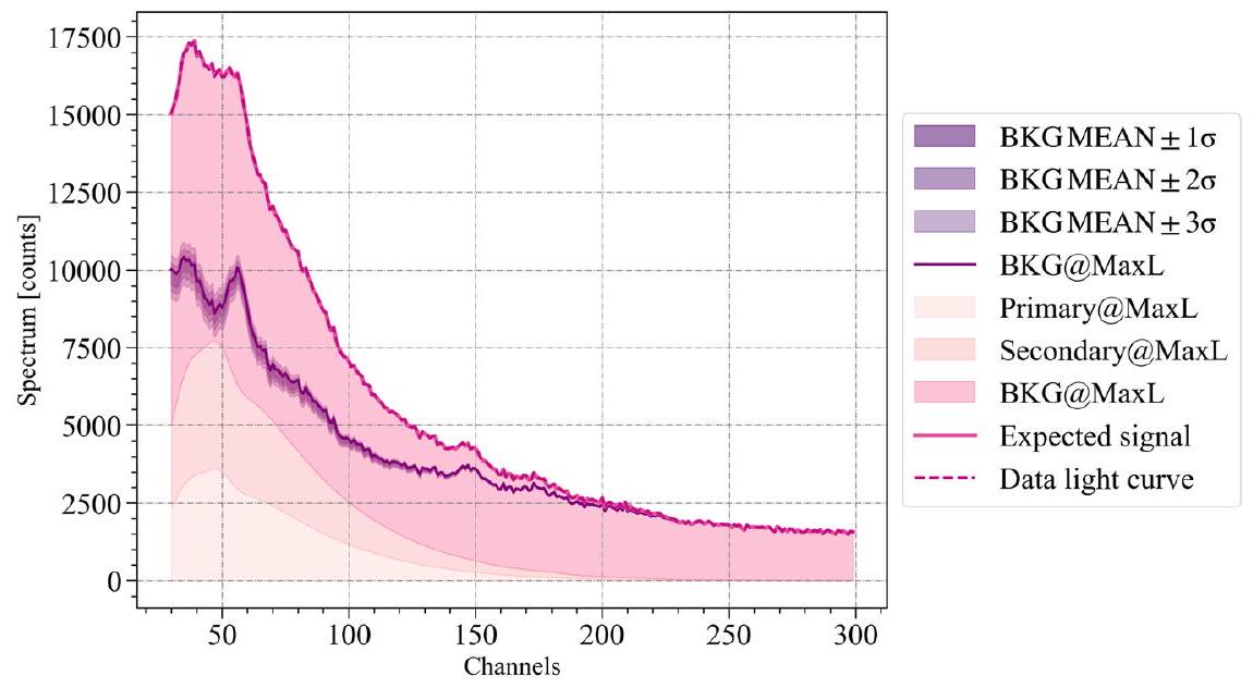
الشكل 5. طيف بيانات NICER وتركيبتها المستنتجة، وفقًا لعينة الاحتمالية القصوى من تحليل X-PSI الخاص بنا. البيانات مرسومة بخط متقطع باللون الأرجواني؛ الإشارة الكلية المتوقعة موضحة بخط وردي متصل؛ الخلفية (BKG) التي تعظم الاحتمالية لعينة الاحتمالية القصوى (MaxL، في الأسطورة) مرسومة بخط أرجواني متصل. يتم الإبلاغ عن مساهمة النقطة الساخنة الرئيسية، والنقطة الساخنة الثانوية، والخلفية، مرة أخرى المرتبطة بعينة الاحتمالية القصوى، فوق بعضها البعض مع مناطق مظللة باللون الوردي، تتلون بشكل متزايد. تُظهر الظلال الأرجوانية من اللون الداكن إلى الفاتح متوسط الخلفيةأو 3 انحرافات معيارية، تم حسابها على 200 عينة لاحقة مختارة عشوائيًا من ملف مخرجات MULTINEST ذو الوزن المتساوي. تتعلق الاستنتاجات لهذا الشكل بالتحليل المشترك لبيانات NICER وXMM-Newton، الذي تم تنفيذه باستخدام نموذج X-PSI PDT-U. مجموعة الأشكال الكاملة (8 صور) متاحة، لنماذج ST-U وST+PST وST+PDT وPDT-U لكل من تحليلات NICER فقط (تشغيلات مرجعية مميزة بالخط العريض في الجدول 4) والاستنتاجات المشتركة لمجموعات بيانات NICER وXMM-Newton (إعدادات التحليل المبلغ عنها في الجدول 4، والتي تتوافق مع إدخالات “نعم” في عمود XMM-Newton).
(مجموعة الأشكال الكاملة (8 صور) متاحة.)
تؤدي إلى تحديد الوضع الثانوي كالوضع الرئيسي. تم تقديم هندسة نقطة ساخنة توضيحية مرتبطة بالوضع الرئيسي، مع أخذ عينة الاحتمالية القصوى كمثال، في اللوحة (B) من الشكل 3. يشبه الوضع الثانوي، أيضًا في الخلفية المستنتجة، الوضع الرئيسي المحدد باستخدام نموذج المبلغ عنه في اللوحة (A) من نفس الشكل. العنصر المفقود مرتبط دائمًا بالنقطة الساخنة الأصغر، الأقرب إلى خط الاستواء، (المعلمة كأولية في اللوحة (A) من الشكل 3). يمكن أن يختلف موقع وحجم العنصر القابل للإخفاء بشكل كبير ضمن الوضع المحدد. تحليل SE 0.3، ET 0.1، LPMM مغلق، تشغيل LR الذي فاته الوضع الرئيسي، لكنه وجد هذا الوضع الثانوي (الذي تم تمثيل كتلته وكثافته ونصف قطره اللاحق بخطوط زرقاء في الرسم البياني في الزاوية اليمنى من الشكل 7)، نلاحظ أنه، بينما تصور عينة الاحتمالية القصوى لهذا التشغيل الأولي كحلقة، تمثل العينة اللاحقة كمنطقة ساخنة شبه دائرية، حيث تلامس المكونات المفقودة بالكاد المكون المنبعث. تشير هذه الفجوة في خصائص النقطة الساخنة PST إلى، كما تم العثور عليه في V23a، أننا حساسون فقط بشكل ضعيف جدًا للتفاصيل الصغيرة لأشكال النقاط الساخنة. في هذه الحالة، يبدو أننا حساسون بشكل أساسي لموقع ومساحة الانبعاث الكلية لنقطة PST الساخنة: هناك بالفعل ارتباط واضح بين حجم الغطاء الكروي القابل للإخفاء والمسافة من مركز النقطة المنبعثة.
تقدم كل من الأوضاع الأولية والثانوية خلفية مستنتجة مشابهة جدًا (انظر الشكل 13 من V23a، لمقارنة الخلفية المرتبطة بحلول ST+PST وST-U الرئيسية) وقيم الكثافة، على الرغم من الاختلافات في الكتلة المستنتجة ونصف القطر (تم استنتاج قيم كثافة قابلة للمقارنة أيضًا من تحليل ST-U المرجعي لدينا). في جوانب أخرى، هذه الحلول مختلفة تمامًا عن بعضها البعض. على وجه الخصوص، الاختلاف في ميل المراقب المستنتج، المقدر من قبل الوضعين، يؤدي إلى تغييرات في موقع النقطة الساخنة وأحجامها، بحيث لا تزال قابلة للرصد في
hالات صحيحة (يمكن العثور على مناقشة أكثر تفصيلًا حول تأثير الميلان المختلف في القسم 5.2.1 من V23a). تسلط هذه الاعتبارات الضوء على وجود تداخلات كبيرة، وأحيانًا غير تافهة، في فضاءات معلمات نموذجنا.
في الرسم البياني الأيمن من الشكل 7، نعرض تأثير السماح لبقية سطح النجم (الجزء غير المغطى من قبل النقاط الساخنة) بإصدار إشعاع الجسم الأسود المميز بدرجة حرارة متجانسة محدودة (ST+PST+T). يستخدم هذا الاستنتاج أيضًا الأوليات المحدثة CoH، ومع ذلك، كما ذُكر أعلاه، لا نتوقع أن يكون لهذا الاختيار تأثير كبير على النتائج النهائية. تشير الفترات الموثوقة فوق الرسوم البيانية 1D إلى نتائج هذا الاستنتاج. يشبه التكوين الذي تم العثور عليه لهذا النموذج، مع إعدادات MULTINEST وX-PSI هذه، ذلك الذي تم الحصول عليه باستخدام نموذج ST-U والممثل، لعينة الاحتمالية القصوى من تشغيل هذا الاستنتاج، في اللوحة (A) من الشكل 3. القناع مرتبط مرة أخرى بالنقطة الساخنة الأقرب إلى خط الاستواء (المعلمة كأولية في اللوحة (A)) ويغير شكله إلى حلقات وأقواس (تظهر كل من الاحتمالية القصوى واللاحقة أشكالًا حلقيّة لهذه النقطة الساخنة الثانوية).
السماح لجميع سطح MSP بالإصدار يزيد من عدم اليقين في الخلفية ويزيد من عدم اليقين في الكثافة المستنتجة. نجد دعمًا لاحقًا شبه مسطح لدرجات الحرارة الأخرى أقل من، من المحتمل أن يكون بسبب المساهمة الضئيلة لإشعاع الجسم الأسود من درجات الحرارة المنخفضة جدًا ضمن نطاق NICER (للمقارنة، درجات حرارة المكونين المنبعثين هي). يمكن أن تفسر هذه المكونة الإضافية جزءًا من الانبعاث غير النبضي الذي يُنسب في الغالب إلى الخلفية وإلى قيم كثافة أعلى (Riley et al. 2021؛ Salmi et al. 2022). هذا التداخل بين هذه المكونات الثلاثة المودلة (، الخلفية، والكثافة)، وبينوكثافة عمود الهيدروجين (التي زادت بالفعل ووسعتفترة الموثوقية،
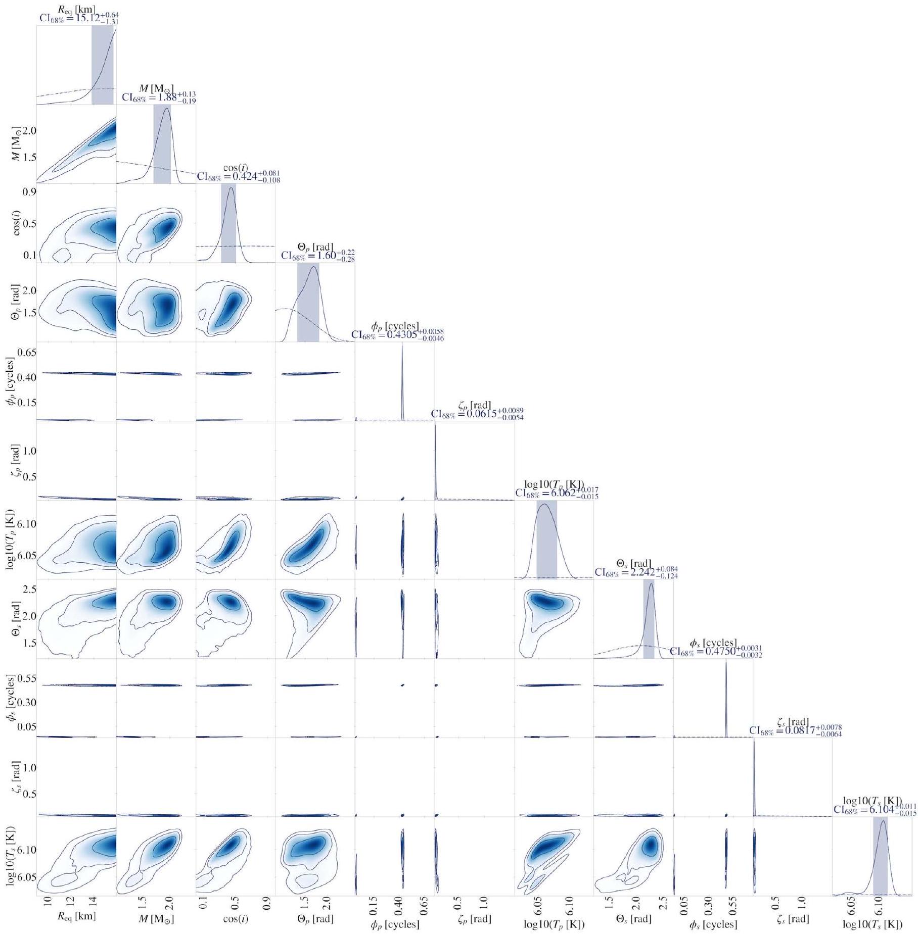
الشكل 6. رسم بياني زوايا بناءً على التحليل المشترك لبيانات NICER وXMM-Newton، الذي تم تنفيذه باستخدام نموذج ST-U. تتضمن هذه الصورة التوزيعات اللاحقة (المعالجة بواسطة GetDist KDEs) للمعلمات التي تصف الكتلة، ونصف القطر، وخصائص النقطة الساخنة المستنتجة لنظام PSR J0030+0451. في التوزيعات اللاحقة 1D المخصصة، نعرض بخطوط متقطعة أولياتنا المقابلة. مجموعة الأشكال الكاملة (8 صور) متاحة، لنماذج، PDT-U لكل من تحليلات NICER فقط (تشغيلات مرجعية مميزة بالخط العريض في الجدول 4) والاستنتاجات المشتركة لمجموعات بيانات NICER وXMM-Newton (إعدادات التحليل المبلغ عنها في الجدول 4، والتي تتوافق مع إدخالات “نعم” في عمود XMM-Newton). توضح الجداول 1 و2 معنى تسميات المعلمات المعتمدة. الهيكل متعدد الأوضاع لللاحق، الموصوف في القسم 4.1.4، مرئي بوضوح هنا. على وجه الخصوص، تُظهر ثنائية الأبعاد في التوزيعات اللاحقة، بما في ذلك نصف القطر، الوضع الرئيسي (التكوين الذي يتوافق مع عينة الاحتمالية القصوى المعروضة في اللوحة (C) من الشكل 3) ووضع ثانوي (التكوين الذي يتوافق مع عينة الاحتمالية القصوى المعروضة في اللوحة (D) من الشكل 3). لمزيد من التفاصيل العامة حول الرسوم البيانية في مجموعة الأشكال هذه، انظر الشكل 1.
(مجموعة الأشكال الكاملة (8 صور) متاحة.)
مقارنة بالتشغيلات بدونالتي حددت كالوضع الرئيسي الوضع الشبيه بـ ST-U)، تولد عدم اليقين المذكور أعلاه، والذي يظهر، على سبيل المثال، عند مقارنة الخطوط الزرقاء مع الخطوط السوداء المتقطعة في الرسم البياني في الزاوية اليمنى من الشكل 7. القطع الطفيف
في قيم الكثافة العالية، بالاقتران مع زيادة عدم اليقين، يؤدي إلى لاحق يتركز عند أنصاف أقطار أكبر (مقارنة بالتشغيلات الأخرى، التي حددت الوضع الشبيه بـ ST-U كالوضع الرئيسي). بشكل عام، التغيير الأكثر بروزًا
الشكل 7. التوزيعات البعدية لـ ST+PST (المُعالجة بواسطة GetDist KDEs) من 14 تجربة، بالنسبة لنصف القطر، والتماسك، والكتلة. يبرز هذا الشكل تأثير اعتماد إعدادات مختلفة لـ MULTINEST. يُظهر الرسم البياني في الجهة اليسرى تأثير اعتماد إعدادات دقة X-PSI المختلفة (منخفضة أو عالية). تمثل المنحنيات الخضراء التوزيعات البعدية المستنتجة من التحليلات التي تعتمد على دقة عالية (HR في الأسطورة)؛ بينما المنحنيات الصفراء مشتقة من إعداد دقة X-PSI المنخفضة (وهو الإعداد الافتراضي لدينا للنماذج الأكثر تعقيدًا من ST-U). هذه الأخيرة لديها إعدادات MULTINEST مختلفة قليلاً، كما هو موضح بالإعدادات بين قوسين، لكنها تُظهر سلوكيات متشابهة جدًا وتم رسمها بشكل فردي في اللوحة اليمنى. تم الحصول على نقطتين شاذتين (واحدة عند HR، خضراء، وواحدة عند LR، صفراء) من خلال تثبيت MULTINEST وبذور عشوائية بايثون على نفس القيم. مع الخطوط المنقطة السوداء، نبلغ أيضًا عن التوزيعات البعدية التي تم الحصول عليها باستخدام SE.على التشغيل؛ الأرقام الموجودة في أعلى التوزيعات الخلفية 1D، بالإضافة إلى المناطق المظللة تشير إلى هذا الاستنتاج. في اللوحة اليمنى، بدلاً من ذلك، نعرض نتائج جديدة لخمس عمليات استدلال ST+PST، بدقة منخفضة X-PSI، مع اعتماد إعدادات MULTINEST الافتراضية لدينا، الاستثناء الوحيد هو العملية الثانية من أعلى القائمة، حيث قمنا بتمكين فصل الأنماط. تم اعتماد إعدادات MULTINEST مشابهة أيضًا في R19 (على الرغم من أنه تم استخدام إعدادات X-PSI أعلى في تلك الحالة). التوزيعات الخلفية ST+PST الموجودة في R19 تظهر هنا باللون البني للمقارنة. هذا الرسم يختبر ما يلي: التباين الناتج عن عشوائية عملية العينة، بالنظر إلى إعدادات التحليل المحددة؛ تأثير تحديث نموذج الأولويات، للسماح للنقطة الساخنة الرئيسية بالتداخل مع الجزء المظلل من الثانوية (CoH، العمليات المميزة في الأسطورة بـ *); وتأثير إدخال الانبعاث من جميع سطح MSP (انظر العملية التي تشملفي الأسطورة). تمثل الخطوط المنقطة السوداء التوزيعات الخلفية التي تم الحصول عليها عند السماح لسطح MSP بالكامل بالإشعاع. تشير المناطق المظللة والأرقام الموجودة أعلى التوزيع الخلفي 1D إلى المناطق والفترات الموثوقة لهذه الاستنتاجات. انظر تعليق الشكل 1 لمزيد من التفاصيل. *: الجولات التي تعتمد على الأولوية المحدثة CoH ST+PST، كما هو موضح في القسم 2.3.4 من V23a.
الذي تم توليده بواسطة درجة الحرارة في مكان آخر هو توسيع التوزيعات الخلفية (بالإضافة إلى مضاعفة الوقت الحاسوبي).
4.2.3. التحليل المشترك لبيانات NICER و XMM-Newton
نقدم توزيعات الكتلة، والكثافة، ونصف القطر اللاحقة التي تم الحصول عليها من خلال اعتماد نموذج ST+PST في تحليل استدلال مشترك باستخدام NICER وXMM-Newton في الرسم البياني في الزاوية اليمنى من الشكل 4. تم الحصول على هذه النتائج بواسطة SE 0.8، ET 0.1، LP.MM إيقاف، LR تشغيل من حيث إعدادات X-PSI.
كما يتضح على الفور، من خلال مقارنة الرسمين الزاويين في الشكل 4، فإن تشغيل استنتاج ST+PST يؤدي إلى توزيعات خلفية للقطر، والضغط، والكتلة مشابهة جدًا لتلك المستمدة من نموذج ST-U. يتم قطع الخلفية الخاصة بالقطر مرة أخرى بالقرب من ذروتها بواسطة قطعنا السابق عند 16 كم. يؤثر هذا على توزيع الكتلة المستنتج، الذي يبدو أنه مدفوع بعد ذلك بالقيود المفروضة على الضغط. لا تقتصر أوجه التشابه على هذه المعلمات؛ في الواقع، فإن الهندسات المستنتجة للنقاط الساخنة متطابقة تقريبًا (كما يمكن رؤيته في الشكل 6)، وبالتالي تشبه التكوين الموضح في اللوحة (C) من الشكل 3. كما هو موضح في اللوحة (C)، فإن كلا النقطتين الساخنتين لهما أحجام صغيرة ودرجات حرارة مشابهة. تؤدي الأحجام الصغيرة إلى (النوع الأول، كما هو موضح في R19) من التداخلات، عندما نفترض هندسات معقدة للنقاط الساخنة (أي عندما يتم وصف النقطة الساخنة بمكونين، كما هو الحال بالنسبة لنقطة PST الساخنة لدينا). في الممارسة العملية، فإن الأحجام الصغيرة المستنتجة للنقاط الساخنة تعني حساسية صغيرة لشكلها. لذلك، فإن هذا يؤدي إلى ضعف القيود على المكون المحذوف، والذي، نظرًا للتشابهات بين النقطتين الساخنتين، يمكن أن يُنسب إلى أي منهما. نظرًا لأننا في هذه الحالة نحدد النقطة الساخنة PST على أنها ثانوية، فإن هذه الغموض يؤدي مرة أخرى إلى وجود ثنائية مرئية في التوزيعات الخلفية للمعلمات التي تصف خصائص النقطتين الساخنتين (انظر مرة أخرى، الشكل 6).
كما هو موضح في القسم 4.1.4، لشرح بيانات NICER المحللة حسب الطور وبيانات XMM-Newton بشكل مشترك، من الضروري زيادة مساهمة PSR J0030+0451 في إجمالي العد. يمكن أن ينتج عن زيادة الانبعاث غير النبضي من MSP قيم كثافة أعلى، كما تم الاستنتاج هنا.
تشير التشابهات في التوزيعات الخلفية للكتلة ونصف القطر، مع تلك التي تم الحصول عليها باستخدام نموذج ST-U، إلى ذيول هذه التوزيعات. وبالتالي، فإنها تلمح إلى وجود وضع ثانٍ، يتميز مرة أخرى بقيم أقل لنصف القطر والكتلة (على التوالي،، و تظهر العينات التي تنتمي إلى هذه الذيول مرة أخرى (انظر اللوحة (D) من الشكل 3، لتمثيل نوعي) ميلًا أعلى، مع زيادة طفيفة في حجم كلا البقعتين الساخنتين وهجرتها نحو خط الاستواء، مقارنة بالنمط الرئيسي. أيضًا في هذه الحالة، نجد تكوينات تتناوب فيها مواقع البقعتين الساخنتين ST و PST. اعتمادًا على حجم المكون المستبعد (الذي ليس محددًا بشكل جيد)، قد يزيد حجم المنطقة المنبعثة التي تم إخفاؤها بواسطته قليلاً، لتعويض
الشكل 8. التوزيعات الخلفية لـ ST+PDT (المُعالجة بواسطة GetDist KDEs) لنصف القطر، والضغط، والكتلة لعمليتي استدلال. نعرض النتائج التي تم الحصول عليها من تحليل بيانات NICER فقط (يسار)، وتلك المستمدة من التحليل المشترك لبيانات NICER وXMM-Newton (يمين). لمزيد من التفاصيل حول الرسم، انظر الشكل 4.
الانبعاثات المنخفضة بشكل عام. يبرز هذا الانتشار على الخصائص المحتملة للمنطقة المستبعدة مرة أخرى حساسيتنا الضعيفة لتفاصيل أشكال النقاط الساخنة.
4.3.
4.3.1. استكشاف النموذج
في الشكل 8، نعرض التوزيعات الخلفية المستنتجة للكتلة، ونصف، والكثافة، معتمدين على نموذج ST+PDT (وهو نموذج أكثر تعقيدًا من نموذج ST+PST المستخدم في النتيجة الرئيسية في R19، الذي لم يتم استكشافه في تلك الورقة). تشير الرسم البياني في الزاوية اليسرى إلى النتائج المستمدة باستخدام SE 0.8، ET 0.1، LP، تشغيل MM، تشغيل LR، تحليل مجموعة بيانات B19v006 NICER فقط. الاستنتاجفترات موثوقة للكتلة ونصف القطر هي و . لذلك، يحدد هذا النموذج قمة ضيقة جدًا في نصف القطر. تشبه تكوين النقاط الساخنة ودرجات الحرارة المرتبطة بها تلك المبلغ عنها في اللوحة (E) من الشكل 3. تصف غالبية التوزيعات المستنتجة أنماط النقاط الساخنة والكتلة ونصف القطر المشابهة لتلك المحددة كالوضع الثانوي في التحليل المشترك لمجموعات بيانات NICER وXMMNewton باستخدام نموذج ST-U.نجد اختلافات كبيرة، ومع ذلك، في درجتي الحرارة المرتبطتين بنقطة الحرارة PDT، مقارنةً بدرجات الحرارة المرتبطة بمناطق الانبعاث ST المستمدة من التحليلات المشتركة لـ NICER و XMM-Newton. انبعاث مشابه لـنقطة ساخنة 6 ST في نموذج ST-U غالبًا ما يتم نمذجتها هنا كنقطة ساخنة PDT، مع وجود مكون واحد أبرد قليلاً.وأكبر وواحد صغير جداً ولكنه حار جداً ). قمة التوزيع الخلفي تحدد المنطقة المتنازلة مع القبة الكروية الساخنة الصغيرة؛ ومع ذلك، هناك بعض الكتلة الخلفية التي تربطها أيضًا بالمكون البارد والأكثر اتساعًا. هذه الثنائية النمطية مرئية أيضًا، في
95% مناطق موثوقة، في التوزيعات الخلفية ثنائية الأبعاد للمعلمات التي تصف خصائص النقطة الساخنة الثانوية (انظر مجموعة الشكل 6). على عكس النتائج المستمدة من نماذج STU و ST+PST في التحليلات المشتركة لـ NICER و XMM-Newton، فإن التوزيعات الخلفية المحددة بواسطة ST+PDT لا تظهر ثنائية الشكل الناتجة عن غموض التسمية. وهذا يعني أن هناك تفضيلًا كبيرًا لموقع النقطة الساخنة PDT؛ أي أن البيانات تمثل بشكل أفضل إذا تم وصف منطقة انبعاث محددة واحدة (الأولى المرئية، في تمثيلنا للبيانات؛ انظر الشكل 9) بواسطة مكونين بدرجات حرارة مختلفة.
مع SE 0.8، ET 0.1، LP، تشغيل MM، تشغيل LR، نجد أيضًا وضعًا ثانويًا. يظهر هذا الوضع احتمالًا أقصى يختلف عن وضع الرئيسي بـالفروق في الأدلة المحلية أكبر قليلاً،في السجل. يحدد الوضع الثانوي التكوينات التي تشبه (مع بعض التباين) الوضع الرئيسي المحدد بنموذج ST-U عند تحليل بيانات NICERonly. في هذه الحالة، قد يكون النقطة الساخنة ذات الدرجة الحرارية المزدوجة مرتبطة بأحد المنطقتين المصدرتين. تظل درجة حرارة المكون المتفوق من النقطة الساخنة PDT من نفس المرتبة كما هو موجود مع نموذج ST-U.وهو مشابه لدرجة الحرارة المرتبطة بنقطة الحرارة ST. المكون المتنازل أبرد بكثير.5.2-5.6. الشبه مع حالة ST-U NICER فقط يشمل أيضًا التوزيعات الخلفية للكتلة ونصف القطر، التي تتجمع حول و ، أقل قليلاً من القيم الخاصة بوضع ST + PDT الرئيسي.
في القسم 5.4، سنوضح كفاية تغطية فضاء معلمات النموذج خلال تحليلات الاستدلال المقدمة في هذا القسم.
4.3.2. التحليل المشترك لبيانات NICER و XMM-Newton
أثر إدخال بيانات XMM-Newton في عملية الاستدلال، عند اعتماد نموذج ST+PDT، هو
الشكل 9. تمثل الألواح الثلاثة من الأعلى إلى الأسفل: عدد البيانات، وعدد التوقعات اللاحقة لنموذج PDT-U، والبقايا كدالة لمرحلة الدورة (على الـ-محور) وقناة أداة NICER (على -المحور). يتم تعريف المتبقيات على أنها الفرق في العد بين البيانات والتوقعات، موزونة بالانحراف المعياري بواسون المقابل (كما هو معبر عنه على المحور اللوني المرتبط):هي بيانات عدّ لـمرحلة الحاويةقناة،أرقام التعداد المتوقعة المقابلة. يتم تقييم التعدادات المتوقعة مع الأخذ في الاعتبار 200 عينة خلفية، تم استنتاجها من خلال تحليل مشترك لبيانات NICER وXMM-Newton. يمكن العثور على مزيد من التفاصيل حول هذه الشكل في تعليق الشكل 13 وفي R19. مجموعة الأشكال الكاملة (8 صور) متاحة، لنماذج ST-U وST+PST وST+PDT وPDT-U لكل من تحليلات NICER فقط (تشغيلات مرجعية مميزة بالخط العريض في الجدول 4) والاستنتاجات المشتركة لبيانات NICER وXMM-Newton (إعدادات التحليل المبلغ عنها في الجدول 4، والتي تتوافق مع إدخالات “نعم” في عمود XMM-Newton). (مجموعة الأشكال الكاملة (8 صور) متاحة.)
الموضح في الزاوية اليمنى من الشكل 8. تم اشتقاق التوزيعات البعدية المبلغ عنها من SE 0.8، ET 0.1، LPMM إيقاف، LR تشغيل. في اللوحة (E) من الشكل 3، نعرض هندسة النقاط الساخنة لعينة الاحتمالية القصوى المحددة.
لأول مرة، فإن إضافة مجموعة بيانات XMM-Newton بشكل متماسك في عملية الاستدلال لا تؤدي إلى حلول تختلف بشكل واضح عن تلك التي تم الحصول عليها من تحليل بيانات NICER فقط. كما هو الحال مع نماذج أخرى، فإن إدخال بيانات XMM-Newton
الشكل 10. التوزيعات الخلفية لـ PDT-U (المُعالجة بواسطة KDEs من GetDist) لنصف القطر، والكثافة، والكتلة لعمليتي استدلال. نعرض النتائج التي تم الحصول عليها من تحليل بيانات NICER فقط (يسار) وتلك المستمدة من التحليل المشترك لبيانات NICER وXMM-Newton (يمين). لمزيد من التفاصيل حول الرسم، انظر الشكل 4.
يقيّد الخلفية إلى قيم أقل قليلاً مما تم استنتاجه في غير ذلك. في هذه الحالة، نرى أيضًا زيادة في الكثافة، على الرغم من أن الفرق أصغر بكثير عند مقارنته بالنماذج الأخرى. ثم يتم استعادة خصائص الانبعاث النبضي من خلال زيادة كل من الكتلة (التيفترة موثوقة الآن ) ونصف القطر (الذيفترة موثوقة الآنفي الواقع، بالنسبة لهذين المعلمين، زادت الكتلة الخلفية عند القيم الأعلى بشكل ملحوظ، بينما انخفض الحجم الخلفي للقيم الأدنى بشكل كبير، مقارنةً بتحليل بيانات NICER فقط.
عند النظر إلى التوزيعات الخلفية لمتغيرات النقاط الساخنة (انظر مجموعة الشكل 6)، تم تحديد فقط التكوين الذي يخصص درجة حرارة عالية جدًا للمكون المتفوق من نقطة الحرارة PDT من خلال هذا التحليل المشترك بين NICER وXMM-Newton (بدلاً من البديل السائد الذي تم العثور عليه باستخدام بيانات NICER فقط، حيث كانت القبة الكروية الساخنة الصغيرة هي المكون المتنازل وبالتالي مخفية جزئيًا بواسطة مكون أكبر وأبرد). هناك أيضًا علاقة عكسية كبيرة بين أحجام النقاط الساخنة (خصوصًا بين ST والمكون المتفوق من نقطة الحرارة PDT) والكتلة ونصف القطر المستنتجين من PSR J0030+0451. من المرجح أن يتم تفسير هذه العلاقة من خلال ضرورة وجود منطقة انبعاث مماثلة، مما يتطلب نصف قطر زاوي أقل للنقطة الساخنة إذا كان MSP له نصف قطر أكبر. ليس من الواضح ما إذا كان هذا نتيجة لإدخال بيانات XMM-Newton، أو إذا كان ناتجًا عن العدد المنخفض من النقاط الحية المعتمدة لاستكشاف مساحة المعلمات الكبيرة ST+PDT. في الواقع، كما تم الإبلاغ عنه أيضًا في الجدول 4، تم إجراء تحليل NICER وXMM-Newton المشترك لـ ST+PDT بعدد أقل بكثير من النقاط الحية.، مقارنةً بالاستنتاج الخاص بـ NICER فقط. وبالمثل للاستنتاج الخاص بـ NICER فقط، فإن عدم اليقين حول الزاوية القطبية لنقطة الحرارة في ST يسمح بتحديد موقعها في نفس نصف الكرة أو في نصف الكرة المعاكس للمراقب. في هذا التحليل المشترك، توجد قمتان متميزتان في التوزيع الخلفي للزاوية القطبية 1D؛ ومع ذلك، يمكن أن يكون هذا مرة أخرى، قد يكون ذلك بسبب العدد المنخفض نسبيًا من النقاط الحية المفعلة لاستكشاف فضاء المعلمات.
4.4.
4.4.1. استكشاف النموذج
نحلل مجموعة بيانات NICER PSR J0030+0451 المعدلة باستخدام SE 0.8 و ET 0.1 و LP، تم تشغيل استدلال LR مع تشغيل MM. في الزاوية اليسرى من الشكل 10، نبلغ عن توزيعات البوستيريور لنصف القطر، والضغط، والكتلة المستمدة من اعتماد نموذج X-PSI PDT-U. نجد توزيعات بوستيريور واسعة نسبيًا وبالتالي كبيرةفترات موثوقة؛ الكتلة المقدرة ونصف القطر هما، على التوالي، و تشبه عدم اليقين والقيم تلك المستنتجة من نموذج ST + PST، عندما لا تتضمن بيانات XMM-نيوتن.
من التوزيعات الخلفية للمعلمات التي تصف هندسة النظام وخصائص النقاط الساخنة (انظر الرسم البياني المقابل في مجموعة الشكل 6)، نلاحظ وجود ثلاثة أنماط متميزة. تم التعرف على هذه الأنماط أيضًا من خلال خيار فصل الأنماط في MULTINEST. يتميز النمط الرئيسي بتكوين نقطة ساخنة مشابه لذلك المبلغ عنه في اللوحة من الشكل 3. الحلول ذات أعلى قيم الاحتمالية من هذه العملية الاستدلالية تنتمي إلى هذا النمط ولها كتلة منخفضة نسبيًا ( ) ونصف قطر مرتفع جداً ( )، مما يملأ معظم الذيل السفلي لتوزيع الكثافة الخلفية الملاحظ في الأبعاد الواحدة. ومع ذلك، فإن هذه الوضعية تمتد أيضًا وتسيطر على أجزاء أخرى من فضاء المعلمات، مما يغطي نطاقًا واسعًا نسبيًا في الكثافة. يشمل هذا الانتشار أشعة أصغر بكثير وكتل أعلى بشكل ملحوظ.
في هذا الوضع، يتميز كلا النقاط الساخنة بمكون بارد وكبير من التنازل ومكون ساخن وصغير من التفوق. النقطة الساخنة الثانوية (كما هو الحال في جميع نماذج X-PSI التي تنتهي بـيشير هذا عادةً إلى النقطة الساخنة ذات العرض الجغرافي الأعلى) التي تتزامن عادةً مع المساحة السطحية توليد أول قمة انبعاث مسجلة في بيانات NICER، وفقًا لتمثيلنا (انظر الشكل 9). يتميز البقعة الساخنة الثانوية بأعلى درجة حرارة (مع المتوسط والانحراف المعياري ضد المكون الأساسي) والمكون المتفوق (مع المتوسط والانحراف المعياري ضد من الأساسي). على عكس ما تم العثور عليه للنماذج التي تم تحليلها في R19، تقع كلا البقعتين الساخنتين عادةً في نصف الكرة الذي يواجه المراقب مباشرةً (كما هو موضح في اللوحة (F) من الشكل 3). ومع ذلك، هناك بعض التباين في موقعهما الدقيق وفي الميل المستنتج (المتوسط والانحراف المعياري لـ ); بشكل خاص، إذا اقترب ميل المراقب مقارنةً بمحور الدوران تميل النقاط الساخنة إلى التحرك نحو خط الاستواء، للحفاظ على الانبعاث النبضي الملحوظ. كما تهيمن التغيرات الطفيفة ضمن هذا النمط الرئيسي أيضًا على الذيلين المرئيين في توزيعات الخلفية ثنائية الأبعاد المبلغ عنها في الرسم البياني في الزاوية اليسرى من الشكل 10.
نظرًا للقيم المتشابهة نسبيًا للعرض الجانبي المستنتج للنقطتين الساخنتين وعدم اليقين المرتبط بهما، من الطبيعي توقع وجود ثنائية النمط بسبب غموض التسميات الأولية والثانوية. توضح التوزيعات اللاحقة للمعلمات التي تصف خصائص النقاط الساخنة هذه الميزة بوضوح. يظهر النمط الثانوي مرة أخرى، لكلا النقطتين الساخنتين، مكونًا باردًا وأكبر من مكون التنازل ومكونًا ساخنًا وصغيرًا جدًا من مكون التفوق. تتشابه نطاقات درجات الحرارة التي تميز مكونات النقاط الساخنة مع النمط الرئيسي، لكن النقطة الساخنة الأكثر دفئًا تُصنف الآن على أنها الأولية. ومع ذلك، فإن النقطة الساخنة الأكثر دفئًا مسؤولة عن ذروة الانبعاث الأولى، نظرًا لتعريف المرحلة صفر في مجموعة البيانات التي نستخدمها. ومع ذلك، يعرض هذا النمط الثانوي، الذي تم التعرف عليه رسميًا أيضًا بفضل خيار فصل الأنماط MULTINEST، ميزات عامة مختلفة قليلاً. تقع كلا النقطتين الساخنتين الآن بشكل أكثر تقليدية في نصف الكرة المعاكس للمراقب، الذي يميل مقارنةً بمحور الدوران الآن بزاويا أعلى قليلاً (مع متوسط وانحراف معياري من ).
المتوسط والانحراف المعياري لعينات الكتلة ونصف القطر المرتبطة بهذا الوضع الثانوي هي و ، وبالتالي تملأ الذروة الرئيسية اللاحقة للكتلة. على الرغم من أن هذه القيم لا تختلف بشكل كبير مقارنة بتلك المستنتجة من الوضع الرئيسي، إلا أنها في هذه الحالة تمثل أيضًا عينات لاحقة بأعلى احتمال.
الاحتمالية القصوى المرتبطة بالعينة التي تنتمي إلى الوضع الثانوي والوضع الرئيسي، على التوالي، تختلف بمقدار 2 فقط بوحدات الاحتمالية اللوغاريتمية، بينما يختلف الدليل المحلي بمقدارالوحدات في السجل. الخلفية المرتبطة بهذين الوضعين الرئيسيين تظهر بعض التباين، لكنها أقل بكثير من تلك المستنتجة لحلول ST-U و ST+PST.
لقد حددت عملية الاستدلال لدينا أيضًا وضعًا ثالثًا، والذي يظهر في بعض التوزيعات الخلفية ثنائية الأبعاد المرتبطة بالمعلمات التي تصف خصائص النقاط الساخنة. ومع ذلك، فإن مساهمته هامشية، كما تؤكد قيم الاحتمالية الأفضل المرتبطة بهذا الوضع. إنها أسوأ بحواليالوحدات في السجل مقارنة بتلك المرتبطة بالنمط الرئيسي (الفرق في الأدلة المحلية حواليوحدات في ). هذا الوضع الثالث هو تمثيل PDT-U للوضع الرئيسي ST-U الذي تم العثور عليه عند تحليل بيانات NICER فقط. وبالمثل، تتجمع العينات المستنتجة حول قيم الكتلة ونصف القطر و ، معبرًا عنها كقيم متوسطة مع الانحراف المعياري عدم اليقين في الانحراف. كما هو متوقع نظرًا لهذا التشابه، فإن الخلفية المرتبطة بالعينات التي تنتمي إلى هذا النمط أعلى بكثير من تلك المستنتجة من النمطين الآخرين.
تظهر التوزيعات الخلفية العامة لهذه الميزة الثالثة أنماط نقاط ساخنة تشبه الحلول الرئيسية لنموذج ST-U وحلها المقابل ضمن فضاء معلمات نموذج ST+PST (في هذا السياق، تصف الوضع الثانوي). كما هو الحال في الحالة الأخيرة، يظهر الوضع الأساسي، والآن أيضًا الثانوي، بعض التباين من حيث العلاقة بين العنصرين، لا سيما في توصيف العنصر البارد المتنازل (المتوسط والانحراف المعياري لـلكلا النقاط الساخنة). بدلاً من ذلك، بالتركيز على حلول الاحتمالية القصوى التي تنتمي إلى هذا النمط، فإن التعقيد الذي تم تقديمه لوصف النقطة الساخنة يؤدي إلى وجود صغير جداً ( ) و حار ( مكون التنازل، الذي تم إخفاؤه تقريبًا بالكامل بواسطة المكون المتفوق.
4.4.2. التحليل المشترك لبيانات NICER و XMM-Newton
في الزاوية اليمنى السفلية من الشكل 10، نعرض التوزيعات البعدية لنصف القطر، والكثافة، والكتلة المستنتجة من التحليل المشترك لمجموعات بيانات NICER وXMM-Newton. تم الحصول على هذه النتائج من خلال SE 0.8، ET 0.1، LP.MM إيقاف، LR تشغيل.
مرة أخرى، يتمثل التأثير الرئيسي لإدخال بيانات XMM-Newton في التحليل في زيادة نسبة الفوتونات المسجلة بواسطة NICER، المخصصة للإشعاع من PSR J0030 +0451. وبالتالي، يتم تقليل العينات اللاحقة المرتبطة بالخلفية العالية بشكل ملحوظ هنا، ويتحول توزيع الكثافة نحو قيم أعلى قليلاً. في هذه الحالة، ومع ذلك، فإن الحلول المحددة التي يمكن أن تعيد إنتاج كلا مجموعتي البيانات متشابهة نوعياً مع تلك التي تم الحصول عليها من تحليل بيانات NICER فقط؛ وبشكل أكثر تحديداً تنتمي إلى الوضعين الرئيسيين والثانويين لتشغيل NICER فقط. تنشأ نفس الوضعين من الهيكل ثنائي الوضعية المرئي بوضوح في بعض التوزيعات اللاحقة التي تصف خصائص البقعتين الساخنتين (انظر مجموعة الشكل 6). من ناحية أخرى، فإن العينات المرتبطة بأقل وضع بارز من استنتاج NICER فقط غير قادرة على تمثيل البيانات بالنظر إلى المعلومات الإضافية المقدمة من XMM-Newton.
في اللوحة (F) من الشكل 3، نعرض، كمثال، تكوين النقاط الساخنة المرتبطة بعينة الاحتمالية القصوى من عملية الاستدلال المشتركة بين NICER وXMM-Newton. الهندسة الخاصة بالنظام تمثل نوعياً الوضع الرئيسي للتوزيع الخلفي، الذي يشبه الوضع الرئيسي المستنتج باستخدام بيانات NICER فقط. تصل عينات الاحتمالية القصوى إلى قيم مرتفعة جداً لنصف القطر، عادةً. ومع ذلك، فإن الكتل المرتبطة الآن أكبر بكثير، وتتركز حولتتحرك الوضعية الثانوية (التي تم وصف خصائصها النوعية في القسم 4.4.1) أيضًا نحو كتل أعلى، بمجرد تضمين بيانات XMM-Newton في التحليل. تظهر عينات الاحتمالية القصوى التي تنتمي إلى هذه الوضعية كتلًا حول; ينتقل نصف القطر المقابل أيضًا نحو قيم أعلى، في نطاق .
نظرًا للقيم العالية نسبيًا لنصف القطر المرتبطة بكلا الوضعين، قررنا فحص الحلول التي تشكل الكتلة الخلفية لنصف القطر الاستوائي.. العينات التي تملأ هذا الجزء من فضاء المعلمات تظهر خصائص تنتمي إلى كلا الوضعين. على الأقل واحدة من النقاط الساخنة
الجدول 6 فترات الثقة بنسبة ثمانية وستين في المئة للكتلة ونصف القطر لتحليلات الاستدلال المختلفة التي تعتمد نماذج ST-U و ST+PST
R19 ST-U
اختبار 1 ST-U
اختبار 2 ST-U
اختبار 3 ST-U
المرجع ST-U
R19 ST+PST
المرجع ST+PST
9.58-11.54
9.94-11.49
9.54-11.56
9.68-11.91
9.64-11.68
11.52-13.85
11.81-14.41
1.02-1.20
1.03-1.17
1.023-1.199
1.03-1.26
1.04-1.25
1.28-1.49
1.2-1.54
ملاحظات. تشير “R19″ إلى النتائج المبلغ عنها في R19، و”المرجع” إلى النتائج المرجعية المقدمة في هذه الورقة، و”اختبار 1-3″ إلى نتائج التحليلات الأولية لمجموعة البيانات الأصلية المستخدمة في R19. تختبر الاختبارات 1-3، بالترتيب: تأثير إطار عمل X-PSI الجديد والافتراضات (للمزيد من التفاصيل، انظر القسم 2.1.3)؛ تأثير إعدادات MULTINEST المختلفة (للمزيد من التفاصيل، انظر القسم 2.1.4)؛ وأخيرًا، تأثير القنوات.يرجى ملاحظة أن كل تغيير يتم تنفيذه بالإضافة إلى التغييرات السابقة. (عادةً ما يكون الأساسي) غالبًا ما يقع في نصف الكرة المواجه للمراقب، والسلوك المرتبط بالنمط الرئيسي. ومع ذلك، فإن ميل المراقب بالنسبة لمحور الدوران كبير جدًا، وهي سمة ترتبط غالبًا بالنمط الثانوي.
الوسيطات وفترات الثقة بنسبة 68% المقدرة للكتلة ونصف القطر وفقًا للتحليل المشترك لمجموعات بيانات NICER وXMM-Newton هي و على التوالي. القيود الناتجة عن بيانات XMM-Newton تحرك قيم الكثافة والكتلة ونصف القطر نحو توزيع أعلى قليلاً.
5. المناقشة
في هذا القسم نناقش ونضع النتائج المقدمة في القسم 4 في سياقها.
5.1. مقارنة مع نتائج R19
النتائج الموضحة في الأقسام 4.1.1 و 4.2.1 تتفق بشكل جيد مع التحليلات المقدمة في R19، عند استخدام نفس نماذج ST-U و ST+PST. تظهر بعض التغييرات الصغيرة بسبب الاختلافات في الإعداد مقارنةً بما تم اعتماده في R19:
استجابة الأداة: في هذه الدراسة، نتبنى أحدث استجابة عامة لأداة NICER (التي تم استخدامها في تحليل PSR J0740+6620 في رايلي وآخرون 2021؛ سالمي وآخرون 2022، 2023);
مجموعات البيانات: كما هو موضح في القسم 3، فإن مجموعة البيانات التي تم تحليلها هنا، B19V006، تم اشتقاقها من نفس قائمة الأحداث المحددة في بودانوف وآخرون (2019a)، ولكن مع الأخذ في الاعتبار استجابة الأداة الجديدة؛
نطاق قناة NICER المستخدم: في هذا العمل [30:300)، في R19 [25:300);
المقدمات على و الزوايا المائلة: هنا متساوية الأبعاد وبالتالي تم أخذ عينات منها من مقدمة موحدة في جيب التمام، في R19 تم أخذ عينات بشكل موحد في الزاوية؛
نموذج مختلف لعدم اليقين في الأدوات: كما هو موضح في القسم 2.1.2، مقارنةً بهذه الدراسة، استخدم R19 معلمين إضافيين لنمذجة عدم اليقين في استجابة الأداة، المتعلقة بمعايرة الكراب (لودلام وآخرون 2018)؛
تحديثات على خط أنابيب X-PSI: في هذا التحليل نستخدم X-PSI v0.7 و v1.0، بينما استخدم R19 v0.1. للحصول على تفاصيل كاملة عن التغييرات، انظر ملف CHANGELOG في مستودع X-PSI على GitHub (انظر الحاشية 12)؛ و
الإعدادات: سواء فيما يتعلق بخط أنابيب X-PSI و MULTINEST (انظر بشكل خاص الاختلافات في النقاط الحية)، كما تم مناقشته في الأقسام 2.1.3 و 2.1.4.
تغيير ذو صلة بشكل خاص، لوحظ في النتائج، يتعلق بتوسيع الفترات الموثوقة المرتبطة ببعض معلمات النموذج، بما في ذلك كتلة MSP ونصف القطر. نرى هذه الزيادة لكل من نماذج ST-U و ST+PST. بالنسبة للنموذج الأقل تكلفة حسابيًا، ST-U، قمنا بالتحقيق بشكل منفصل في تأثيرات العناصر المختلفة المذكورة أعلاه. في الجدول 6، نعرض الفترات الموثوقة بنسبة 68% للكتلة ونصف القطر بدءًا مما تم الإبلاغ عنه في R19 وانتهاءً بنتائجنا المرجعية. في ما بينهما، نعرض نتائج التحليلات الأولية التي تنفذ بالتالي التغييرات التالية، بدءًا من تحليل مجموعة بيانات B19 القديمة ومصفوفة الاستجابة الأصلية، كما تم استخدامها في R19، وانتهاءً بالاستنتاج المقدم في العمل لحالات ST-U المرجعية فقط من NICER.
اختبار 1: نسخة جديدة من X-PSI، نمذجة جديدة لعدم اليقين في استجابة الأداة، مقدمات جديدة؛
اختبار 2: تأثير إعدادات MULTINEST المختلفة وخاصة زيادة عدد النقاط الحية؛ و
اختبار 3: تأثير تغيير القناة الأدنى المدروسة من 25-30. فقط الأعمدة المميزة بـ “مرجع” تظهر نتائج لمجموعات البيانات الجديدة، التي تم تحليلها باستخدام مصفوفة استجابة NICER المحدثة المقابلة.
اعتماد إطار عمل X-PSI الجديد، بما في ذلك نمذجة عدم اليقين في الأدوات والمقدمات المحدثة، له تأثير تقليص الفترات الموثوقة عند استخدام نفس إعدادات MULTINEST. يمكن تفسير ذلك بحقيقة أن هناك عددًا أقل من المعلمات المرتبطة بالنموذج. هذا يقلل من مساحة الحلول الممكنة وبالتالي نطاق الأنصاف المرتبطة بها.
زيادة النقاط الحية لها تأثير زيادة (بشكل غير متساوٍ) الفترات الموثوقة. على الرغم من أنه تم الإشارة إلى ذلك بالفعل بالنسبة لـ PSR J0740+6620 في رايلي وآخرون (2021) وسالمي وآخرون (2022، 2023)، بالنسبة لـ PSR J0030+0451 يبدو أن هذا السلوك يتعارض مع نتائج R19. هناك، قام المؤلفون بإجراء ثلاث جولات استنتاجية مع 1000 نقطة حية. جميعها أنتجت خطوطًا متداخلة بشكل جيد، مما أدى إلى الاستنتاج بأن عددًا أكبر من النقاط الحية لن يؤثر على النتائج (ما لم تكن أوضاع أخرى، بعرض أصغر بكثير ولكن احتمالية أعلى بكثير موجودة أيضًا). يبدو أن هذا ليس هو الحال في الإطار الجديد لنموذج ST-U. بالمثل، اختبر أفلي وآخرون (2023) اعتماد نموذج ST+PST على عدد النقاط الحية. عندما زادوا عدد النقاط الحية من 1000 إلى 4000، وجدوا زيادة صغيرة جدًا في حجم المناطق الموثوقة (على سبيل المثال، زاد نطاق نصف القطر بمقدار 0.1 كم).
تقليل نطاق القنوات عند الطاقات الاسمية المنخفضة يوسع أيضًا الفترات الموثوقة قليلاً. هذا يبرز
الدور المهم الذي تلعبه الأحداث في ذيل الطاقة المنخفضة من نطاق حساسية NICER، حيث من المتوقع أن تصل الانبعاثات الحرارية من النقاط الساخنة إلى ذروتها. نظرًا لأننا في الاختبار 3، نفقد جزءًا من المعلومات المستخدمة سابقًا، فإن التوسيع ليس مفاجئًا.
الانتقال من مجموعة بيانات B19 إلى مجموعة بيانات B19v006 المحدثة واستجابة الأداة الجديدة يقلل قليلاً من الفترات الموثوقة بمجرد دمج جميع التغييرات المذكورة أعلاه في إطار التحليل. ومع ذلك، فهي لا تزال عمومًا أوسع قليلاً من القيم الأصلية المنشورة في R19.
مقارنة نتائج R19 لنموذج ST+PST والفترات الموثوقة لتحليل الاستنتاج المرجعي الجديد لدينا، نجد نتائج مشابهة، لأسباب محتملة مشابهة (انظر أيضًا أفلي وآخرون 2023).
بشكل عام، للحصول على نتائج قوية في إطار التحليل الجديد ومع مجموعة بيانات B19v006 المحدثة، نحتاج إلى إعدادات MULTINEST أكثر تكلفة حسابيًا (لم يتم اختبار جميع التركيبات، ولكن، على سبيل المثال، يبدو أن اعتماد عدد أكبر من النقاط الحية ضروري للحصول على نتائج مستقرة). بشكل خاص، تظهر تحليلاتنا المختلفة لـ ST-U و ST+PST (بما في ذلك تلك المقدمة في الأقسام 4.1.2 و 4.2.1) أن، في وجود هيكل متعدد الأوضاع في الخلفية، فإن اعتماد عدد غير كافٍ من النقاط الحية لا يؤثر فقط على تقدير عرض الخلفية، ولكنه يمكن أن يؤدي أيضًا إلى انحيازات كبيرة.
5.2. مقارنة مع النتائج من المحاكاة
اختبارات المحاكاة التي أجريت في V23a سلطت الضوء على الاعتماديات والسلوكيات المتوقعة وغير المتوقعة لنتائج تحليلاتنا. في هذا القسم نعلق على الأكثر صلة، ربطها بنتائجنا بناءً على تحليل مجموعة بيانات NICER المحدثة B19v006 لـ PSR J0030+0451.
5.2.1. الهيكل متعدد الأوضاع في خلفياتنا
في V23a، كشف المؤلفون عن وجود هياكل متعددة الأوضاع في سطح الخلفية؛ هذا شائع لكل من البيانات الحقيقية والمحاكاة. وجود مثل هذا الهيكل غالبًا ما يكون واضحًا فقط عندما يتم تفعيل إعداد الفصل بين الأوضاع/الأوضاع المتعددة في MULTINEST أو بعد فحص ذيول توزيعات الخلفية. بسبب الاختلافات في كتلة الخلفية بين الأوضاع المختلفة، فقط في بعض الحالات يكون الهيكل متعدد الأوضاع بارزًا بما يكفي ليكون مرئيًا بالعين في توزيعات الخلفية الموزعة. في كل من البيانات والمحاكاة، نرى بوضوح نبضات وخلفية متشابهة جدًا تم إنشاؤها بواسطة تكوينات نقاط ساخنة مختلفة تمامًا، MSP، وخصائص بين النجوم. يمكن لنماذج متعددة ومتجهات المعلمات المقابلة أن تعيد إنتاج بيانات NICER دون التأثير المرئي على جودة المتبقيات. يبدو أن هذا يختلف عن حالة PSR J0740+6620، حيث، مع المقدمات الضيقة للكتلة، المسافة، والانحدار، تم تحديد وضع واحد ومستقر، لكل من نموذج ST-U ونموذج ST+PST، كان مقيدًا جيدًا في كل من نصف قطر MSP وفي هندسة النقاط الساخنة.
يمكن أن تساعد المزيد من البيانات عالية الجودة، بالإضافة إلى القيود الخارجية، في التخفيف من التحديات في تحليل مجموعة بيانات NICER لـ PSR J0030+0451 التي تطرحها هذه الهيكلية متعددة الأوضاع في سطح الخلفية. على سبيل المثال، كما نرى عندما
نقدم بيانات XMM-Newton، إذا كان لدينا تقدير صارم وموثوق للخلفية لـ NICER، فقد يؤدي ذلك إلى حلول في جزء مختلف من مساحة المعلمات ويكون أقل عرضة للتعددية.
تظهر الأوضاع المختلفة التي تميز أسطح الخلفية غالبًا عرضًا مختلفًا للفترات الموثوقة. علاوة على ذلك، كما هو موضح في V23a، فإن عرض الخلفية حساس جدًا لتحقيق الضوضاء المحدد. لذلك، من المعقد التنبؤ مسبقًا بتطور الفترات الموثوقة بمجرد تضمين بيانات وقيود إضافية في التحليل. إذا كان الوضع الرئيسي المحدد غير متغير، نتوقع، مع بعض التشتت، أن عدم اليقين في توزيع الخلفية ثنائي الأبعاد للكتلة ونصف القطر سينخفض مع وقت التعرض أو الجذر التربيعي له، اعتمادًا على مدى قوة الارتباط بين الاثنين في ذلك التحليل المحدد (انظر لو وآخرون 2013؛ بسالتيس وآخرون 2014؛ ميلر ولامب 2015).
5.2.2. البيانات مقابل المحاكاة
بالإضافة إلى الهيكل متعدد الأوضاع، ومثلما هو الحال في بعض التحليلات المستندة إلى البيانات الاصطناعية والمبلغ عنها في V23a، يظهر تحليل بيانات NICER الفعلية أيضًا بعض التباين في النتائج اعتمادًا على إعدادات التحليل. ومع ذلك، عند مقارنة النتائج الموضحة في هذه الورقة مع النتائج من محاكاة V23a، نلاحظ أيضًا بعض الاختلافات.
هنا، كما في R19، تتغير الكتلة ونصف القطر المستنتجين اعتمادًا على نموذج النقطة الساخنة المعتمد، بينما بالنسبة للمحاكاة المقدمة في V23a، لم يكن مهمًا ما إذا تم استخدام نموذج ST-U أو ST+PST: كانت التوزيعات اللاحقة الناتجة عن هذين النموذجين للكتلة ونصف القطر والكثافة متشابهة جدًا في كل الأحوال.
اعتماد إعدادات HR أو LR X-PSI له تأثير مرئي، على الرغم من أنه ليس كبيرًا، على التوزيعات الخلفية للكتلة ونصف القطر (كما يتضح من مقارنة الخطوط الخضراء، HR، والصفراء، LR، في اللوحة اليسرى من الشكل 7)، وهو اختلاف لم يُلاحظ في تحليلات البيانات الاصطناعية المقدمة في V23a.
عند مقارنة الأدلة التي تم الحصول عليها من تحليلات NICER-only عند اعتماد نماذج مختلفة، نرى تفضيلاً كبيراً لأشكال النقاط الساخنة الأكثر تعقيداً. بالنسبة للحالتين اللتين تم اختباره في V23a، بدلاً من ذلك، انخفضت هذه الفجوة في الأدلة إلى عامل من عدة عوامل في اللوغاريتم، وهو ما لا يكفي للتوصل إلى استنتاج حاسم.
يمكن أن يكون أصل هذا السلوك المختلف للبيانات الحقيقية مقابل المحاكاة ناتجًا عن مجموعة من العوامل. قد لا تغطي البيانات الاصطناعية التي تم تحليلها جزءًا تمثيليًا من فضاء المعلمات؛ في الواقع، في V23a، تم اعتبار متجه معلمة واحد فقط لكل نموذج. إذا كانت هناك موارد حسابية أكبر بكثير متاحة، فسيكون من الممكن إنتاج وتحليل مجموعات بيانات اصطناعية متعددة، مما سيوفر عينة أفضل من التوزيع الخلفي المستنتج من البيانات الحقيقية (بدلاً من تقييد المعلمات المدخلة إلى عينات الاحتمالية القصوى). قد تؤدي الطبيعة المختلفة للبيانات المدروسة أيضًا إلى بعض التباينات في نتائجنا. تعتمد المحاكاة على بيانات اصطناعية تم إنشاؤها بافتراض نفس العمليات الفيزيائية والتبسيطات التي تم اعتمادها لاحقًا في تحليلات الاستدلال. ومع ذلك، قد تحتوي البيانات الحقيقية على فيزياء غير محسوبة في نماذجنا: على سبيل المثال، من غير المحتمل أن تكون النقاط الساخنة ذات أشكال بسيطة كهذه ومن المحتمل جدًا أن تظهر بعض تدرجات الحرارة. عادةً ما نفترض أن جودة بياناتنا غير كافية لهذه الأجزاء المفقودة.
الجدول 7 ملخص النتائج لاستنتاجات NICER فقط المرجعية وتشغيلات NICER وXMM-Newton المشتركة
فقط NICER
نموذج
الكتلة ]
نصف القطر (كم)
ساعات العمل الأساسية
ST-U
-35788
-35735
-42950
11462
ST+PST
-٣٥٧٧٨
-35722
-42942
١٣٣٩٧٠
ST+PDT
-35779
-35729
-42705
٣٣٠٦٩
PDT-U
-35777
-35721
-42659
74333
نيزر وإكس إم إم-نيوتن
نموذج
الكتلة ]
نصف القطر (كم)
ساعات العمل الأساسية
ST-U
-42714
-42661
-35760
41219
-42718
-42666
-35769
ST+PST
-42711
-42662
-٣٥٧٦١
84620
ST+PDT
-42684
-42625
-35730
٣٢٦١
PDT-U
-42677
-42617
-35723
12421
ملاحظات. تمثل الشكوك فترات موثوقة تبدأ من الوسيط للتوزيع البعدي الهامشي 1D. بالنسبة لتحليلات NICER فقط، نبلغ عن الوسائط، الفترات الموثوقة، والأدلة.قيم الاحتمالية القصوى (في إطار مشترك بين NICER و XMM-Newton )، وساعات العمل الأساسية المرتبطة بالتشغيل مع إعدادات MULTINEST: SE 0.3، ET 0.1، LP ، MM قيد التشغيل. الـتشير إلى قيم الاحتمالية القصوى للجولة المحددة بواسطة الخط. يتم تنفيذ جولات الاستدلال المشتركة بين NICER وXMM-Newton باستخدام إعدادات MULTINEST: SE 0.8، ET 0.1، LPMM مغلق، باستثناء حالة ST-U، النموذج الوحيد الذي يمكننا فيه تنفيذ SE 0.3، ET 0.1، LP، MM في التشغيل. جميع تحليلات الاستدلال، باستثناء تلك التي تستخدم نموذج ST-U، تفترض دقة منخفضة من حيث إعدادات X-PSI (انظر القسم 2.3.1 من V23a). بالنسبة لنماذج ST-U و ST+PST، أفاد R19، على التوالي، بكتلة و ونصف قطرونصف القطر لـ. الوضع الثانوي لجهاز NICER وXMM-Newton يعمل مع SE 0.3، ET 0.1، LPMM في (في هذه الحالة المحددة، لوصف الكتلة ونصف القطر الخلفي، نستخدم المتوسطات والانحرافات المعيارية، ونبلغ عن قيمة الدليل المحلي، كما تم حسابه بواسطة MULTINEST). فيزياء تؤثر على نتيجة التحليل؛ لكن هذا شيء يجب اختباره بمزيد من التفصيل.
5.3. مقارنة النماذج وتأثير تضمين القيود من XMM-Newton
نقدم النتائج الرئيسية لكل نموذج تم النظر فيه في هذه الدراسة في الجدول 7. تشير الصفوف الأربعة الأولى من الجدول إلى استنتاجات مرجعية تعتمد فقط على NICER (تم تمييز إعدادات الجولات المرجعية بالخط العريض في الجدول 3)؛ بينما تظهر الصفوف الخمسة الأخيرة النتائج لتحليلات مشتركة بين NICER وXMM-Newton (انظر الإعدادات المحددة في الجدول 4، للمدخلات التي تتضمن بيانات XMM-Newton). من اليسار إلى اليمين، نقدم في كل عمود ما يلي: (i) النموذج المعتمد،فترة موثوقة لـ (ii) الكتلة و (iii) نصف القطر، (iv) اللوغاريتم الطبيعي للأدلة، (v) اللوغاريتم الطبيعي لأقصى احتمال، (vi) فقط لتحليلات NICER و XMM-Newton المشتركة – اللوغاريتم الطبيعي لأقصى احتمال ضمن إطار NICER فقط، (vii) فقط لاستنتاجات NICER فقط – اللوغاريتم الطبيعي لأقصى احتمال ضمن إطار NICER و XMM-Newton المشترك (بافتراضمعتحديد المسافة)، و(viii) الساعات الأساسية اللازمة لحساب التشغيل. تشير الصف الثاني في كتلة NICER وXMM-Newton المشتركة إلى الثانويةالوضع، الذي تم تحديده في تشغيل استنتاج ST-U، والذي تلخص نتائجه الرئيسية في الصف الذي يعلوه مباشرة. هذا الوضع مثير للاهتمام بشكل خاص حيث تم العثور على تكوين مشابه أيضًا عند اعتماد نموذج ST+PDT، وهو يشبه النتائج الرئيسية لـ PSR J0740+6620. في هذه الحالة فقط، في العمود الرابع، نبلغ عن الأدلة المحلية؛ بالنسبة لجميع الصفوف الأخرى، نشير إلى الأدلة العالمية.
نبرز آثار نتائجنا، الملخصة في الجدول 7، في الفقرات الفرعية التالية.
5.3.1. تحليلات خاصة بـ NICER فقط
تلخص الصفوف الأربعة الأولى من الجدول 7 نتائج عمليات الاستدلال الخاصة بـ NICER فقط. كما هو الحال في R19، فإن الأدلة بوضوح لا تفضل نموذج ST-U، لكنها لا تظهر تفضيلًا واضحًا لأي من النماذج الأكثر تعقيدًا. ومع ذلك، بينما كانت إعدادات التحليل لجميع عمليات NICER-only التي تظهر نتائجها في الجدول هي نفسها، فإن هذا لا يعني بالضرورة نفس الدقة في تقييم الأدلة، حيث إن أبعاد فضاء المعلمات تزداد مع تعقيد النموذج. وبالتالي، سيكون من المثالي التحقق بشكل أكثر تفصيلًا من مدى استكشاف كل نموذج لفضاء المعلمات لتأكيد نتائجنا. لاحظ، على سبيل المثال، أن قيمة الاحتمالية القصوى التي تم العثور عليها لنموذج ST+PST أعلى من تلك التي تم تحديدها في مرجعنا.تشغيل الاستدلال. نظرًا لأن نموذج ST+PST محصور تقريبًا في النموذج الأكثر تعقيدًا ST+PDT، فإن هذا يعني على الأرجح أن تشغيلنا المرجعي ST+PDT لم يستكشف مساحة المعلمات بشكل كاف.هذا له تداعيات على الأدلة المقدرة، التي من المحتمل أن تكون قيمتها مقدرة بأقل من قيمتها الحقيقية.
حصريًا من حيث الكتلة ونماذج نصف القطر، توجد فئتان رئيسيتان من الحلول: و ; أو و يبدو أن الأول أكثر عدم تماثل وأضيق قليلاً من الثاني (مع الأخذ في الاعتبار نفس الإعدادات المعتمدة، والتي، مع ذلك، لا تضمن مرة أخرى نفس جودة الخلفية المكشوفة).
النماذج الجديدة ST+PDT و PDT-U، التي لم يتم دراستها في R19، تظهر كتلة خلفية كبيرة للتكوينات التي تحتوي على نقطة ساخنة واحدة على الأقل في نفس نصف الكرة الأرضية كالمراقب. لم يتم العثور على هذه التكوينات الهندسية في R19.
5.3.2. التحليلات المشتركة لـ NICER و XMM-Newton
نركز الآن على المدخلات في الجدول 7 التي تتعلق بالتحليلات المشتركة بين NICER و XMM-Newton.
الأدلة. على عكس التحليلات التي تعتمد فقط على NICER، تشير الأدلة في الاستنتاجات المشتركة إلى تفضيل كبير لنموذج PDT-U. يتم رفض كل من نماذج ST-U و ST+PST بشدة، مع قيم أدلة مشابهة تختلف عن الأفضل بعوامل من بوحدات اللوغ. الفرق بين PDT-U و ST+PDT أقل حدة (حوالي فيوحدات)، لكنها لا تزال حاسمة. إذا افترضنا أن تضمين بيانات XMM-Newton يقدم قيودًا غير متحيزة، فإن التحول الكبير في الحلول المدفوعة ببيانات XMM-Newton الإضافية، مقارنةً بتلك المبلغ عنها في R19، يظهر أن نتائج PSR J0030 +0451 من NICER تحتاج إلى تفسير دقيق. وهذا يعني أنه بالنسبة لهذا المصدر، الذي تتميز بياناته بوضوح بهيكل متعدد الأنماط بارز، يمكن أن تؤدي قيود إضافية مرة أخرى إلى تعديل النتائج التي توصلنا إليها بشكل كبير.
الأشعة المستنتجة بـ و النماذج. بالنسبة للتحليلات المشتركة بين NICER وXMM-Newton، فإن الحلول الرئيسية الجديدة المحددة باستخدام نماذج ST-U وST+PST متشابهة جدًا مع بعضها البعض، من حيث الكتلة ونصف القطر وكذلك في تكوينات النقاط الساخنة. بعض أوجه التشابه، خاصة من حيث الكتلة ونصف القطر، قد تكون ناتجة عن ميل تقديرات نصف القطر للوصول إلى الحد الأعلى من التقديرات السابقة وبالتالي تقييد الكتلة من خلال الاستنتاجات حول الكثافة. كما نبرز أن مثل هذه القيم العالية لنصف القطر يصعب التوفيق بينها وبين القيود التي تفرضها ملاحظات أخرى، مثل القابلية للتشوه المداري المستنتجة من الموجات الجاذبية (انظر، على سبيل المثال، أبوت وآخرون 2018، 2019) ومن تحليل بيانات PSR J0740+6620 من NICER (وXMM-Newton) (ميلر وآخرون 2021؛ رايلي وآخرون 2021؛ سالمي وآخرون 2022).
تعقيد النقاط الساخنة. إن تقديم عنصر التمويه الذي يميز نموذج ST+PST عن النموذج الأبسط ST-U لا يحسن قدرتنا على تمثيل بيانات NICER وXMM-Newton. عند النظر إلى توزيعات المعلمات الهندسية المقابلة (انظر مجموعة الشكل 6)، هناك تداخل واضح بسبب الحجم الصغير لكلا النقاط الساخنة (تداخل من النوع الأول، كما هو موصوف في R19). هذا يولد غموضًا في ارتباط تسميات ST وPST بالنقاط الساخنة (أي، يمكن في المبدأ تمثيل أي نقطة ساخنة مع أو بدون عنصر الإغفال). من ناحية أخرى، عندما نقدم عنصرًا مشعًا عبر نموذج ST+PDT، فإن ارتباطه بالنقطة الساخنة، التي نراها أولاً في البيانات، مفضل بشدة، وتتحسن الأدلة المرتبطة وقيم الاحتمالية القصوى بشكل كبير. تقديم
المكون الثاني المنبعث أيضًا للنقاط الساخنة الأخرى، كما هو موجود في نموذج PDT-U، يحسن جودة نتائجنا بشكل أكبر.
تشابهات في ذيول التوزيعات الخلفية. تكشف الفحوصات الإضافية للتوزيعات الخلفية المستمدة من نموذج ST+PST أن التكوينات التي تملأ الذيل عند نصف قطر منخفض من المحتمل أن تشكل وضعًا ثانويًا، كما كان الحال في تحليل ST-U المشترك بين NICER وXMM-Newton. تعرض هذه الأوضاع الثانوية هندسات مشابهة (حيث يتم رؤيتها تقريبًا من خط الاستواء ومع نقاط ساخنة شبه مضادة)، وأحجام، وأشعة مشابهة للوضع الرئيسي ST+PDT. كما سنناقش بمزيد من التفصيل في القسم 5.3.5، فإن هذا التكوين يثير اهتمامًا خاصًا لأنه قد يفسر بشكل أفضل انبعاث أشعة غاما المرتبط بـ PSR J0030+0451؛ علاوة على ذلك، سيكون مشابهًا للهندسة الموجودة لـ PSR J0740+6620 (التي قد نتوقعها إذا كان المجال المغناطيسي الأساسي وتاريخه متشابهين).
5.3.3. الانتقال من تحليلات NICER فقط إلى تحليلات مشتركة بين NICER و XMM-Newton
في هذا القسم، نعرض بإيجاز التأثيرات الرئيسية التي نلاحظها في نتائجنا، حيث ننتقل من تحليل بيانات NICER فقط إلى النظر بشكل مشترك في مجموعتي بيانات NICER وXMM-Newton. ومع ذلك، نذكر القارئ أنه، كما تم مناقشته بشكل أكثر تفصيلاً في القسم 5.4، تم إجراء استنتاجات بيانات NICER فقط باستخدام إعدادات MULTINEST أفضل (وأكثر تكلفة من الناحية الحاسوبية) مقارنةً بالتحليلات المشتركة للأجهزة (حيث كانت التحليلات المشتركة تتطلب عمومًا عددًا أكبر من ساعات المعالجة، بالنظر إلى نفس الإعدادات، للوصول إلى شرط الإنهاء المحدد بواسطة تحمل الأدلة).
نبدأ بالإشارة إلى أن الاختلافات المحتملة في النتائج كانت متوقعة بالفعل في R19 (انظر المناقشة في القسم 4.1.2 من تلك الورقة). إن إدخال بيانات XMM-Newton له تأثير عام يتمثل في تقليل الخلفية المستنتجة، مما يؤدي إلى قيم أكبر من الكثافة (اتباع نفس المنطق المقدم في رايلي وآخرون 2021؛ سالمي وآخرون 2022). هذا صحيح بشكل عام لجميع النماذج، التي، على الرغم من اختلاف الطرق، تصل دائمًا إلى كثافة أعلى من خلال تحريك التوزيعات الخلفية لكل من الكتل والأشعة نحو قيم أعلى. ومع ذلك، فإن النتائج التي تم الحصول عليها من خلال اعتماد نماذج ST-U و ST+PST هي الأكثر تأثرًا بالتغيير. في الواقع، تحدد تحليلات ST-U و ST+PST الخاصة بـ NICERonly، كأوضاع رئيسية، حلولًا مدعومة فقط بمستويات خلفية أعلى، مقارنة بالدعم الخلفي الأوسع لـ و الأوضاع الرئيسية.
بالنسبة لنماذج ST+PDT و PDT-U، فإن إدخال بيانات XMMNewton في التحليلات له تأثير في تقليل الدعم الخلفي للوضعيات الرئيسية المحددة من خلال استنتاجات NICER فقط، مع الحفاظ عليها كأكثر التكوينات احتمالاً (التي تتميز الآن بوجود تباينات أضيق قليلاً، عند النظر، على سبيل المثال، إلى نصف القطر والكتلة، نتيجة للدعم الخلفي المقيد لنفس الوضعية).
بدلاً من ذلك، الحلول التي تم العثور عليها معوتم التقليل من أهمية ST+PST في الاستنتاجات التي تعتمد فقط على NICER بسبب القيود التي تفرضها بيانات XMM-Newton، والتي يمكن الآن تمثيلها بشكل أفضل مع بيانات NICER من خلال وضع مختلف تمامًا. كما ذُكر في القسم 5.3.2،
الشكل 11. مثال يوضح كيف تمثل حل أقصى احتمال (MaxL، في الأسطورة) الخاص بنا باستخدام PDT-U، الذي تم الحصول عليه في التحليل المشترك بين NICER وXMM-Newton، بيانات PSR J0030+0451 من XMM-Newton وبيانات الخلفية (BKG)، لMOS1 (اللوحة اليسرى) وMOS2 (اللوحة اليمنى). يظهر الرسم كميات مشابهة للشكل 5، ولكن لمجموعات بيانات XMM-Newton MOS1 وMOS2 الكلية والخلفية. الخط المنقط المتقطع (باللون الأرجواني، لMOS1 والأزرق الفاتح، لMOS2) يظهر بيانات الخلفية المستخدمة في تحليلنا؛ الخلفية المستنتجة مرسومة بخط صلب (باللون الأرجواني لMOS1 والأزرق الداكن لMOS2). نظرًا لقيمتها المنخفضة، فإن الشكوك (الموضحة بمناطق مظللة، باللون الأرجواني لMOS1 والأزرق الداكن لMOS2) تكاد تكون غير ملحوظة. الخط المنقط الأكثر تشتتًا يظهر البيانات الكلية على المصدر، لMOS1 على اليسار وMOS2 على اليمين؛ الخط الصلب (باللون الأرجواني لMOS1 والأزرق لMOS2) هو الإشارة المتوقعة المستنتجة. نعرض مساهمة الأولية والثانوية والخلفية المرتبطة بعينة أقصى احتمال، مضيفين إياها (بهذا الترتيب) فوق بعضها البعض بمناطق ذات كثافات مختلفة من اللون الأزرق، لMOS1، والأخضر لMOS2.
كلا نموذجَي ST-U و ST+PST يفضلان الحلول ذات قيم نصف القطر العالية )، وتكوينات النقاط الساخنة التي تشبه اللوحة (C) من الشكل 3، للجزء الرئيسي من التوزيعات الخلفية.
تقديم بيانات XMM-Newton والقيود لا يؤثر بشكل كبير على النسبة بينومربع المسافة، أو الـمعامل في تحليلات NICER فقط (يمثل المسافة الوحيدة وتركيبة تكون التحليل حساسًا لها)، والتي تبقى بين و 8.9.
الانتقال إلى التحليلات المشتركة له تأثيرات مختلفة على الكثافة العمودية المستنتجة، اعتمادًا على النموذج المفترض. من المرجح أن يكون هذا نتيجة غير مباشرة للتغيرات (بالنسبة لـ و )، أو غياب التغييرات (لـ و PDT-U)، في الوضع الرئيسي المحدد. بالنسبة لكل من ST-U و ST+PST، فإن الاستنتاج التحولات الخلفية من الوصول إلى ذروتها عند قيم محددة ( و لتكون متسقة تمامًا مع الصفر (أي، محدودة بوضوح عندبحدودنا الدنيا السابقة). بالنسبة لتحليلات ST+PDT، فإن إدخال بيانات XMM-Newton لا يؤثر بشكل كبير علىالخلفي، الذي يتجمع حول. وبالمثل بالنسبة لـ PDT-U، تشير التحليلات المشتركة إلى استنتاج النتائج الخلفية تختلف فقط بشكل طفيف عما تم العثور عليه في استنتاجات NICER فقط، مع تغير القيم الوسيطة منإلى. بالنظر إلى التقديرات المختلفة لـأن النماذج المختلفة توفر، من الواضح أن القيود القوية ستساعد بشكل كبير في تحليلاتنا وتحسن تفسيرنا لنتائجها. في التحليلات المستقبلية، نخطط لتضمين فرضية أكثر واقعية علىاستنادًا إلى الأدبيات. نأمل أن نجد تقديرات محدثة، خاصة للحد الأدنى، حيث سيفيد ذلك تحليلاتنا بشكل كبير.
أخيرًا، يبدو أن تقديم XMM-Newton لا يؤثر بشكل كبير على جودة بقايا NICER (التي لا تزال جيدة؛ انظر مجموعة الشكل 9)، بينما يتم تمثيل بيانات XMM-Newton أيضًا بشكل جيد (للحصول على مثال، انظر الألواح في الشكل 11). من الجدول 7، يمكننا أن نرى أن الاحتمالية القصوى لنموذج NICER فقط تنخفض بشكل كبير إذا استخدمنا الحل الذي تم تحديده في التحليل المشترك لنماذج ST-U و ST+PST (مع انخفاض بحوالي 30 في لوغاريتم الاحتمالية).
ومع ذلك، فإن هذا ليس هو الحال بالنسبة لـ ST+PDT و PDT-U. الأول يظهر قيمة احتمال قصوى مشابهة لتلك التي تم العثور عليها. في تحليل NICER-only المقابل لـ ST+PDT؛ بينما بالنسبة للأخير، فإن أفضل حل يتناسب لديه احتمال NICER قابل للمقارنة مع أفضل حل عام من استنتاجات NICER-only (وبالتالي قريب جدًا من الحل الذي تم تحديده مع تحليل ST+PDT NICER-only).
5.3.4. التكوينات المفضلة الجديدة مقابل القديمة
كما ذُكر في القسم 5.3.2، نجد بشكل عام أن مجموعات بيانات NICER و XMM-Newton يمكن وصفها بشكل جيد معًا من خلال الحلول المحددة مع كلاهماونماذج PDT-U. من المثير للاهتمام، مقارنة بما تم العثور عليه للنماذج والبيانات التي تم تحليلها في R19، أنه في كلتا الحالتين لا توجد حاجة لنقاط ساخنة مطولة أو لوجود كلا النقاط الساخنة في نفس نصف الكرة (انظر الألواح (E) و(F) من الشكل 3). بالنسبة لكلا النموذجين، يتميز نقطة الحرارة PDT، أي تلك الموصوفة بعنصرين منبعثين، بمكون أكبر وأبرد ومكون أصغر وأكثر سخونة. وهذا يشير إلى وجود تدرجات في درجة الحرارة، والتي يبدو أن تحليلنا حساس لها. نعتقد أن هذا يجب أن يحفز التحقيقات التي تهدف إلى تحديد حساسية وموثوقية نتائجنا بالنسبة للخصائص الفيزيائية الأكثر واقعية لنقاط الحرارة على سطح MSP. كما نلاحظ أنه بالنسبة لكلا النموذجين، فإن الأبعاد العامة للنقطتين الساخنتين متقاربة وأنهما تقريبًا متضادتان (على الأقل في الطور). تشبه هذه الخصائص التكوين الذي تم العثور عليه من خلال تحليل ملاحظات NICER فقط ومشتركًا مع بيانات NICER وXMM-Newton لـ PSR J0740+6620. على وجه الخصوص، تظهر الحلول المحددة مع ST+PDT المزيد من التشابه مع النتائج لـ PSR J0740 + 6620، بما في ذلك الميل العالي ( ) وقيمة نصف القطر المنخفضة نسبيًا كما ذُكر سابقًا، توجد حلول مشابهة جدًا أيضًا في ذيل التوزيعات اللاحقة المشتركة لـ NICER و XMM-Newton المستمدة باستخدام و نماذج، كطرق ثانوية.
5.3.5. تكوينات مفضلة جديدة فيما يتعلق بقيود أشعة غاما
تكوينات النقاط الساخنة الموجودة معوكطريقة ثانوية لنموذج ST-U (و ST+PST) ، فإن استنتاجات NICER و XMM-Newton تتوافق، بشكل مثير للاهتمام، مع انبعاث أشعة غاما المرتبط بـ PSR J0030 +0451. اعتبر كالابوثاراكوس وآخرون (2021) هندسات حقول متعددة الأقطاب تتوافق مع الكتلة، ونصف القطر، وزاوية الرؤية (الميل.نتائج R19 وMiller وآخرون (2019)، مع الافتراض أن النقاط الساخنة تت correspond إلى مناطق خطوط المجال المفتوحة. تم تحديد خطوط المجال المفتوحة من خلال التكامل من السطح إلى أسطوانة الضوء في نماذج الفراغ الثابت أو الخالية من القوة، مع افتراض أن المناطق السطحية المحددة متجانسة في درجة الحرارة. تم اعتبار منحنيات الضوء البلومترية فقط في Kalapotharakos وآخرون (2021). أدت الأقطاب المائلة والأرباعية إلى مجموعة متنوعة من الأنماط السطحية المختلفة نوعياً في الشكل ولكنها متسقة في الموقع مع الأشكال ذات أعلى احتمال لـ R19 وMiller وآخرون (2019).
ومع ذلك، وجد كالبوثاراكوس وآخرون (2021) أيضًا تدهورات، أي سطح احتمالية متعدد الأوضاع، عندما تم اعتبار الأشعة السينية فقط. كان جانبًا رئيسيًا من نماذج القوة الحرة لكالبوثاراكوس وآخرون (2021) أنها سمحت بحساب مناطق انبعاث أشعة غاما، خارج أسطوانة الضوء في ورقة التيار. إن شكل منطقة المجال العالية الارتفاع حساس جدًا للهندسة القطبية العالمية للمجال واتجاهه بالنسبة لمحور الدوران. كان جانبًا جديدًا رئيسيًا في كالبوثاراكوس وآخرون (2021) هو حساب ملفات نبض الأشعة السينية وأشعة غاما المتزامنة (في الطور المطلق، بالنسبة للراديو) مع مجالات متعددة الأقطاب – وقد شمل ذلك تصحيح أوقات سفر الضوء والمناطق المنبعثة المختلفة في الزمكان المنحني. من بين نماذج القوة الحرة التي تم النظر فيها في كالبوثاراكوس وآخرون (2021)، يبدو أن نموذجًا واحدًا (النموذج RF4_11) يصف كل من الأشعة السينية وأشعة غاما بشكل جيد في محاذاة الطور. النقاط الساخنة للأشعة السينية في هذا النموذج دائرية وتذكرنا بالنماذج والأوضاع D وE من الشكل 3 في هذا العمل. تشير دراسة كالبوثاراكوس وآخرون (2021) إلى أن معالجة متسقة ذاتيًا لكل من الأشعة السينية وأشعة غاما ستقلل من تدهورات المعلمات وتحدد الأوضاع الصحيحة للنقاط الساخنة والهندسة الرؤية لـ PSR J0030+0451. مثل هذا التحقيق مخطط له. لاحظ أن رؤية كل من الراديو وأشعة غاما من نجم نابض عمومًا تحد من هندسة الرؤية (الراديو يأتي من المناطق القطبية المغناطيسية، بينما تأتي أشعة غاما من أوراق التيار الاستوائية). هذه المناطق المرئية تقطع عبر الزاوية الميل القطبي واتجاه رؤية محور الدوران بشكل شبه عمودي (انظر، على سبيل المثال، كورونغيو وآخرون 2021).
5.4. التحذيرات
في هذا القسم، نذكر التحفظات والافتراضات الرئيسية التي تؤثر على التحليلات المقدمة هنا.
حالة وتركيب الغلاف الجوي. في التحليلات الواردة في هذه الورقة، افترضنا غلافًا جويًا من الهيدروجين مؤين بالكامل. على الرغم من أن هذا الافتراض قياسي تمامًا ومبرر جيدًا، إلا أنه يمكن أن يكون له تأثير كبير على تقديرات المعلمات التي نستعيدها، كما تم مناقشته ووصفه بالتفصيل في سالمي وآخرون (2023).
تبسيط خصائص النقاط الساخنة. هنا، كما في جميع دراسات NICER حتى الآن، نتبنى نماذج تبسط بشكل كبير الفيزياء التي تميز النقاط الساخنة. الفرضية الأساسية هي أن بياناتنا وعدم اليقين النسبي لدينا ليست حساسين بما فيه الكفاية تجاه هذه التفاصيل لدرجة أننا بحاجة إلى أخذها في الاعتبار. تظهر التدهورات، في التحليلات المقدمة هنا وفي V23a، أننا لسنا حساسين، على سبيل المثال، تجاه اتجاه الأقواس، إذا كانت رقيقة وممدودة، أو حتى تجاه وجود هيكل أكثر تعقيدًا من دائرة، إذا كانت النقطة الساخنة صغيرة بما فيه الكفاية (انظر، على سبيل المثال، غموض التسمية في تحليل ST+PST المشترك بين NICER وXMMNewton). ومع ذلك، فإن القفزة في الأدلة وقيم الاحتمالية القصوى التي تم الحصول عليها عند إدخال مكون emitting ثانٍ لكل نقطة ساخنة تشير إلى أن تحليلاتنا حساسة في الواقع لدرجات الحرارة، ومن المحتمل، لتدرجات الحرارة (مع الأخذ في الاعتبار بالفعل الحجم الصغير جدًا عادةً للمكون الأكثر سخونة).
المقدمات. المقدمات مهمة بشكل خاص في تحليلات الاستدلال لدينا، حيث إنها تدفع استكشاف MULTINEST لمساحة المعلمات وأحيانًا تؤثر بوضوح على نطاق فتراتنا الموثوقة. هذا هو الحال، على سبيل المثال، بالنسبة لتوزيعات نصف القطر المستنتجة في تحليلات ST-U و ST+PST المشتركة باستخدام NICER و XMM-Newton، حيث إن حدنا الأعلى الصارم يعدل بوضوح التوزيع الطبيعي لتوزيع posterior أحادي البعد لتلك الوضعية، مما يقطعها عند 16 كم وبالتالي يشوه الطرف الأعلى لنصف القطر في الفترة الموثوقة. تلعب المقدمات أيضًا دورًا حاسمًا في الأدلة ومع ذلك فإن تعريفها يعتمد دائمًا، على الأقل جزئيًا، على اختيارات عشوائية: أولاً من خلال المعلمات المختارة لوصف المشكلة، وثانيًا من خلال تنفيذها العملي، الذي غالبًا ما يتضمن تقريبات وتبسيطات وقيم قطع عشوائية. لحسن الحظ، عندما يكون posterior مهيمنًا على البيانات، فإن تأثير هذه الاختيارات يتم قمعه بشدة. ومع ذلك، في أي وقت نستخدم فيه الأدلة، يجب أن نضع في اعتبارنا أن المقدمات حاسمة لتقييمها. كما هو مذكور، فإن تحليلنا المرجعي ST+PDT في تحليل NICER فقط فاته استكشاف جزء مهم من مساحة المعلمات، حيث إن الحل لـ هو أيضًا في فضاء المعلمات ولديه احتمال أفضل. ومع ذلك، من الممكن أيضًا أن MULTINEST لم يختار مثل هذا الحل لأن حجم الأوليات الداعمة له صغير جدًا (إذا، على سبيل المثال، كان يتطلب درجات حرارة قريبة جدًا من الحدود الدنيا للأوليات) عند وضعه في فضاء المعلمات ذي الأبعاد الأعلى الذي يصف نموذج ST+PDT. يجب التأكيد على أن MULTINEST يستكشف فضاء المعلمات بهدف حساب الأدلة، من خلال تعريفات خطوط العزل الاحتمالية (Feroz & Hobson 2008؛ Feroz et al. 2009، 2019).
استخدام وتفسير بيانات XMM-Newton. قد يؤدي تقديم بيانات XMM-Newton إلى تحيزات إذا لم تكن الافتراضات الأساسية صحيحة، على سبيل المثال، إذا كان الافتراض حول المعايرات المتقاطعة غير صحيح، أو إذا كانت هناك تلوثات فلكية أخرى موجودة في موقع السماء الخاص بالنجم النابض دون أن يتم احتسابها في نماذجنا.
ومع ذلك، بينما يجب أن نأخذ ذلك في الاعتبار ونختبر البدائل عند الإمكان، نعتقد أنه من الضروري إجراء فحص متقاطع لتوافق نتائجنا مع ملاحظات أخرى، نظرًا للكم الكبير من البيانات المتاحة بشكل متزايد. وبالتالي، بغض النظر عن النتيجة، نعتقد أن تضمين بيانات XMM-Newton والقيود يعزز الممارسة العلمية الصحيحة. تعتبر الفحوصات المتقاطعة مهمة بشكل خاص لمصادر NICER مثل PSR J0030+0451، التي تفتقر إلى معلومات مستقلة يمكن دمجها بشكل متماسك في الافتراضات (على عكس PSR J0740 + 6620، ومصادر NICER الأخرى مثل PSR J0437 -4715، حيث يمكن أن تساعد القيود الراديوية بشكل كبير في تحليلاتنا وتقليل مساحة المعلمات السابقة المرتبطة بالكتل والانحدار).
ملاءمة إعدادات التحليل. جودة البيانات لـ PSR J0030 +0451 عالية جدًا، مما يزيد من
التكلفة الحسابية لهذا النوع من التحليل.نظرًا للموارد الحسابية المتاحة لنا، لم نتمكن من اختبار مدى استكشاف مساحة المعلمات بشكل كامل للنماذج الأكثر تعقيدًا؛ كانت التحليلات التي تعتمد على ST-U وتركز على بيانات NICER فقط هي الاستثناء الوحيد. مع الإعدادات المختلفة التي تم اختبارها، كان من الممكن إثبات أنه في هذه الحالة، قد وصلت عملية التشغيل المرجعية لدينا إلى حالة متقاربة (على الرغم من أن عددًا أكبر بكثير من النقاط الحية قد يكشف عن أجزاء غير مستكشفة وذات صلة من مساحة المعلمات). أثبتت عمليات التشغيل الاستكشافية، التي تعتمد على عدد متزايد من النقاط الحية، أيضًا أن دمج نتائج عمليات الاستدلال المتعددة مع نقاط حية أقل ليس دائمًا مكافئًا لعملية واحدة مع نقاط حية أعلى (على سبيل المثال، دمج جميع عمليات ST-U الخاصة بنا مع LP كان سيؤدي إلى التقارب إلى نصف قطر حوالي أعلى مما نجده مع عدد أكثر ملاءمة من النقاط الحية). في الواقع، على عكس التوقعات، نجد، كما تم إظهاره أيضًا بدرجة أقل لـ PSR J0740+6620 في رايلي وآخرون (2021) وسالمي وآخرون (2022)، أن عددًا أقل من النقاط الحية لا يقلل فقط من عرض وضع، ولكن أيضًا يسبب انحيازًا طفيفًا له. في حالات ST-U الخاصة بنا التي تركز على NICER، على سبيل المثال، نرى قيمًا متوسطة أعلى بشكل منهجي عندما يتم استخدام فقط نقاط حية. ومع ذلك، لا تزال هناك حاجة إلى مزيد من الفحوصات؛ على سبيل المثال، لا يزال غير واضح ما إذا كان تقليل تحمل الأدلة إلى 0.001 سيكون له تأثير عند استخدام عدد كبير من النقاط الحية. بالنسبة للنماذج الأكثر تعقيدًا، لا يمكننا ضمان استكشاف شامل لمساحة المعلمات نظرًا لزيادة أبعادها وبالتالي زيادة التكلفة الحسابية.هذا صحيح بشكل خاص بالنسبة للاستدلال المشترك لـ NICER وXMM-Newton، حيث كان يجب خفض متطلباتها من حيث إعدادات التحليل لجعلها قابلة للتعامل معها حسابيًا. كما تم الاقتراح في V23a، ستحتاج التحليلات المستقبلية لمجموعات البيانات المحدثة، التي تستهدف استدلالًا جديدًا لكتلة ونصف قطر PSR J0030 + 0451، إلى دراسات مناسبة لمعالجة ما إذا كانت الإعدادات مناسبة، نظرًا للبيانات وإطار النموذج. قد يتم أيضًا استخدام تقنيات أكثر تخصيصًا لتقييم قوة النتائج المستخلصة وملاءمة النماذج المعتمدة. تحتاج قوة النتائج للنماذج ST, وPDT-U، سواء للاستدلالات التي تركز على NICER فقط أو التحليلات المشتركة لـ NICER وXMM-Newton، إلى مزيد من الاختبارات الشاملة، وسيتم أخذ ذلك في الاعتبار في طلبات ميزانيتنا الحسابية للتحليل المستقبلي.
التفسير الصحيح للأدلة. في وجود هيكل متعدد الأوضاع بشكل كبير لأسطح الخلفية، من المهم التفكير في ما يجب استنتاجه من قيم الأدلة. على وجه الخصوص، إذا كان نموذج واحد مفضلًا من قبل الأدلة، فهذا لا يعني بالضرورة أن نصف القطر الخلفي المرتبط بوضعه الرئيسي مفضل أيضًا. نشير أيضًا إلى أنه، في هذا السياق، يبدو أن التفضيلات من حيث الخلفيات مدفوعة بشكل طبيعي بأدلتها المحلية المقابلة. ومع ذلك، فإن هذا أيضًا اختيار تعسفي. علاوة على ذلك، تعتمد الأدلة على الافتراضات التي، كما ذكرنا أعلاه، يتم تعريفها ببعض المكونات التعسفية. لهذه الأسباب، قد تكون هناك سياقات، خاصة في وجود هياكل متعددة الأوضاع في الخلفية، حيث تكون الحلول التي تحددها الأدلة وتلك التي تتوافق مع
أقصى احتمال أو عينات أقصى خلفية مختلفة بشكل كبير. بين عمليات التشغيل المرجعية لدينا، يحدث هذا بالنسبة للكتلة والنصف القطر فقط لاستدلالات PDT-U. بالنسبة لكل من التحليلات التي تركز على NICER فقط والتحليلات المشتركة لـ NICER وXMM-Newton، تقع عينة أقصى احتمال في ذيل توزيع الكتلة والنصف القطر ثنائي الأبعاد (انظر الشكل 10)، على التوالي، مع [] و[ 14.8 كم].
حساب الأدلة، الذي تم إجراؤه من خلال MULTINEST في تحليلاتنا، مفيد، حيث يسمح لنا بمقارنة نماذج مختلفة من خلال اختلافها النسبي (حيث يُفضل نموذج ذو أدلة أعلى مقارنةً بالآخر، بعامل، حيث. تظهر الجداول 5 و7 القيم المطلقة للأدلة وأقصى الاحتمالات التي تم الحصول عليها في تحليلاتنا. القيم المنخفضة للاحتمالية ناتجة عن احتمال بواسون الصغير للحصول، في كل حاوية مرحلة وقناة، على عدد محدد (الذي تم تسجيله بواسطة البيانات) وللعدد الإجمالي الكبير من الحاويات ثنائية الأبعاد (32 حاوية مرحلة قنوات). ثم يتم حساب الأدلة كالتكامل، على مساحة المعلمات الكاملة، للاحتمالية الموزونة بواسطة الافتراض.
6. الاستنتاجات
في هذه الورقة، قمنا بتحليل مجموعة بيانات NICER المعاد معالجتها لـ PSR J0030+0451، B19v006. اعتمدنا أربعة نماذج مختلفة لوصف زيادة التعقيد في أشكال النقاط الساخنة: ST-U،، وPDT-U. تم العثور على النموذجين الأولين في R19 لتمثيل البيانات بشكل جيد (أي لم يكن لديهم هيكل مشبوه في المتبقيات)؛ ومع ذلك، تم تفضيل النموذج الأكثر تعقيدًا ST+PST من قبل الأدلة. وفقًا لهذا النموذج، فإن PSR J0030+0451 هو MSP يتميز بكتلة تبلغ حوالي ونصف قطر يبلغ. تم تحديد كلا النقاط الساخنة في نفس نصف الكرة، مقابل المراقب، وكان أحدهما له شكل ممدود. ST+PDT وPDT-U هما نموذجين إضافيين تم اختباره لأول مرة لـ PSR J0030+0451. يسمحان بوجود مكون إضافي للإشعاع لوصف واحد، لـ، أو كليهما من النقاط الساخنة، لـ PDT-U.
في هذا العمل، قمنا بترقية إصدار مجموعة البيانات التي تم وصفها في عام 2019 باستخدام استجابة أداة محدثة، وأيضًا تم تضمين بيانات XMM-Newton بشكل متماسك في تحليلاتنا. مقارنةً بـ R19، اعتمدنا هنا أيضًا إعدادات تحليل أكثر شمولاً في استدلالاتنا الرئيسية. ومع ذلك، تمكنا من التحقق من قوة التوزيعات الخلفية المستخلصة فقط للنموذج الأبسط ST-U. كانت الموارد الحسابية اللازمة لاختبار ملاءمة إعدادات التحليل للاستدلالات التي تعتمد على نماذج أكثر تعقيدًا غير قابلة للتحمل. مع وضع هذا التحذير في الاعتبار (انظر أيضًا القسم 5.4)، أدناه نلخص النقاط الرئيسية التي تم أخذها من استدلالاتنا.
من خلال تحليل مجموعة بيانات NICER المحدثة، مع إعدادات جديدة وخط أنابيب محدث، ننتج نتائج متسقة مع ما تم العثور عليه والإبلاغ عنه في R19.
استنادًا إلى اختبارات ST-U، مقارنةً بتحليلات R19، يبدو أن البيانات المعاد معالجتها والإطار الجديد تتطلب عددًا أكبر من النقاط الحية MULTINEST لضمان قوة التوزيعات الخلفية المستخلصة.
يؤثر تقديم XMM-Newton، وبالتالي دمج القيود الخلفية بشكل غير مباشر، بشكل كبير على نتائج PSR J0030+0451.
يمكن أن تتطلب التحليلات المشتركة كمية كبيرة من الموارد الحاسوبية، بينما يمكن أن يؤدي تقليل إعدادات MULTINEST وX-PSI لجعل التحليل قابلاً للتعامل معه حسابيًا إلى تأثيرات كبيرة على النتائج النهائية. لإنتاج نتائج قوية، ستتطلب تحليلات مجموعات البيانات المستقبلية تخصيص المزيد من الموارد الحاسوبية و/أو تسريع كبير في إجراء تقدير المعلمات.
في استنتاجات NICER و XMM-Newton المشتركة، تعطي ST-U و ST + PST حلولًا متشابهة جدًا (لكنها مختلفة تمامًا عن تلك المحددة باستخدام بيانات NICER فقط)، مما يؤدي إلى كتل كبيرة جدًا وأشعة عالية جدًا (والتي ستكون في توتر قوي مع النتائج من GW170817)، حيث تضرب الأخيرة حافة أولوياتنا الصعبة عند 16 كم.
نموذجا ST+PDT و PDT-U، مع تفضيل كبير للأخير من قبل الأدلة، قادران على إعادة إنتاج بيانات NICER و XMM-Newton، دون استدعاء أشكال ممدودة للبقع الساخنة أو الحاجة إلى وجودها في نفس نصف الكرة. من المحتمل أن تكون تكوينات البقع الساخنة التي تم العثور عليها مع هذين النموذجين متوافقة بشكل أفضل مع انبعاث أشعة غاما من PSR J0030+0451 وتشبه النتائج الخاصة بـ PSR J0740+6620، خاصة بالنسبة للحلول المرتبطة بنموذج ST+PDT. الأشعة والكتل المقدرة خلال الجولات الأولية المشتركة لـ NICER و XMM-Newton، المقدمة في هذا العمل، لـ ST+PDT و PDT-U هي، على التوالي، و . ومع ذلك، هناك حاجة إلى دراسات أكثر استهدافًا وتفصيلًا لتقييم قوة هذه النتائج.
تشير التكوينات المحددة بواسطة نماذج و ، ومدى توافقها مع البيانات، إلى وجود تدرجات في درجة الحرارة في البقعة الساخنة. لذلك، من الضروري التحقق من تأثير مثل هذه التدرجات على استعادة معلماتنا، من خلال محاكاة أكثر واقعية.
تشير نتائجنا أيضًا إلى أن تحليلنا حساس بشكل ضعيف للتفاصيل الصغيرة التي تصف البقع الساخنة (على سبيل المثال، بالنسبة للوضع الثانوي الموجود في تحليلات ST+PST الخاصة بـ NICER فقط، يمكن أن تفترض المكونات أحجامًا ومواقع مختلفة، طالما أن مساحة المناطق المنبعثة بشكل فعال تحافظ على حجم مشابه).
النماذج المختلفة والمتجهات المعلمية تتفق حاليًا بشكل جيد، نظرًا لجودة المتبقيات، مع بيانات B19v006 والقيود. إذا لم تتغير هذه الحالة في المستقبل، فقد يكون من المفيد تقديم أولوية أكثر معلوماتية (مقيدة) لنصف قطر PSR J0030 +0451، استنادًا إلى ملاحظات قوية أخرى، مثل تقديرات التشوه المداري من الموجات الجاذبية و/أو قيود من مصادر NICER الأخرى. يمكن أيضًا تطوير إجراءات أكثر ملاءمة للتعامل مع الحلول متعددة الأوضاع لدراسات معادلة الحالة اللاحقة.
يبدو أن هناك عوامل أكثر تعقيدًا لتحليل بيانات NICER PSR J0030+0451 مقارنة بـ PSR J0740 +6620. قد يكون أحد الأسباب هو الميل العالي لـ PSR J0740+6620 وتكوين البقعة الساخنة الداخلي العام. قد يكون ذلك أيضًا بسبب جودة البيانات، حيث نعلم أن معظم فوتونات NICER تأتي فعليًا من الخلفية بالنسبة لـ PSR J0740+6620 (الذي يكون خافتًا في الأشعة السينية). القيود الصارمة على الكتلة والميل القادمة من الملاحظات الراديوية، بفضل معلمات PSR J0740
+6620 والهندسة، مفيدة للغاية أيضًا لتحليل هذا المصدر.
ستكون القيود من دراسات وملاحظات أخرى مفيدة جدًا، على سبيل المثال، من ملف نبض أشعة غاما لـ PSR J0030+0451 أو تقديرات خلفية NICER.
6.1. ملخص
باختصار، قمنا بتحليل مجموعة بيانات PSR J0030+0451، الموصوفة في Bogdanov et al. (2019a)، باستخدام استجابة الأداة الأكثر تحديثًا ووجدنا، مع تحليل وإطار نمذجة محدث، نتائج متوافقة مع النتائج المبلغ عنها في R19. ومع ذلك، يكشف تحليلنا المتعمق عن هيكل معقد لسطح الاحتمالية يصعب استكشافه بشكل موسع، نظرًا لمواردنا الحاسوبية الحالية. نقدم القيود التي فرضتها ملاحظات الأشعة السينية XMM-Newton لـ PSR J0030+0451. وهذا يشير إلى أنه قد لا يكون هناك حاجة لوجود كلا البقعتين الساخنتين في نفس نصف الكرة، ولا لأشكال ممدودة، طالما يمكن تعيين درجات حرارة متعددة لبقعة ساخنة واحدة.
نظرًا لتحليلات الاستنتاج التي أجريت لهذا العمل (مع ملاحظة التحذيرات الموضحة في القسم 5.4)، هناك تفضيل كبير، من حيث قيم الأدلة، للنموذج الأكثر تعقيدًا الذي تم اختباره (PDT-U)، والذي يمكنه على ما يبدو تمثيل بيانات NICER فقط وبيانات NICER و XMM-Newton المشتركة بشكل جيد. نصف القطر والكتلة المرتبطة بهذا الحل هي كم و . ومع ذلك، نجد أن ST+PDT يعيد أيضًا إنتاج بيانات NICER فقط وبيانات NICER و XMM-Newton المشتركة بشكل جيد. يفعل ذلك مع تكوين بقعة ساخنة تشبه PSR J0740 + 6620، وتقدير نصف القطر أكثر توافقًا مع القيمة المستنتجة حاليًا لذلك المصدر. يعطي نموذج ST + PDT نصف قطر وكتلة قدرها و لـ PSR J0030+0451.
تشير هذه إعادة التحليل المتعمقة لمجموعة بيانات NICER لعام 2017-2018 إلى أن PSR J0030+0451 هو مصدر معقد للنمذجة. نظرًا للطبيعة متعددة الأوضاع لمساحة الحل، فإنه مصدر سيكون من المهم فيه فرض قيود إضافية على الخلفية، أو على هندسة النظام، لتحديد استنتاج قوي للكتلة ونصف القطر. توفر هذه الدراسة قاعدة أكثر شمولاً لدعم التحليل الجاري لمجموعات بيانات NICER الجديدة والأكبر لهذا المصدر، بما في ذلك تقييم موارد الحوسبة التي يجب تخصيصها لضمان نتائج قوية.
شكر وتقدير
يشكر المؤلفون إيفرت رول ومارتن هيمسكيك على المساعدة الفنية وفيل أوتلي على المناقشات المفيدة. تم دعم هذا العمل جزئيًا من قبل ناسا من خلال مهمة NICER وبرنامج مستكشفي الفيزياء الفلكية. يقر كل من S.V. و T.S. و A.L.W. و D.C. و Y.K. و T.E.R. بالدعم من منحة ERC Consolidator رقم 865768 AEONS (PI: واتس). تم رعاية هذا العمل من قبل NWO Domain Science لاستخدام المرافق الحاسوبية الوطنية. يتم دعم عمل NICER في NRL من قبل ناسا. يقر S.B. بالدعم من خلال منحة ناسا 80NSSC22K0728. يقر S.G. بدعم CNES. يقر W.C.G.H. بالدعم من خلال منحة 80NSSC23K0078 من ناسا. يقر S.M.M. بالدعم من منحة NSERC Discovery RGPIN-2019-06077. كانت جزء من النتائج المقدمة مستندة إلى ملاحظات تم الحصول عليها باستخدام XMM-Newton، وهي مهمة علمية تابعة لوكالة الفضاء الأوروبية مع أدوات ومساهمات ممولة مباشرة من دول أعضاء ESA وناسا. استخدمت هذه الأبحاث بيانات وبرامج
المقدمة من مركز أبحاث أرشيف علوم الفيزياء الفلكية عالية الطاقة (HEASARC)، وهو خدمة من قسم علوم الفيزياء الفلكية في ناسا/GSFC وقسم الفيزياء الفلكية عالية الطاقة في مرصد سميثسونيان الفلكي. نقر بالاستخدام الواسع لنظام بيانات الفيزياء الفلكية التابع لناسا (ADS) وخدمات الببليوغرافيا و ArXiv.
Abbott, B. P., Abbott, R., Abbott, T. D., et al. 2018, PhRvL, 121, 161101
Abbott, B. P., Abbott, R., Abbott, T. D., et al. 2019, PhRvX, 9, 031040
Afle, C., Miles, P. R., Caino-Lores, S., et al. 2023, arXiv:2304.01035
AlGendy, M., & Morsink, S. M. 2014, ApJ, 791, 78
Arzoumanian, Z., Brazier, A., Burke-Spolaor, S., et al. 2018, ApJS, 235, 37
Bilous, A. V., Watts, A. L., Harding, A. K., et al. 2019, ApJL, 887, L23
Biswas, B. 2022, ApJ, 926, 75
Bogdanov, S., Dittmann, A. J., Ho, W. C. G., et al. 2021, ApJL, 914, L15
Bogdanov, S., & Grindlay, J. E. 2009, ApJ, 703, 1557
Bogdanov, S., Guillot, S., Ray, P. S., et al. 2019a, ApJL, 887, L25
Bogdanov, S., Lamb, F. K., Mahmoodifar, S., et al. 2019b, ApJL, 887, L26
Buchner, J., 2021 MultiNest, GitHub, https://github.com/JohannesBuchner/ MultiNest
Buchner, J., Georgakakis, A., Nandra, K., et al. 2014, A&A, 564, A125
Chen, A. Y., Yuan, Y., & Vasilopoulos, G. 2020, ApJL, 893, L38
Corongiu, A., Mignani, R. P., Seyffert, A. S., et al. 2021, MNRAS, 502, 935
Ding, H., Deller, A. T., Stappers, B. W., et al. 2023, MNRAS, 519, 4982
Drischler, C., Han, S., Lattimer, J. M., et al. 2021, PhRvC, 103, 045808
Feroz, F., & Hobson, M. P. 2008, MNRAS, 384, 449
Feroz, F., Hobson, M. P., & Bridges, M. 2009, MNRAS, 398, 1601
Feroz, F., Hobson, M. P., Cameron, E., & Pettitt, A. N. 2019, OJAp, 2, 10
Fonseca, E., Cromartie, H. T., Pennucci, T. T., et al. 2021, ApJL, 915, L12
Gralla, S. E., Lupsasca, A., & Philippov, A. 2017, ApJ, 851, 137
Harding, A. K., & Muslimov, A. G. 2001, ApJ, 556, 987
Harding, A. K., & Muslimov, A. G. 2011, ApJ, 743, 181
Ho, W. C. G., & Heinke, C. O. 2009, Natur, 462, 71
Ho, W. C. G., & Lai, D. 2001, MNRAS, 327, 1081
Kalapotharakos, C., Harding, A. K., & Kazanas, D. 2014, ApJ, 793, 97
Kalapotharakos, C., Wadiasingh, Z., Harding, A. K., & Kazanas, D. 2021, ApJ, 907, 63
Lo, K. H., Miller, M. C., Bhattacharyya, S., & Lamb, F. K. 2013, ApJ, 776, 19
Lockhart, W., Gralla, S. E., Özel, F., & Psaltis, D. 2019, MNRAS, 490, 1774
Ludlam, R. M., Miller, J. M., Arzoumanian, Z., et al. 2018, ApJL, 858, L5
Miller, M. C., & Lamb, F. K. 2015, ApJ, 808, 31
Miller, M. C., Lamb, F. K., Dittmann, A. J., et al. 2019, ApJL, 887, L24
Miller, M. C., Lamb, F. K., Dittmann, A. J., et al. 2021, ApJL, 918, L28
Morsink, S. M., Leahy, D. A., Cadeau, C., & Braga, J. 2007, ApJ, 663, 1244
Psaltis, D., Özel, F., & Chakrabarty, D. 2014, ApJ, 787, 136
Raaijmakers, G., Greif, S. K., Hebeler, K., et al. 2021, ApJL, 918, L29
Riley, T. E., Choudhury, D., Salmi, T., et al. 2023, JOSS, 8, 4977
Riley, T. E., Watts, A. L., Bogdanov, S., et al. 2019, ApJL, 887, L21
Riley, T. E., Watts, A. L., Ray, P. S., et al. 2021, ApJL, 918, L27
Rutherford, N., Raaijmakers, G., Prescod-Weinstein, C., & Watts, A. 2023, PhRvD, 107, 103051
Sabatucci, A., Benhar, O., Maselli, A., & Pacilio, C. 2022, PhRvD, 106, 083010
Salmi, T., Vinciguerra, S., Choudhury, D., et al. 2022, ApJ, 941, 150
Salmi, T., Vinciguerra, S., Choudhury, D., et al. 2023, ApJ, 956, 138
Skilling, J. 2004, in AIP Conf. Proc. 735, Bayesian Inference and Maximum Entropy Methods in Science and Engineering, ed. R. Fischer, R. Preuss, & U von Toussaint (Melville, NY: AIP)
Sun, X., Miao, Z., Sun, B., & Li, A. 2023, ApJ, 942, 55
Tang, S. P., Jiang, J. L., Han, M. Z., Fan, Y. Z., & Wei, D. M. 2021, PhRvD, 104, 063032
Timokhin, A. N., & Arons, J. 2013, MNRAS, 429, 20
Vinciguerra, S., Salmi, T., Watts, A. L., et al. 2023a, ApJ, 959, 55
Vinciguerra, S., Salmi, T., Watts, A. L., et al. 2023b, An updated mass-radius analysis of the 2017-2018 NICER data set of PSR J0030+0451, v1.0.0, Zenodo, doi:10.5281/zenodo. 8239000
Watts, A. L. 2019, in AIP Conf. Proc. 2127, Xiamen-CUSTIPEN Workshop on the Equation of State of Dense Neutron-Rich Matter in the Era of Gravitational Wave Astronomy, ed. A. Li, B-A Li, & F. Xu (Melville, NY: AIP), 020008
Wilms, J., Allen, A., & McCray, R. 2000, ApJ, 542, 914
Setting what we consider to be an adequate number of cells to present such surface (sqrt_num_cells=512), the core hours required for an ST-U inference run roughly quadrupled. For the ST+PST inference, we had to significantly lower the number of cells (sqrt_num_cells=64) and still also set the sampling efficiency to 0.8 , to make the run affordable (about twice the core hours required with a similar run, excluding the emission from the remaining part of the NS surface). https://pulsar.sternwarte.uni-erlangen.de/wilms/research/tbabs/ As in R19, the rotation is defined by the right-hand rule, with the thumb pointing at North.
With the exception of the imposed condition that they do not overlap.
The XMM-Newton SAS is developed and maintained by the Science Operations Centre at the European Space Astronomy Centre and the Survey Science Centre at the University of Leicester. When computing compactness as defined in Section 2 we use the equatorial radius . https://getdist.readthedocs.io
In fact, as in V23a, in one instance we use the maximum posterior sample to highlight spread in the parameter space corresponding to a single posterior mode. One of the three runs was done with MM set to be on and ET 0.1. However, since the results obtained were very similar to the other two runs, we will hereafter neglect it.
For models that adopt the same complexity to describe both hot spots, we label as primary the hot spot with lower colatitude. This implies that ambiguity on the hot spot associated with a specific label arises if there is a significant posterior mass (see footnote 23) for similar colatitude values for both the hot spots (this chance increases with broader posteriors). Note that this is not the same as the posterior of the pulsar mass parameter (or the mass posterior).
I.e., the mode identified with more adequate MULTINEST settings. That mode is indeed clearly significantly contributing to the estimation of the evidence, as when identified the evidence significantly increases.
Note that the ST+PST model also shows similar posterior samples in its tails, suggesting the presence of a secondary mode.
Each change is implemented in addition to the previous one(s).
We expect the presence of very similar modes and, in general, multimodal structure also in the likelihood surface, given the mostly uninformative priors adopted for the PPM analyses of PSR J0030+0451.
Another possibility could be that the prior mass (see footnote 29) of this mode is too small for MULTINEST to consider it relevant for the evidence estimation. This latter hypothesis is however unconvincing, since a detailed look into the posterior samples showed no solution similar to the one found in , and hence the total contribution of this mode has at least not been accurately estimated by MULTINEST. Note again that this is not the same as mass prior, but represents instead the volume of the prior.
These two groups of mass and radius values do not, however, reflect the hot spot configurations associated with them, which show a greater variety.
Again, however, the main mode, identified by the ST+PDT model in NICER-only analyses, is very unlikely to be the one containing the highest likelihood values (see reasoning in Section 5.3.1).
Here we compare maximum likelihood values to have a rough estimate on what is worsening in matching the data, required to include the XMM-Newton constraints.
For the same settings, the analysis of PSR J0740+6620 NICER data, which have a much lower quality than for PSR J0030+0451, required considerably fewer core hours. This is one of the reasons why that source has been analyzed with better MULTINEST settings: a much larger amount of live points and a lower sampling efficiency. This implies that we cannot guarantee that significant posterior shifts and changes would not appear in case of repeated inference runs with the same analysis settings.
An updated mass-radius analysis of the 2017-2018 NICER data set of PSR J0030+0451
Serena Vinciguerra, Tuomo Salmi, Anna L Watts, Devarshi Choudhury, Thomas E Riley, Paul S Ray, Slavko Bogdanov, Yves Kini, Sebastien Guillot, Deepto Chakrabarty, et al.
To cite this version:
Serena Vinciguerra, Tuomo Salmi, Anna L Watts, Devarshi Choudhury, Thomas E Riley, et al.. An updated mass-radius analysis of the 2017-2018 NICER data set of PSR J0030+0451. Astrophys.J., 2024, 961 (1), pp.62. 10.3847/1538-4357/acfb83 . hal-04196312
HAL Id: hal-04196312
https://hal.science/hal-04196312v1
Submitted on 6 Feb 2024
HAL is a multi-disciplinary open access archive for the deposit and dissemination of scientific research documents, whether they are published or not. The documents may come from teaching and research institutions in France or abroad, or from public or private research centers.
L’archive ouverte pluridisciplinaire HAL, est destinée au dépôt et à la diffusion de documents scientifiques de niveau recherche, publiés ou non, émanant des établissements d’enseignement et de recherche français ou étrangers, des laboratoires publics ou privés.
An Updated Mass-Radius Analysis of the 2017-2018 NICER Data Set of PSR J0030+0451
Serena Vinciguerra (B), Tuomo Salmi (B), Anna L. Watts (B), Devarshi Choudhury (B), Thomas E. Riley (B), Paul S. Ray (B), Slavko Bogdanov (D), Yves Kini (D), Sebastien Guillot (D), Deepto Chakrabarty (D), Wynn C. G. Ho (D), Daniela Huppenkothen (D), Sharon M. Morsink (D), Zorawar Wadiasingh (D), and Michael T. Wolff (D) Anton Pannekoek Institute for Astronomy, University of Amsterdam, Science Park 904, 1098XH Amsterdam, The Netherlands; s.vinciguerra@uva.nl Space Science Division, U.S. Naval Research Laboratory, Washington, DC 20375, USA Columbia Astrophysics Laboratory, Columbia University, 550 West 120th Street, New York, NY 10027, USA Institut de Recherche en Astrophysique et Planétologie, UPS-OMP, CNRS, CNES, 9 avenue du Colonel Roche, BP 44346, F-31028 Toulouse Cedex 4, France MIT Kavli Institute for Astrophysics and Space Research, Massachusetts Institute of Technology, Cambridge, MA 02139, USA Department of Physics and Astronomy, Haverford College, 370 Lancaster Avenue, Haverford, PA 19041, USASRON Netherlands Institute for Space Research, Niels Bohrweg 4, 2333 CA Leiden, The Netherlands Department of Physics, University of Alberta, 4-183 CCIS, Edmonton, AB, T6G 2E1, Canada Department of Astronomy, University of Maryland, College Park, MD 20742, USA Astrophysics Science Division, NASA Goddard Space Flight Center, Greenbelt, MD 20771, USA Center for Research and Exploration in Space Science and Technology, NASA/GSFC, Greenbelt, MD 20771, USAReceived 2023 July 27; revised 2023 September 7; accepted 2023 September 18; published 2024 January 16
Abstract
In 2019 the NICER collaboration published the first mass and radius inferred for PSR J0030+0451, thanks to NICER observations, and consequent constraints on the equation of state characterizing dense matter. Two independent analyses found a mass of and a radius of . They also both found that the hot spots were all located on the same hemisphere, opposite to the observer, and that at least one of them had a significantly elongated shape. Here we reanalyze, in greater detail, the same NICER data set, incorporating the effects of an updated NICER response matrix and using an upgraded analysis framework. We expand the adopted models and also jointly analyze XMM-Newton data, which enables us to better constrain the fraction of observed counts coming from PSR J0030 +0451 . Adopting the same models used in previous publications, we find consistent results, although with more stringent inference requirements. We also find a multimodal structure in the posterior surface. This becomes crucial when XMM-Newton data is accounted for. Including the corresponding constraints disfavors the main solutions found previously, in favor of the new and more complex models. These have inferred masses and radii of and , depending on the assumed model. They display configurations that do not require the two hot spots generating the observed X-rays to be on the same hemisphere, nor to show very elongated features, and point instead to the presence of temperature gradients and the need to account for them.
Unified Astronomy Thesaurus concepts: Neutron stars (1108); Nuclear astrophysics (1129); Astronomy data analysis (1858); High energy astrophysics (739); X-ray astronomy (1810)
Supporting material: figure sets
1. Introduction
The Neutron Star Interior Composition Explorer (NICER) is an instrument installed on the International Space Station to detect the soft thermal X-ray emission of rotation-powered millisecond pulsars (MSPs). By modeling this emission, originating from the hot polar caps, we are able to infer neutron star (NS) masses and radii, hence constraining the equation of state (EoS) governing dense and cold matter. So far the NICER collaboration has released results for two sources: PSR J0030+0451 (Miller et al. 2019; Riley et al. 2019) and the high mass pulsar PSR J0740+6620 (Miller et al. 2021; Riley et al. 2021; Salmi et al. 2022).
The X-ray emission of the MSPs that NICER targets is characterized by pulsations generated by return currents heating up the NS surface at the magnetic poles. Special and general
Original content from this work may be used under the terms of the Creative Commons Attribution 4.0 licence. Any further distribution of this work must maintain attribution to the author(s) and the title of the work, journal citation and DOI.
relativistic effects on the propagation of radiation ensure that the phase-resolved spectrum of the pulsations carries information about the spacetime surrounding the NS. By modeling all of the relevant relativistic effects, a technique known as pulse profile modeling (PPM), it is possible to infer mass and radius (for a general introduction to PPM, see Bogdanov et al. 2019b, 2021; Watts 2019). As a byproduct of the analysis, PPM also allows us to infer the properties (size, shape, and location) of the hot emitting regions.
In this paper we revisit the first source for which NICER results were released, PSR J0030 + 0451, using the X-ray Pulse Simulation and Inference (X-PSI) package (Riley et al. 2023). Our analysis is an update to (Riley et al. 2019, hereafter R19), since validated by Afle et al. (2023) who also used X-PSI; the independent analysis of Miller et al. (2019) used a different pipeline.
PSR J0030+0451 is an isolated MSP rotating at , located at a distance of (Arzoumanian et al. 2018; Ding et al. 2023). The first X-PSI analysis of the NICER data
set for PSR J0030+0451 (R19) found that several models for the size and shape of the hot polar caps could reproduce the data quite well. However, when the models were ranked according to their evidence, the preferred model was one in which emission originated from one small (circular) and one extended (arc-like) hot spot, located in the same rotational hemisphere. An independent analysis of the same data by Miller et al. (2019), using a different parameter estimation code, found qualitatively similar spot shapes and locations on the star, although they used ovals instead of arcs. The shape and location of the hot emitting regions suggested the need for profound changes to the standard picture of the NSs’s magnetic field, as they were incompatible with a classical centered dipole (Bilous et al. 2019; Chen et al. 2020; Kalapotharakos et al. 2021).
For the preferred emission pattern and viewing geometry, the mass and radius inferred by R19 for PSR J0030+0451 was and , where the uncertainties, here and throughout this work, are specified at approximately the and quantiles in the 1D marginal posterior (for comparison, Miller et al. 2019 inferred and ). The mass and radius posteriors have since been used in a variety of studies to constrain the EoS (see, for example, Raaijmakers et al. 2021; Tang et al. 2021; Biswas 2022; Sabatucci et al. 2022; Rutherford et al. 2023; Sun et al. 2023). The fact that PSR J0030+0451 has an inferred radius similar to that inferred for the pulsar PSR J0740+6620 (Fonseca et al. 2021; Miller et al. 2021; Riley et al. 2021; Salmi et al. 2022), despite the much lower inferred mass, is particularly notable (Raaijmakers et al. 2021). The shift in radius as mass increases can be used to distinguish between EoS models (Drischler et al. 2021).
Improving the robustness of the NICER PPM results and updating them whenever possible is therefore crucial for advancing our understanding of the EoS. In a companion paper (Vinciguerra et al. 2023a, hereafter V23a) parameter recovery simulations, tailored to PSR J0030+0451, were carried out to test the reliability of our results for complex hot spot models, and the sensitivity to stochastic fluctuations and inference setups. This study revealed some sensitivity of PPM posteriors to noise, analysis settings and random sampling processes. Their effects are interconnected: depending on the noise realization, specific analysis settings may or may not be sufficient to assert a certain degree of stability in the results and, in general, computationally cheap analysis settings are more prone to variability due to random sampling processes. The other major finding of this work was the presence of a clearly multimodal structure in the posterior. These posterior maxima are often considerably different in terms of associated probabilities, so they do not always appear as clear multimodal structures in the posterior plots. Sometimes they may be present as tails of the distributions, other times they may even be completely obliterated by the main mode. However, their properties can be considerably different, and the application of independent constraints may completely shift their importance.
Due to limitations in the computational resources, the V23a simulation study focused on synthetic data sets based on only two different parameter vectors. This implies that some of its findings may not be general. In particular, comparing the results of V23a with the ones reported in R19, we note some differences that may be tied to the specific choice of parameter vectors. For example, a negligible difference in evidence
between different models was found by V23a but not by R19. V23a also reported that different models could recover consistent mass and radius, given a specific synthetic data set; while R19 showed that when analyzing the original NICER data set, presented in Bogdanov et al. (2019a), employing different models drastically changes the inferred mass and radius posterior distributions. In this paper we apply what we have learned from V23a and revisit the PPM for PSR J0030 +0451, making a number of improvements over the analysis presented in R19.
X-PSI has undergone a series of major updates since the analysis presented in R19: for example, the surface pattern model suite is more comprehensive, and it is now possible to perform joint analysis with data sets observed by multiple instruments. In R19, the inferred background was checked a posteriori against constraints derived from XMM-Newton observations (Bogdanov & Grindlay 2009). In this paper we include XMM-Newton constraints directly in the inference analysis, as was done for PSR J0740+6620 in Miller et al. (2021), Riley et al. (2021), and Salmi et al. (2022). With more computational resources, we were also able to carry out a wider-range and higher-resolution study. This enables us to explore the robustness of the findings in more depth. Another improvement is to the instrument response model of NICER, which has been updated since the analysis presented in R19. What we present here is the analysis of a revised NICER data set (hereafter B19v006), derived from the one presented in Bogdanov et al. (2019a) and covering the same observations, but modified to be consistent with the latest NICER response matrix. This therefore becomes the baseline to which inference of PSR J0030 +0451 data sets containing newer observations should eventually be compared.
Below, for our PPM inferences, we will consider four different models that describe PSR J0030+0451’s system, adopting increasingly more complex surface patterns. With NICER-only analyses, we test the sensitivity of the identified posteriors to various assumptions and analysis settings. We also check the impact of random sampling processes, by repeating (multiple times) inferences that are set up identically. Given the various analyses initiated with NICER-only data, we decided to appoint four reference runs, one for each of the adopted models. These are used for the general discussion and have been performed with computationally expensive analysis settings; however, the robustness of our findings is also in this case not always guaranteed. We only performed one production run per model, when jointly analyzing NICER and XMMNewton data; in this case, there is therefore no need for references. Since joint inferences require considerably higher computing resources, the analysis settings are, most of the time, less optimal compared to the NICER-only case. The corresponding posteriors are therefore not proven to be robust, yet. To help and guide the interpretation of our findings, more details and a wider context are given throughout the text that follows.
In Section 2 we describe the models adopted for this analysis and the most significant upgrades to X-PSI since the R19 analysis. In Section 3 we outline the most relevant properties and changes to the NICER and XMM-Newton data sets that are analyzed. The results of our analysis are then presented in Section 4 and discussed in Section 5. We present our final remarks in Section 6.
2. Methodology: X-PSI Upgrades and Main Setups
In this work, we use the package X-PSI to analyze the X-ray emission produced by PSR J0030 +0451 and detected by NICER. NICER data are registered as events (counts) per PI (instrumental-energy) channel, where each event is characterized by a specific detection time. As described in R19, data collected over many rotational cycles are folded over the spin period of the MSP of interest, in our case PSR J0030 +0451 , and are then binned into 32 phase bins. The data analyzed by X-PSI therefore have the form of number of events (counts) per instrumental channel and rotational phase bin.
X-PSI is a software package that performs parameter estimation by modeling the thermal emission generated at the NS surface and detected by NICER, following the methodology described in Bogdanov et al. (2019b), Riley et al. (2019), Bogdanov et al. (2021), and Riley et al. (2021). Each hot spot on the NS surface is modeled by overlapping spherical caps (see Section 2.1 for more details). To account for the potential well and the shape of the NS, our analysis relies on relativistic ray-tracing described by the Oblate Schwarzschild plus Doppler approximation, introduced by Morsink et al. (2007) and AlGendy & Morsink (2014). The final intensity at the observer is then calculated accounting for the effects of the NS atmosphere and the interstellar medium. Such a signal is generated for every parameter vector sampled by MULTINEST (Feroz & Hobson 2008; Feroz et al. 2009, 2019), the algorithm adopted within X-PSI to explore the model parameter space through a nested sampling algorithm (Skilling 2004). This simulation process is essential for our inference analysis, which then compares these synthetic signals against the actual NICER data within a Bayesian framework.
In this work we use X-PSI versions v 0.7 and v 1 (for inference , and v 0.7 .10 -which differ from one another only by upgrades and minor bug fixes that are not expected to affect the results-and for post-processing). Compared to the version used in R19 (X-PSI v0.1) these X-PSI versions incorporate the possibility of multiple images, as described in Section 2.2.3 of Riley et al. (2021). Note that we do not expect this modification to significantly affect our results, since it is relevant for compactness values (for brevity, we assume ) and R19 found negligible posterior probability for compactness above in all tested models (see Figure 19 of that paper).
2.1. X-PSI Models
A summary of the method underlying the analyses performed with X-PSI and its recent upgrades and modifications can be found in Section 2 of V23a. We expand on that overview by presenting below additional analysis specifications that are necessary to introduce the wider range of tests included in this work.
2.1.1. Atmosphere and Interstellar Medium
Throughout this work we assume that the hot spots of PSR J0030 + 0451 have a fully ionized and nonmagnetic NSX hydrogen atmosphere (Ho & Lai 2001; Ho & Heinke 2009). As in Riley et al. (2021), Salmi et al. (2023), and V23a, the intensity of the radiation field is calculated by interpolating it from a table (extended compared to that used in R19), which expresses it for different values of effective temperature,
surface gravity, photon energy, and the cosine of emission angle calculated from the surface normal (for more details, see Section 2.4.1 of R19). A detailed discussion of the implications of this choice (and possible alternatives) is presented in Salmi et al. (2023), specifically for PSR J0030 +0451 and the data set analyzed here. For the first time, we test the potential impact of adding possible in-band emission from the NS surface, outside the hot spots. For this preliminary test, we still assume a fully ionized hydrogen atmosphere for the hot spots, but model the radiation generated from the remaining part of the surface as blackbody emission, to reduce the corresponding computational cost. Even with this simplification, adding such a component can indeed considerably increase the computational resources required.
The attenuating effects that the interstellar medium has at different energies are simulated with the same precomputed tables, based on the tbnew model, used in R19. As outlined in R19, we parameterize the effect of the interstellar medium with a single variable, the neutral hydrogen column density . Other chemical abundances are then assumed from it, following Wilms et al. (2000).
2.1.2. Parameterizations of Hot Spots
To model the thermal emission of the hot spots in the NICER band, we use parameterized models that are motivated by theoretical studies of return currents and polar cap heating in rotation-powered pulsars (Harding & Muslimov 2001, 2011; Timokhin & Arons 2013; Kalapotharakos et al. 2014; Gralla et al. 2017; Lockhart et al. 2019; Kalapotharakos et al. 2021). In particular, we define each hot spot with one or two overlapping spherical caps on the NS surface. One of these components is always emitting at a constant and uniform temperature; the other can also radiate (forming a hot spot with two temperatures) or mask the X-rays of the emitting component (widening the range of possible hot spot shapes to include arcs or rings).
X-PSI analyses of NICER data have always assumed the presence of two nonoverlapping hot spots, motivated by their theoretical connection to the magnetic poles and the data structure of the pulse profile. We refer to these two hot spots as the primary and the secondary. Within the X-PSI framework we can define different models, given the setup just described. More details about the naming convention adopted for our models and a schematic representation of them are reported in Section 2.3.3 and Figure 1 of V23a.
In this work we adopt nested models that describe the surface patterns with increasing complexity:
: where each of the two (single temperature; ST ) hot spots is described by a single spherical cap. The primary is defined as the hot spot with lower colatitude with respect to the angular momentum vector (spin axis),
2. : where the primary ( ST ) is described by a single spherical cap and the secondary (protruding single temperature; PST) by two components, one emitting and one masking (see Figure 2 of V23a). Within this model, for comparison we adopt both the prior used for analyses in R19 and the more Comprehensive Hot spot prior described in Section 2.3.4 of V23a. The latter allows for the hot spot described by a single spherical cap to overlap with the masking component of the PST one;
3. : where the primary ( ST ) is described by a single spherical cap and the secondary (protruding double temperature; PDT) by two components, both emitting; and
4. PDT-U: where each of the two hot spots is described by two emitting spherical caps. The primary is defined as the hot spot with lower colatitude.
The first two are described in detail in V23a; a more detailed explanation of the others is given below. R19 suggested that one of the hot spots was already well represented by our simplest description (i.e., by a circular component with uniform temperature). For this reason, starting from the simplest model here considered, ST-U, we first increase the complexity of the description of only one of the hot spots: first allowing for the creation of different shapes with the ST+PST model, and then allowing two overlapping circular components to emit at different temperatures, with the ST+PDT model. Only the most complex model, PDT-U allows for both hot spots to be described with such complexity. In this project, for the first time within the NICER PPM analyses, we also consider the emission from the remaining portion of the NS surface, introducing the elsewhere temperature ( ), which can be added to all models.
In Table 1, we briefly list all of the parameters used in this work to describe the ST-U ( ) model. Within our naming convention, the -U , for unshared, signifies that the values of model parameters describing one hot spot are completely independent from the other. Subscripts and are used to mark when a parameter refers to the primary or the secondary hot spot. The parameters in this table are in general common to all of the models used in this paper; if two components are used to describe a hot spot, then the quantities below refer to either the only emitting spherical cap involved or-if both radiate-to the superseding one. The only exception is the phase , which refers to the masking component, if present.
When a hot spot is modeled by two spherical caps, we need to define a few more parameters. We divide them into two cases: PST if only one component is emitting and PDT if both of them are. We describe all of these parameters in Table 2. A more detailed explanation of the adopted parameterization in models using PST and PDT hot spots can be found in Section 2.5.6 of R19.
In this work, unlike in R19 and V23a, we coherently incorporate XMM-Newton data into some of our analyses. XMM-Newton is an imaging X-ray telescope. For this reason, it performs better in identifying the photons that are generated by a particular source. Introducing this data set, with associated background, and trying to simultaneously fit both NICER and XMM-Newton data, allows us to better evaluate which fraction of the registered events (for both data sets) actually come from PSR J0030+0451 and which are due to external contributions (see Section 4.2 of Riley et al. 2021 for more details). We
Table 1
Shared Model Parameters
Symbol
Meaning
Mass of the MSP
Equatorial radius of the MSP
[kpc]
Distance of the MSP
cos of the inclination angle, the angle between the spin axis and line of sight
Hydrogen column density
log of the primary hot spot temperature
log of the secondary hot spot temperature
[rad]
Angular radius of the primary hot spot
Angular radius of the secondary hot spot
[rad]
Colatitude of the primary hot spot
[rad]
Colatitude of the secondary hot spot
[cycles]
Phase shift of the center of the primary hot spot compared to the reference phase set by the data
[cycles]
Phase shift of the center of the secondary hot spot compared to the reference phase set by the data plus half a cycle
(NICER, , or XMM-Newton, ) effective area energy-independent scaling factor
distance scaled effective area parameter (used as an alternative to and )
log of the temperature of the remaining surface of the MSP (only adopted in few analyses)
Notes. Definition of the parameters that are common to all models adopted in this work. More detailed descriptions can be found in Section 2.3.3 of V23a. Hereafter also more simply referred to as radius.
describe below how we model uncertainties in the instrument responses of both NICER and XMM-Newton.
Modeling of the instrument response: When we analyze only the NICER data set B19v006, we use the same parameterization described in Section 2.2 of V23a and summarized below. To model uncertainties in the instrument response, we adopt a variable , where is the pulsar distance in kiloparsecs and is the energy-independent factor that scales the reference response matrix, and hence the total effective area, of the NICER X-ray Timing Instrument (XTI). represents the only combination of and to which our analysis is sensitive. When both XMM-Newton and NICER data sets are used, we instead sample from , and . As described in Table 1, represents the energyindependent scaling factor applied to the reference instrument responses of XMM-Newton two cameras: MOS1 and MOS2 (i.e., we assume , which may not actually be the case). We make this parameterization choice to describe the correlation between the NICER and XMMNewton instrument responses as explained in Section 2.4 of
Table 2
Additional Model Parameters for PST and PDT Hot Spots
Symbol
Meaning
PST
PDT
Radius of the masking /ceding region
Colatitude of the masking /ceding region
[rad]
Azimuthal offset between the two caps
Temperature in log of the ceding region
Notes. Definition of the parameters necessary to describe PST and PDT hot spots. A PST hot spot is characterized by an omitting and an emitting spherical cap, respectively, labeled above with the subscript and . A PDT hot spot is characterized by a ceding and a superseding spherical cap, respectively, labeled with the subscript and . The parameters mentioned in the table with subscripts hence refer to properties of the omitting component, for a PST hot spot, or to the ceding one, for a PDT hot spot. In the presence of two hot spots, additional (initial) subscripts or will indicate whether the parameter refers to the primary or the secondary hot spot. For PST parameters, a more detailed description can be found in Section 2.3.4 of V23a. , where marks phases and the subscripts clarify the corresponding component.
Riley et al. (2021). As in Salmi et al. (2022), in this work we adopt the compressed effective area prior (see Section 4.2 of Riley et al. 2021).
In this paper we chose to apply pretty conservative priors for the parameters. These are comparable to what was used in R19 and more constraining compared to what was adopted for the headline results of Riley et al. (2021), but still broad enough to allow for follow-up tests, adopting importance sampling, with more restricted priors, which could reflect more accurately the current understanding of NICER and XMMNewton calibration uncertainties.
2.1.3. Priors and Settings
For this paper we use the same priors and settings introduced in Section 2.2 of V23a. These include a flat prior in the joint mass and radius parameter space, where hard boundaries are applied: the mass is constrained to be in the range , 3.0) , while the radius must be . Similarly to R19, V23a, and Salmi et al. (2022, 2023), we also limit the compactness and the surface gravity. Differently from R19, we adopt the instrumental PI channels in the range [30, 300) and we consider isotropic priors (flat in cosine) for the inclination angle and the colatitudes of the hot spots’ centers and .
Priors describing the additional emitting component in the and PDT-U models are constrained by the overlapping condition, which imposes overlaps between the superseding and the ceding spherical caps. These priors are therefore coupled to the value of the parameters describing shape and location of the superceding component. These dependencies are similarly implemented as for the ST+PST model, starting from the angular radius of the ceding region (see Section 2.5.6 of R19 for more details). When used, the temperature of the additional elsewhere component
Table 3
Most Relevant Parameters Describing multinest Settings
Symbol
Meaning
Range or Scale
Our Default
SE
Sampling Efficiency
Typically
0.3
ET
Evidence Tolerance
Typically
0.1
LP
Live Points
Order hundreds to thousands
1000
MM
Multimode/Modeseparation
on/off
off
Notes. The term “typically” is used to denote values that we have encountered in the literature. By “our default” we mean the default values used in our analysis unless otherwise specified. The MULTINEST advised values are 0.5 for evidence tolerance and 0.3 or 0.8 for sampling efficiency, respectively, if the main goal is evidence calculation or parameter estimation (Feroz & Hobson 2008; Buchner 2021). No formal number of live points have been suggested, likely because an adequate number would depend on the problem at hand. Given the same settings, adopting the mode-separation modality slightly worsens the precision of the final results, as live points no longer move as efficiently. Lower numbers for sampling efficiency and evidence tolerance, and higher numbers of live points, imply higher accuracy in the calculation; however, they also significantly increase the computational resources required. is sampled uniformly between the bounds (5.0, 6.5).
In this work, as well as in V23a, we use both high-resolution (HR) and low-resolution (LR) X-PSI settings (the specific parameters, that define such settings, and their values are presented in Section 2.3.1 of V23a). The latter allows us to run complex models, while saving significant computational resources. According to the results presented in V23a, no significant changes are expected in the results adopting the lowresolution settings. Below we test whether this hypothesis holds also in the case of the real NICER data.
2.1.4. MULTINEST
X-PSI needs to be coupled with a sampling program. In this work, we use PyMultiNest (Buchner et al. 2014), a library that allows us to interface easily with MULTINEST. MULTINEST is a Bayesian inference technique and a program that targets the estimation of the evidence. Doing so, it explores the parameter space, and so allows for parameter estimation. More details are given in Section 2.4 of V23a; in Table 3 we summarize the most relevant settings for the analyses performed in this work. Our default starting MULTINEST settings are as follows: sampling efficiency 0.3 ; evidence tolerance 0.1 ; live points 1000; and multimode/mode-separation off (SE 0.3, ET 0.1, LP 1000 , MM off). The sampling efficiency initially set is then modified within X-PSI to account for the effective unit hypercube volume of the prior space considered in the analysis.
2.2. Test Cases
The main goal of this paper is to establish a baseline for the analysis of the upcoming new PSR J0030+0451 data sets and their interpretation. It is supported by the simulations carried out in V23a. To achieve this goal we first set up a few exploratory runs, aiming to test the robustness of the solutions found by R19. We first try to reproduce those results, with the new setup we describe here. Then we investigate the effect of background constraints, by including the XMM-Newton data
Table 4
Collection of Inference Runs Performed for This Work and the Corresponding Properties and Settings
Model
X-PSI Settings
SE
ET
LP
MM
XMM-Newton
N
ST-U
HR
0.3
0.1
off
no
3
HR
0.3
0.1
off
no
1
HR
0.3
0.1
off
no
1
HR
0.3
0.1
off
no
1
HR
0.1
0.1
off
no
1
HR
0.8
0.1
off
no
1
HR
0.3
0.001
off
no
3
HR
0.3
0.1
on
no
1
HR
0.3
0.1
on
yes
1
HR
0.3
0.1
off
no
1
ST+PST
HR
0.1
off
no
3
LR
0.3
0.1
off
no
2
HR
0.3
0.1
on
no
1
b
LR
0.3
0.1
off
no
1
b
LR
0.3
0.1
on
no
1
b
LR
0.8
0.1
off
yes
1
LR
0.3
0.1
off
no
1
ST+PDT
LR
0.8
0.1
off
no
1
LR
0.8
0.1
on
no
1
LR
0.8
0.1
on
no
1
LR
0.8
0.1
off
yes
1
PDT-U
LR
0.8
0.1
off
no
1
LR
0.8
0.1
on
no
1
LR
0.8
0.1
off
yes
1
Notes. The first column represents the name of the hot spot model adopted for the run (see Section 2.1.2 and Section 2.5 of R19). When the conventional model name is followed by , the run also includes the modeling of the temperature of the rest of the MSP’s surface, exterior to the two hot spots. The second column describes whether the run was performed with high (HR) or low (LR) resolution for some of the main X-PSI parameters. The four columns that follow represent the MULTINEST settings as described in Table 3. The seventh column is used to flag inference runs where NICER and XMM-Newton data have been fitted at the same time; and the last column shows how many identical repetitions of the same run were performed to test the impact of random sampling processes. Reference runs for this study are highlighted in bold. Two of these three runs were resumed with sampling efficiency 0.8 , as was done in R19. These runs were performed adopting the updated CoH prior.
set in our inference runs. We look at the possible presence of multimodal structures in the posterior surface, as well as conceivable shortcomings of the analysis (in light of what was found in V23a).
Given the scope of this paper, we decided to focus most of our tests on the two simplest models ST-U and ST+PST. The latter was identified as the preferred model in R19 (and associated with the headline mass-radius result); the former was found to be the simplest model that could represent the PSR J0030+0451 NICER data without showing clear structures in the residuals. With these two models we test robustness of the obtained inferred parameter values and their dependencies on random sampling processes and analysis settings. We also begin to explore the parameter space of the more and most complex two hot spot models: ST+PDT and PDT-U. Since V23a uncovered the presence of prominent multimodal structures in the posterior surface, for NICER-only analyses, we here perform one inference adopting the mode-separation variant with live points for each model; these are our (NICER-only) reference runs. These settings are proven (see Section 4.1.2) to generate stable posteriors when the ST-U model is used; however, this is not necessarily the case for the more complex models, for which a more detailed testing would have been computationally too expensive. For all four models, we also perform a preliminary production run including XMMNewton data in the analysis.
We summarize all of the runs carried out, and their settings, in Table 4.
3. Data Sets
3.1. NICER B19v006 Data Set
For this work, we use the same data set as in the initial NICER analyses of PSR J0030+0451 (Miller et al. 2019; Riley et al. 2019), with data processing as described in Bogdanov et al. (2019a, hereafter B19). The data set contains 1.936 Ms of exposure time collected over the period 2017 July 24 to 2018 December 9. However, we have recalibrated the gain using the nicerpi tool, updating the calibration to use the gain calibration file 20170601v006. The response matrices matched to this gain solution are in NICER CALDB file xti20200722. Compared to the inferences reported in R19 (which also included energy channels 25-30), analyses of this recalibrated data set need to be limited to energy channels , as the procedure adopted to create the updated B19v006 data set from the original B19 one allows for possible calibration errors at these excluded lowest channels. In Section 5.1 we demonstrate that the effects of removing these channels are minor. This is in agreement with the analysis of Miller et al. (2019), which considered only channels and found that this choice did not affect their results.
3.2. XMM Data Set
The XMM-Newton data of PSR J0030+0451 used in this analysis (first presented in Bogdanov & Grindlay 2009) are from two archival observations obtained on 2001 June 19 (ObsID 0112320101) and 2007 December 12 (ObsID 0502290101). We only consider the EPIC MOS1 and MOS2 “Full Frame” mode imaging observations; although they do not possess adequate sampling time to resolve pulsations from PSR J0030+0451, they provide reliable low background phase-averaged source spectra. The EPIC pn data acquired in “Timing” mode, which provide imaging only in one direction of the detector, are not used due to the considerably larger uncertainties in the calibration of the instrument in this observing mode. The data reduction and extraction of the EPIC MOS data were carried out using the Science Analysis Software (SAS) version xmmsas_20211130_0941. The event data were screened for instances of high background count rates and the recommended PATTERN ( for MOS1/ 2) and FLAG (0) filters were applied. This resulted in 121.2 ks and 120.9 ks of total effective exposure for MOS1 and MOS2, respectively, from combining both observations.
4. Results
In the following, we present the results of the inference runs described in Section 2.2 and summarized in Table 4. We consider each hot spot model presented in Section 2.1.2, going from the simplest to the most complex. For the simplest, and ST +PST, we start with parameter estimation analyses that allow for an easier comparison with the findings of R19 and explore our sensitivity to settings and random sampling processes, as in V23a. The main data and post-processing routines necessary to reproduce our main results are available on Zenodo at doi:10.5281/ zenodo. 8239000 (Vinciguerra et al. 2023b).
As estimating mass and radius of MSPs is the main science goal of NICER, in this Section we focus in particular on the inferred posterior distributions of these two parameters. We also show posteriors for compactness, since our analysis is expected to be most sensitive to this particular combination of mass and radius. The corner plots reported in most of the figures that follow show the 1D and 2D posterior distributions of these three parameters. As in V23a, R19, Riley et al. (2021), and Salmi et al. (2022), the colored band present in the 1D posterior plots shows the area enclosed within the and quantiles of the 1D marginalized posterior distributions (medians and corresponding lower and upper limits are written on top of each 1D posterior), while the contours in the 2D marginalized distributions represent the , and credible regions. As explained in Section 4 of V23a, the X-PSI post-processing tools adopt the GetDist KDE to smooth the distribution of the posterior samples. In 2D posterior plots, this may introduce artificial gradients in the density, when sharp cutoffs (more complex than a threshold on a single parameter) are present in the prior. This is, for example, the case for the 2D posterior density plot of radius and compactness (see also footnote 15 of V23a).
In this Section, as well as in the discussion (Section 5), for simplicity in guiding our thoughts, we sometimes refer to a single sample, the maximum likelihood of the particular run or mode that we are considering. We use it as a reference point to describe some of the properties of such a portion of the posterior. However, generalizations need to be carefully evaluated since a single sample cannot fully represent the whole range of possibilities spanned by a posterior mode.
4.1.1. Reproducing R19 Results
R19 identified the ST-U as the simplest model that could represent the original NICER data set of PSR J0030+0451 analyzed in that paper. The derived credible interval for mass and radius, assuming ST-U, were, respectively, and . For that inference, the MULTINEST settings adopted to analyze PSR J0030+0451 were: SE 0.3, ET 0.001, LP 1000, MM off (hereafter, we refer to these as the R19 MULTINEST settings for with the posteriors of the three tested runs, overlapping (see, e.g., the posteriors of run 1 in the left panel of Figure 1). Within this new framework (which, compared to the analyses of R19, incorporates an updated NICER data setadapted to the most recent NICER instrument response-as well as upgraded software), we therefore perform three identical and independent analyses using the same MULTINEST settings. The obtained posterior distributions for mass, radius, and compactness are reported in the left corner plot of Figure 1. The variability of the results inferred from these three runs suggests that, in contrast to what was reported in R19, in our current analysis framework (including all of the changes previously described), these settings are insufficient to exhaustively explore the parameter space. For this reason, in the same plot, we also report posterior distributions for the SE 0.3, ET 0.1, LP , MM on, HR run, which we consider effectively representative of the ST-U results in this new framework (see Figure 2). Although we notice a slight increase in the inferred median value of mass and radius as well as in the widths of their posteriors, they are in good agreement with the findings of R19. If instead of focusing on inference runs with live points, we focus on the results derived here with MULTINEST settings similar to those adopted in R19, the newly inferred radius and mass posterior distributions are narrower and display considerably larger medians (differences in radius can be ). We consider the run to be more robust since it explores the parameter space better and is more stable (see indeed the overlap between posteriors with LP reported in Figure 2 and discussed in Section 4.1.2).
The right corner plot of Figure 1 displays the posterior distributions obtained with our default MULTINEST settings (SE 0.3 , ET , MM off). Not surprisingly, also in this case, where the accuracy requirement over the evidence estimate is lower, the results exhibit some variability. In addition, in the same plot, we report the findings obtained adopting the ST-U+T else, which includes the possibility that
Figure 1. ST-U posterior distributions (smoothed by GetDist KDEs) from nine inference runs, for radius, compactness, and mass. The corner plot on the left shows results for three inference runs with MULTINEST settings identical to those adopted by R19, but obtained in the new X-PSI and data framework described in Sections 2 and 3 (differences listed in Section 5.1). For all of these runs, we adopted the high-resolution X-PSI settings. For comparison, in solid yellow lines we also show the distributions found for run model, in R19. With the dashed black lines we present posterior distributions for the SE , MM on run, which we consider to be the reference runs for the ST-U model in this work. The corner plot on the right shows the results for three inference runs with our default MULTINEST settings. We also report posterior distributions for the run allowing the whole surface of the MSP to emit (labeled as ST-U+Telse). Each of the two corner plots shows new posteriors from four inference runs, which use different MULTINEST settings, as reported in the legend (for definitions, see Section 2.1.4). Curves in the representation of the 2D posteriors trace the 68% credible area. On top of the 1D posteriors, we report the 68% credible intervals (representing the area within the and quantiles in the 1D marginalized posterior) starting from the median of the distributions. These values, as well as the colored areas, refer to the two dashed black lines: the run enabling the mode-separation modality, in the left corner plot, and the run adopting the ST-U+T model, in the right corner plot.
the whole surface of the NS could emit in the NICER sensitivity band. We find that adding this further element in the model produces results consistent with the other inference runs performed with the same settings.
4.1.2. Impact of Analysis Settings
The findings of V23a highlight the importance of multinEST settings. For ST-U (computationally the cheapest of our models), we therefore tested the impact of adopting different values of sampling efficiency or evidence tolerance, starting from our default settings (based on the settings adopted for models more complex than ST-U in R19). The inferred posterior distributions are reported in the left corner plot of Figure 2. We report the following: in pink, the results for all three runs with our default settings, and in brown those for the three inference runs, performed with ET 0.001, shown individually in the right and left plot, respectively, of Figure 1.
On the right corner plot, we demonstrate the importance of setting an adequate number of live points to exhaustively cover the model parameter space and derive a stable solution. Again, in pink, we represent parameter estimates for three inference runs adopting our default MULTINEST settings. We then show posterior distributions obtained, respectively, with runs adopting 3 k , 6 k , and 10 k live points, demonstrating the gradual convergence to slightly lower values of radii and larger uncertainties. These results demonstrate that in this setup (and having fixed the sampling efficiency to 0.3 and the evidence
tolerance to 0.1 ) we need a minimum number of live points somewhere in the range to guarantee an adequate exploration of the model parameter space.
In both the corner plots, as a reference, we also plot the posterior distributions obtained by the inference run SE 0.3, ET , MM on, HR. Adopting the latter as a reference, caveat the low-number statistics, these results hint at the following conclusions:
In this new framework, live points are not enough to exhaustively explore the model parameter space;
About one in every three runs seems to give a significantly different median value for the radius posterior, both with our default MULTINEST settings and with the variation on the evidence tolerance (ET 0.001);
Compared to when we adopt ET 0.001, our default MULTINEST settings (with ET 0.1) seem to lead to a greater variation in the radius and mass medians (but smaller in the compactness); these medians are also in general farther away from the values identified with the reference SE on, HR inference run;
However, our default settings seem to also recover wider posteriors compared to their ET 0.001 counterparts; wider posteriors, again compared to the ET 0.001 runs, are also recovered with the ST-U reference run;
Changing the value of sampling efficiency does not seem to significantly affect the median value of the posteriors;
Figure 2. ST-U posterior distributions (smoothed by GetDist KDEs) from 16 runs, for radius, compactness, and mass. This figure highlights the effects of adopting different MULTINEST settings (for all of these runs, we adopted the high-resolution X-PSI settings). On the left plot, we show results for nine ST-U inference runs: they illustrate, for the specific problem at hand, what is the effect of changing evidence tolerance or sampling efficiency, compared to our default settings. The corner plot on the right instead shows the effect of increasing the number of live points. As a reference, in both corner plots, we also report with dashed black lines the posterior distributions obtained with the SE 0.3, ET 0.1, LP , MM on run; numbers on top of the 1D posteriors, as well as shaded areas, refer to this inference run. See the caption of Figure 1 for further details.
however, when lowering it to 0.1 , the widths of the posterior distributions increase, approaching the values obtained if one adopts a higher number of live points; and
6. Given the appearance of a bias toward higher radius values when live points are used, multiple runs with this setting seem unlikely to deliver the same result as one would obtain from a single run with a higher number of live points.
4.1.3. Model Exploration
The different mass and radius values obtained for the sequence of nested surface pattern models analyzed in R19 already suggested the presence of multiple modes in the likelihood surface. In this work, we highlight and expand on these findings. We focus here on the posterior distributions obtained with the SE 0.3 , ET 0.1, LP , MM on, HR ST-U inference run. Here we find three modes in the posterior, with considerably different inclinations and hot spot locations (configuration corresponding to the main one reported in panel (A) of Figure 3). Interestingly, they show the same hot spot configuration modes as found in V23a when analyzing with the ST-U model a synthetic data set produced with the ST+PST model (see Figure 8 of V23a for a visual representation). As in that case, the two secondary solutions have similar likelihood and local evidence values, but they perform considerably worse than the main identified mode (the maximum likelihood geometry, for the equivalent run but with MM off, is reported in panel (A) of Figure 3). They also differ considerably from it in inferred mass and radius (means and standard deviations associated with them are reported in Table 5).
From the right corner plot of Figure 2, we can compare the mass, radius, and compactness posterior distributions of this inference run to those obtained adopting the same MULTINEST settings but disabling the mode-separation. When we enable the mode-separation, the posteriors are slightly narrower but otherwise they are very similar to each other: the credible intervals for the PSR J0030+0451 radius, with and without the activation of the mode-separation, are, respectively, and ; while for the mass they are and . While the latter lets the live points freely and more optimally explore the parameter space, the former, our reference run for ST-U NICER-only analyses, allows us to identify modes in the inferred posterior, even when not visible by eye.
4.1.4. Joint Analysis of NICER and XMM-Newton Data
In the left corner plot of Figure 4, we report the main findings from the joint NICER and XMM-Newton inference analysis. They refer to the SE on, HR run, performed with the setup described in Section 2. The configuration associated with the maximum likelihood sample from its posterior distribution is shown in panel (C) of Figure 3.
The 1D posteriors for mass, radius, and compactness all move to larger values. In particular, the distribution clearly reaches the radius upper boundary of 16 km . Because our analysis is particularly sensitive to the compactness, this radius upper limit is expected to indirectly constrain the mass posterior as well. The plot suggests that the peak of the radius posterior would correspond to even larger radii than allowed by our (physically motivated) prior. There is, however, an elongated tail of the posterior involving considerably lower
Figure 3. Representation of the main geometrical modes found with the analyses presented in this study. The surface patterns are shown from the observer point of view (i.e., according to the inferred inclination of the specific sample considered), at phase zero of the data. Hot spots on the same (opposite) hemisphere compared to the observer are plotted with full (dimmed) colors and a cross (circular) marker at the center. The color of the hot spot components changes from blue to red from the highest to the lowest temperature of the considered surface pattern (with higher precision compared to the temperature reported in the legend). Black is used for masking components. In all cases, we show, as a reference point, the hot spot geometry associated with the maximum likelihood sample of that specific mode within the considered inference run. Although this single sample cannot capture the whole set of possible variations present in a mode, we hope in this way to provide a simplified but more concrete indication of the configurations belonging to the mode. Panels (A) and (B) refer to the configurations associated with the main mode of ST-U (SE 0.3, ET 0.1, LP , MM off, HR) and ST+PST (SE 0.3, ER 0.1, LP , MM on, LR) models, NICER-only analyses. Panels (C), (D), (E), and (F) refer to the configurations found in joint NICER and XMM-Newton inferences. Panels (C) and (D) are representative of the main (C) and secondary (D) modes derived adopting the model (SE 0.3, ER 0.1, LP 104, MM on), while panels (E) and (F) refer to the main mode found with ST+PDT and PDT-U models (SE 0.8, ER 0.1, LP , MM off) (for these last two, low-resolution, LR, X-PSI settings have been adopted).
radii. The posteriors belonging to this tail are also characterized by considerably lower masses (see the 2D posterior distribution of mass and radius), in closer agreement with what was found as the main mode when only the NICER data was analyzed. This tail in the radius posterior of the joint NICER and XMMNewton inference corresponds to the secondary mode found by the sampler, whose configuration is reported in panel (D) of Figure 3. The average and standard deviation of this secondary peak in the posterior, as well as of the main peak, are reported in the last two columns of Table 5. Both modes show a compactness posterior distribution that peaks at considerably higher values compared to the results obtained when only NICER data are analyzed. Including the XMM-Newton data in the inference process limits the contribution of the background (see Figure 5), compared to what is inferred from NICER data alone. To offset the reduction in the unpulsed background, the inferred compactness increases, creating a larger unpulsed signal arising from the star (although with the opposite effect, the same logic was applied to explain the findings from joint
NICER and XMM-Newton analyses also in Riley et al. 2021 and Salmi et al. 2022 for PSR J0740+6620). The same trend emerges for both ST-U and ST+PST models.
The higher radius and compactness values yield lower angular radii describing the two hot spot sizes and allow the hot spot at higher colatitude (closest to the pole) to move slightly closer to the equator. The colatitudes of the hot spots are however not tightly constrained, and this leads to a visible bimodal structure in the posterior of the parameters describing the hot spot properties (see Figure 6). This is due to the ambiguity of the primary and secondary labels associated with the hot spots. Since the MSP radius inferred through the
Table 5
Table Describing the Main Properties of the Three Modes Identified Adopting the ST-U Model
NICER
NICER & XMM
Mode 1
Mode 2
Mode 3
Mode 1
Mode 2
-35735
-35758
-35757
-42661
-42666
-35788
-35810
-35808
-42714
-42718
Configuration
Panel (A), Figure 3
Middle panel of Figure 8, V23a
Rightmost panel of Figure 8, V23a
Panel (C), Figure 3
Panel (D), Figure 3
Note. The first two rows show means and standard deviations of mass and equatorial radius posterior distributions; the last two show the corresponding maximum log-likelihood and local log-evidence values.
secondary mode peaks at values only marginally larger than the one found with NICER-only data, the hot spots’ angular radii still decrease, but not as much as for the main posterior mode (see Figure 6). The configurations arising from the main mode of the joint NICER and XMM-Newton inference show temperatures and inclination that are very similar to those found in the main mode when analyzing NICER-only data. This is not the case for the secondary mode, which points to a more edge-on configuration, with the cosine of inclination compatible with zero. In this new setting, hot spots are located close to the equator and characterized by significantly lower temperatures.
4.1.5. Analysis of XMM-Newton Data Only
The XMM-Newton data of PSR J0030+0451 was first analyzed in Bogdanov & Grindlay (2009) in an attempt to extract information about the NS radius. In this analysis, which employed a frequentist approach, a fixed mass of was assumed and just was allowed to vary. Only two circular hot spots were considered with a configuration equivalent to the ST-U model. In addition, the pulse profile obtained from the XMM-Newton EPIC pn (used in Bogdanov & Grindlay 2009, but not in this work; see Section 3.2) instrument was fit in only two broad energy bands ( and ). Due to the limited photon statistics of the XMM-Newton data, this analysis resulted in only a lower limit on the neutron star radius of (95% confidence) and very broad constraints on the spot locations and geometry, which are generally consistent with the configurations reported in panels (C) and (D) of Figure 3.
Using the pipeline and procedures outlined in this paper, analysis of only the XMM-Newton data yields only very weakly constrained hot spot properties and credible intervals of and mass . These are broader than the values quoted in Bogdanov & Grindlay (2009), likely because some of the assumptions have been relaxed and no timing information has been used. They are also much wider than the posterior distributions derived from NICER data, as expected due to the much smaller XMM-Newton exposure time, effective area, time, and energy resolution.
4.2.
4.2.1. Reproducing R19 Results and Analyzing the Impact of Settings
For ST+PST, R19 reported credible intervals for mass and radius, respectively, of and . These
results were obtained from a run adopting the following MULTINEST settings: SE 0.3 (0.8), ET 0.1, LP , MM off, where the sampling efficiency was increased to 0.8 when resuming the analysis. In Figure 7, we report posterior distributions derived analyzing B19v006 with the ST+PST model in the new inference framework (see Section 2 for more details). The green lines on the left corner plot show results for the runs that match as much as possible the analysis settings adopted in R19. We notice that there is some scatter among these posterior distributions. In particular the major outlier only finds the secondary mode of the posterior surface (see Sections 4.2.2 and 5 for context and discussion over its multimodality); this resembles the mode found for ST-U and is therefore characterized by smaller radii and masses. The other two runs still present some scatter, suggesting that these MULTINEST settings are now (given the various changes to channel choices, instrument response, etc. compared to R19) inadequate to explore the model parameter space. Compared to the credible intervals presented in R19, the new posteriors show slightly higher values (likely due to the difference in channels, as the same trend was found in preliminary analyses and attributed for the ST-U model to the removal of data in channels 25-30) and similar uncertainties. The only HR run with SE 0.3-only is the inference run, which identifies, as its main mode, the secondary (ST-U-like) mode (1D and 2D posteriors for mass, radius, and compactness are represented in Figure 7 by the green outlier); the computational cost of this analysis was three to four times the cost of the two other HR runs.
The same corner plot also shows the effect of lowering the resolution of X-PSI settings; the green curves show the only posteriors obtained with high resolution for models more complex than . The yellow lines represent distributions, derived with low resolution but with the other settings directly comparable to those obtained with high resolution. Note that the two outliers are produced with the same fixed MULTINEST and Python seeds. Excluding the outlier (which is again connected to the identification of the secondary mode), the lowresolution runs seem to converge to slightly more stable solutions located at slightly smaller radii and masses and are characterized by marginally larger posteriors, when the mode favored by the evidence is identified (see Section 4.2.2). The
Figure 4. Posterior distributions (smoothed by GetDist KDEs) of radius, compactness, and mass from joint NICER and XMM-Newton inference runs: left and right corner plots, respectively, obtained adopting the ST-U and the ST+PST model. With the dashed lines here we show the prior distributions. In the 2D posteriors, we plot three curves, defining the , and credible area. Analyses settings for the depicted runs are displayed in Table 4 (see ST-U and ST+PST entries with “yes” in the XMM-Newton column). See caption of Figure 1 for further details.
behavior is different when only the secondary mode is explored by the sampler; comparing the two outliers in the 1D radius plot, indeed, the high-resolution run produces much narrower posteriors, peaking at significantly lower values. We use also low resolution for our new reference ST+PST run, obtained increasing the number of live points to and enabling the mode-separation option of MULTINEST. We report the corresponding posterior with a black dashed line in the same left corner plot of Figure 7. Compared to the results found with the other low-resolution runs (where the number of MULTINEST live points was ), these distributions slightly widen and move toward lower values of mass and radius. Similar widening of the posteriors, with increasing number of MULTINEST live points, was also found in Riley et al. (2021) for PSR J0740+6620 and could indicate a broader true posterior distribution. The credible intervals of mass and radius derived from our new reference inference are: and (as reported on top of the 1D posteriors in the left corner plot of Figure 7), largely in agreement with the findings of R19. The hot spot configuration corresponding to the maximum likelihood sample of this analysis is reported in panel (B) of Figure 3. Our current tests do not guarantee that these analysis settings are sufficient to adequately explore the model parameter space.
In the right corner plot of Figure 7, we show posterior distributions derived from each of the low-resolution runs, reported with yellow lines in the left panel. We also report in ocher the posterior identified by Riley et al. (2019) for the ST + PST model. The outlier, depicted in the right corner plot with blue lines, is found by a replica of an inference run with our default MULTINEST settings. Hence the different results can be attributed solely to the randomness present in the sampling process. The occurrence of such outlier, however, suggests that
the number of live points chosen for these inferences is not sufficient to effectively explore the model parameter space. The black dashed curves represent the results obtained when introducing the elsewhere temperature to the ST+PST model and are presented in more detail in Section 4.2.2.
The other three inference runs show posterior distributions almost perfectly overlapping, despite the differences in MULTINEST settings (the yellow lines show the results obtained enabling the mode-separation option) and in the prior (the green curves outline distributions derived from runs adopting the updated ST+PST CoH prior). With this plot and the associated inference runs, we demonstrate that, in analyzing the NICER data B19v006, introducing the updated ST+PST CoH prior leads to no significant difference in the inferred posterior distributions and evidence estimation. We can draw the same conclusion for the effect of adopting the mode-separation MULTINEST option, even though limited to the specific case here considered.
4.2.2. Model Exploration
Our mode-separation inference runs highlight the multimodal structure present in the posterior surface of this specific model, given the chosen B19v006 data set (although we expect all PSR J0030+0451 NICER data sets to exhibit similar behavior). As briefly mentioned in the previous Section, there are two prominent modes in the posterior, which differ in local log-evidence by a factor of . The maximum likelihood samples belonging to the two modes actually differ by a much larger value ( in log-likelihood), from which we can deduce that the prior space supporting the secondary mode is considerably larger than that supporting the main mode. This also explains why a relatively low number of live points can
Figure 5. Spectrum of NICER data and its inferred composition, according to the maximum likelihood sample of our X-PSI analysis. Data are plotted with a dashed magenta line; the total signal expected is shown with a solid pink line; the background (BKG) that maximizes the likelihood for the (background-maginalized) maximum likelihood posterior sample (MaxL, in the legend) is plotted with a purple solid line. The contribution of the primary hot spot, the secondary hot spot, and the background, again associated with the maximum likelihood sample, are reported on top of each other with pink-shaded regions, increasingly more intensely colored. The purple shades show from darker to lighter color the average background , or 3 standard deviations, calculated over 200 randomly selected posterior samples from the equal weight MULTINEST output file. The inference runs for this figure concern the joint NICER and XMM-Newton analysis, performed with the X-PSI PDT-U model. The complete figure set (8 images) is available, for the ST-U, ST+PST, ST+PDT, and PDT-U models for both NICER-only analyses (reference runs highlighted in bold in Table 4) and joint inferences for NICER and XMM-Newton data sets (analysis settings reported in Table 4, corresponding to “yes” entries in the XMM-Newton column).
(The complete figure set (8 images) is available.)
result in the identification of the secondary mode as the main one. An illustrative hot spot geometry associated with the main mode is rendered, taking as example the maximum likelihood sample, in panel (B) of Figure 3. The secondary mode resembles, also in the inferred background, the main mode identified with the model and reported in panel (A) of the same Figure. The omitting component is always associated with the smaller, closer-to-the-equator, hot spot (labeled as primary in panel (A) of Figure 3). The location and size of the masking element can vary significantly within the identified mode. Analyzing the SE 0.3, ET 0.1, LP , MM off, LR run that missed the main mode, but found this secondary one (whose mass, compactness, and radius posterior are represented with blue lines in the right corner plot of Figure 7), we notice that, while the maximum likelihood sample of this run depicts the primary as a ring, the maximum posterior sample represents it as an almost circular hot spot, where the omitting component barely touches the emitting one. This spread in the PST hot spot characteristics suggests, as found in V23a, that we are only very weakly sensitive to the small details of the hot spot shapes. In this case, it seems that we are mostly sensitive to the location and the overall emitting area of the PST hot spot: there is indeed a clear correlation between the size of the masking spherical cap and its distance from the center of the emitting one.
Both primary and secondary modes deliver a very similar inferred background (see Figure 13 of V23a, for a comparison between the background associated with ST+PST and ST-U main solutions) and compactness values, despite the differences in the inferred mass and radius (comparable compactness values are also deduced with our reference ST-U analysis). In other aspects these two solutions are quite different from each other. In particular the difference in the inferred observer inclination, estimated by the two modes, yields changes in the hot spot location and sizes, such that they are still observable at
the right phases (a more detailed discussion on the effect of different inclinations can be found in Section 5.2.1 of V23a). These considerations highlight the presence of significant, and sometimes nontrivial, degeneracies in our model parameter spaces.
In the right plot of Figure 7, we show the effect of allowing the rest of the surface of the star (the part not covered by the two hot spots) to emit blackbody radiation characterized by a finite, homogeneous temperature (ST+PST+T ). This inference also uses the updated CoH prior, however, as mentioned above, we do not expect this choice to have a significant impact on the final results. The credible intervals on top of the 1D plots refer to the results of this inference. The configuration found for this model, with these multinest and X-PSI settings, resembles that obtained with the ST-U model and represented, for the maximum likelihood sample of that inference run, in panel (A) of Figure 3. The mask is again associated with the hot spot being closer to the equator (labeled as primary in panel (A)) and changes its shape to rings and crescents (both maximum likelihood and posterior exhibit ring-like shapes for this secondary hot spot).
Allowing all of the surface of the MSP to emit introduces more uncertainty on the background and increases uncertainty on the inferred compactness. We find an almost flat posterior support for elsewhere temperatures below , likely due to the negligible contribution of blackbody radiation of such low temperatures within NICER band (for comparison, the temperatures of the two emitting components are ). This additional component can explain part of the unpulsed emission that is otherwise mostly attributed to the background and to higher compactness values (Riley et al. 2021; Salmi et al. 2022). This degeneracy between these three modeled components ( , background, and compactness), and between and the hydrogen column density (whose credible interval has indeed increased and widened,
Figure 6. Corner plot based on the joint analysis of NICER and XMM-Newton data sets, carried out with the ST-U model. This image includes the posterior distributions (smoothed by GetDist KDEs) for the parameters describing mass, radius, and the hot spot properties inferred for PSR J0030+0451’s system. In the marginalized 1D posteriors, we show with dashed lines our corresponding priors. The complete figure set (8 images) is available, for the , PDT-U models for both NICER-only analyses (reference runs highlighted in bold in Table 4) and joint inferences for NICER and XMM-Newton data sets (analysis settings reported in Table 4, corresponding to “yes” entries in the XMM-Newton column). Tables 1 and 2 show the meaning of the adopted parameter labels. The multimodal structure of the posterior, described in Section 4.1.4, is clearly visible here. In particular the bimodality in the 2D posteriors, including the radius, shows the main mode (configuration corresponding to its maximum likelihood sample shown in panel (C) of Figure 3) and a secondary one (configuration corresponding to its maximum likelihood sample shown in panel (D) of Figure 3). For more general details about the plots in this figure set, see Figure 1.
(The complete figure set (8 images) is available.)
compared to the runs without that identified as main mode the ST-U-like mode), generates the aforementioned uncertainties, which are, e.g., visible comparing the blue with the black dashed lines in the right corner plot of Figure 7. The slight cut
in high compactness values, in combination with the increased uncertainties, yields a posterior that peaks at larger radii (compared to the other runs, which identified the ST-U like mode as the main mode). Overall, the most prominent change
Figure 7. ST+PST posterior distributions (smoothed by GetDist KDEs) from 14 runs, for radius, compactness, and mass. This figure highlights the effects of adopting different MULTINEST settings. The corner plot on the left shows the effect of adopting different (low or high) X-PSI resolution settings. The green curves represent the posterior distributions inferred from the analyses that adopt high resolution (HR in the legend); the yellow ones are derived from low X-PSI resolution setting (our default for models more complex than ST-U). These latter have slightly different MULTINEST settings, as marked with settings in parentheses, but show very similar behaviors and are individually plotted on the right panel. The two outliers (one at HR, green, and one at LR, yellow) have been obtained fixing MULTINEST and Python random seeds to the same values. With black dash lines, we also report the posterior distributions obtained with the SE on run; numbers on top of the 1D posteriors, as well as shaded areas refer to this inference. On the right panel, instead, we show new results for five ST+PST inference runs, with low X-PSI resolution, adopting our default MULTINEST settings, the only exception being the second run from the top of the list, for which we enabled the modeseparation. Similar MULTINEST settings have also been adopted in R19 (although higher X-PSI settings were, in that case, used). The ST+PST posteriors found in R19 are here shown in brown for comparison. This plot tests the following: the variability due to the randomness of the sampling process, given the specific analysis settings; the effect of updating the model prior, to allow the primary hot spot to overlap with the masked part of the secondary ( CoH , runs marked in the legend with *); and the effect of introducing emission from all of the MSP surface (see run including in the legend). The black dashed lines represent the posterior distributions obtained when allowing the entire surface of the MSP to emit. Shaded areas and numbers on top of the 1D posterior distribution refer to the credible regions and intervals of this inference. See the caption of Figure 1 for further details. *: runs adopting the updated CoH ST+PST prior, as explained in Section 2.3.4 of V23a.
generated by the elsewhere temperature is the broadening of the posteriors (in addition to doubling the computational time).
4.2.3. Joint Analysis of NICER and XMM-Newton Data
We report the mass, compactness, and radius posterior distributions obtained adopting the ST+PST model in a joint NICER and XMM-Newton inference analysis in the right corner plot of Figure 4. These results were obtained by a SE 0.8, ET 0.1, LP , MM off, LR run in terms of X-PSI settings.
As is immediately clear, comparing the two corner plots of Figure 4, this ST+PST inference run leads to radius, compactness, and mass posterior distributions very similar to those derived with the ST-U model. The radius posterior is again truncated close to its peak by our prior cut at 16 km . This impacts the inferred mass distribution, which appears to be then driven by constraints on the compactness. The similarities are not confined to these parameters; indeed, the inferred hot spot geometries are also almost identical (as can be seen in Figure 6), and therefore resemble the configuration depicted in panel (C) of Figure 3. As shown in panel (C), both hot spots have small sizes and similar temperatures. Small sizes lead to (type I, as explained in R19) degeneracies, when we assume complex hot spot geometries (i.e., when the hot spot is described by two components, as it is the case for our PST hot spot). In practice, the inferred small sizes of the hot spots imply a small sensitivity to their shape. Therefore, this yields weak
constraints on the omitting component, which, given the similarities between the two hot spots, can be assigned to either of them. Since in this case we define the PST hot spot as secondary, this ambiguity gives rise once again to visible bimodality in the posterior distributions of the parameters describing the properties of the two hot spots (see, again, Figure 6).
As described in Section 4.1.4, to jointly explain both the phase-resolved NICER data and the XMM-Newton data, it is necessary to increase the contribution of PSR J0030+0451 to the total counts. An increase of the unpulsed emission from the MSP can be produced by higher compactness values, as inferred here.
The similarities in the mass and radius posteriors with those obtained with the ST-U model extend to the tails of these distributions. They thus hint at the presence of a secondary mode, again characterized by lower radius and mass values (respectively, , and ). The samples belonging to these tails display again (see panel (D) of Figure 3, for a qualitative representation) higher inclination, with both hot spots increasing slightly in size and migrating toward the equator, compared to the main mode. Also in this case, we find configurations in which the location of the ST and PST hot spots alternate. Depending on the size of the omitting component (which is not well constrained), the emitting region masked by it may slightly increase its size, to compensate for
Figure 8. ST+PDT posterior distributions (smoothed by GetDist KDEs) of radius, compactness, and mass for two inference runs. We show results obtained with the analysis of NICER-only data (left), and derived by the joint analysis of NICER and XMM-Newton data (right). For more details about the plot, see Figure 4.
the otherwise decreased emission. This spread over the possible properties of the omitting region highlights again our weak sensitivity to the details of hot spot shapes.
4.3.
4.3.1. Model Exploration
In Figure 8, we show the posterior distributions inferred for mass, radius, and compactness, adopting the ST+PDT model (a more complex model than the ST+PST model used for the headline result in R19, which was not explored in that paper). The left corner plot refers to the results derived with the SE 0.8, ET 0.1, LP , MM on, LR run, analyzing only the B19v006 NICER data set. The inferred credible intervals for mass and radius are and . This model therefore identifies quite a narrow peak in radius. The associated hot spot configuration and temperatures resemble the one reported in panel (E) of Figure 3. The bulk of the inferred posteriors describe hot spot patterns, mass, and radii similar to those identified as secondary mode in the joint analysis of NICER and XMMNewton data sets with the ST-U model. We find considerable differences, however, in the two temperatures associated with the PDT hot spot, compared to the temperatures associated with ST emitting regions derived with the combined NICER and XMM-Newton analyses. Similar emission to the 6 ST hot spot in the ST-U model is often modeled here, as a PDT hot spot, with one component slightly colder and larger and one tiny but very hot ( ). The peak of the posterior identifies the ceding region with the small hot spherical cap; however, there is some posterior mass that also associates it with the cold and more extended component. This bimodality is also visible, in the
95% credible area contours, in the 2D posterior distributions of the parameters describing the properties of the secondary hot spot (see Figure set 6). Unlike the results derived from the STU and ST+PST models in joint NICER and XMM-Newton analyses, the posterior distributions identified with ST+PDT show no bimodality generated by label ambiguity. This means that there is a significant preference for the location of the PDT hot spot; i.e., the data are better represented if one specific emitting region (the first visible, in our representation of the data; see Figure 9) is described by two components with different temperatures.
With the SE 0.8, ET 0.1, LP , MM on, LR run, we also find a secondary mode. This mode shows a maximum likelihood that differs from that of the main mode by . The differences in local evidences are slightly larger, in log. The secondary mode identifies configurations resembling (with some variation) the main mode identified with the ST-U model when analyzing NICERonly data. In this case, the dual temperature hot spot may be associated with either of the two emitting regions. The temperature of the superseding component of the PDT hot spot remains of the same order as that found with the ST-U model and is similar to the temperature associated with the ST hot spot. The ceding component is considerably colder 5.2-5.6. The resemblance to the ST-U NICER-only case also includes the mass and radius posteriors, which cluster around and , slightly lower than the values for the ST + PDT main mode.
In Section 5.4, we will elaborate on the adequacy of the coverage of the model parameter space during the inference analyses presented in this Section.
4.3.2. Joint Analysis of NICER and XMM-Newton Data
The effect of introducing XMM-Newton data into the inference process, when adopting the ST+PDT model, is
Figure 9. The three panels represent from top to bottom: data counts, posterior counts expected for the PDT-U model, and residuals as a function of cycle phase (on the -axis) and NICER instrument channel (on the -axis). Residuals are defined as the difference in counts between data and expectations, weighted by the corresponding Poisson standard deviation (as expressed on the associated color axis): are count data for the phase bin and channel, the corresponding posterior-expected count numbers. Expected counts are evaluated considering 200 posterior samples, inferred jointly analyzing NICER and XMM-Newton data. More details about this Figure can be found in the caption of Figure 13 and in R19. The complete figure set (8 images) is available, for the ST-U, ST+PST, ST+PDT, and PDT-U models for both NICER-only analyses (reference runs highlighted in bold in Table 4) and joint inferences for NICER and XMM-Newton data sets (analysis settings reported in Table 4, corresponding to “yes” entries in the XMM-Newton column).
(The complete figure set (8 images) is available.)
shown in the right corner plot of Figure 8. The reported posterior distributions were derived from an SE 0.8, ET 0.1, LP , MM off, LR run. In panel (E) of Figure 3, we show the hot spot geometry of the identified maximum likelihood sample.
For the first time, coherently adding the XMM-Newton data set in the inference process does not yield solutions that are visibly different from those obtained analyzing only NICER data. As with other models, the introduction of the XMM-Newton data
Figure 10. PDT-U posterior distributions (smoothed by GetDist KDEs) of radius, compactness, and mass for two inference runs. We show results obtained with analysis of NICER-only data (left) and derived by the joint analysis of NICER and XMM-Newton data (right). For more details about the plot, see Figure 4.
constrains the background to slightly lower values than otherwise inferred. In this case, we also see an increase in the compactness, although the difference is significantly smaller when compared to the other models. The properties of the pulsed emission are then recovered by increasing both mass (whose credible interval is now ) and radius (whose credible interval is now ). Indeed for both of these parameters the posterior mass at higher values has considerably increased, while the posterior volume for the lowest values has significantly reduced, compared to analysis of the NICER-only data.
Looking at the posterior distributions of the hot spot parameters (see Figure set 6), only the configuration assigning very high temperature to the superseding component of the PDT hot spot has been identified by this joint NICER and XMM-Newton analysis (instead of the predominant alternative found with NICER-only data, where the tiny hot spherical cap was the ceding component and hence partially hidden by a cooler and larger component). There is also a significant anticorrelation between the sizes of the hot spots (particularly of the ST and the superseding component of the PDT hot spot) and inferred mass and radius of PSR J0030+0451. Most likely, this correlation can be explained by the necessity of a similar emitting area, which requires a lower angular radius of the hot spot if the MSP has a larger radius. It is not clear if this is a consequence of the introduction of the XMM-Newton data, or if it is caused by the low number of live points adopted to explore the large ST+PDT parameter space. Indeed, as also reported in Table 4, the ST+PDT joint NICER and XMMNewton analysis was performed with a considerably lower number of live points , compared to the corresponding NICER-only inference. Similarly to the NICER-only inference, the uncertainty over the colatitude of the ST hot spot allows it to be located on either the same or the opposite hemisphere as the observer. In this joint analysis, two distinct peaks are present in the 1D colatitude posterior; however, this could
again be due to the relatively low number of live points enabled to explore the parameter space.
4.4.
4.4.1. Model Exploration
We analyze the revised NICER PSR J0030+0451 data set with an SE 0.8, ET 0.1, LP , MM on, LR inference run. In the left corner plot of Figure 10, we report the radius, compactness, and mass posterior distributions derived adopting the X-PSI PDT-U model. We find relatively wide posteriors and hence large credible intervals; the estimated mass and radius are, respectively, and . Uncertainties and values resemble those inferred with the ST +PST model, when XMM-Newton data are not included.
From the posterior distributions of the parameters describing the geometry and hot spot properties of the system (see corresponding corner plot in Figure set 6), we note the presence of three distinct modes. These were also identified through the mode-separation MULTINEST option. The main mode is characterized by a hot spot configuration similar to that reported in panel of Figure 3. The solutions with the highest likelihood values from this inference run belong to this mode and have relatively low mass ( ) and quite high radius ( ), populating most of the lower tail of the observed 1D compactness posterior distribution. However, this mode also extends to and dominates other parts of the parameter space, spanning a relatively wide range in compactness. This spread includes considerably smaller radii and significantly higher masses.
Within this mode, both hot spots are characterized by a cold and large ceding component and a hot, small superseding component. The secondary hot spot (as for all of the X-PSI models ending with , this refers to the hot spot with higher colatitude) typically coincides with the surface area
generating the first emission peak recorded in the NICER data, according to our representation (see Figure 9). The secondary hot spot is characterized by both the hottest ceding (with average and standard deviation versus of the primary) and superseding component (with average and standard deviation versus of the primary). In contrast to what was found for the models analyzed in R19, both hot spots are typically located in the hemisphere directly facing the observer (as shown panel (F) of Figure 3). There is however some spread on their exact location and in the inferred inclination (average and standard deviation of ); in particular, if the observer inclination compared to the rotation axis approaches , the hot spots tend to move toward the equator, to maintain the observed pulsed emission. Slight variations within this main mode also dominate the tails seen in the 2D posterior distributions reported in the left corner plot of Figure 10.
Given the relatively similar colatitude values inferred for the two hot spots and their uncertainties, it is natural to expect a bimodality due to the ambiguity of the primary and secondary labels. The posterior distributions of the parameters describing the hot spot properties clearly show this feature. The secondary mode shows again, for both hot spots, a colder and larger ceding component and a hot, very small superseding component. The temperature ranges characterizing the hot spot components are similar to the main mode, but the warmer hot spot is now labeled as the primary. Still, the warmer hot spot is responsible for the first emission peak, given the definition of phase zero in the data set that we use. However, this secondary mode, formally identified also thanks to the mode-separation MULTINEST option, additionally displays slightly different overall features. Both hot spots are now more typically located in the hemisphere opposite to the observer, whose inclination compared to the rotation axis is now favored at slightly higher angles (with average and standard deviation of ).
The average and standard deviation of mass and radius posterior samples associated with this secondary mode are and , and therefore populate the main posterior peak of the compactness. Although these values do not significantly differ compared to the one inferred from the main mode, in this case, these are also representative of the highest likelihood posterior samples.
The maximum likelihood associated with samples belonging to the secondary and the main mode, respectively, differ by only 2 in units of log-likelihood, while the difference in local evidence amounts to units in log. The background associated with these main two modes displays some variability, but it is considerably smaller than that inferred for the ST-U and ST+PST solutions.
Our inference run also identified a third mode, which is visible in some of the 2D posterior distributions corresponding to the parameters describing the hot spot properties. Its contribution is however marginal, as confirmed by the best likelihood values associated with this mode. They are worse by about units in log compared to those associated with the main mode (the difference in local evidence is about units in ). This third mode is the PDT-U representation of the main ST-U mode that was found when analyzing only NICER data. Similarly to that case, the inferred posterior samples cluster around mass and radius values of and , expressed as average values with standard
deviation uncertainties. As expected given this resemblance, the background associated with samples belonging to this mode is considerably higher than that inferred from the other two modes.
The overall posterior distributions of this third mode feature hot spot configurations similar to the main ST-U solutions and their corresponding solution within the ST+PST model parameter space (in that context, describing the secondary mode). As in the latter case, the primary, and now also the secondary, exhibits some variation in terms of the relation between the two components, in particular in the characterization of the cold ceding component (average and standard deviation of for both hot spots). Focusing instead on the maximum likelihood solutions belonging to this mode, the complexity introduced to describe the hot spot leads to the presence of a very small ( ) and hot ( ) ceding component, almost completely masked by the superseding one.
4.4.2. Joint Analysis of NICER and XMM-Newton Data
In the right corner plot of Figure 10, we show the posterior distributions of radius, compactness, and mass inferred by the joint analysis of NICER and XMM-Newton data sets. These results were obtained through the SE 0.8 , ET 0.1 , LP , MM off, LR run.
Again, the main effect of introducing XMM-Newton data in the analysis consists of increasing the fraction of photons recorded by NICER, assigned to the emission from PSR J0030 +0451 . Consequently, posterior samples that are associated with high background are here considerably downplayed, and the compactness distribution shifts toward slightly higher values. In this case, however, the identified solutions that can reproduce both data sets are qualitatively similar to those obtained analyzing only NICER data; more specifically belonging to the main and secondary modes of the NICERonly run. The same two modes originate from the bimodality structure clearly visible in some of the posterior distributions describing the properties of the two hot spots (see Figure set 6). Samples associated with the least prominent mode of the NICER-only inference, on the other hand, are unable to represent the data given the additional information provided by XMM-Newton.
In panel (F) of Figure 3, we show, as example, the hot spot configuration associated with the maximum likelihood sample of the joint NICER and XMM-Newton inference run. The geometry of the system is qualitatively representative of the main mode of the posterior, which resembles the main mode inferred with only NICER data. The maximum likelihood samples reach quite high values for the radius, typically . However, now the associated masses are considerably larger, and cluster around . The secondary mode (whose qualitative characteristics are described in Section 4.4.1) also migrates toward higher masses, once XMM-Newton data are included in the analysis. The maximum likelihood samples belonging to this mode show masses around ; the corresponding radius also shifts toward higher values, in the range of .
Given the relatively high values of radius associated with both modes, we decided to inspect the solutions that form the posterior mass for equatorial radii . The samples populating this part of the parameter space exhibit characteristics belonging to both modes. At least one of the hot spots
Table 6
Sixty-eight percent Credible Intervals for Mass and Radius for Different Inference Analyses Adopting ST-U and ST+PST Models
R19 ST-U
Test 1 ST-U
Test 2 ST-U
Test 3 ST-U
Reference ST-U
R19 ST+PST
Reference ST+PST
9.58-11.54
9.94-11.49
9.54-11.56
9.68-11.91
9.64-11.68
11.52-13.85
11.81-14.41
1.02-1.20
1.03-1.17
1.023-1.199
1.03-1.26
1.04-1.25
1.28-1.49
1.2-1.54
Notes. “R19” refers to the results reported in R19, “Reference” to the reference results presented in this paper, and “Test 1-3” to findings of preliminary analyses of the original data set used in R19. Tests 1-3 check for, in order: the effect of the new X-PSI framework and priors (for more details, see Section 2.1.3); the effect of different MULTINEST settings (for more details, see Section 2.1.4); and finally, the effect of channels . Note that each change is implemented in addition to the previous one(s).
(usually the primary) is often located in the hemisphere facing the observer, behavior associated with the main mode. However, the observer inclination with respect to the spin axis is quite large, a characteristic more often associated with the secondary mode.
Medians and 68% credible intervals estimated for mass and radius according to the joint analysis of NICER and XMMNewton data sets are and , respectively. The constraint coming from XMM-Newton data shifts the compactness, mass, and radius values toward slightly higher distribution.
5. Discussion
In this Section we discuss and contextualize the results presented in Section 4.
5.1. Comparison with R19 Results
The results outlined in Sections 4.1.1 and 4.2.1 are in good agreement with the analyses presented in R19, when using the same ST-U and ST+PST models. A few small changes arise due to the differences in setup compared to that adopted in R19:
Instrument response: for this study we adopt the latest general NICER instrument response (the one used for the analysis of PSR J0740+6620 in Riley et al. 2021; Salmi et al. 2022, 2023);
Data sets: as presented in Section 3, the data set analyzed here, B19V006, has been derived from the same event list defined in Bogdanov et al. (2019a), but accounting for the new instrument response;
NICER channel range used: in this work [30:300), in R19 [25:300);
Priors on and colatitudes: here isotropic and thus sampled from a uniform prior in cosine, in R19 uniformly sampled in angle;
Different modeling of instrument uncertainties: as outlined in Section 2.1.2, compared to this study, R19 used two additional parameters to model uncertainties in the instrument response, dealing with the Crab calibration (Ludlam et al. 2018);
Updates to the X-PSI pipeline: in this analysis we use X-PSI v0.7 and v1.0, whereas R19 used v0.1. For full details of changes, see the CHANGELOG file in the X-PSI GitHub repository (see footnote 12); and
Settings: both in relation to the X-PSI pipeline and MULTINEST (see in particular differences in live points), as discussed in Sections 2.1.3 and 2.1.4.
One particularly relevant change, observed in the results, concerns the widening of the credible intervals associated with some of the model parameters, including the MSP mass and radius. We see this increase for both ST-U and ST+PST models. For the least computationally expensive model, ST-U, we investigated separately the effects of the different elements listed above. In Table 6, we show the 68% credible intervals for mass and radius starting from what was reported in R19 and ending with our reference results. In between we show the results of preliminary analyses that consequently implement the following changes, starting with the analysis of the old B19 data set and original response matrix, as used in R19, and finishing with the inference presented in the work for ST-U NICER-only reference cases.
Test 1: new version of X-PSI, new modeling of uncertainties on instrument response, new priors;
Test 2: the effect of different MULTINEST settings and in particular of increasing the number of live points; and
Test 3: the effect of changing the lowest considered channel from 25-30. Only the columns marked “reference” show results for the new data sets, analyzed with the corresponding updated NICER response matrix.
Adopting the new X-PSI framework, including the updated modeling of instrument uncertainties and priors, has the effect of shrinking the credible intervals when the same MULTINEST settings are used. This can be explained by the fact that there are fewer parameters associated with the model. This reduces the space of possible solutions and hence the range of radii associated with them.
Increasing the live points has the effect of increasing (asymmetrically) the credible interval. Although this was already pointed out for PSR J0740+6620 in Riley et al. (2021) and Salmi et al. (2022, 2023), for PSR J0030+0451 this behavior seems at odds with the findings of R19. There the authors performed three inference runs with 1000 live points. All of them generated well-overlapping contours, leading to the conclusion that a higher number of live points would not have influenced the results (unless other modes, with much smaller width but much higher likelihood were also present). This seems not to be the case in the new framework for the ST-U model. Similarly, Afle et al. (2023) tested the dependence of the ST+PST model on the number of live points. When they increased the number of live points from 1000 to 4000 , they found only a very small increase in the size of the credible regions (for instance, the radius interval increased by 0.1 km ).
Reducing the range of channels at low nominal energies also slightly widens the credible intervals. This highlights the
important role played by events in the low-energy tail of NICER’s sensitivity range, where the thermal emission from the hot spots is expected to peak. Since with test 3, we are losing part of the information used previously, the widening is not surprising.
Moving from the B19 to the updated B19v006 data set and the new instrument response slightly reduces the credible intervals once all of the changes mentioned above have been incorporated in the analysis framework. They are however overall still marginally wider than the original values published in R19.
Comparing the R19 results for the ST+PST model and the credible intervals of our new reference inference analysis, we find similar results, for likely similar reasons (see also Afle et al. 2023).
In general, to obtain robust results in the new analysis framework and with the updated B19v006 data set, we require more computationally expensive MULTINEST settings (not all combinations have been tested, but, e.g., adopting a larger number of live points seems necessary to obtain stable posteriors). In particular our various ST-U and ST+PST analyses (including the ones presented in Sections 4.1.2 and 4.2.1) demonstrate that, in the presence of a multimodal structure in the posterior, adopting an insufficient number of live points has not only the effect of underestimating the posterior widths, but it can also lead to significant biases.
5.2. Comparison with Findings from Simulations
The simulation tests performed in V23a have highlighted expected and unexpected dependencies and behaviors of the results of our analyses. In this Section we comment on the most relevant ones, relating them to our findings based on the analysis of the B19v006 updated NICER data set for PSR J0030+0451.
5.2.1. The Multimodal Structure of Our Posteriors
In V23a, the authors revealed the presence of multimodal structures in the posterior surface; this is common to both real data and simulations. The presence of such structure is often clear only when the multimode/mode-separation setting of MULTINEST is activated or after inspecting tails of the posterior distributions. Due to the differences in posterior mass between the various modes, only for some cases is the multimodal structure prominent enough to be perceptible by eye in the marginalized posterior distributions. In both data and simulations, we clearly see very similar pulses and background generated by considerably different hot spot configurations, MSP, and interstellar properties. Multiple models and corresponding parameter vectors can reproduce NICER data without visibly impacting the quality of the residuals. This seems to differ from the case of PSR J0740+6620, where, with the tight mass, distance, and inclination priors, a single and stable mode was identified, for both the ST-U and the ST+PST model, that was well constrained in both the MSP radius and in its hot spot geometry.
More and higher-quality data, in addition to external constraints, could mitigate the challenges in the analysis of PSR J0030+0451’s NICER data set posed by this multimodal structure of the posterior surface. For example, as we see when
we introduce XMM-Newton data, if we had a stringent and reliable background estimate for NICER, that may lead solutions to a different portion of the parameter space and be less susceptible to multimodality.
The various modes characterizing the posterior surfaces often display different widths of the credible intervals. Moreover, as shown in V23a, posterior widths are quite sensitive to the specific noise realization. It is therefore complicated to predict in advance the evolution of credible intervals once further data and constraints are included in the analysis. If however, the main identified mode is unchanged, we expect, with some scatter, that uncertainties in the 2D posterior distribution of mass and radius will decrease with exposure time or the square root of it, depending on how strong the correlation between the two is in that specific analysis (see Lo et al. 2013; Psaltis et al. 2014; Miller & Lamb 2015).
5.2.2. Data versus Simulations
In addition to the multimodal structure, and just as in some of the analyses based on the synthetic data and reported in V23a, analysis of actual NICER data also shows some variability in the results depending on the analysis settings. However, comparing the results outlined in this paper with the findings from the simulations of V23a, we also notice some differences.
Here, as in R19, the inferred mass and radius change depending on the adopted hot spot model, while for the simulations, presented in V23a, it did not matter whether the ST-U or ST+PST model was used: the resulting posterior distributions found with these two models for mass, radius, and compactness were in any case very similar to each other.
Adopting the HR or LR X-PSI settings has a visible, although not significant, effect on the posterior distributions of mass and radius (as shown by comparing the green, HR, and the yellow, LR, lines in the left panel of Figure 7), a difference that was not observed in the analyses of synthetic data presented in V23a.
Comparing the evidences obtained for NICER-only analyses when adopting different models, we see a significant preference for more complex hot spot shapes. For the two cases tested in V23a, instead, this evidence difference reduced to a factor of a few in log-evidence, not enough to draw a decisive conclusion.
The origin of this different behavior for real data versus simulations could be due to a combination of several factors. The analyzed synthetic data may not cover a representative part of the parameter space; indeed in V23a, only one parameter vector per model was considered. If significantly more computational resources were available, it would be possible to produce and analyze multiple synthetic data sets, which would better sample the posterior inferred from real data (instead of limiting injected parameters to maximum likelihood samples). The different nature of the considered data may also generate some discrepancies in our findings. The simulations are based on synthetic data generated assuming the same physical processes and simplifications later adopted in the inference analyses. However, real data may contain physics that is not accounted for in our models: for example, hot spots are unlikely to have such simple shapes and will very likely display some temperature gradients. Normally we assume that the quality of our data is insufficient for these pieces of missing
Table 7
Summary of the Results for the Reference NICER-only Inferences and the Joint NICER and XMM-Newton Runs
NICER-only
Model
Mass [ ]
Radius (km)
Core Hours
ST-U
-35788
-35735
-42950
11462
ST+PST
-35778
-35722
-42942
133970
ST+PDT
-35779
-35729
-42705
33069
PDT-U
-35777
-35721
-42659
74333
NICER and XMM-Newton
Model
Mass [ ]
Radius (km)
Core Hours
ST-U
-42714
-42661
-35760
41219
-42718
-42666
-35769
ST+PST
-42711
-42662
-35761
84620
ST+PDT
-42684
-42625
-35730
3261
PDT-U
-42677
-42617
-35723
12421
Notes. Uncertainties represent the credible intervals starting from the median of the marginalized 1D posterior distribution. For NICER-only analyses, we report medians, credible intervals, evidences , maximum likelihood values (in a joint NICER and XMM-Newton framework ), and core hours associated with the run with MULTINEST settings: SE 0.3, ET 0.1, LP , MM on. The marks the maximum likelihood values of the run identified by the line. The joint NICER and XMM-Newton inference runs are performed with MULTINEST settings: SE 0.8, ET 0.1, LP , MM off, except for the ST-U case, the only model for which we could perform a SE 0.3, ET 0.1, LP , MM on run. All of the inference analyses, apart from those using the ST-U model, assume low resolution in terms of X-PSI settings (see Section 2.3.1 of V23a). For ST-U and ST+PST models, R19 reported, respectively, a mass of and and a radius of and radius of . Secondary mode of the NICER and XMM-Newton run with SE 0.3, ET 0.1, LP , MM on (in this specific case, to describe mass and radius posterior, we use means and standard deviations, and we report the value of the local evidence, as calculated by MULTINEST).
physics to affect the outcome of the analysis; but this is something that should be tested in more detail.
5.3. Model Comparison and the Effect of Including Constraints from XMM-Newton
We report the main results for each model considered in this study in Table 7. The first four rows of the table refer to NICERonly reference inferences (settings of reference runs are highlighted in bold in Table 3); while the last five show results for joint NICER and XMM-Newton analyses (see specific settings in Table 4, for entries with XMM-Newton data included). From left to right, we report in each column the following: (i) adopted model, credible interval for (ii) mass and (iii) radius, (iv) natural logarithm of evidence, (v) natural logarithm of the maximum likelihood, (vi) only for joint NICER and XMMNewton analyses-natural logarithm of the maximum likelihood within the NICER-only framework, (vii) only for NICER-only inferences-natural logarithm of the maximum likelihood within the joint NICER and XMM-Newton framework (assuming , with defining the distance), and (viii) core hours necessary to compute the run. The second row in the joint NICER and XMM-Newton block refers to the secondary mode, identified in the ST-U inference run, whose main results are summarized in the row just above. This mode is particularly interesting since a similar configuration is also found adopting the ST+PDT model, and it resembles the main findings for PSR J0740+6620. In this case only, in the fourth column, we report the local evidence; for all other rows, we refer to the global evidence.
We highlight the implications of our findings, summarized in Table 7, in the following subsections.
5.3.1. NICER-only Analyses
The first four rows of Table 7 summarize the results of the NICER-only inference runs. As in R19, the evidence clearly disfavors the ST-U model, but does not display a clear preference for any of the more complex models. However, while the analysis settings for all NICER-only runs whose results are displayed in the table are the same, this does not necessarily imply the same accuracy in the evidence evaluation, since the dimension of the parameter space increases with the complexity of the model. Hence, how well each model explored the parameter space would ideally need to be checked in more detail to corroborate our findings. Note, for example, that the maximum likelihood value found for the ST+PST model is higher than that identified in our reference inference run. Since the ST+PST model is approximately contained in the more complex ST+PDT model, this likely implies that our reference ST+PDT run has not adequately explored the parameter space. This has implications for the estimated evidence, whose value is therefore likely underestimated.
Exclusively in terms of mass and radius posteriors, two main classes of solutions are present: and ; or and The former seems to be slightly more asymmetric and narrower than the latter (given the same adopted settings, which, however, again do not guarantee the same quality of the uncovered posterior).
The newly introduced ST+PDT and PDT-U models, which were not studied in R19, show significant posterior mass for configurations with at least one of the hot spots on the same hemisphere as the observer. These geometric configurations were not found in R19.
5.3.2. Joint NICER and XMM-Newton Analyses
We focus now on the entries of Table 7 corresponding to joint NICER and XMM-Newton analyses.
Evidence. Unlike for the NICER-only analyses, for the joint inferences, the evidence indicates a significant preference for the PDT-U model. Both ST-U and ST+PST models are strongly disfavored, with similar evidence values differing from the best one by factors of in log units. The difference between PDT-U and ST+PDT is milder (about in units), but still decisive. If we assume that including XMMNewton data introduces unbiased constraints, the substantial shift in solution(s) driven by the additional XMM-Newton data, compared to those reported in R19, shows that the PSR J0030 +0451 NICER results need to be interpreted carefully. This implies that, for this source, whose data are clearly characterized by a prominent multimodal structure, further constraints could once again significantly modify the results of our inference.
Radii inferred with and models. For the NICER and XMM-Newton joint analyses, the new main solutions identified with the ST-U and ST+PST models are very similar to each other, in mass and radius as well as in hot spot configurations. Some of the similarities, especially in terms of mass and radius, could be caused by the radius posteriors’ tendency of reaching the upper limit of the prior and consequently constraining the mass through inferences on the compactness. We also highlight that such high radius values are difficult to reconcile with constraints posed by other observations, such as the inferred tidal deformability from gravitational waves (see, e.g., Abbott et al. 2018, 2019) and from the analysis of NICER (and XMM-Newton) PSR J0740+6620 data (Miller et al. 2021; Riley et al. 2021; Salmi et al. 2022).
Hot spot complexity. Introducing the masking component that distinguishes the ST+PST model from the simplest ST-U one does not improve our ability to represent both NICER and XMM-Newton data. Looking at the corresponding geometrical parameter posterior distributions (see Figure set 6), there is a clear degeneracy due to the small size of both hot spots (degeneracy of type I, as described in R19). This generates ambiguity in the association of the ST and PST labels with the hot spots (i.e., either hot spot could in principle be represented with or without the omitting component). On the other hand, when we introduce an emitting component via the ST+PDT model, its association with the hot spot, which we see first in the data is strongly favored, and the associated evidence and maximum likelihood values improve drastically. Introducing a
second emitting component also for the other hot spots, as present in the PDT-U model, further improves the quality of our results.
Similarities in the tails of the posteriors. Further examinations of the posterior distributions derived with the ST+PST model reveal that the configurations populating the tails at low radii are likely forming a secondary mode, as was the case for the joint NICER and XMM-Newton ST-U analysis. These secondary modes display similar geometries (being viewed almost from the equator and with almost antipodal hot spots), masses, and radii as the main ST+PDT mode. As we will discuss further in Section 5.3.5, this configuration is of particular interest because it could potentially better explain the gamma-ray emission associated with PSR J0030+0451; moreover, it would be similar to the geometry found for PSR J0740+6620 (which we may expect if the underlying magnetic field and its history are similar).
5.3.3. Transitioning from NICER-only to Joint NICER and XMMNewton Analyses
In this Section we briefly outline the main effects that we observe in our findings, transitioning from analyzing only the NICER data to jointly considering both NICER and XMMNewton data sets. We however remind the reader that, as more extensively discussed in Section 5.4, inferences of NICER-only data were performed with better (and more computationally expensive) MULTINEST settings, compared to the joint instrument analyses (the joint analyses generally required a larger number of core hours, given the same settings, to reach the termination condition set by the evidence tolerance).
We start by noting that possible differences in the results were already anticipated in R19 (see the discussion in Section 4.1.2 of that paper). Introducing XMM-Newton data has the general effect of decreasing the inferred background, leading to higher compactness values (following the same logic presented in Riley et al. 2021; Salmi et al. 2022). This is in general true for all models, which, although in different ways, always reach higher compactness by shifting the posteriors of both masses and radii toward higher values. However, the findings obtained adopting the ST-U and ST+PST models are those mostly affected by the change. Indeed the ST-U and ST+PST NICERonly analyses identify, as main modes, solutions that are only supported by higher background levels, compared to the broader background support for the and main modes.
For the ST+PDT and PDT-U models, introducing XMMNewton data into the analyses has the effect of reducing the background support for the main modes identified with NICER-only inferences, while still maintaining them as the most probable configurations (now characterized by slightly narrower posteriors, looking, e.g., at radius and mass, as a consequence of the restricted background support of the same mode).
Instead, solutions found with and ST+PST in the NICER-only inferences are downplayed by the introduction of the constraints posed by XMM-Newton data, which, jointly with NICER data, can now be better represented by a completely different mode. As mentioned in Section 5.3.2,
Figure 11. Example showing how our PDT-U maximum likelihood (MaxL, in the legend) solution, obtained in the joint NICER and XMM-Newton analysis, represents XMM-Newton PSR J0030+0451 and background (BKG) data, for MOS1 (left panel) and MOS2 (right panel). The plot shows similar quantities as Figure 5, but for the XMM-Newton MOS1 and MOS2 total and background data sets. The dashed-dotted line (magenta, for MOS1 and light blue, for MOS2) shows the background data used in our analysis; the inferred background is plotted with a solid line (in magenta for MOS1 and dark blue for MOS2). Given its low value, the uncertainties (shown with shaded areas, purple for MOS1, and dark blue for MOS2) are almost imperceptible. The dashed, more scattered line shows the total onsource data, for MOS1 on the left and MOS2 on the right; the solid line (purple for MOS1 and blue for MOS2) is the inferred expected signal. We display the contribution of the primary, the secondary, and the background associated with the maximum likelihood sample, adding them (in this order) on top of each other with areas of different intensities of blue, for MOS1, green for MOS2.
both ST-U and ST+PST models favor solutions with high radius values ( ), and hot spot configurations resembling panel (C) of Figure 3, for the main bulk of the posteriors.
Introducing XMM-Newton data and constraints does not significantly affect the ratio between and the distance squared, or the parameter in NICER-only analyses (representing the only distance and combination to which the analysis is sensitive), which remains between and 8.9.
Transitioning to joint analyses has different effects on the inferred column density, depending on the assumed model. This is most likely an indirect consequence of changes (for and ), or the absence of changes (for and PDT-U), in the identified main mode. For both ST-U and ST+PST, the inferred posterior shifts from peaking at specific values ( and ) to be completely consistent with zero (i.e., clearly limited at by the lower limit of our prior). For the ST+PDT analyses, introducing XMM-Newton data does not significantly affect the posterior, which clusters around . Similarly for PDT-U, the joint analysis points toward an inferred posterior only marginally different from what was found in NICER-only inferences, with median values changing from to . Given the different estimates of that the various models provide, it is clear that strong constraints would considerably help our analyses and improve our interpretation of their results. In future analyses, we plan to include a more realistic prior on the , based on literature. We hope to find up-to-date estimates in particular of its lower limit, as this would greatly benefit our analyses.
Finally, introducing XMM-Newton does not seem to significantly affect the quality of the NICER residuals (which are still good; see Figure set 9), while the XMM-Newton data are also well represented (for an example, see panels in Figure 11). From Table 7, we can see that the maximum likelihood for NICER-only drops considerably if we use the maximum likelihood solution identified in the joint analysis for the ST-U and ST+PST models (with a drop of about 30 in log likelihood).
However, this is not the case for ST+PDT and PDT-U. The former shows a similar maximum likelihood value to that found
in the corresponding ST+PDT NICER-only analysis; while for the latter, the best-fitting solution has an NICER likelihood comparable to the overall best solution from the NICER-only inferences (and therefore very close to the one identified with the ST+PDT NICER-only analysis).
5.3.4. New versus Old Favored Configurations
As mentioned in Section 5.3.2, overall we find that the NICER and XMM-Newton data sets can be jointly well described by the solutions identified with both and PDT-U models. Interestingly, compared to what was found for the models and data analyzed in R19, in neither case is there a need for elongated hot spots or for both the hot spots being located in the same hemisphere (see panels (E) and (F) of Figure 3). For both models, the PDT hot spot(s), i.e., the ones described by two emitting elements, are characterized by a larger cooler component and a much hotter and smaller one. This hints at the presence of temperature gradients, to which our analysis is apparently sensitive. We believe this should motivate investigations aimed at characterizing the sensitivity and robustness of our findings to more realistic physical properties of the MSP surface hot spots. We also note that for both models, the overall dimensions of the two hot spots are comparable and that they are almost antipodal (at least in phase). These characteristics resemble the configuration found by analyzing NICER-only observations and jointly the NICER and XMM-Newton data for PSR J0740+6620. In particular, the solutions identified with ST+PDT show even more similarities with the findings for PSR J0740 + 6620, including the high inclination ( ) and the relatively low radius value of . As mentioned previously, very similar solutions are also found in the tail of the joint NICER and XMM-Newton posteriors derived with the and models, as secondary modes.
5.3.5. New Favored Configurations in Relation to Gamma-Ray Constraints
The hot spot configurations found with and as a secondary mode of the ST-U (and ST+PST) joint NICER and XMM-Newton inferences are, interestingly, more consistent with the gamma-ray emission associated with PSR J0030 +0451. Kalapotharakos et al. (2021) considered multipolar field geometries consistent with the mass, radius, and viewing geometry (inclination ) results of R19 and Miller et al. (2019), under the assumption the hot spots correspond to open field line regions. Open field lines were identified by integration from the surface to the light cylinder in either static vacuum or force-free models, with corresponding identified surface regions assumed to be uniform in temperature. Only bolometric light curves were considered in Kalapotharakos et al. (2021). The offset dipoles and quadrupoles resulted in a variety of surface patterns qualitatively different in shape but consistent in position with R19 and Miller et al.’s (2019) highest likelihood shapes.
However, Kalapotharakos et al. (2021) also found degeneracies, i.e., a multimodal likelihood surface, when only the X-rays were considered. A key aspect of the force-free models of Kalapotharakos et al. (2021) was that they allowed for the computation of gamma-ray emitting regions, beyond the light cylinder in the current sheet. This high-altitude field region’s morphology is most sensitive to the global dipolar field geometry and orientation relative to the spin axis. A key novel aspect in Kalapotharakos et al. (2021) was the computation of synchronous (in absolute phase, relative to the radio) X-ray and gamma-ray pulse profiles with multipolar fields-this involved correcting for light travel times and different emitting regions in curved spacetime. Of the force-free models considered in Kalapotharakos et al. (2021), only one (model RF4_11) seems to describe both the X-rays and gamma-rays well in phase alignment. This model’s X-ray hot spots are circular and are reminiscent of models and modes D and E of Figure 3 in this work. The study by Kalapotharakos et al. (2021) implies that a self-consistent treatment of both X-rays and gamma-rays will reduce parameter degeneracies and identify the correct hot spot modes and viewing geometry for PSR J0030+0451. Such an investigation is planned. Note that seeing both radio and gamma-rays from a pulsar generally limits the viewing geometry (the radio is from magnetic polar regions, while the gamma-rays are from equatorial current sheets). These visibility regions cut across almost orthogonally in the space of dipole inclination angle and spin axis viewing direction (see, for example, Corongiu et al. 2021).
5.4. Caveats
In this Section we list the major caveats and assumptions that affect the analyses presented here.
Atmosphere state and composition. For the analyses in this paper, we have assumed a fully ionized hydrogen atmosphere. While this assumption is quite standard, and well motivated, it can have a substantial impact on the parameter posteriors that we recover, as discussed and described in detail in Salmi et al. (2023).
Simplification of the hot spot properties. Here, as in all NICER studies so far, we adopt models that greatly simplify the physics characterizing the hot spots. The underlying assumption is that our data and relative uncertainties are not
sensitive enough to such details for us to need to account for them. Degeneracies, in the analyses presented both here and in V23a, show that we are not sensitive, e.g., to the direction of arcs, if thin and elongated, or even to the presence of a structure more complex than a circle, if the hot spot is small enough (see, e.g., label ambiguity in the ST+PST joint NICER and XMMNewton analysis). However, the jump in evidence and maximum likelihood values obtained when introducing a second emitting component per hot spot suggests that our analyses are in fact sensitive to temperatures and, likely, temperature gradients (considering indeed the usually very small size of the hotter component).
Priors. Priors are particularly important in our inference analyses, as they drive the MULTINEST exploration of the parameter space and sometimes they clearly impact the range of our credible intervals. That is, for example, the case for the radius posteriors inferred in the ST-U and ST+PST joint NICER and XMM-Newton analyses, where our hard upper limit clearly modifies the natural 1D posterior distribution of that mode, truncating it at 16 km and thus skewing the higher radius end of the credible interval. Priors also play a crucial role in the evidence and yet their definition always, at least partially, relies on arbitrary choices: first through the chosen parameterization to describe the problem, and second through their practical implementation, which often includes approximations, simplifications, and arbitrary cutoff values. Thankfully, when the posterior is data-dominated, the impact of these choices is heavily suppressed. However, any time that we use the evidence, we should keep in mind that priors are crucial to evaluate it. As noted, our reference ST+PDT in NICER-only analysis missed exploring an important part of the parameter space, since the solution for is also in the parameter space and has a better likelihood. However, it is also possible that MULTINEST did not pick such a solution because its supporting prior volume is too small (if, for example, it required temperatures very close to the prior lower bounds) when put in the higher dimension parameter space describing the ST+PDT model. It should be stressed that MULTINEST explores the parameter space with the aim of computing the evidence, through definitions of isolikelihood contours (Feroz & Hobson 2008; Feroz et al. 2009, 2019).
Use and interpretation of XMM-Newton data. Introducing XMM-Newton data could lead to biases if the underlying assumptions are not correct, e.g., if the assumption on cross calibrations is incorrect, or other astrophysical contamination is present at the pulsar sky location without being accounted for in our models.
However, while we should keep this in mind and test for alternatives when possible, we think it is a crucial procedure to cross-check the compatibility of our findings with other observations, given the large amount of data increasingly available. Hence, independently of the outcome, we believe including XMM-Newton data and constraints promotes correct scientific practice. Cross checks are especially important for NICER sources like PSR J0030+0451, which lack independent information to coherently incorporate in priors (unlike for PSR J0740 + 6620, and other NICER sources like PSR J0437 -4715, where radio constraints can considerably inform our analyses and reduce the prior parameter space associated with masses and inclination).
Adequacy of the analysis settings. The data quality for PSR J0030 +0451 is very high, which increases the
computational cost of this type of analysis. Given the computational resources available to us, we could not fully test how well the parameter space was explored for the most complex models; analyses adopting ST-U and focusing on NICER-only data were the only exception. With the various tested settings, it was possible to prove that in this case our reference run had reached a converged state (although a significantly higher number of live points could potentially still reveal unexplored and relevant portions of the parameter space). The exploratory runs, which adopt an increasingly higher number of live points, also proved that merging the results of multiple inference runs with lower live points is not always equivalent to a single run with higher live points (e.g., merging all of our ST-U runs with LP would have converged to a radius about higher than what we find with a more adequate amount of live points ). Indeed, contrary to expectations, we find, as also shown to a lesser extent for PSR J0740+6620 in Riley et al. (2021) and Salmi et al. (2022), that a lower number of live points does not only underestimate the width of a mode, but also slightly biases it. In our ST-U NICER-only cases, for example, we see systematically higher median values when only live points are used. However, further checks are still needed; e.g., it is yet unclear if decreasing the evidence tolerance to 0.001 would have an effect when a high number of live points is employed. For the more complex models, we cannot guarantee an exhaustive exploration of the parameter space given its increased dimension and the hence increased computational cost. This is particularly true for the joint NICER and XMMNewton inference, whose requirements in terms of analysis settings had to be lowered to render them computationally tractable. As suggested in V23a, future analyses of upgraded data sets, targeting a new headline inference of mass and radius for PSR J0030 + 0451, will need adequate studies to address whether settings are appropriate, given the data and the model framework. More tailored techniques may also be employed to assess robustness in the obtained posterior and the adequacy of the adopted models. The robustness of the findings for the ST , and PDT-U models, both for NICER-only inferences and joint NICER and XMM-Newton analyses, needs more extensive testing, and this will be considered in our computational budget requests for future analysis.
Correct interpretation of evidence. In the presence of a highly multimodal structure of the posterior surfaces, it is important to reflect on what should be inferred from evidence values. In particular, if one model is preferred by the evidence, it does not necessarily imply that the radius posterior associated with its main mode is also favored. We also point out that, in this context, preferences in terms of posteriors seem to be naturally driven by their correspondent local evidence. However this is also an arbitrary choice. Moreover, the evidence depends on the priors that, as we mention above, are defined with some arbitrary components. For these reasons, there may be contexts, especially in presence of multimodal structures in the posterior, where the solutions identified by the evidence and those corresponding to the
maximum likelihood or maximum posterior samples are significantly different. Among our reference runs, this happens for mass and radius only for the PDT-U inferences. For both the NICER-only and the joint NICER and XMM-Newton analyses, the maximum likelihood sample lies in the tail of the 2D mass and radius distribution (see Figure 10), respectively, with [ ] and [ 14.8 km ].
The evidence calculation, performed through MULTINEST in our analyses, is useful, as it allows us to compare various models through their relative difference (where a model with higher evidence is preferred compared to other, , by a factor , where . Tables 5 and 7 show the absolute values of evidences and maximum likelihoods obtained in our analyses. The low-likelihood values are due to the small Poisson probability of getting, in each phase bin and channel, a specific count (the one registered by the data) and to the high total number of the 2 D bins ( 32 phase channels). The evidence is then calculated as the integral, over the whole parameter space, of the likelihood weighted by the prior.
6. Conclusions
In this paper we analyzed the reprocessed NICER data set for PSR J0030+0451, B19v006. We adopted four different models to describe increasing complexity in the hot spot shapes: ST-U, , and PDT-U. The former two were both found in R19 to well represent the data (i.e., they had no suspicious structure in the residuals); however, the more complex model ST+PST was favored by the evidence. According to this model, PSR J0030+0451 is an MSP characterized by a mass of about and a radius of . Both hot spots were located in the same hemisphere, opposite to the observer, and one of them had an elongated shape. ST+PDT and PDT-U are two additional models tested for the first time for PSR J0030+0451. They allow for an additional emitting component to describe one, for , or both of the hot spots, for PDT-U.
In this work we upgraded the data set release that was described in 2019 using an updated instrument response, and also coherently included XMM-Newton data in our analyses. Compared to R19, we here also adopted more extensive analysis settings in our main inferences. However, we were able to check the robustness of the obtained posterior distributions only for the simplest ST-U model. The computational resources necessary to test the adequacy of the analysis setting for inferences adopting more complex models were instead prohibitive. With this caveat in mind (see also Section 5.4), below we summarize the main takeaway points of our inferences.
Analyzing the updated NICER data set, with new settings and an upgraded pipeline, we produce results consistent with what was found and reported in R19.
Based on ST-U tests, compared to the analyses of R19, the reprocessed data and new framework seem to require a larger number of MULTINEST live points to ensure the robustness of the inferred posterior distributions.
Introducing XMM-Newton, and hence indirectly incorporating background constraints, considerably affects the PSR J0030+0451 findings.
Joint analyses can require a considerable amount of computing resources, while reducing MULTINEST and X-PSI settings to make the analysis computationally tractable can have significant effects on the final findings. To produce robust results, analyses of future data sets will require the allocation of more computational resources and/or a considerable speed-up of the parameter estimation procedure.
In joint NICER and XMM-Newton inferences, ST-U and ST + PST give rise to very similar solutions (but very different from the corresponding ones identified with NICER-only data), which lead to very large masses and very high radii (which would be in strong tension with the results from GW170817), the latter hitting the edge of our hard-cut prior at 16 km .
Both ST+PDT and PDT-U models, with the latter being significantly preferred by the evidence, are able to reproduce both NICER and XMM-Newton data, without invoking elongated shapes for hot spots or requiring them both to be located in the same hemisphere. The hot spot configurations found with these two models are likely in better agreement with the PSR J0030+0451 gamma-ray emission and resemble the findings of PSR J0740+6620, especially for the solutions associated with the ST+PDT model. Radii and masses estimated during the preliminary joint NICER and XMM-Newton runs, presented in this work, for ST+PDT and PDT-U are, respectively, and . However, more targeted and detailed studies are needed to assess the robustness of these findings.
The configurations identified by the and models, and how well they seem to describe the data, suggest the presence of gradients of temperature in the hot spot. It is therefore crucial to check what would be the impact of such gradients on our parameter recovery, through more realistic simulations.
Our findings also suggest that our analysis is only weakly sensitive to small details describing the hot spots (e.g., for the secondary mode found for the ST+PST NICER-only analyses, the omitting component can assume different sizes and location, as long as the area of the effectively emitting regions maintains a similar size).
Different models and parameter vectors are currently in good agreement, given the quality of the residuals, with the B19v006 data and constraints. If this situation does not change in the future, it could be useful to provide a more informative (constrained) prior for PSR J0030 +0451’s radius, based on other robust observations, such as estimates of the tidal deformability from gravitational waves and/or constraints from other NICER sources. One could also develop more adequate procedures to deal with multimodal solutions for follow-up equation-of-state studies.
It appears that more factors complicate the analysis of NICER PSR J0030+0451 data compared to PSR J0740 +6620 . One reason could be PSR J0740+6620’s high inclination and general intrinsic hot spot configuration. It could also be due to the quality of the data, since for PSR J0740+6620 (which is faint in X-ray), we know that most NICER photons actually come from the background. The tight constraints on mass and inclination coming from radio observations, thanks to PSR J0740
+6620’s parameters and geometry, are also extremely helpful for the analysis of that source.
Constraints from other studies and observables would be very useful, for example, from PSR J0030+0451’s gammaray pulse profile or NICER background estimates.
6.1. Summary
In summary, we analyzed the PSR J0030+0451 data set, described in Bogdanov et al. (2019a), with the most updated instrument response and found, with an updated analysis and modeling framework, results compatible with the findings reported in R19. Our in-depth analysis, however, reveals a complicated structure of the likelihood surface that is difficult to explore extensively, given our current computational resources. We introduce constraints posed by the XMMNewton X-ray observations of PSR J0030+0451. This suggests that there may be no need for both hot spots to be located on the same hemisphere, nor for elongated shapes, as long as multiple temperatures can be assigned to a single hot spot.
Given the inference analyses conducted for this work (and noting the caveats outlined in Section 5.4), there is a significant preference, in terms of evidence values, for the most complex model tested (PDT-U), which can seemingly well represent both NICER-only and joint NICER and XMM-Newton data. The radius and mass associated with this solution are km and . However, we find that ST+PDT also well reproduces both NICER-only and joint NICER and XMMNewton data. It does so with a hot spot configuration that resembles PSR J0740 + 6620, and radius estimation is more in line with the value currently inferred for that source. The ST + PDT model yields a radius and mass of and for PSR J0030+0451.
This in-depth re-analysis of the 2017-2018 NICER data set indicates that PSR J0030+0451 is a complex source to model. Due to the multimodal nature of the solution space, it is a source for which additional constraints-on the background, or on the system geometry-will be important in determining a robust inference of mass and radius. This study provides a more comprehensive baseline to support in-progress analysis of new, larger NICER data sets for this source, including benchmarking of the computational resources that need to be allocated to ensure robust results.
Acknowledgments
The authors thank Evert Rol and Martin Heemskerk for technical assistance and Phil Uttley for useful discussions. This work was supported in part by NASA through the NICER mission and the Astrophysics Explorers Program. S.V., T.S., A.L.W., D.C., Y.K., and T.E.R. acknowledge support from ERC Consolidator grant No. 865768 AEONS (PI: Watts). This work was sponsored by NWO Domain Science for the use of the national computer facilities. NICER work at NRL is supported by NASA. S.B. acknowledges support through NASA grant 80NSSC22K0728. S.G. acknowledges the support of the CNES. W.C.G.H. acknowledges support through grant 80NSSC23K0078 from NASA. S.M.M. acknowledges support from NSERC Discovery grant RGPIN-2019-06077. A portion of the results presented was based on observations obtained with XMM-Newton, an ESA science mission with instruments and contributions directly funded by ESA Member States and NASA. This research has made use of data and software
provided by the High Energy Astrophysics Science Archive Research Center (HEASARC), which is a service of the Astrophysics Science Division at NASA/GSFC and the High Energy Astrophysics Division of the Smithsonian Astrophysical Observatory. We acknowledge extensive use of NASA’s Astrophysics Data System (ADS) Bibliographic Services and the ArXiv.
Abbott, B. P., Abbott, R., Abbott, T. D., et al. 2018, PhRvL, 121, 161101
Abbott, B. P., Abbott, R., Abbott, T. D., et al. 2019, PhRvX, 9, 031040
Afle, C., Miles, P. R., Caino-Lores, S., et al. 2023, arXiv:2304.01035
AlGendy, M., & Morsink, S. M. 2014, ApJ, 791, 78
Arzoumanian, Z., Brazier, A., Burke-Spolaor, S., et al. 2018, ApJS, 235, 37
Bilous, A. V., Watts, A. L., Harding, A. K., et al. 2019, ApJL, 887, L23
Biswas, B. 2022, ApJ, 926, 75
Bogdanov, S., Dittmann, A. J., Ho, W. C. G., et al. 2021, ApJL, 914, L15
Bogdanov, S., & Grindlay, J. E. 2009, ApJ, 703, 1557
Bogdanov, S., Guillot, S., Ray, P. S., et al. 2019a, ApJL, 887, L25
Bogdanov, S., Lamb, F. K., Mahmoodifar, S., et al. 2019b, ApJL, 887, L26
Buchner, J., 2021 MultiNest, GitHub, https://github.com/JohannesBuchner/ MultiNest
Buchner, J., Georgakakis, A., Nandra, K., et al. 2014, A&A, 564, A125
Chen, A. Y., Yuan, Y., & Vasilopoulos, G. 2020, ApJL, 893, L38
Corongiu, A., Mignani, R. P., Seyffert, A. S., et al. 2021, MNRAS, 502, 935
Ding, H., Deller, A. T., Stappers, B. W., et al. 2023, MNRAS, 519, 4982
Drischler, C., Han, S., Lattimer, J. M., et al. 2021, PhRvC, 103, 045808
Feroz, F., & Hobson, M. P. 2008, MNRAS, 384, 449
Feroz, F., Hobson, M. P., & Bridges, M. 2009, MNRAS, 398, 1601
Feroz, F., Hobson, M. P., Cameron, E., & Pettitt, A. N. 2019, OJAp, 2, 10
Fonseca, E., Cromartie, H. T., Pennucci, T. T., et al. 2021, ApJL, 915, L12
Gralla, S. E., Lupsasca, A., & Philippov, A. 2017, ApJ, 851, 137
Harding, A. K., & Muslimov, A. G. 2001, ApJ, 556, 987
Harding, A. K., & Muslimov, A. G. 2011, ApJ, 743, 181
Ho, W. C. G., & Heinke, C. O. 2009, Natur, 462, 71
Ho, W. C. G., & Lai, D. 2001, MNRAS, 327, 1081
Kalapotharakos, C., Harding, A. K., & Kazanas, D. 2014, ApJ, 793, 97
Kalapotharakos, C., Wadiasingh, Z., Harding, A. K., & Kazanas, D. 2021, ApJ, 907, 63
Lo, K. H., Miller, M. C., Bhattacharyya, S., & Lamb, F. K. 2013, ApJ, 776, 19
Lockhart, W., Gralla, S. E., Özel, F., & Psaltis, D. 2019, MNRAS, 490, 1774
Ludlam, R. M., Miller, J. M., Arzoumanian, Z., et al. 2018, ApJL, 858, L5
Miller, M. C., & Lamb, F. K. 2015, ApJ, 808, 31
Miller, M. C., Lamb, F. K., Dittmann, A. J., et al. 2019, ApJL, 887, L24
Miller, M. C., Lamb, F. K., Dittmann, A. J., et al. 2021, ApJL, 918, L28
Morsink, S. M., Leahy, D. A., Cadeau, C., & Braga, J. 2007, ApJ, 663, 1244
Psaltis, D., Özel, F., & Chakrabarty, D. 2014, ApJ, 787, 136
Raaijmakers, G., Greif, S. K., Hebeler, K., et al. 2021, ApJL, 918, L29
Riley, T. E., Choudhury, D., Salmi, T., et al. 2023, JOSS, 8, 4977
Riley, T. E., Watts, A. L., Bogdanov, S., et al. 2019, ApJL, 887, L21
Riley, T. E., Watts, A. L., Ray, P. S., et al. 2021, ApJL, 918, L27
Rutherford, N., Raaijmakers, G., Prescod-Weinstein, C., & Watts, A. 2023, PhRvD, 107, 103051
Sabatucci, A., Benhar, O., Maselli, A., & Pacilio, C. 2022, PhRvD, 106, 083010
Salmi, T., Vinciguerra, S., Choudhury, D., et al. 2022, ApJ, 941, 150
Salmi, T., Vinciguerra, S., Choudhury, D., et al. 2023, ApJ, 956, 138
Skilling, J. 2004, in AIP Conf. Proc. 735, Bayesian Inference and Maximum Entropy Methods in Science and Engineering, ed. R. Fischer, R. Preuss, & U von Toussaint (Melville, NY: AIP)
Sun, X., Miao, Z., Sun, B., & Li, A. 2023, ApJ, 942, 55
Tang, S. P., Jiang, J. L., Han, M. Z., Fan, Y. Z., & Wei, D. M. 2021, PhRvD, 104, 063032
Timokhin, A. N., & Arons, J. 2013, MNRAS, 429, 20
Vinciguerra, S., Salmi, T., Watts, A. L., et al. 2023a, ApJ, 959, 55
Vinciguerra, S., Salmi, T., Watts, A. L., et al. 2023b, An updated mass-radius analysis of the 2017-2018 NICER data set of PSR J0030+0451, v1.0.0, Zenodo, doi:10.5281/zenodo. 8239000
Watts, A. L. 2019, in AIP Conf. Proc. 2127, Xiamen-CUSTIPEN Workshop on the Equation of State of Dense Neutron-Rich Matter in the Era of Gravitational Wave Astronomy, ed. A. Li, B-A Li, & F. Xu (Melville, NY: AIP), 020008
Wilms, J., Allen, A., & McCray, R. 2000, ApJ, 542, 914
Setting what we consider to be an adequate number of cells to present such surface (sqrt_num_cells=512), the core hours required for an ST-U inference run roughly quadrupled. For the ST+PST inference, we had to significantly lower the number of cells (sqrt_num_cells=64) and still also set the sampling efficiency to 0.8 , to make the run affordable (about twice the core hours required with a similar run, excluding the emission from the remaining part of the NS surface). https://pulsar.sternwarte.uni-erlangen.de/wilms/research/tbabs/ As in R19, the rotation is defined by the right-hand rule, with the thumb pointing at North.
With the exception of the imposed condition that they do not overlap.
The XMM-Newton SAS is developed and maintained by the Science Operations Centre at the European Space Astronomy Centre and the Survey Science Centre at the University of Leicester. When computing compactness as defined in Section 2 we use the equatorial radius . https://getdist.readthedocs.io
In fact, as in V23a, in one instance we use the maximum posterior sample to highlight spread in the parameter space corresponding to a single posterior mode. One of the three runs was done with MM set to be on and ET 0.1. However, since the results obtained were very similar to the other two runs, we will hereafter neglect it.
For models that adopt the same complexity to describe both hot spots, we label as primary the hot spot with lower colatitude. This implies that ambiguity on the hot spot associated with a specific label arises if there is a significant posterior mass (see footnote 23) for similar colatitude values for both the hot spots (this chance increases with broader posteriors). Note that this is not the same as the posterior of the pulsar mass parameter (or the mass posterior).
I.e., the mode identified with more adequate MULTINEST settings. That mode is indeed clearly significantly contributing to the estimation of the evidence, as when identified the evidence significantly increases.
Note that the ST+PST model also shows similar posterior samples in its tails, suggesting the presence of a secondary mode.
Each change is implemented in addition to the previous one(s).
We expect the presence of very similar modes and, in general, multimodal structure also in the likelihood surface, given the mostly uninformative priors adopted for the PPM analyses of PSR J0030+0451.
Another possibility could be that the prior mass (see footnote 29) of this mode is too small for MULTINEST to consider it relevant for the evidence estimation. This latter hypothesis is however unconvincing, since a detailed look into the posterior samples showed no solution similar to the one found in , and hence the total contribution of this mode has at least not been accurately estimated by MULTINEST. Note again that this is not the same as mass prior, but represents instead the volume of the prior.
These two groups of mass and radius values do not, however, reflect the hot spot configurations associated with them, which show a greater variety.
Again, however, the main mode, identified by the ST+PDT model in NICER-only analyses, is very unlikely to be the one containing the highest likelihood values (see reasoning in Section 5.3.1).
Here we compare maximum likelihood values to have a rough estimate on what is worsening in matching the data, required to include the XMM-Newton constraints.
For the same settings, the analysis of PSR J0740+6620 NICER data, which have a much lower quality than for PSR J0030+0451, required considerably fewer core hours. This is one of the reasons why that source has been analyzed with better MULTINEST settings: a much larger amount of live points and a lower sampling efficiency. This implies that we cannot guarantee that significant posterior shifts and changes would not appear in case of repeated inference runs with the same analysis settings.