DOI: https://doi.org/10.1103/w4c6-1r5j
تاريخ النشر: 2025-10-06
الجامعة، 191 شارع وودروف الغربي، كولومبوس، أوهايو 43210، الولايات المتحدة الأمريكية
النووية والطاقة العالية (LPNHE)، باريس 75005، فرنسا
جامعة كاليفورنيا، 1156 شارع هاي، سانتا كروز، كاليفورنيا 95064، الولايات المتحدة الأمريكية
سانتا كروز، 1156 شارع هاي، سانتا كروز، كاليفورنيا 95065، الولايات المتحدة الأمريكية
مختبر مكفيرسون، 140 ويست 18th أفينيو، كولومبوس، أوهايو 43210، الولايات المتحدة الأمريكية
الملخص
نجري تحليلًا موسعًا لقيود الطاقة المظلمة، دعمًا للنتائج الواردة في الورقة الرئيسية لعلم الكونيات من DESI DR2، بما في ذلك بيانات DESI، وملاحظات CMB من بلانك، وثلاث تجميعات مختلفة للسوبرنوفا. باستخدام مجموعة واسعة من الطرق البارامترية وغير البارامترية، نستكشف ظواهر الطاقة المظلمة ونجد اتجاهات متسقة عبر جميع الأساليب، بما يتماشى مع
المحتويات
II. مجموعات البيانات والمنهجية ….. 4
III. نظرة عامة على
الرابع. تحديد الطاقة المظلمة ….. 8
أ. بديل
ب. إحصائيات العبور ….. 9
V. الطرق غير المعلمية ….. 10
أ. التجميع ….. 10
ب. الانحدار باستخدام العمليات الغاوسية ….. 12
VI. الآثار المترتبة على الطاقة المظلمة ….. 12
أ. طاقة مظلمة ذائبة ….. 12
ب. الطاقة المظلمة الناشئة ….. 15
ج. طاقة المرايا المظلمة ….. 15
د. مقارنة النماذج ….. 16
هل هناك دليل على عبور الشبح؟ ….. 17
VII. الاستنتاجات ….. 17
ثامناً. توفر البيانات ….. 18
شكر وتقدير ….. 18
المراجع ….. 19
أ. مقارنة النماذج البايزية ….. 23
ب. تفاصيل تحليل المكونات الرئيسية بالتجزئة ….. 24
ج. تفاصيل حول الانحدار باستخدام العمليات الغاوسية ….. 25
د. الجوهر ….. 25
هـ. التحقق على النماذج ….. 26
F. المقارنة مع DESI DR1 ….. 27
المقدمة
الذي يجمع بين BAO ومعلومات التجميع الكاملة من مجرات DESI وغيرها من المؤشرات [41، 42، بالإضافة إلى الأوراق الداعمة لـ DESI DR1 التي اعتبرت أوصافًا بديلة لقطاع الطاقة المظلمة [43، 44، جميعها أظهرت تلميحات مثيرة للاهتمام عن الانحرافات عن نموذج الطاقة المظلمة الثابتة الكونية. التلميحات الكونية في قطاع الطاقة المظلمة هي حاليًا مصدر للجدل، ومن الأولويات العالية استكشافها بمزيد من البيانات. في هذا العمل، نستخدم قياسات BAO من الإصدار الثاني للبيانات (DR2 [45-47]) من DESI لاستكشاف إمكانية وجود طاقة مظلمة ديناميكية ومتطورة، وتقييم ما إذا كانت الملاحظات الحالية تدعم مثل هذا التحول في النموذج. هذه الورقة هي جزء من مجموعة من الأوراق الداعمة التي تهدف إلى توسيع التحليل الكوني المقدم في [47] (انظر [48] للورقة الداعمة التي تركز على قيود النيوترينو).
II. مجموعات البيانات والمنهجية
| معاملات | معامل | افتراضي | سابق |
| خط الأساس |
|
– |
|
|
|
– |
|
|
|
|
– |
|
|
|
|
– |
|
|
|
|
– |
|
|
|
|
– |
|
|
| في غياب
|
|
– |
|
| البارامترية البديلة |
|
-1 |
|
|
|
0 |
|
|
| عبور |
|
1 |
|
|
|
0 |
|
|
| التصنيف |
|
-1 |
|
|
|
1 |
|
|
| العمليات الغاوسية |
|
– | المعادلة (C3) |
|
|
-1 |
|
|
| فئات الطاقة المظلمة | |||
| تذويب العيار |
|
– |
|
| ذوبان جبري |
|
– |
|
|
|
– |
|
|
| ناشئ |
|
– |
|
| سراب |
|
– |
|
ناس
- تذبذبات الصوت الباريونية
نستخدم قياسات المسافة BAO من DESI DR2، كما هو موضح في الجدول III في [47]. على وجه الخصوص، بالنسبة لمتتبع BGS، نستخدم قياسات توفير معلومات مضغوطة ذات انزياح أحمر منخفض من النطاق بالنسبة لبقية متتبعي DESI، نستخدم قياسات مسافات BAO لـ و بشكل صريح، نستخدم مجموعتين من LRG في النطاقات و قياس مشترك للمتتبع لـ LRG+ELG في النطاق ، قياس يمتد لأداة تتبع ELG و QSO في النطاق تُعرض الاختبارات النظامية المرتبطة بقياسات BAO من تجمعات المجرات والكوازارات في [66]. كما ندرج قياسات ليا في الذي يوفر أعلى نقطة بيانات لدينا من الانزياح الأحمر. يتم وصف هذه القياسات بالتفصيل في 46 (انظر أيضًا 67) لاختبارات التحقق و[68] لتفاصيل الكتالوج المحددة). نشير إلى هذه المجموعة الكاملة من البيانات، التي تشمل معلومات من الانزياح الأحمر 0.1 إلى 4.2، مقسمة إلى سبع عينات رئيسية، باسم “DESI”.
- السوبرنوفا من النوع Ia (SNe Ia): نحن نجمع بيانات DESI مع أي من مجموعات بيانات SNe Ia الثلاث التالية، وهي PantheonPlus وUnion3 وDESY5. تتكون مجموعة بيانات PantheonPlus 69 من 1550 سوبرنوفا من النوع Ia تم تأكيدها طيفياً في نطاق الانزياح الأحمر
تحتوي مجموعة Union3 [70] على 2087 من المستعرات الأعظمية من النوع Ia في نطاق الانزياح الأحمر التي تتشارك فيها PantheonPlus، على الرغم من أن منهجيات التحليل هي
مختلفة بشكل كبير. أخيرًا، مجموعة بيانات DESY5 هي عينة من 1635 سوبرنوفا من النوع Ia مصنفة فوتومتركياً مع انزياحات حمراء في النطاق، مكملة بـ 194 من المستعرات الأعظمية Ia ذات الانزياح الأحمر المنخفض التاريخي (والتي تتواجد أيضًا في عينة بانثيون بلس) التي تمتد . - خلفية الميكروويف الكونية (CMB): نحن ندرج قياسات درجة الحرارة والاستقطاب لخلفية الميكروويف الكونية من قمر صناعي بلانك [72]. على وجه الخصوص، نستخدم القياسات العالية-
احتمالية TTTEEE (planck_NPIPE_highl_CamSpec.TTTEEE)، جنبًا إلى جنب مع منخفض- تي تي (planck_2018_lowl.TT) ومنخفض EE (planck_2018_lowl.EE) 73، 74، كما تم تنفيذه في Cobaya 75. بالإضافة إلى ذلك، نقوم بدمج تباينات درجة الحرارة والاستقطاب مع قياسات عدسات CMB من مجموعة NPIPE PR4 من Planck [76، 77] وتلسكوب أتاكاما لعلم الكونيات (ACT) DR6 [78، 79]. - الـ CMB المضغوط: نستخدم الأوليات المرتبطة Gaussian على
و كما هو محدد في [47. هنا، المقياس الصوتي الزاوي يضيف معلومات هندسية إضافية من الخلفية الكونية الميكروية، بينما و تعمل على تحديد أفق الصوت ومعايرة قياسات BAO لدينا. هذه الكميات المستندة إلى CMB تلتقط معظم المعلومات ذات الصلة من CMB المبكر من خلال تهميش المساهمات من التأثيرات المتأخرة، مثل تأثير ساكس-وولف المتكامل (ISW) وتكبير CMB، مما يؤدي إلى ضغط قوي لـ CMB لاختبار الفيزياء المتأخرة 80. على وجه الخصوص، نستخدم هذه القياسات المضغوطة كبديل محافظ لتقييد الطاقة المظلمة على مستوى الخلفية، مما يسمح بالقيم السلبية ، كما في الأقسام IV B و V A. للاختصار، نشير إلى هذه باسم .
III. نظرة عامة على
مقارنة النماذج البايزية المفصلة، انظر الملحق أ. من المثير للاهتمام، مع زيادة الدقة، أن بيانات DESI + CMB المجمعة تشير بالفعل إلى
رابعاً. تحديد طاقة الظلام
أ. بديل
| بارام. | الشكل الوظيفي |
|
| با |
|
-17.3 |
| EXP |
|
-17.5 |
| سجل |
|
-17.6 |
| JBP |
|
-13.6 |
| CPL |
|
-17.4 |
ب. إحصائيات العبور
V. الطرق غير المعلمية
و
أ. التجميع
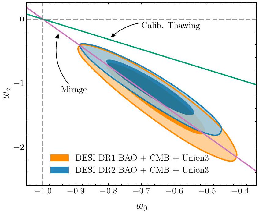
بشكل عام، نتائج التجميع من مخططات مختلفة تتفق بشكل جيد. عبور خط الفاصل الوهمي بواسطة
ب. الانحدار باستخدام العمليات الغاوسية
وإشارات إلى
VI. الآثار المترتبة على الطاقة المظلمة
أ. طاقة مظلمة ذائبة
ب. الطاقة المظلمة الناشئة
ج. طاقة المرايا المظلمة
د. مقارنة النماذج
| ديزي + سي إم بي: | +بانثيون بلس | +اتحاد3 | +DESY5 |
| فصول DE |
|
||
| ذوبان. (كاليفورنيا) | +0.4 (-1.6) | -0.6 (-2.5) | -5.8 (-7.1) |
| ذوبان. (الخوارزمية) | -1.0 (-2.9) | -4.6 (-6.9) | -10.1 (-13.2) |
| ناشئ | +2.1 (-0.05) | +1.8 (-0.1) | +0.2 (-1.5) |
| سراب | -9.1 (-10.5) | -13.8 (-16.2) | -18.7 (-20.7) |
|
|
-6.8 (-10.7) | -13.5 (-17.4) | -17.2 (-21.0) |
هل هناك دليل على عبور الشبح؟
تحت الأداء مقارنةً بتلك التي تفعل. السلوك المحدد لـ
VII. الاستنتاجات
تدعم القيود التطور المشار إليه بواسطة
VIII. توفر البيانات
الشكر والتقدير
تم دعم مسوحات الإرث من قبل: المدير، مكتب العلوم، مكتب فيزياء الطاقة العالية من وزارة الطاقة الأمريكية؛ مركز الحوسبة العلمية للبحث في الطاقة الوطنية، وهو مرفق مستخدم لمكتب العلوم؛ مؤسسة العلوم الوطنية الأمريكية، قسم العلوم الفلكية؛ المراصد الفلكية الوطنية في الصين، الأكاديمية الصينية للعلوم ومؤسسة العلوم الطبيعية الوطنية الصينية. يتم إدارة LBNL بواسطة مجلس إدارة جامعة كاليفورنيا بموجب عقد مع وزارة الطاقة الأمريكية.
يمكن العثور على الشكر الكامل فيhttps://www.legacysurvey.org/
[1] أ. أينشتاين، Sitzungsber. Preuss. Akad. Wiss. برلين (رياضيات. فيزياء) 1917، 142 (1917).
[2] أ. ج. ريس وآخرون (فريق بحث السوبرنوفا)، Astron. J. 116، 1009 (1998)، arXiv:astro-ph/9805201.
[3] س. بيرلموتر وآخرون (مشروع علم الكون السوبرنوفا)، Astrophys. J. 517، 565 (1999) arXiv:astroph/9812133
[4] و. ج. بيرسيفال، و. ساذرلاند، ج. أ. بيكوك، س. م. باو، وآخرون، MNRAS 337، 1068 (2002). arXiv:astro-ph/0206256 [astro-ph]
[5] د. ج. آيزنشتاين، New A Rev. 49، 360 (2005)
[6] س. كول، و. ج. بيرسيفال، ج. أ. بيكوك، ب. نوربرغ، وآخرون، MNRAS 362، 505 (2005) arXiv:astroph/0501174 [astro-ph]
[7] تعاون بلانك، ن. أغانيم، ي. أكرامي، م. أشداون، وآخرون، A&A 641، A6 (2020). arXiv:1807.06209 [astro-ph.CO].
[8] س. علم، م. أوبير، س. أفيلا، س. بالاند، وآخرون، Physical Review D 103، 10.1103/physrevd.103.083533 (2021).
[9] ج. تشاو، أ. فاري، م. هي، د. فوريرو-سانشيز، وآخرون، إشعارات شهرية للجمعية الملكية الفلكية 511، 5492-5524 (2022)
[10] ت. م. ج. أبوت وآخرون (DES)، Phys. Rev. D 98، 043526 (2018)، arXiv:1708.01530 [astro-ph.CO]
[11] م. أ. تروكسل وآخرون (DES)، Phys. Rev. D 98، 043528 (2018)، arXiv:1708.01538 [astro-ph.CO]
[12] س. علم وآخرون (eBOSS)، Phys. Rev. D 103، 083533 (2021)، arXiv:2007.08991 [astro-ph.CO]
[13] ج. هيمنز وآخرون، Astron. Astrophys. 646، A140 (2021)، arXiv:2007.15632 [astro-ph.CO]
[14] ت. م. ج. أبوت وآخرون (DES)، Phys. Rev. D 105، 023520 (2022)، arXiv:2105.13549 [astro-ph.CO]
[15] ج. إيفستاثيو، و. ج. ساذرلاند، و. س. مادوكس، Nature 348، 705 (1990).
[16] ج. فريمان، م. تيرنر، ود. هوتير، Ann. Rev. Astron. Astrophys. 46، 385 (2008)، arXiv:0803.0982 [astroph]
[17] د. ه. وينبرغ، م. ج. مورتونستون، د. ج. آيزنشتاين، س. هيراتا، وآخرون، Phys. Rept. 530، 87 (2013). arXiv:1201.2434 [astro-ph.CO].
[18] ج. ب. أوسترايكر و ب. ج. شتاينهاردت، ناتشر 377، 600 (1995)
[19] س. وينبرغ، ريف. مود. فيز. 61، 1 (1989).
[20] ب. راترا و ب. ج. إ. بيبلز، فيزيكس ريفيو د 37، 3406 (1988)
[21] ب. ج. إي. بيبلز و ب. راترا، أستروفيس. ج. ليتر. 325،
[22] V. Sahni و A. A. Starobinsky، Int. J. Mod. Phys. D 9، 373 (2000)، arXiv:astro-ph/9904398
[23] ب. ج. إي. بيبلز و ب. راترا، مراجعة الفيزياء الحديثة 75، 559 (2003)، arXiv:astro-ph/0207347
[24] إ. ج. كوبلاند، م. سامي، و س. تسوجيكاوا، المجلة الدولية للفيزياء الحديثة D 15، 1753 (2006)، arXiv:hep-th/0603057.
[25] ب. بول وآخرون، فيز. الظلام الكون 12، 56 (2016)، arXiv:1512.05356 [أسترو-ف.ك.أو]
[26] ل. بريفولاروبولوس و ف. سكارا، مراجعة جديدة في علم الفلك 95، 101659 (2022)، arXiv:2105.05208 [أسترو-ف.ك.أو]
[27] م. ليفي، ج. بيبيك، ت. بيرز، ر. بلوم، وآخرون، مطبوعات arXiv، arXiv:1308.0847 (2013)، arXiv:1308.0847 [أسترو-ف.ك.أو].
[28] تعاون DESI، أ. أغموسا، ج. أغيلار، س. أهلي، وآخرون، مطبوعات arXiv، arXiv:1611.00037 (2016)، arXiv:1611.00037 [أسترو-ف.إم]
[29] سي. بوبت، إل. تاياس، ج. أغيلار، سي. بيبيك، وآخرون، AJ 168، 245 (2024).
[30] ج. هـ. سيلبر، ب. فاجريليوس، ك. فانيغ، م. شوبنيل، وآخرون، AJ 165، 9 (2023) arXiv:2205.09014 [أستروف.آي إم].
[31] ت. ن. ميلر، ب. دويل، ج. غوتيريز، ر. بيسونر، وآخرون، AJ 168، 95 (2024)، arXiv:2306.06310 [أسترو-ف.إم].
[32] ج. جاي، س. بيلي، أ. كريمن، س. علم، وآخرون، AJ 165، 144 (2023)، arXiv:2209.14482 [أسترو-ف.إم]
[33] إ. ف. شلافلي، د. كيركبي، د. ج. شليجل، أ. د. مايرز، وآخرون، AJ 166، 259 (2023) arXiv:2306.06309 [أسترو-ف.ك.أو].
[34] تعاون DESI، أ. أغموسا، ج. أغيلار، س. أهلي، وآخرون، مطبوعات arXiv، arXiv:1611.00036 (2016)، arXiv:1611.00036 [أسترو-ف.إم].
[35] تعاون DESI، ب. أبارشي، ج. أغيلار، س. أهلي، وآخرون، AJ 164، 207 (2022)، arXiv:2205.10939 [أسترو-ف.إم]
[36] تعاون DESI، أ. ج. أدام، ج. أغيلار، س. أهلي، وآخرون، AJ 168، 58 (2024)، arXiv:2306.06308 [أستروف.كو].
[37] تعاون DESI، م. أ. كريم، أ. ج. أدام، د. أجادو، وآخرون، مطبوعات arXiv، arXiv:2503.14745 (2025)، arXiv:2503.14745 [أستروف.كو]
[38] تعاون DESI، أ. ج. أدام، ج. أغيلار، س. أهلم، وآخرون، مطبوعات arXiv، arXiv:2404.03000 (2024)، arXiv:2404.03000 [أسترو-ف.ك.أو]
[39] تعاون DESI، أ. ج. أدام، ج. أغيلار، س. أهلي، وآخرون، ج. علم الكونيات وفيزياء الجسيمات 2025، 124
(2025)، arXiv:2404.03001 [أسترو-ف.ك.أو]
[40] تعاون DESI، أ. ج. أدام، ج. أغيلار، س. أهلي، وآخرون، مجلة علم الكونيات وفيزياء الجسيمات 2025، 021 (2025)، arXiv:2404.03002 [أسترو-ف.ك.أو]
[41] تعاون DESI، أ. ج. أدام، ج. أغيلار، س. أهلي، وآخرون، مطبوعات arXiv، arXiv:2411.12022 (2024) arXiv:2411.12022 [أسترو-ف.ك.أو].
[42] تعاون DESI، أ. ج. أدام، ج. أغيلار، س. أهلي، وآخرون، مطبوعات arXiv، arXiv:2411.12021 (2024) arXiv:2411.12021 [أسترو-ف.ك.أو].
[43] ر. كالديرون وآخرون (DESI)، JCAP 10، 048. arXiv:2405.04216 [أسترو-ف.ك.أو].
[44] ك. لودها وآخرون (DESI)، فيزي. ريف. د 111، 023532 (2025)، arXiv:2405.13588 [أسترو-ف.ك.أو]
[45] تعاون DESI، قيد الإعداد (2026).
[46] تعاون DESI، م. أ. كريم، ج. أغيلار، س. أهلي، وآخرون، منشورات arXiv، arXiv:2503.14739 (2025). arXiv:2503.14739 [أسترو-ف.ك.أو].
[47] تعاون DESI، م. أ. كريم، ج. أغيلار، س. أهلم، وآخرون، مطبوعات arXiv، arXiv:2503.14738 (2025) arXiv:2503.14738 [أسترو-ف.ك.أو].
[48] و. إلبيرس، أ. أفيليس، هـ. إ. نورiega، د. شابات، وآخرون، منشورات arXiv، arXiv:2503.14744 (2025). arXiv:2503.14744 [أسترو-ف.ك.أو].
[49] د. هوتيرر و م. س. تيرنر، فيزيكس ريفيو د 64، 123527 (2001)، arXiv:astro-ph/0012510
[50] م. شيفالييه و د. بولارسكي، المجلة الدولية للفيزياء الحديثة D 10، 213-223 (2001).
[51] إ. ف. ليندر، فيزيكال ريفيو ليترز 90، 091301 (2003). arXiv:astro-ph/0208512 [astro-ph]
[52] د. هوتيرر وج. ستاركم، رسائل المراجعة الفيزيائية 90، 10.1103/physrevlett.90.031301 (2003).
[53] أ. شافيليو، أ. علم، ف. ساهني، وأ. أ. ستاروبينسكي، ملاحظات شهرية من الجمعية الملكية لعلم الفلك 366، 1081 (2006). arXiv:astro-ph/0505329.
[54] ر. دي بوتير وإ. ف. ليندر، مجلة علم الكونيات وفيزياء الجسيمات 2008، 042 (2008)، arXiv:0808.0189 [astro-ph]
[55] ر. ج. كريتيندن، ل. بوجوسيان، و ج.-ب. تشاو، مجلة علم الكونيات وفيزياء الجسيمات 2009، 025 (2009) arXiv:astroph/0510293 [astro-ph]
[56] سي. بوغدانو وس. نيسيريس، JCAP 05، 006. arXiv:0903.2805 [أسترو-ف.ك.أو].
[57] ت. هولسكلو، أ. علم، ب. سانسو، هـ. لي، وآخرون، فيزيكال ريفيو ليترز 105، 241302 (2010).
[58] ت. هولسكلو، أ. علم، ب. سانسو، هـ. لي، وآخرون، مراجعة الفيزياء D 84، 10.1103/physrevd.84.083501 (2011).
[59] ج. ب. تشاو، ر. ج. كريتيندن، ل. بوجوسيان، و إكس. زانغ، فيزيكال ريفيو ليترز 109، 171301 (2012). arXiv:1207.3804 [أسترو-ف.ك.أو].
[60] س. نيسيريس و ج. غارسيا-بيليدو، مجلة علم الكون وفيزياء الجسيمات 2012 (11)، 033-033
[61] ب. لويلير وأ. شافيليو، JCAP 01، 015. arXiv:1606.06832 [أسترو-ف.ك.أو].
[62] ر. كالديرون، ب. لوهيلييه، د. بولارسكي، أ. شافيليو، وآخرون، فيزيكال ريفيو دي 106، 083513 (2022). arXiv:2206.13820 [أسترو-ف.ك.أو].
[63] ر. ل. ووركمان، ف. د. بوركرت، ف. كريد، إ. كليمت، وآخرون، تقدم الفيزياء النظرية والتجريبية 2022، 083C01 (2022)
[64] ج. ليسغورغيس و س. باستور، فيزيكال ريبورت 429، 307 (2006) arXiv:astro-ph/0603494 [astro-ph]
[65] د. ج. آيزنشتاين، I. زهافي، د. و. هوج، ر. سكوكيمارّو، وآخرون، ApJ 633، 560 (2005) arXiv:astro-
ph/0501171 [أسترو-ف].
[66] U. أندرادي، E. بايلاس، J. مينا-فرنانديز، Q. لي، وآخرون، أرشيف e-prints، arXiv:2503.14742 (2025)، arXiv:2503.14742 [أسترو-ف.ك.أو]
[67] ل. كاساس، هـ. ك. هيريرا-ألكانتار، ج. تشافيس-مونتيرو، أ. كوتشيو، وآخرون، منشورات arXiv، arXiv:2503.14741 (2025)، arXiv:2503.14741 [أسترو-ف.إم]
[68] أ. برودزيلر، م. وولفسون، د. م. سانتوس، م. هو، وآخرون، مطبوعات arXiv، arXiv:2503.14740 (2025)، arXiv:2503.14740 [أسترو-ف.ك.أو]
[69] د. بروت، د. سكولنيك، ب. بوبوفيتش، أ. ج. ريس، وآخرون، ApJ 938، 110 (2022) arXiv:2202.04077 [أستروف.كو]
[70] د. روبين، ج. ألدرينغ، م. بيتول، أ. فرتشر، وآخرون، مطبوعات arXiv، arXiv:2311.12098 (2023)، arXiv:2311.12098 [أسترو-ف.ك.أو]
[71] ت. م. ك. أبوت وآخرون (DES)، ApJ (مقبول، 2024)، arXiv:2401.02929 [أسترو-ف.ك.أو]
[72] تعاون بلانك، ن. أغانيم، ي. أكرامي، ف. أروجا، وآخرون، A&A 641، A1 (2020). arXiv:1807.06205 [أسترو-ف.ك.أو]
[73] ن. أغانيم وآخرون (بلانك)، أسترو. أستروفيس. 641، A5 (2020)، arXiv:1907.12875 [أسترو-ف.ك.أو]
[74] ج. إيفستاثيو وس. غراتون، المجلة المفتوحة لعلم الفلك 4، 8 (2021)
[75] ج. تورادو وأ. لويس، ج. علم الكونيات وفيزياء الجسيمات 2021، 057 (2021)، arXiv:2005.05290 [أسترو-ف.إم]
[76] ج. كارون، م. ميرميلشتاين، وأ. لويس، JCAP 09، 039 arXiv:2206.07773 [أسترو-ف.ك.أو]
[77] إ. روزنبرغ، س. غراتون، و ج. إيفستاثيو، MNRAS 517، 4620 (2022)، arXiv:2205.10869 [أسترو-ف.ك.أو]
[78] م. س. مدهفاشيريل، ف. ج. كيو، ب. د. شيروين، ن. ماككران وآخرون، ApJ 962، 113 (2024). arXiv:2304.05203 [أسترو-ف.ك.أو]
[79] ج. س. فارين وآخرون (ACT)، مجلة الفيزياء الفلكية 966، 157 (2024)، arXiv:2309.05659 [أسترو-ف.ك.أو].
[80] ب. ليموس وأ. لويس، فيزيكال ريفيو د 107، 103505 (2023)، arXiv:2302.12911 [أسترو-ف.ك.أو]
[81] أ. لويس و س. بريدل، فيزيكال ريفيو د 66، 103511 (2002)، arXiv:astro-ph/0205436 [astro-ph]
[82] أ. لويس، مراجعة الفيزياء د 87، 103529 (2013)، arXiv:1304.4473 [أسترو-ف.ك.أو]
[83] ج. تورادو وأ. لويس، ج. علم الكونيات وفيزياء الجسيمات 05، 057 (2021)، arXiv:2005.05290 [أسترو-ف.إم]
[84] ر. م. نيل، أرشيف الرياضيات الإلكترونية، الرياضيات/0502099 (2005)، أرشيف: الرياضيات/0502099 [الرياضيات.نظرية].
[85] أ. لويس، أ. تشالينور، وأ. لاسنبي، ApJ 538، 473 (2000)، arXiv:astro-ph/9911177 [astro-ph].
[86] سي. هاوليت، أ. لويس، أ. هول، وأ. تشالينور، مجلة علم الكونيات وفيزياء الجسيمات 2012، 027 (2012). arXiv:1201.3654 [أسترو-ف.ك.أو]
[87] و. هو وإي. ساويكي، فيزيكال ريفيو د 76، 104043 (2007)، arXiv:0708.1190 [أسترو-فيزيكس]
[88] و. فنج، و. هو، وأ. لويس، / فيز. ريف. د 78، 087303 (2008)، arXiv:0808.3125 [أسترو-في].
[89] ج. ليسغورغيس، نظام حل التباين الكوني الخطي (CLASS) I: نظرة عامة (2011)، arXiv:1104.2932 [أسترو-ف.إم]
[90] د. بلاز، ج. ليسغورغ، وت. ترام، مجلة علم الكونيات وفيزياء الجسيمات 1107، 034 (2011)، arXiv:1104.2933 [أستروف.كو]
[91] هـ. ديمبينسكي و ب. أ. وآخرون، سكايكت-هيب/إيمينويت (2020).
[92] م. إيشاك، ج. بان، ر. كالديرون، ك. لودها، وآخرون، مطبوعات arXiv، arXiv:2411.12026 (2024).
arXiv:2411.12026 [أسترو-ف.ك.أو].
[93] ف. بولين، ت. ل. سميث، ر. كالديرون، وت. سيمون، arXiv:2407.18292 [أسترو-ف.ك.أو ] (2024).
[94] ر. ر. كالدويل، رسالة فيزيائية ب 545، 23 (2002)، arXiv:astro-ph/9908168.
[95] س. و. هوكينغ و ج. ف. ر. إليس، الهيكل الكبير للزمان والمكان، مؤلفات كامبريدج في الفيزياء الرياضية (مطبعة جامعة كامبريدج، 2023).
[96] في. ساهني، أ. شافيليو، وأ. أ. ستاروبينسكي، فيزي. ريف. د 78، 103502 (2008)، arXiv:0807.3548 [أسترو-في].
[97] I. واسرمان، مراجعة الفيزياء D 66، 123511 (2002). arXiv:astro-ph/0203137.
[98] م. كونز، فيزيكال ريفيو د 80، 123001 (2009).
[99] أ. شافيليو وإي. في. ليندر، فيزيكال ريفيو دي 84، 063519 (2011)
[100] و. جياري، م. نجفي، س. بان، إ. دي فالنتينو، وآخرون، JCAP 10، 035 arXiv:2407.16689 [أسترو-ف.ك.أو].
[101] و. ج. وولف، سي. غارسيا-غارسيا، و ب. ج. فيريرا، arXiv:2502.04929 [أسترو-ف.ك.أو ] (2025).
[102] إ. م. باربوزا و ج. س. ألكانيز، رسائل الفيزياء ب 666، 415 (2008)، arXiv:0805.1713 [astro-ph]
[103] ج. إيفستاثيو، MNRAS 310، 842 (1999) arXiv:astroph/9904356 [astro-ph]
[104] ن. ديمكيس، أ. كاراجيورغوس، أ. زامبيلي، أ. بالياثاناسيس، وآخرون، فيز. ريف. د 93، 123518 (2016). arXiv:1604.05168 [gr-qc]
[105] س. بان، و. يانغ، و أ. بالياثاناسيس، المجلة الأوروبية للفيزياء C 80، 274 (2020)، arXiv:1902.07108 [أستروف.كو]
[106] هـ. ك. جَسّال، ج. س. باجلا، و ت. بادمانابان، فيزيكس ريفيو د 72، 103503 (2005) arXiv:astroph/0506748 [astro-ph]
[107] أ. شافيليو، ت. كليفتون، و ب. فيريرا، مجلة علم الكون وفيزياء الجسيمات 2011 (08)، 017.
[108] أ. شافيليو، مجلة علم الكون وفيزياء الجسيمات 2012 (08)، 002-002
[109] أ. شافيليو، مجلة علم الكون وفيزياء الجسيمات 2012 (05)، 024-024
[110] س. هاود، س. صالحی، س. فيدال، م. ماتوري، وآخرون، arXiv:1912.04560 [أسترو-ف.ك.أو] (2019).
[111] ج. غراندي، ج. سولا بيراكولا، و هـ. ستيفانسيك، JCAP 08، 011، arXiv:gr-qc/0604057.
[112] ج. أ. فاسكيز، س. هي، م. ب. هوبسون، أ. ن. لاسنبي، وآخرون، JCAP 07، 062، arXiv:1208.2542 [أستروف.كو]
[113] ل. فيزينيللي، س. فاجنوزي، وU. دانييلسون، تماثل 11، 1035 (2019)، arXiv:1907.07953 [أسترو-ف.ك.أو]
[114] ر. كالديرون، ر. غانوجي، ب. لوهيليير، و د. بولارسكي، فيزيكال ريفيو دي 103، 10.1103/physrevd.103.023526 (2021).
[115] ت. تشيبا، ت. أوكابي، و م. ياماغوتشي، فيزيكال ريفيو د 62، 023511 (2000)، arXiv:astro-ph/9912463
[116] في. ساهني وي. شتانوفسكي، مجلة علم الكون وفيزياء الجسيمات 2003 (11)، 014
[117] ف. باور، ج. سولّا، و هـ. ستيفانيتش، مجلة علم الكون وفيزياء الجسيمات 2010 (12)، 029
[118] ب. بواسيه، هـ. جياكوميني، د. بولارسكي، و أ. أ. ستاروبينسكي، JCAP 07، 002، arXiv:1504.07927 [gr-qc].
[119] إ. ف. ليندر و د. هوتيرر، فيزيكال ريفيو د 72، 043509 (2005)، arXiv:astro-ph/0505330
[120] د. موثوكريشنا ود. باركنسون، JCAP 11، 052. arXiv:1607.01884 [أسترو-ف.ك.أو].
[121] ر. كاميليري وآخرون (DES)، ملاحظات شهرية للجمعية الملكية للفلك.
[122] م. تيغمارك، مراجعة الفيزياء د 55، 5895-5907 (1997).
[123] د. هوتيرر وأ. كوراى، مراجعة الفيزياء D 71، 10.1103/physrevd.71.023506 (2005).
[124] ر. ج. كريتيندن، ل. بوجوسيان، و ج.-ب. تشاو، JCAP 12، 025، arXiv:astro-ph/0510293.
[125] ف. سيمبسون و س. بريدل، فيزيكال ريفيو د 73، 083001 (2006)، arXiv:astro-ph/0602213
[126] سي. غارسيا-كوينتيرو، م. إيشاك، وأو. نينغ، JCAP 12، 018، arXiv:2010.12519 [أسترو-ف.ك.أو]
[127] ب. أ. ر. أدي وآخرون (بلانك)، أسترو. أستروفيس. 594، A14 (2016)، arXiv:1502.01590 [أسترو-ف.ك.أو]
[128] ج. ب. تشاو وآخرون، ناتشر أسترو. 1، 627 (2017)، arXiv:1701.08165 [أسترو-ف.ك.أو]
[129] م. رافيري، ل. بوجوسيان، ك. كوياما، م. مارتينيلي، وآخرون، إعادة بناء مشتركة للطاقة المظلمة وتطور النمو المعدل (2021)، arXiv:2107.12990 [أسترو-ف.ك.أو].
[130] ل. بوجوسيان، م. رافيري، ك. كوياما، م. مارتينيلي، وآخرون، ناتشر أستران. 6، 1484 (2022). arXiv:2107.12992 [أسترو-ف.ك.أو]
[131] ب. بانسال و د. هوتيرر، arXiv:2502.07185 [أستروف.كو ] (2025).
[132] ج. أ. ريبوساس، د. هـ. ف. دي سوزا، ك. تشونغ، ف. ميراندا، وآخرون، JCAP 02، 024، arXiv:2408.14628 [أسترو-ف.ك.أو].
[133] ي.-هـ. بانغ، إكس. تشانغ، و كيو.-ج. هوانغ، arXiv:2408.14787 [أسترو-ف.ك.أو ] (2024).
[134] و. هاندلي، مجلة البرمجيات مفتوحة المصدر 3، 10.21105/joss.00849 (2018).
[135] سي. راسموسن وسي. ويليامز، العمليات الغاوسية لتعلم الآلة، سلسلة الحوسبة التكيفية وتعلم الآلة (مجموعة جامعة الصحافة المحدودة، 2006).
[136] ت. هولسكلو، أ. علم، ب. سانسو، هـ. لي، وآخرون، مراجعة الفيزياء D 82، 10.1103/physrevd.82.103502 (2010).
[137] ت. هولسكلو، أ. علم، ب. سانسو، هـ. لي، وآخرون، فيزيكال ريفيو ليترز 105، 241302 (2010)
[138] أ. شافيليو، أ. ج. كيم، وإي. في. ليندر، فيزيكال ريفيو دي 85، 123530 (2012) arXiv:1204.2272 [أسترو-ف.ك.أو]
[139] م. سيكل، س. كلاركسون، و م. سميث، مجلة علم الكون وفيزياء الجسيمات 2012 (06)، 036-036.
[140] أ. شافيليو، أ. ج. كيم، وإي. في. ليندر، فيزيكال ريفيو دي 87، 023520 (2013)، arXiv:1211.6128 [أسترو-ف.ك.أو].
[141] ر. إ. كيلي، س. جوداكي، م. كابلينغهات، و د. كيركبي، JCAP 12، 035، arXiv:1905.10198 [أسترو-ف.ك.أو]
[142] إ. بلقاسم، س. فوفا، م. ماجوري، و ت. يانغ، فيزيكال ريفيو دي 101، 063505 (2020)، arXiv:1911.11497أستروف.كو]
[143] ر. إ. كيلي، أ. شافيليو، ب. لوهيليير، وإ. ف. ليندر، ملاحظات شهرية من الجمعية الملكية للفلك 491، 3983 (2020)، arXiv:1905.10216 [أسترو-ف.ك.أو]
[144] ف. جيراردي، م. مارتينيلي، وأ. سيلفستري، JCAP 07، 042 arXiv:1902.09423 [أسترو-ف.ك.أو]
[145] ب. موكيرجي وأ. موكيرجي، ملاحظات شهرية. الجمعية الملكية للفلك 504، 3938 (2021)، arXiv:2104.06066 [أسترو-ف.ك.أو].
[146] ر. كالديرون، ب. لوهيلييه، د. بولارسكي، أ. شافيليو، وآخرون، فيزيكال ريفيو دي 108، 023504 (2023)، arXiv:2301.00640 [أسترو-ف.ك.أو]
[147] ب. ر. ديندا و ر. مارتنز، JCAP 01، 120. arXiv:2407.17252 [أسترو-ف.ك.أو]
[148] ب. موكيرجي وأ. أ. سين، فيزيكال ريفيو د 110، 123502 (2024)، arXiv:2405.19178 [أسترو-ف.ك.أو].
[149] س. جوداكي، م. كابلينغهات، ر. كيلي، و د. كيركبي، فيزيكال ريفيو د 97، 123501 (2018) arXiv:1710.04236 [أسترو-ف.ك.أو]
[150] س.-ج. هوانغ، ب. لوهيلييه، ر. إي. كيلي، م. ج. جي، وآخرون، JCAP 02، 014، arXiv:2206.15081 [أستروف.كو]
[151] ر. ر. كالدويل وإي. في. ليندر، فيزيكال ريفيو ليترز 95، 141301 (2005)، arXiv:astro-ph/0505494.
[152] إ. ف. ليندر، مراجعة الفيزياء د 73، 063010 (2006). arXiv:astro-ph/0601052
[153] ر. ن. كان، ر. دي بوتير، وإي. في. ليندر، JCAP 11، 015، arXiv:0807.1346 [astro-ph].
[154] ب. راترا و ب. ج. إ. بيبلز، فيزيكس ريفيو د 37، 3406 (1988)
[155] C. Wetterich، فيزياء نووية B 302، 668 (1988). arXiv:1711.03844 [hep-th]
[156] ب. ج. فيريرا و م. جويس، فيزيكال ريفيو د 58، 023503 (1998)، arXiv:astro-ph/9711102
[157] ر. ج. شيرر و أ. أ. سين، فيزيكال ريفيو دي 77، 083515 (2008)، arXiv:0712.3450 [أسترو-فيزيكس]
[158] س. تسوجيكاوا، كلاس. كوانت. جراف. 30، 214003 (2013). arXiv:1304.1961 [gr-qc]
[159] ج. مارتن، رسالة فيزياء حديثة A 23، 1252 (2008). arXiv:0803.4076 [أسترو-فيزياء]
[160] ج. أ. فريمان، س. ت. هيل، أ. ستببينز، وإ. واغا، فيزيكال ريفيو ليترز 75، 2077 (1995)، arXiv:astroph/9505060
[161] ج. م. كلاين، س. جيون، و ج. د. مور، فيزيكال ريفيو د 70، 043543 (2004)، arXiv:hep-ph/0311312.
[162] أ. فيكمان، مراجعة الفيزياء د 71، 023515 (2005). arXiv:astro-ph/0407107.
[163] إ. ف. ليندر، الجاذبية العامة والنسبية. 40، 329 (2008). arXiv:0704.2064 [أسترو-فيزيكس]
[164] إ. ف. ليندر، مراجعة الفيزياء د 91، 063006 (2015). arXiv:1501.01634 [أسترو-ف.ك.أو].
[165] ر. كريتيندن، إ. ماجيروتو، و ف. بيازا، فيزيكال ريفيو ليترز 98، 251301 (2007)، arXiv:astro-ph/0702003.
[166] ن. كاليببر و ل. سوربو، JCAP 04، 007، arXiv:astroph/0511543
[167] د. ج. إ. مارش، تقرير فيزيائي 643، 1 (2016). arXiv:1510.07633 [أسترو-ف.ك.أو].
[168] س. دوتا و ر. ج. شيرر، فيزيكال ريفيو د 78، 123525 (2008)، arXiv:0809.4441 [أسترو-فيزيكس]
[169] إكس. لي وأ. شافيليو، مجلة الفيزياء الفلكية. 883، L3 (2019)، arXiv:1906.08275 [أسترو-ف.ك.أو]
[170] إكس. لي وأ. شافيليو، مجلة الفيزياء الفلكية 902، 58 (2020). arXiv:2001.05103 [أسترو-ف.ك.أو].
[171] ل. باركر و أ. رافال، فيزيكال ريفيو D 62، 083503 (2000)، [تصحيح: فيزيكال ريفيو D 67، 029903 (2003)]، arXiv:grqc/0003103
[172] ر. ر. كالدويل، و. كومب، و. باركر، و د. أ. ت. فانتزيلا، فيزيكال ريفيو د 73، 023513 (2006) arXiv:astroph/0507622
[173] أ. بنيهاشمي، ن. خسروي، وأ. شافيليو، JCAP 06، 003، arXiv:2012.01407 [أسترو-ف.ك.أو].
[174] م. س. تيرنر، فيزيكال ريفيو د 31، 1212 (1985).
[175] ل. بارنز، م. ج. فرانسيس، ج. ف. لويس، وإ. ف. ليندر، نشر. جمعية الفلك الأسترالية 22، 315 (2005)، arXiv:astroph/0510791
[176] و. زيمدال، المجلة الدولية للفيزياء الحديثة D 14، 2319 (2005). arXiv:gr-qc/0505056
[177] إ. ف. ليندر، arXiv:0708.0024 [astro-ph] (2007).
[178] إ. ف. ليندر و م. ج. وايت،|فيزي. ريف. د 72، 061304 (2005)، arXiv:astro-ph/0508401
[179] م. ج. فرانسيس، ج. ف. لويس، و إ. ف. ليندر، ملاحظات الجمعية الملكية الفلكية 380، 1079 (2007) arXiv:0704.0312 [astro-ph]
[180] إ. ف. ليندر، (2024)، arXiv:2410.10981 [أسترو-ف.ك.أو].
[181] د. ج. سبايجل هالتير، ن. ج. بيست، ب. ب. كارلين، وأ. فان دير ليندي، مجلة الجمعية الملكية الإحصائية: السلسلة ب (المنهجية الإحصائية) 64، 583 (2002).
[182] أ. ر. ليدل، إشعارات شهرية للجمعية الملكية الفلكية: رسائل 377، L74 (2007).
[183] س. غراندي، د. رابيتي، أ. سارو، ج. ج. موهر، وآخرون، ملاحظات شهرية للجمعية الملكية للفلك 463، 1416 (2016)، arXiv:1604.06463 [أسترو-ف.ك.أو]
[184] و. ج. وولف، س. غارسيا-غارسيا، د. ج. بارتليت، و ب. ج. فيريرا، فيزيكال ريفيو دي 110، 083528 (2024)، arXiv:2408.17318 [أسترو-ف.ك.أو]
[185] د. شليفكو و ب. شتاينهارت، (2024)، arXiv:2405.03933 [أسترو-ف.ك.أو].
[186] ج. بايور، إ. مكدونا، ور. براندنبرغر، arXiv:2411.13637 [أسترو-ف.ك.أو ] (2024).
[187] و. هو، مراجعة الفيزياء د 71، 047301 (2005)، arXiv:astroph/0410680
[188] ز.-ك. قوه، ي.-س. بياو، ش.-م. تشانغ، وي.-ز. تشانغ، فيز. ليت. ب 608، 177 (2005)، arXiv:astro-ph/0410654.
[189] هـ. وي، ر.-ج. كاي، و د.-ف. زينغ، كلاس. كوانت. جراف. 22، 3189 (2005)، arXiv:hep-th/0501160
[190] ر. ر. كالدويل و م. دوران، فيزيكال ريفيو د 72، 043527 (2005)، arXiv:astro-ph/0501104
[191] ي.-ف. كاي، ت. كيو، ر. براندنبرغر، ي.-س. بياو، وآخرون، JCAP 03، 013، arXiv:0711.2187 [hep-th].
[192] ي.-ف. كاي، ت. كيو، ي.-س. بياو، م. لي، وآخرون، JHEP 10، 071 arXiv:0704.1090 [gr-qc].
[193] ل. أماندولا، فيزيكال ريفيو د 62، 043511 (2000)، arXiv:astro-ph/9908023
[194] أ. ب. بيليارد وأ. أ. كولي، فيزيكال ريفيو د 61، 083503 (2000)، arXiv:astro-ph/9908224
[195] ل. أماندولا، فيزيكال ريفيو د 69، 103524 (2004)، arXiv:astro-ph/0311175
[196] س. نوجيري، س. د. أودينتسوف، وس. تسوجيكوا، فيزيكس ريفيو د 71، 063004 (2005) arXiv:hep-th/0501025
[197] ت. كليمسون، ك. كوياما، ج.-ب. تشاو، ر. مارتنز، وآخرون، فيزيكال ريفيو د 85، 043007 (2012)، arXiv:1109.6234 [أسترو-ف.ك.أو]
[198] أ. شافيليو، د. ك. هازرا، ف. ساهني، وأ. أ. ستاروبينسكي، إشعارات شهرية للجمعية الملكية الفلكية 473، 2760-2770 (2017)
[199] ف. س. كارفالو وأ. س. سا، فيزيكال ريفيو د 70، 087302 (2004)، arXiv:astro-ph/0408013
[200] و. هو وإ. ساويكي، فيزيكال ريفيو د 76، 064004 (2007)، arXiv:0705.1158 [أسترو-فيزيكس]
[201] ج. مارتن، س. شيميد، وج. ب. أوزان، فيزيكال ريفيو ليترز 96، 061303 (2006).
[202] أ. أنيسيموف، إ. بابيتشيف، وأ. فيكمان، JCAP 06، 006 arXiv:astro-ph/0504560.
[203] س. نيسيريس و ل. بريفولاروبولوس، فيزي. ريف. د 73، 103511 (2006)، arXiv:astro-ph/0602053
[204] سي. ديفايه، أو. بوجولاس، آي. ساويكي، وآي. فيكمان، JCAP 10، 026، arXiv:1008.0048 [hep-th]
[205] أ. بوجولاس، إ. ساويكي، وأ. فيكمان، JHEP 11، 156. arXiv:1103.5360 [hep-th].
[206] ج. يي، م. مارتينيلي، ب. هو، وأ. سيلفستري، arXiv:2407.15832 [أسترو-ف.ك.أو ] (2024).
[207] و. ج. وولف، ب. ج. فيريرا، و. س. غارسيا-غارسيا، فيزيكال ريفيو د 111، L041303 (2025)، arXiv:2409.17019 [أستروف.كو]
[208] ي. يانغ، إكس. رين، ق. وانغ، ز. لو، وآخرون، مجلة العلوم. 69، 2698 (2024)، arXiv:2404.19437 [أسترو-ف.ك.أو]
[209] أ. كريستيانسن، ف. هاساني، ود. ف. موتا، JCAP 01، 043، arXiv:2405.00668 [أسترو-ف.ك.أو]
[210] م. ريجو، م. سميث، أ. جوبار، ك. ماغواير، وآخرون، مطبوعات arXiv، arXiv:2409.04346 (2024). arXiv:2409.04346 [أسترو-ف.ك.أو].
[211] إ. سي. بيلم، س. ر. كولكارني، م. ج. غراهام، ر. ديكاني، وآخرون، PASP 131، 018002 (2019)، arXiv:1902.01932 [أسترو-ف.إم]
[212] م. لوخنر، د. سكولنيك، هـ. الموباييد، ت. أنغويتا، وآخرون، ApJS 259، 58 (2022) arXiv:2104.05676 [أسترو-ف.ك.أو]
[213] ب. غريس، ن. ريجنو، هـ. أوان، إ. هوك، وآخرون، ApJS 264، 22 (2023)، arXiv:2205.07651 [أسترو-ف.ك.أو].
[214] د. سبيرجل، ن. جيرلز، ج. بالتاي، د. بينيت، وآخرون، تلسكوب المسح بالأشعة تحت الحمراء واسع المجال – أصول التلسكوب المركّز على الفيزياء الفلكية WFIRST-AFTA تقرير 2015 (2015)، arXiv:1503.03757 [أسترو-ف.إم].
[215] ر. لوريجس، ج. أميكس، س. أردوني، ج. ل. أوجير، وآخرون، مطبوعات arXiv، arXiv:1110.3193 (2011). arXiv:1110.3193 [أسترو-ف.ك.أو].
[216] و. ج. هاندلي، م. ب. هوبسون، و أ. ن. لاسنبي، ملاحظات الجمعية الملكية للفلك 450، L61 (2015). arXiv:1502.01856 [أسترو-ف.ك.أو].
[217] و. هاندلي، ج. البرمجيات مفتوحة المصدر. 4، 1414 (2019). arXiv:1905.04768 [أسترو-ف.إم].
[218] ل. ت. هيرغت، و. ج. هاندلي، م. ب. هوبسون، و أ. ن. لاسنبي، فيزيكال ريفيو د 103، 123511 (2021)، arXiv:2102.11511 [أسترو-ف.ك.أو].
[219] هـ. جيفريز، نظرية الاحتمالات، نصوص أكسفورد الكلاسيكية في العلوم الفيزيائية (1939).
[220] ر. تروتا، ملاحظات الجمعية الملكية للفلك 378، 72 (2007)، arXiv:astro-ph/0504022.
[221] ل. أماندولا وس. تسوجيكاوا، الطاقة المظلمة: النظرية والملاحظات (مطبعة جامعة كامبريدج، 2015).
[222] أ. ج. شاجيب وج. أ. فريمان، arXiv:2502.06929 [أستروف.كو ] (2025).
[223] في. سمير-باريتو وأ. ر. ليدل، مجلة علم الكون وفيزياء الجسيمات 2017 (01)، 023-023
[224] أ. أبراهامسي، أ. ألبريخت، م. بارنارد، و ب. بوزيك، فيزيكال ريفيو د 77، 103503 (2008)، arXiv:0712.2879 [أستروف]
[225] م. كاواساكي، ت. موروئي، وت. تاكاهاشي، فيزي. ريف. د 64، 083009 (2001)، arXiv:astro-ph/0105161
[226] س. س. سي. نغ و د. ل. ويلتشر، فيزيكال ريفيو د 63، 023503 (2001) arXiv:astro-ph/0004138.
[227] ك. كوبل، س. دودلسون، وج. أ. فريمان، فيزيكال ريفيو د 55، 1851 (1997)، arXiv:astro-ph/9608122
[228] ج. أ. فريمان و I. واغا، فيزيكال ريفيو D 57، 4642 (1998)، arXiv:astro-ph/9709063
[229] ب. ت. ب. فيانا و أ. ر. ليدل، فيزي. ريف. د 57، 674 (1998)، arXiv:astro-ph/9708247
[230] ف. إكس. إل. سيدينو، أ. إكس. غونزاليس-موراليس، و ل. أ. أورينا لوبيز، فيزيكال ريفيو د 96، 061301 (2017). arXiv:1703.10180 [gr-qc]
[231] ف. إكس. ليناريس سيدينو، أ. إكس. غونزاليس-موراليس، و ل. أ. أورينا لوبيز، JCAP 01، 051، arXiv:2006.05037 [أسترو-ف.ك.أو].
الملحق أ: مقارنة النماذج البايزية
| +بانثيون بلس | +اتحاد3 | +DESY5 | |
| ديزي دي آر 2 باو + سي إم بي | |||
|
|
|
|
|
|
|
|
|
|
|
|
|
|
|
| ديزي دي آر 1 باو + سي إم بي | |||
|
|
|
|
|
|
|
|
|
|
|
|
|
|
|
الملحق ب: تفاصيل تجميع تحليل المكونات الرئيسية
الملحق ج: تفاصيل حول الانحدار باستخدام العمليات الغاوسية
الملحق د: الجوهر
الملحق E: التحقق من النماذج
تحضير نموذج ثالث وفقًا للمعادلة (15) مع
الملحق F: المقارنة مع DESI DR1
لاحظ أنه، كما تم الإشارة في مناقشتنا حول النيوترينوات، فإنها لا تساهم في محتوى المادة في الكون خلال إعادة التركيب، وبالتالي نستخدم بشكل صريح بدلاً من . في النص يستخدم بدلاً من لراحة المستخدم. في التنفيذ العددي نقوم بالقطع عند ترتيب في توسيع تايلور. لاحظ أن نطاق الانزياح الأحمر ذو الصلة بالملاحظات يتم تعيينه إلى حيث يتم تعريف كثيرات حدود تشيبيشيف. لهذا التحليل يتم اختياره، مما يتوافق مع أقل من تغير في سعة الحاوية على مدى على جانبي حافة صندوق الانزياح الأحمر. نستبدل مع لتجنب المشاكل العددية الناجمة عن طريقة الرماية.
DOI: https://doi.org/10.1103/w4c6-1r5j
Publication Date: 2025-10-06
University, 191 West Woodruff Avenue, Columbus, OH 43210, USA
Nucléaire et de Hautes Energies (LPNHE), FR-75005 Paris, France
University of California, 1156 High Street, Santa Cruz, CA 95064, USA
Santa Cruz, 1156 High Street, Santa Cruz, CA 95065, USA
McPherson Laboratory, 140 W 18th Avenue, Columbus, OH 43210, USA
Abstract
We conduct an extended analysis of dark energy constraints, in support of the findings of the DESI DR2 cosmology key paper, including DESI data, Planck CMB observations, and three different supernova compilations. Using a broad range of parametric and non-parametric methods, we explore the dark energy phenomenology and find consistent trends across all approaches, in good agreement with the
CONTENTS
II. Datasets and Methodology ….. 4
III. Overview of the
IV. Parameterizing Dark Energy ….. 8
A. Alternative
B. Crossing Statistics ….. 9
V. Non-Parametric Methods ….. 10
A. Binning ….. 10
B. Gaussian Process Regression ….. 12
VI. Implications for Dark Energy ….. 12
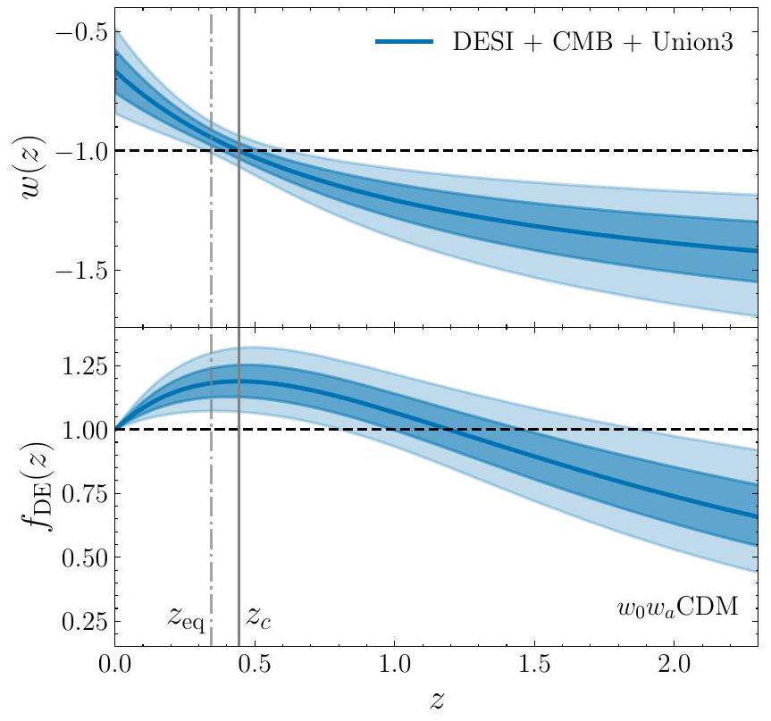
A. Thawing dark energy ….. 12
B. Emergent dark energy ….. 15
C. Mirage dark energy ….. 15
D. Model Comparison ….. 16
E. Is there evidence for phantom crossing?. ….. 17
VII. Conclusions ….. 17
VIII. Data Availability ….. 18
Acknowledgments ….. 18
References ….. 19
A. Bayesian Model Comparison ….. 23
B. Details of Binning PCA ….. 24
C. Details on Gaussian Process Regression ….. 25
D. Quintessence ….. 25
E. Validation on Mocks ….. 26
F. Comparison with DESI DR1 ….. 27
I. INTRODUCTION
that combines the BAO with the full clustering information from DESI galaxies and other tracers [41, 42, as well as the supporting DESI DR1 papers that considered alternative descriptions of the dark energy sector [43, 44, all showed tantalizing hints of the departures from the cosmological constant dark energy model. Cosmological hints in the dark energy sector are currently a source of debate, and it is of high priority to explore them with more data. In this work, we make use of the BAO measurements from the second data release (DR2 [45-47]) from DESI to explore the possibility of an evolving, dynamical dark energy, and evaluate whether existing observations support such a paradigm shift. This paper is part of a set of supporting papers that aim to extend the cosmological analysis presented in [47] (see [48] for the supporting paper focusing on neutrino constraints).
II. DATASETS AND METHODOLOGY
| parametrization | parameter | default | prior |
| Baseline |
|
– |
|
|
|
– |
|
|
|
|
– |
|
|
|
|
– |
|
|
|
|
– |
|
|
|
|
– |
|
|
| in absence of
|
|
– |
|
| Alt. Parametrization |
|
-1 |
|
|
|
0 |
|
|
| Crossing |
|
1 |
|
|
|
0 |
|
|
| Binning |
|
-1 |
|
|
|
1 |
|
|
| Gaussian Processes |
|
– | Eq. (C3) |
|
|
-1 |
|
|
| Dark Energy Classes | |||
| Calib. Thawing |
|
– |
|
| Algebraic Thawing |
|
– |
|
|
|
– |
|
|
| Emergent |
|
– |
|
| Mirage |
|
– |
|
as
- Baryon acoustic oscillations (
): We use the BAO distance measurements from DESI DR2, as detailed in Table III in [47]. In particular, for the BGS tracer, we use measurements of providing compressed low redshift information from the range . For the rest of DESI tracers, we use the BAO distance measurements of and . Explicitly, we use two LRG bins in the ranges and , a combined tracer measurement for LRG+ELG in the range , a measurement spanning for the ELG tracer and the QSO in the range . The systematics tests associated with the BAO measurements from galaxy and quasar clustering are presented in [66]. We also include the Lya measurements in , which provides our highest redshift data-point. This measurement is described in detail in 46 (see also 67) for validation tests and [68] for specific catalog details). We refer to this whole dataset, encompassing information from redshift 0.1 to 4.2 , split into seven main samples, as “DESI”.
- Supernovae Ia (SNe Ia): We combine DESI data with either of the following three SNe Ia datasets, namely PantheonPlus, Union3, and DESY5. The PantheonPlus 69 dataset comprises 1550 spectroscopically-confirmed SNe Ia in the redshift range
. The Union3 compilation [70] has 2087 SNe Ia in the redshift range of which are common to PantheonPlus, though the analysis methodologies are
substantially different. Finally, the DESY5 dataset 71 is a sample of 1635 photometrically-classified SNe Ia with redshifts in the range, complemented by 194 historical low-redshift SNe Ia (which are also present in the PantheonPlus sample) spanning . - Cosmic microwave background (CMB): We include temperature and polarization measurements of the CMB from the Planck satellite [72]. In particular, we use the high-
TTTEEE likelihood (planck_NPIPE_highl_CamSpec.TTTEEE), together with low- TT (planck_2018_lowl.TT) and low EE (planck_2018_lowl.EE) 73, 74, as implemented in Cobaya 75. Additionally, we combine temperature and polarization anisotropies with CMB lensing measurements from the combination of NPIPE PR4 from Planck [76, 77 and the Atacama Cosmology Telescope (ACT) DR6 [78, 79]. - Compressed CMB: We use the Gaussian correlated prior over
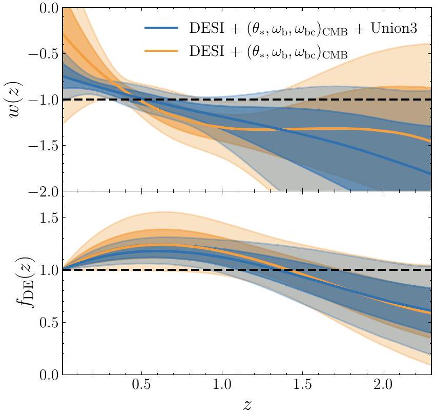
and as defined in [47. Here, the angular acoustic scale adds extra geometrical information from the CMB, while and serve to set the sound horizon and calibrate our BAO measurements. These CMB-based quantities capture most of the relevant information from the early CMB by marginalizing over contributions from late-time effects, such as the integrated Sachs-Wolfe (ISW) effect and CMB lensing, resulting in a robust CMB compression for testing late-time physics 80. In particular, we use these compressed measurements as a conservative alternative for constraining dark energy at the background level, thereby allowing for negative , as in Sections IV B and V A. For brevity, we refer to these as .
III. OVERVIEW OF THE
tailed Bayesian model comparison, see Appendix A. Interestingly, with the increased precision, the combined DESI + CMB data already suggest a
IV. PARAMETERIZING DARK ENERGY
A. Alternative
| Param. | Functional Form |
|
| BA |
|
-17.3 |
| EXP |
|
-17.5 |
| LOG |
|
-17.6 |
| JBP |
|
-13.6 |
| CPL |
|
-17.4 |
B. Crossing Statistics
V. NON-PARAMETRIC METHODS
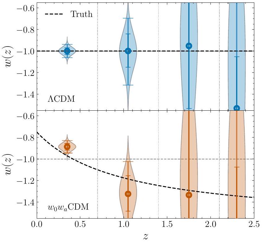
and
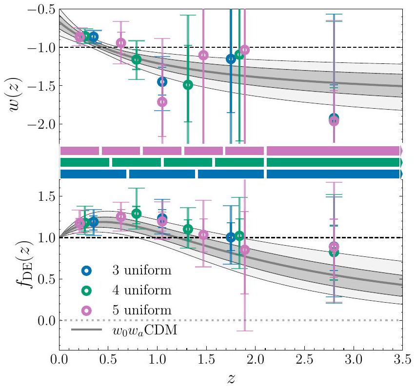
A. Binning
Overall, the binning results from different schemes are in good general agreement. The crossing of phantom divide line by
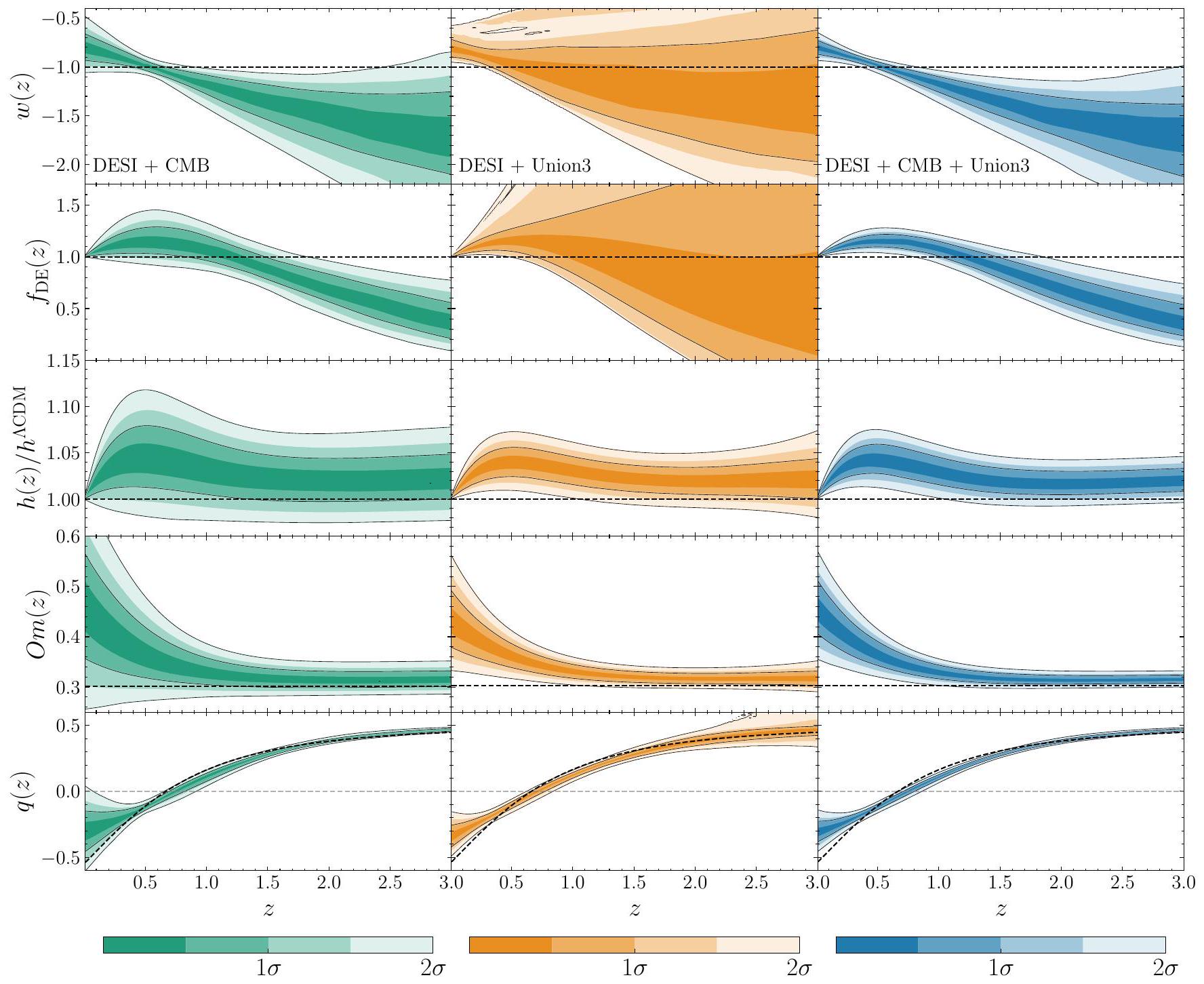
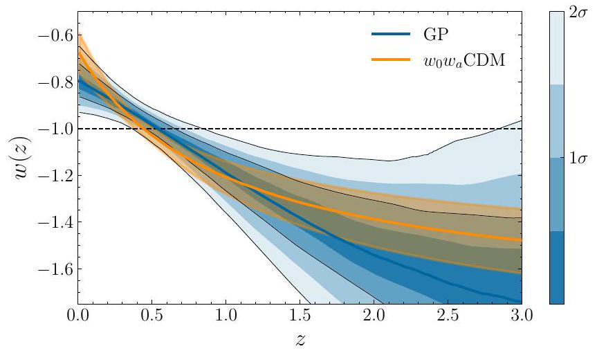
B. Gaussian Process Regression
and hints of
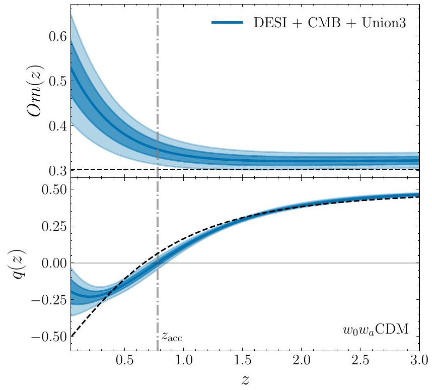
VI. IMPLICATIONS FOR DARK ENERGY
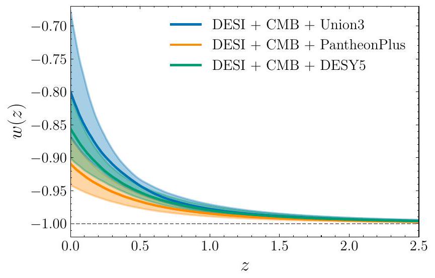
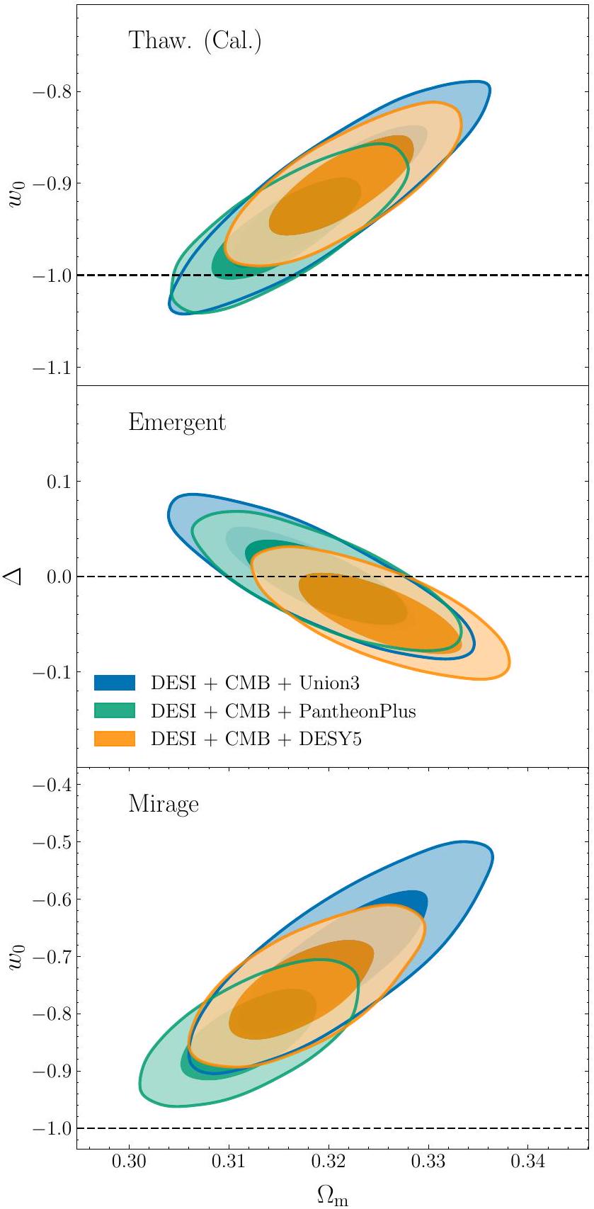
A. Thawing dark energy
B. Emergent dark energy
C. Mirage dark energy
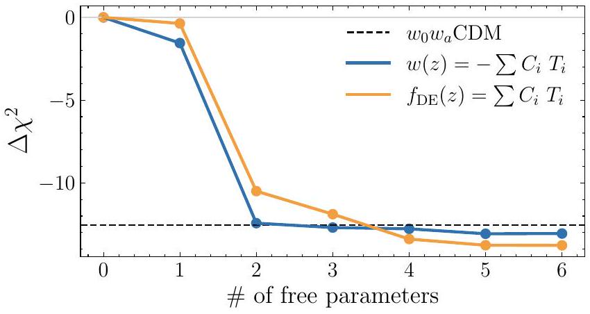
D. Model Comparison
| DESI+CMB: | +PantheonPlus | +Union3 | +DESY5 |
| DE classes |
|
||
| Thaw. (Cal.) | +0.4 (-1.6) | -0.6 (-2.5) | -5.8 (-7.1) |
| Thaw. (Alg.) | -1.0 (-2.9) | -4.6 (-6.9) | -10.1 (-13.2) |
| Emergent | +2.1 (-0.05) | +1.8 (-0.1) | +0.2 (-1.5) |
| Mirage | -9.1 (-10.5) | -13.8 (-16.2) | -18.7 (-20.7) |
|
|
-6.8 (-10.7) | -13.5 (-17.4) | -17.2 (-21.0) |
E. Is there evidence for phantom crossing?
underperform compared to those that do. The specific behavior of
VII. CONCLUSIONS
straints support the evolution indicated by the
VIII. DATA AVAILABILITY
ACKNOWLEDGMENTS
nautics and Space Administration. Legacy Surveys was supported by: the Director, Office of Science, Office of High Energy Physics of the U.S. Department of Energy; the National Energy Research Scientific Computing Center, a DOE Office of Science User Facility; the U.S. National Science Foundation, Division of Astronomical Sciences; the National Astronomical Observatories of China, the Chinese Academy of Sciences and the Chinese National Natural Science Foundation. LBNL is managed by the Regents of the University of California under contract to the U.S. Department of En-
ergy. The complete acknowledgments can be found at https://www.legacysurvey.org/
[1] A. Einstein, Sitzungsber. Preuss. Akad. Wiss. Berlin (Math. Phys. ) 1917, 142 (1917).
[2] A. G. Riess and others (Supernova Search Team), Astron. J. 116, 1009 (1998), arXiv:astro-ph/9805201.
[3] S. Perlmutter and others (Supernova Cosmology Project), Astrophys. J. 517, 565 (1999) arXiv:astroph/9812133
[4] W. J. Percival, W. Sutherland, J. A. Peacock, C. M. Baugh, and others, MNRAS 337, 1068 (2002). arXiv:astro-ph/0206256 [astro-ph]
[5] D. J. Eisenstein, New A Rev. 49, 360 (2005)
[6] S. Cole, W. J. Percival, J. A. Peacock, P. Norberg, and others, MNRAS 362, 505 (2005) arXiv:astroph/0501174 [astro-ph]
[7] Planck Collaboration, N. Aghanim, Y. Akrami, M. Ashdown, and others, A&A 641, A6 (2020). arXiv:1807.06209 [astro-ph.CO].
[8] S. Alam, M. Aubert, S. Avila, C. Balland, and others, Physical Review D 103, 10.1103/physrevd.103.083533 (2021).
[9] C. Zhao, A. Variu, M. He, D. Forero-Sánchez, and others, Monthly Notices of the Royal Astronomical Society 511, 5492-5524 (2022)
[10] T. M. C. Abbott and others (DES), Phys. Rev. D 98, 043526 (2018), arXiv:1708.01530 [astro-ph.CO]
[11] M. A. Troxel and others (DES), Phys. Rev. D 98, 043528 (2018), arXiv:1708.01538 [astro-ph.CO]
[12] S. Alam and others (eBOSS),Phys. Rev. D 103, 083533 (2021), arXiv:2007.08991 [astro-ph.CO]
[13] C. Heymans and others, Astron. Astrophys. 646, A140 (2021), arXiv:2007.15632 [astro-ph.CO]
[14] T. M. C. Abbott and others (DES), Phys. Rev. D 105, 023520 (2022), arXiv:2105.13549 [astro-ph.CO]
[15] G. Efstathiou, W. J. Sutherland, and S. J. Maddox, Nature 348, 705 (1990).
[16] J. Frieman, M. Turner, and D. Huterer, Ann. Rev. Astron. Astrophys. 46, 385 (2008), arXiv:0803.0982 [astroph]
[17] D. H. Weinberg, M. J. Mortonson, D. J. Eisenstein, C. Hirata, and others, Phys. Rept. 530, 87 (2013). arXiv:1201.2434 [astro-ph.CO].
[18] J. P. Ostriker and P. J. Steinhardt, Nature 377, 600 (1995)
[19] S. Weinberg, Rev. Mod. Phys. 61, 1 (1989).
[20] B. Ratra and P. J. E. Peebles, Phys. Rev. D 37, 3406 (1988)
[21] P. J. E. Peebles and B. Ratra, Astrophys. J. Lett. 325,
[22] V. Sahni and A. A. Starobinsky, Int. J. Mod. Phys. D 9, 373 (2000), arXiv:astro-ph/9904398
[23] P. J. E. Peebles and B. Ratra, Rev. Mod. Phys. 75, 559 (2003), arXiv:astro-ph/0207347
[24] E. J. Copeland, M. Sami, and S. Tsujikawa, Int. J. Mod. Phys. D 15, 1753 (2006), arXiv:hep-th/0603057.
[25] P. Bull and others, Phys. Dark Univ. 12, 56 (2016), arXiv:1512.05356 [astro-ph.CO]
[26] L. Perivolaropoulos and F. Skara, New Astron. Rev. 95, 101659 (2022), arXiv:2105.05208 [astro-ph.CO]
[27] M. Levi, C. Bebek, T. Beers, R. Blum, and others, arXiv e-prints , arXiv:1308.0847 (2013), arXiv:1308.0847 [astro-ph.CO].
[28] DESI Collaboration, A. Aghamousa, J. Aguilar, S. Ahlen, and others, arXiv e-prints, arXiv:1611.00037 (2016), arXiv:1611.00037 [astro-ph.IM]
[29] C. Poppett, L. Tyas, J. Aguilar, C. Bebek, and others, AJ 168, 245 (2024).
[30] J. H. Silber, P. Fagrelius, K. Fanning, M. Schubnell, and others, AJ 165, 9 (2023) arXiv:2205.09014 [astroph.IM].
[31] T. N. Miller, P. Doel, G. Gutierrez, R. Besuner, and others, AJ 168, 95 (2024), arXiv:2306.06310 [astro-ph.IM].
[32] J. Guy, S. Bailey, A. Kremin, S. Alam, and others, AJ 165, 144 (2023), arXiv:2209.14482 [astro-ph.IM]
[33] E. F. Schlafly, D. Kirkby, D. J. Schlegel, A. D. Myers, and others, AJ 166, 259 (2023) arXiv:2306.06309 [astro-ph.CO].
[34] DESI Collaboration, A. Aghamousa, J. Aguilar, S. Ahlen, and others, arXiv e-prints, arXiv:1611.00036 (2016), arXiv:1611.00036 [astro-ph.IM].
[35] DESI Collaboration, B. Abareshi, J. Aguilar, S. Ahlen, and others, AJ 164, 207 (2022), arXiv:2205.10939 [astro-ph.IM]
[36] DESI Collaboration, A. G. Adame, J. Aguilar, S. Ahlen, and others, AJ 168, 58 (2024), arXiv:2306.06308 [astroph.CO].
[37] DESI Collaboration, M. A. Karim, A. G. Adame, D. Aguado, and others, arXiv e-prints , arXiv:2503.14745 (2025), arXiv:2503.14745 [astroph.CO]
[38] DESI Collaboration, A. G. Adame, J. Aguilar, S. Ahlen, and others, arXiv e-prints, arXiv:2404.03000 (2024), arXiv:2404.03000 [astro-ph.CO]
[39] DESI Collaboration, A. G. Adame, J. Aguilar, S. Ahlen, and others, J. Cosmology Astropart. Phys. 2025, 124
(2025), arXiv:2404.03001 [astro-ph.CO]
[40] DESI Collaboration, A. G. Adame, J. Aguilar, S. Ahlen, and others, J. Cosmology Astropart. Phys. 2025, 021 (2025), arXiv:2404.03002 [astro-ph.CO]
[41] DESI Collaboration, A. G. Adame, J. Aguilar, S. Ahlen, and others, arXiv e-prints, arXiv:2411.12022 (2024) arXiv:2411.12022 [astro-ph.CO].
[42] DESI Collaboration, A. G. Adame, J. Aguilar, S. Ahlen, and others, arXiv e-prints, arXiv:2411.12021 (2024) arXiv:2411.12021 [astro-ph.CO].
[43] R. Calderon and others (DESI), JCAP 10, 048. arXiv:2405.04216 [astro-ph.CO].
[44] K. Lodha and others (DESI),Phys. Rev. D 111, 023532 (2025), arXiv:2405.13588 [astro-ph.CO]
[45] DESI Collaboration, in preparation (2026).
[46] DESI Collaboration, M. A. Karim, J. Aguilar, S. Ahlen, and others, arXiv e-prints , arXiv:2503.14739 (2025). arXiv:2503.14739 [astro-ph.CO].
[47] DESI Collaboration, M. A. Karim, J. Aguilar, S. Ahlen, and others, arXiv e-prints , arXiv:2503.14738 (2025) arXiv:2503.14738 [astro-ph.CO].
[48] W. Elbers, A. Aviles, H. E. Noriega, D. Chebat, and others, arXiv e-prints, arXiv:2503.14744 (2025). arXiv:2503.14744 [astro-ph.CO].
[49] D. Huterer and M. S. Turner, Phys. Rev. D 64, 123527 (2001), arXiv:astro-ph/0012510
[50] M. Chevallier and D. Polarski, International Journal of Modern Physics D 10, 213-223 (2001).
[51] E. V. Linder, Phys. Rev. Lett. 90, 091301 (2003). arXiv:astro-ph/0208512 [astro-ph]
[52] D. Huterer and G. Starkman, Physical Review Letters 90, 10.1103/physrevlett.90.031301 (2003).
[53] A. Shafieloo, U. Alam, V. Sahni, and A. A. Starobinsky, Mon. Not. Roy. Astron. Soc. 366, 1081 (2006). arXiv:astro-ph/0505329.
[54] R. de Putter and E. V. Linder, J. Cosmology Astropart. Phys. 2008, 042 (2008), arXiv:0808.0189 [astro-ph]
[55] R. G. Crittenden, L. Pogosian, and G.-B. Zhao, J. Cosmology Astropart. Phys. 2009, 025 (2009) arXiv:astroph/0510293 [astro-ph]
[56] C. Bogdanos and S. Nesseris, JCAP 05, 006. arXiv:0903.2805 [astro-ph.CO].
[57] T. Holsclaw, U. Alam, B. Sansó, H. Lee, and others, Phys. Rev. Lett. 105, 241302 (2010).
[58] T. Holsclaw, U. Alam, B. Sansó, H. Lee, and others, Physical Review D 84, 10.1103/physrevd.84.083501 (2011).
[59] G.-B. Zhao, R. G. Crittenden, L. Pogosian, and X. Zhang, Phys. Rev. Lett. 109, 171301 (2012). arXiv:1207.3804 [astro-ph.CO].
[60] S. Nesseris and J. García-Bellido, Journal of Cosmology and Astroparticle Physics 2012 (11), 033-033
[61] B. L’Huillier and A. Shafieloo, JCAP 01, 015. arXiv:1606.06832 [astro-ph.CO].
[62] R. Calderón, B. L’Huillier, D. Polarski, A. Shafieloo, and others, Phys. Rev. D 106, 083513 (2022). arXiv:2206.13820 [astro-ph.CO].
[63] R. L. Workman, V. D. Burkert, V. Crede, E. Klempt, and others, Progress of Theoretical and Experimental Physics 2022, 083C01 (2022)
[64] J. Lesgourgues and S. Pastor, Phys. Rep. 429, 307 (2006) arXiv:astro-ph/0603494 [astro-ph]
[65] D. J. Eisenstein, I. Zehavi, D. W. Hogg, R. Scoccimarro, and others, ApJ 633, 560 (2005) arXiv:astro-
ph/0501171 [astro-ph].
[66] U. Andrade, E. Paillas, J. Mena-Fernández, Q. Li, and others, arXiv e-prints, arXiv:2503.14742 (2025), arXiv:2503.14742 [astro-ph.CO]
[67] L. Casas, H. K. Herrera-Alcantar, J. Chaves-Montero, A. Cuceu, and others, arXiv e-prints, arXiv:2503.14741 (2025), arXiv:2503.14741 [astro-ph.IM]
[68] A. Brodzeller, M. Wolfson, D. M. Santos, M. Ho, and others, arXiv e-prints, arXiv:2503.14740 (2025), arXiv:2503.14740 [astro-ph.CO]
[69] D. Brout, D. Scolnic, B. Popovic, A. G. Riess, and others, ApJ 938, 110 (2022) arXiv:2202.04077 [astroph.CO]
[70] D. Rubin, G. Aldering, M. Betoule, A. Fruchter, and others, arXiv e-prints, arXiv:2311.12098 (2023), arXiv:2311.12098 [astro-ph.CO]
[71] T. M. C. Abbott and others (DES), ApJ (accepted, 2024), arXiv:2401.02929 [astro-ph.CO]
[72] Planck Collaboration, N. Aghanim, Y. Akrami, F. Arroja, and others, A&A 641, A1 (2020). arXiv:1807.06205 [astro-ph.CO]
[73] N. Aghanim and others (Planck), Astron. Astrophys. 641, A5 (2020), arXiv:1907.12875 [astro-ph.CO]
[74] G. Efstathiou and S. Gratton, The Open Journal of Astrophysics 4, 8 (2021)
[75] J. Torrado and A. Lewis, J. Cosmology Astropart. Phys. 2021, 057 (2021), arXiv:2005.05290 [astro-ph.IM]
[76] J. Carron, M. Mirmelstein, and A. Lewis, JCAP 09, 039 arXiv:2206.07773 [astro-ph.CO]
[77] E. Rosenberg, S. Gratton, and G. Efstathiou, MNRAS 517, 4620 (2022), arXiv:2205.10869 [astro-ph.CO]
[78] M. S. Madhavacheril, F. J. Qu, B. D. Sherwin, N. MacCrann, and others, ApJ 962, 113 (2024). arXiv:2304.05203 [astro-ph.CO]
[79] G. S. Farren and others (ACT), Astrophys. J. 966, 157 (2024), arXiv:2309.05659 [astro-ph.CO].
[80] P. Lemos and A. Lewis, Phys. Rev. D 107, 103505 (2023), arXiv:2302.12911 [astro-ph.CO]
[81] A. Lewis and S. Bridle, Phys. Rev. D 66, 103511 (2002), arXiv:astro-ph/0205436 [astro-ph]
[82] A. Lewis, Phys. Rev. D 87, 103529 (2013), arXiv:1304.4473 [astro-ph.CO]
[83] J. Torrado and A. Lewis, J. Cosmology Astropart. Phys. 05, 057 (2021), arXiv:2005.05290 [astro-ph.IM]
[84] R. M. Neal, arXiv Mathematics e-prints , math/0502099 (2005), arXiv:math/0502099 [math.ST].
[85] A. Lewis, A. Challinor, and A. Lasenby, ApJ 538, 473 (2000), arXiv:astro-ph/9911177 [astro-ph].
[86] C. Howlett, A. Lewis, A. Hall, and A. Challinor, J. Cosmology Astropart. Phys. 2012, 027 (2012). arXiv:1201.3654 [astro-ph.CO]
[87] W. Hu and I. Sawicki, Phys. Rev. D 76, 104043 (2007), arXiv:0708.1190 [astro-ph]
[88] W. Fang, W. Hu, and A. Lewis,/Phys. Rev. D 78, 087303 (2008), arXiv:0808.3125 [astro-ph].
[89] J. Lesgourgues, The Cosmic Linear Anisotropy Solving System (CLASS) I: Overview (2011), arXiv:1104.2932 [astro-ph.IM]
[90] D. Blas, J. Lesgourgues, and T. Tram, J. Cosmology Astropart. Phys. 1107, 034 (2011), arXiv:1104.2933 [astroph.CO]
[91] H. Dembinski and P. O. et al., scikit-hep/iminuit (2020).
[92] M. Ishak, J. Pan, R. Calderon, K. Lodha, and others, arXiv e-prints , arXiv:2411.12026 (2024).
arXiv:2411.12026 [astro-ph.CO].
[93] V. Poulin, T. L. Smith, R. Calderón, and T. Simon, arXiv:2407.18292 [astro-ph.CO] (2024).
[94] R. R. Caldwell, Phys. Lett. B 545, 23 (2002), arXiv:astro-ph/9908168.
[95] S. W. Hawking and G. F. R. Ellis, The Large Scale Structure of Space-Time Cambridge Monographs on Mathematical Physics (Cambridge University Press, 2023).
[96] V. Sahni, A. Shafieloo, and A. A. Starobinsky, Phys. Rev. D 78, 103502 (2008), arXiv:0807.3548 [astro-ph].
[97] I. Wasserman, Phys. Rev. D 66, 123511 (2002). arXiv:astro-ph/0203137.
[98] M. Kunz, Phys. Rev. D 80, 123001 (2009).
[99] A. Shafieloo and E. V. Linder, Phys. Rev. D 84, 063519 (2011)
[100] W. Giarè, M. Najafi, S. Pan, E. Di Valentino, and others, JCAP 10, 035 arXiv:2407.16689 [astro-ph.CO].
[101] W. J. Wolf, C. García-García, and P. G. Ferreira, arXiv:2502.04929 [astro-ph.CO] (2025).
[102] E. M. Barboza and J. S. Alcaniz, Physics Letters B 666, 415 (2008), arXiv:0805.1713 [astro-ph]
[103] G. Efstathiou, MNRAS 310, 842 (1999) arXiv:astroph/9904356 [astro-ph]
[104] N. Dimakis, A. Karagiorgos, A. Zampeli, A. Paliathanasis, and others, Phys. Rev. D 93, 123518 (2016). arXiv:1604.05168 [gr-qc]
[105] S. Pan, W. Yang, and A. Paliathanasis, European Physical Journal C 80, 274 (2020), arXiv:1902.07108 [astroph.CO]
[106] H. K. Jassal, J. S. Bagla, and T. Padmanabhan, Phys. Rev. D 72, 103503 (2005) arXiv:astroph/0506748 [astro-ph]
[107] A. Shafieloo, T. Clifton, and P. Ferreira, Journal of Cosmology and Astroparticle Physics 2011 (08), 017.
[108] A. Shafieloo, Journal of Cosmology and Astroparticle Physics 2012 (08), 002-002
[109] A. Shafieloo, Journal of Cosmology and Astroparticle Physics 2012 (05), 024-024
[110] S. Haude, S. Salehi, S. Vidal, M. Maturi, and others, arXiv:1912.04560 [astro-ph.CO] (2019).
[111] J. Grande, J. Solà Peracaula, and H. Stefancic, JCAP 08, 011, arXiv:gr-qc/0604057.
[112] J. A. Vazquez, S. Hee, M. P. Hobson, A. N. Lasenby, and others, JCAP 07, 062, arXiv:1208.2542 [astroph.CO]
[113] L. Visinelli, S. Vagnozzi, and U. Danielsson, Symmetry 11, 1035 (2019), arXiv:1907.07953 [astro-ph.CO]
[114] R. Calderón, R. Gannouji, B. L’Huillier, and D. Polarski, Phys. Rev. D 103, 10.1103/physrevd.103.023526 (2021).
[115] T. Chiba, T. Okabe, and M. Yamaguchi, Phys. Rev. D 62, 023511 (2000), arXiv:astro-ph/9912463
[116] V. Sahni and Y. Shtanov, Journal of Cosmology and Astroparticle Physics 2003 (11), 014
[117] F. Bauer, J. Solà , and H. Stefancić, Journal of Cosmology and Astroparticle Physics 2010 (12), 029
[118] B. Boisseau, H. Giacomini, D. Polarski, and A. A. Starobinsky, JCAP 07, 002, arXiv:1504.07927 [gr-qc].
[119] E. V. Linder and D. Huterer, Phys. Rev. D 72, 043509 (2005), arXiv:astro-ph/0505330
[120] D. Muthukrishna and D. Parkinson, JCAP 11, 052. arXiv:1607.01884 [astro-ph.CO].
[121] R. Camilleri and others (DES), Mon. Not. Roy. Astron.
[122] M. Tegmark, Physical Review D 55, 5895-5907 (1997).
[123] D. Huterer and A. Cooray, Physical Review D 71, 10.1103/physrevd.71.023506 (2005).
[124] R. G. Crittenden, L. Pogosian, and G.-B. Zhao, JCAP 12, 025, arXiv:astro-ph/0510293.
[125] F. Simpson and S. Bridle, Phys. Rev. D 73, 083001 (2006), arXiv:astro-ph/0602213
[126] C. Garcia-Quintero, M. Ishak, and O. Ning, JCAP 12, 018, arXiv:2010.12519 [astro-ph.CO]
[127] P. A. R. Ade and others (Planck), Astron. Astrophys. 594, A14 (2016), arXiv:1502.01590 [astro-ph.CO]
[128] G.-B. Zhao and others, Nature Astron. 1, 627 (2017), arXiv:1701.08165 [astro-ph.CO]
[129] M. Raveri, L. Pogosian, K. Koyama, M. Martinelli, and others, A joint reconstruction of dark energy and modified growth evolution (2021), arXiv:2107.12990 [astro-ph.CO].
[130] L. Pogosian, M. Raveri, K. Koyama, M. Martinelli, and others, Nature Astron. 6, 1484 (2022). arXiv:2107.12992 [astro-ph.CO]
[131] P. Bansal and D. Huterer, arXiv:2502.07185 [astroph.CO] (2025).
[132] J. a. Rebouças, D. H. F. de Souza, K. Zhong, V. Miranda, and others, JCAP 02, 024, arXiv:2408.14628 [astro-ph.CO].
[133] Y.-H. Pang, X. Zhang, and Q.-G. Huang, arXiv:2408.14787 [astro-ph.CO] (2024).
[134] W. Handley, The Journal of Open Source Software 3, 10.21105/joss. 00849 (2018).
[135] C. Rasmussen and C. Williams, Gaussian Processes for Machine Learning, Adaptative computation and machine learning series (University Press Group Limited, 2006).
[136] T. Holsclaw, U. Alam, B. Sansó, H. Lee, and others, Physical Review D 82, 10.1103/physrevd.82.103502 (2010).
[137] T. Holsclaw, U. Alam, B. Sansó, H. Lee, and others, Phys. Rev. Lett. 105, 241302 (2010)
[138] A. Shafieloo, A. G. Kim, and E. V. Linder, Phys. Rev. D 85, 123530 (2012) arXiv:1204.2272 [astro-ph.CO]
[139] M. Seikel, C. Clarkson, and M. Smith, Journal of Cosmology and Astroparticle Physics 2012 (06), 036-036.
[140] A. Shafieloo, A. G. Kim, and E. V. Linder, Phys. Rev. D 87, 023520 (2013), arXiv:1211.6128 [astro-ph.CO].
[141] R. E. Keeley, S. Joudaki, M. Kaplinghat, and D. Kirkby, JCAP 12, 035, arXiv:1905.10198 [astro-ph.CO]
[142] E. Belgacem, S. Foffa, M. Maggiore, and T. Yang, Phys. Rev. D 101, 063505 (2020), arXiv:1911.11497 astroph.CO]
[143] R. E. Keeley, A. Shafieloo, B. L’Huillier, and E. V. Linder, Mon. Not. Roy. Astron. Soc. 491, 3983 (2020), arXiv:1905.10216 [astro-ph.CO]
[144] F. Gerardi, M. Martinelli, and A. Silvestri, JCAP 07, 042 arXiv:1902.09423 [astro-ph.CO]
[145] P. Mukherjee and A. Mukherjee, Mon. Not. Roy. Astron. Soc. 504, 3938 (2021), arXiv:2104.06066 [astro-ph.CO].
[146] R. Calderón, B. L’Huillier, D. Polarski, A. Shafieloo, and others, Phys. Rev. D 108, 023504 (2023), arXiv:2301.00640 [astro-ph.CO]
[147] B. R. Dinda and R. Maartens, JCAP 01, 120. arXiv:2407.17252 [astro-ph.CO]
[148] P. Mukherjee and A. A. Sen, Phys. Rev. D 110, 123502 (2024), arXiv:2405.19178 [astro-ph.CO].
[149] S. Joudaki, M. Kaplinghat, R. Keeley, and D. Kirkby, Phys. Rev. D 97, 123501 (2018) arXiv:1710.04236 [astro-ph.CO]
[150] S.-g. Hwang, B. L’Huillier, R. E. Keeley, M. J. Jee, and others, JCAP 02, 014, arXiv:2206.15081 [astroph.CO]
[151] R. R. Caldwell and E. V. Linder, Phys. Rev. Lett. 95, 141301 (2005), arXiv:astro-ph/0505494.
[152] E. V. Linder, Phys. Rev. D 73, 063010 (2006). arXiv:astro-ph/0601052
[153] R. N. Cahn, R. de Putter, and E. V. Linder, JCAP 11, 015, arXiv:0807.1346 [astro-ph].
[154] B. Ratra and P. J. E. Peebles, Phys. Rev. D 37, 3406 (1988)
[155] C. Wetterich, Nucl. Phys. B 302, 668 (1988). arXiv:1711.03844 [hep-th]
[156] P. G. Ferreira and M. Joyce, Phys. Rev. D 58, 023503 (1998), arXiv:astro-ph/9711102
[157] R. J. Scherrer and A. A. Sen, Phys. Rev. D 77, 083515 (2008), arXiv:0712.3450 [astro-ph]
[158] S. Tsujikawa, Class. Quant. Grav. 30, 214003 (2013). arXiv:1304.1961 [gr-qc]
[159] J. Martin, Mod. Phys. Lett. A 23, 1252 (2008). arXiv:0803.4076 [astro-ph]
[160] J. A. Frieman, C. T. Hill, A. Stebbins, and I. Waga, Phys. Rev. Lett. 75, 2077 (1995), arXiv:astroph/9505060
[161] J. M. Cline, S. Jeon, and G. D. Moore, Phys. Rev. D 70, 043543 (2004), arXiv:hep-ph/0311312.
[162] A. Vikman, Phys. Rev. D 71, 023515 (2005). arXiv:astro-ph/0407107.
[163] E. V. Linder, Gen. Rel. Grav. 40, 329 (2008). arXiv:0704.2064 [astro-ph]
[164] E. V. Linder, Phys. Rev. D 91, 063006 (2015). arXiv:1501.01634 [astro-ph.CO].
[165] R. Crittenden, E. Majerotto, and F. Piazza, Phys. Rev. Lett. 98, 251301 (2007), arXiv:astro-ph/0702003.
[166] N. Kaloper and L. Sorbo, JCAP 04, 007, arXiv:astroph/0511543
[167] D. J. E. Marsh, Phys. Rept. 643, 1 (2016). arXiv:1510.07633 [astro-ph.CO].
[168] S. Dutta and R. J. Scherrer, Phys. Rev. D 78, 123525 (2008), arXiv:0809.4441 [astro-ph]
[169] X. Li and A. Shafieloo, Astrophys. J. Lett. 883, L3 (2019), arXiv:1906.08275 [astro-ph.CO]
[170] X. Li and A. Shafieloo, Astrophys. J. 902, 58 (2020). arXiv:2001.05103 [astro-ph.CO].
[171] L. Parker and A. Raval, Phys. Rev. D 62, 083503 (2000), [Erratum: Phys.Rev.D 67, 029903 (2003)], arXiv:grqc/0003103
[172] R. R. Caldwell, W. Komp, L. Parker, and D. A. T. Vanzella, Phys. Rev. D 73, 023513 (2006) arXiv:astroph/0507622
[173] A. Banihashemi, N. Khosravi, and A. Shafieloo, JCAP 06, 003, arXiv:2012.01407 [astro-ph.CO].
[174] M. S. Turner, Phys. Rev. D 31, 1212 (1985).
[175] L. Barnes, M. J. Francis, G. F. Lewis, and E. V. Linder, Publ. Astron. Soc. Austral. 22, 315 (2005), arXiv:astroph/0510791
[176] W. Zimdahl, Int. J. Mod. Phys. D 14, 2319 (2005). arXiv:gr-qc/0505056
[177] E. V. Linder, arXiv:0708.0024 [astro-ph] (2007).
[178] E. V. Linder and M. J. White,|Phys. Rev. D 72, 061304 (2005), arXiv:astro-ph/0508401
[179] M. J. Francis, G. F. Lewis, and E. V. Linder, Mon. Not. Roy. Astron. Soc. 380, 1079 (2007) arXiv:0704.0312 [astro-ph]
[180] E. V. Linder, (2024), arXiv:2410.10981 [astro-ph.CO].
[181] D. J. Spiegelhalter, N. G. Best, B. P. Carlin, and A. Van Der Linde, Journal of the royal statistical society: Series b (statistical methodology) 64, 583 (2002).
[182] A. R. Liddle, Monthly Notices of the Royal Astronomical Society: Letters 377, L74 (2007).
[183] S. Grandis, D. Rapetti, A. Saro, J. J. Mohr, and others, Mon. Not. Roy. Astron. Soc. 463, 1416 (2016), arXiv:1604.06463 [astro-ph.CO]
[184] W. J. Wolf, C. García-García, D. J. Bartlett, and P. G. Ferreira, Phys. Rev. D 110, 083528 (2024), arXiv:2408.17318 [astro-ph.CO]
[185] D. Shlivko and P. Steinhardt, (2024), arXiv:2405.03933 [astro-ph.CO].
[186] G. Payeur, E. McDonough, and R. Brandenberger, arXiv:2411.13637 [astro-ph.CO] (2024).
[187] W. Hu, Phys. Rev. D 71, 047301 (2005), arXiv:astroph/0410680
[188] Z.-K. Guo, Y.-S. Piao, X.-M. Zhang, and Y.-Z. Zhang, Phys. Lett. B 608, 177 (2005), arXiv:astro-ph/0410654.
[189] H. Wei, R.-G. Cai, and D.-F. Zeng, Class. Quant. Grav. 22, 3189 (2005), arXiv:hep-th/0501160
[190] R. R. Caldwell and M. Doran, Phys. Rev. D 72, 043527 (2005), arXiv:astro-ph/0501104
[191] Y.-F. Cai, T. Qiu, R. Brandenberger, Y.-S. Piao, and others, JCAP 03, 013, arXiv:0711.2187 [hep-th].
[192] Y.-F. Cai, T. Qiu, Y.-S. Piao, M. Li, and others, JHEP 10, 071 arXiv:0704.1090 [gr-qc].
[193] L. Amendola, Phys. Rev. D 62, 043511 (2000), arXiv:astro-ph/9908023
[194] A. P. Billyard and A. A. Coley, Phys. Rev. D 61, 083503 (2000), arXiv:astro-ph/9908224
[195] L. Amendola, Phys. Rev. D 69, 103524 (2004), arXiv:astro-ph/0311175
[196] S. Nojiri, S. D. Odintsov, and S. Tsujikawa, Phys. Rev. D 71, 063004 (2005) arXiv:hep-th/0501025
[197] T. Clemson, K. Koyama, G.-B. Zhao, R. Maartens, and others, Phys. Rev. D 85, 043007 (2012), arXiv:1109.6234 [astro-ph.CO]
[198] A. Shafieloo, D. K. Hazra, V. Sahni, and A. A. Starobinsky, Monthly Notices of the Royal Astronomical Society 473, 2760-2770 (2017)
[199] F. C. Carvalho and A. Saa, Phys. Rev. D 70, 087302 (2004), arXiv:astro-ph/0408013
[200] W. Hu and I. Sawicki, Phys. Rev. D 76, 064004 (2007), arXiv:0705.1158 [astro-ph]
[201] J. Martin, C. Schimd, and J.-P. Uzan, Phys. Rev. Lett. 96, 061303 (2006).
[202] A. Anisimov, E. Babichev, and A. Vikman, JCAP 06, 006 arXiv:astro-ph/0504560.
[203] S. Nesseris and L. Perivolaropoulos, Phys. Rev. D 73, 103511 (2006), arXiv:astro-ph/0602053
[204] C. Deffayet, O. Pujolas, I. Sawicki, and A. Vikman, JCAP 10, 026, arXiv:1008.0048 [hep-th]
[205] O. Pujolas, I. Sawicki, and A. Vikman, JHEP 11, 156. arXiv:1103.5360 [hep-th].
[206] G. Ye, M. Martinelli, B. Hu, and A. Silvestri, arXiv:2407.15832 [astro-ph.CO] (2024).
[207] W. J. Wolf, P. G. Ferreira, and C. García-García, Phys. Rev. D 111, L041303 (2025), arXiv:2409.17019 [astroph.CO]
[208] Y. Yang, X. Ren, Q. Wang, Z. Lu, and others, Sci. Bull. 69, 2698 (2024), arXiv:2404.19437 [astro-ph.CO]
[209] O. Christiansen, F. Hassani, and D. F. Mota, JCAP 01, 043, arXiv:2405.00668 [astro-ph.CO]
[210] M. Rigault, M. Smith, A. Goobar, K. Maguire, and others, arXiv e-prints, arXiv:2409.04346 (2024). arXiv:2409.04346 [astro-ph.CO].
[211] E. C. Bellm, S. R. Kulkarni, M. J. Graham, R. Dekany, and others, PASP 131, 018002 (2019), arXiv:1902.01932 [astro-ph.IM]
[212] M. Lochner, D. Scolnic, H. Almoubayyed, T. Anguita, and others, ApJS 259, 58 (2022) arXiv:2104.05676 [astro-ph.CO]
[213] P. Gris, N. Regnault, H. Awan, I. Hook, and others, ApJS 264, 22 (2023), arXiv:2205.07651 [astro-ph.CO].
[214] D. Spergel, N. Gehrels, C. Baltay, D. Bennett, and others, Wide-field infrarred survey telescope-astrophysics focused telescope assets wfirst-afta 2015 report (2015), arXiv:1503.03757 [astro-ph.IM].
[215] R. Laureijs, J. Amiaux, S. Arduini, J. L. Auguères, and others, arXiv e-prints , arXiv:1110.3193 (2011). arXiv:1110.3193 [astro-ph.CO].
[216] W. J. Handley, M. P. Hobson, and A. N. Lasenby, Mon. Not. Roy. Astron. Soc. 450, L61 (2015). arXiv:1502.01856 [astro-ph.CO].
[217] W. Handley, J. Open Source Softw. 4, 1414 (2019). arXiv:1905.04768 [astro-ph.IM].
[218] L. T. Hergt, W. J. Handley, M. P. Hobson, and A. N. Lasenby, Phys. Rev. D 103, 123511 (2021), arXiv:2102.11511 [astro-ph.CO].
[219] H. Jeffreys, The Theory of Probability, Oxford Classic Texts in the Physical Sciences (1939).
[220] R. Trotta, Mon. Not. Roy. Astron. Soc. 378, 72 (2007), arXiv:astro-ph/0504022.
[221] L. Amendola and S. Tsujikawa, Dark Energy: Theory and Observations (Cambridge University Press, 2015).
[222] A. J. Shajib and J. A. Frieman, arXiv:2502.06929 [astroph.CO] (2025).
[223] V. Smer-Barreto and A. R. Liddle, Journal of Cosmology and Astroparticle Physics 2017 (01), 023-023
[224] A. Abrahamse, A. Albrecht, M. Barnard, and B. Bozek, Phys. Rev. D 77, 103503 (2008), arXiv:0712.2879 [astroph]
[225] M. Kawasaki, T. Moroi, and T. Takahashi, Phys. Rev. D 64, 083009 (2001), arXiv:astro-ph/0105161
[226] S. C. C. Ng and D. L. Wiltshire, Phys. Rev. D 63, 023503 (2001) arXiv:astro-ph/0004138.
[227] K. Coble, S. Dodelson, and J. A. Frieman, Phys. Rev. D 55, 1851 (1997), arXiv:astro-ph/9608122
[228] J. A. Frieman and I. Waga, Phys. Rev. D 57, 4642 (1998), arXiv:astro-ph/9709063
[229] P. T. P. Viana and A. R. Liddle, Phys. Rev. D 57, 674 (1998), arXiv:astro-ph/9708247
[230] F. X. L. Cedeño, A. X. González-Morales, and L. A. Ureña López, Phys. Rev. D 96, 061301 (2017). arXiv:1703.10180 [gr-qc]
[231] F. X. Linares Cedeño, A. X. González-Morales, and L. A. Ureña López, JCAP 01, 051, arXiv:2006.05037 [astro-ph.CO].
Appendix A: Bayesian Model Comparison
| +PantheonPlus | +Union3 | +DESY5 | |
| DESI DR2 BAO + CMB | |||
|
|
|
|
|
|
|
|
|
|
|
|
|
|
|
| DESI DR1 BAO + CMB | |||
|
|
|
|
|
|
|
|
|
|
|
|
|
|
|
Appendix B: Details of Binning PCA
Appendix C: Details on Gaussian Process Regression
Appendix D: Quintessence
Appendix E: Validation on Mocks
preparing a third mock following Eq. (15) with
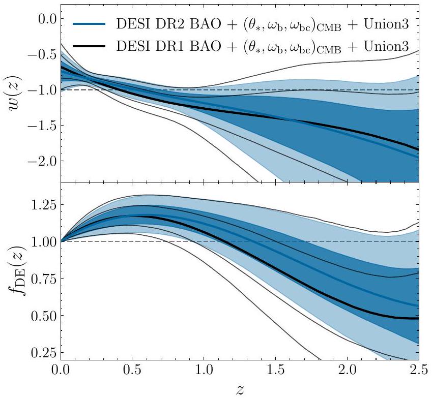
Appendix F: Comparison with DESI DR1
Note that, as pointed out in our discussion about neutrinos, they do not contribute to the matter content of the Universe during recombination, and therefore we use explicitly instead of . In the text is used in place of , for convenience. In the numerical implementation we truncate at order in Taylor expansion. Note that the redshift interval relevant for observations is mapped to , where the Chebyshev polynomials are defined. For this analysis is chosen, corresponding to less than variation in the bin amplitude over the range on either side of the redshift bin edge. We substitute with to avoid numerical issues arising from the shooting method.