المجلة: Scientific Reports، المجلد: 14، العدد: 1
DOI: https://doi.org/10.1038/s41598-023-50889-5
PMID: https://pubmed.ncbi.nlm.nih.gov/38316837
تاريخ النشر: 2024-02-05
DOI: https://doi.org/10.1038/s41598-023-50889-5
PMID: https://pubmed.ncbi.nlm.nih.gov/38316837
تاريخ النشر: 2024-02-05
تصميم نموذج رياضي جديد من الرتبة الكسرية لفيروس كورونا (COVID-19) يتضمن تدابير الإغلاق
تركز هذه الدراسة على تصميم نموذج كسرية جديد لمحاكاة انتشار فيروس كورونا (COVID-19) المستمر. يتكون النموذج من عدة فئات تُسمى القابلين للإصابة
لقد كانت العديد من الأمراض لها عواقب مدمرة على حياة البشر على مدى سنوات وعقود عديدة. على سبيل المثال، الإيبولا هو أحد تلك الأمراض القاتلة التي يمكن أن تنتقل من الحيوانات المصابة، مثل الخفافيش، إلى البشر غير المصابين. على سبيل المثال، التهاب الكبد B هو أحد الفيروسات التي لها تأثير قاتل على الأفراد المصابين. له شكل أصلي تم نقله على مر السنين من الشمبانزي إلى البشر. لم يتم ملاحظة ذلك مع الأعراض خلال القرن التاسع عشر من خلال انتقاله. أبلغت خمس دول عن انتشار هذا المرض، وأصيب أكثر من 300,000 إنسان به. دور النمذجة الرياضية حاسم في محاكاة مثل هذا المرض لفهم ديناميات هذا المرض بشكل أفضل، مما يعيق انتشار مثل هذا الفيروس. بمساعدة النمذجة الرياضية، يمكن للباحثين اقتراح وتقييم عدة تقنيات تدخل قد تساعد في إبطاء الفيروس. بالإضافة إلى ذلك، تلعب دورًا مهمًا في تقدير المعلمات الوبائية الرئيسية مثل رقم التكاثر الأساسي
تأثير برامج التطعيم، والعلاج المضاد للفيروسات، وتدخلات تغيير السلوك على انتشار التهاب الكبد B. لقد استخدم الباحثون هذه النماذج للحصول على رؤى أفضل حول الاستراتيجيات المثلى للوقاية، والفحص، والعلاج، مما يوجه سياسات الصحة العامة وتخصيص الموارد. على سبيل المثال، اقترح دين وآخرون.
بنهاية عام 2019، ظهر متلازمة الجهاز التنفسي في الشرق الأوسط (COVID-19) في الصين، تحديدًا من أسواق المأكولات البحرية في ووهان، ومنذ ذلك الحين انتشر إلى جميع أنحاء العالم. كانت الدول النامية وغير النامية تبلغ عن حالات جديدة يوميًا، مما أدى إلى زيادة مقلقة في الإصابات. العدد الإجمالي للحالات المؤكدة حتى الآن هو أكثر من 676 مليون فرد، مع معدل وفيات إجمالي يزيد عن 6 ملايين، وفقًا لـ
قد تختلف علامات العدوى COVID-19 من شخص لآخر، ولكن الأكثر شيوعًا هي الحمى من
لقد كانت المعادلات التفاضلية الكسرية (FDEs) تلعب دورًا رئيسيًا في فهم ديناميات الظواهر الحياتية الحقيقية. ليس فقط في فهم الديناميات المعقدة للأنظمة البيولوجية، ولكن تم استخدامها أيضًا في مجالات أخرى مثل الديناميكا الحرارية. لقد زاد استخدام المعادلات التفاضلية الكسرية على مدار السنوات القليلة الماضية، مما جعلها واحدة من أهم الأدوات المستخدمة في المحاكاة. كانت هناك عدة تعريفات للمشغلين الكسرين، كل منها له مزايا وعيوب. واحدة من أهم وأصلي التعريفات هي المشتق الكسرى كابوتو.
يمكن العثور على النماذج في المرجع.
يمكن العثور على النماذج في المرجع.
في هذا البحث، نستكشف أيضًا إمكانية استخدام طريقة تحليل لابلاس أدوماين (LADM) لحل نموذج COVID-19 الكسري. هذه الطريقة هي نهج قوي ولكنه بسيط لمعالجة نماذج الأوبئة وقد تم تطبيقها بنجاح في البيولوجيا والهندسة والرياضيات التطبيقية. تجمع بين تحويل لابلاس وطريقة تحليل أدوماين، مما يوفر العديد من المزايا لحل المشكلات المعقدة. واحدة من مزايا هذه الطريقة هي دقتها، حيث من خلال استخدام تحويل لابلاس، يتم تحويل المعادلات التفاضلية إلى معادلات جبرية، والتي غالبًا ما تكون أسهل في الحل. هذه التحويلة تقلل من تعقيد المشكلة وتمكن من استخدام تقنيات جبرية قوية للحصول على حلول دقيقة. بالإضافة إلى ذلك، توفر طريقة تحليل أدوماين نهجًا منهجيًا وقويًا للتعامل مع الحدود غير الخطية، مما يسمح بتقريب دقيق للحل حتى في وجود عدم الخطية. هذه الطريقة لا تتطلب أي اضطراب أو خطية، ولا تحتاج إلى حجم محدد للخطوة مثل تقنية رونغ-كوتا من الدرجة الرابعة. بالإضافة إلى ذلك، فهي مستقلة عن أي معلمات، على عكس طريقة الاضطراب الهوموتوبية (HPM) التي تعتمد على معلمات معينة. وقد أدى ذلك إلى استخدامها في حل نماذج متنوعة، مثل مشكلة خلايا CD4 +T لفيروس نقص المناعة البشرية.
نحن مهتمون بهذه الورقة لالتقاط ديناميات نموذج كوفيد-19 الكسري، مع الأخذ في الاعتبار تأثير الإغلاق الذي اتخذته عدة دول للسيطرة على انتشار الفيروس. إلى أفضل معرفتنا، هذه هي المرة الأولى التي يتم فيها حل هذا النموذج باستخدام تعريف كابوتو. تكمن حداثة الورقة في النقاط التالية:
- تم اقتراح نموذج كابوتو الكسري لفيروس COVID-19 لالتقاط ديناميات النموذج، مع تضمين تدابير الإغلاق.
- تم فحص وجود وخصوصية وإيجابية النموذج الكسري المقترح الجديد بالتفصيل، مما يثبت أن النموذج المقدم له حل فريد.
- يتم تقديم تحليل استقرار مفصل للنموذج لتسليط الضوء على منطقة الاستقرار والشروط الخاصة بالنموذج.
- تم الحصول على نتائج محاكاة الأقسام المختلفة للنموذج لقيم مختلفة من الترتيب الكسري، وتُعرض بيانات حقيقية من إيطاليا.
- تثبت النتائج أن تدابير السيطرة المتمثلة في هذه الحالة بالإغلاق لها تأثير على إبطاء انتشار الفيروس وإنهاء الجائحة.
تنظيم بقية الورقة كما يلي: يتم تفصيل صياغة النموذج في القسم “صياغة النموذج” مع تفاعل الأقسام المختلفة. يوفر القسم “التعريفات الأساسية” بعض التعريفات الأساسية والأسس. يتم مناقشة الإيجابية، والحدود، والوجود، والتفرد بالتفصيل في القسم “الإيجابية، والحدود، والوجود، والتفرد”. يتم توضيح تحليل الاستقرار ونقاط التوازن في القسم “نقاط التوازن وتحليل الاستقرار”. يتم تسليط الضوء على التقنية المقترحة لحل النموذج الرئيسي في القسم “التقنية المقترحة”، جنبًا إلى جنب مع التحقق من البيانات الحقيقية. يقدم القسم “المحاكاة العددية” النتائج العددية للعمل باستخدام تقنيات مختلفة، ويتم تقديم الاستنتاج للعمل في القسم “الاستنتاج”.
صياغة النموذج
في هذا القسم، سنقدم نموذج COVID-19 الجديد، الذي يتكون من أربعة مكونات رئيسية: القابلون للإصابة
يمكن أن يأخذ الشكل العام لنموذج SITR الكسري الشكل التالي
مع الشروط التالية،
الرتبة
في القسم التالي، سنقدم بعض التعريفات الأساسية التي ستكون مطلوبة لاحقًا.
| المعلمات | الوصف |
|
|
عدد الأفراد القابلين للإصابة الذين لم يكونوا تحت الإغلاق بعد |
|
|
السكان القابلون للإصابة الذين تحت الإغلاق |
|
|
عدد السكان المصابين الذين ليسوا تحت الإغلاق |
|
|
السكان المصابين الذين تحت الإغلاق |
|
|
عدد السكان المتعافين بعد الإصابة |
|
|
معدل التوظيف |
|
|
معدل الاتصال بالعدوى |
|
|
معدل الشفاء للأفراد المصابين |
|
|
معدل الشفاء للأفراد المعالجين |
|
|
فرض تدابير الإغلاق على الأفراد القابلين للإصابة |
|
|
فرض تدابير الإغلاق على الأفراد المصابين |
|
|
معدل الوفيات للأفراد المصابين |
|
|
معدل الوفيات للأفراد المعالجين |
|
|
معدل الوفيات بسبب الظروف الطبيعية |
|
|
معدل الانتقال من الأفراد القابلين للإصابة من الإغلاق إلى الفئة الطبيعية |
|
|
معدل الانتقال من الأفراد المصابين من الإغلاق إلى الفئة الطبيعية |
|
|
معدل تطبيق الإغلاق |
|
|
معدل استنفاد الإغلاق |
الجدول 1. تعريفات المتغيرات الحالة لنموذج SITR.
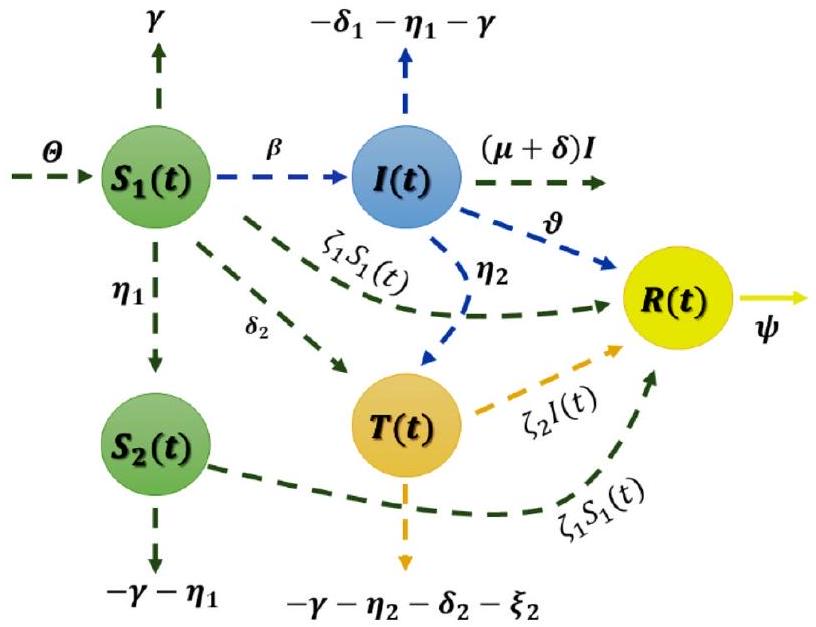
الشكل 1. الرسم التخطيطي لتفاعل الأقسام المختلفة.
التعريفات الأساسية
في هذا القسم، سيتم تقديم بعض التعريفات الأساسية.
التعريف 3.1 مرجع
التعريف 3.1 مرجع
التعريف 3.2 مرجع
التعريف 3.3 مرجع
التعريف 3.3 مرجع
بالإضافة إلى ذلك، فإن الخصائص التالية تنطبق، لـ
يمتلك تعريف الرتبة الكسرية من حيث ريمان-لوفيلي مزايا معينة عند محاكاة النماذج الواقعية. لهذا الغرض، اقترح كابوتو نسخة أفضل من
التعريف 3.4 مرجع
لـ
اللمّة 3.1 إذا كان
اللمّة 3.1 إذا كان
التعريف 3.5 مرجع
التعريف 3.6 لـ
ثم، يتم تعريف تحويل لابلاس لـ
في القسم التالي، سنقدم تفاصيل حول إيجابية الحل المكتسب جنبًا إلى جنب مع حدوده للنموذج (1).
الإيجابية، الحدود، الوجود، والتفرد الإيجابية والحدود
في هذا القسم، سنقدم دراسة مفصلة عن الإيجابية والحدود للنموذج الرئيسي (1). نتبع أولاً نظرية القيم المتوسطة العامة في المرجع.
اللمّة 4.1.1 افترض أن
النتيجة 4.1.1 افترض أن
(ط)
(2)
(ط)
(2)
يمكننا الآن إثبات النظريات التالية.
النظرية 4.1.1 المنطقة
الدليل الخطوة الأولى هي إثبات أن النموذج (1) له حل فريد على الفترة (
لذا فإن المنطقة
نحتاج بعد ذلك إلى النظرية التالية.
النظرية 4.1.2 إجمالي السكان للنموذج (1) يتحقق
الدليل إن جمع المعادلات الأربع الأولى من النموذج الرئيسي يؤدي إلى ما يلي.
النظرية 4.1.2 إجمالي السكان للنموذج (1) يتحقق
الدليل إن جمع المعادلات الأربع الأولى من النموذج الرئيسي يؤدي إلى ما يلي.
الذي يمكن إعادة كتابته كما يلي:
أخذ تحويل لابلاس للشكل المحدد Eq. (12) لكلا جانبي Eq. (15) نحصل على،
لذا،
من (11) و (12) وإذا كان
لذا، نستنتج أن
من عدم المساواة (16) والنظرية 4.1.1، نستنتج أن
الوجود والتفرد
هذا القسم مخصص لإثبات وجود وحدود الحل للنموذج (1). نبدأ بالنظرية التالية.
النظرية 4.2.1 يوجد حل فريد للنموذج (1) لكل حالة أولية غير سالبة.
الدليل لنعرّف المنطقة
الدليل لنعرّف المنطقة
أيضًا، دع
بعد ذلك، لأي
ثم لدينا،
لذا، يتم التحقق من شرط ليبشيتز لـ
سيكون القسم التالي مخصصًا لتحديد نقاط التوازن للنظام وسلوك استقراره.
نقاط التوازن وتحليل الاستقرار
في هذا القسم، نحصل على نقاط التوازن للنموذج (1) جنبًا إلى جنب مع الظروف الأولية في (2). يتم العثور على هذه النقاط من خلال معادلة النظام (1) بالصفر. سيؤدي ذلك إلى أنواع مختلفة من نقاط التوازن. يتم تعريف الأولى كنقطة التوازن الخالية من المرض (DFE) التي يمكن أن تأخذ شكلًا من
حيث
ومن ثم
أخيرًا، يمكن تمثيل
كما يتضح من المعادلة (19)، يعتمد رقم التكاثر
النقطة الثانية هي النقطة الوبائية EEP. في هذه الحالة، لدينا نقاط وبائية متعددة حيث غياب الإغلاق والتدابير المشار إليها بـ
و
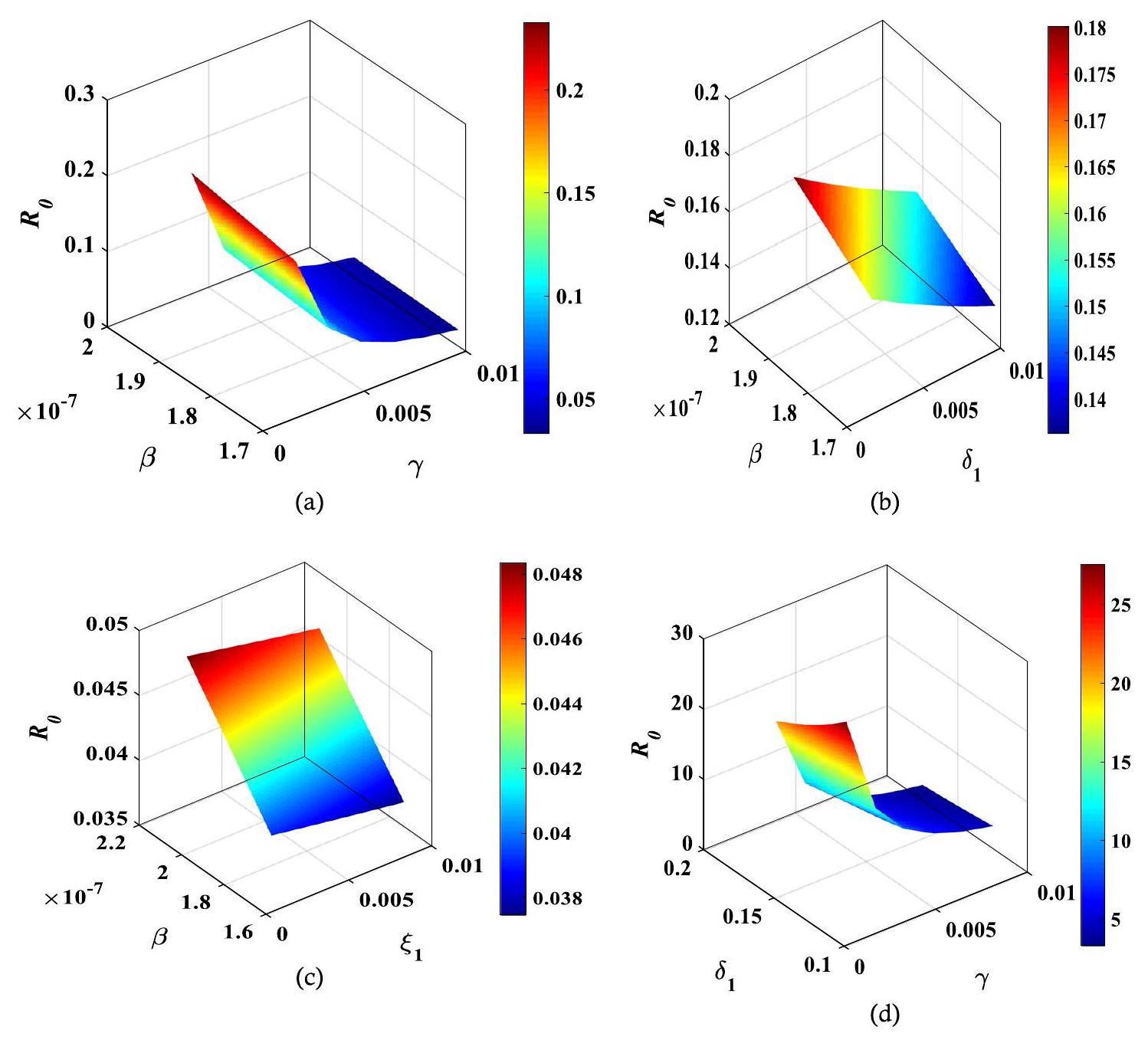
الشكل 2. سلوك رقم التكاثر
يمكن الحصول على مصفوفة جاكوب للنموذج (1) بالشكل التالي،
بالنسبة لـ DFE، يتم إعطاء مصفوفة جاكوب عند
هذا بعد الحصول على القيم الذاتية لـ
يظهر أن هذه النقطة التوازنية مستقرة إذا كان
أما بالنسبة لـ EEP، يمكن العثور على مصفوفة جاكوب عند
أما بالنسبة لـ EEP، يمكن العثور على مصفوفة جاكوب عند
القيم الذاتية هي،
تكون هذه النقطة التوازنية مستقرة إذا كان
بعد ذلك، سنقوم بمحاكاة نتائج كل من أقسام النموذج (1) من خلال LADM.
التقنية المقترحة
هنا، سنقدم الخطوات الرئيسية لتطبيق LADM للتحقيق في ديناميات النموذج (1). نحتاج أولاً إلى التعريفات التالية.
التعريف 6.1 مرجع
التعريف 6.2 المراجع
أين
ستُستخدم هذه التعريفات لمناقشة الإجراء العام للتقنية المقترحة لمحاكاة النموذج (1). الخطوة الأولى هي تطبيق تحويل لابلاس على المعادلة (1) مما سيؤدي إلى
ثم، الخطوة التالية هي تطبيق المعادلة (22) على (24)، نستنتج،
الخطوة التالية هي تطبيق الشروط الأولية المحددة في المعادلة (2)، ثم نحصل على،
يمكن ملاحظة من المعادلة (26) أن الحل الناتج هو في شكل سلسلة لانهائية. بعد ذلك، دع القيم لـ
بعد ذلك، نتعامل مع الجزء غير الخطي من النموذج الرئيسي على أنه،
لذا،
استبدال المعادلة (27) والمعادلة (28) في المعادلة (26) ومساواة الجانبين يعطي ما يلي:
ثم، بتطبيق المعادلة (30) تحويل لابلاس العكسي نصل إلى،
وبالمثل، في الخطوة النهائية، نحصل على بقية الحدود كسلاسل لانهائية كما هو:
المعادلة (32) تحل النموذج الرئيسي لـ SITR في المعادلة (1) التي سيتم توضيحها في القسم التالي.
المحاكاة العددية
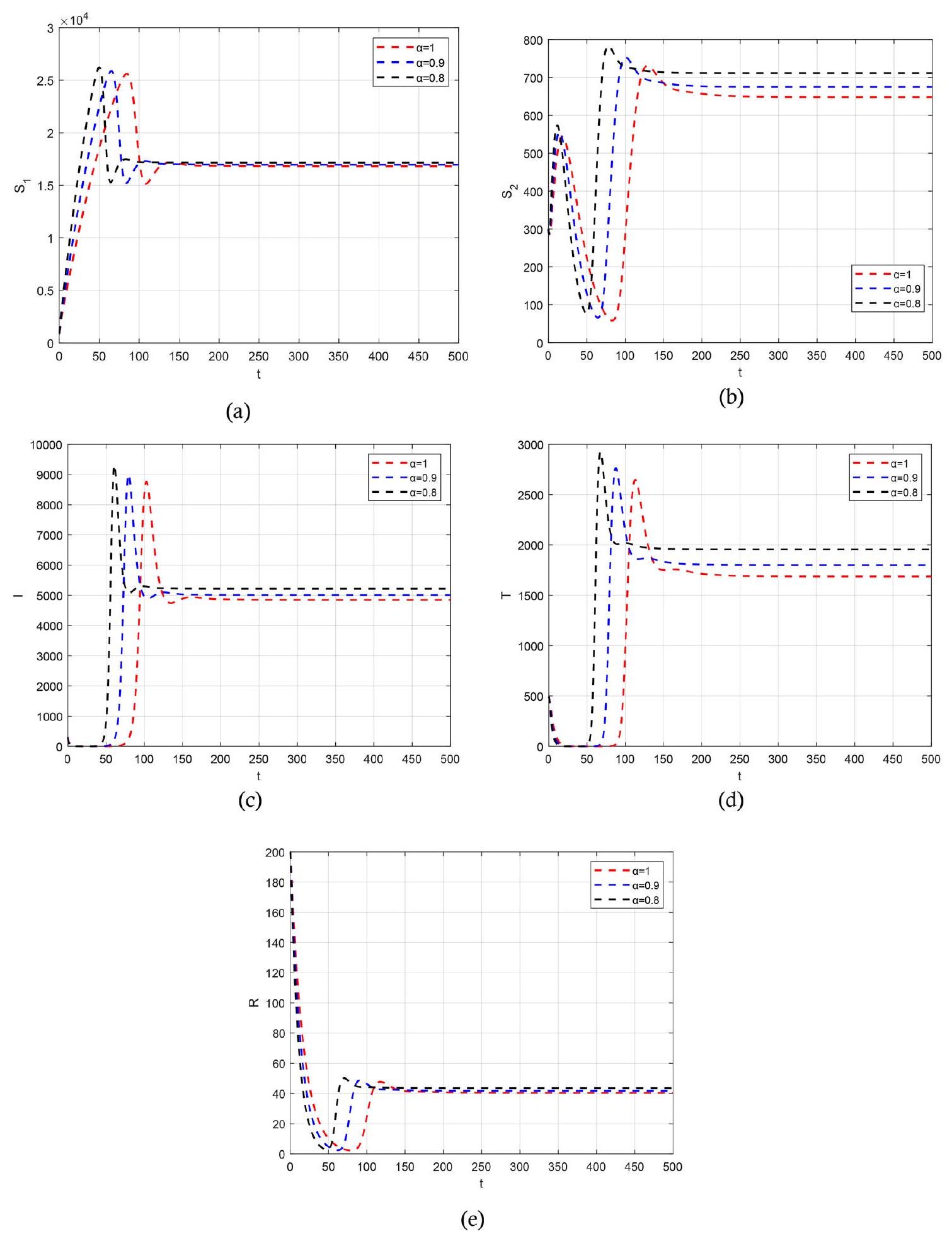
في هذا القسم، سنقوم بعرض المحاكاة للنموذج (1) باستخدام أساليب متعددة. أولاً، في الفقرة الفرعية “تقنية تحليل لابلاس أدوبيان”، سنوضح النتائج التي تم الحصول عليها من خلال تكييف تقنية تحليل لابلاس أدوبيان (LADM) لقيم مختلفة من الترتيب الكسري.
تقنية تحليل أداميان لابلاس
في هذا القسم، نختبر فعالية التقنية المقترحة من خلال فحص النتائج المكتسبة للنموذج (1) لمختلف
تقنية عددية
في هذا القسم، سنحدد النتائج العددية للنموذج (1) من خلال استخدام تقنية عددية فعالة. نحن نستخدم طريقة آدامز-باشفورث-مولتون، المعروفة أيضًا باسم طريقة ABM، لإجراء محاكاة عددية والحصول على حلول للنموذج غير الخطي المقترح من الدرجة الكسرية. تقدم طريقة ABM العديد من المزايا الملحوظة. أولاً وقبل كل شيء، تعزز معدل التقارب للمحاكاة. إحدى المزايا الرئيسية لطريقة ABM هي قدرتها على تجاوز الحاجة إلى الخطية، والتفريق، وفرض افتراضات غير واقعية جسديًا. من خلال تجنب هذه القيود، توفر الطريقة تمثيلًا أكثر دقة للنظام المقترح. تعتبر طريقة ABM مستقرة عمومًا لفئة واسعة من المعادلات التفاضلية الكسرية (FDEs). الاستقرار هو خاصية حاسمة في الطرق العددية لأنه يضمن بقاء الحلول محدودة وعدم ظهور سلوك غير فيزيائي أو تباعد. لقد تم إثبات فعاليتها في حل مجموعة واسعة من المعادلات التفاضلية الكسرية غير الخطية، مما يبرز المزيد من ملاءمة المعادلات التفاضلية من الدرجة الكسرية لنمذجة ديناميات النموذج المقترح بشكل واقعي. أولاً، نستعرض أساسيات الطريقة العددية المقترحة التي تم استخدامها لمحاكاة عددية لمشكلات القيمة الأولية الكسرية باستخدام مشتقات كابوتو. تقدم الصيغ التالية عرضًا كاملاً لنهج ABM الكسرية.
افترض أن نطاق الحل هو
أين
| المعلمات | القيم |
|
|
٩٠٠ |
|
|
٣٠٠ |
|
|
٣٠٠ |
|
|
497 |
|
|
٢٠٠ |
|
|
٤٠٠ |
|
|
0.000017 |
|
|
0.16979 |
|
|
0.16979 |
|
|
0.0002 |
|
|
0.002 |
|
|
0.03275 |
|
|
0.03275 |
|
|
0.0096 |
|
|
0.2 |
|
|
0.02 |
|
|
0.0005 |
|
|
0.06 |
الجدول 2. قيم المعلمات الرئيسية في المعادلة (1).
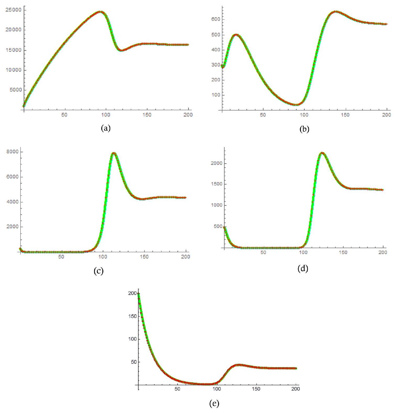
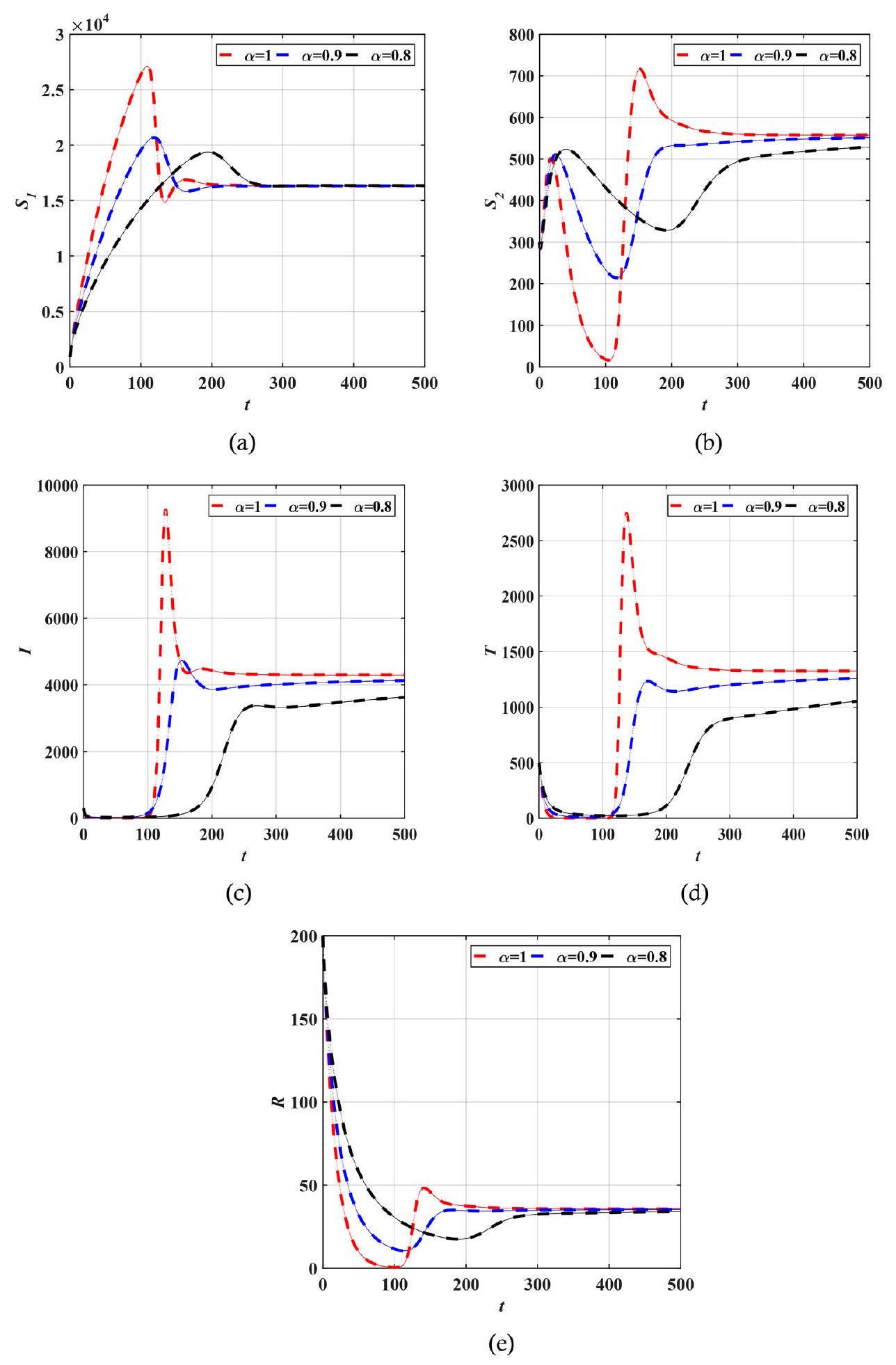
الشكل 3. حل الأقسام (أ)
و
المؤلفون في المراجع.
المؤلفون في المراجع.
التحقق باستخدام بيانات حقيقية
في هذا القسم الفرعي، سنقوم بالتحقق من النتائج التي تم الحصول عليها من LADM والتقنيات العددية من خلال مقارنتها بالبيانات الحقيقية. سنقوم بالتحقق من النتائج التي تم الحصول عليها مع النتائج التي تم الحصول عليها من إيطاليا. خلال بداية عام 2020، وخاصة من مارس حتى مايو 2020، أعلنت إيطاليا عن الإغلاق الأول للعديد من المنشآت في البلاد كاستجابة مناسبة لإبطاء انتشار COVID-19. عدد المصابين (المؤكدين)
الشكل 4. حل الأقسام (أ)
تظهر الحالات لكل مليون، وعدد الحالات التي تم علاجها في المستشفيات، وعدد الوفيات في الشكل 11. تم جمع النتائج المبلغ عنها في الشكل 11 من موقع World in Data.
الشكل 5. ملفات الحلول للأقسام المختلفة لـ
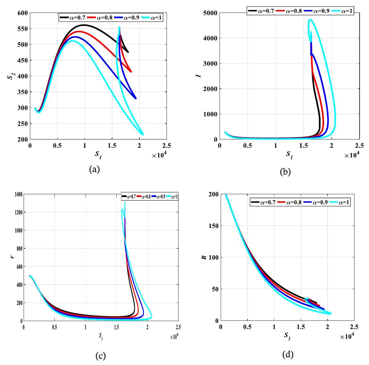
الشكل 6. العلاقة بين القابلية للإصابة
تمت ملاحظة توافق جيد بين النتائج التي تم الحصول عليها من المحاكاة والبيانات الحقيقية من إيطاليا. على سبيل المثال، توضح الشكل 11a عدد حالات الإصابة في إيطاليا حتى أغسطس 2020، حيث يبدو أن عدد حالات الإصابة قد زاد ثم بدأ في الانخفاض اعتبارًا من مارس 2020، ويمكن رؤية ذلك أيضًا من الشكل 11b. يتم ملاحظة تكيف مصطلح الدرجة الكسرية في الشكل 11b حيث يتم تغيير قيمة
الخاتمة
تقدم هذه الدراسة نموذج SITR الكسرية من نوع كابوتو لتسليط الضوء على بعض الديناميكيات الجديدة لفيروس كورونا COVID-19. يتكون النموذج من أربع فئات: القابلون للإصابة
الشكل 7. العلاقة بين القابلية للإصابة
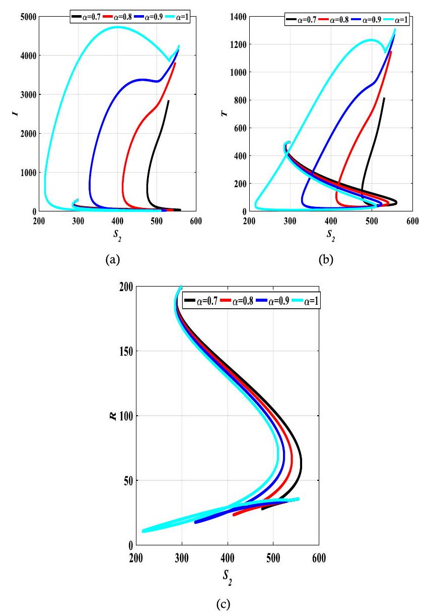
الشكل 8. العلاقة بين الحالة المصابة
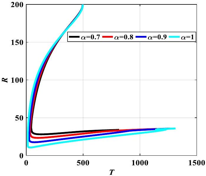
الشكل 9. العلاقة بين
والتحكم فيه. للتحقق من النتائج التي تم الحصول عليها، تم عرض مقارنة مع بيانات حقيقية من إيطاليا خلال فترة الإغلاق. وهذا يظهر توافقًا تامًا بين النتائج الحقيقية والنتائج التي تم الحصول عليها حول تأثير تدابير السيطرة والإغلاق في إبطاء انتشار الفيروس. وبالتالي، نحن مهتمون بمزيد من استكشاف هذا النموذج بشكل أكثر شمولاً مع أخذ المزيد من الفئات في الاعتبار باستخدام طريقة تحليلية فعالة مماثلة ومقارنتها مع بيانات حقيقية من دول أخرى.
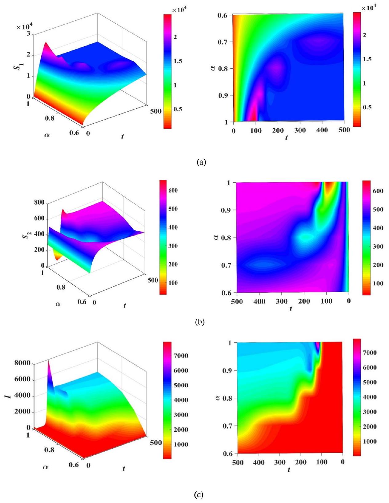
الشكل 10. الرسوم البيانية ثلاثية الأبعاد لعدد سكان الحجرة مقابل الزمن والترتيب الكسري
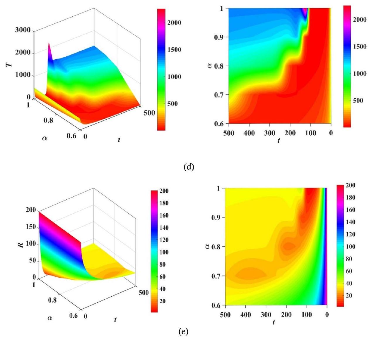
الشكل 10. (مستمر)
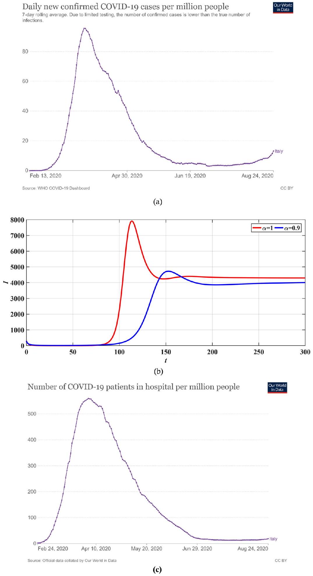
الشكل 11. عدد الحالات المصابة من (أ) بيانات حقيقية من إيطاليا
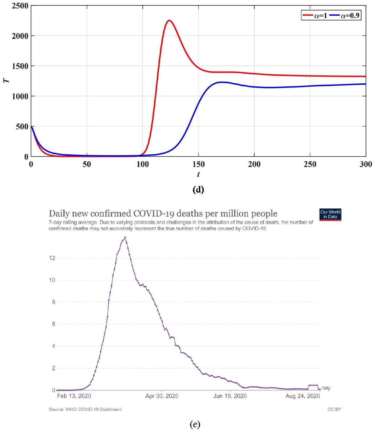
الشكل 11. (مستمر)
توفر البيانات
جميع البيانات التي تم توليدها أو تحليلها خلال هذه الدراسة مشمولة.
تاريخ الاستلام: 8 مايو 2023؛ تاريخ القبول: 27 ديسمبر 2023
نُشر على الإنترنت: 05 فبراير 2024
تاريخ الاستلام: 8 مايو 2023؛ تاريخ القبول: 27 ديسمبر 2023
نُشر على الإنترنت: 05 فبراير 2024
References
- Din, A., Li, Y., Khan, F. M., Khan, Z. U. & Liu, P. On Analysis of fractional order mathematical model of Hepatitis B using AtanganaBaleanu Caputo (ABC) derivative. Fractals 30(01), 2240017 (2022).
- Din, A., Li, Y., Yusuf, A. & Ali, A. I. Caputo type fractional operator applied to Hepatitis B system. Fractals 30(01), 2240023 (2022).
- Liu, P., Din, A. & Zarin, R. Numerical dynamics and fractional modeling of hepatitis B virus model with non-singular and nonlocal kernels. Results Phys. 39, 105757 (2022).
- Sabbar, Y., Din, A. & Kiouach, D. Influence of fractal-fractional differentiation and independent quadratic Lévy jumps on the dynamics of a general epidemic model with vaccination strategy. Chaos Solitons Fractals 171, 113434 (2023).
- Madueme, P.-G. & Chirove, F. Understanding the transmission pathways of Lassa fever: A mathematical modeling approach. Infect. Dis. Model. 8(1), 27-57 (2023).
- Rashid, S., Karim, S., Akgül, A., Bariq, A. & Elagan, S. K. Novel insights for a nonlinear deterministic-stochastic class of fractionalorder Lassa fever model with varying kernels. Sci. Rep. 13(1), 15320 (2023).
- Sabir, Z., Said, S. B. & Al-Mdallal, Q. A fractional order numerical study for the influenza disease mathematical model. Alex. Eng. J. 65, 615-626 (2023).
- Ebenezer, V., Sachin, R., Hiruthic, S. S., Sam Sergius, S. and Shivnesh, R. SDNS: Artificial Neural network scheme to solve the nonlinear skin disease model. In 2023 Second International Conference on Electronics and Renewable Systems (ICEARS), 931-935 (IEEE, 2023).
- El-Mesady, A., Adel, W., Elsadany, A. A. & Elsonbaty, A. Stability analysis and optimal control strategies of a fractional-order monkeypox virus infection model. Phys. Scr. 98(9), 095256 (2023).
- Waleed, A., Elsonbaty, A., Aldurayhim, A. & El-Mesady, A. Investigating the dynamics of a novel fractional-order monkeypox epidemic model with optimal control. Alex. Eng. J. 73, 519-542 (2023).
- Peter, O. J., Abidemi, A., Ojo, M. M. & Ayoola, T. A. Mathematical model and analysis of monkeypox with control strategies. Eur. Phys. J. Plus 138(3), 242 (2023).
- Elsonbaty, A., Adel, W., Aldurayhim, A. & El-Mesady, A. Mathematical modeling and analysis of a novel monkeypox virus spread integrating imperfect vaccination and nonlinear incidence rates. Ain Shams Eng. J. 15, 102451 (2023).
- Sabir, Z., Bhat, S. A., Raja, M. A. Z. & Alhazmi, S. E. A swarming neural network computing approach to solve the Zika virus model. Eng. Appl. Artif. Intell. 126, 106924 (2023).
- Sabir, Z., Ali, M. R., Raja, M. A. Z. & Sadat, R. An efficient computational procedure to solve the biological nonlinear Leptospirosis model using the genetic algorithms. Soft Comput. https://doi.org/10.1007/s00500-023-08315-5 (2023).
- Higazy, M., El-Mesady, A., Mahdy, A. M. S., Ullah, S. & Al-Ghamdi, A. Numerical, approximate solutions, and optimal control on the deathly lassa hemorrhagic fever disease in pregnant women. J. Funct. Spaces 2021, 1-15 (2021).
- https://covid19.who.int/.
- Alrabaiah, H., Arfan, M., Shah, K., Mahariq, I. & Ullah, A. A comparative study of spreading of novel corona virus disease by ussing fractional order modified SEIR model. Alex. Eng. J. 60(1), 573-585 (2021).
- Li, C., Qian, D. & Chen, Y. Q. On Riemann-Liouville and caputo derivatives. Discret. Dyn. Nat. Soc. 2011, 1-15 (2011).
- Khan, M. A. & Atangana, A. Modeling the dynamics of novel coronavirus (2019-nCov) with fractional derivative. Alex. Eng. J. 59(4), 2379-2389 (2020).
- Alkahtani, B. S. T. & Alzaid, S. S. A novel mathematics model of covid-19 with fractional derivative stability and numerical analysis. Chaos Solitons Fractals 138, 110006 (2020).
- Sabir, Z. et al. Numerical computational heuristic through morlet wavelet neural network for solving the dynamics of nonlinear SITR COVID-19. Cmes-Comput. Model. Eng. Sci. 131, 763-785 (2022).
- Okuonghae, D. & Omame, A. Analysis of a mathematical model for COVID-19 population dynamics in Lagos, Nigeria. Chaos Solitons Fractals 139, 110032 (2020).
- Djaoue, S., Kolaye, G. G., Abboubakar, H., Ari, A. A. A. & Damakoa, I. Mathematical modeling, analysis and numerical simulation of the COVID-19 transmission with mitigation of control strategies used in Cameroon. Chaos Solitons Fractals 139, 110281 (2020).
- Annas, S., Pratama, M. I., Rifandi, M., Sanusi, W. & Side, S. Stability analysis and numerical simulation of SEIR model for pandemic COVID-19 spread in Indonesia. Chaos Solitons Fractals 139, 110072 (2020).
- Naveed, M. et al. Mathematical analysis of novel coronavirus (2019-ncov) delay pandemic model. Comput. Mater. Continua 64(3), 1401-1414 (2020).
- Ghasemi, S. E. & Gouran, S. Evaluation of COVID-19 pandemic spreading using computational analysis on nonlinear SITR model. Math. Methods Appl. Sci. 45(17), 11104-11116 (2022).
- Sanchez, Y. G., Sabir, Z. & Guirao, J. L. G. Design of a nonlinear SITR fractal model based on the dynamics of a novel coronavirus (COVID). Fractals https://doi.org/10.1142/S0218348X20400265 (2020).
- Yang, C. & Wang, J. A mathematical model for the novel coronavirus epidemic in Wuhan, China. Math. Biosci. Eng. 17(3), 2708-2724 (2020).
- Ongun, M. Y. The Laplace adomian decomposition method for solving a model for HIV infection of CD4+ T cells. Math. Comput. Model. 53(5-6), 597-603 (2011).
- Wazwaz, A.-M. The combined Laplace transform-Adomian decomposition method for handling nonlinear Volterra integro-differential equations. Appl. Math. Comput. 216(4), 1304-1309 (2010).
- Haq, F., Shah, K., Rahman, G. & Shahzad, M. Numerical solution of fractional order smoking model via Laplace Adomian decomposition method. Alex. Eng. J. 57(2), 1061-1069 (2018).
- Baleanu, D., Aydogn, S. M., Mohammadi, H. & Rezapour, S. On modelling of epidemic childhood diseases with the Caputo-Fabrizio derivative by using the Laplace Adomian decomposition method. Alex. Eng. J. 59(5), 3029-3039 (2020).
- Veeresha, P., Malagi, N. S., Prakasha, D. G. & Baskonus, H. M. An efficient technique to analyze the fractional model of vectorborne diseases. Phys. Scr. 97(5), 054004 (2022).
- Shah, R., Khan, H., Arif, M. & Kumam, P. Application of Laplace-Adomian decomposition method for the analytical solution of third-order dispersive fractional partial differential equations. Entropy 21(4), 335 (2019).
- Gonzalez-Gaxiola, O. & Biswas, A. Optical solitons with Radhakrishnan-Kundu-Lakshmanan equation by Laplace-Adomian decomposition method. Optik 179, 434-442 (2019).
- Baba, I. A., Yusuf, A., Nisar, K. S., Abdel-Aty, A.-H. & Nofal, T. A. Mathematical model to assess the imposition of lockdown during COVID-19 pandemic. Results Phys. 20, 103716 (2021).
- Sefidgar, E., Celik, E. & Shiri, B. Numerical solution of fractional differential equation in a model of HIV infection of CD4 (+) T cells. Int. J. Appl. Math. Stat. 56, 23-32 (2017).
- Caputo, M. Linear models of dissipation whose Q is almost frequency independent-II. Geophys. J. Int. 13(5), 529-539 (1967).
- Kai, D. The analysis of fractional differential equations: An application-oriented exposition using operators of Caputo type (2004).
- Odibat, Z. M. & Shawagfeh, N. T. Generalized Taylor’s formula. Appl. Math. Comput. 186(1), 286-293 (2007).
- Lin, W. Global existence theory and chaos control of fractional differential equations. J. Math. Anal. Appl. 332(1), 709-726 (2007).
- Antosiewicz, H. A. Studies in Ordinary Differential Equations Vol. 14 (Mathematical Assn of Amer, 1977).
- Diethelm, K., Ford, N. J. & Freed, A. D. Detailed error analysis for a fractional Adams method. Numer. Algorithms 36, 31-52 (2004).
- https://ourworldindata.org/explorers/coronavirus-data-explorer.
شكر وتقدير
تدعم هذه الدراسة من خلال تمويل من جامعة الأمير سطام بن عبدالعزيز برقم المشروع (PSAU/2023/R/1444). بالإضافة إلى ذلك، يود المؤلفون أن يعبروا عن شكرهم للمحرر والمراجعين على التعليقات والاقتراحات المفيدة التي حسنت العمل.
مساهمات المؤلفين
ساهم جميع المؤلفين بشكل متساوٍ وملحوظ في كتابة هذه الورقة. قرأ جميع المؤلفين ووافقوا على النسخة النهائية.
المصالح المتنافسة
يعلن المؤلفون عدم وجود مصالح متنافسة.
معلومات إضافية
يجب توجيه المراسلات والطلبات للحصول على المواد إلى و.أ.
معلومات إعادة الطباعة والتصاريح متاحة علىwww.nature.com/reprints.
ملاحظة الناشر: تظل شركة سبرينجر ناتشر محايدة فيما يتعلق بالمطالبات القضائية في الخرائط المنشورة والانتماءات المؤسسية.
ملاحظة الناشر: تظل شركة سبرينجر ناتشر محايدة فيما يتعلق بالمطالبات القضائية في الخرائط المنشورة والانتماءات المؤسسية.
الوصول المفتوح هذه المقالة مرخصة بموجب رخصة المشاع الإبداعي النسب 4.0 الدولية، التي تسمح بالاستخدام والمشاركة والتكيف والتوزيع وإعادة الإنتاج بأي وسيلة أو صيغة، طالما أنك تعطي الائتمان المناسب للمؤلفين الأصليين والمصدر، وتوفر رابطًا لرخصة المشاع الإبداعي، وتوضح إذا ما تم إجراء تغييرات. الصور أو المواد الأخرى من طرف ثالث في هذه المقالة مشمولة في رخصة المشاع الإبداعي الخاصة بالمقالة، ما لم يُشار إلى خلاف ذلك في سطر الائتمان للمواد. إذا لم تكن المادة مشمولة في رخصة المشاع الإبداعي الخاصة بالمقالة وكان استخدامك المقصود غير مسموح به بموجب اللوائح القانونية أو يتجاوز الاستخدام المسموح به، فسيتعين عليك الحصول على إذن مباشرة من صاحب حقوق الطبع والنشر. لعرض نسخة من هذه الرخصة، قم بزيارةhttp://creativecommons.org/licenses/by/4.0/.
© المؤلف(ون) 2024
© المؤلف(ون) 2024
قسم الرياضيات وفيزياء الهندسة، كلية الهندسة، جامعة المنصورة، المنصورة 35511، مصر. المختبر بين التخصصات في الجامعة الفرنسية في مصر (UFEID Lab)، الجامعة الفرنسية في مصر، القاهرة 11837، مصر. قسم الرياضيات، كلية التربية، جامعة كافكاس، قارص، تركيا. وحدة البحث MEU، جامعة الشرق الأوسط، عمان، الأردن. قسم الرياضيات، كلية العلوم والآداب في الخرج، جامعة الأمير سطام بن عبدالعزيز، الخرج 11942، المملكة العربية السعودية. مدرسة التكنولوجيا، جامعة ووكسن، حيدر آباد 502345، تيلانجانا، الهند. قسم الرياضيات، كلية أناند الدولية للهندسة، جايبور 303012، الهند. مركز أبحاث الديناميات غير الخطية (NDRC)، جامعة عجمان، عجمان، الإمارات العربية المتحدة. المركز الدولي للعلوم الأساسية والتطبيقية، جايبور 302029، الهند. قسم الفيزياء ورياضيات الهندسة، كلية الهندسة الإلكترونية، جامعة المنوفية، منوف 32952، مصر. البريد الإلكتروني:waleedadel@mans.edu.eg
Journal: Scientific Reports, Volume: 14, Issue: 1
DOI: https://doi.org/10.1038/s41598-023-50889-5
PMID: https://pubmed.ncbi.nlm.nih.gov/38316837
Publication Date: 2024-02-05
DOI: https://doi.org/10.1038/s41598-023-50889-5
PMID: https://pubmed.ncbi.nlm.nih.gov/38316837
Publication Date: 2024-02-05
Designing a novel fractional order mathematical model for COVID-19 incorporating lockdown measures
This research focuses on the design of a novel fractional model for simulating the ongoing spread of the coronavirus (COVID-19). The model is composed of multiple categories named susceptible
Many diseases have had devastating consequences for human life over many years and decades. For example, Ebola is one of those deadly diseases that can be transmitted from infected animals, like fruit bats, to uninfected humans. For example, Hepatitis B is one of the viruses that has a deadly effect on infected individuals. It has an original form that has been transmitted over the years from Chimps to humans. This was not noticed with symptoms during the nineteenth century through its transmission. Five countries reported the spread of this disease, and more than 300,000 humans were infected with it. The role of mathematical modeling is crucial in simulating such a disease to better understand the dynamics of this disease, which suppresses the spread of such a virus. With the aid of mathematical modeling, researchers can suggest and assess several intervention techniques that may help slow down the virus. In addition, it plays an important role in estimating key epidemiological parameters such as the basic reproduction number
the impact of vaccination programs, antiviral treatment, and behavior change interventions on the prevalence of Hepatitis B. Researchers have been using these models to gain better insight into optimal strategies for prevention, screening, and treatment, guiding public health policies and resource allocation. For example, Din et al.
By the end of 2019, the new Middle East respiratory syndrome (COVID-19) emerged in China, specifically from the seafood markets in Wuhan, and since then it has been spreading to all parts of the world. Both undeveloped and developing countries have been reporting new cases daily, leading to an alarming increase in infections. The total number of confirmed cases until now is more than 676 million individuals, with a total death rate of more than 6 million, according to the
The signs of the infection COVID-19 may vary from person to person, but the most common are a fever of
Fractional differential equations (FDEs) have been playing a major role in understating the dynamics of real-life phenomena. Not only in understanding the complex dynamics of biological systems, but it has also been used in other fields such as thermoelectricity. The use of FDEs has been increasing throughout the last few years, making them one of the most important tools to be used in simulations. There have been several definitions of fractional operators, each of which has advantages and drawbacks. One of the most important and original definitions is the Caputo fractional derivative
models can be found in Ref.
models can be found in Ref.
In this research, we are also exploring the potential of using the Laplace Adomian decomposition method (LADM) to solve the fractional COVID-19 model. This method is a powerful yet straightforward approach to tackling epidemic models and has been successfully applied in biology, engineering, and applied mathematics. It combines the Laplace transform and the Adomian decomposition method, offering several advantages for solving complex problems. One of the advantages of this method is its accuracy, as by employing the Laplace transform, it transforms the differential equations into algebraic equations, which are often easier to solve. This transformation reduces the complexity of the problem and enables the use of powerful algebraic techniques to obtain accurate solutions. Additionally, the Adomian decomposition method provides a systematic and robust approach to handling nonlinear terms, allowing for accurate approximation of the solution even in the presence of nonlinearity. This method does not require any perturbation or linearization, nor does it need a defined size of the step like the Rung-Kutta of order 4 technique. Additionally, it is independent of any parameters, unlike the Homotopy Perturbation Method (HPM), which depends on certain parameters. This has led to its use in solving various models, such as the HIV CD4 +T cell problem
We are interested in this paper to capture the dynamics of the fractional COVID-19 model, taking into account the effect of the lockdown that several countries have been taking to control the spread of the virus. To the best of our knowledge, this is the first time this model has been solved using the Caputo definition. The novelty of the paper lies in the following points:
- A novel Caputo fractional COVID-19 has been propped to capture the dynamics of the model, incorporating lockdown measures.
- The existence, uniqueness, and positivity of the new proposed fractional model are examined in detail, which proves that the presented model has a unique solution.
- A detailed stability analysis for the model is presented to highlight the stability region and conditions for the model.
- The results for simulating the different compartments of the model are obtained for different values of the fractional order, and real data from Italy is presented.
- The results prove that the control measures represented in this case by lockdown have an effect on slowing down the spread of the virus and ending the pandemic.
The organization of the rest of the paper is as follows: The formulation of the model is detailed in Sect. “Model formulation” with the interaction of the different compartments. Section “Basic definitions” provides some basic definitions and fundamentals. Positivity, boundedness, existence, and uniqueness are discussed in detail in Sect. “Positivity, boundedness, existence, and uniqueness”. The stability analysis and the equilibrium points are illustrated in Sect. “Equilibrium points and stability analysis”. The proposed technique for solving the main model is highlighted in Sect. “Proposed technique”, along with a verification with real data. Section “Numerical Simulations” presents the numerical results of the work using different techniques, and the conclusion for the work is provided in Sect. “Conclusion”.
Model formulation
In this section, we will present the novel COVID-19 model, which is composed of four primary components: susceptible
The general form of the fractional SITR model can take the following form
With the following conditions,
The order
In the next section, we will provide some basic definitions that will be needed later.
| Parameters | Description |
|
|
Population of susceptible individuals that aren’t yet under lockdown |
|
|
Susceptible populations that are under lockdown |
|
|
An infected population that isn’t under lockdown |
|
|
Infective populations that are under lockdown |
|
|
Recovered population after infection |
|
|
Recruitment rate |
|
|
Infection contact rate |
|
|
The recovery rate for infected individuals |
|
|
The recovery rate for treated individuals |
|
|
Imposing lockdown measures for susceptible individuals |
|
|
Imposing lockdown measures for infected individuals |
|
|
The death rate for infected individuals |
|
|
Death rate for treated individuals |
|
|
Death rate of natural circumstances |
|
|
Transfer rate from susceptible individuals from lockdown to normal class |
|
|
Transfer rate from infected individuals from lockdown to normal class |
|
|
Lockdown application rate |
|
|
Lockdown depletion rate |
Table 1. State variable definitions for the SITR model.
Figure 1. Schematic diagram of the interaction of different compartments.
Basic definitions
In this section, some basic definitions will be presented.
Definition 3.1 Reference
Definition 3.1 Reference
Definition 3.2 Reference
Definition 3.3 Reference
Definition 3.3 Reference
In addition, the following properties hold, for
The definition of the fractional order in terms of Riemann-Louville possesses certain advantages when simulating real-world models. To this end, Caputo proposed a better version of
Definition 3.4 Reference
for
Lemma 3.1 If
Lemma 3.1 If
Definition 3.5 Reference
Definition 3.6 For
Then, the Laplace transform of
In the next section, we shall provide details on the positivity of the acquired solution along with its boundedness for model (1).
Positivity, boundedness, existence, and uniqueness Positivity and boundedness
In this section, we will provide a detailed study of the positivity and boundedness of the main model (1). We first follow the generalized mean values theorem in Ref.
Lemma 4.1.1 Suppose
Corollary 4.1.1 Suppose
(i)
(ii)
(i)
(ii)
We can now prove the following theorems.
Theorem 4.1.1 The region
Proof The first step is to prove that model (1) has a unique solution on the period (
Hence the region
We then need the following theorem.
Theorem 4.1.2 The total population for the model (1) verifies
Proof Summing the first four equations of the main mode leads to the following.
Theorem 4.1.2 The total population for the model (1) verifies
Proof Summing the first four equations of the main mode leads to the following.
that can be rewritten as follows:
Taking Laplace to transform the defined form Eq. (12) for both sides of Eq. (15) we get,
Hence,
From (11) and (12) and if
Hence, we conclude that
From inequality (16) and Theorem 4.1.1, we deduce that
Existence and uniqueness
This subsection is devoted to proving the existence and boundedness of the solution of model (1). We start with the next theorem.
Theorem 4.2.1 There exists a unique solution for the model (1) for each non-negative initial condition.
Proof Let the region
Proof Let the region
Also, let
Next, for any
Then we have,
Thus, the Lipschitz condition is verified for
The following section will be devoted to determining the system’s equilibrium points and their stability behavior.
Equilibrium points and stability analysis
In this section, we acquire the equilibrium points for model (1) along with the initial conditions in (2). These points are found by equating the system (1) to zero. This shall result in different types of equilibrium points. The first is defined as the disease-free equilibrium point (DFE) which can take the form of
where
and hence
Finally,
As can be seen from Eq. (19), the reproduction number
The second point is the endemic point of EEP. In this case, we have multiple endemic points where the absence of lockdown and measures indicated by
and
Figure 2. Behaviour of reproduction number
The Jacobian matrix for model (1) can be obtained in the following form,
For the DFE, the Jacobian matrix at
This is after acquiring the eigenvalues of
seen that this equilibrium point is stable if
As for the EEP, the Jacobian matrix at
As for the EEP, the Jacobian matrix at
The eigenvalues are,
This equilibrium point is stable if
Next, we will simulate the results of each of the compartments model (1) through the LADM.
Proposed technique
Here, we will provide the main steps of applying the LADM for investigating the dynamics of model (1). We first need the following definitions.
Definition 6.1 Reference
Definition 6.2 References
where
These definitions will be used to discuss the general procedure of the proposed technique for simulating the model (1). The first step is to apply the Laplace transform to Eq. (1) which will result
Then, the next step is to apply formula (22) to (24), we conclude,
The next step is to apply the initial conditions defined in Eq. (2), then we get,
It can be noticed from Eq. (26) that the resulting solution is in the form of an infinite series. Next, let the values of
Next, we treat the nonlinear part of the main model as,
Hence,
Substituting Eq. (27) and Eq. (28) into Eq. (26) and equaling both sides give the following:
Then, applying for Eq. (30) the inverse Laplace we reach,
Similarly, at the final step, we get the rest of the terms as infinite series as,
Equation (32) solves the main SITR model of Eq. (1) which will be illustrated in the next section.
Numerical simulations
In this section, we will demonstrate the simulations for model (1) using multiple approaches. First, in subsection “Laplace Adomian decomposition technique”, we will illustrate the results obtained by adapting the Laplace Adomian decomposition technique (LADM) for different values of the fractional order
Laplace Adomian decomposition technique
In this section, we test the effectiveness of the proposed technique by examining the acquired results for model (1) for different
Numerical technique
In this section, we shall determine the numerical results of model (1) by making use of an effective numerical technique. We employ the Adams-Bashforth-Moulton method, also known as the ABM method, to perform numerical simulations and obtain solutions for the proposed nonlinear fractional order model. The ABM method offers several notable advantages. First and foremost, it enhances the convergence rate of the simulations. One key advantage of the ABM method is its ability to bypass the need for linearization, discretization, and the imposition of physically unrealistic assumptions. By avoiding these limitations, the method provides a more accurate representation of the proposed system. The ABM method is generally stable for a broad class of fractional differential equations (FDEs). Stability is a crucial property in numerical methods since it ensures that the solutions remain bounded and do not exhibit unphysical behavior or divergence. Its efficacy has been demonstrated in solving a wide range of nonlinear FDEs, further emphasizing the suitability of fractional order differential equations for modeling the dynamics of the proposed model realistically. First, we review the fundamentals of the proposed numerical method that has been used to numerically simulate fractional IVPs with Caputo derivatives. The following formulas give a complete presentation of the fractional ABM approach (The same as
Suppose that the domain of the solution is
where
| Parameters | Values |
|
|
900 |
|
|
300 |
|
|
300 |
|
|
497 |
|
|
200 |
|
|
400 |
|
|
0.000017 |
|
|
0.16979 |
|
|
0.16979 |
|
|
0.0002 |
|
|
0.002 |
|
|
0.03275 |
|
|
0.03275 |
|
|
0.0096 |
|
|
0.2 |
|
|
0.02 |
|
|
0.0005 |
|
|
0.06 |
Table 2. Values of the main parameters in Eq. (1).
Figure 3. The solution of the copartments (a)
And
The authors in Refs.
The authors in Refs.
Validation using real data
In this subsection, we will validate the obtained results from the LADM and numerical techniques by comparing them to real data. We will verify the obtained results with the obtained results from Italy. During the beginning of 2020, especially from March until May 2020, Italy declared the first lockdown for several facilities in the country as a proper reaction to slow done the spread of COVID-19. The number of infected (confirmed)
Figure 4. The solution of the copartments (a)
cases per million, number of hospitalized (treated) cases, and number of deaths are shown in Fig. 11. The results reported in Fig. 11 have been collected form World in Data website
Figure 5. Solution profiles of the different compartments for
Figure 6. Relation between susceptible
good agreement between the obtained results from the simulation and the real data from Italy is witnessed. For example, Fig. 11a demonstrates the number of infected cases in Italy until August 2020, where it seems that the number of infected cases increased and then began declining as of March 2020 and this can be also seen from Fig. 11b. The adaptation of the fractional order term is noticed in Fig. 11b where changing the value of
Conclusion
This study presents a Caputo fractional SITR model to highlight some new dynamics of the coronavirus COVID19. The model is composed of four categories: susceptible
Figure 7. Relation between susceptible
Figure 8. Relation between infected state
Figure 9. Relation between
and gaining control over it. To further verify the obtained results, a comparison with real data from Italy was shown during the lockdown. This shows a perfect agreement between the real results and the obtained results of the effect of control measures and lockdown in slowing down the spread of the virus. Thus, we are interested in further exploring this model more thoroughly with more categories taken into account using a similar effective analytic method and comparing it with real data from other countries.
Figure 10. 3D plots of the compartment’s populations versus time and fractional order
Figure 10. (continued)
Figure 11. Number of infectd cases from (a) real data form Italy
Figure 11. (continued)
Data availability
All data generated or analyzed during this study are included.
Received: 8 May 2023; Accepted: 27 December 2023
Published online: 05 February 2024
Received: 8 May 2023; Accepted: 27 December 2023
Published online: 05 February 2024
References
- Din, A., Li, Y., Khan, F. M., Khan, Z. U. & Liu, P. On Analysis of fractional order mathematical model of Hepatitis B using AtanganaBaleanu Caputo (ABC) derivative. Fractals 30(01), 2240017 (2022).
- Din, A., Li, Y., Yusuf, A. & Ali, A. I. Caputo type fractional operator applied to Hepatitis B system. Fractals 30(01), 2240023 (2022).
- Liu, P., Din, A. & Zarin, R. Numerical dynamics and fractional modeling of hepatitis B virus model with non-singular and nonlocal kernels. Results Phys. 39, 105757 (2022).
- Sabbar, Y., Din, A. & Kiouach, D. Influence of fractal-fractional differentiation and independent quadratic Lévy jumps on the dynamics of a general epidemic model with vaccination strategy. Chaos Solitons Fractals 171, 113434 (2023).
- Madueme, P.-G. & Chirove, F. Understanding the transmission pathways of Lassa fever: A mathematical modeling approach. Infect. Dis. Model. 8(1), 27-57 (2023).
- Rashid, S., Karim, S., Akgül, A., Bariq, A. & Elagan, S. K. Novel insights for a nonlinear deterministic-stochastic class of fractionalorder Lassa fever model with varying kernels. Sci. Rep. 13(1), 15320 (2023).
- Sabir, Z., Said, S. B. & Al-Mdallal, Q. A fractional order numerical study for the influenza disease mathematical model. Alex. Eng. J. 65, 615-626 (2023).
- Ebenezer, V., Sachin, R., Hiruthic, S. S., Sam Sergius, S. and Shivnesh, R. SDNS: Artificial Neural network scheme to solve the nonlinear skin disease model. In 2023 Second International Conference on Electronics and Renewable Systems (ICEARS), 931-935 (IEEE, 2023).
- El-Mesady, A., Adel, W., Elsadany, A. A. & Elsonbaty, A. Stability analysis and optimal control strategies of a fractional-order monkeypox virus infection model. Phys. Scr. 98(9), 095256 (2023).
- Waleed, A., Elsonbaty, A., Aldurayhim, A. & El-Mesady, A. Investigating the dynamics of a novel fractional-order monkeypox epidemic model with optimal control. Alex. Eng. J. 73, 519-542 (2023).
- Peter, O. J., Abidemi, A., Ojo, M. M. & Ayoola, T. A. Mathematical model and analysis of monkeypox with control strategies. Eur. Phys. J. Plus 138(3), 242 (2023).
- Elsonbaty, A., Adel, W., Aldurayhim, A. & El-Mesady, A. Mathematical modeling and analysis of a novel monkeypox virus spread integrating imperfect vaccination and nonlinear incidence rates. Ain Shams Eng. J. 15, 102451 (2023).
- Sabir, Z., Bhat, S. A., Raja, M. A. Z. & Alhazmi, S. E. A swarming neural network computing approach to solve the Zika virus model. Eng. Appl. Artif. Intell. 126, 106924 (2023).
- Sabir, Z., Ali, M. R., Raja, M. A. Z. & Sadat, R. An efficient computational procedure to solve the biological nonlinear Leptospirosis model using the genetic algorithms. Soft Comput. https://doi.org/10.1007/s00500-023-08315-5 (2023).
- Higazy, M., El-Mesady, A., Mahdy, A. M. S., Ullah, S. & Al-Ghamdi, A. Numerical, approximate solutions, and optimal control on the deathly lassa hemorrhagic fever disease in pregnant women. J. Funct. Spaces 2021, 1-15 (2021).
- https://covid19.who.int/.
- Alrabaiah, H., Arfan, M., Shah, K., Mahariq, I. & Ullah, A. A comparative study of spreading of novel corona virus disease by ussing fractional order modified SEIR model. Alex. Eng. J. 60(1), 573-585 (2021).
- Li, C., Qian, D. & Chen, Y. Q. On Riemann-Liouville and caputo derivatives. Discret. Dyn. Nat. Soc. 2011, 1-15 (2011).
- Khan, M. A. & Atangana, A. Modeling the dynamics of novel coronavirus (2019-nCov) with fractional derivative. Alex. Eng. J. 59(4), 2379-2389 (2020).
- Alkahtani, B. S. T. & Alzaid, S. S. A novel mathematics model of covid-19 with fractional derivative stability and numerical analysis. Chaos Solitons Fractals 138, 110006 (2020).
- Sabir, Z. et al. Numerical computational heuristic through morlet wavelet neural network for solving the dynamics of nonlinear SITR COVID-19. Cmes-Comput. Model. Eng. Sci. 131, 763-785 (2022).
- Okuonghae, D. & Omame, A. Analysis of a mathematical model for COVID-19 population dynamics in Lagos, Nigeria. Chaos Solitons Fractals 139, 110032 (2020).
- Djaoue, S., Kolaye, G. G., Abboubakar, H., Ari, A. A. A. & Damakoa, I. Mathematical modeling, analysis and numerical simulation of the COVID-19 transmission with mitigation of control strategies used in Cameroon. Chaos Solitons Fractals 139, 110281 (2020).
- Annas, S., Pratama, M. I., Rifandi, M., Sanusi, W. & Side, S. Stability analysis and numerical simulation of SEIR model for pandemic COVID-19 spread in Indonesia. Chaos Solitons Fractals 139, 110072 (2020).
- Naveed, M. et al. Mathematical analysis of novel coronavirus (2019-ncov) delay pandemic model. Comput. Mater. Continua 64(3), 1401-1414 (2020).
- Ghasemi, S. E. & Gouran, S. Evaluation of COVID-19 pandemic spreading using computational analysis on nonlinear SITR model. Math. Methods Appl. Sci. 45(17), 11104-11116 (2022).
- Sanchez, Y. G., Sabir, Z. & Guirao, J. L. G. Design of a nonlinear SITR fractal model based on the dynamics of a novel coronavirus (COVID). Fractals https://doi.org/10.1142/S0218348X20400265 (2020).
- Yang, C. & Wang, J. A mathematical model for the novel coronavirus epidemic in Wuhan, China. Math. Biosci. Eng. 17(3), 2708-2724 (2020).
- Ongun, M. Y. The Laplace adomian decomposition method for solving a model for HIV infection of CD4+ T cells. Math. Comput. Model. 53(5-6), 597-603 (2011).
- Wazwaz, A.-M. The combined Laplace transform-Adomian decomposition method for handling nonlinear Volterra integro-differential equations. Appl. Math. Comput. 216(4), 1304-1309 (2010).
- Haq, F., Shah, K., Rahman, G. & Shahzad, M. Numerical solution of fractional order smoking model via Laplace Adomian decomposition method. Alex. Eng. J. 57(2), 1061-1069 (2018).
- Baleanu, D., Aydogn, S. M., Mohammadi, H. & Rezapour, S. On modelling of epidemic childhood diseases with the Caputo-Fabrizio derivative by using the Laplace Adomian decomposition method. Alex. Eng. J. 59(5), 3029-3039 (2020).
- Veeresha, P., Malagi, N. S., Prakasha, D. G. & Baskonus, H. M. An efficient technique to analyze the fractional model of vectorborne diseases. Phys. Scr. 97(5), 054004 (2022).
- Shah, R., Khan, H., Arif, M. & Kumam, P. Application of Laplace-Adomian decomposition method for the analytical solution of third-order dispersive fractional partial differential equations. Entropy 21(4), 335 (2019).
- Gonzalez-Gaxiola, O. & Biswas, A. Optical solitons with Radhakrishnan-Kundu-Lakshmanan equation by Laplace-Adomian decomposition method. Optik 179, 434-442 (2019).
- Baba, I. A., Yusuf, A., Nisar, K. S., Abdel-Aty, A.-H. & Nofal, T. A. Mathematical model to assess the imposition of lockdown during COVID-19 pandemic. Results Phys. 20, 103716 (2021).
- Sefidgar, E., Celik, E. & Shiri, B. Numerical solution of fractional differential equation in a model of HIV infection of CD4 (+) T cells. Int. J. Appl. Math. Stat. 56, 23-32 (2017).
- Caputo, M. Linear models of dissipation whose Q is almost frequency independent-II. Geophys. J. Int. 13(5), 529-539 (1967).
- Kai, D. The analysis of fractional differential equations: An application-oriented exposition using operators of Caputo type (2004).
- Odibat, Z. M. & Shawagfeh, N. T. Generalized Taylor’s formula. Appl. Math. Comput. 186(1), 286-293 (2007).
- Lin, W. Global existence theory and chaos control of fractional differential equations. J. Math. Anal. Appl. 332(1), 709-726 (2007).
- Antosiewicz, H. A. Studies in Ordinary Differential Equations Vol. 14 (Mathematical Assn of Amer, 1977).
- Diethelm, K., Ford, N. J. & Freed, A. D. Detailed error analysis for a fractional Adams method. Numer. Algorithms 36, 31-52 (2004).
- https://ourworldindata.org/explorers/coronavirus-data-explorer.
Acknowledgements
This study is supported via funding from Prince Sattam bin Abdulaziz University project number (PSAU/2023/R/1444). In addition, authors would like to convey their thanks to the Editor and Reviewers for the helpful comments and suggestions which improved the work.
Author contributions
All authors contributed equally and signicantly in writing this paper. All authors read and approved the final manuscript.
Competing interests
The authors declare no competing interests.
Additional information
Correspondence and requests for materials should be addressed to W.A.
Reprints and permissions information is available at www.nature.com/reprints.
Publisher’s note Springer Nature remains neutral with regard to jurisdictional claims in published maps and institutional affiliations.
Publisher’s note Springer Nature remains neutral with regard to jurisdictional claims in published maps and institutional affiliations.
Open Access This article is licensed under a Creative Commons Attribution 4.0 International License, which permits use, sharing, adaptation, distribution and reproduction in any medium or format, as long as you give appropriate credit to the original author(s) and the source, provide a link to the Creative Commons licence, and indicate if changes were made. The images or other third party material in this article are included in the article’s Creative Commons licence, unless indicated otherwise in a credit line to the material. If material is not included in the article’s Creative Commons licence and your intended use is not permitted by statutory regulation or exceeds the permitted use, you will need to obtain permission directly from the copyright holder. To view a copy of this licence, visit http://creativecommons.org/licenses/by/4.0/.
© The Author(s) 2024
© The Author(s) 2024
Department of Mathematics and Engineering Physics, Faculty of Engineering, Mansoura University, Mansoura 35511, Egypt. Laboratoire Interdisciplinaire de l’Université Française d’Egypte (UFEID Lab), Université Française d’Egypte, Cairo 11837, Egypt. Department of Mathematics, Faculty of Education, Kafkas University, Kars, Turkey. MEU Research Unit, Middle East University, Amman, Jordan. Department of Mathematics, College of Science and Humanities in Alkharj, Prince Sattam Bin Abdulaziz University, Alkharj 11942, Saudi Arabia. School of Technology, Woxsen University, Hyderabad 502345, Telangana, India. Department of Mathematics, Anand International College of Engineering, Jaipur 303012, India. Nonlinear Dynamics Research Center (NDRC), Ajman University, Ajman, United Arab Emirates. International Center for Basic and Applied Sciences, Jaipur 302029, India. Department of Physics and Engineering Mathematics, Faculty of Electronic Engineering, Menoufia University, Menouf 32952, Egypt. email: waleedadel@mans.edu.eg