DOI: https://doi.org/10.55730/1300-0632.4055
تاريخ النشر: 2024-02-07
تقييم قائم على الذكاء الاصطناعي للعوامل المؤثرة على مبيعات شركة الحديد والصلب
جزء من مجتمع هندسة الكمبيوتر، مجتمع علوم الكمبيوتر، ومجتمع الهندسة الكهربائية وهندسة الكمبيوتر
الاستشهاد الموصى به
(2024) 32: 51-67
© TÜBİTAK
doi:10.55730/1300-0632.4055
تقييم قائم على الذكاء الاصطناعي للعوامل المؤثرة على مبيعات شركة الحديد والصلب
| تاريخ الاستلام: 07.08.2023 | • تم القبول/نشره على الإنترنت: 08.12.2023 | • | النسخة النهائية: 07.02.2024 |
الملخص
من المهم التنبؤ بمبيعات شركة الحديد والصلب وتحديد المتغيرات التي تؤثر على هذه المبيعات للتخطيط المستقبلي. كان الهدف من هذه الدراسة هو تحديد ونمذجة العوامل الرئيسية التي تؤثر على حجم مبيعات شركة الحديد والصلب باستخدام الشبكات العصبية الاصطناعية (ANNs). حاولنا الحصول على نتيجة متكاملة من مستويات الأداء/المبيعات لخمسة نماذج، لاستخدام نهج ANN مع خوارزميات هجينة، وأيضًا لتقديم تطبيق نموذجي في صناعة المعادن الأساسية، حيث يوجد عدد محدود من الدراسات. تسهم هذه الدراسة في الأدبيات باعتبارها أول تطبيق لأساليب الذكاء الاصطناعي في صناعة الحديد والصلب. تضمنت نماذج ANN ستة متغيرات اقتصادية كلية وبيانات الأسعار إلى المبيعات وتم تقييم نتائجها. تم أيضًا استخدام نموذج الانحدار العادي لأقل المربعات لتسهيل مقارنة النتائج، بينما تم استخدام تحليل العلاقات الرمادية (GRA) للوصول إلى استنتاج شامل بناءً على نتائج ANN. أظهرت النتائج أن المتغيرات سعر صرف الدولار الأمريكي مقابل الليرة التركية، وأسعار المنتجات، ومعدلات الفائدة، بترتيب تنازلي، كانت لها أعلى درجة من التأثير في تحديد مبيعات شركة الحديد والصلب. علاوة على ذلك، فإن هذه المتغيرات حاسمة لتوقع المبيعات المستقبلية والتخطيط الاستراتيجي. أظهرت الدراسة أن ANN تفوقت على نماذج الانحدار الكلاسيكية من حيث دقة التنبؤ. في تطبيقات النماذج التي أجريت لخمسة مجموعات منتجات مختلفة، لوحظ أن ثلاثة نماذج (النماذج 2 و3 و4)، بما في ذلك النموذج 4، الذي باع حجمًا أكبر من المنتجات مقارنة بإجمالي المنتجات الأخرى، كانت لها أداء عام فوق
1. المقدمة
2. صناعة الحديد والصلب في تركيا وبقية العالم
3. مراجعة الأدبيات حول العوامل التي تحدد مبيعات وطلب الحديد والصلب
| طلب | بلد | ٢٠٢١ | النسبة (%) | طلب | بلد | 2021 | النسبة (%) |
| 1 | الصين | 1,032,790 | ٥٢.٩ | 9 | البرازيل | ٣٦,١٧٤ | 1.9 |
| 2 | الهند | ١١٨,٢٤٤ | 6.1 | 10 | إيران | ٢٨٤٦٠ | 1.5 |
| ٣ | اليابان | ٩٦,٣٣٤ | ٤.٩ | 11 | إيطاليا | ٢٤٤٢٦ | 1.3 |
| ٤ | الولايات المتحدة الأمريكية | ٨٥,٧٩١ | ٤.٤ | 12 | تايوان | ٢٣,٢٣٣ | 1.2 |
| ٥ | روسيا | 75,585 | 3.9 | ١٣ | فيتنام | ٢٣,٠١٩ | 1.2 |
| ٦ | كوريا الجنوبية | ٧٠٤١٨ | 3.6 | 14 | أوكرانيا | ٢١,٣٦٦ | 1.1 |
| ٧ | تركيا | ٤٠٣٦٠ | 2.1 | 15 | المكسيك | 18,454 | 0.9 |
| ٨ | ألمانيا | ٤٠٠٠٦٦ | 2.1 | عالم | 1,951,924 | 100.0 |
| باحث | موضوع | المتغيرات | طريقة |
| [10] | طلب الصلب في المملكة المتحدة | الدخل القومي، سعر الفائدة، سعر الحديد، طلب صناعة الحديد ذات الصلة | الانحدار المتجهي |
| [11] | الاتجاهات المستقبلية في استهلاك الصلب الياباني | الدخل القومي، السكان، الطلب الصناعي المتعلق بالصلب | نموذج كثافة الاستخدام |
| [15] | توقعات مبيعات لوحات الدوائر المطبوعة | الدخل القومي، مؤشر أسعار المستهلك، مؤشر إنتاج التصنيع | الخوارزمية الجينية، الشبكة العصبية المرتدة |
| [16] | طلب الكهرباء في أثينا/لندن | الدخل القومي، الهيكل الديموغرافي، درجة حرارة الهواء | تحليل الاتجاهات، تحليل موسمي |
| [17] | توقعات الطلب على سلسلة إمداد الأجهزة المنزلية البيضاء | سعر المنتج، جودة المنتج، العروض الترويجية | المنطق الضبابي، الشبكات العصبية الاصطناعية |
| [13] | توقعات الاستهلاك في صناعة الصلب الصينية | الدخل القومي، الدخل الفردي، كثافة الاستخدام | الانحدار الذاتي المتجه بايزي |
| [8] | استهلاك الصلب والتنمية الاقتصادية على المدى القصير والطويل في كوريا | الدخل القومي، الدخل الفردي | الانحدار الذاتي المتجه |
| [18] | توقعات مبيعات التعبئة والتغليف | مؤشر تصنيع المستهلك، مؤشر تنافسي، بيانات المبيعات التاريخية | دلفي والشبكات العصبية |
| [19] | توقعات استهلاك الكهرباء | معدل نمو السكان | شبكة عصبية مدعومة بانحدار المتجهات |
| [20] | توقع الطلب في صناعة الحديد/الصلب | الدخل القومي، معدل نمو الدخل القومي، التضخم، بيانات إنتاج الصلب | المنطق الضبابي، الشبكات العصبية الاصطناعية |
| [21] | العوامل المؤثرة على الطلب على الطاقة في الدول النامية | الدخل القومي، الأسعار، الهيكل الاقتصادي، انبعاثات ثاني أكسيد الكربون | تحليل اللوحات الديناميكية |
| [12] | توقعات الطلب في صناعة الحديد والصلب بناءً على مؤشر مناخ الأعمال | الدخل القومي | ARIMA، SARIMA |
| [14] | النهج لتحديد معلمات التنبؤ: تطبيق على كثافة استخدام الصلب في المملكة المتحدة | شدة الاستخدام | نموذج جراي فيرهولست |
| [22] | توقعات الطلب في صناعة السيارات | بيانات المبيعات التاريخية | إيه إن إن |
| [23] | توقعات مبيعات شركة | الدخل القومي، سعر الصرف، التضخم، بيانات المبيعات التاريخية | الشبكات العصبية الاصطناعية مع مراجعة المنطق الضبابي |
| [24] | توقعات مبيعات الفولاذ المقاوم للصدأ | أسعار المواد الخام، دولار أمريكي/ليرة تركية، مؤشر أسعار المنتجين، مؤشر الإنتاج الصناعي | تنقيب البيانات، طريقة شجرة النموذج |
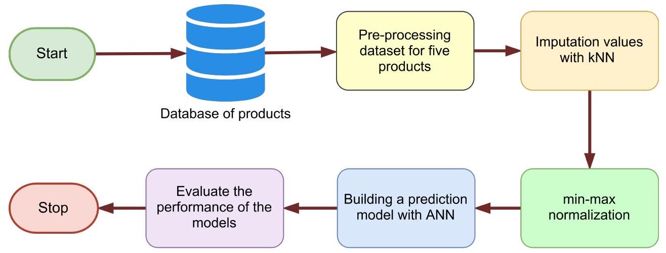
4. المواد والأساليب
4.1. البيانات
تتحرك البطالة وأداء الموردين واتجاهات الأسعار. نظرًا لأن المنتجات يُعتقد أنها تؤثر على المستخدم النهائي، تم تضمين قيمة مؤشر استهلاك التصنيع أيضًا في [18]. كما تم تضمين مؤشر ثقة المستهلك في النموذج لأنه سيظهر الميل نحو استهلاك المنتجات النهائية.
| المتغيرات | وصف المتغير المستخدم | تاريخ البدء | مصدر البيانات |
|
|
|
يناير 2010 | الشركة |
|
|
|
يناير 2010 | الشركة |
| مؤشر أسعار المنتجين | مؤشر أسعار المنتجين (%) [التضخم] | يناير 2010 | البنك المركزي لجمهورية تركيا
|
| الناتج المحلي الإجمالي | الناتج المحلي الإجمالي [الدخل القومي] | يناير 2010 | TSI
|
| IntR | سعر فائدة البنك المركزي التركي | يناير 2010 | البنك المركزي لجمهورية تركيا
|
| دولار أمريكي | سعر USD/TL، بيع الفوركس [سعر الصرف] | يناير 2010 | البنك المركزي لجمهورية تركيا
|
| CCI | مؤشر ثقة المستهلك | يناير 2012 | TSI
|
| PMI | مؤشر مديري المشتريات [مؤشر صناعة التصنيع] | أبريل 2015 | هنا
|
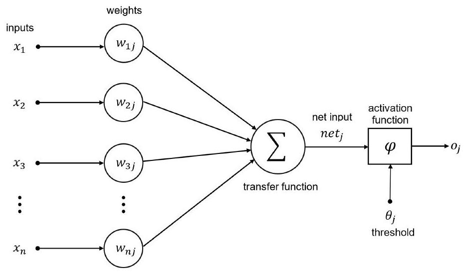
4.2. الشبكات العصبية الاصطناعية
5. النتائج والمناقشة
|
|
|
|
|
|
|
|
|
|
|
|
| من | ٢٤,١٣٢ | ٧٠٨٨ | 6,690 | ٦١,٢٦٠ | ٢٨٨٢ | 263.0 | ٢٩٥.٠ | 310.0 | ١٢٩.٠ | ٣٣٤.٠ |
| ماكس | ١٠٤,٧٤٣ | 60,364 | ٥٤,٥٤٢ | ٤٢٣,٧٩٦ | ٢٨,٢٦٩ | 936.0 |
|
897.0 | ٨٢٣.٠ |
|
| معنى | 71,546 | ٢٦,٠٩١ | ٢٤,٣٠٢ | ٢٤٠,٠٩٦ | 17,179 | 606.8 | ٦٩١.٨ | 568.4 | ٤٨٢.٤ | 911.2 |
| S | ١٣,٢٢٧ | 9,141 | 9,932 | ٦١,٧٩١ | ٤٢٨٧ | 170.8 | 182.3 | ١٤٦.٠ | 161.0 | ٢٩٥.٩ |
| فيروس كورونا | 18.5 | ٣٥.٠ | ٤٠.٩ | ٢٥.٧ | ٢٥.٠ | ٢٨.١ | ٢٦.٤ | ٢٥.٧ | ٣٣.٤ | ٣٢.٥ |
|
|
IntR |
|
|
|
|
|
| من | 1.7 | ٤.٥ | 1.4 | 76.9 | ٣٣.٤ | ١٥٢,٢٦٨ |
| ماكس | ٤٦.٢ | ٢٤.٠ | 8.3 | 97.4 | ٥٦.٩ | ٢٣٥,٨٣٨ |
| معنى | 11.6 | 9.5 | 3.4 | ٨٨.٦ | ٤٩.٦ | 195,260 |
| S | 8.9 | ٥.٤ | 1.9 | 5.0 | 2.8 | 16,883 |
| فيروس كورونا | ٧٦.٧ | ٥٦.٩ | ٥٥.٨ | ٥.٦ | ٥.٦ | ٨.٦ |
5.1. نتائج تقدير النموذج عبر المربعات الصغرى العادية من أجل مقارنة نتائج الشبكة العصبية الاصطناعية
نماذج الانحدار. على وجه التحديد، يُلاحظ أن التوزيع الطبيعي لسلسلة المتبقيات غير مُحقق وأن هناك مشكلة في الارتباط الذاتي في جميع النماذج، كما تشير إليه اختبار الارتباط التسلسلي لبريوش-غودفري بمستوى دلالة 0.05. وبالتالي، يتم تطبيق نهج متسق مع التباين غير المتجانس والارتباط الذاتي (HAC) على مؤشرات النموذج، وبشكل خاص على
| المتغيرات | النموذج 1 | النموذج 2 | موديل 3 | النموذج 4 | النموذج 5 |
| ثابت | -0.0146 (.265) | 0.0109 (.463) | 0.0295 (.408) | 0.0048 (.755) | -0.0187 (.288) |
|
|
-0.3313 (.452) | -0.3342 (.548) | -0.2685 (.677) | 0.1096 (.632) | -1.0057 (.001) |
| مؤشر أسعار المنتجين | -0.0569 (.337) | 0.1062 (.161) | 0.1621 (.186) | -0.0727 (.069) | 0.0515 (.442) |
| IntR | 0.1974 (.156) | -0.1011 (.415) | 0.0889 (.662) | 0.1612 (.370) | 0.0912 (.400) |
| دولار أمريكي | 0.6864 (.150) | -0.5642 (.168) | -1.4303 (.153) | -0.1260 (.796) | 0.7342 (.199) |
| CCI | 1.2644 (.168) | 0.3939 (.539) | 1.0396 (.513) | 1.3086 (.151) | -2.2287 (.026) |
| PMI | -0.6693 (.026) | -0.1184 (.751) | -0.8663 (.045) | -0.4311 (.285) | -0.5308 (.093) |
| الناتج المحلي الإجمالي | 1.5885 (.117) | 0.4023 (.604) | -0.0479 (.974) | -0.4457 (.379) | 1.7129 (.005) |
|
|
-0.4657 (.000) | -0.3380 (.000) | -0.5054 (.000) | -0.3902 (.000) | -0.4536 (.000) |
|
|
0.1106 (.682) | -0.1993 (.568) | 0.4668 (.233) | -0.0095 (.919) | 0.6370 (.000) |
|
|
0.2411 | 0.1591 | 0.2929 | 0.1945 | 0.2661 |
| قيمة p لاختبار F | 0.0002 | 0.0179 | 0.0000 | 0.0030 | 0.0000 |
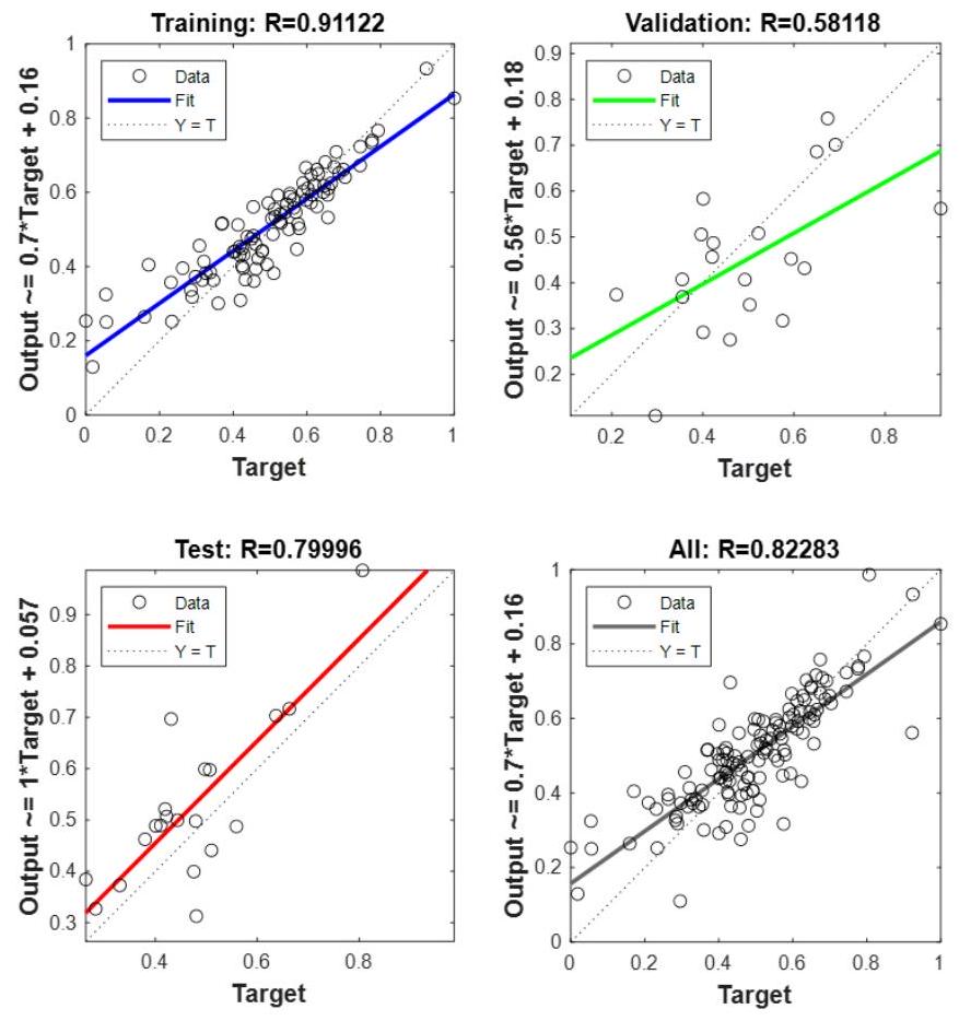
5.2. نتائج تقدير النموذج عبر الشبكة العصبية الاصطناعية
القيمة السابقة لـ
| تدريب | التحقق | اختبار | بشكل عام | |
| النموذج 1 | 0.8773 | 0.2332 | 0.3387 | 0.6112 |
| النموذج 2 | 0.9585 | 0.7036 | 0.7370 | 0.8971 |
| موديل 3 | 0.9333 | 0.7862 | 0.6608 | 0.8614 |
| النموذج 4 | 0.9112 | 0.5812 | 0.7999 | 0.8228 |
| النموذج 5 | 0.7292 | 0.4172 | 0.4438 | 0.5990 |
| عينات | MSE | ر | |
| تدريب | 95 |
|
|
| التحقق | 20 |
|
|
| اختبار | 20 |
|
|
5.3. تقييم أولويات المتغيرات من خلال GRA باستخدام نتائج الشبكة العصبية الاصطناعية
| النموذج 1 | النموذج 2 | موديل 3 | النموذج 4 | النموذج 5 | ||||||
| رتبة | متغير | قيمة | متغير | قيمة | متغير | قيمة | متغير | قيمة | متغير | قيمة |
| 1 |
|
٢.٩٦ | دولار أمريكي | ٤٦.٤٩ | IntR | ٣٥.٣٠ | دولار أمريكي | 27.34 |
|
٤.٤٤ |
| 2 |
|
2.03 | P2 | ٣٧.٠٨ | دولار أمريكي | 30.77 |
|
25.60 | IntR | ٣.٩٥ |
| ٣ |
|
1.86 |
|
27.10 |
|
17.78 | PMI | ٢٢.٦٨ | دولار أمريكي | 3.85 |
| ٤ | الناتج المحلي الإجمالي | 1.29 |
|
19.34 |
|
12.55 | IntR | ٢١.٩٧ |
|
٢.٩٥ |
| ٥ |
|
1.19 | IntR | 18.21 |
|
12.22 |
|
١٣.٧٩ | مؤشر أسعار المنتجين | 1.77 |
| ٦ | PMI | 0.92 | مؤشر مديري المشتريات | 15.46 | مؤشر مديري المشتريات | 8.83 |
|
11.60 | PMI | 1.51 |
| ٧ | دولار أمريكي | 0.26 |
|
٣.٥٤ | مؤشر أسعار المنتجين | ٥.٨٠ |
|
٦.٤٠ | الناتج المحلي الإجمالي | 0.50 |
| ٨ | مؤشر أسعار المنتجين | 0.23 |
|
1.93 |
|
1.92 |
|
٢.٢٣ |
|
0.41 |
| 9 | IntR | 0.10 | مؤشر أسعار المنتجين | 0.69 |
|
0.04 |
|
2.09 |
|
0.18 |
و
| أولويات نماذج موحدة | ترتيب الأولويات المعاير للنماذج | |||||||||
| متغير | النموذج 1 | النموذج 2 | موديل 3 | النموذج 4 | النموذج 5 | النموذج 1 | النموذج 2 | موديل 3 | النموذج 4 | النموذج 5 |
|
|
0.615 | 0.795 | 0.345 | 0.931 | 1.000 | ٣ | 2 | ٥ | 2 | 1 |
| مؤشر أسعار المنتجين | 0.045 | 0.000 | 0.163 | 0.171 | 0.373 | ٨ | 9 | ٧ | ٧ | ٥ |
| IntR | 0.000 | 0.383 | 1.000 | 0.787 | 0.885 | 9 | ٥ | 1 | ٤ | ٢ |
| دولار أمريكي | 0.056 | 1.000 | 0.872 | 1.000 | 0.862 | ٧ | 1 | 2 | 1 | ٣ |
|
|
1.000 | 0.407 | 0.355 | 0.377 | 0.054 | 1 | ٤ | ٤ | ٦ | ٨ |
| PMI | 0.287 | 0.322 | 0.249 | 0.815 | 0.312 | ٦ | ٦ | ٦ | ٣ | ٦ |
| الناتج المحلي الإجمالي | 0.416 | 0.027 | 0.000 | 0.006 | 0.075 | ٤ | ٨ | 9 | ٨ | ٧ |
|
|
0.675 | 0.577 | 0.503 | 0.463 | 0.650 | 2 | ٣ | ٣ | ٥ | ٤ |
|
|
0.381 | 0.062 | 0.053 | 0.000 | 0.000 | ٥ | ٧ | ٨ | 9 | 9 |
| اسم السيناريو وطريقة حساب الأولويات | الأوزان المحسوبة للنماذج | ||||
| النموذج 1 | النموذج 2 | موديل 3 | النموذج 4 | النموذج 5 | |
| Scnr1: كل نموذج له وزن متساوي. | 0.2000 | 0.2000 | 0.2000 | 0.2000 | 0.2000 |
| Scnr2: من خلال استخدام قيم نجاح فترة الاختبار لـ ModPerR عبر NESO. | 0.1137 | 0.2473 | 0.2217 | 0.2684 | 0.1489 |
| Scnr3: من خلال استخدام قيم النجاح العامة لـ ModPerR عبر NESO. | 0.1612 | 0.2366 | 0.2272 | 0.2170 | 0.1580 |
| Scnr4: من خلال استخدام متوسطات كل سلسلة Qi وفقًا للنموذج عبر NESO | 0.2100 | 0.0873 | 0.0668 | 0.5602 | 0.0757 |
| Scnr5: من خلال استخدام قيم كل زوج من ضرب متوسطات سلسلتي Qi و Pi وفقًا للنموذج عبر NESO | |||||
| 0.1887 | 0.0688 | 0.0641 | 0.6331 | 0.0453 | |
| Scnr1 | Scnr2 | Scnr3 | Scnr3 | Scnr5 | متوسط درجات GRA | |||||||
| جرا | رتبة | جرا | رتبة | جرا | رتبة | جرا | رتبة | جرا | رتبة | جرا | رتبة | |
|
|
0.717 | 2 | 0.720 | 2 | 0.706 | 2 | 0.785 | ٢ | 0.778 | 2 | 0.741 | 2 |
| مؤشر أسعار المنتجين | 0.374 | ٧ | 0.371 | ٧ | 0.371 | ٧ | 0.370 | ٧ | 0.371 | ٧ | 0.371 | ٧ |
| IntR | 0.659 | ٣ | 0.680 | ٣ | 0.667 | ٣ | 0.639 | ٣ | 0.630 | ٣ | 0.655 | ٣ |
| دولار أمريكي | 0.785 | 1 | 0.848 | 1 | 0.814 | 1 | 0.854 | 1 | 0.833 | 1 | 0.827 | 1 |
| CCI | 0.537 | ٥ | 0.495 | ٦ | 0.520 | ٥ | 0.546 | ٥ | 0.555 | ٥ | 0.530 | ٥ |
| PMI | 0.478 | ٦ | 0.499 | ٥ | 0.483 | ٦ | 0.614 | ٤ | 0.591 | ٤ | 0.533 | ٤ |
| الناتج المحلي الإجمالي | 0.364 | ٨ | 0.352 | 9 | 0.358 | ٨ | 0.359 | ٨ | 0.363 | ٨ | 0.359 | ٨ |
|
|
0.544 | ٤ | 0.531 | ٤ | 0.537 | ٤ | 0.516 | ٦ | 0.523 | ٦ | 0.530 | ٦ |
|
|
0.361 | 9 | 0.353 | ٨ | 0.358 | 9 | 0.357 | 9 | 0.359 | 9 | 0.358 | ٩ |
5.4. تقييم ومناقشة نتائج GRA
قد تكون الشركات مغرمة بشراء منتجات الحديد والصلب قبل زيادة محتملة في أسعار الصرف من أجل حماية نفسها.
6. الخاتمة
References
[2] Altan A, Karasu S, Bekiros S. Digital currency forecasting with chaotic meta-heuristic bio-inspired signal processing techniques. Chaos, Solitons & Fractals 2019; 126: 325-336.
[3] Chang V. Towards data analysis for weather cloud computing. Knowledge-Based Systems 2017; 127: 29-45.
[4] Chen A, Blue J. Performance analysis of demand planning approaches for aggregating, forecasting and disaggregating interrelated demands. International Journal of Production Economics 2010; 128 (2): 586-602.
[5] Jeon S, Hong B, Chang V. Pattern graph tracking-based stock price prediction using big data. Future Generation Computer Systems 2018; 80: 171-187.
[6] Karasu S, Altan A, Bekiros S, Ahmad W. A new forecasting model with wrapper-based feature selection approach using multi-objective optimization technique for chaotic crude oil time series. Energy 2020; 212: 118750.
[7] Gashler MS, Ashmore SC. Modeling time series data with deep Fourier neural networks. Neurocomputing 2016; 188: 3-11.
[8] Huh KS. Steel consumption and economic growth in Korea: long-term and short-term evidence. Resources Policy 2011; 36 (2): 107-113.
[9] Evans M. Modelling steel demand in the UK. Ironmaking & Steelmaking 1996; 23 (1): 17-24.
[10] Abbott AJ, Lawler KA, Armistead C. The UK demand for steel. Applied Economics 1999; 31 (11): 1299-1302.
[11] Crompton P. Future trends in Japanese steel consumption. Resources Policy 2000; 26 (2): 103-114.
[12] Barska M. Demand forecast with business climate index for a steel and iron industry representative. Metody Ilościowe w Badaniach Ekonomicznych 2014; 15 (2): 27-36.
[13] Crompton P, Wu Y. Bayesian vector autoregression forecasts of Chinese steel consumption. Journal of Chinese Economic and Business Studies 2003; 1 (2): 205-219.
[14] Evans M. An alternative approach to estimating the parameters of a generalised Grey Verhulst model: an application to steel intensity of use in the UK. Expert Systems with Applications 2014; 41 (4): 1236-1244.
[15] Chang PC, Wang YW, Tsai CY. Evolving neural network for printed circuit board sales forecasting. Expert Systems with Applications 2005; 29 (1): 83-92.
[16] Psiloglou BE, Giannakopoulos C, Majithia S, Petrakis M. Factors affecting electricity demand in Athens, Greece and London, UK: a comparative assessment. Energy 2009; 34 (11): 1855-1863.
[17] Efendigil T, Önüt S, Kahraman C. A decision support system for demand forecasting with artificial neural networks and neuro-fuzzy models: a comparative analysis. Expert Systems with Applications 2009; 36 (3): 6697-6707.
[18] Hicham A, Mohammed B, Anas S. Hybrid intelligent system for sale forecasting using Delphi and adaptive fuzzy back-propagation neural networks. Editorial Preface 2012.
[19] Oğcu G, Demirel OF, Zaim S. Forecasting electricity consumption with neural networks and support vector regression. Procedia – Social and Behavioral Sciences 2012; 58: 1576-1585.
[20] Azadeh A, Neshat N, Mardan E, Saberi M. Optimization of steel demand forecasting with complex and uncertain economic inputs by an integrated neural network-fuzzy mathematical programming approach. The International Journal of Advanced Manufacturing Technology 2013; 65: 833-841.
[21] Aziz AA, Mustapha NHN, Ismail R. Factors affecting energy demand in developing countries: a dynamic panel analysis. International Journal of Energy Economics and Policy 2013; 3 (4): 1-6.
[22] Akyurt İZ. Talep tahmininin yapay sinir ağlarıyla modellenmesi: yerli otomobil örneği. Ekonometri ve İstatistik Dergisi 2015; 23: 147-157 (in Turkish).
[23] Koochakpour K, Tarokh MJ. Sales budget forecasting and revision by adaptive network fuzzy base inference system and optimization methods. Journal of Computer & Robotics 2016; 9 (1): 25-38.
[24] Ecemiş O. Model ağaç yöntemiyle satış tahmini: paslanmaz çelik sektöründe bir uygulama. The Journal of Academic Social Science 2019; 84 (84): 336-350 (in Turkish).
[25] Jain AK, Mao J, Mohiuddin KM. Artificial neural networks: a tutorial. Computer 1996; 29 (3): 31-44.
[26] Agatonovic-Kustrin S, Beresford R. Basic concepts of artificial neural network (ANN) modeling and its application in pharmaceutical research. Journal of Pharmaceutical and Biomedical Analysis 2000; 22 (5): 717-727.
[27] Pekkaya M, Pulat Ö, Koca H. Evaluation of healthcare service quality via Servqual scale: an application on a hospital. International Journal of Healthcare Management 2019; 12 (4): 340-347.
[28] Pekkaya M, Pulat Ö, Zeydan İ. Service quality determiners in higher education: the student’s perspective. International Journal of Services, Economics and Management 2023; 14 (3): 270-300.
[29] Dökmen G, Pekkaya M, Saymaz N. Sigara bağımlılığı ve devletin sigara tüketimi ile mücadele yöntemleri arasındaki ilişki. Maliye Dergisi 2019; 176: 599-623 (in Turkish).
[30] Madhukumar M, Sebastian A, Liang X, Jamil M, Shabbir MNSK. Regression model-based short-term load forecasting for university campus load. IEEE Access 2022; 10: 8891-8905.
[31] Singh U, Rizwan M, Alaraj M, Alsaidan I. A machine learning-based gradient boosting regression approach for wind power production forecasting: a step towards smart grid environments. Energies 2021; 14 (16): 5196.
[32] Pekkaya M. ARFIMA ve FIGARCH yöntemlerinin Markowitz ortalama varyans portföy optimizasyonunda kullanılması: İMKB-30 endeks hisseleri üzerine bir uygulama. İstanbul Üniversitesi İşletme Fakültesi Dergisi 2013; 42 (1): 93-112 (in Turkish).
[33] Hayes AF, Cai L. Using heteroskedasticity-consistent standard error estimators in OLS regression: an introduction and software implementation. Behavior Research Methods 2007; 39: 709-722.
[34] Hamzaçebi C, Pekkaya M. Determining of stock investments with grey relational analysis. Expert Systems with Applications 2011; 38 (8): 9186-9195.
- *Correspondence: aytacaltan@beun.edu.tr
TSEA (2022). Turkish Steel Exporters’ Association [online] Website http://www.cib.org.tr/tr/istatistikler.html [accessed 03 August 2023] İhracat Genel Müdürlüğü Maden, Metal ve Orman Ürünleri Daire Başkanlığı (2017). Demir-Çelik, Demir-Çelikten Eşya Sektör Raporu [online]. Website https://www.orhangazitso.org.tr/webFiles/1488897357.pdf [accessed 03 August 2023] WSA (2022). World Steel Association [online] Website http://www.worldsteel.org [accessed 03 August 2023] CBRT (2021). Central Bank of the Republic of Türkiye [online]. Website https://www.tcmb.gov.tr [accessed 03 August 2023].
TSI (2021). Turkish Statistical Institute [online]. Website https://www.tuik.gov.tr [accessed 03 August 2023].
ICI (2021). Istanbul Chamber of Industry [online]. Website http://www.iso.org.tr/ [accessed 03 August 2023]. TSEA (2022). Turkish Steel Exporters’ Association [online] Website http://www.cib.org.tr/tr/istatistikler.html [accessed 03 August 2023]
DOI: https://doi.org/10.55730/1300-0632.4055
Publication Date: 2024-02-07
Artificial intelligence-based evaluation of the factors affecting the sales of an iron and steel company
8 Part of the Computer Engineering Commons, Computer Sciences Commons, and the Electrical and Computer Engineering Commons
Recommended Citation
http://journals.tubitak.gov.tr/elektrik/
Research Article
(2024) 32: 51-67
© TÜBİTAK
doi:10.55730/1300-0632.4055
Artificial intelligence-based evaluation of the factors affecting the sales of an iron and steel company
| Received: 07.08 .2023 | • Accepted/Published Online: 08.12 .2023 | • | Final Version: 07.02 .2024 |
Abstract
It is important to predict the sales of an iron and steel company and to identify the variables that influence these sales for future planning. The aim in this study was to identify and model the key factors that influence the sales volume of an iron and steel company using artificial neural networks (ANNs). We attempted to obtain an integrated result from the performance/sales levels of 5 models, to use the ANN approach with hybrid algorithms, and also to present an exemplary application in the base metals industry, where there is a limited number of studies. This study contributes to the literature as the first application of artificial intelligence methods in the iron and steel industry. The ANN models incorporated 6 macroeconomic variables and price-to-sales data and their results were evaluated. An ordinary least squares regression model was also used to facilitate the comparison of results, while gray relational analysis (GRA) was used to draw a comprehensive conclusion based on the ANN results. The results showed that the variables USD/TL exchange rate, product prices, and interest rates, in descending order, had the highest degree of influence in determining the sales of the iron and steel company. Furthermore, these variables are crucial for forecasting future sales and strategic planning. The study showed that the ANN outperformed classical regression models in terms of prediction accuracy. In the model applications conducted for 5 different product groups, it was observed that 3 models (models 2 , 3, and 4), including model 4, which sold a higher volume of products than the total of the other products, had an overall performance above
1. Introduction
2. Iron and steel industry in Tuirkiye and the rest of the world
3. Literature review on the factors determining the sales of and demand for iron and steel
| Order | Country | 2021 | Rate (%) | Order | Country | 2021 | Rate (%) |
| 1 | China | 1,032,790 | 52.9 | 9 | Brazil | 36,174 | 1.9 |
| 2 | India | 118,244 | 6.1 | 10 | Iran | 28,460 | 1.5 |
| 3 | Japan | 96,334 | 4.9 | 11 | Italy | 24,426 | 1.3 |
| 4 | USA | 85,791 | 4.4 | 12 | Taiwan | 23,233 | 1.2 |
| 5 | Russia | 75,585 | 3.9 | 13 | Vietnam | 23,019 | 1.2 |
| 6 | South Korea | 70,418 | 3.6 | 14 | Ukraine | 21,366 | 1.1 |
| 7 | Turkey | 40,360 | 2.1 | 15 | Mexico | 18,454 | 0.9 |
| 8 | Germany | 40,066 | 2.1 | World | 1,951,924 | 100.0 |
| Researcher | Subject | Variables | Method |
| [10] | UK steel demand | National income, interest rate, steel price, steel-related industry demand | Vectorial regression |
| [11] | Future trends in Japanese steel consumption | National income, population, steel-related, industry demand | Usage intensity model |
| [15] | Printed circuit boards sales forecast | National income, consumer price index, manufacturing product index | Genetic algorithm, feedback ANN |
| [16] | Electricity demand in Athens/London | National income, demographic structure, air temperature | Trend analysis, seasonal analysis |
| [17] | White goods supply chain demand forecasting | Product price, product quality, promotions | Fuzzy logic, ANN |
| [13] | Consumption forecast in the Chinese steel industry | National income, per capita income, intensity of use | Bayesian vectorial autoregression |
| [8] | Steel consumption and long-short-term economic development in Korea | National income, per capita income | Vectorial autoregression |
| [18] | Packaging sales forecast | Manufacturing consumer index, competitive index, historical sales data | Delphi and ANN |
| [19] | Electricity consumption forecast | Population growth rate | Vector regression supported ANN |
| [20] | Demand forecasting in the iron/steel industry | National income, national income growth rate, inflation, steel production data | Fuzzy logic, ANN |
| [21] | Factors affecting energy demand in developing countries | National income, price, economic structure, CO2 emissions | Dynamic panel analysis |
| [12] | Demand forecast in the iron-steel industry based on the business climate index | National income | ARIMA, SARIMA |
| [14] | Approach to determining forecast parameters: An application to steel intensity of use in the UK | Intensity of use | Grey Verhulst model |
| [22] | Automotive demand forecasting | Historical sales data | ANN |
| [23] | Sales forecast of a company | National income, exchange rate, inflation, historical sales data | ANN with fuzzy logic revision |
| [24] | Stainless Steel sales forecast | Raw material prices, USD/TRY, PPI, industrial production index | Data mining, model tree method |
4. Materials and methods
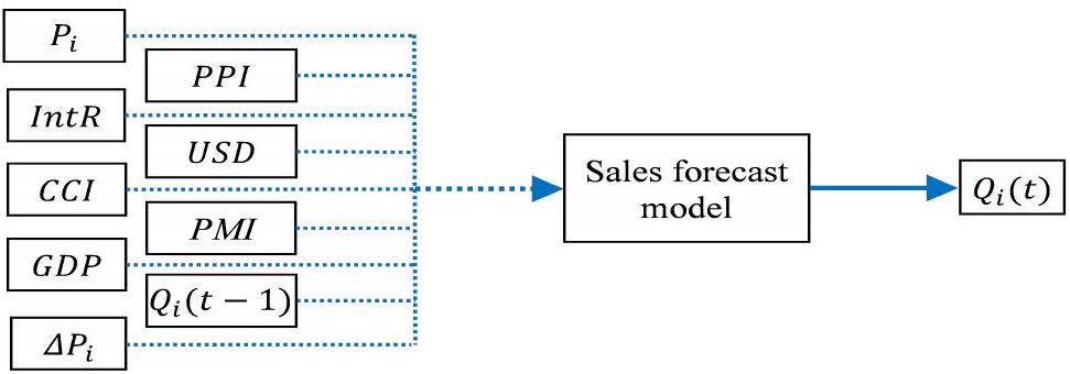
4.1. Data
employment, supplier performance, and price trends are moving. As products are thought to affect the end user, the value of the manufacturing consumer index was also included in [18]. The consumer confidence index is also included in the model as it will show the tendency towards consumption of final products.
| Variables | Used variable description | Start date | Data source |
|
|
|
Jan. 2010 | The company |
|
|
|
Jan. 2010 | The company |
| PPI | Producer price index (%) [inflation] | Jan. 2010 | CBRT
|
| GDP | Gross domestic products [national income] | Jan. 2010 | TSI
|
| IntR | CBRT interest rate | Jan. 2010 | CBRT
|
| USD | USD/TL rate, Forex sale [exchange rate] | Jan. 2010 | CBRT
|
| CCI | Consumer confidence index | Jan. 2012 | TSI
|
| PMI | Purchasing managers index [manufacturing industry index] | Apr. 2015 | ICI
|
4.2. Artificial neural networks
5. Results and discussion
|
|
|
|
|
|
|
|
|
|
|
|
| Min | 24,132 | 7,088 | 6,690 | 61,260 | 2,882 | 263.0 | 295.0 | 310.0 | 129.0 | 334.0 |
| Max | 104,743 | 60,364 | 54,542 | 423,796 | 28,269 | 936.0 |
|
897.0 | 823.0 |
|
| Mean | 71,546 | 26,091 | 24,302 | 240,096 | 17,179 | 606.8 | 691.8 | 568.4 | 482.4 | 911.2 |
| S | 13,227 | 9,141 | 9,932 | 61,791 | 4,287 | 170.8 | 182.3 | 146.0 | 161.0 | 295.9 |
| CoV | 18.5 | 35.0 | 40.9 | 25.7 | 25.0 | 28.1 | 26.4 | 25.7 | 33.4 | 32.5 |
|
|
IntR |
|
|
|
|
|
| Min | 1.7 | 4.5 | 1.4 | 76.9 | 33.4 | 152,268 |
| Max | 46.2 | 24.0 | 8.3 | 97.4 | 56.9 | 235,838 |
| Mean | 11.6 | 9.5 | 3.4 | 88.6 | 49.6 | 195,260 |
| S | 8.9 | 5.4 | 1.9 | 5.0 | 2.8 | 16,883 |
| CoV | 76.7 | 56.9 | 55.8 | 5.6 | 5.6 | 8.6 |
5.1. Model estimate results via ordinary least squares in order to compare ANN results
regression models. Specifically, it is noted that the normal distribution of the residual series is not satisfied and that there is an autocorrelation problem in all models, as indicated by the Breusch-Godfrey serial correlation LM test with a significance level of 0.05 . Consequently, a heteroskedasticity and autocorrelation consistent (HAC) approach is applied to the model indicators, and in particular to the
| Variables | Model 1 | Model 2 | Model 3 | Model 4 | Model 5 |
| Const | -0.0146 (.265) | 0.0109 (.463) | 0.0295 (.408) | 0.0048 (.755) | -0.0187 (.288) |
|
|
-0.3313 (.452) | -0.3342 (.548) | -0.2685 (.677) | 0.1096 (.632) | -1.0057 (.001) |
| PPI | -0.0569 (.337) | 0.1062 (.161) | 0.1621 (.186) | -0.0727 (.069) | 0.0515 (.442) |
| IntR | 0.1974 (.156) | -0.1011 (.415) | 0.0889 (.662) | 0.1612 (.370) | 0.0912 (.400) |
| USD | 0.6864 (.150) | -0.5642 (.168) | -1.4303 (.153) | -0.1260 (.796) | 0.7342 (.199) |
| CCI | 1.2644 (.168) | 0.3939 (.539) | 1.0396 (.513) | 1.3086 (.151) | -2.2287 (.026) |
| PMI | -0.6693 (.026) | -0.1184 (.751) | -0.8663 (.045) | -0.4311 (.285) | -0.5308 (.093) |
| GDP | 1.5885 (.117) | 0.4023 (.604) | -0.0479 (.974) | -0.4457 (.379) | 1.7129 (.005) |
|
|
-0.4657 (.000) | -0.3380 (.000) | -0.5054 (.000) | -0.3902 (.000) | -0.4536 (.000) |
|
|
0.1106 (.682) | -0.1993 (.568) | 0.4668 (.233) | -0.0095 (.919) | 0.6370 (.000) |
|
|
0.2411 | 0.1591 | 0.2929 | 0.1945 | 0.2661 |
| F test p -value | 0.0002 | 0.0179 | 0.0000 | 0.0030 | 0.0000 |
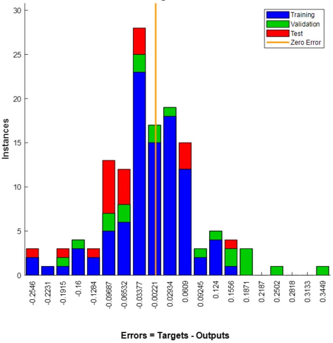
5.2. Model estimate results via ANN
the previous value of the
| Training | Validation | Test | Overall | |
| Model 1 | 0.8773 | 0.2332 | 0.3387 | 0.6112 |
| Model 2 | 0.9585 | 0.7036 | 0.7370 | 0.8971 |
| Model 3 | 0.9333 | 0.7862 | 0.6608 | 0.8614 |
| Model 4 | 0.9112 | 0.5812 | 0.7999 | 0.8228 |
| Model 5 | 0.7292 | 0.4172 | 0.4438 | 0.5990 |
| Samples | MSE | R | |
| Training | 95 |
|
|
| Validation | 20 |
|
|
| Testing | 20 |
|
|
5.3. Variables’ priorities evaluation via GRA using ANN results
| Model 1 | Model 2 | Model 3 | Model 4 | Model 5 | ||||||
| Rank | Variable | Value | Variable | Value | Variable | Value | Variable | Value | Variable | Value |
| 1 |
|
2.96 | USD | 46.49 | IntR | 35.30 | USD | 27.34 |
|
4.44 |
| 2 |
|
2.03 | P2 | 37.08 | USD | 30.77 |
|
25.60 | IntR | 3.95 |
| 3 |
|
1.86 |
|
27.10 |
|
17.78 | PMI | 22.68 | USD | 3.85 |
| 4 | GDP | 1.29 |
|
19.34 |
|
12.55 | IntR | 21.97 |
|
2.95 |
| 5 |
|
1.19 | IntR | 18.21 |
|
12.22 |
|
13.79 | PPI | 1.77 |
| 6 | PMI | 0.92 | PMI | 15.46 | PMI | 8.83 |
|
11.60 | PMI | 1.51 |
| 7 | USD | 0.26 |
|
3.54 | PPI | 5.80 |
|
6.40 | GDP | 0.50 |
| 8 | PPI | 0.23 |
|
1.93 |
|
1.92 |
|
2.23 |
|
0.41 |
| 9 | IntR | 0.10 | PPI | 0.69 |
|
0.04 |
|
2.09 |
|
0.18 |
and
| Normalized priorities for models | Normalized priority ranks for models | |||||||||
| Variable | Model 1 | Model 2 | Model 3 | Model 4 | Model 5 | Model 1 | Model 2 | Model 3 | Model 4 | Model 5 |
|
|
0.615 | 0.795 | 0.345 | 0.931 | 1.000 | 3 | 2 | 5 | 2 | 1 |
| PPI | 0.045 | 0.000 | 0.163 | 0.171 | 0.373 | 8 | 9 | 7 | 7 | 5 |
| IntR | 0.000 | 0.383 | 1.000 | 0.787 | 0.885 | 9 | 5 | 1 | 4 | 2 |
| USD | 0.056 | 1.000 | 0.872 | 1.000 | 0.862 | 7 | 1 | 2 | 1 | 3 |
|
|
1.000 | 0.407 | 0.355 | 0.377 | 0.054 | 1 | 4 | 4 | 6 | 8 |
| PMI | 0.287 | 0.322 | 0.249 | 0.815 | 0.312 | 6 | 6 | 6 | 3 | 6 |
| GDP | 0.416 | 0.027 | 0.000 | 0.006 | 0.075 | 4 | 8 | 9 | 8 | 7 |
|
|
0.675 | 0.577 | 0.503 | 0.463 | 0.650 | 2 | 3 | 3 | 5 | 4 |
|
|
0.381 | 0.062 | 0.053 | 0.000 | 0.000 | 5 | 7 | 8 | 9 | 9 |
| Scenario name and the way of calculating priorities | Calculated weights for models | ||||
| Model 1 | Model 2 | Model 3 | Model 4 | Model 5 | |
| Scnr1: Each model has equal weight. | 0.2000 | 0.2000 | 0.2000 | 0.2000 | 0.2000 |
| Scnr2: By using the test period success values of ModPerR via NESO. | 0.1137 | 0.2473 | 0.2217 | 0.2684 | 0.1489 |
| Scnr3: By using the overall success values of ModPerR via NESO. | 0.1612 | 0.2366 | 0.2272 | 0.2170 | 0.1580 |
| Scnr4: By using each Qi series averages subject to the model via NESO | 0.2100 | 0.0873 | 0.0668 | 0.5602 | 0.0757 |
| Scnr5: By using the values of each pair multiplication of averages of Qi and Pi series subject to the model via NESO | |||||
| 0.1887 | 0.0688 | 0.0641 | 0.6331 | 0.0453 | |
| Scnr1 | Scnr2 | Scnr3 | Scnr3 | Scnr5 | Mean of GRA scores | |||||||
| GRA | Rank | GRA | Rank | GRA | Rank | GRA | Rank | GRA | Rank | GRA | Rank | |
|
|
0.717 | 2 | 0.720 | 2 | 0.706 | 2 | 0.785 | 2 | 0.778 | 2 | 0.741 | 2 |
| PPI | 0.374 | 7 | 0.371 | 7 | 0.371 | 7 | 0.370 | 7 | 0.371 | 7 | 0.371 | 7 |
| IntR | 0.659 | 3 | 0.680 | 3 | 0.667 | 3 | 0.639 | 3 | 0.630 | 3 | 0.655 | 3 |
| USD | 0.785 | 1 | 0.848 | 1 | 0.814 | 1 | 0.854 | 1 | 0.833 | 1 | 0.827 | 1 |
| CCI | 0.537 | 5 | 0.495 | 6 | 0.520 | 5 | 0.546 | 5 | 0.555 | 5 | 0.530 | 5 |
| PMI | 0.478 | 6 | 0.499 | 5 | 0.483 | 6 | 0.614 | 4 | 0.591 | 4 | 0.533 | 4 |
| GDP | 0.364 | 8 | 0.352 | 9 | 0.358 | 8 | 0.359 | 8 | 0.363 | 8 | 0.359 | 8 |
|
|
0.544 | 4 | 0.531 | 4 | 0.537 | 4 | 0.516 | 6 | 0.523 | 6 | 0.530 | 6 |
|
|
0.361 | 9 | 0.353 | 8 | 0.358 | 9 | 0.357 | 9 | 0.359 | 9 | 0.358 | 9 |
5.4. Evaluation and discussion of GRA results
decisions, companies may be tempted to purchase iron and steel products ahead of a possible increase in exchange rates in order to hedge themselves.
6. Conclusion
References
[2] Altan A, Karasu S, Bekiros S. Digital currency forecasting with chaotic meta-heuristic bio-inspired signal processing techniques. Chaos, Solitons & Fractals 2019; 126: 325-336.
[3] Chang V. Towards data analysis for weather cloud computing. Knowledge-Based Systems 2017; 127: 29-45.
[4] Chen A, Blue J. Performance analysis of demand planning approaches for aggregating, forecasting and disaggregating interrelated demands. International Journal of Production Economics 2010; 128 (2): 586-602.
[5] Jeon S, Hong B, Chang V. Pattern graph tracking-based stock price prediction using big data. Future Generation Computer Systems 2018; 80: 171-187.
[6] Karasu S, Altan A, Bekiros S, Ahmad W. A new forecasting model with wrapper-based feature selection approach using multi-objective optimization technique for chaotic crude oil time series. Energy 2020; 212: 118750.
[7] Gashler MS, Ashmore SC. Modeling time series data with deep Fourier neural networks. Neurocomputing 2016; 188: 3-11.
[8] Huh KS. Steel consumption and economic growth in Korea: long-term and short-term evidence. Resources Policy 2011; 36 (2): 107-113.
[9] Evans M. Modelling steel demand in the UK. Ironmaking & Steelmaking 1996; 23 (1): 17-24.
[10] Abbott AJ, Lawler KA, Armistead C. The UK demand for steel. Applied Economics 1999; 31 (11): 1299-1302.
[11] Crompton P. Future trends in Japanese steel consumption. Resources Policy 2000; 26 (2): 103-114.
[12] Barska M. Demand forecast with business climate index for a steel and iron industry representative. Metody Ilościowe w Badaniach Ekonomicznych 2014; 15 (2): 27-36.
[13] Crompton P, Wu Y. Bayesian vector autoregression forecasts of Chinese steel consumption. Journal of Chinese Economic and Business Studies 2003; 1 (2): 205-219.
[14] Evans M. An alternative approach to estimating the parameters of a generalised Grey Verhulst model: an application to steel intensity of use in the UK. Expert Systems with Applications 2014; 41 (4): 1236-1244.
[15] Chang PC, Wang YW, Tsai CY. Evolving neural network for printed circuit board sales forecasting. Expert Systems with Applications 2005; 29 (1): 83-92.
[16] Psiloglou BE, Giannakopoulos C, Majithia S, Petrakis M. Factors affecting electricity demand in Athens, Greece and London, UK: a comparative assessment. Energy 2009; 34 (11): 1855-1863.
[17] Efendigil T, Önüt S, Kahraman C. A decision support system for demand forecasting with artificial neural networks and neuro-fuzzy models: a comparative analysis. Expert Systems with Applications 2009; 36 (3): 6697-6707.
[18] Hicham A, Mohammed B, Anas S. Hybrid intelligent system for sale forecasting using Delphi and adaptive fuzzy back-propagation neural networks. Editorial Preface 2012.
[19] Oğcu G, Demirel OF, Zaim S. Forecasting electricity consumption with neural networks and support vector regression. Procedia – Social and Behavioral Sciences 2012; 58: 1576-1585.
[20] Azadeh A, Neshat N, Mardan E, Saberi M. Optimization of steel demand forecasting with complex and uncertain economic inputs by an integrated neural network-fuzzy mathematical programming approach. The International Journal of Advanced Manufacturing Technology 2013; 65: 833-841.
[21] Aziz AA, Mustapha NHN, Ismail R. Factors affecting energy demand in developing countries: a dynamic panel analysis. International Journal of Energy Economics and Policy 2013; 3 (4): 1-6.
[22] Akyurt İZ. Talep tahmininin yapay sinir ağlarıyla modellenmesi: yerli otomobil örneği. Ekonometri ve İstatistik Dergisi 2015; 23: 147-157 (in Turkish).
[23] Koochakpour K, Tarokh MJ. Sales budget forecasting and revision by adaptive network fuzzy base inference system and optimization methods. Journal of Computer & Robotics 2016; 9 (1): 25-38.
[24] Ecemiş O. Model ağaç yöntemiyle satış tahmini: paslanmaz çelik sektöründe bir uygulama. The Journal of Academic Social Science 2019; 84 (84): 336-350 (in Turkish).
[25] Jain AK, Mao J, Mohiuddin KM. Artificial neural networks: a tutorial. Computer 1996; 29 (3): 31-44.
[26] Agatonovic-Kustrin S, Beresford R. Basic concepts of artificial neural network (ANN) modeling and its application in pharmaceutical research. Journal of Pharmaceutical and Biomedical Analysis 2000; 22 (5): 717-727.
[27] Pekkaya M, Pulat Ö, Koca H. Evaluation of healthcare service quality via Servqual scale: an application on a hospital. International Journal of Healthcare Management 2019; 12 (4): 340-347.
[28] Pekkaya M, Pulat Ö, Zeydan İ. Service quality determiners in higher education: the student’s perspective. International Journal of Services, Economics and Management 2023; 14 (3): 270-300.
[29] Dökmen G, Pekkaya M, Saymaz N. Sigara bağımlılığı ve devletin sigara tüketimi ile mücadele yöntemleri arasındaki ilişki. Maliye Dergisi 2019; 176: 599-623 (in Turkish).
[30] Madhukumar M, Sebastian A, Liang X, Jamil M, Shabbir MNSK. Regression model-based short-term load forecasting for university campus load. IEEE Access 2022; 10: 8891-8905.
[31] Singh U, Rizwan M, Alaraj M, Alsaidan I. A machine learning-based gradient boosting regression approach for wind power production forecasting: a step towards smart grid environments. Energies 2021; 14 (16): 5196.
[32] Pekkaya M. ARFIMA ve FIGARCH yöntemlerinin Markowitz ortalama varyans portföy optimizasyonunda kullanılması: İMKB-30 endeks hisseleri üzerine bir uygulama. İstanbul Üniversitesi İşletme Fakültesi Dergisi 2013; 42 (1): 93-112 (in Turkish).
[33] Hayes AF, Cai L. Using heteroskedasticity-consistent standard error estimators in OLS regression: an introduction and software implementation. Behavior Research Methods 2007; 39: 709-722.
[34] Hamzaçebi C, Pekkaya M. Determining of stock investments with grey relational analysis. Expert Systems with Applications 2011; 38 (8): 9186-9195.
- *Correspondence: aytacaltan@beun.edu.tr
TSEA (2022). Turkish Steel Exporters’ Association [online] Website http://www.cib.org.tr/tr/istatistikler.html [accessed 03 August 2023] İhracat Genel Müdürlüğü Maden, Metal ve Orman Ürünleri Daire Başkanlığı (2017). Demir-Çelik, Demir-Çelikten Eşya Sektör Raporu [online]. Website https://www.orhangazitso.org.tr/webFiles/1488897357.pdf [accessed 03 August 2023] WSA (2022). World Steel Association [online] Website http://www.worldsteel.org [accessed 03 August 2023] CBRT (2021). Central Bank of the Republic of Türkiye [online]. Website https://www.tcmb.gov.tr [accessed 03 August 2023].
TSI (2021). Turkish Statistical Institute [online]. Website https://www.tuik.gov.tr [accessed 03 August 2023].
ICI (2021). Istanbul Chamber of Industry [online]. Website http://www.iso.org.tr/ [accessed 03 August 2023]. TSEA (2022). Turkish Steel Exporters’ Association [online] Website http://www.cib.org.tr/tr/istatistikler.html [accessed 03 August 2023]