DOI: https://doi.org/10.1088/1475-7516/2025/01/120
تاريخ النشر: 2025-01-01
تقييم مستقل عن النموذج للطاقة المظلمة بعد بيانات DESI DR1 BAO
الملخص
قياسات تذبذبات الباريونات الصوتية بواسطة أداة الطيف الضوئي للطاقة المظلمة (إصدار البيانات 1) قد كشفت عن نتائج مثيرة تظهر أدلة على الطاقة المظلمة الديناميكية عند
المحتويات
2 المعادلات الخلفية ….. 3
3 البيانات الملاحظة ….. 4
3.1 بيانات DESI وبيانات BAO الأخرى ….. 4
3.2 قيود المسافة من إشعاع الخلفية الكونية ….. 5
3.3 بيانات السوبرنوفا ….. 6
4 نتائج ….. 7
4.1 DESI DR1 و BAO غير DESI ….. 7
4.2 CMB+DESI DR1 BAO و CMB+non-DESI BAO ….. 10
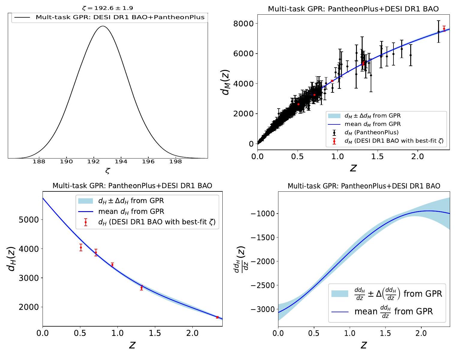
4.3 DESI DR1 BAO+بانثيون بلس ….. 11
4.4 CMB+DESI DR1 BAO+بانثيون بلس ….. 13
4.5 CMB+Non-DESI BAO+PantheonPlus ….. 14
4.6 الثوابت المعاد بناؤها والتحقق من التناسق
4.7 توتر هابل،
5 الاستنتاجات ….. 17
حساب لـ
الانحدار باستخدام العمليات الغاوسية ….. 20
ب. 1 انحدار عملية غاوس ذات مهمة واحدة حتى المشتق من الدرجة الثانية ….. 20
ب.1.1 تدريب نموذج GPR لمهمة واحدة ….. 20
ب.1.2 التنبؤ من GPR لمهمة واحدة ….. 21
ب. 2 الانحدار متعدد المهام GP حتى المشتق من الدرجة الثانية ….. 22
ب.2.1 تدريب نموذج GPR متعدد المهام ….. 23
ب.2.2 التنبؤ من GPR متعدد المهام ….. 24
ب. 3 استعادة GPR لمهمة واحدة من GPR لمهام متعددة ….. 26
تدوين C المستخدم في تحليل GPR ….. 27
تطبيق GPR ذو المهمة الواحدة على بيانات PantheonPlus ودوره
د. 1 بانثيون بلس + أحذية و CMB + بانثيون بلس + أحذية ….. 28
د. 2 بانثيون بلس، بانثيون بلس
د. 3 قائمة موسعة من الثوابت المعاد بناؤها ….. 31
اعتماد على قيود المسافة المختلفة من الخلفية الكونية الميكروويفية ….. 32
اعتماد دالة المتوسط F على توقعات GPR ….. 34
1 المقدمة
في القسم 4، باستخدام منهجية GP متعددة المهام. يتم تلخيص كل من التحليل البسيط لل posterior (مهمة واحدة) وتحليل GP متعدد المهام في الملحق B، مع إدراج الملحق C للترميز المستخدم. يتم مناقشة بعض تطبيقات GP لمهمة واحدة على بيانات PantheonPlus في الملحق D. كما نتناول تأثير (1) أولويات مسافة CMB المختلفة على النتائج، في الملحق E، و(2) دوال المتوسط المختلفة لـ GP والهايبر بارامترات، في الملحق F. يتم تقديم استنتاجاتنا في القسم 5.
2 المعادلات الخلفية
من (2.1)، نجد
تستخدم ملاحظات SNIa معامل المسافة
3 بيانات رصدية
3.1 بيانات DESI وبيانات BAO الأخرى
| تتبع (DESI DR1) |
|
|
|
|
المراجع. | |
| 1 | LRG | 0.510 |
|
|
-0.445 | [70] |
| 2 | LRG | 0.706 |
|
|
-0.420 | [70] |
| ٣ | LRG+ELG | 0.930 |
|
|
-0.389 | [1] |
| ٤ | إل جي | 1.317 |
|
|
-0.444 | [71] |
| ٥ | لي-
|
2.330 |
|
|
-0.477 | [1] |
| متعقب (غير DESI BAO) |
|
|
|
|
المراجع. | |
| 1 | LRG (بوس DR12) | 0.38 |
|
|
-0.228 | [72] |
| 2 | LRG (بوس DR12) | 0.51 |
|
|
-0.233 | [72] |
| ٣ | LRG (eBOSS DR16) | 0.698 |
|
|
-0.239 | [73] |
| ٤ | QSO (eBOSS DR16) | 1.48 |
|
|
0.039 | [74] |
| ٥ | لي-
|
٢.٣٣٤ |
|
|
-0.45 | [75] |
3.2 قيود المسافة من إشعاع الخلفية الكونية
من القيود المذكورة أعلاه نجد قيودًا على
خلال تحليلنا، نعتبر القيم السابقة لهذه المعلمات كبديل لاحتمالية CMB الكاملة. القيم السابقة لـ
3.3 بيانات السوبرنوفا
4 نتائج
4.1 DESI DR1 و BAO غير DESI
تم مناقشته في القسم ب.1، بشكل فردي إلى
-
هو متجه جميع نقاط الانزياح الأحمر الفعالة. -
هو متجه جميع القيم المتوسطة لـ . -
منذ هو متجه جميع القيم المتوسطة لـ . -
هي مصفوفة جميع التغايرات الذاتية لـ . -
هي مصفوفة جميع التغايرات المتقاطعة بين و . -
هي مصفوفة جميع التغايرات المتقاطعة بين و . -
هي مصفوفة جميع التغايرات الذاتية لـ .
4.2 CMB+DESI DR1 BAO و CMB+non-DESI BAO
4.3 DESI DR1 BAO+بانثيون بلس
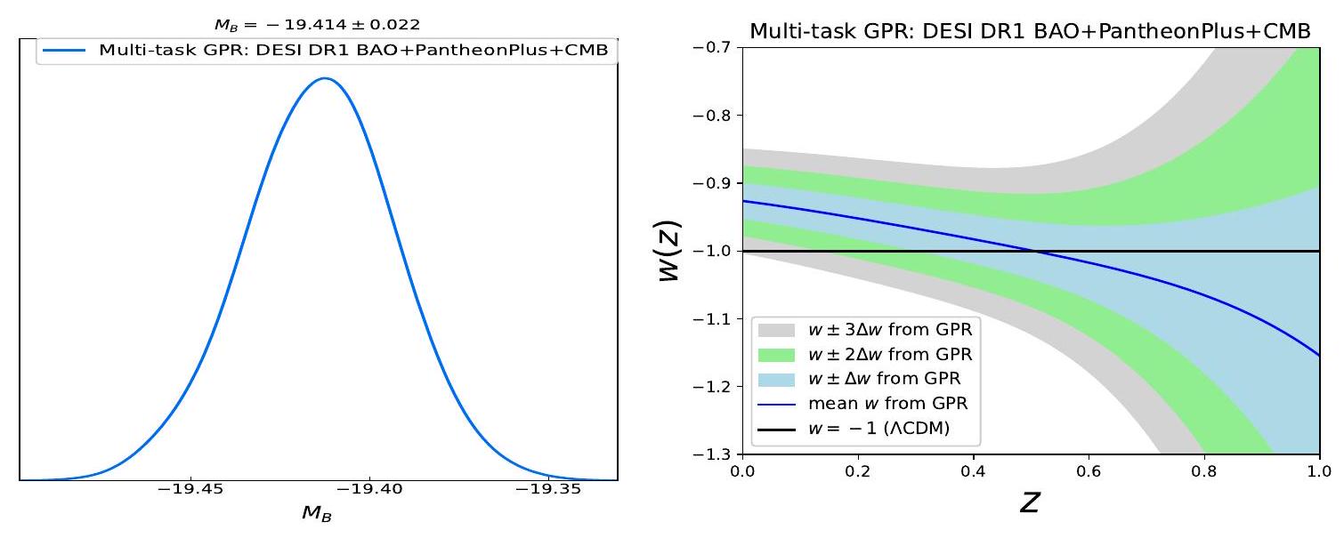
4.4 CMB+DESI DR1 BAO+بانثيون بلس
من المعاد بناءه
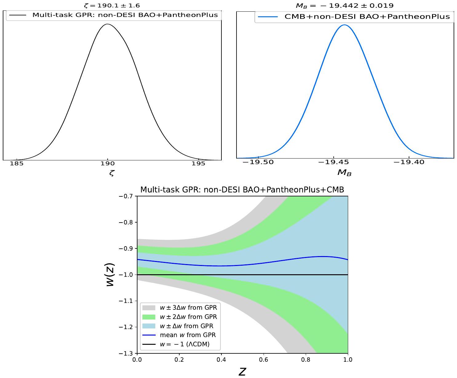
4.5 CMB+غير DESI BAO+بانثيون بلس
| دمج البيانات |
|
|
|
|
| ديزي |
|
– | – | – |
| غير ديسي |
|
– | – | – |
| ديزي + بي بي |
|
– | – | – |
| غير ديسي + بي بي |
|
– | – | – |
| CMB+DESI |
|
|
|
– |
| CMB+غير DESI |
|
|
|
– |
| CMB+DESI+PP |
|
|
|
|
| CMB+غير DESI+PP |
|
|
|
|
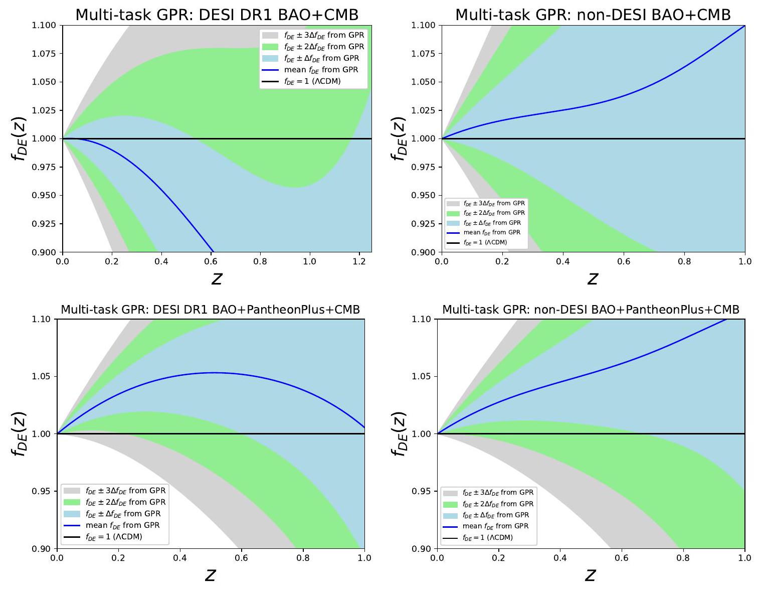
4.6 الثوابت المعاد بناؤها والتحقق من التناسق
بمجرد أن نعرف
الخطوط الزرقاء الصلبة تعطي المتوسط المعاد بناؤه
- بالنسبة لمجموعة بيانات CMB+DESI DR1 BAO، نجد أن
نموذج CDM هو أكثر بقليل من بعيدًا في نطاق الانزياح الأحمر . في مناطق الانزياح الأحمر الأخرى، هو ضمن المنطقة. هذا يعني أنه لا توجد انحرافات كبيرة عن الـ نموذج في مجموعة بيانات CMB+DESI DR1 BAO. - لـ
من خلال مجموعة بيانات DESI DR1 BAO + PantheonPlus، نجد أنه في الـ النموذج هو أكثر بقليل من بعيداً. في ، الـ النموذج حوالي إلى بعيدًا (يتناقص تدريجيًا مع زيادة الانزياح الأحمر). في مناطق الانزياح الأحمر الأخرى، يكون ضمن حد. هذا يعني أن الانحرافات منخفضة إلى متوسطة، لكنها ليست ذات دلالة كبيرة. - لتركيبة بيانات CMB+non-DESI BAO،
النموذج ضمن المنطقة في كامل منطقة الانزياح الأحمر. هذا يعني أنه لا يوجد دليل على الانحرافات عن نموذج CDM. - بالنسبة لمجموعة بيانات CMB+non-DESI BAO+PantheonPlus، فإن
نموذج CDM هو أكثر بقليل من بعيدًا في نطاق الانزياح الأحمر حول وهو ضمن المنطقة في مناطق الانزياح الأحمر الأخرى. هذا يعني أنه بالنسبة لهذا التركيب من البيانات، فإن الانحرافات عن نموذج CDM معتدل.
4.7 توتر هابل،
- المعاد بناءه
القيم، حيث لا تتعلق بيانات الأحذية أو المعنية قيمة لا يُعتبر، أقل من تم الحصول عليها من بيانات SHOES من معايرة SNIa وملاحظات المتغيرات سيفيد. هذه هي التوتر المعروف في هابل [89-91]. - يمكن تطبيق استنتاج مشابه لـ
، الذي يتوافق مع التوتر [92-94]. - نرى أنه كلما زادت قيمة
كلما زادت قيمة ، والعكس صحيح عندما تكون بيانات SNIa متضمنة. وهذا واضح أيضًا في الجدول 4 في الملحق D.3. هذه حقيقة معروفة جيدًا في علم الكونيات [92-94]. - لا نجد أي ارتباط فوري بين
و عندما لا تكون بيانات SNIa متضمنة. ومع ذلك، عندما تكون بيانات SNIa (بانثيون بلس) متضمنة، نرى زيادة أعلى ، الذي يتوافق مع القيمة الأعلى لـ عند الانزياح الأحمر المنخفض. ينطبق نفس الشيء على العلاقة بين و . وبالمثل، ينطبق العلاقة العكسية بين و عند الانزياح الأحمر المنخفض عندما تكون بيانات SNIa متضمنة. - يوجد ارتباط عكسي بين
و عندما تكون بيانات CMB متضمنة (مع أو بدون SNIa) [95، 96]. يوجد نفس الارتباط العكسي بين و عندما تكون بيانات SNIa متضمنة. يمكن رؤية ذلك أيضًا في الجدول 4 في الملحق D.3. هذه أيضًا حقيقة معروفة جيدًا في علم الكونيات.
5 استنتاجات
شكر وتقدير
حساب لـ
ب عملية الانحدار باستخدام العمليات الغاوسية
ب. 1 الانحدار باستخدام عملية غاوسية لمهمة واحدة حتى مشتق من الدرجة الثانية
ب.1.1 تدريب نموذج GPR لمهمة واحدة
ب.1.2 التنبؤ من GPR لمهمة واحدة
ب. 2 الانحدار متعدد المهام GP حتى المشتق من الدرجة الثانية
ب.2.1 تدريب نموذج GPR متعدد المهام
ب.2.2 التنبؤ من GPR متعدد المهام
ب. 3 استعادة GPR لمهمة واحدة من GPR لمهام متعددة
الآن يمكننا أن نرى أنه إذا استخدمنا (B.69) في (B.55)-(B.58)، فإننا نستعيد النتائج القياسية لـ (B.15)-(B.18)، حيث لا توجد معلومات عن مشتق الدالة. وبالمثل، فإن وضع شروط (B.68) في (B.59)-(B.65) يعيد لنا النتائج القياسية (B.19)-(B.25).
تدوين C المستخدم في تحليل GPR
تطبيق GPR ذو المهمة الواحدة على بيانات PantheonPlus ودوره
دي. 1 بانثيون بلس + أحذية و CMB + بانثيون بلس + أحذية
مع نفس رموز الألوان كما في الشكل 3. من هذا الرسم، نرى أن
د. 2 بانثيون بلس، بانثيون بلس
د. 3 قائمة موسعة من الثوابت المعاد بناؤها
| دمج البيانات |
|
|
|
|
|
|
– |
|
– |
|
| بي بي
|
– |
|
– |
|
| بي بي
|
– |
|
– |
|
|
|
|
|
|
|
|
|
|
|
|
|
|
|
|
|
|
|
اعتماد على قيود المسافة المختلفة من إشعاع الخلفية الكوني
اعتماد دالة المتوسط على توقعات GPR
References
[2] Y. Tada and T. Terada, Quintessential interpretation of the evolving dark energy in light of DESI observations, Phys. Rev. D 109 (2024), no. 12 L121305, [arXiv:2404.05722].
[3] W. Yin, Cosmic clues: DESI, dark energy, and the cosmological constant problem, JHEP 05 (2024) 327, [arXiv:2404.06444].
[4] K. V. Berghaus, J. A. Kable, and V. Miranda, Quantifying scalar field dynamics with DESI 2024 Y1 BAO measurements, Phys. Rev. D 110 (2024), no. 10 103524, [arXiv:2404.14341].
[5] D. Shlivko and P. J. Steinhardt, Assessing observational constraints on dark energy, Phys. Lett. B 855 (2024) 138826, [arXiv:2405.03933].
[6] O. F. Ramadan, J. Sakstein, and D. Rubin, DESI constraints on exponential quintessence, Phys. Rev. D 110 (2024), no. 4 L041303, [arXiv:2405.18747].
[7] I. D. Gialamas, G. Hütsi, K. Kannike, A. Racioppi, M. Raidal, M. Vasar, and H. Veermäe, Interpreting DESI 2024 BAO: late-time dynamical dark energy or a local effect?, arXiv:2406.07533.
[8] V. Patel, A. Chakraborty, and L. Amendola, The prior dependence of the DESI results, arXiv:2407.06586.
[9] D. Wang, Constraining Cosmological Physics with DESI BAO Observations, arXiv:2404.06796.
[10] Y. Yang, X. Ren, Q. Wang, Z. Lu, D. Zhang, Y.-F. Cai, and E. N. Saridakis, Quintom cosmology and modified gravity after DESI 2024, Sci. Bull. 69 (2024) 2698-2704, [arXiv:2404.19437].
[11] C. Escamilla-Rivera and R. Sandoval-Orozco,
[12] A. Chudaykin and M. Kunz, Modified gravity interpretation of the evolving dark energy in light of DESI data, arXiv:2407.02558.
[13] O. Luongo and M. Muccino, Model-independent cosmographic constraints from DESI 2024, Astron. Astrophys. 690 (2024) A40, [arXiv:2404.07070].
[14] M. Cortês and A. R. Liddle, Interpreting DESI’s evidence for evolving dark energy, JCAP 12 (2024) 007, [arXiv:2404.08056].
[15] E. O. Colgáin, M. G. Dainotti, S. Capozziello, S. Pourojaghi, M. M. Sheikh-Jabbari, and D. Stojkovic, Does DESI 2024 Confirm 1CDM?, arXiv:2404.08633.
[16] Y. Carloni, O. Luongo, and M. Muccino, Does dark energy really revive using DESI 2024 data?, arXiv:2404.12068.
[17] D. Wang, The Self-Consistency of DESI Analysis and Comment on “Does DESI 2024 Confirm ACDM?”, arXiv:2404.13833.
[18] W. Giarè, M. A. Sabogal, R. C. Nunes, and E. Di Valentino, Interacting Dark Energy after DESI Baryon Acoustic Oscillation measurements, arXiv:2404.15232.
[19] O . Seto and Y . Toda, DESI constraints on the varying electron mass model and axionlike early dark energy, Phys. Rev. D 110 (2024), no. 8 083501, [arXiv:2405.11869].
[20] T.-N. Li, P.-J. Wu, G.-H. Du, S.-J. Jin, H.-L. Li, J.-F. Zhang, and X. Zhang, Constraints on Interacting Dark Energy Models from the DESI Baryon Acoustic Oscillation and DES Supernovae Data, Astrophys. J. 976 (2024), no. 1 1, [arXiv:2407.14934].
[21] F. J. Qu, K. M. Surrao, B. Bolliet, J. C. Hill, B. D. Sherwin, and H. T. Jense, Accelerated inference on accelerated cosmic expansion: New constraints on axion-like early dark energy with DESI BAO and ACT DR6 CMB lensing, arXiv:2404.16805.
[22] H. Wang and Y.-S. Piao, Dark energy in light of recent DESI BAO and Hubble tension, arXiv:2404.18579.
[23] C.-G. Park, J. de Cruz Perez, and B. Ratra, Using non-DESI data to confirm and strengthen the DESI 2024 spatially-flat
[24] DESI Collaboration, R. Calderon et al., DESI 2024: reconstructing dark energy using crossing statistics with DESI DR1 BAO data, JCAP 10 (2024) 048, [arXiv:2405.04216].
[25] B. R. Dinda, A new diagnostic for the null test of dynamical dark energy in light of DESI 2024 and other BAO data, JCAP 09 (2024) 062, [arXiv:2405.06618].
[26] DESI Collaboration, K. Lodha et al., DESI 2024: Constraints on Physics-Focused Aspects of Dark Energy using DESI DR1 BAO Data, arXiv:2405.13588.
[27] P. Mukherjee and A. A. Sen, Model-independent cosmological inference post DESI DR1 BAO measurements, Phys. Rev. D 110 (2024), no. 12 123502, [arXiv:2405.19178].
[28] L. Pogosian, G.-B. Zhao, and K. Jedamzik, A Consistency Test of the Cosmological Model at the Epoch of Recombination Using DESI Baryonic Acoustic Oscillation and Planck Measurements, Astrophys. J. Lett. 973 (2024), no. 1 L13, [arXiv:2405.20306].
[29] N. Roy, Dynamical dark energy in the light of DESI 2024 data, arXiv:2406.00634.
[30] X. D. Jia, J. P. Hu, and F. Y. Wang, Uncorrelated estimations of
[31] J. J. Heckman, O. F. Ramadan, and J. Sakstein, First Constraints on a Pixelated Universe in Light of DESI, arXiv:2406.04408.
[32] A. Notari, M. Redi, and A. Tesi, Consistent theories for the DESI dark energy fit, JCAP 11 (2024) 025, [arXiv:2406.08459].
[33] G. P. Lynch, L. Knox, and J. Chluba, DESI observations and the Hubble tension in light of modified recombination, Phys. Rev. D 110 (2024), no. 8 083538, [arXiv:2406.10202].
[34] G. Liu, Y. Wang, and W. Zhao, Impact of LRG1 and LRG2 in DESI 2024 BAO data on dark energy evolution, arXiv:2407.04385.
[35] L. Orchard and V. H. Cárdenas, Probing dark energy evolution post-DESI 2024, Phys. Dark Univ. 46 (2024) 101678, [arXiv:2407.05579].
[36] A. Hernández-Almada, M. L. Mendoza-Martínez, M. A. García-Aspeitia, and V. Motta, Phenomenological emergent dark energy in the light of DESI Data Release 1, Phys. Dark Univ. 46 (2024) 101668, [arXiv:2407.09430].
[37] S. Pourojaghi, M. Malekjani, and Z. Davari, Cosmological constraints on dark energy parametrizations after DESI 2024: Persistent deviation from standard
[38] U. Mukhopadhayay, S. Haridasu, A. A. Sen, and S. Dhawan, Inferring dark energy properties from the scale factor parametrisation, arXiv:2407. 10845.
[39] G. Ye, M. Martinelli, B. Hu, and A. Silvestri, Non-minimally coupled gravity as a physically viable fit to DESI 2024 BAO, arXiv:2407.15832.
[40] W. Giarè, M. Najafi, S. Pan, E. Di Valentino, and J. T. Firouzjaee, Robust preference for Dynamical Dark Energy in DESI BAO and SN measurements, JCAP 10 (2024) 035, [arXiv:2407.16689].
[41] M. Chevallier and D. Polarski, Accelerating universes with scaling dark matter, Int. J. Mod. Phys. D 10 (2001) 213-224, [gr-qc/0009008].
[42] E. V. Linder, Exploring the expansion history of the universe, Phys. Rev. Lett. 90 (2003) 091301, [astro-ph/0208512].
[43] W. J. Wolf and P. G. Ferreira, Underdetermination of dark energy, Phys. Rev. D 108 (2023), no. 10 103519, [arXiv:2310.07482].
[44] R. R. Caldwell, R. Dave, and P. J. Steinhardt, Cosmological imprint of an energy component with general equation of state, Phys. Rev. Lett. 80 (1998) 1582-1585, [astro-ph/9708069].
[45] I. Zlatev, L.-M. Wang, and P. J. Steinhardt, Quintessence, cosmic coincidence, and the cosmological constant, Phys. Rev. Lett. 82 (1999) 896-899, [astro-ph/9807002].
[46] S. Tsujikawa, Quintessence: A Review, Class. Quant. Grav. 30 (2013) 214003, [arXiv:1304.1961].
[47] B. R. Dinda and A. A. Sen, Imprint of thawing scalar fields on the large scale galaxy overdensity, Phys. Rev. D 97 (2018), no. 8 083506, [arXiv:1607.05123].
[48] C. García-García, E. Bellini, P. G. Ferreira, D. Traykova, and M. Zumalacárregui, Theoretical priors in scalar-tensor cosmologies: Thawing quintessence, Phys. Rev. D 101 (2020), no. 6 063508, [arXiv:1911.02868].
[49] G. Ellis, R. Maartens, and M. A. H. MacCallum, Causality and the speed of sound, Gen. Rel. Grav. 39 (2007) 1651-1660, [gr-qc/0703121].
[50] L. Amendola, C. Quercellini, D. Tocchini-Valentini, and A. Pasqui, Constraints on the interaction and selfinteraction of dark energy from cosmic microwave background, Astrophys. J. Lett. 583 (2003) L53, [astro-ph/0205097].
[51] T. Clemson, K. Koyama, G.-B. Zhao, R. Maartens, and J. Valiviita, Interacting Dark Energy – constraints and degeneracies, Phys. Rev. D 85 (2012) 043007, [arXiv:1109.6234].
[52] A. Pourtsidou, C. Skordis, and E. J. Copeland, Models of dark matter coupled to dark energy, Phys. Rev. D 88 (2013), no. 8 083505, [arXiv:1307.0458].
[53] R. Murgia, S. Gariazzo, and N. Fornengo, Constraints on the Coupling between Dark Energy and Dark Matter from CMB data, JCAP 04 (2016) 014, [arXiv:1602.01765].
[54] E. Di Valentino, A. Melchiorri, O. Mena, and S. Vagnozzi, Interacting dark energy in the early 2020s: A promising solution to the
[55] S. Tsujikawa, Modified gravity models of dark energy, Lect. Notes Phys. 800 (2010) 99-145, [arXiv:1101.0191].
[56] T. Clifton, P. G. Ferreira, A. Padilla, and C. Skordis, Modified Gravity and Cosmology, Phys. Rept. 513 (2012) 1-189, [arXiv:1106.2476].
[57] K. Koyama, Cosmological Tests of Modified Gravity, Rept. Prog. Phys. 79 (2016), no. 4 046902, [arXiv:1504.04623].
[58] L. Perenon, M. Martinelli, R. Maartens, S. Camera, and C. Clarkson, Measuring dark energy with expansion and growth, Phys. Dark Univ. 37 (2022) 101119, [arXiv:2206.12375].
[59] B. R. Dinda and N. Banerjee, A comprehensive data-driven odyssey to explore the equation of state of dark energy, Eur. Phys. J. C 84 (2024), no. 7 688, [arXiv:2403.14223].
[60] C. Williams and C. Rasmussen, Gaussian processes for regression, Advances Neural Information Processing Systems 8 (1995).
[61] C. Rasmussen and C. Williams, Gaussian Processes for Machine Learning. MIT Press, 2006.
[62] A. Shafieloo, A. G. Kim, and E. V. Linder, Gaussian Process Cosmography, Phys. Rev. D 85 (2012) 123530, [arXiv:1204.2272].
[63] M. Seikel, C. Clarkson, and M. Smith, Reconstruction of dark energy and expansion dynamics using Gaussian processes, JCAP 06 (2012) 036, [arXiv:1204.2832].
[64] B. S. Haridasu, V. V. Luković, M. Moresco, and N. Vittorio, An improved model-independent assessment of the late-time cosmic expansion, JCAP
[65] P. Mukherjee and N. Banerjee, Non-parametric reconstruction of the cosmological jerk parameter, Eur. Phys. J. C 81 (2021), no. 1 36, [arXiv:2007.10124].
[66] eBOSS Collaboration, R. E. Keeley, A. Shafieloo, G.-B. Zhao, J. A. Vazquez, and H. Koo, Reconstructing the Universe: Testing the Mutual Consistency of the Pantheon and SDSS/eBOSS BAO Data Sets with Gaussian Processes, Astron. J. 161 (2021), no. 3 151, [arXiv:2010.03234].
[67] L. Perenon, M. Martinelli, S. Ilić, R. Maartens, M. Lochner, and C. Clarkson, Multi-tasking the growth of cosmological structures, Phys. Dark Univ. 34 (2021) 100898, [arXiv:2105.01613].
[68] B. R. Dinda, Minimal model-dependent constraints on cosmological nuisance parameters and cosmic curvature from combinations of cosmological data, Int. J. Mod. Phys. D 32 (2023), no. 11 2350079, [arXiv:2209.14639].
[69] M. A. Sabogal, O. Akarsu, A. Bonilla, E. Di Valentino, and R. C. Nunes, Exploring new physics in the late Universe’s expansion through non-parametric inference, Eur. Phys. J. C 84 (2024), no. 7703 , [arXiv:2407.04223].
[70] DESI Collaboration, R. Zhou et al., Target Selection and Validation of DESI Luminous Red Galaxies, Astron. J. 165 (2023), no. 2 58, [arXiv:2208.08515].
[71] A. Raichoor et al., Target Selection and Validation of DESI Emission Line Galaxies, Astron. J. 165 (2023), no. 3 126, [arXiv:2208.08513].
[72] BOSS Collaboration, S. Alam et al., The clustering of galaxies in the completed SDSS-III Baryon Oscillation Spectroscopic Survey: cosmological analysis of the DR12 galaxy sample, Mon. Not. Roy. Astron. Soc. 470 (2017), no. 3 2617-2652, [arXiv:1607.03155].
[73] eBOSS Collaboration, S. Alam et al., Completed SDSS-IV extended Baryon Oscillation Spectroscopic Survey: Cosmological implications from two decades of spectroscopic surveys at the Apache Point Observatory, Phys. Rev. D 103 (2021), no. 8 083533, [arXiv:2007.08991].
[74] eBOSS Collaboration, J. Hou et al., The Completed SDSS-IV extended Baryon Oscillation Spectroscopic Survey: BAO and RSD measurements from anisotropic clustering analysis of the Quasar Sample in configuration space between redshift 0.8 and 2.2, Mon. Not. Roy. Astron. Soc. 500 (2020), no. 1 1201-1221, [arXiv:2007.08998].
[75] eBOSS Collaboration, H. du Mas des Bourboux et al., The Completed SDSS-IV Extended Baryon Oscillation Spectroscopic Survey: Baryon Acoustic Oscillations with Lya Forests, Astrophys. J. 901 (2020), no. 2 153, [arXiv:2007.08995].
[76] W. Hu and N. Sugiyama, Small scale cosmological perturbations: An Analytic approach, Astrophys. J. 471 (1996) 542-570, [astro-ph/9510117].
[77] L. Chen, Q.-G. Huang, and K. Wang, Distance Priors from Planck Final Release, JCAP 02 (2019) 028, [arXiv:1808.05724].
[78] Z. Zhai, C.-G. Park, Y. Wang, and B. Ratra, CMB distance priors revisited: effects of dark energy dynamics, spatial curvature, primordial power spectrum, and neutrino parameters, JCAP 07 (2020) 009, [arXiv:1912.04921].
[79] Z. Zhai and Y. Wang, Robust and model-independent cosmological constraints from distance measurements, JCAP 07 (2019) 005, [arXiv:1811.07425].
[80] Planck Collaboration, N. Aghanim et al., Planck 2018 results. VI. Cosmological parameters, Astron. Astrophys. 641 (2020) A6, [arXiv:1807.06209]. [Erratum: Astron.Astrophys. 652, C4 (2021)].
[81] D. Scolnic et al., The Pantheon + Analysis: The Full Data Set and Light-curve Release, Astrophys. J. 938 (2022), no. 2 113, [arXiv:2112.03863].
[82] D. Brout et al., The Pantheon+ Analysis: Cosmological Constraints, Astrophys. J. 938 (2022), no. 2 110, [arXiv:2202.04077].
[83] S.-g. Hwang, B. L’Huillier, R. E. Keeley, M. J. Jee, and A. Shafieloo, How to use GP: effects of the mean function and hyperparameter selection on Gaussian process regression, JCAP
[84] A. Heinesen, C. Blake, and D. L. Wiltshire, Quantifying the accuracy of the Alcock-Paczyński scaling of baryon acoustic oscillation measurements, JCAP
[85] J. L. Bernal, T. L. Smith, K. K. Boddy, and M. Kamionkowski, Robustness of baryon acoustic oscillation constraints for early-Universe modifications of
[86] J. Pan, D. Huterer, F. Andrade-Oliveira, and C. Avestruz, Compressed baryon acoustic oscillation analysis is robust to modified-gravity models, JCAP
[87] S. Anselmi, G. D. Starkman, and A. Renzi, Cosmological forecasts for future galaxy surveys with the linear point standard ruler: Toward consistent bao analyses far from a fiducial cosmology, Phys. Rev. D 107 (Jun, 2023) 123506.
[88] M. O’Dwyer, S. Anselmi, G. D. Starkman, P.-S. Corasaniti, R. K. Sheth, and I. Zehavi, Linear point and sound horizon as purely geometric standard rulers, Phys. Rev. D 101 (Apr, 2020) 083517.
[89] E. Di Valentino, O. Mena, S. Pan, L. Visinelli, W. Yang, A. Melchiorri, D. F. Mota, A. G. Riess, and J. Silk, In the realm of the Hubble tension-a review of solutions, Class. Quant. Grav. 38 (2021), no. 15 153001, [arXiv:2103.01183].
[90] S. Vagnozzi, New physics in light of the
[91] C. Krishnan, R. Mohayaee, E. O. Colgáin, M. M. Sheikh-Jabbari, and L. Yin, Does Hubble tension signal a breakdown in FLRW cosmology?, Class. Quant. Grav. 38 (2021), no. 18 184001, [arXiv:2105.09790].
[92] D. Camarena and V. Marra, On the use of the local prior on the absolute magnitude of Type Ia supernovae in cosmological inference, Mon. Not. Roy. Astron. Soc. 504 (2021) 5164-5171, [arXiv:2101.08641].
[93] G. Efstathiou, To H0 or not to H0?, Mon. Not. Roy. Astron. Soc. 505 (2021), no. 3 3866-3872, [arXiv:2103.08723].
[94] B. R. Dinda, Cosmic expansion parametrization: Implication for curvature and HO tension, Phys. Rev. D 105 (2022), no. 6 063524, [arXiv:2106.02963].
[95] Z. Sakr, Testing the hypothesis of a matter density discrepancy within LCDM model using multiple probes, Phys. Rev. D 108 (2023), no. 8 083519, [arXiv:2305.02846].
[96] B. R. Dinda, Analytical Gaussian process cosmography: unveiling insights into matter-energy density parameter at present, Eur. Phys. J. C 84 (2024), no. 4 402, [arXiv:2311.13498].
[97] Y. Chen, S. Kumar, B. Ratra, and T. Xu, Effects of Type Ia Supernovae Absolute Magnitude Priors on the Hubble Constant Value, Astrophys. J. Lett. 964 (2024), no. 1 L4, [arXiv:2401.13187].
[98] A. G. Riess et al., A Comprehensive Measurement of the Local Value of the Hubble Constant with
[99] B. R. Dinda and N. Banerjee, Model independent bounds on type Ia supernova absolute peak magnitude, Phys. Rev. D 107 (2023), no. 6 063513, [arXiv:2208.14740].
[100] Y. Wang, Flux-averaging analysis of type ia supernova data, Astrophys. J. 536 (2000) 531, [astro-ph/9907405].
[101] Supernova Search Team Collaboration, A. G. Riess et al., Observational evidence from supernovae for an accelerating universe and a cosmological constant, Astron. J. 116 (1998) 1009-1038, [astro-ph/9805201].
[102] V. Poulin, T. L. Smith, R. Calderón, and T. Simon, On the implications of the ‘cosmic calibration tension’ beyond
[103] D. Pedrotti, J.-Q. Jiang, L. A. Escamilla, S. S. da Costa, and S. Vagnozzi, Multidimensionality of the Hubble tension: the roles of
Corresponding author. Note that our results are based on the BAO data, which may change if either the primordial or late-time model or both are far from the fiducial model used to obtain the BAO data [84-88]. We did not include CDM in Fig. 15, since we do not find any proper constraints due to the poor constraining power of DESI DR1 BAO data alone on a general model like .
DOI: https://doi.org/10.1088/1475-7516/2025/01/120
Publication Date: 2025-01-01
Model-agnostic assessment of dark energy after DESI DR1 BAO
Abstract
Baryon acoustic oscillation measurements by the Dark Energy Spectroscopic Instrument (Data Release 1) have revealed exciting results that show evidence for dynamical dark energy at
Contents
2 Background equations ….. 3
3 Observational data ….. 4
3.1 DESI and other BAO data ….. 4
3.2 CMB distance priors ….. 5
3.3 Supernova data ….. 6
4 Results ….. 7
4.1 DESI DR1 and non-DESI BAO ….. 7
4.2 CMB+DESI DR1 BAO and CMB+non-DESI BAO ….. 10
4.3 DESI DR1 BAO+PantheonPlus ….. 11
4.4 CMB+DESI DR1 BAO+PantheonPlus ….. 13
4.5 CMB+Non-DESI BAO+PantheonPlus ….. 14
4.6 Reconstructed constants and consistency check of
4.7 Hubble tension,
5 Conclusions ….. 17
A Computation of
B Gaussian Process Regression ….. 20
B. 1 Single-task Gaussian Process regression up to second order derivative ….. 20
B.1.1 Training the single-task GPR ….. 20
B.1.2 Prediction from single-task GPR ….. 21
B. 2 Multi-task GP regression up to second-order derivative ….. 22
B.2.1 Training the multi-task GPR ….. 23
B.2.2 Prediction from multi-task GPR ….. 24
B. 3 Recovering single-task GPR from multi-task GPR ….. 26
C Notation used in the GPR analysis ….. 27
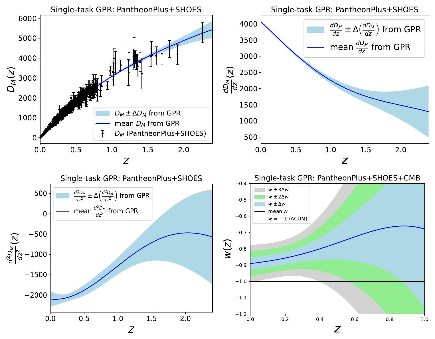
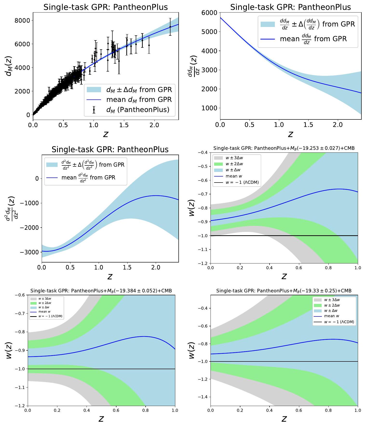
D Application of single-task GPR to PantheonPlus data and role of
D. 1 PantheonPlus+SHOES and CMB+PantheonPlus+SHOES ….. 28
D. 2 PantheonPlus, PantheonPlus
D. 3 Extended list of reconstructed constants ….. 31
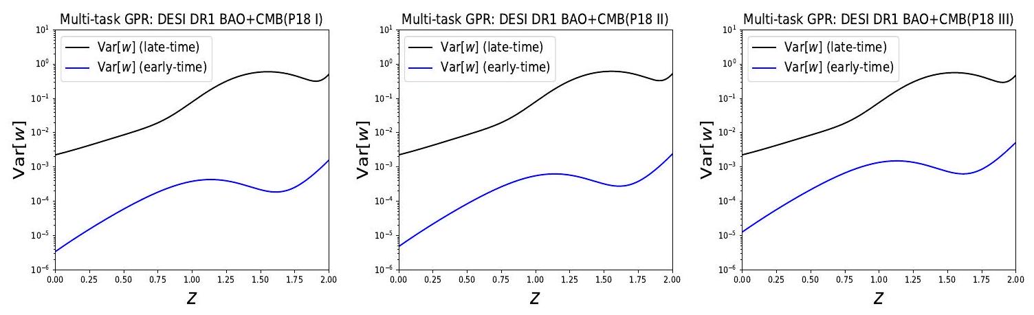
E Dependence on different CMB distance priors ….. 32
F Mean function dependence of GPR predictions ….. 34
1 Introduction
in Section 4, using the multi-task GP methodology. Both the simple posterior (single-task) and the multi-task GP analysis are summarised in Appendix B, with Appendix C listing the notation used. Some applications of single-task GP to PantheonPlus data are discussed in Appendix D. We also address the effect on the results of (1) different CMB distance priors, in Appendix E, and (2) different GP mean functions and hyperparameters, in Appendix F. Our conclusions are presented in Section 5.
2 Background equations
From (2.1), we find
SNIa observations use the distance modulus
3 Observational data
3.1 DESI and other BAO data
| tracer (DESI DR1) |
|
|
|
|
Refs. | |
| 1 | LRG | 0.510 |
|
|
-0.445 | [70] |
| 2 | LRG | 0.706 |
|
|
-0.420 | [70] |
| 3 | LRG+ELG | 0.930 |
|
|
-0.389 | [1] |
| 4 | ELG | 1.317 |
|
|
-0.444 | [71] |
| 5 | Ly-
|
2.330 |
|
|
-0.477 | [1] |
| tracer (non-DESI BAO) |
|
|
|
|
Refs. | |
| 1 | LRG (BOSS DR12) | 0.38 |
|
|
-0.228 | [72] |
| 2 | LRG (BOSS DR12) | 0.51 |
|
|
-0.233 | [72] |
| 3 | LRG (eBOSS DR16) | 0.698 |
|
|
-0.239 | [73] |
| 4 | QSO (eBOSS DR16) | 1.48 |
|
|
0.039 | [74] |
| 5 | Ly-
|
2.334 |
|
|
-0.45 | [75] |
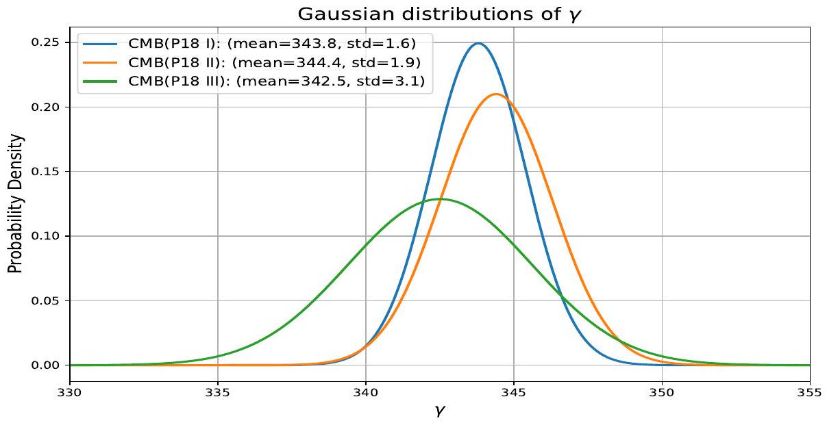
3.2 CMB distance priors
From the above constraints we find constraints on
Throughout our analysis, we consider priors on these parameters as an alternative to the full CMB likelihood. The prior values of
3.3 Supernova data
4 Results
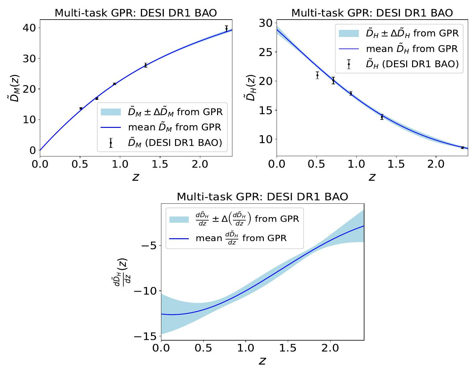
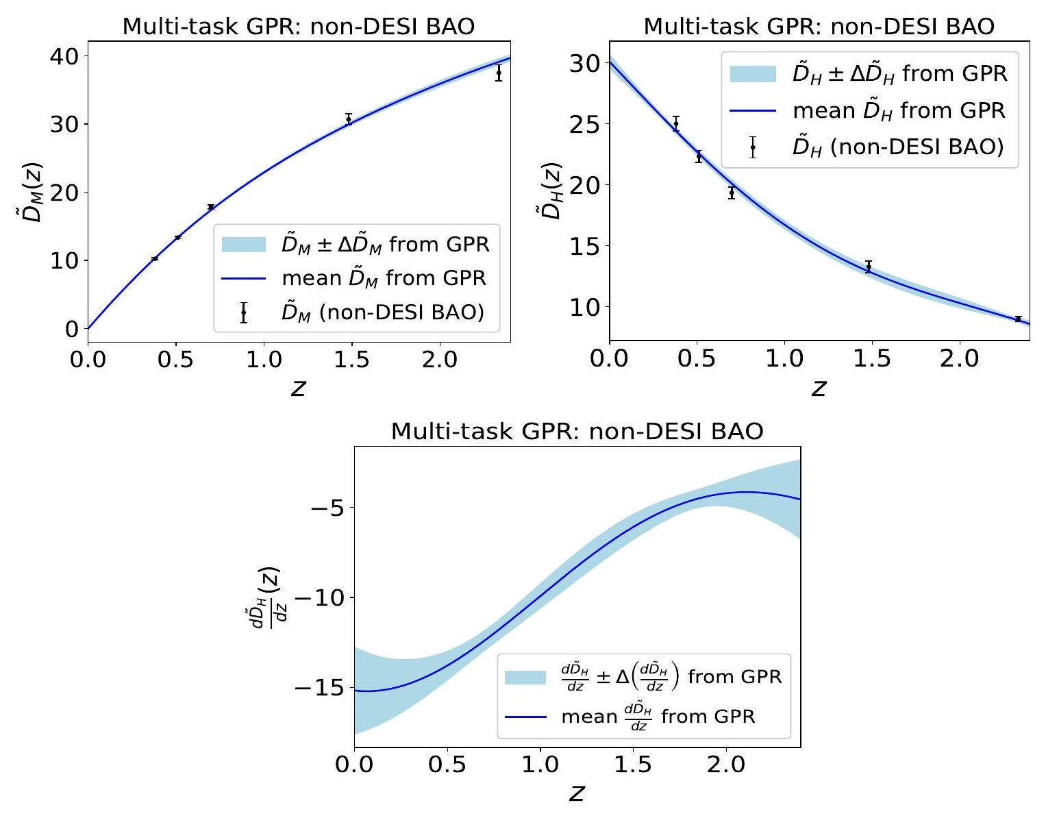
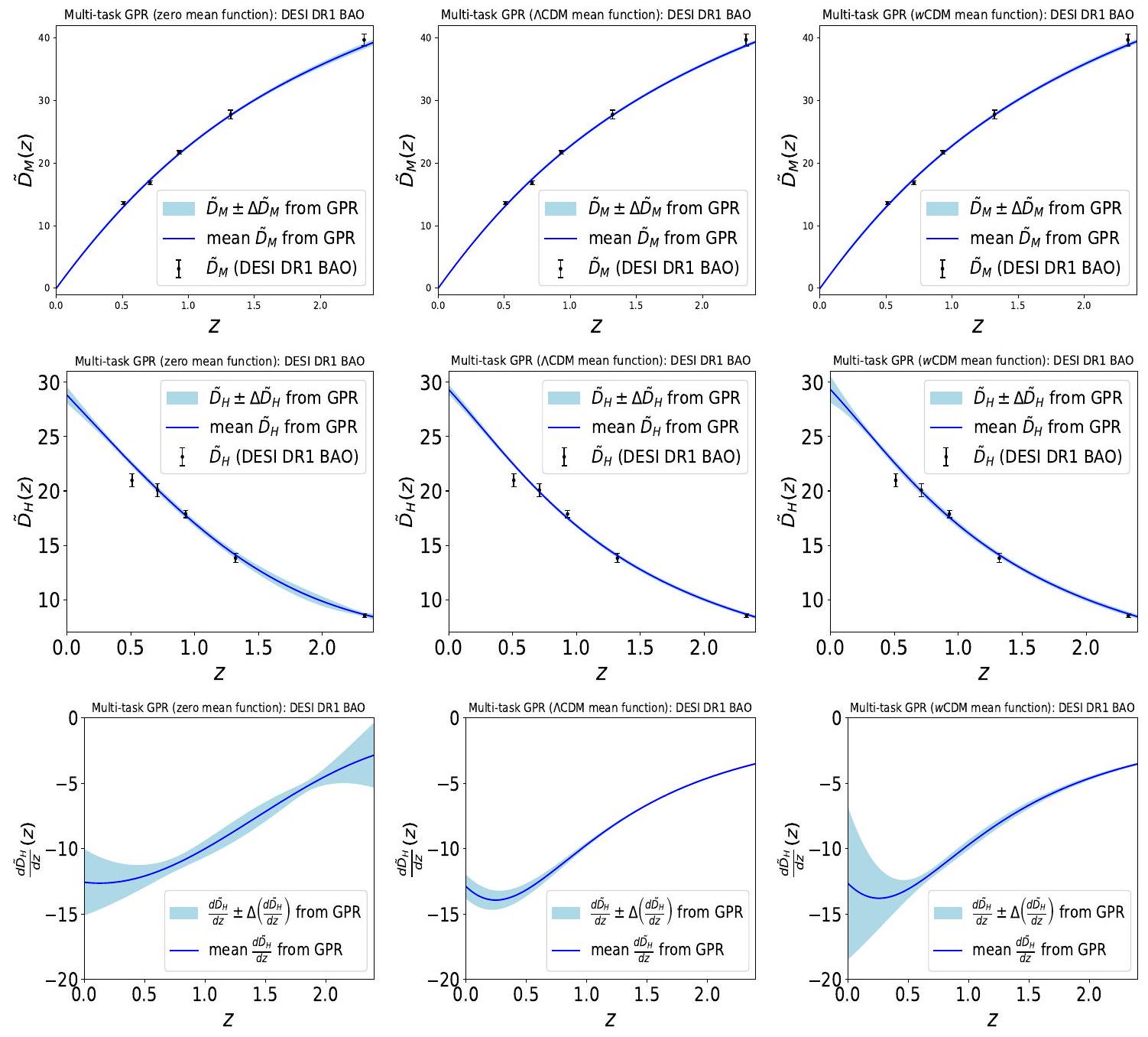
4.1 DESI DR1 and non-DESI BAO
discussed in Section B.1, individually to
-
is the vector of all effective redshift points. -
is the vector of all mean values of . -
since is the vector of all mean values of . -
is the matrix of all self-covariances of . -
is matrix of all cross covariances between and . -
is the matrix of all cross covariances between and . -
is the matrix of all self-covariances of .
4.2 CMB+DESI DR1 BAO and CMB+non-DESI BAO
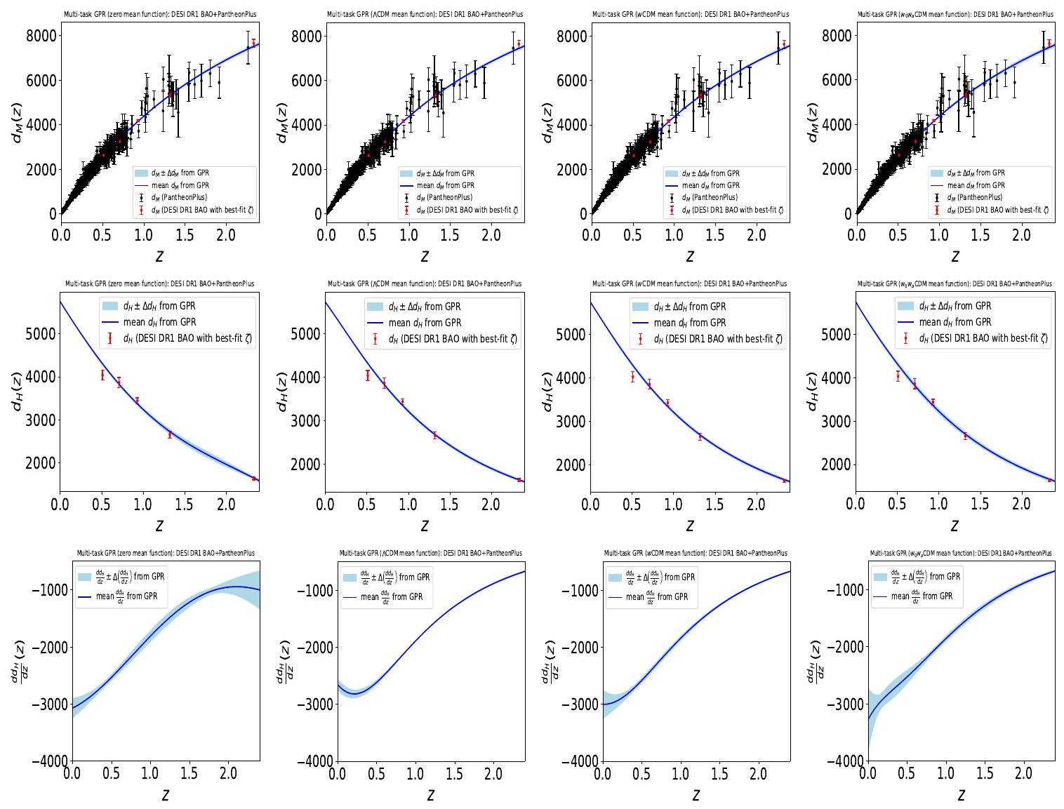
4.3 DESI DR1 BAO+PantheonPlus
4.4 CMB+DESI DR1 BAO+PantheonPlus
From the reconstructed
4.5 CMB+Non-DESI BAO+PantheonPlus
| Data combination |
|
|
|
|
| DESI |
|
– | – | – |
| non-DESI |
|
– | – | – |
| DESI+PP |
|
– | – | – |
| non-DESI+PP |
|
– | – | – |
| CMB+DESI |
|
|
|
– |
| CMB+non-DESI |
|
|
|
– |
| CMB+DESI+PP |
|
|
|
|
| CMB+non-DESI+PP |
|
|
|
|
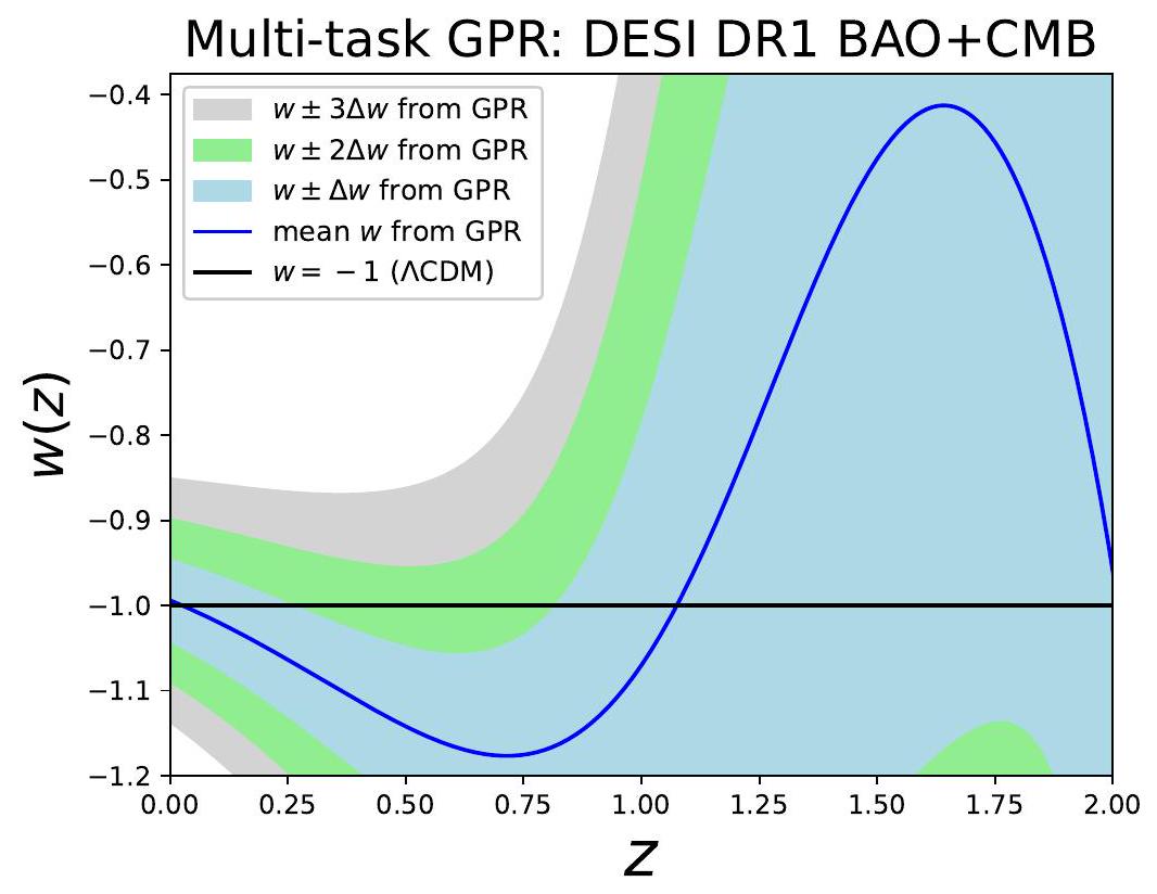
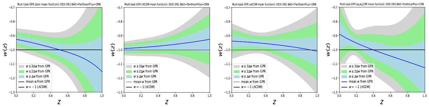
4.6 Reconstructed constants and consistency check of
Once we know
Solid blue lines give the reconstructed mean
- For the CMB+DESI DR1 BAO combination of data, we find that the
CDM model is little more than away in the redshift range . In other redshift regions, it is well within the region. This means there are no significant deviations from the model in the CMB+DESI DR1 BAO data combination. - For the
DESI DR1 BAO+PantheonPlus combination of data, we find that in the model is little more than away. In , the model is around to away (gradually decreasing with increasing redshift). In other redshift regions, it is within the limit. This means that the deviations are low to moderate, but not very significant. - For the CMB+non-DESI BAO combination of data, the
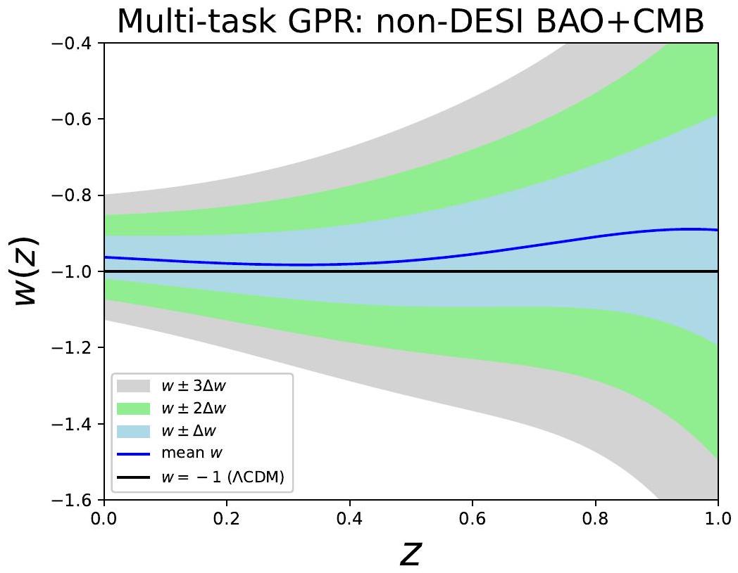
model is well within the region in the entire redshift region. This means there is no evidence for the deviations from the CDM model. - For the CMB+non-DESI BAO+PantheonPlus combination of data, the
CDM model is little more than away in the redshift range around and it is well within the region in the other redshift regions. This means for this combination of data the deviations from the CDM model are mild.
4.7 Hubble tension,
- The reconstructed
values, where no SHOES data is involved or the corresponding value is not considered, are lower than the obtained via the SHOES data from the calibration of SNIa and observations of Cepheid variables. This is the well-established Hubble tension [89-91]. - A similar conclusion is applicable for
, corresponding to the tension [92-94]. - We see that the higher the value of
, the higher the value of , and vice-versa when SNIa data is involved. It is also apparent in Table 4 in Appendix D.3. This is a well-known fact in cosmology [92-94]. - We do not find any immediate connection between
and when SNIa data are not involved. However, when SNIa (PantheonPlus) data is involved, we see a higher , corresponding to the higher value of at lower redshift. The same applies to the correlation between and . Similarly, the inverse relation applies between and at lower redshift when SNIa data is involved. - There is an inverse correlation between
and , when CMB data is involved (with or without SNIa) [95, 96]. The same inverse correlation exists between and when SNIa data is involved. This can also be seen in Table 4 in Appendix D.3. This is also a well-known fact in cosmology.
5 Conclusions
Acknowledgments
A Computation of
B Gaussian Process Regression
B. 1 Single-task Gaussian Process regression up to second order derivative
B.1.1 Training the single-task GPR
B.1.2 Prediction from single-task GPR
B. 2 Multi-task GP regression up to second-order derivative
B.2.1 Training the multi-task GPR
B.2.2 Prediction from multi-task GPR
B. 3 Recovering single-task GPR from multi-task GPR
Now we can see that if we use (B.69) in (B.55)-(B.58), we recover the standard results of (B.15)-(B.18), where there is no information on the derivative of the function. Similarly, putting conditions of (B.68) in (B.59)-(B.65), we recover the standard results (B.19)-(B.25).
C Notation used in the GPR analysis
D Application of single-task GPR to PantheonPlus data and role of
D. 1 PantheonPlus+SHOES and CMB+PantheonPlus+SHOES
with the same color codes as in Fig. 3. From this plot, we see that the
D. 2 PantheonPlus, PantheonPlus
D. 3 Extended list of reconstructed constants
| Data combination |
|
|
|
|
|
|
– |
|
– |
|
| PP
|
– |
|
– |
|
| PP
|
– |
|
– |
|
|
|
|
|
|
|
|
|
|
|
|
|
|
|
|
|
|
|
E Dependence on different CMB distance priors
F Mean function dependence of GPR predictions
References
[2] Y. Tada and T. Terada, Quintessential interpretation of the evolving dark energy in light of DESI observations, Phys. Rev. D 109 (2024), no. 12 L121305, [arXiv:2404.05722].
[3] W. Yin, Cosmic clues: DESI, dark energy, and the cosmological constant problem, JHEP 05 (2024) 327, [arXiv:2404.06444].
[4] K. V. Berghaus, J. A. Kable, and V. Miranda, Quantifying scalar field dynamics with DESI 2024 Y1 BAO measurements, Phys. Rev. D 110 (2024), no. 10 103524, [arXiv:2404.14341].
[5] D. Shlivko and P. J. Steinhardt, Assessing observational constraints on dark energy, Phys. Lett. B 855 (2024) 138826, [arXiv:2405.03933].
[6] O. F. Ramadan, J. Sakstein, and D. Rubin, DESI constraints on exponential quintessence, Phys. Rev. D 110 (2024), no. 4 L041303, [arXiv:2405.18747].
[7] I. D. Gialamas, G. Hütsi, K. Kannike, A. Racioppi, M. Raidal, M. Vasar, and H. Veermäe, Interpreting DESI 2024 BAO: late-time dynamical dark energy or a local effect?, arXiv:2406.07533.
[8] V. Patel, A. Chakraborty, and L. Amendola, The prior dependence of the DESI results, arXiv:2407.06586.
[9] D. Wang, Constraining Cosmological Physics with DESI BAO Observations, arXiv:2404.06796.
[10] Y. Yang, X. Ren, Q. Wang, Z. Lu, D. Zhang, Y.-F. Cai, and E. N. Saridakis, Quintom cosmology and modified gravity after DESI 2024, Sci. Bull. 69 (2024) 2698-2704, [arXiv:2404.19437].
[11] C. Escamilla-Rivera and R. Sandoval-Orozco,
[12] A. Chudaykin and M. Kunz, Modified gravity interpretation of the evolving dark energy in light of DESI data, arXiv:2407.02558.
[13] O. Luongo and M. Muccino, Model-independent cosmographic constraints from DESI 2024, Astron. Astrophys. 690 (2024) A40, [arXiv:2404.07070].
[14] M. Cortês and A. R. Liddle, Interpreting DESI’s evidence for evolving dark energy, JCAP 12 (2024) 007, [arXiv:2404.08056].
[15] E. O. Colgáin, M. G. Dainotti, S. Capozziello, S. Pourojaghi, M. M. Sheikh-Jabbari, and D. Stojkovic, Does DESI 2024 Confirm 1CDM?, arXiv:2404.08633.
[16] Y. Carloni, O. Luongo, and M. Muccino, Does dark energy really revive using DESI 2024 data?, arXiv:2404.12068.
[17] D. Wang, The Self-Consistency of DESI Analysis and Comment on “Does DESI 2024 Confirm ACDM?”, arXiv:2404.13833.
[18] W. Giarè, M. A. Sabogal, R. C. Nunes, and E. Di Valentino, Interacting Dark Energy after DESI Baryon Acoustic Oscillation measurements, arXiv:2404.15232.
[19] O . Seto and Y . Toda, DESI constraints on the varying electron mass model and axionlike early dark energy, Phys. Rev. D 110 (2024), no. 8 083501, [arXiv:2405.11869].
[20] T.-N. Li, P.-J. Wu, G.-H. Du, S.-J. Jin, H.-L. Li, J.-F. Zhang, and X. Zhang, Constraints on Interacting Dark Energy Models from the DESI Baryon Acoustic Oscillation and DES Supernovae Data, Astrophys. J. 976 (2024), no. 1 1, [arXiv:2407.14934].
[21] F. J. Qu, K. M. Surrao, B. Bolliet, J. C. Hill, B. D. Sherwin, and H. T. Jense, Accelerated inference on accelerated cosmic expansion: New constraints on axion-like early dark energy with DESI BAO and ACT DR6 CMB lensing, arXiv:2404.16805.
[22] H. Wang and Y.-S. Piao, Dark energy in light of recent DESI BAO and Hubble tension, arXiv:2404.18579.
[23] C.-G. Park, J. de Cruz Perez, and B. Ratra, Using non-DESI data to confirm and strengthen the DESI 2024 spatially-flat
[24] DESI Collaboration, R. Calderon et al., DESI 2024: reconstructing dark energy using crossing statistics with DESI DR1 BAO data, JCAP 10 (2024) 048, [arXiv:2405.04216].
[25] B. R. Dinda, A new diagnostic for the null test of dynamical dark energy in light of DESI 2024 and other BAO data, JCAP 09 (2024) 062, [arXiv:2405.06618].
[26] DESI Collaboration, K. Lodha et al., DESI 2024: Constraints on Physics-Focused Aspects of Dark Energy using DESI DR1 BAO Data, arXiv:2405.13588.
[27] P. Mukherjee and A. A. Sen, Model-independent cosmological inference post DESI DR1 BAO measurements, Phys. Rev. D 110 (2024), no. 12 123502, [arXiv:2405.19178].
[28] L. Pogosian, G.-B. Zhao, and K. Jedamzik, A Consistency Test of the Cosmological Model at the Epoch of Recombination Using DESI Baryonic Acoustic Oscillation and Planck Measurements, Astrophys. J. Lett. 973 (2024), no. 1 L13, [arXiv:2405.20306].
[29] N. Roy, Dynamical dark energy in the light of DESI 2024 data, arXiv:2406.00634.
[30] X. D. Jia, J. P. Hu, and F. Y. Wang, Uncorrelated estimations of
[31] J. J. Heckman, O. F. Ramadan, and J. Sakstein, First Constraints on a Pixelated Universe in Light of DESI, arXiv:2406.04408.
[32] A. Notari, M. Redi, and A. Tesi, Consistent theories for the DESI dark energy fit, JCAP 11 (2024) 025, [arXiv:2406.08459].
[33] G. P. Lynch, L. Knox, and J. Chluba, DESI observations and the Hubble tension in light of modified recombination, Phys. Rev. D 110 (2024), no. 8 083538, [arXiv:2406.10202].
[34] G. Liu, Y. Wang, and W. Zhao, Impact of LRG1 and LRG2 in DESI 2024 BAO data on dark energy evolution, arXiv:2407.04385.
[35] L. Orchard and V. H. Cárdenas, Probing dark energy evolution post-DESI 2024, Phys. Dark Univ. 46 (2024) 101678, [arXiv:2407.05579].
[36] A. Hernández-Almada, M. L. Mendoza-Martínez, M. A. García-Aspeitia, and V. Motta, Phenomenological emergent dark energy in the light of DESI Data Release 1, Phys. Dark Univ. 46 (2024) 101668, [arXiv:2407.09430].
[37] S. Pourojaghi, M. Malekjani, and Z. Davari, Cosmological constraints on dark energy parametrizations after DESI 2024: Persistent deviation from standard
[38] U. Mukhopadhayay, S. Haridasu, A. A. Sen, and S. Dhawan, Inferring dark energy properties from the scale factor parametrisation, arXiv:2407. 10845.
[39] G. Ye, M. Martinelli, B. Hu, and A. Silvestri, Non-minimally coupled gravity as a physically viable fit to DESI 2024 BAO, arXiv:2407.15832.
[40] W. Giarè, M. Najafi, S. Pan, E. Di Valentino, and J. T. Firouzjaee, Robust preference for Dynamical Dark Energy in DESI BAO and SN measurements, JCAP 10 (2024) 035, [arXiv:2407.16689].
[41] M. Chevallier and D. Polarski, Accelerating universes with scaling dark matter, Int. J. Mod. Phys. D 10 (2001) 213-224, [gr-qc/0009008].
[42] E. V. Linder, Exploring the expansion history of the universe, Phys. Rev. Lett. 90 (2003) 091301, [astro-ph/0208512].
[43] W. J. Wolf and P. G. Ferreira, Underdetermination of dark energy, Phys. Rev. D 108 (2023), no. 10 103519, [arXiv:2310.07482].
[44] R. R. Caldwell, R. Dave, and P. J. Steinhardt, Cosmological imprint of an energy component with general equation of state, Phys. Rev. Lett. 80 (1998) 1582-1585, [astro-ph/9708069].
[45] I. Zlatev, L.-M. Wang, and P. J. Steinhardt, Quintessence, cosmic coincidence, and the cosmological constant, Phys. Rev. Lett. 82 (1999) 896-899, [astro-ph/9807002].
[46] S. Tsujikawa, Quintessence: A Review, Class. Quant. Grav. 30 (2013) 214003, [arXiv:1304.1961].
[47] B. R. Dinda and A. A. Sen, Imprint of thawing scalar fields on the large scale galaxy overdensity, Phys. Rev. D 97 (2018), no. 8 083506, [arXiv:1607.05123].
[48] C. García-García, E. Bellini, P. G. Ferreira, D. Traykova, and M. Zumalacárregui, Theoretical priors in scalar-tensor cosmologies: Thawing quintessence, Phys. Rev. D 101 (2020), no. 6 063508, [arXiv:1911.02868].
[49] G. Ellis, R. Maartens, and M. A. H. MacCallum, Causality and the speed of sound, Gen. Rel. Grav. 39 (2007) 1651-1660, [gr-qc/0703121].
[50] L. Amendola, C. Quercellini, D. Tocchini-Valentini, and A. Pasqui, Constraints on the interaction and selfinteraction of dark energy from cosmic microwave background, Astrophys. J. Lett. 583 (2003) L53, [astro-ph/0205097].
[51] T. Clemson, K. Koyama, G.-B. Zhao, R. Maartens, and J. Valiviita, Interacting Dark Energy – constraints and degeneracies, Phys. Rev. D 85 (2012) 043007, [arXiv:1109.6234].
[52] A. Pourtsidou, C. Skordis, and E. J. Copeland, Models of dark matter coupled to dark energy, Phys. Rev. D 88 (2013), no. 8 083505, [arXiv:1307.0458].
[53] R. Murgia, S. Gariazzo, and N. Fornengo, Constraints on the Coupling between Dark Energy and Dark Matter from CMB data, JCAP 04 (2016) 014, [arXiv:1602.01765].
[54] E. Di Valentino, A. Melchiorri, O. Mena, and S. Vagnozzi, Interacting dark energy in the early 2020s: A promising solution to the
[55] S. Tsujikawa, Modified gravity models of dark energy, Lect. Notes Phys. 800 (2010) 99-145, [arXiv:1101.0191].
[56] T. Clifton, P. G. Ferreira, A. Padilla, and C. Skordis, Modified Gravity and Cosmology, Phys. Rept. 513 (2012) 1-189, [arXiv:1106.2476].
[57] K. Koyama, Cosmological Tests of Modified Gravity, Rept. Prog. Phys. 79 (2016), no. 4 046902, [arXiv:1504.04623].
[58] L. Perenon, M. Martinelli, R. Maartens, S. Camera, and C. Clarkson, Measuring dark energy with expansion and growth, Phys. Dark Univ. 37 (2022) 101119, [arXiv:2206.12375].
[59] B. R. Dinda and N. Banerjee, A comprehensive data-driven odyssey to explore the equation of state of dark energy, Eur. Phys. J. C 84 (2024), no. 7 688, [arXiv:2403.14223].
[60] C. Williams and C. Rasmussen, Gaussian processes for regression, Advances Neural Information Processing Systems 8 (1995).
[61] C. Rasmussen and C. Williams, Gaussian Processes for Machine Learning. MIT Press, 2006.
[62] A. Shafieloo, A. G. Kim, and E. V. Linder, Gaussian Process Cosmography, Phys. Rev. D 85 (2012) 123530, [arXiv:1204.2272].
[63] M. Seikel, C. Clarkson, and M. Smith, Reconstruction of dark energy and expansion dynamics using Gaussian processes, JCAP 06 (2012) 036, [arXiv:1204.2832].
[64] B. S. Haridasu, V. V. Luković, M. Moresco, and N. Vittorio, An improved model-independent assessment of the late-time cosmic expansion, JCAP
[65] P. Mukherjee and N. Banerjee, Non-parametric reconstruction of the cosmological jerk parameter, Eur. Phys. J. C 81 (2021), no. 1 36, [arXiv:2007.10124].
[66] eBOSS Collaboration, R. E. Keeley, A. Shafieloo, G.-B. Zhao, J. A. Vazquez, and H. Koo, Reconstructing the Universe: Testing the Mutual Consistency of the Pantheon and SDSS/eBOSS BAO Data Sets with Gaussian Processes, Astron. J. 161 (2021), no. 3 151, [arXiv:2010.03234].
[67] L. Perenon, M. Martinelli, S. Ilić, R. Maartens, M. Lochner, and C. Clarkson, Multi-tasking the growth of cosmological structures, Phys. Dark Univ. 34 (2021) 100898, [arXiv:2105.01613].
[68] B. R. Dinda, Minimal model-dependent constraints on cosmological nuisance parameters and cosmic curvature from combinations of cosmological data, Int. J. Mod. Phys. D 32 (2023), no. 11 2350079, [arXiv:2209.14639].
[69] M. A. Sabogal, O. Akarsu, A. Bonilla, E. Di Valentino, and R. C. Nunes, Exploring new physics in the late Universe’s expansion through non-parametric inference, Eur. Phys. J. C 84 (2024), no. 7703 , [arXiv:2407.04223].
[70] DESI Collaboration, R. Zhou et al., Target Selection and Validation of DESI Luminous Red Galaxies, Astron. J. 165 (2023), no. 2 58, [arXiv:2208.08515].
[71] A. Raichoor et al., Target Selection and Validation of DESI Emission Line Galaxies, Astron. J. 165 (2023), no. 3 126, [arXiv:2208.08513].
[72] BOSS Collaboration, S. Alam et al., The clustering of galaxies in the completed SDSS-III Baryon Oscillation Spectroscopic Survey: cosmological analysis of the DR12 galaxy sample, Mon. Not. Roy. Astron. Soc. 470 (2017), no. 3 2617-2652, [arXiv:1607.03155].
[73] eBOSS Collaboration, S. Alam et al., Completed SDSS-IV extended Baryon Oscillation Spectroscopic Survey: Cosmological implications from two decades of spectroscopic surveys at the Apache Point Observatory, Phys. Rev. D 103 (2021), no. 8 083533, [arXiv:2007.08991].
[74] eBOSS Collaboration, J. Hou et al., The Completed SDSS-IV extended Baryon Oscillation Spectroscopic Survey: BAO and RSD measurements from anisotropic clustering analysis of the Quasar Sample in configuration space between redshift 0.8 and 2.2, Mon. Not. Roy. Astron. Soc. 500 (2020), no. 1 1201-1221, [arXiv:2007.08998].
[75] eBOSS Collaboration, H. du Mas des Bourboux et al., The Completed SDSS-IV Extended Baryon Oscillation Spectroscopic Survey: Baryon Acoustic Oscillations with Lya Forests, Astrophys. J. 901 (2020), no. 2 153, [arXiv:2007.08995].
[76] W. Hu and N. Sugiyama, Small scale cosmological perturbations: An Analytic approach, Astrophys. J. 471 (1996) 542-570, [astro-ph/9510117].
[77] L. Chen, Q.-G. Huang, and K. Wang, Distance Priors from Planck Final Release, JCAP 02 (2019) 028, [arXiv:1808.05724].
[78] Z. Zhai, C.-G. Park, Y. Wang, and B. Ratra, CMB distance priors revisited: effects of dark energy dynamics, spatial curvature, primordial power spectrum, and neutrino parameters, JCAP 07 (2020) 009, [arXiv:1912.04921].
[79] Z. Zhai and Y. Wang, Robust and model-independent cosmological constraints from distance measurements, JCAP 07 (2019) 005, [arXiv:1811.07425].
[80] Planck Collaboration, N. Aghanim et al., Planck 2018 results. VI. Cosmological parameters, Astron. Astrophys. 641 (2020) A6, [arXiv:1807.06209]. [Erratum: Astron.Astrophys. 652, C4 (2021)].
[81] D. Scolnic et al., The Pantheon + Analysis: The Full Data Set and Light-curve Release, Astrophys. J. 938 (2022), no. 2 113, [arXiv:2112.03863].
[82] D. Brout et al., The Pantheon+ Analysis: Cosmological Constraints, Astrophys. J. 938 (2022), no. 2 110, [arXiv:2202.04077].
[83] S.-g. Hwang, B. L’Huillier, R. E. Keeley, M. J. Jee, and A. Shafieloo, How to use GP: effects of the mean function and hyperparameter selection on Gaussian process regression, JCAP
[84] A. Heinesen, C. Blake, and D. L. Wiltshire, Quantifying the accuracy of the Alcock-Paczyński scaling of baryon acoustic oscillation measurements, JCAP
[85] J. L. Bernal, T. L. Smith, K. K. Boddy, and M. Kamionkowski, Robustness of baryon acoustic oscillation constraints for early-Universe modifications of
[86] J. Pan, D. Huterer, F. Andrade-Oliveira, and C. Avestruz, Compressed baryon acoustic oscillation analysis is robust to modified-gravity models, JCAP
[87] S. Anselmi, G. D. Starkman, and A. Renzi, Cosmological forecasts for future galaxy surveys with the linear point standard ruler: Toward consistent bao analyses far from a fiducial cosmology, Phys. Rev. D 107 (Jun, 2023) 123506.
[88] M. O’Dwyer, S. Anselmi, G. D. Starkman, P.-S. Corasaniti, R. K. Sheth, and I. Zehavi, Linear point and sound horizon as purely geometric standard rulers, Phys. Rev. D 101 (Apr, 2020) 083517.
[89] E. Di Valentino, O. Mena, S. Pan, L. Visinelli, W. Yang, A. Melchiorri, D. F. Mota, A. G. Riess, and J. Silk, In the realm of the Hubble tension-a review of solutions, Class. Quant. Grav. 38 (2021), no. 15 153001, [arXiv:2103.01183].
[90] S. Vagnozzi, New physics in light of the
[91] C. Krishnan, R. Mohayaee, E. O. Colgáin, M. M. Sheikh-Jabbari, and L. Yin, Does Hubble tension signal a breakdown in FLRW cosmology?, Class. Quant. Grav. 38 (2021), no. 18 184001, [arXiv:2105.09790].
[92] D. Camarena and V. Marra, On the use of the local prior on the absolute magnitude of Type Ia supernovae in cosmological inference, Mon. Not. Roy. Astron. Soc. 504 (2021) 5164-5171, [arXiv:2101.08641].
[93] G. Efstathiou, To H0 or not to H0?, Mon. Not. Roy. Astron. Soc. 505 (2021), no. 3 3866-3872, [arXiv:2103.08723].
[94] B. R. Dinda, Cosmic expansion parametrization: Implication for curvature and HO tension, Phys. Rev. D 105 (2022), no. 6 063524, [arXiv:2106.02963].
[95] Z. Sakr, Testing the hypothesis of a matter density discrepancy within LCDM model using multiple probes, Phys. Rev. D 108 (2023), no. 8 083519, [arXiv:2305.02846].
[96] B. R. Dinda, Analytical Gaussian process cosmography: unveiling insights into matter-energy density parameter at present, Eur. Phys. J. C 84 (2024), no. 4 402, [arXiv:2311.13498].
[97] Y. Chen, S. Kumar, B. Ratra, and T. Xu, Effects of Type Ia Supernovae Absolute Magnitude Priors on the Hubble Constant Value, Astrophys. J. Lett. 964 (2024), no. 1 L4, [arXiv:2401.13187].
[98] A. G. Riess et al., A Comprehensive Measurement of the Local Value of the Hubble Constant with
[99] B. R. Dinda and N. Banerjee, Model independent bounds on type Ia supernova absolute peak magnitude, Phys. Rev. D 107 (2023), no. 6 063513, [arXiv:2208.14740].
[100] Y. Wang, Flux-averaging analysis of type ia supernova data, Astrophys. J. 536 (2000) 531, [astro-ph/9907405].
[101] Supernova Search Team Collaboration, A. G. Riess et al., Observational evidence from supernovae for an accelerating universe and a cosmological constant, Astron. J. 116 (1998) 1009-1038, [astro-ph/9805201].
[102] V. Poulin, T. L. Smith, R. Calderón, and T. Simon, On the implications of the ‘cosmic calibration tension’ beyond
[103] D. Pedrotti, J.-Q. Jiang, L. A. Escamilla, S. S. da Costa, and S. Vagnozzi, Multidimensionality of the Hubble tension: the roles of
Corresponding author. Note that our results are based on the BAO data, which may change if either the primordial or late-time model or both are far from the fiducial model used to obtain the BAO data [84-88]. We did not include CDM in Fig. 15, since we do not find any proper constraints due to the poor constraining power of DESI DR1 BAO data alone on a general model like .