تقييم نماذج التنبؤ السريرية (الجزء 3): حساب حجم العينة المطلوب لدراسة التحقق الخارجي Evaluation of clinical prediction models (part 3): calculating the sample size required for an external validation study
تقييم دراسة التحقق الخارجي أداء نموذج التنبؤ في بيانات جديدة، ولكن العديد من هذه الدراسات صغيرة جدًا لتوفير إجابات موثوقة. في المقالة الثالثة من سلسلتهم حول تقييم النماذج، يصف رايلي وزملاؤه كيفية حساب حجم العينة المطلوب لدراسات التحقق الخارجي، ويقترحون تجنب القواعد العامة من خلال تخصيص الحسابات للنموذج والإعداد المعني.
تقييم دراسات التحقق الخارجي أداء نموذج أو أكثر من نماذج التنبؤ (على سبيل المثال، التي تم تطويرها سابقًا باستخدام الأساليب الإحصائية أو التعلم الآلي أو الذكاء الاصطناعي) في مجموعة بيانات مختلفة عن تلك المستخدمة في عملية تطوير النموذج. الجزء 2 في سلسلتنا يصف كيفية إجراء دراسة تحقق خارجي عالية الجودة، بما في ذلك الحاجة إلى تقدير مقاييس أداء النموذج مثل المعايرة (الاتفاق بين القيم المرصودة والمتوقعة)، التمييز (الفصل بين القيم المتوقعة في أولئك الذين لديهم وبدون حدث نتيجة)، الملاءمة العامة (على سبيل المثال، النسبة المئوية من
نقاط ملخص
يجب أن يكون حجم العينة لدراسة التحقق الخارجي كبيرًا بما يكفي لتقدير أداء النموذج التنبؤي بدقة. العديد من دراسات التحقق الحالية صغيرة جدًا، مما يؤدي إلى فترات ثقة واسعة لتقديرات الأداء وادعاءات مضللة محتملة حول موثوقية النموذج أو أدائه مقارنة بالنماذج الأخرى. للتعامل مع مخاوف تقديرات الأداء غير الدقيقة، تم اقتراح قواعد عامة لحجم العينة، مثل وجود 100 حدث و100 عدم حدث على الأقل.
توفر هذه القواعد العامة نقطة انطلاق ولكنها مشكلة، لأنها ليست محددة إما للنموذج أو الإعداد السريري، والدقة تعتمد أيضًا على عوامل أخرى غير عدد الأحداث وعدم الأحداث. يمكن أن يسمح نهج أكثر تخصيصًا للباحثين بحساب حجم العينة المطلوب لاستهداف الدقة المختارة (عرض فترات الثقة) لتقديرات الأداء الرئيسية، مثل R2، منحنى المعايرة، إحصائية c، والفائدة الصافية.
تعتمد الحسابات على تحديد المستخدمين لمعلومات مثل نسبة النتيجة، الأداء المتوقع للنموذج، وتوزيع القيم المتوقعة، والتي يمكن قياسها من دراسة تطوير النموذج الأصلية.
حزمة pmvalsampsize في Stata و R تسمح للباحثين بتنفيذ النهج بسطر واحد من التعليمات البرمجية.
التباين في قيم النتائج المفسرة، وفائدة سريرية (على سبيل المثال، الفائدة الصافية لاستخدام النموذج لإبلاغ قرارات العلاج). في هذا الجزء الثالث من السلسلة، نصف كيفية حساب حجم العينة المطلوب لمثل هذه الدراسات الخارجية للتحقق من تقدير هذه المقاييس بدقة، ونقدم أمثلة موضحة.
الأساس لحسابات حجم العينة في دراسات التحقق الخارجي
يجب أن يكون حجم العينة لدراسة التحقق الخارجي كبيرًا بما يكفي لتقدير أداء النموذج التنبؤي بدقة. الهدف هو تقديم دليل قوي حول دقة توقعات النموذج في مجموعة سكانية مستهدفة معينة، للمساعدة في دعم القرارات حول فائدة النموذج (على سبيل المثال، للإرشاد للمرضى، ضمن الممارسة السريرية).
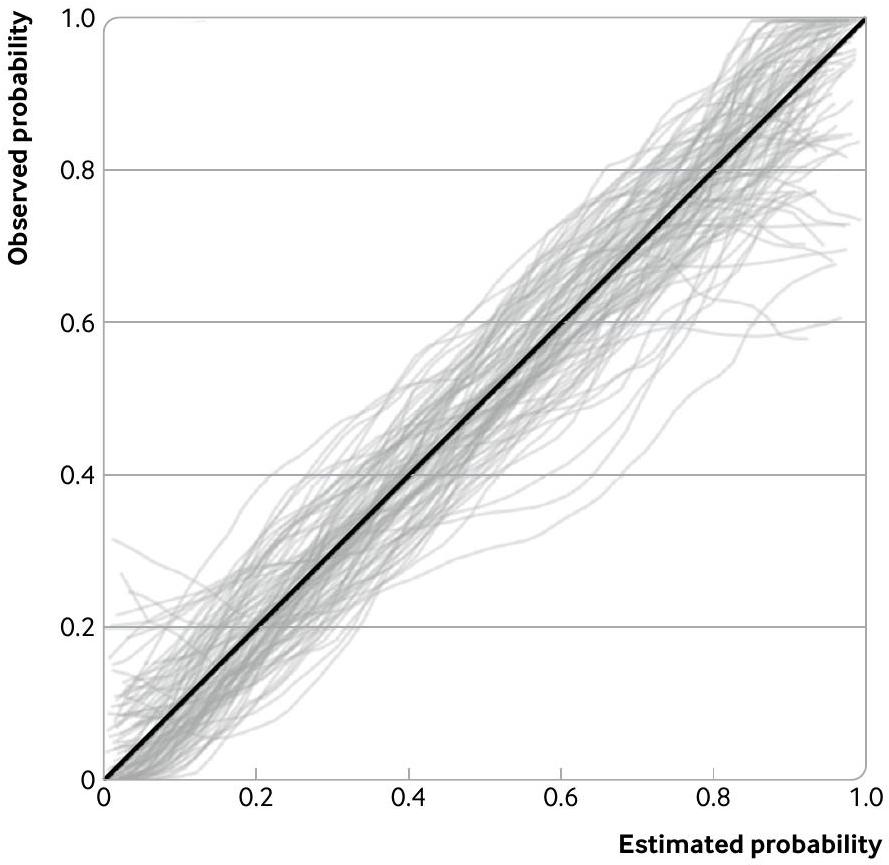
العديد من دراسات التحقق الخارجي المنشورة صغيرة جدًا، كما يتضح من مراجعات التحقق من نماذج التنبؤ المعتمدة على الإحصاءات والتعلم الآلي. يؤدي حجم العينة الصغيرة إلى فترات ثقة واسعة لتقديرات الأداء وادعاءات مضللة محتملة حول موثوقية النموذج أو أدائه مقارنة بالنماذج الأخرى، خاصة إذا تم تجاهل عدم اليقين. يتم توضيح هذه المشكلة في الشكل 1، الذي يظهر 100 منحنى معايرة تم إنشاؤها عشوائيًا للتحقق الخارجي من نموذج التنبؤ لتدهور سريري داخل المستشفى بين البالغين الذين تم إدخالهم مع كوفيد-19. يتم تقدير كل منحنى على عينة عشوائية من 100 مشارك افتراضي (وحوالي 43 حدث نتيجة)، مع نتائج (تدهور: نعم أو لا) تم إنشاؤها عشوائيًا بناءً على افتراض أن الاحتمالات المقدرة من نموذج كوفيد-19 صحيحة في مجموعة التحقق الخارجي. على الرغم من أن توقعات النموذج متوافقة جيدًا في المجموعة (أي، الخط القطري الصلب في الشكل 1 هو الحقيقة الأساسية)، فإن تباين العينة في المنحنيات المرصودة كبير. على سبيل المثال، بالنسبة للأفراد الذين لديهم احتمال مقدر بين 0 و0.05، تتراوح الاحتمالات المرصودة على المنحنيات بين حوالي 0 و0.3. وبالمثل، بالنسبة للأفراد الذين لديهم احتمال مقدر قدره 0.9، تتراوح الاحتمالات المرصودة على المنحنيات من حوالي 0.6 إلى 1. وبالتالي، فإن حجم العينة المكون من 100 مشارك صغير جدًا لضمان أن دراسة التحقق الخارجي تقدم نتائج مستقرة حول أداء المعايرة.
لحل مخاوف تقديرات الأداء غير الدقيقة، وبالتالي النتائج غير الحاسمة أو المضللة، تم اقتراح قواعد عامة لحجم العينة المطلوبة لدراسات التحقق الخارجي. بالنسبة للنتائج الثنائية أو الوقت حتى الحدث، تقترح القواعد العامة المستندة إلى دراسات المحاكاة وإعادة أخذ العينات أن هناك حاجة إلى 100 حدث و100 عدم حدث على الأقل لتقدير مقاييس مثل إحصائية c (المساحة تحت منحنى التشغيل الخاص بالمستقبل) والمعايرة.
الشكل 1 | توضيح القلق بشأن أحجام العينات الصغيرة عند تقييم المعايرة. يظهر الرسم البياني تباينًا كبيرًا في منحنيات المعايرة من 100 دراسة تحقق خارجي (كل منها يحتوي على عينة عشوائية من 100 مشارك، ومتوسط 43 حدث نتيجة، مع نتائج تم إنشاؤها على افتراض أن نموذج التنبؤ متوافق جيدًا حقًا) لنموذج التنبؤ لتدهور سريري داخل المستشفى بين البالغين الذين تم إدخالهم مع كوفيد-19.
الانحدار، وحد أدنى من 200 حدث و200 عدم حدث لاشتقاق منحنيات المعايرة بما في ذلك منحنيات المعايرة. توفر هذه القواعد العامة نقطة انطلاق ولكنها مشكلة، لأنها ليست محددة إما للنموذج أو الإعداد السريري، وتعتمد دقة تقديرات الأداء التنبؤي أيضًا على عوامل أخرى غير عدد الأحداث وعدم الأحداث، مثل توزيع القيم المتوقعة. لذلك، يمكن أن تؤدي القواعد العامة إلى أحجام عينات صغيرة جدًا (تنتج تقديرات أداء غير دقيقة) أو كبيرة جدًا (على سبيل المثال، جمع كميات مفرطة من البيانات بشكل استباقي والتي تستغرق وقتًا طويلاً وغير ضرورية ومكلفة).
للابتعاد عن القواعد العامة، أصبحت حسابات حجم العينة المخصصة متاحة الآن لدراسات التحقق الخارجي. هنا، نلخص هذه الحسابات لجمهور واسع، مع وضع التفاصيل الفنية في صناديق لضمان تركيز النص الرئيسي على المبادئ الرئيسية والأمثلة العملية. فرضيتنا هي أن دراسة التحقق الخارجي تهدف إلى تقدير أداء نموذج التنبؤ في بيانات جديدة (انظر الجزء 1 من سلسلتنا); لا نركز على حجم العينة المطلوب لتعديل أو تحديث نموذج التنبؤ. بالإضافة إلى حجم العينة، وكما تم التأكيد عليه في الجزء 2 من هذه السلسلة، يجب على الباحثين أيضًا التأكد من أن مجموعات بيانات التحقق الخارجي تمثل المجموعة السكانية المستهدفة والإعداد (على سبيل المثال، من حيث مزيج الحالات، مخاطر النتائج، قياس وتوقيت المتنبئين)، وعادة ما تكون من دراسة cohort طولية (لنماذج التنبؤ) أو دراسة مقطعية (لنماذج التشخيص).
حجم العينة للتحقق الخارجي من نماذج التنبؤ ذات النتيجة المستمرة
عند التحقق من أداء نموذج التنبؤ لنتيجة مستمرة (مثل ضغط الدم أو الوزن أو درجة الألم)، هناك العديد من مقاييس الأداء المختلفة التي تهمنا، كما هو موضح بالتفصيل في الجزء الثاني من هذه السلسلة.على الأقل، آرتشر وآخرونتشير إلى أنه من المهم فحص العوامل التالية: الملاءمة العامة كما تقاس بـ (نسبة التباين المفسر في مجموعة بيانات التحقق الخارجي)، والمعايرة كما تقاس بواسطة منحنيات المعايرة وت quantified باستخدام المعايرة في الكل (الفرق بين القيم المتوقعة المتوسطة والقيم المرصودة المتوسطة) وانحدار المعايرة (الاتفاق بين القيم المتوقعة والمرصودة عبر نطاق القيم المتوقعة)، والتباين المتبقي (تباين الفروق بين القيم المتوقعة والمرصودة في بيانات التحقق الخارجي). تم اقتراح أربع حسابات منفصلة لحجم العينة تستهدف التقدير الدقيق لهذه المقاييس، والتي تم تلخيصها في الشكل 2. على عكس القواعد العامة، فإن الحسابات مصممة لتناسب الإعداد السريري والنموذج المعني لأنها تتطلب من الباحثين تحديد القيم الحقيقية المفترضة في مجموعة التحقق الخارجي لـالتعيير على نطاق واسع، ميل التعيير، والتباين (أو الانحراف المعياري) لقيم النتائج عبر الأفراد. تحديد هذه القيم المدخلة يشبه حسابات حجم العينة الأخرى في البحث الطبي، على سبيل المثال، في التجارب العشوائية حيث تكون قيم حجم التأثير المفترض والدقة المستهدفة (أو القوة) مطلوبة. المعضلة هي كيفية اختيار هذه القيم المدخلة. هنا، نقترح أن افتراض القيم التي تتوافق مع تلك المبلغ عنها من دراسة تطوير النموذج الأصلية هو نقطة انطلاق معقولة، خاصة إذا كانت الفئة المستهدفة (للت validation الخارجي) مشابهة لتلك المستخدمة في دراسة تطوير النموذج. من حيث تحديد نقترح استخدام التقدير المعدل بناءً على التفاؤل لـتم الإبلاغ عن دراسة التطوير، حيث يشير “التفاؤل المعدل” إلى أن التقدير قد تم تعديله لأي زيادة في التناسب خلال التطوير (أي، من تحقق داخلي مناسب).; انظر الجزء 1 من السلسلة فيما يتعلق بمعايرة النموذج، نوصي بافتراض أن توقعات النموذج مُعايرة بشكل جيد في مجموعة التحقق الخارجية، بحيث يكون التقدير المتوقع للمعايرة العامة صفرًا ويميل المعايرة الحقيقية إلى 1 (تُعتبر التمديدات التي تفترض عدم المعايرة في أماكن أخرى). )، مما يتوافق مع تقييم من المستوى 2 في تسلسل المعايرة لـ Van Calster وآخرين.يمكن أيضًا الحصول على تباين قيم النتائج من دراسة تطوير النموذج، أو أي دراسات سابقة تلخص النتائج في السكان المستهدفين. كما يُطلب أيضًا الأخطاء المعيارية المستهدفة أو عرض فترات الثقة المستهدفة لتقديرات أداء النموذج ذات الصلة، بهدف ضمان أن تكون عرض فترات الثقة 95% ضيقة بما يكفي للسماح بالتوصل إلى استنتاجات دقيقة. نفترض أنتُقَدَّر عرض فترات الثقة بشكل جيد بواسطةخطأ معياري. تحديد الخطأ المعياري المستهدف أو عرض فترة الثقة
المعيار 1: حساب حجم العينة (N) المطلوب لتقدير دقيقاستخدم المعادلة: هذا يتطلب تحديد قيمة متوقعة للقيمة الحقيقية (نسبة التباين المفسر) و (الخطأ القياسي المستهدف للتقدير ) في مجموعة بيانات التحقق الخارجي.
نوصي باستخدام (لإستهداف عرض فترة الثقة )، واختيار للمساواة مع التفاؤل المعدلالتقدير المبلغ عنه لدراسة تطوير النموذج.
المعيار 2: حساب حجم العينة (N) المطلوب لتقدير دقيق للتعديل العام (CITL) على افتراض أن النموذج مضبوط بشكل جيد (أي أن CITL الحقيقي المتوقع هو 0 و الميل الحقيقي للتعديل (إذا كانت ) 1 )، فقم بتطبيق المعادلة التالية: هذا يتطلب تحديد القيمة المتوقعة للواقع الحقيقي (كما تم اختياره في المعيار 1)، SE(CITL) (الخطأ المعياري المستهدف لتقدير CITL) و (تباين قيم النتائج في مجموعة التحقق). الـيجب أن يستند إلى المعرفة الموجودة (مثل الدراسات السابقة). يجب أن تستهدف قيمة SE(CITL) عرض فترة الثقة الضيقة للاختلاف بين القيم المتوسطة المرصودة والقيم المتوسطة المتوقعة، وهذا يعتمد على السياق لأنه يعتمد على مقياس النتيجة. على سبيل المثال، بالنسبة لضغط الدم المقاس بوحدات مم زئبقي، فإن عرض فترة الثقةقد يتم السعي إليه.
المعيار 3: حساب حجم العينة (N) المطلوب لتقدير ميل المعايرة بدقة ( ) افتراض مرة أخرى أن النموذج مضبوط بشكل جيد (أي، المتوقع الحقيقي لـ CITL 0، الحقيقي )، ثم طبق المعادلة التالية: هذا يتطلب تحديد قيمة متوقعة للقيمة الحقيقية (كما تم اختياره في المعيار 1)، و (الخطأ القياسي المستهدف لحد الانحدار المقدر). لضمان فترة ثقة ضيقة لـنوصي باستخدام (لإستهداف عرض فترة الثقة )، أو (لإستهداف عرض فترة الثقةالاختيار هو ذاتي ولكن يمكن أن يكون مستندًا إلى رسم التوزيع التجريبي المقابل لمنحنيات المعايرة (سنقدم مزيدًا من الإرشادات حول استهداف منحنيات المعايرة الدقيقة لاحقًا في المقال).
المعيار 4: حساب حجم العينة (N) المطلوب لتقدير التباين المتبقي بدقة لإستهداف تقديرات التباين المتبقي في نماذج المعايرة التي لديها هامش خطأ منيتطلب الأمر ما لا يقل عن 235 مشاركًا، كما هو موضح في آرتشر وآخرون.
نوصي بأن تكون هناك قيم متعددة (محتملة) لـتعتبر (على سبيل المثال، القيمة الأصلية المختارة للمعيار 1) وتم تكرار الحسابات للمعايير 1-3 لتحديد ما إذا كانت هناك حاجة إلى حجم عينة أكبر.
الشكل 2 | ملخص الحسابات لأحجام عينات مختلفة للتحقق الخارجي من نموذج التنبؤ السريري لنتيجة مستمرة (معدل من آرتشر وآخرون) )، التي تستهدف عرض فترات الثقة الضيقة (كما هو محدد بواسطة خطأ معياري) لمقاييس الأداء الرئيسية هو ذاتي، وستكون هذه القيم مختلفة لكل مقياس (لأنها على مقاييس مختلفة)، ولكن يتم تقديم إرشادات عامة في الشكل 2. ستاتا والكود لتنفيذ الحساب بالكامل متوفر فيhttps://www.prognosisresearch.com/softwareويمكن تنفيذ بعض العمل في وحدة Stata و R pmvalsampsize (انظر مثال الكود لاحقًا). يؤدي ذلك إلى أربعة أحجام عينة – واحدة لكل معيار في الشكل 2 – ويجب أخذ أكبر هذه الأحجام كحد أدنى لحجم العينة لدراسة التحقق الخارجي، لضمان تلبية جميع المعايير الأربعة.
مثال تطبيقي: التحقق الخارجي من نموذج توقع قائم على التعلم الآلي لشدة الألم في آلام أسفل الظهر استخدم لي وزملاؤه مناورات جسدية فردية لتفاقم الألم السريري لدى المرضى الذين يعانون من آلام أسفل الظهر المزمنة،وبذلك تم إنتاج حالات ألم منخفضة وعالية تجريبيًا وتسجيل شدة الألم المسجلة لدى المرضى. باستخدام البيانات التي تم الحصول عليها، قام الباحثون بتطبيق آلة الدعم الشعاعي لبناء نموذج للتنبؤ بشدة الألم (نتيجة مستمرة تتراوح من 0 إلى 100) مشروطة على قيم عدة متغيرات تنبؤية بما في ذلك ميزات تصوير الدماغ والنشاط الذاتي. بعد تطوير النموذج، تم تقييم الأداء في بيانات التحقق التي تضم 53 مشاركًا، والتي قدرتأن تكون 0.40.
ومع ذلك، بسبب الحجم الصغير لبيانات التحقق، تم إنتاج فترات ثقة واسعة حول أداء النموذج (على سبيل المثال، فترة الثقة 95% لـإلى 0.60)، وبالتالي فإن دراسة تحقق خارجية جديدة مطلوبة لتوفير تقديرات أكثر دقة للأداء في هذه الفئة المستهدفة المحددة. قمنا بحساب حجم العينة المطلوب لهذه الدراسة الخارجية باستخدام النهج الموضح في الشكل 2، والذي يمكن تنفيذه في وحدة Stata pmvalsampsize. افترضنا أنه في مجموعة التحقق الخارجية، فإن الحقيقة هو 0.40 (استنادًا إلى تقدير في بيانات التحقق السابقة)؛ النموذج مضبوط بشكل جيد (أي أن التقدير المتوقع للتقويم العام هو 0 وميل التقويم الحقيقي هو 1)؛ والانحراف المعياري الحقيقي لقيم شدة الألم هو 22.30 (مأخوذ من متوسط الانحراف المعياري في بيانات التحقق والتدريب السابقة في التطوير
المعيار 1: حساب حجم العينة (N) المطلوب لتقدير الملاحظات/المتوقع بدقة (الإحصائيات قم بتطبيق المعادلة التالية: أين هو النسبة المفترضة للحدث الناتج الحقيقي في مجموعة التحقق الخارجية و هو الخطأ القياسي المستهدف لإحصائية In(O/E)، والذي من شأنه ضمان عرض دقيق لفترة الثقة علىالمقياس. اختيارهو محدد بالسياق، لأنه يعتمد على احتمال الحدث العام في السكان – كما يمكن رؤيته في مثال كوفيد-19 المطبق والنقاش الذي قدمه رايلي وآخرون.
المعيار 2: حساب حجم العينة (N) المطلوب لتقدير ميل المعايرة بدقة ( ) طبق المعادلة التالية: أين هو الخطأ القياسي المستهدف لتقدير ميل المعايرة. الـ ، و هي عناصر مصفوفة معلومات فيشر، وتعتمد على توزيع قيم المتنبئ الخطي (، والتي هي القيم المتوقعة على مقياس لوغاريتم الأرجحية) في مجموعة التحقق الخارجية، وتتناسب مع القيمة المتوسطة لـالقيمة المتوسطة لـ، ومتوسط القيمة لـعلى التوالي، حيث:
ستاتا لدينا وكود حساب، و تلقائيًا، بناءً على التوزيع المحدد لـ (انظر المربع 1) والأداء المفترض للمعايرة. نوصي، كنقطة انطلاق، بافتراض أن النموذج مضبوط بشكل جيد (أي، هو 0 و هو 1 ). من حيث دقة الهدف، نقترح استخدام لاستهداف عرض فترة الثقة ، أو لاستهداف عرض فترة الثقة الاختيار ذاتي ولكن يمكن أن يكون مستندًا إلى رسم التوزيع التجريبي لمنحنيات المعايرة (سنقدم مزيدًا من الإرشادات حول استهداف منحنيات المعايرة الدقيقة لاحقًا في المقال).
المعيار 3: حساب حجم العينةمطلوب لتقدير دقيق لإحصائية c نستخدم الصيغة التالية للخطأ المعياري لإحصائية c، التي اقترحها نيوكومب، والتي لا تفترض أي افتراضات حول التوزيع الأساسي لمؤشر التنبؤ الخطي لنموذج التنبؤ: هنا، C هو الإحصاء الحقيقي المتوقع c لمجموعة التحقق الخارجية، هو النسبة المفترضة للحدث الناتج الحقيقي في مجموعة بيانات التحقق الخارجي، و هو الخطأ القياسي المستهدف لـ C (نوصي بالقيم حتى يكون عرض فترة الثقة ). بالنظر إلى هذه القيم المدخلة، فإننا ويستخدم كود Stata عملية تكرارية لتحديد حجم العينةلتحقيق الهدف.
المعيار 4: حساب حجم العينةكان من الضروري تقدير الفائدة الصافية الموحدة (sNB) بدقة عند قيمة عتبة احتمالية واحدة (أو أكثر) ) من الاهتمام لاتخاذ القرارات السريرية (إذا كان ذلك مناسبًا) طبق المعادلة التالية المستمدة من مارش وآخرون:
أين ) يُعرَف بأنه استنادًا إلى قيم الحساسية والنوعية التي تتوافق مع توزيع القيم المتوقعة المختارة، مع افتراض أن النموذج مضبوط بشكل جيد. تضمن المعايرة أن القيمة القصوى هي 1 بغض النظر عن إعداد التحقق الخارجي. أيضًا،وحساسية النموذج وخصوصيته هي القيم المتوقعة عند العتبة، والذي يمكن استنتاجه من التوزيع المفترض للمؤشر الخطي من المعيار 2. إذا كانت هناك مجموعة من العتبات ذات الاهتمام، فيجب تكرار الحساب لكل منها. نهج معقول لتحديد الخطأ المعياري المستهدف للفائدة الصافية المعيارية،، هو اختيار القيمة التي ستؤدي إلى فترة الثقة التي تستبعد على الأقل قيمة الفائدة الصافية لنهج عدم العلاج البالغة 0. وهذا يعني أن، حيث هو القيمة الحقيقية المفترضة للفائدة الصافية المعيارية، بحيث .
الشكل 3 | ملخص لمعايير حجم العينة المختلفة للتحقق الخارجي من نموذج التنبؤ السريري لنتيجة ثنائية، كما اقترحه رالي وآخرون في الأصل.في المعيار 3، تم اقتراح صيغة الخطأ المعياري لإحصائية c بواسطة نيوكومب.في المعيار 4، المعادلة المستخدمة مشتقة من مارش وآخرون نستهدف عرض فترة الثقةللمعايرة على نطاق واسع (التي اعتبرناها دقيقة نظرًا لمقياس النتائج من 0 إلى 100)،لمنحدر المعايرة ولـ.
بتطبيق كل من المعايير الأربعة، يكون كود pmvalsampsize هو: pmvalsampsize، النوع(c) rsquared(.4) varobs(497.29) citlciwidth(5) csciwidth(.3) تشير هذه الحسابات إلى أن عدد المشاركين المطلوب للحصول على تقديرات دقيقة هو 886 لـ184 للتعيير على نطاق واسع، 258 لحد الميل للتعيير، و235 للتباين المتبقي. وبالتالي، عند
الصندوق 1: إرشادات حول المعلومات المحددة مسبقًا المطلوبة عند تطبيق حسابات حجم العينة لنتيجة ثنائية، معدلة من رايلي وآخرون
النسبة المتوقعة لحدوث الأحداث في مجموعة التحقق الخارجي (أي، المخاطر العامة لحدوث الحدث)
يمكن أن تستند هذه النسبة إلى دراسات سابقة أو مجموعات بيانات تُبلغ عن انتشار النتائج (في الحالات التشخيصية) أو الحدوث في نقطة زمنية معينة (في الحالات التنبؤية) للسكان المستهدفين.
الإحصاء المتوقع c في مجموعة التحقق الخارجي
في البداية، يمكن افتراض أن هذه القيمة تساوي التقدير المعدل للتفاؤل لإحصائية c المبلغ عنها لدراسة تطوير النموذج (أو إحصائية c المبلغ عنها لأي دراسة تحقق سابقة في نفس مجموعة الهدف)، ولكن يمكن استخدام قيم بديلة (على سبيل المثال، يمكن أيضًا اعتبار (هذه القيمة).
توقع نموذج التنبؤ (سوء) المعايرة المتوقع في مجموعة التحقق الخارجية
نقطة انطلاق عملية هي افتراض أن النموذج مضبوط بشكل جيد في مجموعة بيانات التحقق، بحيث تكون الإحصائية المتوقعة الحقيقية الملاحظة/المتوقعة هي 1 ويميل الانحدار الحقيقي إلى 1. تظهر العديد من دراسات التحقق عدم الضبط، مع انحدارات ضبط أقل من 1 بسبب الإفراط في التكيف في دراسة تطوير النموذج الأصلية؛ ومع ذلك، من حيث حساب حجم العينة، فإن النهج المحافظ (لأنه يؤدي إلى أعداد أكبر مطلوبة) هو افتراض انحدار ضبط
توزيع احتمالات الأحداث المقدرة للنموذج في مجموعة التحقق الخارجية
قد تكون هذه المهمة هي الأكثر صعوبة، ويجب أن تعطي التوزيعة نفس نسبة نتائج الأحداث الإجمالية كما هو مفترض أعلاه. يتطلب الأمر توزيع القيم المتوقعة على مقياس اللوغاريتمات (المعروف أيضًا بتوزيع المتنبئ الخطي أو تحويل اللوغاريتمات لقيم الاحتمالات)، ونقطة انطلاق عملية عملية هي افتراض نفس التوزيع كما هو موضح في دراسة تطوير النموذج. في دراسة تطوير النموذج، يتم أحيانًا تقديم الرسوم البيانية للاحتمالات كجزء من رسم التحقق، وبالتالي يمكن تقريبها من خلال تحديد توزيع مناسب على مقياس من 0 إلى 1 (على سبيل المثال، يتم استخدام توزيع بيتا في مثالنا التطبيقي حول كوفيد-19 لاحقًا في هذه المقالة)، يلي ذلك التحويل إلى مقياس اللوغاريتمات. أحيانًا يتم تقديم الرسوم البيانية مصنفة حسب حالة النتيجة، ويمكن بعد ذلك تقريبها، مع أخذ عينات من كل منها مع ضمان أن تكون نسبة نتائج الأحداث الإجمالية صحيحة.
إذا لم تكن هناك معلومات مباشرة متاحة لإبلاغ توزيع المتنبئ الخطي، فيمكن أيضًا استخدام إحصائية c المفترضة الحقيقية لاستنتاج التوزيع.تحت افتراض قوي أنه إذا كانت ميل المعايرة 1، فإن المتنبئ الخطي يتوزع بشكل طبيعي مع متوسطات مختلفة ولكن بتباين مشترك لأولئك الذين لديهم حدث نتيجة والذين ليس لديهم. نقترح أن هذه هي الملاذ الأخير، لأنها قد تكون تقريبًا ضعيفًا عندما تنهار الافتراضات.بديل آخر هو إجراء دراسة تجريبية لفهم التوزيع بشكل أفضل. يمكن تضمين هذه البيانات التجريبية في العينة النهائية المستخدمة للتحقق الخارجي.
عتبة احتمالية (مخاطر) محتملة لاتخاذ القرارات السريرية (إذا كان ذلك ذا صلة)
يجب تحديد هذه العتبات من خلال التحدث إلى الخبراء السريريين ومجموعات استشارات المرضى في سياق القرارات التي سيتم اتخاذها (مثل العلاجات، استراتيجيات المراقبة، تغييرات نمط الحياة) والفوائد والأضرار العامة الناتجة عنها. يتطلب الأمر ما لا يقل عن 886 مشاركًا لدراسة التحقق الخارجي، من أجل استهداف تقديرات دقيقة لجميع القياسات الأربعة. إذا تم تجنيد 258 مشاركًا فقط، فإن فترة الثقة المتوقعة لـواسع (0.31 إلى 0.49)، مما سيكون مصدر قلق لأن تقديرلا يكشف فقط عن ملاءمة النموذج بشكل عام، بل يساهم أيضًا في تقدير ميل المعايرة والمعايرة بشكل عام (الشكل 2).
كما هو مفترضقيمة 0.40 هي مجرد تخمين أفضل، قمنا بإعادة حساب حجم العينة باستخدام قيم مختلفة 0.30 و 0.50. استخدام 0.50 قلل من حجم العينة المطلوب، لكن استخدام 0.30 أدى إلى أحجام عينات أكبر مع 905 لـللتعيير على نطاق واسع، 400 لتوجيه التعيير، و235 للتباين المتبقي. لذا، قد يكون من الأكثر حذرًا الافتراض أن0.30 ، وبالتالي تجنيد 905 مشاركين إذا أمكن.
حجم العينة للتحقق الخارجي من نماذج التنبؤ ذات النتيجة الثنائية
عند تقييم أداء نموذج التنبؤ لنتيجة ثنائية (مثل ظهور تسمم الحمل أثناء الحمل)، يجب على الباحثين فحص التمييز كما يقاس بواسطة إحصائية c (أي، المساحة تحت منحنى خصائص التشغيل المستقبلية)، والمعايرة كما تقاس بواسطة المعايرة بشكل عام (مثل إحصائية الملاحظات/المتوقع). وميل المعايرة.علاوة على ذلك، إذا كان من المقرر استخدام النموذج لتوجيه اتخاذ القرارات السريرية، فيمكن قياس الفائدة السريرية من خلال إحصائية الفائدة الصافية.الذي يوازن بين الفوائد (مثل، تحسين نتائج المرضى) والأضرار (مثل، تدهور نتائج المرضى، التكاليف الإضافية) عند اتخاذ قرار بشأن إجراء سريري للمرضى (مثل، علاج معين أو استراتيجية مراقبة) إذا تجاوزت احتمالية الحدث المقدرة عتبة معينة.تم تعريف هذه مقاييس الأداء بالتفصيل في الجزء الثاني من سلسلتنا. للحصول على تقديرات دقيقة لهذه المقاييس الأربعة لأداء النموذج، نقترح إجراء أربع حسابات منفصلة لحجم العينة.تُلخص هذه الحسابات في الشكل 3 مع إرشادات عامة لاختيار الأخطاء المعيارية التي تستهدف عرض فترات الثقة الضيقة (المحددة بـخطأ معياري) لكل مقياس أداء.تم اقتراح أساليب تكميلية أيضًا. أما بالنسبة للنتائج المستمرة، فإن حسابات حجم العينة لهذه النتائج الثنائية تتطلب أيضًا تحديد جوانب من مجموعة التحقق الخارجية (المتوقعة) والأداء النموذجي المفترض في تلك المجموعة – وهي نسبة حدث النتيجة (أي، المخاطر العامة)، وإحصائية c، وإحصائية الملاحظة/التوقع، وانحدار المعايرة، وتوزيع الاحتمالات المقدرة من النموذج، ويفضل أن يكون ذلك.
الشكل 4 | مقارنة بين الهيستوغرام (الأعمدة الرمادية) للقيم المتوقعة (احتمالات الأحداث المقدرة) في مجموعة التحقق من غوبتا وآخرونمع توزيع بيتا المفترض لدينا (الخط المنحني) المستخدم
المحدد على مقياس لوغاريتم الأرجحية (المعروف أيضًا بتوزيع المتنبئ الخطي)، وعوامل الاحتمال (المخاطر) ذات الأهمية لصنع القرار السريري (إذا كان ذلك ذا صلة).
تُعطى إرشادات لاختيار هذه القيم المدخلة في المربع 1؛ كما تم مناقشته بالنسبة للنتائج المستمرة، فإن نقطة انطلاق معقولة لمقاييس الأداء هي أن تستند القيم إلى تلك التقديرات (المعدلة للتفاؤل) المبلغ عنها من دراسة تطوير النموذج.
مثال تطبيقي: التحقق الخارجي من نموذج تدهور الحالة لدى البالغين الذين تم إدخالهم إلى المستشفى بسبب كوفيد-19
في عام 2021، طور غوبتا وآخرون نموذج تدهور ISARIC 4C،نموذج انحدار لوجستي متعدد المتغيرات للتنبؤ بتدهور الحالة السريرية داخل المستشفى (المحدد بأنه أي حاجة لدعم تنفسي أو رعاية حرجة، أو الوفاة) بين البالغين الذين تم إدخالهم إلى المستشفى مع اشتباه قوي أو تأكيد لفيروس كوفيد-19. تم تطوير النموذج باستخدام بيانات من 260 مستشفى تشمل 66705 مشاركًا عبر إنجلترا واسكتلندا وويلز، وتم التحقق من صحته في مجموعة بيانات منفصلة تضم 8239 مشاركًا من لندن. تم الحكم على أداء النموذج في التحقق بأنه مرضٍ (إحصائية c 0.77 (فترة الثقة 95% 0.76 إلى 0.78)؛ المعايرة العامة 0 (-0.05 إلى 0.05)؛ ميل المعايرة 0.96 (0.91 إلى 1.01))، وفائدة صافية أكبر مقارنة بالنماذج الأخرى. ومع ذلك، هناك حاجة الآن إلى مزيد من التحقق الخارجي للتأكد من أن توقعات النموذج لا تزال موثوقة بعد إدخال لقاحات كوفيد-19 وتدخلات أخرى.
لحساب حجم العينة المطلوب، طبقنا النهج الموضح في الشكل 3، مع اختيار قيم المدخلات بناءً على الصندوق 1. افترضنا أنه في مجموعة التحقق الخارجية، سيكون النموذج مضبوطًا بشكل جيد (أي، الإحصائية المتوقعة الحقيقية الملاحظة/المتوقعة هي 1 وميل الضبط الحقيقي هو 1) مع إحصائية c متوقعة تبلغ 0.77 استنادًا إلى دراسة التحقق السابقة. علاوة على ذلك، افترضنا أن توزيع احتمالات الأحداث للنموذج في مجموعة التحقق الخارجية سيكون مشابهًا لذلك في المدرج التكراري المقدم من غوبتا وآخرين.في موادهم التكميلية؛ من خلال التجربة والخطأ، قمنا بتقريب هذا الرسم البياني باستخدام توزيع بيتا(1.33، 1.75) (الشكل 4)، مما أدى إلى شكل مشابه و مع نفس نسبة حدث النتيجة الإجمالية البالغة 0.43.
استهدفنا عرض فترة الثقة بمقدار 0.22 للإحصائية الملاحظة/المتوقعة (والتي تتوافق مع خطأ مطلق صغير يبلغ حوالي 0.05 مقارنةً بالنسبة المفترضة لحدث النتيجة الإجمالية البالغة 0.43؛ انظر الحسابات في مكان آخر).0.3 لمنحدر المعايرة، 0.1 للإحصاء c، و0.2 للفائدة الصافية المعيارية. عند تطبيق حسابات حجم العينة، يكون كود Stata المقابل هو: حجم 423 (182 حدث) للـ ts الملاحظ/المتوقع لحد slope المعايرة، 347 (149 حدث) للاحصائية c، و38 (16 حدث) لفائدة صافية موحدة عند عتبة 0.1؛ و407 (175 حدث) لفائدة صافية موحدة عند عتبة 0.3. وبالتالي، يتطلب الأمر على الأقل 949 مشاركًا (408 حدث) لدراسة التحقق الخارجي لاستهداف تقديرات دقيقة لجميع القياسات الأربعة، وخاصة لضمان تقييم المعايرة بشكل صحيح. هذا الحجم من العينة أكبر بكثير من قاعدة الإبهام التي تقضي بوجود 100 (أو 200) حدث و100 (أو 200) حدث غير.
تم إجراء حسابات إضافية لمعرفة كيف تغير حجم العينة المطلوب عندما تغيرت افتراضاتنا. على سبيل المثال، عند افتراض أن النموذج لديه نفس توزيع الاحتمالات المقدرة ولكن مع أداء أسوأ إما بوجود ميل معايرة قدره 0.9 أو إحصائية c قدرها 0.72، كان حجم العينة المطلوب أقل من 949 مشاركًا الذين تم تحديدهم في الأصل. ومع ذلك، إذا افترضنا أن مجموعة التحقق الخارجية لديها توزيع أضيق لحالات المرض، وبالتالي استخدمنا توزيعًا أكثر ضيقًا للقيم المتوقعة مقارنة بتوزيع بيتا السابق، كان مطلوبًا حجم عينة أكبر من 949 مشاركًا للتقدير الدقيق لميل المعايرة. يبرز هذا التغيير في حجم العينة المستهدف أهمية فهم السكان المستهدفين وتوزيع القيم المتوقعة المحتمل. في غياب أي معلومات، قد تكون دراسة تجريبية مفيدة للمساعدة في قياس هذا التوزيع.
إرشادات لاستهداف منحنيات المعايرة الدقيقة، خاصة في المناطق التي تحتوي على عتبات ذات صلة باتخاذ القرارات السريرية
غالبًا ما يتم تجاهل المعايرة في دراسات التحقق.على الرغم من أنه موصى به على نطاق واسع، على سبيل المثال كعنصر في إرشادات تقرير TRIPOD (التقارير الشفافة لنموذج التنبؤ متعدد المتغيرات للتشخيص أو التنبؤ الفردي).ومع ذلك، في الممارسة السريرية، تُستخدم القيم المتوقعة (وبشكل خاص، احتمالات الأحداث المقدرة) في استشارة المرضى واتخاذ القرارات المشتركة – على سبيل المثال، لتوجيه قرارات العلاج، والتحقيقات الغازية، وتغييرات نمط الحياة، وقرارات المراقبة. لذلك، يجب أن تنتج دراسات التحقق الخارجي تقديرات دقيقة لمنحنيات المعايرة لفحص معايرة القيم المرصودة والمتوقعة بشكل موثوق. من الناحية المثالية، يجب أن تكون المنحنيات دقيقة عبر النطاق الكامل للقيم المتوقعة، وهذا هو السبب في أن معايير حجم العينة لدينا تهدف إلى تقدير المعايرة على نطاق واسع (الإحصائية الملاحظة/المتوقعة) وانحدار المعايرة بدقة. على الأقل، يجب أن تكون المنحنيات دقيقة ضمن المناطق التي تحتوي على عتبات احتمالية محتملة ذات صلة باتخاذ القرارات السريرية. نناقش هذا الموضوع بمزيد من التفصيل في المواد التكميلية.
قد تكون هناك حاجة إلى أحجام عينات كبيرة جدًا لتقدير منحنى المعايرة بالكامل بدقة. علاوة على ذلك، فإن اختيار الأخطاء المعيارية المستهدفة لقياسات المعايرة (الميل والمعايرة بشكل عام) هو أمر ذاتي وصعب القياس، خاصة بالنسبة للنتائج الثنائية لأن الميل يُقدّر على مقياس اللوغيت. للتعامل مع هذه المشكلة، نقترح رسم التوزيع التجريبي لمنحنيات المعايرة التي تنشأ من مجموعة بيانات بحجم العينة المحدد بناءً على الأخطاء المعيارية المستهدفة المختارة (على سبيل المثال، التي تتوافق مع عرض فترة الثقة 0.3 لميل المعايرة)، للتحقق مما إذا كانت تباينها منخفضًا بما فيه الكفاية، خاصة في المناطق التي تشمل العتبات ذات الصلة باتخاذ القرار. يمكن تنفيذ هذا النهج كما يلي:
قم بمحاكاة عدد كبير من مجموعات البيانات (مثل 100 أو 200) مع حجم العينة المحدد (لأخطاء المعايرة المستهدفة المختارة)، تحت نفس الافتراضات المستخدمة في حساب حجم العينة (مثل، افتراض ميل المعايرة 1، نفس توزيع القيم المتوقعة).
لكل مجموعة بيانات على حدة، قم بإعداد رسم بياني للمعايرة يتضمن منحنى المعايرة، كما هو موضح في الورقة الثانية في هذه السلسلة.
على رسم بياني واحد، قم بتراكب جميع منحنيات المعايرة لكشف النطاق المحتمل لمنحنيات المعايرة التي قد تُلاحظ في الممارسة العملية لدراسة تحقق خارجية واحدة بحجم عينة ذلك. إذا اعتُبر التباين مرتفعًا عند الفحص البصري، فإن حجم عينة أكبر مطلوب. وعلى العكس، إذا كان التباين دقيقًا جدًا، فقد يكون حجم عينة أقل كافيًا، خاصة إذا لم يُعتبر حجم العينة الأصلي قابلًا للتحقيق.
كما ذُكر، يجب على الباحثين، كحد أدنى، ضمان انخفاض تباين المنحنيات في المناطق الأكثر أهمية لاتخاذ القرارات السريرية. لتوضيح هذا النهج، تُظهر الشكل 5 التوزيع التجريبي لـ 100 منحنى معايرة لأمثلتنا التطبيقية عندما تم محاكاتها باستخدام حجم العينة الذي تم حسابه سابقًا لاستهداف خطأ معياري قدره 0.0765 (عرض فترة الثقة 0.3) لمنحدر المعايرة. بالنسبة لنتيجة شدة الألم المستمرة، تم تحديد 258 مشاركًا كضروريين لتقدير منحدر المعايرة على افتراض أنه كان 1، والتوزيع المقابل للمنحنيات بناءً على هذا الحجم من العينة ضيق بشكل معقول (الشكل 5A). عند القيم المتوقعة أقل من 80، يتوافق انتشار المنحنيات الملاحظة مع فرق في درجة الألم يبلغ حوالي 5 إلى 10 فقط. فقط في الطرف العلوي تكون التباينات أكثر وضوحًا (اختلافات تصل إلى حوالي 20)، على سبيل المثال، مع منحنيات تمتد من درجات الألم من 80 إلى 100 عند درجة متوقعة قدرها 90. إذا كانت القيم في هذا النطاق تمثل عتبات حاسمة لاتخاذ القرارات السريرية، فقد تكون هناك حاجة إلى أحجام عينات أكبر. ومع ذلك، من المحتمل أن يتم تصنيف أي قيمة تتجاوز 80 دائمًا على أنها مرتفعة جدًا. لذا فإن التباين الملحوظ في هذه النطاق العلوي من غير المحتمل أن يكون مهمًا. ومن ثم، فإن حجم العينة المستهدف المحسوب البالغ 258 مشاركًا لا يزال يبدو منطقيًا. لنموذج تدهور كوفيد-19 مع 949 مشاركًا (408 حدثًا)، فإن التباين أيضًا ضيق جدًا عبر النطاق الكامل لاحتمالات الأحداث، على الرغم من أنه أكبر قليلاً عند الاحتمالات العالية جدًا (0.8 إلى 1)؛ انتشار المنحنيات الملاحظة يتوافق مع فرق في الاحتمالات الملاحظة يبلغ حوالي 0.05 إلى 0.15 في معظم المناطق، وهو دقيق إلى حد معقول. إذا تم تقليص عرض فترة الثقة المستهدفة لحد الميل المعاير إلى 0.2 (بدلاً من 0.3)، فإن الحد الأدنى المطلوب لحجم العينة يزيد بشكل كبير إلى 2137 مشاركًا (918 حدثًا)، ومع ذلك فإن تقليل التباين في منحنيات المعايرة يكون نسبيًا صغيرًا (الشكل التكميلي S1)، مع اختلافات في الاحتمالات الملاحظة تبلغ حوالي 0.05 إلى 0.10 في معظم المناطق. وبالتالي، قد يكون من الصعب تبرير مثل هذا الزيادة الكبيرة في حجم العينة (مع التكاليف والوقت في تجنيد المشاركين، على سبيل المثال). على العكس، فإن قاعدة 100 أو 200 حدث تتوافق مع 233 أو 466 مشاركًا، على التوالي، مما يؤدي إلى تباين أوسع في منحنيات المعايرة الملاحظة التي تمتد إلى فرق في الاحتمالات الملاحظة يتراوح بين حوالي 0.15 إلى 0.2 (200 حدث) إلى 0.2 إلى 0.25 (100 حدث) في معظم المناطق (الشكل التكميلي S2)، ويintroduces الكثير من عدم اليقين بشأن اتفاق المعايرة، بما في ذلك في النطاقات التي قد توجد فيها عتبات خطر عالية (على سبيل المثال، بين 0.05 و 0.1). وبالتالي، فإن تقليل حجم العينة المستهدفة لا يبدو مبررًا هنا، لذا فإن العدد الأصلي المحسوب وهو 949 مشاركًا (408 حدثًا) لا يزال يعكس هدفًا معقولًا وعمليًا لدراسة التحقق الخارجي من حيث المعايرة.
الملحقات
البيانات المفقودة في التحقق الخارجي لنماذج التنبؤ بالنتائج المستمرة أو الثنائية
حتى الآن، افترضنا أن دراسة التحقق الخارجي لم تحتوي على بيانات مفقودة، ولكن في الواقع قد يكون لدى بعض المشاركين نتائج مفقودة (على سبيل المثال، بسبب فقدان المتابعة) أو توقعات مفقودة (على سبيل المثال، بسبب القيم المفقودة للمتنبئين في النموذج). في مثل هذه الحالات، يكون من المفيد زيادة حجم العينة الأصلية لتعويض المعلومات المفقودة المحتملة. على سبيل المثال، إذا كانمن المتوقع أن يكون لدى المشاركين نتائج مفقودة أو قيم متنبئة، لذا يجب تجنيد 999 مشاركًا.، حجم العينة المحسوب سابقًا بناءً على البيانات الكاملة).
نماذج التنبؤ مع نتائج الوقت حتى الحدث
تمديد التحقق الخارجي لنماذج التنبؤ التي تعتمد على نتيجة زمن الحدث (البقاء) يمثل تحديًا، لأن الحسابات المغلقة (أي التحليلية) يصعب اشتقاقها. لحل هذه المشكلة، نقترح نهجًا قائمًا على المحاكاة لتقييم دقة تقديرات المعايرة، والتمييز، والفائدة الصافية.باختصار، يتم محاكاة مجموعات بيانات التحقق الخارجي بحجم عينة معين تحت افتراضات حول توزيع الحدث وتوزيع التوقف، وطول فترة المتابعة، ونموذج الـ
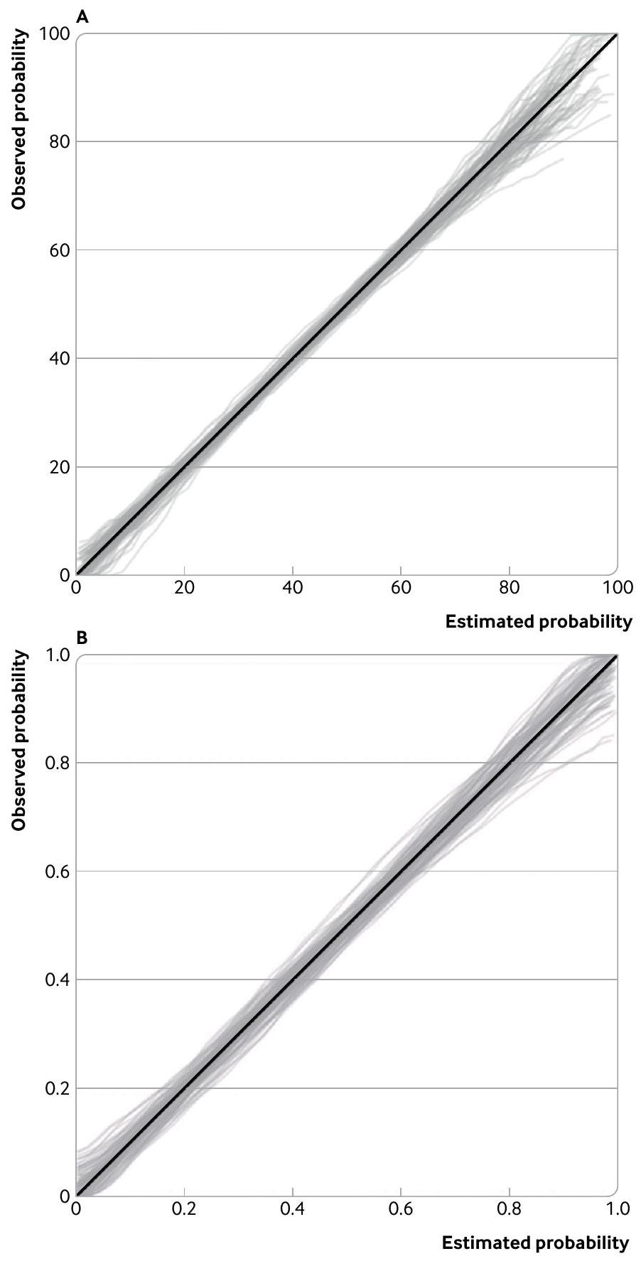
الشكل 5 | توزيع منحنيات المعايرة لنموذج توقع شدة الألم (أ) (استنادًا إلى 258 مشاركًا) ونموذج توقع تدهور كوفيد-19 (ب) (استنادًا إلى 949 مشاركًا (408 أحداث))، المستمدة من 100 مجموعة بيانات محاكاة بحجم العينة المطلوب لتقدير ميل المعايرة بدقة وفقًا لعرض فترة الثقة المستهدفة البالغ 0.3 (خطأ معياري ) لحد الميل المعاير. تفترض المحاكاة أن النماذج تم معايرتها بشكل جيد، مع ميل معاير حقيقي قدره 1 ومعايرة كبيرة تساوي صفر
توزيع المتنبئ الخطي، وأداء (سوء) المعايرة. ثم، لكل مجموعة بيانات خارجية للتحقق، يتم تقدير الأداء التنبؤي ومنحنيات المعايرة في كل نقطة زمنية، ويتم فحص مدى دقتها وتنوعها. تتوفر شيفرات Stata و R علىhttps://www.prognosisresearch.com/البرمجيات.جينكس وآخرون يعتبرون حجم العينة لتقدير دقيق لإحصائية روستون D.
التخطيط للحصول على مجموعات بيانات موجودة
تخطط العديد من دراسات التحقق الخارجي للحصول على مجموعة بيانات موجودة بحجم عينة ثابت (بدلاً من تجنيد مشاركين جدد). في هذه الحالة، يمكن تعديل أساليبنا لحساب الدقة المتوقعة (عرض فترة الثقة) بناءً على حجم عينة تلك المجموعة وأي خصائص معروفة أخرى (مثل، توزيع الاحتمالات المقدرة، التباين الملحوظ للنتائج المستمرة، نسبة حدث النتيجة الملحوظة، معدل التوقف). سيساعد هذا الحساب الباحثين والممولين المحتملين على التأكد مما إذا كانت مجموعة البيانات كبيرة بما يكفي (مثل، لتبرير أي تكاليف ووقت متضمن في الحصول على البيانات)، مع الأخذ في الاعتبار أيضًا جوانب الجودة الأخرى (مثل، الإعداد، تسجيل المتنبئات، طرق القياس). يمكن زيادة أحجام العينات بشكل أكبر من خلال دمج البيانات من مصادر متعددة، مثل بيانات المشاركين الفرديين من دراسات متعددة أو سجلات الرعاية الصحية الإلكترونية عبر ممارسات أو مستشفيات متعددة.
تقرير واضح وشفاف
فيما يتعلق بحجم العينة، تدفع إرشادات تقرير TRIPOD المؤلفين لشرح كيفية الوصول إلى حجم الدراسة.في سياق حسابات حجم العينة المقترحة لدراسات التحقق الخارجي، بالنسبة لنتيجة مستمرة (الشكل 3) سيتطلب هذا العنصر من التقرير تقديم القيم المتوقعة لـ، المعايرة في الكل، وانحدار المعايرة مع الأخطاء المعيارية المستهدفة أو عرض فترات الثقة. بالنسبة لنتيجة ثنائية (الصندوق 1)، سيتطلب هذا العنصر من التقرير تقديم النسبة المفترضة لحدث النتيجة، الإحصائية الملحوظة/المتوقعة، انحدار المعايرة، توزيع المتنبئ الخطي (مثل، توزيع بيتا ومعاييره)، وإحصائية c، مع الأخطاء المعيارية المستهدفة أو عرض فترات الثقة، وأي عتبات احتمالية (لاتخاذ القرارات السريرية).
استنتاجات
تختتم هذه المقالة سلسلتنا المكونة من ثلاثة أجزاء حول تقييم نماذج التنبؤ السريرية، حيث ناقشنا مبادئ أنواع التقييم المختلفة،تصميم وتحليل دراسات التحقق الخارجي،وهنا، أهمية حسابات حجم العينة لاستهداف تقييمات دقيقة لأداء نموذج التنبؤ. تكمل هذه المقالة الأعمال ذات الصلة حول حسابات حجم العينة لتطوير النموذج.
الانتماءات المؤلفين
معهد أبحاث الصحة التطبيقية، كلية العلوم الطبية وطب الأسنان، جامعة برمنغهام، برمنغهام B15 2TT، المملكة المتحدة المعهد الوطني للبحوث الصحية والرعاية (NIHR) مركز أبحاث برمنغهام الحيوية، برمنغهام، المملكة المتحدة مركز يوليوس لعلوم الصحة والرعاية الأولية، مركز جامعة أوترخت الطبي، جامعة أوترخت، أوترخت، هولندا قسم التنمية والتجديد، KU Leuven، لوفين، بلجيكا قسم علوم البيانات الحيوية، مركز جامعة لايدن الطبي، لايدن، هولندا مركز الإحصائيات في الطب، قسم نوفيلد لجراحة العظام والروماتيزم وعلوم العضلات والعظام، جامعة أكسفورد، أكسفورد، المملكة المتحدة
المساهمون: قاد RDR وKIES وLA وGSC الأوراق المنهجية السابقة التي تدعم مقترحات حجم العينة في هذه المقالة، مع مساهمات للتحسين تم تقديمها في مراحل مختلفة من قبل JE وTPAD وMvS وBVC. كتب RDR المسودات الأولى والمحدثة لهذه المقالة، مع مساهمات وتعديلات لاحقة من GSC، ثم من جميع المؤلفين في مراحل متعددة. كتب RDR وGSC وJE الشيفرة المقابلة لتنفيذ الأساليب في Stata وR. قاد JE تطوير حزمة pmsampize. RDR هو الضامن. يؤكد المؤلف المقابل أن جميع المؤلفين المدرجين يستوفون معايير التأليف وأنه لم يتم استبعاد أي آخرين يستوفون المعايير.
التمويل: تقدم هذه الورقة بحثًا مستقلًا مدعومًا (لـ RDR وLA وKIES وJE وGSC) من منحة مجلس أبحاث الهندسة والعلوم الفيزيائية (EPSRC) لـ “ابتكار الذكاء الاصطناعي لتسريع البحث الصحي” (EP/Y018516/1)؛ ومنحة مجلس الأبحاث الطبية (MRC)-المعهد الوطني للبحوث الصحية والرعاية (NIHR) طرق أفضل بحث أفضل (المرجع MR/V038168/1)؛ و(لـ RDR وJE وKIES وLA) مركز أبحاث برمنغهام الحيوية في جامعة مستشفيات برمنغهام NHS Trust وجامعة برمنغهام. الآراء المعبر عنها هي آراء المؤلفين وليست بالضرورة آراء NHS أو NIHR أو وزارة الصحة والرعاية الاجتماعية. كما تم دعم GSC من قبل أبحاث السرطان في المملكة المتحدة (منحة البرنامج C49297/A27294). تم دعم BVC من قبل مؤسسة أبحاث فلاندرز (FWO) (منحة G097322N) وصناديق داخلية KU Leuven (منحة). لم يكن للممولين أي دور في النظر في تصميم الدراسة أو في جمع البيانات أو تحليلها أو تفسيرها أو كتابة التقرير أو اتخاذ القرار لتقديم المقالة للنشر.
المصالح المتنافسة: أكمل جميع المؤلفين نموذج الإفصاح الموحد ICMJE فيhttps://www.icmje.org/disclosure-of-interest/ويعلنون: الدعم من EPSRC وNIHR-MRC ومركز أبحاث برمنغهام الحيوية وCancer Research UK وFWO وصناديق داخلية KU Leuven للعمل المقدم؛ RDR وGSC هما محرران إحصائيان لـ The BMJ؛ لا توجد علاقات مالية مع أي منظمات قد تكون لها مصلحة في العمل المقدم في السنوات الثلاث الماضية؛ لا توجد علاقات أو أنشطة أخرى قد تبدو أنها أثرت على العمل المقدم.
مشاركة المرضى والجمهور: لم يشارك المرضى أو الجمهور في تصميم أو إجراء أو تقرير أو نشر بحثنا.
الأصل والمراجعة من قبل الأقران: لم يتم تكليفه؛ تمت مراجعته من قبل الأقران خارجيًا.
هذه مقالة مفتوحة الوصول موزعة وفقًا لشروط ترخيص المشاع الإبداعي (CC BY 4.0)، الذي يسمح للآخرين بتوزيع وإعادة مزج وتكييف وبناء على هذا العمل، للاستخدام التجاري، بشرط أن يتم الاستشهاد بالعمل الأصلي بشكل صحيح. انظر:http://creativecommons.org/licenses/by/4.0/.
1 هاريل FEJr. استراتيجيات نمذجة الانحدار: مع تطبيقات على النماذج الخطية، والانحدار اللوجستي والترتيبي، وتحليل البقاء. الطبعة الثانية. سبرينغر، 2015. doi:10.1007/978-3-319-19425-7.
2 ستيربرغ EW. نماذج التنبؤ السريرية: نهج عملي للتطوير والتحقق والتحديث. الطبعة الثانية. سبرينغر، 2019. doi:10.1007/978-3-030-16399-0.
3 رايلي RD، فان دير ويندت D، كروفت P، مونس KGM، محررون. أبحاث التنبؤ في الرعاية الصحية: المفاهيم والأساليب والأثر. مطبعة جامعة أكسفورد، 2019. doi:10.1093/med/9780198796619.001.0001.
4 رايلي RD، آرتشر L، سنيل KIE، وآخرون. تقييم نماذج التنبؤ السريرية (الجزء 2): كيفية إجراء دراسة تحقق خارجي. BMJ 2023;383:e074820. doi:10.1136/bmj-2023-074820
5 كولينز GS، دي غروت JA، داتون S، وآخرون. التحقق الخارجي لنماذج التنبؤ متعددة المتغيرات: مراجعة منهجية للسلوك والتقارير المنهجية. BMC Med Res Methodol 2014;14:40. doi:10.1186/1471-2288-14-40
6 غروت OQ، بينديلس BJJ، أوغينك PT، وآخرون. توافر وجودة تقارير التحقق الخارجي لنماذج التنبؤ باستخدام التعلم الآلي مع نتائج جراحة العظام: مراجعة منهجية. Acta Orthop 2021;92:385-93. doi:10.1080/17453674.2021.1910448
7 بيك N، آرتس DG، بوسمان RJ، فان دير فورت PH، دي كيزر NF. تطلب التحقق الخارجي لنماذج التنبؤ للمرضى الحرجين أحجام عينات كبيرة. J Clin Epidemiol 2007;60:491-501. doi:10.1016/j.jclinepi.2006.08.011
8 فيرغوي Y، ستيربرغ EW، إيكيماns MJ، هابما JD. كانت أحجام العينات الفعالة الكبيرة مطلوبة لدراسات التحقق الخارجي لنماذج الانحدار اللوجستي التنبؤية. / Clin Epidemiol 2005;58:47583. doi:10.1016/j.jclinepi.2004.06.017
9 كولينز GS، أوغنديمو EO، ألتمان DG. اعتبارات حجم العينة للتحقق الخارجي لنموذج تنبؤي متعدد المتغيرات: دراسة إعادة أخذ العينات. Stat Med 2016;35:214-26. doi:10.1002/sim.6787
10 فان كالسير B، نيبور D، فيرغوي Y، دي كوك B، بنسينا MJ، ستيربرغ EW. تم تعريف تسلسل المعايرة لنماذج المخاطر:
من اليوتوبيا إلى البيانات التجريبية. / Clin Epidemiol 2016;74:167-76. doi:10.1016/j.jclinepi.2015.12.005 11 رايلي RD، ديبري TPA، كولينز GS، وآخرون. الحد الأدنى لحجم العينة للتحقق الخارجي من نموذج التنبؤ السريري مع نتيجة ثنائية. ستات ميد 2021؛ 40: 4230-51. doi:10.1002/sim.9025 12 رايلي RD، كولينز GS، إنسور J، وآخرون. حسابات الحد الأدنى لحجم العينة للتحقق الخارجي من نموذج التنبؤ السريري مع نتيجة زمنية. ستات ميد 2022؛ 41: 1280-95. doi:10.1002/sim.9275 13 سنيل كيه، آرتشر إل، إنسور ج، وآخرون. التحقق الخارجي من نماذج التنبؤ السريرية: كانت حسابات حجم العينة المعتمدة على المحاكاة أكثر موثوقية من القواعد العامة. مجلة الوبائيات السريرية 2021؛ 135: 79-89. doi:10.1016/j.jclinepi.2021.02.011 14 أرشر إل، سنيل كيه آي إي، إنسور ج، هودا إم تي، كولينز جي إس، رايلي آر دي. الحد الأدنى لحجم العينة للتحقق الخارجي من نموذج التنبؤ السريري مع نتيجة مستمرة. ستات ميد 2021؛ 40: 133-46. doi:10.1002/sim.8766 15 كولينز جي إس، ذيمان بي، ما ج، وآخرون. تقييم نماذج التنبؤ السريرية (الجزء 1): من التطوير إلى التحقق الخارجي. BMJ 2023;383:e074819. doi:10.1136/bmj-2023-074819 16 Moons KG، ألتمان DG، ريتسما JB، وآخرون. التقرير الشفاف لنموذج توقع متعدد المتغيرات للتشخيص أو التنبؤ الفردي (TRIPOD): الشرح والتفصيل. Ann Intern Med 2015؛162:W1-73. doi:10.7326/M14-0698 17 لي J، ماولا I، كيم J، وآخرون. التنبؤ بالألم السريري باستخدام التعلم الآلي مع التصوير العصبي المتعدد الأنماط ومقاييس الجهاز العصبي الذاتي. الألم 2019؛ 160: 550-60. doi:10.1097/j.pain.0000000000001417 18 فيكرز AJ، فان كالسير B، ستيربرغ EW. أساليب الفائدة الصافية لتقييم نماذج التنبؤ، والعلامات الجزيئية، والاختبارات التشخيصية. BMJ 2016؛352:i6. doi:10.1136/bmj.i6 19 مارش تي إل، جانس إتش، بيبي إم إس. الاستدلال الإحصائي لقياسات الفائدة الصافية في دراسات التحقق من العلامات الحيوية. البيومترية 2020؛76:84352. doi:10.1111/biom.13190
20 فيكرز AJ، إلكين EB. تحليل منحنى القرار: طريقة جديدة لتقييم نماذج التنبؤ. اتخاذ القرار الطبي 2006؛ 26: 565-74. doi:10.1177/0272989X06295361 21 نيوكومب RG. فترات الثقة لقياس حجم التأثير بناءً على إحصائية مان-ويتني. الجزء 2: الطرق التقاربية والتقييم. ستات ميد 2006؛ 25: 559-73. doi:10.1002/sim.2324 22 بافلو م، كيو سي، عمر ر. ز، وآخرون. تقدير حجم العينة المطلوب للتحقق الخارجي من نماذج المخاطر للنتائج الثنائية. طرق إحصائية في البحث الطبي 2021؛30:2187-206. doi:10.1177/09622802211007522 23 غوبتا آر كيه، هاريسون إي إم، هو أ، وآخرون، محققو ISARIC4C. تطوير وتقييم نموذج تدهور ISARIC 4C للبالغين الذين تم إدخالهم إلى المستشفى بسبب COVID-19: دراسة جماعية مستقبلية. لانسيت طب الجهاز التنفسي 2021؛9:349-59. doi:10.1016/S2213-2600(20)30559-2 24 فان كالسيرت ب، مكلايرنون دي جي، فان سمدن م، وينانتس ل، ستيربرغ إي دبليو، مجموعة الموضوع ‘تقييم الاختبارات التشخيصية ونماذج التنبؤ’ من مبادرة ستاتوس. المعايرة: كعب أخيل التحليلات التنبؤية. بي إم سي ميد 2019؛ 17:230. doi:10.1186/s12916-019-1466-7 25 كولينز جي إس، ريتسما جي بي، ألتمن دي جي، مونس ك جي إم. التقرير الشفاف لنموذج توقع متعدد المتغيرات للتشخيص أو التنبؤ الفردي (TRIPOD): بيان TRIPOD. آن إنترن ميد 2015؛ 162: 55-63. doi:10.7326/M14-0697 26 جينكس آر سي، رويستون بي، بارمار إم كيه. حسابات حجم العينة المعتمدة على التمييز لنماذج التنبؤ متعددة المتغيرات لبيانات الوقت حتى الحدث. بيم سي ميد ريس ميثودول 2015؛15:82. doi:10.1186/s12874-015-0078-y 27 رايلي RD، إنسور J، سنيل KI، وآخرون. التحقق الخارجي من نماذج التنبؤ السريرية باستخدام مجموعات بيانات كبيرة من سجلات الصحة الإلكترونية أو تحليل البيانات الفردية: الفرص والتحديات. BMJ 2016؛ 353: i3140. doi:10.1136/bmj.i3140 28 رايلي RD، تيرني JF، ستيوارت LA، محررون. تحليل البيانات الفردية للمتابعة: دليل لأبحاث الرعاية الصحية. وايلي، 2021. doi:10.1002/9781119333784. 29 رايلي RD، إنسور J، سنيل KIE، وآخرون. حساب حجم العينة المطلوب لتطوير نموذج توقع سريري. BMJ 2020؛368:m441. doi:10.1136/bmj.m441 30 رايلي RD، سنيل KI، إنسور J، وآخرون. الحد الأدنى لحجم العينة لتطوير نموذج توقع متعدد المتغيرات: الجزء الثاني – النتائج الثنائية ونتائج الوقت للحدث. ستات ميد 2019؛ 38: 1276-96. doi:10.1002/sim.7992 31 رايلي RD، سنيل KIE، إنسور J، وآخرون. الحد الأدنى لحجم العينة لتطوير نموذج توقع متعدد المتغيرات: الجزء الأول – النتائج المستمرة. ستات ميد 2019؛ 38: 1262-75. doi:10.1002/sim.7993 32 فان سمدن م، مونس ك ج، دي غروت ج أ، وآخرون. حجم العينة لنماذج التنبؤ اللوجستي الثنائي: ما وراء معايير الأحداث لكل متغير. طرق إحصائية في البحث الطبي 2019؛ 28: 2455-74. doi:10.1177/0962280218784726 33 وينانتس إل، فان سمدن م، مكلايرنون دي جي، تيمرمان د، ستايربرغ إي دبليو، فان كالسيرت ب، مجموعة الموضوع ‘تقييم الاختبارات التشخيصية ونماذج التنبؤ’ من مبادرة ستراتوس. ثلاثة خرافات حول عتبات المخاطر لنماذج التنبؤ. بي إم سي ميد 2019؛ 17:192. doi:10.1186/s12916-019-1425-3
An external validation study evaluates the performance of a prediction model in new data, but many of these studies are too small to provide reliable answers. In the third article of their series on model evaluation, Riley and colleagues describe how to calculate the sample size required for external validation studies, and propose to avoid rules of thumb by tailoring calculations to the model and setting at hand.
External validation studies evaluate the performance of one or more prediction models (eg, developed previously using statistical, machine learning, or artificial intelligence approaches) in a different dataset to that used in the model development process. Part 2 in our series describes how to undertake a high quality external validation study, including the need to estimate model performance measures such as calibration (agreement between observed and predicted values), discrimination (separation between predicted values in those with and without an outcome event), overall fit (eg, percentage of
SUMMARY POINTS
The sample size for an external validation study should be large enough to precisely estimate the predictive performance of the model of interest Many existing validation studies are too small, which leads to wide confidence intervals of performance estimates and potentially misleading claims about a model’s reliability or its performance compared with other models To deal with concerns of imprecise performance estimates, rules of thumb for sample size have been proposed, such as having at least 100 events and 100 non-events
Such rules of thumb provide a starting point but are problematic, because they are not specific to either the model or the clinical setting, and precision also depends on factors other than the number of events and non-events A more tailored approach can allow researchers to calculate the sample size required to target chosen precision (confidence interval widths) of key performance estimates, such as for R2, calibration curve, c statistic, and net benefit
Calculations depend on users specifying information such as the outcome proportion, expected model performance, and distribution of predicted values, which can be gauged from the original model development study
The pmvalsampsize package in Stata and R allows researchers to implement the approach with one line of code
variation in outcome values explained), and clinical utility (eg, net benefit of using the model to inform treatment decisions). In this third part of the series, we describe how to calculate the sample size required for such external validation studies to estimate these performance measures precisely, and we provide illustrated examples.
Rationale for sample size calculations in external validation studies
The sample size for an external validation study should be large enough to precisely estimate the predictive performance of the model of interest. The aim is to provide strong evidence about the accuracy of the model’s predictions in a particular target population, to help support decisions about the model’s usefulness (eg, for patient counselling, within clinical practice).
Many published external validation studies are too small, as shown by reviews of validations of statistical and machine learning based prediction models. A small sample size leads to wide confidence intervals of performance estimates and potentially misleading claims about a model’s reliability or its performance compared with other models, especially if uncertainty is ignored. This problem is illustrated in figure 1, which shows 100 randomly generated calibration curves for external validation of a prediction model for inhospital clinical deterioration among admitted adults with covid-19. Each curve is estimated on a random sample of 100 hypothetical participants (and about 43 outcome events), with outcomes (deterioration: yes or no) randomly generated based on assuming estimated probabilities from the covid-19 model are correct in the external validation population. Even though the model predictions are well calibrated in the population (ie, the diagonal solid line in fig 1 is the underlying truth), the sampling variability in the observed curves is large. For example, for individuals with an estimated probability between 0 and 0.05, the observed probability on the curves range between about 0 and 0.3 . Similarly, for individuals with an estimated probability of 0.9 , the observed probabilities on the curves range from about 0.6 to 1 . Hence, the sample size of 100 participants is too small to ensure an external validation study provides stable results about calibration performance.
To resolve concerns of imprecise performance estimates, and thus inconclusive or misleading findings, rules of thumb have been proposed for the sample size required for external validation studies. For binary or time-to-event outcomes, rules of thumb based on simulation and resampling studies suggest at least 100 events and 100 non-events are needed to estimate measures such as the c statistic (area under the receiver operating characteristic curve) and calibration
Fig 1 | Illustration of the concern of low sample sizes when assessing calibration. Plot shows large variability in calibration curves from 100 external validation studies (each containing a random sample of 100 participants, and on average 43 outcome events, with outcomes generated assuming that the prediction model is truly well calibrated) of a prediction model for in-hospital clinical deterioration among admitted adults with covid-19
slope, and a minimum of 200 events and 200 nonevents to derive calibration plots including calibration curves. Such rules of thumb provide a starting point but are problematic, because they are not specific to either the model or the clinical setting, and precision of predictive performance estimates also depend on factors other than the number of events and nonevents, such as the distribution of predicted values. Therefore, rules of thumb could lead to sample sizes that are too small (producing imprecise performance estimates) or too large (eg, prospectively collecting excessive amounts of data that are unnecessarily time consuming and expensive).
To move away from rules of thumb, tailored sample size calculations are now available for external validation studies. Here, we summarise these calculations for a broad audience, with technical details placed in boxes to ensure the main text focuses on key principles and worked examples. Our premise is that an external validation study aims to estimate the performance of prediction model in new data (see part 1 of our series) ; we do not focus on sample size required for revising or updating a prediction model. Complementary to sample size, and as emphasised in the part 2 of this series, researchers should also ensure external validation datasets are representative of the target population and setting (eg, in terms of case mix, outcome risks, measurement and timing of predictors), and typically would be from a longitudinal cohort study (for prognostic models) or a cross sectional study (for diagnostic models).
Sample size for external validation of prediction models with a continuous outcome
When validating the performance of a prediction model for a continuous outcome (such as blood pressure, weight or pain score), there are many different performance measures of interest, as defined in detail in part 2 of this series. At a minimum, Archer et al suggest it is important to examine the following factors: overall fit as measured by (the proportion of variance explained in the external validation dataset), calibration as measured by calibration curves and quantified using calibration-in-the-large (the difference between the mean predicted and the mean observed outcome values) and calibration slope (the agreement between predicted and observed values across the range of predicted values), and residual variance (the variance of differences between predicted and observed values in the external validation data). Four separate sample size calculations have been proposed that target precise estimation of these measures, which are summarised in figure 2. Unlike rules of thumb, the calculations are tailored to the clinical setting and model of interest because they require researchers to specify assumed true values in the external validation population for , calibration-in-the-large, calibration slope, and variance (or standard deviation) of outcome values across individuals.
Specifying these input values is analogous to other sample size calculations in medical research, for example, for randomised trials where values of the assumed effect size and target precision (or power) are needed. The dilemma is how to choose these input values. Here, we suggest that assuming values agree with those reported from the original model development study is a sensible starting point, especially if the target population (for external validation) is similar to that used in the model development study. In terms of specifying the true , we suggest use of the optimism adjusted estimate of reported for the development study, where “optimism adjusted” refers to the estimate having been adjusted for any overfitting during development (ie, from an appropriate internal validation ; see part 1 of the series ). In terms of calibration, we recommend that assuming the model’s predictions are well calibrated in the external validation population, such that the anticipated true calibration-in-the-large is zero and the true calibration slope is 1 (extensions assuming miscalibration are considered elsewhere ), corresponding to a level 2 assessment in the calibration hierarchy of Van Calster et al. The variance of outcome values can also be obtained from the model development study, or any previous studies that summarise the outcome in the target population.
Also required are the target standard errors or target confidence interval widths for the model performance estimates of interest, with the goal to ensure that 95% confidence interval widths are narrow enough to allow precise conclusions to be drawn. We assume that confidence interval widths are approximated well by standard error. Defining the target standard error or confidence interval width
Criterion 1: calculate the sample size ( N ) needed to precisely estimate Use the equation:
This requires specifying an anticipated value for the true (the proportion of variance explained) and (the target standard error of the estimated ) in the external validation dataset.
We recommend using (to target a confidence interval width ), and choosing to equal the optimism adjusted estimate reported for the model development study.
Criterion 2: calculate the sample size ( N ) needed to precisely estimate calibration-in-the-large (CITL) Assuming the model is well calibrated (ie, the anticipated true CITL is 0 and the true calibration slope ( ) is 1 ), then apply the following equation:
This requires specifying the anticipated value for the true (as chosen in criterion 1), SE(CITL) (the target standard error of the estimated CITL ) and (the variance of outcome values in the validation population). The should be based on existing knowledge (eg, previous studies). The value of SE(CITL) should target a narrow confidence interval width for the difference in the mean observed and mean predicted values, and this is context specific because it depends on the scale of the outcome. For example, for blood pressure measured in mm Hg , a confidence interval width might be sought.
Criterion 3: calculate the sample size ( N ) needed to precisely estimate calibration slope ( )
Assuming again that the model is well calibrated (ie, anticipated true CITL 0 , true ), then apply the following equation:
This requires specifying an anticipated value for the true (as chosen in criterion 1 ), and (the target standard error of the estimated calibration slope). To ensure a narrow confidence interval for , we recommend using (to target a confidence interval width ), or (to target a confidence interval width ). The choice is subjective but can be informed by plotting the corresponding empirical distribution of calibration curves (we give further guidance on targeting precise calibration curves later in the article).
Criterion 4: calculate the sample size ( N ) needed to precisely estimate the residual variance
To target residual variance estimates in the calibration models that have a margin of error of , at least 235 participants are required, as explained in Archer et al.
We recommend that multiple (plausible) values of are considered (eg, the original chosen value for criterion 1 ) and the calculations repeated for criterions 1-3 to identify whether a larger sample size is required.
Fig 2 | Summary of calculations for different sample sizes for external validation of a clinical prediction model for a continuous outcome (modified from Archer et ), which target narrow confidence interval widths (as defined by standard error) for key performance measures
is subjective, and these values will be different for each measure (because they are on different scales), but general guidance is given in figure 2. Stata and code to implement the entire calculation is provided at https://www.prognosisresearch.com/software, and some of the work can be implemented in the Stata and R module pmvalsampsize (see example code later). It leads to four sample sizes-one for each criterion in figure 2-and the largest of these should be taken as the minimum sample size for the external validation study, to ensure that all four criteria are met.
Applied example: external validation of a machine learning based prediction model for pain intensity in low back pain
Lee and colleagues used individualised physical manoeuvres to exacerbate clinical pain in patients with chronic low back pain, thereby experimentally producing lower and higher pain states and recording patients’ recorded pain intensity. Using the data obtained, the researchers fitted a support vector machine to build a model to predict pain intensity (a continuous outcome ranging from 0 to 100) conditional
on the values of multiple predictor variables including brain imaging and autonomic activity features. After model development, the performance was evaluated in validation data comprising 53 participants, which estimated to be 0.40 .
However, owing to the small size of the validation data, wide confidence intervals about model performance were produced (eg, 95% confidence interval for to 0.60 ), and so a new external validation study is required to provide more precise estimates of performance in this particular target population. We calculated the sample size required for this external validation study using the approach outlined in figure 2, which can be implemented in the Stata module pmvalsampsize. We assumed that in the external validation population the true is 0.40 (based on the estimate of in the previous validation data); the model is well calibrated (ie, the anticipated true calibration-in-the-large is 0 and true calibration slope is 1); and the true standard deviation of pain intensity values is 22.30 (taken from the average standard deviation in the previous validation and training datasets in the development
Criterion 1: calculate the sample size ( N ) needed to precisely estimate the observed/expected ( ) statistic
Apply the following equation:
Where is the assumed true outcome event proportion in the external validation population and is the target standard error of the In(O/E) statistic, which would ensure a precise confidence interval width on the scale. The choice of is context specific, because it depends on the overall event probability in the population-as can be seen in the covid-19 applied example and discussion by Riley et al.
Criterion 2: calculate the sample size ( N ) needed to precisely estimate calibration slope ( ) Apply the following equation:
Where is the target standard error for the calibration slope estimate. The , and are elements of Fisher’s information matrix, and depend on the distribution of the linear predictor values ( , which are the predicted values on the log-odds scale) in the external validation population, and correspond to the mean value of mean value of , and mean value of , respectively, where:
Our Stata and code calculate , and automatically, based on the specified distribution for (see box 1 ) and the assumed calibration performance. We recommend, as a starting point, assuming the model is well calibrated (ie, is 0 and is 1 ). In terms of target precision, we suggest using a to target a confidence interval width , or to target a confidence interval width . The choice is subjective but can be informed by plotting the empirical distribution of calibration curves (we give further guidance on targeting precise calibration curves later in the article).
Criterion 3: calculate the sample size needed to precisely estimate the c statistic
We use the following formula for the standard error of the c statistic, proposed by Newcombe, which makes no assumptions about the underlying distribution of the prediction model’s linear predictor:
Here, C is the anticipated true c statistic for the external validation population, is the assumed true outcome event proportion in the external validation dataset, and is the target standard error of C (we recommend values , so that the confidence interval width is ). Given these input values, our and Stata code use an iterative process to identify the sample size to achieve the target .
Criterion 4: calculate the sample size needed to precisely estimate the standardised net benefit (sNB) at one (or more) probability threshold value ( ) of interest for clinical decision making (if relevant) Apply the following equation derived by Marsh et al:
Where ( ) is defined as , based on sensitivity and specificity values that correspond to the chosen distribution of predicted values and assuming the model is well calibrated. The standardisation ensures that the maximum value is 1 regardless of the external validation setting. Also, and the model’s sensitivity and specificity are the anticipated values at threshold , which can be inferred from the assumed distribution of the linear predictor from criterion 2 . If there are a range of thresholds of interest, then the calculation should be repeated for each. A reasonable approach to specify the target standard error of the standardised net benefit, , is to choose the value that would yield a confidence interval that at least excludes the treat none approach’s net benefit value of 0 . This implies that , where is the assumed true value of the standardised net benefit, such that .
Fig 3 | Summary of different sample size criteria for external validation of a clinical prediction model for a binary outcome, as originally proposed by Riley et al. In criterion 3, the formula for the standard error of the c statistic was proposed by Newcombe. In criterion 4, the equation applied is derived by Marsh et al
study). We targeted a confidence interval width for the calibration-in-the-large (which we considered precise given the outcome scale of 0 to 100), for the calibration slope and for .
Applying each of the four criteria, the pmvalsampsize code is:
pmvalsampsize, type(c) rsquared(.4) varobs(497.29) citlciwidth(5) csciwidth(.3)
This calculation suggests that the number of participants required for precise estimates is 886 for , 184 for calibration-in-the-large, 258 for calibration slope, and 235 for the residual variance. Hence, at
Box 1: Guidance about what prespecified information is needed when applying sample size calculations for a binary outcome, modified from Riley et al
Anticipated proportion of outcome events in the external validation population (ie, the overall risk of the outcome event)
This proportion can be based on previous studies or datasets that report outcome prevalence (for diagnostic situations) or incidence by a particular time point (for prognostic situations) for the target population.
Anticipated c statistic in the external validation population
Initially, this value could be assumed equal to the optimism adjusted estimate of the c statistic reported for the model development study (or the c statistic reported for any previous validation study in the same target population), but alternative values (eg, of this value) can also be considered.
Prediction model’s anticipated (mis)calibration in the external validation population
A practical starting point is to assume that the model is well calibrated in the validation dataset, such that the anticipated true observed/expected statistic is 1 and true calibration slope is 1 . Many validation studies show miscalibration, with calibration slopes less than 1 owing to overfitting in the original model development study; however, in terms of the sample size calculation, a conservative approach (as it leads to larger required numbers) is to assume a calibration slope of
Distribution of the model’s estimated event probabilities in the external validation population
This task is perhaps the most difficult, and the distribution must give the same overall outcome event proportion as assumed above. The distribution of predicted values on the log odds scale (also known as the distribution of the linear predictor or the logit transformation of the probability values) is required, and a practical starting point is to assume the same distribution as reported in the model development study. In the model development study, histograms of event probabilities are occasionally provided as part of a calibration plot, and so could be approximated by a identifying a suitable distribution on the 0 to 1 scale (eg, a beta distribution is used in our applied covid-19 example later in this article), followed by conversion to the log odds scale. Sometimes the histograms are presented stratified by outcome status, and then these can be approximated, with samples taken from each while ensuring that the overall outcome event proportion is correct.
If no direct information is available to inform the linear predictor distribution, then the assumed true c statistic can also be used to infer the distribution, under a strong assumption that if the calibration slope is 1 then the linear predictor is normally distributed with different means but a common variance for those with and without an outcome event. We suggest that this is a last resort, because it could be a poor approximation when the assumptions break down. An alternative is to undertake a pilot study to better gauge the distribution. Such pilot data can still be included in the final sample used for external validation.
Potential probability (risk) threshold(s) for clinical decision making (if relevant)
These thresholds should be determined by speaking to clinical experts and patient advisory groups in the context of the decisions to be taken (eg, treatments, monitoring strategies, lifestyle changes) and the overall benefits and harms from them.
least 886 participants are required for the external validation study, in order to target precise estimates of all four measures. If only 258 participants are recruited, then the anticipated confidence interval for is wide ( 0.31 to 0.49), which would be a concern because the estimate of not only reveals the overall model fit, but also contributes toward the estimate of the calibration slope and calibration-in-the-large (fig 2).
As the assumed value of 0.40 is just a best guess, we repeated the sample size calculations using different values of 0.30 and 0.50 . The use of 0.50 decreased the required sample size, but the use of 0.30 led to larger required sample sizes with 905 for for calibration-in-the-large, 400 for calibration slope, and 235 for the residual variance. Hence, it might be more cautious to assume an of 0.30 , and thus recruit 905 participants if possible.
Sample size for external validation of prediction models with a binary outcome
When evaluating the performance of a prediction model for a binary outcome (such as onset of preeclampsia during pregnancy), researchers must examine discrimination as measured by the c statistic (ie, the area under the receiver operating characteristic curve), and calibration as measured by calibration-in-the-large (eg, the observed/expected statistic)
and calibration slope. Furthermore, if the model is to be used to guide clinical decision making, then clinical utility can be measured by the net benefit statistic, which weighs the benefits (eg, improved patient outcomes) against the harms (eg, worse patient outcomes, additional costs) of deciding on some clinical action for patients (eg, a particular treatment or monitoring strategy) if their estimated event probability exceeds a particular threshold. These performance measures were defined in detail in part 2 of our series.
To target precise estimates of these four measures of model performance, we suggest four separate sample size calculations. These calculations are summarised in figure 3 along with general guidance for choosing standard errors that target narrow confidence interval widths (defined by standard error) for each performance measure. Complementary approaches have also been suggested.
As for continuous outcomes, these sample size calculations for binary outcomes also require prespecifying aspects of the (anticipated) external validation population and assumed true model performance in that population-namely, the outcome event proportion (ie, overall risk), c statistic, observed/ expected statistic, calibration slope, distribution of estimated probabilities from the model, ideally
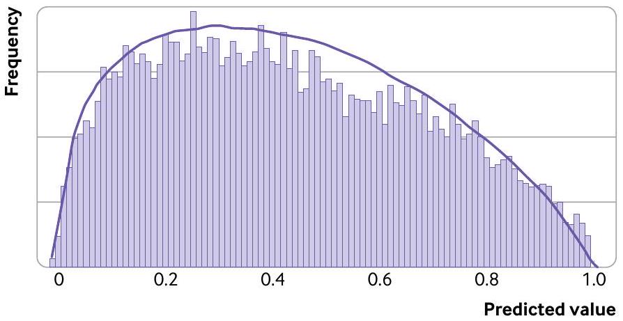
Fig 4 | Comparison of histogram (grey bars) of predicted values (estimated event probabilities) in the validation population of Gupta et al with our assumed beta distribution (curved line) used
specified on the log-odds scale (also known as the linear predictor distribution), and probability (risk) thresholds of interest for clinical decision making (if relevant).
Guidance for choosing these input values is given in box 1; as discussed for continuous outcomes, a sensible starting point for the performance measures is to base values on those (optimism adjusted) estimates reported from the model development study.
Applied example: external validation of a model for deterioration in adults admitted to hospital with covid-19
In 2021, Gupta et al developed the ISARIC 4C deterioration model, a multivariable logistic regression model for predicting in-hospital clinical deterioration (defined as any requirement of ventilatory support or critical care, or death) among adults admitted to hospital with highly suspected or confirmed covid-19. The model was developed using data from 260 hospitals including 66705 participants across England, Scotland, and Wales, and validated in a separate dataset of 8239 participants from London. Model performance on validation was judged satisfactory (c statistic 0.77 (95% confidence interval 0.76 to 0.78); calibration-in-the-large 0 ( -0.05 to 0.05); calibration slope 0.96 (0.91 to 1.01)), and greater net benefit compared with other models. However, further external validation is now required to check that model predictions are still reliable after the introduction of covid-19 vaccines and other interventions.
To calculate the sample size required, we applied the approach outlined in figure 3, with input values chosen based on box 1 . We assumed that in the external validation population, the model would be well calibrated (ie, the anticipated true observed/ expected statistic is 1 and true calibration slope is 1 ) with an anticipated c statistic of 0.77 based on the previous validation study. Further, we assumed that the distribution of the model’s event probabilities in the external validation population would be similar to that in the histogram presented by Gupta et in their supplementary material; by trial and error, we approximated this histogram by using a beta(1.33, 1.75) distribution (fig 4), yielding a similar shape and
with the same overall outcome event proportion of 0.43 .
We targeted a confidence interval width of 0.22 for the observed/expected statistic (which corresponds to a small absolute error of about 0.05 compared with the assumed overall outcome event proportion of 0.43; see calculations elsewhere ), 0.3 for the calibration slope, 0.1 for the c statistic, and 0.2 for the standardised net benefit. Applying the sample size calculations, the corresponding Stata code is:
size of 423 (182 events) for the observed/expected ts) for calibration slope, 347 (149 events) for c statistic, and 38 (16 events) for standardised net benefit at a threshold of 0.1; and 407 (175 events) for standardised net benefit at a threshold of 0.3 . Hence, at least 949 participants ( 408 events) are required for the external validation study to target precise estimates of all four measures and, in particular, to ensure calibration is properly evaluated. This sample size is much larger than the rule of thumb of 100 (or 200) events and 100 (or 200) non-events.
Additional calculations were done to see how the required sample size changed when our assumptions changed. For example, when assuming the model has the same distribution of estimated probabilities but with worse performance of either a calibration slope of 0.9 or a c statistic of 0.72 , the sample size required was fewer than the 949 participants originally identified. However, if we assumed the external validation population had a narrower case mix distribution, and so used a tighter distribution of predicted values than the previous beta distribution, a sample size larger than 949 participants was required for precise estimation of the calibration slope. This change in target sample size emphasises the importance of understanding the target population and its likely distribution of predicted values. In the absence of any information, a pilot study might be useful to help gauge this distribution.
Guidance for targeting precise calibration curves especially in regions containing thresholds relevant to clinical decision making
Calibration is often neglected in validation studies, despite it being widely recommended, for instance as an item in the TRIPOD (Transparent Reporting of a multivariable prediction model for Individual Prognosis or Diagnosis) reporting guideline. Yet in clinical practice, predicted values (in particular, estimated event probabilities) are used for patient counselling and shared decision making-for example, to guide treatment decisions, invasive investigations, lifestyle changes, and monitoring decisions. Hence, external validation studies must produce precise estimates of calibration curves to reliably examine calibration of observed and predicted values. Ideally, curves should be precise across the whole range of predicted values, which is why our sample size criteria aims to estimate
calibration-in-the-large (observed/expected statistic) and calibration slope precisely. At the bare minimum, curves should be precise within regions containing possible probability thresholds relevant for clinical decision making. We discuss this topic further in the supplementary material.
Very large sample sizes might be needed to estimate the whole calibration curve precisely. Furthermore, choosing the target standard errors for the calibration measures (slope and calibration-in-the-large) is subjective and difficult to gauge, especially for binary outcomes because the slope is estimated on the logit scale. To deal with this problem, we suggest plotting the empirical distribution of calibration curves that arise from a dataset with the sample size identified based on particular chosen target standard errors (eg, corresponding to a confidence interval width of 0.3 for the calibration slope), to check whether their variability is sufficiently low, especially in regions encompassing thresholds relevant to decision making. This approach can be done as follows:
Simulate a large number of datasets (eg, 100 or 200) with the sample size identified (for the chosen target standard errors), under the same assumptions as used in the sample size calculation (eg, assumed calibration slope of 1, same distribution of predicted values).
For each dataset separately, derive a calibration plot including a calibration curve, as described in the second paper in this series.
On a single plot, overlay all the calibration curves to reveal the potential range of calibration curves that might be observed in practice for a single external validation study of that sample size. If variability is considered to be high on visual inspection, then a larger sample size is needed. Conversely, if variability is very precise, a lower sample size might suffice, especially if the original sample size is not considered attainable.
As mentioned, at the bare minimum, researchers should ensure low variability of curves in regions of most relevance for clinical decision making.
To illustrate this approach, figure 5 shows the empirical distribution of 100 calibration curves for our two applied examples when simulated using the sample size previously calculated to target a standard error of 0.0765 (confidence interval width of 0.3 ) for the calibration slope. For the pain intensity continuous outcome, 258 participants were identified as necessary for estimating calibration slope assuming it was 1, and the corresponding distribution of curves based on this sample size is reasonably narrow (fig 5A). At predicted values less than 80, the spread of observed curves corresponds to a difference in pain score of only about 5 to 10 . Only at the upper end is the variability more pronounced (differences up to about 20), for example, with curves spanning pain scores of 80 to 100 at a predicted score of 90 . If values in this range represent thresholds critical to clinical decision making, then larger sample sizes might be required. However, any value over 80 is likely to be always classed as very high,
and so the observed variability in this upper range is unlikely to be important. Hence, the calculated target sample size of 258 participants still seems sensible.
For the covid-19 deterioration model with 949 participants (408 events), the variability is also quite narrow across the entire range of event probabilities, although slightly larger at very high probabilities ( 0.8 to 1); the spread of observed curves corresponds to a difference in observed probabilities of about 0.05 to 0.15 in most regions, which is reasonably precise. If the target confidence interval width for the calibration slope is narrowed to 0.2 (rather than 0.3 ), then the minimum required sample size increases dramatically to 2137 participants ( 918 events), and yet the reduction in variability of the calibration curves is relatively small (supplementary fig S1), with differences in observed probabilities of about 0.05 to 0.10 in most regions. Hence, such a large increase in sample size (with costs and time in participant recruitment, for example) might be difficult to justify.
Conversely, the 100 or 200 events rule-of-thumb corresponds to 233 or 466 participants, respectively, which leads to a wider variability of observed calibration curves spanning a difference in observed probabilities of about 0.15 to 0.2 (200 events) to 0.2 to 0.25 (100 events) in most regions (supplementary fig S2), and introduces much more uncertainty about calibration agreement, including in ranges where high risk thresholds (eg, between 0.05 and 0.1) might exist. Hence, reducing the target sample size also does not appear justified here, and so the originally calculated 949 participants (408 events) still reflects a sensible and pragmatic target for the external validation study in terms of calibration.
Extensions
Missing data in external validation of continuous or binary outcome prediction models
So far, we assumed that the external validation study had no missing data, but in practice some participants could have missing outcomes (eg, due to loss to followup) or missing predictions (eg, due to missing values of predictors in the model). In such situations, inflating the original sample size to account for potential missing information is helpful. For example, if of participants are anticipated to have missing outcomes or predictor values, then 999 participants should be recruited ( , the sample size calculated earlier based on complete data).
Prediction models with time-to-event outcomes
Extension to external validation of prediction models with a time-to-event (survival) outcome is challenging, because closed form (ie, analytical) calculations are difficult to derive. To resolve this problem, we suggest a simulation based approach to assess the precision of estimates of calibration, discrimination, and net benefit. In brief, external validation datasets of a particular sample size are simulated under assumptions about the event and censoring distributions, the length of follow-up, the model’s
Fig 5 | Distribution of calibration curves for (A) pain intensity prediction model (based on 258 participants) and (B) covid-19 deterioration prediction model (based on 949 participants ( 408 events)), derived from 100 simulated datasets with the sample size required to estimate the calibration slope precisely according to a target confidence interval width of 0.3 (standard error ) for the calibration slope. Simulations assume that the models are well calibrated, with a true calibration slope of 1 and calibration-in-the-large of zero
linear predictor distribution, and the (mis)calibration performance. Then, for each external validation dataset, predictive performance and calibration curves are estimated at each time point, and the extent of their precision and variability examined. Stata and R code are available at https://www.prognosisresearch.com/ software. Jinks et al consider sample size for precise estimation of Royston’s D statistic.
Planning to obtain existing datasets
Many external validation studies plan to obtain an existing dataset with a fixed sample size (rather than recruit new participants). In that situation, our approaches can be adapted to calculate the expected precision (confidence interval width) conditional on that dataset’s sample size and any other known characteristics (eg, distribution of estimated probabilities, observed variance of continuous outcomes, observed outcome event proportion, censoring rate). This calculation will help researchers and potential funders to ascertain whether the dataset is large enough (eg, to justify any costs and time involved in obtaining the data), while also considering other quality aspects (eg, setting, recording of predictors, measurement methods). Sample sizes can be increased further by combining data from multiple sources, such as individual participant data from multiple studies or electronic healthcare records across multiple practices or hospitals.
Clear and transparent reporting
With regard to sample size, the TRIPOD reporting guideline prompts authors to explain how the study size was arrived at. In the context of our proposed sample size calculations for external validation studies, for a continuous outcome (fig 3 ) this reporting item would entail providing the anticipated values for , calibration-in-the-large, and calibration slope together with target standard errors or confidence interval widths. For a binary outcome (box 1), this reporting item would entail providing the assumed outcome event proportion, observed/expected statistic, calibration slope, distribution of the linear predictor (eg, beta distribution and its parameters), and c statistic, together with target standard errors or confidence interval widths, and any probability thresholds (for clinical decision making).
Conclusions
This article concludes our three part series on evaluation of clinical prediction models, in which we have discussed the principles of different types of evaluation, the design and analysis of external validation studies, and, here, the importance of sample size calculations to target precise assessments of a prediction model’s performance. This article complements related work on sample size calculations for model development.
AUTHOR AFFILIATIONS
Institute of Applied Health Research, College of Medical and Dental Sciences, University of Birmingham, Birmingham B15 2TT, UK National Institute for Health and Care Research (NIHR) Birmingham Biomedical Research Centre, Birmingham, UK Julius Centre for Health Sciences and Primary Care, University Medical Centre Utrecht, Utrecht University, Utrecht, Netherlands Department of Development and Regeneration, KU Leuven, Leuven, Belgium Department of Biomedical Data Sciences, Leiden University Medical Centre, Leiden, Netherlands Centre for Statistics in Medicine, Nuffield Department of Orthopaedics, Rheumatology, and Musculoskeletal Sciences, University of Oxford, Oxford, UK
Contributors: RDR, KIES, LA, and GSC led the previous methodology papers that underpin the sample size proposals in this article, with contributions for improvement made at various stages by JE, TPAD, MvS, and BVC. RDR wrote the first and updated drafts of this article, with subsequent contributions and revisions by GSC, then by all authors at multiple stages. RDR, GSC, and JE wrote the corresponding code to implement the methods in Stata and R. JE led the pmsampize package development. RDR is the guarantor. The corresponding author attests that all listed authors meet authorship criteria and that no others meeting the criteria have been omitted.
Funding: This paper presents independent research supported (for RDR, LA, KIES, JE, and GSC) by an Engineering and Physical Sciences Research Council (EPSRC) grant for “Artificial intelligence innovation to accelerate health research” (EP/Y018516/1); a Medical Research Council (MRC)-National Institute for Health and Care Research (NIHR) Better Methods Better Research grant (reference MR/ V038168/1); and (for RDR, JE, KIES, and LA) the NIHR Birmingham Biomedical Research Centre at the University Hospitals Birmingham NHS Foundation Trust and the University of Birmingham. The views expressed are those of the authors and not necessarily those of the NHS, NIHR or Department of Health and Social Care. GSC was also supported by Cancer Research UK (programme grant C49297/ A27294). BVC was supported by the Research Foundation Flanders (FWO) (grant G097322N) and Internal Funds KU Leuven (grant ). The funders had no role in considering the study design or in the collection, analysis, interpretation of data, writing of the report, or decision to submit the article for publication.
Competing interests: All authors have completed the ICMJE uniform disclosure form at https://www.icmje.org/disclosure-of-interest/ and declare: support from EPSRC, NIHR-MRC, NIHR Birmingham Biomedical Research Centre, Cancer Research UK, FWO, and Internal Funds KU Leuven for the submitted work; RDR and GSC are statistical editors for The BMJ; no financial relationships with any organisations that might have an interest in the submitted work in the previous three years; no other relationships or activities that could appear to have influenced the submitted work.
Patient and public involvement: Patients or the public were not involved in the design, or conduct, or reporting, or dissemination of our research.
Provenance and peer review: Not commissioned; externally peer reviewed.
This is an Open Access article distributed in accordance with the terms of the Creative Commons Attribution (CC BY 4.0) license, which permits others to distribute, remix, adapt and build upon this work, for commercial use, provided the original work is properly cited. See: http://creativecommons.org/licenses/by/4.0/.
1 Harrell FEJr. Regression Modeling Strategies: With Applications to Linear Models, Logistic and Ordinal Regression, and Survival Analysis. 2nd ed. Springer, 2015. doi:10.1007/978-3-319-19425-7.
2 Steyerberg EW. Clinical prediction models: a practical approach to development, validation, and updating. 2nd ed. Springer, 2019. doi:10.1007/978-3-030-16399-0.
3 Riley RD, van der Windt D, Croft P, Moons KGM, eds. Prognosis Research in Healthcare: Concepts, Methods and Impact. Oxford University Press, 2019. doi:10.1093/ med/9780198796619.001.0001.
4 Riley RD, Archer L, Snell KIE, et al. Evaluation of clinical prediction models (part 2): how to undertake an external validation study. BMJ 2023;383:e074820. doi:10.1136/bmj-2023-074820
5 Collins GS, de Groot JA, Dutton S, et al. External validation of multivariable prediction models: a systematic review of methodological conduct and reporting. BMC Med Res Methodol 2014;14:40. doi:10.1186/1471-2288-14-40
6 Groot OQ, Bindels BJJ, Ogink PT, et al. Availability and reporting quality of external validations of machine-learning prediction models with orthopedic surgical outcomes: a systematic review. Acta Orthop 2021;92:385-93. doi:10.1080/17453674.2021.1910448
7 Peek N, Arts DG, Bosman RJ, van der Voort PH, de Keizer NF. External validation of prognostic models for critically ill patients required substantial sample sizes. J Clin Epidemiol 2007;60:491-501. doi:10.1016/j.jclinepi.2006.08.011
8 Vergouwe Y, Steyerberg EW, Eijkemans MJ, Habbema JD. Substantial effective sample sizes were required for external validation studies of predictive logistic regression models. / Clin Epidemiol 2005;58:47583. doi:10.1016/j.jclinepi.2004.06.017
9 Collins GS, Ogundimu EO, Altman DG. Sample size considerations for the external validation of a multivariable prognostic model: a resampling study. Stat Med 2016;35:214-26. doi:10.1002/sim. 6787
10 Van Calster B, Nieboer D, Vergouwe Y, De Cock B, Pencina MJ, Steyerberg EW. A calibration hierarchy for risk models was defined:
from utopia to empirical data. / Clin Epidemiol 2016;74:167-76. doi:10.1016/j.jclinepi.2015.12.005
11 Riley RD, Debray TPA, Collins GS, et al. Minimum sample size for external validation of a clinical prediction model with a binary outcome. Stat Med 2021;40:4230-51. doi:10.1002/sim. 9025
12 Riley RD, Collins GS, Ensor J, et al. Minimum sample size calculations for external validation of a clinical prediction model with a time-toevent outcome. Stat Med 2022;41:1280-95. doi:10.1002/sim. 9275
13 Snell KIE, Archer L, Ensor J, et al. External validation of clinical prediction models: simulation-based sample size calculations were more reliable than rules-of-thumb. J Clin Epidemiol 2021;135:79-89. doi:10.1016/j.jclinepi.2021.02.011
14 Archer L, Snell KIE, Ensor J, Hudda MT, Collins GS, Riley RD. Minimum sample size for external validation of a clinical prediction model with a continuous outcome. Stat Med 2021;40:133-46. doi:10.1002/ sim. 8766
15 Collins GS, Dhiman P, Ma J, et al. Evaluation of clinical prediction models (part 1): from development to external validation. BMJ 2023;383:e074819. doi:10.1136/bmj-2023-074819
16 Moons KG, Altman DG, Reitsma JB, et al. Transparent Reporting of a multivariable prediction model for Individual Prognosis or Diagnosis (TRIPOD): explanation and elaboration. Ann Intern Med 2015;162:W1-73. doi:10.7326/M14-0698
17 Lee J, Mawla I, Kim J, et al. Machine learning-based prediction of clinical pain using multimodal neuroimaging and autonomic metrics. Pain 2019;160:550-60. doi:10.1097/j.pain. 0000000000001417
18 Vickers AJ, Van Calster B, Steyerberg EW. Net benefit approaches to the evaluation of prediction models, molecular markers, and diagnostic tests. BMJ 2016;352:i6. doi:10.1136/bmj.i6
19 Marsh TL, Janes H, Pepe MS. Statistical inference for net benefit measures in biomarker validation studies. Biometrics 2020;76:84352. doi:10.1111/biom. 13190
20 Vickers AJ, Elkin EB. Decision curve analysis: a novel method for evaluating prediction models. Med Decis Making 2006;26:565-74. doi:10.1177/0272989X06295361
21 Newcombe RG. Confidence intervals for an effect size measure based on the Mann-Whitney statistic. Part 2: asymptotic methods and evaluation. Stat Med 2006;25:559-73. doi:10.1002/sim. 2324
22 Pavlou M, Qu C, Omar RZ, et al. Estimation of required sample size for external validation of risk models for binary outcomes. Stat Methods Med Res 2021;30:2187-206. doi:10.1177/09622802211007522
23 Gupta RK, Harrison EM, Ho A, et al, ISARIC4C Investigators. Development and validation of the ISARIC 4C Deterioration model for adults hospitalised with COVID-19: a prospective cohort study. Lancet Respir Med 2021;9:349-59. doi:10.1016/S2213-2600(20)30559-2
24 Van Calster B, McLernon DJ, van Smeden M, Wynants L, Steyerberg EW, Topic Group ‘Evaluating diagnostic tests and prediction models’ of the STRATOS initiative. Calibration: the Achilles heel of predictive analytics. BMC Med 2019;17:230. doi:10.1186/s12916-019-1466-7
25 Collins GS, Reitsma JB, Altman DG, Moons KGM. Transparent Reporting of a multivariable prediction model for Individual Prognosis or Diagnosis (TRIPOD): the TRIPOD statement. Ann Intern Med 2015;162:55-63. doi:10.7326/M14-0697
26 Jinks RC, Royston P, Parmar MK. Discrimination-based sample size calculations for multivariable prognostic models for time-to-event data. BMC Med Res Methodol 2015;15:82. doi:10.1186/s12874-015-0078-y
27 Riley RD, Ensor J, Snell KI, et al. External validation of clinical prediction models using big datasets from e-health records or IPD meta-analysis: opportunities and challenges. BMJ 2016;353:i3140. doi:10.1136/bmj.i3140
28 Riley RD, Tierney JF, Stewart LA, eds. Individual Participant Data Meta-Analysis: A Handbook for Healthcare Research. Wiley, 2021. doi:10.1002/9781119333784.
29 Riley RD, Ensor J, Snell KIE, et al. Calculating the sample size required for developing a clinical prediction model. BMJ 2020;368:m441. doi:10.1136/bmj.m441
30 Riley RD, Snell KI, Ensor J, et al. Minimum sample size for developing a multivariable prediction model: PART II – binary and time-to-event outcomes. Stat Med 2019;38:1276-96. doi:10.1002/sim. 7992
31 Riley RD, Snell KIE, Ensor J, et al. Minimum sample size for developing a multivariable prediction model: Part I – Continuous outcomes. Stat Med 2019;38:1262-75. doi:10.1002/sim. 7993
32 van Smeden M, Moons KG, de Groot JA, et al. Sample size for binary logistic prediction models: Beyond events per variable criteria. Stat Methods Med Res 2019;28:2455-74. doi:10.1177/0962280218784726
33 Wynants L, van Smeden M, McLernon DJ, Timmerman D, Steyerberg EW, Van Calster B, Topic Group ‘Evaluating diagnostic tests and prediction models’ of the STRATOS initiative. Three myths about risk thresholds for prediction models. BMC Med 2019;17:192. doi:10.1186/s12916-019-1425-3