DOI: https://doi.org/10.1038/s41467-023-44614-z
PMID: https://pubmed.ncbi.nlm.nih.gov/38177124
تاريخ النشر: 2024-01-04
تم دمج التباين الزمني في الشجيرات مع الشبكات العصبية النابضة لتعلم الديناميات متعددة الأوقات
تاريخ القبول: 21 ديسمبر 2023
تاريخ النشر على الإنترنت: 04 يناير 2024
(أ) تحقق من التحديثات
الملخص
يعتقد على نطاق واسع أن الشبكات العصبية النابضة المستوحاة من الدماغ لديها القدرة على معالجة المعلومات الزمنية بفضل خصائصها الديناميكية. ومع ذلك، لا يزال من غير المستكشف كيف نفهم الآليات التي تساهم في القدرة على التعلم واستغلال الخصائص الديناميكية الغنية للشبكات العصبية النابضة لحل مهام الحوسبة الزمنية المعقدة بشكل مرضٍ في الممارسة العملية. في هذه المقالة، نحدد أهمية التقاط المكونات متعددة الأوقات، والتي بناءً عليها تم اقتراح نموذج عصبي نابض متعدد الحجرات مع تباين زمني في الشجيرات. يمكّن النموذج الديناميات متعددة الأوقات من خلال تعلم عوامل توقيت غير متجانسة تلقائيًا على فروع الشجيرات المختلفة. تم تحقيق اختراقين من خلال تجارب واسعة: تم الكشف عن آلية عمل النموذج المقترح من خلال مشكلة XOR الزمنية المفصلة لتحليل تكامل الميزات الزمنية على مستويات مختلفة؛ تم تحقيق فوائد أداء شاملة للنموذج مقارنة بالشبكات العصبية النابضة العادية على عدة معايير حوسبة زمنية للتعرف على الكلام، والتعرف البصري، والتعرف على إشارات تخطيط الدماغ، والتعرف على أماكن الروبوت، مما يظهر أفضل دقة مسجلة وملاءمة للنموذج، مما يعد بالمتانة والتعميم، وكفاءة تنفيذ عالية على الأجهزة العصبية. هذه العمل يخطو بالحوسبة العصبية خطوة كبيرة نحو التطبيقات الواقعية من خلال استغلال الملاحظات البيولوجية بشكل مناسب.
فوائد أداء شاملة بما في ذلك أفضل دقة مسجلة مع متانة وتعميم واعدة مقارنة بـ SNNs العادية. مع قيود إضافية على اتصالات الشجيرات، تقدم DH-SNNs ملاءمة عالية للنموذج وكفاءة تنفيذ عالية على الأجهزة العصبية. تشير هذه العمل إلى أن التباين الزمني في الشجيرات الملحوظ في الدماغ هو عنصر حاسم في تعلم الديناميات الزمنية متعددة الأوقات، مما يسلط الضوء على مسار واعد لنمذجة SNN في أداء مهام الحوسبة الزمنية المعقدة.
النتائج
خلية عصبية LIF نابضة مع تباين زمني في الشجيرات (DH-LIF)
المدخلات وأيضًا تتلاشى بعامل توقيت، أي،
بدون ذاكرة شجرية. يمكن لعامل التوقيت لجهد الغشاء أن يتطابق فقط مع مقياس الزمن لأحد المدخلين على الأكثر، على سبيل المثال، تطابق المدخل عالي التردد (عامل توقيت صغير) أو تطابق المدخل منخفض التردد (عامل توقيت كبير). عندما يتطابق العصبون فقط مع مقياس الزمن للمدخل عالي التردد، فإنه يفقد الذاكرة طويلة الأمد للمدخل منخفض التردد بسبب آلية التدهور السريع؛ وعندما يتطابق العصبون فقط مع المدخل منخفض التردد، فإنه لا يمكنه تتبع المدخل عالي التردد عن كثب بسبب الذاكرة الثقيلة للمعلومات التاريخية. وبالتالي، كما هو موضح في الشكل 2ب، لا يمكن لعصبون LIF العادي توليد نبضات متفجرة. على النقيض من ذلك، يمكننا تكوين عوامل توقيت متعددة ومرنة على فروع شجرية متعددة في عصبون DH-LIF، مما يجعله قادرًا على التعامل في الوقت نفسه مع مقاييس زمنية متغيرة لمداخل مختلفة، وتوليد النبضات المتفجرة بنجاح. في العمل السابق
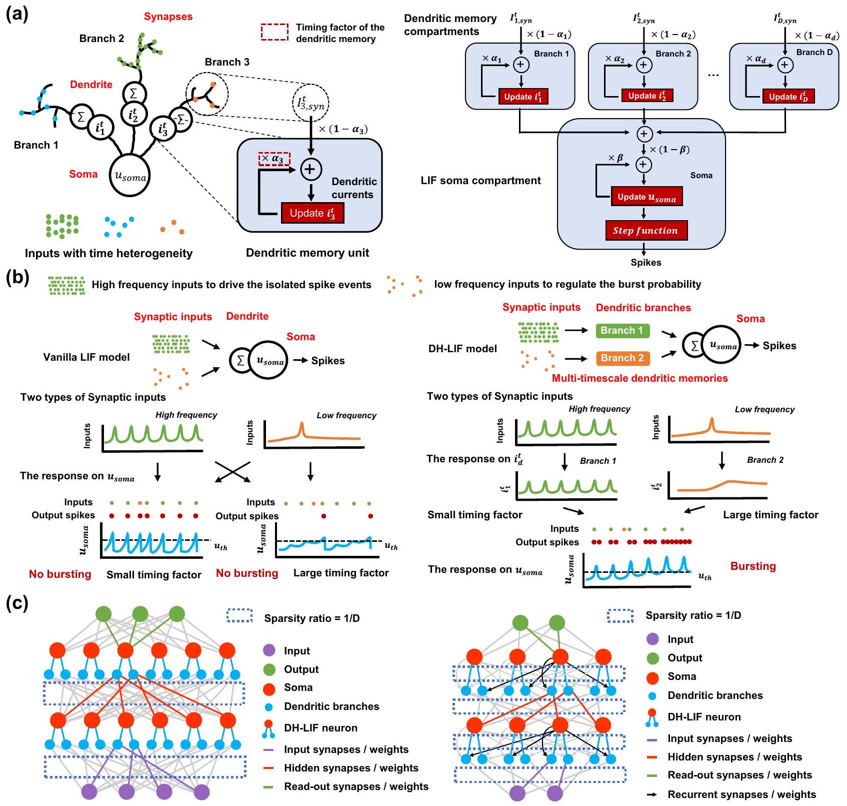
(TPNs) تتلقى إشارتين مدخلتين مستقلتين بترددات مختلفة: واحدة تُحقن في الشجيرات والأخرى تُحقن في الجسم الخلوي. كما قاموا بتحديد جودة الترميز في التعددية الزمنية على مقاييس زمنية مختلفة من خلال حساب التماسك المحلّل بالتردد بين المدخلات والتقديرات. وجدوا أن التماسك بين المدخلات الشجرية والتقديرات المستندة إلى احتمال الانفجار قريب من الواحد لتقلبات المدخلات البطيئة، ولكنه ينخفض إلى الصفر لتقلبات المدخلات السريعة، وهو مشابه لنموذج الشجرة الشجرية لدينا مع عوامل توقيت كبيرة. في الوقت نفسه، وجدوا أن معدل الأحداث يمكنه فك تشفير مدخلات الجسم الخلوي بدقة عالية لترددات المدخلات تصل إلى 100 هرتز، وهو مشابه لنموذج الشجرة الشجرية لدينا مع عوامل توقيت صغيرة. على عكس السابقين
بدلاً من التركيز على فهم التواصل الهرمي في الدماغ من خلال تعددية الشجيرات، نركز على فعالية النموذج المقترح المستوحى من الملاحظات البيولوجية لحل مهام الحوسبة الزمنية المعقدة في الممارسة مع تعقيد حسابي مقبول وخوارزميات تعلم فعالة.
شبكة عصبية متفجرة مع خلايا DH-LIF (DH-SNN)
الذاكرة طويلة الأمد عبر الديناميات الشجرية
إعادة ضبطه. بهذه الطريقة، تمكّن الديناميات الشجرية الزمنية الذاكرة طويلة الأمد.
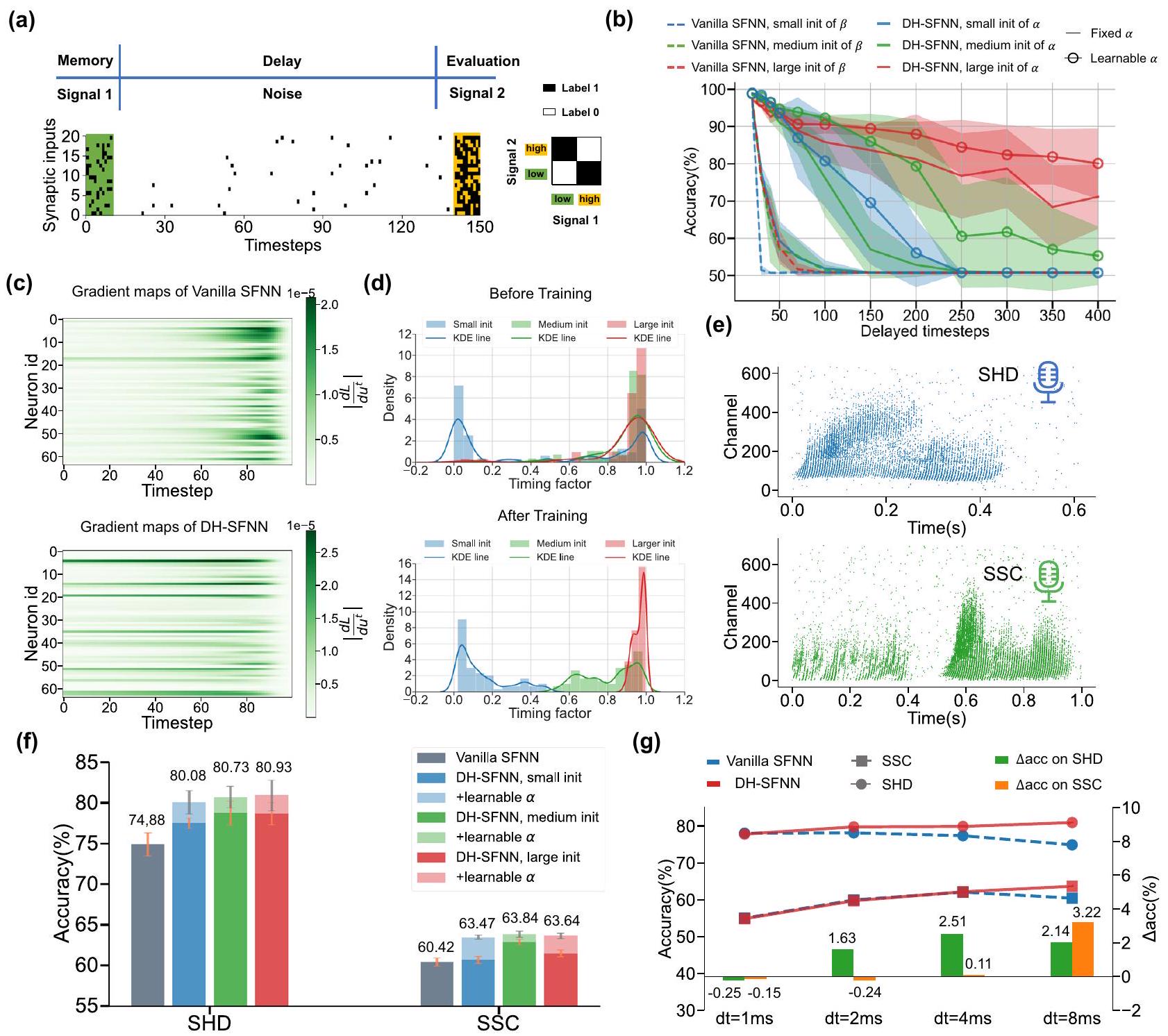
تحقق عوامل توقيت الشجيرات القابلة للتعلم دقة أفضل بكثير من الشبكات العصبية ذات الطبقات السطحية التقليدية بغض النظر عن توزيعات التهيئة. تحت فترة زمنية معينة لأخذ العينات
دقة الشبكات العصبية البسيطة (SFNNs) لا تتحسن دائمًا بل قد تتدهور مع زيادة دقة العينة. الفجوة في الدقة بين الشبكات العصبية البسيطة (DH-SFNNs) والشبكات العصبية البسيطة (vanilla SFNNs) تميل إلى الزيادة مع
دمج الميزات غير المتجانسة داخل الخلايا العصبية
الخلايا العصبية ذات عوامل التوقيت الثابتة أثناء التدريب تحت إعداد مفيد. تصور نمط النبضات الناتجة والتيارات الشجرية لخلايا DH-LIF ذات الشجرة الشجرية الواحدة مع عوامل توقيت ثابتة أثناء التدريب تحت إعداد صغير أو كبير.
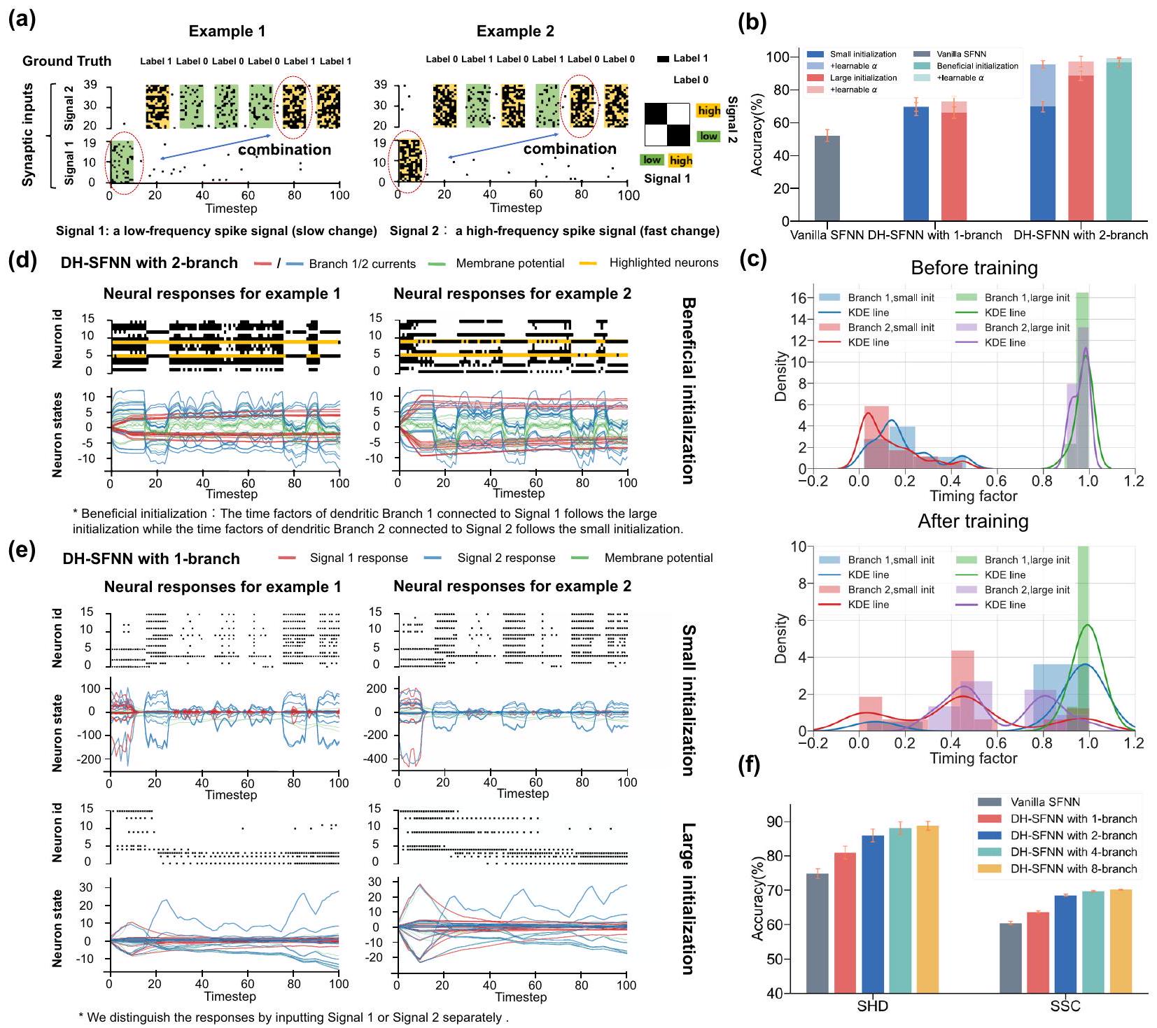
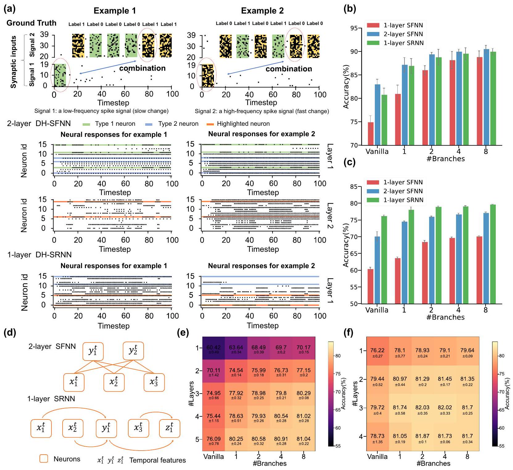
مشكلة XOR المتقطعة متعددة الأوقات لاختبار قدرة النموذج على معالجة المعلومات غير المتجانسة زمنياً لدعم توقعاتنا بشكل أكبر. كما هو موضح في الشكل 4a، تستخدم مشكلة XOR المتقطعة متعددة الأوقات نوعين من إشارات النبض المدخلة. في المرحلة الأولى، يتم إدخال نمط نبض واحد (الإشارة 1) بمعدل إطلاق منخفض (يسار) أو مرتفع (يمين) إلى النموذج، مما يمثل مكوناً منخفض التردد. ثم، يتم حقن عدة أنماط نبض مشابهة بفترات أسرع (الإشارة 2) في النموذج بشكل متسلسل، مما يمثل مكوناً عالي التردد. في كل مرة يتلقى فيها النموذج نمط نبض في الإشارة 2، فإنه أيضاً ينتج نتيجة XOR بين نمط النبض الأول في الإشارة 1 والنمط الحالي في الإشارة 2. الهدف من النموذج هو تذكر الإشارة 1 منخفضة التردد وإجراء عملية XOR.
مع الإشارة عالية التردد 2، التي يمكن أن تعكس بشكل كبير قدرتها المحتملة على معالجة المعلومات غير المتجانسة زمنياً.
الذاكرة كما يتضح من الشكل 3، إلا أنها لا تستطيع معالجة المعلومات ذات الأوقات المتعددة بشكل جيد. مع زيادة عدد الفروع إلى اثنين، تظهر DH-SFNNs أداءً أفضل بكثير بفضل عدم تجانس الدندريت الزمني، خاصة عندما يتم تهيئة عوامل توقيت الدندريت بشكل مناسب وقابل للتعلم. هنا تعني التهيئة المفيدة أننا نهيئ عوامل توقيت دندريت كبيرة للفرع 1 في كل خلية DH-LIF لتمكين الذاكرة طويلة الأمد للإشارة منخفضة التردد 1 بينما نهيئ عوامل توقيت دندريت صغيرة للفرع 2 لتمكين استجابة سريعة للإشارة عالية التردد 2. الشكل 4ج يوضح عوامل توقيت الدندريت قبل وبعد التدريب. كما هو متوقع، تميل عوامل توقيت الدندريت للفرع 1 مع تهيئة صغيرة إلى أن تصبح أكبر بينما تميل عوامل توقيت الدندريت للفرع 2 مع تهيئة كبيرة إلى أن تصبح أصغر، مما يدل على أن عملية التعلم تجعل عوامل توقيت الدندريت تتناسب بشكل أفضل مع الأوقات المتعددة للإشارات المدخلة. لاحظ أنه ما لم يُذكر خلاف ذلك، يتم تهيئة عوامل توقيت الجهد الغشائي وفقًا لتوزيع متوسط وقابلة للتعلم في تجارب الشكل 4.
دمج ميزات الخلايا العصبية عبر الاتصالات المشبكية
أعداد مختلفة من الفروع الدندريّة على مجموعة بيانات SSC.
دمج الميزات الزمنية متعددة الأوقات عبر الاتصالات المشبكية في الشبكات الأمامية والمتكررة، مما يساعد على أداء مهام الحوسبة الزمنية متعددة الأوقات.
قدرتها على التعامل مع عدم التجانس الزمني بدقة أعلى. ثانيًا، مقارنةً بالشبكات العصبية ذات الطبقة الواحدة SFNNs، تظهر الشبكات العصبية ذات الطبقتين SFNNs والشبكات العصبية ذات الطبقة الواحدة SRNNs أداءً أفضل بكثير بفضل دمج الميزات الزمنية بين الخلايا العصبية. ثالثًا، تنتج DH-SFNNs و DH-SRNNs دقة أعلى تدريجيًا مع زيادة عدد الفروع الدندريّة. باختصار، هذه النتائج تثبت القدرة المحسنة على أداء مهام الحوسبة الزمنية متعددة الأوقات المستفيدة من عدم التجانس الزمني الدندري، وتكشف أيضًا عن آلية العمل التآزرية لدمج الميزات على مستوى الخلايا العصبية وعلى مستوى الشبكة.
الصعوبة الأعلى. للتحليل، نوضح طوبولوجيا الاتصال لشبكة عصبية ذات طبقتين SFNN وشبكة عصبية ذات طبقة واحدة SRNN في الشكل 5د كمثال. من الواضح أن خلية عصبية في الطبقة المخفية الثانية من شبكة عصبية ذات طبقتين SFNN يمكنها فقط دمج الميزات المتعلمة من الطبقة السابقة مرة واحدة لتشكيل ميزة ذات مستوى أعلى قليلاً. على العكس، يمكن أن تساعد الاتصالات المتكررة الخلايا العصبية في شبكة عصبية ذات طبقة واحدة SRNN على دمج الميزات المتعلمة عدة مرات لتشكيل ميزات ذات مستوى أعلى بكثير. على سبيل المثال، يتم دمج الميزات ذات المستوى المنخفض
فوائد الأداء الشاملة لشبكات DH-SNNs
تحسين الدقة بشكل كبير مقارنةً بالأنظمة العصبية السريعة الأخرى ونماذج الذاكرة طويلة وقصيرة المدى (LSTM) حتى باستخدام عدد أقل بكثير من المعلمات. على وجه الخصوص، في SHD، مقارنةً بأفضل دقة تم الإبلاغ عنها للأنظمة العصبية السريعة.
تنفيذ فعال على الأجهزة العصبية
| نماذج | #أوزان التغذية الأمامية | #الأوزان المتكررة | #معلمات الخلايا العصبية | #تحيزات | #إجمالي المعلمات | #العمليات الضمنية / خطوة الزمن | #تراكمات تشابكية 1 خطوة زمنية |
| فانيلا SFNN |
|
1 |
|
|
|
0 |
|
| فانيلا SRNN |
|
|
|
|
|
0 |
|
| دي إتش-إس إف إن إن |
|
1 |
|
ND |
|
0 |
|
| دي إتش-إس آر إن إن |
|
|
|
ND |
|
0 |
|
| LSTM |
|
|
1 |
|
|
|
|
الأجهزة، حيث تشارك الخلايا العصبية داخل كل مجموعة نفس النمط لتسهيل التعيين دون تقليل الدقة بشكل كبير. e لوحة تطوير TianjicX وتدفق البيانات عند تنفيذ DH-SNNs على مجموعات بيانات SHD و SSC. يستخدم النموذج على SHD أربعة نوى وظيفية مع ثلاث مجموعات زمنية، بينما يستخدم النموذج على SSC 26 نواة وظيفية مع ست مجموعات زمنية. يتم جدولة مجموعات زمنية متعددة بطريقة متسلسلة. f أداء التنفيذ بما في ذلك الإنتاجية واستهلاك الطاقة الديناميكي عند تنفيذ DHSNNs على شريحة TianjicX العصبية بتردد ساعة 400 ميجاهرتز. لاحظ أن معالجة عينة واحدة تستغرق 1000 خطوة زمنية. تمثل الانحرافات المعيارية (المقدمة كأشرطة خطأ) 5 تجارب متكررة.
أربعة من 160 نواة وظيفية في الشريحة، بينما تستخدم الشبكة العصبية ذات الطبقات الأربعة DH-SFNN 26 نواة وظيفية. نقسم كل نموذج إلى عدة خطوات تنفيذية ونخصص أعدادًا مختلفة من النوى الوظيفية لها كما هو موضح في الشكل 6e. يتيح الجدول الزمني المرن لـ TianjicX تنفيذًا متسلسلًا للخطوات من أجل أداء أفضل. كما هو ملخص في الشكل 6f، يمكن تنفيذ كلا الشبكتين العصبيتين DH-SNN بكفاءة على TianjicX مع إنتاجية عالية واستهلاك منخفض للطاقة. مزيد من التفاصيل حول تنفيذ الأجهزة متاحة في الطرق والشكل التكميلي S11.
تطبيق على التعرف على إشارات EEG والتعرف على مكان الروبوت
| مجموعة بيانات | نموذج | #المعلمات | دقة |
| SHD | SFNN
|
0.09 م | 48.1٪ |
| SRNN
|
1.79 م | ٨٣.٢٪ | |
| SRNN
|
0.17 م | 81.6% | |
| SRNN
|
0.11 م | 82.7% | |
| إس سي إن إن
|
0.21 م | 84.8٪ | |
| SRNN
|
0.14 م | 90.4% | |
| LSTM
|
0.43 م | 89.2% | |
| DH-SRNN (طبقة واحدة، فرعين) | 0.05 م | 91.34% | |
| DH-SFNN (طبقة مزدوجة، 8 فرع) | 0.05 م | 92.1٪ | |
| SSC | SFNN
|
0.09 م | ٣٢.٥٪ |
| SRNN
|
0.11 م | 60.1% | |
| SRNN
|
0.77 م | 74.2% | |
| LSTM
|
0.43 م | 73.1% | |
| DH-SFNN (أربعة طبقات، أربعة فروع) | 0.27 مليون | 81.03% | |
| DH-SRNN (3 طبقات، 4 فروع) | 0.35 مليون | 82.46% | |
| S-MNIST | LSNN
|
0.08 م | 96.4% |
| AHP-SNN
|
0.08 م | ٩٦٫٠٪ | |
| SRNN
|
0.16 مليون | 98.7٪ | |
| LSTM
|
0.06م | 98.2% | |
| DH-SRNN (طبقة 2، فرعان 2) | 0.08 م | 98.9% | |
| بي إس- MNIST | LSTM
|
0.06م | ٨٨٪ |
| SRNN* (مدخلات غير قياسية)
|
0.16 مليون | 94.3٪ | |
| DH-SRNN (طبقة 2، فرع 1) | 0.08 م | 94.52% | |
| جي إس سي | SRNN
|
0.04 م | 86.7% |
| LSNN
|
4.19 م | 91.2% | |
| SRNN
|
0.31 م | 92.1٪ | |
| DH-SRNN (طبقة واحدة، 8 فروع) | 0.13 م | 93.86% | |
| DH-SFNN (3 طبقات، 8 فروع) | 0.11 م | 94.05% | |
| تيمت | LSNN
|
0.4 م | 66.8% |
| LSNN
|
0.4 م | 65.4% | |
| SRNN
|
0.63 م | 66.1% | |
| DH-SRNN (طبقة واحدة، 8 فروع) | 0.18 مليون | 67.42% |
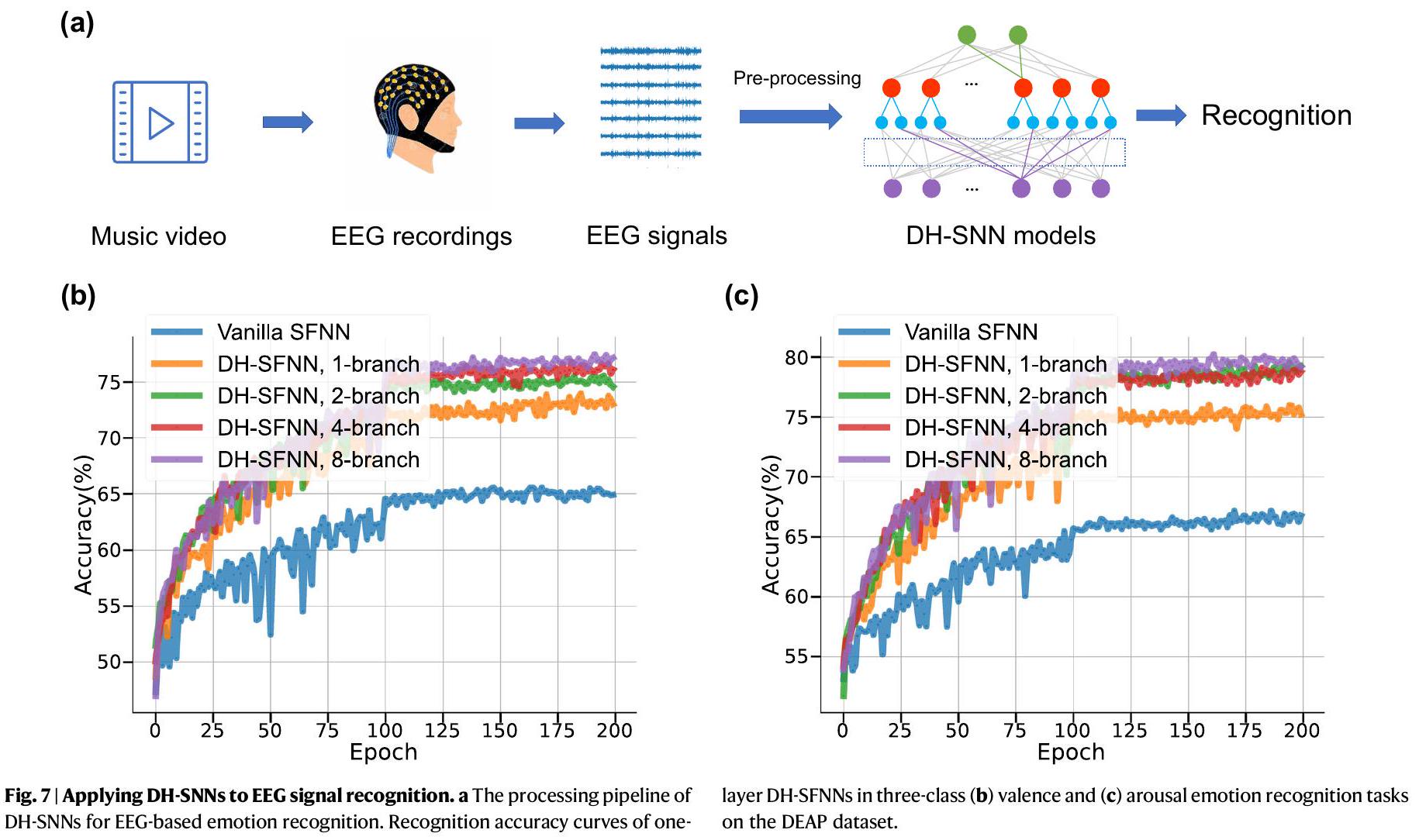
تنبؤ بأن الشبكات العصبية الديناميكية ذات الهيكل المتسلسل (DH-SNNs) لديها إمكانيات كبيرة في معالجة إشارات EEG متعددة الأوقات. كما هو ملخص في الجدول التكميلي S6، تظهر DH-SNNs مرة أخرى أفضل دقة في التعرف على مجموعة بيانات DEAP مع عدد أقل بكثير من المعلمات مقارنة بالأساليب الحالية بما في ذلك الشبكة العصبية متعددة الطبقات (MLP).
نقاش
لإنتاج ميزات زمنية عالية المستوى لاتخاذ قرارات أكثر تعقيدًا. عادةً، تولد الفروع الشجرية الأكثر ملاءمة تنوعًا زمنيًا شجريًا أغنى يعزز من قوة التمثيل لشبكات الأعصاب الزمنية الديناميكية. نظرًا للتعقيد الأعلى لدمج الميزات الناتج عن الاتصالات المتكررة، نلاحظ تشبع الأداء بشكل أسرع في الشبكات الديناميكية مقارنةً بالشبكات الثابتة عند أداء نفس المهمة مع زيادة عدد الفروع الشجرية أو الطبقات. من خلال النظر بشكل شامل في النتائج التجريبية المذكورة أعلاه، نشرح آلية عمل التنوع الزمني الشجري في الشبكات الديناميكية لأداء مهام الحوسبة الزمنية متعددة المقاييس: دمج الميزات بين الفروع في خلية عصبية، ودمج الميزات بين الخلايا العصبية في طبقة متكررة، ودمج الميزات بين الطبقات في شبكة لها تأثيرات مشابهة وتآزرية في التقاط الميزات الزمنية متعددة المقاييس.
نمط في نمذجة لدينا، تظهر الشبكات العصبية البيولوجية اتصالات متطورة على الشجيرات. من خلال استلهامنا من هذه الظاهرة البيولوجية، يمكننا استكشاف الإمكانية لتكييف نمط الاتصال خلال عملية التعلم. على سبيل المثال، يمكننا الاستفادة من طرق مثل DEEP
تقدم خوارزميات التعلم إمكانيات واعدة لتحقيق هذا التوازن، وهو موضوع مثير للاهتمام للعمل في المستقبل.
طرق
نمذجة الذاكرة الشجرية
عصبون نابض قائم على LIF مع تباين في الشجيرات (DH-LIF)
تحكمه
شبكة عصبية صممت باستخدام خلايا DH-LIF (DH-SNN)
قيود الاتصال النادرة
روابط كل خلية عصبية كما يلي
تعلم DH-SNN
مجموعات البيانات والمهام
احتمالية إطلاق 0.2. كل نمط من النبضات يستمر لمدة 10 مللي ثانية وطول كل خطوة زمنية في المحاكاة هو 1 مللي ثانية في كل من مشكلة XOR ذات النبضات المتأخرة ومشكلة XOR ذات النبضات متعددة الأوقات. على وجه التحديد، في مشكلة XOR ذات النبضات متعددة الأوقات، نحدد الفاصل الزمني بين نمطين من نبضات الإدخال إلى
مع فئة إضافية “صمت” تم استخراجها عشوائيًا من ملفات الصوت الضوضائية الخلفية. استخدمنا طريقة استخراج ميزات موجودة
إعداد تجريبي
لكل التجارب، تحتوي الشبكات على جزئين بما في ذلك طبقات SNN المكدسة وطبقة قراءة تالية. لمشاكل XOR النابضة المصممة ذاتيًا ومجموعة بيانات NeuroVPR، تكون طبقة القراءة طبقة خطية بسيطة تقوم بفك تشفير مخرجات النبض من آخر طبقة SNN إلى إمكانية
هي المعلمات المحسّنة حقًا أثناء التدريب.
نحلل تأثير آلية إعادة تعيين الجهد الغشائي على قدرة الذاكرة طويلة الأمد باستخدام عدة مهام. تشمل نماذج الخلايا العصبية المختبرة خلية LIF العادية مع آليات إعادة تعيين مختلفة وخلية DH-LIF. تم اختيار ثلاث آليات لإعادة تعيين الجهد الغشائي: إعادة تعيين صعبة، إعادة تعيين ناعمة، وبدون إعادة تعيين. تُستخدم خلية LIF العادية مع آلية إعادة التعيين الصعبة على نطاق واسع، والتي
هنا.
على SSC. بشكل عام، من ناحية، يجب أن تغطي المدخلات المشبكية المتصلة بكل خلية جميع المدخلات المشبكية للحصول على المعلومات قدر الإمكان. من ناحية أخرى، فإن التداخل المفرط للمدخلات المشبكية المتصلة بفروع شجرية مختلفة قد يسبب الإفراط في التكيف وتدهور الأداء.
ملخص التقرير
توفر البيانات
توفر الشيفرة
References
- Maass, W. Networks of spiking neurons: the third generation of neural network models. Neural Netw. 10, 1659-1671 (1997).
- Sengupta, A., Ye, Y., Wang, R., Liu, C. & Roy, K. Going deeper in spiking neural networks: Vgg and residual architectures. Front. Neurosci. 13, 95 (2019).
- Zheng, H., Wu, Y., Deng, L., Hu, Y. & Li, G. Going deeper with directlytrained larger spiking neural networks. In Proceedings of the AAAI Conference on Artificial Intelligence, vol. 35, 11062-11070 (2021).
- Wu, Y. et al. Efficient visual recognition: A survey on recent advances and brain-inspired methodologies. Machine Intell. Res. 19, 366-411 (2022).
- Wu, Y. et al. Direct training for spiking neural networks: Faster, larger, better. In Proceedings of the AAAI Conference on Artificial Intelligence, vol. 33, 1311-1318 (2019).
- Monsa, R., Peer, M. & Arzy, S. Processing of different temporal scales in the human brain. J. Cogn. Neurosci. 32, 2087-2102 (2020).
- Amir, A. et al. A low power, fully event-based gesture recognition system. In Proceedings of the IEEE conference on computer vision and pattern recognition, 7243-7252 (2017).
- Li, H., Liu, H., Ji, X., Li, G. & Shi, L. Cifar10-dvs: an event-stream dataset for object classification. Front. Neurosci. 11, 309 (2017).
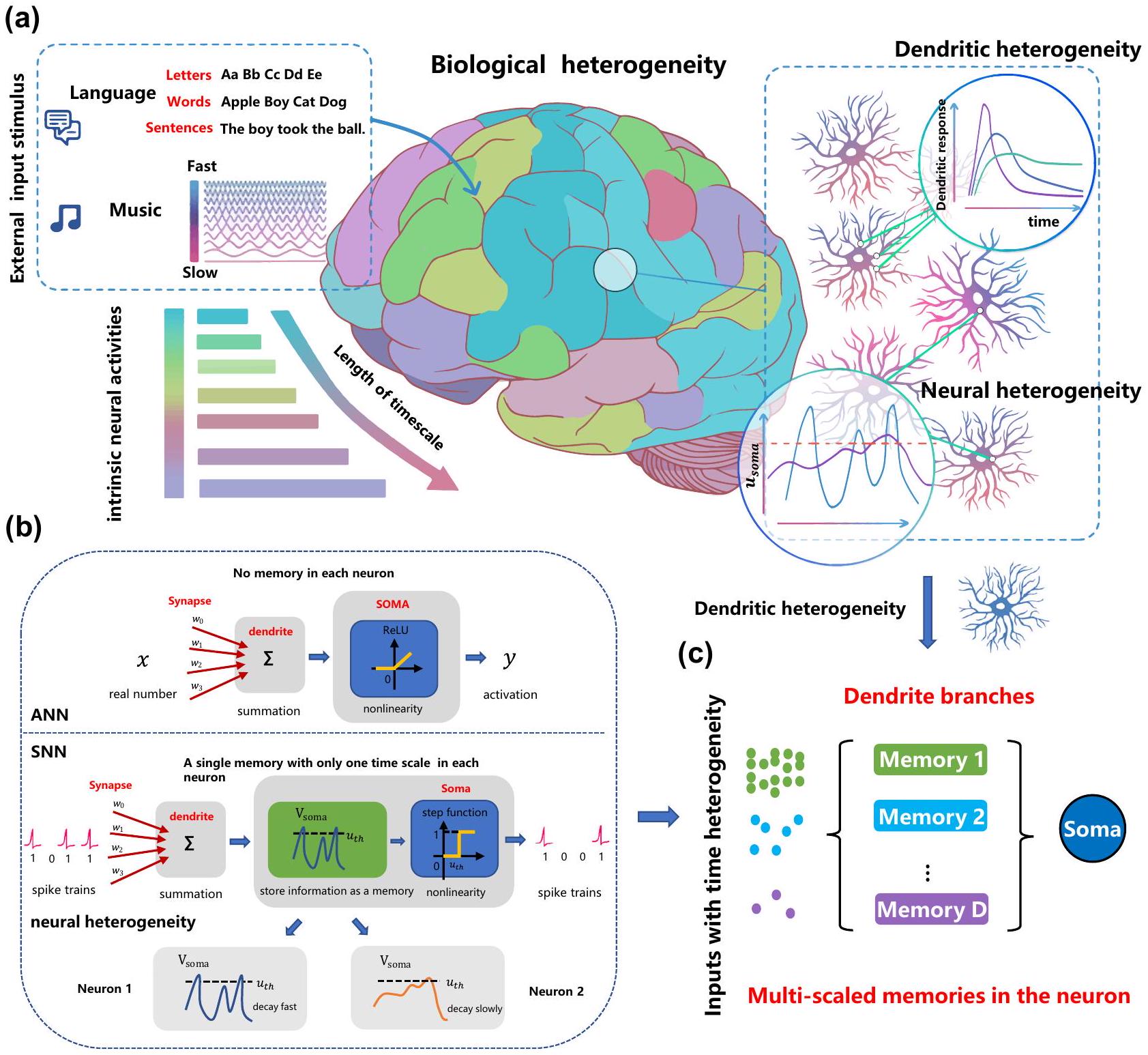
- Golesorkhi, M. et al. The brain and its time: intrinsic neural timescales are key for input processing. Commun. Biol. 4, 1-16 (2021).
- Wolff, A. et al. Intrinsic neural timescales: temporal integration and segregation. Trends Cogn. Sci. 26,159-173 (2022).
- Harris, K. D. & Shepherd, G. M. The neocortical circuit: themes and variations. Nat. Neurosci. 18, 170-181 (2015).
- Gjorgjieva, J., Drion, G. & Marder, E. Computational implications of biophysical diversity and multiple timescales in neurons and synapses for circuit performance. Curr. Opin. Neurobiol. 37, 44-52 (2016).
- Hausser, M., Spruston, N. & Stuart, G. J. Diversity and dynamics of dendritic signaling. Science 290, 739-744 (2000).
- Losonczy, A., Makara, J. K. & Magee, J. C. Compartmentalized dendritic plasticity and input feature storage in neurons. Nature 452, 436-441 (2008).
- Meunier, C. & d’Incamps, B. L. Extending cable theory to heterogeneous dendrites. Neural Comput. 20, 1732-1775 (2008).
- Chabrol, F. P., Arenz, A., Wiechert, M. T., Margrie, T. W. & DiGregorio, D. A. Synaptic diversity enables temporal coding of coincident multisensory inputs in single neurons. Nat. Neurosci. 18, 718-727 (2015).
- Gerstner, W., Kistler, W. M., Naud, R. & Paninski, L.Neuronal dynamics: From single neurons to networks and models of cognition (Cambridge University Press, 2014).
- Bittner, K. C., Milstein, A. D., Grienberger, C., Romani, S. & Magee, J. C. Behavioral time scale synaptic plasticity underlies ca1 place fields. Science 357, 1033-1036 (2017).
- Cavanagh, S. E., Hunt, L. T. & Kennerley, S. W. A diversity of intrinsic timescales underlie neural computations. Front. Neural Circuits 14, 615626 (2020).
- London, M. & Häusser, M. Dendritic computation. Annu. Rev. Neurosci. 28, 503-532 (2005).
- Poirazi, P. & Papoutsi, A. Illuminating dendritic function with computational models. Nat. Rev. Neurosci. 21, 303-321 (2020).
- Bicknell, B. A. & Häusser, M. A synaptic learning rule for exploiting nonlinear dendritic computation. Neuron 109, 4001-4017 (2021).
- Spruston, N. Pyramidal neurons: dendritic structure and synaptic integration. Nat. Rev. Neurosci. 9, 206-221 (2008).
- Branco, T., Clark, B. A. & Häusser, M. Dendritic discrimination of temporal input sequences in cortical neurons. Science 329, 1671-1675 (2010).
- Li, X. et al. Power-efficient neural network with artificial dendrites. Nat. Nanotechnol. 15, 776-782 (2020).
- Boahen, K. Dendrocentric learning for synthetic intelligence. Nature 612, 43-50 (2022).
- Tzilivaki, A., Kastellakis, G. & Poirazi, P. Challenging the point neuron dogma: Fs basket cells as 2-stage nonlinear integrators. Nat. Commun. 10, 3664 (2019).
- Bono, J. & Clopath, C. Modeling somatic and dendritic spike mediated plasticity at the single neuron and network level. Nat. Commun. 8, 706 (2017).
- Naud, R. & Sprekeler, H. Sparse bursts optimize information transmission in a multiplexed neural code. Proc. Nat. Acad. Sci. 115, E6329-E6338 (2018).
- Dayan, P. & Abbott, L. F. et al. Theoretical neuroscience: computational and mathematical modeling of neural systems. J. Cogn. Neurosci. 15, 154-155 (2003).
- Perez-Nieves, N., Leung, V. C., Dragotti, P. L. & Goodman, D. F. Neural heterogeneity promotes robust learning. Nat. Commun. 12, 1-9 (2021).
- Pagkalos, M., Chavlis, S. & Poirazi, P. Introducing the dendrify framework for incorporating dendrites to spiking neural networks. Nat. Commun. 14, 131 (2023).
- Yin, B., Corradi, F. & Bohté, S. M. Accurate and efficient time-domain classification with adaptive spiking recurrent neural networks. Nat. Machine Intell. 3, 905-913 (2021).
- Liu, P., Qiu, X., Chen, X., Wu, S. & Huang, X.-J. Multi-timescale long short-term memory neural network for modelling sentences and documents. In Proceedings of the 2015 conference on empirical methods in natural language processing, 2326-2335 (2015).
- Loewenstein, Y. & Sompolinsky, H. Temporal integration by calcium dynamics in a model neuron. Nat. Neurosci. 6, 961-967 (2003).
- Warden, P. Speech commands: A dataset for limited-vocabulary speech recognition. arXiv preprint arXiv:1804.03209 (2018).
- Garofolo, J. S., Lamel, L. F., Fisher, W. M., Fiscus, J. G. & Pallett, D. S. Darpa timit acoustic-phonetic continous speech corpus cd-rom. nist speech disc 1-1.1. NASA STI/Recon Technical Rep. 93, 27403 (1993).
- Cramer, B., Stradmann, Y., Schemmel, J. & Zenke, F. The Heidelberg spiking data sets for the systematic evaluation of spiking neural networks. IEEE Transactions Neural Netw. Learning Sys. 33, 2744-2757 (2020).
- Pei, J. et al. Towards artificial general intelligence with hybrid tianjic chip architecture. Nature 572, 106-111 (2019).
- Ma, S. et al. Neuromorphic computing chip with spatiotemporal elasticity for multi-intelligent-tasking robots. Sci. Robotics 7, eabk2948 (2022).
- Zhao, R. et al. A framework for the general design and computation of hybrid neural networks. Nat. Commun. 13, 3427 (2022).
- Höppner, S. et al. The spinnaker 2 processing element architecture for hybrid digital neuromorphic computing. arXiv preprint arXiv:2103.08392 (2021).
- Pehle, C. et al. The brainscales-2 accelerated neuromorphic system with hybrid plasticity. Front. Neurosci. 16, 1-21 (2022).
- Li, M. & Lu, B.-L. Emotion classification based on gamma-band eeg. In 2009 Annual International Conference of the IEEE Engineering in medicine and biology society, 1223-1226 (IEEE, 2009).
- Duan, R.-N., Zhu, J.-Y. & Lu, B.-L. Differential entropy feature for eegbased emotion classification. In 2013 6th International IEEE/EMBS Conference on Neural Engineering (NER), 81-84 (IEEE, 2013).
- Tripathi, S., Acharya, S., Sharma, R. D., Mittal, S. & Bhattacharya, S. Using deep and convolutional neural networks for accurate emotion classification on deap dataset. In Twenty-ninth IAAI conference (2017).
- Tao, W. et al. Eeg-based emotion recognition via channel-wise attention and self attention. IEEE Transactions on Affective Computing 14, 382-393 (2020).
- Islam, M. R. et al. Eeg channel correlation based model for emotion recognition. Computers Biol. Med. 136, 104757 (2021).
- Tan, C., Šarlija, M. & Kasabov, N. Neurosense: Short-term emotion recognition and understanding based on spiking neural network modelling of spatio-temporal eeg patterns. Neurocomputing 434, 137-148 (2021).
- Koelstra, S. et al. Deap: A database for emotion analysis; using physiological signals. IEEE Transactions Affective Computing 3, 18-31 (2011).
- Jirayucharoensak, S., Pan-Ngum, S. & Israsena, P. Eeg-based emotion recognition using deep learning network with principal component based covariate shift adaptation. Scientific World J. 2014, 1-10 (2014).
- Lowry, S. et al. Visual place recognition: A survey. IEEE transactions on robotics 32, 1-19 (2015).
- Milford, M. J. & Wyeth, G. F. Seqslam: Visual route-based navigation for sunny summer days and stormy winter nights. In 2012 IEEE international conference on robotics and automation, 1643-1649 (IEEE, 2012).
- Chancán, M., Hernandez-Nunez, L., Narendra, A., Barron, A. B. & Milford, M. A hybrid compact neural architecture for visual place recognition. IEEE Robotics Automation Lett. 5, 993-1000 (2020).
- Chancán, M. & Milford, M. Deepseqslam: a trainable cnn+ rnn for joint global description and sequence-based place recognition. arXiv preprint arXiv:2011.08518 (2020).
- Fischer, T. & Milford, M. Event-based visual place recognition with ensembles of temporal windows. IEEE Robotics Automation Lett. 5, 6924-6931 (2020).
- Milford, M. et al. Place recognition with event-based cameras and a neural implementation of seqslam. arXiv preprint arXiv:1505.04548 (2015).
- Yang, S. et al. Efficient spike-driven learning with dendritic eventbased processing. Front. Neurosci. 15, 601109 (2021).
- Gao, T., Deng, B., Wang, J. & Yi, G. Highly efficient neuromorphic learning system of spiking neural network with multi-compartment leaky integrate-and-fire neurons. Front. Neurosci. 16, 929644 (2022).
- Bellec, G., Kappel, D., Maass, W. & Legenstein, R. Deep rewiring: Training very sparse deep networks. arXiv preprint arXiv:1711.05136 (2017).
- Fang, W. et al. Incorporating learnable membrane time constant to enhance learning of spiking neural networks. In Proceedings of the IEEE/CVF international conference on computer vision, 2661-2671 (2021).
- Sussillo, D. Neural circuits as computational dynamical systems. Curr. Opin. Neurobiol. 25, 156-163 (2014).
- Gerstner, W. & Kistler, W. M.Spiking neuron models: Single neurons, populations, plasticity (Cambridge University Press, 2002).
- Cramer, B. et al. Surrogate gradients for analog neuromorphic computing. Proc. Natl. Acad. Sci. 119, e2109194119 (2022).
- Rossbroich, J., Gygax, J. & Zenke, F. Fluctuation-driven initialization for spiking neural network training. Neuromorphic Comput. Eng. 2, 044016 (2022).
- Bellec, G., Salaj, D., Subramoney, A., Legenstein, R. & Maass, W. Long short-term memory and learning-to-learn in networks of spiking neurons. Adv. Neural Inform. Processing Syst. 31, 795-805 (2018).
- Rao, A., Plank, P., Wild, A. & Maass, W. A long short-term memory for ai applications in spike-based neuromorphic hardware. Nat. Machine Intelligence 4, 467-479 (2022).
- Arjovsky, M., Shah, A. & Bengio, Y. Unitary evolution recurrent neural networks. In International conference on machine learning, 1120-1128 (PMLR, 2016).
- Auge, D., Hille, J., Kreutz, F., Mueller, E. & Knoll, A. End-to-end spiking neural network for speech recognition using resonating input neurons. In Artificial Neural Networks and Machine Learning-ICANN 2021: 30th International Conference on Artificial Neural Networks, Bratislava, Slovakia, September 14-17, 2021, Proceedings, Part V 30, 245-256 (Springer, 2021).
- Salaj, D. et al. Spike frequency adaptation supports network computations on temporally dispersed information. Elife 10, e65459 (2021).
- Bellec, G. et al. A solution to the learning dilemma for recurrent networks of spiking neurons. Nat. Commun. 11, 1-15 (2020).
الشكر والتقدير
2021ZD0200300، المؤسسة الوطنية للعلوم الطبيعية في الصين (رقم 62276151، 62106119، 62236009، U22A20103)، المؤسسة الوطنية للعلوم للعلماء الشباب المتميزين (رقم 62325603)، مركز أبحاث الحوسبة المستوحاة من الدماغ التابع لمجموعة CETC Haikang، والمعهد الصيني لأبحاث الدماغ، بكين. نود أن نشكر البروفيسور لو بينغ شي على المناقشة القيمة.
مساهمات المؤلفين
المصالح المتنافسة
معلومات إضافية
المواد التكميلية المتاحة على
https://doi.org/10.1038/s41467-023-44614-z.
يجب توجيه المراسلات وطلبات المواد إلى لي دينغ.
© المؤلفون 2024
مركز أبحاث الحوسبة المستوحاة من الدماغ (CBICR)، قسم الأدوات الدقيقة، جامعة تسينغوا، بكين، الصين. معهد علوم الكمبيوتر النظرية، جامعة غراتس للتكنولوجيا، غراتس، النمسا. معهد الأتمتة، الأكاديمية الصينية للعلوم، بكين، الصين. - البريد الإلكتروني: leideng@mail.tsinghua.edu.cn
DOI: https://doi.org/10.1038/s41467-023-44614-z
PMID: https://pubmed.ncbi.nlm.nih.gov/38177124
Publication Date: 2024-01-04
Temporal dendritic heterogeneity incorporated with spiking neural networks for learning multi-timescale dynamics
Accepted: 21 December 2023
Published online: 04 January 2024
(A) Check for updates
Abstract
It is widely believed the brain-inspired spiking neural networks have the capability of processing temporal information owing to their dynamic attributes. However, how to understand what kind of mechanisms contributing to the learning ability and exploit the rich dynamic properties of spiking neural networks to satisfactorily solve complex temporal computing tasks in practice still remains to be explored. In this article, we identify the importance of capturing the multi-timescale components, based on which a multicompartment spiking neural model with temporal dendritic heterogeneity, is proposed. The model enables multi-timescale dynamics by automatically learning heterogeneous timing factors on different dendritic branches. Two breakthroughs are made through extensive experiments: the working mechanism of the proposed model is revealed via an elaborated temporal spiking XOR problem to analyze the temporal feature integration at different levels; comprehensive performance benefits of the model over ordinary spiking neural networks are achieved on several temporal computing benchmarks for speech recognition, visual recognition, electroencephalogram signal recognition, and robot place recognition, which shows the best-reported accuracy and model compactness, promising robustness and generalization, and high execution efficiency on neuromorphic hardware. This work moves neuromorphic computing a significant step toward real-world applications by appropriately exploiting biological observations.
comprehensive performance benefits including the best reported accuracy along with promising robustness and generalization compared to ordinary SNNs. With an extra sparse restriction on dendritic connections, DH-SNNs present high model compactness and high execution efficiency on neuromorphic hardware. This work suggests that the temporal dendritic heterogeneity observed in the brain is a critical component in learning multi-timescale temporal dynamics, shedding light on a promising route for SNN modeling in performing complex temporal computing tasks.
Results
Spiking LIF neuron with temporal dendritic heterogeneity (DH-LIF)
inputs and also decays by a timing factor, i.e.,
without dendritic memory. The timing factor of the membrane potential can only match the timescale of at most one of the two inputs, e.g., matching the high-frequency input (small timing factor) or matching the low-frequency input (large timing factor). When the neuron only matches the timescale of the high-frequency input, it loses long-term memory of the low-frequency input due to the fast decaying mechanism; when the neuron only matches the low-frequency input, it cannot closely track the high-frequency input due to the heavy memorization of historic information. Thus, as indicated in Fig. 2b, the vanilla LIF neuron cannot generate bursting spikes. In contrast, we can flexibly configure versatile timing factors on multiple dendritic branches in the DH-LIF neuron, which can make it capable of simultaneously dealing with variable timescales of different inputs, generating the bursting spikes successfully. In the prior work
(TPNs) receiving two independent input signals with different frequencies: one injected into dendrites and the other injected into the soma. They further quantified the encoding quality in multiplexing at different timescales by calculating the frequency-resolved coherence between the inputs and the estimates. They found that the coherence between the dendritic inputs and the estimates based on the burst probability is close to one for slow input fluctuations, but decreases to zero for rapid input fluctuations, which is similar to our dendritic branch modeling with large timing factors. In the meantime, they found that the event rate can decode the soma input with high accuracy for input frequencies up to 100 Hz , which is similar to our dendritic branch modeling with small timing factors. Unlike the previous
focus on understanding hierarchical brain communication through multiplexing dendrites, we focus on the effectiveness of the proposed model inspired by biological observations for solving complex temporal computing tasks in practice with acceptable computational complexity and effective learning algorithms.
Spiking neural network with DH-LIF neurons (DH-SNN)
Long-term memory via dendritic dynamics
be reset. In this way, the temporal dendritic dynamics enables longterm memory.
learnable dendritic timing factors achieve much better accuracy than vanilla SFNNs no matter the initialized distributions. Under the sampling time interval
accuracy of vanilla SFNNs do not always improve and even degrades as the sampling precision grows. The accuracy gap between DH-SFNNs and vanilla SFNNs tends to increase as
Intra-neuron heterogeneous feature integration
neurons with fixed timing factors during training under a beneficial initialization. e Visualization of the output spike pattern and dendritic currents of one-dendriticbranch DH-LIF neurons with fixed timing factors during training under a small or large initialization.
timescale spiking XOR problem for testing the model’s capability of processing temporally heterogeneous information to further support our prediction. As depicted in Fig. 4a, the multi-timescale spiking XOR problem uses two types of input spike signals. At the first stage, a single spike pattern (Signal 1) with a low (left) or high (right) firing rate is fed into the model, representing a low-frequency component. Then, several similar spike patterns with faster periods (Signal 2) are injected into the model sequentially, representing a high-frequency component. Each time the model receives a spike pattern in Signal 2, it also outputs an XOR result between the beginning spike pattern in Signal 1 and the current spike pattern in Signal 2. The goal of the model is to memorize the low-frequency Signal 1 and conduct an XOR operation
with the high-frequency Signal 2, which can substantially reflect its potential capability of processing temporally heterogeneous information.
memory as evidenced by Fig. 3, they cannot process information with multiple timescales well. As the number of branches grows to two, DHSFNNs demonstrate much better performance owing to the temporal dendritic heterogeneity especially when the dendritic timing factors are initialized appropriately and learnable. Here the beneficial initialization means that we initialize large dendritic timing factors for Branch 1 in each DH-LIF neuron to enable long-term memory for lowfrequency Signal 1 while initializing small dendritic timing factors for Branch 2 to enable fast response for high-frequency Signal 2. Figure 4c visualizes the dendritic timing factors before and after training. As expected, the dendritic timing factors of Branch 1 with a small initialization tend to become larger while the dendritic timing factors of Branch 2 with a large initialization tend to become smaller, which evidences that the learning process makes the dendritic timing factors match the multiple timescales of input signals better. Notice that unless otherwise specified, the timing factors of membrane potentials are initialized following a medium distribution and are learnable in the experiments of Fig. 4.
Inter-neuron feature integration via synaptic connections
different numbers of dendritic branches on the SSC dataset.
the integration of multi-timescale temporal features via synaptic connections in feedforward and recurrent networks, which helps perform multi-timescale temporal computing tasks.
the capability of handling temporal heterogeneity with higher accuracy. Second, compared to one-layer SFNNs, two-layer SFNNs and onelayer SRNNs demonstrate much better performance owing to the interneuron integration of temporal features. Third, DH-SFNNs and DHSRNNs gradually produce higher accuracy as the number of dendritic branches grows. In short, these results evidence the improved capability of performing multi-timescale temporal computing tasks benefited from the temporal dendritic heterogeneity, and further reveal the synergistic working mechanism of the neuron-level and network-level feature integration.
difficulty. For analysis, we illustrate the connection topology of a twolayer SFNN and a one-layer SRNN in Fig. 5d as an example. Apparently, a neuron in the second hidden layer of a two-layer SFNN can only spatially integrate the learned features of the previous layer once to form a slightly higher-level feature. In contrast, the recurrent connections can help neurons in a one-layer SRNN integrate the learned features multiple times to form much higher-level features. For example, the low-level features
Comprehensive performance benefits of DH-SNNs
improve accuracy significantly over other SNNs and long short-term memory (LSTM) models even using much fewer parameters. In particular, on SHD, compared to the best reported accuracy of SNNs
Efficient execution on neuromorphic hardware
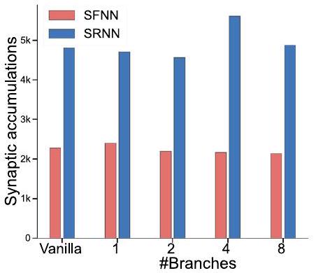
| Models | #Feedforward weights | #Recurrent weights | #Neuron parameters | #Biases | #Total parameters | #Synaptic multiplications / timestep | #Synaptic accumulations 1 timestep |
| Vanilla SFNN |
|
1 |
|
|
|
0 |
|
| Vanilla SRNN |
|
|
|
|
|
0 |
|
| DH-SFNN |
|
1 |
|
ND |
|
0 |
|
| DH-SRNN |
|
|
|
ND |
|
0 |
|
| LSTM |
|
|
1 |
|
|
|
|
hardware, where neurons within each group share the same pattern for easier mapping without degrading much accuracy. e The TianjicX development board and the dataflow when performing DH-SNNs on SHD and SSC datasets. The model on SHD uses four functional cores with three timing phase groups and the model on SSC uses 26 functional cores with six timing phase groups. Multiple timing phase groups are scheduled in a pipelined manner. f The execution performance including throughput and dynamic power consumption when performing DHSNNs on the TianjicX neuromorphic chip at 400 MHz clock frequency. Notice that processing one sample takes 1000 timesteps. The standard deviations (presented as error bars) represent 5 repeated trials.
four of a chip’s 160 functional cores, while the four-layer DH-SFNN uses 26 functional cores. We divide each model into several execution steps and allocate different numbers of functional cores to them as presented in Fig. 6e. The flexible timing schedule of TianjicX enables a pipelined execution of the steps for better performance. As summarized in Fig. 6f, both DH-SNNs can be efficiently performed on TianjicX with high throughput and low power consumption. More details of hardware implementation are provided in Methods and Supplementary Fig. S11.
Application to EEG signal recognition and robot place recognition
| Dataset | Model | #Parameters | Accuracy |
| SHD | SFNN
|
0.09 M | 48.1% |
| SRNN
|
1.79 M | 83.2% | |
| SRNN
|
0.17 M | 81.6% | |
| SRNN
|
0.11 M | 82.7% | |
| SCNN
|
0.21 M | 84.8% | |
| SRNN
|
0.14 M | 90.4% | |
| LSTM
|
0.43 M | 89.2% | |
| DH-SRNN (1-layer, 2-branch) | 0.05M | 91.34% | |
| DH-SFNN (2-layer, 8-branch) | 0.05M | 92.1% | |
| SSC | SFNN
|
0.09 M | 32.5% |
| SRNN
|
0.11 M | 60.1% | |
| SRNN
|
0.77 M | 74.2% | |
| LSTM
|
0.43 M | 73.1% | |
| DH-SFNN (4-layer, 4-branch) | 0.27M | 81.03% | |
| DH-SRNN (3-layer, 4-branch) | 0.35M | 82.46% | |
| S-MNIST | LSNN
|
0.08M | 96.4% |
| AHP-SNN
|
0.08 M | 96.0% | |
| SRNN
|
0.16M | 98.7% | |
| LSTM
|
0.06M | 98.2% | |
| DH-SRNN (2-layer, 2-branch) | 0.08M | 98.9% | |
| PS-MNIST | LSTM
|
0.06M | 88% |
| SRNN* (not standard inputs)
|
0.16M | 94.3% | |
| DH-SRNN (2-layer, 1-branch) | 0.08M | 94.52% | |
| GSC | SRNN
|
0.04 M | 86.7% |
| LSNN
|
4.19 M | 91.2% | |
| SRNN
|
0.31 M | 92.1% | |
| DH-SRNN (1-layer, 8-branch) | 0.13 M | 93.86% | |
| DH-SFNN (3-layer, 8-branch) | 0.11 M | 94.05% | |
| TIMIT | LSNN
|
0.4 M | 66.8% |
| LSNN
|
0.4 M | 65.4% | |
| SRNN
|
0.63 M | 66.1% | |
| DH-SRNN (1-layer, 8-branch) | 0.18M | 67.42% |
prediction that DH-SNNs have great potential in processing multitimescale EEG signals. As summarized in Supplementary Table S6, DHSNNs once more demonstrate the best recognition accuracy on the DEAP dataset with much fewer parameters compared to existing approaches including multi-layered perceptron (MLP)
Discussion
to produce high-level temporal features for making more complicated decisions. Usually, appropriately more dendritic branches generate richer dendritic temporal heterogeneity that enhances the representation power of DH-SNNs. Due to the higher complexity of feature integration given by recurrent connections, we observe faster performance saturation in DH-SRNNs compared to DH-SFNNs when performing the same task as the number of dendritic branches or layers grows. Comprehensively considering the above experimental results, we explain the working mechanism of temporal dendritic heterogeneity in DH-SNNs for performing multi-timescale temporal computing tasks: the inter-branch feature integration in a neuron, the interneuron feature integration in a recurrent layer, and the inter-layer feature integration in a network have similar and synergetic effects in capturing multi-timescale temporal features.
pattern in our modeling, biological neural networks exhibit evolving connections on dendrites. Drawing inspiration from this biological phenomenon, we can investigate the potential for adapting the connection pattern during the learning process. For instance, we can leverage methods like DEEP
in learning algorithms offer promising potential to realize this balance, which is an interesting topic for future work.
Methods
Modeling dendritic memory
LIF-based spiking neuron with dendritic heterogeneity (DH-LIF)
governed by
SNN with DH-LIF neurons (DH-SNN)
Sparse connection restriction
connections of each neuron as follows
Learning of DH-SNN
Datasets and tasks
a firing probability of 0.2 . Each spike pattern lasts 10 ms and the length of each timestep in the simulation is 1 ms in both the delayed spiking XOR problem and the multi-timescale spiking XOR problem. Specifically, in the multi-timescale spiking XOR problem, we set the time interval between two input spike patterns to
with an extra class “Silence” extracted randomly from the background noise audio files. We used an existing feature extraction method
experiments, we divide each trajectory into 100 segments with uniform length and mark the corresponding events in each segment with the same label. The spike events in the duration of 21 ms were fed into the SNN models and generated the prediction which indicates the robot’s position. We randomly chose six trajectories as the training set, three trajectories as the validation set, and one trajectory as the test set.
Experimental setting
Influence of the membrane potential reset mechanism
is governed by
Influence of the dendritic connection pattern
Details of implementation on neuromorphic hardware
Reporting summary
Data availability
Code availability
References
- Maass, W. Networks of spiking neurons: the third generation of neural network models. Neural Netw. 10, 1659-1671 (1997).
- Sengupta, A., Ye, Y., Wang, R., Liu, C. & Roy, K. Going deeper in spiking neural networks: Vgg and residual architectures. Front. Neurosci. 13, 95 (2019).
- Zheng, H., Wu, Y., Deng, L., Hu, Y. & Li, G. Going deeper with directlytrained larger spiking neural networks. In Proceedings of the AAAI Conference on Artificial Intelligence, vol. 35, 11062-11070 (2021).
- Wu, Y. et al. Efficient visual recognition: A survey on recent advances and brain-inspired methodologies. Machine Intell. Res. 19, 366-411 (2022).
- Wu, Y. et al. Direct training for spiking neural networks: Faster, larger, better. In Proceedings of the AAAI Conference on Artificial Intelligence, vol. 33, 1311-1318 (2019).
- Monsa, R., Peer, M. & Arzy, S. Processing of different temporal scales in the human brain. J. Cogn. Neurosci. 32, 2087-2102 (2020).
- Amir, A. et al. A low power, fully event-based gesture recognition system. In Proceedings of the IEEE conference on computer vision and pattern recognition, 7243-7252 (2017).
- Li, H., Liu, H., Ji, X., Li, G. & Shi, L. Cifar10-dvs: an event-stream dataset for object classification. Front. Neurosci. 11, 309 (2017).
- Golesorkhi, M. et al. The brain and its time: intrinsic neural timescales are key for input processing. Commun. Biol. 4, 1-16 (2021).
- Wolff, A. et al. Intrinsic neural timescales: temporal integration and segregation. Trends Cogn. Sci. 26,159-173 (2022).
- Harris, K. D. & Shepherd, G. M. The neocortical circuit: themes and variations. Nat. Neurosci. 18, 170-181 (2015).
- Gjorgjieva, J., Drion, G. & Marder, E. Computational implications of biophysical diversity and multiple timescales in neurons and synapses for circuit performance. Curr. Opin. Neurobiol. 37, 44-52 (2016).
- Hausser, M., Spruston, N. & Stuart, G. J. Diversity and dynamics of dendritic signaling. Science 290, 739-744 (2000).
- Losonczy, A., Makara, J. K. & Magee, J. C. Compartmentalized dendritic plasticity and input feature storage in neurons. Nature 452, 436-441 (2008).
- Meunier, C. & d’Incamps, B. L. Extending cable theory to heterogeneous dendrites. Neural Comput. 20, 1732-1775 (2008).
- Chabrol, F. P., Arenz, A., Wiechert, M. T., Margrie, T. W. & DiGregorio, D. A. Synaptic diversity enables temporal coding of coincident multisensory inputs in single neurons. Nat. Neurosci. 18, 718-727 (2015).
- Gerstner, W., Kistler, W. M., Naud, R. & Paninski, L.Neuronal dynamics: From single neurons to networks and models of cognition (Cambridge University Press, 2014).
- Bittner, K. C., Milstein, A. D., Grienberger, C., Romani, S. & Magee, J. C. Behavioral time scale synaptic plasticity underlies ca1 place fields. Science 357, 1033-1036 (2017).
- Cavanagh, S. E., Hunt, L. T. & Kennerley, S. W. A diversity of intrinsic timescales underlie neural computations. Front. Neural Circuits 14, 615626 (2020).
- London, M. & Häusser, M. Dendritic computation. Annu. Rev. Neurosci. 28, 503-532 (2005).
- Poirazi, P. & Papoutsi, A. Illuminating dendritic function with computational models. Nat. Rev. Neurosci. 21, 303-321 (2020).
- Bicknell, B. A. & Häusser, M. A synaptic learning rule for exploiting nonlinear dendritic computation. Neuron 109, 4001-4017 (2021).
- Spruston, N. Pyramidal neurons: dendritic structure and synaptic integration. Nat. Rev. Neurosci. 9, 206-221 (2008).
- Branco, T., Clark, B. A. & Häusser, M. Dendritic discrimination of temporal input sequences in cortical neurons. Science 329, 1671-1675 (2010).
- Li, X. et al. Power-efficient neural network with artificial dendrites. Nat. Nanotechnol. 15, 776-782 (2020).
- Boahen, K. Dendrocentric learning for synthetic intelligence. Nature 612, 43-50 (2022).
- Tzilivaki, A., Kastellakis, G. & Poirazi, P. Challenging the point neuron dogma: Fs basket cells as 2-stage nonlinear integrators. Nat. Commun. 10, 3664 (2019).
- Bono, J. & Clopath, C. Modeling somatic and dendritic spike mediated plasticity at the single neuron and network level. Nat. Commun. 8, 706 (2017).
- Naud, R. & Sprekeler, H. Sparse bursts optimize information transmission in a multiplexed neural code. Proc. Nat. Acad. Sci. 115, E6329-E6338 (2018).
- Dayan, P. & Abbott, L. F. et al. Theoretical neuroscience: computational and mathematical modeling of neural systems. J. Cogn. Neurosci. 15, 154-155 (2003).
- Perez-Nieves, N., Leung, V. C., Dragotti, P. L. & Goodman, D. F. Neural heterogeneity promotes robust learning. Nat. Commun. 12, 1-9 (2021).
- Pagkalos, M., Chavlis, S. & Poirazi, P. Introducing the dendrify framework for incorporating dendrites to spiking neural networks. Nat. Commun. 14, 131 (2023).
- Yin, B., Corradi, F. & Bohté, S. M. Accurate and efficient time-domain classification with adaptive spiking recurrent neural networks. Nat. Machine Intell. 3, 905-913 (2021).
- Liu, P., Qiu, X., Chen, X., Wu, S. & Huang, X.-J. Multi-timescale long short-term memory neural network for modelling sentences and documents. In Proceedings of the 2015 conference on empirical methods in natural language processing, 2326-2335 (2015).
- Loewenstein, Y. & Sompolinsky, H. Temporal integration by calcium dynamics in a model neuron. Nat. Neurosci. 6, 961-967 (2003).
- Warden, P. Speech commands: A dataset for limited-vocabulary speech recognition. arXiv preprint arXiv:1804.03209 (2018).
- Garofolo, J. S., Lamel, L. F., Fisher, W. M., Fiscus, J. G. & Pallett, D. S. Darpa timit acoustic-phonetic continous speech corpus cd-rom. nist speech disc 1-1.1. NASA STI/Recon Technical Rep. 93, 27403 (1993).
- Cramer, B., Stradmann, Y., Schemmel, J. & Zenke, F. The Heidelberg spiking data sets for the systematic evaluation of spiking neural networks. IEEE Transactions Neural Netw. Learning Sys. 33, 2744-2757 (2020).
- Pei, J. et al. Towards artificial general intelligence with hybrid tianjic chip architecture. Nature 572, 106-111 (2019).
- Ma, S. et al. Neuromorphic computing chip with spatiotemporal elasticity for multi-intelligent-tasking robots. Sci. Robotics 7, eabk2948 (2022).
- Zhao, R. et al. A framework for the general design and computation of hybrid neural networks. Nat. Commun. 13, 3427 (2022).
- Höppner, S. et al. The spinnaker 2 processing element architecture for hybrid digital neuromorphic computing. arXiv preprint arXiv:2103.08392 (2021).
- Pehle, C. et al. The brainscales-2 accelerated neuromorphic system with hybrid plasticity. Front. Neurosci. 16, 1-21 (2022).
- Li, M. & Lu, B.-L. Emotion classification based on gamma-band eeg. In 2009 Annual International Conference of the IEEE Engineering in medicine and biology society, 1223-1226 (IEEE, 2009).
- Duan, R.-N., Zhu, J.-Y. & Lu, B.-L. Differential entropy feature for eegbased emotion classification. In 2013 6th International IEEE/EMBS Conference on Neural Engineering (NER), 81-84 (IEEE, 2013).
- Tripathi, S., Acharya, S., Sharma, R. D., Mittal, S. & Bhattacharya, S. Using deep and convolutional neural networks for accurate emotion classification on deap dataset. In Twenty-ninth IAAI conference (2017).
- Tao, W. et al. Eeg-based emotion recognition via channel-wise attention and self attention. IEEE Transactions on Affective Computing 14, 382-393 (2020).
- Islam, M. R. et al. Eeg channel correlation based model for emotion recognition. Computers Biol. Med. 136, 104757 (2021).
- Tan, C., Šarlija, M. & Kasabov, N. Neurosense: Short-term emotion recognition and understanding based on spiking neural network modelling of spatio-temporal eeg patterns. Neurocomputing 434, 137-148 (2021).
- Koelstra, S. et al. Deap: A database for emotion analysis; using physiological signals. IEEE Transactions Affective Computing 3, 18-31 (2011).
- Jirayucharoensak, S., Pan-Ngum, S. & Israsena, P. Eeg-based emotion recognition using deep learning network with principal component based covariate shift adaptation. Scientific World J. 2014, 1-10 (2014).
- Lowry, S. et al. Visual place recognition: A survey. IEEE transactions on robotics 32, 1-19 (2015).
- Milford, M. J. & Wyeth, G. F. Seqslam: Visual route-based navigation for sunny summer days and stormy winter nights. In 2012 IEEE international conference on robotics and automation, 1643-1649 (IEEE, 2012).
- Chancán, M., Hernandez-Nunez, L., Narendra, A., Barron, A. B. & Milford, M. A hybrid compact neural architecture for visual place recognition. IEEE Robotics Automation Lett. 5, 993-1000 (2020).
- Chancán, M. & Milford, M. Deepseqslam: a trainable cnn+ rnn for joint global description and sequence-based place recognition. arXiv preprint arXiv:2011.08518 (2020).
- Fischer, T. & Milford, M. Event-based visual place recognition with ensembles of temporal windows. IEEE Robotics Automation Lett. 5, 6924-6931 (2020).
- Milford, M. et al. Place recognition with event-based cameras and a neural implementation of seqslam. arXiv preprint arXiv:1505.04548 (2015).
- Yang, S. et al. Efficient spike-driven learning with dendritic eventbased processing. Front. Neurosci. 15, 601109 (2021).
- Gao, T., Deng, B., Wang, J. & Yi, G. Highly efficient neuromorphic learning system of spiking neural network with multi-compartment leaky integrate-and-fire neurons. Front. Neurosci. 16, 929644 (2022).
- Bellec, G., Kappel, D., Maass, W. & Legenstein, R. Deep rewiring: Training very sparse deep networks. arXiv preprint arXiv:1711.05136 (2017).
- Fang, W. et al. Incorporating learnable membrane time constant to enhance learning of spiking neural networks. In Proceedings of the IEEE/CVF international conference on computer vision, 2661-2671 (2021).
- Sussillo, D. Neural circuits as computational dynamical systems. Curr. Opin. Neurobiol. 25, 156-163 (2014).
- Gerstner, W. & Kistler, W. M.Spiking neuron models: Single neurons, populations, plasticity (Cambridge University Press, 2002).
- Cramer, B. et al. Surrogate gradients for analog neuromorphic computing. Proc. Natl. Acad. Sci. 119, e2109194119 (2022).
- Rossbroich, J., Gygax, J. & Zenke, F. Fluctuation-driven initialization for spiking neural network training. Neuromorphic Comput. Eng. 2, 044016 (2022).
- Bellec, G., Salaj, D., Subramoney, A., Legenstein, R. & Maass, W. Long short-term memory and learning-to-learn in networks of spiking neurons. Adv. Neural Inform. Processing Syst. 31, 795-805 (2018).
- Rao, A., Plank, P., Wild, A. & Maass, W. A long short-term memory for ai applications in spike-based neuromorphic hardware. Nat. Machine Intelligence 4, 467-479 (2022).
- Arjovsky, M., Shah, A. & Bengio, Y. Unitary evolution recurrent neural networks. In International conference on machine learning, 1120-1128 (PMLR, 2016).
- Auge, D., Hille, J., Kreutz, F., Mueller, E. & Knoll, A. End-to-end spiking neural network for speech recognition using resonating input neurons. In Artificial Neural Networks and Machine Learning-ICANN 2021: 30th International Conference on Artificial Neural Networks, Bratislava, Slovakia, September 14-17, 2021, Proceedings, Part V 30, 245-256 (Springer, 2021).
- Salaj, D. et al. Spike frequency adaptation supports network computations on temporally dispersed information. Elife 10, e65459 (2021).
- Bellec, G. et al. A solution to the learning dilemma for recurrent networks of spiking neurons. Nat. Commun. 11, 1-15 (2020).
Acknowledgements
2021ZD0200300, National Natural Science Foundation of China (No. 62276151, 62106119, 62236009, U22A20103), National Science Foundation for Distinguished Young Scholars (No. 62325603), CETC Haikang Group-Brain Inspired Computing Joint Research Center, and Chinese Institute for Brain Research, Beijing. We would like to thank Prof. Luping Shi for the valuable discussion.
Author contributions
Competing interests
Additional information
supplementary material available at
https://doi.org/10.1038/s41467-023-44614-z.
Correspondence and requests for materials should be addressed to Lei Deng.
© The Author(s) 2024
Center for Brain Inspired Computing Research (CBICR), Department of Precision Instrument, Tsinghua University, Beijing, China. Institute of Theoretical Computer Science, Graz University of Technology, Graz, Austria. Institute of Automation, Chinese Academy of Sciences, Beijing, China. - e-mail: leideng@mail.tsinghua.edu.cn