توقع نتائج جراحة الفك العلوي كصور جانبية بعد العملية باستخدام الشبكات العصبية البيانية ونماذج الانتشار Predicting orthognathic surgery results as postoperative lateral cephalograms using graph neural networks and diffusion models
تُجرى جراحة الفك التصحيحية، أو جراحة الفك التصحيحي، لتصحيح التشوهات الشديدة في الوجه والفكين، وتزداد الطلبات عليها لأغراض تجميلية. إن التنبؤ الدقيق بنتائج الجراحة أمر ضروري لاختيار خطة العلاج المثلى وضمان رضا المرضى. هنا، نقدم GPOSC-Net، وهو نموذج تنبؤي توليدي لجراحة الفك التصحيحي يقوم بتوليد صور الأشعة الجانبية بعد العملية من البيانات قبل العملية. يتكون GPOSC-Net من مكونين رئيسيين: نموذج توقع المعالم الذي يقدر التغيرات القياسية بعد الجراحة، ونموذج انتشار كامن يقوم بإنشاء صور واقعية للأشعة الجانبية بعد العملية بناءً على المعالم المتوقعة وخطوط الملف الشخصي المجزأة. قمنا بالتحقق من نموذجنا باستخدام مجموعات بيانات مرضى متنوعة، واختبار تورينغ بصري، ودراسة محاكاة. تظهر نتائجنا أن GPOSC-Net يمكنه التنبؤ بدقة بمواقع المعالم القياسية وتوليد صور عالية الدقة للأشعة الجانبية بعد العملية، مما يوفر أداة قيمة للتخطيط الجراحي. من خلال تعزيز دقة التنبؤ والتصور، يتمتع نموذجنا بالقدرة على تحسين اتخاذ القرارات السريرية والتواصل مع المرضى.
تستخدم جراحة الفك التقويمية (OGS) على نطاق واسع لتصحيح التشوهات الشديدة في الوجه والفكين. إن تحديد هدف العلاج الجراحي وتوقع النتائج الجراحية ضروريان لتحقيق توازن بين الجمالية والوظيفة والثبات وضمان رضا المريض.لذلك، من الضروري مقارنة خيارات العلاج المختلفة، مثل ما إذا كان يجب استخراج الأسنان أو إجراء جراحة فك واحد أو فك مزدوج. الجراحة، من حيث النتائج المتوقعة لاختيار خطة علاج مثالية للمريض. إن التخطيط المسبق للإجراءات يكون أكثر أهمية مع زيادة الطلب على تحسين المظهر، حيث يتم إجراء جراحات تقويم الفك بشكل متزايد لتحسين جمالية الوجه، حتى لأولئك الذين لا يعانون من تشوهات وجهية شديدة. وبالتالي، فإن التنبؤ بالتغيرات الوجهية التي ستحدث مع
تعتبر جراحة الفك التقويمي عاملاً مهماً في تحديد ما إذا كان يجب على المريض تلقي العلاج الجراحي.تقليديًا، تم إجراء توقعات OGS من خلال تتبع الأشعة السينية الجانبية للجمجمة. تم توقع التغيرات في مظهر الوجه بناءً على نسبة حركة المعلم النسيجي الرخو المقابل للمعلم النسيجي الصلب باستخدام صورة جمجمة قبل العملية (pre-ceph).. ومع ذلك، فإن هذه النسبة تتأثر بعوامل مختلفة، مثل اتجاه حركة العظام، وسمك أو توتر الأنسجة الرخوة، ونوع الجراحة، ونوع سوء الإطباق، وبالتالي، فإن الدقة منخفضة، والانحراف كبير للغاية للاستخدام السريري. يمكن أن توفر البرامج التجارية المستخدمة في تشخيص تقويم الأسنان إرشادات عملية سريرياً من خلال محاكاة التغيرات بعد العملية (بعد الجراحة) استنادًا إلى نسبة إزاحة العظام والجلد، ولكن لديها قيود في وصف التغيرات الفعلية. نتيجة لذلك، فإن التغيرات بعد العملية التي تقدمها هذه البرامج التجارية لا تعكس بدقة التغيرات الحقيقية.لتجاوز هذه المشكلات، قام العديد من الباحثين بتطوير خوارزميات مختلفة للتنبؤ بدقة بتغيرات الأنسجة الرخوة. ومع ذلك، فإن معظم هذه الخوارزميات لها تطبيقات محدودة، مثل الجراحة الفكية فقط أو جراحة تقدم الفك السفلي فقط.. على الرغم من وجود محاولة نادرة لتطوير خوارزمية تنبؤ لحركات جراحية متنوعةكان خطأ التنبؤ الخاص به كبيرًا للغاية لدرجة أنه لم يكن من الممكن تطبيقه في الحالات السريرية. مؤخرًا، قام بعض الباحثين بدراسة التنبؤ بالنتائج الجراحية في ثلاثة أبعاد (3D).تم إدخال التصوير المقطعي المحوسب بالأشعة السينية (CBCT) في مجال طب الأسنان منذ المراحل المبكرة من تطويره نظرًا لمزاياه في إعادة إنتاج الهياكل القحفية الوجهية بدقة ثلاثية الأبعاد دون تشويه أو تكبير أو تداخل للصور مع جرعة إشعاع منخفضة..
في البداية، كان يتم استخدام التصوير المقطعي المحوسب بالأشعة السينية (CBCT) بشكل رئيسي لتقييم منطقة العظم السنخي.ولكن مع زيادة مجال الرؤية (FOV) تدريجياً، توسعت تطبيقاته لتشمل تقييم الأسنان المتأثرة.تقييم الأمراض أو الإصابات في منطقة الوجه والجمجمة، وتحليل لتقويم الأسنان وجراحة الفم والوجه والفكينلي وآخرونحاولوا التنبؤ بالتغيرات الوجهية في 10 مرضى OGS باستخدام CBCT والمسحات الوجهية. حققوا نتائج مرضية ضمن 2.0 مم، لكن حجم العينة كان صغيرًا جدًا. ريسنيك وآخرون.كما قاموا بتقييم وتوقع التغيرات في الأنسجة الرخوة في ثلاثة أبعاد بعد جراحة الفك العلوي، لكنهم حصلوا على نتائج لم تكن مرضية للتطبيق السريري. بينغتسون وآخرون.قارنوا توقعات الأنسجة الرخوة باستخدام الصور الشعاعية الجانبية ثنائية الأبعاد وصور الأشعة المقطعية ثلاثية الأبعاد ووجدوا أنه لا يوجد فرق كبير في الدقة. ومع ذلك، أفادوا أن التحليل ثلاثي الأبعاد أكثر فائدة في حالات عدم التماثل الوجهي. مع تطبيق الأشعة المقطعية ثلاثية الأبعاد على جراحة الفك العلوي، زادت كمية الإشعاع المعرض له المرضى أيضًا مع زيادة حجم المجال ودقة الصورة..
أظهرت الدراسات السابقة حول قياس الجرعة باستخدام التصوير المقطعي المحوسب بالكمبيوتر أن متوسط جرعة الأعضاء ( ) أعلى بكثير من تلك المقدمة للحصول على صور السيفالومتر الجانبية والأشعة السينية البانورامية . جها وآخرونتم التحقيق في مخاطر السرطان لأعضاء مختلفة بناءً على ظروف تصوير CBCT المتوسطة والقصوى المستخدمة عادة في كوريا. أظهرت النتائج أن مخاطر السرطان كانت أعلى في النساء مقارنة بالرجال، وزادت مع صغر السن، وارتفعت مع عدد جلسات التصوير، حيث تتأثر مخاطر السرطان بعوامل مثل العمر والجنس ومعايير المعدات وعدد جلسات التصوير. لذلك، يجب اتباع مبدأ ALARA (أقل قدر ممكن بشكل معقول) بدقة عند إجراء CBCT في الممارسة السريرية، ولا يمكن تبرير التصوير الروتيني باستخدام CBCT لعلاج تقويم الأسنان. بالنسبة لتحليل OGS، يمكن أن تقدم CBCT مزايا في حالات التباينات الهيكلية الشديدة، مثل عدم التناسق الوجهى الملحوظ مع مستوى إطباق مائل أو اضطرابات نمو.بينما تدعو بعض الدراسات إلى استخدام التصوير المقطعي المحوسب ذو الأشعة المخروطية لجراحة الفك أو مفصل الفك الصدغي، فإن المراجعات المنهجية فشلت في دعم تطبيقها الشامل..
مع التحسن الكبير في مجال الذكاء الاصطناعي التوليدي باستخدام نماذج التعلم العميق، حاول بعض الباحثين تطبيق الصور الاصطناعية في التصوير الطبي وطب الأسنان. حاول كيم وآخرون توليد صور جانبية للجمجمة باستخدام التعلم العميق.. لقد أبلغوا عن اختبار تورينغ البصري تظهر النتائج أن الصور الجانبية الاصطناعية لم تكن قابلة للتمييز عن الصور الجانبية الحقيقية وأن تتبع الصور الاصطناعية كان ممكنًا. استخدام نماذج الانتشارلقد أدى ذلك إلى تقدم في التوليد متعدد الأنماط، مثل توليد النص إلى صورة أو توليد التخطيط إلى صورة، وتم عرض تطبيقات متنوعة في المجال الطبي. على سبيل المثال، الطريقة المقترحة في المرجع 35، تغلبت على قيود الطرق الحالية المعتمدة على الانتشار وحسنت مهام إعادة بناء الصور الطبية ثلاثية الأبعاد مثل التصوير بالرنين المغناطيسي والتصوير المقطعي، من خلال حل المشكلات العكسية ثلاثية الأبعاد بشكل فعال. علاوة على ذلك، يمكن لنموذج الانتشار توليد صور طبية عالية الجودة، مما يحسن أداء تحليل الصور الطبية عندما تكون البيانات نادرة.من بينها، تم تطوير نموذج انتشار كامن لتوليد قوي ومرن مع مدخلات شرطية وتوليف عالي الدقة مع طبقات انتباه متقاطع في بنية النموذج.مع هذه التقدمات، قد يكون من الممكن توليد صور جانبية اصطناعية بعد العملية (spost-cephs) لجراحة الفك العلوي لمقارنة نتائج خيارات العلاج المختلفة. لذلك، الغرض من هذه الدراسة هو التنبؤ بالتغيرات الوجهية بعد جراحة الفك العلوي باستخدام نموذج انتشار كامن. استخدمنا التعلم العميق لتوليد spost-cephs، مما يتيح توقع نتائج الجراحة وتوليد صور لسيناريوهات تخطيط جراحي مختلفة من خلال تعديلات الحالة. اعتمد نهجنا على طريقتين. أولاً، لتعزيز دقة التخطيط الجراحي، استخدمنا GCNN للتنبؤ بالحركات الجراحية المناسبة من الصورة الجانبية السابقة. ثانياً، أخذنا الحركات الجراحية التي تنبأ بها GCNN ومعلومات أخرى من الصورة الجانبية السابقة وتتبع خطها الجانبي كمدخلات لتوليد spost-cephs باستخدام نموذج انتشار. استند هذا التنبؤ التوليدي لجراحة الفك العلوي باستخدام شبكة ceph (GPOSC-Net) إلى الصور الجانبية السابقة لتوليد spost-cephs بناءً على مقدار الحركة الجراحية المقصودة (IASM).
بعد ذلك، قمنا بالتحقق من صحة الصور الجانبية بعد العملية (spost-cephs) من خلال طرق متنوعة. أولاً، لتقييم الجودة والواقعية الطبية للصور الجانبية بعد العملية، تم إجراء اختبار تورينغ بصري (VTT) مع أربعة أطباء جراحة أسنان (DDSs)، وهم اثنان من أطباء تقويم الأسنان (ODs) واثنان من جراحي الفم والوجه والفكين (OMFSs)، بمتوسط خبرة يزيد عن 15 عامًا، لتمييز الصور الجانبية الحقيقية بعد العملية (postceph) عن الصور الجانبية بعد العملية المزيفة (spost-cephs) وحققوا دقة متوسطة بلغت 48%، مما أشار إلى أن الصور الجانبية المزيفة أظهرت جودة وميزات طبية معقولة. ثانيًا، تم التحقق من صحة الصور الجانبية المزيفة من خلال مقارنة المعالم بين الصور الجانبية الحقيقية والصور الجانبية المزيفة المقابلة من قبل اثنين من أطباء تقويم الأسنان. تم تجميع المسافات لهذه المعالم الـ 35 في خمس مجموعات وتم تقييمها. في كل مجموعة، كان متوسط خطأ المسافة الإقليدية للمعالم 1.5 مم، ومعدل التنبؤ الناجح (معدل التنبؤ الناجح، SPR؛ الأخطاء ) لكل معلم متوسط عند ثالثًا، من خلال تعديل وزن توجيه بدون مصنف (CFG)في GPOSC-Net، قمنا بإنشاء spostcephs لسيناريوهات تخطيط جراحي متنوعة. طلبنا تقييمًا من نفس اثنين من أطباء العيون واثنين من جراحي الفم والوجه والفكين. بعد عرض صور جراحة محاكاة تم إنشاؤها عند توجيه IASM تتراوح من كميات تراجع أقل من، بالضبط، وأكثر من 0.1 إلى 1.6 (حيث 0، preceph؛ 1، مقدار التراجع الدقيق، أي مشابه لتلك الخاصة بـ post-ceph؛ 1.6، مقدار التراجع الزائد، أي ما يتجاوز الحركة الجراحية لـ postceph)، اختاروا صور النتائج الجراحية الأكثر ملاءمة لتلك المرضى، مما أسفر عن متوسط IASM المختار منأخيرًا، تم إجراء استبيان يتكون من خمسة أسئلة لتقييم الفائدة السريرية للنموذج المقترح.
النتائج
مقارنة المعالم بين ما بعد السيفالومترية وما بعد السيفالومترية
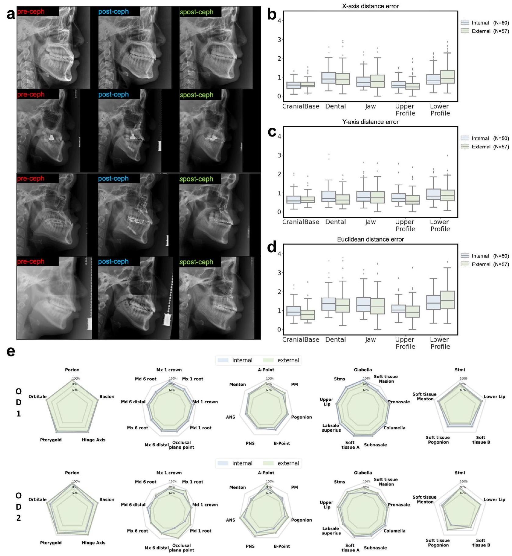
لتقييم دقة النموذج، قام اثنان من أطباء الأسنان بتتبع المعالم في كل من الصور الشعاعية القحفية السابقة والصور الشعاعية القحفية اللاحقة (الموضحة في الشكل 1a) من مجموعة الاختبار. الشكلعرض أخطاء المسافة بالنسبة للمسافة الإقليدية، ومحور x، ومحور y، على التوالي. قمنا بتصنيف جميع المعالم إلى خمس مجموعات تشريحية: قاعدة الجمجمة، الأسنان، الفك، الملف العلوي، والملف السفلي (الجدول 1). كانت الأخطاء المتوسطة للمعالم لمجموعات الاختبار الداخلية والخارجية ضمن 1.5 مم. وكان هذا أقل أو مشابهًا لـ
الشكل 1 | مقارنة بين ما بعد السيف وما بعد السيف مع تحليل المعالم. أ أربع حالات نموذجية من ما قبل السيف، وما بعد السيف، وما بعد السيف. استنادًا إلى هذه الحالات السابقة، والمعالم الخاصة بها، وخطوط الملف الشخصي، وكميات الحركة الجراحية المتوقعة، قام GPOSC-Net بتوليد ما يتوافق مع ما بعد السيف. ب أخطاء مسافة المعالم (LDE، الوحدة: مم) لما بعد السيف وما بعد السيف التي تم قياسها بواسطة اثنين من أطباء تقويم الأسنان (ODs) لمجموعات الاختبار الداخلية والخارجية. ج LDEs للإحداثيات X (الوحدة: مم) لما بعد السيف. وspost-ceph. د LDEs من إحداثيات Y (الوحدة: مم) لـ post-ceph و spost-ceph. توضح الرسوم البيانية الصندوقية الوسيط، ونطاق الربيع الداخلي (الصندوق)، والشعيرات الممتدة إلى 1.5 مرة من النطاق، مع تمثيل القيم الشاذة كنقاط فردية. e معدلات التنبؤ الناجحة (SPR) لكل معلم من حيث النسب المئوية كما تحددها ODين لمجموعات الاختبار الداخلية والخارجية. الفروق بين المراقبين التي تم إظهارها في الدراسات السابقة التي تحقق في قابلية إعادة إنتاج اختيار المعالم في الصور الشعاعية للجمجمة الحقيقية. في الاختبار الداخلي، تراوحت الأخطاء من في قاعدة الجمجمة إلىفي الملف السفلي، مع متوسط خطأ قدره. في الاختبار الخارجي، تراوحت الأخطاء من في قاعدة الجمجمة إلى عند الفك، مع خطأ متوسط قدره (الشكل 1ب). في الاختبار الداخلي، أخطاء المحور تراوحت بينفي قاعدة الجمجمة إلى في الملف السفلي، مع خطأ متوسط يبلغ حوالي. في الاختبار الخارجي، تراوحت أخطاء المحور – في قاعدة الجمجمة إلىفي الملف السفلي، مع متوسط خطأ يبلغ حوالي (الشكل 1ج). في الاختبار الداخلي، تراوحت أخطاء المحور – في قاعدة الجمجمة إلىفي الملف السفلي، مع خطأ متوسط يبلغ حوالي. في الاختبار الخارجي، تراوحت أخطاء المحور y من في قاعدة الجمجمة إلى
الجدول 1 | مقارنة أخطاء مسافة المعالم بين ما بعد السيفالومترية وما بعد السيفالومترية المعدلة (الوحدة: مم)
مجموعة / DDS
اختبار داخلي
اختبار خارجي
OD1
OD2
OD1
OD2
مسافة المحور السيني
مسافة المحور العمودي
خطأ المسافة
SPR
مسافة المحور السيني
مسافة المحور العمودي
خطأ المسافة
SPR
مسافة المحور السيني
مسافة المحور العمودي
خطأ المسافة
SPR
مسافة المحور السيني
مسافة المحور العمودي
خطأ المسافة
SPR
قاعدة الجمجمة
100%
٨٨٪
97.8%
95.2%
أسنان
٨٤.٢٪
75.1%
76.6%
83.4٪
فك
80.8٪
75.4%
78.5%
84%
الملف العلوي
0.98
98%
84.5%
90.8٪
87.8%
ملف أقل
81.8٪
71.2%
75.8%
74%
إجمالي
٨٨.٦٪
78.6٪
٨٣.٢٪
84.6٪
تمت مقارنة كل نتيجة إحصائيًا مع الحقيقة الأساسية باستخدام اختبار التكافؤ المزدوج مع نطاق خطأ مقبول قدره 1.5 مم. أخصائي تقويم الأسنان OD، معدل التنبؤ الناجح SPR (نسبة الحالات التي يكون فيها خطأ المسافة الإقليدية بين ما بعد التصوير الشعاعي للجمجمة وما بعد التصوير الشعاعي للجمجمة بعد العلاج أقل من 2 مم). القيمة <0.05; ** القيمة<0.005. في الملف السفلي، مع خطأ متوسط يبلغ حوالي (الشكل 1د). يمكن العثور على النتائج لكل من المعالم في الجدول التكميلي 2 من المواد التكميلية.
مقارنة SPRs المتراكمة
تم تقييم أخطاء المسافة بين المعالم القياسية الذهبية وتلك التي تم التنبؤ بها بواسطة النماذج للمجموعات الخمس، وهي: قاعدة الجمجمة، الأسنان، الفك، الملف العلوي، والملف السفلي. تم تقييم نسب الأخطاء لكل مجموعة وفقًا للأخطاء.كما تحدده أخصائية بصريات ذات خبرة تزيد عن 15 عامًا (الشكل 1e).
بالنسبة لمجموعات الاختبار الداخلية والخارجية، كانت المعالم عند قاعدة الجمجمة التي لم تتأثر بـ OGS تظهر معدلات دقة عالية جداً، في حين أن المعالم في الأجزاء الأخرى التي تغيرت مواقعها نتيجة لـ OGS أظهرت معدلات دقة أقل. بدت معدلات دقة المعالم اللينة الأنسجة أقل من تلك الخاصة بالمعالم الصلبة الأنسجة، لأن الأخطاء في المعالم اللينة الأنسجة كانت عمومًا أكبر من تلك في المعالم الصلبة الأنسجة.. في الاختبار الداخلي، كانت SPRs للقاعدة القحفية،للطب الأسنان،للذقن،لملف العلوي، ولملف التعريف المنخفض. في الاختبار الخارجي، كانت SPRsللقاعدة القحفية،لأسنانللذقن،لملف العلوي، ولملف التعريف المنخفض (الجدول 1). يمكن العثور على النتائج لكل من المعالم في الجدول التكميلي 2 من المواد التكميلية.
اختبار تورينغ البصري
تم إجراء VTT مع اثنين من أطباء العيون واثنين من جراحي الفم والوجه والفكين، بمتوسط خبرة يزيد عن 15 عامًا، لتقييم جودة الصور الشعاعية بعد التصوير. بشكل عام، يُعتبر VTT لنموذج توليدي مثاليًا عندما تكون الدقة الناتجة “قدمنا 57 زوجًا من الصور المختارة عشوائيًا والتي تتكون من كل من الصور الحقيقية والمولدة.نسبة). على الرغم من أن الخصوصية كانت عالية لممتحن واحد، إلا أن متوسط دقة جميع الممتحنين كانكانت دقة اثنين من أطباء العيون واثنين من جراحي الفم والوجه والفكين، و على التوالي. في هذه الأثناء، كانت قيم الحساسية لـ OD1 و OD2 و OMFS1 و OMFS2 هي 51.7 و 41.4 و 35.5 وعلى التوالي، في حين كانت قيم الخصوصية لديهم، و ، على التوالي. أظهرت هذه النتائج أن جودة الصور الشعاعية بعد التقويم كانت جيدة إلى حد معقول، لأن حتى أطباء الأسنان الخبراء لم يتمكنوا من التمييز بين الصور الشعاعية الحقيقية والمولدة في حالة عمياء.
التوأم الرقمي
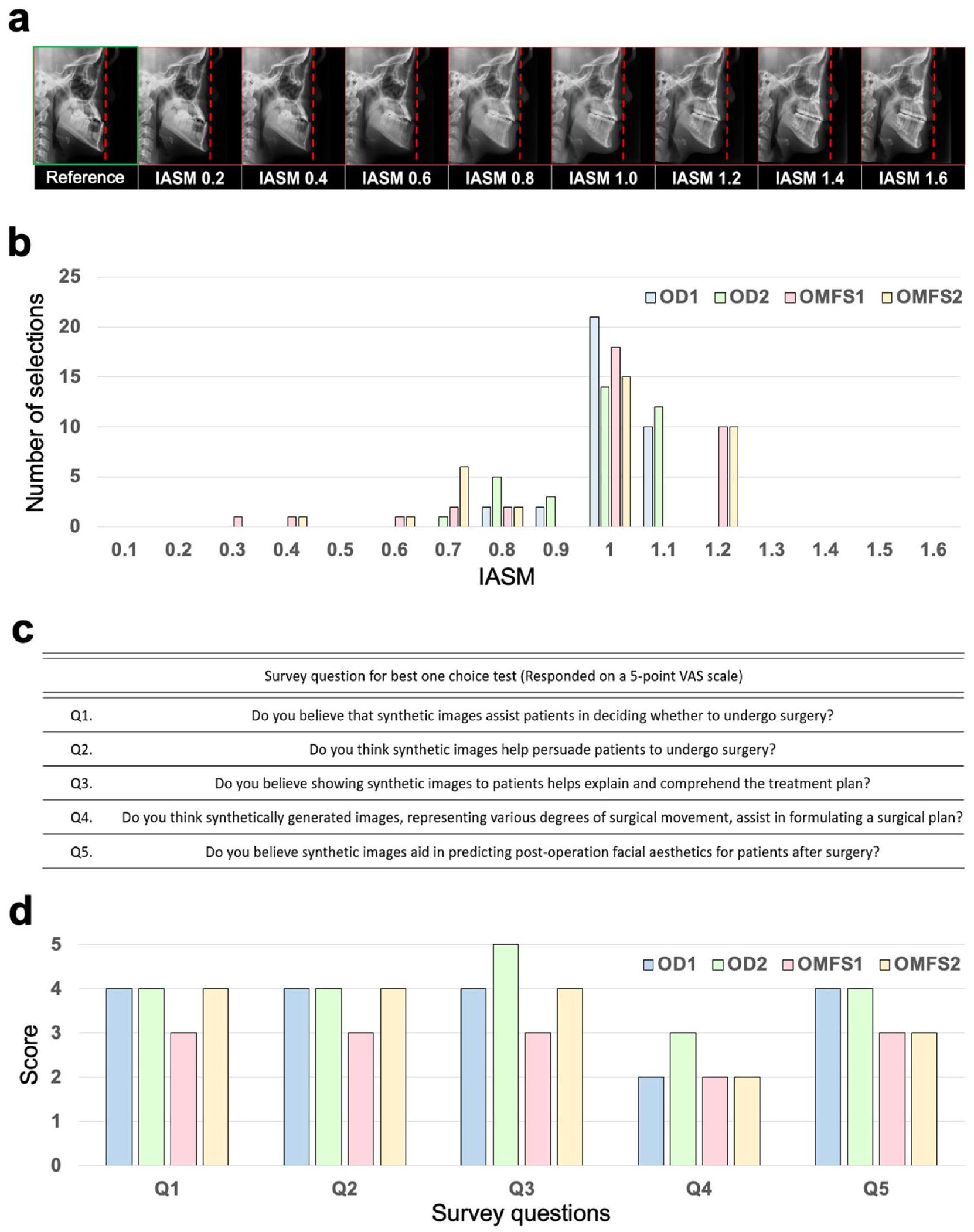
بعد الجيل المتسلسل للصور السلبية بعد العملية بناءً على IASM، كما هو موضح في الشكل 2أ، تم طلب اثنين من أطباء الأسنان واثنين من جراحي الفم والوجه والفكين لاختيار الصور الأكثر ملاءمة من بين الصور السلبية بعد العملية كهدف للعلاج. تم إنشاء الصور السلبية بعد العملية بناءً على IASM 1.0، والذي يدل على مقدار حركة مشابه لتلك الخاصة بالحركة العظمية الجراحية الفعلية. من ناحية أخرى، تم إنشاء الصور السلبية بعد العملية مع IASMs التي تتوافق مع الحركة القليلة أو المفرطة بشكل مستمر كما يلي: صورة تم إنشاؤها بناءً على IASM 0.8، على سبيل المثال، تدل على ضبط الحركة الجراحية لتكون أصغر من مقدار التراجع الفعلي، بينما صورة تم إنشاؤها بناءً على IASM 1.2 تدل على ضبط الحركة الجراحية لتكون أكبر من المقدار الفعلي. بالنسبة لـ IASM من 0.1 إلى 1.6، تم إنشاء خمس صور، بما في ذلك IASM 1.0، بشكل عشوائي. تم طلب من طبيبين الأسنان واثنين من جراحي الفم والوجه والفكين اختيار صورة واحدة فقط كهدف علاج مناسب بناءً على الصورة السلبية السابقة. إذا تم اختيار صورة سلبية بعد العملية تم إنشاؤها بناءً على IASM من 0.8 إلى 1.2، فقد اعتُبرت إجابة صحيحة، أي هدف علاج مناسب. إذا كانت الصورة السلبية بعد العملية المختارة صورة تم إنشاؤها بناءً على حركة مشابهة للحركة الجراحية الفعلية، فيمكن استخدامها كتوأم رقمي للتنبؤ بالنتيجة الجراحية المحاكية. اختار طبيبان الأسنان واثنان من جراحي الفم والوجه والفكين بشكل مستقل ما مجموعه 35 حالة لكل منهم وأظهروا دقة متوسطة تبلغ 90.0%، كما هو موضح في الشكل 2ب.
تم تقييم جدوى التطبيق السريري للصورة السلبية بعد العملية باستخدام الاستبيان الموضح في الشكل 2ج، الذي حاول
الشكل 2 | نظرة عامة على الاستخدام كتوأم رقمي. أ نتائج إنشاء الصور بناءً على مقدار الحركة الجراحية المقصودة (IASM). مع زيادة IASM، ابتعدت الصور عن الخط المنقط الأحمر، مما يدل على زيادة مفترضة في مقادير الحركة.تقييم قابلية الاستخدام كتوأم رقمي من قبل اثنين أطباء الأسنان (ODs) واثنين من جراحي الفم والوجه والفكين (OMFSs). استبيان لتقييم التوأم الرقمي. د ردود على استبيان من قبل طبيبين الأسنان واثنين من جراحي الفم والوجه والفكين.
الجدول 2 | دراسات استئصال مقارنة حول تأثير ظروف مختلفة على النماذج التوليدية
نموذج
معالم
متجهات الحركة الجراحية
خط الملف الشخصي
خطأ المسافة (المتوسط ± الانحراف المعياري)
StyleGAN
x
o
x
انتشار
x
x
x
0
x
x
∘
x
o
يوفر هذا الجدول مقارنة إحصائية لمقاييس خطأ المسافة تحت تكوينات تجريبية مختلفة. تم مقارنة كل تكوين نموذج في الجدول إحصائيًا مع التكوين في الصف السابق باستخدام اختبار -test.
* قيمة p<0.05; ** قيمة p<0.005.
تقييم ما إذا كانت الصورة السلبية بعد العملية ستكون مفيدة في التنبؤ بالنتائج الجراحية وفي استشارة المرضى. كما هو موضح في الشكل 2د، أشار الأربعة DDSs إلى الفائدة الإيجابية لنموذجنا التوليدي لمعظم الأسئلة. ومع ذلك، فيما يتعلق بالسؤال 4، فإن هذا النموذج له قيود في فائدته لمساعدة التخطيط الجراحي في الممارسة السريرية، لأن تقديم الصور بعد العملية ببساطة لن يكون مفيدًا كثيرًا في وضع خطة جراحية.
دراسة استئصال
قمنا بإجراء تجارب مختلفة لمقارنة ظروف وشبكات مختلفة. في البداية، قمنا بمقارنة أداء النماذج التوليدية بين الشبكات التنافسية التوليدية (GAN) ونماذج الانتشار . بعد ذلك، قمنا بتحسين النموذج عن طريق إضافة ظروف مختلفة. كانت الحالة الأولى تستخدم إحداثيات المعالم للصورة السلبية السابقة، بينما استخدمت الحالة الثانية متجهات الحركة الجراحية، مما عزز الأداء بشكل كبير. خلال التجارب، حددنا مشكلة في التوليد غير الصحيح للفك السفلي. لحل هذه المشكلة، أضفنا خط الملف الشخصي للصورة السلبية السابقة كشرط نهائي. أدى هذا الإضافة إلى تحسين كبير في أداء النموذج، مما حسن بشكل خاص تصوير الفك السفلي للمريض. تم تقديم نتائج هذه التجارب في الجدول 2. تم تعيين المعلمات الفائقة للنموذج إلى الإعدادات الافتراضية.
استخدمنا نفس مجموعة البيانات لتدريب كل من نموذج GAN ونموذج الانتشار. كان النموذج الأساسي المستخدم في التدريب هو StyleGAN ، واستخدمنا مشفر للإسقاط. علاوة على ذلك، لتسهيل التلاعب، قمنا بتدريب مشفر إضافي، وهو شبكة رسومية ، لتعلم متجهات الحركة الجراحية . ومع ذلك، خلال التدريب مع GANs، لاحظنا في كثير من الأحيان انهيار النمط. علاوة على ذلك، لم يتم ملاحظة أي تغييرات ملحوظة نتيجة للحركات الجراحية.
نقاش
في هذه الورقة، نقترح نموذج GPOSC-Net، الذي يعتمد على GCNN ونموذج الانتشار، والذي يولد صورًا سلبية بعد العملية للتنبؤ بالتغيرات الوجهية بعد OGS. أولاً، يستخدم نموذج GPOSC-Net وحدتين، وهما وحدة تضمين الصورة (IEM) ووحدة تضمين طوبولوجيا المعالم (LTEM)، للحصول على كميات دقيقة من الحركة الجراحية التي ستخضع لها المعالم السيفالومترية نتيجة للجراحة. بعد ذلك، يستخدم النموذج المعالم المتوقعة بعد العملية وخطوط الملف الشخصي المقسمة على الصورة السلبية السابقة، من بين شروط أخرى ضرورية، لتوليد صور سلبية بعد العملية بدقة. في هذه الدراسة، قمنا بتدريب نموذجين بشكل مستقل، ثم قمنا بدمجهما خلال عملية الاستدلال.
قمنا بإجراء التدريب والتقييم باستخدام مجموعة بيانات عالية الجودة تتكون من 707 زوج من الصور السلبية السابقة والصور السلبية بعد العملية من عام 2007 إلى 2019 مقدمة من تسع مستشفيات جامعية ومستشفى أسنان واحد. لتدريب واختبار النموذج، تم استخدام بيانات من أربعة من المؤسسات للتحقق الداخلي لتقييم دقة النموذج. بعد ذلك، لإظهار قوة النموذج، تم استخدام بيانات من ست مؤسسات أخرى للتحقق الخارجي.
تمت مقارنة المعالم السيفالومترية للصورة السلبية بعد العملية والصورة السلبية بعد العملية. في التحقق الداخلي، لم يتم ملاحظة أي اختلافات ذات دلالة إحصائية لمعظم المعالم (33 من إجمالي 35 معلمًا)، بينما في التحقق الخارجي، لم يتم ملاحظة أي اختلافات ذات دلالة إحصائية لـ 23 من 35 معلمًا. كانت المعالم على قاعدة الجمجمة، التي لم تتغير بسبب الجراحة، لها أخطاء متوسطة قدرها و لمجموعات الاختبار الداخلية والخارجية، على التوالي. كانت هذه القيم قابلة للمقارنة أو أصغر من أخطاء المراقب الداخلي التي لوحظت في دراسات التكرار مع الصور السيفالومترية الحقيقية . وبالتالي، يمكن القول إن المعالم في الصورة السلبية بعد العملية لم تكن مختلفة بشكل كبير عن تلك الخاصة بالصورة السلبية بعد العملية الحقيقية.
الأبحاث التي تتنبأ بنتائج OGS من خلال تدريب الذكاء الاصطناعي على الأشعة السيفالومترية لا تزال قليلة نسبيًا، وبعضها قارن دقة التنبؤات باستخدام مقاييس مثل درجة F1 أو AUC للقياسات السيفالومترية . ومع ذلك، قد لا تكون مثل هذه طرق التقييم مناسبة دائمًا للتطبيق السريري. جادل دوناتيلي ولي بأن في أبحاث تقويم الأسنان، عند تقييم موثوقية البيانات ثنائية الأبعاد، من الأنسب تمثيل الأخطاء بناءً على المحاور الأفقية والعمودية وتقييمها باستخدام المسافة الإقليدية بدلاً من الاعتماد ببساطة على قياسات المسافة أو الزوايا .
ركزت الدراسات السابقة التي تنبأت بنتائج OGS عادةً على التغيرات في الأنسجة الرخوة. حقق سوه وآخرون أن طريقة المربعات الصغرى الجزئية (PLS) كانت أكثر دقة من طريقة المربعات العادية التقليدية في التنبؤ بنتائج جراحة الفك السفلي . وفقًا للدراسة التي أجراها بارك وآخرون، عندما تم إجراء التنبؤات باستخدام خوارزمية PLS، تراوحت المسافة الإقليدية من النتائج الفعلية من 1.4 إلى 3.0 مم، بينما تراوحت خطأ التنبؤ باستخدام خوارزمية Al (TabNet DNN) من 1.9 إلى في هذه الدراسة، توقع خوارزمية PLS التغيرات في الأنسجة الرخوة بدقة أكبر في الجزء العلوي من الشفة العليا، بينما قدمت خوارزمية الذكاء الاصطناعي (TabNet DNN) توقعات أكثر دقة في منطقة الحدود mandibular السفلية والعنق. كانت أخطاء التوقعات لتغيرات الأنسجة الرخوة في دراستنا تتراوح بين 0.8 إلى 1.22 مم في الملف العلوي و1.32 إلى 1.75 مم في الملف السفلي، مما أدى إلى نتائج أفضل مقارنة بالدراسات السابقة. توقع كيم وآخرون مواقع معالم الأنسجة الصلبة بعد الجراحة باستخدام الانحدار الخطي، والانحدار باستخدام الغابة العشوائية، وLTEM، وIEM. وجدوا أن الجمع بين LTEM وIEM سمح بتوقعات أكثر دقة، مع أخطاء تتراوح بين 1.3 إلى.
لقد حققت دراستنا أيضًا نتائج مماثلة، حيث تراوحت أخطاء التنبؤ بين 1.3 إلى 1.6 مم. بالنسبة لمجموعات الاختبار الداخلية والخارجية، كانت الأخطاء المتوسطة لنقاط المعالم السيفالومترية في منطقة الأسنان هي و على التوالي، في حين كانت أخطاء المعالم في الفك هي و ، على التوالي. على الرغم من أن الأخطاء كانت أكبر من تلك الخاصة بالمعالم على قاعدة الجمجمة، إلا أنها كانت قابلة للمقارنة مع أخطاء المراقبين المتداخلين التي تم توضيحها في دراسة سابقة تتعلق بالأشعة السينية للجمجمة الحقيقية. ، وبالتالي، يمكن استنتاج أن النتائج الجراحية الفعلية تم التنبؤ بها بدقة. على وجه الخصوص، كانت المنطقة السنية، التي يصعب إنشاؤها بدقة في نموذج توليدي، قد تم إنشاؤها بدقة مثل الفك. بالنسبة لمجموعة الاختبار الداخلية، لم تكن هناك اختلافات ذات دلالة إحصائية بين جميع المعالم الستة عشر. ومع ذلك، بالنسبة لمجموعة الاختبار الخارجية، كانت هناك اختلافات ذات دلالة إحصائية في 6 من المعالم، أربعة منها كانت موجودة في الفك. بدا أن التنبؤ بهذه المعالم (نقطة A، العمود الأنفي الأمامي أو ANS، بروز الذقن، وبوجونيون) كان صعبًا بسبب إجراءات إعادة التشكيل بعد الجراحة، مثل تقليم ANS وجراحة الذقن. كانت الأخطاء في المعالم في الملف العلوي أصغر نسبيًا من تلك الموجودة في الملف السفلي، ولكن كان هناك المزيد من المعالم التي أظهرت اختلافات ذات دلالة إحصائية في الملف العلوي مقارنة بالملف السفلي. ربما كان ذلك بسبب الانحراف المعياري الصغير لـ أخطاء المعالم في الملف العلوي. يخضع الملف العلوي لتغييرات قليلة أو معدومة نتيجة الجراحة، وبالتالي كانت أخطاء القياس صغيرة. بالمقابل، في الملف السفلي، بدا أن أخطاء التنبؤ كانت أكبر نسبيًا بسبب التغييرات المختلفة في وضع الذقن التي قد تحدث اعتمادًا على ما إذا كانت جراحة تعديل الذقن قد أُجريت. ومع ذلك، كانت أخطاء المعالم في الملف السفلي قابلة للمقارنة مع أخطاء المراقبين المتعددة التي تم توضيحها في دراسة أخرى..
أظهرت نتائج VTT أن الأربعة الممتحنين كانواالدقة، مما يشير إلى أن الصور بعد الجراحة كانت تُعتبر واقعية ولم يكن بالإمكان تمييزها حتى من قبل أطباء العيون وأطباء جراحة الفم والوجه والفكين ذوي الخبرة التي تتجاوز 15 عامًا في المتوسط.
تم إنشاء وتقييم تسلسلات ما بعد الجراحة المعدلة بقيم مختلفة لـ IASM في اختبار لاختيار النتائج الجراحية المناسبة بناءً على ما قبل الجراحة. كانت معظم الإجابات التي اختارها الفاحصون الأربعة في حالة عمياء ضمن المعايير للتوقعات المفضلة.IASM )، مما يعني أنه إذا كان من الممكن تقديم حركة جراحية مناسبة، فإن نموذجنا التوليدي سيكون قادرًا على توليد صور يمكن استخدامها كهدف جراحي محاكى. لذلك، مع نموذجنا المقترح، يمكن التنبؤ بنتائج الجراحة بشكل موثوق واستخدامها في الممارسة السريرية الفعلية. في نفس الاختبار، استجاب معظم أطباء الأسنان وأطباء جراحة الفم والفكين بشكل إيجابي لفائدة الصور بعد العملية. على وجه الخصوص، ستكون الصور بعد العملية مفيدة جدًا في شرح أنواع مختلفة من الخطط الجراحية للمرضى والتنبؤ بنتائج جراحاتهم. ومع ذلك، لم يكن لدى الخبراء توقعات عالية بشأن فائدة الصور بعد العملية في وضع خطة جراحية فعلية. قد يكون ذلك لأن الكميات الفعلية للحركة العظمية لم يكن من الممكن تحديدها ببساطة من الصور بعد العملية. كان من الممكن الحصول على إجابة أكثر إيجابية إذا تم تقديم كميات الحركة العظمية مع مقارنة بين الصور قبل العملية والصور بعد العملية.
كانت لهذه الدراسة عدة قيود. أولاً، يعتمد نموذجنا على صور السيفالومترية ثنائية الأبعاد، والتي لا يمكن أن تمثل الحركة والتغيرات ثلاثية الأبعاد الفعلية بسبب جراحة الفك العلوي. في المستقبل القريب، يمكن توسيع هذه الدراسة لاستخدام التصوير المقطعي المحوسب باستخدام شعاع مخروط (CBCT) لجراحة الفك العلوي. ثانياً، تم إجراء هذه الدراسة في دولة واحدة وعلى عينة من السكان الآسيويين فقط. نحتاج إلى توسيع نموذجنا ليكون قابلاً للتطبيق على أعراق مختلفة من دول أخرى. أخيراً، في هذه الدراسة، كانت هناك إمكانية لاستخدام التوائم الرقمية المستندة إلى المحاكاة لنموذجنا. من أجل أهمية سريرية أفضل، نحتاج إلى مزيد من التقييمات السريرية على التحقق السريري في العالم الحقيقي بمشاركة المزيد من الفاحصين وأداءها بطريقة استباقية.
تهدف هذه الدراسة أساسًا إلى مساعدة الأطباء في اتخاذ قرارات أفضل في الحالات الغامضة، وتعزيز التواصل بين المرضى والأطباء، وفي النهاية تعزيز العلاقة الجيدة. ومع ذلك، هناك قلق من أن نتائج هذه الدراسة قد تؤدي إلى مفاهيم خاطئة بين المرضى، مما يؤدي إلى زيادة في العمليات الجراحية أو العلاجات غير الضرورية. من الضروري أن يكون الأطباء على دراية بهذه المخاطر، وهناك حاجة لوكالات التنظيم لوضع لوائح تمنع العلاجات غير الضرورية. مجموعتنا ملتزمة بمعالجة هذه المخاوف بنشاط. على الرغم من هذه المخاوف، تظهر دراستنا أن نماذج التنبؤ المعتمدة على الذكاء الاصطناعي، مثل GPOSC-Net، يمكن أن توفر رؤى قيمة للتخطيط الجراحي واتخاذ القرارات السريرية.
في هذه الورقة، نقترح GPOSC-Net، وهو نموذج قوي ومؤتمت لتوقع OGS يستخدم صور الأشعة السينية الجانبية. في هذه الدراسة، تم الحصول على هذه الصور من تسعة مستشفيات جامعية ومستشفى أسنان واحد في كوريا الجنوبية. توقع نموذجنا حركة المعالم نتيجة لـ OGS بين الصور السابقة واللاحقة، وولد صورًا لاحقة باستخدام الصور السابقة ونسبة التراجع الافتراضية فقط. استنادًا إلى مقارنة مع الصور اللاحقة، لم تتوقع الصور اللاحقة فقط بدقة مواقع المعالم السيفالومترية، بل ولدت أيضًا صورًا لاحقة دقيقة. على الرغم من أن الصور ثنائية الأبعاد لها قيود في صياغة خطط جراحية دقيقة، فإن نموذجنا لديه القدرة على المساهمة بشكل كبير في المحاكاة. للتخطيط الجراحي والتواصل مع أطباء الأسنان الآخرين والمرضى.
طرق
الموافقة الأخلاقية
تم إجراء هذه الدراسة الاستعادية وفقًا لمبادئ إعلان هلسنكي. تمت مراجعة هذه الدراسة الوطنية والموافقة عليها من قبل لجنة مراجعة المؤسسات لعشر مؤسسات: (أ) مستشفى جامعة سيول الوطنية لطب الأسنان (SNUDH) (ERI20022)، (ب) مستشفى جامعة كيونغ هي لطب الأسنان (KHUDH) (19-007-003)، (ج) مستشفى كوالدام لطب الأسنان (KOO) (P01-202105-21-019)، (د) مستشفى جامعة كيونغبوك الوطنية لطب الأسنان (KNUDH) (KNUDH-2019-03-02-00)، (هـ) مستشفى جامعة وونكوانغ لطب الأسنان (WUDH) (WKDIRB201903-01)، (و) مستشفى جامعة كوريا أنام (KUDH) (2019AN0166)، (ز) مستشفى جامعة إيوها لطب الأسنان (EUMC) (EUMC 2019-04-017-003)، (ح) مستشفى جامعة تشوننام الوطنية لطب الأسنان (CNUDH) (2019-004)، (ط) مستشفى جامعة أجو لطب الأسنان (AUDH) (AJIRB-MED-MDB-19-039)، و(ي) مركز أسن الطبي (AMC) (2019-0927). تم التنازل عن متطلبات موافقة المرضى من قبل لجنة مراجعة المؤسسات في كل مركز.
الإجراء العام
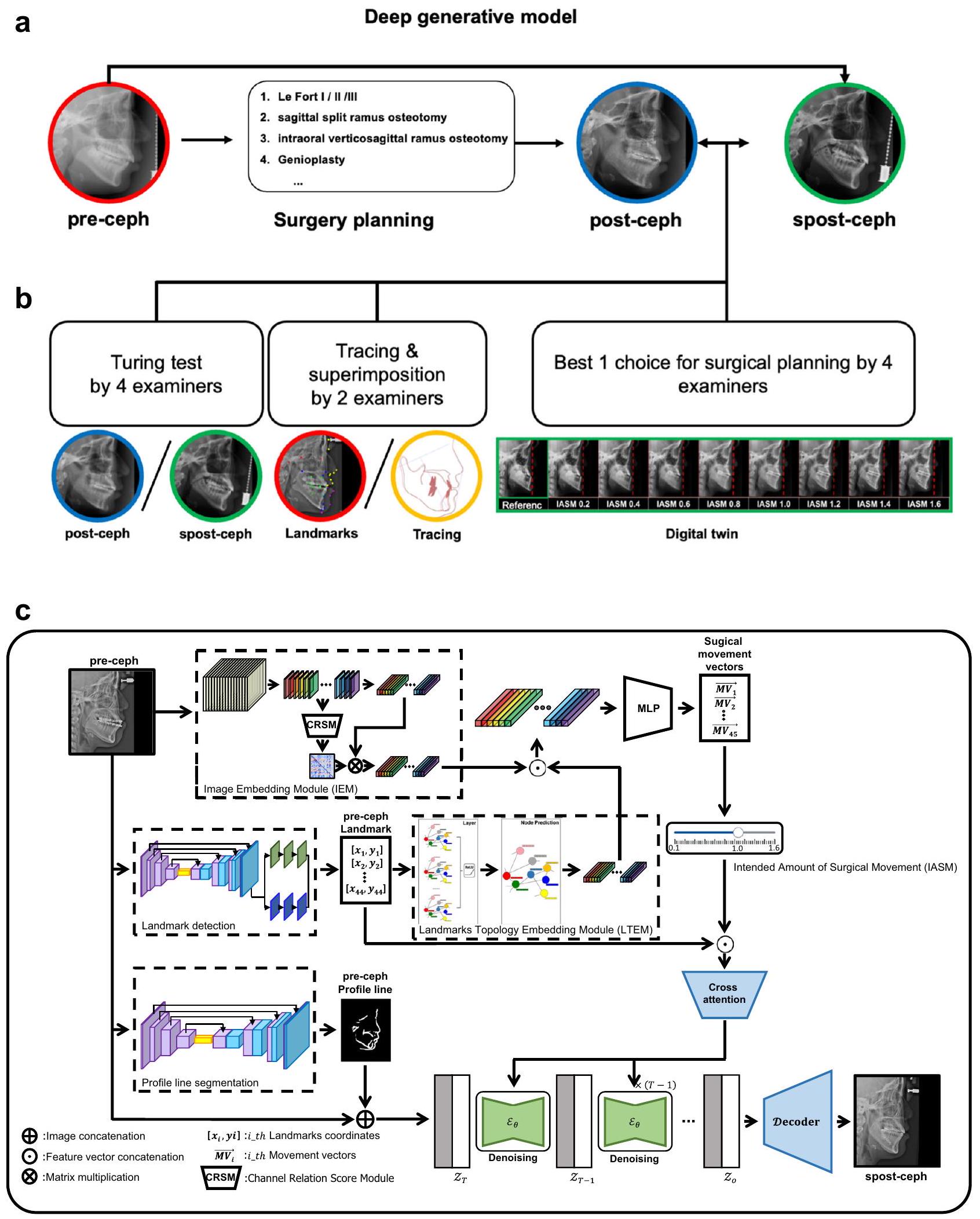
استنادًا إلى IASM وpre-ceph، يتم توليد spost-ceph بواسطة GPOSC-Net. في هذه الدراسة، تتبعت اثنان من أطباء الأسنان spost-cephs وقارناها مع post-cephs لتقييم دقة مواقع المعالم وخطوط ملف الأنسجة الرخوة والصلبة. تم رقمنة 45 معلمًا بواسطة أطباء تقويم أسنان ذوي خبرة باستخدام برنامج V-ceph (الإصدار 8.0، Osstem، سيول، كوريا). بالإضافة إلى ذلك، تم إجراء VTT مع اثنين من أطباء الأسنان واثنين من جراحي الفم والوجه والفكين للتحقق من جودة spost-cephs. خلال عملية توليد spost-ceph، تم إنتاج ومراجعة صور إضافية تعكس كميات مختلفة من الحركة الجراحية لوضع خطة جراحية مناسبة (الشكل 3a، b). يتم تصور نموذج GPOSC-Net المقترح في الشكل 3c.
جمع البيانات
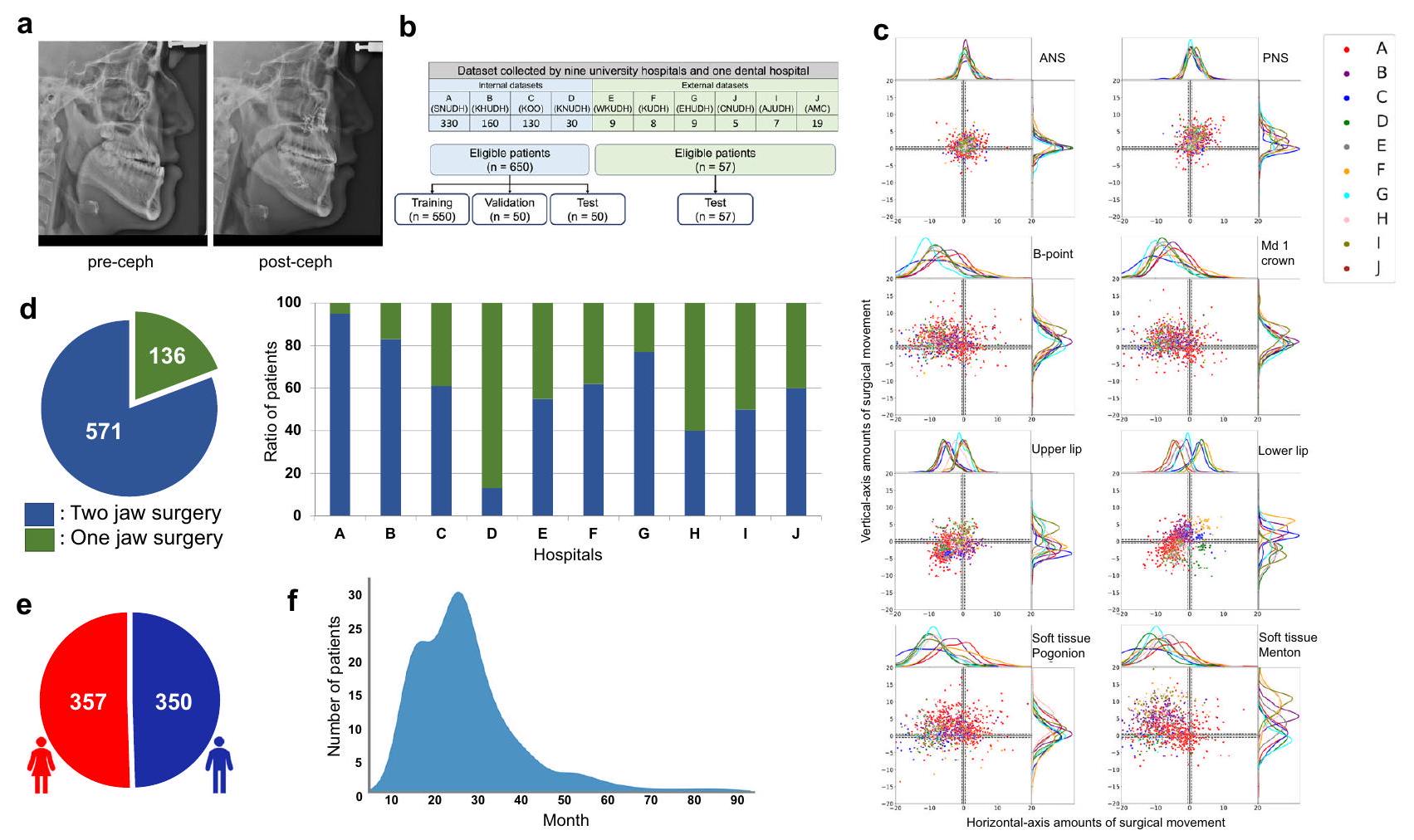
شمل هذا الدراسة 707 مرضى يعانون من سوء الإطباق الذين خضعوا لجراحة تقويم الفك (OGS) بين عامي 2007 و2019 في أحد تسعة مستشفيات جامعية و/أو مستشفى أسنان واحد، والذين تم أخذ صور أشعة جانبية للجمجمة لهم قبل وبعد الجراحة (الشكل 4أ). تراوحت أعمار المرضى بين 16 و50 عامًا. تم إخفاء هوية جميع أزواج صور الأشعة الجانبية للجمجمة وتخزينها بتنسيق الصور الرقمية والاتصالات في الطب (DICOM) كصور رمادية بتدرج 12 بت. كان توزيع الجنس بين المرضى متساويًا تقريبًا (الشكل 4هـ). في هذه الدراسة، لم يتم اعتبار الجنس كعامل في التجارب. كانت مدة العلاج التقويمي قبل الجراحة في المتوسط 14 شهرًا، على الرغم من أن بعض المرضى احتاجوا من 2 إلى 3 سنوات لإكمال المرحلة قبل الجراحة (الشكل 4و).
قمنا في البداية باختيار المستشفيات A وB وC، التي كانت تحتوي على أغنى مجموعات البيانات، كمصادر رئيسية لمجموعة البيانات الداخلية. ومع ذلك، خضع معظم المرضى من المؤسسات A وB لجراحة الفك المزدوج (الشكل 4d). وبالتالي، لتجنب التحيز في نموذج التعلم العميق نحو المرضى الذين خضعوا لجراحات الفك الواحد، قمنا بإدراج بيانات من المؤسسة D، التي كان لديها نسبة أعلى من المرضى الذين خضعوا لجراحة الفك الواحد، في مجموعة بياناتنا الداخلية. من خلال هذه العملية، تم بناء مجموعة بيانات تتكون من إجمالي 707 أزواج، تم استخدام 550 منها كبيانات تدريب، و50 كبيانات تحقق، و50 كمجموعة اختبار داخلية. بالإضافة إلى ذلك، استخدمنا 57 زوجًا من صور الأشعة السينية قبل وبعد من المستشفيات الجامعية E وF وG وH وI وJ كمجموعة اختبار خارجية، لأن المؤسسات المختلفة كانت لديها آلات تصوير أشعة سينية مختلفة. بالإضافة إلى ذلك، كانت هناك اختلافات في بروتوكولات التصوير وفي جودة الأشعة السينية.
فيما يتعلق باتجاه الحركة الجراحية، تحركت الغالبية العظمى من معالم العمود الأنفي الأمامي (ANS) والعمود الأنفي الخلفي (PNS) والشفة العليا إلى الأمام وإلى الأعلى، في حين أن الغالبية من B-
الشكل 3 | الإجراء العام. أ مقارنة نتائج الجراحة بين ما بعد السيفالوجرافيا الحقيقية وما بعد السيفالوجرافيا الاصطناعية. ب تقييم ما بعد السيفالوجرافيا الاصطناعية وتقييم فائدتها السريرية. ج التنبؤ التوليدي لجراحة الفك باستخدام نموذج بنية شبكة السيفالوجرافيا (GPOSC-Net)، الذي يستخدم وحدة تضمين الصور المعتمدة على الشبكة العصبية التلافيفية (CNN) ووحدة تضمين طوبولوجيا المعالم المعتمدة على GCNN لتحويل السيفالوجرامات الجانبية والمعالم إلى متجهات.
البيانات، على التوالي. يتم دمج هذه المتجهات وإدخالها في شبكة عصبية متعددة الطبقات (MLP) للتنبؤ بحركات المعالم الناتجة عن الجراحة. لتوليد الصور الشعاعية بعد الجراحة، يتم استخدام نموذج انتشار كامن مع بعض الشروط، مثل قيمة الحركة الجراحية المتوقعة من قبل IEM و LTEM، والصور الشعاعية السابقة، والمعالم قبل العملية، وخطوط الملف الشخصي، وكمية الحركة الجراحية المقصودة (IASM)، والتي يمكن أن تتحكم في كميات التراجع الافتراضية للصور الشعاعية بعد الجراحة.
الشكل 4 | تكوين مجموعة البيانات، توزيع الحركات الجراحية، وخصائص المرضى. أ صور جانبية مقترنة قبل وبعد الجراحة ( ). تم محاذاة ما قبل وما بعد السيفال باستخدام معالم سلا وناسيون. ب جميع الأزواج ( تم استخدام بيانات ما قبل وما بعد الجراحة من ثلاثة مستشفيات جامعية ومستشفى أسنان واحد (A وB وC وD) كبيانات داخلية. من بين هذه البيانات، تم استخدام 550 و50 و50 زوجًا للتدريب والتحقق والاختبارات الداخلية، على التوالي. توزيع الحركة الجراحية للمعالم التمثيلية للأنسجة الصلبة واللينة، بما في ذلك (من أعلى اليسار إلى أسفل اليمين) العمود الأنفي الأمامي (ANS)، العمود الأنفي الخلفي (PNS)، نقطة B، تاج الفك السفلي 1 (Mandible 1 crown)، الشفة العليا، السفلى شفاه، أنسجة لينة في منطقة الذقن، وذقن أنسجة لينة. د توزيع أنواع الجراحة عبر مجموعة البيانات بالكامل ونسبة كل نوع لكل مستشفى، حيث يمثل المحور الأفقي في الرسم البياني الشريطي المستشفيات، ويشير المحور العمودي إلى نسبة المرضى. وبالتالي، تم استخدام 57 زوجًا من الأشعة السينية قبل وبعد من ستة مستشفيات جامعية (E، F، G، H، I، وJ) للاختبارات الخارجية. هـ توزيع الجنس بين المرضى.توزيع وقت العلاج التقويمي قبل الجراحة، حيث يمثل المحور الأفقي عدد الأشهر، ويمثل المحور العمودي عدد المرضى. النقطة، Md 1 التاج، الشفة السفلية، نقطة البوجونيون للأنسجة الرخوة، ونقطة المينتون للأنسجة الرخوة تحركت إلى الخلف وإلى الأعلى (الشكل 4c). كان سبب هذه الحركات الجراحية هو أن معظم المرضى كانوا يعانون من سوء إطباق هيكلي من الفئة الثالثة، مما استدعى حركة أمامية للفك العلوي وحركة خلفية للفك السفلي. بالنسبة لمعظم عمليات جراحة الفك العلوي والسفلي، تحرك الفك العلوي ضمن 10 مم، بينما تحرك الفك السفلي ضمن 15 مم. تتوفر معلومات مفصلة حول التركيب، الخصائص الديموغرافية، وآلات التصوير الشعاعي، من بين أمور أخرى، في الجدول التكميلي 1 من المواد التكميلية.
وصف النموذج
نظرة عامة على GPOSC-Net. هنا، نقترح التنبؤ التوليدي لجراحة الفك باستخدام شبكة السيفالومتر (GPOSC-Net)الذي يتكون من نموذجين: مجموعة من وحدتين، وحدة تضمين الصور المعتمدة على الشبكات العصبية التلافيفية (IEM) ووحدة تضمين طوبولوجيا المعالم المعتمدة على الشبكات العصبية التلافيفية العامة (LTEM)، والتي تتنبأ بحركة المعالم التي ستحدث نتيجة لـ OGS؛ ونموذج انتشار كامن.، والذي يُستخدم لتوليد spost-cephs (الشكل 3c). يستخدم IEM شبكة عالية الدقة للحفاظ على تمثيلات مفصلة للصور الجانبية السيفالومترية. قبل الانتقال إلى الخطوة التالية، يتم إخضاع مخرجات IEM لربط القنوات بواسطة وحدة حساب درجة العلاقة بين القنوات (CRSM)، التي تحسب درجة العلاقة بين قنوات خريطة الميزات. من ناحية أخرى، يستخدم LTEM شبكة GCNN لتدريب الهياكل الطوبولوجية والعلاقات المكانية لـ 45 نقطة مرجعية من الأنسجة الصلبة واللينة. أخيرًا، يتم توقع حركة هذه النقاط المرجعية بواسطة طبقة متعددة. وحدة البيرسيبترون (MLP) التي تستخدم المخرجات المجمعة من IEM و LTEM.
لتوليد الصور بعد الأشعة السينية الجانبية، يستخدم النموذج مجموعة من الشروط التي تشمل حركة المعالم التي تم الحصول عليها من خلال IEM و LTEM، بالإضافة إلى خطوط الملف المقسمة للأشعة السينية السابقة. تهدف هذه الطريقة إلى ضمان قدرة توليد الحد الأدنى لنظامنا. لتعزيز هذه القدرة، قمنا بتدريب نموذج تلقائي على مجموعة بيانات مزدوجة، تتضمن واحدة تحتوي على صور للأشعة السينية السابقة واللاحقة مع تصنيفات، والأخرى مجموعة كبيرة غير مصنفة من 30,000 صورة أشعة سينية جانبية، تم جمعها عشوائيًا بين عامي 2007 و 2020، والتي لا تتعلق بأي حالات جراحية سابقة أو لاحقة أو علاج تقويمي، ومصدرها من مؤسسة داخلية (مستشفى J). يتم شرح طرق التعلم وبنية النموذج ووصفه بالتفصيل في هذا البحث.
أخيرًا، استخدمنا IASM خلال مرحلة الاختبار لتوليد صور spost-ceph التسلسلية التي تتوافق مع كميات مختلفة من الحركة الجراحية الافتراضية. جعلت IASM من الممكن معايرة نسبة الحركة الجراحية المتوقعة بدقة عبر طيف مستمر من 0 إلى 1.6، حيث تمثل القيمة 0 عدم وجود حركة جراحية (مماثلة لما قبل ceph، ، قيمة 1 تتوافق مع الحركة المتوقعة الكاملة (مماثلة لما بعد السيفال ، )، وقيمة 1.6 تعادل توقعًا محسّنًا مع انتكاسة. هذا مكن من الجيل المتسلسل لصور سبوست-سيف مع تباينات دقيقة في الحركة الجراحية. بالنسبة لـ IASM التي تتراوح من 0.1 إلى 1.6، تم توليد خمس صور سبوست-سيف بشكل عشوائي، بما في ذلك لـ IASM 1، وتم اختيار هدف علاج مناسب بناءً على ما قبل السيف من قبل اثنين من أطباء العيون واثنين من جراحي الفم والوجه والفكين في حالة عمياء.
وحدات توقع متجه الحركة الجراحية. كما تم الإشارة سابقًا، يتكون نموذجنا من IEM و LTEM، والتي تم تدريبها باستخدام الصور والمعالم، على التوالي (الشكل 3ج). اعتمدت IEM على HRكعمود فقري لها وتم تدريبها لتمثيل سيف كخريطة ميزات منخفضة الأبعاد. لتوافق مع كل معلم، تنتج خريطة الميزات 45 قناة، حيث تحتوي كل قناة على أبعاديتم استخدام CRSM لقياس مصفوفة درجة العلاقة بين القنوات المتميزة؛ وبالمثل، تحتوي المصفوفة على أبعادأخيرًا، يتم تقييم متجه ميزات الصورة باستخدام تركيبة موزونة من خريطة الميزات المسطحة ومصفوفة درجة العلاقة.
من ناحية أخرى، تم تصميم LTEM بناءً على GCNNلتعلم الهياكل الطوبولوجية للمعالم. عملية تدريب LTEM هي كما يلي:حيث أنوهي مصفوفات الوزن التي تم تعلمها من التدريب، و f تشير إلى ميزات العقدة، و e هي حافة الرسم البياني. في الوقت نفسه،هي دالة التنشيط غير الخطية، هي الاتصال القابل للتعلم عند العقدةمن A، تشير إلى البيانات التي نريد تدريبها، ويتم التعبير عنها كبيانات إدخال. في تجربتنا،وحيث D هو بعد الإدخال للرسم البياني، وموقع العقدة i، وميزات المسافة من جيران العقدة i؛ وهو عدد العقد، وهو نفس عدد المعالم (الشكل 3ج).
يتكون مشفر LTEM من طبقتين من GCNN، وهو تضمين الرسم البياني، ومصفوفات الوزن المتعلمة في هذه الطبقات. هنا، A هو الاتصال بين جميع العقد المشتركة بين الطبقتين. تم تعيين أبعاد الإخراج للطبقة الأولى والثانية إلى 64 و 32، على التوالي. يستخدم نموذجنا IEM و LTEM للحصول على تضمينات الصور والمعالم، ثم يدمج هذه المتجهات التضمينية للتنبؤ في النهاية بمتجهات الحركة الجراحية. قمنا بتدريب النموذج باستخدام خسارة L1 بين متجهات الحركة الجراحية المتوقعة والمعيار الذهبي.
استخدمنا أيضًا مُحسِّن آدم، الذي جمع بين الزخم وطرق متوسط التحرك الموزون بشكل أسي، لتحديث أوزان شبكاتنا. تم تعيين معدل التعلم في البداية إلى 0.001، ثم تم تقليله بعامل 10 عندما توقفت دقة الشبكات على مجموعة بيانات التحقق عن التحسن. في المجموع، تم تقليل معدل التعلم ثلاث مرات لإنهاء التدريب. تم بناء الشبكات تحت إطار التعلم الآلي مفتوح المصدر PyTorchو Python 3.6، مع إجراء التدريب على وحدة معالجة الرسومات NVIDIA RTX A6000. بالنسبة لتدريب النموذج، اعتمدنا استراتيجية تعزيز البيانات لتعزيز قوتها وقدرتها على التعميم. يمكن أن تمنع هذه الاستراتيجية من الإفراط في التكيف وتؤدي إلى أداء قوي للنموذج، خاصة عند استخدام مجموعة بيانات تدريب محدودة. تم إجراء تعزيز البيانات على مدخلات الصورة والرسم البياني لزيادة مجموعة بيانات التدريب. عندما تم تحويل المعلومات المكانية لصورة، مثل الدوران العشوائي والانزلاق العشوائي، تم تطبيق نفس التعزيز على مدخلات الرسم البياني. بالنسبة للغاما، والحدة، والضبابية، والضوضاء العشوائية، لم يتم تحويل المعلومات المكانية للصورة؛ وبالتالي، تم تطبيقها فقط على الصورة وليس على مدخلات الرسم البياني.
وحدة التوليد. ضغط الصورة (الشكل 3ج). الهدف من وحدة التوليد لدينا هو توليد سبوست-سيف باستخدام ما قبل السيف كمدخل. لتحقيق ذلك، استخدمنا نموذج انتشار كامنيتكون من مشفر تلقائيللمشفروالمفككونموذج انتشار لتوليد الكامن المشفر (الشكل 3ج). لتدريب المشفر التلقائي، استخدمنا ليس فقط بيانات ما قبل السيف وما بعد السيف ولكن أيضًا مجموعة غير مصنفة من 30,000 صورة سيف جانبي مأخوذة من مؤسسة داخلية (مستشفى J). كان هذا مهمًا لضمان أن الفضاء الكامن للمشفر التلقائي كان مُشكلًا بشكل جيد، مما يضمن قدرة توليد الحد الأدنى. بالإضافة إلى ذلك، استخدمنا التكميم المتجه، الذي يستخدم كتاب رموز منفصل، وتقنيات التعلم المعاكس لتحسين استقرار النموذج وتحقيق نتائج عالية الجودة. دالة الخسارة هي كما يلي.
حيث أنهو المميز القائم على الباتش،، و
نموذج الانتشار. يتم تحويل توزيع البيانات المشفرةبشكل تدريجي إلى توزيع جيد التصرفمن خلال التطبيق المتكرر لنواة انتشار ماركوفلـ. ثم،
في الوقت نفسه، المسار الأمامي، الذي يبدأ من توزيع البيانات ويؤدي إلىخطوات عملية الانتشار، هو كما يلي:حيث أنهي الكامنة بنفس أبعاد البيانات. العملية الأمامية هي تلك التي تسمح بأخذ عيناتفي خطوة زمنية عشوائيةبشكل مغلق. باستخدام التدوينو، نحصل بعد ذلك على الشكل التحليلي لـكما يلي.
يمكننا بسهولة الحصول على عينة في التوزيع الفوري لعملية الانتشار.
نماذج الانتشار هي نماذج متغيرة كامنة لتوزيع معلم. المسار العكسي، الذي يبدأ من توزيع سابق، هو كما يلي.
حيث أنو، ووهي أهداف التدريب التي تحدد المتوسط والتباين، على التوالي، للانتقالات العكسية لماركوف لتوزيع غاوسي. لتقريب بين توزيع المعلموتوزيع البيانات، يتم إجراء التدريب عن طريق تحسين الحد الأدنى المتغير على السجل السالب للاحتمالية.
للتدريب الفعال، يتم إجراء تحسين إضافي عن طريق إعادة التعبير عنكما يلي.
تستخدم المعادلة تباين كولباك-ليبلر للمقارنة مباشرةضد ما بعد العملية الأمامية. تكون توزيعات ما بعد العملية قابلة للتعامل عند الشرط على.
حيث أنو، وكانت قيمو0.0015 و 0.0195، على التوالي. ثم، يمكن تعريف دالة الخسارة كما يلي.
بعد التدريب، يمكن توليد عينات عن طريق البدء منواتباع سلسلة ماركوف العكسية المعلمة.
علاوة على ذلك، هدفنا هو توليد سبوست-سيف باستخدام شروط متعددة في نموذج الانتشار. استخدمنا إجمالي أربعة شروط، بما في ذلك ما قبل السيف وخطوط ملفها، التي تم دمجها، بينما تم تحويل معالم ما قبل السيف ومتجهات الحركة المتوقعة من خلال IEM و LTEM إلى كامن باستخدام شبكة رسم بياني ثم تم تضمينها في نموذج الانتشار عبر وحدة انتباه متقاطع. ثم، يمكننا تدريب نموذج الانتشار الشرطي باستخدام الشروطعبر
حيث أن،وهو متجه الحركة الجراحية المتوقع من خلال شبكة الرسم البياني، و،وتمثل ما قبل السيف، ومعالم ما قبل السيف، وخط ملف ما قبل السيف. بالإضافة إلى ذلك، استخدمنا نموذج LTEMلتضمينوفي نموذج الانتشار. استخدمنا نموذجًا غير مدرب، يتم تدريبه معًا كما يتم تدريب نموذج الانتشار. بعد التدريب، يتم أخذ العينات باستخدام نموذج الانتشار المدرب. لتقليل وقت التوليد والحفاظ على الاتساق، تم استخدام DDIM. الصيغة لـ DDIM هي كما يلي:
حيث أنهي سلسلة فرعية من خطوات زمنية بطول. لتدريب وحدة التوليد، استخدمنا مُحسِّن آدم، الذي يجمع بين الزخم وطرق متوسط التحرك الموزون بشكل أسي. تم تعيين معدل التعلم الأولي إلى، وقمنا بتدريب النموذج لمدة إجمالية قدرها 1000 دورة. تم تنفيذ الشبكات باستخدام أطر التعلم الآلي مفتوحة المصدر مثل PyTorchو Python 3.6، مع إجراء التدريب على وحدة معالجة الرسومات NVIDIA RTX A6000 بسعة 48 جيجابايت. ومع ذلك، لم نستخدم تعزيز البيانات في عملية تدريبنا.
إرشادات بدون مصنف للتوأم الرقمي. لإجراء تجارب لتوليد حركات جراحية متنوعة، استخدمنا إرشادات بدون مصنف (CFG). على عكس إرشادات المصنف، فإن CFG مميزة في أن نموذج المصنف ليس منفصلًا عن نموذج الانتشار ولكنه يتم تدريبه معًا. تحقق CFG تأثيرًا مشابهًا لتعديل إبسيلونلتSampling إرشادات المصنف، ولكن بدون المصنف المنفصل. يمكن تدريب نموذج الانتشار عن طريق تعيين شرط أو رمز فارغفي النموذج لبعض الاحتمالات. ثم، قمنا بتعريف الدرجة المقدرةباستخدام النموذجلشرط الإدخالكـ، والدرجة المقدرة للرمز الفارغ كـ. بعد التدريب، قمنا بتعديل الدرجة باستخدام تركيبة خطية من الدرجة غير المشروطة والدرجة المشروطة بواسطة IASM. من المعروف أن طريقة أخذ العينات CFG قوية ضد الهجمات العدائية المعتمدة على التدرج، في حين أن أخذ العينات بتوجيه المصنف بواسطة مصنف مدرب بشكل سيء قد يؤدي إلى مشاكل في الاتساق والولاء. الدرجة المقدرة بواسطة أخذ العينات CFG موضحة كما يلي:
معالجة البيانات
قبل التدريب، تم توحيد جميع الصور الجانبية باستخدام تباعد بكسل قدره 0.1 مم. بعد ذلك، تم محاذاة الصورة بعد التصوير الجانبي تقليديًا مع الصورة قبل التصوير الجانبي بناءً على خط Sella-Nasion (SN). لتضمين جميع المعالم في كل من الصورة قبل التصوير الجانبي والصورة بعد التصوير الجانبي، تم قص مستطيل يحيط بالمناطق المحددة بواسطة نقاط Basion وSofttissue menton وPronasale وGlabella في كل من الصورة قبل التصوير الجانبي والصورة بعد التصوير الجانبي. بالإضافة إلى ذلك، تم تطبيق حشو صفري أفقيًا ورأسيًا لإنشاء صورة مربعة بدقة قدرها.
تم تقسيم الصورة المقصوصة بواسطة القيمة القصوى للبكسل في الصورة. تم إجراء تطبيع البكسل بحيث تكون قيمة البكسل ضمن. بالإضافة إلى ذلك، تم التعبير عن إحداثيات كل معلم والمسافات بين المعالم كمتجهات لتدريب النموذج. قبل الإدخال إلى النموذج، تم تقسيم المسافات على المحورين – و– بواسطة عرض وارتفاع الصورة المقصوصة، وتم إجراء التطبيع بحيث تكون قيمة الميزة ضمن النطاق من 0-1.
التحليل الإحصائي
تم إجراء جميع التحليلات الإحصائية باستخدام IBM SPSS Statistics (IBM Corporation، Armonk، NY، USA) الإصدار 25.
مقارنة مسافة المعالم للصورة بعد التصوير الجانبي والصورة بعد التصوير الجانبي المعدلة. تم تتبع صورتين بعد التصوير الجانبي والصورة المعدلة في مجموعات الاختبار الداخلية () و( ). تم تعيين خط SN كخط مرجعي أفقي، وتم تعيين الخط الذي يمر عبر نقطة S ويكون عموديًا على خط كخط مرجعي عمودي. تم استخدام المسافات الأفقية والعمودية من كل معلم كقيم إحداثية. تم مقارنة قيم الإحداثيات لنفس المعلم في الصورة بعد التصوير الجانبي والصورة المعدلة، وتم حساب المسافة بين المعالم. تم إجراء اختبار تساوي مزدوج لكل معلم. في هذه الحالة، كانت هامش الخطأ المطبق 1.5 مم 41، 42. تم تقييم SPRs لكل نقطة وفقًا للأخطاء. علاوة على ذلك، قمنا بقياس المسافة بين خطوط الملف الشخصي للصورة بعد التصوير الجانبي والصورة المعدلة. مع الأخذ في الاعتبار الهياكل التشريحية، قمنا بتقسيمها إلى أربعة خطوط، وتم قياس المسافات بين الخطوط باستخدام مسافة هاوسدورف. يمكن العثور على تفاصيل حول الأخطاء في خطوط الملف الشخصي وتعريف الخطوط الأربعة في الجدول التكميلي 3 والشكل التكميلي 1 من المواد التكميلية.
اختبار تورينغ البصري. بالنسبة لاختبار VTT، تم استخدام 57 صورة اختبار خارجية (29 صورة بعد التصوير الجانبي و28 صورة معدلة)، حيث كان أطباء الفم والوجه والفكين وأطباء الأسنان قد لاحظوا بالفعل مجموعة البيانات الداخلية المولدة خلال تجربة التوأم الرقمي. تم إجراء VTT مع طبيبين أسنان واثنين من أطباء الفم والوجه والفكين من خلال عرض الصور واحدة تلو الأخرى عبر واجهة ويب مخصصة. كان لدى كل فاحص أكثر من 15 عامًا من الخبرة السريرية. لتقليل التباين البيئي، تم عرض الصور بنفس الترتيب، وكان من المحظور إعادة زيارة الإجابات السابقة. تم إبلاغ الفاحصين بوجود 29 صورة حقيقية و28 صورة مصنعة. بالإضافة إلى ذلك، لم يكن لدى أي منهم خبرة سابقة مع الصور المصنعة قبل الاختبار. أكمل جميع الفاحصين الاختبار بنجاح. تم اشتقاق الحساسية والنوعية والدقة، مع تعريف الصور الحقيقية على أنها إيجابية والصور الاصطناعية على أنها سلبية.
التوأم الرقمي. قمنا بالتحقيق في القابلية السريرية للصورة المعدلة كتوائم رقمية للتخطيط الجراحي المحاكى. تم عرض صورتين من أطباء الأسنان وأطباء الفم والوجه والفكين في نفس الوقت الصورة قبل التصوير الجانبي وخمس صور معدلة تم إنشاؤها عشوائيًا عند درجات مختلفة من الحركة الجراحية. للتركيز على الحالات التي تتضمن تغييرات جراحية كبيرة، تم استبعاد المرضى الذين كانت لديهم حركة جراحية قدرها، مما أدى إلى اختيار 35 حالة من مجموعة الاختبار الداخلية الأولية المكونة من 50. بعد ذلك، طُلب من الفاحصين اختيار مقدار الحركة الجراحية المناسب
مع الأخذ في الاعتبار الصورة قبل التصوير الجانبي. ثم تم حساب نسبة الصور المعدلة التي تعكس الحركات الجراحية الحقيقية.
دراسة الإزالة. تم إجراء دراسة الإزالة باستخدام مجموعة بيانات داخلية مكونة من 50 عينة. قام طبيب أسنان واحد بقياس المعالم يدويًا لكل حالة تجريبية. نظرًا للطبيعة المكثفة لتوضيح المعالم يدويًا، تم استخدام مجموعة البيانات الداخلية فقط لضمان الجدوى مع الحفاظ على اتساق التقييم. تم إجراء اختبارات مزدوجةفي كل من المراحل التجريبية الخمس لمقارنة النتائج مع تلك من المرحلة السابقة، وتقييم تأثير خطأ مسافة المعالم. تم تعيين الدلالة الإحصائية عند، مع اعتباردلالة عالية.
ملخص التقرير
مزيد من المعلومات حول تصميم البحث متاحة في ملخص تقرير Nature Portfolio المرتبط بهذه المقالة.
توفر البيانات
جميع البيانات التي تدعم النتائج الموصوفة في هذه المخطوطة متاحة داخل المقالة ومعلوماتها التكميلية. تتكون مجموعة البيانات المستخدمة لتدريب النموذج وتقييمه من صور أشعة سينية جانبية من 707 مرضى خضعوا لجراحة تقويم الفك. تم تقسيم مجموعة البيانات هذه إلى 600 عينة للتدريب، و50 عينة للتحقق الداخلي، و57 عينة للتحقق الخارجي. بالإضافة إلى ذلك، تم استخدام 30,000 صورة أشعة سينية جانبية غير مصنفة من مؤسسات داخلية للتدريب المسبق للنموذج التوليدي. هذه المجموعات متاحة عند الطلب لأن هناك قيود معينة على التوفر العام، بسبب اللوائح الوطنية وقوانين خصوصية المرضى في كوريا الجنوبية. يجب على الباحثين المهتمين بالوصول إلى هذه المجموعات تقديم طلب رسمي، والذي سيتم مراجعته من قبل المؤلف المقابل، نامكوك كيم (namkugkim@gmail.com) ومجلس مراجعة المؤسسات (IRB). تتطلب عملية الموافقة عادةً من شهر إلى شهرين، اعتمادًا على جدول اجتماع IRB. يُطلب من الباحثين المعتمدين للوصول إلى البيانات الاستشهاد بهذه المخطوطة عند استخدام مجموعة البيانات. تتوفر بيانات المصدر التي تحتوي على القيم العددية الخام التي تستند إليها جميع النتائج التجريبية المقدمة في هذه المخطوطة مع هذه الورقة. تتوفر بيانات المصدر مع هذه الورقة.
توفر الشيفرة
الشيفرة والأوزان المدربة مسبقًا المستخدمة في هذا البحث متاحة في مستودع GitHub (https://github.com/Kim-Junsik/GPOSC-Net)، والذي يمكن الوصول إليه علنًا من قبل أي شخص. يتم تحديد معلومات حول الاستخدام والتعديل وتوزيع الشيفرة في ملف الترخيص داخل المستودع. الشيفرة مخصصة لأغراض البحث فقط وقد تكون مقيدة للاستخدام التجاري. بالإضافة إلى ذلك، يجب على المستخدمين الاستشهاد بالمخطوطة ذات الصلة ومستودع الشيفرة عند استخدام هذا العمل في أبحاثهم.
References
Musich, D. & Chemello, P. in Orthodontics: Current Principles and Techniques Ch. 23 (Elsevier, 2005).
Perkovic, V. et al. Facial aesthetic concern is a powerful predictor of patients’ decision to accept orthognathic surgery. Orthod. Craniofacial Res. 25, 112-118 (2022).
Broder, H. L., Phillips, C. & Kaminetzky S. Issues in decision making: Should I have orthognathic surgery? Semin. Orthod. 6, 249-258 (2000).
Kolokitha, O.-E. & Chatzistavrou, E. Factors influencing the accuracy of cephalometric prediction of soft tissue profile changes following orthognathic surgery. J. Maxillofac. Oral. Surg. 11, 82-90 (2012).
Wolford, L. M., Hilliard, F. W. & Dugan, D. J. STO Surgical Treatment Objective: A Systematic Approach to the Prediction Tracing (The C. V. Mosby Company, 1985).
Upton, P. M., Sadowsky, P. L., Sarver, D. M. & Heaven, T. J. Evaluation of video imaging prediction in combined maxillary and mandibular orthognathic surgery. Am. J. Orthod. Dentofac. Orthopedics 112, 656-665 (1997).
Cousley, R. R., Grant, E. & Kindelan, J. The validity of computerized orthognathic predictions. J. Orthod. 30, 149-154 (2003).
Kaipatur, N. R. & Flores-Mir, C. Accuracy of computer programs in predicting orthognathic surgery soft tissue response. J. Oral. Maxillofac. Surg. 67, 751-759 (2009).
Rasteau, S., Sigaux, N., Louvrier, A. & Bouletreau, P. Threedimensional acquisition technologies for facial soft tissues-applications and prospects in orthognathic surgery. J. Stomatol. Oral. Maxillofac. Surg. 121, 721-728 (2020).
Suh, H.-Y. et al. A more accurate method of predicting soft tissue changes after mandibular setback surgery. J. Oral. Maxillofac. Surg. 70, e553-e562 (2012).
Yoon, K.-S., Lee, H.-J., Lee, S.-J. & Donatelli, R. E. Testing a better method of predicting postsurgery soft tissue response in Class II patients: a prospective study and validity assessment. Angle Orthod. 85, 597-603 (2015).
Lee, Y.-S., Suh, H.-Y., Lee, S.-J. & Donatelli, R. E. A more accurate soft-tissue prediction model for Class III 2-jaw surgeries. Am. J. Orthod. Dentofac. Orthopedics 146, 724-733 (2014).
Suh, H.-Y. et al. Predicting soft tissue changes after orthognathic surgery: the sparse partial least squares method. Angle Orthod. 89, 910-916 (2019).
Lee, K. J. C. et al. Accuracy of 3 -dimensional soft tissue prediction for orthognathic surgery in a Chinese population. J. Stomatol. Oral. Maxillofac. Surg. 123, 551-555 (2022).
Resnick, C., Dang, R., Glick, S. & Padwa, B. Accuracy of threedimensional soft tissue prediction for Le Fort I osteotomy using Dolphin 3D software: a pilot study. Int. J. Oral Maxillofac. Surg. 46, 289-295 (2017).
Bengtsson, M., Wall, G., Greiff, L. & Rasmusson, L. Treatment outcome in orthognathic surgery-a prospective randomized blinded case-controlled comparison of planning accuracy in computerassisted two-and three-dimensional planning techniques (part II). J. Craniomaxillofac. Surg. 45, 1419-1424 (2017).
Arai, Y., Tammisalo, E., Iwai, K., Hashimoto, K. & Shinoda, K. Development of a compact computed tomographic apparatus for dental use. Dentomaxillofac. Radiol. 28, 245-248 (1999).
Lofthag-Hansen, S., Grondahl, K. & Ekestubbe, A. Cone-beam CT for preoperative implant planning in the posterior mandible: visibility of anatomic landmarks. Clin. Implant Dent. Relat. Res. 11, 246-255 (2009).
Momin, M. et al. Correlation of mandibular impacted tooth and bone morphology determined by cone beam computed topography on a premise of third molar operation. Surg. Radiol. Anat. 35, 311-318 (2013).
Patel, S., Dawood, A., Whaites, E. & Pitt Ford, T. New dimensions in endodontic imaging: part 1. Conventional and alternative radiographic systems. Int. Endod. J. 42, 447-462 (2009).
Silva, M. A. G. et al. Cone-beam computed tomography for routine orthodontic treatment planning: a radiation dose evaluation. Am. J. Orthod. Dentofac. Orthopedics 133, e641-640. e645 (2008). 640.
Protection R. Evidence-Based Guidelines on Cone Beam CT for Dental and Maxillofacial Radiology (European Commission, 2012).
Wrzesien, M. & Olszewski, J. Absorbed doses for patients undergoing panoramic radiography, cephalometric radiography and CBCT. Int. J. Occup. Med. Environ. Health 30, 705-713 (2017).
Ludlow, J. et al. Effective dose of dental CBCT-a meta analysis of published data and additional data for nine CBCT units. Dentomaxillofac. Radiol. 44, 20140197 (2015).
Jha, N. et al. Projected lifetime cancer risk from cone-beam computed tomography for orthodontic treatment. Korean J. Orthod. 51, 189-198 (2021).
Jung, Y.-J., Kim, M.-J. & Baek, S.-H. Hard and soft tissue changes after correction of mandibular prognathism and facial asymmetry by mandibular setback surgery: three-dimensional analysis using computerized tomography. Oral. Surg. Oral. Med. Oral. Pathol. Oral. Radiol. Endod. 107, 763-771.e768 (2009).
Kau, C. H. et al. Cone-beam computed tomography of the maxillofacial region-an update. Int. J. Med. Robot. Comput. Assist. Surg. 5, 366-380 (2009).
Kim, M. et al. Realistic high-resolution lateral cephalometric radiography generated by progressive growing generative adversarial network and quality evaluations. Sci. Rep. 11, 12563 (2021).
Song, J., Meng, C. & Ermon, S. Denoising diffusion implicit models. In International Conference on Learning Representations. https:// doi.org/10.48550/arXiv.2010.02502 (ICLR, 2020).
Rombach, R., Blattmann, A., Lorenz, D., Esser, P. & Ommer, B. Highresolution image synthesis with latent diffusion models. In Proceedings of the IEEE/CVF Conference on Computer Vision and Pattern Recognition (IEEE, 2022).
Ho, J. & Salimans, T. Classifier-free diffusion guidance. In NeurIPS 2021 Workshop on Deep Generative Models and Downstream Applications. https://doi.org/10.48550/arXiv.2207.12598 (NIPS, 2021).
Ho, J., Jain, A. & Abbeel, P. Denoising diffusion probabilistic models. Adv. Neural Inf. Process. Syst. 33, 6840-6851 (2020).
Song, Y. et al. Score-based generative modeling through stochastic differential equations. In International Conference on Learning Representations. https://doi.org/10.48550/arXiv.2011.13456 (ICLR, 2020).
Dhariwal, P. & Nichol, A. Diffusion models beat gans on image synthesis. Adv. Neural Inf. Process. Syst. 34, 8780-8794 (2021).
Lee, S. et al. Improving 3D imaging with pre-trained perpendicular 2D diffusion models. In Proc. IEEE/CVF International Conference on Computer Vision (IEEE, 2023).
Pinaya, W. H. et al. Brain imaging generation with latent diffusion models. In MICCAI Workshop on Deep Generative Models. (Springer, 2022).
Takagi, Y. & Nishimoto, S. High-resolution image reconstruction with latent diffusion models from human brain activity. In Proc. IEEE/CVF Conference on Computer Vision and Pattern Recognition (IEEE, 2023).
Khader, F. et al. Denoising diffusion probabilistic models for 3D medical image generation. Sci. Rep. 13, 7303 (2023).
Lyu, Q. & Wang, G. Conversion between CT and MRI images using diffusion and score-matching models. Preprint at https://arxiv.org/ abs/2209.12104 (2022).
Kim, I.-H. et al. Orthognathic surgical planning using graph CNN with dual embedding module: external validations with multihospital datasets. Comput Methods Prog. Biomed. 242, 107853 (2023).
Kim, I.-H., Kim, Y.-G., Kim, S., Park, J.-W. & Kim, N. Comparing intraobserver variation and external variations of a fully automated cephalometric analysis with a cascade convolutional neural net. Sci. Rep. 11, 7925 (2021).
Hwang, H.-W. et al. Automated identification of cephalometric landmarks: part 2-Might it be better than human? Angle Orthod. 90, 69-76 (2020).
Kim, J. et al. Accuracy of automated identification of lateral cephalometric landmarks using cascade convolutional neural networks on lateral cephalograms from nationwide multi-centres. Orthod. Craniofac. Res. 24, 59-67 (2021).
Gil, S.-M. et al. Accuracy of auto-identification of the posteroanterior cephalometric landmarks using cascade convolution neural network algorithm and cephalometric images of different
quality from nationwide multiple centers. Am. J. Orthod. Dentofac. Orthopedics 161, e361-e371 (2022).
Goodfellow, I. et al. Generative adversarial nets. In Proc. 28th International Conference on Neural Information Processing Systems 2672-2680 (MIT Press, 2014).
Karras, T., Laine, S. & Aila, T. A style-based generator architecture for generative adversarial networks. In Proc. IEEE/CVF Conference on Computer Vision and Pattern Recognition (IEEE, 2019).
Karras, T. et al. Analyzing and improving the image quality of stylegan. In Proc. IEEE/CVF Conference on Computer Vision and Pattern Recognition (2020).
Richardson, E. et al. Encoding in style: a stylegan encoder for image-to-image translation. In Proc. IEEE/CVF Conference on Computer Vision and Pattern Recognition (IEEE, 2021).
Kipf, T. N. & Welling, M. Semi-supervised classification with graph convolutional networks. In International Conference on Learning Representations (ICLR, 2017).
Sperduti, A. & Starita, A. Supervised neural networks for the classification of structures. IEEE Trans. Neural Netw. 8, 714-735 (1997).
de Oliveira, P. H. J. et al. Artificial intelligence as a prediction tool for orthognathic surgery assessment. Orthodont. Craniofac. Res. 27, 785-794 (2024).
Donatelli, R. E. & Lee, S.-J. How to report reliability in orthodontic research: Part 2. Am. J. Orthodont. Dentofac. Orthopedics 144, 315-318 (2013).
Park, J.-A. et al. Does artificial intelligence predict orthognathic surgical outcomes better than conventional linear regression methods? Angle Orthod. 94, 549-556 (2024).
Wang, J. et al. Deep high-resolution representation learning for visual recognition. IEEE Trans. Pattern Anal. Mach. Intell. 43, 3349-3364 (2020).
Paszke, A. et al. Pytorch: an imperative style, high-performance deep learning library. In Proc. 33rd International Conference on Neural Information Processing Systems 8026-8037 (Curran Associates Inc., 2019).
Baldi, P. Autoencoders, unsupervised learning, and deep architectures. In Proc. ICML Workshop on Unsupervised and Transfer Learning 37-49 (2012).
Razavi, A., Van den Oord, A. & Vinyals O. Generating diverse highfidelity images with vq-vae-2. In Proc. 33rd International Conference on Neural Information Processing Systems 14866-14876 (Curran Associates Inc., 2019).
Van Den Oord, A. & Vinyals, O. Neural discrete representation learning. In 31st Conference on Neural Information Processing Systems (NIPS) (2017).
Vincent, P. A connection between score matching and denoising autoencoders. Neural Comput. 23, 1661-1674 (2011).
Song, Y., Garg, S., Shi, J. & Ermon, S. Sliced score matching: a scalable approach to density and score estimation. In Proc. 35th Uncertainty in Artificial Intelligence Conference, 574-584 (PMLR, 2020).
Hyvärinen, A. & Dayan, P. Estimation of non-normalized statistical models by score matching. J. Mach. Learn. Res. 6, 695-709 (2005).
الشكر والتقدير
تم دعم هذا البحث من خلال منحة من مشروع تطوير التكنولوجيا الصحية في كوريا من خلال معهد تطوير صناعة الصحة في كوريا (KHIDI)، الممول من وزارة الصحة والرعاية الاجتماعية، جمهورية كوريا (رقم المنحة: HR2OCOO26). يشكر المؤلفون جونغسون ليم، مينسو كوان، جونغمين هوانغ، جي يون أوه وكيوونغ هوا أوه على تحليل البيانات المفيد.
مساهمات المؤلفين
I.-H.K. وJ.J. وJ.-S.K. حصلوا على البيانات وحللوها، وأجروا تجارب التعلم العميق، وصاغوا المخطوطة. قدم N.K. وJ.-W.P. مساهمة كبيرة في التصور والتصميم وتفسير البيانات، وقاموا بمراجعة المخطوطة بشكل نقدي. قدم M.K. وS.-J.S. وY.-J.K. وJ.-H.C. وM.H. وK.-H.K. وS.-H.L. وS.-J.K. وY.H.K. وS-H.B. مساهمة كبيرة في الحصول على البيانات وتفسيرها، وقد قدموا مساهمة كبيرة في تصميم الدراسة وتفسير البيانات. ساهم J.L. في معالجة البيانات وإعداد الأشكال.
ملاحظة الناشر: تظل Springer Nature محايدة فيما يتعلق بالمطالبات القضائية في الخرائط المنشورة والانتماءات المؤسسية.
الوصول المفتوح: هذه المقالة مرخصة بموجب رخصة المشاع الإبداعي للاستخدام غير التجاري، والتي تسمح بأي استخدام غير تجاري، ومشاركة، وتوزيع، وإعادة إنتاج في أي وسيلة أو صيغة، طالما أنك تعطي الائتمان المناسب للمؤلفين الأصليين والمصدر، وتوفر رابطًا لرخصة المشاع الإبداعي، وتوضح إذا قمت بتعديل المادة المرخصة. ليس لديك إذن بموجب هذه الرخصة لمشاركة المواد المعدلة المشتقة من هذه المقالة أو أجزاء منها. الصور أو المواد الأخرى من طرف ثالث في هذه المقالة مشمولة في رخصة المشاع الإبداعي للمقالة، ما لم يُشار إلى خلاف ذلك في سطر الائتمان للمادة. إذا لم تكن المادة مشمولة في رخصة المشاع الإبداعي للمقالة وكان استخدامك المقصود غير مسموح به بموجب اللوائح القانونية أو يتجاوز الاستخدام المسموح به، ستحتاج إلى الحصول على إذن مباشرة من صاحب حقوق الطبع والنشر. لعرض نسخة من هذه الرخصة، قم بزيارة http:// creativecommons.org/licenses/by-nc-nd/4.0/.
(ج) المؤلفون 2025
¹قسم الهندسة الطبية الحيوية، معهد أسن الطبي لعلوم وتقنية التلاقي، مركز أسن الطبي، جامعة أولسان كلية الطب، سيول، جمهورية كوريا.شركة SK Telecom، سيول، جمهورية كوريا.قسم الطب التلاقي، جامعة أولسان، كلية الطب، مركز أسن الطبي، سيول، جمهورية كوريا.قسم تقويم الأسنان، كلية طب الأسنان بجامعة تشوننام الوطنية، غوانغجو، جمهورية كوريا.قسم تقويم الأسنان، كلية طب الأسنان بجامعة كيونغبوك الوطنية، دايجو، جمهورية كوريا.قسم تقويم الأسنان، كلية طب الأسنان بجامعة وونكوانغ، إكسون-سي، جمهورية كوريا.قسم تقويم الأسنان، كلية الطب بجامعة إيوها النسائية، سيول، جمهورية كوريا.قسم تقويم الأسنان، كلية طب الأسنان بجامعة كيونغ هي، سيول، جمهورية كوريا.قسم تقويم الأسنان، مركز أسن الطبي، جامعة أولسان كلية الطب، سيول، جمهورية كوريا.قسم تقويم الأسنان، معهد علوم صحة الفم، كلية الطب بجامعة أجو، سوون-سي، جيونغجي-دو، جمهورية كوريا.قسم تقويم الأسنان، كلية طب الأسنان بجامعة تشوسون، غوانغجو، جمهورية كوريا.قسم تقويم الأسنان، كلية طب الأسنان، معهد أبحاث الأسنان، جامعة سيول الوطنية، سيول، جمهورية كوريا. البريد الإلكتروني: jeuspark@gmail.com; namkugkim@gmail.com
Predicting orthognathic surgery results as postoperative lateral cephalograms using graph neural networks and diffusion models
Received: 24 June 2024
Accepted: 27 February 2025
Published online: 16 March 2025
Abstract
In-Hwan Kim¹, Jiheon Jeong¹,2, Jun-Sik Kim¹, Jisup Lim , Jin-Hyoung Cho , Mihee Hong , Kyung-Hwa Kang , Minji Kim , Su-Jung Kim , Yoon-Ji Kim , Sang-Jin Sung , Young Ho Kim , Sung-Hoon Lim , Seung-Hak Baek , Jae-Woo Park (1) & Namkug Kim (1)
Orthognathic surgery, or corrective jaw surgery, is performed to correct severe dentofacial deformities and is increasingly sought for cosmetic purposes. Accurate prediction of surgical outcomes is essential for selecting the optimal treatment plan and ensuring patient satisfaction. Here, we present GPOSC-Net, a generative prediction model for orthognathic surgery that synthesizes post-operative lateral cephalograms from pre-operative data. GPOSC-Net consists of two key components: a landmark prediction model that estimates post-surgical cephalometric changes and a latent diffusion model that generates realistic synthesizes post-operative lateral cephalograms images based on predicted landmarks and segmented profile lines. We validated our model using diverse patient datasets, a visual Turing test, and a simulation study. Our results demonstrate that GPOSC-Net can accurately predict cephalometric landmark positions and generate high-fidelity synthesized postoperative lateral cephalogram images, providing a valuable tool for surgical planning. By enhancing predictive accuracy and visualization, our model has the potential to improve clinical decision-making and patient communication.
Orthognathic surgery (OGS) is widely used to correct severe dentofacial deformities. Establishing the surgical treatment objective and predicting surgical results are necessary to obtain a balance among esthetics, function, and stability and ensure patient satisfaction . Therefore, it is essential to compare various treatment options, such as whether to extract teeth or perform single-jaw surgery or double-jaw
surgery, in terms of their expected results to select an optimal treatment plan for the patient. Such pre-procedural planning is even more important with the increased demand for appearance enhancements, as orthognathic surgeries are increasingly being done to improve facial esthetics, even for those who do not have severe facial deformities. Thus, the prediction of facial changes that would occur with
orthognathic surgery serves as an important factor in deciding whether a patient should receive surgical treatment . Traditionally, the prediction of OGS has been carried out by tracing lateral cephalometric radiographs. Changes in the facial appearance were predicted based on the ratio of the movement of the soft-tissue landmark corresponding to the hard-tissue landmark using a pre-operational cephalogram (pre-ceph) . However, this ratio is affected by various factors, such as the direction of bony movement, thickness or tension of soft tissue, type of surgery, and type of malocclusion, and thus, the accuracy is low, and the deviation is exceedingly large for clinical usage. Commercial programs used for orthodontic diagnosis can provide clinically practical guidelines by simulating post-operational (post-op) changes based on the bone-skin displacement ratio but have limitations in describing actual changes. As a result, the post-op changes provided by these commercial programs do not accurately reflect real changes . To overcome these problems, several researchers had developed various algorithms for accurately predicting soft-tissue changes. However, most of these algorithms have limited application, such as for mandibular surgery only or for mandibular advance surgery only . Although there had been a rare attempt to develop a prediction algorithm for various surgical movements , its prediction error was exceedingly large that it could not be applied in clinical situations. Recently, some investigators have been studied to predict surgical results in three dimensions(3D) . CBCT was introduced into the field of dentistry from its early stages of development due to its advantages of being accurately reproducing the craniofacial structures in 3D without distortion, magnification, or overlap of images with low radiation dose .
Initially, CBCT was mainly used to evaluate the alveolar bone region , but as the field of view (FOV) gradually increased, its application has expanded to include the evaluation of impacted teeth , assessment of diseases or trauma in the craniofacial region , and analysis for orthodontics and OGS . Lee et al. attempted to predict facial changes in 10 OGS patients using CBCT and facial scans. They achieved satisfactory results within 2.0 mm , but the sample size was too small. Resnick et al. also evaluated and predicted soft tissue changes in three dimensions after maxillary surgery, but obtained results that were unsatisfactory for clinical application. Bengtsson et al. compared soft tissue predictions using 2D cephalograms and 3D CBCT and found no significant difference in accuracy. However, they reported that 3D analysis is more advantageous in cases of facial asymmetry. With the application of CBCT to OGS, the amount of radiation exposed to patients has also increased as the FOV and image resolution have increased .
Previous studies on CBCT dosimetry have shown that the mean organ dose ( ) is significantly higher than that delivered for the acquisition of lateral cephalograms and panoramic radiographs . Jha et al. investigated the cancer risk for various organs based on the median and maximum CBCT imaging conditions commonly used in Korea. The results showed that cancer risk was higher in women than in men, increased with younger age, and rose with the number of imaging sessions, as cancer risk is influenced by factors such as age, gender, equipment parameters, and the number of imaging sessions. Therefore, the ALARA (As Low As Reasonably Achievable) principle must be strictly followed when performing CBCT in clinical practice, and routine CBCT imaging for orthodontic treatment cannot be justified. For the analysis of OGS, CBCT can offer advantages in cases of severe skeletal discrepancies, such as pronounced facial asymmetry with a canted occlusal plane or developmental disorders . While some studies advocate the use of CBCT for orthognathic or TMJ surgery, systematic reviews have failed to support their universal application .
As the field of generative AI using deep-learning models dramatically improved, some researchers tried to apply synthetic images in medical and dental imaging. Kim et al. attempted to generate lateral cephalograms using deep learning . They reported visual Turing test
results showing that the synthetic lateral cephalograms were indistinguishable from real lateral cephalograms and that tracing on the synthetic images was possible. The use of diffusion models has led to advancements in multi-modal generation, such as text-to-image or layout-to-image generation, and various applications were demonstrated in the medical domain. For example, the method proposed by ref. 35, overcame the limitations of existing diffusion-based methods and improved 3D medical image reconstruction tasks such as MRI and CT, by effectively solving 3D inverse problems. Furthermore, the diffusion model can synthesize high-quality medical images, improving medical image analysis performance when data is scarce . Among them, a latent diffusion model has been developed for a powerful and flexible generation with conditioning inputs and high-resolution synthesis with cross-attention layers into the model architecture . With these advances, it could be possible to generate synthetic post-op lateral cephalograms (spost-cephs) for OGS to compare the outcomes of various treatment options. Therefore, the purpose of this study is to predict facial changes after OGS using a latent diffusion model. We utilized deep learning to generate spost-cephs, enabling surgical outcomes to be anticipated and images to be generated for various surgical planning scenarios through condition adjustments. Our approach relied on two methods. First, to enhance surgical planning accuracy, we employed GCNN to predict appropriate surgical movements from the pre-ceph. Second, we took the surgical movements predicted by GCNN and other information from pre-ceph and its profile line tracing as inputs to generate spost-cephs using a diffusion model. This generative prediction for orthognathic surgery using ceph network (GPOSC-Net) leveraged pre-cephs to generate spost-cephs based on the intended amount of surgical movement (IASM).
Afterward, we validated the spost-cephs through various methods. First, to assess the quality and medical realism of the spost-cephs, a visual Turing test (VTT) was performed with four doctors of dental surgery (DDSs), namely, two orthodontists (ODs) and two oral and maxillofacial surgeons (OMFSs), with an average of over 15 years of experience, to differentiate real post-op lateral cephalograms (postceph) from spost-cephs and achieved an average accuracy of 48%, which indicated that the spost-cephs exhibited medically plausible quality and features. Second, the spost-cephs were validated via a landmark comparison between the post-cephs and corresponding spost-cephs by two ODs. The distances of these 35 landmarks were grouped into five and evaluated. In each group, the mean Euclidean distance error of the landmarks was 1.5 mm , and the successful prediction rate (successful prediction rate, SPR; errors ) for each landmark averaged at . Third, by adjusting the weight of classifier-free guidance (CFG) in GPOSC-Net, we generated spostcephs for various surgical planning scenarios. We requested an evaluation from the same two ODs and two OMFSs. After being shown simulated surgery images generated at guidance IASM ranging from under, exactly, and over setback amounts of 0.1 to 1.6 (where 0 , preceph; 1 , exact setback amount, i.e., similar to those of post-ceph; 1.6 , over setback amount, i.e., beyond the surgical movement of postceph), they selected the most appropriate surgical outcome images for those patients, resulting in an average selected IASM of . Finally, a survey consisting of five questions was performed to evaluate the clinical utility of the proposed model.
Results
Comparison of landmarks between post-ceph and spost-ceph
To evaluate the accuracy of the model, two ODs traced the landmarks in both the post-cephs and spost-cephs (shown in Fig. 1a) from the test set. Figure show the distance errors for the Euclidean, x -axis, and y -axis, respectively. We categorized all the landmarks into five anatomical groups: cranial base, dental, jaw, upper profile, and lower profile (Table 1). The average errors of the landmarks for the internal and external test sets were within 1.5 mm . This was smaller or similar to the
Fig. 1 | Comparison of post-ceph and spost-ceph with landmark analysis. a Four typical cases of pre-ceph, post-ceph, and spost-ceph. Based on these pre-cephs, their landmarks, profile lines, and predicted amounts of surgical movement, GPOSC-Net generated corresponding spost-cephs. b Landmark distance errors (LDE, unit: mm ) of post-ceph and spost-ceph measured by two orthodontists (ODs) for internal and external test sets. c LDEs of X-coordinates (unit: mm) of post-ceph
and spost-ceph. d LDEs of Y-coordinates (unit: mm) of post-ceph and spost-ceph. Box plots illustrate the median, interquartile range (box), and whiskers extending to 1.5 times the range, with outliers represented as individual points. e Successful prediction rates (SPR) for each landmark in terms of percentages as determined by two ODs for internal and external test sets.
inter-observer differences shown in past studies investigating the reproducibility of landmark selection in real cephalograms . In the internal test, errors ranged from at the cranial base to at the lower profile, with an average error of . In the external test, errors ranged from at the cranial base to at the jaw, with an average error of (Fig. 1b). In the internal test, -axis errors ranged from at the cranial base to at the lower profile, with an average error of approximately . In the external test, -axis errors ranged from at the cranial base to at the lower profile, with an average error of approximately (Fig. 1c). In the internal test, -axis errors ranged from at the cranial base to at the lower profile, with an average error of approximately . In the external test, y -axis errors ranged from at the cranial base to
Table 1 | Comparison of landmark distance errors between post-ceph and spost-ceph (unit: mm)
Group / DDS
Internal test
External test
OD1
OD2
OD1
OD2
x-axis distance
y-axis distance
Distance error
SPR
x-axis distance
y-axis distance
Distance error
SPR
x-axis distance
y-axis distance
Distance error
SPR
x-axis distance
y-axis distance
Distance error
SPR
Cranial base
100%
88%
97.8%
95.2%
Dental
84.2%
75.1%
76.6%
83.4%
Jaw
80.8%
75.4%
78.5%
84%
Upper profile
0.98
98%
84.5%
90.8%
87.8%
Lower profile
81.8%
71.2%
75.8%
74%
Total
88.6%
78.6%
83.2%
84.6%
Each result was statistically compared to the ground truth using a paired equivalence test with an acceptable error range of 1.5 mm .
OD orthodontist, SPR successful prediction rate (percentage of cases where the Euclidean distance error between post-ceph and spost-ceph is less than 2 mm ). value <0.05; ** value<0.005. at the lower profile, with an average error of approximately (Fig. 1d). The results for each of the landmarks can be found in Supplementary Table 2 of the supplementary materials.
Comparison of accumulated SPRs
The distance errors between the gold standard landmarks and those predicted by the models for the five groups, namely, the cranial base, dental, jaw, upper profile, and lower profile, were evaluated. The SPRs for each group were assessed according to errors as determined by an OD with more than 15 years of experience (Fig. 1e).
For both the internal and external test sets, landmarks at the cranial base that were not affected by OGS exhibited very high SPRs, whereas landmarks at the remaining parts whose positions changed as a result of OGS exhibited lower SPRs. The SPRs for soft-tissue landmarks appeared lower than those for hard-tissue landmarks, because the errors for the soft-tissue landmarks were generally larger than those for the hard-tissue landmarks . In the internal test, the SPRs were for the cranial base, for dental, for the jaw, for the upper profile, and for the lower profile. In the external test, the SPRs were for the cranial base, for dental, for the jaw, for the upper profile, and for the lower profile (Table 1). The results for each of the landmarks can be found in Supplementary Table 2 of the supplementary materials.
Visual Turing test
A VTT was conducted with two ODs and two OMFSs, with an average of over 15 years of experience, to evaluate the quality of the spost-cephs. In general, a VTT for a generative model is considered ideal when the resulting accuracy is . We presented 57 pairs of randomly selected images consisting of both real and generated images ( ratio). Although specificity was high for one examiner, the average accuracy of all examiners was . The accuracies of the two ODs and two OMFSs were , and , respectively. Meanwhile, the sensitivity values for OD1, OD2, OMFS1, and OMFS2 were 51.7, 41.4, 35.5, and , respectively, whereas their specificity values were , and , respectively. These results demonstrated that the quality of the spost-cephs was reasonably good because even expert DDSs were unable to differentiate between real and generated cephs in a blind condition.
Digital twin
After the serial generation of spost-cephs based on IASM, as shown in Fig. 2a, two ODs and two OMFSs were requested to choose the most proper images among the spost-cephs as a treatment goal. The spostcephs were generated based on IASM 1.0, which denotes an amount of movement similar to that of actual surgical bony movement. On the other hand, the spost-cephs with IASMs corresponding to under or excessive movement were continuously generated as follows: an image generated based on IASM 0.8, for example, denotes setting the surgical movement to be smaller than the actual setback amount, whereas an image generated based on IASM 1.2 denotes setting the surgical movement to be larger than the actual amount. For IASM 0.1 to 1.6, five images, including for IASM 1.0, were thus randomly generated. The two ODs and two OMFSs were requested to select only one image as an appropriate treatment goal based on the pre-ceph. If a spost-ceph generated based on IASM 0.8 to 1.2 was selected, it was considered to be a correct answer, i.e., an appropriate treatment goal. If the selected spost-ceph was an image generated based on movement similar to actual surgical movement, then it may be used as a digital twin for predicting the simulated surgical result. The two ODs and two OMFSs independently selected a total of 35 cases each and demonstrated an average accuracy of 90.0%, as shown in Fig. 2b.
The practicality of the clinical application of spost-ceph was evaluated using the questionnaire shown in Fig. 2c, which attempted to
Fig. 2 | Overview of usage as a digital twin. a Results of generating images based on the intended amount of surgical movement (IASM). As the IASM increased, the images moved away from the red dotted line, indicating a presumed increase in the magnitudes of movement. Evaluation of usability as a digital twin by two
orthodontists (ODs) and two oral & maxillofacial surgeons (OMFSs).
c Questionnaire for digital-twin evaluation. d Responses to a questionnaire by the two ODs and two OMFSs.
Table 2 | Comparative ablation studies on the impact of various conditions on generative models
Model
Landmarks
Surgical movement vectors
Profile line
Distance error (mean ± SD)
StyleGAN
x
o
x
diffusion
x
x
x
0
x
x
∘
x
o
This table provides a statistical comparison of distance error metrics under different experimental configurations. Each model configuration in the table was statistically compared to the configuration in the preceding row using a paired -test.
*p value<0.05; **p value<0.005.
assess if spost-ceph would be useful in predicting surgical results and in patient consultation. As shown in Fig. 2d, the four DDSs indicated the positive utility of our generative model for most of the questions. However, with regard to question 4 , this model has a limitation in its usefulness to assist surgical planning in clinical practice, because simply presenting post-op images would not be of much help in establishing a surgical plan.
Ablation study
We conducted various experiments comparing different conditions and networks. Initially, we compared the performance of generative models between generative adversarial networks (GAN) and diffusion models . Subsequently, we enhanced the model by adding various conditions. The first condition used the pre-ceph coordinates of landmarks, whereas the second used surgical movement vectors, which significantly enhanced performance. During the experiments, we identified a problem with the incorrect generation of the mandible. To resolve this, we added the profile line of the pre-ceph as the final condition. This addition significantly enhanced the performance of the model, particularly improving the depiction of the mandibular of the patient. The results of these experiments are presented in Table 2. The hyperparameters of the model were set to default.
We used the same dataset for training both the GAN and diffusion model. The primary backbone model employed for training was StyleGAN , and we utilized a encoder for projection. Furthermore, to facilitate manipulation, we trained an additional encoder, specifically a graph network , to learn surgical movement vectors . However, during the training with GANs, we frequently observed mode collapse. Furthermore, no noticeable changes were observed as a result of surgical movements.
Discussion
In this paper, we propose the GPOSC-Net model, which is based on a GCNN and a diffusion model, which generates spost-cephs to predict facial changes after OGS. First, the GPOSC-Net model employs two modules, i.e., an image embedding module (IEM) and a landmark topology embedding module (LTEM), to accurately obtain the amounts of surgical movement that the cephalometric landmarks would undergo as a result of surgery. Afterward, the model uses the predicted post-op landmarks and profile lines segmented on the preceph, among other necessary conditions, to generate accurate spostcephs. In this study, we independently trained two models, which we then concatenated during the inference process.
We conducted training and evaluation using a dataset of highquality patient data consisting of 707 pairs of pre-cephs and postcephs dated from 2007 to 2019 provided by nine university hospitals and one dental hospital. To train and test the model, data from four of the institutions were used for internal validation to evaluate the accuracy of the model. Subsequently, to demonstrate the robustness
of the model, data from the six other institutions were used for external validation.
The cephalometric landmarks of post-ceph and spost-ceph were then compared. In the internal validation, no statistically significant differences were observed for most of the landmarks ( 33 of the total 35 landmarks), whereas in the external validation, no statistically significant differences were observed for 23 of the 35 landmarks. Landmarks on the cranial base, which were not changed by surgery, had average errors of and for the internal and external test sets, respectively. These values were comparable to or smaller than the intra-observer errors observed in reproducibility studies with real cephalograms . Thus, it could be said that the landmarks in spost-ceph were not significantly different from those of the real post-ceph.
Researches that predict the outcomes of OGS by training artificial intelligence on cephalometric radiographs are still relatively few, and some of them compared the accuracy of predictions using metrics such as F 1 score or AUC for cephalometric measurements . However, such evaluation methods may not always be appropriate for clinical application. Donatelli and Lee argued that in orthodontic research, when assessing the reliability of 2D data, it is more appropriate to represent errors based on horizontal and vertical axes and to evaluate them using Euclidean distance rather than simply relying on measurements of distance or angles .
Previous studies that predicted the outcomes of OGS typically focused on the changes in soft tissue. Suh et al. investigated that the partial least squares (PLS) method was more accurate than the traditional ordinary least squares method in predicting the outcomes of mandibular surgery . According to the study by Park et al., when predictions were made using the PLS algorithm, the Euclidean distance from the actual results ranged from 1.4 to 3.0 mm , whereas the Al (TabNet DNN algorithm) prediction error ranged from 1.9 to . In this study, the PLS algorithm predicted the soft tissue changes more accurately in the upper part of the upper lip, while the AI (TabNet DNN algorithm) provided more accurate predictions in the lower mandibular border and neck area. The prediction errors for soft tissue changes in our study were 0.8 to 1.22 mm in the upper profile and 1.32 to 1.75 mm in the lower profile, resulting in better outcomes compared to previous studies. Kim et al. predicted the positions of hard-tissue landmarks after surgery using linear regression, random forest regression, the LTEM, and the IEM They found that combining LTEM and IEM allowed for more accurate predictions, with errors ranging from 1.3 to .
Our study also achieved similar results, with prediction errors ranging from 1.3 to 1.6 mm . For the internal and external test sets, the average errors of cephalometric landmarks in the dental area were and , respectively, whereas the errors of landmarks in the jaw were and , respectively. Although the errors were larger than those of landmarks on the cranial base, they were comparable to the inter-observer errors demonstrated in a past study involving real cephalograms , and thus, it could be inferred that the actual surgical results were accurately predicted. In particular, the dental area, which is difficult to accurately create in a generative model, was generated as accurately as the jaws. For the internal test set, there were no statistically significant differences among all 16 landmarks. However, for the external test set, there were significant differences in 6 of the landmarks, four of which were positioned at the jaws. It seemed that the prediction of these landmarks (A point, anterior nasal spine or ANS, protuberance menti, and pogonion) was made difficult by remodeling procedures after surgery, such as ANS trimming and genioplasty. The landmarks in the upper profile had relatively smaller errors than those of the landmarks in the lower profile, but there were more landmarks showing statistically significant differences in the upper profile than in the lower profile. This was probably due to the small standard deviation of the
landmark errors in the upper profile. The upper profile undergoes relatively little or no change due to surgery, and thus, the measurement errors were small. By contrast, in the lower profile, it seemed that the prediction errors were relatively larger because of various changes in the chin position that could occur depending on whether genioplasty was done. However, nonetheless, the landmark errors in the lower profile were comparable to the inter-observer errors demonstrated in another study .
VTT results revealed that the four examiners had accuracy, suggesting that the spost-cephs were perceived as realistic and could not be differentiated even by expert ODs and OMFSs with an average of over 15 years of experience.
Serial spost-cephs adjusted with different values for IASM were generated and evaluated in a test on selecting appropriate surgical results based on pre-cephs. Most of the answers chosen by the four examiners in a blind condition were within the criteria for preferred predictions ( IASM ), which meant that if an appropriate surgical movement could be presented, our generative model would be able to synthesize images that could be used as a simulated surgical goal. Therefore, with our proposed model, the surgical results could be reliably predicted and used in actual clinical practice. In the same test, most of the ODs and OMFSs responded positively to the usefulness of spost-cephs. In particular, spost-cephs would be of great help in explaining various kinds of surgical plans to patients and predicting their surgical results. However, the experts did not have a high expectation regarding the usefulness of spost-cephs in establishing an actual surgical plan. This might be because the actual amounts of bony movement could not be determined simply from spost-cephs. A more positive answer could have been obtained if the amounts of bony movement had been presented with a comparison of pre-ceph and spost-ceph.
This study had several limitations. First, our model depends on two-dimensional cephalometric images, which could not represent actual 3D movement and changes due to OGS. In the near future, this study could be extended to use 3D cone beam computed tomography (CBCT) of OGS. Second, this study was performed in a single nation and on an Asian population only. We need to extend our model to be applicable to various races from other nations. Lastly, in this study, there was a possibility of simulation-based digital twins for our model. For better clinical significance, we need more clinical evaluations on real-world clinical validation involving more examiners and performed in a prospective manner.
This study fundamentally aims to assist physicians in making better decisions in ambiguous cases, enhance communication between patients and doctors, and ultimately foster better rapport. However, there is concern that the outcomes of this study could potentially lead to misconceptions among patients, resulting in an increase in unnecessary surgeries or treatments. It is crucial for physicians to be aware of these risks, and there is a need for regulatory agencies to develop regulations that prevent unnecessary treatments. Our group is committed to actively addressing these concerns. Despite these concerns, our study demonstrates that AI-based prediction models, such as GPOSC-Net, can provide valuable insights for surgical planning and clinical decision-making.
In this paper, we propose GPOSC-Net, an automated and powerful OGS prediction model that uses lateral cephalometric X-ray images. In this study, these images were obtained from nine university hospitals and one dental hospital in South Korea. Our model predicted the movement of landmarks as a result of OGS between pre-cephs, postcephs, and generated spost-cephs using pre-ceph and IASM (virtual setback ratio only). Based on a comparison with post-ceph, the spostceph not only accurately predicted the positions of the cephalometric landmarks but also generated accurate spost-cephs. Although 2D images have their limitations in formulating accurate surgical plans, our model has the potential to significantly contribute to simulations
for surgical planning and communications with other dentists and patients.
Methods
Ethical approval
This retrospective study was conducted according to the principles of the Declaration of Helsinki. This nationwide study was reviewed and approved by the Institutional Review Board Committee of ten institutions: (A) Seoul National University Dental Hospital (SNUDH) (ERI20022), (B) Kyung Hee University Dental Hospital (KHUDH) (19-007-003), (C) Kooalldam Dental Hospital (KOO) (P01-202105-21-019), (D) Kyungpook National University Dental Hospital (KNUDH) (KNUDH-2019-03-02-00), (E) Wonkwang University Dental Hospital (WUDH) (WKDIRB201903-01), (F) Korea University Anam Hospital (KUDH) (2019AN0166), (G) Ewha Woman’s University Dental Hospital (EUMC) (EUMC 2019-04-017-003), (H) Chonnam National University Dental Hospital (CNUDH) (2019-004), (I) Ajou University Dental Hospital (AUDH) (AJIRB-MED-MDB-19-039), and (J) Asan Medical Center (AMC) (2019-0927). The requirement for patient consent was waived by each center’s Institutional Review Board Committee.
Overall procedure
Based on the IASM and pre-ceph, the spost-ceph is generated by GPOSC-Net. In this study, two ODs traced the spost-cephs and compared them with post-cephs to evaluate the accuracy of the landmark positions and the soft- and hard-tissue profile lines. 45 landmarks were digitized by experienced orthodontists using the V-ceph software (Version 8.0, Osstem, Seoul, Korea). Additionally, a VTT was conducted with two ODs and two OMFSs to validate the quality of the spost-cephs. During the spost-ceph generation process, additional images reflecting various amounts of surgical movement were generated and reviewed to establish an appropriate surgical plan (Fig. 3a, b). The proposed GPOSC-Net model is visualized in Fig. 3c.
Data acquisition
A total of 707 patients with malocclusion who underwent orthognathic surgery (OGS) between 2007 and 2019 at one of nine university hospitals and/or one dental hospital and had lateral cephalograms taken before and after surgery (Fig. 4a) were included in this study (Fig. 4b). The age of the patients ranged from 16 to 50 years. All lateral cephalogram pairs were anonymized and stored in Digital Imaging and Communications in Medicine (DICOM) format as 12-bit grayscale images. The gender distribution of the patients was nearly equal (Fig. 4e). In this study, sex or gender was not considered as a factor in the experiments. The average duration of pre-surgical orthodontic treatment was 14 months, although some patients required 2 to 3 years to complete the pre-surgical phase (Fig. 4f).
We initially selected hospitals A, B, and C, which had the richest datasets, as our primary sources for the internal dataset. However, the majority of the patients from institutions A and B underwent two-jaw surgery (Fig. 4d). Consequently, to prevent a bias in the deep learning model toward patients that underwent one-jaw surgeries, we incorporated data from institution D , which had a higher proportion of patients who underwent one-jaw surgery, into our internal dataset. Through this process, a dataset comprising a total of 707 pairs was constructed, of which 550 were utilized as the training dataset, 50 as the validation dataset, and 50 as the internal test set. Additionally, we employed 57 pairs of pre-cephs and post-cephs from university hospitals E, F, G, H, I, and J as the external test set, because the different institutions had different cephalogram machines. In addition, there were variations in the imaging protocols and in the quality of the cephalograms.
With regard to the direction of surgical movement, the majority of anterior nasal spine (ANS), posterior nasal spine (PNS), and upper-lip landmarks moved anteriorly and superiorly, whereas the majority of B-
Fig. 3 | Overall procedure. a Comparison of surgical outcome between real postcephs and spost-cephs. b Evaluation of spost-cephs and assessment of their clinical utility. c Generative prediction for orthognathic surgery using ceph network (GPOSC-Net) model architecture, which utilizes a convolutional neural network (CNN)-based image embedding module (IEM) and a GCNN-based landmark topology embedding module (LTEM) to vectorize lateral cephalograms and landmark
data, respectively. These vectors are concatenated and fed into a multi-layer perceptron (MLP) to predict the landmark movements caused by surgery. To generate spost-cephs, a latent diffusion model is employed with a few conditions, such as surgical movement value predicted by IEM and LTEM, pre-cephs, pre-operational landmarks, profile lines, and intended amount of surgical movement (IASM), which can control the virtual setback amounts of spost-cephs.
Fig. 4 | Dataset composition, surgical movement distribution, and patient characteristics. a Paired lateral cephalograms before and after surgery ( ). Pre- and post-cephs were aligned using Sella and Nasion landmarks. b All pairs ( ) of pre- and post-cephs from three university hospitals and one dental hospital (A, B, C, and D) were used as internal datasets. Of these, 550, 50, and 50 pairs were used for training, validation, and internal tests, respectively.
c Distribution of surgical movement for representative landmarks of hard and soft tissues, including (from upper left to lower right) anterior nasal spine (ANS), posterior nasal spine (PNS), B-point, Md 1crown (Mandible 1 crown), upper lip, lower
lip, soft tissue pogonion, and soft-tissue menton. d Distribution of surgery types across the entire dataset and proportion of each type per hospital, where the horizontal axis of the bar graph represents the hospitals, and the vertical axis indicates the ratio of patients. Consequently, 57 pairs of pre- and post-cephs from six university hospitals (E, F, G, H, I, and J) were used for external tests. e Gender distribution of patients. Distribution of pre-surgical orthodontic treatment time, where the horizontal axis represents the number of months, and the vertical axis denotes the number of patients.
point, Md 1 crown, lower lip, soft-tissue pogonion, and soft-tissue menton landmarks moved posteriorly and superiorly (Fig. 4c). The reason for these surgical movements was that most of the patients had skeletal Class III malocclusions, which needed anterior movement of the maxilla and posterior movement of the mandible. For most of the OGSs, the maxilla moved within 10 mm , whereas the mandible moved within 15 mm . Detailed information regarding the composition, demographic characteristics, and cephalography machines, among others, is provided in Supplementary Table 1 of the supplementary materials.
Model description
Overview of GPOSC-Net. Herein, we propose generative prediction for orthognathic surgery using ceph network (GPOSC-Net) , which comprises two models: a two-module combination of our CNN-based image embedding module (IEM) and a GCNN-based landmark topology embedding module (LTEM), which predict the movement of landmarks that would occur as a result of OGS; and a latent diffusion model , which is used to generate spost-cephs (Fig. 3c). The IEM utilizes a high-resolution network to maintain detailed representations of lateral cephalometric images. Before proceeding to the next step, the output of the IEM is subjected to channel coupling by the channel relation score module (CRSM), which calculates the relation score between channels of a feature map. On the other hand, the LTEM employs a GCNN to train the topological structures and spatial relationships of 45 hard- and soft-tissue landmarks. Finally, the movement of these landmarks is predicted by a multi-layer
perceptron (MLP) module, which uses the combined outputs of IEM and LTEM.
To generate spost-cephs, the model uses a set of conditions that includes the movement of landmarks obtained through IEM and LTEM, along with segmented profile lines of pre-ceph. This approach aims to ensure a minimal generation ability for our system. To reinforce this capability, we trained an autoencoder on a dual dataset, including one with labeled pre-ceph and post-ceph images, and The other is an extensive unlabeled set of 30,000 lateral cephalograms, randomly collected between 2007 and 2020, which are unrelated to any pre- or post-surgical conditions or orthodontic treatment, and are sourced from an internal institution (Hospital J). The learning methods and model structure and description are explained in detail further in this paper.
Finally, we employed the IASM during the testing phase to generate serial spost-ceph images corresponding to various amounts of virtual surgical movement. IASM made it possible to calibrate the expected surgical movement ratio precisely across a continuous spectrum from 0 to 1.6 , where a value of 0 represents no surgical movement (similar to pre-ceph, ), a value of 1 corresponds to the full predicted movement (similar to post-ceph, ), and a value of 1.6 equates to an enhanced projection with a setback. This enabled the serial generation of spost-ceph images with nuanced variations in surgical movement. For IASM ranging from 0.1 to 1.6 , five spost-ceph images, including for IASM 1, were randomly generated, and an appropriate treatment goal based on the pre-ceph was selected by two ODs and two OMFSs in a blind condition.
Surgical movement vector prediction modules. As indicated earlier, our model consists of IEM and LTEM , which are trained using images and landmarks, respectively (Fig. 3c). The IEM adopted HR as its backbone and was trained to represent a ceph as a lowdimensional feature map. To correspond to each landmark, the feature map outputs 45 channels, where each channel has dimensions of . CRSM is used to measure a relationship score matrix between distinct channels; similarly, the matrix has dimensions of . Finally, an image feature vector is evaluated using a weighted combination of the flattened feature map and relationship score matrix.
On the other hand, the LTEM was designed based on the GCNN to learn the topological structures of landmarks. The training process of the LTEM is as follows: , where and are weight matrices learned from the training, f denotes node features, and e is the edge of the graph. Meanwhile, is the nonlinear activation function, is the learnable connectivity at the th node from A , denotes the data we want to train, and is expressed as input data. In our experiment, and , where D is the input dimension of the graph, the position of the i-node, and the distance features from the neighborhood of node i ; and is the number of nodes, which is the same as the number of landmarks (Fig. 3c).
The encoder of the LTEM comprises two layers of the GCNN, which is the graph embedding, and the learned weight matrices in these layers. Herein, A is the connectivity of all nodes shared by both layers. The output dimensions of the first and second layers are set to 64 and 32, respectively. Our model utilizes IEM and LTEM to obtain embeddings of images and landmarks, and then concatenates these embedding vectors to ultimately predict the surgical movement vectors. We trained the model using the L1 loss between the predicted surgical movement vectors and the gold standard.
We also used the Adam optimizer , which combined the momentum and exponentially weighted moving average gradients methods, to update the weights of our networks. The learning rate was initially set to 0.001 , and then decreased by a factor of 10 when the accuracy of the networks on the validation dataset stopped improving. In total, the learning rate was decreased three times to end the training. The networks were constructed under the opensource machine learning framework of PyTorch and Python 3.6, with training performed on an NVIDIA RTX A6000 GPU. For the model training, we adopted a data augmentation strategy to enhance its robustness and generalization ability. This data augmentation strategy could prevent overfitting and lead to robust model performance, particularly when a limited training dataset is used. Data augmentation was performed on the image and graph inputs to increase the training dataset. When the spatial information of an image was transformed, such as by random rotation and random shift, the same augmentation was applied to the input of the graph. For the gamma, sharpness, blurriness, and random noise, the spatial information of the image was not transformed; thus, these were applied only to the image and not to the graph input.
Generation module. Image compression (Fig. 3c). The objective of our generation module is to generate spost-cephs using pre-ceph as input. To achieve this, we employed a latent diffusion model consisting of an autoencoder for encoder and decoder and a diffusion model for generating the encoding latent (Fig. 3c). To train the autoencoder, we used not only pre-ceph and post-ceph data but also an unlabeled set of 30,000 lateral cephalograms sourced from an internal institution (Hospital J). This was important to ensure that the latent space of the autoencoder was well-formed, guaranteeing minimal generation capability . Additionally, we employed vector quantization , which uses a discrete codebook , and adversarial learning
techniques to enhance model stability and achieve high-quality results. The loss function is as follows.
where is the patch-based discriminator, , and
Diffusion model. The encoded data distribution is gradually converted into a well-behaved distribution by repeated application of a Markov diffusion kernel for . Then,
Meanwhile, the forward trajectory, starting at the data distribution and performing steps of diffusion process, is as follows: , where are latents of the same dimension as the data . The forward process is that which admits sampling at an arbitary timestep in closed form. Using the notation and , then, we obtain the analytical form of as follows.
We can easily obtain a sample in the immediate distribution of the diffusion process.
Diffusion models are latent variable models of the parameterized distribution . The reverse trajectory, starting at the prior distribution, is as follows.
where and , and and are training targets defining the mean and covariance, respectively, of the reverse Markov transitions for a Gaussian distribution. To approximate between the parameterized distribution and data distribution , training is performed by optimizing the variational lower bound on negative log likelihood.
For efficient training, further improvement is made by reexpressing as follows.
The equation uses Kullback-Leibler divergence to directly compare against forward process posteriors. The posterior distributions are tractable when conditioned on .
where and , and the values of and were 0.0015 and 0.0195 , respectively. Then, the
loss function can be defined as follows.
After training, samples can be generated by starting from and following the parameterized reverse Markov chain.
Furthermore, we aimed to generate spost-cephs using multiple conditions in the diffusion model. We used a total of four conditions, including pre-cephs and their profile lines, which were concatenated, whereas the pre-ceph landmarks and the movement vectors predicted through IEM and LTEM were latentized using a graph network and subsequently embedded into the diffusion model via a cross-attention module. Then, we can train the conditional diffusion model using conditions via
where, and is the surgical movement vector predicted through the graph network, and , and represent the pre-ceph, the landmarks of pre-ceph, and the profile line of the pre-ceph. Additionally, we used the LTEM model to embed and into the diffusion model. We used an untrained model, which is trained together as the diffusion model is trained. After training, sampling is performed using the trained diffusion model. To reduce the generation time and maintain consistency, a DDIM was used. The formula for DDIM is as follows:
where is a sub-sequence of timesteps of length .
To train the generation module, we utilized the Adam optimizer , which combines momentum and exponentially weighted moving average gradient methods. The initial learning rate was set to , and we trained the model for a total of 1000 epochs. The networks were implemented using open-source machine learning frameworks such as PyTorch and Python 3.6, with training performed on an NVIDIA RTX A6000 48 GB GPU. However, we did not employ data augmentation in our training process.
Classifier-free guidance for digital twin. To conduct experiments for generating various surgical movements, we used classifier-free guidance (CFG) . Unlike classifier guidance , CFG is distinct in that the classifier model is not separate from the diffusion model but is trained together. CFG achieves an effect similar to modifying epsilon for classifier guidance sampling, but without the separated classifier. The diffusion model can be trained by setting a condition cor a null token into the model for some probability. Then, we defined the estimated score using model for the input condition as , and the estimated score for the null token as . After training, we modified the score using a linear combination of the unconditional score and conditional score by the IASM. The CFG sampling method is known to be robust against gradient-based adversarial attacks, whereas classifier guidance sampling by a poorly trained classifier may lead to problems in consistency and fidelity. The score estimated by the CFG sampling is shown as follows:
Preprocessing of dataset
Before training, all lateral cephalograms were standardized with a pixel spacing of 0.1 mm . Subsequently, the post-ceph was conventionally aligned with the pre-ceph based on the Sella-Nasion (SN) line. To include all landmarks in both pre-ceph and post-ceph, a rectangle encompassing the regions defined by the Basion, Softtissue menton, Pronasale, and Glabella points in both pre-ceph and post-ceph was cropped. Additionally, zero padding was applied horizontally and vertically to create a square image with a resolution of .
The cropped image was divided by the maximum pixel value of the image. Pixel normalization was performed such that the pixel value was within . In addition, the coordinates of each landmark and the distances among landmarks were expressed as vectors to train the model. Before input to the model, the – and -axis distances were divided by the width and height of the cropped picture, and normalization was performed such that the feature value was within the range of 0-1.
Statistical analysis
All statistical analysis was performed using IBM SPSS Statistics (IBM Corporation, Armonk, NY, USA) version 25.
Landmark distance comparison for post-ceph and spost-ceph. Two ODs traced post-cephs and spost-cephs in the internal ( ) and external ( ) test sets. The SN line was set as the horizontal reference line, and the line passing through the S point and perpendicular to the line was set as the vertical reference line. The horizontal and vertical distances from each landmark were used as coordinate values. The coordinate values of the same landmark in post-ceph and spost-ceph were compared, and the distance between landmarks was calculated. A paired equivalence test was performed for each landmark. In this case, the margin of error applied was 1.5 mm 41 , 42. The SPRs for each point were assessed according to errors . Furthermore, we measured the distance between the profile lines of post-ceph and spost-ceph. Taking anatomical structures into account, we divided them into four lines, and the distances between the lines were measured using the Hausdorff distance. Details on the errors in the profile lines and the definition of the four profile lines can be found in the Supplementary Table 3 and Supplementary Fig. 1 of the supplementary materials.
Visual Turing test. For the VTT, 57 external test images ( 29 postcephs and 28 spost-cephs) were used, as OMFSs and ODs had already observed the generated internal dataset during the digital twin experiment. VTT was conducted with two ODs and two OMFSs by displaying images one by one through a dedicated web-based interface. Each examiner had more than 15 years of clinical experience. To reduce environmental variability, the images were displayed in the same order, and revisiting previous answers was prohibited. The examiners were informed that there were 29 real and 28 synthesized images. In addition, none had prior experience with synthesized images before the test. All examiners successfully completed the test. Sensitivity, specificity, and accuracy were derived, with real images defined as positive and synthetic images as negative.
Digital twin. We investigated the clinical applicability of the spostcephs as digital twins for simulated surgical planning. Two ODs and OMFSs were simultaneously shown pre-ceph and five spost-cephs randomly generated at different degrees of surgical movement. To focus on cases with significant surgical changes, patients with surgical movement of were excluded, resulting in the selection of 35 cases from the initial internal test set of 50 . Subsequently, the examiners were asked to select an appropriate surgical movement amount
considering the pre-ceph. The percentage of spost-cephs reflecting real surgical movements was then calculated.
Ablation study. The ablation study was conducted using an internal dataset of 50 samples. A single OD manually measured landmarks for each experimental condition. Given the intensive nature of manual landmark annotation, only the internal dataset was used to ensure feasibility while maintaining evaluation consistency. Paired -tests were performed at each of the five experimental stages to compare results with those from the preceding stage, assessing the impact of landmarks distance error. Statistical significance was set at , with considered highly significant.
Reporting summary
Further information on research design is available in the Nature Portfolio Reporting Summary linked to this article.
Data availability
All data supporting the findings described in this manuscript are provided within the article and its Supplementary Information. The dataset utilized for model training and evaluation consists of lateral cephalometric radiographs from 707 patients who underwent orthognathic surgery. This dataset is divided into 600 samples for training, 50 samples for internal validation, and 57 samples for external validation. Additionally, 30,000 unlabeled lateral cephalometric radiographs from internal institutions were used for pre-training the generative model. These datasets are available upon request because certain restrictions on public availability apply, owing to national regulations and patient privacy laws in South Korea. Researchers interested in accessing these datasets should submit a formal request, which will be reviewed by the corresponding author, Namkug Kim (namkugkim@gmail.com), and the Institutional Review Board (IRB). The approval process typically requires one to two months, depending on the IRB meeting schedule. Researchers approved for data access are required to cite this manuscript when utilizing the dataset. Source Data containing the raw numerical values underlying all experimental results presented in this manuscript are provided with this paper. Source data are provided with this paper.
Code availability
The code and pretrained weight used in this research is available in the GitHub repository (https://github.com/Kim-Junsik/GPOSC-Net), which is publicly accessible to anyone. Information regarding usage, modification, and distribution of the code is specified in the LICENSE file within the repository. The code is intended for research purposes only and may be restricted to commercial use. Additionally, users must cite the related manuscript and code repository when utilizing this work in their research.
References
Musich, D. & Chemello, P. in Orthodontics: Current Principles and Techniques Ch. 23 (Elsevier, 2005).
Perkovic, V. et al. Facial aesthetic concern is a powerful predictor of patients’ decision to accept orthognathic surgery. Orthod. Craniofacial Res. 25, 112-118 (2022).
Broder, H. L., Phillips, C. & Kaminetzky S. Issues in decision making: Should I have orthognathic surgery? Semin. Orthod. 6, 249-258 (2000).
Kolokitha, O.-E. & Chatzistavrou, E. Factors influencing the accuracy of cephalometric prediction of soft tissue profile changes following orthognathic surgery. J. Maxillofac. Oral. Surg. 11, 82-90 (2012).
Wolford, L. M., Hilliard, F. W. & Dugan, D. J. STO Surgical Treatment Objective: A Systematic Approach to the Prediction Tracing (The C. V. Mosby Company, 1985).
Upton, P. M., Sadowsky, P. L., Sarver, D. M. & Heaven, T. J. Evaluation of video imaging prediction in combined maxillary and mandibular orthognathic surgery. Am. J. Orthod. Dentofac. Orthopedics 112, 656-665 (1997).
Cousley, R. R., Grant, E. & Kindelan, J. The validity of computerized orthognathic predictions. J. Orthod. 30, 149-154 (2003).
Kaipatur, N. R. & Flores-Mir, C. Accuracy of computer programs in predicting orthognathic surgery soft tissue response. J. Oral. Maxillofac. Surg. 67, 751-759 (2009).
Rasteau, S., Sigaux, N., Louvrier, A. & Bouletreau, P. Threedimensional acquisition technologies for facial soft tissues-applications and prospects in orthognathic surgery. J. Stomatol. Oral. Maxillofac. Surg. 121, 721-728 (2020).
Suh, H.-Y. et al. A more accurate method of predicting soft tissue changes after mandibular setback surgery. J. Oral. Maxillofac. Surg. 70, e553-e562 (2012).
Yoon, K.-S., Lee, H.-J., Lee, S.-J. & Donatelli, R. E. Testing a better method of predicting postsurgery soft tissue response in Class II patients: a prospective study and validity assessment. Angle Orthod. 85, 597-603 (2015).
Lee, Y.-S., Suh, H.-Y., Lee, S.-J. & Donatelli, R. E. A more accurate soft-tissue prediction model for Class III 2-jaw surgeries. Am. J. Orthod. Dentofac. Orthopedics 146, 724-733 (2014).
Suh, H.-Y. et al. Predicting soft tissue changes after orthognathic surgery: the sparse partial least squares method. Angle Orthod. 89, 910-916 (2019).
Lee, K. J. C. et al. Accuracy of 3 -dimensional soft tissue prediction for orthognathic surgery in a Chinese population. J. Stomatol. Oral. Maxillofac. Surg. 123, 551-555 (2022).
Resnick, C., Dang, R., Glick, S. & Padwa, B. Accuracy of threedimensional soft tissue prediction for Le Fort I osteotomy using Dolphin 3D software: a pilot study. Int. J. Oral Maxillofac. Surg. 46, 289-295 (2017).
Bengtsson, M., Wall, G., Greiff, L. & Rasmusson, L. Treatment outcome in orthognathic surgery-a prospective randomized blinded case-controlled comparison of planning accuracy in computerassisted two-and three-dimensional planning techniques (part II). J. Craniomaxillofac. Surg. 45, 1419-1424 (2017).
Arai, Y., Tammisalo, E., Iwai, K., Hashimoto, K. & Shinoda, K. Development of a compact computed tomographic apparatus for dental use. Dentomaxillofac. Radiol. 28, 245-248 (1999).
Lofthag-Hansen, S., Grondahl, K. & Ekestubbe, A. Cone-beam CT for preoperative implant planning in the posterior mandible: visibility of anatomic landmarks. Clin. Implant Dent. Relat. Res. 11, 246-255 (2009).
Momin, M. et al. Correlation of mandibular impacted tooth and bone morphology determined by cone beam computed topography on a premise of third molar operation. Surg. Radiol. Anat. 35, 311-318 (2013).
Patel, S., Dawood, A., Whaites, E. & Pitt Ford, T. New dimensions in endodontic imaging: part 1. Conventional and alternative radiographic systems. Int. Endod. J. 42, 447-462 (2009).
Silva, M. A. G. et al. Cone-beam computed tomography for routine orthodontic treatment planning: a radiation dose evaluation. Am. J. Orthod. Dentofac. Orthopedics 133, e641-640. e645 (2008). 640.
Protection R. Evidence-Based Guidelines on Cone Beam CT for Dental and Maxillofacial Radiology (European Commission, 2012).
Wrzesien, M. & Olszewski, J. Absorbed doses for patients undergoing panoramic radiography, cephalometric radiography and CBCT. Int. J. Occup. Med. Environ. Health 30, 705-713 (2017).
Ludlow, J. et al. Effective dose of dental CBCT-a meta analysis of published data and additional data for nine CBCT units. Dentomaxillofac. Radiol. 44, 20140197 (2015).
Jha, N. et al. Projected lifetime cancer risk from cone-beam computed tomography for orthodontic treatment. Korean J. Orthod. 51, 189-198 (2021).
Jung, Y.-J., Kim, M.-J. & Baek, S.-H. Hard and soft tissue changes after correction of mandibular prognathism and facial asymmetry by mandibular setback surgery: three-dimensional analysis using computerized tomography. Oral. Surg. Oral. Med. Oral. Pathol. Oral. Radiol. Endod. 107, 763-771.e768 (2009).
Kau, C. H. et al. Cone-beam computed tomography of the maxillofacial region-an update. Int. J. Med. Robot. Comput. Assist. Surg. 5, 366-380 (2009).
Kim, M. et al. Realistic high-resolution lateral cephalometric radiography generated by progressive growing generative adversarial network and quality evaluations. Sci. Rep. 11, 12563 (2021).
Song, J., Meng, C. & Ermon, S. Denoising diffusion implicit models. In International Conference on Learning Representations. https:// doi.org/10.48550/arXiv.2010.02502 (ICLR, 2020).
Rombach, R., Blattmann, A., Lorenz, D., Esser, P. & Ommer, B. Highresolution image synthesis with latent diffusion models. In Proceedings of the IEEE/CVF Conference on Computer Vision and Pattern Recognition (IEEE, 2022).
Ho, J. & Salimans, T. Classifier-free diffusion guidance. In NeurIPS 2021 Workshop on Deep Generative Models and Downstream Applications. https://doi.org/10.48550/arXiv.2207.12598 (NIPS, 2021).
Ho, J., Jain, A. & Abbeel, P. Denoising diffusion probabilistic models. Adv. Neural Inf. Process. Syst. 33, 6840-6851 (2020).
Song, Y. et al. Score-based generative modeling through stochastic differential equations. In International Conference on Learning Representations. https://doi.org/10.48550/arXiv.2011.13456 (ICLR, 2020).
Dhariwal, P. & Nichol, A. Diffusion models beat gans on image synthesis. Adv. Neural Inf. Process. Syst. 34, 8780-8794 (2021).
Lee, S. et al. Improving 3D imaging with pre-trained perpendicular 2D diffusion models. In Proc. IEEE/CVF International Conference on Computer Vision (IEEE, 2023).
Pinaya, W. H. et al. Brain imaging generation with latent diffusion models. In MICCAI Workshop on Deep Generative Models. (Springer, 2022).
Takagi, Y. & Nishimoto, S. High-resolution image reconstruction with latent diffusion models from human brain activity. In Proc. IEEE/CVF Conference on Computer Vision and Pattern Recognition (IEEE, 2023).
Khader, F. et al. Denoising diffusion probabilistic models for 3D medical image generation. Sci. Rep. 13, 7303 (2023).
Lyu, Q. & Wang, G. Conversion between CT and MRI images using diffusion and score-matching models. Preprint at https://arxiv.org/ abs/2209.12104 (2022).
Kim, I.-H. et al. Orthognathic surgical planning using graph CNN with dual embedding module: external validations with multihospital datasets. Comput Methods Prog. Biomed. 242, 107853 (2023).
Kim, I.-H., Kim, Y.-G., Kim, S., Park, J.-W. & Kim, N. Comparing intraobserver variation and external variations of a fully automated cephalometric analysis with a cascade convolutional neural net. Sci. Rep. 11, 7925 (2021).
Hwang, H.-W. et al. Automated identification of cephalometric landmarks: part 2-Might it be better than human? Angle Orthod. 90, 69-76 (2020).
Kim, J. et al. Accuracy of automated identification of lateral cephalometric landmarks using cascade convolutional neural networks on lateral cephalograms from nationwide multi-centres. Orthod. Craniofac. Res. 24, 59-67 (2021).
Gil, S.-M. et al. Accuracy of auto-identification of the posteroanterior cephalometric landmarks using cascade convolution neural network algorithm and cephalometric images of different
quality from nationwide multiple centers. Am. J. Orthod. Dentofac. Orthopedics 161, e361-e371 (2022).
Goodfellow, I. et al. Generative adversarial nets. In Proc. 28th International Conference on Neural Information Processing Systems 2672-2680 (MIT Press, 2014).
Karras, T., Laine, S. & Aila, T. A style-based generator architecture for generative adversarial networks. In Proc. IEEE/CVF Conference on Computer Vision and Pattern Recognition (IEEE, 2019).
Karras, T. et al. Analyzing and improving the image quality of stylegan. In Proc. IEEE/CVF Conference on Computer Vision and Pattern Recognition (2020).
Richardson, E. et al. Encoding in style: a stylegan encoder for image-to-image translation. In Proc. IEEE/CVF Conference on Computer Vision and Pattern Recognition (IEEE, 2021).
Kipf, T. N. & Welling, M. Semi-supervised classification with graph convolutional networks. In International Conference on Learning Representations (ICLR, 2017).
Sperduti, A. & Starita, A. Supervised neural networks for the classification of structures. IEEE Trans. Neural Netw. 8, 714-735 (1997).
de Oliveira, P. H. J. et al. Artificial intelligence as a prediction tool for orthognathic surgery assessment. Orthodont. Craniofac. Res. 27, 785-794 (2024).
Donatelli, R. E. & Lee, S.-J. How to report reliability in orthodontic research: Part 2. Am. J. Orthodont. Dentofac. Orthopedics 144, 315-318 (2013).
Park, J.-A. et al. Does artificial intelligence predict orthognathic surgical outcomes better than conventional linear regression methods? Angle Orthod. 94, 549-556 (2024).
Wang, J. et al. Deep high-resolution representation learning for visual recognition. IEEE Trans. Pattern Anal. Mach. Intell. 43, 3349-3364 (2020).
Paszke, A. et al. Pytorch: an imperative style, high-performance deep learning library. In Proc. 33rd International Conference on Neural Information Processing Systems 8026-8037 (Curran Associates Inc., 2019).
Baldi, P. Autoencoders, unsupervised learning, and deep architectures. In Proc. ICML Workshop on Unsupervised and Transfer Learning 37-49 (2012).
Razavi, A., Van den Oord, A. & Vinyals O. Generating diverse highfidelity images with vq-vae-2. In Proc. 33rd International Conference on Neural Information Processing Systems 14866-14876 (Curran Associates Inc., 2019).
Van Den Oord, A. & Vinyals, O. Neural discrete representation learning. In 31st Conference on Neural Information Processing Systems (NIPS) (2017).
Vincent, P. A connection between score matching and denoising autoencoders. Neural Comput. 23, 1661-1674 (2011).
Song, Y., Garg, S., Shi, J. & Ermon, S. Sliced score matching: a scalable approach to density and score estimation. In Proc. 35th Uncertainty in Artificial Intelligence Conference, 574-584 (PMLR, 2020).
Hyvärinen, A. & Dayan, P. Estimation of non-normalized statistical models by score matching. J. Mach. Learn. Res. 6, 695-709 (2005).
Acknowledgements
This research was supported by a grant of the Korea Health Technology R&D Project through the Korea Health Industry Development Institute (KHIDI), funded by the Ministry of Health & Welfare, Republic of Korea (grant number : HR2OCOO26). The authors thank Jongseon Lim, Minsu Kwon, Jongmin Hwang, Ji Youn Oh and Kyoung Hwa Oh for their helpful data analysis.
Author contributions
I.-H.K., J.J., and J.-S.K. acquired and analyzed data, conducted deep learning experiments, and drafted the manuscript. N.K. and J.-W.P. has made substantial contribution to the conception and design and data interpretation, and critically revised the manuscript. M.K., S.-J.S., Y.-J.K., J.-H.C., M.H., K.-H.K., S.-H.L., S.-J.K., Y.H.K., and S-H.B. have made a substantial contribution to acquisition and interpretation of data, has made a substantial contribution to study design and interpretation of data. J.L. contributed to data preprocessing and figure preparation.
Correspondence and requests for materials should be addressed to Jae-Woo Park or Namkug Kim.
Peer review information Nature Communications thanks Hyungjin Chung, Daeseok Hwang and Peer Kämmerer for their contribution to the peer review of this work. A peer review file is available.
Publisher’s note Springer Nature remains neutral with regard to jurisdictional claims in published maps and institutional affiliations.
Open Access This article is licensed under a Creative Commons Attribution-NonCommercial-NoDerivatives 4.0 International License, which permits any non-commercial use, sharing, distribution and reproduction in any medium or format, as long as you give appropriate credit to the original author(s) and the source, provide a link to the Creative Commons licence, and indicate if you modified the licensed material. You do not have permission under this licence to share adapted material derived from this article or parts of it. The images or other third party material in this article are included in the article’s Creative Commons licence, unless indicated otherwise in a credit line to the material. If material is not included in the article’s Creative Commons licence and your intended use is not permitted by statutory regulation or exceeds the permitted use, you will need to obtain permission directly from the copyright holder. To view a copy of this licence, visit http:// creativecommons.org/licenses/by-nc-nd/4.0/.
(c) The Author(s) 2025
¹Department of Biomedical Engineering, Asan Medical Institute of Convergence Science and Technology, Asan Medical Center, University of Ulsan College of Medicine, Seoul, Republic of Korea. SK Telecom Incorporation, Seoul, Republic of Korea. Department of Convergence Medicine, University of Ulsan, College of Medicine, Asan Medical Center, Seoul, Republic of Korea. Department of Orthodontics, Chonnam National University School of Dentistry, Gwangju, Republic of Korea. Department of Orthodontics, School of Dentistry, Kyungpook National University, Daegu, Republic of Korea. Department of Orthodontics, School of Dentistry, Wonkwang University, Iksan-si, Republic of Korea. Department of Orthodontics, College of Medicine, Ewha Womans University, Seoul, Republic of Korea. Department of Orthodontics, Kyung Hee University School of Dentistry, Seoul, Republic of Korea. Department of Orthodontics, Asan Medical Center, University of Ulsan College of Medicine, Seoul, Republic of Korea. Department of Orthodontics, Institute of Oral Health Science, Ajou University School of Medicine, Suwon-si, Gyeonggi-do, Republic of Korea. Department of Orthodontics, College of Dentistry, Chosun University, Gwangju, Republic of Korea. Department of Orthodontics, School of Dentistry, Dental Research Institute, Seoul National University, Seoul, Republic of Korea. e-mail: jeuspark@gmail.com; namkugkim@gmail.com