حركيات الغاز المؤين والكتل الديناميكية لمجرات z ≳ 6 من طيفية JADES/NIRSpec عالية الدقة Ionised gas kinematics and dynamical masses of z ≳ 6 galaxies from JADES/NIRSpec high-resolution spectroscopy
(يمكن العثور على الانتماءات بعد المراجع) تاريخ الاستلام 18 أغسطس 2023 / تاريخ القبول 18 ديسمبر 2023
الملخص
نستكشف الخصائص الغازية الحركية لستةالمجرات في مسح جالاكسيات جيمس ويب المتقدم العميق (جيدس)، باستخدام طيف متعدد الكائنات عالي الدقة من تلسكوب جيمس ويب/نيرسبيك لخطوط الانبعاث الضوئي في إطار الراحة [OIII] وHالأجسام صغيرة وذات كتلة نجمية منخفضة )، أقل كتلة من أي مجرة تم دراستها حركياً في حتى الآن. الكتل الغازية الباردة التي تشير إليها معدلات تكوين النجوم المرصودة أعلى بحوالي عشرة أضعاف من الكتل النجمية. نجد أن الغاز المؤين لديها مُحلل مكانيًا بواسطة JWST، مع أدلة على خطوط موسعة وتدرجات سرعة مكانية. باستخدام نموذج قرص رقيق بسيط، نقوم بملاءمة هذه البيانات باستخدام برنامج نمذجة متقدم جديد يأخذ في الاعتبار الهندسة المعقدة، ودالة انتشار النقاط، والتجزئة في أداة NIRSpec. نجد أن العينة تشمل هياكل تهيمن عليها كل من الدوران والتشتت، حيث نكتشف تدرجات سرعة منونجد تباينات السرعة من التي يمكن مقارنتها بتلك في ذروة الكون. الكتل الديناميكية التي تشير إليها هذه النماذج (أعلى من الكتل النجمية بمقدار يصل إلى 40 مرة، وهي أعلى من الكتلة الباريونية الكلية (الغاز + النجوم) بمقدارنوعياً، هذه النتيجة قوية حتى لو كانت تدرجات السرعة الملحوظة تعكس اندماجات جارية بدلاً من أقراص دوارة. ما لم تكن الحركيات الخطية للإشعاع الملحوظ مهيمنة بواسطة التدفقات الخارجة، فإن هذا يعني أن مراكز هذه المجرات مهيمنة بواسطة المادة المظلمة أو أن تشكيل النجوم أقل كفاءة بثلاث مرات، مما يؤدي إلى كتل غاز مستنتجة أعلى.
الكلمات الرئيسية: المجرات: التطور – المجرات: الزخارف العالية – المجرات: الحركيات والديناميات – المجرات: الهيكل
1. المقدمة
في الكون القريب، تظهر المجرات مجموعة متنوعة من الهياكل الديناميكية والمكونات الهيكلية التي تعكس تاريخ تجميع كتلتها (على سبيل المثال، كابيلاري 2016؛ فان دي ساندي وآخرون 2018؛ فالكون-باروسو وآخرون 2019). ومع ذلك، لا تزال تفاصيل تشكيل وتطور هذه الهياكل، التي تدعمها بشكل اسمي الأقراص المدارة دورانيًا والنتوءات الكروية المدعومة بشكل أساسي بالتشتت، غير واضحة. من المحتمل أن تلعب الظروف الفيزيائية في الكون المبكر، والتطور العلماني للمجرات، والاندماجات مع أنظمة أخرى أدوارًا مهمة. سؤال بارز واحد على وجه الخصوص هو متى وكيف استقرت المجرات المبكرة في أقراص ديناميكية باردة.
على الرغم من أن هذا السؤال يُجاب عليه بشكل مثالي من خلال قياس الحركيات النجمية المكانية عبر الزمن الكوني، إلا أن مثل هذه القياسات لم تكن ممكنة إلا حتى (على سبيل المثال، فان هودت وآخرون 2021)، باستثناء عدد قليل من المجرات الضخمة ذات العدسات القوية في (نيو مان وآخرون 2018). بدلاً من ذلك، يوفر الغاز المؤين في الوسط بين النجمي (ISM) رؤى حاسمة حول الخصائص الديناميكية للمجرات (التي تشكل النجوم) عبر نطاق أوسع بكثير من الانزياح الأحمر (للمراجعة، انظر فورستر شرايبر ووو يوتس 2020). وقد ركزت العديد من الدراسات على استنتاج الخصائص الديناميكية للمجرات من خطوط الانبعاث الضوئي في إطار الراحة لرسم تطور تباين السرعة ( ) ونسبة سرعة الدوران والتشتت ( )، الذي يقيس درجة الدعم الدوراني للنظام.
قياسات حركيات الغاز المؤين من عدة مسوحات طيفية كبيرة لمجرات تشكل النجوم في
1-4 أظهرت أن تشتت سرعة المجرات التي تشكل النجوم يزداد مع الانزياح نحو الأحمر، بينما ينخفض الدعم الدوراني إلىبواسطة (على سبيل المثال، ويسنيوفسكي وآخرون 2015، 2019؛ ستوت وآخرون 2016؛ سيمونز وآخرون 2017؛ تيرنر وآخرون 2017؛ برايس وآخرون 2020). بالإضافة إلى ذلك، أظهرت الدراسات التصويرية أن أشكال المجرات أقل شبهاً بالأقراص وأكثر تكتلاً عند أطوال موجات الأشعة فوق البنفسجية في إطار الراحة عند الانزياحات الحمراء الأعلى (على سبيل المثال، فان دير ويل وآخرون 2014؛ قوه وآخرون 2015؛ زانغ وآخرون 2019؛ ساتاري وآخرون 2023). وقد اقترحت النماذج النظرية والمحاكاة أن عدم الاستقرار الجاذبي، وتراكم الغاز والأنظمة الأصغر من الشبكة الكونية، والتغذية الراجعة النجمية قد تسبب زيادة الاضطراب عند الانزياحات الحمراء الأعلى (على سبيل المثال، ديكل وآخرون 2009ب؛ جينيل وآخرون 2012؛ سيفيرينو وآخرون 2012؛ كرمولز وآخرون 2018).
ومع ذلك، باستخدام ملاحظات تحت الملليمتر من مصفوفة أتاكاما الكبيرة للملليمتر (ALMA)، وجدت عدة دراسات أقراصًا ديناميكية باردة في (على سبيل المثال، نيلمان وآخرون 2020؛ جونز وآخرون 2021؛ ليلي وآخرون 2021؛ ريزو وآخرون 2021؛ بارلنتي وآخرون 2023؛ بوب وآخرون 2023)، حتى العثور على في (فراتيرنالي وآخرون 2021). تثير هذه الملاحظات السؤال حول كيفية تشكيل هذه الأنظمة واستقرارها بسرعة كبيرة (خلال )، وكيف يمكن التوفيق بين هذه الملاحظات والدراسات المذكورة آنفًا في وقت الظهيرة الكونية. ومع ذلك، تستنتج ملاحظات ALMA حركيات المجرة من الانتقالات تحت الحمراء البعيدة والمليمترية (CO، [CII])، التي تتبع الغاز الأكثر برودة من خطوط الطيف البصري في إطار الراحة، مما يفسر على الأرجح جزءًا من التباين (Übler et al. 2019؛ Rizzo et al. 2023). بالإضافة إلى ذلك، من المحتمل أن تلعب تأثيرات الاختيار دورًا مهمًا، حيث أن العديد من
الجدول 1. الإحداثيات وأوقات التعرض لـ G395H للعينة المختارة.
معرف جادس
معرّف NIRSpec
(درجة)
ديسمبر (درجة)
(كsec)
خط
جادس-جي إس +53.13002-27.77839
جادس-إن إس-00016745
53.13005
-27.77839
18
٢٥.٢
جادس-جي إس +53.17655-27.77111
جادس-إن إس-00019606
53.17654
-27.77111
٦
٨.٤
[OIII]
جادس-جي إس +53.15407-27.76607
جادس-إن إس-00022251
53.15407
-27.76608
12
16.8
[OIII]
جادس-جي إس +53.18343-27.79097
جادس-إن إس-00047100
53.18343
-27.79098
9
8.0
[OIII]
جادس-جي إس +53.11572-27.77495
جادس-إن إس-10016374
53.11572
-27.77496
12
16.8
جادس-جي إس +53.18374-27.79390
جادس-إن إس-20086025
53.18375
-27.79389
9
8.0
[OIII]
ملاحظات.رقم الهوية يتوافق مع رقم الهوية NIRSpec كما هو موضح في Bunker وآخرون (2023).إحداثيات أفضل ملاءمة من النمذجة الشكلية إلى تصوير NIRCam. هذه تختلف قليلاً عن الإحداثيات في معرف JADES بسبب تحديث علم الفلك. تستكشف ملاحظات ALMA بشكل أساسي أكثر المجرات ضخامة.
لفهم تطور الأنماط الأكثر شيوعًاتتطلب المجرات الطيفية المكانية المحللة لمجرات خافتة عند انزياحات حمراء عالية. في هذا النطاق، لا تستطيع التلسكوبات الأرضية رصد خطوط الانبعاث الضوئي في إطار الراحة، بينما يمكن للمرافق تحت المليمتر (submm) من حيث المبدأ رصد مثل هذه الأنظمة، ولكن بتكلفة مرتفعة للغاية. لقد مكنت إطلاق تلسكوب جيمس ويب الفضائي (JWST) من إجراء الطيفية بحساسية عالية جداً ودقة مكانية عالية (غاردنر وآخرون 2023؛ ريجبي وآخرون 2023). باستخدام وضع الطيفية بدون شق لـ JWST/NIRCam (ريكي وآخرون 2023أ)، يكشف نيلسون وآخرون (قيد الإعداد) عن حركيات الغاز المؤين في مجرة ضخمة عند. ومع ذلك، فإن أداة NIRSpec فقط هي التي توفر الدقة الطيفية اللازمة لحل حركيات المجرات للأنظمة ذات الكتلة المنخفضة (لشق مضاء بشكل موحد؛ جاكوبسن وآخرون 2022). يوفر JWST/NIRSpec أيضًا وضع الطيف المتعدد الأجسام (MOS) (فيرويت وآخرون 2022)، مما يسمح بالمراقبة المتزامنة لـالأجسام، مما يجعل الملاحظات للأهداف ذات الانزياح الأحمر العالي فعالة للغاية. ومع ذلك، فإن الملاحظات المعتمدة على الشقوق باستخدام مصفوفة الميكروشتر (MSA) تضحي بعدٍ مكاني واحد مقارنةً بطيف الحقل المتكامل (IFS؛ بوكر وآخرون 2022، انظر أيضًا برايس وآخرون 2016). لذلك، يتطلب الأمر عناية إضافية لاستخراج المعلومات المكانية والديناميكية من بيانات NIRSpec MSA.
في هذه الورقة، نقدم الخصائص الديناميكية لستة مجرات ذات انزياح أحمر عالٍ ( ) في مسح جي دبليو إس تي المتقدم العميق خارج المجرة (JADES؛ آيزنشتاين وآخرون 2023). هذه الأجسام تمتد مكانيًا في تصوير NIRCam العميق وتمت متابعتها باستخدام وضع MOS عالي الدقة لـ NIRSpec، مما يوفر طيفًا مكانيًا مفصلًا لخطوط انبعاثها الضوئية في إطار الراحة. يتم تقديم البيانات في القسم 2. لنمذجة حركيات المجرة، قمنا بنشر نماذج تحليلية من خلال جهاز NIRSpec المحاكي، واستخدمنا أخذ عينات سلسلة ماركوف مونت كارلو (MCMC) لتناسب البيانات (القسم 3)، باستخدام تصوير NIRCam كأولوية على الشكل. نقدم نتائج نمذجاتنا في القسم 4، مما يظهر مجموعة متنوعة من الهياكل الحركية في مجموعة من المجرات لم يتم استكشافها سابقًا. نناقش إمكانية أن تكون بعض الأنظمة اندماجات في مراحل متأخرة في القسم 5، ونتناول التباين الكبير بين الكتل الديناميكية والكتل النجمية المستنتجة. نلخص نتائجنا في القسم 6.
2. البيانات
2.1. طيف NIRSpec
استخدمنا ملاحظات NIRSpec MOS في مجال مسح أصول المراصد الكبرى العميق جنوبًا (GOODS-S) التي تم أخذها كجزء من برامج JADES العميقة والمتوسطة (أرقام الهوية 1210 و1286، PI ن. لوتزديندورف؛ بانكر وآخرون 2023؛ آيزنشتاين وآخرون 2023). تم اختيار الأهداف من مزيج من تصوير JWST/NIRCam وتلسكوب هابل الفضائي (HST) وتمت متابعتها باستخدام JWST/NIRSpec باستخدام المنشور منخفض الدقة ( )، وثلاثة شبكات متوسطة الدقة ( )، والشبكة عالية الدقة الأكثر احمرارًا ( لشق مضاء بشكل موحد). هنا، نركز بشكل أساسي على الطيف عالي الدقة، على الرغم من أننا استخدمنا أيضًا بيانات المنشور لتقدير الكتل النجمية ومعدلات تكوين النجوم (SFRs). تم الحصول على الأطياف في عينتنا باستخدام نمط تذبذب ثلاثي النقاط، وتختلف في العمق، حيث تتراوح من 2.2 ساعة إلى 7.0 ساعات من إجمالي وقت التكامل لشبكة G 395 H (ملخص في الجدول 1). تتراوح أوقات التعرض الإجمالية للمنشور من 2.2 ساعة إلى 28 ساعة.تم تقليل بيانات NIRSpec باستخدام خط أنابيب تعاون ملاحظات الوقت المضمون لـ NIRSpec (GTO) (كارنياني وآخرون في الإعداد)، والذي تم وصفه أيضًا في كورتيس-ليك وآخرون (2023) وبانكر وآخرون (2023). من المهم، على عكس الدراسات الأخرى التي استخدمت بيانات NIRSpec حتى الآن، أن تحليلنا لا يعتمد إلى حد كبير على الأطياف النهائية المصححة والمجمعة والمستخرجة ثنائية وثنائية الأبعاد التي تم إنشاؤها بواسطة خط الأنابيب. بدلاً من ذلك، نقوم بأداء نمذجة ديناميكية لمنتجات البيانات الوسيطة: نستخدم قصاصات ثنائية الأبعاد من الكاشف من التعرضات الفردية التي تم طرح الخلفية منها وتم تسويتها. بهذه الطريقة، نخفف من الضوضاء المرتبطة والتوسيع الاصطناعي الذي يتم تقديمه بخلاف ذلك بواسطة خوارزمية التصحيح والتركيب لخط أنابيب التخفيض. نلاحظ أيضًا أن هذه المنتجات الوسيطة لا تصحح أي خسائر في الشق بسبب الامتداد المكاني للمصادر لأن هذه التأثيرات قد تم حسابها بالكامل بالفعل في نمذجاتنا (القسم 3).
ومع ذلك، تم استخدام الأطياف عالية الدقة المصححة ثنائية الأبعاد واستخراجاتها أحادية البعد للفحص البصري الأولي واختيار العينة. استخدمنا أيضًا بيانات المنشور المستخرجة أحادية البعد لنمذجة توزيع الطاقة الطيفية (SED) في القسم 4 لتقدير الكتل النجمية ومعدلات تكوين النجوم (SFRs).
2.2. تصوير NIRCam
على الرغم من أنه تم اختيار بعض الأجسام في البداية بناءً على تصوير HST، فإن تصوير JWST/NIRCam متاح لجميع الأهداف في عينتنا من مزيج من برامج الدورة 1. تقع الغالبية العظمى من أهدافنا ضمن بصمة JADES في GOODS-S (ريكي وآخرون 2023ب)، وبالتالي تم تصويرها في تسعة فلاتر مختلفة لـ NIRCam. واحدة من الأهداف المختارة (JADES-NS-10016374) تقع خارج بصمة JADES، ولكنها تقع ضمن بصمة مسح الملاحظات الطيفية الكاملة لحقبة إعادة التأين الأولى (FRESCO) (البرنامج 1895، PI ب. أوش؛ أوش وآخرون 2023). على الرغم من أن
FRESCO هو في الأساس مسح شبكي، إلا أن المسح حصل أيضًا على تصوير بثلاثة فلاتر مختلفة لـ NIRCam (
و و )، على الرغم من أوقات التعرض المخفضة بشكل كبير مقارنة بتصوير JADES.
تم تقليل جميع الصور كما هو موضح في ريكي وآخرون (2023ب). استخدمنا خط أنابيب معايرة JWST v1.9.6 مع سياق خريطة خط أنابيب CRDS (pmap) 1084. قمنا بتشغيل المراحل 1 و2 من خط الأنابيب مع المعلمات الافتراضية، ولكن قدمنا سماء مسطحة خاصة بنا للتسوية. بعد المرحلة 2، قمنا بإجراء طرح مخصص لـ الضوضاء، وتأثيرات الضوء المتناثر (” wisps “)، والخلفية واسعة النطاق. قمنا بإجراء محاذاة فلكية باستخدام نسخة مخصصة من JWST TweakReg، حيث قمنا بمحاذاة صورنا مع mosaics HST وF160W في مجال GOODS-S مع فلكية مرتبطة بإصدار بيانات غايا المبكر 3 (EDR3؛ ج. برامر، اتصال خاص). حققنا محاذاة جيدة بشكل عام مع انزلاقات نسبية بين النطاقات تقل عن 0.1 بكسل قصير الموجة ( ). ثم قمنا بتشغيل المرحلة 3 من خط أنابيب JWST، مجمعين جميع التعرضات لفلاتر معينة وزيارة معينة.
لتحليلنا، اخترنا فلتر NIRCam الذي يمثل بشكل أقرب شكل خط انبعاث الهدف. نظرًا لعرض المعادلات العالية لخطوط الانبعاث في عينتنا، استخدمنا النطاق المتوسط الذي يغطي خط الانبعاث حيثما كان متاحًا (أربعة من أصل ستة أجسام). بالنسبة للجسمين المتبقيين، استخدمنا بدلاً من ذلك فلاتر عريضة النطاق. نستخدم الأطياف المتاحة منخفضة الدقة لتحديد التدفق الناتج عن خطوط الانبعاث مقابل الاستمرارية النجمية في الملحق ب. بالنسبة للأربعة أجسام ذات الصور متوسطة النطاق، نقدر أن من تدفق NIRCam ناتج عن خطوط الانبعاث، وبالتالي نقدم خريطة جيدة للغاز المؤين. بالنسبة للجسمين ذوي الصور عريضة النطاق، تهيمن الاستمرارية النجمية (تساهم تدفقات خطوط الانبعاث )، ونناقش كيف قد يؤثر ذلك على المعلمات الحركية المستنتجة في الأقسام 4 و5.2.
2.3. اختيار العينة
قمنا بفحص بصري لجميع (358) أهداف JADES في GOODS-S التي تتوفر لها طيف NIRSpec عالي الدقة حتى الآن. اخترنا الأجسام التي تقع عند انزياح أحمر مرتفع ( ، أي عندما كان عمر الكون أقل من 1 مليار سنة)، وتمتد مكانيًا في تصوير NIRCam ( )، ولها خطوط انبعاث ساطعة، أي نسبة إشارة إلى ضوضاء متكاملة . بالإضافة إلى ذلك، طلبنا أن لا يظهر الطيف أحادي البعد أي دليل واضح على وجود مكون خط عريض، مما قد يدل على تدفقات واسعة النطاق (أي، العينة التي تم مناقشتها في كارنياني وآخرون 2023). تتكون العينة الناتجة من ستة أجسام تمتد عبر نطاق الانزياح الأحمر . نلاحظ في اثنين من هذه الأجسام، و[OIII] في الأربعة المتبقية. بالنسبة لأعلى هدفين في الانزياح الأحمر، خارج نطاق الطول الموجي لـ NIRSpec ( ). بالنسبة لجسمين ، لا نلاحظ لأن آثار الأطياف عالية الدقة طويلة وبالتالي تقع جزئيًا خارج الكاشف.
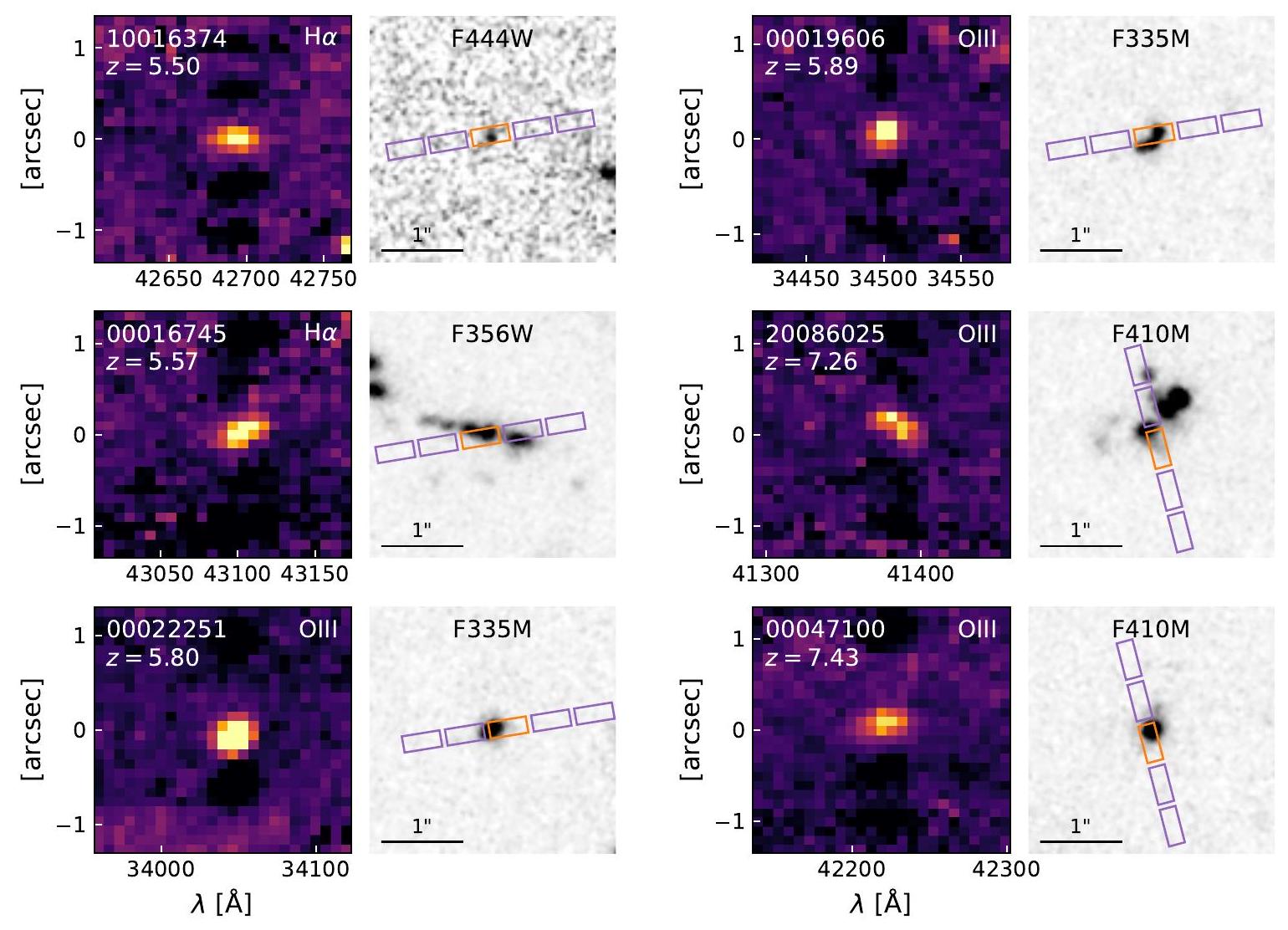
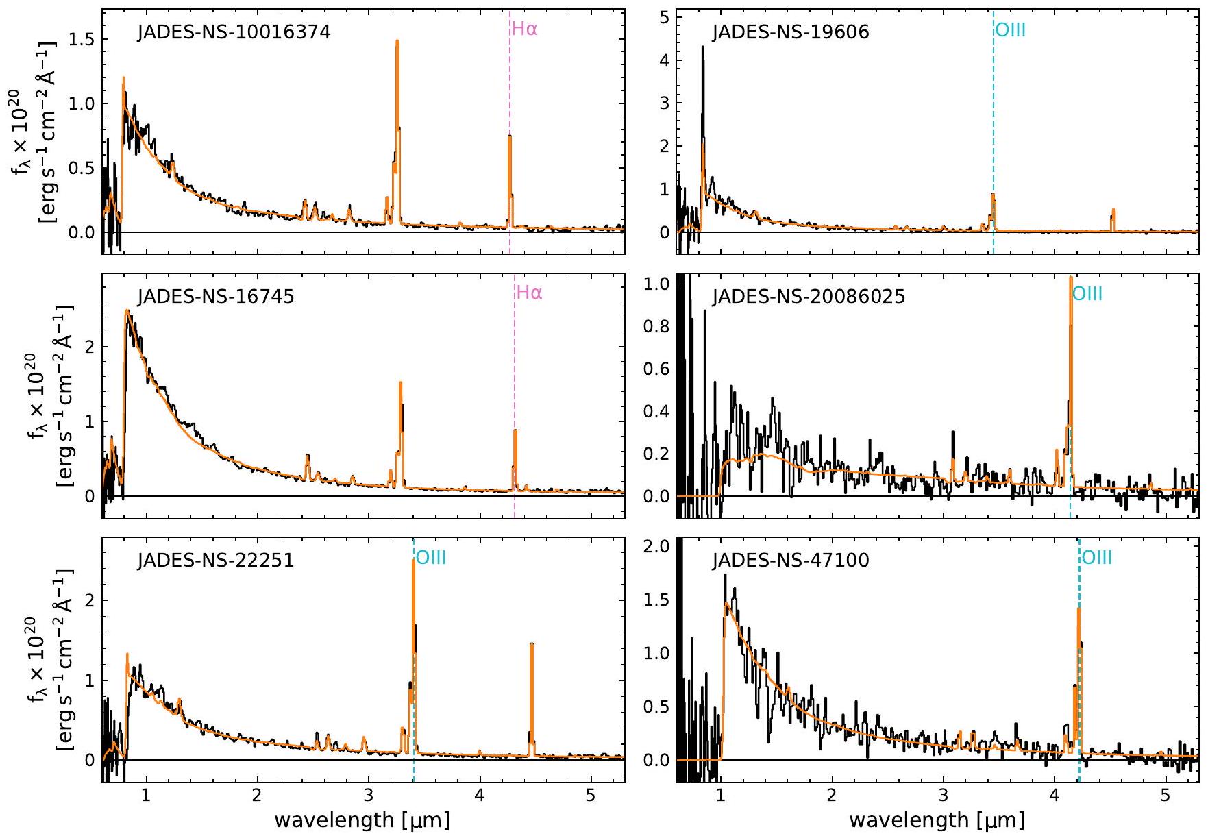
تُعرض الصور المركبة والمصححة ثنائية الأبعاد لخطوط الانبعاث في الشكل 1 مع قصاصات من تصوير NIRCam، حيث اخترنا فلتر NIRCam الأقرب إلى خط الانبعاث كما هو موضح في القسم السابق. تظهر مواقع الميكروشتر في اللون البرتقالي.
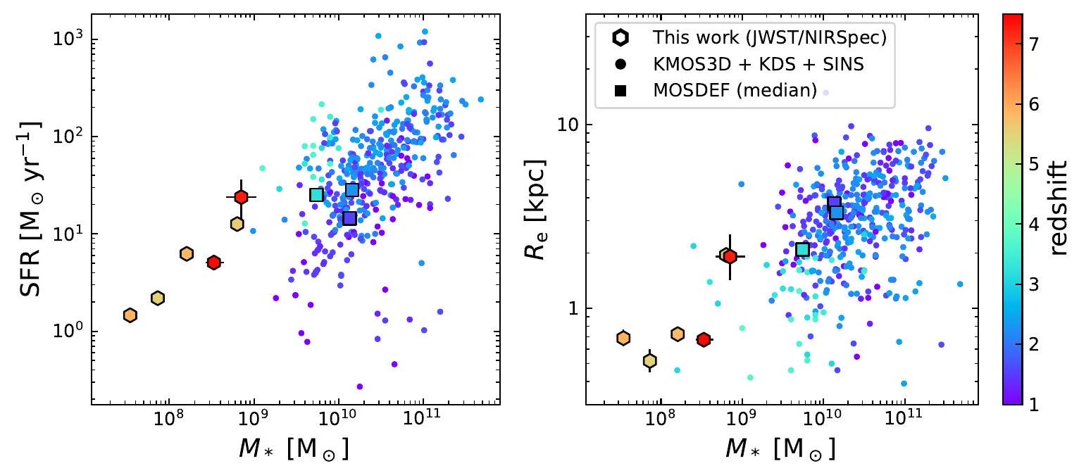
نلاحظ أنه نظرًا لوظيفة الاختيار المعقدة لـ JADES (بانكر وآخرون 2023) ومعايير الاختيار الإضافية التي فرضناها أثناء الفحص البصري، فإن العينة المختارة بعيدة عن الاكتمال من حيث (الكتلة النجمية) أو السطوع أو معدلات تكوين النجوم. ومع ذلك، هدفنا هو إظهار قدرة NIRSpec/MOS على قياس حركيات المجرة في نظام جديد تمامًا: الشكل 2 يظهر
أن الأهداف في عينتنا ليست فقط عند انزياح أحمر أعلى مما كان ممكنًا حتى الآن مع مطياف الأشعة تحت الحمراء القريب القائم على الأرض، ولكنها أيضًا أصغر بكثير وأقل كتلة. نؤجل تحليلًا شاملاً لحركيات المجرة كدالة للانزياح الأحمر والكتلة إلى ورقة مستقبلية، حيث سيتطلب ذلك مجموعات بيانات JADES وNIRSpec WIDE الكاملة (آيزنشتاين وآخرون 2023؛ ماسيدا وآخرون، في الإعداد) بالإضافة إلى فهم شامل لوظائف الاختيار لمستويات المسح المختلفة.
3. النمذجة الديناميكية
استخدمنا نهج النمذجة الأمامية بايزي لتقدير الخصائص الديناميكية للمجرات من طيف الانبعاث ثنائي الأبعاد، الذي تم رصده من خلال فتحات MSA الخاصة بـ NIRSpec. أولاً، قمنا بإنشاء مكعبات نموذجية بارامترية لتوزيع الفلكس ( ) بناءً على ملفات السطوع السطحي التحليلية وملفات السرعة. ثانياً، نمذجة التعقيدات الخاصة بأداة NIRSpec التي تُطبع على البيانات عند رسم النماذج الحركية على كاشف NIRSpec وهمي. ثالثاً، استخدمنا طريقة أخذ العينات MCMC لتناسب النماذج مع الأطياف، معتمدين على ملاءمات ملف سيرسيك لتصوير NIRCam كأولوية. نحن نؤجل وصفًا تفصيليًا لهذا البرنامج الخاص بالنمذجة الأمامية والتناسب (msafit) إلى ورقة مستقبلية، حيث سنظهر أيضًا اختبارات التقارب والمقارنة مع بيانات المعايرة. في هذا القسم، نقدم فقط نظرة عامة ملخصة عن النماذج والبرامج، التي نطلقها علنًا مع هذه الورقة .
3.1. نماذج القرص الرقيق
على الرغم من أن الدقة المكانية والطيفية لـ JWST/NIRSpec عالية، فإن الأنظمة الصغيرة في عينتنا قريبة من حد الدقة. وهذا يشير إلى أنه يجب علينا أن نقتصر على نموذج هندسي وديناميكي بسيط نسبيًا: قرص رقيق دوار. على الرغم من أنه رقيق هندسيًا، سمحنا للقرص بأن يكون دافئًا حركيًا من خلال إضافة ملف تشتت السرعة. نناقش القيود المحتملة لاختيار نموذجنا في القسم 5.
قمنا بنمذجة توزيع الفلكس المكاني لخط الانبعاث كملف سيرسيك (سيرسيك 1968)، الذي يتم وصفه بأربعة معلمات: الفلكس الكلي ، نصف قطر الضوء (المحور الرئيسي)، نسبة المحور الصغير إلى المحور الكبير المتوقعة ، ومؤشر سيرسيك . حيث افترضنا نموذج القرص الرقيق، فإن نسبة المحور المتوقعة مرتبطة مباشرة بزاوية الميل (i) للنظام. بالإضافة إلى ذلك، تدخل ثلاث معلمات مهمة تعتمد على الموقع في النموذج: زاوية الموقع (PA) بالنسبة لفتحة MSA كما تم قياسها من المحور الإيجابي – (أي، درجة تمثل المحاذاة المثالية مع الشق)، وموقع مركز الثقل للجسم داخل الغالق.
بالنسبة لحقل السرعة، استخدمنا الوصف التجريبي الشائع لمنحنى دوران القوس (Courteau 1997)، ,
حيث هي السرعة الحدية أو القصوى بالنسبة للسرعة النظامية للمجرة، و هو نصف قطر التحول. قمنا ببرمجة السرعة النظامية كمتوسط الطول الموجي لخط الانبعاث . للسماح بقرص دافئ حركيًا،
الشكل 1. عينة من ستة أجسام عالية الانزياح الأحمر ذات دقة مكانية في JADES. تظهر الألواح اليسرى قصاصات من خطوط الانبعاث في الأطياف المجمعة والمست rectified ثنائية الأبعاد التي تم الحصول عليها باستخدام شبكة G395H عالية الدقة. السلبيات في القصاصات هي نتيجة لطريقة طرح الخلفية. تظهر الألواح اليمنى قصاصات صورة NIRCam لكل جسم (JADES و FRESCO) للنطاق الذي يشبه أكثر شكل خط الانبعاث (القسم 2.2). تؤدي الشقوق الثلاثة للغالق ونمط التلويح ثلاثي النقاط الذي استخدمناه إلى منطقة فعالة من خمسة غالق: الغالق الذي يحيط بالمصدر يظهر باللون البرتقالي، والغالق المستخدم لطرح الخلفية يظهر باللون الأرجواني.
افترضنا أيضًا ملف تشتت سرعة ثابت عبر القرص.
مجمعة، هذا يشكل نموذجًا مكونًا من 11 معلمة (، ، و ). قمنا بدمج ملف الفلكس وملفات السرعة لتشكيل مكعب فلكس نموذجي ، حيث و هي الإحداثيات في مستوى MSA وتم أخذ عينات في فترات يحددها المستخدم. لبناء هذه المكعبات، تأكدنا من أن الأبعاد المكانية والطول الموجي تم أخذ عينات عليها على الأقل عند تردد نايكويست لوظيفة انتشار النقطة (PSF) عند الطول الموجي المعني أو حجم بكسل NIRSpec (0.1″)، أيهما أصغر. ومع ذلك، ستكون هذه العينة نادرة جدًا لتقييم ملفات سيرسيك الحادة عند نصف قطر صغير. من أجل دمج ملفات سيرسيك بدقة، قمنا أولاً بأخذ عينات زائدة للشبكة المكانية ديناميكيًا، بحيث تم أخذ عينات المنطقة الداخلية () بعامل 500 والمناطق الخارجية () بعامل 10، ثم دمجنا الملف على الشبكة الأكثر خشونة.
3.2. النمذجة الأمامية لـ NIRSpec MSA
على الرغم من أنه تم تطوير برامج النمذجة الأمامية لعلم الطيف متعدد الأجسام القائم على الشقوق من قبل (Price et al. 2016)، هناك العديد من التحديات الفريدة لنمذجة بيانات NIRSpec MOS: (i) PSF المحدودة الانكسار لـ JWST، التي تمكن من دقة مكانية عالية، لكنها معقدة للغاية في الشكل. (ii) الهندسة المعقدة لـ NIRSpec MSA، التي تتكون من ميكروغالق مفصولة بجدران الغالق، تطبع
أنماط انكسار إضافية (على شكل زائد بسبب فتحة الشق) بالإضافة إلى الظلال على الكاشف (“ظلال الشريط”). أخيرًا، (iii) تشير البكسلات الكبيرة نسبيًا () لكاشف NIRSpec إلى أن PSF غير مأخوذ بعين الاعتبار عند جميع الأطوال الموجية .
نتيجة للتحديين الأول والثاني، يتغير شكل PSF داخل الغالق بشكل كبير. غالبًا ما تكون الأجسام خارج المجرة ذات الانزياح الأحمر العالي مشابهة في الحجم لعرض PSF الخاص بـ NIRSpec وحجم البكسل، وبالتالي فإن موقع مركز الثقل للفلكس داخل الغالق يؤثر بشدة على شكل توزيع الفلكس على الكاشف. علاوة على ذلك، فإن جدران الغالق () صغيرة نسبيًا مقارنة بحجم البكسل، مما يجعل تأثيرات ظلال الشريط معقدة للنمذجة. أخيرًا، فإن المنطقة المفتوحة للميكروغالق صغيرة نسبيًا (; Jakobsen et al. 2022) مقارنة بحجم PSF. لذلك، فإن خسائر الشقوق كبيرة، حتى في مركز الغالق.
حاولنا التقاط كل هذه التأثيرات ضمن نمذجة لدينا. أولاً، قمنا بإنشاء مكتبات من نماذج PSF الاصطناعية على مجموعة من الأطوال الموجية المختلفة والانحرافات المكانية، مع مراكز PSF تأخذ عينات من الغالق كل واستخدام عامل أخذ عينات زائد خمسة لصور PSF. تمثل هذه PSFs الصورة ثنائية الأبعاد لمصدر نقطة مع خط انبعاث ضيق بشكل لا نهائي في مستوى الكاشف، والذي يحتوي بالتالي على كل من التوزيع المكاني على طول الشق والتوزيع في اتجاه الطول الموجي. قمنا بإنشاء PSFs باستخدام
الشكل 2. توزيع عينة في فضاء المعلمات لكتلة النجوم، SFR، ونصف قطر خط الانبعاث، مشفر بالألوان حسب الانزياح الأحمر. نقارن هذا مع مجموعة من المسوحات الطيفية القريبة من الأشعة تحت الحمراء التي أجريت على الأرض والتي استخدمت خطوط و [OIII] لقياس الحركيات المجرة عند (Turner et al. 2017; Förster Schreiber et al. 2018; Wisnioski et al. 2019; Price et al. 2020). استخدمنا SFRs من UV+IR من Whitaker et al. (2014) حيثما كان ذلك متاحًا لعينة Turner et al. (2017). نلاحظ أن جميع الأجسام عند من KMOS3D تظهر في هذه الصورة، لكن لم يتم استخدام جميع الأجسام في الدراسات الحركية لأن نسبة الإشارة إلى الضوضاء كانت منخفضة أو كانت الأجسام صغيرة جدًا. العينة المختارة من JADES (السداسيات) تستكشف نظامًا مختلفًا تمامًا: تستهدف JADES في انزياح أحمر أعلى وكتلة نجمية أقل مما تم استكشافه حتى الآن بواسطة المرافق الأرضية.
محاكاة بصرية فورية مخصصة، تتبع مصادر النقاط أحادية اللون عبر NIRSpec إلى مستوى بؤرة الكاشف. تلتقط هذه النماذج PSF المدمجة لـ JWST و NIRSpec، بما في ذلك الانكسار وفقدان الضوء (غالبًا ما يُشار إليه بفقدان المسار) الناتج عن حجب شقوق الميكرو شاتر وبؤرة الطيف. نحن نؤجل الوصف التفصيلي إلى دي غراف وآخرون (قيد الإعداد)، لكن نلاحظ أن بناء هذه PSFs هو إلى حد كبير نفس ما تم تقديمه أو استخدامه في الأعمال السابقة التي قدمت أو استخدمت محاكي أداء أداة NIRSpec (IPS؛ بيكيراس وآخرون 2008، 2010؛ جياردينو وآخرون 2019؛ ياكوبسن وآخرون 2022). الاختلاف الرئيسي هو أن التنفيذ المستخدم في هذا العمل يعتمد على بايثون ويستخدم مكتبات انتشار البصريات الفيزيائية في بايثون (POPPY؛ بيرين وآخرون 2012)، مما يسمح بأخذ عينات مستقلة عن الطول الموجي بدقة في كل من صور الكاميرا ومستوى البؤرة. على الرغم من أن هذه النماذج تعتمد على المعايرات أثناء الطيران حيثما كان ذلك ممكنًا، تم إنشاء عدد من ملفات المرجع الضرورية قبل الإطلاق. لذلك، نحذر من أنه من المحتمل أن يكون هناك عدم يقين منهجي في العرض الحقيقي وشكل هذه PSFs. للأسف، لا توجد حاليًا بيانات معايرة كافية أو مخصصة. نناقش الحالة الحالية للمعايرات بمزيد من التفصيل في الملحق أ، ونقدر عدم اليقين المنهجي في في عرض PSF الكامل عند نصف الحد الأقصى (FWHM؛ كل من المكاني والطيفي) لنماذجنا.
ثانيًا، قمنا بإنشاء مكتبات من المسارات الطيفية لجميع الميكرو شاتر والمشتتات، باستخدام نموذج الأداة لدورنا وآخرون (2016) وجياردينو وآخرون (2016)، والتي تم ضبط معلماتها خلال مرحلة التكليف أثناء الطيران (لوتزديندورف وآخرون 2022؛ ألفيس دي أوليفيرا وآخرون 2022). توفر هذه المسارات خريطة من مركز شاتر معين والطول الموجي المختار إلى مستوى الكاشف . استخدمنا أيضًا هذا النموذج لاشتقاق زاوية الميل للشقوق بالنسبة للمسار في مستوى الكاشف (بضع درجات لـ G 395 H).
ثالثًا، قمنا بإنشاء كواشف نموذجية، حيث يتم أخذ عينات البكسلات في البداية بمعدل 5 مرات. لتقليل التكلفة الحاسوبية، لم نقم بنمذجة الكواشف الكاملة ، ولكن أنشأنا قصاصات بحوالي بكسل حول منطقة ذات اهتمام، مع تتبع إحداثيات الكاشف المقابلة.
مع هذه المكتبات والنماذج في مكانها، قمنا بنمذجة مكعب التدفق التحليلي من القسم 3.1. نظرًا لأن PSF يتغير بشكل كبير مع موضع الشاتر الداخلي، لا يمكن أن يتم دمج مكعب النموذج مع PSF واحد. بدلاً من ذلك، عالجنا مكعب النموذج كمجموعة من مصادر النقاط، وبالتالي قمنا بنشر كل نقطة في المكعب مع PSF المحلي الخاص بها. ثم تم إسقاط شرائح مكعب النموذج على الكاشف النموذجي المأخوذ بعين الاعتبار باستخدام مكتبة المسار، مع تحديد شاتر . أخيرًا، تم تقليل حجم الكاشف بمعدل 5 مرات ليتناسب مع الحجم الحقيقي لبكسل الكاشف، وتم دمجه مع نواة لمحاكاة تأثيرات الربط السعوي بين البكسلات (IPC). أدى ذلك إلى صورة نموذجية خالية من الضوضاء لمكعب بيانات الإدخال على الكاشف.
3.3. ملاءمة النموذج
تولد إجراءات القسم 3.2 نموذجًا لمجموعة واحدة من المعلمات. لتقدير توزيعات الاحتمالات اللاحقة للمعلمات، استخدمنا عينة مجموعة MCMC المنفذة في حزمة emcee (فورمان-ماكي وآخرون 2013).
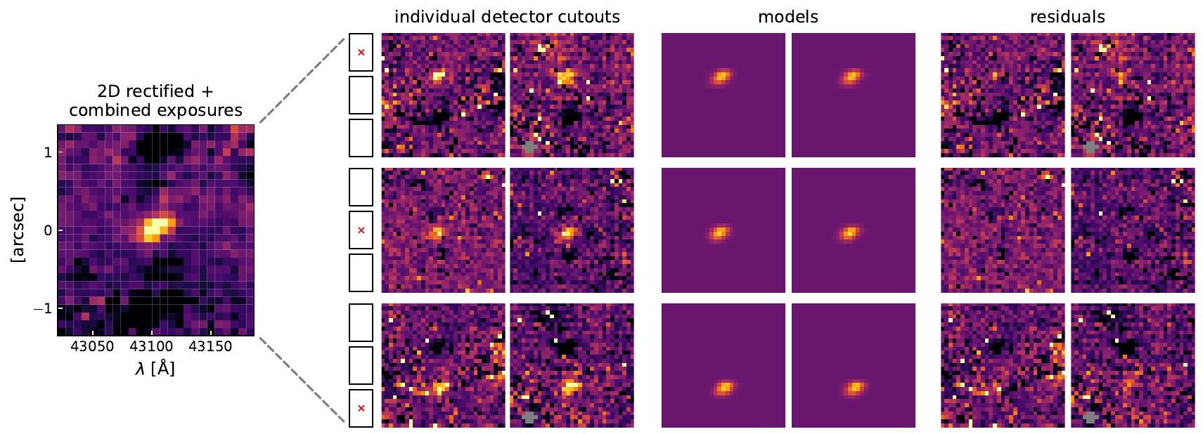
من المهم، أننا قمنا بإجراء المقارنة بين النماذج والبيانات في مستوى الكاشف لتخفيف الضوضاء المرتبطة. لذلك لم نستخدم الطيف المدمج ثنائي الأبعاد، ولكن قمنا بملاءمة متعددة التعرضات في وقت واحد (الشكل 3)، مع حجب البكسلات التي تم الإشارة إليها على أنها متأثرة بأشعة كونية أو بكسلات ساخنة. دالة الاحتمالية لمجموعة من المعلمات هي
حيث هو عدد التعرضات، هو عدد البكسلات غير المحجوبة لكل تعرض، و و و
هي
الشكل 3. مثال على إجراء الملاءمة لكائن JADES-NS-00016745 (الشكل 1). على الرغم من أن التركيبة النهائية لجميع التعرضات (يسار) تم استخدامها لفحصنا البصري الأولي واختيار العينة، فإن البكسلات في هذا الطيف مرتبطة بشدة. بدلاً من استخدام هذا الطيف المدمج، قمنا بملاءمة جميع التعرضات الفردية التي تم الحصول عليها في وقت واحد. في حالة JADES-NS-00016745، تم أخذ تعرضين لكل موضع تمايل، مما أدى إلى ستة قياسات مستقلة لنمط تمايل ثلاثي النقاط مع NIRSpec. لأخذ في الاعتبار PSF غير المأخوذ بعين الاعتبار لـ NIRSpec، قمنا بنمذجة في مستوى الكاشف، ناشرين النماذج البارامترية إلى نفس الموقع بالضبط على الكاشف كما هو الحال مع البيانات الملاحظة. ثم يتم حساب الاحتمالية من تركيبة جميع الصور المتبقية. يتم حجب البكسلات التي تم الإشارة إليها من خلال خط أنابيب التخفيض على أنها متأثرة بأشعة كونية وتظهر باللون الرمادي.التدفق المرصود، التدفق النموذجي، وعدم اليقين في البكسل
، على التوالي.Å) للطول الموجي، و
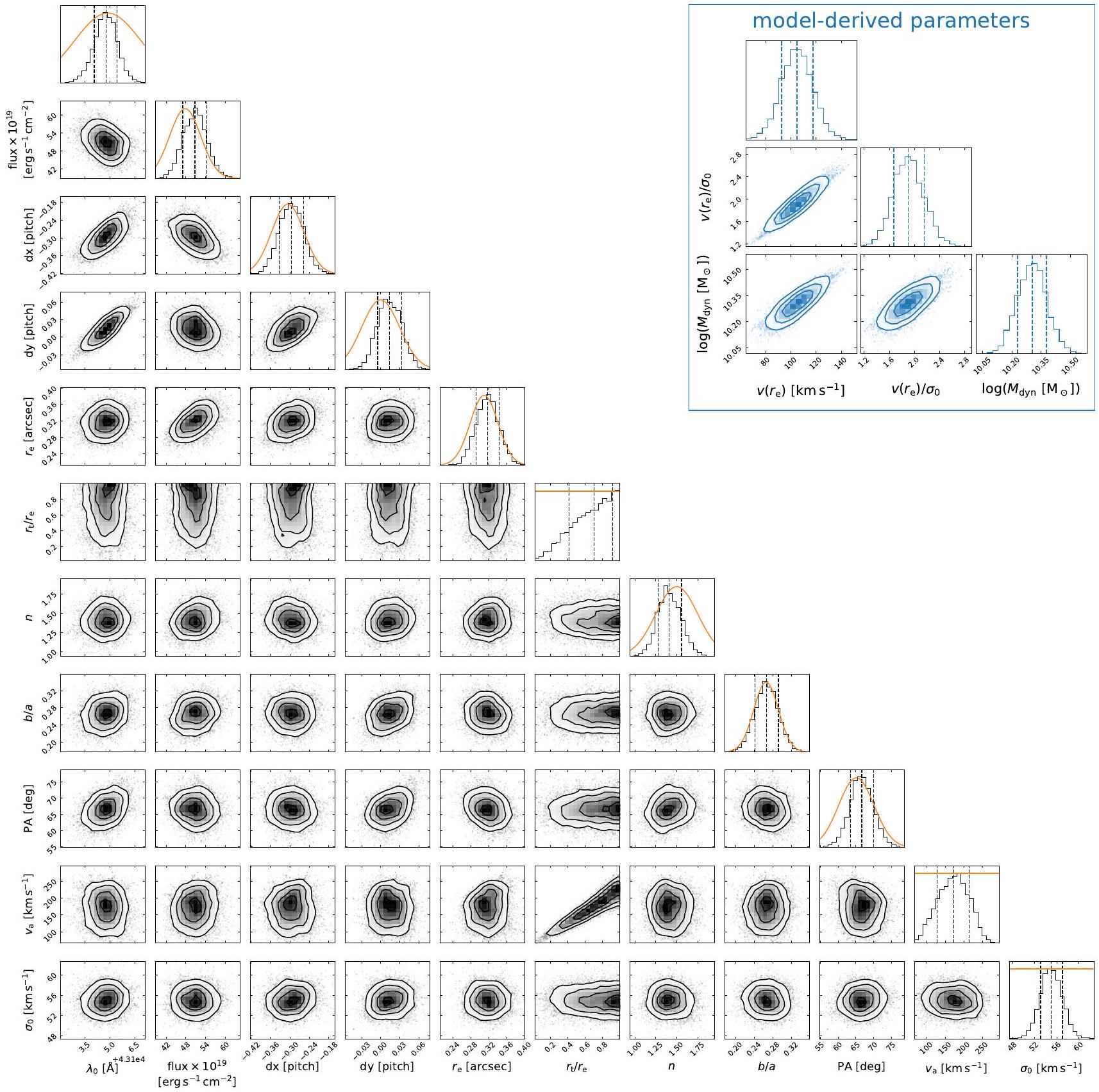
عدم يقين في التدفق الكلي على الكاشف. أخيرًا، سمحنا بعدم يقين صغير في موضع الشاتر الداخلي للمصدر بسبب دقة التوجيه المحدودة لـ JWST، والتي استخدمنا لها أولويات غاوسية بتشتت قدره 25 mas، وهي دقة التوجيه النموذجية بعد اكتساب هدف MSA (بكر وآخرون 2023).بالنسبة لمعلمات النموذج الديناميكي، السرعة القصوى () وتشتت السرعة ()، استخدمنا أولويات موحدة. بالنسبة للملاءمة، قمنا ببارامترية نصف قطر التحول كنسبة ، وافترضنا أولوية موحدة لهذه النسبة. نعرض مثالًا على الملاءمة في الأشكال 3 و 4، مما يوضح أن و محددان بشكل جيد رسميًا ( دلالة). نصف قطر التحول غير محدد بشكل جيد ويشكل أكبر مصدر لعدم اليقين في بسبب التداخل بين و . من المحتمل أن يكون ذلك بسبب مزيج من الدقة المكانية المتوسطة ومدى المساحة المحدودة التي تم استكشافها بواسطة الميكرو شاتر. في القسم 4، نقوم بدلاً من ذلك بحساب السرعة الدورانية عند ، والتي يتم تحديدها بشكل أفضل من خلال البيانات (التوزيعات الزرقاء في الجزء العلوي الأيمن من الشكل 4).
نلاحظ أن مدى المصدر النسبي الكبير مقارنة بحجم الشاتر قد يؤدي أيضًا إلى فقدان التدفق، حيث أن خطوة طرح الخلفية في خط أنابيب التخفيض تطرح التدفق من المصدر (المجاور) الذي يقع في الشاتر المجاور. لاختبار حجم هذا التحيز المحتمل، قمنا أيضًا بنمذجة على تخفيض منفصل استبعد التعرضات التي يقع فيها المصدر في الشاتر المركزي وشمل فقط التمايلات الخارجية، مما يقلل من أي طرح ذاتي وتلوث (لكن على حساب انخفاض طفيف في الإجمالي. نجد أن التدفق المستعاد متسق ضمن حدود الخطأ مع الملاءمة للتقليص القياسي الذي يستخدم جميع مواضع التموج الثلاثة. لذلك، فإن نموذجنا قوي ضد الانخفاض الذاتي الطفيف الموجود في الطيف، والذي ساعده على الأرجح المعلومات السابقة المقدمة من تصوير NIRCam ومدى الامتداد المكاني الصغير نسبيًا للمصادر مقارنة بحجم الغالق.
4. النتائج
4.1. حركيات الغاز المؤين عند
نقدم نتائج نمذجة عينة من ستة أجسام في الجداول 2 و 3. تم الكشف عن دوران كبير في ثلاثة من الأجسام وتم الكشف عنه بشكل هامشي أو متسق مع الصفر في الحالات الأخرى. نظرًا لأننا لم نقم بإزالة المجرات التي تتماشى بشكل كبير مع الشق، قد تحتوي بعض هذه الأجسام (مثل الجسم JADES-NS-00019606) على تدرج سرعة لا يمكن ملاحظته ببساطة عند زاوية موضع الغالق هذه. ومع ذلك، فإن قياس تشتت السرعة لا يزال مفيدًا في هذه الحالات، كما أنه يوفر تأكيدًا على أن نموذجنا قادر على العودة على الرغم من افتراضنا المسبق بأن النظام يدور.
نجد أن تشتت السرعة لخمس أجسام أوسع من وظيفة انتشار الخط (LSF) للأداة لمصدر نقطي ( ; انظر الملحق A)، والذي
الشكل 4. رسم الزاوية لنموذج القرص الرقيق ذو 11 معلمة للجسم في الشكل 3. تُظهر المدرجات توزيع الاحتمالات اللاحقة. تشير الخطوط البرتقالية إلى توزيعات الاحتمالات السابقة. نجد عمومًا قيودًا جيدة على المعلمات الحركية و ، على الرغم من أن نصف القطر المتغير غير محدد بشكل جيد ومتداخل مع سرعة الدوران. تُظهر اللوحات العلوية اليمنى (باللون الأزرق) المعلمات التي استخلصناها من النموذج والتي تم مناقشتها في القسم 4.
هي LSF ذات الصلة بعد الأخذ في الاعتبار شكل المصدر. الشكوك الرسمية حول التشتت صغيرة، وهو ما يرجع على الأرجح إلى افتراضنا لقرص رقيق، مما يعني أن تقديرنا للخطأ على لا يتضمن عدم اليقين الناجم عن التداخل بين سمك القرص الحقيقي وزاوية الميل. الجسم السادس (JADES-NS-20086025) له شكل معقد للغاية مع انبعاث منتشر واضح (خط). نظرًا لانخفاض لهذا الانبعاث والمنطقة المزدحمة حول الهدف، فإن الملاءمة الشكلية لصورة F410M باستخدام lenstronomy لهذا الجسم لا تتقارب. لذلك، لنمذجة الديناميات، قمنا بتخفيف القيود الشكلية بشكل كبير لهذا الجسم: قمنا بتعيين قيود موحدة على مؤشر سيرسيك، وفرضنا فقط قيودًا ضعيفة
على نصف القطر الفعال (قيود غاوسية من )، نسبة المحور (قيود غاوسية من )، وزاوية الموضع ( ). وجدنا تقاربًا للنموذج الديناميكي، على الرغم من أن العديد من المعلمات المستنتجة لديها شكوك أكبر من الأجسام الأخرى في عيّنتنا.
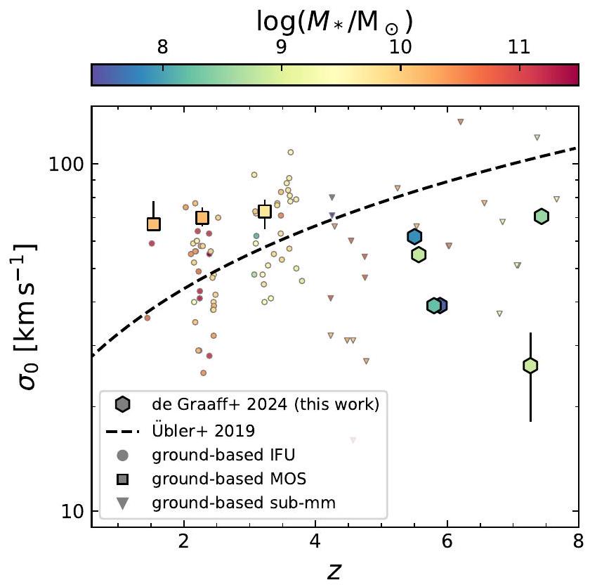
الشكل 5 يُظهر تشتت السرعة لعينة لدينا كدالة من الانزياح الأحمر. قارننا ذلك مع مجموعة من الدراسات القريبة من الأشعة تحت الحمراء القائمة على الأرض: نتائج MOS لـ Price et al. (2020، الوسيطات لعينة مفككة ومتوافقة)، عينات IFU لـ Turner et al. (2017) و Förster Schreiber et al. (2018)، والملاءمة التحليلية لاستطلاع IFU الكبير KMOS3D عند من Übler et al. (2019).
الجدول 2. نتائج النمذجة الديناميكية: الخصائص الشكلية وطول الموجة.
معرف
( )
التدفق ( )
(خط)
dy (خط)
(ثانية قوسية)
زاوية الموضع (درجة)
JADES-NS-00016745
JADES-NS-00019606
JADES-NS-00022251
JADES-NS-00047100
JADES-NS-10016374
JADES-NS-20086025
ملاحظات. القيم هي الوسيط لتوزيعات الاحتمالات اللاحقة، وتعكس الشكوك النسب المئوية 16 و 84. يتم قياس الانحرافات داخل الغالق من حيث خط الغالق بدلاً من الثواني القوسية لأن هذه الوحدة ثابتة لجميع الغالق ولا تعتمد على التشوه المكاني عبر MSA. يتم مناقشة شكل هذا المصدر أيضًا في Baker et al. (2023).
الجدول 3. نتائج النمذجة الديناميكية: الخصائص الديناميكية والكميات المستمدة من النموذج.
معرف
( )
( )
( )
JADES-NS-00016745
JADES-NS-00019606
JADES-NS-00022251
JADES-NS-00047100
JADES-NS-10016374
JADES-NS-20086025
ملاحظات. القيم هي الوسيط لتوزيعات الاحتمالات اللاحقة، وتعكس الشكوك النسب المئوية 16 و 84. تشير إشارة معلمة النموذج إلى الاتجاه المرصود لتدرج السرعة على طول الشق.
تشير استقراء الملاءمة بواسطة Übler et al. (2019) عند إلى إلى أن الغاز المؤين في المجرات متقلب للغاية في العصور المبكرة. بالمقابل، نجد أن جميع الأجسام تقع تحت هذا الاستقراء، وبدلاً من ذلك لديها تشتت سرعات يساوي تقريبًا متوسط التشتت عند . من ناحية أخرى، فإن الكتلة النجمية النموذجية لعينة لدينا أقل بكثير من بيانات الأدبيات (الشكل 2). إذا كان تشتت السرعة يعتمد على الكتلة النجمية (كما تنبأت المحاكاة، مثل Pillepich et al. 2019)، فقد لا يزال يحتوي ISM في هذه الأنظمة منخفضة الكتلة على تقلبات عالية نسبيًا.
كما قارننا نتائجنا مع الدراسات التي استخدمت ALMA لحل حركيات المجرات عند نفس الانزياح الأحمر مثل عيّنتنا (مثلثات زرقاء؛ Neeleman et al. 2020؛ Rizzo et al. 2020، 2021؛ Fraternali et al. 2021؛ Lelli et al. 2021؛ Herrera-Camus et al. 2022؛ Parlanti et al. 2023). على الرغم من أن هذه الأجسام تقع عند نفس الانزياح الأحمر، إلا أن القياسات تختلف بشكل كبير: غالبًا ما تكون المجرات المرصودة بواسطة ALMA أكثر كتلة ( )، وتميل خطوط الانبعاث المرصودة إلى تتبع غاز أبرد بكثير. من المثير للاهتمام، على الرغم من هذه الاختلافات، أن تشتت السرعة المستند إلى ALMA مشابه جدًا لقياساتنا للغاز المؤين بناءً على خطوط الانبعاث الضوئية في إطار الراحة. قد يكون السبب في ذلك هو أن تأثيرات الكتلة الأعلى ودرجة حرارة الغاز المنخفضة على تشتت السرعة تعمل في اتجاهين متعاكسين. ستكون الملاحظات لنفس الأنظمة باستخدام كل من ALMA و JWST حاسمة لتقييد هذه التأثيرات.
بعد ذلك، قمنا بحساب النسبة وفحصنا اعتمادها على الانزياح الأحمر في الشكل 6 من خلال مقارنتها بنفس الأدبيات المذكورة سابقًا. أظهرت الدراسات حول الظهر الكوني انخفاضًا واضحًا وتدريجيًا في درجة الدعم الدوراني نحو انزياح أحمر أعلى. بناءً على هذه القياسات، قد نتوقع أن لا تكون أي من المجرات مهيمنة
بالدوران ( ). ومع ذلك، نجد تنوعًا مثيرًا للاهتمام في عيّنتنا، حيث أن ثلاثة أجسام منها لديها حتى عند أعلى الانزياحات الحمراء ( ). نناقش في القسم 5 ما إذا كانت هذه الأجسام قد تشكل حقًا أقراص دوارة باردة، أو إذا كانت تعكس تدرجات السرعة داخل أنظمة غير مفعلة.
مرة أخرى، قارننا عيّنتنا مع الدراسات المستندة إلى ALMA، والتي هي جميعها أنظمة مهيمنة بالدوران مع نسب مرتفعة نسبيًا. تُظهر عيّنتنا تنوعًا أكبر، وهو ما قد يرجع إلى حقيقة أن مؤشرات الغاز تختلف وأن نطاق الكتلة المستكشف مختلف بشكل كبير. قد يؤدي عدم توافق بعض الأجسام مع الغالق الصغير أيضًا إلى التقليل من تقدير النسبة لبعض الأنظمة. لذلك، هناك حاجة إلى عينات أكبر لفهم الخصائص الحركية المختلفة لمراحل الغاز التي تتبعها ALMA و JWST عند الانزياحات الحمراء العالية.
أخيرًا، نعيد زيارة القسم 2.2، حيث وصفنا أنه بالنسبة لجسمين من ستة، فإن صورة NIRCam المستخدمة كأولوية في نمذجة خطوط الانبعاث تتبع بشكل أساسي انبعاث الاستمرارية النجمية بدلاً من انبعاث الخط. إذا كان شكل خط الانبعاث يختلف بشكل كبير عن الاستمرارية، فقد يؤدي ذلك إلى تحيز المعلمات الحركية المستنتجة، خاصة إذا كانت المجرة ممدودة بدلاً من نموذج القرص الرقيق المفرط الذي نفترضه. أحد هذين الجسمين (JADES-NS-00016745؛ الشكل 3) له محور رئيسي في صورة NIRCam يتماشى جيدًا مع الغالق الصغير، ونلاحظ تدرج سرعة قوي في الطيف ثنائي الأبعاد مع وجود انحراف صغير فقط بين محور PA الرئيسي من التصوير والوسيط لتوزيع الاحتمالات اللاحقة لـ PA (الموضح في الشكل 4). لذلك، فإن الشكل الممدود غير محتمل للغاية لهذا الجسم. طبيعة الجسم الثاني (JADES-NS-100016374) أكثر عدم يقين، حيث أننا نكتشف الدوران بشكل هامشي فقط. إذا كان المحور الرئيسي الحركي للغاز المؤين يختلف بشكل كبير عن المحور الرئيسي الضوئي، فإن الدوران الحقيقي
الشكل 5. تشتت السرعة للغاز المؤين كدالة للانزياح الأحمر. الخط المتقطع يظهر التناسب من Übler وآخرون (2019) للغاز المؤين عند الممتد إلى انزياحات حمراء أعلى، بينما تظهر الدوائر النتائج من مجموعة مختارة من مسوحات IFU الأرضية في الأشعة تحت الحمراء القريبة (Turner وآخرون 2017؛ Förster Schreiber وآخرون 2018) والمربعات نتائج بيانات MOS الأرضية في الأشعة تحت الحمراء القريبة (العينة المحلولة والمتوافقة من Price وآخرون 2020). تظهر المثلثات الزرقاء نتائج من دراسات مختلفة مع ALMA تقيس الحركيات للغاز البارد في المجرات الضخمة التي تشكل النجوم والغنية بالغبار (Neeleman وآخرون 2020؛ Rizzo وآخرون 2020؛ Fraternali وآخرون 2021؛ Lelli وآخرون 2021؛ Rizzo وآخرون 2021؛ Herrera-Camus وآخرون 2022؛ Parlanti وآخرون 2023).
السرعة و قد تكون أعلى بكثير مما تم استنتاجه من نمذجة لدينا.
4.2. مقارنة الكتل الديناميكية والكتل النجمية
استخدمنا النماذج الديناميكية لفحص ميزانية الكتلة للمجرات. بالنسبة لنظام في توازن فيريالي، يتم حساب الكتلة الديناميكية المحصورة ضمن نصف القطر كالتالي
حيث أن هي السرعة الدائرية، و هو معامل فيريال، و هو الثابت الجاذبي. ومع ذلك، للمقارنة مع الكتلة النجمية الكلية، نعرف الكتلة الديناميكية ‘الكلية’ كما هو موصوف في Price وآخرون (2022)،
كما افترضنا نموذج القرص الرقيق، اعتمدنا ، وهو معامل فيريال لإمكان مفلطحة مع و (Price وآخرون 2022، الشكل 4). ومع ذلك، فإن الشكل الحقيقي للإمكان غير محدد بشكل جيد، وبالتالي فإن هذا الاختيار لـ يقدم عدم يقين منهجي في تقديرات الكتلة الديناميكية لأن يمكن أن يتغير بمقدار يصل إلى عامل 2.
بعد Burkert وآخرون (2010)، قمنا بحساب السرعة الدائرية كالتالي
الشكل 6. الدعم الدوراني كدالة للانزياح الأحمر، مقاسًا كنسبة السرعة عند نصف القطر الفعال وتشتت السرعة الثابت: . على الرغم من أن الدراسات المستندة إلى بيانات الأشعة تحت الحمراء القريبة الأرضية (كما هو موصوف في الشكل 5) قد وجدت انخفاضًا واضحًا وتدريجيًا في نحو انزياح أحمر أعلى، نجد تنوعًا مثيرًا للاهتمام بين عينة المجرات منخفضة الكتلة لدينا، مع وجود أقراص ديناميكية باردة ربما موجودة منذ .
الذي يأخذ في الاعتبار تأثيرات تدرجات الضغط على السرعة الدورانية ويعتمد على طول مقياس القرص . عند نصف القطر الفعال، يتقلص مصحح الضغط إلى . نلاحظ أنه بالنسبة للجسم الوحيد ذو الشكل المفلطح أو الممدود غير المؤكد (القسم 4.1)، قد يكون هذا الحساب لـ غير صحيح. ومع ذلك، كما تم مناقشته في القسم 5.2، من المحتمل أن تكون الكتلة الديناميكية المستنتجة أقل تأثرًا.
بعد ذلك، قارننا هذه الكتل الديناميكية الكلية مع الكتل النجمية. لتقدير الكتل النجمية ومعدلات تشكيل النجوم، قمنا بإجراء نمذجة SED باستخدام كود التناسب بايزي BEAGLE (Chevallard & Charlot 2016) لطيف الأشعة تحت الحمراء المنخفضة الدقة. تم تشغيل التناسبات بافتراض تاريخ تشكيل نجمي مكون من مكونين يتكون من أسلوب أسي متأخر مع انفجار حالي، ودالة كتلة أولية من Chabrier (2003) بحد أعلى للكتلة قدره ، وقانون إضعاف الغبار من Charlot & Fall (2000) بافتراض من الغبار في ISM المنتشر. نلاحظ أن أطياف الأشعة تحت الحمراء 1D تم معايرتها من حيث التدفق بافتراض شكل يشبه النقطة ودون النظر في فوتومترية NIRCam. على الرغم من أن تصحيح فقدان الشق هذا يصحح تقريبًا لتغير PSF FWHM مع الطول الموجي، إلا أن هناك انزياحًا منهجيًا بين التدفق الكلي للجسم والتدفق الملتقط بواسطة الشق. قدرنا هذا التصحيح باستخدام برنامج النمذجة لدينا والشكل في فلتر الطول الموجي الطويل (؛ مقاسًا باستخدام lenstronomy كما هو موصوف في القسم 3.3)، ووجدنا عوامل تصحيح في النطاق 1.2-2.5، وطبقنا ذلك على الكتل النجمية ومعدلات تشكيل النجوم. يتم تقديم الخصائص المستنتجة في الملحق ب، مع مثال لطيف طيفي ونموذج SED.
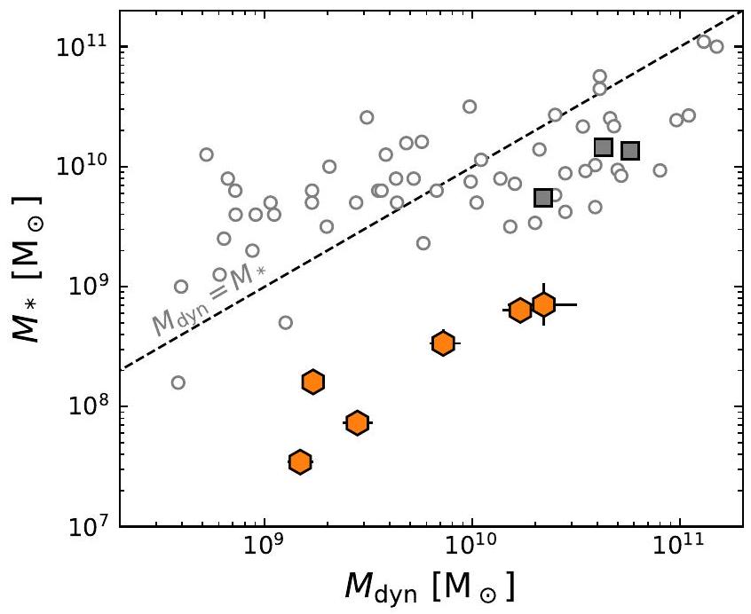
نقارن الكتل الديناميكية والنجمية المقدرة في الشكل 7، وللإشارة، نرسم نفس الدراسات الأرضية في الأشعة تحت الحمراء القريبة كما في الأشكال 5 و6. كما قد يُتوقع من حقيقة أن تشمل الكتلة المظلمة والباريونية، جميع الأجسام
الشكل 7. الكتلة النجمية مقابل الكتلة الديناميكية (المعادلة (4)) كما تم استنتاجها من الطيف الضوئي والطيف عالي الدقة، على التوالي. يظهر الخط المتقطع العلاقة واحد إلى واحد بين الكتلتين. النقاط البيانية من الأدبيات (دوائر، مربعات) كما هو موصوف في الشكل 5. كما هو متوقع، الكتل الديناميكية أعلى من الكتل النجمية لجميع الأجسام في عينة لدينا. ومع ذلك، من المدهش أن الكتل الديناميكية أعلى بكثير (حتى عامل من )، مما يشير على الأرجح إلى كتل غاز عالية أو عدم يقين منهجي كبير في تقديرات الكتلة النجمية.
في عينة لدينا لديها كتل ديناميكية تتجاوز الكتل النجمية المقدرة. ومع ذلك، فإن الفرق بين الكتلتين أكبر بكثير مما كان عليه في الدراسات السابقة. ينحرف بمقدار يصل إلى عامل 30 في المتوسط. فقط Topping وآخرون (2022) أبلغوا عن اختلافات كبيرة مماثلة بين الكتلة النجمية والديناميكية عند ، ولكن لمجرات أكثر ضخامة واستنادًا إلى قياسات عرض الخط المدمجة مكانيًا بدلاً من النمذجة الديناميكية المحللة مكانيًا، كما في هذه الورقة. نناقش الأصول المحتملة لهذا الاختلاف بين الكتل النجمية والديناميكية بالتفصيل في القسم 5.2.
5. المناقشة
هذه البيانات والنمذجة قد أخذتنا إلى نظام جديد تمامًا من حركيات المجرات: المجرات منخفضة الكتلة عند . نتائج نمذجة لدينا مقيدة بشكل جيد للغاية، والقيود الناتجة على المعلمات (مثل، مقابل ) على ظاهرها تعني نتائج مذهلة. ومع ذلك، فإن نظرة على الشكل 1 توضح أيضًا أن نماذجنا البسيطة المتناظرة قد لا تلتقط الهندسة المعقدة للأنظمة. لذلك، فإن نتائجنا تتطلب وتستدعي مناقشة دقيقة.
5.1. أقراص باردة متكتلة أم اندماجات؟
باستخدام نهج النمذجة الأمامية، تمكنا من تقييد الشكل، وتدرج السرعة، وتشتت السرعة الجوهري لكل جسم من JADES بشكل منفصل. للقيام بذلك، افترضنا نموذجًا أساسيًا لقرص رقيق دوار (القسم 3.1). تشير تدرجات السرعة المقاسة في سياق نموذجنا إلى أن الأنظمة ديناميكيًا باردة نسبيًا مع نسب أعلى مما هو متوقع من (الشكل 6) استنادًا إلى استقراء الدراسات الحركية عند .
ومع ذلك، فقد اقترحت كل من الملاحظات والنماذج النظرية أن معدل الاندماجات (الرئيسية) يرتفع بسرعة نحو (على سبيل المثال، Rodriguez-Gomez وآخرون 2015؛ Bowler وآخرون 2017؛ Duncan وآخرون 2019؛ O’Leary وآخرون 2021). لذلك، من المحتمل أن بعض الأجسام في عينة لدينا هي أنظمة اندماج، أو قد اندمجت مؤخرًا مع مجرة أخرى. نجد بالفعل أشكالًا معقدة (خط انبعاث) لعدة أجسام، وخاصةً واضحة في الأجسام JADES-NS-00016745 وJADES-NS-20086025 (انظر الشكل 1)، وأظهر Baker وآخرون (2023) أن الجسم JADES-NS-00047100 يمكن وصفه بثلاثة مكونات شكلية منفصلة. لذلك، من الممكن أن تعكس السرعات الدورانية المستنتجة تحت فرضية نظام فيريالي في الواقع انزياح السرعة بين جسمين (أو أكثر) أو تدرجات السرعة الناتجة عن التفاعل الجاذبي في مرحلة ما قبل أو ما بعد الاندماج.
من ناحية أخرى، تظهر الملاحظات أيضًا أن المجرات عالية الانزياح الأحمر غالبًا ما تحتوي على كتل كبيرة من تشكيل النجوم، وأن تكتل المجرات بشكل عام يزداد نحو انزياحات حمراء أعلى وكتل أقل (على سبيل المثال، Guo وآخرون 2015؛ Carniani وآخرون 2018؛ Zhang وآخرون 2019؛ Sattari وآخرون 2023). من المهم أن هذه الكتل لا تؤدي بالضرورة إلى نظام غير مستقر عالميًا ويمكن أن تستمر ضمن قرص مدعوم دورانيًا ولكنه دافئ (Förster Schreiber وآخرون 2011؛ Mandelker وآخرون 2014).
مع المقاييس الزاوية الصغيرة واختلافات السرعة ( ) المعنية بالأنظمة المدروسة في هذه الورقة، من الصعب جداً التمييز بين نظام اندماج وكتل تتشكل فيها النجوم مع دوران منظم. لقد تم مناقشة هذه التداخلات بشكل موسع في الأدبيات، على الرغم من أنها كانت في انزياحات حمراء أقل ومقاييس زاوية أكبر (على سبيل المثال، Krajnović et al. 2006؛ Shapiro et al. 2008؛ Wisnioski et al. 2015؛ Rodrigues et al. 2017). استخدم Simons et al. (2019) محاكاة لمجرات الاندماج لبناء ملاحظات وهمية وبالتالي تحديد تكرار تصنيف هذه الأنظمة بشكل خاطئ كأقراص دوارة، مما يظهر أن التصنيفات الخاطئة شائعة جداً ( )، ما لم يتم تطبيق معايير اختيار أقراص صارمة جداً. وبالمثل، أظهر Hung et al. أنه يصبح من الصعب بشكل متزايد التمييز بين الاندماجات والأنظمة الدوارة نحو المراحل اللاحقة في التفاعل بين المجرات. من ناحية أخرى، استخدم Robertson et al. (2006) محاكاة هيدروديناميكية لإظهار أن الاندماجات بين الأنظمة الغنية بالغاز يمكن أن تؤدي أيضاً إلى تشكيل أقراص دوارة ذات زخم زاوي عالٍ. وبالتالي، فإن التفاعل الجاذبي بين المجرات وتشكيل الأقراص الدوارة ليس بالضرورة متعارضاً، والنسب العالية من الغاز المستنتجة في القسم التالي 5.2 تتماشى مع السيناريو المقترح في هذه المحاكاة.
لذلك، بالنسبة لأي مجرة فردية في عيّنتنا، لا يمكننا أن نستنتج بشكل قاطع ما إذا كانت حقاً قرصاً دواراً أو نظام اندماج جارٍ. على الرغم من أن بيانات NIRSpec MOS غير مسبوقة من حيث العمق والدقة والحساسية للمجرات في هذه الكتلة والانزياح الأحمر، إلا أن الأجسام تم حلها بواسطة عدد قليل فقط من عناصر الدقة على طول اتجاه مكاني واحد. يمكن أن توفر الملاحظات اللاحقة باستخدام وضع NIRSpec IFS خرائط حقل سرعة ثنائية الأبعاد محسوبة لهذه الأنظمة، والتي يمكن مقارنتها بعد ذلك بمعايير اختيار الأقراص لـ Wisnioski et al. (2015) و Simons et al. (2019) لتحسين القيود على حالاتهم الديناميكية. ومع ذلك، فإن الملاحظات عالية الدقة المطلوبة من NIRSpec IFS ليست ممكنة لعينة كبيرة من الأجسام. لذلك يبدو أنه من الحتمي في الوقت الحالي قبول حقيقة أن طبيعة المجرات الفردية لا تزال غامضة. قد يوفر إطار إحصائي يجمع بين معدلات الاندماج للمجرات وحركيات خطوط الانبعاث المرصودة طريقة للمضي قدماً لتقييد استقرار المجرات في أقراص باردة عند انزياحات حمراء عالية، مع إحصائيات عددية ستوفرها المسوحات القادمة.
5.2. عدم اليقين في ميزانية الكتلة
وجدنا تبايناً كبيراً بين الكتل النجمية والديناميكية لأجسام JADES. الكتلة الديناميكية تعكس على الأرجح مجموع الكتلة المظلمة والنجمية وكتلة الغاز داخل نصف القطر الفعال. لذلك، ليس من غير المتوقع أن تكون الكتل الديناميكية أعلى من الكتل النجمية. ومع ذلك، فإن حجم التباين في الكتلة (أكثر من ترتيب من حيث الحجم) هو أمر مفاجئ لأنه أعلى بكثير من الدراسات السابقة عند انزياحات حمراء أقل وكتلة منخفضة (على سبيل المثال، Maseda et al. 2013).
بالنظر إلى مناقشة القسم السابق، يجب علينا أولاً فحص متانة كتلنا الديناميكية. لحساب الكتلة الديناميكية (المعادلة (4))، افترضنا أن المجرات قد تم تحقيق توازنها؛ لحساب السرعة الدائرية، افترضنا أن ملف الكتلة يتماشى تقريباً مع قرص دوار وتوزيع كتلة أسي. بالنسبة للأجسام التي تهيمن عليها التشتت، قد تكون الفرضية الأخيرة مشكلة. عندما نفترض بدلاً من ذلك توزيع كتلة كروية لهذه الأجسام، يمكننا متابعة حساب الكتلة الديناميكية للأنظمة المدعومة بالتشتت بواسطة Cappellari et al. (2006), ,
حيث يعتمد معامل التوازن على مؤشر Sérsic، . ومع ذلك، بالنسبة لمؤشرات Sérsic المنخفضة في عيّنتنا، وبالتالي فهي قابلة للمقارنة مع المعاملات التي تدخل في المعادلة (4)، كما . وبالمثل، في حالة توزيع كتلة ممدود، نتوقع (Price et al. 2022) و . بعبارة أخرى، لن يتم المبالغة في تقدير الكتلة الديناميكية كثيراً إذا كانت الأنظمة في الواقع مهيمنة بالتشتت. على العكس من ذلك، بالنسبة للجسم في عيّنتنا مع شكل غير مؤكد (Sect. 4.1)، قد يتم التقليل من تقدير السرعة الدورانية، مما سيؤدي إلى تقليل تقدير الكتلة الديناميكية وتباين الكتلة النجمية إلى الديناميكية.
من ناحية أخرى، بالنسبة للأجسام المهيمنة بالدوران، ستتأثر بقيمة . إذا لم تعكس هذه السرعة السرعة الدورانية لنظام متوازن ولكنها تعكس انزياحاً في السرعة بين جسمين، فلا يمكننا توقع أن يكون تقدير الكتلة الديناميكية دقيقاً. استكشفت كل من Simons et al. (2019) و Kohandel et al. (2019) آثار الافتراضات الفيزيائية والملاحظات غير الصحيحة على التقديرات الناتجة لـ و باستخدام ملاحظات وهمية لمجرات محاكاة. أظهر Simons et al. (2019) أنه بالنسبة لنظام اندماج (مع ملاحظة أن هذه مجرد محاكاة واحدة)، يتم المبالغة في تقدير السرعة الدائرية في المتوسط بمقدار ، مما يترجم إلى مبالغة في تقدير بمقدار 2 (0.3 dex). أظهر Kohandel et al. (2019) أنه اعتماداً على زاوية الميل المفترضة، يمكن أن يتم تقدير بشكل أقل أو أكثر في حالة الاندماج، وحصلوا على تباين في الكتلة بمقدار dex لانزياحات السرعة بنفس الحجم كما هو موجود في عيّنتنا. مع عدم اليقين في معامل التوازن (انظر Sect. 4.2)، نستنتج بالتالي أن الكتل الديناميكية قد يتم المبالغة في تقديرها بمقدار يصل إلى ، مما لا يمكن أن يفسر الفروق الكبيرة التي نجدها بين الكتل النجمية والديناميكية.
من المهم، افترضنا أعلاه أن الحركيات الغازية المستنتجة تهيمن عليها الحركات الجاذبية. إذا كانت تشتت السرعات أو تدرجات السرعة بدلاً من ذلك نتيجة لحركات غير جاذبية، أي، الاضطراب والتدفقات الناتجة عن ردود الفعل النجمية، فإن الكتل الديناميكية قد يتم المبالغة في تقديرها بشكل كبير. كما تم مناقشته بالتفصيل في Übler et al. (2019)، استناداً إلى نماذج نظرية، فإن الاضطراب-
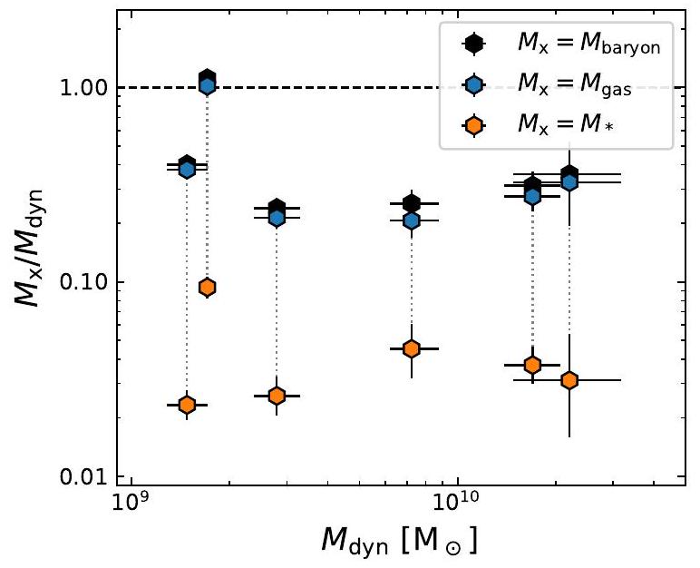
الشكل 8. الكتل الباريونية والنجمية وكتل الغاز (المقدرة باستخدام العلاقة بين و من Kennicutt 1998) كنسب من الكتلة الديناميكية. نجد أن كتلة الغاز، وبالتالي الكتلة الباريونية، أعلى بحوالي ترتيب من حيث الحجم من الكتلة النجمية. على الرغم من أن تضمين مكون الغاز يقلل من التباين الكبير في الكتلة الموجود في الشكل 7، إلا أن الفرق بمقدار 3-4 بين الكتلة الديناميكية والباريونية لا يزال قائماً لجميع الأجسام باستثناء واحدة.
يبدو أن الاضطراب الناتج عن ردود الفعل النجمية يقع في نطاق (Ostriker & Shetty 2011؛ Shetty & Ostriker 2012؛ Krumholz et al. 2018). هذا أقل بكثير من السرعات الدائرية المقاسة لعينة المجرات لدينا وبالتالي لا يمكن أن يؤدي إلى انحياز كبير في كتلنا الديناميكية.
ومع ذلك، قد تشكل التدفقات مصدراً أكبر من عدم اليقين. لقد اخترنا ضد الأجسام في JADES التي تحتوي على تدفقات كما تم تقديمه في Carniani et al. (2023)، الذين قياسوا سرعات التدفق . من الصعب اكتشاف سرعات التدفق المنخفضة، ولكن قد لا تزال موجودة في بياناتنا. لذلك، توجهنا إلى ملاحظات لمجرات انفجار النجوم عند انزياحات حمراء منخفضة للمقارنة. اكتشف Heckman et al. (2015) و Xu et al. (2022) التدفقات باستخدام خطوط امتصاص المعادن في الأشعة فوق البنفسجية وأظهروا أن النسبة تتوافق مع كل من معدل تكوين النجوم المحدد (sSFR ) وكثافة سطح معدل تكوين النجوم ( ). استناداً إلى الشكل 10 من Xu et al. (2022) وحقيقة أنه بالنسبة لعيّنتنا، sSFR و ، نقدر . وهذا يعني مبالغة في تقدير السرعة الدائرية بمقدار 3 أو بمقدار 10 في الكتلة الديناميكية. ومع ذلك، من غير الواضح ما إذا كانت الغاز المتدفقة التي تتبعها خطوط امتصاص الأشعة فوق البنفسجية في إطار الزمان الراهن تتبع أيضاً خطوط الانبعاث الضوئية في إطار الزمان الراهن، وكيف سيترجم ذلك بدوره إلى عدم اليقين في الكتلة الديناميكية. على سبيل المثال، وجد Erb et al. (2006) عدم وجود علاقة بين عرض خط (ومن ثم الكتلة الديناميكية) وسرعات التدفق المجري المقاسة من خطوط امتصاص الأشعة فوق البنفسجية في إطار الزمان الراهن لمجرات تشكيل النجوم الأكثر ضخامة عند .
إذا كانت الكتلة الديناميكية قوية (على مستوى عامل 2)، يجب أن نوجه انتباهنا إلى مكونات الكتلة الأخرى التي تساهم في ميزانية الكتلة الكلية. أحد المكونات الواضحة التي لم يتم مناقشتها حتى الآن هو كتلة الغاز. لقد أظهرت الدراسات الرصدية والنظرية أنه من المهم أخذ محتوى الغاز في الاعتبار (برايس وآخرون 2016؛ ويست وآخرون 2016) لأن نسبة الغاز النموذجية ترتفع بسرعة نحو انزياح أحمر أعلى وكتل أقل (للمراجعة، انظر تاكوني وآخرون 2020). لقد قدرنا كتل الغاز لعينة دراستنا بناءً على معدلات تشكيل النجوم المستمدة من نمذجة SED إلى طيفية المنشور. استخدمنا معكوس علاقة كينيكوت (1998) بين كثافة كتلة الغاز السطحية
( ) ومعدل تشكيل النجوم لاستنتاج الكتلة الكلية للغاز. على الرغم من أنها تم معايرتها فقط عند انزياحات حمراء منخفضة، إلا أن هذا من المحتمل أن يوفر تقديرًا معقولًا لمرتبة الحجم لكثافات سطح معدل تشكيل النجوم العالية لعينة دراستنا (دادّي وآخرون 2010؛ كينيكوت وإيفانز 2012).
من هذا، نجد كتل الغاز بحوالي مع نسبة متوسطة . يمكننا الآن مقارنة هذه الكتل الغازية والكتل الباريونية الناتجة ( ) مع الكتل الديناميكية في الشكل 8. على الرغم من أن كتلة الغاز أعلى من كتلة النجوم ( ; متوافقة مع قياسات المجرات الأكثر كتلة عند من هاينتس وآخرون 2022)، إلا أن هناك تباينًا بحوالي عامل من بين الكتلة الباريونية والديناميكية يبقى لكل شيء ما عدا كائن واحد. يحمل تقديرنا لكتل الغاز عدم يقين منهجي لأنه يفترض، على سبيل المثال، كفاءة ثابتة لتشكيل النجوم. أظهر برايس وآخرون (2020) أن مقدرًا مختلفًا لكتلة الغاز (اتباعًا لتاكوني وآخرون 2018) يؤدي إلى فرق متوسط في كتلة الغاز قدره 0.13 دكس لعينة من المجرات الأكثر كتلة عند الظهر الكوني. العلاقات ذات القياس الغازي نفسها مقيدة بشكل سيء، إن وجدت، عند في نظام كتلة النجوم الذي تم النظر فيه في هذا العمل، وبالتالي لا يمكننا إجراء نفس المقارنة لعينة دراستنا. ومع ذلك، فإن زيادة كتل الغاز وجعل الكتل الباريونية متوافقة مع الكتل الديناميكية ستتطلب، مع ذلك، تقليلًا بعامل من في كفاءة تشكيل النجوم لمعظم عينة دراستنا. ومع ذلك، أظهر بيلبيتش وآخرون (2019) أنه في المحاكاة الكونية TNG50، تزداد نسبة الغاز في المجرات ذات الكتلة المنخفضة ( ) بسرعة مع الانزياح الأحمر حتى ، ولكنها تبدو مسطحة عند انزياحات حمراء أعلى مع . ستكون الملاحظات الإضافية وكذلك البيانات المحاكية عند كتل النجوم الأقل وانزياحات حمراء أعلى ضرورية لتقييد كتل الغاز للكائنات المشابهة لعينة JADES.
من المهم أن كتل النجوم قد تتأثر أيضًا بعدم اليقين المنهجي. تمتد الطيفية ذات الدقة المنخفضة عبر نطاق واسع من الأطوال الموجية ( )، مستكشفة UV إلى بصري في إطار الراحة لجميع الكائنات، وبالتالي، توفر قيودًا جيدة على تاريخ تشكيل النجوم الحديث (SFH). ومع ذلك، قد تتأثر هذه القياسات بتأثير التوهج، حيث تهيمن مجموعة من النجوم الشابة على SED، مما يجعل من شبه المستحيل اكتشاف مجموعة تحتية من النجوم القديمة عند الأطوال الموجية البصرية في إطار الراحة (على سبيل المثال، ماراستون وآخرون 2010؛ بفور وآخرون 2012؛ سوربا وساويكي 2018؛ خيمينيز-أرتياغا وآخرون 2023؛ تاكشيلا وآخرون 2023؛ ويتلر وآخرون 2023). هذا مهم بشكل خاص لعينة دراستنا لأننا اخترنا خطوط انبعاث ساطعة لأداء نمذجة ديناميكية، وتميل هذه الخطوط إلى أن تكون ذات عرض مكافئ عالٍ. باستخدام ملاحظات وهمية من المحاكاة الكونية، أظهر نارايانان وآخرون (2024) أن تأثير التوهج قد يبالغ في تقدير كتل النجوم بمقدار دكس عند اعتمادًا على الأولوية المختارة لـ SFH. هذا يعني أن التقدير المحتمل الكبير لكتلة النجوم هو المصدر الأكثر إشكالية للأخطاء المنهجية في ميزانية كتلنا. قد تقدم التصوير عند أطوال موجية أطول مع JWST/MIRI وتناسب SED المحلولة مكانيًا تحسينات في تقديرات كتل النجوم في المستقبل (على سبيل المثال، عبد الرؤوف وآخرون 2023؛ خيمينيز-أرتياغا وآخرون 2023؛ بيريز-غونزاليس وآخرون 2023). ومع ذلك، نلاحظ أن حتى هذا التأثير سيكون له تأثير ضئيل في النظام حيث هو .
باختصار، قد تساهم عدد من التأثيرات المنهجية في التباين الكبير بعامل 30 بين كتل النجوم والديناميكية لهذه العينة ذات الكتلة المنخفضة والانزياح الأحمر العالي. نحن نؤكد أن الكتل الديناميكية مقيدة بشكل جيد نسبيًا، مع عدم يقين قدره دكس كحد أقصى، حتى في حالة اندماج مستمر، على الرغم من أننا لا يمكننا استبعاد تحيز في بعض
من قياسات الكتلة الديناميكية بسبب تدفقات خارجية على نطاق مجري. من الواضح أن كمية كبيرة من الغاز يجب أن تكون موجودة في هذه المجرات ذات تشكيل النجوم العالي، ونقدر أن هذا يمكن أن يمثل دكس في التباين بين كتلة النجوم والديناميكية. على الرغم من أن كتل الغاز غير مؤكدة وأن العلاقات القياسية بين معدل تشكيل النجوم وكثافات الغاز السطحية لها تباين كبير، نعتبر أنه من غير المحتمل أن يتم التقليل من كتل الغاز بعامل كبير لجميع الكائنات في عينة دراستنا. وهذا يترك إمكانية أن كتل النجوم قد تكون بدلاً من ذلك مقدرة بشكل كبير لأنها تفتقر إلى القيود عند أطوال الموجة الأطول في إطار الراحة حيث قد تكون مجموعة من النجوم القديمة قابلة للقياس.
في هذه المناقشة، تجاهلنا حتى الآن مكون كتلة واحد: المادة المظلمة. على المقاييس المكانية الصغيرة التي تم استكشافها ( )، قد لا يبدو أن هذا عامل مهيمن في ميزانية الكتلة، خاصةً حيث أظهرت دراسات متعددة زيادة سريعة في نسبة الباريون المركزية نحو انزياحات حمراء أعلى (على سبيل المثال، فان دوكوم وآخرون 2015؛ برايس وآخرون 2016؛ ويست وآخرون 2016؛ غينزل وآخرون 2017، 2020). ومع ذلك، من المثير للاهتمام أن نعتبر حالة مع وجود مادة مظلمة كبيرة داخل الأشعة الفعالة عند هذه الانزياحات. ضمن نموذج الكون ، تهيمن المادة المظلمة على محتوى الكتلة في الكون. تحت تشكيل الهيكل الهرمي، تتشكل هالات المادة المظلمة الصغيرة أولاً، بينما تتشكل النجوم فقط بعد أن يبرد الغاز داخل تلك الهالات بشكل كافٍ، مما ينمو لاحقًا إلى مجرات من خلال الالتحام (تيارات الغاز الباردة، الاندماجات؛ على سبيل المثال، وايت وريز 1978؛ ديكل وآخرون 2009a؛ أوسر وآخرون 2010). في هذا السيناريو، قد يكون من الممكن أن تهيمن المجرات الشابة جدًا على المادة المظلمة حتى في المناطق المركزية لأن الكتلة الباريونية لا تزال تتجمع. هذا مهم بشكل خاص لأن المجرات في نظام كتلة النجوم الذي تم استكشافه في هذه الورقة ( ) قد تكون أسلاف المجرات ذات الكتلة عند (موستر وآخرون 2018؛ بهروزي وآخرون 2019)، والتي لديها مراكز مهيمنة من الباريون. نظرًا لأن الملاحظات المذكورة أعلاه عند الظهر الكوني عادةً ما تكون أيضًا لمجرات أكثر كتلة ( )، فقد لا يختلف الفرق في النسب الباريونية المركزية بين عملنا والقياسات عند الظهر الكوني، ولكن يعكس تطور الوقت في توزيع الكتلة المظلمة والباريونية مع نمو المجرات وتجميع كتلتها النجمية. نستكشف هذه الفكرة بشكل أعمق باستخدام المحاكاة الكونية في دي غراف وآخرون (قيد الإعداد). ومع ذلك، سيتطلب الوصول إلى استنتاج قاطع حول ما إذا كان هذا السيناريو قد ينطبق على مجرات JADES فهمًا شاملاً لعدم اليقين المنهجي على مكونات الكتلة المختلفة.
6. الاستنتاجات
استخدمنا عينة JADES الطيفية في GOODS-S لاختيار ستة أهداف عند التي تمتد مكانيًا في تصوير NIRCam، والتي تم الحصول على طيفية عالية الدقة ( ) باستخدام NIRSpec MSA. أظهرنا أن هذه المجرات تقع في جزء غير مستكشف سابقًا من فضاء المعلمات: ليس فقط بسبب انزياحاتها الحمراء العالية، ولكن أيضًا بسبب أحجامها الصغيرة ( ) وكتلها النجمية المنخفضة ( ). تكشف الأطياف عالية الدقة عن خطوط انبعاث بصرية في إطار الراحة ([OIII] و ) التي تم توسيعها ولها تدرجات سرعة مكانية.
لاستخراج الخصائص الديناميكية، قمنا بنمذجة الأجسام كأقراص رقيقة ولكن دافئة تدور. وصفنا برنامج نمذجة متقدم جديد لأخذ عدة تعقيدات في الاعتبار للبيانات المأخوذة باستخدام أداة NIRSpec: دالة الانتشار النقطي، هندسة الغالق وظلال القضبان، والتجزئة. باستخدام تصوير NIRCam كمرجع على شكل خط الانبعاث، تمكنا من تحديد سرعات الدوران وتشتت السرعات للأجسام في عينة لدينا، وبالتالي، تمكنا أيضًا من تقدير الكتل الديناميكية. يمكن تلخيص نتائجنا على النحو التالي.
الأشياء في عيّنتنا صغيرة )، لديها كتلة نجمية منخفضة ( ) ومعدلات تشكيل نجوم متواضعة (SFR ~ 2-20 مالتي استنتجناها من نمذجة SED إلى طيف NIRSpec منخفض الدقة. الكتل الغازية التي تشير إليها معدلات تكوين النجوم أعلى بعشر مرات في المتوسط من الكتل النجمية.
نجد تباينات في السرعة الجوهرية في النطاقوهو ما يتماشى مع الدراسات التي تشير إلى تشتت السرعات في المجرات الأكثر ضخامة في وقت الظهيرة الكونية.
ثلاثة من أصل ستة أجسام تظهر تدرجات ملحوظة في السرعة المكانية، مما يؤدي إلىتحت فرضية نموذج القرص الرقيق لدينا، فإن هذا يعني أن الأجسام ذات الانزياح الأحمر العالي هي أقراص تهيمن عليها الدوران. ومع ذلك، لا يمكننا استبعاد إمكانية أن تعكس تدرجات السرعة المكتشفة انزياحات في السرعة بين المجرات المتفاعلة.
أظهر المقارنة بين الكتل الديناميكية والكتل النجمية تباينًا مفاجئًا بمقدار 10-40. بعد أخذ الكتل الغازية العالية في الاعتبار، لا تزال الكتل الديناميكية أعلى من الكتل الباريونية بمقدار.
نحن نجادل بأن الكتل الديناميكية قوية ضمن عامل يتراوح بين 2-4 حتى في حالة الاندماج الجاري. فقط وجود التدفقات الخارجة، إذا كانت ستسيطر على كينماتيكا خطوط الانبعاث المرصودة، يمكن أن يقلل بشكل كبير من الكتل الديناميكية المستنتجة. ومع ذلك، قد تشير الفجوة بين الكتل الباريونية والديناميكية أيضًا إلى أن مراكز هذه الأجسام تهيمن عليها المادة المظلمة. علاوة على ذلك، هناك عدم يقين منهجي كبير بشأن كتل النجوم والغاز. يمكن التوفيق بين الكتل الباريونية والكتل الديناميكية إذا كانت كفاءة تشكيل النجوم في هذه الأجسام أقل بعامل 3 مما تم افتراضه في البداية. يقدم عملنا أول عرض لقدرات وضع MOS في NIRSpec القوي لأداء تحليلات موضوعة ومطيافية. من الأهمية بمكان أن هذا يمكّن من دراسة حركيات المجرات بطريقة فعالة للغاية لأن الملاحظة الواحدة يمكن أن تستكشف نطاقًا واسعًا من الانزياح الأحمر والكتلة ومعدل تكوين النجوم. مع الحصول على عينات طيفية أكبر باستخدام وضع MOS عالي الدقة، سيسمح NIRSpec التابع لـ JWST في المستقبل القريب بإجراء تحليلات إحصائية لأصول واستقرار المجرات القرصية في الكون المبكر.
الشكر والتقدير. يشكر AdG M. Fouesneau و I. Momcheva على ملاحظاتهم القيمة خلال تطوير msafit، و J. Davies على المناقشات المفيدة حول بيانات JWST و NIRSpec. تستخدم هذه البحث بيانات ESA Datalabs (datalabs.esa.int)، وهي مبادرة من قسم علوم البيانات والأرشيفات في إدارة العلوم والعمليات، مديرية العلوم. استخدمت هذه البحث POPPY، وهي حزمة برمجية مفتوحة المصدر للبصريات تم تطويرها في الأصل لمشروع تلسكوب جيمس ويب الفضائي (Perrin et al. 2012). يعترف SC بالدعم من منحة بدء ERC رقم 101040227 – WINGS من الاتحاد الأوروبي. يعترف ECL بدعم زمالة ويب STFC (ST/W001438/1). يعترف RM و WB بالدعم من مجلس مرافق العلوم والتكنولوجيا (STFC)، ومن ERC من خلال منحة متقدمة 695671 “QUENCH”. كما يعترف RM بالدعم من منحة أبحاث Frontier Research من UKRI RISEandFALL وتمويل من أستاذية بحثية من الجمعية الملكية. يعترف AJB و AJC و JC و GCJ بالتمويل من منحة “FirstGalaxies” المتقدمة من المجلس الأوروبي للبحث (ERC) تحت برنامج الأفق 2020 للبحث والابتكار التابع للاتحاد الأوروبي (اتفاقية المنحة رقم 789056). يعترف SA بالدعم من منحة PID2021127718 NB-I00 الممولة من وزارة العلوم والابتكار الإسبانية/الوكالة الحكومية للبحث (MICIN/AEI/ 10.13039/501100011033). يعترف HÜ بامتنان بالدعم من مؤسسة إسحاق نيوتن ومن مؤسسة كافلي من خلال زمالة نيوتن-كافلي للشباب. يتم دعم DJE كمحقق من سيمونز. يتم دعم DJE و BJJ و CNAW من خلال عقد JWST/NIRCam مع جامعة أريزونا، NAS5-02015. يعترف BER بالدعم من
عقد فريق علوم NIRCam مع جامعة أريزونا، NAS5-02015. يتم دعم أبحاث CCW من قبل NOIRLab، الذي تديره جمعية الجامعات للبحث في علم الفلك (AURA) بموجب اتفاق تعاوني مع المؤسسة الوطنية للعلوم. يقر KB بالدعم المقدم من مركز التميز الأسترالي لعلم الفلك في جميع السماء في ثلاثة أبعاد (ASTRO 3D)، من خلال رقم المشروع CE170100013. يقر RH بالتمويل المقدم من جامعة جونز هوبكنز، معهد الهندسة والعلوم المعتمدة على البيانات (IDIES).
References
Abdurro’uf, Coe, D., Jung, I., et al. 2023, ApJ, 945, 117
Alves de Oliveira, C., Lützgendorf, N., Zeidler, P., et al. 2022, SPIE Conf. Ser., 12180, 121803S
Baker, W. M., Tacchella, S., Johnson, B. D., et al. 2023, Nat. Astron., submitted, [arXiv:2306.02472]
Behroozi, P., Wechsler, R. H., Hearin, A. P., & Conroy, C. 2019, MNRAS, 488, 3143
Birrer, S., & Amara, A. 2018, Phys. Dark Universe, 22, 189
Birrer, S., Shajib, A., Gilman, D., et al. 2021, J. Open Source Software, 6, 3283
Böker, T., Arribas, S., Lützgendorf, N., et al. 2022, A&A, 661, A82
Böker, T., Beck, T. L., Birkmann, S. M., et al. 2023, PASP, 135, 038001
Bowler, R. A. A., Dunlop, J. S., McLure, R. J., & McLeod, D. J. 2017, MNRAS, 466, 3612
Bunker, A. J., Cameron, A. J., Curtis-Lake, E., et al. 2023, A&A, submitted, [arXiv:2306.02467]
Burkert, A., Genzel, R., Bouché, N., et al. 2010, ApJ, 725, 2324
Cappellari, M. 2016, ARA&A, 54, 597
Cappellari, M., Bacon, R., Bureau, M., et al. 2006, MNRAS, 366, 1126
Carniani, S., Maiolino, R., Amorin, R., et al. 2018, MNRAS, 478, 1170
Carniani, S., Venturi, G., Parlanti, E., et al. 2023, A&A, in press, [arXiv:2306.11801]
Ceverino, D., Dekel, A., Mandelker, N., et al. 2012, MNRAS, 420, 3490
Chabrier, G. 2003, ApJ, 586, L133
Charlot, S., & Fall, S. M. 2000, ApJ, 539, 718
Chevallard, J., & Charlot, S. 2016, MNRAS, 462, 1415
Courteau, S. 1997, AJ, 114, 2402
Curtis-Lake, E., Carniani, S., Cameron, A., et al. 2023, Nat. Astron., 7, 622
Daddi, E., Elbaz, D., Walter, F., et al. 2010, ApJ, 714, L118
Dekel, A., Birnboim, Y., Engel, G., et al. 2009a, Nature, 457, 451
Dekel, A., Sari, R., & Ceverino, D. 2009b, ApJ, 703, 785
Dorner, B., Giardino, G., Ferruit, P., et al. 2016, A&A, 592, A113
Duncan, K., Conselice, C. J., Mundy, C., et al. 2019, ApJ, 876, 110
Eisenstein, D. J., Willott, C., Alberts, S., et al. 2023, ApJS, submitted, [arXiv:2306.02465]
Erb, D. K., Steidel, C. C., Shapley, A. E., et al. 2006, ApJ, 646, 107
Falcón-Barroso, J., van de Ven, G., Lyubenova, M., et al. 2019, A&A, 632, A59
Ferruit, P., Jakobsen, P., Giardino, G., et al. 2022, A&A, 661, A81
Foreman-Mackey, D., Hogg, D. W., Lang, D., & Goodman, J. 2013, PASP, 125, 306
Förster Schreiber, N. M., & Wuyts, S. 2020, ARA&A, 58, 661
Förster Schreiber, N. M., Shapley, A. E., Erb, D. K., et al. 2011, ApJ, 731, 65
Förster Schreiber, N. M., Renzini, A., Mancini, C., et al. 2018, ApJS, 238, 21
Fraternali, F., Karim, A., Magnelli, B., et al. 2021, A&A, 647, A194
Gardner, J. P., Mather, J. C., Abbott, R., et al. 2023, PASP, 135, 068001
Genel, S., Dekel, A., & Cacciato, M. 2012, MNRAS, 425, 788
Genzel, R., Förster Schreiber, N. M., Übler, H., et al. 2017, Nature, 543, 397
Genzel, R., Price, S. H., Übler, H., et al. 2020, ApJ, 902, 98
Giardino, G., Luetzgendorf, N., Ferruit, P., et al. 2016, SPIE Conf. Ser., 9904, 990445
Giardino, G., Ferruit, P., Chevallard, J., et al. 2019, in Astronomical Data Analysis Software and Systems XXVII, eds. P. J. Teuben, M. W. Pound, B. A. Thomas, & E. M. Warner, ASP Conf. Ser., 523, 645
Giménez-Arteaga, C., Oesch, P. A., Brammer, G. B., et al. 2023, ApJ, 948, 126
Guo, Y., Ferguson, H. C., Bell, E. F., et al. 2015, ApJ, 800, 39
Heckman, T. M., Alexandroff, R. M., Borthakur, S., Overzier, R., & Leitherer, C. 2015, ApJ, 809, 147
Heintz, K. E., Oesch, P. A., Aravena, M., et al. 2022, ApJ, 934, L27
Herrera-Camus, R., Förster Schreiber, N. M., Price, S. H., et al. 2022, A&A, 665, L8
Hung, C.-L., Rich, J. A., Yuan, T., et al. 2015, ApJ, 803, 62
Hung, C.-L., Hayward, C. C., Smith, H. A., et al. 2016, ApJ, 816, 99
Jakobsen, P., Ferruit, P., Alves de Oliveira, C., et al. 2022, A&A, 661, A80
Johnson, B. D. 2019, SEDPY: Modules for storing and operating on astronomical source spectral energy distribution, Astrophysics Source Code Library [record ascl:1905.026]
Jones, G. C., Vergani, D., Romano, M., et al. 2021, MNRAS, 507, 3540
Kennicutt, R. C., Jr 1998, ARA&A, 36, 189
Kennicutt, R. C., & Evans, N. J. 2012, ARA&A, 50, 531
Kohandel, M., Pallottini, A., Ferrara, A., et al. 2019, MNRAS, 487, 3007
Krajnović, D., Cappellari, M., de Zeeuw, P. T., & Copin, Y. 2006, MNRAS, 366, 787
Krumholz, M. R., Burkhart, B., Forbes, J. C., & Crocker, R. M. 2018, MNRAS, 477, 2716
Lelli, F., Di Teodoro, E. M., Fraternali, F., et al. 2021, Science, 371, 713
Lützgendorf, N., Giardino, G., Alves de Oliveira, C., et al. 2022, SPIE Conf. Ser., 12180, 121800Y
Mandelker, N., Dekel, A., Ceverino, D., et al. 2014, MNRAS, 443, 3675
Maraston, C., Pforr, J., Renzini, A., et al. 2010, MNRAS, 407, 830
Maseda, M. V., van der Wel, A., da Cunha, E., et al. 2013, ApJ, 778, L22
Moster, B. P., Naab, T., & White, S. D. M. 2018, MNRAS, 477, 1822
Narayanan, D., Lower, S., Torrey, P., et al. 2024, ApJ, 961, 73
Neeleman, M., Prochaska, J. X., Kanekar, N., & Rafelski, M. 2020, Nature, 581, 269
Newman, A. B., Belli, S., Ellis, R. S., & Patel, S. G. 2018, ApJ, 862, 126
Nidever, D. L., Gilbert, K., Tollerud, E., et al. 2023, Early Disk-Galaxy Formation from JWST to the Milky Way, eds. F. Tabatabaei, B. Barbuy, & Y.-S. Ting, Proc. Int. Astron. Union, 377, 115
Oesch, P. A., Brammer, G., Naidu, R. P., et al. 2023, MNRAS, 525, 2864
O’Leary, J. A., Moster, B. P., Naab, T., & Somerville, R. S. 2021, MNRAS, 501, 3215
Oser, L., Ostriker, J. P., Naab, T., Johansson, P. H., & Burkert, A. 2010, ApJ, 725, 2312
Ostriker, E. C., & Shetty, R. 2011, ApJ, 731, 41
Parlanti, E., Carniani, S., Pallottini, A., et al. 2023, A&A, 673, A153
Pérez-González, P. G., Barro, G., Annunziatella, M., et al. 2023, ApJ, 946, L16
Perrin, M. D., Soummer, R., Elliott, E. M., Lallo, M. D., & Sivaramakrishnan, A. 2012, SPIE Conf. Ser., 8442, 84423D
Pforr, J., Maraston, C., & Tonini, C. 2012, MNRAS, 422, 3285
Pillepich, A., Nelson, D., Springel, V., et al. 2019, MNRAS, 490, 3196
Piquéras, L., Legay, P. J., Legros, E., et al. 2008, SPIE Conf. Ser., 7017, 70170Z
Piquéras, L., Legros, E., Pons, A., et al. 2010, SPIE Conf. Ser., 7738, 773812
Pope, A., McKinney, J., Kamieneski, P., et al. 2023, ApJ, 951, L46
Price, S. H., Kriek, M., Shapley, A. E., et al. 2016, ApJ, 819, 80
Price, S. H., Kriek, M., Barro, G., et al. 2020, ApJ, 894, 91
Price, S. H., Übler, H., Förster Schreiber, N. M., et al. 2022, A&A, 665, A159
Rieke, M. J., Kelly, D. M., Misselt, K., et al. 2023a, PASP, 135, 028001a
Rieke, M. J., Robertson, B., Tacchella, S., et al. 2023b, ApJS, 269, 16
Rigby, J., Perrin, M., McElwain, M., et al. 2023, PASP, 135, 048001
Rizzo, F., Vegetti, S., Powell, D., et al. 2020, Nature, 584, 201
Rizzo, F., Vegetti, S., Fraternali, F., Stacey, H. R., & Powell, D. 2021, MNRAS, 507, 3952
Rizzo, F., Roman-Oliveira, F., Fraternali, F., et al. 2023, A&A, 679, A129
Robertson, B., Bullock, J. S., Cox, T. J., et al. 2006, ApJ, 645, 986
Rodrigues, M., Hammer, F., Flores, H., Puech, M., & Athanassoula, E. 2017, MNRAS, 465, 1157
Rodriguez-Gomez, V., Genel, S., Vogelsberger, M., et al. 2015, MNRAS, 449, 49
Sattari, Z., Mobasher, B., Chartab, N., et al. 2023, ApJ, 951, 147
Sérsic, J. L. 1968, Atlas de Galaxias Australes (Cordoba, Argentina: Observatorio Astronomico)
Shapiro, K. L., Genzel, R., Förster Schreiber, N. M., et al. 2008, ApJ, 682, 231
Shetty, R., & Ostriker, E. C. 2012, ApJ, 754, 2
Simons, R. C., Kassin, S. A., Weiner, B. J., et al. 2017, ApJ, 843, 46
Simons, R. C., Kassin, S. A., Snyder, G. F., et al. 2019, ApJ, 874, 59
Sorba, R., & Sawicki, M. 2018, MNRAS, 476, 1532
Stott, J. P., Swinbank, A. M., Johnson, H. L., et al. 2016, MNRAS, 457, 1888
Suess, K. A., Williams, C. C., Robertson, B., et al. 2023, ApJ, 956, L42
Tacchella, S., Johnson, B. D., Robertson, B. E., et al. 2023, MNRAS, 522, 6236
Tacconi, L. J., Genzel, R., Saintonge, A., et al. 2018, ApJ, 853, 179
Tacconi, L. J., Genzel, R., & Sternberg, A. 2020, ARA&A, 58, 157
Topping, M. W., Stark, D. P., Endsley, R., et al. 2022, MNRAS, 516, 975
Turner, O. J., Cirasuolo, M., Harrison, C. M., et al. 2017, MNRAS, 471, 1280
Übler, H., Genzel, R., Wisnioski, E., et al. 2019, ApJ, 880, 48
van de Sande, J., Scott, N., Bland-Hawthorn, J., et al. 2018, Nat. Astron., 2, 483 van der Wel, A., Bell, E. F., Häussler, B., et al. 2012, ApJS, 203, 24
van der Wel, A., Chang, Y.-Y., Bell, E. F., et al. 2014, ApJ, 792, L6 van Dokkum, P. G., Nelson, E. J., Franx, M., et al. 2015, ApJ, 813, 23 van Houdt, J., van der Wel, A., Bezanson, R., et al. 2021, ApJ, 923, 11 Whitaker, K. E., Franx, M., Leja, J., et al. 2014, ApJ, 795, 104 White, S. D. M., & Rees, M. J. 1978, MNRAS, 183, 341
Whitler, L., Stark, D. P., Endsley, R., et al. 2023, MNRAS, 519, 5859
Wisnioski, E., Förster Schreiber, N. M., Wuyts, S., et al. 2015, ApJ, 799, 209
Wisnioski, E., Förster Schreiber, N. M., Fossati, M., et al. 2019, ApJ, 886, 124
Wuyts, S., Förster Schreiber, N. M., Wisnioski, E., et al. 2016, ApJ, 831, 149
Xu, X., Heckman, T., Henry, A., et al. 2022, ApJ, 933, 222
Zhang, H., Primack, J. R., Faber, S. M., et al. 2019, MNRAS, 484, 5170 Max-Planck-Institut für Astronomie, Königstuhl 17, 69117 Heidelberg, Germany e-mail: degraaff@mpia.de Scuola Normale Superiore, Piazza dei Cavalieri 7, 56126 Pisa, Italy Department of Astronomy and Astrophysics University of California, Santa Cruz, 1156 High Street, Santa Cruz, CA 96054, USA Kavli Institute for Particle Astrophysics and Cosmology and Department of Physics, Stanford University, Stanford, CA 94305, USA Sorbonne Université, CNRS, UMR 7095, Institut d’Astrophysique de Paris, 98 bis bd Arago, 75014 Paris, France Centre for Astrophysics Research, Department of Physics, Astronomy and Mathematics, University of Hertfordshire, Hatfield AL10 9AB, UK Centro de Astrobiología (CAB), CSIC-INTA, Cra. de Ajalvir Km. 4, 28850 Torrejón de Ardoz, Madrid, Spain Kavli Institute for Cosmology, University of Cambridge, Madingley Road, Cambridge CB3 0HA, UK Cavendish Laboratory – Astrophysics Group, University of Cambridge, 19 JJ Thomson Avenue, Cambridge CB3 0HE, UK School of Physics, University of Melbourne, Parkville 3010, VIC, Australia ARC Centre of Excellence for All Sky Astrophysics in 3 Dimensions (ASTRO 3D), Australia Department of Physics, University of Oxford, Denys Wilkinson Building, Keble Road, Oxford OX1 3RH, UK European Southern Observatory, Karl-Schwarzschild-Strasse 2, 85748 Garching, Germany Center for Astrophysics | Harvard & Smithsonian, 60 Garden St., Cambridge, MA 02138, USA
15 Leiden Observatory, Leiden University, PO Box 9513, 2300 AA Leiden, The Netherlands
16 Steward Observatory, University of Arizona, 933 N. Cherry Avenue, Tucson, AZ 85721, USA
17 Department of Physics and Astronomy, The Johns Hopkins University, 3400 N. Charles St., Baltimore, MD 21218, USA
18 Department of Physics and Astronomy, University College London, Gower Street, London WC1E 6BT, UK
19 Department of Astronomy, University of Wisconsin-Madison, 475 N. Charter St., Madison, WI 53706, USA Department for Astrophysical and Planetary Science, University of Colorado, Boulder, CO 80309, USA European Space Agency (ESA), European Space Astronomy Centre (ESAC), Camino Bajo del Castillo s/n, 28692 Villafranca del Castillo, Madrid, Spain NSF’s National Optical-Infrared Astronomy Research Laboratory, 950 North Cherry Avenue, Tucson, AZ 85719, USA NRC Herzberg, 5071 West Saanich Rd, Victoria, BC V9E 2E7, Canada
الملحق أ: دقة NIRSpec
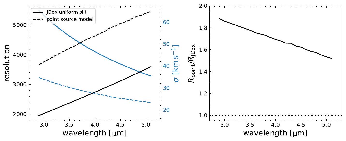
تقدم دقة الأداة لـ NIRSpec الواردة في وثائق مستخدم JWST على الإنترنت (JDox) تقديرًا قبل الإطلاق لدالة الانتشار الخطية (LSF) للأداة في شق مضاء بشكل موحد.. ومع ذلك، حيث أننا نأخذ في الاعتبار شكل المصدر في نمذجة لدينا، فإن دقة المصدر النقطي ذات صلة في عملنا. لتقديم نظرة ثاقبة على دوال انتشار النقاط في نموذجنا، والتي هي صور ثنائية الأبعاد، استخدمنا برنامج النمذجة لدينا لتقدير الدقة أحادية البعد كدالة لطول الموجة لمصدر نقطي.
للقيام بذلك، قمنا بإعداد مكعب نموذج.وفقًا للإجراء الموصوف في القسم 3، ولكن لنمط مصدر نقطي بدلاً من ملف سيرسيك. وضعنا المصدر النقطي في مركز الغالق واستخدمنا غالقًا مركزيًا ( ) من الربع الرابع من MSA. قمنا بتطبيق عينة ضوئية نادرة من عبرلتجنب التداخل وتسريع الحساب. ثم قمنا بنقل هذا النموذج إلى مستوى الكاشف واستخراج طيف أحادي الأبعاد. من خلال نمذجة خطوط الانبعاث الناتجة عند الأطوال الموجية المدخلة المعروفة كسلسلة من الغاوسيات الفردية ذات العرض والسعة المتغيرة، استخرجنا دالة انتشار النقطة (LSF) لمصدر نقطي.
نظهر دقة الناتج وLSF لمصدر نقطي لقرص G 395 H في الشكل A.1. دقة المصدر النقطي لـ NIRSpec (الخطوط المتقطعة) أعلى بكثير من التقدير لشق مضاء بشكل موحد (الخطوط الصلبة). في اللوحة اليمنى، نعرض نسبة الاثنين كدالة للطول الموجي: عند الأطوال الموجية الأقصر، تختلف الدقة بمقدار يقارب 2. عند الأطوال الموجية الأطول، تتناقص هذه الفجوة في الدقة تدريجياً لأن نسبة PSF المكاني FWHM وعرض الشق تزداد مع الطول الموجي (أي أن PSF المكاني يصبح أوسع وبالتالي أقرب إلى تقريب توزيع التدفق الموحد). نود أن نحذر من أن هذا LSF لا يمكن تطبيقه مباشرة على الأطياف المستقيمة والمستخرجة والمجمعة من الملاحظات الحقيقية لأنه لا يتضمن التوسيع الذي يتم تقديمه عادةً بواسطة خط أنابيب التخفيض عند إعادة أخذ العينات ودمج البيانات من عدة تعريضات. من حيث المبدأ، يمكن تمرير كواشف نموذجنا عبر أي خط أنابيب تخفيض لتقدير هذا التوسيع الإضافي، ونحقق في هذه التأثيرات بمزيد من التفصيل في de Graaff et al. (قيد الإعداد).
علاوة على ذلك، كما هو مذكور في القسم 3.2، نؤكد أن نماذج PSF المستخدمة في نمذجة التوقع تعتمد جزئيًا على ملفات مرجعية تم إنشاؤها قبل الإطلاق، مما يؤدي على الأرجح إلى عدم يقين منهجي في FWHM. تم تنفيذ عدد قليل من برامج المعايرة التي تهدف إلى توصيف PSF، والتي نناقشها كما يلي.
بالنسبة لـ MSA، تم رصد نجم قياسي واحد في وضع المنشور داخل الغالق المركزي لكل ربع للحصول على دالة الانتشار النقطي (البرنامج 1128). وبالمثل، بالنسبة للشق الثابت (FS؛ البرامج 1128، 1487)، تم رصد نجم قياسي في مواقع مختلفة داخل الشق. هذه البيانات مناسبة بشكل أساسي و يستخدم لتقدير خسائر المسار. لأن دالة كثافة النقطة (PSF) عينة بشكل غير كافٍ (بكسلات من مقابل عرض النطاق الكامل عند نصف الحد الأقصى إذا كانت PSF محدودة بالتشتت)، وتمت ملاحظة كائن واحد فقط، فإنه من الصعب للغاية في الممارسة العملية استخراج ملف مكاني قوي من هذه البيانات. أفاد جاكوبسن وآخرون (2022) أن PSF المكاني لـ NIRSpec محدود بالتشتت بعد وبالتالي فهو مشابه لـ PSF NIRCam عند الأطوال الموجية الطويلة. جميع خطوط الانبعاث التي تم النظر فيها في هذه الورقة هي عند وفي هذا النظام المحدود بالتشتت.
قمنا بتقييم جودة الاتجاه المكاني (أي الاتجاه العرضي) لنماذج PSF الخاصة بنا من خلال مقارنة أنصاف أضواء الأبعاد المستنتجة من نمذجة لدينا مع صور NIRCam وتلك المستنتجة من النمذجة الطيفية. على الرغم من أننا قد وضعنا سابقة بناءً على المعلومات الشكلية لـ NIRCam لنمذجة الطيف، فإن عرض السابقيات واسع بما فيه الكفاية. لذلك، في حالة وجود انحراف كبير بين PSF الحقيقي و PSF النموذج الخاص بنا، نتوقع أن نجد فرقًا منهجيًا في أنصاف أضواء الأبعاد بين القياسين، خاصة بالنسبة للكائنات المدمجة (; الجدول 2). نجد فرقًا وسطيًا قدره فقط ، ومع ذلك، تشير التعديلات الطيفية إلى أحجام أكبر قليلاً. قد يكون هذا التحيز الصغير أيضًا تأثيرًا فيزيائيًا لأن صور NIRCam تحتوي على تدفق من كل من الاستمرارية النجمية وخطوط الانبعاث.
بالنسبة لاتجاه التشتت، فإن البيانات الوحيدة المتاحة للتقويم هي لنجم كوكبي بعيد (PN)، الذي تم ملاحظته في أوضاع MOS و FS (البرامج 1125، 1492). بعيدًا عن حقيقة أن هذا الكائن قد لا يكون مصدر نقطة حقيقي، فإن عدم العينة مرة أخرى هو القضية السائدة في تقويم التوسع في اتجاه التشتت. مشابهًا لـ PSF المكاني، فإن LSF عينة بشكل كبير لنقطة مصدر (FWHM~1 بكسل). حقيقة أن طيف PN يظهر فقط عددًا قليلاً (حوالي عشرة) من خطوط الانبعاث الضيقة عبر وأنه تم ملاحظة كائن واحد فقط يعني أن تقييد التوسع الطيفي هو تحدٍ كبير.
ومع ذلك، فإن برنامج النمذجة الخاص بنا يقوم أيضًا بعمل توقعات لموزعات NIRSpec الأخرى. التحليل الأولي من نيديفر وآخرون (2023) ذو صلة خاصة. لقد لاحظوا 100 نجم عملاق أحمر في M31 باستخدام شبكة G140H (البرنامج 2609). تظهر هذه الأطياف العديد من ميزات خطوط الامتصاص الضيقة عند ، مما يمكّن من إعادة بناء تجريبية لـ LSF على الرغم من مشاكل عدم العينة. وجد نيديفر وآخرون (2023) أنه بالنسبة لشبكة G 140 H، فإن الدقة أعلى بكثير مما تم الإبلاغ عنه في JDox، مع ، على الرغم من أن نطاق الطول الموجي الدقيق لهذا التقدير غير مذكور. ومع ذلك، فإن هذا يتفق بشكل عام مع التوقعات من برنامج النمذجة الخاص بنا لهذه الشبكة، والتي تقترح اعتمادًا على الطول الموجي. على الرغم من أنها تخضع لمزيد من المعايرة، نستنتج أن نماذج PSF الخاصة بنا واقعية بما فيه الكفاية لغرض هذه الورقة، ونقرب عدم اليقين المنهجي إلى في PSF FWHM.
الشكل A.1. تعتمد دقة ودالة انتشار الخط (LSF) لموزعات NIRSpec بشكل كبير على ملف الضوء للمصدر. اليسار: دقة وتشتت السرعة المقابلين المقدرين باستخدام برنامج النمذجة الخاص بنا لنقطة مصدر في مركز الغالق وشبكة G395H (الخطوط المنقطة). تظهر الخطوط الصلبة منحنيات التشتت المتاحة على صفحة وثائق مستخدم JWST (JDox)، والتي توفر تقريبًا (قبل الإطلاق) لـ LSF لغالق مضاء بشكل موحد. اليمين: نسبة الدقة لنقطة مصدر وتقدير LSF لتوزيع ضوء موحد. عند الأطوال الموجية الأقصر، تكون الدقة الطيفية أعلى بحوالي عامل 2 لنقطة مصدر.
الملحق ب: أطياف المنشور و SEDs
كما هو موضح في القسم ب، قمنا بإجراء نمذجة SED لأطياف المنشور () باستخدام برنامج BEAGLE (Chevallard & Charlot 2016). نعرض هذه الأطياف وأفضل نماذج (الحد الأدنى ) في الشكل ب.1.
بشكل عام، تظهر الأطياف استمرارية UV زرقاء جدًا وخطوط انبعاث قوية. نتيجة لذلك، نستنتج كتلة نجمية منخفضة و SFR محدد مرتفع (وسيط sSFR ). يتم تقديم الكتل النجمية و SFRs، المصححة لفقدان الشق، في الجدول ب.1.
استخدمنا أيضًا أطياف المنشور لحساب مساهمة خطوط الانبعاث في صور NIRCam في الشكل 1 لاختبار افتراضنا بأن الصور تتبع شكل خطوط الانبعاث بدلاً من الاستمرارية النجمية. استخدمنا برنامج sedpy (Johnson 2019) والطيف المرصود للمنشور لحساب إجمالي سطوع AB في فلتر NIRCam المعني. ثم، قمنا بإنشاء طيف يحتوي فقط على خطوط انبعاث قوية (، ثنائية [OIII]، )، باستخدام تدفقات خطوط الانبعاث المقاسة باستخدام pPXF كما هو موضح في D’Eugenio وآخرون (قيد الإعداد)، وحسبنا سطوع AB في فلتر NIRCam من خطوط الانبعاث فقط.
نقدم نسب التدفق في الجدول ب.2. بالنسبة لأربعة من أصل ستة كائنات، التي تم ملاحظتها في النطاقات المتوسطة، تهيمن خطوط الانبعاث على فوتومترية NIRCam ( من التدفق في المتوسط). بالنسبة للكائنين الآخرين اللذين تم ملاحظتهما في النطاقات العريضة، لا تهيمن خطوط الانبعاث، ولكنها تساهم بشكل كبير في الفوتومترية.
الجدول ب.1. نتائج نمذجة BEAGLE. القيم هي الوسيط لتوزيعات الاحتمالات اللاحقة، وتعكس عدم اليقين و النسب المئوية.
معرف
SFR
JADES-NS-00016745
JADES-NS-00019606
JADES-NS-00022251
JADES-NS-00047100
JADES-NS-10016374
JADES-NS-20086025
الجدول ب.2. نسبة تدفقات خطوط الانبعاث إلى التدفقات الإجمالية (الاستمرارية + خطوط الانبعاث) ضمن فلاتر NIRCam المستخدمة في النمذجة الشكلية.
معرف
فلتر
نسبة التدفق
JADES-NS-00016745
F356W
0.37
JADES-NS-00019606
F335M
0.75
JADES-NS-00022251
F335M
0.76
JADES-NS-00047100
F410M
0.69
JADES-NS-10016374
F444W
0.32
JADES-NS-20086025
F410M
0.69
الشكل ب.1. أطياف المنشور () (الخطوط السوداء) وأفضل نماذج SED المقدرة باستخدام BEAGLE (الخطوط البرتقالية). يتم تسليط الضوء على خطوط الانبعاث المستخدمة في النمذجة الديناميكية بواسطة خطوط منقطة. جميع SEDs للكائنات زرقاء جدًا وتظهر خطوط انبعاث قوية، مما يشير إلى تجمعات نجمية شابة تتشكل مع كتل نجمية منخفضة و SFRs محددة عالية.
يمكن العثور على البرنامج، وبيانات المرجع (نماذج PSF، نماذج التتبع) وتعليمات التثبيت هنا: https://github.com/annadeg/ jwst-msafit
للحصول على وصف تقني شامل لـ NIRSpec، نوجه القارئ إلى جاكوبسن وآخرون (2022) وفيرويت وآخرون (2022).
lonised gas kinematics and dynamical masses of galaxies from JADES/NIRSpec high-resolution spectroscopy
Anna de Graaff , Hans-Walter Rix , Stefano Carniani (D) Katherine A. Suess , Stéphane Charlot ( ), Emma Curtis-Lake , Santiago Arribas , William M. Baker , Kristan Boyett , Andrew J. Bunker , Alex J. Cameron , Jacopo Chevallard , Mirko Curti , Daniel J. Eisenstein , Marijn Franx , Kevin Hainline , Ryan Hausen (1), Zhiyuan Ji , Benjamin D. Johnson , Gareth C. Jones , Roberto Maiolino , Michael V. Maseda , Erica Nelson , Eleonora Parlanti (), Tim Rawle , Brant Robertson , Sandro Tacchella , Hannah Übler , Christina C. Williams , Christopher N. A. Willmer , and Chris Willott
(Affiliations can be found after the references)
Received 18 August 2023 / Accepted 18 December 2023
Abstract
We explore the kinematic gas properties of six galaxies in the JWST Advanced Deep Extragalactic Survey (JADES), using highresolution JWST/NIRSpec multi-object spectroscopy of the rest-frame optical emission lines [OIII] and H . The objects are small and of low stellar mass ( ), less massive than any galaxy studied kinematically at thus far. The cold gas masses implied by the observed star formation rates are about ten times higher than the stellar masses. We find that their ionised gas is spatially resolved by JWST, with evidence for broadened lines and spatial velocity gradients. Using a simple thin-disc model, we fit these data with a novel forward-modelling software that accounts for the complex geometry, point spread function, and pixellation of the NIRSpec instrument. We find the sample to include both rotation- and dispersion-dominated structures, as we detect velocity gradients of , and we find velocity dispersions of that are comparable to those at cosmic noon. The dynamical masses implied by these models ( ) are higher than the stellar masses by up to a factor 40 , and they are higher than the total baryonic mass (gas + stars) by a factor of . Qualitatively, this result is robust even if the observed velocity gradients reflect ongoing mergers rather than rotating discs. Unless the observed emission line kinematics is dominated by outflows, this implies that the centres of these galaxies are dominated by dark matter or that star formation is three times less efficient, leading to higher inferred gas masses.
In the nearby Universe, galaxies show a variety of dynamical structures and structural components that reflect their massassembly histories (e.g., Cappellari 2016; van de Sande et al. 2018; Falcón-Barroso et al. 2019). However, the details of the formation and evolution of these structures, which nominally are rotationally supported discs and spheroidal bulges supported primarily by dispersion, are still unclear. The physical conditions in the early Universe, the secular evolution of galaxies, and mergers with other systems are all likely to play important roles. One outstanding question in particular is when and how early galaxies settled into dynamically cold discs.
Although this question is ideally answered by measuring spatially resolved stellar kinematics across cosmic time, such measurements have only been possible up to (e.g., van Houdt et al. 2021), except for a few strongly lensed massive galaxies at (Newman et al. 2018). Instead, the ionised gas of the interstellar medium (ISM) provides critical insight into the dynamical properties of (star-forming) galaxies across a much wider redshift range (for a review, see Förster Schreiber & Wuyts 2020). Many studies have focused on inferring galaxy dynamical properties from rest-frame optical emission lines to map the evolution in the velocity dispersion ( ) and the ratio of the rotation velocity and dispersion ( ), which measures the degree of rotational support of the system.
Measurements of the ionised gas kinematics from multiple large spectroscopic surveys of star-forming galaxies at
1-4 have demonstrated that the velocity dispersion of starforming galaxies increases with redshift, while the rotational support decreases to by (e.g., Wisnioski et al. 2015, 2019; Stott et al. 2016; Simons et al. 2017; Turner et al. 2017; Price et al. 2020). In addition, imaging studies have shown that galaxy morphologies are less disc-like and more clumpy at rest-frame UV wavelengths at higher redshifts (e.g., van der Wel et al. 2014; Guo et al. 2015; Zhang et al. 2019; Sattari et al. 2023). Theoretical models and simulations have suggested that gravitational instabilities, the accretion of gas and smaller systems from the cosmic web, and stellar feedback may cause the increased turbulence at higher redshifts (e.g., Dekel et al. 2009b; Genel et al. 2012; Ceverino et al. 2012; Krumholz et al. 2018).
However, using submillimeter observations from the Atacama Large Millimeter Array (ALMA), several studies have found dynamically cold discs at (e.g., Neeleman et al. 2020; Jones et al. 2021; Lelli et al. 2021; Rizzo et al. 2021; Parlanti et al. 2023; Pope et al. 2023), even finding at (Fraternali et al. 2021). These observations raise the question of how such systems formed and settled so rapidly (within ), and how these observations can be reconciled with the aforementioned studies at cosmic noon. However, the ALMA observations infer the galaxy kinematics from far-infrared and millimetre transitions (CO, [CII]), which trace colder gas than the rest-frame optical lines, likely explaining part of the discrepancy (Übler et al. 2019; Rizzo et al. 2023). Additionally, selection effects likely play an important role, as many
Table 1. Coordinates and G395H exposure times of the selected sample.
JADES ID
NIRSpec ID
(deg)
Dec (deg)
(ksec)
Line
JADES-GS+53.13002-27.77839
JADES-NS-00016745
53.13005
-27.77839
18
25.2
JADES-GS+53.17655-27.77111
JADES-NS-00019606
53.17654
-27.77111
6
8.4
[OIII]
JADES-GS+53.15407-27.76607
JADES-NS-00022251
53.15407
-27.76608
12
16.8
[OIII]
JADES-GS+53.18343-27.79097
JADES-NS-00047100
53.18343
-27.79098
9
8.0
[OIII]
JADES-GS+53.11572-27.77495
JADES-NS-10016374
53.11572
-27.77496
12
16.8
JADES-GS+53.18374-27.79390
JADES-NS-20086025
53.18375
-27.79389
9
8.0
[OIII]
Notes. The ID number corresponds to the NIRSpec ID as described in Bunker et al. (2023). Best-fit coordinates from the morphological modelling to the NIRCam imaging. These differ slightly from the coordinates in the JADES ID due to updated astrometry.
of the ALMA observations primarily probe the most massive galaxies at .
To understand the evolution of more typical ( ) galaxies requires spatially resolved spectroscopy of faint galaxies at high redshifts. In this regime, ground-based telescopes are unable to observe rest-frame optical emission lines, whereas submillimeter (submm) facilities are in principle able to observe such systems, but at extremely high cost. The launch of the James Webb Space Telescope (JWST) has enabled spectroscopy with very high sensitivity and high spatial resolution (Gardner et al. 2023; Rigby et al. 2023). Using the slitless spectroscopy mode of JWST/NIRCam (Rieke et al. 2023a), Nelson et al. (in prep.) reveal the ionised gas kinematics in a massive galaxy at . However, only the NIRSpec instrument provides the spectral resolution needed to resolve galaxy kinematics for lowmass systems ( for a uniformly-illuminated slit; Jakobsen et al. 2022). JWST/NIRSpec additionally provides a multi-object spectroscopic (MOS) mode (Ferruit et al. 2022), allowing for the simultaneous observation of objects, making observations of high-redshift targets highly efficient. The slit-based observations with the microshutter array (MSA), however, sacrifice one spatial dimension with respect to integral field spectroscopy (IFS; Böker et al. 2022, see also Price et al. 2016). Therefore, extra care is required to extract spatial and dynamical information from NIRSpec MSA data.
In this paper, we present the dynamical properties of six high-redshift galaxies ( ) in the JWST Advanced Deep Extragalactic Survey (JADES; Eisenstein et al. 2023). These objects are spatially extended in deep NIRCam imaging and were followed up with the high-resolution NIRSpec MOS mode, providing spatially resolved spectroscopy of their rest-frame optical emission lines. The data are presented in Sect. 2. To model the galaxy kinematics, we propagated analytical models through a simulated NIRSpec instrument, and used Markov chain Monte Carlo (MCMC) sampling to fit the data (Sect. 3), using NIRCam imaging as a prior on the morphology. We present the results of our modelling in Sect. 4, demonstrating a diverse range of kinematic structures in a previously unexplored population of galaxies. We discuss the possibility that some systems may be late-stage mergers in Sect. 5, and examine the large discrepancy between the derived dynamical and stellar masses. We summarise our findings in Sect. 6.
2. Data
2.1. NIRSpec spectroscopy
We used NIRSpec MOS observations in the Great Observatories Origins Deep Survey South (GOODS-S) field taken as
part of the JADES deep and medium programmes (ID numbers 1210 and 1286, PI N. Lützgendorf; Bunker et al. 2023; Eisenstein et al. 2023). The targets were selected from a combination of JWST/NIRCam and Hubble Space Telescope (HST) imaging and were followed up with JWST/NIRSpec using the low-resolution prism ( ), the three medium-resolution gratings ( ), and the reddest high-resolution grating ( for a uniformly illuminated slit). Here, we focus primarily on the high-resolution spectroscopy, although we also used the prism data to estimate stellar masses and star formation rates (SFRs). The spectra in our sample were obtained using a three-point nodding pattern, and they vary in depth, ranging from 2.2 h to 7.0 h of total integration time for the G 395 H grating (summarised in Table 1). The total exposure times for the prism range from 2.2 h to 28 h .
The NIRSpec data were reduced using the NIRSpec guaranteed time observations (GTO) collaboration pipeline (Carniani et al. in prep), which is also described in Curtis-Lake et al. (2023) and Bunker et al. (2023). Crucially, in contrast with other studies using NIRSpec data so far, our analysis largely does not rely on the final rectified, combined, and extracted 2D and 1D spectra generated by the pipeline. Instead, we perform our dynamical modelling to intermediate data products: We use 2D cutouts of the detector from individual exposures that were background subtracted and flat fielded. In this way, we mitigate correlated noise and artificial broadening that is otherwise introduced by the rectification and combination algorithm of the reduction pipeline. We also note that these intermediate data products do not correct for any slit losses due to the spatial extent of the sources because these effects are already fully accounted for in our modelling (Sect. 3).
Nevertheless, the 2D rectified high-resolution spectra and their 1D extractions were used for the initial visual inspection and selection of the sample. We also used the 1D extracted prism data for spectral energy distribution (SED) modelling in Sect. 4 to estimate stellar masses and SFRs.
2.2. NIRCam imaging
Even though some objects were initially selected based on HST imaging, JWST/NIRCam imaging is available for all targets in our sample from a combination of Cycle 1 programmes. The majority of our targets fall within the JADES footprint in GOODS-S (Rieke et al. 2023b), and are therefore imaged in nine different NIRCam filters. One of the selected targets (JADES-NS-10016374) is located outside of the JADES footprint, but falls within the footprint of the First Reionization Epoch Spectroscopically Complete Observations (FRESCO) survey (programme 1895, PI P. Oesch; Oesch et al. 2023). Although
FRESCO is primarily a grism survey, the survey also obtained imaging with three different NIRCam filters ( , and ), although at significantly reduced exposure times compared with JADES imaging.
All images were reduced as described in Rieke et al. (2023b). We used the JWST calibration pipeline v1.9.6 with the CRDS pipeline mapping (pmap) context 1084. We ran stages 1 and 2 of the pipeline with the default parameters, but provided our own sky-flat for the flat-fielding. Following stage 2, we performed a custom subtraction of the noise, scatteredlight effects (“wisps”), and the large-scale background. We performed an astrometric alignment using a custom version of JWST TweakReg, aligning our images to the HST and F160W mosaics in the GOODS-S field with astrometry tied to the Gaia Early Data Release 3 (EDR3; G. Brammer, priv. comm.). We achieved an overall good alignment with relative offsets between bands of less than 0.1 short-wavelength pixel ( ). We then ran stage 3 of the JWST pipeline, combining all exposures of a given filter and a given visit.
For our analysis, we selected the NIRCam filter that most closely represents the emission line morphology of the target. Given the high equivalent widths of the emission lines in our sample, we used the medium band covering the emission line where available (four out of six objects). For the remaining two objects, we instead used broad-band filters. We use the available low-resolution prism spectra to quantify the flux originating from emission lines versus the stellar continuum in Appendix B. For the four objects with medium-band images, we hence estimate that of the NIRCam flux is due to emission lines, and therefore provide a good map of the ionised gas. For the two objects with broad-band images, the stellar continuum dominates (emission line fluxes contribute ), and we discuss how this may affect the inferred kinematic parameters in Sects. 4 and 5.2.
2.3. Sample selection
We visually inspected all (358) JADES targets in GOODS-S for which high-resolution NIRSpec spectroscopy is available thus far. We selected objects that are at high redshift ( , i.e. when the Universe was less than 1 Gyr old), are spatially extended in the NIRCam imaging ( ), and have bright emission lines, that is, an integrated signal-to-noise ratio . Additionally, we required that the 1D spectrum showed no obvious evidence for a broad-line component, which would be indicative of large-scale outflows (i.e., the sample discussed in Carniani et al. 2023). The resulting sample consists of six objects that span the redshift range . We observe in two of these objects, and [OIII] in the remaining four. For the two highest-redshift targets, is outside the wavelength coverage of NIRSpec ( ). For two objects, we do not observe because the traces of the high-resolution spectra are long and therefore fall partially off the detector.
The 2D combined and rectified images of the emission lines are presented in Fig. 1 together with cutouts from the NIRCam imaging, where we selected the NIRCam filter closest to the emission line as described in the previous section. The positions of the microshutters are shown in orange.
We note that given the complex selection function of JADES (Bunker et al. 2023) and our additional imposed selection criteria during the visual inspection, the selected sample is far from complete in (stellar) mass, magnitude, or SFR. However, our aim is to demonstrate the ability of NIRSpec/MOS of measuring galaxy kinematics in an entirely new regime: Fig. 2 shows
that the targets in our sample are not only at a higher redshift than has been attainable so far with ground-based near-infrared spectrographs, but they are also significantly smaller and less massive. We defer a comprehensive analysis of the galaxy kinematics as a function of redshift and mass to a future paper, as this will require the complete JADES and NIRSpec WIDE datasets (Eisenstein et al. 2023; Maseda et al., in prep.) as well as a thorough understanding of the selection functions of the different survey tiers.
3. Dynamical modelling
We used a Bayesian forward-modelling approach to estimate the dynamical properties of the galaxies from 2D emission spectra, observed through the NIRSpec MSA apertures. First, we constructed parametric model cubes for the flux distribution ( ) based on analytical surface brightness and velocity profiles. Second, we modelled the complexities of the NIRSpec instrument that are imprinted on the data when mapping the kinematic models onto a mock NIRSpec detector. Third, we used an MCMC sampling method to fit the models to the spectra, adopting Sérsic profile fits to NIRCam imaging as a prior. We defer a detailed description of this forward-modelling and fitting software (msafit) to a future paper, in which we will also demonstrate convergence tests and comparison with calibration data. In this section, we only provide a summary overview of the models and software, which we release publicly together with this paper .
3.1. Thin-disc models
Although the spatial and spectral resolution of JWST/NIRSpec are high, the small systems in our sample are close to the resolution limit. This suggests that we should limit ourselves to a relatively simple geometric and dynamical model: a thin rotating disc. Although geometrically thin, we allowed for the disc to be kinematically warm by adding a velocity dispersion profile. We discuss the possible limitations of our model choice in Sect. 5.
We modelled the spatial flux distribution of the emission line as a Sérsic profile (Sérsic 1968), which is described by four parameters: the total flux , the half-light radius (major axis), the projected minor-to-major axis ratio , and the Sérsic index . As we assumed a thin-disc model, the projected axis ratio is directly related to the inclination angle (i) of the system. In addition, three important position-dependent parameters enter the model: the position angle (PA) with respect to the MSA slitlet as measured from the positive -axis (i.e. deg represents perfect alignment with the slit), and the centroid position of the object within the shutter.
For the velocity field, we used the common empirical description of an arctangent rotation curve (Courteau 1997), ,
where is the asymptotic or maximum velocity with respect to the systemic velocity of the galaxy, and is the turnover radius. We parametrised the systemic velocity as the mean wavelength of the emission line . To allow for a kinematically warm disc,
Fig. 1. Sample of six spatially resolved high-redshift objects in JADES. The left panels show cutouts of the emission lines in the 2D rectified and combined spectra obtained with the high-resolution G395H grating. The negatives in the cutouts are the result of the background-subtraction method. The right panels show NIRCam image cutouts for each object (JADES and FRESCO) for the band that most closely resembles the emission line morphology (Sect. 2.2). The three-shutter slits and three-point nodding pattern we used result in an effective area of five shutters: The shutter encompassing the source is shown in orange, and the shutters used for background subtraction are shown in purple.
we additionally assumed a constant velocity dispersion profile across the disc.
Combined, this amounts to a 11-parameter model ( , , and ). We convolved the flux profile and velocity profiles to form a model flux cube , where and are the coordinates in the MSA plane and sampled in user-specified intervals. To construct these cubes, we ensured that the spatial and wavelength dimensions were sampled at minimum at Nyquist frequency for the point spread function (PSF) at the wavelength considered or the NIRSpec pixel size (0.1″), whichever was smaller. However, this sampling would be too sparse to evaluate the steep Sérsic profiles at small radii. In order to accurately integrate Sérsic profiles, we therefore first oversampled the spatial grid dynamically, such that the innermost region ( ) was oversampled by a factor of 500 and the outer regions ( ) by a factor of 10 , and then integrated the profile onto the coarser grid.
3.2. Forward-modelling the NIRSpec MSA
Although forward-modelling software for slit-based multi-object spectroscopy has been developed before (Price et al. 2016), there are several unique challenges to modelling NIRSpec MOS data: (i) The diffraction-limited PSF of JWST, which enables high spatial resolution, but is highly complex in shape. (ii) The complex geometry of the NIRSpec MSA, comprising microshutters that are separated by shutter walls, imprints
additional diffraction patterns (plus-shaped due to the slit aperture) as well as shadows on the detector (“bar shadows”). Finally, (iii) the relatively large pixels ( ) of the NIRSpec detector imply that the PSF is undersampled at all wavelengths .
As a consequence of the first and second challenges, the PSF shape within the shutter varies strongly. High-redshift extragalactic objects are often also comparable in size to the NIRSpec PSF width and pixel size, and the position of the flux centroid within the shutter therefore strongly affects the shape of the flux distribution on the detector. Moreover, the shutter walls ( ) are relatively small compared to the pixel size, making the effects of the bar shadows complex to model. Lastly, the open area of the microshutters is relatively small ( ; Jakobsen et al. 2022) compared to the PSF size. Slit losses are therefore substantial, even at the centre of the shutter.
We attempted to capture all these effects within our modelling. First, we constructed libraries of synthetic PSF models at a range of different wavelengths and spatial offsets, with the PSF centres sampling the shutter every and using a five-times oversampling factor for the PSF images. These PSFs represent the 2D image of a point source with an infinitely narrow emission line in the detector plane, which therefore contains both the spatial distribution along the slit and the distribution in the wavelength direction. We constructed the PSFs using
Fig. 2. Sample distribution in the parameter space of the stellar mass, SFR, and emission line half-light radius, colour-coded by redshift. We compare this with a selection of ground-based near-infrared spectroscopic surveys that used the and [OIII] lines to measure galaxy kinematics at (Turner et al. 2017; Förster Schreiber et al. 2018; Wisnioski et al. 2019; Price et al. 2020). We used UV+IR SFRs from Whitaker et al. (2014) where available for the Turner et al. (2017) sample. We note that all objects at from KMOS3D are shown in this figure, but not all objects were used in the kinematic studies because the S/N was low or the objects were too small. The sample selected from JADES (hexagons) probes a very different regime: JADES targets are at higher redshift and lower stellar mass than ground-based facilities have probed thus far.
custom Fourier optical simulations, tracing monochromatic point sources through NIRSpec to the detector focal plane. These models capture the combined PSF of JWST and NIRSpec, including the diffraction and light losses (often referred to as path losses) caused by the masking by the microshutter slitlets and spectrograph pupil. We defer a detailed description to de Graaff et al. (in prep.), but note that the construction of these PSFs is largely the same as in previous works that presented or used the NIRSpec Instrument Performance Simulator (IPS; Piquéras et al. 2008, 2010; Giardino et al. 2019; Jakobsen et al. 2022). The main difference is that the implementation used for this work is Python-based and makes use of the Physical Optics Propagation in Python (POPPY; Perrin et al. 2012) libraries, allowing a carefully tuned wavelength-independent sampling in both the image and pupil planes. Although these models are based on inflight calibrations where possible, a number of necessary reference files were created pre-launch. We therefore caution that there is likely to be a systematic uncertainty in the true width and shape of these PSFs. Unfortunately, neither sufficient nor dedicated calibration data currently exist. We discuss the current status of calibrations in more detail in Appendix A, and estimate a systematic uncertainty of in the PSF full width at half maxima (FWHM; both spatial and spectral) of our models.
Second, we constructed libraries of spectral traces for all microshutters and dispersers, using the instrument model of Dorner et al. (2016) and Giardino et al. (2016), the parameters of which were tuned during the in-flight commissioning phase (Lützgendorf et al. 2022; Alves de Oliveira et al. 2022). These traces provide a mapping from the centre of a given shutter and chosen wavelength to the detector plane . We also used this model to derive the tilt angle of the slitlets with respect to the trace in the detector plane (a few degrees for G 395 H ).
Third, we constructed model detectors, for which the pixels are initially oversampled by a factor of 5. To reduce computational cost, we did not model the full detectors, but created cutouts of approximately pixels around a region of interest, whilst keeping track of the corresponding detector coordinates.
With these libraries and models in place, we forwardmodelled the analytical flux cube of Sect. 3.1. As the PSF strongly varies with the intrashutter position, the model cube cannot be convolved with a single PSF. Instead, we treated the model cube as a collection of point sources, hence propagating each point in the cube with its local PSF. The slices of the model cube were then projected onto the oversampled model detector using the trace library, given a defined shutter . Finally, the detector was downsampled by a factor of 5 to match the true detector pixel size, and convolved with a kernel to mimic the effects of inter-pixel capacitive coupling (IPC). This resulted in a noiseless model image of the input data cube on the detector.
3.3. Model fitting
The procedure of Sect. 3.2 generates a model for a single set of parameters. To estimate the posterior probability distributions of the parameters, we used the MCMC ensemble sampler implemented in the emcee package (Foreman-Mackey et al. 2013).
Importantly, we performed the comparison between the models and data in the detector plane to mitigate correlated noise. We hence did not use the 2D combined spectrum, but simultaneously fit to multiple exposures (Fig. 3), while masking pixels that were flagged as being affected by cosmic rays or hot pixels. The likelihood function for a set of parameters then is
where is the number of exposures, is the number of unmasked pixels per exposure, and , and are the
Fig. 3. Example of the fitting procedure for object JADES-NS-00016745 (Fig. 1). Although the final combination of all exposures (left) was used for our initial visual inspection and sample selection, the pixels in this spectrum are highly correlated. Instead of using this combined spectrum, we simultaneously fit to all individual exposures obtained. In the case of JADES-NS-00016745, two exposures were taken per nodding position, resulting in six independent measurements for one three-point nodding pattern with NIRSpec. To account for the undersampled PSF of NIRSpec, we performed our modelling in the detector plane, propagating parametric models to the exact same location on the detector as the observed data. The likelihood is then computed from the combination of all residual images. Pixels flagged by the reduction pipeline as affected by cosmic rays are masked and shown in grey.
observed flux, model flux, and uncertainty in the th pixel, respectively.
In calculating the posterior, we used informative priors where possible because the geometry is poorly constrained based on the spectroscopic data alone. We performed morphological modelling to the NIRCam images (Fig. 1) with lenstronomy (Birrer & Amara 2018; Birrer et al. 2021), following the procedure described in Suess et al. (2023). Based on the S/N of the object in the image and corresponding typical uncertainties in the structural parameters derived by van der Wel et al. (2012), we set Gaussian priors centred on the best-fit lenstronomy estimates. To allow for uncertainty in the PSF models and deviations between the image morphology and emission line morphology (as described in Sect. 2.2; Appendix B), we doubled all uncertainties in the structural parameters to set the dispersions of the Gaussian priors. The mean wavelength and integrated flux of the emission line can be determined from the 1D spectrum with high accuracy. This line flux needs a correction for the slit losses, which we estimated based on the best-fit lenstronomy model parameters. We then created Gaussian priors for the central wavelength and flux, somewhat conservatively assuming an uncertainty of half a pixel ( ) for the wavelength, and a uncertainty in the total flux on the detector. Lastly, we allowed for a small uncertainty on the intrashutter position of the source due to the finite pointing accuracy of JWST, for which we used Gaussian priors with a dispersion of 25 mas, which is the typical pointing accuracy after the MSA target acquisition (Böker et al. 2023).
For the parameters of the dynamical model, the maximum velocity ( ) and the velocity dispersion ( ), we used uniform priors. For the fitting, we parametrised the turnover radius as the ratio , and assumed a uniform prior for this ratio. We show an example fit in Figs. 3 and 4, which demonstrates that and are formally well constrained ( significance). The turnover radius is poorly constrained and forms the largest source of uncertainty on due to the degeneracy between and . This is likely due to a combination of the moderate spatial resolution and the limited spatial extent probed by the
microshutters. In Sect. 4 we instead compute the rotational velocity at , which is better constrained by the data (blue distributions in the top right of Fig. 4).
We note that the relatively large spatial extent of the source compared to the shutter size may also lead to a loss of flux, as the background subtraction step in the reduction pipeline subtracts flux from the (neighbouring) source that falls in the adjacent shutter. To test the magnitude of this potential bias, we also performed our modelling on a separate reduction that excluded exposures in which the source falls in the central shutter and included only the outer nods, therefore mitigating any self-subtraction and contamination (but at the cost of a slightly lower overall . We find that the recovered flux is consistent within the error bars with the fit to the standard reduction that uses all three nodding positions. Our model is therefore robust against slight self-subtraction present in the spectra, likely helped by the prior information provided by the NIRCam imaging and the relatively small spatial extent of the sources compared to the shutter size.
4. Results
4.1. lonised gas kinematics at
We present the results of our modelling for the sample of six objects in Tables 2 and 3. Significant rotation is detected in three of the objects and is marginally detected or consistent with zero in the other cases. As we did not remove galaxies that are strongly misaligned with the slit, some of these objects (e.g., object JADES-NS-00019606) may have a velocity gradient that is simply not observable at this position angle of the MSA. Nevertheless, the measurement of the velocity dispersion is still useful in these cases, and it also provides confirmation that our model is able to return despite our a priori assumption that the system is rotating.
We find that the velocity dispersions of five objects are broader than the instrument line-spread function (LSF) for a point source ( ; see Appendix A), which
Fig. 4. Corner plot for the 11 -parameter thin-disc model for the object in Fig. 3. Histograms show the posterior probability distributions. The orange lines indicate the prior probability distributions. We generally find good constraints on the kinematic parameters and , although the turnover radius is poorly constrained and degenerate with the rotational velocity. The top right panels show (in blue) the parameters that we derived from the model and are discussed in Sect. 4.
is the relevant LSF after accounting for the source morphology. The formal uncertainties on the dispersions are small, which is likely due to our assumption of a thin disc, meaning that our estimate of the error on does not include an uncertainty caused by the degeneracy between the true disc thickness and inclination angle. The sixth object (JADES-NS-20086025) has a highly complex morphology with apparent extended diffuse (line) emission. Due to the relatively low of this emission and the crowded region around the target, the morphological fit to the F410M image with lenstronomy for this object does not converge. To model the dynamics, we therefore significantly weakened the morphological priors for this object: We set a uniform prior on the Sérsic index, and set only weak constraints
on the effective radius (Gaussian prior of ), axis ratio (Gaussian prior of ), and position angle ( ). We found convergence for the dynamical model, although several of the inferred parameters have larger uncertainties than the other objects in our sample.
Figure 5 shows the velocity dispersions of our sample as a function of redshift. We compared this with a selection of ground-based near-infrared studies: the MOS results of Price et al. (2020, the medians of their resolved and aligned sample), the IFU samples of Turner et al. (2017) and Förster Schreiber et al. (2018), and the analytical fit to the large IFU survey KMOS3D at from Übler et al. (2019).
Table 2. Dynamical modelling results: Morphological properties and wavelength.
ID
( )
Flux ( )
(pitch)
dy (pitch)
(arcsec)
PA (deg)
JADES-NS-00016745
JADES-NS-00019606
JADES-NS-00022251
JADES-NS-00047100
JADES-NS-10016374
JADES-NS-20086025
Notes. The values are the median of the posterior probability distributions, and the uncertainties reflect the 16th and 84th percentiles. The intrashutter offsets are measured in terms of shutter pitch rather than arcseconds because this unit is constant for all shutters and does not depend on the spatial distortion across the MSA. The morphology of this source is also discussed in Baker et al. (2023).
Table 3. Dynamical modelling results: Dynamical properties and model-derived quantities.
ID
( )
( )
( )
JADES-NS-00016745
JADES-NS-00019606
JADES-NS-00022251
JADES-NS-00047100
JADES-NS-10016374
JADES-NS-20086025
Notes. The values are the median of the posterior probability distributions, and the uncertainties reflect the 16th and 84th percentiles. The sign of the model parameter indicates the observed direction of the velocity gradient along the slit.
Extrapolating the fit by Übler et al. (2019) at to suggests that the ionised gas in galaxies is highly turbulent at early epochs. In contrast, we find that all objects lie well below this extrapolation, and instead have velocity dispersions that are approximately equal to the average dispersion at . On the other hand, the typical stellar mass of our sample is substantially lower than the literature data (Fig. 2). If the velocity dispersion depends on stellar mass (as predicted by simulations, e.g., Pillepich et al. 2019), the ISM in these low-mass systems may still have a relatively high turbulence.
We also compared our results with studies that used ALMA to resolve galaxy kinematics at the same redshift as our sample (blue triangles; Neeleman et al. 2020; Rizzo et al. 2020, 2021; Fraternali et al. 2021; Lelli et al. 2021; Herrera-Camus et al. 2022; Parlanti et al. 2023). Although these objects lie at the same redshift, the measurements differ substantially: The galaxies observed with ALMA are often more massive ( ), and the observed emission lines tend to trace much colder gas. Interestingly, despite these differences, the ALMAbased velocity dispersions are very similar to our measurements of the ionised gas based on rest-frame optical emission lines. The reason might be that the effects of the higher mass and lower gas temperature on the velocity dispersion act in opposite directions. Observations of the same systems with both ALMA and JWST will be crucial to constrain these effects.
Next, we computed the ratio and examined its dependence on redshift in Fig. 6 by comparing it with the same literature as mentioned previously. Studies around cosmic noon showed a clear, gradual decline in the degree of rotational support toward higher redshift. Based on these measurements, we may expect that none of the galaxies are dominated
by rotation ( ). We find an interesting diversity in our sample, however, three objects of which have even at the highest redshifts ( ). We discuss in Sect. 5 whether these objects may truly form cold rotating discs, or if they reflect velocity gradients within systems that are not virialised.
We again compared our sample with the ALMA-based studies, which are all rotation-dominated systems with relatively high ratios. Our sample shows greater diversity, which may be due to the fact that the gas tracers differ and the mass range probed is significantly different. The misalignment of some objects with the microshutters also may underestimate the intrinsic ratio of some systems. Larger samples are therefore required to fully understand the different kinematic properties of the gas phases traced with ALMA and JWST at high redshifts
Lastly, we revisit Sect. 2.2, where we described that for two out six objects the NIRCam image used as a prior in the emission line modelling predominantly traces stellar continuum emission instead of line emission. If the morphology of the emission line differs strongly from the continuum, this may bias the inferred kinematic parameters, especially if the galaxy is prolate instead of our assumed oblate thin-disc model. One of these two objects (JADES-NS-00016745; Fig. 3) has a major axis in the NIRCam image that is well-aligned with the microshutter, and we observe a strong velocity gradient in the 2D spectrum with only a small offset between the major axis PA from the imaging and the median of the posterior distribution of the PA (shown in Fig. 4). A prolate morphology is therefore highly unlikely for this object. The nature of the second object (JADES-NS-100016374) is more uncertain, as we only marginally detect rotation. If the kinematic major axis of the ionised gas differs strongly from the photometric major axis, the true rotational
Fig. 5. Velocity dispersion of the ionised gas as a function of redshift. The dashed line shows the fit from Übler et al. (2019) for ionised gas at extrapolated to higher redshifts, while the circles show results from a selection of ground-based IFU surveys in the near-infrared (Turner et al. 2017; Förster Schreiber et al. 2018) and the squares the results from ground-based near-infrared MOS data (the resolved and aligned sample of Price et al. 2020). The blue triangles show results from various studies with ALMA that measure the kinematics of the cold gas for massive, dusty star-forming galaxies (Neeleman et al. 2020; Rizzo et al. 2020; Fraternali et al. 2021; Lelli et al. 2021; Rizzo et al. 2021; Herrera-Camus et al. 2022; Parlanti et al. 2023).
velocity and may be substantially higher than inferred with our modelling.
4.2. Comparing dynamical and stellar masses
We used the dynamical models to examine the mass budget of the galaxies. For a system in virial equilibrium, the dynamical mass enclosed within radius is computed as
where is the circular velocity, is the virial coefficient, and is the gravitational constant. However, for comparison with the total stellar mass, we define a ‘total’ dynamical mass as described in Price et al. (2022),
As we assumed a thin-disc model, we adopted , which is the virial coefficient for an oblate potential with and (Price et al. 2022, Fig. 4). The true shape of the potential is poorly constrained, however, and this choice for therefore introduces a systematic uncertainty in the dynamical mass estimates because can vary by up to a factor of 2 .
Following Burkert et al. (2010), we computed the circular velocity as
Fig. 6. Rotational support as a function of redshift, measured as the ratio of the velocity at the effective radius and the constant velocity dispersion: . Although studies based on ground-based near-infrared data (as described in Fig. 5) have found a clear, gradual decline in toward higher redshift, we find an interesting diversity among our sample of low-mass galaxies, with dynamically cold discs existing possibly as early as .
which accounts for the effects of pressure gradients on the rotational velocity and depends on the disk scale length . At the effective radius, the pressure correction term reduces to . We note that for the one object with uncertain oblate or prolate morphology (Sect. 4.1), this calculation of may be incorrect. However, as discussed in Sect. 5.2, the inferred dynamical mass is likely less affected.
Next, we compared these total dynamical masses to the stellar masses. To estimate the stellar masses and SFRs, we performed SED modelling with the Bayesian fitting code BEAGLE (Chevallard & Charlot 2016) to the low-resolution prism spectra. The fits were run adopting a two-component star formation history consisting of a delayed exponential with current burst, a Chabrier (2003) initial mass function with an upper mass limit of , and a Charlot & Fall (2000) dust-attenuation law assuming of the dust in the diffuse ISM. We note that the 1D prism spectra were flux calibrated assuming a point-like morphology and without considering NIRCam photometry. Although this slit-loss correction approximately corrects for the variation in the PSF FWHM with wavelength, there is a systematic offset between the total flux of the object and the flux captured by the slit. We estimated this aperture correction using our modelling software and the morphology in the long-wavelength filter ( ; measured with lenstronomy as described in Sect. 3.3), finding correction factors in the range 1.2-2.5, and we applied this to the stellar masses and SFRs. The inferred properties are presented in Appendix B, together with an example prism spectrum and SED model.
We compare the estimated dynamical and stellar masses in Fig. 7, and for reference, we plot the same ground-based nearinfrared studies as in Figs. 5 and 6. As may be expected from the fact that includes dark and baryonic mass, all objects
Fig. 7. Stellar mass versus dynamical mass (Eq. (4)) as inferred from the prism and high-resolution spectroscopy, respectively. The dashed line shows the one-to-one relation between the two masses. The data points from the literature (circles, squares) are as described in Fig. 5. As is to be expected, the dynamical masses are higher than the stellar masses for all objects in our sample. Surprisingly, however, the dynamical masses are substantially higher (up to a factor of ), most likely indicating high gas masses or large systematic uncertainties in the stellar mass estimates.
in our sample have dynamical masses that exceed the estimated stellar masses. However, the difference between the two masses is much larger than in previous studies. It deviates by as much as a factor of 30 on average. Only Topping et al. (2022) have reported similarly large stellar-to-dynamical mass discrepancies at , but for more massive galaxies and based on spatially integrated line-width measurements instead of spatially resolved dynamical modelling, as in this paper. We discuss the possible origins of this discrepancy between the stellar and dynamical masses in detail in Sect. 5.2.
5. Discussion
These data and modelling have taken us to a very new regime of galaxy kinematics: low-mass galaxies at . Our modelling results are formally very well constrained, and the resulting parameter constraints (e.g., vs. ) at face value imply spectacular results. A look at Fig. 1 also makes it clear, however, that our simple symmetric models may not capture the complex geometry of the systems. Therefore, our results warrant and require careful discussion.
5.1. Clumpy cold discs or mergers?
Using a forward-modelling approach, we were able to separately constrain the morphology, velocity gradient, and intrinsic velocity dispersion for each JADES object. To do this, we assumed an underlying model of a thin rotating disc (Sect. 3.1). The velocity gradients measured in the context of our model suggest that the systems are dynamically relatively cold with higher than anticipated ratios (Fig. 6) based on an extrapolation of kinematic studies at .
However, both observations and theoretical models have suggested that the rate of (major) mergers rises rapidly toward (e.g., Rodriguez-Gomez et al. 2015; Bowler et al. 2017; Duncan et al. 2019; O’Leary et al. 2021). It is therefore likely that some objects in our sample are merging systems, or have recently merged with another galaxy. We indeed find complex (emission line) morphologies for several objects, most notably apparent in objects JADES-NS-00016745 and JADES-NS-20086025 (see Fig. 1), and Baker et al. (2023) showed that object JADES-NS-00047100 can be described by three separate morphological components. It is therefore possible that the rotational velocities inferred under the assumption of a virialised system may actually reflect the velocity offset between two (or more) objects or the velocity gradients induced by the gravitational interaction in a pre- or post-merger phase.
Observations, on the other hand, also show that high-redshift galaxies often contain large star-forming clumps, and that the overall clumpiness of galaxies increases toward higher redshifts and lower masses (e.g., Guo et al. 2015; Carniani et al. 2018; Zhang et al. 2019; Sattari et al. 2023). Importantly, these clumps do not necessarily lead to a globally unstable system and can be sustained within a rotationally-supported but warm disc (Förster Schreiber et al. 2011; Mandelker et al. 2014).
With the small angular scales and velocity differences ( ) involved for the systems studied in this paper, it is very difficult to distinguish between a merging system and star-forming clumps with ordered rotation. This degeneracy has been discussed extensively in the literature, although for lower redshifts and larger angular scales (e.g., Krajnović et al. 2006; Shapiro et al. 2008; Wisnioski et al. 2015; Rodrigues et al. 2017). Simons et al. (2019) used simulations of merging galaxies to construct mock observations and hence quantify the frequency with which these systems are misclassified as rotating discs, showing that misclassifications are very common ( ), unless very stringent disc-selection criteria are applied. Similarly, Hung et al. demonstrated that it becomes increasingly difficult to distinguish mergers from rotating systems toward later stages in the interaction between galaxies. On the other hand, Robertson et al. (2006) used hydrodynamical simulations to show that mergers between gas-rich systems can also lead to the formation of rotating discs with high angular momentum. Gravitational interaction between galaxies and the formation of rotating discs are thus not necessarily mutually exclusive, and the high gas fractions inferred in the next Sect. 5.2 are at face value consistent with the scenario proposed in these simulations.
Therefore, for any individual galaxy in our sample, we cannot definitively conclude whether it truly is a rotating disc or an ongoing merging system. Although the NIRSpec MOS data are unprecedented in depth, resolution, and sensitivity for galaxies at this mass and redshift, the objects are resolved by only a few resolution elements along a single spatial direction. Follow-up observations with the NIRSpec IFS mode can provide resolved 2D velocity field maps for these systems, which may then be compared against the disc-selection criteria of Wisnioski et al. (2015) and Simons et al. (2019) to improve the constraints on their dynamical states. However, the high-resolution NIRSpec IFS observations needed are not feasible for large samples of objects. It therefore seems inevitable at present to accept the fact that the nature of individual galaxies remains ambiguous. A statistical framework combining merger rates of galaxies and their observed emission line kinematics may provide a way forward to observationally constrain the settling of galaxies into cold discs at high redshifts, with number statistics that will be provided by upcoming surveys.
5.2. Uncertainties in the mass budget
We found a large discrepancy between the stellar and dynamical masses for the JADES objects. The dynamical mass presumably reflects the sum of the dark, stellar, and gas mass within the effective radius. It is therefore not unexpected that the dynamical masses are higher than the stellar masses. However, the magnitude of the mass discrepancy (more than an order of magnitude) is surprising because it is significantly higher than previous studies at lower redshifts at low mass (e.g., Maseda et al. 2013).
Considering the discussion of the previous section, we should first examine the robustness of our dynamical masses. To calculate the dynamical mass (Eq. (4)), we assumed that the galaxies are virialised; to compute the circular velocity, we assumed that the mass profile is approximately consistent with a rotating disc and exponential mass distribution. For the dispersion-dominated objects, the latter assumption may be problematic. When we instead assume a spherical mass distribution for these objects, we can follow the dynamical mass calculation for dispersion-supported systems by Cappellari et al. (2006), ,
where the virial coefficient depends on the Sérsic index, . However, for the low Sérsic indices of our sample, and is therefore comparable to the coefficients that enter Eq. (4), as . Similarly, in case of a prolate mass distribution, we would expect (Price et al. 2022) and . In other words, the dynamical mass would not be overestimated by much if systems were actually dispersion dominated. On the contrary, for the object in our sample with uncertain oblate or prolate morphology (Sect. 4.1), the rotational velocity might be underestimated, which would lead to an underestimation of the dynamical mass and stellar-to-dynamical mass discrepancy.
On the other hand, for the rotation-dominated objects, will be dominated by the value of . If this velocity does not reflect the rotational velocity of a virialised system but a velocity offset between two objects, then we cannot expect the dynamical mass estimate to be accurate. Both Simons et al. (2019) and Kohandel et al. (2019) explored the effects of incorrect physical and observational assumptions on the resulting and estimates using mock observations of simulated galaxies. Simons et al. (2019) showed that for a merging system (noting that this is only a single simulation), the circular velocity is overestimated on average by a factor of , which translates into an overestimation of by a factor of 2 ( 0.3 dex). Kohandel et al. (2019) showed that depending on the assumed inclination angle, can be both under- and overestimated in the case of a merger, and they obtained a mass discrepancy of dex for velocity offsets of the same magnitude as found in our sample. Together with the uncertainty in the virial coefficient (see Sect. 4.2), we therefore conclude that the dynamical masses may be overestimated by up to , which cannot explain the large differences we find between the stellar and dynamical masses.
Crucially, we assumed above that the inferred gas kinematics are dominated by gravitational motions. If the velocity dispersions or velocity gradients are instead the result of non-gravitational motions, that is, turbulence and outflows due to stellar feedback, then the dynamical masses may be severely overestimated. As is discussed in great detail in Übler et al. (2019), based on theoretical models, the turbu-
Fig. 8. Baryonic, stellar, and gas masses (estimated using the relation between and from Kennicutt 1998) as fractions of the dynamical mass. We find that the gas mass, and hence the baryonic mass, is approximately one order of magnitude higher than the stellar mass. Although the inclusion of the gas component reduces the large discrepancy in mass found in Fig. 7, the difference of a factor of 3-4 between the dynamical and baryonic mass still remains for all but one object.
lence due to stellar feedback appears to be in the range of (Ostriker & Shetty 2011; Shetty & Ostriker 2012; Krumholz et al. 2018). This is significantly lower than the circular velocities measured for our sample and therefore cannot lead to a large bias in our dynamical masses.
Outflows, however, may form a larger source of uncertainty. We selected against objects in JADES with outflows as presented in Carniani et al. (2023), who measured outflow velocities . Lower outflow velocities are difficult to detect, but may still be present in our data. We therefore turned to observations of starburst galaxies at low redshift for comparison. Heckman et al. (2015) and Xu et al. (2022) detected outflows using UV metal absorption lines and demonstrated that the ratio correlates with both the specific SFR (sSFR ) and the SFR surface density ( ). Based on Fig. 10 of Xu et al. (2022) and the fact that for our sample, sSFR and , we estimate . This would imply an overestimation of the circular velocity by a factor of 3 or a factor of 10 in the dynamical mass. However, it is unclear whether the outflowing gas traced by the rest-frame UV absorption lines is also traced by the rest-frame optical emission lines, and how this in turn would translate into the uncertainty on the dynamical mass. For example, Erb et al. (2006) found no correlation between the line width (and hence the dynamical mass) and galactic outflow velocities measured from rest-frame UV absorption lines for more massive star-forming galaxies at .
If the dynamical mass is robust (at the level of a factor of 2 ), we should turn our attention to the other mass components that contribute to the total mass budget. An obvious component not discussed so far is the gas mass. Both observational and theoretical studies have shown that it is important to take the gas content into account (Price et al. 2016; Wuyts et al. 2016) because the typical gas fraction rises rapidly toward higher redshift and lower masses (for a review, see Tacconi et al. 2020). We estimated the gas masses of our sample based on the SFRs obtained from the SED modelling to the prism spectroscopy. We used the inverse of the Kennicutt (1998) relation between gas surface mass density
( ) and SFR to infer the total gas mass. Although calibrated only at low redshifts, this likely provides a reasonable order-ofmagnitude estimate for the high SFR surface densities of our sample (Daddi et al. 2010; Kennicutt & Evans 2012).
From this, we find gas masses of about with an average ratio . We can now compare these gas masses and resulting baryonic masses ( ) to the dynamical masses in Fig. 8. Although the gas mass is higher than the stellar mass ( ; consistent with measurements of more massive galaxies at from Heintz et al. 2022), a discrepancy of approximately a factor of between the baryonic and dynamical mass remains for all but one object. Our estimate of the gas masses carries a systematic uncertainty because it assumes, for instance, a constant star formation efficiency. Price et al. (2020) showed that a different estimator for the gas mass (following Tacconi et al. 2018) results in a mean gas mass difference of only 0.13 dex for a sample of more massive galaxies at cosmic noon. The same gasscaling relations are poorly, if at all, constrained at in the stellar mass regime considered in this work, and we therefore cannot make the same comparison for our sample. To increase the gas masses and make the baryonic masses consistent with the dynamical masses would, however, require a decrease of a factor of in the star formation efficiency for the majority of our sample. However, Pillepich et al. (2019) showed that in the cosmological simulation TNG50, the gas fraction in lowmass galaxies ( ) increases rapidly with redshift up to , but then appears to flatten at higher redshifts with . Further observations as well as simulated data at even lower stellar masses and higher redshifts will be necessary to constrain the gas masses for objects similar to the JADES sample.
Importantly, the stellar masses may also be affected by systematic uncertainties. The low-resolution spectroscopy spans a broad wavelength range ( ), probing the restframe UV to optical for all objects, and therefore, it provides good constraints on the recent star formation history (SFH). However, these measurements may be affected by an outshining effect, in which a young star-forming population dominates the SED, making it almost impossible to detect an underlying population of older stars at rest-frame optical wavelengths (e.g., Maraston et al. 2010; Pforr et al. 2012; Sorba & Sawicki 2018; Giménez-Arteaga et al. 2023; Tacchella et al. 2023; Whitler et al. 2023). This is especially relevant for our sample because we selected bright emission lines to perform our dynamical modelling, and these lines tend to have high equivalent widths. Using mock observations of cosmological simulations, Narayanan et al. (2024) showed that the outshining effect may underestimate the stellar masses by dex at depending on the selected prior for the SFH. This means that the possible severe underestimate of the stellar mass is the most problematic potential source of systematic errors in our mass budget. Imaging at longer wavelengths with JWST/MIRI and spatially resolved SED fitting may offer improvements in the stellar mass estimates in the future (e.g., Abdurro’uf et al. 2023; Giménez-Arteaga et al. 2023; Pérez-González et al. 2023). We note, however, that even this effect would have little effect in the regime where is .
In summary, a number of systematic effects may contribute to the large discrepancy of a factor of 30 between the stellar and dynamical masses for this low-mass, high-redshift sample. We argue that the dynamical masses are relatively well constrained, with an uncertainty of dex at most, even in the case of an ongoing merger, although we cannot rule out a bias in some
of the dynamical mass measurements due to galactic-scale outflows. Clearly, a substantial amount of gas must be present in these highly star-forming galaxies, and we estimate that this can account for dex in the discrepancy of stellar to dynamical mass. Although the gas masses are uncertain and the scaling relations between SFR and gas surface densities have significant scatter, we consider it unlikely that the gas masses are underestimated by a large factor for all objects in our sample. This leaves the possibility that the stellar masses may instead be significantly underestimated because we lack constraints at longer rest-frame wavelengths where an older stellar population may be measurable.
In this discussion, we have neglected one mass component thus far: the dark matter. On the small spatial scales probed ( ), this may not appear to be a dominant factor in the mass budget, particularly as multiple studies have shown a rapid increase in the central baryon fraction toward higher redshifts (e.g., van Dokkum et al. 2015; Price et al. 2016; Wuyts et al. 2016; Genzel et al. 2017, 2020). However, it is interesting to consider a situation with significant dark matter within the effective radii at these redshifts. Within the cosmological model, dark matter dominates the mass content of the Universe. Under hierarchical structure formation, small dark matter haloes form first, whereas stars only form after the gas within those haloes has cooled sufficiently, subsequently growing into galaxies through accretion (cold gas streams, mergers; e.g., White & Rees 1978; Dekel et al. 2009a; Oser et al. 2010). In this scenario, it may be possible that very young galaxies are dominated by dark matter even in the central regions because the baryonic mass is still being assembled. This is of particular interest because galaxies in the stellar mass regime probed in this paper ( ) may be the progenitors of galaxies of at (Moster et al. 2018; Behroozi et al. 2019), which have baryon-dominated centres. As the aforementioned observations at cosmic noon are typically also of more massive galaxies ( ), the difference in the central baryon fractions between our work and measurements at cosmic noon may therefore not differ, but reflect the time evolution in the distribution of dark and baryonic mass as galaxies grow and assemble their stellar mass. We explore this idea further using cosmological simulations in de Graaff et al. (in prep.). However, a definitive conclusion whether this scenario may apply to the JADES galaxies will require a thorough understanding of the systematic uncertainties on the different mass components.
6. Conclusions
We used the JADES spectroscopic sample in GOODS-S to select six targets at that are spatially extended in NIRCam imaging, and for which high-resolution ( ) spectroscopy was obtained with the NIRSpec MSA. We showed that these galaxies lie in a previously unprobed part of parameter space: not only because of their high redshifts, but also because of their small sizes ( ) and low stellar masses ( ). The high-resolution spectra reveal rest-frame optical emission lines ([OIII] and ) that are broadened and have spatial velocity gradients.
To extract the dynamical properties, we modelled the objects as thin but warm rotating discs. We described a novel forwardmodelling software to account for several complexities of data taken with the NIRSpec instrument: the PSF, shutter geometry and bar shadows, and pixellation. Using NIRCam imaging as a prior on the emission line morphology, we were able to constrain the rotational velocities and velocity dispersions of the objects in
our sample, and hence, we were also able to estimate the dynamical masses. Our findings can be summarised as follows.
The objects in our sample are small ( ), have a low stellar mass ( ), and modest star formation rates (SFR ~ 2-20 M ), which we inferred from SED modelling to low-resolution NIRSpec spectroscopy. The gas masses implied by the SFRs are ten times higher on average than the stellar masses.
We find intrinsic velocity dispersions in the range , which is consistent with studies reporting the velocity dispersions of more massive galaxies at cosmic noon.
Three out of six objects show significant spatial velocity gradients, resulting in . Under the assumption of our thin-disc model, this implies that the high-redshift objects are rotation-dominated discs. However, we cannot rule out the possibility that the detected velocity gradients reflect velocity offsets between interacting galaxies.
The comparison between the dynamical and stellar masses revealed a surprising discrepancy of a factor of 10-40. After accounting for the high gas masses, the dynamical masses still remain higher than the baryonic masses by a factor of .
We argue that the dynamical masses are robust within a factor of 2-4 even in the case of an ongoing merger. Only the presence of outflows, if these were to dominate the observed emission line kinematics, can substantially lower the inferred dynamical masses. However, the baryonic-todynamical mass discrepancy might also imply that the centres of these objects are dominated by dark matter. Moreover, there are large systematic uncertainties on the stellar and gas masses. The baryonic masses can be reconciled with the dynamical masses if the star formation efficiency in these objects is lower by a factor of 3 than initially assumed.
Our work provides a first demonstration of the powerful capabilities of the NIRSpec MOS mode to perform spatially and spectrally resolved analyses. Crucially, this enables the study of galaxy kinematics in a highly efficient manner because a single observation can probe a wide range in redshift, mass, and SFR. With larger spectroscopic samples using the high-resolution MOS mode currently being acquired, JWST NIRSpec will in the near-future allow statistical analyses of the origins and settling of disc galaxies in the early Universe.
Acknowledgements. AdG thanks M. Fouesneau and I. Momcheva for their valuable feedback during the development of msafit, and J. Davies for helpful discussions on JWST and NIRSpec data. This research makes use of ESA Datalabs (datalabs.esa.int), an initiative by ESA’s Data Science and Archives Division in the Science and Operations Department, Directorate of Science. This research made use of POPPY, an open-source optical propagation Python package originally developed for the James Webb Space Telescope project (Perrin et al. 2012). SC acknowledges support by European Union’s HE ERC Starting Grant No. 101040227 – WINGS. ECL acknowledges support of an STFC Webb Fellowship (ST/W001438/1) RM and WB acknowledge support by the Science and Technology Facilities Council (STFC), by the ERC through Advanced Grant 695671 “QUENCH”. RM also acknowledges support by the UKRI Frontier Research grant RISEandFALL and funding from a research professorship from the Royal Society. AJB, AJC, JC & GCJ acknowledge funding from the “FirstGalaxies” Advanced Grant from the European Research Council (ERC) under the European Union’s Horizon 2020 research and innovation programme (Grant agreement No. 789056). SA acknowledges support from Grant PID2021127718 NB-I00 funded by the Spanish Ministry of Science and Innovation/State Agency of Research (MICIN/AEI/ 10.13039/501100011033). HÜ gratefully acknowledges support by the Isaac Newton Trust and by the Kavli Foundation through a Newton-Kavli Junior Fellowship. DJE is supported as a Simons Investigator. DJE, BJJ and CNAW are supported by a JWST/NIRCam contract to the University of Arizona, NAS5-02015. BER acknowledges support from the
NIRCam Science Team contract to the University of Arizona, NAS5-02015. The research of CCW is supported by NOIRLab, which is managed by the Association of Universities for Research in Astronomy (AURA) under a cooperative agreement with the National Science Foundation. KB acknowledges support from the Australian Research Council Centre of Excellence for All Sky Astrophysics in 3 Dimensions (ASTRO 3D), through project number CE170100013. RH acknowledges funding provided by the Johns Hopkins University, Institute for Data Intensive Engineering and Science (IDIES).
References
Abdurro’uf, Coe, D., Jung, I., et al. 2023, ApJ, 945, 117
Alves de Oliveira, C., Lützgendorf, N., Zeidler, P., et al. 2022, SPIE Conf. Ser., 12180, 121803S
Baker, W. M., Tacchella, S., Johnson, B. D., et al. 2023, Nat. Astron., submitted, [arXiv:2306.02472]
Behroozi, P., Wechsler, R. H., Hearin, A. P., & Conroy, C. 2019, MNRAS, 488, 3143
Birrer, S., & Amara, A. 2018, Phys. Dark Universe, 22, 189
Birrer, S., Shajib, A., Gilman, D., et al. 2021, J. Open Source Software, 6, 3283
Böker, T., Arribas, S., Lützgendorf, N., et al. 2022, A&A, 661, A82
Böker, T., Beck, T. L., Birkmann, S. M., et al. 2023, PASP, 135, 038001
Bowler, R. A. A., Dunlop, J. S., McLure, R. J., & McLeod, D. J. 2017, MNRAS, 466, 3612
Bunker, A. J., Cameron, A. J., Curtis-Lake, E., et al. 2023, A&A, submitted, [arXiv:2306.02467]
Burkert, A., Genzel, R., Bouché, N., et al. 2010, ApJ, 725, 2324
Cappellari, M. 2016, ARA&A, 54, 597
Cappellari, M., Bacon, R., Bureau, M., et al. 2006, MNRAS, 366, 1126
Carniani, S., Maiolino, R., Amorin, R., et al. 2018, MNRAS, 478, 1170
Carniani, S., Venturi, G., Parlanti, E., et al. 2023, A&A, in press, [arXiv:2306.11801]
Ceverino, D., Dekel, A., Mandelker, N., et al. 2012, MNRAS, 420, 3490
Chabrier, G. 2003, ApJ, 586, L133
Charlot, S., & Fall, S. M. 2000, ApJ, 539, 718
Chevallard, J., & Charlot, S. 2016, MNRAS, 462, 1415
Courteau, S. 1997, AJ, 114, 2402
Curtis-Lake, E., Carniani, S., Cameron, A., et al. 2023, Nat. Astron., 7, 622
Daddi, E., Elbaz, D., Walter, F., et al. 2010, ApJ, 714, L118
Dekel, A., Birnboim, Y., Engel, G., et al. 2009a, Nature, 457, 451
Dekel, A., Sari, R., & Ceverino, D. 2009b, ApJ, 703, 785
Dorner, B., Giardino, G., Ferruit, P., et al. 2016, A&A, 592, A113
Duncan, K., Conselice, C. J., Mundy, C., et al. 2019, ApJ, 876, 110
Eisenstein, D. J., Willott, C., Alberts, S., et al. 2023, ApJS, submitted, [arXiv:2306.02465]
Erb, D. K., Steidel, C. C., Shapley, A. E., et al. 2006, ApJ, 646, 107
Falcón-Barroso, J., van de Ven, G., Lyubenova, M., et al. 2019, A&A, 632, A59
Ferruit, P., Jakobsen, P., Giardino, G., et al. 2022, A&A, 661, A81
Foreman-Mackey, D., Hogg, D. W., Lang, D., & Goodman, J. 2013, PASP, 125, 306
Förster Schreiber, N. M., & Wuyts, S. 2020, ARA&A, 58, 661
Förster Schreiber, N. M., Shapley, A. E., Erb, D. K., et al. 2011, ApJ, 731, 65
Förster Schreiber, N. M., Renzini, A., Mancini, C., et al. 2018, ApJS, 238, 21
Fraternali, F., Karim, A., Magnelli, B., et al. 2021, A&A, 647, A194
Gardner, J. P., Mather, J. C., Abbott, R., et al. 2023, PASP, 135, 068001
Genel, S., Dekel, A., & Cacciato, M. 2012, MNRAS, 425, 788
Genzel, R., Förster Schreiber, N. M., Übler, H., et al. 2017, Nature, 543, 397
Genzel, R., Price, S. H., Übler, H., et al. 2020, ApJ, 902, 98
Giardino, G., Luetzgendorf, N., Ferruit, P., et al. 2016, SPIE Conf. Ser., 9904, 990445
Giardino, G., Ferruit, P., Chevallard, J., et al. 2019, in Astronomical Data Analysis Software and Systems XXVII, eds. P. J. Teuben, M. W. Pound, B. A. Thomas, & E. M. Warner, ASP Conf. Ser., 523, 645
Giménez-Arteaga, C., Oesch, P. A., Brammer, G. B., et al. 2023, ApJ, 948, 126
Guo, Y., Ferguson, H. C., Bell, E. F., et al. 2015, ApJ, 800, 39
Heckman, T. M., Alexandroff, R. M., Borthakur, S., Overzier, R., & Leitherer, C. 2015, ApJ, 809, 147
Heintz, K. E., Oesch, P. A., Aravena, M., et al. 2022, ApJ, 934, L27
Herrera-Camus, R., Förster Schreiber, N. M., Price, S. H., et al. 2022, A&A, 665, L8
Hung, C.-L., Rich, J. A., Yuan, T., et al. 2015, ApJ, 803, 62
Hung, C.-L., Hayward, C. C., Smith, H. A., et al. 2016, ApJ, 816, 99
Jakobsen, P., Ferruit, P., Alves de Oliveira, C., et al. 2022, A&A, 661, A80
Johnson, B. D. 2019, SEDPY: Modules for storing and operating on astronomical source spectral energy distribution, Astrophysics Source Code Library [record ascl:1905.026]
Jones, G. C., Vergani, D., Romano, M., et al. 2021, MNRAS, 507, 3540
Kennicutt, R. C., Jr 1998, ARA&A, 36, 189
Kennicutt, R. C., & Evans, N. J. 2012, ARA&A, 50, 531
Kohandel, M., Pallottini, A., Ferrara, A., et al. 2019, MNRAS, 487, 3007
Krajnović, D., Cappellari, M., de Zeeuw, P. T., & Copin, Y. 2006, MNRAS, 366, 787
Krumholz, M. R., Burkhart, B., Forbes, J. C., & Crocker, R. M. 2018, MNRAS, 477, 2716
Lelli, F., Di Teodoro, E. M., Fraternali, F., et al. 2021, Science, 371, 713
Lützgendorf, N., Giardino, G., Alves de Oliveira, C., et al. 2022, SPIE Conf. Ser., 12180, 121800Y
Mandelker, N., Dekel, A., Ceverino, D., et al. 2014, MNRAS, 443, 3675
Maraston, C., Pforr, J., Renzini, A., et al. 2010, MNRAS, 407, 830
Maseda, M. V., van der Wel, A., da Cunha, E., et al. 2013, ApJ, 778, L22
Moster, B. P., Naab, T., & White, S. D. M. 2018, MNRAS, 477, 1822
Narayanan, D., Lower, S., Torrey, P., et al. 2024, ApJ, 961, 73
Neeleman, M., Prochaska, J. X., Kanekar, N., & Rafelski, M. 2020, Nature, 581, 269
Newman, A. B., Belli, S., Ellis, R. S., & Patel, S. G. 2018, ApJ, 862, 126
Nidever, D. L., Gilbert, K., Tollerud, E., et al. 2023, Early Disk-Galaxy Formation from JWST to the Milky Way, eds. F. Tabatabaei, B. Barbuy, & Y.-S. Ting, Proc. Int. Astron. Union, 377, 115
Oesch, P. A., Brammer, G., Naidu, R. P., et al. 2023, MNRAS, 525, 2864
O’Leary, J. A., Moster, B. P., Naab, T., & Somerville, R. S. 2021, MNRAS, 501, 3215
Oser, L., Ostriker, J. P., Naab, T., Johansson, P. H., & Burkert, A. 2010, ApJ, 725, 2312
Ostriker, E. C., & Shetty, R. 2011, ApJ, 731, 41
Parlanti, E., Carniani, S., Pallottini, A., et al. 2023, A&A, 673, A153
Pérez-González, P. G., Barro, G., Annunziatella, M., et al. 2023, ApJ, 946, L16
Perrin, M. D., Soummer, R., Elliott, E. M., Lallo, M. D., & Sivaramakrishnan, A. 2012, SPIE Conf. Ser., 8442, 84423D
Pforr, J., Maraston, C., & Tonini, C. 2012, MNRAS, 422, 3285
Pillepich, A., Nelson, D., Springel, V., et al. 2019, MNRAS, 490, 3196
Piquéras, L., Legay, P. J., Legros, E., et al. 2008, SPIE Conf. Ser., 7017, 70170Z
Piquéras, L., Legros, E., Pons, A., et al. 2010, SPIE Conf. Ser., 7738, 773812
Pope, A., McKinney, J., Kamieneski, P., et al. 2023, ApJ, 951, L46
Price, S. H., Kriek, M., Shapley, A. E., et al. 2016, ApJ, 819, 80
Price, S. H., Kriek, M., Barro, G., et al. 2020, ApJ, 894, 91
Price, S. H., Übler, H., Förster Schreiber, N. M., et al. 2022, A&A, 665, A159
Rieke, M. J., Kelly, D. M., Misselt, K., et al. 2023a, PASP, 135, 028001a
Rieke, M. J., Robertson, B., Tacchella, S., et al. 2023b, ApJS, 269, 16
Rigby, J., Perrin, M., McElwain, M., et al. 2023, PASP, 135, 048001
Rizzo, F., Vegetti, S., Powell, D., et al. 2020, Nature, 584, 201
Rizzo, F., Vegetti, S., Fraternali, F., Stacey, H. R., & Powell, D. 2021, MNRAS, 507, 3952
Rizzo, F., Roman-Oliveira, F., Fraternali, F., et al. 2023, A&A, 679, A129
Robertson, B., Bullock, J. S., Cox, T. J., et al. 2006, ApJ, 645, 986
Rodrigues, M., Hammer, F., Flores, H., Puech, M., & Athanassoula, E. 2017, MNRAS, 465, 1157
Rodriguez-Gomez, V., Genel, S., Vogelsberger, M., et al. 2015, MNRAS, 449, 49
Sattari, Z., Mobasher, B., Chartab, N., et al. 2023, ApJ, 951, 147
Sérsic, J. L. 1968, Atlas de Galaxias Australes (Cordoba, Argentina: Observatorio Astronomico)
Shapiro, K. L., Genzel, R., Förster Schreiber, N. M., et al. 2008, ApJ, 682, 231
Shetty, R., & Ostriker, E. C. 2012, ApJ, 754, 2
Simons, R. C., Kassin, S. A., Weiner, B. J., et al. 2017, ApJ, 843, 46
Simons, R. C., Kassin, S. A., Snyder, G. F., et al. 2019, ApJ, 874, 59
Sorba, R., & Sawicki, M. 2018, MNRAS, 476, 1532
Stott, J. P., Swinbank, A. M., Johnson, H. L., et al. 2016, MNRAS, 457, 1888
Suess, K. A., Williams, C. C., Robertson, B., et al. 2023, ApJ, 956, L42
Tacchella, S., Johnson, B. D., Robertson, B. E., et al. 2023, MNRAS, 522, 6236
Tacconi, L. J., Genzel, R., Saintonge, A., et al. 2018, ApJ, 853, 179
Tacconi, L. J., Genzel, R., & Sternberg, A. 2020, ARA&A, 58, 157
Topping, M. W., Stark, D. P., Endsley, R., et al. 2022, MNRAS, 516, 975
Turner, O. J., Cirasuolo, M., Harrison, C. M., et al. 2017, MNRAS, 471, 1280
Übler, H., Genzel, R., Wisnioski, E., et al. 2019, ApJ, 880, 48
van de Sande, J., Scott, N., Bland-Hawthorn, J., et al. 2018, Nat. Astron., 2, 483 van der Wel, A., Bell, E. F., Häussler, B., et al. 2012, ApJS, 203, 24
van der Wel, A., Chang, Y.-Y., Bell, E. F., et al. 2014, ApJ, 792, L6 van Dokkum, P. G., Nelson, E. J., Franx, M., et al. 2015, ApJ, 813, 23 van Houdt, J., van der Wel, A., Bezanson, R., et al. 2021, ApJ, 923, 11 Whitaker, K. E., Franx, M., Leja, J., et al. 2014, ApJ, 795, 104 White, S. D. M., & Rees, M. J. 1978, MNRAS, 183, 341
Whitler, L., Stark, D. P., Endsley, R., et al. 2023, MNRAS, 519, 5859
Wisnioski, E., Förster Schreiber, N. M., Wuyts, S., et al. 2015, ApJ, 799, 209
Wisnioski, E., Förster Schreiber, N. M., Fossati, M., et al. 2019, ApJ, 886, 124
Wuyts, S., Förster Schreiber, N. M., Wisnioski, E., et al. 2016, ApJ, 831, 149
Xu, X., Heckman, T., Henry, A., et al. 2022, ApJ, 933, 222
Zhang, H., Primack, J. R., Faber, S. M., et al. 2019, MNRAS, 484, 5170 Max-Planck-Institut für Astronomie, Königstuhl 17, 69117 Heidelberg, Germany e-mail: degraaff@mpia.de Scuola Normale Superiore, Piazza dei Cavalieri 7, 56126 Pisa, Italy Department of Astronomy and Astrophysics University of California, Santa Cruz, 1156 High Street, Santa Cruz, CA 96054, USA Kavli Institute for Particle Astrophysics and Cosmology and Department of Physics, Stanford University, Stanford, CA 94305, USA Sorbonne Université, CNRS, UMR 7095, Institut d’Astrophysique de Paris, 98 bis bd Arago, 75014 Paris, France Centre for Astrophysics Research, Department of Physics, Astronomy and Mathematics, University of Hertfordshire, Hatfield AL10 9AB, UK Centro de Astrobiología (CAB), CSIC-INTA, Cra. de Ajalvir Km. 4, 28850 Torrejón de Ardoz, Madrid, Spain Kavli Institute for Cosmology, University of Cambridge, Madingley Road, Cambridge CB3 0HA, UK Cavendish Laboratory – Astrophysics Group, University of Cambridge, 19 JJ Thomson Avenue, Cambridge CB3 0HE, UK School of Physics, University of Melbourne, Parkville 3010, VIC, Australia ARC Centre of Excellence for All Sky Astrophysics in 3 Dimensions (ASTRO 3D), Australia Department of Physics, University of Oxford, Denys Wilkinson Building, Keble Road, Oxford OX1 3RH, UK European Southern Observatory, Karl-Schwarzschild-Strasse 2, 85748 Garching, Germany Center for Astrophysics | Harvard & Smithsonian, 60 Garden St., Cambridge, MA 02138, USA
15 Leiden Observatory, Leiden University, PO Box 9513, 2300 AA Leiden, The Netherlands
16 Steward Observatory, University of Arizona, 933 N. Cherry Avenue, Tucson, AZ 85721, USA
17 Department of Physics and Astronomy, The Johns Hopkins University, 3400 N. Charles St., Baltimore, MD 21218, USA
18 Department of Physics and Astronomy, University College London, Gower Street, London WC1E 6BT, UK
19 Department of Astronomy, University of Wisconsin-Madison, 475 N. Charter St., Madison, WI 53706, USA Department for Astrophysical and Planetary Science, University of Colorado, Boulder, CO 80309, USA European Space Agency (ESA), European Space Astronomy Centre (ESAC), Camino Bajo del Castillo s/n, 28692 Villafranca del Castillo, Madrid, Spain NSF’s National Optical-Infrared Astronomy Research Laboratory, 950 North Cherry Avenue, Tucson, AZ 85719, USA NRC Herzberg, 5071 West Saanich Rd, Victoria, BC V9E 2E7, Canada
Appendix A: NIRSpec resolution
The instrument resolution for NIRSpec provided in the online JWST user documentation (JDox) provides a pre-launch estimate of the 1D instrument LSF for a uniformly illuminated slit . However, as we already account for the source morphology in our modelling, the point source resolution is relevant in our work. To provide insight into our model PSFs, which are 2D images, we used our modelling software to estimate the 1D resolution as a function of wavelength for a point source.
To do this, we set up a model cube following the procedure described in Section 3, but for a point source morphology instead of a Sérsic profile. We placed the point source in the centre of the shutter and used a central shutter ( ) of the fourth quadrant of the MSA. We applied a sparse wavelength sampling of across to avoid overlapping and to speed up the computation. We then propagated this model onto the detector plane and extracted a 1D spectrum. By modelling the resulting emission lines at the known input wavelengths as a series of single Gaussians with variable width and amplitude, we derived the LSF for a point source.
We show the resulting resolution and LSF for a point source for the G 395 H grating in Fig. A.1. The point source resolution of NIRSpec (dashed lines) is substantially higher than the estimate for a uniformly illuminated slit (solid lines). In the right panel, we show the ratio of the two as a function of wavelength: At shorter wavelengths, the resolution differs by nearly a factor of 2. At longer wavelengths, this discrepancy in resolution gradually decreases because the ratio of the spatial PSF FWHM and the slit width increases with wavelength (i.e. the spatial PSF becomes broader and therefore closer to the approximation of a uniform flux distribution). We caution that this LSF cannot be applied directly to 1D rectified, extracted, and combined spectra from real observations because it does not include broadening that is usually introduced by the reduction pipeline when resampling and combining data from multiple exposures. In principle, our model detectors can be propagated through any reduction pipeline to estimate this additional broadening, and we investigate these effects in more detail in de Graaff et al. (in prep).
Moreover, as noted in Section 3.2, we emphasise that the PSF models used in our forward modelling rely partially on reference files that were created pre-launch, which likely leads to a systematic uncertainty in the FWHM. A small number of calibration programs that aim to characterise the PSF have been executed, which we discuss as follows.
For the MSA, a single standard star was observed in the prism mode within the central shutter of each quadrant to obtain the spatial PSF (programme 1128). Similarly, for the fixed slit (FS; programmes 1128, 1487), a standard star was observed at different intraslit positions. These data are primarily suited and
used to estimate path losses. Because the PSF is highly undersampled (pixels of vs. an FWHM if the PSF is diffraction limited), and only one object was observed, it is extremely challenging in practice to extract a robust spatial profile from these data. Jakobsen et al. (2022) reported that the spatial PSF of NIRSpec is diffraction limited beyond and is therefore similar to the NIRCam PSF at long wavelengths. All emission lines considered in this paper are at and in this diffraction-limited regime.
We assessed the quality of the spatial (i.e. cross-dispersion) direction of our PSF models by comparing the half-light radii inferred from our modelling to the NIRCam images and those inferred from the spectral modelling. Although we have set a prior based on the NIRCam morphological information to model the spectra, the widths of the priors are sufficiently broad. Therefore, in the case of a substantial deviation between the true PSF and our model PSF, we would expect to find a systematic difference in the half-light radii between the two measurements, particularly for the objects that are compact ( ; Table 2). We find a median difference of only , however, with the spectral fits indicating slightly larger sizes. This small bias may also be a physical effect because the NIRCam images contain flux from both the stellar continuum and emission lines.
For the dispersion direction, the only available calibration data are of a distant planetary nebula (PN), which was observed in the MOS and FS modes (programmes 1125, 1492). Apart from the fact that this object may not be a true point source, the undersampling again is the dominant issue in calibrating the broadening in the dispersion direction. Similar to the spatial PSF, the LSF is highly undersampled for a point source (FWHM~1 pix). The fact that the PN spectrum shows only few (about ten) narrow emission lines across and that only a single object was observed means that constraining the spectral broadening is a major outstanding challenge.
However, our modelling software also makes predictions for other NIRSpec dispersers. The preliminary analysis by Nidever et al. (2023) is particularly relevant. They observed 100 red giant stars in M31 with the G140H grating (programme 2609). These spectra show many narrow absorption line features at high , thereby enabling an empirical reconstruction of the LSF in spite of the undersampling issues. Nidever et al. (2023) found that for the G 140 H grating the resolution is much higher than reported on the JDox, with , although the precise wavelength range for this estimate is not stated. Nevertheless, this broadly agrees with predictions from our modelling software for this grating, which suggest depending on wavelength. Although subject to further calibration, we conclude that our PSF models are sufficiently realistic for the purpose of this paper, and we approximate a systematic uncertainty of in the PSF FWHM.
Fig. A.1. Resolution and line spread function (LSF) of the NIRSpec dispersers depend strongly on the light profile of the source. Left: Resolution and corresponding velocity dispersion estimated using our modelling software for a point source in the centre of the shutter and G395H grating (dashed lines). The solid lines show the dispersion curves available on the JWST user documentation webpage (JDox), which provides a (prelaunch) approximation for the LSF of a uniformly illuminated shutter. Right: Ratio of the resolution for a point source and LSF approximation for a uniform light distribution. At shorter wavelengths, the spectral resolution is higher by nearly a factor of 2 for a point source.
Appendix B: Prism spectra and SEDs
As described in Section B, we performed SED modelling to the prism ( ) spectroscopy of our sample using the BEAGLE software (Chevallard & Charlot 2016). We show these spectra and best-fit (minimum ) models in Fig. B.1.
Generally, the spectra show very blue UV continua and strong emission lines. As a result, we infer a low stellar mass and high specific SFR (median sSFR ). The stellar masses and SFRs, corrected for slit losses, are presented in Table B.1.
We also used the prism spectra to calculate the contribution of the emission lines to the NIRCam images of Fig. 1 to test our assumption that the images trace the morphology of the emission lines rather than the stellar continua. We used the sedpy software (Johnson 2019) and the observed prism spectrum to compute the total AB magnitude in the relevant NIRCam filter. Then, we constructed a spectrum with only strong emission lines ( , the [OIII] doublet, ), using emission line fluxes measured with pPXF as described in D’Eugenio et al. (in prep.), and computed the AB magnitude in the NIRCam filter from the emission lines alone.
We present the flux ratios in Table B.2. For four out of six objects, which are observed in the medium bands, the emission lines dominate the NIRCam photometry ( of the flux on average). For the other two objects observed in broad bands, the emission lines do not dominate, but contribute substantially to the photometry.
Table B.1. BEAGLE modelling results. The values are the median of the posterior probability distributions, and the uncertainties reflect the and percentiles.
ID
SFR
JADES-NS-00016745
JADES-NS-00019606
JADES-NS-00022251
JADES-NS-00047100
JADES-NS-10016374
JADES-NS-20086025
Table B.2. Ratio of the emission line fluxes to the total fluxes (continuum + emission lines) within the NIRCam filters used for the morphological modelling.
ID
Filter
Flux ratio
JADES-NS-00016745
F356W
0.37
JADES-NS-00019606
F335M
0.75
JADES-NS-00022251
F335M
0.76
JADES-NS-00047100
F410M
0.69
JADES-NS-10016374
F444W
0.32
JADES-NS-20086025
F410M
0.69
Fig. B.1. Prism ( ) spectra (black lines) and best-fit SED models estimated using BEAGLE (orange lines). The emission lines used for the dynamical modelling are highlighted by dashed lines. The SEDs of all objects are very blue and show strong emission lines, pointing to young star-forming stellar populations with low stellar masses and high specific SFRs.
Software, reference data (PSF models, trace models) and installation instructions can be found here: https://github.com/annadeg/ jwst-msafit
For a comprehensive technical description of NIRSpec, we refer the reader to Jakobsen et al. (2022) and Ferruit et al. (2022).