معهد ماكس بلانك لعلم الفلك,كارل-شوارزشيلد-شتراسه 1, 85748 غارشينغ باي ميونيخ,ألمانيا البريد الإلكتروني:edh@mpa-garching.mpg.de جامعة لودفيغ ماكسيميليان في ميونيخ,غيشويتر-شول-بلاتس 1, 80539 ميونيخ,ألمانيا مركز علم الفلك|هارفارد &سميثسونيان, 60 غاردن ست.,كامبريدج,MA 02138,الولايات المتحدة الأمريكية معهد علوم تلسكوب الفضاء, 3700 سان مارتن درايف,بالتيمور,MD 21218,الولايات المتحدة الأمريكية قسم العلوم الإحصائية,جامعة تورونتو,تورونتو ON M5G 1Z5,كندا قسم ديفيد أ. دنلاب لعلم الفلك &علم الفلك,جامعة تورونتو,تورونتو,ON M5S 3H4,كندا معهد دنلاب لعلم الفلك &علم الفلك,جامعة تورونتو,تورونتو,ON M5S 3H4,كندا معهد علوم البيانات,جامعة تورونتو,تورونتو,ON M5G 1Z5,كندا
تم الاستلام في 2 أغسطس 2023 /تم القبول في 19 يناير 2024
الملخص
السياق.تعد الخرائط ثلاثية الأبعاد عالية الدقة للغبار بين النجوم ضرورية لاستكشاف الفيزياء الأساسية التي تشكل بنية الوسط بين النجوم، ولتصحيح الخلفية للملاحظات الفلكية المتأثرة بالغبار. الأهداف.نهدف إلى بناء خريطة ثلاثية الأبعاد جديدة لتوزيع الغبار بين النجوم حتى مسافة 1.25 كيلوبارسيك من الشمس. الطرق.استفدنا من تقديرات المسافة والانقراض لـ 54 مليون نجم قريب مستمدة من طيف غايا BP/RP. باستخدام معلومات المسافة والانقراض النجمية، استنتجنا توزيع الغبار الانقراضي. قمنا بنمذجة الانقراض الغباري اللوغاريتمي باستخدام عملية غاوسية في نظام إحداثيات كروية عبر تحسين مخطط متكرر ونواة ارتباط مستنتجة في الأعمال السابقة. في المجموع، يحتوي ما بعدنا على أكثر من 661 مليون درجة من الحرية. استكشفنا توزيع ما بعد باستخدام طريقة الاستدلال المتغير MGVI. النتائج.تتمتع خريطة الغبار ثلاثية الأبعاد لدينا بدقة زاوية تصل إلى ، ونحقق دقة مسافة على مقياس بارسِك، عينة الغبار في 516 حاوية مسافة موزعة لوغاريتمياً تمتد من 69 بارسِك إلى 1250 بارسِك. قمنا بإنشاء 12 عينة من ما بعد المتغير لتوزيع الغبار ثلاثي الأبعاد ونصدر العينات جنبًا إلى جنب مع خريطة الغبار ثلاثية الأبعاد المتوسطة وعدم اليقين المقابل لها. الاستنتاجات.تقوم خريطتنا بحل البنية الداخلية لمئات من السحب الجزيئية في الجوار الشمسي وستكون مفيدة على نطاق واسع لدراسات تكوين النجوم، وبنية المجرة، والسكان النجميين الشباب. وهي متاحة للتنزيل في مجموعة متنوعة من أنظمة الإحداثيات عبر الإنترنت ويمكن أيضًا الاستعلام عنها عبر حزمة بايثون المتاحة للجمهور dustmaps.
الكلمات الرئيسية.ISM:السحب-ISM:البنية-الغبار، الانقراض-المجرة:البنية-الطرق:إحصائية
1.المقدمة
يتكون الغبار بين النجوم من من الوسط بين النجوم من حيث الكتلة ولكنه يمتص ويعيد إشعاع من ضوء النجوم عند الأطوال الموجية تحت الحمراء(بوبسكو &تافس 2002). وبالتالي، يلعب الغبار دورًا كبيرًا في تطور المجرات، مما يحفز تكوين الهيدروجين الجزيئي، ويحمي الجزيئات المعقدة من مجال الإشعاع فوق البنفسجي، ويربط المجال المغناطيسي بالغاز بين النجوم، وينظم التسخين والتبريد العام للوسط بين النجوم(درين 2011).
تتيح قدرة الغبار على تشتت وامتصاص ضوء النجوم بالضبط السبب الذي يجعلنا نستطيع استكشافه في ثلاثة أبعاد مكانية. إنه يفضل امتصاص الأطوال الموجية الأقصر من طيف النجوم، مما يؤدي إلى ظهور النجوم خلف سحب الغبار الكثيفة باللون الأحمر مقارنة بألوانها الأصلية. الكمية التي تظهر بها النجوم خلف سحب الغبار باللون الأحمر تتيح لنا استنتاج كمية الانقراض الغباري بيننا وبين النجم الذي يظهر باللون الأحمر. بالاقتران مع قياسات المسافة إلى النجوم التي تظهر باللون الأحمر، يمكننا تحويل قياسات الانقراض المتكاملة إلى خريطة ثلاثية الأبعاد للانقراض الغباري التفاضلي.
لقد كانت غايا تحولية في هذا المجال من خلال توفير معلومات دقيقة عن المسافة لأكثر من مليار نجم، بشكل أساسي ضمن بضع كيلوبارسيك من الشمس. لا تحسن المسافات الدقيقة فقط معرفتنا بموقع النجم، بل تكسر أيضًا التداخلات الموجودة في نمذجة الانقراض وتقلل بشكل كبير من عدم اليقين في الانقراض(زوكر وآخرون 2019). بفضل الكمية الكبيرة من قياسات الانقراض والمسافة المتاحة في عصر المسوحات الضوئية، والقياسات الفلكية، والقياسات الطيفية الكبيرة، يمكننا الآن استكشاف توزيع الغبار ثلاثي الأبعاد في درب التبانة على مقاييس بارسِك.
توجد بالفعل عدد من الخرائط ثلاثية الأبعاد للغبار التي تجمع بين غايا ومسوحات ضوئية وطيفية واسعة النطاق. تختلف هذه الخرائط بشكل أساسي في الطريقة التي تأخذ بها في الاعتبار ما يسمى بتأثير أصابع الإله، أو ميل هياكل الغبار إلى أن تُمسح على طول خط البصر(LOS). ينشأ التأثير من القيود المتفوقة على مواقع النجوم في مستوى السماء (POS) بالنسبة لعدم اليقين في مسافة خط البصر الخاصة بهم.
تندرج الخرائط ثلاثية الأبعاد للغبار بشكل أساسي في فئتين، كل منها يمثل تنازلاً بين الدقة الزاوية ودقة المسافة: إعادة بناء على شبكة كارتيسية وإعادة بناء على شبكة كروية. عادةً ما تتميز إعادة البناء الكارتيسية بأصابع إله أقل وضوحًا ولكنها تتدرج بشكل سيء مع حجم الحجم المعاد بناؤه
. إما أن تشمل حجمًا محدودًا من المجرة (لايكي وآخرون 2020؛ لايكي وإنسلين 2019) بدقة عالية أو تغطي حجمًا أكبر من المجرة بدقة منخفضة (فيرجيلي وآخرون 2022؛ لالمان وآخرون 2022، 2019، 2018؛ كابيتانيوا وآخرون 2017). غالبًا ما تتمتع إعادة البناء الكروية بدقة أعلى بكثير وتستكشف أحجامًا أكبر من المجرة ولكن تأتي مع آثار أصابع الإله الأكثر وضوحًا (جرين وآخرون 2019، 2018؛ تشين وآخرون 2019). كانت الأساليب البديلة التي تستخدم العديد من إعادة البناء الصغيرة (لايكي وآخرون 2022)، أو نهج تحليلي (رضائي خ. وكينولاينين 2022؛ رضائي خ. وآخرون 2020، 2018، 2017)، أو طرق النقاط المحفزة (دارماوارديانا وآخرون 2022) حتى الآن غير ناجحة في إعادة بناء الغبار بدقة عالية على أحجام كبيرة دون آثار.
توازن الأولويات السلسة الفيزيائية تأثير أصابع الإله حيث أن الهياكل الشبيهة بالأصابع غير مرجحة مسبقًا. في نظام إحداثيات كارتيسي، من السهل نسبيًا دمج الأولويات الفيزيائية في النموذج، مثل توزيع الغبار الذي يكون سلسًا مكانيًا. غالبًا ما يتم دمج الأولويات السلسة باستخدام أولويات عملية غاوسية (GP). يمكن استغلال الندرة والتماثلات في الأولوية لتطبيق GP بكفاءة على نظام إحداثيات كارتيسي منتظم.
تكسر أنظمة الإحداثيات الكروية هذه الندرة والتماثلات في الأولوية ولكنها تتماشى بشكل أفضل مع التباعد المطلوب للفوكيلات على طول خط البصر. بالقرب من، يمكن أن تكون الفوكيلات متباعدة بكثافة، بينما عند مسافات أكبر يمكن أن تكون الفوكيلات متباعدة بشكل أكبر. استخدام GP كأولوية بشكل ساذج غير ممكن، والتقريبات إما تتاجر بآثار أصابع الإله مقابل آثار أخرى (لايكي وآخرون 2022) أو تكون ضعيفة جدًا لتنظيم إعادة البناء (جرين وآخرون 2019).
في هذا العمل، نقدم خريطة ثلاثية الأبعاد للغبار تحقق دقة عالية في المسافة والزوايا وتستكشف حجمًا كبيرًا من المجرة، كل ذلك بتكلفة حسابية معقولة. تستخدم الخريطة منهجية جديدة لأولوية GP لدمج السلاسة في نظام إحداثيات كروي، مما يقلل من آثار أصابع الإله. باستخدام نظام إحداثيات كروي، تمكنا من استكشاف الغبار إلى ما بعد 1 كيلوبارسيك بينما لا نزال نحل سحب الغبار القريبة بدقة على مقياس بارسِك. في القسم 2، نقدم تقديرات المسافة والانقراض النجمية التي تستند إليها خريطتنا. في القسم 3، نقدم منهجية أولوية GP لدينا لدمج السلاسة في نظام إحداثيات كروي. يصف القسم 4 كيف نجمع البيانات مع نموذج الأولوية لدينا وكيف ندمج عدم اليقين في المسافة للنجوم. في القسم 5، نصف استدلالنا قبل تلخيص جميع التقريبات للنموذج وآثارها في القسم 6. أخيرًا، في القسم 7 نقدم الخريطة النهائية ونقارنها مع الخرائط ثلاثية الأبعاد للغبار الموجودة والملاحظات ثنائية الأبعاد.
2. بيانات المسافة والانقراض النجمية
لبناء خريطة ثلاثية الأبعاد للغبار، استخدمنا تقديرات المسافة النجمية والانقراض من Zhang et al. (2023)، والتي تعتمد بشكل أساسي على طيف Gaia BP/RP (دقة الطيف ). اعتمد زانغ وآخرون (2023) نهجًا قائمًا على البيانات لنمذجة الانقراض والمسافة والمعلمات الجوهرية لكل نجم، بناءً على مجموعة من طيفي Gaia BP/RP والفوتومترية تحت الحمراء من مسح السماء الكامل بمقدار اثنين ميكرون (2MASS) و unWISE، وهو كتالوج مُعالج يعتمد على مسح الاستكشاف تحت الأحمر واسع المجال (WISE) (كاراسكو وآخرون 2021؛ دي أنجيلي وآخرون 2023؛ تعاون غايا 2023؛ مونتغريغو وآخرون 2023؛ شلافلي وآخرون 2019؛ رايت وآخرون 2010؛ سكروتسكي وآخرون 2006). يتم تدريب النموذج باستخدام مجموعة فرعية من النجوم ذات الأطياف عالية الدقة ( ) متاح من تلسكوب لاموست (LAMOST) متعدد الأجسام ذو الألياف البصرية في منطقة السماء الكبيرة (وانغ وآخرون 2022؛ شيانغ وآخرون 2022). يحتوي الفهرس الناتج على المسافة، والانقراض، ونوع النجوم ( ) معلومات عن 220 مليون نجم. خلال هذا العمل، نشير إلى كتالوج زانغ وآخرون (2023) بـ ZGR23.
بالمقارنة مع كتالوجات المسافة والانقراض النجمية الأخرى، يتميز كتالوج ZGR23 بوجود عدم يقين أقل في تقديرات الانقراض مع استهداف عدد كبير من النجوم. حوالي 87 مليون نجم من ZGR23 لديه عدم اليقين أقل من 60 مللي مغ. وبالتالي، يحقق ZGR23 عدم يقين مشابه في الانقراض مقارنة بمجموعة فرعية من 39,538 نجمًا في كتالوج StarHorse (Queiroz et al. 2023) التي تحتوي على طيفيات ذات دقة أعلى من تجربة تطور المجرة في مرصد Apache (APOGEE) وفوتومترية grizy من تلسكوب المسح البانورامي ونظام الاستجابة السريعة (PanSTARRS)، وبالتحديد Pan-STARRS1 (PS1؛ Chambers et al. 2016) (نموذجيعدم اليقين في الانقراض بمقدار 60 مماغ). بينما يقتصر كتالوج ZGR23 على النجوم التي تحتوي على قياسات Gaia BP/RP، فإن جودة البيانات تجعل الاستنتاج من كتالوج ZGR23 تنافسياً مع النماذج المستندة إلى كتالوجات تحتوي على أعداد أكبر من النجوم – 799 مليون نجم في Bayestar 19 (Green et al. 2019)، 265 مليون في StarHorse DR2 (Anders et al. 2019)، و362 مليون في StarHorse EDR3 (Anders et al. 2022). نجد أيضاً أن كتالوج ZGR23 يحتوي على تحولات منهجية أقل في الانقراض وعدم يقين موثوق في الانقراض استناداً إلى تحليل في مناطق خالية من الغبار؛ مزيد من التفاصيل موجودة في الملحق A.
لإعادة البناء لدينا، قمنا بتقييد تحليلنا لنجوم ZGR23 التي لديها علامات جودة، كما أوصى المؤلفون. قمنا أيضًا باختيار النجوم بناءً على مسافتها. كنا بحاجة إلى و معالبارالاكس لنجم وعدم اليقين في المنظور لفرض أن جميع النجوم من المحتمل أن تكون ضمن حجمنا المعاد بناؤه. في المجموع، اخترنا 53880655 نجماً.
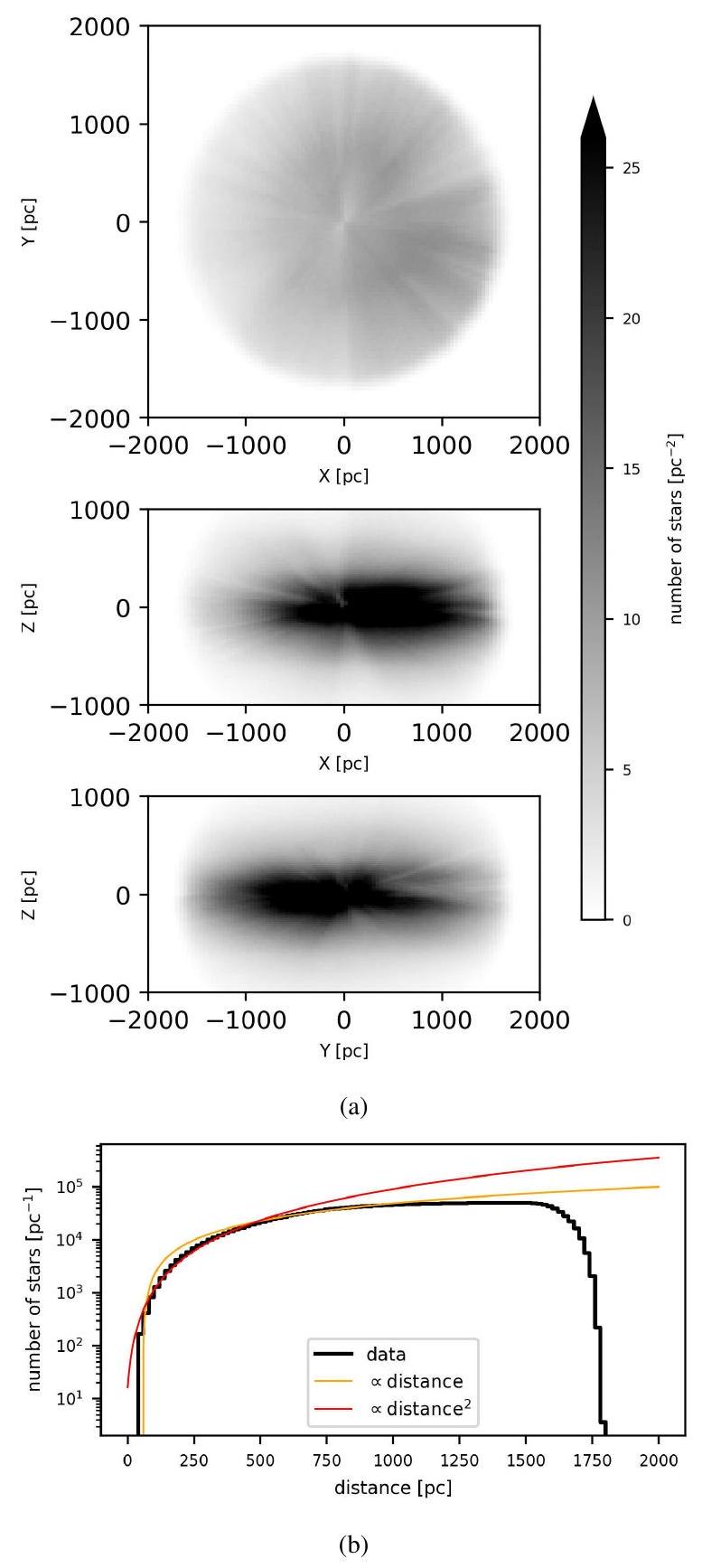
تعتمد موثوقية إعادة البناء لدينا بشكل أساسي على جودة وكمية البيانات. كلاهما يعتمد بشكل كبير على موقع نظام تحديد المواقع العالمي والمسافة. الشكل 1 يظهر مخططات ثنائية الأبعاد لكثافة النجوم في نظام الإحداثيات الكارتيزية المجري الهليوسنتري. ) التوقعات، بالإضافة إلى عدد النجوم كدالة للمسافة. تزداد كثافات النجوم لكل فئة مسافة أولاً تقريبًا بشكل تربيعي مع المسافة قبل أن تنخفض إلى زيادة خطية. عند حوالي 1.5 كيلوبارسيك، يستقر عدد النجوم لكل فئة مسافة بسبب متطلبنا أن تكون النجوم لديها احتمالية سيغما أن تكون ضمن 1.8 كيلوبارسيك في المسافة. الشكل 2 يظهر هيستوغرام POS للنجوم. يوجد بصمة واضحة لوظيفة اختيار Gaia BP/RP (انظر Cantat-Gaudin et al. 2023). كما أن هناك نقص منهجي في عينة النجوم خلف سحب الغبار الكثيفة. نتوقع أن تكون إعادة البناء لدينا أكثر موثوقية في المناطق ذات الكثافة النجمية الأعلى. بسبب تأثير الغبار المعيق، يجب التعامل مع المناطق داخل وخلف سحب الغبار الكثيفة بحذر أكبر.
3. المقدمات
كمية اهتمامنا هي توزيع ZGR23 الانقراض التفاضلي ثلاثي الأبعادبالتعريف، فإن الانقراض التفاضلي إيجابي. علاوة على ذلك، افترضنا أنه سلس مكانيًا. من حيث المبدأ، افترضنا أن مستوى السلاسة ثابت مكانيًا ومتساوي الاتجاه.
الشكل 1. مخططات ثنائية الأبعاد لكثافة النجوم في نظام الإحداثيات الكارتيزي الهليوسنتري. ) التوقعات، بالإضافة إلى كثافة النجوم كدالة للمسافة، لمجموعة فرعية من كتالوج ZGR23 المستخدمة في إعادة بناء خريطة الغبار ثلاثية الأبعاد الخاصة بنا. اللوحة أ: هيستوجرامات كارتيسية مجرية مركزية شمسية. اللوحة ب: عدد النجوم كدالة للمسافة. تظهر هذه اللوحة أيضًا نموًا خطيًا ونموًا تربيعيًا مع المسافة للمقارنة.
لإعادة بناء الحجم ثلاثي الأبعاد بكفاءة، قمنا بتفكيكه في إحداثيات كروية. على وجه التحديد، قمنا بتفكيك حجمنا المعاد بناؤه إلى كرات HEALPix على مسافات متباينة لوغاريتمياً. اعتمدنا على من 256، والتي تتوافق مع 786432 صندوق POS. هذايتوافق مع حجم زاوي لوحدات الفوكسل لدينابالنسبة لاتجاه LOS، اعتمدنا على 772 حاوية مسافة موزعة لوغاريتمياً، منها 256 تُستخدم للتعبئة. أعلى تمييز للمسافة لدينا هو 0.4 فرسخ.
الشكل 2. توزيع POS لمجموعة فرعية من نجوم ZGR23 المستخدمة في إعادة بناء خريطة الغبار ثلاثية الأبعاد الخاصة بنا.
أدنى تمييز للمسافة هو 7 فرسخ. بالمقارنة مع إعادة البناء باستخدام الفوكسيات المتباعدة خطيًا في المسافة، تمكنا من استكشاف أحجام أكبر بكثير مع الحفاظ على عينة عالية عند المسافات القريبة. يوفر التمييز حدًا أدنى للفصل بين هياكل الغبار التي يمكننا حلها. في الممارسة العملية، يعتمد الفصل القابل للحل على كمية وجودة البيانات ويختلف مع موضع النقطة في الفضاء (POS) وموضع خط الرؤية (LOS).
قمنا بتشفير كل من الإيجابية والنعومة في نموذجنا من خلال افتراض أن الانقراض التفاضلي موزع بشكل لوغاريتمي طبيعي:
مع توزيع طبيعي، حيث يتم استخراجه من عملية غاوسية ذات نواة ارتباط متجانسة ومتساوية الاتجاه،. من إعادة بناء سابقة للاختفاء التفاضلي لفرقة G في بيانات Gaia DR2 (Leike وآخرون 2020)، لدينا قيود على نواة الارتباط لوغاريتم الانقراض التفاضلي في حجم حول الشمس 270 قطعة ). كجزء من نموذجنا السابق، استخدمنا المستنتج نواة الانقراض من ليك وآخرون (2020). لأخذ التحويل بين انقراض ZGR23 في الاعتبار والانقراض، أضفنا عامل مضاعف عالمي إلىفي نموذجنا.علاوة على ذلك، استنتجنا انحرافًا إضافيًا في الانقراض التفاضلي. وضعنا أولوية لوغاريتمية طبيعية على المعامل المضاعف وأولوية طبيعية على المعامل الإضافي.
قمنا بفرض نواة الارتباطباستخدام تحسين مخطط تكراري (ICR؛ إيدنهوفر وآخرون 2022). يتيح لنا ICR فرض نواة على الفوكسلات الموزعة بشكل عشوائي من خلال تمثيل الحجم المودل عند عدة تفريغات. يبدأ من رؤية خشنة جدًا لحجمنا المودل. على هذا المقياس الخشن، يقوم ICR بنمذجة GP مع تحفيزات فوكسل متعلمة.ومصفوفة التغاير الكاملة الصريحة. أولا، المعلماتتوزع بشكل طبيعي قياسي ومترابط وفقًا لـعبر ICR. ثم يقوم بتحسينه بشكل تكراريأوقات وجهة نظرها الخشنة للفضاء مع تصحيحات محلية دقيقة ومعيارية موزعة بشكل طبيعي.حتى الوصول إلى التقطيع المطلوب. في كل تحسين، يستخدمالجيران من التحسين السابق لتحسين بكسل خشن إلىبكسلات دقيقة (انظر الخوارزمية 1).
تستخدم عملية التحسين المتكررة المخططة تصحيحات محلية عند تباينات مختلفة، وداخل عملية التحسين تفترض أن التكرار السابق قد نمذَج GP بدون خطأ. كلاهما يؤدي إلى طفيف
الخوارزمية 1: الشيفرة الزائفة لإنشاء GP باستخدام ICRمن الإثارات غير المرتبطة. كل بكسل خشن في الموقعيتم تحسينه بشكل تكراري إلىبكسلات دقيقة باستخدامجيران البكسل الخشنة. يتم الإشارة إلى نواة الارتباط بـتدل الأقواس المربعة بعد المتغيرات والوظيفتين ndindex و shape على روتينات الفهرسة الشبيهة بـ NumPy (هاريس وآخرون 2020). تشير الدالة explicit_gp إلى نموذج عملية غاوسية غير محدد يمثل بشكل صريح التغاير لـللمواقع البكسلية التي تم نمذجتها بواسطة.
أخطاء في تمثيل النواة. بالنسبة لحالة الاستخدام الخاصة بنا، واجهنا أخطاء في تمثيل النواة بنسبة قليلة. قبلنا هذه الأخطاء كتنازل يمكّن إعادة البناء من استكشاف أحجام أكبر. نشير إلى إيدنهوفر وآخرون (2022) لمناقشة مفصلة حول أخطاء تقريب النواة.
بشكل عام، نموذجنا للسابقة يقرأ ,
حيث نحدد التحجيم المضاعف المتعلم بـ بواسطة scl، والانزياح الإضافي المتعلم بـ off، وأعدنا التعبير عن كلاهما من حيث معلمات موزعة بشكل طبيعي قياسي أ بحدس و, على التوالي. يُطلق على فعل التعبير عن scl و off و عبر معلمات ذات توزيع أبسط بشكل مسبق، هنا توزيع طبيعي قياسي، إعادة المعايرة. يتم تقديم مناقشة مفصلة حول هذا الموضوع في ريزيندي ومحمد (2015).
4. الاحتمالية
لبناء الاحتمالية، احتجنا أولاً إلى تحديد كيفية ارتباط الانقراض التفاضلي – الكمية التي تهمنا – بالبيانات المقاسة. تتكون بياناتنا من موضع POS، والانقراض, وبيانات المنظور. موضع POS هو في جوهره
بدون خطأ. بيانات الانقراض هي في شكل انقراضات LOS المدمجة للنجوم والشكوك المرتبطة بها بيانات المنظور هي بالمثل في شكل تقديرات المنظور والشكوك.
يركز نموذجنا على الانقراض المقاس،, ولا يتنبأ بالمنظورات للنجوم. بدلاً من ذلك، قمنا بشرط نموذجنا على بيانات المنظور،, وقسمنا الاحتمالية إلى احتمال الانقراض المقاس بالنظر إلى الانقراض الحقيقي،, واحتمال الانقراض الحقيقي بالنظر إلى معلومات المنظور غير المؤكدة:
يتم تقييد الحد الأول من التكامل بجودة قياسات الانقراض والحد الثاني بجودة قياسات المنظور.
4.1. الاستجابة
يمكن التعبير عن الحد الثاني في المعادلة (4)،، كاحتمال مشترك للانقراض والمسافة الحقيقية،، مع تهميش المسافة الحقيقية:
تجاهلنا تأثيرات اختيار البيانات (أي، اعتماد على بالنظر إلى و اعتماد على بالنظر إلى) واستخدمنا حقيقة أن الانقراض الحقيقي،، عند المسافة المعروفة هو ببساطة التكامل LOS لـ على طول LOS إلى النجم من الصفر إلى
:مع شريحة من عند مواضع POS للنجوم، توزيع دلتا ديراك المحدد بواسطة لأي مستمر بدعم مضغوط، و الاستجابة التي تقوم بتعيين من
إلى مجال الانقراض المقاس.قمنا بتقريب بتوزيع طبيعي، ,
بمتوسط والانحراف المعياري للحصول على تعبير قابل للتعامل للمعادلة (4). متوسط الانقراض،
، هو
الجدول 1. معلمات التوزيعات السابقة.
الاسم
التوزيع
المتوسط
الانحراف المعياري
درجات الحرية
طبيعي
0.0
نواة من ليك وآخرون (2020)
scl
لوغاريتمي-طبيعي
1.0
0.5
1
off
طبيعي
الانقراض الوسيط السابق من ليك وآخرون (2020)
1.0
1
معامل الشكل
معامل المقياس
# النجوم = 53880655
غاما العكسيةملاحظات. المعلمات, و off تحدد بالكامل
. تم اختيارها بشكل مشترك لتوليد النواة المعاد بناؤها في ليك وآخرون (2020).بافتراض أن المنظور موزع بشكل طبيعي (أي، بمتوسط والانحراف المعياري
)، ثممع
دالة البقاء للمنظور الموزع بشكل طبيعي.يمكن فهم الانحراف المعياري
كإسهام خطأ إضافي لتهميش المسافة. يعتمد الخطأ على عدم اليقين في المسافة والغبار على طول LOS الكامل:تقييم كل من و رخيص نسبيًا في نظام إحداثيات كروي حيث أن الكرة المنفصلة هي ببساطة المجموع التراكمي لـ
على طول محور المسافة موزونًا بمدى كل فوكسل.
4.2. الاحتمالية وكثافة الاحتمال المشتركةافترضنا أن الانقراض المقاس موزع بشكل طبيعي حول الانقراض الحقيقي. أخذنا الانقراض المستنتج،، من الكتالوج ليكون متوسط التوزيع الطبيعي. تم افتراض أن الشك المصاحب في الكتالوج هو الانحراف المعياري لـ
.بعض النجوم سيكون لديها شكوك مقدرة بشكل أقل بسبب إما خصائص نجمية داخلية غير مصممة بشكل صحيح في الاستنتاج أو قياسات فوتومترية سيئة لم يتم الإشارة إليها. أردنا أن يكون نموذجنا قادرًا على اكتشاف وإلغاء اختيار النجوم التي تتعارض بشدة مع بقية إعادة البناء. حققنا ذلك من خلال استنتاج عامل مضاعف إضافي لكل نجم،، الذي يقوم بتوسيع. بشكل مسبق، افترضنا أن يتم سحبه من توزيع ذو ذيل ثقيل. بشكل خاص، افترضنا أن يتبع توزيع غاما العكسية. مرة أخرى نعبر عن من حيث معلمات موزعة بشكل طبيعي قياسي
في الاستنتاج.
لتلخيص، فإن احتمالية التقريب لدينا التي تم تقديمها أولاً في المعادلة (4) تقرأيتم توسيع الشك في الانقراض بواسطة لإلغاء اختيار القيم الشاذة وزيادته بواسطة
بسبب تهميش عدم اليقين في المسافة.
تقرأ دالة كثافة الاحتمال المشتركة للبيانات والمعلماتمع كمتجه لجميع معلمات النموذج. تم امتصاص تعقيد التوزيعات السابقة بالكامل في التحولات, off و من المعلمات الموزعة بشكل طبيعي قياسي مسبقًا
.تم تلخيص السابقتنا من حيث المعلمات غير القياسية في الجدول 1. تم اختيار السابقتين لـ و off مسبقًا لتوليد النواة المعاد بناؤها في ليك وآخرون (2020). على عكس ليك وآخرون (2020)، لا نتعلم نواة غير بارامترية كاملة. ومع ذلك، نستنتج scl و off، المقياس، ووضع الصفر للنواة. تم اختيار السابقة لـ
بحيث يكون توزيع غاما العكسية له وضع 1 والانحراف المعياري 2.
5. الاستنتاج البعديفي القسم السابق، أخذنا عناية خاصة للتعبير عن نموذجنا ليس فقط من حيث المعلمات الفيزيائية، مثل كثافة الانقراض التفاضلي، ولكن أيضًا من حيث معلمات أبسط. يُطلق على فعل التعبير عن معلمات النموذج scl و off و و من حيث متغيرات موزعة بشكل طبيعي قياسي مسبقًا
إعادة التوحيد، وهو شكل خاص من إعادة المعايرة (انظر ريزيندي ومحمد 2015). بشكل فعال، نحن ننقل التعقيد من السابقتين إلى الاحتمالية. ومع ذلك، فإن كل من الصياغة غير الموحدة والصياغة الموحدة للنموذج المشترك متكافئة. يمكن أن تؤدي نماذج التوحيد إلى مشاكل استنتاج أفضل شرطًا حيث تتغير المعلمات جميعها على نفس المقاييس – إذا لم تتعارض السابقتين مع الاحتمالية. استخدمنا مخطط استنتاج يعتمد على الصياغة الموحدة. أردنا استنتاج البعدي لنموذجنا الموحد من المعادلة (19). إن استكشاف البعدي مباشرة عبر طرق العينة مثل هاملتونيان مونتي كارلو هوفمان وجيلمان (2014) غير ممكن حسابيًا. بدلاً من ذلك، استخدمنا الاستنتاج المتغير لتقريب البعدي الحقيقي. بشكل خاص، استخدمنا استنتاج متغير غاوسي مقياسي (MGVI؛ كنولمولر وإنسلين 2019). نلخص الفكرة الرئيسية وراء MGVI في الملحق ب. لم نقم بتقريب البعدي للضوضاء
معامل الاستنتاج عبر الاستنتاج المتغير واستخدمنا فقط الحد الأقصى من البعدي لـ
.لتسريع الاستنتاج، بدأنا إعادة البناء عند دقة أقل (196، 608 صناديق POS عند و 388 صناديق مسافة LOS) وقيدنا الاستنتاج على مجموعة فرعية من النجوم مع فرصة سيغما أن تكون ضمن 600 فرسخ فلكي وفرصة سيغما أن تكون أبعد من 40 فرسخ فلكي. قمنا بزيادة نطاق المسافة للخريطة حتى يتم تضمين النجوم في خطوات 300 فرسخ فلكي من 600 فرسخ فلكي إلى 1.8 كيلوبارسيك. في كل مرة قمنا فيها بزيادة نطاق المسافة، قمنا بإعادة تعيين المعلمات لـ. ثم، بعد دمج جميع البيانات، قمنا بزيادة الدقة الزاوية والمسافة لإعادة البناء إلى الدقة النهائية.
اختيار بياناتنا يلغي اختيار النجوم القريبة من أقصى مسافة تم استكشافها (انظر الشكل 1). يؤدي هذا التأثير إلى أن المناطق الخارجية من الخريطة تتأثر بعدد قليل نسبيًا من النجوم مقارنة بالمناطق الداخلية. نلاحظ أن هذه المناطق عرضة لإنتاج ميزات زائفة. بالنسبة لمنتجات بياناتنا النهائية، أزلنا 550 فرسخ فلكي الأبعد من حجم البيانات المقيد حيث لاحظنا آثارًا متوافقة مع استراتيجية زيادة بياناتنا داخل هذه المناطق. نعتقد أن 550 فرسخ فلكي هو قطع محافظ لكننا ننصح بالحذر عند العثور على هياكل متوافقة تمامًا مع كرة حول الشمس عند، أو 1200 فرسخ فلكي.
تفترض ZGR23 أن جميع الانقراضات إيجابية بحتة. لقد تجاهلنا هذا القيد من خلال افتراض أخطاء غاوسية، مما أدى إلى ارتفاع مصطنع في الانقراض في أول بضع فوكيلات في كل اتجاه. كما نعلم أن تلك المناطق خالية فعليًا من الغبار من إعادة الإعمار السابقة، انظر ليك وآخرون (2020)، قمنا بإزالة 69 فرسخًا داخليًا (انظر الملحق C). نحن نطلق خريطة HEALPix إضافية للانقراض المتكامل حتى 69 فرسخًا من الشمس ونقترح استخدامها لتصحيح توقعات LOS المتكاملة للانقراض الذي تمت إزالته.
استنتاجنا يعتمد بشكل كبير على المشتقات لمكونات مختلفة من نموذجنا. تُستخدم المشتقات للتقليل وكذلك للتقريب التغيري لل posterior. النماذج السابقة مثل تلك الموصوفة في ليكي وإنسلين (2019) وليكي وآخرون (2020) اعتمدت على حزمة نظرية المعلومات العددية (NIFTy) (سيليغ وآخرون 2013؛ شتاينينجر وآخرون 2019؛ أراس وآخرون 2019) وكانت محدودة في التشغيل على وحدات المعالجة المركزية.
قمنا بتوظيف إطار عمل جديد يسمىNIFTy.re (Edenhofer وآخرون، قيد الإعداد.) لنشر نماذج NIFTy على وحدات معالجة الرسوميات.NIFTy.reهو جزء من حزمة NIFTy Python ويستخدم داخليًا JAX (برادبري وآخرون 2018) لتشغيل النماذج على وحدة معالجة الرسوميات (GPU). تمكنا من تسريع تقييم القيمة والتدرج للمعادلة (19) بمقدار مرتين من حيث الأوامر من خلال الانتقال من وحدات المعالجة المركزية (CPUs) إلى وحدات معالجة الرسوميات (GPUs). تم تشغيل إعادة البناء لدينا على وحدة معالجة الرسوميات NVIDIA A100 واحدة بسعة 80 جيجابايت من الذاكرة لمدة حوالي أربعة أسابيع.
6. التحذيرات
نعتقد أن الشكوك الإحصائية هي المصدر الرئيسي للشكوك في إعادة البناء لدينا. ومع ذلك، من المهم أيضًا النظر في مصادر الشكوك النظامية. اعتمادًا على التطبيق، قد تكون الشكوك النظامية أكثر أهمية من الشكوك الإحصائية. البيانات التي أبلغت عن إعادة البناء، والنموذج الذي استنتجنا به، وإجراءات الاستنتاج جميعها تساهم في الشكوك النظامية للنموذج.
بالطبع، تعتبر البيانات نفسها مصدرًا لعدم اليقين المنهجي (قانون الاحمرار الثابت مكانيًا، نمذجة خاطئة للثنائيات، إلخ؛ انظر زانغ وآخرون 2023) ومن المعروف أيضًا أنها غير مكتملة، انظر الشكل 2. كثافة نجمية أقل، على سبيل المثال في المناطق الم obscured بشكل كبير، تحد من دقة الخريطة وتؤدي إلى أن تكون أحجام الخريطة خلف سحب الغبار الكثيفة غير محددة بشكل جيد. وبالتالي، نعتقد أن إعادة بناء الغبار لدينا هي تقدير ناقص للاختفاء الحقيقي تجاه سحب الغبار الكثيفة. كما يشير زوكر وآخرون (2021) إلى هذا التأثير عند مقارنة خريطة ليكي وآخرون (2020) مع خرائط الاختفاء المتكاملة ثنائية الأبعاد المستندة إلى الفوتومترية تحت الحمراء، حيث وجدوا أن خريطة ليكي وآخرون (2020) ليست حساسة للمناطق التي تحتوي على.
نوصي بتصور كثافة النجوم في المنطقة المعنية لتقييم حجم الشكوك النظامية الناتجة عن عدم اكتمال البيانات. نحن نطلق جميع النجوم المستخدمة في إعادة البناء كمنتج بيانات إضافي. يمكن استخدام هذا المنتج البياني لتصور كثافة النجوم. في المناطق التي تعاني من نقص كبير في النجوم، نتوقع أن يهيمن النقص النظامي في النجوم على الشكوك الإحصائية في إعادة البناء. ومع ذلك، فإن الشكوك الناتجة لا تعكس سبب النقص النظامي في النجوم حيث يفترض النموذج ضمنيًا أن نقص النجوم ليس نظاميًا بل عشوائيًا بحتًا.
نموذجنا يتضمن عددًا من التقريبات. أولاً، افترضنا وجود أولوية GP على انقراض الغبار اللوغاريتمي باستخدام النواة من ليكي وآخرون (2020) وطبقناها تقريبًا فقط عبر ICR. ثانيًا، افترضناأن تكون مستقلاً عنثالثًا، افترضنا أن خطأ المنظور هو غاوسي، ورابعًا، افترضنا أن خطأ الانقراض هو غاوسي.
بالنسبة للاختفاءات المنخفضة للغاية، فإن الافتراض لـكونها غاوسية يعتبر ضعيفًا بسبب الأولوية الإيجابية في كتالوج ZGR23. قمنا بتصحيح هذا التحيز نحو تقديرات انقراض أعلى في المناطق التي يُفترض فيها انقراضات حقيقية منخفضة للغاية بعد ذلك من خلال قطع 69 فرسخًا فلكيًا من الداخل كما هو موضح في القسم 5. نحن ننشر خريطة مساعدة للانقراض المتكامل حتى 69 فرسخًا فلكيًا من الشمس لتصحيح توقعات خط الرؤية المتكاملة للانقراض الذي تمت إزالته. نقترح إضافة الانقراض المحلي الذي تمت إزالته مرة أخرى إلى الخريطة عند مقارنة الانقراضات المتكاملة. بشكل افتراضي، يتم إضافة الانقراض المحلي الذي تمت إزالته مرة أخرى إلى الخريطة عند استعلام الانقراضات المتكاملة عبر خرائط الغبار.
نحن نطلق أيضًا كتالوجًا بالانقراضات المتوقعة من نموذجنا لجميع النجوم التي استخدمناها في إعادة البناء. في الملحق د، نقوم بإجراء اختبار اتساق غير شامل يقارن توقعاتنا بتوقعات ZGR23. نجد أن كلا التوقعين للانقراض للنجوم لا يتفقان تحت 50 مماغ وفوقهناك المزيد من النجوم مما كان متوقعًا لديها توقعات انقراض أكبر (أو أصغر) مقارنة بـ ZGR23. نتوقع أن يتراوح النطاق من 50 ملليغرام إلى 4 مغ بين النطاقات التي يكون فيها خريطتنا موثوقة. مزيد من التفاصيل متوفرة في الملحق D.
علاوة على ذلك، فإن استنتاجنا اللاحق هو تقريبي. نفترض أن تقريبي للتوزيع اللاحق الحقيقي يلتقط بدقة عدم اليقين النموذجي الجوهري (انظر Arras et al. 2022؛ Leike & Enßlin 2019؛ Leike et al. 2020؛ Mertsch & Phan 2023؛ Roth et al. 2023a,b؛ Hutschenreuter et al. 2023، 2022؛ Tsouros et al. 2024). ومع ذلك، كنا قلقين بشأن هياكل قد تتعرض للاحتراق عندما نزيد المسافة القصوى المستكشفة خلال الاستنتاج من 600 فرسخ فلكي إلى 1800 فرسخ فلكي بخطوات قدرها 300 فرسخ فلكي كما هو موضح في القسم 5. قمنا بفحص إعادة البناء النهائية لهذا التأثير من خلال مقارنتها بإعادة بناء أكبر لا تختار النجوم بناءً على مسافاتها خلال الاستنتاج، بل تستخدم فقط عينة فرعية صغيرة من نجوم ZGR23 مع علامات جودة أكثر صرامة. تم إصدار إعادة البناء الأكبر، التي تمتد إلى 2 كيلو فرسخ فلكي في المسافة، كمنتج بيانات إضافي. لم نجد أي اختلافات كبيرة بين كلا التشغيلين. تم تقديم تفاصيل حول إعادة البناء الأكبر في الملحق E.
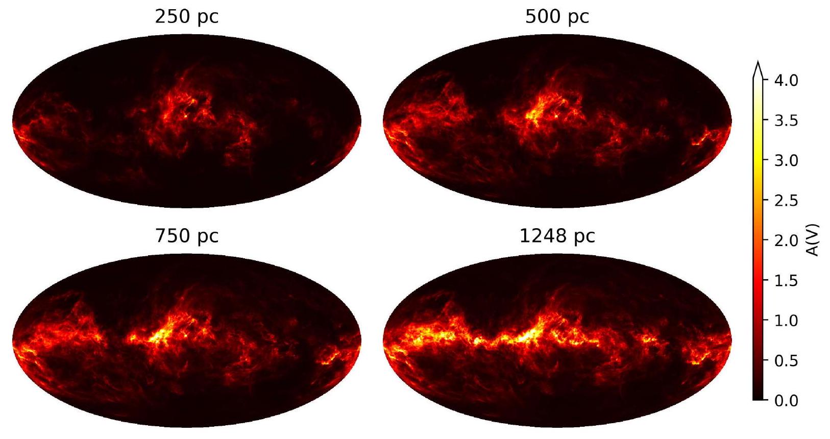
الشكل 3. إسقاط مولوايد لنظام POS المتكاملالانقراض إلى، وحتى أقصى مسافة في خريطتنا. يتشبع شريط الألوان عند كوانتيل
الشكل 4. نفس الشكل 3 ولكن يظهر الفرق بين الانقراضات المتكاملة بين شرائح المسافة المعروضة على نظام الإحداثيات. شريط الألوان يتشبع عندكوانتيل
7. النتائج
قمنا بإعادة بناء 12 عينة (6 عينات مستخرجة بشكل مضاد) من توزيع انقراض الغبار ثلاثي الأبعاد، كل منها يحتوي على 607125504 فوكسيات انقراض تفاضلي. الفوكسيات مرتبة على 772 كرة HEALPix معموزعة على مسافات تزداد بشكل لوغاريتمي. بعد إزالة الأعمقوالخارجيكرات HEALPix، تبقى لدينا 516 كرة HEALPix. العينات، المتوسط البعدي، والانحراف المعياري البعدي لإعادة البناء متاحة للجمهور على الإنترنت.نوصي بشدة باستخدام العينات لأي تحليل كمي. لراحتنا، نحن كما يوفر المتوسط البعدي والانحراف المعياري لإعادة الإعمار الم interpolated إلى إحداثيات كارتesian المجري الهليوسنتري. ) وإحداثيات كروية مجرية ( ، بالإضافة إلى ذلك، يمكن استعلام الخريطة عبر حزمة بايثون dustmaps (جرين 2018). يتم تقديم مزيد من التفاصيل حول استخدام إعادة البناء في الملحق F.
تجزئة المسافة في إعادة البناء لدينا هي الأعلى بالنسبة للفوكسلات القريبة وتتناقص كلما ابتعدنا. أعلى مستوى لدينا
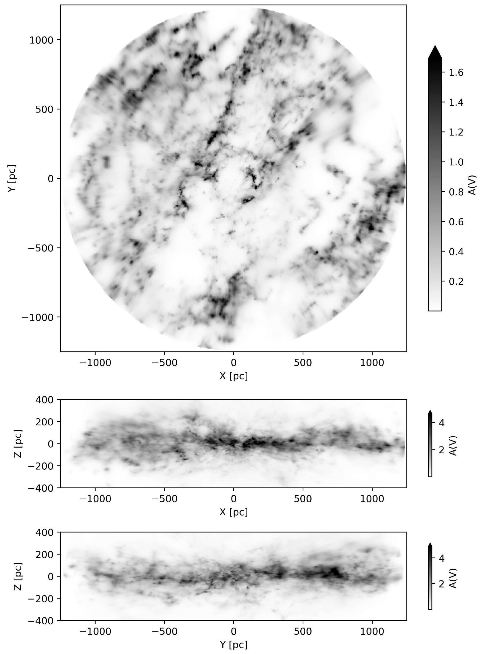
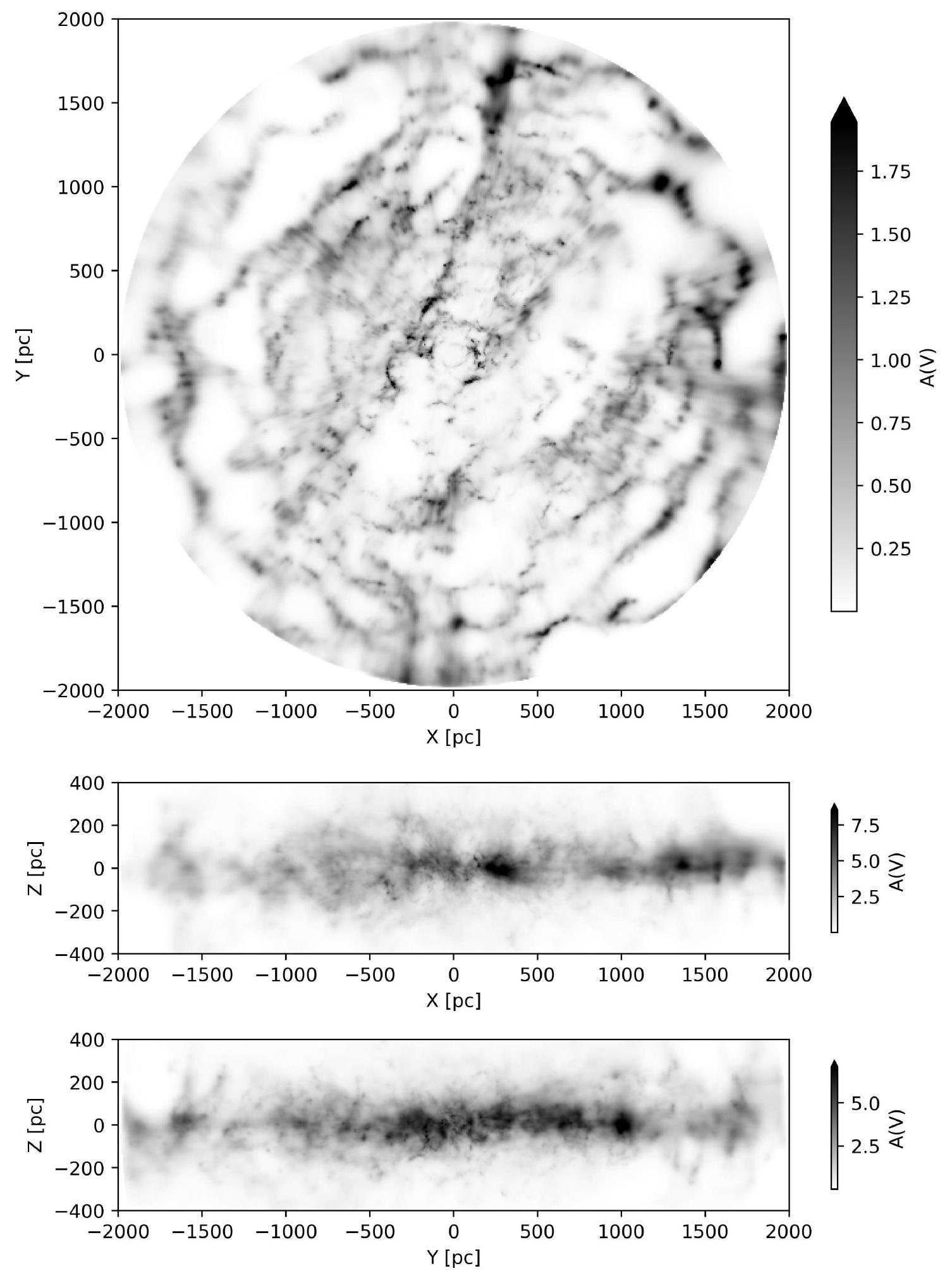
الشكل 5. الإحداثيات الكارتيزية المجسمة الشمسيةتوقعات المتوسط البعدي لخريطة الغبار ثلاثية الأبعاد الخاصة بنا في صندوق بأبعاد0.8 كيلوبارسيك مركزيًا حول الشمس. شريط الألوان خطي ويشبع عندكوانتايل. تتوفر صورة متحركة (GIF) لعينات الخلفية وإصدار تفاعلي ثلاثي الأبعاد منخفض الدقة من هذه الشكل على الإنترنت.
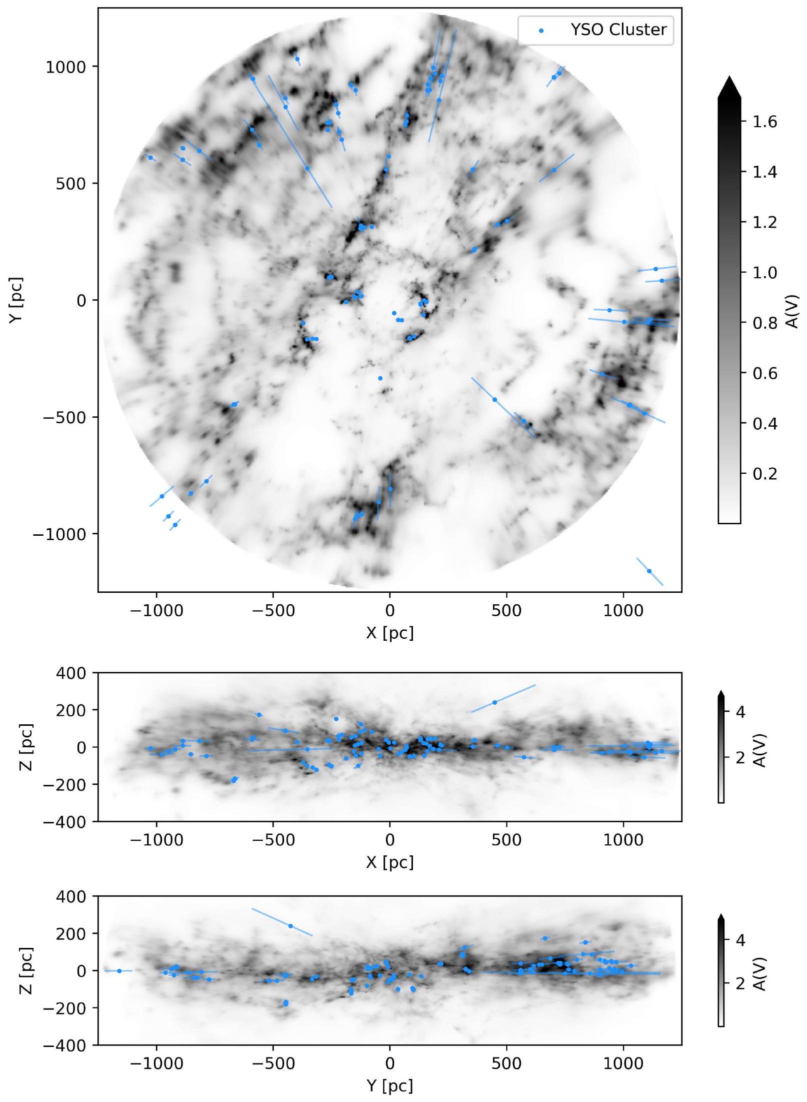
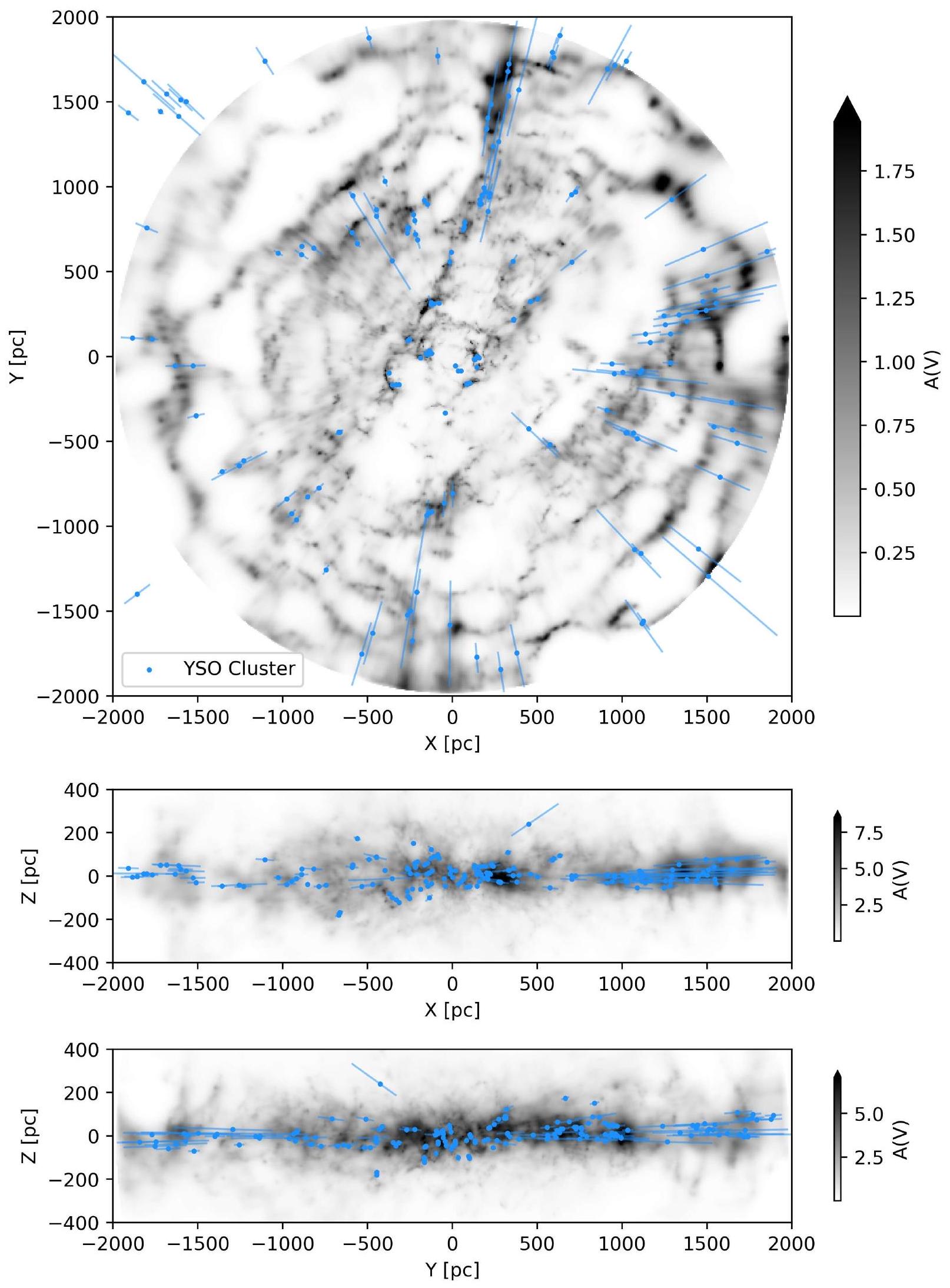
الشكل 6. نفس الشكل 5 ولكن مع كتالوج لمجموعات من الأجسام الشابة (YSOs) (كون 2023، اتصال خاص) استنادًا إلى كون وآخرون (2021)، وينستون وآخرون (2020)، ومارتون وآخرون (2023) موضحة كنقاط زرقاء فوق إعادة البناء؛ وتظهر عدم اليقين في المسافات كخطوط ممتدة.
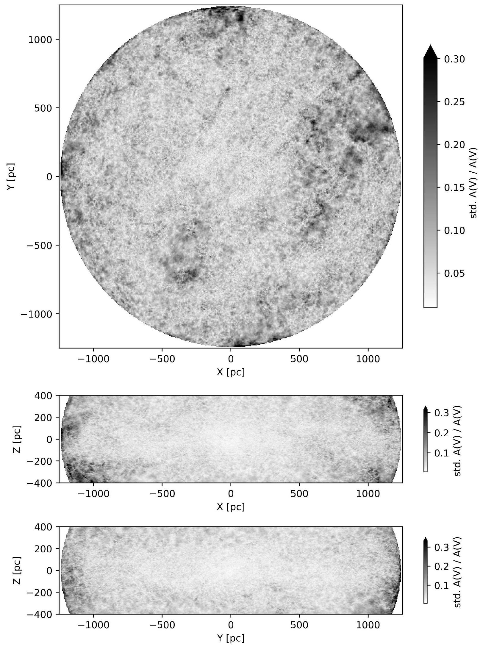
الشكل 7. الإحداثيات الكارتيزية المجرة الشمسية ) إسقاطات عدم اليقين النسبي لامتداد الغبار المعاد بناؤه المدمج ضمن صندوق من مركزه على الشمس. شريط الألوان خطي ويشبع عند الكمية.
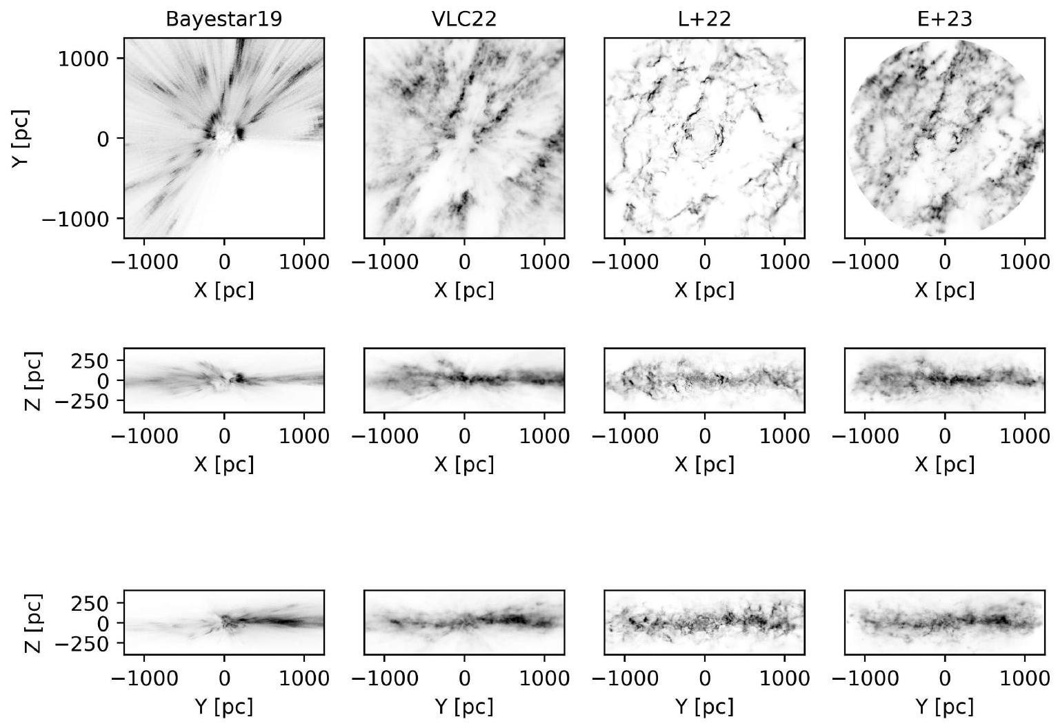
الشكل 8. عرض جانبي لخرائط الغبار ثلاثية الأبعاد من Bayestar19 و VLC22 و L+22 و هذا العمل، المعروضة في إحداثيات كارتيسية مجرية مركزية ( ) إسقاطات. شريط الألوان مشبع عند الكمية الخاصة بإعادة البناء.
الشكل 9. نسخة مكبرة من الشكل 8 للحجم المعاد بناؤه في Leike et al. (2020)، الآن يظهر أيضًا إعادة بناء LGE20 للمقارنة. نحن نستبعد L+22 من المقارنة لأن المؤلفين يركزون بشكل صريح على أحجام أكبر ويتاجرون بعيوب بارزة بشكل قوي في المئات القليلة الداخلية من البارسيك مقابل حجم أكبر تم استكشافه. شريط الألوان مشبع مرة أخرى عند الكمية الخاصة بإعادة البناء.
تجزئة المسافة هي 0.4 بارسيك وأدنى تجزئة مسافة لدينا هي 7 بارسيك بينما تجزئة الزاوية لدينا هي وهي مستقلة عن المسافة. تحدد التجزئات المذكورة الحد الأدنى على دقتنا. الحد الأدنى من الفصل الذي يمكننا حله يعتمد على الموقع ويتم ترميزه في العينات اللاحقة. بالنسبة للمناطق الصغيرة، نقترح تحليل كثافة النجوم (انظر القسم 6) لتقييم قوة عدم اليقين النظامي بسبب كثافة النجوم.
إعادة البناء هي من حيث انقراض ZGR23 بدون وحدة كما هو محدد في Zhang et al. (2023). لأغراض التصوير، قمنا بترجمة انقراض ZGR23 إلى نطاق V الخاص بجونسون 540.0 نانومتر، أي . لأداء التحويل، اعتمدنا على منحنى الانقراض المنشور في ZGR23 وضربنا انقراض ZGR23 بدون وحدة بعامل 2.8. نشير إلى القراء إلى منحنى الانقراض الكامل من Zhang et al. (2023) للحصول على المعاملات اللازمة لترجمة الانقراض إلى نطاقات أخرى.
الشكل 3 يصور إسقاط POS لمتوسط إعادة البناء اللاحق المدمج حتى ، وحتى نهاية كرتنا. القيم هي بوحدات من المقادير. نرى أن الميزات ذات العرض الأعلى مثل شق العقاب قريبة نسبيًا بينما تظهر الهياكل في المستوى المجري تدريجيًا فقط. الشكل 4 يظهر الفرق بين إسقاطات POS المدمجة. نحن نستعيد ميزات معروفة من الغبار المدمج ولكننا قادرون الآن على إعادة إسقاطها.
الشكل 5 يظهر عرضًا من منظور الطائر ( )، من الجانب ( )، و ( ) لمتوسط إعادة البناء اللاحق لدينا في إحداثيات كارتيسية مجرية مركزية. الصورة تصور الأقرب إلى الشمس في الانقراض المدمج على من -400 بارسيك إلى في -1.25 كيلوبارسيك إلى 1.25 كيلوبارسيك، و في -1.25 كيلوبارسيك إلى 1.25 كيلوبارسيك، على التوالي. في الشكل 6، نضع فوقها كتالوج من تجمعات الأجسام النجمية الشابة (YSOs؛ Kuhn 2023، اتصال خاص) بناءً على Kuhn et al. (2021) و Winston et al. (2020) و Marton et al. (2023)، والتي تظهر كنقاط زرقاء. تتفق مواقع تجمعات YSO بصريًا مع مواقع سحب الغبار ضمن عدم اليقين في المسافة المبلغ عنها لتجمعات YSO.
الانحراف المعياري اللاحق مقسومًا على المتوسط اللاحق لإعادة البناء يظهر في الشكل 7. الخريطة تحتوي على نمط بقع باهتة. من المحتمل أن يكون ذلك بسبب العدد المنخفض من العينات بالنسبة لعدد درجات الحرية. الانحراف المعياري هو في حدود من المتوسط اللاحق ويزداد قليلاً مع المسافة. نحو مركز المجرة خلف الغبار في الجوار المباشر لحوالي 300 بارسيك، يكون عدم اليقين النسبي أعلى بشكل ملحوظ.
إعادة البناء لها نطاق ديناميكي عالٍ وتكشف عن مسارات غبار باهتة في الحجم المعاد بناؤه. توجد تجاويف صغيرة تقريبًا كروية في جميع أنحاء الخريطة. سحب الغبار في إعادة البناء مضغوطة وممدودة بشكل ضعيف شعاعيًا. تم حل ميزات كبيرة النطاق بارزة، مثل موجة رادكليف (Alves et al. 2020) والانقسام (Lallement et al. 2019)، بمستوى غير مسبوق من التفاصيل، كان متاحًا سابقًا فقط لأقرب سحب غبار.
مقارنة مع خرائط الغبار ثلاثية الأبعاد الموجودة. في هذا القسم، نقارن خريطتنا مع خرائط الغبار ثلاثية الأبعاد الأخرى في الأدبيات. نشير إلى خريطة الغبار الموصوفة في Leike et al. (2020) بـ LGE20، و Vergely et al. (2022) بـ VLC22، و Green et al. (2019) بـ Bayestar19، و Leike et al. (2022) بـ L+22 في هذا القسم. لأغراض المقارنة، نعرض المتوسط اللاحق. نحن نطلق عدم اليقين الإحصائي كبيانات إضافية
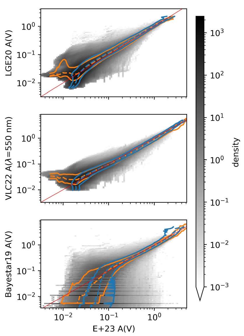
الشكل 10. هيستوغرام للانقراض المتوسط اللاحق لخريطتنا مقابل LGE20 و VLC22 و Bayestar19 لـ 58 مليون نقطة اختبار. لكل مركز بكسل من كرة HEALPix مع تم وضع نقاط اختبار على فترات 1 بارسيك في المسافة بدءًا من 69 بارسيك. تظهر الخطوط البرتقالية الكميات 16 و 50 و 84 من الانقراض المتوقع بواسطة LGE20 و VLC22 و Bayestar19، على التوالي، لكل حاوية من انقراضنا المتوسط. تظهر الكميات الخاصة بتوقعاتنا في حاويات إعادة البناء الأخرى كخطوط زرقاء. تظهر الخطوط المتوسطة باللون الأحمر. شريط الألوان لوغاريتمي ومقصوص في الطرف السفلي عند 1 مماغ.
المنتجات، وننصح بشدة بأخذ عدم اليقين الإحصائي المفرج عنه في الاعتبار لأي تحليل كمي. ومع ذلك، فإن الفروق بين إعادة البناء ثلاثية الأبعاد المختلفة التي تم مناقشتها هنا هي اختلافات نظامية وليست محصورة في عدم اليقين الإحصائي المعاد بناؤه.
في الشكل 8، نعرض إسقاطات ثلاثية الأبعاد ( ) للخرائط، مقارنة بين Bayestar19 و VLC22 و L+22 و هذا العمل جنبًا إلى جنب. تتفق الخرائط الأربعة على الهيكل العام لتوزيع الغبار.
هذا العمل و L+22 و VLC22 لديهم دقة مسافة قابلة للمقارنة، بينما تحتوي Bayestar 19 على عدد قليل نسبيًا من صناديق المسافة وأصابع الله أكثر وضوحًا. مقارنة بـ L+22، لدينا سحب غبار ممتدة بشكل أكثر تجانسًا وعدد أقل بكثير من التموجات في المسافات إلى سحب الغبار. مقارنة بـ VLC22، لدينا سحب غبار أكثر كثافة، وهياكل أقل حبيبية، ونطاق ديناميكي أعلى. كل من هذا العمل و VLC22 تحتوي على سحب غبار في حجم قابل للمقارنة حول الشمس على الرغم من أن خريطة VLC22 تمتد تقنيًا إلى أبعد في X و Y المجريين.
الشكل 9 يظهر نفس الإسقاطات للحجم المعاد بناؤه في خريطة LGE20 ويشمل خريطة LGE20 للمقارنة. يبرز التكبير التشابه الوثيق بين
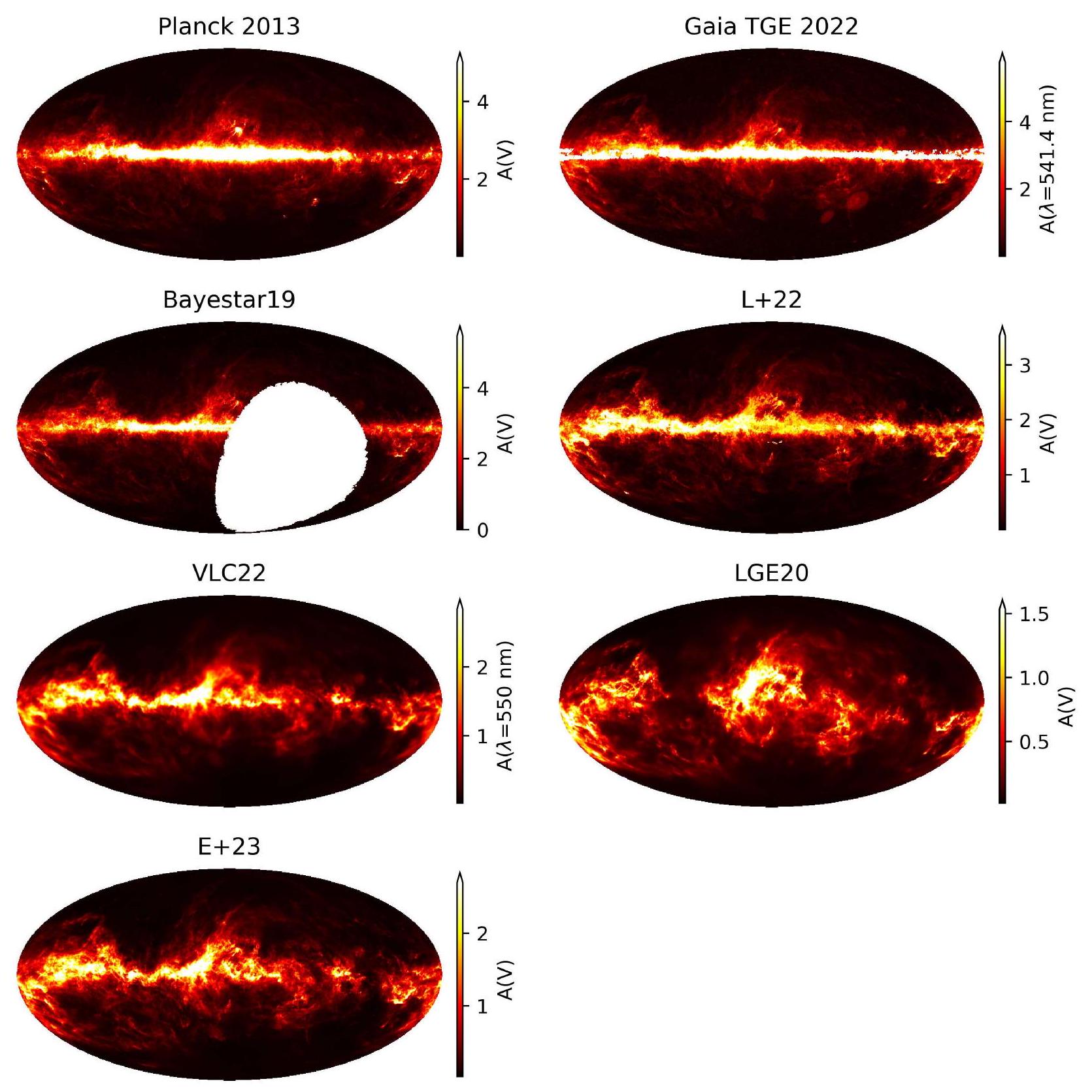
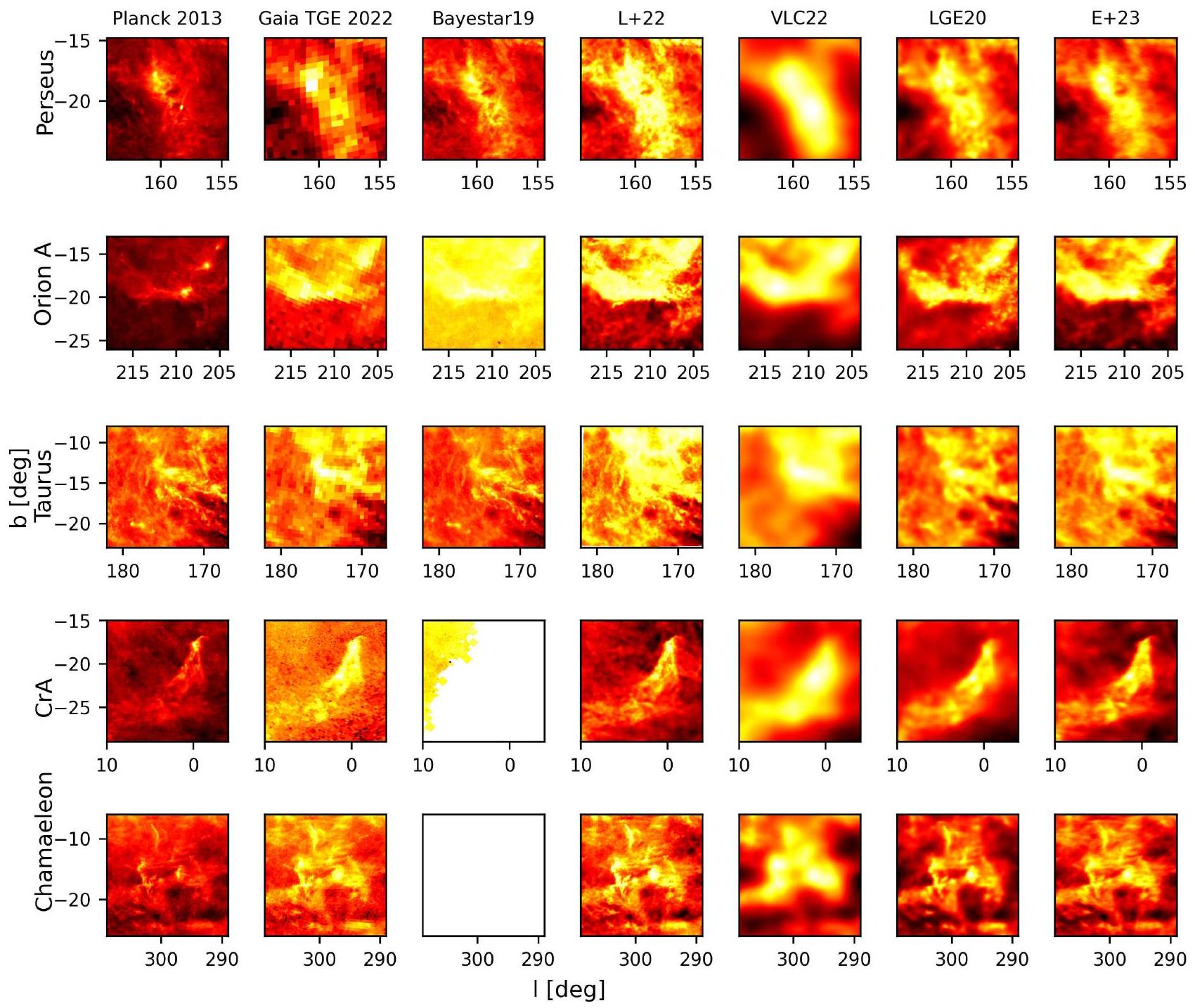
الشكل 11. إسقاطات مولوييد لإجمالي الانقراض المدمج وخرائط الانقراض ثلاثية الأبعاد المدمجة حتى أقصى مسافة للخريطة المعنية. تعيد Bayestar 19 بناء حتى أقصى مسافة تبلغ 63 كيلوبارسيك (أقصى مسافة موثوقة 10 كيلوبارسيك) وتم دمجها حتى ذلك الحجم. تعيد البناء حتى أقصى مسافة تبلغ 16 كيلوبارسيك لكن المؤلفين يثقون بخريطتهم فقط حتى 4 كيلوبارسيك ونقوم بدمج خريطتهم فقط حتى 4 كيلوبارسيك. تعيد VLC22 بناء صندوقًا مجريًا بحجم مع فوكسيلا بحد أقصى في المسافة وتم دمجها حتى نهاية الصندوق. بالمثل، تعيد LGE20 بناء صندوقًا مجريًا بحجم يغطي بحد أقصى في المسافة وتم دمجها حتى نهاية الصندوق. شريط الألوان مشبع عند الكمية الخاصة بالخريطة باستثناء شريط الألوان الخاص بـ Planck 2013، الذي يشبع عند 5 مغ لتسهيل المقارنة.
هذا العمل وخريطة LGE20. جميع الهياكل الأكبر لها تطابقات مباشرة في الخريطة الأخرى، ومع ذلك، فإن المسافات إلى الهياكل مختلفة قليلاً. علاوة على ذلك، تبدو خريطة LGE20 أكثر حدة قليلاً. النموذج في LGE20 مشابه جدًا لنموذجنا ولكنه يستخدم تقديرات أقل. تستخدم LGE20 أيضًا بيانات مجمعة (StarHorse DR2؛ انظر Anders et al. 2019). هناك حاجة إلى مزيد من العمل لتقييم صحة الميزات الأكثر حدة في LGE20 غير الموجودة في هذا العمل. تتفق خريطة VLC22 أيضًا بشكل جيد ولكن بدقة أقل. تعيد Bayestar19 بناء المسافات بشكل سيء على نطاق خريطة LGE20.
الشكل 10 يقارن بشكل كمي خريطتنا مع LGE20 و VLC22 و Bayestar19. قمنا بمقارنة الانقراض المدمج لكل مركز بكسل من كرة HEALPix مع عند 1182 نقطة اختبار موضوعة على فواصل 1 فرسخ فلكي في المسافة بدءًا من 69 فرسخ فلكي. قمنا بمقارنة الانقراضات المتكاملة لأن التحولات الطفيفة في المسافات إلى المناطق المنقرضة يمكن تمييزها بشكل أفضل من التنبؤات المتناقضة باستخدام الانقراضات المتكاملة بدلاً من المقارنة المباشرة للانقراضات التفاضلية. فوق 15 ملليغرام ، تتفق VLC22 و LGE20 بشكل جيد مع خريطتنا. أدناه من 40 ملليغرام وفوق من
الشكل 12. مشاهد مكبرة نحو السحب الجزيئية الفردية (برسيوس ، أوريون ، ثور ، كورونا أستراليس ، وشاميلون) كما هو موضح في الشكل 11. أشرطة الألوان لوغاريتمية وتمتد عبر النطاق الديناميكي الكامل لشريحة POS المختارة في كل صورة. كل صف هو منطقة منفصلة وكل عمود هو إعادة بناء منفصلة.
حوالي 3.5 مغ ، ينحرف Bayestar19 بشكل كبير عن توقعاتنا.
في الشكل 11 ، نقارن عرض POS لـ Bayestar19 و L+22 و VLC22 و LGE20 وهذا العمل. يتم دمج وجهات النظر الخاصة بـ POS إلى أقصى مسافة تم استكشافها بواسطة كل خريطة – أقل من 63 كيلوبارسيخ في المسافة لـ Bayestar19 (أقصى مسافة موثوقة 10 كيلوبارسيخ) ، في المسافة لـ (يثق المؤلفون في الهياكل حتى 4 كيلوبارسيخ على الرغم من أن الخريطة تمتد إلى 16 كيلوبارسيخ) ، صندوق هليوسنتريكي بحجم مع وحدات فوكيل لـ VLC22 بحد أقصى 2.16 كيلوبارسيخ في المسافة ، وصندوق هليوسنتريكي بحجم وحتى 590 فرسخ فلكي في المسافة لـ LGE20. بالإضافة إلى ذلك ، نعرض خريطة الغبار خارج المجرة Planck 2013 (تعاون Planck XI 2014) وخريطة الانقراض الكوني الكلي Gaia (TGE) 2022 (Delchambre et al. 2023).
تتفق جميع الخرائط على الهياكل الدقيقة عند خطوط العرض المجري العالية ولكنها تختلف في المستوى المجري بسبب الاختلاف في المسافة التي تمتد إليها إعادة البناء المعنية. لا تستكشف إعادة بناء الغبار ثلاثية الأبعاد عمقًا كافيًا في المستوى المجري لاستعادة خريطة الغبار خارج المجرة Planck 2013 بالكامل. يستكشف Bayestar 19 و
L+22 عمقًا أكبر بكثير من VLC22 و LGE20 وهذا العمل ، ومع ذلك لا يستكشفون العمود الكامل من الغبار الذي يظهر في Planck 2013 و Gaia TGE 2022. كل من VLC22 وخريطتنا تستكشف حتى عمق مشابه بينما LGE20 تستكشف الغبار فقط على مسافات أقرب بكثير.
يوضح الشكل 12 مقارنة مكبرة لسحب الغبار الجزيئية في برسيوس وأوريون A وثور وكورونا أستراليس (CrA) وشاميلون ، المدمجة حتى أقصى مسافة لكل خريطة (4 كيلوبارسيخ لـ ). من بين إعادة بناء الغبار ثلاثية الأبعاد ، يتمتع Bayestar19 و L+22 على الأرجح بأعلى دقة زاوية (تجزئة زاوية من أو و ، على التوالي). إنهم يحلون سحب الغبار ذات خطوط العرض العالية بتفاصيل كبيرة على الرغم من أن L+22 تعاني من عيوب موضعية في بقع من السماء. كل من LGE20 ( صناديق) وهذا العمل ( ) تحقق دقة زاوية قابلة للمقارنة. إعادة بناء VLC22 ( وحدات فوكيل) أقل بكثير في الدقة ولا تحل بنية السحب الفرعية على POS. يتم تقديم مقارنة بين نفس السحب الجزيئية في شرائح مسافة مختلفة في VLC22 و LGE20 وخريطتنا في الملحق G.
8. الاستنتاجات
نقدم خريطة غبار ثلاثية الأبعاد بدقة POS و LOS قابلة للمقارنة مع Leike et al. (2020) التي تمتد حتى 1.25 كيلوبارسيخ. استخدمنا تقديرات المسافة والانقراض من Zhang et al. (2023) ، والتي لديها عدم يقين في الانقراض أقل بكثير من الكتالوجات المتنافسة بينما تستكشف عددًا مشابهًا من النجوم. إعادة البناء لدينا لها دقة قابلة للمقارنة مع دقة 2 فرسخ فلكي لـ Leike et al. (2020). على وجه التحديد ، لديها دقة زاوية تصل إلى ودقة مسافة على مقياس فرسخ فلكي. خريطتنا تتفق بشكل جيد مع خرائط الغبار ثلاثية الأبعاد الموجودة وتحسن عليها من حيث الحجم المغطى بدقة مكانية عالية. الخريطة متاحة للجمهور عبر الإنترنت ويمكن استعلامها عبر حزمة Python الخاصة بـ dustmaps. نتوقع أن تكون الخريطة مفيدة لمجموعة واسعة من التطبيقات في دراسة توزيع الغبار والوسط بين النجمي بشكل أوسع.
الشكر. نشكر جواو ألفيس على العديد من المناقشات المثمرة في ورشة العمل “التنظيم الذاتي عبر المقاييس: من النانومتر إلى فرسخ فلكي (SOcraSCALES)” في معهد ميونيخ لعلم الفلك والفيزياء الجزيئية والجزئية ، وهو معهد من مجموعة التميز ORIGINS في 2022 وما بعدها. علاوة على ذلك ، نشكر يعقوب روث على العديد من المناقشات القيمة حول النموذج وعلى تقديم ملاحظات حول النسخ المبكرة من إعادة البناء. نشكر أليسا جودمان على تقديم ملاحظات قيمة حول النسخ المتأخرة من إعادة البناء. نشكر أيضًا مايكل أ. كون على تزويدنا بكاتالوج موحد من YSOs. يعترف غوردين إيدنهوفر بدعم مؤسسة المنح الدراسية الأكاديمية الألمانية في شكل منحة دكتوراه (“منحة دراسية من مؤسسة الشعب الألماني”). تعترف كاثرين زوكر بأن الدعم لهذا العمل تم توفيره من قبل ناسا من خلال منحة زمالة هابل من ناسا #HST-HF2-51498.001 الممنوحة من معهد علوم التلسكوب الفضائي (STScI) ، الذي تديره جمعية الجامعات للبحث في علم الفلك ، Inc. ، لصالح ناسا ، بموجب عقد NAS5-26555. يعترف فيليب فرانك بالتمويل من خلال وزارة التعليم والبحث الفيدرالية الألمانية لمشروع ErUM-IFT: نظرية حقل المعلومات للتجارب في المنشآت البحثية الكبرى (رقم الدعم: 05D23EO1). يعترف أندرو ك. سايدجاري بدعم من زمالة أبحاث الدراسات العليا من مؤسسة العلوم الوطنية (DGE-1745303). يعترف أندرو ك. سايدجاري ودوغلاس فينكبيينر بدعم من منحة NASA ADAP 80NSSC21K0634 “تجميع مجرة درب التبانة: نموذج متكامل لنجوم المجرة وغازها وغبارها”. تم دعم هذا العمل من قبل مؤسسة العلوم الوطنية بموجب اتفاقية تعاونية PHY-2019786 (معهد NSF للذكاء الاصطناعي والتفاعلات الأساسية). تم تمكين جزء من هذا العمل بواسطة مجموعة FASRC Cannon المدعومة من مجموعة علوم الأبحاث في FAS بجامعة هارفارد. نعترف بالدعم من مرفق ماكس بلانك للحوسبة والبيانات (MPCDF). استخدم هذا العمل بيانات من مهمة وكالة الفضاء الأوروبية (ESA) Gaia (https://www.cosmos.esa.int/gaia) ، المعالجة بواسطة اتحاد معالجة بيانات Gaia وتحليلها (DPAC ، https://www.cosmos.esa.int/web/gaia/dpac/consortium). تم توفير التمويل لـ DPAC من قبل المؤسسات الوطنية ، وخاصة المؤسسات المشاركة في الاتفاقية متعددة الأطراف Gaia.
References
Alves, J., Zucker, C., Goodman, A. A., et al. 2020, Nature, 578, 237
Anders, F., Khalatyan, A., Chiappini, C., et al. 2019, A&A, 628, A94
Anders, F., Khalatyan, A., Queiroz, A. B. A., et al. 2022, A&A, 658, A91
Arras, P., Baltac, M., Ensslin, T. A., et al. 2019, Astrophysics Source Code Library [record ascl:1903.008]
Arras, P., Frank, P., Haim, P., et al. 2022, Nat. Astron., 6, 259
Astropy Collaboration (Robitaille, T. P., et al.) 2013, A&A, 558, A33
Astropy Collaboration (Price-Whelan, A. M., et al.) 2018, AJ, 156, 123
Astropy Collaboration (Price-Whelan, A. M., et al.) 2022, ApJ, 935, 167
Bradbury, J., Frostig, R., Hawkins, P., et al. 2018, JAX: composable transformations of Python+NumPy programs, https://github.com/google/ jax
Cantat-Gaudin, T., Fouesneau, M., Rix, H.-W., et al. 2023, A&A, 669, A55
Capitanio, L., Lallement, R., Vergely, J. L., Elyajouri, M., & Monreal-Ibero, A. 2017, A&A, 606, A65
Carrasco, J. M., Weiler, M., Jordi, C., et al. 2021, A&A, 652, A86
Chambers, K. C., Magnier, E. A., Metcalfe, N., et al. 2016, arXiv e-prints [arXiv:1612.05560]
Chen, B. Q., Huang, Y., Yuan, H. B., et al. 2019, MNRAS, 483, 4277
De Angeli, F., Weiler, M., Montegriffo, P., et al. 2023, A&A, 674, A2
Delchambre, L., Bailer-Jones, C. A. L., Bellas-Velidis, I., et al. 2023, A&A, 674, A31
Dharmawardena, T. E., Bailer-Jones, C. A. L., Fouesneau, M., & ForemanMackey, D. 2022, A&A, 658, A166
Draine, B. T. 2011, Physics of the Interstellar and Intergalactic Medium (Princeton University Press)
Edenhofer, G., Leike, R. H., Frank, P., & Enßlin, T. A. 2022, arXiv e-prints [arXiv:2206.10634]
Frank, P. 2022, Phys. Sci. Forum, 5, 6
Frank, P., Leike, R. H., & Enßlin, T. A. 2021, Entropy, 23, 853
Gaia Collaboration (Vallenari, A., et al.) 2023, A&A, 674, A1
Górski, K. M., Hivon, E., Banday, A. J., et al. 2005, ApJ, 622, 759
Green, G. 2018, J. Open Source Softw., 3, 695
Green, G. M., Schlafly, E. F., Finkbeiner, D., et al. 2018, MNRAS, 478, 651
Green, G. M., Schlafly, E., Zucker, C., Speagle, J. S., & Finkbeiner, D. 2019, ApJ, 887, 93
Harris, C. R., Millman, K. J., van der Walt, S. J., et al. 2020, Nature, 585, 357
Hoffman, M. D., & Gelman, A. 2014, J. Mach. Learn. Res., 15, 1593
Hutschenreuter, S., Anderson, C. S., Betti, S., et al. 2022, A&A, 657, A43
Hutschenreuter, S., Haverkorn, M., Frank, P., Raycheva, N. C., & Enßlin, T. A. 2023, A&A, submitted [arXiv:2304.12350]
Knollmüller, J., & Enßlin, T. A. 2019, arXiv e-prints [arXiv:1901. 11033]
Kuhn, M. A., de Souza, R. S., Krone-Martins, A., et al. 2021, ApJS, 254, 33
Lallement, R., Capitanio, L., Ruiz-Dern, L., et al. 2018, A&A, 616, A132
Lallement, R., Babusiaux, C., Vergely, J. L., et al. 2019, A&A, 625, A135
Lallement, R., Vergely, J. L., Babusiaux, C., & Cox, N. L. J. 2022, A&A, 661, A147
Leike, R., & Enßlin, T. 2019, A&A, 631, A32
Leike, R. L., Glatzle, M., & Enßlin, T. A. 2020, A&A, 639, A138
Leike, R. H., Edenhofer, G., Knollmüller, J., et al. 2022, A&A, submitted [arXiv:2204.11715]
Marton, G., Ábrahám, P., Rimoldini, L., et al. 2023, A&A, 674, A21
Mertsch, P., & Phan, V. H. M. 2023, A&A, 671, A54
Montegriffo, P., De Angeli, F., Andrae, R., et al. 2023, A&A, 674, A3
Planck Collaboration XI. 2014, A&A, 571, A11
Popescu, C. C., & Tuffs, R. J. 2002, MNRAS, 335, L41
Queiroz, A. B. A., Anders, F., Chiappini, C., et al. 2023, A&A, 673, A155
Rezaei Kh., S., & Kainulainen, J. 2022, ApJ, 930, L22
Rezaei Kh., S., Bailer-Jones, C. A. L., Hanson, R. J., & Fouesneau, M. 2017, A&A, 598, A125
Rezaei Kh., S., Bailer-Jones, C. A. L., Hogg, D. W., & Schultheis, M. 2018, A&A, 618, A168
Rezaei Kh., S., Bailer-Jones, C. A. L., Soler, J. D., & Zari, E. 2020, A&A, 643, A151
Rezende, D. J., & Mohamed, S. 2015, in Proceedings of the 32nd International Conference on International Conference on Machine Learning, 37, 1530
Roth, J., Arras, P., Reinecke, M., et al. 2023a, A&A, 678, A177
Roth, J., Li Causi, G., Testa, V., Arras, P., & Ensslin, T. A. 2023b, AJ, 165, 86
Schlafly, E. F., Meisner, A. M., & Green, G. M. 2019, ApJS, 240, 30
Selig, M., Bell, M. R., Junklewitz, H., et al. 2013, Astrophysics Source Code Library [record ascl:1302.013]
Skrutskie, M. F., Cutri, R. M., Stiening, R., et al. 2006, AJ, 131, 1163
Steininger, T., Dixit, J., Frank, P., et al. 2019, Ann. Phys., 531, 1800290
Tsouros, A., Edenhofer, G., Enßlin, T., Mastorakis, M., & Pavlidou, V. 2024, A&A, 681, A111
Vergely, J. L., Lallement, R., & Cox, N. L. J. 2022, A&A, 664, A174
Wang, C., Huang, Y., Yuan, H., et al. 2022, ApJS, 259, 51
Winston, E., Hora, J. L., & Tolls, V. 2020, AJ, 160, 68
Wright, E. L., Eisenhardt, P. R. M., Mainzer, A. K., et al. 2010, AJ, 140, 1868
Xiang, M., Rix, H.-W., Ting, Y.-S., et al. 2022, A&A, 662, A66
Zhang, X., Green, G. M., & Rix, H.-W. 2023, MNRAS, 524, 1855
Zonca, A., Singer, L., Lenz, D., et al. 2019, J. Open Source Softw., 4, 1298
Zucker, C., Speagle, J. S., Schlafly, E. F., et al. 2019, ApJ, 879, 125
Zucker, C., Goodman, A., Alves, J., et al. 2021, ApJ, 919, 35
الملحق A: ZGR23 في المناطق الخالية من الغبار
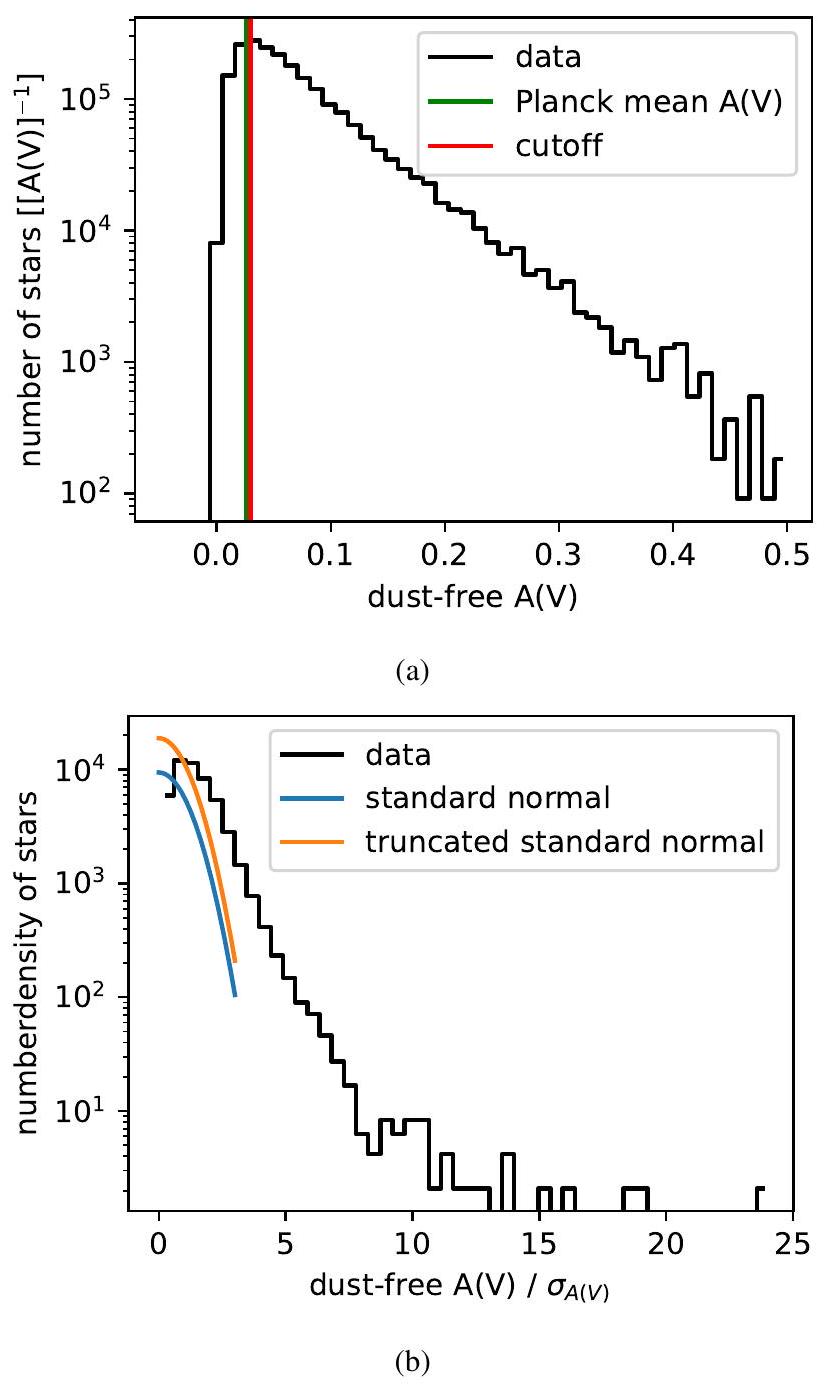
لتقييم موثوقية كتالوج ZGR23 ، قمنا بتحليل الانقراض للنجوم في المناطق الخالية من الغبار (انظر Leike & Enßlin 2019؛ Leike et al. 2020). في المناطق الخالية من الغبار ، نتوقع أن يكون الانقراض صفرًا ضمن عدم اليقين في الكتالوج. لتصنيف منطقة على أنها خالية من الغبار ، استخدمنا خريطة انبعاث الغبار Planck (تعاون Planck XI 2014). يقال إن المنطقة خالية من الغبار إذا كانت خريطة Planck أقل من أو تساوي 9.5 ملليغرام أو حوالي 29 ملليغرام من حيث .
الشكل A.1. الانقراض المطلق والنسبى لـ ZGR23 في المناطق الخالية من الغبار. اللوحة (أ): هيستوغرام لانقراضات ZGR23 في المناطق الخالية من الغبار مترجمة إلى . يتم عرض متوسط الانقراض في المناطق الخالية من الغبار بناءً على Planck كخط أخضر عمودي ، ويتم عرض قيمة القطع المترجمة إلى لتعريفنا عن الخالية من الغبار باللون الأحمر. اللوحة (ب): نفس الشيء كما في اللوحة (أ) ولكن يتم قياس الانقراضات بواسطة عدم يقينها المرافق. يتم رسم توزيع طبيعي قياسي مقطوع وتوزيع طبيعي قياسي فوقه. كلا المحورين لوغاريتميان.
تظهر اللوحة الأولى من الشكل A.1 هيستوغرام انقراض ZGR23 للنجوم مع quality_flags في المناطق الخالية من الغبار مترجمة إلى . نرى أن هيستوغرام الانقراض يصل إلى قيمة القطع ويتزامن مع متوسط الانقراض الكلي كما تم قياسه بواسطة Planck في تلك المناطق مترجمة إلى . تنخفض كثافة قيم الانقراض بشكل أسي
بعد قيمة القطع. بشكل عام ، يبدو أن انقراض ZGR23 يتفق جيدًا مع تعاون Planck XI (2014) للمناطق الخالية من الغبار.
تظهر اللوحة الثانية من الشكل A.1 الانقراض مقسومًا على عدم اليقين الخاص به للنجوم من الشكل A.1. الانقراضات الموحدة مركزة حول الواحد، مما يشير إلى أن انقراض ZGR23 بالفعل يبتعد عن الصفر بحوالي انحراف معياري واحد في المناطق الخالية من الغبار. هذا يتماشى مع الاكتشاف السابق بأن الانقراضات مركزة حول قيمة القطع بدلاً من التكتل حول الصفر. العرض حول المركز قابل للمقارنة مع توزيع طبيعي قياسي مقطوع أو توزيع طبيعي. في المجموع، حواليتوجد كتلة الاحتمال خارج النطاق الممكن لجميع انقراض ZGR23 مع علامات الجودةإذا افترضنا توزيعًا طبيعيًا للانقراضات.
باستثناء القيم الشاذة البعيدة عن المركز، والتي يمكن التقاطها بواسطة نموذج القيم الشاذة، يبدو أن كتالوج ZGR23 يتفق مع قياسات POS في المناطق الخالية من الغبار، وينتشر حول قيمة القطع تقريبًا وفقًا لتوزيع طبيعي (مقصوص). نعتبر كتالوج ZGR23 موثوقًا لأغراضنا ونقرب عدم اليقين باستخدام توزيع طبيعي. لقد قبلنا عدم نمذجة جزء صغير من كتلة الاحتمال من أجل نموذج أبسط (انظر الأقسام 5 و 6).
الملحق ب: الاستدلال المتغير الغاوسي المتركي
تقوم طريقة الاستدلال التبايني MGVI بتقريب التوزيع البعدي الحقيقيمع توزيع طبيعي قياسي في فضاء تم تحويله خطيًا حيث يشبه التوزيع اللاحق بشكل أكبر توزيعًا طبيعيًا قياسيًا. دعكن التوزيع التقريبي الخلفي وتحويل الإحداثيات. في هذه المساحة، يُقرأ التوزيع الخلفي المحول. نحن نحدد المقياس في الفضاء الذي فيههو “أكثر” معيارياً طبيعياً بواسطةافتراضاًمن المعروف أن الصعوبة تكمن فقط في إيجاد الأمثللـ.
استنادًا إلى مقياس معلومات فيشر وإحصائيات التكرارية، يستنتج كل من كنولميلر وإنسلين تحويلًا إحداثيًامركز علىهذا خطي في. في فرانك (2021)، يجد المؤلفون أن مجموعة من الإحداثيات العادية ريمان مركز علىهي تقدير غير خطي محسن لتحويل الإحداثياتومع ذلك، تأتي التحسينات بتكاليف حسابية أعلى قليلاً. نشير إلى القارئ إلى فرانك (2021) وفرانك (2022) لمزيد من التفاصيل حول geoVI وعلاقته بـ MGVI، واختيار المقياس، وتحليل أوضاع فشله. لأسباب حسابية، استخدمنا MGVI لاستنتاجنا.
تبدأ MGVI و geoVI من موقع ابتدائي عشوائي لـوارسمعينات طبيعية قياسية في فضاء. بعد ذلك، يقومون بتحويل العينات إلى فضاء عبرالتقريب المحلي، الخطي (على التوالي، غير الخطي لـ geoVI) إلىفينرمز للعناصر في فضاء المعلمات بـ. بالنسبة لنقطة التوسعالعينات تقرأالعيناتحولتوفير تقدير تجريبي مأخوذ من عينة لـالذي نرمز له بـ. تقوم MGVI و geoVI بعد ذلك بتحسينمن التوزيع المأخوذ عينة منه،، من خلال تقليل تباعد كولباك-ليبلر (KL) التغيري بينوالحقيقة توزيع
يحتفظون بالعناصر النسبيةثابت أثناء التحسين ويتغير فقط. أخيرًا، يقومون بتحديث نقطة التوسعإلى الأمثل المكتشف حديثًا.
بعد التقليل، يقوم MGVI و geoVI برسم مجموعة جديدة من العينات، وتحويلها من خلال توسيع محلي (خطّي) لـ، ثم يتم تقليلها مرة أخرى. يتم تكرار سحب العينات والتقليل حتى الوصول إلى نقطة ثابتة لـ تم الوصول إليه. الخوارزمية 2 تلخص الخطوات الخوارزمية للتقريب التبايني لل posterior الحقيقي.
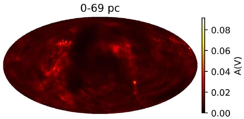
من خلال بناء احتمالنا، نعلم أن نموذجنا متحيز بشكل مرتفع لقيم الانقراض المنخفضة لأننا أهملنا الأولوية الإيجابية لكتالوج ZGR23. وهذا يترك أثره على الخريطة في شكل طبقة رقيقة من انقراض الغبار في بداية الحجم المودل. نظرًا لأن الفوكسلات في إعادة البناء لدينا مترابطة، فإن الطبقة الأولى المنقرضة من الفوكسلات تسحب الطبقة التالية من الفوكسلات إلى انقراضات أعلى قليلاً أيضًا. عند 69 فرسخًا، يصل الانقراض التفاضلي كدالة للمسافة إلى حد أدنى محلي، ونتوقع تأثيرًا ضئيلًا أو معدومًا من الطبقات الداخلية للفوكسلات. وبالتالي، حددنا 69 فرسخًا كحد قطع لدينا.
تظهر الشكل C. 1 الانقراض المتكامل الذي تم قطعه من إعادة البناء النهائية. من المحتمل أن يكون معظم الانقراض زائفًا. بشكل عام، لا تساهم أي بنية بمقدار كبير من الانقراض. ومع ذلك، لتكون متسقًا مع ZGR23، نقترح إضافة الانقراض الذي تم إزالته مرة أخرى إلى الخريطة عند مقارنة الانقراض المتكامل.
الشكل C.1. إسقاط مولوايد للتكاملالانقراض في أقرب 69 فرسخ فلكي، والذي من المحتمل أن يكون مهيمنًا عليه تأثيرات زائفة، وبالتالي يتم استبعاده من إعادة البناء. شريط الألوان خطي ويغطي النطاق الكامل للانقراض الذي تم استبعاده من إعادة البناء.
الملحق د: كتالوج الانقراض
نصدر كتالوجًا بالانقراض المتوقع لجميع النجوم ضمن مجموعة كتالوج ZGR23 التي استخدمناها في إعادة البناء (انظر القسم 2). نتوقع الانقراض المتوقع بناءً على البارالاكس المعروف بما في ذلك عدم اليقين في البارالاكس. توقعنا هو أفضل تقدير لنموذجنا للانقراض نحو نجم، ولكنه ليس بالضرورة أفضل تقدير للانقراض عند متوسط البارالاكس للنجم.
تختلف توقعاتنا للانقراض (انظر الأقسام 3 و4) عن حالات الانقراض في كتالوج ZGR23 من خلال ربط النجوم الفردية عبر كثافة انقراض الغبار ثلاثي الأبعاد. بفضل اعتماد كل نجم على جميع النجوم القريبة عبر السابق، تأتي توقعاتنا للانقراض في شكل توقعات مشتركة لجميع النجوم. في المناطق التي تكون فيها كثافة انقراض الغبار ثلاثي الأبعاد محددة بشكل جيد، تتفكك التوقعات المشتركة من الدرجة الأولى إلى توقعات للنجوم الفردية، ويمكننا حساب الانقراضات المتوقعة للنجوم الفردية وعدم اليقين المرتبط بها.
يتضمن كتالوجنا للانقراض 69 فرسخًا فلكيًا من الداخل من بداية شبكتنا و550 فرسخًا فلكيًا خارج 1.25 كيلوبارسيك التي قمنا بإزالتها في الخريطة ثلاثية الأبعاد. ننصح بالحذر عند تحليل النجوم في كتالوجنا ضمن تلك المناطق حيث قد تحمل تحيزات إضافية. يتم تقديم تفاصيل حول سبب إزالة هذه المناطق من الخريطة النهائية في القسمين 5 و6.
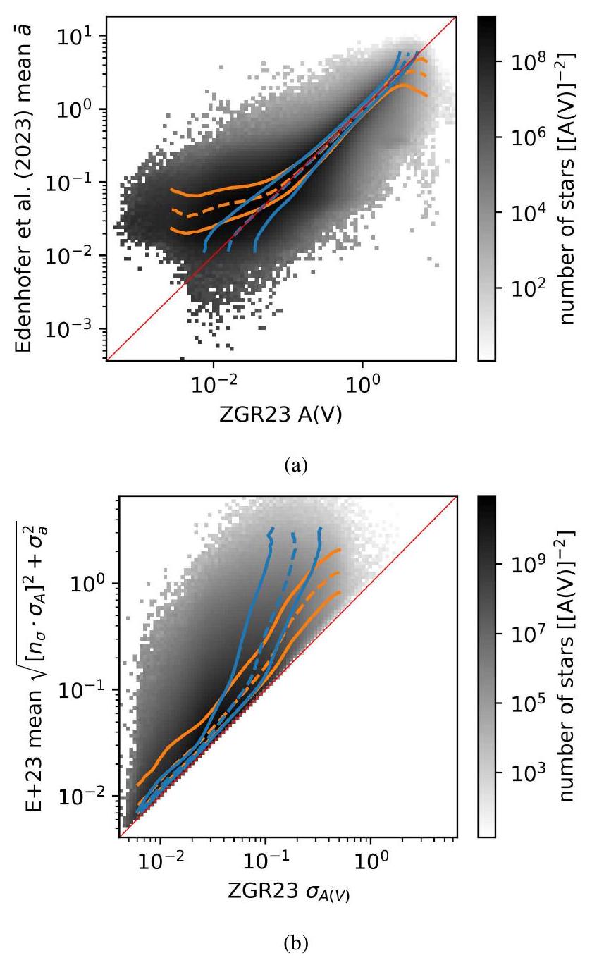
تقوم اللوحة العلوية من الشكل D.1 بمقارنة انقراضات ZGR23 بتوقعاتنا المتوسطة للانقراضات لنجوم Gaia BP/RP. بشكل عام، تتوافق انقراضاتنا المتوسطة بشكل جيد جداً مع الانقراضات في كتالوج ZGR23 لأغلبية النجوم. ومع ذلك، تحت 50 مماغ وفوق 4 مغ، تنحرف توقعاتنا للانقراض عن التوقعات في ZGR23. في أي فئة انقراض معينة من ZGR23 على التوالي، نتوقع أن يكون نصف الانقراضات الأخرى المعنية تحت القاطع والنصف الآخر فوقه. عندهناك نجوم أكثر مما كان متوقعًا لديها انقراضات أعلى من الانقراضات المقابلة في ZGR23. وتزداد الفجوة بشكل أكبر بالنسبة للانقراضات الأقل في ZGR23. عندهناك نجوم أكثر مما كان متوقعًا لديها انقراضات أقل من الانقراضات المقابلة في ZGR23.
تظهر اللوحة السفلية من الشكل D.1 عدم اليقين في الانقراض لدينا و ZGR23. نلاحظ أن عدم اليقين في الانقراض لدينا هو توقعات لعدم اليقين المقاسة في كتالوج ZGR23.وليس عدم اليقين في توقعات انقراضنا (انظر القسم 4). بشكل عام، تتفق كلا عدم اليقين بشكل جيد بالنسبة لأغلب النجوم. عند انخفاض عدم اليقين في الانخفاض، فإن عدم اليقين لدينا يزيد فقط بشكل طفيف من عدم اليقين في ZGR23. ومع ذلك، عند ارتفاع عدم اليقين في الانخفاض، تغطي توقعاتنا نطاقًا أكبر، ونجد أن ZGR23 يقلل بشكل كبير من تقديرات عدم اليقين في الانخفاض للنجوم.
الشكل D.1. انقراض ZGR23 مقابل انقراضنا المتوقع لنجوم Gaia BP/RP. اللوحة (أ): انقراضاتنا المتوسطة اللاحقة مقابل انقراضات ZGR23 للنجوم كهيستوغرام ثنائي الأبعاد.، و تظهر كوانتيلات انقراضات ZGR23 لكل فئة من متوسط انقراضنا كخطوط زرقاء. تظهر الكوانتيلات المقابلة لتوقعاتنا في فئات انقراضات ZGR23 كخطوط برتقالية. اللوحة (ب): نفس المقارنة ولكن لتوقعاتنا المتوسطة اللاحقة لعدم اليقين في قياسات ZGR23., مقابل عدم اليقين في ZGR23. لاحظ أن التنبؤات بشأن عدم اليقين في قياسات ZGR23 ليست عدم اليقين في تنبؤاتنا بالانقراض. انظر القسم 4 وبشكل خاص المعادلة (18) لمزيد من التفاصيل حول الكميات المعروضة هنا. يتم عرض القواطع باللون الأحمر. الأشرطة اللونية لوغاريتمية.
تُلخص الشكل D.2 الانقراضات وعدم اليقين في الانقراض لكل من ZGR23 وتنبؤاتنا في هيستوجرام واحد للانقراض القياسي المتوسط. يتم عرض غاوسي قياسي كمرجع. تحتوي المتبقيات القياسية المتوسطة على كثافتين خفيفتين في كل طرف مقارنة بالغاوسي.
يظهر الشكل D.3 الانحراف المعياري البعدي لتنبؤاتنا بالانقراض مقابل عدم اليقين في ZGR23. ينتج نموذجنا تقريبًا عدم يقين في الانقراض أقل بمقدار ترتيب واحد من عدم اليقين في ZGR23 بالنسبة لأغلب النجوم. التأثير أقل وضوحًا بالنسبة لعدم اليقين في الانقراض المنخفض ZGR23.
تنبؤاتنا بشأن الانقراض للنجوم تحتوي نظريًا على مزيد من المعلومات حيث نسمح بالتداخل بين النجوم القريبة
الشكل D.2. الانقراضات القياسية المتوسطة: (انظر القسم 4 وبشكل خاص المعادلة (18)) ضمن النطاق من -5 إلى 5.
الشكل D.3. مشابه للشكل D.1 ولكن بالنسبة للانحراف المعياري البعدي لانقراضاتنا مقابل عدم اليقين في ZGR23. يتم عرض , و كميات عدم اليقين في ZGR23 لكل حاوية من انحرافنا المعياري كخطوط زرقاء. يتم عرض الكميات المقابلة لانحرافنا المعياري في حاويات عدم اليقين في ZGR23 كخطوط برتقالية. يتم عرض القواطع باللون الأحمر. الأشرطة اللونية لوغاريتمية.
النجوم عبر توزيع ثلاثي الأبعاد للغبار وبالتالي قد تكون أكثر دقة. ومع ذلك، قد يوفر كتالوج ZGR23 نتائج أفضل في الممارسة العملية لأنه لا يقوم بتجزئة الحجم ثلاثي الأبعاد الذي تقيم فيه النجوم. من خلال تجزئة الحجم المودل، يمكننا إنتاج بيانات متناقضة تكون في الفضاء المستمر غير متناقضة، على سبيل المثال من خلال وضع نجوم ذات انقراض عالٍ تقع في سحابة غبار في نفس الفوكسل مع نجوم ذات انقراض أقل مجاورة لسحابة الغبار. بشكل عام، تتفق كلا التنبؤات بشكل جيد جدًا للنجوم التي تقل عن 50 مماغ و4 مغ. هناك حاجة إلى مزيد من العمل للتحقق من التنبؤات المتناقضة عند الانقراضات المنخفضة جدًا والعالية جدًا.
الملحق E: إعادة بناء 2 كيلوبارسيك
في القسم 5 نصف كيف نقوم بزيادة المسافة بشكل تكراري حتى نصل إلى أقصى مسافة معاد بناؤها. فعلنا ذلك لتحسين تقارب إعادة البناء. كما حاولنا بشكل ساذج إعادة بناء الحجم الكامل دفعة واحدة. استخدام جميع البيانات المتاحة مكلف حسابيًا، لذا قمنا بتقييد إعادة البناء إلى بيانات عالية الجودة باستخدام quality_flags , , و.
الشكل E.1. إسقاطات متوازية المحاور للانقراض الناتج عن الغبار في صندوق بأبعاد مركزيًا على الشمس. الشريط اللوني خطي ويشبع عند الكمية.
استخدمنا و لاختيار النجوم ضمن كرة بقطر 3 كيلوبارسيك. لتسريع الاستدلال، بدأنا الاستدلال باستخدام عينة من ، ثم ، وأخيرًا من النجوم. في المجموع، اخترنا نجوم. بعد الاستدلال، قطعنا الجزء الخارجي 1 كيلوبارسيك من كرة المنطقة المقيدة بالبيانات لتجنب تأثيرات التدهور بسبب تباعد النجوم عند الحافة. يمتد الحجم المعاد بناؤه بعد إزالة الكرات الخارجية HEALPix إلى 2 كيلوبارسيك في المسافة.
يظهر إعادة البناء في الشكل E.1 ومرة أخرى في الشكل E.2 مع كتالوج لمجموعات YSO (Kuhn 2023، اتصال خاص.)
الشكل E.2. نفس الشكل E.1 ولكن مع كتالوج لمجموعات YSOs (Kuhn 2023، اتصال خاص.) بناءً على Kuhn et al. (2021)، Winston et al. (2020)، و Marton et al. (2023) تظهر كنقاط زرقاء فوق إعادة البناء؛ يتم عرض عدم اليقين في المسافة كخطوط ممتدة.
مُركبة فوق. يظهر نفس الميزات الكبيرة كما في إعادة البناء الأصغر التي تم مناقشتها في النص الرئيسي. توزيع سحب الغبار الكثيفة يتفق مع مواقع مجموعات YSO ضمن عدم اليقين في المسافات لمجموعات YSO. مقارنة بالشكل 5، إعادة البناء أقل تفصيلاً وتتميز بعيوب أكثر وضوحًا.
استخدمنا إعادة البناء الأكبر للتحقق من استدلال الأصغر. على وجه التحديد، استخدمنا إعادة البناء الأكبر لضمان أن الهياكل المتوافقة مع الحدود الشعاعية التي زادت بها المسافة من إعادة البناء الرئيسية مستقلة عن المواقع التي زادت بها المسافة المغطاة.
نحن نطلق إعادة البناء الأكبر كمنتج بيانات إضافي مع إعادة البناء الرئيسية. ننصح باستخدام إعادة البناء الرئيسية لجميع المناطق التي تقع ضمن حجمها. يجب توخي الحذر عند تفسير الميزات أو الهياكل الصغيرة النطاق على مسافات عالية في إعادة البناء الأكبر.
الملحق F: استخدام إعادة البناء
جميع منتجات البيانات متاحة للجمهور عبر الإنترنت . يتم تخزين منتجات البيانات في تنسيق ملف FITS. المنتجات الرئيسية للبيانات هي عينات ما بعد التوزيع المكاني ثلاثي الأبعاد لانقراض الغبار المجزأ إلى كرات HEALPix على مسافات موزعة لوغاريتميًا. لتسهيل الأمر، نقدم أيضًا المتوسط ما بعد والانحراف المعياري لعينات كرات HEALPix على مسافات موزعة لوغاريتميًا.
قمنا أيضًا بتداخل المتوسط ما بعد والانحراف المعياري إلى شبكة كارتيسية. تم إجراء التداخل عند تجزئة أقل باستخدام فوكسلات للحفاظ على حجم الملف صغيرًا بشكل معقول. نوصي بإعادة تداخل الخريطة عند تجزئة أعلى لدراسة المناطق الفردية داخل الخريطة.
نحن نطلق برنامج التداخل كجزء من إصدار البيانات. توقيعه يقرأ interp2box.py OUTPUT_DIRECTORY] [-b BOX] healpix_path. الصندوق هو سلسلة من زوجين مفصولين بنقطتين. الزوج الأول يحدد عدد الفوكسلات على طول كل محور من الصندوق والزوج الثاني يحدد زوايا الصندوق بوحدات بارسيك في الإحداثيات الشمسية. لتداخل الخريطة إلى صندوق بحجم فوكسلات من الحجم و، استخدم interp2box.py -b ‘ :: -mean_and_std_healpix.fits.
بالإضافة إلى ذلك، قمنا بتداخل المتوسط ما بعد والانحراف المعياري إلى الطول والعرض والمسافة المجري. توقيع برنامج التداخل يقرأ interp2lbd.py [-h] [-o OUTPUT_DIRECTORY] [-b BOX] healpix_path. سلوكه مشابه لـ interp2box.py ولكن يتم تحديد الصندوق من حيث الطول والعرض والمسافة المجري بوحدات درجات، درجات، وبارسيك، على التوالي.
كلا البرنامجين يتطلبان حزم بايثون numpy (Harris et al. 2020)، astropy (Astropy Collaboration et al. 2013، 2018، 2022)، و healpy (Górski et al. 2005؛ Zonca et al. 2019). اعتمادًا على عدد الفوكسلات الناتجة، يمكن أن يكون التداخل مكلفًا جدًا من حيث الذاكرة وحسابيًا.
الملحق G: السحب الجزيئية حسب المسافة
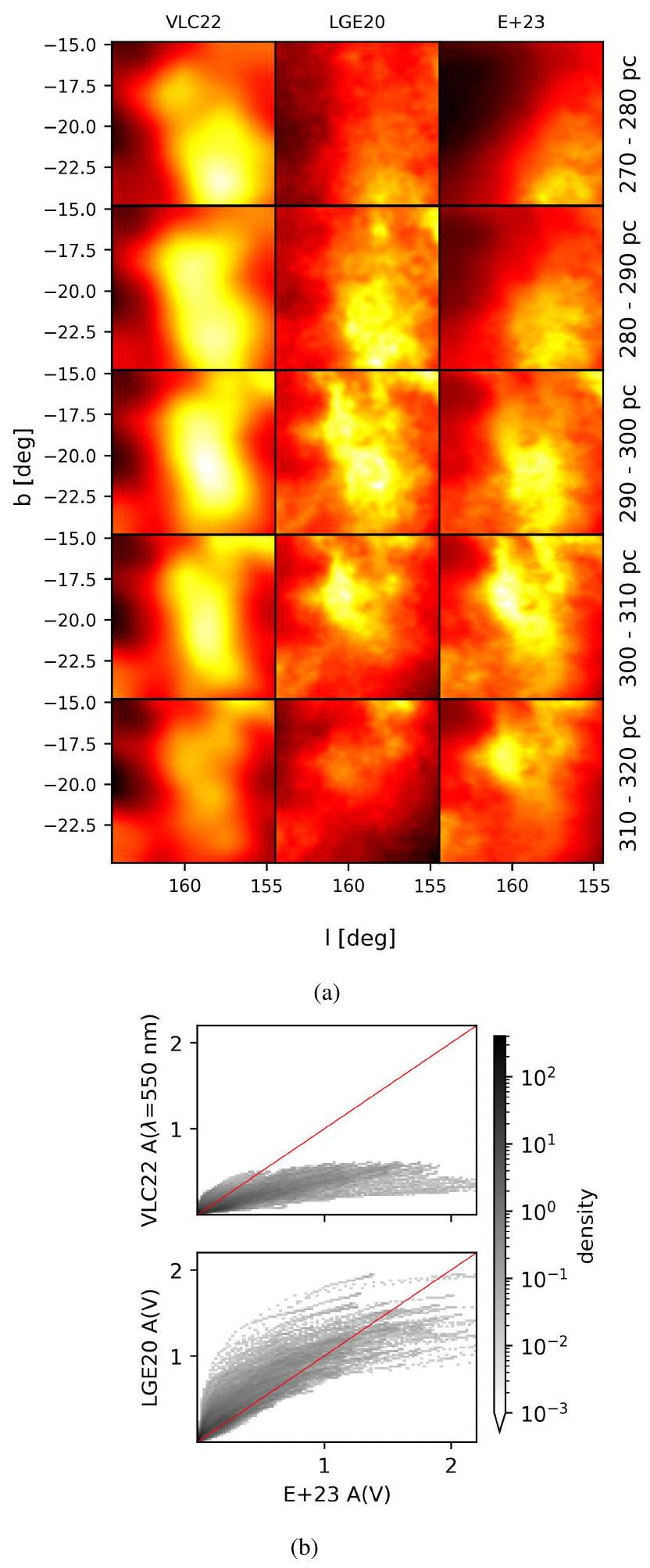
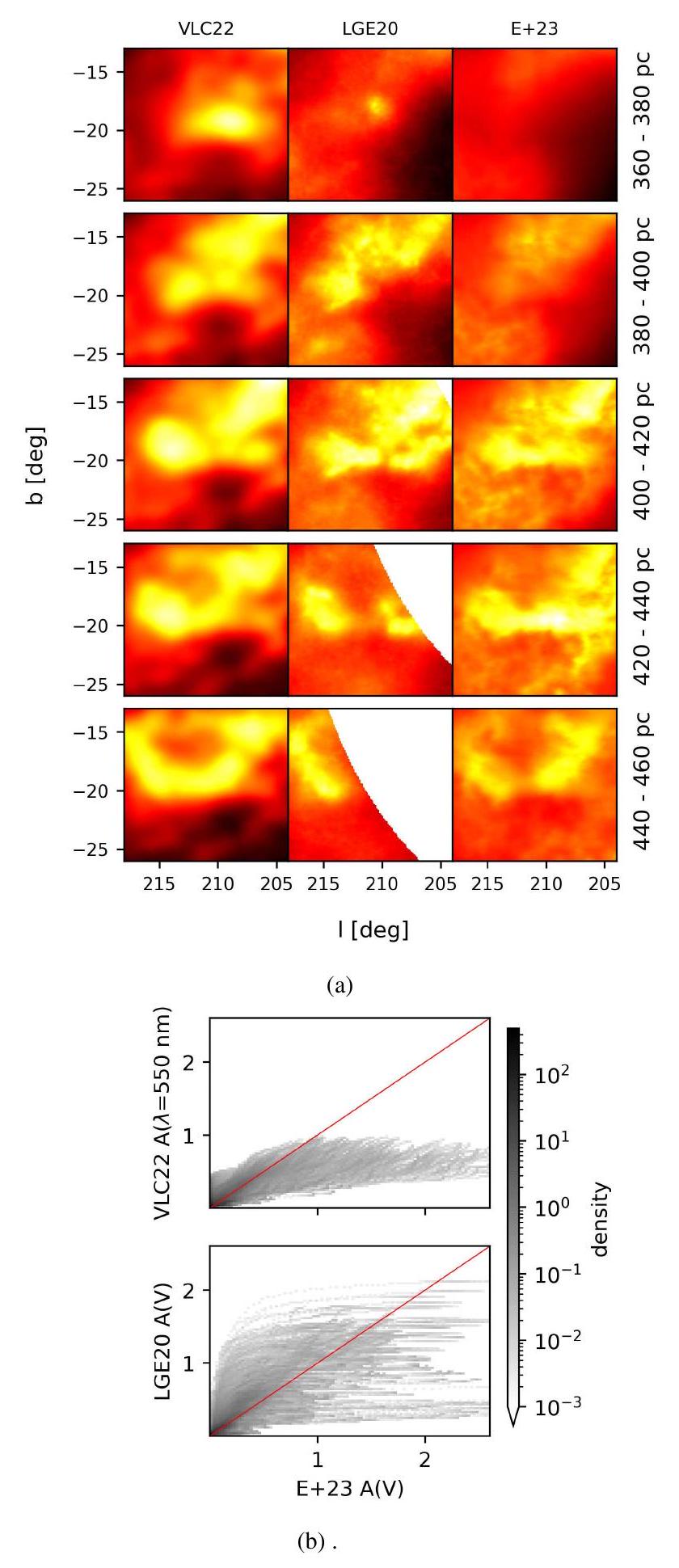
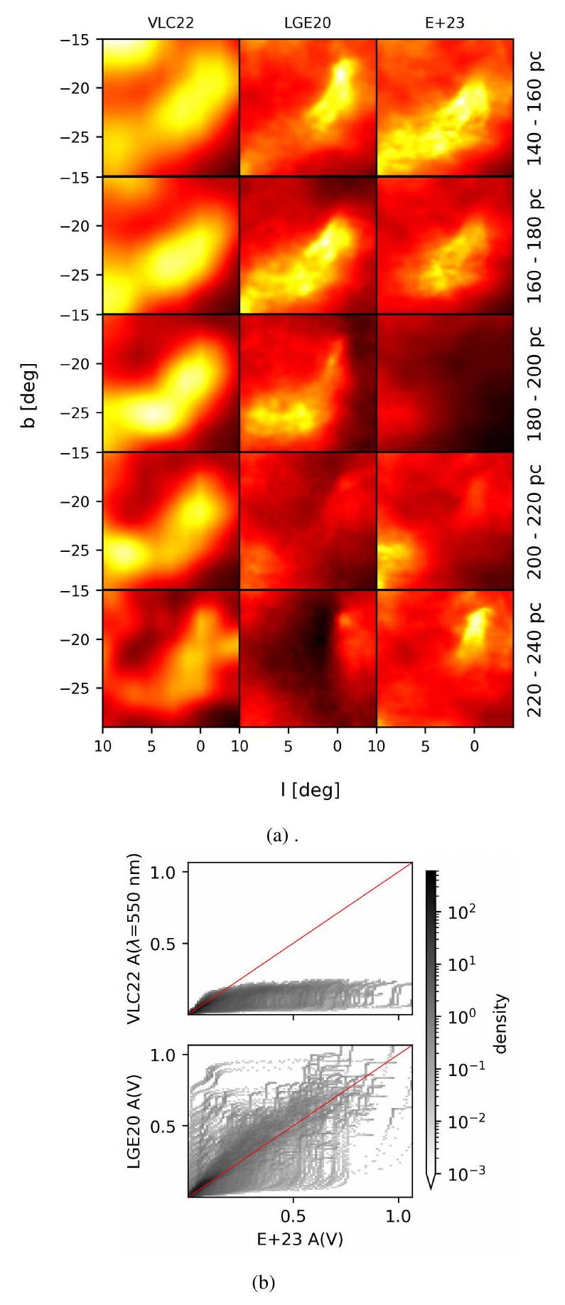
تظهر الأشكال G.1 إلى G.5 مشاهد مكبرة من الشكل 11 في شرائح مسافة مختلفة، جنبًا إلى جنب مع هيستوجرامات تقارن الانقراض لـ VLC22 وLGE20 وخريطتنا المتوسطة نحو بيرسيوس، أوريون A،
الشكل G.1. مقارنة بين خرائط الغبار المختلفة لبيرسيوس. اللوحة (أ): عرض مكبر للشكل 11 نحو بيرسيوس مشابه للشكل 12، في شرائح مسافة مختلفة. الأعمدة تصور إعادة بناء الغبار، بينما الصفوف تصور شرائح المسافة. الأشرطة اللونية اللوغاريتمية منفصلة لإعادة البناء ولكنها مشتركة لشرائح المسافة المختلفة. اللوحة (ب): مقارنة بين الانقراض المتوسط ما بعد المدمج من أدنى مسافة للوحة (أ) إلى نقاط موزعة بانتظام في نطاق المسافة للوحة (أ). يتم عرض تنبؤات الانقراض لخريطتنا مقابل LGE20 وVLC22 كهيستوجرامات. التجميع خطي والشريط اللوني لوغاريتمي. يتم عرض القواطع باللون الأحمر.
الشكل G.2. نفس الشكل G.1 ولكن لأوريون A.
ثور، كورونا أستراليس، وشاميلون. تظهر الألواح العلوية نفس مشاهد POS للسحب كما في الشكل 12، ولكن الآن تظهر الانقراض الناتج عن الغبار في صناديق مسافة محدودة، بدلاً من دمجها عبر نطاق المسافة الكامل. تتوفر صورة تفاعلية ثلاثية الأبعاد منخفضة الدقة لإعادة البناء بما في ذلك جميع السحب الجزيئية المذكورة أعلاه عبر الإنترنت .
تُشبه الألواح السفلية من الأشكال الشكل 10 ولكن تقارن الانقراض ضمن المسافة المحددة ومنطقة POS
الشكل G.3. نفس الشكل G.1 ولكن لتوروس.
من السحابة الجزيئية المعنية فقط. النقاط التي قمنا بالتكامل لها متباعدة في نطاق المسافة من اللوحة العلوية. بدأنا التكامل عند أدنى مسافة من اللوحة العلوية وتكاملنا بشكل متتابع بخطوات قدرها 0.5 فرسخ فلكي. النقاط الاستكشافية متباعدةعلى طول POS.
يتفق LGE20 وخريطتنا بشكل جيد بالنسبة لبرسيوس وأوريون A وتوروس وشاماليون. تظهر بعض الهياكل عند مسافات أكبر قليلاً في خريطتنا كما هو موضح من الأقواس فوق القطر في الألواح الثانية. يتشبع LGE20 أسرع من خريطتنا حيث يتسطح عند الانقراضات العالية تحت القطر. التسطح أقل وضوحًا بالنسبة لشاماليون.
الشكل G.4. نفس الشكل G.1 ولكن لكورونا أستراليس (CrA).
كورونا أستراليس هي حالة شاذة بين مستوى الاتفاق الجيد بشكل عام. في اللوحة السفلية، هناك كثافة ملحوظة أكثر بعيدًا عن القطر. نرى أقواسًا فوق وتحت القطر تشير إلى أن بعض الهياكل أقرب بينما البعض الآخر أبعد في خريطتنا مقارنة بـ LGE20. بينما يضع LGE20 رأس كورونا أستراليس في شريحة المسافة التي تتراوح من 140 فرسخ فلكي إلى 160 فرسخ فلكي، تضع خريطتنا رأس كورونا أستراليس عشرات الفرسخات أبعد في المسافة. الأسباب المحتملة لهذا التحول تشمل عدد غير كافٍ من النجوم لتقييد المسافة إلى رأس كورونا أستراليس أو وضع فشل في تقريبنا اللاحق.
الشكل G.5. نفس الشكل G.1 ولكن لشاماليون.
VLC22 أقل بكثير في الدقة ولا يحل مناطق الانقراض العالية على نطاق الدرجة. الانقراض في VLC22 ضمن شريحة المسافة المحددة أقل بكثير من خريطتنا وبالتبعية في LGE20. الانقراض المفقود يقع جزئيًا خارج الصندوق المحدد حيث يتم تشويهه بشدة شعاعيًا.
الانقراض ZGR23 بوحدات تعسفية ولكن يمكن ترجمته إلى انقراض عند أي طول موجي معين باستخدام منحنى الانقراض المنشور فيhttps://doi.org/10.5281/zenodo.7692680. علاوة على ذلك، يمكن ترجمة انقراض الغبار إلى كثافة حجمية تقريبية للهيدروجين من خلال افتراض نسبة ثابتة بين الانقراض وكثافة عمود الهيدروجين (انظر، على سبيل المثال، زوكر وآخرون 2021).
من خلال القيام بذلك (وباستخدام ZGR23) افترضنا ضمنيًا قانون احمرار ثابت مكاني للغبار.
Max Planck Institute for Astrophysics,Karl-Schwarzschild-Straße 1, 85748 Garching bei München,Germany e-mail:edh@mpa-garching.mpg.de Ludwig Maximilian University of Munich,Geschwister-Scholl-Platz 1, 80539 München,Germany Center for Astrophysics|Harvard &Smithsonian, 60 Garden St.,Cambridge,MA 02138,USA Space Telescope Science Institute, 3700 San Martin Dr,Baltimore,MD 21218,USA Department of Statistical Sciences,University of Toronto,Toronto ON M5G 1Z5,Canada David A.Dunlap Department of Astronomy &Astrophysics,University of Toronto,Toronto,ON M5S 3H4,Canada Dunlap Institute for Astronomy &Astrophysics,University of Toronto,Toronto,ON M5S 3H4,Canada Data Sciences Institute,University of Toronto,Toronto,ON M5G 1Z5,Canada
Received 2 August 2023 /Accepted 19 January 2024
Abstract
Context.High-resolution 3D maps of interstellar dust are critical for probing the underlying physics shaping the structure of the interstellar medium,and for foreground correction of astrophysical observations affected by dust. Aims.We aim to construct a new 3D map of the spatial distribution of interstellar dust extinction out to a distance of 1.25 kpc from the Sun. Methods.We leveraged distance and extinction estimates to 54 million nearby stars derived from the Gaia BP/RP spectra.Using the stellar distance and extinction information,we inferred the spatial distribution of dust extinction.We modeled the logarithmic dust extinction with a Gaussian process in a spherical coordinate system via iterative charted refinement and a correlation kernel inferred in previous work.In total,our posterior has over 661 million degrees of freedom.We probed the posterior distribution using the variational inference method MGVI. Results.Our 3D dust map has an angular resolution of up to ,and we achieve parsec-scale distance resolution, sampling the dust in 516 logarithmically spaced distance bins spanning 69 pc to 1250 pc.We generated 12 samples from the variational posterior of the 3D dust distribution and release the samples alongside the mean 3D dust map and its corresponding uncertainty. Conclusions.Our map resolves the internal structure of hundreds of molecular clouds in the solar neighborhood and will be broadly useful for studies of star formation,Galactic structure,and young stellar populations.It is available for download in a variety of coordinate systems online and can also be queried via the publicly available dustmaps Python package.
Interstellar dust comprises only of the interstellar medium by mass but absorbs and re-radiates of starlight at infrared wavelengths(Popescu &Tuffs 2002).As such,dust plays an out- sized role in the evolution of galaxies,catalyzing the formation of molecular hydrogen,shielding complex molecules from the UV radiation field,coupling the magnetic field to interstellar gas, and regulating the overall heating and cooling of the interstellar medium(Draine 2011).
Dust's ability to scatter and absorb starlight is precisely the reason why we can probe it in three spatial dimensions.It prefer- entially absorbs shorter wavelengths of a stellar spectrum,thus leading to stars behind dense dust clouds appearing reddened rel- ative to their intrinsic colors.The amount by which stars behind dust clouds appear reddened allows us to infer the amount of dust extinction between us and the reddened star.In combination with distance measurements to reddened stars,we can de-project the integrated extinction measurements into a 3D map of differential dust extinction.
Gaia has been transformative for the field by providing accu- rate distance information to more than 1 billion stars,primarily within a few kiloparsecs of the Sun.Precise distances not only improve our knowledge about a star's position,they also break degeneracies inherent in the modeling of extinction and signif- icantly reduce the extinction uncertainties(Zucker et al.2019). Thanks to the large quantity of extinction and distance measure- ments available in the era of large photometric,astrometric,and spectroscopic surveys,we can now probe the 3D distribution of dust in the Milky Way on parsec scales.
A number of 3D dust maps that combine Gaia and vast pho- tometric and spectroscopic surveys already exist.These maps primarily differ in the way they account for the so-called fingers- of-god effect,or the tendency of dust structures to be smeared out along the line of sight(LOS).The effect stems from supe- rior constraints on stars'plane-of-sky(POS)positions relative to their LOS distance uncertainties.
Three-dimensional dust maps predominantly fall into two categories,each representing a trade-off between angular res- olution and distance resolution:reconstructions on a Carte- sian grid and reconstructions on a spherical grid.Cartesian reconstructions commonly feature less pronounced fingers- of-god but scale poorly with the size of the reconstructed
volume. They either encompass a limited volume of the Galaxy (Leike et al. 2020; Leike & Enßlin 2019) at a high resolution or cover a larger volume of the Galaxy at a low resolution (Vergely et al. 2022; Lallement et al. 2022, 2019, 2018; Capitanio et al. 2017). Spherical reconstructions often have a much higher resolution and probe larger volumes of the Galaxy but come with more strongly pronounced fingers-of-god artifacts (Green et al. 2019, 2018; Chen et al. 2019). Alternative approaches using many small reconstructions (Leike et al. 2022), an analytical approach (Rezaei Kh. & Kainulainen 2022; Rezaei Kh. et al. 2020, 2018, 2017), or inducing point methods (Dharmawardena et al. 2022) have so far been unsuccessful in reconstructing dust at high resolution over large volumes without artifacts.
Physical smoothness priors counterbalance the fingers-ofgod effect as finger-like structures are a priori unlikely. In a Cartesian coordinate system it is comparatively easy to incorporate physical priors into the model, such as the distribution of dust being spatially smooth. Smoothness priors are often incorporated using Gaussian process (GP) priors. Sparsities and symmetries in the prior can be exploited to efficiently apply a GP to a regular Cartesian coordinate system.
Spherical coordinate systems break these sparsities and symmetries in the prior but are much better aligned with the desired spacing of voxels along the LOS. Nearby, voxels can be spaced densely, while at greater distances voxels can be spaced further apart. Naively using a GP prior is infeasible, and approximations either trade fingers-of-god artifacts for other artifacts (Leike et al. 2022) or are too weak to regularize the reconstructions (Green et al. 2019).
In this work, we present a 3D dust map that achieves high distance and angular resolution and probes a large volume of the Galaxy, all at a feasible computational cost. The map uses a new GP prior methodology to incorporate smoothness in a spherical coordinate system, mitigating fingers-of-god artifacts. With a spherical coordinate system we were able to probe dust beyond 1 kpc while still resolving nearby dust clouds at parsec-scale resolution. In Sect. 2, we present the stellar distance and extinction estimates upon which our map is based. In Sect. 3, we present our GP prior methodology for incorporating smoothness in a spherical coordinate system. Section 4 describes how we combine the data with our prior model and how we incorporate the distance uncertainties of stars. In Sect. 5, we describe our inference before recapitulating all approximations of the model and their implications in Sect. 6. Finally, in Sect. 7 we present the final map and compare it to existing 3D dust maps and 2D observations.
2. Stellar distance and extinction data
To construct a 3D dust map, we used the stellar distance and extinction estimates from Zhang et al. (2023), which are primarily based on the Gaia BP/RP spectra (spectral resolution ). Zhang et al. (2023) adopted a data-driven approach to forward-model the extinction, distance, and intrinsic parameters of each star given the combination of the Gaia BP/RP spectra and infrared photometry from the two micron all sky survey (2MASS) and unWISE, a processed catalog based on the wide-field infrared survey explorer (WISE) (Carrasco et al. 2021; De Angeli et al. 2023; Gaia Collaboration 2023; Montegriffo et al. 2023; Schlafly et al. 2019; Wright et al. 2010; Skrutskie et al. 2006). The model is trained using a subset of stars with higher resolution spectra ( ) available from the large sky area multi-object fibre spectroscopic telescope (LAMOST) (Wang et al. 2022; Xiang et al. 2022). The resulting catalog contains distance, extinction, and stellar type ( )
information for 220 million stars. Throughout this work, we denote the Zhang et al. (2023) catalog by ZGR23.
Compared to other stellar distance and extinction catalogs, the ZGR23 catalog features smaller uncertainties on the extinction estimates while still targeting a significant number of stars. Approximately 87 million ZGR23 stars have an uncertainty below 60 mmag. Thus, ZGR23 achieves similar extinction uncertainties compared to the subset of 39,538 stars in the StarHorse catalog (Queiroz et al. 2023) that have both higher resolution spectra from the Apache point observatory galactic evolution experiment (APOGEE) and grizy photometry from the panoramic survey telescope and rapid response system (PanSTARRS), specifically Pan-STARRS1 (PS1; Chambers et al. 2016) (typical extinction uncertainty of 60 mmag ). While the ZGR23 catalog is limited to stars with Gaia BP/RP measurements, the quality of the data makes the inference from the ZGR23 catalog competitive with models based on catalogs with larger numbers of stars – 799 million stars in Bayestar 19 (Green et al. 2019), 265 million in StarHorse DR2 (Anders et al. 2019), and 362 million in StarHorse EDR3 (Anders et al. 2022). We further find the ZGR23 catalog to have fewer systematic shifts in the extinction and reliable extinction uncertainties based on an analysis in dust-free regions; further details are given in Appendix A.
For our reconstruction, we restricted our analysis to ZGR23 stars that have quality_flags , as recommended by the authors. We further sub-selected the stars based on their distance. We required and with the parallax of a star and the parallax uncertainty to enforce that all stars are likely within our reconstructed volume. In total, we selected 53880655 stars.
The reliability of our reconstruction is predominantly limited by the quality and quantity of the data. Both strongly depend on the POS position and distance. Figure 1 shows 2D histograms of stellar density in heliocentric Galactic Cartesian ( ) projections, as well as the number of stars as a function of distance. The densities of stars per distance bin first increases approximately quadratically with distance before falling off to a linear increase. At approximately 1.5 kpc the number of stars per distance bin levels off due to our requirement that stars have a sigma chance of being within 1.8 kpc in distance. Figure 2 shows a POS histogram of the stars. A clear imprint of the Gaia BP/RP selection function is visible (cf. Cantat-Gaudin et al. 2023). A systematic under-sampling of stars behind dense dust clouds is also apparent. We expect our reconstruction to be more trustworthy in regions of higher stellar density. Due to the obscuring effect of dust, regions within and behind dense dust clouds should be treated with more caution.
3. Priors
Our quantity of interest is the 3D distribution of differential ZGR23 extinction By definition, the differential extinction is positive. Furthermore, we assumed it to be spatially smooth. A priori we assumed the level of smoothness to be spatially stationary and isotropic.
Fig. 1. 2D histograms of the density of stars in heliocentric Galactic Cartesian ( ) projections, as well as the density of stars as a function of distance, for the subset of the ZGR23 catalog used in the reconstruction of our 3D dust map. Panel a: heliocentric Galactic Cartesian-projected histograms. Panel b: number of stars as a function of distance. This panel also shows a linear growth and a quadratic growth with distance for comparison.
To reconstruct the 3D volume efficiently, we discretized it in spherical coordinates. Specifically, we discretized our reconstructed volume into HEALPix spheres at logarithmically spaced distances. We adopted an of 256 , which corresponds to 786432 POS bins. This corresponds to an angular size of our voxels of . For the LOS direction, we adopted 772 logarithmically spaced distance bins, of which 256 are used for padding. Our highest distance discretization is 0.4 pc and our
Fig. 2. POS distribution of the subset of ZGR23 stars used in the reconstruction of our 3D dust map.
lowest distance discretization is 7 pc . In contrast to reconstructions with linearly spaced voxels in distance, we were able to probe much larger volumes while maintaining a high sampling at nearby distances. The discretization provides a lower bound on the minimum separation between dust structures that we are able to resolve. In practice the resolvable separation depends on the quantity and quality of the data and varies with the POS and LOS position.
We encoded both positivity and smoothness in our model by assuming the differential extinction to be log-normally distributed:
with normally distributed , where is drawn from a GP with a homogeneous and isotropic correlation kernel, . From previous reconstructions of the differential extinction for the Gaia DR2 G-band (Leike et al. 2020), we have constraints on the correlation kernel of the logarithm of the differential extinction in a volume around the Sun 270 pc ). As part of our prior model, we used the inferred extinction kernel from Leike et al. (2020). To account for the conversion between the ZGR23 extinction and extinction, we added a global multiplicative factor to in our model. Furthermore, we inferred an additive offset in the differential extinction. We placed a log-normal prior on the multiplicative parameter and a normal prior on the additive one.
We enforced the correlation kernel using iterative charted refinement (ICR; Edenhofer et al. 2022). ICR enables us to enforce a kernel on arbitrarily spaced voxels by representing the modeled volume at multiple discretizations. It starts from a very coarse view of our modeled volume. On this coarsest scale, ICR models the GP with learned voxel excitations and an explicit full kernel covariance matrix. A priori the parameters are standard normally distributed and coupled according to via ICR. It then iteratively refines times its coarse view of the space with local, fine, a priori standard normally distributed corrections until reaching the desired discretization. In each refinement, it uses neighbors from the previous refinement to refine one coarse pixel into fine pixels (see Algorithm 1).
Iterative charted refinement uses local corrections at varying discretizations and within a refinement assumes the previous iteration to have modeled the GP without error. Both lead to slight
Algorithm 1: Pseudocode for ICR creating a GP from uncorrelated excitations . Each coarse pixel at location is iteratively refined to fine pixels using coarse pixel neighbors. The correlation kernel is denoted by . Square brackets after variables and the two functions ndindex and shape denote NumPy-like (Harris et al. 2020) indexing routines. The call explicit_gp refers to an unspecified Gaussian Process model explicitly representing the covariance of for the pixel positions modeled by .
errors in representing the kernel. For our use case, we encountered errors in representing the kernel of a few percent. We accepted these errors as a trade-off that enables the reconstruction to probe larger volumes. We refer to Edenhofer et al. (2022) for a detailed discussion of the kernel approximation errors.
Overall, our model for the prior reads ,
where we denote the learned multiplicative scaling of by scl, the learned additive offset by off, and re-expressed both in terms of a priori standard normally distributed parameters and , respectively. The act of expressing scl, off and via parameters with an a priori simpler distribution, here a standard normal distribution, is called re-parameterization. A detailed discussion on this subject is given in Rezende & Mohamed (2015).
4. Likelihood
To construct the likelihood we first needed to define how the differential extinction – our quantity of interest – connects to the measured data . Our data comprise POS position, extinction , and parallax data. The POS position is in essence
without error. The extinction data are in the form of integrated LOS extinctions to stars and associated uncertainties The parallax data similarly are in the form of parallax estimates and uncertainties .
Our model focuses on the measured extinction, , and does not predict parallaxes to stars. Instead, we conditioned our model on the parallax data, , and split the likelihood into the probability of the measured extinction given the true extinction, , and the probability of the true extinction given uncertain parallax information:
The first term of the integrand is constrained by the quality of the extinction measurements and the second by the quality of the parallax measurements.
4.1. Response
The second term in Eq. (4), , can be expressed as the joint probability of extinction and true distance, , marginalized over the true distance:
We neglected data selection effects (i.e., ‘s dependence on given and ‘s dependence on given ) and used the fact that the true extinction, , at known distance is simply the LOS integral of along the LOS to the star from zero to :
with the slice of at the POS positions of the stars, the Dirac delta distribution defined by for any continuous with compact support, and the response that maps from to the domain of the measured extinction.
We approximated with a normal distribution, ,
with mean and standard deviation to obtain a tractable expression for Eq. (4). The mean extinction, , is
Table 1. Parameters of the prior distributions.
Name
Distribution
Mean
Standard deviation
Degrees of freedom
Normal
0.0
Kernel from Leike et al. (2020)
scl
Log-Normal
1.0
0.5
1
off
Normal
prior median extinction from Leike et al. (2020)
1.0
1
Shape arameter
Scale parameter
# Stars = 53880655
Inverse Gamma
Notes. The parameters , and off fully determine . They are jointly chosen to a priori yield the kernel reconstructed in Leike et al. (2020).
Assuming the parallax is normally distributed (i.e., with mean and standard deviation ), then
with the survival function of the normal distributed parallax.
The standard deviation can be understood as an additional error contribution for marginalizing over the distance. The error depends on the distance uncertainty and the dust along the full LOS:
Evaluating both and is comparatively cheap in a spherical coordinate system since for a discretized sphere is simply the cumulative sum of along the distance axis weighted by the radial extent of each voxel.
4.2. Likelihood and joint probability density
We assumed the measured extinction to be normally distributed around the true extinction . We took the inferred extinction, , from the catalog to be the mean of the normal distribution. The accompanying uncertainty in the catalog was assumed to be the standard deviation of .
Some stars will have underestimated uncertainties due to either mismodeled intrinsic stellar properties in the inference or bad photometric measurements that were not flagged. We wanted our model to be able to detect and deselect stars that are in strong disagreement with the rest of the reconstruction. We achieved this by inferring an additional multiplicative factor per star, , which scales . A priori, we assumed to be drawn from a heavy-tailed distribution. Specially, we assumed to follow an inverse gamma distributed. We again express in terms of standard normally distributed parameters in the inference.
To summarize, our approximate likelihood first introduced in Eq. (4), reads
The uncertainty in the extinction is scaled by to deselect outliers and increased by due to marginalizing over the distance uncertainty.
The joint probability density function of data and parameters reads
with the vector of all parameters of the model . The complexity of the prior distributions has been fully absorbed into the transformations , off , and from the a priori standard normally distributed parameters .
Our priors in terms of nonstandard-normal parameters are summarized in Table 1. The priors for , and off are chosen to a priori yield the kernel reconstructed in Leike et al. (2020). In contrast to Leike et al. (2020), we do not learn a full nonparametric kernel. However, we do infer scl and off, the scale, and zero-mode of the kernel. The prior for was chosen such that the inverse gamma distribution has mode 1 and standard deviation 2 .
5. Posterior inference
In the previous section we took special care to express our model not only in terms of physical parameters, like the differential extinction density , but also in terms of simpler parameters . The act of expressing the parameters of the model scl, off, , and in terms of a priori standard normal distributed variables is called standardization, a special from of re-parameterization (see Rezende & Mohamed 2015). Effectively, we are shifting complexity from the prior to the likelihood. However, both the nonstandardized and the standardized formulation of the joint model are equivalent. Standardizing models can lead to better conditioned inference problems as the parameters all vary on the same scales – if the prior is not in conflict with the likelihood. We used an inference scheme that relies on the standardized formulation.
We wanted to infer the posterior for our standardized model from Eq. (19). Directly probing the posterior via sampling methods such as Hamiltonian Monte Carlo Hoffman & Gelman (2014) is computationally infeasible. Instead, we used variational inference to approximate the true posterior. Specifically, we used metric Gaussian variational inference (MGVI; Knollmüller & Enßlin 2019). We summarize the main idea behind MGVI in Appendix B. We did not approximate the posterior of the noise
inference parameter via variational inference and instead used only the maximum of the posterior for .
To speed up the inference, we started the reconstruction at a lower resolution (196, 608 POS bins at and 388 LOS distance bins) and restricted the inference to a subset of stars with a sigma chance of being within 600 pc and a sigma chance of being farther than 40 pc . We successively increased the distance range of the map up to which stars are incorporated in steps of 300 pc from 600 pc to 1.8 kpc . Every time we increased the distance range, we reset the parameters for . Then, after all data were incorporated, we increased the angular and distance resolution of the reconstruction to the final resolution.
Our data selection deselects stars close to the maximum distance probed (cf. Fig. 1). This effect leads to the outer regions of the map being informed by relatively few stars compared to the inner regions. We observe that these regions are prone to producing spurious features. For our final data products, we removed the outermost 550 pc from the data-constrained volume as we observed artifacts aligned with our data incrementation strategy within these regions. We believe 550 pc to be a conservative cut but we advise caution when finding structures perfectly aligned with a sphere around the Sun at , or 1200 pc .
ZGR23 assumes all extinctions to be strictly positive. We neglected this constraint by assuming Gaussian errors, which led to an artificial spike in extinction in the first few voxels in each direction. As we know those regions to be effectively free of dust from previous reconstructions cf. Leike et al. (2020), we removed the innermost 69 pc (see Appendix C). We release an additional HEALPix map of integrated extinction out to 69 pc from the Sun and suggest using it to correct integrated LOS predictions for the removed extinction.
Our inference heavily utilizes derivatives of various components of our model. Derivatives are used for the minimization as well as for the variational approximation of the posterior. Previous models such as those described in Leike & Enßlin (2019) and Leike et al. (2020) relied on the Numerical Information Field Theory (NIFTy) package (Selig et al. 2013; Steininger et al. 2019; Arras et al. 2019) and were limited to running on CPUs.
We employed a new framework called NIFTy.re (Edenhofer et al., in prep.) for deploying NIFTy models to GPUs. NIFTy.re is part of the NIFTy Python package and internally uses JAX (Bradbury et al. 2018) to run models on the GPU. We were able to speed up the evaluation of the value and gradient of Eq. (19) by two orders of magnitude by transitioning from CPUs to GPUs. Our reconstruction ran on a single NVIDIA A100 GPU with 80 GB of memory for about four weeks.
6. Caveats
We believe statistical uncertainties are the dominant source of uncertainty for our reconstruction. However, it is important to also consider sources of systematic uncertainties. Depending on the application, the systematic uncertainties may be more important than the statistical uncertainties. The data that informed the reconstruction, the model with which we inferred it, and the inference procedure all contribute to the model systematic uncertainties.
Naturally, the data themselves are a source of systematic uncertainties (spatially stationary reddening law, mismodeling of binaries, etc.; see Zhang et al. 2023) and additionally is known to be incomplete, cf. Fig. 2. A lower stellar density, for example in
heavily obscured regions, limits the map’s resolution and results in volumes of the map behind dense dust clouds being poorly constrained. Thus, we believe our dust reconstruction to be an underestimation of the true extinction toward dense dust clouds. Zucker et al. (2021) also note this effect when comparing the Leike et al. (2020) map with 2D integrated extinction maps based on infrared photometry, finding that the Leike et al. (2020) is not sensitive to regions with .
We advise visualizing the stellar density in the region of interest to assess the magnitude of the systematic uncertainties due to data incompleteness. We release all stars used in the reconstruction as an additional data product. This data product can be used to visualize the stellar density. In regions with a significant underdensity of stars, we expect the systematic lack of stars to dominate the statistical uncertainties in the reconstruction. The reconstruction produced plausible infills in those regions based on adjacent stars. However, the resulting uncertainties do not capture the cause for the systematic lack of stars as the model implicitly assumes that underdensities of stars are not systematic but purely random.
Our model includes a number of approximations. First, we assumed a GP prior on the logarithmic dust extinction using the kernel from Leike et al. (2020) and additionally only applied it approximately via ICR. Second, we assumed to be independent of . Third, we assumed the parallax error to be Gaussian, and fourth, we assumed the extinction error to be Gaussian.
For extremely low extinctions, the assumption of being Gaussian is poor due to the positivity prior in the ZGR23 catalog. We corrected for this bias toward higher estimated extinction in regions with assumed extremely low true extinctions post-hoc by cutting away the innermost 69 pc as described in Sect. 5. We publish an auxiliary map of integrated extinction out to 69 pc from the Sun to correct integrated LOS predictions for the removed extinction. We suggest adding the removed local extinction back to the map when comparing integrated extinctions. By default, the removed local extinction is added back to the map when querying integrated extinctions via dustmaps.
We further release a catalog of the predicted extinctions of our model to all stars that we used for the reconstruction. In Appendix D, we perform a non-exhaustive consistency test comparing our predictions to the ZGR23 ones. We find that both predictions for the extinction to stars disagree below 50 mmag and above more stars than expected have larger (respectively smaller) extinction predictions compared to ZGR23. We expect the range from 50 mmag to 4 mag to correspond to the range within which our map is reliable. More details are provided in Appendix D.
Furthermore, our posterior inference is an approximation. We assume our approximation of the true posterior accurately captures the intrinsic model uncertainties (cf. Arras et al. 2022; Leike & Enßlin 2019; Leike et al. 2020; Mertsch & Phan 2023; Roth et al. 2023a,b; Hutschenreuter et al. 2023, 2022; Tsouros et al. 2024). However, we worried about structures getting burned in when we increase the maximum distance probed during the inference from 600 pc to 1800 pc in steps of 300 pc as described in Sect. 5. We checked the final reconstruction for this effect by comparing it against a larger reconstruction that does not sub-select the stars based on their distance during the inference but uses only a small subsample of ZGR23 stars with more stringent quality flags. The larger reconstruction, which extends out to 2 kpc in distance, is released as an additional data product. We find no significant differences between both runs. Details on the larger reconstruction are provided in Appendix E.
Fig. 3. Mollweide projection of the POS integrated extinction out to , and up to the maximum distance of our map. The colorbar saturates at the quantile.
Fig. 4. Same as Fig. 3 but showing the difference between the integrated extinctions in between distance slices projected on the POS. The colorbar saturates at the quantile.
7. Results
We reconstructed 12 samples (6 antithetically drawn samples) of the 3D dust extinction distribution, each of which encompasses 607125504 differential extinction voxels. The voxels are arranged on 772 HEALPix spheres with spaced at logarithmically increasing distances. After removing the innermost and outermost HEALPix spheres, we are left with 516 HEALPix spheres. The samples, the posterior mean, and the posterior standard deviation for the reconstruction are publicly available online. We strongly advise using the samples for any quantitative analysis. For convenience, we
also provide the posterior mean and standard deviation of the reconstruction interpolated to heliocentric Galactic Cartesian Coordinates ( ) and Galactic spherical Coordinates ( , ) as well as the scripts for the interpolation. Furthermore, the map can be queried via the dustmaps Python package (Green 2018). Further details on using the reconstruction are given in Appendix F.
The distance discretization in our reconstruction is highest for close-by voxels and decreases further out. Our highest
Fig. 5. Heliocentric Galactic Cartesian ( ) projections of the posterior mean of our 3D dust map in a box with dimensions 0.8 kpc centered on the Sun. The colorbar is linear and saturates at the quantile. A GIF of the posterior samples and a low-resolution 3D interactive version of this figure are available online.
Fig. 6. Same as Fig. 5 but with a catalog of clusters of YSOs (Kuhn 2023, priv. comm.) based on Kuhn et al. (2021), Winston et al. (2020), and Marton et al. (2023) shown as blue dots on top of the reconstruction; their distance uncertainties are shown as extended lines.
Fig. 7. Heliocentric Galactic Cartesian ( ) projections of the relative uncertainty of the reconstructed dust extinction integrated within a box of centered on the Sun. The colorbar is linear and saturates at the quantile.
Fig. 8. Side by side views of the 3D dust maps from Bayestar19, VLC22, L+22, and this work, shown in heliocentric Galactic Cartesian ( ) projections. The colorbars are saturated at the quantile of the respective reconstruction.
Fig. 9. Zoomed-in version of Fig. 8 for the volume reconstructed in Leike et al. (2020), now also showing the LGE20 reconstruction for comparison. We omit L+22 from the comparison because the authors explicitly focus on larger volumes and trade strongly pronounced artifacts in the inner couple hundred parsecs for a larger probed volume. The colorbars are again saturated at the quantile of the respective reconstruction.
distance discretization is 0.4 pc and our lowest distance discretization is 7 pc while our angular discretization is and is independent of the distance. The stated discretizations specify the lower bound on our resolution. The minimum separation that we are able to resolve depends on the position and is encoded in the posterior samples. For small regions, we suggest additionally analyzing the stellar density (see Sect. 6) to assess the strength of the systematic uncertainties due to the density of stars.
The reconstruction is in terms of the unitless ZGR23 extinction as defined in Zhang et al. (2023). For visualization purposes, we translated the ZGR23 extinction to Johnson’s V-band 540.0 nm , that is to say, . To perform the conversion, we adopted the extinction curve published in ZGR23 and multiplied the unitless ZGR23 extinction by a factor of 2.8. We refer readers to the full extinction curve from Zhang et al. (2023) for the coefficients needed to translate the extinction to other bands.
Figure 3 depicts the POS projection of the posterior mean reconstruction integrated out to , and up to the end of our sphere. The values are in units of magnitudes. We see that higher-latitude features like the Aquila Rift are comparatively close-by while structures in the Galactic plane appear only gradually. Figure 4 shows the difference between the integrated POS projections. We recover well-known features of integrated dust but are now able to de-project them.
Figure 5 shows a bird’s eye ( ), side-on ( ), and ( ) projection of the posterior mean of our reconstruction in heliocentric Galactic Cartesian coordinates. The image depicts the innermost around the Sun in extinction integrated over from -400 pc to in -1.25 kpc to 1.25 kpc , and in -1.25 kpc to 1.25 kpc , respectively. In Fig. 6, we overlay a catalog of clusters of young stellar objects (YSOs; Kuhn 2023, priv. comm.) based on Kuhn et al. (2021), Winston et al. (2020), and Marton et al. (2023), which are shown as blue dots. The positions of the YSO clusters visually agree with the positions of dust clouds within the YSO clusters’ reported distance uncertainties.
The posterior standard deviation divided by the posterior mean of the reconstruction is shown in Fig. 7. The map features a faint speckle pattern. This is likely due to the low number of samples relative to the number of degrees of freedom. The standard deviation is on the order of of the posterior mean and slightly increases with distance. Toward the galactic center behind the dust in the immediate vicinity of roughly 300 pc , the relative uncertainty is noticeably higher.
The reconstruction has a high dynamic range and reveals faint dust lanes in the reconstructed volume. Small approximately spherical cavities are evident throughout the map. The dust clouds in the reconstruction are compact and only weakly elongated radially. Prominent large-scale features, such as the Radcliffe Wave (Alves et al. 2020) and the Split (Lallement et al. 2019), have been resolved at an unprecedented level of detail, previously only accessible for the most nearby dust clouds.
Comparison to existing 3D dust maps. In this section, we compare our map to other 3D dust maps in the literature. We denote the dust map described in Leike et al. (2020) by LGE20, Vergely et al. (2022) by VLC22, Green et al. (2019) by Bayestar19, and Leike et al. (2022) by L+22 in this section. For the purposes of comparison, we show the posterior mean. We release the statistical uncertainties as additional data
Fig. 10. Histogram of the mean posterior extinction of our map versus LGE20, VLC22, and Bayestar19 for 58 million test points. For each pixel center of a HEALPix sphere with test points are placed at 1 pc intervals in distance starting at 69 pc . The orange lines show the 16th, 50th, and 84th quantiles of the predicted extinction by LGE20, VLC22, and Bayestar19, respectively, for each bin of our mean extinction. The respective quantiles of our predictions in bins of the other reconstruction are shown as blue lines. The bisectors are shown in red. The colorbars are logarithmic and truncated at the lower end at 1 mmag.
products, and we strongly advise taking into account the released statistical uncertainties for any quantitative analysis. However, the differences between the various 3D dust reconstructions discussed here are systematic differences and are not captured by the reconstructed statistical uncertainties.
In Fig. 8, we show 3D ( ) projections of the maps, comparing Bayestar19, VLC22, L+22, and this work side by side. All four maps agree on the general structure of the distribution of dust.
This work, L+22, and VLC22 have comparable distance resolutions, while Bayestar 19 features comparatively few distance bins and more strongly pronounced fingers-of-god. Compared to L+22, we feature more homogeneously extended dust clouds and significantly fewer wiggles in the distances to dust clouds. Compared to VLC22, we feature more compact dust clouds, less grainy structures, and a higher dynamic range. Both this work and VLC22 feature dust clouds in a comparable volume around the Sun despite the VLC22 map technically extending out farther in Galactic heliocentric X and Y .
Figure 9 shows the same projections for the volume reconstructed in the LGE20 map and includes the LGE20 map for comparison. The zoom-in highlights the close similarity between
Fig. 11. Mollweide projections of total integrated extinction and 3D extinction maps integrated out the maximum distance of the respective map. Bayestar 19 reconstructs up to a maximum distance of 63 kpc (maximum reliable distance 10 kpc ) and is integrated out to that volume. reconstructs up to a maximum distance of 16 kpc but the authors trust their map only out to 4 kpc and we integrate their map only to 4 kpc . VLC22 reconstructs a heliocentric box of size with voxels with at most in distance and is integrated out to the end of the box. Likewise, LGE20 reconstructs a heliocentric box of size covering at most in distance and is integrated out to the end of the box. The colorbars saturate at the respective quantile of the map except for the colorbar of Planck 2013, which saturates at 5 mag for better comparability.
this work and the LGE20 map. All larger structures have direct correspondences in the other map, yet the distances to the structures are slightly different. Furthermore, the LGE20 map appears slightly sharper. The model in LGE20 is very similar to ours but uses fewer approximations. LGE20 also uses compiled data (StarHorse DR2; see Anders et al. 2019). More work is needed to assess the validity of the sharper features in LGE20 not present in this work. The VLC22 map is in good agreement as well but lower resolution. Bayestar19 poorly resolves distances at the scale of the LGE20 map.
Figure 10 quantitatively compares our map with LGE20, VLC22, and Bayestar19. We compared the integrated extinction for each pixel center of a HEALPix sphere with at 1182 test points that are placed at 1 pc intervals in distance starting at 69 pc . We compared integrated extinctions because slight shifts in the distances to extincted regions can be better distinguished from discrepant predictions with integrated extinctions than by directly comparing differential extinctions. Above 15 mmag , VLC22 and LGE20 are in good agreement with our map. Below an of 40 mmag and above an of
Fig. 12. Zoomed-in views toward the individual molecular clouds (Perseus, Orion, Taurus, Corona Australis, and Chamaeleon) seen in Fig. 11. The colorbars are logarithmic and span the full dynamic range of the selected POS slice in every image. Each row is a separate region and each column a separate reconstruction.
approximately 3.5 mag, Bayestar19 significantly deviates from our predictions.
In Fig. 11, we compare the POS view of Bayestar19, L+22, VLC22, LGE20, and this work. The respective POS views are integrated out to the maximum distance probed by each map – <63 kpc in distance for Bayestar19 (maximum reliable distance 10 kpc ), in distance for (authors trust structures up to 4 kpc though the map extends to 16 kpc ), a heliocentric box of size with voxels for VLC22 with at most 2.16 kpc in distance, and a heliocentric box of size and up to 590 pc in distance for LGE20. In addition, we show the Planck 2013 extragalactic dust map (Planck Collaboration XI 2014) and the Gaia total galactic extinction (TGE) 2022 map (Delchambre et al. 2023).
All maps agree on fine structures at high galactic latitudes but differ in the Galactic plane due to the difference in distance up to which the respective reconstruction extends. 3D dust reconstructions do not probe deep enough into the Galactic plane to fully recover the Planck 2013 extragalactic dust map. Bayestar 19 and
L+22 probe much deeper than VLC22, LGE20, and this work, yet they do not probe the full column of dust seen in Planck 2013 and Gaia TGE 2022. Both VLC22 and our map probe up to a similar depth while LGE20 only probes dust at much closer distances.
Figure 12 shows a zoomed-in comparison of the Perseus, Orion A, Taurus, Corona Australis ( CrA ), and Chamaeleon molecular clouds, integrated out to the maximum distance of each map ( 4 kpc for ). Among the 3D dust reconstructions, Bayestar19 and L+22 have arguably the highest angular resolution (angular discretization of or and , respectively). They resolve the high latitude dust clouds with great detail although L+22 suffers from localized artifacts in patches of the sky. Both LGE20 ( boxes) and this work ( ) achieve a comparable angular resolution. The VLC22 reconstruction ( voxels) is noticeably lower in resolution and does not resolve the cloud substructure on the POS. A comparison between the same molecular clouds in different distance slices in VLC22, LGE20, and our map is provided in Appendix G.
8. Conclusions
We present a 3D dust map with a POS and LOS resolution comparable to Leike et al. (2020) that extends out to 1.25 kpc . We used the distance and extinction estimates of Zhang et al. (2023), which have much lower extinction uncertainties than competing catalogs while probing a similar number of stars. Our reconstruction has a resolution comparable to the 2 pc resolution of Leike et al. (2020). Specifically, it has an angular resolution of up to and parsec-scale distance resolution. Our map is in good agreement with existing 3D dust maps and improves upon them in terms of volume covered at a high spatial resolution. The map is publicly available online and can be queried via the dustmaps Python package. We anticipate that the map will be useful for a wide range of applications in studying the distribution of dust and the interstellar medium more broadly.
Acknowledgements. We thank Joao Alves for many fruitful discussions at the “Self-Organization Across Scales: from nm to parsec (SOcraSCALES)” workshop at the Munich Institute for Astro-, Particle and BioPhysics, an institute of the Excellence Cluster ORIGINS in 2022 and afterwards. Furthermore, we thank Jakob Roth for many invaluable discussions about the model and for providing feedback on the early versions of the reconstruction. We thank Alyssa Goodman for providing invaluable feedback on the late versions of the reconstructions. We also thank Michael A. Kuhn for providing us with a unified catalog of YSOs. Gordian Edenhofer acknowledges the support of the German Academic Scholarship Foundation in the form of a PhD scholarship (“Promotionsstipendium der Studienstiftung des Deutschen Volkes”). Catherine Zucker acknowledges that support for this work was provided by NASA through the NASA Hubble Fellowship grant #HST-HF2-51498.001 awarded by the Space Telescope Science Institute (STScI), which is operated by the Association of Universities for Research in Astronomy, Inc., for NASA, under contract NAS5-26555. Philipp Frank acknowledges funding through the German Federal Ministry of Education and Research for the project ErUM-IFT: Informationsfeldtheorie für Experimente an Großforschungsanlagen (Förderkennzeichen: 05D23EO1). Andrew K. Saydjari acknowledges support by a National Science Foundation Graduate Research Fellowship (DGE-1745303). Andrew K. Saydjari and Douglas Finkbeiner acknowledge support by NASA ADAP grant 80NSSC21K0634 “Knitting Together the Milky Way: An Integrated Model of the Galaxy’s Stars, Gas, and Dust”. This work was supported by the National Science Foundation under Cooperative Agreement PHY-2019786 (The NSF AI Institute for Artificial Intelligence and Fundamental Interactions). A portion of this work was enabled by the FASRC Cannon cluster supported by the FAS Division of Science Research Computing Group at Harvard University. We acknowledge support by the Max-Planck Computing and Data Facility (MPCDF). This work has made use of data from the European Space Agency (ESA) mission Gaia (https://www.cosmos.esa.int/gaia), processed by the Gaia Data Processing and Analysis Consortium (DPAC, https://www.cosmos.esa.int/web/ gaia/dpac/consortium). Funding for the DPAC has been provided by national institutions, in particular the institutions participating in the Gaia Multilateral Agreement.
References
Alves, J., Zucker, C., Goodman, A. A., et al. 2020, Nature, 578, 237
Anders, F., Khalatyan, A., Chiappini, C., et al. 2019, A&A, 628, A94
Anders, F., Khalatyan, A., Queiroz, A. B. A., et al. 2022, A&A, 658, A91
Arras, P., Baltac, M., Ensslin, T. A., et al. 2019, Astrophysics Source Code Library [record ascl:1903.008]
Arras, P., Frank, P., Haim, P., et al. 2022, Nat. Astron., 6, 259
Astropy Collaboration (Robitaille, T. P., et al.) 2013, A&A, 558, A33
Astropy Collaboration (Price-Whelan, A. M., et al.) 2018, AJ, 156, 123
Astropy Collaboration (Price-Whelan, A. M., et al.) 2022, ApJ, 935, 167
Bradbury, J., Frostig, R., Hawkins, P., et al. 2018, JAX: composable transformations of Python+NumPy programs, https://github.com/google/ jax
Cantat-Gaudin, T., Fouesneau, M., Rix, H.-W., et al. 2023, A&A, 669, A55
Capitanio, L., Lallement, R., Vergely, J. L., Elyajouri, M., & Monreal-Ibero, A. 2017, A&A, 606, A65
Carrasco, J. M., Weiler, M., Jordi, C., et al. 2021, A&A, 652, A86
Chambers, K. C., Magnier, E. A., Metcalfe, N., et al. 2016, arXiv e-prints [arXiv:1612.05560]
Chen, B. Q., Huang, Y., Yuan, H. B., et al. 2019, MNRAS, 483, 4277
De Angeli, F., Weiler, M., Montegriffo, P., et al. 2023, A&A, 674, A2
Delchambre, L., Bailer-Jones, C. A. L., Bellas-Velidis, I., et al. 2023, A&A, 674, A31
Dharmawardena, T. E., Bailer-Jones, C. A. L., Fouesneau, M., & ForemanMackey, D. 2022, A&A, 658, A166
Draine, B. T. 2011, Physics of the Interstellar and Intergalactic Medium (Princeton University Press)
Edenhofer, G., Leike, R. H., Frank, P., & Enßlin, T. A. 2022, arXiv e-prints [arXiv:2206.10634]
Frank, P. 2022, Phys. Sci. Forum, 5, 6
Frank, P., Leike, R. H., & Enßlin, T. A. 2021, Entropy, 23, 853
Gaia Collaboration (Vallenari, A., et al.) 2023, A&A, 674, A1
Górski, K. M., Hivon, E., Banday, A. J., et al. 2005, ApJ, 622, 759
Green, G. 2018, J. Open Source Softw., 3, 695
Green, G. M., Schlafly, E. F., Finkbeiner, D., et al. 2018, MNRAS, 478, 651
Green, G. M., Schlafly, E., Zucker, C., Speagle, J. S., & Finkbeiner, D. 2019, ApJ, 887, 93
Harris, C. R., Millman, K. J., van der Walt, S. J., et al. 2020, Nature, 585, 357
Hoffman, M. D., & Gelman, A. 2014, J. Mach. Learn. Res., 15, 1593
Hutschenreuter, S., Anderson, C. S., Betti, S., et al. 2022, A&A, 657, A43
Hutschenreuter, S., Haverkorn, M., Frank, P., Raycheva, N. C., & Enßlin, T. A. 2023, A&A, submitted [arXiv:2304.12350]
Knollmüller, J., & Enßlin, T. A. 2019, arXiv e-prints [arXiv:1901. 11033]
Kuhn, M. A., de Souza, R. S., Krone-Martins, A., et al. 2021, ApJS, 254, 33
Lallement, R., Capitanio, L., Ruiz-Dern, L., et al. 2018, A&A, 616, A132
Lallement, R., Babusiaux, C., Vergely, J. L., et al. 2019, A&A, 625, A135
Lallement, R., Vergely, J. L., Babusiaux, C., & Cox, N. L. J. 2022, A&A, 661, A147
Leike, R., & Enßlin, T. 2019, A&A, 631, A32
Leike, R. L., Glatzle, M., & Enßlin, T. A. 2020, A&A, 639, A138
Leike, R. H., Edenhofer, G., Knollmüller, J., et al. 2022, A&A, submitted [arXiv:2204.11715]
Marton, G., Ábrahám, P., Rimoldini, L., et al. 2023, A&A, 674, A21
Mertsch, P., & Phan, V. H. M. 2023, A&A, 671, A54
Montegriffo, P., De Angeli, F., Andrae, R., et al. 2023, A&A, 674, A3
Planck Collaboration XI. 2014, A&A, 571, A11
Popescu, C. C., & Tuffs, R. J. 2002, MNRAS, 335, L41
Queiroz, A. B. A., Anders, F., Chiappini, C., et al. 2023, A&A, 673, A155
Rezaei Kh., S., & Kainulainen, J. 2022, ApJ, 930, L22
Rezaei Kh., S., Bailer-Jones, C. A. L., Hanson, R. J., & Fouesneau, M. 2017, A&A, 598, A125
Rezaei Kh., S., Bailer-Jones, C. A. L., Hogg, D. W., & Schultheis, M. 2018, A&A, 618, A168
Rezaei Kh., S., Bailer-Jones, C. A. L., Soler, J. D., & Zari, E. 2020, A&A, 643, A151
Rezende, D. J., & Mohamed, S. 2015, in Proceedings of the 32nd International Conference on International Conference on Machine Learning, 37, 1530
Roth, J., Arras, P., Reinecke, M., et al. 2023a, A&A, 678, A177
Roth, J., Li Causi, G., Testa, V., Arras, P., & Ensslin, T. A. 2023b, AJ, 165, 86
Schlafly, E. F., Meisner, A. M., & Green, G. M. 2019, ApJS, 240, 30
Selig, M., Bell, M. R., Junklewitz, H., et al. 2013, Astrophysics Source Code Library [record ascl:1302.013]
Skrutskie, M. F., Cutri, R. M., Stiening, R., et al. 2006, AJ, 131, 1163
Steininger, T., Dixit, J., Frank, P., et al. 2019, Ann. Phys., 531, 1800290
Tsouros, A., Edenhofer, G., Enßlin, T., Mastorakis, M., & Pavlidou, V. 2024, A&A, 681, A111
Vergely, J. L., Lallement, R., & Cox, N. L. J. 2022, A&A, 664, A174
Wang, C., Huang, Y., Yuan, H., et al. 2022, ApJS, 259, 51
Winston, E., Hora, J. L., & Tolls, V. 2020, AJ, 160, 68
Wright, E. L., Eisenhardt, P. R. M., Mainzer, A. K., et al. 2010, AJ, 140, 1868
Xiang, M., Rix, H.-W., Ting, Y.-S., et al. 2022, A&A, 662, A66
Zhang, X., Green, G. M., & Rix, H.-W. 2023, MNRAS, 524, 1855
Zonca, A., Singer, L., Lenz, D., et al. 2019, J. Open Source Softw., 4, 1298
Zucker, C., Speagle, J. S., Schlafly, E. F., et al. 2019, ApJ, 879, 125
Zucker, C., Goodman, A., Alves, J., et al. 2021, ApJ, 919, 35
Appendix A: ZGR23 in dust-free regions
To gauge the reliability of the ZGR23 catalog, we analyzed the extinction to stars in dust-free regions (cf. Leike & Enßlin 2019; Leike et al. 2020). In dust-free regions, we would expect the extinction to be zero within the uncertainties of the catalog. To classify a region as dust-free, we used the Planck dust emission map (Planck Collaboration XI 2014). A region is said to be dustfree if the Planck map is below or equal to 9.5 mmag or approximately 29 mmag in terms of .
Fig. A.1. Absolute and relative ZGR23 extinction in dust-free regions. Panel (a): Histogram of the ZGR23 extinctions in dust-free regions translated to . The mean extinction in dust-free regions based on Planck is shown as a vertical green line, and the cutoff value translated to for our definition of dust-free is shown in red. Panel (b): Same as panel (a) but the extinctions are scaled by their accompanying uncertainties. A truncated standard normal distribution and a standard normal distribution are plotted on top. Both ordinates are logarithmic.
The first panel of Figure A. 1 shows the histogram of ZGR23 extinction to stars with quality_flags in dust-free regions translated to . We see that the histogram of the extinction peaks at the cutoff value and coincides with the mean total extinction as measured by Planck in those regions translated to . The density of extinction values falls of exponentially
after the cutoff value. Overall, the ZGR23 extinction seems to be in good agreement with Planck Collaboration XI (2014) for dust-free regions.
The second panel of Figure A. 1 shows the extinction divided by their uncertainties for the stars from Figure A.1. The standardized extinctions are centered around unity, indicating that the ZGR23 extinction indeed are offset from zero by about one standard deviation in dust-free regions. This is in agreement with the previous finding that the extinctions are centered around the cutoff value instead of clustering around zero. The width around the center is comparable to a truncated standard normal distribution or a normal distribution. In total, about of the probability mass lies outside the possible range of all ZGR23 extinction with quality_flags if we assume a normal distribution for the extinctions.
Except for outliers far from the center, which can be captured by an outlier model, the ZGR23 catalog seems to be in agreement with POS measurements in dust-free regions and the spread around the cutoff value approximately follows a (truncated) normal distribution. We deem the ZGR23 catalog to be reliable for our purposes and approximate the uncertainties using a normal distribution. We accepted the mismodeling of a small fraction of probability mass for a simpler model (see Sections 5 and 6).
Appendix B: Metric Gaussian variational inference
The variational inference method MGVI approximates the true posterior with a standard normal distribution in a linearly transformed space in which the posterior more closely resembles a standard normal. Let be the approximate posterior and the coordinate transformation. In this space the transformed posterior reads . We denote the metric of the space in which is “more” standard normal by . Assuming is known, the difficulty lies solely in finding the optimal for .
Based on the Fisher information metric and Frequentist statistics, Knollmüller & Enßlin derive a coordinate transformation centered on that is linear in . In Frank (2021), the authors find that a set of Riemannian normal coordinates centered on are an improved, nonlinear estimate of the coordinate transform . The improvements though come at slightly higher computational costs. We refer the reader to Frank (2021) and Frank (2022) for further details on geoVI and its relation to MGVI, the choice of metric, and an analysis of its failure modes. For computational reasons, we used MGVI for our inference.
MGVI and geoVI start at a random initial position for and draw standard normal samples in the space of . Next, they transform the samples to the space of via , the local, linear (respectively, nonlinear for geoVI) approximation to at . We denote the samples in parameter space by . Relative to the expansion point the samples read . The samples around provide an empirical, sampled approximation to , which we denote by . MGVI and geoVI then optimize of the sampled distribution, , by minimizing the variational Kullback-Leibler (KL) divergence between and the true
distribution
They keep the relative samples fixed during the optimization and only vary . Finally, they update the expansion point to the new found optimum .
After the minimization, MGVI and geoVI draw a new set of samples, transform them via a local (linear) expansion of , and then minimize again. The drawing of samples and minimization is repeated until a fixed point for is reached. Algorithm 2 summarizes the algorithmic steps of the variational approximation to the true posterior.
Algorithm 2: Pseudocode for the MGVI and geoVI expansion point variational inference scheme.
Appendix C: Extinction within the innermost 69 pc
By construction of our likelihood, we know that our model is biased high for low extinction values because we neglected the positivity prior of the ZGR23 catalog. This imprints on to the map in the form of a thin layer of dust extinction right at the beginning of the modeled volume. As voxels in our reconstruction are correlated, the extincted first layer of voxels pulls the next layer of voxels to slightly higher extinctions too. At 69 pc the differential extinction as a function of distance reaches a local minimum, and we expect little to now influence of the innermost layers of voxels. Thus, we determined 69 pc to be our cutoff.
Figure C. 1 shows the integrated extinction that is cut out from the final reconstruction. Most of the extinction is likely spurious. Overall, no structure contributes a significant amount of extinction. However, to be consistent with ZGR23, we suggest adding the removed extinction back to the map when comparing integrated extinction.
Fig. C.1. Mollweide projection of the integrated extinction in the innermost 69 pc , which is likely dominated by spurious effects and is therefore excluded from the reconstruction. The colorbar is linear and covers the full range of the extinction that is cut out of the reconstruction.
Appendix D: Extinction catalog
We release a catalog of expected extinction for all stars within the subset of the ZGR23 catalog that we used for our reconstruction (see Section 2). We predict the expected extinction conditional on the known parallax including parallax uncertainties. Our prediction is the best guess of our model for the extinction toward a star but is not necessarily the best guess for the extinction at the mean parallax of the star.
Our extinction predictions (see Sections 3 and 4) differ from the extinctions in the ZGR23 catalog by coupling the individual stars via the 3D dust extinction density. By virtue of every star depending on all nearby stars via the prior, our extinction predictions come in the form of joint predictions for all stars. In regions where the 3D dust extinction density is well constrained, the joint predictions to first order factorize into predictions for individual stars, and we can compute expected extinctions for individual stars and their uncertainties.
Our catalog of extinction includes the innermost 69 pc from the beginning of our grid and the outer 550 pc beyond 1.25 kpc that we cut away in the 3D map. We advise caution when analyzing the stars of our catalog within those regions as they might carry additional biases. Details on why these regions were removed from the final map are given in Sections 5 and 6.
The top panel of Figure D. 1 compares the ZGR23 extinctions to our mean extinction predictions for Gaia BP/RP stars. Overall, our mean extinctions are in very good agreement with the extinctions in the ZGR23 catalog for the vast majority of stars. However, below 50 mmag and above 4 mag , our extinction predictions deviate from the predictions in ZGR23. In any given extinction bin from ZGR23 respectively our work, we would expect half of the respective other extinctions to be below the bisector and the other half to be above. At more stars than expected have higher extinctions than the corresponding extinctions in ZGR23. The difference further widens for lower ZGR23 extinctions. At more stars than expected have lower extinctions than the corresponding extinctions in ZGR23.
The bottom panel of Figure D. 1 shows our and the ZGR23 extinction uncertainties. We note that our extinction uncertainties are predictions for the measured uncertainties of the ZGR23 catalog and not the uncertainties of our extinction predictions (see Section 4). Overall, both uncertainties agree well for the vast majority of stars. At low extinctions uncertainties our uncertainties only marginally inflate the ZGR23 uncertainties. However, at high extinction uncertainties, our predictions cover a larger range, and we find that the ZGR23 significantly underpredicts our extinction uncertainties of stars.
Fig. D.1. ZGR23’s extinction versus our predicted extinction for Gaia BP/RP stars. Panel (a): Our mean posterior extinctions versus the ZGR23 extinctions to stars as 2D histogram. The , and quantiles of the ZGR23 extinctions for each bin of our mean extinction are shown as blue lines. The respective quantiles of our predictions in bins of the ZGR23 extinctions are shown as orange lines. Panel (b): Same comparison but for our posterior mean predictions for the ZGR23 measurement uncertainties, , versus the ZGR23 uncertainties. Note that the predictions for the ZGR23 measurement uncertainties are not the uncertainties of our extinction predictions. See Section 4 and in particular Eq. (18) for further details on the quantities shown here. The bisectors are shown in red. The colorbars are logarithmic.
Figure D. 2 summarizes the extinctions and the extinction uncertainties of both ZGR23 and our predictions into a single histogram of the mean standardized extinction. A standard Gaussian is shown as reference. The mean standardized residuals have two slight overdensities at each tail compared to the Gaussian.
Figure D. 3 shows the posterior standard deviation of our extinction predictions versus the ZGR23 uncertainties. Our model yields approximately one order in magnitude lower extinction uncertainties than the ZGR23 uncertainties for the vast majority of stars. The effect is less pronounced for low ZGR23 extinction uncertainties.
Our predictions for the extinction to stars theoretically contain more information since we allow for the cross-talk of nearby
Fig. D.2. Mean standardized extinctions: (see Section 4 and in particular Equation (18)) within the range -5 to 5 .
Fig. D.3. Similar to Figure D. 1 but for the posterior standard deviation of our extinctions versus the ZGR23 uncertainties. The , and quantiles of the ZGR23 uncertainties for each bin of our standard deviation are shown as blue lines. The respective quantiles of our standard deviation in bins of the ZGR23 uncertainties are shown as orange lines. The bisectors are shown in red. The colorbars is logarithmic.
stars via the 3D distribution of dust and thus might be more accurate. However, the ZGR23 catalog might yield better results in practice because it does not discretize the 3D volume within which the stars reside. By discretizing the modeled volume we can produce contradicting data that in a continuous space is noncontradicting, for example by putting highly extincted stars that lie in a dust cloud into the same voxel as less extincted stars that are adjacent to the dust cloud. Overall, both predictions agree very well for stars below between 50 mmag and 4 mag . More work is needed to validate the discrepant predictions at very low and very high extinctions.
Appendix E: 2 kpc reconstruction
In Section 5 we describe how we iteratively increase the distance out to our maximum reconstructed distance. We did so to improve the convergence of the reconstruction. We also tried naively reconstructing the full volume at once. Using all the available data is computationally prohibitive, so we limited the reconstruction to high quality data using quality_flags , , and .
Fig. E.1. Axis parallel projections of the reconstructed dust extinction in a box of dimensions centered on the Sun. The colorbar is linear and saturates at the quantile.
We used and to select the stars within a 3 kpc sphere. To further speed up the inference, we started the inference using at first only a sample of , then , and finally of the stars. In total, we selected stars. After the inference, we cut away the outermost 1 kpc of the sphere of the data-constrained region
to avoid degradation effects due to the thinning out of stars at the edge. The overall reconstructed volume after removing the outermost HEALPix spheres extends out to 2 kpc in distance.
The reconstruction is shown in Figure E. 1 and again in Figure E. 2 with a catalog of YSO clusters (Kuhn 2023, priv. comm.)
Fig. E.2. Same as Figure E. 1 but with a catalog of clusters of YSOs (Kuhn 2023, priv. comm.) based on Kuhn et al. (2021), Winston et al. (2020), and Marton et al. (2023) shown a blue dots on top of the reconstruction; their distance uncertainties are shown as extended lines.
overlaid on top. It shows the same large-scale features as the smaller reconstruction discussed in the main text. The distribution of dense dust clouds is in agreement with the positions of YSO clusters within the distance uncertainties of the YSO clusters. Compared to Figure 5 the reconstruction is less detailed and features more pronounced artifacts.
We used the larger reconstruction to validate the inference of the smaller one. Specifically, we used the larger reconstruction to ensure that structures aligned with or close to the radial boundaries at which we increased the distance of the main reconstruction are independent of the locations at which we increased the distance covered.
We release the larger reconstruction as an additional data product together with the main reconstruction. We advise using the main reconstruction for all regions that fall within its volume. Care should be taken when interpreting small-scale features or structures at high distances in the larger reconstruction.
Appendix F: Using the reconstruction
All data products are made publicly available online . The data products are stored in the FITS file format. The main data products are the posterior samples of the spatial 3D distribution of dust extinction discretized to HEALPix spheres at logarithmically spaced distances. For convenience, we also provide the posterior mean and standard deviation of the samples of the HEALPix spheres at logarithmically spaced distances.
We additionally interpolated the posterior mean and standard deviation to a Cartesian grid. The interpolation was carried out at a lower discretization using voxels to keep the file size reasonably small. We recommend re-interpolating the map at a higher discretization for the study of individual regions within the map.
We release the interpolation script as part of the data release. Its signature reads interp2box.py OUTPUT_DIRECTORY] [-b BOX] healpix_path. A box is a string of two tuples separated by two colons. The first tuple specifies the number of voxels along each axis of the box and the second tuple specifies the corners of the box in parsecs in heliocentric coordinates. To interpolate the map to a box with voxels of size and , use interp2box.py -b ‘ :: -mean_and_std_healpix.fits.
In addition, we interpolated the posterior mean and standard deviation to galactic longitude, latitude, and distance. The signature of the interpolation script reads interp2lbd.py [-h] [-o OUTPUT_DIRECTORY] [-b BOX] healpix_path. Its behavior is similar to interp2box.py but the box is specified in terms of galactic longitude, latitude, and distance in units of degrees, degrees, and parsecs, respectively.
Both scripts require the Python packages numpy (Harris et al. 2020), astropy (Astropy Collaboration et al. 2013, 2018, 2022), and healpy (Górski et al. 2005; Zonca et al. 2019). Depending on the number of output voxels, the interpolation can be very memory intensive and computationally expensive.
Appendix G: Molecular clouds by distance
Figures G. 1 to G. 5 depict zoomed-in views of Figure 11 at different distant slices, alongside histograms comparing the extinction of VLC22, LGE20, and our mean map toward Perseus, Orion A,
Fig. G.1. Comparison of different dust maps for Perseus. Panel (a): Zoomed-in view of Figure 11 toward Perseus akin to Figure 12, in different distant slices. Columns depict dust reconstructions, while rows depict distance slices. The logarithmic colorbars are separate for the reconstructions but shared for different distance slices. Panel (b): Comparison of the mean posterior extinction integrated from the lowest distance of Panel (a) to regularly spaced points in the distance range of Panel (a). The extinction predictions for our map versus LGE20 and VLC22 are shown as histograms. The binning is linear and the colorbar logarithmic. The bisectors are shown in red.
Fig. G.2. Same as Figure G. 1 but for Orion A.
Taurus, Corona Australis, and Chamaeleon. The top panels depict the same POS views for the clouds as in Figure 12, but now showing the dust extinction in finite distance bins, rather than integrated over the full distance range. A low-resolution 3D interactive figure of the reconstruction including all the above molecular clouds is available online .
The bottom panels of the figures are akin to Figure 10 but compare the extinction within the selected distance and POS area
Fig. G.3. Same as Figure G. 1 but for Taurus.
of the respective molecular cloud only. The probing points to which we integrated are spaced in the distance range of the top panel. We started the integration at the lowermost distance of the top panel and successively integrated out in steps of 0.5 pc . The probing points are spaced apart along the POS.
LGE20 and our map agree well for Perseus, Orion A, Taurus, and Chamaeleon. Some structures appear at slightly larger distances in our map as indicated by the arches above the diagonal in the second panels. LGE20 saturates sooner than our map as it flattens off at high extinctions below the diagonal. The flattening off is less pronounced for Chamaeleon.
Fig. G.4. Same as Figure G. 1 but for Corona Australis (CrA).
Corona Australis is an outlier among the generally good level of agreement. In the lower panel, there is noticeably more density off the diagonal. We see arches both above and below the diagonal indicating that some structures are closer while others are farther in our map compared with LGE20. While LGE20 puts the head of Corona Australis in the distance slice ranging from 140 pc to 160 pc , our map puts the head of Corona Australis dozens of parsecs farther in distance. Possible reasons for this shift include an insufficient number of stars to constrain the distance to the head of Corona Australis or a failure mode in our posterior approximation.
Fig. G.5. Same as Figure G. 1 but for Chamaeleon.
VLC22 is much lower in resolution and does not resolve degree-scale high extinction regions. The extinction in VLC22 within the selected distance slice is much lower than in our map and by extension in LGE20. The missing extinction partially lies outside the selected box as it is strongly smeared out radially.
*A movie and a 3D interactive figure associated with Fig. 5 are available at https://aanda.org
The ZGR23 extinction is in arbitrary units but can be translated to an extinction at any given wavelength by using the extinction curve published at https://doi.org/10.5281/zenodo.7692680. Furthermore, dust extinction can be translated to a rough hydrogen volume density by assuming a constant extinction to hydrogen column density ratio (see, e.g., Zucker et al. 2021).
By doing so (and by using ZGR23) we implicitly assumed a spatially stationary reddening law for dust.