قسم جراحة الفم وطب الفم، كلية طب الأسنان، جامعة برن، برن، سويسرا
قسم علوم التشخيص الفموي، قسم جراحة الفم وطب الفم وعلوم التشخيص الفموي، كلية طب الأسنان، جامعة برن، برن، سويسرا
قسم تقويم الأسنان وطب الأسنان الوجه والفكين، كلية طب الأسنان، جامعة برن، برن، سويسرا

رالف شولتز، قسم علوم التشخيص الفموي، قسم جراحة الفم وطب الفم وعلوم التشخيص الفموي، فرايبورغستراس 7، برن 3010، سويسرا. البريد الإلكتروني: ralf.schulze@unibe.ch

التصوير ثلاثي الأبعاد، التصوير المقطعي المحوسب باستخدام شعاع المخروط، الأشعة الرقمية السنية، النمط الظاهري

في الممارسة السريرية الحالية والبحث، فإن فهم تأثير ميزات النمط الظاهري اللثوي والنمط الظاهري المحيط بالزرع في سيناريوهات سريرية مختلفة يحمل أهمية كبيرة. يتم تحديد النمط الظاهري اللثوي بواسطة نوع العظام، الذي يتميز بسماكة لوحة العظام السنخية، والنمط الظاهري اللثوي، الذي يتكون من سماكة اللثة وعرض الأنسجة الكيراتينية. بينما لم يتم تضمين ارتفاع الأنسجة فوق القمة، المحدد كالبعد الذي يتم الحصول عليه من قمة حافة اللثة إلى الجزء الأكثر قمة
من قمة العظام السنخية، في البداية في تعريف النمط الظاهري اللثوي المقدم في ورشة العمل العالمية 2017، أوصت الدراسات الحديثة بأخذ هذا المكون في الاعتبار كجزء لا يتجزأ من النمط الظاهري اللثوي بسبب ارتباطه بميزات ظاهرية أخرى وأهميته في الممارسة السريرية.

تخضع هذه الأبعاد الظاهرية المحددة للموقع للتغيير مع مرور الوقت اعتمادًا على العوامل البيئية (مثل وجود وتقدم الأمراض الالتهابية، العلاج التقويمي، الصدمة)، والتدخلات العلاجية السريرية (مثل علاجات زيادة الأنسجة الصلبة واللينة). ومع ذلك، تم التعرف على أبعاد

مكونات النمط الظاهري اللثوي كعامل تنبؤي محوري في طب الأسنان اللثوي، وطب الأسنان التقويمي، وجراحة الفم، وفي سياق علاج الزرع. وبالتالي، فإن التقييم الصحيح للأبعاد له أهمية كبيرة.

عندما يتم تحريك الأسنان تقويمياً خارج العظام السنخية، يمكن أن يحدث انفتاق في العظام الشفوية/اللسانية، مما يمكن أن يتبعه تراجع في اللثة. يمكن أن يحدث هذا التحرك للأسنان ليس فقط خلال مرحلة العلاج النشطة ولكن أيضًا في فترة ما بعد العلاج من خلال تنشيط مثبتات الأسلاك الحلزونية الثابتة. لذلك، فإن تحديد نوع العظام والنمط الظاهري اللثوي مهم لتخطيط الحركات التقويمية المحددة. ومع ذلك، فإن التقارير في الأدبيات متناقضة فيما يتعلق بالارتباط المحتمل بين مدى تراجع اللثة في المرضى التقويمييين ودرجة ميل القواطع العلاجية، وعرض اللثة المرتبطة، وسماكة الالتحام الفك السفلي، ونوع الوجه، ونظافة الفم، أو الظروف اللثوية.

ومع ذلك، تم ربط النمط الظاهري اللثوي الرقيق بزيادة احتمال حدوث عيوب لثوية. تلعب سماكة اللثة وعرض الأنسجة الكيراتينية أيضًا دورًا كبيرًا في استقرار حافة الغشاء المخاطي على المدى الطويل في علاجات تعديل النمط الظاهري اللثوي، وقد تم التعرف عليها كمؤشر لنتائج إجراءات تغطية الجذر.

في طب الأسنان الترميمي، أفادت الدراسات الكلاسيكية أن وضع الترميمات تحت اللثوية، والفتحات غير الكافية، وسوء اختيار المادة الترميمية، أو الحواف البارزة من بين أمور أخرى قد تسبب تهيجًا محليًا، وتعطيل الواجهة البيولوجية المرقعة، وبدء مرض التهابي. كشفت دراسات مختلفة أن المواقع التي تقدم نمطًا ظاهريًا سميكًا تستجيب بشكل مختلف مقارنةً بالأنسجة الرقيقة تحت ظروف مماثلة (أي، تراكم البايوفيلم، الصدمة) أو العلاجات. تميل الأنسجة السميكة إلى إظهار استجابة فرط تنسج بينما تكون الأنسجة الرقيقة أكثر عرضة لتطوير تراجع اللثة.

لقد لاحظت عدة دراسات حول موضوع إدارة موقع الاستخراج أنه كلما كانت العظام السنخية أكثر سمكًا بعد استخراج الأسنان مع أو بدون تدخل إضافي، كانت التغيرات الأبعاد بعد الاستخراج أقل عند مستوى الحافة السنخية. وبالمثل، في الحالات التي لم يتم فيها إجراء أي تدخل إضافي، كلما كانت العظام السنخية أرق بعد استخراج الأسنان، كانت أعلى ضمور الحافة السنخية وزيادة سماكة الأنسجة المخاطية. كما لاحظت دراسات أخرى انخفاض الحاجة إلى إجراءات زيادة العظام وتغيرات أقل في الأنسجة اللينة بين الأسنان في المواقع ذات النمط الظاهري العظمي الأكثر سمكًا. مؤخرًا، تم ربط أبعاد حجرة الأنسجة فوق القمة بالتغيرات الأبعاد بعد الاستخراج. لذلك، يبدو واضحًا أن التقييم الكافي والموثوق لأبعاد الميزات الظاهرية أمر حاسم من أجل اتخاذ قرارات سريرية حكيمة في الممارسة السريرية اليومية وفي أبحاث الأسنان المعاصرة لتقييم تأثير هذه الأبعاد في العلاجات المختلفة.

تم تطوير عدة طرق لتصنيف وقياس سماكة العظام والأنسجة اللينة حول الزرعات السنية و
الأسنان، مثل استخدام الفحص البصري فقط للميزات الخارجية للحافة السنخية والأنسجة اللينة، إدخال مسبار لثوي في الشق لتقييم شفافيتها، الموجات فوق الصوتية، الموجات فوق الصوتية غير الغازية، الفحص الأفقي عبر الغشاء المخاطي، أو استخدام التصوير المقطعي المحوسب باستخدام شعاع المخروط (CBCT) مع أو بدون تراكب ملفات النمذجة ثلاثية الأبعاد (STL). على الرغم من القيود الموروثة لكل من طرق التقييم، فإن استخدام CBCT يعد من أكثر الطرق استخدامًا في الممارسة السريرية اليومية والبحث. لذا، تركز هذه المراجعة على تقديم التركيز “التركيز” بواسطة “التأكيد” لاستخدام مسحات CBCT، مع التركيز على الحدود التقنية التي لا يمكن التغلب عليها حاليًا. توفر العوامل التقنية والفيزيائية أدلة في حد ذاتها يمكن استخدامها لاستنتاج استنتاجات واضحة وصارمة للتطبيق السريري.

على عكس صور الأشعة السينية ثنائية الأبعاد (2D) (مثل الأشعة السينية داخل الفم)، فإن التصوير المقطعي المحوسب بالكمبيوتر (CBCT) (وكذلك التصوير المقطعي المحوسب (CT)) هو صورة معاد بناؤها يتم إنشاؤها من المعلومات الموجودة في عدة (عدة مئات) من صور الأشعة السينية ثنائية الأبعاد. مثل التصوير المقطعي المحوسب، ينتج التصوير المقطعي المحوسب بالكمبيوتر تمثيلاً ثلاثي الأبعاد (3D) لكثافة المريض من سلسلة كبيرة من صور الأشعة السينية ثنائية الأبعاد. وعادة ما يتم الحصول على الأخيرة من دائرة ( -) مدار مصدر الأشعة السينية والكاشف حول رأس المريض. إذا كانت الهندسة التصويرية/الهندسة الإسقاطية الدقيقة لكل من مئات الأشعة السينية ثنائية الأبعاد معروفة تمامًا، فإن عملية تُسمى “الإسقاط العكسي” تتيح تقديرًا دقيقًا لكثافة المرضى في كل موقع محدد تم تعريضه في الأشعة السينية ثنائية الأبعاد. من الناحية المفاهيمية، يتم ذلك من خلال ترتيب جميع صور الإسقاط هندسيًا بالنسبة للمريض في الوضعية والمكان الذي تم فيه الحصول على الصورة. سيتم تلخيص المفهوم الأساسي في ما يلي.

نظرًا لأن كثافة أنسجة المريض تحتاج إلى أن تُعرض بطريقة ما على شاشة الكمبيوتر، تم تقديم مفهوم تمثيل الفوكسل ثلاثي الأبعاد. الفوكسلات (اختصار لـ “عنصر الحجم”) هي النظير ثلاثي الأبعاد لبيكسل الصورة (“عنصر الصورة”) المعروف جيدًا، على سبيل المثال، في التصوير الرقمي. بعبارة أخرى، يتم تمثيل كثافة أنسجة المريض في CBCT بواسطة فوكسلات مكعبة صغيرة مرتبة في شبكة فوكسل منتظمة. تُسمى هذه الطريقة في التمثيل “منفصلة” لأنها تقسم تشريح المريض المستمر إلى كيانات صغيرة منفصلة، وهي الفوكسلات. عادةً، تأتي فوكسلات CBCT بطول جانب يتراوح بين 0.08 و 0.3 مم. ما ندركه كصورة CBCT هو مجموعة من هذه الفوكسلات المكعبة الصغيرة، وكل منها له قيمة رمادية مميزة (تمثل بشكل مثالي كثافة المريض الحقيقية).
في ذلك الموقع المحدد) وثلاثة إحداثيات ( يجب ملاحظة أن هذا التمثيل ليس مستمرًا كما هو الحال في الهيكل الحقيقي للمريض، بل يقسم ويمثل التشريح في كيانات مكعبة صغيرة، وهي الفوكسلات. بينما يبدو للوهلة الأولى أن هذا ليس مهمًا، فإن هذا التمثيل يتسبب في العديد من العيوب وله أيضًا عيوب أخرى. بالإضافة إلى ذلك، فإن حجم الفوكسل يحدد في النهاية الدقة المكانية، وهو الموضوع الرئيسي في هذا الاستعراض.

يمكن تلخيص عملية الإرجاع الخلفي باختصار على النحو التالي:
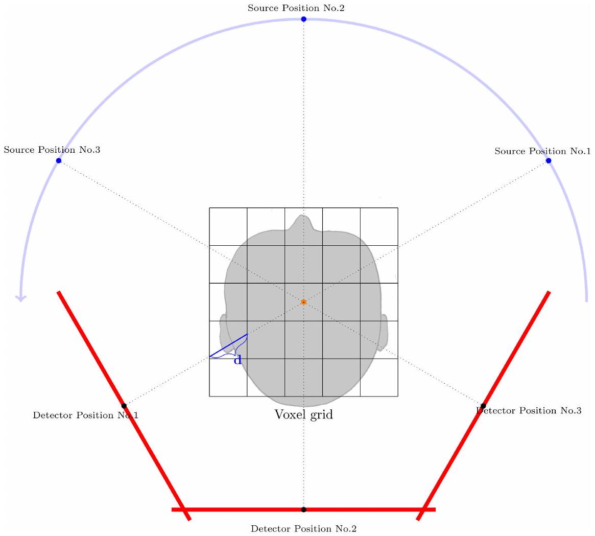
بعد ترتيب جميع مواقع المصدر والكاشف تقريبًا حول شبكة الفوكسل الافتراضية وفقًا للمواقع الحقيقية التي كانت فعالة لكل واحدة من مئات صور الأشعة السينية (الشكل 1)، يتم بناء خط من كل بكسل كاشف يهدف إلى الموقع ثلاثي الأبعاد لمصدر الأشعة السينية. لكل فوكسل وإسقاط k (أي، موقع المصدر إلى الكاشف رقم k) يتم حساب مسافة ) “الأشعة السينية” (الخط المُنشأ) الذي يمر عبر الفوكسل في الموضع يمكن حسابه. يمكن بعد ذلك توزيع قيمة الرمادي المسجلة في بكسل الكاشف في هذا الموضع بين المصدر والمستقبل k على الفوكسيليات التي تم عبورها بواسطة هذه “خط الأشعة السينية” وفقًا للمسافات الخط يتقاطع مع الفوكسلات المعنية (الشكل 1). إذا تم القيام بذلك لجميع البيكسلات لكل موضع مصدر-مستقبل على جميع البيانات المكتسبة
تُعطى التقديرات لهذه المدخلات بعد ذلك، على سبيل المثال، متوسطًا لكل فوكسل، ويتم الحصول على تقدير جيد لكثافة المريض الموجود في كل فوكسل وتمثيله كقيمة رمادية.

قد يستنتج القارئ أنه إذا كان حجم الفوكسل، على سبيل المثال، 0.08 مم، فيجب أن يكون من الممكن تصور هيكل صغير بنفس الحجم. في الواقع، يحدد حجم الفوكسل الحد الفيزيائي لأصغر تفصيل يمكن رؤيته في الصورة. يُطلق على هذا الأخير اسم “الدقة المكانية”، وهو مصطلح تقني يحدد أصغر تفصيل مرئي في الصورة. كما أنه مرتبط ارتباطًا وثيقًا بالحدة، أي أن الصور عالية الدقة فقط هي التي تبدو حادة. لذا، إذا كان حجم الفوكسل يحدد بشكل أساسي الدقة المكانية، فلماذا لا يمكن ترجمته مباشرة إلى الحد الأقصى للدقة المكانية؟ أحد العوامل هو، على سبيل المثال، نظرية نايكويست-شانون المعروفة. ال

ينص النظرية على أنه من أجل إعادة إنتاج إشارة بشكل صحيح، يجب أن يتم أخذ عينات من أي إشارة على الأقل مرتين من أعلى تردد موجود في الإشارة. بالنسبة لصورة CBCT، فهذا يعني أن حجم الفوكسل يحتاج إلى أن يكون أو أقل من حجم أصغر تفصيل قيد الدراسة.

بصرف النظر عن هذا النظرية الأساسية في معالجة الإشارات، هناك العديد من القضايا الأخرى المتعلقة ببيانات CBCT التي تؤدي إلى تدهور دقتها المكانية. حركة المريض هي واحدة من أهم العوامل. كما تم الشرح سابقًا، فإن معرفة الهندسة التصويرية الدقيقة لكل صورة شعاعية ثنائية الأبعاد أمر ضروري لعملية إعادة البناء ثلاثية الأبعاد، وإلا فإن عملية الإرجاع الخلفي لن تكون ممكنة. حيث تفترض عملية إعادة البناء أن المريض ثابت تمامًا خلال المسح الذي يستغرق عدة ثوانٍ، فإن أي انحراف واحد (أي حركة المريض) عن هذا الافتراض ينتقل مباشرة كخطأ إلى عملية إعادة البناء ثلاثية الأبعاد. بعبارة أخرى، يتحرك المريض أثناء الفحص خارج الفوكسيليات التي كان يقع فيها النسيج في بداية الفحص (انظر أيضًا الشكل 1). التأثير الرئيسي بخلاف العيوب الأخرى هو تدهور الدقة المكانية، والمعروف أيضًا باسم ضبابية الحركة (عدم الوضوح في الصورة). أظهر سبين-نيتو وزملاؤه أنه يصل إلى من المرضى يتحركون إلى حد عند النظر في أحجام الفوكسل النموذجية التي تبلغ حوالي 0.1 مم، فإن سعة الحركة هذه البالغة 0.5 مم تعادل خمسة أضعاف حجم الفوكسل. من السهل فهم سبب فشل عملية الإرجاع الخلفي في هذه الحالة في إنتاج صورة حادة، أي ذات دقة عالية. يجب استخدام حلول الأجهزة لتثبيت رأس المريض مثل مسند الذقن أو حزام الرأس للحد من حركة الرأس أثناء الفحص. ومع ذلك، من المعروف أن مثل هذه الأجهزة لها حدودها ومن المحتمل ألا تقضي على الحركة الصغيرة.

دقة الصورة ليست ثابتة في جميع أنحاء حجم CBCT، بل يمكن أن تتفاوت حتى بين مركز الحجم وهوامشه. يمكن أن يُعزى ذلك بشكل رئيسي إلى خوارزمية إعادة البناء FeldkampKress، التي تُستخدم بشكل شائع. بسبب أسباب رياضية، ينتج هذا الخوارزم عن إعادة بناء أكثر دقة في مركز حجم CBCT.

نظرًا لجميع هذه المعايير التي تؤثر على الدقة المكانية، لحسن الحظ، تتوفر مجموعة كبيرة من القياسات الدقيقة للدقة المكانية المتاحة (الحقيقية) لأجهزة CBCT للأجسام غير المتحركة (الأشباح). بشكل أكثر تحديدًا، تأتي هذه القياسات من اختبارات ضمان الجودة التي يجب تكرارها بانتظام (عادةً شهريًا) في بعض البلدان. تُوصى أيضًا بإجراء اختبارات جودة متكررة على الدقة المكانية من قبل الفيزيائيين الطبيين. هذه الاختبارات موصى بها بشدة حيث أن التغييرات الصغيرة جدًا في الإعداد الهندسي ومعايرة الآلات لها تأثير مباشر على الدقة المكانية. على سبيل المثال، إذا لم تكن الآلة مستوية تمامًا بالنسبة لدورانها الأفقي أو إذا حدثت بعض الاهتزازات في وحدة المصدر والكاشف، فإن ذلك سيؤدي على الفور إلى إدخال أخطاء هندسية تظهر على شكل تشويش/تقليل الدقة المكانية في الصور. في الواقع، كل من حركة المريض، بالإضافة إلى عدم دقة الآلة، تسبب أخطاء متطابقة في عملية إعادة البناء. يمكن تلخيص هذه الأخطاء على أنها “أخطاء هندسية.”

يمكن قياس الدقة المكانية بطريقة ذاتية (أزواج الخطوط لكل مليمتر) وموضوعية (دالة نقل التعديل (MTF))
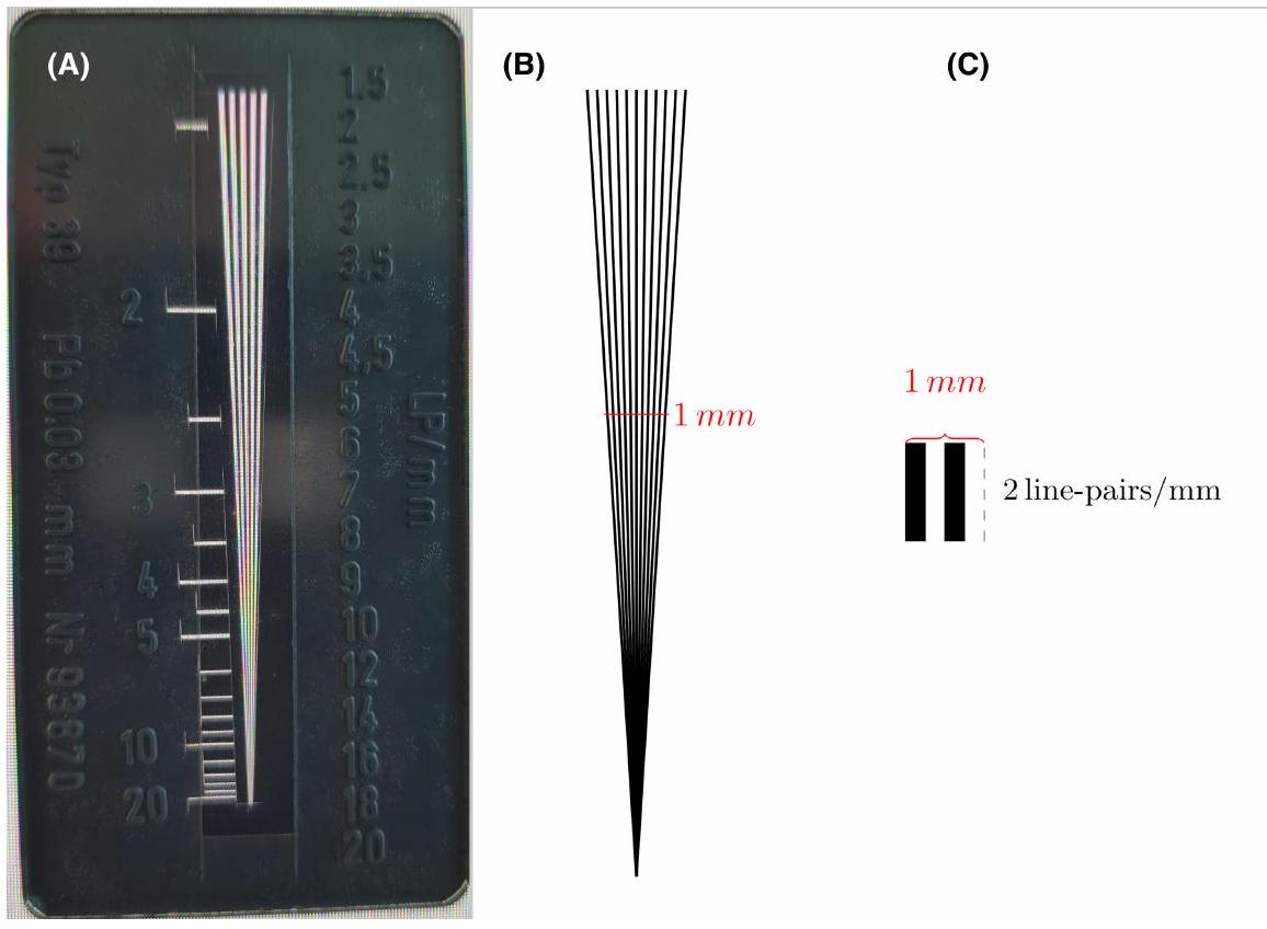
طريقة. بينما تقوم الطريقة الأولى بتقييم بصري لعدد الخطوط القابلة للإدراك لكل مليمتر في صورة وهمية (الشكل 2)، فإن الأخيرة هي مقياس يمكن تقييمه تلقائيًا وموضوعيًا من صور وهمية محددة. بعبارة أخرى، تقيس MTF الدقة المكانية بالنسبة إلى (التباين) المعياري. بينما تنتج مخرجاتها في “دورات لكل مليمتر”، يمكن ترجمتها بأمان إلى “أزواج الخطوط لكل مليمتر” أيضًا. عادةً ما ترتبط الدقة المكانية المحدودة بالقيمة التي تنخفض عندها MTF إلى من التباين الأقصى حيث أن هذه هي حدود الرؤية.

بفضل اختبارات ضمان الجودة المذكورة أعلاه، تتوفر قيم لـ MTF 10% على نطاق واسع. وعادة ما تتراوح بين 0.5 و (المتوسط: ، الوسيط: ). في هذا السياق، يجب ملاحظة أنه للتأهل كـ CBCT أسنان، تطلب منشور من المفوضية الأوروبية حدًا أدنى من الدقة المكانية قدره بعض القيم المقاسة أقل بكثير من هذه القيمة الدنيا. فكيف تترجم قيمة إلى حجم التفاصيل المرئية؟ نظرًا لأن زوج الخطوط يحتوي على خطين (واحد أسود وآخر أبيض في الصورة الوهمية الشكل 3)، فإن أصغر تفصيل هو خطوط خط في الحجم. بعبارة أخرى، فإن CBCT الذي يفي بالحد الأدنى من المتطلبات للتأهل كـ أسنان يحل فقط تفاصيل بحجم أدنى قدره 0.5 مم. تسرد الجدول 1 أحجام التفاصيل المقابلة المحسوبة من هذه المعادلة لبعض قيم الدقة المكانية النموذجية. نلاحظ أنه بالنسبة لأعلى قيم MTF المقاسة -القيم ( ) فإن أصغر حجم تفصيل مرئي يصل إلى 0.2 مم. من الواضح، من هذه القيم الموضوعية التي تم الحصول عليها من صور وهمية غير متحركة نفهم أن الدقة المكانية الحقيقية (المتاحة) لآلات CBCT دائمًا أقل مما قد يوحي به حجم الفوكسل. الضوضاء هي عامل آخر يفرض قيودًا على الدقة المكانية. تمثل قيم التوهين غير المتسقة (الرمادي) في صور الإسقاط، أي، انحرافات معيارية كبيرة في المناطق التي يجب أن يكون فيها رمادي ثابت. في عملية إعادة البناء، تؤدي صور الإسقاط المزعجة أيضًا إلى إعادة بناء ثلاثية الأبعاد مزعجة. بشكل عام، تعتبر صور CBCT لأسباب مختلفة صورًا مزعجة نسبيًا. هناك سببان رئيسيان لهذه السمة: أولاً، تلتقط الكاشف ذو المساحة الواسعة الكثير من الإشعاع المتناثر الذي سيظهر كضوضاء. ثانيًا، تحتاج صور CBCT الأسنان إلى أن تُنتج عند جرعات إشعاعية أقل مقارنة بصور CT الطبية. تزيد الجرعة الأقل من مستوى الضوضاء في الصورة. تظهر الصور المزعجة تقلبات كبيرة في قيم البكسل في الصورة التي يمكن أن تخفي الآفات أو الهياكل ذات الأهمية. لذا فإن الضوضاء تقلل أيضًا من الدقة المكانية المتاحة (الحقيقية) للصور.

بالإضافة إلى هذه العوامل، ستؤثر العيوب في منطقة/جوار الهيكل قيد الدراسة سلبًا على رؤيته. يمكن تعريف العيوب على أنها هيكل مرئي في البيانات المعاد بناؤها غير موجود في الجسم قيد التحقيق. على سبيل المثال، قد تتداخل عيوب تصلب الشعاع من الأجسام عالية الكثافة (مثل المعدن، الشكل 3) بشدة عند تقييم الجسم قيد الدراسة. نظرًا لوجود العديد من العيوب في صور CBCT، فمن الواضح أن هذه قد تكون عاملًا آخر يحد من الدقة المكانية للصور.

نتيجة لذلك، هناك العديد من العوامل المختلفة التي تتداخل مع جودة صورة CBCT، وخاصة مع دقتها المكانية. من هذه القيود التقنية، من الواضح أن

الشكل 3 مثال على عيوب تصلب الشعاع في مسح CBCT بسبب وجود التيجان ومواد قناة الجذر لأغراض علاج الجذور.
“يجب تجاهل الخطأ في”

في هذه الجملة!
ستكون التقييمات المعتمدة على CBCT للهياكل الصغيرة في نطاق أقل من مليمتر محاطة بهامش كبير من الخطأ. يدعم ذلك الملاحظات التي قام بها دوميك وزملاؤه الذين وجدوا دقة اكتشاف تبلغ فقط لطبقة العظام من في زراعة الأسنان. هنا، يجب ملاحظة أن الزرعة المعدنية تطرح
صعوبة أخرى في تقييم الهياكل المجاورة حيث أنها تسبب أيضًا عيوب تصلب الشعاع (بالإضافة إلى عيوب أخرى) في جوارها.

نظرًا لأن هذه العيوب النقية في الدقة مستقلة عن حجم المسافة المقاسة، فمن الواضح أن الخطأ المطلق سيصبح أكثر وضوحًا مع انخفاض حجم الجسم. بعبارة أخرى:

اختصار: MTF 10%، دالة نقل التعديل عند 10% تعديل (انظر الشرح في القسم 2.2.1).
ستتأثر قياسات المسافات الصغيرة بشكل أكبر من تلك الخاصة بالمسافات الكبيرة. إذا كانت المسافة قيد التحقيق في نطاق حجم عدد قليل من الفوكسلات فقط، فإن الخطأ سيساهم بشكل كبير في الحجم المقاس.

خطأ آخر يتعلق بالمراقب هو اختيار الفوكسلات الصحيحة كنقاط نهاية للقياس. من المعروف جيدًا أن حتى صورة حافة مصقولة واضحة يتم توزيعها عبر عدة فوكسلات. هذا يجعل تعيين نقاط نهاية الفوكسلات بشكل صحيح صعبًا. يجب ملاحظة أن هذا الخطأ يضيف إلى عدم الدقة العامة الموجودة في صور CBCT.

بالنظر إلى أن CBCT حاليًا مصمم لتصور تباين الأنسجة الصلبة، يمكن تصور الأنسجة الرخوة مثل اللثة/المخاطية بوضوح فقط إذا كان هناك تباين عالٍ مع الأنسجة أو الهياكل المجاورة. نظرًا لأن الهواء يظهر داكنًا جدًا في الصور، سيكون أفضل تباين بين الأنسجة الرخوة والهواء. إذا لم يكن الهواء على سبيل المثال يملأ الفم لأن الشفاه مجاورة مباشرة للثة/المخاطية (الشكل 4)، فلا يمكن تمييز اللثة/المخاطية على الإطلاق في الصورة.

لذا إذا كان هناك تباين كافٍ، هل يمكن تقييم الأنسجة اللثوية حول الأسنان بدقة في CBCT؟ الجواب مرة أخرى يتحدد بشكل رئيسي من خلال البعد (السماكة) لهذه الطبقة. في دراسة على جثث بشرية استندت إلى قياسات هيستومورفومترية، وُجد أن سماكة الأنسجة الرخوة في الفك العلوي الأمامي كانت في المتوسط أقل تمامًا من 1 مم، مع قيم دنيا قدرها تتراوح هذه القيمة الدنيا تقريبًا في نطاق حجم الفوكسل في CBCT وبالتالي لا يمكن إعادة إنتاجها (وتقييمها) بشكل صحيح بواسطة CBCT. بسبب العوامل التي تم مناقشتها سابقًا، ستواجه أي قيم أقل من 1 مم خطأً كبيرًا عند تقييمها في صورة CBCT. ليس من المستغرب أن المؤلفين وجدوا اختلافات كبيرة بين القيم الهيستومورفومترية (الحقيقة الأرضية) والقيم التي تم تقييمها بواسطة CBCT. في المتوسط، كانت قيم CBCT أقل بمقدار 0.2 مم من نظيراتها التي تم تقييمها هيستولوجيًا.

الأنسجة الصلبة تحت هذه الطبقة الرقيقة من الأنسجة الرخوة، أي، الطبقة العظمية البوكالية/اللسانية على الأسنان الأمامية عادة ما تكون أيضًا هيكلًا رقيقًا جدًا. لاحظ تودوروفيتش وزملاؤه في دراسة ميكرو-CT باستخدام جماجم بشرية أن الطبقة العظمية البوكالية/اللسانية على

الأسنان العلوية عادةً ما تكون (الأشكال 5 و6). في دراسة أخرى على جثث بشرية، وجد باتكاس وزملاؤه، 15 مم نحو الذيل من حافة القطع في الأسنان الأمامية السفلية، سمك عظم متوسط قدره 0.82 مم مع قيمة دنيا قدرها لاحظ أن المؤلفين استخدموا نقطة قياس عميقة نسبيًا في الحويصلات حيث تكون الطبقة العظمية سميكة نسبيًا بالفعل. هذه القيم تثبت الافتراض بأن سمك الطبقة العظمية في الأسنان الأمامية عادةً ما يكون في نطاق حجم دقة الفضاء المتاحة في CBCT. لذلك، حتى حجم 0.125 مم قد لا يستطيع تصوير العظم البوكالي/اللساني الرقيق بشكل موثوق، مما يحمل خطر المبالغة في تقدير الفتحات والانفصالات.

تعود قيود CBCT في التقييم البعدي للهياكل الصغيرة إلى عوامل تقنية لا مفر منها، والتي يجب قبولها لتجنب التفسير المفرط للصور. وبالتالي، فإن التوصية العامة الأكثر أهمية هي عدم توقع دقة أعلى من في صورة CBCT غير المتدهورة حركيًا. في ضوء هذه الحقائق ورغم تعدد القياسات الموجودة (ملخص، على سبيل المثال، في المرجع [52]) للدقة الحقيقية لـ CBCT، من المدهش أن هذه التوصية العامة جدًا في سياق سريري غالبًا ما يتم تجاهلها.

هذا أمر ذو أهمية خاصة لتقييم حجرة الأنسجة الرخوة، حيث يكون التباين المحلي عمومًا ضعيفًا مما يجعل التقييم الصحيح للمسافة الصغيرة قيد التحقيق أكثر تحديًا. لتعزيز هذا التباين المحلي إلى أقصى حد، يجب اتخاذ تدابير لتجنب تداخل هياكل الأنسجة الرخوة. يمكن القيام بذلك، على سبيل المثال، باستخدام حوامل للشفاه أو نفخ الفم بالهواء لإبعاد الشفاه عن اللثة.

تم اقتراح لفات قطنية كموصل للشفاه أيضًا (الشكل 4). ومع ذلك، يجب ملاحظة أن هذه ستؤثر فقط على التباين المحلي، وليس على دقة القياس العامة للأنسجة المعروضة.

إذا كنا نريد حقًا تحقيق قياسات أكثر دقة، فإن إحدى الحلول هي استخدام ماسح ضوئي بصري بالإضافة، إما على التشريح نفسه أو على نموذج جبسي. لقد أظهرت الماسحات الضوئية البصرية أنها تكتشف وتحدد بدقة عالية تراجعات اللثة باستخدام نماذج جبسية كأساس. ومع ذلك، يمكن أيضًا تراكب مسح ضوئي داخل الفم على CBCT بحيث يتم إنشاء صورة مركبة من الطريقتين. هنا، ستظهر السطح اللثوي/المخاطي كخط واضح. نظرًا لأن دقة الفضاء للماسحات الضوئية البصرية أعلى بكثير من تلك الخاصة بـ CBCT، من منظور تقني يجب أن تكون هذه القياسات أكثر دقة بكثير من تلك الخاصة بـ CBCT وحده. يدعم هذا الافتراض النظري نتائج العديد من الدراسات التجريبية والسريرية، لقد أظهرت هذه الطريقة لمسح ضوئي غير غازي للأنسجة أيضًا موثوقية وإعادة إنتاجية كافية. ومع ذلك، يجب إجراء دراسات باستخدام، على سبيل المثال، تقييم هيستومورفومتري لسمك اللثة لمقارنة المسحات المباشرة مقابل المسحات على النموذج الجبسي لهذا الغرض. للأسف، لا تساعد هذه الطريقة في تعزيز الدقة في تقييم الطبقة العظمية البوكالية/اللسانية الرقيقة حيث إنها مخفية في تشريح المريض. هنا لا يمكننا تعزيز التباين المحلي من خلال تدابير خارجية ولا يمكننا بسهولة الحصول على تصور مساعد لسطحها. ستساعد فقط التدابير العامة في زيادة الصورة إلى أقصى حد. أولاً وقبل كل شيء، يجب علينا اختيار حجم الفوكسل المناسب، نسبيًا
صغير لعملية المسح. في هذا السياق، ومع ذلك، يجب ملاحظة أن أحجام الفوكسل الصغيرة عادةً ما تزيد من وقت المسح مما يمنح المريض مزيدًا من الوقت للتحرك. حيث أن الحركة تعاكس دقة الفضاء، من الضروري إيجاد “أفضل توازن ممكن” بين حجم الفوكسل وحركة المريض المحتملة. إذا كان ذلك ممكنًا، يجب تطبيق تثبيت رأس الأجهزة، على الرغم من أن هذا معروف أيضًا أن له حدوده وربما لا يمكنه القضاء على الحركات الصغيرة. يجب تجنب عمومًا الافتراض بوجود عظم مفقود أو عيب عظمي إذا لم يكن هناك تغطية عظمية مرئية في صورة CBCT. بل يجب استخلاص استنتاج دقيق بأنه ببساطة من المستحيل اكتشاف وجود أو عدم وجود طبقة عظمية رقيقة بدقة في صورة CBCT. بالنسبة للأنسجة الرخوة، لأسباب المذكورة أعلاه، يكون من الأكثر تحديًا اكتشاف الهياكل الصغيرة في CBCT. لتعظيم الفرصة لتصور هذه الهياكل، يجب النظر في التدابير التالية البسيطة نسبيًا:

تقدم هذه المراجعة السردية ملخصًا للمعلومات التقنية التي توفر نظرة ثاقبة على الخيارات والقيود الخاصة بـ CBCT في تصور الهياكل الصغيرة/الرقيقة. بينما تعتبر التقنية رائعة للحصول على انطباع ثلاثي الأبعاد عن تشريح المريض، فإنها غالبًا ما تفشل عندما يتعلق الأمر بالكشف عن الهياكل العظمية الصغيرة أو، والأسوأ من ذلك، الأنسجة الرخوة. هناك مجموعة متنوعة من الأسباب التقنية لهذه القيود يمكن تلخيصها في بيان بسيط واحد: CBCT مثل أي صورة أخرى، من الناحية التقنية، هو “تخمين جيد” للتشريح الحقيقي، لكنه ليس “الحقيقة” نفسها. الافتراضات الفيزيائية المبسطة، وطرق إعادة البناء الخشنة، والتمثيل المنفصل للتشريح المستمر للمريض هي الأسباب الأكثر أهمية لعدم عرض صورة CBCT للحقيقة الكاملة، بل مجرد “تخمين” لائق عنها.

ومع ذلك، فإن الصور مفيدة للغاية في السياق السريري، وليس من المستغرب أن تكون التقنية قد حققت نجاحًا باهرًا في العديد من مجالات طب الأسنان. إذا تم تطبيقها بشكل صحيح، فإن استخدامها متنوع ومن المحتمل أن يستفيد المرضى في مجموعة متنوعة من السيناريوهات السريرية المختلفة. ومع ذلك، في سياق تحليل نمط اللثة ونمط العظام، فإن التقنية لها قيود شديدة عندما يتعلق الأمر بتصوير الهياكل الصغيرة بعرض أقل من ملليمتر. قد يأتي هذا كصدمة للمستخدمين السريريين، حيث غالبًا ما تروج الصناعة لدقة بحجم الفوكسلات الصغيرة، أي حتى أقل من 0.1 مم. هذا أكثر إثارة للدهشة نظرًا لأن المعايير المعتمدة لاختبار الجودة توفر رؤى ممتازة حول دقة الفضاء المتاحة لمجموعة متنوعة من الآلات. بالإضافة إلى ذلك، هناك مراجعات منشورة حول هذا الموضوع. كل هذه المعلومات توضح بوضوح أن CBCT يحل بين وربما بحد أقصى . لقد تعلمنا أن هذا يترجم إلى 0.5 و0.16 مم. ومع ذلك، حيث أن هذه القيم تم توليدها جميعًا من أشباح غير متحركة، فإنها لا تحتوي على ضباب الحركة الذي سيحدث تقريبًا بشكل لا مفر منه إلى حد ما في المرضى الأحياء.

من المثير للاهتمام أنه تم إظهار أنه حتى في الأشخاص الشباب والأصحاء ذوي ضغط الدم الطبيعي، فإن السعة المقاسة عند الأسنان الأمامية لكل نبضة قلب هي هنا، كان المشاركون مثبتين على دعامة الذقن وطُلب منهم الاسترخاء. وهذا يعني أنه على مدى فترة تعرض نموذجية، على سبيل المثال، 12 ثانية مع افتراض معدل ضربات قلب طبيعي قدره سيكون هناك على الأقل 12 نبضة فعالة، كل منها يزيح تشريح المريض عن وضعه الأولي. من الواضح أنه كلما كانت الفوكسلات أصغر، زادت أهمية هذا التأثير.

لذا، فإن الدقة الحقيقية في الفضاء في مريض حي أقل قليلاً من تلك التي تم تقييمها في النماذج. إلى أي مدى هي أقل لم يتم التحقيق فيه جيدًا بعد، بشكل رئيسي لأن مثل هذه القياسات في مجموعات البيانات التي تظهر فقط تشريح الإنسان أكثر تعقيدًا. في الواقع، لا توجد طريقة معتمدة مثل هذه.

الهياكل الصغيرة النموذجية ذات الأهمية هي اللثة والدعم العظمي للأسنان الأمامية للفك العلوي والسفلي. في هذا السياق، يجب أن نأخذ في الاعتبار أيضًا أن القيمة الحدية التي تميز بين النمط السميك والرقيق هي بينما تكون صورة طبقة العظم السميك مرئية في CBCT (الشكل 7)، فإن المشكلة تكمن في دقة قياس ذلك العظم

تظل المشكلة في الصورة كما هي. من الواضح أنه، خاصة بالنسبة للنمط الرقيق، بسبب الأسباب المذكورة أعلاه، سيكون من الصعب تصور مثل هذه الهياكل الرقيقة. وحتى إذا تم تصورها، ماذا يعني قيمة سمك 0.32 مم كما تظهرها برامج القياس في الواقع؟ بالتأكيد، يمكننا أن نقترح بأمان تخطي الرقم الثاني، وبالتالي نصل إلى 0.3 مم. يجب اعتبار خطأ القياس يجب اعتبار الفوكسل كعدم يقين محتمل في التصوير بالإضافة إلى عملية القياس. لذا إذا كانت الأبعاد المقاسة، على سبيل المثال، 0.32 مم وكان لدينا حجم فوكسل قدره (أي 0.1 مم)، سيكون لدينا هامش خطأ قدره . ومع ذلك، إذا أظهرت البيانات علامات على زيادة حركة المريض أو/و تصلب الشعاع الإضافي أو غيرها من العيوب في منطقة القياس، يجب تفسير هذه القيمة بحذر أكبر. لأسباب جميعها المذكورة، من الآمن أن نستنتج أن CBCT ليست الطريقة الأكثر دقة في التقييم البعدي للهياكل الصغيرة/الرقيقة بحجم حوالي أو أقل من 0.5 مم.

هنا، على الرغم من أن المؤلفين يدعون عدم وجود دراسات كافية، قد تكون الموجات فوق الصوتية بديلاً قابلاً للتطبيق وخاليًا من الإشعاع. ومع ذلك، فإن هذه الطريقة لها قيود تتمثل في وجود مجال رؤية ضيق، والحاجة إلى استخدام وسط لنقل الصوت، وعدم توفرها على نطاق واسع بسبب تكاليفها وصعوباتها التقنية. بالنسبة لمكونات الأنسجة الرخوة مثل اللثة الشفوية
أو أبعاد الأنسجة فوق القمة، يمكن أن يوفر الجمع بين CBCT ومسح السطح البصري نتائج أكثر دقة. ومع ذلك، يجب أن يؤخذ في الاعتبار أن CBCT يسبب جرعة إشعاعية كبيرة، تتجاوز بكثير تلك الخاصة بتقنيات الأشعة السينية السنية ثنائية الأبعاد. وفقًا لمبدأ التبرير المعتمد دوليًا، يجب تبرير كل صورة شعاعية بشكل فردي، موازنةً بين مخاطر المريض والفائدة المحتملة. نتيجة لذلك، يجب أخذ طرق بديلة في الاعتبار.

في ضوء القيود، يبدو أن دراسات CBCT التي تهدف فقط إلى تقييم سمك اللثة أو أبعاد الدعم العظمي الرقيق يصعب تبريرها. ومع ذلك، إذا تم الحصول عليها لأسباب أخرى، يمكن بالطبع إجراء مثل هذه القياسات على CBCT موجود. إذا تم تطبيقها بحذر وبشكل محافظ، قد تظل هذه القياسات ذات قيمة للتشخيص والعلاج السريري. ما يجب تجنبه، مع ذلك، هو التفسير المفرط والتقدير المفرط للدقة، حيث يمكن أن يؤدي كلاهما إلى آثار سلبية على جانب المريض. على سبيل المثال، قد يؤدي تفسير العظم المفقود في صورة CBCT على أنه عظم مفقود حقًا إلى تعريض سن أمامي للخطر دون سبب حقيقي. يمكن للمرء بالتأكيد التفكير في العديد من الأمثلة المماثلة الأخرى على هذا النحو. ومن ثم، فإن الرسالة الأساسية من هذه المراجعة هي تفسير CBCT بحذر وإدراك أنه تخمين جيد (تم الحصول عليه تقنيًا) للواقع ولكنه ليس الواقع نفسه.

يعد مسح CBCT طريقة قابلة للتطبيق لقياس مكونات الأنسجة الصلبة والرخوة لنمط اللثة. ومع ذلك، فإن التقييم الشامل للعوامل المؤثرة على جودة الصورة والدقة المكانية ضروري لمنع التفسيرات المحتملة الخاطئة. بالإضافة إلى ذلك، في حالة وجود أنماط لثة رقيقة، قد لا تعني غياب طبقات العظم/الأنسجة الرخوة المرئية في مسح CBCT غيابها الحقيقي بالضرورة. هذه القيود التقنية متأصلة في تصوير CBCT ويجب أخذها في الاعتبار عند تفسير مثل هذه الصور.

تم توفير تمويل الوصول المفتوح من قبل جامعة برن.

ليس لدى المؤلفين أي تضارب في المصالح للإبلاغ عنه يتعلق بإجراء هذه المراجعة. لم يتم تلقي أي دعم مالي أو رعاية.

رالف شولتز (D) https://orcid.org/0000-0002-7880-0046

How to cite this article: Schulze R, Couso-Queiruga E, Katsaros C. Accuracy of cone-beam computed tomography in imaging the components of the periodontal phenotype. Periodontol 2000. 2024;00:1-11. doi:10.1111/prd. 12556

Department of Oral Surgery and Stomatology, School of Dental Medicine, University of Bern, Bern, Switzerland
Division of Oral Diagnostic Sciences, Department of Oral Surgery and Stomatology and Oral Diagnostics, School of Dental Medicine, University of Bern, Bern, Switzerland
Department of Orthodontics and Dentofacial Orthopedics, School of Dental Medicine, University of Bern, Bern, Switzerland

Ralf Schulze, Division of Oral Diagnostic Sciences, Department of Oral Surgery and Stomatology and Oral Diagnostics, Freiburgstrasse 7, Bern 3010, Switzerland. Email: ralf.schulze@unibe.ch

3D imaging, cone-beam computed tomography, dental digital radiographs, phenotype

In current clinical practice and research, understanding the effect of the periodontal and peri-implant phenotypical features in different clinical scenarios holds significant importance. The periodontal phenotype is determined by the bone morphotype, which is characterized by the thickness of the alveolar bone plate, and the gingival phenotype, constituted by the gingival thickness and the keratinized tissue width. While the supracrestal tissue height, defined as the dimension obtained from the zenith of the gingival margin to the most coronal part
of the alveolar bone crest, was not initially included in the definition of periodontal phenotype provided in the 2017 World Workshop, recent studies recommended considering this component as an integral component of the periodontal phenotype due to its correlation with other phenotypic features and relevance in clinical practice.

These site-specific phenotypic dimensions are subject to change over time depending on environmental factors (e.g., presence and progression of inflammatory diseases, orthodontic treatment, trauma), and clinical therapeutic interventions (e.g., hard and soft tissue augmentation therapies). Nonetheless, the dimensions of

components of the periodontal phenotype have been recognized as a pivotal prognostic factor in periodontics, orthodontics, oral surgery, and in the context of implant therapy. Thus, correct assessment of the dimensions is of key importance.

When teeth are moved orthodontically outside the alveolar bone, labial/lingual bone dehiscence can occur, which can be followed by gingival recession. This tooth movement can happen not only during the active treatment phase but also in the posttreatment period through the activation of fixed round spiral wire retainers. Therefore, determination of the bone morphotype and gingival phenotype is important for the planning of specific orthodontic movements. Nonetheless, the reports in the literature are contradictory as regards possible association between the extent of gingival recession in orthodontic patients and the degree of therapeutic incisor proclination, the width of the attached gingiva, the thickness of the mandibular symphysis, the facial type, oral hygiene, or periodontal conditions.

Thin gingival phenotype, however, has been associated with a higher probability of mucogingival defects. Gingival thickness and keratinized tissue width play also a big role in the long-term mucosal margin stability in gingival phenotype modification therapies, and have been recognized as a predictor for the outcomes of root coverage procedures.

In restorative dentistry classic studies reported that the placement of subgingival restorations, inadequate embrasures, poor selection of the restorative material, or overhanging margins among others may induce a local irritation, disruption of the hemostatic biological interface, and the subsequent microbial dysbiosis and initiation of inflammatory disease. Different studies revealed that sites presenting a thick phenotype respond differently compared to thin tissues under similar conditions (i.e., biofilm accumulation, trauma) or therapies. Thick tissues tend to exhibit a hyperplastic response whereas thin tissues are more prone to develop gingival recession.

Several studies on the topic of the management of the extraction site have observed that the thicker the alveolar bone after tooth extraction with or without further intervention, the lower the post-extraction dimensional changes at the level of the alveolar ridge. Similarly, in cases where no further intervention was performed, the thinner the alveolar bone after tooth extraction the higher the alveolar ridge atrophy and the thickening of the mucosal tissues. Other studies have also observed a decrease in the need of bone augmentation procedures and less interproximal soft tissue changes in sites with a thicker bone phenotype. Most recently, the dimensions of the supracrestal tissue compartment have been correlated with post-extraction dimensional changes. Therefore, it seems evident that an adequate and reliable assessment of the dimensions of the phenotypical features is crucial in order to make judicious clinical decisions in daily clinical practice and in contemporary dental research to evaluate the effect of these dimensions in different therapies.

Several methods have been developed for classifying and quantifying bone and soft tissue thickness around dental implants and
teeth, such as the use of merely visual inspection of the external features of the alveolar ridge and soft tissues, the insertion of a periodontal probe into the sulcus to evaluate its transparency, ultrasound, non-invasive ultrasonography, transmucosal horizontal probing, or the use of cone-beam computed tomography (CBCT) with or without the superimposition of stereolithography (STL) files. Despite the inherent limitations of each of the assessment modalities, the use of CBCT belongs to the most widely used methods in daily clinical practice and research. Hence, this review is focused on providing the Change “focus” by “emphasis” tion for the use of CBCT scans, with a focus on the technical limits that currently cannot be overcome. Technical and physical factors provide evidence in themselves which can be used to deduct clear and rigorous conclusions for the clinical application reperafe ref of if by “for” review addresses the underlying technical information the use of CBCT scans, and suggests some recommendations on how to optimally use it despite its’ system-inherent limitations.

Unlike two-dimensional (2D) radiographic projection images (e.g., intraoral radiographs), a CBCT (as well as a Computed Tomography (CT) scan) is a reconstructed image generated from the information contained in multiple (several hundred) 2D-projection radiographs. Like a CT a CBCT produces a three-dimensional (3D) representation of patient density from a large series of two-dimensional (2D) radiographic projection images. The latter are generally acquired from a circular ( -) orbit of the X-ray source and the detector about the patient’s head. If the exact imaging/projection-geometry of each of the hundreds of 2D-projection X-rays is exactly known, a process termed “backprojection” allows for accurate estimation of the patients’ density at every specific location that has been exposed in the 2D radiographs. Conceptually, this is done by geometrically arranging all projection images relative to the patient in the pose and position in which the image had been acquired. The basic concept will be summarized in the following.

Due to the fact that patient-tissue density needs to be displayed somehow on a computer monitor, the concept of a 3D voxel representation was introduced. Voxels (acronym from “volume element”) are the 3D analogon to tell-knewixel (“picture element”) well known from, for example, digital photography. In other words, the density of patient tissue in a CBCT is represented by small cubic voxels that are arranged in a regular voxel-grid. This way of representation is termed “discrete” since it divides continuous patient anatomy into separate tiny entities, the voxels. Commonly, CBCT-voxels come with a side length between 0.08 and 0.3 mm . What we perceive as a CBCT-image is the array of these tiny cubic voxels, all of which have a distinct gray value (ideally representing the true patient’s density
at that particular location) and three coordinates ( ). It should be noted that this representation is not continuous as the actual true patient structure, rather it divides and represents anatomy in tiny cubic entities, the voxels. While at first sight, this seems not important, de facto this representation causes multiple artifacts and also has other shortcomings. Plus, the voxel size eventually determines spatial resolution, the main topic of this review.

The backprojection process can be briefly summarized as follows:
After virtually arranging all source and detector positions around the virtual voxel grid according to the true locations which were effective for every single one of the hundreds of X-ray projection images (Figure 1), from every image detector-pixel a line is constructed aiming at the 3D position of the X-ray source. For each voxel and projection k (i.e., source-to-detector position No. k) a distance ) the “X-ray” (the constructed line) traversing through the voxel at position can be computed. The gray value recorded in the detector pixel at this source-receptor position k can then be distributed to the voxels traversed by this “X-ray-line” according to the distances the line intersects the respective voxels (Figure 1). If this is done for all pixels per source-receptor position over all acquired
projections and these entries are subsequently, for example, averaged per voxel, a good estimation of the density of the patient located in each voxel is obtained and represented as gray value.

The reader might conclude that if the voxel has a size of, for example, 0.08 mm , it should be possible to visualize a tiny structure of the same size. Indeed, the voxel size determines the physical limit of how small the smallest detail in the image can be to be visualized. The latter is termed “spatial resolution,” a technical term defining the smallest detail visible in an image. It is also closely related to sharpness, that is, only high-resolution images also appear sharp. So if the voxel size fundamentally determines spatial resolution, why can it not be directly translated into the maximal spatial resolution? One factor is, for example, the well-known Nyquist-Shannon-Theorem. The

theorem states that for a signal to be correctly reproduced, any signal needs to be sampled at least twice the highest frequency contained in the signal. For a CBCT image, this means that the voxel size needs to be or less than the size of the smallest detail under study.

Apart from this fundamental signal processing theorem, there are a multitude of other issues involved with CBCT-data degrading its spatial resolution. Patient motion is one of the most important factors. As explained before, for the 3D-reconstruction process knowledge of the exact imaging geometry of every 2D radiograph is essential, otherwise the backprojection process is not feasible. As the reconstruction assumes a completely steady patient during the scan of several seconds, every single deviation (i.e., patient motion) from this assumption directly propagates as an error into the 3D-reconstruction process. In other words, the patient during the scan moves outside the voxels in which the tissue was located at the beginning of the scan (see also Figure 1). The main effect apart from other artifacts is a degraded spatial resolution, also known as motion blur (unsharpness in the image). Spin-Neto and colleagues showed that up to of the patients move to an extent of When considering typical voxel sizes of around 0.1 mm , this motion amplitude of 0.5 mm is fivefold the voxel size. It is easy to understand why the back projection process in this case fails to produce a sharp, that is, highly resolving image. Hardware solutions to immobilize the patient’s head such as a chin-rest, or head strap should be used to limit head motion during the scan. However, it is known that such devices have their limits and likely will not eliminate small motion.

Spatial resolution is not constant throughout the CBCT volume, rather it can vary up to between the center of the volume and its periphery. This can be mainly attributed to the FeldkampKress reconstruction algorithm, which is commonly applied. Due to mathematical reasons, this algorithm produces a more accurate reconstruction in the center of the CBCT volume.

Given all these parameters influencing spatial resolution, luckily, a multitude of exact measurements of the available (true) spatial resolution of CBCT machines for non-moving objects (phantoms) are available. More specifically, these come from quality assurance measurements which have to be repeated on a regular (commonly monthly) basis in some countries. Repeated quality tests on spatial resolution are also advocated by medical physicists. These tests are very advisable since very small changes in the geometric set-up and calibration of the machines have a direct effect on spatial resolution. For instance, if the machine is not perfectly leveled with respect to its horizontal rotation or if some wobbling of the source-detector-unit occurs, this will immediately introduce geometrical errors that manifest themselves as blurring/reduced spatial resolution in the images. De facto, both patient movement, as well as machine-related inaccuracies, induce identical errors in the reconstruction process. These errors can be summarized as “geometrical errors.”

Spatial resolution can be measured by a subjective (line pairs per millimeter) and objective (Modulation Transfer Function (MTF))
method. While the first method visually assesses the number of perceptible lines per millimeter in a phantom image (Figure 2), the latter is a metric that can be automatically and objectively assessed from specific phantoms. Roughly translated, the MTF measures spatial resolution in relation to (normalized) contrast. While it produces an output in “cycles per millimeter,” this can be safely translated into “line pairs per millimeter” as well. The limiting spatial resolution is normally associated with the value where the MTF falls to of maximum contrast since this is the limit of visibility.

Due to the above-mentioned quality assurance tests, values for MTF 10% are widely available. They typically range between 0.5 and (mean: , median: ). In this context, it should be noted that to qualify as dental CBCT, a publication by the European Commission requests a minimum spatial resolution of Some measured values are clearly below this minimum value. So how does a value of translate into visible detail size? Since a line pair contains two lines (a black one plus a white one in the phantom image Figure 3), the smallest detail is lines line in size. In other words, a CBCT fulfilling the minimum requirements to qualify as dental resolves only details of a minimum size of 0.5 mm . Table 1 lists the respective detail sizes computed from this equation for some typical spatial resolution values. We observe that for the highest measured MTF -values ( ) the smallest visible detail size amounts to 0.2 mm . Clearly, from these objective measurement values obtained from non-moving phantoms we understand that the true (available) spatial resolution of CBCT machines is always lower than the voxel size would imply. Noise is another factor posing limitations on spatial resolution. It represents inconsistent attenuation (gray) values in the projection images, that is, large standard deviations in areas where a constant gray should be present. In the reconstruction process, noisy projection images also yield a noisy 3D-reconstruction. Generally, CBCTs due to different reasons are relatively noisy images. There are two major reasons for this characteristic: first of all, the wide-area detector captures a lot of scattered radiation that will appear as noise. Secondly, dental CBCT images need to be produced at lower radiation doses as compared to medical CT images. A lower dose increases the noise level in the image. Noisy images show large fluctuations in pixel values in the image that can mask lesions or structures of interest. Thus noise also lowers the available (true) spatial resolution of the images.

In addition to these factors, artifacts in the area/vicinity of the structure under study will negatively affect its visibility. Artifacts can be defined as a visualized structure in the reconstructed data that is not present in the object under investigation. For instance, beam hardening artifacts from high-density objects (e.g., metal, Figure 3) in the vicinity may severely interfere when assessing the object under study. As there is a multitude of artifacts contained in CBCT-images it is obvious that these may be another limiting factor for spatial resolution of the images.

As a consequence, there are a multitude of different factors that interfere with CBCT image quality, particularly with its spatial resolution. From these technical limitations, it is evident that

FIGURE 3 Example of beam hardening artifacts in the CBCT scan due to the presence of crowns and root canal material for endodontic purposes.
“the error in” needs to be discarded

in this sentence!
in CBCT-based assessment of tiny structures in the submillimeter range will be beset with a significant margin of error. This is supported by the observations of Domic and colleagues who found a detection accuracy of only for a bone layer of at dental implants. Here, it should be noted that the metallic implant poses
another difficulty in the assessment of adjacent structures as it also induces beam-hardening (plus other) artifacts in its vicinity.

As these pure accuracy deficiencies are independent of the size of a measured distance, obviously the absolute error will become more prominent with decreasing object size. In other words:

Abbreviation: MTF 10%, Modulation Transfer Function at 10% modulation (explanation see Section 2.2.1).
measurements of small distances will be far more affected than those of large distances. If the distance under investigation is in the range of the size of a few voxels only, the error will largely contribute to the measured size.

Another error related to the observer is to pick the correct voxels as measurement endpoints. It is well known that even the image of a clearly visible machined sharp edge is being spread out over several voxels. This makes a correct assignment of the endpoint voxels difficult. It should be noted that this error adds to the general inaccuracy contained in CBCT images.

Considering the fact that a CBCT currently is constructed for visualization of hard-tissue contrast, soft tissues such as the gingiva/ mucosa can only be clearly visualized if there is a high contrast to the adjacent tissue or structures. Since air appears very dark in the images, the best contrast will be between soft-tissue and air. If for instance air is not filling the oral vestibulum since the lip is directly adjacent to the gingiva/mucosa (Figure 4), the gingiva/mucosa cannot at all be discriminated in the image.

So if there is sufficient contrast, can the gingival tissue around teeth be accurately assessed in a CBCT? The answer again is mainly determined by the dimension (thickness) of this layer. In a human cadaver study based on histomorphometric measurements, it was found that soft tissue thickness in the anterior maxilla on average was entirely below 1 mm , with minimum values of This minimum value is roughly in the range of CBCT-voxel size and thus cannot be correctly reproduced (and assessed) by a CBCT. Due to the factors discussed before any values below 1 mm will be beset with considerable error when assessed in a CBCT-image. No wonder, the authors found significant differences between the histomorphometric values (ground truth) and the CBCT assessed values. On average, CBCT values were 0.2 mm smaller than their histologically assessed counterparts.

The hard tissue underneath this thin soft-tissue layer, that is, the buccal/lingual bony layer on frontal teeth commonly is also a very thin structure. Todorovic and colleagues in a micro-CT-study using human skulls observed that the buccal/lingual bone layer on

maxillary teeth commonly is (Figures 5 and 6). In another human cadaver study, Patcas and colleagues found, 15 mm caudally to the incisal edge at mandibular anterior teeth, a median bone thickness of 0.82 mm with a minimum value of Note that the authors used a measurement point rather deep into the alveoli where the bony layer is already relatively thick. These values prove the assumption that the thickness of the bony layer in frontal teeth commonly is in a range of the magnitude of the available CBCT spatial resolution. Therefore, even a 0.125 mm voxel could not depict the thin buccal/lingual alveolar bone covering reliably, having as a risk the overestimation of fenestrations and dehiscences.

The limitations of a CBCT in the dimensional assessment of tiny structures are due to inevitable technical factors, which have to be accepted to avoid overinterpretation of the images. Thus, the most important general recommendation is not to expect a higher accuracy than in a non-visibly motion-deteriorated CBCT image. In light of these facts and despite the multitude of existing measurements (summary, e.g., in Ref. [52]) of the true accuracy of a CBCT, it is surprising that this very general recommendation in a clinical context often is neglected.

This is of particular importance for the assessment of the soft tissue compartment, as here the local contrast is generally poor making correct assessment of the tiny distance under investigation even more challenging. To enhance this local contrast to a maximum, measures to avoid the overlapping of soft tissue structures should be taken. This can be done by, for example, using lip-holders or inflating the mouth with air to keep the lips away from the gingiva.

Cotton rolls as retractor of the lip have also been proposed (Figure 4). However, it should be noted that these will only have an effect on local contrast, not on the general measurement accuracy of the displayed tissue.

If we really want to achieve more accurate measurements, one solution is to use an optical scanner in addition, either on the anatomy itself or on a plaster model. Optical scanners have been shown to highly accurately detect and quantify gingival recessions using plaster models as a basis. However, an intraoral optical scan may also be superimposed to a CBCT so that a combined image from the two modalities is generated. Here, the gingival/mucosal surface will be indicated as a clear line. Since the spatial resolution of optical scanners is much higher than that of a CBCT, from a technical perspective these measurements should be far more accurate than those of a CBCT alone. This theoretical assumption is supported by the findings of several experimental and clinical studies, This non-tissue invasive optical scan method has also demonstrated adequate reliability and reproducibility. Nevertheless, studies should be conducted using, for example, histomorphometric assessment of the gingival thickness to compare direct scans versus scans on the plaster model for this purpose. Unfortunately, this method does not help to enhance accuracy in the assessment of the thin buccal/lingual bony layer since this is hidden in the patient’s anatomy. Here we can neither enhance local contrast by external measures nor can we easily obtain an auxiliary visualization of its surface. Only general measures will help to increase the image to an optimum. First of all, we should carefully select the appropriate, relatively
small voxel size for the scan. In this context, however, it should be noted that small voxel sizes commonly increase scan time giving the patient more time to move. As motion counteracts spatial resolution, it is essential to find the “best possible” balance between voxel size and potential patient motion. If possible, hardware head immobilization should be applied, albeit this is also known to have its limits and probably cannot eliminate small movements. It should be generally avoided to assume missing bone or a bony defect if there is no bony coverage visible in the CBCT image. Rather a careful conclusion should be drawn that it is simply impossible to accurately detect the presence or absence of a thin bony layer on a CBCT-image. For soft tissue, for the reasoning above, it is even more challenging to detect tiny structures in a CBCT. To maximize the chance for visualization of these structures, the following relatively simple measures should be considered:

This narrative review summarizes the technical background information providing insight into the options and limitations of CBCTs in the visualization of small/thin structures. While the technique is great to get a 3D impression of a patient’s anatomy, it often fails when it comes to detecting tiny bony or, even worse, soft tissue. There are a variety of technical reasons for this limitation which can be summarized in one simple statement: the CBCT like any other imagery, technically spoken is a “good guess” of true anatomy, yet it is not “truth” itself. Simplified physical assumptions, coarse reconstruction methods and discrete representation of continuous patient anatomy are the most important reasons why a CBCT image does not show the full truth, but rather a decent “guess” on it.

Nevertheless, the images are extremely helpful in a clinical context, and it is no wonder that the technique has a triumphant success in many areas of dental medicine. If applied correctly, its use is manifold and patients will likely benefit in a multitude of different clinical scenarios. However, in the context of analyzing the gingival phenotype and bone morphotype, the technique has severe limitations when it comes to imaging small structures of submillimeter width. This may come as a surprise to clinical users, as often the industry promotes a resolution in the size of the tiny voxels, that is, even below 0.1 mm . This is even more surprising since established standards for quality testing provide excellent insight into the available spatial resolution of a variety of machines. In addition, there are reviews published on the matter. All this information very clearly shows that a CBCT resolves between and maybe at a maximum . We learned that this translates to 0.5 and 0.16 mm . However, as these values are all generated from non-moving phantoms, they do not contain motion blur which will almost inevitably occur to some extent in living patients.

Interestingly, it has been shown that even in young and healthy subjects with normal blood pressure the amplitude measured at the front teeth for each heartbeat is Here, the subjects were fixated on a chin rest and asked to relax. That means, that over a typical exposition time of, for example, 12 s assuming a normal heart-rate of at least 12 beats will be effective, each of which dislocates the patient’s anatomy out of his/her initial position. Clearly, the smaller the voxels the more this effect will be of interest.

Thus, true spatial resolution in a living patient is somewhat lower than the one assessed in phantoms. To what extent it is lower is not well investigated yet, mainly since such measures in datasets only showing human anatomy are more complicated. De facto no established such method exists.

Typical tiny periodontal structures of interest are the gingiva and the bone-support of the anterior maxillary and mandibular teeth. In this context, we should also bear in mind that the threshold value discriminating between thick and thin phenotype is While the image of a thick morphotype bone-layer is mostly visible in the CBCT (Figure 7), the issue with the accuracy of measuring that bone

in the image remains identical. Obviously, particularly for the thin phenotype due to the reasons above it will be challenging to visualize such thin structures. And even if it is visualized, what does a thickness value of 0.32 mm as displayed by the measuring software mean in reality? Certainly, we can safely suggest skipping the second digit, thus we arrive at 0.3 mm . A measurement error of voxel should be considered as potential uncertainty in the imaging plus the measurement process. So if the measured dimension is, for example, 0.32 mm and we have a voxel size of (i.e., 0.1 mm ), we will have a margin of error of . Yet if the data exhibit signs of increased patient motion or/and additional beam hardening or other artifacts in the measurement region, this value should be even more interpreted cautiously. For all the reasons mentioned, it is safe to conclude that CBCT is not the most accurate method in dimensional assessment of small/tiny structures of a size around or below 0.5 mm .

Here, albeit the authors claim a lack of sufficient studies, ultrasonography may be a viable and radiation-free alternative. However, this method has the limitations of having a narrow field of view, the need to use a medium for sound conduction, and not being widely available due to its costs, and technical difficulties. For soft-tissue components such as the labial gingiva
or the supracrestal tissue dimensions, the combination of a CBCT with an optical surface scan can provide more accurate results. However, it has to be borne in mind that a CBCT induces a significant radiation dose, which greatly exceeds that of the 2D dental radiographic techniques. Following the internationally established justification principle, each and every radiograph has to be individually justified balancing the patient’s risk with the potential benefit. As a consequence, alternative methods need to be taken into account.

In light of the limitations, CBCT studies only aiming to assess gingiva thickness or thin bony support dimensions seem hard to justify. Yet if acquired for other reasons, such measurements on an existing CBCT of course may be conducted. If applied cautiously and conservatively, these may still be valuable for clinical diagnosis and therapy. What should be avoided, however, are overinterpretation and overestimation of the accuracy since both may yield negative effects on the patient’s side. For example, interpreting missing bone in a CBCT image as truly missing bone may jeopardize a front tooth without true reason. One can certainly think of many other similar examples along that line. Hence, the fundamental take-home message of this review is to interpret a CBCT cautiously and to realize it is a good (technically acquired) guess of reality yet not reality itself.

CBCT scan is a viable method to measure the hard and soft tissue components of the periodontal phenotype. However, a thorough evaluation of factors influencing image quality and spatial resolution is necessary to prevent potential misinterpretations. Additionally, in the presence of thin periodontal phenotypes, the absence of visible bone/soft tissue layers in a CBCT scan might not necessarily imply their true absence. These technical limitations are inherent to CBCTimaging and should be borne in mind when interpreting such images.

Open access funding provided by Universitat Bern.

The authors have no conflicts of interest to report pertaining to the conduction of this review. No financial support or sponsorship was received.

Ralf Schulze (D) https://orcid.org/0000-0002-7880-0046

How to cite this article: Schulze R, Couso-Queiruga E, Katsaros C. Accuracy of cone-beam computed tomography in imaging the components of the periodontal phenotype. Periodontol 2000. 2024;00:1-11. doi:10.1111/prd. 12556

REFERENCES

1. Avila-Ortiz G, Gonzalez-Martin O, Couso-Queiruga E, Wang HL. The peri-implant phenotype. J Periodontol. 2020;91:283-288.
2. Kao RT, Curtis DA, Kim DM, et al. American Academy of periodontology best evidence consensus statement on modifying periodontal phenotype in preparation for orthodontic and restorative treatment. J Periodontol. 2020;91:289-298.
3. Jepsen S, Caton JG, Albandar JM, et al. Periodontal manifestations of systemic diseases and developmental and acquired conditions: consensus report of workgroup 3 of the 2017 world workshop on the classification of periodontal and Peri-implant diseases and conditions. J Clin Periodontol. 2018;45:S219-S229.
4. Couso-Queiruga E, Barboza EP, Avila-Ortiz G, Gonzalez-Martin O, Chambrone L, Rodrigues DM. Relationship between supracrestal soft tissue dimensions and other periodontal phenotypic features: a cross-sectional study. J Periodontol. 2023;94:944-955.
5. Couso-Queiruga E, Graham ZA, Peter T, Gonzalez-Martin O, Galindo-Moreno P, Avila-Ortiz G. Effect of periodontal phenotype characteristics on post-extraction dimensional changes of the alveolar ridge: a prospective case series. J Clin Periodontol. 2023;50:694-706.
6. Wennström JL. Mucogingival considerations in orthodontic treatment. Semin Orthod. 1996;2:246-254.
7. Gebistorf M, Mijuskovic M, Pandis N, Fudalej PS, Katsaros C. Gingival recession in orthodontic patients 10 to 15 years posttreatment: a retrospective cohort study. Am J Orthod Dentofacial Orthop. 2018;153:645-655.
8. Katsaros C, Livas C, Renkema AM. Unexpected complications of bonded mandibular lingual retainers. Am J Orthod Dentofacial Orthop. 2007;132:838-841.
9. Joss-Vassalli I, Grebenstein C, Topouzelis N, Sculean A, Katsaros C. Orthodontic therapy and gingival recession: a systematic review. Orthod Craniofac Res. 2010;13:127-141.
10. Cortellini P, Bissada NF. Mucogingival conditions in the natural dentition: narrative review, case definitions, and diagnostic considerations. J Periodontol. 2018;89(Suppl 1):S204-s213.
11. Agudio G, Chambrone L, Selvaggi F, Pini-Prato GP. Effect of gingival augmentation procedure (free gingival graft) on reducing the risk of non-carious cervical lesions: a 25 – to 30 -year follow-up study. J Periodontol. 2019;90:1235-1243.
12. Barootchi S, Tavelli L, Di Gianfilippo R, et al. Soft tissue phenotype modification predicts gingival margin long-term (10-year) stability: longitudinal analysis of six randomized clinical trials. J Clin Periodontol. 2022;49:672-683.
13. Carbone AC, Joly JC, Botelho J, et al. Long-term stability of gingival margin and periodontal soft-tissue phenotype achieved after mucogingival therapy: a systematic review. J Clin Periodontol. 2023;51:177-195.
14. Lang NP, Kiel RA, Anderhalden K. Clinical and microbiological effects of subgingival restorations with overhanging or clinically perfect margins. J Clin Periodontol. 1983;10:563-578.
15. Kells BE, Linden GJ. Overhanging amalgam restorations in young adults attending a periodontal department. J Dent. 1992;20:85-89.
16. Sanavi F, Weisgold AS, Rose LF. Biologic width and its relation to periodontal biotypes. J Esthet Dent. 1998;10:157-163.
17. Olsson M, Lindhe J. Periodontal characteristics in individuals with varying form of the upper central incisors. J Clin Periodontol. 1991;18:78-82.
18. Stellini E, Comuzzi L, Mazzocco F, Parente N, Gobbato L. Relationships between different tooth shapes and patient’s periodontal phenotype. J Periodontal Res. 2013;48:657-662.
19. Chappuis V, Engel O, Reyes M, Shahim K, Nolte LP, Buser D. Ridge alterations post-extraction in the esthetic zone: a 3D analysis with CBCT. J Dent Res. 2013;92:195s-201s.
20. Chappuis V, Engel O, Shahim K, Reyes M, Katsaros C, Buser D. Soft tissue alterations in esthetic Postextraction sites: a 3-dimensional analysis. J Dent Res. 2015;94:187s-193s.
21. Clementini M, Agostinelli A, Castelluzzo W, Cugnata F, Vignoletti F, De Sanctis M. The effect of immediate implant placement on alveolar ridge preservation compared to spontaneous healing after tooth extraction: radiographic results of a randomized controlled clinical trial. J Clin Periodontol. 2019;46:776-786.
22. Avila-Ortiz G, Gubler M, Romero-Bustillos M, Nicholas CL, Zimmerman MB, Barwacz CA. Efficacy of alveolar ridge preservation: a randomized controlled trial. J Dent Res. 2020;99:402-409.
23. Couso-Queiruga E, Stuhr S, Tattan M, Chambrone L, Avila-Ortiz G. Post-extraction dimensional changes: a systematic review and meta-analysis. J Clin Periodontol. 2021;48:126-144.
24. Couso-Queiruga E, Garaicoa-Pazmino C, Fonseca M, Chappuis V, Gonzalez-Martin O, Avila-Ortiz G. Interproximal soft tissue height changes after unassisted socket healing versus alveolar ridge preservation therapy. Int J Periodontics Restorative Dent. 2023. doi:10. 11607/prd. 6809
25. Couso-Queiruga E, Weber HA, Garaicoa-Pazmino C, et al. Influence of healing time on the outcomes of alveolar ridge preservation using a collagenated bovine bone xenograft: a randomized clinical trial. J Clin Periodontol. 2023;50:132-146.
26. Pauwels R, Jacobs R, Singer SR, Mupparapu M. CBCT-based bone quality assessment: are Hounsfield units applicable? Dentomaxillofac Radiol. 2015;44:20140238.
27. Couso-Queiruga E, Mansouri CJ, Alade AA, Allareddy TV, GalindoMoreno P, Avila-Ortiz G. Alveolar ridge preservation reduces the need for ancillary bone augmentation in the context of implant therapy. J Periodontol. 2022;93:847-856.
28. Eghbali A, De Rouck T, De Bruyn H, Cosyn J. The gingival biotype assessed by experienced and inexperienced clinicians. J Clin Periodontol. 2009;36:958-963.
29. De Rouck T, Eghbali R, Collys K, De Bruyn H, Cosyn J. The gingival biotype revisited: transparency of the periodontal probe through the gingival margin as a method to discriminate thin from thick gingiva. J Clin Periodontol. 2009;36:428-433.
30. Kloukos D, Kalimeri E, Koukos G, Stähli A, Sculean A, Katsaros C. Gingival thickness threshold and probe visibility through soft tissue: a cross-sectional study. Clin Oral Investig. 2022;26:5155-5161.
31. Bertl K, Al-Hotheiry M, Sun D, et al. Are colored periodontal probes reliable to classify the gingival phenotype in terms of gingival thickness? J Periodontol. 2022;93:412-422.
32. Kloukos D, Koukos G, Doulis I, Sculean A, Stavropoulos A, Katsaros C. Gingival thickness assessment at the mandibular incisors with four methods: a cross-sectional study. J Periodontol. 2018;89:1300-1309.
33. Tattan M, Sinjab K, Lee E, et al. Ultrasonography for chairside evaluation of periodontal structures: a pilot study. J Periodontol. 2020;91:890-899.
34. Couso-Queiruga E, Raabe C, Belser UC, et al. Non-invasive assessment of peri-implant mucosal thickness: a cross-sectional study. J Periodontol. 2023;94:1315-1323.
35. Kloukos D, Koukos G, Gkantidis N, Sculean A, Katsaros C, Stavropoulos A. Transgingival probing: a clinical gold standard for assessing gingival thickness. Quintessence Int. 2021;52:394-401.
36. Alves PHM, Alves T, Pegoraro TA, Costa YM, Bonfante EA, de Almeida A. Measurement properties of gingival biotype evaluation methods. Clin Implant Dent Relat Res. 2018;20:280-284.
37. Couso-Queiruga E, Tattan M, Ahmad U, Barwacz C, GonzalezMartin O, Avila-Ortiz G. Assessment of gingival thickness using digital file superimposition versus direct clinical measurements. Clin Oral Investig. 2021;25:2353-2361.
38. Gkogkos A, Kloukos D, Koukos G, Liapis G, Sculean A, Katsaros C. Clinical and radiographic gingival thickness assessment at mandibular incisors: an ex vivo study. Oral Health Prev Dent. 2020;18:607-617.
39. Saleh MHA, Couso-Queiruga E, Ravidà A, et al. Impact of the periodontal phenotype in premolar and molar sites on bone loss following full-thickness mucoperiosteal flap: a 1-year prospective clinical trial. J Periodontol. 2022;93:966-976.
40. Nyquist H. Certain topics in telegraph transmission theory. Trans Am Inst Electr Eng. 1928;47:617-644.
41. Shannon CE. Communication in the presence of noise. Proc IRE. 1949;37:10-21.
42. Schulze R, Heil U, Gross D, et al. Artefacts in CBCT: a review. Dentomaxillofac Radiol. 2011;40:265-273.
43. Birklein L, Niebler S, Schömer E, Brylka R, Schwanecke U, Schulze R. Motion correction for separate mandibular and cranial movements in cone beam CT reconstructions. Med Phys. 2023;50:3511-3525.
44. Sun T, Kim JH, Fulton R, Nuyts J. An iterative projection-based motion estimation and compensation scheme for head x-ray CT. Med Phys. 2016;43:5705-5716.
45. Spin-Neto R, Hauge Matzen L, Hermann L, Fuglsig J, Wenzel A. Head motion and perception of discomfort by young children during simulated CBCT examinations. Dentomaxillofac Radiol. 2021;50:20200445.
46. Ozaki Y, Watanabe H, Nomura Y, Honda E, Sumi Y, Kurabayashi T. Location dependency of the spatial resolution of cone beam computed tomography for dental use. Oral Surg Oral Med Oral Pathol Oral Radiol. 2013;116:648-655.
47. Feldkamp LA, Davis LC, Kress JW. Practical cone-beam algorithm. J Opt Soc Am A. 1984;1:612-619.
48. IEC-standard. Evaluation and routine testing in medical imaging departments – Part 3-7: Acceptance and constancy tests – Imaging performance of X-ray equipment for dental cone beam computed tomography. 2022 61223-61223-61227.
49. DIN 6868-15. Image Quality Assurance in X- Ray Departments – Part 15: RöV Constancy Testing of X-Ray Installations for Dental Radiographic Equipment for Digital Cone-Beam Computed Tomography. Deutsches Institut für Normung; 2015 6868-15.
50. de Las Heras Gala H, Torresin A, Dasu A, et al. Quality control in cone-beam computed tomography (CBCT) EFOMP-ESTRO-IAEA protocol (summary report). Phys Med. 2017;39:67-72.
51. Yang K, Kwan AL, Boone JM. Computer modeling of the spatial resolution properties of a dedicated breast CT system. Med Phys. 2007;34:2059-2069.
52. Brüllmann D, Schulze RK. Spatial resolution in CBCT machines for dental/maxillofacial applications-what do we know today? Dentomaxillofac Radiol. 2015;44:20140204.
53. European Commission. Directorate-General for Energy, Criteria for Acceptability of Medical Radiological Equipment Used in Diagnostic Radiology, Nuclear Medicine and Radiotherapy. Publications Office; 2012. doi:10.2768/22561
54. Pauwels R, Nackaerts O, Bellaiche N, et al. Variability of dental cone beam CT grey values for density estimations. Br J Radiol. 2013;86:20120135.
55. Domic D, Bertl K, Ahmad S, Schropp L, Hellén-Halme K, Stavropoulos A. Accuracy of cone-beam computed tomography is limited at implant sites with a thin buccal bone: a laboratory study. J Periodontol. 2021;92:592-601.
56. Rußig LL, Schulze RK. Effects of minute misregistrations of prefabricated markers for image-guided dental implant surgery: an analytical evaluation. Clin Oral Implants Res. 2013;24:1339-1346.
57. Ferry K, AlQallaf H, Blanchard S, Dutra V, Lin WS, Hamada Y. Evaluation of the accuracy of soft tissue thickness measurements with three different methodologies: an in vitro study. J Periodontol. 2022;93:1468-1475.
58. Todorovic VS, Postma TC, Hoffman J, van Zyl AW. Buccal and palatal alveolar bone dimensions in the anterior maxilla: a micro-CT study. Clin Implant Dent Relat Res. 2023;25:261-270.
59. Patcas R, Müller L, Ullrich O, Peltomäki T. Accuracy of conebeam computed tomography at different resolutions assessed on the bony covering of the mandibular anterior teeth. Am J Orthod Dentofacial Orthop. 2012;141:41-50.
60. Januário AL, Barriviera M, Duarte WR. Soft tissue cone-beam computed tomography: a novel method for the measurement of gingival
tissue and the dimensions of the dentogingival unit. J Esthet Restor Dent. 2008;20:366-373. discussion 374.
61. Kloukos D, Kakali L, Koukos G, Sculean A, Stavropoulos A, Katsaros C. Gingival thickness assessment at mandibular incisors of orthodontic patients with ultrasound and cone-beam CT. A crosssectional study. Oral Health Prev Dent. 2021;19:263-270.
62. Dritsas K, Halazonetis D, Ghamri M, Sculean A, Katsaros C, Gkantidis N. Accurate gingival recession quantification using 3D digital dental models. Clin Oral Investig. 2023;27:1697-1705.
63. Khorshed A, Vilarrasa J, Monje A, Nart J, Blasi G. Digital evaluation of facial peri-implant mucosal thickness and its impact on dental implant aesthetics. Clin Oral Investig. 2023;27:581-590.
64. Nascimento M, Boscolo SMA, Haiter-Neto F, et al. Influence of basis images and skull position on evaluation of cortical bone thickness in cone beam computed tomography. Oral Surg Oral Med Oral Pathol Oral Radiol. 2017;123(6):707-713. doi:10.1016/j.oooo.2017.01.015
65. de Kinkelder R, Kalkman J, Faber DJ, et al. Heartbeat-induced axial motion artifacts in optical coherence tomography measurements of the retina. Invest Ophthalmol Vis Sci. 2011;52:3908-3913.
66. Fan S, Sáenz-Ravello G, Al-Nawas B, Schiegnitz E, Diaz L, Sagheb K. The feasibility of ultrasonography for the measurement of
periodontal and peri-implant phenotype: a systematic review and meta-analysis. Clin Implant Dent Relat Res. 2023;25:892-909.
67. Wang J, Cha S, Zhao Q, Bai D. Methods to assess tooth gingival thickness and diagnose gingival phenotypes: a systematic review. J Esthet Restor Dent. 2022;34:620-632.
68. Ludlow JB, Timothy R, Walker C, et al. Effective dose of dental CBCT-a meta analysis of published data and additional data for nine CBCT units. Dentomaxillofac Radiol. 2015;44:20140197.
69. ICRP. The 2007 recommendations of the international commission on radiological protection. ICRP publication 103. Ann ICRP. 2007;37:2-4.