ديناميات نموذج البحيرات الملوثة عبر مشغلات كسرية-فراكتالية باستخدام خوارزميتين عدديتين مختلفتين Dynamics of a model of polluted lakes via fractal–fractional operators with two different numerical algorithms

المجلة: Chaos Solitons & Fractals، المجلد: 181
DOI: https://doi.org/10.1016/j.chaos.2024.114653
تاريخ النشر: 2024-02-26

ديناميات نموذج البحيرات الملوثة عبر مشغلات كسرية-فراكتالية باستخدام خوارزميتين عدديتين مختلفتين

تنزيلا كنوال أظهر حسين إبراهيم أفقجي سينا اعتماد شهرام رضابور ديلفيم ف. م. توريس قسم الرياضيات، جامعة سارجودا، سارجودا 40100، باكستان؛ tanzeelakanwal16@gmail.com (ت.ك.) قسم الرياضيات، جامعة تشاكوال، تشاكوال 48800، باكستان؛ azhar.hussain@uoc.edu.pk (أ.ح.) قسم هندسة الكمبيوتر، كلية الهندسة، الجامعة الدولية النهائية، كيرينيا، شمال قبرص، عبر مرسين 10، تركيا؛ ibrahim.avci@final.edu.tr (إ.أ.) قسم الرياضيات، جامعة أذربيجان شاهيد مدني، تبريز، إيران؛ sina.etemad@azaruniv.ac.ir (س.إ.); sh.rezapour@azaruniv.ac.ir (ش.ر.) مجموعة بحث الرياضيات في العلوم التطبيقية والهندسة، مركز البحث العلمي، جامعة العين، الناصرية 64001، العراق قسم الرياضيات، جامعة كيونغ هي، 26 طريق كيونغ هي داي، منطقة دونغدايمون، سيول، جمهورية كوريا قسم البحث الطبي، مستشفى جامعة الصين الطبية، جامعة الصين الطبية، تايتشونغ، تايوان مركز البحث والتطوير في الرياضيات وتطبيقاتها (CIDMA)، قسم الرياضيات، جامعة أفييرو، 3810-193 أفييرو، البرتغال؛ delfim@ua.pt (D.F.M.T.)

الملخص

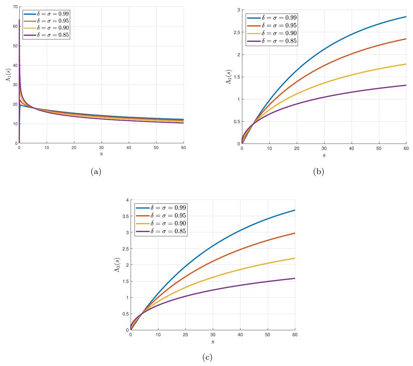
نستخدم نوى من نوع ميتاج-ليفلر لحل نظام من المعادلات التفاضلية الكسرية باستخدام مشغلات كسرية-فراغية (FF) ذات ترتيب كسرية وفراغية. باستخدام مفهوم المشتقات FF ذات الذاكرة غير المتناهية وغير المحلية، يتم دراسة نموذج لثلاثة بحيرات ملوثة مع مصدر واحد للتلوث. تُستخدم خصائص التحويل غير المتناقص والمضغوط لإثبات وجود حل لنموذج FF لنظام البحيرات الملوثة. لهذا الغرض، يتم استخدام نظرية ليراي-شودر. بعد استكشاف متطلبات الاستقرار في أربع نسخ، يتم محاكاة النموذج المقترح لنظام البحيرات الملوثة باستخدام تقنيتين عدديتين جديدتين تستندان إلى طرق متعددات الحدود لأدامز-باشفورث ونيوتن. يتم توضيح تأثير التفاضل الكسرية-الفراغية عدديًا. علاوة على ذلك، يتم عرض تأثير المشتقات FF تحت ثلاثة نماذج إدخال محددة للملوث: خطي، متناقص أسيًا، ودوري.

الكلمات المفتاحية: تلوث المياه؛ نموذج المشتقات الكسرية الفراكتالية؛ الوجود، التفرد والاستقرار؛ طرق بولينوميات آدامز-باشفورث ونيوتن.
MSC: 34A08; 65P99.

1 المقدمة

في القرن الماضي، أصبح تلوث المياه خطرًا شديدًا على العالم الذي نعيش فيه. الخطوة الأولى في الاستعداد للحفاظ على البيئة الطبيعية هي مراقبة مستويات التلوث. يمكن تحقيق مراقبة التلوث باستخدام التحليل الرياضي. يمكن استخدام المعادلات التفاضلية لمحاكاة التلوث البيئي، تمامًا كما يمكن استخدامها في العديد من المجالات الأخرى. على سبيل المثال، استخدم بيازار وآخرون في عام 2006 مجموعة من المعادلات التفاضلية للتنبؤ بمستوى التلوث في سلسلة من البحيرات. بشكل ملموس، اقترحوا نموذجًا لثلاث بحيرات متصلة بواسطة قنوات من خلال نمذجة الحاويات. وقد بحث بعض العلماء الآخرين في هذا المفهوم باستخدام منهجيات متنوعة. قام يوزباشي وآخرون بتحليل مثل هذه المستويات من التلوث تحت طريقة التجميع في عام 2012. لاحقًا، استخدم بنحمودة وآخرون طريقة أخرى لحل نموذج التلوث عبر تحويل تفاضلي معدل. كما أنشأ خضر وآخرون نموذج حالة كسري واستخدموا خصائص المصفوفات في عام 2013. مؤخرًا، في عام 2019، اعتبر بيلديك ودينيز نموذجًا قائمًا على أتانغانا-بالينو لتقريب حلول نظام بحيرة ملوثة. بعد ذلك، انتقل أحمد وخان إلى نموذج مشابه لتلوث البحيرات عبر طرق كسري مختلفة. في عام 2020، حل براكاش وفيريشا مثل هذا النظام من البحيرات الملوثة عبر ما يسمى بطريقة q-HATM. مؤخرًا، في عام 2022، قام شيري وبالينو بإجراء بحث حول كمية التلوث في نموذج ثلاثي الحاويات واستخلصوا بعض النتائج التحليلية. خلال هذه السنوات، تم دراسة النماذج الكسرية للعمليات الواقعية من قبل العديد من الباحثين الآخرين، مما يظهر قابلية تطبيق المشغلين الكسرين في النمذجة الرياضية: انظر، على سبيل المثال، 9، 10، 11، 12، 13، 14، 15. هنا نقترح وندرس نموذجًا رياضيًا عبر عائلة عامة من المشتقات مزودة بمعاملين.
قدم أتانغانا فئة جديدة من المفاهيم الكسريّة الفراكتالية، التي تجمع بين مجالي الفراكتال والكسريّات القابلة للتطبيق. هيكل هذه المشغلات هو تداخل لقانون القوة، والقانون الأسي، وقانون ميتاغ-ليفلر المعدل مع المشتقات الفراكتالية، مما يخلق صلة بين الرياضيات الكسريّة والفراكتالية. البعد الفراكتالي والترتيب هما العنصران الرئيسيان في هذه المشغلات والمعادلات التفاضلية ذات المشتقات الكسريّة الفراكتالية تحول ترتيب النظام المفترض وبعده إلى نظام عقلاني. بسبب هذه الخاصية، يتم توسيع المعادلات التفاضلية التقليدية بشكل طبيعي لتشمل أنظمة ذات أي ترتيب من المشتقات وأبعاد. الهدف من هذه المشغلات المترابطة هو دراسة مشاكل القيمة الحدية غير المحلية (BVPs) أو مشاكل القيمة الابتدائية (IVPs) التي تحمل ميول فراكتالية في طبيعتها. قدم العديد من العلماء نتائج واكتشافات في هذا المجال، مما يثبت أن المشغلات الكسريّة الفراكتالية أكثر فعالية في وصف البيانات الواقعية وللنمذجة الرياضية. تشمل أمثلة هذه النماذج الرياضية: الهياكل الكسريّة الفراكتالية لديناميات فيروس كورونا، انتقال الملاريا، ديناميات COVID-19 في ووهان، انتقال فيروس AH1N1/09، ديناميات حمى Q، فيروس HIV، ديناميات CD4. الخلايا [23، مرض السل 24، إلخ.
إن دمج مشغلات الفراكتال-كسرية (FF) ذات الأوامر الفراكتالية والكسرية المزدوجة في البحث العلمي يمثل طريقًا واعدًا مع مزايا متعددة الأوجه. من خلال الاستفادة من أمرين في وقت واحد، يسمح هذا النهج بتمثيل أكثر دقة وتفصيلاً للأنظمة المعقدة، مما يلتقط الأنماط الدقيقة والاختلالات التي قد تتجاهلها الطرق التقليدية. تعزز تآزر الهندسة الفراكتالية وحساب الكسور نمذجة وتحليل الظواهر الواقعية، مما يوفر انعكاسًا أكثر دقة للهياكل الذاتية المتشابهة والديناميات ذات الأوامر غير الصحيحة. لا يقتصر ذلك على تحسين فهمنا للعمليات المعقدة فحسب، بل يسهل أيضًا تطوير نماذج رياضية أكثر قوة يمكن تطبيقها عبر مختلف التخصصات. إن استخدام مشغلات FF يحمل القدرة على إحداث ثورة في مجالات تتراوح من معالجة الإشارات إلى تحليل الصور، مما يوفر مجموعة أدوات متعددة الاستخدامات لمعالجة التحديات التي تتطلب فهمًا أعمق للسلوكيات المعقدة والمتعددة الفراكتلات. إن تبني هذا النموذج المبتكر يساهم في نهج أكثر شمولية ودقة في التحقيقات العلمية، مما يفتح آفاقًا جديدة للاستكشاف والاكتشاف. هنا نقوم بإجراء تحليل لنموذج فراكتال-كسرية للبحيرات الملوثة من حيث خصائص مختلفة.
الورقة منظمة على النحو التالي. في القسم 2، نقدم نظامًا كسريًا كسريًا لنمذجة البحيرات الملوثة. يتم إثبات وجود حل للنظام المقترح في القسم 3 باستخدام نظرية ليراي-شودر. في القسم 4، نستخدم مبدأ باناش للانكماش-
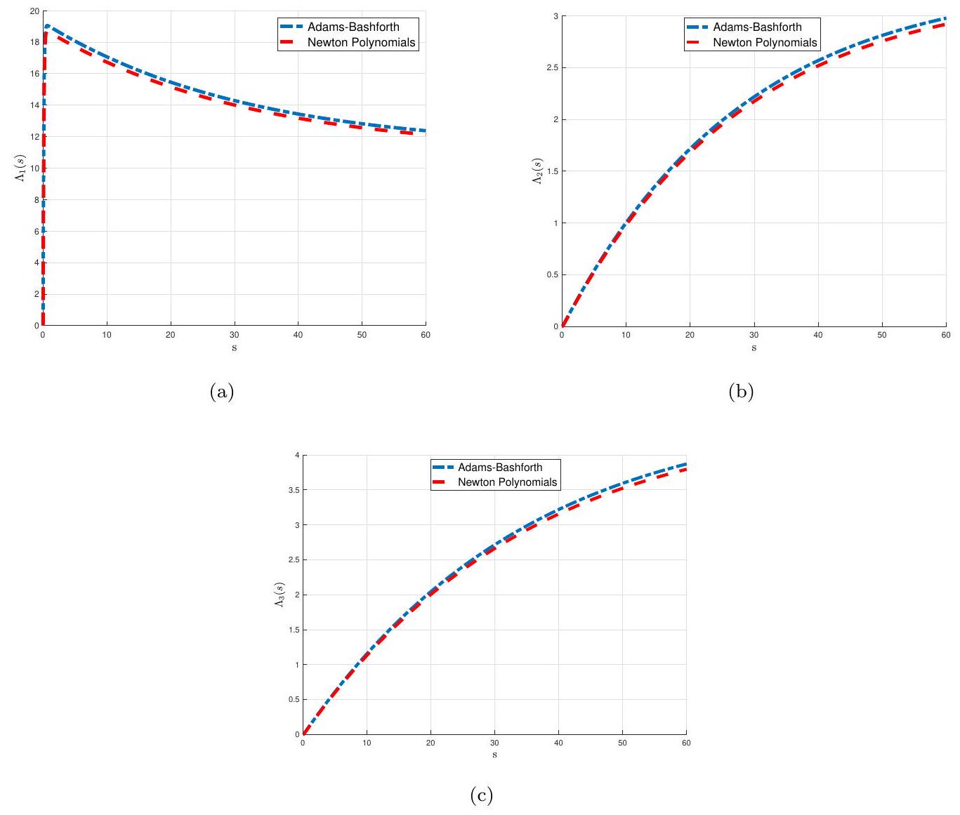
تُظهر الفقرات السابقة تفرد الحل. علاوة على ذلك، باستخدام التحليل الوظيفي، يتم استكشاف العديد من المتطلبات لأنواع مختلفة من الاستقرار لحل نموذج نظام البحيرات الملوثة في القسم 5. لمحاكاة نموذجنا، نستخدم تقنيتين مختلفتين: نهج آدامز-باشفورث الكسري (القسم 6) وأخرى تعتمد على كثيرات الحدود لنيوتن (القسم 7). ثم يتم اختبار النتائج النظرية التي تم الحصول عليها في القسم 8 من خلال تطبيق خوارزمياتنا مع بعض البيانات الملموسة تحت قيم مختلفة من الترتيب الكسري والفركتالي في ثلاث حالات مختلفة: نماذج حقيقية خطية، تتناقص بشكل أسي، ومدخلات دورية. نختتم بالقسم 9 الذي يحتوي على الاستنتاج.

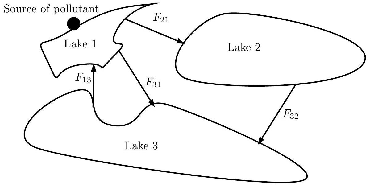
2 نموذج FF لنظام ملوث من ثلاثة بحيرات

نحن نقوم بنمذجة ثلاثة بحيرات. قد يكون استخدام ثلاثة بحيرات في نظام خيارًا عمليًا جيدًا بناءً على عوامل مختلفة مثل توفر الأراضي، والتكلفة، والكفاءة. قرار اعتبار ثلاثة بحيرات هنا ليس رياضيًا بحتًا، بل يتضمن اعتبارات بيئية واقتصادية ولوجستية. يمكن أن تساعد النمذجة الرياضية في تحسين توزيع وحجم البحيرات، ولكن من الضروري تحقيق توازن بين هذه العوامل من أجل حل مستدام وفعال. لذلك، نحن نقتصر على ثلاثة بحيرات وقنواتها مع مصدر ملوث. يمكن تعميم نتائجنا على عدد محدود من البحيرات.
يتم اعتبار كل بحيرة كحجرة، حيث يتم اعتبار القناة الرابطة بين بحيرتين كأنها أنبوب يربط الحجرات. يتم إظهار اتجاه التدفق عبر كل قناة أو أنبوب بواسطة الأسهم. مادة ملوثة يعتبر في البحيرة الأولى. بواسطة نحن نحدد المعدل الذي يدخل به الملوث/الملوث بحيرة 1 في الوقت . الهدف الرئيسي هو تحديد مستويات التلوث في كل بحيرة في أي لحظة معينة. للقيام بذلك، نعتبر التركيز الملوث في البحيرة في الوقت ، بواسطة
أين يشير إلى حجم المياه في البحيرة ، يُفترض أن يكون ثابتًا، و يحدد كمية التلوث التي توزع بالتساوي على كل بحيرة في الوقت . نحن مهتمون بنمذجة الوضع الموضح في الشكل 1، حيث نستخدم الرمز لتمثيل معدل التدفق الداخل إلى البحيرة من استنادًا إلى الشكل 1، نستنتج الشروط التالية:
الشكل 1: مخطط للقنوات التي تربط بين البحيرات الثلاث التي يتم نمذجتها.
لاحظ أن لأنه لا يوجد أنبوب بين البحيرتين الثانية والأولى. التدفق الملوث المتدفق من البحيرة إلى البحيرة في وقت عشوائي يقيس معدل تدفق تركيز الملوث. هذه المؤشر يساوي
استنادًا إلى المبدأ القائل بأن معدل تغير الملوث يُعطى بالفرق بين معدل الإدخال ومعدل الإخراج، نقترح هنا النموذج الكسري الفركتالي التالي للسلوك الديناميكي لنظام البحيرات الملوثة المكون من ثلاث بحيرات عبر نواة ميتاغ-ليفلر العامة:
خاضع لـ
أين هو ( المشتق الكسري الفركتالي مع نواة من نوع ميتاج-ليفلر من الأوامر الكسري والفركتالي و على التوالي، كما قدمه أتانغانا في 16.
التعريف 1 (انظر [16]). دع كن خريطة مستمرة قابلة للاشتقاق الفركتالي من البعد . في هذه الحالة، ريمان-ليوفيلي -مشتق كسري فراكتالي لـ مع نواة من نوع ميتاج-ليفلر العامة من الدرجة يتم إعطاؤه بواسطة
أين
هل المشتق الكسري مع .
فيما يلي، نستخدم أيضًا المفهوم المقابل للتكامل الكسري الفركتالي.
التعريف 2 (انظر [16]). الـ ( التكامل الكسري الفركتالي لدالة مع نواة عامة يُعطى بـ
إذا كان موجودًا، أين .

3 الوجود

نبدأ بإثبات وجود حل لمشكلتنا (4)-(5). للقيام بذلك، نستخدم نظرية النقاط الثابتة. لإجراء تحليلنا النوعي، دعنا نعرف فضاء باناش ، حيث مع
لـ نقوم بإعادة كتابة الجانب الأيمن من نظام البحيرة الملوثة الفركتالية-الكسرية (4) كالتالي
في هذه الحالة، يتم تحويل نظام البحيرة الملوثة الفراكتالية-الكسري (4) إلى النظام التالي:
بالنظر إلى (9)، نعيد كتابة نظام الحالة الشجري لدينا كمسألة قيمة أولية مضغوطة.
أين
و
بالتعريف ووفقًا لـ (10)، لدينا
بتطبيق التكامل الكسري الفركتالي أتانغانا-بالينو على (13)، نحصل على
التعبير الموسع عن (14) يُعطى بواسطة
لاشتقاق مشكلة النقطة الثابتة، نقوم الآن بتعريف الخريطة الذاتية كما
لإثبات وجود حل لنظام بحيرة ملوثة كسري-فركتالي لدينا (4)، نستخدم نظرية ليراي-شودر التالية.
النظرية 3 (نظرية نقطة الثبات ليراي-شودر [25]). دع كن فضاء باناش، مجموعة مغلقة محدبة ومحدودة، و مجموعة مفتوحة مع . ثم، تحت الخريطة المدمجة والمستمرة إما:
(Y1) س.ت. ، أو
(Y2) بحيث .
نظرًا لأن نظام البحيرة الملوثة يمثل مشكلة في العالم الحقيقي، فإن وجوده يخضع لقيود معينة. تلعب هذه القيود، المشار إليها في النظرية 4 بـ (P1) و (P2)، دورًا حاسمًا في تشكيل ديناميات وخصائص النظام. في الواقع، تعتبر (P1) و (P2) ضرورية لتعريف وتنظيم سلوك نظام البحيرة الملوثة ضمن حدود العملية والواقع. إن التعرف على هذه القيود أمر أساسي لبناء فهم شامل للنظام وتطوير استراتيجيات فعالة.
النظرية 4. دع . إذا
(P1) و (غير متناقص) بحيث و ،
(P2) بحيث
مع ؛
ثم توجد حل لنظام البحيرة الملوثة الفراكتالية الكسرية (4).
برهان. أولاً، اعتبر ، الذي تم صياغته في (16)، وافترض
لبعض . بوضوح، كما مستمر، وبالتالي أيضًا كذلك. من (P1)، نحصل على
لـ . ومن ثم،
لذا، محدود بشكل موحد على . الآن، خذ بحيث و من خلال الإشارة إلى
نقدر
نرى أن الجانب الأيمن من (19) يقترب من 0 بغض النظر عن ، كـ . نتيجة لذلك،
عندما . هذا يعطي الاستمرارية المتساوية لـ وبناءً عليه، فإن كثافة على بواسطة نظرية أرسلا-أسكولي. حيث يتم الوفاء بالنظرية 3 على لدينا واحد من (Y1) أو (Y2). من (P2)، نحدد
لبعض بحيث
من (P1) و(18)، لدينا
افترض أن هناك و بحيث . ثم، بواسطة (20)، نكتب
الذي لا يمكن أن يكون صحيحًا. وبالتالي، (Y2) غير مُحقق و يعترف بنقطة ثابتة في بموجب النظرية 3، يثبت هذا وجود حل لنموذج بحيرة ملوثة FF (4).

4 التفرد

كخطوة أولى لإثبات تفرد الحل لمشكلتنا (4)-(5)، نبدأ بالتحقيق في خاصية ليبشيتز لنظام البحيرة الملوثة الكسرية-الفراكتالية (4).
اللمّا 5. اعتبر ، ودع
(C1) لبعض الثوابت .
ثم، ، و المعرفة في (8) تحقق خاصية ليبشيتز مع ثوابت بالنسبة للمكونات المعنية، حيث
برهان. لــ نحن نأخذ بشكل تعسفي، ولدينا
من (22)، نكتشف أن هو ليبشيتز بالنسبة لـ تحت الثابت . ل نحن نختار بشكل عشوائي ، وتقدير
هذا يعني أن هو ليبشيتز بالنسبة لـ تحت الثابت . أخيرًا، للعناصر العشوائية لدينا
هذا يُظهر أن هو ليبشيتزي بالنسبة لـ مع . لذلك، دوال النواة ، و هي ليبشيتز، على التوالي مع ثوابت .
من خلال استدعاء اللمحة 5، نثبت الآن تفرد الحل لنظام FF (4).
نظرية 6. لنفترض أن (C1) صحيحة. إذا
لـ وأين هي ثوابت ليبشيتز المقدمة في (21)، فإن نظام البحيرة الملوثة الكسرية الفراكتالية (4) يمتلك حلاً واحداً بالضبط.
برهان. نقوم بالبرهان عن طريق التناقض. نفترض أن هناك حلاً آخر لنظام بحيرة ملوثة كسرية كسري (4)، وهو ) ، تحت الظروف الأولية
من (15)، لدينا
و
في هذه الحالة، نحن نقدر
لذا
من (23)، يمكننا التأكيد على أن عدم المساواة أعلاه صحيح إذا أو . بالمثل، من
نحصل على
الذي يعطي أو علاوة على ذلك،
الذي ينتج
لذا، . كنتيجة لذلك،
ما يثبت أن الحل لنظام البحيرة الملوثة الفراكتالي-الكسري (4) فريد.

5 استقرار أولام-هايرس-راسياس

في هذا القسم، يتم دراسة استقرار الحلول لنظام البحيرات الملوثة المكون من ثلاث بحيرات. نظرًا للرغبة في تأسيس أسس رياضية قوية للنموذج، نعتبر أربعة مفاهيم مختلفة للاستقرار. بشكل أكثر دقة، نثبت الاستقرار لنظام البحيرات الملوثة الفراكتالية-كسرية (FF) (4) بالنسبة لمفاهيم أولا-هايرز وأولا-هايرز-راسياس وتعميماتها المعنية. تحليل الاستقرار هو أمر حيوي لضمان موثوقية ونبوءة النماذج الرياضية، خاصة في التطبيقات الواقعية مثل نظام البحيرات الملوثة. توفر استقرار أولا، واستقرار هايرز، وتعميماتهما أطرًا قيمة لفهم سلوك الحلول للأنظمة الديناميكية تحت الاضطرابات. نظرًا للطبيعة المعقدة للأنظمة الفراكتالية-كسرية، فإن استخدام هذه المفاهيم للاستقرار يسمح لنا بتحديد مرونة النظام تجاه التغيرات والاضطرابات، مما يوفر رؤى حول السلوك طويل الأمد وموثوقية النموذج المقترح. من خلال اختيار الاستقرار في هذا السياق، نهدف إلى تعزيز مصداقية النموذج وقابليته للتطبيق في معالجة التعقيدات الكامنة في أنظمة البحيرات الملوثة.
التعريف 7. نظام البحيرة الملوثة FF (4) مستقر وفقًا لـ Ulam-Hyers إذا كان هناك ، بحيث أن لكل ولكل مُرضٍ
يوجد تلبية نظام البحيرة الملوثة الفركتالية الكسرية (4) مع
التعريف 8. نظام البحيرة الملوثة FF (4) مستقر بشكل عام وفقًا لمعيار أولام-هايرز إذا كان ، مع بحيث و تحقيق (24)، هناك حل لنظام بحيرة FF الملوثة المعطاة (4) بحيث
ملاحظة 9. الثلاثي هو حل لـ (24) إذا، وفقط إذا، (كل منهم يعتمد على على التوالي” بحيث أن ،
(ط) ،
(ii) لدى المرء
التعريف 10. نموذج البحيرة الملوثة الكسرية الفراكتالية (4) مستقر وفقًا لمعيار أولام-هايرس-راسياس بالنسبة لـ إذا بحيث و مُرضٍ
يوجد حل لنموذج FF لنظام البحيرة الملوثة (4) بحيث
مع .
ملاحظة 11. إذا ثم تصبح التعريف 10 معيار أولام-هايرز.
التعريف 12. نظام البحيرة الملوثة FF (4) مستقر بشكل عام وفقًا لاستقرار أولام-هايرس-راسياس بالنسبة لـ إذا كان موجودًا بحيث أن لكل مُرضٍ
يوجد حل نموذج FF لنظام البحيرة الملوثة (4) بحيث
ملاحظة 13. لاحظ أن هو حل لـ (25) إذا، وفقط إذا، (كل منهم يعتمد على على التوالي” بحيث أن ،
(ط) ،
(ii) لدينا
المفاهيم 14 و 15 مفيدة لإثبات النظريتين 16 و 17، على التوالي.
اللمّا 14. لكل افترض أن هي حل المعادلة (24). ثم، الدوال حقق عدم المساواة الثلاثة التالية:
و
برهان. لن كن عشوائيًا. منذ يُرضي
يتبع من الملاحظة 9 أنه يمكن أخذ دالة بحيث
و . بوضوح،
في هذه الحالة، نحن نقدر
هذا يعني أن (26) قد تحقق. نحن نثبت (27) و (28) بطريقة مشابهة.
لإثبات نتيجتنا التالية (انظر اللمحة 15)، نعتبر الشرط التالي:
(C2) توجد دوال متزايدة ، و بشرط أن
العبارة 15. دع ( ) احتفظ. لكل افترض أن هي حل لـ (25). ثم، الدوال حقق عدم المساواة الثلاثة التالية:
برهان. لنعتبر . منذ يُرضي
يتبع من الملاحظة 13 أننا يمكننا أن نأخذ بحيث
و من الواضح أن
ثم، نقوم بتقدير
نثبت المتباينات المتبقية بطريقة مشابهة.
نحن الآن في وضع يمكننا من دراسة استقرار أولام-هايرز لنموذج FF لنظام البحيرة الملوثة (4).
النظرية 16. افترض أن (C1) صحيحة. ثم نظام بحيرتنا الملوثة (4) مستقر من نوع أولام-هايرز ومستقر من نوع أولام-هايرز العام.
في أي مقدمة بواسطة (21).
برهان. لن و كن حلاً عشوائيًا لـ (24). وفقًا لنظرية 6، دع كن الحل الفريد لنظام بحيرة FF الملوثة (4). ثم يُعرَف بأنه
من عدم المساواة في المثلث، تعطي النتيجة 14
لذا,
مجموعة . في هذه الحالة، . بالمثل، نحصل على
أين
نستنتج أن نموذج FF لنظام البحيرة الملوثة (4) مستقر وفقًا لمعيار أولام-هايرز. من ناحية أخرى، إذا أخذنا
ثم وانتهت البرهان: 4 مستقرة بشكل عام وفقًا لولاة-هايرز.
الم theorem 17 يثبت استقرار أولام-هايرس-راسياس لنظام البحيرة الملوثة الكسرية-الفراكتالية (4).
النظرية 17. إذا كانت (C1) و (C2) صحيحتين، فإن نموذج FF لنظام البحيرة الملوثة (4) مستقر في نفس الوقت بمعنى التعريفات 7 و 8.
برهان. لنفترض أن ، و تلبية (25). بموجب النظرية 6، دع كن الحل (الفريد) لنموذج نظام بحيرة FF الملوثة (4). ثم يصبح
بمساعدة عدم المساواة مثلثية، تعطي اللمحة 15
وبناءً عليه، نحصل على أن
مجموعة
ثم . بالمثل,
أين
نتيجة لذلك، فإن نظام البحيرة الملوثة الفركتالية-الكسريّة (4) مستقر بمعنى التعريف 7. من خلال تعريف نموذج نظام بحيرة FF الملوثة لدينا (4) مستقر أيضًا بمعنى التعريف 8.

6 خوارزمية عددية عبر طريقة آدامز-باشفورث

طريقة آدامز-باشفورث هي تقنية تكامل عددي قوية تُستخدم عادةً لحل معظم المعادلات التفاضلية. تجعل دقتها وكفاءتها العالية منها مناسبة بشكل خاص لتقريب حل الأنظمة الديناميكية، مثل تلك التي تصف سلوك أنظمة البحيرات الملوثة. من خلال اختيار تقنية آدامز-باشفورث، نهدف إلى تحقيق حلول عددية دقيقة ومستقرة لنظام البحيرة الملوثة الفراكتالية-كسرية (4).
للقيام بذلك، نطبق تقنية آدامز-باشفورث الكسرية باستخدام كثيرات الحدود لاغرانج ذات الخطوتين. لذلك، نعيد تعريف معادلات التكامل الكسرية-الفراكتالية (15) عند . بدقة، نقوم بتفكيك المعادلات التكاملية (15) لـ كما يلي:
تُعطى تقريب التكاملات أعلاه بواسطة
بعد ذلك، نقوم بتقريب ، على عن طريق تطبيق كثيرات الحدود الاستيفائية من الدرجة الثانية تحت حجم الخطوة من خلال الحسابات المباشرة، نحصل على الخوارزمية التالية التي تعطي حلولاً عددية لنموذج FF لنظام البحيرة الملوثة (4):
أين
و

7 خوارزمية عددية عبر متعددات نيوتن

هنا نطور خوارزمية تقريبية مختلفة (استنادًا إلى متعددات نيوتن) لحساب الحلول العددية لنظام بحيرة ملوثة كسري (4). إن استخدام متعددات نيوتن في الاستيفاء مدفوعًا ببساطتها وقابليتها للتطبيق في تقريب الدوال استنادًا إلى مجموعة من نقاط البيانات المعطاة. في سياق النمذجة والتحليل، تقدم متعددات نيوتن نهجًا مرنًا لتمثيل العلاقات المعقدة داخل نظام البحيرة الملوثة. تتيح لنا تقنية الاستيفاء المتعدد بناء دالة مستمرة تقرب سلوك النظام، مما يسهل فهمًا أكثر تفصيلًا وشمولية لدينامياته. على حد علمنا، تم تقديم الفكرة لأول مرة في 26. بدقة، نتبع 26 مع المشكلة الأولية (10) الخاضعة للشروط (11) و(12). في هذه الحالة، لدينا
مجموعة . ثم،
من خلال تفكيك المعادلة أعلاه عند نحصل على
لتقريب التكامل أعلاه، يمكننا أن نكتب أن
الآن نقوم بتقريب الدالة مع كثيرات الحدود لنيوتن
عند استبدال (37) في (36)، نحصل على
بتبسيط العلاقات أعلاه، نحصل على
ويترتب على ذلك
من ناحية أخرى، من خلال حساب التكاملات الثلاثة المذكورة أعلاه بشكل منفصل، يحصل المرء على
و
من خلال وضع (39) و(40) و(41) في (38)، نحصل على أن
أخيرًا، نستبدل إلى (42)، ونحصل على أن
أين
باستخدام المخطط العددي (43)، تُعطى الحلول العددية لنظام البحيرة الملوثة الفركتالية-كسرية (4) بواسطة
و
أين مُعَرَّفَة في (44)، .

8 المحاكاة العددية والمناقشة

الآن نطبق طريقة آدامز-باشفورث (ABM) وطريقة كثيرات الحدود لنيوتن (NPM)، المقترحتين على التوالي في القسمين 6 و 7 لفحص وإيجاد الحلول العددية. لنموذج FF المقترح ومراقبة قابلية التطبيق والدقة والضبط للخوارزميات المطورة. لمحاكاة كمية التلوث في البحيرات المودلة، قمنا بترميز الخوارزميات (33)-(35) و(45)-(47) في MATLAB، الإصدار R2019A.
لمقارنة النتائج، نستعير من [1] القيم التالية للمعلمات: سنة سنة سنة سنة . علاوة على ذلك، . أيضًا، أبعاد كسيرية مختلفة وأوامر كسرية، أي، تُعتبر لمحاكاة الوظائف الثلاث للدولة ، و .
نعتبر نموذج FF المقترح في ثلاث حالات: خطي (القسم 8.1)، متناقص أسي (القسم 8.2)، ودوري (القسم 8.3) لنماذج المدخلات.

8.1 نموذج الإدخال الخطي

في هذه الحالة، نعتبر النموذج الذي يحتوي فيه البحيرة 1 على ملوث بتركيز خطي. المدخلات الخطية تشير إلى سلوك ثابت للملوث. في الوقت صفر، يكون تركيز الملوث صفرًا، ولكن مع زيادة الوقت، يبدأ إضافة الملوث ثم يبقى ثابتًا. على سبيل المثال، عندما تبدأ مصنع الإنتاج في الوقت صفر، يبدأ تصريف النفايات بمعدل ثابت وتركيز ثابت. كحالة خاصة، اخترنا . ثم، من أجل ، من (4) لدينا
في الأشكال 2 (أ)، (ب)، و(ج)، سلوك تقريبات نموذج agent-based (ABM) لكل زوج من دوال الحالة ، و على التوالي، يتم تقديمها؛ بينما في الشكل 2 (د)، يتم عرض النموذج ثلاثي الأبعاد
عرض لـ تُظهر المشتقات من الرتبة الصحيحة بشكل بياني لنموذج الإدخال الخطي مع الزمن وحجم الخطوة .
يرجى ملاحظة أن المعامل يتم تعريفه بشكل صريح على أنه حجم الخطوة، متميزًا عن معلمات الاستقرار تم مناقشته في قسم الاستقرار 5. بينما هنا نؤكد على كحجم خطوة في سياق محدد، فإن استقرار أولام-هايرز-راسياس، كنظرية، يهتم بشكل أساسي بخصائص الاستقرار للمعادلات الوظيفية. على عكس الحلول العددية للمعادلات التفاضلية، فإن اختيار حجم الخطوة ليس اعتبارًا مباشرًا في مجال استقرار أولام-هايرز-راسياس. تركز هذه النظرية على فهم كيف تؤدي التغيرات الصغيرة في المعادلات الوظيفية إلى تغييرات متناسبة في الحلول، ولا يلعب مفهوم حجم الخطوة دورًا بارزًا في هذا السياق.
الشكل 2: سلوكيات كل زوج من دوال الحالة (أ) ، (ب) ، (ج) و (د) عرض ثلاثي الأبعاد لـ تحت الرتبة الصحيحة.
في الجدول 1، نقدم بعض النتائج العددية للتقنيتين العدديتين، ABM و NPM، للثلاثة دوال حالة. و في حالة الإدخال الخطي، تحت مشتقات من رتبة صحيحة وحجم خطوة من النتائج العددية التي تم الحصول عليها، يمكننا التأكيد على أن تقريبات آدامز-باشفورث لوظائف الطور ، و أتفق بشدة مع النتائج التي تم الحصول عليها بواسطة طريقة كثيرات الحدود لنيوتن للوقت حتى 10 سنوات.
في الشكل 3، مقارنة النتائج العددية من ABM و NPM لوظائف الحالة ، و يتم عرضه بيانيًا، للوقت وحالة الإدخال الخطي. نلاحظ أن نتائج ABM و NPM تتفق بشكل كبير مع بعضها البعض لكل واحدة من الولايات.
الجدول 1: مقارنة بين ABM و NPM لحالة المدخلات الخطية.
أدامز-باشفورث متعددات نيوتن
0 0.000000 0.00000 0.000000 0.000000 0.000000 0.000000
1 ٥٨.٢٤١٧٦٢ 0.122200 0.136038 ٥٨.٢٤٩٠٢٩ 0.114027 0.126944
2 216.569135 0.912690 1.018175 216.603012 0.891958 0.995030
٣ 472.231987 2.959673 3.308340 ٤٧٢.٢٩١٨٣٩ ٢.٩٢٦٧٢٣ ٣.٢٧١٤٣٨
٤ 824.018631 6.830863 7.650506 824.103833 6.786029 7.600138
٥ 1270.753481 13.074750 14.671769 1270.863423 13.018359 14.608218
٦ 1811.296055 22.221220 ٢٤.٩٨٢٧٢٦ 1811.430139 22.153588 ٢٤.٩٠٦٢٧٣
٧ ٢٤٤٤٫٥٣٩٩٩٠ ٣٤.٧٨٢١٥٦ ٣٩.١٧٧٨٥٤ 2444.697632 ٣٤.٧٠٣٥٩٥ ٣٩٫٠٨٨٧٧٤
٨ ٣١٦٩.٤١٢٠٩٤ 51.252025 57.835881 ٣١٦٩.٥٩٢٧٢١ 51.162836 57.734443
9 3984.871413 72.108440 81.520147 3985.074465 72.008917 81.406618
10 ٤٨٨٩.٩٠٨٣٢٤ 97.812711 ١١٠.٧٧٨٩٦٦ ٤٨٩٠.١٣٣٢٥٤ 97.703141 110.653605
وظائف، حتى في الفترة الأطول التي تبلغ 60 عامًا.
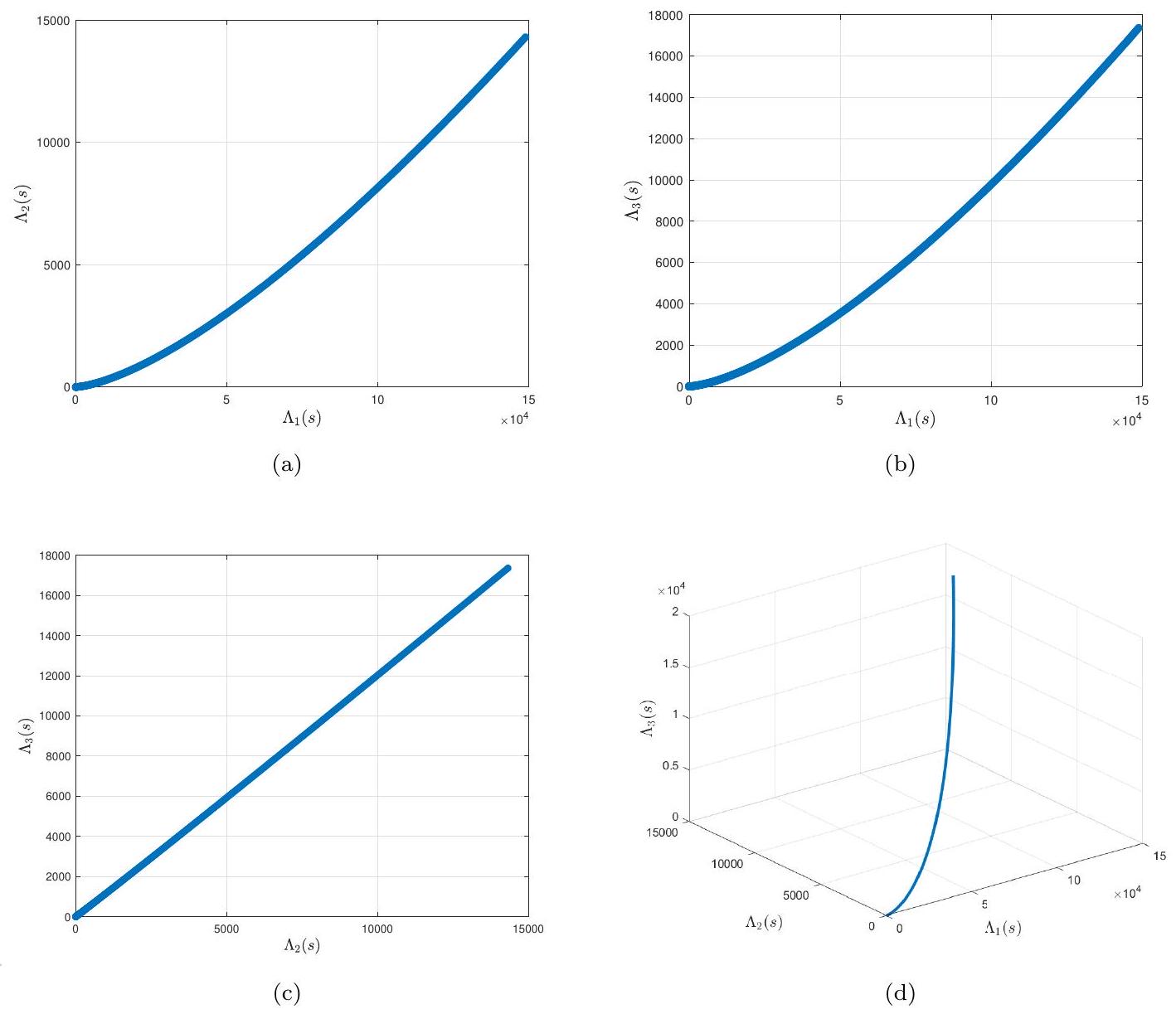
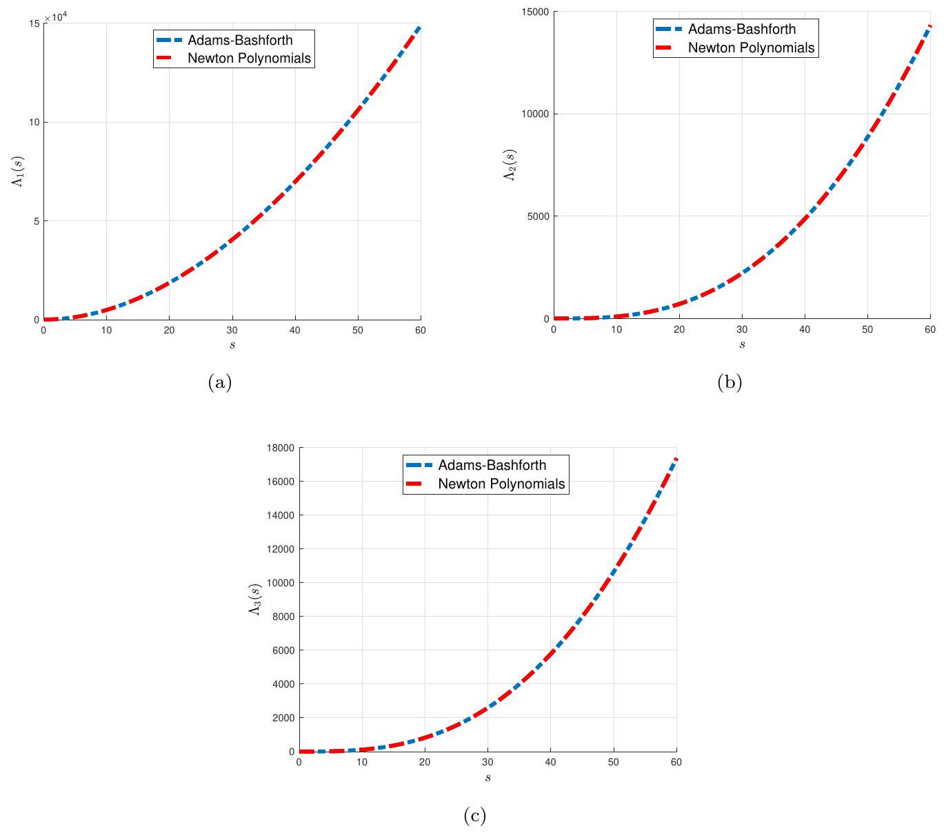
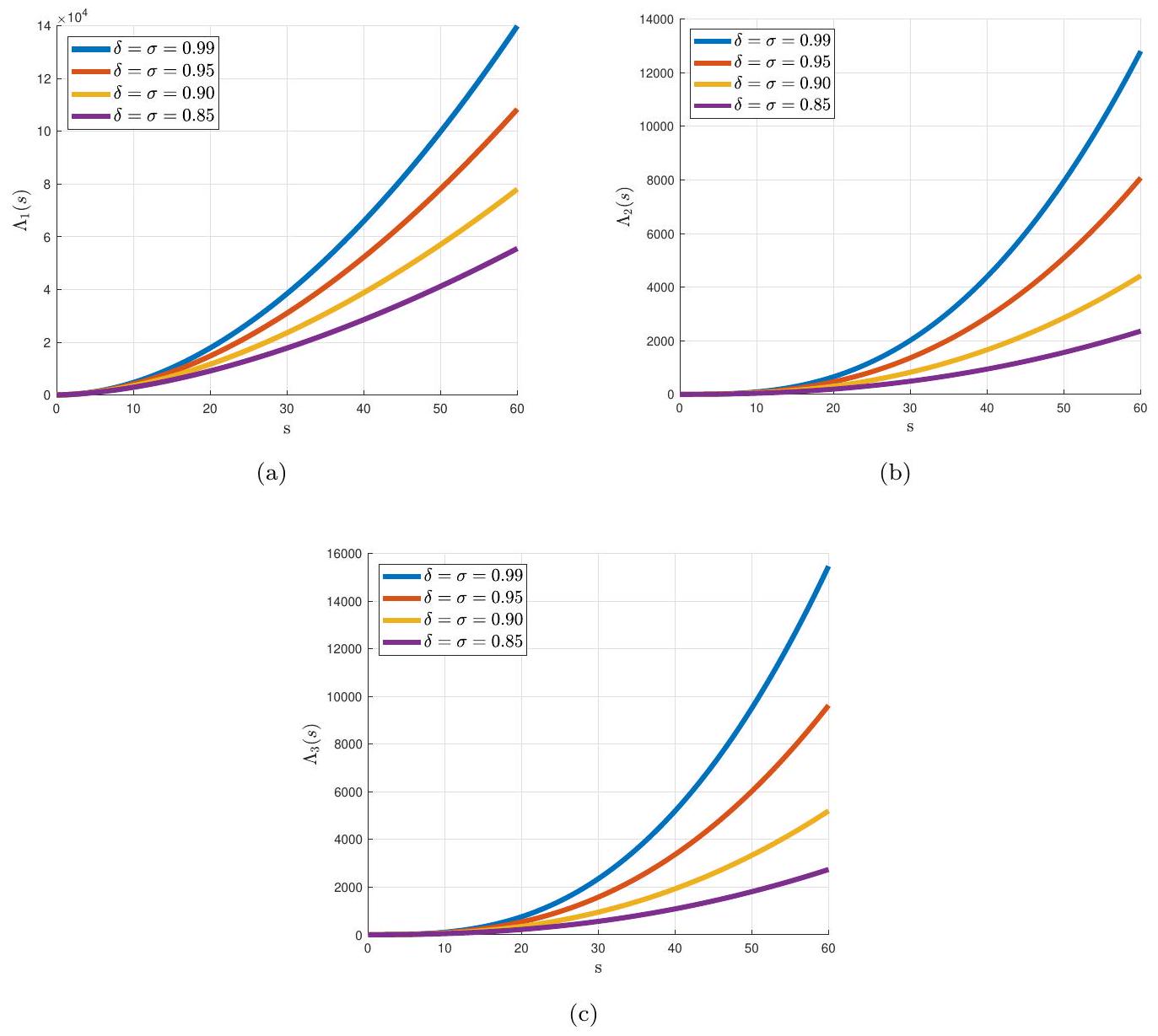
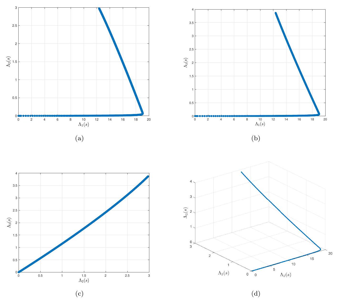
في الشكل 4، نوضح سلوك الدوال الثلاثة للحالة ، و عندما يتم تطبيق نموذج ABM تحت الأوامر الكسريّة الفراكتالية من هذه الأرقام، يمكننا أن نلاحظ أنه عندما يقترب ترتيب الكسر الفركتالي من الحالة الصحيحة، فإن تأثير التلوث يزداد على كل نموذج بحيرة بمعدل تقريبًا متساوٍ. كملحوظة لهذه الرسوم البيانية، يمكن القول إن مشغل الترتيب غير الصحيح له تأثير إيجابي على تقليل التلوث في نموذج تلوث البحيرة.
تستحق كلمة حول اختيارنا لقيم الأوامر الكسريّة. لقد اعتبرنا الأوامر الكسريّة ضمن نطاق لأنه خلال هذه الفترة لاحظنا سلوكيات متسقة لدرجات كسرية مختلفة. على وجه التحديد، مع انخفاض الدرجة الكسرية، لاحظنا تقليصًا متناسبًا في تأثير التلوث على كل نموذج بحيرة بمعدل تقريبًا متساوٍ. أدى هذا الاتجاه المتسق في السلوك مع انخفاض الدرجة الكسرية إلى قطع الفترة عند القيمة 0.85. هذه الاختيار يلتقط الجوانب الأساسية لاستجابة النموذج لدرجات كسرية متغيرة ويوفر تمثيلًا ذا معنى لديناميات النظام.

8.2 نموذج الإدخال المتناقص أسيًا

عندما يكون هناك تفريغ كبير للملوثات، فإنه من المنطقي النظر في نموذج الإدخال المتناقص أسيًا، أي الحالة عندما . مثال على هذه الحالة يحدث إذا قامت كل صناعة موجودة في مدينة ما بجمع وتخزين نفاياتها خلال بعض الأيام ثم تخلصت منها في البحيرة 1 بعد تلك الفترة المخزنة. إذا أخذنا و ثم يصبح النظام (4)
التمثيل البياني لدالة الإدخال موضح في الشكل 5 لحالة الإدخال المتدهور أسيًا .
في الأشكال 6 (أ)، (ب)، و(ج)، سلوك تقريبات نموذج agent-based (ABM) لكل زوج من دوال الحالة ، و على التوالي، كما هو موضح، بينما في الشكل 6 (د)، يتم عرض العرض ثلاثي الأبعاد لـ تحت المشتق من الرتبة الصحيحة يتم توضيحه رسوميًا لنموذج الإدخال المتناقص أسيًا مع الزمن وحجم الخطوة .
في الجدول 2، نقدم مقارنة بين الحلول التقريبية التي تم الحصول عليها باستخدام ABM و NPM لحالة الإدخال المتدهور أسيًا مع الزمن حجم الخطوة ،
الشكل 3: مقارنة بين ABM و NPM لـ (أ) ، (ب) و (ج) في نموذج الإدخال الخطي.
و من الجدول 2، يمكننا أن نستنتج أن تقريبات ABM تتوافق أيضًا بشكل جيد مع تقريبات NPM لنموذج الإدخال المتناقص أسيًا.
في الشكل 7، نقدم مقارنة رسومية بين تقريبات ABM و NPM لدوال الحالة ، و في حالة الإدخال المتناقص بشكل أسي مع الزمن من الشكل 7 يمكن الاستنتاج أن الطريقتين المقدمتين تتفقان بشدة مع بعضهما البعض حتى في نطاق زمني كبير يبلغ 60 عامًا.
في الشكل 8. نوضح النتائج العددية للمتغيرات الثلاثة. ، و لنموذج الإدخال المتناقص بشكل أسي عندما يتم تطبيق نموذج ABM تحت أوامر كسرية فركتالية متنوعة: تظهر الشكل 8 أن العمليات الكسريّة غير الصحيحة لها تأثير على تقليل كمية التلوث لكل نموذج عندما يكون الوقت تزداد، أي أن التلوث يزداد بشكل متناغم مع النظام الكسري الفركتالي، مقتربًا من حالة النظام الصحيح.

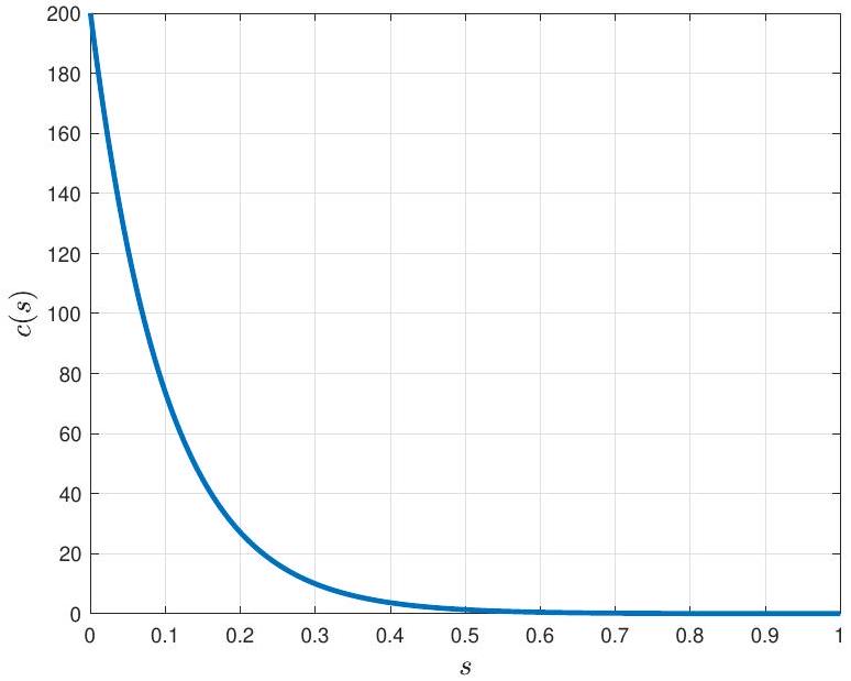
8.3 نموذج الإدخال الدوري

كنموذج دراسي أخير، نعتبر نموذج إدخال دوري حيث يظهر الملوث في البحيرة بشكل دوري. يمكن أن تكون مصنعًا يعمل خلال النهار فقط مثالًا على هذه الحالة: حيث ينتج نفايات ويقوم بإلقائها في البحيرات خلال النهار بينما يتوقف خلط الملوثات الجديدة في الليل. لحالة محددة، اخترنا ، حيث و يمثل
الشكل 4: سلوكيات (أ) ، (ب) و (ج) لنموذج الإدخال الخطي تحت الأبعاد الكسيرية والكسورية .
تغيرات السعة والتردد، على التوالي. أيضًا، يعتبر بمثابة متوسط تركيز الملوثات. في مثل هذه الحالة ، النظام (4) يأخذ الشكل التالي:
التمثيل البياني لدالة الإدخال موضح في الشكل 9 لحالة الإدخال الدوري .
في الأشكال 10 (أ)، (ب)، و(ج)، السلوك الرسومي لكل زوج من دوال الحالة ، ، و على التوالي، كما هو موضح. في الشكل 10 (د)، يتم عرض العرض ثلاثي الأبعاد لـ تحت المشتق من الرتبة الصحيحة موضح لنموذج الإدخال الدوري مع الزمن وحجم الخطوة .
المقارنة الجدولية بين النتائج العددية التي تم الحصول عليها من التقنيات المقترحة، ABM و NPM، للوظائف الثلاثة للدولة ، و تحت حالة الإدخال الدوري، تم الإبلاغ عنها في الجدول 3 للوقت حجم الخطوة ، و من هذه النتائج، نستنتج أن الحلول التي تم الحصول عليها بواسطة ABM و NPM تتفق بشكل كبير مع بعضها البعض.
الشكل 5: رسم بياني للإدخال المتناقص بشكل أسي.
الجدول 2: مقارنة عددية بين ABM و NPM لحالة الإدخال المتدهور أسيًا.
أدامز-باشفورث متعددات نيوتن
0 0.000000 0.00000 0.000000 0.000000 0.000000 0.000000
1 18.988642 0.105437 0.117578 18.988592 0.105145 0.117021
2 18.748146 0.219107 0.245295 18.752821 0.216590 0.242237
٣ 18.513934 0.328934 0.369679 18.523194 0.324269 0.364185
٤ 18.286698 0.435044 0.490805 18.300406 0.428303 0.482940
٥ 18.066244 0.537556 0.608748 18.084267 0.528808 0.598573
٦ 17.852383 0.636586 0.723579 17.874593 0.625901 0.711155
٧ 17.644931 0.732247 0.835369 17.671201 0.719691 0.820757
٨ 17.443709 0.824649 0.944190 17.473918 0.810285 0.927446
9 17.248540 0.913898 1.050109 17.282570 0.897787 1.031291
10 17.059256 1.000097 1.153195 17.096990 0.982299 1.132359
في الشكل 11، نوضح نتائجنا بشكل بياني، مقارنين النتائج العددية من ABM و NPM لكل دالة حالة. ، و ، حيث يحتوي البحيرة 1 على مدخل ملوث دوري. توضح الشكل 11 أن التقنيتين المقدمتيين، ABM و NPM، تتفقان بشدة مع بعضهما البعض بالنسبة للوقت حجم الخطوة ، و .
في الشكل 12، نوضح تقريبيات نموذج agent-based (ABM) للوظائف الثلاثة للدولة. ، و تحت أوامر كسريّة فركتالية مختلفة: لحالة الإدخال الدوري. مشابهة للحالات في الأقسام 8.1 و 8.2، نلاحظ أن المشغلين الكسريين غير الصحيحين لهم تأثير كبير على تقليل كمية التلوث لكل نموذج بينما الوقت يزيد.

9 الخاتمة

استخدمنا نوى من نوع ميتاج-ليفلر لحل نظام من المعادلات التفاضلية الكسرية باستخدام مشغلات كسرية-فراكتالية (FF) مع ترتيبين فراكتالي وكسرين. استخلصنا المعادلات المعادلة-
الشكل 6: سلوكيات كل زوج من الدوال الحالة (أ) ، (ب) (ج) و (د) عرض ثلاثي الأبعاد لـ تحت الرتبة الصحيحة.
الجدول 3: مقارنة بين ABM و NPM في حالة المدخلات الدورية.
أدامز-باشفورث متعددات نيوتن
0 0.000000 0.00000 0.000000 0.000000 0.000000 0.000000
1 1.420794 0.003639 0.004053 1.420289 0.003637 0.004052
2 3.352256 0.018270 0.020396 3.349409 0.017505 0.019538
٣ ٤.٧٩٥٥٢٦ 0.043383 0.048562 ٤.٧٩١٧٩٨ 0.041836 0.046821
٤ 5.304589 0.073971 0.083050 5.303706 0.071660 0.080440
٥ 5.281611 0.104988 0.118274 5.286096 0.101974 0.114856
٦ 5.607511 0.135825 0.153543 5.616323 0.132176 0.149388
٧ 6.832362 0.170701 0.193553 6.841809 0.166454 0.188698
٨ 8.669954 0.214629 0.243923 8.677051 0.209775 0.238353
9 10.261233 0.268650 0.305891 10.266407 0.263162 0.299573
10 10.964396 0.328730 0.375035 10.971053 0.322611 0.367966
الشكل 7: مقارنة بين ABM و NPM لـ (أ) ، (ب) و (ج) في نموذج الإدخال المتناقص بشكل أسي.
تم اشتقاق معادلات FF-التكامل من مشكلة قيمة ابتدائية مضغوطة، ثم تم إثبات نتائج الوجود والتفرد. تم إجراء تحليل استقراري في إصدارات مختلفة. في الأقسام التالية، قمنا بدراسة وتوثيق سلوك نموذج المشغل الفركتالي-الكسري (4) بمساعدة تقنيتين عدديتين مختلفتين: طريقة آدامز-باشفورث (ABM) وطريقة متعددة الحدود لنيوتن (NPM). من النتائج التي تم الحصول عليها، نستنتج أن التقنيات المعتمدة، ABM وNPM، تتفق بشكل كبير وتعتبر فعالة جداً لفحص نظام المعادلات التفاضلية الكسرية تحت المشغلين الفركتاليين-الكسرين الذين يصفون ديناميات التلوث في البحيرات. كما قمنا بتحليل النموذج المعتمد تحت أوامر فركتالية-كسرية متنوعة وفحصنا تأثيرات هذه الأوامر غير الصحيحة على سلوك كل متغير حالة. ، و لثلاثة نماذج إدخال محددة: خطي، متناقص أسيًا، ودوري. بالنسبة لكل نموذج إدخال، لاحظنا أنه عندما يقترب ترتيب الفراكتال-كسر من حالة الترتيب الصحيح الكلاسيكية، فإن تأثير التلوث يزداد بشكل متناغم لكل نموذج بحيرة. كخلاصة لهذه الملاحظات، يمكن القول إن المشغلين ذوي الترتيب غير الصحيح لها تأثيرات إيجابية على تقليل التلوث في نموذج تلوث البحيرة. كعمل مستقبلي، نخطط للتحقيق في نماذج واقعية مختلفة بناءً على التقنيات التي تم تطويرها هنا.

بيان مساهمة مؤلفي CRediT

تنزيلا كانوال: التحليل الرسمي، المنهجية. أظهر حسين: التصور، التحليل الرسمي، المنهجية. إبراهيم أفجي: التحليل الرسمي، المنهجية، البرمجيات. سينا إيتيماد:
الشكل 8: سلوكيات (أ) ، (ب) و (ج) لنموذج الإدخال المتناقص بشكل أسي تحت الأوامر الكسيرية والكسورية .
الشكل 9: رسم بياني للإدخال الدوري.
الشكل 10: سلوكيات كل زوج من دوال الحالة (أ) ، (ب) “، (ج) و (د) عرض ثلاثي الأبعاد لـ تحت الرتبة الصحيحة.
التصور، المنهجية، البرمجيات. شهرام رضابور: التصور، المنهجية. ديلفيم ف. م. توريس: التحليل الرسمي، الحصول على التمويل، المنهجية.

إعلان عن تضارب المصالح

يعلن المؤلفون أنهم ليس لديهم أي مصالح مالية متنافسة معروفة أو علاقات شخصية قد تبدو أنها تؤثر على العمل المبلغ عنه في هذه الورقة.

توفر البيانات

لم يتم استخدام أي بيانات في البحث الموصوف في المقال.

شكر وتقدير

تم دعم توريس من قبل المؤسسة البرتغالية للعلوم والتكنولوجيا (FCT)، المشروع UIDB/04106/2020 (https://doi.org/10.54499/UIDB/04106/2020).
الشكل 11: مقارنة بين ABM و NPM لـ (أ) ، (ب) و (ج) في نموذج الإدخال الدوري.

References

[1] J. Biazar, L. Farrokhi, M. R. Islam, Modeling the pollution of a system of lakes. Appl. Math. Comput., 178(2) (2006) 423-430. https://doi.org/10.1016/j.amc.2005.11.056
[2] Ş. Yüzbaşi, N. Şahin, M. Sezer, A collocation approach to solving the model of pollution for a system of lakes, Math. Computer Model., 55(3-4) (2012) 330-341. https://doi.org/10.1016/j.mcm.2011. 08.007
[3] B. Benhammouda, H. Vazquez-Leal, L. Hernandez-Martinez, Modified differential transform method for solving the model of pollution for a system of lakes, Discr. Dyn. Nat. Soc., 2014 (2014) 645726. https://doi.org/10.1155/2014/645726
[4] M. M. Khader, T. S. El Danaf, A. S. Hendy, A computational matrix method for solving systems of high order fractional differential equations, Appl. Math. Model., 37(6) (2013) 4035-4050. https: //doi.org/10.1016/j.apm.2012.08.009
[5] N. Bildik, S. Deniz, A new fractional analysis on the polluted lakes system, Chaos, Solitons & Fractals, 122 (2019) 17-24. https://doi.org/10.1016/j.chaos.2019.02.001
[6] M. M. D. Ahmed, M. A. Khan, Modeling and analysis of the polluted lakes system with various fractional approaches, Chaos, Solitons & Fractals, 134 (2020) 109720. https://doi.org/10.1016/ j.chaos.2020.109720
[7] D. G. Prakasha, P. Veeresha, Analysis of Lakes pollution model with Mittag-Leffler kernel, J. Ocean Eng. Sci., 5(4) (2020) 310-322. https://doi.org/10.1016/j.joes.2020.01.004
Figure 12: Behaviors of (a) , (b) and (c) for the periodic input model under fractal and fractional orders .
[8] B. Shiri, D. Baleanu, A General Fractional Pollution Model for Lakes, Commun. Appl. Math. Comput., 4 (2022) 1105-1130. https://doi.org/10.1007/s42967-021-00135-4
[9] A. Alsaedi, M. Alsulami, H. M. Srivastava, B. Ahmad, S. K. Ntouyas, Existence theory for nonlinear third-order ordinary differential equations with nonlocal multi-point and multi-strip boundary conditions, Symmetry, 11(2) (2019) 281. https://doi.org/10.3390/sym11020281
[10] M. R. Sidi Ammi, M. Tahiri, D. F. M. Torres, Necessary optimality conditions of a reaction-diffusion SIR model with ABC fractional derivatives, Discrete Contin. Dyn. Syst. Ser. S 15 (2022), no. 3, 621-637. https://doi.org/10.3934/dcdss. 2021155 arXiv:2106. 15055
[11] M. Aslam, R. Murtaza, T. Abdeljawad, G. ur Rahman, A. Khan, H. Khan, H. Gulzar, A fractional order HIV/AIDS epidemic model with Mittag-Leffler kernel, Adv. Differ. Equ., 2021 (2021), 107, 1-5. https://doi.org/10.1186/s13662-021-03264-5
[12] S. W. Ahmad, M. Sarwar, G. Rahmat, K. Shah, H. Ahmad, A. A. A. Mousa, Fractional order model for the Coronavirus (COVID-19) in Wuhan, China, Fractals, 30 (2022), 2240007. https: //doi.org/10.1142/S0218348X22400072
[13] J. K. K. Asamoah, E. Okyere, E. Yankson, A. A. Opoku, A. Adom-Konadu, E. Acheampong, Y. D. Arthur, Non-fractional and fractional mathematical analysis and simulations for Q fever, Chaos, Solitons & Fractals, 156 (2022), 111821. https://doi.org/10.1016/j.chaos.2022.111821
[14] H. Khan, Y. G. Li, W. Chen, D. Baleanu, A. Khan, Existence theorems and Hyers-Ulam stability for a coupled system of fractional differential equations with -Laplacian operator, Bound. Value Probl., 2017 (2017), 157, 1-16. https://doi.org/10.1186/s13661-017-0878-6
[15] Z. Ali, F. Rabiei and K. Hosseini, A fractal-fractional-order modified Predator-Prey mathematical model with immigrations, Math. Comput. Simulation 207 (2023), 466-481. https://doi.org/10. 1016/j.matcom.2023.01.006
[16] A. Atangana, Fractal-fractional differentiation and integration: connecting fractal calculus and fractional calculus to predict complex system, Chaos, Solitons & Fractals, 102 (2017) 396-406. https://doi.org/10.1016/j.chaos.2017.04.027
[17] K. Shah, M. Arfan, I. Mahariq, A. Ahmadian, S. Salahshour, M. Ferrara, Fractal-fractional mathematical model addressing the situation of Corona virus in Pakistan, Res. Phys., 19 (2020) 103560. https://doi.org/10.1016/j.rinp.2020.103560
[18] J. F. Gomez-Aguilar, T. Cordova-Fraga, T. Abdeljawad, A. Khan, H. Khan, Analysis of fractalfractional Malaria transmission model, Fractals, 28(08) (2020) 2040041. https://doi.org/10.1142/ S0218348X20400411
[19] Z. Ali, F. Rabiei, K. Shah, T. Khodadadi, Qualitative analysis of fractal-fractional order COVID19 mathematical model with case study of Wuhan, Alex. Eng. J., 60(1) (2021) 477-489. https: //doi.org/10.1016/j.aej.2020.09.020
[20] S. Etemad, I. Avci, P. Kumar, D. Baleanu, S. Rezapour, Some novel mathematical analysis on the fractal-fractional model of the AH1N1/09 virus and its generalized Caputo-type version, Chaos, Solitons Fractals, 162 (2022) 112511. https://doi.org/10.1016/j.chaos.2022.112511
[21] J. K. K. Asamoah, Fractal-fractional model and numerical scheme based on Newton polynomial for Q fever disease under Atangana-Baleanu derivative, Res. Phys., 34 (2022) 105189. https://doi.org/ 10.1016/j.rinp.2022.105189
[22] S. Ahmad, A. Ullah, A. Akgul, M. De la Sen, Study of HIV disease and its association with immune cells under nonsingular and nonlocal fractal-fractional operator, Complexity, 2021 (2021) 1904067. https://doi.org/10.1155/2021/1904067
[23] H. Najafi, S. Etemad, N. Patanarapeelert, J. K. K. Asamoah, S. Rezapour, T. Sitthiwirattham, A study on dynamics of T-cells under the effect of HIV-1 infection based on a mathematical fractal-fractional model via the Adams-Bashforth scheme and Newton polynomials, Mathematics, 10 (2022) 1366. https://doi.org/10.3390/math10091366
[24] H. Khan, K. Alam, H. Gulzar, S. Etemad, S. Rezapour, A case study of fractal-fractional tuberculosis model in China: Existence and stability theories along with numerical simulations, Math. Comput. Simul., 198 (2022) 455-473. https://doi.org/10.1016/j.matcom.2022.03.009
[25] A. Granas, J. Dugundji, Fixed Point Theory, Springer-Verlag, New York (2003).
[26] A. Atangana, S. İ Araz, New numerical scheme with Newton polynomial-theory, methods, and applications, Elsevier/Academic Press, London, 2021.

  1. This is a preprint of a paper whose final and definite form is published Open Access in Chaos Solitons Fractals at [https://doi.org/10.1016/j.chaos.2024.114653].
    *Correspondence: tanzeelakanwal16@gmail.com (T.K.); sh.rezapour@azaruniv.ac.ir (S.R.); delfim@ua.pt (D.F.M.T.)

Journal: Chaos Solitons & Fractals, Volume: 181
DOI: https://doi.org/10.1016/j.chaos.2024.114653
Publication Date: 2024-02-26

Dynamics of a Model of Polluted Lakes via Fractal-Fractional Operators with Two Different Numerical Algorithms

Tanzeela Kanwal Azhar Hussain İbrahim Avcı Sina Etemad Shahram Rezapour Delfim F. M. Torres Department of Mathematics, University of Sargodha, Sargodha 40100, Pakistan; tanzeelakanwal16@gmail.com (T.K.) Department of Mathematics, University of Chakwal, Chakwal 48800, Pakistan; azhar.hussain@uoc.edu.pk (A.H.) Department of Computer Engineering, Faculty of Engineering, Final International University, Kyrenia, Northern Cyprus, via Mersin 10, Turkey; ibrahim.avci@final.edu.tr (İ.A.) Department of Mathematics, Azarbaijan Shahid Madani University, Tabriz, Iran; sina.etemad@azaruniv.ac.ir (S.E.); sh.rezapour@azaruniv.ac.ir (S.R.) Mathematics in Applied Sciences and Engineering Research Group, Scientific Research Center, Al-Ayen University, Nasiriyah 64001, Iraq Department of Mathematics, Kyung Hee University, 26 Kyungheedae-ro, Dongdaemun-gu, Seoul, Republic of Korea Department of Medical Research, China Medical University Hospital, China Medical University, Taichung, Taiwan Center for Research and Development in Mathematics and Applications (CIDMA), Department of Mathematics, University of Aveiro, 3810-193 Aveiro, Portugal; delfim@ua.pt (D.F.M.T.)

Abstract

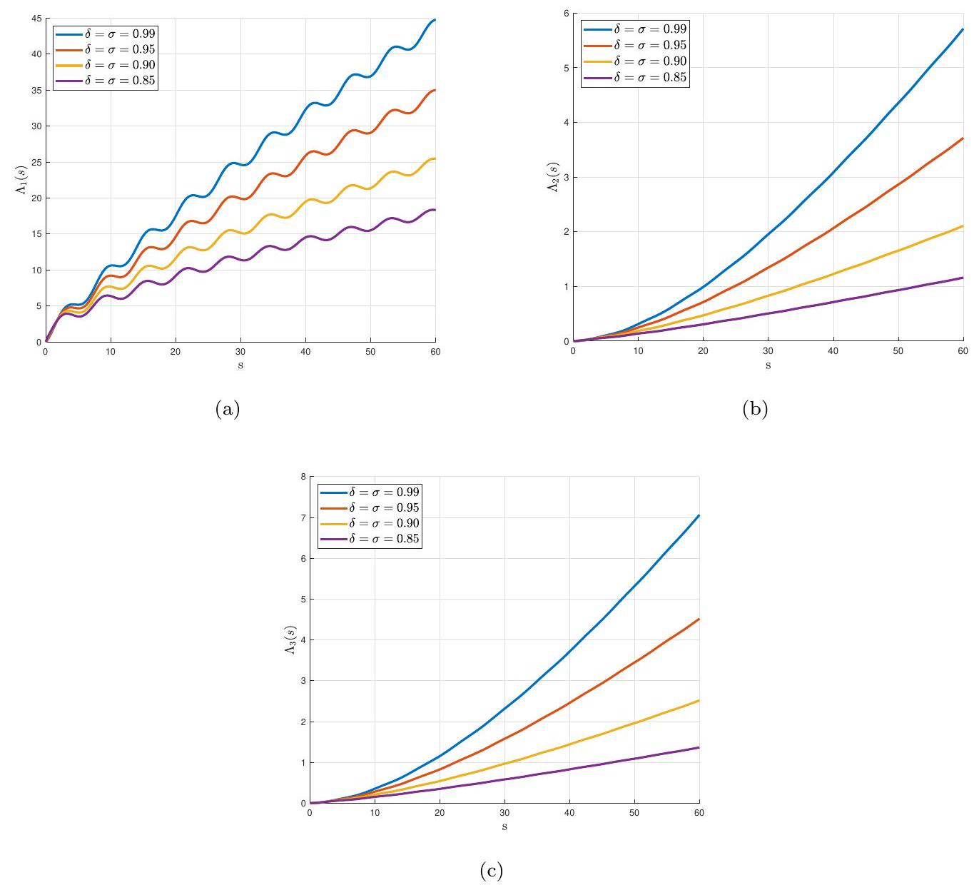
We employ Mittag-Leffler type kernels to solve a system of fractional differential equations using fractal-fractional (FF) operators with two fractal and fractional orders. Using the notion of FF-derivatives with nonsingular and nonlocal fading memory, a model of three polluted lakes with one source of pollution is investigated. The properties of a non-decreasing and compact mapping are used in order to prove the existence of a solution for the FFmodel of polluted lake system. For this purpose, the Leray-Schauder theorem is used. After exploring stability requirements in four versions, the proposed model of polluted lakes system is then simulated using two new numerical techniques based on Adams-Bashforth and Newton polynomials methods. The effect of fractal-fractional differentiation is illustrated numerically. Moreover, the effect of the FF-derivatives is shown under three specific input models of the pollutant: linear, exponentially decaying, and periodic.

Keywords: Pollution of waters; Fractal-fractional derivatives model; Existence, unicity and stability; Adams-Bashforth and Newton polynomials methods.
MSC: 34A08; 65P99.

1 Introduction

In the last century, pollution of waters has become a severe danger to the world we live in. The first step in preparing to conserve the natural environment is to monitor pollution levels. Monitoring pollution is possible to achieve with the use of mathematical analysis. Differential equations may be used to simulate environmental contamination, just as they can be used in many other fields. For example, Biazar et al. utilized in 2006 a set of differential equations to predict the pollution level in a series of lakes [1]. In concrete, they have proposed a model of triple lakes connected by channels through compartment modeling. Some other scholars have investigated this concept using various methodologies. Yüzbaşi et al. 2] analyzed such levels of pollution under the collocation method in 2012. Later, Benhammouda et al. 3] utilized another method to solve the pollution model via a modified differential transform. Khader et al. 4 have also created a fractional case model and used the matrix properties in 2013. Recently, in 2019, Bildik and Deniz [5] considered an Atangana-Baleanu based model for approximating the solutions of a polluted lake system. After that, Ahmed and Khan turned to a similar model of lake pollution via different fractional methods [6]. In 2020, Prakasha and Veeresha [7] solved such a system of polluted lakes via the so-called q-HATM method. More recently, in 2022, Shiri and Baleanu have done a research on the amount of pollution in a three-compartmental model and derived some analytical results [8]. During these years, fractional models of real-world processes have been studied by many other researchers, showing the applicability of fractional operators in mathematical modeling: see, e.g., 9, 10, 11, 12, 13, 14, 15. Here we propose and study a mathematical model via a generalized family of derivatives equipped with two parameters.
Atangana introduced a new class of fractal-fractional notions, which brings together the two applicable areas of fractal and fractional calculi 16. The structure of these operators is a convolution of the power-law, exponential law, and modified Mittag-Leffler law with fractal derivatives, which establishes a connection between fractional and fractal mathematics. The fractal dimension and order are the two components of these operators and differential equations with fractal-fractional derivatives convert the putative system’s order and dimension into a rational system. Because of this characteristic, conventional differential equations are naturally extended to systems with any order of derivatives and dimensions. The goal of these coupled operators is to look at distinct nonlocal boundary value problems (BVPs) or initial value problems (IVPs) that have fractal tendencies in nature. Many scholars provided results and discoveries in this area, demonstrating that fractal-fractional operators are more effective at describing real-world data and for mathematical modeling. Examples of such mathematical models include: fractal-fractional structures of dynamics of corona viruses 17, malaria transmission 18, dynamics of COVID-19 in Wuhan 19, transmission of AH1N1/09 virus [20], dynamics of Q fever [21, HIV [22, dynamics of CD4 cells [23, tuberculosis disease 24, etc.
The incorporation of fractal-fractional (FF) operators with dual fractal and fractional orders in scientific research presents a promising avenue with multifaceted advantages. By leveraging two orders simultaneously, this approach allows for a more nuanced and refined representation of complex systems, capturing intricate patterns and irregularities that traditional methods might overlook. The synergy of fractal geometry and fractional calculus enhances the modeling and analysis of real-world phenomena, providing a more accurate reflection of the inherent self-similar structures and non-integer order dynamics. This not only refines our understanding of intricate processes but also facilitates the development of more robust mathematical models that can be applied across various disciplines. The utilization of FF operators holds the potential to revolutionize fields ranging from signal processing to image analysis, offering a versatile toolkit to address challenges that demand a deeper comprehension of intricate, multifractal behaviors. Embracing this innovative paradigm contributes to a more holistic and precise approach in scientific investigations, opening new frontiers for exploration and discovery. Here we conduct an analysis of a fractal-fractional model of polluted lakes in terms of various different characteristics.
The paper is organized as follows. In Section 2, we introduce a fractal-fractional system to model polluted lakes. Existence of a solution to the proposed system is proved in Section 3 by using the Leray-Schauder theorem. In Section 4, we employ the Banach principle for contrac-
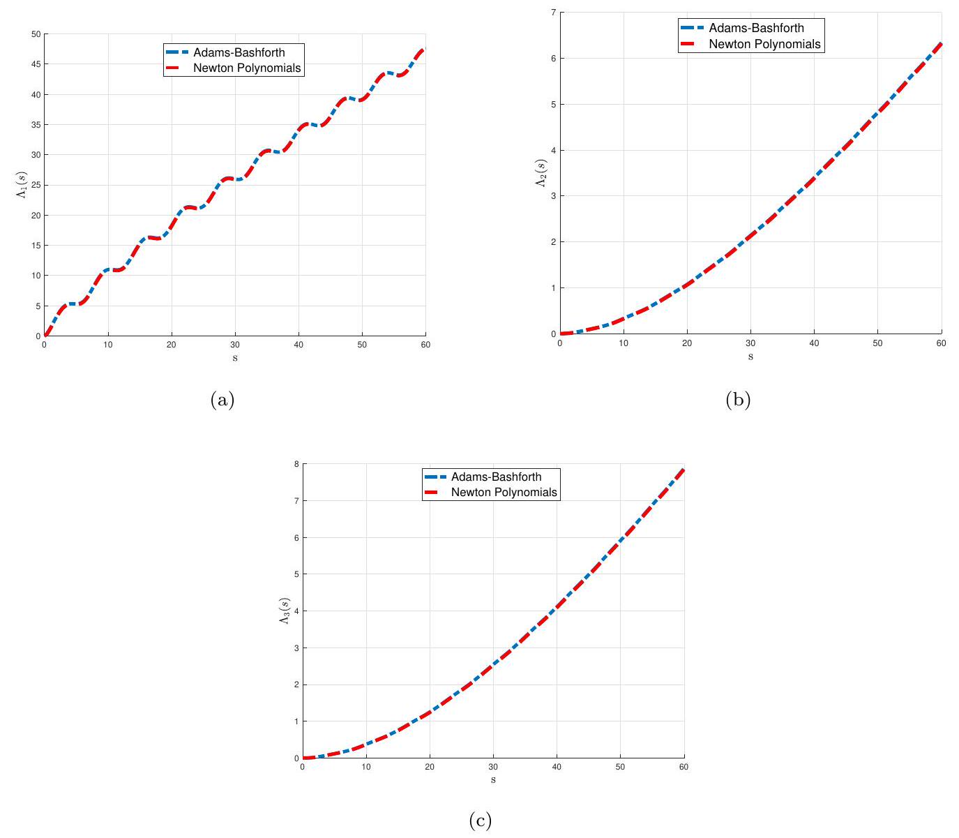
tions to demonstrate uniqueness of solution. Furthermore, using functional analysis, numerous requirements for different types of stability for the solution to the polluted lakes system model are explored in Section 5. To simulate our model, we use two different techniques: a fractional Adams-Bashforth approach (Section 6) and a second one based on Newton’s polynomials (Section 7). The obtained theoretical results are then tested in Section 8 by applying our algorithms with some concrete data under various fractal and fractional order values in three different cases: linear, exponentially decaying and periodic input real models. We end with Section 9 of conclusion.

2 The FF-model for a polluted system of three lakes

We model three lakes. Using three lakes in a system might be a good practical choice based on various factors such as land availability, cost, and efficiency. The decision of considering here three lakes is not purely mathematical, but involves environmental, economic, and logistical considerations. Mathematical modeling could help optimize the distribution and size of the lakes, but it is essential to balance these factors for a sustainable and effective solution. Therefore, we restrict ourselves to three lakes and their channels with a pollutant source. One can generalize our results to a finite number of lakes.
Each lake is treated as a compartment, a linking channel between two lakes being viewed as a pipe connecting the compartments. The direction of the flow across each channel or pipeline is shown by arrows. A contaminant is considered in the first lake. By we denote the rate at which the contaminant/pollutant enters Lake 1 at time . The major purpose is to determine the pollution levels in each lake at any given moment. To do so, we regard the concentration of the pollutant in the lake at time , by
where denotes the water volume at lake , assumed to be constant, and specifies the quantity of pollution that is equally distributed over each lake at time . We are interested to model the situation shown in Figure 1, where we use the symbol to represent the flow rate entering the th lake from the th. Based on Figure 1, we derive the following conditions:
Figure 1: Schematic of channels interconnecting the three lakes being modeled.
Note that since there exists no pipe between the second and the first lakes. The flux of pollutant flowing from the th lake to the th lake at an arbitrary time measures the flow rate of the concentration of pollutant. This index equals
Based on the principle that the rate of change of the pollutant is given by the difference between the input rate and the output rate, we propose here the following fractal-fractional model for the dynamic behavior of the polluted lake system of three lakes via the generalized Mittag-Leffler kernel:
subject to
where is the ( )-fractal-fractional derivative with Mittag-Leffler type kernel of fractional and fractal orders and , respectively, as introduced by Atangana in 16.
Definition 1 (See [16]). Let be a continuous map that is fractal differentiable of dimension . In this case, the Riemann-Liouville -fractal-fractional derivative of with the generalized Mittag-Leffler type kernel of order is given by
where
is the fractal derivative and with .
In what follows, we also use the corresponding notion of fractal-fractional integral.
Definition 2 (See [16]). The ( )-fractal-fractional integral of a function with generalized kernel is given by
if it exists, where .

3 Existence

We begin by proving existence of solution to our problem (4)-(5). For that we use fixed point theory. To conduct our qualitative analysis, let us define the Banach space , where with
for . We rewrite the right-hand-side of the fractal-fractional polluted lake system (4) as
In this case, the fractal-fractional polluted lake system (4) is transformed into the following system:
In view of (9), we rewrite our tree-state system as the compact IVP
where
and
By definition and by (10), we have
Applying the fractal-fractional Atangana-Baleanu integral on (13), we get
The extended representation of (14) is given by
To derive a fixed-point problem, we now define the self-map as
To prove existence of solution to our fractal-fractional polluted lake system (4), we make use of the following Leray-Schauder theorem.
Theorem 3 (Leray-Schauder fixed point theorem [25]). Let be a Banach space, a closed convex and bounded set, and an open set with . Then, under the compact and continuous mapping , either:
(Y1) s.t. , or
(Y2) such that .
Given that the polluted lake system models a real-world problem, its existence is subject to certain constraints. These constraints, denoted in Theorem 4 as (P1) and (P2), play a crucial role in shaping the dynamics and characteristics of the system. Indeed, (P1) and (P2) are indispensable to define and regulate the behavior of the polluted lake system within the confines of practicality and reality. Recognizing these constraints is essential for constructing a comprehensive understanding of the system and developing effective strategies.
Theorem 4. Let . If
(P1) and (A non-decreasing) such that and ,
(P2) such that
with ;
then there exists a solution to the fractal-fractional polluted lake system (4).
Proof. First, consider , which is formulated in (16), and assume
for some . Clearly, as is continuous, thus is also so. From (P1), we get
for . Hence,
Thus, is uniformly bounded on . Now, take such that and . By denoting
we estimate
We see that the right-hand side of (19) approaches to 0 independent of , as . Consequently,
when . This gives the equicontinuity of and, accordingly, the compactness of on by the Arzelá-Ascoli thoerem. As Theorem 3 is fulfilled on , we have one of (Y1) or (Y2). From (P2), we set
for some , such that
From (P1) and (18), we have
Suppose that there are and such that . Then, by (20), we write
which cannot hold true. Thus, (Y2) is not satisfied and admits a fixed-point in by Theorem 3 This proves the existence of a solution to the FF polluted lake model (4).

4 Uniqueness

As a first step to prove uniqueness of solution to our problem (4)-(5), we begin by investigating a Lipschitz property of the fractal-fractional polluted lake system (4).
Lemma 5. Consider , and let
(C1) for some constants .
Then, , and defined in (8) fulfill the Lipschitz property with constants with respect to the relevant components, where
Proof. For , we take arbitrarily, and we have
From (22), we find out that is Lipschitz with respect to under the constant . For , we choose arbitrary , and estimate
This means that is Lipschitz with respect to under the constant . Finally, for arbitrary elements , we have
This shows that is Lipschitzian with respect to with . Therefore, the kernel functions , and are Lipschitz, respectively with constants .
By invoking Lemma 5, we now prove uniqueness of solution to the FF-system (4).
Theorem 6. Let (C1) hold. If
for and where are the Lipschitz constants introduced by (21), then the fractalfractional polluted lake system (4) possesses exactly one solution.
Proof. We do the proof by contradiction. Assume there exists another solution to the fractalfractional polluted lake system (4), namely ), under initial conditions
From (15), we have
and
In this case, we estimate
and so
From (23), we can assert that the above inequality holds if or . Similarly, from
we obtain
which gives or . Furthermore,
which yields
Hence, . As a consequence,
which proves that the solution to the fractal-fractional polluted lake system (4) is unique.

5 Ulam-Hyers-Rassias stability

In this section, the stability of the solutions to the polluted lake system of three lakes is studied. Given the desire to establish robust mathematical foundations for the model, we consider four different notions of stability. More precisely, we prove stability for our fractal-fractional (FF) polluted lake system (4) with respect to Ulam-Hyers and Ulam-Hyers-Rassias notions and their respective generalizations. Stability analysis is pivotal in ensuring mathematical models’ reliability and predictability, especially in real-world applications such as the polluted lake system. Ulam stability, Hyers stability, and their generalizations offer valuable frameworks for understanding the behavior of solutions to dynamic systems under perturbations. Given the intricate nature of fractal-fractional systems, the use of these stability notions allows us to ascertain the system’s resilience to variations and disturbances, providing insights into the long-term behavior and reliability of the proposed model. By choosing stability in this context, we aim to enhance the credibility of the model and its applicability in addressing the complexities inherent in polluted lake systems.
Definition 7. The FF polluted lake system (4) is Ulam-Hyers stable if there exists , such that for all , and for all satisfying
there exists satisfying the fractal-fractional polluted lake system (4) with
Definition 8. The FF polluted lake system (4) is generalized Ulam-Hyers stable if , with such that and fulfilling (24), there is a solution of the given FF polluted lake system (4) such that
Remark 9. The triplet is a solution for (24) if, and only if, (each of them depend on , respectively) such that ,
(i) ,
(ii) one has
Definition 10. The fractal-fractional polluted lake model (4) is Ulam-Hyers-Rassias stable with respect to , if such that and fulfilling
there exists a solution of the FF-model of polluted lake system (4) such that
with .
Remark 11. If , then Definition 10 reduces to the Ulam-Hyers criterion.
Definition 12. The FF polluted lake system (4) is generalized Ulam-Hyers-Rasias stable with respect to if exists such that for all satisfying
there exists a solution of the FF-model of polluted lake system (4) such that
Remark 13. Note that is a solution for (25) if, and only if, (each of them depend on , respectively) such that ,
(i) ,
(ii) we have
Lemmas 14 and 15 are useful to prove Theorems 16 and 17, respectively.
Lemma 14. For each , suppose that is a solution of (24). Then, functions fulfill the following three inequalities:
and
Proof. Let be arbitrary. Since satisfies
it follows from Remark 9 that one can take a function such that
and . Clearly,
In this case, we estimate
This means that (26) is fulfilled. We prove (27) and (28) in a similar way.
To prove our next result (see Lemma 15), we consider the following condition:
(C2) there exists increasing mappings , and , provided that
Lemma 15. Let ( ) hold. For each , suppose that is a solution of (25). Then, functions fulfill the following three inequalities:
Proof. Let . Since satisfies
it follows from Remark 13 that we can take such that
and . Evidently,
Then, we estimate
We prove the remaining inequalities in a similar way.
We are now in a position to investigate the Ulam-Hyers stability for the FF-model of polluted lake system (4).
Theorem 16. Assume (C1) holds. Then our polluted lake system (4) is both Ulam-Hyers and generalized Ulam-Hyers stable with
in which are given by (21).
Proof. Let and be an arbitrary solution of (24). By Theorem 6, let be the unique solution of the FF polluted lake system (4). Then is defined as
From the triangle inequality, Lemma 14 gives
Hence,
Set . In this case, . Similarly, we obtain
where
We conclude that the FF-model of polluted lake system (4) is Ulam-Hyers stable. On the other hand, if we take
then and the proof is finished: 4 is generalized Ulam-Hyers stable.
Theorem 17 establishes Ulam-Hyers-Rassias stability for the fractal-fractional polluted lake system (4).
Theorem 17. If (C1) and (C2) hold, then the FF-model of polluted lake system (4) is simultaneously stable in the sense of Definitions 7 and 8 .
Proof. Let , and satisfy (25). By Theorem 6, let be the (unique) solution of the FF polluted lake system model (4). Then becomes
With the aid of the triangle inequality, Lemma 15 gives
Accordingly, we obtain that
Set
Then . Similarly,
where
As a consequence, the fractal-fractional polluted lake system (4) is stable in the sense of Definition 7. By defining , our FF polluted lake system model (4) is also stable in the sense of Definition 8 .

6 Numerical algorithm via the Adams-Bashforth method

The Adams-Bashforth method is a robust numerical integration technique commonly used for solving most differential equations. Its higher-order accuracy and efficiency make it particularly suitable for approximating the solution of dynamic systems, such as those describing the behavior of polluted lake systems. By choosing the Adams-Bashforth technique, we aim to achieve accurate and stable numerical solutions for the fractal-fractional polluted lake system (4).
To do this, we apply the fractional Adams-Bashforth technique with two-step Lagrange polynomials. For that we redefine the fractal-fractional integral equations (15) at . Precisely, we discretize the integral equations (15) for as follows:
The approximation of the above integrals are given by
Next, we approximate , on by applying twostep Lagrange interpolation polynomials under the step size . By direct computations, we obtain the following algorithm that yields numerical solutions to the FF-model of polluted lake system (4):
where
and

7 Numerical algorithm via Newton’s polynomials

Here we develop a different approximation algorithm (based on Newton’s Polynomials) to compute numerically the solutions of our fractal-fractional polluted lake system (4). The use of Newton’s polynomials in interpolation is motivated by their simplicity and applicability for approximating functions based on a set of given data points. In the context of modeling and analysis, Newton’s polynomials offer a flexible approach to represent complex relationships within the polluted lake system. The polynomial interpolation technique enables us to construct a continuous function that approximates the behavior of the system, facilitating a more detailed and comprehensive understanding of its dynamics. To the best of our knowledge, the idea was first introduced in 26 . Precisely, we follow 26 with the IVP (10) subject to the conditions (11) and (12). In this case, we have
Set . Then,
By discretizing the above equation at , we get
Approximating the above integral, we can write that
Now we approximate function with the Newton polynomial
Substituting (37) into (36), we obtain that
Simplifying the above relations, we get
and it follows that
On the other hand, by computing the above three integrals separately, one gets
and
By putting (39), (40), and (41) into (38), we obtain that
Finally, we replace into (42), and we get that
where
Using the numerical scheme (43), the numerical solutions to the fractal-fractional polluted lake system (4) are given by
and
where are defined in (44), .

8 Numerical simulations and discussion

Now we apply the Adams-Bashforth method (ABM) and Newton’s polynomials method (NPM), proposed respectively in Sections 6 and 7 to examine and find numerical solutions of the proposed FF-model and to observe the applicability, accuracy, and exactness of the developed algorithms. To simulate the quantity of pollution in the modeled lakes, we coded the algorithms (33)-(35) and (45)-(47) in MATLAB, version R2019A.
To compare the results, we borrow from [1] the following values for the parameters: year, year, year, year . Moreover, . Also, various fractal dimensions and fractional orders, i.e., , are considered for the simulations of the three state functions , and .
We consider the suggested FF-model in three cases: linear (Section 8.1), exponentially decaying (Section 8.2), and periodic (Section 8.3) input models.

8.1 Linear input model

In this case, we consider the model in which the Lake 1 has a contaminant with a linear concentration. Linear input states the steady behavior of the pollutant. At time zero, the pollutant concentration is zero but, as the time increases, the addition of pollutant is started and then is remained steadily. For example, when a factory starts production at time zero, waste discharge begins at a fixed rate and concentration. As a particular case, we chose . Then, for , from (4) we have
In Figures 2 (a), (b), and (c), the behavior of the ABM approximations for each pair of the state functions , and , respectively, are given; while in Figure 2 (d), the 3D
view of under integer-order derivatives are graphically illustrated for the linear input model with time and step size .
Note that the parameter is explicitly defined as the step size, distinct from the stability parameters , discussed in the stability Section 5. While here we emphasize as the step size in a specific context, Ulam-Hyers-Rassias stability, as a theory, is primarily concerned with the stability properties of functional equations. Unlike the numerical solution of differential equations, the choice of step size is not a direct consideration in the realm of Ulam-Hyers-Rassias stability. This stability theory focuses on understanding how small variations in functional equations lead to proportionate changes in the solutions, and the concept of a step size does not play a prominent role in that context.
Figure 2: Behaviors of each pair of state functions (a) , (b) , (c) and (d) 3 D view of under the integer-order.
In Table 1, we present some numerical results of the two numerical techniques, ABM and NPM, for the three state functions and in the linear input case, under integer-order derivatives and step size . From the obtained numerical results, we can assert that the Adams-Bashforth approximations for the phase functions , and strongly agree with the ones obtained by the Newton polynomials method for the time up to 10 years.
In Figure 3, the comparison of the numerical results from ABM and NPM for the state functions , and is shown graphically, for the time and the linear input case. We observe that the results of ABM and NPM have a high agreement between them for each one of the state
Table 1: Comparison between ABM and NPM for the linear input case.
Adams-Bashforth Newton Polynomials
0 0.000000 0.00000 0.000000 0.000000 0.000000 0.000000
1 58.241762 0.122200 0.136038 58.249029 0.114027 0.126944
2 216.569135 0.912690 1.018175 216.603012 0.891958 0.995030
3 472.231987 2.959673 3.308340 472.291839 2.926723 3.271438
4 824.018631 6.830863 7.650506 824.103833 6.786029 7.600138
5 1270.753481 13.074750 14.671769 1270.863423 13.018359 14.608218
6 1811.296055 22.221220 24.982726 1811.430139 22.153588 24.906273
7 2444.539990 34.782156 39.177854 2444.697632 34.703595 39.088774
8 3169.412094 51.252025 57.835881 3169.592721 51.162836 57.734443
9 3984.871413 72.108440 81.520147 3985.074465 72.008917 81.406618
10 4889.908324 97.812711 110.778966 4890.133254 97.703141 110.653605
functions, even in the longer period of 60 years.
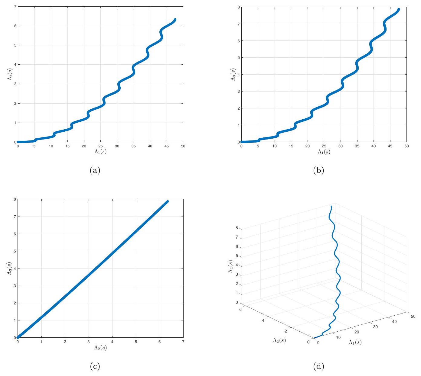
In Figure 4, we illustrate the behavior of the three state functions , and when the ABM is applied under the fractal-fractional orders . From these figures, we can observe that when the fractal-fractional order is getting closer to the integer case, then the effect of the pollution is increasing on each lake model at about the same rate. As an observation of these graphs, it can be said that the non-integer order operator has a positive effect on the pollution reduction in the lake pollution model.
A word is due about our choice of the values of the fractal-fractional orders. We considered fractional orders within the range of because within this interval we observed consistent behaviors for different fractional orders. Specifically, as the fractal-fractional order decreases, we noted a proportional reduction in the impact of pollution on each lake model at about the same rate. This consistent trend in behavior as the fractional order decreases led us to cut the interval at the value 0.85 . This choice captures the essential aspects of the model’s response to varying fractional orders and provides a meaningful representation of the system dynamics.

8.2 Exponentially decaying input model

When heavy dumping of pollutant is present, it makes sense to consider the exponentially decaying input model, i.e., the case when . An example of this case occurs if every industry placed in a city collects and stores its wastage during some days and then dumps it to Lake 1 after that stored period. If we take and , then system (4) becomes
The graphical representation of the input function is illustrated in Figure 5 for the exponentially decaying input case .
In Figures 6 (a), (b), and (c), the behavior of the ABM approximations for each pair of the state functions , and , respectively, is shown, while in Figure 6 (d), the 3D view of under the integer-order derivative is graphically illustrated for the exponentially decaying input model with time and step size .
In Table 2, we provide a comparison between the approximate solutions obtained using ABM and NPM for the exponentially decaying input case with time , step size ,
Figure 3: Comparison between the ABM and NPM for (a) , (b) and (c) in the linear input model.
and . From Table 2, we can conclude that the ABM approximations are also in good agreement with the NPM ones for the exponentially decaying input model.
In Figure 7, we present a graphical comparison between ABM and NPM approximations for the state functions , and in the exponentially decaying input case with time . From Figure 7 it can be concluded that the two introduced methods strongly agree with each other even in a large time domain of 60 years.
In Figure 8. we illustrate the numerical results of the three state variables , and for the exponentially decaying input model when the ABM is applied under various fractal-fractional orders: . Figure 8 shows that the non-integer fractal-fractional operators have an effect on decreasing the amount of pollution for each model when the time increases, that is, the pollution is increasing harmoniously with the fractal-fractional order, getting closer to the integer-order case.

8.3 Periodic input model

As a last case of study, we consider a periodic input model in which the pollutant appears in the lake periodically. A factory that works during daytime only, can be an example of this case: it generates waste and dump it in the lakes during the day while at night the mixing of new pollutants stops. For a concrete case, we selected , where and stands for
Figure 4: Behaviors of (a) , (b) and (c) for the linear input model under fractal and fractional orders .
the variations of amplitude and frequency, respectively. Also, is considered as the average input of pollutant concentration. In such a case , system (4) takes the following form:
The graphical representation of the input function is illustrated in Figure 9 for the periodic input case .
In Figures 10 (a), (b), and (c), the graphical behavior of each pair of the state functions , , and , respectively, is shown. In Figure 10 (d), the 3 D view of under the integer-order derivative is illustrated for the periodic input model with time and step size .
The tabular comparison between the numerical results obtained from the proposed techniques, ABM and NPM, for the three state functions , and under the periodic input case, are reported in Table 3 for time , step size , and . From these results, we conclude that the solutions obtained by ABM and NPM highly agree with each other.
Figure 5: Graphic of the exponentially decaying input.
Table 2: Numerical comparison between ABM and NPM for the exponentially decaying input case.
Adams-Bashforth Newton Polynomials
0 0.000000 0.00000 0.000000 0.000000 0.000000 0.000000
1 18.988642 0.105437 0.117578 18.988592 0.105145 0.117021
2 18.748146 0.219107 0.245295 18.752821 0.216590 0.242237
3 18.513934 0.328934 0.369679 18.523194 0.324269 0.364185
4 18.286698 0.435044 0.490805 18.300406 0.428303 0.482940
5 18.066244 0.537556 0.608748 18.084267 0.528808 0.598573
6 17.852383 0.636586 0.723579 17.874593 0.625901 0.711155
7 17.644931 0.732247 0.835369 17.671201 0.719691 0.820757
8 17.443709 0.824649 0.944190 17.473918 0.810285 0.927446
9 17.248540 0.913898 1.050109 17.282570 0.897787 1.031291
10 17.059256 1.000097 1.153195 17.096990 0.982299 1.132359
In Figure 11, we illustrate our findings graphically, comparing the numerical results from ABM and NPM for each state function , and , where the Lake 1 has a periodic pollutant input. Figure 11 shows that the two introduced techniques, ABM and NPM, strongly agree with each other for the time , step size , and .
In Figure 12, we illustrate the ABM approximations of the three state functions , and under various fractal-fractional orders: for the periodic input case. Similar to cases of Sections 8.1 and 8.2 we observe that the non-integer order fractal-fractional operators have a great effect on decreasing the amount of contamination for each model while the time increases.

9 Conclusion

We employed Mittag-Leffler type kernels to solve a system of fractional differential equations using fractal-fractional (FF) operators with two fractal and fractional orders. We derived equiv-
Figure 6: Behaviors of each pair of state functions (a) , (b) , (c) and (d) 3D view of under the integer-order.
Table 3: Comparison between ABM and NPM in the periodic input case.
Adams-Bashforth Newton Polynomials
0 0.000000 0.00000 0.000000 0.000000 0.000000 0.000000
1 1.420794 0.003639 0.004053 1.420289 0.003637 0.004052
2 3.352256 0.018270 0.020396 3.349409 0.017505 0.019538
3 4.795526 0.043383 0.048562 4.791798 0.041836 0.046821
4 5.304589 0.073971 0.083050 5.303706 0.071660 0.080440
5 5.281611 0.104988 0.118274 5.286096 0.101974 0.114856
6 5.607511 0.135825 0.153543 5.616323 0.132176 0.149388
7 6.832362 0.170701 0.193553 6.841809 0.166454 0.188698
8 8.669954 0.214629 0.243923 8.677051 0.209775 0.238353
9 10.261233 0.268650 0.305891 10.266407 0.263162 0.299573
10 10.964396 0.328730 0.375035 10.971053 0.322611 0.367966
Figure 7: Comparison between the ABM and NPM for (a) , (b) and (c) in the exponentially decaying input model.
alent FF-integral equations from a compact initial value problem, and then proved existence and uniqueness results. A stability analysis was conducted in different versions. In the next sections, we examined and captured the behavior of the considered fractal-fractional operator model (4) with the help of two different numerical techniques: an Adams-Bashforth method (ABM) and a Newton polynomials method (NPM). From the obtained results, we conclude that the considered techniques, ABM and NPM, are in highly agreement and are very efficient to examine the system of fractional differential equations under fractal-fractional operators describing the dynamics of the pollution in the lakes. We also analyzed the considered model under various fractal-fractional orders and examined the effects of these non-integer orders on the behavior of each state variable , and for three specific input models: linear, exponentially decaying, and periodic. For each input model, we observed that when the fractal-fractional order gets closer to the classical integer-order case, then the effect of the pollution is increasing harmoniously for each lake model. As a conclusion of these observations, it can be said that the non-integer order operators have positive effects on the reduction of pollution in the lake pollution model. As future work, we plan to investigate different real-world models based on the techniques here developed.

CRediT authorship contribution statement

Tanzeela Kanwal: Formal analysis, Methodology. Azhar Hussain: Conceptualization, Formal analysis, Methodology. İbrahim Avcı: Formal analysis, Methodology, Software. Sina Etemad:
Figure 8: Behaviors of (a) , (b) and (c) for the exponentially decaying input model under fractal and fractional orders .
Figure 9: Graphic of the periodic input.
Figure 10: Behaviors of each pair of state functions (a) , (b) , (c) and (d) 3D view of under the integer-order.
Conceptualization, Methodology, Software. Shahram Rezapour: Conceptualization, Methodology. Delfim F. M. Torres: Formal analysis, Funding acquisition, Methodology.

Declaration of competing interest

The authors declare that they have no known competing financial interests or personal relationships that could have appeared to influence the work reported in this paper.

Data availability

No data was used for the research described in the article.

Acknowledgments

Torres was supported by the Portuguese Foundation for Science and Technology (FCT), project UIDB/04106/2020 (https://doi.org/10.54499/UIDB/04106/2020).
Figure 11: Comparison between the ABM and NPM for (a) , (b) and (c) in the periodic input model.

References

[1] J. Biazar, L. Farrokhi, M. R. Islam, Modeling the pollution of a system of lakes. Appl. Math. Comput., 178(2) (2006) 423-430. https://doi.org/10.1016/j.amc.2005.11.056
[2] Ş. Yüzbaşi, N. Şahin, M. Sezer, A collocation approach to solving the model of pollution for a system of lakes, Math. Computer Model., 55(3-4) (2012) 330-341. https://doi.org/10.1016/j.mcm.2011. 08.007
[3] B. Benhammouda, H. Vazquez-Leal, L. Hernandez-Martinez, Modified differential transform method for solving the model of pollution for a system of lakes, Discr. Dyn. Nat. Soc., 2014 (2014) 645726. https://doi.org/10.1155/2014/645726
[4] M. M. Khader, T. S. El Danaf, A. S. Hendy, A computational matrix method for solving systems of high order fractional differential equations, Appl. Math. Model., 37(6) (2013) 4035-4050. https: //doi.org/10.1016/j.apm.2012.08.009
[5] N. Bildik, S. Deniz, A new fractional analysis on the polluted lakes system, Chaos, Solitons & Fractals, 122 (2019) 17-24. https://doi.org/10.1016/j.chaos.2019.02.001
[6] M. M. D. Ahmed, M. A. Khan, Modeling and analysis of the polluted lakes system with various fractional approaches, Chaos, Solitons & Fractals, 134 (2020) 109720. https://doi.org/10.1016/ j.chaos.2020.109720
[7] D. G. Prakasha, P. Veeresha, Analysis of Lakes pollution model with Mittag-Leffler kernel, J. Ocean Eng. Sci., 5(4) (2020) 310-322. https://doi.org/10.1016/j.joes.2020.01.004
Figure 12: Behaviors of (a) , (b) and (c) for the periodic input model under fractal and fractional orders .
[8] B. Shiri, D. Baleanu, A General Fractional Pollution Model for Lakes, Commun. Appl. Math. Comput., 4 (2022) 1105-1130. https://doi.org/10.1007/s42967-021-00135-4
[9] A. Alsaedi, M. Alsulami, H. M. Srivastava, B. Ahmad, S. K. Ntouyas, Existence theory for nonlinear third-order ordinary differential equations with nonlocal multi-point and multi-strip boundary conditions, Symmetry, 11(2) (2019) 281. https://doi.org/10.3390/sym11020281
[10] M. R. Sidi Ammi, M. Tahiri, D. F. M. Torres, Necessary optimality conditions of a reaction-diffusion SIR model with ABC fractional derivatives, Discrete Contin. Dyn. Syst. Ser. S 15 (2022), no. 3, 621-637. https://doi.org/10.3934/dcdss. 2021155 arXiv:2106. 15055
[11] M. Aslam, R. Murtaza, T. Abdeljawad, G. ur Rahman, A. Khan, H. Khan, H. Gulzar, A fractional order HIV/AIDS epidemic model with Mittag-Leffler kernel, Adv. Differ. Equ., 2021 (2021), 107, 1-5. https://doi.org/10.1186/s13662-021-03264-5
[12] S. W. Ahmad, M. Sarwar, G. Rahmat, K. Shah, H. Ahmad, A. A. A. Mousa, Fractional order model for the Coronavirus (COVID-19) in Wuhan, China, Fractals, 30 (2022), 2240007. https: //doi.org/10.1142/S0218348X22400072
[13] J. K. K. Asamoah, E. Okyere, E. Yankson, A. A. Opoku, A. Adom-Konadu, E. Acheampong, Y. D. Arthur, Non-fractional and fractional mathematical analysis and simulations for Q fever, Chaos, Solitons & Fractals, 156 (2022), 111821. https://doi.org/10.1016/j.chaos.2022.111821
[14] H. Khan, Y. G. Li, W. Chen, D. Baleanu, A. Khan, Existence theorems and Hyers-Ulam stability for a coupled system of fractional differential equations with -Laplacian operator, Bound. Value Probl., 2017 (2017), 157, 1-16. https://doi.org/10.1186/s13661-017-0878-6
[15] Z. Ali, F. Rabiei and K. Hosseini, A fractal-fractional-order modified Predator-Prey mathematical model with immigrations, Math. Comput. Simulation 207 (2023), 466-481. https://doi.org/10. 1016/j.matcom.2023.01.006
[16] A. Atangana, Fractal-fractional differentiation and integration: connecting fractal calculus and fractional calculus to predict complex system, Chaos, Solitons & Fractals, 102 (2017) 396-406. https://doi.org/10.1016/j.chaos.2017.04.027
[17] K. Shah, M. Arfan, I. Mahariq, A. Ahmadian, S. Salahshour, M. Ferrara, Fractal-fractional mathematical model addressing the situation of Corona virus in Pakistan, Res. Phys., 19 (2020) 103560. https://doi.org/10.1016/j.rinp.2020.103560
[18] J. F. Gomez-Aguilar, T. Cordova-Fraga, T. Abdeljawad, A. Khan, H. Khan, Analysis of fractalfractional Malaria transmission model, Fractals, 28(08) (2020) 2040041. https://doi.org/10.1142/ S0218348X20400411
[19] Z. Ali, F. Rabiei, K. Shah, T. Khodadadi, Qualitative analysis of fractal-fractional order COVID19 mathematical model with case study of Wuhan, Alex. Eng. J., 60(1) (2021) 477-489. https: //doi.org/10.1016/j.aej.2020.09.020
[20] S. Etemad, I. Avci, P. Kumar, D. Baleanu, S. Rezapour, Some novel mathematical analysis on the fractal-fractional model of the AH1N1/09 virus and its generalized Caputo-type version, Chaos, Solitons Fractals, 162 (2022) 112511. https://doi.org/10.1016/j.chaos.2022.112511
[21] J. K. K. Asamoah, Fractal-fractional model and numerical scheme based on Newton polynomial for Q fever disease under Atangana-Baleanu derivative, Res. Phys., 34 (2022) 105189. https://doi.org/ 10.1016/j.rinp.2022.105189
[22] S. Ahmad, A. Ullah, A. Akgul, M. De la Sen, Study of HIV disease and its association with immune cells under nonsingular and nonlocal fractal-fractional operator, Complexity, 2021 (2021) 1904067. https://doi.org/10.1155/2021/1904067
[23] H. Najafi, S. Etemad, N. Patanarapeelert, J. K. K. Asamoah, S. Rezapour, T. Sitthiwirattham, A study on dynamics of T-cells under the effect of HIV-1 infection based on a mathematical fractal-fractional model via the Adams-Bashforth scheme and Newton polynomials, Mathematics, 10 (2022) 1366. https://doi.org/10.3390/math10091366
[24] H. Khan, K. Alam, H. Gulzar, S. Etemad, S. Rezapour, A case study of fractal-fractional tuberculosis model in China: Existence and stability theories along with numerical simulations, Math. Comput. Simul., 198 (2022) 455-473. https://doi.org/10.1016/j.matcom.2022.03.009
[25] A. Granas, J. Dugundji, Fixed Point Theory, Springer-Verlag, New York (2003).
[26] A. Atangana, S. İ Araz, New numerical scheme with Newton polynomial-theory, methods, and applications, Elsevier/Academic Press, London, 2021.

  1. This is a preprint of a paper whose final and definite form is published Open Access in Chaos Solitons Fractals at [https://doi.org/10.1016/j.chaos.2024.114653].
    *Correspondence: tanzeelakanwal16@gmail.com (T.K.); sh.rezapour@azaruniv.ac.ir (S.R.); delfim@ua.pt (D.F.M.T.)