زهرة نادرة: تصحيح مليون خطأ في الثانية لكل نواة باستخدام المطابقة ذات الوزن الأدنى Sparse Blossom: correcting a million errors per core second with minimum-weight matching
زهرة نادرة: تصحيح مليون خطأ في الثانية لكل نواة باستخدام المطابقة ذات الوزن الأدنى
أوسكار هيغوت وكريغ جيدني جوجل كوانتوم إيه آي، سانتا باربرا، كاليفورنيا 93117، الولايات المتحدة الأمريكيةقسم الفيزياء وعلم الفلك، كلية لندن الجامعية، WC1E 6BT لندن، المملكة المتحدة
14 يناير 2025
الملخص
في هذا العمل، نقدم تنفيذًا سريعًا لمشفّر المطابقة المثالية ذات الوزن الأدنى (MWPM)، وهو المشفّر الأكثر استخدامًا لعدة عائلات مهمة من رموز تصحيح الأخطاء الكمية، بما في ذلك رموز السطح. خوارزميتنا، التي نسميها زهرية نادرة، هي نوع من خوارزمية الزهرة التي تحل مباشرة مشكلة فك التشفير المتعلقة بتصحيح الأخطاء الكمية. تتجنب الزهرية النادرة الحاجة إلى بحث دايكسترا الشامل، وهو شائع بين تنفيذات مشفّر MWPM.ضوضاء إزالة الاستقطاب على مستوى الدائرة، بيانات متلازمة عمليات الزهرة النادرة في كل من قواعد X و Z لدارات شفرة السطح ذات المسافة 17 في أقل من ميكروثانية لكل جولة من استخراج المتلازمة على نواة واحدة، وهو ما يتطابق مع المعدل الذي يتم فيه توليد بيانات المتلازمة بواسطة الحواسيب الكمومية الفائقة التوصيل. تنفيذنا مفتوح المصدر، وقد تم إصداره في النسخة 2 من مكتبة PyMatching.
الملخص
يمكن العثور على كود المصدر لتنفيذنا لـ sparse blossom في إصدار PyMatching 2 على github فيhttps://github.com/oscarhiggott/PyMatchingPyMatching متاح أيضًا كحزمة بايثون 3 من pypi يمكن تثبيتها عبر “pip install pymatching”.
1 المقدمة
سيولد حاسوب كمومي فائق التوصيل يعتمد على شفرة السطح مع مليون كيوبت فيزيائي بيانات قياس بمعدل حوالي 1 تيرابت في الثانية. يجب معالجة هذه البيانات على الأقل بنفس سرعة توليدها بواسطة جهاز فك التشفير، وهو البرنامج الكلاسيكي المستخدم للتنبؤ بالأخطاء التي قد تحدث، لمنع تراكم البيانات الذي ينمو بشكل أسي.-عمق البوابة في الحساب [Ter15]. علاوة على ذلك، فإن أجهزة فك التشفير السريعة مهمة ليس فقط لتشغيل الحاسوب الكمومي، ولكن أيضًا كأداة برمجية للبحث في بروتوكولات تصحيح الأخطاء الكمومية. يمكن أن يتطلب تقدير متطلبات الموارد لبروتوكول تصحيح الأخطاء الكمومية (مثل تقدير بصمة التيراقوب تحت العتبة [Gid+21]) استخدام أخذ عينات مونت كارلو المباشر لتقدير احتمال الأحداث النادرة للغاية. يمكن أن تكون هذه التحليلات مكلفة بشكل غير معقول دون الوصول إلى جهاز فك تشفير سريع، قادر على معالجة ملايين اللقطات من الدوائر التي تحتوي علىالبوابات في إطار زمني معقول.
تم تطوير العديد من مفككات الشيفرة لشفرة السطح، وأقدمها والأكثر شعبية هو مفكك الشيفرة ذو المطابقة المثالية ذات الوزن الأدنى (MWPM) [Den+02]، الذي هو أيضًا محور هذا العمل. يقوم مفكك الشيفرة MWPM بتحويل مشكلة فك الشيفرة إلى مشكلة رسومية من خلال تحليل نموذج الخطأ إلى-نوع و-نوع أخطاء باولي [Den+02]. يمكن حل هذه المشكلة الرسومية بمساعدة خوارزمية إدموندز للعثور على تطابق مثالي ذو وزن أدنى في رسم بياني [Edm65b; Edm65a]. إن تنفيذًا ساذجًا لمشفّر MWPM له تعقيد أسوأ حالة يعتمد على عدد العقدفي الرسم البياني لـ، مع الوقت المتوقع للتشغيل للحالات النموذجية التي تم العثور عليها تجريبيًا لتكون تقريبًا [Hig22]. أدت التقريبات والتحسينات على جهاز فك التشفير MWPM إلى تحسينات كبيرة في أوقات التشغيل المتوقعة [FWH12a; Fow15; Hig22]. على وجه الخصوص، اقترح فاولر جهاز فك التشفير MWPM بمتوسط وقت التشغيل المتوازي [Fow15]. ومع ذلك، لم تظهر التطبيقات المنشورة لشفرة MWPM سرعات كافية للتشفير في الوقت الحقيقي على نطاق واسع.
تم اقتراح عدة بدائل لفك تشفير MWPM في الأدبيات. يتمتع فك تشفير Union-Find بوقت تشغيل أسوأ حالة شبه خطي تقريبًا [DN21؛ HNB20]، وقد تم اقتراح تنفيذات سريعة على الأجهزة.وتم تنفيذهامُفكك اتحاد-البحث أقل دقة قليلاً، ويمكن اعتباره تقريبًا لمُفكك MWPM [WLZ22]. يمكن لمفككات الاحتمالية القصوى أن تحقق دقة أعلى من مُفكك MWPM [BSV14؛ Hig+23؛ Sun+23] ولكنها تتمتع بتعقيد حسابي عالٍ، مما يجعلها غير عملية للتفكيك في الوقت الحقيقي. يمكن لمفككات أخرى، مثل MWPM المرتبطة [Fow13]، ومطابقة الاعتقاد [Hig+23]، ومفككات الشبكات العصبية [TM17؛ MPT22] أن تحقق دقة أعلى من MWPM مع زيادة متواضعة جدًا في وقت التشغيل. بينما كان هناك تقدم في تطوير حزم البرمجيات مفتوحة المصدر لتفكيك رموز السطح [Hig22؛ Tuc20]، فإن هذه الأدوات أبطأ بكثير من محاكيات دوائر المثبت [Gid21]، وبالتالي كانت عنق الزجاجة في محاكيات رموز السطح. ربما يكون هذا أحد الأسباب التي جعلت الدراسات العددية لرموز تصحيح الأخطاء تركز غالبًا على تقدير العتبات (التي تتطلب تفكيك عدد أقل من اللقطات)، بدلاً من تكاليف الموارد (التي تكون أكثر فائدة عمليًا لإجراء المقارنات).
في هذا العمل، نقدم تنفيذًا جديدًا لمفكك الشيفرة MWPM. الخوارزمية التي نقدمها، الزهرة المتناثرة، هي نوع من خوارزمية الزهرة التي تشبه من الناحية المفاهيمية النهج المتبع في المراجع [FWH12a; FWH12b; Fow15]، حيث تحل مشكلة فك الشيفرة MWPM مباشرة على رسم الكاشف، بدلاً من تقسيم المشكلة بشكل ساذج إلى خطوات متسلسلة متعددة وحل مشكلة نظرية الرسم التقليدية MWPM كروتين فرعي منفصل. هذا يتجنب عمليات البحث الشاملة باستخدام خوارزمية ديكسترا التي تُستخدم غالبًا في تنفيذات مفكك الشيفرة MWPM. تنفيذنا أسرع بمئات المرات من الأدوات البديلة المتاحة، ويمكنه فك الشيفرة لكل من و أسس دائرة شفرة السطح على بعد 17ضجيج الدائرة) في أقل من ميكروثانية لكل جولة على نواة واحدة، مما يتطابق مع المعدل الذي يتم فيه توليد بيانات المتلازمة على معالج كمي فائق التوصيل. عند المسافة 29 بنفس نموذج الضجيج (أكثر من كافٍ لتحقيقمعدلات الأخطاء المنطقية)، يستغرق PyMatching 3.5 ميكروثانية لكل جولة لفك التشفير على نواة واحدة. تشير هذه النتائج إلى أن خوارزمية الزهرة النادرة لدينا سريعة بما يكفي لفك التشفير في الوقت الحقيقي لأجهزة الكمبيوتر الكمومية الفائقة عند النطاق الكبير؛ من المحتمل تحقيق تنفيذ في الوقت الحقيقي من خلال التوازي عبر عدة نوى، ومن خلال إضافة دعم لفك تشفير تدفق، بدلاً من دفعة، من بيانات المتلازمة. تم إصدار تنفيذنا للزهرة النادرة في الإصدار 2 من حزمة PyMatching بايثون، ويمكن دمجه مع Stim [Gid21] لتشغيل المحاكاة في دقائق على جهاز كمبيوتر محمول كان سيستغرق ساعات على مجموعة حوسبة عالية الأداء.
في عمل مستقل متوازي مثير للإعجاب، طور يوي وو أيضًا تنفيذًا جديدًا لخوارزمية الزهرة يسمى الزهرة المدمجة [WZ23]، المتاحة في [Wu22]. التشابه المفهومي مع نهجنا هو أن الزهرة المدمجة تحل أيضًا مشكلة فك تشفير MWPM مباشرة على رسم الكاشف. ومع ذلك، هناك العديد من الاختلافات في تفاصيل تنفيذاتنا؛ على سبيل المثال، تستكشف الزهرة المدمجة الرسم بطريقة مشابهة لكيفية نمو المجموعات في البحث عن الاتحاد، بينما ينمو نهجنا المناطق الاستكشافية بشكل موحد، يتم إدارتها بواسطة قائمة أولويات عالمية. بينما يتمتع نهجنا بأداء أسرع على نواة واحدة، تدعم الزهرة المدمجة أيضًا التنفيذ المتوازي للخوارزمية نفسها، والتي يمكن استخدامها لتحقيق سرعات معالجة أسرع لحالات فك التشفير الفردية. عند استخدامها لمحاكاة تصحيح الأخطاء، نلاحظ أن الزهرة النادرة قابلة للتوازي بشكل تافه بالفعل من خلال تقسيم المحاكاة إلى دفعات من اللقطات، ومعالجة كل دفعة على نواة منفصلة. ومع ذلك، فإن توازي فك التشفير نفسه مهم لفك التشفير في الوقت الحقيقي، لمنع تراكم بيانات متزايد بشكل أسي داخل حساب واحد [Ter15]، أو لتجنب التباطؤ المتعدد الحدود المفروض من الاعتماد على فك التشفير من خلال النوافذ المتوازية بدلاً من ذلك.تان +23لذلك، يمكن أن تستكشف الأعمال المستقبلية دمج الزهرة النادرة مع التقنيات الخاصة بالتوازي التي تم تقديمها في الزهرة المدمجة.
الورقة منظمة على النحو التالي. في القسم 2 نقدم خلفية عن مشكلة فك التشفير التي نهتم بها ونقدم نظرة عامة على خوارزمية الزهرة. في القسم 3 نشرح خوارزميتنا، الزهرة النادرة، قبل أن نصف الهياكل البيانية التي نستخدمها لتنفيذنا في القسم 4. في القسم 5 نقوم بتحليل زمن تشغيل الزهرة النادرة، وفي القسم 6 نقوم بتقييم زمن فك التشفير، قبل أن نختم في القسم 7.
2 المقدمات
2.1 الكواشف والملاحظات
الكاشف هو زوج من ناتج قياس بتات في دائرة تصحيح الأخطاء الكمومية يكون حتميًا في غياب الأخطاء. يكون ناتج قياس الكاشف 1 إذا كان الزوج الملاحظ يختلف عن الزوج المتوقع لدائرة خالية من الضوضاء، ويكون 0 خلاف ذلك. نقول إن خطأ باوليكاشف الانقلاباتإذا كان يتضمنفي الدائرة يغير نتيجة، وحدث الكشف هو كاشف مع نتيجة 1. نحن نعرف المراقبة المنطقية على أنها تركيبة خطية من بتات القياس، حيث تتوافق نتيجتها بدلاً من ذلك مع قياس مشغل باولي المنطقي.
نحن نعرف نموذج الخطأ المستقل بأنه مجموعة منآليات خطأ مستقلة، حيث آلية الخطأيحدث باحتمالية (حيث هو متجه من الأولويات)، ويقوم بتغيير مجموعة من الكواشف والملاحظات. يمكن استخدام نموذج خطأ مستقل لتمثيل الضوضاء المسببة للانحلال على مستوى الدائرة بدقة، وهو تقريبي جيد للعديد من نماذج الخطأ التي يتم النظر فيها عادةً [Cha+20؛ Gid20]. يمكن أن يكون من المفيد وصف نموذج خطأ في دائرة تصحيح الأخطاء باستخدام مصفوفتين للتحقق من التماثل الثنائي: مصفوفة تحقق الكاشف ومصفوفة منطقية قابلة للملاحظة. نحن نحددإذا كان الكاشفيتم قلبه بواسطة آلية الخطأ، و بخلاف ذلك. بالمثل، نحن نحددإذا كان قابلاً للملاحظة المنطقيةيتم قلبه بواسطة آلية الخطأ، و بخلاف ذلك. من خلال وصف نموذج الخطأ بهذه الطريقة، يتم تعريف كل آلية خطأ من خلال الكواشف والملاحظات التي تقوم بتغييرها، بدلاً من نوع باولي وموقعها في الدائرة. من دائرة مثبتة ونموذج ضوضاء باولي، يمكننا بناء و بكفاءة من خلال نشر أخطاء باولي عبر الدائرة لرؤية أي الكواشف والملاحظات التي تقوم بتغييرها. كل سابقثم يتم حسابه عن طريق جمع احتمالات جميع أخطاء باولي التي تقلب نفس مجموعة الكواشف أو الملاحظات (أو بشكل أكثر دقة، فإن هذه الآليات الخطأ المعادلة مستقلة، ونحسب احتمال حدوث عدد فردي). هذا هو بالأساس ما تفعله أدوات تحليل الأخطاء في Stim، حيث يقوم نموذج خطأ الكاشف (الذي يتم إنشاؤه تلقائيًا من دائرة Stim) بالتقاط المعلومات المحتواة في و [Gid21].
يمكننا تمثيل خطأ (مجموعة من آليات الخطأ) بواسطة متجهمتلازمة هو ناتج قياسات الكاشف، المعطى بـ . أحداث الكشف هي الكواشف التي تتوافق مع العناصر غير الصفرية لـ. خطأ منطقي غير قابل للاكتشاف هو خطأ في ، ومسافة الدائرة هي، حيث هو وزن هامينغ لـنظرًا لمتلازمةبعض الخطأ، بالإضافة إلى المعرفة بـ و ، يقوم جهاز فك التشفير بعمل توقعخطأ يفي بـوينجح إذالاحظ أنه في بعض الأحيان يحتاج جهاز فك التشفير فقط إلى إخراج التوقع المنطقي (النجاح إذا تطابق )، كما سنناقش لاحقًا.
بالنسبة لدائرة معينة، فإن اختيار الكواشف ليس فريدًا. على سبيل المثال، إذا قمنا بإعادة تعريف أي كاشفكـثم لا يزال لدينا خيار صالح للكواشف، وهذه التغييرات تت correspond إلى إضافة صفللصفمن“. منذ خطأين تكون متميزة إذا وفقط إذا يمكن لمصفوفات فحص الكاشفين التمييز بين نفس الأخطاء إذا كان لديهما نفس النواة. بينما العمليات الصفية علىلا تؤثر على الأخطاء التي يمكن تمييزها، وغالبًا ما يكون من الضروري أن يكون اختيار الأساس للكواشف له هيكل معين لكي يكون خوارزمية فك التشفير المعطاة قابلة للتطبيق (كما سيتم مناقشته باختصار في القسم 2.2).
وبالمثل، فإن اختيار الملاحظات المنطقية ليس فريدًا أيضًا. نظرًا لأن نتائج الكاشف تكون صفرًا بشكل حتمي في غياب الضوضاء، يمكننا إضافة أي تركيبة خطية من الكواشف إلى ملاحظة منطقية دون التأثير على قيمتها المتوقعة لدائرة خالية من الضوضاء. من حيث مصفوفات التحقق، فإن هذا التغيير يتوافق مع تعريف بعض مصفوفات الملاحظات المنطقية الجديدة.حيث أضفنا بعض التركيبات الخطية لصفوفإلى كل صف من مصفوفة الملاحظات المنطقية الأصلية :
هناهي مصفوفة ثنائية عشوائية بأبعاد. إذا استخدمنا جهاز فك تشفير مضمون لتقديم توقع يتماشى مع المتلازمة، أي ، ثم إضافة كواشف إلى كل ملاحظة لن يغير ما إذا كان المفسر سينجح أم لا، لأن .
في الملحق د، نوضح كيف تعمل الكواشف، والملاحظات، والمصفوفات و تم تعريفها لمثال صغير لدائرة رمز تكرار بمسافة 2.
2.2 رسومات الكاشف
في هذا العمل، سنقتصر اهتمامنا على نماذج الأخطاء الشبيهة بالرسوم البيانية، والتي تُعرف بأنها نماذج أخطاء مستقلة حيث يقوم كل آلية خطأ بتغيير حالة ما لا يزيد عن كاشفين.لديها وزن عمود لا يزيد عن اثنين). يمكن استخدام نماذج الأخطاء الشبيهة بالرسوم البيانية لتقريب نماذج الضوضاء الشائعة للعديد من الفئات المهمة من رموز تصحيح الأخطاء الكمومية بما في ذلك رموز السطح [Den+02]، والتي-نوع و-نوع أخطاء باولي كلاهما يشبه الرسم البياني. العديد من عائلات الأكواد ذات الصلة لديها أيضًا نماذج أخطاء تشبه الرسم البياني، مثل أكواد التكرار، أكواد الفضاء الزائد ثنائية الأبعاد [BT16]، بعض أكواد النظام الفرعي ثنائية الأبعاد [Bra+13؛ SBT11؛ Bac06؛ HB21] وأكواد فلوكيه [HH21؛ Gid+21]، من بين أمور أخرى. يمكن فك تشفير الأكواد الملونة [BM06] باستخدام خريطة إلى نموذج خطأ يشبه الرسم البياني كروتين فرعي [KD23؛ GJ23]، وتعميم هذا النهج لفك تشفير أكواد أكثر عمومية هو مجال نشط للبحث [Bro22].
يمكننا تمثيل نموذج خطأ شبيه بالرسم البياني باستخدام رسم بياني للكاشف“، يُطلق عليه أيضًا اسم الرسم البياني المطابق أو الرسم البياني لفك التشفير في الأدبيات. كل عقدةيتوافق مع كاشف (عقدة كاشف، صف من ). كل حافة هي مجموعة من عقد الكاشف بعدد واحد أو اثنين تمثل آلية خطأ تقوم بتغيير حالة هذه المجموعة من الكاشفات (عمود منيمكننا تحليل مجموعة الحواف على أنهاأين و حافة منتظمةيقلب زوجًا من الكواشفبينما حافة نصفيةيقلب كاشفًا واحدًا. لنصف الحافةنحن أحيانًا نقول أنمرتبط بالحدود ويستخدم الرموز، حيث هو عقدة حدودية افتراضية (لا تتوافق مع أي كاشف). لذلك، عندما نشير إلى حافةيُفترض أن هو عقدة و إما أن يكون عقدة أو عقدة الحدود. كل حافةيتم تعيين وزنوتذكر أنهي احتمالية أن آلية الخطأيحدث. كما نحدد متجه أوزان الحوافالذي من أجله. نحن أيضًا نضع علامة على كل حافةمع مجموعة الملاحظات المنطقية التي يتم عكسها بواسطة آلية الخطأ، والتي نشير إليها إما بـ أو . نحن نستخدم للدلالة على الفرق المتناظر للمجموعات و . على سبيل المثال، هو مجموعة الملاحظات المنطقية التي تتغير عندما يتم عكس آليتي الخطأ 1 و 2. نحن نعرف المسافة بين عقدتين و في رسم بياني للكاشف ليكون طول أقصر مسار بينهما. نقدم مثالاً على رسم بياني للكاشفلدائرة شفرة التكرار في الملحق د.
2.3 جهاز فك التشفير المطابق المثالي ذو الوزن الأدنى
من الآن فصاعدًا، سنفترض أن لدينا نموذج خطأ مستقل يشبه الرسم البياني مع مصفوفة تحققمصفوفة الملاحظات المنطقيةمتجه الأولياتبالإضافة إلى الرسم البياني للكاشف المقابلمع متجه أوزان الحواف. نظرًا لوجود خطأ ما مأخوذ من نموذج الخطأ الشبيه بالرسم البياني، مع المتلازمة الملحوظةيجد جهاز فك التشفير المطابقة المثالية ذات الوزن الأدنى (MWPM) الخطأ الفيزيائي الأكثر احتمالاً المتوافق مع المتلازمة. بعبارة أخرى، بالنسبة لنموذج الخطأ الشبيه بالرسم البياني، فإنه يجد خطأً فيزيائياً.مُرضٍالذي لديه أقصى احتمال سابقبالنسبة لنموذج الخطأ لدينا، فإن الاحتمال السابقخطأهو
بالمثل نسعى إلى تعظيم، حيث هنا هو ثابت ونتذكر أن وزن الحافة يُعرف على أنه . هذا يتوافق مع العثور على خطأ مُرضٍالذي يقللمجموع أوزان الحواف المقابلة فينلاحظ أن جهاز فك التشفير الذي يعتمد على الاحتمالية القصوى يجد بدلاً من ذلك الخطأ المنطقي الأكثر احتمالاً لأي نموذج خطأ (سواء كان شبيهاً بالرسم أم لا)، ومع ذلك فإن فك التشفير بالاحتمالية القصوى بشكل عام غير فعال من الناحية الحسابية.
على الرغم من اسم جهاز فك تشفير MWPM، إلا أن المشكلة التي يحلها، كما هو محدد أعلاه، لا تتوافق مع إيجاد MWPM فيولكن بدلاً من ذلك يتوافق مع حل نوع من مشكلة MWPM، التي نشير إليها بمشكلة المطابقة المدمجة ذات الوزن الأدنى (MWEM). دعنا أولاً نحدد مشكلة MWPM التقليدية لرسم بياني.. هنا هو رسم بياني مرجح، حيث كل حافة هي زوج من العقدوعلى عكس رسومات الكاشف، لا توجد حواف نصفية. يتم تعيين وزن لكل حافة.مطابقة مثاليةهو مجموعة فرعية من الحواف بحيث يكون كل عقدةيتعلق بحافة واحدة بالضبط. لكل نقول أنيتطابق مع، والعكس صحيح. MWPM هو تطابق مثالي له أقل وزن
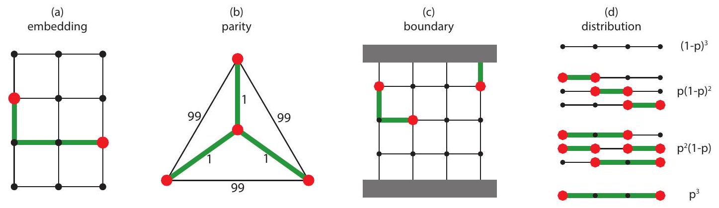
الشكل 1: الاختلافات الرئيسية بين مشكلة فك التشفير الكمي التي تم حلها بواسطة PyMatching ومشكلة المطابقة المثالية ذات الوزن الأدنى. في مشكلة MWPM المعتادة، يجب مطابقة جميع العقد ويتم مطابقتها باستخدام مجموعة غير متداخلة من الحواف. في مشكلة فك التشفير، (أ) يتم تنشيط مجموعة فرعية فقط من العقد، ويجب مطابقة هذه العقد فقط، و(ب) مجموعة الحواف المستخدمة لمطابقتها ليست مطلوبة أن تكون غير متداخلة. يتم مطابقة العقد المنشطة من خلال إيجاد مجموعة حواف حيث تحتوي العقد المنشطة على عدد فردي من الجيران في مجموعة الحواف، والعقد غير المنشطة تحتوي على عدد زوجي من الجيران في مجموعة الحواف، و(ج) قد تكون هناك عقد حدودية يمكن أن تحتوي على أي عدد من الجيران في مجموعة الحواف. (د) التوزيع المتوقع للعقد المنشطة ليس متساويًا. يتم توليده عن طريق أخذ عينات من الحواف، حيث يتم تضمين كل حافة بشكل مستقل مع بعض الاحتمالية، ثم تنشيط أي عقد تحتوي على عدد فردي من الجيران في مجموعة الحواف المأخوذة. وهذا يؤدي إلى أنه من غير المحتمل بشكل كبير رؤية مسافات كبيرة بين العقد المنشطة عند معدلات خطأ منخفضة، مما له آثار كبيرة على الوقت المتوقع لتشغيل الخوارزمية (انظر القسم 5).
. من الواضح أن ليس كل رسم بياني يحتوي على تطابق مثالي (شرط بسيط ضروري هو أنيجب أن يكون عددها زوجيًا؛ الشرط الضروري والكافي موفر من خلال نظرية توتي [Tut47]، ويمكن أن يحتوي الرسم البياني على أكثر من تطابق مثالي واحد بأقل وزن.
بالنظر إلى رسم بياني للكاشفمع مجموعة الرؤوسومجموعة من أحداث الكشف (العقد المميزة)نحن نحدد تطابقًا مضمنًا لـفيأن تكون مجموعة من الحوافبحيث يكون كل عقدة فييتعلق بعدد فردي من الحواف فيوكل عقدة فييتعلق بعدد زوجي من الحواف فيالمطابقة المدمجة ذات الوزن الأدنى هي مطابقة مدمجة لها أقل وزننلاحظ أن مشكلة المطابقة المدمجة ذات الوزن الأدنى لرسم بياني قياسي (لا يحتوي على حواف نصفية) تُعرف باسم الوزن الأدنى.-مشكلة الانضمام في مجال التحسين التوافقي (لـ ) [EJ73; KV18]. الاختلافات الرئيسية بين مشكلة المطابقة المدمجة ذات الوزن الأدنى التي نهتم بها من أجل تصحيح الأخطاء، ومشكلة MWPM التقليدية، موضحة في الشكل 1.
لا يحتاج جهاز فك التشفير إلى إخراج مجموعة الحواف مباشرة، بل يخرج، توقع أي من القياسات المنطقية القابلة للملاحظة قد تم قلبها. لقد نجح جهاز فك التشفير لدينا إذا توقع بشكل صحيح أي من الملاحظات قد تم قلبها، أي إذا. بعبارة أخرى، نحن نطبق تصحيحًا على المستوى المنطقي بدلاً من المستوى الفيزيائي، وهو ما يعادل ذلك لأن. هذه المخرجات عادة ما تكون أكثر ندرة: على سبيل المثال، في تجربة ذاكرة الشيفرة السطحية، التنبؤ هو ببساطة بت واحد، يتنبأ ما إذا كان المنطقي (أو نتيجة القياس القابلة للملاحظة تم قلبها بواسطة الخطأ. كما سنرى لاحقًا، فإن التنبؤ بالملاحظات المنطقيةبدلاً من الخطأ الفيزيائي الكامليؤدي ذلك إلى بعض التحسينات المفيدة. لاحظ أن PyMatching يدعم أيضًا إرجاع الخطأ الفيزيائي الكامل (على سبيل المثال، يمكن تعيين observable فريد لكل حافة)، ولكننا نطبق هذه التحسينات الإضافية عندما يكون عدد الملاحظات المنطقية صغيرًا (حتى 64 ملاحظة).
لاحظ أن وزن الحافةسلبي عندما. تفترض خوارزمية الإزهار النادرة لدينا بدلاً من ذلك أن أوزان الحواف غير سالبة. لحسن الحظ، من السهل فك تشفير متلازمةلرسم بياني للكاشفتحتوي على أوزان حواف سلبية من خلال استخدام معالجة مسبقة وبعدية فعالة لفك تشفير متلازمة معدلة بدلاً من ذلكباستخدام مجموعة من أوزان الحواف المعدلةتحتوي فقط على أوزان حواف غير سالبة. تُستخدم هذه الإجراء للتعامل مع أوزان الحواف السالبة في PyMatching ويتم شرحه في الملحق C. ومع ذلك، من الآن فصاعدًا، سنفترض، دون فقدان العمومية، أن لدينا رسمًا بيانيًا يحتوي فقط على أوزان حواف غير سالبة.
2.4 العلاقة بين المطابقة المثالية ذات الوزن الأدنى والمطابقة المدمجة
على الرغم من أن تطابقات الوزن الأدنى المضمنة والتطابقات المثالية هما مشكلتان مختلفتان، إلا أن هناك ارتباطًا وثيقًا بينهما. على وجه الخصوص، من خلال استخدام خوارزمية زمنية متعددة الحدود لحل مشكلة MWPM (مثل خوارزمية الزهرة)، يمكننا الحصول على خوارزمية زمنية متعددة الحدود لحل مشكلة MWEM من خلال تقليل. سنقوم الآن بوصف هذا التقليل لحالة أن الرسم البياني للكاشفليس له حدود، وفي هذه الحالة تكون مشكلة MWEM مكافئة لأقل وزن-مشكلة الانضمام (انظر [EJ73؛ KV18]). تم استخدام هذا الاختزال من قبل إدموندز وجونسون لخوارزمية الوقت المتعدد الحدود الخاصة بهم لحل مشكلة ساعي البريد الصيني [EJ73]. يمكن أيضًا التعامل مع الحدود مع تعديل صغير (على سبيل المثال، انظر [Fow15]).
بالنظر إلى رسم بياني للكاشفمع أوزان حواف غير سالبة (والتي، في الوقت الحالي، نفترض أنها بلا حدود، أي )، وتم إعطاء مجموعة من أحداث الكشف نحن نحدد رسم المسارأن تكون الرسم البياني الكامل على الرؤوسلكل حافةيتم تعيين وزن يساوي المسافةبين و في. هنا المسافة هو طول أقصر مسار بين و في، حيث هنا طول المسار هو مجموع أوزان الحواف التي يحتويها. بعبارة أخرى، رسم المسارهو الرسم البياني الفرعي للإغلاق المترى لـالمستحثة بواسطة الرؤوس. ميممنفييمكن العثور عليه بكفاءة باستخدام الخطوات الثلاث التالية:
قم بإنشاء رسم بياني مسارباستخدام خوارزمية ديكسترا.
ابحث عن المطابقة المثالية ذات الوزن الأدنىفيباستخدام خوارزمية بلوسوم.
استخدم وخوارزمية ديكسترا لبناء MWEM: . أين هناهو مسار بطول أدنى بين و في. انظر النظرية 12.10 من [KV18] للحصول على إثبات لهذا الاختزال، حيث أن الحد الأدنى لوزنهم-الانضمام هو MWEM الخاص بنا، ومجموعتهميتوافق مع لدينا. انظر أيضًا [Bar82؛ Ber+99] للاختزالات البديلة و[BDL22] لمراجعة حديثة.
لسوء الحظ، فإن حل هذه الخطوات الثلاث بشكل متسلسل مكلف من الناحية الحسابية؛ على سبيل المثال، فإن تكلفة تعداد الحواف فييتزايد بشكل تربيعي في عدد أحداث الكشفبينما نود في المثالي أن يكون لدينا جهاز فك تشفير بوقت تشغيل متوقع يتناسب بشكل خطي فيومع ذلك، تم استخدام هذا النهج التسلسلي على نطاق واسع من قبل باحثي QEC، على الرغم من أن أدائه بعيد جدًا عن الأمثل.
تم تقديم تحسين كبير من قبل فاولر [Fow15]. كانت الملاحظة الرئيسية التي قدمها فاولر هي أنه، بالنسبة لمشاكل QEC، عادةً ما تكون الحواف ذات الوزن المنخفض فقط فيتُستخدم فعليًا بواسطة بلوسوم. استغل نهج فاولر هذه الحقيقة من خلال تحديد نصف قطر استكشاف أولي في رسم كاشف، حيث تم استخدام عمليات بحث منفصلة لبناء بعض الحواف في. تم زيادة نصف قطر الاستكشاف بشكل تكيفي حسب الحاجة بواسطة خوارزمية الزهرة. نهجنا، الزهرة النادرة، مستوحى من عمل فاولر ولكنه يختلف في العديد من التفاصيل. قبل تقديم الزهرة النادرة، سنقدم نظرة عامة على خوارزمية الزهرة القياسية.
2.5 خوارزمية الإزهار
خوارزمية الزهرة، التي قدمها جاك إدموندز [Edm65b; Edm65a]، هي خوارزمية زمنها متعدد الحدود لإيجاد تطابق مثالي ذو وزن أدنى في رسم بياني. في هذا القسم، سنستعرض بعض المفاهيم الرئيسية في خوارزمية الزهرة الأصلية. لن نشرح خوارزمية الزهرة الأصلية بالكامل، حيث يوجد تداخل كبير مع خوارزمية الزهرة النادرة التي نصفها في القسم 3. بينما يوفر هذا القسم دافعًا لخوارزمية الزهرة النادرة، إلا أنه ليس شرطًا مسبقًا لبقية الورقة، لذا قد يرغب القارئ في الانتقال مباشرة إلى القسم 3. نشير القارئ إلى المراجع [Edm65b; Edm65a; Gal83; Kol09] للحصول على نظرة أكثر اكتمالاً على خوارزمية الزهرة.
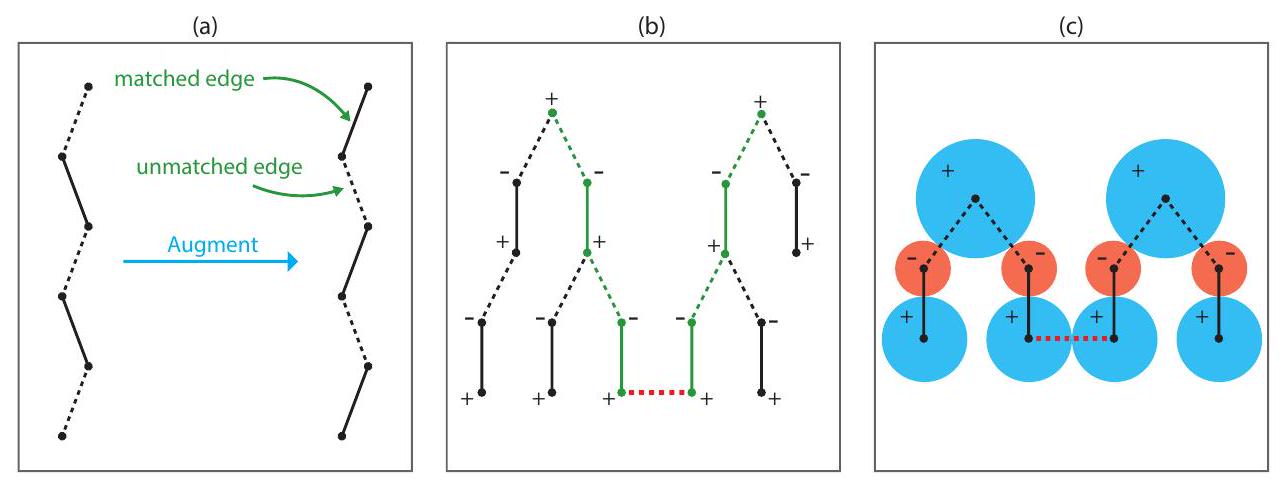
سنقوم أولاً بتقديم بعض المصطلحات. بالنظر إلى بعض المطابقاتفي رسم بيانينقول إن الحافة فييتطابق إذا كان أيضًا في، وغير متطابق في حالات أخرى، والعقدة تكون متطابقة إذا كانت متصلة بحافة متطابقة، وغير متطابقة في حالات أخرى. المطابقة ذات الحد الأقصى في العدد هي مطابقة تحتوي على أكبر عدد ممكن من الحواف. المسار المعزز هو مسار الذي يتناوب بين الحواف المتطابقة وغير المتطابقة، ويبدأ وينتهي عند عقدتين غير متطابقتين متميزتين.
الشكل 2: (أ) تعزيز مسار التعزيز. تصبح الحواف المتطابقة غير متطابقة، وتصبح الحواف غير المتطابقة متطابقة. (ب) أمثلة على شجرتين متناوبتين في خوارزمية الزهرة للعثور على تطابق أقصى. تحتوي كل شجرة على عقدة واحدة غير متطابقة. أصبحت الشجرتان متصلتين عبر الحافة الحمراء المتقطعة. المسار بين جذور الشجرتين، من خلال الحواف الخضراء والحافة الحمراء، هو مسار تعزيز. (ج) مثال على شجرتين متناوبتين في خوارزمية الزهرة للعثور على تطابق مثالي بأقل وزن. تحتوي كل عقدةالآن لديها متغير مزدوجالذي، عندماإيجابي، يمكننا تفسيره على أنه نصف قطر منطقة مركزها العقدة. حافة جديدة ( ) مع الوزن يمكن استكشافه فقط بواسطة الشجرة المتناوبة إذا كانت مشدودة، مما يعني أن المتغيرات المزدوجة و يرضي.
بالنظر إلى مسار معززفييمكننا دائمًا زيادة عدد المطابقاتواحدًا بواحد عن طريق الاستبدالمع المطابقة الجديدة. نشير إلى هذه العملية، التي تتضمن إضافة كل حافة غير متطابقة فيإلىوإزالة كل حافة متطابقة فيمن، كما هو الحال في تعزيز المسار المعزز (انظر الشكل 2(أ)). ينص نظرية بيرج على أن التطابق له أقصى عدد من العناصر إذا وفقط إذا لم يكن هناك مسار معزز [Ber57].
2.5.1 حل مشكلة المطابقة ذات الحد الأقصى من حيث العدد
سنقدم الآن نظرة عامة على النسخة الأصلية غير الموزونة من خوارزمية الزهرة، التي تجد تطابقًا بأقصى عدد من العناصر (كما قدمها إدموندز في [Edm65b]). تُستخدم خوارزمية الزهرة غير الموزونة كروتين فرعي من قبل خوارزمية الزهرة الأكثر عمومية للعثور على تطابق مثالي بأقل وزن (التي اكتشفها أيضًا إدموندز في [Edm65a])، والتي سنستعرضها في القسم 2.5.2. تستند الخوارزمية إلى نظرية بيرج. بدءًا من تطابق تافه، تتقدم من خلال العثور على مسار معزز، وتعزيز المسار، ثم تكرار هذه العملية حتى لا يمكن العثور على مسار معزز، وفي هذه النقطة نعلم أن التطابق هو الأقصى. يتم العثور على المسارات المعززة من خلال بناء أشجار متناوبة داخل الرسم البياني. شجرة متناوبةفي الرسم البيانيهو شجرة فرعية منمع وجود عقدة غير متطابقة كجذر لها، ولكل مسار من الجذر إلى الورقة يتناوب بين الحواف غير المتطابقة والمتطابقة، انظر الشكل 2(b). هناك نوعان من العقد فيعقد “خارجي” (موسوم بـ “+”) وعقد “داخلي” (موسوم بـ “-“). كل عقدة داخلية مفصولة عن عقدة الجذر بواسطة مسار بطول فردي، بينما كل عقدة خارجية مفصولة بواسطة مسار بطول زوجي. كل عقدة داخلية لها طفل واحد (عقدة خارجية). يمكن أن تحتوي كل عقدة خارجية على أي عدد من الأطفال (جميع العقد الداخلية). جميع العقد الورقية هي عقد خارجية.
في البداية، كل عقدة غير متطابقة هي شجرة متناوبة بسيطة (عقدة جذر). للعثور على مسار معزز، يبحث الخوارزم في العقد المجاورة فيالعقد الخارجية في كل شجرة. إذا، خلال هذا البحث، حافة يتم العثور عليه بحيث هو عقدة خارجية لـ و هو عقدة خارجية من شجرة أخرىثم تم العثور على مسار معزز، يربط جذور و ، انظر الشكل 2(b). يتم توسيع هذا المسار، ويتم إزالة الشجرتين، وتستمر عملية البحث. إذا كان هناك حافة ( ) يوجد بين عقدة خارجية فيوعقدة متطابقةليس في أي شجرة (أيتمت المطابقة)، ثموتمت إضافة مباراته إلى“. أخيرًا، إذا كان هناك حافة (إذا وُجدت ) بين عقدتين خارجيّتين من نفس الشجرة، فإن حلقة ذات طول فردي قد وُجدت، وتشكل زهرة. كانت إحدى الرؤى الرئيسية لإدموندز هي أن الزهرة يمكن اعتبارها عقدة افتراضية، يمكن مطابقتها أو أن تنتمي إلى شجرة متناوبة مثل أي عقدة أخرى. ومع ذلك، سنشرح كيف يتم التعامل مع الزهور بمزيد من التفصيل في سياق خوارزمية الزهرة النادرة لدينا في القسم 3.
2.5.2 حل مشكلة المطابقة المثالية ذات الوزن الأدنى
التمديد من إيجاد تطابق بأقصى عدد من العناصر إلى إيجاد تطابق مثالي بأقل وزن مدفوع بصياغة المشكلة كبرنامج خطي [Edm65a]. يتم إضافة قيود على كيفية نمو الأشجار المتناوبة، وتضمن هذه القيود أن يكون وزن التطابق المثالي هو الأدنى بمجرد العثور عليه. صياغة المشكلة كبرنامج خطي ليست مطلوبة لفهم الخوارزمية، أو لإثبات صحتها. ومع ذلك، فإنها توفر دافعًا مفيدًا، وتستخدم القيود والتعريفات المستخدمة في البرنامج الخطي أيضًا في خوارزمية الزهرة نفسها. لذلك، سنصف البرنامج الخطي هنا من أجل الاكتمال.
سنشير إلى حواف الحدود لبعض مجموعة من العقدبواسطة، وسيسمح بـكن مجموعة جميع المجموعات الفرعية لـمن عدد فردي لا يقل عن ثلاثة، أينحن نحدد الحواف المتصلة بعقدة واحدةبواسطة (أي ). سنستخدم متجه الحدوث لتمثيل تطابقأينإذا و إذا. نحن نحدد وزن الحافةبواسطةيمكن بعد ذلك صياغة مشكلة المطابقة المثالية ذات الوزن الأدنى كالتالي كبرنامج عددي:
قدم إدموندز الاسترخاء البرمجي الخطي التالي للبرنامج الصحيح أعلاه:
لاحظ أن القيود في المعادلة 4c تُحقق بواسطة أي تطابق مثالي، لكن إدموندز أظهر أن إضافتها تضمن أن البرنامج الخطي لديه حل مثالي صحيح. بعبارة أخرى، يمكن استبدال قيد التكامل (المعادلة 3c) بالمتباينات في المعادلة 4c والمعادلة 4d.
كل برنامج خطي (يشار إليه بالبرنامج الخطي الأساسي، أو المشكلة الأساسية) له برنامج خطي مزدوج (أو مشكلة مزدوجة). المزدوج للمشكلة الأساسية المذكورة أعلاه هو:
حيث يتم تعريف تراجع الحافة على أنه
نقول إن الحافة مشدودة إذا كانت لديها انزلاق صفر. هنا قمنا بتعريف متغير مزدوجلكل عقدةبالإضافة إلى متغير مزدوجلكل مجموعة. بينما كل متغيرمقيد بأن يكون غير سالب (المعادلة 5ج)، كلمسموح له أن يأخذ أي قيمة. على الرغم من أن لدينا عددًا أسيًا منالمتغيرات، يتبين أن هذه ليست مشكلة لأن فقطغير صفر في أي مرحلة من مراحل خوارزمية الإزهار.
نسترجع الآن بعض المصطلحات والخصائص العامة للبرامج الخطية (انظر [MG07؛ KV18] لمزيد من التفاصيل). تكون حل البرنامج الخطي قابلاً للتطبيق إذا كان يلبي قيود البرنامج الخطي. دون فقدان العمومية، نفترض أن البرنامج الخطي الأساسي هو مشكلة تقليل (وفي هذه الحالة يكون ثنائيه مشكلة تعظيم). بموجب نظرية الازدواجية القوية، إذا كان لكل من البرنامج الخطي الأساسي والثنائي حل قابل للتطبيق، فإن كلاهما يمتلك أيضًا حلاً مثاليًا. علاوة على ذلك، فإن الحد الأدنى من المشكلة الأساسية يساوي الحد الأقصى من ثنائيتها، مما يوفر “دليلاً عددياً” على المثالية.
يمكننا الحصول على دليل “تركيبي” على الأمثلية لأي برنامج خطي باستخدام شروط التراخي التبادلي. كل قيد في المشكلة الأولية مرتبط بمتغير من المشكلة المزدوجة (وعكس ذلك صحيح). دعنا نربط الـ القيد الأساسي مع المتغير الثنائي (وعكس ذلك). تنص شروط التكميلية على أنه، إذا كان لدينا زوج من الحلول المثلى، فإن إذا كان إذا كانت المتغير الثنائي أكبر من الصفر، فإن يتم تحقيق القيد الأساسي بالتساوي. وبالمثل، إذا كان إذا كانت المتغير الأساسي أكبر من الصفر، فإنيتم تحقيق القيد المزدوج بالتساوي. بشكل أكثر تحديدًا، بالنسبة لزوج البرامج الخطية الأولية والثانوية المحددة التي نعتبرها، فإن شروط التراخي التكاملي هي:
تُستخدم هذه الشروط كقاعدة توقف في خوارزمية الزهرة (مع تحقيق المعادلة 7 طوال الوقت) وتوفر دليلاً على الأمثلية.
بينما من الملائم استخدام نظرية الازدواجية القوية، لأنها تنطبق على أي برنامج خطي، إلا أن صحتها ليست بديهية على الفور وإثباتها معقد للغاية (انظر [MG07؛ KV18]). لحسن الحظ، يمكننا الحصول على إثبات بسيط لجدوى مشكلة المطابقة المثالية ذات الوزن الأدنى مباشرة، دون الحاجة إلى نظرية الازدواجية القوية [Gal83]. أولاً، نلاحظ أنه بالنسبة لأي حل مزدوج قابل للتطبيق، لدينا أن أي مطابقة مثاليةيُرضي
حيث هنا المساواة تأتي من تعريف وتستخدم المعادلة 5 ب والمعادلة 5 ج (أي حقيقة أن الحل المزدوج قابل للتطبيق) وحقيقة أن هو تطابق مثالي. ومع ذلك، إذا كان لدينا تطابق مثالي التي تلبي أيضًا المعادلة 7 والمعادلة 8 بدلاً من ذلك لدينا
وهكذا المطابقة المثاليةيتميز بوزن خفيف جداً. حتى الآن في هذا القسم، نظرنا فقط في الحالة التي يكون فيها كل حافة زوجًا من العقد (مجموعة ذات عدد عناصر يساوي اثنين). دعونا الآن نعتبر الحالة الأكثر عمومية (المطلوبة لفك التشفير) حيث يمكن أن يكون لدينا أيضًا حواف نصفية. بشكل أكثر تحديدًا، لدينا الآن مجموعة الحوافحيث كلهو حافة منتظمة وكلهو نصف حافة (مجموعة عقد ذات عدد واحد). نلاحظ أن المطابقة المثالية تُعرف الآن كمجموعة فرعية من هذه المجموعة العامة من الحواف، لكن تعريفها بخلاف ذلك لم يتغير (المطابقة المثالية هي مجموعة حواف).بحيث يكون كل عقدة متصلة بحافة واحدة بالضبط في ). نحن نوسع تعريفنا لـ أن يكون
مع هذا التعديل، لا يزال الدليل البسيط على الصحة أعلاه ساريًا و slack(e) لحافة نصفيةمحدد بشكل جيد بواسطة المعادلة 6.
يبدأ خوارزمية الإزهار لإيجاد تطابق مثالي ذو وزن أدنى بتطابق فارغ وحل ثنائي قابل للتطبيق، ويزيد بشكل تكراري من عدد عناصر التطابق وقيمة الهدف الثنائي مع ضمان بقاء قيود المشكلة الثنائية مُرضية. في النهاية، سيكون لدينا زوج من الحلول القابلة للتطبيق للمشكلة الأولية والثنائية التي تلبي شروط التراخي التبادلي (المعادلة 7 والمعادلة 8) في تلك النقطة نعلم أننا لدينا تطابق مثالي ذو وزن أدنى. تتقدم الخوارزمية على مراحل، حيث تتكون كل مرحلة من تحديث “أساسي” و”ثنائي”. نكرر هذه التحديثات الأساسية والثنائية حتى لا يمكن تحقيق المزيد من التقدم، وفي هذه المرحلة، بشرط أن يقبل الرسم البياني تطابقًا مثاليًا، ستتحقق شروط التراخي التكميلية وبالتالي سيتم العثور على التطابق المثالي ذو الوزن الأدنى. سنقوم الآن بتفصيل التحديثات الأساسية والثنائية بمزيد من التفصيل.
في التحديث الأولي، نعتبر فقط الرسم البياني الفرعيمنيتكون من حواف ضيقة ويحاول العثور على تطابق بمرتبة أعلى، أساسًا من خلال تشغيل تعديل طفيف على خوارزمية الزهرة غير الموزونة على هذه الرسم البياني الفرعي. في [Kol09]، تُشير العمليات الأربعة المسموح بها في التحديث الأساسي إلى “نمو” و”زيادة” و”انكماش” و”توسع”. تحدث الثلاثة الأولى من هذه بالفعل في النسخة غير الموزونة من الزهرة التي تم مناقشتها في القسم 2.5.1. تتكون عملية النمو من إضافة زوج متطابق من العقد إلى شجرة متناوبة. الزيادة هي عملية زيادة المسار بين جذور شجرتين عندما تصبح متصلة. الانكماش هو الاسم المستخدم لعملية تشكيل زهرة عند العثور على دورة ذات طول فردي. العملية التي تختلف قليلاً في النسخة الموزونة هي التوسع. يمكن أن تحدث هذه العملية التوسعية كلما كانت المتغير الثنائيمن أجل زهرةيصبح صفرًا؛ عندما يحدث هذا، تتم إزالة الزهرة، ويتم إضافة المسار ذو الطول الفردي من خلال الزهرة إلى الشجرة المتناوبة، وتصبح العقد في المسار ذو الطول الزوجي متطابقة مع جيرانها. يختلف هذا قليلاً عن النسخة غير الموزونة كما وصفناها، حيث يتم توسيع الزهور فقط عندما يصبح المسار الذي تنتمي إليه معززًا (في هذه المرحلة، تصبح جميع العقد في دورة الزهرة متطابقة). نشير إلى القارئ إلى [Kol09] للحصول على وصف أكثر اكتمالاً لهذه العمليات في التحديث الأساسي (ومخططات مرتبطة)، على الرغم من أننا نكرر أن مفاهيم مشابهة جدًا ستتم تغطيتها بمزيد من التفصيل عندما نصف الزهرة النادرة في القسم 3.
في التحديث الثنائي، نحاول زيادة الهدف الثنائي من خلال تحديث قيمة المتغيرات الثنائية، مع ضمان بقاء الحواف في الأشجار المتناوبة والزهور مشدودة، وأيضًا ضمان بقاء المتغيرات الثنائية حلاً قابلاً للمشكلة الثنائية (يجب أن تظل المتباينات في المعادلة 5 ب والمعادلة 5 ج مُرضية). بشكل عام، الهدف من التحديث الثنائي هو زيادة الهدف الثنائي بطريقة تجعل المزيد من الحواف تصبح مشدودة، مع ضمان بقاء الأشجار المتناوبة الحالية، والزهور، والحواف المتطابقة سليمة. المتغيرات الثنائية الوحيدة التي نقوم بتحديثها هي تلك التي تنتمي إلى العقد في شجرة متناوبة. لكل شجرة متناوبةنحن نختار تغييرًا مزدوجًاونزيد المتغير الثنائي لكل عقدة خارجيةمعلكن قلل المتغير الثنائي لكل عقدة داخليةمعتذكر أن كل عقدة فيإما أن يكون عقدة عادية أو زهرة، وإذا كانت العقدة زهرة، فإننا نقوم بتغيير المتغير الثنائي للزهرة (مع ترك المتغيرات الثنائية للعقد التي تحتويها دون تغيير). لاحظ أن هذا التغيير يضمن أن تظل جميع الحواف الضيقة ضمن شجرة متناوبة معينة ضيقة، ولكن نظرًا لأن المتغيرات الثنائية للعقد الخارجية تزداد، فمن الممكن أن تصبح بعض الحواف المجاورة لها (غير الضيقة) ضيقة (على أمل أن يسمح لنا ذلك بالعثور على مسار معزز بين الأشجار المتناوبة في التحديث الأولي التالي). تفرض قيود المشكلة الثنائية (المتباينات المعادلة 5ب والمعادلة 5ج) قيودًا على اختيار؛ على وجه الخصوص، يجب أن تظل الفجوات لجميع الحواف غير سالبة، ويجب أن تظل المتغيرات الثنائية للزهور أيضًا غير سالبة.
هناك العديد من الاستراتيجيات المختلفة الصالحة التي يمكن اتخاذها للتحديث المزدوج. في نهج الشجرة الواحدة، نختار شجرة واحدة.وتحديث المتغيرات الثنائية فقط للعقد فيبالحد الأقصىبحيث تظل قيود المشكلة المزدوجة مُرضية (على سبيل المثال، نقوم بتغيير المتغيرات المزدوجة حتى يصبح حافة مشدودة أو يصبح متغير الزهرة المزدوجة صفرًا). في شجرة ثابتة متعددةنقوم بتحديث المتغيرات المزدوجة لجميع الأشجار المتناوبة بنفس المقدار (مرة أخرى بأقصى قدر يضمن بقاء القيود المزدوجة مُرضية). في متغير شجرة متعددةنهج، نختار مختلفاًلكل شجرةنسختنا من خوارزمية الزهرة (زهرة متفرقة) تستخدم شجرة ثابتة متعددةالنهج. هذه هي الفروق الرئيسية مع المراجع [FWH12a; FWH12b; Fow15]، التي تستخدم بدلاً من ذلك نهج الشجرة الواحدة. انظر [Kol09] لمناقشة أكثر تفصيلاً ومقارنة بين هذه الاستراتيجيات المختلفة.
في الشكل 2(c) نقدم مثالاً مع شجرتين متناوبتين، ونصور متغيراً مزدوجاً كونه نصف قطر منطقة دائرية مركزة على عقدته. من خلال تصور المتغيرات المزدوجة بهذه الطريقة، يكون الحافة بين عقدتين تافهتين مشدودة إذا كانت المناطق عند نقاط نهايتها تلامس. في هذا المثال، نقوم بتحديث المتغيرات المزدوجة (الأشعة) حتى تلامس الشجرتان المتناوبتان، في هذه النقطة تصبح الحافة التي تربط الشجرتين مشدودة، ويمكننا زيادة المسار بين جذور الشجرتين. لاحظ أنه يمكننا فقط تصور المتغيرات المزدوجة كأشعة مناطق بهذه الطريقة عندما تكون غير سالبة. بينما تكون المتغيرات المزدوجة للزهور دائماً غير سالبة (كما يفرضه المعادلة 5c)، يمكن أن تصبح المتغيرات المزدوجة للعقد العادية سالبة بشكل عام. ومع ذلك، عند تشغيل خوارزمية الزهرة في رسم بياني على شكل مسار، فإن المتغير الثنائي لكل عقدة منتظمة يكون دائمًا غير سالب، وذلك بسبب هيكل الرسم البياني. يمكن فهم ذلك على النحو التالي. اعتبر أي عقدة داخلية منتظمة.هذا ليس زهرة، التي يجب أن تحتوي بالضرورة على عقدة خارجية واحدة فقط.في شجرتها المتناوبة (مطابقتها)، بالإضافة إلى عقدتها الخارجية الأم الواحدةتذكر أن رسم المسار هو رسم بياني كامل حيث الوزن لكل حافة ( ) هو طول أقصر مسار بين العقد و في بعض الرسوم البيانية الأخرى (على سبيل المثال، في حالتنا دائمًا رسم بياني للكاشف). لذلك هناك أيضًا حافة ( ) في رسم المسار مع الوزن ، حيث نعلم أن هناك على الأقل مسار واحد منإلىبطول، الذي يتوافق مع اتحاد أقصر مسار منإلىوأقصر طريق منإلى. لذلك، لا يمكننا أن نملكدون أن يكونالذي سينتهك المعادلة 5 ب. بشكل أكثر تحديدًا، إذاثم نعلم أن الحافةيجب أن تكون محكمة، مما يعني أنه يمكننا تشكيل زهرة جديدة من دورة الزهور (يمكن أن تصبح هذه الزهرة عقدة خارجية في الشجرة المتناوبة (التي قد تكون الآن تافهة).
3 زهرة نادرة
النسخة من خوارزمية الزهرة التي نقدمها، والتي نسميها الزهرة النادرة، تحل مباشرةً مشكلة المطابقة المدمجة ذات الوزن الأدنى المتعلقة بتصحيح أخطاء الكم. الزهرة النادرة لا تحتوي على خطوة ديكسترا منفصلة لبناء الحواف في رسم المسار.. بدلاً من ذلك، يتم استرداد معلومات أقصر مسار كجزء من نمو الأشجار المتناوبة نفسها. بعبارة أخرى، نحن نكتشف ونخزن حافة فقطفيبالضبط إذا ومتى كانت مطلوبة من قبل خوارزمية بلوسوم؛ الحواف التي نتتبعها في أي نقطة في الخوارزمية تتوافق تمامًا مع مجموعة الحواف الضيقة فييتم استخدامه لتمثيل شجرة متناوبة، أو زهرة، أو مباراة. وهذا يؤدي إلى تسريع كبير جداً مقارنة بالنهج التسلسلي، حيث تكون جميع الحواف فيتوجد باستخدام بحث ديكسترا، على الرغم من أن الغالبية العظمى منها لا تصبح أبدًا حوافًا ضيقة في خوارزمية الزهرة. نحن نسمي الخوارزمية زهرة متناثرة، لأنها تستغل حقيقة أن نسبة صغيرة فقط من عقد الكاشف تتوافق مع أحداث الكشف لمشاكل تصحيح الأخطاء الكمية النموذجية (ويمكن ربط أحداث الكشف محليًا)، ولتلك المشاكل، تفحص طريقتنا فقط مجموعة صغيرة من العقد والحواف في رسم الكاشف.
قبل شرح الزهرة النادرة وتنفيذنا، سنقوم أولاً بتقديم وتعريف بعض المفاهيم.
3.1 المفاهيم الرئيسية
3.1.1 ملء مناطق الرسم البياني
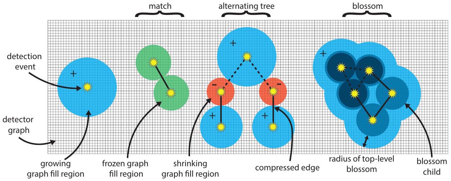
منطقة تعبئة الرسم البيانينصف القطرهو منطقة استكشافية من رسم بياني للكاشف. منطقة ملء الرسم البيانيتحتوي على العقد في رسم الكاشف التي تقع ضمن مسافةمصدره. مصدر منطقة تعبئة الرسم البياني هو إما حدث اكتشاف واحد، أو سطح مناطق تعبئة رسم بياني أخرى تشكل زهرة. سنقوم بتعريف الزهور لاحقًا، ومع ذلك في حالة أن منطقة تعبئة الرسم البيانيلديه حدث كشف واحدكمصدره، كل عقدة تقع ضمن مسافةمنمحتوى فيتذكر أن المسافةبين عقدتين و هو مجموع أوزان الحواف على طول أقصر مسار وزني بينهما. لاحظ أن منطقة ملء الرسم البياني في الزهرة النادرة تشبه عقدة أو زهرة في خوارزمية الزهرة القياسية، ونصف قطر منطقة ملء الرسم البياني يشبه المتغير الثنائي لعقدة أو زهرة في الزهرة القياسية. تتقدم خوارزمية الزهرة النادرة على طول خط زمني (انظر القسم 3.1.7)، ويمكن أن يكون لنصف قطر كل منطقة ملء رسم بياني واحد من ثلاثة معدلات نمو: +1 (تنمو)، -1 (تنكمش) أو 0 (مجمدة). لذلك، في أي وقتيمكننا تمثيل نصف قطر منطقة باستخدام معادلة، حيث سنشير أحيانًا إلى منطقة ملء الرسم البياني ببساطة على أنها منطقة عندما يكون ذلك واضحًا من السياق.
نرمز بـمجموعة أحداث الكشف في منطقةعندما تحتوي منطقة على حدث كشف واحد فقط،نحن نشير إلى ذلك على أنه منطقة تافهة. يمكن أن تحتوي المنطقة على أحداث كشف متعددة إذا كان لديها زهرة كمصدر لها. بالإضافة إلى معادلة نصف القطر الخاصة بها، قد تحتوي كل منطقة ملء رسم بياني أيضًا على أطفال زهرة ووالد زهرة (كلاهما معرف في القسم 3.1.6). كما أن لديها منطقة قشرة، مخزنة ككومة. منطقة القشرة لمنطقة ما هي مجموعة من عقد الكاشف التي تحتوي عليها، باستثناء عقد الكاشف الموجودة في أطفال الزهرة الخاصة بها. نقول إن ملء الرسم البياني
الشكل 3: المفاهيم الرئيسية في الإزهار النادر
المنطقة نشطة إذا لم يكن لديها والد مزهر. سنسمح بـتشير إلى مجموعة جميع مناطق ملء الرسم البياني.
3.1.2 الحواف المضغوطة
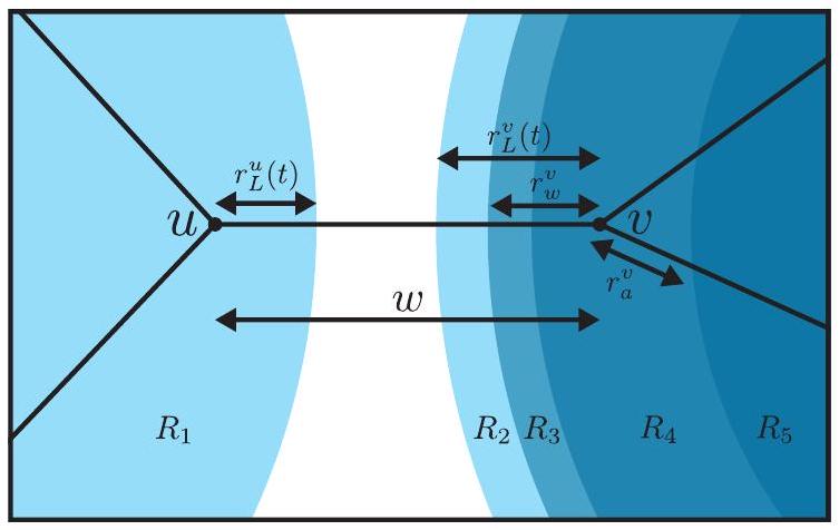
يمثل الحافة المضغوطة مسارًا عبر رسم الكاشف بين حدثين للكشف، أو بين حدث كشف وحدود. بالنظر إلى مساربين و ، حيث هو حدث اكتشاف و إما حدث اكتشاف أو يدل على الحدود، الحافة المضغوطةمرتبط بـ هو زوج من العقد ( ) عند نقاط النهاية لـ بالإضافة إلى مجموعة الملاحظات المنطقيةمقلوب عن طريق قلب جميع الحواف فيالحافة المضغوطةلذلك هو تمثيل مضغوط للمسارتحتوي على جميع المعلومات المتعلقة بتصحيح الأخطاء، ويمكن تخزينها، بالنسبة لرسم بياني للكاشف معين، باستخدام كمية ثابتة من البيانات (غير معتمدة على طول المسار). عندما يكون اختيار المسارلزوج من أحداث الكشف المعطاة (من الواضح من السياق، يمكننا الإشارة إلى الحافة المضغوطة بدلاً من ( )، وقد تشير أيضًا إلى مجموعة الملاحظات المنطقية بواسطةنحدد طول الحافة المضغوطة بأنه المسافةبين نقطتي نهايته و .
كل حافة مضغوطةفي الإزهار المتناثر يتوافق مع أقصر مساربين و . ومع ذلك، يمكننا استخدام حافة مضغوطة لتمثيل أي مسار بين و وعند استخدامها في خوارزمية الاتحاد-البحث (انظر الملحق أ) فإن المسارلا تحتاج أن تكون بحد أدنى من الوزن. تُستخدم الحواف المضغوطة في تمثيل عدة هياكل بيانات في الزهرة النادرة (الأشجار المتناوبة، المطابقات والزهور). على وجه الخصوص، كل حافة مضغوطة ( ) يتوافق مع حافة في رسم المسار ، ولكن على عكس النهج التسلسلي القياسي لتنفيذ جهاز فك التشفير MWPM، نحن نكتشف ونبني فقط مجموعة صغيرة من الحواف فيمطلوب من الزهرة النادرة.
سنسمحكن مجموعة جميع الحواف المضغوطة الممكنة التي يمكن أن تمثل أقصر المسارات بين عقد الكاشف (أي المجموعة يحتوي على حافة مضغوطة ( ) لكل حافة في ). لمنطقة نرمز بـحواف مضغوطة على الحدود، يُعرَّف بأنه
3.1.3 حواف المنطقة
يصف حافة المنطقة علاقة بين منطقتين مملوءتين في الرسم البياني، أو بين منطقة وحدودها. نحن نستخدم ( ) للدلالة على حافة منطقة، حيث هنا و كلاهما منطقتان. كلما وصفنا حافة بين منطقتين، أو بين منطقة وحدود، فإنه يُفهم أنه حافة منطقة. حافة المنطقة ( ) تتضمن نقاط نهايتها و بالإضافة إلى حافة مضغوطةيمثل أقصر مسار بين أي حدث اكتشاف فيوأي حدث اكتشاف في“. نحن نستخدم أحيانًا الرموز ( ) لحافة المنطقة لتحديد الاثنين بشكل صريح المناطق و جنبًا إلى جنب مع نقاط النهاية ( ) من الحافة المضغوطة مرتبط به.
بالنسبة لأي حافة منطقة تظهر في الإزهار النادر، فإن الثوابت التالية دائمًا ما تكون صحيحة:
إذا و كلا المنطقتين، إذن إما و كلاهما مناطق نشطة (بدون والد زهور)، أو كلاهما له نفس والد الزهور.
الحافة المضغوطة (مرتبط بحافة منطقة ) دائمًا ضيق (سيتوافق مع حافة ضيقة في في الإزهار). بشكل أكثر دقة، حافة مضغوطة ( ) ضيق إذا كان يفي بـ
بعبارة أخرى، إذا كان هناك حافة منطقة ( )، ثم المناطق و يجب أن يكون مؤثراً.
3.1.4 المباريات
نحن نسمي زوجًا من المناطق و التي تتطابق مع بعضها البعض مباراة. إذا و تتطابق، وهذا يتوافق مع الحافة المضغوطة بين و التطابق على رسم المسار. المناطق المتطابقة و يجب أن تكون متلامسة، مُعينة بمعدل نمو صفر (إنها مجمدة)، ويجب أن تكون متصلة بحافة المنطقة ( ) والتي نشير إليها باسم حافة المطابقة. مثال على المطابقة موضح في منتصف الشكل 3. في البداية، تكون جميع المناطق غير متطابقة، وعندما تنتهي الخوارزمية، تكون كل منطقة (سواء كانت منطقة تافهة أو زهرة) متطابقة إما مع منطقة أخرى أو مع الحدود.
3.1.5 الأشجار المتناوبة
الشجرة المتناوبة هي شجرة حيث يتوافق كل عقدة مع منطقة ملء نشطة في الرسم البياني، ويتوافق كل حافة مع حافة المنطقة. نشير إلى كل حافة منطقة في الشجرة المتناوبة باسم حافة الشجرة. يجب أن تكون المنطقتان المتصلتان بحافة الشجرة متلامستين دائمًا (نظرًا لأن كل حافة شجرة هي حافة منطقة).
تحتوي الشجرة المتناوبة على منطقة نمو واحدة على الأقل ويمكن أن تحتوي أيضًا على مناطق انكماش، وتحتوي دائمًا على منطقة نمو واحدة أكثر من منطقة انكماش. يمكن أن تحتوي كل منطقة نمو على أي عدد من الأطفال (كل منهم طفل شجرة)، يجب أن تكون جميعها مناطق انكماش، ويمكن أن يكون لها والد واحد (والد شجرة)، وهو أيضًا منطقة انكماش. تحتوي كل منطقة انكماش على طفل واحد، وهو منطقة نمو، بالإضافة إلى والد واحد، وهو أيضًا منطقة نمو. لذلك، فإن أوراق الشجرة المتناوبة هي دائمًا مناطق نمو. مثال على شجرة متناوبة موضح في الشكل 3.
3.1.6 الأزهار
عندما تصطدم منطقتان نمو من نفس الشجرة المتناوبة ببعضهما البعض، فإنهما تشكلان زهرة، وهي منطقة تحتوي على دورة ذات طول فردي من المناطق تُسمى دورة الزهرة. بشكل أكثر تحديدًا، سنشير إلى دورة الزهرة كزوج مرتب من المناطق ( ) لبعض الأعداد الفردية وكل منطقة في دورة الزهرة متصلة بكل من جيرانهما بواسطة حافة منطقة. بعبارة أخرى، تحتوي دورة الزهرة على حواف مناطق . مثال على زهرة موضح على الجانب الأيمن من الشكل 3.
تُسمى المناطق في دورة الزهرة بأطفال الزهرة. إذا كانت زهرة تحتوي على منطقة كواحد من أطفالها، فإننا نقول إن هو والد الزهرة لـ . يجب أن تكون المناطق المجاورة في دورة الزهرة متلامسة (كما يتطلب الأمر من كونها متصلة بواسطة حافة منطقة). يمكن أيضًا أن تكون الأزهار متداخلة؛ يمكن أن يكون كل طفل زهرة بنفسه زهرة، مع أطفاله الخاصين. على سبيل المثال، فإن الطفل الأيسر العلوي من الزهرة في الشكل 3 هو زهرة بنفسه، مع ثلاثة أطفال زهرة. يُعتبر سليل زهرة من زهرة منطقة إما أنها طفل زهرة لـ أو أنها بشكل متكرر سليل لأي طفل زهرة من . وبالمثل، فإن سلف زهرة من هو منطقة إما أنها والد الزهرة لـ أو (بشكل متكرر) سلف والد الزهرة لـ . نصف القطر لزهرة (متغيرها المزدوج في خوارزمية الزهرة القياسية) هو المسافة التي نمتها منذ تشكيلها (أقل مسافة بين نقطة على
سطحها وأي نقطة على مصدرها). يتم تصور ذلك على أنه المسافة عبر قشرة الزهرة في الشكل 3.
نقول إن عقدة الكاشف موجودة في منطقة إذا كانت في منطقة القشرة لـ . يمكن أن توجد عقدة الكاشف فقط في منطقة واحدة على الأكثر (تكون مناطق القشرة غير متداخلة). إذا لم تكن عقدة الكاشف موجودة في منطقة، نقول إن العقدة فارغة، وإذا كانت موجودة فهي مشغولة. نقول إن عقدة الكاشف مملوكة لمنطقة إما إذا كانت موجودة في ، أو إذا كانت موجودة في سليل زهرة من . المسافة بين عقدة الكاشف وسطح منطقة هي
حيث هنا تشير إلى أن إما أنها سليل لـ أو . إذا كانت فإن عقدة الكاشف مملوكة للمنطقة ، إذا كانت فإن عقدة الكاشف ليست مملوكة لـ ، بينما إذا كانت فإن قد تكون مملوكة أو لا تكون مملوكة لـ (إنها على سطح ).
3.1.7 الجدول الزمني
تتقدم الخوارزمية على طول جدول زمني مع الوقت الذي يزداد بشكل أحادي مع حدوث ومعالجة أحداث مختلفة. تشمل أمثلة الأحداث وصول منطقة إلى عقدة، أو اصطدامها بمنطقة أخرى. يتم تحديد الوقت الذي يحدث فيه كل حدث بناءً على معادلات نصف القطر للمناطق المعنية، بالإضافة إلى هيكل الرسم البياني. تنتهي الخوارزمية عندما لا يتبقى المزيد من الأحداث ليتم معالجتها، وهو ما يحدث عندما يتم مطابقة جميع المناطق، وبالتالي تصبح مجمدة.
3.2 الهيكل
تنقسم زهرة متفرقة إلى مكونات مختلفة: مطابقة، ومغمر، ومتتبع. كل مكون له مسؤوليات مختلفة. المطابق مسؤول عن إدارة هيكل الأشجار المتناوبة والأزهار، دون معرفة الهيكل الأساسي لرسم الكاشف. يتعامل المغمر مع كيفية نمو مناطق ملء الرسم البياني وانكماشها في رسم الكاشف، بالإضافة إلى ملاحظة متى تصطدم منطقة بمنطقة أخرى أو الحدود. عندما يلاحظ المغمر اصطدامًا يتضمن منطقة، أو عندما تصل منطقة إلى نصف قطر صفر، يقوم المغمر بإخطار المطابق، الذي يكون مسؤولًا بعد ذلك عن تعديل هيكل الأشجار المتناوبة أو الأزهار. المتتبع مسؤول عن التعامل مع متى تحدث الأحداث المختلفة، ويضمن أن يتعامل المغمر مع الأحداث بالترتيب الصحيح، بمساعدة قائمة انتظار ذات أولوية واحدة. قائمة انتظار ذات أولوية هي نوع من قائمة الانتظار، تحتفظ بمجموعة من العناصر، مع خاصية أن العنصر الذي تمت إزالته من قائمة الانتظار (مع عملية “استخراج الحد الأدنى”) مضمون أن يكون له أعلى أولوية بين جميع العناصر في قائمة الانتظار (في حالتنا، كل عنصر هو حدث، مع أوقات الأحداث السابقة التي تتوافق مع أولوية أعلى). يستخدم المتتبع هذه القائمة ذات الأولوية لإبلاغ المغمر متى يجب التعامل مع كل حدث.
3.3 المطابق
في مرحلة التهيئة للخوارزمية، يتم تهيئة كل حدث كشف كمصدر لمنطقة نمو، وهي شجرة متناوبة بسيطة. مع نمو هذه المناطق واستكشافها للرسم البياني، يمكن أن تصطدم بمناطق أخرى (نمو أو مجمدة)، بالإضافة إلى الحدود، حتى يتم مطابقة جميع المناطق وتنتهي الخوارزمية. لا يمكن لمنطقة نمو أن تصطدم بمنطقة انكماش، حيث تتراجع مناطق الانكماش بالضبط بنفس سرعة توسع مناطق النمو.
عندما يلاحظ المغمر أن منطقة نمو قد اصطدمت بمنطقة أخرى (نمو أو مجمدة) أو الحدود، فإنه يجد حافة الاصطدام ويعطيها للمطابق. حافة الاصطدام هي حافة منطقة بين و (أو، إذا كانت قد اصطدمت بالحدود، فإنها تكون بين والحدود). يمكن بناء حافة الاصطدام بواسطة المغمر من المعلومات المحلية في نقطة الاصطدام، كما سيتم شرحه في القسم 3.4، وتستخدم من قبل المطابق عند التعامل مع الأحداث التي تغير هيكل الشجرة المتناوبة (التي نشير إليها بأحداث الشجرة المتناوبة). المطابق مسؤول عن التعامل مع أحداث الشجرة المتناوبة، وكذلك عن استرداد أزواج أحداث الكشف المتطابقة بمجرد مطابقة جميع المناطق.
3.3.1 أحداث الشجرة المتناوبة
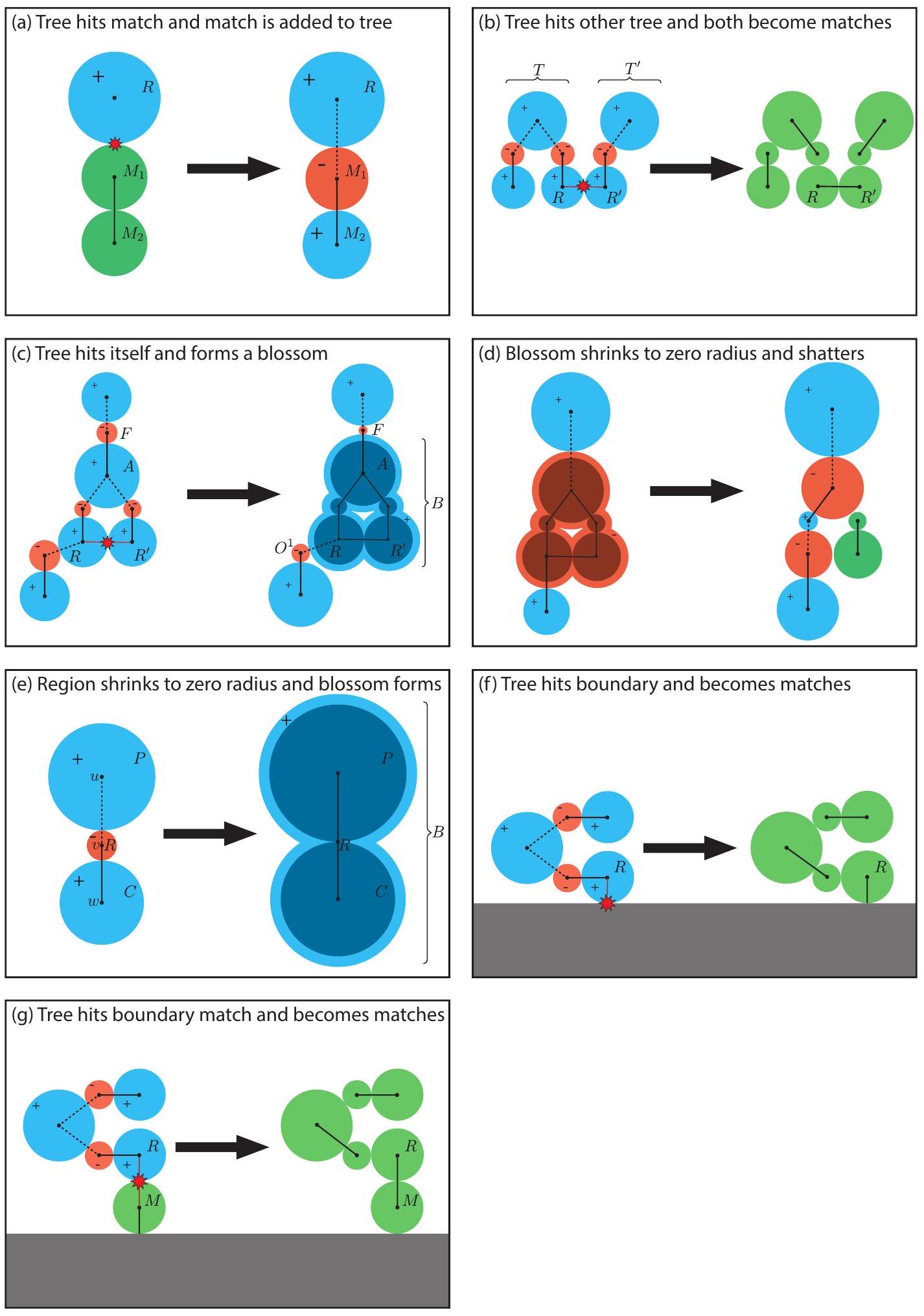
هناك سبعة أنواع مختلفة من الأحداث التي يمكن أن تغير هيكل شجرة متناوبة، والتي يتم التعامل معها من قبل المطابق، موضحة في الشكل 4:
(أ) يمكن أن تصطدم منطقة نمو في شجرة متناوبة بمنطقة التي تم مطابقتها مع منطقة أخرى . في هذه الحالة، تصبح طفلاً شجرة لـ في (وتبدأ في الانكماش)، وتصبح طفلاً شجرة لـ في (وتبدأ في النمو). تصبح حافة الاصطدام ( ) وحافة المطابقة ( ) كلاهما حواف شجرة ( هو والد الشجرة لـ ، و هو والد الشجرة لـ ).
(ب) تصطدم منطقة نمو في شجرة متناوبة بمنطقة نمو في شجرة متناوبة مختلفة . عندما يحدث ذلك، يتم مطابقة مع وتصبح المناطق المتبقية في و أيضًا متطابقة. تصبح حافة الاصطدام ( ) حافة مطابقة، وتصبح مجموعة من حواف الشجرة أيضًا حواف مطابقة. تصبح جميع المناطق في و مجمدة.
(ج) يمكن أن تصطدم منطقة نمو في شجرة متناوبة بمنطقة نمو أخرى في نفس الشجرة المتناوبة . يؤدي ذلك إلى دورة ذات طول فردي من المناطق التي تشكل دورة الزهرة لزهرة جديدة . تتشكل حواف المناطق (حواف الزهرة) في دورة الزهرة من حافة الاصطدام ( )، بالإضافة إلى حواف الشجرة على طول المسارات من و إلى سلفهما المشترك الأكثر حداثة في . تصبح الزهرة الجديدة المتكونة عقدة نمو في . عند تشكيل الدورة ، نعرف الأيتام على أنهم مجموعة من مناطق الانكماش في ولكن ليس التي كانت كل منها طفلاً لمنطقة نمو في . تصبح الأيتام أطفال شجرة لـ في . الحافة المضغوطة المرتبطة بحافة الشجرة الجديدة ( ) (التي تربط منطقة الزهرة الجديدة بوالد شجرتها ) هي فقط الحافة المضغوطة التي كانت مرتبطة بحافة الشجرة القديمة ( ). وبالمثل، تبقى الحواف المضغوطة التي تربط كل يتيم بوالده في الشجرة المتناوبة دون تغيير (حتى لو أصبحت منطقة والده ). بعبارة أخرى، إذا كان يتيم قد تم توصيله بوالده في الشجرة بواسطة حافة الشجرة قبل تشكيل الزهرة، فإن حافة الشجرة الجديدة التي تربطه بوالده الجديد في الشجرة ستكون ( ) بمجرد تشكيل الزهرة وتصبح المنطقة جزءًا من دورة الزهرة .
(د) عندما تكون زهرة في شجرة متناوبة ينكمش إلى نصف قطر صفر، بدلاً من أن يصبح نصف القطر سالبًا، يجب أن يتشقق الزهرة. عندما تتشقق الزهرة، فإن المسار ذو الطول الفردي من خلال دورة زهورها من شجرة الطفلإلى شجرة الوالدين لـيتم إضافته إلىكمناطق متزايدة ومتقلصة. يصبح المسار ذو الطول الزوجي مطابقات. تصبح حواف الزهرة في المسار ذو الطول الفردي حواف شجرية، وبعض حواف الزهرة في المسار ذو الطول الزوجي تصبح حواف مطابقة (تُنسى حواف الزهرة المتبقية). لاحظ أن نقاط النهاية للحواف المضغوطة المرتبطة بالحواف الشجرية التي تربطيتم استخدام الشجرة الأم والشجرة الابنة لتحديد مكان وكيفية تقسيم دورة الإزهار إلى مسارين. (هـ) عندما تكون المنطقة تافهةينكمش إلى نصف قطر صفر، بدلاً من أن يصبح نصف القطر سالبًا، تتشكل زهرة. إذالديه طفلوالوالدفي الشجرة المتناوبةعندماله نصف قطر صفر، يجب أن يكون ذلكيؤثركأنهقد تصادم مع ). الزهرة التي تشكلت حديثًا لديه دورة الإزهار ( ). حواف الشجرة القديمة ( ) و ( تتحول حواف الزهرة في دورة الإزهار. الحافة الزهرية التي تربطمعفي دورة الإزهار يتم حسابها من الحواف ( ) و ( ) و هو ( ). بعبارة أخرى، فإن حافته المضغوطة لها نقاط نهاية ( ) مع الملاحظات المنطقية . (و) عندما تكون منطقة ناميةفي شجرة متناوبةيصل إلى الحدود،تتطابق مع الحدود ويصبح حافة الاصطدام هي حافة المباراة. المناطق المتبقية فيأيضًا تصبح مباريات. (ز) عندما تكون منطقة ناميةفي شجرة متناوبةيضرب منطقةالذي يتطابق مع الحدود، ثمبدلاً من ذلك يصبح متطابقًا مع (ويصبح حافة الاصطدام هي حافة المباراة)، والحواف المتبقية في أيضًا تصبح مباريات. بعض هذه الأحداث تتضمن تغيير معدل نمو المناطق (على سبيل المثال، تصبح منطقتان تنموان كلتاهما مناطق متجمدة عندما تتطابقان مع بعضهما). لذلك، عند التعامل مع كل حدث شجرة متناوبة، يقوم المطابق بإبلاغ الفاضح بأي تغييرات مطلوبة في نمو المنطقة.
الشكل 4: الأحداث الرئيسية التي تغير هيكل الأشجار المتناوبة. لتوضيح الأمر، تم حذف رسم بياني للكاشف الخلفي. كل عقدة تتوافق مع حدث اكتشاف، وكل حافة تتوافق مع حافة مضغوطة. تم تضمين بعض التسميات (مثل المناطق) في الرسوم البيانية وتتناسب مع تلك المشار إليها في النص الرئيسي في القسم 3.3.1.
الشكل 5: تحطيم زهرة متطابقة. الخطوط الصلبة داخل الزهرة هي حواف في دورة الزهرة العليا. الخطوط المتقطعة هي حواف في دورة الزهرة لزهرة الطفل للزهرة العليا.
3.3.2 أحداث الكشف المتطابقة من المناطق المتطابقة
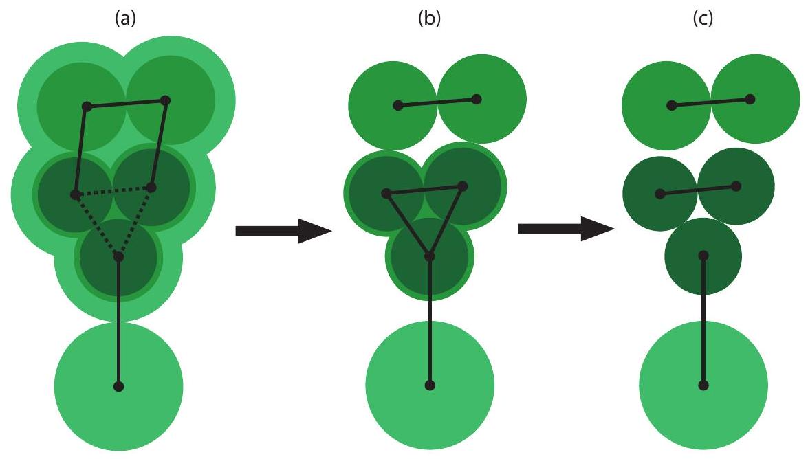
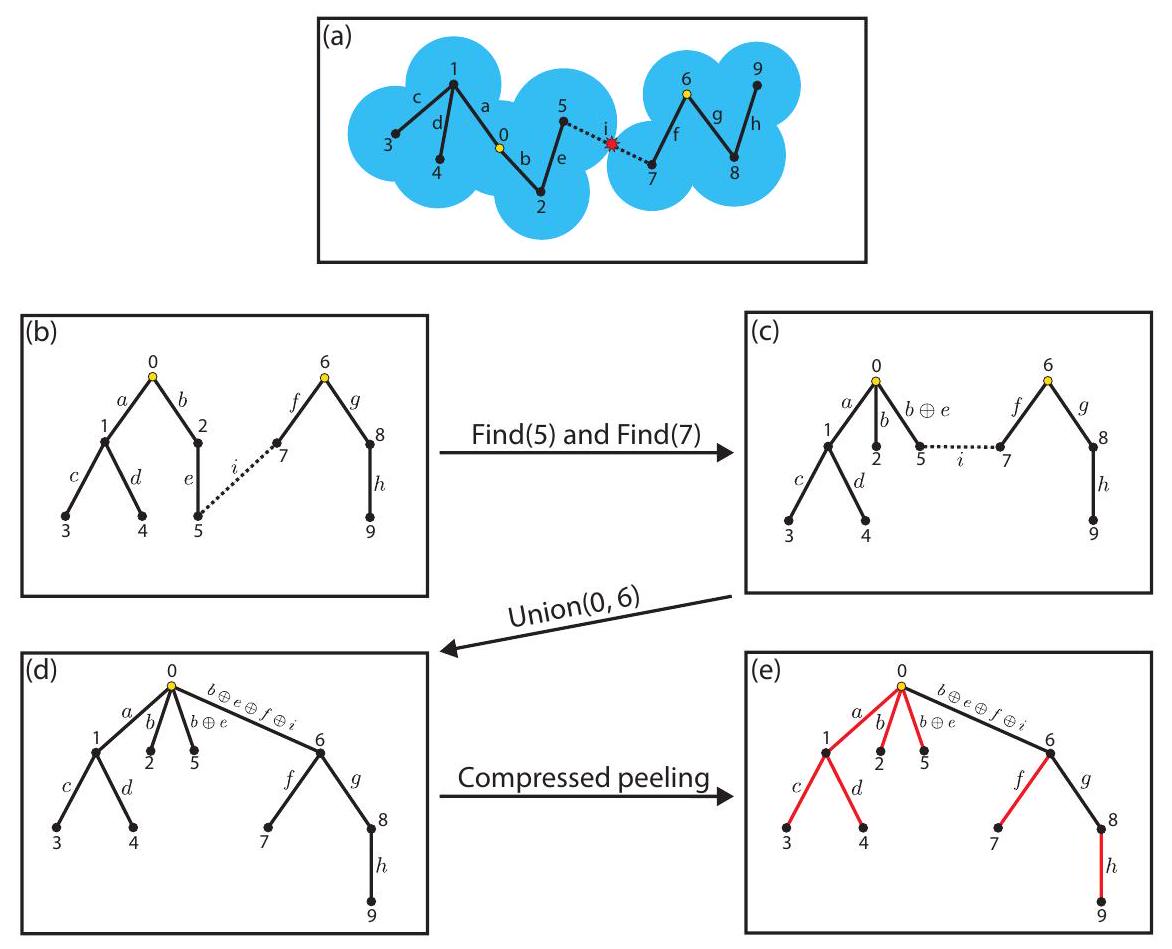
طالما أن هناك حلًا صالحًا، فإن جميع المناطق في النهاية تصبح متطابقة مع مناطق أخرى، أو مع الحدود. ومع ذلك، قد تكون بعض هذه المناطق المتطابقة أزهارًا، وليست مناطق تافهة. لاستخراج الحافة المضغوطة التي تمثل المطابقة لكل حدث اكتشاف بدلاً من ذلك، من الضروري تكسير كل زهرة متبقية، ومطابقة أطفالها الزهريين، كما هو موضح في الشكل 5. لنفترض أن زهرةمع دورة الإزهاريتطابق مع منطقة أخرى مع حافة المباراة ( )، حيث نتذكر أن هو حدث اكتشاف في و هو حدث اكتشاف في نجد الطفل المتفتحمنالذي يحتوي على حدث الكشفنحن نحطم ومطابقة إلى مع الحافة المضغوطة ( ). المناطق المتبقية في دورة الإزهار ثم يتم تقسيمها إلى أزواج مجاورة، والتي تصبح مباريات. تتكرر هذه العملية بشكل متكرر حتى تصبح جميع المناطق المتطابقة مناطق تافهة.
3.4 الفيضانات
المغمر مسؤول عن إدارة كيفية نمو أو انكماش أو تصادم مناطق ملء الرسم البياني في الرسم البياني للكاشف، ولا يهتم بهيكل الأشجار المتناوبة والزهور، والتي يتم التعامل معها بدلاً من ذلك بواسطة المطابق. نشير إلى الأحداث التي يتعامل معها المغمر بأحداث المغمر.
بشكل عام، يمكننا تصنيف أحداث الفيضانات إلى أربعة أنواع مختلفة:
الوصول: منطقة ناميةيمكن أن ينمو إلى عقدة كاشف فارغة.
المغادرة: منطقة تتقلصيمكن أن يغادر عقدة الكاشف.
تصادم: يمكن أن تضرب منطقة متنامية منطقة أخرى، أو الحدود.
انفجار: يمكن أن تصل منطقة متقلصة إلى نصف قطر صفر.
دعونا أولاً نعتبر ما يحدث لفعاليات الوصول والمغادرة. لا يمكن لأي من هذين النوعين من الفعاليات تغيير هيكل الأشجار المتناوبة أو الزهور، لذا لا يحتاج المطابق إلى أن يتم إخطاره. بدلاً من ذلك، فإن مسؤولية الفاضح هي التأكد من جدولة أي فعاليات فاضحة جديدة (إدراجها في قائمة الأولويات للمتعقب) بعد معالجة الفعاليات. عندما تنمو منطقة إلى عقدة، يقوم الفاضح بإعادة جدولة العقدةمن خلال إبلاغ المتعقب بحدث الفيضانات التالي الذي يمكن أن يحدث على حافة مجاورة لـ (إما حدث وصول أو تصادم، انظر القسم 3.4.1). عندما يغادر منطقة متقلصة عقدة، يقوم الفلّاح على الفور بالتحقق من قمة كومة منطقة القشرة ويجدول الحدث التالي للخروج أو الانفجار (انظر القسم 3.4.2).
يحتاج الفلّودير فقط إلى إبلاغ المطابق بحدث COLLIDE أو IMPLODE، وعندما يحدث تصادم، يقوم الفلّودير بتمرير حافة التصادم إلى المطابق أيضًا. عندما يحدث أي من هذه الأمور
الشكل 6: منطقتان و تصادم على حافة ( ). عقدة محتوى في المنطقة، وهو منطقة نشطة (لا يوجد والد زهور). العقدةمحتوى في المنطقةوتمتلكهبالإضافة إلى أسلافه المزهرة و منطقةأيضًا لديهكواحد من أطفالها المتفتحين. لقد قمنا بتسمية نصف القطر المحليعقدةونصف القطر المحليعقدةبالإضافة إلى نصف القطر الملفوفمنونصف قطر الوصول لـوزن الحافةمن الحافة ( ) يظهر أيضًا.
تحدث أنواع من الأحداث، قد يقوم المطابق بتغيير معدل النمو لبعض المناطق عند تحديث هيكل الأشجار المتناوبة أو الزهور. ثم يقوم المطابق بإخطار الموزع بأي تغيير في معدل النمو، مما قد يتطلب من الموزع إعادة جدولة بعض أحداث الفيضانات. على سبيل المثال، إذا كانت منطقةكان يتقلص، لكنه بعد ذلك يتجمد أو يبدأ في النمو، يقوم الفيضانات بإعادة جدولة جميع العقد المحتواة في (بما في ذلك أطفال الزهور، وأطفالهم، وما إلى ذلك)، للتحقق من أحداث ARRIVE أو COLLIDE الجديدة. عندما يبدأ منطقة في الانكماش، يقوم الفاضح بإبلاغ المتتبع بالحدث التالي LEAVE أو IMPLODE من خلال التحقق من قمة كومة منطقة القشرة.
يتم ضمان الترتيب الصحيح لهذه الأحداث الفيضانية بواسطة المتعقب، ونقوم بإنشاء منطقة متزايدة لكل حدث اكتشاف في نفس الوقت.. لذلك، تستخدم تنفيذنا استراتيجية نمو شجرة متناوبة تشبه ما يُوصف بأنه “نهج الأشجار المتعددة مع ثابت ” في [Kol09].
3.4.1 إعادة جدولة عقدة
عندما يعيد الفاضح جدولة عقدة، يبحث عن حدث وصول أو تصادم على كل حافة مجاورة. سيكون هناك حدث وصول على حافة إذا كانت إحدى العقد مشغولة بمنطقة نامية والأخرى فارغة. سيكون هناك حدث تصادم إذا كانت كلتا العقدتين مملوكتين لمناطق نشطة. ) بمعدلات نمو ( 1,1 )، ( 0,1 ) أو ( 1,0 )، أو إذا كانت منطقة واحدة تنمو نحو حد، لحد نصف.
لحساب متى سيحدث حدث الوصول أو الاصطدام على طول حافة، نستخدم نصف القطر المحلي لكل عقدة. نصف القطر المحليعقدة هو المبلغ الذي تملكه المناطق تجاوزت (انظر الشكل 6). لتعريف نصف القطر المحلي بدقة أكبر، سنحتاج إلى بعض التعريفات الإضافية. نصف قطر الوصوللعقدة مشغولةمحتوى في منطقة هو نصف القطر الذي كان عندما وصلت إلىنحن نحدد نصف قطر منطقةبواسطةونحن نسمحكن مجموعة المناطق التي تمتلك عقدة كاشف (المنطقة التي محتوى في، بالإضافة إلى أسلافه المزهرة). يتم تعريف نصف القطر المحلي بعد ذلك على أنه
يمكن فهم هذا التعريف من خلال النظر في المثال في الشكل 6، حيث نتذكر أن نصف قطر منطقة الإزهار يمكن تصوره كسمك (أي المسافة عبر) قشرة الإزهار. كل من نصف القطر المحلي ونصف قطر وصول العقدةتعرف بأنها صفر إذا فارغ. لذلك، بالنسبة لحافة ( ) مع الوزن يمكن العثور على وقت حدث الوصول أو الاصطدام من خلال حللـ. الحالة الوحيدة التي تتضمن فيها هذه العملية القسمة هي عندما يكون نصف قطر كلا العقدتين في حالة نمو (لديهما تدرج واحد)، وفي هذه الحالة يحدث التصادم في الوقت . ومع ذلك، بشرط أن يتم تعيين جميع الحواف بأوزان صحيحة زوجية، تحدث جميع أحداث الفيضانات، بما في ذلك هذه التصادمات بين المناطق المتزايدة، في أوقات صحيحة.
الشكل 7: مثال على بعض أحداث الفيضانات في رسم بياني للكاشف مع ثلاث مناطق متزايدة.
3.4.2 إعادة جدولة منطقة متقلصة
عندما تتقلص منطقة، نجد وقت الحدث التالي LEAVE أو IMPLODE من خلال فحص كومة منطقة السطح الخاصة بالمنطقة. إذا كانت الكومة فارغة، أو إذا لم يكن للمنطقة أي أطفال من الزهور وكان هناك عقدة واحدة فقط متبقية في الكومة (حدث الكشف عن مصدر المنطقة)، فإن الحدث التالي هو حدث IMPLODE، ويمكن العثور على وقته من -الاعتراض لمعادلة نصف قطر المنطقة. خلاف ذلك، فإن الحدث التالي هو حدث LEAVE، مع العقدة في أعلى الكومة تغادر المنطقة. نجد وقت هذا الحدث LEAVE التالي باستخدام نصف القطر المحلي لـ ، من خلال حل لـ . باستخدام هذا النهج، فإن تقليص منطقة أرخص بكثير من زيادة منطقة، حيث إنه لا يتطلب تعداد الحواف في رسم بياني للكاشف.
3.4.3 مثال
نقدم مثالًا صغيرًا عن كيفية تقدم الجدول الزمني للفيضانات في الشكل 7. نظرًا لأن المناطق و تم تهيئتها جميعًا عند ، فإن معادلات نصف قطرها جميعًا متساوية لـ . المناطق و مفصولة بحافة واحدة بوزن 8 وبالتالي تتصادم في الوقت (وتذكر أن أوزان الحواف دائمًا أعداد صحيحة زوجية لضمان حدوث التصادمات في أوقات صحيحة). عندما يتم إبلاغ المطابق بالتصادم، يتم مطابقة و وتصبح مناطق متجمدة. تصل المنطقة إلى العقدة الفارغة والحدود في نفس الوقت ( )، وبالتالي هناك سلسلتان من الأحداث صحيحتان بالتساوي. إما أن المنطقة تتطابق مع الحدود، ولا تصل أبدًا إلى ، أو أن تصل إلى ثم تتطابق مع الحدود. من الواضح أن الحالة النهائية للخوارزمية ليست فريدة، ومع ذلك هناك وزن حل فريد، وفي هذه الحالة، تؤدي كلا النتيجتين إلى نفس مجموعة الحواف المضغوطة في الحل.
3.4.4 تتبع مضغوط
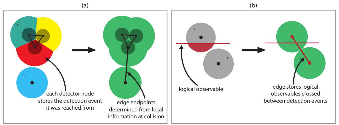
كلما حدث تصادم بين منطقتين و ، يقوم الفيضانات بإنشاء حافة منطقة ( )، والتي نتذكر أنها تتضمن حافة مضغوطة تتوافق مع أقصر مسار بين حدث الكشف في وحدث الكشف في . من خلال تخزين المعلومات ذات الصلة على العقد أثناء نمو المناطق، يمكن بناء الحافة المضغوطة بكفاءة باستخدام المعلومات المحلية في نقطة التصادم (أي باستخدام المعلومات المخزنة فقط على الحافة التي يحدث عليها التصادم، وعلى العقد و ).
يتم شرح ذلك في الشكل 8. عندما تصل منطقة إلى عقدة فارغة من خلال النمو على طول حافة ( ) من عقدة سابقة ، نقوم بتخزين على مؤشراً إلى حدث الكشف الذي تم الوصول إليه منه (والذي يمكن ببساطة نسخه من ). بعبارة أخرى، نقوم بتعيين بمجرد الوصول إلى من . في البداية، عندما يبدأ البحث من حدث الكشف (أي يتم إنشاء منطقة متزايدة تافهة تحتوي على )، نقوم بتعيين . نشير إلى كحدث الكشف المصدر لـ .
الشكل 8: (أ) عندما تتوسع منطقة، يقوم كل عقدة كاشف تحتوي عليها بتخزين حدث الكشف الذي تم الوصول إليه منه (مصور بواسطة تلوين على طراز فورونوي للزهور على اليسار). عندما يحدث تصادم، يسمح ذلك بتحديد نقاط النهاية للحافة المضغوطة المقابلة (حافة التصادم) من المعلومات المحلية في نقطة التصادم. (ب) يقوم كل عقدة كاشف أيضًا بتخزين (كقناع بت 64 بت) المتغيرات التي تم عبورها للوصول إليه من حدث الكشف الذي تم الوصول إليه منه. يسمح ذلك باستعادة قناع المتغيرات للحافة المضغوطة بكفاءة، أيضًا من المعلومات المحلية في نقطة التصادم.
نقوم أيضًا بتخزين على مجموعة المتغيرات التي تم عبورها أثناء نمو المنطقة (أي المتغيرات التي تم عبورها على طول أقصر مسار من إلى ). يمكن حساب هذه المجموعة من المتغيرات المعبورة بكفاءة عندما يتم الوصول إلى من على طول الحافة ( ) من ، حيث نقوم بتنفيذ كعملية XOR بتية حيث يتم تخزين و كأقنعة بت. في البداية، عندما يتم إنشاء منطقة متزايدة تافهة عند حدث الكشف نقوم بتعيين إلى المجموعة الفارغة.
لذلك، عندما يحدث تصادم بين المناطق و على طول حافة ( )، يمكن بعد ذلك تحديد نقاط النهاية للحافة المضغوطة المرتبطة بحافة التصادم ( ) محليًا كـ و . يمكن حساب المتغيرات المرتبطة بحافة التصادم محليًا كـ . لاحظ أن تتبع المضغوط يمكن أيضًا استخدامه لإزالة خطوة التقشير من فك التشفير بالاتحاد-العثور [DN21]، كما نشرح في الملحق A. نلاحظ أنه سيكون من المثير للاهتمام أيضًا استكشاف كيفية تعميم تتبع المضغوط لتحسين فك التشفير لعائلات أخرى من الرموز التي لا يمكن فك تشفيرها بالمطابقة (حيث لا تكون نماذج الخطأ المقابلة شبيهة بالرسم البياني).
في PyMatching، نعتمد بالكامل على تتبع المضغوط فقط عندما يكون هناك 64 متغيرًا منطقيًا أو أقل. عندما يكون هناك أكثر من 64 متغيرًا منطقيًا، لا نقوم بتضمين قناع المتغيرات في الحواف المضغوطة، بل نقوم فقط بتخزين أحداث الكشف عند نقاط نهايتها. لا يزال يسمح لنا ذلك باستخدام الزهرة النادرة للعثور على أي أحداث كشف متطابقة مع بعضها البعض. ثم بعد أن تكتمل الزهرة النادرة، لكل زوج متطابق ( ) نستخدم بحث دايكسترا ثنائي الاتجاه (تم تنفيذه عن طريق تعديل الفيضانات والمتعقب حسب الحاجة) للعثور على أقصر مسار بين و . إذا كانت هي مجموعة جميع الحواف على طول أقصر المسارات التي تم العثور عليها بهذه الطريقة بواسطة معالجة ما بعد بحث دايكسترا، فإن الحل الناتج عن PyMatching هو . لاحظ أنه نظرًا لأننا نقوم فقط بمعالجة ما بعد باستخدام دايكسترا بدلاً من بناء الرسم البياني الكامل للمسار، فإن هذا يضيف فقط عبئًا نسبيًا صغيرًا (عادة أقل من ) إلى وقت التشغيل.
3.5 المتعقب
المتعقب مسؤول عن ضمان حدوث أحداث الفيضانات بالترتيب الصحيح. يمكن أن تكون طريقة بسيطة يمكن اتخاذها لتنفيذ المتعقب هي وضع كل حدث فيضان في قائمة انتظار ذات أولوية. ومع ذلك، فإن العديد من أحداث الفيضانات المحتملة هي حشائش. على سبيل المثال، عندما تكون منطقة في حالة نمو، سيتم إضافة حدث فيضان إلى قائمة الانتظار لكل من حوافها المجاورة. نقول إن حافة ( ) هي جار لمنطقة إذا كانت في و ليست (أو العكس). على طول كل حافة مجاورة، سيكون هناك حدث إما يتوافق مع المنطقة التي تنمو إلى عقدة فارغة، أو تتصادم مع منطقة أخرى أو حدود. ومع ذلك، إذا أصبحت المنطقة مجمدة أو متقلصة، فإن جميع هذه الأحداث المتبقية ستصبح غير صالحة.
لتقليل هذه الحشائش، بدلاً من إضافة كل حدث فيضان إلى قائمة انتظار ذات أولوية، يقوم المتعقب بدلاً من ذلك بإضافة أحداث النظر إلى العقدة والنظر إلى المنطقة إلى قائمة انتظار ذات أولوية. يقوم الفيضانات فقط بالعثور على
وقت الحدث التالي في عقدة أو منطقة، ويطلب من المتعقب تذكيرًا للنظر إلى الوراء في ذلك الوقت. نتيجة لذلك، في كل عقدة، نحتاج فقط إلى إضافة الحدث التالي إلى قائمة الانتظار ذات الأولوية. لن تتم إضافة الأحداث المحتملة المتبقية على طول الحواف المجاورة إذا أصبحت غير صالحة.
عندما يعيد الفيضانات جدولة عقدة، فإنه يجد وقت الحدث التالي ARRIVE أو COLLIDE على طول حافة مجاورة، ويطلب من المتعقب تذكيرًا للنظر إلى الوراء في ذلك الوقت (حدث النظر إلى العقدة). يجد الفيضانات وقت الحدث التالي LEAVE أو IMPLODE لمنطقة متقلصة من خلال فحص أعلى كومة منطقة السطح، ويطلب من المتعقب تذكيرًا للنظر إلى الوراء في المنطقة في ذلك الوقت (حدث النظر إلى المنطقة). لتقليل الحشائش بشكل أكبر، يضيف المتعقب فقط حدث النظر إلى العقدة أو النظر إلى المنطقة إلى قائمة الانتظار ذات الأولوية إذا كان سيحدث في وقت أبكر من حدث موجود بالفعل في قائمة الانتظار لنفس العقدة أو المنطقة. بمجرد أن يذكر المتعقب الفيضانات بالنظر إلى الوراء في عقدة أو منطقة، يتحقق الفيضانات مما إذا كانت لا تزال حدثًا صالحًا من خلال إعادة حساب الحدث التالي للعقدة أو المنطقة، ومعالجته إذا كان الأمر كذلك.
3.6 مقارنة بين الزهرة والزهرة النادرة
في الجدول 1، نلخص كيف تترجم بعض المفاهيم في خوارزمية الزهرة التقليدية إلى مفاهيم في الزهرة النادرة. إذا تم تشغيل خوارزمية الزهرة التقليدية على الرسم البياني للمسار باستخدام نهج الشجرة المتعددة (ومع تهيئة جميع المتغيرات الثنائية إلى الصفر في البداية)، فإن حالة الزهرة الصالحة في مرحلة معينة تتوافق مع حالة الزهرة النادرة الصالحة لنفس المشكلة في النقطة المناسبة في الجدول الزمني. تحدد المتغيرات الثنائية في الزهرة مناطق الأشعة في الزهرة النادرة (ويمكن استخدام هذه الأشعة لبناء المناطق الاستكشافية المقابلة). وبالمثل، يمكن ترجمة الحواف في الأشجار المتناوبة، ودورات الزهرة، والمطابقات في الزهرة التقليدية إلى حواف مضغوطة في الكيانات المقابلة في الزهرة النادرة. ومع ذلك، نلاحظ أنه عندما تحدث أحداث شجرة متناوبة متعددة في نفس الوقت في الزهرة النادرة، فإن أي ترتيب لمعالجة هذه الأحداث هو خيار صالح. لذا، لمجرد أننا نستطيع ترجمة حالة صالحة لخوارزمية واحدة إلى حالة الأخرى، لا يعني ذلك أن تنفيذين للخوارزميات (أو نفس الخوارزمية) سيكون لهما نفس تسلسل التلاعبات في الشجرة المتناوبة (في الواقع، من غير المحتمل أن يكونوا كذلك). هذه المطابقة بين الزهرة النادرة التي تعمل على رسم كاشف والزهرة التقليدية التي تعمل على رسم مسار، وصحة الزهرة نفسها في العثور على MWPM، هي إحدى طرق فهم لماذا تجد الزهرة النادرة بشكل صحيح MWEM في رسم الكاشف.
4 هياكل البيانات
في هذا القسم، نوضح هياكل البيانات التي نستخدمها في الزهرة النادرة. كل عقدة كاشف تخزن حوافها المجاورة في رسم الكاشف كقائمة جوار. لكل حافة مجاورة ( )، نقوم بتخزين وزنها كعدد صحيح 32 بت، والملاحظات التي تقلبها كقناع بت 64 بت، بالإضافة إلى عقدتها المجاورة كمؤشر (أو كـ nullptr للحدود). يتم تمييز أوزان الحواف كأعداد صحيحة زوجية، مما يضمن أن جميع الأحداث (بما في ذلك تصادم منطقتين متزايدتين) تحدث في أوقات صحيحة.
كل عقدة كاشف مشغولة تخزن مؤشراً إلى حدث الكشف المصدر الذي وصلت منه ، وقناع بت للملاحظات التي تم عبورها على طول المسار من حدث الكشف المصدر ومؤشر إلى منطقة ملء الرسم التي تحتوي عليها (المنطقة التي وصلت إلى العقدة). هناك بعض الخصائص التي نقوم بتخزينها في كل عقدة مشغولة كلما تغيرت بنية الزهرة، من أجل تسريع عملية العثور على الحدث التالي COLLIDE أو ARRIVE على طول حافة. يشمل ذلك تخزين مؤشر إلى المنطقة النشطة التي تمتلكها عقدة الكاشف المشغولة (أعلى سلف زهرة للمنطقة التي تحتوي عليها) بالإضافة إلى نصف قطر وصولها ، وهو نصف القطر الذي كانت عليه المنطقة المحتوية على العقدة عندما وصلت إلى (انظر القسم 3.4.1). بالإضافة إلى ذلك، نقوم بتخزين نصف القطر المغلف لكل عقدة كاشف كلما تغيرت بنية زهرة المناطق المالكة لها (إذا تم تشكيل زهرة أو تحطيمها). نصف القطر المغلف لعقدة مشغولة هو نصف القطر المحلي للعقدة، باستثناء نصف القطر (الذي قد يتزايد أو يتقلص) للمنطقة النشطة التي تمتلكها. إذا دعونا يكون نصف القطر للمنطقة النشطة التي تمتلك ، يمكننا استعادة نصف القطر المحلي من نصف القطر المغلف مع .
مفاهيم الزهرة (نهج الشجرة المتعددة، المطبق على )
مفاهيم الزهرة النادرة
متغير ثنائي (لعقدة ) أو (لمجموعة من العقد ذات عدد فردي لا يقل عن ثلاثة)
نصف القطر لمنطقة ملء الرسم ، منطقة استكشافية تحتوي على عقد وحواف في رسم الكاشف بما في ذلك عدد فردي من أحداث الكشف.
حافة ضيقة ( ) بين عقدتين و في التي هي في المطابقة أو تنتمي إلى شجرة متناوبة أو دورة زهرة. نظرًا لأن ( ) هي حافة في رسم المسار، فإن وزنها هو طول أقصر مسار بين حدثي الكشف و في رسم الكاشف (تم العثور عليه باستخدام بحث ديكسترا عند بناء رسم المسار). إنها ضيقة لأن المتغيرات الثنائية المرتبطة بـ و تؤدي إلى انزلاق صفري كما هو محدد في المعادلة 6.
حافة مضغوطة ( ) مرتبطة بحافة منطقة، تنتمي إلى مطابقة، شجرة متناوبة أو دورة زهرة. تمثل الحافة المضغوطة ( ) أقصر مسار بين حدثي الكشف و في رسم الكاشف . المرتبطة بـ ( ) هي مجموعة من الملاحظات المنطقية التي تم قلبها عن طريق قلب الحواف في على طول المسار المقابل بين و . المنطقتان في حافة المنطقة المقابلة تلامسان (الحافة ضيقة).
حافة ( ) بين عقدتين و في التي ليست ضيقة. وزنها هو طول أقصر مسار بين و في رسم الكاشف ، تم العثور عليه باستخدام بحث ديكسترا عند بناء رسم المسار. بالنسبة لمشاكل QEC النموذجية، فإن الغالبية العظمى من الحواف في لا تصبح ضيقة أبدًا، ولكن بالنسبة للزهرة القياسية لا يزال يتعين بناؤها صراحة باستخدام بحث ديكسترا.
لا توجد بنية بيانات مماثلة لهذه الحافة في الزهرة النادرة. لم يتم استكشاف أقصر مسار بين و بالكامل حاليًا بواسطة مناطق ملء الرسم. وهذا يعني أن إما أن المسار لم يتم اكتشافه بعد بواسطة الزهرة النادرة (وقد لا يتم اكتشافه أبدًا)، أو ربما تم اكتشافه سابقًا (ينتمي إلى حافة منطقة) ولكن على الأقل واحدة من المناطق المالكة لـ أو قد تقلصت (على سبيل المثال، تم مطابقتها ثم أصبحت منطقة متقلصة في شجرة متناوبة).
في مرحلة تحديث المتغير الثنائي، قم بتحديث كل متغير ثنائي لعقدة خارجية مع وقم بتحديث كل متغير ثنائي لعقدة داخلية مع . يتم تعيين المتغير إلى القيمة القصوى بحيث تظل المتغيرات الثنائية حلاً قابلاً للتطبيق للمشكلة الثنائية.
مع مرور الوقت ، تستكشف كل منطقة متزايدة الرسم ويزداد نصف قطرها بمقدار وتقلص كل منطقة متقلصة في الرسم ويقل نصف قطرها بمقدار . في النهاية عند يحدث تصادم أو انفجار (واحد من أحداث المطابقة في الشكل 4)، والذي يجب التعامل معه بواسطة المطابق.
حافة ( ) بين عقدة في شجرة متناوبة وعقدة في شجرة متناوبة أخرى تصبح ضيقة بعد تحديث ثنائي. يتم تعزيز المسار بين جذر وجذر وتصبح جميع العقد في الشجرتين مطابقة.
تتصادم منطقة متزايدة من شجرة متناوبة مع منطقة متزايدة من شجرة متناوبة أخرى . يتم بناء حافة التصادم ( ) من معلومات محلية في نقطة التصادم. يتم مطابقتها مع مع حافة التصادم ( ) كحافة مطابقة. تصبح جميع المناطق الأخرى في الأشجار أيضًا مطابقة. تصبح جميع المناطق في الشجرتين مجمدة.
حافة ( ) بين عقدتين خارجيتين و في نفس الشجرة تصبح ضيقة بعد تحديث ثنائي. يشكل هذا دورة فردية الطول في والتي تصبح زهرة، والتي تصبح بدورها عقدة خارجية في .
تتصادم منطقتان متزايدتان و من نفس الشجرة المتناوبة . تصبح حافة التصادم المكتشفة ( ) بالإضافة إلى المناطق وحواف الشجرة على طول المسار بين و في دورة زهرة في زهرة جديدة تم تشكيلها. تبدأ الزهرة في النمو، وهي الآن منطقة متزايدة في .
الجدول 1: المطابقة بين المفاهيم في خوارزمية الزهرة القياسية والمفاهيم في الزهرة النادرة. بالنسبة لخوارزمية الزهرة القياسية نفترض أنه يتم استخدام نهج “شجرة متعددة مع ” ثابت، وعلاوة على ذلك نفترض أن الخوارزمية تطبق على رسم المسار .
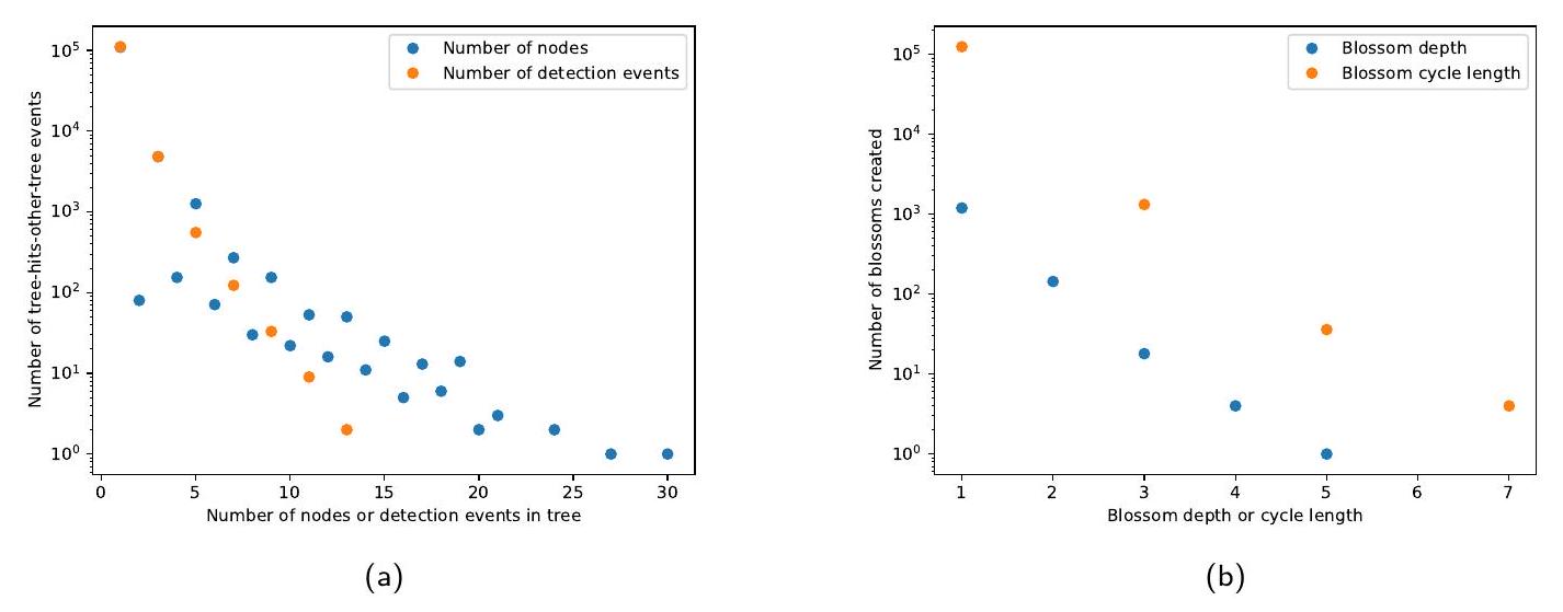
الشكل 9: توزيع أحجام الأشجار المتناوبة والزهور التي لوحظت في الزهرة النادرة عند فك تشفير 1000 لقطة من دوائر كود السطح ذات المسافة 11 مع ضوضاء على مستوى الدائرة. (أ) رسم بياني لحجم الأشجار المتناوبة التي لوحظت في الأحداث حيث تصطدم شجرة بأخرى، من حيث عدد أحداث الكشف وعقد الكاشف المحتواة في كل شجرة. (ب) رسم بياني لحجم الزهور التي تم تشكيلها، من حيث طول دورة زهرة كل زهرة، بالإضافة إلى عمقها التكراري. عمق زهرة أو دورة بحجم واحد هو زهرة تافهة (منطقة ملء رسم بدون أطفال زهرة).
كل منطقة ملء رسم لديها مؤشر إلى والد الزهرة الخاص بها وأعلى سلف زهرة لها. يتم تخزين دورة الزهرة الخاصة بها كصفيف من حواف الدورة، حيث تخزن حافة الدورة مؤشراً إلى طفل الزهرة ، جنبًا إلى جنب مع الحافة المضغوطة المرتبطة بحافة المنطقة التي تربط الطفل بالطفل ، حيث هو عدد أطفال الزهرة لـ . يتم استخدام مصفوفة منطقة قشرتها كمجموعة من المؤشرات إلى عقد الكاشف التي تحتوي عليها (بالترتيب الذي تمت إضافتها به). بالنسبة لنصف قطرها نستخدم 62 بت لتخزين -الاعتراض ومع استخدام 2 بت لتخزين الميل . كل منطقة تخزن أيضًا تطابقها كمؤشر إلى المنطقة التي تتطابق معها، جنبًا إلى جنب مع الحافة المضغوطة المرتبطة بحافة التطابق. أخيرًا، تحتوي كل منطقة تتوسع أو تتقلص على مؤشر إلى AltTreeNode.
يتم استخدام AltTreeNode لتمثيل هيكل شجرة متناوبة. كل AltTreeNode يتوافق مع منطقة نمو في الشجرة، بالإضافة إلى منطقة الوالد المتقلصة (إذا كانت موجودة). يحتوي كل AltTreeNode على مؤشر إلى منطقة ملء الرسم البياني المتنامية ومنطقة ملء الرسم البياني المتقلصة (إذا كانت موجودة). كما يحتوي على مؤشر إلى AltTreeNode الوالد في الشجرة المتناوبة (كمؤشر وحافة مضغوطة)، بالإضافة إلى مؤشرات إلى أبنائه (كمصفوفة من المؤشرات والحواف المضغوطة). نقوم أيضًا بتخزين الحافة المضغوطة التي تتوافق مع أقصر مسار بين المنطقة المتنامية والمنطقة المتقلصة في AltTreeNode.
كل عقدة كاشف ومنطقة ملء الرسم البياني تحتوي أيضًا على حقل متتبع، الذي يخزن الوقت المرغوب فيه الذي يجب أن يتم النظر فيه إلى العقدة أو المنطقة بعد ذلك، بالإضافة إلى الوقت (إن وجد) الذي تم جدولته بالفعل للنظر فيه نتيجة لحدث النظر إلى العقدة أو النظر إلى المنطقة الموجود بالفعل في قائمة الأولويات (المسمى الوقت المجدول). لذلك، يحتاج المتتبع فقط إلى إضافة حدث جديد للنظر إلى العقدة أو النظر إلى المنطقة إلى قائمة الأولويات إذا كان الوقت المرغوب فيه محددًا ليكون سابقًا لوقته المجدول الحالي.
خاصية الخوارزمية هي أن كل حدث يتم إزالته من قائمة الأولويات يجب أن يكون له وقت أكبر من أو يساوي جميع الأحداث السابقة التي تم إزالتها. وهذا يسمح لنا باستخدام كومة راديكس [Ahu+90]، وهي قائمة أولويات أحادية فعالة مع أداء جيد في التخزين المؤقت. نظرًا لأن الحدث التالي للفيضانات لا يمكن أن يكون أبعد من طول حافة واحدة عن الوقت الحالي، نستخدم نافذة زمنية دورية للأولوية، بدلاً من الوقت الكلي. نستخدم دقة عدد صحيح تبلغ 24 و32 و64 بت لأوزان الحواف، وأولويات أحداث الفيضانات، والوقت الكلي، على التوالي.
5 الوقت المتوقع للتشغيل
نلاحظ تجريبيًا وقت تشغيل شبه خطي لخوارزميتنا لرموز السطح تحت العتبة (انظر الشكل 10). نتوقع أن يكون وقت التشغيل خطيًا عند معدلات الخطأ الفيزيائية المنخفضة، حيث في هذه الحالة ستتكون تكوينات الأخطاء النموذجية من مجموعات صغيرة معزولة من الأخطاء. بشرط أن تكون المجموعات مفصولة بشكل كافٍ عن بعضها البعض، يتم التعامل مع كل مجموعة بشكل أساسي كمشكلة مطابقة مستقلة بواسطة زهور نادرة. علاوة على ذلك، باستخدام نتائج من نظرية الترشيح [Men86]، نتوقع أن يتناقص عدد المجموعات بحجم معين بشكل أسي في هذا الحجم [Fow15]. نظرًا لأن عدد العمليات المطلوبة لمطابقة مجموعة هو متعدد الحدود في حجمها، فإن هذا يؤدي إلى تكلفة ثابتة لكل مجموعة، وبالتالي وقت تشغيل متوقع يكون خطيًا في حجم الرسم البياني.
بمزيد من التفصيل، لنفترض أننا نبرز كل حافة في رسم كاشف.لمسها أزهار نادرة عند فك شفرة متلازمة معينة. الآن اعتبر الرسم الفرعيمنالتي تسببها هذه الحواف المميزة. سيكون لهذا الرسم البياني عمومًا العديد من المكونات المتصلة، وسنشير إلى كل مكون متصل على أنه منطقة تجمع. من الواضح أن تشغيل خوارزمية الزهرة النادرة على كل منطقة تجمع بشكل منفصل سيعطي حلاً مطابقًا لتشغيل الخوارزمية علىككل. دعنا نفترض أن احتمال أن يكون هناك عقدة كاشف فيداخل منطقة تجمع منعقد الكاشف لا تزيد عنلبعضنظرًا لأن أسوأ حالة زمن التشغيل لزهرة متفرقة هي متعددة الحدود في عدد العقد (على الأكثر، انظر الملحق ب)، الوقت المتوقع لفك تشفير منطقة العنقود (إن وجدت) في عقدة معينة هو في أقصى حد، أي ثابت. لذلك، فإن وقت التشغيل خطي بالنسبة لعدد العقد. هنا افترضنا أن احتمال ملاحظة منطقة عنقودية عند عقدة يتناقص بشكل أسي مع حجمها. ومع ذلك، في [Fow15] تم إظهار أن هذه هي الحالة بالفعل عند معدلات خطأ منخفضة جداً. علاوة على ذلك، نقدم أدلة تجريبية على هذا التناقص الأسي لمعدلات الخطأ ذات الأهمية العملية في الشكل 9، حيث نرسم توزيع أحجام الأشجار المتناوبة والزهور التي تم ملاحظتها عند استخدام الزهرة النادرة لفك تشفير رموز السطح مع ضوضاء على مستوى الدائرة. إن معاييرنا في الشكل 10 والشكل 11 تتماشى أيضًا مع وقت تشغيل يتناسب تقريبًا بشكل خطي مع عدد العقد، وحتى فوق العتبة (الشكل 12) فإن التعقيد الملحوظ لـأسوأ قليلاً فقط من الخطية.
لاحظ أننا هنا تجاهلنا حقيقة أن قائمة الأولويات باستخدام كومة الراديكس مشتركة بين جميع المجموعات. هذا لا يؤثر على التعقيد النظري العام، حيث أن عمليات الإدراج والاستخراج الأدنى في كومة الراديكس لها تعقيد زمني متوسط مستقل عن عدد العناصر في القائمة. على وجه الخصوص، يستغرق إدراج عنصرالوقت، وعمليه استخراج الحد الأدنى تأخذ في المتوسطالوقت، حيث هو عدد البتات المستخدمة لتخزين الأولوية (بالنسبة لنا ).
ومع ذلك، فإن استخدامنا لمفهوم الجدول الزمني وشجرة متعددة ثابتةالنهج (الذي يعتمد على قائمة الأولويات) يؤدي إلى المزيد من فقدان الذاكرة المؤقتة في حالات المشاكل الكبيرة جدًا، مما يؤدي تجريبيًا إلى زيادة في وقت المعالجة لكل حدث اكتشاف. وذلك لأن الأحداث التي تكون محلية في الزمن (وبالتالي تتم معالجتها قريبًا من بعضها البعض) عمومًا ليست محلية في الذاكرة، حيث يمكن أن تتطلب فحص مناطق أو حواف بعيدة جدًا عن بعضها البعض في رسم بياني للكاشف. بالمقابل، نتوقع أن يكون لنهج الشجرة الواحدة أفضلية في محلية الذاكرة لحالات المشاكل الكبيرة جدًا. ومع ذلك، فإن ميزة نهج الأشجار المتعددة الذي اتخذناه هي أنه “يؤثر” على جزء أقل من رسم بياني للكاشف. على سبيل المثال، اعتبر مشكلة بسيطة تتعلق بحدثي اكتشاف معزولين في رسم بياني للكاشف موحد، مفصولين بمسافة. في الإزهار النادر، نظرًا لأننا نستخدم نهج الشجرة المتعددة، ستنمو هاتان المنطقتان بنفس المعدل وستكونان قد استكشفتا منطقة نصف قطرهاعندما يتصادمان. في رسم ثلاثي الأبعاد، دعنا نفترض أن منطقة نصف قطرهالمساتحواف لبعض الثوابت. بالمقابل، في نهج الشجرة الواحدة (كما هو مستخدم في المراجع [FWH12a; FWH12b; Fow15])، ستنمو منطقة واحدة إلى نصف قطروتصطدم مع منطقة حدث الكشف الآخر، الذي سيظل له نصف قطر 0. لذلك، فإن نهج الشجرة المتعددة قد لمسحواف،أقل منالحواف التي تلامسها طريقة الشجرة الواحدة. هذه في الأساس نفس الميزة التي تتمتع بها خوارزمية دايكسترا ثنائية الاتجاه مقارنة بخوارزمية دايكسترا العادية.
6 النتائج الحسابية
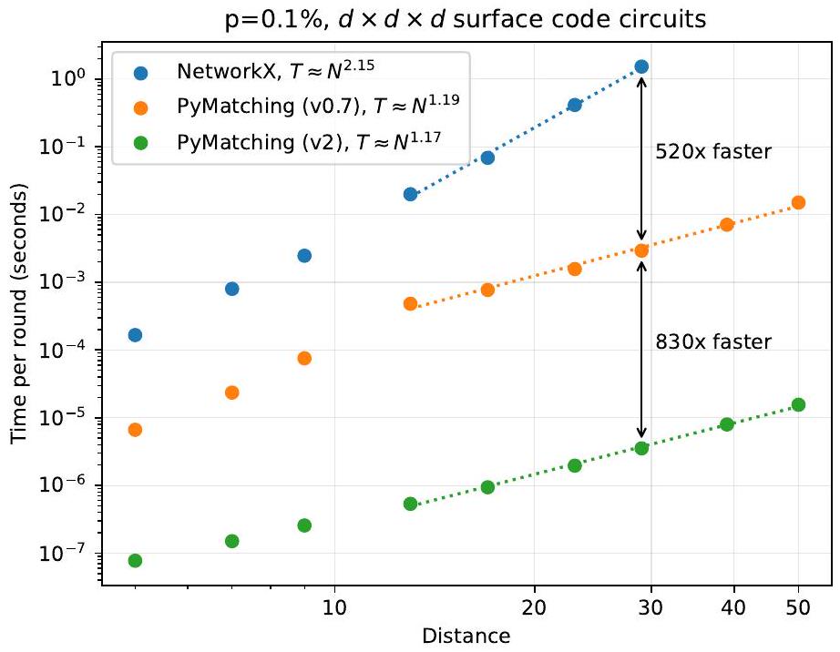
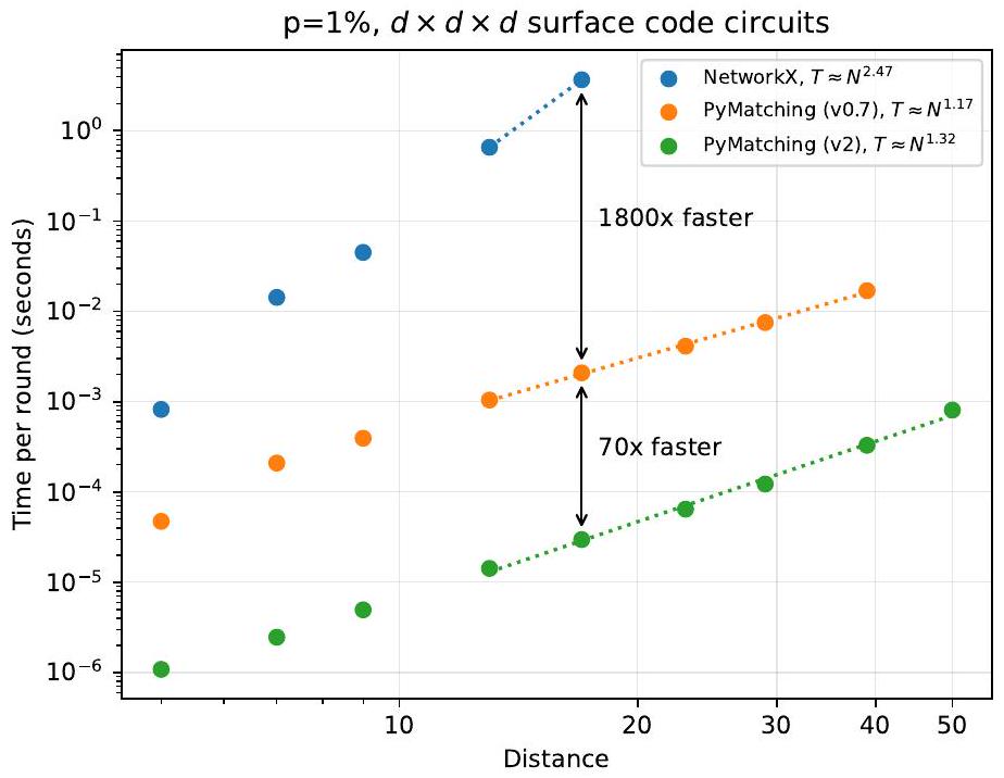
قمنا بتقييم زمن التشغيل لتنفيذنا لـ sparse blossom (PyMatching 2) لتشفير تجارب ذاكرة الشيفرة السطحية (انظر الشكل 10، الشكل 11 والشكل 12). بالنسبة للضوضاء المشتتة على مستوى الدائرة بنسبة 0.1%، يقوم sparse blossom بمعالجة كل من قواعد X و Z لدورات الشيفرة السطحية ذات المسافة 17 في أقل من ميكروثانية لكل جولة من استخراج المتلازمات على نواة واحدة، وهو ما يتوافق مع المعدل الذي يتم به توليد بيانات المتلازمات بواسطة الحواسيب الكمومية الفائقة التوصيل.
عند معدلات خطأ جسدي منخفضة (مثل الشكل 10)، فإن التوسع الخطي تقريبًا لـ PyMatching v2 هو تحسين تربيعي مقارنة بالتوسع التجريبي لتنفيذ يقوم بإنشاء المسار.
الشكل 10: وقت فك التشفير لكل جولة لـ PyMatching v2 (تنفيذنا لـ sparse blossom)، مقارنةً بـ PyMatching v0.7 وتنفيذ NetworkX. بالنسبة للمسافةنجد الوقت لفك الشفرةجولات من مسافةدائرة شفرة السطح وقسم هذا الوقت بواسطةللحصول على الوقت لكل جولة. نستخدم نموذج ضوضاء تفكيك على مستوى الدائرة حيث الاحتماليةيحدد قوة الضوضاء المضعفة ذات الكيوبتات الثنائية بعد كل بوابة CNOT، واحتمالية فشل كل إعادة تعيين أو قياس، بالإضافة إلى قوة الضوضاء المضعفة ذات الكيوبت الواحد المطبقة قبل كل جولة. العتبة لهذا النموذج من الضوضاء حوالي. تستخدم PyMatching الإصدار 0.7 تنفيذًا بلغة C++ لخوارزمية المطابقة المحلية الموضحة في [Hig22]. يقوم تنفيذ NetworkX بلغة بايثون أولاً بإنشاء رسم بياني كامل على أحداث الكشف، حيث يمثل كل حافة ( ) يمثل أقصر مسار بين و ، ثم يستخدم خوارزمية الزهرة القياسية على هذه الرسمة لفك التشفير. تستخدم جميع أجهزة فك التشفير الثلاثة نواة واحدة من معالج M1 Max.
الشكل 11: وقت فك التشفير لكل جولة لـ PyMatching v2 (تنفيذنا للزهرة النادرة)، مقارنة بـ PyMatching v0.7 وتنفيذ NetworkX. الاختلاف الوحيد مع الشكل 10 هو أننا هنا نحدد .
الشكل 12: وقت فك التشفير لكل جولة لـ PyMatching v2 (تنفيذنا للزهرة النادرة)، مقارنة بـ PyMatching v0.7 وتنفيذ NetworkX. الاختلاف الوحيد مع الشكل 10 هو أننا هنا نحدد .
الرسمة بشكل صريح وتحل مشكلة MWPM التقليدية كروتين فرعي منفصل. بالنسبة لـ معدلات الأخطاء الفيزيائية والمسافة 29 وما فوق، فإن PyMatching v2 هو أسرع من تنفيذ بايثون النقي الذي يستخدم التخفيض الدقيق إلى MWPM. مقارنةً بتقريب المطابقة المحلية لجهاز فك التشفير MWPM المستخدم في [Hig22]، فإن PyMatching v2 له مقياس تجريبي مشابه ولكنه أسرع بحوالي بالقرب من العتبة (معدلات الأخطاء من إلى ) وأسرع تقريبًا تحت العتبة ( ). يعود جزء كبير من هذا التسريع بالنسبة للمطابقة المحلية إلى حقيقة أن المطابقة المحلية لا تزال تبني بشكل صريح الكثير من رسم المسار أكثر مما يتم استخدامه في النهاية بواسطة خوارزمية الزهرة. وذلك لأن تقليم رسم المسار في المطابقة المحلية لا يتم بشكل تكيفي أثناء خوارزمية الزهرة ولكن بدلاً من ذلك في خطوة منفصلة قبل بدء خوارزمية الزهرة. علاوة على ذلك، فإن المطابقة المحلية هي تقريب لجهاز فك التشفير MWPM، على عكس الزهرة النادرة (التي هي دقيقة).
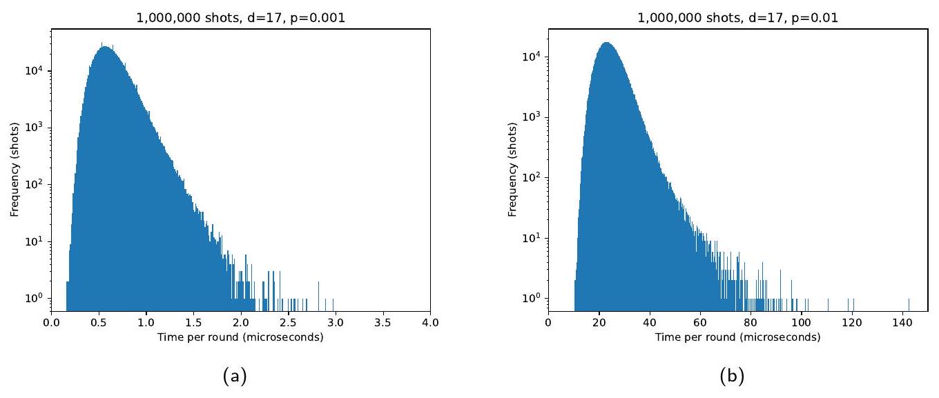
قمنا بتحليل توزيع وقت التشغيل لكل لقطة من PyMatching v2 لبيانات شفرة السطح المحاكية، انظر الشكل 13 والشكل 14. على سبيل المثال، بالنسبة لدارات شفرة السطح ذات المسافة 17 مع ضوضاء على مستوى الدائرة، نلاحظ متوسط وقت تشغيل قدره 0.62 ميكروثانية لكل جولة ونجد أن من مليون لقطة تم فك تشفيرها بوقت تشغيل أقل من 1 ميكروثانية لكل جولة. كما نرسم الانحراف المعياري النسبي لوقت التشغيل لكل لقطة في الشكل 14 ونجد أن ينخفض مع زيادة المسافة أو معدل الخطأ.
كما قارننا سرعة PyMatching v0.7 مع سرعة PyMatching v2 على بيانات تجريبية، من خلال تشغيل كلا جهازين فك التشفير على مجموعة البيانات الكاملة لتجربة جوجل الأخيرة التي تظهر قمع الأخطاء الكمومية عن طريق توسيع كيوبيت منطقي من شفرة السطح من المسافة 3 إلى المسافة 5 [AI23; Tea22]. على شريحة M2، استغرق PyMatching v0.7 3 ساعات و43 دقيقة لفك تشفير جميع 7 ملايين لقطة في مجموعة البيانات، بينما استغرق PyMatching v2 71 ثانية.
7 الخاتمة
في هذا العمل، قدمنا متغيرًا من خوارزمية الزهرة، والتي نسميها الزهرة النادرة، التي تحل مباشرة مشكلة فك التشفير المطابقة المثالية ذات الوزن الأدنى ذات الصلة بتصحيح الأخطاء. تتجنب طريقتنا عمليات البحث المكلفة Dijkstra من الكل إلى الكل التي غالبًا ما تستخدم في تنفيذات جهاز فك التشفير MWPM، حيث يتم استخدام تخفيض إلى خوارزمية الزهرة التقليدية. يمكن لتنفيذنا، المتاح في الإصدار 2 من حزمة بايثون مفتوحة المصدر PyMatching، معالجة حوالي مليون خطأ في الثانية على نواة واحدة. بالنسبة لمسافة 17
الشكل 13: الرسوم البيانية التي تظهر توزيع أوقات التشغيل للزهرة النادرة باستخدام دارات شفرة السطح ذات 17 جولة، والمسافة 17 ونموذج ضوضاء على مستوى الدائرة القياسي. في (أ) نستخدم وعرض حاوية الرسم البياني 0.01 ميكروثانية. من اللقطات لديها وقت تشغيل لكل جولة أقل من 1 ميكروثانية. في (ب) نستخدم بدلاً من ذلك وعرض حاوية الرسم البياني 0.2 ميكروثانية.
الشكل 14: الانحراف المعياري النسبي للوقت لكل لقطة لدارات شفرة السطح ذات المسافة- (مع جولات) وضوضاء على مستوى الدائرة القياسية. هنا و هما الانحراف المعياري والمتوسط، على التوالي، للوقت لكل لقطة، مع أخذ عينة من مليون لقطة لكل نقطة بيانات.
شفرة السطح، يمكنها فك تشفير كل من و الأسس في أقل من ثوانٍ لكل جولة من تصحيح الأخطاء، مما يتطابق مع المعدل الذي يتم فيه توليد بيانات المتلازمة على كمبيوتر كمومي فائق التوصيل.
بعض التقنيات التي قدمناها يمكن تطبيقها مباشرة لتحسين أداء أجهزة فك التشفير الأخرى. على سبيل المثال، قدمنا تتبع مضغوط، الذي يستغل حقيقة أن جهاز فك التشفير يحتاج فقط إلى التنبؤ بأي الملاحظات المنطقية قد تم قلبها، بدلاً من الأخطاء الفيزيائية نفسها. سمح لنا ذلك باستخدام تمثيل نادر للمسارات في رسم كاشف، مع تخزين فقط نقاط النهاية لمسار، جنبًا إلى جنب مع الملاحظات المنطقية التي يقلبها (كقناع بت). أظهرنا أن التتبع المضغوط يمكن استخدامه لتبسيط جهاز فك التشفير union-find بشكل كبير (انظر الملحق A)، مما يؤدي إلى تمثيل مضغوط لبنية بيانات المجموعة المنفصلة وإلغاء الحاجة إلى بناء شجرة ممتدة في خطوة التقشير للخوارزمية.
عند استخدامه لمحاكاة تصحيح الأخطاء، يمكن تنفيذنا أن يتم توازنه بشكل تافه عبر دفعات من اللقطات. ومع ذلك، فإن تحقيق الإنتاجية اللازمة لفك التشفير في الوقت الحقيقي على نطاق واسع يحفز تطوير تنفيذ متوازي للزهرة النادرة. على سبيل المثال، بالنسبة للمهمة ذات الصلة عمليًا لفك تشفير شفرة السطح ذات المسافة 30 عند ضوضاء على مستوى الدائرة، فإن إنتاجية الزهرة النادرة هي حوالي أبطأ من الإنتاجية المطلوبة لكل جولة لكمبيوتر كمومي فائق التوصيل. لذلك سيكون من المثير للاهتمام التحقيق فيما إذا كان تنفيذًا متعدد النوى أو قائمًا على FPGA يمكن أن يحقق الإنتاجية اللازمة لفك التشفير في الوقت الحقيقي على نطاق واسع من خلال تكييف التقنيات في [WZ23] للزهرة النادرة. أخيرًا، سيكون من المثير للاهتمام تكييف الزهرة النادرة لاستغلال الأخطاء المرتبطة التي تنشأ في نماذج الضوضاء الواقعية، على سبيل المثال باستخدام الزهرة النادرة كروتين فرعي في تنفيذ محسن لمطابقة مرتبطة [Fow13] أو جهاز فك تشفير مطابقة الاعتقاد [Hig+23].
المساهمات
عمل المؤلفان معًا على تصميم خوارزمية الزهرة النادرة. كتب أوسكار هيغوت الورقة ومعظم الشيفرة. قاد كريغ جيدني المشروع ونفذ بعض التحسينات النهائية مثل كومة الراديكس.
الشكر والتقدير
نود أن نشكر نيكولاس بروكمان، دان براون، أوستن فاولر، نوح شوتي وباربرا تيرهال على الملاحظات المفيدة التي حسنت المخطوطة.
References
[Ahu+90] Ravindra K Ahuja, Kurt Mehlhorn, James Orlin, and Robert E Tarjan. “Faster algorithms for the shortest path problem”. In: Journal of the ACM (JACM) 37.2 (1990), pp. 213-223. DOI: 10.1145/77600.77615.
[AI23] Google Quantum AI. “Suppressing quantum errors by scaling a surface code logical qubit”. In: Nature 614.7949 (Feb. 2023), pp. 676-681. ISSN: 1476-4687. DOI: 10.1038/s41586-022-05434-1.
[Bac06] Dave Bacon. “Operator quantum error-correcting subsystems for self-correcting quantum memories”. In: Phys. Rev. A 73 (1 Jan. 2006), p. 012340. dor: 10.1103/PhysRevA.73.012340.
[Bar82] F Barahona. “On the computational complexity of Ising spin glass models”. In: Journal of Physics A: Mathematical and General 15.10 (Oct. 1982), p. 3241. dor: 10.1088/03054470/15/10/028.
[BDL22] Burak Boyacı, Thu Huong Dang, and Adam N. Letchford. “On matchings, T-joins, and arc routing in road networks”. In: Networks 79.1 (2022), pp. 20-31. DOI: 10.1002/net.22033.
[Ber+99] Piotr Berman, Andrew B. Kahng, Devendra Vidhani, and Alexander Zelikovsky. “The T-join Problem in Sparse Graphs: Applications to Phase Assignment Problem in VLSI Mask Layout”. In: Algorithms and Data Structures. Ed. by Frank Dehne, Jörg-Rüdiger Sack, Arvind Gupta, and Roberto Tamassia. Berlin, Heidelberg: Springer Berlin Heidelberg, 1999, pp. 25-36. ISBN: 978-3-540-48447-9. doi: 10.1007/3-540-48447-73.
[Ber57] Claude Berge. “Two theorems in graph theory”. In: Proceedings of the National Academy of Sciences 43.9 (1957), pp. 842-844. dor: 10.1073/pnas.43.9.842.
[BM06] H. Bombin and M. A. Martin-Delgado. “Topological Quantum Distillation”. In: Phys. Rev. Lett. 97 (18 Oct. 2006), p. 180501. dor: 10.1103/PhysRevLett.97.180501.
[Bra+13] Sergey Bravyi, Guillaume Duclos-Cianci, David Poulin, and Martin Suchara. “Subsystem surface codes with three-qubit check operators”. In: Quantum Info. Comput. 13.11-12 (Nov. 2013), pp. 963-985. ISSN: 1533-7146. DOI: 10.26421/QIC13.11-12-4.
[Bro22] Benjamin J. Brown. “Conservation Laws and Quantum Error Correction: Toward a Generalized Matching Decoder”. In: IEEE BITS the Information Theory Magazine 2.3 (2022), pp. 5-19. doi: 10.1109/MBITS.2023.3246025.
[BSV14] Sergey Bravyi, Martin Suchara, and Alexander Vargo. “Efficient algorithms for maximum likelihood decoding in the surface code”. In: Phys. Rev. A 90 (3 Sept. 2014), p. 032326. DOI: 10.1103/PhysRevA.90.032326.
[BT16] Nikolas P. Breuckmann and Barbara M. Terhal. “Constructions and Noise Threshold of Hyperbolic Surface Codes”. In: IEEE Transactions on Information Theory 62.6 (2016), pp. 3731-3744. DOI: 10.1109/TIT.2016.2555700.
[Cha+20] Rui Chao, Michael E. Beverland, Nicolas Delfosse, and Jeongwan Haah. “Optimization of the surface code design for Majorana-based qubits”. In: Quantum 4 (Oct. 2020), p. 352. ISSN: 2521-327X. DOI: 10.22331/q-2020-10-28-352.
[Das+22] Poulami Das, Christopher A. Pattison, Srilatha Manne, Douglas M. Carmean, Krysta M. Svore, Moinuddin Qureshi, and Nicolas Delfosse. “AFS: Accurate, Fast, and Scalable Error-Decoding for Fault-Tolerant Quantum Computers”. In: 2022 IEEE International Symposium on High-Performance Computer Architecture (HPCA). 2022, pp. 259-273. doI: 10.1109/HPCA53966.2022.00027.
[Den+02] Eric Dennis, Alexei Kitaev, Andrew Landahl, and John Preskill. “Topological quantum memory”. In: Journal of Mathematical Physics 43.9 (2002), pp. 4452-4505. dor: 10.1063/1.1499754.
[Der+24] Peter-Jan H. S. Derks, Alex Townsend-Teague, Ansgar G. Burchards, and Jens Eisert. “Designing fault-tolerant circuits using detector error models”. In: (2024). arXiv: 240 7.13826 [quant-ph]. URL: https://arxiv.org/abs/2407. 13826.
[DN21] Nicolas Delfosse and Naomi H. Nickerson. “Almost-linear time decoding algorithm for topological codes”. In: Quantum 5 (Dec. 2021), p. 595. ISSN: 2521-327X. dor: 10.22331/q-2021-12-02-595.
[DZ20] Nicolas Delfosse and Gilles Zémor. “Linear-time maximum likelihood decoding of surface codes over the quantum erasure channel”. In: Phys. Rev. Res. 2 (3 July 2020), p. 033042. DOI: 10.1103/PhysRevResearch.2.033042.
[Edm65a] Jack Edmonds. “Maximum matching and a polyhedron with 0,1 -vertices”. In: Journal of Research of the National Bureau of Standards Section B Mathematics and Mathematical Physics (1965), p. 125. DOI: 10.6028/jres.069b.013. URL: https://api. semanticscholar.org/CorpusID:15379135.
[Edm65b] Jack Edmonds. “Paths, Trees, and Flowers”. In: Canadian Journal of Mathematics 17 (1965), pp. 449-467. doi: 10.4153/CJM-1965-045-4.
[EJ73] Jack Edmonds and Ellis L. Johnson. “Matching, Euler tours and the Chinese postman”. In: Mathematical Programming 5.1 (Dec. 1973), pp. 88-124. ISSN: 1436-4646. DOI: 10.1007/BF01580113.
[Fow13] Austin G Fowler. “Optimal complexity correction of correlated errors in the surface code”. In: arXiv preprint arXiv:1310.0863 (2013).
[Fow15] Austin G. Fowler. “Minimum weight perfect matching of fault-tolerant topological quantum error correction in average parallel time”. In: Quantum Info. Comput. 15.1-2 (Jan. 2015), pp. 145-158. ISSN: 1533-7146. DOI: 10.26421/QIC15.1-2-9.
[FWH12a] Austin G. Fowler, Adam C. Whiteside, and Lloyd C. L. Hollenberg. “Towards Practical Classical Processing for the Surface Code”. In: Phys. Rev. Lett. 108 (18 May 2012), p. 180501. DOI: 10.1103/PhysRevLett.108.180501.
[FWH12b] Austin G. Fowler, Adam C. Whiteside, and Lloyd C. L. Hollenberg. “Towards practical classical processing for the surface code: Timing analysis”. In: Phys. Rev. A 864 (4 Oct. 2012), p. 042313. DOI: 10.1103/PhysRevA.86.042313. URL: https://link.aps.org/ doi/10.1103/PhysRevA.86.042313.
[Gal83] Zvi Galil. “Efficient algorithms for finding maximal matching in graphs”. In: CAAP’83. Ed. by Giorgio Ausiello and Marco Protasi. Berlin, Heidelberg: Springer Berlin Heidelberg, 1983, pp. 90-113. ISBN: 978-3-540-38714-5. doi: .
[Gid+21] Craig Gidney, Michael Newman, Austin Fowler, and Michael Broughton. “A FaultTolerant Honeycomb Memory”. In: Quantum 5 (Dec. 2021), p. 605. ISSN: 2521-327X. DOI: 10.22331/q-2021-12-20-605.
[Gid20] Craig Gidney. Decorrelated Depolarization. https://algassert.com/post/2001. Accessed: 2021-10-04. 2020.
[Gid21] Craig Gidney. “Stim: a fast stabilizer circuit simulator”. In: Quantum 5 (July 2021), p. 497. ISSN: 2521-327X. DOI: 10.22331/q-2021-07-06-497.
[GJ23] Craig Gidney and Cody Jones. “New circuits and an open source decoder for the color code”. In: (2023). arXiv: 2312.08813 [quant-ph]. uRL: https://arxiv.org/abs/ 2312.08813.
[HB21] Oscar Higgott and Nikolas P. Breuckmann. “Subsystem Codes with High Thresholds by Gauge Fixing and Reduced Qubit Overhead”. In: Phys. Rev. X 11 (3 Aug. 2021), p. 031039. DOI: 10.1103/PhysRevX.11.031039.
[HH21] Matthew B. Hastings and Jeongwan Haah. “Dynamically Generated Logical Qubits”. In: Quantum 5 (Oct. 2021), p. 564. ISSN: 2521-327X. dor: 10.22331/q-2021-10-19-564.
[Hig+23] Oscar Higgott, Thomas C. Bohdanowicz, Aleksander Kubica, Steven T. Flammia, and Earl T. Campbell. “Improved Decoding of Circuit Noise and Fragile Boundaries of Tailored Surface Codes”. In: Phys. Rev. X 13 (3 July 2023), p. 031007. doi: 10.1103/PhysRevX.13.031007.
[Hig22] Oscar Higgott. “PyMatching: A Python Package for Decoding Quantum Codes with Minimum-Weight Perfect Matching”. In: ACM Transactions on Quantum Computing 3.3 (June 2022). DOI: 10.1145/3505637.
[HNB20] Shilin Huang, Michael Newman, and Kenneth R. Brown. “Fault-tolerant weighted union-find decoding on the toric code”. In: Phys. Rev. A 102 (1 July 2020), p. 012419. dor: 10.1103/PhysRevA.102.012419.
[KD23] Aleksander Kubica and Nicolas Delfosse. “Efficient color code decoders in dimensions from toric code decoders”. In: Quantum 7 (Feb. 2023), p. 929. ISSN: 2521327X. dor: 10.22331/q-2023-02-21-929.
[Kol09] Vladimir Kolmogorov. “Blossom V: a new implementation of a minimum cost perfect matching algorithm”. In: Mathematical Programming Computation 1.1 (July 2009), pp. 43-67. ISSN: 1867-2957. DOI: 10.1007/s12532-009-0002-8.
[KV18] Bernhard H Korte and Jens Vygen. Combinatorial optimization. Springer, 2018. ISBN: 978-3-662-56039-6. DOI: 10.1007/978-3-662-56039-6.
[Liy+23] Namitha Liyanage, Yue Wu, Alexander Deters, and Lin Zhong. “Scalable Quantum Error Correction for Surface Codes using FPGA”. In: 2023 IEEE 31st Annual International Symposium on Field-Programmable Custom Computing Machines (FCCM). 2023, pp. 217-217. DOI: 10.1109/FCCM57271.2023.00045.
[MBG23] Matt McEwen, Dave Bacon, and Craig Gidney. “Relaxing Hardware Requirements for Surface Code Circuits using Time-dynamics”. In: Quantum 7 (Nov. 2023), p. 1172. ISSN: 2521-327X. DOI: 10.22331/q-2023-11-07-1172.
[Men86] Mikhail V Menshikov. “Coincidence of critical points in percolation problems”. In: Soviet Mathematics Doklady. Vol. 33. 1986, pp. 856-859.
[MG07] Jiri Matoušek and Bernd Gärtner. Understanding and using linear programming. Springer, 2007. ISBN: 978-3-540-30697-9. doi: 10.1007/978-3-540-30717-4.
[MPT22] Kai Meinerz, Chae-Yeun Park, and Simon Trebst. “Scalable Neural Decoder for Topological Surface Codes”. In: Phys. Rev. Lett. 128 (8 Feb. 2022), p. 080505. dor: 10.1103/PhysRevLett.128.080505.
[SBT11] Martin Suchara, Sergey Bravyi, and Barbara Terhal. “Constructions and noise threshold of topological subsystem codes”. In: Journal of Physics A: Mathematical and Theoretical 44.15 (Mar. 2011), p. 155301. DOI: 10.1088/1751-8113/44/15/155301.
[Sko+23] Luka Skoric, Dan E. Browne, Kenton M. Barnes, Neil I. Gillespie, and Earl T. Campbell. “Parallel window decoding enables scalable fault tolerant quantum computation”. In: Nature Communications 14.1 (Nov. 2023), p. 7040. ISSN: 2041-1723. dor: 10.1038/s41467-023-42482-1.
[Sun+23] Neereja Sundaresan, Theodore J. Yoder, Youngseok Kim, Muyuan Li, Edward H. Chen, Grace Harper, Ted Thorbeck, Andrew W. Cross, Antonio D. Córcoles, and Maika Takita. “Demonstrating multi-round subsystem quantum error correction using matching and maximum likelihood decoders”. In: Nature Communications 14.1 (May 2023), p. 2852. ISSN: 2041-1723. DOI: 10.1038/s41467-023-38247-5.
[Tan+23] Xinyu Tan, Fang Zhang, Rui Chao, Yaoyun Shi, and Jianxin Chen. “Scalable SurfaceCode Decoders with Parallelization in Time”. In: PRX Quantum 4 (4 Dec. 2023), p. 040344. doi: 10.1103/PRXQuantum.4.040344.
[Tea22] Google Quantum AI Team. Data for “Suppressing quantum errors by scaling a surface code logical qubit”. Zenodo, July 2022. DOI: 10.5281/zenodo.6804040. URL: https: //doi.org/10.5281/zenodo. 6804040.
[Ter15] Barbara M. Terhal. “Quantum error correction for quantum memories”. In: Rev. Mod. Phys. 87 (2 Apr. 2015), pp. 307-346. doi: 10.1103/RevModPhys.87.307.
[TM17] Giacomo Torlai and Roger G. Melko. “Neural Decoder for Topological Codes”. In: Phys. Rev. Lett. 119 (3 July 2017), p. 030501. Dor: 10.1103/PhysRevLett.119.030501.
[Tuc20] David Kingsley Tuckett. “Tailoring surface codes: Improvements in quantum error correction with biased noise”. (qecsim: https://github.com/qecsim/qecsim). PhD thesis. University of Sydney, 2020. doi: 10.25910/x8xw-9077.
[Tut47] W. T. Tutte. “The Factorization of Linear Graphs”. In: Journal of the London Mathematical Society s1-22.2 (1947), pp. 107-111. dor: 10.1112/jlms/s1-22.2.107.
[WLZ22] Yue Wu, Namitha Liyanage, and Lin Zhong. “An interpretation of Union-Find Decoder on Weighted Graphs”. In: (2022). arXiv: 2211.03288 [quant-ph].
[Wu22] Yue Wu. Fusion Blossom. https://github.com/yuewuo/fusion-blossom. 2022.
[WZ23] Yue Wu and Lin Zhong. “Fusion Blossom: Fast MWPM Decoders for QEC”. In: 2023 IEEE International Conference on Quantum Computing and Engineering (QCE). Vol. 01. 2023, pp. 928-938. doi: 10.1109/QCE57702.2023.00107.
A تتبع مضغوط في Union-Find
يمكن تكييف التتبع المضغوط بشكل طبيعي مع جهاز فك التشفير Union-Find [DN21; HNB20]، كما هو موضح في الشكل 15. يتم تهيئة كل حدث كشف مع منطقة، والتي نشير إليها على أنها مجموعة، لتكون متسقة مع المرجع [DN21]. باستخدام نفس النهج كما هو الحال في التتبع المضغوط في الزهرة النادرة، يمكننا تتبع حدث الكشف الذي تم الوصول إليه من كل عقدة كاشف، بالإضافة إلى الملاحظات التي تم عبورها للوصول إليه. بشكل أكثر وضوحًا، دع مرة أخرى تشير إلى
الشكل 15: التتبع المضغوط في Union-Find. (أ) تصطدم مجموعتان. كل عقدة في شجرة المجموعة تشير إلى حدث كشف، وكل حافة هي حافة مضغوطة تمثل مسارًا بين حدثي الكشف في رسم الكاشف (ليس بالضرورة أقصر مسار). يتم وضع علامة على كل حافة بحرف يدل على قناع البت للملاحظات التي تم عبورها على طول المسار الذي تمثله. يختلف هذا عن تنفيذات Union-Find التقليدية، حيث كل عقدة كاشف في مجموعة هي عقدة في شجرة المجموعة. عندما تصطدم مجموعتان، نقوم بتخزين حافة مضغوطة للمسار بين أحداث الكشف التي حدثت فيها الاصطدام (حافة الاصطدام). (ب) شجرتا المجموعتين، جنبًا إلى جنب مع حافة الاصطدام (خط متقطع). (ج) بعد العثور على أحداث الكشف المصدر (5 و7) المعنية في الاصطدام، نستدعي Find(5) وFind(7). عند استخدام ضغط المسار (الذي هنا يربط العقدة 5 بالعقدة الجذرية)، نتأكد من تحديث قناع الملاحظات بشكل مستمر من خلال أخذ مجموع (نموذج 2) لأقنعة البت على طول المسار إلى العقدة الجذرية. (د) اتحاد يضيف العنقود الأصغر كفرع من العقدة الجذرية للعناقيد الأكبر (تصبح العقدة 6 طفلاً للعقدة 0). نقوم بتخزين قناع البت القابل للملاحظة على الحافة (0،6) من خلال أخذ المجموع (باقي 2) لأقنعة البت القابلة للملاحظة على الحواف (0،5)، (6،7) وحافة الاصطدام (5،7). (هـ) العنقود المدمج الآن له توازن زوجي. نستخدم التقشير المضغوط لتسليط الضوء على مجموعة من الحواف (الموضحة باللون الأحمر) بحيث تكون كل عقدة متصلة بعدد فردي من الحواف. نأخذ المجموع (باقي 2) لأقنعة البت القابلة للملاحظة على هذه الحواف المميزة للعثور على القابل للملاحظة المنطقي المتوقع.
حدث الكشف عن المصدر لعقدة الكاشف، ونقوم بتهيئةلكل حدث كشففي بداية الخوارزمية. نحدد مجموعة من القابل للملاحظة المنطقية التي تم عبورها عدد فردي من المرات من حدث الكشف عن مصدر العقدة بواسطة، ونقوم بتهيئةكمجموعة فارغة لكل حدث كشف. ننمو عنقودًاعن طريق إضافة عقدةمن حافةعلى حدود(أي حافة بحيثو). بينما نضيفإلى، نقوم بتعيينو. تذكر أنهي مجموعة القابل للملاحظة المنطقية التي تم قلبها بواسطة الحافةو⊕ تشير إلى الفرق المتماثل للمجموعات. نظرًا لأننا نخزنكقناع بت لكل حافة، يمكن تنفيذ الفرق المتماثل بين حافتينبشكل فعال للغاية باستخدام XOR بت.
نمثل كل عنقود كشجرة عنقود مضغوطة. كل عقدة في شجرة العنقود المضغوطة تتوافق مع حدث كشف، على عكس شجرة العنقود المقدمة في [DN21]، حيث كل عقدة هي عقدة كاشف. كل حافةفي شجرة العنقود هي حافة مضغوطة، تمثل مسارًامن خلال رسم الكاشف بين أحداث الكشفو. على عكس الحواف المضغوطة في الزهرة النادرة، فإن هذا المسار عمومًا ليس المسار الأقصر. يتم تعيين الحافة المضغوطةللقابل للملاحظة المنطقية التي تم عبورها عدد فردي من المرات بواسطة، المشار إليها بـأو. نتحقق من أي عنقود تنتمي إليه عقدة الكاشفعن طريق استدعاء Find.
نعدل خطوة ضغط المسار لعملية Find بحيث كلما تم استبدال مسار(يتكون من حواف مضغوطة) عبر شجرة العنقود بين حدثي كشفوبواسطة حافة مضغوطة، يتم حساب مجموعة القابل للملاحظة المنطقيةللحافة المضغوطة الجديدة. يمكن إجراء تعديل مشابه إذا تم استخدام تقسيم المسار أو تقسيم المسار بدلاً من ضغط المسار لعملية Find.
تم تعديل عملية الاتحاد بطريقة مشابهة. لنفترض أن عنقودًايتصادم مع عنقودعلى طول حافة (). بعبارة أخرى، () هي حافة في رسم الكاشف بحيثو. نقوم بإنشاء حافة الاصطدام () من المعلومات المحلية عند نقطة الاصطدام، ونعينها مجموعة القابل للملاحظة المنطقية. عندما ندمج العنقودمع العنقودباستخدام عملية الاتحاد، نضيف العقدة الجذريةمن شجرة العنقود الأصغر (لنقل) كطفل للعقدة الجذريةمن شجرة العنقود الأكبرعن طريق إضافة حافة مضغوطةإلى الشجرة. نقوم بتعيين مجموعة القابل للملاحظة المنطقيةلتكونحيثهو المسار عبر الشجرة بينو.
أخيرًا، بمجرد أن يكون لدى جميع العناقيد توازن زوجي (عدد زوجي من أحداث الكشف، أو متصلة بالحدود)، يمكننا تطبيق خوارزمية التقشير [DZ20] على أشجار العنقود المضغوطة، والتي تعيد مجموعة من الحواف المضغوطة. نقول إن الحواف المضغوطة فيهي حواف مميزة في شجرة العنقود. مجموعة القابل للملاحظة المنطقية التي يتوقع المفسر أن تكون قد تم قلبها هي بعد ذلك. هذه المرحلة أكثر كفاءة بكثير من خطوة التقشير التقليدية لـ UF، حيث لا نحتاج إلى بناء شجرة ممتدة في كل عنقود. بدلاً من ذلك، نقوم فقط بتشغيل التقشير على تمثيلنا المضغوط لأشجار العنقود. التقشير المضغوط خطي في عدد الحواف المضغوطة في شجرة العنقود. من أجل الاكتمال، نقدم كود زائف للتقشير المضغوط في الخوارزمية 1، ومع ذلك، فإن هذا ببساطة تعريف تكراري لخوارزمية التقشير لـ [DZ20] المطبقة على حالة شجرة العنقود المضغوطة المكونة من رسم لحواف مضغوطة تربط أحداث الكشف، بدلاً من رسم فرعي لشجرة ممتدة من عنقود تقليدي في رسم الكاشف (المكون من عقد كاشف وحواف رسم كاشف). الإجراء تكراري ويأخذ كمدخل عقدةفي شجرة العنقود المضغوطة، ويعيدو. هنا،هي مجموعة القابل للملاحظة المنطقية التي تم قلبها عن طريق قلب الحواف المضغوطة المميزة التي هي أحفاد لـفي شجرة العنقود (حافة أحفاد لـهي حافة في الشجرة الفرعية المتجذرة في). المتغير المساعد(المستخدم في التكرار) هو توازن عدد الحواف المميزة للأطفال لـفي العنقود (حيث تكون حافة الطفل هي حافة تربطبأحد أطفالها في شجرة العنقود). في البداية، نفترض أنه لا توجد عقدة في شجرة العنقود متصلة بالحدود، وفي هذه الحالة نقوم بتهيئةزوجيًا لكل عقدة. نقوم بتشغيل التقشير المضغوط على العقدة الجذريةللعثور على مجموعة القابل للملاحظة المنطقيةالتي تم قلبها بواسطة جميع الحواف المميزة في شجرة العنقود. لاحظ أنيجب أن تكون دائمًا فردية للعقدة الجذرية إذا لم يكن هناك حدود.
تذكر أن التقشير يجب أن يجد مجموعة من الحواف المميزة (الحواف في) بحيث تكون كل عقدة في الشجرة متصلة بعدد فردي من الحواف المميزة. سنظهر أولاً أن(التي تم إرجاعها بواسطة التقشير المضغوط) هي بالفعل مجموعة القابل للملاحظة المنطقية التي تم قلبها بواسطة الحواف المميزة التي هي أحفاد لـ، وأنهو توازن عدد الحواف المميزة للأطفال لـ. اعتبر الحالة الأساسية التي تكون فيهاعقدة ورقية، وفي هذه الحالة ليس لديها حواف أطفال أو أحفاد. في هذه الحالة، يقوم التقشير المضغوط بتعيينإلى زوجي (نظرًا لأننا نقوم بتهيئةزوجيًا) وإلى المجموعة الفارغة. الآن اعتبر خطوة الاستقراء، حيث تحتويعلى أطفالفي شجرة العنقود. لكلنبرز الحافة () إذا كانتزوجية، ويتم تعيينإلى توازن عدد هذه الحواف المميزة للأطفال لـ، كما هو مطلوب. الحلقة الرئيسية للخوارزمية تعينإلى
وإذا افترضنا أنهي مجموعة القابل للملاحظة المنطقية التي تم قلبها بواسطة الحواف المميزة الأحفاد لـفمن الواضح أنهي مجموعة القابل للملاحظة المنطقية التي تم قلبها بواسطة الحواف المميزة الأحفاد لـ. أخيرًا، لاحظ أنه نظرًا لأننا نطبق التقشير المضغوط على شجرة، يتم استدعاء الدالة على كل عقدةبالضبط مرة واحدة، ونبرز حافة () إلى طفلمنإذا وفقط إذا كانتزوجية. لذلك، تصبح كل عقدة متصلة بعدد فردي من الحواف المميزة، كما هو مطلوب.
لم نأخذ في الاعتبار الحدود بعد. إذا كانت هناك حافة مضغوطة () في شجرة العنقودتربط حدث كشفبالحدود(يمكن أن تكون هناك حافة واحدة على الأكثر مثل هذه الحافة نظرًا لأن العنقود يصبح محايدًا بمجرد أن يصطدم بالحدود)، نقوم أولاً بإضافةإلى الحل وإزالة من، ثم نقوم بتعيينفرديًا قبل تطبيق التقشير المضغوط على العقدة الجذريةمن شجرة العنقود المتبقية، مضيفين الناتجإلى الحل.
Algorithm 1 Compressed Peeling
procedure CompressedPeeling( $x$ )
$p_{x} leftarrow p_{x}^{text {init }} quad triangleright$ Parity of the number of highlighted child edges of $x$
$l_{x} leftarrow{ } quad$ - Observables flipped by highlighted descendant edges of $x$
for each child $y$ of $x$ do
$p_{y}, l_{y} leftarrow$ CompressedPeeling $(y)$
$l_{x} leftarrow l_{x} oplus l_{y}$
if $p_{y}$ is even then
$l_{x} leftarrow l_{x} oplus l(x, y) quad triangleright$ Compressed edge ( $x, y$ ) becomes highlighted
flip $p_{x}$
end if
end for
return $p_{x}, l_{x}$
end procedure
ب أسوأ وقت تشغيل
في هذا القسم، سنجد حدًا أعلى في أسوأ الحالات لوقت تشغيل الزهرة النادرة. لاحظ أن هذا الحد الأعلى من المحتمل أن يكون فضفاضًا، وعلاوة على ذلك يختلف كثيرًا عن وقت التشغيل المتوقع للزهرة النادرة لمشاكل QEC النموذجية، والتي نعتقد أنها خطية في حجم الرسم. دعنا نحدد عدد عقد الكاشف بـ، عدد الحواف في رسم الكاشف بـوعدد أحداث الكشف بـ. أولاً، لاحظ أن كل شجرة متناوبة تحتوي دائمًا على حدث كشف غير متطابق واحد بالضبط، بمعنى أنه يحتاج فقط إلى منطقة واحدة متنامية أن تصبح متطابقة حتى تنفصل الشجرة بالكامل إلى مناطق متطابقة. لذلك، فإن أحداث الشجرة المتناوبة التي تنمو الشجرة المتناوبة، تشكل الزهور أو تنفصل الزهور (أحداث من النوع أ، ج، د أو هـ في الشكل 4) لا تغير عدد أحداث الكشف التي تبقى لتكون متطابقة. من ناحية أخرى، عندما تصطدم شجرة بشجرة أخرى (النوع ب)، ينخفض عدد أحداث الكشف غير المتطابقة بمقدار اثنين، وعندما تصطدم شجرة بالحدود (النوع ف)، أو تطابق حدود (النوع ج)، فإن عدد أحداث الكشف غير المتطابقة ينخفض بمقدار واحد. نشير إلى حدث شجرة متناوبة يقلل عدد أحداث الكشف غير المتطابقة على أنه زيادة، ونشير إلى جزء من الخوارزمية بين الزيادات المتتالية على أنه مرحلة. من الواضح أنه يمكن أن يكون هناك على الأكثرزيادات وعلى الأكثرمراحل.
نحن الآن نحدد تعقيد كل تحسين، وكل مرحلة. في كل مرحلة، هناك على الأكثرتكونت الأزهار أو تحطمت، وفي أقصى الحدودتمت إضافة المباريات إلى الأشجار، حيث لا يمكن لنفس الزهرة أن تتشكل ثم تتحطم ضمن مرحلة واحدة. لتوضيح الأمر بشكل أكثر وضوحًا، لاحظ أولاً أنه لا يوجد أكثر منتتفتح أو مناطق تافهة في أي لحظة في الخوارزمية. ضمن مرحلة، فإن الأحداث الشجرية المتناوبة الوحيدة المسموح بها هي من النوع و e (نظرًا لـ b، و الأحداث هي تعزيزات). بمجرد أن يبدأ ازدهار، لا يمكن لنفس الزهرة أن تصبح منطقة متقلصة وتتحطم حتى بعد تعزيز، حيث يجب أن تصبح الزهرة أولاً تطابقًا (من خلال تعزيز) ثم تصبح عقدة داخلية في حدث من النوع أ. لذلك، في أقصى حديمكن أن تتشكل الأزهار في كل مرحلة. أخيرًا، ضمن كل مرحلة، الأزهار الوحيدة التي يمكن أن تنكسر، أو تُضاف إلى شجرة كجزء من مباراة، هي تلك الأزهار (أو المناطق التافهة) التي تم تشكيلها بالفعل في بداية المرحلة، وهناك في أقصى حدمن هذه.
نحن الآن نعتبر تعقيد أسوأ الحالات لكل من هذه العمليات الممكنة ضمن مرحلة. عندما يتشكل الزهرة، يقوم كل عقدة تملكها بتحديث سلف الزهرة الأعلى المخزن في الذاكرة ونصف القطر المغلف، بتكلفة تتناسب مع عمق شجرة الزهرة، وهذه الخطوة لها تعقيد. بالإضافة إلى ذلك، يتم إعادة جدولة كل عقدة مملوكة للزهرة، مع التكلفة. تحديث هيكل الزهرة وهيكل الشجرة المتناوبة (مثل الحواف المضغوطة) هو في أقصى حد. إجمالاً، يتطلب تشكيل زهرة وقت تشغيل لا يتجاوز ، وينطبق نفس الحد الأعلى على تدمير زهرة. عندما يتم إضافة تطابق إلى شجرة متناوبة، تكون التعقيد هو من إعادة جدولة العقد، التي تتجاوز الـتكلفة تحديث الـ هيكل الشجرة المتناوبة. أخيرًا، هناك تكلفة نمو وتقلص المناطق. في كل مرحلة، يمكن أن يكون العقدة معنية فقط فيأحداث الفيضانات ARRIVE أو LEAVE: بمجرد أن تبدأ منطقة ما في النمو، فإنها (أو سلفها الأزهار الأعلى) تستمر في النمو حتى التوسيع التالي. لذلك، فإن تكلفة إعادة جدولة العقد بسبب أحداث ARRIVE أو LEAVE في كل مرحلة هي. كما نذكر القارئ أن المتتبع له تعقيد زمني ثابت لكل عملية (نظرًا لأن كومة الراديكس لها عمليات إدخال واستخراج-الأدنى في زمن ثابت)، لذا فإنه لا يساهم في التعقيد الكلي. لذلك، في كل مرحلة، يتم السيطرة على أسوأ حالة زمن التشغيل بواسطة التكلفة المرتبطة بما يصل إلىتتكون الأزهار أو تتحطم. هناكمراحل، تؤدي إلىتعقيد أسوأ الحالات.
معالجة الأوزان السلبية في الحواف
تذكر أن وزن الحافةيمكن أن يصبح سلبياً لأننا يمكن أن نملكلذلك من الضروري التعامل مع أوزان الحواف السلبية لفك التشفير بشكل صحيح لهذه النماذج الخطأ. على سبيل المثال، اعتبر مصفوفة التحقق من كود التكرار ثلاثي المسافة.
مع التوزيع السابق وخطأ مع المتلازمةالأخطاء الاثنان المتوافقان مع المتلازمة هما، الذي لديه احتمال سابق، و ( )، الذي لديه احتمال سابق تذكر أن فك تشفير MWPM يستخدم متجه الأوزانويجد تصحيحًامُرضٍوزنها ضئيللذلك، من المهم أن تكون أوزان الحوافهي سلبية بالفعل هنا، حيث يؤدي ذلك إلى توقع جهاز فك التشفير للأكثر احتمالًا (على الرغم من الوزن الهامش الأعلى).بدلاً من الخطأ.
نحن الآن نوضح كيف يمكن التعامل مع أوزان الحواف السلبية لمشكلة فك تشفير MWPM لبعض مصفوفات التحققمع متجهات الأوزان وخطأ مع المتلازمةعلى الرغم من أن خوارزمية الزهرة النادرة تتعامل فقط مع أوزان الحواف غير السلبية، إلا أنه يمكننا still تنفيذ فك تشفير MWPM عندما تكون هناك أوزان حواف سلبية باستخدام الإجراء التالي، الذي يستخدم الزهرة النادرة كروتين فرعي:
حددبحيثإذا و وإلا.
منحدد أوزان الحواف المعدلةأينبالإضافة إلى المتلازمة المعدلة.
استخدم الإزهار النادر للعثور على تصحيحمُرضٍوزن معدّل أدنى. لاحظ أن تعريف يضمن أن كل عنصرغير سالب.
إرجاع التصحيحالذي من المؤكد أنه سيلبيمع وزن إجمالي minimal. يمكننا التحقق من صحة هذه الإجراءات على النحو التالي. أولاً، لاحظ أنيُرضيإذا وفقط إذايُرضي. ثانياً، لاحظ أن
هنا، تستخدم المعادلة الأولى والمصطلح يأخذ في الاعتبار حقيقة أن المجموعيتم الاستيلاء على الحقل الثنائيلذا أي بت تم تعيينه في كلاهما و يجب ألا يكون له وزنه المقابلتساهم في المجموع. لذلك، إذا وجدنا وزن معدّل أدنىمُرضٍ، من المؤكد أن التصحيحيتميز بوزن خفيف جداًمُرضٍبشكل بديهي، حيثما كان لدينا آلية خطأ مع احتمال خطأ مرتفعنحن نعيد صياغة مشكلة فك الشيفرة بدلاً من ذلك للتنبؤ بما إذا كانت آلية الخطأ لم تحدث. تم مناقشة التعامل مع أوزان الحواف السلبية أيضًا في [Hig22]، وكذلك في النتيجة 12.12 من [KV18]، حيث يشير كورت وفايجن إلى ما يسمى بوزن الحد الأدنى -join يعادل ما نسميه MWEM.
مثال على الكواشف والملاحظات لشفرة التكرار
في الشكل 16 نعرض الكواشف، والملاحظات، والمصفوفات و ورسم البياني للكاشف للدائرة المرتبطة بتجربة الذاكرة باستخدام رمز تكرار قلب البت [[2,1,2]] مع جولتين من استخراج المتلازمات.
لاحظ أنه بالنسبة لتجربة ذاكرة شفرة السطح، فإن الدائرة ورسم الكاشف تكون ثلاثية الأبعاد بدلاً من ذلك. في هذه الحالة، فإن منطقة الحساسية التي تتوافق مع منطقتشكل القياسات القابلة للملاحظة ورقة ثنائية الأبعاد في الزمكان. نشير إلى هذه القياسات القابلة للملاحظة المنطقية. هذا القابل للملاحظةمضمن في المجموعةمن حافةإذا كانت آلية الخطأ المرتبطة بـتقلبات. لكي يحدث هذا، الحافةيجب أن يخترق الورقة ثنائية الأبعاد (منطقة الحساسية) وأن يكون-نوع الكواشف (الكواشف التي هي أزواج منالقياسات) عند نقاط نهايتها.
الشكل 16: تمثيلات للكواشف، الملاحظات المنطقية وآليات الخطأ للدائرة المرتبطة بتجربة ذاكرة رمز التكرار [[2,1,2]] مع جولتين من استخراج المتلازمات. نستخدم رمز قلب البت (مع مجموعة المثبتات ) وتنفيذ التهيئة والقياس العرضي في الأساس. (أ) الكواشف الثلاثة في الدائرة. المناطق المميزة باللون الأزرق هي -نوع الكشف عن المناطق [MBG23] (خطأ داخل هذه المنطقة يتعارض مع نوعها سيتسبب في قلب الكاشف المقابل). (ب) منطقي الملاحظ. هنا، المنطقة المميزة باللون الأزرق هي-نوع منطقة الحساسية المرتبطة بالمنطققابل للملاحظة – أخطاء تتعارض معفي هذه المنطقة ستغير نتيجة القياس المنطقي المقابل. (ج) نظرًا لوجود نموذج ضوضاء باولي العشوائي في الدائرة، يمكننا تصنيف الأخطاء بناءً على مجموعة الكواشف والملاحظات المنطقية التي تقوم بتغييرها. بالنسبة لنموذج الضوضاء المعياري على مستوى الدائرة، هناك ثماني فئات مختلفة من آلية الخطأ في هذه الدائرة، عند تصنيفها بهذه الطريقة. لكل آلية خطأ، نبرز باللون الأحمر منطقة من الدائرة حيث يتم تغيير كيوبت واحد.الخطأ سيقلب نفس الكواشف والملاحظات. لاحظ أن هذه الكيوبت الفرديالأخطاء هي مجرد أمثلة على أخطاء باولي التي تساهم في آليات الخطأ؛ على سبيل المثال، خطأ باولي آخر يساهم فيستكون كيوبيت مزدوجةخطأ بعد أول CNOT. (د) من الملائم أحيانًا وصف الكواشف، والملاحظات، وآليات الخطأ من حيث مصفوفة فحص الكاشف.ومصفوفة قابلة للملاحظة. كل عمود في أو يتوافق مع آلية خطأ. كل صف فييتوافق مع كاشف، حيث تشير العناصر غير الصفرية إلى آليات الخطأ التي تعكس الكاشف. وبالمثل، كل صف فييتوافق مع ملاحظة منطقية، حيث تشير العناصر غير الصفرية إلى آليات الخطأ التي تعكس الملاحظة. (هـ) إذالديه وزن عمود لا يزيد عن اثنين، يمكننا تمثيله برسم بياني للكاشف. كل عقدةيتوافق مع كاشف. كل حافةيتوافق مع آلية خطأ تقوم بتبديل و كل نصف حافةيتوافق مع آلية خطأ تعكس فقط، المشار إليه هنا بحافة متصلة بالحدود. كل حافةيتم تعيين مجموعة من الملاحظات المنطقيةإنه يقلب، بالإضافة إلى وزن (الوزن غير موضح في الرسم البياني) حيث هي احتمالية حدوث آلية الخطأ المقابلة في نموذج الضوضاء. لاحظ أنه هنا يوجد حافتان نصفيتان متوازيتان متجاورتان لكل عقدة؛ هذه علامة على أن الشيفرة لها مسافة 2، وبالتالي لديها آليات خطأ مميزة تقوم بتغيير نفس مجموعة من الكواشف ولكن مجموعات مختلفة من الملاحظات المنطقية. في هذه الحالة، يمكننا فقط الاحتفاظ بالحافة ذات الوزن الأقل (نظرًا لأن تنفيذنا لزهرة رقيقة لا يتعامل مباشرة مع الحواف المتوازية).
Sparse Blossom: correcting a million errors per core second with minimum-weight matching
Oscar Higgott and Craig Gidney Google Quantum AI, Santa Barbara, California 93117, USA Department of Physics & Astronomy, University College London, WC1E 6BT London, United Kingdom
January 14, 2025
Abstract
In this work, we introduce a fast implementation of the minimum-weight perfect matching (MWPM) decoder, the most widely used decoder for several important families of quantum error correcting codes, including surface codes. Our algorithm, which we call sparse blossom, is a variant of the blossom algorithm which directly solves the decoding problem relevant to quantum error correction. Sparse blossom avoids the need for all-to-all Dijkstra searches, common amongst MWPM decoder implementations. For circuit-level depolarising noise, sparse blossom processes syndrome data in both X and Z bases of distance-17 surface code circuits in less than one microsecond per round of syndrome extraction on a single core, which matches the rate at which syndrome data is generated by superconducting quantum computers. Our implementation is open-source, and has been released in version 2 of the PyMatching library.
Abstract
The source code for our implementation of sparse blossom in PyMatching version 2 can be found on github at https://github.com/oscarhiggott/PyMatching. PyMatching is also available as a Python 3 pypi package installed via “pip install pymatching”.
1 Introduction
A surface code superconducting quantum computer with a million physical qubits will generate measurement data at a rate of around 1 terabit per second. This data must be processed at least as fast as it is generated by a decoder, the classical software used to predict which errors may have occurred, to prevent a backlog of data that grows exponentially in the -gate depth of the computation [Ter15]. Moreover, fast decoders are important not only for operating a quantum computer, but also as a software tool for researching quantum error correction protocols. Estimating the resource requirements of a quantum error correction protocol (e.g. estimating the teraquop footprint below threshold [Gid+21]) can require the use of direct Monte Carlo sampling to estimate the probability of extremely rare events. These analyses can be prohibitively expensive without access to a fast decoder, capable of processing millions of shots from circuits containing gates in a reasonable time-frame.
Many decoders have been developed for the surface code, the oldest and most popular of which is the minimum-weight perfect matching (MWPM) decoder [Den+02], which is also the focus of this work. The MWPM decoder maps the decoding problem onto a graphical problem by decomposing the error model into -type and -type Pauli errors [Den+02]. This graphical problem can then be solved with the help of Edmonds’ blossom algorithm for finding a minimum-weight perfect matching in a graph [Edm65b; Edm65a]. A naive implementation of the MWPM decoder has a worst-case complexity in the number of nodes in the graph of , with the expected running time for typical instances found empirically to be roughly [Hig22]. Approximations and optimisations of the MWPM decoder have led to significantly improved expected running times [FWH12a; Fow15; Hig22]. In particular, Fowler proposed a MWPM decoder with average parallel running time [Fow15]. However, published implementations of MWPM decoders have not demonstrated speeds fast enough for real-time decoding at scale.
There have been several alternatives to the MWPM decoder proposed in the literature. The Union-Find decoder has an almost-linear worst-case running time [DN21; HNB20], and fast hardware implementations have been proposed and implemented . The Union-Find decoder is slightly less accurate than, and can be seen as an approximation of, the MWPM decoder [WLZ22]. Maximum-likelihood decoders can achieve a higher accuracy than the MWPM decoder [BSV14; Hig+23; Sun+23] but have high computational complexity, rendering them impractical for real-time decoding. Other decoders, such as correlated MWPM [Fow13], beliefmatching [Hig+23] and neural network [TM17; MPT22] decoders can achieve higher accuracy than MWPM with a much more modest increase in running time. While there has been progress in the development of open-source software packages for decoding surface codes [Hig22; Tuc20], these tools are much slower than stabilizer circuit simulators [Gid21], and have therefore been a bottleneck in surface code simulations. This is perhaps one of the reasons why numerical studies of error correcting codes have often focused on estimating thresholds (which require decoding fewer shots), instead of resource overheads (which are more practically useful for making comparisons).
In this work, we introduce a new implementation of the MWPM decoder. The algorithm we introduce, sparse blossom, is a variant of the blossom algorithm which is conceptually similar to the approach taken in Refs. [FWH12a; FWH12b; Fow15], in that it solves the MWPM decoding problem directly on the detector graph, rather than naively breaking up the problem into multiple sequential steps and solving the traditional MWPM graph theory problem as a separate subroutine. This avoids the all-to-all Dijkstra searches often used in implementations of the MWPM decoder. Our implementation is orders of magnitude faster than alternative available tools, and can decode both and bases of a distance-17 surface code circuit (for circuit-noise) in under one microsecond per round on a single core, matching the rate at which syndrome data is generated on a superconducting quantum processor. At distance 29 with the same noise model (more than sufficient to achieve logical error rates), PyMatching takes 3.5 microseconds per round to decode on a single core. These results suggest that our sparse blossom algorithm is fast enough for real-time decoding of superconducting quantum computers at scale; a real-time implementation is likely achievable through parallelisation across multiple cores, and by adding support for decoding a stream, rather than a batch, of syndrome data. Our implementation of sparse blossom has been released in version 2 of the PyMatching Python package, and can be combined with Stim [Gid21] to run simulations in minutes on a laptop that previously would have taken hours on a highperformance computing cluster.
In impressive parallel independent work, Yue Wu has also developed a new implementation of the blossom algorithm called fusion blossom [WZ23], available at [Wu22]. The conceptual similarity with our approach is that fusion blossom also solves the MWPM decoding problem directly on the detector graph. However, there are many differences in the details of our respective implementations; for example, fusion blossom explores the graph in a similar way to how clusters are grown in union-find, whereas our approach grows exploratory regions uniformly, managed by a global priority queue. While our approach has faster single-core performance, fusion blossom also supports parallel execution of the algorithm itself, which can be used to achieve faster processing speeds for individual decoding instances. When used for error correction simulations, we note that sparse blossom is already trivially parallelisable by splitting the simulation into batches of shots, and processing each batch on a separate core. However, parallelisation of the decoder itself is important for real-time decoding, to prevent an exponentially increasing backlog of data building up within a single computation [Ter15], or to avoid the polynomial slowdown imposed by relying on parallel window decoding instead Tan +23. Therefore, future work could explore combining sparse blossom with the techniques for parallelisation introduced in fusion blossom.
The paper is structured as follows. In Section 2 we give background on the decoding problem we are interested in and give an overview of the blossom algorithm. In Section 3 we explain our algorithm, sparse blossom, before describing the data structures we use for our implementation in Section 4. In Section 5 we analyse the running time of sparse blossom, and in Section 6 we benchmark its decoding time, before concluding in Section 7.
2 Preliminaries
2.1 Detectors and observables
A detector is a parity of measurement outcome bits in a quantum error correction circuit that is deterministic in the absence of errors. The outcome of a detector measurement is 1 if the observed parity differs from the expected parity for a noiseless circuit, and is 0 otherwise. We say that a Pauli error flips detector if including in the circuit changes the outcome of , and a detection event is a detector with outcome 1 . We define a logical observable to be a linear combination of measurement bits, whose outcome instead corresponds to the measurement of a logical Pauli operator.
We define an independent error model to be a set of independent error mechanisms, where error mechanism occurs with probability (where is a vector of priors), and flips a set of detectors and observables. An independent error model can be used to represent circuitlevel depolarising noise exactly, and is a good approximation of many commonly considered error models [Cha+20; Gid20]. It can be useful to describe an error model in an error correction circuit using two binary parity check matrices: a detector check matrix and a logical observable matrix . We set if detector is flipped by error mechanism , and otherwise. Likewise, we set if logical observable is flipped by error mechanism , and otherwise. By describing the error model this way, each error mechanism is defined by which detectors and observables it flips, rather than by its Pauli type and location in the circuit. From a stabilizer circuit and Pauli noise model, we can construct and efficiently by propagating Pauli errors through the circuit to see which detectors and observables they flip. Each prior is then computed by summing over the probabilities of all the Pauli errors that flip the same set of detectors or observables (or more precisely, these equivalent error mechanisms are independent, and we compute the probability that an odd number occurred). This is essentially what the error analysis tools do in Stim, where a detector error model (automatically constructed from a Stim circuit) captures the information contained in and [Gid21].
We can represent an error (a set of error mechanisms) by a vector . The syndrome of is the outcome of detector measurements, given by . The detection events are the detectors corresponding to the non-zero elements of . An undetectable logical error is an error in , and the distance of the circuit is , where is the Hamming weight of . Given a syndrome of some error , as well as knowledge of and , a decoder makes a prediction of an error satisfying and succeeds if . Note that sometimes a decoder need only output the logical prediction (succeeding if it matches ), as we discuss later.
For a given circuit, the choice of detectors is not unique. For example, if we redefine any detector as then we still have a valid choice of detectors, and this change corresponds to adding row to row of . Since two errors are distinguishable if and only if , two detector check matrices can distinguish the same errors if they have the same kernel . While row operations on do not affect which errors can be distinguished, it is often necessary that the choice of basis for the detectors has a particular structure in order for a given decoding algorithm to be applicable (as discussed shortly in Section 2.2).
Similarly, the choice of logical observables is also not unique. Since detector outcomes are deterministically zero in the absence of noise, we can add any linear combination of detectors to a logical observable without effecting its expectation value for a noiseless circuit. In terms of check matrices, this change corresponds to defining some new logical observables matrix where we have added some linear combinations of the rows of to each row of the original logical observables matrix :
Here is an arbitrary binary matrix of dimensions . If we use a decoder that is guaranteed to provide a prediction consistent with the syndrome, i.e. , then adding detectors to each observable will not change whether or not the decoder succeeds, since .
In Appendix D, we show how the detectors, observables and the matrices and are defined for a small example of a distance 2 repetition code circuit.
2.2 Detector graphs
In this work, we will restrict our attention to graphlike error models, defined to be independent error models for which each error mechanism flips at most two detectors ( has column weight at most two). Graphlike error models can be used to approximate common noise models for many important classes of quantum error correction codes including surface codes [Den+02], for which -type and -type Pauli errors are both graphlike. Many related code families also have graphlike error models, such as repetition codes, 2D hyperbolic codes [BT16], some 2D subsystem codes [Bra+13; SBT11; Bac06; HB21] and Floquet codes [HH21; Gid+21], amongst others. Color codes [BM06] can be decoded by using a mapping to a graphlike error model as a subroutine [KD23; GJ23], and generalizing this approach to decode more general codes is an active area of research [Bro22].
We can represent a graphlike error model using a detector graph , also called a matching graph or decoding graph in the literature. Each node corresponds to a detector (a detector node, a row of ). Each edge is a set of detector nodes of cardinality one or two representing an error mechanism that flips this set of detectors (a column of ). We can decompose the edge set as where and . A regular edge flips a pair of detectors , whereas a half-edge flips a single detector . For a half-edge we sometimes say that is connected to the boundary and use the notation , where is a virtual boundary node (which does not correspond to any detector). Therefore, when we refer to an edge it is assumed that is a node and is either a node or the boundary node . Each edge is assigned a weight , and recall that is the probability that error mechanism occurs. We also define an edge weights vector for which . We also label each edge with the set of logical observables that are flipped by the error mechanism, which we denote either by or . We use to denote the symmetric difference of sets and . For example, is the set of logical observables flipped when the error mechanisms 1 and 2 are both flipped. We define the distance between two nodes and in the detector graph to be the length of the shortest path between them. We give an example of a detector graph for a repetition code circuit in Appendix D.
2.3 The minimum-weight perfect matching decoder
From now on, we will assume that we have an independent graphlike error model with check matrix , logical observables matrix , priors vector , as well as the corresponding detector graph with edge weights vector . Given some error sampled from the graphlike error model, with the observed syndrome , the minimum-weight perfect matching (MWPM) decoder finds the most probable physical error consistent with the syndrome. In other words, for a graphlike error model it finds a physical error satisfying that has maximum prior probability . For our error model the prior probability of an error is
Equivalently we seek to maximise , where here is a constant and we recall that the edge weight is defined as . This corresponds to finding an error satisfying that minimises , the sum of the weights of the corresponding edges in . We note that a maximum likelihood decoder instead finds the most probable logical error for any error model (graphlike or not), however maximum likelihood decoding is in general computationally inefficient.
Despite the MWPM decoder’s name, the problem it solves, defined above, does not correspond to finding a MWPM in , but instead corresponds to solving a variation of the MWPM problem, which we refer to as the minimum weight embedded matching (MWEM) problem. Let us first define the traditional MWPM problem for a graph . Here is a weighted graph, where each edge is a pair of nodes and, unlike detector graphs, there are no half-edges. Each edge is assigned a weight . A perfect matching is a subset of edges such that each node is incident to exactly one edge . For each we say that is matched to , and vice versa. A MWPM is a perfect matching that has minimum weight
Figure 1: Key differences between the quantum decoding problem solved by PyMatching and the minimum weight perfect matching problem. In the usual MWPM problem, all nodes must be matched and they are matched using a disjoint set of edges. In the decoding problem, (a) only a subset of nodes is excited, only these nodes need to be matched, and (b) the edge set used to match them is not required to be disjoint. The excited nodes are matched by finding an edge set where excited nodes have an odd number of neighbors in the edge set, non-excited nodes have an even number of neighbors in the edge set, and (c) there may be boundary nodes that can have any number of neighbors in the edge set. (d) The expected distribution of excited nodes is not uniform. It is generated by sampling edges, where each edge is independently included with some probability, and then exciting any nodes that have an odd number of neighbors in the sampled edge set. This results in it being exponentially unlikely to see large distances between excited nodes at low error rates, which has major implications on the expected runtime of the algorithm (see Section 5).
. Clearly, not every graph has a perfect matching (a simple necessary condition is that must be even; a necessary and sufficient condition is provided by Tutte’s theorem [Tut47]), and a graph may have more than one perfect matching of minimum weight.
Given a detector graph with vertex set , and a set of detection events (highlighted nodes) , we define an embedded matching of in to be a set of edges such that every node in is incident to an odd number of edges in , and every node in is incident to an even number of edges in . The minimum-weight embedded matching is an embedded matching that has minimum weight . We note that the minimum-weight embedded matching problem for a standard graph (containing no half-edges) is known as the minimumweight -join problem in the field of combinatorial optimisation (for ) [EJ73; KV18]. The key differences between the minimum-weight embedded matching problem we are interested in for error correction, and the traditional MWPM problem, are shown in Figure 1.
The decoder does not need to output the set of edges directly, but rather outputs , a prediction of which logical observable measurements were flipped. Our decoder has succeeded if it correctly predicts which observables were flipped, i.e. if . In other words, we apply a correction at the logical level rather than at the physical level, which is equivalent since . This output is generally much more sparse: for example, in a surface code memory experiment the prediction is simply a single bit, predicting whether or not the logical (or ) observable measurement outcome was flipped by the error. As we will see later, predicting logical observables rather than the full physical error leads to some useful optimizations. Note that PyMatching does also support returning the full physical error (e.g. a unique observable can be assigned to each edge), but we apply these additional optimizations when the number of logical observables is small (up to 64 observables).
Note that the edge weight is negative when . Our sparse blossom algorithm instead assumes that edge weights are non-negative. Fortunately, it is straightforward to decode a syndrome for a detector graph containing negative edge weights by using efficient pre- and post-processing to instead decode a modified syndrome using a set of adjusted edge weights containing only non-negative edge weights. This procedure is used to handle negative edge weights in PyMatching and is explained in Appendix C. However, from now on we will assume, without loss of generality, that we have a graph containing only non-negative edge weights.
2.4 Connection between minimum-weight perfect and embedded matching
Although minimum-weight embedded and perfect matchings are different problems, there is a close connection between them. In particular, by using a polynomial-time algorithm for solving the MWPM problem (e.g. the blossom algorithm), we can obtain a polynomial-time algorithm for solving the MWEM problem via a reduction. We will now describe this reduction for the case that the detector graph has no boundary, in which case the MWEM problem is equivalent to the minimum-weight -join problem (see [EJ73; KV18]). This reduction was used by Edmonds and Johnson for their polynomial-time algorithm for solving the Chinese postman problem [EJ73]. The boundary can also be handled with a small modification (e.g. see [Fow15]).
Given a detector graph with non-negative edge weights (and which, for now, we assume has no boundary, i.e. ), and given a set of detection events , we define the path graph to be the complete graph on the vertices for which each edge is assigned a weight equal to the distance between and in . Here the distance is the length of the shortest path between and in , where here the length of the path is the sum of the weights of the edges it contains. In other words, the path graph is the subgraph of the metric closure of induced by the vertices . A MWEM of in can be found efficiently using the following three steps:
Construct the path graph using Dijkstra’s algorithm.
Find the minimum-weight perfect matching in using the blossom algorithm.
Use and Dijkstra’s algorithm to construct the MWEM: .
where here is a minimum-length path between and in . See Theorem 12.10 of [KV18] for a proof of this reduction, where their minimum-weight -join is our MWEM, and their set corresponds to our . See also [Bar82; Ber+99] for alternative reductions and [BDL22] for a recent review.
Unfortunately, solving these three steps sequentially is quite computationally expensive; for example, just the cost of enumerating the edges in scales quadratically in the number of detection events , whereas we would ideally like a decoder with an expected running time that scales linearly in . This sequential approach has nevertheless been widely used by QEC researchers, despite its performance being very far from optimal.
A significant improvement was introduced by Fowler [Fow15]. A key observation made by Fowler was that, for QEC problems, typically only low-weight edges in are actually used by blossom. Fowler’s approach exploited this fact by setting an initial exploration radius in the detector graph, within which separate searches were used to construct some of the edges in . This exploration radius was then adaptively increased as required by the blossom algorithm. Our approach, sparse blossom, is inspired by Fowler’s work but is different in many of the details. Before introducing sparse blossom, we will next give an overview of the standard blossom algorithm.
2.5 The blossom algorithm
The blossom algorithm, introduced by Jack Edmonds [Edm65b; Edm65a], is a polynomial-time algorithm for finding a minimum-weight perfect matching in a graph. In this section we will outline some of the key concepts in the original blossom algorithm. We will not explain the original blossom algorithm in full, since there is significant overlap with our sparse blossom algorithm, which we describe in Section 3. While this section provides motivation for sparse blossom, it is not a prerequisite for the rest of the paper, so the reader may wish to skip straight to Section 3. We refer the reader to references [Edm65b; Edm65a; Gal83; Kol09] for a more complete overview of the blossom algorithm.
We will first introduce some terminology. Given some matching in a graph , we say that an edge in is matched if it is also in , and unmatched otherwise, and a node is matched if it is incident to a matched edge, and unmatched otherwise. A maximum cardinality matching is a matching that contains as many edges as possible. An augmenting path is a path which alternates between matched and unmatched edges, and begins and terminates at two distinct unmatched nodes.
Figure 2: (a) Augmenting an augmenting path. Matched edges become unmatched, and unmatched edges become matched. (b) Examples of two alternating trees in the blossom algorithm for finding a maximum matching. Each tree has one unmatched node. The two trees have become connected via the red dashed edge. The path between the roots of the two trees, through the green edges and red edge, is an augmenting path. (c) An example of two alternating trees in the blossom algorithm for finding a minimum-weight perfect matching. Each node now has a dual variable which, when is positive, we can interpret as the radius of a region centred on the node. A new edge ( ) with weight can only be explored by the alternating tree if it is tight, meaning that the dual variables and satisfy .
Given an augmenting path in , we can always increase the cardinality of the matching by one by replacing with the new matching . We refer to this process, of adding each unmatched edge in to and removing each matched edge in from , as augmenting the augmenting path (see Figure 2(a)). Berge’s theorem states that a matching has maximum cardinality if and only if there is no augmenting path [Ber57].
2.5.1 Solving the maximum cardinality matching problem
We will now give an overview of the original unweighted version the blossom algorithm, which finds a maximum cardinality matching (as introduced by Edmonds in [Edm65b]). The unweighted blossom algorithm is used as a subroutine by the more general blossom algorithm for finding a minimum-weight perfect matching (discovered, also by Edmonds, in [Edm65a]), which we will outline in Section 2.5.2. The algorithm is motivated by Berge’s theorem. Starting with a trivial matching, it proceeds by finding an augmenting path, augmenting the path, and then repeating this process until no augmenting path can be found, at which point we know that the matching is maximum. Augmenting paths are found by constructing alternating trees within the graph. An alternating tree in the graph is a tree subgraph of with an unmatched node as its root, and for which every path from root to leaf alternates between unmatched and matched edges, see Figure 2(b). There are two types of nodes in : “outer” nodes (labelled “+”) and “inner” nodes (labelled “-“). Each inner node is separated from the root node by an odd-length path, whereas each outer node is separated by an even-length path. Each inner node has a single child (an outer node). Each outer node can have any number of children (all inner nodes). All leaf nodes are outer nodes.
Initially, every unmatched node is a trivial alternating tree (a root node). To find an augmenting path, the algorithm searches the neighboring nodes in of the outer nodes in each tree . If, during this search, an edge is found such that is an outer node of and is an outer node of some other tree then an augmenting path has been found, which connects the roots of and , see Figure 2(b). This path is augmented, the two trees are removed, and the search continues. If an edge ( ) is found between an outer node in and a matched node not in any tree (i.e. is matched), then and its match are added to . Finally, if an edge ( ) is found between two outer nodes of the same tree then an odd-length cycle has been found, and forms a blossom. A key insight of Edmonds was that a blossom can be treated as a virtual node, which can be matched or belong to an alternating tree like any other node. However, we will explain how blossoms are handled in more detail in the context of our sparse blossom algorithm in Section 3.
2.5.2 Solving the minimum-weight perfect matching problem
The extension from finding a maximum cardinality matching to finding a minimum-weight perfect matching is motivated by formulating the problem as a linear program [Edm65a]. Constraints are added on how the alternating trees are allowed to grow, and these constraints ensure that the weight of the perfect matching is minimal once it has been found. The formulation of the problem as a linear program is not required either to understand the algorithm, or for the proof of correctness. However, it does provide useful motivation, and the constraints and definitions used in the linear program are also used in the blossom algorithm itself. We will therefore describe the linear program here for completeness.
We will denote the boundary edges of some subset of the nodes by , and will let be the set of all subsets of of odd cardinality at least three, i.e. . We denote the edges incident to a single node by (i.e. ). We will use an incidence vector to represent a matching where if and if . We denote the weight of an edge by . The minimum-weight perfect matching problem can then be formulated as the following integer program:
Edmonds introduced the following linear programming relaxation of the above integer program:
Note that the constraints in Equation 4c are satisfied by any perfect matching, but Edmonds showed that adding them ensures that the linear program has an integral optimal solution. In other words, the integrality constraint (Equation 3c) can be replaced by the inequalities in Equation 4c and Equation 4d.
Every linear program (referred to as the primal linear program, or primal problem) has a dual linear program (or dual problem). The dual of the above primal problem is:
where the slack of an edge is defined as
We say that an edge is tight if it has zero slack. Here we have defined a dual variable for each node , as well as a dual variable for each set . While each variable is constrained to be non-negative (Equation 5c), each is permitted to take any value. Although we have an exponential number of variables, this turns out not to be an issue since only are non-zero at any given stage of the blossom algorithm.
We now recall some terminology and general properties of linear programs (see [MG07; KV18] for more details). A solution of a linear program is feasible if it satisfies the constraints of the linear program. Without loss of generality, we assume that the primal linear program is a minimisation problem (in which case its dual is a maximisation problem). By the strong duality theorem, if both the primal and the dual linear program have a feasible solution, then they both also have an optimal solution. Furthermore, the minimum of the primal problem is equal to the maximum of its dual, providing a “numerical” proof of optimality.
We can obtain a “combinatorial” proof of optimality for any linear program using the complementary slackness conditions. Each constraint in the primal problem is associated with a variable of the dual problem (and vice versa). Let us associate the th primal constraint with the th dual variable (and vice versa). The complementary slackness conditions state that, if and only if we have a pair of optimal solutions, then if the th dual variable is greater than zero then the th primal constraint is satisfied with equality. Similarly, if the th primal variable is greater than zero then the th dual constraint is satisfied with equality. More concretely, for the specific primal-dual pair of linear programs we are considering, the complementary slackness conditions are:
These conditions are used as a stopping rule in the blossom algorithm (with Equation 7 satisfied throughout) and provide a proof of optimality.
While it is convenient to use the strong duality theorem, since it applies to any linear program, its correctness is not immediately intuitive and its proof is quite involved (see [MG07; KV18]). Fortunately, we can obtain a simple proof of optimality of the minimum-weight perfect matching problem directly, without the need for the strong duality theorem [Gal83]. First, we note that for any feasible dual solution, we have that any perfect matching satisfies
where here the equality is from the definition of and the inequality uses Equation 5 b and Equation 5c (i.e. the fact that the dual solution is feasible) and the fact that is a perfect matching. However, if we have a perfect matching which additionally satisfies Equation 7 and Equation 8 we instead have
and thus the perfect matching has minimal weight.
So far in this section, we have only considered the case that each edge is a pair of nodes (a set of cardinality two). Let us now consider the more general case (required for decoding) where we can also have half-edges. More specifically, we now have the edge set where each is a regular edge and each is a half-edge (a node set of cardinality one). We note that a perfect matching is now defined as a subset of this more general edge set, but its definition is otherwise unchanged (a perfect matching is an edge set such that each node is incident to exactly one edge in ). We extend our definition of to be
With this modification, the simple proof of correctness above still holds and the slack(e) of a half-edge is well defined by Equation 6.
The blossom algorithm for finding a minimum-weight perfect matching starts with an empty matching and a feasible dual solution, and iteratively increases the cardinality of the matching and the value of the dual objective while ensuring the dual problem constraints remain satisfied. Eventually, we will have a pair of feasible solutions to the primal and dual problem satisfying the complementary slackness conditions (Equation 7 and Equation 8) at which point we know we have a perfect matching of minimal weight. The algorithm proceeds in stages, where each stage consists
of a “primal update” and a “dual update”. We repeat these primal and dual updates until no more progress can be made at which point, provided the graph admits a perfect matching, the complementary slackness conditions will be satisfied and so the minimum-weight perfect matching has been found. We will now outline the primal and dual update in more detail.
In the primal update, we consider only the subgraph of consisting of tight edges and try to find a matching of higher cardinality, essentially by running a slight modification to the unweighted blossom algorithm on this subgraph. In [Kol09], the four allowed operations in the primal update are referred to as “GROW”, “AUGMENT”, “SHRINK” and “EXPAND”. The first three of these already occur in the unweighted variant of blossom discussed in Section 2.5.1. The GROW operation consists of adding a matched pair of nodes to an alternating tree. AUGMENT is the process of augmenting the path between the roots of two trees when they become connected. SHRINK is the name for the process of forming a blossom when an odd length cycle is found. The operation that differs slightly in the weighted variant is EXPAND. This EXPAND operation can occur whenever the dual variable for a blossom becomes zero; when this happens the blossom is removed, the odd-length path through the blossom is added into the alternating tree, and nodes in the even-length path become matched to their neighbours. This differs slightly from the unweighted variant as we described it, where blossoms are only expanded when a path they belong to becomes augmented (at which point all the nodes in a blossom cycle become matched). We refer the reader to [Kol09] for a more complete description of these operations in the primal update (and associated diagrams), although we reiterate that very similar concepts will be covered in more detail when we describe sparse blossom in Section 3.
In the dual update, we try to increase the dual objective by updating the value of the dual variables, ensuring that edges in alternating trees and blossoms remain tight, and also ensuring that the dual variables remain a feasible solution to the dual problem (the inequalities Equation 5 b and Equation 5c must remain satisfied). Loosely speaking, the goal of the dual update is to increase the dual objective in such a way that more edges become tight, while ensuring existing alternating trees, blossoms and matched edges remain intact. The only dual variables we update are those belonging to nodes in an alternating tree. For each alternating tree we choose a dual change and we increase the dual variable of every outer node with but decrease the dual variable of every inner node with . Recall that each node in is either a regular node or a blossom, and if the node is a blossom then we are changing the blossom’s dual variable (while leaving the dual variables of the nodes it contains unchanged). Note that this change ensures that all tight edges within a given alternating tree remain tight, but since outer node dual variables are increasing, it is possible that some of their neighbouring (non-tight) edges may become tight (hopefully allowing us to find an augmenting path between alternating trees in the next primal update). The constraints of the dual problem (the inequalities Equation 5b and Equation 5c) impose constraints on the choice of ; in particular, the slacks of all edges must remain non-negative, and blossom dual variables must also remain non-negative.
There are many different valid strategies that can be taken for the dual update. In a single tree approach, we pick a single tree and update the dual variables only of the nodes in by the maximum amount such that the constraints of the dual problem remain satisfied (e.g. we change the dual variables until an edge becomes tight or a blossom dual variable becomes zero). In a multiple tree fixed approach, we update the dual variables of all alternating trees by the same amount (again by the maximum amount that ensures the dual constraints remain satisfied). In a multiple tree variable approach, we choose a different for each tree . Our variant of the blossom algorithm (sparse blossom) uses a multiple tree fixed approach. This is a key difference with Refs. [FWH12a; FWH12b; Fow15], which instead use a single tree approach. See [Kol09] for a more detailed discussion and comparison of these different strategies.
In Figure 2(c) we give an example with two alternating trees, and visualise a dual variable as the radius of a circular region centred on its node. Visualising dual variables this way, an edge between two trivial nodes is tight if the regions at its endpoints touch. In this example, we update the dual variables (radiuses) until the two alternating trees touch, at which point the edge joining the two trees becomes tight, and we can augment the path between the roots of the two trees. Note that we can only visualise dual variables as region radiuses like this when they are non-negative. While dual variables of blossoms are always non-negative (as imposed by Equation 5c), dual variables of regular nodes can become negative in general. However, when running the blossom algorithm
on a path graph, the dual variable of every regular node is also always non-negative, owing to the structure of the graph. This can be understood as follows. Consider any regular inner node that is not a blossom, which by definition must have exactly one child outer node in its alternating tree (its match), as well as its one parent outer node . Recall that the path graph is a complete graph where the weight of each edge ( ) is the length of shortest path between nodes and in some other graph (e.g. in our case always the detector graph). Therefore there is also an edge ( ) in the path graph with weight , since we know that there is at least one path from to of length , corresponding to the union of the shortest path from to and the shortest path from to . Therefore, we cannot have without having which would violate Equation 5 b . More specifically, if then we know that the edge must be tight, which means we can form a new blossom from the blossom cycle ( ) and this blossom can become an outer node in the (possibly now trivial) alternating tree.
3 Sparse Blossom
The variant of the blossom algorithm we introduce, which we call sparse blossom, directly solves the minimum-weight embedded matching problem relevant to quantum error correction. Sparse blossom does not have a separate Dijkstra step for constructing edges in the path graph . Instead, shortest path information is recovered as part of the growth of alternating trees themselves. Put another way, we only discover and store an edge in exactly if and when it is needed by the blossom algorithm; the edges that we track at any point in the algorithm correspond exactly to the subset of tight edges in being used to represent an alternating tree, a blossom or a match. This leads to very large speedups relative to the sequential approach, where all edges in are found using Dijkstra searches, despite the vast majority never becoming tight edges in the blossom algorithm. We name the algorithm sparse blossom, since it exploits the fact that only a small fraction of the detector nodes correspond to detection events for typical QEC problems (and detection events can be paired up locally), and for these problems our approach only ever inspects a small subset of the nodes and edges in the detector graph.
Before explaining sparse blossom and our implementation, we will first introduce and define some concepts.
3.1 Key concepts
3.1.1 Graph fill regions
A graph fill region of radius is an exploratory region of the detector graph. A graph fill region contains the nodes in the detector graph which are within distance of its source. The source of a graph fill region is either a single detection event, or the surface of other graph fill regions forming a blossom. We will define blossoms later on, however for the case that the graph fill region has a single detection event as its source, every node that is within distance of is contained in . Recall that the distance between two nodes and is the sum of the weights of edges along the weighted shortest path between them. Note that a graph fill region in sparse blossom is analogous to a node or blossom in the standard blossom algorithm, and the graph fill region’s radius is analogous to a node or blossom’s dual variable in standard blossom. The sparse blossom algorithm proceeds along a timeline (see Section 3.1.7), and the radius of each graph fill region can have one of three growth rates: +1 (growing), -1 (shrinking) or 0 (frozen). Therefore, at any time we can represent the radius of a region using an equation , where . We will at times refer to a graph fill region just as a region when it is clear from context.
We denote by the set of detection events in a region . When a region contains only a single detection event, , we refer to it as a trivial region. A region can contain multiple detection events if it has a blossom as its source. As well as its radius equation, each graph fill region may also have blossom children and a blossom parent (both defined in Section 3.1.6). It also has a shell area, stored as a stack. The shell area of a region is the set of detector nodes it contains, excluding the detector nodes contained in its blossom children. We say that a graph fill
Figure 3: Key concepts in sparse blossom
region is active if it does not have a blossom parent. We will let denote the set of all graph fill regions.
3.1.2 Compressed edges
A compressed edge represents a path through the detector graph between two detection events, or between a detection event and the boundary. Given a path between and , where is a detection event and is either a detection event or denotes the boundary, the compressed edge associated with is the pair of nodes ( ) at the endpoints of , as well as the set of logical observables flipped by flipping all edges in . The compressed edge is therefore a compressed representation of the path containing all the information relevant for error correction and, for a given detector graph, can be stored using a constant amount of data (independent of the path length). When the choice of path for some given pair of detection events ( ) is clear from context, we may denote the compressed edge instead by ( ), and may also denote the set of logical observables by . We define the length of a compressed edge to be the distance between its endpoints and .
Every compressed edge in sparse blossom corresponds to a shortest path between and . However, we can use a compressed edge to represent any path between and , and when used in union-find (see Appendix A) the path need not be minimum weight. Compressed edges are used in the representation of several data structures in sparse blossom (alternating trees, matches and blossoms). In particular, each compressed edge ( ) corresponds to an edge in the path graph , but unlike in the standard serial approach to implementing the MWPM decoder, we only every discover and construct the small subset of the edges in needed by sparse blossom.
We will let be the set of all possible compressed edges that can represent shortest paths between detector nodes (i.e. the set contains a compressed edge ( ) for each edge in ). For a region , we denote by the boundary-compressed-edges of , defined as
3.1.3 Region edges
A region edge describes a relationship between two graph fill regions, or between a region and the boundary. We use ( ) to denote a region edge, where here and are both regions. Whenever we describe an edge between two regions, or between a region and the boundary, it is implied that it is a region edge. A region edge ( ) comprises its endpoints and as well as a compressed edge representing the shortest path between any detection event in and any detection event in . We sometimes use the notation ( ) for a region edge to explicitly specify the two
regions and along with the endpoints ( ) of the compressed edge associated with it.
For any region edge that arises in sparse blossom, the following invariants always hold:
If and are both regions, then either and are both active regions (with no blossomparent), or both have the same blossom-parent.
The compressed edge ( ) associated with a region edge ( ) is always tight (it would correspond to a tight edge in in blossom). More precisely, a compressed edge ( ) is tight if it satisfies
In other words, if there is a region edge ( ), then regions and must be touching.
3.1.4 Matches
We call a pair of regions and that are matched to each other a match. If and are matched, this corresponds to the compressed edge between and being matched on the path graph. The matched regions and must be touching, assigned a growth rate of zero (they are frozen), and must be joined by a region edge ( ) which we refer to as a match edge. An example of a match is shown in the middle of Figure 3. Initially, all regions are unmatched, and once the algorithm terminates, every region (either a trivial region or a blossom) is matched either to another region or to the boundary.
3.1.5 Alternating trees
An alternating tree is a tree where each node corresponds to an active graph fill region and each edge corresponds to a region edge. We refer to each region edge in the alternating tree as a treeedge. Two regions connected by a tree-edge must always be touching (since every tree-edge is a region edge).
An alternating tree contains at least one growing region and can also contain shrinking regions, and always contains exactly one more growing region than shrinking region. Each growing region can have any number of children (each a tree-child), all of which must be shrinking regions, and can have a single parent (a tree-parent), also a shrinking region. Each shrinking region has a single child, a growing region, as well as a single parent, also a growing region. The leaves of an alternating tree are therefore always growing regions. An example of an alternating tree is shown in Figure 3.
3.1.6 Blossoms
When two growing regions from within the same alternating tree hit each other they form a blossom, which is a region containing an odd-length cycle of regions called a blossom cycle. More concretely, we will denote a blossom cycle as an ordered tuple of regions ( ) for some odd and each region in the blossom cycle is connected to each of its two neighbours by a region edge. In other words, the blossom cycle has region edges . An example of a blossom is shown on the right side of Figure 3.
The regions in the blossom cycle are called the blossom’s blossom-children. If a blossom has region as one of its blossom-children, then we say that is the blossom-parent of . Neighbouring regions in a blossom cycle must be touching (as required by the fact that they are connected by a region edge). Blossoms can also be nested; each blossom-child can itself be a blossom, with its own blossom-children. For example, the top-left blossom-child of the blossom in Figure 3 is itself a blossom, with three blossom-children. A blossom descendant of a blossom is a region that is either a blossom child of or is recursively a descendant of any blossom child of . Similarly, a blossom ancestor of is a region that is either the blossom parent of or (recursively) an ancestor of the blossom parent of . The radius of a blossom (its dual variable in the standard blossom algorithm) is the distance it has grown since it formed (the minimum distance between a point on
its surface and any point on its source). This is visualised as the distance across the shell of the blossom in Figure 3.
We say that a detector node is contained in a region if is in the shell area of . A detector node can only be contained in at most one region (shell areas are disjoint). If a detector node is not contained in a region we say that the node is empty, and otherwise it is occupied. We say that a detector node is owned by a region either if is contained in , or if is contained in a blossom descendant of . The distance between a detector node and the surface of a region is
where here denotes that is either a descendant of or . If then detector node is owned by region , if then detector node is not owned by , whereas if then may or may not be owned by (it is on the surface of ).
3.1.7 The timeline
The algorithm proceeds along a timeline with the time increasing monotonically as different events occur and are processed. Examples of events include a region arriving at a node, or colliding with another region. The time that each event occurs is determined based on the radius equations of the regions involved, as well as the structure of the graph. The algorithm terminates when there are no more events left to be processed, which happens when all regions have been matched, and have therefore become frozen.
3.2 Architecture
Sparse blossom is split into different components: a matcher, a flooder and a tracker. Each component has different responsibilities. The matcher is responsible for managing the structure of the alternating trees and blossoms, without knowledge of the underlying structure of the detector graph. The flooder handles how graph fill regions grow and shrink in the detector graph, as well as noticing when a region collides with another region or the boundary. When the flooder notices a collision involving a region, or when a region reaches zero radius, the flooder notifies the matcher, which is then responsible for modifying the structure of the alternating trees or blossoms. The tracker is responsible for handling when the different events occur, and ensures that the flooder handles events in the correct order, with the help of a single priority queue. A priority queue is a type of queue, holding a collection of items, with the property that an item removed from the queue (with the “extract-min” operation) is guaranteed to have the highest priority among all items in the queue (in our case each item is an event, with earlier event times corresponding to a higher priority). The tracker uses this priority queue to inform the flooder when every event should be handled.
3.3 The matcher
At the initialisation stage of the algorithm, every detection event is initialised as the source of a growing region, a trivial alternating tree. As these regions grow and explore the graph, they can hit other (growing or frozen) regions, as well as the boundary, until eventually all regions are matched and the algorithm terminates. A growing region cannot hit a shrinking region, since shrinking regions recede exactly as quickly as growing regions expand.
When the flooder notices that a growing region has hit another (growing or frozen) region or the boundary, it finds the collision edge and gives it to the matcher. The collision edge is a region edge between and (or, if hit the boundary, then between and the boundary). The collision edge can be constructed by the flooder from local information at the point of collision, as will be explained in Section 3.4, and it is used by the matcher when handling events that change the structure of the alternating tree (which we refer to as alternating tree events). The matcher is responsible for handling alternating tree events, as well as for recovering the pairs of matched detection events once all regions have been matched.
3.3.1 Alternating tree events
There are seven different types of events that can change the structure of an alternating tree, and which are handled by the matcher, shown in Figure 4:
(a) A growing region in an alternating tree can hit a region that is matched to another region . In this case, becomes a tree-child of in (and starts shrinking), and becomes a tree-child of in (and starts growing). The collision edge ( ) and match edge ( ) both become tree-edges ( is the tree-parent of , and is the tree-parent of ).
(b) A growing region in an alternating tree hits a growing region in a different alternating tree . When this happens, is matched to and the remaining regions in and also become matched. The collision edge ( ) becomes a match edge, and a subset of the tree-edges also become match edges. All the regions in and become frozen.
(c) A growing region in an alternating tree can hit another growing region in the same alternating tree . This leads to an odd-length cycle of regions which form the blossom cycle of a new blossom . The region edges (blossom edges) in the blossom cycle are formed from the collision edge ( ), as well as the tree-edges along the paths from and to their most recent common ancestor in . The newly formed blossom becomes a growing node in . When forming the cycle , we define the orphans to be the set of shrinking regions in but not that were each a child of a growing region in . The orphans become tree-children of in . The compressed edge associated with the new tree-edge ( ) (connecting the new blossom region to its tree-parent ) is just the compressed edge that was associated with the old tree-edge ( ). Similarly, the compressed edges connecting each orphan to its alternating tree parent remains unchanged (even though its parent region becomes ). In other words, if an orphan had been connected to its tree-parent by the tree-edge before the blossom formed, the new tree-edge connecting it to its new tree-parent will be ( ) once the blossom forms and the region becomes part of the blossom cycle .
(d) When a blossom in an alternating tree shrinks to a radius of zero, instead of the radius becoming negative the blossom must shatter. When the blossom shatters, the odd-length path through its blossom cycle from the tree-child of to the tree-parent of is added to as growing and shrinking regions. The even length path becomes matches. The blossomedges in the odd length path become tree-edges, and some of the blossom-edges in the even length path become match edges (the remaining blossom-edges are forgotten). Note that the endpoints of the compressed edges associated with the tree-edges joining to its tree-parent and tree-child are used to determine where and how the blossom cycle is cut into two paths.
(e) When a trivial region shrinks to a radius of zero, instead of the radius becoming negative a blossom forms. If has a child and parent in the alternating tree , when has zero radius it must be that is touching (it is as if has collided with ). The newly formed blossom has the blossom cycle ( ). The old tree-edges ( ) and ( ) become blossom edges in the blossom cycle. The blossom edge connecting with in the blossom cycle is computed from edges ( ) and ( ) and is ( ). In other words, its compressed edge has endpoints ( ) with logical observables .
(f) When a growing region in an alternating tree hits the boundary, matches to the boundary and the collision edge becomes the match edge. The remaining regions in also become matches.
(g) When a growing region in an alternating tree hits a region that is matched to the boundary, then instead becomes matched to (and the collision edge becomes the match edge), and the remaining edges in also become matches.
Some of these events involve changing the growth rate of regions (for example, two growing regions both become frozen regions when they match to each other). Therefore, when handling each alternating tree event, the matcher informs the flooder of any required changes to region growth.
Figure 4: The main events that change the structure of alternating trees. For clarity, the background detector graph has been omitted. Each node corresponds to a detection event, and each edge corresponds to a compressed edge. Some labels (e.g. of regions) have been included in the diagrams and correspond to those referred to in the main text in Section 3.3.1.
Figure 5: Shattering a matched blossom. Solid lines within a blossom are edges in the topmost blossom cycle. Dashed lines are edges in the blossom cycle of the blossom-child of the topmost blossom.
3.3.2 Matched detection events from matched regions
Provided there is a valid solution, eventually all regions become matched to other regions, or to the boundary. However, some of these matched regions may be blossoms, not trivial regions. To extract the compressed edge representing the match for each detection event instead, it is necessary to shatter each remaining blossom, and match its blossom children, as shown in in Figure 5. Suppose a blossom , with blossom cycle , is matched to some other region with the match edge ( ), where we recall that is a detection event in and is a detection event in . We find the blossom child of which contains the detection event . We shatter and match to with the compressed edge ( ). The remaining regions in the blossom cycle are then split into neighbouring pairs, which become matches. This process is repeated recursively until all matched regions are trivial regions.
3.4 The flooder
The flooder is responsible for managing how graph fill regions grow, shrink or collide in the detector graph, and is not concerned with the structure of the alternating trees and blossoms, which is instead handled by the matcher. We refer to the events handled by the flooder as flooder events.
Broadly speaking, we can categorise flooder events into four different types:
ARRIVE: A growing region can grow into an empty detector node .
LEAVE: A shrinking region can leave a detector node .
COLLIDE: A growing region can hit another region, or the boundary.
IMPLODE: A shrinking region can reach a radius of zero.
Let us first consider what happens for ARRIVE and LEAVE events. Neither of these types of events can change the structure of the alternating trees or blossoms, so the matcher does not need to be notified. Instead, it is the flooder’s responsibility to ensure that any new flooder events get scheduled (inserted into the tracker’s priority queue) after the events have been processed. When a region grows into a node , the flooder reschedules the node , by notifying the tracker of the next flooder event that can occur along an edge adjacent to (either an ARRIVE or COLLIDE event, see Section 3.4.1). When a shrinking region leaves a node, the flooder immediately checks the top of the shell area stack and schedules the next LEAVE or IMPLODE event (see Section 3.4.2).
The flooder only needs to notify the matcher of a COLLIDE or IMPLODE event, and when a collision occurs the flooder passes the collision edge to the matcher as well. When either of these
Figure 6: Two regions and colliding along an edge ( ). Node is contained in region , which is an active region (no blossom parent). Node is contained in region , and is owned by as well as its blossom ancestors and . Region also has as one of its blossom children. We have labelled the local radius of node and the local radius of node , as well as the wrapped radius of and the radius of arrival for . The edge weight of the edge ( ) is also shown.
types of events occur, the matcher may change the growth rate of some regions when updating the structure of alternating trees or blossoms. The matcher then notifies the flooder of any change of growth rate, which may require the flooder to reschedule some flooder events. For example, if a region was shrinking, but then becomes frozen or starts growing, the flooder reschedules all nodes contained in (including blossom children, and their children etc.), to check for new ARRIVE or COLLIDE events. When a region starts shrinking, then the flooder informs the tracker of the next LEAVE or IMPLODE event by checking the top of the shell area stack.
The correct ordering of these flooder events is ensured by the tracker, and we create a growing region for each detection event simultaneously at time . Our implementation therefore uses an alternating tree growth strategy that is analogous to what’s described as a “multiple tree approach with fixed ” in [Kol09].
3.4.1 Rescheduling a node
When the flooder reschedules a node, it looks for an ARRIVE or COLLIDE event along each neighboring edge. There will be an ARRIVE event along an edge if one node is occupied by a growing region and the other is empty. There will be a COLLIDE event if both nodes are owned by active regions ( ) with growth rates ( 1,1 ), ( 0,1 ) or ( 1,0 ), or if one region is growing towards a boundary, for a half-edge.
In order to calculate when an ARRIVE or COLLIDE event will occur along an edge, we use the local radius of each node. The local radius of an node is the amount that regions owning have grown beyond (see Figure 6). To define the local radius more precisely, we will need some more definitions. The radius of arrival for an occupied node contained in a region is the radius that had when it arrived at . We denote the radius of a region by and we let be the set of regions that own a detector node (the region that is contained in, as well as its blossom ancestors). The local radius is then defined as
This definition can be understood by considering the example in Figure 6, for which we recall that the radius of a blossom region can be visualized as the thickness of (i.e. distance across) the shell of the blossom. Both the local radius and radius of arrival of a node are defined to be zero if is empty. Therefore, for an edge ( ) with weight , the time of an ARRIVE or COLLIDE event can be found by solving for . The only situation in which this involves division is when the local radius of both nodes are growing (have gradient one), in which case the collision occurs at time . However, provided all edges are assigned even integer weights all flooder events, including these collisions between growing regions, occur at integer times.
Figure 7: An example of some flooder events in a detector graph with three growing regions.
3.4.2 Rescheduling a shrinking region
When a region is shrinking, we find the time of the next LEAVE or IMPLODE event by inspecting the shell area stack of the region. If the stack is empty, or if the region has no blossom children and only a single node remains on the stack (the region’s source detection event), then the next event is an IMPLODE event, the time of which can be found from the -intercept of the region’s radius equation. Otherwise, the next event is a LEAVE event, with the node at the top of the stack leaving the region. We find the time of this next LEAVE event using the local radius of , by solving for . Using this approach, shrinking a region is much cheaper than growing a region, as it doesn’t require enumerating edges in the detector graph.
3.4.3 An example
We give a small example of how the timeline of the flooder progresses in Figure 7. Since regions and are all initialised at , their radius equations are all equal to . Regions and are separated by a single edge with weight 8 and therefore collide at time (and recall that edge weights are always even integers to ensure collisions occur at integer times). When the matcher is informed of the collision, and are matched and become frozen regions. Region reaches empty node and the boundary at the same time ( ), and so there are two equally valid sequences of events. Either region matches to the boundary, and never reaches , or reaches and then matches to the boundary. Clearly the final state of the algorithm is not unique, however there is a unique solution weight, and in this instance, both outcomes lead to the same set of compressed edges in the solution.
3.4.4 Compressed tracking
Whenever a collision occurs between two regions and , the flooder constructs a region edge ( ), which we recall includes a compressed edge corresponding to the shortest path between a detection event in and a detection event in . By storing relevant information on nodes as regions grow, the compressed edge can be constructed efficiently using local information at the point of collision (i.e. using only information stored on the edge that the collision occurs on, and on the nodes and ).
This is explained in Figure 8. As a region reaches an empty node by growing along an edge ( ) from a predecessor node , we store on a pointer to the detection event it was reached from (which can simply be copied from ). In other words, we set once is reached from . Initially, when a search is started from a detection event (i.e. a trivial growing region is created containing ), then we set . We refer to as the source detection event of .
Figure 8: (a) As a region expands, each detector node it contains stores the detection event it was reached from (visualised by the Voronoi-style colouring of the blossom on the left). When a collision occurs, this allows the endpoints of the corresponding compressed edge (collision edge) to be determined from local information at the point of collision. (b) Each detector node also stores (as a 64-bit bitmask) the observables that were crossed to reach it from the detection event it was reached from. This allows the observables bitmask of the compressed edge to be recovered efficiently, also from local information at the point of collision.
We also store on the set of observables crossed during the region growth (i.e. the observables crossed along a shortest path from to ). This set of crossed observables can be efficiently computed when is reached from along edge ( ) from , where we implement as a bitwise XOR since and are stored as bitmasks. Initially, when a trivial growing region is created at a detection event we set to the empty set.
Therefore, when a collision occurs between regions and along an edge ( ), the endpoints of the compressed edge associated with the collision edge ( ) can then be determined locally as and . The observables associated with the collision edge can be computed locally as . Note that compressed tracking can also be used to remove the peeling step of the union-find decoder [DN21], as we explain in Appendix A. We note that it would also be interesting to explore how compressed tracking could be generalised to improve decoding for other families of codes that are not decodable with matching (for which the corresponding error models are not graphlike).
In PyMatching, we only fully rely on compressed tracking when there are 64 logical observables or fewer. When there are more than 64 logical observables, we don’t include the observable bitmask in the compressed edges, instead only storing the detection events at its endpoints. This still allows us to use sparse blossom to find which detection events are matched to each other. Then after sparse blossom has completed, for each matched pair ( ) we use a bi-directional Dijkstra search (implemented by adapting the flooder and tracker as required) to find the shortest path between and . If is the set of all edges along the shortest paths found this way by the Dijkstra search post-processing, then the solution output by PyMatching is . Note that since we are only post-processing with Dijkstra rather than constructing the full path graph, this only adds a small relative overhead (typically less than ) to the runtime.
3.5 Tracker
The tracker is responsible for ensuring flooder events occur in the correct order. A simple approach one could take to implement the tracker would just be to place every flooder event in a priority queue. However, many of the potential flooder events are chaff. For example, when a region is growing, a flooder event would be added to the queue for each of its neighboring edges. We say an edge ( ) is a neighbor of a region if is in and is not (or vice versa). Along each neighboring edge, there will be an event either corresponding to the region growing into an empty node, or colliding with another region or boundary. However, if the region becomes frozen or shrinking, then all of these remaining events will be invalidated.
To reduce this chaff, rather than adding every flooder event to a priority queue, the tracker instead adds look-at-node and look-at-region events to a priority queue. The flooder just finds the
time of the next event at a node or region, and asks the tracker for a reminder to look back at that time. As a result, at each node, we only need to add the next event to the priority queue. The remaining potential flooder events along neighboring edges will not be added if they have become invalidated.
When the flooder reschedules a node, it finds the time of the next ARRIVE or COLLIDE event along a neighboring edge, and asks the tracker for a reminder to look back at that time (a look-at-node event). The flooder finds the time of the next LEAVE or IMPLODE event for a shrinking region by checking the top of the shell area stack, and asks the tracker for a reminder to look back at the region at that time (a look-at-region event). To further reduce chaff, the tracker only adds a look-at-node or look-at-region event to the priority queue if it will occur at an earlier time than an event already in the queue for the same node or region. Once the tracker reminds the flooder to look back at a node or region, the flooder checks if it is still a valid event by recomputing the next event for the node or region, processing it if so.
3.6 Comparison between blossom and sparse blossom
In Table 1 we summarise how some of the concepts in the traditional blossom algorithm translate into concepts in sparse blossom. If the traditional blossom algorithm is run on the path graph using a multiple tree approach (and with all dual variables initialised to zero at the start), then a valid state of blossom at a particular stage corresponds to a valid state of sparse blossom for the same problem at the appropriate point in the timeline. The dual variables in blossom define the region radiuses in sparse blossom (and these radiuses can be used to construct the corresponding exploratory regions). Likewise the edges in the alternating trees, blossom cycles and matches in traditional blossom can all be translated into compressed edges in the corresponding entities in sparse blossom. We note, however, that when multiple alternating tree events happen at the same time in sparse blossom, any ordering for the processing of these events is a valid choice. So just because we can translate a valid state of one algorithm to that of the other, does not imply that two implementations of the algorithms (or the same algorithm) will have the same sequence of alternating tree manipuations (indeed it is unlikely that they will). This correspondence between sparse blossom run on the detector graph and traditional blossom run on a path graph, and the correctness of blossom itself for finding a MWPM, is one way understanding why sparse blossom correctly finds a MWEM in the detector graph.
4 Data structures
In this section, we outline the data structures we use in sparse blossom. Each detector node stores its neighbouring edges in the detector graph as an adjacency list. For each neighbouring edge ( ), we store its weight as a 32-bit integer, the observables it flips as a 64-bit bitmask, as well as its neighbouring node as a pointer (or as nullptr for the boundary). Edge weights are discretised as even integers, which ensures that all events (including two growing regions colliding) occur at integer times.
Each occupied detector node stores a pointer to the source detection event it was reached from , a bitmask of the observables crosssed along the path from its source detection event and a pointer to the graph fill region it is contained in (the region that arrived at the node). There are some properties that we cache on each occupied node whenever the blossom structure changes, in order to speed up the process of finding the next COLLIDE or ARRIVE event along an edge. This includes storing a pointer to the active region the occupied detector node is owned by (the topmost blossom ancestor of the region it is contained in) as well as its radius of arrival , which is the radius that the node’s containing region had when it arrived at (see Section 3.4.1). Additionally, we cache the wrapped radius of each detector node whenever its owning regions’ blossom structure changes (if a blossom is formed or shattered). The wrapped radius of an occupied node is the local radius of the node, excluding the (potentially growing or shrinking) radius of the active region it is owned by. If we let be the radius of the active region that owns , we can recover the local radius from the wrapped radius with .
Blossom concepts (multiple tree approach, applied to )
Sparse blossom concepts
Dual variable (for a node ) or (for a set of nodes of odd cardinality at least three)
Radius of a graph fill region , an exploratory region containing nodes and edges in the detector graph including an odd number of detection events.
A tight edge ( ) between two nodes and in that is in the matching or belongs to an alternating tree or a blossom cycle. Since ( ) is an edge in the path graph, its weight is the length of a shortest path between the two detection events and in the detector graph (found using a Dijkstra search when the path graph was constructed). It is tight since the dual variables associated with and result in zero slack as defined in Equation 6.
A compressed edge ( ) associated with a region edge, belonging to a match, alternating tree or blossom cycle. The compressed edge ( ) represents a shortest path between two detection events and in the detector graph . Associated with ( ) is the set of logical observables flipped by flipping edges in along the corresponding path between and . The two regions in the corresponding region edge are touching (the edge is tight).
An edge ( ) between two nodes and in that is not tight. Its weight is the length of the shortest path between and in the detector graph , found using a Dijkstra search when constructing the path graph. For typical QEC problems, the vast majority of edges in never become tight, but for standard blossom they still must be explicitly constructed using a Dijkstra search.
There is no analogous data structure for this edge in sparse blossom. The shortest path between and is not currently fully explored by graph fill regions. This means that either the path has not yet been discovered by sparse blossom (and may never be), or perhaps it had previously been discovered (belonging to a region edge) but at least one of the regions owning or since shrunk (e.g. it was matched and then became a shrinking region in an alternating tree).
In the dual update stage, update each dual variable of an outer node with and update each dual variable of an inner node with . The variable is set to the maximum value such that the dual variables remain a feasible solution to the dual problem.
As time passes, each growing region explores the graph and its radius increases by and each shrinking region shrinks in the graph and its radius decreases by . Eventually at a collision or implosion occurs (one of the matcher events in Figure 4), which must be handled by the matcher.
An edge ( ) between a node in an alternating tree and a node in another alternating tree becomes tight after a dual update. The path between the root of and the root of is augmented and all nodes in the two trees become matches.
A growing region of an alternating tree collides with a growing region of another alternating tree . The collision edge ( ) is constructed from local information at the point of collision. is matched to with the collision edge ( ) as a match edge. All other regions in the trees also become matched. All regions in the two trees become frozen.
An edge ( ) between two outer nodes and in the same tree becomes tight after a dual update. This forms an odd-length cycle in which becomes a blossom, which itself becomes an outer node in .
Two growing regions and from the same alternating tree collide. The discovered collision edge ( ) as well as the regions and tree-edges along the path between and in become a blossom cycle in a newly formed blossom. The blossom starts growing, and is now a growing region in .
Table 1: The correspondence between concepts in the standard blossom algorithm and concepts in sparse blossom. For the standard blossom algorithm we assume a “multiple tree with fixed ” approach is used, and further we assume that the algorithm is applied to the path graph .
Figure 9: Distribution of alternating tree and blossom sizes observed in sparse blossom when decoding 1000 shots of distance- 11 surface code circuits with circuit-level noise. (a) A histogram of the size of alternating trees observed in events where a tree hits another tree, in terms of both the number of detection events and detector nodes contained in each tree. (b) A histogram of the size of blossoms formed, in terms of both the length of each blossom’s blossom cycle, as well as its recursive depth. A blossom depth or cycle of size one is a trivial blossom (a graph fill region without blossom children).
Each graph fill region has a pointer to its blossom parent and its topmost blossom ancestor. Its blossom cycle is stored as an array of cycle edges, where the cycle edge stores a pointer to the th blossom child of , along with the compressed edge associated with the region edge joining child to child , where is the number of blossom children of . Its shell area stack is an array of pointers to the detector nodes it contains (in the order they were added). For its radius we use 62 bits to store the -intercept and with 2 bits used to store the gradient . Each region also stores its match as a pointer to the region it is matched to, along with the compressed edge associated with the match edge. Finally, each growing or shrinking region has a pointer to an AltTreeNode.
An AltTreeNode is used to represent the structure of an alternating tree. Each AltTreeNode corresponds to a growing region in the tree, as well as its shrinking parent region (if it has one). Each AltTreeNode has a pointer to its growing graph fill region and its shrinking graph fill region (if it has one). It also has a pointer to its parent AltTreeNode in the alternating tree (as a pointer and a compressed edge), as well as to its children (as an array of pointers and compressed edges). We also store the compressed edge corresponding to the shortest path between the growing and shrinking region in the AltTreeNode.
Each detector node and graph fill region also has a tracker field, which stores the desired time the node or region should next be looked at, as well as the time (if any) it is already scheduled to be looked at as a result of a look-at-node or look-at-region event already in the priority queue (called the queued time). The tracker therefore only needs to add a new look-at-node or look-at-region event to the priority queue if its desired time is set to be earlier than its current queued time.
A property of the algorithm is that each event dequeued from the priority queue must have a time that is greater than or equal to all previous events dequeued. This allows us to use a radix heap [Ahu+90], which is an efficient monotone priority queue with good caching performance. Since the next flooder event can never be more than one edge length away from the current time, we use a cyclic time window for the priority, rather than the total time. We use 24,32 and 64 bits of integer precision for the edge weights, flooder event priorities and total time, respectively.
5 Expected running time
Empirically, we observe an almost-linear running time of our algorithm for surface codes below threshold (see Figure 10). We would expect the running time to be linear at low physical error rates, since in this regime a typical error configuration will consist of small isolated clusters of
errors. Provided the clusters are sufficiently well separated from one another, each cluster is essentially handled as an independent matching problem by sparse blossom. Furthermore, using results from percolation theory [Men86], we would expect the number of clusters of a given size to decay exponentially in this size [Fow15]. Since the number of operations required to match a cluster is polynomial in its size, this leads to a constant cost per cluster, and therefore an expected running time that is linear in the size of the graph.
In more detail, suppose we highlight every edge in the detector graph ever touched by sparse blossom when decoding a particular syndrome. Now consider the subgraph of induced by these highlighted edges. This graph will generally have many connected components, and we will refer to each connected component as a cluster region. Clearly, running sparse blossom on each cluster region separately will give an identical solution to running the algorithm on as a whole. Let us assume that the probability that a detector node in is within a cluster region of detector nodes is at most for some . Since the worst-case running time of sparse blossom is polynomial in the number of nodes (at most , see Appendix B), the expected running time to decode a cluster region (if any) at a given node is at most , i.e. constant. Therefore, the running time is linear in the number of nodes. Here we have assumed that the probability of observing a cluster region at a node decays exponentially in its size. However, in [Fow15] it was shown that this is indeed the case at very low error rates. Furthermore, we provide empirical evidence for this exponential decay for error rates of practical interest in Figure 9, where we plot the distribution of the sizes of alternating trees and blossoms observed when using sparse blossom to decode surface codes with circuit-level noise. Our benchmarks in Figure 10 and Figure 11 are also consistent with a running time that is roughly linear in the number of nodes, and even above threshold (Figure 12) the observed complexity of is only slightly worse than linear.
Note that here we have ignored the fact that our radix heap priority queue is shared by all clusters. This does not impact the overall theoretical complexity, since the insert and extract-min operations of the radix heap have an amortized time complexity that is independent of the number of items in the queue. In particular, inserting an element takes time, and extract-min takes amortized time, where is the number of bits used to store the priority (for us ).
Nevertheless, our use of the timeline concept and a multiple tree fixed approach (relying on the priority queue) does result in more cache misses for very large problem instances, empirically resulting in an increase in the processing time per detection event. This is because events that are local in time (and therefore processed soon after one another) are in general not local in memory, since they can require inspecting regions or edges that are very far from one another in the detector graph. In contrast we would expect a single tree approach to have better memory locality for very large problem instances. However, an advantage of the multiple tree approach we have taken is that it “touches” less of the detector graph. For example, consider a simple problem of two isolated detection events in a uniform detector graph, separated by distance . In sparse blossom, since we use a multiple tree approach, these two regions will grow at the same rate and will have explored a region of radius when they collide. In a 3D graph, let’s assume that a region of radius touches edges for some constant . In contrast, in a single tree approach (such as used by Refs. [FWH12a; FWH12b; Fow15]), one region will grow to radius and collide with the region of the other detection event, which will still have radius 0 . Therefore, the multiple tree approach has touched edges, fewer than the edges touched by the single tree approach. This is essentially the same advantage that a bidirectional Dijkstra search has over a regular Dijkstra search.
6 Computational results
We benchmarked the running time of our implementation of sparse blossom (PyMatching 2) for decoding surface code memory experiments (see Figure 10, Figure 11 and Figure 12). For 0.1% circuit-level depolarising noise, sparse blossom processes both X and Z bases of distance-17 surface code circuits in less than one microsecond per round of syndrome extraction on a single core, which matches the rate at which syndrome data is generated by superconducting quantum computers.
At low physical error rates (e.g. Figure 10), the roughly linear scaling of PyMatching v2 is a quadratic improvement over the empirical scaling of an implementation that constructs the path
Figure 10: Decoding time per round for PyMatching v2 (our implementation of sparse blossom), compared to PyMatching v0.7 and a NetworkX implementation. For distance , we find the time to decode rounds of a distance surface code circuit and divide this time by to obtain the time per round. We use a circuit-level depolarising noise model where the probability sets the strength of two-qubit depolarising noise after each CNOT gate, the probability that each reset or measurement fails, as well as the strength of single-qubit depolarising noise applied before each round. The threshold for this noise model is around . PyMatching v 0.7 uses a C++ implementation of the local matching algorithm described in [Hig22]. The pure Python NetworkX implementation first constructs a complete graph on the detection events, where each edge ( ) represents a shortest path between and , and then uses the standard blossom algorithm on this graph to decode. All three decoders use a single core of an M1 Max processor.
Figure 11: Decoding time per round for PyMatching v2 (our implementation of sparse blossom), compared to PyMatching v0.7 and a NetworkX implementation. The only difference with Figure 10 is that here we set .
Figure 12: Decoding time per round for PyMatching v2 (our implementation of sparse blossom), compared to PyMatching v0.7 and a NetworkX implementation. The only difference with Figure 10 is that here we set .
graph explicitly and solves the traditional MWPM problem as a separate subroutine. For physical error rates and distance 29 and larger, PyMatching v2 is faster than a pure Python implementation that uses the exact reduction to MWPM. Compared to the local matching approximation of the MWPM decoder used in [Hig22], PyMatching v2 has a similar empirical scaling but is around faster near threshold (error rates of to ) and almost faster below threshold ( ). Much of this speedup relative to local matching is due to the fact that local matching still explicitly constructs much more of the path graph than is ultimately used by the blossom algorithm. This is because the truncation of the path graph in local matching is not done adaptively during the blossom algorithm but instead in a separate step before the blossom algorithm begins. Furthermore, local matching is an approximation of the MWPM decoder, in contrast to Sparse Blossom (which is exact).
We analysed the distribution of the running time per shot of PyMatching v2 for simulated surface code data, see Figure 13 and Figure 14. For example, for distance-17 surface code circuits with circuit-level noise, we observe a mean running time of 0.62 microseconds per round and find that of the million shots were decoded with a running time below 1 microsecond per round. We also plot the relative standard deviation of the running time per shot in Figure 14 and find that decreases as either the distance or error rate is increased.
We also compared the speed of PyMatching v0.7 with that of PyMatching v2 on experimental data, by running both decoders on the full dataset of Google’s recent experiment demonstrating the suppression of quantum errors by scaling a surface code logical qubit from distance 3 to distance 5 [AI23; Tea22]. On an M2 chip, PyMatching v0.7 took 3 hours and 43 minutes to decode all 7 million shots in the dataset, whereas PyMatching v2 took 71 seconds.
7 Conclusion
In this work, we have introduced a variant of the blossom algorithm, which we call sparse blossom, that directly solves the minimum-weight perfect matching decoding problem relevant to error correction. Our approach avoids the computationally expensive all-to-all Dijkstra searches often used in implementations of the MWPM decoder, where a reduction to the traditional blossom algorithm is used. Our implementation, available in version 2 of the open-source PyMatching Python package, can process around a million errors per second on a single core. For a distance-17
Figure 13: Histograms showing the distribution of running times of sparse blossom using 17-round, distance17 surface code circuits and a standard circuit-level depolarising noise model. In (a) we use and a histogram bin width of 0.01 microseconds. of the shots have a running time per round below 1 microsecond. In (b) we instead use and a histogram bin width of 0.2 microseconds.
Figure 14: Relative standard deviation of the time per shot for distance- surface code circuits (with rounds) and standard circuit-level depolarising noise. Here and are the standard deviation and mean, respectively, of the time per shot, sampling 1 million shots for each data point.
surface code, it can decode both and bases in under s per round of error correction, which matches the rate at which syndrome data is generated on a superconducting quantum computer.
Some of the techniques we have introduced can be directly applied to improve the performance of other decoders. For example, we introduced compressed tracking, which exploits the fact that the decoder only needs to predict which logical observables were flipped, rather than the physical errors themselves. This allowed us to use a sparse representation of paths in the detector graph, storing only the endpoints of a path, along with the logical observables it flips (as a bitmask). We showed that compressed tracking can be used to significantly simplify the union-find decoder (see Appendix A), leading to a compressed representation of the disjoint-set data structure and eliminating the need to construct a spanning tree in the peeling step of the algorithm.
When used for error correction simulations, our implementation can be trivially parallelised across batches of shots. However, achieving the throughput necessary for real-time decoding at scale motivates the development of a parallelised implementation of sparse blossom. For example, for the practically relevant task of decoding a distance- 30 surface code at circuit-level noise, the throughput of sparse blossom is around slower than the per round throughput desired for a superconducting quantum computer. It would therefore be interesting to investigate whether a multi-core CPU or FPGA-based implementation could achieve the throughput necessary for real-time decoding at scale by adapting techniques in [WZ23] for sparse blossom. Finally, it would be interesting to adapt sparse blossom to exploit correlated errors that arise in realistic noise models, for example by using sparse blossom as a subroutine in an optimised implementation of a correlated matching [Fow13] or belief-matching [Hig+23] decoder.
Contributions
Both authors worked together on the design of the sparse blossom algorithm. Oscar Higgott wrote the paper and the majority of the code. Craig Gidney guided the project and implemented some final optimisations such as the radix heap.
Acknowledgements
We would like to thank Nikolas Breuckmann, Dan Browne, Austin Fowler, Noah Shutty and Barbara Terhal for helpful feedback that improved the manuscript.
References
[Ahu+90] Ravindra K Ahuja, Kurt Mehlhorn, James Orlin, and Robert E Tarjan. “Faster algorithms for the shortest path problem”. In: Journal of the ACM (JACM) 37.2 (1990), pp. 213-223. DOI: 10.1145/77600.77615.
[AI23] Google Quantum AI. “Suppressing quantum errors by scaling a surface code logical qubit”. In: Nature 614.7949 (Feb. 2023), pp. 676-681. ISSN: 1476-4687. DOI: 10.1038/s41586-022-05434-1.
[Bac06] Dave Bacon. “Operator quantum error-correcting subsystems for self-correcting quantum memories”. In: Phys. Rev. A 73 (1 Jan. 2006), p. 012340. dor: 10.1103/PhysRevA.73.012340.
[Bar82] F Barahona. “On the computational complexity of Ising spin glass models”. In: Journal of Physics A: Mathematical and General 15.10 (Oct. 1982), p. 3241. dor: 10.1088/03054470/15/10/028.
[BDL22] Burak Boyacı, Thu Huong Dang, and Adam N. Letchford. “On matchings, T-joins, and arc routing in road networks”. In: Networks 79.1 (2022), pp. 20-31. DOI: 10.1002/net.22033.
[Ber+99] Piotr Berman, Andrew B. Kahng, Devendra Vidhani, and Alexander Zelikovsky. “The T-join Problem in Sparse Graphs: Applications to Phase Assignment Problem in VLSI Mask Layout”. In: Algorithms and Data Structures. Ed. by Frank Dehne, Jörg-Rüdiger Sack, Arvind Gupta, and Roberto Tamassia. Berlin, Heidelberg: Springer Berlin Heidelberg, 1999, pp. 25-36. ISBN: 978-3-540-48447-9. doi: 10.1007/3-540-48447-73.
[Ber57] Claude Berge. “Two theorems in graph theory”. In: Proceedings of the National Academy of Sciences 43.9 (1957), pp. 842-844. dor: 10.1073/pnas.43.9.842.
[BM06] H. Bombin and M. A. Martin-Delgado. “Topological Quantum Distillation”. In: Phys. Rev. Lett. 97 (18 Oct. 2006), p. 180501. dor: 10.1103/PhysRevLett.97.180501.
[Bra+13] Sergey Bravyi, Guillaume Duclos-Cianci, David Poulin, and Martin Suchara. “Subsystem surface codes with three-qubit check operators”. In: Quantum Info. Comput. 13.11-12 (Nov. 2013), pp. 963-985. ISSN: 1533-7146. DOI: 10.26421/QIC13.11-12-4.
[Bro22] Benjamin J. Brown. “Conservation Laws and Quantum Error Correction: Toward a Generalized Matching Decoder”. In: IEEE BITS the Information Theory Magazine 2.3 (2022), pp. 5-19. doi: 10.1109/MBITS.2023.3246025.
[BSV14] Sergey Bravyi, Martin Suchara, and Alexander Vargo. “Efficient algorithms for maximum likelihood decoding in the surface code”. In: Phys. Rev. A 90 (3 Sept. 2014), p. 032326. DOI: 10.1103/PhysRevA.90.032326.
[BT16] Nikolas P. Breuckmann and Barbara M. Terhal. “Constructions and Noise Threshold of Hyperbolic Surface Codes”. In: IEEE Transactions on Information Theory 62.6 (2016), pp. 3731-3744. DOI: 10.1109/TIT.2016.2555700.
[Cha+20] Rui Chao, Michael E. Beverland, Nicolas Delfosse, and Jeongwan Haah. “Optimization of the surface code design for Majorana-based qubits”. In: Quantum 4 (Oct. 2020), p. 352. ISSN: 2521-327X. DOI: 10.22331/q-2020-10-28-352.
[Das+22] Poulami Das, Christopher A. Pattison, Srilatha Manne, Douglas M. Carmean, Krysta M. Svore, Moinuddin Qureshi, and Nicolas Delfosse. “AFS: Accurate, Fast, and Scalable Error-Decoding for Fault-Tolerant Quantum Computers”. In: 2022 IEEE International Symposium on High-Performance Computer Architecture (HPCA). 2022, pp. 259-273. doI: 10.1109/HPCA53966.2022.00027.
[Den+02] Eric Dennis, Alexei Kitaev, Andrew Landahl, and John Preskill. “Topological quantum memory”. In: Journal of Mathematical Physics 43.9 (2002), pp. 4452-4505. dor: 10.1063/1.1499754.
[Der+24] Peter-Jan H. S. Derks, Alex Townsend-Teague, Ansgar G. Burchards, and Jens Eisert. “Designing fault-tolerant circuits using detector error models”. In: (2024). arXiv: 240 7.13826 [quant-ph]. URL: https://arxiv.org/abs/2407. 13826.
[DN21] Nicolas Delfosse and Naomi H. Nickerson. “Almost-linear time decoding algorithm for topological codes”. In: Quantum 5 (Dec. 2021), p. 595. ISSN: 2521-327X. dor: 10.22331/q-2021-12-02-595.
[DZ20] Nicolas Delfosse and Gilles Zémor. “Linear-time maximum likelihood decoding of surface codes over the quantum erasure channel”. In: Phys. Rev. Res. 2 (3 July 2020), p. 033042. DOI: 10.1103/PhysRevResearch.2.033042.
[Edm65a] Jack Edmonds. “Maximum matching and a polyhedron with 0,1 -vertices”. In: Journal of Research of the National Bureau of Standards Section B Mathematics and Mathematical Physics (1965), p. 125. DOI: 10.6028/jres.069b.013. URL: https://api. semanticscholar.org/CorpusID:15379135.
[Edm65b] Jack Edmonds. “Paths, Trees, and Flowers”. In: Canadian Journal of Mathematics 17 (1965), pp. 449-467. doi: 10.4153/CJM-1965-045-4.
[EJ73] Jack Edmonds and Ellis L. Johnson. “Matching, Euler tours and the Chinese postman”. In: Mathematical Programming 5.1 (Dec. 1973), pp. 88-124. ISSN: 1436-4646. DOI: 10.1007/BF01580113.
[Fow13] Austin G Fowler. “Optimal complexity correction of correlated errors in the surface code”. In: arXiv preprint arXiv:1310.0863 (2013).
[Fow15] Austin G. Fowler. “Minimum weight perfect matching of fault-tolerant topological quantum error correction in average parallel time”. In: Quantum Info. Comput. 15.1-2 (Jan. 2015), pp. 145-158. ISSN: 1533-7146. DOI: 10.26421/QIC15.1-2-9.
[FWH12a] Austin G. Fowler, Adam C. Whiteside, and Lloyd C. L. Hollenberg. “Towards Practical Classical Processing for the Surface Code”. In: Phys. Rev. Lett. 108 (18 May 2012), p. 180501. DOI: 10.1103/PhysRevLett.108.180501.
[FWH12b] Austin G. Fowler, Adam C. Whiteside, and Lloyd C. L. Hollenberg. “Towards practical classical processing for the surface code: Timing analysis”. In: Phys. Rev. A 864 (4 Oct. 2012), p. 042313. DOI: 10.1103/PhysRevA.86.042313. URL: https://link.aps.org/ doi/10.1103/PhysRevA.86.042313.
[Gal83] Zvi Galil. “Efficient algorithms for finding maximal matching in graphs”. In: CAAP’83. Ed. by Giorgio Ausiello and Marco Protasi. Berlin, Heidelberg: Springer Berlin Heidelberg, 1983, pp. 90-113. ISBN: 978-3-540-38714-5. doi: .
[Gid+21] Craig Gidney, Michael Newman, Austin Fowler, and Michael Broughton. “A FaultTolerant Honeycomb Memory”. In: Quantum 5 (Dec. 2021), p. 605. ISSN: 2521-327X. DOI: 10.22331/q-2021-12-20-605.
[Gid20] Craig Gidney. Decorrelated Depolarization. https://algassert.com/post/2001. Accessed: 2021-10-04. 2020.
[Gid21] Craig Gidney. “Stim: a fast stabilizer circuit simulator”. In: Quantum 5 (July 2021), p. 497. ISSN: 2521-327X. DOI: 10.22331/q-2021-07-06-497.
[GJ23] Craig Gidney and Cody Jones. “New circuits and an open source decoder for the color code”. In: (2023). arXiv: 2312.08813 [quant-ph]. uRL: https://arxiv.org/abs/ 2312.08813.
[HB21] Oscar Higgott and Nikolas P. Breuckmann. “Subsystem Codes with High Thresholds by Gauge Fixing and Reduced Qubit Overhead”. In: Phys. Rev. X 11 (3 Aug. 2021), p. 031039. DOI: 10.1103/PhysRevX.11.031039.
[HH21] Matthew B. Hastings and Jeongwan Haah. “Dynamically Generated Logical Qubits”. In: Quantum 5 (Oct. 2021), p. 564. ISSN: 2521-327X. dor: 10.22331/q-2021-10-19-564.
[Hig+23] Oscar Higgott, Thomas C. Bohdanowicz, Aleksander Kubica, Steven T. Flammia, and Earl T. Campbell. “Improved Decoding of Circuit Noise and Fragile Boundaries of Tailored Surface Codes”. In: Phys. Rev. X 13 (3 July 2023), p. 031007. doi: 10.1103/PhysRevX.13.031007.
[Hig22] Oscar Higgott. “PyMatching: A Python Package for Decoding Quantum Codes with Minimum-Weight Perfect Matching”. In: ACM Transactions on Quantum Computing 3.3 (June 2022). DOI: 10.1145/3505637.
[HNB20] Shilin Huang, Michael Newman, and Kenneth R. Brown. “Fault-tolerant weighted union-find decoding on the toric code”. In: Phys. Rev. A 102 (1 July 2020), p. 012419. dor: 10.1103/PhysRevA.102.012419.
[KD23] Aleksander Kubica and Nicolas Delfosse. “Efficient color code decoders in dimensions from toric code decoders”. In: Quantum 7 (Feb. 2023), p. 929. ISSN: 2521327X. dor: 10.22331/q-2023-02-21-929.
[Kol09] Vladimir Kolmogorov. “Blossom V: a new implementation of a minimum cost perfect matching algorithm”. In: Mathematical Programming Computation 1.1 (July 2009), pp. 43-67. ISSN: 1867-2957. DOI: 10.1007/s12532-009-0002-8.
[KV18] Bernhard H Korte and Jens Vygen. Combinatorial optimization. Springer, 2018. ISBN: 978-3-662-56039-6. DOI: 10.1007/978-3-662-56039-6.
[Liy+23] Namitha Liyanage, Yue Wu, Alexander Deters, and Lin Zhong. “Scalable Quantum Error Correction for Surface Codes using FPGA”. In: 2023 IEEE 31st Annual International Symposium on Field-Programmable Custom Computing Machines (FCCM). 2023, pp. 217-217. DOI: 10.1109/FCCM57271.2023.00045.
[MBG23] Matt McEwen, Dave Bacon, and Craig Gidney. “Relaxing Hardware Requirements for Surface Code Circuits using Time-dynamics”. In: Quantum 7 (Nov. 2023), p. 1172. ISSN: 2521-327X. DOI: 10.22331/q-2023-11-07-1172.
[Men86] Mikhail V Menshikov. “Coincidence of critical points in percolation problems”. In: Soviet Mathematics Doklady. Vol. 33. 1986, pp. 856-859.
[MG07] Jiri Matoušek and Bernd Gärtner. Understanding and using linear programming. Springer, 2007. ISBN: 978-3-540-30697-9. doi: 10.1007/978-3-540-30717-4.
[MPT22] Kai Meinerz, Chae-Yeun Park, and Simon Trebst. “Scalable Neural Decoder for Topological Surface Codes”. In: Phys. Rev. Lett. 128 (8 Feb. 2022), p. 080505. dor: 10.1103/PhysRevLett.128.080505.
[SBT11] Martin Suchara, Sergey Bravyi, and Barbara Terhal. “Constructions and noise threshold of topological subsystem codes”. In: Journal of Physics A: Mathematical and Theoretical 44.15 (Mar. 2011), p. 155301. DOI: 10.1088/1751-8113/44/15/155301.
[Sko+23] Luka Skoric, Dan E. Browne, Kenton M. Barnes, Neil I. Gillespie, and Earl T. Campbell. “Parallel window decoding enables scalable fault tolerant quantum computation”. In: Nature Communications 14.1 (Nov. 2023), p. 7040. ISSN: 2041-1723. dor: 10.1038/s41467-023-42482-1.
[Sun+23] Neereja Sundaresan, Theodore J. Yoder, Youngseok Kim, Muyuan Li, Edward H. Chen, Grace Harper, Ted Thorbeck, Andrew W. Cross, Antonio D. Córcoles, and Maika Takita. “Demonstrating multi-round subsystem quantum error correction using matching and maximum likelihood decoders”. In: Nature Communications 14.1 (May 2023), p. 2852. ISSN: 2041-1723. DOI: 10.1038/s41467-023-38247-5.
[Tan+23] Xinyu Tan, Fang Zhang, Rui Chao, Yaoyun Shi, and Jianxin Chen. “Scalable SurfaceCode Decoders with Parallelization in Time”. In: PRX Quantum 4 (4 Dec. 2023), p. 040344. doi: 10.1103/PRXQuantum.4.040344.
[Tea22] Google Quantum AI Team. Data for “Suppressing quantum errors by scaling a surface code logical qubit”. Zenodo, July 2022. DOI: 10.5281/zenodo.6804040. URL: https: //doi.org/10.5281/zenodo. 6804040.
[Ter15] Barbara M. Terhal. “Quantum error correction for quantum memories”. In: Rev. Mod. Phys. 87 (2 Apr. 2015), pp. 307-346. doi: 10.1103/RevModPhys.87.307.
[TM17] Giacomo Torlai and Roger G. Melko. “Neural Decoder for Topological Codes”. In: Phys. Rev. Lett. 119 (3 July 2017), p. 030501. Dor: 10.1103/PhysRevLett.119.030501.
[Tuc20] David Kingsley Tuckett. “Tailoring surface codes: Improvements in quantum error correction with biased noise”. (qecsim: https://github.com/qecsim/qecsim). PhD thesis. University of Sydney, 2020. doi: 10.25910/x8xw-9077.
[Tut47] W. T. Tutte. “The Factorization of Linear Graphs”. In: Journal of the London Mathematical Society s1-22.2 (1947), pp. 107-111. dor: 10.1112/jlms/s1-22.2.107.
[WLZ22] Yue Wu, Namitha Liyanage, and Lin Zhong. “An interpretation of Union-Find Decoder on Weighted Graphs”. In: (2022). arXiv: 2211.03288 [quant-ph].
[Wu22] Yue Wu. Fusion Blossom. https://github.com/yuewuo/fusion-blossom. 2022.
[WZ23] Yue Wu and Lin Zhong. “Fusion Blossom: Fast MWPM Decoders for QEC”. In: 2023 IEEE International Conference on Quantum Computing and Engineering (QCE). Vol. 01. 2023, pp. 928-938. doi: 10.1109/QCE57702.2023.00107.
A Compressed tracking in Union-Find
Compressed tracking can be naturally adapted to the Union-Find decoder [DN21; HNB20], as shown in Figure 15. Each detection event is initialised with a region, which we refer to as a cluster, to be consistent with Ref. [DN21]. Using the same approach as for the compressed tracking in sparse blossom, we can track the detection event that each detector node has been reached from, as well as the observables that have been crossed to reach it. More explicitly, let again denote
Figure 15: Compressed tracking in Union-Find. (a) Two clusters collide. Each node in the cluster tree denotes a detection event, and each edge is a compressed edge representing a path between the two detection events in the detector graph (not necessarily a shortest path). Each edge is labelled with a letter denoting the bitmask of the observables crossed along the path it represents. This differs from traditional Union-Find implementations, where every detector node in a cluster is a node in the cluster tree. When two clusters collide, we store a compressed edge for the path between detection events along which the collision occurred (the collision edge). (b) The two cluster trees, along with the collision edge (dashed line). (c) After finding the source detection events ( 5 and 7) involved in the collision, we call Find(5) and Find(7). When using path compression (which here connects node 5 to the root node), we ensure the observable bitmask is kept up-to-date by taking the sum (modulo 2) of bitmasks along the path to the root node. (d) Union adds the smaller cluster as a subtree of the root node of the larger cluster (node 6 becomes a child of node 0 ). We store the observable bitmask along edge ( 0,6 ), by taking the sum (modulo 2 ) of the observable bitmasks on edges ( 0,5 ), ( 6,7 ) and the collision edge (5, 7). (e) The combined cluster now has even parity. We use compressed peeling to highlight a set of edges (shown in red) such that each node is incident to an odd number of edges. We take the sum (modulo 2) of the observable bitmasks on these highlighted edges to find the predicted logical observable.
the source detection event of a detector node , and we initialise for each detection event at the start of the algorithm. We denote the set of logical observables crossed an odd number of times from a node’s source detection event by , and we initialise as the empty set for each detection event . We grow a cluster by adding a node from an edge on the boundary of (i.e. an edge such that and ). As we add to , we set and . Recall that is the set of logical observables flipped by edge and ⊕ denotes the symmetric difference of sets. Since we store as a bitmask for each edge , the symmetric difference of two edges can be implemented particularly efficiently using a bitwise XOR.
We represent each cluster as a compressed cluster tree. Each node in the compressed cluster tree corresponds to a detection event, in contrast to the cluster tree introduced in [DN21], where each node is a detector node. Each edge in the cluster tree is a compressed edge, representing a path through the detector graph between detection events and . In contrast to compressed edges in sparse blossom, this path is in general not the minimum-length path. The compressed edge is assigned the logical observables crossed an odd number of times by , denoted or . We check which cluster a detector node belongs to by calling Find .
We modify the path compression step of the Find operation such that whenever a path (consisting of compressed edges) through the cluster tree between two detection events and is replaced by a compressed edge , the set of logical observables of the new compressed edge is calculated . A similar modification can be made if path splitting or path halving is used instead of path compression for the Find operation.
The Union operation is adapted in a similar manner. Suppose a cluster collides with a cluster along an edge ( ). In other words, ( ) is an edge in the detector graph such that and . We construct the collision edge ( ) from local information at the point of collision, and assign it the set of logical observables . When we merge cluster with cluster using the Union operation, we add the root node of the smaller cluster tree (say ) as a child of the root node of the larger cluster tree by adding a compressed edge to the tree. We assign its set of logical observables to be , where is the path through the tree between and .
Finally, once all clusters have even parity (an even number of detection events, or connected to the boundary), we can apply the peeling algorithm [DZ20] to the compressed cluster trees, which returns a set of compressed edges . We say the compressed edges in are highlighted edges in the cluster tree. The set of logical observables that the decoder predicts to have been flippsed is then . This stage is much more efficient than the traditional peeling step of UF, as we do not need to construct a spanning tree in each cluster. Instead, we only run peeling on our compressed representation of the cluster trees. Compressed peeling is linear in the number of compressed edges in the cluster tree. For completeness, we give pseudocode for compressed peeling in Algorithm 1, however this is simply a recursive definition of the peeling algorithm of [DZ20] applied to the case of a compressed cluster tree comprised of a graph of compressed edges joining detection events, rather than to a spanning tree subgraph of a conventional union-find cluster in the detector graph (comprised of detector nodes and detector graph edges). The procedure is recursive and takes as input a node in the compressed cluster tree, returning and . Here, is the set of logical observables flipped by flipping the highlighted compressed edges that are descendants of in the cluster tree (a descendant edge of is an edge in the subtree rooted at ). The auxiliary variable (used in the recursion) is the parity of the number of highlighted child edges of in the cluster (where a child edge is an edge connecting to one of its children in the cluster tree). Initially, we assume no node in the cluster tree is connected to the boundary, in which case we initialise even for each node . We run compressed peeling on the root node to find the set of logical observables flipped by all highlighted edges in the cluster tree. Note that should always be odd for the root node if there is no boundary.
Recall that peeling should find a set of highlighted edges (edges in ) such that each node in the tree is incident to an odd number of highlighted edges. We will first show that (returned by compressed peeling) is indeed the set of logical observables flipped by highlighted edges that are descendants of , and that is the parity of the number of highlighted child edges of . Consider the base case that is a leaf node, in which case it has no child edges or descendants. In this case, compressed peeling correctly sets to even (since we initialise even) and to the empty set. Now consider the inductive step, where has children in the cluster tree. For each we highlight the edge ( ) if is even, and is set to the parity of the number of these highlighted child edges of , as required. The main loop of the algorithm sets to
and if we assume is the set of logical observables flipped by highlighted descendant edges of then clearly is the set of logical observables flipped by highlighted descendant edges of . Finally, note that since we apply compressed peeling to a tree, the function is called on each node exactly once, and we highlight an edge ( ) to a child of if and only if is even. Therefore, each node becomes incident to an odd number of highlighted edges, as required.
We haven’t yet considered the boundary. If there is a compressed edge ( ) in a cluster tree connecting a detection event to the boundary (there can be at most one such edge since a cluster becomes neutral once it hits the boundary), we first add to the solution and remove from , then we set odd before applying compressed peeling to the root node of the remaining cluster tree, adding the resulting to the solution.
Algorithm 1 Compressed Peeling
procedure CompressedPeeling( $x$ )
$p_{x} leftarrow p_{x}^{text {init }} quad triangleright$ Parity of the number of highlighted child edges of $x$
$l_{x} leftarrow{ } quad$ - Observables flipped by highlighted descendant edges of $x$
for each child $y$ of $x$ do
$p_{y}, l_{y} leftarrow$ CompressedPeeling $(y)$
$l_{x} leftarrow l_{x} oplus l_{y}$
if $p_{y}$ is even then
$l_{x} leftarrow l_{x} oplus l(x, y) quad triangleright$ Compressed edge ( $x, y$ ) becomes highlighted
flip $p_{x}$
end if
end for
return $p_{x}, l_{x}$
end procedure
B Worst-case running time
In this section, we will find a worst-case upper bound of the running time of sparse blossom. Note that this upper bound is likely loose, and furthermore differs greatly from the expected running time of sparse blossom for typical QEC problems, which we believe to be linear in the size of the graph. Let us denote the number of detector nodes by , the number of edges in the detector graph by and the number of detection events by . First, note that each alternating tree always contains exactly one unmatched detection event, in the sense that only a single growing region needs to become matched for the whole tree to shatter into matched regions. Therefore, the alternating tree events that grow the alternating tree, form blossoms or shatter blossoms (events of type a, c, d or e in Figure 4) do not change the number of detection events that remain to be matched. On the other hand, when a tree hits another tree (type b), the number of unmatched detection events reduces by two, and when a tree hits the boundary (type f), or a boundary match (type g), then the number of unmatched detection events reduces by one. We refer to an alternating tree event that reduces the number of unmatched detection events as an augmentation, and refer to a portion of the algorithm between consecutive augmentations as a stage. Clearly, there can be at most augmentations and at most stages.
We now bound the complexity of each augmentation, and of each stage. In each stage, there are at most blossoms formed or shattered, and at most matches added to trees, since the same blossom cannot form and then shatter within a stage. To explain more concretely, first note that there are at most blossoms or trivial regions at any moment in the algorithm. Within a stage, the only alternating tree events that are allowed are of type and e (since b, and events are augmentations). Once a blossom is growing, the same blossom cannot become a shrinking region and shatter until after an augmentation, since the blossom must first become a match (through an augmentation) and then become an inner node in a type-a event. Therefore at most blossoms can form in each stage. Finally, within each stage the only blossoms that can shatter, or be added to a tree as part of a match, are those blossoms (or trivial regions) that were already formed at the beginning of the stage, and there at most of these.
We now consider the worst-case complexity of each of these possible operations within a stage. When a blossom forms, each node it owns updates its cached topmost blossom ancestor and wrapped radius, with cost proportional to the depth of the blossom tree, and this step has complexity . Additionally, every node owned by the blossom is rescheduled, with cost. Updating the blossom structure and alternating tree structure (e.g. the compressed edges) is at most . In total, forming a blossom has a running time of at most , and the same upper bound applies for shattering a blossom. When a match is added to an alternating tree, the complexity is from rescheduling the nodes, which exceeds the cost of updating the
alternating tree structure. Finally, there is the cost of growing and shrinking regions. In each stage, a node can only be involved in ARRIVE or LEAVE flooder events: once a region is growing, it (or its topmost blossom ancestor) continues to grow until the next augmentation. The cost of rescheduling nodes due to ARRIVE or LEAVE events in each stage is therefore . We also remind the reader that the tracker has constant-time complexity per operation (since the radix heap has constant-time insert and extract-min operations), so it does not contribute to the overall complexity. Therefore, in each stage the worst-case running time is dominated by the cost associated with up to blossoms forming or shattering. There are stages, leading to a worst-case complexity.
C Handling negative edge weights
Recall that an edge weight can become negative since we can have . It is therefore necessary to to handle negative edge weights to decode correctly for these error models. For example, consider the distance three repetition code check matrix
with prior distribution and an error with syndrome . The two errors consistent with the syndrome are , which has prior probability , and ( ), which has prior probability . Recall that MWPM decoding uses a weights vector and finds a correction satisfying of minimal weight . Therefore, it is important that the edge weights are indeed negative here, as this leads the decoder to predict the more probable (albeit higher hamming weight) instead of the incorrect .
We now show how negative edge weights can be handled for the MWPM decoding problem for some check matrix with weights vector and an error with syndrome . Even though sparse blossom only handles non-negative edge weights, we can still perform MWPM decoding when there are negative edge weights using the following procedure, which uses sparse blossom as a subroutine:
Define such that if and otherwise.
From , define adjusted edge weights where , as well as the adjusted syndrome .
Use sparse blossom to find a correction satisfying of minimal adjusted weight . Note that the definition of guarantees that every element is non-negative.
Return the correction , which is guaranteed to satisfy with minimal total weight .
We can verify the correctness of this procedure as follows. Firstly, note that satisfies if and only if satisfies . Secondly, note that
Here, the first equality uses and the term accounts for the fact that the sum is taken over the binary field , so any bit set in both and should not have its corresponding weight contribute to the sum. Therefore, if we find a of minimal adjusted weight satisfying , it is guaranteed that the correction has minimal weight satisfying . Intuitively, wherever we have an error mechanism with high error probability ( ), we are re-framing the decoding problem to instead predict if the error mechanism didn’t occur. The handling of negative edge weights was also discussed in [Hig22], as well as in Corollary 12.12 of [KV18], where what Korte and Vygen refer to as a minimum-weight -join is equivalent to what we call a MWEM.
D Example of detectors and observables for a repetition code
In Figure 16 we show the detectors, observables, matrices and and the detector graph for the circuit corresponding to a memory experiment using a [[2,1,2]] bit-flip repetition code with two rounds of syndrome extraction.
Note that for a surface code memory experiment, the circuit and detector graph are instead three-dimensional. In this case, the sensitivity region corresponding to a logical observable measurement forms a 2D sheet in spacetime. We denote this logical observable measurement . This observable is included in the set of an edge if the error mechanism associated with flips . For this to happen, the edge must pierce the 2D sheet (sensitivity region) and have -type detectors (detectors that are parities of measurements) at its endpoints.
Figure 16: Representations of detectors, logical observables and error mechanisms for the circuit corresponding to a [[2,1,2]] repetition code memory experiment with two rounds of syndrome extraction. We use a bit-flip code (with stabilizer group ) and implement transversal initialisation and measurement in the basis. (a) The three detectors in the circuit. The blue highlighted regions are the corresponding -type detecting regions [MBG23] (an error within this region which anti-commutes with its type will cause the corresponding detector to flip). (b) A logical observable. Here, the blue highlighted region is the -type sensitivity region corresponding to the logical observable – errors that anti-commute with in this region will flip the outcome of the corresponding logical measurement . (c) Given a stochastic Pauli noise model in the circuit, we can characterise errors based on the set of detectors and logical observables they flip. For a standard circuit-level depolarising noise model, there are eight different classes of error mechanism in this circuit, when classified this way. For each error mechanism, we highlight in red a region of the circuit where a single-qubit error would flip the same detectors and observables. Note that these single-qubit errors are just examples of Pauli errors contributing to the error mechanisms; for example, another Pauli error contributing to would be a two-qubit error after the first CNOT. (d) It is sometimes convenient to describe the detectors, observables and error mechanisms in terms of a detector check matrix and observable matrix . Each column in or corresponds to an error mechanism. Each row in corresponds to a detector, with non-zero elements denoting the error mechanisms that flip the detector. Similarly, each row in corresponds to a logical observable, with non-zero elements denoting the error mechanisms that flip the observable. (e) If has column weight at most two, we can represent it with a detector graph . Each node corresponds to a detector. Each edge corresponds to an error mechanism that flips and , each half-edge corresponds to an error mechanism that flips just , denoted here by an edge connected to the boundary. Each edge is assigned the set of logical observables it flips, as well as a weight (the weight is not shown in the diagram) where is the probability that the corresponding error mechanism occurs in the noise model. Note that here there are two parallel half-edges adjacent to each node; this is a symptom of the fact that the code has distance 2, and therefore has distinct error mechanisms that flip the same set of detectors but different sets of logical observables. In this instance, we can just keep the edge with the lower weight (since our implementation of sparse blossom does not directly handle parallel edges).