كيتلين م. كيسي (ب)، هوليس ب. أكينز (D)، ماركو شونتوف (D)، أوليفييه إيلبيرت (D)، لويز باكيرو (D)، ماكسيميليان فرانكو (D)، كريستوفر سي. هايوارد (D)، ستيفن ل. فينكلشتاين (D)، مايكل بويلان-كولتشين (D)، برانت إي. روبرتسون (D)، ناتالي ألين (D)، مالتي برينش (D)، أوليفيا ر. كوبر (D)، شيوهينغ دينغ (D)، نيكول إي. دراكسوس (D)، أندرياس ل. فايست (D)، سيجي فوجيموتو (D)، ستيفن جيلمان (D)، سانتوش هاريش (D)، ميكايلا هيرشمان (D)، شيوون جين (D)، جيهان س. كارتالتيبي (D)، أنطون م. كوكيمور (D)، فاسيلي كوكوريف (D)، دايزهونغ ليو (D)، أريانا س. لونغ (د)، جورجيوس ماغديس (D)، كلوديا ماراستون (D)، كريستال ل. مارتن (D)، هنري جوي مكراكين (D)، جيد مكيني (د)، بهرام مباشر (D)، جيسون رودس (د)، ر. مايكل ريتش (د)، ديفيد ب. ساندرز (د)، جون د. سيلفرمان (D)، سوني توفت (D)، أشفين ب. فيجيان (D)، جون ر. ويفر (D)، ستيفن م. ويلكنز (D)، ليلا يانغ (D) ، وخورخي أ. زافالا (د)جامعة تكساس في أوستن، 2515 بوليفارد سبيدواي، محطة C1400، أوستن، تكساس 78712، الولايات المتحدة الأمريكية؛ cmcasey@utexas.eduمركز فجر الكون (داون)، الدنماركمعهد نيلز بور، جامعة كوبنهاغن، جاجتفي 128، DK-2200 كوبنهاغن، الدنماركجامعة إكس مارسيليا، المركز الوطني للبحث العلمي، المركز الوطني للدراسات الفضائية، مختبر علم الفلك، مارسيليا، فرنسامعهد astrophysique في باريس، UMR 7095، CNRS وجامعة السوربون، 98 بيس بوليفارد أراجو، F-75014 باريس، فرنسامركز علم الفلك الحاسوبي، معهد فلاتايرون، 162 الجادة الخامسة، نيويورك، نيويورك 10010، الولايات المتحدة الأمريكيةقسم علم الفلك والفيزياء الفلكية، جامعة كاليفورنيا، سانتا كروز، 1156 شارع هاي، سانتا كروز، كاليفورنيا 95064، الولايات المتحدة الأمريكيةDTU-Space، المعهد الوطني للفضاء، الجامعة التقنية في الدنمارك، Elektrovej 327، 2800 Kgs، لينغبي، الدنماركمعهد كافلي لفيزياء ورياضيات الكون (WPI)، جامعة طوكيو، كاشيوا، تشيبا 277-8583، اليابانكالتيك/IPAC، MS 314-6، 1200 E. كاليفورنيا بوليفارد، باسادينا، CA 91125، الولايات المتحدة الأمريكيةمختبر الفيزياء الفلكية متعددة الأطوال الموجية، كلية الفيزياء وعلم الفلك، معهد روتشستر للتكنولوجيا، 84 طريق لومب التذكاري، روتشستر، نيويورك 14623، الولايات المتحدة الأمريكيةمعهد الفيزياء، غالسبك، المدرسة الفيدرالية Polytechnic في لوزان، مرصد سافيرني، طريق بيغاسي 51، 1290 فيرسو، سويسراINAF، المرصد الفلكي في ترييستي، شارع تييبولو 11، 34131 ترييستي، إيطاليامعهد علوم تلسكوب الفضاء، 3700 سان مارتن درايف، بالتيمور، MD 21218، الولايات المتحدة الأمريكيةمعهد كابتين الفلكي، جامعة غرونينغن، صندوق بريد 800، 9700 AV غرونينغن، هولندامعهد ماكس بلانك لفيزياء الفضاء الخارجي (MPE)، شارع جيزنباخ 1، D-85748 غارشينغ، ألمانيامعهد علم الكون والجاذبية، جامعة بورتسموث، مبنى دينيس شياما، طريق بورنابي، بورتسموث PO1 3FX، المملكة المتحدةقسم الفيزياء، جامعة كاليفورنيا سانتا باربرا، سانتا باربرا، كاليفورنيا 93109، الولايات المتحدة الأمريكيةقسم الفيزياء وعلم الفلك، جامعة كاليفورنيا ريفرسايد، 900 شارع الجامعة، ريفرسايد، كاليفورنيا 92521، الولايات المتحدة الأمريكيةمختبر الدفع النفاث، معهد كاليفورنيا للتكنولوجيا، 4800 شارع أوك غروف، باسادينا، كاليفورنيا 91001، الولايات المتحدة الأمريكيةقسم الفيزياء وعلم الفلك، جامعة كاليفورنيا لوس أنجلوس، PAB 430 بورتولا بلازا، لوس أنجلوس، كاليفورنيا 90095، الولايات المتحدة الأمريكيةمعهد الفلك، جامعة هاواي في مانوا، 2680 شارع وودلاون، هونولولو، هاواي 96822، الولايات المتحدة الأمريكيةقسم الفلك، كلية العلوم، جامعة طوكيو، 7-3-1 هونغو، بونكيو، طوكيو 113-0033، اليابانقسم الفلك، جامعة ماساتشوستس، أمهرست، MA 01003، الولايات المتحدة الأمريكيةمركز الفلك، جامعة ساسكس، فالمير، برايتون BN1 9QH، المملكة المتحدةمعهد علوم الفضاء والفلك، جامعة مالطا، مسيدا MSD 2080، مالطاالمرصد الوطني الفلكي في اليابان، 2-21-1 أوساوا، ميتاكا، طوكيو 181-8588، الياباناستلم في 21 أغسطس 2023؛ تم تنقيحه في 11 ديسمبر 2023؛ تم قبوله في 4 يناير 2024؛ نُشر في 10 أبريل 2024
الملخص
نعلن عن اكتشاف 15 نجمًا ساطعًا بشكل استثنائيالمجرات المرشحة المكتشفة في الأولتصوير JWST/NIRCam من مسح COSMOS-Web. تمتد هذه المصادر عبر درجات سطوع الأشعة فوق البنفسجية في إطار الراحة، وبالتالي تشكل الأكثر إشراقًا من الناحية الجوهرية المرشحين الذين تم تحديدهم بواسطة JWST حتى الآن. تم اختيارهم من خلال تصوير NIRCam، وتؤكد الملاحظات العميقة من الأرض اكتشافهم وتساعد بشكل كبير في تحديد انزياحاتهم الضوئية. نقوم بتحليل توزيعات الطاقة الطيفية الخاصة بهم باستخدام عدة أكواد مفتوحة المصدر ونقيم احتمال حلول الانزياح المنخفض؛ ونستنتج أن ( من المحتمل أن تكون حقيقيةالمصادر و ( ) من المحتمل أن تكون ملوثات ذات انزياح أحمر منخفض. ثلاثة من لدينا المرشحون يدفعون حدود تجميع الكتلة النجمية المبكرة: لقد قدروا الكتل النجميةمما يعني نسبة فعالة للباريونات النجمية من، حيث إن تجميع مثل هذه الخزانات النجمية يصبح ممكنًا بفضل تكوين النجوم السريع المدفوع بالانفجارات على مقاييس زمنيةحيث قد تتجاوز معدل تشكيل النجوم بشكل كبير نمو هالات المادة المظلمة الأساسية. وهذا مدعوم بكثافات الحجم المماثلة المستنتجة لـالمجرات بالنسبة إلى-كلاهما عن-مما يعني أنهم يعيشون في هالات ذات كتلة مماثلة. عند هذه الانزياحات الحمراء العالية، سيكون معدل النشاط للانفجارات النجمية في حدود الوحدة، مما قد يتسبب في التغيير الملحوظ في شكل دالة اللمعان فوق البنفسجي من
زميل أبحاث الدراسات العليا في NSF. زميل تلسكوب هابل الفضائي التابع لناسا. قانون القوة المزدوجة إلى دالة شكتير عندستكون تأكيدات الانزياح الأحمر الطيفي والقيود الناتجة على كتلها حاسمة لفهم كيفية، وإذا ما كانت، مثل هذه المجرات الضخمة المبكرة تدفع حدود تشكيل المجرات في نموذج المادة المظلمة الباردة لامدا. مفاهيم معجم الفلك الموحد: إعادة التأين (1383)؛ المجرات ذات الانزياح الأحمر العالي (734)؛ مسوحات الانزياح الأحمر (1378)؛ مجرات كسر لايمان (979)
1. المقدمة
لقد كشفت السنة الأولى من ملاحظات تلسكوب جيمس ويب الفضائي (JWST) عن ثروة من المفاجآت، بما في ذلك الزيادة الملحوظة في عدد المجرات اللامعة في عصر إعادة التأين (EoR) مقارنةً بالتوقعات السابقة (Bouwens et al. 2015; Finkelstein 2016; Stark 2016; Finkelstein et al. 2022a; Robertson 2022). اكتشافات تلسكوب هابل الفضائي (HST) فيروى قصة عن كون ينمو بسرعة في (أوش وآخرون 2018)، ومع ذلك تم تحديد عدد قليل جداً من المرشحين في. وهذا يشير إلى أن المجرات تنمو بالتزامن مع هالاتها بكفاءات تشكيل نجوم متساوية تقريبًا في جميع الأوقات، حيث يتم تعريف “الكفاءة” هنا على أنها النسبة الفعالة للباريونات النجمية، ( )، حيث هو الكتلة النجمية، هو كسر الباريونات الكونية (تعاون بلانك وآخرون 2020)، وهو كتلة الهالة. خلال المئات القليلة الأولى من الملايين من السنين (عندكان نقص مرشحي المجرات من عصر ما قبل JWST يعتبر نتيجة طبيعية لتحويل الباريونات إلى نجوم المحدود بنمو الهالة (Bagley et al. 2024; Harikane et al. 2023)، وهي عملية كان يُعتقد أنها مستقلة عن الانزياح الأحمر في الأوقات المبكرة (على سبيل المثال، Tacchella et al. 2013; Mashian et al. 2016; Stefanon et al. 2017; Oesch et al. 2018; Bouwens et al. 2023؛ على الرغم من أن بعض الأعمال اقترحت تطورها؛ على سبيل المثال، Coe et al. 2013; McLeod et al. 2015; Finkelstein 2016; McLeod et al. 2016; Finkelstein et al. 2022b).
ومع ذلك، أدت أعمق مسوحات HST إلى اكتشاف GN-z11 (Oesch et al. 2014; Skelton et al. 2014; Oesch et al. 2016)، والتي كانت آنذاك مرشحًا لم يكن فقط أبعد مرشح مجرة تم تحديده قبل إطلاق JWST، ولكن أيضًا واحدة من أكثرها سطوعًا، مع سطوع UV في إطار الراحة تم ملاحظته بمقدار . تم اختيارها من من تصوير HST العميق المجمع، وكانت كثافتها الحجمية المفترضة نادرة إلى حد ما ولكن من الصعب تحديدها بمصدر واحد.
نحن نعلم الآن أن GN-z11 تقع عند بفضل ملاحظات JWST NIRSpec (Bunker et al. 2023) بمعدل تكوين نجمي (SFR) وكتلة نجمية (Tacchella et al. 2023) – كل ذلك في مكانه ضمن أول 400 مليون سنة بعد الانفجار العظيم. بالإضافة إلى سطوعها الاستثنائي، تكشف ملاحظات JWST الإضافية لـ GN-z11 عن المزيد من المفاجآت: إنها تظهر Lyo في الانبعاث، ولديها جناح تخميد محتمل للوسط بين المجرات (IGM) تم ملاحظته كملف امتصاص لورنتزي في Ly (الذي تم رؤيته سابقًا فقط كعلامة على امتصاص IGM المحايد في الكوازارات؛ Miralda-Escudé 1998)، بالإضافة إلى علامات على مرشح ثقب أسود فائق الكتلة يتجمع، وهالة Ly ، ورفاق محتملين قريبين (Scholtz et al. 2023). تضع هذه الملاحظات قيودًا جديدة على التجميع المبكر لأعلى قمم الكثافة في الشبكة الكونية.
الآن بعد أن بدأ JWST في اكتشاف مجرات جديدة تتجاوز بالعشرات (إن لم يكن بالمئات؛ Adams et al. 2023a, 2023b; Finkelstein et al. 2023a; Franco et al. 2023; Harikane et al. 2023)، يمكننا تقييم ما إذا كانت GN-z11 فريدة من نوعها (Mason et al. 2023). غطت معظم الاكتشافات الجديدة سطوعًا داخليًا أضعف بكثير مع بيانات NIRCam العميقة التي تم الحصول عليها عبر مجالات رؤية ضيقة إلى حد ما ( )، لكن مسح COSMOS-Web (GO#1727؛ Casey et al. 2023) مناسب بشكل فريد لاكتشاف مصادر ساطعة ونادرة في
EoR. في هذه الورقة، نبلغ عن اكتشاف عدة مجرات مرشحة ساطعة للغاية تتجاوز التي تم العثور عليها في أول من بيانات تصوير NIRCam من COSMOS-Web. على الرغم من العثور عليها في منطقة مسح مشابهة لـ من تصوير HST المستخدم للعثور على GN-z11، لم يكن بإمكان HST اختيار مرشحينا، حيث يعتمد اكتشافهم على العمق الاستثنائي الذي توفره تصوير JWST بطول الموجة الطويلة (LW). طوال الوقت، نستخدم نموذج كون بلانك (Planck Collaboration et al. 2020)، ومقادير AB (Oke & Gunn 1983)، ودالة الكتلة الأولية Chabrier (IMF؛ Chabrier 2003).
2. البيانات
نختار هذه العينة من المرشحين من مسح COSMOS-Web (GO #1727، PIs: J. Kartaltepe و C. Casey؛ Casey et al. 2023)، وهو برنامج تصوير مدته 255 ساعة يغطي متصل في أربعة فلاتر NIRCam (F115W، F150W، F277W، و F444W)؛ بالتوازي، يتم الحصول على ملاحظات مع MIRI في فلتر واحد (F770W). نشير إلى القارئ إلى Casey et al. (2023) لوصف مفصل لتصميم المسح. في هذه الورقة، نستكشف الفترتين الأوليين من بيانات COSMOS-Web التي تم أخذها في يناير 2023 وأبريل 2023، على التوالي. في المجموع، فإن المنطقة التي تم مسحها في هاتين الفترتين هي لـ NIRCam و لـ MIRI (تغطي 25% من فسيفساء NIRCam).
تم إجراء تقليل بيانات COSMOS-Web NIRCam باستخدام خط أنابيب معايرة JWST (Bushouse et al. 2023) الإصدار 1.10.0، مع إضافة عدة تعديلات مخصصة تم تنفيذها أيضًا في أعمال أخرى (على سبيل المثال، Bagley et al. 2024). يشمل ذلك طرح الضوضاء والخلفية. تم استخدام نظام بيانات مرجعية للمعايرة pmap-1075، والذي يتوافق مع رسم خرائط أداة NIRCam imap-0252. تم تثبيت علم الفلك على Gaia EDR3 وتمت إعادة بنائه من تصوير HST/الكاميرا المتقدمة للمسح F814W (Koekemoer et al. 2007) وكاتالوجات COSMOS2020 (Weaver et al. 2022). الانحراف المطلق الوسيط المنظم لعلم الفلك أقل من 12 mas لجميع الفلاتر. يتم إنتاج فسيفساء بمقياس بكسل 30 mas في المرحلة 3 من خط الأنابيب. ستوفر ورقة قادمة (M. Franco et al. 2024، قيد الإعداد) وصفًا أكثر اكتمالًا لمعالجة صور COSMOS-Web NIRCam. بالمثل، نقوم بتقليل بيانات MIRI باستخدام نفس خط الأنابيب مع تعديلات مخصصة مماثلة؛ سيتبع وصف أكثر اكتمالًا لتصوير COSMOS-Web MIRI (S. Harish et al. 2024، قيد الإعداد).
بعيدًا عن JWST، نستخدم ثروة من البيانات متعددة الأطوال الموجية في مجال COSMOS للتحقق من الاكتشافات المقدمة في هذه الورقة، من تصوير HST/F814W من مسح COSMOS الأصلي (Koekemoer et al. 2007؛ Scoville et al. 2007)، ومسح Spitzer COSMOS (Sanders et al. 2007)، وتصوير تلسكوب Subaru Hyper Suprime-Cam (HSC) (Aihara et al. 2022)، وتصوير UltraVISTA (McCracken et al. 2012)، المحدث إلى الإصدار الأخير DR5. يتم تقديم وصف كامل لهذه المجموعات البيانية في Weaver et al. (2022) و Casey et al. (2023).نلاحظ أن أيًا من الأهداف المدرجة في تحليلنا لم يتم اكتشافها في
كاتالوج COSMOS2020 الفوتومتري (Weaver et al. 2022)، الذي استخدم صورة اكتشاف عميقة CHI_MEAN (Drlica-Wagner et al. 2018) تم إنشاؤها باستخدام UltraVISTA YJHKs بالإضافة إلى نطاقات HSC لاستخراج فوتومتر المصدر. بينما تحتوي بعض المصادر على إشارة هامشية في تصوير UltraVISTA (موضحة لاحقًا في الجدول 1)، إلا أنها ليست ذات نسبة إشارة إلى ضوضاء كافية ( ) لتلبية معايير تحليل COSMOS2020. كانت المصادر المحددة في COSMOS2020 محدودة بتلك المقدمة في Kauffmann et al. (2022)، والتي لديها سطوع UV في إطار الراحة مشابه ( ) لتلك المقدمة هنا، ولكنها عمومًا عند انزياحات حمراء أقل ومحددة على منطقة أوسع. بالمثل، لا تحتوي أي من مصادرنا على انبعاث كبير في المليمتر (أربعة من 12 مصدرًا لديها بعض تغطية Atacama Large Millimeter/submillimeter Array (ALMA)، بينما جميعها مغطاة ببيانات عميقة من SCUBA-2؛ Simpson et al. 2019؛ J. McKinney et al. 2024، قيد الإعداد)، أو الأشعة السينية (Civano et al. 2016)، أو الراديو (Jarvis et al. 2016؛ Smolčić et al. 2017).
نلاحظ أن بيانات MIRI تغطي فقط من التي تم تغطيتها حتى الآن في COSMOS-Web ( )؛ من بين 15 مرشحًا نناقشها في هذه الورقة (التي تم توضيح اختيارها في القسم التالي)، تم تغطية ثلاثة فقط بواسطة MIRI نقاط. من بين هؤلاء، تم اكتشاف واحد فقط: COS-z12-2 عند (يتم إعطاء كثافة التدفق المقاسة لاحقًا في القسم 4). نلاحظ أن الاكتشاف عند هذا العتبة، وكذلك عدم الاكتشاف، ليس مقيدًا بشكل خاص لتوزيع الطاقة الطيفية (SED) الملائمة، على الرغم من أن القيود مدرجة في تحليلنا. لو تم اكتشاف أي مرشحين عند بمعنى أعلى ( )، فإن ذلك سيقترح أنهم أكثر احتمالًا أن يكونوا ملوثات ذات انزياح أحمر أقل.
3. الفوتومترية، اختيار المصدر، والقياسات
تم بناء كتالوجات فوتومترية لتصوير COSMOS-Web باستخدام حزمة فوتومترية قائمة على النموذج SourceXtractor++ (SE++ Bertin et al. 2020؛ Kümmel et al. 2020). يتم بناء صورة اكتشاف باستخدام مجموعة CHI_MEAN (Szalay et al. 1999؛ Drlica-Wagner et al. 2018) لجميع فلاتر NIRCam الأربعة (F115W، F150W، F277W، و F444W). بعد اكتشاف المصدر، يتم ملاءمة نموذج سيرسيت الأمثل باستخدام كل نطاق NIRCam فرديًا. ثم يتم استخراج البيانات باستخدام أفضل نموذج سيرسيت المستمد من NIRCam على تصوير JWST، وتصوير HST، وجميع مجموعات البيانات الأرضية الموصوفة في Weaver et al. (2022). يسمح الفوتومترية القائمة على النموذج بإجراء قياسات فوتومترية متزامنة على الصور ذات PSFs مختلفة دون تدهور. وهذا يسمح لنا بإدخال قيود من البيانات الأرضية العميقة دون فقدان الدقة (وبالتالي دقة الفوتومترية) في بياناتنا المستندة إلى الفضاء.
بالإضافة إلى فوتومترية SE++ الأساسية، نستخدم SE “الكلاسيكية” (Bertin & Arnouts 1996) لأداء فوتومترية الفتحة على الصور المتماثلة PSF من HST وJWST. يتم تنفيذ تجانس PSF باستخدام PSFs المقاسة تجريبيًا التي تم بناؤها باستخدام PSFEx (Bertin 2011) وحزمة pypher (Boucaud et al. 2016)، التي تحسب نواة تجانس بين PSFs مختلفة. يتم تجانس جميع الصور إلى صورة F444W. يتم استخدام نفس صورة الاكتشاف لـ SE “الكلاسيكية” كما كانت لـ . تم إجراء عدد من الاختبارات للتحقق من اتساق الفوتومترية القائمة على النموذج والفوتومترية القائمة على الفتحة، والتي سيتم وصفها جميعًا في ورقة قادمة (M. Shuntov et al. 2024، قيد الإعداد). هنا نصف بإيجاز التعديلات الرئيسية التي تم إجراؤها على عدم اليقين في فهرس لأغراض هذا العمل. لم يكن بإمكاننا بناء الفهرس الأولي باستخدام SE++ إلا يمكن تحقيق ذلك باستخدام خرائط الوزن، التي تأخذ في الاعتبار ضوضاء القراءة ولكنها تفشل في احتساب ضوضاء بواسون من السماء أو المصادر، وبالتالي تم تقدير الأخطاء بشكل غير كافٍ بالنسبة للمصادر الخافتة أو غير المكتشفة. نحن نتناول هذا من خلال اشتقاق مقياس مستقل لضوضاء السماء بواسون باستخدام آلاف الفتحات الدائرية الموضوعة عشوائيًا بأقطار مختلفة. ثم قمنا بمقارنة تقديرات ضوضاء السماء بواسون مع الانحراف المعياري لقياسات كثافة التدفق لملف سيرسيك المثالي (المتداخل مع PSF) الموضوعة عشوائيًا في جميع أنحاء الفسيفساء ووجدناقطر (للتصوير بواسطة HST و JWST) وفتحات القطر (للتصوير القائم على الأرض) التقطت عدم اليقين في النموذج المثالي بشكل جيد. ثم تم إضافة هذا القياس لضوضاء السماء بواسون بشكل تربيعي معتم استخدام عدم اليقين المستمد من النموذج لتوليد تقديرات الفوتومترية للمصدر الموضحة في الجدول 1. لأغراض هذا العمل، نعتمد على الفوتومترية المستندة إلى النموذج ولكن نقدم أيضًا قياسات مستندة إلى الفتحة كمرجع للقارئ.
ثم يتم ملاءمة جميع المصادر في كتالوجات SE++ و SE “الكلاسيكية” باستخدام انزياحات حمراء فوتومترية باستخدام أداة EAzY لتناسب SED (بريمر وآخرون 2008) مع مجموعة من قوالب توليف السكان النجمي المرنة الافتراضية (كونروي وغن 2010؛ تحديدًا QSF 12 v 3) وقوالب أكثر زُرقة مُحسّنة لاختيار المجرات الأقل غبارًا في فترة إعادة التأين من لارسون وآخرون (2023)، والتي توفر عددًا من النماذج ذات Ly المتغيرة.الهروب من الكسور. في تجاربنا الأولية، نتبنى لي المختزلةتم تعيين القالب؛ نقوم بتشغيل EAzY مرة ثانية على المرشحالمجرات باستخدام مجموعة القوالب بدون ليولا نلاحظ أي تغيير في توزيعات كثافة احتمالية الانزياح الأحمر الناتجة (PDFs). نحن لا نستخدم أولوية المقدار في تشغيلات EAzY الخاصة بنا، بل نعتمد بدلاً من ذلك على أولوية الانزياح الأحمر المسطحة الافتراضية.
التحديد الأولي للمرشحيتم تنفيذ المجرات باستخدام المعايير التالية على كتالوج التصوير الفوتوغرافي القائم على نموذج SE++:
، و ،
أفضل انزياح ضوئي ملائم من EAzY لـ،
تكامل توزيع احتمالية الانزياح الأحمر فوق الانزياح 6 هووأعلى من انزياح أحمر 8 هو، و
الحجم في F 277 واط هو.
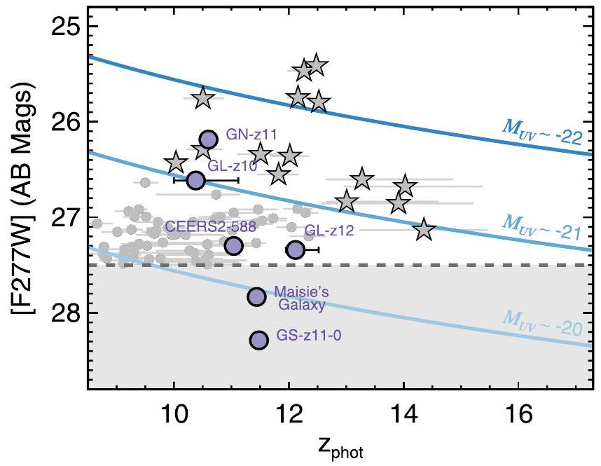
منالمصادر المحددة فيتفي المصادر بهذه المعايير، والتييتم تحديدها على أنها بكسلات ساخنة ويتم التخلص منها باستخدام معايير عتبة الحجم (أي، المصادر التي تحتوي على منطقة SE++ أصغر من 100 بكسل مصمم ونصف قطر أصغر من ). يتم فحص جميع المرشحين المتبقيين البالغ عددهم 280 بصريًا. نظرًا لأننا لم نحدد المصادر مباشرة باستخدام قطع الألوان من JWST، فإن العديد منها يبدو أحمر إلى حد ما ([F277W]-[F444W] > 1) بالإضافة إلى كونها ممتدة مكانيًا. ونتيجة لذلك، من المحتمل أن تكون عند انزياحات حمراء أقل من وبالتالي تمت إزالتها؛ تبقى 86 مصدراً كاحتمالات معقولةالمرشحين. يتم عرض توزيعهم في [F277W] المرصود مقابل الانزياح الأحمر الفوتومتري في الشكل 1 بما في ذلك بعض المصادر المعروفة الأخرى ذات الزاوية العالية في الأدبيات بما في ذلك GN-z11 (Bunker et al. 2023; Tacchella et al. 2023). من بين هؤلاء الـ 86، نقوم بفحص دقيق للمصادر التي يُقدّر أن لديها سطوع مطلق في الأشعة فوق البنفسجية أكثر سطوعًا من و كما هو موضح في الشكل 1. هناك 15 مصدرًا مفصولًا بوضوح عن مجموعة المصادر الأضعف الموجودة عند انزياحات حمراء مشابهة في COSMOS-Web. لاحظ أن جميع المصادر الـ 15 تتجاوز أيضًا معايير نسبة الإشارة إلى الضوضاء في اختيارنا باستخدام فوتومترية الفتحة “الكلاسيكية”. نحن نقتصر تحليلنا على هذه العينة الفرعية فقط في هذه الورقة، مع التركيز على المجرات عند أقصى حدود السطوع والانزياح الأحمر.
الجدول 1 فوتومترية مرشحة للمجرة
المصدر
فوتومترية مرشحي المجرة
قياس الفوتومترية القائم على الفتحة “الكلاسيكية” SE
فوتومترية قائمة على النموذج SE++
F814W (نانو جولي)
F115W (نانو جولي في الثانية)
F150W (نانو جاي)
F277W (نانو جول لكل ثانية)
F444W (نانو جولي في الثانية)
F814W (نانو جولي في الثانية)
F115W (نانو جولي في الثانية)
F150W (نانو جاي)
F277W (نانو جول لكل ياردة)
F444W (نانو جيا)
يوفيستا(ن ج ي)
يوفيستا(نJy)
يوفيستا(ن ج ي)
يوفيستا(ن ج ي)
COS-z10-1
COS-z12-1
COS-z12-2
COS-z12-3
COS-z10-2
COS-z10-3
COS-z10-4
COS-z11-1
COS-z11-2
COS-z13-1
COS-z13-2
COS-z14-1
COS-z12-4
COS-z13-3
COS-z14-2
طول الموجة الفعّالة للفلتر ]
0.814
1.15
1.50
2.77
٤.٤٤
0.814
1.15
1.50
2.77
٤.٤٤
1.02
1.25
1.65
2.15
وظيفة الانتشار (PSF) – التصوير الموحد للبيانات المستندة إلى الفضاء فقط، ومن SourceXtractor++ (SE++) قياسات الفوتومترية المعتمدة على نموذج سيرسِك الفردي التي تم قياسها على الصور بدقتها الأصلية.
ثم نطبق ملاءمات أكثر صرامة علىالمرشحين في مجموعة بياناتنا. أولاً، نكرر عملية ملاءمة الانزياح الضوئي لجميع المرشحين باستخدام LePhare (Arnouts et al. 2002؛ Ilbert et al. 2006)، Bagpipes (Carnall et al. 2018)، و EAzY. نقوم بإنشاء ملاءمات مثالية بعد تشغيل كل أداة مرتين: مرة مع فرضية انزياح ثابتة منومرة ثانية مع أولوية مسطحة منلإنتاج أفضل ملاءمة لقوالب الانزياح الأحمر المنخفض. تستخدم جميع الأكواد قيود كثافة التدفق الكاملة وعدم اليقين في جميع فلاتر النطاق العريض (بدلاً من الحدود العليا).
تشغيلات EAzY لدينا هي تعديلات طفيفة على الاختبارات الأولية المستخدمة لاختيار العينة: نحن نسمح بنطاق أوسع من الحلول الممكنة للانزياح الأحمر مع أخذ عينات أكثر دقة للانزياح الأحمر، وننقل مجموعة القوالب المعتمدة من لارسن وآخرون (2023) إلى تلك التي لا تحتوي على Ly.انبعاث ليأخذ في الاعتبار IGM محايد على الأرجح في.
لتحقيق الملاءمات المثلى لـ LePhare، نتبع منهجية كوفمان وآخرون (2022) ونلخصها هنا بإيجاز. تُستخدم قوالب بروزوال وشارلوت (2003) التي تغطي مجموعة من تاريخ تشكيل النجوم (SFHs؛ المتناقص بشكل أسي والمتأخر).تاو) كما في إيلبرت وآخرون (2015)، مع منحنيين مختلفين لامتصاص الغبار (كالزتي وآخرون 2000؛ أرنوتس وآخرون 2013). يتم إضافة تدفقات خطوط الانبعاث وفقًا لسيتو وآخرون (2020)، مما يسمح بتغير في قوة الخط بمقدار 0.3 دكس من التوقع (شاريه ودي باروس 2009). لاحظ أن لايتم تضمين الانبعاث في هذه التعديلات، على الرغم من أنه ليس بعرض مكافئ مرتفع بشكل كبير ليؤثر على التعديلات الخاصة بالتصوير الضوئي لهذه المصادر الساطعة.
للحصول على أفضل ملاءمة للأنابيب الاسكتلندية، نقوم بتنفيذ تأخير-SFH كنسبة من عمر الكونعند الانزياح الأحمربالإضافة إلى انفجار حديث وفوري يستمر بين 1 و 100 مليون سنة. نستخدم قانون تضعيف الغبار من كالزتي (كالزتي وآخرون 2000) مع نماذج السكان النجميين من بروزوال وشارلوت (2003). نسمح بالقدر المطلق للتضعيفيمتدللالتقاط نطاق معقول من التوهين، يتراوح من غير المحجوب إلى قيم أكثر توهينًا مما يُرى في الضوء المتكامل لمجرات تحت المليمتر النموذجية (على سبيل المثال، دا كونها وآخرون 2015). نلاحظ أن التقييد بـمطلوب لمنع النوبات باستخدام نماذج غير فيزيائية إلى حد كبير، على سبيل المثال، المجرات القزمة التي تعاني من تضعيف شديد بسبب الغبار مععند الانزياح الأحمر المنخفض. نناقش لاحقًا لماذا تعتبر نماذج التخفيف الشديد ذات الكتلة المنخفضة غير متوافقة مع العينة.
نقوم أيضًا بتناسب مكتبات نماذج الأطياف الطيفية للأقزام البنية من مورلي وآخرون (2012) ومورلي وآخرون (2014) مع الفوتومترية، التي تغطي درجات حرارةومدى من جاذبية السطح؛ لا يتناسب أي من عينتنا بشكل جيد مع نماذج الأقزام البنية. كما تم مناقشته في القسم 3.2، جميع المصادر في عينتنا أيضًا مفصولة مكانيًا، مما يعزز الفكرة أنه من غير المحتمل أن تكون أي منها أقزامًا بنية.
ثم نقوم بتكرار عدد من هذه الملاءمات على الفوتومترية المستخرجة من فتحات قطرها 0.3 بوصة من SE “الكلاسيكية” على جميع الصور المستندة إلى الفضاء (أي، HST/F814W و JWST/NIRCam). نحدد أن الاختلافات في الفوتومترية المقاسة لا تؤثر بشكل كبير على النتائج، على الرغم من مناقشة بعض تفاصيل الاختلافات (وأثرها على توزيعات احتمالات الانزياح الأحمر) مرة أخرى لاحقًا في القسم 5.1. نتبنى الفوتومترية المستندة إلى النموذج من SE++ كفوتومترية مرجعية لنا ونجد أن جميع الملاءمات (مع EAzY و LePhare و Bagpipes) تقدرتوزيعات احتمالية الانزياح الأحمر تكون عند.
في هذا العمل، نعتمد على التوزيعات اللاحقة للمعلمات الفيزيائية من اختباراتنا باستخدام Bagpipes لوصف
الشكل 1. توزيع المرشحين اللامعينالمجرات التي نحددها في البدايةمن COSMOS-Web (نقاط رمادية). المجرات الموصوفة في هذه الورقة (نجوم رمادية) مأخوذة من هذه العينة، مع التركيز على المجموعة اللامعة بشكل خاص (المجرات ذات التقديرات الأولية لـ ). لاحظ أن التحويل من [F277W] إلى كما هو موضح، فإن القيم المرسومة تقريبية فقط، حيث تعتمد التحويلات الدقيقة على ميل الأشعة فوق البنفسجية في إطار الراحة. المنطقة الرمادية تحدد مساحة المعلمات التي لم يتم استكشافها في هذا العمل ([F277W] > 27.5). المصادر الأدبية المعروفة موضحة باللون الأرجواني عند انزياحاتها الطيفية المقاسة. تم إعطاء انزياحات GL-z10 و GL-z12 وفقًا لاكتشافاتها الهامشية لـ [O III] من ALMA (باكس وآخرون 2023؛ يون وآخرون 2023) وعدم اليقين الفوتومتري الخاص بها (كاستيلانو وآخرون 2022).
خصائص العينة، مثل الكتلة النجمية، ومتوسط معدلات تكوين النجوم على مدى 100 مليون سنة،ميل الأشعة فوق البنفسجية في إطار الراحة، ودرجة الانخفاض المطلقة. يتم مناقشة الدافع وراء هذا الاختيار بشكل أعمق في القسم 3.2. بالإضافة إلى ذلك، تعتبر Bagpipes هي الشيفرة الوحيدة التي توفر توزيعًا خلفيًا مباشرًا لجميع المعلمات الفيزيائية، مما يوفر رؤى قيمة حول التغايرات وطبيعة الملوثات المحتملة. بالنسبة للمصادر التي تحتوي على نسبة كبيرة من حلول الانزياح الأحمر الخاصة بها تتجاوز (المقدمة في القسم 4.3)، نفرض حدًا اصطناعيًا عند لخصائصهم الجسدية، إدراك الحلول بينأقل احتمالاً بكثير مننحن نعرض جميع ملاءمات SED لعينة من 15 مرشحًا في الشكل 2.
3.1. قياس جودة الملاءمة
لكل مصدر، نقوم بتحديد قيمة موحدةمقياس، الذي نحسبه على أنه، حيث هو عدد النطاقات الفعالة المتاحة لنا والتي تقيدنا بشكل مباشر لـالمجرات. هنا نتبنى، مع الأخذ في الاعتبار الخمسة نطاقات المستندة إلى الفضاء (HST F814W، وJWST F115W، F150W، F277W، وF444W) ونحسب فلترين مستندين إلى الأرض تكون أعماقهما الأكثر فائدة لهذا العمل: UltraVISTA و ستستكشف دراسة مستقبلية حول دالة اللمعان فوق البنفسجي (UVLF) من COSMOS-Web تعريفًا أكثر دقة وكمية لـ.
لاحظ أنليس مخفضًاوالذي سيأخذ أيضًا في الاعتبار درجات الحرية في ملاءمات النموذج.هذه مشكلة معقدة في ملاءمة SED، حيث غالبًا ما تحتوي النماذج (المستخدمة لإنشاء قوالب في ملاءمة SED) على المزيد من المعلمات القابلة للتعديل من
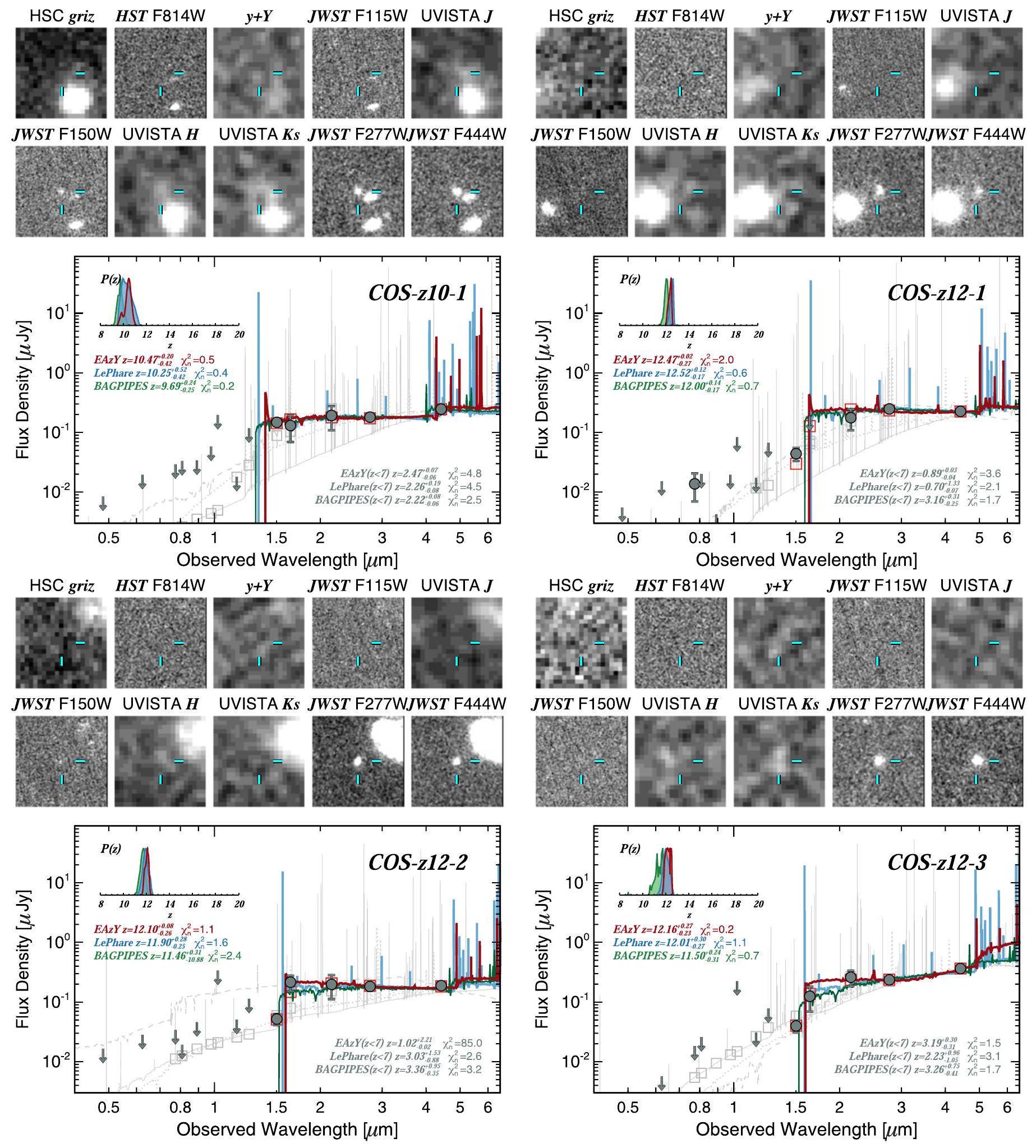
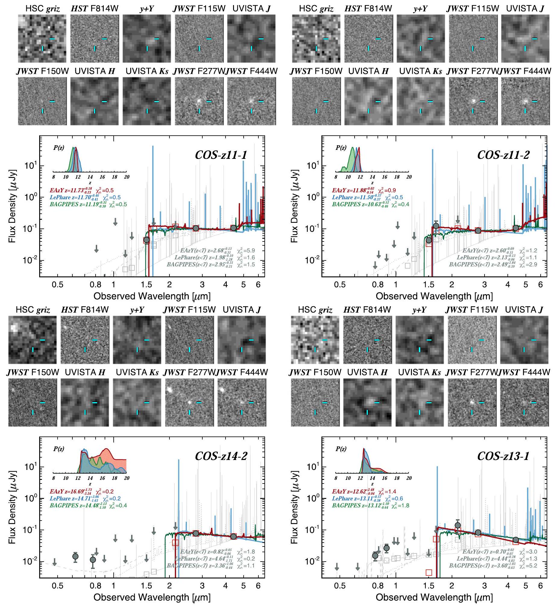
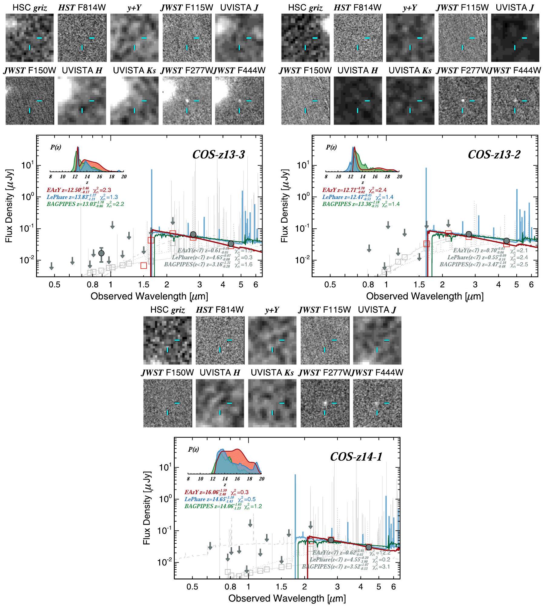
الشكل 2. قصاصات وSEDs لجميع المصادر في عيّنتنا. القصاصات هيوتتضمن، من اليسار إلى اليمين: مجموعة من HSC griz، HST F814W، مجموعة من UltraVISTA و HSC JWST F115W، UltraVISTAJWST F150W، UltraVISTA و “، و JWST F277W و F444W. يظهر SED المرسوم فوتومترية قائمة على النموذج و الحدود العليا لنقاط الفوتومترية أدناه الأهمية (رمادي). نحن نرسم الحلول الأفضل الملائمة عند الانزياح الأحمر العالي من EAzY (أحمر)، LePhare (أزرق)، وBagpipes (أخضر)، وملفات PDF الخاصة بالانزياح الأحمر المقابلة بينهافي الرسم البياني المرفق. باللون الرمادي نعرض أفضل حلول الانزياح الأحمر المفروضة علىمن EAzY (متقطع)، LePhare (صلب)، وBagpipes (منقط). يتم عرض الفوتومترية المُركبة في صناديق مفتوحة لاثنين من SEDs فقط من أجل الوضوح: الحل القائم على EAzY عالي الزاوية (أحمر) وLePhare المنخفض-حل (رمادي). مُعَدلالقيم (انظر القسم 3.1) موضحة في كل لوحة لكل من القيم العالية-ومنخفض-حلول.
تمتلك المجرات اكتشافات فوتومترية، وتقليل مساحة المعلمات القابلة للبحث من خلال اتخاذ خيارات فيزيائية مدروسة يختلف بشكل كبير بين أدوات ملاءمة SED.
نحن نحفز مثل هذا التnormalizedلديها كمية تسمح بمقارنتها مباشرة بين الاستطلاعات التي تستخدم مجموعة متنوعة من الفلاتر لاختيار عيناتها. من أجل
الشكل 2. (مستمر.)
على سبيل المثال، المجرات المختارة في مسح CEERS (فينكلشتاين وآخرون 2023a) مقيدة بمزيد من الأطياف الضوئية المستندة إلى الفضاء العميق، ومن الطبيعي أن يكون لها قيمة أعلى منوبالتالي قيم تفاضلية أكبربين الحلول ذات الانزياح الأحمر المنخفض والعالي. إن تطبيع عدد النطاقات المحددة سيجعل اختيار المصادر في هذه الاستطلاعات المختلفة قابلاً للمقارنة بشكل مباشر. على سبيل المثال، العبارة المستخدمة كثيرًامعيار (على سبيل المثال، فينكلشتاين وآخرون 2023أ؛
هاينلاين وآخرون 2024بالنظر إلى النطاقات السبعة التي تقيد COSMOS-Webالمرشحين. نظرًا للاختلافات الفريدة لكل أداة من أدوات ملاءمة الانزياح الأحمر، نقوم فقط بالمقارنة المباشرةلـ منخفض-وعالي-يتناسب باستخدام نفس رمز التركيب (على سبيل المثال، EAzY منخفضإلى EAzY العاليلو فار لوإلى لي فاري هاي، وقرون البقر منخفضةإلى الأنبوب العالي ). وبالتالي فإن المعيار للمرشح القوي هو .
الشكل 2. (مستمر.)
لشفافية في اختيارنا، يوضح الشكل 2 جميع الـ 15مرشحين مععلى الرغم من أن بعضهم لديهم حلول منخفضة الانزياح الأحمر قابلة للتطبيق كما تم قياسها عبر. يشمل ذلك COS-z12-4، الذي لدينا أسباب متعددة للاعتقاد بأنه في حالة منخفضة (موضح في القسم 4)، بالإضافة إلى COS-z13-3 و COS-z14-2، اللذان يتم اكتشافهما فقط في F277W و
أشرطة F444W، ويتم مناقشتها بمزيد من التفصيل في القسم 4.3. لاحظ أن المصادر التي تم اكتشافها في شريحتين فقط تكون بطبيعتها أكثر صعوبة في الاختيار بشكل نظيف باستخدام المقياس حيث أن معظم قيود البيانات هي حدود عليا. ومع ذلك، يتم مناقشة هذه المصادر بشكل فردي في القسم 4.3 ومرة أخرى في القسم 5.1 فيما يتعلق باحتمالية كونها متداخلة ذات انزياح أحمر منخفض.
3.2. قياسات أخرى
قمنا بإجراء اختبار بسيط لتقييم دقة تقديرات الانزياح الأحمر الفوتومتري التي تم إجراؤها باستخدام مجموعة من أفضل ملاءمات SEDs للعينة الكاملة من EAzY وLePhare وBagpipes. يُفترض أن هذه المجموعات من القوالب تمثل تنوع SEDs الواقعية لـالمجرات. قمنا بتحريك SEDs للأمام والخلف في الانزياح الأحمر، ونمذجة الفوتومترية الاصطناعية مع الضوضاء المميزة لبياناتنا، وأعدنا قياس الانزياحات الفوتومترية. وجدنا انحرافًا منهجيًا نحو انزياحات أعلى باستخدام EAzY، بينما لم يظهر Bagpipes أي انحراف منهجي. هذا مشابه للانحرافات النظامية التي لوحظت في Bagpipes و EAzY في الحقبة الأولى من COSMOS-Web.المجرات من فرانكو وآخرون (2023). نتبنى المعلمات الفيزيائية والانزياحات الحمراء التي تم قياسها بواسطة بايبيبس لبقية هذا العمل.
نقيس أحجام العينة باستخدام نطاق F277W باستخدام كل من GALFIT (بينغ وآخرون 2002، 2010) و GALIGHT (دينغ وآخرون 2020). تم اختيار نطاق F277W لأنه يوفر أعلىالقياسات لجميع المجرات في العينة مع أفضل دقة مكانية. يستخدم GALFIT خوارزمية ملاءمة بأقل المربعات بينما يستخدم GALIGHT نهج النمذجة الأمامية للعثور على أفضل ملاءمة لسيرسيك لملف الضوء ثنائي الأبعاد لمجرة، بعد أخذ PSF في الاعتبار. نستخدم صور PSF المتوسطة التي تم إنشاؤها من بياناتنا في أبريل 2023 التي تم قياسها باستخدام PSFEx (بيرتين 2011). كانت قياسات الحجم متسقة بشكل عام بين تقنيتي الملاءمة وفي جميع الحالات تم حلها مكانيًا؛ نقدم قياسات نصف قطر الضوء من GALFIT في الجدول 2.
4. تفاصيل المصدر
هنا نقدم أوصافًا أكثر تفصيلًا ومعلومات ذات صلة حول كل من المجرات الخمسة عشر المرشحة في. نلاحظ أن العينة يمكن تقسيمها إلى ثلاثة مجموعات تقريبًا: لامعة بشكل استثنائيمرشحين ( )، ساطع مرشحين ( )، و مرشحين مع. تحتوي هذه العينات الثلاث على خمسة مصادر لكل منها. تم الكشف عن المرشحين فقط في نطاقين من تلسكوب جيمس ويب (JWST)، F277W و F444W، وبالتالي لا تكون قيودهم على الخصائص الفيزيائية واضحة كما ينبغي. يتم تقديم قياسات الفوتومترية لجميع المصادر في الجدول 1، بينما يتم إعطاء المواقع والخصائص الفيزيائية المستمدة في الجدول 2.
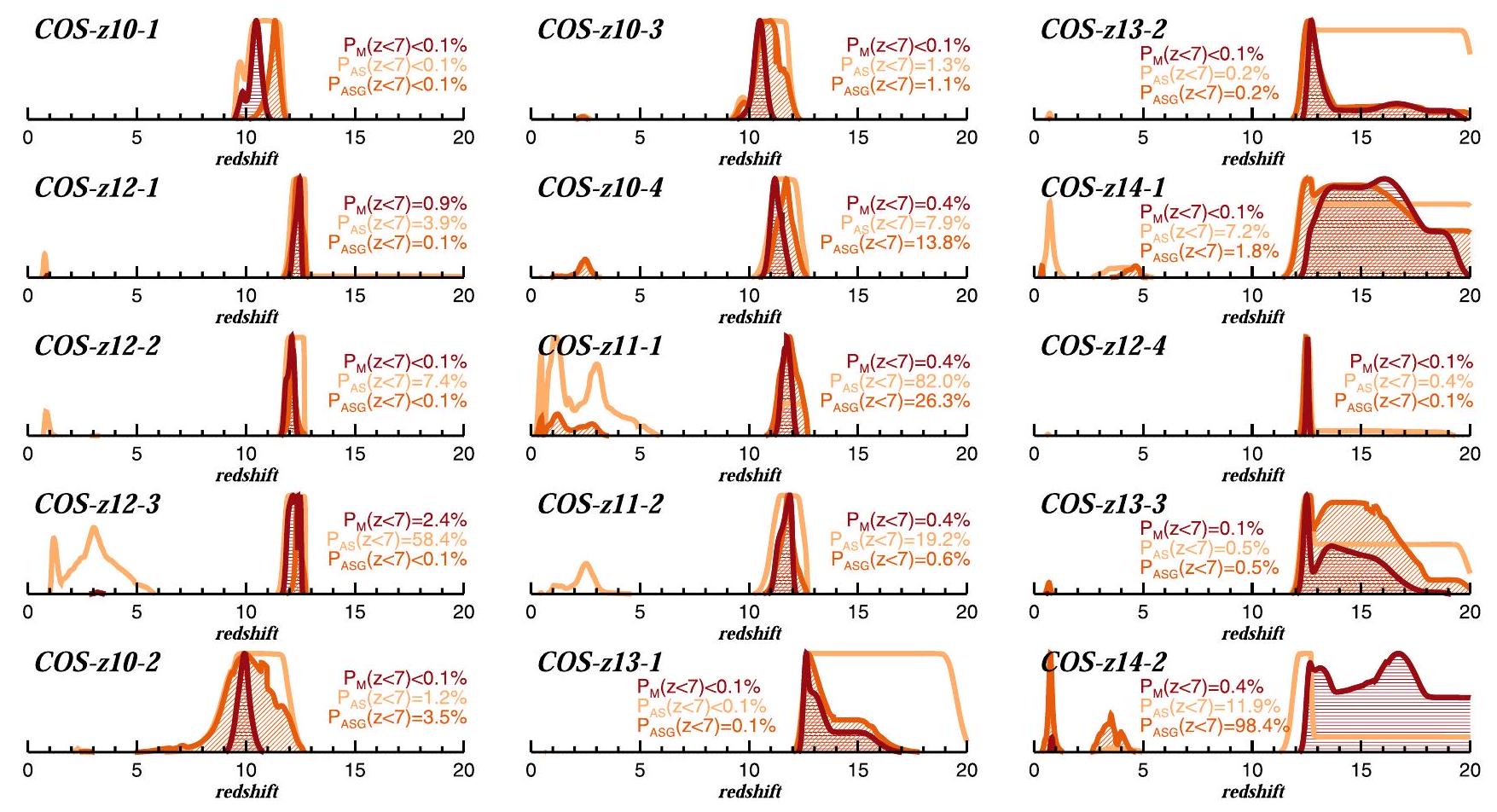
في الأوصاف التالية، نقتبس الاحتمالية النسبية لأن يكون المصدر متداخلاً منخفض الانزياح الأحمر؛ نحن نستمد هذه الاحتمالات من ملاءمات الانزياح الضوئي EAzY باستخدام فوتومترية SE++، التي تُعرض توزيعاتها في الشكل 3 وتناقش لاحقًا كمجموعة في القسم 5.1. اخترنا PDFs للانزياح الضوئي EAzY بسبب بساطتها وسهولة اعتمادها على انزياح (ومقدار) مسطح. ومع ذلك، فإن تحذيرًا عامًا من تفسير PDFs للانزياح الضوئي هو أن السعة الدقيقة لقمة الانزياح الضوئي حساسة جدًا لمجموعة القوالب المعتمدة، ونطاق المعلمات الفيزيائية التي تحكم SEDs المدخلة، وللاختلافات الصغيرة في الفوتومترية المعتمدة. لذا، بينما تجد عمومًا عدة أكواد مستقلة قمم متسقة في التوزيع (كما هو موضح أيضًا في الألواح الفرعية في الشكل 2)، فإن التكامل تحت كل قمة غير مؤكد إلى حد ما.
نحن أيضًا نتناول وجود الجيران في السماء كجمعيات فيزيائية محتملة، ونتحقق من التوافق مع الحلول ذات الانزياح الأحمر المنخفض لمرشحينا (خصوصًا لأن الجيران القريبين في السماء هم إحصائيًا أكثر احتمالًا أن يكونوا مرتبطين فيزيائيًا؛ كارتالتبي وآخرون 2007؛ شاه وآخرون 2020). كما نقيم المساهمة المحتملة للجاذبية تأثير العدسات من الجيران ونجد أنه غير مهم في جميع الحالات (يكون الأكثر أهمية لـ COS-z10-1، حيث نوضح تضخيم العدسة لا يتجاوز ).
4.1. مضيء بشكل استثنائيالمجرات 4.1.1. COS-z10-1
تم اكتشاف هذا المصدر في خمس نطاقات ويظهر انخفاضًا قدره 2.5 مغ بين F 150 W والحد الأعلى في F115W. تم الكشف عن COS-z10-1 رسميًا في UltraVISTA – و تصوير متعدد الأطياف بالإضافة إلى ثلاثة من مرشحات NIRCam الأكثر احمرارًا. يتم ضبط انزياحه الأحمر على باستخدام EAzY و LePhare وأقل قليلاً في من آلات القربة. COS-z10-1 لديه جاران ضمن 1 “5: واحد 0!” 47 إلى الجنوب الغربي وآخرإلى الجنوب-الجنوب الغربي. الأول لديه انزياح ضوئي أحمر قدرهوالأخير2.04، وكلاهما غير متوافق مع الحلول المنخفضة الزخم القسري لـ COS-z10-1 عندمما يشير إلى أن الارتباط الجسدي مع الجيران (اعتماد الحل المنخفض الانزياح) غير محتمل. نحن نقدر الحد الأقصى للتشويه الذي يمكن أن يحدث من هذه المصادر الأمامية على أنهبالنظر إلى الكتل المقدرة للأجسام في المقدمةلا يوجد ذروة منخفضة التحول الأحمر ذات دلالة في PDF التحول الأحمر عند التحول الأحمر المنخفض لـ COS-z10-1، الذي تبلغ احتمالية تكامله أن يكون عند هو .
تم اكتشاف هذه المجرةعاليفي، و F444W مع هامش الإشارات في UltraVISTA و . لديها عامل كبير من انخفاض كثافة التدفق (1.7 مغ) في فلتر F150W، وعامل آخر منانخفاض إلىالحد الأعلى في F115W. COS-z12-1 لا يحتوي على انقطاع طيفي مفاجئ، على الرغم من أن قياس الضوء الخاص به يمكن تفسيره بشكل جيد مع الانزياح الأحمر.تنتج الحلول المفروضة ذات الانزياح الأحمر المنخفض تقديرات الانزياح الأحمر الفوتومتري عندلـ EAzY و LePhare و فيلآلات القربة. حلول فيسيتطلب ذلك قوة خطوط انبعاث شديدة لجرم سماوي منخفض الكتلة نسبيًا (مع معدل تكوين نجمي محدد (sSFR) من )، وبالتالي من غير المرجح أن تكون أكثر من حل الأجراس، على الرغم من أن جميعها أقل ملاءمة للبيانات بشكل ملحوظ من الحلول ذات الانزياح الأحمر العالي.جار في المقدمة، يقعإلى الجنوب الشرقي، مزود بتحويل ضوئي أحمر قدرهولكن بعيدًا بما فيه الكفاية لعدم تلوث قياسات الضوء لـ COS-z12-1؛ قياس الضوء الخاص به ويختلف أيضًا عن حلول COS-z12-1 ذات الانزياح الأحمر المنخفض بعدم الاشتباه في الارتباط الفيزيائي. COS-z12-1 هو الأكثر سطوعًا من الناحية الجوهرية.المجرة الموجودة في عينتنا مع.
4.1.3.
تم الكشف عنه في أربع نطاقات (F150W، UltraVISTA H، F277W، وF444W، مع إشارة في UltraVISTA )، COS-z12-2 لديه عامل من انخفاض في كثافة التدفق (1.5 مغ) بين UltraVISTAو F150W، الذي يحدد انكسار ليمان للمرشح. تمتد تقديرات الانزياح الأحمر الفوتومتريمع حلول محتملة عند انزياح أحمر منخفضالحل ذو الانزياح الأحمر المنخفض الأكثر احتمالاً هو على الأرجح مصدر الخطوط القوية فيوجدت مع LePhare، على الرغم من أن الانخفاض لم يكن شديدًا كما هو الحال حولكان من المتوقع مقارنته بالملاحظات. كما اختبرنا اعتماد الانزياح الأحمر الفوتومتري على بيانات UltraVISTA ذات الإشارة المنخفضة إلى الضوضاء؛ بعد إزالة قيود UltraVISTA،
الجدول 2 خصائص العينة
مصدر
الأبواق
إيزي
المصباح
( )
(غالفيت) (بي سي)
سوبر برايتعينة
COS-z10-1
10:01:26.00
+01:55:59.70
COS-z12-1
09:58:55.21
+02:07:16.77
COS-z12-2
09:59:59.91
+02:06:59.90
COS-z12-3
09:59:49.04
+01:53:26.19
مشرقعينة
COS-z10-2
09:59:51.77
+02:07:15.02
COS-z10-3
09:59:57.50
+02:06:20.06
COS-z10-4
10:00:37.96
+01:49:32.43
COS-z11-1
09:59:52.53
+02:00:23.53
COS-z11-2
10:01:34.80
+02:05:41.48
عينة في
COS-z13-1
09:59:05.75
+02:04:04.39
COS-z13-2
10:00:04.24
+02:02:11.19
كوس- ز14-1
10:01:31.17
+01:58:45.00
عينة مرفوضة كاحتمال منخفض-الملوثات
COS-z12-4
09:59:30.49
+02:14:44.10
COS-z13-3
09:59:31.30
+02:08:33.85
COS-z14-2
10:00:20.38
+01:49:58.33
ملاحظة. يتم قياس المواقع من الصورة المكتشفة المستخدمة لكتالوجات SE++ و SE “الكلاسيكية”. نحن نقدم ثلاثة انزياحات ضوئية فوتومترية لكل مصدر من Bagpipes و EAzY و LePhare، ولكن لاحظ أن معظم الخصائص المستمدة – بما في ذلك، و -يتم قياسها من توزيعات بايبس الخلفية الأفضل ملاءمة.يتم قياسه من تصوير F277W باستخدام GALFIT. نقوم بتصنيف مجموعات فرعية من عيّنتنا كما هو موضح في النص في القسم 4، ونتضمن ثلاثة مصادر تم إزالتها لمزيد من التحليل بسبب الشك في أنها منخفضة-الم contaminants؛ إذا تم التأكيد عليها كعاليةقد تعكس خصائصها ما هو مذكور في هذا الجدول. لا يزال الحل مفضلًا لـ COS-z12-2، على الرغم من زيادة احتمال وجود حل منخفض الانزياح الأحمر. ). يتم تقليل احتمال الانزياح الأحمر المنخفض مع -كشف النطاق بشكل خاص. لا توجد جيران قريبون ضمنمن COS-z12-2، مما يجعل فوتومتريته خالية من التلوث. هناك مصدربعيد إلى الشمال الغربي وله انزياح ضوئي من COSMOS2020 قدره، والذي هو أقرب إلى ولكن لا يزال متميزًا إحصائيًا عن حل COS-z12-2 ذو الانزياح الأحمر المنخفض. نلاحظ أنه، اعتمادًا على الضبط الدقيق لمجموعات القوالب لـ EAzY أو النطاق المعتمد من المعلمات الفيزيائية المستخدمة في Bagpipes، قد يصل إلىمن ملف PDF الخاص بالانزياح الأحمر يقع في (وترتفع إلى باستخدام قياسات الفوتومترية من الفضاء فقط). نلاحظ أن COS-z12-2 تم اكتشافه أيضًا باستخدام MIRI في، المجرة الوحيدة في عيّنتنا التي تمتلك مثل هذا الكشف؛ كثافة تدفقها هيعلى الرغم من أن قيد MIRI غير موضح في الشكل 2، فإن هذا الكشف يتماشى مع طيف مسطح تقريبًا (في ) من الأشعة تحت الحمراء القريبة ويُدرج في ملاءمات SED كقيد إضافي. بينما قد يعتقد المرء بشكل اسمي أن له تأثيرًا كبيرًا على تقدير الكتلة النجمية (في إطار الإطار الزمني البصري)، فإن هذه القياس المحدد ليس له تأثير كبير بسبب انخفاضه؛ ومع ذلك، فإنه يقلل من عدم اليقين في الكتلة النجمية قليلاً. COS-z12-2 هو ثاني أضخم مجرة في هذه العينة.
4.1.4. COS-z12-3
تم اكتشاف هذا المصدر في أربع نطاقات (F150W، UltraVISTAF277W و F444W، مع هامشانبعاث في UltraVISTA ) بعامل من سقوط من UltraVISTAإلى F150W. COS-z12-3 لديه إطار زمني أكثر احمرارًا
ميل الأشعة فوق البنفسجية مقارنةً مع المجرات الأخرى في هذه العينة، مما يقدم المزيد من الاحتمالات للتداخل مع أصل منخفض الانزياح الأحمر في فوتومتريتها. ومع ذلك، فإن الانكسار القوي عندعامل منفي كثافة التدفق (يجادل من أجل حل عالي الانزياح الأحمر، ويتم ضبط انزياحه الضوئي بشكل متسق علىبدون قياسات UltraVISTA، سيكون من الصعب تحديد COS-z12-3. على سبيل المثال، من خلال إزالة قيود UltraVISTA وإعادة ضبط انزياحه الأحمر، يعود COS-z12-3 إلىالحلول؛ الفرقة الأكثر أهمية التي تضع المصدر في هو ، تم اكتشافه في توافق الانزياح الأحمر الفوتومتري باستخدام HSC وHST وUltraVISTA، ونتائج بيانات NIRCam في حل معفرصة منخفضة-حل؛ هذا يُختصر إلىعند تضمين الحدود في الأشرطة الأخرى من UltraVISTA، على وجه الخصوصفرقة، حيث أن النغمة المنخفضة-الحل سيتطلب كثافة تدفق أكثر سطوعًا من مساهمة [O III] 5007 أ. COS-z12-3 ليس لديه جيران ضمن.
القدر المطلق المستنتج للأشعة فوق البنفسجية لـ COS-z12-3 هوومعدل تكوين النجوم المصحح للغبار الخاص بههو الأعلى في العينة. مع ميل UV في إطار الراحة من و ، إنه الأكثر احمرارًا من المصادر الساطعة في هذه الورقة؛ وهذا، مع معدل تكوين النجوم العالي، يقود بشكل طبيعي إلى فرضية أنه قد يتم اكتشافه (أو يمكن اكتشافه) عند أطوال موجية ملليمترية. COS-z12-3 هو واحد من المصادر القليلة التي تغطيها بيانات الأرشيف الحالية من ALMA عند 2 مم من البرنامج 2021.1.00705.S (المحقق: O. Cooper)؛ ولم يتم اكتشافه مع قياس الجذر التربيعي للمتوسط الذي يحدد تقريبًاالحد الأقصى لكتلة الغبار عندمن و ؛ كلا الحدين ليسا مقيدين بما فيه الكفاية ليكونا في تعارض مع القياساتمن الأنابيب المناسبة. اكتشاف الاستمرارية المليمترية في
الشكل 3. مقارنة بين PDFs الانزياح الأحمر التي تم ملاءمتها باستخدام EAzY لثلاث مجموعات من الفوتومترية لكل مرشح مجري عالي الانزياح الأحمر. تظهر النتائج للفوتومترية المعتمدة على نموذج SE++ (“M”)، والتي تشمل كل من الفوتومترية المستندة إلى الفضاء والأرض، باللون الأحمر الداكن. بينما تظهر النتائج للفوتومترية “الكلاسيكية” SE المستخرجة باللون البرتقالي الفاتح.فتحات القطر من صور HST و JWST NIRCam المعالجة بواسطة PSF فقط (“AS” للفتحة، فقط من الفضاء). اللون البرتقالي الداكن يظهر التوزيعات بعد دمج الفوتومترية المعتمدة على الفتحة من SE “الكلاسيكية” مع القياسات الفوتومترية المعتمدة على النموذج من البيانات الأرضية (“ASG”، الفتحة مع الفضاء والأرض). هذه الملائمة الأخيرة تهدف إلى تسليط الضوء على القيمة النسبية وأهمية القيود المستندة إلى الأرض، لا سيما تلك الناتجة عن تصوير Subaru/HSC العميق في البصري وتصوير UltraVISTA في الأشعة تحت الحمراء القريبة. في الزاوية، النسب المئوية لملفات PDF الخاصة بالانزياح الأحمر التي تقع عند. في الغالبية العظمى من الحالات، تنتج الفوتومترية المعتمدة على النموذج والفوتومترية المعتمدة على الفتحة PDFs مشابهة للانزياح الأحمر، وإضافة القيود المستندة إلى الأرض إلى الفوتومترية المعتمدة على الفتحة تقلل بشكل كبير من التكامل الخاص بـ PDF الانزياح الأحمر أدناهلأغلب المصادر.
قد تتطلب مثل هذه المصادر ملاحظات بسمك 2 مم مع حساسيةعلى الرغم من أننا نؤكد أنه بسبب تصحيح K السلبي، فإن ملاحظات استمرارية الغبار لمثل هذه المصادر لا تؤكد أو تنفي حلاً منخفض أو مرتفع الانزياح الأحمر؛ فالتصوير الطيفي ضروري.
4.1.5. COS-z12-4
المرشح الخامس المشرق بشكل استثنائي الذي نحدده هو COS-z12-4. الحد الرئيسي في توصيف COS-z12-4 هو قرب مجرتين جارتين حيث يتم الخلط بين انبعاثهما في البيانات المستندة إلى الأرض. بينما يتم ملاءمته بشكل اسمي لزمن أحمر فوتومتري من و تدعي القياسات المستندة إلى نموذج SE++ لـ COS-z12-4 الكشف في HSCفرقة، وتصوير من تصوير i-band الأصلي لكاميرا سوبرم في COSMOS (Capak et al. 2007) قد يظهركشف سيغما؛ ومع ذلك، عند الفحص الدقيق، قد تكون كلاهما تقلبات ضوضاء إيجابية من انبعاثات الجيران. إن عدم وجود قيود بصرية عميقة مع تصوير عالي الدقة يجعل المصدر أقل أمانًا. الجيران همبعيدًا إلى الغرب وبعيدًا إلى الجنوب الغربي ومزودين بالتحولات الحمراء الفوتومترية لـو 4.50، على التوالي. كما تم اكتشاف الأول في COSMOS2020 مع انزياح ضوئي فوتومتري متسق قدره. في الواقع، يتوافق التناسب الضوئي منخفض الانزياح الأحمر لـ LePhare مع انزياحات الجيران، عند . على الرغم من أن أفضل ال-لا يزال الملاءمة بشكل رسمي أقلمن هذا المنخفض-الحل، الفوتومترية المتسقة مع جار منخفض الز هو كافٍ لإثارة شكوك كبيرة حول ال-حل. الوضع مشابه للوضع البيئي صدفة جادلت بأن CEERS-93316 كانتوليسمن نايدو وآخرون (2022a)، وتم تأكيد ذلك لاحقًا من قبل أرابال هارو وآخرون (2023). لذلك، نختار إزالة COS-z12-4 من تحليلنا لبقية هذه الورقة. ومع ذلك، نقدم خصائصه الفيزيائية المقاسة إذا كان في في الجدول 2. نؤكد على أن الحصول على طيف COS-z12-4 مهم في حال كان بالفعل مصدرًا ذو انزياح أحمر فائق الارتفاع؛ في هذه الحالة، سنتعلم درسًا قيمًا حول الادعاء بتمامية مسحنا، ومعدلات حدوث الإسقاطات العشوائية مع المصادر ذات الانزياح الأحمر المنخفض، ووفرة المصادر الفائقة السطوع.المصادر.
4.2. ساطعمرشحون
4.2.1.
COS-z10-2 هو واحد من المجرات الأكثر حمراء بشكل جوهري في عينتنا وله شكل ثنائي الشكل قليلاً في نطاقات NIRCam LW. تم اكتشافه رسميًا في ثلاث نطاقات NIRCam. تتراوح تقديرات الانزياح الأحمر الضوئي بين-10.1. الميل المستمد في إطار الراحة للأشعة فوق البنفسجية لـ COS-z10-2 هو، الأحمر الثاني في العينة؛ على الرغم من لونه الأحمر، إلا أنه يجتاز جميعالمعايير بفضل قوة انكسار ليمان، والتي تعادل 6 في التدفق (2 مغ). المصدر ليس له جيران، لكن مورفولوجيته ذات المكونين قد تثير بعض الشكوك حول موثوقية قياسات الفوتومترية المعتمدة على ملف سيرسيك الفردي. ومع ذلك، فإن الفوتومترية عبر الفتحة لهذا المصدر متوافقة تمامًا مع النتائج المستندة إلى النموذج (على الرغم من وجود مزيد من عدم اليقين في PDF الانزياح الأحمر، انظر الشكل 3). COS-z10-2 لديه أعلى تقدير مستمد للكتلة النجمية من أي في عينتنا مع (نتيجة لونه الأكثر احمرارًا في إطار الأشعة فوق البنفسجية).
4.2.2.
COS-z10-3 تم اكتشافه في ثلاث نطاقات من NIRCam. COS-z10-3 لديه جار قريب.إلى الجنوب الشرقي الذي لديه انزياح ضوئي أحمر قدرهالذي يوجد أيضًا في COSMOS2020 مع انزياح ضوئي فوتومتري مشابه. نلاحظ أن هذا يتماشى إلى حد ما مع أحد الحلول الثلاثة ذات الانزياح المنخفض لـ COS-z10-3 التي وجدها EAzY.، مما يزيد من احتمال أن يكون هذا كائنًا متداخلًا ذو انزياح أحمر منخفض. ومع ذلك، نلاحظ أن مثل هذا الحل هو ملاءمة ضعيفة نسبيًا مقارنةً بحل الانزياح الأحمر العالي المقابل له ( )، مرتفعة بما فيه الكفاية للبقاء في العينة.
4.2.3. COS-z10-4
COS-z10-4 يتم اكتشافه بشكل مشابه في ثلاث نطاقات من NIRCam مع نواة مضغوطة وانبعاث ممتد منتشر. لا توجد دلائل على أنه تم اكتشافه في تصوير UltraVISTA. تعرض مجموعة تصوير HSC griz انبعاثًا زائدًا محيرًا نحو الجنوب الغربي؛ لأن هذا ليس متطابقًا مكانيًا مع موقع المصدر ضمن، ليس هناك قلق كبير. COS-z10-4 ليس لديه جيران قريبون، ولديه حلول انزياح أحمر تمتد ، مع تحسينات ملحوظة في الأداء العالي-يتناسب أكثر من أن يكون مفروضًا منخفضًاحلول.
4.2.4. COS-z11-1
COS-z11-1 لديه أعلى انزياح أحمر في مجموعة “المشرقة” ويتم اكتشافه فقط في الثلاثة نطاقات NIRCam، مع اكتشافات في F150W وF277W وF444W. لا توجد أدلة من القصاصات المستندة إلى الأرض على انبعاث كبير فوق ضوضاء الخلفية. ليس لديه جيران وهو مناسب للانزياحات الحمراء.باستخدام الفوتومترية المستمدة من النموذج،ملف PDF الخاص بالانزياح الأحمر موجود في، على الرغم من أن هناك ارتفاعًا كبيرًا في يتم العثور على الاحتمالية عند استخدام الفوتومترية المعتمدة على الفتحة فقط (ومع ذلك، عند إضافة القيود المستندة إلى الأرض إلى الفوتومترية المعتمدة على الفتحة، فإنتشغل الحلول نسبة أقل من التوزيع في.
4.2.5.
تم الكشف عن COS-z11-2 في ثلاث نطاقات من NIRCam ولديه هامشإشارة في UltraVISTAفرقة، بحيث يتم الكشف عن انقطاع واضح بين UltraVISTA و F150W. تفتقر إلى الجيران ولديها حلول انزياح أحمر تمتد الحلول ذات الانزياح الأحمر المنخفض لهذا المصدر تتركز حول-2.6 وهم أسوأ قليلاً فقط ) من الحلول ذات الانزياح الأحمر العالي، على الأرجح لأنها خافتة نسبيًا وأحمر أكثر من المصادر الأخرى في العينة، مع و تحتل الحلول ذات الانزياح الأحمر المنخفضلتوزيع احتمالية الانزياح الأحمر، على الرغم من أننا نلاحظ أن اعتماد الفوتومترية المعتمدة على الفتحة يؤدي إلى نسبة أكبر من PDF الانزياح الأحمر عندعند استخدام الفوتومترية المعتمدة على الفتحة فقط، وعند استخدام الفوتومترية المعتمدة على الفتحة مع القيود المستندة إلى النماذج المستندة إلى الأرض (كما هو موضح في الشكل 3). قد تجعل إضافة القيود المستندة إلى الأرض التمييز بين الحلول ذات الانزياح الأحمر المنخفض والحل ذو الانزياح الأحمر العالي صعبًا بالنسبة لـ COS-z11-2 بسبب الفرق النسبي في التدفق بين F150W و UltraVISTA.فرقة. على الرغم من الإضافي نظرًا للغموض المحيط بـ COS-z11-2، نحتفظ به في عينة الارتفاع العالي لمزيد من التحليل.
4.3. المرشحون في
في محاولة لاستكشاف أكثر مجموعة متطرفة من الاكتشافات الجديدة ضمن فترة إعادة الانبعاث، قمنا أيضًا بتحديد عينة من المجرات المرشحة فيمن التصوير الحالي لدينا. كنتيجة طبيعية لتصميم مسحنا، المصادر التييتم اكتشافها ظاهريًا فقط في F277W و F444W. لا يوجد أي منها ساطع بما يكفي ليتم اكتشافه بواسطة سبitzer في (طول موج غير مغطى بتصوير JWST في COSMOS-Web)، فلاتر UltraVISTA، أو MIRI عند بعيدًا عن مجموعة الفلاتر المحدودة، فإن الفجوة الطولية الموجية بين F277W و F150W تمثل تحديًا آخر، مما يجعل من الصعب اقتباس انزياحات ضوئية أكثر دقة من. نتيجة أخرى للقياسات الضوئية المحدودة هي أن الفرق في بين التعديلات ذات الانزياح الأحمر المنخفض والعالي يتضاءل:أقل بشكل عام لأن هناك فرقتين فقط. في الواقع، جميع المصادر في هذه الفئة تفشل في الأقل في واحدةقطع (بالأساس EAzY و LePhare).
نهجنا تجاه المرشحين في هذا النظام هو بالتالي محافظ إلى حد ما. من مجموعة أولية تضم 31 مصدرًا في كتالوج EAZY الأولي القابل لقياسات الزخرفة الضوئية.مع [F277W] < 27.5، نقوم بتقليص الاختيار إلى خمسة مرشحين قابلين في هذه الورقة. يتم استبعاد المصادر من العينة لأنها تفشل في جميعمعايير (لـ EAzY و LePhare و Bagpipes)، لديهااحتمالات لـالحلول، لديها إما أشكال منتشرة مع أنصاف أقطار5، أو أنها غير محددة مكانيًا في F277W ” 15 )، أو أنهم أحمرون بما فيه الكفاية ( )، والتي تثير شكوكًا كبيرة حول الحل. كنتيجة طبيعية لهذا النهج، فإن المصادر الخمسة المتبقية – COS-z14-2، COS-z13-1، COS-z13-3، COS-z13-2، و COS-z14-1 تظهر ألوانًا زرقاء بعض الشيء مقارنة بالسكان الأصليين مع. جميعها تحتوي على احتمالات متكاملة للوجود فيأقل منباستخدام الفوتومترية المعتمدة على النموذج المرجعي.
نلاحظ أن COS-z13-2 و COS-z14-1 كلاهما لهما تغطية MIRI عندعلى الرغم من عدم اكتشاف أي منهما. الكثافات التدفقية المقاسة التي نحصل عليها لهما باستخدام الفوتومترية المعتمدة على نموذج SE++ هي و 31 نJy ، على التوالي.
من بين المرشحين الخمسة، يظهر اثنان فقط احتمالات منخفضة الانزياح الحمراء مرتفعة بشكل ملحوظ عند استخدام فوتومترية الفتحة “الكلاسيكية” SE: COS-z14-2 لديهمن ملف PDF الخاص به فيو COS-z14-1 لديهمن ملف PDF الخاص به فيعند إضافة فوتومترية الفتحة مع القيود المستندة إلى الأرضتم تقليل الاحتمالية في COS-z14-1 إلى، ولكنه أعلى بكثير ( ) لـ COS-z14-2. على الرغم من أن هذه النتيجة غير متسقة مع قيودنا المستندة إلى النموذج على COS-z14-2، فإننا نزيلها من التحليل في المناقشة. كما أننا نزيل المصدر COS-z13-3 من التحليل الإضافي لأنه يفشل في جميع معايير، على الرغم من أن تكاملهاالاحتمال هو.
لأغراض المناقشة والخصائص الفيزيائية الناتجة، نحتفظ فقط بثلاثة مصادر فيعينة: COS-z13-1، COS-z13-2، وCOS-z14-1، لكننا نقدم أوصافًا لجميع العينات الخمس. نواصل التأكيد على أن هذه العينة أقل قوة بشكل عام من المصادر الموصوفة في الأقسام 4.1 و4.2 وجميعها، بما في ذلك تلك التي استبعدناها للاشتباه في أنها منخفضة.تتطلب تأكيدًا طيفيًا.
5. المناقشة
هنا نقدم مناقشة أكثر تفصيلاً حول تداعيات هذه الاكتشافات. أولاً، نقدم مناقشة تتعلق بالمتداخلين ذوي الانزياح الأحمر المنخفض، وقياس مباشر لكثافتهم الحجمية ومساهمتهم في دالة توزيع الضوء فوق البنفسجي، وملخص لخصائصهم الفيزيائية المقاسة. ثم نقدم مناقشة أكثر تفصيلاً حول تقديرات كتلتهم النجمية وكفاءات تشكيل النجوم المستنتجة لديهم ضمن نموذج المادة المظلمة الباردة لامدا.نموذج CDM). ثم نناقش المحتوى الغازي المحتمل للأنظمة وأخيرًا نثير إمكانية الملاحظات المستقبلية التي تحد من كتل هالات المجرات المضيفة، والتي يمكن أن تُفيد أيضًا في تحديد القيود على الأطر الكونية البديلة.
5.1. إمكانية وجود متداخلين عند الانزياح الأحمر المنخفض
لقد أوضحت ملاحظات تلسكوب جيمس ويب الفضائي (JWST) حول المجرات ذات الانزياح الأحمر العالي حتى الآن أن المجرات فيمع عرض خطوط انبعاث قوية في إطار الراحة البصرية يمكن أن تتنكر كأجسام ذات انزياح أحمر فائق الارتفاعمرشحي المجرات في مرشحات النطاق العريض لـ JWST (فوجيموتو وآخرون 2023؛ نايدو وآخرون 2022a؛ زافالا وآخرون 2023؛ مكيني وآخرون 2023a). بينما ظهرت مناقشة هذه الظاهرة بشكل بارز من خلال ملاءمة النماذج لـ CEERS93316، وهو مرشح (Naidu et al. 2022a; Zavala et al. 2023; Donnan et al. 2023)، متابعة حديثة بواسطة NIRSpec تؤكد حلاً منخفض الانزياح الأحمر ( ) يبرز التعقيد والصعوبة في اختيار مرشحين قويين ذوي انزياح أحمر فائق (Arrabal Haro et al. 2023). قد تكون هذه النوعية من الملوثات ذات الخطوط الانبعاثية القوية مصدر قلق كبير فقط لـ الملوثات في الحقول التي يوجد فيها تغطية في الغالبية العظمى من فلاتر NIRCam العريضة. عند تلك الانزياحات الحمراء، قد تظهر مصادر خطوط الانبعاث القوية كمرشحين لكسر لايمان.. ومع ذلك، يحتوي COSMOS-Web على عدد أقل من الفلاتر، لذا فإن ملوثات خطوط الانبعاث ممكنة على نطاق أوسع من الانزياحات الحمراء. أمثلة على حلول الانزياح الأحمر المنخفض الأفضل ملاءمة (مقيدة بـ ) تظهر باللون الرمادي في الشكل 2.
تظهر الشكل 3 ثلاثة اشتقاقات مختلفة من PDFs الانزياح الأحمر الكامل منلكل مصدر تم قياسه باستخدام EAzY مع افتراض أوليات انزياح أحمر مسطحة. نقارن قيودنا الفوتومترية المستندة إلى النموذج القياسي مع الفوتومترية عبر الفتحة. في جميع الحالات، فإن احتمال الحل باستخدام الفوتومترية المعتمدة على النموذج هولكل مصدر. المصدر الذي لديه أعلى احتمال عند هو COS-z12-3 مع ، على الأرجح بسبب لونه الأحمر النسبي؛ بقية العينة لديهانؤكد مرة أخرى أن قياسات الفوتومترية المعتمدة على نموذج SE++ والفوتومترية المعتمدة على الفتحة SE “الكلاسيكية” تم قياسها بشكل مستقل: الأولى من الصور بدقتها الأصلية، والثانية من الصور الموحدة باستخدام PSF. نظرًا لأن الفوتومترية المعتمدة على الفتحة تشمل فقط قياسات من خمس نطاقات (HST F814W ونطاقات JWST NIRCam)، فإن PDFs الخاصة بالزمن الأحمر المستمد منها تكون أوسع وعادة ما تظهر احتمالًا متزايدًا لحل زمن أحمر منخفض. يمكن أن يُعزى هذا الغموض المتزايد في PDF الزمن الأحمر إلى العدد المحدود من النطاقات المستخدمة لتقييد الزمن الأحمر. لإظهار أهمية الفوتومترية المستندة إلى الأرض لزمن الفوتومترية، نقوم بإنشاء كتالوج فوتومتري هجين يجمع بين قيود HST + JWST للفوتومترية المعتمدة على الفتحة والملاحظات المستندة إلى النموذج من الأرض. نلاحظ أنه بالنسبة لهذهالمرشحين، القيود الأرضية تقيد تقريبًا جميع عدم الاكتشافات بشكل معتدل (أو عدد قليل من الاكتشافات ذات الإشارة المنخفضة).
UltraVISTA). نتيجة لذلك، يمكن اعتبار هذا الكتالوج الهجين بمثابة اختبار عقلاني على قياساتنا الضوئية المعتمدة على النماذج، حيث قمنا باستبدال الأكثر تقييدًا، العالي- الفرق (أي، JWST NIRCam) مع قياسات فوتومترية للفتحة. في جميع الحالات باستثناء حالتين، COS-z10-4 و COS-z14-2، فإن تلك القيود الإضافية المستندة إلى الأرض تقلل بشكل كبير من احتمال وجود مستوى منخفض قابل للحياة.الحل على ملفات PDF المعتمدة فقط على الفضاء. يتم الاحتفاظ بـ COS-z10-4 في العينة نظرًا لأنه يمر رسميًا بـمعايير الإدراج و COS-z14-2 تم إزالته كما تم مناقشته سابقًا في القسم 4.3.
تحذير مهم من الفقرة السابقة هو اعتماد أولويات الانزياح الأحمر المسطحة، وهي تقليد أدبي يعتبر somewhat standard، على الرغم من أنها قد تكون معيبة. الكثافة السطحية للمجرات في السماء كدالة للانزياح الأحمر تنخفض بشكل حاد مع زيادة الانزياح الأحمر، بغض النظر عن السطوع. على سبيل المثال، الكثافة السطحية في السماء لـمصدر بقدرة 27 (AB) هوأعلى بمرات عديدة من المماثلين في السطوعالمصادر وفقًا لبعض من أحدث التجميعات لـ UVLF (على سبيل المثال، فينكلشتاين 2016؛ هاريكان وآخرون 2023). من خلال هذا الحجة، أي مصدر له قمة منخفضة الانزياح تتجاوزقد يكون له نفس القدر منفرصة أن تكون مصدرًا حقيقيًا منخفض الانزياح، وأولئك الذينقد يكون أكثر عرضة بـ 10 مرات ليكون منخفضًامن العالي. ومع ذلك، فإن مثل هذه التجربة الفكرية لا تأخذ في الاعتبار بشكل كافٍ التباينات في SEDs الجوهرية، وعدم الكشف في التراكمات الضوئية العميقة، أو الأحجام المقاسة للعينة. سيكون من المناسب إجراء دراسة مخصصة تركز على أفضل الممارسات في ملاءمة الانزياح الأحمر الفوتومتري لمثل هذه العينات، على الرغم من أنها تتجاوز نطاق هذا العمل.
نظرًا للنطاق الأوسع من الملوثات المحتملة في COSMOS-Web، استكشفنا ما إذا كانت المعلمات المشتقة الناتجة عن مثل هذه الحلول ذات الانزياح الأحمر المنخفض فيكانت الفضاءات مادية. عند التعمق في التوزيعات الخلفية للخصائص الفيزيائية المستخلصة من ملاءمات بايبس ذات الانزياح الأحمر المنخفض، نجد أن نطاق الانزياح الأحمر للملوثات المحتملة يمتدمع انزياح أحمر متوسطكتلة نجمية، ، والتخفيفإن التوهين (وبالتالي احمرار الاستمرارية النجمية)، جنبًا إلى جنب مع معدلات تكوين النجوم العالية، هو ما يلزم لإعادة إنتاج الفوتومترية لـكسر ليمان. لاحظ أنه يسمحلتتفاوت بمقدار يصل إلى 6 يولد مجموعة أخرى من الحلول المحتملة عندمع؛ هذه غير واقعية إلى حد كبير، حيث ستشير إلى تضعيف شديد ومعدلات تكوين نجوم مرتفعة في المجرات القزمة ذات الكتلة المنخفضة (Bisigello et al. 2023). إذا كان مثل هذا الظاهرة شائعة، فمن المحتمل أن تهيمن مثل هذه المصادر على عدد العدادات تحت الملليمتر، لكنها ليست كذلك (Casey et al. 2014; Fujimoto et al. 2016).
حتى مع وضع حدود أكثر منطقية علىنلاحظ أنه يمكن للمرء أن يتوقع نسبة غير قابلة للإهمال ( ) من الملوثات التي يمكن اكتشافها في التصوير (تحت) الملليمتر القائم في الميدان؛ نحن نقدر هذه النسبة من خلال الاستدلال من (حيث )، التحويل إلى وبالتالي توسيعإلى. المصادر أعلاه سيكون قابلاً للاكتشاف في خرائط SCUBA-2 و AzTEC الحالية في الميدان (Aretxaga et al. 2011; Casey et al. 2014; Simpson et al. 2019). لم يتم الكشف عن أي من عينتنا فوقحدود الكشف في تلك المجموعات البيانية.
5.2. كثافة الحجم ومساهمة UVLF
زاوية الصلابة التي تغطيها COSMOS-Web حتى الآن هي، مما يعني حجم الاستطلاع بين. هذه الفترة من الانزياح الأحمر تحدد المرشحين الأكثر ثقة الذين تم اكتشافهم في أكثر من نطاقين
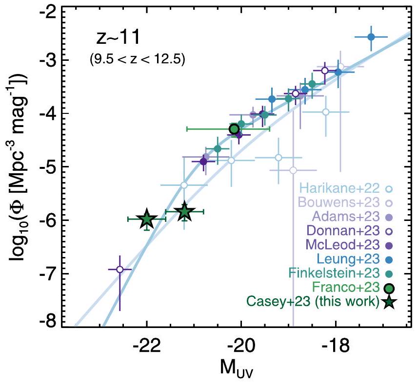
الشكل 4. المساهمة المباشرة للمصادر المعروضة في هذه الورقة في UVLF عند (النجوم الخضراء) مقابل قياسات الأدبيات الحديثة لـ JWST (أدامز وآخرون 2023أ؛ بوانز وآخرون 2023؛ دونان وآخرون 2023؛ فينكلشتاين وآخرون 2023ب؛ فرانكو وآخرون 2023؛ هاريكان وآخرون 2023؛ ليونغ وآخرون 2023؛ مكليود وآخرون 2024). التناسبان الوظيفيان المعروضان هما دونان وآخرون (2023) ملاءمة قانون القوة المزدوجة (الأزرق الفاتح) و ليونغ وآخرون (2023)ملاءمة قانون القوة المزدوجة (باللون الأزرق الداكن). يتم تقديم بيانات UVLF المجمعة من هذه الورقة في الجدول 3 مع قياس عند (غير معروض هنا). الـالقياس من الحقبة الأولى لبيانات COSMOS-Web في فرانكو وآخرون (2023) موضح باللون الأخضر الفاتح. هذه القياسات لا تأخذ في الاعتبار النقص، ولكنها تأخذ في الاعتبار التلوث من خلال تعديل مساهمة كل مصدر بناءً على الاحتمالية بأنه بالفعلتتوافق قياساتنا مع تقديرات الأدبيات الأخرى لـ UVLF عند انزياحات حمراء مماثلة.
والمعدل المتوسط للانزياح الأحمر للمجرات في الفئة قريب من. بينما نحن المرشحون لديهم PDFs انزياح أحمر تمتد إلىحلول فيمن غير المحتمل، لذا نحدد تقدير الحجم المتعلق بتلك المصادر عند، مما يتوافق مع (الـعينة).
تظهر الشكل 4 المساهمة المباشرة للمصادر المكتشفة (المحسوبة باستخدام الطريقة) المقدمة في هذه الورقة إلى UVLF في، مع توفير القياسات أيضًا في الجدول 3. نحن نحسب مساهمة هذه المصادر في UVLF من خلال 500 سحب مونت كارلو من التوزيعات الخلفية للقياساتوقيم الانزياح الأحمر من Bagpipes، حيث يمكن أن تُحتسب المصادر في فئات سطوع مختلفة في سحوبات مختلفة أو تقع خارج النطاق المحدد للانزياح الأحمر. لم يتم تصحيح هذه القياسات لعدم الاكتمال، ومع ذلك فهي تتناول التلوث المحتمل. بشكل عام، نجد أن كثافة الحجم للمجرات الساطعة جداً الموجودة في COSMOS-Web تتماشى بشكل جيد مع التوقعات من وظائف اللمعان المقاسة حديثاً بواسطة JWST فيتظهر الشكل 4 القياسات فيمن دونان وآخرون (2023)، فرانكو وآخرون (2023)، هاريكان وآخرون (2023)، ليونغ وآخرون (2023)، مكليود وآخرون (2024)، وبيانات من تعاون CEERS (S. Finkelstein، اتصال خاص). التناسبات الوظيفية المزدوجة المعروضة هي من دونان وآخرون (2023) وليونغ وآخرون (2023).
أكثر ما يلفت الانتباه من بياناتنا هو الميل النسبي المسطح لـ UVLF في الطرف الساطع؛ قد يكون هذا ناتجًا عن عدم الاكتمال في فئة اللمعان المنخفضة لدينا، والتي لا نقوم بتصحيحها في هذا العمل. بالنظر إلى أن فئة المقدار عندنسبيًا مكتمل، بياناتنا لا تدعم
الجدول 3 قيود دالة اللمعان فوق البنفسجي
نطاق
( )
11
[9.5, 12.5]
-22.0
0.8
11
[9.5, 12.5]
-21.2
0.8
14
[13، 15]
-21.0
1.0
ملاحظة. المساهمة المقاسة لمرشحينا في UVLF عند و لم يتم تصحيحها لعدم الاكتمال.
تمت ملاءمة دالة شكتير إلى دالة توزيع اللمعان فوق البنفسجي مشابهة لأعمال أخرى. ستتبع اشتقاق ملاحظي أكثر شمولاً لدالة توزيع اللمعان فوق البنفسجي من COSMOS-Web في ورقة قادمة (M. Franco et al. 2024، قيد الإعداد) وستتضمن محاكاة الاكتمال وقياسًا موسعًا حتى حد الكشف الأدنى للاستطلاع.
5.3. الخصائص الفيزيائية للسطوعمرشحون
نظهر في الشكل 5 توزيع المصادر المعروضة في هذه الورقة من حيث اللمعان فوق البنفسجي المطلق، وانحدار فوق البنفسجي في إطار الراحة ( ) وكتلة النجوم. نقارن مع مرشحين آخرين تم الإبلاغ عنهم في الأدبيات التي تم تلخيصها مؤخرًا في فرانكو وآخرون (2023). يتم عرض المصادر الأربعة الأكثر سطوعًا التي تم مناقشتها في القسم 4.1 باللون الأخضر في كل لوحة. هذه المصادر الأربعة لها سطوع متطابق جيدًا وتجاوز GN-z11 عند انزياحات حمراء مماثلة. نظرًا للمساحة الواسعة التي تغطيها COSMOS-Web حتى الآن، من الواضح أننا حساسون لاكتشاف المزيد من المصادر اللامعة جوهريًا التي تكون أكثر سطوعًا من ما وراءفي انزياح أحمر ثابت، فإن معظم اكتشافات تلسكوب جيمس ويب من مجالات أعمق ولكن أضيق تتعلق بـ (أو أضعف بمقدار (عدد) مرات من العينة المقدمة هنا.
منحدرات الأشعة فوق البنفسجية في إطار الراحة لهذه العينة أكثر احمرارًا قليلاً من معظم مجرات ليمان-كسر (LBGs) في هذه الحقبة (الوسيط المقدم في الأدبيات عند هو ووسيط هذه العينة هو ); مصدر واحد، COS، هو نقطة شاذة كبيرة مع بينما جميع الآخرين أزرقون أكثر منمن المحتمل أن تكون عينتنا أكثر احمرارًا من العينات الأخرى لعدة أسباب: كأجسام ساطعة بشكل استثنائي، تميل إلى أن يكون لديها كتل نجمية مقدرة أعلى (انظر القياسات السابقة لهذه العلاقة من Finkelstein et al. 2012؛ Tacchella et al. 2022). وقد قيست تلك الأعمال علاقة مباشرة بين و لكن ليس و (على الرغم من أن العلاقة الأخيرة مشتقة في Topping et al. 2023). مع الكتل الأعلى، من المرجح أن تكون مجموعة النجوم عمومًا أكبر سنًا أو أن تاريخ تشكيل النجوم أكثر تعقيدًا، بحيث يكون هناك إما عدد أقل نسبيًا من النجوم O التي تساهم في تدفق الأشعة فوق البنفسجية في إطار الزمان أو أن خزانات الغبار في مثل هذه المجرات المبكرة قد تراكمت بما يكفي لتجعل الأشعة فوق البنفسجية أكثر احمرارًا قليلاً (انظر Ferrara et al. 2023؛ Ziparo et al. 2023). بينما قد تفسر زيادة المعدن أيضًا اللون الأحمر النسبيالميل مقارنةً بالمجرات ذات المعدن المنخفض التي تمتلك تاريخ تشكيل نجمي مشابه، فوق -2.0 نقاط إما إلى تضعيف الغبار أو إلى تشكيل النجوم الأقل حداثة كسبب لانحدار الأشعة فوق البنفسجية الأكثر اعتدالًا. نحن نوجه بعض الحذر في تفسير العلاقة، حيث أن كلا الكميتين مشتقتان من ملاءمة SED ولديهما تغاير غير قابل للإهمال.
بينما تُوجد انحدارات الأشعة فوق البنفسجية الأكثر زُرقة في أعلى انزياح أحمر لدينانموذج، نحذر من أن هذا من المحتمل أن يكون تأثير اختيار: المجرات ذات القيم الأكثر احمرارًا منفيستكون لها تداخلات كبيرة مع الحلول ذات الانزياح الأحمر المنخفض وبالتالي
الشكل 5. الخصائص الفيزيائية المستمدة لنجومنا اللامعةالمرشحين بالنسبة لعينة أخرى من مجرات الكون المبكر في الأدبيات (نقاط رمادية، معظمها من عينة JADES في اللوحة اليسرى؛ هينلاين وآخرون 2024)، مع تسليط الضوء بشكل صريح على عينة COSMOS-Web التي وجدها فرانكو وآخرون (2023) باللون الرمادي الداكن. المجرتان الأربع اللتان تتمتعان بسطوع استثنائي تظهران كنجمات خضراء، الساطعةالعينة تظهر كنجوم زرقاء داكنة، والعينة موضحة على شكل نجوم زرقاء فاتحة؛ يستمر هذا نظام الألوان في الأشكال 6 و7 و9. اليسار: المقدار المطلق للأشعة فوق البنفسجية في إطار الراحة مقابل الانزياح الأحمر بالمقارنة مع عينات الأدبيات. نبرز ثلاثة مصادر لامعة أخرى.المصادر: GN-z11 (التي تم تأكيدها طيفيًا الآن عند; أوش وآخرون 2016؛ بانكر وآخرون 2023)، GL-z10 و GL-z12 (نايدو وآخرون 2022ب؛ كاستيلانو وآخرون 2022) مع تحديدات طيفية مؤقتة من ALMA (باكس وآخرون 2023؛ يون وآخرون 2023). اليمين: ميل الأشعة فوق البنفسجية في إطار الراحةمع الكتلة النجمية. عيّنتنا هي أكثر مجموعة حمراء من المرشحين المبلغ عنها في الأدبيات (فينكلشتاين وآخرون 2012؛ تاكشيلا وآخرون 2022؛ توبينغ وآخرون 2023). الخط المنقط المتقطع هو العلاقة الأفضل التي تم اشتقاقها لـالمجرات من فينكلشتاين وآخرون (2012). لا يتم الكشف عن أي اتجاه في مقابل (انظر توبينغ وآخرون 2023).
يجب إزالتها من عيّنتنا لعدم استيفائها معايير الاختيار لدينا. لا يمكن معالجة هذا التحيز، الذي ينتشر في اختيار LBGs عند جميع الانزياحات الحمراء، بسهولة دون استثمارات كبيرة في الطيفية لعينات كبيرة.
تظهر الشكل 6 أحجام المجرات في العينة مقابل كثافة الكتلة النجمية السطحية وكثافة معدل تكوين النجوم السطحية. جميع المصادر مفصولة مكانيًا بأحجام متوسطة، مما يقلل من القلق من أن انبعاثهم قد يهيمن عليه نواة مجرية نشطة (AGN؛ على الرغم من أن شكل غير محسوم لن يضمن ذلك). يتم حساب كثافات الكتلة النجمية وكثافات معدل تكوين النجوم عن طريق قسمة الإجمالي أو SFR بمقدار 2 لأخذ في الاعتبار أو SFR داخلي إلىثم نقسم علىكثافات السطح الكتلية النجمية مشابهة جدًا لبعض من أكثر المجرات الإهليلجية المحلية كثافة (لاور وآخرون 2007؛ هوبكنز وآخرون 2010)، والأقزام الفائقة الكثافة ومجموعات النجوم الفائقة (هاشغان وآخرون 2005؛ إيفستينييفا وآخرون 2007؛ هيلكر وآخرون 2007؛ مكرايدي وغراهام 2007) على الرغم من أن عينتنا أكبر بحوالي 10 مرات في. قد يشير هذا إلى أنه، كما لوحظ، يمكن أن تكون هذه المجرات من الأصول القابلة لنجوم النواة المجرية البيضاوية ذات الكثافات المماثلة. كثافات سطح تكوين النجوم مشابهة جدًا لتلك التي تُرى في بعضالمجرات اللامعة ذات الانزياح الأحمر العالي (مثل، باولر وآخرون 2017)، وبعض الانفجارات النجمية المحلية (مثل، عينة مسح المجرات اللامعة بالأشعة تحت الحمراء من المراصد الكبرى؛ أرموس وآخرون 2009؛ مكيني وآخرون 2023ب) ومجرات تحت المليمتر ذات الانزياح الأحمر العالي (هودج وآخرون 2016؛ بيرنهام وآخرون 2021)، على الرغم من أن الأنظمة الأخيرة تميل إلى أن تكون أكبر بكثير ( ) بمعدلات SFR أعلى.
5.4. عدم اليقين في الكتلة النجمية
الاشتقاقات الكتلية من بيانات الأشعة فوق البنفسجية في إطار السكون غير مؤكدة بطبيعتها. ومع ذلك، يوفر تلسكوب جيمس ويب الفضائي ذراع طول موجي أطول من تلسكوب هابل الفضائي، في النطاق البصري لإطار السكون، لتقييد الأطياف الطيفية للنجوم حتى ما بعدتفتقر القليل من الفرق ونقص التغطية في نطاق الأشعة تحت الحمراء القريبة في إطار الزمان إلى المعيار الذهبي لاشتقاق الكتلة النجمية. ومع ذلك، فإن العمر الشاب لـ
الشكل 6. نصف أضواء نصف القطر المقاسة بواسطة F277W لعينة البيانات موضوعة مقابل كثافة الكتلة النجمية السطحية (اللوحة العلوية) وكثافة تشكيل النجوم السطحية (اللوحة السفلية). في الأعلى، نعرض كثافات الكتلة النجمية السطحية المتوسطة للمجرات الإهليلجية المحلية من لور (2007) والأقزام الفائقة الكثافة ومجموعات النجوم الفائقة من التجميع في هوبكنز وآخرون (2010). بالإضافة إلى ذلك، نعرض الأحجام والكثافات السطحية المقاسة لـ المصادر التي اكتشفها لابي وآخرون (2023) والتي تم تحليل أحجامها في باجن وآخرون (2023). كثافات سطح تشكيل النجوم تتماشى مع غيرهاالمجرات اللامعة ذات الانزياح الأحمر (Bowler et al. 2017)، الانفجارات النجمية المحلية (Armus et al. 2009؛ McKinney et al. 2023b)، والمجرات تحت المليمترية ذات الأحجام المقاسة (مع؛ برنهام وآخرون 2021). المصادر من عيّنتنا ملونة حسب العينة الفرعية كما في الشكل 5.
الكون في ( يقلل بشكل كبير من النطاق الديناميكي لسيناريوهات تاريخ تشكيل النجوم الممكنة للأجسام اللامعة من نوع LBG. وهذا يضع حدودًا معقولة على نسبة الكتلة إلى الضوء وبالتالي الكتلة النجمية الأساسية لمصادر فردية، مع عدم اليقين المستمد.ديكس على الرغم من عدم وجود قيود في الإطار الزمني للراحة البصرية. نظرًا للاحتمالات المحتملة لكتل النجوم التي تتجاوزفي (كل مصدر في عيّنتنا يتجاوز هذا الحد)، نتناول هنا المصادر المحتملة لعدم اليقين في اشتقاق كتلة النجوم لدينا.
نحن أولاً نتحقق من حساسية نموذج تاريخ تشكيل النجوم المعتمد على الكتلة النجمية الناتجة؛ بشكل عام، فإن تشكيل النجوم الذي يحدث في الماضي سيكون له نسبة كتلة إلى ضوء أعلى مستنتجة لإطار الأشعة فوق البنفسجية، وبالتالي كتلة نجمية أعلى. نقارن نموذج بايبس المرجعي الخاص بنا، الذي يضع نموذجاً مؤجلاً-مع انفجار نجمي حديث ومستمر إلى نموذج يحتوي فقط على تأخير- SFH. التأخير--نماذج SFH فقط تزيد بشكل فعال من تقديرات الكتلة النجمية للفيزياء الضوئية الثابتة بعوامل من (انظر أيضًا ميهالوسكي وآخرون 2012؛ ميتشل وآخرون 2013؛ ميهالوسكي وآخرون 2014). بالمقابل، يمكننا أن نسأل ما هي النسبة من الكتلة النجمية في عيّنتنا التي تتجمع خلال مرحلة الانفجار النجمي الثابت الأخيرة؛ في الغالبية العظمى من الحالات، تُعزى الكتلة النجمية إلى انفجار حديث (تشكل خلال الخمسين مليون سنة الماضية في المتوسط). إذا سمحنا بانفجار أكثر تطرفًا وحداثة دون المساهمة من التأخير-النموذج، يتم تقليل الكتل النجمية فقط بواسطةأقل من التقديرات المرجعية، ضمن نطاق عدم اليقين المبلغ عنه. من هذه الناحية، يوضح ذلك أن الكتل النجمية التي نستخلصها في هذا العمل هي حد أدنى محافظ لسكان نجميين يتصرفون بشكل طبيعي، يتكون من نجوم من النوع الثاني والنوع الأول ذات معدنية منخفضة، ولكن ليست منخفضة للغاية.
إذا كانت نجوم الجيل الثالث من السكان تهيمن على الضوء في إطار الأشعة فوق البنفسجية، فإن دالة الكتلة الأولية الثقيلة المتوقعة لها (Hirano et al. 2014, 2015) ستؤدي إلى استمرارية فوق بنفسجية تهيمن عليها الانبعاثات السديمية، بدلاً من الانبعاثات النجمية. وهذا سيؤدي إلى نسبة ضوء إلى كتلة أعلى من الأشعة فوق البنفسجية (على سبيل المثال، Schaerer & de Barros 2009) بعواملديكس، مما يقلل من أعلى تقديرات الكتلة في عيّنتنا عندمنإلى. وهذا من شأنه، بالطبع، أن يعني أن تشكيل النجوم من الجيل الأول يهيمن على إنتاج الطاقة في هذه الأنظمة، وهو ما قد يكون شرطًا حدوديًا صعبًا إلى حد ما ومتطرفًا، حتى بالنسبة لمثل هذه المجرات ذات الانزياح الأحمر العالي نظرًا لأن تقديرات كتل هالاتها مرتفعة جدًا، . من المحتمل أن تكون نتيجة أخرى لهيمنة النجوم من الجيل الثالث على الأشعة فوق البنفسجية في إطار الراحة هي ميل أزرق أكثر بكثير، أكثر مما تم قياسه هنا.
أخيرًا، نعتبر تأثير AGN على تقديرات الكتلة النجمية لدينا. لقد أصبح من الواضح أن الثقوب السوداء الهائلة التي تتراكم بشكل نشط قد تكون مصدرًا بارزًا لإنتاج الطاقة في الأوقات المبكرة، وقد مكن تلسكوب جيمس ويب الفضائي من تحديد AGN مع ثقوب سوداء ذات كتل أقل في أوقات سابقة (لارسون وآخرون 2023). لكي يؤثر AGN بشكل كبير على الكتل في عيّنتنا، يجب أن يهيمنوا على سطوع الأشعة فوق البنفسجية في إطار الزمان بمقدار عدة مرات مقارنة بالمساهمة النجمية. وهذا سيترجم فعليًا إلى حد أدنى لسطوع AGN قدره أو عند نسبة إيدينغتون لـهذا يعني حدًا أدنى لكتلة الثقب الأسود قدرهستكون هذه الكتل كبيرة بشكل غير متوقع إلى حد ما بالنسبة لتقديرات الكتلة النجمية المنقحة downward لمدنها المضيفة،لذا نقيم هذه النتيجة على أنها أقل احتمالًا من تقديرات كتلة النجوم لدينا دون مساهمة كبيرة من AGN. بينما يبدو أن بعض الثقوب السوداء العملاقة في الزمان البعيد غير عادية في كتلتها بالنسبة لمجراتها المضيفة (Kocevski et al. 2023; Larson et al. 2023)، إلا أنه لا يبدو أنها تساهم بشكل كبير في الانبعاث المستمر.
الكتل النجمية لعينة لدينا، كما تم تقديرها باستخدام نموذجنا القياسي لبرامج Bagpipes للانفجارات + التأخير-النموذج، يتم عرضه
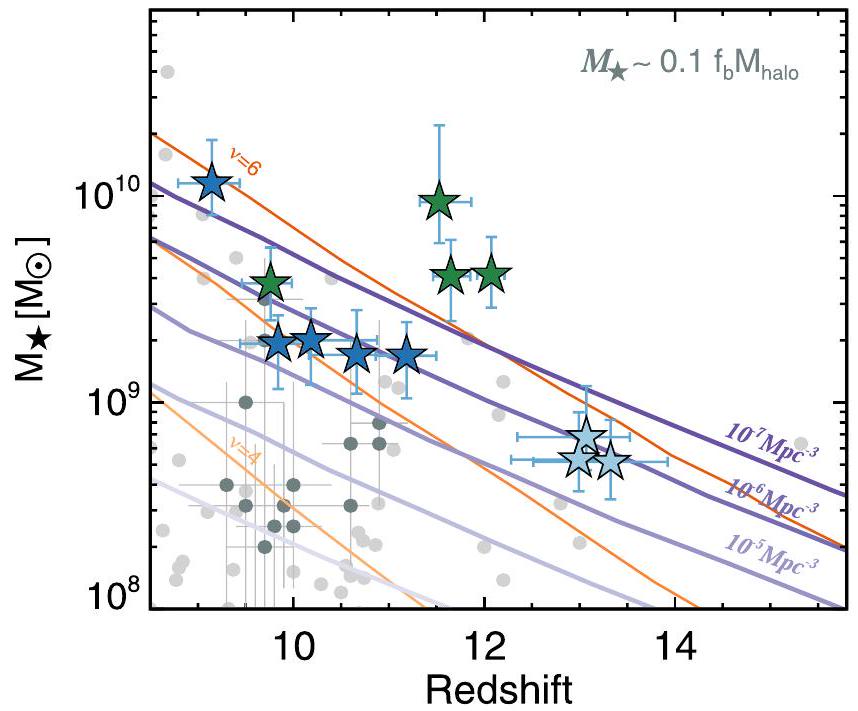
الشكل 7. الكتلة النجمية مقابل الانزياح الأحمر لعينة لدينا بالنسبة لمنحنيات كثافة الحجم الثابتة، وارتفاع الذروة، وغيرها من المجرات المرشحة المبلغ عنها في الأدبيات (نقاط رمادية فاتحة). يتم توليد منحنيات كثافة الحجم (باللون الأرجواني) وارتفاع الذروة (باللون البرتقالي) من توقع دالة كتلة الهالة مقاسة بواسطة نسبة الباريونات الكونية.وكفاءة لتحويل الباريونات إلى نجوم تبلغكما في Boylan-Kolchin (2023). الحجم في مجموعة بيانات COSMOSWeb الحالية هوفي حاوية بعرض. هذه المقارنة تبرز الطبيعة غير العادية بشكل خاص للثلاثة مجرات الضخمة في، COS-z12-1 و COS-z12-2 و COS-z12-3، التي تتحدى وجودها التوقعات. وجودها يتطلب إما وفرة أعلى من الهالات الضخمة فيأو نسبة الباريونات النجمية المعززة، مما يوحي بأن كفاءة تشكيل النجوم مرتفعة ( ) لجزء كبير من تاريخ تشكيل النجوم في المجرات. يتم عرض تاريخ تشكيل النجوم المحتمل لهذه الأنظمة في الشكل 9 ويتم استكشاف المزيد من التفاصيل حول تداعيات كتلها في المناقشة. يتم تلوين المصادر من عينتنا حسب المجموعة الفرعية كما في الشكل 5.
ضد الانزياح الأحمر في الشكل 7. في المتوسط، فإن عدم اليقين لديهم هوديكس؛ هذه أصغر من تقديرات الكتلة النجمية المتوسطة لغيرها من المجرات المشابهة المختارة بواسطة تلسكوب هابل أو تلسكوب جيمس ويب في فترة إعادةionization. مرة أخرى، يعود ذلك إلى عمر الكون فيكائنوكون اللمعان لهذه المصادر ساطعًا جدًا؛ فإن هذين القيدين يحدان بشدة من نطاق مسارات تكوين النجوم المسموح بها (مع افتراضات دالة الكتلة الأولية التقليدية)، مما يتطلب نموًا حادًا عبر انفجارات حديثة، ومع مسارات تكوين النجوم المحدودة تأتي حدود أكثر دقة على كتل النجوم.
في فضاء الكتلة النجمية، تدفع مجموعة فرعية من عينتنا حدود المصادر الأكثر ضخامة التي يمكن العثور عليها بشكل معقول في مسوحات JWST العميقة عند; على وجه الخصوص، COS-z121 و COS-z12-2 و COS-z12-3، مع كتل في. نحن نرسم منحنيات ذات كثافة عددية ثابتة في الشكل 7 مستمدة من دالة كتلة الهالة (شيث وتورمن 1999) مقاسة بواسطة نسبة الباريونات الكونية و”كفاءة” معقولة من، حيث يمثل الكسر من الباريونات التي تم تحويلها إلى نجوم داخل هالة على مدى عمرها المتكامل، . نلاحظ أن الذروة النموذجية لعلاقة الكتلة النجمية إلى كتلة الهالة (SMHR) هي عبر مجموعة من الانزياحات الحمراء (Mandelbaum et al. 2006; Shankar et al. 2006; Conroy & Wechsler 2009; Behroozi et al. 2010, 2019; Shuntov et al. 2022)، مما يعني أقصى (وقد يتوقع المرء أن يكون هذا الكسر أقل في أوقات كونية سابقة حيث لا توجد قيود على SMHR بعد). نحن أيضًا نرسم
منحنيات ارتفاع الذروة الثابتة ، وهو مقياس للكسر من الكتلة المحتواة في الهالات فوق عتبة كتلة معينة؛ القيم الأعلى من تشير إلى هالات أكثر كثافة حيث عند تتوافق مع هالة بكتلة . هذا يوضح أن التطور الضمني لعينة لدينا هو تطور متطرف مع المعطاة : تمثل أعلى كثافات كتلة ممكنة ستنمو لاستضافة تجمعات مجرات ضخمة في الكون الحالي.
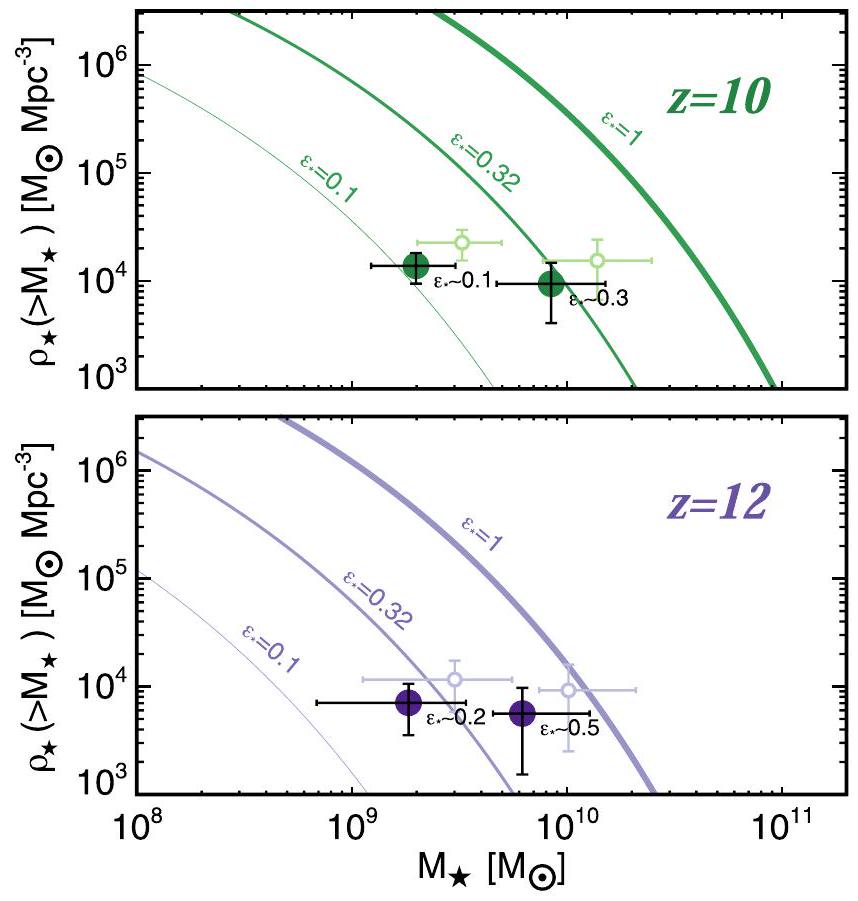
في الشكل 8، نحسب مباشرة كثافة الكتلة النجمية التراكمية في صندوقين مركزيين عند و بعرض . نستخدم التوزيعات البعدية الكاملة في و كما تم اشتقاقها باستخدام Bagpipes لهذه الحسابات ونفترض عدم اليقين بواسع بواسون. المقارنة المباشرة مع دالة كتلة الهالة تشير إلى كسور باريونية نجمية معقولة إلى عالية مع عند ، ليست بعيدة جدًا عن التوقعات من SMHR (Behroozi et al. 2019). ومع ذلك، عند ، تشير اكتشافاتنا إلى كسور كتلة نجمية أعلى، مع (انظر أيضًا المنشورات القادمة من K. Chworowsky et al. 2024، قيد الإعداد؛ M. Shuntov et al. 2024، قيد الإعداد). يقدم Harikane et al. (2023) نظرة شاملة على اكتشافات الكون المبكر من JWST في عامه الأول، ويجدون أن المجرات الساطعة بشكل خاص () الموجودة في مسوحات أعمق وأصغر حجمًا تتطلب كفاءات عالية، حيث 0.3، لإنتاج كتل نجمية عند . لم يكن من المتوقع أن تكون مثل هذه المرشحات ذات كسور باريونية نجمية عالية من واقعية؟
تشير بعض الأعمال النظرية إلى أنها كذلك. على وجه الخصوص، فإن المجرات عند ، المدفونة إلى حد كبير في الكون المحايد قبل إعادة التأين، لن تتعرض لقصف من خلفية الإشعاع فوق البنفسجي وبالتالي فإن الانهيار السريع للسحب الجزيئية قد يشهد معدلات عالية جدًا من تشكيل النجوم (Susa & Umemura 2004). يوفر سيناريو الانفجار النجمي بدون تغذية راجعة (FFB) المقدم في Dekel et al. (2023) حسابًا مفصلًا من المبادئ الأولى حول كيفية تشغيل مثل هذا الانفجار النجمي؛ في مثل هذه الأنظمة، يكون وقت السقوط الحر هو ويحدث تشكيل النجوم السريع قبل أن تتطور النجوم الضخمة إلى رياح وتحدث تغذية راجعة من السوبرنوفا، ولم يتم تأسيس خلفية الإشعاع فوق البنفسجي الخارجية بعد. هذا مشابه جدًا للأعمال السابقة في المحاكاة التي أظهرت بعض الأنظمة حيث تفشل التغذية الراجعة في تنظيم تشكيل النجوم (Torrey et al. 2017; Grudić et al. 2018).
مع بداية متأخرة للتغذية الراجعة، قد يتوقع المرء أن كفاءة تشكيل النجوم الفورية () لفترات قصيرة () ستؤدي إلى زيادة ملحوظة في من ترتيب بضع أعشار. قد يُتوقع أن تحتوي المجرات الموجودة في هالات بكتلة عند على كثافات غاز FFB، وبالتالي قد يكون لديها كتل نجمية تصل إلى ، ومعدلات تشكيل نجوم في عشرات الكتل الشمسية سنويًا، وأشكال مضغوطة زرقاء (تحت الكيلوبارسيك). هذا يصف خصائص العينة الفرعية الضخمة بشكل جيد: و . قد توضح الطيفية المستقبلية لمثل هذه الأهداف المزيد من تطبيق نموذج FFB على مثل هذه الأنظمة، خاصة في قياسات المعدن والانحدار فوق البنفسجي في إطار الراحة (وبالتالي وجود الغبار).
تقدم Ferrara et al. (2023) تفسيرًا نظريًا آخر للأنظمة المبكرة اللامعة جدًا، الذين يقترحون أن
الشكل 8. كثافة حجم الكتلة النجمية التراكمية كدالة للكتلة النجمية المحسوبة عند و من عينتنا. تم اشتقاق منحنيات كتلة الهالة، مع ثلاث كفاءات نجمية متكاملة مختلفة أو كسور باريونية نجمية من و 1 باستخدام المنهجية الموضحة في BoylanKolchin (2023). تم اشتقاق النقاط باستخدام التوزيعات البعدية الكاملة في و لكل مصدر في صناديق بعرض مركزة على أي انزياح أحمر. عند نستنتج كسور باريونية نجمية ، بينما عند نستنتج كسور باريونية نجمية أعلى، . تمثل الدوائر المفتوحة مجموع النجوم والغاز الجزيئي المستخرج؛ يتم استنتاج كتل الغاز من علاقة Kennicutt-Schmidt (KS). عند أعلى الكتل عند ، من الواضح أن جميع الباريونات يمكن أن تتكون من نجوم وغاز جزيئي، مما يترك مجالًا ضئيلًا لخزانات كبيرة من، على سبيل المثال، الغاز الذري. هذا يبرز الحاجة إلى جمع ملاحظات الغاز البارد من العينة.
قد تؤدي الانفجارات القصيرة الأمد لتشكيل النجوم فوق إيدينغتون إلى نفخ الغالبية العظمى من الغبار في المجرات المبكرة (مع sSFR )، مما يجعل من الممكن اكتشاف مجرات زرقاء ساطعة جدًا تتجاوز . الوسيط المقدر لـ SFR المحدد في عينتنا المحسوبة على مقياس زمني هو . هذا يتناقض مع، على سبيل المثال، المرشحات الزرقاء جدًا ولكن اللامعة بشكل مشابه التي حددها Topping et al. (2022) مع sSFR . قد تحتوي مثل هذه الأنظمة على كتل نجمية مرتفعة نسبيًا ، ومعدنية ، وانحدارات فوق البنفسجية زرقاء في إطار الراحة (). يصف Ziparo et al. (2023) أن إما طرد الغبار بواسطة ضغط الإشعاع قد يؤدي إلى مثل هذه الانحدارات الزرقاء، أو بدلاً من ذلك، وسط بين النجوم متقطع مع مناطق متميزة مكشوفة ومخفية من الضوء النجمي. عيّنتنا ليست زرقاء تمامًا (مع الوسيط ) كنموذجهم القياسي، مما يظهر بعض التناقض مع فرضية طرد الغبار فوق إيدينغتون، لكن نموذج التخفيف المتقطع قد يكون بالفعل قابلًا للتطبيق على هذه الأنظمة. ستوفر ملاحظات ALMA المستقبلية معلومات حاسمة حول محتوى الغبار في مثل هذه الأنظمة.
يوضح الشكل 9 عرضًا آخر للكتل النجمية في عينتنا مقابل الانزياح الأحمر. هنا أظهرنا مباشرة كيف قد تبدو مجموعة الأجداد للأنظمة الثلاثة الأكثر ضخامة عند ، عبر البعديات (فترة الثقة الداخلية ) على SFHs، أو نمو الكتلة النجمية التراكمية. نمو الكتلة النجمية في هذه الأنظمة هو بشكل ساحق
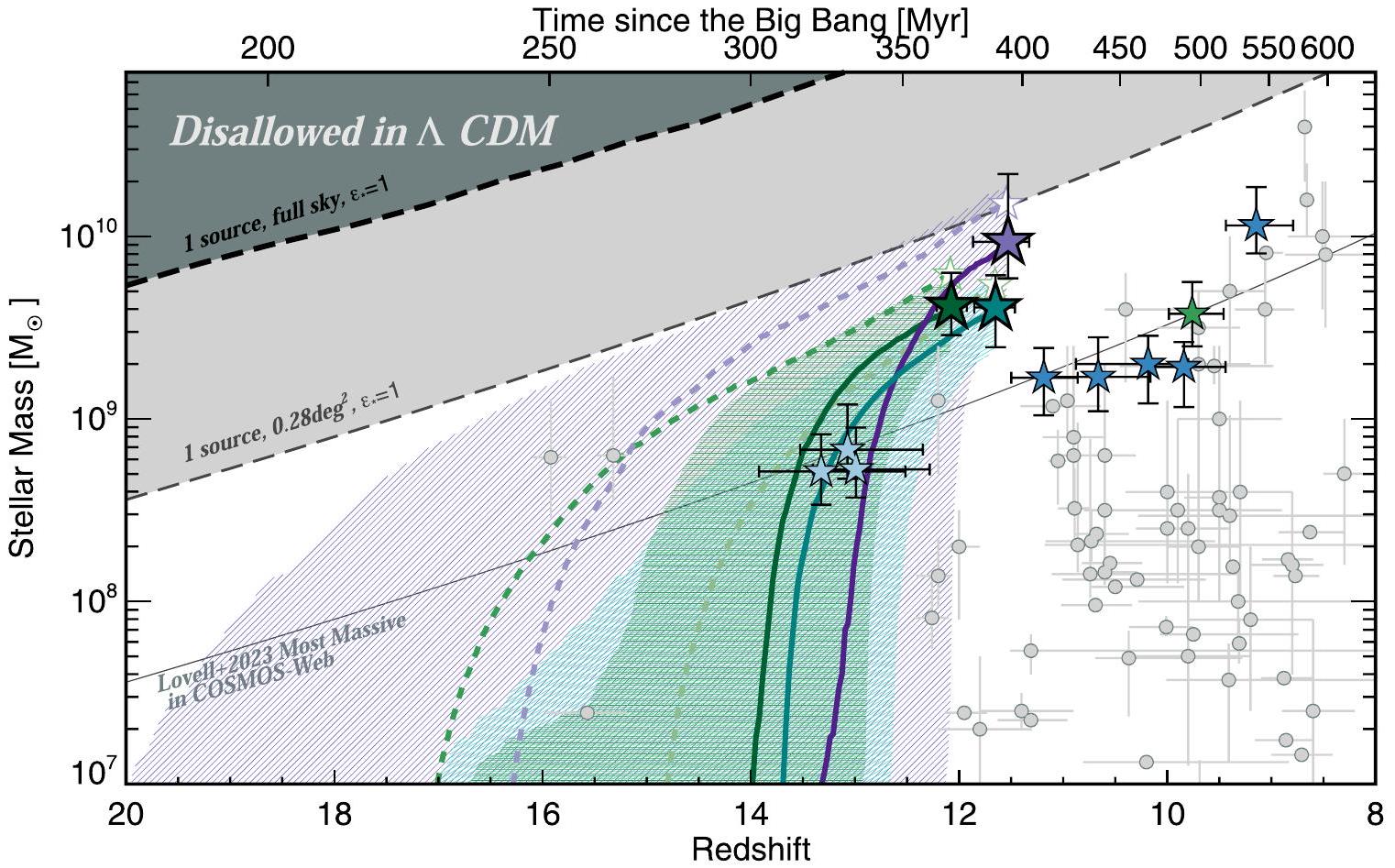
الشكل 9. الكتلة النجمية مقابل الانزياح الأحمر للمرشحات المحددة في هذه الورقة (النجوم). هنا نبرز SFHs المتكاملة للمرشحات الثلاثة الأكثر ضخامة ، والتي تتضمن انفجارات متأخرة- بالإضافة إلى انفجارات حديثة: COS-z12-1 (الأخضر الداكن)، COS-z12-2 (الأزرق الفاتح)، وCOS-z12-3 (البنفسجي). توضح الخطوط المنقطة تاريخ نمو الكتلة النجمية إذا تم افتراض أن SFH هو فقط متأخر- بدون انفجار؛ هذا يؤدي إلى كتل نجمية أعلى كانت ستتراكم المزيد من الكتلة في وقت مبكر . مع نموذج المتأخر- بالإضافة إلى الانفجار، قد تكون الكتل النجمية قد زادت بمقدار ترتيب من حيث الحجم في أقل من 100 مليون سنة، من الأجداد التي تبدو مشابهة جدًا للمرشحات التي نحددها في القسم 4.3. تُظهر نقاط المرشحات العالية- الأخرى من الأدبيات في نقاط رمادية. الكتل النجمية التي يتم منعها رسميًا في CDM مذكورة باللون الرمادي الداكن، مما يتوافق مع عتبة الكتلة النجمية لأكثر هالة ضخمة في السماء الكاملة بافتراض . نعرض أيضًا نفس العتبة التي تتوافق مع ، المنطقة التي تغطيها COSMOS-Web في هذا العمل. بالمثل، فإن أكثر مجرة ضخمة متوقعة في جميع COSMOS-Web، المحسوبة بواسطة Lovell et al. (2023)، تظهر في الخط الرمادي الرفيع؛ تفترض أن كفاءة تحويل الباريون إلى نجوم في الهالة تختلف، مع متوسط ، وتغطي فترات الثقة حول تلك العتبة الكتلية أكثر مجرة ضخمة (COS-z12-3) ضمن .
تسيطر عليها انفجارات حديثة، بحيث نمت كتلها النجمية بمعدلات تفوق بكثير نمو هالات المادة المظلمة الأم (عند كثافة حجم ثابتة). كما تم الإشارة إليه في القسم 5.4، فإن هذا النمو السريع والحديث في الكتلة النجمية يوفر أكثر تقديرات الكتلة النجمية تحفظًا للعينة ككل. الطبيعة المدفوعة بالانفجارات المقترحة لـ COS-z12-1 وCOS-z12-2 وCOS-z12-3 على وجه الخصوص قد تعني أن كتل هالات المجرات المضيفة لها قد تكون في جوهرها أقل مما قد يتوقعه المرء بالنظر إلى كتلها النجمية، بما يتماشى مع بعض المجرات الأقل سطوعًا في عينتنا. وقد أظهرت الأعمال الأخيرة من محاكاة FIRE (Sun et al. 2023) أنه، في الواقع، لا توجد تعديلات خاصة مطلوبة لإعادة إنتاج الخصائص الملحوظة لاكتشافات JWST المبكرة الساطعة جدًا، والتي يجدون أنها مدفوعة بانفجارات عشوائية وحديثة لتكوين النجوم.
يجب أن نلاحظ أنه في معظم، إن لم يكن في جميع، النماذج النظرية التي تم بناؤها لشرح الكتل الضخمة جداًتحدث انفجارات سريعة لتكوين النجوم في المجرات على فترات زمنية قصيرة،م. يسمح لنا استخدام Bagpipes في ملاءمة SED بأن تكون الانفجارات ذات مدة قصيرة جدًا أو طويلة نسبيًا، تصل إلى 100 مليون سنة. للأسف، لا تتيح القيود في مجموعة البيانات الحالية وضع قيود مباشرة ذات مغزى على مقياس زمن الانفجار (أي، توزيع الأعمار لمكون الانفجار مسطح). ومع ذلك، قد يكون من الممكن، بل ومن الضروري، أن تكون هذه الأنظمة اللامعة بشكل استثنائي قد شهدت سلسلة من الانفجارات القصيرة التي يتم نمذجتها بشكل جيد بواسطة انفجار طويل الأمد يستمر حتى 100 مليون سنة.
صعود مثل هذه الضخمةالأنظمة سريعة جدًا لدرجة أن السكان الذين نحددهم في-بكتل نجمية أقل بمقدار ترتيب واحد-يمكن أن تخدم بشكل معقول كـ سكان السلف، على الرغم من الإطار الزمني القصيربين الفترتين. في أوقات لاحقة، من الممكن أن تتطور مجرات مثل COS-z12-1 وCOS-z12-2 وCOS-z12-3 لتصبح بعضًا من أولى المجرات الضخمة في الكون (كارنل وآخرون 2023؛ غلازبروك وآخرون 2023).
5.6. ليست جميع الباريونات نجومًا
معظم الباريونات في هالات المجرات تتجاوزيجب أن تكون محتواة في الغاز وليس في النجوم (والتر وآخرون 2020). ما هي العواقب التي تترتب على هذه الكتل النجمية العالية في عينتنا على إمكانية رصد خزاناتها من الغاز الجزيئي والذري؟ قد تثبت هذه الملاحظات أنها حاسمة في تفسير كتلها، وبالتالي كفاءاتها.
أولاً، من الجدير بالاعتراف أن الكفاءات الملاحظة النموذجية في عملية تشكيل النجوم نادراً ما تتجاوز (إيفانز وآخرون 2009؛ بيجييل وآخرون 2010؛ كينيكوت وإيفانز 2012). في سياق إمدادات الغاز في المجرات، فإن كفاءة تشكيل النجوم هي كما (عكس زمن استنفاد الغاز) ومُعدل إلى ، وبالتالي يمثل نسبة الغاز المستهلك كل 100 مليون سنة. هذا ليس هو نفسه الذي نسميه نسبة الباريونات النجمية في هذا العمل، لكن الآخرين يشيرون إليه بكفاءة تشكيل النجوم؛يمكن أن يُنظر إلى الشكل التكامل لـ. بالمثل ليس هو نفسه ، حيث أن الأخيرة تلتقط فقط العمليات الباريونية. إذا قمنا بتقريب (وهو حد أقصى صارم لـ ) مع SFR نجد أن متوسط كفاءة تشكيل النجوم يجب أن يكون، بما يتجاوز الحدود التي لوحظت محليًا السحب الجزيئية ولكنها ضرورية لبناء المجموعات النجمية المرصودة.
على الرغم من عدم ارتباطها بالملاحظات المباشرة فييمكننا بدلاً من ذلك تقدير كتل الغاز في عيّنتنا باستخدام تحويل كثافة سطح تكوين النجوم إلى كثافة سطح كتلة الغاز، أو علاقة كينكوت (Schmidt 1959؛ Kennicutt 1998). باعتماد علاقة كينكوت أحادية النمط مع مؤشر قانون القوة يبلغ تقريبًا 2 (Ostriker & Shetty 2011؛ Narayanan et al. 2012) ومع قياسات لكثافات سطح تكوين النجوم تتراوحنستنتج أن الجزيئيستتراوح كتل الغاز من. هذا يفترض أن حجم خزان الغاز مشابه لحجم الخزان النجمي. وهذا يعني أن نسب الغاز الجزيئي (إلى الكتلة الباريونية الإجمالية)في المتوسط. تأثير المكون الإضافي من الغاز الجزيئي على كثافة الكتلة الباريونية الكلية موضح في الشكل 8 في دوائر مفتوحة. في حالة الـالمرشحون، هذا يُظهر أن جمع الكتلة النجمية وكتلة الغاز الجزيئي يعوض تمامًا عن المحتوى الباريوني المتوقع لهذه الهالات المبكرة، مما يترك مجالًا ضئيلًا لمساهمات باريونية أخرى، على سبيل المثال، مثل الهيدروجين الذري، H I، الذي يُعتبر عنصرًا أساسيًا في بناء الغاز الجزيئي وحالة انتقالية لتحويل الغاز البدائي إلى نجوم.
ستكون المتابعات اللاحقة لملاحظات ALMA لهذه الأنظمة ذات قيمة لا تقدر بثمن لتوفير تقدير مستقل للميزانيات الباريونية الإجمالية للمجرات. على سبيل المثال، المسحات الطيفية لـ [O III] (في إطار الراحة )، لن توفر فقط تأكيدًا طيفيًا ضروريًا لهذه المصادر ولكن أيضًا ستسهل تقدير الكتلة الديناميكية المباشرة، مع الأخذ في الاعتبار كل من الغاز والنجوم. في حالة تشكيل النجوم بكفاءة، قد نتوقع أن يكون قيد الكتلة الديناميكية من [O III] تقريبًا مساويًا لـ في حالة الكفاءة المنخفضة وكتلة الهالة الأعلى (كما قد يتوقع المرء من نماذج كونية بديلة، انظر القسم التالي)، من المتوقع أن تكون قيود الكتلة الديناميكية أعلى بعدة مرات بسبب الكتلة الباريونية الإجمالية الأكبر الموجودة في الهالة.
5.7. الكوزمولوجيات البديلة تتنبأ بهالات أكثر ضخامة في وقت مبكر
تفسير بديل للنسب العالية جدًا من الباريونات النجمية التي تشير إليها عينتنا (مع ) هو أن المعلمة الستة نموذج CDM يقلل من تقدير كثافة العدد للهالات الضخمة في الأوقات المبكرة. يمكن تفسير هذا التعديل في الإطار الكوني من خلال نموذج الطاقة المظلمة المبكرة (EDE) (كاروال وكاميونكوفسكي 2016؛ بولين وآخرون 2018)، الذي يقترح أن هناك فترة مبكرة من حقن الطاقة المظلمة، بالقرب من وقت تساوي المادة والإشعاع (تليهاالتطور)، يمكن أن يفسر كلاهما الوفرة المتصورة الأعلى للهالات الضخمة في الأوقات المبكرة (Klypin et al. 2021) وحل قياسات التوتر في ثابت هابل الأخيرة (على سبيل المثال، Riess et al. 2022). كما تم مناقشته في Boylan-Kolchin (2023)، فإن الكثافة المعززة للمادة، وانحدار طيف القوة، ويمكن استخدام EDE حتى لشرح الكتل النجمية العالية التي تم قياسها لبعض من أكثر المرشحين ضخامة الذين تم العثور عليهم حتى الآن بواسطة JWST (لابي وآخرون 2023) على مناطق أصغر بكثير من السماء (على الرغم من أننا نلاحظ أيضًا أن الأعمال الأكثر حداثة قد اقترحت مراجعة هبوطية لتقديرات كتلهم النجمية بسبب مساهمة خطوط الانبعاث القوية و/أو AGN؛ إندسلي وآخرون 2023a؛ لابي وآخرون 2023). في الواقع، يتنبأ EDE بأكثر الاختلافات عمقًا بالنسبة لأكثر هالات ضخمة، نحن حساسون لاكتشافها في COSMOS-Web؛ فيتتوقع EDE مرات عدد الهالات أكثر مما كان متوقعًا منCDM. على الرغم من أنه لا يمكن قياسه مباشرة في البيانات التي نقدمها في هذا العمل، قد تتمكن التحليلات الطيفية المستقبلية من وضع قيود أكثر دلالة على الكتل الديناميكية لهذه الأجسام الساطعة.المصادر، مما يوفر قياسات أكثر مباشرة لوفرة الهالات الضخمة في الأوقات المبكرة.
5.8. الانفجارات العشوائية المحركةالمجرات في عصر إعادة التأين
مقدملا يزال نموذج الكون المتسارع (CDM) يحتفظ بأبسط تفسير لوجود مثل هذه المجرات الضخمة بشكل استثنائي فيهو نموهم السريع من خلال انفجارات عشوائية لتكوين النجوم حيث يتم تبريد جزء كبير من الباريونات المتاحة بكفاءة، وتكثيفها، وتحويلها إلى نجوم علىأوقات مقياس ميري. الكثافات الحجمية المماثلة التي تم قياسها للعديد من المجرات الضخمة جداً (بالنسبة لتلك الكتل الأقل بعشر مرات، يشير ذلك إلى نسب باريون نجمية عالية جداً. ) ليست نموذجية للسكان الأوسع؛ فإن انحدار دالة كتلة الهالة سيتطلب خلاف ذلك أن تكون المصادر أقل كتلة بمقدار 10 مرات مرات أكثر شيوعًا. مع تشكيل النجوم المدفوع بالانفجارات، يمكن أن تنحرف المجرات إلى مستويات أعلى، ويضمن انحياز مالموكويست أن تكون هي الأولى التي يتم توصيفها.
هذه الفرضية تتماشى مع هيمنة تشكيل النجوم المدفوع بالانفجارات في الطرف الساطع من دالة توزيع اللمعان فوق البنفسجي كما اقترحتها المحاكاة الكونية (شين وآخرون 2023؛ صن وآخرون 2023). من شأن هذا النمو الفعال والسريع أن يسهل غياب الخلفية فوق البنفسجية في عصر ما قبل إعادة التأين. قد تتكون هذه الانفجارات من عدة فترات قصيرة ( ) حلقات من تشكيل النجوم الفائق إيدينغتون (على سبيل المثال، فيرارا وآخرون 2023)، متوافقة مع نموذج FFB (ديكل وآخرون 2023)، على الرغم من أن الملاحظات المستقبلية للغبار والغاز والطيف قد توفر اختبارات حاسمة لمثل هذه النماذج الفقيرة من الغبار ومنخفضة المعدن. تم اقتراح نمو سريع مدفوع بالانفجارات لمجموعات أخرى مشابهة من المجرات اللامعة بالأشعة فوق البنفسجية التي اكتشفها JWST مؤخرًا (إندسلي وآخرون 2023ب؛ دريسلر وآخرون 2023؛ لوسر وآخرون 2023). من الناحية المثالية، يجب أن تكون هناك قيود مباشرة على الكتلة لكل يمكن أن يساعد المرشح المحدد في تحسين معلوماتهم حول SFHs. تقنية رئيسية أخرى يمكن استخدامها لتقييد العشوائية في المجرات الساطعة في فترة إعادة التأين هي تحليل التجمع، كما اقترح في موينو وآخرون (2023) حيث قد يوفر انحياز السكان رؤى حول كتل هالاتها المضيفة.
إذا كان الطرف الساطع من UVLF (على سبيل المثال، تسيطر عليه انفجارات عشوائية ذات مقاييس زمنية داخلية من، إذن فإن النتيجة الطبيعية هي تطور في شكل UVLF حولمن قانون القوة المزدوجة (عند ) إلى دالة شكتير (عند ). ستكون هذه هي النتيجة إذا تم حساب UVLF في صناديق بعرض ثابت تقريبًا؛ على سبيل المثال، عند صندوق بعرضيتوافق مع مقياس زمني أقل من 100 مليون سنة، مما يعني انفجارات بمقاييس زمنيةسيتم ملاحظته بدورة عمل من رتبة الوحدة ( )، بينما في سيكون معدل التشغيل أقل بكثير ). على العكس من ذلك، فإن التحليل الدقيق للفترة التي تميز الانتقال بين قانوني القوة المزدوجين
وقد تساعد دالة شكتير في تقييد زمن الانفجار المميز للأجسام الساطعة جدًاالمجرات دون الحاجة إلى استدعاء الغبار أو ردود الفعل لقمع الطرف الساطع من UVLF.
6. الاستنتاجات
لقد قدمنا 15 مجرة مرشحة مضيئة بطبيعتها فيمع تقديرات لدرجات اللمعان المطلقة للأشعة فوق البنفسجية تتراوح؛ تم تحديد ثلاثة على أنها محتملة منخفضة-الم contaminants و12 المتبقية مقسمة إلى ثلاث مجموعات فرعية: ساطعة بشكل استثنائيمرشحي المجرة معمشرقمرشحي المجرة الممتدة، و مرشحين مع، التي يتم اكتشافها فقط في F277W و F444W مع خصائص فيزيائية أكثر عدم اليقين. تم تحديد هذه المصادر في الأول المساحة التي تغطيها مسح COSMOS-Web (Casey et al. 2023)؛ إن اكتشافها ممكن فقط بفضل الحساسية الرائعة لقنوات JWST NIRCam LW.
تعتبر اللمعان في نطاق الأشعة فوق البنفسجية في إطار الراحة من بين brightest المصادر التي تم التعرف عليها على الإطلاق عند هذه الانزياحات الحمراء، في المتوسط.أكثر سطوعًا من غيره من التلسكوبات الجديدة التي تم تحديدهامرشحي المجرة. ألوان الأشعة فوق البنفسجية في إطار الراحة لديهم أكثر احمرارًا قليلاً أيضًا (مع )، ربما تشير إلى وجود SFHs أكثر تعقيدًا أو وجود خزانات غبارية مبكرة تؤدي إلى احمرار الاستمراريات النجمية. جميع المصادر مفصولة مكانيًا بمتوسط كثافات سطح الكتلة النجمية لديهم تعادل تلك الموجودة في المجرات الإهليلجية المحلية والمجرات القزمة الفائقة الكثافة. كثافات سطح تشكيل النجوم لديهم مشابهة لتلك الموجودة في مجرات أخرى ذات سطوع استثنائي.مرشحو LBG بالإضافة إلى المجرات القريبة اللامعة بالأشعة تحت الحمراء. تتراوح كتلها النجمية بكثافات حجمية تقارب من حيث الترتيب .
أربعة من الـ 12 القويةتتمتع المرشحات بسطوع فوق بنفسجي مشابه لـ GN-z11 عند انزياحات حمراء مشابهة أو أعلى. ثلاثة من هذه المصادر الأربعة، COS-z12-1 و COS-z12-2 و COS-z12-3، تختبر حدود تجميع الكتلة النجمية المبكرة معفينظرًا لكثافات الكتلة النجمية الضمنية لديهمفينستنتج أنمن الباريونات في هالاتها تم تحويلها إلى نجوم (، حيث ). يتطلب ذلك إما كفاءة عالية جدًا في تشكيل النجوم منذ أوقات مبكرة جدًا ( في ) مع نمو كتلة النجوم الذي يتجاوز بكثير نمو المادة المظلمة في الهالات الأساسية، أو بدلاً من ذلك، وفرة أعلى من الهالات ذات الكتلة العالية التي قد تكون ممكنة في البدائل لـ CDM. نحن نفضل التفسير الأول، وهو النمو السريع المدفوع بالانفجارات في خزانات النجوم، مما يجعل من الممكن بناءالنجوم في أقل من 100 مليون سنة. قد تكون هذه الحلقات العشوائية من تشكيل النجوم مسؤولة عن الشكل الأساسي للنهاية الساطعة من توزيع كثافة الضوء فوق البنفسجي؛ قد ينشأ قانون القوة المزدوج ببساطة عندبعد الأخذ في الاعتبار دورة العمل للانفجارات العشوائية عند أعلى الانزياحات الحمراء مقارنة بـ.
بينما بذلنا جهدًا كبيرًا لتقديم أمانالمرشحين في هذه الورقة، يعتبر التحليل الطيفي المتابع أمرًا حاسمًا لتأكيد الطبيعة الاستثنائية لهؤلاء المرشحين. المرافق الأكثر تجهيزًا لهذا العمل المتابع هي تلسكوب جيمس ويب الفضائي نفسه – الذي يمكن أن يقدم طيفًا مباشرًا للأشعة فوق البنفسجية والإشعاع البصري في إطار الزمكان – وALMA، التي يمكن استخدامها لتقييد محتوى الغاز البارد في وحول هالاتهم. قد تمثل هذه المصادر brightest galaxies التي سيكتشفها تلسكوب جيمس ويب في أي مجال عند (ما لم يكن هناك مسح آخر واسع المجال مثل COSMOS-
تُجرى الأبحاث في المستقبل)، وبالتالي فهي تعمل كمختبر مهم لتشكيل وتطور أول المجرات اللامعة، بما في ذلك البحث عن نجوم المجموعة السكانية الثالثة، وبداية إنتاج المعادن والغبار، بالإضافة إلى القيود المباشرة على نسبة الغاز المحايد في أوقات مبكرة جداً.
شكر وتقدير
نود أن نشكر المراجع المجهول على الملاحظات البناءة خلال عملية التحكيم. تم تقديم الدعم لهذا العمل من قبل ناسا من خلال منحة JWST-GO01727 الممنوحة من معهد علوم التلسكوب الفضائي، الذي تديره جمعية الجامعات للبحث في علم الفلك، بموجب عقد ناسا NAS526555. يقر كل من C.M.C. وH.A. وM.F. وJ.M. وA.S.L. وO.R.C. بالدعم المقدم من مؤسسة العلوم الوطنية من خلال المنح AST-2307006 وAST-2009577، ومن كلية العلوم الطبيعية بجامعة تكساس في أوستن. كما يقر C.M.C. بالدعم المقدم من مؤسسة الأبحاث لتقدم العلوم من خلال جائزة كوتريل للعالم لعام 2019 برعاية IF/THEN، وهي مبادرة من مؤسسات ليدا هيل الخيرية.
مركز dawn الكوني (DAWN) ممول من قبل مؤسسة الأبحاث الوطنية الدنماركية (DNRF) بموجب المنحة رقم 140. وقد أصبح هذا العمل ممكنًا بفضل مجموعة CANDIDE في معهد علم الفلك في باريس، التي تم تمويلها من خلال منح من PNCG و CNES و DIM-ACAV ومركز dawn الكوني؛ يتم صيانة CANDIDE بواسطة S. Rouberol. يتم دعم الفريق الفرنسي من COSMOS جزئيًا من قبل المركز الوطني للدراسات الفضائية (CNES). O.I. يعترف بتمويل الوكالة الوطنية الفرنسية للبحث لمشروع iMAGE (المنحة ANR-22-CE31-0007). M.B.K. يعترف بالدعم من جائزة NSF CAREER AST-1752913، ومنح NSF AST-1910346 و AST-2108962، ومنحة NASA 80NSSC22K0827، و HST-AR-15809، و HST-GO-15658، و HST-GO-15901، و HST-GO15902، و HST-AR-16159، و HST-GO-16226، و HST-GO-16686، و HST-AR-17028، و HST-AR-17043 من معهد علوم تلسكوب الفضاء، الذي تديره AURA، Inc.، بموجب عقد NASA NAS5-26555. S.G. يعترف بالدعم المالي من منح Villum Young Investigator 37440 و 13160.
استنادًا جزئيًا إلى الملاحظات التي تم جمعها في المرصد الجنوبي الأوروبي تحت برامج ESO 179.A-2005 و198.A-2003 وعلى البيانات التي تم الحصول عليها من مرفق أرشيف علوم ESO برقم doi:10.18727/archive/52، وعلى منتجات البيانات التي تم إنتاجها بواسطة CALET ووحدة مسح الفلك في كامبريدج نيابة عن اتحاد UltraVISTA. تم الحصول على بعض البيانات المقدمة في هذه الورقة من أرشيف ميكولسكي لتلسكوبات الفضاء (MAST) في معهد علوم التلسكوب الفضائي. يمكن الوصول إلى الملاحظات المحددة التي تم تحليلها عبر doi:10.17909/ahg3-e826.
Adams, N. J., Bowler, R. A. A., Jarvis, M. J., et al. 2020, MNRAS, 494, 1771
Adams, N. J., Conselice, C. J., Austin, D., et al. 2023a, arXiv:2304.13721
Adams, N. J., Conselice, C. J., Ferreira, L., et al. 2023b, MNRAS, 518, 4755
Aihara, H., AlSayyad, Y., Ando, M., et al. 2022, PASJ, 74, 247
Aretxaga, I., Wilson, G., Aguilar, E., et al. 2011, MNRAS, 415, 3831
Armus, L., Mazzarella, J., Evans, A., et al. 2009, PASP, 121, 559
Arnouts, S., Le Floc’h, E., Chevallard, J., et al. 2013, A&A, 558, A67
Arnouts, S., Moscardini, L., Vanzella, E., et al. 2002, MNRAS, 329, 355
Arrabal Haro, P., Dickinson, M., Finkelstein, S. L., et al. 2023, Natur, 622, 707
Baggen, J. F. W., van Dokkum, P., Labbe, I., et al. 2023, ApJL, 955, L12
Bagley, M. B., Finkelstein, S. L., Rojas-Ruiz, S., et al. 2024, ApJ, 961, 209
Bakx, T. J. L. C., Zavala, J. A., Mitsuhashi, I., et al. 2023, MNRAS, 519, 5076
Behroozi, P., Conroy, C., & Wechsler, R. 2010, ApJ, 717, 379
Behroozi, P., Wechsler, R. H., Hearin, A. P., & Conroy, C. 2019, MNRAS, 488, 3143
Bertin, E. 2011, in ASP Conf. Ser. 442, Astronomical Data Analysis Software and Systems XX, ed. I. N. Evans et al. (San Francisco, CA: ASP), 435
Bertin, E., & Arnouts, S. 1996, A&AS, 117, 393
Bertin, E., Schefer, M., Apostolakos, N., et al. 2020, in ASP Conf. Ser. 527, Astronomical Data Analysis Software and Systems XXIX, ed. R. Pizzo et al. (San Francisco, CA: ASP), 461
Bigiel, F., Leroy, A., Walter, F., et al. 2010, AJ, 140, 1194
Bisigello, L., Gandolfi, G., Grazian, A., et al. 2023, A&A, 676, A76
Boucaud, A., Bocchio, M., Abergel, A., et al. 2016, A&A, 596, A63
Bouwens, R., Illingworth, G., Oesch, P., et al. 2015, ApJ, 803, 34
Bouwens, R. J., Stefanon, M., Brammer, G., et al. 2023, MNRAS, 523, 1036
Bowler, R., Dunlop, J., McLure, R., & McLeod, D. 2017, MNRAS, 466, 3612
Boylan-Kolchin, M. 2023, NatAs, 7, 731
Brammer, G., van Dokkum, P., & Coppi, P. 2008, ApJ, 686, 1503
Bruzual, G., & Charlot, S. 2003, MNRAS, 344, 1000
Bunker, A. J., Saxena, A., Cameron, A. J., et al. 2023, A&A, 677, A88
Burnham, A. D., Casey, C. M., Zavala, J. A., et al. 2021, ApJ, 910, 89
Bushouse, H., Eisenhamer, J., Dencheva, N., et al. 2023, JWST Calibration Pipeline, v1.10.0, Zenodo, doi:10.5281/zenodo. 7795697
Calzetti, D., Armus, L., Bohlin, R., et al. 2000, ApJ, 533, 682
Capak, P., Aussel, H., Ajiki, M., et al. 2007, ApJS, 172, 99
Carnall, A. C., McLure, R. J., Dunlop, J. S., & Davé, R. 2018, MNRAS, 480, 4379
Carnall, A. C., McLure, R. J., Dunlop, J. S., et al. 2023, Natur, 619, 716
Casey, C., Narayanan, D., & Cooray, A. 2014, PhR, 541, 45
Casey, C. M., Kartaltepe, J. S., Drakos, N. E., et al. 2023, ApJ, 954, 31
Castellano, M., Fontana, A., Treu, T., et al. 2022, ApJL, 938, L15
Chabrier, G. 2003, PASP, 115, 763
Civano, F., Marchesi, S., Comastri, A., et al. 2016, ApJ, 819, 62
Coe, D., Zitrin, A., Carrasco, M., et al. 2013, ApJ, 762, 32
Conroy, C., & Gunn, J. E. 2010, ApJ, 712, 833
Conroy, C., & Wechsler, R. 2009, ApJ, 696, 620
da Cunha, E., Walter, F., Smail, I., et al. 2015, ApJ, 806, 110
Dekel, A., Sarkar, K. C., Birnboim, Y., Mandelker, N., & Li, Z. 2023, MNRAS, 523, 3201
Ding, X., Silverman, J., Treu, T., et al. 2020, ApJ, 888, 37
Donnan, C. T., McLeod, D. J., Dunlop, J. S., et al. 2023, MNRAS, 518, 6011
Dressler, A., Rieke, M., Eisenstein, D., et al. 2023, arXiv:2306.02469
Drlica-Wagner, A., Sevilla-Noarbe, I., Rykoff, E. S., et al. 2018, ApJS, 235, 33
Endsley, R., Stark, D. P., Whitler, L., et al. 2023a, MNRAS, 524, 2312
Endsley, R., Stark, D. P., Whitler, L., et al. 2023b, arXiv:2306.05295
Evans, N., II, Dunham, M., Jørgensen, J., et al. 2009, ApJS, 181, 321
Evstigneeva, E. A., Gregg, M. D., Drinkwater, M. J., & Hilker, M. 2007, AJ, 133, 1722
Ferrara, A., Pallottini, A., & Dayal, P. 2023, MNRAS, 522, 3986
Finkelstein, S. 2016, PASA, 33, e037
Finkelstein, S., Papovich, C., Salmon, B., et al. 2012, ApJ, 756, 164
Finkelstein, S. L., Bagley, M., Song, M., et al. 2022a, ApJ, 928, 52
Finkelstein, S. L., & Bagley, M. B. 2022, ApJ, 938, 25
Finkelstein, S. L., Bagley, M. B., Arrabal Haro, P., et al. 2022b, ApJL, 940, L55
Finkelstein, S. L., Bagley, M. B., Ferguson, H. C., et al. 2023a, ApJL, 946, L13
Finkelstein, S. L., Leung, G. C. K., Bagley, M. B., et al. 2023b, arXiv:2311. 04279
Franco, M., Akins, H. B., Casey, C. M., et al. 2023, arXiv:2308.00751
Fujimoto, S., Finkelstein, S. L., Burgarella, D., et al. 2023, ApJ, 955, 130
Fujimoto, S., Ouchi, M., Ono, Y., et al. 2016, ApJS, 222, 1
Glazebrook, K., Nanayakkara, T., Schreiber, C., et al. 2023, arXiv:2308.05606
Grudić, M. Y., Hopkins, P. F., Faucher-Giguère, C.-A., et al. 2018, MNRAS, 475, 3511
Haşegan, M., Jordán, A., Côté, P., et al. 2005, ApJ, 627, 203
Hainline, K. N., Johnson, B. D., Robertson, B., et al. 2024, ApJ, 964, 71
Harikane, Y., Ono, Y., Ouchi, M., et al. 2022, ApJS, 259, 20
Harikane, Y., Ouchi, M., Oguri, M., et al. 2023, ApJS, 265, 5
Hilker, M., Baumgardt, H., Infante, L., et al. 2007, A&A, 463, 119
Hirano, S., Hosokawa, T., Yoshida, N., Omukai, K., & Yorke, H. W. 2015, MNRAS, 448, 568
Hirano, S., Hosokawa, T., Yoshida, N., et al. 2014, ApJ, 781, 60
Hodge, J., Swinbank, A., Simpson, J., et al. 2016, ApJ, 833, 103
Hopkins, P. F., Murray, N., Quataert, E., & Thompson, T. A. 2010, MNRAS, 401, L19
Ilbert, O., Arnouts, S., Le Floc’h, E., et al. 2015, A&A, 579, A2
Ilbert, O., Arnouts, S., McCracken, H. J., et al. 2006, A&A, 457, 841
Jarvis, M., Taylor, R., Agudo, I., et al. 2016, in Proc. of MeerKAT Science, On the Pathway to the SKA, 6
Kartaltepe, J., Sanders, D., Scoville, N., et al. 2007, ApJS, 172, 320
Karwal, T., & Kamionkowski, M. 2016, PhRvD, 94, 103523
Kauffmann, O. B., Ilbert, O., Weaver, J. R., et al. 2022, A&A, 667, A65
Kennicutt, R., & Evans, N. 2012, ARA&A, 50, 531
Kennicutt, R., Jr 1998, ApJ, 498, 541
Klypin, A., Poulin, V., Prada, F., et al. 2021, MNRAS, 504, 769
Kocevski, D. D., Onoue, M., Inayoshi, K., et al. 2023, ApJL, 954, L4
Koekemoer, A., Aussel, H., Calzetti, D., et al. 2007, ApJS, 172, 196
Kümmel, M., Bertin, E., Schefer, M., et al. 2020, in ASP Conf. Ser. 527, Astronomical Data Analysis Software and Systems XXIX, ed. R. Pizzo et al. (San Francisco, CA: ASP), 29
Labbe, I., Greene, J. E., Bezanson, R., et al. 2023, arXiv:2306.07320
Labbe, I., van Dokkum, P., Nelson, E., et al. 2023, Natur, 616, 266
Larson, R. L., Finkelstein, S. L., Kocevski, D. D., et al. 2023, ApJL, 953, L29
Larson, R. L., Hutchison, T. A., Bagley, M., et al. 2023, ApJ, 958, 141
Lauer, T., Tremaine, S., Richstone, D., & Faber, S. 2007, ApJ, 670, 249
Leung, G. C. K., Bagley, M. B., Finkelstein, S. L., et al. 2023, ApJL, 954, L46
Looser, T. J., D’Eugenio, F., Maiolino, R., et al. 2023, arXiv:2306.02470
Lovell, C. C., Harrison, I., Harikane, Y., Tacchella, S., & Wilkins, S. M. 2023, MNRAS, 518, 2511
Mandelbaum, R., Seljak, U., Kauffmann, G., Hirata, C., & Brinkmann, J. 2006, MNRAS, 368, 715
Mashian, N., Oesch, P. A., & Loeb, A. 2016, MNRAS, 455, 2101
Mason, C. A., Trenti, M., & Treu, T. 2023, MNRAS, 521, 497
McCracken, H., Milvang-Jensen, B., Dunlop, J., et al. 2012, A&A, 544, A156
McCrady, N., & Graham, J. R. 2007, ApJ, 663, 844
McKinney, J., Finnerty, L., Casey, C. M., et al. 2023a, ApJL, 946, L39
McKinney, J., Pope, A., Kirkpatrick, A., et al. 2023b, ApJ, 955, 136
McLeod, D., McLure, R., Dunlop, J., et al. 2015, MNRAS, 450, 3032
McLeod, D. J., Donnan, C. T., McLure, R. J., et al. 2024, MNRAS, 527, 5004
McLeod, D. J., McLure, R. J., & Dunlop, J. S. 2016, MNRAS, 459, 3812
Michałowski, M. J., Dunlop, J. S., Cirasuolo, M., et al. 2012, A&A, 541, A85
Michałowski, M. J., Hayward, C. C., Dunlop, J. S., et al. 2014, A&A, 571, A75
Miralda-Escudé, J. 1998, ApJ, 501, 15
Mitchell, P. D., Lacey, C. G., Baugh, C. M., & Cole, S. 2013, MNRAS, 435, 87
Morley, C. V., Fortney, J. J., Marley, M. S., et al. 2012, ApJ, 756, 172
Morley, C. V., Marley, M. S., Fortney, J. J., et al. 2014, ApJ, 787, 78
Muñoz, J. B., Mirocha, J., Furlanetto, S., & Sabti, N. 2023, MNRAS, 526, L47
Naidu, R. P., Oesch, P. A., Setton, D. J., et al. 2022a, arXiv:2208.02794
Naidu, R. P., Oesch, P. A., van Dokkum, P., et al. 2022b, ApJL, 940, L14
Narayanan, D., Krumholz, M., Ostriker, E., & Hernquist, L. 2012, MNRAS, 421, 3127
Oesch, P., Bouwens, R., Illingworth, G., et al. 2014, ApJ, 786, 108
Oesch, P., Brammer, G., van Dokkum, P., et al. 2016, ApJ, 819, 129
Oesch, P. A., Bouwens, R. J., Illingworth, G. D., Labbé, I., & Stefanon, M. 2018, ApJ, 855, 105
Oke, J. B., & Gunn, J. E. 1983, ApJ, 266, 713
Ostriker, E. C., & Shetty, R. 2011, ApJ, 731, 41
Peng, C., Ho, L., Impey, C., & Rix, H. 2002, AJ, 124, 266
Peng, C. Y., Ho, L. C., Impey, C. D., & Rix, H.-W. 2010, AJ, 139, 2097
Planck Collaboration, Aghanim, N., Akrami, Y., et al. 2020, A&A, 641, A6
Poulin, V., Boddy, K. K., Bird, S., & Kamionkowski, M. 2018, PhRvD, 97, 123504
Riess, A. G., Yuan, W., Macri, L. M., et al. 2022, ApJL, 934, L7
Robertson, B. E. 2022, ARA&A, 60, 121
Saito, S., de la Torre, S., Ilbert, O., et al. 2020, MNRAS, 494, 199
Sanders, D., Salvato, M., Aussel, H., et al. 2007, ApJS, 172, 86
Schaerer, D., & de Barros, S. 2009, A&A, 502, 423
Schmidt, M. 1959, ApJ, 129, 243
Scholtz, J., Witten, C., Laporte, N., et al. 2023, arXiv:2306.09142
Scoville, N., Aussel, H., Brusa, M., et al. 2007, ApJS, 172, 1
Shah, E. A., Kartaltepe, J. S., Magagnoli, C. T., et al. 2020, ApJ, 904, 107
Shankar, F., Lapi, A., Salucci, P., De Zotti, G., & Danese, L. 2006, ApJ, 643, 14
Shen, X., Vogelsberger, M., Boylan-Kolchin, M., Tacchella, S., & Kannan, R. 2023, MNRAS, 525, 3254
Sheth, R. K., & Tormen, G. 1999, MNRAS, 308, 119
Shuntov, M., McCracken, H. J., Gavazzi, R., et al. 2022, A&A, 664, A61
Simpson, J., Smail, I., Swinbank, A., et al. 2019, ApJ, 880, 43
Skelton, R., Whitaker, K., Momcheva, I., et al. 2014, ApJS, 214, 24
Smolčić, V., Novak, M., Bondi, M., et al. 2017, A&A, 602, A1
Stark, D. 2016, ARA&A, 54, 761
Stefanon, M., Bouwens, R. J., Labbé, I., et al. 2017, ApJ, 843, 36
Stevans, M. L., Finkelstein, S. L., Wold, I., et al. 2018, ApJ, 863, 63
Sun, G., Faucher-Giguère, C.-A., Hayward, C. C., et al. 2023, ApJL, 955, L35
Susa, H., & Umemura, M. 2004, ApJ, 600, 1
Szalay, A. S., Connolly, A. J., & Szokoly, G. P. 1999, AJ, 117, 68
Tacchella, S., Eisenstein, D. J., Hainline, K., et al. 2023, ApJ, 952, 74
Tacchella, S., Finkelstein, S. L., Bagley, M., et al. 2022, ApJ, 927, 170
Tacchella, S., Trenti, M., & Carollo, C. M. 2013, ApJL, 768, L37
Topping, M. W., Stark, D. P., Endsley, R., et al. 2022, ApJ, 941, 153
Topping, M. W., Stark, D. P., Endsley, R., et al. 2023, arXiv:2307.08835
Torrey, P., Hopkins, P. F., Faucher-Giguère, C.-A., et al. 2017, MNRAS, 467, 2301
Walter, F., Carilli, C., Neeleman, M., et al. 2020, ApJ, 902, 111
Weaver, J. R., Kauffmann, O. B., Ilbert, O., et al. 2022, ApJS, 258, 11
Yoon, I., Carilli, C. L., Fujimoto, S., et al. 2023, ApJ, 950, 61
Zavala, J. A., Buat, V., Casey, C. M., et al. 2023, ApJL, 943, L9
Ziparo, F., Ferrara, A., Sommovigo, L., & Kohandel, M. 2023, MNRAS, 520, 2445
General rights
Copyright and moral rights for the publications made accessible in the public portal are retained by the authors and/or other copyright
owners and it is a condition of accessing publications that users recognise and abide by the legal requirements associated with these rights.
Users may download and print one copy of any publication from the public portal for the purpose of private study or research.
You may not further distribute the material or use it for any profit-making activity or commercial gain
You may freely distribute the URL identifying the publication in the public portal
If you believe that this document breaches copyright please contact us providing details, and we will remove access to the work immediately and investigate your claim.
COSMOS2020 used UltraVISTA DR4 imaging, while this work uses UltraVISTA DR5.
This is done to ensure that a flat prior is assumed as a function of redshift rather than a flat prior on the age of the stellar population, which is automatically capped at the age of the Universe at any given redshift.
A subtlety of is that it may dip below unity. While the same behavior for a reduced would be an indication of an overfit data set, that is not the case for where we are not accounting for the number of free parameters in the model (if we were, the value of would increase).
Note that efficiency, , in Harikane et al. (2023) captures the instantaneous “efficiency” of a halo whereas is the integrated efficiency; both are distinct from , the star-forming efficiency which is the inverse of the gas depletion time, discussed more in Section 5.6.
We note that several works have argued the UVLF is intrinsically a double power law down to , though such works primarily relate to sources whose luminosities are likely attributable to AGN (Stevans et al. 2018; Adams et al. 2020; Finkelstein & Bagley 2022; Harikane et al. 2022), and here we discuss the regime not thought to be AGN dominated.
Intrinsically Luminous z 10 Galaxy Candidates Test Early Stellar Mass Assembly
Casey, Caitlin M.; Akins, Hollis B.; Shuntov, Marko; Ilbert, Olivier; Paquereau, Louise; Franco, Maximilien; Hayward, Christopher C.; Finkelstein, Steven L.; Boylan-Kolchin, Michael; Robertson, Brant E.
Total number of authors:
42
Published in:
Astrophysical Journal
Link to article, DOI:
10.3847/1538-4357/ad2075
Publication date:
2024
Document Version
Publisher’s PDF, also known as Version of record
Link back to DTU Orbit
Citation (APA):
Casey, C. M., Akins, H. B., Shuntov, M., Ilbert, O., Paquereau, L., Franco, M., Hayward, C. C., Finkelstein, S. L., Boylan-Kolchin, M., Robertson, B. E., Allen, N., Brinch, M., Cooper, O. R., Ding, X., Drakos, N. E., Faisst, A. L., Fujimoto, S., Gillman, S., Harish, S., … Zavala, J. A. (2024). COSMOS-Web: Intrinsically Luminous z 10 Galaxy Candidates Test Early Stellar Mass Assembly. Astrophysical Journal, 965(1), Article 98. https://doi.org/10.3847/1538-4357/ad2075
COSMOS-Web: Intrinsically Luminous Galaxy Candidates Test Early Stellar Mass Assembly
Caitlin M. Casey (B), Hollis B. Akins (D), Marko Shuntov (D), Olivier Ilbert (D), Louise Paquereau (D), Maximilien Franco (D), Christopher C. Hayward (D), Steven L. Finkelstein (D), Michael Boylan-Kolchin (D), Brant E. Robertson (D), Natalie Allen (D), Malte Brinch (D), Olivia R. Cooper (D), Xuheng Ding (D), Nicole E. Drakos (D), Andreas L. Faisst (D), Seiji Fujimoto (D), Steven Gillman (D), Santosh Harish (D), Michaela Hirschmann (D), Shuowen Jin (D), Jeyhan S. Kartaltepe (D), Anton M. Koekemoer (D), Vasily Kokorev (D), Daizhong Liu (D), Arianna S. Long (D), Georgios Magdis (D), Claudia Maraston (D), Crystal L. Martin (D), Henry Joy McCracken (D), Jed McKinney (D), Bahram Mobasher (D), Jason Rhodes (D), R. Michael Rich (D), David B. Sanders (D), John D. Silverman (D), Sune Toft (D), Aswin P. Vijayan (D), John R. Weaver (D), Stephen M. Wilkins (D), Lilan Yang (D), and Jorge A. Zavala (D) The University of Texas at Austin, 2515 Speedway Boulevard, Stop C1400, Austin, TX 78712, USA; cmcasey@utexas.edu Cosmic Dawn Center (DAWN), Denmark Niels Bohr Institute, University of Copenhagen, Jagtvej 128, DK-2200 Copenhagen, Denmark Aix Marseille Université, CNRS, CNES, LAM, Marseille, France Institut d’Astrophysique de Paris, UMR 7095, CNRS and Sorbonne Université, 98 bis boulevard Arago, F-75014 Paris, France Center for Computational Astrophysics, Flatiron Institute, 162 Fifth Avenue, New York, NY 10010, USA Department of Astronomy and Astrophysics, University of California, Santa Cruz, 1156 High Street, Santa Cruz, CA 95064, USA DTU-Space, National Space Institute, Technical University of Denmark, Elektrovej 327, 2800 Kgs, Lyngby, Denmark Kavli Institute for the Physics and Mathematics of the Universe (WPI), The University of Tokyo, Kashiwa, Chiba 277-8583, Japan Caltech/IPAC, MS 314-6, 1200 E. California Boulevard, Pasadena, CA 91125, USA Laboratory for Multiwavelength Astrophysics, School of Physics and Astronomy, Rochester Institute of Technology, 84 Lomb Memorial Drive, Rochester, NY 14623, USA Institute of Physics, GalSpec, Ecole Polytechnique Federale de Lausanne, Observatoire de Sauverny, Chemin Pegasi 51, 1290 Versoix, Switzerland INAF, Astronomical Observatory of Trieste, Via Tiepolo 11, 34131 Trieste, Italy Space Telescope Science Institute, 3700 San Martin Drive, Baltimore, MD 21218, USA Kapteyn Astronomical Institute, University of Groningen, PO Box 800, 9700 AV Groningen, The Netherlands Max-Planck-Institut für Extraterrestrische Physik (MPE), Giessenbachstr. 1, D-85748 Garching, Germany Institute of Cosmology and Gravitation, University of Portsmouth, Dennis Sciama Building, Burnaby Road, Portsmouth PO1 3FX, UK Department of Physics, University of California Santa Barbara, Santa Barbara, CA 93109, USA Department of Physics and Astronomy, University of California Riverside, 900 University Avenue, Riverside, CA 92521, USA Jet Propulsion Laboratory, California Institute of Technology, 4800 Oak Grove Drive, Pasadena, CA 91001, USA Department of Physics and Astronomy, University of California Los Angeles, PAB 430 Portola Plaza, Los Angeles, CA 90095, USA Institute for Astronomy, University of Hawai’i at Manoa, 2680 Woodlawn Drive, Honolulu, HI 96822, USA Department of Astronomy, School of Science, The University of Tokyo, 7-3-1 Hongo, Bunkyo, Tokyo 113-0033, Japan Department of Astronomy, University of Massachusetts, Amherst, MA 01003, USA Astronomy Centre, University of Sussex, Falmer, Brighton BN1 9QH, UK Institute of Space Sciences and Astronomy, University of Malta, Msida MSD 2080, Malta National Astronomical Observatory of Japan, 2-21-1 Osawa, Mitaka, Tokyo 181-8588, JapanReceived 2023 August 21; revised 2023 December 11; accepted 2024 January 4; published 2024 April 10
Abstract
We report the discovery of 15 exceptionally luminous candidate galaxies discovered in the first of JWST/NIRCam imaging from the COSMOS-Web survey. These sources span rest-frame UV magnitudes of , and thus constitute the most intrinsically luminous candidates identified by JWST to date. Selected via NIRCam imaging, deep ground-based observations corroborate their detection and help significantly constrain their photometric redshifts. We analyze their spectral energy distributions using multiple open-source codes and evaluate the probability of low-redshift solutions; we conclude that ( ) are likely genuine sources and ( ) likely low-redshift contaminants. Three of our candidates push the limits of early stellar mass assembly: they have estimated stellar masses , implying an effective stellar baryon fraction of , where . The assembly of such stellar reservoirs is made possible due to rapid, burst-driven star formation on timescales where the star formation rate may far outpace the growth of the underlying dark matter halos. This is supported by the similar volume densities inferred for galaxies relative to -both about -implying they live in halos of comparable mass. At such high redshifts, the duty cycle for starbursts would be of order unity, which could cause the observed change in the shape of the UV luminosity function from a
NSF Graduate Research Fellow. NASA HST Fellow.
double power law to a Schechter function at . Spectroscopic redshift confirmation and ensuing constraints of their masses will be critical to understand how, and if, such early massive galaxies push the limits of galaxy formation in the Lambda cold dark matter paradigm.
Unified Astronomy Thesaurus concepts: Reionization (1383); High-redshift galaxies (734); Redshift surveys (1378); Lyman-break galaxies (979)
1. Introduction
The first year of JWST observations has revealed a wealth of surprises, including the remarkable overabundance of luminous galaxies in the epoch of reionization (EoR) relative to earlier expectations (Bouwens et al. 2015; Finkelstein 2016; Stark 2016; Finkelstein et al. 2022a; Robertson 2022). The Hubble Space Telescope (HST)’s discoveries at told a story of a Universe rapidly growing at (Oesch et al. 2018), yet very few candidates were identified at . This suggested that galaxies grow in lock step with their halos with roughly equal starforming efficiencies at all times, where “efficiency” is here defined as the effective stellar baryon fraction, ( ), where is the stellar mass, is the cosmic baryon fraction (Planck Collaboration et al. 2020), and is the halo mass. Within the first few hundred million years (at ) the dearth of galaxy candidates from the pre-JWST era was considered to be a natural consequence of the halo-growthlimited conversion of baryons into stars (Bagley et al. 2024; Harikane et al. 2023), a process that was thought to be independent of redshift at early times (e.g., Tacchella et al. 2013; Mashian et al. 2016; Stefanon et al. 2017; Oesch et al. 2018; Bouwens et al. 2023; though some work has suggested its evolution; e.g., Coe et al. 2013; McLeod et al. 2015; Finkelstein 2016; McLeod et al. 2016; Finkelstein et al. 2022b).
Nevertheless, HST’s deepest surveys led to the discovery of GN-z11 (Oesch et al. 2014; Skelton et al. 2014; Oesch et al. 2016), then a candidate that was not only the most distant galaxy candidate identified before JWST’s launch, but also one of the most luminous, with an observed rest-frame UV magnitude of . Selected from of aggregate deep HST imaging, its implied volume density was rather rare but difficult to constrain with a single source.
We now know GN-z11 to be at thanks to JWST NIRSpec observations (Bunker et al. 2023) with a star formation rate (SFR) and stellar mass (Tacchella et al. 2023)-all well in place within the first 400 Myr after the Big Bang. Beyond its extraordinary brightness, further JWST observations of GN-z11 reveal even more surprises: it exhibits Lyo in emission, has a possible damping wing of the intergalactic medium (IGM) observed as a Lorentzian absorption profile in Ly (previously only seen as a signature of neutral IGM absorption in quasars; Miralda-Escudé 1998), as well as signatures of a candidate accreting supermassive black hole, Ly halo, and possible nearby companions (Scholtz et al. 2023). These observations place new constraints on the early assembly of the highest density peaks in the cosmic web.
Now that JWST is discovering new galaxies beyond by the dozens (if not hundreds; Adams et al. 2023a, 2023b; Finkelstein et al. 2023a; Franco et al. 2023; Harikane et al. 2023), we can directly assess whether or not GN-z11 is so unique (Mason et al. 2023). Most new discoveries have covered much fainter intrinsic luminosities with deep NIRCam data obtained over somewhat narrow fields of view ( ), but the COSMOS-Web survey (GO#1727; Casey et al. 2023) is uniquely suited to the discovery of bright, rare sources in the
EoR. In this paper we report the discovery of several extremely bright candidate galaxies beyond found in the first of NIRCam imaging data from COSMOS-Web. Though found in a similar survey area as the of HST imaging used to find GN-z11, HST could not have selected our candidates, as their detection relies on the extraordinary depth provided by JWST’s long wavelength (LW) imaging. Throughout, we use a Planck cosmology (Planck Collaboration et al. 2020), AB magnitudes (Oke & Gunn 1983), and a Chabrier initial mass function (IMF; Chabrier 2003).
2. Data
We select this sample of candidates from the COSMOS-Web survey (GO #1727, PIs: J. Kartaltepe and C. Casey; Casey et al. 2023), a 255 hr imaging program covering a contiguous in four NIRCam filters (F115W, F150W, F277W, and F444W); in parallel, observations with MIRI in one filter (F770W) are obtained. We refer the reader to Casey et al. (2023) for a detailed description of the survey design. In this paper, we explore the first two epochs of COSMOS-Web data taken in January 2023 and April 2023, respectively. In total, the area surveyed in these two epochs is for NIRCam and for MIRI (covering 25% of the NIRCam mosaic).
COSMOS-Web NIRCam data reduction was performed using the JWST Calibration Pipeline (Bushouse et al. 2023) version 1.10.0, with the addition of several custom modifications also implemented in other works (e.g., Bagley et al. 2024). This includes subtraction of noise and the background. The Calibration Reference Data System pmap-1075 was used, corresponding to NIRCam instrument mapping imap-0252. Astrometry is anchored to Gaia EDR3 and bootstrapped from HST/Advanced Camera for Surveys F814W imaging (Koekemoer et al. 2007) and COSMOS2020 catalogs (Weaver et al. 2022). The normalized median absolute deviation of the astrometry is less than 12 mas for all filters. Mosaics with a 30 mas pixel scale are produced in stage 3 of the pipeline. A forthcoming paper (M. Franco et al. 2024, in preparation) will provide a more complete description of the COSMOS-Web NIRCam image processing. Similarly, we reduce MIRI data using the same pipeline with similar custom modifications; a more complete description of COSMOS-Web MIRI imaging (S. Harish et al. 2024, in preparation) will follow.
Beyond JWST, we use the wealth of multiwavelength data in the COSMOS field to vet detections presented in this paper, from the HST/F814W imaging from the original COSMOS Survey (Koekemoer et al. 2007; Scoville et al. 2007), the Spitzer COSMOS Survey (Sanders et al. 2007), Subaru Telescope Hyper Suprime-Cam (HSC) imaging (Aihara et al. 2022), and UltraVISTA imaging (McCracken et al. 2012), updated to the most recent release DR5. A full description of these data sets is provided in Weaver et al. (2022) and Casey et al. (2023). We note that none of the targets included in our analysis are detected in the
COSMOS2020 photometric catalog (Weaver et al. 2022), which used a deep CHI_MEAN detection (Drlica-Wagner et al. 2018) image constructed using UltraVISTA YJHKs plus HSC bands to extract source photometry. While some of the sources have a marginal signal in UltraVISTA imaging (detailed later in Table 1), they are not of sufficient signal-tonoise ratio ( ) to have satisfied the COSMOS2020 analysis criteria. The sources identified in COSMOS2020 were limited to those presented in Kauffmann et al. (2022), which have similar rest-frame UV luminosities ( ) to those presented here, but are generally at lower redshifts and identified over a wider area. Similarly, none of our sources have significant emission in the millimeter (four of 12 sources have some Atacama Large Millimeter/submillimeter Array (ALMA) coverage, while all are covered by deep single-dish data from SCUBA-2; Simpson et al. 2019; J. McKinney et al. 2024, in preparation), X-ray (Civano et al. 2016), or radio (Jarvis et al. 2016; Smolčić et al. 2017).
We note that the MIRI data cover only of the covered to date in COSMOS-Web ( ); of the 15 candidates we discuss in this paper (whose selection is outlined in the next section), only three are covered by MIRI pointings. Of those, only one is detected: COS-z12-2 at (the measured flux density is given later in Section 4). We note that detection at this threshold, as well as nondetection, is not particularly constraining to the spectral energy distribution (SED) fits, though the constraints are included in our analysis. Had any candidates been detected at at higher significance ( ), it would suggest they are more likely to be lower-redshift contaminants.
3. Photometry, Source Selection, and Measurements
Photometric catalogs for COSMOS-Web imaging were constructed using the model-based photometric package SourceXtractor++ (SE++ Bertin et al. 2020; Kümmel et al. 2020). A detection image is constructed using a CHI_MEAN combination (Szalay et al. 1999; Drlica-Wagner et al. 2018) of all four NIRCam filters (F115W, F150W, F277W, and F444W). After source detection, an optimal Sérsic model is fit using each individual NIRCam band. Then extraction is carried out using the best-fit NIRCam-derived Sérsic model on the JWST imaging, HST imaging, and all ground-based data sets described in Weaver et al. (2022). Model-based photometry allows simultaneous photometric measurements to be made on images with different PSFs without degradation. This allows us to fold in constraints from the deep ground-based data without loss of resolution (thus photometric precision) in our space-based data.
Alongside the primary SE++ photometry, we use SE “classic” (Bertin & Arnouts 1996) to perform aperture photometry on PSFhomogenized images from HST and JWST. PSF homogenization is performed using empirically measured PSFs built with PSFEx (Bertin 2011) and the pypher package (Boucaud et al. 2016), which computes a homogenization kernel between two different PSFs. All images are PSF homogenized to the F444W image. The same detection image is used for SE “classic” as was for . A number of tests were performed to check the consistency of the model-based and aperture-based photometry, all of which will be described in a forthcoming paper (M. Shuntov et al. 2024, in preparation). Here we briefly describe key adjustments that were made to the uncertainties in the catalog for the purposes of this work. Our initial catalog construction with SE++ could only
be achieved with weight maps, which accounts for read noise but fails to account for Poisson noise from the sky or sources, thus SE ++ underestimated errors for faint or undetected sources. We address this by independently deriving a measure of the Poisson sky noise using thousands of randomly placed circular apertures of varying diameter. We then compared the Poisson sky noise estimates to the standard deviation of flux density measurements for an idealized Sérsic profile (convolved with the PSF) placed randomly throughout the mosaic and found diameter (for HST and JWST imaging) and diameter apertures (for groundbased imaging) captured the idealized model uncertainty well. This measure of the Poisson sky noise was then added in quadrature with the -derived uncertainty to generate the estimates of the source photometry given in Table 1. For the purposes of this work, we adopt the model-based photometry but also provide aperture-based measurements for reference to the reader.
All sources in the SE++ and SE “classic” catalogs are then fit with photometric redshifts using the EAzY SED-fitting tool (Brammer et al. 2008) with a combination of the default Flexible Stellar Population Synthesis templates (Conroy & Gunn 2010; specifically QSF 12 v 3 ) and bluer templates optimized for selecting less dusty galaxies in the EoR from Larson et al. (2023), which provide a number of models with variable Ly escape fractions. For our initial runs we adopt the reduced Ly template set; we run EAzY a second time on candidate galaxies using the template set without Ly , and perceive no change in the resulting redshift probability density distributions (PDFs). We do not use a magnitude prior in our EAzY runs, but instead adopt the default flat redshift prior.
The initial identification of candidate galaxies is performed using the following criteria on the SE++ modelbased photometric catalog:
, and ,
best-fit photometric redshift from EAzY of ,
the integral of the redshift probability distribution above redshift 6 is and above redshift 8 is , and
the magnitude in F 277 W is .
Of the sources identified in the sources fulfill these criteria, of which are identified as hot pixels and are thrown out using size threshold criteria (i.e., sources with an SE++ area smaller than 100 modeled pixels and a radius smaller than ). All remaining 280 candidates are visually vetted. Because we did not directly select sources using JWST color cuts, many are somewhat red ([F277W]-[F444W] > 1) as well as spatially extended. As a result they are likely to be at lower redshifts than and thus removed; 86 sources remain as plausible candidates. Their distribution in observed [F277W] against photometric redshift is shown in Figure 1 including some other well-known high-z sources in the literature including GN-z11 (Bunker et al. 2023; Tacchella et al. 2023). From these 86, we closely scrutinize sources that are estimated to have absolute UV magnitudes brighter than and as shown in Figure 1. There are 15 clearly separated from the population of fainter sources found at similar redshifts in COSMOS-Web. Note that all 15 sources also pass the S/N criteria of our selection using SE “classic” aperture photometry. We limit our analysis to this subsample only in this paper, focusing on galaxies at the most extreme margins of luminosity and redshift.
Table 1 Galaxy Candidate Photometry
SOURCE
Galaxy Candidate Photometry
SE “CLASSIC” APERTURE-BASED PHOTOMETRY
SE++ MODEL-BASED PHOTOMETRY
F814W (nJy)
F115W (nJy)
F150W (nJy)
F277W (nJy)
F444W (nJy)
F814W (nJy)
F115W (nJy)
F150W (nJy)
F277W (nJy)
F444W (nJy)
UVISTA (nJy)
UVISTA (nJy)
UVISTA (nJy)
UVISTA (nJy)
COS-z10-1
COS-z12-1
COS-z12-2
COS-z12-3
COS-z10-2
COS-z10-3
COS-z10-4
COS-z11-1
COS-z11-2
COS-z13-1
COS-z13-2
COS-z14-1
COS-z12-4
COS-z13-3
COS-z14-2
EFFECTIVE WAVELENGTH OF FILTER [ ]
0.814
1.15
1.50
2.77
4.44
0.814
1.15
1.50
2.77
4.44
1.02
1.25
1.65
2.15
spread function (PSF)-homogenized imaging for space-based data only, and from SourceXtractor++ (SE++) single-Sérsic-model-based photometry measured on images in their native resolution.
We then apply more stringent fits to the candidates in our data set. First, we repeat the photometric redshift fitting of all candidates using LePhare (Arnouts et al. 2002; Ilbert et al. 2006), Bagpipes (Carnall et al. 2018), and EAzY. We generate optimal fits after running each tool twice: once with a flat redshift prior from and a second time with a flat prior from to generate best-fit low-redshift template fits. All codes use the full flux density constraints and their uncertainties in all broadband filters (rather than upper limits).
Our EAzY runs are slight modifications of the initial tests used to select the sample: we allow a wider range of possible redshift solutions with finer redshift sampling, and shift the adopted template set from Larson et al. (2023) to those with no Ly emission to account for a presumably neutral IGM at .
For LePhare optimal fits, we follow the methodology of Kauffmann et al. (2022) and briefly summarize it here. Bruzual & Charlot (2003) templates are used spanning a range of star formation histories (SFHs; exponentially declining and delayed tau) as in Ilbert et al. (2015), with two different dust attenuation curves (Calzetti et al. 2000; Arnouts et al. 2013). Emission line fluxes are added following Saito et al. (2020), allowing variation in line strength by a factor of 0.3 dex from expectation (Schaerer & de Barros 2009). Note that Ly emission is included in these fits, though not at significantly high equivalent widths to impact the fits to the photometry of these bright sources.
For Bagpipes optimal fits, we implement a delayed- SFH as a fraction of the age of the Universe at redshift plus a recent, instantaneous burst lasting between 1 and 100 Myr . We use a Calzetti dust attenuation law (Calzetti et al. 2000) with stellar population models from Bruzual & Charlot (2003). We allow the absolute magnitudes of attenuation to span to capture a reasonable range of attenuation, ranging from unobscured to values more heavy attenuated than are seen in the integrated light of typical submillimeter galaxies (e.g., da Cunha et al. 2015). We note that restricting to is required to prevent fits using rather unphysical models, for example extremely dust-attenuated dwarf galaxies with at low redshift . We later discuss why such low-mass, extreme attenuation models are inconsistent with the sample.
We also fit model libraries of brown dwarf SEDs from Morley et al. (2012) and Morley et al. (2014) to the photometry, which span temperatures and a range of surface gravities; none of our sample are well fit by brown dwarf templates. As discussed in Section 3.2, all sources in our sample are also spatially resolved, further reinforcing the idea that it is unlikely any are brown dwarfs.
We then repeat a number of these fits on the photometry extracted from the SE “classic” 0 !” 3 diameter apertures on all constraining space-based imaging (i.e., HST/F814W and the JWST/NIRCam filters). We determine that differences in the measured photometry largely do not impact the results, though some nuances of the differences (and their effects on the redshift probability distributions) are discussed again later in Section 5.1. We adopt the model-based photometry from SE++ as our fiducial photometry and find that all fits (with EAzY, LePhare, and Bagpipes) estimate of the redshift probability distributions is at .
In this work, we adopt the posterior distributions of physical parameters from our Bagpipes tests to describe the
Figure 1. The distribution of bright candidate galaxies we identify in the first of COSMOS-Web (gray points). The galaxies described in this paper (gray stars) are drawn from this sample, focusing on the particularly luminous subset (galaxies with initial estimates of ). Note that the conversion from [F277W] to as plotted is only approximate, as exact conversions depend on the rest-frame UV slope. The gray region marks the parameter space not explored in this work ([F277W] > 27.5). Well-known literature sources are shown in purple at their measured spectroscopic redshifts. The redshifts of GL-z10 and GL-z12 are given in accordance with their marginal detections of [O III] from ALMA (Bakx et al. 2023; Yoon et al. 2023) and their photometric uncertainties (Castellano et al. 2022).
characteristics of the sample, such as stellar mass, 100 Myr averaged SFRs, , the rest-frame UV slope , and the absolute magnitude of attenuation . The motivation for such a choice is further discussed in Section 3.2. In addition, Bagpipes is the only code that directly provides posterior distributions for all physical parameters, giving valuable insight into the covariances and the nature of potential contaminants. For sources with a significant fraction of their redshift solutions beyond (those presented in Section 4.3), we enforce an artificial cap at for their physical characteristics, realizing solutions between are far less likely than . We show all of the SED fits for the sample of 15 candidates in Figure 2.
3.1. Quantifying the Goodness of Fit
For each source, we quantify a normalized metric, which we calculate as , where is the number of effective bands available to us that are most directly constraining for galaxies. Here we adopt , taking the five space-based bands (HST F814W, and JWST F115W, F150W, F277W, and F444W) and we count two ground-based filters whose depths are most useful for this work: UltraVISTA and . A future work on the UV luminosity function (UVLF) from COSMOS-Web will explore a more careful, quantitative definition of .
Note that is not a reduced , which would also account for the degrees of freedom in model fits. That is a complex problem in SED fitting, as often models (used to generate templates in SED fitting) have more tunable parameters than
Figure 2. Cutouts and SEDs of all sources in our sample. Cutouts are and include, from left to right: a stack of HSC griz, HST F814W, a stack of UltraVISTA and HSC , JWST F115W, UltraVISTA , JWST F150W, UltraVISTA and , and JWST F277W and F444W. The plotted SED shows model-based photometry and upper limits for photometric points below significance (gray). We overplot the best-fit high-redshift solutions from EAzY (red), LePhare (blue), and Bagpipes (green), and their corresponding redshift PDFs between in the inset plot. In gray we show the best-fit redshift solutions forced to from EAzY (dashed), LePhare (solid), and Bagpipes (dotted). Synthesized photometry is shown in open boxes for two SEDs only for clarity: the EAzY-based high-z solution (red) and the LePhare low- solution (gray). Normalized values (see Section 3.1) are given in each panel for both the high- and low- solutions.
galaxies have photometric detections, and reducing the searchable parameter space by making well-motivated physical choices differs greatly between SED-fitting tools.
We motivate such a normalized to have a quantity that allows it to be directly compared between surveys that have a variety of different filters used to select their samples. For
Figure 2. (Continued.)
example, galaxies selected in the CEERS survey (Finkelstein et al. 2023a) are constrained with more deep space-based photometric bands, and would naturally have a higher value of , and thus larger differential values between low- and high-redshift solutions. Normalizing by the number of constraining bands would make the selection of sources in these different surveys directly comparable. For example, the oft-used criterion (e.g., Finkelstein et al. 2023a;
Hainline et al. 2024) here would translate to given the seven bands that are constraining for COSMOS-Web candidates. Given the unique nuances of each redshiftfitting tool, we only directly compare for low- and high- fits using the same fitting code (e.g., EAzY low to EAzY high , LePhare low to LePhare high , and Bagpipes low to Bagpipes high ). Thus the criterion for a robust candidate is .
Figure 2. (Continued.)
For transparency in our selection, Figure 2 shows all 15 candidates with , though some of them have viable low-redshift solutions as measured via . This includes COS-z12-4, which we have multiple reasons to believe is at low (detailed in Section 4), as well as COS-z13-3 and COS-z14-2, which are only detected in the F277W and
F444W bands, and are discussed further in Section 4.3. Note that sources detected in only two bands are naturally more difficult to select cleanly using a metric as most data constraints are upper limits. Nevertheless, these sources are discussed individually in Section 4.3 and again in Section 5.1 regarding the probability that they are low-redshift interlopers.
3.2. Other Measurements
We conducted a simple test to assess the accuracy of the photometric redshift estimates made using the suite of best-fit SEDs for the whole sample from EAzY, LePhare, and Bagpipes. These sets of templates are assumed to sample the breadth of realistic SEDs for galaxies. We shifted the SEDs forward and backward in redshift, modeled synthetic photometry with the characteristic noise of our data, and remeasured the photometric redshifts. We found a systematic offset toward higher redshifts using EAzY, while Bagpipes exhibited no systematic offset. This is similar to the Bagpipes and EAzY systemic offsets seen in the first epoch of COSMOS-Web galaxies from Franco et al. (2023). We adopt the physical parameters and redshifts measured by Bagpipes for the rest of this work.
We measure the sizes of the sample using the F277W band using both GALFIT (Peng et al. 2002, 2010) and GALIGHT (Ding et al. 2020). The F277W band is chosen as it provides the highest measurements for all galaxies in the sample with the best spatial resolution. GALFIT uses a least-squares fitting algorithm while GALIGHT uses a forward modeling approach to find the optimum Sérsic fit to a galaxy’s twodimensional light profile, after accounting for the PSF. We use average PSF images generated from our 2023 April epoch of data measured using PSFEx (Bertin 2011). The size measurements were broadly consistent between the two fitting techniques and in all cases spatially resolved; we provide the half-light radius measurements from GALFIT in Table 2.
4. Source Details
Here we provide more detailed descriptions and relevant information about each of the 15 candidate galaxies at . We note that the sample may be delineated into roughly three subsets: exceptionally luminous candidates ( ), bright candidates ( ), and candidates with . These three samples contain five sources each. The candidates are only detected in two JWST bands, F277W and F444W, and thus are not as well constrained in terms of their physical properties. Photometry is provided for all sources in Table 1 and the positions and derived physical properties are given in Table 2.
In the descriptions that follow, we quote the relative probability that a source is a low-redshift interloper; we draw these probabilities from the EAzY photometric redshift fits using the SE++ photometry, whose distributions are presented in Figure 3 and later discussed as an ensemble in Section 5.1. We chose EAzY redshift PDFs due to their simplicity and straightforward adoption of a flat redshift (and magnitude) prior. However, a general caveat of interpreting redshift PDFs is that the exact amplitude of the redshift peak is quite sensitive to the adopted template set, range of physical parameters governing the input SEDs, and to small differences in the adopted photometry. So while generally multiple independent codes find consist peaks in the distribution (also shown in the inset panels in Figure 2), the integral under each peak is somewhat uncertain.
We also address the presence of on-sky neighbors as possible physical associations, checking for consistency with low-redshift solutions to our candidates (particularly because close neighbors on the sky are statistically more likely to be physically associated; Kartaltepe et al. 2007; Shah et al. 2020). We also assess the possible contribution of gravitational
lensing from neighbors and find it to be insignificant in all cases (it is most significant for COS-z10-1, where we demonstrate a lensing magnification no greater than ).
This source is detected in five bands and exhibits a 2.5 mag drop between F 150 W and the upper limit in F115W. COS-z10-1 is formally detected in UltraVISTA – and -band imaging in addition to the three reddest NIRCam filters. Its redshift is fit to using EAzY and LePhare and slightly lower at from Bagpipes. COS-z10-1 has two neighbors within 1 ” 5 : one 0 !” 47 to the southwest and another to the south-southwest. The former has a photometric redshift of , and the latter 2.04, both of which are inconsistent with the forced lowredshift solutions for COS-z10-1 at , indicating that physical association with the neighbors (adopting the lowredshift solution) is unlikely. We estimate the maximum lensing that could occur from these foreground sources as given the estimated masses of the foreground objects of . There is no significant low-redshift peak in the redshift PDF at low redshift for COS-z10-1, whose integrated probability of being at is .
This galaxy is detected at high in , and F444W with marginal signals in UltraVISTA and . It has a substantial factor of flux density drop ( 1.7 mag ) in the F150W filter, and another factor of drop to the upper limit in F115W. COS-z12-1 does not have an abrupt spectral break, though its photometry can be explained well with redshift . Forced low-redshift solutions produce photometric redshift estimates at for EAzY and LePhare and at for Bagpipes. Solutions at would require extreme emission line strengths for a relatively low-mass galaxy (with a specific star formation rate (sSFR) of ), thus are less likely than the Bagpipes solution, though all are significantly less well fit to the data than the high-redshift solutions . A foreground neighbor, located to the southeast, is fit with a photometric redshift of but sufficiently distant to not contaminate COS-z12-1’s photometry; its photometry and is also distinct from COS-z12-1’s lowredshift solutions to not suspect physical association. COS-z12-1 is the most intrinsically luminous galaxy found in our sample with .
4.1.3.
Detected in four bands (F150W, UltraVISTA H, F277W, and F444W, with a marginal signal in UltraVISTA ), COS-z12-2 has a factor of drop in flux density ( 1.5 mag ) between UltraVISTA and F150W, which demarcates the candidate’s Lyman break. Its photometric redshift estimates span with possible low-redshift solutions . The low-redshift solution that is most plausible is likely the strong-line emitter at found with LePhare, though not quite as extreme a drop around would be expected compared to observations. We also tested the reliance of the photometric redshift on the low-S/N UltraVISTA data; after removing the UltraVISTA constraints, a
Table 2
Sample Characteristics
Source
BAGPIPES
EAZY
LEPHARE
( )
(GALFIT) (pc)
SUPERBRIGHT SAMPLE
COS-z10-1
10:01:26.00
+01:55:59.70
COS-z12-1
09:58:55.21
+02:07:16.77
COS-z12-2
09:59:59.91
+02:06:59.90
COS-z12-3
09:59:49.04
+01:53:26.19
BRIGHT SAMPLE
COS-z10-2
09:59:51.77
+02:07:15.02
COS-z10-3
09:59:57.50
+02:06:20.06
COS-z10-4
10:00:37.96
+01:49:32.43
COS-z11-1
09:59:52.53
+02:00:23.53
COS-z11-2
10:01:34.80
+02:05:41.48
SAMPLE AT
COS-z13-1
09:59:05.75
+02:04:04.39
COS-z13-2
10:00:04.24
+02:02:11.19
COS- z14-1
10:01:31.17
+01:58:45.00
SAMPLE REJECTED AS LIKELY LOW- CONTAMINANTS
COS-z12-4
09:59:30.49
+02:14:44.10
COS-z13-3
09:59:31.30
+02:08:33.85
COS-z14-2
10:00:20.38
+01:49:58.33
Note. The positions are measured from the detection image used for the SE++ and SE “classic” catalogs. We provide three photometric redshifts for each source from Bagpipes, EAzY, and LePhare, but note most of the derived properties -including , and -are measured from the best-fit Bagpipes posterior distributions. is measured from F277W imaging using GALFIT. We catagorize subsets of our sample as described in the text in Section 4, and include three sources which were removed for further analysis on suspicion they are low- contaminants; if confirmed as high , their properties may reflect what is given in this table. solution is still favored for COS-z12-2, though with increased probability of a low-redshift solution ( ). The low-redshift probability is decreased with the -band detection in particular. There are no close neighbors within of COS-z12-2, rendering its photometry clean from contamination. There is a source distant to the northwest that has a photometric redshift from COSMOS2020 of , which is closer to but still statistically distinct from COS-z12-2’s low-redshift solution. We note that, depending on the exact tuning of template sets for EAzY or the adopted range of physical parameters used in Bagpipes, as much as of the redshift PDF sits at (and it goes as high as using only aperture photometry from space-based constraints). We note that COS-z12-2 is also detected with MIRI at , the only galaxy in our sample to have such a detection; its flux density is . Though the MIRI constraint is not plotted in Figure 2, this detection is consistent with an approximately flat spectrum (in ) from the near-infrared and is included in the SED fits as an additional constraint. While nominally one might think it has a significant impact on the stellar mass estimate (in the rest-frame optical), this particular measurement has no significant impact due to its low ; it does reduce the uncertainty on the stellar mass slightly though. COS-z12-2 is the second brightest galaxy in this sample.
4.1.4. COS-z12-3
This source is detected in four bands (F150W, UltraVISTA , F277W, and F444W, with marginal emission in UltraVISTA ) with a factor of drop from UltraVISTA to F150W. COS-z12-3 has a redder rest-frame
UV slope than the other galaxies in this sample, which introduces more possible degeneracies with a low-redshift origin to its photometry. Nevertheless, the strong break at factor of in flux density ( )argues for a high-redshift solution, and its photometric redshift is consistently fit to . Without the UltraVISTA photometry, COS-z12-3 would be difficult to identify. For example, by removing the UltraVISTA constraints and refitting its redshift, COS-z12-3 defaults to solutions; the most critical band that places the source at is , detected at . Fitting the photometric redshift using the HSC, HST, UltraVISTA , and NIRCam data results in the solution with a chance of a low- solution; this is reduced to when including the limits in the other UltraVISTA bands, in particular band, where the low- solution would demand a brighter flux density from the contribution of [O III] 5007 A. COS-z12-3 has no neighbors within .
The inferred absolute UV magnitude of COS-z12-3 is , and its dust-corrected SFR of is the highest of the sample. With a rest-frame UV slope of and , it is the reddest of the bright sources in this paper; this combined with the high SFR leads naturally to a hypothesis that it may be detected (or detectable) at millimeter wavelengths. COS-z12-3 is one of the few sources covered by existing archival ALMA data at 2 mm from program 2021.1.00705.S (PI: O. Cooper); it is undetected with measured rms , which sets an approximate upper limit to the dust mass at of and ; both limits are not sufficiently constraining to be in conflict with the measured from the Bagpipes fit. Detecting millimeter continuum in
Figure 3. A comparison of redshift PDFs fit using EAzY to three sets of photometry for each high-z galaxy candidate. The results for the SE++ model-based photometry (“M”), which includes both space- and ground-based photometry, are shown in dark red. Light orange shows the results for the SE “classic” photometry extracted in diameter apertures from PSF-homogenized HST and JWST NIRCam images only (“AS” for aperture, space-based only). Dark orange shows the distributions after joining together the aperture-based photometry from SE “classic” with the model-based photometric measurements from the ground-based data (“ASG,” aperture with space and ground). This last fit is meant to highlight the relative value and importance of the ground-based constraints, particularly those from deep Subaru/HSC imaging in the optical and UltraVISTA imaging in the near-infrared. Inset are the percentages of the redshift PDFs that lie at . In the majority of cases, the model-based photometry and aperture-based photometry produce similar redshift PDFs and the addition of the ground-based constraints to the aperturebased photometry dramatically reduces the integral of the redshift PDF below for most sources.
such sources may require 2 mm observations with a sensitivity , though we stress that due to the negative K-correction, dust continuum observations of such sources do not confirm or refute a low- or high-redshift solution; spectroscopy is necessary.
4.1.5. COS-z12-4
The fifth exceptionally bright candidate we identify is COS-z12-4. The primary limitation in characterizing COS-z12-4 is the proximity of two neighbor galaxies whose emission is spatially confused in ground-based data. While nominally fit to a photometric redshift of and , the SE++-model-based measurements for COS-z12-4 claim a detection in the HSC band, and imaging from the original COSMOS SuprimeCam i-band imaging (Capak et al. 2007) may show a sigma detection; however, on close inspection, both may be positive noise fluctuations from the neighbors’ emission. The lack of deep, optical constraints with high-resolution imaging deems the source less secure. The neighbors are away to the west and away to the southwest and are fit with photometric redshifts of and 4.50 , respectively. The former is also detected in COSMOS2020 with a consistent photometric redshift of . Indeed, the LePhare low-redshift photometric fit to COS-z12-4 is consistent with the neighbors’ redshifts, at . Though the best high- fit still has a formally lower than this low- solution, the consistent photometry with a low-z neighbor is sufficient to cast significant doubt on the high- solution. The situation is similar to the environmental
coincidence that argued CEERS-93316 was and not from Naidu et al. (2022a), later confirmed by Arrabal Haro et al. (2023). We therefore choose to remove COS-z12-4 from our analysis for the rest of this paper. Nevertheless, we provide its measured physical characteristics if it were at in Table 2. We emphasize that obtaining a spectrum of COS-z12-4 is important in case it is indeed an ultrahigh-redshift source; in that case we will have learned a valuable lesson about the claimed completeness of our survey, the true occurrence rates of chance projections with low-z sources, and the abundance of ultrabright sources.
4.2. Bright Candidates
4.2.1.
COS-z10-2 is one of the more intrinsically red galaxies in our sample and has a slightly bimodal morphology in the NIRCam LW bands. It is formally detected in three NIRCam bands. The photometric redshift estimates fall between -10.1 . The derived rest-frame UV slope for COS-z10-2 is , the second reddest of the sample; despite its red color, it passes all criteria thanks to the strength of its Lyman break, which is a factor of 6 in flux ( 2 mag ). The source has no neighbors, but its double-component morphology may cast some doubt on the reliability of single-Sérsic-profile-based measured photometry. However, the aperture photometry for this source is fully consistent with the model-based results (albeit with more uncertainty in the redshift PDF, see Figure 3). COS-z10-2 has the highest derived stellar mass estimate of any
in our sample with (a consequence of its redder color in the rest-frame UV).
4.2.2.
COS-z10-3 is detected in three NIRCam bands. COS-z10-3 has a close neighbor to the southeast that has a photometric redshift of that is also found in COSMOS2020 with a similar photometric redshift. We note that this is somewhat consistent with one of the three lowredshift solutions for COS-z10-3 found by EAzY of , which raises the probability this is a low-redshift interloper. However, we note that such a solution is a relatively poor fit compared to its corresponding high-redshift solution ( ), sufficiently high to remain in the sample.
4.2.3. COS-z10-4
COS-z10-4 is similarly detected in three NIRCam bands with a compact core and diffuse extended emission. There is no indication that it is detected in UltraVISTA imaging. The stack of HSC griz imaging displays a puzzling excess emission to the southwest; because this is not spatially coincident with the source’s position within , it is not of significant concern. COS-z10-4 has no close neighbors, and has redshift solutions spanning , with significantly better high- fits than forced low- solutions.
4.2.4. COS-z11-1
COS-z11-1 has the highest redshift of the “bright” subset and is detected in the three NIRCam bands only, with detections in F150W, F277W, and F444W. There is no evidence from the ground-based cutouts of significant emission above the background noise. It has no neighbors and is fit to redshifts . Using model-derived photometry, of the redshift PDF is at , though a significantly higher probability is found while using aperture-based photometry alone ( ). However, when adding the groundbased constraints to the aperture-based photometry, the solutions occupy a lower percentage of the distribution at .
4.2.5.
COS-z11-2 is detected in three NIRCam bands and has a marginal signal in UltraVISTA band, such that a clear break is detected between UltraVISTA and F150W. It lacks neighbors and has redshift solutions spanning . The low-redshift solutions for this source cluster around -2.6 and are only marginally worse ( ) than the high-redshift solutions, likely because it is both relatively faint and redder than the other sources in the sample, with and . The low-redshift solutions occupy of the redshift probability distribution, though we note that adopting the aperture-based photometry results in a larger fraction of the redshift PDF at when using aperture-based photometry alone, and when using aperture-based photometry added with model-derived ground-based constraints (as seen in Figure 3). The addition of the ground-based constraints perhaps makes the distinction between low-redshift and high-redshift solutions difficult for COS-z11-2 because of the relative offset in flux between F150W and UltraVISTA band. Despite the additional
ambiguity surrounding COS-z11-2, we keep it in the high-z sample for further analysis.
4.3. Candidates at
In an effort to explore the most extreme subset of new discoveries within the EoR, we have also identified a sample of candidate galaxies at from our existing imaging. As a natural consequence of the design of our survey, sources with are ostensibly only detected in F277W and F444W. None are sufficiently bright to be detected with Spitzer at (a wavelength not covered with JWST imaging in COSMOS-Web), UltraVISTA filters, or MIRI at . Beyond the limited filter set, the wavelength gap between F277W and F150W presents another challenge, making it difficult to quote photometric redshifts more precise than . Another consequence of the limited photometry is that the difference in between low- and high-redshift fits is diminished: is overall lower because only two bands have . Indeed, all sources in this category fail at least one cut (primarily EAzY and LePhare).
Our approach toward candidates in this regime is thus somewhat conservative. Of an initial set of 31 sources in our initial EAZY catalog fit to photometric redshifts with [F277W] < 27.5, we down-select to five viable candidates in this paper. Sources are rejected from the sample because they fail all criteria (for EAzY, LePhare, and Bagpipes), have probabilities for solutions, they have either diffuse morphologies with radii ” 5 , or they are spatially unresolved in F277W ( ” 15 ), or they are sufficiently red ( ), all of which cast significant doubt on a solution. As a natural consequence of this approach, the five remaining sources-COS-z14-2, COS-z13-1, COS-z13-3, COS-z13-2, and COS-z14-1span somewhat bluer colors than the parent population with . All have integrated probabilities of being at less than using the fiducial model-based photometry.
We note that COS-z13-2 and COS-z14-1 both have MIRI coverage at though neither is detected. The measured flux densities we obtain for them using SE++-model-based photometry are and 31 nJy , respectively.
Of the five candidates, only two show significantly elevated low-redshift probabilities when using the SE “classic” aperture photometry: COS-z14-2 has of its PDF at and COS-z14-1 has of its PDF at . When adding the aperture photometry with ground-based constraints the probability is reduced in COS-z14-1 to , but is much higher ( ) for COS-z14-2. Though this result is inconsistent with our model-based constraints on COS-z14-2, we remove it from the analysis in the discussion. We also remove source COS-z13-3 from further analysis because it fails all criteria, even though the integral of its probability is .
For the purposes of the discussion and ensuing physical characteristics, we only retain three sources in the sample: COS-z13-1, COS-z13-2, and COS-z14-1, but we provide descriptions of all five. We continue to stress that this sample is overall less robust than the sources described in Sections 4.1 and 4.2 and all, including those we have thrown out on suspicion they are low , require spectroscopic confirmation.
5. Discussion
Here we present a more detailed discussion of the ramifications of these discoveries. First we present a discussion regarding low-redshift interlopers, a direct measurement of their volume density and contribution to the UVLF, and a summary of their measured physical characteristics. We then present a more detailed discussion of their stellar mass estimates and their implied star formation efficiencies within the Lambda cold dark matter ( CDM ) paradigm. We then discuss the potential gas content of the systems and last raise the possibility of future observations constraining the host galaxies’ halo masses, which could also inform constraints on alternate cosmological frameworks.
5.1. The Possibility of Low-redshift Interlopers
JWST observations of high-redshift galaxies so far have made clear that galaxies at with strong emission line equivalent widths in the rest-frame optical can masquerade as ultrahigh-redshift galaxy candidates in JWST’s broadband filters (Fujimoto et al. 2023; Naidu et al. 2022a; Zavala et al. 2023; McKinney et al. 2023a). While discussion of this phenomenon arose prominently via model fitting to CEERS93316, an exceptionally exciting and bright candidate (Naidu et al. 2022a; Zavala et al. 2023; Donnan et al. 2023), recent NIRSpec follow up confirming a low-redshift solution ( ) highlights the complexity and difficulty in selecting robust, ultrahigh-redshift candidates (Arrabal Haro et al. 2023). This type of strong emission line contaminant may only be a substantial concern for contaminants in fields where coverage exists in a majority of NIRCam broadband filters. At those redshifts, strong emission line sources may appear as Lyman-break candidates at . However, COSMOS-Web has fewer filters and so emission line contaminants are possible over a broader range of redshifts. Examples of best-fit low-redshift solutions (restricted to ) are shown in gray in Figure 2.
Figure 3 shows three different derivations of the full redshift PDFs from for each source measured using EAzY assuming flat redshift priors. We compare our fiducial modelbased photometric constraints to aperture photometry. In all cases, the probability of a solution using the model-based photometry is for each source. The source with the highest probability at is COS-z12-3 with , likely caused by its comparatively red color; the rest of the sample has . We emphasize again that the SE++-modelbased and SE “classic” aperture-based photometry are independently measured: the first from images in their native resolution, and the second from PSF-homogenized images. Because the aperture photometry only includes measurements from five bands (HST F814W and the JWST NIRCam bands), its derived redshift PDFs are broader and generally show an increased probability for a low-redshift solution. This increased uncertainty in the redshift PDF can be attributed to the limited number of bands used to constrain the redshift. To demonstrate the importance of the ground-based photometry for the photometric redshifts, we construct a hybrid photometric catalog which marries the HST + JWST constraints of the aperture photometry to the model-derived ground-based observations. We note that for these candidates, the ground-based constraints are almost all modestly constraining nondetections (or a handful of low-S/N detections in
UltraVISTA). As a result, this hybrid catalog can be thought of as a sanity check on our model-based photometry, as we have replaced the most constraining, high- bands (i.e., JWST NIRCam) with aperture-photometry measurements. In all but two cases, COS-z10-4 and COS-z14-2, those additional ground-based constraints significantly reduce the probability of a viable low- solution over the space-based-only PDFs. COS-z10-4 is kept in the sample given that it formally passes our criteria for inclusion and COS-z14-2 is removed as previously discussed in Section 4.3.
An important caveat of the previous paragraph is the adoption of flat redshift priors, which is a somewhat standard, though potentially flawed, literature convention. The on-sky surface density of galaxies as a function of redshift declines steeply with increasing redshift, regardless of brightness. For example, the on-sky surface density of a 27th magnitude (AB) source is times higher than similarly bright sources according to some of the latest compilations of the UVLF (e.g., Finkelstein 2016; Harikane et al. 2023). By this argument, any source with a low-redshift peak exceeding may have as much of a chance of being a true lowredshift source, and those with may be 10 times more likely to be low than high . Nevertheless, such a thought experiment does not adequately account for variations in the intrinsic SEDs, the lack of detection in deep optical stacks, or the measured sizes of the sample. A dedicated study focused on best practices in photometric redshift fitting to such samples would be timely, though beyond the scope of this work.
Given the broader range of potential contaminants in COSMOS-Web, we explored if the ensuing derived parameters for such low-redshift solutions in space were physical. Digging into the posterior distributions of the physical properties found from Bagpipes low-redshift fits, we find the redshift range of probable contaminants spans with median redshift , stellar mass , , and attenuation . The attenuation (thus reddening of the stellar continuum), combined with high SFRs, is what is needed to reproduce the photometry of a Lyman break. Note that allowing to vary by up to 6 generates another cluster of possible solutions at with ; these are largely unphysical, as they would imply extreme attenuation and high SFRs in low-mass dwarf galaxies (Bisigello et al. 2023). If such a phenomenon were common, submillimeter number counts would likely be dominated by such sources, and they are not (Casey et al. 2014; Fujimoto et al. 2016).
Even with more reasonable limits set on , we note that one may expect a nonnegligible fraction ( ) of contaminants to be detectable in existing (sub)millimeter imaging in the field; we estimate this fraction by inferring from (where ), converting to , and thus scaling to . Sources above would be detectable in existing SCUBA-2 and AzTEC maps in the field (Aretxaga et al. 2011; Casey et al. 2014; Simpson et al. 2019). None of our sample are detected above detection limits in those data sets.
5.2. Volume Density and UVLF Contribution
The solid angle covered by COSMOS-Web to date is , implying a survey volume between . This redshift interval brackets the more confident candidates that are detected in more than two bands
Figure 4. The direct contribution of sources presented in this paper to the UVLF at (green stars) against recent JWST literature measurements (Adams et al. 2023a; Bouwens et al. 2023; Donnan et al. 2023; Finkelstein et al. 2023b; Franco et al. 2023; Harikane et al. 2023; Leung et al. 2023; McLeod et al. 2024). The two functional fits shown are the Donnan et al. (2023) double power-law fit (lighter blue) and the Leung et al. (2023) double power-law fit (darker blue). The tabulated UVLF data from this paper are provided in Table 3 along with a measurement at (not shown here). The measurement from the first epoch of COSMOS-Web data in Franco et al. (2023) is shown in light green. These measurements do not account for incompleteness, but do account for contamination by adjusting the contribution of each source by the probability that it is indeed . Our measurements are in agreement with other literature estimates of the UVLF at similar redshifts.
and the average redshift for galaxies in the bin is near . While our candidates have redshift PDFs extending out to , solutions at are unlikely, so we cap the volume estimate relevant for those sources at , corresponding to (the sample).
Figure 4 shows the direct contribution of detected sources (calculated using the method) presented in this paper to the UVLF at , with measurements also provided in Table 3. We calculate the contribution of these sources to the UVLF through 500 Monte Carlo draws from the posterior distributions of measured and redshift values from Bagpipes, where sources may be counted in different magnitude bins in different draws or fall outside of the designated redshift range. These measurements have not been corrected for incompleteness, yet they do address potential contamination. Broadly, we find that the volume density of very bright galaxies found in COSMOS-Web is well aligned with expectation from other recent JWST-measured LFs at . Figure 4 shows measurements at from Donnan et al. (2023), Franco et al. (2023), Harikane et al. (2023), Leung et al. (2023), McLeod et al. (2024), and data from the CEERS collaboration (S. Finkelstein, private communication). The two functional double power-law fits shown are from Donnan et al. (2023) and Leung et al. (2023).
Most noticeable from our data is the relatively flat slope of the UVLF at the bright end; this could be caused by incompleteness in our lower-luminosity bin, which we do not correct in this work. Considering that the magnitude bin at is relatively complete, our data disfavor a
Table 3
UV Luminosity Function Constraints
RANGE
( )
11
[9.5, 12.5]
-22.0
0.8
11
[9.5, 12.5]
-21.2
0.8
14
[13, 15]
-21.0
1.0
Note. The measured contribution of our candidates to the UVLF at and have not been corrected for incompleteness.
Schechter function fit to the UVLF similar to other work. A more thorough observational derivation of the UVLF from COSMOS-Web will follow in a forthcoming paper (M. Franco et al. 2024, in preparation) and it will include completeness simulations and an extended measurement down to the threshold detection limit of the survey.
5.3. Physical Properties of Bright Candidates
We show in Figure 5 the distribution of sources presented in this paper in absolute UV magnitude, rest-frame UV slope ( ), and stellar mass. We compare to other reported candidates in the literature summarized recently in Franco et al. (2023). The four brightest sources discussed in Section 4.1 are shown in green in each panel. Those four sources have luminosities well matched to and exceeding GN-z11 at similar redshifts. Given the wide area covered by COSMOS-Web to date, it is clear that we are sensitive to the discovery of more intrinsically luminous sources brighter than beyond . At a fixed redshift, most JWST discoveries from deeper but narrower fields are about (or times) fainter than the sample presented herein.
The rest-frame UV slopes of this sample are a bit redder than most Lyman-break galaxies (LBGs) at this epoch (the median presented in the literature at is and the median of this sample is ); one source, COS, is a significant outlier with while all others are bluer than . Our sample is likely more red than the other samples for a few reasons: as exceptionally bright sources, they tend to have higher estimated stellar masses (see the earlier measurements of this relation from Finkelstein et al. 2012; Tacchella et al. 2022). Those works measured a direct correlation between and but not and (though the latter relationship is derived in Topping et al. 2023). With higher masses, it is more likely that the stellar population is generally older or the SFH more complex, such that there are either proportionally fewer O stars contributing to the restframe UV flux or the dust reservoirs in such early galaxies has built up enough to redden the UV a small amount (see Ferrara et al. 2023; Ziparo et al. 2023). While more enhanced metallicity may also account for relatively red slopes compared to low-metallicity galaxies with similar SFHs, a above -2.0 points to either dust attenuation or less recent star formation as the cause of the flatter UV slope. We do issue some caution in the interpretation of the relationship, as both quantities are derived from SED fitting and have nonnegligible covariance.
While bluer UV slopes are found in our highest-redshift sample, we caution that this is likely a selection effect: galaxies with redder values of at would have significant degeneracies with low-redshift solutions and thus
Figure 5. The derived physical characteristics of our luminous candidates relative to other samples of early Universe galaxies in the literature (gray points, the majority of which are from the JADES sample in the left panel; Hainline et al. 2024), explicitly highlighting the COSMOS-Web sample found by Franco et al. (2023) in dark gray. The four galaxies that are exceptionally luminous are shown as green stars, the bright sample is shown as dark blue stars, and the sample is shown as light blue stars; this color scheme persists in Figures 6, 7, and 9. Left: the rest-frame absolute UV magnitude against redshift in comparison to the literature samples. We highlight three other luminous sources: GN-z11 (now spectroscopically confirmed at ; Oesch et al. 2016; Bunker et al. 2023), GL-z10, and GL-z12 (Naidu et al. 2022b; Castellano et al. 2022) with tentative spectroscopic identifications from ALMA (Bakx et al. 2023; Yoon et al. 2023). Right: the rest-frame UV slope with stellar mass. Our sample is the reddest subset of candidates reported in the literature (Finkelstein et al. 2012; Tacchella et al. 2022; Topping et al. 2023). The dotted-dashed line is the best-fit relation derived for galaxies from Finkelstein et al. (2012). No trend is detected in vs. (see Topping et al. 2023).
be removed from our sample for failing our selection criteria. This bias, which is prevalent in the selection of LBGs at all redshifts, cannot easily be addressed without significant investments in spectroscopy for large samples.
Figure 6 shows the sizes of galaxies in the sample against stellar mass surface density and SFR surface density. All sources are spatially resolved with average sizes , which reduces concern that their emission may be dominated by an active galactic nucleus (AGN; though an unresolved morphology would not guarantee it). Stellar mass and SFR surface densities are calculated by dividing the total or SFR by 2 to account for the or SFR internal to , then we divide by . The stellar mass surface densities are very similar to some of the most compact local elliptical galaxies (Lauer et al. 2007; Hopkins et al. 2010), and ultracompact dwarfs and superstar clusters (Haşegan et al. 2005; Evstigneeva et al. 2007; Hilker et al. 2007; McCrady & Graham 2007) though our sample is about 10 times larger in . This may suggest that, as observed, these galaxies could be viable progenitors of elliptical galaxy cores with similar densities. The star formation surface densities are very similar to those seen in some bright LBGs (e.g., Bowler et al. 2017), some local starbursts (e.g., the Great Observatories All-sky Luminous Infrared Galaxy Survey sample; Armus et al. 2009; McKinney et al. 2023b) and highredshift submillimeter galaxies (Hodge et al. 2016; Burnham et al. 2021), though the latter systems tend to be much larger ( ) with higher SFRs.
5.4. Stellar Mass Uncertainties
Mass derivations from rest-frame UV data are naturally uncertain. Nevertheless, JWST provides a longer wavelength lever arm than HST, into the rest-frame optical, to constrain the SEDs of galaxies even beyond . The few bands and lack of coverage in the rest-frame near-infrared miss the gold standard of stellar mass derivation. However, the young age of
Figure 6. The F277W-measured half-light radii of the sample plotted against the stellar mass surface density (top panel) and star formation surface density (bottom panel). At the top, we overplot the average stellar mass surface densities of local elliptical galaxies from Lauer et al. (2007) and ultracompact dwarfs and superstar clusters from the compilation in Hopkins et al. (2010). In addition, we overplot the measured sizes and surface densities of the compact sources first discovered by Labbe et al. (2023) and whose sizes were analyzed in Baggen et al. (2023). The star formation surface densities are on par with other bright LBGs (Bowler et al. 2017), local starbursts (Armus et al. 2009; McKinney et al. 2023b), and submillimeter galaxies with measured sizes (with ; Burnham et al. 2021). The sources from our sample are colored by subsample as in Figure 5.
the Universe at ( ) significantly narrows the dynamic range of possible SFHs of luminous LBGs. This places reasonable limits on the mass-to-light ratio and thus the underlying stellar mass of individual sources, with derived uncertainties dex despite the lack of constraints in the
rest-frame optical. Given the potential implications of stellar masses exceeding at (every source in our sample exceeds this limit), we address possible sources of uncertainty in our stellar mass derivation here.
We first check the sensitivity of the adopted SFH on the resultant stellar mass; generally, star formation that occurs further in the past will have a higher mass-to-light ratio implied for the rest-frame UV, and thus a higher stellar mass. We compare our fiducial Bagpipes model, which superimposes a delayed- with a recent, constant starburst to a model with only a delayed- SFH. The delayed- -only SFH models effectively increase the stellar mass estimates for fixed photometry by factors of (see also Michałowski et al. 2012; Mitchell et al. 2013; Michałowski et al. 2014). Conversely, we can ask what fraction of stellar mass in our sample assembles during the recent, constant starburst phase; in the majority of cases, of the stellar mass is attributed to a recent burst (forming within the previous 50 Myr on average). If we allow for an even more extreme and recent burst without the contribution from the delayed- model, the stellar masses are only reduced by below the fiducial estimates, well within the reported uncertainties. In that sense, this illustrates that the stellar masses we derive in this work are a conservative lower limit for a normally behaved stellar population, one comprised of Population II and I stars with low, but not extremely low, metallicity.
If Population III stars dominate the light in the rest-frame UV, their expected top-heavy IMF (Hirano et al. 2014, 2015) would result in a UV continuum dominated by nebular, rather than stellar, emission. This would lead to a higher light-to-mass ratio from the UV (e.g., Schaerer & de Barros 2009) by factors dex, reducing the highest mass estimates in our sample at from to . This would, of course, imply that first generation star formation dominates the energy output of these systems, which may be a difficult and somewhat extreme boundary condition, even for such highredshift galaxies given that their estimated halo masses are quite high, . Another likely consequence of the rest-frame UV being dominated by Population III stars would be a much bluer slope, , than measured here.
Lastly, we consider the impact of AGN on our stellar mass estimates. It has become clear that actively accreting supermassive black holes may be a fairly prominent source of energy output at early times, and JWST has enabled the identification of AGN with lower-mass black holes out to earlier times (Larson et al. 2023). For AGN to impact the masses in our sample significantly, they would need to dominate the restframe UV luminosity by a factor of several over the stellar contribution. This would effectively translate to a lower limit on the AGN luminosity of or . At an Eddington ratio of , this would imply a minimum black hole mass of . Such masses would be somewhat unexpectedly large for the downward-revised stellar mass estimates of their host galaxies, , so we assess this outcome as less likely than our stellar mass estimates without a significant AGN contribution. While some high-z supermassive black holes do seem unusually massive for their host galaxies (Kocevski et al. 2023; Larson et al. 2023), it does not appear that they contribute significant emission to the continuum.
The stellar masses of our sample, as estimated using our fiducial Bagpipes burst + delayed- model, are shown
Figure 7. Stellar mass vs. redshift for our sample relative to curves of fixed volume density, peak height, and other candidate galaxies reported in the literature (light gray points). Volume density curves (purple) and peak height (orange) are generated from the expectation of the halo mass function scaled by the cosmic baryon fraction and an efficiency to convert baryons to stars of as in Boylan-Kolchin (2023). The volume in the current COSMOSWeb data set is in a bin of width . This comparison highlights the particularly unusual nature of the three massive galaxies at , COS-z12-1, COS-z12-2, and COS-z12-3, whose existence defies expectation. Their presence demands either a higher abundance of massive halos at or an enhanced stellar baryon fraction , implying that the star-forming efficiency is elevated ( ) for a significant fraction of the galaxies’ SFHs. The possible SFHs of these systems are shown in Figure 9 and more details on the implications of their masses are explored in the discussion. The sources from our sample are colored by subsample as in Figure 5.
against redshift in Figure 7. On average their uncertainties are dex; these are smaller than the average stellar mass estimates for other similar HST-selected or JWST-selected galaxies in the EoR. Again this is due to the age of the Universe at being and the luminosities of these sources being so bright; these two restrictions severely limit the range of allowable SFHs (with conventional IMF assumptions), demanding steep growth via recent bursts, and with limited SFHs come more refined limits on stellar masses.
5.5. Massive Beacons: Assembly of the First Megalithic Halos?
In stellar mass space, a subset of our sample pushes the bounds of the most massive sources that could plausibly be found in deep JWST surveys at ; in particular, COS-z121, COS-z12-2, and COS-z12-3, with masses at . We overplot curves of constant number density in Figure 7 implied from the halo mass function (Sheth & Tormen 1999) scaled by the cosmic baryon fraction and a reasonable “efficiency” of , where represents the fraction of baryons that have been converted into stars within a halo over its integrated lifetime, . We note that the typical peak of the stellar mass-to-halo mass relation (SMHR) is across a range of redshifts (Mandelbaum et al. 2006; Shankar et al. 2006; Conroy & Wechsler 2009; Behroozi et al. 2010, 2019; Shuntov et al. 2022), implying a maximum (and one might expect this fraction to be lower at much earlier cosmic times where constraints on the SMHR do not yet exist). We also overplot
curves of constant peak height , a measure of the fraction of mass contained in halos above a given mass threshold; higher values of mark increasingly massive halos where at corresponds to a halo of mass . This makes clear that the implied evolution of our sample is extreme with given : they represent the highest possible mass overdensities that will grow to host massive galaxy clusters in the present-day Universe.
In Figure 8, we directly calculate the cumulative stellar mass density in two bins centered at and with width . We use the full posterior distributions in and as derived using Bagpipes for these calculations and assume Poisson uncertainties. Direct comparison to the halo mass function implies reasonable to high stellar baryon fractions with at , not too distinct from expectations from the SMHR (Behroozi et al. 2019). However, at , our discoveries imply higher stellar mass fractions, with (see also the forthcoming publications by K . Chworowsky et al. 2024, in preparation; M. Shuntov et al. 2024, in preparation). Harikane et al. (2023) present a comprehensive overview of early Universe discoveries from JWST in its first year, and they find that particularly bright galaxies ( ) found in deeper, smaller volume surveys require high efficiencies, where 0.3 , to produce stellar masses at . Such candidates were not expected before JWST. Are such high stellar baryon fractions of realistic?
Some theoretical work suggests they are. In particular, galaxies at , largely embedded in the neutral Universe before reionization, would not be bombarded with a background of UV radiation and thus the rapid collapse of molecular clouds could see very high rates of star formation (Susa & Umemura 2004). The feedback-free starburst (FFB) scenario presented in Dekel et al. (2023) provides a detailed account from first principles of how such a starburst might be powered; in such systems, the freefall time is and rapid star formation occurs before massive stars develop winds and supernova feedback occurs, and the external UV background has not yet been established. This is very similar to prior simulation work which has demonstrated certain regimes where feedback fails to regulate star formation (Torrey et al. 2017; Grudić et al. 2018).
With a delayed onset of feedback, one might expect the instantaneous star-forming efficiency ( ) for short periods ( ), to lead to to appreciably larger of order a few tenths. Galaxies residing in halos of mass at may be expected to have FFB gas densities, thus they might have stellar masses as high as , SFRs in the tens of solar masses per year, and blue, compact (subkiloparsec) morphologies. This describes the properties of the massive subsample well: , and . Future spectroscopy of such targets may further clarify the applicability of the FFB model to such systems, particularly in measurements of metallicity and rest-frame UV slope (and thus presence of dust).
Another theoretical interpretation of the very luminous, early systems is provided in Ferrara et al. (2023), who suggest that
Figure 8. The cumulative stellar mass volume density as a function of stellar mass calculated at and from our sample. The halo mass curves, with three different integrated stellar efficiencies or stellar baryon fractions of , and 1 are derived using the methodology outlined in BoylanKolchin (2023). The points are derived using the full posterior distributions in and for each source in bins of width centered on either redshift. At we infer stellar baryon fractions , while at we infer higher stellar baryon fractions, . Open circles represent the extrapolated sum of stars and molecular gas; the gas masses are inferred from the Kennicutt-Schmidt (KS) relation. At the highest masses at , it is apparent that all baryons could be comprised of stars and molecular gas, leaving little room for substantial reservoirs of, e.g., atomic gas. This highlights the need to gather cold gas observations of the sample.
short-lived bursts of super-Eddington star formation may blow out the majority of dust in early galaxies (with sSFR ), making it possible to detect very blue, luminous galaxies beyond . The median estimated specific SFR in our sample calculated on a timescale is . This contrasts with, e.g., the very blue but similarly luminous candidates identified by Topping et al. (2022) with sSFR . Such systems may have relatively high stellar masses , metallicity , and blue rest-frame UV slopes ( ). Ziparo et al. (2023) describe that either dust ejection by radiation pressure could result in such blue slopes, or alternatively, a patchy interstellar medium with spatially distinct regions of obscured and unobscured stellar light. Our sample is not quite as blue (with median ) as their fiducial model, which demonstrates some inconsistency with the super-Eddington dust ejection hypothesis, but the patchy attenuation model may indeed be applicable to these systems. Future ALMA observations will provide crucial information as to the dust content of such systems.
Figure 9 shows another rendering of the stellar masses in our sample against redshift. Here we have directly shown what the progenitor population of the three most massive systems at might look like, via posteriors (inner confidence interval) on the SFHs, or cumulative stellar mass growth. The stellar mass growth in these systems is overwhelmingly
Figure 9. Stellar mass against redshift for the candidates identified in this paper (stars). Here we highlight the integrated SFHs for the three most massive candidates, which incorporate a delayed- plus recent starbursts: COS-z12-1 (dark green), COS-z12-2 (teal), and COS-z12-3 (purple). The dashed lines show stellar mass growth histories if the SFH is instead assumed to be delayed- only without a burst; this results in higher stellar masses that would have built up more mass early . With the delayed- plus burst model, the stellar masses may have increased by an order of magnitude in less than 100 Myr , from progenitors that look much like the candidates we identify in Section 4.3. Other high- candidate galaxies from the literature are shown in gray points. Stellar masses that are formally disallowed in CDM are noted in dark gray, corresponding to the stellar mass threshold for the most massive halo in the full sky assuming . We also show the same threshold corresponding to , the area covered by COSMOS-Web in this work. Similarly, the most massive galaxy anticipated in all of COSMOS-Web, calculated by Lovell et al. (2023), is shown in the thin gray line; it assumes the halo baryon-to-stellar conversion efficiency varies, with average , and the confidence intervals about that mass threshold encompass the most massive galaxy (COS-z12-3) within .
dominated by a recent burst, such that their stellar masses have grown at rates that far outpace the growth of their parent dark matter halos (at a fixed volume density). As pointed out in Section 5.4, such rapid and recent stellar mass growth provides the most conservative stellar mass estimates for the sample as a whole. The suggested burst-driven nature of COS-z12-1, COS-z12-2, and COS-z12-3 in particular would imply that their host galaxy halo masses may intrinsically be lower than one might expect given their stellar masses, on par with some of the less luminous galaxies in our sample. Recent work from the FIRE simulation (Sun et al. 2023) has shown that, indeed, no special adjustments are needed to reproduce the observed characteristics of very bright early JWST discoveries, which they find are driven by stochastic and recent bursts of star formation.
We should note that in most, if not all, theoretical models built to explain very massive galaxies, rapid bursts of star formation happen on short timescales, Myr. Our SED fitting using Bagpipes allows bursts to have either a very short or relatively long duration, up to 100 Myr . Unfortunately limitations in the current data set do not enable meaningful direct constraints to be placed on the burst timescale (i.e., the posterior distribution of the ages of the burst component is flat). However, it may be possible and indeed necessary that such exceptionally luminous systems have experienced a series of short bursts that are fairly well modeled by one long-duration burst lasting up to 100 Myr .
The ascent of such massive systems is so rapid that the population we identify at -with stellar masses an order of magnitude lower-could plausibly serve as a
progenitor population, despite the short timescale ( ) between the two epochs. At later times, it is possible that galaxies like COS-z12-1, COS-z12-2, and COS-z12-3 evolve to become some of the Universe’s first massive galaxies (Carnall et al. 2023; Glazebrook et al. 2023).
5.6. Not All Baryons Are Stars
Most baryons in galaxy halos beyond should be contained in gas and not stars (Walter et al. 2020). What ramifications do such high stellar masses in our sample have on the potential to observe their reservoirs of molecular and atomic gas? Such observations may yet prove crucial to our interpretation of their masses, and thus efficiencies.
First, it is worth recognizing that typical observed efficiencies in the star formation process rarely exceed (Evans et al. 2009; Bigiel et al. 2010; Kennicutt & Evans 2012). In the context of the galaxies’ gas supply, the star-forming efficiency is as (the inverse of the gas depletion timescale) and normalized to , thus represents the fraction of gas consumed every 100 Myr. This is not the same as , which we call the stellar baryon fraction in this work, but others refer to it as the star formation efficiency; may be thought of the integral form of . Similarly is also not the same as , as the later captures only baryonic processes. If we approximate (which is a firm upper limit to ) with SFR , we find the average star-forming efficiency would need to be , in excess of limits seen in local
molecular clouds but necessary to build the observed stellar populations.
Though untethered to direct observations at , we can alternatively estimate gas masses in our sample using the star formation surface density to gas mass surface density conversion, or the KS relation (Schmidt 1959; Kennicutt 1998). Adopting a unimodal KS relation with a power-law index of roughly 2 (Ostriker & Shetty 2011; Narayanan et al. 2012) and with measured star formation surface densities ranging , we extrapolate that the molecular gas masses would range from . This presumes that the size of the gas reservoir is similar to the stellar reservoir. This would imply molecular gas fractions ( to total baryonic mass) on average. The effect of the added component of molecular gas on the total baryonic mass volume density is shown in Figure 8 in open circles. In the case of the candidates, this shows that summing the stellar mass and molecular gas mass fully compensates for the predicted baryonic content of these early halos, leaving little room for other baryonic contributions, for example, like atomic hydrogen, H I, which is an essential building block of molecular gas and transitional state for primordial gas to be transformed into stars.
Follow-up ALMA observations of these systems will prove invaluable to provide an independent estimate of the galaxies’ total baryonic budgets. For example, spectral scans for [O III] (at rest-frame ), will not only provide much needed spectroscopic confirmation of these sources but also facilitate a direct dynamical mass estimate, accounting for both gas and stars. In the case of efficient star formation, we might expect the dynamical mass constraint from [O III] to be approximately equal to . In the case of a lower efficiency and higher halo mass (as one may expect from alternative cosmological models, see the next section), one would expect the dynamical mass constraint to be factors of several times higher due to the overall larger baryonic mass present in the halo.
5.7. Alternative Cosmologies Predict More Massive Halos Early
An alternative interpretation to the very high stellar baryon fractions implied in our sample (with ) is that the six-parameter CDM model underestimates the number density of massive halos at early times. This revision to the cosmological framework could be explained through the early dark energy (EDE) model (Karwal & Kamionkowski 2016; Poulin et al. 2018), which suggests that an early episode of dark energy injection, near the time of matter-radiation equality (followed by evolution), could both explain the higher perceived abundance of massive halos at early times (Klypin et al. 2021) and resolve recent measurements of the Hubble constant tension (e.g., Riess et al. 2022). As discussed in Boylan-Kolchin (2023), the enhanced matter density, power spectrum slope, and in EDE could even be used to explain the high stellar masses measured for some of the most massive candidates found to date by JWST (Labbe et al. 2023) over much smaller regions of the sky (though we also note that more recent work has suggested downward revision of their stellar mass estimates due to the contribution of strong emission lines and/or AGN; Endsley et al. 2023a; Labbe et al. 2023). Indeed, EDE predicts the most profound differences for the most
massive halos, which we are sensitive to detecting in COSMOS-Web; at , EDE predicts times the number of halos than expected by CDM. Though not directly measurable in the data we present in this work, future follow-up spectroscopy may be able to place more meaningful constraints on the dynamical masses of these bright sources, thus giving more direct measurements of the abundance of massive halos at early times.
5.8. Stochastic Bursts Driving Galaxies in the Epoch of Reionization
Provided CDM still holds, the most straightforward explanation for the presence of such extraordinarily massive galaxies at is their rapid growth through stochastic bursts of star formation where a significant fraction of available baryons is efficiently cooled, condensed, and transformed to stars on Myr timescales. The similar volume densities measured for very massive galaxies ( ) relative to those 10 time less massive suggests that very high stellar baryon fractions ( ) are not typical of the broader population; the steepness of the halo mass function would otherwise demand that sources 10 times less massive are times more common. With burst-driven star formation, galaxies can deviate to higher , and Malmquist bias ensures they are the first to be characterized.
This hypothesis is consistent with burst-driven star formation dominating the bright end of the UVLF as suggested in cosmological simulations (Shen et al. 2023; Sun et al. 2023). Such efficient and quick growth would be facilitated by the lack of a UV background in the prereionization era. These bursts may be comprised of several brief ( ) episodes of super-Eddington star formation (e.g., Ferrara et al. 2023), consistent with the FFB model (Dekel et al. 2023), though future dust, gas, and spectroscopic observations may provide crucial tests for such dust-poor, low-metallicity models. Similar burst-driven rapid growth has been suggested for other, similar populations of UV-luminous galaxies recently discovered by JWST (Endsley et al. 2023b; Dressler et al. 2023; Looser et al. 2023). Ideally, direct mass constraints on every luminous candidate identified may better inform their SFHs. Another key technique that might be used to constrain the stochasticity of bright galaxies in the EoR is a clustering analysis, as proposed in Muñoz et al. (2023) where the population bias may provide insights into their host halo masses.
If the bright end of the UVLF (e.g., ) is dominated by stochastic bursts with intrinsic timescales of , then a natural consequence is an evolution in the shape of the UVLF around from a double power law (at ) to a Schechter function (at ). This would be the result if the UVLF is calculated in approximately fixed-width bins; for example, at , a bin of width corresponds to a timescale less than 100 Myr , meaning bursts with timescales will be observed with a duty cycle of order unity ( ), whereas at the duty cycle would be substantially lower ( ). Conversely, a careful analysis of the epoch marking the transition between a double power law
and Schechter function may help us directly constrain the characteristic burst timescale of very bright ( ) galaxies without the need to invoke dust or feedback to suppress the bright end of the UVLF.
6. Conclusions
We have presented 15 intrinsically luminous candidate galaxies at with estimated UV absolute magnitudes spanning ; three are identified as probable low- contaminants and the remaining 12 are separated in three subsets: exceptionally bright galaxy candidates with , bright galaxy candidates spanning , and candidates with , which are only detected in F277W and F444W with more uncertain physical characteristics. These sources were identified in the first area covered by the COSMOS-Web survey (Casey et al. 2023); their detection is only made possible by the exquisite sensitivity of the JWST NIRCam LW channels.
The rest-frame UV luminosities are among the brightest sources ever identified at these redshifts, on average brighter than other newly identified JWST galaxy candidates. Their rest-frame UV colors are slightly redder as well (with ), perhaps hinting at more complex underlying SFHs or the existence of early dust reservoirs that redden the stellar continua. All sources are spatially resolved with average . Their stellar mass surface densities are on par with local elliptical galaxies and ultracompact dwarf galaxies. Their star formation surface densities are similar to other exceptionally luminous LBG candidates as well as local luminous infrared galaxies. Their stellar masses span with volume densities roughly of order .
Four of the 12 robust candidates have UV luminosities similar to GN-z11 at similar or higher redshifts. Three of these four sources, COS-z12-1, COS-z12-2, and COS-z12-3, test the limits of early stellar mass assembly with at . Given their implied stellar mass densities at , we infer that of the baryons in their halos have been converted into stars ( , where ). This requires either a very high star formation efficiency from very early times ( at ) with stellar mass growth that far outpaces dark matter growth of the underlying halos, or alternatively, a higher abundance of high mass halos that might be possible in alternatives to CDM. We favor the first explanation, of rapid burst-driven growth in the stellar reservoirs, making it possible to build of stars in less than 100 Myr. Such stochastic episodes of star formation may be responsible for the underlying shape of the bright end of the UVLF; a double power law could simply arise at after accounting for the duty cycle of stochastic bursts at the highest redshifts compared to .
While we have made a best effort to present secure candidates in this paper, follow-up spectroscopy is crucial to confirm the extraordinary nature of these candidates. The facilities best equipped for that follow-up work are JWST itself -which could give a direct spectrum of the rest-frame UV and optical-and ALMA, which could be used to constrain the cold gas content in and around their halos. These sources could represent the brightest galaxies JWST will find in any field at (unless another large field-of-view survey like COSMOS-
Web is conducted in the future), and thus they serve as an important laboratory for the formation and evolution of the first bright galaxies, including the search for Population III stars, the onset of metal and dust production, as well as direct constraints on the neutral gas fraction at very early times.
Acknowledgments
We would like to thank the anonymous reviewer for constructive feedback during the refereeing process. Support for this work was provided by NASA through grant JWST-GO01727 awarded by the Space Telescope Science Institute, which is operated by the Association of Universities for Research in Astronomy, Inc., under NASA contract NAS526555. C.M.C., H.A., M.F., J.M., A.S.L., and O.R.C. acknowledge support from the National Science Foundation through grants AST-2307006, AST-2009577, and the UT Austin College of Natural Sciences for support. C.M.C. also acknowledges support from the Research Corporation for Science Advancement from a 2019 Cottrell Scholar Award sponsored by IF/THEN, an initiative of the Lyda Hill Philanthropies.
The Cosmic Dawn Center (DAWN) is funded by the Danish National Research Foundation (DNRF) under grant No. 140. This work was made possible thanks to the CANDIDE cluster at the Institut d’Astrophysique de Paris, which was funded through grants from the PNCG, CNES, DIM-ACAV, and the Cosmic Dawn Center; CANDIDE is maintained by S . Rouberol. The French contingent of the COSMOS team is partly supported by the Centre National d’Etudes Spatiales (CNES). O.I. acknowledges the funding of the French Agence Nationale de la Recherche for the project iMAGE (grant ANR-22-CE31-0007). M.B.K. acknowledges support from NSF CAREER award AST-1752913, NSF grants AST-1910346 and AST-2108962, NASA grant 80NSSC22K0827, and HST-AR-15809, HST-GO-15658, HST-GO-15901, HST-GO15902, HST-AR-16159, HST-GO-16226, HST-GO-16686, HST-AR-17028, and HST-AR-17043 from the Space Telescope Science Institute, which is operated by AURA, Inc., under NASA contract NAS5-26555. S.G. acknowledges financial support from the Villum Young Investigator grants 37440 and 13160.
Based in part on observations collected at the European Southern Observatory under ESO programmes 179.A-2005 and 198.A-2003 and on data obtained from the ESO Science Archive Facility with doi:10.18727/archive/52, and on data products produced by CALET and the Cambridge Astronomy Survey Unit on behalf of the UltraVISTA consortium. Some of the data presented in this paper were obtained from the Mikulski Archive for Space Telescopes (MAST) at the Space Telescope Science Institute. The specific observations analyzed can be accessed via doi:10.17909/ahg3-e826.
Adams, N. J., Bowler, R. A. A., Jarvis, M. J., et al. 2020, MNRAS, 494, 1771
Adams, N. J., Conselice, C. J., Austin, D., et al. 2023a, arXiv:2304.13721
Adams, N. J., Conselice, C. J., Ferreira, L., et al. 2023b, MNRAS, 518, 4755
Aihara, H., AlSayyad, Y., Ando, M., et al. 2022, PASJ, 74, 247
Aretxaga, I., Wilson, G., Aguilar, E., et al. 2011, MNRAS, 415, 3831
Armus, L., Mazzarella, J., Evans, A., et al. 2009, PASP, 121, 559
Arnouts, S., Le Floc’h, E., Chevallard, J., et al. 2013, A&A, 558, A67
Arnouts, S., Moscardini, L., Vanzella, E., et al. 2002, MNRAS, 329, 355
Arrabal Haro, P., Dickinson, M., Finkelstein, S. L., et al. 2023, Natur, 622, 707
Baggen, J. F. W., van Dokkum, P., Labbe, I., et al. 2023, ApJL, 955, L12
Bagley, M. B., Finkelstein, S. L., Rojas-Ruiz, S., et al. 2024, ApJ, 961, 209
Bakx, T. J. L. C., Zavala, J. A., Mitsuhashi, I., et al. 2023, MNRAS, 519, 5076
Behroozi, P., Conroy, C., & Wechsler, R. 2010, ApJ, 717, 379
Behroozi, P., Wechsler, R. H., Hearin, A. P., & Conroy, C. 2019, MNRAS, 488, 3143
Bertin, E. 2011, in ASP Conf. Ser. 442, Astronomical Data Analysis Software and Systems XX, ed. I. N. Evans et al. (San Francisco, CA: ASP), 435
Bertin, E., & Arnouts, S. 1996, A&AS, 117, 393
Bertin, E., Schefer, M., Apostolakos, N., et al. 2020, in ASP Conf. Ser. 527, Astronomical Data Analysis Software and Systems XXIX, ed. R. Pizzo et al. (San Francisco, CA: ASP), 461
Bigiel, F., Leroy, A., Walter, F., et al. 2010, AJ, 140, 1194
Bisigello, L., Gandolfi, G., Grazian, A., et al. 2023, A&A, 676, A76
Boucaud, A., Bocchio, M., Abergel, A., et al. 2016, A&A, 596, A63
Bouwens, R., Illingworth, G., Oesch, P., et al. 2015, ApJ, 803, 34
Bouwens, R. J., Stefanon, M., Brammer, G., et al. 2023, MNRAS, 523, 1036
Bowler, R., Dunlop, J., McLure, R., & McLeod, D. 2017, MNRAS, 466, 3612
Boylan-Kolchin, M. 2023, NatAs, 7, 731
Brammer, G., van Dokkum, P., & Coppi, P. 2008, ApJ, 686, 1503
Bruzual, G., & Charlot, S. 2003, MNRAS, 344, 1000
Bunker, A. J., Saxena, A., Cameron, A. J., et al. 2023, A&A, 677, A88
Burnham, A. D., Casey, C. M., Zavala, J. A., et al. 2021, ApJ, 910, 89
Bushouse, H., Eisenhamer, J., Dencheva, N., et al. 2023, JWST Calibration Pipeline, v1.10.0, Zenodo, doi:10.5281/zenodo. 7795697
Calzetti, D., Armus, L., Bohlin, R., et al. 2000, ApJ, 533, 682
Capak, P., Aussel, H., Ajiki, M., et al. 2007, ApJS, 172, 99
Carnall, A. C., McLure, R. J., Dunlop, J. S., & Davé, R. 2018, MNRAS, 480, 4379
Carnall, A. C., McLure, R. J., Dunlop, J. S., et al. 2023, Natur, 619, 716
Casey, C., Narayanan, D., & Cooray, A. 2014, PhR, 541, 45
Casey, C. M., Kartaltepe, J. S., Drakos, N. E., et al. 2023, ApJ, 954, 31
Castellano, M., Fontana, A., Treu, T., et al. 2022, ApJL, 938, L15
Chabrier, G. 2003, PASP, 115, 763
Civano, F., Marchesi, S., Comastri, A., et al. 2016, ApJ, 819, 62
Coe, D., Zitrin, A., Carrasco, M., et al. 2013, ApJ, 762, 32
Conroy, C., & Gunn, J. E. 2010, ApJ, 712, 833
Conroy, C., & Wechsler, R. 2009, ApJ, 696, 620
da Cunha, E., Walter, F., Smail, I., et al. 2015, ApJ, 806, 110
Dekel, A., Sarkar, K. C., Birnboim, Y., Mandelker, N., & Li, Z. 2023, MNRAS, 523, 3201
Ding, X., Silverman, J., Treu, T., et al. 2020, ApJ, 888, 37
Donnan, C. T., McLeod, D. J., Dunlop, J. S., et al. 2023, MNRAS, 518, 6011
Dressler, A., Rieke, M., Eisenstein, D., et al. 2023, arXiv:2306.02469
Drlica-Wagner, A., Sevilla-Noarbe, I., Rykoff, E. S., et al. 2018, ApJS, 235, 33
Endsley, R., Stark, D. P., Whitler, L., et al. 2023a, MNRAS, 524, 2312
Endsley, R., Stark, D. P., Whitler, L., et al. 2023b, arXiv:2306.05295
Evans, N., II, Dunham, M., Jørgensen, J., et al. 2009, ApJS, 181, 321
Evstigneeva, E. A., Gregg, M. D., Drinkwater, M. J., & Hilker, M. 2007, AJ, 133, 1722
Ferrara, A., Pallottini, A., & Dayal, P. 2023, MNRAS, 522, 3986
Finkelstein, S. 2016, PASA, 33, e037
Finkelstein, S., Papovich, C., Salmon, B., et al. 2012, ApJ, 756, 164
Finkelstein, S. L., Bagley, M., Song, M., et al. 2022a, ApJ, 928, 52
Finkelstein, S. L., & Bagley, M. B. 2022, ApJ, 938, 25
Finkelstein, S. L., Bagley, M. B., Arrabal Haro, P., et al. 2022b, ApJL, 940, L55
Finkelstein, S. L., Bagley, M. B., Ferguson, H. C., et al. 2023a, ApJL, 946, L13
Finkelstein, S. L., Leung, G. C. K., Bagley, M. B., et al. 2023b, arXiv:2311. 04279
Franco, M., Akins, H. B., Casey, C. M., et al. 2023, arXiv:2308.00751
Fujimoto, S., Finkelstein, S. L., Burgarella, D., et al. 2023, ApJ, 955, 130
Fujimoto, S., Ouchi, M., Ono, Y., et al. 2016, ApJS, 222, 1
Glazebrook, K., Nanayakkara, T., Schreiber, C., et al. 2023, arXiv:2308.05606
Grudić, M. Y., Hopkins, P. F., Faucher-Giguère, C.-A., et al. 2018, MNRAS, 475, 3511
Haşegan, M., Jordán, A., Côté, P., et al. 2005, ApJ, 627, 203
Hainline, K. N., Johnson, B. D., Robertson, B., et al. 2024, ApJ, 964, 71
Harikane, Y., Ono, Y., Ouchi, M., et al. 2022, ApJS, 259, 20
Harikane, Y., Ouchi, M., Oguri, M., et al. 2023, ApJS, 265, 5
Hilker, M., Baumgardt, H., Infante, L., et al. 2007, A&A, 463, 119
Hirano, S., Hosokawa, T., Yoshida, N., Omukai, K., & Yorke, H. W. 2015, MNRAS, 448, 568
Hirano, S., Hosokawa, T., Yoshida, N., et al. 2014, ApJ, 781, 60
Hodge, J., Swinbank, A., Simpson, J., et al. 2016, ApJ, 833, 103
Hopkins, P. F., Murray, N., Quataert, E., & Thompson, T. A. 2010, MNRAS, 401, L19
Ilbert, O., Arnouts, S., Le Floc’h, E., et al. 2015, A&A, 579, A2
Ilbert, O., Arnouts, S., McCracken, H. J., et al. 2006, A&A, 457, 841
Jarvis, M., Taylor, R., Agudo, I., et al. 2016, in Proc. of MeerKAT Science, On the Pathway to the SKA, 6
Kartaltepe, J., Sanders, D., Scoville, N., et al. 2007, ApJS, 172, 320
Karwal, T., & Kamionkowski, M. 2016, PhRvD, 94, 103523
Kauffmann, O. B., Ilbert, O., Weaver, J. R., et al. 2022, A&A, 667, A65
Kennicutt, R., & Evans, N. 2012, ARA&A, 50, 531
Kennicutt, R., Jr 1998, ApJ, 498, 541
Klypin, A., Poulin, V., Prada, F., et al. 2021, MNRAS, 504, 769
Kocevski, D. D., Onoue, M., Inayoshi, K., et al. 2023, ApJL, 954, L4
Koekemoer, A., Aussel, H., Calzetti, D., et al. 2007, ApJS, 172, 196
Kümmel, M., Bertin, E., Schefer, M., et al. 2020, in ASP Conf. Ser. 527, Astronomical Data Analysis Software and Systems XXIX, ed. R. Pizzo et al. (San Francisco, CA: ASP), 29
Labbe, I., Greene, J. E., Bezanson, R., et al. 2023, arXiv:2306.07320
Labbe, I., van Dokkum, P., Nelson, E., et al. 2023, Natur, 616, 266
Larson, R. L., Finkelstein, S. L., Kocevski, D. D., et al. 2023, ApJL, 953, L29
Larson, R. L., Hutchison, T. A., Bagley, M., et al. 2023, ApJ, 958, 141
Lauer, T., Tremaine, S., Richstone, D., & Faber, S. 2007, ApJ, 670, 249
Leung, G. C. K., Bagley, M. B., Finkelstein, S. L., et al. 2023, ApJL, 954, L46
Looser, T. J., D’Eugenio, F., Maiolino, R., et al. 2023, arXiv:2306.02470
Lovell, C. C., Harrison, I., Harikane, Y., Tacchella, S., & Wilkins, S. M. 2023, MNRAS, 518, 2511
Mandelbaum, R., Seljak, U., Kauffmann, G., Hirata, C., & Brinkmann, J. 2006, MNRAS, 368, 715
Mashian, N., Oesch, P. A., & Loeb, A. 2016, MNRAS, 455, 2101
Mason, C. A., Trenti, M., & Treu, T. 2023, MNRAS, 521, 497
McCracken, H., Milvang-Jensen, B., Dunlop, J., et al. 2012, A&A, 544, A156
McCrady, N., & Graham, J. R. 2007, ApJ, 663, 844
McKinney, J., Finnerty, L., Casey, C. M., et al. 2023a, ApJL, 946, L39
McKinney, J., Pope, A., Kirkpatrick, A., et al. 2023b, ApJ, 955, 136
McLeod, D., McLure, R., Dunlop, J., et al. 2015, MNRAS, 450, 3032
McLeod, D. J., Donnan, C. T., McLure, R. J., et al. 2024, MNRAS, 527, 5004
McLeod, D. J., McLure, R. J., & Dunlop, J. S. 2016, MNRAS, 459, 3812
Michałowski, M. J., Dunlop, J. S., Cirasuolo, M., et al. 2012, A&A, 541, A85
Michałowski, M. J., Hayward, C. C., Dunlop, J. S., et al. 2014, A&A, 571, A75
Miralda-Escudé, J. 1998, ApJ, 501, 15
Mitchell, P. D., Lacey, C. G., Baugh, C. M., & Cole, S. 2013, MNRAS, 435, 87
Morley, C. V., Fortney, J. J., Marley, M. S., et al. 2012, ApJ, 756, 172
Morley, C. V., Marley, M. S., Fortney, J. J., et al. 2014, ApJ, 787, 78
Muñoz, J. B., Mirocha, J., Furlanetto, S., & Sabti, N. 2023, MNRAS, 526, L47
Naidu, R. P., Oesch, P. A., Setton, D. J., et al. 2022a, arXiv:2208.02794
Naidu, R. P., Oesch, P. A., van Dokkum, P., et al. 2022b, ApJL, 940, L14
Narayanan, D., Krumholz, M., Ostriker, E., & Hernquist, L. 2012, MNRAS, 421, 3127
Oesch, P., Bouwens, R., Illingworth, G., et al. 2014, ApJ, 786, 108
Oesch, P., Brammer, G., van Dokkum, P., et al. 2016, ApJ, 819, 129
Oesch, P. A., Bouwens, R. J., Illingworth, G. D., Labbé, I., & Stefanon, M. 2018, ApJ, 855, 105
Oke, J. B., & Gunn, J. E. 1983, ApJ, 266, 713
Ostriker, E. C., & Shetty, R. 2011, ApJ, 731, 41
Peng, C., Ho, L., Impey, C., & Rix, H. 2002, AJ, 124, 266
Peng, C. Y., Ho, L. C., Impey, C. D., & Rix, H.-W. 2010, AJ, 139, 2097
Planck Collaboration, Aghanim, N., Akrami, Y., et al. 2020, A&A, 641, A6
Poulin, V., Boddy, K. K., Bird, S., & Kamionkowski, M. 2018, PhRvD, 97, 123504
Riess, A. G., Yuan, W., Macri, L. M., et al. 2022, ApJL, 934, L7
Robertson, B. E. 2022, ARA&A, 60, 121
Saito, S., de la Torre, S., Ilbert, O., et al. 2020, MNRAS, 494, 199
Sanders, D., Salvato, M., Aussel, H., et al. 2007, ApJS, 172, 86
Schaerer, D., & de Barros, S. 2009, A&A, 502, 423
Schmidt, M. 1959, ApJ, 129, 243
Scholtz, J., Witten, C., Laporte, N., et al. 2023, arXiv:2306.09142
Scoville, N., Aussel, H., Brusa, M., et al. 2007, ApJS, 172, 1
Shah, E. A., Kartaltepe, J. S., Magagnoli, C. T., et al. 2020, ApJ, 904, 107
Shankar, F., Lapi, A., Salucci, P., De Zotti, G., & Danese, L. 2006, ApJ, 643, 14
Shen, X., Vogelsberger, M., Boylan-Kolchin, M., Tacchella, S., & Kannan, R. 2023, MNRAS, 525, 3254
Sheth, R. K., & Tormen, G. 1999, MNRAS, 308, 119
Shuntov, M., McCracken, H. J., Gavazzi, R., et al. 2022, A&A, 664, A61
Simpson, J., Smail, I., Swinbank, A., et al. 2019, ApJ, 880, 43
Skelton, R., Whitaker, K., Momcheva, I., et al. 2014, ApJS, 214, 24
Smolčić, V., Novak, M., Bondi, M., et al. 2017, A&A, 602, A1
Stark, D. 2016, ARA&A, 54, 761
Stefanon, M., Bouwens, R. J., Labbé, I., et al. 2017, ApJ, 843, 36
Stevans, M. L., Finkelstein, S. L., Wold, I., et al. 2018, ApJ, 863, 63
Sun, G., Faucher-Giguère, C.-A., Hayward, C. C., et al. 2023, ApJL, 955, L35
Susa, H., & Umemura, M. 2004, ApJ, 600, 1
Szalay, A. S., Connolly, A. J., & Szokoly, G. P. 1999, AJ, 117, 68
Tacchella, S., Eisenstein, D. J., Hainline, K., et al. 2023, ApJ, 952, 74
Tacchella, S., Finkelstein, S. L., Bagley, M., et al. 2022, ApJ, 927, 170
Tacchella, S., Trenti, M., & Carollo, C. M. 2013, ApJL, 768, L37
Topping, M. W., Stark, D. P., Endsley, R., et al. 2022, ApJ, 941, 153
Topping, M. W., Stark, D. P., Endsley, R., et al. 2023, arXiv:2307.08835
Torrey, P., Hopkins, P. F., Faucher-Giguère, C.-A., et al. 2017, MNRAS, 467, 2301
Walter, F., Carilli, C., Neeleman, M., et al. 2020, ApJ, 902, 111
Weaver, J. R., Kauffmann, O. B., Ilbert, O., et al. 2022, ApJS, 258, 11
Yoon, I., Carilli, C. L., Fujimoto, S., et al. 2023, ApJ, 950, 61
Zavala, J. A., Buat, V., Casey, C. M., et al. 2023, ApJL, 943, L9
Ziparo, F., Ferrara, A., Sommovigo, L., & Kohandel, M. 2023, MNRAS, 520, 2445
General rights
Copyright and moral rights for the publications made accessible in the public portal are retained by the authors and/or other copyright
owners and it is a condition of accessing publications that users recognise and abide by the legal requirements associated with these rights.
Users may download and print one copy of any publication from the public portal for the purpose of private study or research.
You may not further distribute the material or use it for any profit-making activity or commercial gain
You may freely distribute the URL identifying the publication in the public portal
If you believe that this document breaches copyright please contact us providing details, and we will remove access to the work immediately and investigate your claim.
COSMOS2020 used UltraVISTA DR4 imaging, while this work uses UltraVISTA DR5.
This is done to ensure that a flat prior is assumed as a function of redshift rather than a flat prior on the age of the stellar population, which is automatically capped at the age of the Universe at any given redshift.
A subtlety of is that it may dip below unity. While the same behavior for a reduced would be an indication of an overfit data set, that is not the case for where we are not accounting for the number of free parameters in the model (if we were, the value of would increase).
Note that efficiency, , in Harikane et al. (2023) captures the instantaneous “efficiency” of a halo whereas is the integrated efficiency; both are distinct from , the star-forming efficiency which is the inverse of the gas depletion time, discussed more in Section 5.6.
We note that several works have argued the UVLF is intrinsically a double power law down to , though such works primarily relate to sources whose luminosities are likely attributable to AGN (Stevans et al. 2018; Adams et al. 2020; Finkelstein & Bagley 2022; Harikane et al. 2022), and here we discuss the regime not thought to be AGN dominated.
 وظيفة الانتشار (PSF) – التصوير الموحد للبيانات المستندة إلى الفضاء فقط، ومن SourceXtractor++ (SE++) قياسات الفوتومترية المعتمدة على نموذج سيرسِك الفردي التي تم قياسها على الصور بدقتها الأصلية.