نصف قطر النجم النابض عالي الكتلة PSR J0740+6620 مع بيانات NICER لمدة 3.6 سنة The Radius of the High-mass Pulsar PSR J0740+6620 with 3.6 yr of NICER Data
توومو سالمي، ديفارشي تشودري، إيف كيني، توماس إي رايلي، سيرينا فينتشيغيرا، وآخرون. نصف قطر النجم النابض عالي الكتلة PSR J0740+6620 مع 3.6 سنوات من بيانات NICER. مجلة الفيزياء الفلكية، 2024، 974 (2)، الصفحات 294. 10.3847/1538-4357/ad5f1f. hal-04641868
HAL هو أرشيف مفتوح متعدد التخصصات لإيداع ونشر الوثائق البحثية العلمية، سواء كانت منشورة أم لا. قد تأتي الوثائق من مؤسسات التعليم والبحث في فرنسا أو في الخارج، أو من مراكز البحث العامة أو الخاصة.
الأرشيف المفتوح متعدد التخصصات HAL مخصص لإيداع وتوزيع الوثائق العلمية على مستوى البحث، سواء كانت منشورة أم لا، والتي تصدر عن مؤسسات التعليم والبحث الفرنسية أو الأجنبية، أو المختبرات العامة أو الخاصة.
نصف قطر النجم النابض عالي الكتلة PSR J0740+6620 معبيانات NICER
توومو سالمي (ب)، ديفارشي تشودري (بي دي، إيف كيني (D)، توماس إي. رايلي (D)، سيرينا فينتشيغيرا (D)، آنا ل. واتس (D)، مايكل ت. وولف (D)، زافين أروزومانيان (D)، سلافكو بوغدانوف (D)، ديبتو تشاكرابارتي (D)، كيث جيندرو (D)، سيباستيان غيّو (D)، وين سي. جي. هو (D)، دانييلا هوبينكوتن (D)، رينيه م. لودلام (D)، شارون م. مورسنك (D)، وبول س. راي (10)معهد أنطون بانيكوك لعلم الفلك، جامعة أمستردام، حديقة العلوم 904، 1098XH أمستردام، هولندا؛ t.h.j.salmi@uva.nlقسم علوم الفضاء، مختبر أبحاث البحرية الأمريكية، واشنطن، العاصمة 20375، الولايات المتحدة الأمريكيةمختبر فيزياء الأشعة السينية، مركز غودارد لرحلات الفضاء التابع لناسا، الرمز 662، غرينبيلت، MD 20771، الولايات المتحدة الأمريكيةمختبر الفيزياء الفلكية في كولومبيا، جامعة كولومبيا، 550 غرب 120 شارع، نيويورك، نيويورك 10027، الولايات المتحدة الأمريكيةمعهد ماساتشوستس للتكنولوجيا، كامبريدج، ماساتشوستس، الولايات المتحدة الأمريكيةمعهد البحث في علم الفلك والكواكب، UPS-OMP، CNRS، CNES، 9 شارع الكولونيل روش، BP 44346، F-31028 تولوز سيدكس 4، فرنساقسم الفيزياء وعلم الفلك، كلية هافرفورد، 370 شارع لانكستر، هافرفورد، بنسلفانيا 19041، الولايات المتحدة الأمريكيةمعهد SRON الهولندي لأبحاث الفضاء، نيلس بوهريلان 4، 2333 CA ليدن، هولنداقسم الفيزياء وعلم الفلك، جامعة وين ستيت، 666 شارع هانكوك الغربي، ديترويت، ميشيغان 48201، الولايات المتحدة الأمريكيةقسم الفيزياء، جامعة ألبرتا، 4-183 CCIS، إدمونتون، AB T6G 2E1، كندااستلم في 24 يناير 2024؛ تم تنقيحه في 29 مايو 2024؛ تم قبوله في 31 مايو 2024؛ نُشر في 18 أكتوبر 2024
الملخص
نقدم تحليلًا محدثًا لنصف القطر والكتلة والمناطق السطحية المسخنة للنجم النابض الضخم PSR J0740 +6620 باستخدام بيانات مستكشف تركيب داخل النجوم النيوترونية (NICER) من 21 سبتمبر 2018 إلى 21 أبريل 2022، وهو زيادة كبيرة في حجم مجموعة البيانات مقارنةً بالتحليلات السابقة. باستخدام قيود كتلة صارمة من قياسات توقيت الراديو ونمذجة بيانات NICER الجديدة مع بيانات XMM-Newton، فإن نصف القطر الاستوائي والكتلة الجاذبية المستنتجة هي و ، على التوالي، تم الإبلاغ عن كل منها كفترة موثوقة خلفية محددة بـ و النسب المئوية، مع خطأ منهجي مقدر. تم الحصول على هذه النتيجة باستخدام أفضل إعدادات العينة الممكنة حسابياً، مما يوفر حد أدنى قوي لنصف القطر ولكن حد أقصى لنصف القطر أكثر عدم يقين قليلاً. كما أن فترة نصف القطر المستنتجة قريبة من تم الحصول عليها بواسطة ديتمن وآخرين، عندما يتطلبون أن يكون نصف القطر أقل من 16 كم كما نفعل. تستمر النتائج في عدم تفضيل المعادلات اللينة جداً للحالة للمادة الكثيفة، معلنبضات الكتلة العالية هذه المستبعدة عند الاحتمالية. لا تعتمد النتائج بشكل كبير على عدم اليقين المفترض في المعايرة المتبادلة بين NICER و XMM-Newton. باستخدام بيانات محاكاة تشبه الملاحظات الفعلية، نوضح أيضًا أن نظامنا قادر على استعادة المعلمات للنماذج المستنتجة المبلغ عنها في هذه الورقة.
مفاهيم معجم الفلك الموحد: النجوم النيوترونية (1108)؛ علم الفلك بالأشعة السينية (1810) المواد المتاحة فقط في النسخة الإلكترونية من السجل: مجموعات الأشكال
1. المقدمة
يمكن استخدام تحديد كتل وأشعة مجموعة من النجوم النيوترونية (NSs) لاستنتاج خصائص المادة عالية الكثافة في نواها. هذا ممكن بفضل العلاقة المباشرة بين معادلة الحالة (EOS) واعتماد الكتلة على الشعاع للنجوم النيوترونية (انظر، على سبيل المثال، Lattimer & Prakash 2016؛ Baym et al. 2018). إحدى الطرق لاستنتاج الكتلة والشعاع هي نمذجة نبضات الأشعة السينية الناتجة عن المناطق الساخنة على سطح نجم نيوتروني يدور بسرعة، بما في ذلك التأثيرات النسبية (انظر، على سبيل المثال، Watts et al. 2016؛ Bogdanov et al. 2019، والمراجع هناك). على سبيل المثال، تم تطبيق هذه التقنية في تحليل البيانات من مستكشف تركيب داخل نجم نيوتروني التابع لناسا (NICER؛ Gendreau et al. 2016) للنبضات السريعة المدفوعة بالدوران. هيمن الإشعاع الحراري الخاص بهم على المناطق السطحية التي تم تسخينها نتيجة قصف الجسيمات المشحونة من تيار عائد مغناطيسي (انظر، على سبيل المثال، Ruderman & Sutherland 1975؛ Arons 1981؛ Harding & Muslimov 2001). تم إصدار نتائج لمصدرين (Miller et al. 2019، 2021؛ Riley et al. 2019، 2021a؛ Salmi et al.
يمكن استخدام المحتوى الأصلي من هذا العمل بموجب شروط رخصة المشاع الإبداعي النسب 4.0. يجب أن تحافظ أي توزيع إضافي لهذا العمل على النسبة للمؤلفين وعنوان العمل، واستشهاد المجلة ورقم DOI.
2022، والتي ستعرف فيما بعد بـ M21 و R21 و S22، على التوالي؛ فينتشيغويرا وآخرون 2024)، مما يوفر قيودًا مفيدة لنماذج المادة الكثيفة (انظر، على سبيل المثال، M21؛ رائيماكرز وآخرون 2021؛ بيسواس 2022؛ أنالا وآخرون 2023؛ تاكاسي وآخرون 2023). كما أدت هذه النتائج إلى تحفيز دراسات حول هندسة الحقول المغناطيسية ومدى عدم تماثلها (انظر، على سبيل المثال، بيلوس وآخرون 2019؛ تشين وآخرون 2020؛ كالا باثاراكوس وآخرون 2021؛ كاراسكو وآخرون 2023).
في هذا العمل، نستخدم مجموعة بيانات NICER جديدة (مع زيادة في وقت التعرض) لتحليل النجم النابض عالي الكتلة PSR J0740 +6620، الذي تم دراسته سابقًا في M21 و R21 و S22. في تلك الأعمال، كانت كتلة النجم النيوتروني لها تقدير دقيق من توقيت الراديو.; فونسكا وآخرون 2021)، وتم استنتاج نصف قطر NS باستخدام بيانات كل من NICER و XMM-Newton، في R21 و في M21. ومع ذلك، كانت النتائج حساسة قليلاً لإدراج بيانات XMM-نيوتن (المستخدمة لتقييد طيف المصدر المتوسط الطور بشكل أفضل وبالتالي – بشكل غير مباشر – خلفية NICER) والافتراضات التي تم اتخاذها في المعايرة المتبادلة بين الأداتين. في S22، أظهر استخدام تقديرات خلفية NICER (مثل “3C50” من رميلارد وآخرون 2022) أنه يعطي نتائج مشابهة لتحليل NICER وXMM-نيوتن المشترك، مما يمنح الثقة في استخدام بيانات XMM-نيوتن كطريقة غير مباشرة لتقييد الخلفية.
في هذه الورقة نستخدم مجموعة بيانات NICER جديدة تحتوي على أكثر من 1 مليون ثانية من وقت التعرض الإضافي وأكثر من 0.5 مليون عدٍّ إضافي تم ملاحظته،زيادة في الأعداد، مقارنةً بمجموعات البيانات المستخدمة في M21 و R21. من المتوقع أن يقلل هذا من الشكوك في معلمات NS المستنتجة (لو وآخرون 2013؛ بسالتيس وآخرون 2014)، ونستكشف ما إذا كان هذا هو الحال بالفعل. كما ننظر بالتفصيل في تأثير إعدادات العينة على الفترات الموثوقة.
يتكون باقي هذه الورقة على النحو التالي. في القسم 2.1، نقدم مجموعة البيانات الجديدة المستخدمة لـ PSR J0740 +6620. في القسم 2، نقوم بتلخيص إجراء النمذجة، وفي القسم 3 نقدم النتائج للتحليل المحدث. نناقش تداعيات النتائج في القسم 4 ونختتم في القسم 5. تظهر نتائج الاستدلال باستخدام بيانات محاكاة، تشبه بياناتنا الجديدة، في الملحق A.
2. إجراء النمذجة
إجراء النمذجة مشترك إلى حد كبير مع إجراء بوجدانوف وآخرين (2019، 2021)، رايلي وآخرين (2019)، R21، وS22. نحن نستخدم محاكاة نبضات الأشعة السينية والاستدلال. (X-PSI؛ رايلي وآخرون 2023) كود، مع إصدارات تتراوح من v 0.7 .10 إلىلتشغيل الاستدلال (تم استخدام الإصدار 1.2.1 للنتائج الرئيسية)، والإصدار 2.2.1 لإنتاج الأشكال. يمكن العثور على المعلومات الكاملة لكل تشغيل، بما في ذلك الإصدار الدقيق من X-PSI، ومنتجات البيانات، وملفات العينة اللاحقة، وجميع ملفات التحليل في مستودع Zenodo على doi:10.5281/zenodo.10519473. في الأقسام التالية، نقوم بتلخيص إجراء النمذجة ونركز على كيفية اختلافه عن ذلك المستخدم في الأعمال السابقة.
2.1. بيانات أحداث الأشعة السينية
تمت معالجة بيانات أحداث الأشعة السينية من NICER المستخدمة في هذا العمل بإجراء مشابه للبيانات السابقة المبلغ عنها في Wolff et al. (2021) والتي استخدمت في M21 و R21، ولكن مع بعض الاختلافات الملحوظة (لاحظ أنه تم تطبيق إجراء 3C50 مختلف تمامًا في S22). تم جمع البيانات الجديدة من سلسلة من التعرضات، في الفترة من 21 سبتمبر 2018 إلى 21 أبريل 2022 (معرفات المراقبة، المشار إليها فيما بعد بـ obsIDs، من 1031020101 إلى 5031020445)، بينما بدأت فترة مجموعة البيانات السابقة في نفس تاريخ البدء ولكن انتهت في 17 أبريل 2020 (باستخدام obsIDs الموضحة في Wolff et al. 2021). بعد تصفية البيانات (الموصوفة أدناه)، أسفر ذلك عن 2.73381 مللي ثانية من وقت التعرض على المصدر، مقارنةً بـ 1.60268 مللي ثانية السابقة.
اختلفت إجراءات التصفية قليلاً عن تلك المستخدمة في الأعمال السابقة. أولاً، على غرار العمل السابق، قمنا برفض البيانات التي تم الحصول عليها عند صلابة منخفضة لحقول المغناطيسية الأرضية (COR_SAX ) لتقليل تفاعلات الجسيمات عالية الطاقة التي لا يمكن تمييزها عن أحداث الأشعة السينية، واستبعدنا جميع الأحداث من الكاشف المزعج DetID 34 والأحداث من DetID 14 عندما كان معدل العد أكبر من 1.0 عد في الثانية (cps) في صناديق 8.0 ثوان. كما قطعنا جميع صناديق 2 ثوان بمعدل عد إجمالي أكبر من 6 cps لإزالة الفترات الزمنية المزعجة بشكل عام. ومع ذلك، هنا
العد
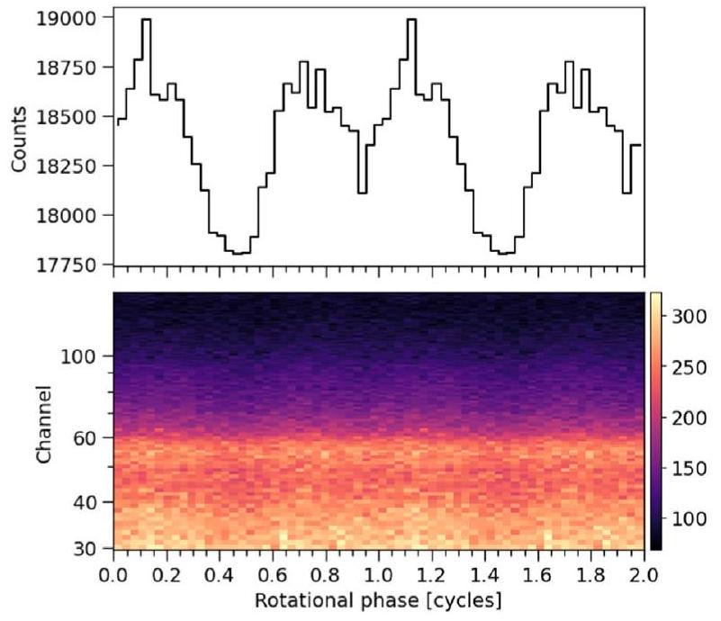
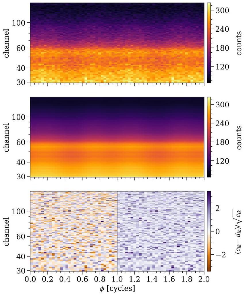
الشكل 1. بيانات أحداث PSR J0740+6620 الجديدة المجمعة على مراحل لدورتين دوريتين (للتوضيح). تُظهر اللوحة العلوية ملف النبض المجموع عبر القنوات. كما في الشكل 1 من R21، يتم إعطاء العدد الإجمالي للعد من خلال المجموع عبر جميع أزواج القنوات المرحلية (على مدار الدورتين). بالنسبة للنمذجة، يتم تجميع جميع بيانات الأحداث في دورة دورية واحدة بدلاً من ذلك.
لم يتم تطبيق طريقة الفرز المستخدمة سابقًا لفترات الوقت الجيدة (GTIs) من Guillot et al. (2019) والتصفية بناءً على الزاوية بين PSR J0740+6620 والشمس. بدلاً من ذلك، تم فرض “معدل نقص” أقصى (أي، معدل إعادة تعيين الكاشف) قدره 100 cps لكل كاشف لإنتاج قائمة أحداث نظيفة مع تلوث أقل من تراكم الفوتونات الشمسية الضوئية (“تحميل ضوئي”، حتى) يحدث عادةً ولكن ليس حصريًا عند زوايا شمسية منخفضة. أظهر اختبار إجراء استخراج الأحداث مع الحفاظ على جميع المعايير الأخرى ثابتة وتغيير معدل النقص الأقصى من قيمة 50 إلى 200 cps (بزيادات قدرها 50 cps) أربعة قوائم أحداث مصفاة مختلفة من نفس القائمة الأساسية من obsIDs. أظهر اختبار كل قائمة أحداث لمدى أهمية الكشف عن النبض باستخدام اختبار(Buccheri et al. 1983) أن النجم النابض تم اكتشافه بوضوح بأعلى أهمية لمعدل النقص الأقصى البالغ 100 cps وبالتالي فإن هذه القائمة من الأحداث هي التي استقرينا عليها لهذا التحليل.
نلاحظ أن الإجراء الجديد لدينا من المتوقع أن يكون أقل عرضة لنوع التحيز الانتقائي المنهجي المقترح لطريقة فرز GTI القديمة في Essick (2022؛ على الرغم من أن التأثير هناك كان هامشيًا فقط، كما نوقش في القسم 2.1 من S22). وذلك لأن معدلات النقص لا تتوافق مع التدفق من النجم النابض الخافت بصريًا، ويتم تعظيم أهمية الكشف فقط من خلال الاختيار من بين أربعة خيارات مختلفة لتصفية البيانات.
في تحليل ملف النبض، استخدمنا مرة أخرى مجموعة القنوات الثابتة للنبض (PI) [30، 150)، والتي تتوافق مع نطاق طاقة الفوتون الاسمي، كما في R 21 و S22، ما لم يُذكر خلاف ذلك. عدد صناديق المرحلة الدورانية في البيانات هو أيضًا 32 كما كان من قبل. يتم تصور البيانات المقسمة على دورتين دوريتين في الشكل 1.
بالنسبة للتحليلات التي تشمل ملاحظات XMM-Newton، استخدمنا نفس بيانات الطيف المتوسطة على المراحل وملاحظات السماء الفارغة (لقيود الخلفية) كما في M21 و R21 و S22 مع ثلاثة أجهزة EPIC (pn و MOS1 و MOS2). ما لم يُذكر خلاف ذلك، قمنا بتضمين قنوات الطاقة [57، 299) لـ pn، و [20،100) لكل من MOS1 و MOS2، وهي نفس الخيارات كما في R21 و S22
(على الرغم من أنه لم يتم ذكر ذلك صراحة في تلك الأوراق). قامت M21 بنفس الاختيارات باستثناء تضمين قناة طاقة عالية واحدة إضافية لجهاز pn. يتم تصور البيانات في الأشكال 4 و 16 من R21.
2.2. نماذج استجابة الأجهزة
بالنسبة لأجهزة XMM-Newton EPIC، استخدمنا نفس ملفات الاستجابة المساعدة (ARFs) وملفات مصفوفة إعادة التوزيع (RMFs) كما في R21 و S22. بالنسبة لأحداث NICER المستخدمة في هذه الدراسة، فإن إصدار المعايرة هو xti20210707، وإصدار HEASOFT هو 6.30.1 الذي يحتوي على NICERDAS 2022-01-17V009. قمنا بإنشاء مصفوفات الاستجابة بشكل مختلف عن التحليلات السابقة حيث استخدمنا ملف استجابة مجمع،الذي تم تصميمه لمعلومات وحدة الطائرة البؤرية (FPM) التي يتم الاحتفاظ بها الآن في ملفات أحداث NICER FITS. وبالتالي، بالنسبة للتحليل في هذه الدراسة، ستعكس المنطقة الفعالة التعرضات الدقيقة لـ FPM مما يؤدي إلى إعادة قياس المنطقة الفعالة لحساب الإزالة الكاملة لكاشف واحد (DetID 34) والإزالة الجزئية لكاشف آخر (DetID 14) كما تم تناولها أعلاه. المنتجات الناتجة عن المعايرة متاحة على Zenodo على doi:10.5281/zenodo. 10519473.
عند نمذجة الإشارة المرصودة، سمحنا بعدم اليقين في المناطق الفعالة لكل من NICER وجميع كواشف XMM-Newton الثلاثة، بسبب عدم وجود مصدر معايرة مطلق. كما في R21 و S22، نحدد عوامل قياس المنطقة الفعالة المستقلة عن الطاقة على أنها
حيثوهي عوامل القياس العامة لـ NICER و XMM-Newton، على التوالي (تستخدم لضرب المنطقة الفعالة للجهاز)،هي عامل قياس مشترك بين جميع الأجهزة (لتمثيل عدم اليقين المطلق في معايرة تدفق الأشعة السينية)، ووهي عوامل قياس محددة للتلسكوب (لتمثيل عدم اليقين النسبي بين معايرة NICER و XMM-Newton). كما كان من قبل، نفترض أن العوامل متطابقة لـ pn و MOS1 و MOS2 (وهو ما قد لا يكون صحيحًا). في نتائجنا الرئيسية، نطبقعدم اليقين (Ishida et al. 2011؛ Madsen et al. 2017؛ Plucinsky et al. 2017)في عوامل القياس العامة، كما في التحليل الاستكشافي للقسم 4.2 في R21 (انظر أيضًا القسم 3.3 من S22)، والذي ينتج عن افتراضعدم اليقين فيوعدم اليقين في عوامل القياس المحددة للتلسكوب. هذا الاختيار أكثر صرامة منعدم اليقين المستخدم في النتائج الرئيسية لـ R21 (الذي افترضعدم اليقين في كل من العوامل المشتركة والمحددة للتلسكوب)، ولكنه مشابه لذلك المستخدم في M21 و S22. ومع ذلك، فقد استكشفنا أيضًا تأثير خيارات مختلفة لعوامل قياس المنطقة الفعالة في القسم 3.2.
2.3. نمذجة ملف النبض باستخدام X-PSI
كما في التحليلات السابقة لـ NICER (على سبيل المثال، M21؛ R21؛ S22)، نستخدم تقريب “Schwarzschild المفلطح” لنمذجة نبضات الأشعة السينية ذات الطاقة المحددة من NS (انظر، على سبيل المثال، Miller & Lamb 1998؛ Nath et al. 2002؛ Poutanen & Gierliński 2003؛ Cadeau et al. 2007؛ Morsink et al. 2007؛ Lo et al. 2013؛ AlGendy
ومورسينك 2014؛ بودغانوف وآخرون 2019؛ واتس 2019). بالإضافة إلى ذلك، نستخدم الآن عامل BACK_SCAL المصحح (انظر القسم 3.4 من S22). كما في السابق، نستخدم الكتلة، الميل، والقيود المسافة من فونسيكا وآخرون (2021)، نموذج التوهين بين النجمي TBabs (ويلمز وآخرون 2000، تم تحديثه في 2016)، ونموذج الغلاف الجوي للهيدروجين المؤين بالكامل NSX (هو ولاي 2001). كما هو موضح في سالمي وآخرون (2023)، لا يبدو أن الافتراضات المتعلقة بالغلاف الجوي تؤثر بشكل كبير على نصف قطر PSR J0740+6620 المستنتج. تم العثور على حساسية أكبر لاختيارات الغلاف الجوي في ديتمان وآخرون (2024)، ولكن قد يكون ذلك مرتبطًا بمنهجية أخذ العينات الخاصة بهم أو فضاء القيود الأكبر لديهم، على سبيل المثال، بما في ذلك أنصاف أقطار النجوم النيوترونية فوق 16 كم. يتميز شكل المناطق الساخنة المنبعثة مرة أخرى باستخدام نموذج درجة الحرارة الواحدة غير المشتركة (ST-U) مع منطقتين دائريتين بدرجة حرارة موحدة (رايلي وآخرون 2019).
2.4. الحساب البعدي
نحسب عينات الخلفية باستخدام pymultinest (Buchner et al. 2014) و multinest (Feroz & Hobson 2008؛ Feroz et al. 2009، 2019)، كما في تحليلات X-PSI السابقة. بالنسبة لنتائج NICER و XMM-Newton المشتركة الرئيسية في هذا العمل، نستخدم إعدادات MULTINEST التالية:نقاط حية وكفاءة أخذ عينات تبلغ 0.01.لتحليل NICERonly، ولتحليل NICER-XMM الاستكشافي، استخدمنا نفس عدد النقاط الحية ولكننناقش الحساسية لإعدادات العينة بشكل أعمق في القسم 3.
3. الاستنتاجات
نبدأ أولاً بتقديم نتائج الاستدلال لتحليل NICER-only المحدث، ثم ننتقل إلى النتائج الرئيسية التي تم الحصول عليها من خلال ملاءمة بيانات NICER وXMM-Newton بشكل مشترك. لاختبار قوة التحليل، يتم تقديم نتائج الاستدلال المقابلة باستخدام مجموعة بيانات اصطناعية في الملحق A. فيما يلي، نركز بشكل أساسي على القيود المفروضة على نصف القطر حيث أن التوزيع اللاحق على الكتلة لم يتغير بشكل أساسي عن التوزيع الإذاعي الغني بالمعلومات.
3.1. ملاءمة خاصة بـ NICER
عند تحليل مجموعة بيانات NICER الجديدة فقط (الموصوفة في القسم 2.1)، نجد قيودًا أفضل لبعض معلمات النموذج، ولكن ليس لجميعها. كما هو موضح في اللوحة اليسرى من الشكل 2، لم يتم العثور على تحسين كبير في قيود نصف القطر مقارنةً بالنتائج القديمة من R21 (حيث ). استخدمت هذه النتائج القديمة عدم يقين أكبر في المساحة الفعالة وطبقت أخذ العينات الهامة بدلاً من أخذ العينات مباشرة باستخدام أحدث أولويات الكتلة والمسافة والميل.بالنسبة للبيانات الجديدة، فإن نصف القطر المستنتج هو والكتلة هي . ومع ذلك، فإن بعض المعلمات الأخرى، مثل أحجام ودرجات حرارة المناطق المنبعثة، أصبحت محددة بشكل أفضل مع البيانات الجديدة، كما هو موضح في الصور الموجودة على الإنترنت في الشكل 3.
الخلفية المستنتجة مقيدة بشكل أكثر صرامة ونسبة معدل العد بين المصدر والإجمالي أقل بكثير للبيانات الجديدة (حوالي، على عكس السابق
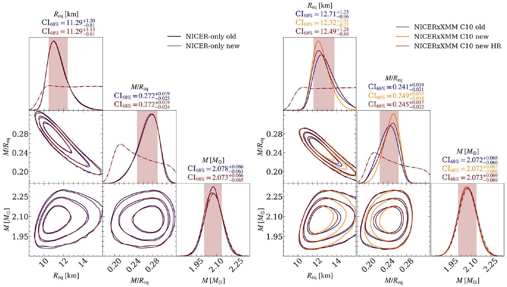
الشكل 2. توزيعات البوستيريور لنصف القطر، والصلابة، والكتلة باستخدام مجموعة بيانات NICER الجديدة ونموذج ST-U في تحليل NICER فقط (اللوحة اليسرى) وفي التحليل المشترك بين NICER وXMM-Newton (اللوحة اليمنى) مقارنةً بالنتائج القديمة من R21. هنا “C10” تشير إلى عدم اليقين في المعايرة في عوامل مقياس المساحة الفعالة الإجمالية، “الجديدة” و”القديمة” دون تأهيل لديهاو “HR” تشير إلى النتائج الرئيسية الجديدة معتمثل الدوال المنقطة المتقطعة دوال كثافة الاحتمال السابقة الهامشية (PDFs). تُظهر الأشرطة الرأسية المظللة فترات موثوقة (للاحتمالات اللاحقة المرتبطة بالمنحنيات الحمراء)، وتظهر الخطوط في اللوحات غير القطرية ، و المناطق الموثوقة. راجع تسميات الشكل 5 من S22 والشكل 5 من R21 لمزيد من التفاصيل حول عناصر الشكل.
كما هو موضح في اللوحة اليسرى من الشكل 4. قد يفسر هذا سبب عدم تشديد قيود نصف القطر (انظر المناقشة في القسم 4). على وجه الخصوص، فإن الخلفية المرتبطة بعينة الاحتمالية القصوى أكبر للبيانات الجديدة (نسبة المصدر إلى الإجمالي حواليبدلاً من ). ومع ذلك، نلاحظ أنه مع البيانات القديمة، فإن معظم العينات البعدية المتساوية الوزن (وأيضًا العينة البعدية القصوى) لديها خلفيات أكبر من عينة الاحتمالية القصوى، كما هو موضح في الشكل 4 حيث تكون المنحنى الأرجواني أسفل معظم المنحنيات الخضراء (ونسبة المصدر البعدي الأقصى إلى الإجمالي صغيرة جدًا كما هو الحال في بالمقابل، فإن عينة الاحتمالية القصوى للبيانات الجديدة تحتوي على خلفية قريبة من المتوسط وعينات ما بعد الحد الأقصى.
3.2. ملاءمة NICER و XMM-Newton
من خلال تحليل بيانات NICER الجديدة بالتزامن مع بيانات XMM-Newton (اللوحة اليمنى من الشكل 2)، نجد أن نصف القطر المستنتج هولنتائجنا الرئيسية (“HR الجديدة” في الشكل، انظر القسم 2.4). للمقارنة، نعرض قيود نصف القطر التي تم الحصول عليها في R21 مع عدم اليقين في المعايرة المتقاطعة المماثل (“C10 القديمة” هنا، الشكل 14 من R21) ) ، كم، والقيود التي حصلنا عليها للبيانات الجديدة ولكن بنفس إعدادات العينة كما في التحليل السابق ( ) ،
. وبالتالي فإن فترة نصف القطر الجديدة تبلغ حوالي أكثر تشددًا (ومنتقلًا إلى قيم أصغر) من القديمة عند استخدام نفس إعدادات العينة، ولكن متشدد تقريبًا بنفس القدر عند استخدام الإعدادات الجديدة.
الحد الأدنى علىinterval الموثوق لنصف القطر يبدو أقل حساسية لإعدادات العينة مقارنة بالحد الأعلى. يكشف التحقيق في سطح الاحتمالية لماذا يحدث ذلك. تنخفض الاحتمالية بشكل حاد عند أدنى نصف أقطار؛ بالنسبة للنجوم الصغيرة جداً، ببساطة لا يمكن تلبية كل من قيود الخلفية وقيود السعة النبضية بالنظر إلى الأولوية الهندسية الضيقة لزاوية ميل المراقب لهذا المصدر (فونسيكا وآخرون 2021). ومع ذلك، فإن سطح الاحتمالية لنصف الأقطار التي تتجاوز الحد الأقصى عندمسطح جداً، مما يجعل من الصعب تحديد الحد الأعلى. بالإضافة إلى ذلك، مع الاقتراب من أعلى الأبعاد، هناك المزيد من الحلول التي تحتوي على بقع ساخنة أصغر وأعلى حرارة وأقرب إلى الأقطاب (انظر الشكل 3). تحتوي سطح الاحتمالية في فضاء حجم البقعة ودرجة الحرارة على نقطة حادة في هذه المنطقة من فضاء المعلمات، ولذلك من المهم حلها بشكل جيد. عند الانتقال منإلىلقد لاحظنا أن هذه المنطقة تم أخذ عينات منها بشكل أكثر شمولاً، ويبدو أن هذا التغيير هو الذي يؤدي إلى زيادة الحد الأعلى لفترة الثقة للنصف القطر مع انخفاض SE. ومع ذلك، فإن التكلفة الحسابية لـ SE الأصغر أعلى بكثير، ولم تكن الزيادات الإضافية في النقاط الحية أو التخفيضات في SE للتحقق من تقارب فترة الثقة ممكنة.
للتحقق مما إذا كنا قد رسمنا الآن سطح الاحتمالية في مساحة حجم البقعة – درجة الحرارة بشكل كافٍ لتحديد بالضبط كيف تنخفض الاحتمالية، قمنا بإجراء تحليل إضافي بدقة عالية (40,000 نقطة حية، ) تشغيل، ولكن تقييد السابق على درجة حرارة النقطة الثانوية إلى
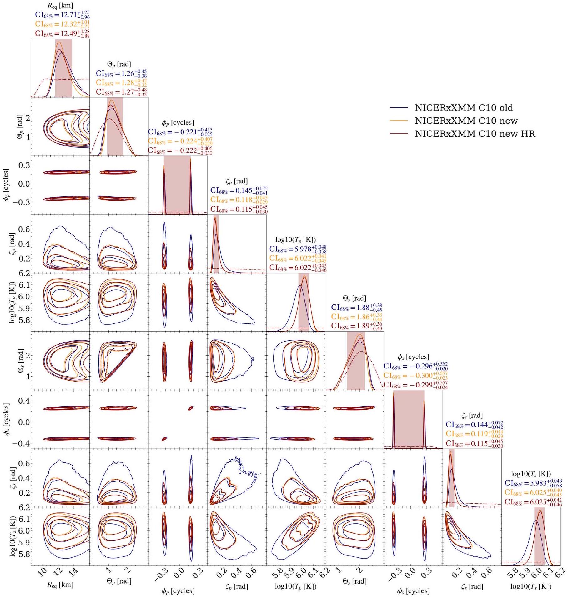
الشكل 3. التوزيعات الخلفية لبارامترات المنطقة الساخنة باستخدام مجموعة بيانات NICER الجديدة ونموذج ST-U في التحليل المشترك بين NICER وXMM-Newton مقارنةً بالنتائج القديمة من R21. راجع تعليق الشكل 2 لمزيد من التفاصيل حول عناصر الشكل. تتضمن مجموعة الأشكال الكاملة التوزيعات الخلفية للبارامترات المتبقية (لكل من تحليلات NICER فقط والتحليل المشترك بين NICER وXMM-Newton). (مجموعة الأشكال الكاملة (أربع صور) متاحة في المقالة على الإنترنت.)
. تم أخذ عينات أكثر شمولاً من الطرف الحاد لسطح الاحتمالية، حيث تم الآن وصف الانخفاض في الاحتمالية بشكل جيد. نصف القطر المستنتج لتشغيل الأولوية المقيدة هو، ولكن مع احتمالات قصوى إجمالية أقل من تلك في التشغيل الكامل السابق. وهذا يشير إلى أن أي زيادة إضافية في الحد الأعلى لفترة الثقة لنصف القطر في التشغيل الكامل السابق (باستخدام المزيد من الحوسبة من غير المحتمل أن تكون أكثر مننأخذ هذا كتقدير للخطأ المنهجي في التشغيل الكامل السابق.
كما هو الحال في R21 و S22، فإن نصف القطر المستنتج لحالة NICER و XMM-Newton المشتركة أكبر من حالة NICER فقط. ومع ذلك، فإن القيم الوسيطة من التحليلات المشتركة هذه المرة أقرب قليلاً إلى نتيجة NICER فقط. كما أن نتائج نصف القطر الجديدة أكثر تقييدًا قليلاً من S22.
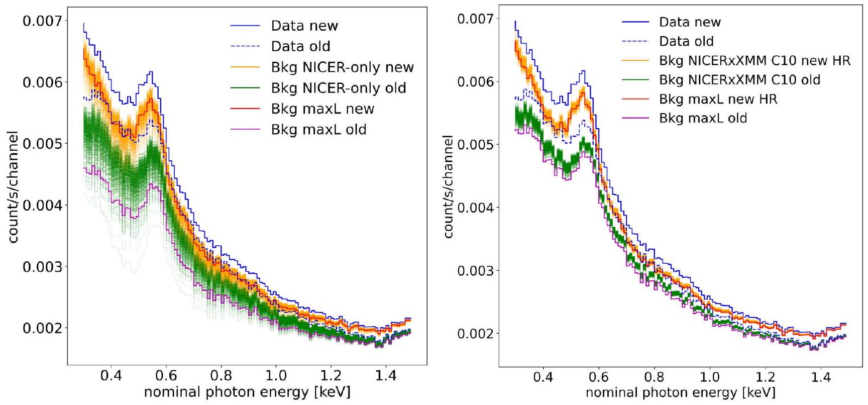
الشكل 4. مقارنة الخلفية المستنتجة من NICER لمجموعات البيانات والتحليلات المختلفة. اللوحة اليسرى: تظهر المنحنيات الزرقاء الصلبة والمخططة المعدلة معدل الطيف الكلي لعدد العد من NICER لمجموعات البيانات الجديدة والقديمة، على التوالي (لاحظ أن معدل العد قد تغير قليلاً بسبب التصفية المختلفة الموضحة في القسم 2.1). تظهر المنحنيات البرتقالية والخضراء المنحنية الخلفيات التي تعظم الاحتمالية لـ 1000 عينة لاحقة متساوية الوزن في تحليل NICER فقط مع البيانات الجديدة والقديمة، على التوالي. وبناءً عليه، تظهر المنحنيات الحمراء والمغنتا المنحنية الخلفيات التي تتوافق مع عينة الاحتمالية القصوى لكل تشغيل. اللوحة اليمنى: نفس الشيء كما في اللوحة اليسرى، باستثناء أن الخلفيات المستنتجة تُظهر الآن للتشغيل المشترك بين NICER وXMM-Newton مع البيانات الجديدة والقديمة، على التوالي (تظهر نتائج جديدة لتشغيل HR، ولكن يتم استنتاج خلفية متطابقة تقريبًا عند استخدام إعدادات العينة القديمة).
حيث كان نصف القطر المستنتجباستخدام مجموعة بيانات NICER المفلترة 3C50 (مع حد أدنى للخلفية أقل) وبيانات XMM-Newton. القيم المستنتجة لجميع المعلمات لجولة HR موضحة في الجدول 1، والتوزيعات اللاحقة المتبقية موضحة في الشكل 3. من هناك نرى أنه، مقارنةً بنتائج R21 القديمة، تم الحصول على قيود متسقة ولكنها أكثر دقة قليلاً لدرجات حرارة المناطق الساخنة وأحجامها. لا تبدو الفترات الموثوقة لهذه المعلمات معتمدة بشكل كبير على إعدادات العينة المستخدمة. على الرغم من أن البيانات الجديدة أكثر تقييدًا، نجد أن نموذج ST-U المستخدم لا يزال قادرًا على إعادة إنتاج البيانات بشكل جيد، كما يتضح من البقايا في الشكل 5.
تمامًا كما هو الحال في حالة NICER فقط (في القسم 3.1)، فإن نسبة عدد الخلفية المستنتجة الأفضل ملاءمة مقابل عدد المصدر تتغير مقارنة بالتحليل السابق (انظر اللوحة اليمنى من الشكل 4). ومع ذلك، فإن التغيير أصغر في التحليل المشترك لـ NICER و XMM-Newton (بغض النظر عن إعدادات العينة)؛ فإن معدل عدد المصدر الأقصى المحتمل مقابل إجمالي معدل العد هو الآن حواليبدلاً من السابقعند النظر إلى غالبية العينات اللاحقة المتساوية الوزن، يكون الفرق أصغر حتى؛ في كلتا الحالتين، يتراوح معدل عدد المصادر مقابل المعدل الإجمالي للعد حولالتغيير الأصغر هو أمر متوقع تمامًا، حيث يعمل XMM-Newton بشكل غير مباشر كقيد على خلفية NICER وقد فعل ذلك بالفعل في التحليل الأقدم.
وجدنا أيضًا (لتحليل استكشافي باستخدام ) أن الافتراضات المختلفة لعوامل التحجيم للتقويم المتبادل لا تؤثر بشكل كبير على النتائج الجديدة. يتضح ذلك في الشكل 6. نرى أن نصف القطر الوسيط يزيد فقط من حوالي 12.1 إلى حوالي 12.3 كم عند تطبيق بدلاً من عدم اليقين في عوامل القياس العامة. ومع ذلك، فإن تطبيقعدم اليقينيُنتج تقريبًا
نتائج متطابقة لتلك الخاصة بـ. كما استكشفنا أيضًا تأثير اختيار مختلف لقنوات الطاقة المضمنة في التحليل. كما هو موضح في الشكل 6، لم نجد فرقًا كبيرًا في نصف القطر المستنتج عند استخدام اختيارات القنوات الخاصة بـ M21 بدلاً من تلك المبلغ عنها في القسم 2.1 (أي، قنوات NICER فقط حتى 123 بدلاً من 149 وقنوات XMM-Newton pn حتى 299 بدلاً من 298).
4. المناقشة
4.1. تحديث معلمات PSR J0740+6620 ومقارنتها بالنتائج القديمة
كتلتنا ونصف قطرنا المستنتجين الجديدين لـ PSR J0740+6620، باستخدام بيانات NICER من 21 سبتمبر 2018 إلى 21 أبريل 2022 ونمذجة مشتركة مع XMM-Newton، هي (بشكل كبير دون تغيير عن السابق) و ( فترات موثوقة). الـفترة موثوقة لنصف القطر هي و الـ فترة موثوقة هي. النتائج تستمر في عدم تفضيل EOS ناعمة جداً، مع مستبعد فيمستوى ومستبعد فيالمستوى (الـفترة الثقة تمتد منإلى الـ2)% النسبة المئوية). هذه الحدود الدنيا أكثر تقييدًا من القيم الرئيسية المقابلة المبلغ عنها في R 21 (كم مستثناة فيمستوى ومستبعد في المستوى). مع الأخذ في الاعتبار أن ملاحظات موجات الجاذبية تفضل النجوم الأصغر للكتل المتوسطة ( تقدم تقنيتا القياس هاتان قيودًا صارمة ومتكاملة على نماذج معادلة الحالة (EOS) (أبوت وآخرون 2018، 2019). يجب أن تكون الحدود الدنيا الأكثر صرامة على نصف قطر مثل هذا النجم النابض عالي الكتلة أكثر إفادة فيما يتعلق، على سبيل المثال، بالوجود المحتمل لمادة الكوارك في نوى النجوم النيوترونية (انظر، على سبيل المثال، أنالا وآخرون 2022).
تُعقِّد المقارنة مع النتائج القديمة حقيقة أنه قد تم إجراء تغييرات على كل من مجموعة البيانات و
الجدول 1 جدول ملخص لنتائج NICER و XMM-Newton المشتركة الجديدة
معامل
وصف
PDF السابق (الكثافة والدعم)
فترة دوران الإحداثيات
، ثابت
…
الكتلة الجاذبية
0.01
٢.٠٠٥
جيب التمام لزاوية ميل الأرض إلى محور الدوران مع دالة كثافة الاحتمال السابقة المشتركة
0.00
0.040
نصف القطر الاستوائي المنسق
0.66
11.24
مع شرط التراص
مع شرط الجاذبية الفعالة
[راديان]
مركز المنطقة خط العرض
0.32
1.28
[راديان]
مركز المنطقة خط العرض
0.29
1.70
[دورات]
المرحلة الأولية للمنطقة
مغلف
ثنائي النمط
3.72
-0.255
[دورات]
المرحلة الأولية للمنطقة
مغلف
ثنائي النمط
3.68
-0.323
[راديان]
نصف قطر الزاوية للمنطقة
2.72
0.151
[راديان]
نصف قطر الزاوية للمنطقة
٢.٧٠
0.124
لا توجد تناظر تبادل المناطق، مناطق حارة غير متداخلة
دالة ( )
درجة حرارة المنطقة NSX الفعالة
حدود NSX
٣.٢٠
6.054
درجة حرارة فعالة في منطقة NSX
حدود NSX
٣.٢٣
6.093
مسافة الأرض
0.07
1.57
كثافة عمود الهيدروجين المحايد بين النجوم
1.33
0.25
توسيع منطقة الفعالية لنظام NICER
0.00
1.00
توسيع منطقة الفعالية لـ XMM-Newton مع توزيع الاحتمالات السابق المشترك
0.02
0.89
معلومات عملية أخذ العينات
عدد المعلمات الحرة: 15
عدد العمليات (متعددة الأوضاع): 1
عدد النقاط الحية:
SE:
شرط الإنهاء: 0.1
دليل:
عدد ساعات المعالجة الأساسية: 84,348
تقييمات الاحتمالية:
ملاحظات. نحن نعرض ملفات PDF السابقة،فترات موثوقة حول الوسيطتباين كولباك-لايبلربالبتات التي تمثل اكتساب المعلومات من السابق إلى اللاحق، وعينة الاحتمالية القصوى المتداخلةلكل المعلمات. يتم الإشارة إلى معلمات المنطقة الساخنة الرئيسية باستخدام حرف تحتها ومعلمات المنطقة الساخنة الثانوية مع رمز فرعي . لاحظ أن تعريف الطور الصفري لـ و يختلف بمقدار 0.5 دورة. يتم تقديم تفاصيل إضافية عن أوصاف المعلمات، وملفات PDF السابقة، ومعلومات عملية العينة في ملاحظات الجدول 1 في R21. يسمى معكوس عامل توسع الهيبرفولوم في R21. طريقة التحليل. العنوان القديم نتج عن R21، مع نصف قطرتم الحصول على ذلك باستخدام عدم اليقين في مقياس المساحة الفعالة أكبر من تلك المستخدمة في هذه الورقة. باستخدام عدم اليقين في مقياس المساحة الفعالة المضغوطة (كما هو مستخدم في هذه الورقة)، وعينة أهمية النتائج الأصلية مع أولوية جديدة، أفاد R21كنصف القطر. ومع ذلك، في هذه الورقة نستخدم أيضًا إعدادات عينة أكثر شمولاً من قبل (انظر القسم 2.4)، وهذا يساهم أيضًا في الاختلافات في القيم الرئيسية المبلغ عنها حديثًا. يبدو أن الحد الأدنى لفترات الثقة لنصف القطر غير حساس إلى حد كبير لإعدادات العينة، بينما الحد الأقصى أكثر حساسية – ويرجع ذلك إلى حد كبير – إلى تسطح سطح الاحتمالية عند أنصاف أقطار عالية. بينما لا نستطيع إثبات تقارب نصف القطر المستنتج بشكل رسمي، فقد بحثنا في العوامل التي تؤثر على الحد الأعلى للفترة الموثوقة، وعلى أساس التحليلات التي تم إجراؤها لا نتوقع توسيعًا كبيرًا آخر (للتفاصيل انظر القسم 3.2). نلاحظ أن ديتمان وآخرون (2024) يحصلون علىحد أعلى أعلى لنصف القطر (عند تحديد نصف القطر ليكون أقل من 16 كم كما نفعل)؛ يتم مناقشة الأسباب المحتملة لذلك في القسم 4.3.
عند فحص التوزيعات الخلفية في الشكل 3، يمكن للمرء أن يرى أن معظم الحلول ذات نصف القطر الكبير (التي تم استكشافها بشكل أفضل من خلال تشغيل HR) مرتبطة في المتوسط بمناطق أصغر وأكثر حرارة بالقرب من الأقطاب الدورانية. يمكن أن تكون الأطراف المدببة للتوزيعات المنحنية التي تُرى في طائرات نصف القطر-زاوية العرض وحجم البقعة-درجة الحرارة تحديًا للمستكشفين، ومن هنا جاء استخدامنا في هذه الورقة لإعدادات MULTINEST الأكثر شمولاً وتشغيلات مستهدفة (أولويات مقيدة) لاستكشاف هذه المساحة.
الشكل 5. بيانات العد الجديدة من NICER، أعداد العد المتوقعة بعدية (المتوسط من 200 عينة بعدية متساوية الوزن)، والبقايا (بواسون) لنموذج ST-U في التحليل المشترك بين NICER وXMM-Newton (لعملية HR). انظر الشكل 6 من R21 لمزيد من التفاصيل حول عناصر الشكل.
الانتقال منإلىأدى ذلك إلى أخذ عينات أكثر شمولاً من هذه المنطقة مما قد يسبب توسيع فترة الثقة لنصف القطر. لم يتم مواجهة توسيع بطيء مماثل حتى الآن في تحليلات X-PSI لمصادر NICER الأخرى، التي هي أكثر سطوعًا، ولكن من الواضح أنه شيء يجب أن نكون حذرين بشأنه (على الرغم من أن الحساسية لإعدادات العينة لوحظت أيضًا في تحليل PSR J0030+0451 في Vinciguerra وآخرون 2024). ستكون القيود المستقلة الإضافية على خصائص النقاط الساخنة التي قد تقلل من نطاق الاحتمالات مفيدة للغاية لـ PSR J0740+6620.
بعض معلمات النموذج مقيدة بشكل أكثر صرامة مع مجموعة بيانات NICER الجديدة (مع كونها متوافقة مع النتائج القديمة) في كل من تحليلات NICER فقط وتحليلات NICER وXMM-Newton المشتركة (بغض النظر عن إعدادات العينة). على وجه الخصوص، تم تقييد الزوايا الشعاعية للمناطق الساخنة الآن حولبشكل أكثر إحكامًا، ودرجات حرارة حولبشكل أكثر إحكامًا. المناطق المستنتجة أصغر وأعلى حرارة قليلاً في المتوسط مقارنةً بالسابق. بالإضافة إلى ذلك، يتم تقييد كثافة عمود الهيدروجين بين النجوم على الأقلأكثر إحكامًا نحو الطرف السفلي من السابق. كما تصبح الفترات الموثوقة لزوايا الكولاتيتيود في المنطقة الساخنة أضيق أيضًا، ولكن فقط عند استخدام نفس إعدادات العينة. بالنسبة لتحليل العنوان النهائي المشترك بين NICER و XMM-Newton، فإن قيود الزاوية الجانبية لا تختلف بشكل كبير عن النتائج القديمة. يُستنتج أن زاوية الإزاحة من تكوين منطقة ساخنة مضادة تمامًا هي، وهو مشابه لقيمة مستنتج من التحليل القديم. وبالتالي، في كلا الحالتين، تكون زاوية الإزاحة أعلىمعالاحتمالية (وهي نفس ما تم الإبلاغ عنه في S22 باستخدام مجموعة بيانات 3C50). وهذا يعني احتمال وجود انحراف عن حقل مغناطيسي مركزي ثنائي القطب.
الشكل 6. التوزيعات الخلفية لبارامترات الزمكان باستخدام مجموعة بيانات NICER الجديدة ونموذج ST-U في التحليلات المشتركة لـ NICER وXMM-Newton، مع افتراضات مختلفة لعدم اليقين في مقياس المنطقة الفعالة والقنوات الطاقية المستخدمة. هنا تشير “C15″ و”C10″ و”C6” إلى التجارب مع، و عدم اليقين في عوامل قياس المساحة الفعالة الإجمالية، على التوالي، و ” C 10 b ” لتشغيل مع عدم اليقين وخيار قناة بديلة (انظر النص في نهاية القسم 3.2). تتداخل الخطوط الخاصة بالحالات الثلاثة الأخيرة تقريبًا تمامًا. انظر تعليق الشكل 2 لمزيد من التفاصيل حول عناصر الشكل.
4.2. توسيع الفترات الموثوقة مع نسبة عدد المصدر إلى الخلفية
كما هو موضح في القسم 3، وجدنا أنه بالنسبة لإعدادات العينة المتطابقة، فإن القيود على نصف قطر NS هي تقريبًاأصبح أكثر دقة عند استخدام مجموعة بيانات NICER الجديدة المدمجة مع بيانات XMM-Newton الأصلية. ومع ذلك، عند تحليل بيانات NICER فقط، ظلت قيود نصف القطر دون تغيير تقريبًا. يمكن أن يُعزى ذلك إلى الاختلافات في النسبة المستنتجة بين فوتونات المصدر والخلفية.
من المتوقع أن يؤثر هذا النسبة على فترة الثقة لنصف القطر كما هو موضح، على سبيل المثال، في المعادلة (4) من Psaltis et al. (2014). يتم الحصول على هذه التعبير من خلال افتراض خصائص نموذج مبسطة، مثل اعتبار مناطق ساخنة صغيرة مع انبعاث متساوي الاتجاه (انظر أيضًا Poutanen & Beloborodov 2006)، وفرض عدم وجود عدم يقين في السعة الأساسية، والخلفية، ومعلمات الهندسة. بموجب هذه الافتراضات، يجب أن يتناسب عدم اليقين في نصف القطر مع
أين هو عدد العدادات المصدرية، هو عدد الإجماليات، و هو عدد العدادات الخلفية. على الرغم من أن هذه العلاقة مبسطة للغاية، يمكننا استخدامها لإجراء مقارنة تقريبية مع مقياس فترة الثقة لنصف القطر المرصود. هنا نقارن فقط التجارب التي تم إجراؤها بنفس إعدادات العينة (لتجنب تأثيرها).
وجدنا أن نسبة الفوتونات الخلفية المستنتجة تزداد مع مجموعة البيانات الجديدة، خاصة في حالة تحليل NICER فقط (على الأرجح بسبب تصفية البيانات المختلفة). العدد المتوقع لعدسات المصدر أصغر حتى للبيانات الجديدة مقارنة بالبيانات القديمة في نسبة كبيرة من العينات؛ وبشكل خاص في عينة الاحتمالية القصوى.أصغر. كانت البيانات القديمة تسمح بتنوع كبير من الحلول المختلفة لعدد الخلفيات مقابل عدد المصادر (انظر المنحنى المتدرج الأخضر في اللوحة اليسرى من الشكل 4)، ولكن بالنسبة للبيانات الجديدة، فإن الخلفية أكثر تقييدًا وأعلى في المتوسط (مقارنة بعدد المصادر). وبالتالي، ليس من السهل التنبؤ بكيفية تغير فترات الثقة لنصف القطر عند زيادة عدد العدات الملاحظة.
لتحليل NICER و XMM-Newton المشترك، هو أفضل تقييدًا، ولا يتغير بشكل كبير عند استخدام بيانات NICER الجديدة، كما ذُكر في القسم 3.2. الاستنتاج لأغلب العينات في التحليل المشترك، تكون أعلى مع البيانات الجديدة، على عكس تحليل NICER فقط. ومع ذلك، حتى في هذه الحالة، فإن أخذ الشكوك في الخلفيات المستنتجة من NICER في الاعتبار سيسمح بتغير كبير في التقدير المتوقع لمقياس فترات الثقة لنصف القطر. باستخدام و قيم مستندة إلى حدود انحراف معياري واحد للخلفيات المستنتجة، المعادلة (2) تتنبأ بأن الفترات الموثوقة يمكن أن تصبح أي شيء من أوسع إلىأكثر إحكامًا.الملاحظالتشديد يتماشى مع ذلك.
استنادًا إلى نتائجنا، ليس من السهل التنبؤ بكيفية تطور فترات الثقة لنصف القطر مع زيادة عدد الفوتونات، على الأقل في وجود خلفية كبيرة وعدم يقين كبير مرتبط بها. ومع ذلك، يبدو أن النسبة المستنتجة بين فوتونات المصدر والخلفية أصبحت أكثر تحديدًا مع مجموعة البيانات الجديدة. وبالتالي، بمجرد أن تصبح هذه النسبة مستقرة بما فيه الكفاية، من المتوقع أن تتقلص فترات نصف القطر عند زيادة العدد الإجمالي للفوتونات، كما تم رؤيته بالفعل في تحليلنا المشترك باستخدام NICER وXMM-Newton. تحقيق قيمة صغيرةمن المحتمل أن يتطلب عدم اليقين في نصف قطر PSR J0740+6620 زيادة وقت التعرض الحالي مع NICER إلى ما لا يقل عن 8 ميغاس، استنادًا إلى النتائج الرئيسية الجديدة والاعتماد على عدد العدّات.
4.3. مقارنة بنتائج ديتمان وآخرون (2024)
باستخدام نفس مجموعات بيانات NICER و XMM-Newton كما في هذه الورقة، أفاد تحليل مستقل أجراه ديتمان وآخرون (2024، فيما بعد D24) أن نصف قطر PSR J0740+6620 هو. هذا يتماشى بشكل عام مع الـالمبلغ عنه في هذه الورقة. على الرغم من أن فترة الثقة لنصف القطر لـ D24 تبلغ حواليأوسع من هنا، الفرق ملحوظ أنه أصغر منالفرق بين النتائج الرئيسية المبلغ عنها من قبل M21 و R21 (الأولى تستخدم نفس الشيفرة مثل D24، والأخيرة تستخدم X-PSI). على وجه الخصوص، فإن الحد الأدنى لنصف القطر – الذي كما تم مناقشته سابقًا من الأسهل تحديده – مشابه جدًا لكليهما، كما كان الحال بالفعل في تحليلات 3C50 لـ S22.
يمكن أن تكون الفروق المتبقية بين نتائج هذه الورقة وD24 مرتبطة باختيارات سابقة مختلفة و/أو إجراءات أخذ عينات مختلفة.عندما تتطلب D24 أن يكون نصف القطر أقل من 16 كم (الحد الأقصى السابق المستخدم في
تحليل)، يحصلون على. بالإضافة إلى ذلك، تستخدم D24 تقنية أخذ العينات الهجينة المتداخلة (MULTINEST) ومخطط سلسلة ماركوف مونت كارلو الجماعية (EMCEE؛ فورمان-ماكي وآخرون 2013)، حيث يمكن أن يقضي جزء كبير من الوقت في مرحلة أخذ العينات الجماعية. عند استخدام multinest، تكون إعدادات الدقة لدينا أعلى من حيث النقاط الحية للجولات المبلغ عنها في هذه الورقة. ومع ذلك، تم إجراء مقارنات اختبارية باستخدام multinest فقط باستخدام إعدادات مماثلة؛ عندما تستخدم كلا الفريقين 4096 نقطة حية والنتائج هيلـ D24 وباستخدام X-PSI. عند إزالة العينات ذات نصف القطر فوق 16 كم، تصبح نتيجة D24كما تم مناقشته في الملحق ب، فإن تأثير SE مرتبط بالحجم الأولي السابق وقد لا يكون قابلاً للمقارنة المباشرة مع D24 الذين يفترضون أحجامًا أكبر في العديد من المعلمات (انظر M21 و R21 للتفاصيل). إذا استخدمنا نفس عدد النقاط الحية (4096) كما في D24 ولكننا خفضنا SE X-PSI إلى 0.0001، فإننا نحصل على نصف قطرقريب جدًا من نتيجة D24 MULTINEST المحدودة بنصف القطر فقط.
باختصار، تتطابق نتائج MULTINEST فقط في هذه الورقة وD24 بشكل جيد عند استخدام نفس الحد الأعلى للقطر وضبط إعدادات العينة. وبالتالي، قد تكون الاختلافات بين النتائج الرئيسية مرتبطة باختيارات سابقة مختلفة، وبالاختلافات بين عيّنات mulTINEST وEMCEE (أشتون وآخرون 2019)، وباحتمال عدم التقاء العينة بسبب إعدادات غير مثالية.
5. الاستنتاجات
لقد استخدمنا مجموعة بيانات NICER جديدة، مع حوالي 1.13 مللي ثانية من وقت التعرض الإضافي، لإعادة تحليل ملفات النبض لجهاز PSR J0740+6620. من خلال تحليل البيانات بشكل مشترك مع نفس بيانات XMM-Newton كما في R21، نستنتج أن نصف قطر النجم النيوتروني هومحدود بـ و النسب المئوية. هذه الفترة تتماشى مع النتيجة السابقة وعرضها متساوي تقريبًا. تم الحصول عليها مع إعدادات عينة محسّنة، والتي وُجد أنها تزيد من الحد الأعلى لنصف القطر مقارنةً بالنتيجة عند استخدام الإعدادات القديمة. على الرغم من أننا لم نتمكن من إثبات تقارب الحد الأعلى بشكل قاطع، إلا أننا نعتبر النتائج الجديدة أكثر موثوقية بعد استكشاف شامل لسطح الاحتمالية ونقدر الخطأ المنهجي المتبقي ليكون. بالإضافة إلى ذلك، وجدنا استعادة معلمات متوقعة في تحليل البيانات المحاكاة التي تشبه ملاحظة PSR J0740+6620 الجديدة (انظر الملحق أ). الحد الأدنى لنصف القطر الآن أيضًا أكثر تقييدًا قليلاً مما كان عليه من قبل؛ نحن نستبعدفياحتمالية هذا النجم النابض، وبالتالي أضعف معادلات الحالة.
شكر وتقدير
تم دعم هذا العمل جزئيًا من قبل ناسا من خلال مهمة NICER وبرنامج مستكشفي الفيزياء الفلكية. يقر كل من T.S. وD.C. وY.K. وS.V. وA.L.W. بالدعم من منحة ERC Consolidator رقم 865768 AEONS (المحقق: واتس). تم دعم استخدام المرافق الحاسوبية الوطنية في هذا البحث من قبل NWO Domain Science. بالإضافة إلى ذلك، استخدم هذا العمل البنية التحتية الوطنية الهولندية الإلكترونية بدعم من التعاون SURF باستخدام منحة رقم EINF-4664. تم تنفيذ جزء من العمل على مجموعة HELIOS بما في ذلك العقد المخصصة.
تم تمويله عبر برنامج ERC CoG المذكور أعلاه. يتم دعم أبحاث الفيزياء الفلكية في مختبر الأبحاث البحرية من قبل برنامج NASA Astrophysics Explorer. يشكر S.G. دعم المركز الوطني للدراسات الفضائية (CNES). يشكر W.C. G.H. الدعم من خلال المنحة 80NSSC23K0078 من NASA. يشكر S.M. الدعم من منحة NSERC Discovery RGPIN-2019-06077. لقد استخدمت هذه الأبحاث منتجات البيانات والبرامج المقدمة من مركز أبحاث أرشيف علوم الفيزياء الفلكية عالية الطاقة (HEASARC)، وهو خدمة من قسم علوم الفيزياء الفلكية في NASA/GSFC وقسم الفيزياء الفلكية عالية الطاقة في مرصد سميثسونيان الفلكي. نود أيضًا أن نشكر Will Handley و Johannes Buchner و Jason Farquhar و Cole Miller و Alexander Dittmann على المناقشات المفيدة.
المرافق: NICER، XMM البرمجيات: Cython (Behnel et al. 2011)، GetDist (Lewis 2019)، مكتبة GNU العلمية (Galassi et al. 2009)، HEASoft (مركز أبحاث أرشيف علوم الفيزياء الفلكية عالية الطاقة التابع لناسا (Heasarc)، 2014)، Matplotlib (Hunter 2007)، MPI لـ Python (Dalcín et al. 2008)، MULTINEST (Feroz et al. 2009)، nestcheck (Higson 2018)، NumPy (van der Walt et al. 2011)، PYMULTINEST (Buchner et al. 2014)، لغة Python/C (Oliphant 2007)، SciPy (Virtanen et al. 2020)، و X-PSI (Riley et al. 2023).
الملحق أ
المحاكاة
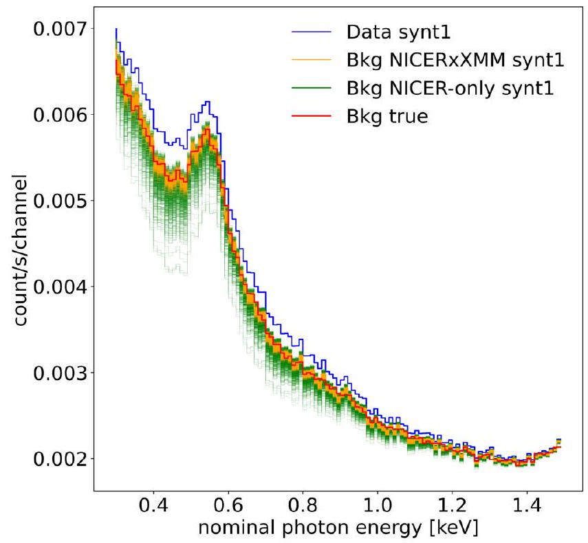
لاختبار قوة التحليلات في هذه الورقة، قمنا بإجراء عدة جولات استدلال باستخدام بيانات اصطناعية. قمنا بتوليد ثلاث تجسيدات مختلفة للضوضاء لكل من بيانات NICER الاصطناعية وXMM-Newton باستخدام متجه معلمات الاحتمالية القصوى الذي تم العثور عليه في التحليل المشترك الجديد الأول لـ NICER وXMM-Newton مع البيانات الحقيقية (الجولة التي استخدمت نفس إعدادات العينة كما في R21). المعلمات موضحة في الجدول 2. تم تعيين طيف الخلفية المدخل لكل جهاز ليكون هو الذي يحقق أقصى احتمال خاص بالجهاز للبيانات الحقيقية (على سبيل المثال، بالنسبة لـ NICER، المنحنى الأحمر في الشكل 7). لكل مجموعة بيانات اصطناعية، تمت إضافة تقلبات بواسون إلى مجموع العد من النقاط الساخنة والخلفية باستخدام بذور مختلفة لمولد الأرقام العشوائية. تم مطابقة أوقات التعرض مع تلك الخاصة بالملاحظات الحقيقية.
بالنسبة لجولات الاستدلال، طبقنا نفس توزيعات الأولويات كما في تحليل البيانات الحقيقية. بالنسبة لإعدادات دقة المولتي ناست، استخدمنا نفس الخيارات كما في البيانات الحقيقية، ولكن معللحفاظ على تكلفة الحساب ضمن الحدود المعقولة. نلاحظ أن الفاصل الموثوق لقطر الدائرة وبعض المعلمات الأخرى كان أكبر بالنسبة للنتائج الرئيسية معومع ذلك، فإن استعادة المعلمات المتوقعة التي تم العثور عليها من المحاكاة لا تزال تشير إلى أن الفترات الرئيسية على الأقل من غير المحتمل أن تكون متوقعة بشكل منخفض بشكل كبير.
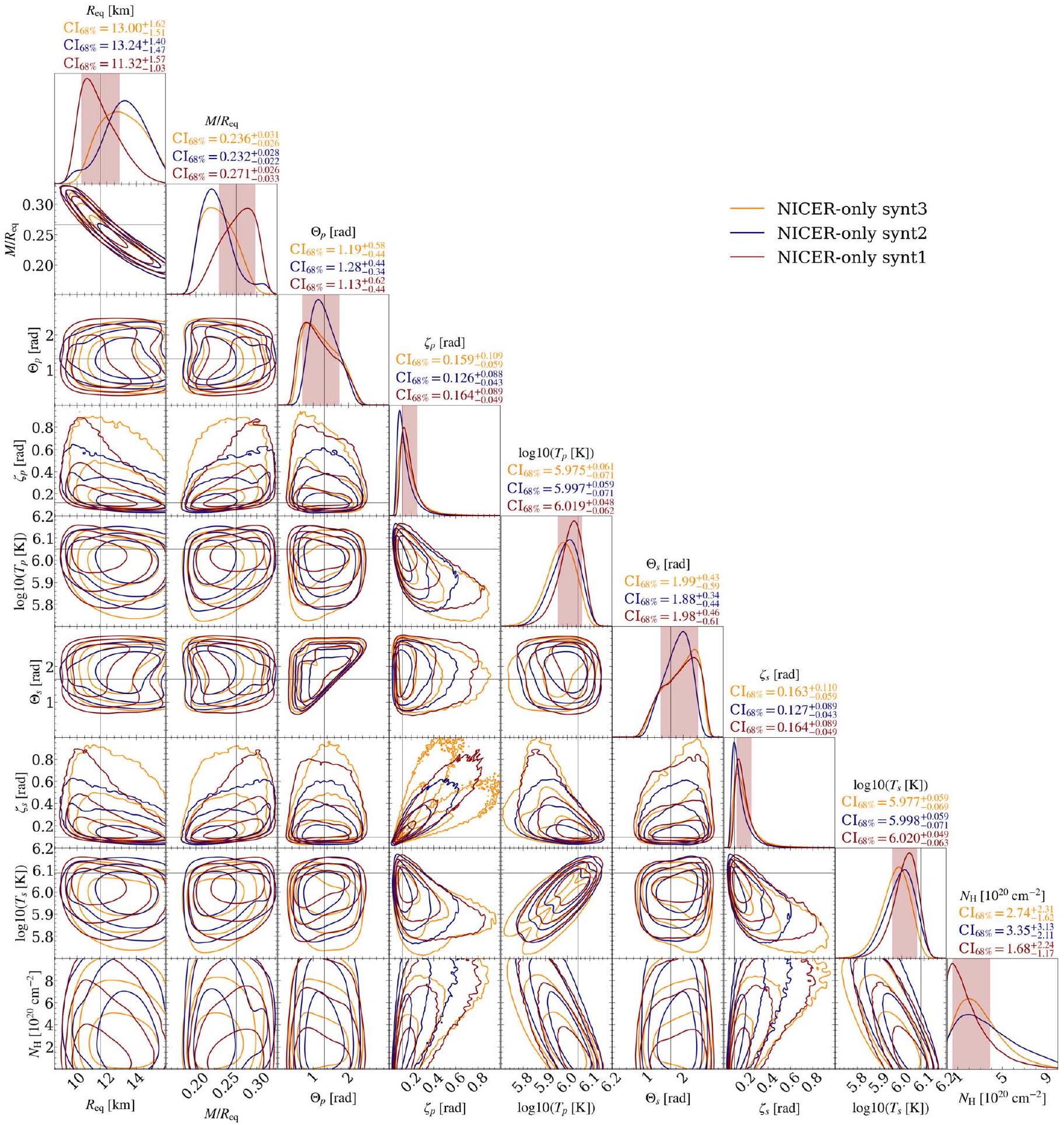
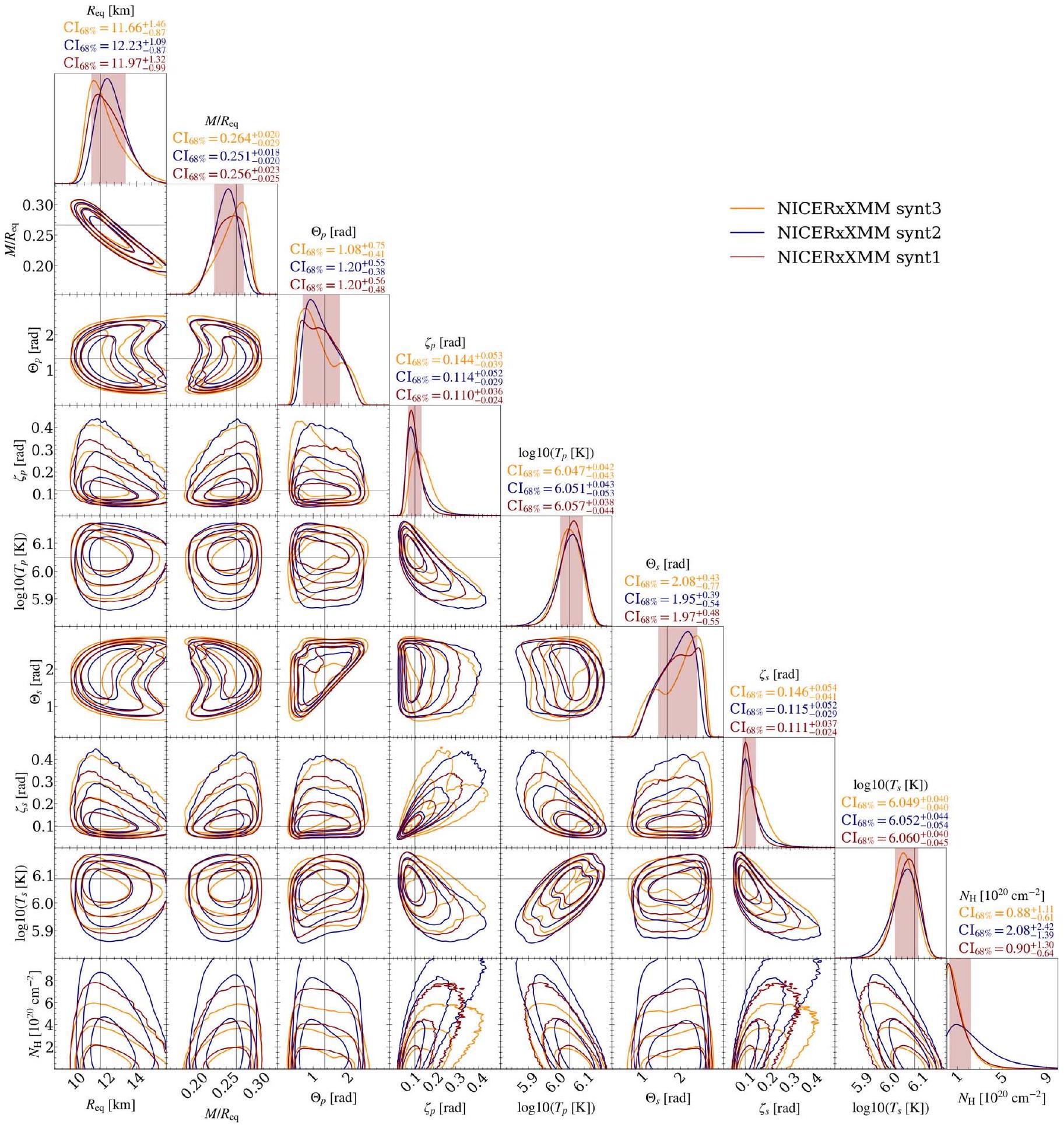
قمنا بإجراء ستة عمليات استدلال في المجموع: ثلاثة تحلل بيانات NICER فقط (واحدة لكل تحقق من الضوضاء) وثلاثة تحلل بيانات NICER وXMM-Newton بشكل مشترك (واحدة لكل زوج بيانات بنفس البذور عند إنشاء البيانات). تظهر نتائج هذه العمليات في الأشكال 8 (NICER فقط) و9 (NICER وXMM-Newton المشتركة) لأكثر المعلمات تباينًا (على العكس، كانت النتائج اللاحقة للكتلة، الميل، والمسافة دائمًا قريبة من توقعاتها). نرى أن نصف القطر الحقيقي، والكثافة، وخصائص النقاط الساخنة، وكثافة عمود الهيدروجينتكون القيم أفضل استعادة عند التوفيق المشترك بين NICER وXMM-Newton في جميع الحالات الثلاث. ومع ذلك، حتى في تحليل NICER فقط، يتم العثور على نصف القطر المدخل ضمنحدود موثوقة في حالتين من أصل ثلاث
الشكل 7. مقارنة الخلفية المستنتجة من NICER لمجموعة البيانات الاصطناعية “synt1” بناءً على تحليل NICER فقط أو تحليل مشترك لـ NICER و XMM-Newton. تُظهر المنحنى المتدرج الأزرق البيانات الاصطناعية. تُظهر المنحنيات المتدرجة البرتقالية منحنيات الخلفية التي تعظم الاحتمالية لـ 1000 عينة خلفية متساوية الوزن من التشغيل المشترك لـ NICER و XMM-Newton. تُظهر المنحنيات المتدرجة الخضراء (المخفية جزئيًا بواسطة البرتقالية) نفس الشيء لعينات من التشغيل الخاص بـ NICER فقط. تُظهر المنحنى المتدرج الأحمر الخلفية المدخلة للبيانات الاصطناعية. تتضمن مجموعة الأشكال الكاملة الخلفيات المستنتجة لواقعين اصطناعيين آخرين. (مجموعة الأشكال الكاملة (ثلاث صور) متاحة في المقالة على الإنترنت.)
الجدول 2 معلمات النموذج المحقونة
معامل
القيمة المُحقَنة
٢.٠٨٨
11.57
[راديان]
1.324
[راديان]
1.649
[دورات]
-0.258
[دورات]
-0.328
[راديان]
0.117
[راديان]
0.098
6.048
6.086
0.041
[kpc]
1.187
0.067
0.905
0.811
ملاحظة. انظر أوصاف المعلمات في الجدول 1. (التوقع يتراوح بين واحد وثلاثة).إذا تم احتساب جميع المعلمات المأخوذة في عينات فقط من NICER، فإن القيم المدخلة توجد ضمنالفترات في من الحالات (التوقع يكون بين و ). بالنسبة للتحليلات المشتركة بين NICER و XMM-Newton، جميع الأبعاد المدخلة، ومن بين جميع المعلمات المدخلة، توجد داخل
الشكل 8. التوزيعات الخلفية للمعلمات الأكثر تغيرًا من جولة إلى أخرى باستخدام مجموعات بيانات NICER الاصطناعية ونموذج ST-U. تُظهر الأشرطة الرأسية المظللة فترات موثوقة للجري مع بيانات اصطناعية موسومة بـ “synt1.” تمثل الخطوط السوداء الرفيعة القيم المدخلة. راجع تعليق الشكل 2 لمزيد من التفاصيل حول عناصر الشكل.
الالفترة (حيث تكون التوقعات مماثلة لحالة NICER فقط). كما وُجد أن الأطياف الخلفية المستنتجة تشبه الخلفية الحقيقية لجميع الجولات، على الرغم من وجود تباين أقل في حالة الجولات المشتركة بين NICER وXMM-Newton، كما هو موضح في الشكل 7.
يمكننا أيضًا أن نرى أن الفترات الموثوقة المستنتجة للبيانات المحاكاة أكبر قليلاً من تلك الخاصة بالبيانات الحقيقية المقابلة (انظر القسم 3 للبيانات الحقيقية). في حالة NICER- فقط التحليل، عرض الـفترة نصف القطر حواليلكل المحاكاة، وحوالي 1.9 كم للبيانات الحقيقية. في حالة التحليل المشترك بين NICER و XMM-Newton، فإن عرض نفس الفاصل الزمني حواليللسيمulations، وحوالي 1.8 كم للبيانات الحقيقية بنفس إعدادات العينة (لكن 2.2 كم لنتائج العناوين عالية الدقة). ومع ذلك، من المحتمل أن يكون هذا الاختلاف ناتجًا عن العدد القليل من الجولات على البيانات المحاكاة. كما قمنا بإجراء
الشكل 9. التوزيعات الخلفية للمعلمات الأكثر تغيرًا من جولة إلى أخرى باستخدام مجموعات بيانات NICER وXMM-Newton الاصطناعية ونموذج ST-U. تُظهر الأشرطة الرأسية المظللة فترات موثوقة للجري مع بيانات اصطناعية موسومة بـ “synt1.” تمثل الخطوط السوداء الرفيعة القيم المدخلة. راجع تعليق الشكل 2 لمزيد من التفاصيل حول عناصر الشكل.
جريتان إضافيتان بدقة منخفضة فقط باستخدام NICER (معنقاط حية بدلاً مناستخدمت بطريقة أخرى) لرؤية كيف تعتمد الفترات الموثوقة للبيانات الاصطناعية على دقة العينة. وجدناأوسعفترات لنصف القطر عند استخدام الدقة الأعلى، والتي تتماشى مع ما تم العثور عليه للبيانات الحقيقية في R21.
في التحليل الحالي، لم نختبر كيف يمكن أن يتغير استرداد المعلمات الملاحظة إذا تم اختيار حقنات أخرى. القيم. تم الإبلاغ مؤخرًا عن المزيد من اختبارات المحاكاة باستخدام X-PSI من قبل كيني وآخرين (2023) وفينسيتشويرا وآخرين (2023) مع معلمات ونماذج وأدوات مختلفة، مما يظهر الاسترداد المتوقع عندما تم إنشاء البيانات وتناسبها مع نفس النموذج. تدعم نتائجنا مع بيانات محاكاة مشابهة لـ PSR J0740+6620 تلك النتائج ولكنها تظهر أيضًا أن تحليل العديد من الأدوات بشكل مشترك قد يحسن دقة القيم المستردة، نظرًا لافتراضاتنا حول عدم اليقين في المعايرة المتبادلة.
الملحق ب: معالجة كفاءة العينة في X-PSI
لتوضيح المصطلحات ومعالجة معامل SE المتعدد الأعشاش في X-PSI، نستعرض هنا الإجراء الموصوف في الملحق B.5.3 من رالي (2019). كما ذُكر هناك (وفي الحاشية 16)، يتم تعديل إعداد SE الأصلي لأخذ حجم الأولوية الأول في الاعتبار، والذي يمكن أن يختلف عن الواحد في نماذجنا على عكس خوارزمية MULTINEST الأصلية (انظر الخوارزمية 1 في فيروز وآخرون 2009). تستخدم تلك الخوارزمية حجم أولية يتم تقليصه في كل تكرار بحيث يكون حجم الأولوية المتوقع المتبقي هو، حيث هو رقم التكرار و هو عدد النقاط الحية. يتم استخدامه لتحديد الحد الأدنى للحجممن الإهليلجي الذي يحدد حدود الاحتمالية التقريبية والذي يتم سحب نقاط ذات احتمالية أعلى منه في كل تكرار. لتجنب أخذ عينات من حجم صغير جداً (في حال كانت التقريب الإهليلجي غير دقيقة)، يتم أيضاً توسيع الحد الأدنى للحجم إلى، حيث هو عامل التوسع وعكس SE. هذا يعني، في الممارسة العملية، أنيتقلص بشكل أسي في كل تكرار، لكن القيمة الأولية الآنبدلاً من 1.
في تحليلات X-PSI، يكون حجم الأولي السابق عادة أقل من 1 بسبب قواعد الرفض المطبقة. على سبيل المثال، إذا كانت النجمة مضغوطة جداً، يتم إرجاع قيمة احتمال أقل من عتبة log_zero لـ MULTINEST بحيث يتم تجاهل العينة تلقائيًا. لذلك، نقوم بتحديد انكماشللشروع من (بدلاً من )، حيث هو الحجم المبدئي المقدر الحقيقي. يتم ذلك عن طريق تعيين القيمة المدخلة الاسمية لبارامتر SE إلىفي الشيفرة. عند الإبلاغ عن قيم SE لا زلنا نشير إلى، حيث أن ذلك يصف التوسع بالنسبة للأولوية الحقيقية الأولية.
Abbott, B. P., Abbott, R., Abbott, T. D., et al. 2018, PhRvL, 121, 161101
Abbott, B. P., Abbott, R., Abbott, T. D., et al. 2019, PhRvX, 9, 011001 AlGendy, M., & Morsink, S. M. 2014, ApJ, 791, 78
Annala, E., Gorda, T., Hirvonen, J., et al. 2023, NatCo, 14, 8451
Annala, E., Gorda, T., Katerini, E., et al. 2022, PhRvX, 12, 011058
Arons, J. 1981, ApJ, 248, 1099
Ashton, G., Hübner, M., Lasky, P. D., et al. 2019, ApJS, 241, 27
Baym, G., Hatsuda, T., Kojo, T., et al. 2018, RPPh, 81, 056902
Behnel, S., Bradshaw, R., Citro, C., et al. 2011, CSE, 13, 31
Bilous, A. V., Watts, A. L., Harding, A. K., et al. 2019, ApJL, 887, L23
Biswas, B. 2022, ApJ, 926, 75
Bogdanov, S., Dittmann, A. J., Ho, W. C. G., et al. 2021, ApJL, 914, L15
Bogdanov, S., Lamb, F. K., Mahmoodifar, S., et al. 2019, ApJL, 887, L26
Buccheri, R., Bennett, K., Bignami, G. F., et al. 1983, A&A, 128, 245
Buchner, J., Georgakakis, A., Nandra, K., et al. 2014, A&A, 564, A125
Cadeau, C., Morsink, S. M., Leahy, D., & Campbell, S. S. 2007, ApJ, 654, 458
Carrasco, F., Pelle, J., Reula, O., Viganò, D., & Palenzuela, C. 2023, MNRAS, 520, 3151
Chen, A. Y., Yuan, Y., & Vasilopoulos, G. 2020, ApJL, 893, L38
Dalcín, L., Paz, R., Storti, M., & D’Elía, J. 2008, JPDC, 68, 655
Dittmann, A. J., Miller, M. C., Lamb, F. K., et al. 2024, ApJ, 974, 295
Essick, R. 2022, ApJ, 927, 195
Feroz, F., & Hobson, M. P. 2008, MNRAS, 384, 449
Feroz, F., Hobson, M. P., & Bridges, M. 2009, MNRAS, 398, 1601
Feroz, F., Hobson, M. P., Cameron, E., & Pettitt, A. N. 2019, OJAp, 2, 10
Fonseca, E., Cromartie, H. T., Pennucci, T. T., et al. 2021, ApJL, 915, L12
Foreman-Mackey, D., Hogg, D. W., Lang, D., & Goodman, J. 2013, PASP, 125, 306
Gendreau, K. C., Arzoumanian, Z., Adkins, P. W., et al. 2016, Proc. SPIE, 9905, 99051H
Galassi, M., Davies, J., Theiler, J., et al. 2009, GNU Scientific Library Reference Manual (3rd ed.; Godalming: Network Theory Ltd.)
Guillot, S., Kerr, M., Ray, P. S., et al. 2019, ApJL, 887, L27
Harding, A. K., & Muslimov, A. G. 2001, ApJ, 556, 987
Higson, E. 2018, JOSS, 3, 916
Ho, W. C. G., & Lai, D. 2001, MNRAS, 327, 1081
Hunter, J. D. 2007, CSE, 9, 90
Ishida, M., Tsujimoto, M., Kohmura, T., et al. 2011, PASJ, 63, S657
Kalapotharakos, C., Wadiasingh, Z., Harding, A. K., & Kazanas, D. 2021, ApJ, 907, 63
Kini, Y., Salmi, T., Watts, A. L., et al. 2023, MNRAS, 522, 3389
Lattimer, J. M., & Prakash, M. 2016, PhR, 621, 127
Lewis, A. 2019, arXiv:1910.13970
Lo, K. H., Miller, M. C., Bhattacharyya, S., & Lamb, F. K. 2013, ApJ, 776, 19
Madsen, K. K., Beardmore, A. P., Forster, K., et al. 2017, AJ, 153, 2
Miller, M. C., & Lamb, F. K. 1998, ApJL, 499, L37
Miller, M. C., Lamb, F. K., Dittmann, A. J., et al. 2019, ApJL, 887, L24
Miller, M. C., Lamb, F. K., Dittmann, A. J., et al. 2021, ApJL, 918, L28
Morsink, S. M., Leahy, D. A., Cadeau, C., & Braga, J. 2007, ApJ, 663, 1244
NASA High Energy Astrophysics Science Archive Research Center (Heasarc) 2014, HEAsoft: Unified Release of FTOOLS and XANADU, Astrophysics Source Code Library, ascl: 1408.004
Nath, N. R., Strohmayer, T. E., & Swank, J. H. 2002, ApJ, 564, 353
Oliphant, T. E. 2007, CSE, 9, 10
Plucinsky, P. P., Beardmore, A. P., Foster, A., et al. 2017, A&A, 597, A35
Poutanen, J., & Beloborodov, A. M. 2006, MNRAS, 373, 836
Poutanen, J., & Gierliński, M. 2003, MNRAS, 343, 1301
Psaltis, D., Özel, F., & Chakrabarty, D. 2014, ApJ, 787, 136
Raaijmakers, G., Greif, S. K., Hebeler, K., et al. 2021, ApJL, 918, L29
Remillard, R. A., Loewenstein, M., Steiner, J. F., et al. 2022, AJ, 163, 130
Riley, T. E. 2019, PhD Thesis, University of Amsterdam, https://hdl.handle. net/11245.1/aa86fcf3-2437-4bc2-810e-cf9f30a98f7a
Riley, T. E., Choudhury, D., Salmi, T., et al. 2023, JOSS, 8, 4977
Riley, T. E., Watts, A. L., Bogdanov, S., et al. 2019, ApJL, 887, L21
Riley, T. E., Watts, A. L., Ray, P. S., et al. 2021a, ApJL, 918, L27
Riley, T. E., Watts, A. L., Ray, P. S., et al. 2021b, A NICER View of the Massive Pulsar PSR J0740+6620 Informed by Radio Timing and XMMNewton Spectroscopy: Nested Samples for Millisecond Pulsar Parameter Estimation, v1.0.1, Zenodo, doi:10.5281/zenodo. 5735003
Ruderman, M. A., & Sutherland, P. G. 1975, ApJ, 196, 51
Salmi, T., Vinciguerra, S., Choudhury, D., et al. 2022, ApJ, 941, 150
Salmi, T., Vinciguerra, S., Choudhury, D., et al. 2023, ApJ, 956, 138
Takátsy, J., Kovács, P., Wolf, G., & Schaffner-Bielich, J. 2023, PhRvD, 108, 043002
van der Walt, S., Colbert, S. C., & Varoquaux, G. 2011, CSE, 13, 22
Vinciguerra, S., Salmi, T., Watts, A. L., et al. 2023, ApJ, 959, 55
Vinciguerra, S., Salmi, T., Watts, A. L., et al. 2024, ApJ, 961, 62
Virtanen, P., Gommers, R., Oliphant, T. E., et al. 2020, NatMe, 17, 261
Watts, A. L. 2019, in AIP Conf. Proc. 2127, Xiamen-CUSTIPEN Workshop on the Equation of State of Dense Neutron-Rich Matter in the Era of Gravitational Wave Astronomy, ed. A. Li, B.-A. Li, & F. Xu (Melville, NY: AIP), 020008
Watts, A. L., Andersson, N., Chakrabarty, D., et al. 2016, RvMP, 88, 021001
Wilms, J., Allen, A., & McCray, R. 2000, ApJ, 542, 914
Wolff, M. T., Guillot, S., Bogdanov, S., et al. 2021, ApJL, 918, L26
https://github.com/xpsi-group/xpsi The versions are practically identical for the considered models; the only actual difference is the fix of a numerical ray-tracing issue since v 0.7 .12 , affecting only a few parameter vectors with emission angles extremely close to (https://github.com/xpsi-group/xpsi/issues/53). This is not expected to alter the inferred radius. Note this number was reported incorrectly in M21 and R21 but this had no effect on the outcome of the analysis.
Note that this factor is not the nominal MULTINEST SE parameter (SE’), since is modified in X-PSI to account for the initial prior volume that is smaller than unity as explained in Riley (2019) and in Appendix B. The SE’ value is about 6.9 times higher than the SE value for all the models in this paper. However, we checked that reanalyzing the old data with the new model choices does not significantly affect the results.
Note that the old joint NICER and XMM-Newton results had an incorrect BACK_SCAL factor and were obtained by importance sampling from a larger effective-area uncertainty to the uncertainty, rather than directly sampling with the uncertainty. However, these issues are not expected to have any significant effect on the results (the BACK_SCAL issue was also tested in Riley et al. 2021b, with a low-resolution run).
Which comes from assuming a uncertainty in the shared scaling factor and a uncertainty in the telescope-specific factors as in the test case of S22.
Using 30 randomly drawn samples from the equally weighted posterior samples. Here we neglected the number of counts from XMM-Newton as it is much smaller than that from NICER. D24 follow also the instrument channel choices of M21, but the effect of this was shown to be very small, see Figure 6.
Note that our headline result used instead of but also 40,000 live points instead of 4096 , leading to roughly 10 times more accepted samples in the highest likelihood parameter space (also across other regions).
We estimate the expected ranges based on the sample size and and quantiles of the percent point function of the binomial distribution with success rate. When considering many model parameters combined, the range is only indicative since it assumes independence between the parameters, which are instead correlated.
The Radius of the High Mass Pulsar PSR J0740+6620 With 3.6 Years of NICER Data
Tuomo Salmi, Devarshi Choudhury, Yves Kini, Thomas E Riley, Serena Vinciguerra, Anna L Watts, Michael T Wolff, Zaven Arzoumanian, Slavko Bogdanov, Deepto Chakrabarty, et al.
To cite this version:
Tuomo Salmi, Devarshi Choudhury, Yves Kini, Thomas E Riley, Serena Vinciguerra, et al.. The Radius of the High Mass Pulsar PSR J0740+6620 With 3.6 Years of NICER Data. Astrophys.J., 2024, 974 (2), pp.294. 10.3847/1538-4357/ad5f1f. hal-04641868
HAL is a multi-disciplinary open access archive for the deposit and dissemination of scientific research documents, whether they are published or not. The documents may come from teaching and research institutions in France or abroad, or from public or private research centers.
L’archive ouverte pluridisciplinaire HAL, est destinée au dépôt et à la diffusion de documents scientifiques de niveau recherche, publiés ou non, émanant des établissements d’enseignement et de recherche français ou étrangers, des laboratoires publics ou privés.
The Radius of the High-mass Pulsar PSR J0740+6620 with of NICER Data
Tuomo Salmi (B), Devarshi Choudhury (BD, Yves Kini (D), Thomas E. Riley (D), Serena Vinciguerra (D), Anna L. Watts (D), Michael T. Wolff (D), Zaven Arzoumanian (D), Slavko Bogdanov (D), Deepto Chakrabarty (D), Keith Gendreau (D), Sebastien Guillot (D), Wynn C. G. Ho (D), Daniela Huppenkothen (D), Renee M. Ludlam (D), Sharon M. Morsink (D), and Paul S. Ray (10) Anton Pannekoek Institute for Astronomy, University of Amsterdam, Science Park 904, 1098XH Amsterdam, The Netherlands; t.h.j.salmi@uva.nl Space Science Division, U.S. Naval Research Laboratory, Washington, DC 20375, USA X-Ray Astrophysics Laboratory, NASA Goddard Space Flight Center, Code 662, Greenbelt, MD 20771, USA Columbia Astrophysics Laboratory, Columbia University, 550 W 120th Street, New York, NY 10027, USA Massachusetts Institute of Technology, Cambridge, MA, USA Institut de Recherche en Astrophysique et Planétologie, UPS-OMP, CNRS, CNES, 9 avenue du Colonel Roche, BP 44346, F-31028 Toulouse Cedex 4, France Department of Physics and Astronomy, Haverford College, 370 Lancaster Avenue, Haverford, PA 19041, USA SRON Netherlands Institute for Space Research, Niels Bohrlaan 4, 2333 CA Leiden, The Netherlands Department of Physics and Astronomy, Wayne State University, 666 W Hancock Street, Detroit, MI 48201, USA Department of Physics, University of Alberta, 4-183 CCIS, Edmonton, AB T6G 2E1, CanadaReceived 2024 January 24; revised 2024 May 29; accepted 2024 May 31; published 2024 October 18
Abstract
We report an updated analysis of the radius, mass, and heated surface regions of the massive pulsar PSR J0740 +6620 using Neutron Star Interior Composition Explorer (NICER) data from 2018 September 21 to 2022 April 21, a substantial increase in data set size compared to previous analyses. Using a tight mass prior from radio-timing measurements and jointly modeling the new NICER data with XMM-Newton data, the inferred equatorial radius and gravitational mass are and , respectively, each reported as the posterior credible interval bounded by the and quantiles, with an estimated systematic error . This result was obtained using the best computationally feasible sampler settings providing a strong radius lower limit but a slightly more uncertain radius upper limit. The inferred radius interval is also close to the obtained by Dittmann et al., when they require the radius to be less than 16 km as we do. The results continue to disfavor very soft equations of state for dense matter, with for this high-mass pulsar excluded at the probability. The results do not depend significantly on the assumed cross-calibration uncertainty between NICER and XMM-Newton. Using simulated data that resemble the actual observations, we also show that our pipeline is capable of recovering parameters for the inferred models reported in this paper.
Unified Astronomy Thesaurus concepts: Neutron stars (1108); X-ray astronomy (1810)
Materials only available in the online version of record: figure sets
1. Introduction
Determination of the masses and radii of a set of neutron stars (NSs) can be used to infer properties of the high-density matter in their cores. This is possible due to the one-to-one mapping between the equation of state (EOS) and the massradius dependence of the NS (see, e.g., Lattimer & Prakash 2016; Baym et al. 2018). One way to infer mass and radius is to model the X-ray pulses produced by hot regions on the surface of a rapidly rotating NS including relativistic effects (see, e.g., Watts et al. 2016; Bogdanov et al. 2019, and references therein). For example, this technique has been applied in analyzing the data from NASA’s Neutron Star Interior Composition Explorer (NICER; Gendreau et al. 2016) for rotation-powered millisecond pulsars. Their thermal emission is dominated by surface regions heated by the bombardment of charged particles from a magnetospheric return current (see, e.g., Ruderman & Sutherland 1975; Arons 1981; Harding & Muslimov 2001). Results for two sources have been released (Miller et al. 2019, 2021; Riley et al. 2019, 2021a; Salmi et al.
Original content from this work may be used under the terms of the Creative Commons Attribution 4.0 licence. Any further distribution of this work must maintain attribution to the author(s) and the title of the work, journal citation and DOI.
2022, hereafter M21, R21, and S22, respectively; Vinciguerra et al. 2024), providing useful constraints for dense matter models (see, e.g., M21; Raaijmakers et al. 2021; Biswas 2022; Annala et al. 2023; Takátsy et al. 2023). These results have also triggered studies on the magnetic field geometries and how nonantipodal they can be (see, e.g., Bilous et al. 2019; Chen et al. 2020; Kalapotharakos et al. 2021; Carrasco et al. 2023).
In this work, we use a new NICER data set (with increased exposure time) to analyze the high-mass pulsar PSR J0740 +6620, previously studied in M21, R21, and S22. In those works, the NS mass had a tight prior from radio timing ( ; Fonseca et al. 2021), and the NS radius was inferred to be, using both NICER and XMM-Newton data, in R21 and in M21. However, the results were slightly sensitive to the inclusion of the XMMNewton data (used to better constrain the phase-averaged source spectrum and hence-indirectly-the NICER background) and assumptions made in the cross-calibration between the two instruments. In S22, the use of NICER background estimates (such as “3C50” from Remillard et al. 2022) was shown to yield results similar to the joint NICER and XMM-Newton analysis, giving confidence in the use of XMM-Newton data as an indirect method of background constraint.
In this paper we use a new NICER data set with more than 1 Ms additional exposure time and more than 0.5 million additional observed counts, an increase in the counts, compared to the data sets used in M21 and R21. This is expected to reduce the uncertainties in the inferred NS parameters (Lo et al. 2013; Psaltis et al. 2014), and we explore whether this is indeed the case. We also look in detail at the influence of sampler settings on the credible intervals.
The remainder of this paper is structured as follows. In Section 2.1, we introduce the new data set used for PSR J0740 +6620. In Section 2, we summarize the modeling procedure, and in Section 3 we present the results for the updated analysis. We discuss the implications of the results in Section 4 and conclude in Section 5. Inference results using simulated data, resembling our new data, are shown in Appendix A.
2. Modeling Procedure
The modeling procedure is largely shared with that of Bogdanov et al. (2019, 2021), Riley et al. (2019), R21, and S22. We use the X-ray Pulse Simulation and Inference (X-PSI; Riley et al. 2023) code, with versions ranging from v 0.7 .10 to for inference runs ( v 1.2 .1 used for the headline results), and v 2.2 .1 for producing the figures. Complete information of each run, including the exact X-PSI version, data products, posterior sample files, and all the analysis files can be found in the Zenodo repository at doi:10.5281/zenodo.10519473. In the next sections we summarize the modeling procedure and focus on how it differs from that used in previous work.
2.1. X-Ray Event Data
The NICER X-ray event data used in this work were processed with a similar procedure as the previous data reported in Wolff et al. (2021) and used in M21 and R21, but with some notable differences (note that a completely different 3C50 procedure was applied in S22). The new data were collected from a sequence of exposures, in the period 2018 September 21-2022 April 21 (observation IDs, hereafter obsIDs, 1031020101 through 5031020445), whereas the period of the previous data set began on the same start date but ended on 2020 April 17 (using the obsIDs shown in Wolff et al. 2021). After filtering the data (described below), this resulted in 2.73381 Ms of on-source exposure time, compared to the previous 1.60268 Ms .
The filtering procedure differed slightly from that used in earlier work. First, similarly to the previous work, we rejected data obtained at low cut-off rigidities of the Earth’s magnetic field (COR_SAX ) to minimize highenergy particle interactions indistinguishable from X-ray events, and we excluded all the events from the noisy detector DetID 34 and the events from DetID 14 when it had a count rate greater than 1.0 counts per second (cps) in 8.0 s bins. We also cut all 2 s bins with total count rate larger than 6 cps to remove generally noisy time intervals. However, here the
Counts
Figure 1. The new phase-folded PSR J0740+6620 event data for two rotational cycles (for clarity). The top panel shows the pulse profile summed over the channels. As in Figure 1 of R21, the total number of counts is given by the sum over all phase-channel pairs (over both cycles). For the modeling all the event data are grouped into a single rotational cycle instead.
previously used sorting method of good time intervals (GTIs) from Guillot et al. (2019) and filtering based on the angle between PSR J0740+6620 and the Sun were not applied. Instead, a maximum “undershoot rate” (i.e., detector reset rate) of 100 cps per detector was imposed to produce a cleaned event list with less contamination from the accumulation of solar optical photons (“optical loading,” up to ) typicallybut not exclusively-happening at low Sun angles. A test of the event extraction procedure holding all other criteria constant and just varying the maximum undershoot rate from a value of 50 to 200 cps (in increments of 50 cps ) gave us four different filtered event lists from the same basic list of obsIDs. Testing each event list for pulsation detection significance using a test (Buccheri et al. 1983) showed that the pulsar was clearly detected at highest significance for the maximum undershoot rate of 100 cps and thus it is this event list that we settled on for this analysis.
We note that our new procedure is expected to be less prone to the type of systematic selection bias suggested for the older GTI sorting method in Essick (2022; although even there the effect was only marginal, as discussed in Section 2.1 of S22). This is because the undershoot rates do not correlate with the flux from the optically dim pulsar, and the detection significance is maximized only by selecting from four different data-filtering options.
In the pulse profile analysis, we used again the pulse invariant (PI) channel subset [30, 150), corresponding to the nominal photon energy range , as in R 21 and S22, unless mentioned otherwise. The number of rotational phase bins in the data is also 32 as before. The data split over two rotational cycles are visualized in Figure 1.
For the analyses including XMM-Newton observations, we used the same phase-averaged spectral data and blank-sky observations (for background constraints) as in M21, R21, and S22 with the three EPIC instruments (pn, MOS1, and MOS2). Unless mentioned otherwise, we included the energy channels [57, 299) for pn , and [20,100) for both MOS1 and MOS2, which are the same choices as in R21 and S22
(although this was not explicitly stated in those papers). M21 made the same choices except for including one more high-energy channel for the pn instrument. The data are visualized in Figures 4 and 16 of R21.
2.2. Instrument Response Models
For the XMM-Newton EPIC instruments we used the same ancillary response files (ARFs) and redistribution matrix files (RMFs) as in R21 and S22. For the NICER events utilized in this study, the calibration version is xti20210707, and the HEASOFT version is 6.30 .1 containing NICERDAS 2022-01-17V009. We generated response matrices differently from the previous analyses in that we used a combined response file, which was tailored for the focal plane module (FPM) information now maintained in the NICER FITS event files. Thus, for the analysis in this study, the effective area will reflect the exact FPM exposures resulting in the rescaling of effective area to account for the complete removal of one detector (DetID 34) and the partial removal of another detector (DetID 14) as addressed above. The resulting calibration products are available on Zenodo at doi:10.5281/zenodo. 10519473.
When modeling the observed signal, we allowed uncertainty in the effective areas of both NICER and all three XMMNewton detectors, due the lack of an absolute calibration source. As in R21 and S22, we define energy-independent effective-area scaling factors as
where and are the overall scaling factors for NICER and XMM-Newton, respectively (used to multiply the effective area of the instrument), is a shared scaling factor between all the instruments (to simulate absolute uncertainty of the X-ray flux calibration), and and are telescope-specific scaling factors (to simulate relative uncertainty between the NICER and XMM-Newton calibration). As before, we assume that the factors are identical for pn, MOS1, and MOS2 (which may not be true). In our headline results, we apply the restricted uncertainty (Ishida et al. 2011; Madsen et al. 2017; Plucinsky et al. 2017) in the overall scaling factors, as in the exploratory analysis of Section 4.2 in R21 (see also Section 3.3 of S22), which results from assuming a uncertainty in and a uncertainty in the telescope-specific factors. This choice is tighter than the uncertainty used in the main results of R21 (who assumed uncertainty in both shared and telescope-specific factors), but is similar to that used in M21 and S22. However we have also explored the effect of different choices for the effective-area scaling factors in Section 3.2.
2.3. Pulse Profile Modeling Using X-PSI
As in previous NICER analyses (e.g., M21; R21; S22), we use the “Oblate Schwarzschild” approximation to model the energyresolved X-ray pulses from the NS (see, e.g., Miller & Lamb 1998; Nath et al. 2002; Poutanen & Gierliński 2003; Cadeau et al. 2007; Morsink et al. 2007; Lo et al. 2013; AlGendy
& Morsink 2014; Bogdanov et al. 2019; Watts 2019). In addition, we use now a corrected BACK_SCAL factor (see Section 3.4 of S22). As before, we use the mass, inclination, and distance priors from Fonseca et al. (2021), interstellar attenuation model TBabs (Wilms et al. 2000, updated in 2016), and the fully ionized hydrogen atmosphere model NSX (Ho & Lai 2001). As shown in Salmi et al. (2023), the assumptions for the atmosphere do not seem to significantly affect the inferred radius of PSR J0740+6620. A larger sensitivity to the atmosphere choices was found in Dittmann et al. (2024), but this could be related to their sampling methodology or their larger prior space, e.g., including NS radii above 16 km . The shapes of the hot emitting regions are again characterized using the single-temperatureunshared (ST-U) model with two circular uniform temperature regions (Riley et al. 2019).
2.4. Posterior Computation
We compute the posterior samples using pymultinest (Buchner et al. 2014) and multinest (Feroz & Hobson 2008; Feroz et al. 2009, 2019), as in the previous X-PSI analyses. For the headline joint NICER and XMM-Newton results of this work, we use the following MULTINEST settings: live points and a 0.01 sampling efficiency (SE). For the NICERonly analysis, and the exploratory NICER-XMM analysis, we used the same number of live points but . We discuss sensitivity to sampler settings further in Section 3.
3. Inferences
We start first by presenting the inference results for the updated NICER-only analysis, and then proceed to the headline results obtained by fitting jointly the NICER and XMMNewton data. To test the robustness of the analysis, the corresponding inference results using a synthetic data set are presented in Appendix A. In what follows we focus primarily on the constraints on radius since the posterior on the mass is essentially unchanged from the highly informative radio prior.
3.1. NICER-only Fit
When analyzing only the new NICER data set (described in Section 2.1), we find better constraints for some of the model parameters, but not for all of them. As seen in the left panel of Figure 2, no significant improvement in radius constraints is found compared to the old results from R21 (where ). These old results used a larger effective-area uncertainty and applied importance sampling instead of directly sampling with the most updated mass, distance, and inclination priors. For the new data, the inferred radius is and mass is . However, a few of the other parameters, e.g., the sizes and temperatures of the emitting regions, are better constrained with the new data, as seen in the online images of Figure 3.
The inferred background is also more tightly constrained and the source versus total count-rate ratio is significantly smaller for the new data (about , in contrast to the previous
Figure 2. Radius, compactness, and mass posterior distributions using the new NICER data set and ST-U model in the NICER-only analysis (left panel) and in the joint NICER and XMM-Newton analysis (right panel) compared to the old results from R21. Here “C10” refers to a calibration uncertainty in the overall effective-area scaling factors, “new” and “old” without qualification have and “HR” refers to the new headline results with . Dash-dotted functions represent the marginal prior probability density functions (PDFs). The shaded vertical bands show the credible intervals (for the posteriors corresponding to the red curves), and the contours in the off-diagonal panels show the , and credible regions. See the captions of Figure 5 of S22 and Figure 5 of R21 for additional details about the figure elements.
as seen in the left panel of Figure 4. This could explain why the radius constraints do not get tighter (see the discussion in Section 4). In particular, the background corresponding to the maximum likelihood sample is larger for the new data (source versus total ratio is about instead of ). However, we note that with the old data most of the equally weighted posterior samples (and also the maximum posterior sample) have larger backgrounds than the maximum likelihood sample, which is shown in Figure 4 where the magenta curve is below most of the green curves (and the maximum posterior source versus total ratio is as small as ). In contrast, the maximum likelihood sample for the new data has a background that is close to the average and maximum posterior samples.
3.2. NICER and XMM-Newton Fit
Analyzing the new NICER data jointly with the XMMNewton data (right panel of Figure 2), we find an inferred radius of for our headline results (“new HR” in the figure, see Section 2.4). For comparison we show the radius constraints obtained in R21 with comparable cross-calibration uncertainty (“C10 old” here, Figure 14 of R21 ), km , and the constraints we obtained for the new data but with the same sampler settings as in the older analysis ( ),
. The new radius interval is thus about tighter (and shifted to smaller values) than the old when using the same sampler settings, but roughly equally tight when using the new settings.
The lower limit on the credible interval for the radius appears less sensitive to the sampler settings than the upper limit. Investigation of the likelihood surface reveals why this is the case. The likelihood falls off sharply at the lowest radii; for very small stars it is simply not possible to meet both the background and pulsed amplitude constraints given the tight geometric prior on the observer inclination for this source (Fonseca et al. 2021). However the likelihood surface for radii above the maximum at is very flat, making it harder to constrain the upper limit. In addition, as one approaches the highest radii, there are more solutions with hot spots that are smaller, hotter, and closer to the poles (see Figure 3). The likelihood surface in the space of spot size and temperature has a sharp point in this region of parameter space, and it is therefore important to resolve it well. In moving from to we observed that this region was sampled more extensively, and it appears to be this change that leads to the increase in the upper limit of the radius credible interval as SE gets smaller. The computational cost for the smaller SE, however, is much higher, and further increases in live points or reductions in SE to check convergence of the credible interval were not feasible.
To check whether we had now mapped the likelihood surface in spot size-temperature space sufficiently well to determine exactly how the likelihood falls off, we performed an additional high-resolution ( 40,000 live points, ) run, but restricting the prior on the secondary spot temperature to
Figure 3. Posterior distributions for the hot region parameters using the new NICER data set and ST-U model in the joint NICER and XMM-Newton analysis compared to the old results from R21. See the caption of Figure 2 for more details about the figure elements. The complete figure set includes the posterior distributions for the remaining parameters (both for the NICER-only and the joint NICER and XMM-Newton analyses).
(The complete figure set (four images) is available in the online article.)
. The sharp end of the likelihood surface was much more thoroughly sampled, with the drop-off in likelihood now well characterized. The inferred radius for the restricted prior run is , but with overall maximum likelihoods lower than those in the full prior run. This suggests that any further increase of the upper limit of the radius credible interval in the full prior run (using more computational
resources) is unlikely to be more than . We take this as an estimate for the systematic error in the full prior run.
As in R21 and S22, the inferred radius for the joint NICER and XMM-Newton case is larger than for the NICER-only case. However, this time the median values from the joint analyses are slightly closer to the NICER-only result. The new radius results are also slightly more constrained than in S22,
Figure 4. Comparison of the inferred NICER background for different data sets and analyses. Left panel: the blue solid and dashed stepped curves show the total NICER count-rate spectra for the new and old data sets, respectively (note that the count rate has slightly changed because of the different filtering described in Section 2.1). The orange and green stepped curves show the background curves that maximize the likelihood for 1000 equally weighted posterior samples in the NICER-only analysis with the new and old data, respectively. Accordingly, the red and magenta stepped curves show the background curves corresponding to the maximum likelihood sample for each run. Right panel: same as the left panel, except the inferred backgrounds are now shown for the joint NICER and XMM-Newton runs with the new and old data, respectively (new results are shown for the HR run, but an almost identical background is inferred when using the old sampler settings).
where the inferred radius was using the 3C50filtered NICER data set (with a lower background limit) and XMM-Newton data. The inferred values for all of the parameters for the HR run are shown in Table 1, and the remaining posterior distributions are shown in Figure 3. From there we see that, compared to the old R21 results, consistent but slightly tighter constraints are obtained for hot region temperatures and sizes. The credible intervals for these parameters do not seem to depend significantly on the sampler settings used. Even though the new data are more restrictive, we find that the ST-U model employed can still reproduce the data well, as seen from the residuals in Figure 5.
Just as for the NICER-only case (in Section 3.1), the new inferred best-fitting NICER background versus source count ratio changes compared to the previous analysis (see the right panel of Figure 4). However the change is smaller for the joint NICER and XMM-Newton analysis (regardless of the sampler settings); the maximum likelihood source count rate versus total count rate is now around instead of the previous . When looking at the bulk of the equally weighted posterior samples, the difference is even smaller; in both cases the range of the source count rate versus the total count rate is around . The smaller change is entirely to be expected, since XMM-Newton acts indirectly as a constraint on the NICER background and already did so in the older analysis.
We also found (for exploratory analysis using ) that different assumptions for the cross-calibration scaling factors do not significantly affect the new results. This is shown in Figure 6. We see that the median radius only increases from around 12.1 to around 12.3 km when applying a instead of a uncertainty in the overall scaling factors. However, applying a uncertainty produces almost
identical results to those of . We also explored the effect of a different choice for the energy channels included in the analysis. As shown in Figure 6, we found no significant difference in the inferred radius when using the channel choices of M21 instead of those reported in Section 2.1 (i.e., NICER channels only up to 123 instead of 149 and XMM-Newton pn channels up to 299 instead of 298 ).
4. Discussion
4.1. Updated PSR J0740+6620 Parameters and Comparison to Older Results
Our new inferred mass and radius for PSR J0740+6620, using NICER data from 2018 September 21 to 2022 April 21 and joint modeling with XMM-Newton, are (largely unchanged from the prior) and ( credible intervals). The credible interval for the radius is and the credible interval is . The results continue to disfavor a very soft EOS, with excluded at the level and excluded at the level (the credible interval runs from the to the 2 )% quantile). These lower limits are more constraining than the corresponding headline values reported in R 21 ( km excluded at the level and excluded at the level). Taken together with the fact that gravitationalwave observations favor smaller stars for intermediate-mass ( ) NSs (Abbott et al. 2018, 2019) the two measurement techniques provide tight and complementary bounding constraints on EOS models. Tighter lower limits on the radius of such a high-mass pulsar should be more informative regarding, for example, the possible presence of quark matter in NS cores (see, e.g., Annala et al. 2022).
Comparison to the older results is complicated by the fact that changes have been made to both the data set and the
Table 1
Summary Table for the New Joint NICER and XMM-Newton Results
Parameter
Description
Prior PDF (Density and Support)
coordinate spin period
, fixed
…
gravitational mass
0.01
2.005
cosine Earth inclination to spin axis with joint prior PDF
0.00
0.040
coordinate equatorial radius
0.66
11.24
with compactness condition
with effective gravity condition
[radians]
region center colatitude
0.32
1.28
[radians]
region center colatitude
0.29
1.70
[cycles]
region initial phase
, wrapped
bimodal
3.72
-0.255
[cycles]
region initial phase
, wrapped
bimodal
3.68
-0.323
[radians]
region angular radius
2.72
0.151
[radians]
region angular radius
2.70
0.124
no region-exchange degeneracy nonoverlapping hot regions
function of ( )
region NSX effective temperature
, NSXlimits
3.20
6.054
region NSX effective temperature
, NSXlimits
3.23
6.093
Earth distance
0.07
1.57
interstellar neutral H column density
1.33
0.25
NICER effective-area scaling
0.00
1.00
XMM-Newton effective-area scaling with joint prior PDF
0.02
0.89
Sampling process information
number of free parameters: 15
number of processes (multimodes): 1
number of live points:
SE:
termination condition: 0.1
evidence:
number of core hours: 84,348
likelihood evaluations:
Notes. We show the prior PDFs, credible intervals around the median , Kullback-Leibler divergence in bits representing the prior-to-posterior information gain, and the maximum likelihood nested sample for all the parameters. Parameters for the primary hot region are denoted with a subscript and the parameters for the secondary hot region with a subscript . Note that the zero phase definition for and differs by 0.5 cycles. Additional details of the parameter descriptions, the prior PDFs, and the sampling process information are given in the notes of Table 1 in R21. Called the inverse of the hypervolume expansion factor in R21.
analysis method. The old headline results from R21, with a radius of , were obtained using a larger effectivearea scaling uncertainty than in this paper. Using compressed effective-area scaling uncertainties (as used in this paper), and importance sampling the original results with a new prior, R21 reported as the radius. However, in this paper we also use more extensive sampler settings than before (see Section 2.4), and this also contributes to the differences in the new reported headline values. The lower limit for the radius credible intervals seems largely insensitive to the sampler settings, whereas the upper limit is more sensitive due-in large part-to flatness of the likelihood surface at high radii. While we are not able to formally prove convergence of our inferred radius we have investigated the factors driving the
upper limit of the credible interval, and on the basis of the analyses carried out do not expect substantial further broadening (for details see Section 3.2). We note that Dittmann et al. (2024) obtain an higher upper limit for the radius (when limiting the radius to be below 16 km as we do); possible reasons for this are discussed in Section 4.3.
Inspecting the posterior distributions in Figure 3, one can see that most of the large-radius solutions (explored better by the HR run) are on average connected to smaller and hotter regions closer to the rotational poles. The pointy ends of the curved posteriors seen in the radius-colatitude and spot size-temperature planes can be challenging for samplers to explore, hence our use in this paper of more extensive MULTINEST settings and targeted (restricted prior) runs to explore this space.
Figure 5. The new NICER count data, posterior-expected count numbers (averaged from 200 equally weighted posterior samples), and (Poisson) residuals for the ST-U model in the joint NICER and XMM-Newton analysis (for the HR run). See Figure 6 of R21 for additional details about the figure elements.
Moving from to resulted in more extensive sampling of this region likely causing the broadening of the radius credible interval. Similar slow broadening has not yet been encountered in X-PSI analyses for other NICER sources, which are brighter, but it is clearly something to be alert to (although sensitivity to the sampler settings was also seen in the analysis of PSR J0030+0451 in Vinciguerra et al. 2024). Additional independent prior constraints on hot spot properties that might cut down the range of possibilities would be extremely helpful for PSR J0740+6620.
Some of the model parameters are constrained more tightly with the new NICER data set (while still consistent with the old results) in both the NICER-only and the joint NICER and XMM-Newton analyses (mostly regardless of the sampler settings). In particular, the angular radii of the hot regions are now constrained around more tightly, and temperatures around more tightly. The inferred regions are on average slightly smaller and hotter than before. In addition, the interstellar hydrogen column density is constrained at least more tightly toward the lower end of the prior. The credible intervals for the hot region colatitudes also become narrower by , but only when using the same sampler settings. For the final headline joint NICER and XMM-Newton analysis the colatitude constraints do not significantly differ from the old results. The offset angle from an exactly antipodal hot region configuration is inferred to be , which is similar to the value of inferred from the old analysis. Thus, in both cases the offset angle is above with probability (which is the same as reported in S22 using the 3C50 data set). This implies a likely deviation from a centereddipolar magnetic field.
Figure 6. Posterior distributions for the spacetime parameters using the new NICER data set and ST-U model in the joint NICER and XMM-Newton analyses, with different assumptions for the effective-area scaling uncertainty and the used energy channels. Here “C15,” “C10,” and “C6” refer to runs with , and uncertainties in the overall effective-area scaling factors, respectively, and ” C 10 b ” to a run with a uncertainty and an alternative channel choice (see the text at the end of Section 3.2). The contours for the three latter cases are almost exactly overlapping. See the caption of Figure 2 for additional details about the figure elements.
4.2. Scaling of Credible Intervals with the Source-tobackground Count Ratio
As shown in Section 3, for identical sampler settings, we found that the constraints for the NS radius are roughly tighter when using the new NICER data set combined with the original XMM-Newton data. However, when analyzing only the NICER data, the radius constraints remained essentially unchanged. This can be attributed to the differences in the inferred ratio between source and background photons.
This ratio is expected to influence the radius credible interval as outlined, for example, in Equation (4) of Psaltis et al. (2014). This expression is obtained by assuming simplified model properties, e.g., considering small hot regions with isotropic emission (see also Poutanen & Beloborodov 2006), and assuming no uncertainty in the fundamental amplitude, background, and geometry parameters. Under these assumptions the uncertainty in the radius should scale as
where is the number of source counts, is the number of total counts, and is the number of background counts. Although this relation is extremely simplified, we can use it to make a rough comparison to the observed radius credible interval scaling. Here we only compare runs performed with the same sampler settings (to avoid their influence).
We found that the fraction of inferred background photons increases with the new data set, especially in the case of the NICER-only analysis (likely due to the different filtering of the data). The expected number of source counts is even smaller for the new data than for the old data in a large fraction of samples; for the maximum likelihood sample in particular it is smaller. The old data allowed a large variety of different background versus source count solutions (see the green stepped curve in the left panel of Figure 4), but for the new data the background is better constrained and higher on average (in comparison to the source counts). Thus, it is not trivial to predict how the radius credible intervals should change when increasing the number of observed counts.
For the joint NICER and XMM-Newton analysis, is better constrained, and does not change drastically when using the new NICER data, as mentioned in Section 3.2. The inferred for most samples in the joint analysis is higher with the new data, unlike for the NICER-only analysis. However, even in this case, accounting for the uncertainties in the inferred NICER backgrounds would allow a significant variation in the predicted scaling for the radius credible intervals. Using and values based on one standard deviation limits of the inferred backgrounds, Equation (2) predicts that credible intervals can become anything from broader to tighter. The observed tightening is consistent with this.
Based on our results, it is not trivial to predict how the radius credible intervals evolve with more photons, at least in the presence of a large background and a large associated uncertainty. Promisingly though, the inferred ratio between the source and background photons seems to be better constrained with the new data set. Thus, once this ratio is stable enough, the radius intervals are expected to tighten when increasing the total number of photons, as seen already in our joint NICER and XMM-Newton analysis. Achieving a small uncertainty for the PSR J0740+6620 radius would still likely require increasing the current exposure time with NICER to at least 8 Ms , based on the new headline results and the dependence on the number of counts.
4.3. Comparison to the Results of Dittmann et al. (2024)
Using the same NICER and XMM-Newton data sets as in this paper, an independent analysis carried out by Dittmann et al. (2024, hereafter D24) reports the PSR J0740+6620 radius to be . This is broadly consistent with the reported in this paper. Although the radius credible interval of D24 is about broader than here, the difference is notably smaller than the difference between the headline results reported by M21 and R21 (the former using the same code as D24, the latter using X-PSI). In particular, the radius lower limit-which as discussed previously is easier to constrain-is very similar for both, as was already the case in the 3C50 analyses of S22.
The remaining differences between the results of this paper and D24 could be related to different prior choices and/or different sampling procedures. When D24 require the radius to be less than 16 km (the prior upper limit used in our
analysis), they get . In addition, D24 use a hybrid nested sampling (MULTINEST) and ensemble Markov Chain Monte Carlo (EMCEE; Foreman-Mackey et al. 2013) scheme, where a significant amount of the time can be spent in the ensemble sampling phase. When multinest is used, our resolution settings are higher in terms of the live points for runs reported in this paper. However, multinest-only test comparisons were made using similar settings; when both teams use 4096 live points and the results are for D24 and using X-PSI. Removing the samples with radius above 16 km the D24 result becomes . As discussed in Appendix B however, the effect of SE is connected to the initial prior volume and may thus not be directly comparable to D24 who assume larger priors in many of the parameters (see M21 and R21 for details). If we use the same number of live points (4096) as D24 but drop the X-PSI SE to 0.0001 we get a radius of , very close to the radius-limited D24 MULTINEST-only result.
In summary, the MULTINEST-only results of this paper and D24 match fairly well when using the same radius prior upper limit and adjusting the sampler settings. Thus, the variation between the headline results may be related to different prior choices, to the differences between the mulTINEST and EMCEE samplers (Ashton et al. 2019), and to the possible lack of convergence due to imperfect sampler settings.
5. Conclusions
We have used a new NICER data set, with about 1.13 Ms additional exposure time, to reanalyze the pulse profiles of PSR J0740+6620. Analyzing the data jointly with the same XMM-Newton data as in R21, we infer the NS radius to be , bounded by the and quantiles. This interval is consistent with the previous result and roughly equally wide. It was obtained with enhanced sampler settings, which were found to increase the radius upper limit compared to the result if using the old settings. Even though we could not conclusively prove convergence of the upper limit, we consider the new results more robust after an extensive exploration of the likelihood surface and estimate the remaining systematic error to be . In addition, we found an expected parameter recovery in the analysis of simulated data resembling the new PSR J0740+6620 observation (see Appendix A). The radius lower limit is now also slightly more constraining than before; we exclude at probability for this pulsar, and therefore the softest EOSs.
Acknowledgments
This work was supported in part by NASA through the NICER mission and the Astrophysics Explorers Program. T.S., D.C., Y.K., S.V., and A.L.W. acknowledge support from ERC Consolidator grant No. 865768 AEONS (PI: Watts). The use of the national computer facilities in this research was subsidized by NWO Domain Science. In addition, this work used the Dutch national e-infrastructure with the support of the SURF Cooperative using grant No. EINF-4664. Part of the work was carried out on the HELIOS cluster including dedicated nodes
funded via the abovementioned ERC CoG. Astrophysics research at the Naval Research Laboratory is supported by the NASA Astrophysics Explorer Program. S.G. acknowledges the support of the Centre National d’Etudes Spatiales (CNES). W.C. G.H. acknowledges support through grant 80NSSC23K0078 from NASA. S.M. acknowledges support from NSERC Discovery grant RGPIN-2019-06077. This research has made use of data products and software provided by the High Energy Astrophysics Science Archive Research Center (HEASARC), which is a service of the Astrophysics Science Division at NASA/GSFC and the High Energy Astrophysics Division of the Smithsonian Astrophysical Observatory. We would also like to thank Will Handley, Johannes Buchner, Jason Farquhar, Cole Miller, and Alexander Dittmann for useful discussions.
Facilities: NICER, XMM
Software: Cython (Behnel et al. 2011), GetDist (Lewis 2019), GNU Scientific Library (Galassi et al. 2009), HEASoft (NASA High Energy Astrophysics Science Archive Research Center (Heasarc), 2014), Matplotlib (Hunter 2007), MPI for Python (Dalcín et al. 2008), MULTINEST (Feroz et al. 2009), nestcheck (Higson 2018), NumPy (van der Walt et al. 2011), PYMULTINEST (Buchner et al. 2014), Python/C language (Oliphant 2007), SciPy (Virtanen et al. 2020), and X-PSI (Riley et al. 2023).
Appendix A
Simulations
To test the robustness of the analyses of this paper, we performed several inference runs using synthetic data. We generated three different noise realizations for both the synthetic NICER and XMM-Newton data using the maximum likelihood parameter vector found in the initial new joint NICER and XMMNewton analysis with real data (the run using the same sampler settings as in R21). The parameters are shown in Table 2. The input background spectrum for each instrument was set to be the one that maximized the instrument-specific likelihood for the real data (e.g., for NICER the red curve in Figure 7). For each synthetic data set, Poisson fluctuations were added to the sum of counts from the hot spots and the background using a different seed for the random number generator. The exposure times were matched to those of the true observations.
For the inference runs, we applied the same prior distributions as in the analysis of the real data. For the multinest resolution settings we used the same choices as for the real data, but with to keep the computational cost manageable. We note that the credible interval for the radius and a couple of other parameters was larger for the headline results with . However, the expected parameter recovery found from the simulations still indicates that at least the headline intervals are unlikely to be heavily underpredicted.
We performed six inference runs in total: three analyzing only NICER data (one for each noise realization) and three analyzing the NICER and XMM-Newton data jointly (one for each data pair with the same seed when creating the data). The results of these runs are shown in Figures 8 (NICER only) and 9 (joint NICER and XMM-Newton) for the most varying parameters (in contrast, the posteriors for the mass, inclination, and distance were always found to follow closely their priors). We see that the true radius, compactness, hot spot properties, and the hydrogen column density values are better recovered when jointly fitting NICER and XMM-Newton in all the three cases. However, even for the NICER-only analysis, the injected radius is found within the credible limits in two out of three cases
Figure 7. Comparison of the inferred NICER background for the synthetic data set “synt1” based on either the NICER-only or joint NICER and XMM-Newton analysis. The blue stepped curve shows the synthetic data. The orange stepped curves show background curves that maximize the likelihood for 1000 equally weighted posterior samples from the joint NICER and XMM-Newton run. The green stepped curves (partly hidden by the orange) show the same for samples from the NICER-only run. The red stepped curve shows the injected background for the synthetic data. The complete figure set includes the inferred backgrounds for two other synthetic data realizations.
(The complete figure set (three images) is available in the online article.)
Table 2
Injected Model Parameters
Parameter
Injected Value
2.088
11.57
[radians]
1.324
[radians]
1.649
[cycles]
-0.258
[cycles]
-0.328
[radians]
0.117
[radians]
0.098
6.048
6.086
0.041
[kpc]
1.187
0.067
0.905
0.811
Note. See the parameter descriptions in Table 1.
(the expectation being between one and three). If accounting for all the sampled parameters in the NICER-only runs, the injected values are found within the intervals in of the cases (the expectation being between and ). For the joint NICER and XMM-Newton analyses, all the injected radii, and of all the injected parameters, are found inside
Figure 8. Posterior distributions for the most run-to-run varying parameters using the synthetic NICER data sets and the ST-U model. The shaded vertical bands show the credible intervals for the run with synthetic data labeled as “synt1.” The thin black lines represent the injected values. See the caption of Figure 2 for more details about the figure elements.
the interval (the expectations being the same as for the NICER-only case). The inferred background spectra were also found to resemble the true background for all the runs, although with less scatter in the case of the joint NICER and XMMNewton runs, as seen in Figure 7.
We can also see that the inferred credible intervals for the simulated data are a bit larger than for the corresponding true data (see Section 3 for the true data). In the case of the NICER-
only analysis, the width of the radius interval is around for all simulations, and about 1.9 km for the true data. In the case of the joint NICER and XMM-Newton analysis, the width of the same interval is around for the simulations, and about 1.8 km for the true data with the same sampler settings (but 2.2 km for the higher-resolution headline results). However, this difference is likely due to the small number of runs on the simulated data. We also performed
Figure 9. Posterior distributions for the most run-to-run varying parameters using the synthetic NICER and XMM-Newton data sets and the ST-U model. The shaded vertical bands show the credible intervals for the run with synthetic data labeled as “synt1.” The thin black lines represent the injected values. See the caption of Figure 2 for more details about the figure elements.
two additional low-resolution NICER-only runs (with live points instead of used otherwise) to see how the credible intervals for synthetic data depend on the sampling resolution. We found wider intervals for the radius when using the higher resolution, which is in accordance with what was found for the true data in R21.
In the current analysis, we did not test how the observed parameter recovery could change if selecting other injected
values. More simulation tests with X-PSI were recently reported by Kini et al. (2023) and Vinciguerra et al. (2023) with different parameters, models, and instruments, showing the expected recovery when the data were created and fitted with the same model. Our results with the PSR J0740+6620-like simulated data support those findings but show also that analyzing many instruments jointly may improve the accuracy of the recovered values, given our assumptions of cross-calibration uncertainties.
Appendix B Treatment of Sampling Efficiency in X-PSI
To clarify the terminology and treatment of the multinest SE parameter in X-PSI, we recap here the procedure described in Appendix B.5.3 of Riley (2019). As mentioned there (and in Footnote 16), the native SE setting is modified to account for the initial prior volume, which can differ from unity in our models unlike in the original MULTINEST algorithm (see Algorithm 1 in Feroz et al. 2009). That algorithm uses a prior volume that is shrunk at each iteration so that the remaining expected prior volume is , where is the iteration number and is the number of live points. This is used to set the minimum volume of the approximate isolikelihood-bounding ellipsoid from which higher-likelihood points are drawn at each iteration. To avoid sampling from a too small volume (in case the ellipsoidal approximation is not accurate), the minimum volume is additionally enlarged to , where is the expansion factor and the inverse of SE. This means, in practice, that shrinks exponentially at every iteration, but the initial value is now instead of 1 .
In X-PSI analyses, however, the initial prior volume is usually less than 1 due to the rejection rules applied. For example, if the star is too compact, a likelihood value below the MULTINEST log_zero threshold is returned so that the sample will be automatically ignored. Therefore, we set the shrinkage of to start from (instead of ), where is the true estimated initial prior volume. This is done by setting the nominal input value of the SE parameter to in the code. When reporting SE values we still refer to , since that describes the enlargement relative to the true initial prior.
Abbott, B. P., Abbott, R., Abbott, T. D., et al. 2018, PhRvL, 121, 161101
Abbott, B. P., Abbott, R., Abbott, T. D., et al. 2019, PhRvX, 9, 011001 AlGendy, M., & Morsink, S. M. 2014, ApJ, 791, 78
Annala, E., Gorda, T., Hirvonen, J., et al. 2023, NatCo, 14, 8451
Annala, E., Gorda, T., Katerini, E., et al. 2022, PhRvX, 12, 011058
Arons, J. 1981, ApJ, 248, 1099
Ashton, G., Hübner, M., Lasky, P. D., et al. 2019, ApJS, 241, 27
Baym, G., Hatsuda, T., Kojo, T., et al. 2018, RPPh, 81, 056902
Behnel, S., Bradshaw, R., Citro, C., et al. 2011, CSE, 13, 31
Bilous, A. V., Watts, A. L., Harding, A. K., et al. 2019, ApJL, 887, L23
Biswas, B. 2022, ApJ, 926, 75
Bogdanov, S., Dittmann, A. J., Ho, W. C. G., et al. 2021, ApJL, 914, L15
Bogdanov, S., Lamb, F. K., Mahmoodifar, S., et al. 2019, ApJL, 887, L26
Buccheri, R., Bennett, K., Bignami, G. F., et al. 1983, A&A, 128, 245
Buchner, J., Georgakakis, A., Nandra, K., et al. 2014, A&A, 564, A125
Cadeau, C., Morsink, S. M., Leahy, D., & Campbell, S. S. 2007, ApJ, 654, 458
Carrasco, F., Pelle, J., Reula, O., Viganò, D., & Palenzuela, C. 2023, MNRAS, 520, 3151
Chen, A. Y., Yuan, Y., & Vasilopoulos, G. 2020, ApJL, 893, L38
Dalcín, L., Paz, R., Storti, M., & D’Elía, J. 2008, JPDC, 68, 655
Dittmann, A. J., Miller, M. C., Lamb, F. K., et al. 2024, ApJ, 974, 295
Essick, R. 2022, ApJ, 927, 195
Feroz, F., & Hobson, M. P. 2008, MNRAS, 384, 449
Feroz, F., Hobson, M. P., & Bridges, M. 2009, MNRAS, 398, 1601
Feroz, F., Hobson, M. P., Cameron, E., & Pettitt, A. N. 2019, OJAp, 2, 10
Fonseca, E., Cromartie, H. T., Pennucci, T. T., et al. 2021, ApJL, 915, L12
Foreman-Mackey, D., Hogg, D. W., Lang, D., & Goodman, J. 2013, PASP, 125, 306
Gendreau, K. C., Arzoumanian, Z., Adkins, P. W., et al. 2016, Proc. SPIE, 9905, 99051H
Galassi, M., Davies, J., Theiler, J., et al. 2009, GNU Scientific Library Reference Manual (3rd ed.; Godalming: Network Theory Ltd.)
Guillot, S., Kerr, M., Ray, P. S., et al. 2019, ApJL, 887, L27
Harding, A. K., & Muslimov, A. G. 2001, ApJ, 556, 987
Higson, E. 2018, JOSS, 3, 916
Ho, W. C. G., & Lai, D. 2001, MNRAS, 327, 1081
Hunter, J. D. 2007, CSE, 9, 90
Ishida, M., Tsujimoto, M., Kohmura, T., et al. 2011, PASJ, 63, S657
Kalapotharakos, C., Wadiasingh, Z., Harding, A. K., & Kazanas, D. 2021, ApJ, 907, 63
Kini, Y., Salmi, T., Watts, A. L., et al. 2023, MNRAS, 522, 3389
Lattimer, J. M., & Prakash, M. 2016, PhR, 621, 127
Lewis, A. 2019, arXiv:1910.13970
Lo, K. H., Miller, M. C., Bhattacharyya, S., & Lamb, F. K. 2013, ApJ, 776, 19
Madsen, K. K., Beardmore, A. P., Forster, K., et al. 2017, AJ, 153, 2
Miller, M. C., & Lamb, F. K. 1998, ApJL, 499, L37
Miller, M. C., Lamb, F. K., Dittmann, A. J., et al. 2019, ApJL, 887, L24
Miller, M. C., Lamb, F. K., Dittmann, A. J., et al. 2021, ApJL, 918, L28
Morsink, S. M., Leahy, D. A., Cadeau, C., & Braga, J. 2007, ApJ, 663, 1244
NASA High Energy Astrophysics Science Archive Research Center (Heasarc) 2014, HEAsoft: Unified Release of FTOOLS and XANADU, Astrophysics Source Code Library, ascl: 1408.004
Nath, N. R., Strohmayer, T. E., & Swank, J. H. 2002, ApJ, 564, 353
Oliphant, T. E. 2007, CSE, 9, 10
Plucinsky, P. P., Beardmore, A. P., Foster, A., et al. 2017, A&A, 597, A35
Poutanen, J., & Beloborodov, A. M. 2006, MNRAS, 373, 836
Poutanen, J., & Gierliński, M. 2003, MNRAS, 343, 1301
Psaltis, D., Özel, F., & Chakrabarty, D. 2014, ApJ, 787, 136
Raaijmakers, G., Greif, S. K., Hebeler, K., et al. 2021, ApJL, 918, L29
Remillard, R. A., Loewenstein, M., Steiner, J. F., et al. 2022, AJ, 163, 130
Riley, T. E. 2019, PhD Thesis, University of Amsterdam, https://hdl.handle. net/11245.1/aa86fcf3-2437-4bc2-810e-cf9f30a98f7a
Riley, T. E., Choudhury, D., Salmi, T., et al. 2023, JOSS, 8, 4977
Riley, T. E., Watts, A. L., Bogdanov, S., et al. 2019, ApJL, 887, L21
Riley, T. E., Watts, A. L., Ray, P. S., et al. 2021a, ApJL, 918, L27
Riley, T. E., Watts, A. L., Ray, P. S., et al. 2021b, A NICER View of the Massive Pulsar PSR J0740+6620 Informed by Radio Timing and XMMNewton Spectroscopy: Nested Samples for Millisecond Pulsar Parameter Estimation, v1.0.1, Zenodo, doi:10.5281/zenodo. 5735003
Ruderman, M. A., & Sutherland, P. G. 1975, ApJ, 196, 51
Salmi, T., Vinciguerra, S., Choudhury, D., et al. 2022, ApJ, 941, 150
Salmi, T., Vinciguerra, S., Choudhury, D., et al. 2023, ApJ, 956, 138
Takátsy, J., Kovács, P., Wolf, G., & Schaffner-Bielich, J. 2023, PhRvD, 108, 043002
van der Walt, S., Colbert, S. C., & Varoquaux, G. 2011, CSE, 13, 22
Vinciguerra, S., Salmi, T., Watts, A. L., et al. 2023, ApJ, 959, 55
Vinciguerra, S., Salmi, T., Watts, A. L., et al. 2024, ApJ, 961, 62
Virtanen, P., Gommers, R., Oliphant, T. E., et al. 2020, NatMe, 17, 261
Watts, A. L. 2019, in AIP Conf. Proc. 2127, Xiamen-CUSTIPEN Workshop on the Equation of State of Dense Neutron-Rich Matter in the Era of Gravitational Wave Astronomy, ed. A. Li, B.-A. Li, & F. Xu (Melville, NY: AIP), 020008
Watts, A. L., Andersson, N., Chakrabarty, D., et al. 2016, RvMP, 88, 021001
Wilms, J., Allen, A., & McCray, R. 2000, ApJ, 542, 914
Wolff, M. T., Guillot, S., Bogdanov, S., et al. 2021, ApJL, 918, L26
https://github.com/xpsi-group/xpsi The versions are practically identical for the considered models; the only actual difference is the fix of a numerical ray-tracing issue since v 0.7 .12 , affecting only a few parameter vectors with emission angles extremely close to (https://github.com/xpsi-group/xpsi/issues/53). This is not expected to alter the inferred radius. Note this number was reported incorrectly in M21 and R21 but this had no effect on the outcome of the analysis.
Note that this factor is not the nominal MULTINEST SE parameter (SE’), since is modified in X-PSI to account for the initial prior volume that is smaller than unity as explained in Riley (2019) and in Appendix B. The SE’ value is about 6.9 times higher than the SE value for all the models in this paper. However, we checked that reanalyzing the old data with the new model choices does not significantly affect the results.
Note that the old joint NICER and XMM-Newton results had an incorrect BACK_SCAL factor and were obtained by importance sampling from a larger effective-area uncertainty to the uncertainty, rather than directly sampling with the uncertainty. However, these issues are not expected to have any significant effect on the results (the BACK_SCAL issue was also tested in Riley et al. 2021b, with a low-resolution run).
Which comes from assuming a uncertainty in the shared scaling factor and a uncertainty in the telescope-specific factors as in the test case of S22.
Using 30 randomly drawn samples from the equally weighted posterior samples. Here we neglected the number of counts from XMM-Newton as it is much smaller than that from NICER. D24 follow also the instrument channel choices of M21, but the effect of this was shown to be very small, see Figure 6.
Note that our headline result used instead of but also 40,000 live points instead of 4096 , leading to roughly 10 times more accepted samples in the highest likelihood parameter space (also across other regions).
We estimate the expected ranges based on the sample size and and quantiles of the percent point function of the binomial distribution with success rate. When considering many model parameters combined, the range is only indicative since it assumes independence between the parameters, which are instead correlated.